Learning Python 5E Manual
User Manual:
Open the PDF directly: View PDF ![]() .
.
Page Count: 1594 [warning: Documents this large are best viewed by clicking the View PDF Link!]
- Table of Contents
- Preface
- Part I. Getting Started
- Chapter 1. A Python Q&A Session
- Why Do People Use Python?
- Is Python a “Scripting Language”?
- OK, but What’s the Downside?
- Who Uses Python Today?
- What Can I Do with Python?
- How Is Python Developed and Supported?
- What Are Python’s Technical Strengths?
- How Does Python Stack Up to Language X?
- Chapter Summary
- Test Your Knowledge: Quiz
- Test Your Knowledge: Answers
- Chapter 2. How Python Runs Programs
- Chapter 3. How You Run Programs
- The Interactive Prompt
- System Command Lines and Files
- Unix-Style Executable Scripts: #!
- Clicking File Icons
- Module Imports and Reloads
- Using exec to Run Module Files
- The IDLE User Interface
- Other IDEs
- Other Launch Options
- Which Option Should I Use?
- Chapter Summary
- Test Your Knowledge: Quiz
- Test Your Knowledge: Answers
- Test Your Knowledge: Part I Exercises
- Chapter 1. A Python Q&A Session
- Part II. Types and Operations
- Chapter 4. Introducing Python Object Types
- Chapter 5. Numeric Types
- Numeric Type Basics
- Numbers in Action
- Other Numeric Types
- Numeric Extensions
- Chapter Summary
- Test Your Knowledge: Quiz
- Test Your Knowledge: Answers
- Chapter 6. The Dynamic Typing Interlude
- Chapter 7. String Fundamentals
- This Chapter’s Scope
- String Basics
- String Literals
- Strings in Action
- String Methods
- String Formatting Expressions
- String Formatting Method Calls
- Formatting Method Basics
- Adding Keys, Attributes, and Offsets
- Advanced Formatting Method Syntax
- Advanced Formatting Method Examples
- Comparison to the % Formatting Expression
- Why the Format Method?
- Extra features: Special-case “batteries” versus general techniques
- Flexible reference syntax: Extra complexity and functional overlap
- Explicit value references: Now optional and unlikely to be used
- Named method and context-neutral arguments: Aesthetics versus practice
- Functions versus expressions: A minor convenience
- General Type Categories
- Chapter Summary
- Test Your Knowledge: Quiz
- Test Your Knowledge: Answers
- Chapter 8. Lists and Dictionaries
- Lists
- Lists in Action
- Dictionaries
- Dictionaries in Action
- Chapter Summary
- Test Your Knowledge: Quiz
- Test Your Knowledge: Answers
- Chapter 9. Tuples, Files, and Everything Else
- Part III. Statements and Syntax
- Chapter 10. Introducing Python Statements
- Chapter 11. Assignments, Expressions, and Prints
- Assignment Statements
- Expression Statements
- Print Operations
- Chapter Summary
- Test Your Knowledge: Quiz
- Test Your Knowledge: Answers
- Chapter 12. if Tests and Syntax Rules
- Chapter 13. while and for Loops
- while Loops
- break, continue, pass, and the Loop else
- for Loops
- Loop Coding Techniques
- Chapter Summary
- Test Your Knowledge: Quiz
- Test Your Knowledge: Answers
- Chapter 14. Iterations and Comprehensions
- Chapter 15. The Documentation Interlude
- Python Documentation Sources
- Common Coding Gotchas
- Chapter Summary
- Test Your Knowledge: Quiz
- Test Your Knowledge: Answers
- Test Your Knowledge: Part III Exercises
- Part IV. Functions and Generators
- Chapter 16. Function Basics
- Chapter 17. Scopes
- Chapter 18. Arguments
- Argument-Passing Basics
- Special Argument-Matching Modes
- The min Wakeup Call!
- Generalized Set Functions
- Emulating the Python 3.X print Function
- Chapter Summary
- Test Your Knowledge: Quiz
- Test Your Knowledge: Answers
- Chapter 19. Advanced Function Topics
- Chapter 20. Comprehensions and Generations
- List Comprehensions and Functional Tools
- Generator Functions and Expressions
- Generator Functions: yield Versus return
- Generator Expressions: Iterables Meet Comprehensions
- Generator Functions Versus Generator Expressions
- Generators Are Single-Iteration Objects
- Generation in Built-in Types, Tools, and Classes
- Example: Generating Scrambled Sequences
- Don’t Abuse Generators: EIBTI
- Example: Emulating zip and map with Iteration Tools
- Comprehension Syntax Summary
- Chapter Summary
- Test Your Knowledge: Quiz
- Test Your Knowledge: Answers
- Chapter 21. The Benchmarking Interlude
- Timing Iteration Alternatives
- Timing Iterations and Pythons with timeit
- Other Benchmarking Topics: pystones
- Function Gotchas
- Chapter Summary
- Test Your Knowledge: Quiz
- Test Your Knowledge: Answers
- Test Your Knowledge: Part IV Exercises
- Part V. Modules and Packages
- Chapter 22. Modules: The Big Picture
- Chapter 23. Module Coding Basics
- Chapter 24. Module Packages
- Package Import Basics
- Package Import Example
- Why Use Package Imports?
- Package Relative Imports
- Python 3.3 Namespace Packages
- Chapter Summary
- Test Your Knowledge: Quiz
- Test Your Knowledge: Answers
- Chapter 25. Advanced Module Topics
- Module Design Concepts
- Data Hiding in Modules
- Enabling Future Language Features: __future__
- Mixed Usage Modes: __name__ and __main__
- Example: Dual Mode Code
- Changing the Module Search Path
- The as Extension for import and from
- Example: Modules Are Objects
- Importing Modules by Name String
- Example: Transitive Module Reloads
- Module Gotchas
- Chapter Summary
- Test Your Knowledge: Quiz
- Test Your Knowledge: Answers
- Test Your Knowledge: Part V Exercises
- Part VI. Classes and OOP
- Chapter 26. OOP: The Big Picture
- Chapter 27. Class Coding Basics
- Chapter 28. A More Realistic Example
- Step 1: Making Instances
- Step 2: Adding Behavior Methods
- Step 3: Operator Overloading
- Step 4: Customizing Behavior by Subclassing
- Step 5: Customizing Constructors, Too
- Step 6: Using Introspection Tools
- Step 7 (Final): Storing Objects in a Database
- Future Directions
- Chapter Summary
- Test Your Knowledge: Quiz
- Test Your Knowledge: Answers
- Chapter 29. Class Coding Details
- Chapter 30. Operator Overloading
- The Basics
- Indexing and Slicing: __getitem__ and __setitem__
- Index Iteration: __getitem__
- Iterable Objects: __iter__ and __next__
- Membership: __contains__, __iter__, and __getitem__
- Attribute Access: __getattr__ and __setattr__
- String Representation: __repr__ and __str__
- Right-Side and In-Place Uses: __radd__ and __iadd__
- Call Expressions: __call__
- Comparisons: __lt__, __gt__, and Others
- Boolean Tests: __bool__ and __len__
- Object Destruction: __del__
- Chapter Summary
- Test Your Knowledge: Quiz
- Test Your Knowledge: Answers
- Chapter 31. Designing with Classes
- Python and OOP
- OOP and Inheritance: “Is-a” Relationships
- OOP and Composition: “Has-a” Relationships
- OOP and Delegation: “Wrapper” Proxy Objects
- Pseudoprivate Class Attributes
- Methods Are Objects: Bound or Unbound
- Classes Are Objects: Generic Object Factories
- Multiple Inheritance: “Mix-in” Classes
- Other Design-Related Topics
- Chapter Summary
- Test Your Knowledge: Quiz
- Test Your Knowledge: Answers
- Chapter 32. Advanced Class Topics
- Extending Built-in Types
- The “New Style” Class Model
- New-Style Class Changes
- New-Style Class Extensions
- Static and Class Methods
- Decorators and Metaclasses: Part 1
- The super Built-in Function: For Better or Worse?
- Class Gotchas
- Chapter Summary
- Test Your Knowledge: Quiz
- Test Your Knowledge: Answers
- Test Your Knowledge: Part VI Exercises
- Part VII. Exceptions and Tools
- Chapter 33. Exception Basics
- Chapter 34. Exception Coding Details
- Chapter 35. Exception Objects
- Chapter 36. Designing with Exceptions
- Part VIII. Advanced Topics
- Chapter 37. Unicode and Byte Strings
- Chapter 38. Managed Attributes
- Chapter 39. Decorators
- What’s a Decorator?
- The Basics
- Coding Function Decorators
- Coding Class Decorators
- Managing Functions and Classes Directly
- Example: “Private” and “Public” Attributes
- Implementing Private Attributes
- Implementation Details I
- Generalizing for Public Declarations, Too
- Implementation Details II
- Open Issues
- Python Isn’t About Control
- Example: Validating Function Arguments
- Chapter Summary
- Test Your Knowledge: Quiz
- Test Your Knowledge: Answers
- Chapter 40. Metaclasses
- Chapter 41. All Good Things
- Part IX. Appendixes
- Appendix A. Installation and Configuration
- Appendix B. The Python 3.3 Windows Launcher
- Appendix C. Python Changes and This Book
- Appendix D. Solutions to End-of-Part Exercises
- Index

Learning Python, Fifth Edition
by Mark Lutz
Copyright © 2013 Mark Lutz. All rights reserved.
Printed in the United States of America.
Published by O’Reilly Media, Inc., 1005 Gravenstein Highway North, Sebastopol, CA 95472.
O’Reilly books may be purchased for educational, business, or sales promotional use. Online editions
are also available for most titles (http://my.safaribooksonline.com). For more information, contact our
corporate/institutional sales department: 800-998-9938 or corporate@oreilly.com.
Editor: Rachel Roumeliotis
Production Editor: Christopher Hearse
Copyeditor: Rachel Monaghan
Proofreader: Julie Van Keuren
Indexer: Lucie Haskins
Cover Designer: Randy Comer
Interior Designer: David Futato
Illustrator: Rebecca Demarest
June 2013: Fifth Edition.
Revision History for the Fifth Edition:
2013-06-07 First release
See http://oreilly.com/catalog/errata.csp?isbn=9781449355739 for release details.
Nutshell Handbook, the Nutshell Handbook logo, and the O’Reilly logo are registered trademarks of
O’Reilly Media, Inc. Learning Python, 5th Edition, the image of a wood rat, and related trade dress are
trademarks of O’Reilly Media, Inc.
Many of the designations used by manufacturers and sellers to distinguish their products are claimed as
trademarks. Where those designations appear in this book, and O’Reilly Media, Inc., was aware of a
trademark claim, the designations have been printed in caps or initial caps.
While every precaution has been taken in the preparation of this book, the publisher and authors assume
no responsibility for errors or omissions, or for damages resulting from the use of the information con-
tained herein.
ISBN: 978-1-449-35573-9
[QG]
1370970520
www.it-ebooks.info

Table of Contents
Preface .................................................................. xxxiii
Part I. Getting Started
1. A Python Q&A Session ................................................... 3
Why Do People Use Python? 3
Software Quality 4
Developer Productivity 5
Is Python a “Scripting Language”? 5
OK, but What’s the Downside? 7
Who Uses Python Today? 9
What Can I Do with Python? 10
Systems Programming 11
GUIs 11
Internet Scripting 11
Component Integration 12
Database Programming 12
Rapid Prototyping 13
Numeric and Scientific Programming 13
And More: Gaming, Images, Data Mining, Robots, Excel... 14
How Is Python Developed and Supported? 15
Open Source Tradeoffs 15
What Are Python’s Technical Strengths? 16
It’s Object-Oriented and Functional 16
It’s Free 17
It’s Portable 17
It’s Powerful 18
It’s Mixable 19
It’s Relatively Easy to Use 19
It’s Relatively Easy to Learn 20
It’s Named After Monty Python 20
v
www.it-ebooks.info

How Does Python Stack Up to Language X? 21
Chapter Summary 22
Test Your Knowledge: Quiz 23
Test Your Knowledge: Answers 23
2. How Python Runs Programs ............................................. 27
Introducing the Python Interpreter 27
Program Execution 28
The Programmer’s View 28
Python’s View 30
Execution Model Variations 33
Python Implementation Alternatives 33
Execution Optimization Tools 37
Frozen Binaries 39
Future Possibilities? 40
Chapter Summary 40
Test Your Knowledge: Quiz 41
Test Your Knowledge: Answers 41
3. How You Run Programs ................................................. 43
The Interactive Prompt 43
Starting an Interactive Session 44
The System Path 45
New Windows Options in 3.3: PATH, Launcher 46
Where to Run: Code Directories 47
What Not to Type: Prompts and Comments 48
Running Code Interactively 49
Why the Interactive Prompt? 50
Usage Notes: The Interactive Prompt 52
System Command Lines and Files 54
A First Script 55
Running Files with Command Lines 56
Command-Line Usage Variations 57
Usage Notes: Command Lines and Files 58
Unix-Style Executable Scripts: #! 59
Unix Script Basics 59
The Unix env Lookup Trick 60
The Python 3.3 Windows Launcher: #! Comes to Windows 60
Clicking File Icons 62
Icon-Click Basics 62
Clicking Icons on Windows 63
The input Trick on Windows 63
Other Icon-Click Limitations 66
vi | Table of Contents
www.it-ebooks.info

Module Imports and Reloads 66
Import and Reload Basics 66
The Grander Module Story: Attributes 68
Usage Notes: import and reload 71
Using exec to Run Module Files 72
The IDLE User Interface 73
IDLE Startup Details 74
IDLE Basic Usage 75
IDLE Usability Features 76
Advanced IDLE Tools 77
Usage Notes: IDLE 78
Other IDEs 79
Other Launch Options 81
Embedding Calls 81
Frozen Binary Executables 82
Text Editor Launch Options 82
Still Other Launch Options 82
Future Possibilities? 83
Which Option Should I Use? 83
Chapter Summary 85
Test Your Knowledge: Quiz 85
Test Your Knowledge: Answers 86
Test Your Knowledge: Part I Exercises 87
Part II. Types and Operations
4. Introducing Python Object Types ......................................... 93
The Python Conceptual Hierarchy 93
Why Use Built-in Types? 94
Python’s Core Data Types 95
Numbers 97
Strings 99
Sequence Operations 99
Immutability 101
Type-Specific Methods 102
Getting Help 104
Other Ways to Code Strings 105
Unicode Strings 106
Pattern Matching 108
Lists 109
Sequence Operations 109
Type-Specific Operations 109
Table of Contents | vii
www.it-ebooks.info

Bounds Checking 110
Nesting 110
Comprehensions 111
Dictionaries 113
Mapping Operations 114
Nesting Revisited 115
Missing Keys: if Tests 116
Sorting Keys: for Loops 118
Iteration and Optimization 120
Tuples 121
Why Tuples? 122
Files 122
Binary Bytes Files 123
Unicode Text Files 124
Other File-Like Tools 126
Other Core Types 126
How to Break Your Code’s Flexibility 128
User-Defined Classes 129
And Everything Else 130
Chapter Summary 130
Test Your Knowledge: Quiz 131
Test Your Knowledge: Answers 131
5. Numeric Types ....................................................... 133
Numeric Type Basics 133
Numeric Literals 134
Built-in Numeric Tools 136
Python Expression Operators 136
Numbers in Action 141
Variables and Basic Expressions 141
Numeric Display Formats 143
Comparisons: Normal and Chained 144
Division: Classic, Floor, and True 146
Integer Precision 150
Complex Numbers 151
Hex, Octal, Binary: Literals and Conversions 151
Bitwise Operations 153
Other Built-in Numeric Tools 155
Other Numeric Types 157
Decimal Type 157
Fraction Type 160
Sets 163
Booleans 171
viii | Table of Contents
www.it-ebooks.info

Numeric Extensions 172
Chapter Summary 172
Test Your Knowledge: Quiz 173
Test Your Knowledge: Answers 173
6. The Dynamic Typing Interlude .......................................... 175
The Case of the Missing Declaration Statements 175
Variables, Objects, and References 176
Types Live with Objects, Not Variables 177
Objects Are Garbage-Collected 178
Shared References 180
Shared References and In-Place Changes 181
Shared References and Equality 183
Dynamic Typing Is Everywhere 185
Chapter Summary 186
Test Your Knowledge: Quiz 186
Test Your Knowledge: Answers 186
7. String Fundamentals .................................................. 189
This Chapter’s Scope 189
Unicode: The Short Story 189
String Basics 190
String Literals 192
Single- and Double-Quoted Strings Are the Same 193
Escape Sequences Represent Special Characters 193
Raw Strings Suppress Escapes 196
Triple Quotes Code Multiline Block Strings 198
Strings in Action 200
Basic Operations 200
Indexing and Slicing 201
String Conversion Tools 205
Changing Strings I 208
String Methods 209
Method Call Syntax 209
Methods of Strings 210
String Method Examples: Changing Strings II 211
String Method Examples: Parsing Text 213
Other Common String Methods in Action 214
The Original string Module’s Functions (Gone in 3.X) 215
String Formatting Expressions 216
Formatting Expression Basics 217
Advanced Formatting Expression Syntax 218
Advanced Formatting Expression Examples 220
Table of Contents | ix
www.it-ebooks.info

Dictionary-Based Formatting Expressions 221
String Formatting Method Calls 222
Formatting Method Basics 222
Adding Keys, Attributes, and Offsets 223
Advanced Formatting Method Syntax 224
Advanced Formatting Method Examples 225
Comparison to the % Formatting Expression 227
Why the Format Method? 230
General Type Categories 235
Types Share Operation Sets by Categories 235
Mutable Types Can Be Changed in Place 236
Chapter Summary 237
Test Your Knowledge: Quiz 237
Test Your Knowledge: Answers 237
8. Lists and Dictionaries .................................................. 239
Lists 239
Lists in Action 242
Basic List Operations 242
List Iteration and Comprehensions 242
Indexing, Slicing, and Matrixes 243
Changing Lists in Place 244
Dictionaries 250
Dictionaries in Action 252
Basic Dictionary Operations 253
Changing Dictionaries in Place 254
More Dictionary Methods 254
Example: Movie Database 256
Dictionary Usage Notes 258
Other Ways to Make Dictionaries 262
Dictionary Changes in Python 3.X and 2.7 264
Chapter Summary 271
Test Your Knowledge: Quiz 272
Test Your Knowledge: Answers 272
9. Tuples, Files, and Everything Else . . . . . . . . . . . . . . . . . . . . . . . . . . . . . . . . . . . . . . . . 275
Tuples 276
Tuples in Action 277
Why Lists and Tuples? 279
Records Revisited: Named Tuples 280
Files 282
Opening Files 283
Using Files 284
x | Table of Contents
www.it-ebooks.info

Files in Action 285
Text and Binary Files: The Short Story 287
Storing Python Objects in Files: Conversions 288
Storing Native Python Objects: pickle 290
Storing Python Objects in JSON Format 291
Storing Packed Binary Data: struct 293
File Context Managers 294
Other File Tools 294
Core Types Review and Summary 295
Object Flexibility 297
References Versus Copies 297
Comparisons, Equality, and Truth 300
The Meaning of True and False in Python 304
Python’s Type Hierarchies 306
Type Objects 306
Other Types in Python 308
Built-in Type Gotchas 308
Assignment Creates References, Not Copies 308
Repetition Adds One Level Deep 309
Beware of Cyclic Data Structures 310
Immutable Types Can’t Be Changed in Place 311
Chapter Summary 311
Test Your Knowledge: Quiz 311
Test Your Knowledge: Answers 312
Test Your Knowledge: Part II Exercises 313
Part III. Statements and Syntax
10. Introducing Python Statements ......................................... 319
The Python Conceptual Hierarchy Revisited 319
Python’s Statements 320
A Tale of Two ifs 322
What Python Adds 322
What Python Removes 323
Why Indentation Syntax? 324
A Few Special Cases 327
A Quick Example: Interactive Loops 329
A Simple Interactive Loop 329
Doing Math on User Inputs 331
Handling Errors by Testing Inputs 332
Handling Errors with try Statements 333
Nesting Code Three Levels Deep 335
Table of Contents | xi
www.it-ebooks.info

Chapter Summary 336
Test Your Knowledge: Quiz 336
Test Your Knowledge: Answers 336
11. Assignments, Expressions, and Prints . . . . . . . . . . . . . . . . . . . . . . . . . . . . . . . . . . . . 339
Assignment Statements 339
Assignment Statement Forms 340
Sequence Assignments 341
Extended Sequence Unpacking in Python 3.X 344
Multiple-Target Assignments 348
Augmented Assignments 350
Variable Name Rules 352
Expression Statements 356
Expression Statements and In-Place Changes 357
Print Operations 358
The Python 3.X print Function 359
The Python 2.X print Statement 361
Print Stream Redirection 363
Version-Neutral Printing 366
Chapter Summary 369
Test Your Knowledge: Quiz 370
Test Your Knowledge: Answers 370
12. if Tests and Syntax Rules ............................................... 371
if Statements 371
General Format 371
Basic Examples 372
Multiway Branching 372
Python Syntax Revisited 375
Block Delimiters: Indentation Rules 376
Statement Delimiters: Lines and Continuations 378
A Few Special Cases 379
Truth Values and Boolean Tests 380
The if/else Ternary Expression 382
Chapter Summary 385
Test Your Knowledge: Quiz 385
Test Your Knowledge: Answers 386
13. while and for Loops ................................................... 387
while Loops 387
General Format 388
Examples 388
break, continue, pass, and the Loop else 389
xii | Table of Contents
www.it-ebooks.info

General Loop Format 389
pass 390
continue 391
break 391
Loop else 392
for Loops 395
General Format 395
Examples 395
Loop Coding Techniques 402
Counter Loops: range 402
Sequence Scans: while and range Versus for 403
Sequence Shufflers: range and len 404
Nonexhaustive Traversals: range Versus Slices 405
Changing Lists: range Versus Comprehensions 406
Parallel Traversals: zip and map 407
Generating Both Offsets and Items: enumerate 410
Chapter Summary 413
Test Your Knowledge: Quiz 414
Test Your Knowledge: Answers 414
14. Iterations and Comprehensions ......................................... 415
Iterations: A First Look 416
The Iteration Protocol: File Iterators 416
Manual Iteration: iter and next 419
Other Built-in Type Iterables 422
List Comprehensions: A First Detailed Look 424
List Comprehension Basics 425
Using List Comprehensions on Files 426
Extended List Comprehension Syntax 427
Other Iteration Contexts 429
New Iterables in Python 3.X 434
Impacts on 2.X Code: Pros and Cons 434
The range Iterable 435
The map, zip, and filter Iterables 436
Multiple Versus Single Pass Iterators 438
Dictionary View Iterables 439
Other Iteration Topics 440
Chapter Summary 441
Test Your Knowledge: Quiz 441
Test Your Knowledge: Answers 441
15. The Documentation Interlude ........................................... 443
Python Documentation Sources 443
Table of Contents | xiii
www.it-ebooks.info

# Comments 444
The dir Function 444
Docstrings: __doc__ 446
PyDoc: The help Function 449
PyDoc: HTML Reports 452
Beyond docstrings: Sphinx 461
The Standard Manual Set 461
Web Resources 462
Published Books 463
Common Coding Gotchas 463
Chapter Summary 465
Test Your Knowledge: Quiz 466
Test Your Knowledge: Answers 466
Test Your Knowledge: Part III Exercises 467
Part IV. Functions and Generators
16. Function Basics ....................................................... 473
Why Use Functions? 474
Coding Functions 475
def Statements 476
def Executes at Runtime 477
A First Example: Definitions and Calls 478
Definition 478
Calls 478
Polymorphism in Python 479
A Second Example: Intersecting Sequences 480
Definition 481
Calls 481
Polymorphism Revisited 482
Local Variables 483
Chapter Summary 483
Test Your Knowledge: Quiz 483
Test Your Knowledge: Answers 484
17. Scopes .............................................................. 485
Python Scope Basics 485
Scope Details 486
Name Resolution: The LEGB Rule 488
Scope Example 490
The Built-in Scope 491
The global Statement 494
xiv | Table of Contents
www.it-ebooks.info

Program Design: Minimize Global Variables 495
Program Design: Minimize Cross-File Changes 497
Other Ways to Access Globals 498
Scopes and Nested Functions 499
Nested Scope Details 500
Nested Scope Examples 500
Factory Functions: Closures 501
Retaining Enclosing Scope State with Defaults 504
The nonlocal Statement in 3.X 508
nonlocal Basics 508
nonlocal in Action 509
Why nonlocal? State Retention Options 512
State with nonlocal: 3.X only 512
State with Globals: A Single Copy Only 513
State with Classes: Explicit Attributes (Preview) 513
State with Function Attributes: 3.X and 2.X 515
Chapter Summary 519
Test Your Knowledge: Quiz 519
Test Your Knowledge: Answers 520
18. Arguments .......................................................... 523
Argument-Passing Basics 523
Arguments and Shared References 524
Avoiding Mutable Argument Changes 526
Simulating Output Parameters and Multiple Results 527
Special Argument-Matching Modes 528
Argument Matching Basics 529
Argument Matching Syntax 530
The Gritty Details 531
Keyword and Default Examples 532
Arbitrary Arguments Examples 534
Python 3.X Keyword-Only Arguments 539
The min Wakeup Call! 542
Full Credit 542
Bonus Points 544
The Punch Line... 544
Generalized Set Functions 545
Emulating the Python 3.X print Function 547
Using Keyword-Only Arguments 548
Chapter Summary 550
Test Your Knowledge: Quiz 551
Test Your Knowledge: Answers 552
Table of Contents | xv
www.it-ebooks.info

19. Advanced Function Topics .............................................. 553
Function Design Concepts 553
Recursive Functions 555
Summation with Recursion 555
Coding Alternatives 556
Loop Statements Versus Recursion 557
Handling Arbitrary Structures 558
Function Objects: Attributes and Annotations 562
Indirect Function Calls: “First Class” Objects 562
Function Introspection 563
Function Attributes 564
Function Annotations in 3.X 565
Anonymous Functions: lambda 567
lambda Basics 568
Why Use lambda? 569
How (Not) to Obfuscate Your Python Code 571
Scopes: lambdas Can Be Nested Too 572
Functional Programming Tools 574
Mapping Functions over Iterables: map 574
Selecting Items in Iterables: filter 576
Combining Items in Iterables: reduce 576
Chapter Summary 578
Test Your Knowledge: Quiz 578
Test Your Knowledge: Answers 578
20. Comprehensions and Generations . . . . . . . . . . . . . . . . . . . . . . . . . . . . . . . . . . . . . . . 581
List Comprehensions and Functional Tools 581
List Comprehensions Versus map 582
Adding Tests and Nested Loops: filter 583
Example: List Comprehensions and Matrixes 586
Don’t Abuse List Comprehensions: KISS 588
Generator Functions and Expressions 591
Generator Functions: yield Versus return 592
Generator Expressions: Iterables Meet Comprehensions 597
Generator Functions Versus Generator Expressions 602
Generators Are Single-Iteration Objects 604
Generation in Built-in Types, Tools, and Classes 606
Example: Generating Scrambled Sequences 609
Don’t Abuse Generators: EIBTI 614
Example: Emulating zip and map with Iteration Tools 617
Comprehension Syntax Summary 622
Scopes and Comprehension Variables 623
Comprehending Set and Dictionary Comprehensions 624
xvi | Table of Contents
www.it-ebooks.info

Extended Comprehension Syntax for Sets and Dictionaries 625
Chapter Summary 626
Test Your Knowledge: Quiz 626
Test Your Knowledge: Answers 626
21. The Benchmarking Interlude ........................................... 629
Timing Iteration Alternatives 629
Timing Module: Homegrown 630
Timing Script 634
Timing Results 635
Timing Module Alternatives 638
Other Suggestions 642
Timing Iterations and Pythons with timeit 642
Basic timeit Usage 643
Benchmark Module and Script: timeit 647
Benchmark Script Results 649
More Fun with Benchmarks 651
Other Benchmarking Topics: pystones 656
Function Gotchas 656
Local Names Are Detected Statically 657
Defaults and Mutable Objects 658
Functions Without returns 660
Miscellaneous Function Gotchas 661
Chapter Summary 661
Test Your Knowledge: Quiz 662
Test Your Knowledge: Answers 662
Test Your Knowledge: Part IV Exercises 663
Part V. Modules and Packages
22. Modules: The Big Picture ............................................... 669
Why Use Modules? 669
Python Program Architecture 670
How to Structure a Program 671
Imports and Attributes 671
Standard Library Modules 673
How Imports Work 674
1. Find It 674
2. Compile It (Maybe) 675
3. Run It 675
Byte Code Files: __pycache__ in Python 3.2+ 676
Byte Code File Models in Action 677
Table of Contents | xvii
www.it-ebooks.info

The Module Search Path 678
Configuring the Search Path 681
Search Path Variations 681
The sys.path List 681
Module File Selection 682
Chapter Summary 685
Test Your Knowledge: Quiz 685
Test Your Knowledge: Answers 685
23. Module Coding Basics .................................................. 687
Module Creation 687
Module Filenames 687
Other Kinds of Modules 688
Module Usage 688
The import Statement 689
The from Statement 689
The from * Statement 689
Imports Happen Only Once 690
import and from Are Assignments 691
import and from Equivalence 692
Potential Pitfalls of the from Statement 693
Module Namespaces 694
Files Generate Namespaces 695
Namespace Dictionaries: __dict__ 696
Attribute Name Qualification 697
Imports Versus Scopes 698
Namespace Nesting 699
Reloading Modules 700
reload Basics 701
reload Example 702
Chapter Summary 703
Test Your Knowledge: Quiz 704
Test Your Knowledge: Answers 704
24. Module Packages ..................................................... 707
Package Import Basics 708
Packages and Search Path Settings 708
Package __init__.py Files 709
Package Import Example 711
from Versus import with Packages 713
Why Use Package Imports? 713
A Tale of Three Systems 714
Package Relative Imports 717
xviii | Table of Contents
www.it-ebooks.info

Changes in Python 3.X 718
Relative Import Basics 718
Why Relative Imports? 720
The Scope of Relative Imports 722
Module Lookup Rules Summary 723
Relative Imports in Action 723
Pitfalls of Package-Relative Imports: Mixed Use 729
Python 3.3 Namespace Packages 734
Namespace Package Semantics 735
Impacts on Regular Packages: Optional __init__.py 736
Namespace Packages in Action 737
Namespace Package Nesting 738
Files Still Have Precedence over Directories 740
Chapter Summary 742
Test Your Knowledge: Quiz 742
Test Your Knowledge: Answers 742
25. Advanced Module Topics ............................................... 745
Module Design Concepts 745
Data Hiding in Modules 747
Minimizing from * Damage: _X and __all__ 747
Enabling Future Language Features: __future__ 748
Mixed Usage Modes: __name__ and __main__ 749
Unit Tests with __name__ 750
Example: Dual Mode Code 751
Currency Symbols: Unicode in Action 754
Docstrings: Module Documentation at Work 756
Changing the Module Search Path 756
The as Extension for import and from 758
Example: Modules Are Objects 759
Importing Modules by Name String 761
Running Code Strings 762
Direct Calls: Two Options 762
Example: Transitive Module Reloads 763
A Recursive Reloader 764
Alternative Codings 767
Module Gotchas 770
Module Name Clashes: Package and Package-Relative Imports 771
Statement Order Matters in Top-Level Code 771
from Copies Names but Doesn’t Link 772
from * Can Obscure the Meaning of Variables 773
reload May Not Impact from Imports 773
reload, from, and Interactive Testing 774
Table of Contents | xix
www.it-ebooks.info

Recursive from Imports May Not Work 775
Chapter Summary 776
Test Your Knowledge: Quiz 777
Test Your Knowledge: Answers 777
Test Your Knowledge: Part V Exercises 778
Part VI. Classes and OOP
26. OOP: The Big Picture ................................................... 783
Why Use Classes? 784
OOP from 30,000 Feet 785
Attribute Inheritance Search 785
Classes and Instances 788
Method Calls 788
Coding Class Trees 789
Operator Overloading 791
OOP Is About Code Reuse 792
Chapter Summary 795
Test Your Knowledge: Quiz 795
Test Your Knowledge: Answers 795
27. Class Coding Basics .................................................... 797
Classes Generate Multiple Instance Objects 797
Class Objects Provide Default Behavior 798
Instance Objects Are Concrete Items 798
A First Example 799
Classes Are Customized by Inheritance 801
A Second Example 802
Classes Are Attributes in Modules 804
Classes Can Intercept Python Operators 805
A Third Example 806
Why Use Operator Overloading? 808
The World’s Simplest Python Class 809
Records Revisited: Classes Versus Dictionaries 812
Chapter Summary 814
Test Your Knowledge: Quiz 815
Test Your Knowledge: Answers 815
28. A More Realistic Example ............................................... 817
Step 1: Making Instances 818
Coding Constructors 818
Testing As You Go 819
xx | Table of Contents
www.it-ebooks.info

Using Code Two Ways 820
Step 2: Adding Behavior Methods 822
Coding Methods 824
Step 3: Operator Overloading 826
Providing Print Displays 826
Step 4: Customizing Behavior by Subclassing 828
Coding Subclasses 828
Augmenting Methods: The Bad Way 829
Augmenting Methods: The Good Way 829
Polymorphism in Action 832
Inherit, Customize, and Extend 833
OOP: The Big Idea 833
Step 5: Customizing Constructors, Too 834
OOP Is Simpler Than You May Think 836
Other Ways to Combine Classes 836
Step 6: Using Introspection Tools 840
Special Class Attributes 840
A Generic Display Tool 842
Instance Versus Class Attributes 843
Name Considerations in Tool Classes 844
Our Classes’ Final Form 845
Step 7 (Final): Storing Objects in a Database 847
Pickles and Shelves 847
Storing Objects on a Shelve Database 848
Exploring Shelves Interactively 849
Updating Objects on a Shelve 851
Future Directions 853
Chapter Summary 855
Test Your Knowledge: Quiz 855
Test Your Knowledge: Answers 856
29. Class Coding Details ................................................... 859
The class Statement 859
General Form 860
Example 860
Methods 862
Method Example 863
Calling Superclass Constructors 864
Other Method Call Possibilities 864
Inheritance 865
Attribute Tree Construction 865
Specializing Inherited Methods 866
Class Interface Techniques 867
Table of Contents | xxi
www.it-ebooks.info

Abstract Superclasses 869
Namespaces: The Conclusion 872
Simple Names: Global Unless Assigned 872
Attribute Names: Object Namespaces 872
The “Zen” of Namespaces: Assignments Classify Names 873
Nested Classes: The LEGB Scopes Rule Revisited 875
Namespace Dictionaries: Review 878
Namespace Links: A Tree Climber 880
Documentation Strings Revisited 882
Classes Versus Modules 884
Chapter Summary 884
Test Your Knowledge: Quiz 884
Test Your Knowledge: Answers 885
30. Operator Overloading ................................................. 887
The Basics 887
Constructors and Expressions: __init__ and __sub__ 888
Common Operator Overloading Methods 888
Indexing and Slicing: __getitem__ and __setitem__ 890
Intercepting Slices 891
Slicing and Indexing in Python 2.X 893
But 3.X’s __index__ Is Not Indexing! 894
Index Iteration: __getitem__ 894
Iterable Objects: __iter__ and __next__ 895
User-Defined Iterables 896
Multiple Iterators on One Object 899
Coding Alternative: __iter__ plus yield 902
Membership: __contains__, __iter__, and __getitem__ 906
Attribute Access: __getattr__ and __setattr__ 909
Attribute Reference 909
Attribute Assignment and Deletion 910
Other Attribute Management Tools 912
Emulating Privacy for Instance Attributes: Part 1 912
String Representation: __repr__ and __str__ 913
Why Two Display Methods? 914
Display Usage Notes 916
Right-Side and In-Place Uses: __radd__ and __iadd__ 917
Right-Side Addition 917
In-Place Addition 920
Call Expressions: __call__ 921
Function Interfaces and Callback-Based Code 923
Comparisons: __lt__, __gt__, and Others 925
The __cmp__ Method in Python 2.X 926
xxii | Table of Contents
www.it-ebooks.info

Boolean Tests: __bool__ and __len__ 927
Boolean Methods in Python 2.X 928
Object Destruction: __del__ 929
Destructor Usage Notes 930
Chapter Summary 931
Test Your Knowledge: Quiz 931
Test Your Knowledge: Answers 931
31. Designing with Classes ................................................. 933
Python and OOP 933
Polymorphism Means Interfaces, Not Call Signatures 934
OOP and Inheritance: “Is-a” Relationships 935
OOP and Composition: “Has-a” Relationships 937
Stream Processors Revisited 938
OOP and Delegation: “Wrapper” Proxy Objects 942
Pseudoprivate Class Attributes 944
Name Mangling Overview 945
Why Use Pseudoprivate Attributes? 945
Methods Are Objects: Bound or Unbound 948
Unbound Methods Are Functions in 3.X 950
Bound Methods and Other Callable Objects 951
Classes Are Objects: Generic Object Factories 954
Why Factories? 955
Multiple Inheritance: “Mix-in” Classes 956
Coding Mix-in Display Classes 957
Other Design-Related Topics 977
Chapter Summary 977
Test Your Knowledge: Quiz 978
Test Your Knowledge: Answers 978
32. Advanced Class Topics ................................................. 979
Extending Built-in Types 980
Extending Types by Embedding 980
Extending Types by Subclassing 981
The “New Style” Class Model 983
Just How New Is New-Style? 984
New-Style Class Changes 985
Attribute Fetch for Built-ins Skips Instances 987
Type Model Changes 992
All Classes Derive from “object” 995
Diamond Inheritance Change 997
More on the MRO: Method Resolution Order 1001
Example: Mapping Attributes to Inheritance Sources 1004
Table of Contents | xxiii
www.it-ebooks.info

New-Style Class Extensions 1010
Slots: Attribute Declarations 1010
Properties: Attribute Accessors 1020
__getattribute__ and Descriptors: Attribute Tools 1023
Other Class Changes and Extensions 1023
Static and Class Methods 1024
Why the Special Methods? 1024
Static Methods in 2.X and 3.X 1025
Static Method Alternatives 1027
Using Static and Class Methods 1028
Counting Instances with Static Methods 1030
Counting Instances with Class Methods 1031
Decorators and Metaclasses: Part 1 1034
Function Decorator Basics 1035
A First Look at User-Defined Function Decorators 1037
A First Look at Class Decorators and Metaclasses 1038
For More Details 1040
The super Built-in Function: For Better or Worse? 1041
The Great super Debate 1041
Traditional Superclass Call Form: Portable, General 1042
Basic super Usage and Its Tradeoffs 1043
The super Upsides: Tree Changes and Dispatch 1049
Runtime Class Changes and super 1049
Cooperative Multiple Inheritance Method Dispatch 1050
The super Summary 1062
Class Gotchas 1064
Changing Class Attributes Can Have Side Effects 1064
Changing Mutable Class Attributes Can Have Side Effects, Too 1065
Multiple Inheritance: Order Matters 1066
Scopes in Methods and Classes 1068
Miscellaneous Class Gotchas 1069
KISS Revisited: “Overwrapping-itis” 1070
Chapter Summary 1070
Test Your Knowledge: Quiz 1071
Test Your Knowledge: Answers 1071
Test Your Knowledge: Part VI Exercises 1072
Part VII. Exceptions and Tools
33. Exception Basics ..................................................... 1081
Why Use Exceptions? 1081
Exception Roles 1082
xxiv | Table of Contents
www.it-ebooks.info

Exceptions: The Short Story 1083
Default Exception Handler 1083
Catching Exceptions 1084
Raising Exceptions 1085
User-Defined Exceptions 1086
Termination Actions 1087
Chapter Summary 1089
Test Your Knowledge: Quiz 1090
Test Your Knowledge: Answers 1090
34. Exception Coding Details .............................................. 1093
The try/except/else Statement 1093
How try Statements Work 1094
try Statement Clauses 1095
The try else Clause 1098
Example: Default Behavior 1098
Example: Catching Built-in Exceptions 1100
The try/finally Statement 1100
Example: Coding Termination Actions with try/finally 1101
Unified try/except/finally 1102
Unified try Statement Syntax 1104
Combining finally and except by Nesting 1104
Unified try Example 1105
The raise Statement 1106
Raising Exceptions 1107
Scopes and try except Variables 1108
Propagating Exceptions with raise 1110
Python 3.X Exception Chaining: raise from 1110
The assert Statement 1112
Example: Trapping Constraints (but Not Errors!) 1113
with/as Context Managers 1114
Basic Usage 1114
The Context Management Protocol 1116
Multiple Context Managers in 3.1, 2.7, and Later 1118
Chapter Summary 1119
Test Your Knowledge: Quiz 1120
Test Your Knowledge: Answers 1120
35. Exception Objects .................................................... 1123
Exceptions: Back to the Future 1124
String Exceptions Are Right Out! 1124
Class-Based Exceptions 1125
Coding Exceptions Classes 1126
Table of Contents | xxv
www.it-ebooks.info

Why Exception Hierarchies? 1128
Built-in Exception Classes 1131
Built-in Exception Categories 1132
Default Printing and State 1133
Custom Print Displays 1135
Custom Data and Behavior 1136
Providing Exception Details 1136
Providing Exception Methods 1137
Chapter Summary 1139
Test Your Knowledge: Quiz 1139
Test Your Knowledge: Answers 1139
36. Designing with Exceptions ............................................ 1141
Nesting Exception Handlers 1141
Example: Control-Flow Nesting 1143
Example: Syntactic Nesting 1143
Exception Idioms 1145
Breaking Out of Multiple Nested Loops: “go to” 1145
Exceptions Aren’t Always Errors 1146
Functions Can Signal Conditions with raise 1147
Closing Files and Server Connections 1148
Debugging with Outer try Statements 1149
Running In-Process Tests 1149
More on sys.exc_info 1150
Displaying Errors and Tracebacks 1151
Exception Design Tips and Gotchas 1152
What Should Be Wrapped 1152
Catching Too Much: Avoid Empty except and Exception 1153
Catching Too Little: Use Class-Based Categories 1155
Core Language Summary 1155
The Python Toolset 1156
Development Tools for Larger Projects 1157
Chapter Summary 1160
Test Your Knowledge: Quiz 1161
Test Your Knowledge: Answers 1161
Test Your Knowledge: Part VII Exercises 1161
Part VIII. Advanced Topics
37. Unicode and Byte Strings ............................................. 1165
String Changes in 3.X 1166
String Basics 1167
xxvi | Table of Contents
www.it-ebooks.info

Character Encoding Schemes 1167
How Python Stores Strings in Memory 1170
Python’s String Types 1171
Text and Binary Files 1173
Coding Basic Strings 1174
Python 3.X String Literals 1175
Python 2.X String Literals 1176
String Type Conversions 1177
Coding Unicode Strings 1178
Coding ASCII Text 1178
Coding Non-ASCII Text 1179
Encoding and Decoding Non-ASCII text 1180
Other Encoding Schemes 1181
Byte String Literals: Encoded Text 1183
Converting Encodings 1184
Coding Unicode Strings in Python 2.X 1185
Source File Character Set Encoding Declarations 1187
Using 3.X bytes Objects 1189
Method Calls 1189
Sequence Operations 1190
Other Ways to Make bytes Objects 1191
Mixing String Types 1192
Using 3.X/2.6+ bytearray Objects 1192
bytearrays in Action 1193
Python 3.X String Types Summary 1195
Using Text and Binary Files 1195
Text File Basics 1196
Text and Binary Modes in 2.X and 3.X 1197
Type and Content Mismatches in 3.X 1198
Using Unicode Files 1199
Reading and Writing Unicode in 3.X 1199
Handling the BOM in 3.X 1201
Unicode Files in 2.X 1204
Unicode Filenames and Streams 1205
Other String Tool Changes in 3.X 1206
The re Pattern-Matching Module 1206
The struct Binary Data Module 1207
The pickle Object Serialization Module 1209
XML Parsing Tools 1211
Chapter Summary 1215
Test Your Knowledge: Quiz 1215
Test Your Knowledge: Answers 1216
Table of Contents | xxvii
www.it-ebooks.info

38. Managed Attributes .................................................. 1219
Why Manage Attributes? 1219
Inserting Code to Run on Attribute Access 1220
Properties 1221
The Basics 1222
A First Example 1222
Computed Attributes 1224
Coding Properties with Decorators 1224
Descriptors 1226
The Basics 1227
A First Example 1229
Computed Attributes 1231
Using State Information in Descriptors 1232
How Properties and Descriptors Relate 1236
__getattr__ and __getattribute__ 1237
The Basics 1238
A First Example 1241
Computed Attributes 1243
__getattr__ and __getattribute__ Compared 1245
Management Techniques Compared 1246
Intercepting Built-in Operation Attributes 1249
Example: Attribute Validations 1256
Using Properties to Validate 1256
Using Descriptors to Validate 1259
Using __getattr__ to Validate 1263
Using __getattribute__ to Validate 1265
Chapter Summary 1266
Test Your Knowledge: Quiz 1266
Test Your Knowledge: Answers 1267
39. Decorators .......................................................... 1269
What’s a Decorator? 1269
Managing Calls and Instances 1270
Managing Functions and Classes 1270
Using and Defining Decorators 1271
Why Decorators? 1271
The Basics 1273
Function Decorators 1273
Class Decorators 1277
Decorator Nesting 1279
Decorator Arguments 1281
Decorators Manage Functions and Classes, Too 1282
Coding Function Decorators 1283
xxviii | Table of Contents
www.it-ebooks.info

Tracing Calls 1283
Decorator State Retention Options 1285
Class Blunders I: Decorating Methods 1289
Timing Calls 1295
Adding Decorator Arguments 1298
Coding Class Decorators 1301
Singleton Classes 1301
Tracing Object Interfaces 1303
Class Blunders II: Retaining Multiple Instances 1308
Decorators Versus Manager Functions 1309
Why Decorators? (Revisited) 1310
Managing Functions and Classes Directly 1312
Example: “Private” and “Public” Attributes 1314
Implementing Private Attributes 1314
Implementation Details I 1317
Generalizing for Public Declarations, Too 1318
Implementation Details II 1320
Open Issues 1321
Python Isn’t About Control 1329
Example: Validating Function Arguments 1330
The Goal 1330
A Basic Range-Testing Decorator for Positional Arguments 1331
Generalizing for Keywords and Defaults, Too 1333
Implementation Details 1336
Open Issues 1338
Decorator Arguments Versus Function Annotations 1340
Other Applications: Type Testing (If You Insist!) 1342
Chapter Summary 1343
Test Your Knowledge: Quiz 1344
Test Your Knowledge: Answers 1345
40. Metaclasses ......................................................... 1355
To Metaclass or Not to Metaclass 1356
Increasing Levels of “Magic” 1357
A Language of Hooks 1358
The Downside of “Helper” Functions 1359
Metaclasses Versus Class Decorators: Round 1 1361
The Metaclass Model 1364
Classes Are Instances of type 1364
Metaclasses Are Subclasses of Type 1366
Class Statement Protocol 1367
Declaring Metaclasses 1368
Declaration in 3.X 1369
Table of Contents | xxix
www.it-ebooks.info

Declaration in 2.X 1369
Metaclass Dispatch in Both 3.X and 2.X 1370
Coding Metaclasses 1370
A Basic Metaclass 1371
Customizing Construction and Initialization 1372
Other Metaclass Coding Techniques 1373
Inheritance and Instance 1378
Metaclass Versus Superclass 1381
Inheritance: The Full Story 1382
Metaclass Methods 1388
Metaclass Methods Versus Class Methods 1389
Operator Overloading in Metaclass Methods 1390
Example: Adding Methods to Classes 1391
Manual Augmentation 1391
Metaclass-Based Augmentation 1393
Metaclasses Versus Class Decorators: Round 2 1394
Example: Applying Decorators to Methods 1400
Tracing with Decoration Manually 1400
Tracing with Metaclasses and Decorators 1401
Applying Any Decorator to Methods 1403
Metaclasses Versus Class Decorators: Round 3 (and Last) 1404
Chapter Summary 1407
Test Your Knowledge: Quiz 1407
Test Your Knowledge: Answers 1408
41. All Good Things ...................................................... 1409
The Python Paradox 1409
On “Optional” Language Features 1410
Against Disquieting Improvements 1411
Complexity Versus Power 1412
Simplicity Versus Elitism 1412
Closing Thoughts 1413
Where to Go From Here 1414
Encore: Print Your Own Completion Certificate! 1414
Part IX. Appendixes
A. Installation and Configuration ......................................... 1421
Installing the Python Interpreter 1421
Is Python Already Present? 1421
Where to Get Python 1422
Installation Steps 1423
xxx | Table of Contents
www.it-ebooks.info

Configuring Python 1427
Python Environment Variables 1427
How to Set Configuration Options 1429
Python Command-Line Arguments 1432
Python 3.3 Windows Launcher Command Lines 1435
For More Help 1436
B. The Python 3.3 Windows Launcher . . . . . . . . . . . . . . . . . . . . . . . . . . . . . . . . . . . . . 1437
The Unix Legacy 1437
The Windows Legacy 1438
Introducing the New Windows Launcher 1439
A Windows Launcher Tutorial 1441
Step 1: Using Version Directives in Files 1441
Step 2: Using Command-Line Version Switches 1444
Step 3: Using and Changing Defaults 1445
Pitfalls of the New Windows Launcher 1447
Pitfall 1: Unrecognized Unix !# Lines Fail 1447
Pitfall 2: The Launcher Defaults to 2.X 1448
Pitfall 3: The New PATH Extension Option 1449
Conclusions: A Net Win for Windows 1450
C. Python Changes and This Book ......................................... 1451
Major 2.X/3.X Differences 1451
3.X Differences 1452
3.X-Only Extensions 1453
General Remarks: 3.X Changes 1454
Changes in Libraries and Tools 1454
Migrating to 3.X 1455
Fifth Edition Python Changes: 2.7, 3.2, 3.3 1456
Changes in Python 2.7 1456
Changes in Python 3.3 1457
Changes in Python 3.2 1458
Fourth Edition Python Changes: 2.6, 3.0, 3.1 1458
Changes in Python 3.1 1458
Changes in Python 3.0 and 2.6 1459
Specific Language Removals in 3.0 1460
Third Edition Python Changes: 2.3, 2.4, 2.5 1462
Earlier and Later Python Changes 1463
D. Solutions to End-of-Part Exercises . . . . . . . . . . . . . . . . . . . . . . . . . . . . . . . . . . . . . . 1465
Part I, Getting Started 1465
Part II, Types and Operations 1467
Part III, Statements and Syntax 1473
Table of Contents | xxxi
www.it-ebooks.info


Preface
If you’re standing in a bookstore looking for the short story on this book, try this:
•Python is a powerful multiparadigm computer programming language, optimized
for programmer productivity, code readability, and software quality.
•This book provides a comprehensive and in-depth introduction to the Python lan-
guage itself. Its goal is to help you master Python fundamentals before moving on
to apply them in your work. Like all its prior editions, this book is designed to serve
as a single, all-inclusive learning resource for all Python newcomers, whether they
will be using Python 2.X, Python 3.X, or both.
•This edition has been brought up to date with Python releases 3.3 and 2.7, and has
been expanded substantially to reflect current practice in the Python world.
This preface describes this book’s goals, scope, and structure in more detail. It’s optional
reading, but is designed to provide some orientation before you get started with the
book at large.
This Book’s “Ecosystem”
Python is a popular open source programming language used for both standalone pro-
grams and scripting applications in a wide variety of domains. It is free, portable, pow-
erful, and is both relatively easy and remarkably fun to use. Programmers from every
corner of the software industry have found Python’s focus on developer productivity
and software quality to be a strategic advantage in projects both large and small.
Whether you are new to programming or are a professional developer, this book is
designed to bring you up to speed on the Python language in ways that more limited
approaches cannot. After reading this book, you should know enough about Python
to apply it in whatever application domains you choose to explore.
By design, this book is a tutorial that emphasizes the core Python language itself, rather
than specific applications of it. As such, this book is intended to serve as the first in a
two-volume set:
xxxiii
www.it-ebooks.info

•Learning Python, this book, teaches Python itself, focusing on language funda-
mentals that span domains.
•Programming Python, among others, moves on to show what you can do with
Python after you’ve learned it.
This division of labor is deliberate. While application goals can vary per reader, the
need for useful language fundamentals coverage does not. Applications-focused books
such as Programming Python pick up where this book leaves off, using realistically
scaled examples to explore Python’s role in common domains such as the Web, GUIs,
systems, databases, and text. In addition, the book Python Pocket Reference provides
reference materials not included here, and it is designed to supplement this book.
Because of this book’s focus on foundations, though, it is able to present Python lan-
guage fundamentals with more depth than many programmers see when first learning
the language. Its bottom-up approach and self-contained didactic examples are de-
signed to teach readers the entire language one step at a time.
The core language skills you’ll gain in the process will apply to every Python software
system you’ll encounter—be it today’s popular tools such as Django, NumPy, and App
Engine, or others that may be a part of both Python’s future and your programming
career.
Because it’s based upon a three-day Python training class with quizzes and exercises
throughout, this book also serves as a self-paced introduction to the language. Although
its format lacks the live interaction of a class, it compensates in the extra depth and
flexibility that only a book can provide. Though there are many ways to use this book,
linear readers will find it roughly equivalent to a semester-long Python class.
About This Fifth Edition
The prior fourth edition of this book published in 2009 covered Python versions 2.6
and 3.0.1 It addressed the many and sometimes incompatible changes introduced in
the Python 3.X line in general. It also introduced a new OOP tutorial, and new chapters
on advanced topics such as Unicode text, decorators, and metaclasses, derived from
both the live classes I teach and evolution in Python “best practice.”
This fifth edition completed in 2013 is a revision of the prior, updated to cover both
Python 3.3 and 2.7, the current latest releases in the 3.X and 2.X lines. It incorporates
1. And 2007’s short-lived third edition covered Python 2.5, and its simpler—and shorter—single-line Python
world. See http://www.rmi.net/~lutz for more on this book’s history. Over the years, this book has grown
in size and complexity in direct proportion to Python’s own growth. Per Appendix C, Python 3.0 alone
introduced 27 additions and 57 changes in the language that found their way into this book, and Python
3.3 continues this trend. Today’s Python programmer faces two incompatible lines, three major
paradigms, a plethora of advanced tools, and a blizzard of feature redundancy—most of which do not
divide neatly between the 2.X and 3.X lines. That’s not as daunting as it may sound (many tools are
variations on a theme), but all are fair game in an inclusive, comprehensive Python text.
xxxiv | Preface
www.it-ebooks.info

all language changes introduced in each line since the prior edition was published, and
has been polished throughout to update and sharpen its presentation. Specifically:
•Python 2.X coverage here has been updated to include features such as dictionary
and set comprehensions that were formerly for 3.X only, but have been back-ported
for use in 2.7.
•Python 3.X coverage has been augmented for new yield and raise syntax; the
__pycache__ bytecode model; 3.3 namespace packages; PyDoc’s all-browser
mode; Unicode literal and storage changes; and the new Windows launcher
shipped with 3.3.
•Assorted new or expanded coverage for JSON, timeit, PyPy, os.popen, generators,
recursion, weak references, __mro__, __iter__, super, __slots__, metaclasses, de-
scriptors, random, Sphinx, and more has been added, along with a general increase
in 2.X compatibility in both examples and narrative.
This edition also adds a new conclusion as Chapter 41 (on Python’s evolution), two
new appendixes (on recent Python changes and the new Windows launcher), and one
new chapter (on benchmarking: an expanded version of the former code timing exam-
ple). See Appendix C for a concise summary of Python changes between the prior edition
and this one, as well as links to their coverage in the book. This appendix also sum-
marizes initial differences between 2.X and 3.X in general that were first addressed in
the prior edition, though some, such as new-style classes, span versions and simply
become mandated in 3.X (more on what the X’s mean in a moment).
Per the last bullet in the preceding list, this edition has also experienced some growth
because it gives fuller coverage to more advanced language features—which many of us
have tried very hard to ignore as optional for the last decade, but which have now grown
more common in Python code. As we’ll see, these tools make Python more powerful,
but also raise the bar for newcomers, and may shift Python’s scope and definition.
Because you might encounter any of these, this book covers them head-on, instead of
pretending they do not exist.
Despite the updates, this edition retains most of the structure and content of the prior
edition, and is still designed to be a comprehensive learning resource for both the 2.X
and 3.X Python lines. While it is primarily focused on users of Python 3.3 and 2.7—
the latest in the 3.X line and the likely last in the 2.X line—its historical perspective
also makes it relevant to older Pythons that still see regular use today.
Though it’s impossible to predict the future, this book stresses fundamentals that have
been valid for nearly two decades, and will likely apply to future Pythons too. As usual,
I’ll be posting Python updates that impact this book at the book’s website described
ahead. The “What’s New” documents in Python’s manuals set can also serve to fill in
the gaps as Python surely evolves after this book is published.
Preface | xxxv
www.it-ebooks.info

The Python 2.X and 3.X Lines
Because it bears heavily on this book’s content, I need to say a few more words about
the Python 2.X/3.X story up front. When the fourth edition of this book was written in
2009, Python had just become available in two flavors:
• Version 3.0 was the first in the line of an emerging and incompatible mutation of
the language known generically as 3.X.
• Version 2.6 retained backward compatibility with the vast body of existing Python
code, and was the latest in the line known collectively as 2.X.
While 3.X was largely the same language, it ran almost no code written for prior re-
leases. It:
• Imposed a Unicode model with broad consequences for strings, files, and libraries
• Elevated iterators and generators to a more pervasive role, as part of fuller func-
tional paradigm
• Mandated new-style classes, which merge with types, but grow more powerful and
complex
• Changed many fundamental tools and libraries, and replaced or removed others
entirely
The mutation of print from statement to function alone, aesthetically sound as it may
be, broke nearly every Python program ever written. And strategic potential aside, 3.X’s
mandatory Unicode and class models and ubiquitous generators made for a different
programming experience.
Although many viewed Python 3.X as both an improvement and the future of Python,
Python 2.X was still very widely used and was to be supported in parallel with Python
3.X for years to come. The majority of Python code in use was 2.X, and migration to
3.X seemed to be shaping up to be a slow process.
The 2.X/3.X Story Today
As this fifth edition is being written in 2013, Python has moved on to versions 3.3 and
2.7, but this 2.X/3.X story is still largely unchanged. In fact, Python is now a dual-version
world, with many users running both 2.X and 3.X according to their software goals and
dependencies. And for many newcomers, the choice between 2.X and 3.X remains one
of existing software versus the language’s cutting edge. Although many major Python
packages have been ported to 3.X, many others are still 2.X-only today.
To some observers, Python 3.X is now seen as a sandbox for exploring new ideas, while
2.X is viewed as the tried-and-true Python, which doesn’t have all of 3.X’s features but
is still more pervasive. Others still see Python 3.X as the future, a view that seems
supported by current core developer plans: Python 2.7 will continue to be supported
but is to be the last 2.X, while 3.3 is the latest in the 3.X line’s continuing evolution.
xxxvi | Preface
www.it-ebooks.info

On the other hand, initiatives such as PyPy—today a still 2.X-only implementation of
Python that offers stunning performance improvements—represent a 2.X future, if not
an outright faction.
All opinions aside, almost five years after its release, 3.X has yet to supersede 2.X, or
even match its user base. As one metric, 2.X is still downloaded more often than 3.X
for Windows at python.org today, despite the fact that this measure would be naturally
skewed to new users and the most recent release. Such statistics are prone to change,
of course, but after five years are indicative of 3.X uptake nonetheless. The existing 2.X
software base still trumps 3.X’s language extensions for many. Moreover, being last in
the 2.X line makes 2.7 a sort of de facto standard, immune to the constant pace of change
in the 3.X line—a positive to those who seek a stable base, and a negative to those who
seek growth and ongoing relevance.
Personally, I think today’s Python world is large enough to accommodate both 3.X and
2.X; they seem to satisfy different goals and appeal to different camps, and there is
precedence for this in other language families (C and C++, for example, have a long-
standing coexistence, though they may differ more than Python 2.X and 3.X). More-
over, because they are so similar, the skills gained by learning either Python line transfer
almost entirely to the other, especially if you’re aided by dual-version resources like
this book. In fact, as long as you understand how they diverge, it’s often possible to
write code that runs on both.
At the same time, this split presents a substantial dilemma for both programmers and
book authors, which shows no signs of abating. While it would be easier for a book to
pretend that Python 2.X never existed and cover 3.X only, this would not address the
needs of the large Python user base that exists today. A vast amount of existing code
was written for Python 2.X, and it won’t be going away anytime soon. And while some
newcomers to the language can and should focus on Python 3.X, anyone who must use
code written in the past needs to keep one foot in the Python 2.X world today. Since it
may still be years before many third-party libraries and extensions are ported to Python
3.X, this fork might not be entirely temporary.
Coverage for Both 3.X and 2.X
To address this dichotomy and to meet the needs of all potential readers, this book has
been updated to cover both Python 3.3 and Python 2.7, and should apply to later re-
leases in both the 3.X and 2.X lines. It’s intended for programmers using Python 2.X,
programmers using Python 3.X, and programmers stuck somewhere between the two.
That is, you can use this book to learn either Python line. Although 3.X is often em-
phasized, 2.X differences and tools are also noted along the way for programmers using
older code. While the two versions are largely similar, they diverge in some important
ways, and I’ll point these out as they crop up.
Preface | xxxvii
www.it-ebooks.info

For instance, I’ll use 3.X print calls in most examples, but will also describe the 2.X
print statement so you can make sense of earlier code, and will often use portable
printing techniques that run on both lines. I’ll also freely introduce new features, such
as the nonlocal statement in 3.X and the string format method available as of 2.6 and
3.0, and will point out when such extensions are not present in older Pythons.
By proxy, this edition addresses other Python version 2.X and 3.X releases as well,
though some older version 2.X code may not be able to run all the examples here.
Although class decorators are available as of both Python 2.6 and 3.0, for example, you
cannot use them in an older Python 2.X that did not yet have this feature. Again, see
the change tables in Appendix C for summaries of recent 2.X and 3.X changes.
Which Python Should I Use?
Version choice may be mandated by your organization, but if you’re new to Python
and learning on your own, you may be wondering which version to install. The answer
here depends on your goals. Here are a few suggestions on the choice.
When to choose 3.X: new features, evolution
If you are learning Python for the first time and don’t need to use any existing 2.X
code, I encourage you to begin with Python 3.X. It cleans up some longstanding
warts in the language and trims some dated cruft, while retaining all the original
core ideas and adding some nice new tools. For example, 3.X’s seamless Unicode
model and broader use of generators and functional techniques are seen by many
users as assets. Many popular Python libraries and tools are already available for
Python 3.X, or will be by the time you read these words, especially given the con-
tinual improvements in the 3.X line. All new language evolution occurs in 3.X only,
which adds features and keeps Python relevant, but also makes language definition
a constantly moving target—a tradeoff inherent on the leading edge.
When to choose 2.X: existing code, stability
If you’ll be using a system based on Python 2.X, the 3.X line may not be an option
for you today. However, you’ll find that this book addresses your concerns, too,
and will help if you migrate to 3.X in the future. You’ll also find that you’re in large
company. Every group I taught in 2012 was using 2.X only, and I still regularly see
useful Python software in 2.X-only form. Moreover, unlike 3.X, 2.X is no longer
being changed—which is either an asset or liability, depending on whom you ask.
There’s nothing wrong with using and writing 2.X code, but you may wish to keep
tabs on 3.X and its ongoing evolution as you do. Python’s future remains to be
written, and is largely up to its users, including you.
When to choose both: version-neutral code
Probably the best news here is that Python’s fundamentals are the same in both its
lines—2.X and 3.X differ in ways that many users will find minor, and this book
is designed to help you learn both. In fact, as long as you understand their differ-
ences, it’s often straightforward to write version-neutral code that runs on both
xxxviii | Preface
www.it-ebooks.info

Pythons, as we regularly will in this book. See Appendix C for pointers on 2.X/3.X
migration and tips on writing code for both Python lines and audiences.
Regardless of which version or versions you choose to focus on first, your skills will
transfer directly to wherever your Python work leads you.
About the Xs: Throughout this book, “3.X” and “2.X” are used to refer
collectively to all releases in these two lines. For instance, 3.X includes
3.0 through 3.3, and future 3.X releases; 2.X means all from 2.0 through
2.7 (and presumably no others). More specific releases are mentioned
when a topic applies to it only (e.g., 2.7’s set literals and 3.3’s launcher
and namespace packages). This notation may occasionally be too broad
—some features labeled 2.X here may not be present in early 2.X releases
rarely used today—but it accommodates a 2.X line that has already
spanned 13 years. The 3.X label is more easily and accurately applied
to this younger five-year-old line.
This Book’s Prerequisites and Effort
It’s impossible to give absolute prerequisites for this book, because its utility and value
can depend as much on reader motivation as on reader background. Both true beginners
and crusty programming veterans have used this book successfully in the past. If you
are motivated to learn Python, and willing to invest the time and focus it requires, this
text will probably work for you.
Just how much time is required to learn Python? Although this will vary per learner,
this book tends to work best when read. Some readers may use this book as an on-
demand reference resource, but most people seeking Python mastery should expect to
spend at least weeks and probably months going through the material here, depending
on how closely they follow along with its examples. As mentioned, it’s roughly equiv-
alent to a full-semester course on the Python language itself.
That’s the estimate for learning just Python itself and the software skills required to use
it well. Though this book may suffice for basic scripting goals, readers hoping to pursue
software development at large as a career should expect to devote additional time after
this book to large-scale project experience, and possibly to follow-up texts such as
Programming Python.2
2. The standard disclaimer: I wrote this and another book mentioned earlier, which work together as a set:
Learning Python for language fundamentals, Programming Python for applications basics, and Python
Pocket Reference as a companion to the other two. All three derive from 1995’s original and broad
Programming Python. I encourage you to explore the many Python books available today (I stopped
counting at 200 at Amazon.com just now because there was no end in sight, and this didn’t include related
subjects like Django). My own publisher has recently produced Python-focused books on
instrumentation, data mining, App Engine, numeric analysis, natural language processing, MongoDB,
AWS, and more—specific domains you may wish to explore once you’ve mastered Python language
fundamentals here. The Python story today is far too rich for any one book to address alone.
Preface | xxxix
www.it-ebooks.info

That may not be welcome news to people looking for instant proficiency, but pro-
gramming is not a trivial skill (despite what you may have heard!). Today’s Python,
and software in general, are both challenging and rewarding enough to merit the effort
implied by comprehensive books such as this. Here are a few pointers on using this
book for readers on both sides of the experience spectrum:
To experienced programmers
You have an initial advantage and can move quickly through some earlier chapters;
but you shouldn’t skip the core ideas, and may need to work at letting go of some
baggage. In general terms, exposure to any programming or scripting before this
book might be helpful because of the analogies it may provide. On the other hand,
I’ve also found that prior programming experience can be a handicap due to ex-
pectations rooted in other languages (it’s far too easy to spot the Java or C++
programmers in classes by the first Python code they write!). Using Python well
requires adopting its mindset. By focusing on key core concepts, this book is de-
signed to help you learn to code Python in Python.
To true beginners
You can learn Python here too, as well as programming itself; but you may need
to work a bit harder, and may wish to supplement this text with gentler introduc-
tions. If you don’t consider yourself a programmer already, you will probably find
this book useful too, but you’ll want to be sure to proceed slowly and work through
the examples and exercises along the way. Also keep in mind that this book will
spend more time teaching Python itself than programming basics. If you find your-
self lost here, I encourage you to explore an introduction to programming in general
before tackling this book. Python’s website has links to many helpful resources for
beginners.
Formally, this book is designed to serve as a first Python text for newcomers of all
kinds. It may not be an ideal resource for someone who has never touched a computer
before (for instance, we’re not going to spend any time exploring what a computer is),
but I haven’t made many assumptions about your programming background or edu-
cation.
On the other hand, I won’t insult readers by assuming they are “dummies,” either,
whatever that means—it’s easy to do useful things in Python, and this book will show
you how. The text occasionally contrasts Python with languages such as C, C++, Java,
and others, but you can safely ignore these comparisons if you haven’t used such lan-
guages in the past.
This Book’s Structure
To help orient you, this section provides a quick rundown of the content and goals of
the major parts of this book. If you’re anxious to get to it, you should feel free to skip
xl | Preface
www.it-ebooks.info

this section (or browse the table of contents instead). To some readers, though, a book
this large probably merits a brief roadmap up front.
By design, each part covers a major functional area of the language, and each part is
composed of chapters focusing on a specific topic or aspect of the part’s area. In addi-
tion, each chapter ends with quizzes and their answers, and each part ends with larger
exercises, whose solutions show up in Appendix D.
Practice matters: I strongly recommend that readers work through the
quizzes and exercises in this book, and work along with its examples in
general if you can. In programming, there’s no substitute for practicing
what you’ve read. Whether you do it with this book or a project of your
own, actual coding is crucial if you want the ideas presented here to
stick.
Overall, this book’s presentation is bottom-up because Python is too. The examples
and topics grow more challenging as we move along. For instance, Python’s classes are
largely just packages of functions that process built-in types. Once you’ve mastered
built-in types and functions, classes become a relatively minor intellectual leap. Because
each part builds on those preceding it this way, most readers will find a linear reading
makes the most sense. Here’s a preview of the book’s main parts you’ll find along the
way:
Part I
We begin with a general overview of Python that answers commonly asked initial
questions—why people use the language, what it’s useful for, and so on. The first
chapter introduces the major ideas underlying the technology to give you some
background context. The rest of this part moves on to explore the ways that both
Python and programmers run programs. The main goal here is to give you just
enough information to be able to follow along with later examples and exercises.
Part II
Next, we begin our tour of the Python language, studying Python’s major built-in
object types and what you can do with them in depth: numbers, lists, dictionaries,
and so on. You can get a lot done with these tools alone, and they are at the heart
of every Python script. This is the most substantial part of the book because we lay
groundwork here for later chapters. We’ll also explore dynamic typing and its
references—keys to using Python well—in this part.
Part III
The next part moves on to introduce Python’s statements—the code you type to
create and process objects in Python. It also presents Python’s general syntax
model. Although this part focuses on syntax, it also introduces some related tools
(such as the PyDoc system), takes a first look at iteration concepts, and explores
coding alternatives.
Preface | xli
www.it-ebooks.info

Part IV
This part begins our look at Python’s higher-level program structure tools. Func-
tions turn out to be a simple way to package code for reuse and avoid code redun-
dancy. In this part, we will explore Python’s scoping rules, argument-passing tech-
niques, the sometimes-notorious lambda, and more. We’ll also revisit iterators
from a functional programming perspective, introduce user-defined generators,
and learn how to time Python code to measure performance here.
Part V
Python modules let you organize statements and functions into larger components,
and this part illustrates how to create, use, and reload modules. We’ll also look at
some more advanced topics here, such as module packages, module reloading,
package-relative imports, 3.3’s new namespace packages, and the __name__ vari-
able.
Part VI
Here, we explore Python’s object-oriented programming tool, the class—an op-
tional but powerful way to structure code for customization and reuse, which al-
most naturally minimizes redundancy. As you’ll see, classes mostly reuse ideas we
will have covered by this point in the book, and OOP in Python is mostly about
looking up names in linked objects with a special first argument in functions. As
you’ll also see, OOP is optional in Python, but most find Python’s OOP to be much
simpler than others, and it can shave development time substantially, especially
for long-term strategic project development.
Part VII
We conclude the language fundamentals coverage in this text with a look at
Python’s exception handling model and statements, plus a brief overview of de-
velopment tools that will become more useful when you start writing larger pro-
grams (debugging and testing tools, for instance). Although exceptions are a fairly
lightweight tool, this part appears after the discussion of classes because user-de-
fined exceptions should now all be classes. We also cover some more advanced
topics, such as context managers, here.
Part VIII
In the final part, we explore some advanced topics: Unicode and byte strings,
managed attribute tools like properties and descriptors, function and class deco-
rators, and metaclasses. These chapters are all optional reading, because not all
programmers need to understand the subjects they address. On the other hand,
readers who must process internationalized text or binary data, or are responsible
for developing APIs for other programmers to use, should find something of in-
terest in this part. The examples here are also larger than most of those in this book,
and can serve as self-study material.
Part IX
The book wraps up with a set of four appendixes that give platform-specific tips
for installing and using Python on various computers; present the new Windows
xlii | Preface
www.it-ebooks.info

launcher that ships with Python 3.3; summarize changes in Python addressed by
recent editions and give links to their coverage here; and provide solutions to the
end-of-part exercises. Solutions to end-of-chapter quizzes appear in the chapters
themselves.
See the table of contents for a finer-grained look at this book’s components.
What This Book Is Not
Given its relatively large audience over the years, some have inevitably expected this
book to serve a role outside its scope. So now that I’ve told you what this book is, I also
want to be clear on what it isn’t:
• This book is a tutorial, not a reference.
• This book covers the language itself, not applications, standard libraries, or third-
party tools.
• This book is a comprehensive look at a substantial topic, not a watered-down
overview.
Because these points are key to this book’s content, I want to say a few more words
about them up front.
It’s Not a Reference or a Guide to Specific Applications
This book is a language tutorial, not a reference, and not an applications book. This is
by design: today’s Python—with its built-in types, generators, closures, comprehen-
sions, Unicode, decorators, and blend of procedural, object-oriented, and functional
programming paradigms—makes the core language a substantial topic all by itself, and
a prerequisite to all your future Python work, in whatever domains you pursue. When
you are ready for other resources, though, here are a few suggestions and reminders:
Reference resources
As implied by the preceding structural description, you can use the index and table
of contents to hunt for details, but there are no reference appendixes in this book.
If you are looking for Python reference resources (and most readers probably will
be very soon in their Python careers), I suggest the previously mentioned book that
I also wrote as a companion to this one—Python Pocket Reference—as well as other
reference books you’ll find with a quick search, and the standard Python reference
manuals maintained at http://www.python.org. The latter of these are free, always
up to date, and available both on the Web and on your computer after a Windows
install.
Applications and libraries
As also discussed earlier, this book is not a guide to specific applications such as
the Web, GUIs, or systems programming. By proxy, this includes the libraries and
Preface | xliii
www.it-ebooks.info

tools used in applications work; although some standard libraries and tools are
introduced here—including timeit, shelve, pickle, struct, json, pdb, os, urllib,
re, xml, random, PyDoc and IDLE—they are not officially in this book’s primary
scope. If you’re looking for more coverage on such topics and are already proficient
with Python, I recommend the follow-up book Programming Python, among oth-
ers. That book assumes this one as its prerequisite, though, so be sure you have a
firm grasp of the core language first. Especially in an engineering domain like soft-
ware, one must walk before one runs.
It’s Not the Short Story for People in a Hurry
As you can tell from its size, this book also doesn’t skimp on the details: it presents the
full Python language, not a brief look at a simplified subset. Along the way it also covers
software principles that are essential to writing good Python code. As mentioned, this
is a multiple-week or -month book, designed to impart the skill level you’d acquire
from a full-term class on Python.
This is also deliberate. Many of this book’s readers don’t need to acquire full-scale
software development skills, of course, and some can absorb Python in a piecemeal
fashion. At the same time, because any part of the language may be used in code you
will encounter, no part is truly optional for most programmers. Moreover, even casual
scripters and hobbyists need to know basic principles of software development in order
to code well, and even to use precoded tools properly.
This book aims to address both of these needs—language and principles—in enough
depth to be useful. In the end, though, you’ll find that Python’s more advanced tools,
such as its object-oriented and functional programming support, are relatively easy to
learn once you’ve mastered their prerequisites—and you will, if you work through this
book one chapter at a time.
It’s as Linear as Python Allows
Speaking of reading order, this edition also tries hard to minimize forward references,
but Python 3.X’s changes make this impossible in some cases (in fact, 3.X sometimes
seems to assume you already know Python while you’re learning it!). As a handful of
representative examples:
• Printing, sorts, the string format method, and some dict calls rely on function
keyword arguments.
• Dictionary key lists and tests, and the list calls used around many tools, imply
iteration concepts.
• Using exec to run code now assumes knowledge of file objects and interfaces.
• Coding new exceptions requires classes and OOP fundamentals.
xliv | Preface
www.it-ebooks.info

• And so on—even basic inheritance broaches advanced topics such as metaclasses
and descriptors.
Python is still best learned as a progression from simple to advanced, and a linear
reading here still makes the most sense. Still, some topics may require nonlinear jumps
and random lookups. To minimize these, this book will point out forward dependencies
when they occur, and will ease their impacts as much as possible.
But if your time is tight: Though depth is crucial to mastering Python,
some readers may have limited time. If you are interested in starting out
with a quick Python tour, I suggest Chapter 1, Chapter 4, Chapter 10,
and Chapter 28 (and perhaps 26)—a short survey that will hopefully
pique your interest in the more complete story told in the rest of the
book, and which most readers will need in today’s Python software
world. In general, this book is intentionally layered this way to make its
material easier to absorb—with introductions followed by details, so
you can start with overviews, and dig deeper over time. You don’t need
to read this book all at once, but its gradual approach is designed to help
you tackle its material eventually.
This Book’s Programs
In general, this book has always strived to be agnostic about both Python versions and
platforms. It’s designed to be useful to all Python users. Nevertheless, because Python
changes over time and platforms tend to differ in pragmatic ways, I need to describe
the specific systems you’ll see in action in most examples here.
Python Versions
This fifth edition of this book, and all the program examples in it, are based on Python
versions 3.3 and 2.7. In addition, many of its examples run under prior 3.X and 2.X
releases, and notes about the history of language changes in earlier versions are mixed
in along the way for users of older Pythons.
Because this text focuses on the core language, however, you can be fairly sure that
most of what it has to say won’t change very much in future releases of Python, as noted
earlier. Most of this book applies to earlier Python versions, too, except when it does
not; naturally, if you try using extensions added after a release you’re using, all bets are
off. As a rule of thumb, the latest Python is the best Python if you are able to upgrade.
Because this book focuses on the core language, most of it also applies to both Jython
and IronPython, the Java- and .NET-based Python language implementations, as well
as other Python implementations such as Stackless and PyPy (described in Chapter 2).
Such alternatives differ mostly in usage details, not language.
Preface | xlv
www.it-ebooks.info

Platforms
The examples in this book were run on a Windows 7 and 8 ultrabook,3 though Python’s
portability makes this mostly a moot point, especially in this fundamentals-focused
book. You’ll notice a few Windows-isms—including command-line prompts, a hand-
ful of screenshots, install pointers, and an appendix on the new Windows launcher in
3.3—but this reflects the fact that most Python newcomers will probably get started
on this platform, and these can be safely ignored by users of other operating systems.
I also give a few launching details for other platforms like Linux, such as “#!” line use,
but as we’ll see in Chapter 3 and Appendix B, the 3.3 Windows launcher makes even
this a more portable technique.
Fetching This Book’s Code
Source code for the book’s examples, as well as exercise solutions, can be fetched as a
zip file from the book’s website at the following address:
http://oreil.ly/LearningPython-5E
This site includes both all the code in this book as well as package usage instructions,
so I’ll defer to it for more details. Of course, the examples work best in the context of
their appearance in this book, and you’ll need some background knowledge on running
Python programs in general to make use of them. We’ll study startup details in Chap-
ter 3, so please stay tuned for information on this front.
Using This Book’s Code
The code in my Python books is designed to teach, and I’m glad when it assists readers
in that capacity. O’Reilly itself has an official policy regarding reusing the book’s ex-
amples in general, which I’ve pasted into the rest of this section for reference:
This book is here to help you get your job done. In general, you may use the code in this
book in your programs and documentation. You do not need to contact us for permission
unless you’re reproducing a significant portion of the code. For example, writing a pro-
gram that uses several chunks of code from this book does not require permission. Selling
or distributing a CD-ROM of examples from O’Reilly books does require permission.
Answering a question by citing this book and quoting example code does not require
permission. Incorporating a significant amount of example code from this book into your
product’s documentation does require permission.
3. Mostly under Windows 7, but it’s irrelevant to this book. At this writing, Python installs on Windows 8
and runs in its desktop mode, which is essentially the same as Windows 7 without a Start button as I
write this (you may need to create shortcuts for former Start button menu items). Support for WinRT/
Metro “apps” is still pending. See Appendix A for more details. Frankly, the future of Windows 8 is
unclear as I type these words, so this book will be as version-neutral as possible.
xlvi | Preface
www.it-ebooks.info
We appreciate, but do not require, attribution. An attribution usually includes the title,
author, publisher, and ISBN. For example: “Learning Python, Fifth Edition, by Mark
Lutz. Copyright 2013 Mark Lutz, 978-1-4493-5573-9.”
If you feel your use of code examples falls outside fair use or the permission given above,
feel free to contact us at permissions@oreilly.com.
Font Conventions
This book’s mechanics will make more sense once you start reading it, of course, but
as a reference, this book uses the following typographical conventions:
Italic
Used for email addresses, URLs, filenames, pathnames, and emphasizing new
terms when they are first introduced
Constant width
Used for program code, the contents of files and the output from commands, and
to designate modules, methods, statements, and system commands
Constant width bold
Used in code sections to show commands or text that would be typed by the user,
and, occasionally, to highlight portions of code
Constant width italic
Used for replaceables and some comments in code sections
Indicates a tip, suggestion, or general note relating to the nearby text.
Indicates a warning or caution relating to the nearby text.
You’ll also find occasional sidebars (delimited by boxes) and footnotes (at page end)
throughout, which are often optional reading, but provide additional context on the
topics being presented. The sidebars in “Why You Will Care: Slices” on page 204,
for example, often give example use cases for the subjects being explored.
Book Updates and Resources
Improvements happen (and so do mis^H^H^H typos). Updates, supplements, and cor-
rections (a.k.a. errata) for this book will be maintained on the Web, and may be sug-
gested at either the publisher’s website or by email. Here are the main coordinates:
Preface | xlvii
www.it-ebooks.info

Publisher’s site: http://oreil.ly/LearningPython-5E
This site will maintain this edition’s official list of book errata, and chronicle spe-
cific patches applied to the text in reprints. It’s also the official site for the book’s
examples as described earlier.
Author’s site: http://www.rmi.net/~lutz/about-lp5e.html
This site will be used to post more general updates related to this text or Python
itself—a hedge against future changes, which should be considered a sort of virtual
appendix to this book.
My publisher also has an email address for comments and technical questions about
this book:
bookquestions@oreilly.com
For more information about my publisher’s books, conferences, Resource Centers, and
the O’Reilly Network, see its general website:
http://www.oreilly.com
For more on my books, see my own book support site:
http://rmi.net/~lutz
Also be sure to search the Web if any of the preceding links become invalid over time;
if I could become more clairvoyant, I would, but the Web changes faster than published
books.
Acknowledgments
As I write this fifth edition of this book in 2013, it’s difficult to not be somewhat ret-
rospective. I have now been using and promoting Python for 21 years, writing books
about it for 18, and teaching live classes on it for 16. Despite the passage of time, I’m
still regularly amazed at how successful Python has been—in ways that most of us could
not possibly have imagined in the early 1990s. So at the risk of sounding like a hopelessly
self-absorbed author, I hope you’ll pardon a few closing words of history and gratitude
here.
The Backstory
My own Python history predates both Python 1.0 and the Web (and goes back to a
time when an install meant fetching email messages, concatenating, decoding, and
hoping it all somehow worked). When I first discovered Python as a frustrated C++
software developer in 1992, I had no idea what an impact it would have on the next
two decades of my life. Two years after writing the first edition of Programming
Python in 1995 for Python 1.3, I began traveling around the country and world teaching
Python to beginners and experts. Since finishing the first edition of Learning Python in
xlviii | Preface
www.it-ebooks.info

1999, I’ve been an independent Python trainer and writer, thanks in part to Python’s
phenomenal growth in popularity.
Here’s the damage so far. I’ve now written 13 Python books (5 of this, and 4 of two
others), which have together sold some 400,000 units by my data. I’ve also been teach-
ing Python for over a decade and a half; have taught some 260 Python training sessions
in the U.S., Europe, Canada, and Mexico; and have met roughly 4,000 students along
the way. Besides propelling me toward frequent flyer utopia, these classes helped me
refine this text and my other Python books. Teaching honed the books, and vice versa,
with the net result that my books closely parallel what happens in my classes, and can
serve as a viable alternative to them.
As for Python itself, in recent years it has grown to become one of the top 5 to 10 most
widely used programming languages in the world (depending on which source you cite
and when you cite it). Because we’ll be exploring Python’s status in the first chapter of
this book, I’ll defer the rest of this story until then.
Python Thanks
Because teaching teaches teachers to teach, this book owes much to my live classes. I’d
like to thank all the students who have participated in my courses during the last 16
years. Along with changes in Python itself, your feedback played a major role in shaping
this text; there’s nothing quite as instructive as watching 4,000 people repeat the same
beginner mistakes live and in person! This book’s recent editions owe their training-
based changes primarily to recent classes, though every class held since 1997 has in
some way helped refine this book. I’d like to thank clients who hosted classes in Dublin,
Mexico City, Barcelona, London, Edmonton, and Puerto Rico; such experiences have
been one of my career’s most lasting rewards.
Because writing teaches writers to write, this book also owes much to its audience. I
want to thank the countless readers who took time to offer suggestions over the last 18
years, both online and in person. Your feedback has also been vital to this book’s evo-
lution and a substantial factor in its success, a benefit that seems inherent in the open
source world. Reader comments have run the gamut from “You should be banned from
writing books” to “God bless you for writing this book”; if consensus is possible in
such matters it probably lies somewhere between these two, though to borrow a line
from Tolkien: the book is still too short.
I’d also like to express my gratitude to everyone who played a part in this book’s
production. To all those who have helped make this book a solid product over the years
—including its editors, formatters, marketers, technical reviewers, and more. And to
O’Reilly for giving me a chance to work on 13 book projects; it’s been net fun (and only
feels a little like the movie Groundhog Day).
Additional thanks is due to the entire Python community; like most open source sys-
tems, Python is the product of many unsung efforts. It’s been my privilege to watch
Preface | xlix
www.it-ebooks.info

Python grow from a new kid on the scripting languages block to a widely used tool,
deployed in some fashion by almost every organization writing software. Technical
disagreements aside, that’s been an exciting endeavor to be a part of.
I also want to thank my original editor at O’Reilly, the late Frank Willison. This book
was largely Frank’s idea. He had a profound impact on both my career and the success
of Python when it was new, a legacy that I remember each time I’m tempted to misuse
the word “only.”
Personal Thanks
Finally, a few more personal notes of thanks. To the late Carl Sagan, for inspiring an
18-year-old kid from Wisconsin. To my Mother, for courage. To my siblings, for the
truths to be found in museum peanuts. To the book The Shallows, for a much-needed
wakeup call.
To my son Michael and daughters Samantha and Roxanne, for who you are. I’m not
quite sure when you grew up, but I’m proud of how you did, and look forward to seeing
where life takes you next.
And to my wife Vera, for patience, proofing, Diet Cokes, and pretzels. I’m glad I finally
found you. I don’t know what the next 50 years hold, but I do know that I hope to
spend all of them holding you.
—Mark Lutz, Amongst the Larch, Spring 2013
l | Preface
www.it-ebooks.info


CHAPTER 1
A Python Q&A Session
If you’ve bought this book, you may already know what Python is and why it’s an
important tool to learn. If you don’t, you probably won’t be sold on Python until you’ve
learned the language by reading the rest of this book and have done a project or two.
But before we jump into details, this first chapter of this book will briefly introduce
some of the main reasons behind Python’s popularity. To begin sculpting a definition
of Python, this chapter takes the form of a question-and-answer session, which poses
some of the most common questions asked by beginners.
Why Do People Use Python?
Because there are many programming languages available today, this is the usual first
question of newcomers. Given that there are roughly 1 million Python users out there
at the moment, there really is no way to answer this question with complete accuracy;
the choice of development tools is sometimes based on unique constraints or personal
preference.
But after teaching Python to roughly 260 groups and over 4,000 students during the
last 16 years, I have seen some common themes emerge. The primary factors cited by
Python users seem to be these:
Software quality
For many, Python’s focus on readability, coherence, and software quality in general
sets it apart from other tools in the scripting world. Python code is designed to be
readable, and hence reusable and maintainable—much more so than traditional
scripting languages. The uniformity of Python code makes it easy to understand,
even if you did not write it. In addition, Python has deep support for more advanced
software reuse mechanisms, such as object-oriented (OO) and function program-
ming.
Developer productivity
Python boosts developer productivity many times beyond compiled or statically
typed languages such as C, C++, and Java. Python code is typically one-third to
3
www.it-ebooks.info

one-fifth the size of equivalent C++ or Java code. That means there is less to type,
less to debug, and less to maintain after the fact. Python programs also run imme-
diately, without the lengthy compile and link steps required by some other tools,
further boosting programmer speed.
Program portability
Most Python programs run unchanged on all major computer platforms. Porting
Python code between Linux and Windows, for example, is usually just a matter of
copying a script’s code between machines. Moreover, Python offers multiple op-
tions for coding portable graphical user interfaces, database access programs, web-
based systems, and more. Even operating system interfaces, including program
launches and directory processing, are as portable in Python as they can possibly
be.
Support libraries
Python comes with a large collection of prebuilt and portable functionality, known
as the standard library. This library supports an array of application-level pro-
gramming tasks, from text pattern matching to network scripting. In addition,
Python can be extended with both homegrown libraries and a vast collection of
third-party application support software. Python’s third-party domain offers tools
for website construction, numeric programming, serial port access, game devel-
opment, and much more (see ahead for a sampling). The NumPy extension, for
instance, has been described as a free and more powerful equivalent to the Matlab
numeric programming system.
Component integration
Python scripts can easily communicate with other parts of an application, using a
variety of integration mechanisms. Such integrations allow Python to be used as a
product customization and extension tool. Today, Python code can invoke C and
C++ libraries, can be called from C and C++ programs, can integrate with Java
and .NET components, can communicate over frameworks such as COM and Sil-
verlight, can interface with devices over serial ports, and can interact over networks
with interfaces like SOAP, XML-RPC, and CORBA. It is not a standalone tool.
Enjoyment
Because of Python’s ease of use and built-in toolset, it can make the act of pro-
gramming more pleasure than chore. Although this may be an intangible benefit,
its effect on productivity is an important asset.
Of these factors, the first two (quality and productivity) are probably the most com-
pelling benefits to most Python users, and merit a fuller description.
Software Quality
By design, Python implements a deliberately simple and readable syntax and a highly
coherent programming model. As a slogan at a past Python conference attests, the net
result is that Python seems to “fit your brain”—that is, features of the language interact
4 | Chapter 1: A Python Q&A Session
www.it-ebooks.info

in consistent and limited ways and follow naturally from a small set of core concepts.
This makes the language easier to learn, understand, and remember. In practice, Python
programmers do not need to constantly refer to manuals when reading or writing code;
it’s a consistently designed system that many find yields surprisingly uniform code.
By philosophy, Python adopts a somewhat minimalist approach. This means that al-
though there are usually multiple ways to accomplish a coding task, there is usually
just one obvious way, a few less obvious alternatives, and a small set of coherent in-
teractions everywhere in the language. Moreover, Python doesn’t make arbitrary deci-
sions for you; when interactions are ambiguous, explicit intervention is preferred over
“magic.” In the Python way of thinking, explicit is better than implicit, and simple is
better than complex.1
Beyond such design themes, Python includes tools such as modules and OOP that
naturally promote code reusability. And because Python is focused on quality, so too,
naturally, are Python programmers.
Developer Productivity
During the great Internet boom of the mid-to-late 1990s, it was difficult to find enough
programmers to implement software projects; developers were asked to implement
systems as fast as the Internet evolved. In later eras of layoffs and economic recession,
the picture shifted. Programming staffs were often asked to accomplish the same tasks
with even fewer people.
In both of these scenarios, Python has shined as a tool that allows programmers to get
more done with less effort. It is deliberately optimized for speed of development—its
simple syntax, dynamic typing, lack of compile steps, and built-in toolset allow pro-
grammers to develop programs in a fraction of the time needed when using some other
tools. The net effect is that Python typically boosts developer productivity many times
beyond the levels supported by traditional languages. That’s good news in both boom
and bust times, and everywhere the software industry goes in between.
Is Python a “Scripting Language”?
Python is a general-purpose programming language that is often applied in scripting
roles. It is commonly defined as an object-oriented scripting language—a definition that
blends support for OOP with an overall orientation toward scripting roles. If pressed
for a one-liner, I’d say that Python is probably better known as a general-purpose pro-
1. For a more complete look at the Python philosophy, type the command import this at any Python
interactive prompt (you’ll see how in Chapter 3). This invokes an “Easter egg” hidden in Python—a
collection of design principles underlying Python that permeate both the language and its user
community. Among them, the acronym EIBTI is now fashionable jargon for the “explicit is better than
implicit” rule. These principles are not religion, but are close enough to qualify as a Python motto and
creed, which we’ll be quoting from often in this book.
Is Python a “Scripting Language”? | 5
www.it-ebooks.info

gramming language that blends procedural, functional, and object-oriented paradigms—
a statement that captures the richness and scope of today’s Python.
Still, the term “scripting” seems to have stuck to Python like glue, perhaps as a contrast
with larger programming effort required by some other tools. For example, people often
use the word “script” instead of “program” to describe a Python code file. In keeping
with this tradition, this book uses the terms “script” and “program” interchangeably,
with a slight preference for “script” to describe a simpler top-level file and “program”
to refer to a more sophisticated multifile application.
Because the term “scripting language” has so many different meanings to different
observers, though, some would prefer that it not be applied to Python at all. In fact,
people tend to make three very different associations, some of which are more useful
than others, when they hear Python labeled as such:
Shell tools
Sometimes when people hear Python described as a scripting language, they think
it means that Python is a tool for coding operating-system-oriented scripts. Such
programs are often launched from console command lines and perform tasks such
as processing text files and launching other programs.
Python programs can and do serve such roles, but this is just one of dozens of
common Python application domains. It is not just a better shell-script language.
Control language
To others, scripting refers to a “glue” layer used to control and direct (i.e., script)
other application components. Python programs are indeed often deployed in the
context of larger applications. For instance, to test hardware devices, Python pro-
grams may call out to components that give low-level access to a device. Similarly,
programs may run bits of Python code at strategic points to support end-user
product customization without the need to ship and recompile the entire system’s
source code.
Python’s simplicity makes it a naturally flexible control tool. Technically, though,
this is also just a common Python role; many (perhaps most) Python programmers
code standalone scripts without ever using or knowing about any integrated com-
ponents. It is not just a control language.
Ease of use
Probably the best way to think of the term “scripting language” is that it refers to
a simple language used for quickly coding tasks. This is especially true when the
term is applied to Python, which allows much faster program development than
compiled languages like C++. Its rapid development cycle fosters an exploratory,
incremental mode of programming that has to be experienced to be appreciated.
Don’t be fooled, though—Python is not just for simple tasks. Rather, it makes tasks
simple by its ease of use and flexibility. Python has a simple feature set, but it allows
programs to scale up in sophistication as needed. Because of that, it is commonly
used for quick tactical tasks and longer-term strategic development.
6 | Chapter 1: A Python Q&A Session
www.it-ebooks.info

So, is Python a scripting language or not? It depends on whom you ask. In general, the
term “scripting” is probably best used to describe the rapid and flexible mode of de-
velopment that Python supports, rather than a particular application domain.
OK, but What’s the Downside?
After using it for 21 years, writing about it for 18, and teaching it for 16, I’ve found that
the only significant universal downside to Python is that, as currently implemented, its
execution speed may not always be as fast as that of fully compiled and lower-level
languages such as C and C++. Though relatively rare today, for some tasks you may
still occasionally need to get “closer to the iron” by using lower-level languages such
as these that are more directly mapped to the underlying hardware architecture.
We’ll talk about implementation concepts in detail later in this book. In short, the
standard implementations of Python today compile (i.e., translate) source code state-
ments to an intermediate format known as byte code and then interpret the byte code.
Byte code provides portability, as it is a platform-independent format. However, be-
cause Python is not normally compiled all the way down to binary machine code (e.g.,
instructions for an Intel chip), some programs will run more slowly in Python than in
a fully compiled language like C. The PyPy system discussed in the next chapter can
achieve a 10X to 100X speedup on some code by compiling further as your program
runs, but it’s a separate, alternative implementation.
Whether you will ever care about the execution speed difference depends on what kinds
of programs you write. Python has been optimized numerous times, and Python code
runs fast enough by itself in most application domains. Furthermore, whenever you do
something “real” in a Python script, like processing a file or constructing a graphical
user interface (GUI), your program will actually run at C speed, since such tasks are
immediately dispatched to compiled C code inside the Python interpreter. More fun-
damentally, Python’s speed-of-development gain is often far more important than any
speed-of-execution loss, especially given modern computer speeds.
Even at today’s CPU speeds, though, there still are some domains that do require op-
timal execution speeds. Numeric programming and animation, for example, often need
at least their core number-crunching components to run at C speed (or better). If you
work in such a domain, you can still use Python—simply split off the parts of the
application that require optimal speed into compiled extensions, and link those into
your system for use in Python scripts.
We won’t talk about extensions much in this text, but this is really just an instance of
the Python-as-control-language role we discussed earlier. A prime example of this dual
language strategy is the NumPy numeric programming extension for Python; by com-
bining compiled and optimized numeric extension libraries with the Python language,
NumPy turns Python into a numeric programming tool that is simultaneously efficient
and easy to use. When needed, such extensions provide a powerful optimization tool.
OK, but What’s the Downside? | 7
www.it-ebooks.info

Other Python Tradeoffs: The Intangible Bits
I mentioned that execution speed is the only major downside to Python. That’s indeed
the case for most Python users, and especially for newcomers. Most people find Python
to be easy to learn and fun to use, especially when compared with its contemporaries
like Java, C#, and C++. In the interest of full disclosure, though, I should also note up
front some more abstract tradeoffs I’ve observed in my two decades in the Python world
—both as an educator and developer.
As an educator, I’ve sometimes found the rate of change in Python and its libraries to
be a negative, and have on occasion lamented its growth over the years. This is partly
because trainers and book authors live on the front lines of such things—it’s been my
job to teach the language despite its constant change, a task at times akin to chronicling
the herding of cats! Still, it’s a broadly shared concern. As we’ll see in this book, Python’s
original “keep it simple” motif is today often subsumed by a trend toward more so-
phisticated solutions at the expense of the learning curve of newcomers. This book’s
size is indirect evidence of this trend.
On the other hand, by most measures Python is still much simpler than its alternatives,
and perhaps only as complex as it needs to be given the many roles it serves today. Its
overall coherence and open nature remain compelling features to most. Moreover, not
everyone needs to stay up to date with the cutting edge—as Python 2.X’s ongoing
popularity clearly shows.
As a developer, I also at times question the tradeoffs inherent in Python’s “batteries
included” approach to development. Its emphasis on prebuilt tools can add dependen-
cies (what if a battery you use is changed, broken, or deprecated?), and encourage
special-case solutions over general principles that may serve users better in the long run
(how can you evaluate or use a tool well if you don’t understand its purpose?). We’ll
see examples of both of these concerns in this book.
For typical users, and especially for hobbyists and beginners, Python’s toolset approach
is a major asset. But you shouldn’t be surprised when you outgrow precoded tools, and
can benefit from the sorts of skills this book aims to impart. Or, to paraphrase a proverb:
give people a tool, and they’ll code for a day; teach them how to build tools, and they’ll
code for a lifetime. This book’s job is more the latter than the former.
As mentioned elsewhere in this chapter, both Python and its toolbox model are also
susceptible to downsides common to open source projects in general—the potential
triumph of the personal preference of the few over common usage of the many, and the
occasional appearance of anarchy and even elitism—though these tend to be most
grievous on the leading edge of new releases.
We’ll return to some of these tradeoffs at the end of the book, after you’ve learned
Python well enough to draw your own conclusions. As an open source system, what
Python “is” is up to its users to define. In the end, Python is more popular today than
ever, and its growth shows no signs of abating. To some, that may be a more telling
metric than individual opinions, both pro and con.
8 | Chapter 1: A Python Q&A Session
www.it-ebooks.info

Who Uses Python Today?
At this writing, the best estimate anyone can seem to make of the size of the Python
user base is that there are roughly 1 million Python users around the world today (plus
or minus a few). This estimate is based on various statistics, like download rates, web
statistics, and developer surveys. Because Python is open source, a more exact count is
difficult—there are no license registrations to tally. Moreover, Python is automatically
included with Linux distributions, Macintosh computers, and a wide range of products
and hardware, further clouding the user-base picture.
In general, though, Python enjoys a large user base and a very active developer com-
munity. It is generally considered to be in the top 5 or top 10 most widely used pro-
gramming languages in the world today (its exact ranking varies per source and date).
Because Python has been around for over two decades and has been widely used, it is
also very stable and robust.
Besides being leveraged by individual users, Python is also being applied in real revenue-
generating products by real companies. For instance, among the generally known
Python user base:
•Google makes extensive use of Python in its web search systems.
• The popular YouTube video sharing service is largely written in Python.
• The Dropbox storage service codes both its server and desktop client software pri-
marily in Python.
• The Raspberry Pi single-board computer promotes Python as its educational lan-
guage.
•EVE Online, a massively multiplayer online game (MMOG) by CCP Games, uses
Python broadly.
• The widespread BitTorrent peer-to-peer file sharing system began its life as a
Python program.
•Industrial Light & Magic, Pixar, and others use Python in the production of ani-
mated movies.
•ESRI uses Python as an end-user customization tool for its popular GIS mapping
products.
• Google’s App Engine web development framework uses Python as an application
language.
• The IronPort email server product uses more than 1 million lines of Python code
to do its job.
•Maya, a powerful integrated 3D modeling and animation system, provides a
Python scripting API.
• The NSA uses Python for cryptography and intelligence analysis.
•iRobot uses Python to develop commercial and military robotic devices.
Who Uses Python Today? | 9
www.it-ebooks.info

• The Civilization IV game’s customizable scripted events are written entirely in
Python.
• The One Laptop Per Child (OLPC) project built its user interface and activity model
in Python.
•Netflix and Yelp have both documented the role of Python in their software infra-
structures.
•Intel, Cisco, Hewlett-Packard, Seagate, Qualcomm, and IBM use Python for hard-
ware testing.
•JPMorgan Chase, UBS, Getco, and Citadel apply Python to financial market fore-
casting.
•NASA, Los Alamos, Fermilab, JPL, and others use Python for scientific program-
ming tasks.
And so on—though this list is representative, a full accounting is beyond this book’s
scope, and is almost guaranteed to change over time. For an up-to-date sampling of
additional Python users, applications, and software, try the following pages currently
at Python’s site and Wikipedia, as well as a search in your favorite web browser:
• Success stories: http://www.python.org/about/success
• Application domains: http://www.python.org/about/apps
• User quotes: http://www.python.org/about/quotes
• Wikipedia page: http://en.wikipedia.org/wiki/List_of_Python_software
Probably the only common thread among the companies using Python today is that
Python is used all over the map, in terms of application domains. Its general-purpose
nature makes it applicable to almost all fields, not just one. In fact, it’s safe to say that
virtually every substantial organization writing software is using Python, whether for
short-term tactical tasks, such as testing and administration, or for long-term strategic
product development. Python has proven to work well in both modes.
What Can I Do with Python?
In addition to being a well-designed programming language, Python is useful for ac-
complishing real-world tasks—the sorts of things developers do day in and day out.
It’s commonly used in a variety of domains, as a tool for scripting other components
and implementing standalone programs. In fact, as a general-purpose language,
Python’s roles are virtually unlimited: you can use it for everything from website de-
velopment and gaming to robotics and spacecraft control.
However, the most common Python roles currently seem to fall into a few broad cat-
egories. The next few sections describe some of Python’s most common applications
today, as well as tools used in each domain. We won’t be able to explore the tools
10 | Chapter 1: A Python Q&A Session
www.it-ebooks.info

mentioned here in any depth—if you are interested in any of these topics, see the Python
website or other resources for more details.
Systems Programming
Python’s built-in interfaces to operating-system services make it ideal for writing
portable, maintainable system-administration tools and utilities (sometimes called shell
tools). Python programs can search files and directory trees, launch other programs, do
parallel processing with processes and threads, and so on.
Python’s standard library comes with POSIX bindings and support for all the usual OS
tools: environment variables, files, sockets, pipes, processes, multiple threads, regular
expression pattern matching, command-line arguments, standard stream interfaces,
shell-command launchers, filename expansion, zip file utilities, XML and JSON pars-
ers, CSV file handlers, and more. In addition, the bulk of Python’s system interfaces
are designed to be portable; for example, a script that copies directory trees typically
runs unchanged on all major Python platforms. The Stackless Python implementation,
described in Chapter 2 and used by EVE Online, also offers advanced solutions to
multiprocessing requirements.
GUIs
Python’s simplicity and rapid turnaround also make it a good match for graphical user
interface programming on the desktop. Python comes with a standard object-oriented
interface to the Tk GUI API called tkinter (Tkinter in 2.X) that allows Python programs
to implement portable GUIs with a native look and feel. Python/tkinter GUIs run un-
changed on Microsoft Windows, X Windows (on Unix and Linux), and the Mac OS
(both Classic and OS X). A free extension package, PMW, adds advanced widgets to
the tkinter toolkit. In addition, the wxPython GUI API, based on a C++ library, offers
an alternative toolkit for constructing portable GUIs in Python.
Higher-level toolkits such as Dabo are built on top of base APIs such as wxPython and
tkinter. With the proper library, you can also use GUI support in other toolkits in
Python, such as Qt with PyQt, GTK with PyGTK, MFC with PyWin32, .NET with
IronPython, and Swing with Jython (the Java version of Python, described in Chap-
ter 2) or JPype. For applications that run in web browsers or have simple interface
requirements, both Jython and Python web frameworks and server-side CGI scripts,
described in the next section, provide additional user interface options.
Internet Scripting
Python comes with standard Internet modules that allow Python programs to perform
a wide variety of networking tasks, in client and server modes. Scripts can communicate
over sockets; extract form information sent to server-side CGI scripts; transfer files by
FTP; parse and generate XML and JSON documents; send, receive, compose, and parse
What Can I Do with Python? | 11
www.it-ebooks.info

email; fetch web pages by URLs; parse the HTML of fetched web pages; communicate
over XML-RPC, SOAP, and Telnet; and more. Python’s libraries make these tasks re-
markably simple.
In addition, a large collection of third-party tools are available on the Web for doing
Internet programming in Python. For instance, the HTMLGen system generates HTML
files from Python class-based descriptions, the mod_python package runs Python effi-
ciently within the Apache web server and supports server-side templating with its
Python Server Pages, and the Jython system provides for seamless Python/Java inte-
gration and supports coding of server-side applets that run on clients.
In addition, full-blown web development framework packages for Python, such as
Django, TurboGears, web2py, Pylons, Zope, and WebWare, support quick construction
of full-featured and production-quality websites with Python. Many of these include
features such as object-relational mappers, a Model/View/Controller architecture,
server-side scripting and templating, and AJAX support, to provide complete and en-
terprise-level web development solutions.
More recently, Python has expanded into rich Internet applications (RIAs), with tools
such as Silverlight in IronPython, and pyjs (a.k.a. pyjamas) and its Python-to-JavaScript
compiler, AJAX framework, and widget set. Python also has moved into cloud com-
puting, with App Engine, and others described in the database section ahead. Where
the Web leads, Python quickly follows.
Component Integration
We discussed the component integration role earlier when describing Python as a con-
trol language. Python’s ability to be extended by and embedded in C and C++ systems
makes it useful as a flexible glue language for scripting the behavior of other systems
and components. For instance, integrating a C library into Python enables Python to
test and launch the library’s components, and embedding Python in a product enables
onsite customizations to be coded without having to recompile the entire product (or
ship its source code at all).
Tools such as the SWIG and SIP code generators can automate much of the work
needed to link compiled components into Python for use in scripts, and the Cython
system allows coders to mix Python and C-like code. Larger frameworks, such as
Python’s COM support on Windows, the Jython Java-based implementation, and the
IronPython .NET-based implementation provide alternative ways to script compo-
nents. On Windows, for example, Python scripts can use frameworks to script Word
and Excel, access Silverlight, and much more.
Database Programming
For traditional database demands, there are Python interfaces to all commonly used
relational database systems—Sybase, Oracle, Informix, ODBC, MySQL, PostgreSQL,
12 | Chapter 1: A Python Q&A Session
www.it-ebooks.info

SQLite, and more. The Python world has also defined a portable database API for ac-
cessing SQL database systems from Python scripts, which looks the same on a variety
of underlying database systems. For instance, because the vendor interfaces implement
the portable API, a script written to work with the free MySQL system will work largely
unchanged on other systems (such as Oracle); all you generally have to do is replace
the underlying vendor interface. The in-process SQLite embedded SQL database engine
is a standard part of Python itself since 2.5, supporting both prototyping and basic
program storage needs.
In the non-SQL department, Python’s standard pickle module provides a simple object
persistence system—it allows programs to easily save and restore entire Python objects
to files and file-like objects. On the Web, you’ll also find third-party open source sys-
tems named ZODB and Durus that provide complete object-oriented database systems
for Python scripts; others, such as SQLObject and SQLAlchemy, that implement object
relational mappers (ORMs), which graft Python’s class model onto relational tables;
and PyMongo, an interface to MongoDB, a high-performance, non-SQL, open source
JSON-style document database, which stores data in structures very similar to Python’s
own lists and dictionaries, and whose text may be parsed and created with Python’s
own standard library json module.
Still other systems offer more specialized ways to store data, including the datastore in
Google’s App Engine, which models data with Python classes and provides extensive
scalability, as well as additional emerging cloud storage options such as Azure, Pi-
Cloud, OpenStack, and Stackato.
Rapid Prototyping
To Python programs, components written in Python and C look the same. Because of
this, it’s possible to prototype systems in Python initially, and then move selected com-
ponents to a compiled language such as C or C++ for delivery. Unlike some prototyping
tools, Python doesn’t require a complete rewrite once the prototype has solidified. Parts
of the system that don’t require the efficiency of a language such as C++ can remain
coded in Python for ease of maintenance and use.
Numeric and Scientific Programming
Python is also heavily used in numeric programming—a domain that would not tra-
ditionally have been considered to be in the scope of scripting languages, but has grown
to become one of Python’s most compelling use cases. Prominent here, the NumPy
high-performance numeric programming extension for Python mentioned earlier in-
cludes such advanced tools as an array object, interfaces to standard mathematical
libraries, and much more. By integrating Python with numeric routines coded in a
compiled language for speed, NumPy turns Python into a sophisticated yet easy-to-use
numeric programming tool that can often replace existing code written in traditional
compiled languages such as FORTRAN or C++.
What Can I Do with Python? | 13
www.it-ebooks.info

Additional numeric tools for Python support animation, 3D visualization, parallel pro-
cessing, and so on. The popular SciPy and ScientificPython extensions, for example,
provide additional libraries of scientific programming tools and use NumPy as a core
component. The PyPy implementation of Python (discussed in Chapter 2) has also
gained traction in the numeric domain, in part because heavily algorithmic code of the
sort that’s common in this domain can run dramatically faster in PyPy—often 10X to
100X quicker.
And More: Gaming, Images, Data Mining, Robots, Excel...
Python is commonly applied in more domains than can be covered here. For example,
you’ll find tools that allow you to use Python to do:
• Game programming and multimedia with pygame, cgkit, pyglet, PySoy,
Panda3D, and others
• Serial port communication on Windows, Linux, and more with the PySerial ex-
tension
• Image processing with PIL and its newer Pillow fork, PyOpenGL, Blender, Maya,
and more
• Robot control programming with the PyRo toolkit
• Natural language analysis with the NLTK package
• Instrumentation on the Raspberry Pi and Arduino boards
• Mobile computing with ports of Python to the Google Android and Apple iOS
platforms
• Excel spreadsheet function and macro programming with the PyXLL or DataNi-
tro add-ins
• Media file content and metadata tag processing with PyMedia, ID3, PIL/Pillow,
and more
• Artificial intelligence with the PyBrain neural net library and the Milk machine
learning toolkit
• Expert system programming with PyCLIPS, Pyke, Pyrolog, and pyDatalog
• Network monitoring with zenoss, written in and customized with Python
• Python-scripted design and modeling with PythonCAD, PythonOCC, FreeCAD,
and others
• Document processing and generation with ReportLab, Sphinx, Cheetah, PyPDF,
and so on
• Data visualization with Mayavi, matplotlib, VTK, VPython, and more
• XML parsing with the xml library package, the xmlrpclib module, and third-party
extensions
• JSON and CSV file processing with the json and csv modules
14 | Chapter 1: A Python Q&A Session
www.it-ebooks.info

• Data mining with the Orange framework, the Pattern bundle, Scrapy, and custom
code
You can even play solitaire with the PySolFC program. And of course, you can always
code custom Python scripts in less buzzword-laden domains to perform day-to-day
system administration, process your email, manage your document and media libraries,
and so on. You’ll find links to the support in many fields at the PyPI website, and via
web searches (search Google or http://www.python.org for links).
Though of broad practical use, many of these specific domains are largely just instances
of Python’s component integration role in action again. Adding it as a frontend to
libraries of components written in a compiled language such as C makes Python useful
for scripting in a wide variety of domains. As a general-purpose language that supports
integration, Python is widely applicable.
How Is Python Developed and Supported?
As a popular open source system, Python enjoys a large and active development com-
munity that responds to issues and develops enhancements with a speed that many
commercial software developers might find remarkable. Python developers coordinate
work online with a source-control system. Changes are developed per a formal proto-
col, which includes writing a PEP (Python Enhancement Proposal) or other document,
and extensions to Python’s regression testing system. In fact, modifying Python today
is roughly as involved as changing commercial software—a far cry from Python’s early
days, when an email to its creator would suffice, but a good thing given its large user
base today.
The PSF (Python Software Foundation), a formal nonprofit group, organizes confer-
ences and deals with intellectual property issues. Numerous Python conferences are
held around the world; O’Reilly’s OSCON and the PSF’s PyCon are the largest. The
former of these addresses multiple open source projects, and the latter is a Python-only
event that has experienced strong growth in recent years. PyCon 2012 and 2013 reached
2,500 attendees each; in fact, PyCon 2013 had to cap its limit at this level after a surprise
sell-out in 2012 (and managed to grab wide attention on both technical and nontech-
nical grounds that I won’t chronicle here). Earlier years often saw attendance double
—from 586 attendees in 2007 to over 1,000 in 2008, for example—indicative of
Python’s growth in general, and impressive to those who remember early conferences
whose attendees could largely be served around a single restaurant table.
Open Source Tradeoffs
Having said that, it’s important to note that while Python enjoys a vigorous develop-
ment community, this comes with inherent tradeoffs. Open source software can also
appear chaotic and even resemble anarchy at times, and may not always be as smoothly
implemented as the prior paragraphs might imply. Some changes may still manage to
How Is Python Developed and Supported? | 15
www.it-ebooks.info

defy official protocols, and as in all human endeavors, mistakes still happen despite the
process controls (Python 3.2.0, for instance, came with a broken console input function
on Windows).
Moreover, open source projects exchange commercial interests for the personal pref-
erences of a current set of developers, which may or may not be the same as yours—
you are not held hostage by a company, but you are at the mercy of those with spare
time to change the system. The net effect is that open source software evolution is often
driven by the few, but imposed on the many.
In practice, though, these tradeoffs impact those on the “bleeding” edge of new releases
much more than those using established versions of the system, including prior releases
in both Python 3.X and 2.X. If you kept using classic classes in Python 2.X, for example,
you were largely immune to the explosion of class functionality and change in new-style
classes that occurred in the early-to-mid 2000s. Though these become mandatory in
3.X (along with much more), many 2.X users today still happily skirt the issue.
What Are Python’s Technical Strengths?
Naturally, this is a developer’s question. If you don’t already have a programming
background, the language in the next few sections may be a bit baffling—don’t worry,
we’ll explore all of these terms in more detail as we proceed through this book. For
developers, though, here is a quick introduction to some of Python’s top technical
features.
It’s Object-Oriented and Functional
Python is an object-oriented language, from the ground up. Its class model supports
advanced notions such as polymorphism, operator overloading, and multiple inheri-
tance; yet, in the context of Python’s simple syntax and typing, OOP is remarkably easy
to apply. In fact, if you don’t understand these terms, you’ll find they are much easier
to learn with Python than with just about any other OOP language available.
Besides serving as a powerful code structuring and reuse device, Python’s OOP nature
makes it ideal as a scripting tool for other object-oriented systems languages. For ex-
ample, with the appropriate glue code, Python programs can subclass (specialize)
classes implemented in C++, Java, and C#.
Of equal significance, OOP is an option in Python; you can go far without having to
become an object guru all at once. Much like C++, Python supports both procedural
and object-oriented programming modes. Its object-oriented tools can be applied if
and when constraints allow. This is especially useful in tactical development modes,
which preclude design phases.
In addition to its original procedural (statement-based) and object-oriented (class-
based) paradigms, Python in recent years has acquired built-in support for functional
16 | Chapter 1: A Python Q&A Session
www.it-ebooks.info

programming—a set that by most measures includes generators, comprehensions, clo-
sures, maps, decorators, anonymous function lambdas, and first-class function objects.
These can serve as both complement and alternative to its OOP tools.
It’s Free
Python is completely free to use and distribute. As with other open source software,
such as Tcl, Perl, Linux, and Apache, you can fetch the entire Python system’s source
code for free on the Internet. There are no restrictions on copying it, embedding it in
your systems, or shipping it with your products. In fact, you can even sell Python’s
source code, if you are so inclined.
But don’t get the wrong idea: “free” doesn’t mean “unsupported.” On the contrary,
the Python online community responds to user queries with a speed that most com-
mercial software help desks would do well to try to emulate. Moreover, because Python
comes with complete source code, it empowers developers, leading to the creation of
a large team of implementation experts. Although studying or changing a programming
language’s implementation isn’t everyone’s idea of fun, it’s comforting to know that
you can do so if you need to. You’re not dependent on the whims of a commercial
vendor, because the ultimate documentation—source code—is at your disposal as a
last resort.
As mentioned earlier, Python development is performed by a community that largely
coordinates its efforts over the Internet. It consists of Python’s original creator—Guido
van Rossum, the officially anointed Benevolent Dictator for Life (BDFL) of Python—
plus a supporting cast of thousands. Language changes must follow a formal enhance-
ment procedure and be scrutinized by both other developers and the BDFL. This tends
to make Python more conservative with changes than some other languages and sys-
tems. While the Python 3.X/2.X split broke with this tradition soundly and deliberately,
it still holds generally true within each Python line.
It’s Portable
The standard implementation of Python is written in portable ANSI C, and it compiles
and runs on virtually every major platform currently in use. For example, Python pro-
grams run today on everything from PDAs to supercomputers. As a partial list, Python
is available on:
• Linux and Unix systems
• Microsoft Windows (all modern flavors)
• Mac OS (both OS X and Classic)
• BeOS, OS/2, VMS, and QNX
• Real-time systems such as VxWorks
• Cray supercomputers and IBM mainframes
What Are Python’s Technical Strengths? | 17
www.it-ebooks.info

• PDAs running Palm OS, PocketPC, and Linux
• Cell phones running Symbian OS, and Windows Mobile
• Gaming consoles and iPods
• Tablets and smartphones running Google’s Android and Apple’s iOS
• And more
Like the language interpreter itself, the standard library modules that ship with Python
are implemented to be as portable across platform boundaries as possible. Further,
Python programs are automatically compiled to portable byte code, which runs the
same on any platform with a compatible version of Python installed (more on this in
the next chapter).
What that means is that Python programs using the core language and standard libraries
run the same on Linux, Windows, and most other systems with a Python interpreter.
Most Python ports also contain platform-specific extensions (e.g., COM support on
Windows), but the core Python language and libraries work the same everywhere. As
mentioned earlier, Python also includes an interface to the Tk GUI toolkit called tkinter
(Tkinter in 2.X), which allows Python programs to implement full-featured graphical
user interfaces that run on all major GUI desktop platforms without program changes.
It’s Powerful
From a features perspective, Python is something of a hybrid. Its toolset places it be-
tween traditional scripting languages (such as Tcl, Scheme, and Perl) and systems de-
velopment languages (such as C, C++, and Java). Python provides all the simplicity
and ease of use of a scripting language, along with more advanced software-engineering
tools typically found in compiled languages. Unlike some scripting languages, this
combination makes Python useful for large-scale development projects. As a preview,
here are some of the main things you’ll find in Python’s toolbox:
Dynamic typing
Python keeps track of the kinds of objects your program uses when it runs; it
doesn’t require complicated type and size declarations in your code. In fact, as
you’ll see in Chapter 6, there is no such thing as a type or variable declaration
anywhere in Python. Because Python code does not constrain data types, it is also
usually automatically applicable to a whole range of objects.
Automatic memory management
Python automatically allocates objects and reclaims (“garbage collects”) them
when they are no longer used, and most can grow and shrink on demand. As you’ll
learn, Python keeps track of low-level memory details so you don’t have to.
Programming-in-the-large support
For building larger systems, Python includes tools such as modules, classes, and
exceptions. These tools allow you to organize systems into components, use OOP
18 | Chapter 1: A Python Q&A Session
www.it-ebooks.info

to reuse and customize code, and handle events and errors gracefully. Python’s
functional programming tools, described earlier, provide additional ways to meet
many of the same goals.
Built-in object types
Python provides commonly used data structures such as lists, dictionaries, and
strings as intrinsic parts of the language; as you’ll see, they’re both flexible and easy
to use. For instance, built-in objects can grow and shrink on demand, can be ar-
bitrarily nested to represent complex information, and more.
Built-in tools
To process all those object types, Python comes with powerful and standard op-
erations, including concatenation (joining collections), slicing (extracting sec-
tions), sorting, mapping, and more.
Library utilities
For more specific tasks, Python also comes with a large collection of precoded
library tools that support everything from regular expression matching to net-
working. Once you learn the language itself, Python’s library tools are where much
of the application-level action occurs.
Third-party utilities
Because Python is open source, developers are encouraged to contribute precoded
tools that support tasks beyond those supported by its built-ins; on the Web, you’ll
find free support for COM, imaging, numeric programming, XML, database ac-
cess, and much more.
Despite the array of tools in Python, it retains a remarkably simple syntax and design.
The result is a powerful programming tool with all the usability of a scripting language.
It’s Mixable
Python programs can easily be “glued” to components written in other languages in a
variety of ways. For example, Python’s C API lets C programs call and be called by
Python programs flexibly. That means you can add functionality to the Python system
as needed, and use Python programs within other environments or systems.
Mixing Python with libraries coded in languages such as C or C++, for instance, makes
it an easy-to-use frontend language and customization tool. As mentioned earlier, this
also makes Python good at rapid prototyping—systems may be implemented in Python
first, to leverage its speed of development, and later moved to C for delivery, one piece
at a time, according to performance demands.
It’s Relatively Easy to Use
Compared to alternatives like C++, Java, and C#, Python programming seems aston-
ishingly simple to most observers. To run a Python program, you simply type it and
run it. There are no intermediate compile and link steps, like there are for languages
What Are Python’s Technical Strengths? | 19
www.it-ebooks.info

such as C or C++. Python executes programs immediately, which makes for an inter-
active programming experience and rapid turnaround after program changes—in many
cases, you can witness the effect of a program change nearly as fast as you can type it.
Of course, development cycle turnaround is only one aspect of Python’s ease of use. It
also provides a deliberately simple syntax and powerful built-in tools. In fact, some
have gone so far as to call Python executable pseudocode. Because it eliminates much
of the complexity in other tools, Python programs are simpler, smaller, and more flex-
ible than equivalent programs in other popular languages.
It’s Relatively Easy to Learn
This brings us to the point of this book: especially when compared to other widely used
programming languages, the core Python language is remarkably easy to learn. In fact,
if you’re an experienced programmer, you can expect to be coding small-scale Python
programs in a matter of days, and may be able to pick up some limited portions of the
language in just hours—though you shouldn’t expect to become an expert quite that
fast (despite what you may have heard from marketing departments!).
Naturally, mastering any topic as substantial as today’s Python is not trivial, and we’ll
devote the rest of this book to this task. But the true investment required to master
Python is worthwhile—in the end, you’ll gain programming skills that apply to nearly
every computer application domain. Moreover, most find Python’s learning curve to
be much gentler than that of other programming tools.
That’s good news for professional developers seeking to learn the language to use on
the job, as well as for end users of systems that expose a Python layer for customization
or control. Today, many systems rely on the fact that end users can learn enough Python
to tailor their Python customization code onsite, with little or no support. Moreover,
Python has spawned a large group of users who program for fun instead of career, and
may never need full-scale software development skills. Although Python does have
advanced programming tools, its core language essentials will still seem relatively sim-
ple to beginners and gurus alike.
It’s Named After Monty Python
OK, this isn’t quite a technical strength, but it does seem to be a surprisingly well-kept
secret in the Python world that I wish to expose up front. Despite all the reptiles on
Python books and icons, the truth is that Python is named after the British comedy
group Monty Python—makers of the 1970s BBC comedy series Monty Python’s Flying
Circus and a handful of later full-length films, including Monty Python and the Holy
Grail, that are still widely popular today. Python’s original creator was a fan of Monty
Python, as are many software developers (indeed, there seems to be a sort of symmetry
between the two fields...).
20 | Chapter 1: A Python Q&A Session
www.it-ebooks.info

This legacy inevitably adds a humorous quality to Python code examples. For instance,
the traditional “foo” and “bar” for generic variable names become “spam” and “eggs”
in the Python world. The occasional “Brian,” “ni,” and “shrubbery” likewise owe their
appearances to this namesake. It even impacts the Python community at large: some
events at Python conferences are regularly billed as “The Spanish Inquisition.”
All of this is, of course, very funny if you are familiar with the shows, but less so other-
wise. You don’t need to be familiar with Monty Python’s work to make sense of ex-
amples that borrow references from it, including many you will see in this book, but at
least you now know their root. (Hey—I’ve warned you.)
How Does Python Stack Up to Language X?
Finally, to place it in the context of what you may already know, people sometimes
compare Python to languages such as Perl, Tcl, and Java. This section summarizes
common consensus in this department.
I want to note up front that I’m not a fan of winning by disparaging the competition—
it doesn’t work in the long run, and that’s not the goal here. Moreover, this is not a
zero sum game—most programmers will use many languages over their careers. Nev-
ertheless, programming tools present choices and tradeoffs that merit consideration.
After all, if Python didn’t offer something over its alternatives, it would never have been
used in the first place.
We talked about performance tradeoffs earlier, so here we’ll focus on functionality.
While other languages are also useful tools to know and use, many people find that
Python:
• Is more powerful than Tcl. Python’s strong support for “programming in the large”
makes it applicable to the development of larger systems, and its library of appli-
cation tools is broader.
• Is more readable than Perl. Python has a clear syntax and a simple, coherent design.
This in turn makes Python more reusable and maintainable, and helps reduce pro-
gram bugs.
• Is simpler and easier to use than Java and C#. Python is a scripting language, but
Java and C# both inherit much of the complexity and syntax of larger OOP systems
languages like C++.
• Is simpler and easier to use than C++. Python code is simpler than the equivalent
C++ and often one-third to one-fifth as large, though as a scripting language,
Python sometimes serves different roles.
• Is simpler and higher-level than C. Python’s detachment from underlying hardware
architecture makes code less complex, better structured, and more approachable
than C, C++’s progenitor.
How Does Python Stack Up to Language X? | 21
www.it-ebooks.info

• Is more powerful, general-purpose, and cross-platform than Visual Basic. Python
is a richer language that is used more widely, and its open source nature means it
is not controlled by a single company.
• Is more readable and general-purpose than PHP. Python is used to construct web-
sites too, but it is also applied to nearly every other computer domain, from robotics
to movie animation and gaming.
• Is more powerful and general-purpose than JavaScript. Python has a larger toolset,
and is not as tightly bound to web development. It’s also used for scientific mod-
eling, instrumentation, and more.
• Is more readable and established than Ruby. Python syntax is less cluttered, espe-
cially in nontrivial code, and its OOP is fully optional for users and projects to
which it may not apply.
• Is more mature and broadly focused than Lua. Python’s larger feature set and more
extensive library support give it a wider scope than Lua, an embedded “glue” lan-
guage like Tcl.
• Is less esoteric than Smalltalk, Lisp, and Prolog. Python has the dynamic flavor of
languages like these, but also has a traditional syntax accessible to both developers
and end users of customizable systems.
Especially for programs that do more than scan text files, and that might have to be
read in the future by others (or by you!), many people find that Python fits the bill better
than any other scripting or programming language available today. Furthermore, unless
your application requires peak performance, Python is often a viable alternative to
systems development languages such as C, C++, and Java: Python code can often ach-
ieve the same goals, but will be much less difficult to write, debug, and maintain.
Of course, your author has been a card-carrying Python evangelist since 1992, so take
these comments as you may (and other languages’ advocates’ mileage may vary arbi-
trarily). They do, however, reflect the common experience of many developers who
have taken time to explore what Python has to offer.
Chapter Summary
And that concludes the “hype” portion of this book. In this chapter, we’ve explored
some of the reasons that people pick Python for their programming tasks. We’ve also
seen how it is applied and looked at a representative sample of who is using it today.
My goal is to teach Python, though, not to sell it. The best way to judge a language is
to see it in action, so the rest of this book focuses entirely on the language details we’ve
glossed over here.
The next two chapters begin our technical introduction to the language. In them, we’ll
explore ways to run Python programs, peek at Python’s byte code execution model,
and introduce the basics of module files for saving code. The goal will be to give you
22 | Chapter 1: A Python Q&A Session
www.it-ebooks.info

just enough information to run the examples and exercises in the rest of the book. You
won’t really start programming per se until Chapter 4, but make sure you have a handle
on the startup details before moving on.
Test Your Knowledge: Quiz
In this edition of the book, we will be closing each chapter with a quick open-book
quiz about the material presented herein to help you review the key concepts. The
answers for these quizzes appear immediately after the questions, and you are encour-
aged to read the answers once you’ve taken a crack at the questions yourself, as they
sometimes give useful context.
In addition to these end-of-chapter quizzes, you’ll find lab exercises at the end of each
part of the book, designed to help you start coding Python on your own. For now,
here’s your first quiz. Good luck, and be sure to refer back to this chapter’s material as
needed.
1. What are the six main reasons that people choose to use Python?
2. Name four notable companies or organizations using Python today.
3. Why might you not want to use Python in an application?
4. What can you do with Python?
5. What’s the significance of the Python import this statement?
6. Why does “spam” show up in so many Python examples in books and on the Web?
7. What is your favorite color?
Test Your Knowledge: Answers
How did you do? Here are the answers I came up with, though there may be multiple
solutions to some quiz questions. Again, even if you’re sure of your answer, I encourage
you to look at mine for additional context. See the chapter’s text for more details if any
of these responses don’t make sense to you.
1. Software quality, developer productivity, program portability, support libraries,
component integration, and simple enjoyment. Of these, the quality and produc-
tivity themes seem to be the main reasons that people choose to use Python.
2. Google, Industrial Light & Magic, CCP Games, Jet Propulsion Labs, Maya, ESRI,
and many more. Almost every organization doing software development uses
Python in some fashion, whether for long-term strategic product development or
for short-term tactical tasks such as testing and system administration.
3. Python’s main downside is performance: it won’t run as quickly as fully compiled
languages like C and C++. On the other hand, it’s quick enough for most appli-
cations, and typical Python code runs at close to C speed anyhow because it invokes
Test Your Knowledge: Answers | 23
www.it-ebooks.info

linked-in C code in the interpreter. If speed is critical, compiled extensions are
available for number-crunching parts of an application.
4. You can use Python for nearly anything you can do with a computer, from website
development and gaming to robotics and spacecraft control.
5. This was mentioned in a footnote: import this triggers an Easter egg inside Python
that displays some of the design philosophies underlying the language. You’ll learn
how to run this statement in the next chapter.
6. “Spam” is a reference from a famous Monty Python skit in which people trying to
order food in a cafeteria are drowned out by a chorus of Vikings singing about
spam. Oh, and it’s also a common variable name in Python scripts...
7. Blue. No, yellow! (See the prior answer.)
Python Is Engineering, Not Art
When Python first emerged on the software scene in the early 1990s, it spawned what
is now something of a classic conflict between its proponents and those of another
popular scripting language, Perl. Personally, I think the debate is tired and unwarranted
today—developers are smart enough to draw their own conclusions. Still, this is one
of the most common topics I’m asked about on the training road, and underscores one
of the main reasons people choose to use Python; it seems fitting to say a few brief
words about it here.
The short story is this: you can do everything in Python that you can in Perl, but you can
read your code after you do it. That’s it—their domains largely overlap, but Python is
more focused on producing readable code. For many, the enhanced readability of
Python translates to better code reusability and maintainability, making Python a better
choice for programs that will not be written once and thrown away. Perl code is easy
to write, but can be difficult to read. Given that most software has a lifespan much
longer than its initial creation, many see Python as the more effective tool.
The somewhat longer story reflects the backgrounds of the designers of the two lan-
guages. Python originated with a mathematician by training, who seems to have natu-
rally produced an orthogonal language with a high degree of uniformity and coherence.
Perl was spawned by a linguist, who created a programming tool closer to natural
language, with its context sensitivities and wide variability. As a well-known Perl motto
states, there’s more than one way to do it. Given this mindset, both the Perl language
and its user community have historically encouraged untethered freedom of expression
when writing code. One person’s Perl code can be radically different from another’s.
In fact, writing unique, tricky code is often a source of pride among Perl users.
But as anyone who has done any substantial code maintenance should be able to attest,
freedom of expression is great for art, but lousy for engineering. In engineering, we need
a minimal feature set and predictability. In engineering, freedom of expression can lead
to maintenance nightmares. As more than one Perl user has confided to me, the result
of too much freedom is often code that is much easier to rewrite from scratch than to
modify. This is clearly less than ideal.
24 | Chapter 1: A Python Q&A Session
www.it-ebooks.info

Consider this: when people create a painting or a sculpture, they do so largely for
themselves; the prospect of someone else changing their work later doesn’t enter into
it. This is a critical difference between art and engineering. When people write soft-
ware, they are not writing it for themselves. In fact, they are not even writing primarily
for the computer. Rather, good programmers know that code is written for the next
human being who has to read it in order to maintain or reuse it. If that person cannot
understand the code, it’s all but useless in a realistic development scenario. In other
words, programming is not about being clever and obscure—it’s about how clearly your
program communicates its purpose.
This readability focus is where many people find that Python most clearly differentiates
itself from other scripting languages. Because Python’s syntax model almost forces the
creation of readable code, Python programs lend themselves more directly to the full
software development cycle. And because Python emphasizes ideas such as limited
interactions, code uniformity, and feature consistency, it more directly fosters code that
can be used long after it is first written.
In the long run, Python’s focus on code quality in itself boosts programmer productivity,
as well as programmer satisfaction. Python programmers can be wildly creative, too,
of course, and as we’ll see, the language does offer multiple solutions for some tasks—
sometimes even more than it should today, an issue we’ll confront head-on in this book
too. In fact, this sidebar can also be read as a cautionary tale: quality turns out to be a
fragile state, one that depends as much on people as on technology. Python has histor-
ically encouraged good engineering in ways that other scripting languages often did
not, but the rest of the quality story is up to you.
At least, that’s some of the common consensus among many people who have adopted
Python. You should judge such claims for yourself, of course, by learning what Python
has to offer. To help you get started, let’s move on to the next chapter.
Test Your Knowledge: Answers | 25
www.it-ebooks.info

CHAPTER 2
How Python Runs Programs
This chapter and the next take a quick look at program execution—how you launch
code, and how Python runs it. In this chapter, we’ll study how the Python interpreter
executes programs in general. Chapter 3 will then show you how to get your own
programs up and running.
Startup details are inherently platform-specific, and some of the material in these two
chapters may not apply to the platform you work on, so more advanced readers should
feel free to skip parts not relevant to their intended use. Likewise, readers who have
used similar tools in the past and prefer to get to the meat of the language quickly may
want to file some of these chapters away as “for future reference.” For the rest of us,
let’s take a brief look at the way that Python will run our code, before we learn how to
write it.
Introducing the Python Interpreter
So far, I’ve mostly been talking about Python as a programming language. But, as cur-
rently implemented, it’s also a software package called an interpreter. An interpreter is
a kind of program that executes other programs. When you write a Python program,
the Python interpreter reads your program and carries out the instructions it contains.
In effect, the interpreter is a layer of software logic between your code and the computer
hardware on your machine.
When the Python package is installed on your machine, it generates a number of com-
ponents—minimally, an interpreter and a support library. Depending on how you use
it, the Python interpreter may take the form of an executable program, or a set of
libraries linked into another program. Depending on which flavor of Python you run,
the interpreter itself may be implemented as a C program, a set of Java classes, or
something else. Whatever form it takes, the Python code you write must always be run
by this interpreter. And to enable that, you must install a Python interpreter on your
computer.
27
www.it-ebooks.info

Python installation details vary by platform and are covered in more depth in Appen-
dix A. In short:
• Windows users fetch and run a self-installing executable file that puts Python on
their machines. Simply double-click and say Yes or Next at all prompts.
• Linux and Mac OS X users probably already have a usable Python preinstalled on
their computers—it’s a standard component on these platforms today.
• Some Linux and Mac OS X users (and most Unix users) compile Python from its
full source code distribution package.
• Linux users can also find RPM files, and Mac OS X users can find various Mac-
specific installation packages.
• Other platforms have installation techniques relevant to those platforms. For in-
stance, Python is available on cell phones, tablets, game consoles, and iPods, but
installation details vary widely.
Python itself may be fetched from the downloads page on its main website, http://www
.python.org. It may also be found through various other distribution channels. Keep in
mind that you should always check to see whether Python is already present before
installing it. If you’re working on Windows 7 and earlier, you’ll usually find Python in
the Start menu, as captured in Figure 2-1; we’ll discuss the menu options shown here
in the next chapter. On Unix and Linux, Python probably lives in your /usr directory
tree.
Because installation details are so platform-specific, we’ll postpone the rest of this story
here. For more details on the installation process, consult Appendix A. For the purposes
of this chapter and the next, I’ll assume that you’ve got Python ready to go.
Program Execution
What it means to write and run a Python script depends on whether you look at these
tasks as a programmer, or as a Python interpreter. Both views offer important perspec-
tives on Python programming.
The Programmer’s View
In its simplest form, a Python program is just a text file containing Python statements.
For example, the following file, named script0.py, is one of the simplest Python scripts
I could dream up, but it passes for a fully functional Python program:
print('hello world')
print(2 ** 100)
This file contains two Python print statements, which simply print a string (the text in
quotes) and a numeric expression result (2 to the power 100) to the output stream.
Don’t worry about the syntax of this code yet—for this chapter, we’re interested only
28 | Chapter 2: How Python Runs Programs
www.it-ebooks.info
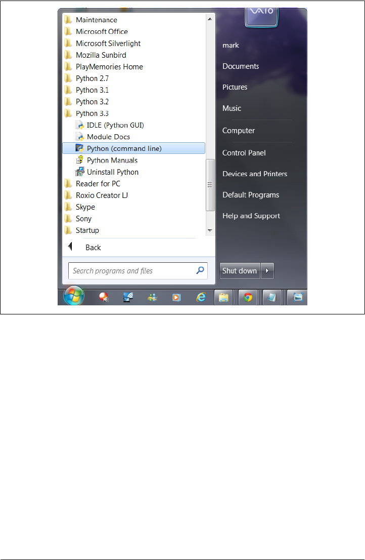
in getting it to run. I’ll explain the print statement, and why you can raise 2 to the
power 100 in Python without overflowing, in the next parts of this book.
You can create such a file of statements with any text editor you like. By convention,
Python program files are given names that end in .py; technically, this naming scheme
is required only for files that are “imported”—a term clarified in the next chapter—but
most Python files have .py names for consistency.
After you’ve typed these statements into a text file, you must tell Python to execute the
file—which simply means to run all the statements in the file from top to bottom, one
after another. As you’ll see in the next chapter, you can launch Python program files
by shell command lines, by clicking their icons, from within IDEs, and with other
standard techniques. If all goes well, when you execute the file, you’ll see the results of
the two print statements show up somewhere on your computer—by default, usually
in the same window you were in when you ran the program:
Figure 2-1. When installed on Windows 7 and earlier, this is how Python shows up in your Start
button menu. This can vary across releases, but IDLE starts a development GUI, and Python starts
a simple interactive session. Also here are the standard manuals and the PyDoc documentation engine
(Module Docs). See Chapter 3 and Appendix A for pointers on Windows 8 and other platforms.
Program Execution | 29
www.it-ebooks.info

hello world
1267650600228229401496703205376
For example, here’s what happened when I ran this script from a Command Prompt
window’s command line on a Windows laptop, to make sure it didn’t have any silly
typos:
C:\code> python script0.py
hello world
1267650600228229401496703205376
See Chapter 3 for the full story on this process, especially if you’re new to programming;
we’ll get into all the gory details of writing and launching programs there. For our
purposes here, we’ve just run a Python script that prints a string and a number. We
probably won’t win any programming awards with this code, but it’s enough to capture
the basics of program execution.
Python’s View
The brief description in the prior section is fairly standard for scripting languages, and
it’s usually all that most Python programmers need to know. You type code into text
files, and you run those files through the interpreter. Under the hood, though, a bit
more happens when you tell Python to “go.” Although knowledge of Python internals
is not strictly required for Python programming, a basic understanding of the runtime
structure of Python can help you grasp the bigger picture of program execution.
When you instruct Python to run your script, there are a few steps that Python carries
out before your code actually starts crunching away. Specifically, it’s first compiled to
something called “byte code” and then routed to something called a “virtual machine.”
Byte code compilation
Internally, and almost completely hidden from you, when you execute a program
Python first compiles your source code (the statements in your file) into a format known
as byte code. Compilation is simply a translation step, and byte code is a lower-level,
platform-independent representation of your source code. Roughly, Python translates
each of your source statements into a group of byte code instructions by decomposing
them into individual steps. This byte code translation is performed to speed execution
—byte code can be run much more quickly than the original source code statements
in your text file.
You’ll notice that the prior paragraph said that this is almost completely hidden from
you. If the Python process has write access on your machine, it will store the byte code
of your programs in files that end with a .pyc extension (“.pyc” means compiled “.py”
source). Prior to Python 3.2, you will see these files show up on your computer after
you’ve run a few programs alongside the corresponding source code files—that is, in
the same directories. For instance, you’ll notice a script.pyc after importing a script.py.
30 | Chapter 2: How Python Runs Programs
www.it-ebooks.info

In 3.2 and later, Python instead saves its .pyc byte code files in a subdirectory named
__pycache__ located in the directory where your source files reside, and in files whose
names identify the Python version that created them (e.g., script.cpython-33.pyc). The
new __pycache__ subdirectory helps to avoid clutter, and the new naming convention
for byte code files prevents different Python versions installed on the same computer
from overwriting each other’s saved byte code. We’ll study these byte code file models
in more detail in Chapter 22, though they are automatic and irrelevant to most Python
programs, and are free to vary among the alternative Python implementations described
ahead.
In both models, Python saves byte code like this as a startup speed optimization. The
next time you run your program, Python will load the .pyc files and skip the compilation
step, as long as you haven’t changed your source code since the byte code was last
saved, and aren’t running with a different Python than the one that created the byte
code. It works like this:
•Source changes: Python automatically checks the last-modified timestamps of
source and byte code files to know when it must recompile—if you edit and resave
your source code, byte code is automatically re-created the next time your program
is run.
•Python versions: Imports also check to see if the file must be recompiled because
it was created by a different Python version, using either a “magic” version number
in the byte code file itself in 3.2 and earlier, or the information present in byte code
filenames in 3.2 and later.
The result is that both source code changes and differing Python version numbers will
trigger a new byte code file. If Python cannot write the byte code files to your machine,
your program still works—the byte code is generated in memory and simply discarded
on program exit. However, because .pyc files speed startup time, you’ll want to make
sure they are written for larger programs. Byte code files are also one way to ship Python
programs—Python is happy to run a program if all it can find are .pyc files, even if the
original .py source files are absent. (See “Frozen Binaries” on page 39 for another
shipping option.)
Finally, keep in mind that byte code is saved in files only for files that are imported, not
for the top-level files of a program that are only run as scripts (strictly speaking, it’s an
import optimization). We’ll explore import basics in Chapter 3, and take a deeper look
at imports in Part V. Moreover, a given file is only imported (and possibly compiled)
once per program run, and byte code is also never saved for code typed at the interactive
prompt—a programming mode we’ll learn about in Chapter 3.
The Python Virtual Machine (PVM)
Once your program has been compiled to byte code (or the byte code has been loaded
from existing .pyc files), it is shipped off for execution to something generally known
as the Python Virtual Machine (PVM, for the more acronym-inclined among you). The
Program Execution | 31
www.it-ebooks.info
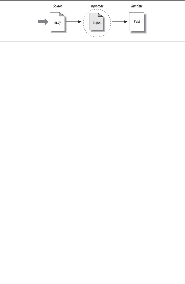
PVM sounds more impressive than it is; really, it’s not a separate program, and it need
not be installed by itself. In fact, the PVM is just a big code loop that iterates through
your byte code instructions, one by one, to carry out their operations. The PVM is the
runtime engine of Python; it’s always present as part of the Python system, and it’s the
component that truly runs your scripts. Technically, it’s just the last step of what is
called the “Python interpreter.”
Figure 2-2 illustrates the runtime structure described here. Keep in mind that all of this
complexity is deliberately hidden from Python programmers. Byte code compilation is
automatic, and the PVM is just part of the Python system that you have installed on
your machine. Again, programmers simply code and run files of statements, and Python
handles the logistics of running them.
Performance implications
Readers with a background in fully compiled languages such as C and C++ might notice
a few differences in the Python model. For one thing, there is usually no build or “make”
step in Python work: code runs immediately after it is written. For another, Python byte
code is not binary machine code (e.g., instructions for an Intel or ARM chip). Byte code
is a Python-specific representation.
This is why some Python code may not run as fast as C or C++ code, as described in
Chapter 1—the PVM loop, not the CPU chip, still must interpret the byte code, and
byte code instructions require more work than CPU instructions. On the other hand,
unlike in classic interpreters, there is still an internal compile step—Python does not
need to reanalyze and reparse each source statement’s text repeatedly. The net effect
is that pure Python code runs at speeds somewhere between those of a traditional
compiled language and a traditional interpreted language. See Chapter 1 for more on
Python performance tradeoffs.
Development implications
Another ramification of Python’s execution model is that there is really no distinction
between the development and execution environments. That is, the systems that com-
pile and execute your source code are really one and the same. This similarity may have
Figure 2-2. Python’s traditional runtime execution model: source code you type is translated to byte
code, which is then run by the Python Virtual Machine. Your code is automatically compiled, but then
it is interpreted.
32 | Chapter 2: How Python Runs Programs
www.it-ebooks.info

a bit more significance to readers with a background in traditional compiled languages,
but in Python, the compiler is always present at runtime and is part of the system that
runs programs.
This makes for a much more rapid development cycle. There is no need to precompile
and link before execution may begin; simply type and run the code. This also adds a
much more dynamic flavor to the language—it is possible, and often very convenient,
for Python programs to construct and execute other Python programs at runtime. The
eval and exec built-ins, for instance, accept and run strings containing Python program
code. This structure is also why Python lends itself to product customization—because
Python code can be changed on the fly, users can modify the Python parts of a system
onsite without needing to have or compile the entire system’s code.
At a more fundamental level, keep in mind that all we really have in Python is runtime—
there is no initial compile-time phase at all, and everything happens as the program is
running. This even includes operations such as the creation of functions and classes
and the linkage of modules. Such events occur before execution in more static lan-
guages, but happen as programs execute in Python. As we’ll see, this makes for a much
more dynamic programming experience than that to which some readers may be ac-
customed.
Execution Model Variations
Now that we’ve studied the internal execution flow described in the prior section, I
should note that it reflects the standard implementation of Python today but is not
really a requirement of the Python language itself. Because of that, the execution model
is prone to changing with time. In fact, there are already a few systems that modify the
picture in Figure 2-2 somewhat. Before moving on, let’s briefly explore the most prom-
inent of these variations.
Python Implementation Alternatives
Strictly speaking, as this book edition is being written, there are at least five imple-
mentations of the Python language—CPython, Jython, IronPython, Stackless, and
PyPy. Although there is much cross-fertilization of ideas and work between these Py-
thons, each is a separately installed software system, with its own developers and user
base. Other potential candidates here include the Cython and Shed Skin systems, but
they are discussed later as optimization tools because they do not implement the stan-
dard Python language (the former is a Python/C mix, and the latter is implicitly stati-
cally typed).
In brief, CPython is the standard implementation, and the system that most readers
will wish to use (if you’re not sure, this probably includes you). This is also the version
used in this book, though the core Python language presented here is almost entirely
the same in the alternatives. All the other Python implementations have specific pur-
Execution Model Variations | 33
www.it-ebooks.info

poses and roles, though they can often serve in most of CPython’s capacities too. All
implement the same Python language but execute programs in different ways.
For example, PyPy is a drop-in replacement for CPython, which can run most programs
much quicker. Similarly, Jython and IronPython are completely independent imple-
mentations of Python that compile Python source for different runtime architectures,
to provide direct access to Java and .NET components. It is also possible to access Java
and .NET software from standard CPython programs—JPype and Python for .NET
systems, for instance, allow standard CPython code to call out to Java and .NET com-
ponents. Jython and IronPython offer more complete solutions, by providing full im-
plementations of the Python language.
Here’s a quick rundown on the most prominent Python implementations available
today.
CPython: The standard
The original, and standard, implementation of Python is usually called CPython when
you want to contrast it with the other options (and just plain “Python” otherwise). This
name comes from the fact that it is coded in portable ANSI C language code. This is
the Python that you fetch from http://www.python.org, get with the ActivePython and
Enthought distributions, and have automatically on most Linux and Mac OS X ma-
chines. If you’ve found a preinstalled version of Python on your machine, it’s probably
CPython, unless your company or organization is using Python in more specialized
ways.
Unless you want to script Java or .NET applications with Python or find the benefits
of Stackless or PyPy compelling, you probably want to use the standard CPython sys-
tem. Because it is the reference implementation of the language, it tends to run the
fastest, be the most complete, and be more up-to-date and robust than the alternative
systems. Figure 2-2 reflects CPython’s runtime architecture.
Jython: Python for Java
The Jython system (originally known as JPython) is an alternative implementation of
the Python language, targeted for integration with the Java programming language.
Jython consists of Java classes that compile Python source code to Java byte code and
then route the resulting byte code to the Java Virtual Machine (JVM). Programmers
still code Python statements in .py text files as usual; the Jython system essentially just
replaces the rightmost two bubbles in Figure 2-2 with Java-based equivalents.
Jython’s goal is to allow Python code to script Java applications, much as CPython
allows Python to script C and C++ components. Its integration with Java is remarkably
seamless. Because Python code is translated to Java byte code, it looks and feels like a
true Java program at runtime. Jython scripts can serve as web applets and servlets, build
Java-based GUIs, and so on. Moreover, Jython includes integration support that allows
Python code to import and use Java classes as though they were coded in Python, and
34 | Chapter 2: How Python Runs Programs
www.it-ebooks.info

Java code to run Python code as an embedded language. Because Jython is slower and
less robust than CPython, though, it is usually seen as a tool of interest primarily to
Java developers looking for a scripting language to serve as a frontend to Java code. See
Jython’s website http://jython.org for more details.
IronPython: Python for .NET
A third implementation of Python, and newer than both CPython and Jython, IronPy-
thon is designed to allow Python programs to integrate with applications coded to work
with Microsoft’s .NET Framework for Windows, as well as the Mono open source
equivalent for Linux. .NET and its C# programming language runtime system are de-
signed to be a language-neutral object communication layer, in the spirit of Microsoft’s
earlier COM model. IronPython allows Python programs to act as both client and server
components, gain accessibility both to and from other .NET languages, and lever-
age .NET technologies such as the Silverlight framework from their Python code.
By implementation, IronPython is very much like Jython (and, in fact, was developed
by the same creator)—it replaces the last two bubbles in Figure 2-2 with equivalents
for execution in the .NET environment. Also like Jython, IronPython has a special focus
—it is primarily of interest to developers integrating Python with .NET components.
Formerly developed by Microsoft and now an open source project, IronPython might
also be able to take advantage of some important optimization tools for better perfor-
mance. For more details, consult http://ironpython.net and other resources to be had
with a web search.
Stackless: Python for concurrency
Still other schemes for running Python programs have more focused goals. For example,
the Stackless Python system is an enhanced version and reimplementation of the stan-
dard CPython language oriented toward concurrency. Because it does not save state on
the C language call stack, Stackless Python can make Python easier to port to small
stack architectures, provides efficient multiprocessing options, and fosters novel pro-
gramming structures such as coroutines.
Among other things, the microthreads that Stackless adds to Python are an efficient and
lightweight alternative to Python’s standard multitasking tools such as threads and
processes, and promise better program structure, more readable code, and increased
programmer productivity. CCP Games, the creator of EVE Online, is a well-known
Stackless Python user, and a compelling Python user success story in general. Try http:
//stackless.com for more information.
PyPy: Python for speed
The PyPy system is another standard CPython reimplementation, focused on perfor-
mance. It provides a fast Python implementation with a JIT (just-in-time) compiler,
provides tools for a “sandbox” model that can run untrusted code in a secure environ-
Execution Model Variations | 35
www.it-ebooks.info

ment, and by default includes support for the prior section’s Stackless Python systems
and its microthreads to support massive concurrency.
PyPy is the successor to the original Psyco JIT, described ahead, and subsumes it with
a complete Python implementation built for speed. A JIT is really just an extension to
the PVM—the rightmost bubble in Figure 2-2—that translates portions of your byte
code all the way to binary machine code for faster execution. It does this as your pro-
gram is running, not in a prerun compile step, and is able to created type-specific ma-
chine code for the dynamic Python language by keeping track of the data types of the
objects your program processes. By replacing portions of your byte code this way, your
program runs faster and faster as it is executing. In addition, some Python programs
may also take up less memory under PyPy.
At this writing, PyPy supports Python 2.7 code (not yet 3.X) and runs on Intel x86
(IA-32) and x86_64 platforms (including Windows, Linux, and recent Macs), with
ARM and PPC support under development. It runs most CPython code, though C
extension modules must generally be recompiled, and PyPy has some minor but subtle
language differences, including garbage collection semantics that obviate some com-
mon coding patterns. For instance, its non-reference-count scheme means that tem-
porary files may not close and flush output buffers immediately, and may require man-
ual close calls in some cases.
In return, your code may run much quicker. PyPy currently claims a 5.7X speedup over
CPython across a range of benchmark programs (per http://speed.pypy.org/). In some
cases, its ability to take advantage of dynamic optimization opportunities can make
Python code as quick as C code, and occasionally faster. This is especially true for
heavily algorithmic or numeric programs, which might otherwise be recoded in C.
For instance, in one simple benchmark we’ll see in Chapter 21, PyPy today clocks in
at 10X faster than CPython 2.7, and 100X faster than CPython 3.X. Though other
benchmarks will vary, such speedups may be a compelling advantage in many domains,
perhaps even more so than leading-edge language features. Just as important, memory
space is also optimized in PyPy—in the case of one posted benchmark, requiring 247
MB and completing in 10.3 seconds, compared to CPython’s 684 MB and 89 seconds.
PyPy’s tool chain is also general enough to support additional languages, including
Pyrolog, a Prolog interpreter written in Python using the PyPy translator. Search for
PyPy’s website for more. PyPy currently lives at http://pypy.org, though the usual web
search may also prove fruitful over time. For an overview of its current performance,
also see http://www.pypy.org/performance.html.
36 | Chapter 2: How Python Runs Programs
www.it-ebooks.info

Just after I wrote this, PyPy 2.0 was released in beta form, adding support
for the ARM processor, and still a Python 2.X-only implementation. Per
its 2.0 beta release notes:
“PyPy is a very compliant Python interpreter, almost a drop-in replace-
ment for CPython 2.7.3. It’s fast due to its integrated tracing JIT com-
piler. This release supports x86 machines running Linux 32/64, Mac OS
X 64 or Windows 32. It also supports ARM machines running Linux.”
The claims seem accurate. Using the timing tools we’ll study in Chap-
ter 21, PyPy is often an order of magnitude (factor of 10) faster than
CPython 2.X and 3.X on tests I’ve run, and sometimes even better. This
is despite the fact that PyPy is a 32-bit build on my Windows test ma-
chine, while CPython is a faster 64-bit compile.
Naturally the only benchmark that truly matters is your own code, and
there are cases where CPython wins the race; PyPy’s file iterators, for
instance, may clock in slower today. Still, given PyPy’s focus on perfor-
mance over language mutation, and especially its support for the nu-
meric domain, many today see PyPy as an important path for Python.
If you write CPU-intensive code, PyPy deserves your attention.
Execution Optimization Tools
CPython and most of the alternatives of the prior section all implement the Python
language in similar ways: by compiling source code to byte code and executing the byte
code on an appropriate virtual machine. Some systems, such as the Cython hybrid, the
Shed Skin C++ translator, and the just-in-time compilers in PyPy and Psyco instead
attempt to optimize the basic execution model. These systems are not required knowl-
edge at this point in your Python career, but a quick look at their place in the execution
model might help demystify the model in general.
Cython: A Python/C hybrid
The Cython system (based on work done by the Pyrex project) is a hybrid language that
combines Python code with the ability to call C functions and use C type declarations
for variables, parameters, and class attributes. Cython code can be compiled to C code
that uses the Python/C API, which may then be compiled completely. Though not
completely compatible with standard Python, Cython can be useful both for wrapping
external C libraries and for coding efficient C extensions for Python. See http://cython
.org for current status and details.
Shed Skin: A Python-to-C++ translator
Shed Skin is an emerging system that takes a different approach to Python program
execution—it attempts to translate Python source code to C++ code, which your com-
puter’s C++ compiler then compiles to machine code. As such, it represents a platform-
neutral approach to running Python code.
Execution Model Variations | 37
www.it-ebooks.info

Shed Skin is still being actively developed as I write these words. It currently supports
Python 2.4 to 2.6 code, and it limits Python programs to an implicit statically typed
constraint that is typical of most programs but is technically not normal Python, so we
won’t go into further detail here. Initial results, though, show that it has the potential
to outperform both standard Python and Psyco-like extensions in terms of execution
speed. Search the Web for details on the project’s current status.
Psyco: The original just-in-time compiler
The Psyco system is not another Python implementation, but rather a component that
extends the byte code execution model to make programs run faster. Today, Psyco is
something of an ex-project: it is still available for separate download, but has fallen out
of date with Python’s evolution, and is no longer actively maintained. Instead, its ideas
have been incorporated into the more complete PyPy system described earlier. Still, the
ongoing importance of the ideas Psyco explored makes them worth a quick look.
In terms of Figure 2-2, Psyco is an enhancement to the PVM that collects and uses type
information while the program runs to translate portions of the program’s byte code
all the way down to true binary machine code for faster execution. Psyco accomplishes
this translation without requiring changes to the code or a separate compilation step
during development.
Roughly, while your program runs, Psyco collects information about the kinds of ob-
jects being passed around; that information can be used to generate highly efficient
machine code tailored for those object types. Once generated, the machine code then
replaces the corresponding part of the original byte code to speed your program’s over-
all execution. The result is that with Psyco, your program becomes quicker over time
as it runs. In ideal cases, some Python code may become as fast as compiled C code
under Psyco.
Because this translation from byte code happens at program runtime, Psyco is known
as a just-in-time compiler. Psyco is different from the JIT compilers some readers may
have seen for the Java language, though. Really, Psyco is a specializing JIT compiler—
it generates machine code tailored to the data types that your program actually uses.
For example, if a part of your program uses different data types at different times, Psyco
may generate a different version of machine code to support each different type com-
bination.
Psyco was shown to speed some Python code dramatically. According to its web page,
Psyco provides “2X to 100X speed-ups, typically 4X, with an unmodified Python in-
terpreter and unmodified source code, just a dynamically loadable C extension mod-
ule.” Of equal significance, the largest speedups are realized for algorithmic code writ-
ten in pure Python—exactly the sort of code you might normally migrate to C to op-
timize. For more on Psyco, search the Web or see its successor—the PyPy project de-
scribed previously.
38 | Chapter 2: How Python Runs Programs
www.it-ebooks.info

Frozen Binaries
Sometimes when people ask for a “real” Python compiler, what they’re really seeking
is simply a way to generate standalone binary executables from their Python programs.
This is more a packaging and shipping idea than an execution-flow concept, but it’s
somewhat related. With the help of third-party tools that you can fetch off the Web, it
is possible to turn your Python programs into true executables, known as frozen bi-
naries in the Python world. These programs can be run without requiring a Python
installation.
Frozen binaries bundle together the byte code of your program files, along with the
PVM (interpreter) and any Python support files your program needs, into a single
package. There are some variations on this theme, but the end result can be a single
binary executable program (e.g., an .exe file on Windows) that can easily be shipped
to customers. In Figure 2-2, it is as though the two rightmost bubbles—byte code and
PVM—are merged into a single component: a frozen binary file.
Today, a variety of systems are capable of generating frozen binaries, which vary in
platforms and features: py2exe for Windows only, but with broad Windows support;
PyInstaller, which is similar to py2exe but also works on Linux and Mac OS X and is
capable of generating self-installing binaries; py2app for creating Mac OS X applica-
tions; freeze, the original; and cx_freeze, which offers both Python 3.X and cross-plat-
form support. You may have to fetch these tools separately from Python itself, but they
are freely available.
These tools are also constantly evolving, so consult http://www.python.org or your fa-
vorite web search engine for more details and status. To give you an idea of the scope
of these systems, py2exe can freeze standalone programs that use the tkinter, PMW,
wxPython, and PyGTK GUI libraries; programs that use the pygame game program-
ming toolkit; win32com client programs; and more.
Frozen binaries are not the same as the output of a true compiler—they run byte code
through a virtual machine. Hence, apart from a possible startup improvement, frozen
binaries run at the same speed as the original source files. Frozen binaries are also not
generally small (they contain a PVM), but by current standards they are not unusually
large either. Because Python is embedded in the frozen binary, though, it does not have
to be installed on the receiving end to run your program. Moreover, because your code
is embedded in the frozen binary, it is more effectively hidden from recipients.
This single file-packaging scheme is especially appealing to developers of commercial
software. For instance, a Python-coded user interface program based on the tkinter
toolkit can be frozen into an executable file and shipped as a self-contained program
on a CD or on the Web. End users do not need to install (or even have to know about)
Python to run the shipped program.
Execution Model Variations | 39
www.it-ebooks.info

Future Possibilities?
Finally, note that the runtime execution model sketched here is really an artifact of the
current implementation of Python, not of the language itself. For instance, it’s not
impossible that a full, traditional compiler for translating Python source code to ma-
chine code may appear during the shelf life of this book (although the fact that one has
not in over two decades makes this seem unlikely!).
New byte code formats and implementation variants may also be adopted in the future.
For instance:
• The ongoing Parrot project aims to provide a common byte code format, virtual
machine, and optimization techniques for a variety of programming languages,
including Python. Python’s own PVM runs Python code more efficiently than Par-
rot (as famously demonstrated by a pie challenge at a software conference—search
the Web for details), but it’s unclear how Parrot will evolve in relation to Python
specifically. See http://parrot.org or the Web at large for details.
• The former Unladen Swallow project—an open source project developed by Goo-
gle engineers—sought to make standard Python faster by a factor of at least 5, and
fast enough to replace the C language in many contexts. This was an optimization
branch of CPython (specifically Python 2.6), intended to be compatible yet faster
by virtue of adding a JIT to standard Python. As I write this in 2012, this project
seems to have drawn to a close (per its withdrawn Python PEP, it was “going the
way of the Norwegian Blue”). Still, its lessons gained may be leveraged in other
forms; search the Web for breaking developments.
Although future implementation schemes may alter the runtime structure of Python
somewhat, it seems likely that the byte code compiler will still be the standard for some
time to come. The portability and runtime flexibility of byte code are important features
of many Python systems. Moreover, adding type constraint declarations to support
static compilation would likely break much of the flexibility, conciseness, simplicity,
and overall spirit of Python coding. Due to Python’s highly dynamic nature, any future
implementation will likely retain many artifacts of the current PVM.
Chapter Summary
This chapter introduced the execution model of Python—how Python runs your pro-
grams—and explored some common variations on that model: just-in-time compilers
and the like. Although you don’t really need to come to grips with Python internals to
write Python scripts, a passing acquaintance with this chapter’s topics will help you
truly understand how your programs run once you start coding them. In the next
chapter, you’ll start actually running some code of your own. First, though, here’s the
usual chapter quiz.
40 | Chapter 2: How Python Runs Programs
www.it-ebooks.info

Test Your Knowledge: Quiz
1. What is the Python interpreter?
2. What is source code?
3. What is byte code?
4. What is the PVM?
5. Name two or more variations on Python’s standard execution model.
6. How are CPython, Jython, and IronPython different?
7. What are Stackless and PyPy?
Test Your Knowledge: Answers
1. The Python interpreter is a program that runs the Python programs you write.
2. Source code is the statements you write for your program—it consists of text in
text files that normally end with a .py extension.
3. Byte code is the lower-level form of your program after Python compiles it. Python
automatically stores byte code in files with a .pyc extension.
4. The PVM is the Python Virtual Machine—the runtime engine of Python that in-
terprets your compiled byte code.
5. Psyco, Shed Skin, and frozen binaries are all variations on the execution model. In
addition, the alternative implementations of Python named in the next two answers
modify the model in some fashion as well—by replacing byte code and VMs, or by
adding tools and JITs.
6. CPython is the standard implementation of the language. Jython and IronPython
implement Python programs for use in Java and .NET environments, respectively;
they are alternative compilers for Python.
7. Stackless is an enhanced version of Python aimed at concurrency, and PyPy is a
reimplementation of Python targeted at speed. PyPy is also the successor to Psyco,
and incorporates the JIT concepts that Psyco pioneered.
Test Your Knowledge: Answers | 41
www.it-ebooks.info

CHAPTER 3
How You Run Programs
OK, it’s time to start running some code. Now that you have a handle on the program
execution model, you’re finally ready to start some real Python programming. At this
point, I’ll assume that you have Python installed on your computer; if you don’t, see
the start of the prior chapter and Appendix A for installation and configuration hints
on various platforms. Our goal here is to learn how to run Python program code.
There are multiple ways to tell Python to execute the code you type. This chapter
discusses all the program launching techniques in common use today. Along the way,
you’ll learn how to both type code interactively, and how to save it in files to be run as
often as you like in a variety of ways: with system command lines, icon clicks, module
imports, exec calls, menu options in the IDLE GUI, and more.
As for the previous chapter, if you have prior programming experience and are anxious
to start digging into Python itself, you may want to skim this chapter and move on to
Chapter 4. But don’t skip this chapter’s early coverage of preliminaries and conven-
tions, its overview of debugging techniques, or its first look at module imports—a topic
essential to understanding Python’s program architecture, which we won’t revisit until
a later part. I also encourage you to see the sections on IDLE and other IDEs, so you’ll
know what tools are available when you start developing more sophisticated Python
programs.
The Interactive Prompt
This section gets us started with interactive coding basics. Because it’s our first look at
running code, we also cover some preliminaries here, such as setting up a working
directory and the system path, so be sure to read this section first if you’re relatively
new to programming. This section also explains some conventions used throughout
the book, so most readers should probably take at least a quick look here.
43
www.it-ebooks.info

Starting an Interactive Session
Perhaps the simplest way to run Python programs is to type them at Python’s interactive
command line, sometimes called the interactive prompt. There are a variety of ways to
start this command line: in an IDE, from a system console, and so on. Assuming the
interpreter is installed as an executable program on your system, the most platform-
neutral way to start an interactive interpreter session is usually just to type python at
your operating system’s prompt, without any arguments. For example:
% python
Python 3.3.0 (v3.3.0:bd8afb90ebf2, Sep 29 2012, 10:57:17) [MSC v.1600 64 bit ...
Type "help", "copyright", "credits" or "license" for more information.
>>> ^Z
Typing the word “python” at your system shell prompt like this begins an interactive
Python session; the “%” character at the start of this listing stands for a generic system
prompt in this book—it’s not input that you type yourself. On Windows, a Ctrl-Z gets
you out of this session; on Unix, try Ctrl-D instead.
The notion of a system shell prompt is generic, but exactly how you access it varies by
platform:
• On Windows, you can type python in a DOS console window—a program named
cmd.exe and usually known as Command Prompt. For more details on starting this
program, see this chapter’s sidebar “Where Is Command Prompt on Win-
dows?” on page 45.
• On Mac OS X, you can start a Python interactive interpreter by double-clicking on
Applications→Utilities→Terminal, and then typing python in the window that
opens up.
• On Linux (and other Unixes), you might type this command in a shell or terminal
window (for instance, in an xterm or console running a shell such as ksh or csh).
• Other systems may use similar or platform-specific devices. On handheld devices,
for example, you might click the Python icon in the home or application window
to launch an interactive session.
On most platforms, you can start the interactive prompt in additional ways that don’t
require typing a command, but they vary per platform even more widely:
• On Windows 7 and earlier, besides typing python in a shell window, you can also
begin similar interactive sessions by starting the IDLE GUI (discussed later), or by
selecting the “Python (command line)” menu option from the Start button menu
for Python, as shown in Figure 2-1 in Chapter 2. Both spawn a Python interactive
prompt with the same functionality obtained with a “python” command.
• On Windows 8, you don’t have a Start button (at least as I write this), but there are
other ways to get to the tools described in the prior bullet, including tiles, Search,
File Explorer, and the “All apps” interface on the Start screen. See Appendix A for
more pointers on this platform.
44 | Chapter 3: How You Run Programs
www.it-ebooks.info

• Other platforms have similar ways to start a Python interactive session without
typing commands, but they’re too specific to get into here; see your system’s doc-
umentation for details.
Anytime you see the >>> prompt, you’re in an interactive Python interpreter session—
you can type any Python statement or expression here and run it immediately. We will
in a moment, but first we need to get a few startup details sorted out to make sure all
readers are set to go.
Where Is Command Prompt on Windows?
So how do you start the command-line interface on Windows? Some Windows readers
already know, but Unix developers and beginners may not; it’s not as prominent as
terminal or console windows on Unix systems. Here are some pointers on finding your
Command Prompt, which vary slightly per Windows version.
On Windows 7 and earlier, this is usually found in the Accessories section of the
Start→All Programs menu, or you can run it by typing cmd in the Start→Run... dialog
box or the Start menu’s search entry field. You can drag out a desktop shortcut to get
to it quicker if desired.
On Windows 8, you can access Command Prompt in the menu opened by right-clicking
on the preview in the screen’s lower-left corner; in the Windows System section of the
“All apps” display reached by right-clicking your Start screen; or by typing cmd or
command prompt in the input field of the Search charm pulled down from the screen’s
upper-right corner. There are probably additional routes, and touch screens offer sim-
ilar access. And if you want to forget all that, pin it to your desktop taskbar for easy
access next time around.
These procedures are prone to vary over time, and possibly even per computer and
user. I’m trying to avoid making this a book on Windows, though, so I’ll cut this topic
short here. When in doubt, try the system Help interface (whose usage may differ as
much as the tools it provides help for!).
A note to any Unix users reading this sidebar who may be starting to feel like a fish out
of water: you may also be interested in the Cygwin system, which brings a full Unix
command prompt to Windows. See Appendix A for more pointers.
The System Path
When we typed python in the last section to start an interactive session, we relied on
the fact that the system located the Python program for us on its program search path.
Depending on your Python version and platform, if you have not set your system’s
PATH environment variable to include Python’s install directory, you may need to replace
the word “python” with the full path to the Python executable on your machine. On
Unix, Linux, and similar, something like /usr/local/bin/python or /usr/bin/python3
will often suffice. On Windows, try typing C:\Python33\python (for version 3.3):
The Interactive Prompt | 45
www.it-ebooks.info

c:\code> c:\python33\python
Python 3.3.0 (v3.3.0:bd8afb90ebf2, Sep 29 2012, 10:57:17) [MSC v.1600 64 bit ...
Type "help", "copyright", "credits" or "license" for more information.
>>> ^Z
Alternatively, you can run a “cd” change-directory command to go to Python’s install
directory before typing python—try the cd c:\python33 command on Windows, for
example:
c:\code> cd c:\python33
c:\Python33> python
Python 3.3.0 (v3.3.0:bd8afb90ebf2, Sep 29 2012, 10:57:17) [MSC v.1600 64 bit ...
Type "help", "copyright", "credits" or "license" for more information.
>>> ^Z
But you’ll probably want to set your PATH eventually, so a simple “python” suffices. If
you don’t know what PATH is or how to set it, see Appendix A—it covers environment
variables like this whose usage varies per platform, as well as Python command-line
arguments we won’t be using much in this book. The short story for Windows users:
see the Advanced settings in the System entry of your Control Panel. If you’re using
Python 3.3 and later, this is now automatic on Windows, as the next section explains.
New Windows Options in 3.3: PATH, Launcher
The foregoing section and much of this chapter at large describe the generic state of
play for all 2.X and 3.X Pythons prior to version 3.3. Starting with Python 3.3, the
Windows installer has an option to automatically add Python 3.3’s directory to your
system PATH, if enabled in the installer’s windows. If you use this option, you won’t
need to type a directory path or issue a “cd” to run python commands as in the prior
section. Be sure to select this option during the install if you want it, as it’s currently
disabled by default.
More dramatically, Python 3.3 for Windows ships with and automatically installs the
new Windows launcher—a system that comes with new executable programs, py with
a console and pyw without, that are placed in directories on your system path, and so
may be run out of the box without any PATH configurations, change-directory com-
mands, or directory path prefixes:
c:\code> py
Python 3.3.0 (v3.3.0:bd8afb90ebf2, Sep 29 2012, 10:57:17) [MSC v.1600 64 bit ...
Type "help", "copyright", "credits" or "license" for more information.
>>> ^Z
c:\code> py −2
Python 2.7.3 (default, Apr 10 2012, 23:24:47) [MSC v.1500 64 bit (AMD64)] ...
Type "help", "copyright", "credits" or "license" for more information.
>>> ^Z
c:\code> py −3.1
Python 3.1.4 (default, Jun 12 2011, 14:16:16) [MSC v.1500 64 bit (AMD64)] ...
46 | Chapter 3: How You Run Programs
www.it-ebooks.info

Type "help", "copyright", "credits" or "license" for more information.
>>> ^Z
As shown in the last two commands here, these executables also accept Python version
numbers on the command line (and in Unix-style #! lines at the top of scripts, as dis-
cussed later), and are associated to open Python files when clicked just like the original
python executable—which is still available and works as before, but is somewhat su-
perseded by the launcher’s new programs.
The launcher is a standard part of Python 3.3, and is available standalone for use with
other versions. We’ll see more on this new launcher in this and later chapters, including
a brief look at its #! line support here. However, because it is of interest only to Windows
users, and even for this group is present only in 3.3 or where installed separately, I’ve
collected almost all of the details about the launcher in Appendix B.
If you’ll be working on Windows under Python 3.3 or later, I suggest taking a brief
detour to that appendix now, as it provides an alternative, and in some ways better,
way to run Python command lines and scripts. At a base level, launcher users can type
py instead of python in most of the system commands shown in this book, and may
avoid some configuration steps. Especially on computers with multiple Python ver-
sions, though, the new launcher gives you more explicit control over which Python
runs your code.
Where to Run: Code Directories
Now that I’ve started showing you how to run code, I want to say a few words up front
about where to run code. To keep things simple, in this chapter and book at large I’m
going to be running code from a working directory (a.k.a. folder) I’ve created on my
Windows computer called C:\code—a subdirectory at the top of my main drive. That’s
where I’ll start most interactive sessions, and where I’ll be both saving and running
most script files. This also means the files that examples will create will mostly show
up in this directory.
If you’ll be working along, you should probably do something similar before we get
started. Here are some pointers if you need help getting set up with a working directory
on your computer:
• On Windows, you can make your working code directory in File Explorer or a
Command Prompt window. In File Explorer, look for New Folder, see the File
menu, or try a right-click. In Command Prompt, type and run a mkdir command,
usually after you cd to your desired parent directory (e.g., cd c\: and mkdir code).
Your working directory can be located wherever you like and called whatever you
wish, and doesn’t have to be C:\code (I chose this name because it’s short in
prompts). But running out of one directory will help you keep track of your work
and simplify some tasks. For more Windows hints, see this chapter’s sidebar on
Command Prompt, as well as Appendix A.
The Interactive Prompt | 47
www.it-ebooks.info

• On Unix-based systems (including Mac OS X and Linux), your working directory
might be in /usr/home and be created by a mkdir command in a shell window or
file explorer GUI specific to your platform, but the same concepts apply. The Cyg-
win Unix-like system for Windows is similar too, though your directory names
may vary (/home and /cygdrive/c are candidates).
You can store your code in Python’s install directory too (e.g., C:\Python33 on Win-
dows) to simplify some command lines before setting PATH, but you probably shouldn’t
—this is for Python itself, and your files may not survive a move or uninstall.
Once you’ve made your working directory, always start there to work along with the
examples in this book. The prompts in this book that show the directory that I’m
running code in will reflect my Windows laptop’s working directory; when you see C:
\code> or %, think the location and name of your own directory.
What Not to Type: Prompts and Comments
Speaking of prompts, this book sometimes shows system prompts as a generic %, and
sometimes in full C:\code> Windows form. The former is meant to be platform agnostic
(and derives from earlier editions’ use of Linux), and the latter is used in Windows-
specific contexts. I also add a space after system prompts just for readability in this
book. When used, the % character at the start of a system command line stands for the
system’s prompt, whatever that may be on your machine. For instance, on my machine
% stands for C:\code> in Windows Command Prompt, and just $ in my Cygwn install.
To beginners: don’t type the % character (or the C:\code system prompt it sometimes
stands for) you see in this book’s interaction listings yourself—this is text the system
prints. Type just the text after these system prompts. Similarly, do not type the >>>
and ... characters shown at the start of lines in interpreter interaction listings—these
are prompts that Python displays automatically as visual guides for interactive code
entry. Type just the text after these Python prompts. For instance, the ... prompt is
used for continuation lines in some shells, but doesn’t appear in IDLE, and shows up
in some but not all of this book’s listings; don’t type it yourself if it’s absent in your
interface.
To help you remember this, user inputs are shown in bold in this book, and prompts
are not. In some systems these prompts may differ (for instance, the PyPy performance-
focused implementation described in Chapter 2 uses four-character >>>> and ....), but
the same rules apply. Also keep in mind that commands typed after these system and
Python prompts are meant to be run immediately, and are not generally to be saved in
the source files we will be creating; we’ll see why this distinction matters ahead.
In the same vein, you normally don’t need to type text that starts with a # character in
listings in this book—as you’ll learn, these are comments, not executable code. Except
when # is used to introduce a directive at the top of a script for Unix or the Python 3.3
48 | Chapter 3: How You Run Programs
www.it-ebooks.info

Windows launcher, you can safely ignore the text that follows it (more on Unix and
the launcher later in this chapter and in Appendix B).
If you’re working along, interactive listings will drop most “...” contin-
uation prompts as of Chapter 17 to aid cut-and-paste of larger code such
as functions and classes from ebooks or other; until then, paste or type
one line at a time and omit the prompts. At least initially, it’s important
to type code manually, to get a feel for syntax details and errors. Some
examples will be listed either by themselves or in named files available
in the book’s examples package (per the preface), and we’ll switch be-
tween listing formats often; when in doubt, if you see “>>>”, it means
the code is being typed interactively.
Running Code Interactively
With those preliminaries out of the way, let’s move on to typing some actual code.
However it’s started, the Python interactive session begins by printing two lines of
informational text giving the Python version number and a few hints shown earlier
(which I’ll omit from most of this book’s examples to save space), then prompts for
input with >>> when it’s waiting for you to type a new Python statement or expression.
When working interactively, the results of your code are displayed below the >>> input
lines after you press the Enter key. For instance, here are the results of two Python
print statements (print is really a function call in Python 3.X, but not in 2.X, so the
parentheses here are required in 3.X only):
% python
>>> print('Hello world!')
Hello world!
>>> print(2 ** 8)
256
There it is—we’ve just run some Python code (were you expecting the Spanish Inqui-
sition?). Don’t worry about the details of the print statements shown here yet; we’ll
start digging into syntax in the next chapter. In short, they print a Python string and
an integer, as shown by the output lines that appear after each >>> input line (2 ** 8
means 2 raised to the power 8 in Python).
When coding interactively like this, you can type as many Python commands as you
like; each is run immediately after it’s entered. Moreover, because the interactive ses-
sion automatically prints the results of expressions you type, you don’t usually need to
say “print” explicitly at this prompt:
>>> lumberjack = 'okay'
>>> lumberjack
'okay'
>>> 2 ** 8
256
The Interactive Prompt | 49
www.it-ebooks.info

>>> ^Z # Use Ctrl-D (on Unix) or Ctrl-Z (on Windows) to exit
%
Here, the first line saves a value by assigning it to a variable (lumberjack), which is
created by the assignment; and the last two lines typed are expressions (lumberjack and
2 ** 8), whose results are displayed automatically. Again, to exit an interactive session
like this and return to your system shell prompt, type Ctrl-D on Unix-like machines,
and Ctrl-Z on Windows. In the IDLE GUI discussed later, either type Ctrl-D or simply
close the window.
Notice the italicized note about this on the right side of this listing (staring with “#”
here). I’ll use these throughout to add remarks about what is being illustrated, but you
don’t need to type this text yourself. In fact, just like system and Python prompts, you
shouldn’t type this when it’s on a system command line; the “#” part is taken as a
comment by Python but may be an error at a system prompt.
Now, we didn’t do much in this session’s code—just typed some Python print and
assignment statements, along with a few expressions, which we’ll study in detail later.
The main thing to notice is that the interpreter executes the code entered on each line
immediately, when the Enter key is pressed.
For example, when we typed the first print statement at the >>> prompt, the output (a
Python string) was echoed back right away. There was no need to create a source code
file, and no need to run the code through a compiler and linker first, as you’d normally
do when using a language such as C or C++. As you’ll see in later chapters, you can
also run multiline statements at the interactive prompt; such a statement runs imme-
diately after you’ve entered all of its lines and pressed Enter twice to add a blank line.
Why the Interactive Prompt?
The interactive prompt runs code and echoes results as you go, but it doesn’t save your
code in a file. Although this means you won’t do the bulk of your coding in interactive
sessions, the interactive prompt turns out to be a great place to both experiment with
the language and test program files on the fly.
Experimenting
Because code is executed immediately, the interactive prompt is a perfect place to ex-
periment with the language and will be used often in this book to demonstrate smaller
examples. In fact, this is the first rule of thumb to remember: if you’re ever in doubt
about how a piece of Python code works, fire up the interactive command line and try
it out to see what happens.
For instance, suppose you’re reading a Python program’s code and you come across
an expression like 'Spam!' * 8 whose meaning you don’t understand. At this point,
you can spend 10 minutes wading through manuals, books, and the Web to try to figure
out what the code does, or you can simply run it interactively:
50 | Chapter 3: How You Run Programs
www.it-ebooks.info

% python
>>> 'Spam!' * 8 # Learning by trying
'Spam!Spam!Spam!Spam!Spam!Spam!Spam!Spam!'
The immediate feedback you receive at the interactive prompt is often the quickest way
to deduce what a piece of code does. Here, it’s clear that it does string repetition: in
Python * means multiply for numbers, but repeat for strings—it’s like concatenating a
string to itself repeatedly (more on strings in Chapter 4).
Chances are good that you won’t break anything by experimenting this way—at least,
not yet. To do real damage, like deleting files and running shell commands, you must
really try, by importing modules explicitly (you also need to know more about Python’s
system interfaces in general before you will become that dangerous!). Straight Python
code is almost always safe to run.
For instance, watch what happens when you make a mistake at the interactive prompt:
>>> X # Making mistakes
Traceback (most recent call last):
File "<stdin>", line 1, in <module>
NameError: name 'X' is not defined
In Python, using a variable before it has been assigned a value is always an error—
otherwise, if names were filled in with defaults, some errors might go undetected. This
means you must initial counters to zero before you can add to them, must initial lists
before extending them, and so on; you don’t declare variables, but they must be as-
signed before you can fetch their values.
We’ll learn more about that later; the important point here is that you don’t crash
Python or your computer when you make a mistake this way. Instead, you get a mean-
ingful error message pointing out the mistake and the line of code that made it, and
you can continue on in your session or script. In fact, once you get comfortable with
Python, its error messages may often provide as much debugging support as you’ll need
(you’ll learn more about debugging options in the sidebar “Debugging Python
Code” on page 83).
Testing
Besides serving as a tool for experimenting while you’re learning the language, the
interactive interpreter is also an ideal place to test code you’ve written in files. You can
import your module files interactively and run tests on the tools they define by typing
calls at the interactive prompt on the fly.
For instance, the following tests a function in a precoded module that ships with Python
in its standard library (it prints the name of the directory you’re currently working in,
with a doubled-up backslash that stands for just one), but you can do the same once
you start writing module files of your own:
>>> import os
>>> os.getcwd() # Testing on the fly
'c:\\code'
The Interactive Prompt | 51
www.it-ebooks.info

More generally, the interactive prompt is a place to test program components, regard-
less of their source—you can import and test functions and classes in your Python files,
type calls to linked-in C functions, exercise Java classes under Jython, and more. Partly
because of its interactive nature, Python supports an experimental and exploratory
programming style you’ll find convenient when getting started. Although Python pro-
grammers also test with in-file code (and we’ll learn ways to make this simple later in
the book), for many, the interactive prompt is still their first line of testing defense.
Usage Notes: The Interactive Prompt
Although the interactive prompt is simple to use, there are a few tips that beginners
should keep in mind. I’m including lists of common mistakes like the following in this
chapter for reference, but they might also spare you from a few headaches if you read
them up front:
•Type Python commands only. First of all, remember that you can only type
Python code at Python’s >>> prompt, not system commands. There are ways to
run system commands from within Python code (e.g., with os.system), but they
are not as direct as simply typing the commands themselves.
•print statements are required only in files. Because the interactive interpreter
automatically prints the results of expressions, you do not need to type complete
print statements interactively. This is a nice feature, but it tends to confuse users
when they move on to writing code in files: within a code file, you must use
print statements to see your output because expression results are not automati-
cally echoed. Remember, you must say print in files, but it’s optional interactively.
•Don’t indent at the interactive prompt (yet). When typing Python programs,
either interactively or into a text file, be sure to start all your unnested statements
in column 1 (that is, all the way to the left). If you don’t, Python may print a
“SyntaxError” message, because blank space to the left of your code is taken to be
indentation that groups nested statements. Until Chapter 10, all statements you
write will be unnested, so this includes everything for now. Remember, a leading
space generates an error message, so don’t start with a space or tab at the interactive
prompt unless it’s nested code.
•Watch out for prompt changes for compound statements. We won’t meet
compound (multiline) statements until Chapter 4 and not in earnest until Chap-
ter 10, but as a preview, you should know that when typing lines 2 and beyond of
a compound statement interactively, the prompt may change. In the simple shell
window interface, the interactive prompt changes to ... instead of >>> for lines 2
and beyond; in the IDLE GUI interface, lines after the first are instead automatically
indented.
You’ll see why this matters in Chapter 10. For now, if you happen to come across
a ... prompt or a blank line when entering your code, it probably means that you’ve
somehow confused interactive Python into thinking you’re typing a multiline
52 | Chapter 3: How You Run Programs
www.it-ebooks.info

statement. Try hitting the Enter key or a Ctrl-C combination to get back to the
main prompt. The >>> and ... prompt strings can also be changed (they are avail-
able in the built-in module sys), but I’ll assume they have not been in the book’s
example listings.
•Terminate compound statements at the interactive prompt with a blank
line. At the interactive prompt, inserting a blank line (by hitting the Enter key at
the start of a line) is necessary to tell interactive Python that you’re done typing the
multiline statement. That is, you must press Enter twice to make a compound
statement run. By contrast, blank lines are not required in files and are simply
ignored if present. If you don’t press Enter twice at the end of a compound state-
ment when working interactively, you’ll appear to be stuck in a limbo state, because
the interactive interpreter will do nothing at all—it’s waiting for you to press Enter
again!
•The interactive prompt runs one statement at a time. At the interactive prompt,
you must run one statement to completion before typing another. This is natural
for simple statements, because pressing the Enter key runs the statement entered.
For compound statements, though, remember that you must submit a blank line
to terminate the statement and make it run before you can type the next statement.
Entering multiline statements
At the risk of repeating myself, I’ve received multiple emails from readers who’d gotten
burned by the last two points, so they probably merit emphasis. I’ll introduce multiline
(a.k.a. compound) statements in the next chapter, and we’ll explore their syntax more
formally later in this book. Because their behavior differs slightly in files and at the
interactive prompt, though, two cautions are in order here.
First, be sure to terminate multiline compound statements like for loops and if tests
at the interactive prompt with a blank line. In other words, you must press the Enter
key twice, to terminate the whole multiline statement and then make it run. For example
(pun not intended):
>>> for x in 'spam':
... print(x) # Press Enter twice here to make this loop run
...
You don’t need the blank line after compound statements in a script file, though; this
is required only at the interactive prompt. In a file, blank lines are not required and are
simply ignored when present; at the interactive prompt, they terminate multiline state-
ments. Reminder: the ... continuation line prompt in the preceding is printed by
Python automatically as a visual guide; it may not appear in your interface (e.g., IDLE),
and is sometimes omitted by this book, but do not type it yourself if it’s absent.
Also bear in mind that the interactive prompt runs just one statement at a time: you
must press Enter twice to run a loop or other multiline statement before you can type
the next statement:
The Interactive Prompt | 53
www.it-ebooks.info

>>> for x in 'spam':
... print(x) # Press Enter twice before a new statement
... print('done')
File "<stdin>", line 3
print('done')
^
SyntaxError: invalid syntax
This means you can’t cut and paste multiple lines of code into the interactive prompt,
unless the code includes blank lines after each compound statement. Such code is better
run in a file—which brings us to the next section’s topic.
System Command Lines and Files
Although the interactive prompt is great for experimenting and testing, it has one big
disadvantage: programs you type there go away as soon as the Python interpreter ex-
ecutes them. Because the code you type interactively is never stored in a file, you can’t
run it again without retyping it from scratch. Cut-and-paste and command recall can
help some here, but not much, especially when you start writing larger programs. To
cut and paste code from an interactive session, you would have to edit out Python
prompts, program outputs, and so on—not exactly a modern software development
methodology!
To save programs permanently, you need to write your code in files, which are usually
known as modules. Modules are simply text files containing Python statements. Once
they are coded, you can ask the Python interpreter to execute the statements in such a
file any number of times, and in a variety of ways—by system command lines, by file
icon clicks, by options in the IDLE user interface, and more. Regardless of how it is
run, Python executes all the code in a module file from top to bottom each time you
run the file.
Terminology in this domain can vary somewhat. For instance, module files are often
referred to as programs in Python—that is, a program is considered to be a series of
precoded statements stored in a file for repeated execution. Module files that are run
directly are also sometimes called scripts—an informal term usually meaning a top-level
program file. Some reserve the term “module” for a file imported from another file, and
“script” for the main file of a program; we generally will here, too (though you’ll have
to stay tuned for more on the meaning of “top-level,” imports, and main files later in
this chapter).
Whatever you call them, the next few sections explore ways to run code typed into
module files. In this section, you’ll learn how to run files in the most basic way: by
listing their names in a python command line entered at your computer’s system
prompt. Though it might seem primitive to some—and can often be avoided altogether
by using a GUI like IDLE, discussed later—for many programmers a system shell com-
mand-line window, together with a text editor window, constitutes as much of an
54 | Chapter 3: How You Run Programs
www.it-ebooks.info

integrated development environment as they will ever need, and provides more direct
control over programs.
A First Script
Let’s get started. Open your favorite text editor (e.g., vi, Notepad, or the IDLE editor),
type the following statements into a new text file named script1.py, and save it in your
working code directory that you set up earlier:
# A first Python script
import sys # Load a library module
print(sys.platform)
print(2 ** 100) # Raise 2 to a power
x = 'Spam!'
print(x * 8) # String repetition
This file is our first official Python script (not counting the two-liner in Chapter 2). You
shouldn’t worry too much about this file’s code, but as a brief description, this file:
• Imports a Python module (libraries of additional tools), to fetch the name of the
platform
• Runs three print function calls, to display the script’s results
• Uses a variable named x, created when it’s assigned, to hold onto a string object
• Applies various object operations that we’ll begin studying in the next chapter
The sys.platform here is just a string that identifies the kind of computer you’re work-
ing on; it lives in a standard Python module called sys, which you must import to load
(again, more on imports later).
For color, I’ve also added some formal Python comments here—the text after the #
characters. I mentioned these earlier, but should be more formal now that they’re
showing up in scripts. Comments can show up on lines by themselves, or to the right
of code on a line. The text after a # is simply ignored as a human-readable comment
and is not considered part of the statement’s syntax. If you’re copying this code, you
can ignore the comments; they are just informative. In this book, we usually use a
different formatting style to make comments more visually distinctive, but they’ll ap-
pear as normal text in your code.
Again, don’t focus on the syntax of the code in this file for now; we’ll learn about all
of it later. The main point to notice is that you’ve typed this code into a file, rather than
at the interactive prompt. In the process, you’ve coded a fully functional Python script.
Notice that the module file is called script1.py. As for all top-level files, it could also be
called simply script, but files of code you want to import into a client have to end with
a .py suffix. We’ll study imports later in this chapter. Because you may want to import
them in the future, it’s a good idea to use .py suffixes for most Python files that you
code. Also, some text editors detect Python files by their .py suffix; if the suffix is not
present, you may not get features like syntax colorization and automatic indentation.
System Command Lines and Files | 55
www.it-ebooks.info

Running Files with Command Lines
Once you’ve saved this text file, you can ask Python to run it by listing its full filename
as the first argument to a python command like the following typed at the system shell
prompt (don’t type this at Python’s interactive prompt, and read on to the next para-
graph if this doesn’t work right away for you):
% python script1.py
win32
1267650600228229401496703205376
Spam!Spam!Spam!Spam!Spam!Spam!Spam!Spam!
Again, you can type such a system shell command in whatever your system provides
for command-line entry—a Windows Command Prompt window, an xterm window,
or similar. But be sure to run this in the same working directory where you’ve saved
your script file (“cd” there first if needed), and be sure to run this at the system prompt,
not Python’s “>>>” prompt. Also remember to replace the command’s word “python”
with a full directory path as we did before if your PATH setting is not configured, though
this isn’t required for the “py” Windows launcher program, and may not be required
in 3.3 and later.
Another note to beginners: do not type any of the preceding text in the script1.py source
file you created in the prior section. This text is a system command and program output,
not program code. The first line here is the shell command used to run the source file,
and the lines following it are the results produced by the source file’s print statements.
And again, remember that the % stands for the system prompt—don’t type it yourself
(not to nag, but it’s a remarkably common early mistake).
If all works as planned, this shell command makes Python run the code in this file line
by line, and you will see the output of the script’s three print statements—the name
of the underlying platform as known Python, 2 raised to the power 100, and the result
of the same string repetition expression we saw earlier (again, more on the meaning of
the last two of these in Chapter 4).
If all didn’t work as planned, you’ll get an error message—make sure you’ve entered
the code in your file exactly as shown, and try again. The next section has additional
options and pointers on this process, and we’ll talk about debugging options in the
sidebar “Debugging Python Code” on page 83, but at this point in the book your best
bet is probably rote imitation. And if all else fails, you might also try running under the
IDLE GUI discussed ahead—a tool that sugarcoats some launching details, though
sometimes at the expense of the more explicit control you have when using command
lines.
You can also fetch the code examples off the Web if copying grows too tedious or error-
prone, though typing some code initially will help you learn to avoid syntax errors. See
the preface for details on how to obtain the book’s example files.
56 | Chapter 3: How You Run Programs
www.it-ebooks.info

Command-Line Usage Variations
Because this scheme uses shell command lines to start Python programs, all the usual
shell syntax applies. For instance, you can route the printed output of a Python script
to a file to save it for later use or inspection by using special shell syntax:
% python script1.py > saveit.txt
In this case, the three output lines shown in the prior run are stored in the file sa-
veit.txt instead of being printed. This is generally known as stream redirection; it works
for input and output text and is available on Windows and Unix-like systems. This is
nice for testing, as you can write programs that watch for changes in other programs’
outputs. It also has little to do with Python, though (Python simply supports it), so we
will skip further details on shell redirection syntax here.
If you are working on a Windows platform, this example works the same, but the system
prompt is normally different as described earlier:
C:\code> python script1.py
win32
1267650600228229401496703205376
Spam!Spam!Spam!Spam!Spam!Spam!Spam!Spam!
As usual, if you haven’t set your PATH environment variable to include the full directory
path to python, be sure to include this in your command, or run a change-directory
command to go to the path first:
C:\code> C:\python33\python script1.py
win32
1267650600228229401496703205376
Spam!Spam!Spam!Spam!Spam!Spam!Spam!Spam!
Alternatively, if you’re using the Windows launcher new in Python 3.3 (described ear-
lier), a py command will have the same effect, but does not require a directory path or
PATH settings, and allows you to specify Python version numbers on the command line
too:
c:\code> py −3 script1.py
win32
1267650600228229401496703205376
Spam!Spam!Spam!Spam!Spam!Spam!Spam!Spam!
On all recent versions of Windows, you can also type just the name of your script, and
omit the name of Python itself. Because newer Windows systems use the Windows
Registry (a.k.a. filename associations) to find a program with which to run a file, you
don’t need to name “python” or “py” on the command line explicitly to run a .py file.
The prior command, for example, could be simplified to the following on most Win-
dows machines, and will automatically be run by python prior to 3.3, and by py in 3.3
and later—just as though you had clicked on the file’s icon in Explorer (more on this
option ahead):
C:\code> script1.py
System Command Lines and Files | 57
www.it-ebooks.info

Finally, remember to give the full path to your script file if it lives in a different directory
from the one in which you are working. For example, the following system command
line, run from D:\other, assumes Python is in your system path but runs a file located
elsewhere:
C:\code> cd D:\other
D:\other> python c:\code\script1.py
If your PATH doesn’t include Python’s directory, you’re not using the Windows
launcher’s py program, and neither Python nor your script file is in the directory you’re
working in, use full paths for both:
D:\other> C:\Python33\python c:\code\script1.py
Usage Notes: Command Lines and Files
Running program files from system command lines is a fairly straightforward launch
option, especially if you are familiar with command lines in general from prior work.
It’s also perhaps the most portable way to run Python programs since nearly every
computer has some notion of a command line and directory structure. For newcomers,
though, here are a few pointers about common beginner traps that might help you
avoid some frustration:
•Beware of automatic extensions on Windows and IDLE. If you use the Note-
pad program to code program files on Windows, be careful to pick the type All
Files when it comes time to save your file, and give the file a .py suffix explicitly.
Otherwise, Notepad will save your file with a .txt extension (e.g., as
script1.py.txt), making it difficult to use in some schemes; it won’t be importable,
for example.
Worse, Windows hides file extensions by default, so unless you have changed your
view options you may not even notice that you’ve coded a text file and not a Python
file. The file’s icon may give this away—if it doesn’t have a snake of some sort on
it, you may have trouble. Uncolored code in IDLE and files that open to edit instead
of run when clicked are other symptoms of this problem.
Microsoft Word similarly adds a .doc extension by default; much worse, it adds
formatting characters that are not legal Python syntax. As a rule of thumb, always
pick All Files when saving under Windows, or use a more programmer-friendly
text editor such as IDLE. IDLE does not even add a .py suffix automatically—a
feature some programmers tend to like, but some users do not.
•Use file extensions and directory paths at system prompts, but not for im-
ports. Don’t forget to type the full name of your file in system command lines—
that is, use python script1.py rather than python script1. By contrast, Python’s
import statements, which we’ll meet later in this chapter, omit both the .py file
suffix and the directory path (e.g., import script1). This may seem trivial, but
confusing these two is a common mistake.
58 | Chapter 3: How You Run Programs
www.it-ebooks.info

At the system prompt, you are in a system shell, not Python, so Python’s module
file search rules do not apply. Because of that, you must include both the .py ex-
tension and, if necessary, the full directory path leading to the file you wish to run.
For instance, to run a file that resides in a different directory from the one in which
you are working, you would typically list its full path (e.g., python d:\tests
\spam.py). Within Python code, however, you can just say import spam and rely on
the Python module search path to locate your file, as described later.
•Use print statements in files. Yes, we’ve already been over this, but it is such a
common mistake that it’s worth repeating at least once here. Unlike in interactive
coding, you generally must use print statements to see output from program files.
If you don’t see any output, make sure you’ve said “print” in your file. print state-
ments are not required in an interactive session, since Python automatically echoes
expression results; prints don’t hurt here, but are superfluous typing.
Unix-Style Executable Scripts: #!
Our next launching technique is really a specialized form of the prior, which, despite
this section’s title, can apply to program files run on both Unix and Windows today.
Since it has its roots on Unix, let’s begin this story there.
Unix Script Basics
If you are going to use Python on a Unix, Linux, or Unix-like system, you can also turn
files of Python code into executable programs, much as you would for programs coded
in a shell language such as csh or ksh. Such files are usually called executable scripts. In
simple terms, Unix-style executable scripts are just normal text files containing Python
statements, but with two special properties:
•Their first line is special. Scripts usually start with a line that begins with the
characters #! (often called “hash bang” or “shebang”), followed by the path to the
Python interpreter on your machine.
•They usually have executable privileges. Script files are usually marked as ex-
ecutable to tell the operating system that they may be run as top-level programs.
On Unix systems, a command such as chmod +x file.py usually does the trick.
Let’s look at an example for Unix-like systems. Use your text editor again to create a
file of Python code called brian:
#!/usr/local/bin/python
print('The Bright Side ' + 'of Life...') # + means concatenate for strings
The special line at the top of the file tells the system where the Python interpreter lives.
Technically, the first line is a Python comment. As mentioned earlier, all comments in
Python programs start with a # and span to the end of the line; they are a place to insert
extra information for human readers of your code. But when a comment such as the
Unix-Style Executable Scripts: #! | 59
www.it-ebooks.info

first line in this file appears, it’s special on Unix because the operating system shell uses
it to find an interpreter for running the program code in the rest of the file.
Also, note that this file is called simply brian, without the .py suffix used for the module
file earlier. Adding a .py to the name wouldn’t hurt (and might help you remember that
this is a Python program file), but because you don’t plan on letting other modules
import the code in this file, the name of the file is irrelevant. If you give the file executable
privileges with a chmod +x brian shell command, you can run it from the operating
system shell as though it were a binary program (for the following, either make
sure ., the current directory, is in your system PATH setting, or run this with ./brian):
% brian
The Bright Side of Life...
The Unix env Lookup Trick
On some Unix systems, you can avoid hardcoding the path to the Python interpreter
in your script file by writing the special first-line comment like this:
#!/usr/bin/env python
...script goes here...
When coded this way, the env program locates the Python interpreter according to your
system search path settings (in most Unix shells, by looking in all the directories listed
in your PATH environment variable). This scheme can be more portable, as you don’t
need to hardcode a Python install path in the first line of all your scripts. That way, if
your scripts ever move to a new machine, or your Python ever moves to a new location,
you must update just PATH, not all your scripts.
Provided you have access to env everywhere, your scripts will run no matter where
Python lives on your system. In fact, this env form is generally recommended today over
even something as generic as /usr/bin/python, because some platforms may install
Python elsewhere. Of course, this assumes that env lives in the same place everywhere
(on some machines, it may be in /sbin, /bin, or elsewhere); if not, all portability bets are
off!
The Python 3.3 Windows Launcher: #! Comes to Windows
A note for Windows users running Python 3.2 and earlier: the method described here
is a Unix trick, and it may not work on your platform. Not to worry; just use the basic
command-line technique explored earlier. List the file’s name on an explicit python
command line:1
C:\code> python brian
The Bright Side of Life...
In this case, you don’t need the special #! comment at the top (although Python just
ignores it if it’s present), and the file doesn’t need to be given executable privileges. In
fact, if you want to run files portably between Unix and Microsoft Windows, your life
60 | Chapter 3: How You Run Programs
www.it-ebooks.info

will probably be simpler if you always use the basic command-line approach, not Unix-
style scripts, to launch programs.
If you’re using Python 3.3 or later, though, or have its Windows launcher installed
separately, it turns out that Unix-style #! lines do mean something on Windows too.
Besides offering the py executable described earlier, the new Windows launcher men-
tioned earlier attempts to parse #! lines to determine which Python version to launch
to run your script’s code. Moreover, it allows you to give the version number in full or
partial forms, and recognizes most common Unix patterns for this line, including
the /usr/bin/env form.
The launcher’s #! parsing mechanism is applied when you run scripts from command
lines with the py program, and when you click Python file icons (in which case py is run
implicitly by filename associations). Unlike Unix, you do not need to mark files with
executable privileges for this to work on Windows, because filename associations ach-
ieve similar results.
For example, the first of the following is run by Python 3.X and the second by 2.X
(without an explicit number, the launcher defaults to 2.X unless you set a PY_PYTHON
environment variable):
c:\code> type robin3.py
#!/usr/bin/python3
print('Run', 'away!...') # 3.X function
c:\code> py robin3.py # Run file per #! line version
Run away!...
c:\code> type robin2.py
#!python2
print 'Run', 'away more!...' # 2.X statement
c:\code> py robin2.py # Run file per #! line version
Run away more!...
This works in addition to passing versions on command lines—we saw this briefly
earlier for starting the interactive prompt, but it works the same when launching a script
file:
c:\code> py −3.1 robin3.py # Run per command-line argument
Run away!...
The net effect is that the launcher allows Python versions to be specified on both a per-
file and per-command basis, by using #! lines and command-line arguments, respec-
1. As we discussed when exploring command lines, all recent Windows versions also let you type just the
name of a .py file at the system command line—they use the Registry to determine that the file should be
opened with Python (e.g., typing brian.py is equivalent to typing python brian.py). This command-line
mode is similar in spirit to the Unix #!, though it is system-wide on Windows, not per-file. It also requires
an explicit .py extension: filename associations won’t work without it. Some programs may actually
interpret and use a first #! line on Windows much like on Unix (including Python 3.3’s Windows
launcher), but the system shell on Windows itself simply ignores it.
Unix-Style Executable Scripts: #! | 61
www.it-ebooks.info

tively. At least that’s the very short version of the launcher’s story. If you’re using Python
3.3 or later on Windows or may in the future, I recommend a side trip to the full
launcher story in Appendix B if you haven’t made one already.
Clicking File Icons
If you’re not a fan of command lines, you can generally avoid them by launching Python
scripts with file icon clicks, development GUIs, and other schemes that vary per plat-
form. Let’s take a quick look at the first of these alternatives here.
Icon-Click Basics
Icon clicks are supported on most platforms in one form or another. Here’s a rundown
of how these might be structured on your computer:
Windows icon clicks
On Windows, the Registry makes opening files with icon clicks easy. When in-
stalled, Python uses Windows filename associations to automatically register itself
to be the program that opens Python program files when they are clicked. Because
of that, it is possible to launch the Python programs you write by simply clicking
(or double-clicking) on their file icons with your mouse cursor.
Specifically, a clicked file will be run by one of two Python programs, depending
on its extension and the Python you’re running. In Pythons 3.2 and earlier, .py files
are run by python.exe with a console (Command Prompt) window, and .pyw files
are run by pythonw.exe files without a console. Byte code files are also run by these
programs if clicked. Per Appendix B, in Python 3.3 and later (and where it’s in-
stalled separately), the new Window’s launchers’s py.exe and pyw.exe programs
serve the same roles, opening .py and .pyw files, respectively.
Non-Windows icon clicks
On non-Windows systems, you will probably be able to perform a similar feat, but
the icons, file explorer navigation schemes, and more may differ slightly. On Mac
OS X, for instance, you might use PythonLauncher in the MacPython (or Python
N.M) folder of your Applications folder to run by clicking in Finder.
On some Linux and other Unix systems, you may need to register the .py extension
with your file explorer GUI, make your script executable using the #! line scheme
of the preceding section, or associate the file MIME type with an application or
command by editing files, installing programs, or using other tools. See your file
explorer’s documentation for more details.
In other words, icon clicks generally work as you’d expect for your platform, but be
sure to see the platform usage documentation “Python Setup and Usage” in Python’s
standard manual set for more details as needed.
62 | Chapter 3: How You Run Programs
www.it-ebooks.info

Clicking Icons on Windows
To illustrate, let’s keep using the script we wrote earlier, script1.py, repeated here to
minimize page flipping:
# A first Python script
import sys # Load a library module
print(sys.platform)
print(2 ** 100) # Raise 2 to a power
x = 'Spam!'
print(x * 8) # String repetition
As we’ve seen, you can always run this file from a system command line:
C:\code> python script1.py
win32
1267650600228229401496703205376
Spam!Spam!Spam!Spam!Spam!Spam!Spam!Spam!
However, icon clicks allow you to run the file without any typing at all. To do so, you
have to find this file’s icon on your computer. On Windows 8, you might right-click
the screen’s lower-left corner to open a File Explorer. On earlier Windows, you can
select Computer (or My Computer in XP) in your Start button’s menu. There are ad-
ditional ways to open a file explorer; once you do, work your way down on the C drive
to your working directory.
At this point, you should have a file explorer window similar to that captured in Fig-
ure 3-1 (Windows 8 is being used here). Notice how the icons for Python files show up:
• Source files have white backgrounds on Windows.
• Byte code files show with black backgrounds.
Per the prior chapter, I created the byte code file in this figure by importing in Python
3.1; 3.2 and later instead store byte code files in the __pycache__ subdirectory also
shown here, which I created by importing in 3.3 too. You will normally want to click
(or otherwise run) the white source code files in order to pick up your most recent
changes, not the byte code files—Python won’t check the source code file for changes
if you launch byte code directly. To launch the file here, simply click on the icon for
script1.py.
The input Trick on Windows
Unfortunately, on Windows, the result of clicking on a file icon may not be incredibly
satisfying. In fact, as it is, this example script might generate a perplexing “flash” when
clicked—not exactly the sort of feedback that budding Python programmers usually
hope for! This is not a bug, but has to do with the way the Windows version of Python
handles printed output.
By default, Python generates a pop-up black DOS console window (Command Prompt)
to serve as a clicked file’s input and output. If a script just prints and exits, well, it just
Clicking File Icons | 63
www.it-ebooks.info
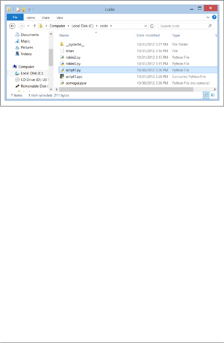
prints and exits—the console window appears, and text is printed there, but the console
window closes and disappears on program exit. Unless you are very fast, or your ma-
chine is very slow, you won’t get to see your output at all. Although this is normal
behavior, it’s probably not what you had in mind.
Luckily, it’s easy to work around this. If you need your script’s output to stick around
when you launch it with an icon click, simply put a call to the built-in input function
at the very bottom of the script in 3.X (in 2.X use the name raw_input instead: see the
note ahead). For example:
# A first Python script
import sys # Load a library module
print(sys.platform)
print(2 ** 100) # Raise 2 to a power
x = 'Spam!'
print(x * 8) # String repetition
input() # <== ADDED
In general, input reads and returns the next line of standard input, waiting if there is
none yet available. The net effect in this context will be to pause the script, thereby
keeping the output window shown in Figure 3-2 open until you press the Enter key.
Now that I’ve shown you this trick, keep in mind that it is usually only required for
Windows, and then only if your script prints text and exits and only if you will launch
the script by clicking its file icon. You should add this call to the bottom of your top-
level files if and only if all of these three conditions apply. There is no reason to add
this call in any other contexts, such as scripts you’ll run in command lines or the IDLE
GUI (unless you’re unreasonably fond of pressing your computer’s Enter key!).2 That
may sound obvious, but it’s been another common mistake in live classes.
Figure 3-1. On Windows, Python program files show up as icons in file explorer windows and can
automatically be run with a double-click of the mouse (though you might not see printed output or
error messages this way).
64 | Chapter 3: How You Run Programs
www.it-ebooks.info
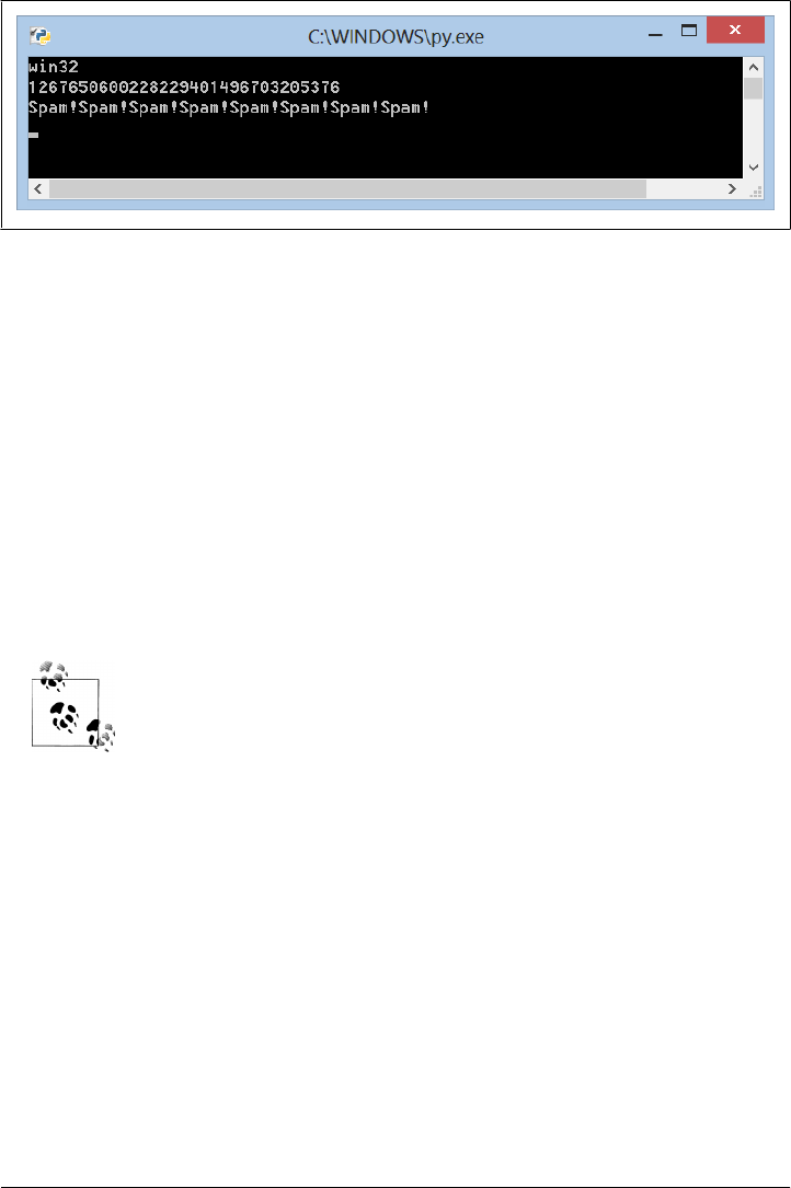
Before we move ahead, note that the input call applied here is the input counterpart of
using the print function (and 2.X statement) for outputs. It is the simplest way to read
user input, and it is more general than this example implies. For instance, input:
• Optionally accepts a string that will be printed as a prompt (e.g., input('Press
Enter to exit'))
• Returns to your script a line of text read as a string (e.g., nextinput = input())
• Supports input stream redirections at the system shell level (e.g., python spam.py
< input.txt), just as the print statement does for output
We’ll use input in more advanced ways later in this text; for instance, Chapter 10 will
apply it in an interactive loop. For now, it will help you see the output of simple scripts
that you click to launch.
Version skew note: If you are working in Python 2.X, use raw_input()
instead of input() in this code. The former was renamed to the latter in
Python 3.X. Technically, 2.X has an input function too, but it also eval-
uates strings as though they are program code typed into a script, and
so will not work in this context (an empty string is an error). Python
3.X’s input (and 2.X’s raw_input) simply returns the entered text as a
character string, unevaluated. To simulate 2.X’s input in 3.X, use
eval(input()).
Be aware, though, that because this runs the entered text as though it
were program code, this may have security implications that we’ll largely
Figure 3-2. When you click a program’s icon on Windows, you will be able to see its printed output
if you include an input call at the very end of the script. But you only need to do so in this one context!
2. Conversely, it is also possible to completely suppress the pop-up console window (a.k.a. Command
Prompt) for clicked files on Windows when you don’t want to see printed text. Files whose names end in
a .pyw extension will display only windows constructed by your script, not the default console
window. .pyw files are simply .py source files that have this special operational behavior on Windows.
They are mostly used for Python-coded user interfaces that build windows of their own, often in
conjunction with various techniques for saving printed output and errors to files. As implied earlier,
Python achieves this when it is installed by associating a special executable (pythonw.exe in 3.2 and earlier
and pyw.exe as of 3.3) to open .pyw files when clicked.
Clicking File Icons | 65
www.it-ebooks.info

ignore here, except to say that you should trust the source of the entered
text; if you don’t, stick to just plain input in 3.X and raw_input in 2.X.
Other Icon-Click Limitations
Even with the prior section’s input trick, clicking file icons is not without its perils. You
also may not get to see Python error messages. If your script generates an error, the
error message text is written to the pop-up console window—which then immediately
disappears! Worse, adding an input call to your file will not help this time because your
script will likely abort long before it reaches this call. In other words, you won’t be able
to tell what went wrong.
When we discuss exceptions later in this book, you’ll learn that it is possible to write
code to intercept, process, and recover from errors so that they do not terminate your
programs. Watch for the discussion of the try statement later in this book for an al-
ternative way to keep the console window from closing on errors. We’ll also learn how
to redirect printed text to files for later inspection when we study print operations.
Barring such support in your code, though, errors and prints disappear for clicked
programs.
Because of these limitations, it is probably best to view icon clicks as a way to launch
programs after they have been debugged, or have been instrumented to write their
output to a file and catch and process any important errors. Especially when you’re
starting out, I recommend using other techniques—such as system command lines and
IDLE (discussed further in the section “The IDLE User Interface” on page 73)—so
that you can see generated error messages and view your normal output without re-
sorting to extra coding.
Module Imports and Reloads
So far, I’ve been talking about “importing modules” without really explaining what this
term means. We’ll study modules and larger program architecture in depth in Part V,
but because imports are also a way to launch programs, this section will introduce
enough module basics to get you started.
Import and Reload Basics
In simple terms, every file of Python source code whose name ends in a .py extension
is a module. No special code or syntax is required to make a file a module: any such
file will do. Other files can access the items a module defines by importing that module
—import operations essentially load another file and grant access to that file’s contents.
The contents of a module are made available to the outside world through its attributes
(a term I’ll define in the next section).
66 | Chapter 3: How You Run Programs
www.it-ebooks.info

This module-based services model turns out to be the core idea behind program archi-
tecture in Python. Larger programs usually take the form of multiple module files, which
import tools from other module files. One of the modules is designated as the main or
top-level file, or “script”—the file launched to start the entire program, which runs line
by line as usual. Below this level, it’s all modules importing modules.
We’ll delve into such architectural issues in more detail later in this book. This chapter
is mostly interested in the fact that import operations run the code in a file that is being
loaded as a final step. Because of this, importing a file is yet another way to launch it.
For instance, if you start an interactive session (from a system command line or other-
wise), you can run the script1.py file you created earlier with a simple import (be sure
to delete the input line you added in the prior section first, or you’ll need to press Enter
for no reason):
C:\code> C:\python33\python
>>> import script1
win32
1267650600228229401496703205376
Spam!Spam!Spam!Spam!Spam!Spam!Spam!Spam!
This works, but only once per session (really, process—a program run) by default. After
the first import, later imports do nothing, even if you change and save the module’s
source file again in another window:
...Change script1.py in a text edit window to print 2 ** 16...
>>> import script1
>>> import script1
This is by design; imports are too expensive an operation to repeat more than once per
file, per program run. As you’ll learn in Chapter 22, imports must find files, compile
them to byte code, and run the code.
If you really want to force Python to run the file again in the same session without
stopping and restarting the session, you need to instead call the reload function avail-
able in the imp standard library module (this function is also a simple built-in in Python
2.X, but not in 3.X):
>>> from imp import reload # Must load from module in 3.X (only)
>>> reload(script1)
win32
65536
Spam!Spam!Spam!Spam!Spam!Spam!Spam!Spam!
<module 'script1' from '.\\script1.py'>
>>>
The from statement here simply copies a name out of a module (more on this soon).
The reload function itself loads and runs the current version of your file’s code, picking
up changes if you’ve modified and saved it in another window.
Module Imports and Reloads | 67
www.it-ebooks.info

This allows you to edit and pick up new code on the fly within the current Python
interactive session. In this session, for example, the second print statement in
script1.py was changed in another window to print 2 ** 16 between the time of the
first import and the reload call—hence the different result.
The reload function expects the name of an already loaded module object, so you have
to have successfully imported a module once before you reload it (if the import reported
an error, you can’t yet reload and must import again). Notice that reload also expects
parentheses around the module object name, whereas import does not. reload is a
function that is called, and import is a statement.
That’s why you must pass the module name to reload as an argument in parentheses,
and that’s why you get back an extra output line when reloading—the last output line
is just the display representation of the reload call’s return value, a Python module
object. We’ll learn more about using functions in general in Chapter 16; for now, when
you hear “function,” remember that parentheses are required to run a call.
Version skew note: Python 3.X moved the reload built-in function to the
imp standard library module. It still reloads files as before, but you must
import it in order to use it. In 3.X, run an import imp and use
imp.reload(M), or run a from imp import reload and use reload(M), as
shown here. We’ll discuss import and from statements in the next sec-
tion, and more formally later in this book.
If you are working in Python 2.X, reload is available as a built-in func-
tion, so no import is required. In Python 2.6 and 2.7, reload is available
in both forms—built-in and module function—to aid the transition to
3.X. In other words, reloading is still available in 3.X, but an extra line
of code is required to fetch the reload call.
The move in 3.X was likely motivated in part by some well-known issues
involving reload and from statements that we’ll encounter in the next
section. In short, names loaded with a from are not directly updated by
a reload, but names accessed with an import statement are. If your
names don’t seem to change after a reload, try using import and mod
ule.attribute name references instead.
The Grander Module Story: Attributes
Imports and reloads provide a natural program launch option because import opera-
tions execute files as a last step. In the broader scheme of things, though, modules serve
the role of libraries of tools, as you’ll learn in detail in Part V. The basic idea is straight-
forward, though: a module is mostly just a package of variable names, known as a
namespace, and the names within that package are called attributes. An attribute is
simply a variable name that is attached to a specific object (like a module).
In more concrete terms, importers gain access to all the names assigned at the top level
of a module’s file. These names are usually assigned to tools exported by the module
68 | Chapter 3: How You Run Programs
www.it-ebooks.info

—functions, classes, variables, and so on—that are intended to be used in other files
and other programs. Externally, a module file’s names can be fetched with two Python
statements, import and from, as well as the reload call.
To illustrate, use a text editor to create a one-line Python module file called myfile.py
in your working directory, with the following contents:
title = "The Meaning of Life"
This may be one of the world’s simplest Python modules (it contains a single assignment
statement), but it’s enough to illustrate the point. When this file is imported, its code
is run to generate the module’s attribute. That is, the assignment statement creates a
variable and module attribute named title.
You can access this module’s title attribute in other components in two different ways.
First, you can load the module as a whole with an import statement, and then qualify
the module name with the attribute name to fetch it (note that we’re letting the inter-
preter print automatically here):
% python # Start Python
>>> import myfile # Run file; load module as a whole
>>> myfile.title # Use its attribute names: '.' to qualify
'The Meaning of Life'
In general, the dot expression syntax object.attribute lets you fetch any attribute
attached to any object, and is one of the most common operations in Python code.
Here, we’ve used it to access the string variable title inside the module myfile—in
other words, myfile.title.
Alternatively, you can fetch (really, copy) names out of a module with from statements:
% python # Start Python
>>> from myfile import title # Run file; copy its names
>>> title # Use name directly: no need to qualify
'The Meaning of Life'
As you’ll see in more detail later, from is just like an import, with an extra assignment
to names in the importing component. Technically, from copies a module’s attributes,
such that they become simple variables in the recipient—thus, you can simply refer to
the imported string this time as title (a variable) instead of myfile.title (an attribute
reference).3
Whether you use import or from to invoke an import operation, the statements in the
module file myfile.py are executed, and the importing component (here, the interactive
prompt) gains access to names assigned at the top level of the file. There’s only one
such name in this simple example—the variable title, assigned to a string—but the
3. Notice that import and from both list the name of the module file as simply myfile without its .py extension
suffix. As you’ll learn in Part V, when Python looks for the actual file, it knows to include the suffix in its
search procedure. Again, you must include the .py suffix in system shell command lines, but not in
import statements.
Module Imports and Reloads | 69
www.it-ebooks.info

concept will be more useful when you start defining objects such as functions and
classes in your modules: such objects become reusable software components that can
be accessed by name from one or more client modules.
In practice, module files usually define more than one name to be used in and outside
the files. Here’s an example that defines three:
a = 'dead' # Define three attributes
b = 'parrot' # Exported to other files
c = 'sketch'
print(a, b, c) # Also used in this file (in 2.X: print a, b, c)
This file, threenames.py, assigns three variables, and so generates three attributes for
the outside world. It also uses its own three variables in a 3.X print statement, as we
see when we run this as a top-level file (in Python 2.X print differs slightly, so omit its
outer parenthesis to match the output here exactly; watch for a more complete ex-
planation of this in Chapter 11):
% python threenames.py
dead parrot sketch
All of this file’s code runs as usual the first time it is imported elsewhere, by either an
import or from. Clients of this file that use import get a module with attributes, while
clients that use from get copies of the file’s names:
% python
>>> import threenames # Grab the whole module: it runs here
dead parrot sketch
>>>
>>> threenames.b, threenames.c # Access its attributes
('parrot', 'sketch')
>>>
>>> from threenames import a, b, c # Copy multiple names out
>>> b, c
('parrot', 'sketch')
The results here are printed in parentheses because they are really tuples—a kind of
object created by the comma in the inputs (and covered in the next part of this book)
—that you can safely ignore for now.
Once you start coding modules with multiple names like this, the built-in dir function
starts to come in handy—you can use it to fetch a list of all the names available inside
a module. The following returns a Python list of strings in square brackets (we’ll start
studying lists in the next chapter):
>>> dir(threenames)
['__builtins__', '__doc__', '__file__', '__name__', '__package__', 'a', 'b', 'c']
The contents of this list have been edited here because they vary per Python version.
The point to notice here is that when the dir function is called with the name of an
imported module in parentheses like this, it returns all the attributes inside that module.
Some of the names it returns are names you get “for free”: names with leading and
trailing double underscores (__X__) are built-in names that are always predefined by
70 | Chapter 3: How You Run Programs
www.it-ebooks.info
Python and have special meaning to the interpreter, but they aren’t important at this
point in this book. The variables our code defined by assignment—a, b, and c—show
up last in the dir result.
Modules and namespaces
Module imports are a way to run files of code, but, as we’ll expand on later in the book,
modules are also the largest program structure in Python programs, and one of the first
key concepts in the language.
As we’ve seen, Python programs are composed of multiple module files linked together
by import statements, and each module file is a package of variables—that is, a name-
space. Just as importantly, each module is a self-contained namespace: one module file
cannot see the names defined in another file unless it explicitly imports that other file.
Because of this, modules serve to minimize name collisions in your code—because each
file is a self-contained namespace, the names in one file cannot clash with those in
another, even if they are spelled the same way.
In fact, as you’ll see, modules are one of a handful of ways that Python goes to great
lengths to package your variables into compartments to avoid name clashes. We’ll
discuss modules and other namespace constructs—including local scopes defined by
classes and functions—further later in the book. For now, modules will come in handy
as a way to run your code many times without having to retype it, and will prevent your
file’s names from accidentally replacing each other.
import versus from: I should point out that the from statement in a sense
defeats the namespace partitioning purpose of modules—because the
from copies variables from one file to another, it can cause same-named
variables in the importing file to be overwritten, and won’t warn you if
it does. This essentially collapses namespaces together, at least in terms
of the copied variables.
Because of this, some recommend always using import instead of from.
I won’t go that far, though; not only does from involve less typing (an
asset at the interactive prompt), but its purported problem is relatively
rare in practice. Besides, this is something you control by listing the
variables you want in the from; as long as you understand that they’ll be
assigned to values in the target module, this is no more dangerous than
coding assignment statements—another feature you’ll probably want
to use!
Usage Notes: import and reload
For some reason, once people find out about running files using import and reload,
many tend to focus on this alone and forget about other launch options that always
run the current version of the code (e.g., icon clicks, IDLE menu options, and system
command lines). This approach can quickly lead to confusion, though—you need to
Module Imports and Reloads | 71
www.it-ebooks.info

remember when you’ve imported to know if you can reload, you need to remember to
use parentheses when you call reload (only), and you need to remember to use
reload in the first place to get the current version of your code to run. Moreover, reloads
aren’t transitive—reloading a module reloads that module only, not any modules it
may import—so you sometimes have to reload multiple files.
Because of these complications (and others we’ll explore later, including the reload/
from issue mentioned briefly in a prior note in this chapter), it’s generally a good idea
to avoid the temptation to launch by imports and reloads for now. The IDLE
Run→Run Module menu option described in the next section, for example, provides a
simpler and less error-prone way to run your files, and always runs the current version
of your code. System shell command lines offer similar benefits. You don’t need to use
reload if you use any of these other techniques.
In addition, you may run into trouble if you use modules in unusual ways at this point
in the book. For instance, if you want to import a module file that is stored in a directory
other than the one you’re working in, you’ll have to skip ahead to Chapter 22 and learn
about the module search path. For now, if you must import, try to keep all your files in
the directory you are working in to avoid complications.4
That said, imports and reloads have proven to be a popular testing technique in Python
classes, and you may prefer using this approach too. As usual, though, if you find
yourself running into a wall, stop running into a wall!
Using exec to Run Module Files
Strictly speaking, there are more ways to run code stored in module files than have yet
been presented here. For instance, the exec(open('module.py').read()) built-in func-
tion call is another way to launch files from the interactive prompt without having to
import and later reload. Each such exec runs the current version of the code read from
a file, without requiring later reloads (script1.py is as we left it after a reload in the prior
section):
% python
>>> exec(open('script1.py').read())
win32
65536
Spam!Spam!Spam!Spam!Spam!Spam!Spam!Spam!
...Change script1.py in a text edit window to print 2 ** 32...
>>> exec(open('script1.py').read())
4. If you’re too curious to wait, the short story is that Python searches for imported modules in every directory
listed in sys.path—a Python list of directory name strings in the sys module, which is initialized from a
PYTHONPATH environment variable, plus a set of standard directories. If you want to import from a directory
other than the one you are working in, that directory must generally be listed in your PYTHONPATH setting.
For more details, see Chapter 22 and Appendix A.
72 | Chapter 3: How You Run Programs
www.it-ebooks.info

win32
4294967296
Spam!Spam!Spam!Spam!Spam!Spam!Spam!Spam!
The exec call has an effect similar to an import, but it doesn’t actually import the module
—by default, each time you call exec this way it runs the file’s code anew, as though
you had pasted it in at the place where exec is called. Because of that, exec does not
require module reloads after file changes—it skips the normal module import logic.
On the downside, because it works as if you’ve pasted code into the place where it is
called, exec, like the from statement mentioned earlier, has the potential to silently
overwrite variables you may currently be using. For example, our script1.py assigns to
a variable named x. If that name is also being used in the place where exec is called, the
name’s value is replaced:
>>> x = 999
>>> exec(open('script1.py').read()) # Code run in this namespace by default
...same output...
>>> x # Its assignments can overwrite names here
'Spam!'
By contrast, the basic import statement runs the file only once per process, and it makes
the file a separate module namespace so that its assignments will not change variables
in your scope. The price you pay for the namespace partitioning of modules is the need
to reload after changes.
Version skew note: Python 2.X also includes an execfile('module.py')
built-in function, in addition to allowing the form exec(open('mod
ule.py')), which both automatically read the file’s content. Both of
these are equivalent to the exec(open('module.py').read()) form,
which is more complex but runs in both 2.X and 3.X.
Unfortunately, neither of these two simpler 2.X forms is available in 3.X,
which means you must understand both files and their read methods to
fully understand this technique today (this seems to be a case of aes-
thetics trouncing practicality in 3.X). In fact, the exec form in 3.X in-
volves so much typing that the best advice may simply be not to do it—
it’s usually easier to launch files by typing system shell command lines
or by using the IDLE menu options described in the next section.
For more on the file interfaces used by the 3.X exec form, see Chap-
ter 9. For more on exec and its cohorts, eval and compile, see Chap-
ter 10 and Chapter 25.
The IDLE User Interface
So far, we’ve seen how to run Python code with the interactive prompt, system com-
mand lines, Unix-style scripts, icon clicks, module imports, and exec calls. If you’re
looking for something a bit more visual, IDLE provides a graphical user interface for
The IDLE User Interface | 73
www.it-ebooks.info

doing Python development, and it’s a standard and free part of the Python system. IDLE
is usually referred to as an integrated development environment (IDE), because it binds
together various development tasks into a single view.5
In short, IDLE is a desktop GUI that lets you edit, run, browse, and debug Python
programs, all from a single interface. It runs portably on most Python platforms, in-
cluding Microsoft Windows, X Windows (for Linux, Unix, and Unix-like platforms),
and the Mac OS (both Classic and OS X). For many, IDLE represents an easy-to-use
alternative to typing command lines, a less problem-prone alternative to clicking on
icons, and a great way for newcomers to get started editing and running code. You’ll
sacrifice some control in the bargain, but this typically becomes important later in your
Python career.
IDLE Startup Details
Most readers should be able to use IDLE immediately, as it is a standard component
on Mac OS X and most Linux installations today, and is installed automatically with
standard Python on Windows. Because platforms specifics vary, though, I need to give
a few pointers before we open the GUI.
Technically, IDLE is a Python program that uses the standard library’s tkinter GUI
toolkit (named Tkinter in Python 2.X) to build its windows. This makes IDLE portable
—it works the same on all major desktop platforms—but it also means that you’ll need
to have tkinter support in your Python to use IDLE. This support is standard on Win-
dows, Macs, and Linux, but it comes with a few caveats on some systems, and startup
can vary per platform. Here are a few platform-specific tips:
• On Windows 7 and earlier, IDLE is easy to start—it’s always present after a Python
install, and has an entry in the Start button menu for Python in Windows 7 and
earlier (see Figure 2-1, shown previously). You can also select it by right-clicking
on a Python program icon, and launch it by clicking on the icon for the files
idle.pyw or idle.py located in the idlelib subdirectory of Python’s Lib directory. In
this mode, IDLE is a clickable Python script that lives in C:\Python33\Lib\idlelib,
C:\Python27\Lib\idlelib, or similar, which you can drag out to a shortcut for one-
click access if desired.
• On Windows 8, look for IDLE in your Start tiles, by a search for “idle,” by browsing
your “All apps” Start screen display, or by using File Explorer to find the idle.py
file mentioned earlier. You may want a shortcut here, as you have no Start button
menu in desktop mode (at least today; see Appendix A for more pointers).
• On Mac OS X everything required for IDLE is present as standard components in
your operating system. IDLE should be available to launch in Applications under
the MacPython (or Python N.M) program folder. One note here: some OS X ver-
5. IDLE is officially a corruption of IDE, but it’s really named in honor of Monty Python member Eric Idle.
See Chapter 1 if you’re not sure why.
74 | Chapter 3: How You Run Programs
www.it-ebooks.info

sions may require installing updated tkinter support due to subtle version depen-
dencies I’ll spare readers from here; see python.org’s Download page for details.
• On Linux IDLE is also usually present as a standard component today. It might
take the form of an idle executable or script in your path; type this in a shell to
check. On some machines, it may require an install (see Appendix A for pointers),
and on others you may need to launch IDLE’s top-level script from a command
line or icon click: run the file idle.py located in the idlelib subdirectory of
Python’s /usr/lib directory (run a find for the exact location).
Because IDLE is just a Python script on the module search path in the standard library,
you can also generally run it on any platform and from any directory by typing the
following in a system command shell window (e.g., in a Command Prompt on Win-
dows), though you’ll have to see Appendix A for more on Python’s –m flag, and
Part V for more on the “.” package syntax required here (blind trust will suffice at this
point in the book):
c:\code> python -m idlelib.idle # Run idle.py in a package on module path
For more on install issues and usage notes for Windows and other platforms, be sure
to see both Appendix A as well as the notes for your platform in “Python Setup and
Usage” in Python’s standard manuals.
IDLE Basic Usage
Let’s jump into an example. Figure 3-3 shows the scene after you start IDLE on Win-
dows. The Python shell window that opens initially is the main window, which runs
an interactive session (notice the >>> prompt). This works like all interactive sessions
—code you type here is run immediately after you type it—and serves as a testing and
experimenting tool.
IDLE uses familiar menus with keyboard shortcuts for most of its operations. To make
a new script file under IDLE, use File→New: in the main shell window, select the File
pull-down menu, and pick New to open a new text edit window where you can type,
save, and run your file’s code. Use File→Open... instead to open a new text edit window
displaying an existing file’s code to edit and run.
Although it may not show up fully in this book’s graphics, IDLE uses syntax-directed
colorization for the code typed in both the main window and all text edit windows—
keywords are one color, literals are another, and so on. This helps give you a better
picture of the components in your code (and can even help you spot mistakes—run-
on strings are all one color, for example).
To run a file of code that you are editing in IDLE, use Run→Run Module in that file’s
text edit window. That is, select the file’s text edit window, open that window’s Run
pull-down menu, and choose the Run Module option listed there (or use the equivalent
keyboard shortcut, given in the menu). Python will let you know that you need to save
The IDLE User Interface | 75
www.it-ebooks.info
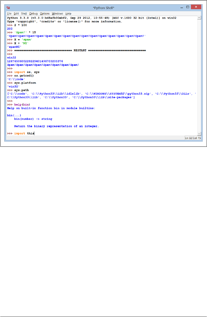
your file first if you’ve changed it since it was opened or last saved and forgot to save
your changes—a common mistake when you’re knee-deep in coding.
When run this way, the output of your script and any error messages it may generate
show up back in the main interactive window (the Python shell window). In Fig-
ure 3-3, for example, the three lines after the “RESTART” line near the middle of the
window reflect an execution of our script1.py file opened in a separate edit window.
The “RESTART” message tells us that the user-code process was restarted to run the
edited script and serves to separate script output (it does not appear if IDLE is started
without a user-code subprocess—more on this mode in a moment).
IDLE Usability Features
Like most GUIs, the best way to learn IDLE may be to test-drive it for yourself, but
some key usage points seem to be less than obvious. For example, if you want to repeat
prior commands in IDLE’s main interactive window, you can use the Alt-P key combi-
nation to scroll backward through the command history, and Alt-N to scroll forward
(on some Macs, try Ctrl-P and Ctrl-N instead). Your prior commands will be recalled
and displayed, and may be edited and rerun.
Figure 3-3. The main Python shell window of the IDLE development GUI, shown here running on
Windows. Use the File menu to begin (New Window) or change (Open...) a source file; use the text
edit window’s Run menu to run the code in that window (Run Module).
76 | Chapter 3: How You Run Programs
www.it-ebooks.info

You can also recall commands by positioning the cursor on them and clicking and
pressing Enter to insert their text at the input prompt, or using standard cut-and-paste
operations, though these techniques tend to involve more steps (and can sometimes be
triggered accidentally). Outside IDLE, you may be able to recall commands in an in-
teractive session with the arrow keys on Windows.
Besides command history and syntax colorization, IDLE has additional usability fea-
tures such as:
•Auto-indent and unindent for Python code in the editor (Backspace goes back one
level)
• Word auto-completion while typing, invoked by a Tab press
• Balloon help pop ups for a function call when you type its opening “(”
• Pop-up selection lists of object attributes when you type a “.” after an object’s name
and either pause or press Tab
Some of these may not work on every platform, and some can be configured or disabled
if you find that their defaults get in the way of your personal coding style.
Advanced IDLE Tools
Besides the basic edit and run functions and the prior section’s usability tools, IDLE
provides more advanced features, including a point-and-click program graphical de-
bugger and an object browser. The IDLE debugger is enabled via the Debug menu and
the object browser via the File menu. The browser allows you to navigate through the
module search path to files and objects in files; clicking on a file or object opens the
corresponding source in a text edit window.
You initiate IDLE debugging by selecting the Debug→Debugger menu option in the
main window and then starting your script by selecting the Run→Run Module option
in the text edit window; once the debugger is enabled, you can set breakpoints in your
code that stop its execution by right-clicking on lines in the text edit windows, show
variable values, and so on. You can also watch program execution when debugging—
the current line of code is noted as you step through your code.
For simpler debugging operations, you can also right-click with your mouse on the text
of an error message to quickly jump to the line of code where the error occurred—a
trick that makes it simple and fast to repair and run again. In addition, IDLE’s text
editor offers a large collection of programmer-friendly tools, including advanced text
and file search operations we won’t cover here. Because IDLE uses intuitive GUI in-
teractions, you should experiment with the system live to get a feel for its other tools.
The IDLE User Interface | 77
www.it-ebooks.info

Usage Notes: IDLE
IDLE is free, easy to use, portable, and automatically available on most platforms. I
generally recommend it to Python newcomers because it simplifies some startup details
and does not assume prior experience with system command lines. However, it is
somewhat limited compared to more advanced commercial IDEs, and may seem heav-
ier than a command line to some. To help you avoid some common pitfalls, here is a
list of issues that IDLE beginners should bear in mind:
•You must add “.py” explicitly when saving your files. I mentioned this when
talking about files in general, but it’s a common IDLE stumbling block, especially
for Windows users. IDLE does not automatically add a .py extension to filenames
when files are saved. Be careful to type the .py extension yourself when saving a
file for the first time. If you don’t, while you will be able to run your file from IDLE
(and system command lines), you will not be able to import it either interactively
or from other modules.
•Run scripts by selecting Run→Run Module in text edit windows, not by in-
teractive imports and reloads. Earlier in this chapter, we saw that it’s possible
to run a file by importing it interactively. However, this scheme can grow complex
because it requires you to manually reload files after changes. By contrast, using
the Run→Run Module menu option in IDLE always runs the most current version
of your file, just like running it using a system shell command line. IDLE also
prompts you to save your file first, if needed (another common mistake outside
IDLE).
•You need to reload only modules being tested interactively. Like system shell
command lines, IDLE’s Run→Run Module menu option always runs the current
version of both the top-level file and any modules it imports. Because of this,
Run→Run Module eliminates common confusions surrounding imports. You need
to reload only modules that you are importing and testing interactively in IDLE. If
you choose to use the import and reload technique instead of Run→Run Module,
remember that you can use the Alt-P/Alt-N key combinations to recall prior com-
mands.
•You can customize IDLE. To change the text fonts and colors in IDLE, select the
Configure option in the Options menu of any IDLE window. You can also cus-
tomize key combination actions, indentation settings, autocompletions, and more;
see IDLE’s Help pull-down menu for more hints.
•There is currently no clear-screen option in IDLE. This seems to be a frequent
request (perhaps because it’s an option available in similar IDEs), and it might be
added eventually. Today, though, there is no way to clear the interactive window’s
text. If you want the window’s text to go away, you can either press and hold the
Enter key, or type a Python loop to print a series of blank lines (nobody really uses
the latter technique, of course, but it sounds more high-tech than pressing the Enter
key!).
78 | Chapter 3: How You Run Programs
www.it-ebooks.info

•tkinter GUI and threaded programs may not work well with IDLE. Because
IDLE is a Python/tkinter program, it can hang if you use it to run certain types of
advanced Python/tkinter programs. This has become less of an issue in more recent
versions of IDLE that run user code in one process and the IDLE GUI itself in
another, but some programs (especially those that use multithreading) might still
hang the GUI. Even just calling the tkinter quit function in your code, the normal
way to exit a GUI program, may be enough to cause your program’s GUI to hang
if run in IDLE (destroy may be better here only). Your code may not exhibit such
problems, but as a rule of thumb, it’s always safe to use IDLE to edit GUI programs
but launch them using other options, such as icon clicks or system command lines.
When in doubt, if your code fails in IDLE, try it outside the GUI.
•If connection errors arise, try starting IDLE in single-process mode. This
issue appears to have gone away in recent Pythons, but may still impact readers
using older versions. Because IDLE requires communication between its separate
user and GUI processes, it can sometimes have trouble starting up on certain plat-
forms (notably, it fails to start occasionally on some Windows machines, due to
firewall software that blocks connections). If you run into such connection errors,
it’s always possible to start IDLE with a system command line that forces it to run
in single-process mode without a user-code subprocess and therefore avoids com-
munication issues: its -n command-line flag forces this mode. On Windows, for
example, start a Command Prompt window and run the system command line
idle.py -n from within the directory C:\Python33\Lib\idlelib (cd there first if
needed). A python -m idlelib.idle –n command works from anywhere (see Ap-
pendix A for –m).
•Beware of some IDLE usability features. IDLE does much to make life easier
for beginners, but some of its tricks won’t apply outside the IDLE GUI. For in-
stance, IDLE runs your scripts in its own interactive namespace, so variables in
your code show up automatically in the IDLE interactive session—you don’t al-
ways need to run import commands to access names at the top level of files you’ve
already run. This can be handy, but it can also be confusing, because outside the
IDLE environment names must always be imported from files explicitly to be used.
When you run a file of code, IDLE also automatically changes to that file’s direc-
tory and adds it to the module import search path—a handy feature that allows
you to use files and import modules there without search path settings, but also
something that won’t work the same when you run files outside IDLE. It’s OK to
use such features, but don’t forget that they are IDLE behavior, not Python be-
havior.
Other IDEs
Because IDLE is free, portable, and a standard part of Python, it’s a nice first develop-
ment tool to become familiar with if you want to use an IDE at all. Again, I recommend
Other IDEs | 79
www.it-ebooks.info

that you use IDLE for this book’s exercises if you’re just starting out, unless you are
already familiar with and prefer a command-line-based development mode. There are,
however, a handful of alternative IDEs for Python developers, some of which are sub-
stantially more powerful and robust than IDLE. Apart from IDLE, here are some of
Python’s most commonly used IDEs:
Eclipse and PyDev
Eclipse is an advanced open source IDE GUI. Originally developed as a Java IDE,
Eclipse also supports Python development when you install the PyDev (or a similar)
plug-in. Eclipse is a popular and powerful option for Python development, and it
goes well beyond IDLE’s feature set. It includes support for code completion, syn-
tax highlighting, syntax analysis, refactoring, debugging, and more. Its downsides
are that it is a large system to install and may require shareware extensions for some
features (this may vary over time). Still, when you are ready to graduate from IDLE,
the Eclipse/PyDev combination is worth your attention.
Komodo
A full-featured development environment GUI for Python (and other languages),
Komodo includes standard syntax coloring, text editing, debugging, and other
features. In addition, Komodo offers many advanced features that IDLE does not,
including project files, source-control integration, and regular-expression debug-
ging. At this writing, Komodo is not free, but see the Web for its current status—
it is available at http://www.activestate.com from ActiveState, which also offers the
ActivePython distribution package mentioned in Appendix A.
NetBeans IDE for Python
NetBeans is a powerful open source development environment GUI with support
for many advanced features for Python developers: code completion, automatic
indentation and code colorization, editor hints, code folding, refactoring, debug-
ging, code coverage and testing, projects, and more. It may be used to develop both
CPython and Jython code. Like Eclipse, NetBeans requires installation steps be-
yond those of the included IDLE GUI, but it is seen by many as more than worth
the effort. Search the Web for the latest information and links.
PythonWin
PythonWin is a free Windows-only IDE for Python that ships as part of Active-
State’s ActivePython distribution (and may also be fetched separately from http://
www.python.org resources). It is roughly like IDLE, with a handful of useful Win-
dows-specific extensions added; for example, PythonWin has support for COM
objects. Today, IDLE is probably more advanced than PythonWin (for instance,
IDLE’s dual-process architecture often prevents it from hanging). However, Py-
thonWin still offers tools for Windows developers that IDLE does not. See http://
www.activestate.com for more information.
Wing, Visual Studio, and others
Other IDEs are popular among Python developers too, including the mostly com-
mercial Wing IDE, Microsoft Visual Studio via a plug-in, and PyCharm, PyScrip-
80 | Chapter 3: How You Run Programs
www.it-ebooks.info

ter, Pyshield, and Spyder—but I do not have space to do justice to them here, and
more will undoubtedly appear over time. In fact, almost every programmer-friendly
text editor has some sort of support for Python development these days, whether
it be preinstalled or fetched separately. Emacs and Vim, for instance, have sub-
stantial Python support.
IDE choices are often subjective, so I encourage you to browse to find tools that
fit your development style and goals. For more information, see the resources
available at http://www.python.org or search the Web for “Python IDE” or similar.
A search for “Python editors” today leads you to a wiki page that maintains infor-
mation about dozens of IDE and text-editor options for Python programming.
Other Launch Options
At this point, we’ve seen how to run code typed interactively, and how to launch code
saved in files in a variety of ways—system command lines, icon clicks, imports and
execs, GUIs like IDLE, and more. That covers most of the techniques in common use,
and enough to run the code you’ll see in this book. There are additional ways to run
Python code, though, most of which have special or narrow roles. For completeness
and reference, the next few sections take a quick look at some of these.
Embedding Calls
In some specialized domains, Python code may be run automatically by an enclosing
system. In such cases, we say that the Python programs are embedded in (i.e., run by)
another program. The Python code itself may be entered into a text file, stored in a
database, fetched from an HTML page, parsed from an XML document, and so on.
But from an operational perspective, another system—not you—may tell Python to
run the code you’ve created.
Such an embedded execution mode is commonly used to support end-user customi-
zation—a game program, for instance, might allow for play modifications by running
user-accessible embedded Python code at strategic points in time. Users can modify
this type of system by providing or changing Python code. Because Python code is
interpreted, there is no need to recompile the entire system to incorporate the change
(see Chapter 2 for more on how Python code is run).
In this mode, the enclosing system that runs your code might be written in C, C++, or
even Java when the Jython system is used. As an example, it’s possible to create and
run strings of Python code from a C program by calling functions in the Python runtime
API (a set of services exported by the libraries created when Python is compiled on your
machine):
#include <Python.h>
...
Other Launch Options | 81
www.it-ebooks.info

Py_Initialize(); // This is C, not Python
PyRun_SimpleString("x = 'brave ' + 'sir robin'"); // But it runs Python code
In this C code snippet, a program coded in the C language embeds the Python inter-
preter by linking in its libraries, and passes it a Python assignment statement string to
run. C programs may also gain access to Python modules and objects and process or
execute them using other Python API tools.
This book isn’t about Python/C integration, but you should be aware that, depending
on how your organization plans to use Python, you may or may not be the one who
actually starts the Python programs you create. Regardless, you can usually still use the
interactive and file-based launching techniques described here to test code in isolation
from those enclosing systems that may eventually use it.6
Frozen Binary Executables
Frozen binary executables, described in Chapter 2, are packages that combine your
program’s byte code and the Python interpreter into a single executable program. This
approach enables Python programs to be launched in the same ways that you would
launch any other executable program (icon clicks, command lines, etc.). While this
option works well for delivery of products, it is not really intended for use during pro-
gram development; you normally freeze just before shipping (after development is fin-
ished). See the prior chapter for more on this option.
Text Editor Launch Options
As mentioned previously, although they’re not full-blown IDE GUIs, most program-
mer-friendly text editors have support for editing, and possibly running, Python pro-
grams. Such support may be built in or fetchable on the Web. For instance, if you are
familiar with the Emacs text editor, you can do all your Python editing and launching
from inside that text editor. See the text editor resources page at http://www.python
.org/editors for more details, or search the Web for the phrase “Python editors.”
Still Other Launch Options
Depending on your platform, there may be additional ways that you can start Python
programs. For instance, on some Macintosh systems you may be able to drag Python
program file icons onto the Python interpreter icon to make them execute, and on some
Windows systems you can always start Python scripts with the Run... option in the
Start menu. Additionally, the Python standard library has utilities that allow Python
programs to be started by other Python programs in separate processes (e.g., os.popen,
6. See Programming Python (O’Reilly) for more details on embedding Python in C/C++. The embedding
API can call Python functions directly, load modules, and more. Also, note that the Jython system allows
Java programs to invoke Python code using a Java-based API (a Python interpreter class).
82 | Chapter 3: How You Run Programs
www.it-ebooks.info

os.system), and Python scripts might also be spawned in larger contexts like the Web
(for instance, a web page might invoke a script on a server); however, these are beyond
the scope of the present chapter.
Future Possibilities?
This chapter reflects current practice, but much of the material is both platform- and
time-specific. Indeed, many of the execution and launch details presented arose during
the shelf life of this book’s various editions. As with program execution options, it’s
not impossible that new program launch options may arise over time.
New operating systems, and new versions of existing systems, may also provide exe-
cution techniques beyond those outlined here. In general, because Python keeps pace
with such changes, you should be able to launch Python programs in whatever way
makes sense for the machines you use, both now and in the future—be that by swiping
on tablet PCs and smartphones, grabbing icons in a virtual reality, or shouting a script’s
name over your coworkers’ conversations.
Implementation changes may also impact launch schemes somewhat (e.g., a full com-
piler could produce normal executables that are launched much like frozen binaries
today). If I knew what the future truly held, though, I would probably be talking to a
stockbroker instead of writing these words!
Which Option Should I Use?
With all these options, true beginners might naturally ask: which one is best for me?
In general, you should give the IDLE interface a try if you are just getting started with
Python. It provides a user-friendly GUI environment and hides some of the underlying
configuration details. It also comes with a platform-neutral text editor for coding your
scripts, and it’s a standard and free part of the Python system.
If, on the other hand, you are an experienced programmer, you might be more com-
fortable with simply the text editor of your choice in one window, and another window
for launching the programs you edit via system command lines and icon clicks (in fact,
this is how I develop Python programs, but I have a Unix-biased distant past). Because
the choice of development environments is very subjective, I can’t offer much more in
the way of universal guidelines. In general, whatever environment you like to use will
be the best for you to use.
Debugging Python Code
Naturally, none of my readers or students ever have bugs in their code (insert smiley
here), but for less fortunate friends of yours who may, here’s a quick review of the
strategies commonly used by real-world Python programmers to debug code, for you
to refer to as you start coding in earnest:
Which Option Should I Use? | 83
www.it-ebooks.info

•Do nothing. By this, I don’t mean that Python programmers don’t debug their
code—but when you make a mistake in a Python program, you get a very useful
and readable error message (you’ll get to see some soon, if you haven’t already).
If you already know Python, and especially for your own code, this is often enough
—read the error message, and go fix the tagged line and file. For many, this is
debugging in Python. It may not always be ideal for larger systems you didn’t write,
though.
•Insert print statements. Probably the main way that Python programmers debug
their code (and the way that I debug Python code) is to insert print statements and
run again. Because Python runs immediately after changes, this is usually the
quickest way to get more information than error messages provide. The print
statements don’t have to be sophisticated—a simple “I am here” or display of
variable values is usually enough to provide the context you need. Just remember
to delete or comment out (i.e., add a # before) the debugging prints before you
ship your code!
•Use IDE GUI debuggers. For larger systems you didn’t write, and for beginners
who want to trace code in more detail, most Python development GUIs have some
sort of point-and-click debugging support. IDLE has a debugger too, but it doesn’t
appear to be used very often in practice—perhaps because it has no command line,
or perhaps because adding print statements is usually quicker than setting up a
GUI debugging session. To learn more, see IDLE’s Help, or simply try it on your
own; its basic interface is described in the section “Advanced IDLE
Tools” on page 77. Other IDEs, such as Eclipse, NetBeans, Komodo, and Wing
IDE, offer advanced point-and-click debuggers as well; see their documentation if
you use them.
•Use the pdb command-line debugger. For ultimate control, Python comes with
a source code debugger named pdb, available as a module in Python’s standard
library. In pdb, you type commands to step line by line, display variables, set and
clear breakpoints, continue to a breakpoint or error, and so on. You can launch
pdb interactively by importing it, or as a top-level script. Either way, because you
can type commands to control the session, it provides a powerful debugging tool.
pdb also includes a postmortem function (pdb.pm()) that you can run after an
exception occurs, to get information from the time of the error. See the Python
library manual and Chapter 36 for more details on pdb, and Appendix A for an
example or running pdb as a script with Python’s –m command argument.
•Use Python’s –i command-line argument. Short of adding prints or running
under pdb, you can still see what went wrong on errors. If you run your script from
a command line and pass a -i argument between python and the name of your
script (e.g., python –i m.py), Python will enter into its interactive interpreter mode
(the >>> prompt) when your script exits, whether it ends successfully or runs into
an error. At this point, you can print the final values of variables to get more details
about what happened in your code because they are in the top-level namespace.
You can also then import and run the pdb debugger for even more context; its
postmortem mode will let you inspect the latest error if your script failed. Appen-
dix A also shows -i in action.
84 | Chapter 3: How You Run Programs
www.it-ebooks.info

•Other options. For more specific debugging requirements, you can find additional
tools in the open source domain, including support for multithreaded programs,
embedded code, and process attachment. The Winpdb system, for example, is a
standalone debugger with advanced debugging support and cross-platform GUI
and console interfaces.
These options will become more important as we start writing larger scripts. Probably
the best news on the debugging front, though, is that errors are detected and reported
in Python, rather than passing silently or crashing the system altogether. In fact, errors
themselves are a well-defined mechanism known as exceptions, which you can catch
and process (more on exceptions in Part VII). Making mistakes is never fun, of course,
but take it from someone who recalls when debugging meant getting out a hex calcu-
lator and poring over piles of memory dump printouts: Python’s debugging support
makes errors much less painful than they might otherwise be.
Chapter Summary
In this chapter, we’ve looked at common ways to launch Python programs: by running
code typed interactively, and by running code stored in files with system command
lines, file icon clicks, module imports, exec calls, and IDE GUIs such as IDLE. We’ve
covered a lot of pragmatic startup territory here. This chapter’s goal was to equip you
with enough information to enable you to start writing some code, which you’ll do in
the next part of the book. There, we will start exploring the Python language itself,
beginning with its core data types—the objects that are the subjects of your programs.
First, though, take the usual chapter quiz to exercise what you’ve learned here. Because
this is the last chapter in this part of the book, it’s followed with a set of more complete
exercises that test your mastery of this entire part’s topics. For help with the latter set
of problems, or just for a refresher, be sure to turn to Appendix D after you’ve given
the exercises a try.
Test Your Knowledge: Quiz
1. How can you start an interactive interpreter session?
2. Where do you type a system command line to launch a script file?
3. Name four or more ways to run the code saved in a script file.
4. Name two pitfalls related to clicking file icons on Windows.
5. Why might you need to reload a module?
6. How do you run a script from within IDLE?
7. Name two pitfalls related to using IDLE.
8. What is a namespace, and how does it relate to module files?
Test Your Knowledge: Quiz | 85
www.it-ebooks.info

Test Your Knowledge: Answers
1. You can start an interactive session on Windows 7 and earlier by clicking your Start
button, picking the All Programs option, clicking the Python entry, and selecting
the “Python (command line)” menu option. You can also achieve the same effect
on Windows and other platforms by typing python as a system command line in
your system’s console window (a Command Prompt window on Windows). An-
other alternative is to launch IDLE, as its main Python shell window is an interactive
session. Depending on your platform and Python, if you have not set your system’s
PATH variable to find Python, you may need to cd to where Python is installed, or
type its full directory path instead of just python (e.g., C:\Python33\python on Win-
dows, unless you’re using the 3.3 launcher).
2. You type system command lines in whatever your platform provides as a system
console: a Command Prompt window on Windows; an xterm or terminal window
on Unix, Linux, and Mac OS X; and so on. You type this at the system’s prompt,
not at the Python interactive interpreter’s “>>>” prompt—be careful not to con-
fuse these prompts.
3. Code in a script (really, module) file can be run with system command lines, file
icon clicks, imports and reloads, the exec built-in function, and IDE GUI selections
such as IDLE’s Run→Run Module menu option. On Unix, they can also be run as
executables with the #! trick, and some platforms support more specialized launch-
ing techniques (e.g., drag and drop). In addition, some text editors have unique
ways to run Python code, some Python programs are provided as standalone “fro-
zen binary” executables, and some systems use Python code in embedded mode,
where it is run automatically by an enclosing program written in a language like
C, C++, or Java. The latter technique is usually done to provide a user customi-
zation layer.
4. Scripts that print and then exit cause the output file to disappear immediately,
before you can view the output (which is why the input trick comes in handy);
error messages generated by your script also appear in an output window that
closes before you can examine its contents (which is one reason that system com-
mand lines and IDEs such as IDLE are better for most development).
5. Python imports (loads) a module only once per process, by default, so if you’ve
changed its source code and want to run the new version without stopping and
restarting Python, you’ll have to reload it. You must import a module at least once
before you can reload it. Running files of code from a system shell command line,
via an icon click, or via an IDE such as IDLE generally makes this a nonissue, as
those launch schemes usually run the current version of the source code file each
time.
6. Within the text edit window of the file you wish to run, select the window’s
Run→Run Module menu option. This runs the window’s source code as a top-level
script file and displays its output back in the interactive Python shell window.
86 | Chapter 3: How You Run Programs
www.it-ebooks.info

7. IDLE can still be hung by some types of programs—especially GUI programs that
perform multithreading (an advanced technique beyond this book’s scope). Also,
IDLE has some usability features that can burn you once you leave the IDLE GUI:
a script’s variables are automatically imported to the interactive scope in IDLE and
working directories are changed when you run a file, for instance, but Python itself
does not take such steps in general.
8. A namespace is just a package of variables (i.e., names). It takes the form of an
object with attributes in Python. Each module file is automatically a namespace—
that is, a package of variables reflecting the assignments made at the top level of
the file. Namespaces help avoid name collisions in Python programs: because each
module file is a self-contained namespace, files must explicitly import other files
in order to use their names.
Test Your Knowledge: Part I Exercises
It’s time to start doing a little coding on your own. This first exercise session is fairly
simple, but it’s designed to make sure you’re ready to work along with the rest of the
book, and a few of its questions hint at topics to come in later chapters. Be sure to check
Part I in Appendix D for the answers; the exercises and their solutions sometimes con-
tain supplemental information not discussed in the main text, so you should take a
peek at the solutions even if you manage to answer all the questions on your own.
1. Interaction. Using a system command line, IDLE, or any other method that works
on your platform, start the Python interactive command line (>>> prompt), and
type the expression "Hello World!" (including the quotes). The string should be
echoed back to you. The purpose of this exercise is to get your environment con-
figured to run Python. In some scenarios, you may need to first run a cd shell
command, type the full path to the Python executable, or add its path to your
PATH environment variable. If desired, you can set PATH in your .cshrc or .kshrc file
to make Python permanently available on Unix systems; on Windows, the envi-
ronment variable GUI is usually what you want for this. See Appendix A for help
with environment variable settings.
2. Programs. With the text editor of your choice, write a simple module file containing
the single statement print('Hello module world!') and store it as module1.py.
Now, run this file by using any launch option you like: running it in IDLE, clicking
on its file icon, passing it to the Python interpreter on the system shell’s command
line (e.g., python module1.py), built-in exec calls, imports and reloads, and so on.
In fact, experiment by running your file with as many of the launch techniques
discussed in this chapter as you can. Which technique seems easiest? (There is no
right answer to this, of course.)
3. Modules. Start the Python interactive command line (>>> prompt) and import the
module you wrote in exercise 2. Try moving the file to a different directory and
importing it again from its original directory (i.e., run Python in the original di-
Test Your Knowledge: Part I Exercises | 87
www.it-ebooks.info
rectory when you import). What happens? (Hint: is there still a module1.pyc byte
code file in the original directory, or something similar in a __pycache__ subdir-
ectory there?)
4. Scripts. If your platform supports it, add the #! line to the top of your mod-
ule1.py module file, give the file executable privileges, and run it directly as an
executable. What does the first line need to contain? #! usually only has meaning
on Unix, Linux, and Unix-like platforms such as Mac OS X; if you’re working on
Windows, instead try running your file by listing just its name in a Command
Prompt window without the word “python” before it (this works on recent versions
of Windows), via the Start→Run... dialog box, or similar. If you are using Python
3.3 or the Windows launcher that installs with it, experiment with changing your
script’s #! line to launch different Python versions you may have installed on your
computer (or equivalently, work through the tutorial in Appendix B).
5. Errors and debugging. Experiment with typing mathematical expressions and as-
signments at the Python interactive command line. Along the way, type the ex-
pressions 2 ** 500 and 1 / 0, and reference an undefined variable name as we did
early on in this chapter. What happens?
You may not know it yet, but when you make a mistake, you’re doing exception
processing: a topic we’ll explore in depth in Part VII. As you’ll learn there, you are
technically triggering what’s known as the default exception handler—logic that
prints a standard error message. If you do not catch an error, the default handler
does and prints the standard error message in response.
Exceptions are also bound up with the notion of debugging in Python. When you’re
first starting out, Python’s default error messages on exceptions will probably pro-
vide as much error-handling support as you need—they give the cause of the error,
as well as showing the lines in your code that were active when the error occurred.
For more about debugging, see the sidebar “Debugging Python Code”
on page 83.
6. Breaks and cycles. At the Python command line, type:
L = [1, 2] # Make a 2-item list
L.append(L) # Append L as a single item to itself
L # Print L: a cyclic/circular object
What happens? In all recent versions of Python, you’ll see a strange output that
we’ll describe in the solutions appendix, and which will make more sense when
we study references in the next part of the book. If you’re using a Python version
older than 1.5.1, a Ctrl-C key combination will probably help on most platforms.
Why do you think your version of Python responds the way it does for this code?
If you do have a Python older than Release 1.5.1 (a hopefully rare
scenario today!), make sure your machine can stop a program with
a Ctrl-C key combination of some sort before running this test, or
you may be waiting a long time.
88 | Chapter 3: How You Run Programs
www.it-ebooks.info

7. Documentation. Spend at least 15 minutes browsing the Python library and lan-
guage manuals before moving on to get a feel for the available tools in the standard
library and the structure of the documentation set. It takes at least this long to
become familiar with the locations of major topics in the manual set; once you’ve
done this, it’s easy to find what you need. You can find this manual via the Python
Start button entry on some Windows, in the Python Docs option on the Help pull-
down menu in IDLE, or online at http://www.python.org/doc. I’ll also have a few
more words to say about the manuals and other documentation sources available
(including PyDoc and the help function) in Chapter 15. If you still have time, go
explore the Python website, as well as its PyPI third-party extension repository.
Especially check out the Python.org (http://www.python.org) documentation and
search pages; they can be crucial resources.
Test Your Knowledge: Part I Exercises | 89
www.it-ebooks.info


CHAPTER 4
Introducing Python Object Types
This chapter begins our tour of the Python language. In an informal sense, in Python
we do things with stuff.1 “Things” take the form of operations like addition and con-
catenation, and “stuff” refers to the objects on which we perform those operations. In
this part of the book, our focus is on that stuff, and the things our programs can do with
it.
Somewhat more formally, in Python, data takes the form of objects—either built-in
objects that Python provides, or objects we create using Python classes or external
language tools such as C extension libraries. Although we’ll firm up this definition later,
objects are essentially just pieces of memory, with values and sets of associated oper-
ations. As we’ll see, everything is an object in a Python script. Even simple numbers
qualify, with values (e.g., 99), and supported operations (addition, subtraction, and so
on).
Because objects are also the most fundamental notion in Python programming, we’ll
start this chapter with a survey of Python’s built-in object types. Later chapters provide
a second pass that fills in details we’ll gloss over in this survey. Here, our goal is a brief
tour to introduce the basics.
The Python Conceptual Hierarchy
Before we get to the code, let’s first establish a clear picture of how this chapter fits into
the overall Python picture. From a more concrete perspective, Python programs can be
decomposed into modules, statements, expressions, and objects, as follows:
1. Programs are composed of modules.
2. Modules contain statements.
3. Statements contain expressions.
4. Expressions create and process objects.
1. Pardon my formality. I’m a computer scientist.
93
www.it-ebooks.info

The discussion of modules in Chapter 3 introduced the highest level of this hierarchy.
This part’s chapters begin at the bottom—exploring both built-in objects and the ex-
pressions you can code to use them.
We’ll move on to study statements in the next part of the book, though we will find
that they largely exist to manage the objects we’ll meet here. Moreover, by the time we
reach classes in the OOP part of this book, we’ll discover that they allow us to define
new object types of our own, by both using and emulating the object types we will
explore here. Because of all this, built-in objects are a mandatory point of embarkation
for all Python journeys.
Traditional introductions to programming often stress its three pillars
of sequence (“Do this, then that”), selection (“Do this if that is true”),
and repetition (“Do this many times”). Python has tools in all three cat-
egories, along with some for definition—of functions and classes. These
themes may help you organize your thinking early on, but they are a bit
artificial and simplistic. Expressions such as comprehensions, for ex-
ample, are both repetition and selection; some of these terms have other
meanings in Python; and many later concepts won’t seem to fit this mold
at all. In Python, the more strongly unifying principle is objects, and
what we can do with them. To see why, read on.
Why Use Built-in Types?
If you’ve used lower-level languages such as C or C++, you know that much of your
work centers on implementing objects—also known as data structures—to represent
the components in your application’s domain. You need to lay out memory structures,
manage memory allocation, implement search and access routines, and so on. These
chores are about as tedious (and error-prone) as they sound, and they usually distract
from your program’s real goals.
In typical Python programs, most of this grunt work goes away. Because Python pro-
vides powerful object types as an intrinsic part of the language, there’s usually no need
to code object implementations before you start solving problems. In fact, unless you
have a need for special processing that built-in types don’t provide, you’re almost al-
ways better off using a built-in object instead of implementing your own. Here are some
reasons why:
•Built-in objects make programs easy to write. For simple tasks, built-in types
are often all you need to represent the structure of problem domains. Because you
get powerful tools such as collections (lists) and search tables (dictionaries) for free,
you can use them immediately. You can get a lot of work done with Python’s built-
in object types alone.
•Built-in objects are components of extensions. For more complex tasks, you
may need to provide your own objects using Python classes or C language inter-
94 | Chapter 4: Introducing Python Object Types
www.it-ebooks.info

faces. But as you’ll see in later parts of this book, objects implemented manually
are often built on top of built-in types such as lists and dictionaries. For instance,
a stack data structure may be implemented as a class that manages or customizes
a built-in list.
•Built-in objects are often more efficient than custom data structures.
Python’s built-in types employ already optimized data structure algorithms that
are implemented in C for speed. Although you can write similar object types on
your own, you’ll usually be hard-pressed to get the level of performance built-in
object types provide.
•Built-in objects are a standard part of the language. In some ways, Python
borrows both from languages that rely on built-in tools (e.g., LISP) and languages
that rely on the programmer to provide tool implementations or frameworks of
their own (e.g., C++). Although you can implement unique object types in Python,
you don’t need to do so just to get started. Moreover, because Python’s built-ins
are standard, they’re always the same; proprietary frameworks, on the other hand,
tend to differ from site to site.
In other words, not only do built-in object types make programming easier, but they’re
also more powerful and efficient than most of what can be created from scratch. Re-
gardless of whether you implement new object types, built-in objects form the core of
every Python program.
Python’s Core Data Types
Table 4-1 previews Python’s built-in object types and some of the syntax used to code
their literals—that is, the expressions that generate these objects.2 Some of these types
will probably seem familiar if you’ve used other languages; for instance, numbers and
strings represent numeric and textual values, respectively, and file objects provide an
interface for processing real files stored on your computer.
To some readers, though, the object types in Table 4-1 may be more general and pow-
erful than what you are accustomed to. For instance, you’ll find that lists and diction-
aries alone are powerful data representation tools that obviate most of the work you
do to support collections and searching in lower-level languages. In short, lists provide
ordered collections of other objects, while dictionaries store objects by key; both lists
and dictionaries may be nested, can grow and shrink on demand, and may contain
objects of any type.
2. In this book, the term literal simply means an expression whose syntax generates an object—sometimes
also called a constant. Note that the term “constant” does not imply objects or variables that can never
be changed (i.e., this term is unrelated to C++’s const or Python’s “immutable”—a topic explored in the
section “Immutability” on page 101).
Python’s Core Data Types | 95
www.it-ebooks.info

Table 4-1. Built-in objects preview
Object type Example literals/creation
Numbers 1234, 3.1415, 3+4j, 0b111, Decimal(), Fraction()
Strings 'spam', "Bob's", b'a\x01c', u'sp\xc4m'
Lists [1, [2, 'three'], 4.5], list(range(10))
Dictionaries {'food': 'spam', 'taste': 'yum'}, dict(hours=10)
Tuples (1, 'spam', 4, 'U'), tuple('spam'), namedtuple
Files open('eggs.txt'), open(r'C:\ham.bin', 'wb')
Sets set('abc'), {'a', 'b', 'c'}
Other core types Booleans, types, None
Program unit types Functions, modules, classes (Part IV, Part V, Part VI)
Implementation-related types Compiled code, stack tracebacks (Part IV, Part VII)
Also shown in Table 4-1, program units such as functions, modules, and classes—which
we’ll meet in later parts of this book—are objects in Python too; they are created with
statements and expressions such as def, class, import, and lambda and may be passed
around scripts freely, stored within other objects, and so on. Python also provides a
set of implementation-related types such as compiled code objects, which are generally
of interest to tool builders more than application developers; we’ll explore these in later
parts too, though in less depth due to their specialized roles.
Despite its title, Table 4-1 isn’t really complete, because everything we process in Python
programs is a kind of object. For instance, when we perform text pattern matching in
Python, we create pattern objects, and when we perform network scripting, we use
socket objects. These other kinds of objects are generally created by importing and
using functions in library modules—for example, in the re and socket modules for
patterns and sockets—and have behavior all their own.
We usually call the other object types in Table 4-1 core data types, though, because
they are effectively built into the Python language—that is, there is specific expression
syntax for generating most of them. For instance, when you run the following code
with characters surrounded by quotes:
>>> 'spam'
you are, technically speaking, running a literal expression that generates and returns a
new string object. There is specific Python language syntax to make this object. Simi-
larly, an expression wrapped in square brackets makes a list, one in curly braces makes
a dictionary, and so on. Even though, as we’ll see, there are no type declarations in
Python, the syntax of the expressions you run determines the types of objects you create
and use. In fact, object-generation expressions like those in Table 4-1 are generally
where types originate in the Python language.
96 | Chapter 4: Introducing Python Object Types
www.it-ebooks.info

Just as importantly, once you create an object, you bind its operation set for all time—
you can perform only string operations on a string and list operations on a list. In formal
terms, this means that Python is dynamically typed, a model that keeps track of types
for you automatically instead of requiring declaration code, but it is also strongly ty-
ped, a constraint that means you can perform on an object only operations that are
valid for its type.
We’ll study each of the object types in Table 4-1 in detail in upcoming chapters. Before
digging into the details, though, let’s begin by taking a quick look at Python’s core
objects in action. The rest of this chapter provides a preview of the operations we’ll
explore in more depth in the chapters that follow. Don’t expect to find the full story
here—the goal of this chapter is just to whet your appetite and introduce some key
ideas. Still, the best way to get started is to get started, so let’s jump right into some
real code.
Numbers
If you’ve done any programming or scripting in the past, some of the object types in
Table 4-1 will probably seem familiar. Even if you haven’t, numbers are fairly straight-
forward. Python’s core objects set includes the usual suspects: integers that have no
fractional part, floating-point numbers that do, and more exotic types—complex num-
bers with imaginary parts, decimals with fixed precision, rationals with numerator and
denominator, and full-featured sets. Built-in numbers are enough to represent most
numeric quantities—from your age to your bank balance—but more types are available
as third-party add-ons.
Although it offers some fancier options, Python’s basic number types are, well, basic.
Numbers in Python support the normal mathematical operations. For instance, the
plus sign (+) performs addition, a star (*) is used for multiplication, and two stars (**)
are used for exponentiation:
>>> 123 + 222 # Integer addition
345
>>> 1.5 * 4 # Floating-point multiplication
6.0
>>> 2 ** 100 # 2 to the power 100, again
1267650600228229401496703205376
Notice the last result here: Python 3.X’s integer type automatically provides extra pre-
cision for large numbers like this when needed (in 2.X, a separate long integer type
handles numbers too large for the normal integer type in similar ways). You can, for
instance, compute 2 to the power 1,000,000 as an integer in Python, but you probably
shouldn’t try to print the result—with more than 300,000 digits, you may be waiting
awhile!
>>> len(str(2 ** 1000000)) # How many digits in a really BIG number?
301030
Numbers | 97
www.it-ebooks.info

This nested-call form works from inside out—first converting the ** result’s number
to a string of digits with the built-in str function, and then getting the length of the
resulting string with len. The end result is the number of digits. str and len work on
many object types; more on both as we move along.
On Pythons prior to 2.7 and 3.1, once you start experimenting with floating-point
numbers, you’re likely to stumble across something that may look a bit odd at first
glance:
>>> 3.1415 * 2 # repr: as code (Pythons < 2.7 and 3.1)
6.2830000000000004
>>> print(3.1415 * 2) # str: user-friendly
6.283
The first result isn’t a bug; it’s a display issue. It turns out that there are two ways to
print every object in Python—with full precision (as in the first result shown here), and
in a user-friendly form (as in the second). Formally, the first form is known as an object’s
as-code repr, and the second is its user-friendly str. In older Pythons, the floating-point
repr sometimes displays more precision than you might expect. The difference can also
matter when we step up to using classes. For now, if something looks odd, try showing
it with a print built-in function call statement.
Better yet, upgrade to Python 2.7 and the latest 3.X, where floating-point numbers
display themselves more intelligently, usually with fewer extraneous digits—since this
book is based on Pythons 2.7 and 3.3, this is the display form I’ll be showing throughout
this book for floating-point numbers:
>>> 3.1415 * 2 # repr: as code (Pythons >= 2.7 and 3.1)
6.283
Besides expressions, there are a handful of useful numeric modules that ship with
Python—modules are just packages of additional tools that we import to use:
>>> import math
>>> math.pi
3.141592653589793
>>> math.sqrt(85)
9.219544457292887
The math module contains more advanced numeric tools as functions, while the ran
dom module performs random-number generation and random selections (here, from a
Python list coded in square brackets—an ordered collection of other objects to be in-
troduced later in this chapter):
>>> import random
>>> random.random()
0.7082048489415967
>>> random.choice([1, 2, 3, 4])
1
Python also includes more exotic numeric objects—such as complex, fixed-precision,
and rational numbers, as well as sets and Booleans—and the third-party open source
98 | Chapter 4: Introducing Python Object Types
www.it-ebooks.info

extension domain has even more (e.g., matrixes and vectors, and extended precision
numbers). We’ll defer discussion of these types until later in this chapter and book.
So far, we’ve been using Python much like a simple calculator; to do better justice to
its built-in types, let’s move on to explore strings.
Strings
Strings are used to record both textual information (your name, for instance) as well
as arbitrary collections of bytes (such as an image file’s contents). They are our first
example of what in Python we call a sequence—a positionally ordered collection of
other objects. Sequences maintain a left-to-right order among the items they contain:
their items are stored and fetched by their relative positions. Strictly speaking, strings
are sequences of one-character strings; other, more general sequence types include
lists and tuples, covered later.
Sequence Operations
As sequences, strings support operations that assume a positional ordering among
items. For example, if we have a four-character string coded inside quotes (usually of
the single variety), we can verify its length with the built-in len function and fetch its
components with indexing expressions:
>>> S = 'Spam' # Make a 4-character string, and assign it to a name
>>> len(S) # Length
4
>>> S[0] # The first item in S, indexing by zero-based position
'S'
>>> S[1] # The second item from the left
'p'
In Python, indexes are coded as offsets from the front, and so start from 0: the first item
is at index 0, the second is at index 1, and so on.
Notice how we assign the string to a variable named S here. We’ll go into detail on how
this works later (especially in Chapter 6), but Python variables never need to be declared
ahead of time. A variable is created when you assign it a value, may be assigned any
type of object, and is replaced with its value when it shows up in an expression. It must
also have been previously assigned by the time you use its value. For the purposes of
this chapter, it’s enough to know that we need to assign an object to a variable in order
to save it for later use.
In Python, we can also index backward, from the end—positive indexes count from
the left, and negative indexes count back from the right:
>>> S[-1] # The last item from the end in S
'm'
>>> S[-2] # The second-to-last item from the end
'a'
Strings | 99
www.it-ebooks.info

Formally, a negative index is simply added to the string’s length, so the following two
operations are equivalent (though the first is easier to code and less easy to get wrong):
>>> S[-1] # The last item in S
'm'
>>> S[len(S)-1] # Negative indexing, the hard way
'm'
Notice that we can use an arbitrary expression in the square brackets, not just a hard-
coded number literal—anywhere that Python expects a value, we can use a literal, a
variable, or any expression we wish. Python’s syntax is completely general this way.
In addition to simple positional indexing, sequences also support a more general form
of indexing known as slicing, which is a way to extract an entire section (slice) in a single
step. For example:
>>> S # A 4-character string
'Spam'
>>> S[1:3] # Slice of S from offsets 1 through 2 (not 3)
'pa'
Probably the easiest way to think of slices is that they are a way to extract an entire
column from a string in a single step. Their general form, X[I:J], means “give me ev-
erything in X from offset I up to but not including offset J.” The result is returned in a
new object. The second of the preceding operations, for instance, gives us all the char-
acters in string S from offsets 1 through 2 (that is, 1 through 3 – 1) as a new string. The
effect is to slice or “parse out” the two characters in the middle.
In a slice, the left bound defaults to zero, and the right bound defaults to the length of
the sequence being sliced. This leads to some common usage variations:
>>> S[1:] # Everything past the first (1:len(S))
'pam'
>>> S # S itself hasn't changed
'Spam'
>>> S[0:3] # Everything but the last
'Spa'
>>> S[:3] # Same as S[0:3]
'Spa'
>>> S[:-1] # Everything but the last again, but simpler (0:-1)
'Spa'
>>> S[:] # All of S as a top-level copy (0:len(S))
'Spam'
Note in the second-to-last command how negative offsets can be used to give bounds
for slices, too, and how the last operation effectively copies the entire string. As you’ll
learn later, there is no reason to copy a string, but this form can be useful for sequences
like lists.
Finally, as sequences, strings also support concatenation with the plus sign (joining two
strings into a new string) and repetition (making a new string by repeating another):
>>> S
'Spam'
100 | Chapter 4: Introducing Python Object Types
www.it-ebooks.info

>>> S + 'xyz' # Concatenation
'Spamxyz'
>>> S # S is unchanged
'Spam'
>>> S * 8 # Repetition
'SpamSpamSpamSpamSpamSpamSpamSpam'
Notice that the plus sign (+) means different things for different objects: addition for
numbers, and concatenation for strings. This is a general property of Python that we’ll
call polymorphism later in the book—in sum, the meaning of an operation depends on
the objects being operated on. As you’ll see when we study dynamic typing, this poly-
morphism property accounts for much of the conciseness and flexibility of Python code.
Because types aren’t constrained, a Python-coded operation can normally work on
many different types of objects automatically, as long as they support a compatible
interface (like the + operation here). This turns out to be a huge idea in Python; you’ll
learn more about it later on our tour.
Immutability
Also notice in the prior examples that we were not changing the original string with
any of the operations we ran on it. Every string operation is defined to produce a new
string as its result, because strings are immutable in Python—they cannot be changed
in place after they are created. In other words, you can never overwrite the values of
immutable objects. For example, you can’t change a string by assigning to one of its
positions, but you can always build a new one and assign it to the same name. Because
Python cleans up old objects as you go (as you’ll see later), this isn’t as inefficient as it
may sound:
>>> S
'Spam'
>>> S[0] = 'z' # Immutable objects cannot be changed
...error text omitted...
TypeError: 'str' object does not support item assignment
>>> S = 'z' + S[1:] # But we can run expressions to make new objects
>>> S
'zpam'
Every object in Python is classified as either immutable (unchangeable) or not. In terms
of the core types, numbers, strings, and tuples are immutable; lists, dictionaries, and
sets are not—they can be changed in place freely, as can most new objects you’ll code
with classes. This distinction turns out to be crucial in Python work, in ways that we
can’t yet fully explore. Among other things, immutability can be used to guarantee that
an object remains constant throughout your program; mutable objects’ values can be
changed at any time and place (and whether you expect it or not).
Strings | 101
www.it-ebooks.info

Strictly speaking, you can change text-based data in place if you either expand it into a
list of individual characters and join it back together with nothing between, or use the
newer bytearray type available in Pythons 2.6, 3.0, and later:
>>> S = 'shrubbery'
>>> L = list(S) # Expand to a list: [...]
>>> L
['s', 'h', 'r', 'u', 'b', 'b', 'e', 'r', 'y']
>>> L[1] = 'c' # Change it in place
>>> ''.join(L) # Join with empty delimiter
'scrubbery'
>>> B = bytearray(b'spam') # A bytes/list hybrid (ahead)
>>> B.extend(b'eggs') # 'b' needed in 3.X, not 2.X
>>> B # B[i] = ord(c) works here too
bytearray(b'spameggs')
>>> B.decode() # Translate to normal string
'spameggs'
The bytearray supports in-place changes for text, but only for text whose characters
are all at most 8-bits wide (e.g., ASCII). All other strings are still immutable—bytear
ray is a distinct hybrid of immutable bytes strings (whose b'...' syntax is required in
3.X and optional in 2.X) and mutable lists (coded and displayed in []), and we have to
learn more about both these and Unicode text to fully grasp this code.
Type-Specific Methods
Every string operation we’ve studied so far is really a sequence operation—that is, these
operations will work on other sequences in Python as well, including lists and tuples.
In addition to generic sequence operations, though, strings also have operations all
their own, available as methods—functions that are attached to and act upon a specific
object, which are triggered with a call expression.
For example, the string find method is the basic substring search operation (it returns
the offset of the passed-in substring, or −1 if it is not present), and the string replace
method performs global searches and replacements; both act on the subject that they
are attached to and called from:
>>> S = 'Spam'
>>> S.find('pa') # Find the offset of a substring in S
1
>>> S
'Spam'
>>> S.replace('pa', 'XYZ') # Replace occurrences of a string in S with another
'SXYZm'
>>> S
'Spam'
Again, despite the names of these string methods, we are not changing the original
strings here, but creating new strings as the results—because strings are immutable,
this is the only way this can work. String methods are the first line of text-processing
102 | Chapter 4: Introducing Python Object Types
www.it-ebooks.info

tools in Python. Other methods split a string into substrings on a delimiter (handy as
a simple form of parsing), perform case conversions, test the content of the string (digits,
letters, and so on), and strip whitespace characters off the ends of the string:
>>> line = 'aaa,bbb,ccccc,dd'
>>> line.split(',') # Split on a delimiter into a list of substrings
['aaa', 'bbb', 'ccccc', 'dd']
>>> S = 'spam'
>>> S.upper() # Upper- and lowercase conversions
'SPAM'
>>> S.isalpha() # Content tests: isalpha, isdigit, etc.
True
>>> line = 'aaa,bbb,ccccc,dd\n'
>>> line.rstrip() # Remove whitespace characters on the right side
'aaa,bbb,ccccc,dd'
>>> line.rstrip().split(',') # Combine two operations
['aaa', 'bbb', 'ccccc', 'dd']
Notice the last command here—it strips before it splits because Python runs from left
to right, making a temporary result along the way. Strings also support an advanced
substitution operation known as formatting, available as both an expression (the orig-
inal) and a string method call (new as of 2.6 and 3.0); the second of these allows you
to omit relative argument value numbers as of 2.7 and 3.1:
>>> '%s, eggs, and %s' % ('spam', 'SPAM!') # Formatting expression (all)
'spam, eggs, and SPAM!'
>>> '{0}, eggs, and {1}'.format('spam', 'SPAM!') # Formatting method (2.6+, 3.0+)
'spam, eggs, and SPAM!'
>>> '{}, eggs, and {}'.format('spam', 'SPAM!') # Numbers optional (2.7+, 3.1+)
'spam, eggs, and SPAM!'
Formatting is rich with features, which we’ll postpone discussing until later in this
book, and which tend to matter most when you must generate numeric reports:
>>> '{:,.2f}'.format(296999.2567) # Separators, decimal digits
'296,999.26'
>>> '%.2f | %+05d' % (3.14159, −42) # Digits, padding, signs
'3.14 | −0042'
One note here: although sequence operations are generic, methods are not—although
some types share some method names, string method operations generally work only
on strings, and nothing else. As a rule of thumb, Python’s toolset is layered: generic
operations that span multiple types show up as built-in functions or expressions (e.g.,
len(X), X[0]), but type-specific operations are method calls (e.g., aString.upper()).
Finding the tools you need among all these categories will become more natural as you
use Python more, but the next section gives a few tips you can use right now.
Strings | 103
www.it-ebooks.info

Getting Help
The methods introduced in the prior section are a representative, but small, sample of
what is available for string objects. In general, this book is not exhaustive in its look at
object methods. For more details, you can always call the built-in dir function. This
function lists variables assigned in the caller’s scope when called with no argument;
more usefully, it returns a list of all the attributes available for any object passed to it.
Because methods are function attributes, they will show up in this list. Assuming S is
still the string, here are its attributes on Python 3.3 (Python 2.X varies slightly):
>>> dir(S)
['__add__', '__class__', '__contains__', '__delattr__', '__dir__', '__doc__',
'__eq__', '__format__', '__ge__', '__getattribute__', '__getitem__',
'__getnewargs__', '__gt__', '__hash__', '__init__', '__iter__', '__le__',
'__len__', '__lt__', '__mod__', '__mul__', '__ne__', '__new__', '__reduce__',
'__reduce_ex__', '__repr__', '__rmod__', '__rmul__', '__setattr__', '__sizeof__',
'__str__', '__subclasshook__', 'capitalize', 'casefold', 'center', 'count',
'encode', 'endswith', 'expandtabs', 'find', 'format', 'format_map', 'index',
'isalnum', 'isalpha', 'isdecimal', 'isdigit', 'isidentifier', 'islower',
'isnumeric', 'isprintable', 'isspace', 'istitle', 'isupper', 'join', 'ljust',
'lower', 'lstrip', 'maketrans', 'partition', 'replace', 'rfind', 'rindex',
'rjust', 'rpartition', 'rsplit', 'rstrip', 'split', 'splitlines', 'startswith',
'strip', 'swapcase', 'title', 'translate', 'upper', 'zfill']
You probably won’t care about the names with double underscores in this list until later
in the book, when we study operator overloading in classes—they represent the im-
plementation of the string object and are available to support customization. The
__add__ method of strings, for example, is what really performs concatenation; Python
maps the first of the following to the second internally, though you shouldn’t usually
use the second form yourself (it’s less intuitive, and might even run slower):
>>> S + 'NI!'
'spamNI!'
>>> S.__add__('NI!')
'spamNI!'
In general, leading and trailing double underscores is the naming pattern Python uses
for implementation details. The names without the underscores in this list are the call-
able methods on string objects.
The dir function simply gives the methods’ names. To ask what they do, you can pass
them to the help function:
>>> help(S.replace)
Help on built-in function replace:
replace(...)
S.replace(old, new[, count]) -> str
Return a copy of S with all occurrences of substring
old replaced by new. If the optional argument count is
given, only the first count occurrences are replaced.
104 | Chapter 4: Introducing Python Object Types
www.it-ebooks.info

help is one of a handful of interfaces to a system of code that ships with Python known
as PyDoc—a tool for extracting documentation from objects. Later in the book, you’ll
see that PyDoc can also render its reports in HTML format for display on a web browser.
You can also ask for help on an entire string (e.g., help(S)), but you may get more or
less help than you want to see—information about every string method in older Py-
thons, and probably no help at all in newer versions because strings are treated specially.
It’s generally better to ask about a specific method.
Both dir and help also accept as arguments either a real object (like our string S), or
the name of a data type (like str, list, and dict). The latter form returns the same list
for dir but shows full type details for help, and allows you to ask about a specific method
via type name (e.g., help on str.replace).
For more details, you can also consult Python’s standard library reference manual or
commercially published reference books, but dir and help are the first level of docu-
mentation in Python.
Other Ways to Code Strings
So far, we’ve looked at the string object’s sequence operations and type-specific meth-
ods. Python also provides a variety of ways for us to code strings, which we’ll explore
in greater depth later. For instance, special characters can be represented as backslash
escape sequences, which Python displays in \xNN hexadecimal escape notation, unless
they represent printable characters:
>>> S = 'A\nB\tC' # \n is end-of-line, \t is tab
>>> len(S) # Each stands for just one character
5
>>> ord('\n') # \n is a byte with the binary value 10 in ASCII
10
>>> S = 'A\0B\0C' # \0, a binary zero byte, does not terminate string
>>> len(S)
5
>>> S # Non-printables are displayed as \xNN hex escapes
'a\x00B\x00C'
Python allows strings to be enclosed in single or double quote characters—they mean
the same thing but allow the other type of quote to be embedded with an escape (most
programmers prefer single quotes). It also allows multiline string literals enclosed in
triple quotes (single or double)—when this form is used, all the lines are concatenated
together, and end-of-line characters are added where line breaks appear. This is a minor
syntactic convenience, but it’s useful for embedding things like multiline HTML, XML,
or JSON code in a Python script, and stubbing out lines of code temporarily—just add
three quotes above and below:
>>> msg = """
aaaaaaaaaaaaa
Strings | 105
www.it-ebooks.info

bbb'''bbbbbbbbbb""bbbbbbb'bbbb
cccccccccccccc
"""
>>> msg
'\naaaaaaaaaaaaa\nbbb\'\'\'bbbbbbbbbb""bbbbbbb\'bbbb\ncccccccccccccc\n'
Python also supports a raw string literal that turns off the backslash escape mechanism.
Such literals start with the letter r and are useful for strings like directory paths on
Windows (e.g., r'C:\text\new').
Unicode Strings
Python’s strings also come with full Unicode support required for processing text in
internationalized character sets. Characters in the Japanese and Russian alphabets, for
example, are outside the ASCII set. Such non-ASCII text can show up in web pages,
emails, GUIs, JSON, XML, or elsewhere. When it does, handling it well requires Uni-
code support. Python has such support built in, but the form of its Unicode support
varies per Python line, and is one of their most prominent differences.
In Python 3.X, the normal str string handles Unicode text (including ASCII, which is
just a simple kind of Unicode); a distinct bytes string type represents raw byte values
(including media and encoded text); and 2.X Unicode literals are supported in 3.3 and
later for 2.X compatibility (they are treated the same as normal 3.X str strings):
>>> 'sp\xc4m' # 3.X: normal str strings are Unicode text
'spÄm'
>>> b'a\x01c' # bytes strings are byte-based data
b'a\x01c'
>>> u'sp\u00c4m' # The 2.X Unicode literal works in 3.3+: just str
'spÄm'
In Python 2.X, the normal str string handles both 8-bit character strings (including
ASCII text) and raw byte values; a distinct unicode string type represents Unicode text;
and 3.X bytes literals are supported in 2.6 and later for 3.X compatibility (they are
treated the same as normal 2.X str strings):
>>> print u'sp\xc4m' # 2.X: Unicode strings are a distinct type
spÄm
>>> 'a\x01c' # Normal str strings contain byte-based text/data
'a\x01c'
>>> b'a\x01c' # The 3.X bytes literal works in 2.6+: just str
'a\x01c'
Formally, in both 2.X and 3.X, non-Unicode strings are sequences of 8-bit bytes that
print with ASCII characters when possible, and Unicode strings are sequences of Uni-
code code points—identifying numbers for characters, which do not necessarily map to
single bytes when encoded to files or stored in memory. In fact, the notion of bytes
doesn’t apply to Unicode: some encodings include character code points too large for
a byte, and even simple 7-bit ASCII text is not stored one byte per character under some
encodings and memory storage schemes:
106 | Chapter 4: Introducing Python Object Types
www.it-ebooks.info

>>> 'spam' # Characters may be 1, 2, or 4 bytes in memory
'spam'
>>> 'spam'.encode('utf8') # Encoded to 4 bytes in UTF-8 in files
b'spam'
>>> 'spam'.encode('utf16') # But encoded to 10 bytes in UTF-16
b'\xff\xfes\x00p\x00a\x00m\x00'
Both 3.X and 2.X also support the bytearray string type we met earlier, which is es-
sentially a bytes string (a str in 2.X) that supports most of the list object’s in-place
mutable change operations.
Both 3.X and 2.X also support coding non-ASCII characters with \x hexadecimal and
short \u and long \U Unicode escapes, as well as file-wide encodings declared in program
source files. Here’s our non-ASCII character coded three ways in 3.X (add a leading
“u” and say “print” to see the same in 2.X):
>>> 'sp\xc4\u00c4\U000000c4m'
'spÄÄÄm'
What these values mean and how they are used differs between text strings, which are
the normal string in 3.X and Unicode in 2.X, and byte strings, which are bytes in 3.X
and the normal string in 2.X. All these escapes can be used to embed actual Unicode
code-point ordinal-value integers in text strings. By contrast, byte strings use only \x
hexadecimal escapes to embed the encoded form of text, not its decoded code point
values—encoded bytes are the same as code points, only for some encodings and char-
acters:
>>> '\u00A3', '\u00A3'.encode('latin1'), b'\xA3'.decode('latin1')
('£', b'\xa3', '£')
As a notable difference, Python 2.X allows its normal and Unicode strings to be mixed
in expressions as long as the normal string is all ASCII; in contrast, Python 3.X has a
tighter model that never allows its normal and byte strings to mix without explicit
conversion:
u'x' + b'y' # Works in 2.X (where b is optional and ignored)
u'x' + 'y' # Works in 2.X: u'xy'
u'x' + b'y' # Fails in 3.3 (where u is optional and ignored)
u'x' + 'y' # Works in 3.3: 'xy'
'x' + b'y'.decode() # Works in 3.X if decode bytes to str: 'xy'
'x'.encode() + b'y' # Works in 3.X if encode str to bytes: b'xy'
Apart from these string types, Unicode processing mostly reduces to transferring text
data to and from files—text is encoded to bytes when stored in a file, and decoded into
characters (a.k.a. code points) when read back into memory. Once it is loaded, we
usually process text as strings in decoded form only.
Because of this model, though, files are also content-specific in 3.X: text files implement
named encodings and accept and return str strings, but binary files instead deal in
Strings | 107
www.it-ebooks.info

bytes strings for raw binary data. In Python 2.X, normal files’ content is str bytes, and
a special codecs module handles Unicode and represents content with the unicode type.
We’ll meet Unicode again in the files coverage later in this chapter, but save the rest of
the Unicode story for later in this book. It crops up briefly in a Chapter 25 example in
conjunction with currency symbols, but for the most part is postponed until this book’s
advanced topics part. Unicode is crucial in some domains, but many programmers can
get by with just a passing acquaintance. If your data is all ASCII text, the string and file
stories are largely the same in 2.X and 3.X. And if you’re new to programming, you can
safely defer most Unicode details until you’ve mastered string basics.
Pattern Matching
One point worth noting before we move on is that none of the string object’s own
methods support pattern-based text processing. Text pattern matching is an advanced
tool outside this book’s scope, but readers with backgrounds in other scripting lan-
guages may be interested to know that to do pattern matching in Python, we import a
module called re. This module has analogous calls for searching, splitting, and re-
placement, but because we can use patterns to specify substrings, we can be much more
general:
>>> import re
>>> match = re.match('Hello[ \t]*(.*)world', 'Hello Python world')
>>> match.group(1)
'Python '
This example searches for a substring that begins with the word “Hello,” followed by
zero or more tabs or spaces, followed by arbitrary characters to be saved as a matched
group, terminated by the word “world.” If such a substring is found, portions of the
substring matched by parts of the pattern enclosed in parentheses are available as
groups. The following pattern, for example, picks out three groups separated by slashes,
and is similar to splitting by an alternatives pattern:
>>> match = re.match('[/:](.*)[/:](.*)[/:](.*)', '/usr/home:lumberjack')
>>> match.groups()
('usr', 'home', 'lumberjack')
>>> re.split('[/:]', '/usr/home/lumberjack')
['', 'usr', 'home', 'lumberjack']
Pattern matching is an advanced text-processing tool by itself, but there is also support
in Python for even more advanced text and language processing, including XML and
HTML parsing and natural language analysis. We’ll see additional brief examples of
patterns and XML parsing at the end of Chapter 37, but I’ve already said enough about
strings for this tutorial, so let’s move on to the next type.
108 | Chapter 4: Introducing Python Object Types
www.it-ebooks.info

Lists
The Python list object is the most general sequence provided by the language. Lists are
positionally ordered collections of arbitrarily typed objects, and they have no fixed size.
They are also mutable—unlike strings, lists can be modified in place by assignment to
offsets as well as a variety of list method calls. Accordingly, they provide a very flexible
tool for representing arbitrary collections—lists of files in a folder, employees in a
company, emails in your inbox, and so on.
Sequence Operations
Because they are sequences, lists support all the sequence operations we discussed for
strings; the only difference is that the results are usually lists instead of strings. For
instance, given a three-item list:
>>> L = [123, 'spam', 1.23] # A list of three different-type objects
>>> len(L) # Number of items in the list
3
we can index, slice, and so on, just as for strings:
>>> L[0] # Indexing by position
123
>>> L[:-1] # Slicing a list returns a new list
[123, 'spam']
>>> L + [4, 5, 6] # Concat/repeat make new lists too
[123, 'spam', 1.23, 4, 5, 6]
>>> L * 2
[123, 'spam', 1.23, 123, 'spam', 1.23]
>>> L # We're not changing the original list
[123, 'spam', 1.23]
Type-Specific Operations
Python’s lists may be reminiscent of arrays in other languages, but they tend to be more
powerful. For one thing, they have no fixed type constraint—the list we just looked at,
for example, contains three objects of completely different types (an integer, a string,
and a floating-point number). Further, lists have no fixed size. That is, they can grow
and shrink on demand, in response to list-specific operations:
>>> L.append('NI') # Growing: add object at end of list
>>> L
[123, 'spam', 1.23, 'NI']
>>> L.pop(2) # Shrinking: delete an item in the middle
1.23
>>> L # "del L[2]" deletes from a list too
[123, 'spam', 'NI']
Lists | 109
www.it-ebooks.info

Here, the list append method expands the list’s size and inserts an item at the end; the
pop method (or an equivalent del statement) then removes an item at a given offset,
causing the list to shrink. Other list methods insert an item at an arbitrary position
(insert), remove a given item by value (remove), add multiple items at the end
(extend), and so on. Because lists are mutable, most list methods also change the list
object in place, instead of creating a new one:
>>> M = ['bb', 'aa', 'cc']
>>> M.sort()
>>> M
['aa', 'bb', 'cc']
>>> M.reverse()
>>> M
['cc', 'bb', 'aa']
The list sort method here, for example, orders the list in ascending fashion by default,
and reverse reverses it—in both cases, the methods modify the list directly.
Bounds Checking
Although lists have no fixed size, Python still doesn’t allow us to reference items that
are not present. Indexing off the end of a list is always a mistake, but so is assigning off
the end:
>>> L
[123, 'spam', 'NI']
>>> L[99]
...error text omitted...
IndexError: list index out of range
>>> L[99] = 1
...error text omitted...
IndexError: list assignment index out of range
This is intentional, as it’s usually an error to try to assign off the end of a list (and a
particularly nasty one in the C language, which doesn’t do as much error checking as
Python). Rather than silently growing the list in response, Python reports an error. To
grow a list, we call list methods such as append instead.
Nesting
One nice feature of Python’s core data types is that they support arbitrary nesting—we
can nest them in any combination, and as deeply as we like. For example, we can have
a list that contains a dictionary, which contains another list, and so on. One immediate
application of this feature is to represent matrixes, or “multidimensional arrays” in
Python. A list with nested lists will do the job for basic applications (you’ll get “...”
continuation-line prompts on lines 2 and 3 of the following in some interfaces, but not
in IDLE):
110 | Chapter 4: Introducing Python Object Types
www.it-ebooks.info

>>> M = [[1, 2, 3], # A 3 × 3 matrix, as nested lists
[4, 5, 6], # Code can span lines if bracketed
[7, 8, 9]]
>>> M
[[1, 2, 3], [4, 5, 6], [7, 8, 9]]
Here, we’ve coded a list that contains three other lists. The effect is to represent a
3 × 3 matrix of numbers. Such a structure can be accessed in a variety of ways:
>>> M[1] # Get row 2
[4, 5, 6]
>>> M[1][2] # Get row 2, then get item 3 within the row
6
The first operation here fetches the entire second row, and the second grabs the third
item within that row (it runs left to right, like the earlier string strip and split). Stringing
together index operations takes us deeper and deeper into our nested-object structure.3
Comprehensions
In addition to sequence operations and list methods, Python includes a more advanced
operation known as a list comprehension expression, which turns out to be a powerful
way to process structures like our matrix. Suppose, for instance, that we need to extract
the second column of our sample matrix. It’s easy to grab rows by simple indexing
because the matrix is stored by rows, but it’s almost as easy to get a column with a list
comprehension:
>>> col2 = [row[1] for row in M] # Collect the items in column 2
>>> col2
[2, 5, 8]
>>> M # The matrix is unchanged
[[1, 2, 3], [4, 5, 6], [7, 8, 9]]
List comprehensions derive from set notation; they are a way to build a new list by
running an expression on each item in a sequence, one at a time, from left to right. List
comprehensions are coded in square brackets (to tip you off to the fact that they make
a list) and are composed of an expression and a looping construct that share a variable
name (row, here). The preceding list comprehension means basically what it says: “Give
me row[1] for each row in matrix M, in a new list.” The result is a new list containing
column 2 of the matrix.
List comprehensions can be more complex in practice:
3. This matrix structure works for small-scale tasks, but for more serious number crunching you will
probably want to use one of the numeric extensions to Python, such as the open source NumPy and
SciPy systems. Such tools can store and process large matrixes much more efficiently than our nested list
structure. NumPy has been said to turn Python into the equivalent of a free and more powerful version
of the Matlab system, and organizations such as NASA, Los Alamos, JPL, and many others use this tool
for scientific and financial tasks. Search the Web for more details.
Lists | 111
www.it-ebooks.info

>>> [row[1] + 1 for row in M] # Add 1 to each item in column 2
[3, 6, 9]
>>> [row[1] for row in M if row[1] % 2 == 0] # Filter out odd items
[2, 8]
The first operation here, for instance, adds 1 to each item as it is collected, and the
second uses an if clause to filter odd numbers out of the result using the % modulus
expression (remainder of division). List comprehensions make new lists of results, but
they can be used to iterate over any iterable object—a term we’ll flesh out later in this
preview. Here, for instance, we use list comprehensions to step over a hardcoded list
of coordinates and a string:
>>> diag = [M[i][i] for i in [0, 1, 2]] # Collect a diagonal from matrix
>>> diag
[1, 5, 9]
>>> doubles = [c * 2 for c in 'spam'] # Repeat characters in a string
>>> doubles
['ss', 'pp', 'aa', 'mm']
These expressions can also be used to collect multiple values, as long as we wrap those
values in a nested collection. The following illustrates using range—a built-in that gen-
erates successive integers, and requires a surrounding list to display all its values in
3.X only (2.X makes a physical list all at once):
>>> list(range(4)) # 0..3 (list() required in 3.X)
[0, 1, 2, 3]
>>> list(range(−6, 7, 2)) # −6 to +6 by 2 (need list() in 3.X)
[−6, −4, −2, 0, 2, 4, 6]
>>> [[x ** 2, x ** 3] for x in range(4)] # Multiple values, "if" filters
[[0, 0], [1, 1], [4, 8], [9, 27]]
>>> [[x, x / 2, x * 2] for x in range(−6, 7, 2) if x > 0]
[[2, 1, 4], [4, 2, 8], [6, 3, 12]]
As you can probably tell, list comprehensions, and relatives like the map and filter
built-in functions, are too involved to cover more formally in this preview chapter. The
main point of this brief introduction is to illustrate that Python includes both simple
and advanced tools in its arsenal. List comprehensions are an optional feature, but they
tend to be very useful in practice and often provide a substantial processing speed
advantage. They also work on any type that is a sequence in Python, as well as some
types that are not. You’ll hear much more about them later in this book.
As a preview, though, you’ll find that in recent Pythons, comprehension syntax has
been generalized for other roles: it’s not just for making lists today. For example, en-
closing a comprehension in parentheses can also be used to create generators that pro-
duce results on demand. To illustrate, the sum built-in sums items in a sequence—in
this example, summing all items in our matrix’s rows on request:
>>> G = (sum(row) for row in M) # Create a generator of row sums
>>> next(G) # iter(G) not required here
112 | Chapter 4: Introducing Python Object Types
www.it-ebooks.info

6
>>> next(G) # Run the iteration protocol next()
15
>>> next(G)
24
The map built-in can do similar work, by generating the results of running items through
a function, one at a time and on request. Like range, wrapping it in list forces it to
return all its values in Python 3.X; this isn’t needed in 2.X where map makes a list of
results all at once instead, and is not needed in other contexts that iterate automatically,
unless multiple scans or list-like behavior is also required:
>>> list(map(sum, M)) # Map sum over items in M
[6, 15, 24]
In Python 2.7 and 3.X, comprehension syntax can also be used to create sets and
dictionaries:
>>> {sum(row) for row in M} # Create a set of row sums
{24, 6, 15}
>>> {i : sum(M[i]) for i in range(3)} # Creates key/value table of row sums
{0: 6, 1: 15, 2: 24}
In fact, lists, sets, dictionaries, and generators can all be built with comprehensions in
3.X and 2.7:
>>> [ord(x) for x in 'spaam'] # List of character ordinals
[115, 112, 97, 97, 109]
>>> {ord(x) for x in 'spaam'} # Sets remove duplicates
{112, 97, 115, 109}
>>> {x: ord(x) for x in 'spaam'} # Dictionary keys are unique
{'p': 112, 'a': 97, 's': 115, 'm': 109}
>>> (ord(x) for x in 'spaam') # Generator of values
<generator object <genexpr> at 0x000000000254DAB0>
To understand objects like generators, sets, and dictionaries, though, we must move
ahead.
Dictionaries
Python dictionaries are something completely different (Monty Python reference in-
tended)—they are not sequences at all, but are instead known as mappings. Mappings
are also collections of other objects, but they store objects by key instead of by relative
position. In fact, mappings don’t maintain any reliable left-to-right order; they simply
map keys to associated values. Dictionaries, the only mapping type in Python’s core
objects set, are also mutable: like lists, they may be changed in place and can grow and
shrink on demand. Also like lists, they are a flexible tool for representing collections,
but their more mnemonic keys are better suited when a collection’s items are named or
labeled—fields of a database record, for example.
Dictionaries | 113
www.it-ebooks.info

Mapping Operations
When written as literals, dictionaries are coded in curly braces and consist of a series
of “key: value” pairs. Dictionaries are useful anytime we need to associate a set of values
with keys—to describe the properties of something, for instance. As an example, con-
sider the following three-item dictionary (with keys “food,” “quantity,” and “color,”
perhaps the details of a hypothetical menu item?):
>>> D = {'food': 'Spam', 'quantity': 4, 'color': 'pink'}
We can index this dictionary by key to fetch and change the keys’ associated values.
The dictionary index operation uses the same syntax as that used for sequences, but
the item in the square brackets is a key, not a relative position:
>>> D['food'] # Fetch value of key 'food'
'Spam'
>>> D['quantity'] += 1 # Add 1 to 'quantity' value
>>> D
{'color': 'pink', 'food': 'Spam', 'quantity': 5}
Although the curly-braces literal form does see use, it is perhaps more common to see
dictionaries built up in different ways (it’s rare to know all your program’s data before
your program runs). The following code, for example, starts with an empty dictionary
and fills it out one key at a time. Unlike out-of-bounds assignments in lists, which are
forbidden, assignments to new dictionary keys create those keys:
>>> D = {}
>>> D['name'] = 'Bob' # Create keys by assignment
>>> D['job'] = 'dev'
>>> D['age'] = 40
>>> D
{'age': 40, 'job': 'dev', 'name': 'Bob'}
>>> print(D['name'])
Bob
Here, we’re effectively using dictionary keys as field names in a record that describes
someone. In other applications, dictionaries can also be used to replace searching op-
erations—indexing a dictionary by key is often the fastest way to code a search in
Python.
As we’ll learn later, we can also make dictionaries by passing to the dict type name
either keyword arguments (a special name=value syntax in function calls), or the result
of zipping together sequences of keys and values obtained at runtime (e.g., from files).
Both the following make the same dictionary as the prior example and its equivalent
{} literal form, though the first tends to make for less typing:
>>> bob1 = dict(name='Bob', job='dev', age=40) # Keywords
>>> bob1
{'age': 40, 'name': 'Bob', 'job': 'dev'}
114 | Chapter 4: Introducing Python Object Types
www.it-ebooks.info

>>> bob2 = dict(zip(['name', 'job', 'age'], ['Bob', 'dev', 40])) # Zipping
>>> bob2
{'job': 'dev', 'name': 'Bob', 'age': 40}
Notice how the left-to-right order of dictionary keys is scrambled. Mappings are not
positionally ordered, so unless you’re lucky, they’ll come back in a different order than
you typed them. The exact order may vary per Python, but you shouldn’t depend on
it, and shouldn’t expect yours to match that in this book.
Nesting Revisited
In the prior example, we used a dictionary to describe a hypothetical person, with three
keys. Suppose, though, that the information is more complex. Perhaps we need to
record a first name and a last name, along with multiple job titles. This leads to another
application of Python’s object nesting in action. The following dictionary, coded all at
once as a literal, captures more structured information:
>>> rec = {'name': {'first': 'Bob', 'last': 'Smith'},
'jobs': ['dev', 'mgr'],
'age': 40.5}
Here, we again have a three-key dictionary at the top (keys “name,” “jobs,” and “age”),
but the values have become more complex: a nested dictionary for the name to support
multiple parts, and a nested list for the jobs to support multiple roles and future ex-
pansion. We can access the components of this structure much as we did for our list-
based matrix earlier, but this time most indexes are dictionary keys, not list offsets:
>>> rec['name'] # 'name' is a nested dictionary
{'last': 'Smith', 'first': 'Bob'}
>>> rec['name']['last'] # Index the nested dictionary
'Smith'
>>> rec['jobs'] # 'jobs' is a nested list
['dev', 'mgr']
>>> rec['jobs'][-1] # Index the nested list
'mgr'
>>> rec['jobs'].append('janitor') # Expand Bob's job description in place
>>> rec
{'age': 40.5, 'jobs': ['dev', 'mgr', 'janitor'], 'name': {'last': 'Smith',
'first': 'Bob'}}
Notice how the last operation here expands the nested jobs list—because the jobs list
is a separate piece of memory from the dictionary that contains it, it can grow and shrink
freely (object memory layout will be discussed further later in this book).
The real reason for showing you this example is to demonstrate the flexibility of
Python’s core data types. As you can see, nesting allows us to build up complex infor-
mation structures directly and easily. Building a similar structure in a low-level language
like C would be tedious and require much more code: we would have to lay out and
Dictionaries | 115
www.it-ebooks.info

declare structures and arrays, fill out values, link everything together, and so on. In
Python, this is all automatic—running the expression creates the entire nested object
structure for us. In fact, this is one of the main benefits of scripting languages like
Python.
Just as importantly, in a lower-level language we would have to be careful to clean up
all of the object’s space when we no longer need it. In Python, when we lose the last
reference to the object—by assigning its variable to something else, for example—all
of the memory space occupied by that object’s structure is automatically cleaned up
for us:
>>> rec = 0 # Now the object's space is reclaimed
Technically speaking, Python has a feature known as garbage collection that cleans up
unused memory as your program runs and frees you from having to manage such details
in your code. In standard Python (a.k.a. CPython), the space is reclaimed immediately,
as soon as the last reference to an object is removed. We’ll study how this works later
in Chapter 6; for now, it’s enough to know that you can use objects freely, without
worrying about creating their space or cleaning up as you go.
Also watch for a record structure similar to the one we just coded in Chapter 8, Chap-
ter 9, and Chapter 27, where we’ll use it to compare and contrast lists, dictionaries,
tuples, named tuples, and classes—an array of data structure options with tradeoffs
we’ll cover in full later.4
Missing Keys: if Tests
As mappings, dictionaries support accessing items by key only, with the sorts of oper-
ations we’ve just seen. In addition, though, they also support type-specific operations
with method calls that are useful in a variety of common use cases. For example, al-
though we can assign to a new key to expand a dictionary, fetching a nonexistent key
is still a mistake:
>>> D = {'a': 1, 'b': 2, 'c': 3}
>>> D
4. Two application notes here. First, as a preview, the rec record we just created really could be an actual
database record, when we employ Python’s object persistence system—an easy way to store native Python
objects in simple files or access-by-key databases, which translates objects to and from serial byte streams
automatically. We won’t go into details here, but watch for coverage of Python’s pickle and shelve
persistence modules in Chapter 9, Chapter 28, Chapter 31, and Chapter 37, where we’ll explore them in
the context of files, an OOP use case, classes, and 3.X changes, respectively.
Second, if you are familiar with JSON (JavaScript Object Notation)—an emerging data-interchange
format used for databases and network transfers—this example may also look curiously similar, though
Python’s support for variables, arbitrary expressions, and changes can make its data structures more
general. Python’s json library module supports creating and parsing JSON text, but the translation to
Python objects is often trivial. Watch for a JSON example that uses this record in Chapter 9 when we
study files. For a larger use case, see MongoDB, which stores data using a language-neutral binary-encoded
serialization of JSON-like documents, and its PyMongo interface.
116 | Chapter 4: Introducing Python Object Types
www.it-ebooks.info

{'a': 1, 'c': 3, 'b': 2}
>>> D['e'] = 99 # Assigning new keys grows dictionaries
>>> D
{'a': 1, 'c': 3, 'b': 2, 'e': 99}
>>> D['f'] # Referencing a nonexistent key is an error
...error text omitted...
KeyError: 'f'
This is what we want—it’s usually a programming error to fetch something that isn’t
really there. But in some generic programs, we can’t always know what keys will be
present when we write our code. How do we handle such cases and avoid errors? One
solution is to test ahead of time. The dictionary in membership expression allows us
to query the existence of a key and branch on the result with a Python if statement. In
the following, be sure to press Enter twice to run the if interactively after typing its
code (as explained in Chapter 3, an empty line means “go” at the interactive prompt),
and just as for the earlier multiline dictionaries and lists, the prompt changes to “...”
on some interfaces for lines two and beyond:
>>> 'f' in D
False
>>> if not 'f' in D: # Python's sole selection statement
print('missing')
missing
This book has more to say about the if statement in later chapters, but the form we’re
using here is straightforward: it consists of the word if, followed by an expression that
is interpreted as a true or false result, followed by a block of code to run if the test is
true. In its full form, the if statement can also have an else clause for a default case,
and one or more elif (“else if”) clauses for other tests. It’s the main selection statement
tool in Python; along with both its ternary if/else expression cousin (which we’ll meet
in a moment) and the if comprehension filter lookalike we saw earlier, it’s the way we
code the logic of choices and decisions in our scripts.
If you’ve used some other programming languages in the past, you might be wondering
how Python knows when the if statement ends. I’ll explain Python’s syntax rules in
depth in later chapters, but in short, if you have more than one action to run in a
statement block, you simply indent all their statements the same way—this both pro-
motes readable code and reduces the number of characters you have to type:
>>> if not 'f' in D:
print('missing')
print('no, really...') # Statement blocks are indented
missing
no, really...
Dictionaries | 117
www.it-ebooks.info

Besides the in test, there are a variety of ways to avoid accessing nonexistent keys in
the dictionaries we create: the get method, a conditional index with a default; the
Python 2.X has_key method, an in work-alike that is no longer available in 3.X; the
try statement, a tool we’ll first meet in Chapter 10 that catches and recovers from
exceptions altogether; and the if/else ternary (three-part) expression, which is essen-
tially an if statement squeezed onto a single line. Here are a few examples:
>>> value = D.get('x', 0) # Index but with a default
>>> value
0
>>> value = D['x'] if 'x' in D else 0 # if/else expression form
>>> value
0
We’ll save the details on such alternatives until a later chapter. For now, let’s turn to
another dictionary method’s role in a common use case.
Sorting Keys: for Loops
As mentioned earlier, because dictionaries are not sequences, they don’t maintain any
dependable left-to-right order. If we make a dictionary and print it back, its keys may
come back in a different order than that in which we typed them, and may vary per
Python version and other variables:
>>> D = {'a': 1, 'b': 2, 'c': 3}
>>> D
{'a': 1, 'c': 3, 'b': 2}
What do we do, though, if we do need to impose an ordering on a dictionary’s items?
One common solution is to grab a list of keys with the dictionary keys method, sort
that with the list sort method, and then step through the result with a Python for loop
(as for if, be sure to press the Enter key twice after coding the following for loop, and
omit the outer parenthesis in the print in Python 2.X):
>>> Ks = list(D.keys()) # Unordered keys list
>>> Ks # A list in 2.X, "view" in 3.X: use list()
['a', 'c', 'b']
>>> Ks.sort() # Sorted keys list
>>> Ks
['a', 'b', 'c']
>>> for key in Ks: # Iterate though sorted keys
print(key, '=>', D[key]) # <== press Enter twice here (3.X print)
a => 1
b => 2
c => 3
This is a three-step process, although, as we’ll see in later chapters, in recent versions
of Python it can be done in one step with the newer sorted built-in function. The
118 | Chapter 4: Introducing Python Object Types
www.it-ebooks.info

sorted call returns the result and sorts a variety of object types, in this case sorting
dictionary keys automatically:
>>> D
{'a': 1, 'c': 3, 'b': 2}
>>> for key in sorted(D):
print(key, '=>', D[key])
a => 1
b => 2
c => 3
Besides showcasing dictionaries, this use case serves to introduce the Python for loop.
The for loop is a simple and efficient way to step through all the items in a sequence
and run a block of code for each item in turn. A user-defined loop variable (key, here)
is used to reference the current item each time through. The net effect in our example
is to print the unordered dictionary’s keys and values, in sorted-key order.
The for loop, and its more general colleague the while loop, are the main ways we code
repetitive tasks as statements in our scripts. Really, though, the for loop, like its relative
the list comprehension introduced earlier, is a sequence operation. It works on any
object that is a sequence and, like the list comprehension, even on some things that are
not. Here, for example, it is stepping across the characters in a string, printing the
uppercase version of each as it goes:
>>> for c in 'spam':
print(c.upper())
S
P
A
M
Python’s while loop is a more general sort of looping tool; it’s not limited to stepping
across sequences, but generally requires more code to do so:
>>> x = 4
>>> while x > 0:
print('spam!' * x)
x -= 1
spam!spam!spam!spam!
spam!spam!spam!
spam!spam!
spam!
We’ll discuss looping statements, syntax, and tools in depth later in the book. First,
though, I need to confess that this section has not been as forthcoming as it might have
been. Really, the for loop, and all its cohorts that step through objects from left to right,
are not just sequence operations, they are iterable operations—as the next section de-
scribes.
Dictionaries | 119
www.it-ebooks.info

Iteration and Optimization
If the last section’s for loop looks like the list comprehension expression introduced
earlier, it should: both are really general iteration tools. In fact, both will work on any
iterable object that follows the iteration protocol—pervasive ideas in Python that un-
derlie all its iteration tools.
In a nutshell, an object is iterable if it is either a physically stored sequence in memory,
or an object that generates one item at a time in the context of an iteration operation
—a sort of “virtual” sequence. More formally, both types of objects are considered
iterable because they support the iteration protocol—they respond to the iter call with
an object that advances in response to next calls and raises an exception when finished
producing values.
The generator comprehension expression we saw earlier is such an object: its values
aren’t stored in memory all at once, but are produced as requested, usually by iteration
tools. Python file objects similarly iterate line by line when used by an iteration tool:
file content isn’t in a list, it’s fetched on demand. Both are iterable objects in Python—
a category that expands in 3.X to include core tools like range and map.
I’ll have more to say about the iteration protocol later in this book. For now, keep in
mind that every Python tool that scans an object from left to right uses the iteration
protocol. This is why the sorted call used in the prior section works on the dictionary
directly—we don’t have to call the keys method to get a sequence because dictionaries
are iterable objects, with a next that returns successive keys.
It may also help you to see that any list comprehension expression, such as this one,
which computes the squares of a list of numbers:
>>> squares = [x ** 2 for x in [1, 2, 3, 4, 5]]
>>> squares
[1, 4, 9, 16, 25]
can always be coded as an equivalent for loop that builds the result list manually by
appending as it goes:
>>> squares = []
>>> for x in [1, 2, 3, 4, 5]: # This is what a list comprehension does
squares.append(x ** 2) # Both run the iteration protocol internally
>>> squares
[1, 4, 9, 16, 25]
Both tools leverage the iteration protocol internally and produce the same result. The
list comprehension, though, and related functional programming tools like map and
filter, will often run faster than a for loop today on some types of code (perhaps even
twice as fast)—a property that could matter in your programs for large data sets. Having
said that, though, I should point out that performance measures are tricky business in
Python because it optimizes so much, and they may vary from release to release.
120 | Chapter 4: Introducing Python Object Types
www.it-ebooks.info

A major rule of thumb in Python is to code for simplicity and readability first and worry
about performance later, after your program is working, and after you’ve proved that
there is a genuine performance concern. More often than not, your code will be quick
enough as it is. If you do need to tweak code for performance, though, Python includes
tools to help you out, including the time and timeit modules for timing the speed of
alternatives, and the profile module for isolating bottlenecks.
You’ll find more on these later in this book (see especially Chapter 21’s benchmarking
case study) and in the Python manuals. For the sake of this preview, let’s move ahead
to the next core data type.
Tuples
The tuple object (pronounced “toople” or “tuhple,” depending on whom you ask) is
roughly like a list that cannot be changed—tuples are sequences, like lists, but they are
immutable, like strings. Functionally, they’re used to represent fixed collections of
items: the components of a specific calendar date, for instance. Syntactically, they are
normally coded in parentheses instead of square brackets, and they support arbitrary
types, arbitrary nesting, and the usual sequence operations:
>>> T = (1, 2, 3, 4) # A 4-item tuple
>>> len(T) # Length
4
>> T + (5, 6) # Concatenation
(1, 2, 3, 4, 5, 6)
>>> T[0] # Indexing, slicing, and more
1
Tuples also have type-specific callable methods as of Python 2.6 and 3.0, but not nearly
as many as lists:
>>> T.index(4) # Tuple methods: 4 appears at offset 3
3
>>> T.count(4) # 4 appears once
1
The primary distinction for tuples is that they cannot be changed once created. That
is, they are immutable sequences (one-item tuples like the one here require a trailing
comma):
>>> T[0] = 2 # Tuples are immutable
...error text omitted...
TypeError: 'tuple' object does not support item assignment
>>> T = (2,) + T[1:] # Make a new tuple for a new value
>>> T
(2, 2, 3, 4)
Tuples | 121
www.it-ebooks.info

Like lists and dictionaries, tuples support mixed types and nesting, but they don’t grow
and shrink because they are immutable (the parentheses enclosing a tuple’s items can
usually be omitted, as done here):
>>> T = 'spam', 3.0, [11, 22, 33]
>>> T[1]
3.0
>>> T[2][1]
22
>>> T.append(4)
AttributeError: 'tuple' object has no attribute 'append'
Why Tuples?
So, why have a type that is like a list, but supports fewer operations? Frankly, tuples
are not generally used as often as lists in practice, but their immutability is the whole
point. If you pass a collection of objects around your program as a list, it can be changed
anywhere; if you use a tuple, it cannot. That is, tuples provide a sort of integrity con-
straint that is convenient in programs larger than those we’ll write here. We’ll talk more
about tuples later in the book, including an extension that builds upon them called
named tuples. For now, though, let’s jump ahead to our last major core type: the file.
Files
File objects are Python code’s main interface to external files on your computer. They
can be used to read and write text memos, audio clips, Excel documents, saved email
messages, and whatever else you happen to have stored on your machine. Files are a
core type, but they’re something of an oddball—there is no specific literal syntax for
creating them. Rather, to create a file object, you call the built-in open function, passing
in an external filename and an optional processing mode as strings.
For example, to create a text output file, you would pass in its name and the 'w' pro-
cessing mode string to write data:
>>> f = open('data.txt', 'w') # Make a new file in output mode ('w' is write)
>>> f.write('Hello\n') # Write strings of characters to it
6
>>> f.write('world\n') # Return number of items written in Python 3.X
6
>>> f.close() # Close to flush output buffers to disk
This creates a file in the current directory and writes text to it (the filename can be a
full directory path if you need to access a file elsewhere on your computer). To read
back what you just wrote, reopen the file in 'r' processing mode, for reading text input
—this is the default if you omit the mode in the call. Then read the file’s content into
a string, and display it. A file’s contents are always a string in your script, regardless of
the type of data the file contains:
122 | Chapter 4: Introducing Python Object Types
www.it-ebooks.info

>>> f = open('data.txt') # 'r' (read) is the default processing mode
>>> text = f.read() # Read entire file into a string
>>> text
'Hello\nworld\n'
>>> print(text) # print interprets control characters
Hello
world
>>> text.split() # File content is always a string
['Hello', 'world']
Other file object methods support additional features we don’t have time to cover here.
For instance, file objects provide more ways of reading and writing (read accepts an
optional maximum byte/character size, readline reads one line at a time, and so on),
as well as other tools (seek moves to a new file position). As we’ll see later, though, the
best way to read a file today is to not read it at all—files provide an iterator that auto-
matically reads line by line in for loops and other contexts:
>>> for line in open('data.txt'): print(line)
We’ll meet the full set of file methods later in this book, but if you want a quick preview
now, run a dir call on any open file and a help on any of the method names that come
back:
>>> dir(f)
[ ...many names omitted...
'buffer', 'close', 'closed', 'detach', 'encoding', 'errors', 'fileno', 'flush',
'isatty', 'line_buffering', 'mode', 'name', 'newlines', 'read', 'readable',
'readline', 'readlines', 'seek', 'seekable', 'tell', 'truncate', 'writable',
'write', 'writelines']
>>>help(f.seek)
...try it and see...
Binary Bytes Files
The prior section’s examples illustrate file basics that suffice for many roles. Techni-
cally, though, they rely on either the platform’s Unicode encoding default in Python
3.X, or the 8-bit byte nature of files in Python 2.X. Text files always encode strings in
3.X, and blindly write string content in 2.X. This is irrelevant for the simple ASCII data
used previously, which maps to and from file bytes unchanged. But for richer types of
data, file interfaces can vary depending on both content and the Python line you use.
As hinted when we met strings earlier, Python 3.X draws a sharp distinction between
text and binary data in files: text files represent content as normal str strings and per-
form Unicode encoding and decoding automatically when writing and reading data,
while binary files represent content as a special bytes string and allow you to access file
content unaltered. Python 2.X supports the same dichotomy, but doesn’t impose it as
rigidly, and its tools differ.
Files | 123
www.it-ebooks.info

For example, binary files are useful for processing media, accessing data created by C
programs, and so on. To illustrate, Python’s struct module can both create and unpack
packed binary data—raw bytes that record values that are not Python objects—to be
written to a file in binary mode. We’ll study this technique in detail later in the book,
but the concept is simple: the following creates a binary file in Python 3.X (binary files
work the same in 2.X, but the “b” string literal prefix isn’t required and won’t be dis-
played):
>>> import struct
>>> packed = struct.pack('>i4sh', 7, b'spam', 8) # Create packed binary data
>>> packed # 10 bytes, not objects or text
b'\x00\x00\x00\x07spam\x00\x08'
>>>
>>> file = open('data.bin', 'wb') # Open binary output file
>>> file.write(packed) # Write packed binary data
10
>>> file.close()
Reading binary data back is essentially symmetric; not all programs need to tread so
deeply into the low-level realm of bytes, but binary files make this easy in Python:
>>> data = open('data.bin', 'rb').read() # Open/read binary data file
>>> data # 10 bytes, unaltered
b'\x00\x00\x00\x07spam\x00\x08'
>>> data[4:8] # Slice bytes in the middle
b'spam'
>>> list(data) # A sequence of 8-bit bytes
[0, 0, 0, 7, 115, 112, 97, 109, 0, 8]
>>> struct.unpack('>i4sh', data) # Unpack into objects again
(7, b'spam', 8)
Unicode Text Files
Text files are used to process all sorts of text-based data, from memos to email content
to JSON and XML documents. In today’s broader interconnected world, though, we
can’t really talk about text without also asking “what kind?”—you must also know the
text’s Unicode encoding type if either it differs from your platform’s default, or you
can’t rely on that default for data portability reasons.
Luckily, this is easier than it may sound. To access files containing non-ASCII Unicode
text of the sort introduced earlier in this chapter, we simply pass in an encoding name
if the text in the file doesn’t match the default encoding for our platform. In this mode,
Python text files automatically encode on writes and decode on reads per the encoding
scheme name you provide. In Python 3.X:
>>> S = 'sp\xc4m' # Non-ASCII Unicode text
>>> S
'spÄm'
>>> S[2] # Sequence of characters
'Ä'
>>> file = open('unidata.txt', 'w', encoding='utf-8') # Write/encode UTF-8 text
124 | Chapter 4: Introducing Python Object Types
www.it-ebooks.info

>>> file.write(S) # 4 characters written
4
>>> file.close()
>>> text = open('unidata.txt', encoding='utf-8').read() # Read/decode UTF-8 text
>>> text
'spÄm'
>>> len(text) # 4 chars (code points)
4
This automatic encoding and decoding is what you normally want. Because files handle
this on transfers, you may process text in memory as a simple string of characters
without concern for its Unicode-encoded origins. If needed, though, you can also see
what’s truly stored in your file by stepping into binary mode:
>>> raw = open('unidata.txt', 'rb').read() # Read raw encoded bytes
>>> raw
b'sp\xc3\x84m'
>>> len(raw) # Really 5 bytes in UTF-8
5
You can also encode and decode manually if you get Unicode data from a source other
than a file—parsed from an email message or fetched over a network connection, for
example:
>>> text.encode('utf-8') # Manual encode to bytes
b'sp\xc3\x84m'
>>> raw.decode('utf-8') # Manual decode to str
'spÄm'
This is also useful to see how text files would automatically encode the same string
differently under different encoding names, and provides a way to translate data to
different encodings—it’s different bytes in files, but decodes to the same string in
memory if you provide the proper encoding name:
>>> text.encode('latin-1') # Bytes differ in others
b'sp\xc4m'
>>> text.encode('utf-16')
b'\xff\xfes\x00p\x00\xc4\x00m\x00'
>>> len(text.encode('latin-1')), len(text.encode('utf-16'))
(4, 10)
>>> b'\xff\xfes\x00p\x00\xc4\x00m\x00'.decode('utf-16') # But same string decoded
'spÄm'
This all works more or less the same in Python 2.X, but Unicode strings are coded and
display with a leading “u,” byte strings don’t require or show a leading “b,” and Unicode
text files must be opened with codecs.open, which accepts an encoding name just like
3.X’s open, and uses the special unicode string to represent content in memory. Binary
file mode may seem optional in 2.X since normal files are just byte-based data, but it’s
required to avoid changing line ends if present (more on this later in the book):
Files | 125
www.it-ebooks.info

>>> import codecs
>>> codecs.open('unidata.txt', encoding='utf8').read() # 2.X: read/decode text
u'sp\xc4m'
>>> open('unidata.txt', 'rb').read() # 2.X: read raw bytes
'sp\xc3\x84m'
>>> open('unidata.txt').read() # 2.X: raw/undecoded too
'sp\xc3\x84m'
Although you won’t generally need to care about this distinction if you deal only with
ASCII text, Python’s strings and files are an asset if you deal with either binary data
(which includes most types of media) or text in internationalized character sets (which
includes most content on the Web and Internet at large today). Python also supports
non-ASCII file names (not just content), but it’s largely automatic; tools such as walkers
and listers offer more control when needed, though we’ll defer further details until
Chapter 37.
Other File-Like Tools
The open function is the workhorse for most file processing you will do in Python. For
more advanced tasks, though, Python comes with additional file-like tools: pipes,
FIFOs, sockets, keyed-access files, persistent object shelves, descriptor-based files, re-
lational and object-oriented database interfaces, and more. Descriptor files, for in-
stance, support file locking and other low-level tools, and sockets provide an interface
for networking and interprocess communication. We won’t cover many of these topics
in this book, but you’ll find them useful once you start programming Python in earnest.
Other Core Types
Beyond the core types we’ve seen so far, there are others that may or may not qualify
for membership in the category, depending on how broadly it is defined. Sets, for ex-
ample, are a recent addition to the language that are neither mappings nor sequences;
rather, they are unordered collections of unique and immutable objects. You create sets
by calling the built-in set function or using new set literals and expressions in 3.X and
2.7, and they support the usual mathematical set operations (the choice of new {...}
syntax for set literals makes sense, since sets are much like the keys of a valueless dic-
tionary):
>>> X = set('spam') # Make a set out of a sequence in 2.X and 3.X
>>> Y = {'h', 'a', 'm'} # Make a set with set literals in 3.X and 2.7
>>> X, Y # A tuple of two sets without parentheses
({'m', 'a', 'p', 's'}, {'m', 'a', 'h'})
>>> X & Y # Intersection
{'m', 'a'}
>>> X | Y # Union
{'m', 'h', 'a', 'p', 's'}
>>> X - Y # Difference
126 | Chapter 4: Introducing Python Object Types
www.it-ebooks.info

{'p', 's'}
>>> X > Y # Superset
False
>>> {n ** 2 for n in [1, 2, 3, 4]} # Set comprehensions in 3.X and 2.7
{16, 1, 4, 9}
Even less mathematically inclined programmers often find sets useful for common tasks
such as filtering out duplicates, isolating differences, and performing order-neutral
equality tests without sorting—in lists, strings, and all other iterable objects:
>>> list(set([1, 2, 1, 3, 1])) # Filtering out duplicates (possibly reordered)
[1, 2, 3]
>>> set('spam') - set('ham') # Finding differences in collections
{'p', 's'}
>>> set('spam') == set('asmp') # Order-neutral equality tests (== is False)
True
Sets also support in membership tests, though all other collection types in Python do
too:
>>> 'p' in set('spam'), 'p' in 'spam', 'ham' in ['eggs', 'spam', 'ham']
(True, True, True)
In addition, Python recently grew a few new numeric types: decimal numbers, which
are fixed-precision floating-point numbers, and fraction numbers, which are rational
numbers with both a numerator and a denominator. Both can be used to work around
the limitations and inherent inaccuracies of floating-point math:
>>> 1 / 3 # Floating-point (add a .0 in Python 2.X)
0.3333333333333333
>>> (2/3) + (1/2)
1.1666666666666665
>>> import decimal # Decimals: fixed precision
>>> d = decimal.Decimal('3.141')
>>> d + 1
Decimal('4.141')
>>> decimal.getcontext().prec = 2
>>> decimal.Decimal('1.00') / decimal.Decimal('3.00')
Decimal('0.33')
>>> from fractions import Fraction # Fractions: numerator+denominator
>>> f = Fraction(2, 3)
>>> f + 1
Fraction(5, 3)
>>> f + Fraction(1, 2)
Fraction(7, 6)
Python also comes with Booleans (with predefined True and False objects that are es-
sentially just the integers 1 and 0 with custom display logic), and it has long supported
a special placeholder object called None commonly used to initialize names and objects:
Other Core Types | 127
www.it-ebooks.info

>>> 1 > 2, 1 < 2 # Booleans
(False, True)
>>> bool('spam') # Object's Boolean value
True
>>> X = None # None placeholder
>>> print(X)
None
>>> L = [None] * 100 # Initialize a list of 100 Nones
>>> L
[None, None, None, None, None, None, None, None, None, None, None, None,
None, None, None, None, None, None, None, None, ...a list of 100 Nones...]
How to Break Your Code’s Flexibility
I’ll have more to say about all of Python’s object types later, but one merits special
treatment here. The type object, returned by the type built-in function, is an object that
gives the type of another object; its result differs slightly in 3.X, because types have
merged with classes completely (something we’ll explore in the context of “new-style”
classes in Part VI). Assuming L is still the list of the prior section:
# In Python 2.X:
>>> type(L) # Types: type of L is list type object
<type 'list'>
>>> type(type(L)) # Even types are objects
<type 'type'>
# In Python 3.X:
>>> type(L) # 3.X: types are classes, and vice versa
<class 'list'>
>>> type(type(L)) # See Chapter 32 for more on class types
<class 'type'>
Besides allowing you to explore your objects interactively, the type object in its most
practical application allows code to check the types of the objects it processes. In fact,
there are at least three ways to do so in a Python script:
>>> if type(L) == type([]): # Type testing, if you must...
print('yes')
yes
>>> if type(L) == list: # Using the type name
print('yes')
yes
>>> if isinstance(L, list): # Object-oriented tests
print('yes')
yes
Now that I’ve shown you all these ways to do type testing, however, I am required by
law to tell you that doing so is almost always the wrong thing to do in a Python program
(and often a sign of an ex-C programmer first starting to use Python!). The reason why
128 | Chapter 4: Introducing Python Object Types
www.it-ebooks.info

won’t become completely clear until later in the book, when we start writing larger
code units such as functions, but it’s a (perhaps the) core Python concept. By checking
for specific types in your code, you effectively break its flexibility—you limit it to
working on just one type. Without such tests, your code may be able to work on a
whole range of types.
This is related to the idea of polymorphism mentioned earlier, and it stems from
Python’s lack of type declarations. As you’ll learn, in Python, we code to object inter-
faces (operations supported), not to types. That is, we care what an object does, not
what it is. Not caring about specific types means that code is automatically applicable
to many of them—any object with a compatible interface will work, regardless of its
specific type. Although type checking is supported—and even required in some rare
cases—you’ll see that it’s not usually the “Pythonic” way of thinking. In fact, you’ll
find that polymorphism is probably the key idea behind using Python well.
User-Defined Classes
We’ll study object-oriented programming in Python—an optional but powerful feature
of the language that cuts development time by supporting programming by customi-
zation—in depth later in this book. In abstract terms, though, classes define new types
of objects that extend the core set, so they merit a passing glance here. Say, for example,
that you wish to have a type of object that models employees. Although there is no such
specific core type in Python, the following user-defined class might fit the bill:
>>> class Worker:
def __init__(self, name, pay): # Initialize when created
self.name = name # self is the new object
self.pay = pay
def lastName(self):
return self.name.split()[-1] # Split string on blanks
def giveRaise(self, percent):
self.pay *= (1.0 + percent) # Update pay in place
This class defines a new kind of object that will have name and pay attributes (sometimes
called state information), as well as two bits of behavior coded as functions (normally
called methods). Calling the class like a function generates instances of our new type,
and the class’s methods automatically receive the instance being processed by a given
method call (in the self argument):
>>> bob = Worker('Bob Smith', 50000) # Make two instances
>>> sue = Worker('Sue Jones', 60000) # Each has name and pay attrs
>>> bob.lastName() # Call method: bob is self
'Smith'
>>> sue.lastName() # sue is the self subject
'Jones'
>>> sue.giveRaise(.10) # Updates sue's pay
>>> sue.pay
66000.0
Other Core Types | 129
www.it-ebooks.info

The implied “self” object is why we call this an object-oriented model: there is always
an implied subject in functions within a class. In a sense, though, the class-based type
simply builds on and uses core types—a user-defined Worker object here, for example,
is just a collection of a string and a number (name and pay, respectively), plus functions
for processing those two built-in objects.
The larger story of classes is that their inheritance mechanism supports software hier-
archies that lend themselves to customization by extension. We extend software by
writing new classes, not by changing what already works. You should also know that
classes are an optional feature of Python, and simpler built-in types such as lists and
dictionaries are often better tools than user-coded classes. This is all well beyond the
bounds of our introductory object-type tutorial, though, so consider this just a preview;
for full disclosure on user-defined types coded with classes, you’ll have to read on.
Because classes build upon other tools in Python, they are one of the major goals of
this book’s journey.
And Everything Else
As mentioned earlier, everything you can process in a Python script is a type of object,
so our object type tour is necessarily incomplete. However, even though everything in
Python is an “object,” only those types of objects we’ve met so far are considered part
of Python’s core type set. Other types in Python either are objects related to program
execution (like functions, modules, classes, and compiled code), which we will study
later, or are implemented by imported module functions, not language syntax. The
latter of these also tend to have application-specific roles—text patterns, database in-
terfaces, network connections, and so on.
Moreover, keep in mind that the objects we’ve met here are objects, but not necessarily
object-oriented—a concept that usually requires inheritance and the Python class
statement, which we’ll meet again later in this book. Still, Python’s core objects are the
workhorses of almost every Python script you’re likely to meet, and they usually are
the basis of larger noncore types.
Chapter Summary
And that’s a wrap for our initial data type tour. This chapter has offered a brief intro-
duction to Python’s core object types and the sorts of operations we can apply to them.
We’ve studied generic operations that work on many object types (sequence operations
such as indexing and slicing, for example), as well as type-specific operations available
as method calls (for instance, string splits and list appends). We’ve also defined some
key terms, such as immutability, sequences, and polymorphism.
Along the way, we’ve seen that Python’s core object types are more flexible and pow-
erful than what is available in lower-level languages such as C. For instance, Python’s
lists and dictionaries obviate most of the work you do to support collections and
130 | Chapter 4: Introducing Python Object Types
www.it-ebooks.info

searching in lower-level languages. Lists are ordered collections of other objects, and
dictionaries are collections of other objects that are indexed by key instead of by posi-
tion. Both dictionaries and lists may be nested, can grow and shrink on demand, and
may contain objects of any type. Moreover, their space is automatically cleaned up as
you go. We’ve also seen that strings and files work hand in hand to support a rich
variety of binary and text data.
I’ve skipped most of the details here in order to provide a quick tour, so you shouldn’t
expect all of this chapter to have made sense yet. In the next few chapters we’ll start to
dig deeper, taking a second pass over Python’s core object types that will fill in details
omitted here, and give you a deeper understanding. We’ll start off the next chapter
with an in-depth look at Python numbers. First, though, here is another quiz to review.
Test Your Knowledge: Quiz
We’ll explore the concepts introduced in this chapter in more detail in upcoming
chapters, so we’ll just cover the big ideas here:
1. Name four of Python’s core data types.
2. Why are they called “core” data types?
3. What does “immutable” mean, and which three of Python’s core types are con-
sidered immutable?
4. What does “sequence” mean, and which three types fall into that category?
5. What does “mapping” mean, and which core type is a mapping?
6. What is “polymorphism,” and why should you care?
Test Your Knowledge: Answers
1. Numbers, strings, lists, dictionaries, tuples, files, and sets are generally considered
to be the core object (data) types. Types, None, and Booleans are sometimes clas-
sified this way as well. There are multiple number types (integer, floating point,
complex, fraction, and decimal) and multiple string types (simple strings and Uni-
code strings in Python 2.X, and text strings and byte strings in Python 3.X).
2. They are known as “core” types because they are part of the Python language itself
and are always available; to create other objects, you generally must call functions
in imported modules. Most of the core types have specific syntax for generating
the objects: 'spam', for example, is an expression that makes a string and deter-
mines the set of operations that can be applied to it. Because of this, core types are
hardwired into Python’s syntax. In contrast, you must call the built-in open function
to create a file object (even though this is usually considered a core type too).
3. An “immutable” object is an object that cannot be changed after it is created.
Numbers, strings, and tuples in Python fall into this category. While you cannot
Test Your Knowledge: Answers | 131
www.it-ebooks.info

change an immutable object in place, you can always make a new one by running
an expression. Bytearrays in recent Pythons offer mutability for text, but they are
not normal strings, and only apply directly to text if it’s a simple 8-bit kind (e.g.,
ASCII).
4. A “sequence” is a positionally ordered collection of objects. Strings, lists, and tuples
are all sequences in Python. They share common sequence operations, such as
indexing, concatenation, and slicing, but also have type-specific method calls. A
related term, “iterable,” means either a physical sequence, or a virtual one that
produces its items on request.
5. The term “mapping” denotes an object that maps keys to associated values.
Python’s dictionary is the only mapping type in the core type set. Mappings do not
maintain any left-to-right positional ordering; they support access to data stored
by key, plus type-specific method calls.
6. “Polymorphism” means that the meaning of an operation (like a +) depends on the
objects being operated on. This turns out to be a key idea (perhaps the key idea)
behind using Python well—not constraining code to specific types makes that code
automatically applicable to many types.
132 | Chapter 4: Introducing Python Object Types
www.it-ebooks.info

CHAPTER 5
Numeric Types
This chapter begins our in-depth tour of the Python language. In Python, data takes
the form of objects—either built-in objects that Python provides, or objects we create
using Python tools and other languages such as C. In fact, objects are the basis of every
Python program you will ever write. Because they are the most fundamental notion in
Python programming, objects are also our first focus in this book.
In the preceding chapter, we took a quick pass over Python’s core object types. Al-
though essential terms were introduced in that chapter, we avoided covering too many
specifics in the interest of space. Here, we’ll begin a more careful second look at data
type concepts, to fill in details we glossed over earlier. Let’s get started by exploring
our first data type category: Python’s numeric types and operations.
Numeric Type Basics
Most of Python’s number types are fairly typical and will probably seem familiar if
you’ve used almost any other programming language in the past. They can be used to
keep track of your bank balance, the distance to Mars, the number of visitors to your
website, and just about any other numeric quantity.
In Python, numbers are not really a single object type, but a category of similar types.
Python supports the usual numeric types (integers and floating points), as well as literals
for creating numbers and expressions for processing them. In addition, Python provides
more advanced numeric programming support and objects for more advanced work.
A complete inventory of Python’s numeric toolbox includes:
• Integer and floating-point objects
• Complex number objects
• Decimal: fixed-precision objects
• Fraction: rational number objects
• Sets: collections with numeric operations
133
www.it-ebooks.info
• Booleans: true and false
• Built-in functions and modules: round, math, random, etc.
• Expressions; unlimited integer precision; bitwise operations; hex, octal, and binary
formats
• Third-party extensions: vectors, libraries, visualization, plotting, etc.
Because the types in this list’s first bullet item tend to see the most action in Python
code, this chapter starts with basic numbers and fundamentals, then moves on to ex-
plore the other types on this list, which serve specialized roles. We’ll also study sets
here, which have both numeric and collection qualities, but are generally considered
more the former than the latter. Before we jump into code, though, the next few sections
get us started with a brief overview of how we write and process numbers in our scripts.
Numeric Literals
Among its basic types, Python provides integers, which are positive and negative whole
numbers, and floating-point numbers, which are numbers with a fractional part (some-
times called “floats” for verbal economy). Python also allows us to write integers using
hexadecimal, octal, and binary literals; offers a complex number type; and allows in-
tegers to have unlimited precision—they can grow to have as many digits as your mem-
ory space allows. Table 5-1 shows what Python’s numeric types look like when written
out in a program as literals or constructor function calls.
Table 5-1. Numeric literals and constructors
Literal Interpretation
1234, −24, 0, 99999999999999 Integers (unlimited size)
1.23, 1., 3.14e-10, 4E210, 4.0e+210 Floating-point numbers
0o177, 0x9ff, 0b101010 Octal, hex, and binary literals in 3.X
0177, 0o177, 0x9ff, 0b101010 Octal, octal, hex, and binary literals in 2.X
3+4j, 3.0+4.0j, 3J Complex number literals
set('spam'), {1, 2, 3, 4} Sets: 2.X and 3.X construction forms
Decimal('1.0'), Fraction(1, 3) Decimal and fraction extension types
bool(X), True, False Boolean type and constants
In general, Python’s numeric type literals are straightforward to write, but a few coding
concepts are worth highlighting here:
Integer and floating-point literals
Integers are written as strings of decimal digits. Floating-point numbers have a
decimal point and/or an optional signed exponent introduced by an e or E and
followed by an optional sign. If you write a number with a decimal point or expo-
nent, Python makes it a floating-point object and uses floating-point (not integer)
134 | Chapter 5: Numeric Types
www.it-ebooks.info

math when the object is used in an expression. Floating-point numbers are imple-
mented as C “doubles” in standard CPython, and therefore get as much precision
as the C compiler used to build the Python interpreter gives to doubles.
Integers in Python 2.X: normal and long
In Python 2.X there are two integer types, normal (often 32 bits) and long (un-
limited precision), and an integer may end in an l or L to force it to become a long
integer. Because integers are automatically converted to long integers when their
values overflow their allocated bits, you never need to type the letter L yourself—
Python automatically converts up to long integer when extra precision is needed.
Integers in Python 3.X: a single type
In Python 3.X, the normal and long integer types have been merged—there is only
integer, which automatically supports the unlimited precision of Python 2.X’s sep-
arate long integer type. Because of this, integers can no longer be coded with a
trailing l or L, and integers never print with this character either. Apart from this,
most programs are unaffected by this change, unless they do type testing that
checks for 2.X long integers.
Hexadecimal, octal, and binary literals
Integers may be coded in decimal (base 10), hexadecimal (base 16), octal (base 8),
or binary (base 2), the last three of which are common in some programming do-
mains. Hexadecimals start with a leading 0x or 0X, followed by a string of hexa-
decimal digits (0–9 and A–F). Hex digits may be coded in lower- or uppercase. Octal
literals start with a leading 0o or 0O (zero and lower- or uppercase letter o), followed
by a string of digits (0–7). In 2.X, octal literals can also be coded with just a leading
0, but not in 3.X—this original octal form is too easily confused with decimal, and
is replaced by the new 0o format, which can also be used in 2.X as of 2.6. Binary
literals, new as of 2.6 and 3.0, begin with a leading 0b or 0B, followed by binary
digits (0–1).
Note that all of these literals produce integer objects in program code; they are just
alternative syntaxes for specifying values. The built-in calls hex(I), oct(I), and
bin(I) convert an integer to its representation string in these three bases, and
int(str, base) converts a runtime string to an integer per a given base.
Complex numbers
Python complex literals are written as realpart+imaginarypart, where the imagi
narypart is terminated with a j or J. The realpart is technically optional, so the
imaginarypart may appear on its own. Internally, complex numbers are imple-
mented as pairs of floating-point numbers, but all numeric operations perform
complex math when applied to complex numbers. Complex numbers may also be
created with the complex(real, imag) built-in call.
Coding other numeric types
As we’ll see later in this chapter, there are additional numeric types at the end of
Table 5-1 that serve more advanced or specialized roles. You create some of these
Numeric Type Basics | 135
www.it-ebooks.info

by calling functions in imported modules (e.g., decimals and fractions), and others
have literal syntax all their own (e.g., sets).
Built-in Numeric Tools
Besides the built-in number literals and construction calls shown in Table 5-1, Python
provides a set of tools for processing number objects:
Expression operators
+, -, *, /, >>, **, &, etc.
Built-in mathematical functions
pow, abs, round, int, hex, bin, etc.
Utility modules
random, math, etc.
We’ll meet all of these as we go along.
Although numbers are primarily processed with expressions, built-ins, and modules,
they also have a handful of type-specific methods today, which we’ll meet in this chapter
as well. Floating-point numbers, for example, have an as_integer_ratio method that
is useful for the fraction number type, and an is_integer method to test if the number
is an integer. Integers have various attributes, including a new bit_length method in-
troduced in Python 3.1 that gives the number of bits necessary to represent the object’s
value. Moreover, as part collection and part number, sets also support both methods
and expressions.
Since expressions are the most essential tool for most number types, though, let’s turn
to them next.
Python Expression Operators
Perhaps the most fundamental tool that processes numbers is the expression: a com-
bination of numbers (or other objects) and operators that computes a value when ex-
ecuted by Python. In Python, you write expressions using the usual mathematical no-
tation and operator symbols. For instance, to add two numbers X and Y you would say
X + Y, which tells Python to apply the + operator to the values named by X and Y. The
result of the expression is the sum of X and Y, another number object.
Table 5-2 lists all the operator expressions available in Python. Many are self-explana-
tory; for instance, the usual mathematical operators (+, −, *, /, and so on) are supported.
A few will be familiar if you’ve used other languages in the past: % computes a division
remainder, << performs a bitwise left-shift, & computes a bitwise AND result, and so
on. Others are more Python-specific, and not all are numeric in nature: for example,
the is operator tests object identity (i.e., address in memory, a strict form of equality),
and lambda creates unnamed functions.
136 | Chapter 5: Numeric Types
www.it-ebooks.info

Table 5-2. Python expression operators and precedence
Operators Description
yield x Generator function send protocol
lambda args: expression Anonymous function generation
x if y else z Ternary selection (x is evaluated only if y is true)
x or y Logical OR (y is evaluated only if x is false)
x and y Logical AND (y is evaluated only if x is true)
not x Logical negation
x in y, x not in y Membership (iterables, sets)
x is y, x is not y Object identity tests
x < y, x <= y, x > y, x >= y
x == y, x != y
Magnitude comparison, set subset and superset;
Value equality operators
x | y Bitwise OR, set union
x ^ y Bitwise XOR, set symmetric difference
x & y Bitwise AND, set intersection
x << y, x >> y Shift x left or right by y bits
x + y
x – y
Addition, concatenation;
Subtraction, set difference
x * y
x % y
x / y, x // y
Multiplication, repetition;
Remainder, format;
Division: true and floor
−x, +x Negation, identity
˜x Bitwise NOT (inversion)
x ** y Power (exponentiation)
x[i] Indexing (sequence, mapping, others)
x[i:j:k] Slicing
x(...) Call (function, method, class, other callable)
x.attr Attribute reference
(...) Tuple, expression, generator expression
[...] List, list comprehension
{...} Dictionary, set, set and dictionary comprehensions
Since this book addresses both Python 2.X and 3.X, here are some notes about version
differences and recent additions related to the operators in Table 5-2:
Numeric Type Basics | 137
www.it-ebooks.info

• In Python 2.X, value inequality can be written as either X != Y or X <> Y. In Python
3.X, the latter of these options is removed because it is redundant. In either version,
best practice is to use X != Y for all value inequality tests.
• In Python 2.X, a backquotes expression `X` works the same as repr(X) and converts
objects to display strings. Due to its obscurity, this expression is removed in Python
3.X; use the more readable str and repr built-in functions, described in “Numeric
Display Formats.”
• The X // Y floor division expression always truncates fractional remainders in both
Python 2.X and 3.X. The X / Y expression performs true division in 3.X (retaining
remainders) and classic division in 2.X (truncating for integers). See “Division:
Classic, Floor, and True” on page 146.
• The syntax [...] is used for both list literals and list comprehension expressions.
The latter of these performs an implied loop and collects expression results in a
new list. See Chapter 4, Chapter 14, and Chapter 20 for examples.
• The syntax (...) is used for tuples and expression grouping, as well as generator
expressions—a form of list comprehension that produces results on demand, in-
stead of building a result list. See Chapter 4 and Chapter 20 for examples. The
parentheses may sometimes be omitted in all three contexts.
• The syntax {...} is used for dictionary literals, and in Python 3.X and 2.7 for set
literals and both dictionary and set comprehensions. See the set coverage in this
chapter as well as Chapter 4, Chapter 8, Chapter 14, and Chapter 20 for examples.
• The yield and ternary if/else selection expressions are available in Python 2.5 and
later. The former returns send(...) arguments in generators; the latter is shorthand
for a multiline if statement. yield requires parentheses if not alone on the right
side of an assignment statement.
• Comparison operators may be chained: X < Y < Z produces the same result as X <
Y and Y < Z. See “Comparisons: Normal and Chained” on page 144 for details.
• In recent Pythons, the slice expression X[I:J:K] is equivalent to indexing with a
slice object: X[slice(I, J, K)].
• In Python 2.X, magnitude comparisons of mixed types are allowed, and convert
numbers to a common type, and order other mixed types according to type names.
In Python 3.X, nonnumeric mixed-type magnitude comparisons are not allowed
and raise exceptions; this includes sorts by proxy.
• Magnitude comparisons for dictionaries are also no longer supported in Python
3.X (though equality tests are); comparing sorted(aDict.items()) is one possible
replacement.
We’ll see most of the operators in Table 5-2 in action later; first, though, we need to
take a quick look at the ways these operators may be combined in expressions.
138 | Chapter 5: Numeric Types
www.it-ebooks.info

Mixed operators follow operator precedence
As in most languages, in Python, you code more complex expressions by stringing
together the operator expressions in Table 5-2. For instance, the sum of two multipli-
cations might be written as a mix of variables and operators:
A * B + C * D
So, how does Python know which operation to perform first? The answer to this ques-
tion lies in operator precedence. When you write an expression with more than one
operator, Python groups its parts according to what are called precedence rules, and
this grouping determines the order in which the expression’s parts are computed.
Table 5-2 is ordered by operator precedence:
• Operators lower in the table have higher precedence, and so bind more tightly in
mixed expressions.
• Operators in the same row in Table 5-2 generally group from left to right when
combined (except for exponentiation, which groups right to left, and comparisons,
which chain left to right).
For example, if you write X + Y * Z, Python evaluates the multiplication first (Y *
Z), then adds that result to X because * has higher precedence (is lower in the table)
than +. Similarly, in this section’s original example, both multiplications (A * B and C
* D) will happen before their results are added.
Parentheses group subexpressions
You can forget about precedence completely if you’re careful to group parts of expres-
sions with parentheses. When you enclose subexpressions in parentheses, you override
Python’s precedence rules; Python always evaluates expressions in parentheses first
before using their results in the enclosing expressions.
For instance, instead of coding X + Y * Z, you could write one of the following to force
Python to evaluate the expression in the desired order:
(X + Y) * Z
X + (Y * Z)
In the first case, + is applied to X and Y first, because this subexpression is wrapped in
parentheses. In the second case, the * is performed first (just as if there were no paren-
theses at all). Generally speaking, adding parentheses in large expressions is a good
idea—it not only forces the evaluation order you want, but also aids readability.
Mixed types are converted up
Besides mixing operators in expressions, you can also mix numeric types. For instance,
you can add an integer to a floating-point number:
40 + 3.14
Numeric Type Basics | 139
www.it-ebooks.info

But this leads to another question: what type is the result—integer or floating point?
The answer is simple, especially if you’ve used almost any other language before: in
mixed-type numeric expressions, Python first converts operands up to the type of the
most complicated operand, and then performs the math on same-type operands. This
behavior is similar to type conversions in the C language.
Python ranks the complexity of numeric types like so: integers are simpler than floating-
point numbers, which are simpler than complex numbers. So, when an integer is mixed
with a floating point, as in the preceding example, the integer is converted up to a
floating-point value first, and floating-point math yields the floating-point result:
>>> 40 + 3.14 # Integer to float, float math/result
43.14
Similarly, any mixed-type expression where one operand is a complex number results
in the other operand being converted up to a complex number, and the expression
yields a complex result. In Python 2.X, normal integers are also converted to long in-
tegers whenever their values are too large to fit in a normal integer; in 3.X, integers
subsume longs entirely.
You can force the issue by calling built-in functions to convert types manually:
>>> int(3.1415) # Truncates float to integer
3
>>> float(3) # Converts integer to float
3.0
However, you won’t usually need to do this: because Python automatically converts
up to the more complex type within an expression, the results are normally what you
want.
Also, keep in mind that all these mixed-type conversions apply only when mixing
numeric types (e.g., an integer and a floating point) in an expression, including those
using numeric and comparison operators. In general, Python does not convert across
any other type boundaries automatically. Adding a string to an integer, for example,
results in an error, unless you manually convert one or the other; watch for an example
when we meet strings in Chapter 7.
In Python 2.X, nonnumeric mixed types can be compared, but no con-
versions are performed—mixed types compare according to a rule that
seems deterministic but not aesthetically pleasing: it compares the string
names of the objects’ types. In 3.X, nonnumeric mixed-type magnitude
comparisons are never allowed and raise exceptions. Note that this ap-
plies to comparison operators such as > only; other operators like + do
not allow mixed nonnumeric types in either 3.X or 2.X.
140 | Chapter 5: Numeric Types
www.it-ebooks.info

Preview: Operator overloading and polymorphism
Although we’re focusing on built-in numbers right now, all Python operators may be
overloaded (i.e., implemented) by Python classes and C extension types to work on
objects you create. For instance, you’ll see later that objects coded with classes may be
added or concatenated with x+y expressions, indexed with x[i] expressions, and so on.
Furthermore, Python itself automatically overloads some operators, such that they
perform different actions depending on the type of built-in objects being processed.
For example, the + operator performs addition when applied to numbers but performs
concatenation when applied to sequence objects such as strings and lists. In fact, + can
mean anything at all when applied to objects you define with classes.
As we saw in the prior chapter, this property is usually called polymorphism—a term
indicating that the meaning of an operation depends on the type of the objects being
operated on. We’ll revisit this concept when we explore functions in Chapter 16, be-
cause it becomes a much more obvious feature in that context.
Numbers in Action
On to the code! Probably the best way to understand numeric objects and expressions
is to see them in action, so with those basics in hand let’s start up the interactive com-
mand line and try some simple but illustrative operations (be sure to see Chapter 3 for
pointers if you need help starting an interactive session).
Variables and Basic Expressions
First of all, let’s exercise some basic math. In the following interaction, we first assign
two variables (a and b) to integers so we can use them later in a larger expression.
Variables are simply names—created by you or Python—that are used to keep track of
information in your program. We’ll say more about this in the next chapter, but in
Python:
• Variables are created when they are first assigned values.
• Variables are replaced with their values when used in expressions.
• Variables must be assigned before they can be used in expressions.
• Variables refer to objects and are never declared ahead of time.
In other words, these assignments cause the variables a and b to spring into existence
automatically:
% python
>>> a = 3 # Name created: not declared ahead of time
>>> b = 4
I’ve also used a comment here. Recall that in Python code, text after a # mark and
continuing to the end of the line is considered to be a comment and is ignored by
Numbers in Action | 141
www.it-ebooks.info

Python. Comments are a way to write human-readable documentation for your code,
and an important part of programming. I’ve added them to most of this book’s exam-
ples to help explain the code. In the next part of the book, we’ll meet a related but more
functional feature—documentation strings—that attaches the text of your comments
to objects so it’s available after your code is loaded.
Because code you type interactively is temporary, though, you won’t normally write
comments in this context. If you’re working along, this means you don’t need to type
any of the comment text from the # through to the end of the line; it’s not a required
part of the statements we’re running this way.
Now, let’s use our new integer objects in some expressions. At this point, the values of
a and b are still 3 and 4, respectively. Variables like these are replaced with their values
whenever they’re used inside an expression, and the expression results are echoed back
immediately when we’re working interactively:
>>> a + 1, a − 1 # Addition (3 + 1), subtraction (3 − 1)
(4, 2)
>>> b * 3, b / 2 # Multiplication (4 * 3), division (4 / 2)
(12, 2.0)
>>> a % 2, b ** 2 # Modulus (remainder), power (4 ** 2)
(1, 16)
>>> 2 + 4.0, 2.0 ** b # Mixed-type conversions
(6.0, 16.0)
Technically, the results being echoed back here are tuples of two values because the
lines typed at the prompt contain two expressions separated by commas; that’s why
the results are displayed in parentheses (more on tuples later). Note that the expressions
work because the variables a and b within them have been assigned values. If you use
a different variable that has not yet been assigned, Python reports an error rather than
filling in some default value:
>>> c * 2
Traceback (most recent call last):
File "<stdin>", line 1, in <module>
NameError: name 'c' is not defined
You don’t need to predeclare variables in Python, but they must have been assigned at
least once before you can use them. In practice, this means you have to initialize coun-
ters to zero before you can add to them, initialize lists to an empty list before you can
append to them, and so on.
Here are two slightly larger expressions to illustrate operator grouping and more about
conversions, and preview a difference in the division operator in Python 3.X and 2.X:
>>> b / 2 + a # Same as ((4 / 2) + 3) [use 2.0 in 2.X]
5.0
>>> b / (2.0 + a) # Same as (4 / (2.0 + 3)) [use print before 2.7]
0.8
In the first expression, there are no parentheses, so Python automatically groups the
components according to its precedence rules—because / is lower in Table 5-2 than
142 | Chapter 5: Numeric Types
www.it-ebooks.info

+, it binds more tightly and so is evaluated first. The result is as if the expression had
been organized with parentheses as shown in the comment to the right of the code.
Also, notice that all the numbers are integers in the first expression. Because of that,
Python 2.X’s / performs integer division and addition and will give a result of 5, whereas
Python 3.X’s / performs true division, which always retains fractional remainders and
gives the result 5.0 shown. If you want 2.X’s integer division in 3.X, code this as b //
2 + a; if you want 3.X’s true division in 2.X, code this as b / 2.0 + a (more on division
in a moment).
In the second expression, parentheses are added around the + part to force Python to
evaluate it first (i.e., before the /). We also made one of the operands floating point by
adding a decimal point: 2.0. Because of the mixed types, Python converts the integer
referenced by a to a floating-point value (3.0) before performing the +. If instead all the
numbers in this expression were integers, integer division (4 / 5) would yield the trun-
cated integer 0 in Python 2.X but the floating point 0.8 shown in Python 3.X. Again,
stay tuned for formal division details.
Numeric Display Formats
If you’re using Python 2.6, Python 3.0, or earlier, the result of the last of the preceding
examples may look a bit odd the first time you see it:
>>> b / (2.0 + a) # Pythons <= 2.6: echoes give more (or fewer) digits
0.80000000000000004
>>> print(b / (2.0 + a)) # But print rounds off digits
0.8
We met this phenomenon briefly in the prior chapter, and it’s not present in Pythons
2.7, 3.1, and later. The full story behind this odd result has to do with the limitations
of floating-point hardware and its inability to exactly represent some values in a limited
number of bits. Because computer architecture is well beyond this book’s scope,
though, we’ll finesse this by saying that your computer’s floating-point hardware is
doing the best it can, and neither it nor Python is in error here.
In fact, this is really just a display issue—the interactive prompt’s automatic result echo
shows more digits than the print statement here only because it uses a different algo-
rithm. It’s the same number in memory. If you don’t want to see all the digits, use
print; as this chapter’s sidebar “str and repr Display Formats” on page 144 will explain,
you’ll get a user-friendly display. As of 2.7 and 3.1, Python’s floating-point display logic
tries to be more intelligent, usually showing fewer decimal digits, but occasionally
more.
Note, however, that not all values have so many digits to display:
>>> 1 / 2.0
0.5
Numbers in Action | 143
www.it-ebooks.info

and that there are more ways to display the bits of a number inside your computer than
using print and automatic echoes (the following are all run in Python 3.3, and may
vary slightly in older versions):
>>> num = 1 / 3.0
>>> num # Auto-echoes
0.3333333333333333
>>> print(num) # Print explicitly
0.3333333333333333
>>> '%e' % num # String formatting expression
'3.333333e-01'
>>> '%4.2f' % num # Alternative floating-point format
'0.33'
>>> '{0:4.2f}'.format(num) # String formatting method: Python 2.6, 3.0, and later
'0.33'
The last three of these expressions employ string formatting, a tool that allows for for-
mat flexibility, which we will explore in the upcoming chapter on strings (Chapter 7).
Its results are strings that are typically printed to displays or reports.
str and repr Display Formats
Technically, the difference between default interactive echoes and print corresponds
to the difference between the built-in repr and str functions:
>>> repr('spam') # Used by echoes: as-code form
"'spam'"
>>> str('spam') # Used by print: user-friendly form
'spam'
Both of these convert arbitrary objects to their string representations: repr (and the
default interactive echo) produces results that look as though they were code; str (and
the print operation) converts to a typically more user-friendly format if available. Some
objects have both—a str for general use, and a repr with extra details. This notion will
resurface when we study both strings and operator overloading in classes, and you’ll
find more on these built-ins in general later in the book.
Besides providing print strings for arbitrary objects, the str built-in is also the name of
the string data type, and in 3.X may be called with an encoding name to decode a
Unicode string from a byte string (e.g., str(b'xy', 'utf8')), and serves as an alternative
to the bytes.decode method we met in Chapter 4. We’ll study the latter advanced role
in Chapter 37 of this book.
Comparisons: Normal and Chained
So far, we’ve been dealing with standard numeric operations (addition and multipli-
cation), but numbers, like all Python objects, can also be compared. Normal compar-
isons work for numbers exactly as you’d expect—they compare the relative magnitudes
144 | Chapter 5: Numeric Types
www.it-ebooks.info

of their operands and return a Boolean result, which we would normally test and take
action on in a larger statement and program:
>>> 1 < 2 # Less than
True
>>> 2.0 >= 1 # Greater than or equal: mixed-type 1 converted to 1.0
True
>>> 2.0 == 2.0 # Equal value
True
>>> 2.0 != 2.0 # Not equal value
False
Notice again how mixed types are allowed in numeric expressions (only); in the second
test here, Python compares values in terms of the more complex type, float.
Interestingly, Python also allows us to chain multiple comparisons together to perform
range tests. Chained comparisons are a sort of shorthand for larger Boolean expres-
sions. In short, Python lets us string together magnitude comparison tests to code
chained comparisons such as range tests. The expression (A < B < C), for instance,
tests whether B is between A and C; it is equivalent to the Boolean test (A < B and B <
C) but is easier on the eyes (and the keyboard). For example, assume the following
assignments:
>>> X = 2
>>> Y = 4
>>> Z = 6
The following two expressions have identical effects, but the first is shorter to type, and
it may run slightly faster since Python needs to evaluate Y only once:
>>> X < Y < Z # Chained comparisons: range tests
True
>>> X < Y and Y < Z
True
The same equivalence holds for false results, and arbitrary chain lengths are allowed:
>>> X < Y > Z
False
>>> X < Y and Y > Z
False
>>> 1 < 2 < 3.0 < 4
True
>>> 1 > 2 > 3.0 > 4
False
You can use other comparisons in chained tests, but the resulting expressions can be-
come nonintuitive unless you evaluate them the way Python does. The following, for
instance, is false just because 1 is not equal to 2:
>>> 1 == 2 < 3 # Same as: 1 == 2 and 2 < 3
False # Not same as: False < 3 (which means 0 < 3, which is true!)
Numbers in Action | 145
www.it-ebooks.info

Python does not compare the 1 == 2 expression’s False result to 3—this would tech-
nically mean the same as 0 < 3, which would be True (as we’ll see later in this chapter,
True and False are just customized 1 and 0).
One last note here before we move on: chaining aside, numeric comparisons are based
on magnitudes, which are generally simple—though floating-point numbers may not
always work as you’d expect, and may require conversions or other massaging to be
compared meaningfully:
>>> 1.1 + 2.2 == 3.3 # Shouldn't this be True?...
False
>>> 1.1 + 2.2 # Close to 3.3, but not exactly: limited precision
3.3000000000000003
>>> int(1.1 + 2.2) == int(3.3) # OK if convert: see also round, floor, trunc ahead
True # Decimals and fractions (ahead) may help here too
This stems from the fact that floating-point numbers cannot represent some values
exactly due to their limited number of bits—a fundamental issue in numeric program-
ming not unique to Python, which we’ll learn more about later when we meet deci-
mals and fractions, tools that can address such limitations. First, though, let’s continue
our tour of Python’s core numeric operations, with a deeper look at division.
Division: Classic, Floor, and True
You’ve seen how division works in the previous sections, so you should know that it
behaves slightly differently in Python 3.X and 2.X. In fact, there are actually three flavors
of division, and two different division operators, one of which changes in 3.X. This
story gets a bit detailed, but it’s another major change in 3.X and can break 2.X code,
so let’s get the division operator facts straight:
X / Y
Classic and true division. In Python 2.X, this operator performs classic division,
truncating results for integers, and keeping remainders (i.e., fractional parts) for
floating-point numbers. In Python 3.X, it performs true division, always keeping
remainders in floating-point results, regardless of types.
X // Y
Floor division. Added in Python 2.2 and available in both Python 2.X and 3.X, this
operator always truncates fractional remainders down to their floor, regardless of
types. Its result type depends on the types of its operands.
True division was added to address the fact that the results of the original classic division
model are dependent on operand types, and so can be difficult to anticipate in a dy-
namically typed language like Python. Classic division was removed in 3.X because of
this constraint—the / and // operators implement true and floor division in 3.X. Python
2.X defaults to classic and floor division, but you can enable true division as an option.
In sum:
146 | Chapter 5: Numeric Types
www.it-ebooks.info

•In 3.X, the / now always performs true division, returning a float result that includes
any remainder, regardless of operand types. The // performs floor division, which
truncates the remainder and returns an integer for integer operands or a float if any
operand is a float.
•In 2.X, the / does classic division, performing truncating integer division if both
operands are integers and float division (keeping remainders) otherwise. The //
does floor division and works as it does in 3.X, performing truncating division for
integers and floor division for floats.
Here are the two operators at work in 3.X and 2.X—the first operation in each set is
the crucial difference between the lines that may impact code:
C:\code> C:\Python33\python
>>>
>>> 10 / 4 # Differs in 3.X: keeps remainder
2.5
>>> 10 / 4.0 # Same in 3.X: keeps remainder
2.5
>>> 10 // 4 # Same in 3.X: truncates remainder
2
>>> 10 // 4.0 # Same in 3.X: truncates to floor
2.0
C:\code> C:\Python27\python
>>>
>>> 10 / 4 # This might break on porting to 3.X!
2
>>> 10 / 4.0
2.5
>>> 10 // 4 # Use this in 2.X if truncation needed
2
>>> 10 // 4.0
2.0
Notice that the data type of the result for // is still dependent on the operand types in
3.X: if either is a float, the result is a float; otherwise, it is an integer. Although this may
seem similar to the type-dependent behavior of / in 2.X that motivated its change in
3.X, the type of the return value is much less critical than differences in the return value
itself.
Moreover, because // was provided in part as a compatibility tool for programs that
rely on truncating integer division (and this is more common than you might expect),
it must return integers for integers. Using // instead of / in 2.X when integer truncation
is required helps make code 3.X-compatible.
Supporting either Python
Although / behavior differs in 2.X and 3.X, you can still support both versions in your
code. If your programs depend on truncating integer division, use // in both 2.X and
3.X as just mentioned. If your programs require floating-point results with remainders
Numbers in Action | 147
www.it-ebooks.info

for integers, use float to guarantee that one operand is a float around a / when run in
2.X:
X = Y // Z # Always truncates, always an int result for ints in 2.X and 3.X
X = Y / float(Z) # Guarantees float division with remainder in either 2.X or 3.X
Alternatively, you can enable 3.X / division in 2.X with a __future__ import, rather
than forcing it with float conversions:
C:\code> C:\Python27\python
>>> from __future__ import division # Enable 3.X "/" behavior
>>> 10 / 4
2.5
>>> 10 // 4 # Integer // is the same in both
2
This special from statement applies to the rest of your session when typed interactively
like this, and must appear as the first executable line when used in a script file (and
alas, we can import from the future in Python, but not the past; insert something about
talking to “the Doc” here...).
Floor versus truncation
One subtlety: the // operator is informally called truncating division, but it’s more
accurate to refer to it as floor division—it truncates the result down to its floor, which
means the closest whole number below the true result. The net effect is to round down,
not strictly truncate, and this matters for negatives. You can see the difference for
yourself with the Python math module (modules must be imported before you can use
their contents; more on this later):
>>> import math
>>> math.floor(2.5) # Closest number below value
2
>>> math.floor(-2.5)
-3
>>> math.trunc(2.5) # Truncate fractional part (toward zero)
2
>>> math.trunc(-2.5)
-2
When running division operators, you only really truncate for positive results, since
truncation is the same as floor; for negatives, it’s a floor result (really, they are both
floor, but floor is the same as truncation for positives). Here’s the case for 3.X:
C:\code> c:\python33\python
>>> 5 / 2, 5 / −2
(2.5, −2.5)
>>> 5 // 2, 5 // −2 # Truncates to floor: rounds to first lower integer
(2, −3) # 2.5 becomes 2, −2.5 becomes −3
>>> 5 / 2.0, 5 / −2.0
(2.5, −2.5)
148 | Chapter 5: Numeric Types
www.it-ebooks.info

>>> 5 // 2.0, 5 // −2.0 # Ditto for floats, though result is float too
(2.0, −3.0)
The 2.X case is similar, but / results differ again:
C:code> c:\python27\python
>>> 5 / 2, 5 / −2 # Differs in 3.X
(2, −3)
>>> 5 // 2, 5 // −2 # This and the rest are the same in 2.X and 3.X
(2, −3)
>>> 5 / 2.0, 5 / −2.0
(2.5, −2.5)
>>> 5 // 2.0, 5 // −2.0
(2.0, −3.0)
If you really want truncation toward zero regardless of sign, you can always run a float
division result through math.trunc, regardless of Python version (also see the round
built-in for related functionality, and the int built-in, which has the same effect here
but requires no import):
C:\code> c:\python33\python
>>> import math
>>> 5 / −2 # Keep remainder
−2.5
>>> 5 // −2 # Floor below result
-3
>>> math.trunc(5 / −2) # Truncate instead of floor (same as int())
−2
C:\code> c:\python27\python
>>> import math
>>> 5 / float(−2) # Remainder in 2.X
−2.5
>>> 5 / −2, 5 // −2 # Floor in 2.X
(−3, −3)
>>> math.trunc(5 / float(−2)) # Truncate in 2.X
−2
Why does truncation matter?
As a wrap-up, if you are using 3.X, here is the short story on division operators for
reference:
>>> (5 / 2), (5 / 2.0), (5 / −2.0), (5 / −2) # 3.X true division
(2.5, 2.5, −2.5, −2.5)
>>> (5 // 2), (5 // 2.0), (5 // −2.0), (5 // −2) # 3.X floor division
(2, 2.0, −3.0, −3)
>>> (9 / 3), (9.0 / 3), (9 // 3), (9 // 3.0) # Both
(3.0, 3.0, 3, 3.0)
Numbers in Action | 149
www.it-ebooks.info

For 2.X readers, division works as follows (the three bold outputs of integer division
differ from 3.X):
>>> (5 / 2), (5 / 2.0), (5 / −2.0), (5 / −2) # 2.X classic division (differs)
(2, 2.5, −2.5, −3)
>>> (5 // 2), (5 // 2.0), (5 // −2.0), (5 // −2) # 2.X floor division (same)
(2, 2.0, −3.0, −3)
>>> (9 / 3), (9.0 / 3), (9 // 3), (9 // 3.0) # Both
(3, 3.0, 3, 3.0)
It’s possible that the nontruncating behavior of / in 3.X may break a significant number
of 2.X programs. Perhaps because of a C language legacy, many programmers rely on
division truncation for integers and will have to learn to use // in such contexts instead.
You should do so in all new 2.X and 3.X code you write today—in the former for 3.X
compatibility, and in the latter because / does not truncate in 3.X. Watch for a simple
prime number while loop example in Chapter 13, and a corresponding exercise at the
end of Part IV that illustrates the sort of code that may be impacted by this / change.
Also stay tuned for more on the special from command used in this section; it’s discussed
further in Chapter 25.
Integer Precision
Division may differ slightly across Python releases, but it’s still fairly standard. Here’s
something a bit more exotic. As mentioned earlier, Python 3.X integers support un-
limited size:
>>> 999999999999999999999999999999 + 1 # 3.X
1000000000000000000000000000000
Python 2.X has a separate type for long integers, but it automatically converts any
number too large to store in a normal integer to this type. Hence, you don’t need to
code any special syntax to use longs, and the only way you can tell that you’re using
2.X longs is that they print with a trailing “L”:
>>> 999999999999999999999999999999 + 1 # 2.X
1000000000000000000000000000000L
Unlimited-precision integers are a convenient built-in tool. For instance, you can use
them to count the U.S. national debt in pennies in Python directly (if you are so inclined,
and have enough memory on your computer for this year’s budget). They are also why
we were able to raise 2 to such large powers in the examples in Chapter 3. Here are the
3.X and 2.X cases:
>>> 2 ** 200
1606938044258990275541962092341162602522202993782792835301376
>>> 2 ** 200
1606938044258990275541962092341162602522202993782792835301376L
150 | Chapter 5: Numeric Types
www.it-ebooks.info

Because Python must do extra work to support their extended precision, integer math
is usually substantially slower than normal when numbers grow large. However, if you
need the precision, the fact that it’s built in for you to use will likely outweigh its
performance penalty.
Complex Numbers
Although less commonly used than the types we’ve been exploring thus far, complex
numbers are a distinct core object type in Python. They are typically used in engineering
and science applications. If you know what they are, you know why they are useful; if
not, consider this section optional reading.
Complex numbers are represented as two floating-point numbers—the real and imag-
inary parts—and you code them by adding a j or J suffix to the imaginary part. We
can also write complex numbers with a nonzero real part by adding the two parts with
a +. For example, the complex number with a real part of 2 and an imaginary part of
−3 is written 2 + −3j. Here are some examples of complex math at work:
>>> 1j * 1J
(-1+0j)
>>> 2 + 1j * 3
(2+3j)
>>> (2 + 1j) * 3
(6+3j)
Complex numbers also allow us to extract their parts as attributes, support all the usual
mathematical expressions, and may be processed with tools in the standard cmath
module (the complex version of the standard math module). Because complex numbers
are rare in most programming domains, though, we’ll skip the rest of this story here.
Check Python’s language reference manual for additional details.
Hex, Octal, Binary: Literals and Conversions
Python integers can be coded in hexadecimal, octal, and binary notation, in addition
to the normal base-10 decimal coding we’ve been using so far. The first three of these
may at first seem foreign to 10-fingered beings, but some programmers find them con-
venient alternatives for specifying values, especially when their mapping to bytes and
bits is important. The coding rules were introduced briefly at the start of this chapter;
let’s look at some live examples here.
Keep in mind that these literals are simply an alternative syntax for specifying the value
of an integer object. For example, the following literals coded in Python 3.X or 2.X
produce normal integers with the specified values in all three bases. In memory, an
integer’s value is the same, regardless of the base we use to specify it:
>>> 0o1, 0o20, 0o377 # Octal literals: base 8, digits 0-7 (3.X, 2.6+)
(1, 16, 255)
>>> 0x01, 0x10, 0xFF # Hex literals: base 16, digits 0-9/A-F (3.X, 2.X)
Numbers in Action | 151
www.it-ebooks.info

(1, 16, 255)
>>> 0b1, 0b10000, 0b11111111 # Binary literals: base 2, digits 0-1 (3.X, 2.6+)
(1, 16, 255)
Here, the octal value 0o377, the hex value 0xFF, and the binary value 0b11111111 are all
decimal 255. The F digits in the hex value, for example, each mean 15 in decimal and a
4-bit 1111 in binary, and reflect powers of 16. Thus, the hex value 0xFF and others
convert to decimal values as follows:
>>> 0xFF, (15 * (16 ** 1)) + (15 * (16 ** 0)) # How hex/binary map to decimal
(255, 255)
>>> 0x2F, (2 * (16 ** 1)) + (15 * (16 ** 0))
(47, 47)
>>> 0xF, 0b1111, (1*(2**3) + 1*(2**2) + 1*(2**1) + 1*(2**0))
(15, 15, 15)
Python prints integer values in decimal (base 10) by default but provides built-in func-
tions that allow you to convert integers to other bases’ digit strings, in Python-literal
form—useful when programs or users expect to see values in a given base:
>>> oct(64), hex(64), bin(64) # Numbers=>digit strings
('0o100', '0x40', '0b1000000')
The oct function converts decimal to octal, hex to hexadecimal, and bin to binary. To
go the other way, the built-in int function converts a string of digits to an integer, and
an optional second argument lets you specify the numeric base—useful for numbers
read from files as strings instead of coded in scripts:
>>> 64, 0o100, 0x40, 0b1000000 # Digits=>numbers in scripts and strings
(64, 64, 64, 64)
>>> int('64'), int('100', 8), int('40', 16), int('1000000', 2)
(64, 64, 64, 64)
>>> int('0x40', 16), int('0b1000000', 2) # Literal forms supported too
(64, 64)
The eval function, which you’ll meet later in this book, treats strings as though they
were Python code. Therefore, it has a similar effect, but usually runs more slowly—it
actually compiles and runs the string as a piece of a program, and it assumes the string
being run comes from a trusted source—a clever user might be able to submit a string
that deletes files on your machine, so be careful with this call:
>>> eval('64'), eval('0o100'), eval('0x40'), eval('0b1000000')
(64, 64, 64, 64)
Finally, you can also convert integers to base-specific strings with string formatting
method calls and expressions, which return just digits, not Python literal strings:
>>> '{0:o}, {1:x}, {2:b}'.format(64, 64, 64) # Numbers=>digits, 2.6+
'100, 40, 1000000'
>>> '%o, %x, %x, %X' % (64, 64, 255, 255) # Similar, in all Pythons
'100, 40, ff, FF'
152 | Chapter 5: Numeric Types
www.it-ebooks.info

String formatting is covered in more detail in Chapter 7.
Two notes before moving on. First, per the start of this chapter, Python 2.X users should
remember that you can code octals with simply a leading zero, the original octal format
in Python:
>>> 0o1, 0o20, 0o377 # New octal format in 2.6+ (same as 3.X)
(1, 16, 255)
>>> 01, 020, 0377 # Old octal literals in all 2.X (error in 3.X)
(1, 16, 255)
In 3.X, the syntax in the second of these examples generates an error. Even though it’s
not an error in 2.X, be careful not to begin a string of digits with a leading zero unless
you really mean to code an octal value. Python 2.X will treat it as base 8, which may
not work as you’d expect—010 is always decimal 8 in 2.X, not decimal 10 (despite what
you may or may not think!). This, along with symmetry with the hex and binary forms,
is why the octal format was changed in 3.X—you must use 0o010 in 3.X, and probably
should in 2.6 and 2.7 both for clarity and forward-compatibility with 3.X.
Secondly, note that these literals can produce arbitrarily long integers. The following,
for instance, creates an integer with hex notation and then displays it first in decimal
and then in octal and binary with converters (run in 3.X here: in 2.X the decimal and
octal displays have a trailing L to denote its separate long type, and octals display
without the letter o):
>>> X = 0xFFFFFFFFFFFFFFFFFFFFFFFFFFFF
>>> X
5192296858534827628530496329220095
>>> oct(X)
'0o17777777777777777777777777777777777777'
>>> bin(X)
'0b111111111111111111111111111111111111111111111111111111111 ...and so on... 11111'
Speaking of binary digits, the next section shows tools for processing individual bits.
Bitwise Operations
Besides the normal numeric operations (addition, subtraction, and so on), Python sup-
ports most of the numeric expressions available in the C language. This includes oper-
ators that treat integers as strings of binary bits, and can come in handy if your Python
code must deal with things like network packets, serial ports, or packed binary data
produced by a C program.
We can’t dwell on the fundamentals of Boolean math here—again, those who must
use it probably already know how it works, and others can often postpone the topic
altogether—but the basics are straightforward. For instance, here are some of Python’s
bitwise expression operators at work performing bitwise shift and Boolean operations
on integers:
>>> x = 1 # 1 decimal is 0001 in bits
>>> x << 2 # Shift left 2 bits: 0100
Numbers in Action | 153
www.it-ebooks.info

4
>>> x | 2 # Bitwise OR (either bit=1): 0011
3
>>> x & 1 # Bitwise AND (both bits=1): 0001
1
In the first expression, a binary 1 (in base 2, 0001) is shifted left two slots to create a
binary 4 (0100). The last two operations perform a binary OR to combine bits (0001|
0010 = 0011) and a binary AND to select common bits (0001&0001 = 0001). Such bit-
masking operations allow us to encode and extract multiple flags and other values
within a single integer.
This is one area where the binary and hexadecimal number support in Python as of 3.0
and 2.6 become especially useful—they allow us to code and inspect numbers by bit-
strings:
>>> X = 0b0001 # Binary literals
>>> X << 2 # Shift left
4
>>> bin(X << 2) # Binary digits string
'0b100'
>>> bin(X | 0b010) # Bitwise OR: either
'0b11'
>>> bin(X & 0b1) # Bitwise AND: both
'0b1'
This is also true for values that begin life as hex literals, or undergo base conversions:
>>> X = 0xFF # Hex literals
>>> bin(X)
'0b11111111'
>>> X ^ 0b10101010 # Bitwise XOR: either but not both
85
>>> bin(X ^ 0b10101010)
'0b1010101'
>>> int('01010101', 2) # Digits=>number: string to int per base
85
>>> hex(85) # Number=>digits: Hex digit string
'0x55'
Also in this department, Python 3.1 and 2.7 introduced a new integer bit_length
method, which allows you to query the number of bits required to represent a number’s
value in binary. You can often achieve the same effect by subtracting 2 from the length
of the bin string using the len built-in function we met in Chapter 4 (to account for the
leading “0b”), though it may be less efficient:
>>> X = 99
>>> bin(X), X.bit_length(), len(bin(X)) - 2
('0b1100011', 7, 7)
>>> bin(256), (256).bit_length(), len(bin(256)) - 2
('0b100000000', 9, 9)
154 | Chapter 5: Numeric Types
www.it-ebooks.info

We won’t go into much more detail on such “bit twiddling” here. It’s supported if you
need it, but bitwise operations are often not as important in a high-level language such
as Python as they are in a low-level language such as C. As a rule of thumb, if you find
yourself wanting to flip bits in Python, you should think about which language you’re
really coding. As we’ll see in upcoming chapters, Python’s lists, dictionaries, and the
like provide richer—and usually better—ways to encode information than bit strings,
especially when your data’s audience includes readers of the human variety.
Other Built-in Numeric Tools
In addition to its core object types, Python also provides both built-in functions and
standard library modules for numeric processing. The pow and abs built-in functions,
for instance, compute powers and absolute values, respectively. Here are some exam-
ples of the built-in math module (which contains most of the tools in the C language’s
math library) and a few built-in functions at work in 3.3; as described earlier, some
floating-point displays may show more or fewer digits in Pythons before 2.7 and 3.1:
>>> import math
>>> math.pi, math.e # Common constants
(3.141592653589793, 2.718281828459045)
>>> math.sin(2 * math.pi / 180) # Sine, tangent, cosine
0.03489949670250097
>>> math.sqrt(144), math.sqrt(2) # Square root
(12.0, 1.4142135623730951)
>>> pow(2, 4), 2 ** 4, 2.0 ** 4.0 # Exponentiation (power)
(16, 16, 16.0)
>>> abs(-42.0), sum((1, 2, 3, 4)) # Absolute value, summation
(42.0, 10)
>>> min(3, 1, 2, 4), max(3, 1, 2, 4) # Minimum, maximum
(1, 4)
The sum function shown here works on a sequence of numbers, and min and max accept
either a sequence or individual arguments. There are a variety of ways to drop the
decimal digits of floating-point numbers. We met truncation and floor earlier; we can
also round, both numerically and for display purposes:
>>> math.floor(2.567), math.floor(-2.567) # Floor (next-lower integer)
(2, −3)
>>> math.trunc(2.567), math.trunc(−2.567) # Truncate (drop decimal digits)
(2, −2)
>>> int(2.567), int(−2.567) # Truncate (integer conversion)
(2, −2)
>>> round(2.567), round(2.467), round(2.567, 2) # Round (Python 3.X version)
Numbers in Action | 155
www.it-ebooks.info

(3, 2, 2.57)
>>> '%.1f' % 2.567, '{0:.2f}'.format(2.567) # Round for display (Chapter 7)
('2.6', '2.57')
As we saw earlier, the last of these produces strings that we would usually print and
supports a variety of formatting options. As also described earlier, the second-to-last
test here will also output (3, 2, 2.57) prior to 2.7 and 3.1 if we wrap it in a print call
to request a more user-friendly display. String formatting is still subtly different, though,
even in 3.X; round rounds and drops decimal digits but still produces a floating-point
number in memory, whereas string formatting produces a string, not a number:
>>> (1 / 3.0), round(1 / 3.0, 2), ('%.2f' % (1 / 3.0))
(0.3333333333333333, 0.33, '0.33')
Interestingly, there are three ways to compute square roots in Python: using a module
function, an expression, or a built-in function (if you’re interested in performance, we
will revisit these in an exercise and its solution at the end of Part IV, to see which runs
quicker):
>>> import math
>>> math.sqrt(144) # Module
12.0
>>> 144 ** .5 # Expression
12.0
>>> pow(144, .5) # Built-in
12.0
>>> math.sqrt(1234567890) # Larger numbers
35136.41828644462
>>> 1234567890 ** .5
35136.41828644462
>>> pow(1234567890, .5)
35136.41828644462
Notice that standard library modules such as math must be imported, but built-in func-
tions such as abs and round are always available without imports. In other words, mod-
ules are external components, but built-in functions live in an implied namespace that
Python automatically searches to find names used in your program. This namespace
simply corresponds to the standard library module called builtins in Python 3.X (and
__builtin__ in 2.X). There is much more about name resolution in the function and
module parts of this book; for now, when you hear “module,” think “import.”
The standard library random module must be imported as well. This module provides
an array of tools, for tasks such as picking a random floating-point number between 0
and 1, and selecting a random integer between two numbers:
>>> import random
>>> random.random()
0.5566014960423105
>>> random.random() # Random floats, integers, choices, shuffles
0.051308506597373515
156 | Chapter 5: Numeric Types
www.it-ebooks.info

>>> random.randint(1, 10)
5
>>> random.randint(1, 10)
9
This module can also choose an item at random from a sequence, and shuffle a list of
items randomly:
>>> random.choice(['Life of Brian', 'Holy Grail', 'Meaning of Life'])
'Holy Grail'
>>> random.choice(['Life of Brian', 'Holy Grail', 'Meaning of Life'])
'Life of Brian'
>>> suits = ['hearts', 'clubs', 'diamonds', 'spades']
>>> random.shuffle(suits)
>>> suits
['spades', 'hearts', 'diamonds', 'clubs']
>>> random.shuffle(suits)
>>> suits
['clubs', 'diamonds', 'hearts', 'spades']
Though we’d need additional code to make this more tangible here, the random module
can be useful for shuffling cards in games, picking images at random in a slideshow
GUI, performing statistical simulations, and much more. We’ll deploy it again later in
this book (e.g., in Chapter 20’s permutations case study), but for more details, see
Python’s library manual.
Other Numeric Types
So far in this chapter, we’ve been using Python’s core numeric types—integer, floating
point, and complex. These will suffice for most of the number crunching that most
programmers will ever need to do. Python comes with a handful of more exotic numeric
types, though, that merit a brief look here.
Decimal Type
Python 2.4 introduced a new core numeric type: the decimal object, formally known
as Decimal. Syntactically, you create decimals by calling a function within an imported
module, rather than running a literal expression. Functionally, decimals are like float-
ing-point numbers, but they have a fixed number of decimal points. Hence, decimals
are fixed-precision floating-point values.
For example, with decimals, we can have a floating-point value that always retains just
two decimal digits. Furthermore, we can specify how to round or truncate the extra
decimal digits beyond the object’s cutoff. Although it generally incurs a performance
penalty compared to the normal floating-point type, the decimal type is well suited to
representing fixed-precision quantities like sums of money and can help you achieve
better numeric accuracy.
Other Numeric Types | 157
www.it-ebooks.info

Decimal basics
The last point merits elaboration. As previewed briefly when we explored comparisons,
floating-point math is less than exact because of the limited space used to store values.
For example, the following should yield zero, but it does not. The result is close to zero,
but there are not enough bits to be precise here:
>>> 0.1 + 0.1 + 0.1 - 0.3 # Python 3.3
5.551115123125783e-17
On Pythons prior to 3.1 and 2.7, printing the result to produce the user-friendly display
format doesn’t completely help either, because the hardware related to floating-point
math is inherently limited in terms of accuracy (a.k.a. precision). The following in 3.3
gives the same result as the previous output:
>>> print(0.1 + 0.1 + 0.1 - 0.3) # Pythons < 2.7, 3.1
5.55111512313e-17
However, with decimals, the result can be dead-on:
>>> from decimal import Decimal
>>> Decimal('0.1') + Decimal('0.1') + Decimal('0.1') - Decimal('0.3')
Decimal('0.0')
As shown here, we can make decimal objects by calling the Decimal constructor function
in the decimal module and passing in strings that have the desired number of decimal
digits for the resulting object (using the str function to convert floating-point values
to strings if needed). When decimals of different precision are mixed in expressions,
Python converts up to the largest number of decimal digits automatically:
>>> Decimal('0.1') + Decimal('0.10') + Decimal('0.10') - Decimal('0.30')
Decimal('0.00')
In Pythons 2.7, 3.1, and later, it’s also possible to create a decimal object from a floating-
point object, with a call of the form decimal.Decimal.from_float(1.25), and recent
Pythons allow floating-point numbers to be used directly. The conversion is exact but
can sometimes yield a large default number of digits, unless they are fixed per the next
section:
>>> Decimal(0.1) + Decimal(0.1) + Decimal(0.1) - Decimal(0.3)
Decimal('2.775557561565156540423631668E-17')
In Python 3.3 and later, the decimal module was also optimized to improve its perfor-
mance radically: the reported speedup for the new version is 10X to 100X, depending
on the type of program benchmarked.
Setting decimal precision globally
Other tools in the decimal module can be used to set the precision of all decimal num-
bers, arrange error handling, and more. For instance, a context object in this module
allows for specifying precision (number of decimal digits) and rounding modes (down,
158 | Chapter 5: Numeric Types
www.it-ebooks.info

ceiling, etc.). The precision is applied globally for all decimals created in the calling
thread:
>>> import decimal
>>> decimal.Decimal(1) / decimal.Decimal(7) # Default: 28 digits
Decimal('0.1428571428571428571428571429')
>>> decimal.getcontext().prec = 4 # Fixed precision
>>> decimal.Decimal(1) / decimal.Decimal(7)
Decimal('0.1429')
>>> Decimal(0.1) + Decimal(0.1) + Decimal(0.1) - Decimal(0.3) # Closer to 0
Decimal('1.110E-17')
This is especially useful for monetary applications, where cents are represented as two
decimal digits. Decimals are essentially an alternative to manual rounding and string
formatting in this context:
>>> 1999 + 1.33 # This has more digits in memory than displayed in 3.3
2000.33
>>>
>>> decimal.getcontext().prec = 2
>>> pay = decimal.Decimal(str(1999 + 1.33))
>>> pay
Decimal('2000.33')
Decimal context manager
In Python 2.6 and 3.0 and later, it’s also possible to reset precision temporarily by using
the with context manager statement. The precision is reset to its original value on
statement exit; in a new Python 3.3 session (per Chapter 3 the “...” here is Python’s
interactive prompt for continuation lines in some interfaces and requires manual in-
dentation; IDLE omits this prompt and indents for you):
C:\code> C:\Python33\python
>>> import decimal
>>> decimal.Decimal('1.00') / decimal.Decimal('3.00')
Decimal('0.3333333333333333333333333333')
>>>
>>> with decimal.localcontext() as ctx:
... ctx.prec = 2
... decimal.Decimal('1.00') / decimal.Decimal('3.00')
...
Decimal('0.33')
>>>
>>> decimal.Decimal('1.00') / decimal.Decimal('3.00')
Decimal('0.3333333333333333333333333333')
Though useful, this statement requires much more background knowledge than you’ve
obtained at this point; watch for coverage of the with statement in Chapter 34.
Because use of the decimal type is still relatively rare in practice, I’ll defer to Python’s
standard library manuals and interactive help for more details. And because decimals
Other Numeric Types | 159
www.it-ebooks.info

address some of the same floating-point accuracy issues as the fraction type, let’s move
on to the next section to see how the two compare.
Fraction Type
Python 2.6 and 3.0 debuted a new numeric type, Fraction, which implements a rational
number object. It essentially keeps both a numerator and a denominator explicitly, so
as to avoid some of the inaccuracies and limitations of floating-point math. Like deci-
mals, fractions do not map as closely to computer hardware as floating-point numbers.
This means their performance may not be as good, but it also allows them to provide
extra utility in a standard tool where required or useful.
Fraction basics
Fraction is a functional cousin to the Decimal fixed-precision type described in the prior
section, as both can be used to address the floating-point type’s numerical inaccura-
cies. It’s also used in similar ways—like Decimal, Fraction resides in a module; import
its constructor and pass in a numerator and a denominator to make one (among other
schemes). The following interaction shows how:
>>> from fractions import Fraction
>>> x = Fraction(1, 3) # Numerator, denominator
>>> y = Fraction(4, 6) # Simplified to 2, 3 by gcd
>>> x
Fraction(1, 3)
>>> y
Fraction(2, 3)
>>> print(y)
2/3
Once created, Fractions can be used in mathematical expressions as usual:
>>> x + y
Fraction(1, 1)
>>> x − y # Results are exact: numerator, denominator
Fraction(−1, 3)
>>> x * y
Fraction(2, 9)
Fraction objects can also be created from floating-point number strings, much like
decimals:
>>> Fraction('.25')
Fraction(1, 4)
>>> Fraction('1.25')
Fraction(5, 4)
>>>
>>> Fraction('.25') + Fraction('1.25')
Fraction(3, 2)
160 | Chapter 5: Numeric Types
www.it-ebooks.info

Numeric accuracy in fractions and decimals
Notice that this is different from floating-point-type math, which is constrained by the
underlying limitations of floating-point hardware. To compare, here are the same op-
erations run with floating-point objects, and notes on their limited accuracy—they may
display fewer digits in recent Pythons than they used to, but they still aren’t exact values
in memory:
>>> a = 1 / 3.0 # Only as accurate as floating-point hardware
>>> b = 4 / 6.0 # Can lose precision over many calculations
>>> a
0.3333333333333333
>>> b
0.6666666666666666
>>> a + b
1.0
>>> a - b
-0.3333333333333333
>>> a * b
0.2222222222222222
This floating-point limitation is especially apparent for values that cannot be repre-
sented accurately given their limited number of bits in memory. Both Fraction and
Decimal provide ways to get exact results, albeit at the cost of some speed and code
verbosity. For instance, in the following example (repeated from the prior section),
floating-point numbers do not accurately give the zero answer expected, but both of
the other types do:
>>> 0.1 + 0.1 + 0.1 - 0.3 # This should be zero (close, but not exact)
5.551115123125783e-17
>>> from fractions import Fraction
>>> Fraction(1, 10) + Fraction(1, 10) + Fraction(1, 10) - Fraction(3, 10)
Fraction(0, 1)
>>> from decimal import Decimal
>>> Decimal('0.1') + Decimal('0.1') + Decimal('0.1') - Decimal('0.3')
Decimal('0.0')
Moreover, fractions and decimals both allow more intuitive and accurate results than
floating points sometimes can, in different ways—by using rational representation and
by limiting precision:
>>> 1 / 3 # Use a ".0" in Python 2.X for true "/"
0.3333333333333333
>>> Fraction(1, 3) # Numeric accuracy, two ways
Fraction(1, 3)
>>> import decimal
>>> decimal.getcontext().prec = 2
>>> Decimal(1) / Decimal(3)
Decimal('0.33')
Other Numeric Types | 161
www.it-ebooks.info

In fact, fractions both retain accuracy and automatically simplify results. Continuing
the preceding interaction:
>>> (1 / 3) + (6 / 12) # Use a ".0" in Python 2.X for true "/"
0.8333333333333333
>>> Fraction(6, 12) # Automatically simplified
Fraction(1, 2)
>>> Fraction(1, 3) + Fraction(6, 12)
Fraction(5, 6)
>>> decimal.Decimal(str(1/3)) + decimal.Decimal(str(6/12))
Decimal('0.83')
>>> 1000.0 / 1234567890
8.100000073710001e-07
>>> Fraction(1000, 1234567890) # Substantially simpler!
Fraction(100, 123456789)
Fraction conversions and mixed types
To support fraction conversions, floating-point objects now have a method that yields
their numerator and denominator ratio, fractions have a from_float method, and
float accepts a Fraction as an argument. Trace through the following interaction to
see how this pans out (the * in the second test is special syntax that expands a tuple
into individual arguments; more on this when we study function argument passing in
Chapter 18):
>>> (2.5).as_integer_ratio() # float object method
(5, 2)
>>> f = 2.5
>>> z = Fraction(*f.as_integer_ratio()) # Convert float -> fraction: two args
>>> z # Same as Fraction(5, 2)
Fraction(5, 2)
>>> x # x from prior interaction
Fraction(1, 3)
>>> x + z
Fraction(17, 6) # 5/2 + 1/3 = 15/6 + 2/6
>>> float(x) # Convert fraction -> float
0.3333333333333333
>>> float(z)
2.5
>>> float(x + z)
2.8333333333333335
>>> 17 / 6
2.8333333333333335
>>> Fraction.from_float(1.75) # Convert float -> fraction: other way
Fraction(7, 4)
162 | Chapter 5: Numeric Types
www.it-ebooks.info

>>> Fraction(*(1.75).as_integer_ratio())
Fraction(7, 4)
Finally, some type mixing is allowed in expressions, though Fraction must sometimes
be manually propagated to retain accuracy. Study the following interaction to see how
this works:
>>> x
Fraction(1, 3)
>>> x + 2 # Fraction + int -> Fraction
Fraction(7, 3)
>>> x + 2.0 # Fraction + float -> float
2.3333333333333335
>>> x + (1./3) # Fraction + float -> float
0.6666666666666666
>>> x + (4./3)
1.6666666666666665
>>> x + Fraction(4, 3) # Fraction + Fraction -> Fraction
Fraction(5, 3)
Caveat: although you can convert from floating point to fraction, in some cases there
is an unavoidable precision loss when you do so, because the number is inaccurate in
its original floating-point form. When needed, you can simplify such results by limiting
the maximum denominator value:
>>> 4.0 / 3
1.3333333333333333
>>> (4.0 / 3).as_integer_ratio() # Precision loss from float
(6004799503160661, 4503599627370496)
>>> x
Fraction(1, 3)
>>> a = x + Fraction(*(4.0 / 3).as_integer_ratio())
>>> a
Fraction(22517998136852479, 13510798882111488)
>>> 22517998136852479 / 13510798882111488. # 5 / 3 (or close to it!)
1.6666666666666667
>>> a.limit_denominator(10) # Simplify to closest fraction
Fraction(5, 3)
For more details on the Fraction type, experiment further on your own and consult the
Python 2.6, 2.7, and 3.X library manuals and other documentation.
Sets
Besides decimals, Python 2.4 also introduced a new collection type, the set—an unor-
dered collection of unique and immutable objects that supports operations corre-
sponding to mathematical set theory. By definition, an item appears only once in a set,
no matter how many times it is added. Accordingly, sets have a variety of applications,
especially in numeric and database-focused work.
Other Numeric Types | 163
www.it-ebooks.info

Because sets are collections of other objects, they share some behavior with objects
such as lists and dictionaries that are outside the scope of this chapter. For example,
sets are iterable, can grow and shrink on demand, and may contain a variety of object
types. As we’ll see, a set acts much like the keys of a valueless dictionary, but it supports
extra operations.
However, because sets are unordered and do not map keys to values, they are neither
sequence nor mapping types; they are a type category unto themselves. Moreover, be-
cause sets are fundamentally mathematical in nature (and for many readers, may seem
more academic and be used much less often than more pervasive objects like diction-
aries), we’ll explore the basic utility of Python’s set objects here.
Set basics in Python 2.6 and earlier
There are a few ways to make sets today, depending on which Python you use. Since
this book covers all, let’s begin with the case for 2.6 and earlier, which also is available
(and sometimes still required) in later Pythons; we’ll refine this for 2.7 and 3.X exten-
sions in a moment. To make a set object, pass in a sequence or other iterable object to
the built-in set function:
>>> x = set('abcde')
>>> y = set('bdxyz')
You get back a set object, which contains all the items in the object passed in (notice
that sets do not have a positional ordering, and so are not sequences—their order is
arbitrary and may vary per Python release):
>>> x
set(['a', 'c', 'b', 'e', 'd']) # Pythons <= 2.6 display format
Sets made this way support the common mathematical set operations with expres-
sion operators. Note that we can’t perform the following operations on plain sequences
like strings, lists, and tuples—we must create sets from them by passing them to set in
order to apply these tools:
>>> x − y # Difference
set(['a', 'c', 'e'])
>>> x | y # Union
set(['a', 'c', 'b', 'e', 'd', 'y', 'x', 'z'])
>>> x & y # Intersection
set(['b', 'd'])
>>> x ^ y # Symmetric difference (XOR)
set(['a', 'c', 'e', 'y', 'x', 'z'])
>>> x > y, x < y # Superset, subset
(False, False)
The notable exception to this rule is the in set membership test—this expression is also
defined to work on all other collection types, where it also performs membership (or a
164 | Chapter 5: Numeric Types
www.it-ebooks.info

search, if you prefer to think in procedural terms). Hence, we do not need to convert
things like strings and lists to sets to run this test:
>>> 'e' in x # Membership (sets)
True
>>> 'e' in 'Camelot', 22 in [11, 22, 33] # But works on other types too
(True, True)
In addition to expressions, the set object provides methods that correspond to these
operations and more, and that support set changes—the set add method inserts one
item, update is an in-place union, and remove deletes an item by value (run a dir call on
any set instance or the set type name to see all the available methods). Assuming x and
y are still as they were in the prior interaction:
>>> z = x.intersection(y) # Same as x & y
>>> z
set(['b', 'd'])
>>> z.add('SPAM') # Insert one item
>>> z
set(['b', 'd', 'SPAM'])
>>> z.update(set(['X', 'Y'])) # Merge: in-place union
>>> z
set(['Y', 'X', 'b', 'd', 'SPAM'])
>>> z.remove('b') # Delete one item
>>> z
set(['Y', 'X', 'd', 'SPAM'])
As iterable containers, sets can also be used in operations such as len, for loops, and
list comprehensions. Because they are unordered, though, they don’t support sequence
operations like indexing and slicing:
>>> for item in set('abc'): print(item * 3)
aaa
ccc
bbb
Finally, although the set expressions shown earlier generally require two sets, their
method-based counterparts can often work with any iterable type as well:
>>> S = set([1, 2, 3])
>>> S | set([3, 4]) # Expressions require both to be sets
set([1, 2, 3, 4])
>>> S | [3, 4]
TypeError: unsupported operand type(s) for |: 'set' and 'list'
>>> S.union([3, 4]) # But their methods allow any iterable
set([1, 2, 3, 4])
>>> S.intersection((1, 3, 5))
set([1, 3])
>>> S.issubset(range(-5, 5))
True
Other Numeric Types | 165
www.it-ebooks.info

For more details on set operations, see Python’s library reference manual or a reference
book. Although set operations can be coded manually in Python with other types, like
lists and dictionaries (and often were in the past), Python’s built-in sets use efficient
algorithms and implementation techniques to provide quick and standard operation.
Set literals in Python 3.X and 2.7
If you think sets are “cool,” they eventually became noticeably cooler, with new syntax
for set literals and comprehensions initially added in the Python 3.X line only, but back-
ported to Python 2.7 by popular demand. In these Pythons we can still use the set built-
in to make set objects, but also a new set literal form, using the curly braces formerly
reserved for dictionaries. In 3.X and 2.7, the following are equivalent:
set([1, 2, 3, 4]) # Built-in call (all)
{1, 2, 3, 4} # Newer set literals (2.7, 3.X)
This syntax makes sense, given that sets are essentially like valueless dictionaries—
because a set’s items are unordered, unique, and immutable, the items behave much
like a dictionary’s keys. This operational similarity is even more striking given that
dictionary key lists in 3.X are view objects, which support set-like behavior such as
intersections and unions (see Chapter 8 for more on dictionary view objects).
Regardless of how a set is made, 3.X displays it using the new literal format. Python
2.7 accepts the new literal syntax, but still displays sets using the 2.6 display form of
the prior section. In all Pythons, the set built-in is still required to create empty sets
and to build sets from existing iterable objects (short of using set comprehensions,
discussed later in this chapter), but the new literal is convenient for initializing sets of
known structure.
Here’s what sets look like in 3.X; it’s the same in 2.7, except that set results display
with 2.X’s set([...]) notation, and item order may vary per version (which by defini-
tion is irrelevant in sets anyhow):
C:\code> c:\python33\python
>>> set([1, 2, 3, 4]) # Built-in: same as in 2.6
{1, 2, 3, 4}
>>> set('spam') # Add all items in an iterable
{'s', 'a', 'p', 'm'}
>>> {1, 2, 3, 4} # Set literals: new in 3.X (and 2.7)
{1, 2, 3, 4}
>>> S = {'s', 'p', 'a', 'm'}
>>> S
{'s', 'a', 'p', 'm'}
>>> S.add('alot') # Methods work as before
>>> S
{'s', 'a', 'p', 'alot', 'm'}
All the set processing operations discussed in the prior section work the same in 3.X,
but the result sets print differently:
166 | Chapter 5: Numeric Types
www.it-ebooks.info

>>> S1 = {1, 2, 3, 4}
>>> S1 & {1, 3} # Intersection
{1, 3}
>>> {1, 5, 3, 6} | S1 # Union
{1, 2, 3, 4, 5, 6}
>>> S1 - {1, 3, 4} # Difference
{2}
>>> S1 > {1, 3} # Superset
True
Note that {} is still a dictionary in all Pythons. Empty sets must be created with the
set built-in, and print the same way:
>>> S1 - {1, 2, 3, 4} # Empty sets print differently
set()
>>> type({}) # Because {} is an empty dictionary
<class 'dict'>
>>> S = set() # Initialize an empty set
>>> S.add(1.23)
>>> S
{1.23}
As in Python 2.6 and earlier, sets created with 3.X/2.7 literals support the same meth-
ods, some of which allow general iterable operands that expressions do not:
>>> {1, 2, 3} | {3, 4}
{1, 2, 3, 4}
>>> {1, 2, 3} | [3, 4]
TypeError: unsupported operand type(s) for |: 'set' and 'list'
>>> {1, 2, 3}.union([3, 4])
{1, 2, 3, 4}
>>> {1, 2, 3}.union({3, 4})
{1, 2, 3, 4}
>>> {1, 2, 3}.union(set([3, 4]))
{1, 2, 3, 4}
>>> {1, 2, 3}.intersection((1, 3, 5))
{1, 3}
>>> {1, 2, 3}.issubset(range(-5, 5))
True
Immutable constraints and frozen sets
Sets are powerful and flexible objects, but they do have one constraint in both 3.X and
2.X that you should keep in mind—largely because of their implementation, sets can
only contain immutable (a.k.a. “hashable”) object types. Hence, lists and dictionaries
cannot be embedded in sets, but tuples can if you need to store compound values.
Tuples compare by their full values when used in set operations:
>>> S
{1.23}
>>> S.add([1, 2, 3]) # Only immutable objects work in a set
TypeError: unhashable type: 'list'
Other Numeric Types | 167
www.it-ebooks.info

>>> S.add({'a':1})
TypeError: unhashable type: 'dict'
>>> S.add((1, 2, 3))
>>> S # No list or dict, but tuple OK
{1.23, (1, 2, 3)}
>>> S | {(4, 5, 6), (1, 2, 3)} # Union: same as S.union(...)
{1.23, (4, 5, 6), (1, 2, 3)}
>>> (1, 2, 3) in S # Membership: by complete values
True
>>> (1, 4, 3) in S
False
Tuples in a set, for instance, might be used to represent dates, records, IP addresses,
and so on (more on tuples later in this part of the book). Sets may also contain modules,
type objects, and more. Sets themselves are mutable too, and so cannot be nested in
other sets directly; if you need to store a set inside another set, the frozenset built-in
call works just like set but creates an immutable set that cannot change and thus can
be embedded in other sets.
Set comprehensions in Python 3.X and 2.7
In addition to literals, Python 3.X grew a set comprehension construct that was back-
ported for use to Python 2.7 too. Like the 3.X set literal, 2.7 accepts its syntax, but
displays its results in 2.X set notation. The set comprehension expression is similar in
form to the list comprehension we previewed in Chapter 4, but is coded in curly braces
instead of square brackets and run to make a set instead of a list. Set comprehensions
run a loop and collect the result of an expression on each iteration; a loop variable gives
access to the current iteration value for use in the collection expression. The result is a
new set you create by running the code, with all the normal set behavior. Here is a set
comprehension in 3.3 (again, result display and order differs in 2.7):
>>> {x ** 2 for x in [1, 2, 3, 4]} # 3.X/2.7 set comprehension
{16, 1, 4, 9}
In this expression, the loop is coded on the right, and the collection expression is coded
on the left (x ** 2). As for list comprehensions, we get back pretty much what this
expression says: “Give me a new set containing X squared, for every X in a list.” Com-
prehensions can also iterate across other kinds of objects, such as strings (the first of
the following examples illustrates the comprehension-based way to make a set from an
existing iterable):
>>> {x for x in 'spam'} # Same as: set('spam')
{'m', 's', 'p', 'a'}
>>> {c * 4 for c in 'spam'} # Set of collected expression results
{'pppp', 'aaaa', 'ssss', 'mmmm'}
>>> {c * 4 for c in 'spamham'}
{'pppp', 'aaaa', 'hhhh', 'ssss', 'mmmm'}
>>> S = {c * 4 for c in 'spam'}
168 | Chapter 5: Numeric Types
www.it-ebooks.info

>>> S | {'mmmm', 'xxxx'}
{'pppp', 'xxxx', 'mmmm', 'aaaa', 'ssss'}
>>> S & {'mmmm', 'xxxx'}
{'mmmm'}
Because the rest of the comprehensions story relies upon underlying concepts we’re
not yet prepared to address, we’ll postpone further details until later in this book. In
Chapter 8, we’ll meet a first cousin in 3.X and 2.7, the dictionary comprehension, and
I’ll have much more to say about all comprehensions—list, set, dictionary, and gener-
ator—later on, especially in Chapter 14 and Chapter 20. As we’ll learn there, all com-
prehensions support additional syntax not shown here, including nested loops and
if tests, which can be challenging to understand until you’ve had a chance to study
larger statements.
Why sets?
Set operations have a variety of common uses, some more practical than mathematical.
For example, because items are stored only once in a set, sets can be used to filter
duplicates out of other collections, though items may be reordered in the process be-
cause sets are unordered in general. Simply convert the collection to a set, and then
convert it back again (sets work in the list call here because they are iterable, another
technical artifact that we’ll unearth later):
>>> L = [1, 2, 1, 3, 2, 4, 5]
>>> set(L)
{1, 2, 3, 4, 5}
>>> L = list(set(L)) # Remove duplicates
>>> L
[1, 2, 3, 4, 5]
>>> list(set(['yy', 'cc', 'aa', 'xx', 'dd', 'aa'])) # But order may change
['cc', 'xx', 'yy', 'dd', 'aa']
Sets can be used to isolate differences in lists, strings, and other iterable objects too—
simply convert to sets and take the difference—though again the unordered nature of
sets means that the results may not match that of the originals. The last two of the
following compare attribute lists of string object types in 3.X (results vary in 2.7):
>>> set([1, 3, 5, 7]) - set([1, 2, 4, 5, 6]) # Find list differences
{3, 7}
>>> set('abcdefg') - set('abdghij') # Find string differences
{'c', 'e', 'f'}
>>> set('spam') - set(['h', 'a', 'm']) # Find differences, mixed
{'p', 's'}
>>> set(dir(bytes)) - set(dir(bytearray)) # In bytes but not bytearray
{'__getnewargs__'}
>>> set(dir(bytearray)) - set(dir(bytes))
{'append', 'copy', '__alloc__', '__imul__', 'remove', 'pop', 'insert', ...more...]
You can also use sets to perform order-neutral equality tests by converting to a set before
the test, because order doesn’t matter in a set. More formally, two sets are equal if and
Other Numeric Types | 169
www.it-ebooks.info

only if every element of each set is contained in the other—that is, each is a subset of
the other, regardless of order. For instance, you might use this to compare the outputs
of programs that should work the same but may generate results in different order.
Sorting before testing has the same effect for equality, but sets don’t rely on an expensive
sort, and sorts order their results to support additional magnitude tests that sets do not
(greater, less, and so on):
>>> L1, L2 = [1, 3, 5, 2, 4], [2, 5, 3, 4, 1]
>>> L1 == L2 # Order matters in sequences
False
>>> set(L1) == set(L2) # Order-neutral equality
True
>>> sorted(L1) == sorted(L2) # Similar but results ordered
True
>>> 'spam' == 'asmp', set('spam') == set('asmp'), sorted('spam') == sorted('asmp')
(False, True, True)
Sets can also be used to keep track of where you’ve already been when traversing a
graph or other cyclic structure. For example, the transitive module reloader and inher-
itance tree lister examples we’ll study in Chapter 25 and Chapter 31, respectively, must
keep track of items visited to avoid loops, as Chapter 19 discusses in the abstract. Using
a list in this context is inefficient because searches require linear scans. Although re-
cording states visited as keys in a dictionary is efficient, sets offer an alternative that’s
essentially equivalent (and may be more or less intuitive, depending on whom you ask).
Finally, sets are also convenient when you’re dealing with large data sets (database
query results, for example)—the intersection of two sets contains objects common to
both categories, and the union contains all items in either set. To illustrate, here’s a
somewhat more realistic example of set operations at work, applied to lists of people
in a hypothetical company, using 3.X/2.7 set literals and 3.X result displays (use set in
2.6 and earlier):
>>> engineers = {'bob', 'sue', 'ann', 'vic'}
>>> managers = {'tom', 'sue'}
>>> 'bob' in engineers # Is bob an engineer?
True
>>> engineers & managers # Who is both engineer and manager?
{'sue'}
>>> engineers | managers # All people in either category
{'bob', 'tom', 'sue', 'vic', 'ann'}
>>> engineers - managers # Engineers who are not managers
{'vic', 'ann', 'bob'}
>>> managers - engineers # Managers who are not engineers
{'tom'}
>>> engineers > managers # Are all managers engineers? (superset)
False
170 | Chapter 5: Numeric Types
www.it-ebooks.info

>>> {'bob', 'sue'} < engineers # Are both engineers? (subset)
True
>>> (managers | engineers) > managers # All people is a superset of managers
True
>>> managers ^ engineers # Who is in one but not both?
{'tom', 'vic', 'ann', 'bob'}
>>> (managers | engineers) - (managers ^ engineers) # Intersection!
{'sue'}
You can find more details on set operations in the Python library manual and some
mathematical and relational database theory texts. Also stay tuned for Chapter 8’s
revival of some of the set operations we’ve seen here, in the context of dictionary view
objects in Python 3.X.
Booleans
Some may argue that the Python Boolean type, bool, is numeric in nature because its
two values, True and False, are just customized versions of the integers 1 and 0 that
print themselves differently. Although that’s all most programmers need to know, let’s
explore this type in a bit more detail.
More formally, Python today has an explicit Boolean data type called bool, with the
values True and False available as preassigned built-in names. Internally, the names
True and False are instances of bool, which is in turn just a subclass (in the object-
oriented sense) of the built-in integer type int. True and False behave exactly like the
integers 1 and 0, except that they have customized printing logic—they print them-
selves as the words True and False, instead of the digits 1 and 0. bool accomplishes this
by redefining str and repr string formats for its two objects.
Because of this customization, the output of Boolean expressions typed at the interac-
tive prompt prints as the words True and False instead of the older and less obvious 1
and 0. In addition, Booleans make truth values more explicit in your code. For instance,
an infinite loop can now be coded as while True: instead of the less intuitive while
1:. Similarly, flags can be initialized more clearly with flag = False. We’ll discuss these
statements further in Part III.
Again, though, for most practical purposes, you can treat True and False as though
they are predefined variables set to integers 1 and 0. Most programmers had been pre-
assigning True and False to 1 and 0 anyway; the bool type simply makes this standard.
Its implementation can lead to curious results, though. Because True is just the integer
1 with a custom display format, True + 4 yields integer 5 in Python!
>>> type(True)
<class 'bool'>
>>> isinstance(True, int)
True
Other Numeric Types | 171
www.it-ebooks.info

>>> True == 1 # Same value
True
>>> True is 1 # But a different object: see the next chapter
False
>>> True or False # Same as: 1 or 0
True
>>> True + 4 # (Hmmm)
5
Since you probably won’t come across an expression like the last of these in real Python
code, you can safely ignore any of its deeper metaphysical implications.
We’ll revisit Booleans in Chapter 9 to define Python’s notion of truth, and again in
Chapter 12 to see how Boolean operators like and and or work.
Numeric Extensions
Finally, although Python core numeric types offer plenty of power for most applica-
tions, there is a large library of third-party open source extensions available to address
more focused needs. Because numeric programming is a popular domain for Python,
you’ll find a wealth of advanced tools.
For example, if you need to do serious number crunching, an optional extension for
Python called NumPy (Numeric Python) provides advanced numeric programming
tools, such as a matrix data type, vector processing, and sophisticated computation
libraries. Hardcore scientific programming groups at places like Los Alamos and NASA
use Python with NumPy to implement the sorts of tasks they previously coded in
C++, FORTRAN, or Matlab. The combination of Python and NumPy is often com-
pared to a free, more flexible version of Matlab—you get NumPy’s performance, plus
the Python language and its libraries.
Because it’s so advanced, we won’t talk further about NumPy in this book. You can
find additional support for advanced numeric programming in Python, including
graphics and plotting tools, extended precision floats, statistics libraries, and the pop-
ular SciPy package by searching the Web. Also note that NumPy is currently an optional
extension; it doesn’t come with Python and must be installed separately, though you’ll
probably want to do so if you care enough about this domain to look it up on the Web.
Chapter Summary
This chapter has taken a tour of Python’s numeric object types and the operations we
can apply to them. Along the way, we met the standard integer and floating-point types,
as well as some more exotic and less commonly used types such as complex numbers,
decimals, fractions, and sets. We also explored Python’s expression syntax, type con-
versions, bitwise operations, and various literal forms for coding numbers in scripts.
172 | Chapter 5: Numeric Types
www.it-ebooks.info

Later in this part of the book, we’ll continue our in-depth type tour by filling in some
details about the next object type—the string. In the next chapter, however, we’ll take
some time to explore the mechanics of variable assignment in more detail than we have
here. This turns out to be perhaps the most fundamental idea in Python, so make sure
you check out the next chapter before moving on. First, though, it’s time to take the
usual chapter quiz.
Test Your Knowledge: Quiz
1. What is the value of the expression 2 * (3 + 4) in Python?
2. What is the value of the expression 2 * 3 + 4 in Python?
3. What is the value of the expression 2 + 3 * 4 in Python?
4. What tools can you use to find a number’s square root, as well as its square?
5. What is the type of the result of the expression 1 + 2.0 + 3?
6. How can you truncate and round a floating-point number?
7. How can you convert an integer to a floating-point number?
8. How would you display an integer in octal, hexadecimal, or binary notation?
9. How might you convert an octal, hexadecimal, or binary string to a plain integer?
Test Your Knowledge: Answers
1. The value will be 14, the result of 2 * 7, because the parentheses force the addition
to happen before the multiplication.
2. The value will be 10, the result of 6 + 4. Python’s operator precedence rules are
applied in the absence of parentheses, and multiplication has higher precedence
than (i.e., happens before) addition, per Table 5-2.
3. This expression yields 14, the result of 2 + 12, for the same precedence reasons as
in the prior question.
4. Functions for obtaining the square root, as well as pi, tangents, and more, are
available in the imported math module. To find a number’s square root, import
math and call math.sqrt(N). To get a number’s square, use either the exponent
expression X ** 2 or the built-in function pow(X, 2). Either of these last two can
also compute the square root when given a power of 0.5 (e.g., X ** .5).
5. The result will be a floating-point number: the integers are converted up to floating
point, the most complex type in the expression, and floating-point math is used to
evaluate it.
6. The int(N) and math.trunc(N) functions truncate, and the round(N, digits) func-
tion rounds. We can also compute the floor with math.floor(N) and round for
display with string formatting operations.
Test Your Knowledge: Answers | 173
www.it-ebooks.info

7. The float(I) function converts an integer to a floating point; mixing an integer
with a floating point within an expression will result in a conversion as well. In
some sense, Python 3.X / division converts too—it always returns a floating-point
result that includes the remainder, even if both operands are integers.
8. The oct(I) and hex(I) built-in functions return the octal and hexadecimal string
forms for an integer. The bin(I) call also returns a number’s binary digits string in
Pythons 2.6, 3.0, and later. The % string formatting expression and format string
method also provide targets for some such conversions.
9. The int(S, base) function can be used to convert from octal and hexadecimal
strings to normal integers (pass in 8, 16, or 2 for the base). The eval(S) function
can be used for this purpose too, but it’s more expensive to run and can have
security issues. Note that integers are always stored in binary form in computer
memory; these are just display string format conversions.
174 | Chapter 5: Numeric Types
www.it-ebooks.info

CHAPTER 6
The Dynamic Typing Interlude
In the prior chapter, we began exploring Python’s core object types in depth by studying
Python numeric types and operations. We’ll resume our object type tour in the next
chapter, but before we move on, it’s important that you get a handle on what may be
the most fundamental idea in Python programming and is certainly the basis of much
of both the conciseness and flexibility of the Python language—dynamic typing, and
the polymorphism it implies.
As you’ll see here and throughout this book, in Python, we do not declare the specific
types of the objects our scripts use. In fact, most programs should not even care about
specific types; in exchange, they are naturally applicable in more contexts than we can
sometimes even plan ahead for. Because dynamic typing is the root of this flexibility,
and is also a potential stumbling block for newcomers, let’s take a brief side trip to
explore the model here.
The Case of the Missing Declaration Statements
If you have a background in compiled or statically typed languages like C, C++, or Java,
you might find yourself a bit perplexed at this point in the book. So far, we’ve been
using variables without declaring their existence or their types, and it somehow works.
When we type a = 3 in an interactive session or program file, for instance, how does
Python know that a should stand for an integer? For that matter, how does Python
know what a is at all?
Once you start asking such questions, you’ve crossed over into the domain of Python’s
dynamic typing model. In Python, types are determined automatically at runtime, not
in response to declarations in your code. This means that you never declare variables
ahead of time (a concept that is perhaps simpler to grasp if you keep in mind that it all
boils down to variables, objects, and the links between them).
175
www.it-ebooks.info

Variables, Objects, and References
As you’ve seen in many of the examples used so far in this book, when you run an
assignment statement such as a = 3 in Python, it works even if you’ve never told Python
to use the name a as a variable, or that a should stand for an integer-type object. In the
Python language, this all pans out in a very natural way, as follows:
Variable creation
A variable (i.e., name), like a, is created when your code first assigns it a value.
Future assignments change the value of the already created name. Technically,
Python detects some names before your code runs, but you can think of it as though
initial assignments make variables.
Variable types
A variable never has any type information or constraints associated with it. The
notion of type lives with objects, not names. Variables are generic in nature; they
always simply refer to a particular object at a particular point in time.
Variable use
When a variable appears in an expression, it is immediately replaced with the object
that it currently refers to, whatever that may be. Further, all variables must be
explicitly assigned before they can be used; referencing unassigned variables results
in errors.
In sum, variables are created when assigned, can reference any type of object, and must
be assigned before they are referenced. This means that you never need to declare names
used by your script, but you must initialize names before you can update them; coun-
ters, for example, must be initialized to zero before you can add to them.
This dynamic typing model is strikingly different from the typing model of traditional
languages. When you are first starting out, the model is usually easier to understand if
you keep clear the distinction between names and objects. For example, when we say
this to assign a variable a value:
>>> a = 3 # Assign a name to an object
at least conceptually, Python will perform three distinct steps to carry out the request.
These steps reflect the operation of all assignments in the Python language:
1. Create an object to represent the value 3.
2. Create the variable a, if it does not yet exist.
3. Link the variable a to the new object 3.
The net result will be a structure inside Python that resembles Figure 6-1. As sketched,
variables and objects are stored in different parts of memory and are associated by links
(the link is shown as a pointer in the figure). Variables always link to objects and never
to other variables, but larger objects may link to other objects (for instance, a list object
has links to the objects it contains).
176 | Chapter 6: The Dynamic Typing Interlude
www.it-ebooks.info
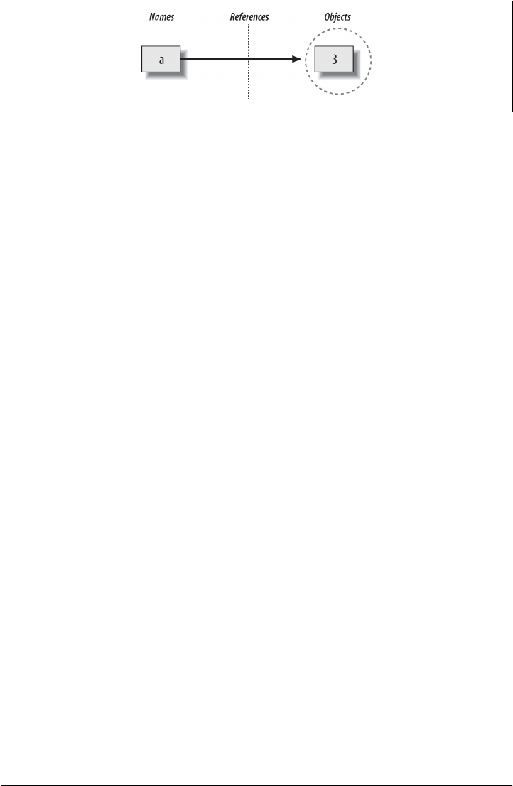
These links from variables to objects are called references in Python—that is, a reference
is a kind of association, implemented as a pointer in memory.1 Whenever the variables
are later used (i.e., referenced), Python automatically follows the variable-to-object
links. This is all simpler than the terminology may imply. In concrete terms:
•Variables are entries in a system table, with spaces for links to objects.
•Objects are pieces of allocated memory, with enough space to represent the values
for which they stand.
•References are automatically followed pointers from variables to objects.
At least conceptually, each time you generate a new value in your script by running an
expression, Python creates a new object (i.e., a chunk of memory) to represent that
value. As an optimization, Python internally caches and reuses certain kinds of un-
changeable objects, such as small integers and strings (each 0 is not really a new piece
of memory—more on this caching behavior later). But from a logical perspective, it
works as though each expression’s result value is a distinct object and each object is a
distinct piece of memory.
Technically speaking, objects have more structure than just enough space to represent
their values. Each object also has two standard header fields: a type designator used to
mark the type of the object, and a reference counter used to determine when it’s OK to
reclaim the object. To understand how these two header fields factor into the model,
we need to move on.
Types Live with Objects, Not Variables
To see how object types come into play, watch what happens if we assign a variable
multiple times:
Figure 6-1. Names and objects after running the assignment a = 3. Variable a becomes a reference to
the object 3. Internally, the variable is really a pointer to the object’s memory space created by running
the literal expression 3.
1. Readers with a background in C may find Python references similar to C pointers (memory addresses).
In fact, references are implemented as pointers, and they often serve the same roles, especially with objects
that can be changed in place (more on this later). However, because references are always automatically
dereferenced when used, you can never actually do anything useful with a reference itself; this is a feature
that eliminates a vast category of C bugs. But you can think of Python references as C “void*” pointers,
which are automatically followed whenever used.
The Case of the Missing Declaration Statements | 177
www.it-ebooks.info

>>> a = 3 # It's an integer
>>> a = 'spam' # Now it's a string
>>> a = 1.23 # Now it's a floating point
This isn’t typical Python code, but it does work—a starts out as an integer, then be-
comes a string, and finally becomes a floating-point number. This example tends to
look especially odd to ex-C programmers, as it appears as though the type of a changes
from integer to string when we say a = 'spam'.
However, that’s not really what’s happening. In Python, things work more simply.
Names have no types; as stated earlier, types live with objects, not names. In the pre-
ceding listing, we’ve simply changed a to reference different objects. Because variables
have no type, we haven’t actually changed the type of the variable a; we’ve simply made
the variable reference a different type of object. In fact, again, all we can ever say about
a variable in Python is that it references a particular object at a particular point in time.
Objects, on the other hand, know what type they are—each object contains a header
field that tags the object with its type. The integer object 3, for example, will contain
the value 3, plus a designator that tells Python that the object is an integer (strictly
speaking, a pointer to an object called int, the name of the integer type). The type
designator of the 'spam' string object points to the string type (called str) instead.
Because objects know their types, variables don’t have to.
To recap, types are associated with objects in Python, not with variables. In typical
code, a given variable usually will reference just one kind of object. Because this isn’t
a requirement, though, you’ll find that Python code tends to be much more flexible
than you may be accustomed to—if you use Python well, your code might work on
many types automatically.
I mentioned that objects have two header fields, a type designator and a reference
counter. To understand the latter of these, we need to move on and take a brief look
at what happens at the end of an object’s life.
Objects Are Garbage-Collected
In the prior section’s listings, we assigned the variable a to different types of objects in
each assignment. But when we reassign a variable, what happens to the value it was
previously referencing? For example, after the following statements, what happens to
the object 3?
>>> a = 3
>>> a = 'spam'
The answer is that in Python, whenever a name is assigned to a new object, the space
held by the prior object is reclaimed if it is not referenced by any other name or object.
This automatic reclamation of objects’ space is known as garbage collection, and makes
life much simpler for programmers of languages like Python that support it.
178 | Chapter 6: The Dynamic Typing Interlude
www.it-ebooks.info

To illustrate, consider the following example, which sets the name x to a different object
on each assignment:
>>> x = 42
>>> x = 'shrubbery' # Reclaim 42 now (unless referenced elsewhere)
>>> x = 3.1415 # Reclaim 'shrubbery' now
>>> x = [1, 2, 3] # Reclaim 3.1415 now
First, notice that x is set to a different type of object each time. Again, though this is
not really the case, the effect is as though the type of x is changing over time. Remember,
in Python types live with objects, not names. Because names are just generic references
to objects, this sort of code works naturally.
Second, notice that references to objects are discarded along the way. Each time x is
assigned to a new object, Python reclaims the prior object’s space. For instance, when
it is assigned the string 'shrubbery', the object 42 is immediately reclaimed (assuming
it is not referenced anywhere else)—that is, the object’s space is automatically thrown
back into the free space pool, to be reused for a future object.
Internally, Python accomplishes this feat by keeping a counter in every object that keeps
track of the number of references currently pointing to that object. As soon as (and
exactly when) this counter drops to zero, the object’s memory space is automatically
reclaimed. In the preceding listing, we’re assuming that each time x is assigned to a new
object, the prior object’s reference counter drops to zero, causing it to be reclaimed.
The most immediately tangible benefit of garbage collection is that it means you can
use objects liberally without ever needing to allocate or free up space in your script.
Python will clean up unused space for you as your program runs. In practice, this
eliminates a substantial amount of bookkeeping code required in lower-level languages
such as C and C++.
More on Python Garbage Collection
Technically speaking, Python’s garbage collection is based mainly upon reference coun-
ters, as described here; however, it also has a component that detects and reclaims
objects with cyclic references in time. This component can be disabled if you’re sure
that your code doesn’t create cycles, but it is enabled by default.
Circular references are a classic issue in reference count garbage collectors. Because
references are implemented as pointers, it’s possible for an object to reference itself, or
reference another object that does. For example, exercise 3 at the end of Part I and its
solution in Appendix D show how to create a cycle easily by embedding a reference to
a list within itself (e.g., L.append(L)). The same phenomenon can occur for assignments
to attributes of objects created from user-defined classes. Though relatively rare, be-
cause the reference counts for such objects never drop to zero, they must be treated
specially.
For more details on Python’s cycle detector, see the documentation for the gc module
in Python’s library manual. The best news here is that garbage-collection-based mem-
ory management is implemented for you in Python, by people highly skilled at the task.
The Case of the Missing Declaration Statements | 179
www.it-ebooks.info
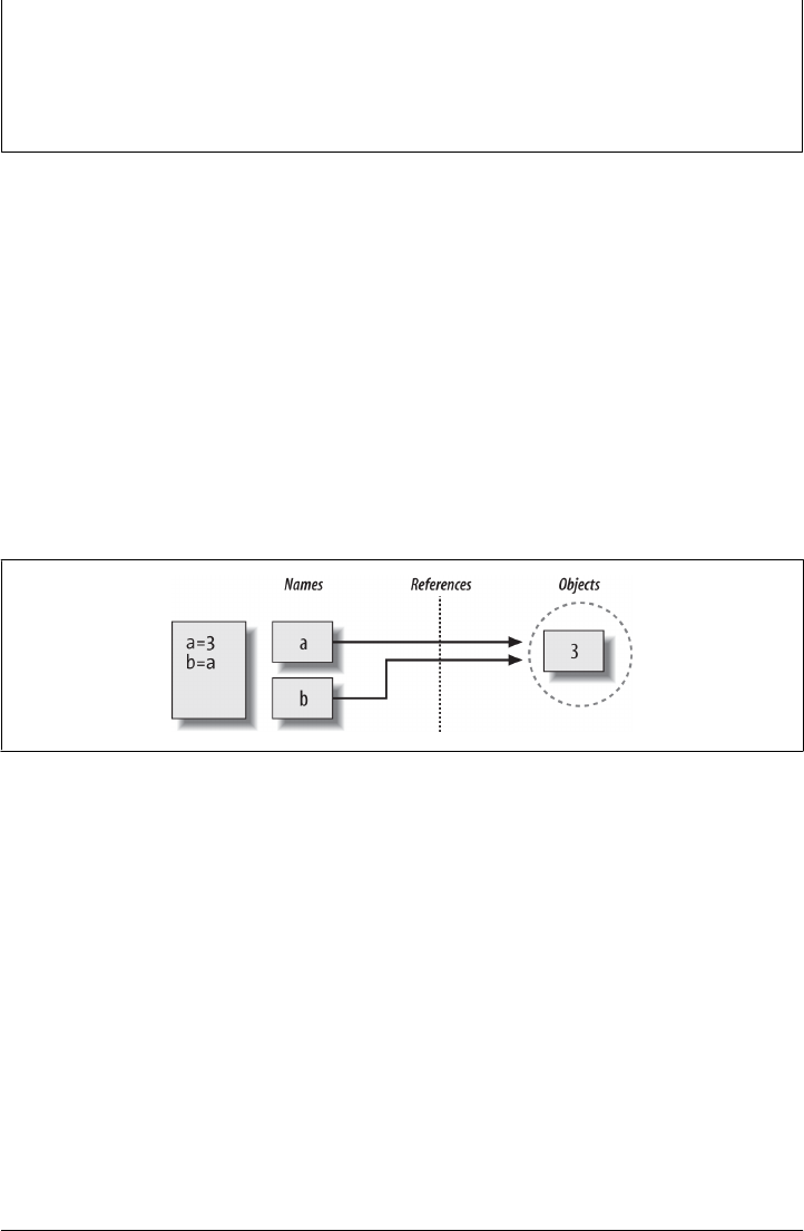
Also note that this chapter’s description of Python’s garbage collector applies to the
standard Python (a.k.a. CPython) only; Chapter 2’s alternative implementations such
as Jython, IronPython, and PyPy may use different schemes, though the net effect in
all is similar—unused space is reclaimed for you automatically, if not always as imme-
diately.
Shared References
So far, we’ve seen what happens as a single variable is assigned references to objects.
Now let’s introduce another variable into our interaction and watch what happens to
its names and objects:
>>> a = 3
>>> b = a
Typing these two statements generates the scene captured in Figure 6-2. The second
command causes Python to create the variable b; the variable a is being used and not
assigned here, so it is replaced with the object it references (3), and b is made to reference
that object. The net effect is that the variables a and b wind up referencing the same
object (that is, pointing to the same chunk of memory).
Figure 6-2. Names and objects after next running the assignment b = a. Variable b becomes a reference
to the object 3. Internally, the variable is really a pointer to the object’s memory space created by
running the literal expression 3.
This scenario in Python—with multiple names referencing the same object—is usually
called a shared reference (and sometimes just a shared object). Note that the names a
and b are not linked to each other directly when this happens; in fact, there is no way
to ever link a variable to another variable in Python. Rather, both variables point to the
same object via their references.
Next, suppose we extend the session with one more statement:
>>> a = 3
>>> b = a
>>> a = 'spam'
As with all Python assignments, this statement simply makes a new object to represent
the string value 'spam' and sets a to reference this new object. It does not, however,
180 | Chapter 6: The Dynamic Typing Interlude
www.it-ebooks.info
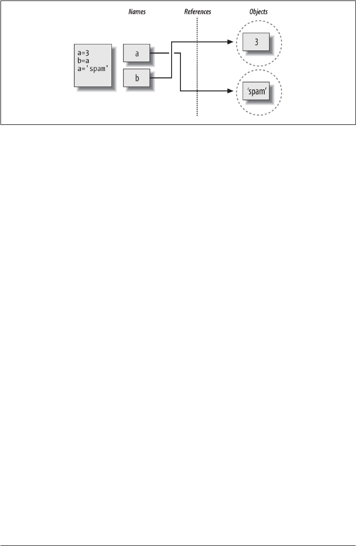
change the value of b; b still references the original object, the integer 3. The resulting
reference structure is shown in Figure 6-3.
The same sort of thing would happen if we changed b to 'spam' instead—the assignment
would change only b, not a. This behavior also occurs if there are no type differences
at all. For example, consider these three statements:
>>> a = 3
>>> b = a
>>> a = a + 2
In this sequence, the same events transpire. Python makes the variable a reference the
object 3 and makes b reference the same object as a, as in Figure 6-2; as before, the last
assignment then sets a to a completely different object (in this case, the integer 5, which
is the result of the + expression). It does not change b as a side effect. In fact, there is
no way to ever overwrite the value of the object 3—as introduced in Chapter 4, integers
are immutable and thus can never be changed in place.
One way to think of this is that, unlike in some languages, in Python variables are always
pointers to objects, not labels of changeable memory areas: setting a variable to a new
value does not alter the original object, but rather causes the variable to reference an
entirely different object. The net effect is that assignment to a variable itself can impact
only the single variable being assigned. When mutable objects and in-place changes
enter the equation, though, the picture changes somewhat; to see how, let’s move on.
Shared References and In-Place Changes
As you’ll see later in this part’s chapters, there are objects and operations that perform
in-place object changes—Python’s mutable types, including lists, dictionaries, and sets.
For instance, an assignment to an offset in a list actually changes the list object itself in
place, rather than generating a brand-new list object.
Figure 6-3. Names and objects after finally running the assignment a = ‘spam’. Variable a references
the new object (i.e., piece of memory) created by running the literal expression ‘spam’, but variable b
still refers to the original object 3. Because this assignment is not an in-place change to the object 3,
it changes only variable a, not b.
Shared References | 181
www.it-ebooks.info

Though you must take it somewhat on faith at this point in the book, this distinction
can matter much in your programs. For objects that support such in-place changes,
you need to be more aware of shared references, since a change from one name may
impact others. Otherwise, your objects may seem to change for no apparent reason.
Given that all assignments are based on references (including function argument pass-
ing), it’s a pervasive potential.
To illustrate, let’s take another look at the list objects introduced in Chapter 4. Recall
that lists, which do support in-place assignments to positions, are simply collections
of other objects, coded in square brackets:
>>> L1 = [2, 3, 4]
>>> L2 = L1
L1 here is a list containing the objects 2, 3, and 4. Items inside a list are accessed by their
positions, so L1[0] refers to object 2, the first item in the list L1. Of course, lists are also
objects in their own right, just like integers and strings. After running the two prior
assignments, L1 and L2 reference the same shared object, just like a and b in the prior
example (see Figure 6-2). Now say that, as before, we extend this interaction to say the
following:
>>> L1 = 24
This assignment simply sets L1 to a different object; L2 still references the original list.
If we change this statement’s syntax slightly, however, it has a radically different effect:
>>> L1 = [2, 3, 4] # A mutable object
>>> L2 = L1 # Make a reference to the same object
>>> L1[0] = 24 # An in-place change
>>> L1 # L1 is different
[24, 3, 4]
>>> L2 # But so is L2!
[24, 3, 4]
Really, we haven’t changed L1 itself here; we’ve changed a component of the object that
L1 references. This sort of change overwrites part of the list object’s value in place.
Because the list object is shared by (referenced from) other variables, though, an in-
place change like this doesn’t affect only L1—that is, you must be aware that when you
make such changes, they can impact other parts of your program. In this example, the
effect shows up in L2 as well because it references the same object as L1. Again, we
haven’t actually changed L2, either, but its value will appear different because it refers
to an object that has been overwritten in place.
This behavior only occurs for mutable objects that support in-place changes, and is
usually what you want, but you should be aware of how it works, so that it’s expected.
It’s also just the default: if you don’t want such behavior, you can request that Python
copy objects instead of making references. There are a variety of ways to copy a list,
including using the built-in list function and the standard library copy module. Perhaps
182 | Chapter 6: The Dynamic Typing Interlude
www.it-ebooks.info

the most common way is to slice from start to finish (see Chapter 4 and Chapter 7 for
more on slicing):
>>> L1 = [2, 3, 4]
>>> L2 = L1[:] # Make a copy of L1 (or list(L1), copy.copy(L1), etc.)
>>> L1[0] = 24
>>> L1
[24, 3, 4]
>>> L2 # L2 is not changed
[2, 3, 4]
Here, the change made through L1 is not reflected in L2 because L2 references a copy
of the object L1 references, not the original; that is, the two variables point to different
pieces of memory.
Note that this slicing technique won’t work on the other major mutable core types,
dictionaries and sets, because they are not sequences—to copy a dictionary or set,
instead use their X.copy() method call (lists have one as of Python 3.3 as well), or pass
the original object to their type names, dict and set. Also, note that the standard library
copy module has a call for copying any object type generically, as well as a call for
copying nested object structures—a dictionary with nested lists, for example:
import copy
X = copy.copy(Y) # Make top-level "shallow" copy of any object Y
X = copy.deepcopy(Y) # Make deep copy of any object Y: copy all nested parts
We’ll explore lists and dictionaries in more depth, and revisit the concept of shared
references and copies, in Chapter 8 and Chapter 9. For now, keep in mind that objects
that can be changed in place (that is, mutable objects) are always open to these kinds
of effects in any code they pass through. In Python, this includes lists, dictionaries, sets,
and some objects defined with class statements. If this is not the desired behavior, you
can simply copy your objects as needed.
Shared References and Equality
In the interest of full disclosure, I should point out that the garbage-collection behavior
described earlier in this chapter may be more conceptual than literal for certain types.
Consider these statements:
>>> x = 42
>>> x = 'shrubbery' # Reclaim 42 now?
Because Python caches and reuses small integers and small strings, as mentioned earlier,
the object 42 here is probably not literally reclaimed; instead, it will likely remain in a
system table to be reused the next time you generate a 42 in your code. Most kinds of
objects, though, are reclaimed immediately when they are no longer referenced; for
those that are not, the caching mechanism is irrelevant to your code.
For instance, because of Python’s reference model, there are two different ways to check
for equality in a Python program. Let’s create a shared reference to demonstrate:
Shared References | 183
www.it-ebooks.info

>>> L = [1, 2, 3]
>>> M = L # M and L reference the same object
>>> L == M # Same values
True
>>> L is M # Same objects
True
The first technique here, the == operator, tests whether the two referenced objects have
the same values; this is the method almost always used for equality checks in Python.
The second method, the is operator, instead tests for object identity—it returns True
only if both names point to the exact same object, so it is a much stronger form of
equality testing and is rarely applied in most programs.
Really, is simply compares the pointers that implement references, and it serves as a
way to detect shared references in your code if needed. It returns False if the names
point to equivalent but different objects, as is the case when we run two different literal
expressions:
>>> L = [1, 2, 3]
>>> M = [1, 2, 3] # M and L reference different objects
>>> L == M # Same values
True
>>> L is M # Different objects
False
Now, watch what happens when we perform the same operations on small numbers:
>>> X = 42
>>> Y = 42 # Should be two different objects
>>> X == Y
True
>>> X is Y # Same object anyhow: caching at work!
True
In this interaction, X and Y should be == (same value), but not is (same object) because
we ran two different literal expressions (42). Because small integers and strings are
cached and reused, though, is tells us they reference the same single object.
In fact, if you really want to look under the hood, you can always ask Python how many
references there are to an object: the getrefcount function in the standard sys module
returns the object’s reference count. When I ask about the integer object 1 in the IDLE
GUI, for instance, it reports 647 reuses of this same object (most of which are in IDLE’s
system code, not mine, though this returns 173 outside IDLE so Python must be
hoarding 1s as well):
>>> import sys
>>> sys.getrefcount(1) # 647 pointers to this shared piece of memory
647
This object caching and reuse is irrelevant to your code (unless you run the is check!).
Because you cannot change immutable numbers or strings in place, it doesn’t matter
how many references there are to the same object—every reference will always see the
184 | Chapter 6: The Dynamic Typing Interlude
www.it-ebooks.info

same, unchanging value. Still, this behavior reflects one of the many ways Python op-
timizes its model for execution speed.
Dynamic Typing Is Everywhere
Of course, you don’t really need to draw name/object diagrams with circles and arrows
to use Python. When you’re starting out, though, it sometimes helps you understand
unusual cases if you can trace their reference structures as we’ve done here. If a mutable
object changes out from under you when passed around your program, for example,
chances are you are witnessing some of this chapter’s subject matter firsthand.
Moreover, even if dynamic typing seems a little abstract at this point, you probably will
care about it eventually. Because everything seems to work by assignment and refer-
ences in Python, a basic understanding of this model is useful in many different con-
texts. As you’ll see, it works the same in assignment statements, function arguments,
for loop variables, module imports, class attributes, and more. The good news is that
there is just one assignment model in Python; once you get a handle on dynamic typing,
you’ll find that it works the same everywhere in the language.
At the most practical level, dynamic typing means there is less code for you to write.
Just as importantly, though, dynamic typing is also the root of Python’s polymor-
phism, a concept we introduced in Chapter 4 and will revisit again later in this book.
Because we do not constrain types in Python code, it is both concise and highly flexible.
As you’ll see, when used well, dynamic typing—and the polymorphism it implies—
produces code that automatically adapts to new requirements as your systems evolve.
“Weak” References
You may occasionally see the term “weak reference” in the Python world. This is a
somewhat advanced tool, but is related to the reference model we’ve explored here,
and like the is operator, can’t really be understood without it.
In short, a weak reference, implemented by the weakref standard library module, is a
reference to an object that does not by itself prevent the referenced object from being
garbage-collected. If the last remaining references to an object are weak references, the
object is reclaimed and the weak references to it are automatically deleted (or otherwise
notified).
This can be useful in dictionary-based caches of large objects, for example; otherwise,
the cache’s reference alone would keep the object in memory indefinitely. Still, this is
really just a special-case extension to the reference model. For more details, see Python’s
library manual.
Dynamic Typing Is Everywhere | 185
www.it-ebooks.info

Chapter Summary
This chapter took a deeper look at Python’s dynamic typing model—that is, the way
that Python keeps track of object types for us automatically, rather than requiring us
to code declaration statements in our scripts. Along the way, we learned how variables
and objects are associated by references in Python; we also explored the idea of garbage
collection, learned how shared references to objects can affect multiple variables, and
saw how references impact the notion of equality in Python.
Because there is just one assignment model in Python, and because assignment pops
up everywhere in the language, it’s important that you have a handle on the model
before moving on. The following quiz should help you review some of this chapter’s
ideas. After that, we’ll resume our core object tour in the next chapter, with strings.
Test Your Knowledge: Quiz
1. Consider the following three statements. Do they change the value printed for A?
A = "spam"
B = A
B = "shrubbery"
2. Consider these three statements. Do they change the printed value of A?
A = ["spam"]
B = A
B[0] = "shrubbery"
3. How about these—is A changed now?
A = ["spam"]
B = A[:]
B[0] = "shrubbery"
Test Your Knowledge: Answers
1. No: A still prints as "spam". When B is assigned to the string "shrubbery", all that
happens is that the variable B is reset to point to the new string object. A and B
initially share (i.e., reference/point to) the same single string object "spam", but two
names are never linked together in Python. Thus, setting B to a different object has
no effect on A. The same would be true if the last statement here were B = B +
'shrubbery', by the way—the concatenation would make a new object for its result,
which would then be assigned to B only. We can never overwrite a string (or num-
ber, or tuple) in place, because strings are immutable.
2. Yes: A now prints as ["shrubbery"]. Technically, we haven’t really changed either
A or B; instead, we’ve changed part of the object they both reference (point to) by
overwriting that object in place through the variable B. Because A references the
same object as B, the update is reflected in A as well.
186 | Chapter 6: The Dynamic Typing Interlude
www.it-ebooks.info

3. No: A still prints as ["spam"]. The in-place assignment through B has no effect this
time because the slice expression made a copy of the list object before it was as-
signed to B. After the second assignment statement, there are two different list
objects that have the same value (in Python, we say they are ==, but not is). The
third statement changes the value of the list object pointed to by B, but not that
pointed to by A.
Test Your Knowledge: Answers | 187
www.it-ebooks.info

CHAPTER 7
String Fundamentals
So far, we’ve studied numbers and explored Python’s dynamic typing model. The next
major type on our in-depth core object tour is the Python string—an ordered collection
of characters used to store and represent text- and bytes-based information. We looked
briefly at strings in Chapter 4. Here, we will revisit them in more depth, filling in some
of the details we skipped earlier.
This Chapter’s Scope
Before we get started, I also want to clarify what we won’t be covering here. Chap-
ter 4 briefly previewed Unicode strings and files—tools for dealing with non-ASCII text.
Unicode is a key tool for some programmers, especially those who work in the Internet
domain. It can pop up, for example, in web pages, email content and headers, FTP
transfers, GUI APIs, directory tools, and HTML, XML and JSON text.
At the same time, Unicode can be a heavy topic for programmers just starting out, and
many (or most) of the Python programmers I meet today still do their jobs in blissful
ignorance of the entire topic. In light of that, this book relegates most of the Unicode
story to Chapter 37 of its Advanced Topics part as optional reading, and focuses on
string basics here.
That is, this chapter tells only part of the string story in Python—the part that most
scripts use and most programmers need to know. It explores the fundamental str string
type, which handles ASCII text, and works the same regardless of which version of
Python you use. Despite this intentionally limited scope, because str also handles Uni-
code in Python 3.X, and the separate unicode type works almost identically to str in
2.X, everything we learn here will apply directly to Unicode processing too.
Unicode: The Short Story
For readers who do care about Unicode, I’d like to also provide a quick summary of its
impacts and pointers for further study. From a formal perspective, ASCII is a simple
189
www.it-ebooks.info

form of Unicode text, but just one of many possible encodings and alphabets. Text
from non-English-speaking sources may use very different letters, and may be encoded
very differently when stored in files.
As we saw in Chapter 4, Python addresses this by distinguishing between text and
binary data, with distinct string object types and file interfaces for each. This support
varies per Python line:
• In Python 3.X there are three string types: str is used for Unicode text (including
ASCII), bytes is used for binary data (including encoded text), and bytearray is a
mutable variant of bytes. Files work in two modes: text, which represents content
as str and implements Unicode encodings, and binary, which deals in raw bytes
and does no data translation.
• In Python 2.X, unicode strings represent Unicode text, str strings handle both 8-
bit text and binary data, and bytearray is available in 2.6 and later as a back-port
from 3.X. Normal files’ content is simply bytes represented as str, but a codecs
module opens Unicode text files, handles encodings, and represents content as
unicode objects.
Despite such version differences, if and when you do need to care about Unicode you’ll
find that it is a relatively minor extension—once text is in memory, it’s a Python string
of characters that supports all the basics we’ll study in this chapter. In fact, the primary
distinction of Unicode often lies in the translation (a.k.a. encoding) step required to
move it to and from files. Beyond that, it’s largely just string processing.
Again, though, because most programmers don’t need to come to grips with Unicode
details up front, I’ve moved most of them to Chapter 37. When you’re ready to learn
about these more advanced string concepts, I encourage you to see both their preview
in Chapter 4 and the full Unicode and bytes disclosure in Chapter 37 after reading the
string fundamentals material here.
For this chapter, we’ll focus on the basic string type and its operations. As you’ll find,
the techniques we’ll study here also apply directly to the more advanced string types
in Python’s toolset.
String Basics
From a functional perspective, strings can be used to represent just about anything that
can be encoded as text or bytes. In the text department, this includes symbols and
words (e.g., your name), contents of text files loaded into memory, Internet addresses,
Python source code, and so on. Strings can also be used to hold the raw bytes used for
media files and network transfers, and both the encoded and decoded forms of non-
ASCII Unicode text used in internationalized programs.
You may have used strings in other languages, too. Python’s strings serve the same role
as character arrays in languages such as C, but they are a somewhat higher-level tool
190 | Chapter 7: String Fundamentals
www.it-ebooks.info

than arrays. Unlike in C, in Python, strings come with a powerful set of processing
tools. Also unlike languages such as C, Python has no distinct type for individual char-
acters; instead, you just use one-character strings.
Strictly speaking, Python strings are categorized as immutable sequences, meaning that
the characters they contain have a left-to-right positional order and that they cannot
be changed in place. In fact, strings are the first representative of the larger class of
objects called sequences that we will study here. Pay special attention to the sequence
operations introduced in this chapter, because they will work the same on other se-
quence types we’ll explore later, such as lists and tuples.
Table 7-1 previews common string literals and operations we will discuss in this chap-
ter. Empty strings are written as a pair of quotation marks (single or double) with
nothing in between, and there are a variety of ways to code strings. For processing,
strings support expression operations such as concatenation (combining strings), slic-
ing (extracting sections), indexing (fetching by offset), and so on. Besides expressions,
Python also provides a set of string methods that implement common string-specific
tasks, as well as modules for more advanced text-processing tasks such as pattern
matching. We’ll explore all of these later in the chapter.
Table 7-1. Common string literals and operations
Operation Interpretation
S = '' Empty string
S = "spam's" Double quotes, same as single
S = 's\np\ta\x00m' Escape sequences
S = """...multiline...""" Triple-quoted block strings
S = r'\temp\spam' Raw strings (no escapes)
B = b'sp\xc4m' Byte strings in 2.6, 2.7, and 3.X (Chapter 4, Chapter 37)
U = u'sp\u00c4m' Unicode strings in 2.X and 3.3+ (Chapter 4, Chapter 37)
S1 + S2
S * 3
Concatenate, repeat
S[i]
S[i:j]
len(S)
Index, slice, length
"a %s parrot" % kind String formatting expression
"a {0} parrot".format(kind) String formatting method in 2.6, 2.7, and 3.X
S.find('pa')
S.rstrip()
S.replace('pa', 'xx')
S.split(',')
String methods (see ahead for all 43): search,
remove whitespace,
replacement,
split on delimiter,
String Basics | 191
www.it-ebooks.info

Operation Interpretation
S.isdigit()
S.lower()
S.endswith('spam')
'spam'.join(strlist)
S.encode('latin-1')
B.decode('utf8')
content test,
case conversion,
end test,
delimiter join,
Unicode encoding,
Unicode decoding, etc. (see Table 7-3)
for x in S: print(x)
'spam' in S
[c * 2 for c in S]
map(ord, S)
Iteration, membership
re.match('sp(.*)am', line) Pattern matching: library module
Beyond the core set of string tools in Table 7-1, Python also supports more advanced
pattern-based string processing with the standard library’s re (for “regular expression”)
module, introduced in Chapter 4 and Chapter 36, and even higher-level text processing
tools such as XML parsers (discussed briefly in Chapter 37). This book’s scope, though,
is focused on the fundamentals represented by Table 7-1.
To cover the basics, this chapter begins with an overview of string literal forms and
string expressions, then moves on to look at more advanced tools such as string meth-
ods and formatting. Python comes with many string tools, and we won’t look at them
all here; the complete story is chronicled in the Python library manual and reference
books. Our goal here is to explore enough commonly used tools to give you a repre-
sentative sample; methods we won’t see in action here, for example, are largely anal-
ogous to those we will.
String Literals
By and large, strings are fairly easy to use in Python. Perhaps the most complicated
thing about them is that there are so many ways to write them in your code:
• Single quotes: 'spa"m'
• Double quotes: "spa'm"
• Triple quotes: '''... spam ...''', """... spam ..."""
• Escape sequences: "s\tp\na\0m"
• Raw strings: r"C:\new\test.spm"
• Bytes literals in 3.X and 2.6+ (see Chapter 4, Chapter 37): b'sp\x01am'
• Unicode literals in 2.X and 3.3+ (see Chapter 4, Chapter 37): u'eggs\u0020spam'
192 | Chapter 7: String Fundamentals
www.it-ebooks.info

The single- and double-quoted forms are by far the most common; the others serve
specialized roles, and we’re postponing further discussion of the last two advanced
forms until Chapter 37. Let’s take a quick look at all the other options in turn.
Single- and Double-Quoted Strings Are the Same
Around Python strings, single- and double-quote characters are interchangeable. That
is, string literals can be written enclosed in either two single or two double quotes—
the two forms work the same and return the same type of object. For example, the
following two strings are identical, once coded:
>>> 'shrubbery', "shrubbery"
('shrubbery', 'shrubbery')
The reason for supporting both is that it allows you to embed a quote character of the
other variety inside a string without escaping it with a backslash. You may embed a
single-quote character in a string enclosed in double-quote characters, and vice versa:
>>> 'knight"s', "knight's"
('knight"s', "knight's")
This book generally prefers to use single quotes around strings just because they are
marginally easier to read, except in cases where a single quote is embedded in the string.
This is a purely subjective style choice, but Python displays strings this way too and
most Python programmers do the same today, so you probably should too.
Note that the comma is important here. Without it, Python automatically concate-
nates adjacent string literals in any expression, although it is almost as simple to add a
+ operator between them to invoke concatenation explicitly (as we’ll see in Chap-
ter 12, wrapping this form in parentheses also allows it to span multiple lines):
>>> title = "Meaning " 'of' " Life" # Implicit concatenation
>>> title
'Meaning of Life'
Adding commas between these strings would result in a tuple, not a string. Also notice
in all of these outputs that Python prints strings in single quotes unless they embed
one. If needed, you can also embed quote characters by escaping them with backslashes:
>>> 'knight\'s', "knight\"s"
("knight's", 'knight"s')
To understand why, you need to know how escapes work in general.
Escape Sequences Represent Special Characters
The last example embedded a quote inside a string by preceding it with a backslash.
This is representative of a general pattern in strings: backslashes are used to introduce
special character codings known as escape sequences.
String Literals | 193
www.it-ebooks.info
Escape sequences let us embed characters in strings that cannot easily be typed on a
keyboard. The character \, and one or more characters following it in the string literal,
are replaced with a single character in the resulting string object, which has the binary
value specified by the escape sequence. For example, here is a five-character string that
embeds a newline and a tab:
>>> s = 'a\nb\tc'
The two characters \n stand for a single character—the binary value of the newline
character in your character set (in ASCII, character code 10). Similarly, the sequence
\t is replaced with the tab character. The way this string looks when printed depends
on how you print it. The interactive echo shows the special characters as escapes, but
print interprets them instead:
>>> s
'a\nb\tc'
>>> print(s)
a
b c
To be completely sure how many actual characters are in this string, use the built-in
len function—it returns the actual number of characters in a string, regardless of how
it is coded or displayed:
>>> len(s)
5
This string is five characters long: it contains an ASCII a, a newline character, an ASCII
b, and so on.
If you’re accustomed to all-ASCII text, it’s tempting to think of this
result as meaning 5 bytes too, but you probably shouldn’t. Really,
“bytes” has no meaning in the Unicode world. For one thing, the string
object is probably larger in memory in Python.
More critically, string content and length both reflect code points (iden-
tifying numbers) in Unicode-speak, where a single character does not
necessarily map directly to a single byte, either when encoded in files or
when stored in memory. This mapping might hold true for simple 7-bit
ASCII text, but even this depends on both the external encoding type
and the internal storage scheme used. Under UTF-16, for example, AS-
CII characters are multiple bytes in files, and they may be 1, 2, or 4 bytes
in memory depending on how Python allocates their space. For other,
non-ASCII text, whose characters’ values might be too large to fit in an
8-bit byte, the character-to-byte mapping doesn’t apply at all.
In fact, 3.X defines str strings formally as sequences of Unicode code
points, not bytes, to make this clear. There’s more on how strings are
stored internally in Chapter 37 if you care to know. For now, to be safest,
think characters instead of bytes in strings. Trust me on this; as an ex-
C programmer, I had to break the habit too!
194 | Chapter 7: String Fundamentals
www.it-ebooks.info

Note that the original backslash characters in the preceding result are not really stored
with the string in memory; they are used only to describe special character values to be
stored in the string. For coding such special characters, Python recognizes a full set of
escape code sequences, listed in Table 7-2.
Table 7-2. String backslash characters
Escape Meaning
\newline Ignored (continuation line)
\\ Backslash (stores one \)
\' Single quote (stores ')
\" Double quote (stores ")
\a Bell
\b Backspace
\f Formfeed
\n Newline (linefeed)
\r Carriage return
\t Horizontal tab
\v Vertical tab
\xhh Character with hex value hh (exactly 2 digits)
\ooo Character with octal value ooo (up to 3 digits)
\0 Null: binary 0 character (doesn’t end string)
\N{ id } Unicode database ID
\uhhhh Unicode character with 16-bit hex value
\Uhhhhhhhh Unicode character with 32-bit hex valuea
\other Not an escape (keeps both \ and other)
aThe \Uhhhh... escape sequence takes exactly eight hexadecimal digits (h); both \u and \U are recognized only in Unicode string literals
in 2.X, but can be used in normal strings (which are Unicode) in 3.X. In a 3.X bytes literal, hexadecimal and octal escapes denote the byte
with the given value; in a string literal, these escapes denote a Unicode character with the given code-point value. There is more on Unicode
escapes in Chapter 37.
Some escape sequences allow you to embed absolute binary values into the characters
of a string. For instance, here’s a five-character string that embeds two characters with
binary zero values (coded as octal escapes of one digit):
>>> s = 'a\0b\0c'
>>> s
'a\x00b\x00c'
>>> len(s)
5
In Python, a zero (null) character like this does not terminate a string the way a “null
byte” typically does in C. Instead, Python keeps both the string’s length and text in
memory. In fact, no character terminates a string in Python. Here’s a string that is all
String Literals | 195
www.it-ebooks.info

absolute binary escape codes—a binary 1 and 2 (coded in octal), followed by a binary
3 (coded in hexadecimal):
>>> s = '\001\002\x03'
>>> s
'\x01\x02\x03'
>>> len(s)
3
Notice that Python displays nonprintable characters in hex, regardless of how they were
specified. You can freely combine absolute value escapes and the more symbolic escape
types in Table 7-2. The following string contains the characters “spam”, a tab and
newline, and an absolute zero value character coded in hex:
>>> S = "s\tp\na\x00m"
>>> S
's\tp\na\x00m'
>>> len(S)
7
>>> print(S)
s p
a m
This becomes more important to know when you process binary data files in Python.
Because their contents are represented as strings in your scripts, it’s OK to process
binary files that contain any sorts of binary byte values—when opened in binary modes,
files return strings of raw bytes from the external file (there’s much more on files in
Chapter 4, Chapter 9, and Chapter 37).
Finally, as the last entry in Table 7-2 implies, if Python does not recognize the character
after a \ as being a valid escape code, it simply keeps the backslash in the resulting string:
>>> x = "C:\py\code" # Keeps \ literally (and displays it as \\)
>>> x
'C:\\py\\code'
>>> len(x)
10
However, unless you’re able to commit all of Table 7-2 to memory (and there are ar-
guably better uses for your neurons!), you probably shouldn’t rely on this behavior. To
code literal backslashes explicitly such that they are retained in your strings, double
them up (\\ is an escape for one \) or use raw strings; the next section shows how.
Raw Strings Suppress Escapes
As we’ve seen, escape sequences are handy for embedding special character codes
within strings. Sometimes, though, the special treatment of backslashes for introducing
escapes can lead to trouble. It’s surprisingly common, for instance, to see Python new-
comers in classes trying to open a file with a filename argument that looks something
like this:
myfile = open('C:\new\text.dat', 'w')
196 | Chapter 7: String Fundamentals
www.it-ebooks.info

thinking that they will open a file called text.dat in the directory C:\new. The problem
here is that \n is taken to stand for a newline character, and \t is replaced with a tab.
In effect, the call tries to open a file named C:(newline)ew(tab)ext.dat, with usually less-
than-stellar results.
This is just the sort of thing that raw strings are useful for. If the letter r (uppercase or
lowercase) appears just before the opening quote of a string, it turns off the escape
mechanism. The result is that Python retains your backslashes literally, exactly as you
type them. Therefore, to fix the filename problem, just remember to add the letter r on
Windows:
myfile = open(r'C:\new\text.dat', 'w')
Alternatively, because two backslashes are really an escape sequence for one backslash,
you can keep your backslashes by simply doubling them up:
myfile = open('C:\\new\\text.dat', 'w')
In fact, Python itself sometimes uses this doubling scheme when it prints strings with
embedded backslashes:
>>> path = r'C:\new\text.dat'
>>> path # Show as Python code
'C:\\new\\text.dat'
>>> print(path) # User-friendly format
C:\new\text.dat
>>> len(path) # String length
15
As with numeric representation, the default format at the interactive prompt prints
results as if they were code, and therefore escapes backslashes in the output. The
print statement provides a more user-friendly format that shows that there is actually
only one backslash in each spot. To verify this is the case, you can check the result of
the built-in len function, which returns the number of characters in the string, inde-
pendent of display formats. If you count the characters in the print(path) output, you’ll
see that there really is just 1 character per backslash, for a total of 15.
Besides directory paths on Windows, raw strings are also commonly used for regular
expressions (text pattern matching, supported with the re module introduced in Chap-
ter 4 and Chapter 37). Also note that Python scripts can usually use forward slashes in
directory paths on Windows and Unix because Python tries to interpret paths portably
(i.e., 'C:/new/text.dat' works when opening files, too). Raw strings are useful if you
code paths using native Windows backslashes, though.
String Literals | 197
www.it-ebooks.info

Despite its role, even a raw string cannot end in a single backslash, be-
cause the backslash escapes the following quote character—you still
must escape the surrounding quote character to embed it in the string.
That is, r"...\" is not a valid string literal—a raw string cannot end in
an odd number of backslashes. If you need to end a raw string with a
single backslash, you can use two and slice off the second (r'1\nb\tc\
\'[:-1]), tack one on manually (r'1\nb\tc' + '\\'), or skip the raw
string syntax and just double up the backslashes in a normal string ('1\
\nb\\tc\\'). All three of these forms create the same eight-character
string containing three backslashes.
Triple Quotes Code Multiline Block Strings
So far, you’ve seen single quotes, double quotes, escapes, and raw strings in action.
Python also has a triple-quoted string literal format, sometimes called a block string,
that is a syntactic convenience for coding multiline text data. This form begins with
three quotes (of either the single or double variety), is followed by any number of lines
of text, and is closed with the same triple-quote sequence that opened it. Single and
double quotes embedded in the string’s text may be, but do not have to be, escaped—
the string does not end until Python sees three unescaped quotes of the same kind used
to start the literal. For example (the “...” here is Python’s prompt for continuation lines
outside IDLE: don’t type it yourself):
>>> mantra = """Always look
... on the bright
... side of life."""
>>>
>>> mantra
'Always look\n on the bright\nside of life.'
This string spans three lines. As we learned in Chapter 3, in some interfaces, the inter-
active prompt changes to ... on continuation lines like this, but IDLE simply drops
down one line; this book shows listings in both forms, so extrapolate as needed. Either
way, Python collects all the triple-quoted text into a single multiline string, with em-
bedded newline characters (\n) at the places where your code has line breaks. Notice
that, as in the literal, the second line in the result has leading spaces, but the third does
not—what you type is truly what you get. To see the string with the newlines inter-
preted, print it instead of echoing:
>>> print(mantra)
Always look
on the bright
side of life.
In fact, triple-quoted strings will retain all the enclosed text, including any to the right
of your code that you might intend as comments. So don’t do this—put your comments
above or below the quoted text, or use the automatic concatenation of adjacent strings
mentioned earlier, with explicit newlines if desired, and surrounding parentheses to
198 | Chapter 7: String Fundamentals
www.it-ebooks.info

allow line spans (again, more on this latter form when we study syntax rules in Chap-
ter 10 and Chapter 12):
>>> menu = """spam # comments here added to string!
... eggs # ditto
... """
>>> menu
'spam # comments here added to string!\neggs # ditto\n'
>>> menu = (
... "spam\n" # comments here ignored
... "eggs\n" # but newlines not automatic
... )
>>> menu
'spam\neggs\n'
Triple-quoted strings are useful anytime you need multiline text in your program; for
example, to embed multiline error messages or HTML, XML, or JSON code in your
Python source code files. You can embed such blocks directly in your scripts by triple-
quoting without resorting to external text files or explicit concatenation and newline
characters.
Triple-quoted strings are also commonly used for documentation strings, which are
string literals that are taken as comments when they appear at specific points in your
file (more on these later in the book). These don’t have to be triple-quoted blocks, but
they usually are to allow for multiline comments.
Finally, triple-quoted strings are also sometimes used as a “horribly hackish” way to
temporarily disable lines of code during development (OK, it’s not really too horrible,
and it’s actually a fairly common practice today, but it wasn’t the intent). If you wish
to turn off a few lines of code and run your script again, simply put three quotes above
and below them, like this:
X = 1
"""
import os # Disable this code temporarily
print(os.getcwd())
"""
Y = 2
I said this was hackish because Python really might make a string out of the lines of
code disabled this way, but this is probably not significant in terms of performance.
For large sections of code, it’s also easier than manually adding hash marks before each
line and later removing them. This is especially true if you are using a text editor that
does not have support for editing Python code specifically. In Python, practicality often
beats aesthetics.
String Literals | 199
www.it-ebooks.info

Strings in Action
Once you’ve created a string with the literal expressions we just met, you will almost
certainly want to do things with it. This section and the next two demonstrate string
expressions, methods, and formatting—the first line of text-processing tools in the
Python language.
Basic Operations
Let’s begin by interacting with the Python interpreter to illustrate the basic string op-
erations listed earlier in Table 7-1. You can concatenate strings using the + operator
and repeat them using the * operator:
% python
>>> len('abc') # Length: number of items
3
>>> 'abc' + 'def' # Concatenation: a new string
'abcdef'
>>> 'Ni!' * 4 # Repetition: like "Ni!" + "Ni!" + ...
'Ni!Ni!Ni!Ni!'
The len built-in function here returns the length of a string (or any other object with a
length). Formally, adding two string objects with + creates a new string object, with the
contents of its operands joined, and repetition with * is like adding a string to itself a
number of times. In both cases, Python lets you create arbitrarily sized strings; there’s
no need to predeclare anything in Python, including the sizes of data structures—you
simply create string objects as needed and let Python manage the underlying memory
space automatically (see Chapter 6 for more on Python’s memory management
“garbage collector”).
Repetition may seem a bit obscure at first, but it comes in handy in a surprising number
of contexts. For example, to print a line of 80 dashes, you can count up to 80, or let
Python count for you:
>>> print('------- ...more... ---') # 80 dashes, the hard way
>>> print('-' * 80) # 80 dashes, the easy way
Notice that operator overloading is at work here already: we’re using the same + and
* operators that perform addition and multiplication when using numbers. Python does
the correct operation because it knows the types of the objects being added and mul-
tiplied. But be careful: the rules aren’t quite as liberal as you might expect. For instance,
Python doesn’t allow you to mix numbers and strings in + expressions: 'abc'+9 raises
an error instead of automatically converting 9 to a string.
As shown in the last row in Table 7-1, you can also iterate over strings in loops using
for statements, which repeat actions, and test membership for both characters and
substrings with the in expression operator, which is essentially a search. For substrings,
in is much like the str.find() method covered later in this chapter, but it returns a
200 | Chapter 7: String Fundamentals
www.it-ebooks.info

Boolean result instead of the substring’s position (the following uses a 3.X print call
and may leave your cursor a bit indented; in 2.X say print c, instead):
>>> myjob = "hacker"
>>> for c in myjob: print(c, end=' ') # Step through items, print each (3.X form)
...
h a c k e r
>>> "k" in myjob # Found
True
>>> "z" in myjob # Not found
False
>>> 'spam' in 'abcspamdef' # Substring search, no position returned
True
The for loop assigns a variable to successive items in a sequence (here, a string) and
executes one or more statements for each item. In effect, the variable c becomes a cursor
stepping across the string’s characters here. We will discuss iteration tools like these
and others listed in Table 7-1 in more detail later in this book (especially in Chap-
ter 14 and Chapter 20).
Indexing and Slicing
Because strings are defined as ordered collections of characters, we can access their
components by position. In Python, characters in a string are fetched by indexing—
providing the numeric offset of the desired component in square brackets after the
string. You get back the one-character string at the specified position.
As in the C language, Python offsets start at 0 and end at one less than the length of the
string. Unlike C, however, Python also lets you fetch items from sequences such as
strings using negative offsets. Technically, a negative offset is added to the length of a
string to derive a positive offset. You can also think of negative offsets as counting
backward from the end. The following interaction demonstrates:
>>> S = 'spam'
>>> S[0], S[−2] # Indexing from front or end
('s', 'a')
>>> S[1:3], S[1:], S[:−1] # Slicing: extract a section
('pa', 'pam', 'spa')
The first line defines a four-character string and assigns it the name S. The next line
indexes it in two ways: S[0] fetches the item at offset 0 from the left—the one-character
string 's'; S[−2] gets the item at offset 2 back from the end—or equivalently, at offset
(4 + (−2)) from the front. In more graphic terms, offsets and slices map to cells as shown
in Figure 7-1.1
1. More mathematically minded readers (and students in my classes) sometimes detect a small asymmetry
here: the leftmost item is at offset 0, but the rightmost is at offset −1. Alas, there is no such thing as a
distinct −0 value in Python.
Strings in Action | 201
www.it-ebooks.info
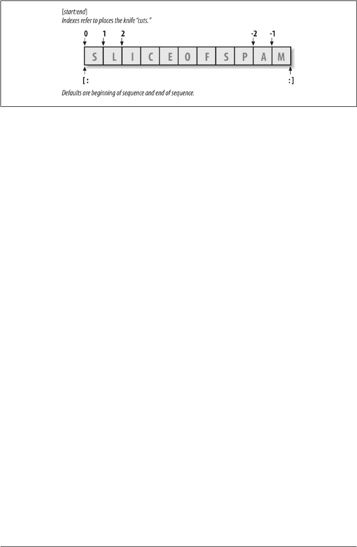
The last line in the preceding example demonstrates slicing, a generalized form of in-
dexing that returns an entire section, not a single item. Probably the best way to think
of slicing is that it is a type of parsing (analyzing structure), especially when applied to
strings—it allows us to extract an entire section (substring) in a single step. Slices can
be used to extract columns of data, chop off leading and trailing text, and more. In fact,
we’ll explore slicing in the context of text parsing later in this chapter.
The basics of slicing are straightforward. When you index a sequence object such as a
string on a pair of offsets separated by a colon, Python returns a new object containing
the contiguous section identified by the offset pair. The left offset is taken to be the
lower bound (inclusive), and the right is the upper bound (noninclusive). That is, Python
fetches all items from the lower bound up to but not including the upper bound, and
returns a new object containing the fetched items. If omitted, the left and right bounds
default to 0 and the length of the object you are slicing, respectively.
For instance, in the example we just saw, S[1:3] extracts the items at offsets 1 and 2:
it grabs the second and third items, and stops before the fourth item at offset 3. Next,
S[1:] gets all items beyond the first—the upper bound, which is not specified, defaults
to the length of the string. Finally, S[:−1] fetches all but the last item—the lower bound
defaults to 0, and −1 refers to the last item, noninclusive.
This may seem confusing at first glance, but indexing and slicing are simple and pow-
erful tools to use, once you get the knack. Remember, if you’re unsure about the effects
of a slice, try it out interactively. In the next chapter, you’ll see that it’s even possible
to change an entire section of another object in one step by assigning to a slice (though
not for immutables like strings). Here’s a summary of the details for reference:
Indexing (S[i]) fetches components at offsets:
• The first item is at offset 0.
• Negative indexes mean to count backward from the end or right.
•S[0] fetches the first item.
•S[−2] fetches the second item from the end (like S[len(S)−2]).
Figure 7-1. Offsets and slices: positive offsets start from the left end (offset 0 is the first item), and
negatives count back from the right end (offset −1 is the last item). Either kind of offset can be used
to give positions in indexing and slicing operations.
202 | Chapter 7: String Fundamentals
www.it-ebooks.info

Slicing (S[i:j]) extracts contiguous sections of sequences:
• The upper bound is noninclusive.
• Slice boundaries default to 0 and the sequence length, if omitted.
•S[1:3] fetches items at offsets 1 up to but not including 3.
•S[1:] fetches items at offset 1 through the end (the sequence length).
•S[:3] fetches items at offset 0 up to but not including 3.
•S[:−1] fetches items at offset 0 up to but not including the last item.
•S[:] fetches items at offsets 0 through the end—making a top-level copy of S.
Extended slicing (S[i:j:k]) accepts a step (or stride) k, which defaults to +1:
• Allows for skipping items and reversing order—see the next section.
The second-to-last bullet item listed here turns out to be a very common technique: it
makes a full top-level copy of a sequence object—an object with the same value, but a
distinct piece of memory (you’ll find more on copies in Chapter 9). This isn’t very useful
for immutable objects like strings, but it comes in handy for objects that may be changed
in place, such as lists.
In the next chapter, you’ll see that the syntax used to index by offset (square brackets)
is used to index dictionaries by key as well; the operations look the same but have
different interpretations.
Extended slicing: The third limit and slice objects
In Python 2.3 and later, slice expressions have support for an optional third index, used
as a step (sometimes called a stride). The step is added to the index of each item ex-
tracted. The full-blown form of a slice is now X[I:J:K], which means “extract all the
items in X, from offset I through J−1, by K.” The third limit, K, defaults to +1, which is
why normally all items in a slice are extracted from left to right. If you specify an explicit
value, however, you can use the third limit to skip items or to reverse their order.
For instance, X[1:10:2] will fetch every other item in X from offsets 1–9; that is, it will
collect the items at offsets 1, 3, 5, 7, and 9. As usual, the first and second limits default
to 0 and the length of the sequence, respectively, so X[::2] gets every other item from
the beginning to the end of the sequence:
>>> S = 'abcdefghijklmnop'
>>> S[1:10:2] # Skipping items
'bdfhj'
>>> S[::2]
'acegikmo'
You can also use a negative stride to collect items in the opposite order. For example,
the slicing expression "hello"[::−1] returns the new string "olleh"—the first two
bounds default to 0 and the length of the sequence, as before, and a stride of −1 indicates
that the slice should go from right to left instead of the usual left to right. The effect,
therefore, is to reverse the sequence:
Strings in Action | 203
www.it-ebooks.info

>>> S = 'hello'
>>> S[::−1] # Reversing items
'olleh'
With a negative stride, the meanings of the first two bounds are essentially reversed.
That is, the slice S[5:1:−1] fetches the items from 2 to 5, in reverse order (the result
contains items from offsets 5, 4, 3, and 2):
>>> S = 'abcedfg'
>>> S[5:1:−1] # Bounds roles differ
'fdec'
Skipping and reversing like this are the most common use cases for three-limit slices,
but see Python’s standard library manual for more details (or run a few experiments
interactively). We’ll revisit three-limit slices again later in this book, in conjunction
with the for loop statement.
Later in the book, we’ll also learn that slicing is equivalent to indexing with a slice
object, a finding of importance to class writers seeking to support both operations:
>>> 'spam'[1:3] # Slicing syntax
'pa'
>>> 'spam'[slice(1, 3)] # Slice objects with index syntax + object
'pa'
>>> 'spam'[::-1]
'maps'
>>> 'spam'[slice(None, None, −1)]
'maps'
Why You Will Care: Slices
Throughout this book, I will include common use-case sidebars (such as this one) to
give you a peek at how some of the language features being introduced are typically
used in real programs. Because you won’t be able to make much sense of realistic use
cases until you’ve seen more of the Python picture, these sidebars necessarily contain
many references to topics not introduced yet; at most, you should consider them pre-
views of ways that you may find these abstract language concepts useful for common
programming tasks.
For instance, you’ll see later that the argument words listed on a system command line
used to launch a Python program are made available in the argv attribute of the built-
in sys module:
# File echo.py
import sys
print(sys.argv)
% python echo.py −a −b −c
['echo.py', '−a', '−b', '−c']
Usually, you’re only interested in inspecting the arguments that follow the program
name. This leads to a typical application of slices: a single slice expression can be used
to return all but the first item of a list. Here, sys.argv[1:] returns the desired list,
204 | Chapter 7: String Fundamentals
www.it-ebooks.info

['−a', '−b', '−c']. You can then process this list without having to accommodate the
program name at the front.
Slices are also often used to clean up lines read from input files. If you know that a line
will have an end-of-line character at the end (a \n newline marker), you can get rid of
it with a single expression such as line[:−1], which extracts all but the last character
in the line (the lower limit defaults to 0). In both cases, slices do the job of logic that
must be explicit in a lower-level language.
Having said that, calling the line.rstrip method is often preferred for stripping newline
characters because this call leaves the line intact if it has no newline character at the
end—a common case for files created with some text-editing tools. Slicing works if
you’re sure the line is properly terminated.
String Conversion Tools
One of Python’s design mottos is that it refuses the temptation to guess. As a prime
example, you cannot add a number and a string together in Python, even if the string
looks like a number (i.e., is all digits):
# Python 3.X
>>> "42" + 1
TypeError: Can't convert 'int' object to str implicitly
# Python 2.X
>>> "42" + 1
TypeError: cannot concatenate 'str' and 'int' objects
This is by design: because + can mean both addition and concatenation, the choice of
conversion would be ambiguous. Instead, Python treats this as an error. In Python,
magic is generally omitted if it will make your life more complex.
What to do, then, if your script obtains a number as a text string from a file or user
interface? The trick is that you need to employ conversion tools before you can treat a
string like a number, or vice versa. For instance:
>>> int("42"), str(42) # Convert from/to string
(42, '42')
>>> repr(42) # Convert to as-code string
'42'
The int function converts a string to a number, and the str function converts a number
to its string representation (essentially, what it looks like when printed). The repr
function (and the older backquotes expression, removed in Python 3.X) also converts
an object to its string representation, but returns the object as a string of code that can
be rerun to recreate the object. For strings, the result has quotes around it if displayed
with a print statement, which differs in form between Python lines:
>>> print(str('spam'), repr('spam')) # 2.X: print str('spam'), repr('spam')
spam 'spam'
Strings in Action | 205
www.it-ebooks.info

>>> str('spam'), repr('spam') # Raw interactive echo displays
('spam', "'spam'")
See the sidebar in Chapter 5’s “str and repr Display Formats” on page 144 for more on
these topics. Of these, int and str are the generally prescribed to-number and to-string
conversion techniques.
Now, although you can’t mix strings and number types around operators such as +,
you can manually convert operands before that operation if needed:
>>> S = "42"
>>> I = 1
>>> S + I
TypeError: Can't convert 'int' object to str implicitly
>>> int(S) + I # Force addition
43
>>> S + str(I) # Force concatenation
'421'
Similar built-in functions handle floating-point-number conversions to and from
strings:
>>> str(3.1415), float("1.5")
('3.1415', 1.5)
>>> text = "1.234E-10"
>>> float(text) # Shows more digits before 2.7 and 3.1
1.234e-10
Later, we’ll further study the built-in eval function; it runs a string containing Python
expression code and so can convert a string to any kind of object. The functions int
and float convert only to numbers, but this restriction means they are usually faster
(and more secure, because they do not accept arbitrary expression code). As we saw
briefly in Chapter 5, the string formatting expression also provides a way to convert
numbers to strings. We’ll discuss formatting further later in this chapter.
Character code conversions
On the subject of conversions, it is also possible to convert a single character to its
underlying integer code (e.g., its ASCII byte value) by passing it to the built-in ord
function—this returns the actual binary value used to represent the corresponding
character in memory. The chr function performs the inverse operation, taking an integer
code and converting it to the corresponding character:
>>> ord('s')
115
>>> chr(115)
's'
Technically, both of these convert characters to and from their Unicode ordinals or
“code points,” which are just their identifying number in the underlying character set.
206 | Chapter 7: String Fundamentals
www.it-ebooks.info

For ASCII text, this is the familiar 7-bit integer that fits in a single byte in memory, but
the range of code points for other kinds of Unicode text may be wider (more on char-
acter sets and Unicode in Chapter 37). You can use a loop to apply these functions to
all characters in a string if required. These tools can also be used to perform a sort of
string-based math. To advance to the next character, for example, convert and do the
math in integer:
>>> S = '5'
>>> S = chr(ord(S) + 1)
>>> S
'6'
>>> S = chr(ord(S) + 1)
>>> S
'7'
At least for single-character strings, this provides an alternative to using the built-in
int function to convert from string to integer (though this only makes sense in character
sets that order items as your code expects!):
>>> int('5')
5
>>> ord('5') - ord('0')
5
Such conversions can be used in conjunction with looping statements, introduced in
Chapter 4 and covered in depth in the next part of this book, to convert a string of
binary digits to their corresponding integer values. Each time through the loop, multiply
the current value by 2 and add the next digit’s integer value:
>>> B = '1101' # Convert binary digits to integer with ord
>>> I = 0
>>> while B != '':
... I = I * 2 + (ord(B[0]) - ord('0'))
... B = B[1:]
...
>>> I
13
A left-shift operation (I << 1) would have the same effect as multiplying by 2 here.
We’ll leave this change as a suggested exercise, though, both because we haven’t stud-
ied loops in detail yet and because the int and bin built-ins we met in Chapter 5 handle
binary conversion tasks for us as of Python 2.6 and 3.0:
>>> int('1101', 2) # Convert binary to integer: built-in
13
>>> bin(13) # Convert integer to binary: built-in
'0b1101'
Given enough time, Python tends to automate most common tasks!
Strings in Action | 207
www.it-ebooks.info

Changing Strings I
Remember the term “immutable sequence”? As we’ve seen, the immutable part means
that you cannot change a string in place—for instance, by assigning to an index:
>>> S = 'spam'
>>> S[0] = 'x' # Raises an error!
TypeError: 'str' object does not support item assignment
How to modify text information in Python, then? To change a string, you generally
need to build and assign a new string using tools such as concatenation and slicing,
and then, if desired, assign the result back to the string’s original name:
>>> S = S + 'SPAM!' # To change a string, make a new one
>>> S
'spamSPAM!'
>>> S = S[:4] + 'Burger' + S[−1]
>>> S
'spamBurger!'
The first example adds a substring at the end of S, by concatenation. Really, it makes
a new string and assigns it back to S, but you can think of this as “changing” the original
string. The second example replaces four characters with six by slicing, indexing, and
concatenating. As you’ll see in the next section, you can achieve similar effects with
string method calls like replace:
>>> S = 'splot'
>>> S = S.replace('pl', 'pamal')
>>> S
'spamalot'
Like every operation that yields a new string value, string methods generate new string
objects. If you want to retain those objects, you can assign them to variable names.
Generating a new string object for each string change is not as inefficient as it may
sound—remember, as discussed in the preceding chapter, Python automatically
garbage-collects (reclaims the space of) old unused string objects as you go, so newer
objects reuse the space held by prior values. Python is usually more efficient than you
might expect.
Finally, it’s also possible to build up new text values with string formatting expressions.
Both of the following substitute objects into a string, in a sense converting the objects
to strings and changing the original string according to a format specification:
>>> 'That is %d %s bird!' % (1, 'dead') # Format expression: all Pythons
That is 1 dead bird!
>>> 'That is {0} {1} bird!'.format(1, 'dead') # Format method in 2.6, 2.7, 3.X
'That is 1 dead bird!'
Despite the substitution metaphor, though, the result of formatting is a new string
object, not a modified one. We’ll study formatting later in this chapter; as we’ll find,
formatting turns out to be more general and useful than this example implies. Because
208 | Chapter 7: String Fundamentals
www.it-ebooks.info

the second of the preceding calls is provided as a method, though, let’s get a handle on
string method calls before we explore formatting further.
As previewed in Chapter 4 and to be covered in Chapter 37, Python 3.0
and 2.6 introduced a new string type known as bytearray, which is mu-
table and so may be changed in place. bytearray objects aren’t really
text strings; they’re sequences of small, 8-bit integers. However, they
support most of the same operations as normal strings and print as AS-
CII characters when displayed. Accordingly, they provide another op-
tion for large amounts of simple 8-bit text that must be changed fre-
quently (richer types of Unicode text imply different techniques). In
Chapter 37 we’ll also see that ord and chr handle Unicode characters,
too, which might not be stored in single bytes.
String Methods
In addition to expression operators, strings provide a set of methods that implement
more sophisticated text-processing tasks. In Python, expressions and built-in functions
may work across a range of types, but methods are generally specific to object types—
string methods, for example, work only on string objects. The method sets of some
types intersect in Python 3.X (e.g., many types have count and copy methods), but they
are still more type-specific than other tools.
Method Call Syntax
As introduced in Chapter 4, methods are simply functions that are associated with and
act upon particular objects. Technically, they are attributes attached to objects that
happen to reference callable functions which always have an implied subject. In finer-
grained detail, functions are packages of code, and method calls combine two opera-
tions at once—an attribute fetch and a call:
Attribute fetches
An expression of the form object.attribute means “fetch the value of attribute
in object.”
Call expressions
An expression of the form function(arguments) means “invoke the code of func
tion, passing zero or more comma-separated argument objects to it, and return
function’s result value.”
Putting these two together allows us to call a method of an object. The method call
expression:
object.method(arguments)
String Methods | 209
www.it-ebooks.info

is evaluated from left to right—Python will first fetch the method of the object and then
call it, passing in both object and the arguments. Or, in plain words, the method call
expression means this:
Call method to process object with arguments.
If the method computes a result, it will also come back as the result of the entire method-
call expression. As a more tangible example:
>>> S = 'spam'
>>> result = S.find('pa') # Call the find method to look for 'pa' in string S
This mapping holds true for methods of both built-in types, as well as user-defined
classes we’ll study later. As you’ll see throughout this part of the book, most objects
have callable methods, and all are accessed using this same method-call syntax. To call
an object method, as you’ll see in the following sections, you have to go through an
existing object; methods cannot be run (and make little sense) without a subject.
Methods of Strings
Table 7-3 summarizes the methods and call patterns for built-in string objects in Python
3.3; these change frequently, so be sure to check Python’s standard library manual for
the most up-to-date list, or run a dir or help call on any string (or the str type name)
interactively. Python 2.X’s string methods vary slightly; it includes a decode, for exam-
ple, because of its different handling of Unicode data (something we’ll discuss in
Chapter 37). In this table, S is a string object, and optional arguments are enclosed in
square brackets. String methods in this table implement higher-level operations such
as splitting and joining, case conversions, content tests, and substring searches and
replacements.
Table 7-3. String method calls in Python 3.3
S.capitalize() S.ljust(width [, fill])
S.casefold() S.lower()
S.center(width [, fill]) S.lstrip([chars])
S.count(sub [, start [, end]]) S.maketrans(x[, y[, z]])
S.encode([encoding [,errors]]) S.partition(sep)
S.endswith(suffix [, start [, end]]) S.replace(old, new [, count])
S.expandtabs([tabsize]) S.rfind(sub [,start [,end]])
S.find(sub [, start [, end]]) S.rindex(sub [, start [, end]])
S.format(fmtstr, *args, **kwargs) S.rjust(width [, fill])
S.index(sub [, start [, end]]) S.rpartition(sep)
S.isalnum() S.rsplit([sep[, maxsplit]])
S.isalpha() S.rstrip([chars])
S.isdecimal() S.split([sep [,maxsplit]])
210 | Chapter 7: String Fundamentals
www.it-ebooks.info

S.isdigit() S.splitlines([keepends])
S.isidentifier() S.startswith(prefix [, start [, end]])
S.islower() S.strip([chars])
S.isnumeric() S.swapcase()
S.isprintable() S.title()
S.isspace() S.translate(map)
S.istitle() S.upper()
S.isupper() S.zfill(width)
S.join(iterable)
As you can see, there are quite a few string methods, and we don’t have space to cover
them all; see Python’s library manual or reference texts for all the fine points. To help
you get started, though, let’s work through some code that demonstrates some of the
most commonly used methods in action, and illustrates Python text-processing basics
along the way.
String Method Examples: Changing Strings II
As we’ve seen, because strings are immutable, they cannot be changed in place directly.
The bytearray supports in-place text changes in 2.6, 3.0, and later, but only for simple
8-bit types. We explored changes to text strings earlier, but let’s take a quick second
look here in the context of string methods.
In general, to make a new text value from an existing string, you construct a new string
with operations such as slicing and concatenation. For example, to replace two char-
acters in the middle of a string, you can use code like this:
>>> S = 'spammy'
>>> S = S[:3] + 'xx' + S[5:] # Slice sections from S
>>> S
'spaxxy'
But, if you’re really just out to replace a substring, you can use the string replace method
instead:
>>> S = 'spammy'
>>> S = S.replace('mm', 'xx') # Replace all mm with xx in S
>>> S
'spaxxy'
The replace method is more general than this code implies. It takes as arguments the
original substring (of any length) and the string (of any length) to replace it with, and
performs a global search and replace:
>>> 'aa$bb$cc$dd'.replace('$', 'SPAM')
'aaSPAMbbSPAMccSPAMdd'
String Methods | 211
www.it-ebooks.info

In such a role, replace can be used as a tool to implement template replacements (e.g.,
in form letters). Notice that this time we simply printed the result, instead of assigning
it to a name—you need to assign results to names only if you want to retain them for
later use.
If you need to replace one fixed-size string that can occur at any offset, you can do a
replacement again, or search for the substring with the string find method and then
slice:
>>> S = 'xxxxSPAMxxxxSPAMxxxx'
>>> where = S.find('SPAM') # Search for position
>>> where # Occurs at offset 4
4
>>> S = S[:where] + 'EGGS' + S[(where+4):]
>>> S
'xxxxEGGSxxxxSPAMxxxx'
The find method returns the offset where the substring appears (by default, searching
from the front), or −1 if it is not found. As we saw earlier, it’s a substring search operation
just like the in expression, but find returns the position of a located substring.
Another option is to use replace with a third argument to limit it to a single substitution:
>>> S = 'xxxxSPAMxxxxSPAMxxxx'
>>> S.replace('SPAM', 'EGGS') # Replace all
'xxxxEGGSxxxxEGGSxxxx'
>>> S.replace('SPAM', 'EGGS', 1) # Replace one
'xxxxEGGSxxxxSPAMxxxx'
Notice that replace returns a new string object each time. Because strings are immut-
able, methods never really change the subject strings in place, even if they are called
“replace”!
The fact that concatenation operations and the replace method generate new string
objects each time they are run is actually a potential downside of using them to change
strings. If you have to apply many changes to a very large string, you might be able to
improve your script’s performance by converting the string to an object that does sup-
port in-place changes:
>>> S = 'spammy'
>>> L = list(S)
>>> L
['s', 'p', 'a', 'm', 'm', 'y']
The built-in list function (an object construction call) builds a new list out of the items
in any sequence—in this case, “exploding” the characters of a string into a list. Once
the string is in this form, you can make multiple changes to it without generating a new
copy for each change:
>>> L[3] = 'x' # Works for lists, not strings
>>> L[4] = 'x'
212 | Chapter 7: String Fundamentals
www.it-ebooks.info

>>> L
['s', 'p', 'a', 'x', 'x', 'y']
If, after your changes, you need to convert back to a string (e.g., to write to a file), use
the string join method to “implode” the list back into a string:
>>> S = ''.join(L)
>>> S
'spaxxy'
The join method may look a bit backward at first sight. Because it is a method of strings
(not of lists), it is called through the desired delimiter. join puts the strings in a list (or
other iterable) together, with the delimiter between list items; in this case, it uses an
empty string delimiter to convert from a list back to a string. More generally, any string
delimiter and iterable of strings will do:
>>> 'SPAM'.join(['eggs', 'sausage', 'ham', 'toast'])
'eggsSPAMsausageSPAMhamSPAMtoast'
In fact, joining substrings all at once might often run faster than concatenating them
individually. Be sure to also see the earlier note about the mutable bytearray string
available as of Python 3.0 and 2.6, described fully in Chapter 37; because it may be
changed in place, it offers an alternative to this list/join combination for some kinds
of 8-bit text that must be changed often.
String Method Examples: Parsing Text
Another common role for string methods is as a simple form of text parsing—that is,
analyzing structure and extracting substrings. To extract substrings at fixed offsets, we
can employ slicing techniques:
>>> line = 'aaa bbb ccc'
>>> col1 = line[0:3]
>>> col3 = line[8:]
>>> col1
'aaa'
>>> col3
'ccc'
Here, the columns of data appear at fixed offsets and so may be sliced out of the original
string. This technique passes for parsing, as long as the components of your data have
fixed positions. If instead some sort of delimiter separates the data, you can pull out its
components by splitting. This will work even if the data may show up at arbitrary
positions within the string:
>>> line = 'aaa bbb ccc'
>>> cols = line.split()
>>> cols
['aaa', 'bbb', 'ccc']
The string split method chops up a string into a list of substrings, around a delimiter
string. We didn’t pass a delimiter in the prior example, so it defaults to whitespace—
String Methods | 213
www.it-ebooks.info

the string is split at groups of one or more spaces, tabs, and newlines, and we get back
a list of the resulting substrings. In other applications, more tangible delimiters may
separate the data. This example splits (and hence parses) the string at commas, a sep-
arator common in data returned by some database tools:
>>> line = 'bob,hacker,40'
>>> line.split(',')
['bob', 'hacker', '40']
Delimiters can be longer than a single character, too:
>>> line = "i'mSPAMaSPAMlumberjack"
>>> line.split("SPAM")
["i'm", 'a', 'lumberjack']
Although there are limits to the parsing potential of slicing and splitting, both run very
fast and can handle basic text-extraction chores. Comma-separated text data is part of
the CSV file format; for more advanced tools on this front, see also the csv module in
Python’s standard library.
Other Common String Methods in Action
Other string methods have more focused roles—for example, to strip off whitespace
at the end of a line of text, perform case conversions, test content, and test for a substring
at the end or front:
>>> line = "The knights who say Ni!\n"
>>> line.rstrip()
'The knights who say Ni!'
>>> line.upper()
'THE KNIGHTS WHO SAY NI!\n'
>>> line.isalpha()
False
>>> line.endswith('Ni!\n')
True
>>> line.startswith('The')
True
Alternative techniques can also sometimes be used to achieve the same results as string
methods—the in membership operator can be used to test for the presence of a sub-
string, for instance, and length and slicing operations can be used to mimic endswith:
>>> line
'The knights who say Ni!\n'
>>> line.find('Ni') != −1 # Search via method call or expression
True
>>> 'Ni' in line
True
>>> sub = 'Ni!\n'
>>> line.endswith(sub) # End test via method call or slice
True
214 | Chapter 7: String Fundamentals
www.it-ebooks.info

>>> line[-len(sub):] == sub
True
See also the format string formatting method described later in this chapter; it provides
more advanced substitution tools that combine many operations in a single step.
Again, because there are so many methods available for strings, we won’t look at every
one here. You’ll see some additional string examples later in this book, but for more
details you can also turn to the Python library manual and other documentation sour-
ces, or simply experiment interactively on your own. You can also check the
help(S.method) results for a method of any string object S for more hints; as we saw in
Chapter 4, running help on str.method likely gives the same details.
Note that none of the string methods accepts patterns—for pattern-based text pro-
cessing, you must use the Python re standard library module, an advanced tool that
was introduced in Chapter 4 but is mostly outside the scope of this text (one further
brief example appears at the end of Chapter 37). Because of this limitation, though,
string methods may sometimes run more quickly than the re module’s tools.
The Original string Module’s Functions (Gone in 3.X)
The history of Python’s string methods is somewhat convoluted. For roughly the first
decade of its existence, Python provided a standard library module called string that
contained functions that largely mirrored the current set of string object methods. By
popular demand, in Python 2.0 these functions were made available as methods of
string objects. Because so many people had written so much code that relied on the
original string module, however, it was retained for backward compatibility.
Today, you should use only string methods, not the original string module. In fact, the
original module call forms of today’s string methods have been removed completely
from Python 3.X, and you should not use them in new code in either 2.X or 3.X. How-
ever, because you may still see the module in use in older Python 2.X code, and this
text covers both Pythons 2.X and 3.X, a brief look is in order here.
The upshot of this legacy is that in Python 2.X, there technically are still two ways to
invoke advanced string operations: by calling object methods, or by calling string
module functions and passing in the objects as arguments. For instance, given a variable
X assigned to a string object, calling an object method:
X.method(arguments)
is usually equivalent to calling the same operation through the string module (provided
that you have already imported the module):
string.method(X, arguments)
Here’s an example of the method scheme in action:
>>> S = 'a+b+c+'
>>> x = S.replace('+', 'spam')
String Methods | 215
www.it-ebooks.info

>>> x
'aspambspamcspam'
To access the same operation through the string module in Python 2.X, you need to
import the module (at least once in your process) and pass in the object:
>>> import string
>>> y = string.replace(S, '+', 'spam')
>>> y
'aspambspamcspam'
Because the module approach was the standard for so long, and because strings are
such a central component of most programs, you might see both call patterns in Python
2.X code you come across.
Again, though, today you should always use method calls instead of the older module
calls. There are good reasons for this, besides the fact that the module calls have gone
away in 3.X. For one thing, the module call scheme requires you to import the string
module (methods do not require imports). For another, the module makes calls a few
characters longer to type (when you load the module with import, that is, not using
from). And, finally, the module runs more slowly than methods (the module maps most
calls back to the methods and so incurs an extra call along the way).
The original string module itself, without its string method equivalents, is retained in
Python 3.X because it contains additional tools, including predefined string constants
(e.g., string.digits) and a Template object system—a relatively obscure formatting
tool that predates the string format method and is largely omitted here (for details, see
the brief note comparing it to other formatting tools ahead, as well as Python’s library
manual). Unless you really want to have to change your 2.X code to use 3.X, though,
you should consider any basic string operation calls in it to be just ghosts of Python past.
String Formatting Expressions
Although you can get a lot done with the string methods and sequence operations we’ve
already met, Python also provides a more advanced way to combine string processing
tasks—string formatting allows us to perform multiple type-specific substitutions on a
string in a single step. It’s never strictly required, but it can be convenient, especially
when formatting text to be displayed to a program’s users. Due to the wealth of new
ideas in the Python world, string formatting is available in two flavors in Python today
(not counting the less-used string module Template system mentioned in the prior
section):
String formatting expressions: '...%s...' % (values)
The original technique available since Python’s inception, this form is based upon
the C language’s “printf” model, and sees widespread use in much existing code.
216 | Chapter 7: String Fundamentals
www.it-ebooks.info

String formatting method calls: '...{}...'.format(values)
A newer technique added in Python 2.6 and 3.0, this form is derived in part from
a same-named tool in C#/.NET, and overlaps with string formatting expression
functionality.
Since the method call flavor is newer, there is some chance that one or the other of these
may become deprecated and removed over time. When 3.0 was released in 2008, the
expression seemed more likely to be deprecated in later Python releases. Indeed, 3.0’s
documentation threatened deprecation in 3.1 and removal thereafter. This hasn’t hap-
pened as of 2013 and 3.3, and now looks unlikely given the expression’s wide use—in
fact, it still appears even in Python’s own standard library thousands of times today!
Naturally, this story’s development depends on the future practice of Python’s users.
On the other hand, because both the expression and method are valid to use today and
either may appear in code you’ll come across, this book covers both techniques in full
here. As you’ll see, the two are largely variations on a theme, though the method has
some extra features (such as thousands separators), and the expression is often more
concise and seems second nature to most Python programmers.
This book itself uses both techniques in later examples for illustrative purposes. If its
author has a preference, he will keep it largely classified, except to quote from Python’s
import this motto:
There should be one—and preferably only one—obvious way to do it.
Unless the newer string formatting method is compellingly better than the original and
widely used expression, its doubling of Python programmers’ knowledge base require-
ments in this domain seems unwarranted—and even un-Pythonic, per the original and
longstanding meaning of that term. Programmers should not have to learn two com-
plicated tools if those tools largely overlap. You’ll have to judge for yourself whether
formatting merits the added language heft, of course, so let’s give both a fair hearing.
Formatting Expression Basics
Since string formatting expressions are the original in this department, we’ll start with
them. Python defines the % binary operator to work on strings (you may recall that this
is also the remainder of division, or modulus, operator for numbers). When applied to
strings, the % operator provides a simple way to format values as strings according to a
format definition. In short, the % operator provides a compact way to code multiple
string substitutions all at once, instead of building and concatenating parts individually.
To format strings:
1. On the left of the % operator, provide a format string containing one or more em-
bedded conversion targets, each of which starts with a % (e.g., %d).
String Formatting Expressions | 217
www.it-ebooks.info

2. On the right of the % operator, provide the object (or objects, embedded in a tuple)
that you want Python to insert into the format string on the left in place of the
conversion target (or targets).
For instance, in the formatting example we saw earlier in this chapter, the integer 1
replaces the %d in the format string on the left, and the string 'dead' replaces the %s.
The result is a new string that reflects these two substitutions, which may be printed
or saved for use in other roles:
>>> 'That is %d %s bird!' % (1, 'dead') # Format expression
That is 1 dead bird!
Technically speaking, string formatting expressions are usually optional—you can
generally do similar work with multiple concatenations and conversions. However,
formatting allows us to combine many steps into a single operation. It’s powerful
enough to warrant a few more examples:
>>> exclamation = 'Ni'
>>> 'The knights who say %s!' % exclamation # String substitution
'The knights who say Ni!'
>>> '%d %s %g you' % (1, 'spam', 4.0) # Type-specific substitutions
'1 spam 4 you'
>>> '%s -- %s -- %s' % (42, 3.14159, [1, 2, 3]) # All types match a %s target
'42 -- 3.14159 -- [1, 2, 3]'
The first example here plugs the string 'Ni' into the target on the left, replacing the
%s marker. In the second example, three values are inserted into the target string. Note
that when you’re inserting more than one value, you need to group the values on the
right in parentheses (i.e., put them in a tuple). The % formatting expression operator
expects either a single item or a tuple of one or more items on its right side.
The third example again inserts three values—an integer, a floating-point object, and
a list object—but notice that all of the targets on the left are %s, which stands for con-
version to string. As every type of object can be converted to a string (the one used
when printing), every object type works with the %s conversion code. Because of this,
unless you will be doing some special formatting, %s is often the only code you need to
remember for the formatting expression.
Again, keep in mind that formatting always makes a new string, rather than changing
the string on the left; because strings are immutable, it must work this way. As before,
assign the result to a variable name if you need to retain it.
Advanced Formatting Expression Syntax
For more advanced type-specific formatting, you can use any of the conversion type
codes listed in Table 7-4 in formatting expressions; they appear after the % character in
substitution targets. C programmers will recognize most of these because Python string
formatting supports all the usual C printf format codes (but returns the result, instead
218 | Chapter 7: String Fundamentals
www.it-ebooks.info

of displaying it, like printf). Some of the format codes in the table provide alternative
ways to format the same type; for instance, %e, %f, and %g provide alternative ways to
format floating-point numbers.
Table 7-4. String formatting type codes
Code Meaning
sString (or any object’s str(X) string)
rSame as s, but uses repr, not str
cCharacter (int or str)
dDecimal (base-10 integer)
iInteger
uSame as d (obsolete: no longer unsigned)
oOctal integer (base 8)
xHex integer (base 16)
XSame as x, but with uppercase letters
eFloating point with exponent, lowercase
ESame as e, but uses uppercase letters
fFloating-point decimal
FSame as f, but uses uppercase letters
gFloating-point e or f
GFloating-point E or F
%Literal % (coded as %%)
In fact, conversion targets in the format string on the expression’s left side support a
variety of conversion operations with a fairly sophisticated syntax all their own. The
general structure of conversion targets looks like this:
%[(keyname)][flags][width][.precision]typecode
The type code characters in the first column of Table 7-4 show up at the end of this
target string’s format. Between the % and the type code character, you can do any of the
following:
• Provide a key name for indexing the dictionary used on the right side of the ex-
pression
• List flags that specify things like left justification (−), numeric sign (+), a blank before
positive numbers and a – for negatives (a space), and zero fills (0)
• Give a total minimum field width for the substituted text
• Set the number of digits (precision) to display after a decimal point for floating-
point numbers
String Formatting Expressions | 219
www.it-ebooks.info

Both the width and precision parts can also be coded as a * to specify that they should
take their values from the next item in the input values on the expression’s right side
(useful when this isn’t known until runtime). And if you don’t need any of these extra
tools, a simple %s in the format string will be replaced by the corresponding value’s
default print string, regardless of its type.
Advanced Formatting Expression Examples
Formatting target syntax is documented in full in the Python standard manuals and
reference texts, but to demonstrate common usage, let’s look at a few examples. This
one formats integers by default, and then in a six-character field with left justification
and zero padding:
>>> x = 1234
>>> res = 'integers: ...%d...%−6d...%06d' % (x, x, x)
>>> res
'integers: ...1234...1234 ...001234'
The %e, %f, and %g formats display floating-point numbers in different ways, as the
following interaction demonstrates—%E is the same as %e but the exponent is uppercase,
and g chooses formats by number content (it’s formally defined to use exponential
format e if the exponent is less than −4 or not less than precision, and decimal format
f otherwise, with a default total digits precision of 6):
>>> x = 1.23456789
>>> x # Shows more digits before 2.7 and 3.1
1.23456789
>>> '%e | %f | %g' % (x, x, x)
'1.234568e+00 | 1.234568 | 1.23457'
>>> '%E' % x
'1.234568E+00'
For floating-point numbers, you can achieve a variety of additional formatting effects
by specifying left justification, zero padding, numeric signs, total field width, and digits
after the decimal point. For simpler tasks, you might get by with simply converting to
strings with a %s format expression or the str built-in function shown earlier:
>>> '%−6.2f | %05.2f | %+06.1f' % (x, x, x)
'1.23 | 01.23 | +001.2'
>>> '%s' % x, str(x)
('1.23456789', '1.23456789')
When sizes are not known until runtime, you can use a computed width and precision
by specifying them with a * in the format string to force their values to be taken from
the next item in the inputs to the right of the % operator—the 4 in the tuple here gives
precision:
>>> '%f, %.2f, %.*f' % (1/3.0, 1/3.0, 4, 1/3.0)
'0.333333, 0.33, 0.3333'
220 | Chapter 7: String Fundamentals
www.it-ebooks.info

If you’re interested in this feature, experiment with some of these examples and oper-
ations on your own for more insight.
Dictionary-Based Formatting Expressions
As a more advanced extension, string formatting also allows conversion targets on the
left to refer to the keys in a dictionary coded on the right and fetch the corresponding
values. This opens the door to using formatting as a sort of template tool. We’ve only
met dictionaries briefly thus far in Chapter 4, but here’s an example that demonstrates
the basics:
>>> '%(qty)d more %(food)s' % {'qty': 1, 'food': 'spam'}
'1 more spam'
Here, the (qty) and (food) in the format string on the left refer to keys in the dictionary
literal on the right and fetch their associated values. Programs that generate text such
as HTML or XML often use this technique—you can build up a dictionary of values
and substitute them all at once with a single formatting expression that uses key-based
references (notice the first comment is above the triple quote so it’s not added to the
string, and I’m typing this in IDLE without a “...” prompt for continuation lines):
>>> # Template with substitution targets
>>> reply = """
Greetings...
Hello %(name)s!
Your age is %(age)s
"""
>>> values = {'name': 'Bob', 'age': 40} # Build up values to substitute
>>> print(reply % values) # Perform substitutions
Greetings...
Hello Bob!
Your age is 40
This trick is also used in conjunction with the vars built-in function, which returns a
dictionary containing all the variables that exist in the place it is called:
>>> food = 'spam'
>>> qty = 10
>>> vars()
{'food': 'spam', 'qty': 10, ...plus built-in names set by Python... }
When used on the right side of a format operation, this allows the format string to refer
to variables by name—as dictionary keys:
>>> '%(qty)d more %(food)s' % vars() # Variables are keys in vars()
'10 more spam'
We’ll study dictionaries in more depth in Chapter 8. See also Chapter 5 for examples
that convert to hexadecimal and octal number strings with the %x and %o formatting
expression target codes, which we won’t repeat here. Additional formatting expression
String Formatting Expressions | 221
www.it-ebooks.info

examples also appear ahead as comparisons to the formatting method—this chapter’s
next and final string topic.
String Formatting Method Calls
As mentioned earlier, Python 2.6 and 3.0 introduced a new way to format strings that
is seen by some as a bit more Python-specific. Unlike formatting expressions, formatting
method calls are not closely based upon the C language’s “printf” model, and are
sometimes more explicit in intent. On the other hand, the new technique still relies on
core “printf” concepts, such as type codes and formatting specifications. Moreover, it
largely overlaps with—and sometimes requires a bit more code than—formatting ex-
pressions, and in practice can be just as complex in many roles. Because of this, there
is no best-use recommendation between expressions and method calls today, and most
programmers would be well served by a cursory understanding of both schemes. Luck-
ily, the two are similar enough that many core concepts overlap.
Formatting Method Basics
The string object’s format method, available in Python 2.6, 2.7, and 3.X, is based on
normal function call syntax, instead of an expression. Specifically, it uses the subject
string as a template, and takes any number of arguments that represent values to be
substituted according to the template.
Its use requires knowledge of functions and calls, but is mostly straightforward. Within
the subject string, curly braces designate substitution targets and arguments to be in-
serted either by position (e.g., {1}), or keyword (e.g., {food}), or relative position in
2.7, 3.1, and later ({}). As we’ll learn when we study argument passing in depth in
Chapter 18, arguments to functions and methods may be passed by position or keyword
name, and Python’s ability to collect arbitrarily many positional and keyword argu-
ments allows for such general method call patterns. For example:
>>> template = '{0}, {1} and {2}' # By position
>>> template.format('spam', 'ham', 'eggs')
'spam, ham and eggs'
>>> template = '{motto}, {pork} and {food}' # By keyword
>>> template.format(motto='spam', pork='ham', food='eggs')
'spam, ham and eggs'
>>> template = '{motto}, {0} and {food}' # By both
>>> template.format('ham', motto='spam', food='eggs')
'spam, ham and eggs'
>>> template = '{}, {} and {}' # By relative position
>>> template.format('spam', 'ham', 'eggs') # New in 3.1 and 2.7
'spam, ham and eggs'
222 | Chapter 7: String Fundamentals
www.it-ebooks.info

By comparison, the last section’s formatting expression can be a bit more concise, but
uses dictionaries instead of keyword arguments, and doesn’t allow quite as much flex-
ibility for value sources (which may be an asset or liability, depending on your per-
spective); more on how the two techniques compare ahead:
>>> template = '%s, %s and %s' # Same via expression
>>> template % ('spam', 'ham', 'eggs')
'spam, ham and eggs'
>>> template = '%(motto)s, %(pork)s and %(food)s'
>>> template % dict(motto='spam', pork='ham', food='eggs')
'spam, ham and eggs'
Note the use of dict() to make a dictionary from keyword arguments here, introduced
in Chapter 4 and covered in full in Chapter 8; it’s an often less-cluttered alternative to
the {...} literal. Naturally, the subject string in the format method call can also be a
literal that creates a temporary string, and arbitrary object types can be substituted at
targets much like the expression’s %s code:
>>> '{motto}, {0} and {food}'.format(42, motto=3.14, food=[1, 2])
'3.14, 42 and [1, 2]'
Just as with the % expression and other string methods, format creates and returns a
new string object, which can be printed immediately or saved for further work (recall
that strings are immutable, so format really must make a new object). String formatting
is not just for display:
>>> X = '{motto}, {0} and {food}'.format(42, motto=3.14, food=[1, 2])
>>> X
'3.14, 42 and [1, 2]'
>>> X.split(' and ')
['3.14, 42', '[1, 2]']
>>> Y = X.replace('and', 'but under no circumstances')
>>> Y
'3.14, 42 but under no circumstances [1, 2]'
Adding Keys, Attributes, and Offsets
Like % formatting expressions, format calls can become more complex to support more
advanced usage. For instance, format strings can name object attributes and dictionary
keys—as in normal Python syntax, square brackets name dictionary keys and dots
denote object attributes of an item referenced by position or keyword. The first of the
following examples indexes a dictionary on the key “spam” and then fetches the at-
tribute “platform” from the already imported sys module object. The second does the
same, but names the objects by keyword instead of position:
>>> import sys
>>> 'My {1[kind]} runs {0.platform}'.format(sys, {'kind': 'laptop'})
'My laptop runs win32'
String Formatting Method Calls | 223
www.it-ebooks.info

>>> 'My {map[kind]} runs {sys.platform}'.format(sys=sys, map={'kind': 'laptop'})
'My laptop runs win32'
Square brackets in format strings can name list (and other sequence) offsets to perform
indexing, too, but only single positive offsets work syntactically within format strings,
so this feature is not as general as you might think. As with % expressions, to name
negative offsets or slices, or to use arbitrary expression results in general, you must run
expressions outside the format string itself (note the use of *parts here to unpack a
tuple’s items into individual function arguments, as we did in Chapter 5 when studying
fractions; more on this form in Chapter 18):
>>> somelist = list('SPAM')
>>> somelist
['S', 'P', 'A', 'M']
>>> 'first={0[0]}, third={0[2]}'.format(somelist)
'first=S, third=A'
>>> 'first={0}, last={1}'.format(somelist[0], somelist[-1]) # [-1] fails in fmt
'first=S, last=M'
>>> parts = somelist[0], somelist[-1], somelist[1:3] # [1:3] fails in fmt
>>> 'first={0}, last={1}, middle={2}'.format(*parts) # Or '{}' in 2.7/3.1+
"first=S, last=M, middle=['P', 'A']"
Advanced Formatting Method Syntax
Another similarity with % expressions is that you can achieve more specific layouts by
adding extra syntax in the format string. For the formatting method, we use a colon
after the possibly empty substitution target’s identification, followed by a format speci-
fier that can name the field size, justification, and a specific type code. Here’s the formal
structure of what can appear as a substitution target in a format string—its four parts
are all optional, and must appear without intervening spaces:
{fieldname component !conversionflag :formatspec}
In this substitution target syntax:
•fieldname is an optional number or keyword identifying an argument, which may
be omitted to use relative argument numbering in 2.7, 3.1, and later.
•component is a string of zero or more “.name” or “[index]” references used to fetch
attributes and indexed values of the argument, which may be omitted to use the
whole argument value.
•conversionflag starts with a ! if present, which is followed by r, s, or a to call repr,
str, or ascii built-in functions on the value, respectively.
•formatspec starts with a : if present, which is followed by text that specifies how
the value should be presented, including details such as field width, alignment,
padding, decimal precision, and so on, and ends with an optional data type code.
224 | Chapter 7: String Fundamentals
www.it-ebooks.info

The formatspec component after the colon character has a rich format all its own, and
is formally described as follows (brackets denote optional components and are not
coded literally):
[[fill]align][sign][#][0][width][,][.precision][typecode]
In this, fill can be any fill character other than { or }; align may be <, >, =, or ^, for
left alignment, right alignment, padding after a sign character, or centered alignment,
respectively; sign may be +, −, or space; and the , (comma) option requests a comma
for a thousands separator as of Python 2.7 and 3.1. width and precision are much as
in the % expression, and the formatspec may also contain nested {} format strings with
field names only, to take values from the arguments list dynamically (much like the *
in formatting expressions).
The method’s typecode options almost completely overlap with those used in % ex-
pressions and listed previously in Table 7-4, but the format method also allows a b type
code used to display integers in binary format (it’s equivalent to using the bin built-in
call), allows a % type code to display percentages, and uses only d for base-10 integers
(i or u are not used here). Note that unlike the expression’s %s, the s type code here
requires a string object argument; omit the type code to accept any type generically.
See Python’s library manual for more on substitution syntax that we’ll omit here. In
addition to the string’s format method, a single object may also be formatted with the
format(object, formatspec) built-in function (which the method uses internally), and
may be customized in user-defined classes with the __format__ operator-overloading
method (see Part VI).
Advanced Formatting Method Examples
As you can tell, the syntax can be complex in formatting methods. Because your best
ally in such cases is often the interactive prompt here, let’s turn to some examples. In
the following, {0:10} means the first positional argument in a field 10 characters wide,
{1:<10} means the second positional argument left-justified in a 10-character-wide
field, and {0.platform:>10} means the platform attribute of the first argument right-
justified in a 10-character-wide field (note again the use of dict() to make a dictionary
from keyword arguments, covered in Chapter 4 and Chapter 8):
>>> '{0:10} = {1:10}'.format('spam', 123.4567) # In Python 3.3
'spam = 123.4567'
>>> '{0:>10} = {1:<10}'.format('spam', 123.4567)
' spam = 123.4567 '
>>> '{0.platform:>10} = {1[kind]:<10}'.format(sys, dict(kind='laptop'))
' win32 = laptop '
In all cases, you can omit the argument number as of Python 2.7 and 3.1 if you’re
selecting them from left to right with relative autonumbering—though this makes your
String Formatting Method Calls | 225
www.it-ebooks.info

code less explicit, thereby negating one of the reported advantages of the formatting
method over the formatting expression (see the related note ahead):
>>> '{:10} = {:10}'.format('spam', 123.4567)
'spam = 123.4567'
>>> '{:>10} = {:<10}'.format('spam', 123.4567)
' spam = 123.4567 '
>>> '{.platform:>10} = {[kind]:<10}'.format(sys, dict(kind='laptop'))
' win32 = laptop '
Floating-point numbers support the same type codes and formatting specificity in for-
matting method calls as in % expressions. For instance, in the following {2:g} means
the third argument formatted by default according to the “g” floating-point represen-
tation, {1:.2f} designates the “f” floating-point format with just two decimal digits,
and {2:06.2f} adds a field with a width of six characters and zero padding on the left:
>>> '{0:e}, {1:.3e}, {2:g}'.format(3.14159, 3.14159, 3.14159)
'3.141590e+00, 3.142e+00, 3.14159'
>>> '{0:f}, {1:.2f}, {2:06.2f}'.format(3.14159, 3.14159, 3.14159)
'3.141590, 3.14, 003.14'
Hex, octal, and binary formats are supported by the format method as well. In fact,
string formatting is an alternative to some of the built-in functions that format integers
to a given base:
>>> '{0:X}, {1:o}, {2:b}'.format(255, 255, 255) # Hex, octal, binary
'FF, 377, 11111111'
>>> bin(255), int('11111111', 2), 0b11111111 # Other to/from binary
('0b11111111', 255, 255)
>>> hex(255), int('FF', 16), 0xFF # Other to/from hex
('0xff', 255, 255)
>>> oct(255), int('377', 8), 0o377 # Other to/from octal, in 3.X
('0o377', 255, 255) # 2.X prints and accepts 0377
Formatting parameters can either be hardcoded in format strings or taken from the
arguments list dynamically by nested format syntax, much like the * syntax in format-
ting expressions’ width and precision:
>>> '{0:.2f}'.format(1 / 3.0) # Parameters hardcoded
'0.33'
>>> '%.2f' % (1 / 3.0) # Ditto for expression
'0.33'
>>> '{0:.{1}f}'.format(1 / 3.0, 4) # Take value from arguments
'0.3333'
>>> '%.*f' % (4, 1 / 3.0) # Ditto for expression
'0.3333'
226 | Chapter 7: String Fundamentals
www.it-ebooks.info

Finally, Python 2.6 and 3.0 also introduced a new built-in format function, which can
be used to format a single item. It’s a more concise alternative to the string format
method, and is roughly similar to formatting a single item with the % formatting ex-
pression:
>>> '{0:.2f}'.format(1.2345) # String method
'1.23'
>>> format(1.2345, '.2f') # Built-in function
'1.23'
>>> '%.2f' % 1.2345 # Expression
'1.23'
Technically, the format built-in runs the subject object’s __format__ method, which the
str.format method does internally for each formatted item. It’s still more verbose than
the original % expression’s equivalent here, though—which leads us to the next section.
Comparison to the % Formatting Expression
If you study the prior sections closely, you’ll probably notice that at least for positional
references and dictionary keys, the string format method looks very much like the %
formatting expression, especially in advanced use with type codes and extra formatting
syntax. In fact, in common use cases formatting expressions may be easier to code than
formatting method calls, especially when you’re using the generic %s print-string sub-
stitution target, and even with autonumbering of fields added in 2.7 and 3.1:
print('%s=%s' % ('spam', 42)) # Format expression: in all 2.X/3.X
print('{0}={1}'.format('spam', 42)) # Format method: in 3.0+ and 2.6+
print('{}={}'.format('spam', 42)) # With autonumbering: in 3.1+ and 2.7
As we’ll see in a moment, more complex formatting tends to be a draw in terms of
complexity (difficult tasks are generally difficult, regardless of approach), and some see
the formatting method as redundant given the pervasiveness of the expression.
On the other hand, the formatting method also offers a few potential advantages. For
example, the original % expression can’t handle keywords, attribute references, and
binary type codes, although dictionary key references in % format strings can often
achieve similar goals. To see how the two techniques overlap, compare the following
% expressions to the equivalent format method calls shown earlier:
>>> '%s, %s and %s' % (3.14, 42, [1, 2]) # Arbitrary types
'3.14, 42 and [1, 2]'
>>> 'My %(kind)s runs %(platform)s' % {'kind': 'laptop', 'platform': sys.platform}
'My laptop runs win32'
>>> 'My %(kind)s runs %(platform)s' % dict(kind='laptop', platform=sys.platform)
'My laptop runs win32'
>>> somelist = list('SPAM')
String Formatting Method Calls | 227
www.it-ebooks.info

>>> parts = somelist[0], somelist[-1], somelist[1:3]
>>> 'first=%s, last=%s, middle=%s' % parts
"first=S, last=M, middle=['P', 'A']"
When more complex formatting is applied the two techniques approach parity in terms
of complexity, although if you compare the following with the format method call
equivalents listed earlier you’ll again find that the % expressions tend to be a bit simpler
and more concise; in Python 3.3:
# Adding specific formatting
>>> '%-10s = %10s' % ('spam', 123.4567)
'spam = 123.4567'
>>> '%10s = %-10s' % ('spam', 123.4567)
' spam = 123.4567 '
>>> '%(plat)10s = %(kind)-10s' % dict(plat=sys.platform, kind='laptop')
' win32 = laptop '
# Floating-point numbers
>>> '%e, %.3e, %g' % (3.14159, 3.14159, 3.14159)
'3.141590e+00, 3.142e+00, 3.14159'
>>> '%f, %.2f, %06.2f' % (3.14159, 3.14159, 3.14159)
'3.141590, 3.14, 003.14'
# Hex and octal, but not binary (see ahead)
>>> '%x, %o' % (255, 255)
'ff, 377'
The format method has a handful of advanced features that the % expression does not,
but even more involved formatting still seems to be essentially a draw in terms of com-
plexity. For instance, the following shows the same result generated with both techni-
ques, with field sizes and justifications and various argument reference methods:
# Hardcoded references in both
>>> import sys
>>> 'My {1[kind]:<8} runs {0.platform:>8}'.format(sys, {'kind': 'laptop'})
'My laptop runs win32'
>>> 'My %(kind)-8s runs %(plat)8s' % dict(kind='laptop', plat=sys.platform)
'My laptop runs win32'
In practice, programs are less likely to hardcode references like this than to execute
code that builds up a set of substitution data ahead of time (for instance, to collect
input form or database data to substitute into an HTML template all at once). When
we account for common practice in examples like this, the comparison between the
format method and the % expression is even more direct:
228 | Chapter 7: String Fundamentals
www.it-ebooks.info

# Building data ahead of time in both
>>> data = dict(platform=sys.platform, kind='laptop')
>>> 'My {kind:<8} runs {platform:>8}'.format(**data)
'My laptop runs win32'
>>> 'My %(kind)-8s runs %(platform)8s' % data
'My laptop runs win32'
As we’ll see in Chapter 18, the **data in the method call here is special syntax that
unpacks a dictionary of keys and values into individual “name=value” keyword argu-
ments so they can be referenced by name in the format string—another unavoidable
far conceptual forward reference to function call tools, which may be another downside
of the format method in general, especially for newcomers.
As usual, though, the Python community will have to decide whether % expressions,
format method calls, or a toolset with both techniques proves better over time. Experi-
ment with these techniques on your own to get a feel for what they offer, and be sure
to see the library reference manuals for Python 2.6, 3.0, and later for more details.
String format method enhancements in Python 3.1 and 2.7: Python 3.1
and 2.7 added a thousand-separator syntax for numbers, which inserts
commas between three-digit groups. To make this work, add a comma
before the type code, and between the width and precision if present,
as follows:
>>> '{0:d}'.format(999999999999)
'999999999999'
>>> '{0:,d}'.format(999999999999)
'999,999,999,999'
These Pythons also assign relative numbers to substitution targets au-
tomatically if they are not included explicitly, though using this exten-
sion doesn’t apply in all use cases, and may negate one of the main
benefits of the formatting method—its more explicit code:
>>> '{:,d}'.format(999999999999)
'999,999,999,999'
>>> '{:,d} {:,d}'.format(9999999, 8888888)
'9,999,999 8,888,888'
>>> '{:,.2f}'.format(296999.2567)
'296,999.26'
See the 3.1 release notes for more details. See also the formats.py comma-
insertion and money-formatting function examples in Chapter 25 for a
simple manual solution that can be imported and used prior to Python
3.1 and 2.7. As typical in programming, it’s straightforward to imple-
ment new functionality in a callable, reusable, and customizable func-
tion of your own, rather than relying on a fixed set of built-in tools:
>>> from formats import commas, money
>>> '%s' % commas(999999999999)
'999,999,999,999'
>>> '%s %s' % (commas(9999999), commas(8888888))
String Formatting Method Calls | 229
www.it-ebooks.info

'9,999,999 8,888,888'
>>> '%s' % money(296999.2567)
'$296,999.26'
And as usual, a simple function like this can be applied in more advanced
contexts too, such as the iteration tools we met in Chapter 4 and will
study fully in later chapters:
>>> [commas(x) for x in (9999999, 8888888)]
['9,999,999', '8,888,888']
>>> '%s %s' % tuple(commas(x) for x in (9999999, 8888888))
'9,999,999 8,888,888'
>>> ''.join(commas(x) for x in (9999999, 8888888))
'9,999,9998,888,888'
For better or worse, Python developers often seem to prefer adding spe-
cial-case built-in tools over general development techniques—a tradeoff
explored in the next section.
Why the Format Method?
Now that I’ve gone to such lengths to compare and contrast the two formatting tech-
niques, I wish to also explain why you still might want to consider using the format
method variant at times. In short, although the formatting method can sometimes re-
quire more code, it also:
• Has a handful of extra features not found in the % expression itself (though % can
use alternatives)
• Has more flexible value reference syntax (though it may be overkill, and % often
has equivalents)
• Can make substitution value references more explicit (though this is now optional)
• Trades an operator for a more mnemonic method name (though this is also more
verbose)
• Does not allow different syntax for single and multiple values (though practice
suggests this is trivial)
• As a function can be used in places an expression cannot (though a one-line func-
tion renders this moot)
Although both techniques are available today and the formatting expression is still
widely used, the format method might eventually grow in popularity and may receive
more attention from Python developers in the future. Further, with both the expression
and method in the language, either may appear in code you will encounter so it be-
hooves you to understand both. But because the choice is currently still yours to make
in new code, let’s briefly expand on the tradeoffs before closing the book on this topic.
Extra features: Special-case “batteries” versus general techniques
The method call supports a few extras that the expression does not, such as binary type
codes and (as of Python 2.7 and 3.1) thousands groupings. As we’ve seen, though, the
230 | Chapter 7: String Fundamentals
www.it-ebooks.info

formatting expression can usually achieve the same effects in other ways. Here’s the
case for binary formatting:
>>> '{0:b}'.format((2 ** 16) − 1) # Expression (only) binary format code
'1111111111111111'
>>> '%b' % ((2 ** 16) − 1)
ValueError: unsupported format character 'b'...
>>> bin((2 ** 16) − 1) # But other more general options work too
'0b1111111111111111'
>>> '%s' % bin((2 ** 16) - 1) # Usable with both method and % expression
'0b1111111111111111'
>>> '{}'.format(bin((2 ** 16) - 1)) # With 2.7/3.1+ relative numbering
'0b1111111111111111'
>>> '%s' % bin((2 ** 16) - 1)[2:] # Slice off 0b to get exact equivalent
'1111111111111111'
The preceding note showed that general functions could similarly stand in for the for-
mat method’s thousands groupings option, and more fully support customization. In
this case, a simple 8-line reusable function buys us the same utility without extra special-
case syntax:
>>> '{:,d}'.format(999999999999) # New str.format method feature in 3.1/2.7
'999,999,999,999'
>>> '%s' % commas(999999999999) # But % is same with simple 8-line function
'999,999,999,999'
See the prior note for more comma comparisons. This is essentially the same as the
preceding bin case for binary formatting, but the commas function here is user-defined,
not built in. As such, this technique is far more general purpose than precoded tools or
special syntax added for a single purpose.
This case also seems indicative, perhaps, of a trend in Python (and scripting language
in general) toward relying more on special-case “batteries included” tools than on gen-
eral development techniques—a mindset that makes code dependent on those batter-
ies, and seems difficult to justify unless one views software development as an end-user
enterprise. To some, programmers might be better served learning how to code an
algorithm to insert commas than be provided a tool that does.
We’ll leave that philosophical debate aside here, but in practical terms the net effect of
the trend in this case is extra syntax for you to have to both learn and remember. Given
their alternatives, it’s not clear that these extra features of the methods by themselves
are compelling enough to be decisive.
Flexible reference syntax: Extra complexity and functional overlap
The method call also supports key and attribute references directly, which some may
see as more flexible. But as we saw in earlier examples comparing dictionary-based
formatting in the % expression to key and attribute references in the format method, the
String Formatting Method Calls | 231
www.it-ebooks.info

two are usually too similar to warrant a preference on these grounds. For instance, both
can reference the same value multiple times:
>>> '{name} {job} {name}'.format(name='Bob', job='dev')
'Bob dev Bob'
>>> '%(name)s %(job)s %(name)s' % dict(name='Bob', job='dev')
'Bob dev Bob'
Especially in common practice, though, the expression seems just as simple, or simpler:
>>> D = dict(name='Bob', job='dev')
>>> '{0[name]} {0[job]} {0[name]}'.format(D) # Method, key references
'Bob dev Bob'
>>> '{name} {job} {name}'.format(**D) # Method, dict-to-args
'Bob dev Bob'
>>> '%(name)s %(job)s %(name)s' % D # Expression, key references
'Bob dev Bob'
To be fair, the method has even more specialized substitution syntax, and other com-
parisons might favor either scheme in small ways. But given the overlap and extra
complexity, one could argue that the format method’s utility seems either a wash, or
features in search of use cases. At the least, the added conceptual burden on Python
programmers who may now need to know both tools doesn’t seem clearly justified.
Explicit value references: Now optional and unlikely to be used
One use case where the format method is at least debatably clearer is when there are
many values to be substituted into the format string. The lister.py classes example we’ll
meet in Chapter 31, for example, substitutes six items into a single string, and in this
case the method’s {i} position labels seem marginally easier to read than the expres-
sion’s %s:
'\n%s<Class %s, address %s:\n%s%s%s>\n' % (...) # Expression
'\n{0}<Class {1}, address {2}:\n{3}{4}{5}>\n'.format(...) # Method
On the other hand, using dictionary keys in % expressions can mitigate much of this
difference. This is also something of a worst-case scenario for formatting complexity,
and not very common in practice; more typical use cases seem more of a tossup. Further,
as of Python 3.1 and 2.7, numbering substitution targets becomes optional when rel-
ative to position, potentially subverting this purported benefit altogether:
>>> 'The {0} side {1} {2}'.format('bright', 'of', 'life') # Python 3.X, 2.6+
'The bright side of life'
>>> 'The {} side {} {}'.format('bright', 'of', 'life') # Python 3.1+, 2.7+
'The bright side of life'
>>> 'The %s side %s %s' % ('bright', 'of', 'life') # All Pythons
'The bright side of life'
Given its conciseness, the second of these is likely to be preferred to the first, but seems
to negate part of the method’s advantage. Compare the effect on floating-point for-
232 | Chapter 7: String Fundamentals
www.it-ebooks.info

matting, for example—the formatting expression is still more concise, and still seems
less cluttered:
>>> '{0:f}, {1:.2f}, {2:05.2f}'.format(3.14159, 3.14159, 3.14159)
'3.141590, 3.14, 03.14'
>>> '{:f}, {:.2f}, {:06.2f}'.format(3.14159, 3.14159, 3.14159)
'3.141590, 3.14, 003.14'
>>> '%f, %.2f, %06.2f' % (3.14159, 3.14159, 3.14159)
'3.141590, 3.14, 003.14'
Named method and context-neutral arguments: Aesthetics versus practice
The formatting method also claims an advantage in replacing the % operator with a
more mnemonic format method name, and not distinguishing between single and mul-
tiple substitution values. The former may make the method appear simpler to beginners
at first glance (“format” may be easier to parse than multiple “%” characters), though
this probably varies per reader and seems minor.
Some may see the latter difference as more significant—with the format expression, a
single value can be given by itself, but multiple values must be enclosed in a tuple:
>>> '%.2f' % 1.2345 # Single value
'1.23'
>>> '%.2f %s' % (1.2345, 99) # Multiple values tuple
'1.23 99'
Technically, the formatting expression accepts either a single substitution value, or a
tuple of one or more items. As a consequence, because a single item can be given either
by itself or within a tuple, a tuple to be formatted must be provided as a nested tuple
—a perhaps rare but plausible case:
>>> '%s' % 1.23 # Single value, by itself
'1.23'
>>> '%s' % (1.23,) # Single value, in a tuple
'1.23'
>>> '%s' % ((1.23,),) # Single value that is a tuple
'(1.23,)'
The formatting method, on the other hand, tightens this up by accepting only general
function arguments in both cases, instead of requiring a tuple both for multiple values
or a single value that is a tuple:
>>> '{0:.2f}'.format(1.2345) # Single value
'1.23'
>>> '{0:.2f} {1}'.format(1.2345, 99) # Multiple values
'1.23 99'
>>> '{0}'.format(1.23) # Single value, by itself
'1.23'
>>> '{0}'.format((1.23,)) # Single value that is a tuple
'(1.23,)'
String Formatting Method Calls | 233
www.it-ebooks.info

Consequently, the method might be less confusing to beginners and cause fewer pro-
gramming mistakes. This seems a fairly minor issue, though—if you always enclose
values in a tuple and ignore the nontupled option, the expression is essentially the same
as the method call here. Moreover, the method incurs a price in inflated code size to
achieve its constrained usage mode. Given the expression’s wide use over Python’s
history, this issue may be more theoretical than practical, and may not justify porting
existing code to a new tool that is so similar to that it seeks to subsume.
Functions versus expressions: A minor convenience
The final rationale for the format method—it’s a function that can appear where an
expression cannot—requires more information about functions than we yet have at
this point in the book, so we won’t dwell on it here. Suffice it to say that both the
str.format method and the format built-in function can be passed to other functions,
stored in other objects, and so on. An expression like % cannot directly, but this may
be narrow-sighted—it’s trivial to wrap any expression in a one-line def or partial-line
lambda once to turn it into a function with the same properties (though finding a reason
to do so may be more challenging):
def myformat(fmt, args): return fmt % args # See Part IV
myformat('%s %s', (88, 99)) # Call your function object
str.format('{} {}', 88, 99) # Versus calling the built-in
otherfunction(myformat) # Your function is an object too
In the end, this may not be an either/or choice. While the expression still seems more
pervasive in Python code, both formatting expressions and methods are available for
use in Python today, and most programmers will benefit from being familiar with both
techniques for years to come. That may double the work of newcomers to the language
in this department, but in this bazaar of ideas we call the open source software world,
there always seems to be room for more.2
Plus one more: Technically speaking, there are 3 (not 2) formatting tools
built into Python, if we include the obscure string module’s Template
tool mentioned earlier. Now that we’ve seen the other two, I can show
you how it compares. The expression and method can be used as tem-
plating tools too, referring to substitution values by name via dictionary
keys or keyword arguments:
>>> '%(num)i = %(title)s' % dict(num=7, title='Strings')
'7 = Strings'
2. See also the Chapter 31 note about a str.format bug (or regression) in Pythons 3.2 and 3.3 concerning
generic empty substitution targets for object attributes that define no __format__ handler. This impacted
a working example from this book’s prior edition. While it may be a temporary regression, it does at the
least underscore that this method is still a bit of a moving target—yet another reason to question the
feature redundancy it implies.
234 | Chapter 7: String Fundamentals
www.it-ebooks.info

>>> '{num:d} = {title:s}'.format(num=7, title='Strings')
'7 = Strings'
>>> '{num} = {title}'.format(**dict(num=7, title='Strings'))
'7 = Strings'
The module’s templating system allows values to be referenced by name
too, prefixed by a $, as either dictionary keys or keywords, but does not
support all the utilities of the other two methods—a limitation that
yields simplicity, the prime motivation for this tool:
>>> import string
>>> t = string.Template('$num = $title')
>>> t.substitute({'num': 7, 'title': 'Strings'})
'7 = Strings'
>>> t.substitute(num=7, title='Strings')
'7 = Strings'
>>> t.substitute(dict(num=7, title='Strings'))
'7 = Strings'
See Python’s manuals for more details. It’s possible that you may see
this alternative (as well as additional tools in the third-party domain) in
Python code too; thankfully this technique is simple, and is used rarely
enough to warrant its limited coverage here. The best bet for most new-
comers today is to learn and use %, str.format, or both.
General Type Categories
Now that we’ve explored the first of Python’s collection objects, the string, let’s close
this chapter by defining a few general type concepts that will apply to most of the types
we look at from here on. With regard to built-in types, it turns out that operations work
the same for all the types in the same category, so we’ll only need to define most of
these ideas once. We’ve only examined numbers and strings so far, but because they
are representative of two of the three major type categories in Python, you already know
more about several other types than you might think.
Types Share Operation Sets by Categories
As you’ve learned, strings are immutable sequences: they cannot be changed in place
(the immutable part), and they are positionally ordered collections that are accessed by
offset (the sequence part). It so happens that all the sequences we’ll study in this part
of the book respond to the same sequence operations shown in this chapter at work
on strings—concatenation, indexing, iteration, and so on. More formally, there are
three major type (and operation) categories in Python that have this generic nature:
Numbers (integer, floating-point, decimal, fraction, others)
Support addition, multiplication, etc.
Sequences (strings, lists, tuples)
Support indexing, slicing, concatenation, etc.
General Type Categories | 235
www.it-ebooks.info

Mappings (dictionaries)
Support indexing by key, etc.
I’m including the Python 3.X byte strings and 2.X Unicode strings I mentioned at the
start of this chapter under the general “strings” label here (see Chapter 37). Sets are
something of a category unto themselves (they don’t map keys to values and are not
positionally ordered sequences), and we haven’t yet explored mappings on our in-depth
tour (we will in the next chapter). However, many of the other types we will encounter
will be similar to numbers and strings. For example, for any sequence objects X and Y:
•X + Y makes a new sequence object with the contents of both operands.
•X * N makes a new sequence object with N copies of the sequence operand X.
In other words, these operations work the same way on any kind of sequence, including
strings, lists, tuples, and some user-defined object types. The only difference is that the
new result object you get back is of the same type as the operands X and Y—if you
concatenate lists, you get back a new list, not a string. Indexing, slicing, and other
sequence operations work the same on all sequences, too; the type of the objects being
processed tells Python which flavor of the task to perform.
Mutable Types Can Be Changed in Place
The immutable classification is an important constraint to be aware of, yet it tends to
trip up new users. If an object type is immutable, you cannot change its value in place;
Python raises an error if you try. Instead, you must run code to make a new object
containing the new value. The major core types in Python break down as follows:
Immutables (numbers, strings, tuples, frozensets)
None of the object types in the immutable category support in-place changes,
though we can always run expressions to make new objects and assign their results
to variables as needed.
Mutables (lists, dictionaries, sets, bytearray)
Conversely, the mutable types can always be changed in place with operations that
do not create new objects. Although such objects can be copied, in-place changes
support direct modification.
Generally, immutable types give some degree of integrity by guaranteeing that an object
won’t be changed by another part of a program. For a refresher on why this matters,
see the discussion of shared object references in Chapter 6. To see how lists, diction-
aries, and tuples participate in type categories, we need to move ahead to the next
chapter.
236 | Chapter 7: String Fundamentals
www.it-ebooks.info

Chapter Summary
In this chapter, we took an in-depth tour of the string object type. We learned about
coding string literals, and we explored string operations, including sequence expres-
sions, string method calls, and string formatting with both expressions and method
calls. Along the way, we studied a variety of concepts in depth, such as slicing, method
call syntax, and triple-quoted block strings. We also defined some core ideas common
to a variety of types: sequences, for example, share an entire set of operations.
In the next chapter, we’ll continue our types tour with a look at the most general object
collections in Python—lists and dictionaries. As you’ll find, much of what you’ve
learned here will apply to those types as well. And as mentioned earlier, in the final part
of this book we’ll return to Python’s string model to flesh out the details of Unicode
text and binary data, which are of interest to some, but not all, Python programmers.
Before moving on, though, here’s another chapter quiz to review the material covered
here.
Test Your Knowledge: Quiz
1. Can the string find method be used to search a list?
2. Can a string slice expression be used on a list?
3. How would you convert a character to its ASCII integer code? How would you
convert the other way, from an integer to a character?
4. How might you go about changing a string in Python?
5. Given a string S with the value "s,pa,m", name two ways to extract the two char-
acters in the middle.
6. How many characters are there in the string "a\nb\x1f\000d"?
7. Why might you use the string module instead of string method calls?
Test Your Knowledge: Answers
1. No, because methods are always type-specific; that is, they only work on a single
data type. Expressions like X+Y and built-in functions like len(X) are generic,
though, and may work on a variety of types. In this case, for instance, the in mem-
bership expression has a similar effect as the string find, but it can be used to search
both strings and lists. In Python 3.X, there is some attempt to group methods by
categories (for example, the mutable sequence types list and bytearray have sim-
ilar method sets), but methods are still more type-specific than other operation sets.
2. Yes. Unlike methods, expressions are generic and apply to many types. In this case,
the slice expression is really a sequence operation—it works on any type of se-
Test Your Knowledge: Answers | 237
www.it-ebooks.info

quence object, including strings, lists, and tuples. The only difference is that when
you slice a list, you get back a new list.
3. The built-in ord(S) function converts from a one-character string to an integer
character code; chr(I) converts from the integer code back to a string. Keep in
mind, though, that these integers are only ASCII codes for text whose characters
are drawn only from ASCII character set. In the Unicode model, text strings are
really sequences of Unicode code point identifying integers, which may fall outside
the 7-bit range of numbers reserved by ASCII (more on Unicode in Chapter 4 and
Chapter 37).
4. Strings cannot be changed; they are immutable. However, you can achieve a similar
effect by creating a new string—by concatenating, slicing, running formatting ex-
pressions, or using a method call like replace—and then assigning the result back
to the original variable name.
5. You can slice the string using S[2:4], or split on the comma and index the string
using S.split(',')[1]. Try these interactively to see for yourself.
6. Six. The string "a\nb\x1f\000d" contains the characters a, newline (\n), b, binary
31 (a hex escape \x1f), binary 0 (an octal escape \000), and d. Pass the string to the
built-in len function to verify this, and print each of its character’s ord results to
see the actual code point (identifying number) values. See Table 7-2 for more details
on escapes.
7. You should never use the string module instead of string object method calls today
—it’s deprecated, and its calls are removed completely in Python 3.X. The only
valid reason for using the string module at all today is for its other tools, such as
predefined constants. You might also see it appear in what is now very old and
dusty Python code (and books of the misty past—like the 1990s).
238 | Chapter 7: String Fundamentals
www.it-ebooks.info

CHAPTER 8
Lists and Dictionaries
Now that we’ve learned about numbers and strings, this chapter moves on to give the
full story on Python’s list and dictionary object types—collections of other objects, and
the main workhorses in almost all Python scripts. As you’ll see, both types are remark-
ably flexible: they can be changed in place, can grow and shrink on demand, and may
contain and be nested in any other kind of object. By leveraging these types, you can
build up and process arbitrarily rich information structures in your scripts.
Lists
The next stop on our built-in object tour is the Python list. Lists are Python’s most
flexible ordered collection object type. Unlike strings, lists can contain any sort of ob-
ject: numbers, strings, and even other lists. Also, unlike strings, lists may be changed
in place by assignment to offsets and slices, list method calls, deletion statements, and
more—they are mutable objects.
Python lists do the work of many of the collection data structures you might have to
implement manually in lower-level languages such as C. Here is a quick look at their
main properties. Python lists are:
Ordered collections of arbitrary objects
From a functional view, lists are just places to collect other objects so you can treat
them as groups. Lists also maintain a left-to-right positional ordering among the
items they contain (i.e., they are sequences).
Accessed by offset
Just as with strings, you can fetch a component object out of a list by indexing the
list on the object’s offset. Because items in lists are ordered by their positions, you
can also do tasks such as slicing and concatenation.
Variable-length, heterogeneous, and arbitrarily nestable
Unlike strings, lists can grow and shrink in place (their lengths can vary), and they
can contain any sort of object, not just one-character strings (they’re heterogene-
239
www.it-ebooks.info

ous). Because lists can contain other complex objects, they also support arbitrary
nesting; you can create lists of lists of lists, and so on.
Of the category “mutable sequence”
In terms of our type category qualifiers, lists are mutable (i.e., can be changed in
place) and can respond to all the sequence operations used with strings, such as
indexing, slicing, and concatenation. In fact, sequence operations work the same
on lists as they do on strings; the only difference is that sequence operations such
as concatenation and slicing return new lists instead of new strings when applied
to lists. Because lists are mutable, however, they also support other operations that
strings don’t, such as deletion and index assignment operations, which change the
lists in place.
Arrays of object references
Technically, Python lists contain zero or more references to other objects. Lists
might remind you of arrays of pointers (addresses) if you have a background in
some other languages. Fetching an item from a Python list is about as fast as in-
dexing a C array; in fact, lists really are arrays inside the standard Python inter-
preter, not linked structures. As we learned in Chapter 6, though, Python always
follows a reference to an object whenever the reference is used, so your program
deals only with objects. Whenever you assign an object to a data structure com-
ponent or variable name, Python always stores a reference to that same object, not
a copy of it (unless you request a copy explicitly).
As a preview and reference, Table 8-1 summarizes common and representative list
object operations. It is fairly complete for Python 3.3, but for the full story, consult the
Python standard library manual, or run a help(list) or dir(list) call interactively for
a complete list of list methods—you can pass in a real list, or the word list, which is
the name of the list data type. The set of methods here is especially prone to change—
in fact, two are new as of Python 3.3.
Table 8-1. Common list literals and operations
Operation Interpretation
L = [] An empty list
L = [123, 'abc', 1.23, {}] Four items: indexes 0..3
L = ['Bob', 40.0, ['dev', 'mgr']] Nested sublists
L = list('spam')
L = list(range(-4, 4))
List of an iterable’s items, list of successive integers
L[i]
L[i][j]
L[i:j]
len(L)
Index, index of index, slice, length
L1 + L2 Concatenate, repeat
240 | Chapter 8: Lists and Dictionaries
www.it-ebooks.info

Operation Interpretation
L * 3
for x in L: print(x)
3 in L
Iteration, membership
L.append(4)
L.extend([5,6,7])
L.insert(i, X)
Methods: growing
L.index(X)
L.count(X)
Methods: searching
L.sort()
L.reverse()
L.copy()
L.clear()
Methods: sorting, reversing,
copying (3.3+), clearing (3.3+)
L.pop(i)
L.remove(X)
del L[i]
del L[i:j]
L[i:j] = []
Methods, statements: shrinking
L[i] = 3
L[i:j] = [4,5,6]
Index assignment, slice assignment
L = [x**2 for x in range(5)]
list(map(ord, 'spam'))
List comprehensions and maps (Chapter 4, Chapter 14, Chapter 20)
When written down as a literal expression, a list is coded as a series of objects (really,
expressions that return objects) in square brackets, separated by commas. For instance,
the second row in Table 8-1 assigns the variable L to a four-item list. A nested list is
coded as a nested square-bracketed series (row 3), and the empty list is just a square-
bracket pair with nothing inside (row 1).1
Many of the operations in Table 8-1 should look familiar, as they are the same sequence
operations we put to work on strings earlier—indexing, concatenation, iteration, and
so on. Lists also respond to list-specific method calls (which provide utilities such as
sorting, reversing, adding items to the end, etc.), as well as in-place change operations
1. In practice, you won’t see many lists written out like this in list-processing programs. It’s more common
to see code that processes lists constructed dynamically (at runtime), from user inputs, file contents, and
so on. In fact, although it’s important to master literal syntax, many data structures in Python are built
by running program code at runtime.
Lists | 241
www.it-ebooks.info

(deleting items, assignment to indexes and slices, and so forth). Lists have these tools
for change operations because they are a mutable object type.
Lists in Action
Perhaps the best way to understand lists is to see them at work. Let’s once again turn
to some simple interpreter interactions to illustrate the operations in Table 8-1.
Basic List Operations
Because they are sequences, lists support many of the same operations as strings. For
example, lists respond to the + and * operators much like strings—they mean concat-
enation and repetition here too, except that the result is a new list, not a string:
% python
>>> len([1, 2, 3]) # Length
3
>>> [1, 2, 3] + [4, 5, 6] # Concatenation
[1, 2, 3, 4, 5, 6]
>>> ['Ni!'] * 4 # Repetition
['Ni!', 'Ni!', 'Ni!', 'Ni!']
Although the + operator works the same for lists and strings, it’s important to know
that it expects the same sort of sequence on both sides—otherwise, you get a type error
when the code runs. For instance, you cannot concatenate a list and a string unless you
first convert the list to a string (using tools such as str or % formatting) or convert the
string to a list (the list built-in function does the trick):
>>> str([1, 2]) + "34" # Same as "[1, 2]" + "34"
'[1, 2]34'
>>> [1, 2] + list("34") # Same as [1, 2] + ["3", "4"]
[1, 2, '3', '4']
List Iteration and Comprehensions
More generally, lists respond to all the sequence operations we used on strings in the
prior chapter, including iteration tools:
>>> 3 in [1, 2, 3] # Membership
True
>>> for x in [1, 2, 3]:
... print(x, end=' ') # Iteration (2.X uses: print x,)
...
1 2 3
We will talk more formally about for iteration and the range built-ins of Table 8-1 in
Chapter 13, because they are related to statement syntax. In short, for loops step
through items in any sequence from left to right, executing one or more statements for
each item; range produces successive integers.
242 | Chapter 8: Lists and Dictionaries
www.it-ebooks.info

The last items in Table 8-1, list comprehensions and map calls, are covered in more detail
in Chapter 14 and expanded on in Chapter 20. Their basic operation is straightforward,
though—as introduced in Chapter 4, list comprehensions are a way to build a new list
by applying an expression to each item in a sequence (really, in any iterable), and are
close relatives to for loops:
>>> res = [c * 4 for c in 'SPAM'] # List comprehensions
>>> res
['SSSS', 'PPPP', 'AAAA', 'MMMM']
This expression is functionally equivalent to a for loop that builds up a list of results
manually, but as we’ll learn in later chapters, list comprehensions are simpler to code
and likely faster to run today:
>>> res = []
>>> for c in 'SPAM': # List comprehension equivalent
... res.append(c * 4)
...
>>> res
['SSSS', 'PPPP', 'AAAA', 'MMMM']
As also introduced briefly in Chapter 4, the map built-in function does similar work, but
applies a function to items in a sequence and collects all the results in a new list:
>>> list(map(abs, [−1, −2, 0, 1, 2])) # Map a function across a sequence
[1, 2, 0, 1, 2]
Because we’re not quite ready for the full iteration story, we’ll postpone further details
for now, but watch for a similar comprehension expression for dictionaries later in this
chapter.
Indexing, Slicing, and Matrixes
Because lists are sequences, indexing and slicing work the same way for lists as they do
for strings. However, the result of indexing a list is whatever type of object lives at the
offset you specify, while slicing a list always returns a new list:
>>> L = ['spam', 'Spam', 'SPAM!']
>>> L[2] # Offsets start at zero
'SPAM!'
>>> L[−2] # Negative: count from the right
'Spam'
>>> L[1:] # Slicing fetches sections
['Spam', 'SPAM!']
One note here: because you can nest lists and other object types within lists, you will
sometimes need to string together index operations to go deeper into a data structure.
For example, one of the simplest ways to represent matrixes (multidimensional arrays)
in Python is as lists with nested sublists. Here’s a basic 3 × 3 two-dimensional list-based
array:
>>> matrix = [[1, 2, 3], [4, 5, 6], [7, 8, 9]]
Lists in Action | 243
www.it-ebooks.info

With one index, you get an entire row (really, a nested sublist), and with two, you get
an item within the row:
>>> matrix[1]
[4, 5, 6]
>>> matrix[1][1]
5
>>> matrix[2][0]
7
>>> matrix = [[1, 2, 3],
... [4, 5, 6],
... [7, 8, 9]]
>>> matrix[1][1]
5
Notice in the preceding interaction that lists can naturally span multiple lines if you
want them to because they are contained by a pair of brackets; the “...”s here are
Python’s continuation line prompt (see Chapter 4 for comparable code without the
“...”s, and watch for more on syntax in the next part of the book).
For more on matrixes, watch later in this chapter for a dictionary-based matrix repre-
sentation, which can be more efficient when matrixes are largely empty. We’ll also
continue this thread in Chapter 20 where we’ll write additional matrix code, especially
with list comprehensions. For high-powered numeric work, the NumPy extension
mentioned in Chapter 4 and Chapter 5 provides other ways to handle matrixes.
Changing Lists in Place
Because lists are mutable, they support operations that change a list object in place.
That is, the operations in this section all modify the list object directly—overwriting
its former value—without requiring that you make a new copy, as you had to for strings.
Because Python deals only in object references, this distinction between changing an
object in place and creating a new object matters; as discussed in Chapter 6, if you
change an object in place, you might impact more than one reference to it at the same
time.
Index and slice assignments
When using a list, you can change its contents by assigning to either a particular item
(offset) or an entire section (slice):
>>> L = ['spam', 'Spam', 'SPAM!']
>>> L[1] = 'eggs' # Index assignment
>>> L
['spam', 'eggs', 'SPAM!']
>>> L[0:2] = ['eat', 'more'] # Slice assignment: delete+insert
>>> L # Replaces items 0,1
['eat', 'more', 'SPAM!']
244 | Chapter 8: Lists and Dictionaries
www.it-ebooks.info

Both index and slice assignments are in-place changes—they modify the subject list
directly, rather than generating a new list object for the result. Index assignment in
Python works much as it does in C and most other languages: Python replaces the single
object reference at the designated offset with a new one.
Slice assignment, the last operation in the preceding example, replaces an entire section
of a list in a single step. Because it can be a bit complex, it is perhaps best thought of
as a combination of two steps:
1. Deletion. The slice you specify to the left of the = is deleted.
2. Insertion. The new items contained in the iterable object to the right of the = are
inserted into the list on the left, at the place where the old slice was deleted.2
This isn’t what really happens, but it can help clarify why the number of items inserted
doesn’t have to match the number of items deleted. For instance, given a list L of two
or more items, an assignment L[1:2]=[4,5] replaces one item with two—Python first
deletes the one-item slice at [1:2] (from offset 1, up to but not including offset 2), then
inserts both 4 and 5 where the deleted slice used to be.
This also explains why the second slice assignment in the following is really an insert
—Python replaces an empty slice at [1:1] with two items; and why the third is really
a deletion—Python deletes the slice (the item at offset 1), and then inserts nothing:
>>> L = [1, 2, 3]
>>> L[1:2] = [4, 5] # Replacement/insertion
>>> L
[1, 4, 5, 3]
>>> L[1:1] = [6, 7] # Insertion (replace nothing)
>>> L
[1, 6, 7, 4, 5, 3]
>>> L[1:2] = [] # Deletion (insert nothing)
>>> L
[1, 7, 4, 5, 3]
In effect, slice assignment replaces an entire section, or “column,” all at once—even if
the column or its replacement is empty. Because the length of the sequence being as-
signed does not have to match the length of the slice being assigned to, slice assignment
can be used to replace (by overwriting), expand (by inserting), or shrink (by deleting)
the subject list. It’s a powerful operation, but frankly, one that you may not see very
often in practice. There are often more straightforward and mnemonic ways to replace,
insert, and delete (concatenation, and the insert, pop, and remove list methods, for
example), which Python programmers tend to prefer in practice.
2. This description requires elaboration when the value and the slice being assigned overlap:
L[2:5]=L[3:6], for instance, works fine because the value to be inserted is fetched before the deletion
happens on the left.
Lists in Action | 245
www.it-ebooks.info

On the other hand, this operation can be used as a sort of in-place concatenation at the
front of the list—per the next section’s method coverage, something the list’s extend
does more mnemonically at list end:
>>> L = [1]
>>> L[:0] = [2, 3, 4] # Insert all at :0, an empty slice at front
>>> L
[2, 3, 4, 1]
>>> L[len(L):] = [5, 6, 7] # Insert all at len(L):, an empty slice at end
>>> L
[2, 3, 4, 1, 5, 6, 7]
>>> L.extend([8, 9, 10]) # Insert all at end, named method
>>> L
[2, 3, 4, 1, 5, 6, 7, 8, 9, 10]
List method calls
Like strings, Python list objects also support type-specific method calls, many of which
change the subject list in place:
>>> L = ['eat', 'more', 'SPAM!']
>>> L.append('please') # Append method call: add item at end
>>> L
['eat', 'more', 'SPAM!', 'please']
>>> L.sort() # Sort list items ('S' < 'e')
>>> L
['SPAM!', 'eat', 'more', 'please']
Methods were introduced in Chapter 7. In brief, they are functions (really, object at-
tributes that reference functions) that are associated with and act upon particular ob-
jects. Methods provide type-specific tools; the list methods presented here, for instance,
are generally available only for lists.
Perhaps the most commonly used list method is append, which simply tacks a single
item (object reference) onto the end of the list. Unlike concatenation, append expects
you to pass in a single object, not a list. The effect of L.append(X) is similar to L+[X],
but while the former changes L in place, the latter makes a new list.3 The sort method
orders the list’s items here, but merits a section of its own.
More on sorting lists
Another commonly seen method, sort, orders a list in place; it uses Python standard
comparison tests (here, string comparisons, but applicable to every object type), and
3. Unlike + concatenation, append doesn’t have to generate new objects, so it’s usually faster than + too. You
can also mimic append with the clever slice assignments of the prior section: L[len(L):]=[X] is like
L.append(X), and L[:0]=[X] is like appending at the front of a list. Both delete an empty slice and insert
X, changing L in place quickly, like append. Both are arguably more complex than list methods, though.
For instance, L.insert(0, X) can also append an item to the front of a list, and seems noticeably more
mnemonic; L.insert(len(L), X) inserts one object at the end too, but unless you like typing, you might
as well use L.append(X)!
246 | Chapter 8: Lists and Dictionaries
www.it-ebooks.info
by default sorts in ascending order. You can modify sort behavior by passing in keyword
arguments—a special “name=value” syntax in function calls that specifies passing by
name and is often used for giving configuration options.
In sorts, the reverse argument allows sorts to be made in descending instead of as-
cending order, and the key argument gives a one-argument function that returns the
value to be used in sorting—the string object’s standard lower case converter in the
following (though its newer casefold may handle some types of Unicode text better):
>>> L = ['abc', 'ABD', 'aBe']
>>> L.sort() # Sort with mixed case
>>> L
['ABD', 'aBe', 'abc']
>>> L = ['abc', 'ABD', 'aBe']
>>> L.sort(key=str.lower) # Normalize to lowercase
>>> L
['abc', 'ABD', 'aBe']
>>>
>>> L = ['abc', 'ABD', 'aBe']
>>> L.sort(key=str.lower, reverse=True) # Change sort order
>>> L
['aBe', 'ABD', 'abc']
The sort key argument might also be useful when sorting lists of dictionaries, to pick
out a sort key by indexing each dictionary. We’ll study dictionaries later in this chapter,
and you’ll learn more about keyword function arguments in Part IV.
Comparison and sorts in 3.X: In Python 2.X, relative magnitude com-
parisons of differently typed objects (e.g., a string and a list) work—the
language defines a fixed ordering among different types, which is de-
terministic, if not aesthetically pleasing. That is, the ordering is based
on the names of the types involved: all integers are less than all strings,
for example, because "int" is less than "str". Comparisons never au-
tomatically convert types, except when comparing numeric type ob-
jects.
In Python 3.X, this has changed: magnitude comparison of mixed types
raises an exception instead of falling back on the fixed cross-type or-
dering. Because sorting uses comparisons internally, this means that
[1, 2, 'spam'].sort() succeeds in Python 2.X but will raise an excep-
tion in Python 3.X. Sorting mixed-types fails by proxy.
Python 3.X also no longer supports passing in an arbitrary comparison
function to sorts, to implement different orderings. The suggested work-
around is to use the key=func keyword argument to code value trans-
formations during the sort, and use the reverse=True keyword argument
to change the sort order to descending. These were the typical uses of
comparison functions in the past.
Lists in Action | 247
www.it-ebooks.info

One warning here: beware that append and sort change the associated list object in
place, but don’t return the list as a result (technically, they both return a value called
None). If you say something like L=L.append(X), you won’t get the modified value of L
(in fact, you’ll lose the reference to the list altogether!). When you use attributes such
as append and sort, objects are changed as a side effect, so there’s no reason to reassign.
Partly because of such constraints, sorting is also available in recent Pythons as a built-
in function, which sorts any collection (not just lists) and returns a new list for the result
(instead of in-place changes):
>>> L = ['abc', 'ABD', 'aBe']
>>> sorted(L, key=str.lower, reverse=True) # Sorting built-in
['aBe', 'ABD', 'abc']
>>> L = ['abc', 'ABD', 'aBe']
>>> sorted([x.lower() for x in L], reverse=True) # Pretransform items: differs!
['abe', 'abd', 'abc']
Notice the last example here—we can convert to lowercase prior to the sort with a list
comprehension, but the result does not contain the original list’s values as it does with
the key argument. The latter is applied temporarily during the sort, instead of changing
the values to be sorted altogether. As we move along, we’ll see contexts in which the
sorted built-in can sometimes be more useful than the sort method.
Other common list methods
Like strings, lists have other methods that perform other specialized operations. For
instance, reverse reverses the list in-place, and the extend and pop methods insert mul-
tiple items at and delete an item from the end of the list, respectively. There is also a
reversed built-in function that works much like sorted and returns a new result object,
but it must be wrapped in a list call in both 2.X and 3.X here because its result is an
iterator that produces results on demand (more on iterators later):
>>> L = [1, 2]
>>> L.extend([3, 4, 5]) # Add many items at end (like in-place +)
>>> L
[1, 2, 3, 4, 5]
>>> L.pop() # Delete and return last item (by default: −1)
5
>>> L
[1, 2, 3, 4]
>>> L.reverse() # In-place reversal method
>>> L
[4, 3, 2, 1]
>>> list(reversed(L)) # Reversal built-in with a result (iterator)
[1, 2, 3, 4]
Technically, the extend method always iterates through and adds each item in an itera-
ble object, whereas append simply adds a single item as is without iterating through it
—a distinction that will be more meaningful by Chapter 14. For now, it’s enough to
know that extend adds many items, and append adds one. In some types of programs,
248 | Chapter 8: Lists and Dictionaries
www.it-ebooks.info

the list pop method is often used in conjunction with append to implement a quick last-
in-first-out (LIFO) stack structure. The end of the list serves as the top of the stack:
>>> L = []
>>> L.append(1) # Push onto stack
>>> L.append(2)
>>> L
[1, 2]
>>> L.pop() # Pop off stack
2
>>> L
[1]
The pop method also accepts an optional offset of the item to be deleted and returned
(the default is the last item at offset −1). Other list methods remove an item by value
(remove), insert an item at an offset (insert), count the number of occurrences
(count), and search for an item’s offset (index—a search for the index of an item, not
to be confused with indexing!):
>>> L = ['spam', 'eggs', 'ham']
>>> L.index('eggs') # Index of an object (search/find)
1
>>> L.insert(1, 'toast') # Insert at position
>>> L
['spam', 'toast', 'eggs', 'ham']
>>> L.remove('eggs') # Delete by value
>>> L
['spam', 'toast', 'ham']
>>> L.pop(1) # Delete by position
'toast'
>>> L
['spam', 'ham']
>>> L.count('spam') # Number of occurrences
1
Note that unlike other list methods, count and index do not change the list itself, but
return information about its content. See other documentation sources or experiment
with these calls interactively on your own to learn more about list methods.
Other common list operations
Because lists are mutable, you can use the del statement to delete an item or section in
place:
>>> L = ['spam', 'eggs', 'ham', 'toast']
>>> del L[0] # Delete one item
>>> L
['eggs', 'ham', 'toast']
>>> del L[1:] # Delete an entire section
>>> L # Same as L[1:] = []
['eggs']
As we saw earlier, because slice assignment is a deletion plus an insertion, you can also
delete a section of a list by assigning an empty list to a slice (L[i:j]=[]); Python deletes
Lists in Action | 249
www.it-ebooks.info

the slice named on the left, and then inserts nothing. Assigning an empty list to an
index, on the other hand, just stores a reference to the empty list object in the specified
slot, rather than deleting an item:
>>> L = ['Already', 'got', 'one']
>>> L[1:] = []
>>> L
['Already']
>>> L[0] = []
>>> L
[[]]
Although all the operations just discussed are typical, there may be additional list
methods and operations not illustrated here. The method set, for example, may change
over time, and in fact has in Python 3.3—its new L.copy() method makes a top-level
copy of the list, much like L[:] and list(L), but is symmetric with copy in sets and
dictionaries. For a comprehensive and up-to-date list of type tools, you should always
consult Python’s manuals, Python’s dir and help functions (which we first met in
Chapter 4), or one of the reference texts mentioned in the preface.
And because it’s such a common hurdle, I’d also like to remind you again that all the
in-place change operations discussed here work only for mutable objects: they won’t
work on strings (or tuples, discussed in Chapter 9), no matter how hard you try. Mu-
tability is an inherent property of each object type.
Dictionaries
Along with lists, dictionaries are one of the most flexible built-in data types in Python.
If you think of lists as ordered collections of objects, you can think of dictionaries as
unordered collections; the chief distinction is that in dictionaries, items are stored and
fetched by key, instead of by positional offset. While lists can serve roles similar to
arrays in other languages, dictionaries take the place of records, search tables, and any
other sort of aggregation where item names are more meaningful than item positions.
For example, dictionaries can replace many of the searching algorithms and data struc-
tures you might have to implement manually in lower-level languages—as a highly
optimized built-in type, indexing a dictionary is a very fast search operation. Diction-
aries also sometimes do the work of records, structs, and symbol tables used in other
languages; can be used to represent sparse (mostly empty) data structures; and much
more. Here’s a rundown of their main properties. Python dictionaries are:
Accessed by key, not offset position
Dictionaries are sometimes called associative arrays or hashes (especially by users
of other scripting languages). They associate a set of values with keys, so you can
fetch an item out of a dictionary using the key under which you originally stored
it. You use the same indexing operation to get components in a dictionary as you
do in a list, but the index takes the form of a key, not a relative offset.
250 | Chapter 8: Lists and Dictionaries
www.it-ebooks.info

Unordered collections of arbitrary objects
Unlike in a list, items stored in a dictionary aren’t kept in any particular order; in
fact, Python pseudo-randomizes their left-to-right order to provide quick lookup.
Keys provide the symbolic (not physical) locations of items in a dictionary.
Variable-length, heterogeneous, and arbitrarily nestable
Like lists, dictionaries can grow and shrink in place (without new copies being
made), they can contain objects of any type, and they support nesting to any depth
(they can contain lists, other dictionaries, and so on). Each key can have just one
associated value, but that value can be a collection of multiple objects if needed,
and a given value can be stored under any number of keys.
Of the category “mutable mapping”
You can change dictionaries in place by assigning to indexes (they are mutable),
but they don’t support the sequence operations that work on strings and lists.
Because dictionaries are unordered collections, operations that depend on a fixed
positional order (e.g., concatenation, slicing) don’t make sense. Instead, diction-
aries are the only built-in, core type representatives of the mapping category—
objects that map keys to values. Other mappings in Python are created by imported
modules.
Tables of object references (hash tables)
If lists are arrays of object references that support access by position, dictionaries
are unordered tables of object references that support access by key. Internally,
dictionaries are implemented as hash tables (data structures that support very fast
retrieval), which start small and grow on demand. Moreover, Python employs op-
timized hashing algorithms to find keys, so retrieval is quick. Like lists, dictionaries
store object references (not copies, unless you ask for them explicitly).
For reference and preview again, Table 8-2 summarizes some of the most common and
representative dictionary operations, and is relatively complete as of Python 3.3. As
usual, though, see the library manual or run a dir(dict) or help(dict) call for a com-
plete list—dict is the name of the type. When coded as a literal expression, a dictionary
is written as a series of key:value pairs, separated by commas, enclosed in curly
braces.4 An empty dictionary is an empty set of braces, and you can nest dictionaries
by simply coding one as a value inside another dictionary, or within a list or tuple.
4. As for lists, you might not see dictionaries coded in full using literals very often—programs rarely know
all their data before they are run, and more typically extract it dynamically from users, files, and so on.
Lists and dictionaries are grown in different ways, though. In the next section you’ll see that you often
build up dictionaries by assigning to new keys at runtime; this approach fails for lists, which are commonly
grown with append or extend instead.
Dictionaries | 251
www.it-ebooks.info

Table 8-2. Common dictionary literals and operations
Operation Interpretation
D = {} Empty dictionary
D = {'name': 'Bob', 'age': 40} Two-item dictionary
E = {'cto': {'name': 'Bob', 'age': 40}} Nesting
D = dict(name='Bob', age=40)
D = dict([('name', 'Bob'), ('age', 40)])
D = dict(zip(keyslist, valueslist))
D = dict.fromkeys(['name', 'age'])
Alternative construction techniques:
keywords, key/value pairs, zipped key/value pairs, key lists
D['name']
E['cto']['age']
Indexing by key
'age' in D Membership: key present test
D.keys()
D.values()
D.items()
D.copy()
D.clear()
D.update(D2)
D.get(key, default?)
D.pop(key, default?)
D.setdefault(key, default?)
D.popitem()
Methods: all keys,
all values,
all key+value tuples,
copy (top-level),
clear (remove all items),
merge by keys,
fetch by key, if absent default (or None),
remove by key, if absent default (or error)
fetch by key, if absent set default (or None),
remove/return any (key, value) pair; etc.
len(D) Length: number of stored entries
D[key] = 42 Adding/changing keys
del D[key] Deleting entries by key
list(D.keys())
D1.keys() & D2.keys()
Dictionary views (Python 3.X)
D.viewkeys(), D.viewvalues() Dictionary views (Python 2.7)
D = {x: x*2 for x in range(10)} Dictionary comprehensions (Python 3.X, 2.7)
Dictionaries in Action
As Table 8-2 suggests, dictionaries are indexed by key, and nested dictionary entries
are referenced by a series of indexes (keys in square brackets). When Python creates a
dictionary, it stores its items in any left-to-right order it chooses; to fetch a value back,
252 | Chapter 8: Lists and Dictionaries
www.it-ebooks.info

you supply the key with which it is associated, not its relative position. Let’s go back
to the interpreter to get a feel for some of the dictionary operations in Table 8-2.
Basic Dictionary Operations
In normal operation, you create dictionaries with literals and store and access items by
key with indexing:
% python
>>> D = {'spam': 2, 'ham': 1, 'eggs': 3} # Make a dictionary
>>> D['spam'] # Fetch a value by key
2
>>> D # Order is "scrambled"
{'eggs': 3, 'spam': 2, 'ham': 1}
Here, the dictionary is assigned to the variable D; the value of the key 'spam' is the
integer 2, and so on. We use the same square bracket syntax to index dictionaries by
key as we did to index lists by offset, but here it means access by key, not by position.
Notice the end of this example—much like sets, the left-to-right order of keys in a
dictionary will almost always be different from what you originally typed. This is on
purpose: to implement fast key lookup (a.k.a. hashing), keys need to be reordered in
memory. That’s why operations that assume a fixed left-to-right order (e.g., slicing,
concatenation) do not apply to dictionaries; you can fetch values only by key, not by
position. Technically, the ordering is pseudo-random—it’s not truly random (you might
be able to decipher it given Python’s source code and a lot of time to kill), but it’s
arbitrary, and might vary per release and platform, and even per interactive session in
Python 3.3.
The built-in len function works on dictionaries, too; it returns the number of items
stored in the dictionary or, equivalently, the length of its keys list. The dictionary in
membership operator allows you to test for key existence, and the keys method returns
all the keys in the dictionary. The latter of these can be useful for processing dictionaries
sequentially, but you shouldn’t depend on the order of the keys list. Because the keys
result can be used as a normal list, however, it can always be sorted if order matters
(more on sorting and dictionaries later):
>>> len(D) # Number of entries in dictionary
3
>>> 'ham' in D # Key membership test alternative
True
>>> list(D.keys()) # Create a new list of D's keys
['eggs', 'spam', 'ham']
Observe the second expression in this listing. As mentioned earlier, the in membership
test used for strings and lists also works on dictionaries—it checks whether a key is
stored in the dictionary. Technically, this works because dictionaries define iterators
that step through their keys lists automatically. Other types provide iterators that reflect
Dictionaries in Action | 253
www.it-ebooks.info

their common uses; files, for example, have iterators that read line by line. We’ll discuss
iterators more formally in Chapter 14 and Chapter 20.
Also note the syntax of the last example in this listing. We have to enclose it in a list
call in Python 3.X for similar reasons—keys in 3.X returns an iterable object, instead
of a physical list. The list call forces it to produce all its values at once so we can print
them interactively, though this call isn’t required some other contexts. In 2.X, keys
builds and returns an actual list, so the list call isn’t even needed to display a result;
more on this later in this chapter.
Changing Dictionaries in Place
Let’s continue with our interactive session. Dictionaries, like lists, are mutable, so you
can change, expand, and shrink them in place without making new dictionaries: simply
assign a value to a key to change or create an entry. The del statement works here, too;
it deletes the entry associated with the key specified as an index. Notice also the nesting
of a list inside a dictionary in this example (the value of the key 'ham'). All collection
data types in Python can nest inside each other arbitrarily:
>>> D
{'eggs': 3, 'spam': 2, 'ham': 1}
>>> D['ham'] = ['grill', 'bake', 'fry'] # Change entry (value=list)
>>> D
{'eggs': 3, 'spam': 2, 'ham': ['grill', 'bake', 'fry']}
>>> del D['eggs'] # Delete entry
>>> D
{'spam': 2, 'ham': ['grill', 'bake', 'fry']}
>>> D['brunch'] = 'Bacon' # Add new entry
>>> D
{'brunch': 'Bacon', 'spam': 2, 'ham': ['grill', 'bake', 'fry']}
Like lists, assigning to an existing index in a dictionary changes its associated value.
Unlike lists, however, whenever you assign a new dictionary key (one that hasn’t been
assigned before) you create a new entry in the dictionary, as was done in the previous
example for the key 'brunch'. This doesn’t work for lists because you can only assign
to existing list offsets—Python considers an offset beyond the end of a list out of bounds
and raises an error. To expand a list, you need to use tools such as the append method
or slice assignment instead.
More Dictionary Methods
Dictionary methods provide a variety of type-specific tools. For instance, the dictionary
values and items methods return all of the dictionary’s values and (key,value) pair
tuples, respectively; along with keys, these are useful in loops that need to step through
dictionary entries one by one (we’ll start coding examples of such loops in the next
254 | Chapter 8: Lists and Dictionaries
www.it-ebooks.info

section). As for keys, these two methods also return iterable objects in 3.X, so wrap
them in a list call there to collect their values all at once for display:
>>> D = {'spam': 2, 'ham': 1, 'eggs': 3}
>>> list(D.values())
[3, 2, 1]
>>> list(D.items())
[('eggs', 3), ('spam', 2), ('ham', 1)]
In realistic programs that gather data as they run, you often won’t be able to predict
what will be in a dictionary before the program is launched, much less when it’s coded.
Fetching a nonexistent key is normally an error, but the get method returns a default
value—None, or a passed-in default—if the key doesn’t exist. It’s an easy way to fill in
a default for a key that isn’t present, and avoid a missing-key error when your program
can’t anticipate contents ahead of time:
>>> D.get('spam') # A key that is there
2
>>> print(D.get('toast')) # A key that is missing
None
>>> D.get('toast', 88)
88
The update method provides something similar to concatenation for dictionaries,
though it has nothing to do with left-to-right ordering (again, there is no such thing in
dictionaries). It merges the keys and values of one dictionary into another, blindly
overwriting values of the same key if there’s a clash:
>>> D
{'eggs': 3, 'spam': 2, 'ham': 1}
>>> D2 = {'toast':4, 'muffin':5} # Lots of delicious scrambled order here
>>> D.update(D2)
>>> D
{'eggs': 3, 'muffin': 5, 'toast': 4, 'spam': 2, 'ham': 1}
Notice how mixed up the key order is in the last result; again, that’s just how diction-
aries work. Finally, the dictionary pop method deletes a key from a dictionary and re-
turns the value it had. It’s similar to the list pop method, but it takes a key instead of
an optional position:
# pop a dictionary by key
>>> D
{'eggs': 3, 'muffin': 5, 'toast': 4, 'spam': 2, 'ham': 1}
>>> D.pop('muffin')
5
>>> D.pop('toast') # Delete and return from a key
4
>>> D
{'eggs': 3, 'spam': 2, 'ham': 1}
# pop a list by position
>>> L = ['aa', 'bb', 'cc', 'dd']
>>> L.pop() # Delete and return from the end
'dd'
Dictionaries in Action | 255
www.it-ebooks.info
>>> L
['aa', 'bb', 'cc']
>>> L.pop(1) # Delete from a specific position
'bb'
>>> L
['aa', 'cc']
Dictionaries also provide a copy method; we’ll revisit this in Chapter 9, as it’s a way to
avoid the potential side effects of shared references to the same dictionary. In fact,
dictionaries come with more methods than those listed in Table 8-2; see the Python
library manual, dir and help, or other reference sources for a comprehensive list.
Your dictionary ordering may vary: Don’t be alarmed if your dictionaries
print in a different order than shown here. As mentioned, key order is
arbitrary, and might vary per release, platform, and interactive session
in 3.3 (and quite possibly per day of the week, and phase of the moon!).
Most of the dictionary examples in this book reflect Python 3.3’s key
ordering, but it has changed both since and prior to 3.0. Your Python’s
key order may vary, but you’re not supposed to care anyhow: diction-
aries are processed by key, not position. Programs shouldn’t rely on the
arbitrary order of keys in dictionaries, even if shown in books.
There are extension types in Python’s standard library that maintain
insertion order among their keys—see OrderedDict in the collections
module—but they are hybrids that incur extra space and speed over-
heads to achieve their extra utility, and are not true dictionaries. In short,
keys are kept redundantly in a linked list to support sequence opera-
tions.
As we’ll see in Chapter 9, this module also implements a namedtuple that
allows tuple items to be accessed by both attribute name and sequence
position—a sort of tuple/class/dictionary hybrid that adds processing
steps and is not a core object type in any event. Python’s library manual
has the full story on these and other extension types.
Example: Movie Database
Let’s look at a more realistic dictionary example. In honor of Python’s namesake, the
following example creates a simple in-memory Monty Python movie database, as a
table that maps movie release date years (the keys) to movie titles (the values). As coded,
you fetch movie names by indexing on release year strings:
>>> table = {'1975': 'Holy Grail', # Key: Value
... '1979': 'Life of Brian',
... '1983': 'The Meaning of Life'}
>>>
>>> year = '1983'
>>> movie = table[year] # dictionary[Key] => Value
>>> movie
'The Meaning of Life'
256 | Chapter 8: Lists and Dictionaries
www.it-ebooks.info

>>> for year in table: # Same as: for year in table.keys()
... print(year + '\t' + table[year])
...
1979 Life of Brian
1975 Holy Grail
1983 The Meaning of Life
The last command uses a for loop, which we previewed in Chapter 4 but haven’t cov-
ered in detail yet. If you aren’t familiar with for loops, this command simply iterates
through each key in the table and prints a tab-separated list of keys and their values.
We’ll learn more about for loops in Chapter 13.
Dictionaries aren’t sequences like lists and strings, but if you need to step through the
items in a dictionary, it’s easy—calling the dictionary keys method returns all stored
keys, which you can iterate through with a for. If needed, you can index from key to
value inside the for loop as you go, as was done in this code.
In fact, Python also lets you step through a dictionary’s keys list without actually calling
the keys method in most for loops. For any dictionary D, saying for key in D works
the same as saying the complete for key in D.keys(). This is really just another instance
of the iterators mentioned earlier, which allow the in membership operator to work on
dictionaries as well; more on iterators later in this book.
Preview: Mapping values to keys
Notice how the prior table maps year to titles, but not vice versa. If you want to map
the other way—titles to years—you can either code the dictionary differently, or use
methods like items that give searchable sequences, though using them to best effect
requires more background information than we yet have:
>>> table = {'Holy Grail': '1975', # Key=>Value (title=>year)
... 'Life of Brian': '1979',
... 'The Meaning of Life': '1983'}
>>>
>>> table['Holy Grail']
'1975'
>>> list(table.items()) # Value=>Key (year=>title)
[('The Meaning of Life', '1983'), ('Holy Grail', '1975'), ('Life of Brian', '1979')]
>>> [title for (title, year) in table.items() if year == '1975']
['Holy Grail']
The last command here is in part a preview for the comprehension syntax introduced
in Chapter 4 and covered in full in Chapter 14. In short, it scans the dictionary’s (key,
value) tuple pairs returned by the items method, selecting keys having a specified value.
The net effect is to index backward—from value to key, instead of key to value—useful
if you want to store data just once and map backward only rarely (searching through
sequences like this is generally much slower than a direct key index).
Dictionaries in Action | 257
www.it-ebooks.info

In fact, although dictionaries by nature map keys to values unidirectionally, there are
multiple ways to map values back to keys with a bit of extra generalizable code:
>>> K = 'Holy Grail'
>>> table[K] # Key=>Value (normal usage)
'1975'
>>> V = '1975'
>>> [key for (key, value) in table.items() if value == V] # Value=>Key
['Holy Grail']
>>> [key for key in table.keys() if table[key] == V] # Ditto
['Holy Grail']
Note that both of the last two commands return a list of titles: in dictionaries, there’s
just one value per key, but there may be many keys per value. A given value may be
stored under multiple keys (yielding multiple keys per value), and a value might be a
collection itself (supporting multiple values per key). For more on this front, also watch
for a dictionary inversion function in Chapter 32’s mapattrs.py example—code that
would surely stretch this preview past its breaking point if included here. For this
chapter’s purposes, let’s explore more dictionary basics.
Dictionary Usage Notes
Dictionaries are fairly straightforward tools once you get the hang of them, but here
are a few additional pointers and reminders you should be aware of when using them:
•Sequence operations don’t work. Dictionaries are mappings, not sequences; be-
cause there’s no notion of ordering among their items, things like concatenation
(an ordered joining) and slicing (extracting a contiguous section) simply don’t ap-
ply. In fact, Python raises an error when your code runs if you try to do such things.
•Assigning to new indexes adds entries. Keys can be created when you write a
dictionary literal (embedded in the code of the literal itself), or when you assign
values to new keys of an existing dictionary object individually. The end result is
the same.
•Keys need not always be strings. Our examples so far have used strings as keys,
but any other immutable objects work just as well. For instance, you can use inte-
gers as keys, which makes the dictionary look much like a list (when indexing, at
least). Tuples may be used as dictionary keys too, allowing compound key values
—such as dates and IP addresses—to have associated values. User-defined class
instance objects (discussed in Part VI) can also be used as keys, as long as they have
the proper protocol methods; roughly, they need to tell Python that their values
are “hashable” and thus won’t change, as otherwise they would be useless as fixed
keys. Mutable objects such as lists, sets, and other dictionaries don’t work as keys,
but are allowed as values.
258 | Chapter 8: Lists and Dictionaries
www.it-ebooks.info

Using dictionaries to simulate flexible lists: Integer keys
The last point in the prior list is important enough to demonstrate with a few examples.
When you use lists, it is illegal to assign to an offset that is off the end of the list:
>>> L = []
>>> L[99] = 'spam'
Traceback (most recent call last):
File "<stdin>", line 1, in ?
IndexError: list assignment index out of range
Although you can use repetition to preallocate as big a list as you’ll need (e.g.,
[0]*100), you can also do something that looks similar with dictionaries that does not
require such space allocations. By using integer keys, dictionaries can emulate lists that
seem to grow on offset assignment:
>>> D = {}
>>> D[99] = 'spam'
>>> D[99]
'spam'
>>> D
{99: 'spam'}
Here, it looks as if D is a 100-item list, but it’s really a dictionary with a single entry; the
value of the key 99 is the string 'spam'. You can access this structure with offsets much
like a list, catching nonexistent keys with get or in tests if required, but you don’t have
to allocate space for all the positions you might ever need to assign values to in the
future. When used like this, dictionaries are like more flexible equivalents of lists.
As another example, we might also employ integer keys in our first movie database’s
code earlier to avoid quoting the year, albeit at the expense of some expressiveness
(keys cannot contain nondigit characters):
>>> table = {1975: 'Holy Grail',
... 1979: 'Life of Brian', # Keys are integers, not strings
... 1983: 'The Meaning of Life'}
>>> table[1975]
'Holy Grail'
>>> list(table.items())
[(1979, 'Life of Brian'), (1983, 'The Meaning of Life'), (1975, 'Holy Grail')]
Using dictionaries for sparse data structures: Tuple keys
In a similar way, dictionary keys are also commonly leveraged to implement sparse data
structures—for example, multidimensional arrays where only a few positions have val-
ues stored in them:
>>> Matrix = {}
>>> Matrix[(2, 3, 4)] = 88
>>> Matrix[(7, 8, 9)] = 99
>>>
>>> X = 2; Y = 3; Z = 4 # ; separates statements: see Chapter 10
>>> Matrix[(X, Y, Z)]
88
Dictionaries in Action | 259
www.it-ebooks.info

>>> Matrix
{(2, 3, 4): 88, (7, 8, 9): 99}
Here, we’ve used a dictionary to represent a three-dimensional array that is empty
except for the two positions (2,3,4) and (7,8,9). The keys are tuples that record the
coordinates of nonempty slots. Rather than allocating a large and mostly empty three-
dimensional matrix to hold these values, we can use a simple two-item dictionary. In
this scheme, accessing an empty slot triggers a nonexistent key exception, as these slots
are not physically stored:
>>> Matrix[(2,3,6)]
Traceback (most recent call last):
File "<stdin>", line 1, in ?
KeyError: (2, 3, 6)
Avoiding missing-key errors
Errors for nonexistent key fetches are common in sparse matrixes, but you probably
won’t want them to shut down your program. There are at least three ways to fill in a
default value instead of getting such an error message—you can test for keys ahead of
time in if statements, use a try statement to catch and recover from the exception
explicitly, or simply use the dictionary get method shown earlier to provide a default
for keys that do not exist. Consider the first two of these previews for statement syntax
we’ll begin studying in Chapter 10:
>>> if (2, 3, 6) in Matrix: # Check for key before fetch
... print(Matrix[(2, 3, 6)]) # See Chapters 10 and 12 for if/else
... else:
... print(0)
...
0
>>> try:
... print(Matrix[(2, 3, 6)]) # Try to index
... except KeyError: # Catch and recover
... print(0) # See Chapters 10 and 34 for try/except
...
0
>>> Matrix.get((2, 3, 4), 0) # Exists: fetch and return
88
>>> Matrix.get((2, 3, 6), 0) # Doesn't exist: use default arg
0
Of these, the get method is the most concise in terms of coding requirements, but the
if and try statements are much more general in scope; again, more on these starting
in Chapter 10.
Nesting in dictionaries
As you can see, dictionaries can play many roles in Python. In general, they can replace
search data structures (because indexing by key is a search operation) and can represent
many types of structured information. For example, dictionaries are one of many ways
260 | Chapter 8: Lists and Dictionaries
www.it-ebooks.info

to describe the properties of an item in your program’s domain; that is, they can serve
the same role as “records” or “structs” in other languages.
The following, for example, fills out a dictionary describing a hypothetical person, by
assigning to new keys over time (if you are a Bob, my apologies for picking on your
name in this book—it’s easy to type!):
>>> rec = {}
>>> rec['name'] = 'Bob'
>>> rec['age'] = 40.5
>>> rec['job'] = 'developer/manager'
>>>
>>> print(rec['name'])
Bob
Especially when nested, Python’s built-in data types allow us to easily represent struc-
tured information. The following again uses a dictionary to capture object properties,
but it codes it all at once (rather than assigning to each key separately) and nests a list
and a dictionary to represent structured property values:
>>> rec = {'name': 'Bob',
... 'jobs': ['developer', 'manager'],
... 'web': 'www.bobs.org/˜Bob',
... 'home': {'state': 'Overworked', 'zip': 12345}}
To fetch components of nested objects, simply string together indexing operations:
>>> rec['name']
'Bob'
>>> rec['jobs']
['developer', 'manager']
>>> rec['jobs'][1]
'manager'
>>> rec['home']['zip']
12345
Although we’ll learn in Part VI that classes (which group both data and logic) can be
better in this record role, dictionaries are an easy-to-use tool for simpler requirements.
For more on record representation choices, see also the upcoming sidebar “Why You
Will Care: Dictionaries Versus Lists” on page 263, as well as its extension to tuples in
Chapter 9 and classes in Chapter 27.
Also notice that while we’ve focused on a single “record” with nested data here, there’s
no reason we couldn’t nest the record itself in a larger, enclosing database collection
coded as a list or dictionary, though an external file or formal database interface often
plays the role of top-level container in realistic programs:
db = []
db.append(rec) # A list "database"
db.append(other)
db[0]['jobs']
db = {}
db['bob'] = rec # A dictionary "database"
Dictionaries in Action | 261
www.it-ebooks.info

db['sue'] = other
db['bob']['jobs']
Later in the book we’ll meet tools such as Python’s shelve, which works much the same
way, but automatically maps objects to and from files to make them permanent (watch
for more in this chapter’s sidebar “Why You Will Care: Dictionary Inter-
faces” on page 271).
Other Ways to Make Dictionaries
Finally, note that because dictionaries are so useful, more ways to build them have
emerged over time. In Python 2.3 and later, for example, the last two calls to the dict
constructor (really, type name) shown here have the same effect as the literal and key-
assignment forms above them:
{'name': 'Bob', 'age': 40} # Traditional literal expression
D = {} # Assign by keys dynamically
D['name'] = 'Bob'
D['age'] = 40
dict(name='Bob', age=40) # dict keyword argument form
dict([('name', 'Bob'), ('age', 40)]) # dict key/value tuples form
All four of these forms create the same two-key dictionary, but they are useful in dif-
fering circumstances:
• The first is handy if you can spell out the entire dictionary ahead of time.
• The second is of use if you need to create the dictionary one field at a time on the
fly.
• The third involves less typing than the first, but it requires all keys to be strings.
• The last is useful if you need to build up keys and values as sequences at runtime.
We met keyword arguments earlier when sorting; the third form illustrated in this code
listing has become especially popular in Python code today, since it has less syntax (and
hence there is less opportunity for mistakes). As suggested previously in Table 8-2, the
last form in the listing is also commonly used in conjunction with the zip function, to
combine separate lists of keys and values obtained dynamically at runtime (parsed out
of a data file’s columns, for instance):
dict(zip(keyslist, valueslist)) # Zipped key/value tuples form (ahead)
More on zipping dictionary keys in the next section. Provided all the key’s values are
the same initially, you can also create a dictionary with this special form—simply pass
in a list of keys and an initial value for all of the values (the default is None):
>>> dict.fromkeys(['a', 'b'], 0)
{'a': 0, 'b': 0}
262 | Chapter 8: Lists and Dictionaries
www.it-ebooks.info

Although you could get by with just literals and key assignments at this point in your
Python career, you’ll probably find uses for all of these dictionary-creation forms as
you start applying them in realistic, flexible, and dynamic Python programs.
The listings in this section document the various ways to create dictionaries in both
Python 2.X and 3.X. However, there is yet another way to create dictionaries, available
only in Python 3.X and 2.7: the dictionary comprehension expression. To see how this
last form looks, we need to move on to the next and final section of this chapter.
Why You Will Care: Dictionaries Versus Lists
With all the objects in Python’s core types arsenal, some readers may be puzzled over
the choice between lists and dictionaries. In short, although both are flexible collections
of other objects, lists assign items to positions, and dictionaries assign them to more
mnemonic keys. Because of this, dictionary data often carries more meaning to human
readers. For example, the nested list structure in row 3 of Table 8-1 could be used to
represent a record too:
>>> L = ['Bob', 40.5, ['dev', 'mgr']] # List-based "record"
>>> L[0]
'Bob'
>>> L[1] # Positions/numbers for fields
40.5
>>> L[2][1]
'mgr'
For some types of data, the list’s access-by-position makes sense—a list of employees
in a company, the files in a directory, or numeric matrixes, for example. But a more
symbolic record like this may be more meaningfully coded as a dictionary along the
lines of row 2 in Table 8-2, with labeled fields replacing field positions (this is similar
to a record we coded in Chapter 4):
>>> D = {'name': 'Bob', 'age': 40.5, 'jobs': ['dev', 'mgr']}
>>> D['name']
'Bob'
>>> D['age'] # Dictionary-based "record"
40.5
>>> D['jobs'][1] # Names mean more than numbers
'mgr'
For variety, here is the same record recoded with keywords, which may seem even more
readable to some human readers:
>>> D = dict(name='Bob', age=40.5, jobs=['dev', 'mgr'])
>>> D['name']
'Bob'
>>> D['jobs'].remove('mgr')
>>> D
{'jobs': ['dev'], 'age': 40.5, 'name': 'Bob'}
In practice, dictionaries tend to be best for data with labeled components, as well as
structures that can benefit from quick, direct lookups by name, instead of slower linear
searches. As we’ve seen, they also may be better for sparse collections and collections
that grow at arbitrary positions.
Dictionaries in Action | 263
www.it-ebooks.info

Python programmers also have access to the sets we studied in Chapter 5, which are
much like the keys of a valueless dictionary; they don’t map keys to values, but can
often be used like dictionaries for fast lookups when there is no associated value, es-
pecially in search routines:
>>> D = {}
>>> D['state1'] = True # A visited-state dictionary
>>> 'state1' in D
True
>>> S = set()
>>> S.add('state1') # Same, but with sets
>>> 'state1' in S
True
Watch for a rehash of this record representation thread in the next chapter, where we’ll
see how tuples and named tuples compare to dictionaries in this role, as well as in
Chapter 27, where we’ll learn how user-defined classes factor into this picture, com-
bining both data and logic to process it.
Dictionary Changes in Python 3.X and 2.7
This chapter has so far focused on dictionary basics that span releases, but the dictio-
nary’s functionality has mutated in Python 3.X. If you are using Python 2.X code, you
may come across some dictionary tools that either behave differently or are missing
altogether in 3.X. Moreover, 3.X coders have access to additional dictionary tools not
available in 2.X, apart from two back-ports to 2.7.
Specifically, dictionaries in Python 3.X:
• Support a new dictionary comprehension expression, a close cousin to list and set
comprehensions
• Return set-like iterable views instead of lists for the methods D.keys, D.values, and
D.items
• Require new coding styles for scanning by sorted keys, because of the prior point
• No longer support relative magnitude comparisons directly—compare manually
instead
• No longer have the D.has_key method—the in membership test is used instead
As later back-ports from 3.X, dictionaries in Python 2.7 (but not earlier in 2.X):
• Support item 1 in the prior list—dictionary comprehensions—as a direct back-port
from 3.X
• Support item 2 in the prior list—set-like iterable views—but do so with special
method names D.viewkeys, D.viewvalues, D.viewitems); their nonview methods
return lists as before
264 | Chapter 8: Lists and Dictionaries
www.it-ebooks.info

Because of this overlap, some of the material in this section pertains both to 3.X and
2.7, but is presented here in the context of 3.X extensions because of its origin. With
that in mind, let’s take a look at what’s new in dictionaries in 3.X and 2.7.
Dictionary comprehensions in 3.X and 2.7
As mentioned at the end of the prior section, dictionaries in 3.X and 2.7 can also be
created with dictionary comprehensions. Like the set comprehensions we met in
Chapter 5, dictionary comprehensions are available only in 3.X and 2.7 (not in 2.6 and
earlier). Like the longstanding list comprehensions we met briefly in Chapter 4 and
earlier in this chapter, they run an implied loop, collecting the key/value results of
expressions on each iteration and using them to fill out a new dictionary. A loop variable
allows the comprehension to use loop iteration values along the way.
To illustrate, a standard way to initialize a dictionary dynamically in both 2.X and 3.X
is to combine its keys and values with zip, and pass the result to the dict call. The
zip built-in function is the hook that allows us to construct a dictionary from key and
value lists this way—if you cannot predict the set of keys and values in your code, you
can always build them up as lists and zip them together. We’ll study zip in detail in
Chapter 13 and Chapter 14 after exploring statements; it’s an iterable in 3.X, so we
must wrap it in a list call to show its results there, but its basic usage is otherwise
straightforward:
>>> list(zip(['a', 'b', 'c'], [1, 2, 3])) # Zip together keys and values
[('a', 1), ('b', 2), ('c', 3)]
>>> D = dict(zip(['a', 'b', 'c'], [1, 2, 3])) # Make a dict from zip result
>>> D
{'b': 2, 'c': 3, 'a': 1}
In Python 3.X and 2.7, though, you can achieve the same effect with a dictionary com-
prehension expression. The following builds a new dictionary with a key/value pair for
every such pair in the zip result (it reads almost the same in Python, but with a bit more
formality):
>>> D = {k: v for (k, v) in zip(['a', 'b', 'c'], [1, 2, 3])}
>>> D
{'b': 2, 'c': 3, 'a': 1}
Comprehensions actually require more code in this case, but they are also more general
than this example implies—we can use them to map a single stream of values to dic-
tionaries as well, and keys can be computed with expressions just like values:
>>> D = {x: x ** 2 for x in [1, 2, 3, 4]} # Or: range(1, 5)
>>> D
{1: 1, 2: 4, 3: 9, 4: 16}
>>> D = {c: c * 4 for c in 'SPAM'} # Loop over any iterable
>>> D
{'S': 'SSSS', 'P': 'PPPP', 'A': 'AAAA', 'M': 'MMMM'}
Dictionaries in Action | 265
www.it-ebooks.info

>>> D = {c.lower(): c + '!' for c in ['SPAM', 'EGGS', 'HAM']}
>>> D
{'eggs': 'EGGS!', 'spam': 'SPAM!', 'ham': 'HAM!'}
Dictionary comprehensions are also useful for initializing dictionaries from keys lists,
in much the same way as the fromkeys method we met at the end of the preceding
section:
>>> D = dict.fromkeys(['a', 'b', 'c'], 0) # Initialize dict from keys
>>> D
{'b': 0, 'c': 0, 'a': 0}
>>> D = {k:0 for k in ['a', 'b', 'c']} # Same, but with a comprehension
>>> D
{'b': 0, 'c': 0, 'a': 0}
>>> D = dict.fromkeys('spam') # Other iterables, default value
>>> D
{'s': None, 'p': None, 'a': None, 'm': None}
>>> D = {k: None for k in 'spam'}
>>> D
{'s': None, 'p': None, 'a': None, 'm': None}
Like related tools, dictionary comprehensions support additional syntax not shown
here, including nested loops and if clauses. Unfortunately, to truly understand dictio-
nary comprehensions, we need to also know more about iteration statements and con-
cepts in Python, and we don’t yet have enough information to address that story well.
We’ll learn much more about all flavors of comprehensions (list, set, dictionary, and
generator) in Chapter 14 and Chapter 20, so we’ll defer further details until later. We’ll
also revisit the zip built-in we used in this section in more detail in Chapter 13, when
we explore for loops.
Dictionary views in 3.X (and 2.7 via new methods)
In 3.X the dictionary keys, values, and items methods all return view objects, whereas
in 2.X they return actual result lists. This functionality is also available in Python 2.7,
but in the guise of the special, distinct method names listed at the start of this section
(2.7’s normal methods still return simple lists, so as to avoid breaking existing 2.X
code); because of this, I’ll refer to this as a 3.X feature in this section.
View objects are iterables, which simply means objects that generate result items one
at a time, instead of producing the result list all at once in memory. Besides being
iterable, dictionary views also retain the original order of dictionary components, reflect
future changes to the dictionary, and may support set operations. On the other hand,
because they are not lists, they do not directly support operations like indexing or the
list sort method, and do not display their items as a normal list when printed (they do
show their components as of Python 3.1 but not as a list, and are still a divergence from
2.X).
266 | Chapter 8: Lists and Dictionaries
www.it-ebooks.info

We’ll discuss the notion of iterables more formally in Chapter 14, but for our purposes
here it’s enough to know that we have to run the results of these three methods through
the list built-in if we want to apply list operations or display their values. For example,
in Python 3.3 (other version’s outputs may differ slightly):
>>> D = dict(a=1, b=2, c=3)
>>> D
{'b': 2, 'c': 3, 'a': 1}
>>> K = D.keys() # Makes a view object in 3.X, not a list
>>> K
dict_keys(['b', 'c', 'a'])
>>> list(K) # Force a real list in 3.X if needed
['b', 'c', 'a']
>>> V = D.values() # Ditto for values and items views
>>> V
dict_values([2, 3, 1])
>>> list(V)
[2, 3, 1]
>>> D.items()
dict_items([('b', 2), ('c', 3), ('a', 1)])
>>> list(D.items())
[('b', 2), ('c', 3), ('a', 1)]
>>> K[0] # List operations fail unless converted
TypeError: 'dict_keys' object does not support indexing
>>> list(K)[0]
'b'
Apart from result displays at the interactive prompt, you will probably rarely even
notice this change, because looping constructs in Python automatically force iterable
objects to produce one result on each iteration:
>>> for k in D.keys(): print(k) # Iterators used automatically in loops
...
b
c
a
In addition, 3.X dictionaries still have iterators themselves, which return successive
keys—as in 2.X, it’s still often not necessary to call keys directly:
>>> for key in D: print(key) # Still no need to call keys() to iterate
...
b
c
a
Unlike 2.X’s list results, though, dictionary views in 3.X are not carved in stone when
created—they dynamically reflect future changes made to the dictionary after the view
object has been created:
Dictionaries in Action | 267
www.it-ebooks.info

>>> D = {'a': 1, 'b': 2, 'c': 3}
>>> D
{'b': 2, 'c': 3, 'a': 1}
>>> K = D.keys()
>>> V = D.values()
>>> list(K) # Views maintain same order as dictionary
['b', 'c', 'a']
>>> list(V)
[2, 3, 1]
>>> del D['b'] # Change the dictionary in place
>>> D
{'c': 3, 'a': 1}
>>> list(K) # Reflected in any current view objects
['c', 'a']
>>> list(V) # Not true in 2.X! - lists detached from dict
[3, 1]
Dictionary views and sets
Also unlike 2.X’s list results, 3.X’s view objects returned by the keys method are set-
like and support common set operations such as intersection and union; values views
are not set-like, but items results are if their (key, value) pairs are unique and hashable
(immutable). Given that sets behave much like valueless dictionaries (and may even be
coded in curly braces like dictionaries in 3.X and 2.7), this is a logical symmetry. Per
Chapter 5, set items are unordered, unique, and immutable, just like dictionary keys.
Here is what keys views look like when used in set operations (continuing the prior
section’s session); dictionary value views are never set-like, since their items are not
necessarily unique or immutable:
>>> K, V
(dict_keys(['c', 'a']), dict_values([3, 1]))
>>> K | {'x': 4} # Keys (and some items) views are set-like
{'c', 'x', 'a'}
>>> V & {'x': 4}
TypeError: unsupported operand type(s) for &: 'dict_values' and 'dict'
>>> V & {'x': 4}.values()
TypeError: unsupported operand type(s) for &: 'dict_values' and 'dict_values'
In set operations, views may be mixed with other views, sets, and dictionaries; dic-
tionaries are treated the same as their keys views in this context:
>>> D = {'a': 1, 'b': 2, 'c': 3}
>>> D.keys() & D.keys() # Intersect keys views
{'b', 'c', 'a'}
>>> D.keys() & {'b'} # Intersect keys and set
{'b'}
>>> D.keys() & {'b': 1} # Intersect keys and dict
{'b'}
268 | Chapter 8: Lists and Dictionaries
www.it-ebooks.info

>>> D.keys() | {'b', 'c', 'd'} # Union keys and set
{'b', 'c', 'a', 'd'}
Items views are set-like too if they are hashable—that is, if they contain only immutable
objects:
>>> D = {'a': 1}
>>> list(D.items()) # Items set-like if hashable
[('a', 1)]
>>> D.items() | D.keys() # Union view and view
{('a', 1), 'a'}
>>> D.items() | D # dict treated same as its keys
{('a', 1), 'a'}
>>> D.items() | {('c', 3), ('d', 4)} # Set of key/value pairs
{('d', 4), ('a', 1), ('c', 3)}
>>> dict(D.items() | {('c', 3), ('d', 4)}) # dict accepts iterable sets too
{'c': 3, 'a': 1, 'd': 4}
See Chapter 5’s coverage of sets if you need a refresher on these operations. Here, let’s
wrap up with three other quick coding notes for 3.X dictionaries.
Sorting dictionary keys in 3.X
First of all, because keys does not return a list in 3.X, the traditional coding pattern for
scanning a dictionary by sorted keys in 2.X won’t work in 3.X:
>>> D = {'a': 1, 'b': 2, 'c': 3}
>>> D
{'b': 2, 'c': 3, 'a': 1}
>>> Ks = D.keys() # Sorting a view object doesn't work!
>>> Ks.sort()
AttributeError: 'dict_keys' object has no attribute 'sort'
To work around this, in 3.X you must either convert to a list manually or use the
sorted call (introduced in Chapter 4 and covered in this chapter) on either a keys view
or the dictionary itself:
>>> Ks = list(Ks) # Force it to be a list and then sort
>>> Ks.sort()
>>> for k in Ks: print(k, D[k]) # 2.X: omit outer parens in prints
...
a 1
b 2
c 3
>>> D
{'b': 2, 'c': 3, 'a': 1}
>>> Ks = D.keys() # Or you can use sorted() on the keys
>>> for k in sorted(Ks): print(k, D[k]) # sorted() accepts any iterable
... # sorted() returns its result
a 1
Dictionaries in Action | 269
www.it-ebooks.info

b 2
c 3
Of these, using the dictionary’s keys iterator is probably preferable in 3.X, and works
in 2.X as well:
>>> D
{'b': 2, 'c': 3, 'a': 1} # Better yet, sort the dict directly
>>> for k in sorted(D): print(k, D[k]) # dict iterators return keys
...
a 1
b 2
c 3
Dictionary magnitude comparisons no longer work in 3.X
Secondly, while in Python 2.X dictionaries may be compared for relative magnitude
directly with <, >, and so on, in Python 3.X this no longer works. However, you can
simulate it by comparing sorted keys lists manually:
sorted(D1.items()) < sorted(D2.items()) # Like 2.X D1 < D2
Dictionary equality tests (e.g., D1 == D2) still work in 3.X, though. Since we’ll revisit
this near the end of the next chapter in the context of comparisons at large, we’ll post-
pone further details here.
The has_key method is dead in 3.X: Long live in!
Finally, the widely used dictionary has_key key presence test method is gone in 3.X.
Instead, use the in membership expression, or a get with a default test (of these, in is
generally preferred):
>>> D
{'b': 2, 'c': 3, 'a': 1}
>>> D.has_key('c') # 2.X only: True/False
AttributeError: 'dict' object has no attribute 'has_key'
>>> 'c' in D # Required in 3.X
True
>>> 'x' in D # Preferred in 2.X today
False
>>> if 'c' in D: print('present', D['c']) # Branch on result
...
present 3
>>> print(D.get('c')) # Fetch with default
3
>>> print(D.get('x'))
None
>>> if D.get('c') != None: print('present', D['c']) # Another option
...
present 3
270 | Chapter 8: Lists and Dictionaries
www.it-ebooks.info

To summarize, the dictionary story changes substantially in 3.X. If you work in 2.X
and care about 3.X compatibility (or suspect that you might someday), here are some
pointers. Of the 3.X changes we’ve met in this section:
• The first (dictionary comprehensions) can be coded only in 3.X and 2.7.
• The second (dictionary views) can be coded only in 3.X, and with special method
names in 2.7.
However, the last three techniques—sorted, manual comparisons, and in—can be
coded in 2.X today to ease 3.X migration in the future.
Why You Will Care: Dictionary Interfaces
Dictionaries aren’t just a convenient way to store information by key in your programs
—some Python extensions also present interfaces that look like and work the same as
dictionaries. For instance, Python’s interface to DBM access-by-key files looks much
like a dictionary that must be opened. You store and fetch strings using key indexes:
import dbm # Named anydbm in Python 2.X
file = dbm.open("filename") # Link to file
file['key'] = 'data' # Store data by key
data = file['key'] # Fetch data by key
In Chapter 28, you’ll see that you can store entire Python objects this way, too, if you
replace dbm in the preceding code with shelve (shelves are access-by-key databases that
store persistent Python objects, not just strings). For Internet work, Python’s CGI script
support also presents a dictionary-like interface. A call to cgi.FieldStorage yields a
dictionary-like object with one entry per input field on the client’s web page:
import cgi
form = cgi.FieldStorage() # Parse form data
if 'name' in form:
showReply('Hello, ' + form['name'].value)
Though dictionaries are the only core mapping type, all of these others are instances
of mappings, and support most of the same operations. Once you learn dictionary
interfaces, you’ll find that they apply to a variety of built-in tools in Python.
For another dictionary use case, see also Chapter 9’s upcoming overview of JSON—a
language-neutral data format used for databases and data transfer. Python dictionaries,
lists, and nested combinations of them can almost pass for records in this format as is,
and may be easily translated to and from formal JSON text strings with Python’s
json standard library module.
Chapter Summary
In this chapter, we explored the list and dictionary types—probably the two most
common, flexible, and powerful collection types you will see and use in Python code.
We learned that the list type supports positionally ordered collections of arbitrary ob-
Chapter Summary | 271
www.it-ebooks.info

jects, and that it may be freely nested and grown and shrunk on demand. The dictionary
type is similar, but it stores items by key instead of by position and does not maintain
any reliable left-to-right order among its items. Both lists and dictionaries are mutable,
and so support a variety of in-place change operations not available for strings: for
example, lists can be grown by append calls, and dictionaries by assignment to new keys.
In the next chapter, we will wrap up our in-depth core object type tour by looking at
tuples and files. After that, we’ll move on to statements that code the logic that processes
our objects, taking us another step toward writing complete programs. Before we tackle
those topics, though, here are some chapter quiz questions to review.
Test Your Knowledge: Quiz
1. Name two ways to build a list containing five integer zeros.
2. Name two ways to build a dictionary with two keys, 'a' and 'b', each having an
associated value of 0.
3. Name four operations that change a list object in place.
4. Name four operations that change a dictionary object in place.
5. Why might you use a dictionary instead of a list?
Test Your Knowledge: Answers
1. A literal expression like [0, 0, 0, 0, 0] and a repetition expression like [0] * 5
will each create a list of five zeros. In practice, you might also build one up with a
loop that starts with an empty list and appends 0 to it in each iteration, with
L.append(0). A list comprehension ([0 for i in range(5)]) could work here, too,
but this is more work than you need to do for this answer.
2. A literal expression such as {'a': 0, 'b': 0} or a series of assignments like D =
{}, D['a'] = 0, and D['b'] = 0 would create the desired dictionary. You can also
use the newer and simpler-to-code dict(a=0, b=0) keyword form, or the more
flexible dict([('a', 0), ('b', 0)]) key/value sequences form. Or, because all the
values are the same, you can use the special form dict.fromkeys('ab', 0). In 3.X
and 2.7, you can also use a dictionary comprehension: {k:0 for k in 'ab'}, though
again, this may be overkill here.
3. The append and extend methods grow a list in place, the sort and reverse methods
order and reverse lists, the insert method inserts an item at an offset, the remove
and pop methods delete from a list by value and by position, the del statement
deletes an item or slice, and index and slice assignment statements replace an item
or entire section. Pick any four of these for the quiz.
4. Dictionaries are primarily changed by assignment to a new or existing key, which
creates or changes the key’s entry in the table. Also, the del statement deletes a
272 | Chapter 8: Lists and Dictionaries
www.it-ebooks.info

key’s entry, the dictionary update method merges one dictionary into another in
place, and D.pop(key) removes a key and returns the value it had. Dictionaries also
have other, more exotic in-place change methods not presented in this chapter,
such as setdefault; see reference sources for more details.
5. Dictionaries are generally better when the data is labeled (a record with field names,
for example); lists are best suited to collections of unlabeled items (such as all the
files in a directory). Dictionary lookup is also usually quicker than searching a list,
though this might vary per program.
Test Your Knowledge: Answers | 273
www.it-ebooks.info
CHAPTER 9
Tuples, Files, and Everything Else
This chapter rounds out our in-depth tour of the core object types in Python by ex-
ploring the tuple, a collection of other objects that cannot be changed, and the file, an
interface to external files on your computer. As you’ll see, the tuple is a relatively simple
object that largely performs operations you’ve already learned about for strings and
lists. The file object is a commonly used and full-featured tool for processing files on
your computer. Because files are so pervasive in programming, the basic overview of
files here is supplemented by larger examples in later chapters.
This chapter also concludes this part of the book by looking at properties common to
all the core object types we’ve met—the notions of equality, comparisons, object
copies, and so on. We’ll also briefly explore other object types in Python’s toolbox,
including the None placeholder and the namedtuple hybrid; as you’ll see, although we’ve
covered all the primary built-in types, the object story in Python is broader than I’ve
implied thus far. Finally, we’ll close this part of the book by taking a look at a set of
common object type pitfalls and exploring some exercises that will allow you to ex-
periment with the ideas you’ve learned.
This chapter’s scope—files: As in Chapter 7 on strings, our look at files
here will be limited in scope to file fundamentals that most Python pro-
grammers—including newcomers to programming—need to know. In
particular, Unicode text files were previewed in Chapter 4, but we’re
going to postpone full coverage of them until Chapter 37, as optional
or deferred reading in the Advanced Topics part of this book.
For this chapter’s purpose, we’ll assume any text files used will be en-
coded and decoded per your platform’s default, which may be UTF-8
on Windows, and ASCII or other elsewhere (and if you don’t know why
this matters, you probably don’t need to up front). We’ll also assume
that filenames encode properly on the underlying platform, though we’ll
stick with ASCII names for portability here.
If Unicode text and files is a critical subject for you, I suggest reading
the Chapter 4 preview for a quick first look, and continuing on to
275
www.it-ebooks.info

Chapter 37 after you master the file basics covered here. For all others,
the file coverage here will apply both to typical text and binary files of
the sort we’ll meet here, as well as to more advanced file-processing
modes you may choose to explore later.
Tuples
The last collection type in our survey is the Python tuple. Tuples construct simple
groups of objects. They work exactly like lists, except that tuples can’t be changed in
place (they’re immutable) and are usually written as a series of items in parentheses,
not square brackets. Although they don’t support as many methods, tuples share most
of their properties with lists. Here’s a quick look at the basics. Tuples are:
Ordered collections of arbitrary objects
Like strings and lists, tuples are positionally ordered collections of objects (i.e.,
they maintain a left-to-right order among their contents); like lists, they can embed
any kind of object.
Accessed by offset
Like strings and lists, items in a tuple are accessed by offset (not by key); they
support all the offset-based access operations, such as indexing and slicing.
Of the category “immutable sequence”
Like strings and lists, tuples are sequences; they support many of the same opera-
tions. However, like strings, tuples are immutable; they don’t support any of the
in-place change operations applied to lists.
Fixed-length, heterogeneous, and arbitrarily nestable
Because tuples are immutable, you cannot change the size of a tuple without mak-
ing a copy. On the other hand, tuples can hold any type of object, including other
compound objects (e.g., lists, dictionaries, other tuples), and so support arbitrary
nesting.
Arrays of object references
Like lists, tuples are best thought of as object reference arrays; tuples store access
points to other objects (references), and indexing a tuple is relatively quick.
Table 9-1 highlights common tuple operations. A tuple is written as a series of objects
(technically, expressions that generate objects), separated by commas and normally
enclosed in parentheses. An empty tuple is just a parentheses pair with nothing inside.
Table 9-1. Common tuple literals and operations
Operation Interpretation
() An empty tuple
T = (0,) A one-item tuple (not an expression)
T = (0, 'Ni', 1.2, 3) A four-item tuple
T = 0, 'Ni', 1.2, 3 Another four-item tuple (same as prior line)
276 | Chapter 9: Tuples, Files, and Everything Else
www.it-ebooks.info

Operation Interpretation
T = ('Bob', ('dev', 'mgr')) Nested tuples
T = tuple('spam') Tuple of items in an iterable
T[i]
T[i][j]
T[i:j]
len(T)
Index, index of index, slice, length
T1 + T2
T * 3
Concatenate, repeat
for x in T: print(x)
'spam' in T
[x ** 2 for x in T]
Iteration, membership
T.index('Ni')
T.count('Ni')
Methods in 2.6, 2.7, and 3.X: search, count
namedtuple('Emp', ['name', 'jobs']) Named tuple extension type
Tuples in Action
As usual, let’s start an interactive session to explore tuples at work. Notice in Ta-
ble 9-1 that tuples do not have all the methods that lists have (e.g., an append call won’t
work here). They do, however, support the usual sequence operations that we saw for
both strings and lists:
>>> (1, 2) + (3, 4) # Concatenation
(1, 2, 3, 4)
>>> (1, 2) * 4 # Repetition
(1, 2, 1, 2, 1, 2, 1, 2)
>>> T = (1, 2, 3, 4) # Indexing, slicing
>>> T[0], T[1:3]
(1, (2, 3))
Tuple syntax peculiarities: Commas and parentheses
The second and fourth entries in Table 9-1 merit a bit more explanation. Because
parentheses can also enclose expressions (see Chapter 5), you need to do something
special to tell Python when a single object in parentheses is a tuple object and not a
simple expression. If you really want a single-item tuple, simply add a trailing comma
after the single item, before the closing parenthesis:
>>> x = (40) # An integer!
>>> x
40
Tuples | 277
www.it-ebooks.info

>>> y = (40,) # A tuple containing an integer
>>> y
(40,)
As a special case, Python also allows you to omit the opening and closing parentheses
for a tuple in contexts where it isn’t syntactically ambiguous to do so. For instance, the
fourth line of Table 9-1 simply lists four items separated by commas. In the context of
an assignment statement, Python recognizes this as a tuple, even though it doesn’t have
parentheses.
Now, some people will tell you to always use parentheses in your tuples, and some will
tell you to never use parentheses in tuples (and still others have lives, and won’t tell
you what to do with your tuples!). The most common places where the parentheses
are required for tuple literals are those where:
•Parentheses matter—within a function call, or nested in a larger expression.
•Commas matter—embedded in the literal of a larger data structure like a list or
dictionary, or listed in a Python 2.X print statement.
In most other contexts, the enclosing parentheses are optional. For beginners, the best
advice is that it’s probably easier to use the parentheses than it is to remember when
they are optional or required. Many programmers (myself included) also find that
parentheses tend to aid script readability by making the tuples more explicit and ob-
vious, but your mileage may vary.
Conversions, methods, and immutability
Apart from literal syntax differences, tuple operations (the middle rows in Table 9-1)
are identical to string and list operations. The only differences worth noting are that
the +, *, and slicing operations return new tuples when applied to tuples, and that tuples
don’t provide the same methods you saw for strings, lists, and dictionaries. If you want
to sort a tuple, for example, you’ll usually have to either first convert it to a list to gain
access to a sorting method call and make it a mutable object, or use the newer sorted
built-in that accepts any sequence object (and other iterables—a term introduced in
Chapter 4 that we’ll be more formal about in the next part of this book):
>>> T = ('cc', 'aa', 'dd', 'bb')
>>> tmp = list(T) # Make a list from a tuple's items
>>> tmp.sort() # Sort the list
>>> tmp
['aa', 'bb', 'cc', 'dd']
>>> T = tuple(tmp) # Make a tuple from the list's items
>>> T
('aa', 'bb', 'cc', 'dd')
>>> sorted(T) # Or use the sorted built-in, and save two steps
['aa', 'bb', 'cc', 'dd']
278 | Chapter 9: Tuples, Files, and Everything Else
www.it-ebooks.info

Here, the list and tuple built-in functions are used to convert the object to a list and
then back to a tuple; really, both calls make new objects, but the net effect is like a
conversion.
List comprehensions can also be used to convert tuples. The following, for example,
makes a list from a tuple, adding 20 to each item along the way:
>>> T = (1, 2, 3, 4, 5)
>>> L = [x + 20 for x in T]
>>> L
[21, 22, 23, 24, 25]
List comprehensions are really sequence operations—they always build new lists, but
they may be used to iterate over any sequence objects, including tuples, strings, and
other lists. As we’ll see later in the book, they even work on some things that are not
physically stored sequences—any iterable objects will do, including files, which are
automatically read line by line. Given this, they may be better called iteration tools.
Although tuples don’t have the same methods as lists and strings, they do have two of
their own as of Python 2.6 and 3.0—index and count work as they do for lists, but they
are defined for tuple objects:
>>> T = (1, 2, 3, 2, 4, 2) # Tuple methods in 2.6, 3.0, and later
>>> T.index(2) # Offset of first appearance of 2
1
>>> T.index(2, 2) # Offset of appearance after offset 2
3
>>> T.count(2) # How many 2s are there?
3
Prior to 2.6 and 3.0, tuples have no methods at all—this was an old Python convention
for immutable types, which was violated years ago on grounds of practicality with
strings, and more recently with both numbers and tuples.
Also, note that the rule about tuple immutability applies only to the top level of the
tuple itself, not to its contents. A list inside a tuple, for instance, can be changed as usual:
>>> T = (1, [2, 3], 4)
>>> T[1] = 'spam' # This fails: can't change tuple itself
TypeError: object doesn't support item assignment
>>> T[1][0] = 'spam' # This works: can change mutables inside
>>> T
(1, ['spam', 3], 4)
For most programs, this one-level-deep immutability is sufficient for common tuple
roles. Which, coincidentally, brings us to the next section.
Why Lists and Tuples?
This seems to be the first question that always comes up when teaching beginners about
tuples: why do we need tuples if we have lists? Some of the reasoning may be historic;
Tuples | 279
www.it-ebooks.info

Python’s creator is a mathematician by training, and he has been quoted as seeing a
tuple as a simple association of objects and a list as a data structure that changes over
time. In fact, this use of the word “tuple” derives from mathematics, as does its frequent
use for a row in a relational database table.
The best answer, however, seems to be that the immutability of tuples provides some
integrity—you can be sure a tuple won’t be changed through another reference else-
where in a program, but there’s no such guarantee for lists. Tuples and other immut-
ables, therefore, serve a similar role to “constant” declarations in other languages,
though the notion of constantness is associated with objects in Python, not variables.
Tuples can also be used in places that lists cannot—for example, as dictionary keys
(see the sparse matrix example in Chapter 8). Some built-in operations may also require
or imply tuples instead of lists (e.g., the substitution values in a string format expres-
sion), though such operations have often been generalized in recent years to be more
flexible. As a rule of thumb, lists are the tool of choice for ordered collections that might
need to change; tuples can handle the other cases of fixed associations.
Records Revisited: Named Tuples
In fact, the choice of data types is even richer than the prior section may have implied
—today’s Python programmers can choose from an assortment of both built-in core
types, and extension types built on top of them. For example, in the prior chapter’s
sidebar “Why You Will Care: Dictionaries Versus Lists” on page 263, we saw how to
represent record-like information with both a list and a dictionary, and noted that
dictionaries offer the advantage of more mnemonic keys that label data. As long as we
don’t require mutability, tuples can serve similar roles, with positions for record fields
like lists:
>>> bob = ('Bob', 40.5, ['dev', 'mgr']) # Tuple record
>>> bob
('Bob', 40.5, ['dev', 'mgr'])
>>> bob[0], bob[2] # Access by position
('Bob', ['dev', 'mgr'])
As for lists, though, field numbers in tuples generally carry less information than the
names of keys in a dictionary. Here’s the same record recoded as a dictionary with
named fields:
>>> bob = dict(name='Bob', age=40.5, jobs=['dev', 'mgr']) # Dictionary record
>>> bob
{'jobs': ['dev', 'mgr'], 'name': 'Bob', 'age': 40.5}
>>> bob['name'], bob['jobs'] # Access by key
('Bob', ['dev', 'mgr'])
In fact, we can convert parts of the dictionary to a tuple if needed:
280 | Chapter 9: Tuples, Files, and Everything Else
www.it-ebooks.info

>>> tuple(bob.values()) # Values to tuple
(['dev', 'mgr'], 'Bob', 40.5)
>>> list(bob.items()) # Items to tuple list
[('jobs', ['dev', 'mgr']), ('name', 'Bob'), ('age', 40.5)]
But with a bit of extra work, we can implement objects that offer both positional and
named access to record fields. For example, the namedtuple utility, available in the
standard library’s collections module mentioned in Chapter 8, implements an exten-
sion type that adds logic to tuples that allows components to be accessed by both
position and attribute name, and can be converted to dictionary-like form for access by
key if desired. Attribute names come from classes and are not exactly dictionary keys,
but they are similarly mnemonic:
>>> from collections import namedtuple # Import extension type
>>> Rec = namedtuple('Rec', ['name', 'age', 'jobs']) # Make a generated class
>>> bob = Rec('Bob', age=40.5, jobs=['dev', 'mgr']) # A named-tuple record
>>> bob
Rec(name='Bob', age=40.5, jobs=['dev', 'mgr'])
>>> bob[0], bob[2] # Access by position
('Bob', ['dev', 'mgr'])
>>> bob.name, bob.jobs # Access by attribute
('Bob', ['dev', 'mgr'])
Converting to a dictionary supports key-based behavior when needed:
>>> O = bob._asdict() # Dictionary-like form
>>> O['name'], O['jobs'] # Access by key too
('Bob', ['dev', 'mgr'])
>>> O
OrderedDict([('name', 'Bob'), ('age', 40.5), ('jobs', ['dev', 'mgr'])])
As you can see, named tuples are a tuple/class/dictionary hybrid. They also represent
a classic tradeoff. In exchange for their extra utility, they require extra code (the two
startup lines in the preceding examples that import the type and make the class), and
incur some performance costs to work this magic. (In short, named tuples build new
classes that extend the tuple type, inserting a property accessor method for each named
field that maps the name to its position—a technique that relies on advanced topics
we’ll explore in Part VIII, and uses formatted code strings instead of class annotation
tools like decorators and metaclasses.) Still, they are a good example of the kind of
custom data types that we can build on top of built-in types like tuples when extra
utility is desired.
Named tuples are available in Python 3.X, 2.7, 2.6 (where _asdict returns a true dic-
tionary), and perhaps earlier, though they rely on features relatively modern by Python
standards. They are also extensions, not core types—they live in the standard library
and fall into the same category as Chapter 5’s Fraction and Decimal—so we’ll delegate
to the Python library manual for more details.
As a quick preview, though, both tuples and named tuples support unpacking tuple
assignment, which we’ll study formally in Chapter 13, as well as the iteration contexts
Tuples | 281
www.it-ebooks.info

we’ll explore in Chapter 14 and Chapter 20 (notice the positional initial values here:
named tuples accept these by name, position, or both):
>>> bob = Rec('Bob', 40.5, ['dev', 'mgr']) # For both tuples and named tuples
>>> name, age, jobs = bob # Tuple assignment (Chapter 11)
>>> name, jobs
('Bob', ['dev', 'mgr'])
>>> for x in bob: print(x) # Iteration context (Chapters 14, 20)
...prints Bob, 40.5, ['dev', 'mgr']...
Tuple-unpacking assignment doesn’t quite apply to dictionaries, short of fetching and
converting keys and values and assuming or imposing an positional ordering on them
(dictionaries are not sequences), and iteration steps through keys, not values (notice
the dictionary literal form here: an alternative to dict):
>>> bob = {'name': 'Bob', 'age': 40.5, 'jobs': ['dev', 'mgr']}
>>> job, name, age = bob.values()
>>> name, job # Dict equivalent (but order may vary)
('Bob', ['dev', 'mgr'])
>>> for x in bob: print(bob[x]) # Step though keys, index values
...prints values...
>>> for x in bob.values(): print(x) # Step through values view
...prints values...
Watch for a final rehash of this record representation thread when we see how user-
defined classes compare in Chapter 27; as we’ll find, classes label fields with names too,
but can also provide program logic to process the record’s data in the same package.
Files
You may already be familiar with the notion of files, which are named storage com-
partments on your computer that are managed by your operating system. The last major
built-in object type that we’ll examine on our object types tour provides a way to access
those files inside Python programs.
In short, the built-in open function creates a Python file object, which serves as a link
to a file residing on your machine. After calling open, you can transfer strings of data
to and from the associated external file by calling the returned file object’s methods.
Compared to the types you’ve seen so far, file objects are somewhat unusual. They are
considered a core type because they are created by a built-in function, but they’re not
numbers, sequences, or mappings, and they don’t respond to expression operators;
they export only methods for common file-processing tasks. Most file methods are
concerned with performing input from and output to the external file associated with
a file object, but other file methods allow us to seek to a new position in the file, flush
output buffers, and so on. Table 9-2 summarizes common file operations.
282 | Chapter 9: Tuples, Files, and Everything Else
www.it-ebooks.info

Table 9-2. Common file operations
Operation Interpretation
output = open(r'C:\spam', 'w') Create output file ('w' means write)
input = open('data', 'r') Create input file ('r' means read)
input = open('data') Same as prior line ('r' is the default)
aString = input.read() Read entire file into a single string
aString = input.read(N) Read up to next N characters (or bytes) into a string
aString = input.readline() Read next line (including \n newline) into a string
aList = input.readlines() Read entire file into list of line strings (with \n)
output.write(aString) Write a string of characters (or bytes) into file
output.writelines(aList) Write all line strings in a list into file
output.close() Manual close (done for you when file is collected)
output.flush() Flush output buffer to disk without closing
anyFile.seek(N) Change file position to offset N for next operation
for line in open('data'): use line File iterators read line by line
open('f.txt', encoding='latin-1') Python 3.X Unicode text files (str strings)
open('f.bin', 'rb') Python 3.X bytes files (bytes strings)
codecs.open('f.txt', encoding='utf8') Python 2.X Unicode text files (unicode strings)
open('f.bin', 'rb') Python 2.X bytes files (str strings)
Opening Files
To open a file, a program calls the built-in open function, with the external filename
first, followed by a processing mode. The call returns a file object, which in turn has
methods for data transfer:
afile = open(filename, mode)
afile.method()
The first argument to open, the external filename, may include a platform-specific and
absolute or relative directory path prefix. Without a directory path, the file is assumed
to exist in the current working directory (i.e., where the script runs). As we’ll see in
Chapter 37’s expanded file coverage, the filename may also contain non-ASCII Unicode
characters that Python automatically translates to and from the underlying platform’s
encoding, or be provided as a pre-encoded byte string.
The second argument to open, processing mode, is typically the string 'r' to open for
text input (the default), 'w' to create and open for text output, or 'a' to open for
appending text to the end (e.g., for adding to logfiles). The processing mode argument
can specify additional options:
Files | 283
www.it-ebooks.info

• Adding a b to the mode string allows for binary data (end-of-line translations and
3.X Unicode encodings are turned off).
• Adding a + opens the file for both input and output (i.e., you can both read and
write to the same file object, often in conjunction with seek operations to reposition
in the file).
Both of the first two arguments to open must be Python strings. An optional third ar-
gument can be used to control output buffering—passing a zero means that output is
unbuffered (it is transferred to the external file immediately on a write method call),
and additional arguments may be provided for special types of files (e.g., an encoding
for Unicode text files in Python 3.X).
We’ll cover file fundamentals and explore some basic examples here, but we won’t go
into all file-processing mode options; as usual, consult the Python library manual for
additional details.
Using Files
Once you make a file object with open, you can call its methods to read from or write
to the associated external file. In all cases, file text takes the form of strings in Python
programs; reading a file returns its content in strings, and content is passed to the write
methods as strings. Reading and writing methods come in multiple flavors; Table 9-2
lists the most common. Here are a few fundamental usage notes:
File iterators are best for reading lines
Though the reading and writing methods in the table are common, keep in mind
that probably the best way to read lines from a text file today is to not read the file
at all—as we’ll see in Chapter 14, files also have an iterator that automatically reads
one line at a time in a for loop, list comprehension, or other iteration context.
Content is strings, not objects
Notice in Table 9-2 that data read from a file always comes back to your script as
a string, so you’ll have to convert it to a different type of Python object if a string
is not what you need. Similarly, unlike with the print operation, Python does not
add any formatting and does not convert objects to strings automatically when you
write data to a file—you must send an already formatted string. Because of this,
the tools we have already met to convert objects to and from strings (e.g., int,
float, str, and the string formatting expression and method) come in handy when
dealing with files.
Python also includes advanced standard library tools for handling generic object
storage (the pickle module), for dealing with packed binary data in files (the
struct module), and for processing special types of content such as JSON, XML,
and CSV text. We’ll see these at work later in this chapter and book, but Python’s
manuals document them in full.
284 | Chapter 9: Tuples, Files, and Everything Else
www.it-ebooks.info

Files are buffered and seekable
By default, output files are always buffered, which means that text you write may
not be transferred from memory to disk immediately—closing a file, or running its
flush method, forces the buffered data to disk. You can avoid buffering with extra
open arguments, but it may impede performance. Python files are also random-
access on a byte offset basis—their seek method allows your scripts to jump around
to read and write at specific locations.
close is often optional: auto-close on collection
Calling the file close method terminates your connection to the external file, re-
leases its system resources, and flushes its buffered output to disk if any is still in
memory. As discussed in Chapter 6, in Python an object’s memory space is auto-
matically reclaimed as soon as the object is no longer referenced anywhere in the
program. When file objects are reclaimed, Python also automatically closes the files
if they are still open (this also happens when a program shuts down). This means
you don’t always need to manually close your files in standard Python, especially
those in simple scripts with short runtimes, and temporary files used by a single
line or expression.
On the other hand, including manual close calls doesn’t hurt, and may be a good
habit to form, especially in long-running systems. Strictly speaking, this auto-close-
on-collection feature of files is not part of the language definition—it may change
over time, may not happen when you expect it to in interactive shells, and may not
work the same in other Python implementations whose garbage collectors may not
reclaim and close files at the same points as standard CPython. In fact, when many
files are opened within loops, Pythons other than CPython may require close calls
to free up system resources immediately, before garbage collection can get around
to freeing objects. Moreover, close calls may sometimes be required to flush buf-
fered output of file objects not yet reclaimed. For an alternative way to guarantee
automatic file closes, also see this section’s later discussion of the file object’s
context manager, used with the with/as statement in Python 2.6, 2.7, and 3.X.
Files in Action
Let’s work through a simple example that demonstrates file-processing basics. The
following code begins by opening a new text file for output, writing two lines (strings
terminated with a newline marker, \n), and closing the file. Later, the example opens
the same file again in input mode and reads the lines back one at a time with read
line. Notice that the third readline call returns an empty string; this is how Python file
methods tell you that you’ve reached the end of the file (empty lines in the file come
back as strings containing just a newline character, not as empty strings). Here’s the
complete interaction:
>>> myfile = open('myfile.txt', 'w') # Open for text output: create/empty
>>> myfile.write('hello text file\n') # Write a line of text: string
16
Files | 285
www.it-ebooks.info
>>> myfile.write('goodbye text file\n')
18
>>> myfile.close() # Flush output buffers to disk
>>> myfile = open('myfile.txt') # Open for text input: 'r' is default
>>> myfile.readline() # Read the lines back
'hello text file\n'
>>> myfile.readline()
'goodbye text file\n'
>>> myfile.readline() # Empty string: end-of-file
''
Notice that file write calls return the number of characters written in Python 3.X; in
2.X they don’t, so you won’t see these numbers echoed interactively. This example
writes each line of text, including its end-of-line terminator, \n, as a string; write meth-
ods don’t add the end-of-line character for us, so we must include it to properly ter-
minate our lines (otherwise the next write will simply extend the current line in the file).
If you want to display the file’s content with end-of-line characters interpreted, read
the entire file into a string all at once with the file object’s read method and print it:
>>> open('myfile.txt').read() # Read all at once into string
'hello text file\ngoodbye text file\n'
>>> print(open('myfile.txt').read()) # User-friendly display
hello text file
goodbye text file
And if you want to scan a text file line by line, file iterators are often your best option:
>>> for line in open('myfile.txt'): # Use file iterators, not reads
... print(line, end='')
...
hello text file
goodbye text file
When coded this way, the temporary file object created by open will automatically read
and return one line on each loop iteration. This form is usually easiest to code, good
on memory use, and may be faster than some other options (depending on many vari-
ables, of course). Since we haven’t reached statements or iterators yet, though, you’ll
have to wait until Chapter 14 for a more complete explanation of this code.
Windows users: As mentioned in Chapter 7, open accepts Unix-style for-
ward slashes in place of backward slashes on Windows, so any of the
following forms work for directory paths—raw strings, forward slashes,
or doubled-up backslashes:
>>> open(r'C:\Python33\Lib\pdb.py').readline()
'#! /usr/bin/env python3\n'
>>> open('C:/Python33/Lib/pdb.py').readline()
'#! /usr/bin/env python3\n'
286 | Chapter 9: Tuples, Files, and Everything Else
www.it-ebooks.info

>>> open('C:\\Python33\\Lib\\pdb.py').readline()
'#! /usr/bin/env python3\n'
The raw string form in the second command is still useful to turn off
accidental escapes when you can’t control string content, and in other
contexts.
Text and Binary Files: The Short Story
Strictly speaking, the example in the prior section uses text files. In both Python 3.X
and 2.X, file type is determined by the second argument to open, the mode string—an
included “b” means binary. Python has always supported both text and binary files,
but in Python 3.X there is a sharper distinction between the two:
•Text files represent content as normal str strings, perform Unicode encoding and
decoding automatically, and perform end-of-line translation by default.
•Binary files represent content as a special bytes string type and allow programs to
access file content unaltered.
In contrast, Python 2.X text files handle both 8-bit text and binary data, and a special
string type and file interface (unicode strings and codecs.open) handles Unicode text.
The differences in Python 3.X stem from the fact that simple and Unicode text have
been merged in the normal string type—which makes sense, given that all text is Uni-
code, including ASCII and other 8-bit encodings.
Because most programmers deal only with ASCII text, they can get by with the basic
text file interface used in the prior example, and normal strings. All strings are techni-
cally Unicode in 3.X, but ASCII users will not generally notice. In fact, text files and
strings work the same in 3.X and 2.X if your script’s scope is limited to such simple
forms of text.
If you need to handle internationalized applications or byte-oriented data, though, the
distinction in 3.X impacts your code (usually for the better). In general, you must use
bytes strings for binary files, and normal str strings for text files. Moreover, because
text files implement Unicode encodings, you should not open a binary data file in text
mode—decoding its content to Unicode text will likely fail.
Let’s look at an example. When you read a binary data file you get back a bytes object
—a sequence of small integers that represent absolute byte values (which may or may
not correspond to characters), which looks and feels almost exactly like a normal string.
In Python 3.X, and assuming an existing binary file:
>>> data = open('data.bin', 'rb').read() # Open binary file: rb=read binary
>>> data # bytes string holds binary data
b'\x00\x00\x00\x07spam\x00\x08'
>>> data[4:8] # Act like strings
b'spam'
>>> data[4:8][0] # But really are small 8-bit integers
115
Files | 287
www.it-ebooks.info

>>> bin(data[4:8][0]) # Python 3.X/2.6+ bin() function
'0b1110011'
In addition, binary files do not perform any end-of-line translation on data; text files by
default map all forms to and from \n when written and read and implement Unicode
encodings on transfers in 3.X. Binary files like this one work the same in Python 2.X,
but byte strings are simply normal strings and have no leading b when displayed, and
text files must use the codecs module to add Unicode processing.
Per the note at the start of this chapter, though, that’s as much as we’re going to say
about Unicode text and binary data files here, and just enough to understand upcoming
examples in this chapter. Since the distinction is of marginal interest to many Python
programmers, we’ll defer to the files preview in Chapter 4 for a quick tour and postpone
the full story until Chapter 37. For now, let’s move on to some more substantial file
examples to demonstrate a few common use cases.
Storing Python Objects in Files: Conversions
Our next example writes a variety of Python objects into a text file on multiple lines.
Notice that it must convert objects to strings using conversion tools. Again, file data is
always strings in our scripts, and write methods do not do any automatic to-string
formatting for us (for space, I’m omitting byte-count return values from write methods
from here on):
>>> X, Y, Z = 43, 44, 45 # Native Python objects
>>> S = 'Spam' # Must be strings to store in file
>>> D = {'a': 1, 'b': 2}
>>> L = [1, 2, 3]
>>>
>>> F = open('datafile.txt', 'w') # Create output text file
>>> F.write(S + '\n') # Terminate lines with \n
>>> F.write('%s,%s,%s\n' % (X, Y, Z)) # Convert numbers to strings
>>> F.write(str(L) + '$' + str(D) + '\n') # Convert and separate with $
>>> F.close()
Once we have created our file, we can inspect its contents by opening it and reading it
into a string (strung together as a single operation here). Notice that the interactive
echo gives the exact byte contents, while the print operation interprets embedded end-
of-line characters to render a more user-friendly display:
>>> chars = open('datafile.txt').read() # Raw string display
>>> chars
"Spam\n43,44,45\n[1, 2, 3]${'a': 1, 'b': 2}\n"
>>> print(chars) # User-friendly display
Spam
43,44,45
[1, 2, 3]${'a': 1, 'b': 2}
We now have to use other conversion tools to translate from the strings in the text file
to real Python objects. As Python never converts strings to numbers (or other types of
288 | Chapter 9: Tuples, Files, and Everything Else
www.it-ebooks.info

objects) automatically, this is required if we need to gain access to normal object tools
like indexing, addition, and so on:
>>> F = open('datafile.txt') # Open again
>>> line = F.readline() # Read one line
>>> line
'Spam\n'
>>> line.rstrip() # Remove end-of-line
'Spam'
For this first line, we used the string rstrip method to get rid of the trailing end-of-line
character; a line[:−1] slice would work, too, but only if we can be sure all lines end in
the \n character (the last line in a file sometimes does not).
So far, we’ve read the line containing the string. Now let’s grab the next line, which
contains numbers, and parse out (that is, extract) the objects on that line:
>>> line = F.readline() # Next line from file
>>> line # It's a string here
'43,44,45\n'
>>> parts = line.split(',') # Split (parse) on commas
>>> parts
['43', '44', '45\n']
We used the string split method here to chop up the line on its comma delimiters; the
result is a list of substrings containing the individual numbers. We still must convert
from strings to integers, though, if we wish to perform math on these:
>>> int(parts[1]) # Convert from string to int
44
>>> numbers = [int(P) for P in parts] # Convert all in list at once
>>> numbers
[43, 44, 45]
As we have learned, int translates a string of digits into an integer object, and the list
comprehension expression introduced in Chapter 4 can apply the call to each item in
our list all at once (you’ll find more on list comprehensions later in this book). Notice
that we didn’t have to run rstrip to delete the \n at the end of the last part; int and
some other converters quietly ignore whitespace around digits.
Finally, to convert the stored list and dictionary in the third line of the file, we can run
them through eval, a built-in function that treats a string as a piece of executable pro-
gram code (technically, a string containing a Python expression):
>>> line = F.readline()
>>> line
"[1, 2, 3]${'a': 1, 'b': 2}\n"
>>> parts = line.split('$') # Split (parse) on $
>>> parts
['[1, 2, 3]', "{'a': 1, 'b': 2}\n"]
>>> eval(parts[0]) # Convert to any object type
[1, 2, 3]
>>> objects = [eval(P) for P in parts] # Do same for all in list
Files | 289
www.it-ebooks.info

>>> objects
[[1, 2, 3], {'a': 1, 'b': 2}]
Because the end result of all this parsing and converting is a list of normal Python objects
instead of strings, we can now apply list and dictionary operations to them in our script.
Storing Native Python Objects: pickle
Using eval to convert from strings to objects, as demonstrated in the preceding code,
is a powerful tool. In fact, sometimes it’s too powerful. eval will happily run any Python
expression—even one that might delete all the files on your computer, given the nec-
essary permissions! If you really want to store native Python objects, but you can’t trust
the source of the data in the file, Python’s standard library pickle module is ideal.
The pickle module is a more advanced tool that allows us to store almost any Python
object in a file directly, with no to- or from-string conversion requirement on our part.
It’s like a super-general data formatting and parsing utility. To store a dictionary in a
file, for instance, we pickle it directly:
>>> D = {'a': 1, 'b': 2}
>>> F = open('datafile.pkl', 'wb')
>>> import pickle
>>> pickle.dump(D, F) # Pickle any object to file
>>> F.close()
Then, to get the dictionary back later, we simply use pickle again to re-create it:
>>> F = open('datafile.pkl', 'rb')
>>> E = pickle.load(F) # Load any object from file
>>> E
{'a': 1, 'b': 2}
We get back an equivalent dictionary object, with no manual splitting or converting
required. The pickle module performs what is known as object serialization—convert-
ing objects to and from strings of bytes—but requires very little work on our part. In
fact, pickle internally translates our dictionary to a string form, though it’s not much
to look at (and may vary if we pickle in other data protocol modes):
>>> open('datafile.pkl', 'rb').read() # Format is prone to change!
b'\x80\x03}q\x00(X\x01\x00\x00\x00bq\x01K\x02X\x01\x00\x00\x00aq\x02K\x01u.'
Because pickle can reconstruct the object from this format, we don’t have to deal with
it ourselves. For more on the pickle module, see the Python standard library manual,
or import pickle and pass it to help interactively. While you’re exploring, also take a
look at the shelve module. shelve is a tool that uses pickle to store Python objects in
an access-by-key filesystem, which is beyond our scope here (though you will get to see
an example of shelve in action in Chapter 28, and other pickle examples in Chap-
ter 31 and Chapter 37).
290 | Chapter 9: Tuples, Files, and Everything Else
www.it-ebooks.info

Notice that I opened the file used to store the pickled object in binary
mode; binary mode is always required in Python 3.X, because the pickler
creates and uses a bytes string object, and these objects imply binary-
mode files (text-mode files imply str strings in 3.X). In earlier Pythons
it’s OK to use text-mode files for protocol 0 (the default, which creates
ASCII text), as long as text mode is used consistently; higher protocols
require binary-mode files. Python 3.X’s default protocol is 3 (binary),
but it creates bytes even for protocol 0. See Chapter 28, Chapter 31, and
Chapter 37; Python’s library manual; or reference books for more details
on and examples of pickled data.
Python 2.X also has a cPickle module, which is an optimized version of
pickle that can be imported directly for speed. Python 3.X renames this
module _pickle and uses it automatically in pickle—scripts simply im-
port pickle and let Python optimize itself.
Storing Python Objects in JSON Format
The prior section’s pickle module translates nearly arbitrary Python objects to a pro-
prietary format developed specifically for Python, and honed for performance over
many years. JSON is a newer and emerging data interchange format, which is both
programming-language-neutral and supported by a variety of systems. MongoDB, for
instance, stores data in a JSON document database (using a binary JSON format).
JSON does not support as broad a range of Python object types as pickle, but its
portability is an advantage in some contexts, and it represents another way to serialize
a specific category of Python objects for storage and transmission. Moreover, because
JSON is so close to Python dictionaries and lists in syntax, the translation to and from
Python objects is trivial, and is automated by the json standard library module.
For example, a Python dictionary with nested structures is very similar to JSON data,
though Python’s variables and expressions support richer structuring options (any part
of the following can be an arbitrary expression in Python code):
>>> name = dict(first='Bob', last='Smith')
>>> rec = dict(name=name, job=['dev', 'mgr'], age=40.5)
>>> rec
{'job': ['dev', 'mgr'], 'name': {'last': 'Smith', 'first': 'Bob'}, 'age': 40.5}
The final dictionary format displayed here is a valid literal in Python code, and almost
passes for JSON when printed as is, but the json module makes the translation official
—here translating Python objects to and from a JSON serialized string representation
in memory:
>>> import json
>>> json.dumps(rec)
'{"job": ["dev", "mgr"], "name": {"last": "Smith", "first": "Bob"}, "age": 40.5}'
>>> S = json.dumps(rec)
>>> S
Files | 291
www.it-ebooks.info
'{"job": ["dev", "mgr"], "name": {"last": "Smith", "first": "Bob"}, "age": 40.5}'
>>> O = json.loads(S)
>>> O
{'job': ['dev', 'mgr'], 'name': {'last': 'Smith', 'first': 'Bob'}, 'age': 40.5}
>>> O == rec
True
It’s similarly straightforward to translate Python objects to and from JSON data strings
in files. Prior to being stored in a file, your data is simply Python objects; the JSON
module recreates them from the JSON textual representation when it loads it from the
file:
>>> json.dump(rec, fp=open('testjson.txt', 'w'), indent=4)
>>> print(open('testjson.txt').read())
{
"job": [
"dev",
"mgr"
],
"name": {
"last": "Smith",
"first": "Bob"
},
"age": 40.5
}
>>> P = json.load(open('testjson.txt'))
>>> P
{'job': ['dev', 'mgr'], 'name': {'last': 'Smith', 'first': 'Bob'}, 'age': 40.5}
Once you’ve translated from JSON text, you process the data using normal Python
object operations in your script. For more details on JSON-related topics, see Python’s
library manuals and search the Web.
Note that strings are all Unicode in JSON to support text drawn from international
character sets, so you’ll see a leading u on strings after translating from JSON data in
Python 2.X (but not in 3.X); this is just the syntax of Unicode objects in 2.X, as intro-
duced Chapter 4 and Chapter 7, and covered in full in Chapter 37. Because Unicode
text strings support all the usual string operations, the difference is negligible to your
code while text resides in memory; the distinction matters most when transferring text
to and from files, and then usually only for non-ASCII types of text where encodings
come into play.
There is also support in the Python world for translating objects to and
from XML, a text format used in Chapter 37; see the web for details.For
another semirelated tool that deals with formatted data files, see the
standard library’s csv module. It parses and creates CSV (comma-sep-
arated value) data in files and strings. This doesn’t map as directly to
Python objects, but is another common data exchange format:
>>> import csv
>>> rdr = csv.reader(open('csvdata.txt'))
292 | Chapter 9: Tuples, Files, and Everything Else
www.it-ebooks.info

>>> for row in rdr: print(row)
...
['a', 'bbb', 'cc', 'dddd']
['11', '22', '33', '44']
Storing Packed Binary Data: struct
One other file-related note before we move on: some advanced applications also need
to deal with packed binary data, created perhaps by a C language program or a network
connection. Python’s standard library includes a tool to help in this domain—the
struct module knows how to both compose and parse packed binary data. In a sense,
this is another data-conversion tool that interprets strings in files as binary data.
We saw an overview of this tool in Chapter 4, but let’s take another quick look here
for more perspective. To create a packed binary data file, open it in 'wb' (write binary)
mode, and pass struct a format string and some Python objects. The format string used
here means pack as a 4-byte integer, a 4-character string (which must be a bytes string
as of Python 3.2), and a 2-byte integer, all in big-endian form (other format codes handle
padding bytes, floating-point numbers, and more):
>>> F = open('data.bin', 'wb') # Open binary output file
>>> import struct
>>> data = struct.pack('>i4sh', 7, b'spam', 8) # Make packed binary data
>>> data
b'\x00\x00\x00\x07spam\x00\x08'
>>> F.write(data) # Write byte string
>>> F.close()
Python creates a binary bytes data string, which we write out to the file normally—this
one consists mostly of nonprintable characters printed in hexadecimal escapes, and is
the same binary file we met earlier. To parse the values out to normal Python objects,
we simply read the string back and unpack it using the same format string. Python
extracts the values into normal Python objects—integers and a string:
>>> F = open('data.bin', 'rb')
>>> data = F.read() # Get packed binary data
>>> data
b'\x00\x00\x00\x07spam\x00\x08'
>>> values = struct.unpack('>i4sh', data) # Convert to Python objects
>>> values
(7, b'spam', 8)
Binary data files are advanced and somewhat low-level tools that we won’t cover in
more detail here; for more help, see the struct coverage in Chapter 37, consult the
Python library manual, or import struct and pass it to the help function interactively.
Also note that you can use the binary file-processing modes 'wb' and 'rb' to process a
simpler binary file, such as an image or audio file, as a whole without having to unpack
its contents; in such cases your code might pass it unparsed to other files or tools.
Files | 293
www.it-ebooks.info

File Context Managers
You’ll also want to watch for Chapter 34’s discussion of the file’s context manager
support, new as of Python 3.0 and 2.6. Though more a feature of exception processing
than files themselves, it allows us to wrap file-processing code in a logic layer that
ensures that the file will be closed (and if needed, have its output flushed to disk)
automatically on exit, instead of relying on the auto-close during garbage collection:
with open(r'C:\code\data.txt') as myfile: # See Chapter 34 for details
for line in myfile:
...use line here...
The try/finally statement that we’ll also study in Chapter 34 can provide similar
functionality, but at some cost in extra code—three extra lines, to be precise (though
we can often avoid both options and let Python close files for us automatically):
myfile = open(r'C:\code\data.txt')
try:
for line in myfile:
...use line here...
finally:
myfile.close()
The with context manager scheme ensures release of system resources in all Pythons,
and may be more useful for output files to guarantee buffer flushes; unlike the more
general try, though, it is also limited to objects that support its protocol. Since both
these options require more information than we have yet obtained, however, we’ll
postpone details until later in this book.
Other File Tools
There are additional, more specialized file methods shown in Table 9-2, and even more
that are not in the table. For instance, as mentioned earlier, seek resets your current
position in a file (the next read or write happens at that position), flush forces buffered
output to be written out to disk without closing the connection (by default, files are
always buffered), and so on.
The Python standard library manual and the reference books described in the preface
provide complete lists of file methods; for a quick look, run a dir or help call interac-
tively, passing in an open file object (in Python 2.X but not 3.X, you can pass in the
name file instead). For more file-processing examples, watch for the sidebar “Why
You Will Care: File Scanners” on page 400 in Chapter 13. It sketches common file-
scanning loop code patterns with statements we have not covered enough yet to use
here.
Also, note that although the open function and the file objects it returns are your main
interface to external files in a Python script, there are additional file-like tools in the
Python toolset. Among these:
294 | Chapter 9: Tuples, Files, and Everything Else
www.it-ebooks.info

Standard streams
Preopened file objects in the sys module, such as sys.stdout (see “Print Opera-
tions” on page 358 in Chapter 11 for details)
Descriptor files in the os module
Integer file handles that support lower-level tools such as file locking (see also the
“x” mode in Python 3.3’s open for exclusive creation)
Sockets, pipes, and FIFOs
File-like objects used to synchronize processes or communicate over networks
Access-by-key files known as “shelves”
Used to store unaltered and pickled Python objects directly, by key (used in Chap-
ter 28)
Shell command streams
Tools such as os.popen and subprocess.Popen that support spawning shell com-
mands and reading and writing to their standard streams (see Chapter 13 and
Chapter 21 for examples)
The third-party open source domain offers even more file-like tools, including support
for communicating with serial ports in the PySerial extension and interactive programs
in the pexpect system. See applications-focused Python texts and the Web at large for
additional information on file-like tools.
Version skew note: In Python 2.X, the built-in name open is essentially a
synonym for the name file, and you may technically open files by call-
ing either open or file (though open is generally preferred for opening).
In Python 3.X, the name file is no longer available, because of its re-
dundancy with open.
Python 2.X users may also use the name file as the file object type, in
order to customize files with object-oriented programming (described
later in this book). In Python 3.X, files have changed radically. The
classes used to implement file objects live in the standard library module
io. See this module’s documentation or code for the classes it makes
available for customization, and run a type(F) call on an open file F for
hints.
Core Types Review and Summary
Now that we’ve seen all of Python’s core built-in types in action, let’s wrap up our
object types tour by reviewing some of the properties they share. Table 9-3 classifies
all the major types we’ve seen so far according to the type categories introduced earlier.
Here are some points to remember:
Core Types Review and Summary | 295
www.it-ebooks.info
• Objects share operations according to their category; for instance, sequence objects
—strings, lists, and tuples—all share sequence operations such as concatenation,
length, and indexing.
• Only mutable objects—lists, dictionaries, and sets—may be changed in place; you
cannot change numbers, strings, or tuples in place.
• Files export only methods, so mutability doesn’t really apply to them—their state
may be changed when they are processed, but this isn’t quite the same as Python
core type mutability constraints.
• “Numbers” in Table 9-3 includes all number types: integer (and the distinct long
integer in 2.X), floating point, complex, decimal, and fraction.
• “Strings” in Table 9-3 includes str, as well as bytes in 3.X and unicode in 2.X; the
bytearray string type in 3.X, 2.6, and 2.7 is mutable.
• Sets are something like the keys of a valueless dictionary, but they don’t map to
values and are not ordered, so sets are neither a mapping nor a sequence type;
frozenset is an immutable variant of set.
• In addition to type category operations, as of Python 2.6 and 3.0 all the types in
Table 9-3 have callable methods, which are generally specific to their type.
Table 9-3. Object classifications
Object type Category Mutable?
Numbers (all) Numeric No
Strings (all) Sequence No
Lists Sequence Yes
Dictionaries Mapping Yes
Tuples Sequence No
Files Extension N/A
Sets Set Yes
Frozenset Set No
bytearray Sequence Yes
Why You Will Care: Operator Overloading
In Part VI of this book, we’ll see that objects we implement with classes can pick and
choose from these categories arbitrarily. For instance, if we want to provide a new kind
of specialized sequence object that is consistent with built-in sequences, we can code
a class that overloads things like indexing and concatenation:
class MySequence:
def __getitem__(self, index):
# Called on self[index], others
def __add__(self, other):
# Called on self + other
296 | Chapter 9: Tuples, Files, and Everything Else
www.it-ebooks.info

def __iter__(self):
# Preferred in iterations
and so on. We can also make the new object mutable or not by selectively implementing
methods called for in-place change operations (e.g., __setitem__ is called on
self[index]=value assignments). Although it’s beyond this book’s scope, it’s also pos-
sible to implement new objects in an external language like C as C extension types. For
these, we fill in C function pointer slots to choose between number, sequence, and
mapping operation sets.
Object Flexibility
This part of the book introduced a number of compound object types—collections
with components. In general:
• Lists, dictionaries, and tuples can hold any kind of object.
• Sets can contain any type of immutable object.
• Lists, dictionaries, and tuples can be arbitrarily nested.
• Lists, dictionaries, and sets can dynamically grow and shrink.
Because they support arbitrary structures, Python’s compound object types are good
at representing complex information in programs. For example, values in dictionaries
may be lists, which may contain tuples, which may contain dictionaries, and so on. The
nesting can be as deep as needed to model the data to be processed.
Let’s look at an example of nesting. The following interaction defines a tree of nested
compound sequence objects, shown in Figure 9-1. To access its components, you may
include as many index operations as required. Python evaluates the indexes from left
to right, and fetches a reference to a more deeply nested object at each step. Fig-
ure 9-1 may be a pathologically complicated data structure, but it illustrates the syntax
used to access nested objects in general:
>>> L = ['abc', [(1, 2), ([3], 4)], 5]
>>> L[1]
[(1, 2), ([3], 4)]
>>> L[1][1]
([3], 4)
>>> L[1][1][0]
[3]
>>> L[1][1][0][0]
3
References Versus Copies
Chapter 6 mentioned that assignments always store references to objects, not copies
of those objects. In practice, this is usually what you want. Because assignments can
generate multiple references to the same object, though, it’s important to be aware that
Core Types Review and Summary | 297
www.it-ebooks.info
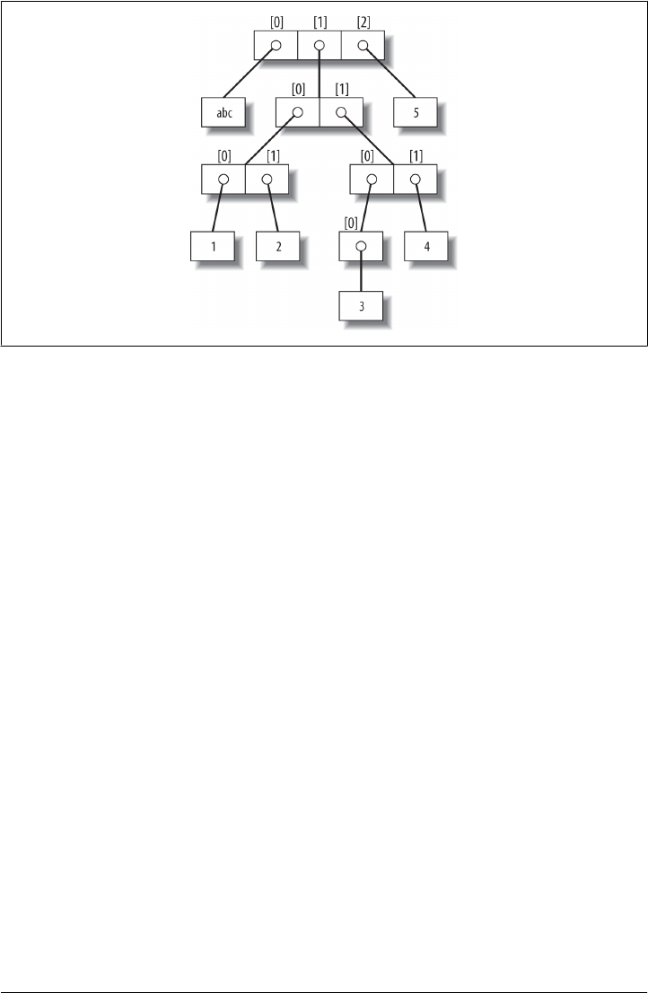
changing a mutable object in place may affect other references to the same object else-
where in your program. If you don’t want such behavior, you’ll need to tell Python to
copy the object explicitly.
We studied this phenomenon in Chapter 6, but it can become more subtle when larger
objects of the sort we’ve explored since then come into play. For instance, the following
example creates a list assigned to X, and another list assigned to L that embeds a refer-
ence back to list X. It also creates a dictionary D that contains another reference back to
list X:
>>> X = [1, 2, 3]
>>> L = ['a', X, 'b'] # Embed references to X's object
>>> D = {'x':X, 'y':2}
At this point, there are three references to the first list created: from the name X, from
inside the list assigned to L, and from inside the dictionary assigned to D. The situation
is illustrated in Figure 9-2.
Because lists are mutable, changing the shared list object from any of the three refer-
ences also changes what the other two reference:
>>> X[1] = 'surprise' # Changes all three references!
>>> L
['a', [1, 'surprise', 3], 'b']
>>> D
{'x': [1, 'surprise', 3], 'y': 2}
References are a higher-level analog of pointers in other languages that are always fol-
lowed when used. Although you can’t grab hold of the reference itself, it’s possible to
Figure 9-1. A nested object tree with the offsets of its components, created by running the literal
expression [‘abc’, [(1, 2), ([3], 4)], 5]. Syntactically nested objects are internally represented as
references (i.e., pointers) to separate pieces of memory.
298 | Chapter 9: Tuples, Files, and Everything Else
www.it-ebooks.info
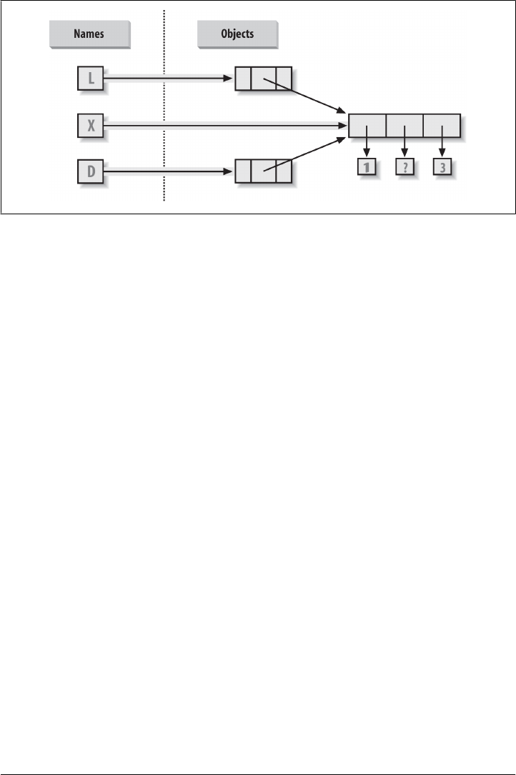
store the same reference in more than one place (variables, lists, and so on). This is a
feature—you can pass a large object around a program without generating expensive
copies of it along the way. If you really do want copies, however, you can request them:
• Slice expressions with empty limits (L[:]) copy sequences.
• The dictionary, set, and list copy method (X.copy()) copies a dictionary, set, or list
(the list’s copy is new as of 3.3).
• Some built-in functions, such as list and dict make copies (list(L), dict(D),
set(S)).
• The copy standard library module makes full copies when needed.
For example, say you have a list and a dictionary, and you don’t want their values to
be changed through other variables:
>>> L = [1,2,3]
>>> D = {'a':1, 'b':2}
To prevent this, simply assign copies to the other variables, not references to the same
objects:
>>> A = L[:] # Instead of A = L (or list(L))
>>> B = D.copy() # Instead of B = D (ditto for sets)
This way, changes made from the other variables will change the copies, not the orig-
inals:
>>> A[1] = 'Ni'
>>> B['c'] = 'spam'
>>>
>>> L, D
([1, 2, 3], {'a': 1, 'b': 2})
Figure 9-2. Shared object references: because the list referenced by variable X is also referenced from
within the objects referenced by L and D, changing the shared list from X makes it look different from
L and D, too.
Core Types Review and Summary | 299
www.it-ebooks.info

>>> A, B
([1, 'Ni', 3], {'a': 1, 'c': 'spam', 'b': 2})
In terms of our original example, you can avoid the reference side effects by slicing the
original list instead of simply naming it:
>>> X = [1, 2, 3]
>>> L = ['a', X[:], 'b'] # Embed copies of X's object
>>> D = {'x':X[:], 'y':2}
This changes the picture in Figure 9-2—L and D will now point to different lists than
X. The net effect is that changes made through X will impact only X, not L and D; similarly,
changes to L or D will not impact X.
One final note on copies: empty-limit slices and the dictionary copy method only make
top-level copies; that is, they do not copy nested data structures, if any are present. If
you need a complete, fully independent copy of a deeply nested data structure (like the
various record structures we’ve coded in recent chapters), use the standard copy mod-
ule, introduced in Chapter 6:
import copy
X = copy.deepcopy(Y) # Fully copy an arbitrarily nested object Y
This call recursively traverses objects to copy all their parts. This is a much more rare
case, though, which is why you have to say more to use this scheme. References are
usually what you will want; when they are not, slices and copy methods are usually as
much copying as you’ll need to do.
Comparisons, Equality, and Truth
All Python objects also respond to comparisons: tests for equality, relative magnitude,
and so on. Python comparisons always inspect all parts of compound objects until a
result can be determined. In fact, when nested objects are present, Python automatically
traverses data structures to apply comparisons from left to right, and as deeply as
needed. The first difference found along the way determines the comparison result.
This is sometimes called a recursive comparison—the same comparison requested on
the top-level objects is applied to each of the nested objects, and to each of their nested
objects, and so on, until a result is found. Later in this book—in Chapter 19—we’ll see
how to write recursive functions of our own that work similarly on nested structures.
For now, think about comparing all the linked pages at two websites if you want a
metaphor for such structures, and a reason for writing recursive functions to process
them.
In terms of core types, the recursion is automatic. For instance, a comparison of list
objects compares all their components automatically until a mismatch is found or the
end is reached:
>>> L1 = [1, ('a', 3)] # Same value, unique objects
>>> L2 = [1, ('a', 3)]
300 | Chapter 9: Tuples, Files, and Everything Else
www.it-ebooks.info

>>> L1 == L2, L1 is L2 # Equivalent? Same object?
(True, False)
Here, L1 and L2 are assigned lists that are equivalent but distinct objects. As a review
of what we saw in Chapter 6, because of the nature of Python references, there are two
ways to test for equality:
•The == operator tests value equivalence. Python performs an equivalence test,
comparing all nested objects recursively.
•The is operator tests object identity. Python tests whether the two are really the
same object (i.e., live at the same address in memory).
In the preceding example, L1 and L2 pass the == test (they have equivalent values because
all their components are equivalent) but fail the is check (they reference two different
objects, and hence two different pieces of memory). Notice what happens for short
strings, though:
>>> S1 = 'spam'
>>> S2 = 'spam'
>>> S1 == S2, S1 is S2
(True, True)
Here, we should again have two distinct objects that happen to have the same value:
== should be true, and is should be false. But because Python internally caches and
reuses some strings as an optimization, there really is just a single string 'spam' in
memory, shared by S1 and S2; hence, the is identity test reports a true result. To trigger
the normal behavior, we need to use longer strings:
>>> S1 = 'a longer string'
>>> S2 = 'a longer string'
>>> S1 == S2, S1 is S2
(True, False)
Of course, because strings are immutable, the object caching mechanism is irrelevant
to your code—strings can’t be changed in place, regardless of how many variables refer
to them. If identity tests seem confusing, see Chapter 6 for a refresher on object refer-
ence concepts.
As a rule of thumb, the == operator is what you will want to use for almost all equality
checks; is is reserved for highly specialized roles. We’ll see cases later in the book where
both operators are put to use.
Relative magnitude comparisons are also applied recursively to nested data structures:
>>> L1 = [1, ('a', 3)]
>>> L2 = [1, ('a', 2)]
>>> L1 < L2, L1 == L2, L1 > L2 # Less, equal, greater: tuple of results
(False, False, True)
Here, L1 is greater than L2 because the nested 3 is greater than 2. By now you should
know that the result of the last line is really a tuple of three objects—the results of the
three expressions typed (an example of a tuple without its enclosing parentheses).
Core Types Review and Summary | 301
www.it-ebooks.info

More specifically, Python compares types as follows:
•Numbers are compared by relative magnitude, after conversion to the common
highest type if needed.
•Strings are compared lexicographically (by the character set code point values re-
turned by ord), and character by character until the end or first mismatch ("abc"
< "ac").
•Lists and tuples are compared by comparing each component from left to right,
and recursively for nested structures, until the end or first mismatch ([2] > [1, 2]).
•Sets are equal if both contain the same items (formally, if each is a subset of the
other), and set relative magnitude comparisons apply subset and superset tests.
•Dictionaries compare as equal if their sorted (key, value) lists are equal. Relative
magnitude comparisons are not supported for dictionaries in Python 3.X, but they
work in 2.X as though comparing sorted (key, value) lists.
• Nonnumeric mixed-type magnitude comparisons (e.g., 1 < 'spam') are errors in
Python 3.X. They are allowed in Python 2.X, but use a fixed but arbitrary ordering
rule based on type name string. By proxy, this also applies to sorts, which use
comparisons internally: nonnumeric mixed-type collections cannot be sorted in
3.X.
In general, comparisons of structured objects proceed as though you had written the
objects as literals and compared all their parts one at a time from left to right. In later
chapters, we’ll see other object types that can change the way they get compared.
Python 2.X and 3.X mixed-type comparisons and sorts
Per the last point in the preceding section’s list, the change in Python 3.X for nonnu-
meric mixed-type comparisons applies to magnitude tests, not equality, but it also ap-
plies by proxy to sorting, which does magnitude testing internally. In Python 2.X these
all work, though mixed types compare by an arbitrary ordering:
c:\code> c:\python27\python
>>> 11 == '11' # Equality does not convert non-numbers
False
>>> 11 >= '11' # 2.X compares by type name string: int, str
False
>>> ['11', '22'].sort() # Ditto for sorts
>>> [11, '11'].sort()
But Python 3.X disallows mixed-type magnitude testing, except numeric types and
manually converted types:
c:\code> c:\python33\python
>>> 11 == '11' # 3.X: equality works but magnitude does not
False
>>> 11 >= '11'
TypeError: unorderable types: int() > str()
302 | Chapter 9: Tuples, Files, and Everything Else
www.it-ebooks.info

>>> ['11', '22'].sort() # Ditto for sorts
>>> [11, '11'].sort()
TypeError: unorderable types: str() < int()
>>> 11 > 9.123 # Mixed numbers convert to highest type
True
>>> str(11) >= '11', 11 >= int('11') # Manual conversions force the issue
(True, True)
Python 2.X and 3.X dictionary comparisons
The second-to-last point in the preceding section also merits illustration. In Python
2.X, dictionaries support magnitude comparisons, as though you were comparing sor-
ted key/value lists:
C:\code> c:\python27\python
>>> D1 = {'a':1, 'b':2}
>>> D2 = {'a':1, 'b':3}
>>> D1 == D2 # Dictionary equality: 2.X + 3.X
False
>>> D1 < D2 # Dictionary magnitude: 2.X only
True
As noted briefly in Chapter 8, though, magnitude comparisons for dictionaries are
removed in Python 3.X because they incur too much overhead when equality is desired
(equality uses an optimized scheme in 3.X that doesn’t literally compare sorted key/
value lists):
C:\code> c:\python33\python
>>> D1 = {'a':1, 'b':2}
>>> D2 = {'a':1, 'b':3}
>>> D1 == D2
False
>>> D1 < D2
TypeError: unorderable types: dict() < dict()
The alternative in 3.X is to either write loops to compare values by key, or compare the
sorted key/value lists manually—the items dictionary methods and sorted built-in suf-
fice:
>>> list(D1.items())
[('b', 2), ('a', 1)]
>>> sorted(D1.items())
[('a', 1), ('b', 2)]
>>>
>>> sorted(D1.items()) < sorted(D2.items()) # Magnitude test in 3.X
True
>>> sorted(D1.items()) > sorted(D2.items())
False
This takes more code, but in practice, most programs requiring this behavior will de-
velop more efficient ways to compare data in dictionaries than either this workaround
or the original behavior in Python 2.X.
Core Types Review and Summary | 303
www.it-ebooks.info
The Meaning of True and False in Python
Notice that the test results returned in the last two examples represent true and false
values. They print as the words True and False, but now that we’re using logical tests
like these in earnest, I should be a bit more formal about what these names really mean.
In Python, as in most programming languages, an integer 0 represents false, and an
integer 1 represents true. In addition, though, Python recognizes any empty data struc-
ture as false and any nonempty data structure as true. More generally, the notions of
true and false are intrinsic properties of every object in Python—each object is either
true or false, as follows:
• Numbers are false if zero, and true otherwise.
• Other objects are false if empty, and true otherwise.
Table 9-4 gives examples of true and false values of objects in Python.
Table 9-4. Example object truth values
Object Value
"spam" True
"" False
[1, 2] True
[] False
{'a': 1} True
{} False
1 True
0.0 False
None False
As one application, because objects are true or false themselves, it’s common to see
Python programmers code tests like if X:, which, assuming X is a string, is the same
as if X != '':. In other words, you can test the object itself to see if it contains anything,
instead of comparing it to an empty, and therefore false, object of the same type (more
on if statements in the next chapter).
The None object
As shown in the last row in Table 9-4, Python also provides a special object called
None, which is always considered to be false. None was introduced briefly in Chap-
ter 4; it is the only value of a special data type in Python and typically serves as an empty
placeholder (much like a NULL pointer in C).
For example, recall that for lists you cannot assign to an offset unless that offset already
exists—the list does not magically grow if you attempt an out-of-bounds assignment.
304 | Chapter 9: Tuples, Files, and Everything Else
www.it-ebooks.info

To preallocate a 100-item list such that you can add to any of the 100 offsets, you can
fill it with None objects:
>>> L = [None] * 100
>>>
>>> L
[None, None, None, None, None, None, None, ... ]
This doesn’t limit the size of the list (it can still grow and shrink later), but simply
presets an initial size to allow for future index assignments. You could initialize a list
with zeros the same way, of course, but best practice dictates using None if the type of
the list’s contents is variable or not yet known.
Keep in mind that None does not mean “undefined.” That is, None is something, not
nothing (despite its name!)—it is a real object and a real piece of memory that is created
and given a built-in name by Python itself. Watch for other uses of this special object
later in the book; as we’ll learn in Part IV, it is also the default return value of functions
that don’t exit by running into a return statement with a result value.
The bool type
While we’re on the topic of truth, also keep in mind that the Python Boolean type
bool, introduced in Chapter 5, simply augments the notions of true and false in Python.
As we learned in Chapter 5, the built-in words True and False are just customized
versions of the integers 1 and 0—it’s as if these two words have been preassigned to 1
and 0 everywhere in Python. Because of the way this new type is implemented, this is
really just a minor extension to the notions of true and false already described, designed
to make truth values more explicit:
• When used explicitly in truth test code, the words True and False are equivalent
to 1 and 0, but they make the programmer’s intent clearer.
• Results of Boolean tests run interactively print as the words True and False, instead
of as 1 and 0, to make the type of result clearer.
You are not required to use only Boolean types in logical statements such as if; all
objects are still inherently true or false, and all the Boolean concepts mentioned in this
chapter still work as described if you use other types. Python also provides a bool built-
in function that can be used to test the Boolean value of an object if you want to make
this explicit (i.e., whether it is true—that is, nonzero or nonempty):
>>> bool(1)
True
>>> bool('spam')
True
>>> bool({})
False
In practice, though, you’ll rarely notice the Boolean type produced by logic tests, be-
cause Boolean results are used automatically by if statements and other selection tools.
We’ll explore Booleans further when we study logical statements in Chapter 12.
Core Types Review and Summary | 305
www.it-ebooks.info

Python’s Type Hierarchies
As a summary and reference, Figure 9-3 sketches all the built-in object types available
in Python and their relationships. We’ve looked at the most prominent of these; most
of the other kinds of objects in Figure 9-3 correspond to program units (e.g., functions
and modules) or exposed interpreter internals (e.g., stack frames and compiled code).
The largest point to notice here is that everything in a Python system is an object type
and may be processed by your Python programs. For instance, you can pass a class to
a function, assign it to a variable, stuff it in a list or dictionary, and so on.
Type Objects
In fact, even types themselves are an object type in Python: the type of an object is an
object of type type (say that three times fast!). Seriously, a call to the built-in function
type(X) returns the type object of object X. The practical application of this is that type
objects can be used for manual type comparisons in Python if statements. However,
for reasons introduced in Chapter 4, manual type testing is usually not the right thing
to do in Python, since it limits your code’s flexibility.
One note on type names: as of Python 2.2, each core type has a new built-in name
added to support type customization through object-oriented subclassing: dict, list,
str, tuple, int, float, complex, bytes, type, set, and more. In Python 3.X names all
references classes, and in Python 2.X but not 3.X, file is also a type name and a syn-
onym for open. Calls to these names are really object constructor calls, not simply con-
version functions, though you can treat them as simple functions for basic usage.
In addition, the types standard library module in Python 3.X provides additional type
names for types that are not available as built-ins (e.g., the type of a function; in Python
2.X but not 3.X, this module also includes synonyms for built-in type names), and it is
possible to do type tests with the isinstance function. For example, all of the following
type tests are true:
type([1]) == type([]) # Compare to type of another list
type([1]) == list # Compare to list type name
isinstance([1], list) # Test if list or customization thereof
import types # types has names for other types
def f(): pass
type(f) == types.FunctionType
Because types can be subclassed in Python today, the isinstance technique is generally
recommended. See Chapter 32 for more on subclassing built-in types in Python 2.2
and later.
306 | Chapter 9: Tuples, Files, and Everything Else
www.it-ebooks.info
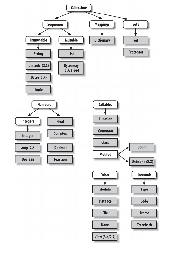
Figure 9-3. Python’s major built-in object types, organized by categories. Everything is a type of object
in Python, even the type of an object! Some extension types, such as named tuples, might belong in
this figure too, but the criteria for inclusion in the core types set are not formal.
Core Types Review and Summary | 307
www.it-ebooks.info

Also in Chapter 32, we will explore how type(X) and type testing in
general apply to instances of user-defined classes. In short, in Python
3.X and for new-style classes in Python 2.X, the type of a class instance
is the class from which the instance was made. For classic classes in
Python 2.X, all class instances are instead of the type “instance,” and
we must compare instance __class__ attributes to compare their types
meaningfully. Since we’re not yet equipped to tackle the subject of
classes, we’ll postpone the rest of this story until Chapter 32.
Other Types in Python
Besides the core objects studied in this part of the book, and the program-unit objects
such as functions, modules, and classes that we’ll meet later, a typical Python instal-
lation has dozens of additional object types available as linked-in C extensions or
Python classes—regular expression objects, DBM files, GUI widgets, network sockets,
and so on. Depending on whom you ask, the named tuple we met earlier in this chapter
may fall in this category too (Decimal and Fraction of Chapter 5 tend to be more am-
biguous).
The main difference between these extra tools and the built-in types we’ve seen so far
is that the built-ins provide special language creation syntax for their objects (e.g., 4 for
an integer, [1,2] for a list, the open function for files, and def and lambda for functions).
Other tools are generally made available in standard library modules that you must first
import to use, and aren’t usually considered core types. For instance, to make a regular
expression object, you import re and call re.compile(). See Python’s library reference
for a comprehensive guide to all the tools available to Python programs.
Built-in Type Gotchas
That’s the end of our look at core data types. We’ll wrap up this part of the book with
a discussion of common problems that seem to trap new users (and the occasional
expert), along with their solutions. Some of this is a review of ideas we’ve already cov-
ered, but these issues are important enough to warn about again here.
Assignment Creates References, Not Copies
Because this is such a central concept, I’ll mention it again: shared references to mutable
objects in your program can matter. For instance, in the following example, the list
object assigned to the name L is referenced both from L and from inside the list assigned
to the name M. Changing L in place changes what M references, too:
>>> L = [1, 2, 3]
>>> M = ['X', L, 'Y'] # Embed a reference to L
>>> M
['X', [1, 2, 3], 'Y']
308 | Chapter 9: Tuples, Files, and Everything Else
www.it-ebooks.info

>>> L[1] = 0 # Changes M too
>>> M
['X', [1, 0, 3], 'Y']
This effect usually becomes important only in larger programs, and shared references
are often exactly what you want. If objects change out from under you in unwanted
ways, you can avoid sharing objects by copying them explicitly. For lists, you can always
make a top-level copy by using an empty-limits slice, among other techniques described
earlier:
>>> L = [1, 2, 3]
>>> M = ['X', L[:], 'Y'] # Embed a copy of L (or list(L), or L.copy())
>>> L[1] = 0 # Changes only L, not M
>>> L
[1, 0, 3]
>>> M
['X', [1, 2, 3], 'Y']
Remember, slice limits default to 0 and the length of the sequence being sliced; if both
are omitted, the slice extracts every item in the sequence and so makes a top-level copy
(a new, unshared object).
Repetition Adds One Level Deep
Repeating a sequence is like adding it to itself a number of times. However, when
mutable sequences are nested, the effect might not always be what you expect. For
instance, in the following example X is assigned to L repeated four times, whereas Y is
assigned to a list containing L repeated four times:
>>> L = [4, 5, 6]
>>> X = L * 4 # Like [4, 5, 6] + [4, 5, 6] + ...
>>> Y = [L] * 4 # [L] + [L] + ... = [L, L,...]
>>> X
[4, 5, 6, 4, 5, 6, 4, 5, 6, 4, 5, 6]
>>> Y
[[4, 5, 6], [4, 5, 6], [4, 5, 6], [4, 5, 6]]
Because L was nested in the second repetition, Y winds up embedding references back
to the original list assigned to L, and so is open to the same sorts of side effects noted
in the preceding section:
>>> L[1] = 0 # Impacts Y but not X
>>> X
[4, 5, 6, 4, 5, 6, 4, 5, 6, 4, 5, 6]
>>> Y
[[4, 0, 6], [4, 0, 6], [4, 0, 6], [4, 0, 6]]
This may seem artificial and academic—until it happens unexpectedly in your code!
The same solutions to this problem apply here as in the previous section, as this is really
just another way to create the shared mutable object reference case—make copies when
you don’t want shared references:
Built-in Type Gotchas | 309
www.it-ebooks.info

>>> L = [4, 5, 6]
>>> Y = [list(L)] * 4 # Embed a (shared) copy of L
>>> L[1] = 0
>>> Y
[[4, 5, 6], [4, 5, 6], [4, 5, 6], [4, 5, 6]]
Even more subtly, although Y doesn’t share an object with L anymore, it still embeds
four references to the same copy of it. If you must avoid that sharing too, you’ll want
to make sure each embedded copy is unique:
>>> Y[0][1] = 99 # All four copies are still the same
>>> Y
[[4, 99, 6], [4, 99, 6], [4, 99, 6], [4, 99, 6]]
>>> L = [4, 5, 6]
>>> Y = [list(L) for i in range(4)]
>>> Y
[[4, 5, 6], [4, 5, 6], [4, 5, 6], [4, 5, 6]]
>>> Y[0][1] = 99
>>> Y
[[4, 99, 6], [4, 5, 6], [4, 5, 6], [4, 5, 6]]
If you remember that repetition, concatenation, and slicing copy only the top level of
their operand objects, these sorts of cases make much more sense.
Beware of Cyclic Data Structures
We actually encountered this concept in a prior exercise: if a collection object contains
a reference to itself, it’s called a cyclic object. Python prints a [...] whenever it detects
a cycle in the object, rather than getting stuck in an infinite loop (as it once did long ago):
>>> L = ['grail'] # Append reference to same object
>>> L.append(L) # Generates cycle in object: [...]
>>> L
['grail', [...]]
Besides understanding that the three dots in square brackets represent a cycle in the
object, this case is worth knowing about because it can lead to gotchas—cyclic struc-
tures may cause code of your own to fall into unexpected loops if you don’t anticipate
them.
For instance, some programs that walk through structured data must keep a list, dic-
tionary, or set of already visited items, and check it when they’re about to step into a
cycle that could cause an unwanted loop. See the solutions to the “Test Your Knowl-
edge: Part I Exercises” on page 87 in Appendix D for more on this problem. Also watch
for general discussion of recursion in Chapter 19, as well as the reloadall.py program
in Chapter 25 and the ListTree class in Chapter 31, for concrete examples of programs
where cycle detection can matter.
The solution is knowledge: don’t use cyclic references unless you really need to, and
make sure you anticipate them in programs that must care. There are good reasons to
310 | Chapter 9: Tuples, Files, and Everything Else
www.it-ebooks.info

create cycles, but unless you have code that knows how to handle them, objects that
reference themselves may be more surprise than asset.
Immutable Types Can’t Be Changed in Place
And once more for completeness: you can’t change an immutable object in place. In-
stead, you construct a new object with slicing, concatenation, and so on, and assign it
back to the original reference, if needed:
T = (1, 2, 3)
T[2] = 4 # Error!
T = T[:2] + (4,) # OK: (1, 2, 4)
That might seem like extra coding work, but the upside is that the previous gotchas in
this section can’t happen when you’re using immutable objects such as tuples and
strings; because they can’t be changed in place, they are not open to the sorts of side
effects that lists are.
Chapter Summary
This chapter explored the last two major core object types—the tuple and the file. We
learned that tuples support all the usual sequence operations, have just a few methods,
do not allow any in-place changes because they are immutable, and are extended by
the named tuple type. We also learned that files are returned by the built-in open func-
tion and provide methods for reading and writing data.
Along the way we explored how to translate Python objects to and from strings for
storing in files, and we looked at the pickle, json, and struct modules for advanced
roles (object serialization and binary data). Finally, we wrapped up by reviewing some
properties common to all object types (e.g., shared references) and went through a list
of common mistakes (“gotchas”) in the object type domain.
In the next part of this book, we’ll shift gears, turning to the topic of statement syntax—
the way you code processing logic in your scripts. Along the way, this next part explores
all of Python’s basic procedural statements. The next chapter kicks off this topic with
an introduction to Python’s general syntax model, which is applicable to all statement
types. Before moving on, though, take the chapter quiz, and then work through the
end-of-part lab exercises to review type concepts. Statements largely just create and
process objects, so make sure you’ve mastered this domain by working through all the
exercises before reading on.
Test Your Knowledge: Quiz
1. How can you determine how large a tuple is? Why is this tool located where it is?
Test Your Knowledge: Quiz | 311
www.it-ebooks.info

2. Write an expression that changes the first item in a tuple. (4, 5, 6) should become
(1, 5, 6) in the process.
3. What is the default for the processing mode argument in a file open call?
4. What module might you use to store Python objects in a file without converting
them to strings yourself?
5. How might you go about copying all parts of a nested structure at once?
6. When does Python consider an object true?
7. What is your quest?
Test Your Knowledge: Answers
1. The built-in len function returns the length (number of contained items) for any
container object in Python, including tuples. It is a built-in function instead of a
type method because it applies to many different types of objects. In general, built-
in functions and expressions may span many object types; methods are specific to
a single object type, though some may be available on more than one type (index,
for example, works on lists and tuples).
2. Because they are immutable, you can’t really change tuples in place, but you can
generate a new tuple with the desired value. Given T = (4, 5, 6), you can change
the first item by making a new tuple from its parts by slicing and concatenating: T
= (1,) + T[1:]. (Recall that single-item tuples require a trailing comma.) You could
also convert the tuple to a list, change it in place, and convert it back to a tuple,
but this is more expensive and is rarely required in practice—simply use a list if
you know that the object will require in-place changes.
3. The default for the processing mode argument in a file open call is 'r', for reading
text input. For input text files, simply pass in the external file’s name.
4. The pickle module can be used to store Python objects in a file without explicitly
converting them to strings. The struct module is related, but it assumes the data
is to be in packed binary format in the file; json similarly converts a limited set of
Python objects to and from strings per the JSON format.
5. Import the copy module, and call copy.deepcopy(X) if you need to copy all parts of
a nested structure X. This is also rarely seen in practice; references are usually the
desired behavior, and shallow copies (e.g., aList[:], aDict.copy(), set(aSet))
usually suffice for most copies.
6. An object is considered true if it is either a nonzero number or a nonempty collec-
tion object. The built-in words True and False are essentially predefined to have
the same meanings as integer 1 and 0, respectively.
7. Acceptable answers include “To learn Python,” “To move on to the next part of
the book,” or “To seek the Holy Grail.”
312 | Chapter 9: Tuples, Files, and Everything Else
www.it-ebooks.info

Test Your Knowledge: Part II Exercises
This session asks you to get your feet wet with built-in object fundamentals. As before,
a few new ideas may pop up along the way, so be sure to flip to the answers in Appen-
dix D when you’re done (or even when you’re not). If you have limited time, I suggest
starting with exercises 10 and 11 (the most practical of the bunch), and then working
from first to last as time allows. This is all fundamental material, so try to do as many
of these as you can; programming is a hands-on activity, and there is no substitute for
practicing what you’ve read to make ideas gel.
1. The basics. Experiment interactively with the common type operations found in
the various operation tables in this part of the book. To get started, bring up the
Python interactive interpreter, type each of the following expressions, and try to
explain what’s happening in each case. Note that the semicolon in some of these
is being used as a statement separator, to squeeze multiple statements onto a single
line: for example, X=1;X assigns and then prints a variable (more on statement
syntax in the next part of the book). Also remember that a comma between ex-
pressions usually builds a tuple, even if there are no enclosing parentheses: X,Y,Z
is a three-item tuple, which Python prints back to you in parentheses.
2 ** 16
2 / 5, 2 / 5.0
"spam" + "eggs"
S = "ham"
"eggs " + S
S * 5
S[:0]
"green %s and %s" % ("eggs", S)
'green {0} and {1}'.format('eggs', S)
('x',)[0]
('x', 'y')[1]
L = [1,2,3] + [4,5,6]
L, L[:], L[:0], L[−2], L[−2:]
([1,2,3] + [4,5,6])[2:4]
[L[2], L[3]]
L.reverse(); L
L.sort(); L
L.index(4)
{'a':1, 'b':2}['b']
D = {'x':1, 'y':2, 'z':3}
D['w'] = 0
D['x'] + D['w']
D[(1,2,3)] = 4
list(D.keys()), list(D.values()), (1,2,3) in D
[[]], ["",[],(),{},None]
Test Your Knowledge: Part II Exercises | 313
www.it-ebooks.info

2. Indexing and slicing. At the interactive prompt, define a list named L that contains
four strings or numbers (e.g., L=[0,1,2,3]). Then, experiment with the following
boundary cases. You may never see these cases in real programs (especially not in
the bizarre ways they appear here!), but they are intended to make you think about
the underlying model, and some may be useful in less artificial forms—slicing out
of bounds can help, for example, if a sequence is as long as you expect:
a. What happens when you try to index out of bounds (e.g., L[4])?
b. What about slicing out of bounds (e.g., L[−1000:100])?
c. Finally, how does Python handle it if you try to extract a sequence in reverse,
with the lower bound greater than the higher bound (e.g., L[3:1])? Hint: try
assigning to this slice (L[3:1]=['?']), and see where the value is put. Do you
think this may be the same phenomenon you saw when slicing out of bounds?
3. Indexing, slicing, and del. Define another list L with four items, and assign an empty
list to one of its offsets (e.g., L[2]=[]). What happens? Then, assign an empty list
to a slice (L[2:3]=[]). What happens now? Recall that slice assignment deletes the
slice and inserts the new value where it used to be.
The del statement deletes offsets, keys, attributes, and names. Use it on your list
to delete an item (e.g., del L[0]). What happens if you delete an entire slice (del
L[1:])? What happens when you assign a nonsequence to a slice (L[1:2]=1)?
4. Tuple assignment. Type the following lines:
>>> X = 'spam'
>>> Y = 'eggs'
>>> X, Y = Y, X
What do you think is happening to X and Y when you type this sequence?
5. Dictionary keys. Consider the following code fragments:
>>> D = {}
>>> D[1] = 'a'
>>> D[2] = 'b'
You’ve learned that dictionaries aren’t accessed by offsets, so what’s going on here?
Does the following shed any light on the subject? (Hint: strings, integers, and tuples
share which type category?)
>>> D[(1, 2, 3)] = 'c'
>>> D
{1: 'a', 2: 'b', (1, 2, 3): 'c'}
6. Dictionary indexing. Create a dictionary named D with three entries, for keys 'a',
'b', and 'c'. What happens if you try to index a nonexistent key (D['d'])? What
does Python do if you try to assign to a nonexistent key 'd' (e.g., D['d']='spam')?
How does this compare to out-of-bounds assignments and references for lists?
Does this sound like the rule for variable names?
7. Generic operations. Run interactive tests to answer the following questions:
314 | Chapter 9: Tuples, Files, and Everything Else
www.it-ebooks.info

a. What happens when you try to use the + operator on different/mixed types
(e.g., string + list, list + tuple)?
b. Does + work when one of the operands is a dictionary?
c. Does the append method work for both lists and strings? How about using the
keys method on lists? (Hint: what does append assume about its subject object?)
d. Finally, what type of object do you get back when you slice or concatenate two
lists or two strings?
8. String indexing. Define a string S of four characters: S = "spam". Then type the
following expression: S[0][0][0][0][0]. Any clue as to what’s happening this time?
(Hint: recall that a string is a collection of characters, but Python characters are
one-character strings.) Does this indexing expression still work if you apply it to a
list such as ['s', 'p', 'a', 'm']? Why?
9. Immutable types. Define a string S of four characters again: S = "spam". Write an
assignment that changes the string to "slam", using only slicing and concatenation.
Could you perform the same operation using just indexing and concatenation?
How about index assignment?
10. Nesting. Write a data structure that represents your personal information: name
(first, middle, last), age, job, address, email address, and phone number. You may
build the data structure with any combination of built-in object types you like (lists,
tuples, dictionaries, strings, numbers). Then, access the individual components of
your data structures by indexing. Do some structures make more sense than others
for this object?
11. Files. Write a script that creates a new output file called myfile.txt and writes the
string "Hello file world!" into it. Then write another script that opens my-
file.txt and reads and prints its contents. Run your two scripts from the system
command line. Does the new file show up in the directory where you ran your
scripts? What if you add a different directory path to the filename passed to open?
Note: file write methods do not add newline characters to your strings; add an
explicit \n at the end of the string if you want to fully terminate the line in the file.
Test Your Knowledge: Part II Exercises | 315
www.it-ebooks.info


CHAPTER 10
Introducing Python Statements
Now that you’re familiar with Python’s core built-in object types, this chapter begins
our exploration of its fundamental statement forms. As in the previous part, we’ll begin
here with a general introduction to statement syntax, and we’ll follow up with more
details about specific statements in the next few chapters.
In simple terms, statements are the things you write to tell Python what your programs
should do. If, as suggested in Chapter 4, programs “do things with stuff,” then state-
ments are the way you specify what sort of things a program does. Less informally,
Python is a procedural, statement-based language; by combining statements, you spec-
ify a procedure that Python performs to satisfy a program’s goals.
The Python Conceptual Hierarchy Revisited
Another way to understand the role of statements is to revisit the concept hierarchy
introduced in Chapter 4, which talked about built-in objects and the expressions used
to manipulate them. This chapter climbs the hierarchy to the next level of Python
program structure:
1. Programs are composed of modules.
2. Modules contain statements.
3. Statements contain expressions.
4. Expressions create and process objects.
At their base, programs written in the Python language are composed of statements
and expressions. Expressions process objects and are embedded in statements. State-
ments code the larger logic of a program’s operation—they use and direct expressions
to process the objects we studied in the preceding chapters. Moreover, statements are
where objects spring into existence (e.g., in expressions within assignment statements),
and some statements create entirely new kinds of objects (functions, classes, and so
on). At the top, statements always exist in modules, which themselves are managed
with statements.
319
www.it-ebooks.info

Python’s Statements
Table 10-1 summarizes Python’s statement set. Each statement in Python has its own
specific purpose and its own specific syntax—the rules that define its structure—
though, as we’ll see, many share common syntax patterns, and some statements’ roles
overlap. Table 10-1 also gives examples of each statement, when coded according to
its syntax rules. In your programs, these units of code can perform actions, repeat tasks,
make choices, build larger program structures, and so on.
This part of the book deals with entries in the table from the top through break and
continue. You’ve informally been introduced to a few of the statements in Table 10-1
already; this part of the book will fill in details that were skipped earlier, introduce the
rest of Python’s procedural statement set, and cover the overall syntax model. State-
ments lower in Table 10-1 that have to do with larger program units—functions,
classes, modules, and exceptions—lead to larger programming ideas, so they will each
have a section of their own. More focused statements (like del, which deletes various
components) are covered elsewhere in the book, or in Python’s standard manuals.
Table 10-1. Python statements
Statement Role Example
Assignment Creating references a, b = 'good', 'bad'
Calls and other expressions Running functions log.write("spam, ham")
print calls Printing objects print('The Killer', joke)
if/elif/else Selecting actions if "python" in text:
print(text)
for/else Iteration for x in mylist:
print(x)
while/else General loops while X > Y:
print('hello')
pass Empty placeholder while True:
pass
break Loop exit while True:
if exittest(): break
continue Loop continue while True:
if skiptest(): continue
def Functions and methods def f(a, b, c=1, *d):
print(a+b+c+d[0])
return Functions results def f(a, b, c=1, *d):
return a+b+c+d[0]
yield Generator functions def gen(n):
for i in n: yield i*2
global Namespaces x = 'old'
def function():
global x, y; x = 'new'
nonlocal Namespaces (3.X) def outer():
x = 'old'
320 | Chapter 10: Introducing Python Statements
www.it-ebooks.info

Statement Role Example
def function():
nonlocal x; x = 'new'
import Module access import sys
from Attribute access from sys import stdin
class Building objects class Subclass(Superclass):
staticData = []
def method(self): pass
try/except/ finally Catching exceptions try:
action()
except:
print('action error')
raise Triggering exceptions raise EndSearch(location)
assert Debugging checks assert X > Y, 'X too small'
with/as Context managers (3.X, 2.6+) with open('data') as myfile:
process(myfile)
del Deleting references del data[k]
del data[i:j]
del obj.attr
del variable
Technically, Table 10-1 reflects Python 3.X’s statements. Though sufficient as a quick
preview and reference, it’s not quite complete as is. Here are a few fine points about its
content:
• Assignment statements come in a variety of syntax flavors, described in Chap-
ter 11: basic, sequence, augmented, and more.
•print is technically neither a reserved word nor a statement in 3.X, but a built-in
function call; because it will nearly always be run as an expression statement,
though (and often on a line by itself), it’s generally thought of as a statement type.
We’ll study print operations in Chapter 11.
•yield is also an expression instead of a statement as of 2.5; like print, it’s typically
used as an expression statement and so is included in this table, but scripts occa-
sionally assign or otherwise use its result, as we’ll see in Chapter 20. As an expres-
sion, yield is also a reserved word, unlike print.
Most of this table applies to Python 2.X, too, except where it doesn’t—if you are using
Python 2.X, here are a few notes for your Python, too:
• In 2.X, nonlocal is not available; as we’ll see in Chapter 17, there are alternative
ways to achieve this statement’s writeable state-retention effect.
• In 2.X, print is a statement instead of a built-in function call, with specific syntax
covered in Chapter 11.
• In 2.X, the 3.X exec code execution built-in function is a statement, with specific
syntax; since it supports enclosing parentheses, though, you can generally use its
3.X call form in 2.X code.
Python’s Statements | 321
www.it-ebooks.info

• In 2.5, the try/except and try/finally statements were merged: the two were for-
merly separate statements, but we can now say both except and finally in the same
try statement.
• In 2.5, with/as is an optional extension, and it is not available unless you explicitly
turn it on by running the statement from __future__ import with_statement (see
Chapter 34).
A Tale of Two ifs
Before we delve into the details of any of the concrete statements in Table 10-1, I want
to begin our look at Python statement syntax by showing you what you are not going
to type in Python code so you can compare and contrast it with other syntax models
you might have seen in the past.
Consider the following if statement, coded in a C-like language:
if (x > y) {
x = 1;
y = 2;
}
This might be a statement in C, C++, Java, JavaScript, or similar. Now, look at the
equivalent statement in the Python language:
if x > y:
x = 1
y = 2
The first thing that may pop out at you is that the equivalent Python statement is less,
well, cluttered—that is, there are fewer syntactic components. This is by design; as a
scripting language, one of Python’s goals is to make programmers’ lives easier by re-
quiring less typing.
More specifically, when you compare the two syntax models, you’ll notice that Python
adds one new thing to the mix, and that three items that are present in the C-like
language are not present in Python code.
What Python Adds
The one new syntax component in Python is the colon character (:). All Python com-
pound statements—statements that have other statements nested inside them—follow
the same general pattern of a header line terminated in a colon, followed by a nested
block of code usually indented underneath the header line, like this:
Header line:
Nested statement block
The colon is required, and omitting it is probably the most common coding mistake
among new Python programmers—it’s certainly one I’ve witnessed thousands of times
322 | Chapter 10: Introducing Python Statements
www.it-ebooks.info

in Python training classes I’ve taught. In fact, if you are new to Python, you’ll almost
certainly forget the colon character very soon. You’ll get an error message if you do,
and most Python-friendly editors make this mistake easy to spot. Including it eventually
becomes an unconscious habit (so much so that you may start typing colons in your
C-like language code, too, generating many entertaining error messages from that lan-
guage’s compiler!).
What Python Removes
Although Python requires the extra colon character, there are three things programmers
in C-like languages must include that you don’t generally have to in Python.
Parentheses are optional
The first of these is the set of parentheses around the tests at the top of the statement:
if (x < y)
The parentheses here are required by the syntax of many C-like languages. In Python,
though, they are not—we simply omit the parentheses, and the statement works the
same way:
if x < y
Technically speaking, because every expression can be enclosed in parentheses, in-
cluding them will not hurt in this Python code, and they are not treated as an error if
present.
But don’t do that: you’ll be wearing out your keyboard needlessly, and broadcasting to
the world that you’re a programmer of a C-like language still learning Python (I know,
because I was once, too). The “Python way” is to simply omit the parentheses in these
kinds of statements altogether.
End-of-line is end of statement
The second and more significant syntax component you won’t find in Python code is
the semicolon. You don’t need to terminate statements with semicolons in Python the
way you do in C-like languages:
x = 1;
In Python, the general rule is that the end of a line automatically terminates the state-
ment that appears on that line. In other words, you can leave off the semicolons, and
it works the same way:
x = 1
There are some ways to work around this rule, as you’ll see in a moment (for instance,
wrapping code in a bracketed structure allows it to span lines). But, in general, you
A Tale of Two ifs | 323
www.it-ebooks.info

write one statement per line for the vast majority of Python code, and no semicolon is
required.
Here, too, if you are pining for your C programming days (if such a state is possible)
you can continue to use semicolons at the end of each statement—the language lets
you get away with them if they are present, because the semicolon is also a separator
when statements are combined.
But don’t do that either (really!). Again, doing so tells the world that you’re a program-
mer of a C-like language who still hasn’t quite made the switch to Python coding. The
Pythonic style is to leave off the semicolons altogether. Judging from students in classes,
this seems a tough habit for some veteran programmers to break. But you’ll get there;
semicolons are useless noise in this role in Python.
End of indentation is end of block
The third and final syntax component that Python removes, and the one that may seem
the most unusual to soon-to-be-ex-programmers of C-like languages (until they’ve used
it for 10 minutes and realize it’s actually a feature), is that you do not type anything
explicit in your code to syntactically mark the beginning and end of a nested block of
code. You don’t need to include begin/end, then/endif, or braces around the nested
block, as you do in C-like languages:
if (x > y) {
x = 1;
y = 2;
}
Instead, in Python, we consistently indent all the statements in a given single nested
block the same distance to the right, and Python uses the statements’ physical inden-
tation to determine where the block starts and stops:
if x > y:
x = 1
y = 2
By indentation, I mean the blank whitespace all the way to the left of the two nested
statements here. Python doesn’t care how you indent (you may use either spaces or
tabs), or how much you indent (you may use any number of spaces or tabs). In fact, the
indentation of one nested block can be totally different from that of another. The syntax
rule is only that for a given single nested block, all of its statements must be indented
the same distance to the right. If this is not the case, you will get a syntax error, and
your code will not run until you repair its indentation to be consistent.
Why Indentation Syntax?
The indentation rule may seem unusual at first glance to programmers accustomed to
C-like languages, but it is a deliberate feature of Python, and it’s one of the main ways
that Python almost forces programmers to produce uniform, regular, and readable
324 | Chapter 10: Introducing Python Statements
www.it-ebooks.info

code. It essentially means that you must line up your code vertically, in columns, ac-
cording to its logical structure. The net effect is to make your code more consistent and
readable (unlike much of the code written in C-like languages).
To put that more strongly, aligning your code according to its logical structure is a
major part of making it readable, and thus reusable and maintainable, by yourself and
others. In fact, even if you never use Python after reading this book, you should get into
the habit of aligning your code for readability in any block-structured language. Python
underscores the issue by making this a part of its syntax, but it’s an important thing to
do in any programming language, and it has a huge impact on the usefulness of your
code.
Your experience may vary, but when I was still doing development on a full-time basis,
I was mostly paid to work on large old C++ programs that had been worked on by
many programmers over the years. Almost invariably, each programmer had his or her
own style for indenting code. For example, I’d often be asked to change a while loop
coded in the C++ language that began like this:
while (x > 0) {
Before we even get into indentation, there are three or four ways that programmers can
arrange these braces in a C-like language, and organizations often endure political bat-
tles and standards manuals to address the options (which seems more than a little off-
topic for the problem to be solved by programming). Be that as it may, here’s the
scenario I often encountered in C++ code. The first person who worked on the code
indented the loop four spaces:
while (x > 0) {
--------;
--------;
That person eventually moved on to management, only to be replaced by someone who
liked to indent further to the right:
while (x > 0) {
--------;
--------;
--------;
--------;
That person later moved on to other opportunities (ending that individual’s reign of
coding terror...), and someone else picked up the code who liked to indent less:
while (x > 0) {
--------;
--------;
--------;
--------;
--------;
--------;
}
A Tale of Two ifs | 325
www.it-ebooks.info

And so on. Eventually, the block is terminated by a closing brace (}), which of course
makes this “block-structured code” (he says, sarcastically). No: in any block-structured
language, Python or otherwise, if nested blocks are not indented consistently, they
become very difficult for the reader to interpret, change, or reuse, because the code no
longer visually reflects its logical meaning. Readability matters, and indentation is a
major component of readability.
Here is another example that may have burned you in the past if you’ve done much
programming in a C-like language. Consider the following statement in C:
if (x)
if (y)
statement1;
else
statement2;
Which if does the else here go with? Surprisingly, the else is paired with the nested
if statement (if (y)) in C, even though it looks visually as though it is associated with
the outer if (x). This is a classic pitfall in the C language, and it can lead to the reader
completely misinterpreting the code and changing it incorrectly in ways that might not
be uncovered until the Mars rover crashes into a giant rock!
This cannot happen in Python—because indentation is significant, the way the code
looks is the way it will work. Consider an equivalent Python statement:
if x:
if y:
statement1
else:
statement2
In this example, the if that the else lines up with vertically is the one it is associated
with logically (the outer if x). In a sense, Python is a WYSIWYG language—what you
see is what you get—because the way code looks is the way it runs, regardless of who
coded it.
If this still isn’t enough to underscore the benefits of Python’s syntax, here’s another
anecdote. Early in my career, I worked at a successful company that developed systems
software in the C language, where consistent indentation is not required. Even so, when
we checked our code into source control at the end of the day, this company ran an
automated script that analyzed the indentation used in the code. If the script noticed
that we’d indented our code inconsistently, we received an automated email about it
the next morning—and so did our managers!
The point is that even when a language doesn’t require it, good programmers know
that consistent use of indentation has a huge impact on code readability and quality.
The fact that Python promotes this to the level of syntax is seen by most as a feature of
the language.
Also keep in mind that nearly every programmer-friendly text editor has built-in sup-
port for Python’s syntax model. In the IDLE Python GUI, for example, lines of code
326 | Chapter 10: Introducing Python Statements
www.it-ebooks.info

are automatically indented when you are typing a nested block; pressing the Backspace
key backs up one level of indentation, and you can customize how far to the right IDLE
indents statements in a nested block. There is no universal standard on this: four spaces
or one tab per level is common, but it’s generally up to you to decide how and how
much you wish to indent (unless you work at a company that’s endured politics and
manuals to standardize this too). Indent further to the right for further nested blocks,
and less to close the prior block.
As a rule of thumb, you probably shouldn’t mix tabs and spaces in the same block in
Python, unless you do so consistently; use tabs or spaces in a given block, but not both
(in fact, Python 3.X now issues an error for inconsistent use of tabs and spaces, as we’ll
see in Chapter 12). Then again, you probably shouldn’t mix tabs or spaces in inden-
tation in any structured language—such code can cause major readability issues if the
next programmer has his or her editor set to display tabs differently than yours. C-like
languages might let coders get away with this, but they shouldn’t: the result can be a
mangled mess.
Regardless of which language you code in, you should be indenting consistently for
readability. In fact, if you weren’t taught to do this earlier in your career, your teachers
did you a disservice. Most programmers—especially those who must read others’ code
—consider it a major asset that Python elevates this to the level of syntax. Moreover,
generating tabs instead of braces is no more difficult in practice for tools that must
output Python code. In general, if you do what you should be doing in a C-like language
anyhow, but get rid of the braces, your code will satisfy Python’s syntax rules.
A Few Special Cases
As mentioned previously, in Python’s syntax model:
• The end of a line terminates the statement on that line (without semicolons).
• Nested statements are blocked and associated by their physical indentation
(without braces).
Those rules cover almost all Python code you’ll write or see in practice. However,
Python also provides some special-purpose rules that allow customization of both
statements and nested statement blocks. They’re not required and should be used
sparingly, but programmers have found them useful in practice.
Statement rule special cases
Although statements normally appear one per line, it is possible to squeeze more than
one statement onto a single line in Python by separating them with semicolons:
a = 1; b = 2; print(a + b) # Three statements on one line
This is the only place in Python where semicolons are required: as statement separa-
tors. This only works, though, if the statements thus combined are not themselves
A Tale of Two ifs | 327
www.it-ebooks.info

compound statements. In other words, you can chain together only simple statements,
like assignments, prints, and function calls. Compound statements like if tests and
while loops must still appear on lines of their own (otherwise, you could squeeze an
entire program onto one line, which probably would not make you very popular among
your coworkers!).
The other special rule for statements is essentially the inverse: you can make a single
statement span across multiple lines. To make this work, you simply have to enclose
part of your statement in a bracketed pair—parentheses (()), square brackets ([]), or
curly braces ({}). Any code enclosed in these constructs can cross multiple lines: your
statement doesn’t end until Python reaches the line containing the closing part of the
pair. For instance, to continue a list literal:
mylist = [1111,
2222,
3333]
Because the code is enclosed in a square brackets pair, Python simply drops down to
the next line until it encounters the closing bracket. The curly braces surrounding dic-
tionaries (as well as set literals and dictionary and set comprehensions in 3.X and 2.7)
allow them to span lines this way too, and parentheses handle tuples, function calls,
and expressions. The indentation of the continuation lines does not matter, though
common sense dictates that the lines should be aligned somehow for readability.
Parentheses are the catchall device—because any expression can be wrapped in them,
simply inserting a left parenthesis allows you to drop down to the next line and continue
your statement:
X = (A + B +
C + D)
This technique works with compound statements, too, by the way. Anywhere you need
to code a large expression, simply wrap it in parentheses to continue it on the next line:
if (A == 1 and
B == 2 and
C == 3):
print('spam' * 3)
An older rule also allows for continuation lines when the prior line ends in a backslash:
X = A + B + \
C + D # An error-prone older alternative
This alternative technique is dated, though, and is frowned on today because it’s dif-
ficult to notice and maintain the backslashes. It’s also fairly brittle and error-prone—
there can be no spaces after the backslash, and accidentally omitting it can have unex-
pected effects if the next line is mistaken to be a new statement (in this example, “C +
D” is a valid statement by itself if it’s not indented). This rule is also another throwback
to the C language, where it is commonly used in “#define” macros; again, when in
Pythonland, do as Pythonistas do, not as C programmers do.
328 | Chapter 10: Introducing Python Statements
www.it-ebooks.info

Block rule special case
As mentioned previously, statements in a nested block of code are normally associated
by being indented the same amount to the right. As one special case here, the body of
a compound statement can instead appear on the same line as the header in Python,
after the colon:
if x > y: print(x)
This allows us to code single-line if statements, single-line while and for loops, and
so on. Here again, though, this will work only if the body of the compound statement
itself does not contain any compound statements. That is, only simple statements—
assignments, prints, function calls, and the like—are allowed after the colon. Larger
statements must still appear on lines by themselves. Extra parts of compound state-
ments (such as the else part of an if, which we’ll meet in the next section) must also
be on separate lines of their own. Compound statement bodies can also consist of
multiple simple statements separated by semicolons, but this tends to be frowned upon.
In general, even though it’s not always required, if you keep all your statements on
individual lines and always indent your nested blocks, your code will be easier to read
and change in the future. Moreover, some code profiling and coverage tools may not
be able to distinguish between multiple statements squeezed onto a single line or the
header and body of a one-line compound statement. It is almost always to your ad-
vantage to keep things simple in Python. You can use the special-case exceptions to
write Python code that’s hard to read, but it takes a lot of work, and there are probably
better ways to spend your time.
To see a prime and common exception to one of these rules in action, however (the use
of a single-line if statement to break out of a loop), and to introduce more of Python’s
syntax, let’s move on to the next section and write some real code.
A Quick Example: Interactive Loops
We’ll see all these syntax rules in action when we tour Python’s specific compound
statements in the next few chapters, but they work the same everywhere in the Python
language. To get started, let’s work through a brief, realistic example that demonstrates
the way that statement syntax and statement nesting come together in practice, and
introduces a few statements along the way.
A Simple Interactive Loop
Suppose you’re asked to write a Python program that interacts with a user in a console
window. Maybe you’re accepting inputs to send to a database, or reading numbers to
be used in a calculation. Regardless of the purpose, you need to code a loop that reads
one or more inputs from a user typing on a keyboard, and prints back a result for each.
In other words, you need to write a classic read/evaluate/print loop program.
A Quick Example: Interactive Loops | 329
www.it-ebooks.info

In Python, typical boilerplate code for such an interactive loop might look like this:
while True:
reply = input('Enter text:')
if reply == 'stop': break
print(reply.upper())
This code makes use of a few new ideas and some we’ve already seen:
• The code leverages the Python while loop, Python’s most general looping state-
ment. We’ll study the while statement in more detail later, but in short, it consists
of the word while, followed by an expression that is interpreted as a true or false
result, followed by a nested block of code that is repeated while the test at the top
is true (the word True here is considered always true).
• The input built-in function we met earlier in the book is used here for general
console input—it prints its optional argument string as a prompt and returns the
user’s typed reply as a string. Use raw_input in 2.X instead, per the upcoming note.
• A single-line if statement that makes use of the special rule for nested blocks also
appears here: the body of the if appears on the header line after the colon instead
of being indented on a new line underneath it. This would work either way, but as
it’s coded, we’ve saved an extra line.
• Finally, the Python break statement is used to exit the loop immediately—it simply
jumps out of the loop statement altogether, and the program continues after the
loop. Without this exit statement, the while would loop forever, as its test is always
true.
In effect, this combination of statements essentially means “read a line from the user
and print it in uppercase until the user enters the word ‘stop.’” There are other ways
to code such a loop, but the form used here is very common in Python code.
Notice that all three lines nested under the while header line are indented the same
amount—because they line up vertically in a column this way, they are the block of
code that is associated with the while test and repeated. Either the end of the source
file or a lesser-indented statement will suffice to terminate the loop body block.
When this code is run, either interactively or as a script file, here is the sort of interaction
we get—all of the code for this example is in interact.py in the book’s examples package:
Enter text:spam
SPAM
Enter text:42
42
Enter text:stop
330 | Chapter 10: Introducing Python Statements
www.it-ebooks.info

Version skew note: This example is coded for Python 3.X. If you are
working in Python 2.X, the code works the same, but you must use
raw_input instead of input in all of this chapter’s examples, and you can
omit the outer parentheses in print statements (though they don’t hurt).
In fact, if you study the interact.py file in the examples package, you’ll
see that it does this automatically—to support 2.X compatibility, it re-
sets input if the running Python’s major version is 2 (“input” winds up
running raw_input):
import sys
if sys.version[0] == '2': input = raw_input # 2.X compatible
In 3.X, raw_input was renamed input, and print is a built-in function
instead of a statement (more on prints in the next chapter). Python 2.X
has an input too, but it tries to evaluate the input string as though it
were Python code, which probably won’t work in this context;
eval(input()) can yield the same effect 3.X.
Doing Math on User Inputs
Our script works, but now suppose that instead of converting a text string to uppercase,
we want to do some math with numeric input—squaring it, for example, perhaps in
some misguided effort of an age-input program to tease its users. We might try state-
ments like these to achieve the desired effect:
>>> reply = '20'
>>> reply ** 2
...error text omitted...
TypeError: unsupported operand type(s) for ** or pow(): 'str' and 'int'
This won’t quite work in our script, though, because (as discussed in the prior part of
the book) Python won’t convert object types in expressions unless they are all numeric,
and input from a user is always returned to our script as a string. We cannot raise a
string of digits to a power unless we convert it manually to an integer:
>>> int(reply) ** 2
400
Armed with this information, we can now recode our loop to perform the necessary
math. Type the following in a file to test it:
while True:
reply = input('Enter text:')
if reply == 'stop': break
print(int(reply) ** 2)
print('Bye')
This script uses a single-line if statement to exit on “stop” as before, but it also converts
inputs to perform the required math. This version also adds an exit message at the
bottom. Because the print statement in the last line is not indented as much as the
A Quick Example: Interactive Loops | 331
www.it-ebooks.info

nested block of code, it is not considered part of the loop body and will run only once,
after the loop is exited:
Enter text:2
4
Enter text:40
1600
Enter text:stop
Bye
Usage note: From this point on I’ll assume that this code is stored in and
run from a script file, via command line, IDLE menu option, or any of
the other file launching techniques we met in Chapter 3. Again, it’s
named interact.py in the book’s examples. If you are entering this code
interactively, though, be sure to include a blank line (i.e., press Enter
twice) before the final print statement, to terminate the loop. This im-
plies that you also can’t cut and paste the code in its entirety into an
interactive prompt: an extra blank line is required interactively, but not
in script files. The final print doesn’t quite make sense in interactive
mode, though—you’ll have to code it after interacting with the loop!
Handling Errors by Testing Inputs
So far so good, but notice what happens when the input is invalid:
Enter text:xxx
...error text omitted...
ValueError: invalid literal for int() with base 10: 'xxx'
The built-in int function raises an exception here in the face of a mistake. If we want
our script to be robust, we can check the string’s content ahead of time with the string
object’s isdigit method:
>>> S = '123'
>>> T = 'xxx'
>>> S.isdigit(), T.isdigit()
(True, False)
This also gives us an excuse to further nest the statements in our example. The following
new version of our interactive script uses a full-blown if statement to work around the
exception on errors:
while True:
reply = input('Enter text:')
if reply == 'stop':
break
elif not reply.isdigit():
print('Bad!' * 8)
else:
print(int(reply) ** 2)
print('Bye')
332 | Chapter 10: Introducing Python Statements
www.it-ebooks.info

We’ll study the if statement in more detail in Chapter 12, but it’s a fairly lightweight
tool for coding logic in scripts. In its full form, it consists of the word if followed by a
test and an associated block of code, one or more optional elif (“else if”) tests and
code blocks, and an optional else part, with an associated block of code at the bottom
to serve as a default. Python runs the block of code associated with the first test that is
true, working from top to bottom, or the else part if all tests are false.
The if, elif, and else parts in the preceding example are associated as part of the same
statement because they all line up vertically (i.e., share the same level of indentation).
The if statement spans from the word if to the start of the print statement on the last
line of the script. In turn, the entire if block is part of the while loop because all of it
is indented under the loop’s header line. Statement nesting like this is natural once you
get the hang of it.
When we run our new script, its code catches errors before they occur and prints an
error message before continuing (which you’ll probably want to improve in a later
release), but “stop” still gets us out, and valid numbers are still squared:
Enter text:5
25
Enter text:xyz
Bad!Bad!Bad!Bad!Bad!Bad!Bad!Bad!
Enter text:10
100
Enter text:stop
Handling Errors with try Statements
The preceding solution works, but as you’ll see later in the book, the most general way
to handle errors in Python is to catch and recover from them completely using the
Python try statement. We’ll explore this statement in depth in Part VII of this book,
but as a preview, using a try here can lead to code that some would see as simpler than
the prior version:
while True:
reply = input('Enter text:')
if reply == 'stop': break
try:
num = int(reply)
except:
print('Bad!' * 8)
else:
print(num ** 2)
print('Bye')
This version works exactly like the previous one, but we’ve replaced the explicit error
check with code that assumes the conversion will work and wraps it in an exception
handler for cases when it doesn’t. In other words, rather than detecting an error, we
simply respond if one occurs.
A Quick Example: Interactive Loops | 333
www.it-ebooks.info

This try statement is another compound statement, and follows the same pattern as
if and while. It’s composed of the word try, followed by the main block of code (the
action we are trying to run), followed by an except part that gives the exception handler
code and an else part to be run if no exception is raised in the try part. Python first
runs the try part, then runs either the except part (if an exception occurs) or the else
part (if no exception occurs).
In terms of statement nesting, because the words try, except, and else are all indented
to the same level, they are all considered part of the same single try statement. Notice
that the else part is associated with the try here, not the if. As we’ve seen, else can
appear in if statements in Python, but it can also appear in try statements and loops
—its indentation tells you what statement it is a part of. In this case, the try statement
spans from the word try through the code indented under the word else, because the
else is indented the same as try. The if statement in this code is a one-liner and ends
after the break.
Supporting floating-point numbers
Again, we’ll come back to the try statement later in this book. For now, be aware that
because try can be used to intercept any error, it reduces the amount of error-checking
code you have to write, and it’s a very general approach to dealing with unusual cases.
If we’re sure that print won’t fail, for instance, this example could be even more concise:
while True:
reply = input('Enter text:')
if reply == 'stop': break
try:
print(int(reply) ** 2)
except:
print('Bad!' * 8)
print('Bye')
And if we wanted to support input of floating-point numbers instead of just integers,
for example, using try would be much easier than manual error testing—we could
simply run a float call and catch its exceptions:
while True:
reply = input('Enter text:')
if reply == 'stop': break
try:
print(float(reply) ** 2)
except:
print('Bad!' * 8)
print('Bye')
There is no isfloat for strings today, so this exception-based approach spares us from
having to analyze all possible floating-point syntax in an explicit error check. When
coding this way, we can enter a wider variety of numbers, but errors and exits still work
as before:
334 | Chapter 10: Introducing Python Statements
www.it-ebooks.info

Enter text:50
2500.0
Enter text:40.5
1640.25
Enter text:1.23E-100
1.5129e-200
Enter text:spam
Bad!Bad!Bad!Bad!Bad!Bad!Bad!Bad!
Enter text:stop
Bye
Python’s eval call, which we used in Chapter 5 and Chapter 9 to convert
data in strings and files, would work in place of float here too, and
would allow input of arbitrary expressions (“2 ** 100” would be a legal,
if curious, input, especially if we’re assuming the program is processing
ages!). This is a powerful concept that is open to the same security issues
mentioned in the prior chapters. If you can’t trust the source of a code
string, use more restrictive conversion tools like int and float.
Python’s exec, used in Chapter 3 to run code read from a file, is similar
to eval (but assumes the string is a statement instead of an expression
and has no result), and its compile call precompiles frequently used code
strings to bytecode objects for speed. Run a help on any of these for
more details; as mentioned, exec is a statement in 2.X but a function in
3.X, so see its manual entry in 2.X instead. We’ll also use exec to import
modules by name string in Chapter 25—an example of its more dynamic
roles.
Nesting Code Three Levels Deep
Let’s look at one last mutation of our code. Nesting can take us even further if we need
it to—we could, for example, extend our prior integer-only script to branch to one of
a set of alternatives based on the relative magnitude of a valid input:
while True:
reply = input('Enter text:')
if reply == 'stop':
break
elif not reply.isdigit():
print('Bad!' * 8)
else:
num = int(reply)
if num < 20:
print('low')
else:
print(num ** 2)
print('Bye')
This version adds an if statement nested in the else clause of another if statement,
which is in turn nested in the while loop. When code is conditional or repeated like
A Quick Example: Interactive Loops | 335
www.it-ebooks.info

this, we simply indent it further to the right. The net effect is like that of prior versions,
but we’ll now print “low” for numbers less than 20:
Enter text:19
low
Enter text:20
400
Enter text:spam
Bad!Bad!Bad!Bad!Bad!Bad!Bad!Bad!
Enter text:stop
Bye
Chapter Summary
That concludes our quick look at Python statement syntax. This chapter introduced
the general rules for coding statements and blocks of code. As you’ve learned, in Python
we normally code one statement per line and indent all the statements in a nested block
the same amount (indentation is part of Python’s syntax). However, we also looked at
a few exceptions to these rules, including continuation lines and single-line tests and
loops. Finally, we put these ideas to work in an interactive script that demonstrated a
handful of statements and showed statement syntax in action.
In the next chapter, we’ll start to dig deeper by going over each of Python’s basic pro-
cedural statements in depth. As you’ll see, though, all statements follow the same gen-
eral rules introduced here.
Test Your Knowledge: Quiz
1. What three things are required in a C-like language but omitted in Python?
2. How is a statement normally terminated in Python?
3. How are the statements in a nested block of code normally associated in Python?
4. How can you make a single statement span multiple lines?
5. How can you code a compound statement on a single line?
6. Is there any valid reason to type a semicolon at the end of a statement in Python?
7. What is a try statement for?
8. What is the most common coding mistake among Python beginners?
Test Your Knowledge: Answers
1. C-like languages require parentheses around the tests in some statements, semi-
colons at the end of each statement, and braces around a nested block of code.
2. The end of a line terminates the statement that appears on that line. Alternatively,
if more than one statement appears on the same line, they can be terminated with
336 | Chapter 10: Introducing Python Statements
www.it-ebooks.info

semicolons; similarly, if a statement spans many lines, you must terminate it by
closing a bracketed syntactic pair.
3. The statements in a nested block are all indented the same number of tabs or spaces.
4. You can make a statement span many lines by enclosing part of it in parentheses,
square brackets, or curly braces; the statement ends when Python sees a line that
contains the closing part of the pair.
5. The body of a compound statement can be moved to the header line after the colon,
but only if the body consists of only noncompound statements.
6. Only when you need to squeeze more than one statement onto a single line of code.
Even then, this only works if all the statements are noncompound, and it’s dis-
couraged because it can lead to code that is difficult to read.
7. The try statement is used to catch and recover from exceptions (errors) in a Python
script. It’s usually an alternative to manually checking for errors in your code.
8. Forgetting to type the colon character at the end of the header line in a compound
statement is the most common beginner’s mistake. If you’re new to Python and
haven’t made it yet, you probably will soon!
Test Your Knowledge: Answers | 337
www.it-ebooks.info

CHAPTER 11
Assignments, Expressions, and Prints
Now that we’ve had a quick introduction to Python statement syntax, this chapter
begins our in-depth tour of specific Python statements. We’ll begin with the basics:
assignment statements, expression statements, and print operations. We’ve already
seen all of these in action, but here we’ll fill in important details we’ve skipped so far.
Although they’re relatively simple, as you’ll see, there are optional variations for each
of these statement types that will come in handy once you begin writing realistic Python
programs.
Assignment Statements
We’ve been using the Python assignment statement for a while to assign objects to
names. In its basic form, you write the target of an assignment on the left of an equals
sign, and the object to be assigned on the right. The target on the left may be a name
or object component, and the object on the right can be an arbitrary expression that
computes an object. For the most part, assignments are straightforward, but here are
a few properties to keep in mind:
•Assignments create object references. As discussed in Chapter 6, Python as-
signments store references to objects in names or data structure components. They
always create references to objects instead of copying the objects. Because of that,
Python variables are more like pointers than data storage areas.
•Names are created when first assigned. Python creates a variable name the first
time you assign it a value (i.e., an object reference), so there’s no need to predeclare
names ahead of time. Some (but not all) data structure slots are created when
assigned, too (e.g., dictionary entries, some object attributes). Once assigned, a
name is replaced with the value it references whenever it appears in an expression.
•Names must be assigned before being referenced. It’s an error to use a name
to which you haven’t yet assigned a value. Python raises an exception if you try,
rather than returning some sort of ambiguous default value. This turns out to be
crucial in Python because names are not predeclared—if Python provided default
339
www.it-ebooks.info
values for unassigned names used in your program instead of treating them as
errors, it would be much more difficult for you to spot name typos in your code.
•Some operations perform assignments implicitly. In this section we’re con-
cerned with the = statement, but assignment occurs in many contexts in Python.
For instance, we’ll see later that module imports, function and class definitions,
for loop variables, and function arguments are all implicit assignments. Because
assignment works the same everywhere it pops up, all these contexts simply bind
names to object references at runtime.
Assignment Statement Forms
Although assignment is a general and pervasive concept in Python, we are primarily
interested in assignment statements in this chapter. Table 11-1 illustrates the different
assignment statement forms in Python, and their syntax patterns.
Table 11-1. Assignment statement forms
Operation Interpretation
spam = 'Spam' Basic form
spam, ham = 'yum', 'YUM' Tuple assignment (positional)
[spam, ham] = ['yum', 'YUM'] List assignment (positional)
a, b, c, d = 'spam' Sequence assignment, generalized
a, *b = 'spam' Extended sequence unpacking (Python 3.X)
spam = ham = 'lunch' Multiple-target assignment
spams += 42 Augmented assignment (equivalent to spams = spams + 42)
The first form in Table 11-1 is by far the most common: binding a name (or data struc-
ture component) to a single object. In fact, you could get all your work done with this
basic form alone. The other table entries represent special forms that are all optional,
but that programmers often find convenient in practice:
Tuple- and list-unpacking assignments
The second and third forms in the table are related. When you code a tuple or list
on the left side of the =, Python pairs objects on the right side with targets on the
left by position and assigns them from left to right. For example, in the second line
of Table 11-1, the name spam is assigned the string 'yum', and the name ham is bound
to the string 'YUM'. In this case Python internally may make a tuple of the items on
the right, which is why this is called tuple-unpacking assignment.
Sequence assignments
In later versions of Python, tuple and list assignments were generalized into in-
stances of what we now call sequence assignment—any sequence of names can be
assigned to any sequence of values, and Python assigns the items one at a time by
position. We can even mix and match the types of the sequences involved. The
340 | Chapter 11: Assignments, Expressions, and Prints
www.it-ebooks.info

fourth line in Table 11-1, for example, pairs a tuple of names with a string of
characters: a is assigned 's', b is assigned 'p', and so on.
Extended sequence unpacking
In Python 3.X (only), a new form of sequence assignment allows us to be more
flexible in how we select portions of a sequence to assign. The fifth line in Ta-
ble 11-1, for example, matches a with the first character in the string on the right
and b with the rest: a is assigned 's', and b is assigned 'pam'. This provides a simpler
alternative to assigning the results of manual slicing operations.
Multiple-target assignments
The sixth line in Table 11-1 shows the multiple-target form of assignment. In this
form, Python assigns a reference to the same object (the object farthest to the right)
to all the targets on the left. In the table, the names spam and ham are both assigned
references to the same string object, 'lunch'. The effect is the same as if we had
coded ham = 'lunch' followed by spam = ham, as ham evaluates to the original string
object (i.e., not a separate copy of that object).
Augmented assignments
The last line in Table 11-1 is an example of augmented assignment—a shorthand
that combines an expression and an assignment in a concise way. Saying spam +=
42, for example, has the same effect as spam = spam + 42, but the augmented form
requires less typing and is generally quicker to run. In addition, if the subject is
mutable and supports the operation, an augmented assignment may run even
quicker by choosing an in-place update operation instead of an object copy. There
is one augmented assignment statement for every binary expression operator in
Python.
Sequence Assignments
We’ve already used and explored basic assignments in this book, so we’ll take them as
a given. Here are a few simple examples of sequence-unpacking assignments in action:
% python
>>> nudge = 1 # Basic assignment
>>> wink = 2
>>> A, B = nudge, wink # Tuple assignment
>>> A, B # Like A = nudge; B = wink
(1, 2)
>>> [C, D] = [nudge, wink] # List assignment
>>> C, D
(1, 2)
Notice that we really are coding two tuples in the third line in this interaction—we’ve
just omitted their enclosing parentheses. Python pairs the values in the tuple on the
right side of the assignment operator with the variables in the tuple on the left side and
assigns the values one at a time.
Assignment Statements | 341
www.it-ebooks.info

Tuple assignment leads to a common coding trick in Python that was introduced in a
solution to the exercises at the end of Part II. Because Python creates a temporary tuple
that saves the original values of the variables on the right while the statement runs,
unpacking assignments are also a way to swap two variables’ values without creating
a temporary variable of your own—the tuple on the right remembers the prior values
of the variables automatically:
>>> nudge = 1
>>> wink = 2
>>> nudge, wink = wink, nudge # Tuples: swaps values
>>> nudge, wink # Like T = nudge; nudge = wink; wink = T
(2, 1)
In fact, the original tuple and list assignment forms in Python have been generalized to
accept any type of sequence (really, iterable) on the right as long as it is of the same
length as the sequence on the left. You can assign a tuple of values to a list of variables,
a string of characters to a tuple of variables, and so on. In all cases, Python assigns items
in the sequence on the right to variables in the sequence on the left by position, from
left to right:
>>> [a, b, c] = (1, 2, 3) # Assign tuple of values to list of names
>>> a, c
(1, 3)
>>> (a, b, c) = "ABC" # Assign string of characters to tuple
>>> a, c
('A', 'C')
Technically speaking, sequence assignment actually supports any iterable object on the
right, not just any sequence. This is a more general category that includes collections
both physical (e.g., lists) and virtual (e.g., a file’s lines), which was defined briefly in
Chapter 4 and has popped up in passing ever since. We’ll firm up this term when we
explore iterables in Chapter 14 and Chapter 20.
Advanced sequence assignment patterns
Although we can mix and match sequence types around the = symbol, we must generally
have the same number of items on the right as we have variables on the left, or we’ll get
an error. Python 3.X allows us to be more general with extended unpacking * syntax,
described in the next section. But normally in 3.X—and always in 2.X—the number of
items in the assignment target and subject must match:
>>> string = 'SPAM'
>>> a, b, c, d = string # Same number on both sides
>>> a, d
('S', 'M')
>>> a, b, c = string # Error if not
...error text omitted...
ValueError: too many values to unpack (expected 3)
342 | Chapter 11: Assignments, Expressions, and Prints
www.it-ebooks.info

To be more flexible, we can slice in both 2.X and 3.X. There are a variety of ways to
employ slicing to make this last case work:
>>> a, b, c = string[0], string[1], string[2:] # Index and slice
>>> a, b, c
('S', 'P', 'AM')
>>> a, b, c = list(string[:2]) + [string[2:]] # Slice and concatenate
>>> a, b, c
('S', 'P', 'AM')
>>> a, b = string[:2] # Same, but simpler
>>> c = string[2:]
>>> a, b, c
('S', 'P', 'AM')
>>> (a, b), c = string[:2], string[2:] # Nested sequences
>>> a, b, c
('S', 'P', 'AM')
As the last example in this interaction demonstrates, we can even assign nested se-
quences, and Python unpacks their parts according to their shape, as expected. In this
case, we are assigning a tuple of two items, where the first item is a nested sequence (a
string), exactly as though we had coded it this way:
>>> ((a, b), c) = ('SP', 'AM') # Paired by shape and position
>>> a, b, c
('S', 'P', 'AM')
Python pairs the first string on the right ('SP') with the first tuple on the left ((a, b))
and assigns one character at a time, before assigning the entire second string ('AM') to
the variable c all at once. In this event, the sequence-nesting shape of the object on the
left must match that of the object on the right. Nested sequence assignment like this is
somewhat rare to see, but it can be convenient for picking out the parts of data struc-
tures with known shapes.
For example, we’ll see in Chapter 13 that this technique also works in for loops, because
loop items are assigned to the target given in the loop header:
for (a, b, c) in [(1, 2, 3), (4, 5, 6)]: ... # Simple tuple assignment
for ((a, b), c) in [((1, 2), 3), ((4, 5), 6)]: ... # Nested tuple assignment
In a note in Chapter 18, we’ll also see that this nested tuple (really, sequence) unpacking
assignment form works for function argument lists in Python 2.X (though not in 3.X),
because function arguments are passed by assignment as well:
def f(((a, b), c)): ... # For arguments too in Python 2.X, but not 3.X
f(((1, 2), 3))
Sequence-unpacking assignments also give rise to another common coding idiom in
Python—assigning an integer series to a set of variables:
Assignment Statements | 343
www.it-ebooks.info

>>> red, green, blue = range(3)
>>> red, blue
(0, 2)
This initializes the three names to the integer codes 0, 1, and 2, respectively (it’s Python’s
equivalent of the enumerated data types you may have seen in other languages). To
make sense of this, you need to know that the range built-in function generates a list
of successive integers (in 3.X only, it requires a list around it if you wish to display its
values all at once like this):
>>> list(range(3)) # list() required in Python 3.X only
[0, 1, 2]
This call was previewed briefly in Chapter 4; because range is commonly used in for
loops, we’ll say more about it in Chapter 13.
Another place you may see a tuple assignment at work is for splitting a sequence into
its front and the rest in loops like this:
>>> L = [1, 2, 3, 4]
>>> while L:
... front, L = L[0], L[1:] # See next section for 3.X * alternative
... print(front, L)
...
1 [2, 3, 4]
2 [3, 4]
3 [4]
4 []
The tuple assignment in the loop here could be coded as the following two lines instead,
but it’s often more convenient to string them together:
... front = L[0]
... L = L[1:]
Notice that this code is using the list as a sort of stack data structure, which can often
also be achieved with the append and pop methods of list objects; here, front =
L.pop(0) would have much the same effect as the tuple assignment statement, but it
would be an in-place change. We’ll learn more about while loops, and other (often
better) ways to step through a sequence with for loops, in Chapter 13.
Extended Sequence Unpacking in Python 3.X
The prior section demonstrated how to use manual slicing to make sequence assign-
ments more general. In Python 3.X (but not 2.X), sequence assignment has been gen-
eralized to make this easier. In short, a single starred name, *X, can be used in the
assignment target in order to specify a more general matching against the sequence—
the starred name is assigned a list, which collects all items in the sequence not assigned
to other names. This is especially handy for common coding patterns such as splitting
a sequence into its “front” and “rest,” as in the preceding section’s last example.
344 | Chapter 11: Assignments, Expressions, and Prints
www.it-ebooks.info

Extended unpacking in action
Let’s look at an example. As we’ve seen, sequence assignments normally require exactly
as many names in the target on the left as there are items in the subject on the right.
We get an error if the lengths disagree in both 2.X and 3.X (unless we manually sliced
on the right, as shown in the prior section):
C:\code> c:\python33\python
>>> seq = [1, 2, 3, 4]
>>> a, b, c, d = seq
>>> print(a, b, c, d)
1 2 3 4
>>> a, b = seq
ValueError: too many values to unpack (expected 2)
In Python 3.X, though, we can use a single starred name in the target to match more
generally. In the following continuation of our interactive session, a matches the first
item in the sequence, and b matches the rest:
>>> a, *b = seq
>>> a
1
>>> b
[2, 3, 4]
When a starred name is used, the number of items in the target on the left need not
match the length of the subject sequence. In fact, the starred name can appear anywhere
in the target. For instance, in the next interaction b matches the last item in the se-
quence, and a matches everything before the last:
>>> *a, b = seq
>>> a
[1, 2, 3]
>>> b
4
When the starred name appears in the middle, it collects everything between the other
names listed. Thus, in the following interaction a and c are assigned the first and last
items, and b gets everything in between them:
>>> a, *b, c = seq
>>> a
1
>>> b
[2, 3]
>>> c
4
More generally, wherever the starred name shows up, it will be assigned a list that
collects every unassigned name at that position:
>>> a, b, *c = seq
>>> a
Assignment Statements | 345
www.it-ebooks.info

1
>>> b
2
>>> c
[3, 4]
Naturally, like normal sequence assignment, extended sequence unpacking syntax
works for any sequence types (really, again, any iterable), not just lists. Here it is un-
packing characters in a string and a range (an iterable in 3.X):
>>> a, *b = 'spam'
>>> a, b
('s', ['p', 'a', 'm'])
>>> a, *b, c = 'spam'
>>> a, b, c
('s', ['p', 'a'], 'm')
>>> a, *b, c = range(4)
>>> a, b, c
(0, [1, 2], 3)
This is similar in spirit to slicing, but not exactly the same—a sequence unpacking
assignment always returns a list for multiple matched items, whereas slicing returns a
sequence of the same type as the object sliced:
>>> S = 'spam'
>>> S[0], S[1:] # Slices are type-specific, * assignment always returns a list
('s', 'pam')
>>> S[0], S[1:3], S[3]
('s', 'pa', 'm')
Given this extension in 3.X, as long as we’re processing a list the last example of the
prior section becomes even simpler, since we don’t have to manually slice to get the
first and rest of the items:
>>> L = [1, 2, 3, 4]
>>> while L:
... front, *L = L # Get first, rest without slicing
... print(front, L)
...
1 [2, 3, 4]
2 [3, 4]
3 [4]
4 []
Boundary cases
Although extended sequence unpacking is flexible, some boundary cases are worth
noting. First, the starred name may match just a single item, but is always assigned a list:
>>> seq = [1, 2, 3, 4]
346 | Chapter 11: Assignments, Expressions, and Prints
www.it-ebooks.info

>>> a, b, c, *d = seq
>>> print(a, b, c, d)
1 2 3 [4]
Second, if there is nothing left to match the starred name, it is assigned an empty list,
regardless of where it appears. In the following, a, b, c, and d have matched every item
in the sequence, but Python assigns e an empty list instead of treating this as an error
case:
>>> a, b, c, d, *e = seq
>>> print(a, b, c, d, e)
1 2 3 4 []
>>> a, b, *e, c, d = seq
>>> print(a, b, c, d, e)
1 2 3 4 []
Finally, errors can still be triggered if there is more than one starred name, if there are
too few values and no star (as before), and if the starred name is not itself coded inside
a sequence:
>>> a, *b, c, *d = seq
SyntaxError: two starred expressions in assignment
>>> a, b = seq
ValueError: too many values to unpack (expected 2)
>>> *a = seq
SyntaxError: starred assignment target must be in a list or tuple
>>> *a, = seq
>>> a
[1, 2, 3, 4]
A useful convenience
Keep in mind that extended sequence unpacking assignment is just a convenience. We
can usually achieve the same effects with explicit indexing and slicing (and in fact must
in Python 2.X), but extended unpacking is simpler to code. The common “first, rest”
splitting coding pattern, for example, can be coded either way, but slicing involves extra
work:
>>> seq
[1, 2, 3, 4]
>>> a, *b = seq # First, rest
>>> a, b
(1, [2, 3, 4])
>>> a, b = seq[0], seq[1:] # First, rest: traditional
>>> a, b
(1, [2, 3, 4])
Assignment Statements | 347
www.it-ebooks.info

The also-common “rest, last” splitting pattern can similarly be coded either way, but
the new extended unpacking syntax requires noticeably fewer keystrokes:
>>> *a, b = seq # Rest, last
>>> a, b
([1, 2, 3], 4)
>>> a, b = seq[:-1], seq[-1] # Rest, last: traditional
>>> a, b
([1, 2, 3], 4)
Because it is not only simpler but, arguably, more natural, extended sequence unpack-
ing syntax will likely become widespread in Python code over time.
Application to for loops
Because the loop variable in the for loop statement can be any assignment target, ex-
tended sequence assignment works here too. We met the for loop iteration tool briefly
in Chapter 4 and will study it formally in Chapter 13. In Python 3.X, extended assign-
ments may show up after the word for, where a simple variable name is more commonly
used:
for (a, *b, c) in [(1, 2, 3, 4), (5, 6, 7, 8)]:
...
When used in this context, on each iteration Python simply assigns the next tuple of
values to the tuple of names. On the first loop, for example, it’s as if we’d run the
following assignment statement:
a, *b, c = (1, 2, 3, 4) # b gets [2, 3]
The names a, b, and c can be used within the loop’s code to reference the extracted
components. In fact, this is really not a special case at all, but just an instance of general
assignment at work. As we saw earlier in this chapter, we can do the same thing with
simple tuple assignment in both Python 2.X and 3.X:
for (a, b, c) in [(1, 2, 3), (4, 5, 6)]: # a, b, c = (1, 2, 3), ...
And we can always emulate 3.X’s extended assignment behavior in 2.X by manually
slicing:
for all in [(1, 2, 3, 4), (5, 6, 7, 8)]:
a, b, c = all[0], all[1:3], all[3]
Since we haven’t learned enough to get more detailed about the syntax of for loops,
we’ll return to this topic in Chapter 13.
Multiple-Target Assignments
A multiple-target assignment simply assigns all the given names to the object all the
way to the right. The following, for example, assigns the three variables a, b, and c to
the string 'spam':
348 | Chapter 11: Assignments, Expressions, and Prints
www.it-ebooks.info

>>> a = b = c = 'spam'
>>> a, b, c
('spam', 'spam', 'spam')
This form is equivalent to (but easier to code than) these three assignments:
>>> c = 'spam'
>>> b = c
>>> a = b
Multiple-target assignment and shared references
Keep in mind that there is just one object here, shared by all three variables (they all
wind up pointing to the same object in memory). This behavior is fine for immutable
types—for example, when initializing a set of counters to zero (recall that variables
must be assigned before they can be used in Python, so you must initialize counters to
zero before you can start adding to them):
>>> a = b = 0
>>> b = b + 1
>>> a, b
(0, 1)
Here, changing b only changes b because numbers do not support in-place changes. As
long as the object assigned is immutable, it’s irrelevant if more than one name references
it.
As usual, though, we have to be more cautious when initializing variables to an empty
mutable object such as a list or dictionary:
>>> a = b = []
>>> b.append(42)
>>> a, b
([42], [42])
This time, because a and b reference the same object, appending to it in place through
b will impact what we see through a as well. This is really just another example of the
shared reference phenomenon we first met in Chapter 6. To avoid the issue, initialize
mutable objects in separate statements instead, so that each creates a distinct empty
object by running a distinct literal expression:
>>> a = []
>>> b = [] # a and b do not share the same object
>>> b.append(42)
>>> a, b
([], [42])
A tuple assignment like the following has the same effect—by running two list expres-
sions, it creates two distinct objects:
>>> a, b = [], [] # a and b do not share the same object
Assignment Statements | 349
www.it-ebooks.info

Augmented Assignments
Beginning with Python 2.0, the set of additional assignment statement formats listed
in Table 11-2 became available. Known as augmented assignments, and borrowed from
the C language, these formats are mostly just shorthand. They imply the combination
of a binary expression and an assignment. For instance, the following two formats are
roughly equivalent:
X = X + Y # Traditional form
X += Y # Newer augmented form
Table 11-2. Augmented assignment statements
X += Y X &= Y X −= Y X |= Y
X *= Y X ^= Y X /= Y X >>= Y
X %= Y X <<= Y X **= Y X //= Y
Augmented assignment works on any type that supports the implied binary expression.
For example, here are two ways to add 1 to a name:
>>> x = 1
>>> x = x + 1 # Traditional
>>> x
2
>>> x += 1 # Augmented
>>> x
3
When applied to a sequence such as a string, the augmented form performs concate-
nation instead. Thus, the second line here is equivalent to typing the longer S = S +
"SPAM":
>>> S = "spam"
>>> S += "SPAM" # Implied concatenation
>>> S
'spamSPAM'
As shown in Table 11-2, there are analogous augmented assignment forms for every
Python binary expression operator (i.e., each operator with values on the left and right
side). For instance, X *= Y multiplies and assigns, X >>= Y shifts right and assigns, and
so on. X //= Y (for floor division) was added in version 2.2.
Augmented assignments have three advantages:1
• There’s less for you to type. Need I say more?
• The left side has to be evaluated only once. In X += Y, X may be a complicated object
expression. In the augmented form, its code must be run only once. However, in
1. C/C++ programmers take note: although Python now supports statements like X += Y, it still does not
have C’s auto-increment/decrement operators (e.g., X++, −−X). These don’t quite map to the Python object
model because Python has no notion of in-place changes to immutable objects like numbers.
350 | Chapter 11: Assignments, Expressions, and Prints
www.it-ebooks.info

the long form, X = X + Y, X appears twice and must be run twice. Because of this,
augmented assignments usually run faster.
• The optimal technique is automatically chosen. That is, for objects that support
in-place changes, the augmented forms automatically perform in-place change op-
erations instead of slower copies.
The last point here requires a bit more explanation. For augmented assignments, in-
place operations may be applied for mutable objects as an optimization. Recall that
lists can be extended in a variety of ways. To add a single item to the end of a list, we
can concatenate or call append:
>>> L = [1, 2]
>>> L = L + [3] # Concatenate: slower
>>> L
[1, 2, 3]
>>> L.append(4) # Faster, but in place
>>> L
[1, 2, 3, 4]
And to add a set of items to the end, we can either concatenate again or call the list
extend method:2
>>> L = L + [5, 6] # Concatenate: slower
>>> L
[1, 2, 3, 4, 5, 6]
>>> L.extend([7, 8]) # Faster, but in place
>>> L
[1, 2, 3, 4, 5, 6, 7, 8]
In both cases, concatenation is less prone to the side effects of shared object references
but will generally run slower than the in-place equivalent. Concatenation operations
must create a new object, copy in the list on the left, and then copy in the list on the
right. By contrast, in-place method calls simply add items at the end of a memory block
(it can be a bit more complicated than that internally, but this description suffices).
When we use augmented assignment to extend a list, we can largely forget these details
—Python automatically calls the quicker extend method instead of using the slower
concatenation operation implied by +:
>>> L += [9, 10] # Mapped to L.extend([9, 10])
>>> L
[1, 2, 3, 4, 5, 6, 7, 8, 9, 10]
Note however, that because of this equivalence += for a list is not exactly the same as a
+ and = in all cases—for lists += allows arbitrary sequences (just like extend), but con-
catenation normally does not:
>>> L = []
>>> L += 'spam' # += and extend allow any sequence, but + does not!
2. As suggested in Chapter 6, we can also use slice assignment (e.g., L[len(L):] = [11,12,13]), but this
works roughly the same as the simpler and more mnemonic list extend method.
Assignment Statements | 351
www.it-ebooks.info

>>> L
['s', 'p', 'a', 'm']
>>> L = L + 'spam'
TypeError: can only concatenate list (not "str") to list
Augmented assignment and shared references
This behavior is usually what we want, but notice that it implies that the += is an in-
place change for lists; thus, it is not exactly like + concatenation, which always makes
a new object. As for all shared reference cases, this difference might matter if other
names reference the object being changed:
>>> L = [1, 2]
>>> M = L # L and M reference the same object
>>> L = L + [3, 4] # Concatenation makes a new object
>>> L, M # Changes L but not M
([1, 2, 3, 4], [1, 2])
>>> L = [1, 2]
>>> M = L
>>> L += [3, 4] # But += really means extend
>>> L, M # M sees the in-place change too!
([1, 2, 3, 4], [1, 2, 3, 4])
This only matters for mutables like lists and dictionaries, and it is a fairly obscure case
(at least, until it impacts your code!). As always, make copies of your mutable objects
if you need to break the shared reference structure.
Variable Name Rules
Now that we’ve explored assignment statements, it’s time to get more formal about the
use of variable names. In Python, names come into existence when you assign values
to them, but there are a few rules to follow when choosing names for the subjects of
your programs:
Syntax: (underscore or letter) + (any number of letters, digits, or underscores)
Variable names must start with an underscore or letter, which can be followed by
any number of letters, digits, or underscores. _spam, spam, and Spam_1 are legal
names, but 1_Spam, spam$, and @#! are not.
Case matters: SPAM is not the same as spam
Python always pays attention to case in programs, both in names you create and
in reserved words. For instance, the names X and x refer to two different variables.
For portability, case also matters in the names of imported module files, even on
platforms where the filesystems are case-insensitive. That way, your imports still
work after programs are copied to differing platforms.
Reserved words are off-limits
Names you define cannot be the same as words that mean special things in the
Python language. For instance, if you try to use a variable name like class, Python
352 | Chapter 11: Assignments, Expressions, and Prints
www.it-ebooks.info

will raise a syntax error, but klass and Class work fine. Table 11-3 lists the words
that are currently reserved (and hence off-limits for names of your own) in Python.
Table 11-3. Python 3.X reserved words
False class finally is return
None continue for lambda try
True def from nonlocal while
and del global not with
as elif if or yield
assert else import pass
break except in raise
Table 11-3 is specific to Python 3.X. In Python 2.X, the set of reserved words differs
slightly:
•print is a reserved word, because printing is a statement, not a built-in function
(more on this later in this chapter).
•exec is a reserved word, because it is a statement, not a built-in function.
•nonlocal is not a reserved word because this statement is not available.
In older Pythons the story is also more or less the same, with a few variations:
•with and as were not reserved until 2.6, when context managers were officially
enabled.
•yield was not reserved until Python 2.3, when generator functions came online.
•yield morphed from statement to expression in 2.5, but it’s still a reserved word,
not a built-in function.
As you can see, most of Python’s reserved words are all lowercase. They are also all
truly reserved—unlike names in the built-in scope that you will meet in the next part
of this book, you cannot redefine reserved words by assignment (e.g., and = 1 results
in a syntax error).3
Besides being of mixed case, the first three entries in Table 11-3, True, False, and
None, are somewhat unusual in meaning—they also appear in the built-in scope of
Python described in Chapter 17, and they are technically names assigned to objects. In
3.X they are truly reserved in all other senses, though, and cannot be used for any other
purpose in your script other than that of the objects they represent. All the other re-
served words are hardwired into Python’s syntax and can appear only in the specific
contexts for which they are intended.
3. In standard CPython, at least. Alternative implementations of Python might allow user-defined variable
names to be the same as Python reserved words. See Chapter 2 for an overview of alternative
implementations, such as Jython.
Assignment Statements | 353
www.it-ebooks.info

Furthermore, because module names in import statements become variables in your
scripts, variable name constraints extend to your module filenames too. For instance,
you can code files called and.py and my-code.py and run them as top-level scripts, but
you cannot import them: their names without the “.py” extension become variables in
your code and so must follow all the variable rules just outlined. Reserved words are
off-limits, and dashes won’t work, though underscores will. We’ll revisit this module
idea in Part V of this book.
Python’s Deprecation Protocol
It is interesting to note how reserved word changes are gradually phased into the lan-
guage. When a new feature might break existing code, Python normally makes it an
option and begins issuing “deprecation” warnings one or more releases before the fea-
ture is officially enabled. The idea is that you should have ample time to notice the
warnings and update your code before migrating to the new release. This is not true
for major new releases like 3.0 (which breaks existing code freely), but it is generally
true in other cases.
For example, yield was an optional extension in Python 2.2, but is a standard keyword
as of 2.3. It is used in conjunction with generator functions. This was one of a small
handful of instances where Python broke with backward compatibility. Still, yield was
phased in over time: it began generating deprecation warnings in 2.2 and was not en-
abled until 2.3.
Similarly, in Python 2.6, the words with and as become new reserved words for use in
context managers (a newer form of exception handling). These two words are not re-
served in 2.5, unless the context manager feature is turned on manually with a
from__future__import (discussed later in this book). When used in 2.5, with and as
generate warnings about the upcoming change—except in the version of IDLE in
Python 2.5, which appears to have enabled this feature for you (that is, using these
words as variable names does generate errors in 2.5, but only in its version of the IDLE
GUI).
Naming conventions
Besides these rules, there is also a set of naming conventions—rules that are not required
but are followed in normal practice. For instance, because names with two leading and
trailing underscores (e.g., __name__) generally have special meaning to the Python in-
terpreter, you should avoid this pattern for your own names. Here is a list of the con-
ventions Python follows:
• Names that begin with a single underscore (_X) are not imported by a from module
import * statement (described in Chapter 23).
• Names that have two leading and trailing underscores (__X__) are system-defined
names that have special meaning to the interpreter.
354 | Chapter 11: Assignments, Expressions, and Prints
www.it-ebooks.info
• Names that begin with two underscores and do not end with two more (__X) are
localized (“mangled”) to enclosing classes (see the discussion of pseudoprivate
attributes in Chapter 31).
• The name that is just a single underscore (_) retains the result of the last expression
when you are working interactively.
In addition to these Python interpreter conventions, there are various other conventions
that Python programmers usually follow. For instance, later in the book we’ll see that
class names commonly start with an uppercase letter and module names with a low-
ercase letter, and that the name self, though not reserved, usually has a special role in
classes. In Chapter 17 we’ll also study another, larger category of names known as the
built-ins, which are predefined but not reserved (and so can be reassigned: open = 42
works, though sometimes you might wish it didn’t!).
Names have no type, but objects do
This is mostly review, but remember that it’s crucial to keep Python’s distinction be-
tween names and objects clear. As described in Chapter 6, objects have a type (e.g.,
integer, list) and may be mutable or not. Names (a.k.a. variables), on the other hand,
are always just references to objects; they have no notion of mutability and have no
associated type information, apart from the type of the object they happen to reference
at a given point in time.
Thus, it’s OK to assign the same name to different kinds of objects at different times:
>>> x = 0 # x bound to an integer object
>>> x = "Hello" # Now it's a string
>>> x = [1, 2, 3] # And now it's a list
In later examples, you’ll see that this generic nature of names can be a decided advantage
in Python programming. In Chapter 17, you’ll also learn that names also live in some-
thing called a scope, which defines where they can be used; the place where you assign
a name determines where it is visible.4
For additional naming suggestions, see the discussion of naming con-
ventions in Python’s semi-official style guide, known as PEP 8. This
guide is available at http://www.python.org/dev/peps/pep-0008, or via a
web search for “Python PEP 8.” Technically, this document formalizes
coding standards for Python library code.
Though useful, the usual caveats about coding standards apply here.
For one thing, PEP 8 comes with more detail than you are probably ready
4. If you’ve used a more restrictive language like C++, you may be interested to know that there is no notion
of C++’s const declaration in Python; certain objects may be immutable, but names can always be
assigned. Python also has ways to hide names in classes and modules, but they’re not the same as C++’s
declarations (if hiding attributes matters to you, see the coverage of _X module names in Chapter 25,
__X class names in Chapter 31, and the Private and Public class decorators example in Chapter 39).
Assignment Statements | 355
www.it-ebooks.info

for at this point in the book. And frankly, it has become more complex,
rigid, and subjective than it may need to be—some of its suggestions
are not at all universally accepted or followed by Python programmers
doing real work. Moreover, some of the most prominent companies
using Python today have adopted coding standards of their own that
differ.
PEP 8 does codify useful rule-of-thumb Python knowledge, though, and
it’s a great read for Python beginners, as long as you take its recom-
mendations as guidelines, not gospel.
Expression Statements
In Python, you can use an expression as a statement, too—that is, on a line by itself.
But because the result of the expression won’t be saved, it usually makes sense to do
so only if the expression does something useful as a side effect. Expressions are com-
monly used as statements in two situations:
For calls to functions and methods
Some functions and methods do their work without returning a value. Such func-
tions are sometimes called procedures in other languages. Because they don’t return
values that you might be interested in retaining, you can call these functions with
expression statements.
For printing values at the interactive prompt
Python echoes back the results of expressions typed at the interactive command
line. Technically, these are expression statements, too; they serve as a shorthand
for typing print statements.
Table 11-4 lists some common expression statement forms in Python. Calls to functions
and methods are coded with zero or more argument objects (really, expressions that
evaluate to objects) in parentheses, after the function/method name.
Table 11-4. Common Python expression statements
Operation Interpretation
spam(eggs, ham) Function calls
spam.ham(eggs) Method calls
spam Printing variables in the interactive interpreter
print(a, b, c, sep='') Printing operations in Python 3.X
yield x ** 2 Yielding expression statements
The last two entries in Table 11-4 are somewhat special cases—as we’ll see later in this
chapter, printing in Python 3.X is a function call usually coded on a line by itself, and
the yield operation in generator functions (discussed in Chapter 20) is often coded as
a statement as well. Both are really just instances of expression statements.
356 | Chapter 11: Assignments, Expressions, and Prints
www.it-ebooks.info

For instance, though you normally run a 3.X print call on a line by itself as an expression
statement, it returns a value like any other function call (its return value is None, the
default return value for functions that don’t return anything meaningful):
>>> x = print('spam') # print is a function call expression in 3.X
spam
>>> print(x) # But it is coded as an expression statement
None
Also keep in mind that although expressions can appear as statements in Python, state-
ments cannot be used as expressions. A statement that is not an expression must gen-
erally appear on a line all by itself, not nested in a larger syntactic structure. For example,
Python doesn’t allow you to embed assignment statements (=) in other expressions.
The rationale for this is that it avoids common coding mistakes; you can’t accidentally
change a variable by typing = when you really mean to use the == equality test. You’ll
see how to code around this restriction when you meet the Python while loop in Chap-
ter 13.
Expression Statements and In-Place Changes
This brings up another mistake that is common in Python work. Expression statements
are often used to run list methods that change a list in place:
>>> L = [1, 2]
>>> L.append(3) # Append is an in-place change
>>> L
[1, 2, 3]
However, it’s not unusual for Python newcomers to code such an operation as an as-
signment statement instead, intending to assign L to the larger list:
>>> L = L.append(4) # But append returns None, not L
>>> print(L) # So we lose our list!
None
This doesn’t quite work, though. Calling an in-place change operation such as append,
sort, or reverse on a list always changes the list in place, but these methods do not
return the list they have changed; instead, they return the None object. Thus, if you
assign such an operation’s result back to the variable name, you effectively lose the list
(and it is probably garbage-collected in the process!).
The moral of the story is, don’t do this—call in-place change operations without as-
signing their results. We’ll revisit this phenomenon in the section “Common Coding
Gotchas” on page 463 because it can also appear in the context of some looping state-
ments we’ll meet in later chapters.
Expression Statements | 357
www.it-ebooks.info

Print Operations
In Python, print prints things—it’s simply a programmer-friendly interface to the stan-
dard output stream.
Technically, printing converts one or more objects to their textual representations, adds
some minor formatting, and sends the resulting text to either standard output or an-
other file-like stream. In a bit more detail, print is strongly bound up with the notions
of files and streams in Python:
File object methods
In Chapter 9, we learned about file object methods that write text (e.g.,
file.write(str)). Printing operations are similar, but more focused—whereas file
write methods write strings to arbitrary files, print writes objects to the stdout
stream by default, with some automatic formatting added. Unlike with file meth-
ods, there is no need to convert objects to strings when using print operations.
Standard output stream
The standard output stream (often known as stdout) is simply a default place to
send a program’s text output. Along with the standard input and error streams,
it’s one of three data connections created when your script starts. The standard
output stream is usually mapped to the window where you started your Python
program, unless it’s been redirected to a file or pipe in your operating system’s shell.
Because the standard output stream is available in Python as the stdout file object
in the built-in sys module (i.e., sys.stdout), it’s possible to emulate print with file
write method calls. However, print is noticeably easier to use and makes it easy to
print text to other files and streams.
Printing is also one of the most visible places where Python 3.X and 2.X have diverged.
In fact, this divergence is usually the first reason that most 2.X code won’t run un-
changed under 3.X. Specifically, the way you code print operations depends on which
version of Python you use:
• In Python 3.X, printing is a built-in function, with keyword arguments for special
modes.
• In Python 2.X, printing is a statement with specific syntax all its own.
Because this book covers both 3.X and 2.X, we will look at each form in turn here. If
you are fortunate enough to be able to work with code written for just one version of
Python, feel free to pick the section that is relevant to you. Because your needs may
change, however, it probably won’t hurt to be familiar with both cases. Moreover, users
of recent Python 2.X releases can also import and use 3.X’s flavor of printing in their
Pythons if desired—both for its extra functionality and to ease future migration to 3.X.
358 | Chapter 11: Assignments, Expressions, and Prints
www.it-ebooks.info

The Python 3.X print Function
Strictly speaking, printing is not a separate statement form in 3.X. Instead, it is simply
an instance of the expression statement we studied in the preceding section.
The print built-in function is normally called on a line of its own, because it doesn’t
return any value we care about (technically, it returns None, as we saw in the preceding
section). Because it is a normal function, though, printing in 3.X uses standard function-
call syntax, rather than a special statement form. And because it provides special op-
eration modes with keyword arguments, this form is both more general and supports
future enhancements better.
By comparison, Python 2.X print statements have somewhat ad hoc syntax to support
extensions such as end-of-line suppression and target files. Further, the 2.X statement
does not support separator specification at all; in 2.X, you wind up building strings
ahead of time more often than you do in 3.X. Rather than adding yet more ad hoc
syntax, Python 3.X’s print takes a single, general approach that covers them all.
Call format
Syntactically, calls to the 3.X print function have the following form (the flush argu-
ment is new as of Python 3.3):
print([object, ...][, sep=' '][, end='\n'][, file=sys.stdout][, flush=False])
In this formal notation, items in square brackets are optional and may be omitted in a
given call, and values after = give argument defaults. In English, this built-in function
prints the textual representation of one or more objects separated by the string sep and
followed by the string end to the stream file, flushing buffered output or not per flush.
The sep, end, file, and (in 3.3 and later) flush parts, if present, must be given as keyword
arguments—that is, you must use a special “name=value” syntax to pass the arguments
by name instead of position. Keyword arguments are covered in depth in Chapter 18,
but they’re straightforward to use. The keyword arguments sent to this call may appear
in any left-to-right order following the objects to be printed, and they control the
print operation:
•sep is a string inserted between each object’s text, which defaults to a single space
if not passed; passing an empty string suppresses separators altogether.
•end is a string added at the end of the printed text, which defaults to a \n newline
character if not passed. Passing an empty string avoids dropping down to the next
output line at the end of the printed text—the next print will keep adding to the
end of the current output line.
•file specifies the file, standard stream, or other file-like object to which the text
will be sent; it defaults to the sys.stdout standard output stream if not passed. Any
object with a file-like write(string) method may be passed, but real files should
be already opened for output.
Print Operations | 359
www.it-ebooks.info

•flush, added in 3.3, defaults to False. It allows prints to mandate that their text be
flushed through the output stream immediately to any waiting recipients. Nor-
mally, whether printed output is buffered in memory or not is determined by
file; passing a true value to flush forcibly flushes the stream.
The textual representation of each object to be printed is obtained by passing the object
to the str built-in call (or its equivalent inside Python); as we’ve seen, this built-in
returns a “user friendly” display string for any object.5 With no arguments at all, the
print function simply prints a newline character to the standard output stream, which
usually displays a blank line.
The 3.X print function in action
Printing in 3.X is probably simpler than some of its details may imply. To illustrate,
let’s run some quick examples. The following prints a variety of object types to the
default standard output stream, with the default separator and end-of-line formatting
added (these are the defaults because they are the most common use case):
C:\code> c:\python33\python
>>> print() # Display a blank line
>>> x = 'spam'
>>> y = 99
>>> z = ['eggs']
>>>
>>> print(x, y, z) # Print three objects per defaults
spam 99 ['eggs']
There’s no need to convert objects to strings here, as would be required for file write
methods. By default, print calls add a space between the objects printed. To suppress
this, send an empty string to the sep keyword argument, or send an alternative separator
of your choosing:
>>> print(x, y, z, sep='') # Suppress separator
spam99['eggs']
>>>
>>> print(x, y, z, sep=', ') # Custom separator
spam, 99, ['eggs']
Also by default, print adds an end-of-line character to terminate the output line. You
can suppress this and avoid the line break altogether by passing an empty string to the
end keyword argument, or you can pass a different terminator of your own including a
\n character to break the line manually if desired (the second of the following is two
statements on one line, separated by a semicolon):
5. Technically, printing uses the equivalent of str in the internal implementation of Python, but the effect
is the same. Besides this to-string conversion role, str is also the name of the string data type and can be
used to decode Unicode strings from raw bytes with an extra encoding argument, as we’ll learn in
Chapter 37; this latter role is an advanced usage that we can safely ignore here.
360 | Chapter 11: Assignments, Expressions, and Prints
www.it-ebooks.info

>>> print(x, y, z, end='') # Suppress line break
spam 99 ['eggs']>>>
>>>
>>> print(x, y, z, end=''); print(x, y, z) # Two prints, same output line
spam 99 ['eggs']spam 99 ['eggs']
>>> print(x, y, z, end='...\n') # Custom line end
spam 99 ['eggs']...
>>>
You can also combine keyword arguments to specify both separators and end-of-line
strings—they may appear in any order but must appear after all the objects being
printed:
>>> print(x, y, z, sep='...', end='!\n') # Multiple keywords
spam...99...['eggs']!
>>> print(x, y, z, end='!\n', sep='...') # Order doesn't matter
spam...99...['eggs']!
Here is how the file keyword argument is used—it directs the printed text to an open
output file or other compatible object for the duration of the single print (this is really
a form of stream redirection, a topic we will revisit later in this section):
>>> print(x, y, z, sep='...', file=open('data.txt', 'w')) # Print to a file
>>> print(x, y, z) # Back to stdout
spam 99 ['eggs']
>>> print(open('data.txt').read()) # Display file text
spam...99...['eggs']
Finally, keep in mind that the separator and end-of-line options provided by print op-
erations are just conveniences. If you need to display more specific formatting, don’t
print this way. Instead, build up a more complex string ahead of time or within the
print itself using the string tools we met in Chapter 7, and print the string all at once:
>>> text = '%s: %-.4f, %05d' % ('Result', 3.14159, 42)
>>> print(text)
Result: 3.1416, 00042
>>> print('%s: %-.4f, %05d' % ('Result', 3.14159, 42))
Result: 3.1416, 00042
As we’ll see in the next section, almost everything we’ve just seen about the 3.X
print function also applies directly to 2.X print statements—which makes sense, given
that the function was intended to both emulate and improve upon 2.X printing support.
The Python 2.X print Statement
As mentioned earlier, printing in Python 2.X uses a statement with unique and specific
syntax, rather than a built-in function. In practice, though, 2.X printing is mostly a
variation on a theme; with the exception of separator strings (which are supported in
3.X but not 2.X) and flushes on prints (available as of 3.3 only), everything we can do
with the 3.X print function has a direct translation to the 2.X print statement.
Print Operations | 361
www.it-ebooks.info

Statement forms
Table 11-5 lists the print statement’s forms in Python 2.X and gives their Python 3.X
print function equivalents for reference. Notice that the comma is significant in
print statements—it separates objects to be printed, and a trailing comma suppresses
the end-of-line character normally added at the end of the printed text (not to be con-
fused with tuple syntax!). The >> syntax, normally used as a bitwise right-shift opera-
tion, is used here as well, to specify a target output stream other than the sys.stdout
default.
Table 11-5. Python 2.X print statement forms
Python 2.X statement Python 3.X equivalent Interpretation
print x, y print(x, y) Print objects’ textual forms to sys.stdout; add a
space between the items and an end-of-line at the end
print x, y, print(x, y, end='') Same, but don’t add end-of-line at end of text
print >> afile, x, y print(x, y, file=afile) Send text to afile.write, not to
sys.stdout.write
The 2.X print statement in action
Although the 2.X print statement has more unique syntax than the 3.X function, it’s
similarly easy to use. Let’s turn to some basic examples again. The 2.X print statement
adds a space between the items separated by commas and by default adds a line break
at the end of the current output line:
C:\code> c:\python27\python
>>> x = 'a'
>>> y = 'b'
>>> print x, y
a b
This formatting is just a default; you can choose to use it or not. To suppress the line
break so you can add more text to the current line later, end your print statement with
a comma, as shown in the second line of Table 11-5 (the following uses a semicolon to
separate two statements on one line again):
>>> print x, y,; print x, y
a b a b
To suppress the space between items, again, don’t print this way. Instead, build up an
output string using the string concatenation and formatting tools covered in Chap-
ter 7, and print the string all at once:
>>> print x + y
ab
>>> print '%s...%s' % (x, y)
a...b
362 | Chapter 11: Assignments, Expressions, and Prints
www.it-ebooks.info

As you can see, apart from their special syntax for usage modes, 2.X print statements
are roughly as simple to use as 3.X’s function. The next section uncovers the way that
files are specified in 2.X prints.
Print Stream Redirection
In both Python 3.X and 2.X, printing sends text to the standard output stream by
default. However, it’s often useful to send it elsewhere—to a text file, for example, to
save results for later use or testing purposes. Although such redirection can be accom-
plished in system shells outside Python itself, it turns out to be just as easy to redirect
a script’s streams from within the script.
The Python “hello world” program
Let’s start off with the usual (and largely pointless) language benchmark—the “hello
world” program. To print a “hello world” message in Python, simply print the string
per your version’s print operation:
>>> print('hello world') # Print a string object in 3.X
hello world
>>> print 'hello world' # Print a string object in 2.X
hello world
Because expression results are echoed on the interactive command line, you often don’t
even need to use a print statement there—simply type the expressions you’d like to
have printed, and their results are echoed back:
>>> 'hello world' # Interactive echoes
'hello world'
This code isn’t exactly an earth-shattering piece of software mastery, but it serves to
illustrate printing behavior. Really, the print operation is just an ergonomic feature of
Python—it provides a simple interface to the sys.stdout object, with a bit of default
formatting. In fact, if you enjoy working harder than you must, you can also code print
operations this way:
>>> import sys # Printing the hard way
>>> sys.stdout.write('hello world\n')
hello world
This code explicitly calls the write method of sys.stdout—an attribute preset when
Python starts up to an open file object connected to the output stream. The print
operation hides most of those details, providing a simple tool for simple printing tasks.
Manual stream redirection
So, why did I just show you the hard way to print? The sys.stdout print equivalent
turns out to be the basis of a common technique in Python. In general, print and
sys.stdout are directly related as follows. This statement:
Print Operations | 363
www.it-ebooks.info

print(X, Y) # Or, in 2.X: print X, Y
is equivalent to the longer:
import sys
sys.stdout.write(str(X) + ' ' + str(Y) + '\n')
which manually performs a string conversion with str, adds a separator and newline
with +, and calls the output stream’s write method. Which would you rather code? (He
says, hoping to underscore the programmer-friendly nature of prints...)
Obviously, the long form isn’t all that useful for printing by itself. However, it is useful
to know that this is exactly what print operations do because it is possible to reas-
sign sys.stdout to something different from the standard output stream. In other words,
this equivalence provides a way of making your print operations send their text to other
places. For example:
import sys
sys.stdout = open('log.txt', 'a') # Redirects prints to a file
...
print(x, y, x) # Shows up in log.txt
Here, we reset sys.stdout to a manually opened file named log.txt, located in the script’s
working directory and opened in append mode (so we add to its current content). After
the reset, every print operation anywhere in the program will write its text to the end
of the file log.txt instead of to the original output stream. The print operations are
happy to keep calling sys.stdout’s write method, no matter what sys.stdout happens
to refer to. Because there is just one sys module in your process, assigning
sys.stdout this way will redirect every print anywhere in your program.
In fact, as the sidebar “Why You Will Care: print and stdout” on page 368 will explain,
you can even reset sys.stdout to an object that isn’t a file at all, as long as it has the
expected interface: a method named write to receive the printed text string argument.
When that object is a class, printed text can be routed and processed arbitrarily per a
write method you code yourself.
This trick of resetting the output stream might be more useful for programs originally
coded with print statements. If you know that output should go to a file to begin with,
you can always call file write methods instead. To redirect the output of a print-based
program, though, resetting sys.stdout provides a convenient alternative to changing
every print statement or using system shell-based redirection syntax.
In other roles, streams may be reset to objects that display them in pop-up windows in
GUIs, colorize then in IDEs like IDLE, and so on. It’s a general technique.
Automatic stream redirection
Although redirecting printed text by assigning sys.stdout is a useful tool, a potential
problem with the last section’s code is that there is no direct way to restore the original
output stream should you need to switch back after printing to a file. Because
364 | Chapter 11: Assignments, Expressions, and Prints
www.it-ebooks.info

sys.stdout is just a normal file object, though, you can always save it and restore it if
needed:6
C:\code> c:\python33\python
>>> import sys
>>> temp = sys.stdout # Save for restoring later
>>> sys.stdout = open('log.txt', 'a') # Redirect prints to a file
>>> print('spam') # Prints go to file, not here
>>> print(1, 2, 3)
>>> sys.stdout.close() # Flush output to disk
>>> sys.stdout = temp # Restore original stream
>>> print('back here') # Prints show up here again
back here
>>> print(open('log.txt').read()) # Result of earlier prints
spam
1 2 3
As you can see, though, manual saving and restoring of the original output stream like
this involves quite a bit of extra work. Because this crops up fairly often, a print ex-
tension is available to make it unnecessary.
In 3.X, the file keyword allows a single print call to send its text to the write method
of a file (or file-like object), without actually resetting sys.stdout. Because the redirec-
tion is temporary, normal print calls keep printing to the original output stream. In
2.X, a print statement that begins with a >> followed by an output file object (or other
compatible object) has the same effect. For example, the following again sends printed
text to a file named log.txt:
log = open('log.txt', 'a') # 3.X
print(x, y, z, file=log) # Print to a file-like object
print(a, b, c) # Print to original stdout
log = open('log.txt', 'a') # 2.X
print >> log, x, y, z # Print to a file-like object
print a, b, c # Print to original stdout
These redirected forms of print are handy if you need to print to both files and the
standard output stream in the same program. If you use these forms, however, be sure
to give them a file object (or an object that has the same write method as a file object),
not a file’s name string. Here is the technique in action:
C:\code> c:\python33\python
>>> log = open('log.txt', 'w')
>>> print(1, 2, 3, file=log) # For 2.X: print >> log, 1, 2, 3
>>> print(4, 5, 6, file=log)
>>> log.close()
>>> print(7, 8, 9) # For 2.X: print 7, 8, 9
6. In both 2.X and 3.X you may also be able to use the __stdout__ attribute in the sys module, which refers
to the original value sys.stdout had at program startup time. You still need to restore sys.stdout to
sys.__stdout__ to go back to this original stream value, though. See the sys module documentation for
more details.
Print Operations | 365
www.it-ebooks.info

7 8 9
>>> print(open('log.txt').read())
1 2 3
4 5 6
These extended forms of print are also commonly used to print error messages to the
standard error stream, available to your script as the preopened file object
sys.stderr. You can either use its file write methods and format the output manually,
or print with redirection syntax:
>>> import sys
>>> sys.stderr.write(('Bad!' * 8) + '\n')
Bad!Bad!Bad!Bad!Bad!Bad!Bad!Bad!
>>> print('Bad!' * 8, file=sys.stderr) # In 2.X: print >> sys.stderr, 'Bad!' * 8
Bad!Bad!Bad!Bad!Bad!Bad!Bad!Bad!
Now that you know all about print redirections, the equivalence between printing and
file write methods should be fairly obvious. The following interaction prints both ways
in 3.X, then redirects the output to an external file to verify that the same text is printed:
>>> X = 1; Y = 2
>>> print(X, Y) # Print: the easy way
1 2
>>> import sys # Print: the hard way
>>> sys.stdout.write(str(X) + ' ' + str(Y) + '\n')
1 2
4
>>> print(X, Y, file=open('temp1', 'w')) # Redirect text to file
>>> open('temp2', 'w').write(str(X) + ' ' + str(Y) + '\n') # Send to file manually
4
>>> print(open('temp1', 'rb').read()) # Binary mode for bytes
b'1 2\r\n'
>>> print(open('temp2', 'rb').read())
b'1 2\r\n'
As you can see, unless you happen to enjoy typing, print operations are usually the best
option for displaying text. For another example of the equivalence between prints and
file writes, watch for a 3.X print function emulation example in Chapter 18; it uses this
code pattern to provide a general 3.X print function equivalent for use in Python 2.X.
Version-Neutral Printing
Finally, if you need your prints to work on both Python lines, you have some options.
This is true whether you’re writing 2.X code that strives for 3.X compatibility, or 3.X
code that aims to support 2.X too.
2to3 converter
For one, you can code 2.X print statements and let 3.X’s 2to3 conversion script translate
them to 3.X function calls automatically. See the Python 3.X manuals for more details
366 | Chapter 11: Assignments, Expressions, and Prints
www.it-ebooks.info

about this script; it attempts to translate 2.X code to run under 3.X—a useful tool, but
perhaps more than you want to make just your print operations version-neutral. A
related tool named 3to2 attempts to do the inverse: convert 3.X code to run on 2.X; see
Appendix C for more information.
Importing from __future__
Alternatively, you can code 3.X print function calls in code to be run by 2.X, by enabling
the function call variant with a statement like the following coded at the top of a script,
or anywhere in an interactive session:
from __future__ import print_function
This statement changes 2.X to support 3.X’s print functions exactly. This way, you
can use 3.X print features and won’t have to change your prints if you later migrate to
3.X. Two usage notes here:
• This statement is simply ignored if it appears in code run by 3.X—it doesn’t hurt
if included in 3.X code for 2.X compatibility.
• This statement must appear at the top of each file that prints in 2.X—because it
modifies that parser for a single file only, it’s not enough to import another file that
includes this statement.
Neutralizing display differences with code
Also keep in mind that simple prints, like those in the first row of Table 11-5, work in
either version of Python—because any expression may be enclosed in parentheses, we
can always pretend to be calling a 3.X print function in 2.X by adding outer parenthe-
ses. The main downside to this is that it makes a tuple out of your printed objects if
there are more than one, or none—they will print with extra enclosing parentheses. In
3.X, for example, any number of objects may be listed in the call’s parentheses:
C:\code> c:\python33\python
>>> print('spam') # 3.X print function call syntax
spam
>>> print('spam', 'ham', 'eggs') # These are multiple arguments
spam ham eggs
The first of these works the same in 2.X, but the second generates a tuple in the output:
C:\code> c:\python27\python
>>> print('spam') # 2.X print statement, enclosing parens
spam
>>> print('spam', 'ham', 'eggs') # This is really a tuple object!
('spam', 'ham', 'eggs')
The same applies when there are no objects printed to force a line-feed: 2.X shows a
tuple, unless you print an empty string:
c:\code> py −2
>> print() # This is just a line-feed on 3.X
Print Operations | 367
www.it-ebooks.info
()
>>> print('') # This is a line-feed in both 2.X and 3.X
Strictly speaking, outputs may in some cases differ in more than just extra enclosing
parentheses in 2.X. If you look closely at the preceding results, you’ll notice that the
strings also print with enclosing quotes in 2.X only. This is because objects may print
differently when nested in another object than they do as top-level items. Technically,
nested appearances display with repr and top-level objects with str—the two alterna-
tive display formats we noted in Chapter 5.
Here this just means extra quotes around strings nested in the tuple that is created for
printing multiple parenthesized items in 2.X. Displays of nested objects can differ much
more for other object types, though, and especially for class objects that define alter-
native displays with operator overloading—a topic we’ll cover in Part VI in general and
Chapter 30 in particular.
To be truly portable without enabling 3.X prints everywhere, and to sidestep display
difference for nested appearances, you can always format the print string as a single
object to unify displays across versions, using the string formatting expression or
method call, or other string tools that we studied in Chapter 7:
>>> print('%s %s %s' % ('spam', 'ham', 'eggs'))
spam ham eggs
>>> print('{0} {1} {2}'.format('spam', 'ham', 'eggs'))
spam ham eggs
>>> print('answer: ' + str(42))
answer: 42
Of course, if you can use 3.X exclusively you can forget such mappings entirely, but
many Python programmers will at least encounter, if not write, 2.X code and systems
for some time to come. We’ll use both __future__ and version-neutral code to achieve
2.X/3.X portability in many examples in this book.
I use Python 3.X print function calls throughout this book. I’ll often
make prints version-neutral, and will usually warn you when the results
may differ in 2.X, but I sometimes don’t, so please consider this note a
blanket warning. If you see extra parentheses in your printed text in 2.X,
either drop the parentheses in your print statements, import 3.X prints
from the __future__, recode your prints using the version-neutral
scheme outlined here, or learn to love superfluous text.
Why You Will Care: print and stdout
The equivalence between the print operation and writing to sys.stdout is important.
It makes it possible to reassign sys.stdout to any user-defined object that provides the
same write method as files. Because the print statement just sends text to the
sys.stdout.write method, you can capture printed text in your programs by assigning
sys.stdout to an object whose write method processes the text in arbitrary ways.
368 | Chapter 11: Assignments, Expressions, and Prints
www.it-ebooks.info

For instance, you can send printed text to a GUI window, or tee it off to multiple
destinations, by defining an object with a write method that does the required routing.
You’ll see an example of this trick when we study classes in Part VI of this book, but
abstractly, it looks like this:
class FileFaker:
def write(self, string):
# Do something with printed text in string
import sys
sys.stdout = FileFaker()
print(someObjects) # Sends to class write method
This works because print is what we will call in the next part of this book a polymor-
phic operation—it doesn’t care what sys.stdout is, only that it has a method (i.e.,
interface) called write. This redirection to objects is made even simpler with the file
keyword argument in 3.X and the >> extended form of print in 2.X, because we don’t
need to reset sys.stdout explicitly—normal prints will still be routed to the stdout
stream:
myobj = FileFaker() # 3.X: Redirect to object for one print
print(someObjects, file=myobj) # Does not reset sys.stdout
myobj = FileFaker() # 2.X: same effect
print >> myobj, someObjects # Does not reset sys.stdout
Python’s 3.X’s built-in input function (named raw_input in 2.X) reads from the
sys.stdin file, so you can intercept read requests in a similar way, using classes that
implement file-like read methods instead. See the input and while loop example in
Chapter 10 for more background on this function.
Notice that because printed text goes to the stdout stream, it’s also the way to print
HTML reply pages in CGI scripts used on the Web, and enables you to redirect Python
script input and output at the operating system’s shell command line as usual:
python script.py < inputfile > outputfile
python script.py | filterProgram
Python’s print operation redirection tools are essentially pure-Python alternatives to
these shell syntax forms. See other resources for more on CGI scripts and shell syntax.
Chapter Summary
In this chapter, we began our in-depth look at Python statements by exploring assign-
ments, expressions, and print operations. Although these are generally simple to use,
they have some alternative forms that, while optional, are often convenient in practice
—augmented assignment statements and the redirection form of print operations, for
example, allow us to avoid some manual coding work. Along the way, we also studied
the syntax of variable names, stream redirection techniques, and a variety of common
mistakes to avoid, such as assigning the result of an append method call back to a vari-
able.
Chapter Summary | 369
www.it-ebooks.info

In the next chapter, we’ll continue our statement tour by filling in details about the
if statement, Python’s main selection tool; there, we’ll also revisit Python’s syntax
model in more depth and look at the behavior of Boolean expressions. Before we move
on, though, the end-of-chapter quiz will test your knowledge of what you’ve learned
here.
Test Your Knowledge: Quiz
1. Name three ways that you can assign three variables to the same value.
2. Why might you need to care when assigning three variables to a mutable object?
3. What’s wrong with saying L = L.sort()?
4. How might you use the print operation to send text to an external file?
Test Your Knowledge: Answers
1. You can use multiple-target assignments (A = B = C = 0), sequence assignment
(A, B, C = 0, 0, 0), or multiple assignment statements on three separate lines (A
= 0, B = 0, and C = 0). With the latter technique, as introduced in Chapter 10, you
can also string the three separate statements together on the same line by separating
them with semicolons (A = 0; B = 0; C = 0).
2. If you assign them this way:
A = B = C = []
all three names reference the same object, so changing it in place from one (e.g.,
A.append(99)) will affect the others. This is true only for in-place changes to mu-
table objects like lists and dictionaries; for immutable objects such as numbers and
strings, this issue is irrelevant.
3. The list sort method is like append in that it makes an in-place change to the subject
list—it returns None, not the list it changes. The assignment back to L sets L to
None, not to the sorted list. As discussed both earlier and later in this book (e.g.,
Chapter 8), a newer built-in function, sorted, sorts any sequence and returns a new
list with the sorting result; because this is not an in-place change, its result can be
meaningfully assigned to a name.
4. To print to a file for a single print operation, you can use 3.X’s print(X, file=F)
call form, use 2.X’s extended print >> file, X statement form, or assign
sys.stdout to a manually opened file before the print and restore the original after.
You can also redirect all of a program’s printed text to a file with special syntax in
the system shell, but this is outside Python’s scope.
370 | Chapter 11: Assignments, Expressions, and Prints
www.it-ebooks.info

CHAPTER 12
if Tests and Syntax Rules
This chapter presents the Python if statement, which is the main statement used for
selecting from alternative actions based on test results. Because this is our first in-depth
look at compound statements—statements that embed other statements—we will also
explore the general concepts behind the Python statement syntax model here in more
detail than we did in the introduction in Chapter 10. Because the if statement intro-
duces the notion of tests, this chapter will also deal with Boolean expressions, cover
the “ternary” if expression, and fill in some details on truth tests in general.
if Statements
In simple terms, the Python if statement selects actions to perform. Along with its
expression counterpart, it’s the primary selection tool in Python and represents much
of the logic a Python program possesses. It’s also our first compound statement. Like
all compound Python statements, the if statement may contain other statements, in-
cluding other ifs. In fact, Python lets you combine statements in a program sequentially
(so that they execute one after another), and in an arbitrarily nested fashion (so that
they execute only under certain conditions such as selections and loops).
General Format
The Python if statement is typical of if statements in most procedural languages. It
takes the form of an if test, followed by one or more optional elif (“else if”) tests and
a final optional else block. The tests and the else part each have an associated block
of nested statements, indented under a header line. When the if statement runs, Python
executes the block of code associated with the first test that evaluates to true, or the
else block if all tests prove false. The general form of an if statement looks like this:
if test1: # if test
statements1 # Associated block
elif test2: # Optional elifs
statements2
371
www.it-ebooks.info

else: # Optional else
statements3
Basic Examples
To demonstrate, let’s look at a few simple examples of the if statement at work. All
parts are optional, except the initial if test and its associated statements. Thus, in the
simplest case, the other parts are omitted:
>>> if 1:
... print('true')
...
true
Notice how the prompt changes to ... for continuation lines when you’re typing in-
teractively in the basic interface used here; in IDLE, you’ll simply drop down to an
indented line instead (hit Backspace to back up). A blank line (which you can get by
pressing Enter twice) terminates and runs the entire statement. Remember that 1 is
Boolean true (as we’ll see later, the word True is its equivalent), so this statement’s test
always succeeds. To handle a false result, code the else:
>>> if not 1:
... print('true')
... else:
... print('false')
...
false
Multiway Branching
Now here’s an example of a more complex if statement, with all its optional parts
present:
>>> x = 'killer rabbit'
>>> if x == 'roger':
... print("shave and a haircut")
... elif x == 'bugs':
... print("what's up doc?")
... else:
... print('Run away! Run away!')
...
Run away! Run away!
This multiline statement extends from the if line through the block nested under the
else. When it’s run, Python executes the statements nested under the first test that is
true, or the else part if all tests are false (in this example, they are). In practice, both
the elif and else parts may be omitted, and there may be more than one statement
nested in each section. Note that the words if, elif, and else are associated by the fact
that they line up vertically, with the same indentation.
372 | Chapter 12: if Tests and Syntax Rules
www.it-ebooks.info

If you’ve used languages like C or Pascal, you might be interested to know that there
is no switch or case statement in Python that selects an action based on a variable’s
value. Instead, you usually code multiway branching as a series of if/elif tests, as in
the prior example, and occasionally by indexing dictionaries or searching lists. Because
dictionaries and lists can be built at runtime dynamically, they are sometimes more
flexible than hardcoded if logic in your script:
>>> choice = 'ham'
>>> print({'spam': 1.25, # A dictionary-based 'switch'
... 'ham': 1.99, # Use has_key or get for default
... 'eggs': 0.99,
... 'bacon': 1.10}[choice])
1.99
Although it may take a few moments for this to sink in the first time you see it, this
dictionary is a multiway branch—indexing on the key choice branches to one of a set
of values, much like a switch in C. An almost equivalent but more verbose Python if
statement might look like the following:
>>> if choice == 'spam': # The equivalent if statement
... print(1.25)
... elif choice == 'ham':
... print(1.99)
... elif choice == 'eggs':
... print(0.99)
... elif choice == 'bacon':
... print(1.10)
... else:
... print('Bad choice')
...
1.99
Though it’s perhaps more readable, the potential downside of an if like this is that,
short of constructing it as a string and running it with tools like the prior chapter’s
eval or exec, you cannot construct it at runtime as easily as a dictionary. In more dy-
namic programs, data structures offer added flexibility.
Handling switch defaults
Notice the else clause on the if here to handle the default case when no key matches.
As we saw in Chapter 8, dictionary defaults can be coded with in expressions, get
method calls, or exception catching with the try statement introduced in the preceding
chapter. All of the same techniques can be used here to code a default action in a
dictionary-based multiway branch. As a review in the context of this use case, here’s
the get scheme at work with defaults:
>>> branch = {'spam': 1.25,
... 'ham': 1.99,
... 'eggs': 0.99}
>>> print(branch.get('spam', 'Bad choice'))
1.25
if Statements | 373
www.it-ebooks.info

>>> print(branch.get('bacon', 'Bad choice'))
Bad choice
An in membership test in an if statement can have the same default effect:
>>> choice = 'bacon'
>>> if choice in branch:
... print(branch[choice])
... else:
... print('Bad choice')
...
Bad choice
And the try statement is a general way to handle defaults by catching and handling the
exceptions they’d otherwise trigger (for more on exceptions, see Chapter 11’s overview
and Part VII’s full treatment):
>>> try:
... print(branch[choice])
... except KeyError:
... print('Bad choice')
...
Bad choice
Handling larger actions
Dictionaries are good for associating values with keys, but what about the more com-
plicated actions you can code in the statement blocks associated with if statements?
In Part IV, you’ll learn that dictionaries can also contain functions to represent more
complex branch actions and implement general jump tables. Such functions appear as
dictionary values, they may be coded as function names or inline lambdas, and they are
called by adding parentheses to trigger their actions. Here’s an abstract sampler, but
stay tuned for a rehash of this topic in Chapter 19 after we’ve learned more about
function definition:
def function(): ...
def default(): ...
branch = {'spam': lambda: ..., # A table of callable function objects
'ham': function,
'eggs': lambda: ...}
branch.get(choice, default)()
Although dictionary-based multiway branching is useful in programs that deal with
more dynamic data, most programmers will probably find that coding an if statement
is the most straightforward way to perform multiway branching. As a rule of thumb in
coding, when in doubt, err on the side of simplicity and readability; it’s the “Pythonic”
way.
374 | Chapter 12: if Tests and Syntax Rules
www.it-ebooks.info

Python Syntax Revisited
I introduced Python’s syntax model in Chapter 10. Now that we’re stepping up to larger
statements like if, this section reviews and expands on the syntax ideas introduced
earlier. In general, Python has a simple, statement-based syntax. However, there are a
few properties you need to know about:
•Statements execute one after another, until you say otherwise. Python nor-
mally runs statements in a file or nested block in order from first to last as a
sequence, but statements like if (as well as loops and exceptions) cause the inter-
preter to jump around in your code. Because Python’s path through a program is
called the control flow, statements such as if that affect it are often called control-
flow statements.
•Block and statement boundaries are detected automatically. As we’ve seen,
there are no braces or “begin/end” delimiters around blocks of code in Python;
instead, Python uses the indentation of statements under a header to group the
statements in a nested block. Similarly, Python statements are not normally ter-
minated with semicolons; rather, the end of a line usually marks the end of the
statement coded on that line. As a special case, statements can span lines and be
combined on a line with special syntax.
•Compound statements = header + “:” + indented statements. All Python com-
pound statements—those with nested statements—follow the same pattern: a
header line terminated with a colon, followed by one or more nested statements,
usually indented under the header. The indented statements are called a block (or
sometimes, a suite). In the if statement, the elif and else clauses are part of the
if, but they are also header lines with nested blocks of their own. As a special case,
blocks can show up on the same line as the header if they are simple noncompound
code.
•Blank lines, spaces, and comments are usually ignored. Blank lines are both
optional and ignored in files (but not at the interactive prompt, when they termi-
nate compound statements). Spaces inside statements and expressions are almost
always ignored (except in string literals, and when used for indentation). Com-
ments are always ignored: they start with a # character (not inside a string literal)
and extend to the end of the current line.
•Docstrings are ignored but are saved and displayed by tools. Python supports
an additional comment form called documentation strings (docstrings for short),
which, unlike # comments, are retained at runtime for inspection. Docstrings are
simply strings that show up at the top of program files and some statements. Python
ignores their contents, but they are automatically attached to objects at runtime
and may be displayed with documentation tools like PyDoc. Docstrings are part
of Python’s larger documentation strategy and are covered in the last chapter in
this part of the book.
Python Syntax Revisited | 375
www.it-ebooks.info
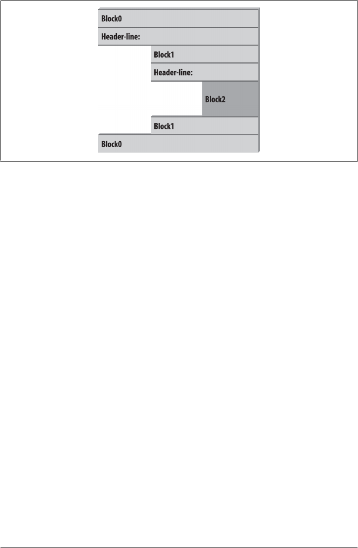
As you’ve seen, there are no variable type declarations in Python; this fact alone makes
for a much simpler language syntax than what you may be used to. However, for most
new users the lack of the braces and semicolons used to mark blocks and statements
in many other languages seems to be the most novel syntactic feature of Python, so let’s
explore what this means in more detail.
Block Delimiters: Indentation Rules
As introduced in Chapter 10, Python detects block boundaries automatically, by line
indentation—that is, the empty space to the left of your code. All statements indented
the same distance to the right belong to the same block of code. In other words, the
statements within a block line up vertically, as in a column. The block ends when the
end of the file or a lesser-indented line is encountered, and more deeply nested blocks
are simply indented further to the right than the statements in the enclosing block.
Compound statement bodies can appear on the header’s line in some cases we’ll explore
later, but most are indented under it.
For instance, Figure 12-1 demonstrates the block structure of the following code:
x = 1
if x:
y = 2
if y:
print('block2')
print('block1')
print('block0')
This code contains three blocks: the first (the top-level code of the file) is not indented
at all, the second (within the outer if statement) is indented four spaces, and the third
(the print statement under the nested if) is indented eight spaces.
Figure 12-1. Nested blocks of code: a nested block starts with a statement indented further to the right
and ends with either a statement that is indented less, or the end of the file.
376 | Chapter 12: if Tests and Syntax Rules
www.it-ebooks.info

In general, top-level (unnested) code must start in column 1. Nested blocks can start
in any column; indentation may consist of any number of spaces and tabs, as long as
it’s the same for all the statements in a given single block. That is, Python doesn’t care
how you indent your code; it only cares that it’s done consistently. Four spaces or one
tab per indentation level are common conventions, but there is no absolute standard
in the Python world.
Indenting code is quite natural in practice. For example, the following (arguably silly)
code snippet demonstrates common indentation errors in Python code:
x = 'SPAM' # Error: first line indented
if 'rubbery' in 'shrubbery':
print(x * 8)
x += 'NI' # Error: unexpected indentation
if x.endswith('NI'):
x *= 2
print(x) # Error: inconsistent indentation
The properly indented version of this code looks like the following—even for an arti-
ficial example like this, proper indentation makes the code’s intent much more appa-
rent:
x = 'SPAM'
if 'rubbery' in 'shrubbery':
print(x * 8) # Prints 8 "SPAM"
x += 'NI'
if x.endswith('NI'):
x *= 2
print(x) # Prints "SPAMNISPAMNI"
It’s important to know that the only major place in Python where whitespace matters
is where it’s used to the left of your code, for indentation; in most other contexts, space
can be coded or not. However, indentation is really part of Python syntax, not just a
stylistic suggestion: all the statements within any given single block must be indented
to the same level, or Python reports a syntax error. This is intentional—because you
don’t need to explicitly mark the start and end of a nested block of code, some of the
syntactic clutter found in other languages is unnecessary in Python.
As described in Chapter 10, making indentation part of the syntax model also enforces
consistency, a crucial component of readability in structured programming languages
like Python. Python’s syntax is sometimes described as “what you see is what you get”
—the indentation of each line of code unambiguously tells readers what it is associated
with. This uniform and consistent appearance makes Python code easier to maintain
and reuse.
Indentation is simpler in practice than its details might initially imply, and it makes
your code reflect its logical structure. Consistently indented code always satisfies
Python’s rules. Moreover, most text editors (including IDLE) make it easy to follow
Python’s indentation model by automatically indenting code as you type it.
Python Syntax Revisited | 377
www.it-ebooks.info

Avoid mixing tabs and spaces: New error checking in 3.X
One rule of thumb: although you can use spaces or tabs to indent, it’s usually not a
good idea to mix the two within a block—use one or the other. Technically, tabs count
for enough spaces to move the current column number up to a multiple of 8, and your
code will work if you mix tabs and spaces consistently. However, such code can be
difficult to change. Worse, mixing tabs and spaces makes your code difficult to read
completely apart from Python’s syntax rules—tabs may look very different in the next
programmer’s editor than they do in yours.
In fact, Python 3.X issues an error, for these very reasons, when a script mixes tabs and
spaces for indentation inconsistently within a block (that is, in a way that makes it
dependent on a tab’s equivalent in spaces). Python 2.X allows such scripts to run, but
it has a -t command-line flag that will warn you about inconsistent tab usage and a
-tt flag that will issue errors for such code (you can use these switches in a command
line like python –t main.py in a system shell window). Python 3.X’s error case is equiv-
alent to 2.X’s -tt switch.
Statement Delimiters: Lines and Continuations
A statement in Python normally ends at the end of the line on which it appears. When
a statement is too long to fit on a single line, though, a few special rules may be used
to make it span multiple lines:
•Statements may span multiple lines if you’re continuing an open syntactic
pair. Python lets you continue typing a statement on the next line if you’re coding
something enclosed in a (), {}, or [] pair. For instance, expressions in parentheses
and dictionary and list literals can span any number of lines; your statement doesn’t
end until the Python interpreter reaches the line on which you type the closing part
of the pair (a ), }, or ]). Continuation lines—lines 2 and beyond of the statement
—can start at any indentation level you like, but you should try to make them align
vertically for readability if possible. This open pairs rule also covers set and dic-
tionary comprehensions in Python 3.X and 2.7.
•Statements may span multiple lines if they end in a backslash. This is a some-
what outdated feature that’s not generally recommended, but if a statement needs
to span multiple lines, you can also add a backslash (a \ not embedded in a string
literal or comment) at the end of the prior line to indicate you’re continuing on the
next line. Because you can also continue by adding parentheses around most con-
structs, backslashes are rarely used today. This approach is also error-prone: ac-
cidentally forgetting a \ usually generates a syntax error and might even cause the
next line to be silently mistaken (i.e., without warning) for a new statement, with
unexpected results.
•Special rules for string literals. As we learned in Chapter 7, triple-quoted string
blocks are designed to span multiple lines normally. We also learned in Chap-
ter 7 that adjacent string literals are implicitly concatenated; when it’s used in
378 | Chapter 12: if Tests and Syntax Rules
www.it-ebooks.info

conjunction with the open pairs rule mentioned earlier, wrapping this construct in
parentheses allows it to span multiple lines.
•Other rules. There are a few other points to mention with regard to statement
delimiters. Although it is uncommon, you can terminate a statement with a semi-
colon—this convention is sometimes used to squeeze more than one simple (non-
compound) statement onto a single line. Also, comments and blank lines can ap-
pear anywhere in a file; comments (which begin with a # character) terminate at
the end of the line on which they appear.
A Few Special Cases
Here’s what a continuation line looks like using the open syntactic pairs rule just de-
scribed. Delimited constructs, such as lists in square brackets, can span across any
number of lines:
L = ["Good",
"Bad",
"Ugly"] # Open pairs may span lines
This also works for anything in parentheses (expressions, function arguments, function
headers, tuples, and generator expressions), as well as anything in curly braces (dic-
tionaries and, in 3.X and 2.7, set literals and set and dictionary comprehensions). Some
of these are tools we’ll study in later chapters, but this rule naturally covers most con-
structs that span lines in practice.
If you like using backslashes to continue lines, you can, but it’s not common practice
in Python:
if a == b and c == d and \
d == e and f == g:
print('olde') # Backslashes allow continuations...
Because any expression can be enclosed in parentheses, you can usually use the open
pairs technique instead if you need your code to span multiple lines—simply wrap a
part of your statement in parentheses:
if (a == b and c == d and
d == e and e == f):
print('new') # But parentheses usually do too, and are obvious
In fact, backslashes are generally frowned on by most Python developers, because
they’re too easy to not notice and too easy to omit altogether. In the following, x is
assigned 10 with the backslash, as intended; if the backslash is accidentally omitted,
though, x is assigned 6 instead, and no error is reported (the +4 is a valid expression
statement by itself).
In a real program with a more complex assignment, this could be the source of a very
nasty bug:1
x = 1 + 2 + 3 \ # Omitting the \ makes this very different!
+4
Python Syntax Revisited | 379
www.it-ebooks.info

As another special case, Python allows you to write more than one noncompound
statement (i.e., statements without nested statements) on the same line, separated by
semicolons. Some coders use this form to save program file real estate, but it usually
makes for more readable code if you stick to one statement per line for most of your
work:
x = 1; y = 2; print(x) # More than one simple statement
As we learned in Chapter 7, triple-quoted string literals span lines too. In addition, if
two string literals appear next to each other, they are concatenated as if a + had been
added between them—when used in conjunction with the open pairs rule, wrapping
in parentheses allows this form to span multiple lines. For example, the first of the
following inserts newline characters at line breaks and assigns S to '\naaaa\nbbbb
\ncccc', and the second implicitly concatenates and assigns S to 'aaaabbbbcccc'; as we
also saw in Chapter 7, # comments are ignored in the second form, but included in the
string in the first:
S = """
aaaa
bbbb
cccc"""
S = ('aaaa'
'bbbb' # Comments here are ignored
'cccc')
Finally, Python lets you move a compound statement’s body up to the header line,
provided the body contains just simple (noncompound) statements. You’ll most often
see this used for simple if statements with a single test and action, as in the interactive
loops we coded in Chapter 10:
if 1: print('hello') # Simple statement on header line
You can combine some of these special cases to write code that is difficult to read, but
I don’t recommend it; as a rule of thumb, try to keep each statement on a line of its
own, and indent all but the simplest of blocks. Six months down the road, you’ll be
happy you did.
Truth Values and Boolean Tests
The notions of comparison, equality, and truth values were introduced in Chapter 9.
Because the if statement is the first statement we’ve looked at that actually uses test
1. Candidly, it was a bit surprising that backslash continuations were not removed in Python 3.0, given the
broad scope of its other changes! See the 3.0 changes tables in Appendix C for a list of 3.0 removals; some
seem fairly innocuous in comparison with the dangers inherent in backslash continuations. Then again,
this book’s goal is Python instruction, not populist outrage, so the best advice I can give is simply: don’t
do this. You should generally avoid backslash continuations in new Python code, even if you developed
the habit in your C programming days.
380 | Chapter 12: if Tests and Syntax Rules
www.it-ebooks.info

results, we’ll expand on some of these ideas here. In particular, Python’s Boolean oper-
ators are a bit different from their counterparts in languages like C. In Python:
• All objects have an inherent Boolean true or false value.
• Any nonzero number or nonempty object is true.
• Zero numbers, empty objects, and the special object None are considered false.
• Comparisons and equality tests are applied recursively to data structures.
• Comparisons and equality tests return True or False (custom versions of 1 and 0).
• Boolean and and or operators return a true or false operand object.
• Boolean operators stop evaluating (“short circuit”) as soon as a result is known.
The if statement takes action on truth values, but Boolean operators are used to com-
bine the results of other tests in richer ways to produce new truth values. More formally,
there are three Boolean expression operators in Python:
X and Y
Is true if both X and Y are true
X or Y
Is true if either X or Y is true
not X
Is true if X is false (the expression returns True or False)
Here, X and Y may be any truth value, or any expression that returns a truth value (e.g.,
an equality test, range comparison, and so on). Boolean operators are typed out as
words in Python (instead of C’s &&, ||, and !). Also, Boolean and and or operators return
a true or false object in Python, not the values True or False. Let’s look at a few examples
to see how this works:
>>> 2 < 3, 3 < 2 # Less than: return True or False (1 or 0)
(True, False)
Magnitude comparisons such as these return True or False as their truth results, which,
as we learned in Chapter 5 and Chapter 9, are really just custom versions of the integers
1 and 0 (they print themselves differently but are otherwise the same).
On the other hand, the and and or operators always return an object—either the object
on the left side of the operator or the object on the right. If we test their results in if or
other statements, they will be as expected (remember, every object is inherently true
or false), but we won’t get back a simple True or False.
For or tests, Python evaluates the operand objects from left to right and returns the first
one that is true. Moreover, Python stops at the first true operand it finds. This is usually
called short-circuit evaluation, as determining a result short-circuits (terminates) the
rest of the expression as soon as the result is known:
>>> 2 or 3, 3 or 2 # Return left operand if true
(2, 3) # Else, return right operand (true or false)
Truth Values and Boolean Tests | 381
www.it-ebooks.info

>>> [] or 3
3
>>> [] or {}
{}
In the first line of the preceding example, both operands (2 and 3) are true (i.e., are
nonzero), so Python always stops and returns the one on the left—it determines the
result because true or anything is always true. In the other two tests, the left operand
is false (an empty object), so Python simply evaluates and returns the object on the
right—which may happen to have either a true or a false value when tested.
Python and operations also stop as soon as the result is known; however, in this case
Python evaluates the operands from left to right and stops if the left operand is a false
object because it determines the result—false and anything is always false:
>>> 2 and 3, 3 and 2 # Return left operand if false
(3, 2) # Else, return right operand (true or false)
>>> [] and {}
[]
>>> 3 and []
[]
Here, both operands are true in the first line, so Python evaluates both sides and returns
the object on the right. In the second test, the left operand is false ([]), so Python stops
and returns it as the test result. In the last test, the left side is true (3), so Python evaluates
and returns the object on the right—which happens to be a false [].
The end result of all this is the same as in C and most other languages—you get a value
that is logically true or false if tested in an if or while according to the normal definitions
of or and and. However, in Python Booleans return either the left or the right object,
not a simple integer flag.
This behavior of and and or may seem esoteric at first glance, but see this chapter’s
sidebar “Why You Will Care: Booleans” on page 384 for examples of how it is some-
times used to advantage in coding by Python programmers. The next section also shows
a common way to leverage this behavior, and its more mnemonic replacement in recent
versions of Python.
The if/else Ternary Expression
One common role for the prior section’s Boolean operators is to code an expression
that runs the same as an if statement. Consider the following statement, which sets
A to either Y or Z, based on the truth value of X:
if X:
A = Y
else:
A = Z
382 | Chapter 12: if Tests and Syntax Rules
www.it-ebooks.info

Sometimes, though, the items involved in such a statement are so simple that it seems
like overkill to spread them across four lines. At other times, we may want to nest such
a construct in a larger statement instead of assigning its result to a variable. For these
reasons (and, frankly, because the C language has a similar tool), Python 2.5 introduced
a new expression format that allows us to say the same thing in one expression:
A = Y if X else Z
This expression has the exact same effect as the preceding four-line if statement, but
it’s simpler to code. As in the statement equivalent, Python runs expression Y only if
X turns out to be true, and runs expression Z only if X turns out to be false. That is, it
short-circuits, just like the Boolean operators described in the prior section, running
just Y or Z but not both. Here are some examples of it in action:
>>> A = 't' if 'spam' else 'f' # For strings, nonempty means true
>>> A
't'
>>> A = 't' if '' else 'f'
>>> A
'f'
Prior to Python 2.5 (and after 2.5, if you insist), the same effect can often be achieved
by a careful combination of the and and or operators, because they return either the
object on the left side or the object on the right as the preceding section described:
A = ((X and Y) or Z)
This works, but there is a catch—you have to be able to assume that Y will be Boolean
true. If that is the case, the effect is the same: the and runs first and returns Y if X is true;
if X if false the and skips Y, and the or simply returns Z. In other words, we get “if X then
Y else Z.” This is equivalent to the ternary form:
A = Y if X else Z
The and/or combination form also seems to require a “moment of great clarity” to
understand the first time you see it, and it’s no longer required as of 2.5—use the
equivalent and more robust and mnemonic if/else expression when you need this
structure, or use a full if statement if the parts are nontrivial.
As a side note, using the following expression in Python is similar because the bool
function will translate X into the equivalent of integer 1 or 0, which can then be used as
offsets to pick true and false values from a list:
A = [Z, Y][bool(X)]
For example:
>>> ['f', 't'][bool('')]
'f'
>>> ['f', 't'][bool('spam')]
't'
However, this isn’t exactly the same, because Python will not short-circuit—it will al-
ways run both Z and Y, regardless of the value of X. Because of such complexities, you’re
The if/else Ternary Expression | 383
www.it-ebooks.info

better off using the simpler and more easily understood if/else expression as of Python
2.5 and later. Again, though, you should use even that sparingly, and only if its parts
are all fairly simple; otherwise, you’re better off coding the full if statement form to
make changes easier in the future. Your coworkers will be happy you did.
Still, you may see the and/or version in code written prior to 2.5 (and in Python code
written by ex–C programmers who haven’t quite let go of their dark coding pasts).2
Why You Will Care: Booleans
One common way to use the somewhat unusual behavior of Python Boolean operators
is to select from a set of objects with an or. A statement such as this:
X = A or B or C or None
assigns X to the first nonempty (that is, true) object among A, B, and C, or to None if all
of them are empty. This works because the or operator returns one of its two objects,
and it turns out to be a fairly common coding paradigm in Python: to select a nonempty
object from among a fixed-size set, simply string them together in an or expression. In
simpler form, this is also commonly used to designate a default—the following sets X
to A if A is true (or nonempty), and to default otherwise:
X = A or default
It’s also important to understand the short-circuit evaluation of Boolean operators and
the if/else, because it may prevent actions from running. Expressions on the right of
a Boolean operator, for example, might call functions that perform substantial or im-
portant work, or have side effects that won’t happen if the short-circuit rule takes effect:
if f1() or f2(): ...
Here, if f1 returns a true (or nonempty) value, Python will never run f2. To guarantee
that both functions will be run, call them before the or:
tmp1, tmp2 = f1(), f2()
if tmp1 or tmp2: ...
You’ve already seen another application of this behavior in this chapter: because of the
way Booleans work, the expression ((A and B) or C) can be used to emulate an if
statement—almost (see this chapter’s discussion of this form for details).
We met additional Boolean use cases in prior chapters. As we saw in Chapter 9, because
all objects are inherently true or false, it’s common and easier in Python to test an object
directly (if X:) than to compare it to an empty value (if X != '':). For a string, the
two tests are equivalent. As we also saw in Chapter 5, the preset Boolean values True
and False are the same as the integers 1 and 0 and are useful for initializing variables
2. In fact, Python’s Y if X else Z has a slightly different order than C’s X ? Y : Z, and uses more readable
words. Its differing order was reportedly chosen in response to analysis of common usage patterns in
Python code. According to the Python folklore, this order was also chosen in part to discourage ex–C
programmers from overusing it! Remember, simple is better than complex, in Python and elsewhere. If
you have to work at packing logic into expressions like this, statements are probably your better bet.
384 | Chapter 12: if Tests and Syntax Rules
www.it-ebooks.info

(X = False), for loop tests (while True:), and for displaying results at the interactive
prompt.
Also watch for related discussion in operator overloading in Part VI: when we define
new object types with classes, we can specify their Boolean nature with either the
__bool__ or __len__ methods (__bool__ is named __nonzero__ in 2.7). The latter of these
is tried if the former is absent and designates false by returning a length of zero—an
empty object is considered false.
Finally, and as a preview, other tools in Python have roles similar to the or chains at
the start of this sidebar: the filter call and list comprehensions we’ll meet later can be
used to select true values when the set of candidates isn’t known until runtime (though
they evaluate all values and return all that are true), and the any and all built-ins can
be used to test if any or all items in a collection are true (though they don’t select an
item):
>>> L = [1, 0, 2, 0, 'spam', '', 'ham', []]
>>> list(filter(bool, L)) # Get true values
[1, 2, 'spam', 'ham']
>>> [x for x in L if x] # Comprehensions
[1, 2, 'spam', 'ham']
>>> any(L), all(L) # Aggregate truth
(True, False)
As seen in Chapter 9, the bool function here simply returns its argument’s true or false
value, as though it were tested in an if. Watch for more on these related tools in
Chapter 14, Chapter 19, and Chapter 20.
Chapter Summary
In this chapter, we studied the Python if statement. Additionally, because this was our
first compound and logical statement, we reviewed Python’s general syntax rules and
explored the operation of truth values and tests in more depth than we were able to
previously. Along the way, we also looked at how to code multiway branching in
Python, learned about the if/else expression introduced in Python 2.5, and explored
some common ways that Boolean values crop up in code.
The next chapter continues our look at procedural statements by expanding on the
while and for loops. There, we’ll learn about alternative ways to code loops in Python,
some of which may be better than others. Before that, though, here is the usual chapter
quiz.
Test Your Knowledge: Quiz
1. How might you code a multiway branch in Python?
2. How can you code an if/else statement as an expression in Python?
3. How can you make a single statement span many lines?
Test Your Knowledge: Quiz | 385
www.it-ebooks.info

4. What do the words True and False mean?
Test Your Knowledge: Answers
1. An if statement with multiple elif clauses is often the most straightforward way
to code a multiway branch, though not necessarily the most concise or flexible.
Dictionary indexing can often achieve the same result, especially if the dictionary
contains callable functions coded with def statements or lambda expressions.
2. In Python 2.5 and later, the expression form Y if X else Z returns Y if X is true, or
Z otherwise; it’s the same as a four-line if statement. The and/or combination
(((X and Y) or Z)) can work the same way, but it’s more obscure and requires that
the Y part be true.
3. Wrap up the statement in an open syntactic pair ((), [], or {}), and it can span as
many lines as you like; the statement ends when Python sees the closing (right) half
of the pair, and lines 2 and beyond of the statement can begin at any indentation
level. Backslash continuations work too, but are broadly discouraged in the Python
world.
4. True and False are just custom versions of the integers 1 and 0, respectively: they
always stand for Boolean true and false values in Python. They’re available for use
in truth tests and variable initialization, and are printed for expression results at
the interactive prompt. In all these roles, they serve as a more mnemonic and hence
readable alternative to 1 and 0.
386 | Chapter 12: if Tests and Syntax Rules
www.it-ebooks.info

CHAPTER 13
while and for Loops
This chapter concludes our tour of Python procedural statements by presenting the
language’s two main looping constructs—statements that repeat an action over and
over. The first of these, the while statement, provides a way to code general loops. The
second, the for statement, is designed for stepping through the items in a sequence or
other iterable object and running a block of code for each.
We’ve seen both of these informally already, but we’ll fill in additional usage details
here. While we’re at it, we’ll also study a few less prominent statements used within
loops, such as break and continue, and cover some built-ins commonly used with loops,
such as range, zip, and map.
Although the while and for statements covered here are the primary syntax provided
for coding repeated actions, there are additional looping operations and concepts in
Python. Because of that, the iteration story is continued in the next chapter, where we’ll
explore the related ideas of Python’s iteration protocol (used by the for loop) and list
comprehensions (a close cousin to the for loop). Later chapters explore even more exotic
iteration tools such as generators, filter, and reduce. For now, though, let’s keep things
simple.
while Loops
Python’s while statement is the most general iteration construct in the language. In
simple terms, it repeatedly executes a block of (normally indented) statements as long
as a test at the top keeps evaluating to a true value. It is called a “loop” because control
keeps looping back to the start of the statement until the test becomes false. When the
test becomes false, control passes to the statement that follows the while block. The
net effect is that the loop’s body is executed repeatedly while the test at the top is true.
If the test is false to begin with, the body never runs and the while statement is skipped.
387
www.it-ebooks.info

General Format
In its most complex form, the while statement consists of a header line with a test
expression, a body of one or more normally indented statements, and an optional
else part that is executed if control exits the loop without a break statement being
encountered. Python keeps evaluating the test at the top and executing the statements
nested in the loop body until the test returns a false value:
while test: # Loop test
statements # Loop body
else: # Optional else
statements # Run if didn't exit loop with break
Examples
To illustrate, let’s look at a few simple while loops in action. The first, which consists
of a print statement nested in a while loop, just prints a message forever. Recall that
True is just a custom version of the integer 1 and always stands for a Boolean true value;
because the test is always true, Python keeps executing the body forever, or until you
stop its execution. This sort of behavior is usually called an infinite loop—it’s not really
immortal, but you may need a Ctrl-C key combination to forcibly terminate one:
>>> while True:
... print('Type Ctrl-C to stop me!')
The next example keeps slicing off the first character of a string until the string is empty
and hence false. It’s typical to test an object directly like this instead of using the more
verbose equivalent (while x != '':). Later in this chapter, we’ll see other ways to step
through the items in a string more easily with a for loop.
>>> x = 'spam'
>>> while x: # While x is not empty
... print(x, end=' ') # In 2.X use print x,
... x = x[1:] # Strip first character off x
...
spam pam am m
Note the end=' ' keyword argument used here to place all outputs on the same line
separated by a space; see Chapter 11 if you’ve forgotten why this works as it does. This
may leave your input prompt in an odd state at the end of your output; type Enter to
reset. Python 2.X readers: also remember to use a trailing comma instead of end in the
prints like this.
The following code counts from the value of a up to, but not including, b. We’ll also
see an easier way to do this with a Python for loop and the built-in range function later:
>>> a=0; b=10
>>> while a < b: # One way to code counter loops
... print(a, end=' ')
... a += 1 # Or, a = a + 1
388 | Chapter 13: while and for Loops
www.it-ebooks.info

...
0 1 2 3 4 5 6 7 8 9
Finally, notice that Python doesn’t have what some languages call a “do until” loop
statement. However, we can simulate one with a test and break at the bottom of the
loop body, so that the loop’s body is always run at least once:
while True:
...loop body...
if exitTest(): break
To fully understand how this structure works, we need to move on to the next section
and learn more about the break statement.
break, continue, pass, and the Loop else
Now that we’ve seen a few Python loops in action, it’s time to take a look at two simple
statements that have a purpose only when nested inside loops—the break and con
tinue statements. While we’re looking at oddballs, we will also study the loop else
clause here because it is intertwined with break, and Python’s empty placeholder state-
ment, pass (which is not tied to loops per se, but falls into the general category of simple
one-word statements). In Python:
break
Jumps out of the closest enclosing loop (past the entire loop statement)
continue
Jumps to the top of the closest enclosing loop (to the loop’s header line)
pass
Does nothing at all: it’s an empty statement placeholder
Loop else block
Runs if and only if the loop is exited normally (i.e., without hitting a break)
General Loop Format
Factoring in break and continue statements, the general format of the while loop looks
like this:
while test:
statements
if test: break # Exit loop now, skip else if present
if test: continue # Go to top of loop now, to test1
else:
statements # Run if we didn't hit a 'break'
break and continue statements can appear anywhere inside the while (or for) loop’s
body, but they are usually coded further nested in an if test to take action in response
to some condition.
break, continue, pass, and the Loop else | 389
www.it-ebooks.info

Let’s turn to a few simple examples to see how these statements come together in
practice.
pass
Simple things first: the pass statement is a no-operation placeholder that is used when
the syntax requires a statement, but you have nothing useful to say. It is often used to
code an empty body for a compound statement. For instance, if you want to code an
infinite loop that does nothing each time through, do it with a pass:
while True: pass # Type Ctrl-C to stop me!
Because the body is just an empty statement, Python gets stuck in this loop. pass is
roughly to statements as None is to objects—an explicit nothing. Notice that here the
while loop’s body is on the same line as the header, after the colon; as with if state-
ments, this only works if the body isn’t a compound statement.
This example does nothing forever. It probably isn’t the most useful Python program
ever written (unless you want to warm up your laptop computer on a cold winter’s
day!); frankly, though, I couldn’t think of a better pass example at this point in the book.
We’ll see other places where pass makes more sense later—for instance, to ignore ex-
ceptions caught by try statements, and to define empty class objects with attributes
that behave like “structs” and “records” in other languages. A pass is also sometime
coded to mean “to be filled in later,” to stub out the bodies of functions temporarily:
def func1():
pass # Add real code here later
def func2():
pass
We can’t leave the body empty without getting a syntax error, so we say pass instead.
Version skew note: Python 3.X (but not 2.X) allows ellipses coded
as ... (literally, three consecutive dots) to appear any place an expres-
sion can. Because ellipses do nothing by themselves, this can serve as
an alternative to the pass statement, especially for code to be filled in
later—a sort of Python “TBD”:
def func1():
... # Alternative to pass
def func2():
...
func1() # Does nothing if called
Ellipses can also appear on the same line as a statement header and may
be used to initialize variable names if no specific type is required:
def func1(): ... # Works on same line too
def func2(): ...
390 | Chapter 13: while and for Loops
www.it-ebooks.info

>>> X = ... # Alternative to None
>>> X
Ellipsis
This notation is new in Python 3.X—and goes well beyond the original
intent of ... in slicing extensions—so time will tell if it becomes wide-
spread enough to challenge pass and None in these roles.
continue
The continue statement causes an immediate jump to the top of a loop. It also some-
times lets you avoid statement nesting. The next example uses continue to skip odd
numbers. This code prints all even numbers less than 10 and greater than or equal to
0. Remember, 0 means false and % is the remainder of division (modulus) operator, so
this loop counts down to 0, skipping numbers that aren’t multiples of 2—it prints 8 6
4 2 0:
x = 10
while x:
x = x−1 # Or, x -= 1
if x % 2 != 0: continue # Odd? -- skip print
print(x, end=' ')
Because continue jumps to the top of the loop, you don’t need to nest the print state-
ment here inside an if test; the print is only reached if the continue is not run. If this
sounds similar to a “go to” in other languages, it should. Python has no “go to” state-
ment, but because continue lets you jump about in a program, many of the warnings
about readability and maintainability you may have heard about “go to” apply. con
tinue should probably be used sparingly, especially when you’re first getting started
with Python. For instance, the last example might be clearer if the print were nested
under the if:
x = 10
while x:
x = x−1
if x % 2 == 0: # Even? -- print
print(x, end=' ')
Later in this book, we’ll also learn that raised and caught exceptions can also emulate
“go to” statements in limited and structured ways; stay tuned for more on this technique
in Chapter 36 where we will learn how to use it to break out of multiple nested loops,
a feat not possible with the next section’s topic alone.
break
The break statement causes an immediate exit from a loop. Because the code that fol-
lows it in the loop is not executed if the break is reached, you can also sometimes avoid
nesting by including a break. For example, here is a simple interactive loop (a variant
break, continue, pass, and the Loop else | 391
www.it-ebooks.info

of a larger example we studied in Chapter 10) that inputs data with input (known as
raw_input in Python 2.X) and exits when the user enters “stop” for the name request:
>>> while True:
... name = input('Enter name:') # Use raw_input() in 2.X
... if name == 'stop': break
... age = input('Enter age: ')
... print('Hello', name, '=>', int(age) ** 2)
...
Enter name:bob
Enter age: 40
Hello bob => 1600
Enter name:sue
Enter age: 30
Hello sue => 900
Enter name:stop
Notice how this code converts the age input to an integer with int before raising it to
the second power; as you’ll recall, this is necessary because input returns user input as
a string. In Chapter 36, you’ll see that input also raises an exception at end-of-file (e.g.,
if the user types Ctrl-Z on Windows or Ctrl-D on Unix); if this matters, wrap input in
try statements.
Loop else
When combined with the loop else clause, the break statement can often eliminate the
need for the search status flags used in other languages. For instance, the following
piece of code determines whether a positive integer y is prime by searching for factors
greater than 1:
x = y // 2 # For some y > 1
while x > 1:
if y % x == 0: # Remainder
print(y, 'has factor', x)
break # Skip else
x -= 1
else: # Normal exit
print(y, 'is prime')
Rather than setting a flag to be tested when the loop is exited, it inserts a break where
a factor is found. This way, the loop else clause can assume that it will be executed
only if no factor is found; if you don’t hit the break, the number is prime. Trace through
this code to see how this works.
The loop else clause is also run if the body of the loop is never executed, as you don’t
run a break in that event either; in a while loop, this happens if the test in the header
is false to begin with. Thus, in the preceding example you still get the “is prime” message
if x is initially less than or equal to 1 (for instance, if y is 2).
392 | Chapter 13: while and for Loops
www.it-ebooks.info

This example determines primes, but only informally so. Numbers less
than 2 are not considered prime by the strict mathematical definition.
To be really picky, this code also fails for negative numbers and succeeds
for floating-point numbers with no decimal digits. Also note that its
code must use // instead of / in Python 3.X because of the migration
of / to “true division,” as described in Chapter 5 (we need the initial
division to truncate remainders, not retain them!). If you want to ex-
periment with this code, be sure to see the exercise at the end of
Part IV, which wraps it in a function for reuse.
More on the loop else
Because the loop else clause is unique to Python, it tends to perplex some newcomers
(and go unused by some veterans; I’ve met some who didn’t even know there was an
else on loops!). In general terms, the loop else simply provides explicit syntax for a
common coding scenario—it is a coding structure that lets us catch the “other” way
out of a loop, without setting and checking flags or conditions.
Suppose, for instance, that we are writing a loop to search a list for a value, and we
need to know whether the value was found after we exit the loop. We might code such
a task this way (this code is intentionally abstract and incomplete; x is a sequence and
match is a tester function to be defined):
found = False
while x and not found:
if match(x[0]): # Value at front?
print('Ni')
found = True
else:
x = x[1:] # Slice off front and repeat
if not found:
print('not found')
Here, we initialize, set, and later test a flag to determine whether the search succeeded
or not. This is valid Python code, and it does work; however, this is exactly the sort of
structure that the loop else clause is there to handle. Here’s an else equivalent:
while x: # Exit when x empty
if match(x[0]):
print('Ni')
break # Exit, go around else
x = x[1:]
else:
print('Not found') # Only here if exhausted x
This version is more concise. The flag is gone, and we’ve replaced the if test at the loop
end with an else (lined up vertically with the word while). Because the break inside the
main part of the while exits the loop and goes around the else, this serves as a more
structured way to catch the search-failure case.
break, continue, pass, and the Loop else | 393
www.it-ebooks.info

Some readers might have noticed that the prior example’s else clause could be replaced
with a test for an empty x after the loop (e.g., if not x:). Although that’s true in this
example, the else provides explicit syntax for this coding pattern (it’s more obviously
a search-failure clause here), and such an explicit empty test may not apply in some
cases. The loop else becomes even more useful when used in conjunction with the
for loop—the topic of the next section—because sequence iteration is not under your
control.
Why You Will Care: Emulating C while Loops
The section on expression statements in Chapter 11 stated that Python doesn’t allow
statements such as assignments to appear in places where it expects an expression. That
is, each statement must generally appear on a line by itself, not nested in a larger con-
struct. That means this common C language coding pattern won’t work in Python:
while ((x = next(obj)) != NULL) {...process x...}
C assignments return the value assigned, but Python assignments are just statements,
not expressions. This eliminates a notorious class of C errors: you can’t accidentally
type = in Python when you mean ==. If you need similar behavior, though, there are at
least three ways to get the same effect in Python while loops without embedding as-
signments in loop tests. You can move the assignment into the loop body with a break:
while True:
x = next(obj)
if not x: break
...process x...
or move the assignment into the loop with tests:
x = True
while x:
x = next(obj)
if x:
...process x...
or move the first assignment outside the loop:
x = next(obj)
while x:
...process x...
x = next(obj)
Of these three coding patterns, the first may be considered by some to be the least
structured, but it also seems to be the simplest and is the most commonly used. A simple
Python for loop may replace such C loops as well and be more Pythonic, but C doesn’t
have a directly analogous tool:
for x in obj: ...process x...
394 | Chapter 13: while and for Loops
www.it-ebooks.info

for Loops
The for loop is a generic iterator in Python: it can step through the items in any ordered
sequence or other iterable object. The for statement works on strings, lists, tuples, and
other built-in iterables, as well as new user-defined objects that we’ll learn how to create
later with classes. We met for briefly in Chapter 4 and in conjunction with sequence
object types; let’s expand on its usage more formally here.
General Format
The Python for loop begins with a header line that specifies an assignment target (or
targets), along with the object you want to step through. The header is followed by a
block of (normally indented) statements that you want to repeat:
for target in object: # Assign object items to target
statements # Repeated loop body: use target
else: # Optional else part
statements # If we didn't hit a 'break'
When Python runs a for loop, it assigns the items in the iterable object to the target
one by one and executes the loop body for each. The loop body typically uses the
assignment target to refer to the current item in the sequence as though it were a cursor
stepping through the sequence.
The name used as the assignment target in a for header line is usually a (possibly new)
variable in the scope where the for statement is coded. There’s not much unique about
this name; it can even be changed inside the loop’s body, but it will automatically be
set to the next item in the sequence when control returns to the top of the loop again.
After the loop this variable normally still refers to the last item visited, which is the last
item in the sequence unless the loop exits with a break statement.
The for statement also supports an optional else block, which works exactly as it does
in a while loop—it’s executed if the loop exits without running into a break statement
(i.e., if all items in the sequence have been visited). The break and continue statements
introduced earlier also work the same in a for loop as they do in a while. The for loop’s
complete format can be described this way:
for target in object: # Assign object items to target
statements
if test: break # Exit loop now, skip else
if test: continue # Go to top of loop now
else:
statements # If we didn't hit a 'break'
Examples
Let’s type a few for loops interactively now, so you can see how they are used in practice.
for Loops | 395
www.it-ebooks.info

Basic usage
As mentioned earlier, a for loop can step across any kind of sequence object. In our
first example, for instance, we’ll assign the name x to each of the three items in a list in
turn, from left to right, and the print statement will be executed for each. Inside the
print statement (the loop body), the name x refers to the current item in the list:
>>> for x in ["spam", "eggs", "ham"]:
... print(x, end=' ')
...
spam eggs ham
The next two examples compute the sum and product of all the items in a list. Later in
this chapter and later in the book we’ll meet tools that apply operations such as + and
* to items in a list automatically, but it’s often just as easy to use a for:
>>> sum = 0
>>> for x in [1, 2, 3, 4]:
... sum = sum + x
...
>>> sum
10
>>> prod = 1
>>> for item in [1, 2, 3, 4]: prod *= item
...
>>> prod
24
Other data types
Any sequence works in a for, as it’s a generic tool. For example, for loops work on
strings and tuples:
>>> S = "lumberjack"
>>> T = ("and", "I'm", "okay")
>>> for x in S: print(x, end=' ') # Iterate over a string
...
l u m b e r j a c k
>>> for x in T: print(x, end=' ') # Iterate over a tuple
...
and I'm okay
In fact, as we’ll learn in the next chapter when we explore the notion of “iterables,”
for loops can even work on some objects that are not sequences—files and dictionaries
work, too.
Tuple assignment in for loops
If you’re iterating through a sequence of tuples, the loop target itself can actually be a
tuple of targets. This is just another case of the tuple-unpacking assignment we studied
396 | Chapter 13: while and for Loops
www.it-ebooks.info

in Chapter 11 at work. Remember, the for loop assigns items in the sequence object
to the target, and assignment works the same everywhere:
>>> T = [(1, 2), (3, 4), (5, 6)]
>>> for (a, b) in T: # Tuple assignment at work
... print(a, b)
...
1 2
3 4
5 6
Here, the first time through the loop is like writing (a,b) = (1,2), the second time is
like writing (a,b) = (3,4), and so on. The net effect is to automatically unpack the
current tuple on each iteration.
This form is commonly used in conjunction with the zip call we’ll meet later in this
chapter to implement parallel traversals. It also makes regular appearances in conjunc-
tion with SQL databases in Python, where query result tables are returned as sequences
of sequences like the list used here—the outer list is the database table, the nested tuples
are the rows within the table, and tuple assignment extracts columns.
Tuples in for loops also come in handy to iterate through both keys and values in
dictionaries using the items method, rather than looping through the keys and indexing
to fetch the values manually:
>>> D = {'a': 1, 'b': 2, 'c': 3}
>>> for key in D:
... print(key, '=>', D[key]) # Use dict keys iterator and index
...
a => 1
c => 3
b => 2
>>> list(D.items())
[('a', 1), ('c', 3), ('b', 2)]
>>> for (key, value) in D.items():
... print(key, '=>', value) # Iterate over both keys and values
...
a => 1
c => 3
b => 2
It’s important to note that tuple assignment in for loops isn’t a special case; any as-
signment target works syntactically after the word for. We can always assign manually
within the loop to unpack:
>>> T
[(1, 2), (3, 4), (5, 6)]
>>> for both in T:
... a, b = both # Manual assignment equivalent
... print(a, b) # 2.X: prints with enclosing tuple "()"
...
for Loops | 397
www.it-ebooks.info

1 2
3 4
5 6
But tuples in the loop header save us an extra step when iterating through sequences
of sequences. As suggested in Chapter 11, even nested structures may be automatically
unpacked this way in a for:
>>> ((a, b), c) = ((1, 2), 3) # Nested sequences work too
>>> a, b, c
(1, 2, 3)
>>> for ((a, b), c) in [((1, 2), 3), ((4, 5), 6)]: print(a, b, c)
...
1 2 3
4 5 6
Even this is not a special case, though—the for loop simply runs the sort of assignment
we ran just before it, on each iteration. Any nested sequence structure may be unpacked
this way, simply because sequence assignment is so generic:
>>> for ((a, b), c) in [([1, 2], 3), ['XY', 6]]: print(a, b, c)
...
1 2 3
X Y 6
Python 3.X extended sequence assignment in for loops
In fact, because the loop variable in a for loop can be any assignment target, we can
also use Python 3.X’s extended sequence-unpacking assignment syntax here to extract
items and sections of sequences within sequences. Really, this isn’t a special case either,
but simply a new assignment form in 3.X, as discussed in Chapter 11; because it works
in assignment statements, it automatically works in for loops.
Consider the tuple assignment form introduced in the prior section. A tuple of values
is assigned to a tuple of names on each iteration, exactly like a simple assignment state-
ment:
>>> a, b, c = (1, 2, 3) # Tuple assignment
>>> a, b, c
(1, 2, 3)
>>> for (a, b, c) in [(1, 2, 3), (4, 5, 6)]: # Used in for loop
... print(a, b, c)
...
1 2 3
4 5 6
In Python 3.X, because a sequence can be assigned to a more general set of names with
a starred name to collect multiple items, we can use the same syntax to extract parts of
nested sequences in the for loop:
>>> a, *b, c = (1, 2, 3, 4) # Extended seq assignment
>>> a, b, c
398 | Chapter 13: while and for Loops
www.it-ebooks.info

(1, [2, 3], 4)
>>> for (a, *b, c) in [(1, 2, 3, 4), (5, 6, 7, 8)]:
... print(a, b, c)
...
1 [2, 3] 4
5 [6, 7] 8
In practice, this approach might be used to pick out multiple columns from rows of
data represented as nested sequences. In Python 2.X starred names aren’t allowed, but
you can achieve similar effects by slicing. The only difference is that slicing returns a
type-specific result, whereas starred names always are assigned lists:
>>> for all in [(1, 2, 3, 4), (5, 6, 7, 8)]: # Manual slicing in 2.X
... a, b, c = all[0], all[1:3], all[3]
... print(a, b, c)
...
1 (2, 3) 4
5 (6, 7) 8
See Chapter 11 for more on this assignment form.
Nested for loops
Now let’s look at a for loop that’s a bit more sophisticated than those we’ve seen so
far. The next example illustrates statement nesting and the loop else clause in a for.
Given a list of objects (items) and a list of keys (tests), this code searches for each key
in the objects list and reports on the search’s outcome:
>>> items = ["aaa", 111, (4, 5), 2.01] # A set of objects
>>> tests = [(4, 5), 3.14] # Keys to search for
>>>
>>> for key in tests: # For all keys
... for item in items: # For all items
... if item == key: # Check for match
... print(key, "was found")
... break
... else:
... print(key, "not found!")
...
(4, 5) was found
3.14 not found!
Because the nested if runs a break when a match is found, the loop else clause can
assume that if it is reached, the search has failed. Notice the nesting here. When this
code runs, there are two loops going at the same time: the outer loop scans the keys
list, and the inner loop scans the items list for each key. The nesting of the loop else
clause is critical; it’s indented to the same level as the header line of the inner for loop,
so it’s associated with the inner loop, not the if or the outer for.
This example is illustrative, but it may be easier to code if we employ the in operator
to test membership. Because in implicitly scans an object looking for a match (at least
logically), it replaces the inner loop:
for Loops | 399
www.it-ebooks.info

>>> for key in tests: # For all keys
... if key in items: # Let Python check for a match
... print(key, "was found")
... else:
... print(key, "not found!")
...
(4, 5) was found
3.14 not found!
In general, it’s a good idea to let Python do as much of the work as possible (as in this
solution) for the sake of brevity and performance.
The next example is similar, but builds a list as it goes for later use instead of printing.
It performs a typical data-structure task with a for—collecting common items in two
sequences (strings)—and serves as a rough set intersection routine. After the loop runs,
res refers to a list that contains all the items found in seq1 and seq2:
>>> seq1 = "spam"
>>> seq2 = "scam"
>>>
>>> res = [] # Start empty
>>> for x in seq1: # Scan first sequence
... if x in seq2: # Common item?
... res.append(x) # Add to result end
...
>>> res
['s', 'a', 'm']
Unfortunately, this code is equipped to work only on two specific variables: seq1 and
seq2. It would be nice if this loop could somehow be generalized into a tool you could
use more than once. As you’ll see, that simple idea leads us to functions, the topic of
the next part of the book.
This code also exhibits the classic list comprehension pattern—collecting a results list
with an iteration and optional filter test—and could be coded more concisely too:
>>> [x for x in seq1 if x in seq2] # Let Python collect results
['s', 'a', 'm']
But you’ll have to read on to the next chapter for the rest of this story.
Why You Will Care: File Scanners
In general, loops come in handy anywhere you need to repeat an operation or process
something more than once. Because files contain multiple characters and lines, they are
one of the more typical use cases for loops. To load a file’s contents into a string all at
once, you simply call the file object’s read method:
file = open('test.txt', 'r') # Read contents into a string
print(file.read())
But to load a file in smaller pieces, it’s common to code either a while loop with breaks
on end-of-file, or a for loop. To read by characters, either of the following codings will
suffice:
400 | Chapter 13: while and for Loops
www.it-ebooks.info

file = open('test.txt')
while True:
char = file.read(1) # Read by character
if not char: break # Empty string means end-of-file
print(char)
for char in open('test.txt').read():
print(char)
The for loop here also processes each character, but it loads the file into memory all at
once (and assumes it fits!). To read by lines or blocks instead, you can use while loop
code like this:
file = open('test.txt')
while True:
line = file.readline() # Read line by line
if not line: break
print(line.rstrip()) # Line already has a \n
file = open('test.txt', 'rb')
while True:
chunk = file.read(10) # Read byte chunks: up to 10 bytes
if not chunk: break
print(chunk)
You typically read binary data in blocks. To read text files line by line, though, the
for loop tends to be easiest to code and the quickest to run:
for line in open('test.txt').readlines():
print(line.rstrip())
for line in open('test.txt'): # Use iterators: best for text input
print(line.rstrip())
Both of these versions work in both Python 2.X and 3.X. The first uses the file read
lines method to load a file all at once into a line-string list, and the last example here
relies on file iterators to automatically read one line on each loop iteration.
The last example is also generally the best option for text files—besides its simplicity,
it works for arbitrarily large files because it doesn’t load the entire file into memory all
at once. The iterator version may also be the quickest, though I/O performance may
vary per Python line and release.
File readlines calls can still be useful, though—to reverse a file’s lines, for example,
assuming its content can fit in memory. The reversed built-in accepts a sequence, but
not an arbitrary iterable that generates values; in other words, a list works, but a file
object doesn’t:
for line in reversed(open('test.txt').readlines()): ...
In some 2.X Python code, you may also see the name open replaced with file and the
file object’s older xreadlines method used to achieve the same effect as the file’s auto-
matic line iterator (it’s like readlines but doesn’t load the file into memory all at once).
Both file and xreadlines are removed in Python 3.X, because they are redundant. You
should generally avoid them in new 2.X code too—use file iterators and open call in
recent 2.X releases—but they may pop up in older code and resources.
for Loops | 401
www.it-ebooks.info

See the library manual for more on the calls used here, and Chapter 14 for more on file
line iterators. Also watch for the sidebar “Why You Will Care: Shell Commands and
More” on page 411 in this chapter; it applies these same file tools to the os.popen
command-line launcher to read program output. There’s more on reading files in
Chapter 37 too; as we’ll see there, text and binary files have slightly different semantics
in 3.X.
Loop Coding Techniques
The for loop we just studied subsumes most counter-style loops. It’s generally simpler
to code and often quicker to run than a while, so it’s the first tool you should reach for
whenever you need to step through a sequence or other iterable. In fact, as a general
rule, you should resist the temptation to count things in Python—its iteration tools au-
tomate much of the work you do to loop over collections in lower-level languages like
C.
Still, there are situations where you will need to iterate in more specialized ways. For
example, what if you need to visit every second or third item in a list, or change the list
along the way? How about traversing more than one sequence in parallel, in the same
for loop? What if you need indexes too?
You can always code such unique iterations with a while loop and manual indexing,
but Python provides a set of built-ins that allow you to specialize the iteration in a for:
• The built-in range function (available since Python 0.X) produces a series of suc-
cessively higher integers, which can be used as indexes in a for.
• The built-in zip function (available since Python 2.0) returns a series of parallel-
item tuples, which can be used to traverse multiple sequences in a for.
• The built-in enumerate function (available since Python 2.3) generates both the
values and indexes of items in an iterable, so we don’t need to count manually.
• The built-in map function (available since Python 1.0) can have a similar effect to
zip in Python 2.X, though this role is removed in 3.X.
Because for loops may run quicker than while-based counter loops, though, it’s to your
advantage to use tools like these that allow you to use for whenever possible. Let’s look
at each of these built-ins in turn, in the context of common use cases. As we’ll see, their
usage may differ slightly between 2.X and 3.X, and some of their applications are more
valid than others.
Counter Loops: range
Our first loop-related function, range, is really a general tool that can be used in a
variety of contexts. We met it briefly in Chapter 4. Although it’s used most often to
generate indexes in a for, you can use it anywhere you need a series of integers. In
402 | Chapter 13: while and for Loops
www.it-ebooks.info

Python 2.X range creates a physical list; in 3.X, range is an iterable that generates items
on demand, so we need to wrap it in a list call to display its results all at once in 3.X
only:
>>> list(range(5)), list(range(2, 5)), list(range(0, 10, 2))
([0, 1, 2, 3, 4], [2, 3, 4], [0, 2, 4, 6, 8])
With one argument, range generates a list of integers from zero up to but not including
the argument’s value. If you pass in two arguments, the first is taken as the lower bound.
An optional third argument can give a step; if it is used, Python adds the step to each
successive integer in the result (the step defaults to +1). Ranges can also be nonpositive
and nonascending, if you want them to be:
>>> list(range(−5, 5))
[−5, −4, −3, −2, −1, 0, 1, 2, 3, 4]
>>> list(range(5, −5, −1))
[5, 4, 3, 2, 1, 0, −1, −2, −3, −4]
We’ll get more formal about iterables like this one in Chapter 14. There, we’ll also see
that Python 2.X has a cousin named xrange, which is like its range but doesn’t build
the result list in memory all at once. This is a space optimization, which is subsumed
in 3.X by the generator behavior of its range.
Although such range results may be useful all by themselves, they tend to come in most
handy within for loops. For one thing, they provide a simple way to repeat an action
a specific number of times. To print three lines, for example, use a range to generate
the appropriate number of integers:
>>> for i in range(3):
... print(i, 'Pythons')
...
0 Pythons
1 Pythons
2 Pythons
Note that for loops force results from range automatically in 3.X, so we don’t need to
use a list wrapper here in 3.X (in 2.X we get a temporary list unless we call xrange
instead).
Sequence Scans: while and range Versus for
The range call is also sometimes used to iterate over a sequence indirectly, though it’s
often not the best approach in this role. The easiest and generally fastest way to step
through a sequence exhaustively is always with a simple for, as Python handles most
of the details for you:
>>> X = 'spam'
>>> for item in X: print(item, end=' ') # Simple iteration
...
s p a m
Loop Coding Techniques | 403
www.it-ebooks.info

Internally, the for loop handles the details of the iteration automatically when used
this way. If you really need to take over the indexing logic explicitly, you can do it with
a while loop:
>>> i = 0
>>> while i < len(X): # while loop iteration
... print(X[i], end=' ')
... i += 1
...
s p a m
You can also do manual indexing with a for, though, if you use range to generate a list
of indexes to iterate through. It’s a multistep process, but it’s sufficient to generate
offsets, rather than the items at those offsets:
>>> X
'spam'
>>> len(X) # Length of string
4
>>> list(range(len(X))) # All legal offsets into X
[0, 1, 2, 3]
>>>
>>> for i in range(len(X)): print(X[i], end=' ') # Manual range/len iteration
...
s p a m
Note that because this example is stepping over a list of offsets into X, not the actual
items of X, we need to index back into X within the loop to fetch each item. If this seems
like overkill, though, it’s because it is: there’s really no reason to work this hard in this
example.
Although the range/len combination suffices in this role, it’s probably not the best
option. It may run slower, and it’s also more work than we need to do. Unless you have
a special indexing requirement, you’re better off using the simple for loop form in
Python:
>>> for item in X: print(item, end=' ') # Use simple iteration if you can
As a general rule, use for instead of while whenever possible, and don’t use range calls
in for loops except as a last resort. This simpler solution is almost always better. Like
every good rule, though, there are plenty of exceptions—as the next section demon-
strates.
Sequence Shufflers: range and len
Though not ideal for simple sequence scans, the coding pattern used in the prior ex-
ample does allow us to do more specialized sorts of traversals when required. For ex-
ample, some algorithms can make use of sequence reordering—to generate alternatives
in searches, to test the effect of different value orderings, and so on. Such cases may
require offsets in order to pull sequences apart and put them back together, as in the
404 | Chapter 13: while and for Loops
www.it-ebooks.info

following; the range’s integers provide a repeat count in the first, and a position for
slicing in the second:
>>> S = 'spam'
>>> for i in range(len(S)): # For repeat counts 0..3
... S = S[1:] + S[:1] # Move front item to end
... print(S, end=' ')
...
pams amsp mspa spam
>>> S
'spam'
>>> for i in range(len(S)): # For positions 0..3
... X = S[i:] + S[:i] # Rear part + front part
... print(X, end=' ')
...
spam pams amsp mspa
Trace through these one iteration at a time if they seem confusing. The second creates
the same results as the first, though in a different order, and doesn’t change the original
variable as it goes. Because both slice to obtain parts to concatenate, they also work on
any type of sequence, and return sequences of the same type as that being shuffled—
if you shuffle a list, you create reordered lists:
>>> L = [1, 2, 3]
>>> for i in range(len(L)):
... X = L[i:] + L[:i] # Works on any sequence type
... print(X, end=' ')
...
[1, 2, 3] [2, 3, 1] [3, 1, 2]
We’ll make use of code like this to test functions with different argument orderings in
Chapter 18, and will extend it to functions, generators, and more complete permuta-
tions in Chapter 20—it’s a widely useful tool.
Nonexhaustive Traversals: range Versus Slices
Cases like that of the prior section are valid applications for the range/len combination.
We might also use this technique to skip items as we go:
>>> S = 'abcdefghijk'
>>> list(range(0, len(S), 2))
[0, 2, 4, 6, 8, 10]
>>> for i in range(0, len(S), 2): print(S[i], end=' ')
...
a c e g i k
Here, we visit every second item in the string S by stepping over the generated range
list. To visit every third item, change the third range argument to be 3, and so on. In
effect, using range this way lets you skip items in loops while still retaining the simplicity
of the for loop construct.
Loop Coding Techniques | 405
www.it-ebooks.info

In most cases, though, this is also probably not the “best practice” technique in Python
today. If you really mean to skip items in a sequence, the extended three-limit form of
the slice expression, presented in Chapter 7, provides a simpler route to the same goal.
To visit every second character in S, for example, slice with a stride of 2:
>>> S = 'abcdefghijk'
>>> for c in S[::2]: print(c, end=' ')
...
a c e g i k
The result is the same, but substantially easier for you to write and for others to read.
The potential advantage to using range here instead is space: slicing makes a copy of
the string in both 2.X and 3.X, while range in 3.X and xrange in 2.X do not create a list;
for very large strings, they may save memory.
Changing Lists: range Versus Comprehensions
Another common place where you may use the range/len combination with for is in
loops that change a list as it is being traversed. Suppose, for example, that you need to
add 1 to every item in a list (maybe you’re giving everyone a raise in an employee
database list). You can try this with a simple for loop, but the result probably won’t
be exactly what you want:
>>> L = [1, 2, 3, 4, 5]
>>> for x in L:
... x += 1 # Changes x, not L
...
>>> L
[1, 2, 3, 4, 5]
>>> x
6
This doesn’t quite work—it changes the loop variable x, not the list L. The reason is
somewhat subtle. Each time through the loop, x refers to the next integer already pulled
out of the list. In the first iteration, for example, x is integer 1. In the next iteration, the
loop body sets x to a different object, integer 2, but it does not update the list where 1
originally came from; it’s a piece of memory separate from the list.
To really change the list as we march across it, we need to use indexes so we can assign
an updated value to each position as we go. The range/len combination can produce
the required indexes for us:
>>> L = [1, 2, 3, 4, 5]
>>> for i in range(len(L)): # Add one to each item in L
... L[i] += 1 # Or L[i] = L[i] + 1
...
>>> L
[2, 3, 4, 5, 6]
406 | Chapter 13: while and for Loops
www.it-ebooks.info

When coded this way, the list is changed as we proceed through the loop. There is no
way to do the same with a simple for x in L:–style loop, because such a loop iterates
through actual items, not list positions. But what about the equivalent while loop? Such
a loop requires a bit more work on our part, and might run more slowly depending on
your Python (it does on 2.7 and 3.3, though less so on 3.3—we’ll see how to verify this
in Chapter 21):
>>> i = 0
>>> while i < len(L):
... L[i] += 1
... i += 1
...
>>> L
[3, 4, 5, 6, 7]
Here again, though, the range solution may not be ideal either. A list comprehension
expression of the form:
[x + 1 for x in L]
likely runs faster today and would do similar work, albeit without changing the original
list in place (we could assign the expression’s new list object result back to L, but this
would not update any other references to the original list). Because this is such a central
looping concept, we’ll save a complete exploration of list comprehensions for the next
chapter, and continue this story there.
Parallel Traversals: zip and map
Our next loop coding technique extends a loop’s scope. As we’ve seen, the range built-
in allows us to traverse sequences with for in a nonexhaustive fashion. In the same
spirit, the built-in zip function allows us to use for loops to visit multiple sequences
in parallel—not overlapping in time, but during the same loop. In basic operation,
zip takes one or more sequences as arguments and returns a series of tuples that pair
up parallel items taken from those sequences. For example, suppose we’re working
with two lists (a list of names and addresses paired by position, perhaps):
>>> L1 = [1,2,3,4]
>>> L2 = [5,6,7,8]
To combine the items in these lists, we can use zip to create a list of tuple pairs. Like
range, zip is a list in Python 2.X, but an iterable object in 3.X where we must wrap it
in a list call to display all its results at once (again, there’s more on iterables coming
up in the next chapter):
>>> zip(L1, L2)
<zip object at 0x026523C8>
>>> list(zip(L1, L2)) # list() required in 3.X, not 2.X
[(1, 5), (2, 6), (3, 7), (4, 8)]
Such a result may be useful in other contexts as well, but when wedded with the for
loop, it supports parallel iterations:
Loop Coding Techniques | 407
www.it-ebooks.info

>>> for (x, y) in zip(L1, L2):
... print(x, y, '--', x+y)
...
1 5 -- 6
2 6 -- 8
3 7 -- 10
4 8 -- 12
Here, we step over the result of the zip call—that is, the pairs of items pulled from the
two lists. Notice that this for loop again uses the tuple assignment form we met earlier
to unpack each tuple in the zip result. The first time through, it’s as though we ran the
assignment statement (x, y) = (1, 5).
The net effect is that we scan both L1 and L2 in our loop. We could achieve a similar
effect with a while loop that handles indexing manually, but it would require more
typing and would likely run more slowly than the for/zip approach.
Strictly speaking, the zip function is more general than this example suggests. For in-
stance, it accepts any type of sequence (really, any iterable object, including files), and
it accepts more than two arguments. With three arguments, as in the following exam-
ple, it builds a list of three-item tuples with items from each sequence, essentially pro-
jecting by columns (technically, we get an N-ary tuple for N arguments):
>>> T1, T2, T3 = (1,2,3), (4,5,6), (7,8,9)
>>> T3
(7, 8, 9)
>>> list(zip(T1, T2, T3)) # Three tuples for three arguments
[(1, 4, 7), (2, 5, 8), (3, 6, 9)]
Moreover, zip truncates result tuples at the length of the shortest sequence when the
argument lengths differ. In the following, we zip together two strings to pick out char-
acters in parallel, but the result has only as many tuples as the length of the shortest
sequence:
>>> S1 = 'abc'
>>> S2 = 'xyz123'
>>>
>>> list(zip(S1, S2)) # Truncates at len(shortest)
[('a', 'x'), ('b', 'y'), ('c', 'z')]
map equivalence in Python 2.X
In Python 2.X only, the related built-in map function pairs items from sequences in a
similar fashion when passed None for its function argument, but it pads shorter se-
quences with None if the argument lengths differ instead of truncating to the shortest
length:
>>> S1 = 'abc'
>>> S2 = 'xyz123'
>>> map(None, S1, S2) # 2.X only: pads to len(longest)
[('a', 'x'), ('b', 'y'), ('c', 'z'), (None, '1'), (None, '2'), (None,'3')]
408 | Chapter 13: while and for Loops
www.it-ebooks.info

This example is using a degenerate form of the map built-in, which is no longer supported
in 3.X. Normally, map takes a function and one or more sequence arguments and collects
the results of calling the function with parallel items taken from the sequence(s).
We’ll study map in detail in Chapter 19 and Chapter 20, but as a brief example, the
following maps the built-in ord function across each item in a string and collects the
results (like zip, map is a value generator in 3.X and so must be passed to list to collect
all its results at once in 3.X only):
>>> list(map(ord, 'spam'))
[115, 112, 97, 109]
This works the same as the following loop statement, but map is often quicker, as
Chapter 21 will show:
>>> res = []
>>> for c in 'spam': res.append(ord(c))
>>> res
[115, 112, 97, 109]
Version skew note: The degenerate form of map using a function argu-
ment of None is no longer supported in Python 3.X, because it largely
overlaps with zip (and was, frankly, a bit at odds with map’s function-
application purpose). In 3.X, either use zip or write loop code to pad
results yourself. In fact, we’ll see how to write such loop code in Chap-
ter 20, after we’ve had a chance to study some additional iteration con-
cepts.
Dictionary construction with zip
Let’s look at another zip use case. Chapter 8 suggested that the zip call used here can
also be handy for generating dictionaries when the sets of keys and values must be
computed at runtime. Now that we’re becoming proficient with zip, let’s explore more
fully how it relates to dictionary construction. As you’ve learned, you can always create
a dictionary by coding a dictionary literal, or by assigning to keys over time:
>>> D1 = {'spam':1, 'eggs':3, 'toast':5}
>>> D1
{'eggs': 3, 'toast': 5, 'spam': 1}
>>> D1 = {}
>>> D1['spam'] = 1
>>> D1['eggs'] = 3
>>> D1['toast'] = 5
What to do, though, if your program obtains dictionary keys and values in lists at
runtime, after you’ve coded your script? For example, say you had the following keys
and values lists, collected from a user, parsed from a file, or obtained from another
dynamic source:
Loop Coding Techniques | 409
www.it-ebooks.info

>>> keys = ['spam', 'eggs', 'toast']
>>> vals = [1, 3, 5]
One solution for turning those lists into a dictionary would be to zip the lists and step
through them in parallel with a for loop:
>>> list(zip(keys, vals))
[('spam', 1), ('eggs', 3), ('toast', 5)]
>>> D2 = {}
>>> for (k, v) in zip(keys, vals): D2[k] = v
...
>>> D2
{'eggs': 3, 'toast': 5, 'spam': 1}
It turns out, though, that in Python 2.2 and later you can skip the for loop altogether
and simply pass the zipped keys/values lists to the built-in dict constructor call:
>>> keys = ['spam', 'eggs', 'toast']
>>> vals = [1, 3, 5]
>>> D3 = dict(zip(keys, vals))
>>> D3
{'eggs': 3, 'toast': 5, 'spam': 1}
The built-in name dict is really a type name in Python (you’ll learn more about type
names, and subclassing them, in Chapter 32). Calling it achieves something like a list-
to-dictionary conversion, but it’s really an object construction request.
In the next chapter we’ll explore the related but richer concept, the list comprehension,
which builds lists in a single expression; we’ll also revisit Python 3.X and 2.7 dictionary
comprehensions, an alternative to the dict call for zipped key/value pairs:
>>> {k: v for (k, v) in zip(keys, vals)}
{'eggs': 3, 'toast': 5, 'spam': 1}
Generating Both Offsets and Items: enumerate
Our final loop helper function is designed to support dual usage modes. Earlier, we
discussed using range to generate the offsets of items in a string, rather than the items
at those offsets. In some programs, though, we need both: the item to use, plus an offset
as we go. Traditionally, this was coded with a simple for loop that also kept a counter
of the current offset:
>>> S = 'spam'
>>> offset = 0
>>> for item in S:
... print(item, 'appears at offset', offset)
... offset += 1
...
s appears at offset 0
p appears at offset 1
a appears at offset 2
m appears at offset 3
410 | Chapter 13: while and for Loops
www.it-ebooks.info

This works, but in all recent Python 2.X and 3.X releases (since 2.3) a new built-in
named enumerate does the job for us—its net effect is to give loops a counter “for free,”
without sacrificing the simplicity of automatic iteration:
>>> S = 'spam'
>>> for (offset, item) in enumerate(S):
... print(item, 'appears at offset', offset)
...
s appears at offset 0
p appears at offset 1
a appears at offset 2
m appears at offset 3
The enumerate function returns a generator object—a kind of object that supports the
iteration protocol that we will study in the next chapter and will discuss in more detail
in the next part of the book. In short, it has a method called by the next built-in function,
which returns an (index, value) tuple each time through the loop. The for steps
through these tuples automatically, which allows us to unpack their values with tuple
assignment, much as we did for zip:
>>> E = enumerate(S)
>>> E
<enumerate object at 0x0000000002A8B900>
>>> next(E)
(0, 's')
>>> next(E)
(1, 'p')
>>> next(E)
(2, 'a')
We don’t normally see this machinery because all iteration contexts—including list
comprehensions, the subject of Chapter 14—run the iteration protocol automatically:
>>> [c * i for (i, c) in enumerate(S)]
['', 'p', 'aa', 'mmm']
>>> for (i, l) in enumerate(open('test.txt')):
... print('%s) %s' % (i, l.rstrip()))
...
0) aaaaaa
1) bbbbbb
2) cccccc
To fully understand iteration concepts like enumerate, zip, and list comprehensions,
though, we need to move on to the next chapter for a more formal dissection.
Why You Will Care: Shell Commands and More
An earlier sidebar showed loops applied to files. As briefly noted in Chapter 9, Python’s
related os.popen call also gives a file-like interface, for reading the outputs of spawned
shell commands. Now that we’ve studied looping statements in full, here’s an example
of this tool in action—to run a shell command and read its standard output text, pass
the command as a string to os popen, and read text from the file-like object it returns
Loop Coding Techniques | 411
www.it-ebooks.info

(if this triggers a Unicode encoding issue on your computer, Chapter 25’s discussion
of currency symbols may apply):
>>> import os
>>> F = os.popen('dir') # Read line by line
>>> F.readline()
' Volume in drive C has no label.\n'
>>> F = os.popen('dir') # Read by sized blocks
>>> F.read(50)
' Volume in drive C has no label.\n Volume Serial Nu'
>>> os.popen('dir').readlines()[0] # Read all lines: index
' Volume in drive C has no label.\n'
>>> os.popen('dir').read()[:50] # Read all at once: slice
' Volume in drive C has no label.\n Volume Serial Nu'
>>> for line in os.popen('dir'): # File line iterator loop
... print(line.rstrip())
...
Volume in drive C has no label.
Volume Serial Number is D093-D1F7
...and so on...
This runs a dir directory listing on Windows, but any program that can be started with
a command line can be launched this way. We might use this scheme, for example, to
display the output of the windows systeminfo command—os.system simply runs a shell
command, but os.popen also connects to its streams; both of the following show the
shell command’s output in a simple console window, but the first might not in a GUI
interface such as IDLE:
>>> os.system('systeminfo')
...output in console, popup in IDLE...
0
>>> for line in os.popen('systeminfo'): print(line.rstrip())
Host Name: MARK-VAIO
OS Name: Microsoft Windows 7 Professional
OS Version: 6.1.7601 Service Pack 1 Build 7601
...lots of system information text...
And once we have a command’s output in text form, any string processing tool or
technique applies—including display formatting and content parsing:
# Formatted, limited display
>>> for (i, line) in enumerate(os.popen('systeminfo')):
... if i == 4: break
... print('%05d) %s' % (i, line.rstrip()))
...
00000)
00001) Host Name: MARK-VAIO
00002) OS Name: Microsoft Windows 7 Professional
00003) OS Version: 6.1.7601 Service Pack 1 Build 7601
# Parse for specific lines, case neutral
>>> for line in os.popen('systeminfo'):
... parts = line.split(':')
... if parts and parts[0].lower() == 'system type':
... print(parts[1].strip())
412 | Chapter 13: while and for Loops
www.it-ebooks.info

...
x64-based PC
We’ll see os.popen in action again in Chapter 21, where we’ll deploy it to read the results
of a constructed command line that times code alternatives, and in Chapter 25, where
it will be used to compare outputs of scripts being tested.
Tools like os.popen and os.system (and the subprocess module not shown here) allow
you to leverage every command-line program on your computer, but you can also write
emulators with in-process code. For example, simulating the Unix awk utility’s ability
to strip columns out of text files is almost trivial in Python, and can become a reusable
function in the process:
# awk emulation: extract column 7 from whitespace-delimited file
for val in [line.split()[6] for line in open('input.txt')]:
print(val)
# Same, but more explicit code that retains result
col7 = []
for line in open('input.txt'):
cols = line.split()
col7.append(cols[6])
for item in col7: print(item)
# Same, but a reusable function (see next part of book)
def awker(file, col):
return [line.rstrip().split()[col-1] for line in open(file)]
print(awker('input.txt', 7)) # List of strings
print(','.join(awker('input.txt', 7))) # Put commas between
By itself, though, Python provides file-like access to a wide variety of data—including
the text returned by websites and their pages identified by URL, though we’ll have to
defer to Part V for more on the package import used here, and other resources for more
on such tools in general (e.g., this works in 2.X, but uses urllib instead of
urlib.request, and returns text strings):
>>> from urllib.request import urlopen
>>> for line in urlopen('http://home.rmi.net/~lutz'):
... print(line)
...
b'<HTML>\n'
b'\n'
b'<HEAD>\n'
b"<TITLE>Mark Lutz's Book Support Site</TITLE>\n"
...etc...
Chapter Summary
In this chapter, we explored Python’s looping statements as well as some concepts
related to looping in Python. We looked at the while and for loop statements in depth,
and we learned about their associated else clauses. We also studied the break and
continue statements, which have meaning only inside loops, and met several built-in
Chapter Summary | 413
www.it-ebooks.info

tools commonly used in for loops, including range, zip, map, and enumerate, although
some of the details regarding their roles as iterables in Python 3.X were intentionally
cut short.
In the next chapter, we continue the iteration story by discussing list comprehensions
and the iteration protocol in Python—concepts strongly related to for loops. There,
we’ll also give the rest of the picture behind the iterable tools we met here, such as
range and zip, and study some of the subtleties of their operation. As always, though,
before moving on let’s exercise what you’ve picked up here with a quiz.
Test Your Knowledge: Quiz
1. What are the main functional differences between a while and a for?
2. What’s the difference between break and continue?
3. When is a loop’s else clause executed?
4. How can you code a counter-based loop in Python?
5. What can a range be used for in a for loop?
Test Your Knowledge: Answers
1. The while loop is a general looping statement, but the for is designed to iterate
across items in a sequence or other iterable. Although the while can imitate the
for with counter loops, it takes more code and might run slower.
2. The break statement exits a loop immediately (you wind up below the entire
while or for loop statement), and continue jumps back to the top of the loop (you
wind up positioned just before the test in while or the next item fetch in for).
3. The else clause in a while or for loop will be run once as the loop is exiting, if the
loop exits normally (without running into a break statement). A break exits the
loop immediately, skipping the else part on the way out (if there is one).
4. Counter loops can be coded with a while statement that keeps track of the index
manually, or with a for loop that uses the range built-in function to generate suc-
cessive integer offsets. Neither is the preferred way to work in Python, if you need
to simply step across all the items in a sequence. Instead, use a simple for loop
instead, without range or counters, whenever possible; it will be easier to code and
usually quicker to run.
5. The range built-in can be used in a for to implement a fixed number of repetitions,
to scan by offsets instead of items at offsets, to skip successive items as you go, and
to change a list while stepping across it. None of these roles requires range, and
most have alternatives—scanning actual items, three-limit slices, and list compre-
hensions are often better solutions today (despite the natural inclinations of ex–C
programmers to want to count things!).
414 | Chapter 13: while and for Loops
www.it-ebooks.info

CHAPTER 14
Iterations and Comprehensions
In the prior chapter we met Python’s two looping statements, while and for. Although
they can handle most repetitive tasks programs need to perform, the need to iterate
over sequences is so common and pervasive that Python provides additional tools to
make it simpler and more efficient. This chapter begins our exploration of these tools.
Specifically, it presents the related concepts of Python’s iteration protocol, a method-
call model used by the for loop, and fills in some details on list comprehensions, which
are a close cousin to the for loop that applies an expression to items in an iterable.
Because these tools are related to both the for loop and functions, we’ll take a two-pass
approach to covering them in this book, along with a postscript:
• This chapter introduces their basics in the context of looping tools, serving as
something of a continuation of the prior chapter.
•Chapter 20 revisits them in the context of function-based tools, and extends the
topic to include built-in and user-defined generators.
•Chapter 30 also provides a shorter final installment in this story, where we’ll learn
about user-defined iterable objects coded with classes.
In this chapter, we’ll also sample additional iteration tools in Python, and touch on the
new iterables available in Python 3.X—where the notion of iterables grows even more
pervasive.
One note up front: some of the concepts presented in these chapters may seem ad-
vanced at first glance. With practice, though, you’ll find that these tools are useful and
powerful. Although never strictly required, because they’ve become commonplace in
Python code, a basic understanding can also help if you must read programs written
by others.
415
www.it-ebooks.info

Iterations: A First Look
In the preceding chapter, I mentioned that the for loop can work on any sequence type
in Python, including lists, tuples, and strings, like this:
>>> for x in [1, 2, 3, 4]: print(x ** 2, end=' ') # In 2.X: print x ** 2,
...
1 4 9 16
>>> for x in (1, 2, 3, 4): print(x ** 3, end=' ')
...
1 8 27 64
>>> for x in 'spam': print(x * 2, end=' ')
...
ss pp aa mm
Actually, the for loop turns out to be even more generic than this—it works on any
iterable object. In fact, this is true of all iteration tools that scan objects from left to right
in Python, including for loops, the list comprehensions we’ll study in this chapter, in
membership tests, the map built-in function, and more.
The concept of “iterable objects” is relatively recent in Python, but it has come to
permeate the language’s design. It’s essentially a generalization of the notion of se-
quences—an object is considered iterable if it is either a physically stored sequence, or
an object that produces one result at a time in the context of an iteration tool like a
for loop. In a sense, iterable objects include both physical sequences and virtual se-
quences computed on demand.
Terminology in this topic tends to be a bit loose. The terms “iterable”
and “iterator” are sometimes used interchangeably to refer to an object
that supports iteration in general. For clarity, this book has a very strong
preference for using the term iterable to refer to an object that supports
the iter call, and iterator to refer to an object returned by an iterable on
iter that supports the next(I) call. Both these calls are defined ahead.
That convention is not universal in either the Python world or this book,
though; “iterator” is also sometimes used for tools that iterate. Chap-
ter 20 extends this category with the term “generator”—which refers to
objects that automatically support the iteration protocol, and hence are
iterable—even though all iterables generate results!
The Iteration Protocol: File Iterators
One of the easiest ways to understand the iteration protocol is to see how it works with
a built-in type such as the file. In this chapter, we’ll be using the following input file to
demonstrate:
>>> print(open('script2.py').read())
import sys
416 | Chapter 14: Iterations and Comprehensions
www.it-ebooks.info

print(sys.path)
x = 2
print(x ** 32)
>>> open('script2.py').read()
'import sys\nprint(sys.path)\nx = 2\nprint(x ** 32)\n'
Recall from Chapter 9 that open file objects have a method called readline, which reads
one line of text from a file at a time—each time we call the readline method, we advance
to the next line. At the end of the file, an empty string is returned, which we can detect
to break out of the loop:
>>> f = open('script2.py') # Read a four-line script file in this directory
>>> f.readline() # readline loads one line on each call
'import sys\n'
>>> f.readline()
'print(sys.path)\n'
>>> f.readline()
'x = 2\n'
>>> f.readline() # Last lines may have a \n or not
'print(x ** 32)\n'
>>> f.readline() # Returns empty string at end-of-file
''
However, files also have a method named __next__ in 3.X (and next in 2.X) that has a
nearly identical effect—it returns the next line from a file each time it is called. The
only noticeable difference is that __next__ raises a built-in StopIteration exception at
end-of-file instead of returning an empty string:
>>> f = open('script2.py') # __next__ loads one line on each call too
>>> f.__next__() # But raises an exception at end-of-file
'import sys\n'
>>> f.__next__() # Use f.next() in 2.X, or next(f) in 2.X or 3.X
'print(sys.path)\n'
>>> f.__next__()
'x = 2\n'
>>> f.__next__()
'print(x ** 32)\n'
>>> f.__next__()
Traceback (most recent call last):
File "<stdin>", line 1, in <module>
StopIteration
This interface is most of what we call the iteration protocol in Python. Any object with
a __next__ method to advance to a next result, which raises StopIteration at the end
of the series of results, is considered an iterator in Python. Any such object may also
be stepped through with a for loop or other iteration tool, because all iteration tools
normally work internally by calling __next__ on each iteration and catching the StopIt
eration exception to determine when to exit. As we’ll see in a moment, for some objects
the full protocol includes an additional first step to call iter, but this isn’t required for
files.
Iterations: A First Look | 417
www.it-ebooks.info

The net effect of this magic is that, as mentioned in Chapter 9 and Chapter 13, the best
way to read a text file line by line today is to not read it at all—instead, allow the for
loop to automatically call __next__ to advance to the next line on each iteration. The
file object’s iterator will do the work of automatically loading lines as you go. The
following, for example, reads a file line by line, printing the uppercase version of each
line along the way, without ever explicitly reading from the file at all:
>>> for line in open('script2.py'): # Use file iterators to read by lines
... print(line.upper(), end='') # Calls __next__, catches StopIteration
...
IMPORT SYS
PRINT(SYS.PATH)
X = 2
PRINT(X ** 32)
Notice that the print uses end='' here to suppress adding a \n, because line strings
already have one (without this, our output would be double-spaced; in 2.X, a trailing
comma works the same as the end). This is considered the best way to read text files
line by line today, for three reasons: it’s the simplest to code, might be the quickest to
run, and is the best in terms of memory usage. The older, original way to achieve the
same effect with a for loop is to call the file readlines method to load the file’s content
into memory as a list of line strings:
>>> for line in open('script2.py').readlines():
... print(line.upper(), end='')
...
IMPORT SYS
PRINT(SYS.PATH)
X = 2
PRINT(X ** 32)
This readlines technique still works but is not considered the best practice today and
performs poorly in terms of memory usage. In fact, because this version really does load
the entire file into memory all at once, it will not even work for files too big to fit into
the memory space available on your computer. By contrast, because it reads one line
at a time, the iterator-based version is immune to such memory-explosion issues. The
iterator version might run quicker too, though this can vary per release
As mentioned in the prior chapter’s sidebar, “Why You Will Care: File Scan-
ners” on page 400, it’s also possible to read a file line by line with a while loop:
>>> f = open('script2.py')
>>> while True:
... line = f.readline()
... if not line: break
... print(line.upper(), end='')
...
...same output...
However, this may run slower than the iterator-based for loop version, because itera-
tors run at C language speed inside Python, whereas the while loop version runs Python
byte code through the Python virtual machine. Anytime we trade Python code for C
418 | Chapter 14: Iterations and Comprehensions
www.it-ebooks.info

code, speed tends to increase. This is not an absolute truth, though, especially in Python
3.X; we’ll see timing techniques later in Chapter 21 for measuring the relative speed of
alternatives like these.1
Version skew note: In Python 2.X, the iteration method is named
X.next() instead of X.__next__(). For portability, a next(X) built-in
function is also available in both Python 3.X and 2.X (2.6 and later), and
calls X.__next__() in 3.X and X.next() in 2.X. Apart from method
names, iteration works the same in 2.X and 3.X in all other ways. In 2.6
and 2.7, simply use X.next() or next(X) for manual iterations instead of
3.X’s X.__next__(); prior to 2.6, use X.next() calls instead of next(X).
Manual Iteration: iter and next
To simplify manual iteration code, Python 3.X also provides a built-in function, next,
that automatically calls an object’s __next__ method. Per the preceding note, this call
also is supported on Python 2.X for portability. Given an iterator object X, the call
next(X) is the same as X.__next__() on 3.X (and X.next() on 2.X), but is noticeably
simpler and more version-neutral. With files, for instance, either form may be used:
>>> f = open('script2.py')
>>> f.__next__() # Call iteration method directly
'import sys\n'
>>> f.__next__()
'print(sys.path)\n'
>>> f = open('script2.py')
>>> next(f) # The next(f) built-in calls f.__next__() in 3.X
'import sys\n'
>>> next(f) # next(f) => [3.X: f.__next__()], [2.X: f.next()]
'print(sys.path)\n'
Technically, there is one more piece to the iteration protocol alluded to earlier. When
the for loop begins, it first obtains an iterator from the iterable object by passing it to
the iter built-in function; the object returned by iter in turn has the required next
method. The iter function internally runs the __iter__ method, much like next and
__next__.
1. Spoiler alert: the file iterator still appears to be slightly faster than readlines and at least 30% faster than
the while loop in both 2.7 and 3.3 on tests I’ve run with this chapter’s code on a 1,000-line file (while is
twice as slow on 2.7). The usual benchmarking caveats apply—this is true only for my Pythons, my
computer, and my test file, and Python 3.X complicates such analyses by rewriting I/O libraries to support
Unicode text and be less system-dependent. Chapter 21 covers tools and techniques you can use to time
these loop statements on your own.
Iterations: A First Look | 419
www.it-ebooks.info
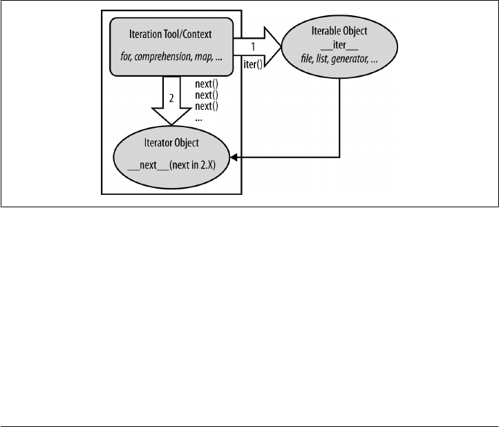
The full iteration protocol
As a more formal definition, Figure 14-1 sketches this full iteration protocol, used by
every iteration tool in Python, and supported by a wide variety of object types. It’s really
based on two objects, used in two distinct steps by iteration tools:
• The iterable object you request iteration for, whose __iter__ is run by iter
• The iterator object returned by the iterable that actually produces values during
the iteration, whose __next__ is run by next and raises StopIteration when finished
producing results
These steps are orchestrated automatically by iteration tools in most cases, but it helps
to understand these two objects’ roles. For example, in some cases these two objects
are the same when only a single scan is supported (e.g., files), and the iterator object is
often temporary, used internally by the iteration tool.
Moreover, some objects are both an iteration context tool (they iterate) and an iterable
object (their results are iterable)—including Chapter 20’s generator expressions, and
map and zip in Python 3.X. As we’ll see ahead, more tools become iterables in 3.X—
including map, zip, range, and some dictionary methods—to avoid constructing result
lists in memory all at once.
Figure 14-1. The Python iteration protocol, used by for loops, comprehensions, maps, and more, and
supported by files, lists, dictionaries, Chapter 20’s generators, and more. Some objects are both
iteration context and iterable object, such as generator expressions and 3.X’s flavors of some tools
(such as map and zip). Some objects are both iterable and iterator, returning themselves for the iter()
call, which is then a no-op.
In actual code, the protocol’s first step becomes obvious if we look at how for loops
internally process built-in sequence types such as lists:
>>> L = [1, 2, 3]
>>> I = iter(L) # Obtain an iterator object from an iterable
>>> I.__next__() # Call iterator's next to advance to next item
1
420 | Chapter 14: Iterations and Comprehensions
www.it-ebooks.info

>>> I.__next__() # Or use I.next() in 2.X, next(I) in either line
2
>>> I.__next__()
3
>>> I.__next__()
...error text omitted...
StopIteration
This initial step is not required for files, because a file object is its own iterator. Because
they support just one iteration (they can’t seek backward to support multiple active
scans), files have their own __next__ method and do not need to return a different object
that does:
>>> f = open('script2.py')
>>> iter(f) is f
True
>>> iter(f) is f.__iter__()
True
>>> f.__next__()
'import sys\n'
Lists and many other built-in objects, though, are not their own iterators because they
do support multiple open iterations—for example, there may be multiple iterations in
nested loops all at different positions. For such objects, we must call iter to start iter-
ating:
>>> L = [1, 2, 3]
>>> iter(L) is L
False
>>> L.__next__()
AttributeError: 'list' object has no attribute '__next__'
>>> I = iter(L)
>>> I.__next__()
1
>>> next(I) # Same as I.__next__()
2
Manual iteration
Although Python iteration tools call these functions automatically, we can use them to
apply the iteration protocol manually, too. The following interaction demonstrates the
equivalence between automatic and manual iteration:2
>>> L = [1, 2, 3]
>>>
>>> for X in L: # Automatic iteration
... print(X ** 2, end=' ') # Obtains iter, calls __next__, catches exceptions
...
1 4 9
2. Technically speaking, the for loop calls the internal equivalent of I.__next__, instead of the next(I) used
here, though there is rarely any difference between the two. Your manual iterations can generally use
either call scheme.
Iterations: A First Look | 421
www.it-ebooks.info

>>> I = iter(L) # Manual iteration: what for loops usually do
>>> while True:
... try: # try statement catches exceptions
... X = next(I) # Or call I.__next__ in 3.X
... except StopIteration:
... break
... print(X ** 2, end=' ')
...
1 4 9
To understand this code, you need to know that try statements run an action and catch
exceptions that occur while the action runs (we met exceptions briefly in Chapter 11
but will explore them in depth in Part VII). I should also note that for loops and other
iteration contexts can sometimes work differently for user-defined classes, repeatedly
indexing an object instead of running the iteration protocol, but prefer the iteration
protocol if it’s used. We’ll defer that story until we study class operator overloading in
Chapter 30.
Other Built-in Type Iterables
Besides files and physical sequences like lists, other types have useful iterators as well.
The classic way to step through the keys of a dictionary, for example, is to request its
keys list explicitly:
>>> D = {'a':1, 'b':2, 'c':3}
>>> for key in D.keys():
... print(key, D[key])
...
a 1
b 2
c 3
In recent versions of Python, though, dictionaries are iterables with an iterator that
automatically returns one key at a time in an iteration context:
>>> I = iter(D)
>>> next(I)
'a'
>>> next(I)
'b'
>>> next(I)
'c'
>>> next(I)
Traceback (most recent call last):
File "<stdin>", line 1, in <module>
StopIteration
The net effect is that we no longer need to call the keys method to step through dic-
tionary keys—the for loop will use the iteration protocol to grab one key each time
through:
422 | Chapter 14: Iterations and Comprehensions
www.it-ebooks.info

>>> for key in D:
... print(key, D[key])
...
a 1
b 2
c 3
We can’t delve into their details here, but other Python object types also support the
iteration protocol and thus may be used in for loops too. For instance, shelves (an
access-by-key filesystem for Python objects) and the results from os.popen (a tool for
reading the output of shell commands, which we met in the preceding chapter) are
iterable as well:
>>> import os
>>> P = os.popen('dir')
>>> P.__next__()
' Volume in drive C has no label.\n'
>>> P.__next__()
' Volume Serial Number is D093-D1F7\n'
>>> next(P)
TypeError: _wrap_close object is not an iterator
Notice that popen objects themselves support a P.next() method in Python 2.X. In 3.X,
they support the P.__next__() method, but not the next(P) built-in. Since the latter is
defined to call the former, this may seem unusual, though both calls work correctly if
we use the full iteration protocol employed automatically by for loops and other iter-
ation contexts, with its top-level iter call (this performs internal steps required to also
support next calls for this object):
>>> P = os.popen('dir')
>>> I = iter(P)
>>> next(I)
' Volume in drive C has no label.\n'
>>> I.__next__()
' Volume Serial Number is D093-D1F7\n'
Also in the systems domain, the standard directory walker in Python, os.walk, is sim-
ilarly iterable, but we’ll save an example until Chapter 20’s coverage of this tool’s basis
—generators and yield.
The iteration protocol also is the reason that we’ve had to wrap some results in a
list call to see their values all at once. Objects that are iterable return results one at a
time, not in a physical list:
>>> R = range(5)
>>> R # Ranges are iterables in 3.X
range(0, 5)
>>> I = iter(R) # Use iteration protocol to produce results
>>> next(I)
0
>>> next(I)
1
>>> list(range(5)) # Or use list to collect all results at once
[0, 1, 2, 3, 4]
Iterations: A First Look | 423
www.it-ebooks.info

Note that the list call here is not required in 2.X (where range builds a real list), and
is not needed in 3.X for contexts where iteration happens automatically (such as within
for loops). It is needed for displaying values here in 3.X, though, and may also be
required when list-like behavior or multiple scans are required for objects that produce
results on demand in 2.X or 3.X (more on this ahead).
Now that you have a better understanding of this protocol, you should be able to see
how it explains why the enumerate tool introduced in the prior chapter works the way
it does:
>>> E = enumerate('spam') # enumerate is an iterable too
>>> E
<enumerate object at 0x00000000029B7678>
>>> I = iter(E)
>>> next(I) # Generate results with iteration protocol
(0, 's')
>>> next(I) # Or use list to force generation to run
(1, 'p')
>>> list(enumerate('spam'))
[(0, 's'), (1, 'p'), (2, 'a'), (3, 'm')]
We don’t normally see this machinery because for loops run it for us automatically to
step through results. In fact, everything that scans left to right in Python employs the
iteration protocol in the same way—including the topic of the next section.
List Comprehensions: A First Detailed Look
Now that we’ve seen how the iteration protocol works, let’s turn to one of its most
common use cases. Together with for loops, list comprehensions are one of the most
prominent contexts in which the iteration protocol is applied.
In the previous chapter, we learned how to use range to change a list as we step across
it:
>>> L = [1, 2, 3, 4, 5]
>>> for i in range(len(L)):
... L[i] += 10
...
>>> L
[11, 12, 13, 14, 15]
This works, but as I mentioned there, it may not be the optimal “best practice” approach
in Python. Today, the list comprehension expression makes many such prior coding
patterns obsolete. Here, for example, we can replace the loop with a single expression
that produces the desired result list:
>>> L = [x + 10 for x in L]
>>> L
[21, 22, 23, 24, 25]
424 | Chapter 14: Iterations and Comprehensions
www.it-ebooks.info

The net result is similar, but it requires less coding on our part and is likely to run
substantially faster. The list comprehension isn’t exactly the same as the for loop
statement version because it makes a new list object (which might matter if there are
multiple references to the original list), but it’s close enough for most applications and
is a common and convenient enough approach to merit a closer look here.
List Comprehension Basics
We met the list comprehension briefly in Chapter 4. Syntactically, its syntax is derived
from a construct in set theory notation that applies an operation to each item in a set,
but you don’t have to know set theory to use this tool. In Python, most people find that
a list comprehension simply looks like a backward for loop.
To get a handle on the syntax, let’s dissect the prior section’s example in more detail:
L = [x + 10 for x in L]
List comprehensions are written in square brackets because they are ultimately a way
to construct a new list. They begin with an arbitrary expression that we make up, which
uses a loop variable that we make up (x + 10). That is followed by what you should
now recognize as the header of a for loop, which names the loop variable, and an
iterable object (for x in L).
To run the expression, Python executes an iteration across L inside the interpreter,
assigning x to each item in turn, and collects the results of running the items through
the expression on the left side. The result list we get back is exactly what the list com-
prehension says—a new list containing x + 10, for every x in L.
Technically speaking, list comprehensions are never really required because we can
always build up a list of expression results manually with for loops that append results
as we go:
>>> res = []
>>> for x in L:
... res.append(x + 10)
...
>>> res
[31, 32, 33, 34, 35]
In fact, this is exactly what the list comprehension does internally.
However, list comprehensions are more concise to write, and because this code pattern
of building up result lists is so common in Python work, they turn out to be very useful
in many contexts. Moreover, depending on your Python and code, list comprehensions
might run much faster than manual for loop statements (often roughly twice as fast)
because their iterations are performed at C language speed inside the interpreter, rather
than with manual Python code. Especially for larger data sets, there is often a major
performance advantage to using this expression.
List Comprehensions: A First Detailed Look | 425
www.it-ebooks.info

Using List Comprehensions on Files
Let’s work through another common application of list comprehensions to explore
them in more detail. Recall that the file object has a readlines method that loads the
file into a list of line strings all at once:
>>> f = open('script2.py')
>>> lines = f.readlines()
>>> lines
['import sys\n', 'print(sys.path)\n', 'x = 2\n', 'print(x ** 32)\n']
This works, but the lines in the result all include the newline character (\n) at the end.
For many programs, the newline character gets in the way—we have to be careful to
avoid double-spacing when printing, and so on. It would be nice if we could get rid of
these newlines all at once, wouldn’t it?
Anytime we start thinking about performing an operation on each item in a sequence,
we’re in the realm of list comprehensions. For example, assuming the variable lines is
as it was in the prior interaction, the following code does the job by running each line
in the list through the string rstrip method to remove whitespace on the right side (a
line[:−1] slice would work, too, but only if we can be sure all lines are properly \n
terminated, and this may not always be the case for the last line in a file):
>>> lines = [line.rstrip() for line in lines]
>>> lines
['import sys', 'print(sys.path)', 'x = 2', 'print(x ** 32)']
This works as planned. Because list comprehensions are an iteration context just like
for loop statements, though, we don’t even have to open the file ahead of time. If we
open it inside the expression, the list comprehension will automatically use the iteration
protocol we met earlier in this chapter. That is, it will read one line from the file at a
time by calling the file’s next handler method, run the line through the rstrip expres-
sion, and add it to the result list. Again, we get what we ask for—the rstrip result of
a line, for every line in the file:
>>> lines = [line.rstrip() for line in open('script2.py')]
>>> lines
['import sys', 'print(sys.path)', 'x = 2', 'print(x ** 32)']
This expression does a lot implicitly, but we’re getting a lot of work for free here—
Python scans the file by lines and builds a list of operation results automatically. It’s
also an efficient way to code this operation: because most of this work is done inside
the Python interpreter, it may be faster than an equivalent for statement, and won’t
load a file into memory all at once like some other techniques. Again, especially for
large files, the advantages of list comprehensions can be significant.
Besides their efficiency, list comprehensions are also remarkably expressive. In our
example, we can run any string operation on a file’s lines as we iterate. To illustrate,
here’s the list comprehension equivalent to the file iterator uppercase example we met
earlier, along with a few other representative operations:
426 | Chapter 14: Iterations and Comprehensions
www.it-ebooks.info

>>> [line.upper() for line in open('script2.py')]
['IMPORT SYS\n', 'PRINT(SYS.PATH)\n', 'X = 2\n', 'PRINT(X ** 32)\n']
>>> [line.rstrip().upper() for line in open('script2.py')]
['IMPORT SYS', 'PRINT(SYS.PATH)', 'X = 2', 'PRINT(X ** 32)']
>>> [line.split() for line in open('script2.py')]
[['import', 'sys'], ['print(sys.path)'], ['x', '=', '2'], ['print(x', '**', '32)']]
>>> [line.replace(' ', '!') for line in open('script2.py')]
['import!sys\n', 'print(sys.path)\n', 'x!=!2\n', 'print(x!**!32)\n']
>>> [('sys' in line, line[:5]) for line in open('script2.py')]
[(True, 'impor'), (True, 'print'), (False, 'x = 2'), (False, 'print')]
Recall that the method chaining in the second of these examples works because string
methods return a new string, to which we can apply another string method. The last
of these shows how we can also collect multiple results, as long as they’re wrapped in
a collection like a tuple or list.
One fine point here: recall from Chapter 9 that file objects close them-
selves automatically when garbage-collected if still open. Hence, these
list comprehensions will also automatically close the file when their
temporary file object is garbage-collected after the expression runs.
Outside CPython, though, you may want to code these to close man-
ually if this is run in a loop, to ensure that file resources are freed im-
mediately. See Chapter 9 for more on file close calls if you need a re-
fresher on this.
Extended List Comprehension Syntax
In fact, list comprehensions can be even richer in practice, and even constitute a sort
of iteration mini-language in their fullest forms. Let’s take a quick look at their syntax
tools here.
Filter clauses: if
As one particularly useful extension, the for loop nested in a comprehension expression
can have an associated if clause to filter out of the result items for which the test is not
true.
For example, suppose we want to repeat the prior section’s file-scanning example, but
we need to collect only lines that begin with the letter p (perhaps the first character on
each line is an action code of some sort). Adding an if filter clause to our expression
does the trick:
>>> lines = [line.rstrip() for line in open('script2.py') if line[0] == 'p']
>>> lines
['print(sys.path)', 'print(x ** 32)']
List Comprehensions: A First Detailed Look | 427
www.it-ebooks.info

Here, the if clause checks each line read from the file to see whether its first character
is p; if not, the line is omitted from the result list. This is a fairly big expression, but it’s
easy to understand if we translate it to its simple for loop statement equivalent. In
general, we can always translate a list comprehension to a for statement by appending
as we go and further indenting each successive part:
>>> res = []
>>> for line in open('script2.py'):
... if line[0] == 'p':
... res.append(line.rstrip())
...
>>> res
['print(sys.path)', 'print(x ** 32)']
This for statement equivalent works, but it takes up four lines instead of one and may
run slower. In fact, you can squeeze a substantial amount of logic into a list compre-
hension when you need to—the following works like the prior but selects only lines
that end in a digit (before the newline at the end), by filtering with a more sophisticated
expression on the right side:
>>> [line.rstrip() for line in open('script2.py') if line.rstrip()[-1].isdigit()]
['x = 2']
As another if filter example, the first result in the following gives the total lines in a
text file, and the second strips whitespace on both ends to omit blank links in the tally
in just one line of code (this file, not included, contains lines describing typos found in
the first draft of this book by my proofreader):
>>> fname = r'd:\books\5e\lp5e\draft1typos.txt'
>>> len(open(fname).readlines()) # All lines
263
>>> len([line for line in open(fname) if line.strip() != '']) # Nonblank lines
185
Nested loops: for
List comprehensions can become even more complex if we need them to—for instance,
they may contain nested loops, coded as a series of for clauses. In fact, their full syntax
allows for any number of for clauses, each of which can have an optional associated
if clause.
For example, the following builds a list of the concatenation of x + y for every x in one
string and every y in another. It effectively collects all the ordered combinations of the
characters in two strings:
>>> [x + y for x in 'abc' for y in 'lmn']
['al', 'am', 'an', 'bl', 'bm', 'bn', 'cl', 'cm', 'cn']
Again, one way to understand this expression is to convert it to statement form by
indenting its parts. The following is an equivalent, but likely slower, alternative way to
achieve the same effect:
428 | Chapter 14: Iterations and Comprehensions
www.it-ebooks.info

>>> res = []
>>> for x in 'abc':
... for y in 'lmn':
... res.append(x + y)
...
>>> res
['al', 'am', 'an', 'bl', 'bm', 'bn', 'cl', 'cm', 'cn']
Beyond this complexity level, though, list comprehension expressions can often be-
come too compact for their own good. In general, they are intended for simple types
of iterations; for more involved work, a simpler for statement structure will probably
be easier to understand and modify in the future. As usual in programming, if something
is difficult for you to understand, it’s probably not a good idea.
Because comprehensions are generally best taken in multiple doses, we’ll cut this story
short here for now. We’ll revisit list comprehensions in Chapter 20 in the context of
functional programming tools, and will define their syntax more formally and explore
additional examples there. As we’ll find, comprehensions turn out to be just as related
to functions as they are to looping statements.
A blanket qualification for all performance claims in this book, list com-
prehension or other: the relative speed of code depends much on the
exact code tested and Python used, and is prone to change from release
to release.
For example, in CPython 2.7 and 3.3 today, list comprehensions can
still be twice as fast as corresponding for loops on some tests, but just
marginally quicker on others, and perhaps even slightly slower on some
when if filter clauses are used.
We’ll see how to time code in Chapter 21, and will learn how to interpret
the file listcomp-speed.txt in the book examples package, which times
this chapter’s code. For now, keep in mind that absolutes in perfor-
mance benchmarks are as elusive as consensus in open source projects!
Other Iteration Contexts
Later in the book, we’ll see that user-defined classes can implement the iteration pro-
tocol too. Because of this, it’s sometimes important to know which built-in tools make
use of it—any tool that employs the iteration protocol will automatically work on any
built-in type or user-defined class that provides it.
So far, I’ve been demonstrating iterators in the context of the for loop statement, be-
cause this part of the book is focused on statements. Keep in mind, though, that
every built-in tool that scans from left to right across objects uses the iteration protocol.
This includes the for loops we’ve seen:
>>> for line in open('script2.py'): # Use file iterators
... print(line.upper(), end='')
Other Iteration Contexts | 429
www.it-ebooks.info

...
IMPORT SYS
PRINT(SYS.PATH)
X = 2
PRINT(X ** 32)
But also much more. For instance, list comprehensions and the map built-in function
use the same protocol as their for loop cousin. When applied to a file, they both leverage
the file object’s iterator automatically to scan line by line, fetching an iterator with
__iter__ and calling __next__ each time through:
>>> uppers = [line.upper() for line in open('script2.py')]
>>> uppers
['IMPORT SYS\n', 'PRINT(SYS.PATH)\n', 'X = 2\n', 'PRINT(X ** 32)\n']
>>> map(str.upper, open('script2.py')) # map is itself an iterable in 3.X
<map object at 0x00000000029476D8>
>>> list(map(str.upper, open('script2.py')))
['IMPORT SYS\n', 'PRINT(SYS.PATH)\n', 'X = 2\n', 'PRINT(X ** 32)\n']
We introduced the map call used here briefly in the preceding chapter (and in passing
in Chapter 4); it’s a built-in that applies a function call to each item in the passed-in
iterable object. map is similar to a list comprehension but is more limited because it
requires a function instead of an arbitrary expression. It also returns an iterable object
itself in Python 3.X, so we must wrap it in a list call to force it to give us all its values
at once; more on this change later in this chapter. Because map, like the list compre-
hension, is related to both for loops and functions, we’ll also explore both again in
Chapter 19 and Chapter 20.
Many of Python’s other built-ins process iterables, too. For example, sorted sorts items
in an iterable; zip combines items from iterables; enumerate pairs items in an iterable
with relative positions; filter selects items for which a function is true; and reduce
runs pairs of items in an iterable through a function. All of these accept iterables, and
zip, enumerate, and filter also return an iterable in Python 3.X, like map. Here they are
in action running the file’s iterator automatically to read line by line:
>>> sorted(open('script2.py'))
['import sys\n', 'print(sys.path)\n', 'print(x ** 32)\n', 'x = 2\n']
>>> list(zip(open('script2.py'), open('script2.py')))
[('import sys\n', 'import sys\n'), ('print(sys.path)\n', 'print(sys.path)\n'),
('x = 2\n', 'x = 2\n'), ('print(x ** 32)\n', 'print(x ** 32)\n')]
>>> list(enumerate(open('script2.py')))
[(0, 'import sys\n'), (1, 'print(sys.path)\n'), (2, 'x = 2\n'),
(3, 'print(x ** 32)\n')]
>>> list(filter(bool, open('script2.py'))) # nonempty=True
['import sys\n', 'print(sys.path)\n', 'x = 2\n', 'print(x ** 32)\n']
>>> import functools, operator
>>> functools.reduce(operator.add, open('script2.py'))
'import sys\nprint(sys.path)\nx = 2\nprint(x ** 32)\n'
430 | Chapter 14: Iterations and Comprehensions
www.it-ebooks.info

All of these are iteration tools, but they have unique roles. We met zip and enumerate
in the prior chapter; filter and reduce are in Chapter 19’s functional programming
domain, so we’ll defer their details for now; the point to notice here is their use of the
iteration protocol for files and other iterables.
We first saw the sorted function used here at work in, and we used it for dictionaries
in Chapter 8. sorted is a built-in that employs the iteration protocol—it’s like the orig-
inal list sort method, but it returns the new sorted list as a result and runs on any iterable
object. Notice that, unlike map and others, sorted returns an actual list in Python 3.X
instead of an iterable.
Interestingly, the iteration protocol is even more pervasive in Python today than the
examples so far have demonstrated—essentially everything in Python’s built-in toolset
that scans an object from left to right is defined to use the iteration protocol on the
subject object. This even includes tools such as the list and tuple built-in functions
(which build new objects from iterables), and the string join method (which makes a
new string by putting a substring between strings contained in an iterable). Conse-
quently, these will also work on an open file and automatically read one line at a time:
>>> list(open('script2.py'))
['import sys\n', 'print(sys.path)\n', 'x = 2\n', 'print(x ** 32)\n']
>>> tuple(open('script2.py'))
('import sys\n', 'print(sys.path)\n', 'x = 2\n', 'print(x ** 32)\n')
>>> '&&'.join(open('script2.py'))
'import sys\n&&print(sys.path)\n&&x = 2\n&&print(x ** 32)\n'
Even some tools you might not expect fall into this category. For example, sequence
assignment, the in membership test, slice assignment, and the list’s extend method also
leverage the iteration protocol to scan, and thus read a file by lines automatically:
>>> a, b, c, d = open('script2.py') # Sequence assignment
>>> a, d
('import sys\n', 'print(x ** 32)\n')
>>> a, *b = open('script2.py') # 3.X extended form
>>> a, b
('import sys\n', ['print(sys.path)\n', 'x = 2\n', 'print(x ** 32)\n'])
>>> 'y = 2\n' in open('script2.py') # Membership test
False
>>> 'x = 2\n' in open('script2.py')
True
>>> L = [11, 22, 33, 44] # Slice assignment
>>> L[1:3] = open('script2.py')
>>> L
[11, 'import sys\n', 'print(sys.path)\n', 'x = 2\n', 'print(x ** 32)\n', 44]
>>> L = [11]
>>> L.extend(open('script2.py')) # list.extend method
Other Iteration Contexts | 431
www.it-ebooks.info

>>> L
[11, 'import sys\n', 'print(sys.path)\n', 'x = 2\n', 'print(x ** 32)\n']
Per Chapter 8 extend iterates automatically, but append does not—use the latter (or
similar) to add an iterable to a list without iterating, with the potential to be iterated
across later:
>>> L = [11]
>>> L.append(open('script2.py')) # list.append does not iterate
>>> L
[11, <_io.TextIOWrapper name='script2.py' mode='r' encoding='cp1252'>]
>>> list(L[1])
['import sys\n', 'print(sys.path)\n', 'x = 2\n', 'print(x ** 32)\n']
Iteration is a broadly supported and powerful model. Earlier, we saw that the built-in
dict call accepts an iterable zip result, too (see Chapter 8 and Chapter 13). For that
matter, so does the set call, as well as the newer set and dictionary comprehension
expressions in Python 3.X and 2.7, which we met in Chapter 4, Chapter 5, and Chap-
ter 8:
>>> set(open('script2.py'))
{'print(x ** 32)\n', 'import sys\n', 'print(sys.path)\n', 'x = 2\n'}
>>> {line for line in open('script2.py')}
{'print(x ** 32)\n', 'import sys\n', 'print(sys.path)\n', 'x = 2\n'}
>>> {ix: line for ix, line in enumerate(open('script2.py'))}
{0: 'import sys\n', 1: 'print(sys.path)\n', 2: 'x = 2\n', 3: 'print(x ** 32)\n'}
In fact, both set and dictionary comprehensions support the extended syntax of list
comprehensions we met earlier in this chapter, including if tests:
>>> {line for line in open('script2.py') if line[0] == 'p'}
{'print(x ** 32)\n', 'print(sys.path)\n'}
>>> {ix: line for (ix, line) in enumerate(open('script2.py')) if line[0] == 'p'}
{1: 'print(sys.path)\n', 3: 'print(x ** 32)\n'}
Like the list comprehension, both of these scan the file line by line and pick out lines
that begin with the letter p. They also happen to build sets and dictionaries in the end,
but we get a lot of work “for free” by combining file iteration and comprehension
syntax. Later in the book we’ll meet a relative of comprehensions—generator expres-
sions—that deploys the same syntax and works on iterables too, but is also iterable
itself:
>>> list(line.upper() for line in open('script2.py')) # See Chapter 20
['IMPORT SYS\n', 'PRINT(SYS.PATH)\n', 'X = 2\n', 'PRINT(X ** 32)\n']
Other built-in functions support the iteration protocol as well, but frankly, some are
harder to cast in interesting examples related to files! For example, the sum call computes
the sum of all the numbers in any iterable; the any and all built-ins return True if any
or all items in an iterable are True, respectively; and max and min return the largest and
smallest item in an iterable, respectively. Like reduce, all of the tools in the following
432 | Chapter 14: Iterations and Comprehensions
www.it-ebooks.info

examples accept any iterable as an argument and use the iteration protocol to scan it,
but return a single result:
>>> sum([3, 2, 4, 1, 5, 0]) # sum expects numbers only
15
>>> any(['spam', '', 'ni'])
True
>>> all(['spam', '', 'ni'])
False
>>> max([3, 2, 5, 1, 4])
5
>>> min([3, 2, 5, 1, 4])
1
Strictly speaking, the max and min functions can be applied to files as well—they auto-
matically use the iteration protocol to scan the file and pick out the lines with the highest
and lowest string values, respectively (though I’ll leave valid use cases to your imagi-
nation):
>>> max(open('script2.py')) # Line with max/min string value
'x = 2\n'
>>> min(open('script2.py'))
'import sys\n'
There’s one last iteration context that’s worth mentioning, although it’s mostly a pre-
view: in Chapter 18, we’ll learn that a special *arg form can be used in function calls
to unpack a collection of values into individual arguments. As you can probably predict
by now, this accepts any iterable, too, including files (see Chapter 18 for more details
on this call syntax; Chapter 20 for a section that extends this idea to generator expres-
sions; and Chapter 11 for tips on using the following’s 3.X print in 2.X as usual):
>>> def f(a, b, c, d): print(a, b, c, d, sep='&')
...
>>> f(1, 2, 3, 4)
1&2&3&4
>>> f(*[1, 2, 3, 4]) # Unpacks into arguments
1&2&3&4
>>>
>>> f(*open('script2.py')) # Iterates by lines too!
import sys
&print(sys.path)
&x = 2
&print(x ** 32)
In fact, because this argument-unpacking syntax in calls accepts iterables, it’s also pos-
sible to use the zip built-in to unzip zipped tuples, by making prior or nested zip results
arguments for another zip call (warning: you probably shouldn’t read the following
example if you plan to operate heavy machinery anytime soon!):
>>> X = (1, 2)
>>> Y = (3, 4)
>>>
>>> list(zip(X, Y)) # Zip tuples: returns an iterable
[(1, 3), (2, 4)]
Other Iteration Contexts | 433
www.it-ebooks.info

>>>
>>> A, B = zip(*zip(X, Y)) # Unzip a zip!
>>> A
(1, 2)
>>> B
(3, 4)
Still other tools in Python, such as the range built-in and dictionary view objects,
return iterables instead of processing them. To see how these have been absorbed into
the iteration protocol in Python 3.X as well, we need to move on to the next section.
New Iterables in Python 3.X
One of the fundamental distinctions of Python 3.X is its stronger emphasis on iterators
than 2.X. This, along with its Unicode model and mandated new-style classes, is one
of 3.X’s most sweeping changes.
Specifically, in addition to the iterators associated with built-in types such as files and
dictionaries, the dictionary methods keys, values, and items return iterable objects in
Python 3.X, as do the built-in functions range, map, zip, and filter. As shown in the
prior section, the last three of these functions both return iterables and process them.
All of these tools produce results on demand in Python 3.X, instead of constructing
result lists as they do in 2.X.
Impacts on 2.X Code: Pros and Cons
Although this saves memory space, it can impact your coding styles in some contexts.
In various places in this book so far, for example, we’ve had to wrap up some function
and method call results in a list(...) call in order to force them to produce all their
results at once for display:
>>> zip('abc', 'xyz') # An iterable in Python 3.X (a list in 2.X)
<zip object at 0x000000000294C308>
>>> list(zip('abc', 'xyz')) # Force list of results in 3.X to display
[('a', 'x'), ('b', 'y'), ('c', 'z')]
A similar conversion is required if we wish to apply list or sequence operations to most
iterables that generate items on demand—to index, slice, or concatenate the iterable
itself, for example. The list results for these tools in 2.X support such operations di-
rectly:
>>> Z = zip((1, 2), (3, 4)) # Unlike 2.X lists, cannot index, etc.
>>> Z[0]
TypeError: 'zip' object is not subscriptable
As we’ll see in more detail in Chapter 20, conversion to lists may also be more subtly
required to support multiple iterations for newly iterable tools that support just one
434 | Chapter 14: Iterations and Comprehensions
www.it-ebooks.info

scan such as map and zip—unlike their 2.X list forms, their values in 3.X are exhausted
after a single pass:
>>> M = map(lambda x: 2 ** x, range(3))
>>> for i in M: print(i)
...
1
2
4
>>> for i in M: print(i) # Unlike 2.X lists, one pass only (zip too)
...
>>>
Such conversion isn’t required in 2.X, because functions like zip return lists of results.
In 3.X, though, they return iterable objects, producing results on demand. This may
break 2.X code, and means extra typing is required to display the results at the inter-
active prompt (and possibly in some other contexts), but it’s an asset in larger programs
—delayed evaluation like this conserves memory and avoids pauses while large result
lists are computed. Let’s take a quick look at some of the new 3.X iterables in action.
The range Iterable
We studied the range built-in’s basic behavior in the preceding chapter. In 3.X, it returns
an iterable that generates numbers in the range on demand, instead of building the
result list in memory. This subsumes the older 2.X xrange (see the upcoming version
skew note), and you must use list(range(...)) to force an actual range list if one is
needed (e.g., to display results):
C:\code> c:\python33\python
>>> R = range(10) # range returns an iterable, not a list
>>> R
range(0, 10)
>>> I = iter(R) # Make an iterator from the range iterable
>>> next(I) # Advance to next result
0 # What happens in for loops, comprehensions, etc.
>>> next(I)
1
>>> next(I)
2
>>> list(range(10)) # To force a list if required
[0, 1, 2, 3, 4, 5, 6, 7, 8, 9]
Unlike the list returned by this call in 2.X, range objects in 3.X support only iteration,
indexing, and the len function. They do not support any other sequence operations
(use list(...) if you require more list tools):
>>> len(R) # range also does len and indexing, but no others
10
>>> R[0]
0
New Iterables in Python 3.X | 435
www.it-ebooks.info
>>> R[-1]
9
>>> next(I) # Continue taking from iterator, where left off
3
>>> I.__next__() # .next() becomes .__next__(), but use new next()
4
Version skew note: As first mentioned in the preceding chapter, Python
2.X also has a built-in called xrange, which is like range but produces
items on demand instead of building a list of results in memory all at
once. Since this is exactly what the new iterator-based range does in
Python 3.X, xrange is no longer available in 3.X—it has been subsumed.
You may still both see and use it in 2.X code, though, especially since
range builds result lists there and so is not as efficient in its memory
usage.
As noted in the prior chapter, the file.xreadlines() method used to
minimize memory use in 2.X has been dropped in Python 3.X for similar
reasons, in favor of file iterators.
The map, zip, and filter Iterables
Like range, the map, zip, and filter built-ins also become iterables in 3.X to conserve
space, rather than producing a result list all at once in memory. All three not only
process iterables, as in 2.X, but also return iterable results in 3.X. Unlike range, though,
they are their own iterators—after you step through their results once, they are ex-
hausted. In other words, you can’t have multiple iterators on their results that maintain
different positions in those results.
Here is the case for the map built-in we met in the prior chapter. As with other iterables,
you can force a list with list(...) if you really need one, but the default behavior can
save substantial space in memory for large result sets:
>>> M = map(abs, (-1, 0, 1)) # map returns an iterable, not a list
>>> M
<map object at 0x00000000029B75C0>
>>> next(M) # Use iterator manually: exhausts results
1 # These do not support len() or indexing
>>> next(M)
0
>>> next(M)
1
>>> next(M)
StopIteration
>>> for x in M: print(x) # map iterator is now empty: one pass only
...
>>> M = map(abs, (-1, 0, 1)) # Make a new iterable/iterator to scan again
>>> for x in M: print(x) # Iteration contexts auto call next()
436 | Chapter 14: Iterations and Comprehensions
www.it-ebooks.info

...
1
0
1
>>> list(map(abs, (-1, 0, 1))) # Can force a real list if needed
[1, 0, 1]
The zip built-in, introduced in the prior chapter, is an iteration context itself, but also
returns an iterable with an iterator that works the same way:
>>> Z = zip((1, 2, 3), (10, 20, 30)) # zip is the same: a one-pass iterator
>>> Z
<zip object at 0x0000000002951108>
>>> list(Z)
[(1, 10), (2, 20), (3, 30)]
>>> for pair in Z: print(pair) # Exhausted after one pass
...
>>> Z = zip((1, 2, 3), (10, 20, 30))
>>> for pair in Z: print(pair) # Iterator used automatically or manually
...
(1, 10)
(2, 20)
(3, 30)
>>> Z = zip((1, 2, 3), (10, 20, 30)) # Manual iteration (iter() not needed)
>>> next(Z)
(1, 10)
>>> next(Z)
(2, 20)
The filter built-in, which we met briefly in Chapter 12 and will study in the next part
of this book, is also analogous. It returns items in an iterable for which a passed-in
function returns True (as we’ve learned, in Python True includes nonempty objects, and
bool returns an object’s truth value):
>>> filter(bool, ['spam', '', 'ni'])
<filter object at 0x00000000029B7B70>
>>> list(filter(bool, ['spam', '', 'ni']))
['spam', 'ni']
Like most of the tools discussed in this section, filter both accepts an iterable to process
and returns an iterable to generate results in 3.X. It can also generally be emulated by
extended list comprehension syntax that automatically tests truth values:
>>> [x for x in ['spam', '', 'ni'] if bool(x)]
['spam', 'ni']
>>> [x for x in ['spam', '', 'ni'] if x]
['spam', 'ni']
New Iterables in Python 3.X | 437
www.it-ebooks.info

Multiple Versus Single Pass Iterators
It’s important to see how the range object differs from the built-ins described in this
section—it supports len and indexing, it is not its own iterator (you make one with
iter when iterating manually), and it supports multiple iterators over its result that
remember their positions independently:
>>> R = range(3) # range allows multiple iterators
>>> next(R)
TypeError: range object is not an iterator
>>> I1 = iter(R)
>>> next(I1)
0
>>> next(I1)
1
>>> I2 = iter(R) # Two iterators on one range
>>> next(I2)
0
>>> next(I1) # I1 is at a different spot than I2
2
By contrast, in 3.X zip, map, and filter do not support multiple active iterators on the
same result; because of this the iter call is optional for stepping through such objects’
results—their iter is themselves (in 2.X these built-ins return multiple-scan lists so the
following does not apply):
>>> Z = zip((1, 2, 3), (10, 11, 12))
>>> I1 = iter(Z)
>>> I2 = iter(Z) # Two iterators on one zip
>>> next(I1)
(1, 10)
>>> next(I1)
(2, 11)
>>> next(I2) # (3.X) I2 is at same spot as I1!
(3, 12)
>>> M = map(abs, (-1, 0, 1)) # Ditto for map (and filter)
>>> I1 = iter(M); I2 = iter(M)
>>> print(next(I1), next(I1), next(I1))
1 0 1
>>> next(I2) # (3.X) Single scan is exhausted!
StopIteration
>>> R = range(3) # But range allows many iterators
>>> I1, I2 = iter(R), iter(R)
>>> [next(I1), next(I1), next(I1)]
[0 1 2]
>>> next(I2) # Multiple active scans, like 2.X lists
0
When we code our own iterable objects with classes later in the book (Chapter 30),
we’ll see that multiple iterators are usually supported by returning new objects for the
iter call; a single iterator generally means an object returns itself. In Chapter 20, we’ll
438 | Chapter 14: Iterations and Comprehensions
www.it-ebooks.info

also find that generator functions and expressions behave like map and zip instead of
range in this regard, supporting just a single active iteration scan. In that chapter, we’ll
see some subtle implications of one-shot iterators in loops that attempt to scan multiple
times—code that formerly treated these as lists may fail without manual list conver-
sions.
Dictionary View Iterables
Finally, as we saw briefly in Chapter 8, in Python 3.X the dictionary keys, values, and
items methods return iterable view objects that generate result items one at a time,
instead of producing result lists all at once in memory. Views are also available in 2.7
as an option, but under special method names to avoid impacting existing code. View
items maintain the same physical ordering as that of the dictionary and reflect changes
made to the underlying dictionary. Now that we know more about iterables here’s the
rest of this story—in Python 3.3 (your key order may vary):
>>> D = dict(a=1, b=2, c=3)
>>> D
{'a': 1, 'b': 2, 'c': 3}
>>> K = D.keys() # A view object in 3.X, not a list
>>> K
dict_keys(['a', 'b', 'c'])
>>> next(K) # Views are not iterators themselves
TypeError: dict_keys object is not an iterator
>>> I = iter(K) # View iterables have an iterator,
>>> next(I) # which can be used manually,
'a' # but does not support len(), index
>>> next(I)
'b'
>>> for k in D.keys(): print(k, end=' ') # All iteration contexts use auto
...
a b c
As for all iterables that produce values on request, you can always force a 3.X dictionary
view to build a real list by passing it to the list built-in. However, this usually isn’t
required except to display results interactively or to apply list operations like indexing:
>>> K = D.keys()
>>> list(K) # Can still force a real list if needed
['a', 'b', 'c']
>>> V = D.values() # Ditto for values() and items() views
>>> V
dict_values([1, 2, 3])
>>> list(V) # Need list() to display or index as list
[1, 2, 3]
>>> V[0]
New Iterables in Python 3.X | 439
www.it-ebooks.info

TypeError: 'dict_values' object does not support indexing
>>> list(V)[0]
1
>>> list(D.items())
[('a', 1), ('b', 2), ('c', 3)]
>>> for (k, v) in D.items(): print(k, v, end=' ')
...
a 1 b 2 c 3
In addition, 3.X dictionaries still are iterables themselves, with an iterator that returns
successive keys. Thus, it’s not often necessary to call keys directly in this context:
>>> D # Dictionaries still produce an iterator
{'a': 1, 'b': 2, 'c': 3} # Returns next key on each iteration
>>> I = iter(D)
>>> next(I)
'a'
>>> next(I)
'b'
>>> for key in D: print(key, end=' ') # Still no need to call keys() to iterate
... # But keys is an iterable in 3.X too!
a b c
Finally, remember again that because keys no longer returns a list, the traditional coding
pattern for scanning a dictionary by sorted keys won’t work in 3.X. Instead, convert
keys views first with a list call, or use the sorted call on either a keys view or the
dictionary itself, as follows. We saw this in Chapter 8, but it’s important enough to 2.X
programmers making the switch to demonstrate again:
>>> D
{'a': 1, 'b': 2, 'c': 3}
>>> for k in sorted(D.keys()): print(k, D[k], end=' ')
...
a 1 b 2 c 3
>>> for k in sorted(D): print(k, D[k], end=' ') # "Best practice" key sorting
...
a 1 b 2 c 3
Other Iteration Topics
As mentioned in this chapter’s introduction, there is more coverage of both list com-
prehensions and iterables in Chapter 20, in conjunction with functions, and again in
Chapter 30 when we study classes. As you’ll see later:
• User-defined functions can be turned into iterable generator functions, with
yield statements.
• List comprehensions morph into iterable generator expressions when coded in
parentheses.
440 | Chapter 14: Iterations and Comprehensions
www.it-ebooks.info

• User-defined classes are made iterable with __iter__ or __getitem__ operator over-
loading.
In particular, user-defined iterables defined with classes allow arbitrary objects and
operations to be used in any of the iteration contexts we’ve met in this chapter. By
supporting just a single operation—iteration—objects may be used in a wide variety of
contexts and tools.
Chapter Summary
In this chapter, we explored concepts related to looping in Python. We took our first
substantial look at the iteration protocol in Python—a way for nonsequence objects to
take part in iteration loops—and at list comprehensions. As we saw, a list comprehen-
sion is an expression similar to a for loop that applies another expression to all the
items in any iterable object. Along the way, we also saw other built-in iteration tools
at work and studied recent iteration additions in Python 3.X.
This wraps up our tour of specific procedural statements and related tools. The next
chapter closes out this part of the book by discussing documentation options for Python
code. Though a bit of a diversion from the more detailed aspects of coding, documen-
tation is also part of the general syntax model, and it’s an important component of well-
written programs. In the next chapter, we’ll also dig into a set of exercises for this part
of the book before we turn our attention to larger structures such as functions. As usual,
though, let’s first exercise what we’ve learned here with a quiz.
Test Your Knowledge: Quiz
1. How are for loops and iterable objects related?
2. How are for loops and list comprehensions related?
3. Name four iteration contexts in the Python language.
4. What is the best way to read line by line from a text file today?
5. What sort of weapons would you expect to see employed by the Spanish Inquisi-
tion?
Test Your Knowledge: Answers
1. The for loop uses the iteration protocol to step through items in the iterable object
across which it is iterating. It first fetches an iterator from the iterable by passing
the object to iter, and then calls this iterator object’s __next__ method in 3.X on
each iteration and catches the StopIteration exception to determine when to stop
looping. The method is named next in 2.X, and is run by the next built-in function
in both 3.x and 2.X. Any object that supports this model works in a for loop and
Test Your Knowledge: Answers | 441
www.it-ebooks.info

in all other iteration contexts. For some objects that are their own iterator, the
initial iter call is extraneous but harmless.
2. Both are iteration tools and contexts. List comprehensions are a concise and often
efficient way to perform a common for loop task: collecting the results of applying
an expression to all items in an iterable object. It’s always possible to translate a
list comprehension to a for loop, and part of the list comprehension expression
looks like the header of a for loop syntactically.
3. Iteration contexts in Python include the for loop; list comprehensions; the map
built-in function; the in membership test expression; and the built-in functions
sorted, sum, any, and all. This category also includes the list and tuple built-ins,
string join methods, and sequence assignments, all of which use the iteration pro-
tocol (see answer #1) to step across iterable objects one item at a time.
4. The best way to read lines from a text file today is to not read it explicitly at all:
instead, open the file within an iteration context tool such as a for loop or list
comprehension, and let the iteration tool automatically scan one line at a time by
running the file’s next handler method on each iteration. This approach is generally
best in terms of coding simplicity, memory space, and possibly execution speed
requirements.
5. I’ll accept any of the following as correct answers: fear, intimidation, nice red uni-
forms, a comfy chair, and soft pillows.
442 | Chapter 14: Iterations and Comprehensions
www.it-ebooks.info

CHAPTER 15
The Documentation Interlude
This part of the book concludes with a look at techniques and tools used for docu-
menting Python code. Although Python code is designed to be readable, a few well-
placed human-accessible comments can do much to help others understand the work-
ings of your programs. As we’ll see, Python includes both syntax and tools to make
documentation easier. In particular, the PyDoc system covered here can render a mod-
ule’s internal documentation as either plain text in a shell, or HTML in a web browser.
Although this is something of a tools-related concept, this topic is presented here partly
because it involves Python’s syntax model, and partly as a resource for readers strug-
gling to understand Python’s toolset. For the latter purpose, I’ll also expand here on
documentation pointers first given in Chapter 4. As usual, because this chapter closes
out its part, it also ends with some warnings about common pitfalls and a set of exercises
for this part of the text, in addition to its chapter quiz.
Python Documentation Sources
By this point in the book, you’re probably starting to realize that Python comes with
an amazing amount of prebuilt functionality—built-in functions and exceptions, pre-
defined object attributes and methods, standard library modules, and more. And we’ve
really only scratched the surface of each of these categories.
One of the first questions that bewildered beginners often ask is: how do I find infor-
mation on all the built-in tools? This section provides hints on the various documen-
tation sources available in Python. It also presents documentation strings (docstrings)
and the PyDoc system that makes use of them. These topics are somewhat peripheral
to the core language itself, but they become essential knowledge as soon as your code
reaches the level of the examples and exercises in this part of the book.
As summarized in Table 15-1, there are a variety of places to look for information on
Python, with generally increasing verbosity. Because documentation is such a crucial
tool in practical programming, we’ll explore each of these categories in the sections
that follow.
443
www.it-ebooks.info

Table 15-1. Python documentation sources
Form Role
# comments In-file documentation
The dir function Lists of attributes available in objects
Docstrings: __doc__ In-file documentation attached to objects
PyDoc: the help function Interactive help for objects
PyDoc: HTML reports Module documentation in a browser
Sphinx third-party tool Richer documentation for larger projects
The standard manual set Official language and library descriptions
Web resources Online tutorials, examples, and so on
Published books Commercially polished reference texts
# Comments
As we’ve learned, hash-mark comments are the most basic way to document your code.
Python simply ignores all the text following a # (as long as it’s not inside a string literal),
so you can follow this character with any words and descriptions meaningful to pro-
grammers. Such comments are accessible only in your source files, though; to code
comments that are more widely available, you’ll need to use docstrings.
In fact, current best practice generally dictates that docstrings are best for larger func-
tional documentation (e.g., “my file does this”), and # comments are best limited to
smaller code documentation (e.g., “this strange expression does that”) and are best
limited in scope to a statement or small group of statements within a script or function.
More on docstrings in a moment; first, let’s see how to explore objects.
The dir Function
As we’ve also seen, the built-in dir function is an easy way to grab a list of all the
attributes available inside an object (i.e., its methods and simpler data items). It can be
called with no arguments to list variables in the caller’s scope. More usefully, it can also
be called on any object that has attributes, including imported modules and built-in
types, as well as the name of a data type. For example, to find out what’s available in
a module such as the standard library’s sys, import it and pass it to dir:
>>> import sys
>>> dir(sys)
['__displayhook__', ...more names omitted..., 'winver']
These results are from Python 3.3, and I’m omitting most returned names because they
vary slightly elsewhere; run this on your own for a better look. In fact, there are currently
78 attributes in sys, though we generally care only about the 69 that do not have leading
double underscores (two usually means interpreter-related) or the 62 that have no
444 | Chapter 15: The Documentation Interlude
www.it-ebooks.info

leading underscore at all (one underscore usually means informal implementation pri-
vate)—a prime example of the preceding chapter’s list comprehension at work:
>>> len(dir(sys)) # Number names in sys
78
>>> len([x for x in dir(sys) if not x.startswith('__')]) # Non __X names only
69
>>> len([x for x in dir(sys) if not x[0] == '_']) # Non underscore names
62
To find out what attributes are provided in objects of built-in types, run dir on a literal
or an existing instance of the desired type. For example, to see list and string attributes,
you can pass empty objects:
>>> dir([])
['__add__', '__class__', '__contains__', ...more..., 'append', 'clear', 'copy',
'count', 'extend', 'index', 'insert', 'pop', 'remove', 'reverse', 'sort']
>>> dir('')
['__add__', '__class__', '__contains__', ...more..., 'split', 'splitlines',
'startswith','strip', 'swapcase', 'title', 'translate', 'upper', 'zfill']
The dir results for any built-in type include a set of attributes that are related to the
implementation of that type (technically, operator overloading methods); much as in
modules they all begin and end with double underscores to make them distinct, and
you can safely ignore them at this point in the book (they are used for OOP). For
instance, there are 45 list attributes, but only 11 that correspond to named methods:
>>> len(dir([])), len([x for x in dir([]) if not x.startswith('__')])
(45, 11)
>>> len(dir('')), len([x for x in dir('') if not x.startswith('__')])
(76, 44)
In fact, to filter out double-underscored items that are not of common program interest,
run the same list comprehensions but print the attributes. For instance, here are the
named attributes in lists and dictionaries in Python 3.3:
>>> [a for a in dir(list) if not a.startswith('__')]
['append', 'clear', 'copy', 'count', 'extend', 'index', 'insert', 'pop',
'remove', 'reverse', 'sort']
>>> [a for a in dir(dict) if not a.startswith('__')]
['clear', 'copy', 'fromkeys', 'get', 'items', 'keys', 'pop', 'popitem',
'setdefault', 'update', 'values']
This may seem like a lot to type to get an attribute list, but beginning in the next chapter
we’ll learn how to wrap such code in an importable and reusable function so we don’t
need to type it again:
>>> def dir1(x): return [a for a in dir(x) if not a.startswith('__')] # See Part IV
...
>>> dir1(tuple)
['count', 'index']
Python Documentation Sources | 445
www.it-ebooks.info

Notice that you can list built-in type attributes by passing a type name to dir instead
of a literal:
>>> dir(str) == dir('') # Same result, type name or literal
True
>>> dir(list) == dir([])
True
This works because names like str and list that were once type converter functions
are actually names of types in Python today; calling one of these invokes its constructor
to generate an instance of that type. Part VI will have more to say about constructors
and operator overloading methods when we discuss classes.
The dir function serves as a sort of memory-jogger—it provides a list of attribute names,
but it does not tell you anything about what those names mean. For such extra infor-
mation, we need to move on to the next documentation source.
Some IDEs for Python work, including IDLE, have features that list at-
tributes on objects automatically within their GUIs, and can be viewed
as alternatives to dir. IDLE, for example, will list an object’s attributes
in a pop-up selection window when you type a period after the object’s
name and pause or press Tab. This is mostly meant as an autocomplete
feature, though, not an information source. Chapter 3 has more on
IDLE.
Docstrings: __doc__
Besides # comments, Python supports documentation that is automatically attached to
objects and retained at runtime for inspection. Syntactically, such comments are coded
as strings at the tops of module files and function and class statements, before any other
executable code (# comments, including Unix-stye #! lines are OK before them). Python
automatically stuffs the text of these strings, known informally as docstrings, into the
__doc__ attributes of the corresponding objects.
User-defined docstrings
For example, consider the following file, docstrings.py. Its docstrings appear at the
beginning of the file and at the start of a function and a class within it. Here, I’ve used
triple-quoted block strings for multiline comments in the file and the function, but any
sort of string will work; single- or double-quoted one-liners like those in the class are
fine, but don’t allow multiple-line text. We haven’t studied the def or class statements
in detail yet, so ignore everything about them here except the strings at their tops:
"""
Module documentation
Words Go Here
"""
446 | Chapter 15: The Documentation Interlude
www.it-ebooks.info

spam = 40
def square(x):
"""
function documentation
can we have your liver then?
"""
return x ** 2 # square
class Employee:
"class documentation"
pass
print(square(4))
print(square.__doc__)
The whole point of this documentation protocol is that your comments are retained
for inspection in __doc__ attributes after the file is imported. Thus, to display the doc-
strings associated with the module and its objects, we simply import the file and print
their __doc__ attributes, where Python has saved the text:
>>> import docstrings
16
function documentation
can we have your liver then?
>>> print(docstrings.__doc__)
Module documentation
Words Go Here
>>> print(docstrings.square.__doc__)
function documentation
can we have your liver then?
>>> print(docstrings.Employee.__doc__)
class documentation
Note that you will generally want to use print to print docstrings; otherwise, you’ll get
a single string with embedded \n newline characters.
You can also attach docstrings to methods of classes (covered in Part VI), but because
these are just def statements nested in class statements, they’re not a special case. To
fetch the docstring of a method function inside a class within a module, you would
simply extend the path to go through the class: module.class.method.__doc__ (we’ll see
an example of method docstrings in Chapter 29).
Docstring standards and priorities
As mentioned earlier, common practice today recommends hash-mark comments for
only smaller-scale documentation about an expression, statement, or small group of
Python Documentation Sources | 447
www.it-ebooks.info

statements. Docstrings are better used for higher-level and broader functional docu-
mentation for a file, function, or class, and have become an expected part of Python
software. Beyond these guidelines, though, you still must decide what to write.
Although some companies have internal standards, there is no broad standard about
what should go into the text of a docstring. There have been various markup language
and template proposals (e.g., HTML or XML), but they don’t seem to have caught on
in the Python world. Frankly, convincing Python programmers to document their code
using handcoded HTML is probably not going to happen in our lifetimes. That may
be too much to ask, but this doesn’t apply to documenting code in general.
Documentation tends to have a lower priority among some programmers than it
should. Too often, if you get any comments in a file at all, you count yourself lucky
(and even better if it’s accurate and up to date). I strongly encourage you to document
your code liberally—it really is an important part of well-written programs. When you
do, though, there is presently no standard on the structure of docstrings; if you want
to use them, anything goes today. Just as for writing code itself, it’s up to you to create
documentation content and keep it up to date, but common sense is probably your
best ally on this task too.
Built-in docstrings
As it turns out, built-in modules and objects in Python use similar techniques to attach
documentation above and beyond the attribute lists returned by dir. For example, to
see an actual human-readable description of a built-in module, import it and print its
__doc__ string:
>>> import sys
>>> print(sys.__doc__)
This module provides access to some objects used or maintained by the
interpreter and to functions that interact strongly with the interpreter.
Dynamic objects:
argv -- command line arguments; argv[0] is the script pathname if known
path -- module search path; path[0] is the script directory, else ''
modules -- dictionary of loaded modules
...more text omitted...
Functions, classes, and methods within built-in modules have attached descriptions in
their __doc__ attributes as well:
>>> print(sys.getrefcount.__doc__)
getrefcount(object) -> integer
Return the reference count of object. The count returned is generally
one higher than you might expect, because it includes the (temporary)
reference as an argument to getrefcount().
You can also read about built-in functions via their docstrings:
448 | Chapter 15: The Documentation Interlude
www.it-ebooks.info

>>> print(int.__doc__)
int(x[, base]) -> integer
Convert a string or number to an integer, if possible. A floating
point argument will be truncated towards zero (this does not include a
...more text omitted...
>>> print(map.__doc__)
map(func, *iterables) --> map object
Make an iterator that computes the function using arguments from
each of the iterables. Stops when the shortest iterable is exhausted.
You can get a wealth of information about built-in tools by inspecting their docstrings
this way, but you don’t have to—the help function, the topic of the next section, does
this automatically for you.
PyDoc: The help Function
The docstring technique proved to be so useful that Python eventually added a tool
that makes docstrings even easier to display. The standard PyDoc tool is Python code
that knows how to extract docstrings and associated structural information and format
them into nicely arranged reports of various types. Additional tools for extracting and
formatting docstrings are available in the open source domain (including tools that may
support structured text—search the Web for pointers), but Python ships with PyDoc
in its standard library.
There are a variety of ways to launch PyDoc, including command-line script options
that can save the resulting documentation for later viewing (described both ahead and
in the Python library manual). Perhaps the two most prominent PyDoc interfaces are
the built-in help function and the PyDoc GUI- and web-based HTML report interfaces.
We met the help function briefly in Chapter 4; it invokes PyDoc to generate a simple
textual report for any Python object. In this mode, help text looks much like a “man-
page” on Unix-like systems, and in fact pages the same way as a Unix “more” outside
GUIs like IDLE when there are multiple pages of text—press the space bar to move to
the next page, Enter to go to the next line, and Q to quit:
>>> import sys
>>> help(sys.getrefcount)
Help on built-in function getrefcount in module sys:
getrefcount(...)
getrefcount(object) -> integer
Return the reference count of object. The count returned is generally
one higher than you might expect, because it includes the (temporary)
reference as an argument to getrefcount().
Note that you do not have to import sys in order to call help, but you do have to import
sys to get help on sys this way; it expects an object reference to be passed in. In Pythons
Python Documentation Sources | 449
www.it-ebooks.info

3.3 and 2.7, you can get help for a module you have not imported by quoting the
module’s name as a string—for example, help('re'), help('email.message')—but
support for this and other modes may differ across Python versions.
For larger objects such as modules and classes, the help display is broken down into
multiple sections, the preambles of which are shown here. Run this interactively to see
the full report (I’m running this on 3.3):
>>> help(sys)
Help on built-in module sys:
NAME
sys
MODULE REFERENCE
http://docs.python.org/3.3/library/sys
...more omitted...
DESCRIPTION
This module provides access to some objects used or maintained by the
interpreter and to functions that interact strongly with the interpreter.
...more omitted...
FUNCTIONS
__displayhook__ = displayhook(...)
displayhook(object) -> None
...more omitted...
DATA
__stderr__ = <_io.TextIOWrapper name='<stderr>' mode='w' encoding='cp4...
__stdin__ = <_io.TextIOWrapper name='<stdin>' mode='r' encoding='cp437...
__stdout__ = <_io.TextIOWrapper name='<stdout>' mode='w' encoding='cp4...
...more omitted...
FILE
(built-in)
Some of the information in this report is docstrings, and some of it (e.g., function call
patterns) is structural information that PyDoc gleans automatically by inspecting ob-
jects’ internals, when available.
Besides modules, you can also use help on built-in functions, methods, and types. Usage
varies slightly across Python versions, but to get help for a built-in type, try either the
type name (e.g., dict for dictionary, str for string, list for list); an actual object of the
type (e.g., {}, '', []); or a method of an actual object or type name (e.g., str.join,
450 | Chapter 15: The Documentation Interlude
www.it-ebooks.info

's'.join).1 You’ll get a large display that describes all the methods available for that
type or the usage of that method:
>>> help(dict)
Help on class dict in module builtins:
class dict(object)
| dict() -> new empty dictionary.
| dict(mapping) -> new dictionary initialized from a mapping object's
...more omitted...
>>> help(str.replace)
Help on method_descriptor:
replace(...)
S.replace (old, new[, count]) -> str
Return a copy of S with all occurrences of substring
...more omitted...
>>> help(''.replace)
...similar to prior result...
>>> help(ord)
Help on built-in function ord in module builtins:
ord(...)
ord(c) -> integer
Return the integer ordinal of a one-character string.
Finally, the help function works just as well on your modules as it does on built-ins.
Here it is reporting on the docstrings.py file we coded earlier. Again, some of this is
docstrings, and some is information automatically extracted by inspecting objects’
structures:
>>> import docstrings
>>> help(docstrings.square)
Help on function square in module docstrings:
square(x)
function documentation
can we have your liver then?
>>> help(docstrings.Employee)
Help on class Employee in module docstrings:
1. Note that asking for help on an actual string object directly (e.g., help('')) doesn’t work in recent Pythons:
you usually get no help, because strings are interpreted specially—as a request for help on an unimported
module, for instance (see earlier). You must use the str type name in this context, though both other
types of actual objects (help([])) and string method names referenced through actual objects
(help(''.join)) work fine (at least in Python 3.3—this has been prone to change over time). There is also
an interactive help mode, which you start by typing just help().
Python Documentation Sources | 451
www.it-ebooks.info

class Employee(builtins.object)
| class documentation
|
...more omitted...
>>> help(docstrings)
Help on module docstrings:
NAME
docstrings
DESCRIPTION
Module documentation
Words Go Here
CLASSES
builtins.object
Employee
class Employee(builtins.object)
| class documentation
|
...more omitted...
FUNCTIONS
square(x)
function documentation
can we have your liver then?
DATA
spam = 40
FILE
c:\code\docstrings.py
PyDoc: HTML Reports
The text displays of the help function are adequate in many contexts, especially at the
interactive prompt. To readers who’ve grown accustomed to richer presentation me-
diums, though, they may seem a bit primitive. This section presents the HTML-based
flavor of PyDoc, which renders module documentation more graphically for viewing
in a web browser, and can even open one automatically for you. The way this is run
has changed as of Python 3.3:
•Prior to 3.3, Python ships with a simple GUI desktop client for submitting search
requests. This client launches a web browser to view documentation produced by
an automatically started local server.
•As of 3.3, the former GUI client is replaced by an all-browser interface scheme,
which combines both search and display in a web page that communicates with
an automatically started local server.
452 | Chapter 15: The Documentation Interlude
www.it-ebooks.info

•Python 3.2 straddles this fence, supporting both the original GUI client scheme, as
well as the newer all-browser mode mandated as of 3.3.
Because this book’s audience is both users of the latest-and-greatest as well as the
masses still using older tried-and-true Pythons, we’ll explore both schemes here. As we
do, keep in mind that the way these schemes differ pertains only to the top level of their
user interfaces. Their documentation displays are nearly identical, and under either
regime PyDoc can also be used to generate both text in a console, and HTML files for
later viewing in whatever manner you wish.
Python 3.2 and later: PyDoc’s all-browser mode
As of Python 3.3 the original GUI client mode of PyDoc, present in 2.X and earlier 3.X
releases, is no longer available. This mode is present through Python 3.2 with the
“Module Docs” Start button entry on Windows 7 and earlier, and via the pydoc -g
command line. This GUI mode was reportedly deprecated in 3.2, though you had to
look closely to notice—it works fine and without warning on 3.2 on my machine.
In 3.3, though, this mode goes away altogether, and is replaced with a pydoc -b com-
mand line, which instead spawns both a locally running documentation server, as well
as a web browser that functions as both search engine client and page display. The
browser is initially opened on a module index page with enhanced functionality. There
are additional ways to use PyDoc (e.g., to save the HTML page to a file for later viewing,
as described ahead), so this is a relatively minor operational change.
To launch the newer browser-only mode of PyDoc in Python 3.2 and later, a command-
line like any of the following suffice: they all use the –m Python command-line argument
for convenience to locate PyDoc’s module file on your module import search path. The
first assumes Python is on your system path; the second employs Python 3.3’s new
Windows launcher; and the third gives the full path to your Python if the other two
schemes won’t work. See Appendix A for more on –m, and Appendix B for coverage of
the Windows launcher.
c:\code> python -m pydoc -b
Server ready at http://localhost:62135/
Server commands: [b]rowser, [q]uit
server> q
Server stopped
c:\code> py −3 -m pydoc -b
Server ready at http://localhost:62144/
Server commands: [b]rowser, [q]uit
server> q
Server stopped
c:\code> C:\python33\python -m pydoc -b
Server ready at http://localhost:62153/
Server commands: [b]rowser, [q]uit
server> q
Server stopped
Python Documentation Sources | 453
www.it-ebooks.info
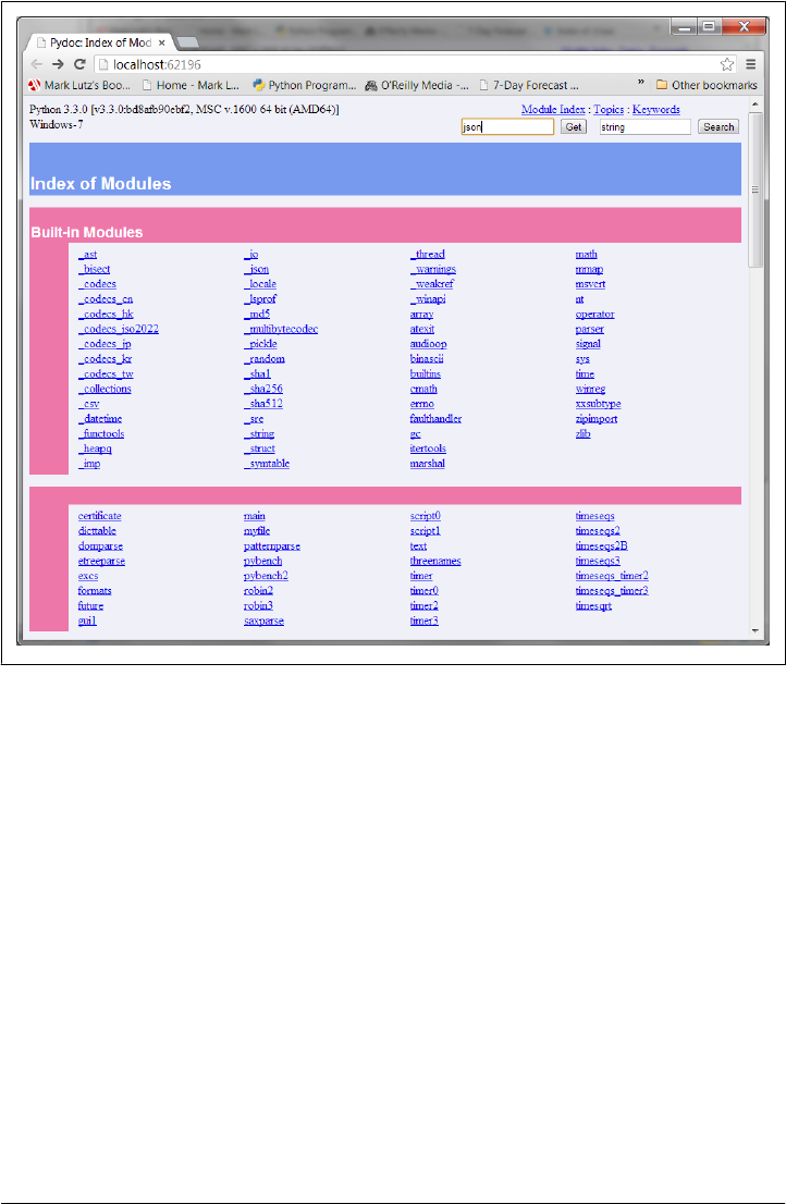
However you run this command line, the effect is to start PyDoc as a locally running
web server on a dedicated (but by default arbitrary unused) port, and pop up a web
browser to act as client, displaying a page giving links to documentation for all the
modules importable on your module search path (including the directory where PyDoc
is launched). PyDoc’s top-level web page interface is captured in Figure 15-1.
Besides the module index, PyDoc’s web page also includes input fields at the top to
request a specific module’s documentation page (Get) and search for related entries
(Search), which stand in for the prior interface’s GUI client fields. You can also click
on this page’s links to go to the Module Index (the start page), Topics (general Python
subjects), and Keywords (overviews of statements and some expressions).
Notice that the index page in Figure 15-1 lists both modules and top-level scripts in the
current directory—the book’s C:\code, where PyDoc was started by the earlier com-
mand lines. PyDoc is mostly intended for documenting importable modules, but can
sometimes be used to show documentation for scripts too. A selected file must be
Figure 15-1. The top-level index start page of the all-browser PyDoc HTML interface in Python 3.2
and later, which as of 3.3 replaces the former GUI client in earlier Pythons.
454 | Chapter 15: The Documentation Interlude
www.it-ebooks.info

imported in order to render its documentation, and as we’ve learned, importing runs
a file’s code. Modules normally just define tools when run, so this is usually irrelevant.
If you ask for documentation for a top-level script file, though, the shell window where
you launched PyDoc serves as the script’s standard input and output for any user in-
teraction. The net effect is that the documentation page for a script will appear after it
runs, and after its printed output shows up in the shell window. This may work better
for some scripts than others, though; interactive input, for example, may interleave
oddly with PyDoc’s own server command prompts.
Once you get past the new start page in Figure 15-1, the documentation pages for
specific modules are essentially the same in both the newer all-browser mode and the
earlier GUI-client scheme, apart from the additional input fields at the top of page in
the former. For instance, Figure 15-2 shows the new documentation display pages—
opened on two user-defined modules we’ll be writing in the next part of this book, as
part of Chapter 21’s benchmarking case study. In either scheme, documentation pages
contain automatically created hyperlinks that allow you to click your way through the
documentation of related components in your application. For instance, you’ll find
links to open imported modules’ pages too.
Because of the similarity in their display pages, the next section on pre-3.2 PyDoc and
its screen shots largely apply after 3.2 too, so be sure to read ahead for additional notes
even if you’re using more recent Python. In effect, 3.3’s PyDoc simply cuts out the
pre-3.2 GUI client “middleman,” while retaining its browser and server.
PyDoc in Python 3.3 also still supports other former usage modes. For instance, pydoc
–p port can be used to set its PyDoc server port, and pydoc -w module still writes a
module’s HTML documentation to a file named module.html for later viewing. Only
the pydoc -g GUI client mode is removed and replaced by pydoc -b. You can also run
PyDoc to generate a plain-text form of the documentation (its Unix “manpage” flavor
shown earlier in this chapter)—the following command line is equivalent to the help
call at an interactive Python prompt:
c:\code> py −3 -m pydoc timeit # Command-line text help
c:\code> py −3
>>> help("timeit") # Interactive prompt text help
As an interactive system, your best bet is to take PyDoc’s web-based interface for a test
drive, so we’ll cut its usage details short here; see Python’s manuals for additional details
and command-line options. Also note that PyDoc’s server and browser functionality
come largely “for free” from tools that automate such utility in the portable modules
of Python’s standard library (e.g., webbrowser, http.server). Consult PyDoc’s Python
code in the standard library file pydoc.py for additional details and inspiration.
Python Documentation Sources | 455
www.it-ebooks.info
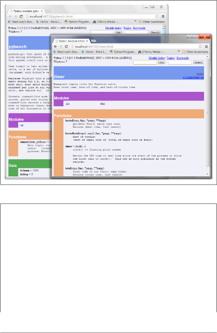
Changing PyDoc’s Colors
You won’t be able to tell in the paper version of this book, but if you have an ebook or
start PyDoc live, you’ll notice that it chooses colors that may or may not be to your
liking. Unfortunately, there presently is no easy way to customize PyDoc’s colors. They
are hardcoded deep in its source code, and can’t be passed in as arguments to functions
or command lines, or changed in configuration files or global variables in the PyDoc
module itself.
Except that, in an open source system, you can always change the code—PyDoc lives
in the file pydoc.py in Python’s standard library, which is directory C:\Python33\Lib on
Windows for Python 3.3. Its colors are hardcoded RGB value hex strings embedded
throughout its code. For instance, its string '#eeaa77' specifies 2-byte (16-bit) values
for red, green, and blue levels (decimal 238, 170, and 119), yielding a shade of orange
for function banners. The string '#ee77aa' similarly renders the dark pinkish color used
in nine places, including class and index page banners.
Figure 15-2. PyDoc’s module display page in Python 3.2 and later with input fields at the top,
displaying two modules we will be coding in the next part of this book (Chapter 21).
456 | Chapter 15: The Documentation Interlude
www.it-ebooks.info

To tailor, search for these color value strings and replace them with your preferences.
In IDLE, an Edit/Find for regular expression #\w{6} will locate color strings (this
matches six alphanumeric characters after a # per Python’s re module pattern syntax;
see the library manual for details).
To pick colors, in most programs with color selection dialogs you can map to and from
RGB values; the book’s examples include a GUI script setcolor.py that does the same.
In my copy of PyDoc, I replaced all #ee77aa with #008080 (teal) to banish the dark pink.
Replacing #ffc8d8 with #c0c0c0 (grey) does similar for the light pink background of
class docstrings.
Such surgery isn’t for the faint of heart—PyDoc’s file is currently 2,600 lines long—but
makes for a fair exercise in code maintenance. Be cautious when replacing colors like
#ffffff and #000000 (white and black), and be sure to make a backup copy of py-
doc.py first so you have a fallback. This file uses tools we haven’t yet met, but you can
safely ignore the rest of its code while you make your tactical changes.
Be sure to watch for PyDoc changes on the configurations front; this seems a prime
candidate for improvement. In fact, there already is an effort under way: issue 10716
on the Python developers’ list seeks to make PyDoc more user-customizable by chang-
ing it to support CSS style sheets. If successful, this may allow users to make color and
other display choices in external CSS files instead of PyDoc’s source code.
On the other hand, this is currently not planned to appear until Python 3.4, and will
require PyDoc’s users to also be proficient with CSS code—which unfortunately has a
nontrivial structure all its own that many people using Python may not understand well
enough to change. As I write this, for example, the proposed PyDoc CSS file is already
234 lines of code that probably won’t mean much to people not already familiar with
web development (and it hardly seems reasonable to ask them to learn a web develop-
ment tool just to tailor PyDoc!).
Today’s PyDoc in 3.3 already supports a CSS style sheet that offers some customization
options, but only half-heartedly, and ships with one that is empty. Until this is hashed
out, code changes seem the best option. In any event, CSS style sheets are well beyond
this Python book’s scope—see the Web for details, and check future Python release
notes for PyDoc developments.
Python 3.2 and earlier: GUI client
This section documents the original GUI client mode of PyDoc, for readers using 3.2
and earlier, and gives some addition PyDoc context in general. It builds on the basics
covered in the prior section, which aren’t repeated here, so be sure to at least scan the
prior section if you’re using an older Python.
As mentioned, through Python 3.2, PyDoc provides a top-level GUI interface—a simple
but portable Python/tkinter script for submitting requests—as well as a documentation
server. Requests in the client are routed to the server, which produces reports displayed
in a popped-up web browser. Apart from your having to submit search requests, this
process is largely automatic.
Python Documentation Sources | 457
www.it-ebooks.info
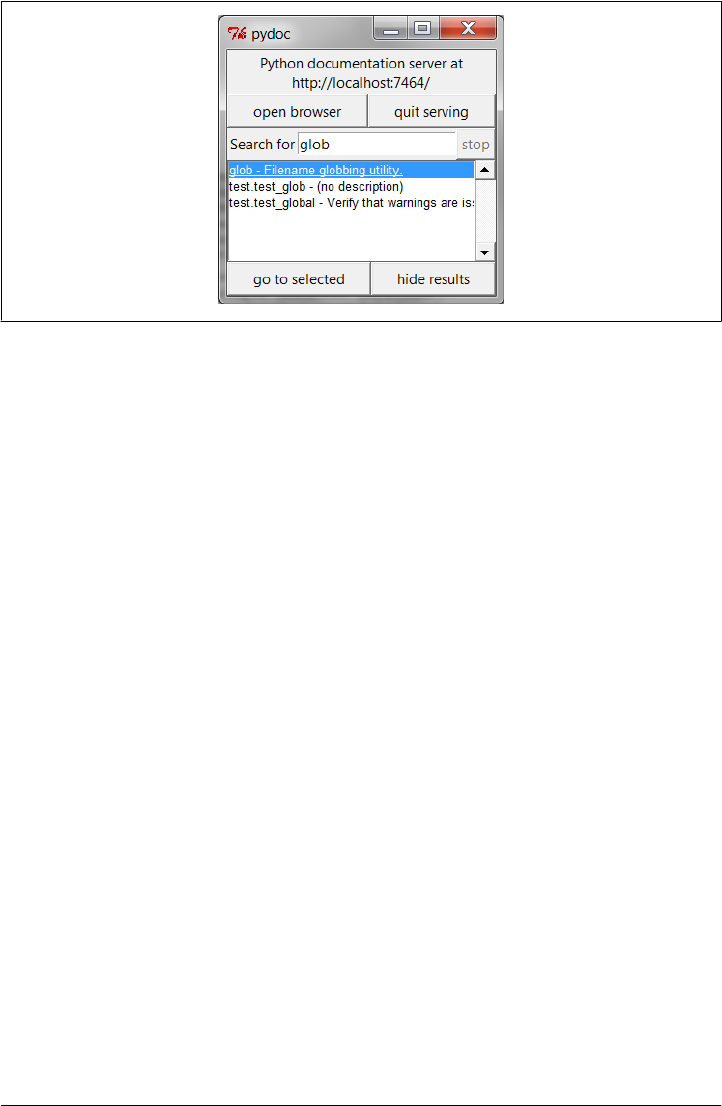
To start PyDoc in this mode, you generally first launch the search engine GUI captured
in Figure 15-3. You can start this either by selecting the Module Docs item in Python’s
Start button menu on Windows 7 and earlier, or by launching the pydoc.py script in
Python’s standard library directory with a -g command-line argument: it lives in Lib
on Windows, but you can use Python’s –m flag to avoid typing script paths here too:
c:\code> c:\python32\python -m pydoc -g # Explicit Python path
c:\code> py −3.2 -m pydoc -g # Windows 3.3+ launcher version
Enter the name of a module you’re interested in, and press the Enter key; PyDoc will
march down your module import search path (sys.path), looking for the requested
module and references to it.
Once you’ve found a promising entry, select it and click “go to selected.” PyDoc will
spawn a web browser on your machine to display the report rendered in HTML format.
Figure 15-4 shows the information PyDoc displays for the built-in glob module. Notice
the hyperlinks in the Modules section of this page—you can click these to jump to the
PyDoc pages for related (imported) modules. For larger pages, PyDoc also generates
hyperlinks to sections within the page.
Like the help function interface, the GUI interface works on user-defined modules as
well as built-ins. Figure 15-5 shows the page generated for our docstrings.py module
file coded earlier.
Make sure that the directory containing your module is on your module import search
path—as mentioned, PyDoc must be able to import a file to render its documentation.
This includes the current working directory—PyDoc might not check the directory it
was launched from (which is probably meaningless when started from the Windows
Start button anyhow), so you may need to extend your PYTHONPATH setting to get this to
Figure 15-3. The PyDoc top-level search engine GUI client in 3.2 and earlier: type the name of a
module you want documentation for, press Enter, select the module, and then press “go to selected”
(or omit the module name and press “open browser” to see all available modules).
458 | Chapter 15: The Documentation Interlude
www.it-ebooks.info
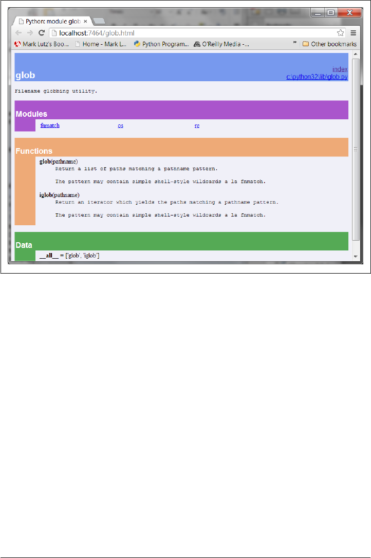
work. On Pythons 3.2 and 2.7, I had to add “.” to my PYTHONPATH to get PyDoc’s GUI
client mode to look in the directory it was started from by command line:
c:\code> set PYTHONPATH=.;%PYTYONPATH%
c:\code> py −3.2 -m pydoc -g
This setting was also required to see the current directory for the new all-browser pydoc
-b mode in 3.2. However, Python 3.3 automatically includes “.” in its index list, so no
path setting is required to view files in the directory where PyDoc is started—a minor
but noteworthy improvement.
PyDoc can be customized and launched in various ways we won’t cover here; see its
entry in Python’s standard library manual for more details. The main thing to take away
from this section is that PyDoc essentially gives you implementation reports “for free”
—if you are good about using docstrings in your files, PyDoc does all the work of
collecting and formatting them for display. PyDoc helps only for objects like functions
and modules, but it provides an easy way to access a middle level of documentation for
such tools—its reports are more useful than raw attribute lists, and less exhaustive than
the standard manuals.
Figure 15-4. When you find a module in the Figure 15-3 GUI (such as this built-in standard library
module) and press “go to selected,” the module’s documentation is rendered in HTML and displayed
in a web browser window like this one.
Python Documentation Sources | 459
www.it-ebooks.info
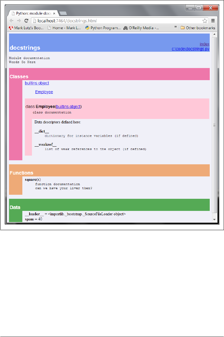
PyDoc can also be run to save the HTML documentation for a module in a file for later
viewing or printing; see the preceding section for pointers. Also, note that PyDoc might
not work well if run on scripts that read from standard input—PyDoc imports the target
module to inspect its contents, and there may be no connection for standard input text
when it is run in GUI mode, especially if run from the Windows Start button. Modules
that can be imported without immediate input requirements will always work under
PyDoc, though. See also the preceding section’s notes regarding scripts in PyDoc’s -b
mode in 3.2 and later; launching PyDoc’s GUI mode by command line works the same
—you interact in the launch window.
Figure 15-5. PyDoc can serve up documentation pages for both built-in and user-coded modules on
the module search path. Here is the page for a user-defined module, showing all its documentation
strings (docstrings) extracted from the source file.
460 | Chapter 15: The Documentation Interlude
www.it-ebooks.info

PyDoc GUI client trick of the day: If you press the “open browser” button
in Figure 15-3’s window, PyDoc will produce an index page containing
a hyperlink to every module you can possibly import on your computer.
This includes Python standard library modules, modules of installed
third-party extensions, user-defined modules on your import search
path, and even statically or dynamically linked-in C-coded modules.
Such information is hard to come by otherwise without writing code
that inspects all module sources. On Python 3.2, you’ll want to do this
immediately after the GUI opens, as it may not fully work after searches.
Also note that in PyDoc’s all-browser –b interface in 3.2 and later, you
get the same index functionality on its top-level start page of Figure 15-1.
Beyond docstrings: Sphinx
If you’re looking for a way to document your Python system in a more sophisticated
way, you may wish to check out Sphinx (currently at http://sphinx-doc.org). Sphinx is
used by the standard Python documentation described in the next section, and many
other projects. It uses simple reStructuredText as its markup language, and inherits
much from the Docutils suite of reStructuredText parsing and translating tools.
Among other things, Sphinx supports a variety of output formats (HTML including
Windows HTML Help, LaTeX for printable PDF versions, manual pages, and plain
text); extensive and automatic cross-references; hierarchical structure with automatic
links to relatives; automatic indexes; automatic code highlighting using Pygments (itself
a notable Python tool); and more. This is probably overkill for smaller programs where
docstrings and PyDoc may suffice, but can yield professional-grade documentation for
large projects. See the Web for more details on Sphinx and its related tools.
The Standard Manual Set
For the complete and most up-to-date description of the language and its toolset,
Python’s standard manuals stand ready to serve. Python’s manuals ship in HTML and
other formats, and they are installed with the Python system on Windows—they are
available in your Start button’s menu for Python on Windows 7 and earlier, and they
can also be opened from the Help menu within IDLE. You can also fetch the manual
set separately from http://www.python.org in a variety of formats, or read it online at
that site (follow the Documentation link). On Windows, the manuals are a compiled
help file to support searches, and the online versions at the Python website include a
web-based search page.
When opened, the Windows format of the manuals displays a root page like that in
Figure 15-6, showing the local copy on Windows. The two most important entries here
are most likely the Library Reference (which documents built-in types, functions, ex-
ceptions, and standard library modules) and the Language Reference (which provides
Python Documentation Sources | 461
www.it-ebooks.info
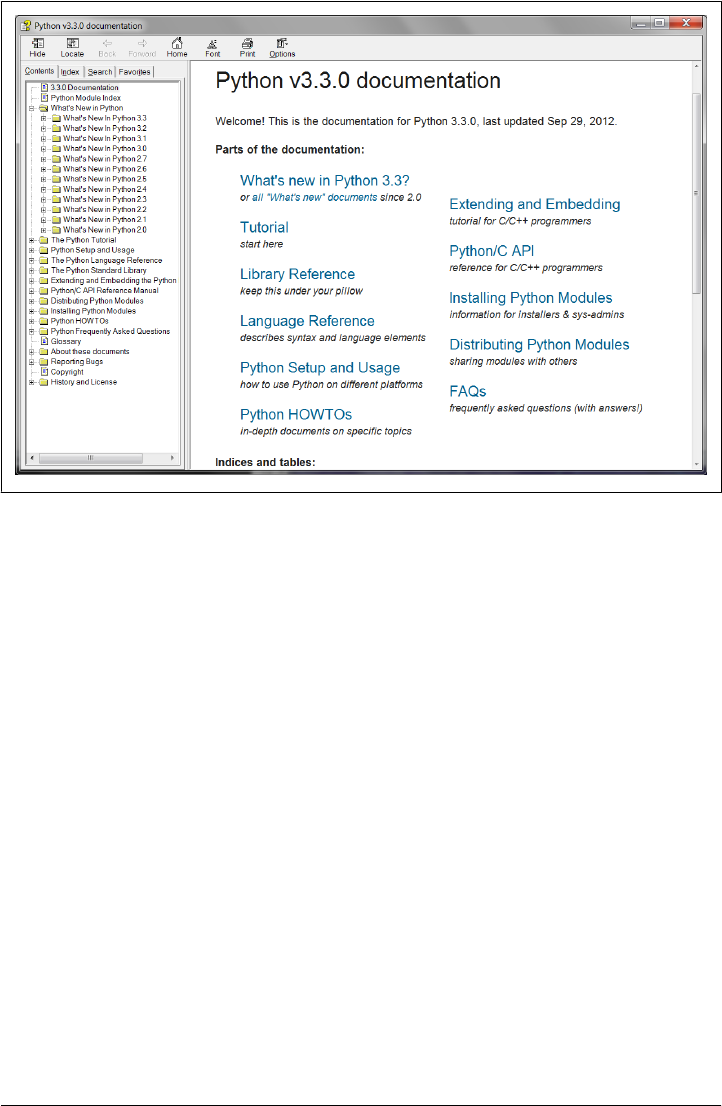
a formal description of language-level details). The tutorial listed on this page also
provides a brief introduction for newcomers, which you’re probably already beyond.
Of notable interest, the What’s New documents in this standard manual set chronicle
Python changes made in each release beginning with Python 2.0, which came out in
late 2000—useful for those porting older Python code, or older Python skills. These
documents are especially useful for uncovering additional details on the differences in
the Python 2.X and 3.X language lines covered in this book, as well as in their standard
libraries.
Web Resources
At the official Python website (http://www.python.org), you’ll find links to various
Python resources, some of which cover special topics or domains. Click the Documen-
tation link to access an online tutorial and the Beginners Guide to Python. The site also
lists non-English Python resources, and introductions scaled to different target audi-
ences.
Today you will also find numerous Python wikis, blogs, websites, and a host of other
resources on the Web at large. To sample the online community, try searching for a
Figure 15-6. Python’s standard manual set, available online at http://www.python.org, from IDLE’s
Help menu, and in the Windows 7 and earlier Start button menu. It’s a searchable help file on
Windows, and there is a search engine for the online version. Of these, the Library Reference is the
one you’ll want to use most of the time.
462 | Chapter 15: The Documentation Interlude
www.it-ebooks.info

term like “Python programming” in Google, or search on any topic of interest; chances
are good you’ll find ample material to browse.
Published Books
As a final resource, you can choose from a collection of professionally edited and pub-
lished reference books for Python. Bear in mind that books tend to lag behind the
cutting edge of Python changes, partly because of the work involved in writing, and
partly because of the natural delays built into the publishing cycle. Usually, by the time
a book comes out, it’s three or more months behind the current Python state (trust me
on that—my books have a nasty habit of falling out of date in minor ways between the
time I write them and the time they hit the shelves!). Unlike standard manuals, books
are also generally not free.
Still, for many, the convenience and quality of a professionally published text is worth
the cost. Moreover, Python changes so slowly that books are usually still relevant years
after they are published, especially if their authors post updates on the Web. See the
preface for pointers to other Python books.
Common Coding Gotchas
Before the programming exercises for this part of the book, let’s run through some of
the most common mistakes beginners make when coding Python statements and pro-
grams. Many of these are warnings I’ve thrown out earlier in this part of the book,
collected here for ease of reference. You’ll learn to avoid these pitfalls once you’ve
gained a bit of Python coding experience, but a few words now might help you avoid
falling into some of these traps initially:
•Don’t forget the colons. Always remember to type a : at the end of compound
statement headers—the first line of an if, while, for, etc. You’ll probably forget at
first (I did, and so have most of my roughly 4,000 Python students over the years),
but you can take some comfort from the fact that it will soon become an uncon-
scious habit.
•Start in column 1. Be sure to start top-level (unnested) code in column 1. That
includes unnested code typed into module files, as well as unnested code typed at
the interactive prompt.
•Blank lines matter at the interactive prompt. Blank lines in compound state-
ments are always irrelevant and ignored in module files, but when you’re typing
code at the interactive prompt, they end the statement. In other words, blank lines
tell the interactive command line that you’ve finished a compound statement; if
you want to continue, don’t hit the Enter key at the ... prompt (or in IDLE) until
you’re really done. This also means you can’t paste multiline code at this prompt;
it must run one full statement at a time.
Common Coding Gotchas | 463
www.it-ebooks.info

•Indent consistently. Avoid mixing tabs and spaces in the indentation of a block,
unless you know what your text editor does with tabs. Otherwise, what you see in
your editor may not be what Python sees when it counts tabs as a number of spaces.
This is true in any block-structured language, not just Python—if the next pro-
grammer has tabs set differently, it will be difficult or impossible to understand the
structure of your code. It’s safer to use all tabs or all spaces for each block.
•Don’t code C in Python. A reminder for C/C++ programmers: you don’t need to
type parentheses around tests in if and while headers (e.g., if (X==1):). You can,
if you like (any expression can be enclosed in parentheses), but they are fully su-
perfluous in this context. Also, do not terminate all your statements with semico-
lons; it’s technically legal to do this in Python as well, but it’s totally useless unless
you’re placing more than one statement on a single line (the end of a line normally
terminates a statement). And remember, don’t embed assignment statements in
while loop tests, and don’t use {} around blocks (indent your nested code blocks
consistently instead).
•Use simple for loops instead of while or range. Another reminder: a simple
for loop (e.g., for x in seq:) is almost always simpler to code and often quicker
to run than a while- or range-based counter loop. Because Python handles indexing
internally for a simple for, it can sometimes be faster than the equivalent while,
though this can vary per code and Python. For code simplicity alone, though, avoid
the temptation to count things in Python!
•Beware of mutables in assignments. I mentioned this in Chapter 11: you need
to be careful about using mutables in a multiple-target assignment (a = b = []),
as well as in an augmented assignment (a += [1, 2]). In both cases, in-place
changes may impact other variables. See Chapter 11 for details if you’ve forgotten
why this is true.
•Don’t expect results from functions that change objects in place. We en-
countered this one earlier, too: in-place change operations like the list.append and
list.sort methods introduced in Chapter 8 do not return values (other than
None), so you should call them without assigning the result. It’s not uncommon for
beginners to say something like mylist = mylist.append(X) to try to get the result
of an append, but what this actually does is assign mylist to None, not to the modified
list (in fact, you’ll lose your reference to the list altogether).
A more devious example of this pops up in Python 2.X code when trying to step
through dictionary items in a sorted fashion. It’s fairly common to see code like
for k in D.keys().sort():. This almost works—the keys method builds a keys
list, and the sort method orders it—but because the sort method returns None, the
loop fails because it is ultimately a loop over None (a nonsequence). This fails even
sooner in Python 3.X, because dictionary keys are views, not lists! To code this
correctly, either use the newer sorted built-in function, which returns the sorted
list, or split the method calls out to statements: Ks = list(D.keys()), then
Ks.sort(), and finally, for k in Ks:. This, by the way, is one case where you may
464 | Chapter 15: The Documentation Interlude
www.it-ebooks.info

still want to call the keys method explicitly for looping, instead of relying on the
dictionary iterators—iterators do not sort.
•Always use parentheses to call a function. You must add parentheses after a
function name to call it, whether it takes arguments or not (e.g., use function(),
not function). In the next part of this book, we’ll learn that functions are simply
objects that have a special operation—a call that you trigger with the parentheses.
They can be referenced like any other object without triggering a call.
In classes, this problem seems to occur most often with files; it’s common to see
beginners type file.close to close a file, rather than file.close(). Because it’s
legal to reference a function without calling it, the first version with no parentheses
succeeds silently, but it does not close the file!
•Don’t use extensions or paths in imports and reloads. Omit directory paths
and file extensions in import statements—say import mod, not import mod.py. We
discussed module basics in Chapter 3 and will continue studying modules in
Part V. Because modules may have other extensions besides .py (.pyc, for instance),
hardcoding a particular extension is not only illegal syntax, it doesn’t make sense.
Python picks an extension automatically, and any platform-specific directory path
syntax comes from module search path settings, not the import statement.
•And other pitfalls in other parts. Be sure to also see the built-in type warnings
at the end of the prior part, as they may qualify as coding issues too. There are
additional “gotchas” that crop up commonly in Python coding—losing a built-in
function by reassigning its name, hiding a library module by using its name for one
of your own, changing mutable argument defaults, and so on—but we don’t have
enough background to cover them yet. To learn more about both what you should
and shouldn’t do in Python, you’ll have to read on; later parts extend the set of
“gotchas” and fixes we’ve added to here.
Chapter Summary
This chapter took us on a tour of program documentation—both documentation we
write ourselves for our own programs, and documentation available for tools we use.
We met docstrings, explored the online and manual resources for Python reference,
and learned how PyDoc’s help function and web page interfaces provide extra sources
of documentation. Because this is the last chapter in this part of the book, we also
reviewed common coding mistakes to help you avoid them.
In the next part of this book, we’ll start applying what we already know to larger pro-
gram constructs. Specifically, the next part takes up the topic of functions—a tool used
to group statements for reuse. Before moving on, however, be sure to work through
the set of lab exercises for this part of the book that appear at the end of this chapter.
And even before that, let’s run through this chapter’s quiz.
Chapter Summary | 465
www.it-ebooks.info

Test Your Knowledge: Quiz
1. When should you use documentation strings instead of hash-mark comments?
2. Name three ways you can view documentation strings.
3. How can you obtain a list of the available attributes in an object?
4. How can you get a list of all available modules on your computer?
5. Which Python book should you purchase after this one?
Test Your Knowledge: Answers
1. Documentation strings (docstrings) are considered best for larger, functional doc-
umentation, describing the use of modules, functions, classes, and methods in your
code. Hash-mark comments are today best limited to smaller-scale documentation
about arcane expressions or statements at strategic points on your code. This is
partly because docstrings are easier to find in a source file, but also because they
can be extracted and displayed by the PyDoc system.
2. You can see docstrings by printing an object’s __doc__ attribute, by passing it to
PyDoc’s help function, and by selecting modules in PyDoc’s HTML-based user
interfaces—either the -g GUI client mode in Python 3.2 and earlier, or the -b all-
browser mode in Python 3.2 and later (and required as of 3.3). Both run a client/
server system that displays documentation in a popped-up web browser. PyDoc
can also be run to save a module’s documentation in an HTML file for later viewing
or printing.
3. The built-in dir(X) function returns a list of all the attributes attached to any object.
A list comprehension of the form [a for a in dir(X) if not a.starts
with('__')] can be used to filter out internals names with underscores (we’ll learn
how to wrap this in a function in the next part of the book to make it easier to use).
4. In Python 3.2 and earlier, you can run the PyDoc GUI interface, and select “open
browser”; this opens a web page containing a link to every module available to
your programs. This GUI mode no longer works as of Python 3.3. In Python 3.2
and later, you get the same functionality by running PyDoc’s newer all-browser
mode with a -b command-line switch; the top-level start page displayed in a web
browser in this newer mode has the same index page listing all available modules.
5. Mine, of course. (Seriously, there are hundreds today; the preface lists a few rec-
ommended follow-up books, both for reference and for application tutorials, and
you should browse for books that fit your needs.)
466 | Chapter 15: The Documentation Interlude
www.it-ebooks.info

Test Your Knowledge: Part III Exercises
Now that you know how to code basic program logic, the following exercises will ask
you to implement some simple tasks with statements. Most of the work is in exercise
4, which lets you explore coding alternatives. There are always many ways to arrange
statements, and part of learning Python is learning which arrangements work better
than others. You’ll eventually gravitate naturally toward what experienced Python
programmers call “best practice,” but best practice takes practice.
See Part III in Appendix D for the solutions.
1. Coding basic loops. This exercise asks you to experiment with for loops.
a. Write a for loop that prints the ASCII code of each character in a string named
S. Use the built-in function ord(character) to convert each character to an
ASCII integer. This function technically returns a Unicode code point in
Python 3.X, but if you restrict its content to ASCII characters, you’ll get back
ASCII codes. (Test it interactively to see how it works.)
b. Next, change your loop to compute the sum of the ASCII codes of all the
characters in a string.
c. Finally, modify your code again to return a new list that contains the ASCII
codes of each character in the string. Does the expression map(ord, S) have a
similar effect? How about [ord(c) for c in S]? Why? (Hint: see Chapter 14.)
2. Backslash characters. What happens on your machine when you type the following
code interactively?
for i in range(50):
print('hello %d\n\a' % i)
Beware that if it’s run outside of the IDLE interface this example may beep at you,
so you may not want to run it in a crowded room! IDLE prints odd characters
instead of beeping—spoiling much of the joke (see the backslash escape characters
in Table 7-2).
3. Sorting dictionaries. In Chapter 8, we saw that dictionaries are unordered collec-
tions. Write a for loop that prints a dictionary’s items in sorted (ascending) order.
(Hint: use the dictionary keys and list sort methods, or the newer sorted built-in
function.)
4. Program logic alternatives. Consider the following code, which uses a while loop
and found flag to search a list of powers of 2 for the value of 2 raised to the fifth
power (32). It’s stored in a module file called power.py.
L = [1, 2, 4, 8, 16, 32, 64]
X = 5
found = False
i = 0
while not found and i < len(L):
Test Your Knowledge: Part III Exercises | 467
www.it-ebooks.info

if 2 ** X == L[i]:
found = True
else:
i = i+1
if found:
print('at index', i)
else:
print(X, 'not found')
C:\book\tests> python power.py
at index 5
As is, the example doesn’t follow normal Python coding techniques. Follow the
steps outlined here to improve it (for all the transformations, you may either type
your code interactively or store it in a script file run from the system command line
—using a file makes this exercise much easier):
a. First, rewrite this code with a while loop else clause to eliminate the found flag
and final if statement.
b. Next, rewrite the example to use a for loop with an else clause, to eliminate
the explicit list-indexing logic. (Hint: to get the index of an item, use the list
index method—L.index(X) returns the offset of the first X in list L.)
c. Next, remove the loop completely by rewriting the example with a simple in
operator membership expression. (See Chapter 8 for more details, or type this
to test: 2 in [1,2,3].)
d. Finally, use a for loop and the list append method to generate the powers-of-2
list (L) instead of hardcoding a list literal.
Deeper thoughts:
e. Do you think it would improve performance to move the 2 ** X expression
outside the loops? How would you code that?
f. As we saw in exercise 1, Python includes a map(function, list) tool that can
generate a powers-of-2 list, too: map(lambda x: 2 ** x, range(7)). Try typing
this code interactively; we’ll meet lambda more formally in the next part of this
book, especially in Chapter 19. Would a list comprehension help here (see
Chapter 14)?
5. Code maintenance. If you haven’t already done so, experiment with making the
code changes suggested in this chapter’s sidebar “Changing PyDoc’s Col-
ors” on page 456. Much of the work of real software development is in changing
existing code, so the sooner you begin doing so, the better. For reference, my edited
copy of PyDoc is in the book’s examples package, named mypydoc.py; to see how
it differs, you can run a file compare (fc on Windows) with the original pydoc.py
in 3.3 (also included, lest it change radically in 3.4 as the sidebar describes). If
PyDoc is more easily customized by the time you read these words, customize
468 | Chapter 15: The Documentation Interlude
www.it-ebooks.info


CHAPTER 16
Function Basics
In Part III, we studied basic procedural statements in Python. Here, we’ll move on to
explore a set of additional statements and expressions that we can use to create func-
tions of our own.
In simple terms, a function is a device that groups a set of statements so they can be run
more than once in a program—a packaged procedure invoked by name. Functions also
can compute a result value and let us specify parameters that serve as function inputs
and may differ each time the code is run. Coding an operation as a function makes it
a generally useful tool, which we can use in a variety of contexts.
More fundamentally, functions are the alternative to programming by cutting and past-
ing—rather than having multiple redundant copies of an operation’s code, we can fac-
tor it into a single function. In so doing, we reduce our future work radically: if the
operation must be changed later, we have only one copy to update in the function, not
many scattered throughout the program.
Functions are also the most basic program structure Python provides for maximizing
code reuse, and lead us to the larger notions of program design. As we’ll see, functions
let us split complex systems into manageable parts. By implementing each part as a
function, we make it both reusable and easier to code.
Table 16-1 previews the primary function-related tools we’ll study in this part of the
book—a set that includes call expressions, two ways to make functions (def and
lambda), two ways to manage scope visibility (global and nonlocal), and two ways to
send results back to callers (return and yield).
Table 16-1. Function-related statements and expressions
Statement or expression Examples
Call expressions myfunc('spam', 'eggs', meat=ham, *rest)
def def printer(messge):
print('Hello ' + message)
return def adder(a, b=1, *c):
return a + b + c[0]
473
www.it-ebooks.info

Statement or expression Examples
global x = 'old'
def changer():
global x; x = 'new'
nonlocal (3.X) def outer():
x = 'old'
def changer():
nonlocal x; x = 'new'
yield def squares(x):
for i in range(x): yield i ** 2
lambda funcs = [lambda x: x**2, lambda x: x**3]
Why Use Functions?
Before we get into the details, let’s establish a clear picture of what functions are all
about. Functions are a nearly universal program-structuring device. You may have
come across them before in other languages, where they may have been called subrou-
tines or procedures. As a brief introduction, functions serve two primary development
roles:
Maximizing code reuse and minimizing redundancy
As in most programming languages, Python functions are the simplest way to
package logic you may wish to use in more than one place and more than one time.
Up until now, all the code we’ve been writing has run immediately. Functions allow
us to group and generalize code to be used arbitrarily many times later. Because
they allow us to code an operation in a single place and use it in many places,
Python functions are the most basic factoring tool in the language: they allow us
to reduce code redundancy in our programs, and thereby reduce maintenance ef-
fort.
Procedural decomposition
Functions also provide a tool for splitting systems into pieces that have well-defined
roles. For instance, to make a pizza from scratch, you would start by mixing the
dough, rolling it out, adding toppings, baking it, and so on. If you were program-
ming a pizza-making robot, functions would help you divide the overall “make
pizza” task into chunks—one function for each subtask in the process. It’s easier
to implement the smaller tasks in isolation than it is to implement the entire process
at once. In general, functions are about procedure—how to do something, rather
than what you’re doing it to. We’ll see why this distinction matters in Part VI, when
we start making new objects with classes.
In this part of the book, we’ll explore the tools used to code functions in Python: func-
tion basics, scope rules, and argument passing, along with a few related concepts such
as generators and functional tools. Because its importance begins to become more ap-
parent at this level of coding, we’ll also revisit the notion of polymorphism, which was
474 | Chapter 16: Function Basics
www.it-ebooks.info

introduced earlier in the book. As you’ll see, functions don’t imply much new syntax,
but they do lead us to some bigger programming ideas.
Coding Functions
Although it wasn’t made very formal, we’ve already used some functions in earlier
chapters. For instance, to make a file object, we called the built-in open function; sim-
ilarly, we used the len built-in function to ask for the number of items in a collection
object.
In this chapter, we will explore how to write new functions in Python. Functions we
write behave the same way as the built-ins we’ve already seen: they are called in ex-
pressions, are passed values, and return results. But writing new functions requires the
application of a few additional ideas that haven’t yet been introduced. Moreover, func-
tions behave very differently in Python than they do in compiled languages like C. Here
is a brief introduction to the main concepts behind Python functions, all of which we
will study in this part of the book:
•def is executable code. Python functions are written with a new statement, the
def. Unlike functions in compiled languages such as C, def is an executable state-
ment—your function does not exist until Python reaches and runs the def. In fact,
it’s legal (and even occasionally useful) to nest def statements inside if statements,
while loops, and even other defs. In typical operation, def statements are coded in
module files and are naturally run to generate functions when the module file they
reside in is first imported.
•def creates an object and assigns it to a name. When Python reaches and runs
a def statement, it generates a new function object and assigns it to the function’s
name. As with all assignments, the function name becomes a reference to the func-
tion object. There’s nothing magic about the name of a function—as you’ll see,
the function object can be assigned to other names, stored in a list, and so on.
Function objects may also have arbitrary user-defined attributes attached to them
to record data.
•lambda creates an object but returns it as a result. Functions may also be created
with the lambda expression, a feature that allows us to in-line function definitions
in places where a def statement won’t work syntactically. This is a more advanced
concept that we’ll defer until Chapter 19.
•return sends a result object back to the caller. When a function is called, the
caller stops until the function finishes its work and returns control to the caller.
Functions that compute a value send it back to the caller with a return statement;
the returned value becomes the result of the function call. A return without a value
simply returns to the caller (and sends back None, the default result).
•yield sends a result object back to the caller, but remembers where it left
off. Functions known as generators may also use the yield statement to send back
Coding Functions | 475
www.it-ebooks.info

a value and suspend their state such that they may be resumed later, to produce a
series of results over time. This is another advanced topic covered later in this part
of the book.
•global declares module-level variables that are to be assigned. By default, all
names assigned in a function are local to that function and exist only while the
function runs. To assign a name in the enclosing module, functions need to list it
in a global statement. More generally, names are always looked up in scopes—
places where variables are stored—and assignments bind names to scopes.
•nonlocal declares enclosing function variables that are to be assigned. Simi-
larly, the nonlocal statement added in Python 3.X allows a function to assign a
name that exists in the scope of a syntactically enclosing def statement. This allows
enclosing functions to serve as a place to retain state—information remembered
between function calls—without using shared global names.
•Arguments are passed by assignment (object reference). In Python, arguments
are passed to functions by assignment (which, as we’ve learned, means by object
reference). As you’ll see, in Python’s model the caller and function share objects
by references, but there is no name aliasing. Changing an argument name within
a function does not also change the corresponding name in the caller, but changing
passed-in mutable objects in place can change objects shared by the caller, and
serve as a function result.
•Arguments are passed by position, unless you say otherwise. Values you pass
in a function call match argument names in a function’s definition from left to right
by default. For flexibility, function calls can also pass arguments by name with
name=value keyword syntax, and unpack arbitrarily many arguments to send with
*pargs and **kargs starred-argument notation. Function definitions use the same
two forms to specify argument defaults, and collect arbitrarily many arguments
received.
•Arguments, return values, and variables are not declared. As with everything
in Python, there are no type constraints on functions. In fact, nothing about a
function needs to be declared ahead of time: you can pass in arguments of any type,
return any kind of object, and so on. As one consequence, a single function can
often be applied to a variety of object types—any objects that sport a compatible
interface (methods and expressions) will do, regardless of their specific types.
If some of the preceding words didn’t sink in, don’t worry—we’ll explore all of these
concepts with real code in this part of the book. Let’s get started by expanding on some
of these ideas and looking at a few examples.
def Statements
The def statement creates a function object and assigns it to a name. Its general format
is as follows:
476 | Chapter 16: Function Basics
www.it-ebooks.info

def name(arg1, arg2,... argN):
statements
As with all compound Python statements, def consists of a header line followed by a
block of statements, usually indented (or a simple statement after the colon). The
statement block becomes the function’s body—that is, the code Python executes each
time the function is later called.
The def header line specifies a function name that is assigned the function object, along
with a list of zero or more arguments (sometimes called parameters) in parentheses.
The argument names in the header are assigned to the objects passed in parentheses at
the point of call.
Function bodies often contain a return statement:
def name(arg1, arg2,... argN):
...
return value
The Python return statement can show up anywhere in a function body; when reached,
it ends the function call and sends a result back to the caller. The return statement
consists of an optional object value expression that gives the function’s result. If the
value is omitted, return sends back a None.
The return statement itself is optional too; if it’s not present, the function exits when
the control flow falls off the end of the function body. Technically, a function without
a return statement also returns the None object automatically, but this return value is
usually ignored at the call.
Functions may also contain yield statements, which are designed to produce a series
of values over time, but we’ll defer discussion of these until we survey generator topics
in Chapter 20.
def Executes at Runtime
The Python def is a true executable statement: when it runs, it creates a new function
object and assigns it to a name. (Remember, all we have in Python is runtime; there is
no such thing as a separate compile time.) Because it’s a statement, a def can appear
anywhere a statement can—even nested in other statements. For instance, although
defs normally are run when the module enclosing them is imported, it’s also completely
legal to nest a function def inside an if statement to select between alternative defini-
tions:
if test:
def func(): # Define func this way
...
else:
def func(): # Or else this way
...
...
func() # Call the version selected and built
Coding Functions | 477
www.it-ebooks.info

One way to understand this code is to realize that the def is much like an = statement:
it simply assigns a name at runtime. Unlike in compiled languages such as C, Python
functions do not need to be fully defined before the program runs. More generally,
defs are not evaluated until they are reached and run, and the code inside defs is not
evaluated until the functions are later called.
Because function definition happens at runtime, there’s nothing special about the
function name. What’s important is the object to which it refers:
othername = func # Assign function object
othername() # Call func again
Here, the function was assigned to a different name and called through the new name.
Like everything else in Python, functions are just objects; they are recorded explicitly
in memory at program execution time. In fact, besides calls, functions allow arbitrary
attributes to be attached to record information for later use:
def func(): ... # Create function object
func() # Call object
func.attr = value # Attach attributes
A First Example: Definitions and Calls
Apart from such runtime concepts (which tend to seem most unique to programmers
with backgrounds in traditional compiled languages), Python functions are straight-
forward to use. Let’s code a first real example to demonstrate the basics. As you’ll see,
there are two sides to the function picture: a definition (the def that creates a function)
and a call (an expression that tells Python to run the function’s body).
Definition
Here’s a definition typed interactively that defines a function called times, which re-
turns the product of its two arguments:
>>> def times(x, y): # Create and assign function
... return x * y # Body executed when called
...
When Python reaches and runs this def, it creates a new function object that packages
the function’s code and assigns the object to the name times. Typically, such a state-
ment is coded in a module file and runs when the enclosing file is imported; for some-
thing this small, though, the interactive prompt suffices.
Calls
The def statement makes a function but does not call it. After the def has run, you can
call (run) the function in your program by adding parentheses after the function’s name.
478 | Chapter 16: Function Basics
www.it-ebooks.info

The parentheses may optionally contain one or more object arguments, to be passed
(assigned) to the names in the function’s header:
>>> times(2, 4) # Arguments in parentheses
8
This expression passes two arguments to times. As mentioned previously, arguments
are passed by assignment, so in this case the name x in the function header is assigned
the value 2, y is assigned the value 4, and the function’s body is run. For this function,
the body is just a return statement that sends back the result as the value of the call
expression. The returned object was printed here interactively (as in most languages,
2 * 4 is 8 in Python), but if we needed to use it later we could instead assign it to a
variable. For example:
>>> x = times(3.14, 4) # Save the result object
>>> x
12.56
Now, watch what happens when the function is called a third time, with very different
kinds of objects passed in:
>>> times('Ni', 4) # Functions are "typeless"
'NiNiNiNi'
This time, our function means something completely different (Monty Python reference
again intended). In this third call, a string and an integer are passed to x and y, instead
of two numbers. Recall that * works on both numbers and sequences; because we never
declare the types of variables, arguments, or return values in Python, we can use
times to either multiply numbers or repeat sequences.
In other words, what our times function means and does depends on what we pass into
it. This is a core idea in Python (and perhaps the key to using the language well), which
merits a bit of expansion here.
Polymorphism in Python
As we just saw, the very meaning of the expression x * y in our simple times function
depends completely upon the kinds of objects that x and y are—thus, the same function
can perform multiplication in one instance and repetition in another. Python leaves it
up to the objects to do something reasonable for the syntax. Really, * is just a dispatch
mechanism that routes control to the objects being processed.
This sort of type-dependent behavior is known as polymorphism, a term we first met
in Chapter 4 that essentially means that the meaning of an operation depends on the
objects being operated upon. Because it’s a dynamically typed language, polymorphism
runs rampant in Python. In fact, every operation is a polymorphic operation in Python:
printing, indexing, the * operator, and much more.
This is deliberate, and it accounts for much of the language’s conciseness and flexibility.
A single function, for instance, can generally be applied to a whole category of object
A First Example: Definitions and Calls | 479
www.it-ebooks.info

types automatically. As long as those objects support the expected interface (a.k.a.
protocol), the function can process them. That is, if the objects passed into a function
have the expected methods and expression operators, they are plug-and-play compat-
ible with the function’s logic.
Even in our simple times function, this means that any two objects that support a * will
work, no matter what they may be, and no matter when they are coded. This function
will work on two numbers (performing multiplication), or a string and a number (per-
forming repetition), or any other combination of objects supporting the expected in-
terface—even class-based objects we have not even imagined yet.
Moreover, if the objects passed in do not support this expected interface, Python will
detect the error when the * expression is run and raise an exception automatically. It’s
therefore usually pointless to code error checking ourselves. In fact, doing so would
limit our function’s utility, as it would be restricted to work only on objects whose types
we test for.
This turns out to be a crucial philosophical difference between Python and statically
typed languages like C++ and Java: in Python, your code is not supposed to care about
specific data types. If it does, it will be limited to working on just the types you antici-
pated when you wrote it, and it will not support other compatible object types that
may be coded in the future. Although it is possible to test for types with tools like the
type built-in function, doing so breaks your code’s flexibility. By and large, we code to
object interfaces in Python, not data types.1
Of course, some programs have unique requirements, and this polymorphic model of
programming means we have to test our code to detect errors, rather than providing
type declarations a compiler can use to detect some types of errors for us ahead of time.
In exchange for an initial bit of testing, though, we radically reduce the amount of code
we have to write and radically increase our code’s flexibility. As you’ll learn, it’s a net
win in practice.
A Second Example: Intersecting Sequences
Let’s look at a second function example that does something a bit more useful than
multiplying arguments and further illustrates function basics.
In Chapter 13, we coded a for loop that collected items held in common in two strings.
We noted there that the code wasn’t as useful as it could be because it was set up to
work only on specific variables and could not be rerun later. Of course, we could copy
1. This polymorphic behavior has in recent years come to also be known as duck typing—the essential idea
being that your code is not supposed to care if an object is a duck, only that it quacks. Anything that
quacks will do, duck or not, and the implementation of quacks is up to the object, a principle which will
become even more apparent when we study classes in Part VI. Graphic metaphor to be sure, though this
is really just a new label for an older idea, and use cases for quacking software would seem limited in the
tangible world (he says, bracing for emails from militant ornithologists...).
480 | Chapter 16: Function Basics
www.it-ebooks.info

the code and paste it into each place where it needs to be run, but this solution is neither
good nor general—we’d still have to edit each copy to support different sequence
names, and changing the algorithm would then require changing multiple copies.
Definition
By now, you can probably guess that the solution to this dilemma is to package the
for loop inside a function. Doing so offers a number of advantages:
• Putting the code in a function makes it a tool that you can run as many times as
you like.
• Because callers can pass in arbitrary arguments, functions are general enough to
work on any two sequences (or other iterables) you wish to intersect.
• When the logic is packaged in a function, you have to change code in only one
place if you ever need to change the way the intersection works.
• Coding the function in a module file means it can be imported and reused by any
program run on your machine.
In effect, wrapping the code in a function makes it a general intersection utility:
def intersect(seq1, seq2):
res = [] # Start empty
for x in seq1: # Scan seq1
if x in seq2: # Common item?
res.append(x) # Add to end
return res
The transformation from the simple code of Chapter 13 to this function is straightfor-
ward; we’ve just nested the original logic under a def header and made the objects on
which it operates passed-in parameter names. Because this function computes a result,
we’ve also added a return statement to send a result object back to the caller.
Calls
Before you can call a function, you have to make it. To do this, run its def statement,
either by typing it interactively or by coding it in a module file and importing the file.
Once you’ve run the def, you can call the function by passing any two sequence objects
in parentheses:
>>> s1 = "SPAM"
>>> s2 = "SCAM"
>>> intersect(s1, s2) # Strings
['S', 'A', 'M']
Here, we’ve passed in two strings, and we get back a list containing the characters in
common. The algorithm the function uses is simple: “for every item in the first argu-
ment, if that item is also in the second argument, append the item to the result.” It’s a
little shorter to say that in Python than in English, but it works out the same.
A Second Example: Intersecting Sequences | 481
www.it-ebooks.info

To be fair, our intersect function is fairly slow (it executes nested loops), isn’t really
mathematical intersection (there may be duplicates in the result), and isn’t required at
all (as we’ve seen, Python’s set data type provides a built-in intersection operation).
Indeed, the function could be replaced with a single list comprehension expression, as
it exhibits the classic loop collector code pattern:
>>> [x for x in s1 if x in s2]
['S', 'A', 'M']
As a function basics example, though, it does the job—this single piece of code can
apply to an entire range of object types, as the next section explains. In fact, we’ll
improve and extend this to support arbitrarily many operands in Chapter 18, after we
learn more about argument passing modes.
Polymorphism Revisited
Like all good functions in Python, intersect is polymorphic. That is, it works on ar-
bitrary types, as long as they support the expected object interface:
>>> x = intersect([1, 2, 3], (1, 4)) # Mixed types
>>> x # Saved result object
[1]
This time, we passed in different types of objects to our function—a list and a tuple
(mixed types)—and it still picked out the common items. Because you don’t have to
specify the types of arguments ahead of time, the intersect function happily iterates
through any kind of sequence objects you send it, as long as they support the expected
interfaces.
For intersect, this means that the first argument has to support the for loop, and the
second has to support the in membership test. Any two such objects will work, re-
gardless of their specific types—that includes physically stored sequences like strings
and lists; all the iterable objects we met in Chapter 14, including files and dictionaries;
and even any class-based objects we code that apply operator overloading techniques
we’ll discuss later in the book.2
Here again, if we pass in objects that do not support these interfaces (e.g., numbers),
Python will automatically detect the mismatch and raise an exception for us—which
is exactly what we want, and the best we could do on our own if we coded explicit type
2. This code will always work if we intersect files’ contents obtained with file.readlines(). It may not work
to intersect lines in open input files directly, though, depending on the file object’s implementation of
the in operator or general iteration. Files must generally be rewound (e.g., with a file.seek(0) or another
open) after they have been read to end-of-file once, and so are single-pass iterators. As we’ll see in
Chapter 30 when we study operator overloading, objects implement the in operator either by providing
the specific __contains__ method or by supporting the general iteration protocol with the __iter__ or
older __getitem__ methods; classes can code these methods arbitrarily to define what iteration means for
their data.
482 | Chapter 16: Function Basics
www.it-ebooks.info

tests. By not coding type tests and allowing Python to detect the mismatches for us, we
both reduce the amount of code we need to write and increase our code’s flexibility.
Local Variables
Probably the most interesting part of this example, though, is its names. It turns out
that the variable res inside intersect is what in Python is called a local variable—a
name that is visible only to code inside the function def and that exists only while the
function runs. In fact, because all names assigned in any way inside a function are
classified as local variables by default, nearly all the names in intersect are local vari-
ables:
•res is obviously assigned, so it is a local variable.
• Arguments are passed by assignment, so seq1 and seq2 are, too.
• The for loop assigns items to a variable, so the name x is also local.
All these local variables appear when the function is called and disappear when the
function exits—the return statement at the end of intersect sends back the result
object, but the name res goes away. Because of this, a function’s variables won’t re-
member values between calls; although the object returned by a function lives on, re-
taining other sorts of state information requires other sorts of techniques. To fully
explore the notion of locals and state, though, we need to move on to the scopes
coverage of Chapter 17.
Chapter Summary
This chapter introduced the core ideas behind function definition—the syntax and
operation of the def and return statements, the behavior of function call expressions,
and the notion and benefits of polymorphism in Python functions. As we saw, a def
statement is executable code that creates a function object at runtime; when the func-
tion is later called, objects are passed into it by assignment (recall that assignment
means object reference in Python, which, as we learned in Chapter 6, really means
pointer internally), and computed values are sent back by return. We also began ex-
ploring the concepts of local variables and scopes in this chapter, but we’ll save all the
details on those topics for Chapter 17. First, though, a quick quiz.
Test Your Knowledge: Quiz
1. What is the point of coding functions?
2. At what time does Python create a function?
3. What does a function return if it has no return statement in it?
4. When does the code nested inside the function definition statement run?
Test Your Knowledge: Quiz | 483
www.it-ebooks.info

5. What’s wrong with checking the types of objects passed into a function?
Test Your Knowledge: Answers
1. Functions are the most basic way of avoiding code redundancy in Python—factor-
ing code into functions means that we have only one copy of an operation’s code
to update in the future. Functions are also the basic unit of code reuse in Python
—wrapping code in functions makes it a reusable tool, callable in a variety of pro-
grams. Finally, functions allow us to divide a complex system into manageable
parts, each of which may be developed individually.
2. A function is created when Python reaches and runs the def statement; this state-
ment creates a function object and assigns it the function’s name. This normally
happens when the enclosing module file is imported by another module (recall that
imports run the code in a file from top to bottom, including any defs), but it can
also occur when a def is typed interactively or nested in other statements, such as
ifs.
3. A function returns the None object by default if the control flow falls off the end of
the function body without running into a return statement. Such functions are
usually called with expression statements, as assigning their None results to vari-
ables is generally pointless. A return statement with no expression in it also returns
None.
4. The function body (the code nested inside the function definition statement) is run
when the function is later called with a call expression. The body runs anew each
time the function is called.
5. Checking the types of objects passed into a function effectively breaks the func-
tion’s flexibility, constraining the function to work on specific types only. Without
such checks, the function would likely be able to process an entire range of object
types—any objects that support the interface expected by the function will work.
(The term interface means the set of methods and expression operators the func-
tion’s code runs.)
484 | Chapter 16: Function Basics
www.it-ebooks.info

CHAPTER 17
Scopes
Chapter 16 introduced basic function definitions and calls. As we saw, Python’s core
function model is simple to use, but even simple function examples quickly led us to
questions about the meaning of variables in our code. This chapter moves on to present
the details behind Python’s scopes—the places where variables are defined and looked
up. Like module files, scopes help prevent name clashes across your program’s code:
names defined in one program unit don’t interfere with names in another.
As we’ll see, the place where a name is assigned in our code is crucial to determining
what the name means. We’ll also find that scope usage can have a major impact on
program maintenance effort; overuse of globals, for example, is a generally bad thing.
On the plus side, we’ll learn that scopes can provide a way to retain state information
between function calls, and offer an alternative to classes in some roles.
Python Scope Basics
Now that you’re ready to start writing your own functions, we need to get more formal
about what names mean in Python. When you use a name in a program, Python creates,
changes, or looks up the name in what is known as a namespace—a place where names
live. When we talk about the search for a name’s value in relation to code, the term
scope refers to a namespace: that is, the location of a name’s assignment in your source
code determines the scope of the name’s visibility to your code.
Just about everything related to names, including scope classification, happens at as-
signment time in Python. As we’ve seen, names in Python spring into existence when
they are first assigned values, and they must be assigned before they are used. Because
names are not declared ahead of time, Python uses the location of the assignment of a
name to associate it with (i.e., bind it to) a particular namespace. In other words, the
place where you assign a name in your source code determines the namespace it will
live in, and hence its scope of visibility.
Besides packaging code for reuse, functions add an extra namespace layer to your pro-
grams to minimize the potential for collisions among variables of the same name—by
485
www.it-ebooks.info

default, all names assigned inside a function are associated with that function’s namespace,
and no other. This rule means that:
• Names assigned inside a def can only be seen by the code within that def. You
cannot even refer to such names from outside the function.
• Names assigned inside a def do not clash with variables outside the def, even if the
same names are used elsewhere. A name X assigned outside a given def (i.e., in a
different def or at the top level of a module file) is a completely different variable
from a name X assigned inside that def.
In all cases, the scope of a variable (where it can be used) is always determined by where
it is assigned in your source code and has nothing to do with which functions call which.
In fact, as we’ll learn in this chapter, variables may be assigned in three different places,
corresponding to three different scopes:
• If a variable is assigned inside a def, it is local to that function.
• If a variable is assigned in an enclosing def, it is nonlocal to nested functions.
• If a variable is assigned outside all defs, it is global to the entire file.
We call this lexical scoping because variable scopes are determined entirely by the lo-
cations of the variables in the source code of your program files, not by function calls.
For example, in the following module file, the X = 99 assignment creates a global vari-
able named X (visible everywhere in this file), but the X = 88 assignment creates a
local variable X (visible only within the def statement):
X = 99 # Global (module) scope X
def func():
X = 88 # Local (function) scope X: a different variable
Even though both variables are named X, their scopes make them different. The net
effect is that function scopes help to avoid name clashes in your programs and help to
make functions more self-contained program units—their code need not be concerned
with names used elsewhere.
Scope Details
Before we started writing functions, all the code we wrote was at the top level of a
module (i.e., not nested in a def), so the names we used either lived in the module itself
or were built-ins predefined by Python (e.g., open). Technically, the interactive prompt
is a module named __main__ that prints results and doesn’t save its code; in all other
ways, though, it’s like the top level of a module file.
Functions, though, provide nested namespaces (scopes) that localize the names they
use, such that names inside a function won’t clash with those outside it (in a module
or another function). Functions define a local scope and modules define a global
scope with the following properties:
486 | Chapter 17: Scopes
www.it-ebooks.info

•The enclosing module is a global scope. Each module is a global scope—that
is, a namespace in which variables created (assigned) at the top level of the module
file live. Global variables become attributes of a module object to the outside world
after imports but can also be used as simple variables within the module file itself.
•The global scope spans a single file only. Don’t be fooled by the word “global”
here—names at the top level of a file are global to code within that single file only.
There is really no notion of a single, all-encompassing global file-based scope in
Python. Instead, names are partitioned into modules, and you must always import
a module explicitly if you want to be able to use the names its file defines. When
you hear “global” in Python, think “module.”
•Assigned names are local unless declared global or nonlocal. By default, all
the names assigned inside a function definition are put in the local scope (the
namespace associated with the function call). If you need to assign a name that
lives at the top level of the module enclosing the function, you can do so by de-
claring it in a global statement inside the function. If you need to assign a name
that lives in an enclosing def, as of Python 3.X you can do so by declaring it in a
nonlocal statement.
•All other names are enclosing function locals, globals, or built-ins. Names
not assigned a value in the function definition are assumed to be enclosing scope
locals, defined in a physically surrounding def statement; globals that live in the
enclosing module’s namespace; or built-ins in the predefined built-ins module
Python provides.
•Each call to a function creates a new local scope. Every time you call a function,
you create a new local scope—that is, a namespace in which the names created
inside that function will usually live. You can think of each def statement (and
lambda expression) as defining a new local scope, but the local scope actually cor-
responds to a function call. Because Python allows functions to call themselves to
loop—an advanced technique known as recursion and noted briefly in Chapter 9
when we explored comparisons—each active call receives its own copy of the
function’s local variables. Recursion is useful in functions we write as well, to pro-
cess structures whose shapes can’t be predicted ahead of time; we’ll explore it more
fully in Chapter 19.
There are a few subtleties worth underscoring here. First, keep in mind that code typed
at the interactive command prompt lives in a module, too, and follows the normal scope
rules: they are global variables, accessible to the entire interactive session. You’ll learn
more about modules in the next part of this book.
Also note that any type of assignment within a function classifies a name as local. This
includes = statements, module names in import, function names in def, function argu-
ment names, and so on. If you assign a name in any way within a def, it will become a
local to that function by default.
Python Scope Basics | 487
www.it-ebooks.info

Conversely, in-place changes to objects do not classify names as locals; only actual name
assignments do. For instance, if the name L is assigned to a list at the top level of a
module, a statement L = X within a function will classify L as a local, but L.append(X)
will not. In the latter case, we are changing the list object that L references, not L itself
—L is found in the global scope as usual, and Python happily modifies it without re-
quiring a global (or nonlocal) declaration. As usual, it helps to keep the distinction
between names and objects clear: changing an object is not an assignment to a name.
Name Resolution: The LEGB Rule
If the prior section sounds confusing, it really boils down to three simple rules. With a
def statement:
• Name assignments create or change local names by default.
• Name references search at most four scopes: local, then enclosing functions (if any),
then global, then built-in.
• Names declared in global and nonlocal statements map assigned names to en-
closing module and function scopes, respectively.
In other words, all names assigned inside a function def statement (or a lambda, an
expression we’ll meet later) are locals by default. Functions can freely use names as-
signed in syntactically enclosing functions and the global scope, but they must declare
such nonlocals and globals in order to change them.
Python’s name-resolution scheme is sometimes called the LEGB rule, after the scope
names:
• When you use an unqualified name inside a function, Python searches up to four
scopes—the local (L) scope, then the local scopes of any enclosing (E) defs and
lambdas, then the global (G) scope, and then the built-in (B) scope—and stops at
the first place the name is found. If the name is not found during this search, Python
reports an error.
• When you assign a name in a function (instead of just referring to it in an expres-
sion), Python always creates or changes the name in the local scope, unless it’s
declared to be global or nonlocal in that function.
• When you assign a name outside any function (i.e., at the top level of a module
file, or at the interactive prompt), the local scope is the same as the global scope—
the module’s namespace.
Because names must be assigned before they can be used (as we learned in Chap-
ter 6), there are no automatic components in this model: assignments always determine
name scopes unambiguously. Figure 17-1 illustrates Python’s four scopes. Note that
the second scope lookup layer, E—the scopes of enclosing defs or lambdas—can tech-
nically correspond to more than one lookup level. This case only comes into play when
you nest functions within functions, and is enhanced by the nonlocal statement in 3.X.1
488 | Chapter 17: Scopes
www.it-ebooks.info
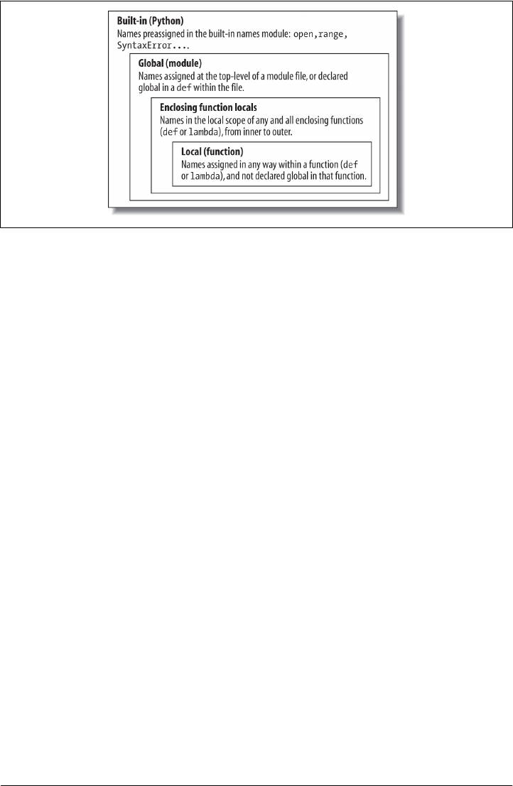
Also keep in mind that these rules apply only to simple variable names (e.g., spam). In
Parts V and VI, we’ll see that qualified attribute names (e.g., object.spam) live in par-
ticular objects and follow a completely different set of lookup rules than those covered
here. References to attribute names following periods (.) search one or more objects,
not scopes, and in fact may invoke something called inheritance in Python’s OOP
model; more on this in Part VI of this book.
Other Python scopes: Preview
Though obscure at this point in the book, there are technically three more scopes in
Python—temporary loop variables in some comprehensions, exception reference vari-
ables in some try handlers, and local scopes in class statements. The first two of these
are special cases that rarely impact real code, and the third falls under the LEGB um-
brella rule.
Most statement blocks and other constructs do not localize the names used within
them, with the following version-specific exceptions (whose variables are not available
to, but also will not clash with, surrounding code, and which involve topics covered in
full later):
Figure 17-1. The LEGB scope lookup rule. When a variable is referenced, Python searches for it in
this order: in the local scope, in any enclosing functions’ local scopes, in the global scope, and finally
in the built-in scope. The first occurrence wins. The place in your code where a variable is assigned
usually determines its scope. In Python 3.X, nonlocal declarations can also force names to be mapped
to enclosing function scopes, whether assigned or not.
1. The scope lookup rule was called the “LGB rule” in the first edition of this book. The enclosing def “E”
layer was added later in Python to obviate the task of passing in enclosing scope names explicitly with
default arguments—a topic usually of marginal interest to Python beginners that we’ll defer until later in
this chapter. Since this scope is now addressed by the nonlocal statement in Python 3.X, the lookup rule
might be better named “LNGB” today, but backward compatibility matters in books, too. The present
form of this acronym also does not account for the newer obscure scopes of some comprehensions and
exception handlers, but acronyms longer than four letters tend to defeat their purpose!
Python Scope Basics | 489
www.it-ebooks.info

•Comprehension variables—the variable X used to refer to the current iteration item
in a comprehension expression such as [X for X in I]. Because they might clash
with other names and reflect internal state in generators, in 3.X, such variables are
local to the expression itself in all comprehension forms: generator, list, set, and
dictionary. In 2.X, they are local to generator expressions and set and dictionary
compressions, but not to list comprehensions that map their names to the scope
outside the expression. By contrast, for loop statements never localize their vari-
ables to the statement block in any Python. See Chapter 20 for more details and
examples.
•Exception variables—the variable X used to reference the raised exception in a
try statement handler clause such as except E as X. Because they might defer
garbage collection’s memory recovery, in 3.X, such variables are local to that
except block, and in fact are removed when the block is exited (even if you’ve used
it earlier in your code!). In 2.X, these variables live on after the try statement. See
Chapter 34 for additional information.
These contexts augment the LEGB rule, rather than modifying it. Variables assigned
in a comprehension, for example, are simply bound to a further nested and special-case
scope; other names referenced within these expressions follow the usual LEGB lookup
rules.
It’s also worth noting that the class statement we’ll meet in Part VI creates a new
local scope too for the names assigned inside the top level of its block. As for def, names
assigned inside a class don’t clash with names elsewhere, and follow the LEGB lookup
rule, where the class block is the “L” level. Like modules and imports, these names
also morph into class object attributes after the class statements ends.
Unlike functions, though, class names are not created per call: class object calls gen-
erate instances, which inherit names assigned in the class and record per-object state
as attributes. As we’ll also learn in Chapter 29, although the LEGB rule is used to resolve
names used in both the top level of a class itself as well as the top level of method
functions nested within it, classes themselves are skipped by scope lookups—their
names must be fetched as object attributes. Because Python searches enclosing func-
tions for referenced names, but not enclosing classes, the LEGB rule still applies to
OOP code.
Scope Example
Let’s step through a larger example that demonstrates scope ideas. Suppose we wrote
the following code in a module file:
# Global scope
X = 99 # X and func assigned in module: global
def func(Y): # Y and Z assigned in function: locals
# Local scope
Z = X + Y # X is a global
490 | Chapter 17: Scopes
www.it-ebooks.info

return Z
func(1) # func in module: result=100
This module and the function it contains use a number of names to do their business.
Using Python’s scope rules, we can classify the names as follows:
Global names: X, func
X is global because it’s assigned at the top level of the module file; it can be refer-
enced inside the function as a simple unqualified variable without being declared
global. func is global for the same reason; the def statement assigns a function
object to the name func at the top level of the module.
Local names: Y, Z
Y and Z are local to the function (and exist only while the function runs) because
they are both assigned values in the function definition: Z by virtue of the = state-
ment, and Y because arguments are always passed by assignment.
The underlying rationale for this name-segregation scheme is that local variables serve
as temporary names that you need only while a function is running. For instance, in
the preceding example, the argument Y and the addition result Z exist only inside the
function; these names don’t interfere with the enclosing module’s namespace (or any
other function, for that matter). In fact, local variables are removed from memory when
the function call exits, and objects they reference may be garbage-collected if not ref-
erenced elsewhere. This is an automatic, internal step, but it helps minimize memory
requirements.
The local/global distinction also makes functions easier to understand, as most of the
names a function uses appear in the function itself, not at some arbitrary place in a
module. Also, because you can be sure that local names will not be changed by some
remote function in your program, they tend to make programs easier to debug and
modify. Functions are self-contained units of software.
The Built-in Scope
We’ve been talking about the built-in scope in the abstract, but it’s a bit simpler than
you may think. Really, the built-in scope is just a built-in module called builtins, but
you have to import builtins to query built-ins because the name builtins is not itself
built in...
No, I’m serious! The built-in scope is implemented as a standard library module named
builtins in 3.X, but that name itself is not placed in the built-in scope, so you have to
import it in order to inspect it. Once you do, you can run a dir call to see which names
are predefined. In Python 3.3 (see ahead for 2.X usage):
>>> import builtins
>>> dir(builtins)
['ArithmeticError', 'AssertionError', 'AttributeError', 'BaseException',
'BlockingIOError', 'BrokenPipeError', 'BufferError', 'BytesWarning',
Python Scope Basics | 491
www.it-ebooks.info

...many more names omitted...
'ord', 'pow', 'print', 'property', 'quit', 'range', 'repr', 'reversed',
'round', 'set', 'setattr', 'slice', 'sorted', 'staticmethod', 'str', 'sum',
'super', 'tuple', 'type', 'vars', 'zip']
The names in this list constitute the built-in scope in Python; roughly the first half are
built-in exceptions, and the second half are built-in functions. Also in this list are the
special names None, True, and False, though they are treated as reserved words in 3.X.
Because Python automatically searches this module last in its LEGB lookup, you get
all the names in this list “for free”—that is, you can use them without importing any
modules. Thus, there are really two ways to refer to a built-in function—by taking
advantage of the LEGB rule, or by manually importing the builtins module:
>>> zip # The normal way
<class 'zip'>
>>> import builtins # The hard way: for customizations
>>> builtins.zip
<class 'zip'>
>>> zip is builtins.zip # Same object, different lookups
True
The second of these approaches is sometimes useful in advanced ways we’ll meet in
this chapter’s sidebars.
Redefining built-in names: For better or worse
The careful reader might also notice that because the LEGB lookup procedure takes
the first occurrence of a name that it finds, names in the local scope may override
variables of the same name in both the global and built-in scopes, and global names
may override built-ins. A function can, for instance, create a local variable called open
by assigning to it:
def hider():
open = 'spam' # Local variable, hides built-in here
...
open('data.txt') # Error: this no longer opens a file in this scope!
However, this will hide the built-in function called open that lives in the built-in (outer)
scope, such that the name open will no longer work within the function to open files—
it’s now a string, not the opener function. This isn’t a problem if you don’t need to
open files in this function, but triggers an error if you attempt to open through this
name.
This can even occur more simply at the interactive prompt, which works as a global,
module scope:
>>> open = 99 # Assign in global scope, hides built-in here too
Now, there is nothing inherently wrong with using a built-in name for variables of your
own, as long as you don’t need the original built-in version. After all, if these were truly
492 | Chapter 17: Scopes
www.it-ebooks.info
off limits, we would need to memorize the entire built-in names list and treat all its
names as reserved. With over 140 names in this module in 3.3, that would be far too
restrictive and daunting:
>>> len(dir(builtins)), len([x for x in dir(builtins) if not x.startswith('__')])
(148, 142)
In fact, there are times in advanced programming where you may really want to replace
a built-in name by redefining it in your code—to define a custom open that verifies
access attempts, for instance (see this chapter’s sidebar “Breaking the Universe in
Python 2.X” on page 494 for more on this thread).
Still, redefining a built-in name is often a bug, and a nasty one at that, because Python
will not issue a warning message about it. Tools like PyChecker (see the Web) can warn
you of such mistakes, but knowledge may be your best defense on this point: don’t
redefine a built-in name you need. If you accidentally reassign a built-in name at the
interactive prompt this way, you can either restart your session or run a del name state-
ment to remove the redefinition from your scope, thereby restoring the original in the
built-in scope.
Note that functions can similarly hide global variables of the same name with locals,
but this is more broadly useful, and in fact is much of the point of local scopes—because
they minimize the potential for name clashes, your functions are self-contained name-
space scopes:
X = 88 # Global X
def func():
X = 99 # Local X: hides global, but we want this here
func()
print(X) # Prints 88: unchanged
Here, the assignment within the function creates a local X that is a completely different
variable from the global X in the module outside the function. As one consequence,
though, there is no way to change a name outside a function without adding a global
(or nonlocal) declaration to the def, as described in the next section.
Version skew note: Actually, the tongue twisting gets a bit worse. The
Python 3.X builtins module used here is named __builtin__ in Python
2.X. In addition, the name __builtins__ (with the s) is preset in most
global scopes, including the interactive session, to reference the module
known as builtins in 3.X and __builtin__ in 2.X, so you can often use
__builtins__ without an import but cannot run an import on that name
itself—it’s a preset variable, not a module’s name.
That is, in 3.X builtins is __builtins__ is True after you import buil
tins, and in 2.X __builtin__ is __builtins__ is True after you import
__builtin__. The upshot is that we can usually inspect the built-in scope
by simply running dir(__builtins__) with no import in both 3.X and
Python Scope Basics | 493
www.it-ebooks.info

2.X, but we are advised to use builtins for real work and customization
in 3.X, and __builtin__ for the same in 2.X. Who said documenting this
stuff was easy?
Breaking the Universe in Python 2.X
Here’s another thing you can do in Python that you probably shouldn’t—because the
names True and False in 2.X are just variables in the built-in scope and are not reserved,
it’s possible to reassign them with a statement like True = False. Don’t worry: you
won’t actually break the logical consistency of the universe in so doing! This statement
merely redefines the word True for the single scope in which it appears to return
False. All other scopes still find the originals in the built-in scope.
For more fun, though, in Python 2.X you could say __builtin__.True = False, to reset
True to False for the entire Python process. This works because there is only one built-
in scope module in a program, shared by all its clients. Alas, this type of assignment
has been disallowed in Python 3.X, because True and False are treated as actual reserved
words, just like None. In 2.X, though, it sends IDLE into a strange panic state that resets
the user code process (in other words, don’t try this at home, kids).
This technique can be useful, however, both to illustrate the underlying namespace
model, and for tool writers who must change built-ins such as open to customized
functions. By reassigning a function’s name in the built-in scope, you reset it to your
customization for every module in the process. If you do, you’ll probably also need to
remember the original version to call from your customization—in fact, we’ll see one
way to achieve this for a custom open in the sidebar “Why You Will Care: Customizing
open” on page 517 after we’ve had a chance to explore nested scope closures and state
retention options.
Also, note again that third-party tools such as PyChecker, and others such as PyLint,
will warn about common programming mistakes, including accidental assignment to
built-in names (this is usually known as “shadowing” a built-in in such tools). It’s not
a bad idea to run your first few Python programs through tools like these to see what
they point out.
The global Statement
The global statement and its nonlocal 3.X cousin are the only things that are remotely
like declaration statements in Python. They are not type or size declarations, though;
they are namespace declarations. The global statement tells Python that a function plans
to change one or more global names—that is, names that live in the enclosing module’s
scope (namespace).
We’ve talked about global in passing already. Here’s a summary:
• Global names are variables assigned at the top level of the enclosing module file.
494 | Chapter 17: Scopes
www.it-ebooks.info

• Global names must be declared only if they are assigned within a function.
• Global names may be referenced within a function without being declared.
In other words, global allows us to change names that live outside a def at the top level
of a module file. As we’ll see later, the nonlocal statement is almost identical but applies
to names in the enclosing def’s local scope, rather than names in the enclosing module.
The global statement consists of the keyword global, followed by one or more names
separated by commas. All the listed names will be mapped to the enclosing module’s
scope when assigned or referenced within the function body. For instance:
X = 88 # Global X
def func():
global X
X = 99 # Global X: outside def
func()
print(X) # Prints 99
We’ve added a global declaration to the example here, such that the X inside the def
now refers to the X outside the def; they are the same variable this time, so changing
X inside the function changes the X outside it. Here is a slightly more involved example
of global at work:
y, z = 1, 2 # Global variables in module
def all_global():
global x # Declare globals assigned
x = y + z # No need to declare y, z: LEGB rule
Here, x, y, and z are all globals inside the function all_global. y and z are global because
they aren’t assigned in the function; x is global because it was listed in a global statement
to map it to the module’s scope explicitly. Without the global here, x would be con-
sidered local by virtue of the assignment.
Notice that y and z are not declared global; Python’s LEGB lookup rule finds them in
the module automatically. Also, notice that x does not even exist in the enclosing mod-
ule before the function runs; in this case, the first assignment in the function creates
x in the module.
Program Design: Minimize Global Variables
Functions in general, and global variables in particular, raise some larger design ques-
tions. How should our functions communicate? Although some of these will become
more apparent when you begin writing larger functions of your own, a few guidelines
up front might spare you from problems later. In general, functions should rely on
arguments and return values instead of globals, but I need to explain why.
By default, names assigned in functions are locals, so if you want to change names
outside functions you have to write extra code (e.g., global statements). This is delib-
The global Statement | 495
www.it-ebooks.info

erate—as is common in Python, you have to say more to do the potentially “wrong”
thing. Although there are times when globals are useful, variables assigned in a def are
local by default because that is normally the best policy. Changing globals can lead to
well-known software engineering problems: because the variables’ values are depen-
dent on the order of calls to arbitrarily distant functions, programs can become difficult
to debug, or to understand at all.
Consider this module file, for example, which is presumably imported and used else-
where:
X = 99
def func1():
global X
X = 88
def func2():
global X
X = 77
Now, imagine that it is your job to modify or reuse this code. What will the value of
X be here? Really, that question has no meaning unless it’s qualified with a point of
reference in time—the value of X is timing-dependent, as it depends on which function
was called last (something we can’t tell from this file alone).
The net effect is that to understand this code, you have to trace the flow of control
through the entire program. And, if you need to reuse or modify the code, you have to
keep the entire program in your head all at once. In this case, you can’t really use one
of these functions without bringing along the other. They are dependent on—that is,
coupled with—the global variable. This is the problem with globals: they generally make
code more difficult to understand and reuse than code consisting of self-contained
functions that rely on locals.
On the other hand, short of using tools like nested scope closures or object-oriented
programming with classes, global variables are probably the most straightforward way
in Python to retain shared state information—information that a function needs to
remember for use the next time it is called. Local variables disappear when the function
returns, but globals do not. As we’ll see later, other techniques can achieve this, too,
and allow for multiple copies of the retained information, but they are generally more
complex than pushing values out to the global scope for retention in simple use cases
where this applies.
Moreover, some programs designate a single module to collect globals; as long as this
is expected, it is not as harmful. Programs that use multithreading to do parallel pro-
cessing in Python also commonly depend on global variables—they become shared
memory between functions running in parallel threads, and so act as a communication
device.2
For now, though, especially if you are relatively new to programming, avoid the temp-
tation to use globals whenever you can—they tend to make programs difficult to un-
496 | Chapter 17: Scopes
www.it-ebooks.info

derstand and reuse, and won’t work for cases where one copy of saved data is not
enough. Try to communicate with passed-in arguments and return values instead. Six
months from now, both you and your coworkers may be happy you did.
Program Design: Minimize Cross-File Changes
Here’s another scope-related design issue: although we can change variables in another
file directly, we usually shouldn’t. Module files were introduced in Chapter 3 and are
covered in more depth in the next part of this book. To illustrate their relationship to
scopes, consider these two module files:
# first.py
X = 99 # This code doesn't know about second.py
# second.py
import first
print(first.X) # OK: references a name in another file
first.X = 88 # But changing it can be too subtle and implicit
The first defines a variable X, which the second prints and then changes by assignment.
Notice that we must import the first module into the second file to get to its variable
at all—as we’ve learned, each module is a self-contained namespace (package of vari-
ables), and we must import one module to see inside it from another. That’s the main
point about modules: by segregating variables on a per-file basis, they avoid name
collisions across files, in much the same way that local variables avoid name clashes
across functions.
Really, though, in terms of this chapter’s topic, the global scope of a module file be-
comes the attribute namespace of the module object once it is imported—importers
automatically have access to all of the file’s global variables, because a file’s global scope
morphs into an object’s attribute namespace when it is imported.
After importing the first module, the second module prints its variable and then assigns
it a new value. Referencing the module’s variable to print it is fine—this is how modules
are linked together into a larger system normally. The problem with the assignment to
first.X, however, is that it is far too implicit: whoever’s charged with maintaining or
reusing the first module probably has no clue that some arbitrarily far-removed module
on the import chain can change X out from under him or her at runtime. In fact, the
2. Multithreading runs function calls in parallel with the rest of the program and is supported by Python’s
standard library modules _thread, threading, and queue (thread, threading, and Queue in Python 2.X).
Because all threaded functions run in the same process, global scopes often serve as one form of shared
memory between them (threads may share both names in global scopes, as well as objects in a process’s
memory space). Threading is commonly used for long-running tasks in GUIs, to implement nonblocking
operations in general and to maximize CPU capacity. It is also beyond this book’s scope; see the Python
library manual, as well as the follow-up texts listed in the preface (such as O’Reilly’s Programming
Python), for more details.
The global Statement | 497
www.it-ebooks.info

second module may be in a completely different directory, and so difficult to notice at
all.
Although such cross-file variable changes are always possible in Python, they are usually
much more subtle than you will want. Again, this sets up too strong a coupling between
the two files—because they are both dependent on the value of the variable X, it’s
difficult to understand or reuse one file without the other. Such implicit cross-file de-
pendencies can lead to inflexible code at best, and outright bugs at worst.
Here again, the best prescription is generally to not do this—the best way to commu-
nicate across file boundaries is to call functions, passing in arguments and getting back
return values. In this specific case, we would probably be better off coding an accessor
function to manage the change:
# first.py
X = 99
def setX(new): # Accessor make external changes explit
global X # And can manage access in a single place
X = new
# second.py
import first
first.setX(88) # Call the function instead of changing directly
This requires more code and may seem like a trivial change, but it makes a huge dif-
ference in terms of readability and maintainability—when a person reading the first
module by itself sees a function, that person will know that it is a point of interface and
will expect the change to the X. In other words, it removes the element of surprise that
is rarely a good thing in software projects. Although we cannot prevent cross-file
changes from happening, common sense dictates that they should be minimized unless
widely accepted across the program.
When we meet classes in Part VI, we’ll see similar techniques for coding
attribute accessors. Unlike modules, classes can also intercept attribute
fetches automatically with operator overloading, even when accessors
aren’t used by their clients.
Other Ways to Access Globals
Interestingly, because global-scope variables morph into the attributes of a loaded
module object, we can emulate the global statement by importing the enclosing module
and assigning to its attributes, as in the following example module file. Code in this file
imports the enclosing module, first by name, and then by indexing the sys.modules
loaded modules table (more on this table in Chapter 22 and Chapter 25):
# thismod.py
var = 99 # Global variable == module attribute
498 | Chapter 17: Scopes
www.it-ebooks.info

def local():
var = 0 # Change local var
def glob1():
global var # Declare global (normal)
var += 1 # Change global var
def glob2():
var = 0 # Change local var
import thismod # Import myself
thismod.var += 1 # Change global var
def glob3():
var = 0 # Change local var
import sys # Import system table
glob = sys.modules['thismod'] # Get module object (or use __name__)
glob.var += 1 # Change global var
def test():
print(var)
local(); glob1(); glob2(); glob3()
print(var)
When run, this adds 3 to the global variable (only the first function does not impact it):
>>> import thismod
>>> thismod.test()
99
102
>>> thismod.var
102
This works, and it illustrates the equivalence of globals to module attributes, but it’s
much more work than using the global statement to make your intentions explicit.
As we’ve seen, global allows us to change names in a module outside a function. It has
a close relative named nonlocal that can be used to change names in enclosing func-
tions, too—but to understand how that can be useful, we first need to explore enclosing
functions in general.
Scopes and Nested Functions
So far, I’ve omitted one part of Python’s scope rules on purpose, because it’s relatively
uncommon to encounter it in practice. However, it’s time to take a deeper look at the
letter E in the LEGB lookup rule. The E layer was added in Python 2.2; it takes the form
of the local scopes of any and all enclosing function’s local scopes. Enclosing scopes
are sometimes also called statically nested scopes. Really, the nesting is a lexical one—
nested scopes correspond to physically and syntactically nested code structures in your
program’s source code text.
Scopes and Nested Functions | 499
www.it-ebooks.info

Nested Scope Details
With the addition of nested function scopes, variable lookup rules become slightly more
complex. Within a function:
•A reference (X) looks for the name X first in the current local scope (function); then
in the local scopes of any lexically enclosing functions in your source code, from
inner to outer; then in the current global scope (the module file); and finally in the
built-in scope (the module builtins). global declarations make the search begin
in the global (module file) scope instead.
•An assignment (X = value) creates or changes the name X in the current local
scope, by default. If X is declared global within the function, the assignment creates
or changes the name X in the enclosing module’s scope instead. If, on the other
hand, X is declared nonlocal within the function in 3.X (only), the assignment
changes the name X in the closest enclosing function’s local scope.
Notice that the global declaration still maps variables to the enclosing module. When
nested functions are present, variables in enclosing functions may be referenced, but
they require 3.X nonlocal declarations to be changed.
Nested Scope Examples
To clarify the prior section’s points, let’s illustrate with some real code. Here is what
an enclosing function scope looks like (type this into a script file or at the interactive
prompt to run it live):
X = 99 # Global scope name: not used
def f1():
X = 88 # Enclosing def local
def f2():
print(X) # Reference made in nested def
f2()
f1() # Prints 88: enclosing def local
First off, this is legal Python code: the def is simply an executable statement, which can
appear anywhere any other statement can—including nested in another def. Here, the
nested def runs while a call to the function f1 is running; it generates a function and
assigns it to the name f2, a local variable within f1’s local scope. In a sense, f2 is a
temporary function that lives only during the execution of (and is visible only to code
in) the enclosing f1.
But notice what happens inside f2: when it prints the variable X, it refers to the X that
lives in the enclosing f1 function’s local scope. Because functions can access names in
all physically enclosing def statements, the X in f2 is automatically mapped to the X in
f1, by the LEGB lookup rule.
500 | Chapter 17: Scopes
www.it-ebooks.info

This enclosing scope lookup works even if the enclosing function has already returned.
For example, the following code defines a function that makes and returns another
function, and represents a more common usage pattern:
def f1():
X = 88
def f2():
print(X) # Remembers X in enclosing def scope
return f2 # Return f2 but don't call it
action = f1() # Make, return function
action() # Call it now: prints 88
In this code, the call to action is really running the function we named f2 when f1 ran.
This works because functions are objects in Python like everything else, and can be
passed back as return values from other functions. Most importantly, f2 remembers
the enclosing scope’s X in f1, even though f1 is no longer active—which leads us to the
next topic.
Factory Functions: Closures
Depending on whom you ask, this sort of behavior is also sometimes called a closure
or a factory function—the former describing a functional programming technique, and
the latter denoting a design pattern. Whatever the label, the function object in question
remembers values in enclosing scopes regardless of whether those scopes are still
present in memory. In effect, they have attached packets of memory (a.k.a. state re-
tention), which are local to each copy of the nested function created, and often provide
a simple alternative to classes in this role.
A simple function factory
Factory functions (a.k.a. closures) are sometimes used by programs that need to gen-
erate event handlers on the fly in response to conditions at runtime. For instance,
imagine a GUI that must define actions according to user inputs that cannot be antici-
pated when the GUI is built. In such cases, we need a function that creates and returns
another function, with information that may vary per function made.
To illustrate this in simple terms, consider the following function, typed at the inter-
active prompt (and shown here without the “...” continuation-line prompts, per the
presentation note ahead):
>>> def maker(N):
def action(X): # Make and return action
return X ** N # action retains N from enclosing scope
return action
This defines an outer function that simply generates and returns a nested function,
without calling it—maker makes action, but simply returns action without running it.
If we call the outer function:
Scopes and Nested Functions | 501
www.it-ebooks.info

>>> f = maker(2) # Pass 2 to argument N
>>> f
<function maker.<locals>.action at 0x0000000002A4A158>
what we get back is a reference to the generated nested function—the one created when
the nested def runs. If we now call what we got back from the outer function:
>>> f(3) # Pass 3 to X, N remembers 2: 3 ** 2
9
>>> f(4) # 4 ** 2
16
we invoke the nested function—the one called action within maker. In other words,
we’re calling the nested function that maker created and passed back.
Perhaps the most unusual part of this, though, is that the nested function remembers
integer 2, the value of the variable N in maker, even though maker has returned and exited
by the time we call action. In effect, N from the enclosing local scope is retained as state
information attached to the generated action, which is why we get back its argument
squared when it is later called.
Just as important, if we now call the outer function again, we get back a new nested
function with different state information attached. That is, we get the argument cubed
instead of squared when calling the new function, but the original still squares as before:
>>> g = maker(3) # g remembers 3, f remembers 2
>>> g(4) # 4 ** 3
64
>>> f(4) # 4 ** 2
16
This works because each call to a factory function like this gets its own set of state
information. In our case, the function we assign to name g remembers 3, and f remem-
bers 2, because each has its own state information retained by the variable N in maker.
This is a somewhat advanced technique that you may not see very often in most code,
and may be popular among programmers with backgrounds in functional program-
ming languages. On the other hand, enclosing scopes are often employed by the
lambda function-creation expressions we’ll expand on later in this chapter—because
they are expressions, they are almost always nested within a def. For example, a
lambda would serve in place of a def in our example:
>>> def maker(N):
return lambda X: X ** N # lambda functions retain state too
>>> h = maker(3)
>>> h(4) # 4 ** 3 again
64
For a more tangible example of closures at work, see the upcoming sidebar “Why You
Will Care: Customizing open” on page 517. It uses similar techniques to store infor-
mation for later use in an enclosing scope.
502 | Chapter 17: Scopes
www.it-ebooks.info

Presentation note: In this chapter, I’ve started listing interactive exam-
ples without the “...” continuation-line prompts that may or may not
appear in your interface (they do at the shell, but not in IDLE). This
convention will be followed from this point on to make larger code ex-
amples a bit easier to cut and paste from an ebook or other. I’m assuming
that by now you understand indentation rules and have had your fair
share of typing Python code, and some functions and classes ahead may
be too large for rote input.
I’m also listing more and more code alone or in files, and switching
between these and interactive input arbitrarily; when you see a “>>>”
prompt, the code is typed interactively, and can generally be cut and
pasted into your Python shell if you omit the “>>>” itself. If this fails,
you can still run by pasting line by line, or editing in a file.
Closures versus classes, round 1
To some, classes, described in full in Part VI of this book, may seem better at state
retention like this, because they make their memory more explicit with attribute as-
signments. Classes also directly support additional tools that closure functions do not,
such as customization by inheritance and operator overloading, and more naturally
implement multiple behaviors in the form of methods. Because of such distinctions,
classes may be better at implementing more complete objects.
Still, closure functions often provide a lighter-weight and viable alternative when re-
taining state is the only goal. They provide for per-call localized storage for data required
by a single nested function. This is especially true when we add the 3.X nonlocal state-
ment described ahead to allow enclosing scope state changes (in 2.X, enclosing scopes
are read-only, and so have more limited uses).
From a broader perspective, there are multiple ways for Python functions to retain state
between calls. Although the values of normal local variables go away when a function
returns, values can be retained from call to call in global variables; in class instance
attributes; in the enclosing scope references we’ve met here; and in argument defaults
and function attributes. Some might include mutable default arguments to this list too
(though others may wish they didn’t).
We’ll preview class-based alternatives and meet function attributes later in this chapter,
and get the full story on arguments and defaults in Chapter 18. To help us judge how
defaults compete on state retention, though, the next section gives enough of an in-
troduction to get us started.
Scopes and Nested Functions | 503
www.it-ebooks.info

Closures can also be created when a class is nested in a def: the values
of the enclosing function’s local names are retained by references within
the class, or one of its method functions. See Chapter 29 for more on
nested classes. As we’ll see in later examples (e.g., Chapter 39’s deco-
rators), the outer def in such code serves a similar role: it becomes a
class factory, and provides state retention for the nested class.
Retaining Enclosing Scope State with Defaults
In early versions of Python (prior to 2.2), the sort of code in the prior section failed
because nested defs did not do anything about scopes—a reference to a variable within
f2 in the following would search only the local (f2), then global (the code outside f1),
and then built-in scopes. Because it skipped the scopes of enclosing functions, an error
would result. To work around this, programmers typically used default argument val-
ues to pass in and remember the objects in an enclosing scope:
def f1():
x = 88
def f2(x=x): # Remember enclosing scope X with defaults
print(x)
f2()
f1() # Prints 88
This coding style works in all Python releases, and you’ll still see this pattern in some
existing Python code. In fact, it’s still required for loop variables, as we’ll see in a mo-
ment, which is why it remains worth studying today. In short, the syntax arg=val in a
def header means that the argument arg will default to the value val if no real value is
passed to arg in a call. This syntax is used here to explicitly assign enclosing scope state
to be retained.
Specifically, in the modified f2 here, the x=x means that the argument x will default to
the value of x in the enclosing scope—because the second x is evaluated before Python
steps into the nested def, it still refers to the x in f1. In effect, the default argument
remembers what x was in f1: the object 88.
That’s fairly complex, and it depends entirely on the timing of default value evaluations.
In fact, the nested scope lookup rule was added to Python to make defaults unnecessary
for this role—today, Python automatically remembers any values required in the en-
closing scope for use in nested defs.
Of course, the best prescription for much code is simply to avoid nesting defs within
defs, as it will make your programs much simpler—in the Pythonic view, flat is generally
better than nested. The following is an equivalent of the prior example that avoids
nesting altogether. Notice the forward reference in this code—it’s OK to call a function
defined after the function that calls it, as long as the second def runs before the first
function is actually called. Code inside a def is never evaluated until the function is
actually called:
504 | Chapter 17: Scopes
www.it-ebooks.info

>>> def f1():
x = 88 # Pass x along instead of nesting
f2(x) # Forward reference OK
>>> def f2(x):
print(x) # Flat is still often better than nested!
>>> f1()
88
If you avoid nesting this way, you can almost forget about the nested scopes concept
in Python. On the other hand, the nested functions of closure (factory) functions are
fairly common in modern Python code, as are lambda functions—which almost natu-
rally appear nested in defs and often rely on the nested scopes layer, as the next section
explains.
Nested scopes, defaults, and lambdas
Although they see increasing use in defs these days, you may be more likely to care
about nested function scopes when you start coding or reading lambda expressions.
We’ve met lambda briefly and won’t cover it in depth until Chapter 19, but in short, it’s
an expression that generates a new function to be called later, much like a def statement.
Because it’s an expression, though, it can be used in places that def cannot, such as
within list and dictionary literals.
Like a def, a lambda expression also introduces a new local scope for the function it
creates. Thanks to the enclosing scopes lookup layer, lambdas can see all the variables
that live in the functions in which they are coded. Thus, the following code—a variation
on the factory we saw earlier—works, but only because the nested scope rules are
applied:
def func():
x = 4
action = (lambda n: x ** n) # x remembered from enclosing def
return action
x = func()
print(x(2)) # Prints 16, 4 ** 2
Prior to the introduction of nested function scopes, programmers used defaults to pass
values from an enclosing scope into lambdas, just as for defs. For instance, the following
works on all Pythons:
def func():
x = 4
action = (lambda n, x=x: x ** n) # Pass x in manually
return action
Because lambdas are expressions, they naturally (and even normally) nest inside en-
closing defs. Hence, they were perhaps the biggest initial beneficiaries of the addition
Scopes and Nested Functions | 505
www.it-ebooks.info

of enclosing function scopes in the lookup rules; in most cases, it is no longer necessary
to pass values into lambdas with defaults.
Loop variables may require defaults, not scopes
There is one notable exception to the rule I just gave (and a reason why I’ve shown you
the otherwise dated default argument technique we just saw): if a lambda or def defined
within a function is nested inside a loop, and the nested function references an enclosing
scope variable that is changed by that loop, all functions generated within the loop will
have the same value—the value the referenced variable had in the last loop iteration.
In such cases, you must still use defaults to save the variable’s current value instead.
This may seem a fairly obscure case, but it can come up in practice more often than
you may think, especially in code that generates callback handler functions for a num-
ber of widgets in a GUI—for instance, handlers for button-clicks for all the buttons in
a row. If these are created in a loop, you may need to be careful to save state with
defaults, or all your buttons’ callbacks may wind up doing the same thing.
Here’s an illustration of this phenomenon reduced to simple code: the following at-
tempts to build up a list of functions that each remember the current variable i from
the enclosing scope:
>>> def makeActions():
acts = []
for i in range(5): # Tries to remember each i
acts.append(lambda x: i ** x) # But all remember same last i!
return acts
>>> acts = makeActions()
>>> acts[0]
<function makeActions.<locals>.<lambda> at 0x0000000002A4A400>
This doesn’t quite work, though—because the enclosing scope variable is looked up
when the nested functions are later called, they all effectively remember the same value:
the value the loop variable had on the last loop iteration. That is, when we pass a power
argument of 2 in each of the following calls, we get back 4 to the power of 2 for each
function in the list, because i is the same in all of them—4:
>>> acts[0](2) # All are 4 ** 2, 4=value of last i
16
>>> acts[1](2) # This should be 1 ** 2 (1)
16
>>> acts[2](2) # This should be 2 ** 2 (4)
16
>>> acts[4](2) # Only this should be 4 ** 2 (16)
16
This is the one case where we still have to explicitly retain enclosing scope values with
default arguments, rather than enclosing scope references. That is, to make this sort of
code work, we must pass in the current value of the enclosing scope’s variable with a
506 | Chapter 17: Scopes
www.it-ebooks.info

default. Because defaults are evaluated when the nested function is created (not when
it’s later called), each remembers its own value for i:
>>> def makeActions():
acts = []
for i in range(5): # Use defaults instead
acts.append(lambda x, i=i: i ** x) # Remember current i
return acts
>>> acts = makeActions()
>>> acts[0](2) # 0 ** 2
0
>>> acts[1](2) # 1 ** 2
1
>>> acts[2](2) # 2 ** 2
4
>>> acts[4](2) # 4 ** 2
16
This seems an implementation artifact that is prone to change, and may become more
important as you start writing larger programs. We’ll talk more about defaults in
Chapter 18 and lambdas in Chapter 19, so you may also want to return and review this
section later.3
Arbitrary scope nesting
Before ending this discussion, we should note that scopes may nest arbitrarily, but only
enclosing function def statements (not classes, described in Part VI) are searched when
names are referenced:
>>> def f1():
x = 99
def f2():
def f3():
print(x) # Found in f1's local scope!
f3()
f2()
>>> f1()
99
Python will search the local scopes of all enclosing defs, from inner to outer, after the
referencing function’s local scope and before the module’s global scope or built-ins.
However, this sort of code is even less likely to pop up in practice. Again, in Python,
we say flat is better than nested, and this still holds generally true even with the addition
3. In the section “Function Gotchas” on page 656, we’ll also see that there is a similar issue with using
mutable objects like lists and dictionaries for default arguments (e.g., def f(a=[]))—because defaults are
implemented as single objects attached to functions, mutable defaults retain state from call to call, rather
then being initialized anew on each call. Depending on whom you ask, this is either considered a feature
that supports another way to implement state retention, or a strange corner of the language; more on this
at the end of Chapter 21.
Scopes and Nested Functions | 507
www.it-ebooks.info

of nested scope closures. Except in limited contexts, your life (and the lives of your
coworkers) will generally be better if you minimize nested function definitions.
The nonlocal Statement in 3.X
In the prior section we explored the way that nested functions can reference variables
in an enclosing function’s scope, even if that function has already returned. It turns out
that, in Python 3.X (though not in 2.X), we can also change such enclosing scope vari-
ables, as long as we declare them in nonlocal statements. With this statement, nested
defs can have both read and write access to names in enclosing functions. This makes
nested scope closures more useful, by providing changeable state information.
The nonlocal statement is similar in both form and role to global, covered earlier. Like
global, nonlocal declares that a name will be changed in an enclosing scope. Unlike
global, though, nonlocal applies to a name in an enclosing function’s scope, not the
global module scope outside all defs. Also unlike global, nonlocal names must already
exist in the enclosing function’s scope when declared—they can exist only in enclosing
functions and cannot be created by a first assignment in a nested def.
In other words, nonlocal both allows assignment to names in enclosing function scopes
and limits scope lookups for such names to enclosing defs. The net effect is a more
direct and reliable implementation of changeable state information, for contexts that
do not desire or need classes with attributes, inheritance, and multiple behaviors.
nonlocal Basics
Python 3.X introduces a new nonlocal statement, which has meaning only inside a
function:
def func():
nonlocal name1, name2, ... # OK here
>>> nonlocal X
SyntaxError: nonlocal declaration not allowed at module level
This statement allows a nested function to change one or more names defined in a
syntactically enclosing function’s scope. In Python 2.X, when one function def is nested
in another, the nested function can reference any of the names defined by assignment
in the enclosing def’s scope, but it cannot change them. In 3.X, declaring the enclosing
scopes’ names in a nonlocal statement enables nested functions to assign and thus
change such names as well.
This provides a way for enclosing functions to provide writeable state information,
remembered when the nested function is later called. Allowing the state to change
makes it more useful to the nested function (imagine a counter in the enclosing scope,
for instance). In 2.X, programmers usually achieve similar goals by using classes or
508 | Chapter 17: Scopes
www.it-ebooks.info

other schemes. Because nested functions have become a more common coding pattern
for state retention, though, nonlocal makes it more generally applicable.
Besides allowing names in enclosing defs to be changed, the nonlocal statement also
forces the issue for references—much like the global statement, nonlocal causes
searches for the names listed in the statement to begin in the enclosing defs’ scopes,
not in the local scope of the declaring function. That is, nonlocal also means “skip my
local scope entirely.”
In fact, the names listed in a nonlocal must have been previously defined in an enclosing
def when the nonlocal is reached, or an error is raised. The net effect is much like global:
global means the names reside in the enclosing module, and nonlocal means they reside
in an enclosing def. nonlocal is even more strict, though—scope search is restricted to
only enclosing defs. That is, nonlocal names can appear only in enclosing defs, not in
the module’s global scope or built-in scopes outside the defs.
The addition of nonlocal does not alter name reference scope rules in general; they still
work as before, per the “LEGB” rule described earlier. The nonlocal statement mostly
serves to allow names in enclosing scopes to be changed rather than just referenced.
However, both global and nonlocal statements do tighten up and even restrict the
lookup rules somewhat, when coded in a function:
•global makes scope lookup begin in the enclosing module’s scope and allows
names there to be assigned. Scope lookup continues on to the built-in scope if the
name does not exist in the module, but assignments to global names always create
or change them in the module’s scope.
•nonlocal restricts scope lookup to just enclosing defs, requires that the names al-
ready exist there, and allows them to be assigned. Scope lookup does not continue
on to the global or built-in scopes.
In Python 2.X, references to enclosing def scope names are allowed, but not assignment.
However, you can still use classes with explicit attributes to achieve the same change-
able state information effect as nonlocals (and you may be better off doing so in some
contexts); globals and function attributes can sometimes accomplish similar goals as
well. More on this in a moment; first, let’s turn to some working code to make this
more concrete.
nonlocal in Action
On to some examples, all run in 3.X. References to enclosing def scopes work in 3X as
they do in 2.X—in the following, tester builds and returns the function nested, to be
called later, and the state reference in nested maps the local scope of tester using the
normal scope lookup rules:
C:\code> c:\python33\python
>>> def tester(start):
The nonlocal Statement in 3.X | 509
www.it-ebooks.info

state = start # Referencing nonlocals works normally
def nested(label):
print(label, state) # Remembers state in enclosing scope
return nested
>>> F = tester(0)
>>> F('spam')
spam 0
>>> F('ham')
ham 0
Changing a name in an enclosing def’s scope is not allowed by default, though; this is
the normal case in 2.X as well:
>>> def tester(start):
state = start
def nested(label):
print(label, state)
state += 1 # Cannot change by default (never in 2.X)
return nested
>>> F = tester(0)
>>> F('spam')
UnboundLocalError: local variable 'state' referenced before assignment
Using nonlocal for changes
Now, under 3.X, if we declare state in the tester scope as nonlocal within nested, we
get to change it inside the nested function, too. This works even though tester has
returned and exited by the time we call the returned nested function through the name
F:
>>> def tester(start):
state = start # Each call gets its own state
def nested(label):
nonlocal state # Remembers state in enclosing scope
print(label, state)
state += 1 # Allowed to change it if nonlocal
return nested
>>> F = tester(0)
>>> F('spam') # Increments state on each call
spam 0
>>> F('ham')
ham 1
>>> F('eggs')
eggs 2
As usual with enclosing scope references, we can call the tester factory (closure) func-
tion multiple times to get multiple copies of its state in memory. The state object in
the enclosing scope is essentially attached to the nested function object returned; each
call makes a new, distinct state object, such that updating one function’s state won’t
impact the other. The following continues the prior listing’s interaction:
510 | Chapter 17: Scopes
www.it-ebooks.info

>>> G = tester(42) # Make a new tester that starts at 42
>>> G('spam')
spam 42
>>> G('eggs') # My state information updated to 43
eggs 43
>>> F('bacon') # But F's is where it left off: at 3
bacon 3 # Each call has different state information
In this sense, Python’s nonlocals are more functional than function locals typical in
some other languages: in a closure function, nonlocals are per-call, multiple copy data.
Boundary cases
Though useful, nonlocals come with some subtleties to be aware of. First, unlike the
global statement, nonlocal names really must have previously been assigned in an en-
closing def’s scope when a nonlocal is evaluated, or else you’ll get an error—you cannot
create them dynamically by assigning them anew in the enclosing scope. In fact, they
are checked at function definition time before either an enclosing or nested function is
called:
>>> def tester(start):
def nested(label):
nonlocal state # Nonlocals must already exist in enclosing def!
state = 0
print(label, state)
return nested
SyntaxError: no binding for nonlocal 'state' found
>>> def tester(start):
def nested(label):
global state # Globals don't have to exist yet when declared
state = 0 # This creates the name in the module now
print(label, state)
return nested
>>> F = tester(0)
>>> F('abc')
abc 0
>>> state
0
Second, nonlocal restricts the scope lookup to just enclosing defs; nonlocals are not
looked up in the enclosing module’s global scope or the built-in scope outside all
defs, even if they are already there:
>>> spam = 99
>>> def tester():
def nested():
nonlocal spam # Must be in a def, not the module!
print('Current=', spam)
spam += 1
The nonlocal Statement in 3.X | 511
www.it-ebooks.info

return nested
SyntaxError: no binding for nonlocal 'spam' found
These restrictions make sense once you realize that Python would not otherwise gen-
erally know which enclosing scope to create a brand-new name in. In the prior listing,
should spam be assigned in tester, or the module outside? Because this is ambiguous,
Python must resolve nonlocals at function creation time, not function call time.
Why nonlocal? State Retention Options
Given the extra complexity of nested functions, you might wonder what the fuss is
about. Although it’s difficult to see in our small examples, state information becomes
crucial in many programs. While functions can return results, their local variables won’t
normally retain other values that must live on between calls. Moreover, many appli-
cations require such values to differ per context of use.
As mentioned earlier, there are a variety of ways to “remember” information across
function and method calls in Python. While there are tradeoffs for all, nonlocal does
improve this story for enclosing scope references—the nonlocal statement allows mul-
tiple copies of changeable state to be retained in memory. It addresses simple state-
retention needs where classes may not be warranted and global variables do not apply,
though function attributes can often serve similar roles more portably. Let’s review the
options to see how they stack up.
State with nonlocal: 3.X only
As we saw in the prior section, the following code allows state to be retained and
modified in an enclosing scope. Each call to tester creates a self-contained package of
changeable information, whose names do not clash with any other part of the program:
>>> def tester(start):
state = start # Each call gets its own state
def nested(label):
nonlocal state # Remembers state in enclosing scope
print(label, state)
state += 1 # Allowed to change it if nonlocal
return nested
>>> F = tester(0)
>>> F('spam') # State visible within closure only
spam 0
>>> F.state
AttributeError: 'function' object has no attribute 'state'
We need to declare variables nonlocal only if they must be changed (other enclosing
scope name references are automatically retained as usual), and nonlocal names are
still not visible outside the enclosing function.
512 | Chapter 17: Scopes
www.it-ebooks.info

Unfortunately, this code works in Python 3.X only. If you are using Python 2.X, other
options are available, depending on your goals. The next three sections present some
alternatives. Some of the code in these sections uses tools we haven’t covered yet and
is intended partially as preview, but we’ll keep the examples simple here so that you
can compare and contrast along the way.
State with Globals: A Single Copy Only
One common prescription for achieving the nonlocal effect in 2.X and earlier is to
simply move the state out to the global scope (the enclosing module):
>>> def tester(start):
global state # Move it out to the module to change it
state = start # global allows changes in module scope
def nested(label):
global state
print(label, state)
state += 1
return nested
>>> F = tester(0)
>>> F('spam') # Each call increments shared global state
spam 0
>>> F('eggs')
eggs 1
This works in this case, but it requires global declarations in both functions and is
prone to name collisions in the global scope (what if “state” is already being used?). A
worse, and more subtle, problem is that it only allows for a single shared copy of the
state information in the module scope—if we call tester again, we’ll wind up resetting
the module’s state variable, such that prior calls will see their state overwritten:
>>> G = tester(42) # Resets state's single copy in global scope
>>> G('toast')
toast 42
>>> G('bacon')
bacon 43
>>> F('ham') # But my counter has been overwritten!
ham 44
As shown earlier, when you are using nonlocal and nested function closures instead of
global, each call to tester remembers its own unique copy of the state object.
State with Classes: Explicit Attributes (Preview)
The other prescription for changeable state information in 2.X and earlier is to use
classes with attributes to make state information access more explicit than the implicit
magic of scope lookup rules. As an added benefit, each instance of a class gets a fresh
Why nonlocal? State Retention Options | 513
www.it-ebooks.info

copy of the state information, as a natural byproduct of Python’s object model. Classes
also support inheritance, multiple behaviors, and other tools.
We haven’t explored classes in detail yet, but as a brief preview for comparison, the
following is a reformulation of the earlier tester/nested functions as a class, which
records state in objects explicitly as they are created. To make sense of this code, you
need to know that a def within a class like this works exactly like a normal def, except
that the function’s self argument automatically receives the implied subject of the call
(an instance object created by calling the class itself). The function named __init__ is
run automatically when the class is called:
>>> class tester: # Class-based alternative (see Part VI)
def __init__(self, start): # On object construction,
self.state = start # save state explicitly in new object
def nested(self, label):
print(label, self.state) # Reference state explicitly
self.state += 1 # Changes are always allowed
>>> F = tester(0) # Create instance, invoke __init__
>>> F.nested('spam') # F is passed to self
spam 0
>>> F.nested('ham')
ham 1
In classes, we save every attribute explicitly, whether it’s changed or just referenced,
and they are available outside the class. As for nested functions and nonlocal, the class
alternative supports multiple copies of the retained data:
>>> G = tester(42) # Each instance gets new copy of state
>>> G.nested('toast') # Changing one does not impact others
toast 42
>>> G.nested('bacon')
bacon 43
>>> F.nested('eggs') # F's state is where it left off
eggs 2
>>> F.state # State may be accessed outside class
3
With just slightly more magic—which we’ll delve into later in this book—we could
also make our class objects look like callable functions using operator overloading.
__call__ intercepts direct calls on an instance, so we don’t need to call a named method:
>>> class tester:
def __init__(self, start):
self.state = start
def __call__(self, label): # Intercept direct instance calls
print(label, self.state) # So .nested() not required
self.state += 1
>>> H = tester(99)
>>> H('juice') # Invokes __call__
juice 99
514 | Chapter 17: Scopes
www.it-ebooks.info

>>> H('pancakes')
pancakes 100
Don’t sweat the details in this code too much at this point in the book; it’s mostly a
preview, intended for general comparison to closures only. We’ll explore classes in
depth in Part VI, and will look at specific operator overloading tools like __call__ in
Chapter 30. The point to notice here is that classes can make state information more
obvious, by leveraging explicit attribute assignment instead of implicit scope lookups.
In addition, class attributes are always changeable and don’t require a nonlocal state-
ment, and classes are designed to scale up to implementing richer objects with many
attributes and behaviors.
While using classes for state information is generally a good rule of thumb to follow,
they might also be overkill in cases like this, where state is a single counter. Such trivial
state cases are more common than you might think; in such contexts, nested defs are
sometimes more lightweight than coding classes, especially if you’re not familiar with
OOP yet. Moreover, there are some scenarios in which nested defs may actually work
better than classes—stay tuned for the description of method decorators in Chap-
ter 39 for an example that is far beyond this chapter’s already well-stretched scope!
State with Function Attributes: 3.X and 2.X
As a portable and often simpler state-retention option, we can also sometimes achieve
the same effect as nonlocals with function attributes—user-defined names attached to
functions directly. When you attach user-defined attributes to nested functions gener-
ated by enclosing factory functions, they can also serve as per-call, multiple copy, and
writeable state, just like nonlocal scope closures and class attributes. Such user-defined
attribute names won’t clash with names Python creates itself, and as for nonlocal, need
be used only for state variables that must be changed; other scope references are retained
and work normally.
Crucially, this scheme is portable—like classes, but unlike nonlocal, function attributes
work in both Python 3.X and 2.X. In fact, they’ve been available since 2.1, much longer
than 3.X’s nonlocal. Because factory functions make a new function on each call any-
how, this does not require extra objects—the new function’s attributes become per-
call state in much the same way as nonlocals, and are similarly associated with the
generated function in memory.
Moreover, function attributes allow state variables to be accessed outside the nested
function, like class attributes; with nonlocal, state variables can be seen directly only
within the nested def. If you need to access a call counter externally, it’s a simple func-
tion attribute fetch in this model.
Here’s a final version of our example based on this technique—it replaces a nonlocal
with an attribute attached to the nested function. This scheme may not seem as intuitive
to some at first glance; you access state though the function’s name instead of as simple
Why nonlocal? State Retention Options | 515
www.it-ebooks.info

variables, and must initialize after the nested def. Still, it’s far more portable, allows
state to be accessed externally, and saves a line by not requiring a nonlocal declaration:
>>> def tester(start):
def nested(label):
print(label, nested.state) # nested is in enclosing scope
nested.state += 1 # Change attr, not nested itself
nested.state = start # Initial state after func defined
return nested
>>> F = tester(0)
>>> F('spam') # F is a 'nested' with state attached
spam 0
>>> F('ham')
ham 1
>>> F.state # Can access state outside functions too
2
Because each call to the outer function produces a new nested function object, this
scheme supports multiple copy per-call changeable data just like nonlocal closures and
classes—a usage mode that global variables cannot provide:
>>> G = tester(42) # G has own state, doesn't overwrite F's
>>> G('eggs')
eggs 42
>>> F('ham')
ham 2
>>> F.state # State is accessible and per-call
3
>>> G.state
43
>>> F is G # Different function objects
False
This code relies on the fact that the function name nested is a local variable in the
tester scope enclosing nested; as such, it can be referenced freely inside nested. This
code also relies on the fact that changing an object in place is not an assignment to a
name; when it increments nested.state, it is changing part of the object nested refer-
ences, not the name nested itself. Because we’re not really assigning a name in the
enclosing scope, no nonlocal declaration is required.
Function attributes are supported in both Python 3.X and 2.X; we’ll explore them
further in Chapter 19. Importantly, we’ll see there that Python uses naming conventions
in both 2.X and 3.X that ensure that the arbitrary names you assign as function at-
tributes won’t clash with names related to internal implementation, making the name-
space equivalent to a scope. Subjective factors aside, function attributes’ utility does
overlap with the newer nonlocal in 3.X, making the latter technically redundant and
far less portable.
516 | Chapter 17: Scopes
www.it-ebooks.info

State with mutables: Obscure ghost of Pythons past?
On a related note, it’s also possible to change a mutable object in the enclosing scope
in 2.X and 3.X without declaring its name nonlocal. The following, for example, works
the same as the previous version, is just as portable, and provides changeable per-call
state:
def tester(start):
def nested(label):
print(label, state[0]) # Leverage in-place mutable change
state[0] += 1 # Extra syntax, deep magic?
state = [start]
return nested
This leverages the mutability of lists, and like function attributes, relies on the fact that
in-place object changes do not classify a name as local. This is perhaps more obscure
than either function attributes or 3.X’s nonlocal, though—a technique that predates
even function attributes, and seems to lie today somewhere on the spectrum from clever
hack to dark magic! You’re probably better off using named function attributes than
lists and numeric offsets this way, though this may show up in code you must use.
To summarize: globals, nonlocals, classes, and function attributes all offer changeable
state-retention options. Globals support only single-copy shared data; nonlocals can
be changed in 3.X only; classes require a basic knowledge of OOP; and both classes
and function attributes provide portable solutions that allow state to be accessed di-
rectly from outside the stateful callable object itself. As usual, the best tool for your
program depends upon your program’s goals.
We’ll revisit all the state options introduced here in Chapter 39 in a more realistic
context—decorators, a tool that by nature involves multilevel state retention. State
options have additional selection factors (e.g., performance), which we’ll have to leave
unexplored here for space (we’ll learn how to time code speed in Chapter 21). For now,
it’s time to move on to explore argument passing modes.
Why You Will Care: Customizing open
For another example of closures at work, consider changing the built-in open call to a
custom version, as suggested in this chapter’s earlier sidebar “Breaking the Universe in
Python 2.X” on page 494 If the custom version needs to call the original, it must save
it before changing it, and retain it for later use—a classic state retention scenario.
Moreover, if we wish to support multiple customizations to the same function, globals
won’t do: we need per-customizer state.
The following, coded for Python 3.X in file makeopen.py, is one way to achieve this (in
2.X, change the built-in scope name and prints). It uses a nested scope closure to re-
member a value for later use, without relying on global variables—which can clash and
allow just one value, and without using a class—that may require more code than is
warranted here:
import builtins
Why nonlocal? State Retention Options | 517
www.it-ebooks.info

def makeopen(id):
original = builtins.open
def custom(*kargs, **pargs):
print('Custom open call %r:' % id , kargs, pargs)
return original(*kargs, **pargs)
builtins.open = custom
To change open for every module in a process, this code reassigns it in the built-in scope
to a custom version coded with a nested def, after it saving the original in the enclosing
scope so the customization can call it later. This code is also partially preview, as it
relies on starred-argument forms to collect and later unpack arbitrary positional and
keyword arguments meant for open—a topic coming up in the next chapter. Much of
the magic here, though, is nested scope closures: the custom open found by the scope
lookup rules retains the original for later use:
>>> F = open('script2.py') # Call built-in open in builtins
>>> F.read()
'import sys\nprint(sys.path)\nx = 2\nprint(x ** 32)\n'
>>> from makeopen import makeopen # Import open resetter function
>>> makeopen('spam') # Custom open calls built-in open
>>> F = open('script2.py') # Call custom open in builtins
Custom open call 'spam': ('script2.py',) {}
>>> F.read()
'import sys\nprint(sys.path)\nx = 2\nprint(x ** 32)\n'
Because each customization remembers the former built-in scope version in its own
enclosing scope, they can even be nested naturally in ways that global variables cannot
support—each call to the makeopen closure function remembers its own versions of id
and original, so multiple customizations may be run:
>>> makeopen('eggs') # Nested customizers work too!
>>> F = open('script2.py') # Because each retains own state
Custom open call 'eggs': ('script2.py',) {}
Custom open call 'spam': ('script2.py',) {}
>>> F.read()
'import sys\nprint(sys.path)\nx = 2\nprint(x ** 32)\n'
As is, our function simply adds possibly nested call tracing to a built-in function, but
the general technique may have other applications. A class-based equivalent to this may
require more code because it would need to save the id and original values explicitly
in object attributes—but requires more background knowledge than we yet have, so
consider this a Part VI preview only:
import builtins
class makeopen: # See Part VI: call catches self()
def __init__(self, id):
self.id = id
self.original = builtins.open
builtins.open = self
def __call__(self, *kargs, **pargs):
print('Custom open call %r:' % self.id, kargs, pargs)
return self.original(*kargs, **pargs)
518 | Chapter 17: Scopes
www.it-ebooks.info

The point to notice here is that classes may be more explicit but also may take extra
code when state retention is the only goal. We’ll see additional closure use cases later,
especially when exploring decorators in Chapter 39, where we’ll find the closures are
actually preferred to classes in certain roles.
Chapter Summary
In this chapter, we studied one of two key concepts related to functions: scopes, which
determine how variables are looked up when used. As we learned, variables are con-
sidered local to the function definitions in which they are assigned, unless they are
specifically declared to be global or nonlocal. We also explored some more advanced
scope concepts here, including nested function scopes and function attributes. Finally,
we looked at some general design ideas, such as the need to avoid globals and cross-
file changes.
In the next chapter, we’re going to continue our function tour with the second key
function-related concept: argument passing. As we’ll find, arguments are passed into
a function by assignment, but Python also provides tools that allow functions to be
flexible in how items are passed. Before we move on, let’s take this chapter’s quiz to
review the scope concepts we’ve covered here.
Test Your Knowledge: Quiz
1. What is the output of the following code, and why?
>>> X = 'Spam'
>>> def func():
print(X)
>>> func()
2. What is the output of this code, and why?
>>> X = 'Spam'
>>> def func():
X = 'NI!'
>>> func()
>>> print(X)
3. What does this code print, and why?
>>> X = 'Spam'
>>> def func():
X = 'NI'
print(X)
>>> func()
>>> print(X)
Test Your Knowledge: Quiz | 519
www.it-ebooks.info

4. What output does this code produce? Why?
>>> X = 'Spam'
>>> def func():
global X
X = 'NI'
>>> func()
>>> print(X)
5. What about this code—what’s the output, and why?
>>> X = 'Spam'
>>> def func():
X = 'NI'
def nested():
print(X)
nested()
>>> func()
>>> X
6. How about this example: what is its output in Python 3.X, and why?
>>> def func():
X = 'NI'
def nested():
nonlocal X
X = 'Spam'
nested()
print(X)
>>> func()
7. Name three or more ways to retain state information in a Python function.
Test Your Knowledge: Answers
1. The output here is 'Spam', because the function references a global variable in the
enclosing module (because it is not assigned in the function, it is considered global).
2. The output here is 'Spam' again because assigning the variable inside the function
makes it a local and effectively hides the global of the same name. The print state-
ment finds the variable unchanged in the global (module) scope.
3. It prints 'NI' on one line and 'Spam' on another, because the reference to the vari-
able within the function finds the assigned local and the reference in the print
statement finds the global.
4. This time it just prints 'NI' because the global declaration forces the variable as-
signed inside the function to refer to the variable in the enclosing global scope.
5. The output in this case is again 'NI' on one line and 'Spam' on another, because
the print statement in the nested function finds the name in the enclosing func-
tion’s local scope, and the print at the end finds the variable in the global scope.
520 | Chapter 17: Scopes
www.it-ebooks.info

6. This example prints 'Spam', because the nonlocal statement (available in Python
3.X but not 2.X) means that the assignment to X inside the nested function changes
X in the enclosing function’s local scope. Without this statement, this assignment
would classify X as local to the nested function, making it a different variable; the
code would then print 'NI' instead.
7. Although the values of local variables go away when a function returns, you can
make a Python function retain state information by using shared global variables,
enclosing function scope references within nested functions, or using default ar-
gument values. Function attributes can sometimes allow state to be attached to the
function itself, instead of looked up in scopes. Another alternative, using classes
and OOP, sometimes supports state retention better than any of the scope-based
techniques because it makes it explicit with attribute assignments; we’ll explore
this option in Part VI.
Test Your Knowledge: Answers | 521
www.it-ebooks.info

CHAPTER 18
Arguments
Chapter 17 explored the details behind Python’s scopes—the places where variables
are defined and looked up. As we learned, the place where a name is defined in our
code determines much of its meaning. This chapter continues the function story by
studying the concepts in Python argument passing—the way that objects are sent to
functions as inputs. As we’ll see, arguments (a.k.a. parameters) are assigned to names
in a function, but they have more to do with object references than with variable scopes.
We’ll also find that Python provides extra tools, such as keywords, defaults, and arbi-
trary argument collectors and extractors that allow for wide flexibility in the way ar-
guments are sent to a function, and we’ll put them to work in examples.
Argument-Passing Basics
Earlier in this part of the book, I noted that arguments are passed by assignment. This
has a few ramifications that aren’t always obvious to newcomers, which I’ll expand on
in this section. Here is a rundown of the key points in passing arguments to functions:
•Arguments are passed by automatically assigning objects to local variable
names. Function arguments—references to (possibly) shared objects sent by the
caller—are just another instance of Python assignment at work. Because references
are implemented as pointers, all arguments are, in effect, passed by pointer. Objects
passed as arguments are never automatically copied.
•Assigning to argument names inside a function does not affect the caller.
Argument names in the function header become new, local names when the func-
tion runs, in the scope of the function. There is no aliasing between function ar-
gument names and variable names in the scope of the caller.
•Changing a mutable object argument in a function may impact the caller.
On the other hand, as arguments are simply assigned to passed-in objects, func-
tions can change passed-in mutable objects in place, and the results may affect the
caller. Mutable arguments can be input and output for functions.
523
www.it-ebooks.info

For more details on references, see Chapter 6; everything we learned there also applies
to function arguments, though the assignment to argument names is automatic and
implicit.
Python’s pass-by-assignment scheme isn’t quite the same as C++’s reference parame-
ters option, but it turns out to be very similar to the argument-passing model of the C
language (and others) in practice:
•Immutable arguments are effectively passed “by value.” Objects such as in-
tegers and strings are passed by object reference instead of by copying, but because
you can’t change immutable objects in place anyhow, the effect is much like making
a copy.
•Mutable arguments are effectively passed “by pointer.” Objects such as lists
and dictionaries are also passed by object reference, which is similar to the way C
passes arrays as pointers—mutable objects can be changed in place in the function,
much like C arrays.
Of course, if you’ve never used C, Python’s argument-passing mode will seem simpler
still—it involves just the assignment of objects to names, and it works the same whether
the objects are mutable or not.
Arguments and Shared References
To illustrate argument-passing properties at work, consider the following code:
>>> def f(a): # a is assigned to (references) the passed object
a = 99 # Changes local variable a only
>>> b = 88
>>> f(b) # a and b both reference same 88 initially
>>> print(b) # b is not changed
88
In this example the variable a is assigned the object 88 at the moment the function is
called with f(b), but a lives only within the called function. Changing a inside the
function has no effect on the place where the function is called; it simply resets the local
variable a to a completely different object.
That’s what is meant by a lack of name aliasing—assignment to an argument name
inside a function (e.g., a=99) does not magically change a variable like b in the scope of
the function call. Argument names may share passed objects initially (they are essen-
tially pointers to those objects), but only temporarily, when the function is first called.
As soon as an argument name is reassigned, this relationship ends.
At least, that’s the case for assignment to argument names themselves. When arguments
are passed mutable objects like lists and dictionaries, we also need to be aware that in-
place changes to such objects may live on after a function exits, and hence impact callers.
Here’s an example that demonstrates this behavior:
524 | Chapter 18: Arguments
www.it-ebooks.info

>>> def changer(a, b): # Arguments assigned references to objects
a = 2 # Changes local name's value only
b[0] = 'spam' # Changes shared object in place
>>> X = 1
>>> L = [1, 2] # Caller:
>>> changer(X, L) # Pass immutable and mutable objects
>>> X, L # X is unchanged, L is different!
(1, ['spam', 2])
In this code, the changer function assigns values to argument a itself, and to a compo-
nent of the object referenced by argument b. These two assignments within the function
are only slightly different in syntax but have radically different results:
• Because a is a local variable name in the function’s scope, the first assignment has
no effect on the caller—it simply changes the local variable a to reference a com-
pletely different object, and does not change the binding of the name X in the caller’s
scope. This is the same as in the prior example.
• Argument b is a local variable name, too, but it is passed a mutable object (the list
that L references in the caller’s scope). As the second assignment is an in-place
object change, the result of the assignment to b[0] in the function impacts the value
of L after the function returns.
Really, the second assignment statement in changer doesn’t change b—it changes part
of the object that b currently references. This in-place change impacts the caller only
because the changed object outlives the function call. The name L hasn’t changed either
—it still references the same, changed object—but it seems as though L differs after the
call because the value it references has been modified within the function. In effect, the
list name L serves as both input to and output from the function.
Figure 18-1 illustrates the name/object bindings that exist immediately after the func-
tion has been called, and before its code has run.
If this example is still confusing, it may help to notice that the effect of the automatic
assignments of the passed-in arguments is the same as running a series of simple as-
signment statements. In terms of the first argument, the assignment has no effect on
the caller:
>>> X = 1
>>> a = X # They share the same object
>>> a = 2 # Resets 'a' only, 'X' is still 1
>>> print(X)
1
The assignment through the second argument does affect a variable at the call, though,
because it is an in-place object change:
>>> L = [1, 2]
>>> b = L # They share the same object
>>> b[0] = 'spam' # In-place change: 'L' sees the change too
>>> print(L)
['spam', 2]
Argument-Passing Basics | 525
www.it-ebooks.info
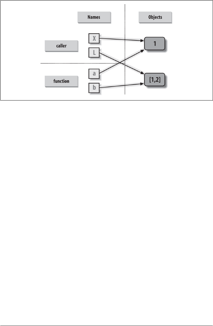
Figure 18-1. References: arguments. Because arguments are passed by assignment, argument names
in the function may share objects with variables in the scope of the call. Hence, in-place changes to
mutable arguments in a function can impact the caller. Here, a and b in the function initially reference
the objects referenced by variables X and L when the function is first called. Changing the list through
variable b makes L appear different after the call returns.
If you recall our discussions about shared mutable objects in Chapter 6 and Chap-
ter 9, you’ll recognize the phenomenon at work: changing a mutable object in place
can impact other references to that object. Here, the effect is to make one of the argu-
ments work like both an input and an output of the function.
Avoiding Mutable Argument Changes
This behavior of in-place changes to mutable arguments isn’t a bug—it’s simply the
way argument passing works in Python, and turns out to be widely useful in practice.
Arguments are normally passed to functions by reference because that is what we nor-
mally want. It means we can pass large objects around our programs without making
multiple copies along the way, and we can easily update these objects as we go. In fact,
as we’ll see in Part VI, Python’s class model depends upon changing a passed-in “self”
argument in place, to update object state.
If we don’t want in-place changes within functions to impact objects we pass to them,
though, we can simply make explicit copies of mutable objects, as we learned in Chap-
ter 6. For function arguments, we can always copy the list at the point of call, with tools
like list, list.copy as of 3.3, or an empty slice:
L = [1, 2]
changer(X, L[:]) # Pass a copy, so our 'L' does not change
We can also copy within the function itself, if we never want to change passed-in ob-
jects, regardless of how the function is called:
526 | Chapter 18: Arguments
www.it-ebooks.info

def changer(a, b):
b = b[:] # Copy input list so we don't impact caller
a = 2
b[0] = 'spam' # Changes our list copy only
Both of these copying schemes don’t stop the function from changing the object—they
just prevent those changes from impacting the caller. To really prevent changes, we can
always convert to immutable objects to force the issue. Tuples, for example, raise an
exception when changes are attempted:
L = [1, 2]
changer(X, tuple(L)) # Pass a tuple, so changes are errors
This scheme uses the built-in tuple function, which builds a new tuple out of all the
items in a sequence (really, any iterable). It’s also something of an extreme—because
it forces the function to be written to never change passed-in arguments, this solution
might impose more limitations on the function than it should, and so should generally
be avoided (you never know when changing arguments might come in handy for other
calls in the future). Using this technique will also make the function lose the ability to
call any list-specific methods on the argument, including methods that do not change
the object in place.
The main point to remember here is that functions might update mutable objects like
lists and dictionaries passed into them. This isn’t necessarily a problem if it’s expected,
and often serves useful purposes. Moreover, functions that change passed-in mutable
objects in place are probably designed and intended to do so—the change is likely part
of a well-defined API that you shouldn’t violate by making copies.
However, you do have to be aware of this property—if objects change out from under
you unexpectedly, check whether a called function might be responsible, and make
copies when objects are passed if needed.
Simulating Output Parameters and Multiple Results
We’ve already discussed the return statement and used it in a few examples. Here’s
another way to use this statement: because return can send back any sort of object, it
can return multiple values by packaging them in a tuple or other collection type. In fact,
although Python doesn’t support what some languages label “call by reference” argu-
ment passing, we can usually simulate it by returning tuples and assigning the results
back to the original argument names in the caller:
>>> def multiple(x, y):
x = 2 # Changes local names only
y = [3, 4]
return x, y # Return multiple new values in a tuple
>>> X = 1
>>> L = [1, 2]
>>> X, L = multiple(X, L) # Assign results to caller's names
Argument-Passing Basics | 527
www.it-ebooks.info

>>> X, L
(2, [3, 4])
It looks like the code is returning two values here, but it’s really just one—a two-item
tuple with the optional surrounding parentheses omitted. After the call returns, we can
use tuple assignment to unpack the parts of the returned tuple. (If you’ve forgotten why
this works, flip back to “Tuples” in Chapter 4 and Chapter 9, and “Assignment State-
ments” in Chapter 11.) The net effect of this coding pattern is to both send back multiple
results and simulate the output parameters of other languages by explicit assignments.
Here, X and L change after the call, but only because the code said so.
Unpacking arguments in Python 2.X: The preceding example unpacks a
tuple returned by the function with tuple assignment. In Python 2.X,
it’s also possible to automatically unpack tuples in arguments passed
to a function. In 2.X (only), a function defined by this header:
def f((a, (b, c))):
can be called with tuples that match the expected structure: f((1, (2,
3))) assigns a, b, and c to 1, 2, and 3, respectively. Naturally, the passed
tuple can also be an object created before the call (f(T)). This def syntax
is no longer supported in Python 3.X. Instead, code this function as:
def f(T): (a, (b, c)) = T
to unpack in an explicit assignment statement. This explicit form works
in both 3.X and 2.X. Argument unpacking is reportedly an obscure and
rarely used feature in Python 2.X (except in code that uses it!). More-
over, a function header in 2.X supports only the tuple form of sequence
assignment; more general sequence assignments (e.g., def f((a, [b,
c])):) fail on syntax errors in 2.X as well and require the explicit as-
signment form mandated in 3.X. Conversely, arbitrary sequences in the
call successfully match tuples in the header (e.g., f((1, [2, 3])), f((1,
"ab"))).
Tuple unpacking argument syntax is also disallowed by 3.X in lambda
function argument lists: see the Chapter 20 sidebar “Why You Will
Care: List Comprehensions and map” on page 590 for a lambda un-
packing example. Somewhat asymmetrically, tuple unpacking assign-
ment is still automatic in 3.X for loops targets; see Chapter 13 for ex-
amples.
Special Argument-Matching Modes
As we’ve just seen, arguments are always passed by assignment in Python; names in the
def header are assigned to passed-in objects. On top of this model, though, Python
provides additional tools that alter the way the argument objects in a call are
matched with argument names in the header prior to assignment. These tools are all
528 | Chapter 18: Arguments
www.it-ebooks.info

optional, but they allow us to write functions that support more flexible calling pat-
terns, and you may encounter some libraries that require them.
By default, arguments are matched by position, from left to right, and you must pass
exactly as many arguments as there are argument names in the function header. How-
ever, you can also specify matching by name, provide default values, and use collectors
for extra arguments.
Argument Matching Basics
Before we go into the syntactic details, I want to stress that these special modes are
optional and deal only with matching objects to names; the underlying passing mech-
anism after the matching takes place is still assignment. In fact, some of these tools are
intended more for people writing libraries than for application developers. But because
you may stumble across these modes even if you don’t code them yourself, here’s a
synopsis of the available tools:
Positionals: matched from left to right
The normal case, which we’ve mostly been using so far, is to match passed argu-
ment values to argument names in a function header by position, from left to right.
Keywords: matched by argument name
Alternatively, callers can specify which argument in the function is to receive a
value by using the argument’s name in the call, with the name=value syntax.
Defaults: specify values for optional arguments that aren’t passed
Functions themselves can specify default values for arguments to receive if the call
passes too few values, again using the name=value syntax.
Varargs collecting: collect arbitrarily many positional or keyword arguments
Functions can use special arguments preceded with one or two * characters to
collect an arbitrary number of possibly extra arguments. This feature is often re-
ferred to as varargs, after a variable-length argument list tool in the C language; in
Python, the arguments are collected in a normal object.
Varargs unpacking: pass arbitrarily many positional or keyword arguments
Callers can also use the * syntax to unpack argument collections into separate
arguments. This is the inverse of a * in a function header—in the header it means
collect arbitrarily many arguments, while in the call it means unpack arbitrarily
many arguments, and pass them individually as discrete values.
Keyword-only arguments: arguments that must be passed by name
In Python 3.X (but not 2.X), functions can also specify arguments that must be
passed by name with keyword arguments, not by position. Such arguments are
typically used to define configuration options in addition to actual arguments.
Special Argument-Matching Modes | 529
www.it-ebooks.info

Argument Matching Syntax
Table 18-1 summarizes the syntax that invokes the special argument-matching modes.
Table 18-1. Function argument-matching forms
Syntax Location Interpretation
func(value) Caller Normal argument: matched by position
func(name=value) Caller Keyword argument: matched by name
func(*iterable) Caller Pass all objects in iterable as individual positional arguments
func(**dict) Caller Pass all key/value pairs in dict as individual keyword arguments
def func(name) Function Normal argument: matches any passed value by position or name
def func(name=value) Function Default argument value, if not passed in the call
def func(*name) Function Matches and collects remaining positional arguments in a tuple
def func(**name) Function Matches and collects remaining keyword arguments in a dictionary
def func(*other, name) Function Arguments that must be passed by keyword only in calls (3.X)
def func(*, name=value) Function Arguments that must be passed by keyword only in calls (3.X)
These special matching modes break down into function calls and definitions as fol-
lows:
• In a function call (the first four rows of the table), simple values are matched by
position, but using the name=value form tells Python to match by name to argu-
ments instead; these are called keyword arguments. Using a *iterable or **dict in
a call allows us to package up arbitrarily many positional or keyword objects in
sequences (and other iterables) and dictionaries, respectively, and unpack them as
separate, individual arguments when they are passed to the function.
• In a function header (the rest of the table), a simple name is matched by position or
name depending on how the caller passes it, but the name=value form specifies a
default value. The *name form collects any extra unmatched positional arguments
in a tuple, and the **name form collects extra keyword arguments in a dictionary.
In Python 3.X, any normal or defaulted argument names following a *name or a
bare * are keyword-only arguments and must be passed by keyword in calls.
Of these, keyword arguments and defaults are probably the most commonly used in
Python code. We’ve informally used both of these earlier in this book:
• We’ve already used keywords to specify options to the 3.X print function, but they
are more general—keywords allow us to label any argument with its name, to make
calls more informational.
• We met defaults earlier, too, as a way to pass in values from the enclosing function’s
scope, but they are also more general—they allow us to make any argument op-
tional, providing its default value in a function definition.
530 | Chapter 18: Arguments
www.it-ebooks.info

As we’ll see, the combination of defaults in a function header and keywords in a call
further allows us to pick and choose which defaults to override.
In short, special argument-matching modes let you be fairly liberal about how many
arguments must be passed to a function. If a function specifies defaults, they are used
if you pass too few arguments. If a function uses the * variable argument list forms, you
can seemingly pass too many arguments; the * names collect the extra arguments in
data structures for processing in the function.
The Gritty Details
If you choose to use and combine the special argument-matching modes, Python will
ask you to follow these ordering rules among the modes’ optional components:
• In a function call, arguments must appear in this order: any positional arguments
(value); followed by a combination of any keyword arguments (name=value) and
the *iterable form; followed by the **dict form.
• In a function header, arguments must appear in this order: any normal arguments
(name); followed by any default arguments (name=value); followed by the *name (or
* in 3.X) form; followed by any name or name=value keyword-only arguments (in
3.X); followed by the **name form.
In both the call and header, the **args form must appear last if present. If you mix
arguments in any other order, you will get a syntax error because the combinations can
be ambiguous. The steps that Python internally carries out to match arguments before
assignment can roughly be described as follows:
1. Assign nonkeyword arguments by position.
2. Assign keyword arguments by matching names.
3. Assign extra nonkeyword arguments to *name tuple.
4. Assign extra keyword arguments to **name dictionary.
5. Assign default values to unassigned arguments in header.
After this, Python checks to make sure each argument is passed just one value; if not,
an error is raised. When all matching is complete, Python assigns argument names to
the objects passed to them.
The actual matching algorithm Python uses is a bit more complex (it must also account
for keyword-only arguments in 3.X, for instance), so we’ll defer to Python’s standard
language manual for a more exact description. It’s not required reading, but tracing
Python’s matching algorithm may help you to understand some convoluted cases, es-
pecially when modes are mixed.
Special Argument-Matching Modes | 531
www.it-ebooks.info

In Python 3.X only, argument names in a function header can also have
annotation values, specified as name:value (or name:value=default when
defaults are present). This is simply additional syntax for arguments and
does not augment or change the argument-ordering rules described
here. The function itself can also have an annotation value, given as def
f()->value. Python attaches annotation values to the function object.
See the discussion of function annotation in Chapter 19 for more details.
Keyword and Default Examples
This is all simpler in code than the preceding descriptions may imply. If you don’t use
any special matching syntax, Python matches names by position from left to right, like
most other languages. For instance, if you define a function that requires three argu-
ments, you must call it with three arguments:
>>> def f(a, b, c): print(a, b, c)
>>> f(1, 2, 3)
1 2 3
Here, we pass by position—a is matched to 1, b is matched to 2, and so on (this works
the same in Python 3.X and 2.X, but extra tuple parentheses are displayed in 2.X be-
cause we’re using 3.X print calls again).
Keywords
In Python, though, you can be more specific about what goes where when you call a
function. Keyword arguments allow us to match by name, instead of by position. Using
the same function:
>>> f(c=3, b=2, a=1)
1 2 3
The c=3 in this call, for example, means send 3 to the argument named c. More formally,
Python matches the name c in the call to the argument named c in the function defi-
nition’s header, and then passes the value 3 to that argument. The net effect of this call
is the same as that of the prior call, but notice that the left-to-right order of the argu-
ments no longer matters when keywords are used because arguments are matched by
name, not by position. It’s even possible to combine positional and keyword arguments
in a single call. In this case, all positionals are matched first from left to right in the
header, before keywords are matched by name:
>>> f(1, c=3, b=2) # a gets 1 by position, b and c passed by name
1 2 3
When most people see this the first time, they wonder why one would use such a tool.
Keywords typically have two roles in Python. First, they make your calls a bit more self-
documenting (assuming that you use better argument names than a, b, and c!). For
example, a call of this form:
532 | Chapter 18: Arguments
www.it-ebooks.info

func(name='Bob', age=40, job='dev')
is much more meaningful than a call with three naked values separated by commas,
especially in larger programs—the keywords serve as labels for the data in the call. The
second major use of keywords occurs in conjunction with defaults, which we turn to
next.
Defaults
We talked about defaults in brief earlier, when discussing nested function scopes. In
short, defaults allow us to make selected function arguments optional; if not passed a
value, the argument is assigned its default before the function runs. For example, here
is a function that requires one argument and defaults two:
>>> def f(a, b=2, c=3): print(a, b, c) # a required, b and c optional
When we call this function, we must provide a value for a, either by position or by
keyword; however, providing values for b and c is optional. If we don’t pass values to
b and c, they default to 2 and 3, respectively:
>>> f(1) # Use defaults
1 2 3
>>> f(a=1)
1 2 3
If we pass two values, only c gets its default, and with three values, no defaults are used:
>>> f(1, 4) # Override defaults
1 4 3
>>> f(1, 4, 5)
1 4 5
Finally, here is how the keyword and default features interact. Because they subvert the
normal left-to-right positional mapping, keywords allow us to essentially skip over
arguments with defaults:
>>> f(1, c=6) # Choose defaults
1 2 6
Here, a gets 1 by position, c gets 6 by keyword, and b, in between, defaults to 2.
Be careful not to confuse the special name=value syntax in a function header and a
function call; in the call it means a match-by-name keyword argument, while in the
header it specifies a default for an optional argument. In both cases, this is not an
assignment statement (despite its appearance); it is special syntax for these two con-
texts, which modifies the default argument-matching mechanics.
Combining keywords and defaults
Here is a slightly larger example that demonstrates keywords and defaults in action. In
the following, the caller must always pass at least two arguments (to match spam and
Special Argument-Matching Modes | 533
www.it-ebooks.info

eggs), but the other two are optional. If they are omitted, Python assigns toast and
ham to the defaults specified in the header:
def func(spam, eggs, toast=0, ham=0): # First 2 required
print((spam, eggs, toast, ham))
func(1, 2) # Output: (1, 2, 0, 0)
func(1, ham=1, eggs=0) # Output: (1, 0, 0, 1)
func(spam=1, eggs=0) # Output: (1, 0, 0, 0)
func(toast=1, eggs=2, spam=3) # Output: (3, 2, 1, 0)
func(1, 2, 3, 4) # Output: (1, 2, 3, 4)
Notice again that when keyword arguments are used in the call, the order in which the
arguments are listed doesn’t matter; Python matches by name, not by position. The
caller must supply values for spam and eggs, but they can be matched by position or by
name. Again, keep in mind that the form name=value means different things in the call
and the def: a keyword in the call and a default in the header.
Beware mutable defaults: As footnoted in the prior chapter, if you code
a default to be a mutable object (e.g., def f(a=[])), the same, single
mutable object is reused every time the function is later called—even if
it is changed in place within the function. The net effect is that the ar-
gument’s default retains its value from the prior call, and is not reset to
its original value coded in the def header. To reset anew on each call,
move the assignment into the function body instead. Mutable defaults
allow state retention, but this is often a surprise. Since this is such a
common trap, we’ll postpone further exploration until this part’s
“gotchas” list at the end of Chapter 21.
Arbitrary Arguments Examples
The last two matching extensions, * and **, are designed to support functions that take
any number of arguments. Both can appear in either the function definition or a function
call, and they have related purposes in the two locations.
Headers: Collecting arguments
The first use, in the function definition, collects unmatched positional arguments into
a tuple:
>>> def f(*args): print(args)
When this function is called, Python collects all the positional arguments into a new
tuple and assigns the variable args to that tuple. Because it is a normal tuple object, it
can be indexed, stepped through with a for loop, and so on:
>>> f()
()
>>> f(1)
(1,)
534 | Chapter 18: Arguments
www.it-ebooks.info

>>> f(1, 2, 3, 4)
(1, 2, 3, 4)
The ** feature is similar, but it only works for keyword arguments—it collects them
into a new dictionary, which can then be processed with normal dictionary tools. In a
sense, the ** form allows you to convert from keywords to dictionaries, which you can
then step through with keys calls, dictionary iterators, and the like (this is roughly what
the dict call does when passed keywords, but it returns the new dictionary):
>>> def f(**args): print(args)
>>> f()
{}
>>> f(a=1, b=2)
{'a': 1, 'b': 2}
Finally, function headers can combine normal arguments, the *, and the ** to imple-
ment wildly flexible call signatures. For instance, in the following, 1 is passed to a by
position, 2 and 3 are collected into the pargs positional tuple, and x and y wind up in
the kargs keyword dictionary:
>>> def f(a, *pargs, **kargs): print(a, pargs, kargs)
>>> f(1, 2, 3, x=1, y=2)
1 (2, 3) {'y': 2, 'x': 1}
Such code is rare, but shows up in functions that need to support multiple call patterns
(for backward compatibility, for instance). In fact, these features can be combined in
even more complex ways that may seem ambiguous at first glance—an idea we will
revisit later in this chapter. First, though, let’s see what happens when * and ** are
coded in function calls instead of definitions.
Calls: Unpacking arguments
In all recent Python releases, we can use the * syntax when we call a function, too. In
this context, its meaning is the inverse of its meaning in the function definition—it
unpacks a collection of arguments, rather than building a collection of arguments. For
example, we can pass four arguments to a function in a tuple and let Python unpack
them into individual arguments:
>>> def func(a, b, c, d): print(a, b, c, d)
>>> args = (1, 2)
>>> args += (3, 4)
>>> func(*args) # Same as func(1, 2, 3, 4)
1 2 3 4
Similarly, the ** syntax in a function call unpacks a dictionary of key/value pairs into
separate keyword arguments:
>>> args = {'a': 1, 'b': 2, 'c': 3}
>>> args['d'] = 4
Special Argument-Matching Modes | 535
www.it-ebooks.info
>>> func(**args) # Same as func(a=1, b=2, c=3, d=4)
1 2 3 4
Again, we can combine normal, positional, and keyword arguments in the call in very
flexible ways:
>>> func(*(1, 2), **{'d': 4, 'c': 3}) # Same as func(1, 2, d=4, c=3)
1 2 3 4
>>> func(1, *(2, 3), **{'d': 4}) # Same as func(1, 2, 3, d=4)
1 2 3 4
>>> func(1, c=3, *(2,), **{'d': 4}) # Same as func(1, 2, c=3, d=4)
1 2 3 4
>>> func(1, *(2, 3), d=4) # Same as func(1, 2, 3, d=4)
1 2 3 4
>>> func(1, *(2,), c=3, **{'d':4}) # Same as func(1, 2, c=3, d=4)
1 2 3 4
This sort of code is convenient when you cannot predict the number of arguments that
will be passed to a function when you write your script; you can build up a collection
of arguments at runtime instead and call the function generically this way. Again, don’t
confuse the */** starred-argument syntax in the function header and the function call
—in the header it collects any number of arguments, while in the call it unpacks any
number of arguments. In both, one star means positionals, and two applies to key-
words.
As we saw in Chapter 14, the *pargs form in a call is an iteration con-
text, so technically it accepts any iterable object, not just tuples or other
sequences as shown in the examples here. For instance, a file object
works after the *, and unpacks its lines into individual arguments (e.g.,
func(*open('fname')). Watch for additional examples of this utility in
Chapter 20, after we study generators.
This generality is supported in both Python 3.X and 2.X, but it holds
true only for calls—a *pargs in a call allows any iterable, but the same
form in a def header always bundles extra arguments into a tuple. This
header behavior is similar in spirit and syntax to the * in Python 3.X
extended sequence unpacking assignment forms we met in Chap-
ter 11 (e.g., x, *y = z), though that star usage always creates lists, not
tuples.
Applying functions generically
The prior section’s examples may seem academic (if not downright esoteric), but they
are used more often than you might expect. Some programs need to call arbitrary func-
tions in a generic fashion, without knowing their names or arguments ahead of time.
In fact, the real power of the special “varargs” call syntax is that you don’t need to know
how many arguments a function call requires before you write a script. For example,
you can use if logic to select from a set of functions and argument lists, and call any
of them generically (functions in some of the following examples are hypothetical):
536 | Chapter 18: Arguments
www.it-ebooks.info

if sometest:
action, args = func1, (1,) # Call func1 with one arg in this case
else:
action, args = func2, (1, 2, 3) # Call func2 with three args here
...etc...
action(*args) # Dispatch generically
This leverages both the * form, and the fact that functions are objects that may be both
referenced by, and called through, any variable. More generally, this varargs call syntax
is useful anytime you cannot predict the arguments list. If your user selects an arbitrary
function via a user interface, for instance, you may be unable to hardcode a function
call when writing your script. To work around this, simply build up the arguments list
with sequence operations, and call it with starred-argument syntax to unpack the ar-
guments:
>>> ...define or import func3...
>>> args = (2,3)
>>> args += (4,)
>>> args
(2, 3, 4)
>>> func3(*args)
Because the arguments list is passed in as a tuple here, the program can build it at
runtime. This technique also comes in handy for functions that test or time other func-
tions. For instance, in the following code we support any function with any arguments
by passing along whatever arguments were sent in (this is file tracer0.py in the book
examples package):
def tracer(func, *pargs, **kargs): # Accept arbitrary arguments
print('calling:', func.__name__)
return func(*pargs, **kargs) # Pass along arbitrary arguments
def func(a, b, c, d):
return a + b + c + d
print(tracer(func, 1, 2, c=3, d=4))
This code uses the built-in __name__ attribute attached to every function (as you might
expect, it’s the function’s name string), and uses stars to collect and then unpack the
arguments intended for the traced function. In other words, when this code is run,
arguments are intercepted by the tracer and then propagated with varargs call syntax:
calling: func
10
For another example of this technique, see the preview near the end of the preceding
chapter, where it was used to reset the built-in open function. We’ll code additional
examples of such roles later in this book; see especially the sequence timing examples
in Chapter 21 and the various decorator utilities we will code in Chapter 39. It’s a
common technique in general tools.
Special Argument-Matching Modes | 537
www.it-ebooks.info

The defunct apply built-in (Python 2.X)
Prior to Python 3.X, the effect of the *args and **args varargs call syntax could be
achieved with a built-in function named apply. This original technique has been re-
moved in 3.X because it is now redundant (3.X cleans up many such dusty tools that
have been subsumed over the years). It’s still available in all Python 2.X releases,
though, and you may come across it in older 2.X code.
In short, the following are equivalent prior to Python 3.X:
func(*pargs, **kargs) # Newer call syntax: func(*sequence, **dict)
apply(func, pargs, kargs) # Defunct built-in: apply(func, sequence, dict)
For example, consider the following function, which accepts any number of positional
or keyword arguments:
>>> def echo(*args, **kwargs): print(args, kwargs)
>>> echo(1, 2, a=3, b=4)
(1, 2) {'a': 3, 'b': 4}
In Python 2.X, we can call it generically with apply, or with the call syntax that is now
required in 3.X:
>>> pargs = (1, 2)
>>> kargs = {'a':3, 'b':4}
>>> apply(echo, pargs, kargs)
(1, 2) {'a': 3, 'b': 4}
>>> echo(*pargs, **kargs)
(1, 2) {'a': 3, 'b': 4}
Both forms work for built-in functions in 2.X too (notice 2.X’s trailing L for its long
integers):
>>> apply(pow, (2, 100))
1267650600228229401496703205376L
>>> pow(*(2, 100))
1267650600228229401496703205376L
The unpacking call syntax form is newer than the apply function, is preferred in general,
and is required in 3.X. (Technically, it was added in 2.0, was documented as deprecated
in 2.3, is still usable without warning in 2.7, and is gone in 3.0 and later.) Apart from
its symmetry with the * collector forms in def headers, and the fact that it requires fewer
keystrokes, the newer call syntax also allows us to pass along additional arguments
without having to manually extend argument sequences or dictionaries:
>>> echo(0, c=5, *pargs, **kargs) # Normal, keyword, *sequence, **dictionary
(0, 1, 2) {'a': 3, 'c': 5, 'b': 4}
That is, the call syntax form is more general. Since it’s required in 3.X, you should now
disavow all knowledge of apply (unless, of course, it appears in 2.X code you must use
or maintain...).
538 | Chapter 18: Arguments
www.it-ebooks.info

Python 3.X Keyword-Only Arguments
Python 3.X generalizes the ordering rules in function headers to allow us to specify
keyword-only arguments—arguments that must be passed by keyword only and will
never be filled in by a positional argument. This is useful if we want a function to both
process any number of arguments and accept possibly optional configuration options.
Syntactically, keyword-only arguments are coded as named arguments that may appear
after *args in the arguments list. All such arguments must be passed using keyword
syntax in the call. For example, in the following, a may be passed by name or position,
b collects any extra positional arguments, and c must be passed by keyword only. In 3.X:
>>> def kwonly(a, *b, c):
print(a, b, c)
>>> kwonly(1, 2, c=3)
1 (2,) 3
>>> kwonly(a=1, c=3)
1 () 3
>>> kwonly(1, 2, 3)
TypeError: kwonly() missing 1 required keyword-only argument: 'c'
We can also use a * character by itself in the arguments list to indicate that a function
does not accept a variable-length argument list but still expects all arguments following
the * to be passed as keywords. In the next function, a may be passed by position or
name again, but b and c must be keywords, and no extra positionals are allowed:
>>> def kwonly(a, *, b, c):
print(a, b, c)
>>> kwonly(1, c=3, b=2)
1 2 3
>>> kwonly(c=3, b=2, a=1)
1 2 3
>>> kwonly(1, 2, 3)
TypeError: kwonly() takes 1 positional argument but 3 were given
>>> kwonly(1)
TypeError: kwonly() missing 2 required keyword-only arguments: 'b' and 'c'
You can still use defaults for keyword-only arguments, even though they appear after
the * in the function header. In the following code, a may be passed by name or position,
and b and c are optional but must be passed by keyword if used:
>>> def kwonly(a, *, b='spam', c='ham'):
print(a, b, c)
>>> kwonly(1)
1 spam ham
>>> kwonly(1, c=3)
1 spam 3
>>> kwonly(a=1)
1 spam ham
>>> kwonly(c=3, b=2, a=1)
1 2 3
Special Argument-Matching Modes | 539
www.it-ebooks.info

>>> kwonly(1, 2)
TypeError: kwonly() takes 1 positional argument but 2 were given
In fact, keyword-only arguments with defaults are optional, but those without defaults
effectively become required keywords for the function:
>>> def kwonly(a, *, b, c='spam'):
print(a, b, c)
>>> kwonly(1, b='eggs')
1 eggs spam
>>> kwonly(1, c='eggs')
TypeError: kwonly() missing 1 required keyword-only argument: 'b'
>>> kwonly(1, 2)
TypeError: kwonly() takes 1 positional argument but 2 were given
>>> def kwonly(a, *, b=1, c, d=2):
print(a, b, c, d)
>>> kwonly(3, c=4)
3 1 4 2
>>> kwonly(3, c=4, b=5)
3 5 4 2
>>> kwonly(3)
TypeError: kwonly() missing 1 required keyword-only argument: 'c'
>>> kwonly(1, 2, 3)
TypeError: kwonly() takes 1 positional argument but 3 were given
Ordering rules
Finally, note that keyword-only arguments must be specified after a single star, not two
—named arguments cannot appear after the **args arbitrary keywords form, and a
** can’t appear by itself in the arguments list. Both attempts generate a syntax error:
>>> def kwonly(a, **pargs, b, c):
SyntaxError: invalid syntax
>>> def kwonly(a, **, b, c):
SyntaxError: invalid syntax
This means that in a function header, keyword-only arguments must be coded before
the **args arbitrary keywords form and after the *args arbitrary positional form, when
both are present. Whenever an argument name appears before *args, it is a possibly
default positional argument, not keyword-only:
>>> def f(a, *b, **d, c=6): print(a, b, c, d) # Keyword-only before **!
SyntaxError: invalid syntax
>>> def f(a, *b, c=6, **d): print(a, b, c, d) # Collect args in header
>>> f(1, 2, 3, x=4, y=5) # Default used
1 (2, 3) 6 {'y': 5, 'x': 4}
>>> f(1, 2, 3, x=4, y=5, c=7) # Override default
1 (2, 3) 7 {'y': 5, 'x': 4}
540 | Chapter 18: Arguments
www.it-ebooks.info

>>> f(1, 2, 3, c=7, x=4, y=5) # Anywhere in keywords
1 (2, 3) 7 {'y': 5, 'x': 4}
>>> def f(a, c=6, *b, **d): print(a, b, c, d) # c is not keyword-only here!
>>> f(1, 2, 3, x=4)
1 (3,) 2 {'x': 4}
In fact, similar ordering rules hold true in function calls: when keyword-only arguments
are passed, they must appear before a **args form. The keyword-only argument can
be coded either before or after the *args, though, and may be included in **args:
>>> def f(a, *b, c=6, **d): print(a, b, c, d) # KW-only between * and **
>>> f(1, *(2, 3), **dict(x=4, y=5)) # Unpack args at call
1 (2, 3) 6 {'y': 5, 'x': 4}
>>> f(1, *(2, 3), **dict(x=4, y=5), c=7) # Keywords before **args!
SyntaxError: invalid syntax
>>> f(1, *(2, 3), c=7, **dict(x=4, y=5)) # Override default
1 (2, 3) 7 {'y': 5, 'x': 4}
>>> f(1, c=7, *(2, 3), **dict(x=4, y=5)) # After or before *
1 (2, 3) 7 {'y': 5, 'x': 4}
>>> f(1, *(2, 3), **dict(x=4, y=5, c=7)) # Keyword-only in **
1 (2, 3) 7 {'y': 5, 'x': 4}
Trace through these cases on your own, in conjunction with the general argument-
ordering rules described formally earlier. They may appear to be worst cases in the
artificial examples here, but they can come up in real practice, especially for people
who write libraries and tools for other Python programmers to use.
Why keyword-only arguments?
So why care about keyword-only arguments? In short, they make it easier to allow a
function to accept both any number of positional arguments to be processed, and con-
figuration options passed as keywords. While their use is optional, without keyword-
only arguments extra work may be required to provide defaults for such options and
to verify that no superfluous keywords were passed.
Imagine a function that processes a set of passed-in objects and allows a tracing flag to
be passed:
process(X, Y, Z) # Use flag's default
process(X, Y, notify=True) # Override flag default
Without keyword-only arguments we have to use both *args and **args and manually
inspect the keywords, but with keyword-only arguments less code is required. The
following guarantees that no positional argument will be incorrectly matched against
notify and requires that it be a keyword if passed:
Special Argument-Matching Modes | 541
www.it-ebooks.info

def process(*args, notify=False): ...
Since we’re going to see a more realistic example of this later in this chapter, in “Em-
ulating the Python 3.X print Function,” I’ll postpone the rest of this story until then.
For an additional example of keyword-only arguments in action, see the iteration op-
tions timing case study in Chapter 21. And for additional function definition enhance-
ments in Python 3.X, stay tuned for the discussion of function annotation syntax in
Chapter 19.
The min Wakeup Call!
OK—it’s time for something more realistic. To make this chapter’s concepts more
concrete, let’s work through an exercise that demonstrates a practical application of
argument-matching tools.
Suppose you want to code a function that is able to compute the minimum value from
an arbitrary set of arguments and an arbitrary set of object data types. That is, the
function should accept zero or more arguments, as many as you wish to pass. Moreover,
the function should work for all kinds of Python object types: numbers, strings, lists,
lists of dictionaries, files, and even None.
The first requirement provides a natural example of how the * feature can be put to
good use—we can collect arguments into a tuple and step over each of them in turn
with a simple for loop. The second part of the problem definition is easy: because every
object type supports comparisons, we don’t have to specialize the function per type (an
application of polymorphism); we can simply compare objects blindly and let Python
worry about what sort of comparison to perform according to the objects being com-
pared.
Full Credit
The following file shows three ways to code this operation, at least one of which was
suggested by a student in one of my courses (this example is often a group exercise to
circumvent dozing after lunch):
• The first function fetches the first argument (args is a tuple) and traverses the rest
by slicing off the first (there’s no point in comparing an object to itself, especially
if it might be a large structure).
• The second version lets Python pick off the first and rest of the arguments auto-
matically, and so avoids an index and slice.
• The third converts from a tuple to a list with the built-in list call and employs the
list sort method.
542 | Chapter 18: Arguments
www.it-ebooks.info

The sort method is coded in C, so it can be quicker than the other approaches at times,
but the linear scans of the first two techniques may make them faster much of the
time.1 The file mins.py contains the code for all three solutions:
def min1(*args):
res = args[0]
for arg in args[1:]:
if arg < res:
res = arg
return res
def min2(first, *rest):
for arg in rest:
if arg < first:
first = arg
return first
def min3(*args):
tmp = list(args) # Or, in Python 2.4+: return sorted(args)[0]
tmp.sort()
return tmp[0]
print(min1(3, 4, 1, 2))
print(min2("bb", "aa"))
print(min3([2,2], [1,1], [3,3]))
All three solutions produce the same result when the file is run. Try typing a few calls
interactively to experiment with these on your own:
% python mins.py
1
aa
[1, 1]
Notice that none of these three variants tests for the case where no arguments are passed
in. They could, but there’s no point in doing so here—in all three solutions, Python
will automatically raise an exception if no arguments are passed in. The first variant
raises an exception when we try to fetch item 0, the second when Python detects an
argument list mismatch, and the third when we try to return item 0 at the end.
This is exactly what we want to happen—because these functions support any data
type, there is no valid sentinel value that we could pass back to designate an error, so
we may as well let the exception be raised. There are exceptions to this rule (e.g., you
1. Actually, this is fairly complicated. The Python sort routine is coded in C and uses a highly optimized
algorithm that attempts to take advantage of partial ordering in the items to be sorted. It’s named “timsort”
after Tim Peters, its creator, and in its documentation it claims to have “supernatural performance” at
times (pretty good, for a sort!). Still, sorting is an inherently exponential operation (it must chop up the
sequence and put it back together many times), and the other versions simply perform one linear left-to-
right scan. The net effect is that sorting is quicker if the arguments are partially ordered, but is likely to
be slower otherwise (this still holds true in test runs in 3.3). Even so, Python performance can change
over time, and the fact that sorting is implemented in the C language can help greatly; for an exact analysis,
you should time the alternatives with the time or timeit modules—we’ll see how in Chapter 21.
The min Wakeup Call! | 543
www.it-ebooks.info

might test for errors yourself if you’d rather avoid actions run before reaching the code
that triggers an error automatically), but in general it’s better to assume that arguments
will work in your functions’ code and let Python raise errors for you when they do not.
Bonus Points
You can get bonus points here for changing these functions to compute the maxi-
mum, rather than minimum, values. This one’s easy: the first two versions only require
changing < to >, and the third simply requires that we return tmp[−1] instead of
tmp[0]. For an extra point, be sure to set the function name to “max” as well (though
this part is strictly optional).
It’s also possible to generalize a single function to compute either a minimum or a
maximum value, by evaluating comparison expression strings with a tool like the
eval built-in function (see the library manual, and various appearances here, especially
in Chapter 10) or passing in an arbitrary comparison function. The file minmax.py
shows how to implement the latter scheme:
def minmax(test, *args):
res = args[0]
for arg in args[1:]:
if test(arg, res):
res = arg
return res
def lessthan(x, y): return x < y # See also: lambda, eval
def grtrthan(x, y): return x > y
print(minmax(lessthan, 4, 2, 1, 5, 6, 3)) # Self-test code
print(minmax(grtrthan, 4, 2, 1, 5, 6, 3))
% python minmax.py
1
6
Functions are another kind of object that can be passed into a function like this one.
To make this a max (or other) function, for example, we simply pass in the right sort of
test function. This may seem like extra work, but the main point of generalizing func-
tions this way—instead of cutting and pasting to change just a single character—is that
we’ll only have one version to change in the future, not two.
The Punch Line...
Of course, all this was just a coding exercise. There’s really no reason to code min or
max functions, because both are built-ins in Python! We met them briefly in Chap-
ter 5 in conjunction with numeric tools, and again in Chapter 14 when exploring iter-
ation contexts. The built-in versions work almost exactly like ours, but they’re coded
in C for optimal speed and accept either a single iterable or multiple arguments. Still,
544 | Chapter 18: Arguments
www.it-ebooks.info

though it’s superfluous in this context, the general coding pattern we used here might
be useful in other scenarios.
Generalized Set Functions
Let’s look at a more useful example of special argument-matching modes at work. At
the end of Chapter 16, we wrote a function that returned the intersection of two se-
quences (it picked out items that appeared in both). Here is a version that intersects an
arbitrary number of sequences (one or more) by using the varargs matching form
*args to collect all the passed-in arguments. Because the arguments come in as a tuple,
we can process them in a simple for loop. Just for fun, we’ll code a union function that
also accepts an arbitrary number of arguments to collect items that appear in any of
the operands:
def intersect(*args):
res = []
for x in args[0]: # Scan first sequence
if x in res: continue # Skip duplicates
for other in args[1:]: # For all other args
if x not in other: break # Item in each one?
else: # No: break out of loop
res.append(x) # Yes: add items to end
return res
def union(*args):
res = []
for seq in args: # For all args
for x in seq: # For all nodes
if not x in res:
res.append(x) # Add new items to result
return res
Because these are tools potentially worth reusing (and they’re too big to retype inter-
actively), we’ll store the functions in a module file called inter2.py (if you’ve forgotten
how modules and imports work, see the introduction in Chapter 3, or stay tuned for
in-depth coverage in Part V). In both functions, the arguments passed in at the call
come in as the args tuple. As in the original intersect, both work on any kind of
sequence. Here, they are processing strings, mixed types, and more than two sequences:
% python
>>> from inter2 import intersect, union
>>> s1, s2, s3 = "SPAM", "SCAM", "SLAM"
>>> intersect(s1, s2), union(s1, s2) # Two operands
(['S', 'A', 'M'], ['S', 'P', 'A', 'M', 'C'])
>>> intersect([1, 2, 3], (1, 4)) # Mixed types
[1]
>>> intersect(s1, s2, s3) # Three operands
['S', 'A', 'M']
Generalized Set Functions | 545
www.it-ebooks.info

>>> union(s1, s2, s3)
['S', 'P', 'A', 'M', 'C', 'L']
To test more thoroughly, the following codes a function to apply the two tools to
arguments in different orders using a simple shuffling technique that we saw in Chap-
ter 13—it slices to move the first to the end on each loop, uses a * to unpack arguments,
and sorts so results are comparable:
>>> def tester(func, items, trace=True):
for i in range(len(items)):
items = items[1:] + items[:1]
if trace: print(items)
print(sorted(func(*items)))
>>> tester(intersect, ('a', 'abcdefg', 'abdst', 'albmcnd'))
('abcdefg', 'abdst', 'albmcnd', 'a')
['a']
('abdst', 'albmcnd', 'a', 'abcdefg')
['a']
('albmcnd', 'a', 'abcdefg', 'abdst')
['a']
('a', 'abcdefg', 'abdst', 'albmcnd')
['a']
>>> tester(union, ('a', 'abcdefg', 'abdst', 'albmcnd'), False)
['a', 'b', 'c', 'd', 'e', 'f', 'g', 'l', 'm', 'n', 's', 't']
['a', 'b', 'c', 'd', 'e', 'f', 'g', 'l', 'm', 'n', 's', 't']
['a', 'b', 'c', 'd', 'e', 'f', 'g', 'l', 'm', 'n', 's', 't']
['a', 'b', 'c', 'd', 'e', 'f', 'g', 'l', 'm', 'n', 's', 't']
>>> tester(intersect, ('ba', 'abcdefg', 'abdst', 'albmcnd'), False)
['a', 'b']
['a', 'b']
['a', 'b']
['a', 'b']
The argument scrambling here doesn’t generate all possible argument orders (that
would require a full permutation, and 24 orderings for 4 arguments), but suffices to
check if argument order impacts results here. If you test these further, you’ll notice that
duplicates won’t appear in either intersection or union results, which qualify them as
set operations from a mathematical perspective:
>>> intersect([1, 2, 1, 3], (1, 1, 4))
[1]
>>> union([1, 2, 1, 3], (1, 1, 4))
[1, 2, 3, 4]
>>> tester(intersect, ('ababa', 'abcdefga', 'aaaab'), False)
['a', 'b']
['a', 'b']
['a', 'b']
These are still far from optimal from an algorithmic perspective, but due to the fol-
lowing note, we’ll leave further improvements to this code as suggested exercise. Also
546 | Chapter 18: Arguments
www.it-ebooks.info

notice that the argument scrambling in our tester function might be a generally useful
tool, and the tester would be simpler if we delegated this to another function, one that
would be free to create or generate argument combinations as it saw fit:
>>> def tester(func, items, trace=True):
for args in scramble(items):
...use args...
In fact we will—watch for this example to be revised in Chapter 20 to address this last
point, after we’ve learned how to code user-defined generators. We’ll also recode the
set operations one last time in Chapter 32 and a solution to a Part VI exercise as
classes that extend the list object with methods.
Because Python now has a set object type (described in Chapter 5), none
of the set-processing examples in this book are strictly required any-
more; they are included just as demonstrations of coding techniques,
and are today instructional only. Because it’s constantly improving and
growing, Python has an uncanny way of conspiring to make my book
examples obsolete over time!
Emulating the Python 3.X print Function
To round out the chapter, let’s look at one last example of argument matching at work.
The code you’ll see here is intended for use in Python 2.X or earlier (it works in 3.X,
too, but is pointless there): it uses both the *args arbitrary positional tuple and the
**args arbitrary keyword-arguments dictionary to simulate most of what the Python
3.X print function does. Python might have offered code like this as an option in 3.X
rather than removing the 2.X print entirely, but 3.X chose a clean break with the past
instead.
As we learned in Chapter 11, this isn’t actually required, because 2.X programmers can
always enable the 3.X print function with an import of this form (available in 2.6 and
2.7):
from __future__ import print_function
To demonstrate argument matching in general, though, the following file, print3.py,
does the same job in a small amount of reusable code, by building up the print string
and routing it per configuration arguments:
#!python
"""
Emulate most of the 3.X print function for use in 2.X (and 3.X).
Call signature: print3(*args, sep=' ', end='\n', file=sys.stdout)
"""
import sys
def print3(*args, **kargs):
sep = kargs.get('sep', ' ') # Keyword arg defaults
Emulating the Python 3.X print Function | 547
www.it-ebooks.info

end = kargs.get('end', '\n')
file = kargs.get('file', sys.stdout)
output = ''
first = True
for arg in args:
output += ('' if first else sep) + str(arg)
first = False
file.write(output + end)
To test it, import this into another file or the interactive prompt, and use it like the 3.X
print function. Here is a test script, testprint3.py (notice that the function must be called
“print3”, because “print” is a reserved word in 2.X):
from print3 import print3
print3(1, 2, 3)
print3(1, 2, 3, sep='') # Suppress separator
print3(1, 2, 3, sep='...')
print3(1, [2], (3,), sep='...') # Various object types
print3(4, 5, 6, sep='', end='') # Suppress newline
print3(7, 8, 9)
print3() # Add newline (or blank line)
import sys
print3(1, 2, 3, sep='??', end='.\n', file=sys.stderr) # Redirect to file
When this is run under 2.X, we get the same results as 3.X’s print function:
C:\code> c:\python27\python testprint3.py
1 2 3
123
1...2...3
1...[2]...(3,)
4567 8 9
1??2??3.
Although pointless in 3.X, the results are identical when run there. As usual, the gen-
erality of Python’s design allows us to prototype or develop concepts in the Python
language itself. In this case, argument-matching tools are as flexible in Python code as
they are in Python’s internal implementation.
Using Keyword-Only Arguments
It’s interesting to notice that this example could be coded with Python 3.X keyword-
only arguments, described earlier in this chapter, to automatically validate configura-
tion arguments. The following variant, in the file print3_alt1.py, illustrates:
#!python3
"Use 3.X only keyword-only args"
import sys
def print3(*args, sep=' ', end='\n', file=sys.stdout):
output = ''
548 | Chapter 18: Arguments
www.it-ebooks.info

first = True
for arg in args:
output += ('' if first else sep) + str(arg)
first = False
file.write(output + end)
This version works the same as the original, and it’s a prime example of how keyword-
only arguments come in handy. The original version assumes that all positional argu-
ments are to be printed, and all keywords are for options only. That’s almost sufficient,
but any extra keyword arguments are silently ignored. A call like the following, for
instance, will generate an exception correctly with the keyword-only form:
>>> print3(99, name='bob')
TypeError: print3() got an unexpected keyword argument 'name'
but will silently ignore the name argument in the original version. To detect superfluous
keywords manually, we could use dict.pop() to delete fetched entries, and check if the
dictionary is not empty. The following version, in the file print3_alt2.py, is equivalent
to the keyword-only version—it triggers a built-in exception with a raise statement,
which works just as though Python had done so (we’ll study this in more detail in
Part VII):
#!python
"Use 2.X/3.X keyword args deletion with defaults"
import sys
def print3(*args, **kargs):
sep = kargs.pop('sep', ' ')
end = kargs.pop('end', '\n')
file = kargs.pop('file', sys.stdout)
if kargs: raise TypeError('extra keywords: %s' % kargs)
output = ''
first = True
for arg in args:
output += ('' if first else sep) + str(arg)
first = False
file.write(output + end)
This works as before, but it now catches extraneous keyword arguments, too:
>>> print3(99, name='bob')
TypeError: extra keywords: {'name': 'bob'}
This version of the function runs under Python 2.X, but it requires four more lines of
code than the keyword-only version. Unfortunately, the extra code is unavoidable in
this case—the keyword-only version works on 3.X only, which negates most of the
reason that I wrote this example in the first place: a 3.X emulator that only works on
3.X isn’t incredibly useful! In programs written to run on 3.X only, though, keyword-
only arguments can simplify a specific category of functions that accept both arguments
and options. For another example of 3.X keyword-only arguments, be sure to see the
iteration timing case study in Chapter 21.
Emulating the Python 3.X print Function | 549
www.it-ebooks.info

Why You Will Care: Keyword Arguments
As you can probably tell, advanced argument-matching modes can be complex. They
are also largely optional in your code; you can get by with just simple positional match-
ing, and it’s probably a good idea to do so when you’re starting out. However, because
some Python tools make use of them, some general knowledge of these modes is im-
portant.
For example, keyword arguments play an important role in tkinter, the de facto stan-
dard GUI API for Python (this module’s name is Tkinter in Python 2.X). We touch on
tkinter only briefly at various points in this book, but in terms of its call patterns,
keyword arguments set configuration options when GUI components are built. For
instance, a call of the form:
from tkinter import *
widget = Button(text="Press me", command=someFunction)
creates a new button and specifies its text and callback function, using the text and
command keyword arguments. Since the number of configuration options for a widget
can be large, keyword arguments let you pick and choose which to apply. Without
them, you might have to either list all the possible options by position or hope for a
judicious positional argument defaults protocol that would handle every possible op-
tion arrangement.
Many built-in functions in Python expect us to use keywords for usage-mode options
as well, which may or may not have defaults. As we learned in Chapter 8, for instance,
the sorted built-in:
sorted(iterable, key=None, reverse=False)
expects us to pass an iterable object to be sorted, but also allows us to pass in optional
keyword arguments to specify a dictionary sort key and a reversal flag, which default
to None and False, respectively. Since we normally don’t use these options, they may
be omitted to use defaults.
As we’ve also seen, the dict, str.format, and 3.X print calls accept keywords as well
—other usages we had to introduce in earlier chapters because of their forward de-
pendence on argument-passing modes we’ve studied here (alas, those who change
Python already know Python!).
Chapter Summary
In this chapter, we studied the second of two key concepts related to functions: argu-
ments—how objects are passed into a function. As we learned, arguments are passed
into a function by assignment, which means by object reference (which really means
by pointer). We also studied some more advanced extensions, including default and
keyword arguments, tools for using arbitrarily many arguments, and keyword-only
arguments in 3.X. Finally, we saw how mutable arguments can exhibit the same be-
550 | Chapter 18: Arguments
www.it-ebooks.info

havior as other shared references to objects—unless the object is explicitly copied when
it’s sent in, changing a passed-in mutable in a function can impact the caller.
The next chapter continues our look at functions by exploring some more advanced
function-related ideas: function annotations, recursion, lambdas, and functional tools
such as map and filter. Many of these concepts stem from the fact that functions are
normal objects in Python, and so support some advanced and very flexible processing
modes. Before diving into those topics, however, take this chapter’s quiz to review the
argument ideas we’ve studied here.
Test Your Knowledge: Quiz
In most of this quiz’s questions, results may vary slightly in 2.X—with enclosing paren-
theses and commas when multiple values are printed. To match the 3.X answers exactly
in 2.X, import print_function from __future__ before starting.
1. What is the output of the following code, and why?
>>> def func(a, b=4, c=5):
print(a, b, c)
>>> func(1, 2)
2. What is the output of this code, and why?
>>> def func(a, b, c=5):
print(a, b, c)
>>> func(1, c=3, b=2)
3. How about this code: what is its output, and why?
>>> def func(a, *pargs):
print(a, pargs)
>>> func(1, 2, 3)
4. What does this code print, and why?
>>> def func(a, **kargs):
print(a, kargs)
>>> func(a=1, c=3, b=2)
5. What gets printed by this, and why?
>>> def func(a, b, c=3, d=4): print(a, b, c, d)
>>> func(1, *(5, 6))
6. One last time: what is the output of this code, and why?
>>> def func(a, b, c): a = 2; b[0] = 'x'; c['a'] = 'y'
>>> l=1; m=[1]; n={'a':0}
Test Your Knowledge: Quiz | 551
www.it-ebooks.info

>>> func(l, m, n)
>>> l, m, n
Test Your Knowledge: Answers
1. The output here is 1 2 5, because 1 and 2 are passed to a and b by position, and
c is omitted in the call and defaults to 5.
2. The output this time is 1 2 3: 1 is passed to a by position, and b and c are passed
2 and 3 by name (the left-to-right order doesn’t matter when keyword arguments
are used like this).
3. This code prints 1 (2, 3), because 1 is passed to a and the *pargs collects the
remaining positional arguments into a new tuple object. We can step through the
extra positional arguments tuple with any iteration tool (e.g., for arg in
pargs: ...).
4. This time the code prints 1 {'b': 2, 'c': 3}, because 1 is passed to a by name
and the **kargs collects the remaining keyword arguments into a dictionary. We
could step through the extra keyword arguments dictionary by key with any iter-
ation tool (e.g., for key in kargs: ...). Note that the order of the dictionary’s
keys may vary per Python and other variables.
5. The output here is 1 5 6 4: the 1 matches a by position, 5 and 6 match b and c by
*name positionals (6 overrides c’s default), and d defaults to 4 because it was not
passed a value.
6. This displays (1, ['x'], {'a': 'y'})—the first assignment in the function doesn’t
impact the caller, but the second two do because they change passed-in mutable
objects in place.
552 | Chapter 18: Arguments
www.it-ebooks.info

CHAPTER 19
Advanced Function Topics
This chapter introduces a collection of more advanced function-related topics: recur-
sive functions, function attributes and annotations, the lambda expression, and func-
tional programming tools such as map and filter. These are all somewhat advanced
tools that, depending on your job description, you may not encounter on a regular
basis. Because of their roles in some domains, though, a basic understanding can be
useful; lambdas, for instance, are regular customers in GUIs, and functional program-
ming techniques are increasingly common in Python code.
Part of the art of using functions lies in the interfaces between them, so we will also
explore some general function design principles here. The next chapter continues this
advanced theme with an exploration of generator functions and expressions and a re-
vival of list comprehensions in the context of the functional tools we will study here.
Function Design Concepts
Now that we’ve had a chance to study function basics in Python, let’s begin this chapter
with a few words of context. When you start using functions in earnest, you’re faced
with choices about how to glue components together—for instance, how to decompose
a task into purposeful functions (known as cohesion), how your functions should com-
municate (called coupling), and so on. You also need to take into account concepts such
as the size of your functions, because they directly impact code usability. Some of this
falls into the category of structured analysis and design, but it applies to Python code
as to any other.
We introduced some ideas related to function and module coupling in Chapter 17 when
studying scopes, but here is a review of a few general guidelines for readers new to
function design principles:
•Coupling: use arguments for inputs and return for outputs. Generally, you
should strive to make a function independent of things outside of it. Arguments
and return statements are often the best ways to isolate external dependencies to
a small number of well-known places in your code.
553
www.it-ebooks.info

•Coupling: use global variables only when truly necessary. Global variables
(i.e., names in the enclosing module) are usually a poor way for functions to com-
municate. They can create dependencies and timing issues that make programs
difficult to debug, change, and reuse.
•Coupling: don’t change mutable arguments unless the caller expects it.
Functions can change parts of passed-in mutable objects, but (as with global vari-
ables) this creates a tight coupling between the caller and callee, which can make
a function too specific and brittle.
•Cohesion: each function should have a single, unified purpose. When de-
signed well, each of your functions should do one thing—something you can sum-
marize in a simple declarative sentence. If that sentence is very broad (e.g., “this
function implements my whole program”), or contains lots of conjunctions (e.g.,
“this function gives employee raises and submits a pizza order”), you might want
to think about splitting it into separate and simpler functions. Otherwise, there is
no way to reuse the code behind the steps mixed together in the function.
•Size: each function should be relatively small. This naturally follows from the
preceding goal, but if your functions start spanning multiple pages on your display,
it’s probably time to split them. Especially given that Python code is so concise to
begin with, a long or deeply nested function is often a symptom of design problems.
Keep it simple, and keep it short.
•Coupling: avoid changing variables in another module file directly. We in-
troduced this concept in Chapter 17, and we’ll revisit it in the next part of the book
when we focus on modules. For reference, though, remember that changing vari-
ables across file boundaries sets up a coupling between modules similar to how
global variables couple functions—the modules become difficult to understand
and reuse. Use accessor functions whenever possible, instead of direct assignment
statements.
Figure 19-1 summarizes the ways functions can talk to the outside world; inputs may
come from items on the left side, and results may be sent out in any of the forms on the
right. Good function designers prefer to use only arguments for inputs and return
statements for outputs, whenever possible.
Of course, there are plenty of exceptions to the preceding design rules, including some
related to Python’s OOP support. As you’ll see in Part VI, Python classes depend on
changing a passed-in mutable object—class functions set attributes of an automatically
passed-in argument called self to change per-object state information (e.g.,
self.name='bob'). Moreover, if classes are not used, global variables are often the most
straightforward way for functions in modules to retain single-copy state between calls.
Side effects are usually dangerous only if they’re unexpected.
In general though, you should strive to minimize external dependencies in functions
and other program components. The more self-contained a function is, the easier it will
be to understand, reuse, and modify.
554 | Chapter 19: Advanced Function Topics
www.it-ebooks.info
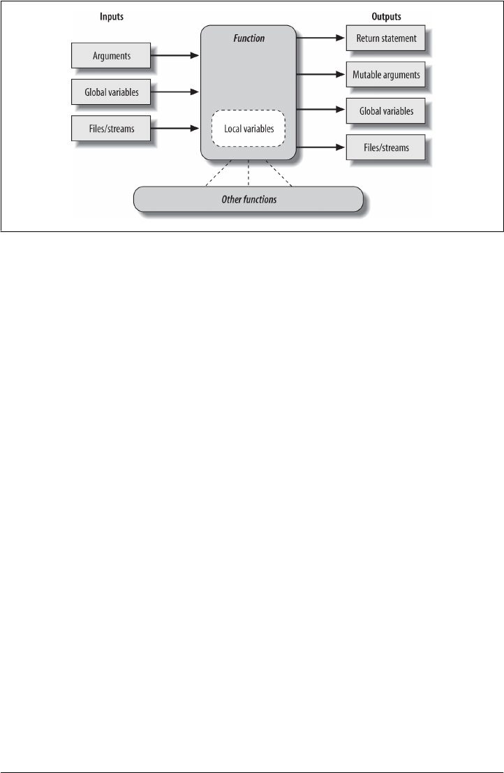
Recursive Functions
We mentioned recursion in relation to comparisons of core types in Chapter 9. While
discussing scope rules near the start of Chapter 17, we also briefly noted that Python
supports recursive functions—functions that call themselves either directly or indirectly
in order to loop. In this section, we’ll explore what this looks like in our functions’ code.
Recursion is a somewhat advanced topic, and it’s relatively rare to see in Python, partly
because Python’s procedural statements include simpler looping structures. Still, it’s a
useful technique to know about, as it allows programs to traverse structures that have
arbitrary and unpredictable shapes and depths—planning travel routes, analyzing lan-
guage, and crawling links on the Web, for example. Recursion is even an alternative to
simple loops and iterations, though not necessarily the simplest or most efficient one.
Summation with Recursion
Let’s look at some examples. To sum a list (or other sequence) of numbers, we can
either use the built-in sum function or write a more custom version of our own. Here’s
what a custom summing function might look like when coded with recursion:
>>> def mysum(L):
if not L:
return 0
else:
return L[0] + mysum(L[1:]) # Call myself recursively
Figure 19-1. Function execution environment. Functions may obtain input and produce output in a
variety of ways, though functions are usually easier to understand and maintain if you use arguments
for input and return statements and anticipated mutable argument changes for output. In Python 3.X
only, outputs may also take the form of declared nonlocal names that exist in an enclosing function
scope.
Recursive Functions | 555
www.it-ebooks.info

>>> mysum([1, 2, 3, 4, 5])
15
At each level, this function calls itself recursively to compute the sum of the rest of the
list, which is later added to the item at the front. The recursive loop ends and zero is
returned when the list becomes empty. When using recursion like this, each open level
of call to the function has its own copy of the function’s local scope on the runtime call
stack—here, that means L is different in each level.
If this is difficult to understand (and it often is for new programmers), try adding a
print of L to the function and run it again, to trace the current list at each call level:
>>> def mysum(L):
print(L) # Trace recursive levels
if not L: # L shorter at each level
return 0
else:
return L[0] + mysum(L[1:])
>>> mysum([1, 2, 3, 4, 5])
[1, 2, 3, 4, 5]
[2, 3, 4, 5]
[3, 4, 5]
[4, 5]
[5]
[]
15
As you can see, the list to be summed grows smaller at each recursive level, until it
becomes empty—the termination of the recursive loop. The sum is computed as the
recursive calls unwind on returns.
Coding Alternatives
Interestingly, we can use Python’s if/else ternary expression (described in Chap-
ter 12) to save some code real estate here. We can also generalize for any summable
type (which is easier if we assume at least one item in the input, as we did in Chap-
ter 18’s minimum value example) and use Python 3.X’s extended sequence assignment
to make the first/rest unpacking simpler (as covered in Chapter 11):
def mysum(L):
return 0 if not L else L[0] + mysum(L[1:]) # Use ternary expression
def mysum(L):
return L[0] if len(L) == 1 else L[0] + mysum(L[1:]) # Any type, assume one
def mysum(L):
first, *rest = L
return first if not rest else first + mysum(rest) # Use 3.X ext seq assign
The latter two of these fail for empty lists but allow for sequences of any object type
that supports +, not just numbers:
556 | Chapter 19: Advanced Function Topics
www.it-ebooks.info

>>> mysum([1]) # mysum([]) fails in last 2
1
>>> mysum([1, 2, 3, 4, 5])
15
>>> mysum(('s', 'p', 'a', 'm')) # But various types now work
'spam'
>>> mysum(['spam', 'ham', 'eggs'])
'spamhameggs'
Run these on your own for more insight. If you study these three variants, you’ll find
that:
• The latter two also work on a single string argument (e.g., mysum('spam')), because
strings are sequences of one-character strings.
• The third variant works on arbitrary iterables, including open input files
(mysum(open(name))), but the others do not because they index (Chapter 14 illus-
trates extended sequence assignment on files).
• The function header def mysum(first, *rest), although similar to the third var-
iant, wouldn’t work at all, because it expects individual arguments, not a single
iterable.
Keep in mind that recursion can be direct, as in the examples so far, or indirect, as in
the following (a function that calls another function, which calls back to its caller). The
net effect is the same, though there are two function calls at each level instead of one:
>>> def mysum(L):
if not L: return 0
return nonempty(L) # Call a function that calls me
>>> def nonempty(L):
return L[0] + mysum(L[1:]) # Indirectly recursive
>>> mysum([1.1, 2.2, 3.3, 4.4])
11.0
Loop Statements Versus Recursion
Though recursion works for summing in the prior sections’ examples, it’s probably
overkill in this context. In fact, recursion is not used nearly as often in Python as in
more esoteric languages like Prolog or Lisp, because Python emphasizes simpler pro-
cedural statements like loops, which are usually more natural. The while, for example,
often makes things a bit more concrete, and it doesn’t require that a function be defined
to allow recursive calls:
>>> L = [1, 2, 3, 4, 5]
>>> sum = 0
>>> while L:
sum += L[0]
L = L[1:]
Recursive Functions | 557
www.it-ebooks.info

>>> sum
15
Better yet, for loops iterate for us automatically, making recursion largely extraneous
in many cases (and, in all likelihood, less efficient in terms of memory space and exe-
cution time):
>>> L = [1, 2, 3, 4, 5]
>>> sum = 0
>>> for x in L: sum += x
>>> sum
15
With looping statements, we don’t require a fresh copy of a local scope on the call stack
for each iteration, and we avoid the speed costs associated with function calls in general.
(Stay tuned for Chapter 21’s timer case study for ways to compare the execution times
of alternatives like these.)
Handling Arbitrary Structures
On the other hand, recursion—or equivalent explicit stack-based algorithms we’ll meet
shortly—can be required to traverse arbitrarily shaped structures. As a simple example
of recursion’s role in this context, consider the task of computing the sum of all the
numbers in a nested sublists structure like this:
[1, [2, [3, 4], 5], 6, [7, 8]] # Arbitrarily nested sublists
Simple looping statements won’t work here because this is not a linear iteration. Nested
looping statements do not suffice either, because the sublists may be nested to arbitrary
depth and in an arbitrary shape—there’s no way to know how many nested loops to
code to handle all cases. Instead, the following code accommodates such general nest-
ing by using recursion to visit sublists along the way:
# file sumtree.py
def sumtree(L):
tot = 0
for x in L: # For each item at this level
if not isinstance(x, list):
tot += x # Add numbers directly
else:
tot += sumtree(x) # Recur for sublists
return tot
L = [1, [2, [3, 4], 5], 6, [7, 8]] # Arbitrary nesting
print(sumtree(L)) # Prints 36
# Pathological cases
print(sumtree([1, [2, [3, [4, [5]]]]])) # Prints 15 (right-heavy)
print(sumtree([[[[[1], 2], 3], 4], 5])) # Prints 15 (left-heavy)
558 | Chapter 19: Advanced Function Topics
www.it-ebooks.info

Trace through the test cases at the bottom of this script to see how recursion traverses
their nested lists.
Recursion versus queues and stacks
It sometimes helps to understand that internally, Python implements recursion by
pushing information on a call stack at each recursive call, so it remembers where it must
return and continue later. In fact, it’s generally possible to implement recursive-style
procedures without recursive calls, by using an explicit stack or queue of your own to
keep track of remaining steps.
For instance, the following computes the same sums as the prior example, but uses an
explicit list to schedule when it will visit items in the subject, instead of issuing recursive
calls; the item at the front of the list is always the next to be processed and summed:
def sumtree(L): # Breadth-first, explicit queue
tot = 0
items = list(L) # Start with copy of top level
while items:
front = items.pop(0) # Fetch/delete front item
if not isinstance(front, list):
tot += front # Add numbers directly
else:
items.extend(front) # <== Append all in nested list
return tot
Technically, this code traverses the list in breadth-first fashion by levels, because it adds
nested lists’ contents to the end of the list, forming a first-in-first-out queue. To emulate
the traversal of the recursive call version more closely, we can change it to perform
depth-first traversal simply by adding the content of nested lists to the front of the list,
forming a last-in-first-out stack:
def sumtree(L): # Depth-first, explicit stack
tot = 0
items = list(L) # Start with copy of top level
while items:
front = items.pop(0) # Fetch/delete front item
if not isinstance(front, list):
tot += front # Add numbers directly
else:
items[:0] = front # <== Prepend all in nested list
return tot
For more on the last two examples (and another variant), see file sumtree2.py in the
book’s examples. It adds items list tracing so you can watch it grow in both schemes,
and can show numbers as they are visited so you see the search order. For instance, the
breadth-first and depth-first variants visit items in the same three test lists used for the
recursive version in the following orders, respectively (sums are shown last):
c:\code> sumtree2.py
1, 6, 2, 5, 7, 8, 3, 4, 36
1, 2, 3, 4, 5, 15
Recursive Functions | 559
www.it-ebooks.info

5, 4, 3, 2, 1, 15
----------------------------------------
1, 2, 3, 4, 5, 6, 7, 8, 36
1, 2, 3, 4, 5, 15
1, 2, 3, 4, 5, 15
----------------------------------------
In general, though, once you get the hang of recursive calls, they are more natural than
the explicit scheduling lists they automate, and are generally preferred unless you need
to traverse structure in specialized ways. Some programs, for example, perform a best-
first search that requires an explicit search queue ordered by relevance or other criteria.
If you think of a web crawler that scores pages visited by content, the applications may
start to become clearer.
Cycles, paths, and stack limits
As is, these programs suffice for our example, but larger recursive applications can
sometimes require a bit more infrastructure than shown here: they may need to avoid
cycles or repeats, record paths taken for later use, and expand stack space when using
recursive calls instead of explicit queues or stacks.
For instance, neither the recursive call nor the explicit queue/stack examples in this
section do anything about avoiding cycles—visiting a location already visited. That’s
not required here, because we’re traversing strictly hierarchical list object trees. If data
can be a cyclic graph, though, both these schemes will fail: the recursive call version
will fall into an infinite recursive loop (and may run out of call-stack space), and the
others will fall into simple infinite loops, re-adding the same items to their lists (and
may or may not run out of general memory). Some programs also need to avoid repeated
processing for a state reached more than once, even if that wouldn’t lead to a loop.
To do better, the recursive call version could simply keep and pass a set, dictionary, or
list of states visited so far and check for repeats as it goes. We will use this scheme in
later recursive examples in this book:
if state not in visited:
visited.add(state) # x.add(state), x[state]=True, or x.append(state)
...proceed...
The nonrecursive alternatives could similarly avoid adding states already visited with
code like the following. Note that checking for duplicates already on the items list
would avoid scheduling a state twice, but would not prevent revisiting a state traversed
earlier and hence removed from that list:
visited.add(front)
...proceed...
items.extend([x for x in front if x not in visited])
This model doesn’t quite apply to this section’s use case that simply adds numbers in
lists, but larger applications will be able to identify repeated states—a URL of a previ-
560 | Chapter 19: Advanced Function Topics
www.it-ebooks.info

ously visited web page, for instance. In fact, we’ll use such techniques to avoid cycles
and repeats in later examples listed in the next section.
Some programs may also need to record complete paths for each state followed so they
can report solutions when finished. In such cases, each item in the nonrecursive
scheme’s stack or queue may be a full path list that suffices for a record of states visited,
and contains the next item to explore at either end.
Also note that standard Python limits the depth of its runtime call stack—crucial to
recursive call programs—to trap infinite recursion errors. To expand it, use the sys
module:
>>> sys.getrecursionlimit() # 1000 calls deep default
1000
>>> sys.setrecursionlimit(10000) # Allow deeper nesting
>>> help(sys.setrecursionlimit) # Read more about it
The maximum allowed setting can vary per platform. This isn’t required for programs
that use stacks or queues to avoid recursive calls and gain more control over the traversal
process.
More recursion examples
Although this section’s example is artificial, it is representative of a larger class of pro-
grams; inheritance trees and module import chains, for example, can exhibit similarly
general structures, and computing structures such as permutations can require arbi-
trarily many nested loops. In fact, we will use recursion again in such roles in more
realistic examples later in this book:
• In Chapter 20’s permute.py, to shuffle arbitrary sequences
• In Chapter 25’s reloadall.py, to traverse import chains
• In Chapter 29’s classtree.py, to traverse class inheritance trees
• In Chapter 31’s lister.py, to traverse class inheritance trees again
• In Appendix D’s solutions to two exercises at the end of this part of the book:
countdowns and factorials
The second and third of these will also detect states already visited to avoid cycles and
repeats. Although simple loops should generally be preferred to recursion for linear
iterations on the grounds of simplicity and efficiency, we’ll find that recursion is es-
sential in scenarios like those in these later examples.
Moreover, you sometimes need to be aware of the potential of unintended recursion in
your programs. As you’ll also see later in the book, some operator overloading methods
in classes such as __setattr__ and __getattribute__ and even __repr__ have the po-
tential to recursively loop if used incorrectly. Recursion is a powerful tool, but it tends
to be best when both understood and expected!
Recursive Functions | 561
www.it-ebooks.info

Function Objects: Attributes and Annotations
Python functions are more flexible than you might think. As we’ve seen in this part of
the book, functions in Python are much more than code-generation specifications for
a compiler—Python functions are full-blown objects, stored in pieces of memory all
their own. As such, they can be freely passed around a program and called indirectly.
They also support operations that have little to do with calls at all—attribute storage
and annotation.
Indirect Function Calls: “First Class” Objects
Because Python functions are objects, you can write programs that process them ge-
nerically. Function objects may be assigned to other names, passed to other functions,
embedded in data structures, returned from one function to another, and more, as if
they were simple numbers or strings. Function objects also happen to support a special
operation: they can be called by listing arguments in parentheses after a function ex-
pression. Still, functions belong to the same general category as other objects.
This is usually called a first-class object model; it’s ubiquitous in Python, and a necessary
part of functional programming. We’ll explore this programming mode more fully in
this and the next chapter; because its motif is founded on the notion of applying func-
tions, functions must be treated as data.
We’ve seen some of these generic use cases for functions in earlier examples, but a quick
review helps to underscore the object model. For example, there’s really nothing special
about the name used in a def statement: it’s just a variable assigned in the current scope,
as if it had appeared on the left of an = sign. After a def runs, the function name is simply
a reference to an object—you can reassign that object to other names freely and call it
through any reference:
>>> def echo(message): # Name echo assigned to function object
print(message)
>>> echo('Direct call') # Call object through original name
Direct call
>>> x = echo # Now x references the function too
>>> x('Indirect call!') # Call object through name by adding ()
Indirect call!
Because arguments are passed by assigning objects, it’s just as easy to pass functions to
other functions as arguments. The callee may then call the passed-in function just by
adding arguments in parentheses:
>>> def indirect(func, arg):
func(arg) # Call the passed-in object by adding ()
>>> indirect(echo, 'Argument call!') # Pass the function to another function
Argument call!
562 | Chapter 19: Advanced Function Topics
www.it-ebooks.info

You can even stuff function objects into data structures, as though they were integers
or strings. The following, for example, embeds the function twice in a list of tuples, as
a sort of actions table. Because Python compound types like these can contain any sort
of object, there’s no special case here, either:
>>> schedule = [ (echo, 'Spam!'), (echo, 'Ham!') ]
>>> for (func, arg) in schedule:
func(arg) # Call functions embedded in containers
Spam!
Ham!
This code simply steps through the schedule list, calling the echo function with one
argument each time through (notice the tuple-unpacking assignment in the for loop
header, introduced in Chapter 13). As we saw in Chapter 17’s examples, functions can
also be created and returned for use elsewhere—the closure created in this mode also
retains state from the enclosing scope:
>>> def make(label): # Make a function but don't call it
def echo(message):
print(label + ':' + message)
return echo
>>> F = make('Spam') # Label in enclosing scope is retained
>>> F('Ham!') # Call the function that make returned
Spam:Ham!
>>> F('Eggs!')
Spam:Eggs!
Python’s universal first-class object model and lack of type declarations make for an
incredibly flexible programming language.
Function Introspection
Because they are objects, we can also process functions with normal object tools. In
fact, functions are more flexible than you might expect. For instance, once we make a
function, we can call it as usual:
>>> def func(a):
b = 'spam'
return b * a
>>> func(8)
'spamspamspamspamspamspamspamspam'
But the call expression is just one operation defined to work on function objects. We
can also inspect their attributes generically (the following is run in Python 3.3, but 2.X
results are similar):
>>> func.__name__
'func'
>>> dir(func)
['__annotations__', '__call__', '__class__', '__closure__', '__code__',
Function Objects: Attributes and Annotations | 563
www.it-ebooks.info

...more omitted: 34 total...
'__repr__', '__setattr__', '__sizeof__', '__str__', '__subclasshook__']
Introspection tools allow us to explore implementation details too—functions have
attached code objects, for example, which provide details on aspects such as the func-
tions’ local variables and arguments:
>>> func.__code__
<code object func at 0x00000000021A6030, file "<stdin>", line 1>
>>> dir(func.__code__)
['__class__', '__delattr__', '__dir__', '__doc__', '__eq__', '__format__', '__ge__',
...more omitted: 37 total...
'co_argcount', 'co_cellvars', 'co_code', 'co_consts', 'co_filename',
'co_firstlineno', 'co_flags', 'co_freevars', 'co_kwonlyargcount', 'co_lnotab',
'co_name', 'co_names', 'co_nlocals', 'co_stacksize', 'co_varnames']
>>> func.__code__.co_varnames
('a', 'b')
>>> func.__code__.co_argcount
1
Tool writers can make use of such information to manage functions (in fact, we will
too in Chapter 39, to implement validation of function arguments in decorators).
Function Attributes
Function objects are not limited to the system-defined attributes listed in the prior
section, though. As we learned in Chapter 17, it’s been possible to attach arbitrary user-
defined attributes to them as well since Python 2.1:
>>> func
<function func at 0x000000000296A1E0>
>>> func.count = 0
>>> func.count += 1
>>> func.count
1
>>> func.handles = 'Button-Press'
>>> func.handles
'Button-Press'
>>> dir(func)
['__annotations__', '__call__', '__class__', '__closure__', '__code__',
...and more: in 3.X all others have double underscores so your names won't clash...
__str__', '__subclasshook__', 'count', 'handles']
Python’s own implementation-related data stored on functions follows naming con-
ventions that prevent them from clashing with the more arbitrary attribute names you
might assign yourself. In 3.X, all function internals’ names have leading and trailing
double underscores (“__X__”); 2.X follows the same scheme, but also assigns some
names that begin with “func_X”:
c:\code> py −3
>>> def f(): pass
564 | Chapter 19: Advanced Function Topics
www.it-ebooks.info

>>> dir(f)
...run on your own to see...
>>> len(dir(f))
34
>>> [x for x in dir(f) if not x.startswith('__')]
[]
c:\code> py −2
>>> def f(): pass
>>> dir(f)
...run on your own to see...
>>> len(dir(f))
31
>>> [x for x in dir(f) if not x.startswith('__')]
['func_closure', 'func_code', 'func_defaults', 'func_dict', 'func_doc',
'func_globals', 'func_name']
If you’re careful not to name attributes the same way, you can safely use the function’s
namespace as though it were your own namespace or scope.
As we saw in that chapter, such attributes can be used to attach state information to
function objects directly, instead of using other techniques such as globals, nonlocals,
and classes. Unlike nonlocals, such attributes are accessible anywhere the function itself
is, even from outside its code.
In a sense, this is also a way to emulate “static locals” in other languages—variables
whose names are local to a function, but whose values are retained after a function
exits. Attributes are related to objects instead of scopes (and must be referenced through
the function name within its code), but the net effect is similar.
Moreover, as we learned in Chapter 17, when attributes are attached to functions gen-
erated by other factory functions, they also support multiple copy, per-call, and write-
able state retention, much like nonlocal closures and class instance attributes.
Function Annotations in 3.X
In Python 3.X (but not 2.X), it’s also possible to attach annotation information—arbi-
trary user-defined data about a function’s arguments and result—to a function object.
Python provides special syntax for specifying annotations, but it doesn’t do anything
with them itself; annotations are completely optional, and when present are simply
attached to the function object’s __annotations__ attribute for use by other tools. For
instance, such a tool might use annotations in the context of error testing.
We met Python 3.X’s keyword-only arguments in the preceding chapter; annotations
generalize function header syntax further. Consider the following nonannotated func-
tion, which is coded with three arguments and returns a result:
>>> def func(a, b, c):
return a + b + c
Function Objects: Attributes and Annotations | 565
www.it-ebooks.info

>>> func(1, 2, 3)
6
Syntactically, function annotations are coded in def header lines, as arbitrary expres-
sions associated with arguments and return values. For arguments, they appear after a
colon immediately following the argument’s name; for return values, they are written
after a -> following the arguments list. This code, for example, annotates all three of
the prior function’s arguments, as well as its return value:
>>> def func(a: 'spam', b: (1, 10), c: float) -> int:
return a + b + c
>>> func(1, 2, 3)
6
Calls to an annotated function work as usual, but when annotations are present Python
collects them in a dictionary and attaches it to the function object itself. Argument
names become keys, the return value annotation is stored under key “return” if coded
(which suffices because this reserved word can’t be used as an argument name), and
the values of annotation keys are assigned to the results of the annotation expressions:
>>> func.__annotations__
{'c': <class 'float'>, 'b': (1, 10), 'a': 'spam', 'return': <class 'int'>}
Because they are just Python objects attached to a Python object, annotations are
straightforward to process. The following annotates just two of three arguments and
steps through the attached annotations generically:
>>> def func(a: 'spam', b, c: 99):
return a + b + c
>>> func(1, 2, 3)
6
>>> func.__annotations__
{'c': 99, 'a': 'spam'}
>>> for arg in func.__annotations__:
print(arg, '=>', func.__annotations__[arg])
c => 99
a => spam
There are two fine points to note here. First, you can still use defaults for arguments if
you code annotations—the annotation (and its : character) appear before the default
(and its = character). In the following, for example, a: 'spam' = 4 means that argument
a defaults to 4 and is annotated with the string 'spam':
>>> def func(a: 'spam' = 4, b: (1, 10) = 5, c: float = 6) -> int:
return a + b + c
>>> func(1, 2, 3)
6
>>> func() # 4 + 5 + 6 (all defaults)
15
566 | Chapter 19: Advanced Function Topics
www.it-ebooks.info

>>> func(1, c=10) # 1 + 5 + 10 (keywords work normally)
16
>>> func.__annotations__
{'c': <class 'float'>, 'b': (1, 10), 'a': 'spam', 'return': <class 'int'>}
Second, note that the blank spaces in the prior example are all optional—you can use
spaces between components in function headers or not, but omitting them might de-
grade your code’s readability to some observers (and probably improve it to others!):
>>> def func(a:'spam'=4, b:(1,10)=5, c:float=6)->int:
return a + b + c
>>> func(1, 2) # 1 + 2 + 6
9
>>> func.__annotations__
{'c': <class 'float'>, 'b': (1, 10), 'a': 'spam', 'return': <class 'int'>}
Annotations are a new feature in 3.X, and some of their potential uses remain to be
uncovered. It’s easy to imagine annotations being used to specify constraints for argu-
ment types or values, though, and larger APIs might use this feature as a way to register
function interface information.
In fact, we’ll see a potential application in Chapter 39, where we’ll look at annotations
as an alternative to function decorator arguments—a more general concept in which
information is coded outside the function header and so is not limited to a single role.
Like Python itself, annotation is a tool whose roles are shaped by your imagination.
Finally, note that annotations work only in def statements, not lambda expressions,
because lambda’s syntax already limits the utility of the functions it defines. Coinci-
dentally, this brings us to our next topic.
Anonymous Functions: lambda
Besides the def statement, Python also provides an expression form that generates
function objects. Because of its similarity to a tool in the Lisp language, it’s called
lambda.1 Like def, this expression creates a function to be called later, but it returns the
function instead of assigning it to a name. This is why lambdas are sometimes known
as anonymous (i.e., unnamed) functions. In practice, they are often used as a way to
inline a function definition, or to defer execution of a piece of code.
1. The lambda tends to intimidate people more than it should. This reaction seems to stem from the name
“lambda” itself—a name that comes from the Lisp language, which got it from lambda calculus, which
is a form of symbolic logic. In Python, though, it’s really just a keyword that introduces the expression
syntactically. Obscure mathematical heritage aside, lambda is simpler to use than you may think.
Anonymous Functions: lambda | 567
www.it-ebooks.info

lambda Basics
The lambda’s general form is the keyword lambda, followed by one or more arguments
(exactly like the arguments list you enclose in parentheses in a def header), followed
by an expression after a colon:
lambda argument1, argument2,... argumentN : expression using arguments
Function objects returned by running lambda expressions work exactly the same as
those created and assigned by defs, but there are a few differences that make lambdas
useful in specialized roles:
•lambda is an expression, not a statement. Because of this, a lambda can appear in
places a def is not allowed by Python’s syntax—inside a list literal or a function
call’s arguments, for example. With def, functions can be referenced by name but
must be created elsewhere. As an expression, lambda returns a value (a new func-
tion) that can optionally be assigned a name. In contrast, the def statement always
assigns the new function to the name in the header, instead of returning it as a
result.
•lambda’s body is a single expression, not a block of statements. The lambda’s
body is similar to what you’d put in a def body’s return statement; you simply type
the result as a naked expression, instead of explicitly returning it. Because it is
limited to an expression, a lambda is less general than a def—you can only squeeze
so much logic into a lambda body without using statements such as if. This is by
design, to limit program nesting: lambda is designed for coding simple functions,
and def handles larger tasks.
Apart from those distinctions, defs and lambdas do the same sort of work. For instance,
we’ve seen how to make a function with a def statement:
>>> def func(x, y, z): return x + y + z
>>> func(2, 3, 4)
9
But you can achieve the same effect with a lambda expression by explicitly assigning its
result to a name through which you can later call the function:
>>> f = lambda x, y, z: x + y + z
>>> f(2, 3, 4)
9
Here, f is assigned the function object the lambda expression creates; this is how def
works, too, but its assignment is automatic.
Defaults work on lambda arguments, just like in a def:
>>> x = (lambda a="fee", b="fie", c="foe": a + b + c)
>>> x("wee")
'weefiefoe'
568 | Chapter 19: Advanced Function Topics
www.it-ebooks.info

The code in a lambda body also follows the same scope lookup rules as code inside a
def. lambda expressions introduce a local scope much like a nested def, which auto-
matically sees names in enclosing functions, the module, and the built-in scope (via the
LEGB rule, and per Chapter 17):
>>> def knights():
title = 'Sir'
action = (lambda x: title + ' ' + x) # Title in enclosing def scope
return action # Return a function object
>>> act = knights()
>>> msg = act('robin') # 'robin' passed to x
>>> msg
'Sir robin'
>>> act # act: a function, not its result
<function knights.<locals>.<lambda> at 0x00000000029CA488>
In this example, prior to Release 2.2, the value for the name title would typically have
been passed in as a default argument value instead; flip back to the scopes coverage in
Chapter 17 if you’ve forgotten why.
Why Use lambda?
Generally speaking, lambda comes in handy as a sort of function shorthand that allows
you to embed a function’s definition within the code that uses it. They are entirely
optional—you can always use def instead, and should if your function requires the
power of full statements that the lambda’s expression cannot easily provide—but they
tend to be simpler coding constructs in scenarios where you just need to embed small
bits of executable code inline at the place it is to be used.
For instance, we’ll see later that callback handlers are frequently coded as inline
lambda expressions embedded directly in a registration call’s arguments list, instead of
being defined with a def elsewhere in a file and referenced by name (see the sidebar
“Why You Will Care: lambda Callbacks” on page 573 for an example).
lambda is also commonly used to code jump tables, which are lists or dictionaries of
actions to be performed on demand. For example:
L = [lambda x: x ** 2, # Inline function definition
lambda x: x ** 3,
lambda x: x ** 4] # A list of three callable functions
for f in L:
print(f(2)) # Prints 4, 8, 16
print(L[0](3)) # Prints 9
The lambda expression is most useful as a shorthand for def, when you need to stuff
small pieces of executable code into places where statements are illegal syntactically.
The preceding code snippet, for example, builds up a list of three functions by embed-
Anonymous Functions: lambda | 569
www.it-ebooks.info

ding lambda expressions inside a list literal; a def won’t work inside a list literal like this
because it is a statement, not an expression. The equivalent def coding would require
temporary function names (which might clash with others) and function definitions
outside the context of intended use (which might be hundreds of lines away):
def f1(x): return x ** 2
def f2(x): return x ** 3 # Define named functions
def f3(x): return x ** 4
L = [f1, f2, f3] # Reference by name
for f in L:
print(f(2)) # Prints 4, 8, 16
print(L[0](3)) # Prints 9
Multiway branch switches: The finale
In fact, you can do the same sort of thing with dictionaries and other data structures
in Python to build up more general sorts of action tables. Here’s another example to
illustrate, at the interactive prompt:
>>> key = 'got'
>>> {'already': (lambda: 2 + 2),
'got': (lambda: 2 * 4),
'one': (lambda: 2 ** 6)}[key]()
8
Here, when Python makes the temporary dictionary, each of the nested lambdas gen-
erates and leaves behind a function to be called later. Indexing by key fetches one of
those functions, and parentheses force the fetched function to be called. When coded
this way, a dictionary becomes a more general multiway branching tool than what I
could fully show you in Chapter 12’s coverage of if statements.
To make this work without lambda, you’d need to instead code three def statements
somewhere else in your file, outside the dictionary in which the functions are to be
used, and reference the functions by name:
>>> def f1(): return 2 + 2
>>> def f2(): return 2 * 4
>>> def f3(): return 2 ** 6
>>> key = 'one'
>>> {'already': f1, 'got': f2, 'one': f3}[key]()
64
This works, too, but your defs may be arbitrarily far away in your file, even if they are
just little bits of code. The code proximity that lambdas provide is especially useful for
functions that will only be used in a single context—if the three functions here are not
useful anywhere else, it makes sense to embed their definitions within the dictionary
570 | Chapter 19: Advanced Function Topics
www.it-ebooks.info

as lambdas. Moreover, the def form requires you to make up names for these little
functions that may clash with other names in this file (perhaps unlikely, but always
possible).2
lambdas also come in handy in function-call argument lists as a way to inline temporary
function definitions not used anywhere else in your program; we’ll see some examples
of such other uses later in this chapter, when we study map.
How (Not) to Obfuscate Your Python Code
The fact that the body of a lambda has to be a single expression (not a series of state-
ments) would seem to place severe limits on how much logic you can pack into a
lambda. If you know what you’re doing, though, you can code most statements in
Python as expression-based equivalents.
For example, if you want to print from the body of a lambda function, simply say
print(X) in Python 3.X where this becomes a call expression instead of a statement, or
say sys.stdout.write(str(X)+'\n') in either Python 2.X or 3.X to make sure it’s an
expression portably (recall from Chapter 11 that this is what print really does). Simi-
larly, to nest selection logic in a lambda, you can use the if/else ternary expression
introduced in Chapter 12, or the equivalent but trickier and/or combination also de-
scribed there. As you learned earlier, the following statement:
if a:
b
else:
c
can be emulated by either of these roughly equivalent expressions:
b if a else c
((a and b) or c)
Because expressions like these can be placed inside a lambda, they may be used to im-
plement selection logic within a lambda function:
>>> lower = (lambda x, y: x if x < y else y)
>>> lower('bb', 'aa')
'aa'
>>> lower('aa', 'bb')
'aa'
2. A student once noted that you could skip the dispatch table dictionary in such code if the function name
is the same as its string lookup key—run an eval(funcname)() to kick off the call. While true in this case
and sometimes useful, as we saw earlier (e.g., Chapter 10), eval is relatively slow (it must compile and
run code), and insecure (you must trust the string’s source). More fundamentally, jump tables are
generally subsumed by polymorphic method dispatch in Python: calling a method does the “right thing”
based on the type of object. To see why, stay tuned for Part VI.
Anonymous Functions: lambda | 571
www.it-ebooks.info

Furthermore, if you need to perform loops within a lambda, you can also embed things
like map calls and list comprehension expressions—tools we met in earlier chapters and
will revisit in this and the next chapter:
>>> import sys
>>> showall = lambda x: list(map(sys.stdout.write, x)) # 3.X: must use list
>>> t = showall(['spam\n', 'toast\n', 'eggs\n']) # 3.X: can use print
spam
toast
eggs
>>> showall = lambda x: [sys.stdout.write(line) for line in x]
>>> t = showall(('bright\n', 'side\n', 'of\n', 'life\n'))
bright
side
of
life
>>> showall = lambda x: [print(line, end='') for line in x] # Same: 3.X only
>>> showall = lambda x: print(*x, sep='', end='') # Same: 3.X only
There is a limit to emulating statements with expressions: you can’t directly achieve an
assignment statement’s effect, for instance, though tools like the setattr built-in, the
__dict__ of namespaces, and methods that change mutable objects in place can some-
times stand in, and functional programming techniques can take you deep into the dark
realm of convoluted expression.
Now that I’ve shown you these tricks, I am required to ask you to please only use them
as a last resort. Without due care, they can lead to unreadable (a.k.a. obfuscated) Python
code. In general, simple is better than complex, explicit is better than implicit, and full
statements are better than arcane expressions. That’s why lambda is limited to expres-
sions. If you have larger logic to code, use def; lambda is for small pieces of inline code.
On the other hand, you may find these techniques useful in moderation.
Scopes: lambdas Can Be Nested Too
lambdas are the main beneficiaries of nested function scope lookup (the E in the LEGB
scope rule we studied in Chapter 17). As a review, in the following the lambda appears
inside a def—the typical case—and so can access the value that the name x had in the
enclosing function’s scope at the time that the enclosing function was called:
>>> def action(x):
return (lambda y: x + y) # Make and return function, remember x
>>> act = action(99)
>>> act
<function action.<locals>.<lambda> at 0x00000000029CA2F0>
>>> act(2) # Call what action returned
101
What wasn’t illustrated in the prior discussion of nested function scopes is that a
lambda also has access to the names in any enclosing lambda. This case is somewhat
obscure, but imagine if we recoded the prior def with a lambda:
572 | Chapter 19: Advanced Function Topics
www.it-ebooks.info

>>> action = (lambda x: (lambda y: x + y))
>>> act = action(99)
>>> act(3)
102
>>> ((lambda x: (lambda y: x + y))(99))(4)
103
Here, the nested lambda structure makes a function that makes a function when called.
In both cases, the nested lambda’s code has access to the variable x in the enclosing
lambda. This works, but it seems fairly convoluted code; in the interest of readability,
nested lambdas are generally best avoided.
Why You Will Care: lambda Callbacks
Another very common application of lambda is to define inline callback functions for
Python’s tkinter GUI API (this module is named Tkinter in Python 2.X). For example,
the following creates a button that prints a message on the console when pressed, as-
suming tkinter is available on your computer (it is by default on Windows, Mac, Linux,
and other OSs):
import sys
from tkinter import Button, mainloop # Tkinter in 2.X
x = Button(
text='Press me',
command=(lambda:sys.stdout.write('Spam\n'))) # 3.X: print()
x.pack()
mainloop() # This may be optional in console mode
Here, we register the callback handler by passing a function generated with a lambda to
the command keyword argument. The advantage of lambda over def here is that the code
that handles a button press is right here, embedded in the button-creation call.
In effect, the lambda defers execution of the handler until the event occurs: the write
call happens on button presses, not when the button is created, and effectively “knows”
the string it should write when the event occurs.
Because the nested function scope rules apply to lambdas as well, they are also easier to
use as callback handlers, as of Python 2.2—they automatically see names in the func-
tions in which they are coded and no longer require passed-in defaults in most cases.
This is especially handy for accessing the special self instance argument that is a local
variable in enclosing class method functions (more on classes in Part VI):
class MyGui:
def makewidgets(self):
Button(command=(lambda: self.onPress("spam")))
def onPress(self, message):
...use message...
In early versions of Python, even self had to be passed in to a lambda with defaults. As
we’ll see later, class objects with __call__ and bound methods often serve in callback
roles too—watch for coverage of these in Chapter 30 and Chapter 31.
Anonymous Functions: lambda | 573
www.it-ebooks.info

Functional Programming Tools
By most definitions, today’s Python blends support for multiple programming para-
digms: procedural (with its basic statements), object-oriented (with its classes), and
functional. For the latter of these, Python includes a set of built-ins used for functional
programming—tools that apply functions to sequences and other iterables. This set
includes tools that call functions on an iterable’s items (map); filter out items based on
a test function (filter); and apply functions to pairs of items and running results
(reduce).
Though the boundaries are sometimes a bit grey, by most definitions Python’s func-
tional programming arsenal also includes the first-class object model explored earlier,
the nested scope closures and anonymous function lambdas we met earlier in this part
of the book, the generators and comprehensions we’ll be expanding on in the next
chapter, and perhaps the function and class decorators of this book’s final part. For our
purposes here, let’s wrap up this chapter with a quick survey of built-in functions that
apply other functions to iterables automatically.
Mapping Functions over Iterables: map
One of the more common things programs do with lists and other sequences is apply
an operation to each item and collect the results—selecting columns in database tables,
incrementing pay fields of employees in a company, parsing email attachments, and so
on. Python has multiple tools that make such collection-wide operations easy to code.
For instance, updating all the counters in a list can be done easily with a for loop:
>>> counters = [1, 2, 3, 4]
>>>
>>> updated = []
>>> for x in counters:
updated.append(x + 10) # Add 10 to each item
>>> updated
[11, 12, 13, 14]
But because this is such a common operation, Python also provides built-ins that do
most of the work for you. The map function applies a passed-in function to each item
in an iterable object and returns a list containing all the function call results. For ex-
ample:
>>> def inc(x): return x + 10 # Function to be run
>>> list(map(inc, counters)) # Collect results
[11, 12, 13, 14]
We met map briefly in Chapter 13 and Chapter 14, as a way to apply a built-in function
to items in an iterable. Here, we make more general use of it by passing in a user-
defined function to be applied to each item in the list—map calls inc on each list item
and collects all the return values into a new list. Remember that map is an iterable in
574 | Chapter 19: Advanced Function Topics
www.it-ebooks.info

Python 3.X, so a list call is used to force it to produce all its results for display here;
this isn’t necessary in 2.X (see Chapter 14 if you’ve forgotten this requirement).
Because map expects a function to be passed in and applied, it also happens to be one
of the places where lambda commonly appears:
>>> list(map((lambda x: x + 3), counters)) # Function expression
[4, 5, 6, 7]
Here, the function adds 3 to each item in the counters list; as this little function isn’t
needed elsewhere, it was written inline as a lambda. Because such uses of map are equiv-
alent to for loops, with a little extra code you can always code a general mapping utility
yourself:
>>> def mymap(func, seq):
res = []
for x in seq: res.append(func(x))
return res
Assuming the function inc is still as it was when it was shown previously, we can map
it across a sequence (or other iterable) with either the built-in or our equivalent:
>>> list(map(inc, [1, 2, 3])) # Built-in is an iterable
[11, 12, 13]
>>> mymap(inc, [1, 2, 3]) # Ours builds a list (see generators)
[11, 12, 13]
However, as map is a built-in, it’s always available, always works the same way, and has
some performance benefits (as we’ll prove in Chapter 21, it’s faster than a manually
coded for loop in some usage modes). Moreover, map can be used in more advanced
ways than shown here. For instance, given multiple sequence arguments, it sends items
taken from sequences in parallel as distinct arguments to the function:
>>> pow(3, 4) # 3**4
81
>>> list(map(pow, [1, 2, 3], [2, 3, 4])) # 1**2, 2**3, 3**4
[1, 8, 81]
With multiple sequences, map expects an N-argument function for N sequences. Here,
the pow function takes two arguments on each call—one from each sequence passed to
map. It’s not much extra work to simulate this multiple-sequence generality in code,
too, but we’ll postpone doing so until later in the next chapter, after we’ve met some
additional iteration tools.
The map call is similar to the list comprehension expressions we studied in Chap-
ter 14 and will revisit in the next chapter from a functional perspective:
>>> list(map(inc, [1, 2, 3, 4]))
[11, 12, 13, 14]
>>> [inc(x) for x in [1, 2, 3, 4]] # Use () parens to generate items instead
[11, 12, 13, 14]
In some cases, map may be faster to run than a list comprehension (e.g., when mapping
a built-in function), and it may also require less coding. On the other hand, because
Functional Programming Tools | 575
www.it-ebooks.info

map applies a function call to each item instead of an arbitrary expression, it is a somewhat
less general tool, and often requires extra helper functions or lambdas. Moreover, wrap-
ping a comprehension in parentheses instead of square brackets creates an object that
generates values on request to save memory and increase responsiveness, much like
map in 3.X—a topic we’ll take up in the next chapter.
Selecting Items in Iterables: filter
The map function is a primary and relatively straightforward representative of Python’s
functional programming toolset. Its close relatives, filter and reduce, select an itera-
ble’s items based on a test function and apply functions to item pairs, respectively.
Because it also returns an iterable, filter (like range) requires a list call to display all
its results in 3.X. For example, the following filter call picks out items in a sequence
that are greater than zero:
>>> list(range(−5, 5)) # An iterable in 3.X
[−5, −4, −3, −2, −1, 0, 1, 2, 3, 4]
>>> list(filter((lambda x: x > 0), range(−5, 5))) # An iterable in 3.X
[1, 2, 3, 4]
We met filter briefly earlier in a Chapter 12 sidebar, and while exploring 3.X iterables
in Chapter 14. Items in the sequence or iterable for which the function returns a true
result are added to the result list. Like map, this function is roughly equivalent to a for
loop, but it is built-in, concise, and often fast:
>>> res = []
>>> for x in range(−5, 5): # The statement equivalent
if x > 0:
res.append(x)
>>> res
[1, 2, 3, 4]
Also like map, filter can be emulated by list comprehension syntax with often-simpler
results (especially when it can avoid creating a new function), and with a similar gen-
erator expression when delayed production of results is desired—though we’ll save the
rest of this story for the next chapter:
>>> [x for x in range(−5, 5) if x > 0] # Use () to generate items
[1, 2, 3, 4]
Combining Items in Iterables: reduce
The functional reduce call, which is a simple built-in function in 2.X but lives in the
functools module in 3.X, is more complex. It accepts an iterable to process, but it’s not
an iterable itself—it returns a single result. Here are two reduce calls that compute the
sum and product of the items in a list:
576 | Chapter 19: Advanced Function Topics
www.it-ebooks.info

>>> from functools import reduce # Import in 3.X, not in 2.X
>>> reduce((lambda x, y: x + y), [1, 2, 3, 4])
10
>>> reduce((lambda x, y: x * y), [1, 2, 3, 4])
24
At each step, reduce passes the current sum or product, along with the next item from
the list, to the passed-in lambda function. By default, the first item in the sequence
initializes the starting value. To illustrate, here’s the for loop equivalent to the first of
these calls, with the addition hardcoded inside the loop:
>>> L = [1,2,3,4]
>>> res = L[0]
>>> for x in L[1:]:
res = res + x
>>> res
10
Coding your own version of reduce is actually fairly straightforward. The following
function emulates most of the built-in’s behavior and helps demystify its operation in
general:
>>> def myreduce(function, sequence):
tally = sequence[0]
for next in sequence[1:]:
tally = function(tally, next)
return tally
>>> myreduce((lambda x, y: x + y), [1, 2, 3, 4, 5])
15
>>> myreduce((lambda x, y: x * y), [1, 2, 3, 4, 5])
120
The built-in reduce also allows an optional third argument placed before the items in
the sequence to serve as a default result when the sequence is empty, but we’ll leave
this extension as a suggested exercise.
If this coding technique has sparked your interest, you might also be interested in the
standard library operator module, which provides functions that correspond to built-
in expressions and so comes in handy for some uses of functional tools (see Python’s
library manual for more details on this module):
>>> import operator, functools
>>> functools.reduce(operator.add, [2, 4, 6]) # Function-based +
12
>>> functools.reduce((lambda x, y: x + y), [2, 4, 6])
12
Together, map, filter, and reduce support powerful functional programming techni-
ques. As mentioned, many observers would also extend the functional programming
toolset in Python to include nested function scope closures (a.k.a. factory functions)
and the anonymous function lambda—both discussed earlier—as well as generators and
comprehensions, topics we will return to in the next chapter.
Functional Programming Tools | 577
www.it-ebooks.info

Chapter Summary
This chapter took us on a tour of advanced function-related concepts: recursive func-
tions; function annotations; lambda expression functions; functional tools such as map,
filter, and reduce; and general function design ideas. The next chapter continues the
advanced topics motif with a look at generators and a reprisal of iterables and list
comprehensions—tools that are just as related to functional programming as to looping
statements. Before you move on, though, make sure you’ve mastered the concepts
covered here by working through this chapter’s quiz.
Test Your Knowledge: Quiz
1. How are lambda expressions and def statements related?
2. What’s the point of using lambda?
3. Compare and contrast map, filter, and reduce.
4. What are function annotations, and how are they used?
5. What are recursive functions, and how are they used?
6. What are some general design guidelines for coding functions?
7. Name three or more ways that functions can communicate results to a caller.
Test Your Knowledge: Answers
1. Both lambda and def create function objects to be called later. Because lambda is an
expression, though, it returns a function object instead of assigning it to a name,
and it can be used to nest a function definition in places where a def will not work
syntactically. A lambda allows for only a single implicit return value expression,
though; because it does not support a block of statements, it is not ideal for larger
functions.
2. lambdas allow us to “inline” small units of executable code, defer its execution, and
provide it with state in the form of default arguments and enclosing scope variables.
Using a lambda is never required; you can always code a def instead and reference
the function by name. lambdas come in handy, though, to embed small pieces of
deferred code that are unlikely to be used elsewhere in a program. They commonly
appear in callback-based programs such as GUIs, and they have a natural affinity
with functional tools like map and filter that expect a processing function.
3. These three built-in functions all apply another function to items in a sequence (or
other iterable) object and collect results. map passes each item to the function and
collects all results, filter collects items for which the function returns a True value,
and reduce computes a single value by applying the function to an accumulator
578 | Chapter 19: Advanced Function Topics
www.it-ebooks.info

and successive items. Unlike the other two, reduce is available in the functools
module in 3.X, not the built-in scope; reduce is a built-in in 2.X.
4. Function annotations, available in 3.X (3.0 and later), are syntactic embellishments
of a function’s arguments and result, which are collected into a dictionary assigned
to the function’s __annotations__ attribute. Python places no semantic meaning
on these annotations, but simply packages them for potential use by other tools.
5. Recursive functions call themselves either directly or indirectly in order to loop.
They may be used to traverse arbitrarily shaped structures, but they can also be
used for iteration in general (though the latter role is often more simply and effi-
ciently coded with looping statements). Recursion can often be simulated or re-
placed by code that uses explicit stacks or queues to have more control over tra-
versals.
6. Functions should generally be small and as self-contained as possible, have a single
unified purpose, and communicate with other components through input argu-
ments and return values. They may use mutable arguments to communicate results
too if changes are expected, and some types of programs imply other communi-
cation mechanisms.
7. Functions can send back results with return statements, by changing passed-in
mutable arguments, and by setting global variables. Globals are generally frowned
upon (except for very special cases, like multithreaded programs) because they can
make code more difficult to understand and use. return statements are usually
best, but changing mutables is fine (and even useful), if expected. Functions may
also communicate results with system devices such as files and sockets, but these
are beyond our scope here.
Test Your Knowledge: Answers | 579
www.it-ebooks.info

CHAPTER 20
Comprehensions and Generations
This chapter continues the advanced function topics theme, with a reprisal of the com-
prehension and iteration concepts previewed in Chapter 4 and introduced in Chap-
ter 14. Because comprehensions are as much related to the prior chapter’s functional
tools (e.g., map and filter) as they are to for loops, we’ll revisit them in this context
here. We’ll also take a second look at iterables in order to study generator functions and
their generator expression relatives—user-defined ways to produce results on demand.
Iteration in Python also encompasses user-defined classes, but we’ll defer that final part
of this story until Part VI, when we study operator overloading. As this is the last pass
we’ll make over built-in iteration tools, though, we will summarize the various tools
we’ve met thus far. The next chapter continues this thread by timing the relative per-
formance of these tools as a larger case study. Before that, though, let’s continue the
comprehensions and iterations story, and extend it to include value generators.
List Comprehensions and Functional Tools
As mentioned early in this book, Python supports the procedural, object-oriented, and
function programming paradigms. In fact, Python has a host of tools that most would
considered functional in nature, which we enumerated in the preceding chapter—clo-
sures, generators, lambdas, comprehensions, maps, decorators, function objects, and
more. These tools allow us to apply and combine functions in powerful ways, and often
offer state retention and coding solutions that are alternatives to classes and OOP.
For instance, the prior chapter explored tools such as map and filter—key members
of Python’s early functional programming toolset inspired by the Lisp language—that
map operations over iterables and collect results. Because this is such a common task
in Python coding, Python eventually sprouted a new expression—the list comprehen-
sion—that is even more flexible than the tools we just studied.
Per Python history, list comprehensions were originally inspired by a similar tool in the
functional programming language Haskell, around the time of Python 2.0. In short, list
comprehensions apply an arbitrary expression to items in an iterable, rather than ap-
581
www.it-ebooks.info

plying a function. Accordingly, they can be more general tools. In later releases, the
comprehension was extended to other roles—sets, dictionaries, and even the value
generator expressions we’ll explore in this chapter. It’s not just for lists anymore.
We first met list comprehensions in Chapter 4’s preview, and studied them further in
Chapter 14, in conjunction with looping statements. Because they’re also related to
functional programming tools like the map and filter calls, though, we’ll resurrect the
topic here for one last look. Technically, this feature is not tied to functions—as we’ll
see, list comprehensions can be a more general tool than map and filter—but it is
sometimes best understood by analogy to function-based alternatives.
List Comprehensions Versus map
Let’s work through an example that demonstrates the basics. As we saw in Chap-
ter 7, Python’s built-in ord function returns the integer code point of a single character
(the chr built-in is the converse—it returns the character for an integer code point).
These happen to be ASCII codes if your characters fall into the ASCII character set’s 7-
bit code point range:
>>> ord('s')
115
Now, suppose we wish to collect the ASCII codes of all characters in an entire string.
Perhaps the most straightforward approach is to use a simple for loop and append the
results to a list:
>>> res = []
>>> for x in 'spam':
res.append(ord(x)) # Manual results collection
>>> res
[115, 112, 97, 109]
Now that we know about map, though, we can achieve similar results with a single
function call without having to manage list construction in the code:
>>> res = list(map(ord, 'spam')) # Apply function to sequence (or other)
>>> res
[115, 112, 97, 109]
However, we can get the same results from a list comprehension expression—while
map maps a function over an iterable, list comprehensions map an expression over a
sequence or other iterable:
>>> res = [ord(x) for x in 'spam'] # Apply expression to sequence (or other)
>>> res
[115, 112, 97, 109]
List comprehensions collect the results of applying an arbitrary expression to an iterable
of values and return them in a new list. Syntactically, list comprehensions are enclosed
in square brackets—to remind you that they construct lists. In their simple form, within
582 | Chapter 20: Comprehensions and Generations
www.it-ebooks.info

the brackets you code an expression that names a variable followed by what looks like
a for loop header that names the same variable. Python then collects the expression’s
results for each iteration of the implied loop.
The effect of the preceding example is similar to that of the manual for loop and the
map call. List comprehensions become more convenient, though, when we wish to apply
an arbitrary expression to an iterable instead of a function:
>>> [x ** 2 for x in range(10)]
[0, 1, 4, 9, 16, 25, 36, 49, 64, 81]
Here, we’ve collected the squares of the numbers 0 through 9 (we’re just letting the
interactive prompt print the resulting list object; assign it to a variable if you need to
retain it). To do similar work with a map call, we would probably need to invent a little
function to implement the square operation. Because we won’t need this function else-
where, we’d typically (but not necessarily) code it inline, with a lambda, instead of using
a def statement elsewhere:
>>> list(map((lambda x: x ** 2), range(10)))
[0, 1, 4, 9, 16, 25, 36, 49, 64, 81]
This does the same job, and it’s only a few keystrokes longer than the equivalent list
comprehension. It’s also only marginally more complex (at least, once you understand
the lambda). For more advanced kinds of expressions, though, list comprehensions will
often require considerably less typing. The next section shows why.
Adding Tests and Nested Loops: filter
List comprehensions are even more general than shown so far. For instance, as we
learned in Chapter 14, you can code an if clause after the for to add selection logic.
List comprehensions with if clauses can be thought of as analogous to the filter built-
in discussed in the preceding chapter—they skip an iterable’s items for which the if
clause is not true.
To demonstrate, following are both schemes picking up even numbers from 0 to 4; like
the map list comprehension alternative of the prior section, the filter version here must
invent a little lambda function for the test expression. For comparison, the equivalent
for loop is shown here as well:
>>> [x for x in range(5) if x % 2 == 0]
[0, 2, 4]
>>> list(filter((lambda x: x % 2 == 0), range(5)))
[0, 2, 4]
>>> res = []
>>> for x in range(5):
if x % 2 == 0:
res.append(x)
List Comprehensions and Functional Tools | 583
www.it-ebooks.info

>>> res
[0, 2, 4]
All of these use the modulus (remainder of division) operator, %, to detect even numbers:
if there is no remainder after dividing a number by 2, it must be even. The filter call
here is not much longer than the list comprehension either. However, we can combine
an if clause and an arbitrary expression in our list comprehension, to give it the effect
of a filter and a map, in a single expression:
>>> [x ** 2 for x in range(10) if x % 2 == 0]
[0, 4, 16, 36, 64]
This time, we collect the squares of the even numbers from 0 through 9: the for loop
skips numbers for which the attached if clause on the right is false, and the expression
on the left computes the squares. The equivalent map call would require a lot more work
on our part—we would have to combine filter selections with map iteration, making
for a noticeably more complex expression:
>>> list( map((lambda x: x**2), filter((lambda x: x % 2 == 0), range(10))) )
[0, 4, 16, 36, 64]
Formal comprehension syntax
In fact, list comprehensions are more general still. In their simplest form, you must
always code an accumulation expression and a single for clause:
[ expression for target in iterable ]
Though all other parts are optional, they allow richer iterations to be expressed—you
can code any number of nested for loops in a list comprehension, and each may have
an optional associated if test to act as a filter. The general structure of list compre-
hensions looks like this:
[ expression for target1 in iterable1 if condition1
for target2 in iterable2 if condition2 ...
for targetN in iterableN if conditionN ]
This same syntax is inherited by set and dictionary comprehensions as well as the
generator expressions coming up, though these use different enclosing characters (curly
braces or often-optional parentheses), and the dictionary comprehension begins with
two expressions separated by a colon (for key and value).
We experimented with the if filter clause in the previous section. When for clauses
are nested within a list comprehension, they work like equivalent nested for loop state-
ments. For example:
>>> res = [x + y for x in [0, 1, 2] for y in [100, 200, 300]]
>>> res
[100, 200, 300, 101, 201, 301, 102, 202, 302]
This has the same effect as this substantially more verbose equivalent:
>>> res = []
>>> for x in [0, 1, 2]:
584 | Chapter 20: Comprehensions and Generations
www.it-ebooks.info

for y in [100, 200, 300]:
res.append(x + y)
>>> res
[100, 200, 300, 101, 201, 301, 102, 202, 302]
Although list comprehensions construct list results, remember that they can iterate over
any sequence or other iterable type. Here’s a similar bit of code that traverses strings
instead of lists of numbers, and so collects concatenation results:
>>> [x + y for x in 'spam' for y in 'SPAM']
['sS', 'sP', 'sA', 'sM', 'pS', 'pP', 'pA', 'pM',
'aS', 'aP', 'aA', 'aM', 'mS', 'mP', 'mA', 'mM']
Each for clause can have an associated if filter, no matter how deeply the loops are
nested—though use cases for the following sort of code, apart from perhaps multidi-
mensional arrays, start to become more and more difficult to imagine at this level:
>>> [x + y for x in 'spam' if x in 'sm' for y in 'SPAM' if y in ('P', 'A')]
['sP', 'sA', 'mP', 'mA']
>>> [x + y + z for x in 'spam' if x in 'sm'
for y in 'SPAM' if y in ('P', 'A')
for z in '123' if z > '1']
['sP2', 'sP3', 'sA2', 'sA3', 'mP2', 'mP3', 'mA2', 'mA3']
Finally, here is a similar list comprehension that illustrates the effect of attached if
selections on nested for clauses applied to numeric objects rather than strings:
>>> [(x, y) for x in range(5) if x % 2 == 0 for y in range(5) if y % 2 == 1]
[(0, 1), (0, 3), (2, 1), (2, 3), (4, 1), (4, 3)]
This expression combines even numbers from 0 through 4 with odd numbers from 0
through 4. The if clauses filter out items in each iteration. Here is the equivalent state-
ment-based code:
>>> res = []
>>> for x in range(5):
if x % 2 == 0:
for y in range(5):
if y % 2 == 1:
res.append((x, y))
>>> res
[(0, 1), (0, 3), (2, 1), (2, 3), (4, 1), (4, 3)]
Recall that if you’re confused about what a complex list comprehension does, you can
always nest the list comprehension’s for and if clauses inside each other like this—
indenting each clause successively further to the right—to derive the equivalent state-
ments. The result is longer, but perhaps clearer in intent to some human readers on
first glance, especially those more familiar with basic statements.
List Comprehensions and Functional Tools | 585
www.it-ebooks.info

The map and filter equivalent of this last example would be wildly complex and deeply
nested, so I won’t even try showing it here. I’ll leave its coding as an exercise for Zen
masters, ex–Lisp programmers, and the criminally insane!
Example: List Comprehensions and Matrixes
Not all list comprehensions are so artificial, of course. Let’s look at one more applica-
tion to stretch a few synapses. As we saw in Chapter 4 and Chapter 8, one basic way
to code matrixes (a.k.a. multidimensional arrays) in Python is with nested list struc-
tures. The following, for example, defines two 3 × 3 matrixes as lists of nested lists:
>>> M = [[1, 2, 3],
[4, 5, 6],
[7, 8, 9]]
>>> N = [[2, 2, 2],
[3, 3, 3],
[4, 4, 4]]
Given this structure, we can always index rows, and columns within rows, using normal
index operations:
>>> M[1] # Row 2
[4, 5, 6]
>>> M[1][2] # Row 2, item 3
6
List comprehensions are powerful tools for processing such structures, though, because
they automatically scan rows and columns for us. For instance, although this structure
stores the matrix by rows, to collect the second column we can simply iterate across the
rows and pull out the desired column, or iterate through positions in the rows and
index as we go:
>>> [row[1] for row in M] # Column 2
[2, 5, 8]
>>> [M[row][1] for row in (0, 1, 2)] # Using offsets
[2, 5, 8]
Given positions, we can also easily perform tasks such as pulling out a diagonal. The
first of the following expressions uses range to generate the list of offsets and then
indexes with the row and column the same, picking out M[0][0], then M[1][1], and so
on. The second scales the column index to fetch M[0][2], M[1][1], etc. (we assume the
matrix has the same number of rows and columns):
>>> [M[i][i] for i in range(len(M))] # Diagonals
[1, 5, 9]
>>> [M[i][len(M)-1-i] for i in range(len(M))]
[3, 5, 7]
586 | Chapter 20: Comprehensions and Generations
www.it-ebooks.info

Changing such a matrix in place requires assignment to offsets (use range twice if shapes
differ):
>>> L = [[1, 2, 3], [4, 5, 6]]
>>> for i in range(len(L)):
for j in range(len(L[i])): # Update in place
L[i][j] += 10
>>> L
[[11, 12, 13], [14, 15, 16]]
We can’t really do the same with list comprehensions, as they make new lists, but we
could always assign their results to the original name for a similar effect. For example,
we can apply an operation to every item in a matrix, producing results in either a simple
vector or a matrix of the same shape:
>>> [col + 10 for row in M for col in row] # Assign to M to retain new value
[11, 12, 13, 14, 15, 16, 17, 18, 19]
>>> [[col + 10 for col in row] for row in M]
[[11, 12, 13], [14, 15, 16], [17, 18, 19]]
To understand these, translate to their simple statement form equivalents that follow
—indent parts that are further to the right in the expression (as in the first loop in the
following), and make a new list when comprehensions are nested on the left (like the
second loop in the following). As its statement equivalent makes clearer, the second
expression in the preceding works because the row iteration is an outer loop: for each
row, it runs the nested column iteration to build up one row of the result matrix:
>>> res = []
>>> for row in M: # Statement equivalents
for col in row: # Indent parts further right
res.append(col + 10)
>>> res
[11, 12, 13, 14, 15, 16, 17, 18, 19]
>>> res = []
>>> for row in M:
tmp = [] # Left-nesting starts new list
for col in row:
tmp.append(col + 10)
res.append(tmp)
>>> res
[[11, 12, 13], [14, 15, 16], [17, 18, 19]]
Finally, with a bit of creativity, we can also use list comprehensions to combine values
of multiple matrixes. The following first builds a flat list that contains the result of
multiplying the matrixes pairwise, and then builds a nested list structure having the
same values by nesting list comprehensions again:
>>> M
[[1, 2, 3], [4, 5, 6], [7, 8, 9]]
List Comprehensions and Functional Tools | 587
www.it-ebooks.info

>>> N
[[2, 2, 2], [3, 3, 3], [4, 4, 4]]
>>> [M[row][col] * N[row][col] for row in range(3) for col in range(3)]
[2, 4, 6, 12, 15, 18, 28, 32, 36]
>>> [[M[row][col] * N[row][col] for col in range(3)] for row in range(3)]
[[2, 4, 6], [12, 15, 18], [28, 32, 36]]
This last expression works because the row iteration is an outer loop again; it’s equiv-
alent to this statement-based code:
res = []
for row in range(3):
tmp = []
for col in range(3):
tmp.append(M[row][col] * N[row][col])
res.append(tmp)
And for more fun, we can use zip to pair items to be multiplied—the following com-
prehension and loop statement forms both produce the same list-of-lists pairwise mul-
tiplication result as the last preceding example (and because zip is a generator of values
in 3.X, this isn’t as inefficient as it may seem):
[[col1 * col2 for (col1, col2) in zip(row1, row2)] for (row1, row2) in zip(M, N)]
res = []
for (row1, row2) in zip(M, N):
tmp = []
for (col1, col2) in zip(row1, row2):
tmp.append(col1 * col2)
res.append(tmp)
Compared to their statement equivalents, the list comprehension versions here require
only one line of code, might run substantially faster for large matrixes, and just might
make your head explode! Which brings us to the next section.
Don’t Abuse List Comprehensions: KISS
With such generality, list comprehensions can quickly become, well, incomprehensi-
ble, especially when nested. Some programming tasks are inherently complex, and we
can’t sugarcoat them to make them any simpler than they are (see the upcoming per-
mutations for a prime example). Tools like comprehensions are powerful solutions
when used wisely, and there’s nothing inherently wrong with using them in your scripts.
At the same time, code like that of the prior section may push the complexity envelope
more than it should—and, frankly, tends to disproportionately pique the interest of
those holding the darker and misguided assumption that code obfuscation somehow
implies talent. Because such tools tend to appeal to some people more than they prob-
ably should, I need to be clear about their scope here.
588 | Chapter 20: Comprehensions and Generations
www.it-ebooks.info

This book demonstrates advanced comprehensions to teach, but in the real world,
using complicated and tricky code where not warranted is both bad engineering and
bad software citizenship. To repurpose a line from the first chapter: programming is
not about being clever and obscure—it’s about how clearly your program communi-
cates its purpose.
Or, to quote from Python’s import this motto:
Simple is better than complex.
Writing complicated comprehension code may be a fun academic recreation, but it
doesn’t have a place in programs that others will someday need to understand.
Consequently, my advice is to use simple for loops when getting started with Python,
and comprehensions or map in isolated cases where they are easy to apply. The “keep
it simple” rule applies here as always: code conciseness is a much less important goal
than code readability. If you have to translate code to statements to understand it, it
should probably be statements in the first place. In other words, the age-old acronym
KISS still applies: Keep It Simple—followed either by a word that is today too sexist
(Sir), or another that is too colorful for a family-oriented book like this...
On the other hand: performance, conciseness, expressiveness
However, in this case, there is currently a substantial performance advantage to the
extra complexity: based on tests run under Python today, map calls can be twice as fast
as equivalent for loops, and list comprehensions are often faster than map calls. This
speed difference can vary per usage pattern and Python, but is generally due to the fact
that map and list comprehensions run at C language speed inside the interpreter, which
is often much faster than stepping through Python for loop bytecode within the PVM.
In addition, list comprehensions offer a code conciseness that’s compelling and even
warranted when that reduction in size doesn’t also imply a reduction in meaning for
the next programmer. Moreover, many find the expressiveness of comprehensions to
be a powerful ally. Because map and list comprehensions are both expressions, they also
can show up syntactically in places that for loop statements cannot, such as in the
bodies of lambda functions, within list and dictionary literals, and more.
Because of this, list comprehensions and map calls are worth knowing and using for
simpler kinds of iterations, especially if your application’s speed is an important con-
sideration. Still, because for loops make logic more explicit, they are generally recom-
mended on the grounds of simplicity, and often make for more straightforward code.
When used, you should try to keep your map calls and list comprehensions simple; for
more complex tasks, use full statements instead.
List Comprehensions and Functional Tools | 589
www.it-ebooks.info

As I’ve stated before, performance generalizations like those just given
here can depend on call patterns, as well as changes and optimizations
in Python itself. Recent Python releases have sped up the simple for loop
statement, for example. On some code, though, list comprehensions are
still substantially faster than for loops and even faster than map, though
map can still win when the alternatives must apply a function call, built-
in functions or otherwise. At least until this story changes arbitrarily—
to time these alternatives yourself, see tools in the standard library’s
time module or in the newer timeit module added in Release 2.4, or
stay tuned for the extended coverage of both of these in the next chapter,
where we’ll prove the prior paragraph’s claims.
Why You Will Care: List Comprehensions and map
Here are some more realistic examples of list comprehensions and map in action. We
solved the first with list comprehensions in Chapter 14, but we’ll revive it here to add
map alternatives. Recall that the file readlines method returns lines with \n end-of-line
characters at the ends (the following assumes a 3-line text file in the current directory):
>>> open('myfile').readlines()
['aaa\n', 'bbb\n', 'ccc\n']
If you don’t want the end-of-line characters, you can slice them off all the lines in a
single step with a list comprehension or a map call (map results are iterables in Python
3.X, so we must run them through list to display all their results at once):
>>> [line.rstrip() for line in open('myfile').readlines()]
['aaa', 'bbb', 'ccc']
>>> [line.rstrip() for line in open('myfile')]
['aaa', 'bbb', 'ccc']
>>> list(map((lambda line: line.rstrip()), open('myfile')))
['aaa', 'bbb', 'ccc']
The last two of these make use of file iterators; as we saw in Chapter 14, this means
that you don’t need a method call to read lines in iteration contexts such as these. The
map call is slightly longer than the list comprehension, but neither has to manage result
list construction explicitly.
A list comprehension can also be used as a sort of column projection operation.
Python’s standard SQL database API returns query results as a sequence of sequences
like the following—the list is the table, tuples are rows, and items in tuples are column
values:
>>> listoftuple = [('bob', 35, 'mgr'), ('sue', 40, 'dev')]
A for loop could pick up all the values from a selected column manually, but map and
list comprehensions can do it in a single step, and faster:
>>> [age for (name, age, job) in listoftuple]
[35, 40]
590 | Chapter 20: Comprehensions and Generations
www.it-ebooks.info

>>> list(map((lambda row: row[1]), listoftuple))
[35, 40]
The first of these makes use of tuple assignment to unpack row tuples in the list, and
the second uses indexing. In Python 2.X (but not in 3.X—see the note on 2.X argument
unpacking in Chapter 18), map can use tuple unpacking on its argument, too:
# 2.X only
>>> list(map((lambda (name, age, job): age), listoftuple))
[35, 40]
See other books and resources for more on Python’s database API.
Besides the distinction between running functions versus expressions, the biggest dif-
ference between map and list comprehensions in Python 3.X is that map is an iterable,
generating results on demand. To achieve the same memory economy and execution
time division, list comprehensions must be coded as generator expressions—a major
topic of this chapter.
Generator Functions and Expressions
Python today supports procrastination much more than it did in the past—it provides
tools that produce results only when needed, instead of all at once. We’ve seen this at
work in built-in tools: files that read lines on request, and functions like map and zip
that produce items on demand in 3.X. Such laziness isn’t confined to Python itself,
though. In particular, two language constructs delay result creation whenever possible
in user-defined operations:
•Generator functions (available since 2.3) are coded as normal def statements, but
use yield statements to return results one at a time, suspending and resuming their
state between each.
•Generator expressions (available since 2.4) are similar to the list comprehensions
of the prior section, but they return an object that produces results on demand
instead of building a result list.
Because neither constructs a result list all at once, they save memory space and allow
computation time to be split across result requests. As we’ll see, both of these ultimately
perform their delayed-results magic by implementing the iteration protocol we studied
in Chapter 14.
These features are not new (generator expressions were available as an option as early
as Python 2.2), and are fairly common in Python code today. Python’s notion of gen-
erators owes much to other programming languages, especially Icon. Though they may
initially seem unusual if you’re accustomed to simpler programming models, you’ll
probably find generators to be a powerful tool where applicable. Moreover, because
they are a natural extension to the function, comprehension, and iteration ideas we’ve
Generator Functions and Expressions | 591
www.it-ebooks.info

already explored, you already know more about coding generators than you might
expect.
Generator Functions: yield Versus return
In this part of the book, we’ve learned about coding normal functions that receive input
parameters and send back a single result immediately. It is also possible, however, to
write functions that may send back a value and later be resumed, picking up where they
left off. Such functions, available in both Python 2.X and 3.X, are known as generator
functions because they generate a sequence of values over time.
Generator functions are like normal functions in most respects, and in fact are coded
with normal def statements. However, when created, they are compiled specially into
an object that supports the iteration protocol. And when called, they don’t return a
result: they return a result generator that can appear in any iteration context. We stud-
ied iterables in Chapter 14, and Figure 14-1 gave a formal and graphic summary of their
operation. Here, we’ll revisit them to see how they relate to generators.
State suspension
Unlike normal functions that return a value and exit, generator functions automatically
suspend and resume their execution and state around the point of value generation.
Because of that, they are often a useful alternative to both computing an entire series
of values up front and manually saving and restoring state in classes. The state that
generator functions retain when they are suspended includes both their code location,
and their entire local scope. Hence, their local variables retain information between
results, and make it available when the functions are resumed.
The chief code difference between generator and normal functions is that a generator
yields a value, rather than returning one—the yield statement suspends the function
and sends a value back to the caller, but retains enough state to enable the function to
resume from where it left off. When resumed, the function continues execution im-
mediately after the last yield run. From the function’s perspective, this allows its code
to produce a series of values over time, rather than computing them all at once and
sending them back in something like a list.
Iteration protocol integration
To truly understand generator functions, you need to know that they are closely bound
up with the notion of the iteration protocol in Python. As we’ve seen, iterator objects
define a __next__ method (next in 2.X), which either returns the next item in the iter-
ation, or raises the special StopIteration exception to end the iteration. An iterable
object’s iterator is fetched initially with the iter built-in function, though this step is a
no-op for objects that are their own iterator.
592 | Chapter 20: Comprehensions and Generations
www.it-ebooks.info
Python for loops, and all other iteration contexts, use this iteration protocol to step
through a sequence or value generator, if the protocol is supported (if not, iteration
falls back on repeatedly indexing sequences instead). Any object that supports this
interface works in all iteration tools.
To support this protocol, functions containing a yield statement are compiled specially
as generators—they are not normal functions, but rather are built to return an object
with the expected iteration protocol methods. When later called, they return a gener-
ator object that supports the iteration interface with an automatically created method
named __next__ to start or resume execution.
Generator functions may also have a return statement that, along with falling off the
end of the def block, simply terminates the generation of values—technically, by raising
a StopIteration exception after any normal function exit actions. From the caller’s
perspective, the generator’s __next__ method resumes the function and runs until either
the next yield result is returned or a StopIteration is raised.
The net effect is that generator functions, coded as def statements containing yield
statements, are automatically made to support the iteration object protocol and thus
may be used in any iteration context to produce results over time and on demand.
As noted in Chapter 14, in Python 2.X, iterator objects define a method
named next instead of __next__. This includes the generator objects we
are using here. In 3.X this method is renamed to __next__. The next
built-in function is provided as a convenience and portability tool:
next(I) is the same as I.__next__() in 3.X and I.next() in 2.6 and 2.7.
Prior to 2.6, programs simply call I.next() instead to iterate manually.
Generator functions in action
To illustrate generator basics, let’s turn to some code. The following code defines a
generator function that can be used to generate the squares of a series of numbers over
time:
>>> def gensquares(N):
for i in range(N):
yield i ** 2 # Resume here later
This function yields a value, and so returns to its caller, each time through the loop;
when it is resumed, its prior state is restored, including the last values of its variables
i and N, and control picks up again immediately after the yield statement. For example,
when it’s used in the body of a for loop, the first iteration starts the function and gets
its first result; thereafter, control returns to the function after its yield statement each
time through the loop:
>>> for i in gensquares(5): # Resume the function
print(i, end=' : ') # Print last yielded value
Generator Functions and Expressions | 593
www.it-ebooks.info

0 : 1 : 4 : 9 : 16 :
>>>
To end the generation of values, functions either use a return statement with no value
or simply allow control to fall off the end of the function body.
To most people, this process seems a bit implicit (if not magical) on first encounter.
It’s actually quite tangible, though. If you really want to see what is going on inside the
for, call the generator function directly:
>>> x = gensquares(4)
>>> x
<generator object gensquares at 0x000000000292CA68>
You get back a generator object that supports the iteration protocol we met in Chap-
ter 14—the generator function was compiled to return this automatically. The returned
generator object in turn has a __next__ method that starts the function or resumes it
from where it last yielded a value, and raises a StopIteration exception when the end
of the series of values is reached and the function returns. For convenience, the
next(X) built-in calls an object’s X.__next__() method for us in 3.X (and X.next() in
2.X):
>>> next(x) # Same as x.__next__() in 3.X
0
>>> next(x) # Use x.next() or next() in 2.X
1
>>> next(x)
4
>>> next(x)
9
>>> next(x)
Traceback (most recent call last):
File "<stdin>", line 1, in <module>
StopIteration
As we learned in Chapter 14, for loops (and other iteration contexts) work with gen-
erators in the same way—by calling the __next__ method repeatedly, until an exception
is caught. For a generator, the result is to produce yielded values over time. If the object
to be iterated over does not support this protocol, for loops instead use the indexing
protocol to iterate.
Notice that the top-level iter call of the iteration protocol isn’t required here because
generators are their own iterator, supporting just one active iteration scan. To put that
another way generators return themselves for iter, because they support next directly.
This also holds true in the generator expressions we’ll meet later in this chapter (more
on this ahead):
>>> y = gensquares(5) # Returns a generator which is its own iterator
>>> iter(y) is y # iter() is not required: a no-op here
True
>>> next(y) # Can run next()immediately
0
594 | Chapter 20: Comprehensions and Generations
www.it-ebooks.info

Why generator functions?
Given the simple examples we’re using to illustrate fundamentals, you might be won-
dering just why you’d ever care to code a generator at all. In this section’s example, for
instance, we could also simply build the list of yielded values all at once:
>>> def buildsquares(n):
res = []
for i in range(n): res.append(i ** 2)
return res
>>> for x in buildsquares(5): print(x, end=' : ')
0 : 1 : 4 : 9 : 16 :
For that matter, we could use any of the for loop, map, or list comprehension techniques:
>>> for x in [n ** 2 for n in range(5)]:
print(x, end=' : ')
0 : 1 : 4 : 9 : 16 :
>>> for x in map((lambda n: n ** 2), range(5)):
print(x, end=' : ')
0 : 1 : 4 : 9 : 16 :
However, generators can be better in terms of both memory use and performance in
larger programs. They allow functions to avoid doing all the work up front, which is
especially useful when the result lists are large or when it takes a lot of computation to
produce each value. Generators distribute the time required to produce the series of
values among loop iterations.
Moreover, for more advanced uses, generators can provide a simpler alternative to
manually saving the state between iterations in class objects—with generators, vari-
ables accessible in the function’s scopes are saved and restored automatically.1 We’ll
discuss class-based iterables in more detail in Part VI.
Generator functions are also much more broadly focused than implied so far. They can
operate on and return any type of object, and as iterables may appear in any of Chap-
ter 14’s iteration contexts, including tuple calls, enumerations, and dictionary com-
prehensions:
1. Interestingly, generator functions are also something of a “poor man’s” multithreading device—they
interleave a function’s work with that of its caller, by dividing its operation into steps run between
yields. Generators are not threads, though: the program is explicitly directed to and from the function
within a single thread of control. In one sense, threading is more general (producers can run truly
independently and post results to a queue), but generators may be simpler to code. See the footnote in
Chapter 17 for a brief introduction to Python multithreading tools. Note that because control is routed
explicitly at yield and next calls, generators are also not backtracking, but are more strongly related to
coroutines—formal concepts that are both beyond this chapter’s scope.
Generator Functions and Expressions | 595
www.it-ebooks.info

>>> def ups(line):
for sub in line.split(','): # Substring generator
yield sub.upper()
>>> tuple(ups('aaa,bbb,ccc')) # All iteration contexts
('AAA', 'BBB', 'CCC')
>>> {i: s for (i, s) in enumerate(ups('aaa,bbb,ccc'))}
{0: 'AAA', 1: 'BBB', 2: 'CCC'}
In a moment we’ll see the same assets for generator expressions—a tool that trades
function flexibility for comprehension conciseness. Later in this chapter we’ll also see
that generators can sometimes make the impossible possible, by producing compo-
nents of result sets that would be far too large to create all at once. First, though, let’s
explore some advanced generator function features.
Extended generator function protocol: send versus next
In Python 2.5, a send method was added to the generator function protocol. The send
method advances to the next item in the series of results, just like __next__, but also
provides a way for the caller to communicate with the generator, to affect its operation.
Technically, yield is now an expression form that returns the item passed to send, not
a statement (though it can be called either way—as yield X, or A = (yield X)). The
expression must be enclosed in parentheses unless it’s the only item on the right side
of the assignment statement. For example, X = yield Y is OK, as is X = (yield Y) + 42.
When this extra protocol is used, values are sent into a generator G by calling
G.send(value). The generator’s code is then resumed, and the yield expression in the
generator returns the value passed to send. If the regular G.__next__() method (or its
next(G) equivalent) is called to advance, the yield simply returns None. For example:
>>> def gen():
for i in range(10):
X = yield i
print(X)
>>> G = gen()
>>> next(G) # Must call next() first, to start generator
0
>>> G.send(77) # Advance, and send value to yield expression
77
1
>>> G.send(88)
88
2
>>> next(G) # next() and X.__next__() send None
None
3
596 | Chapter 20: Comprehensions and Generations
www.it-ebooks.info

The send method can be used, for example, to code a generator that its caller can ter-
minate by sending a termination code, or redirect by passing a new position in data
being processed inside the generator.
In addition, generators in 2.5 and later also support a throw(type) method to raise an
exception inside the generator at the latest yield, and a close method that raises a
special GeneratorExit exception inside the generator to terminate the iteration entirely.
These are advanced features that we won’t delve into in more detail here; see reference
texts and Python’s standard manuals for more information, and watch for more on
exceptions in Part VII.
Note that while Python 3.X provides a next(X) convenience built-in that calls the
X.__next__() method of an object, other generator methods, like send, must be called
as methods of generator objects directly (e.g., G.send(X)). This makes sense if you re-
alize that these extra methods are implemented on built-in generator objects only,
whereas the __next__ method applies to all iterable objects—both built-in types and
user-defined classes.
Also note that Python 3.3 introduces an extension to yield—a from clause—that allows
generators to delegate to nested generators. Since this is an extension to what is already
a fairly advanced topic, we’ll delegate this topic itself to a sidebar, and move on here
to a tool that’s close enough to be called a twin.
Generator Expressions: Iterables Meet Comprehensions
Because the delayed evaluation of generator functions was so useful, it eventually
spread to other tools. In both Python 2.X and 3.X, the notions of iterables and list
comprehensions are combined in a new tool: generator expressions. Syntactically, gen-
erator expressions are just like normal list comprehensions, and support all their syntax
—including if filters and loop nesting—but they are enclosed in parentheses instead
of square brackets (like tuples, their enclosing parentheses are often optional):
>>> [x ** 2 for x in range(4)] # List comprehension: build a list
[0, 1, 4, 9]
>>> (x ** 2 for x in range(4)) # Generator expression: make an iterable
<generator object <genexpr> at 0x00000000029A8288>
In fact, at least on a functionality basis, coding a list comprehension is essentially the
same as wrapping a generator expression in a list built-in call to force it to produce
all its results in a list at once:
>>> list(x ** 2 for x in range(4)) # List comprehension equivalence
[0, 1, 4, 9]
Operationally, however, generator expressions are very different: instead of building
the result list in memory, they return a generator object—an automatically created
iterable. This iterable object in turn supports the iteration protocol to yield one piece
of the result list at a time in any iteration context. The iterable object also retains gen-
Generator Functions and Expressions | 597
www.it-ebooks.info

erator state while active—the variable x in the preceding expressions, along with the
generator’s code location.
The net effect is much like that of generator functions, but in the context of a compre-
hension expression: we get back an object that remembers where it left off after each
part of its result is returned. Also like generator functions, looking under the hood at
the protocol that these objects automatically support can help demystify them; the
iter call is again not required at the top here, for reasons we’ll expand on ahead:
>>> G = (x ** 2 for x in range(4))
>>> iter(G) is G # iter(G) optional: __iter__ returns self
True
>>> next(G) # Generator objects: automatic methods
0
>>> next(G)
1
>>> next(G)
4
>>> next(G)
9
>>> next(G)
Traceback (most recent call last):
File "<stdin>", line 1, in <module>
StopIteration
>>> G
<generator object <genexpr> at 0x00000000029A8318>
Again, we don’t typically see the next iterator machinery under the hood of a generator
expression like this because for loops trigger it for us automatically:
>>> for num in (x ** 2 for x in range(4)): # Calls next() automatically
print('%s, %s' % (num, num / 2.0))
0, 0.0
1, 0.5
4, 2.0
9, 4.5
As we’ve already learned, every iteration context does this—including for loops; the
sum, map, and sorted built-in functions; list comprehensions; and other iteration con-
texts we learned about in Chapter 14, such as the any, all, and list built-in functions.
As iterables, generator expressions can appear in any of these iteration contexts, just
like the result of a generator function call.
For example, the following deploys generator expressions in the string join method
call and tuple assignment, iteration contexts both. In the first test here, join runs the
generator and joins the substrings it produces with nothing between—to simply con-
catenate:
>>> ''.join(x.upper() for x in 'aaa,bbb,ccc'.split(','))
'AAABBBCCC'
>>> a, b, c = (x + '\n' for x in 'aaa,bbb,ccc'.split(','))
598 | Chapter 20: Comprehensions and Generations
www.it-ebooks.info

>>> a, c
('aaa\n', 'ccc\n')
Notice how the join call in the preceding doesn’t require extra parentheses around the
generator. Syntactically, parentheses are not required around a generator expression
that is the sole item already enclosed in parentheses used for other purposes—like those
of a function call. Parentheses are required in all other cases, however, even if they seem
extra, as in the second call to sorted that follows:
>>> sum(x ** 2 for x in range(4)) # Parens optional
14
>>> sorted(x ** 2 for x in range(4)) # Parens optional
[0, 1, 4, 9]
>>> sorted((x ** 2 for x in range(4)), reverse=True) # Parens required
[9, 4, 1, 0]
Like the often-optional parentheses in tuples, there is no widely accepted rule on this,
though a generator expression does not have as clear a role as a fixed collection of other
objects as a tuple, making extra parentheses seem perhaps more spurious here.
Why generator expressions?
Just like generator functions, generator expressions are a memory-space optimization
—they do not require the entire result list to be constructed all at once, as the square-
bracketed list comprehension does. Also like generator functions, they divide the work
of results production into smaller time slices—they yield results in piecemeal fashion,
instead of making the caller wait for the full set to be created in a single call.
On the other hand, generator expressions may also run slightly slower than list com-
prehensions in practice, so they are probably best used only for very large result sets,
or applications that cannot wait for full results generation. A more authoritative state-
ment about performance, though, will have to await the timing scripts we’ll code in the
next chapter.
Though more subjective, generator expressions offer coding advantages too—as the
next sections show.
Generator expressions versus map
One way to see the coding benefits of generator expressions is to compare them to other
functional tools, as we did for list comprehensions. For example, generator expressions
often are equivalent to 3.X map calls, because both generate result items on request. Like
list comprehensions, though, generator expressions may be simpler to code when the
operation applied is not a function call. In 2.X, map makes temporary lists and generator
expressions do not, but the same coding comparisons apply:
>>> list(map(abs, (−1, −2, 3, 4))) # Map function on tuple
[1, 2, 3, 4]
>>> list(abs(x) for x in (−1, −2, 3, 4)) # Generator expression
[1, 2, 3, 4]
Generator Functions and Expressions | 599
www.it-ebooks.info

>>> list(map(lambda x: x * 2, (1, 2, 3, 4))) # Nonfunction case
[2, 4, 6, 8]
>>> list(x * 2 for x in (1, 2, 3, 4)) # Simpler as generator?
[2, 4, 6, 8]
The same holds true for text-processing use cases like the join call we saw earlier—a
list comprehension makes an extra temporary list of results, which is completely point-
less in this context because the list is not retained, and map loses simplicity points com-
pared to generator expression syntax when the operation being applied is not a call:
>>> line = 'aaa,bbb,ccc'
>>> ''.join([x.upper() for x in line.split(',')]) # Makes a pointless list
'AAABBBCCC'
>>> ''.join(x.upper() for x in line.split(',')) # Generates results
'AAABBBCCC'
>>> ''.join(map(str.upper, line.split(','))) # Generates results
'AAABBBCCC'
>>> ''.join(x * 2 for x in line.split(',')) # Simpler as generator?
'aaaaaabbbbbbcccccc'
>>> ''.join(map(lambda x: x * 2, line.split(',')))
'aaaaaabbbbbbcccccc'
Both map and generator expressions can also be arbitrarily nested, which supports gen-
eral use in programs, and requires a list call or other iteration context to start the
process of producing results. For example, the list comprehension in the following
produces the same result as the 3.X map and generator equivalents that follow it, but
makes two physical lists; the others generate just one integer at a time with nested
generators, and the generator expression form may more clearly reflect its intent:
>>> [x * 2 for x in [abs(x) for x in (−1, −2, 3, 4)]] # Nested comprehensions
[2, 4, 6, 8]
>>> list(map(lambda x: x * 2, map(abs, (−1, −2, 3, 4)))) # Nested maps
[2, 4, 6, 8]
>>> list(x * 2 for x in (abs(x) for x in (−1, −2, 3, 4))) # Nested generators
[2, 4, 6, 8]
Although the effect of all three of these is to combine operations, the generators do so
without making multiple temporary lists. In 3.X, the next example both nests and
combines generators—the nested generator expression is activated by map, which in
turn is only activated by list.
>>> import math
>>> list(map(math.sqrt, (x ** 2 for x in range(4)))) # Nested combinations
[0.0, 1.0, 2.0, 3.0]
Technically speaking, the range on the right in the preceding is a value generator in 3.X
too, activated by the generator expression itself—three levels of value generation, which
produce individual values from inner to outer only on request, and which “just works”
600 | Chapter 20: Comprehensions and Generations
www.it-ebooks.info

because of Python’s iteration tools and protocol. In fact, generator nestings can be
arbitrarily mixed and deep, though some may be more valid than others:
>>> list(map(abs, map(abs, map(abs, (−1, 0, 1))))) # Nesting gone bad?
[1, 0, 1]
>>> list(abs(x) for x in (abs(x) for x in (abs(x) for x in (−1, 0, 1))))
[1, 0, 1]
These last examples illustrate how general generators can be, but are also coded in an
intentionally complex form to underscore that generator expressions have the same
potential for abuse as the list comprehensions discussed earlier—as usual, you should
keep them simple unless they must be complex, a theme we’ll revisit later in this chap-
ter.
When used well, though, generator expressions combine the expressiveness of list
comprehensions with the space and time benefits of other iterables. Here, for example,
nonnested approaches provide simpler solutions but still leverage generators’ strengths
—per a Python motto, flat is generally better than nested:
>>> list(abs(x) * 2 for x in (−1, −2, 3, 4)) # Unnested equivalents
[2, 4, 6, 8]
>>> list(math.sqrt(x ** 2) for x in range(4)) # Flat is often better
[0.0, 1.0, 2.0, 3.0]
>>> list(abs(x) for x in (−1, 0, 1))
[1, 0, 1]
Generator expressions versus filter
Generator expressions also support all the usual list comprehension syntax—including
if clauses, which work like the filter call we met earlier. Because filter is an iterable
in 3.X that generates its results on request, a generator expression with an if clause is
operationally equivalent (in 2.X, filter produces a temporary list that the generator
does not, but the code comparisons again apply). Again, the join in the following
suffices to force all forms to produce their results:
>>> line = 'aa bbb c'
>>> ''.join(x for x in line.split() if len(x) > 1) # Generator with 'if'
'aabbb'
>>> ''.join(filter(lambda x: len(x) > 1, line.split())) # Similar to filter
'aabbb'
The generator seems marginally simpler than the filter here. As for list comprehen-
sions, though, adding processing steps to filter results requires a map too, which makes
filter noticeably more complex than a generator expression:
>>> ''.join(x.upper() for x in line.split() if len(x) > 1)
'AABBB'
>>> ''.join(map(str.upper, filter(lambda x: len(x) > 1, line.split())))
'AABBB'
In effect, generator expressions do for 3.X iterables like map and filter what list com-
prehensions do for the 2.X list-builder flavors of these calls—they provide more general
Generator Functions and Expressions | 601
www.it-ebooks.info

coding structures that do not rely on functions, but still delay results production. Also
like list comprehensions, there is always a statement-based equivalent to a generator
expression, though it sometimes renders substantially more code:
>>> ''.join(x.upper() for x in line.split() if len(x) > 1)
'AABBB'
>>> res = ''
>>> for x in line.split(): # Statement equivalent?
if len(x) > 1: # This is also a join
res += x.upper()
>>> res
'AABBB'
In this case, though, the statement form isn’t quite the same—it cannot produce items
one at a time, and it’s also emulating the effect of the join that forces results to be
produced all at once. The true equivalent to a generator expression would be a generator
function with a yield, as the next section shows.
Generator Functions Versus Generator Expressions
Let’s recap what we’ve covered so far in this section:
Generator functions
A function def statement that contains a yield statement is turned into a generator
function. When called, it returns a new generator object with automatic retention
of local scope and code position; an automatically created __iter__ method that
simply returns itself; and an automatically created __next__ method (next in 2.X)
that starts the function or resumes it where it last left off, and raises StopItera
tion when finished producing results.
Generator expressions
A comprehension expression enclosed in parentheses is known as a generator ex-
pression. When run, it returns a new generator object with the same automatically
created method interface and state retention as a generator function call’s results
—with an __iter__ method that simply returns itself; and a _next__ method
(next in 2.X) that starts the implied loop or resumes it where it last left off, and
raises StopIteration when finished producing results.
The net effect is to produce results on demand in iteration contexts that employ these
interfaces automatically.
As implied by some of the preceding sections, the same iteration can often be coded
with either a generator function or a generator expression. The following generator
expression, for example, repeats each character in a string four times:
>>> G = (c * 4 for c in 'SPAM') # Generator expression
>>> list(G) # Force generator to produce all results
['SSSS', 'PPPP', 'AAAA', 'MMMM']
602 | Chapter 20: Comprehensions and Generations
www.it-ebooks.info

The equivalent generator function requires slightly more code, but as a multiple-state-
ment function it will be able to code more logic and use more state information if
needed. In fact, this is essentially the same as the prior chapter’s tradeoff between
lambda and def—expression conciseness versus statement power:
>>> def timesfour(S): # Generator function
for c in S:
yield c * 4
>>> G = timesfour('spam')
>>> list(G) # Iterate automatically
['ssss', 'pppp', 'aaaa', 'mmmm']
To clients, the two are more similar than different. Both expressions and functions
support both automatic and manual iteration—the prior list call iterates automati-
cally, and the following iterate manually:
>>> G = (c * 4 for c in 'SPAM')
>>> I = iter(G) # Iterate manually (expression)
>>> next(I)
'SSSS'
>>> next(I)
'PPPP'
>>> G = timesfour('spam')
>>> I = iter(G) # Iterate manually (function)
>>> next(I)
'ssss'
>>> next(I)
'pppp'
In either case, Python automatically creates a generator object, which has both the
methods required by the iteration protocol, and state retention for variables in the
generator’s code and its current code location. Notice how we make new generators
here to iterate again—as explained in the next section, generators are one-shot iterators.
First, though, here’s the true statement-based equivalent of expression at the end of
the prior section: a function that yields values—though the difference is irrelevant if
the code using it produces all results with a tool like join:
>>> line = 'aa bbb c'
>>> ''.join(x.upper() for x in line.split() if len(x) > 1) # Expression
'AABBB'
>>> def gensub(line): # Function
for x in line.split():
if len(x) > 1:
yield x.upper()
>>> ''.join(gensub(line)) # But why generate?
'AABBB'
Generator Functions and Expressions | 603
www.it-ebooks.info

Though generators have valid roles, in cases like this the use of generators over the
simple statement equivalent shown earlier may be difficult to justify, except on stylistic
grounds. On the other hand, trading four lines for one may to many seem fairly com-
pelling stylistic grounds!
Generators Are Single-Iteration Objects
A subtle but important point: both generator functions and generator expressions are
their own iterators and thus support just one active iteration—unlike some built-in
types, you can’t have multiple iterators of either positioned at different locations in the
set of results. Because of this, a generator’s iterator is the generator itself; in fact, as
suggested earlier, calling iter on a generator expression or function is an optional no-
op:
>>> G = (c * 4 for c in 'SPAM')
>>> iter(G) is G # My iterator is myself: G has __next__
True
If you iterate over the results stream manually with multiple iterators, they will all point
to the same position:
>>> G = (c * 4 for c in 'SPAM') # Make a new generator
>>> I1 = iter(G) # Iterate manually
>>> next(I1)
'SSSS'
>>> next(I1)
'PPPP'
>>> I2 = iter(G) # Second iterator at same position!
>>> next(I2)
'AAAA'
Moreover, once any iteration runs to completion, all are exhausted—we have to make
a new generator to start again:
>>> list(I1) # Collect the rest of I1's items
['MMMM']
>>> next(I2) # Other iterators exhausted too
StopIteration
>>> I3 = iter(G) # Ditto for new iterators
>>> next(I3)
StopIteration
>>> I3 = iter(c * 4 for c in 'SPAM') # New generator to start over
>>> next(I3)
'SSSS'
The same holds true for generator functions—the following def statement-based equiv-
alent supports just one active iterator and is exhausted after one pass:
>>> def timesfour(S):
for c in S:
yield c * 4
604 | Chapter 20: Comprehensions and Generations
www.it-ebooks.info

>>> G = timesfour('spam') # Generator functions work the same way
>>> iter(G) is G
True
>>> I1, I2 = iter(G), iter(G)
>>> next(I1)
'ssss'
>>> next(I1)
'pppp'
>>> next(I2) # I2 at same position as I1
'aaaa'
This is different from the behavior of some built-in types, which support multiple iter-
ators and passes and reflect their in-place changes in active iterators:
>>> L = [1, 2, 3, 4]
>>> I1, I2 = iter(L), iter(L)
>>> next(I1)
1
>>> next(I1)
2
>>> next(I2) # Lists support multiple iterators
1
>>> del L[2:] # Changes reflected in iterators
>>> next(I1)
StopIteration
Though not readily apparent in these simple examples, this can matter in your code: if
you wish to scan a generator’s values multiple times, you must either create a new
generator for each scan or build a rescannable list out of its values—a single generator’s
values will be consumed and exhausted after a single pass. See this chapter’s sidebar
“Why You Will Care: One-Shot Iterations” on page 621 for a prime example of the
sort of code that must accommodate this generator property.
When we begin coding class-based iterables in Part VI, we’ll also see that it’s up to us
to decide how many iterations we wish to support for our objects, if any. In general,
objects that wish to support multiple scans will return supplemental class objects in-
stead of themselves. The next section previews more of this model.
The Python 3.3 yield from Extension
Python 3.3 introduces extended syntax for the yield statement that allows delegation
to a subgenerator with a from generator clause. In simple cases, it’s the equivalent to a
yielding for loop—the list here in the following forces the generator to produce all its
values, and the comprehension in parentheses is a generator expression, covered in this
chapter:
>>> def both(N):
for i in range(N): yield i
for i in (x ** 2 for x in range(N)): yield i
>>> list(both(5))
[0, 1, 2, 3, 4, 0, 1, 4, 9, 16]
Generator Functions and Expressions | 605
www.it-ebooks.info

The new 3.3 syntax makes this arguably more concise and explicit, and supports all
the usual generator usage contexts:
>>> def both(N):
yield from range(N)
yield from (x ** 2 for x in range(N))
>>> list(both(5))
[0, 1, 2, 3, 4, 0, 1, 4, 9, 16]
>>> ' : '.join(str(i) for i in both(5))
'0 : 1 : 2 : 3 : 4 : 0 : 1 : 4 : 9 : 16'
In more advanced roles, however, this extension allows subgenerators to receive sent
and thrown values directly from the calling scope, and return a final value to the outer
generator. The net effect is to allow such generators to be split into multiple subgen-
erators much as a single function can be split into multiple subfunctions.
Since this is only available in 3.3 and later, and is beyond this chapter’s generator cov-
erage in general, we’ll defer to Python 3.3’s manuals for additional details. For an ad-
ditional yield from example, also see the solution to this part’s Exercise 11 described
at the end of Chapter 21.
Generation in Built-in Types, Tools, and Classes
Finally, although we’ve focused on coding value generators ourselves in this section,
don’t forget that many built-in types behave in similar ways—as we saw in Chap-
ter 14, for example, dictionaries are iterables with iterators that produce keys on each
iteration:
>>> D = {'a':1, 'b':2, 'c':3}
>>> x = iter(D)
>>> next(x)
'c'
>>> next(x)
'b'
Like the values produced by handcoded generators, dictionary keys may be iterated
over both manually and with automatic iteration tools including for loops, map calls,
list comprehensions, and the many other contexts we met in Chapter 14:
>>> for key in D:
print(key, D[key])
c 3
b 2
a 1
As we’ve also seen, for file iterators, Python simply loads lines from the file on demand:
>>> for line in open('temp.txt'):
print(line, end='')
606 | Chapter 20: Comprehensions and Generations
www.it-ebooks.info

Tis but
a flesh wound.
While built-in type iterables are bound to a specific type of value generation, the con-
cept is similar to the multipurpose generators we code with expressions and functions.
Iteration contexts like for loops accept any iterable that has the expected methods,
whether user-defined or built-in.
Generators and library tools: Directory walkers
Though beyond this book’s scope, many Python standard library tools generate values
today too, including email parsers, and the standard directory walker—which at each
level of a tree yields a tuple of the current directory, its subdirectories, and its files:
>>> import os
>>> for (root, subs, files) in os.walk('.'): # Directory walk generator
for name in files: # A Python 'find' operation
if name.startswith('call'):
print(root, name)
. callables.py
.\dualpkg callables.py
In fact, os.walk is coded as a recursive function in Python in its os.py standard library
file, in C:\Python33\Lib on Windows. Because it uses yield (and in 3.3 yield from
instead of a for loop) to return results, it’s a normal generator function, and hence an
iterable object:
>>> G = os.walk(r'C:\code\pkg')
>>> iter(G) is G # Single-scan iterator: iter(G) optional
True
>>> I = iter(G)
>>> next(I)
('C:\\code\\pkg', ['__pycache__'], ['eggs.py', 'eggs.pyc', 'main.py', ...etc...])
>>> next(I)
('C:\\code\\pkg\\__pycache__', [], ['eggs.cpython-33.pyc', ...etc...])
>>> next(I)
StopIteration
By yielding results as it goes, the walker does not require its clients to wait for an entire
tree to be scanned. See Python’s manuals and follow-up books such as Programming
Python for more on this tool. Also see Chapter 14 and others for os.popen—a related
iterable used to run a shell command and read its output.
Generators and function application
In Chapter 18, we noted that starred arguments can unpack an iterable into individual
arguments. Now that we’ve seen generators, we can also see what this means in code.
In both 3.X and 2.X (though 2.X’s range is a list):
>>> def f(a, b, c): print('%s, %s, and %s' % (a, b, c))
>>> f(0, 1, 2) # Normal positionals
Generator Functions and Expressions | 607
www.it-ebooks.info

0, 1, and 2
>>> f(*range(3)) # Unpack range values: iterable in 3.X
0, 1, and 2
>>> f(*(i for i in range(3))) # Unpack generator expression values
0, 1, and 2
This applies to dictionaries and views too (though dict.values is also a list in 2.X, and
order is arbitrary when passing values by position):
>>> D = dict(a='Bob', b='dev', c=40.5); D
{'b': 'dev', 'c': 40.5, 'a': 'Bob'}
>>> f(a='Bob', b='dev', c=40.5) # Normal keywords
Bob, dev, and 40.5
>>> f(**D) # Unpack dict: key=value
Bob, dev, and 40.5
>>> f(*D) # Unpack keys iterator
b, c, and a
>>> f(*D.values()) # Unpack view iterator: iterable in 3.X
dev, 40.5, and Bob
Because the built-in print function in 3.X prints all its variable number of arguments,
this also makes the following three forms equivalent—the latter using a * to unpack
the results forced from a generator expression (though the second also creates a list of
return values, and the first may leave your cursor at the end of the output line in some
shells, but not in the IDLE GUI):
>>> for x in 'spam': print(x.upper(), end=' ')
S P A M
>>> list(print(x.upper(), end=' ') for x in 'spam')
S P A M [None, None, None, None]
>>> print(*(x.upper() for x in 'spam'))
S P A M
See Chapter 14 for an additional example that unpacks a file’s lines by iterator into
arguments.
Preview: User-defined iterables in classes
Although beyond the scope of this chapter, it is also possible to implement arbitrary
user-defined generator objects with classes that conform to the iteration protocol. Such
classes define a special __iter__ method run by the iter built-in function, which in
turn returns an object having a __next__ method (next in 2.X) run by the next built-in
function:
class SomeIterable:
def __init__(...): ... # On iter(): return self or supplemental object
def __next__(...): ... # On next(): coded here, or in another class
As the prior section suggested, these classes usually return their objects directly for
single-iteration behavior, or a supplemental object with scan-specific state for multiple-
scan support.
608 | Chapter 20: Comprehensions and Generations
www.it-ebooks.info

Alternatively, a user-defined iterable class’s method functions can sometimes use
yield to transform themselves into generators, with an automatically created
__next__ method—a common application of yield we’ll meet in Chapter 30 that is
both wildly implicit and potentially useful! A __getitem__ indexing method is also
available as a fallback option for iteration, though this is often not as flexible as the
__iter__ and __next__ scheme (but has advantages for coding sequences).
The instance objects created from such a class are considered iterable and may be used
in for loops and all other iteration contexts. With classes, though, we have access to
richer logic and data structuring options, such as inheritance, that other generator
constructs cannot offer by themselves. By coding methods, classes also can make iter-
ation behavior much more explicit than the “magic” generator objects associated with
built-in types and generator functions and expressions (though classes wield some
magic of their own).
Hence, the iterator and generator story won’t really be complete until we’ve seen how
it maps to classes, too. For now, we’ll have to settle for postponing its conclusion—
and its final sequel—until we study class-based iterables in Chapter 30.
Example: Generating Scrambled Sequences
To demonstrate the power of iteration tools in action, let’s turn to some more complete
use case examples. In Chapter 18, we wrote a testing function that scrambled the order
of arguments used to test generalized intersection and union functions. There, I noted
that this might be better coded as a generator of values. Now that we’ve learned how
to write generators, this serves to illustrate a practical application.
One note up front: because they slice and concatenate objects, all the examples in the
section (including the permutations at the end) work only on sequences like strings and
list, not on arbitrary iterables like files, maps, and other generators. That is, some of
these examples will be generators themselves, producing values on request, but they
cannot process generators as their inputs. Generalization for broader categories is left
as an open issue, though the code here will suffice unchanged if you wrap nonsequence
generators in list calls before passing them in.
Scrambling sequences
As coded in Chapter 18, we can reorder a sequence with slicing and concatenation,
moving the front item to the end on each loop; slicing instead of indexing the item
allows + to work for arbitrary sequence types:
>>> L, S = [1, 2, 3], 'spam'
>>> for i in range(len(S)): # For repeat counts 0..3
S = S[1:] + S[:1] # Move front item to the end
print(S, end=' ')
pams amsp mspa spam
Generator Functions and Expressions | 609
www.it-ebooks.info

>>> for i in range(len(L)):
L = L[1:] + L[:1] # Slice so any sequence type works
print(L, end=' ')
[2, 3, 1] [3, 1, 2] [1, 2, 3]
Alternatively, as we saw in Chapter 13, we get the same results by moving an entire
front section to the end, though the order of the results varies slightly:
>>> for i in range(len(S)): # For positions 0..3
X = S[i:] + S[:i] # Rear part + front part (same effect)
print(X, end=' ')
spam pams amsp mspa
Simple functions
As is, this code works on specific named variables only. To generalize, we can turn it
into a simple function to work on any object passed to its argument and return a result;
since the first of these exhibits the classic list comprehension pattern, we can save some
work by coding it as such in the second:
>>> def scramble(seq):
res = []
for i in range(len(seq)):
res.append(seq[i:] + seq[:i])
return res
>>> scramble('spam')
['spam', 'pams', 'amsp', 'mspa']
>>> def scramble(seq):
return [seq[i:] + seq[:i] for i in range(len(seq))]
>>> scramble('spam')
['spam', 'pams', 'amsp', 'mspa']
>>> for x in scramble((1, 2, 3)):
print(x, end=' ')
(1, 2, 3) (2, 3, 1) (3, 1, 2)
We could use recursion here as well, but it’s probably overkill in this context.
Generator functions
The preceding section’s simple approach works, but must build an entire result list in
memory all at once (not great on memory usage if it’s massive), and requires the caller
to wait until the entire list is complete (less than ideal if this takes a substantial amount
of time). We can do better on both fronts by translating this to a generator function that
yields one result at a time, using either coding scheme:
>>> def scramble(seq):
for i in range(len(seq)):
610 | Chapter 20: Comprehensions and Generations
www.it-ebooks.info

seq = seq[1:] + seq[:1] # Generator function
yield seq # Assignments work here
>>> def scramble(seq):
for i in range(len(seq)): # Generator function
yield seq[i:] + seq[:i] # Yield one item per iteration
>>> list(scramble('spam')) # list()generates all results
['spam', 'pams', 'amsp', 'mspa']
>>> list(scramble((1, 2, 3))) # Any sequence type works
[(1, 2, 3), (2, 3, 1), (3, 1, 2)]
>>>
>>> for x in scramble((1, 2, 3)): # for loops generate results
print(x, end=' ')
(1, 2, 3) (2, 3, 1) (3, 1, 2)
Generator functions retain their local scope state while active, minimize memory space
requirements, and divide the work into shorter time slices. As full functions, they are
also very general. Importantly, for loops and other iteration tools work the same
whether stepping through a real list or a generator of values—the function can select
between the two schemes freely, and even change strategies in the future.
Generator expressions
As we’ve seen, generator expressions—comprehensions in parentheses instead of
square brackets—also generate values on request and retain their local state. They’re
not as flexible as full functions, but because they yield their values automatically, ex-
pressions can often be more concise in specific use cases like this:
>>> S
'spam'
>>> G = (S[i:] + S[:i] for i in range(len(S))) # Generator expression equivalent
>>> list(G)
['spam', 'pams', 'amsp', 'mspa']
Notice that we can’t use the assignment statement of the first generator function version
here, because generator expressions cannot contain statements. This makes them a bit
narrower in scope; in many cases, though, expressions can do similar work, as shown
here. To generalize a generator expression for an arbitrary subject, wrap it in a simple
function that takes an argument and returns a generator that uses it:
>>> F = lambda seq: (seq[i:] + seq[:i] for i in range(len(seq)))
>>> F(S)
<generator object <genexpr> at 0x00000000029883F0>
>>>
>>> list(F(S))
['spam', 'pams', 'amsp', 'mspa']
>>> list(F([1, 2, 3]))
[[1, 2, 3], [2, 3, 1], [3, 1, 2]]
>>> for x in F((1, 2, 3)):
print(x, end=' ')
Generator Functions and Expressions | 611
www.it-ebooks.info

(1, 2, 3) (2, 3, 1) (3, 1, 2)
Tester client
Finally, we can use either the generator function or its expression equivalent in Chap-
ter 18’s tester to produce scrambled arguments—the sequence scrambling function
becomes a tool we can use in other contexts:
# file scramble.py
def scramble(seq):
for i in range(len(seq)): # Generator function
yield seq[i:] + seq[:i] # Yield one item per iteration
scramble2 = lambda seq: (seq[i:] + seq[:i] for i in range(len(seq)))
And by moving the values generation out to an external tool, the tester becomes simpler:
>>> from scramble import scramble
>>> from inter2 import intersect, union
>>>
>>> def tester(func, items, trace=True):
for args in scramble(items): # Use generator (or: scramble2(items))
if trace: print(args)
print(sorted(func(*args)))
>>> tester(intersect, ('aab', 'abcde', 'ababab'))
('aab', 'abcde', 'ababab')
['a', 'b']
('abcde', 'ababab', 'aab')
['a', 'b']
('ababab', 'aab', 'abcde')
['a', 'b']
>>> tester(intersect, ([1, 2], [2, 3, 4], [1, 6, 2, 7, 3]), False)
[2]
[2]
[2]
Permutations: All possible combinations
These techniques have many other real-world applications—consider generating at-
tachments in an email message or points to be plotted in a GUI. Moreover, other types
of sequence scrambles serve central roles in other applications, from searches to math-
ematics. As is, our sequence scrambler is a simple reordering, but some programs war-
rant the more exhaustive set of all possible orderings we get from permutations—pro-
duced using recursive functions in both list-builder and generator forms by the follow-
ing module file:
# File permute.py
def permute1(seq):
if not seq: # Shuffle any sequence: list
612 | Chapter 20: Comprehensions and Generations
www.it-ebooks.info

return [seq] # Empty sequence
else:
res = []
for i in range(len(seq)):
rest = seq[:i] + seq[i+1:] # Delete current node
for x in permute1(rest): # Permute the others
res.append(seq[i:i+1] + x) # Add node at front
return res
def permute2(seq):
if not seq: # Shuffle any sequence: generator
yield seq # Empty sequence
else:
for i in range(len(seq)):
rest = seq[:i] + seq[i+1:] # Delete current node
for x in permute2(rest): # Permute the others
yield seq[i:i+1] + x # Add node at front
Both of these functions produce the same results, though the second defers much of its
work until it is asked for a result. This code is a bit advanced, especially the second of
these functions (and to some Python newcomers might even be categorized as cruel
and inhumane punishment!). Still, as I’ll explain in a moment, there are cases where
the generator approach can be highly useful.
Study and test this code for more insight, and add prints to trace if it helps. If it’s still
a mystery, try to make sense of the first version first; remember that generator functions
simply return objects with methods that handle next operations run by for loops at
each level, and don’t produce any results until iterated; and trace through some of the
following examples to see how they’re handled by this code.
Permutations produce more orderings than the original shuffler—for N items, we get
N! (factorial) results instead of just N (24 for 4: 4 * 3 * 2 * 1). In fact, that’s why we need
recursion here: the number of nested loops is arbitrary, and depends on the length of
the sequence permuted:
>>> from scramble import scramble
>>> from permute import permute1, permute2
>>> list(scramble('abc')) # Simple scrambles: N
['abc', 'bca', 'cab']
>>> permute1('abc') # Permutations larger: N!
['abc', 'acb', 'bac', 'bca', 'cab', 'cba']
>>> list(permute2('abc')) # Generate all combinations
['abc', 'acb', 'bac', 'bca', 'cab', 'cba']
>>> G = permute2('abc') # Iterate (iter() not needed)
>>> next(G)
'abc'
>>> next(G)
'acb'
>>> for x in permute2('abc'): print(x) # Automatic iteration
...prints six lines...
Generator Functions and Expressions | 613
www.it-ebooks.info

The list and generator versions’ results are the same, though the generator minimizes
both space usage and delays for results. For larger items, the set of all permutations is
much larger than the simpler scrambler’s:
>>> permute1('spam') == list(permute2('spam'))
True
>>> len(list(permute2('spam'))), len(list(scramble('spam')))
(24, 4)
>>> list(scramble('spam'))
['spam', 'pams', 'amsp', 'mspa']
>>> list(permute2('spam'))
['spam', 'spma', 'sapm', 'samp', 'smpa', 'smap', 'psam', 'psma', 'pasm', 'pams',
'pmsa', 'pmas', 'aspm', 'asmp', 'apsm', 'apms', 'amsp', 'amps', 'mspa', 'msap',
'mpsa', 'mpas', 'masp', 'maps']
Per Chapter 19, there are nonrecursive alternatives here too, using explicit stacks or
queues, and other sequence orderings are common (e.g., fixed-size subsets and com-
binations that filter out duplicates of differing order), but these require coding exten-
sions we’ll forgo here. See the book Programming Python for more on this theme, or
experiment further on your own.
Don’t Abuse Generators: EIBTI
Generators are a somewhat advanced tool, and might be better treated as an optional
topic, but for the fact that they permeate the Python language, especially in 3.X. In fact,
they seem less optional to this book’s audience than Unicode (which was exiled to
Part VIII). As we’ve seen, fundamental built-in tools such as range, map, dictionary
keys, and even files are now generators, so you must be familiar with the concept even
if you don’t write new generators of your own. Moreover, user-defined generators are
increasingly common in Python code that you might come across today—in the Python
standard library, for instance.
In general, the same cautions I gave for list comprehensions apply here as well: don’t
complicate your code with user-defined generators if they are not warranted. Especially
for smaller programs and data sets, there may be no good reason to use these tools. In
such cases, simple lists of results will suffice, will be easier to understand, will be
garbage-collected automatically, and may be produced quicker (and they are today: see
the next chapter). Advanced tools like generators that rely on implicit “magic” can be
fun to experiment with, but they have no place in real code that must be used by others
except when clearly justified.
Or, to quote from Python’s import this motto again:
Explicit is better than implicit.
The acronym for this, EIBTI, is one of Python’s core guidelines, and for good reason:
the more explicit your code is about its behavior, the more likely it is that the next
programmer will be able to understand it. This applies directly to generators, whose
614 | Chapter 20: Comprehensions and Generations
www.it-ebooks.info

implicit behavior may very well be more difficult for some to grasp than less obscure
alternatives. Always: keep it simple unless it must be complicated!
On the other hand: Space and time, conciseness, expressiveness
That being said, there are specific use cases that generators can address well. They can
reduce memory footprint in some programs, reduce delays in others, and can occa-
sionally make the impossible possible. Consider, for example, a program that must
produce all possible permutations of a nontrivial sequence. Since the number of com-
binations is a factorial that explodes exponentially, the preceding permute1 recursive
list-builder function will either introduce a noticeable and perhaps interminable pause
or fail completely due to memory requirements, whereas the permute2 recursive gen-
erator will not—it returns each individual result quickly, and can handle very large
result sets:
>>> import math
>>> math.factorial(10) # 10 * 9 * 8 * 7 * 6 * 5 * 4 * 3 * 2 * 1
3628800
>>> from permute import permute1, permute2
>>> seq = list(range(10))
>>> p1 = permute1(seq) # 37 seconds on a 2GHz quad-core machine
# Creates a list of 3.6M numbers
>>> len(p1), p1[0], p1[1]
(3628800, [0, 1, 2, 3, 4, 5, 6, 7, 8, 9], [0, 1, 2, 3, 4, 5, 6, 7, 9, 8])
In this case, the list builder pauses for 37 seconds on my computer to build a 3.6-million-
item list, but the generator can begin returning results immediately:
>>> p2 = permute2(seq) # Returns generator immediately
>>> next(p2) # And produces each result quickly on request
[0, 1, 2, 3, 4, 5, 6, 7, 8, 9]
>>> next(p2)
[0, 1, 2, 3, 4, 5, 6, 7, 9, 8]
>>> p2 = list(permute2(seq)) # About 28 seconds, though still impractical
>>> p1 == p2 # Same set of results generated
True
Naturally, we might be able to optimize the list builder’s code to run quicker (e.g., an
explicit stack instead of recursion might change its performance), but for larger se-
quences, it’s not an option at all—at just 50 items, the number of permutations pre-
cludes building a results list, and would take far too long for mere mortals like us (and
larger values will overflow the preset recursion stack depth limit: see the preceding
chapter). The generator, however, is still viable—it is able to produce individual results
immediately:
>>> math.factorial(50)
30414093201713378043612608166064768844377641568960512000000000000
>>> p3 = permute2(list(range(50)))
>>> next(p3) # permute1 is not an option here!
[0, 1, 2, 3, 4, 5, 6, 7, 8, 9, 10, 11, 12, 13, 14, 15, 16, 17, 18, 19, 20, 21, 22,
Generator Functions and Expressions | 615
www.it-ebooks.info

23, 24, 25, 26, 27, 28, 29, 30, 31, 32, 33, 34, 35, 36, 37, 38, 39, 40, 41, 42, 43,
44, 45, 46, 47, 48, 49]
For more fun—and to yield results that are more variable and less obviously determin-
istic—we could also use Python’s random module of Chapter 5 to randomly shuffle the
sequence to be permuted before the permuter begins its work. (In fact, we might be
able to use the random shuffler as a permutation generator in general, as long as we
either can assume that it won’t repeat shuffles during the time we consume them, or
test its results against prior shuffles to avoid repeats—and hope that we do not live in
the strange universe where a random sequence repeats the same result an infinite num-
ber of times!). In the following, each permute2 and next call returns immediately as
before, but a permute1 hangs:
>>> import random
>>> math.factorial(20) # permute1 is not an option here
2432902008176640000
>>> seq = list(range(20))
>>> random.shuffle(seq) # Shuffle sequence randomly first
>>> p = permute2(seq)
>>> next(p)
[10, 17, 4, 14, 11, 3, 16, 19, 12, 8, 6, 5, 2, 15, 18, 7, 1, 0, 13, 9]
>>> next(p)
[10, 17, 4, 14, 11, 3, 16, 19, 12, 8, 6, 5, 2, 15, 18, 7, 1, 0, 9, 13]
>>> random.shuffle(seq)
>>> p = permute2(seq)
>>> next(p)
[16, 1, 5, 14, 15, 12, 0, 2, 6, 19, 10, 17, 11, 18, 13, 7, 4, 9, 8, 3]
>>> next(p)
[16, 1, 5, 14, 15, 12, 0, 2, 6, 19, 10, 17, 11, 18, 13, 7, 4, 9, 3, 8]
The main point here is that generators can sometimes produce results from large sol-
ution sets when list builders cannot. Then again, it’s not clear how common such use
cases may be in the real world, and this doesn’t necessarily justify the implicit flavor of
value generation that we get with generator functions and expressions. As we’ll see in
Part VI, value generation can also be coded as iterable objects with classes. Class-based
iterables can produce items on request too, and are far more explicit than the magic
objects and methods produced for generator functions and expressions.
Part of programming is finding a balance among tradeoffs like these, and there are no
absolute rules here. While the benefits of generators may sometimes justify their use,
maintainability should always be a top priority too. Like comprehensions, generators
also offer an expressiveness and code economy that’s hard to resist if you understand
how they work—but you’ll want to weigh this against the frustration of coworkers who
might not.
616 | Chapter 20: Comprehensions and Generations
www.it-ebooks.info

Example: Emulating zip and map with Iteration Tools
To help you evaluate their roles further, let’s take a quick look at one more example of
generators in action that illustrates just how expressive they can be. Once you know
about comprehensions, generators, and other iteration tools, it turns out that emulating
many of Python’s functional built-ins is both straightforward and instructive. For ex-
ample, we’ve already seen how the built-in zip and map functions combine iterables and
project functions across them, respectively. With multiple iterable arguments, map
projects the function across items taken from each iterable in much the same way that
zip pairs them up:
>>> S1 = 'abc'
>>> S2 = 'xyz123'
>>> list(zip(S1, S2)) # zip pairs items from iterables
[('a', 'x'), ('b', 'y'), ('c', 'z')]
# zip pairs items, truncates at shortest
>>> list(zip([−2, −1, 0, 1, 2])) # Single sequence: 1-ary tuples
[(−2,), (−1,), (0,), (1,), (2,)]
>>> list(zip([1, 2, 3], [2, 3, 4, 5])) # N sequences: N-ary tuples
[(1, 2), (2, 3), (3, 4)]
# map passes paired items to function, truncates
>>> list(map(abs, [−2, −1, 0, 1, 2])) # Single sequence: 1-ary function
[2, 1, 0, 1, 2]
>>> list(map(pow, [1, 2, 3], [2, 3, 4, 5])) # N sequences: N-ary function
[1, 8, 81]
# map and zip accept arbitrary iterables
>>> map(lambda x, y: x + y, open('script2.py'), open('script2.py'))
['import sys\nimport sys\n', 'print(sys.path)\nprint(sys.path)\n', ...etc...]
>>> [x + y for (x, y) in zip(open('script2.py'), open('script2.py'))]
['import sys\nimport sys\n', 'print(sys.path)\nprint(sys.path)\n', ...etc...]
Though they’re being used for different purposes, if you study these examples long
enough, you might notice a relationship between zip results and mapped function
arguments that our next example can exploit.
Coding your own map(func, ...)
Although the map and zip built-ins are fast and convenient, it’s always possible to em-
ulate them in code of our own. In the preceding chapter, for example, we saw a function
that emulated the map built-in for a single sequence (or other iterable) argument. It
doesn’t take much more work to allow for multiple sequences, as the built-in does:
# map(func, seqs...) workalike with zip
def mymap(func, *seqs):
res = []
for args in zip(*seqs):
res.append(func(*args))
Generator Functions and Expressions | 617
www.it-ebooks.info

return res
print(mymap(abs, [-2, −1, 0, 1, 2]))
print(mymap(pow, [1, 2, 3], [2, 3, 4, 5]))
This version relies heavily upon the special *args argument-passing syntax—it collects
multiple sequence (really, iterable) arguments, unpacks them as zip arguments to com-
bine, and then unpacks the paired zip results as arguments to the passed-in function.
That is, we’re using the fact that the zipping is essentially a nested operation in mapping.
The test code at the bottom applies this to both one and two sequences to produce this
output—the same we would get with the built-in map (this code is in file mymap.py in
the book’s examples if you want to run it live):
[2, 1, 0, 1, 2]
[1, 8, 81]
Really, though, the prior version exhibits the classic list comprehension pattern, building
a list of operation results within a for loop. We can code our map more concisely as
an equivalent one-line list comprehension:
# Using a list comprehension
def mymap(func, *seqs):
return [func(*args) for args in zip(*seqs)]
print(mymap(abs, [−2, −1, 0, 1, 2]))
print(mymap(pow, [1, 2, 3], [2, 3, 4, 5]))
When this is run the result is the same as before, but the code is more concise and might
run faster (more on performance in the section “Timing Iteration Alterna-
tives” on page 629). Both of the preceding mymap versions build result lists all at once,
though, and this can waste memory for larger lists. Now that we know about generator
functions and expressions, it’s simple to recode both these alternatives to produce results
on demand instead:
# Using generators: yield and (...)
def mymap(func, *seqs):
res = []
for args in zip(*seqs):
yield func(*args)
def mymap(func, *seqs):
return (func(*args) for args in zip(*seqs))
These versions produce the same results but return generators designed to support the
iteration protocol—the first yields one result at a time, and the second returns a gen-
erator expression’s result to do the same. They produce the same results if we wrap
them in list calls to force them to produce their values all at once:
print(list(mymap(abs, [−2, −1, 0, 1, 2])))
print(list(mymap(pow, [1, 2, 3], [2, 3, 4, 5])))
618 | Chapter 20: Comprehensions and Generations
www.it-ebooks.info

No work is really done here until the list calls force the generators to run, by activating
the iteration protocol. The generators returned by these functions themselves, as well
as that returned by the Python 3.X flavor of the zip built-in they use, produce results
only on demand.
Coding your own zip(...) and map(None, ...)
Of course, much of the magic in the examples shown so far lies in their use of the zip
built-in to pair arguments from multiple sequences or iterables. Our map workalikes are
also really emulating the behavior of the Python 3.X map—they truncate at the length
of the shortest argument, and they do not support the notion of padding results when
lengths differ, as map does in Python 2.X with a None argument:
C:code> c:\python27\python
>>> map(None, [1, 2, 3], [2, 3, 4, 5])
[(1, 2), (2, 3), (3, 4), (None, 5)]
>>> map(None, 'abc', 'xyz123')
[('a', 'x'), ('b', 'y'), ('c', 'z'), (None, '1'), (None, '2'), (None, '3')]
Using iteration tools, we can code workalikes that emulate both truncating zip and
2.X’s padding map—these turn out to be nearly the same in code:
# zip(seqs...) and 2.X map(None, seqs...) workalikes
def myzip(*seqs):
seqs = [list(S) for S in seqs]
res = []
while all(seqs):
res.append(tuple(S.pop(0) for S in seqs))
return res
def mymapPad(*seqs, pad=None):
seqs = [list(S) for S in seqs]
res = []
while any(seqs):
res.append(tuple((S.pop(0) if S else pad) for S in seqs))
return res
S1, S2 = 'abc', 'xyz123'
print(myzip(S1, S2))
print(mymapPad(S1, S2))
print(mymapPad(S1, S2, pad=99))
Both of the functions coded here work on any type of iterable object, because they run
their arguments through the list built-in to force result generation (e.g., files would
work as arguments, in addition to sequences like strings). Notice the use of the all and
any built-ins here—these return True if all and any items in an iterable are True (or
equivalently, nonempty), respectively. These built-ins are used to stop looping when
any or all of the listified arguments become empty after deletions.
Also note the use of the Python 3.X keyword-only argument, pad; unlike the 2.X map,
our version will allow any pad object to be specified (if you’re using 2.X, use a
Generator Functions and Expressions | 619
www.it-ebooks.info

**kargs form to support this option instead; see Chapter 18 for details). When these
functions are run, the following results are printed—a zip, and two padding maps:
[('a', 'x'), ('b', 'y'), ('c', 'z')]
[('a', 'x'), ('b', 'y'), ('c', 'z'), (None, '1'), (None, '2'), (None, '3')]
[('a', 'x'), ('b', 'y'), ('c', 'z'), (99, '1'), (99, '2'), (99, '3')]
These functions aren’t amenable to list comprehension translation because their loops
are too specific. As before, though, while our zip and map workalikes currently build
and return result lists, it’s just as easy to turn them into generators with yield so that
they each return one piece of their result set at a time. The results are the same as before,
but we need to use list again to force the generators to yield their values for display:
# Using generators: yield
def myzip(*seqs):
seqs = [list(S) for S in seqs]
while all(seqs):
yield tuple(S.pop(0) for S in seqs)
def mymapPad(*seqs, pad=None):
seqs = [list(S) for S in seqs]
while any(seqs):
yield tuple((S.pop(0) if S else pad) for S in seqs)
S1, S2 = 'abc', 'xyz123'
print(list(myzip(S1, S2)))
print(list(mymapPad(S1, S2)))
print(list(mymapPad(S1, S2, pad=99)))
Finally, here’s an alternative implementation of our zip and map emulators—rather than
deleting arguments from lists with the pop method, the following versions do their job
by calculating the minimum and maximum argument lengths. Armed with these
lengths, it’s easy to code nested list comprehensions to step through argument index
ranges:
# Alternate implementation with lengths
def myzip(*seqs):
minlen = min(len(S) for S in seqs)
return [tuple(S[i] for S in seqs) for i in range(minlen)]
def mymapPad(*seqs, pad=None):
maxlen = max(len(S) for S in seqs)
index = range(maxlen)
return [tuple((S[i] if len(S) > i else pad) for S in seqs) for i in index]
S1, S2 = 'abc', 'xyz123'
print(myzip(S1, S2))
print(mymapPad(S1, S2))
print(mymapPad(S1, S2, pad=99))
Because these use len and indexing, they assume that arguments are sequences or sim-
ilar, not arbitrary iterables, much like our earlier sequence scramblers and permuters.
620 | Chapter 20: Comprehensions and Generations
www.it-ebooks.info
The outer comprehensions here step through argument index ranges, and the inner
comprehensions (passed to tuple) step through the passed-in sequences to pull out
arguments in parallel. When they’re run, the results are as before.
Most strikingly, generators and iterators seem to run rampant in this example. The
arguments passed to min and max are generator expressions, which run to completion
before the nested comprehensions begin iterating. Moreover, the nested list compre-
hensions employ two levels of delayed evaluation—the Python 3.X range built-in is an
iterable, as is the generator expression argument to tuple.
In fact, no results are produced here until the square brackets of the list comprehensions
request values to place in the result list—they force the comprehensions and generators
to run. To turn these functions themselves into generators instead of list builders, use
parentheses instead of square brackets again. Here’s the case for our zip:
# Using generators: (...)
def myzip(*seqs):
minlen = min(len(S) for S in seqs)
return (tuple(S[i] for S in seqs) for i in range(minlen))
S1, S2 = 'abc', 'xyz123'
print(list(myzip(S1, S2))) # Go!... [('a', 'x'), ('b', 'y'), ('c', 'z')]
In this case, it takes a list call to activate the generators and other iterables to produce
their results. Experiment with these on your own for more details. Developing further
coding alternatives is left as a suggested exercise (see also the sidebar “Why You Will
Care: One-Shot Iterations” on page 621 for investigation of one such option).
Watch for more yield examples in Chapter 30, where we’ll use it in
conjunction with the __iter__ operator overloading method to imple-
ment user-defined iterable objects in an automated fashion. The state
retention of local variables in this role serves as an alternative to class
attributes in the same spirit as the closure functions of Chapter 17; as
we’ll see, though, this technique combines classes and functional tools
instead of posing a paradigm alternative.
Why You Will Care: One-Shot Iterations
In Chapter 14, we saw how some built-ins (like map) support only a single traversal and
are empty after it occurs, and I promised to show you an example of how that can
become subtle but important in practice. Now that we’ve studied a few more iteration
topics, I can make good on this promise. Consider the following clever alternative cod-
ing for this chapter’s zip emulation examples, adapted from one in Python’s manuals
at the time I wrote these words:
def myzip(*args):
iters = map(iter, args)
while iters:
Generator Functions and Expressions | 621
www.it-ebooks.info

res = [next(i) for i in iters]
yield tuple(res)
Because this code uses iter and next, it works on any type of iterable. Note that there
is no reason to catch the StopIteration raised by the next(it) inside the comprehension
here when any one of the arguments’ iterators is exhausted—allowing it to pass ends
this generator function and has the same effect that a return statement would. The
while iters: suffices to loop if at least one argument is passed, and avoids an infinite
loop otherwise (the list comprehension would always return an empty list).
This code works fine in Python 2.X as is:
>>> list(myzip('abc', 'lmnop'))
[('a', 'l'), ('b', 'm'), ('c', 'n')]
But it falls into an infinite loop and fails in Python 3.X, because the 3.X map returns a
one-shot iterable object instead of a list as in 2.X. In 3.X, as soon as we’ve run the list
comprehension inside the loop once, iters will be exhausted but still True (and res will
be []) forever. To make this work in 3.X, we need to use the list built-in function to
create an object that can support multiple iterations:
def myzip(*args):
iters = list(map(iter, args)) # Allow multiple scans
...rest as is...
Run this on your own to trace its operation. The lesson here: wrapping map calls in
list calls in 3.X is not just for display!
Comprehension Syntax Summary
We’ve been focusing on list comprehensions and generators in this chapter, but keep
in mind that there are two other comprehension expression forms available in both 3.X
and 2.7: set and dictionary comprehensions. We met these briefly in Chapter 5 and
Chapter 8, but with our new knowledge of comprehensions and generators, you should
now be able to grasp these extensions in full:
• For sets, the new literal form {1, 3, 2} is equivalent to set([1, 3, 2]), and the
new set comprehension syntax {f(x) for x in S if P(x)} is like the generator
expression set(f(x) for x in S if P(x)), where f(x) is an arbitrary expression.
• For dictionaries, the new dictionary comprehension syntax {key: val for (key,
val) in zip(keys, vals)} works like the form dict(zip(keys, vals)), and {x:
f(x) for x in items} is like the generator expression dict((x, f(x)) for x in
items).
Here’s a summary of all the comprehension alternatives in 3.X and 2.7. The last two
are new and are not available in 2.6 and earlier:
>>> [x * x for x in range(10)] # List comprehension: builds list
[0, 1, 4, 9, 16, 25, 36, 49, 64, 81] # Like list(generator expr)
622 | Chapter 20: Comprehensions and Generations
www.it-ebooks.info

>>> (x * x for x in range(10)) # Generator expression: produces items
<generator object at 0x009E7328> # Parens are often optional
>>> {x * x for x in range(10)} # Set comprehension, 3.X and 2.7
{0, 1, 4, 81, 64, 9, 16, 49, 25, 36} # {x, y} is a set in these versions too
>>> {x: x * x for x in range(10)} # Dictionary comprehension, 3.X and 2.7
{0: 0, 1: 1, 2: 4, 3: 9, 4: 16, 5: 25, 6: 36, 7: 49, 8: 64, 9: 81}
Scopes and Comprehension Variables
Now that we’ve seen all comprehension forms, be sure to also review Chapter 17’s
overview of the localization of loop variables in these expressions. Python 3.X localizes
loop variables in all four forms—temporary loop variable names in generator, set, dic-
tionary, and list comprehensions are local to the expression. They don’t clash with
names outside, but are also not available there, and work differently than the for loop
iteration statement:
c:\code> py −3
>>> (X for X in range(5))
<generator object <genexpr> at 0x00000000028E4798>
>>> X
NameError: name 'X' is not defined
>>> X = 99
>>> [X for X in range(5)] # 3.X: generator, set, dict, and list localize
[0, 1, 2, 3, 4]
>>> X
99
>>> Y = 99
>>> for Y in range(5): pass # But loop statements do not localize names
>>> Y
4
As mentioned in Chapter 17, 3.X variables assigned in a comprehension are really a
further nested special-case scope; other names referenced within these expressions fol-
low the usual LEGB rules. In the following generator, for example, Z is localized in the
comprehension, but Y and X are found in the enclosing local and global scopes as usual:
>>> X = 'aaa'
>>> def func():
Y = 'bbb'
print(''.join(Z for Z in X + Y)) # Z comprehension, Y local, X global
>>> func()
aaabbb
Python 2.X is the same in this regard, except that list comprehension variables are not
localized—they work just like for loops and keep their last iteration values, but are also
Comprehension Syntax Summary | 623
www.it-ebooks.info

open to unexpected clashes with outside names. Generator, set, and dictionary forms
localize names as in 3.X:
c:\code> py −2
>>> (X for X in range(5))
<generator object <genexpr> at 0x0000000002147EE8>
>>> X
NameError: name 'X' is not defined
>>> X = 99
>>> [X for X in range(5)] # 2.X: List does not localize its names, like for
[0, 1, 2, 3, 4]
>>> X
4
>>> Y = 99
>>> for Y in range(5): pass # for loops do not localize names in 2.X or 3.X
>>> Y
4
If you care about version portability, and symmetry with the for loop statement, use
unique names for variables in comprehension expressions as a rule of thumb. The 2.X
behavior makes sense given that a generator object is discarded after it finishes pro-
ducing results, but a list comprehension is equivalent to a for loop—though this anal-
ogy doesn’t hold for the set and dictionary forms that localize their names in both
Pythons, and are, somewhat coincidentally, the topic of the next section.
Comprehending Set and Dictionary Comprehensions
In a sense, set and dictionary comprehensions are just syntactic sugar for passing gen-
erator expressions to the type names. Because both accept any iterable, a generator
works well here:
>>> {x * x for x in range(10)} # Comprehension
{0, 1, 4, 81, 64, 9, 16, 49, 25, 36}
>>> set(x * x for x in range(10)) # Generator and type name
{0, 1, 4, 81, 64, 9, 16, 49, 25, 36}
>>> {x: x * x for x in range(10)}
{0: 0, 1: 1, 2: 4, 3: 9, 4: 16, 5: 25, 6: 36, 7: 49, 8: 64, 9: 81}
>>> dict((x, x * x) for x in range(10))
{0: 0, 1: 1, 2: 4, 3: 9, 4: 16, 5: 25, 6: 36, 7: 49, 8: 64, 9: 81}
>>> x # Loop variable localized in 2.X + 3.X
NameError: name 'x' is not defined
As for list comprehensions, though, we can always build the result objects with manual
code, too. Here are statement-based equivalents of the last two comprehensions
(though they differ in that name localization):
>>> res = set()
>>> for x in range(10): # Set comprehension equivalent
624 | Chapter 20: Comprehensions and Generations
www.it-ebooks.info

res.add(x * x)
>>> res
{0, 1, 4, 81, 64, 9, 16, 49, 25, 36}
>>> res = {}
>>> for x in range(10): # Dict comprehension equivalent
res[x] = x * x
>>> res
{0: 0, 1: 1, 2: 4, 3: 9, 4: 16, 5: 25, 6: 36, 7: 49, 8: 64, 9: 81}
>>> x # Localized in comprehension expressions, but not in loop statements
9
Notice that although both set and dictionary comprehensions accept and scan iterables,
they have no notion of generating results on demand—both forms build complete ob-
jects all at once. If you mean to produce keys and values upon request, a generator
expression is more appropriate:
>>> G = ((x, x * x) for x in range(10))
>>> next(G)
(0, 0)
>>> next(G)
(1, 1)
Extended Comprehension Syntax for Sets and Dictionaries
Like list comprehensions and generator expressions, both set and dictionary compre-
hensions support nested associated if clauses to filter items out of the result—the
following collect squares of even items (i.e., items having no remainder for division by
2) in a range:
>>> [x * x for x in range(10) if x % 2 == 0] # Lists are ordered
[0, 4, 16, 36, 64]
>>> {x * x for x in range(10) if x % 2 == 0} # But sets are not
{0, 16, 4, 64, 36}
>>> {x: x * x for x in range(10) if x % 2 == 0} # Neither are dict keys
{0: 0, 8: 64, 2: 4, 4: 16, 6: 36}
Nested for loops work as well, though the unordered and no-duplicates nature of both
types of objects can make the results a bit less straightforward to decipher:
>>> [x + y for x in [1, 2, 3] for y in [4, 5, 6]] # Lists keep duplicates
[5, 6, 7, 6, 7, 8, 7, 8, 9]
>>> {x + y for x in [1, 2, 3] for y in [4, 5, 6]} # But sets do not
{8, 9, 5, 6, 7}
>>> {x: y for x in [1, 2, 3] for y in [4, 5, 6]} # Neither do dict keys
{1: 6, 2: 6, 3: 6}
Like list comprehensions, the set and dictionary varieties can also iterate over any type
of iterable—lists, strings, files, ranges, and anything else that supports the iteration
protocol:
Comprehension Syntax Summary | 625
www.it-ebooks.info

>>> {x + y for x in 'ab' for y in 'cd'}
{'ac', 'bd', 'bc', 'ad'}
>>> {x + y: (ord(x), ord(y)) for x in 'ab' for y in 'cd'}
{'ac': (97, 99), 'bd': (98, 100), 'bc': (98, 99), 'ad': (97, 100)}
>>> {k * 2 for k in ['spam', 'ham', 'sausage'] if k[0] == 's'}
{'sausagesausage', 'spamspam'}
>>> {k.upper(): k * 2 for k in ['spam', 'ham', 'sausage'] if k[0] == 's'}
{'SAUSAGE': 'sausagesausage', 'SPAM': 'spamspam'}
For more details, experiment with these tools on your own. They may or may not have
a performance advantage over the generator or for loop alternatives, but we would
have to time their performance explicitly to be sure—which seems a natural segue to
the next chapter.
Chapter Summary
This chapter wrapped up our coverage of built-in comprehension and iteration tools.
It explored list comprehensions in the context of functional tools, and presented gen-
erator functions and expressions as additional iteration protocol tools. As a finale, we
also summarized the four forms of comprehension in Python today—list, generator,
set, and dictionary. Though we’ve now seen all the built-in iteration tools, the subject
will resurface when we study user-defined iterable class objects in Chapter 30.
The next chapter is something of a continuation of the theme of this one—it rounds
out this part of the book with a case study that times the performance of the tools we’ve
studied here, and serves as a more realistic example at the midpoint in this book. Before
we move ahead to benchmarking comprehensions and generators, though, this chap-
ter’s quizzes give you a chance to review what you’ve learned about them here.
Test Your Knowledge: Quiz
1. What is the difference between enclosing a list comprehension in square brackets
and parentheses?
2. How are generators and iterators related?
3. How can you tell if a function is a generator function?
4. What does a yield statement do?
5. How are map calls and list comprehensions related? Compare and contrast the two.
Test Your Knowledge: Answers
1. List comprehensions in square brackets produce the result list all at once in mem-
ory. When they are enclosed in parentheses instead, they are actually generator
626 | Chapter 20: Comprehensions and Generations
www.it-ebooks.info

expressions—they have a similar meaning but do not produce the result list all at
once. Instead, generator expressions return a generator object, which yields one
item in the result at a time when used in an iteration context.
2. Generators are iterable objects that support the iteration protocol automatically—
they have an iterator with a __next__ method (next in 2.X) that repeatedly advances
to the next item in a series of results and raises an exception at the end of the series.
In Python, we can code generator functions with def and yield, generator expres-
sions with parenthesized comprehensions, and generator objects with classes that
define a special method named __iter__ (discussed later in the book).
3. A generator function has a yield statement somewhere in its code. Generator
functions are otherwise identical to normal functions syntactically, but they are
compiled specially by Python so as to return an iterable generator object when
called. That object retains state and code location between values.
4. When present, this statement makes Python compile the function specially as a
generator; when called, the function returns a generator object that supports the
iteration protocol. When the yield statement is run, it sends a result back to the
caller and suspends the function’s state; the function can then be resumed after the
last yield statement, in response to a next built-in or __next__ method call issued
by the caller. In more advanced roles, the generator send method similarly resumes
the generator, but can also pass a value that shows up as the yield expression’s
value. Generator functions may also have a return statement, which terminates the
generator.
5. The map call is similar to a list comprehension—both produce a series of values, by
collecting the results of applying an operation to each item in a sequence or other
iterable, one item at a time. The primary difference is that map applies a function
call to each item, and list comprehensions apply arbitrary expressions. Because of
this, list comprehensions are more general; they can apply a function call expres-
sion like map, but map requires a function to apply other kinds of expressions. List
comprehensions also support extended syntax such as nested for loops and if
clauses that subsume the filter built-in. In Python 3.X, map also differs in that it
produces a generator of values; the list comprehension materializes the result list
in memory all at once. In 2.X, both tools create result lists.
Test Your Knowledge: Answers | 627
www.it-ebooks.info

CHAPTER 21
The Benchmarking Interlude
Now that we know about coding functions and iteration tools, we’re going to take a
short side trip to put both of them to work. This chapter closes out the function part
of this book with a larger case study that times the relative performance of the iteration
tools we’ve met so far.
Along the way, this case study surveys Python’s code timing tools, discusses bench-
marking techniques in general, and allows us to explore code that’s a bit more realistic
and useful than most of what we’ve seen up to this point. We’ll also measure the speed
of current Python implementations—a data point that may or may not be significant,
depending on the type of code you write.
Finally, because this is the last chapter in this part of the book, we’ll close with the
usual sets of “gotchas” and exercises to help you start coding the ideas you’ve read
about. First, though, let’s have some fun with a tangible Python application.
Timing Iteration Alternatives
We’ve met quite a few iteration alternatives in this book. Like much in programming,
they represent tradeoffs—in terms of both subjective factors like expressiveness, and
more objective criteria such as performance. Part of your job as a programmer and
engineer is selecting tools based on factors like these.
In terms of performance, I’ve mentioned a few times that list comprehensions some-
times have a speed advantage over for loop statements, and that map calls can be faster
or slower than both depending on call patterns. The generator functions and expres-
sions of the preceding chapter tend to be slightly slower than list comprehensions,
though they minimize memory space requirements and don’t delay result generation.
All that is generally true today, but relative performance can vary over time because
Python’s internals are constantly being changed and optimized, and code structure can
influence speed arbitrarily. If you want to verify their performance for yourself, you
need to time these alternatives on your own computer and your own version of Python.
629
www.it-ebooks.info

Timing Module: Homegrown
Luckily, Python makes it easy to time code. For example, to get the total time taken to
run multiple calls to a function with arbitrary positional arguments, the following first-
cut function might suffice:
# File timer0.py
import time
def timer(func, *args): # Simplistic timing function
start = time.clock()
for i in range(1000):
func(*args)
return time.clock() - start # Total elapsed time in seconds
This works—it fetches time values from Python’s time module, and subtracts the sys-
tem start time from the stop time after running 1,000 calls to the passed-in function
with the passed-in arguments. On my computer in Python 3.3:
>>> from timer0 import timer
>>> timer(pow, 2, 1000) # Time to call pow(2, 1000) 1000 times
0.00296260674205626
>>> timer(str.upper, 'spam') # Time to call 'spam'.upper() 1000 times
0.0005165746166859719
Though simple, this timer is also fairly limited, and deliberately exhibits some classic
mistakes in both function design and benchmarking. Among these, it:
• Doesn’t support keyword arguments in the tested function call
• Hardcodes the repetitions count
• Charges the cost of range to the tested function’s time
• Always uses time.clock, which might not be best outside Windows
• Doesn’t give callers a way to verify that the tested function actually worked
• Only gives total time, which might fluctuate on some heavily loaded machines
In other words, timing code is more complex than you might expect! To be more general
and accurate, let’s expand this into still simple but more useful timer utility functions
we can use both to see how iteration alternative options stack up now, and apply to
other timing needs in the future. These functions are coded in a module file so they can
be used in a variety of programs, and have docstrings giving some basic details that
PyDoc can display on request—see Figure 15-2 in Chapter 15 for a screenshot of the
documentation pages rendered for the timing modules we’re coding here:
# File timer.py
"""
Homegrown timing tools for function calls.
Does total time, best-of time, and best-of-totals time
"""
import time, sys
timer = time.clock if sys.platform[:3] == 'win' else time.time
630 | Chapter 21: The Benchmarking Interlude
www.it-ebooks.info

def total(reps, func, *pargs, **kargs):
"""
Total time to run func() reps times.
Returns (total time, last result)
"""
repslist = list(range(reps)) # Hoist out, equalize 2.x, 3.x
start = timer() # Or perf_counter/other in 3.3+
for i in repslist:
ret = func(*pargs, **kargs)
elapsed = timer() - start
return (elapsed, ret)
def bestof(reps, func, *pargs, **kargs):
"""
Quickest func() among reps runs.
Returns (best time, last result)
"""
best = 2 ** 32 # 136 years seems large enough
for i in range(reps): # range usage not timed here
start = timer()
ret = func(*pargs, **kargs)
elapsed = timer() - start # Or call total() with reps=1
if elapsed < best: best = elapsed # Or add to list and take min()
return (best, ret)
def bestoftotal(reps1, reps2, func, *pargs, **kargs):
"""
Best of totals:
(best of reps1 runs of (total of reps2 runs of func))
"""
return bestof(reps1, total, reps2, func, *pargs, **kargs)
Operationally, this module implements both total time and best time calls, and a nested
best of totals that combines the other two. In each, it times a call to any function with
any positional and keyword arguments passed individually, by fetching the start time,
calling the function, and subtracting the start time from the stop time. Points to notice
about how this version addresses the shortcomings of its predecessor:
• Python’s time module gives access to the current time, with precision that varies
per platform. On Windows its clock function is claimed to give microsecond gran-
ularity and so is very accurate. Because the time function may be better on Unix,
this script selects between them automatically based on the platform string in the
sys module; it starts with “win” if running in Windows. See also the sidebar “New
Timer Calls in 3.3” on page 633 on other time options in 3.3 and later not used
here for portability; we will also be timing Python 2.X where these newer calls are
not available, and their results on Windows appear similar in 3.3 in any event.
• The range call is hoisted out of the timing loop in the total function, so its con-
struction cost is not charged to the timed function in Python 2.X. In 3.X range is
an iterable, so this step is neither required nor harmful, but we still run the result
through list so its traversal cost is the same in both 2.X and 3.X. This doesn’t
apply to the bestof function, since no range factors are charged to the test’s time.
Timing Iteration Alternatives | 631
www.it-ebooks.info

• The reps count is passed in as an argument, before the test function and its argu-
ments, to allow repetition to vary per call.
• Any number of both positional and keyword arguments are collected with starred-
argument syntax, so they must be sent individually, not in a sequence or dictionary.
If needed, callers can unpack argument collections into individual arguments with
stars in the call, as done by the bestoftotal function at the end. See Chapter 18 for
a refresher if this code doesn’t make sense.
• The first function in this module returns total elapsed time for all calls in a tuple,
along with the timed function’s final return value so callers can verify its operation.
• The second function does similar, but returns the best (minimum) time among all
calls instead of the total—more useful if you wish to filter out the impacts of other
activity on your computer, but less for tests that run too quickly to produce sub-
stantial runtimes.
• To address the prior point, the last function in this file runs nested total tests within
a best-of test, to get the best-of-totals time. The nested total operation can make
runtimes more useful, but we still get the best-of filter. This function’s code may
be easier to understand if you remember that every function is a passable object,
even the testing functions themselves.
From a larger perspective, because these functions are coded in a module file, they
become generally useful tools anywhere we wish to import them. Modules and imports
were introduced in Chapter 3, and you’ll learn more about them in the next part of this
book; for now, simply import the module and call the function to use one of this file’s
timers. In simple usage, this module is similar to its predecessor, but will be more robust
in larger contexts. In Python 3.3 again:
>>> import timer
>>> timer.total(1000, pow, 2, 1000)[0] # Compare to timer0 results above
0.0029542985410557776
>>> timer.total(1000, str.upper, 'spam') # Returns (time, last call's result)
(0.000504845391709686, 'SPAM')
>>> timer.bestof(1000, str.upper, 'spam') # 1/1000 as long as total time
(4.887177027512735e-07, 'SPAM')
>>> timer.bestof(1000, pow, 2, 1000000)[0]
0.00393515497972885
>>> timer.bestof(50, timer.total, 1000, str.upper, 'spam')
(0.0005468751145372153, (0.0005004469323637295, 'SPAM'))
>>> timer.bestoftotal(50, 1000, str.upper, 'spam')
(0.000566912540591602, (0.0005195069228989269, 'SPAM'))
The last two calls here calculate the best-of-totals times—the lowest time among 50
runs, each of which computes the total time to call str.upper 1,000 times (roughly
corresponding to the total times at the start of this listing). The function used in the
last call is really just a convenience that maps to the call form preceding it; both return
the best-of tuple, which embeds the last total call’s result tuple.
632 | Chapter 21: The Benchmarking Interlude
www.it-ebooks.info

Compare these last two results to the following generator-based alternative:
>>> min(timer.total(1000, str.upper, 'spam') for i in range(50))
(0.0005155971812769167, 'SPAM')
Taking the min of an iteration of total results this way has a similar effect because the
times in the result tuples dominate comparisons made by min (they are leftmost in the
tuple). We could use this in our module too (and will in later variations); it varies slightly
by omitting a very small overhead in the best-of function’s code and not nesting result
tuples, though either result suffices for relative comparisons. As is, the best-of function
must pick a high initial lowest time value—though 136 years is probably longer than
most of the tests you’re likely to run!
>>> ((((2 ** 32) / 60) / 60) / 24) / 365 # Plus a few extra days
136.19251953323186
>>> ((((2 ** 32) // 60) // 60) // 24) // 365 # Floor: see Chapter 5
136
New Timer Calls in 3.3
This section uses the time module’s clock and time calls because they apply to all readers
of this book. Python 3.3 introduces new interfaces in this module that are designed to
be more portable. Specifically, the behavior of this module’s clock and time calls varies
per platform, but its new perf_counter and process_time functions have well-defined
and platform-neutral semantics:
•time.perf_counter() returns the value in fractional seconds of a performance
counter, defined as a clock with the highest available resolution to measure a short
duration. It includes time elapsed during sleep states and is system-wide.
•time.process_time() returns the value in fractional seconds of the sum of the sys-
tem and user CPU time of the current process. It does not include time elapsed
during sleep, and is process-wide by definition.
For both of these calls, the reference point of the returned value is undefined, so that
only the difference between the results of consecutive calls is valid. The perf_counter
call can be thought of as wall time, and as of Python 3.3 is used by default for bench-
marking in the timeit module discussed ahead; process_time gives CPU time portably.
The time.clock call is still usable on Windows today, as shown in this book. It is doc-
umented as being deprecated in 3.3’s manuals, but issues no warning when used there
—meaning it may or may not become officially deprecated in later releases. If needed,
you can detect a Python 3.3 or later with code like this, which I opted to not use for
the sake of brevity and timer comparability:
if sys.version_info[0] >= 3 and sys.version_info[1] >= 3:
timer = time.perf_counter # or process_time
else:
timer = time.clock if sys.platform[:3] == 'win' else time.time
Alternatively, the following code would also add portability and insulate you from
future deprecations, though it depends on exception topics we haven’t studied in full
Timing Iteration Alternatives | 633
www.it-ebooks.info

yet, and its choices may also make cross-version speed comparisons invalid—timers
may differ in resolution!
try:
timer = time.perf_counter # or process_time
except AttributeError:
timer = time.clock if sys.platform[:3] == 'win' else time.time
If I were writing this book for Python 3.3+ readers only, I’d use the new and apparently
improved calls here, and you should in your work too if they apply to you. The newer
calls won’t work for users of any other Pythons, though, and that’s still the majority of
the Python world today. It would be easier to pretend that the past doesn’t matter, but
that would not only be evasive of reality, it might also be just plain rude.
Timing Script
Now, to time iteration tool speed (our original goal), run the following script—it uses
the timer module we wrote to time the relative speeds of the list construction techniques
we’ve studied:
# File timeseqs.py
"Test the relative speed of iteration tool alternatives."
import sys, timer # Import timer functions
reps = 10000
repslist = list(range(reps)) # Hoist out, list in both 2.X/3.X
def forLoop():
res = []
for x in repslist:
res.append(abs(x))
return res
def listComp():
return [abs(x) for x in repslist]
def mapCall():
return list(map(abs, repslist)) # Use list() here in 3.X only!
# return map(abs, repslist)
def genExpr():
return list(abs(x) for x in repslist) # list() required to force results
def genFunc():
def gen():
for x in repslist:
yield abs(x)
return list(gen()) # list() required to force results
print(sys.version)
for test in (forLoop, listComp, mapCall, genExpr, genFunc):
(bestof, (total, result)) = timer.bestoftotal(5, 1000, test)
634 | Chapter 21: The Benchmarking Interlude
www.it-ebooks.info

print ('%-9s: %.5f => [%s...%s]' %
(test.__name__, bestof, result[0], result[-1]))
This script tests five alternative ways to build lists of results. As shown, its reported
times reflect on the order of 10 million steps for each of the five test functions—each
builds a list of 10,000 items 1,000 times. This process is repeated 5 times to get the
best-of time for each of the 5 test functions, yielding a whopping 250 million total steps
for the script at large (impressive but reasonable on most machines these days).
Notice how we have to run the results of the generator expression and function through
the built-in list call to force them to yield all of their values; if we did not, in both 2.X
and 3.X we would just produce generators that never do any real work. In Python 3.X
only we must do the same for the map result, since it is now an iterable object as well;
for 2.X, the list around map must be removed manually to avoid charging an extra list
construction overhead per test (though its impact seems negligible in most tests).
In a similar way, the inner loops’ range result is hoisted out to the top of the module
to remove its construction cost from total time, and wrapped in a list call so that its
traversal cost isn’t skewed by being a generator in 3.X only (much as we did in the timer
module too). This may be overshadowed by the cost of the inner iterations loop, but
it’s best to remove as many variables as we can.
Also notice how the code at the bottom steps through a tuple of five function objects
and prints the __name__ of each: as we’ve seen, this is a built-in attribute that gives a
function’s name.1
Timing Results
When the script of the prior section is run under Python 3.3, I get these results on my
Windows 7 laptop—map is slightly faster than list comprehensions, both are quicker
than for loops, and generator expressions and functions place in the middle (times here
are total time in seconds):
C:\code> c:\python33\python timeseqs.py
3.3.0 (v3.3.0:bd8afb90ebf2, Sep 29 2012, 10:57:17) [MSC v.1600 64 bit (AMD64)]
forLoop : 1.33290 => [0...9999]
listComp : 0.69658 => [0...9999]
mapCall : 0.56483 => [0...9999]
genExpr : 1.08457 => [0...9999]
genFunc : 1.07623 => [0...9999]
If you study this code and its output long enough, you’ll notice that generator expres-
sions run slower than list comprehensions today. Although wrapping a generator ex-
1. A preview: notice how we must pass functions into the timer manually here. In Chapter 39 and
Chapter 40 we’ll see decorator-based timer alternatives with which timed functions are called normally,
but require extra “@” syntax where defined. Decorators may be more useful to instrument functions with
timing logic when they are already being used within a larger system, and don’t as easily support the more
isolated test call patterns assumed here—when decorated, every call to the function runs the timing logic,
which is either a plus or minus depending on your goals.
Timing Iteration Alternatives | 635
www.it-ebooks.info

pression in a list call makes it functionally equivalent to a square-bracketed list com-
prehension, the internal implementations of the two expressions appear to differ
(though we’re also effectively timing the list call for the generator test):
return [abs(x) for x in repslist] # 0.69 seconds
return list(abs(x) for x in repslist) # 1.08 seconds: differs internally
Though the exact cause would require deeper analysis (and possibly source code study),
this seems to make sense given that the generator expression must do extra work to
save and restore its state during value production; the list comprehension does not, and
runs quicker by a small constant here and in later tests.
Interestingly, when I ran this on Windows Vista under Python 3.0 for the fourth edition
of this book, and on Windows XP with Python 2.5 for the third, the results were rela-
tively similar—list comprehensions were nearly twice as fast as equivalent for loop
statements, and map was slightly quicker than list comprehensions when mapping a
function such as the abs (absolute value) built-in this way. Python 2.5’s absolute times
were roughly four to five times slower than the current 3.3 output, but this likely reflects
quicker laptops much more than any improvements in Python.
In fact, most of the Python 2.7 results for this script are slightly quicker than 3.3 on this
same machine today—I removed the list call from the map test in the following to avoid
creating the results list twice in that test, though it adds only a very small constant time
if left in:
c:\code> c:\python27\python timeseqs.py
2.7.3 (default, Apr 10 2012, 23:24:47) [MSC v.1500 64 bit (AMD64)]
forLoop : 1.24902 => [0...9999]
listComp : 0.66970 => [0...9999]
mapCall : 0.57018 => [0...9999]
genExpr : 0.90339 => [0...9999]
genFunc : 0.90542 => [0...9999]
For comparison, following are the same tests’ speed results under the current PyPy, the
optimized Python implementation discussed in Chapter 2, whose current 1.9 release
implements the Python 2.7 language. PyPy is roughly 10X (an order of magnitude)
quicker here; it will do even better when we revisit Python version comparisons later
in this chapter using tools with different code structures (though it will lose on a few
other tests as well):
c:\code> c:\PyPy\pypy-1.9\pypy.exe timeseqs.py
2.7.2 (341e1e3821ff, Jun 07 2012, 15:43:00)
[PyPy 1.9.0 with MSC v.1500 32 bit]
forLoop : 0.10106 => [0...9999]
listComp : 0.05629 => [0...9999]
mapCall : 0.10022 => [0...9999]
genExpr : 0.17234 => [0...9999]
genFunc : 0.17519 => [0...9999]
636 | Chapter 21: The Benchmarking Interlude
www.it-ebooks.info

On PyPy alone, list comprehensions beat map in this test, but the fact that all of PyPy’s
results are so much quicker today seems the larger point here. On CPython, map is still
quickest so far.
The impact of function calls: map
Watch what happens, though, if we change this script to perform an inline operation
on each iteration, such as addition, instead of calling a built-in function like abs (the
omitted parts of the following file are the same as before, and I put list back in around
map for testing on 3.3 only):
# File timeseqs2.py (differing parts)
...
def forLoop():
res = []
for x in repslist:
res.append(x + 10)
return res
def listComp():
return [x + 10 for x in repslist]
def mapCall():
return list(map((lambda x: x + 10), repslist)) # list() in 3.X only
def genExpr():
return list(x + 10 for x in repslist) # list() in 2.X + 3.X
def genFunc():
def gen():
for x in repslist:
yield x + 10
return list(gen()) # list in 2.X + 3.X
...
Now the need to call a user-defined function for the map call makes it slower than the
for loop statements, despite the fact that the looping statements version is larger in
terms of code—or equivalently, the removal of function calls may make the others
quicker (more on this in an upcoming note). On Python 3.3:
c:\code> c:\python33\python timeseqs2.py
3.3.0 (v3.3.0:bd8afb90ebf2, Sep 29 2012, 10:57:17) [MSC v.1600 64 bit (AMD64)]
forLoop : 1.35136 => [10...10009]
listComp : 0.73730 => [10...10009]
mapCall : 1.68588 => [10...10009]
genExpr : 1.10963 => [10...10009]
genFunc : 1.11074 => [10...10009]
These results have also been consistent in CPython. The prior edition’s Python 3.0
results on a slower machine were again relatively similar, though about twice as slow
due to test machine differences (Python 2.5 results on an even slower machine were
again four to five times as slow as the current results).
Timing Iteration Alternatives | 637
www.it-ebooks.info
Because the interpreter optimizes so much internally, performance analysis of Python
code like this is a very tricky affair. Without numbers, though, it’s virtually impossible
to guess which method will perform the best—the best you can do is time your own
code, on your computer, with your version of Python.
In this case, what we can say for certain is that on this Python, using a user-defined
function in map calls seems to slow performance substantially (though + may also be
slower than a trivial abs), and that list comprehensions run quickest in this case (though
slower than map in some others). List comprehensions seem consistently twice as fast
as for loops, but even this must be qualified—the list comprehension’s relative speed
might be affected by its extra syntax (e.g., if filters), Python changes, and usage modes
we did not time here.
As I’ve mentioned before, however, performance should not be your primary concern
when writing Python code—the first thing you should do to optimize Python code is
to not optimize Python code! Write for readability and simplicity first, then optimize
later, if and only if needed. It could very well be that any of the five alternatives is quick
enough for the data sets your program needs to process; if so, program clarity should
be the chief goal.
For deeper truth, change this code to apply a simple user-defined func-
tion in all five iteration techniques timed. For instance (from time-
seqs2B.py of the book’s examples):
def F(x): return x
def listComp():
return [F(x) for x in repslist]
def mapCall():
return list(map(F, repslist))
The results, in file timeseqs-results.txt, are then relatively similar to using
a built-in function like abs—at least in CPython, map is quickest. More
generally, among the five iteration techniques, map is fastest today if all
five call any function, built in or not, but slowest when the others do not.
That is, map appears to be slower simply because it requires function
calls, and function calls are relatively slow in general. Since map can’t
avoid calling functions, it can lose simply by association! The other iter-
ation tools win because they can operate without function calls. We’ll
prove this finding in tests run under the timeit module ahead.
Timing Module Alternatives
The timing module of the preceding section works, but it could be a bit more user-
friendly. Most obviously, its functions require passing in a repetitions count as a first
argument, and provide no default for it—a minor point, perhaps, but less than ideal in
a general-purpose tool. We could also leverage the min technique we saw earlier to
simplify the return value slightly and remove a minor overhead charge.
638 | Chapter 21: The Benchmarking Interlude
www.it-ebooks.info

The following implements an alternative timer module that addresses these points,
allowing the repeat count to be passed in as a keyword argument named _reps:
# File timer2.py (2.X and 3.X)
"""
total(spam, 1, 2, a=3, b=4, _reps=1000) calls and times spam(1, 2, a=3, b=4)
_reps times, and returns total time for all runs, with final result.
bestof(spam, 1, 2, a=3, b=4, _reps=5) runs best-of-N timer to attempt to
filter out system load variation, and returns best time among _reps tests.
bestoftotal(spam 1, 2, a=3, b=4, _rep1=5, reps=1000) runs best-of-totals
test, which takes the best among _reps1 runs of (the total of _reps runs);
"""
import time, sys
timer = time.clock if sys.platform[:3] == 'win' else time.time
def total(func, *pargs, **kargs):
_reps = kargs.pop('_reps', 1000) # Passed-in or default reps
repslist = list(range(_reps)) # Hoist range out for 2.X lists
start = timer()
for i in repslist:
ret = func(*pargs, **kargs)
elapsed = timer() - start
return (elapsed, ret)
def bestof(func, *pargs, **kargs):
_reps = kargs.pop('_reps', 5)
best = 2 ** 32
for i in range(_reps):
start = timer()
ret = func(*pargs, **kargs)
elapsed = timer() - start
if elapsed < best: best = elapsed
return (best, ret)
def bestoftotal(func, *pargs, **kargs):
_reps1 = kargs.pop('_reps1', 5)
return min(total(func, *pargs, **kargs) for i in range(_reps1))
This module’s docstring at the top of the file describes its intended usage. It uses dic-
tionary pop operations to remove the _reps argument from arguments intended for the
test function and provide it with a default (it has an unusual name to avoid clashing
with real keyword arguments meant for the function being timed).
Notice how the best of totals here uses the min and generator scheme we saw earlier
instead of nested calls, in part because this simplifies results and avoids a minor time
overhead in the prior version (whose code fetches best of time after total time has been
computed), but also because it must support two distinct repetition keywords with
defaults—total and bestof can’t both use the same argument name. Add argument
prints in the code if it would help to trace its operation.
Timing Iteration Alternatives | 639
www.it-ebooks.info

To test with this new timer module, you can change the timing scripts as follows, or
use the precoded version in the book’s examples file timeseqs_timer2.py; the results are
essentially the same as before (this is primarily just an API change), so I won’t list them
again here:
import sys, timer2
...
for test in (forLoop, listComp, mapCall, genExpr, genFunc):
(total, result) = timer2.bestoftotal(test, _reps1=5, _reps=1000)
# Or:
# (total, result) = timer2.bestoftotal(test)
# (total, result) = timer2.bestof(test, _reps=5)
# (total, result) = timer2.total(test, _reps=1000)
# (bestof, (total, result)) = timer2.bestof(timer2.total, test, _reps=5)
print ('%-9s: %.5f => [%s...%s]' %
(test.__name__, total, result[0], result[-1]))
You can also run a few interactive tests as we did for the original version—the results
are again essentially the same as before, but we pass in the repetition counts as keywords
that provide defaults if omitted; in Python 3.3:
>>> from timer2 import total, bestof, bestoftotal
>>> total(pow, 2, 1000)[0] # 2 ** 1000, 1K dflt reps
0.0029562534118596773
>>> total(pow, 2, 1000, _reps=1000)[0] # 2 ** 1000, 1K reps
0.0029733585316193967
>>> total(pow, 2, 1000, _reps=1000000)[0] # 2 ** 1000, 1M reps
1.2451676814889865
>>> bestof(pow, 2, 100000)[0] # 2 ** 100K, 5 dflt reps
0.0007550688578703557
>>> bestof(pow, 2, 1000000, _reps=30)[0] # 2 ** 1M, best of 30
0.004040229286800923
>>> bestoftotal(str.upper, 'spam', _reps1=30, _reps=1000) # Best of 30, tot of 1K
(0.0004945823198454491, 'SPAM')
>>> bestof(total, str.upper, 'spam', _reps=30) # Nested calls work too
(0.0005463863968202531, (0.0004994694969298052, 'SPAM'))
To see how keywords are supported now, define a function with more arguments and
pass some by name:
>>> def spam(a, b, c, d): return a + b + c + d
>>> total(spam, 1, 2, c=3, d=4, _reps=1000)
(0.0009730369554290519, 10)
>>> bestof(spam, 1, 2, c=3, d=4, _reps=1000)
(9.774353202374186e-07, 10)
>>> bestoftotal(spam, 1, 2, c=3, d=4, _reps1=1000, _reps=1000)
(0.00037289161070930277, 10)
>>> bestoftotal(spam, *(1, 2), _reps1=1000, _reps=1000, **dict(c=3, d=4))
(0.00037289161070930277, 10)
640 | Chapter 21: The Benchmarking Interlude
www.it-ebooks.info

Using keyword-only arguments in 3.X
One last point on this thread: we can also make use of Python 3.X keyword-only argu-
ments here to simplify the timer module’s code. As we learned in Chapter 18, keyword-
only arguments are ideal for configuration options such as our functions’ _reps argu-
ment. They must be coded after a * and before a ** in the function header, and in a
function call they must be passed by keyword and appear before the ** if used. The
following is a keyword-only-based alternative to the prior module. Though simpler, it
compiles and runs under Python 3.X only, not 2.X:
# File timer3.py (3.X only)
"""
Same usage as timer2.py, but uses 3.X keyword-only default arguments
instead of dict pops for simpler code. No need to hoist range() out
of tests in 3.X: always a generator in 3.X, and this can't run on 2.X.
"""
import time, sys
timer = time.clock if sys.platform[:3] == 'win' else time.time
def total(func, *pargs, _reps=1000, **kargs):
start = timer()
for i in range(_reps):
ret = func(*pargs, **kargs)
elapsed = timer() - start
return (elapsed, ret)
def bestof(func, *pargs, _reps=5, **kargs):
best = 2 ** 32
for i in range(_reps):
start = timer()
ret = func(*pargs, **kargs)
elapsed = timer() - start
if elapsed < best: best = elapsed
return (best, ret)
def bestoftotal(func, *pargs, _reps1=5, **kargs):
return min(total(func, *pargs, **kargs) for i in range(_reps1))
This version is used the same way as the prior version and produces identical results,
so I won’t relist its outputs on the same tests here; experiment on your own as you
wish. If you do, pay attention to the argument ordering rules in calls. A former bes
tof that ran total, for instance, called like this:
(elapsed, ret) = total(func, *pargs, _reps=1, **kargs)
See Chapter 18 for more on keyword-only arguments in 3.X; they can simplify code for
configurable tools like this one but are not backward compatible with 2.X Pythons. If
you want to compare 2.X and 3.X speed, or support programmers using either Python
line, the prior version is likely a better choice.
Also keep in mind that for trivial functions like some of those tested for the prior version,
the costs of the timer’s code may sometimes be as significant as those of a simple timed
function, so you should not take timer results too absolutely. The timer’s results can
Timing Iteration Alternatives | 641
www.it-ebooks.info

help you judge relative speeds of coding alternatives, though, and may be more mean-
ingful for operations that run longer or are repeated often.
Other Suggestions
For more insight, try modifying the repetition counts used by these modules, or explore
the alternative timeit module in Python’s standard library, which automates timing of
code, supports command-line usage modes, and finesses some platform-specific issues
—in fact, we’ll put it to work in the next section.
You might also want to look at the profile standard library module for a complete
source code profiler tool. We’ll learn more about it in Chapter 36 in the context of
development tools for large projects. In general, you should profile code to isolate bot-
tlenecks before recoding and timing alternatives as we’ve done here.
You might try modifying or emulating the timing script to measure the speed of the 3.X
and 2.7 set and dictionary comprehensions shown in the preceding chapter, and their
for loop equivalents. Using them is less common in Python programs than building
lists of results, so we’ll leave this task in the suggested exercise column (please, no
wagering...); the next section will partly spoil the surprise.
Finally, keep the timing module we wrote here filed away for future reference—we’ll
repurpose it to measure performance of alternative numeric square root operations in
an exercise at the end of this chapter. If you’re interested in pursuing this topic further,
we’ll also experiment with techniques for timing dictionary comprehensions versus
for loops interactively in the exercises.
Timing Iterations and Pythons with timeit
The preceding section used homegrown timing functions to compare code speed. As
mentioned there, the standard library also ships with a module named timeit that can
be used in similar ways, but offers added flexibility and may better insulate clients from
some platform differences.
As usual in Python, it’s important to understand fundamental principles like those
illustrated in the prior section. Python’s “batteries included” approach means you’ll
usually find precoded options as well, though you still need to know the ideas under-
lying them to use them properly. Indeed, this module is a prime example of this—it
seems to have had a history of being misused by people who don’t yet understand the
principles it embodies. Now that we’ve learned the basics, though, let’s move ahead to
a tool that can automate much of our work.
642 | Chapter 21: The Benchmarking Interlude
www.it-ebooks.info

Basic timeit Usage
Let’s start with this module’s fundamentals before leveraging them in larger scripts.
With timeit, tests are specified by either callable objects or statement strings; the latter
can hold multiple statements if they use ; separators or \n characters for line breaks,
and spaces or tabs to indent statements in nested blocks (e.g., \n\t). Tests may also
give setup actions, and can be launched from both command lines and API calls, and
from both scripts and the interactive prompt.
Interactive usage and API calls
For example, the timeit module’s repeat call returns a list giving the total time taken
to run a test a number of times, for each of repeat runs—the min of this list yields the
best time among the runs, and helps filter out system load fluctuations that can other-
wise skew timing results artificially high.
The following shows this call in action, timing a list comprehension on two versions
of CPython and the optimized PyPy implementation of Python described in Chap-
ter 2 (it currently supports Python 2.7 code). The results here give the best total time
in seconds among 5 runs that each execute the code string 1,000 times; the code string
itself constructs a 1,000-item list of integers each time through (see Appendix B for the
Windows launcher used for variety in the first two of these commands):
c:\code> py −3
Python 3.3.0 (v3.3.0:bd8afb90ebf2, Sep 29 2012, 10:57:17) [MSC v.1600 64 bit...
>>> import timeit
>>> min(timeit.repeat(stmt="[x ** 2 for x in range(1000)]", number=1000, repeat=5))
0.5062382371756811
c:\code> py −2
Python 2.7.3 (default, Apr 10 2012, 23:24:47) [MSC v.1500 64 bit (AMD64)] on win32
>>> import timeit
>>> min(timeit.repeat(stmt="[x ** 2 for x in range(1000)]", number=1000, repeat=5))
0.0708020004193198
c:\code> c:\pypy\pypy-1.9\pypy.exe
Python 2.7.2 (341e1e3821ff, Jun 07 2012, 15:43:00)
[PyPy 1.9.0 with MSC v.1500 32 bit] on win32
>>>> import timeit
>>>> min(timeit.repeat(stmt="[x ** 2 for x in range(1000)]", number=1000, repeat=5))
0.0059330329674303905
You’ll notice that PyPy checks in at 10X faster than CPython 2.7 here, and a whopping
100X faster than CPython 3.3, despite the fact that PyPy is a potentially slower 32-bit
build. This is a small artificial benchmark, of course, but seems arguably stunning
nonetheless, and reflects a relative speed ranking that is generally supported by other
tests run in this book (though as we’ll see, CPython still beats PyPy on some types of
code).
Timing Iterations and Pythons with timeit | 643
www.it-ebooks.info

This particular test measures the speed of both a list comprehension and integer math.
The latter varies between lines: CPython 3.X has a single integer type, and CPython
2.X has both short and long integers. This may explain part of the size of the difference,
but the results are valid nonetheless. Noninteger tests yield similar rankings (e.g., a
floating-point test in the solutions to this part’s exercises), and integer math matters—
the one and two order of magnitude (power of 10) speedups here will be realized by
many real programs, because integers and iterations are ubiquitous in Python code.
These results also differ from the preceding section’s relative version speeds, where
CPython 2.7 was slightly quicker than 3.3, and PyPy was 10X quicker overall, a figure
affirmed by most other tests in this book too. Apart from the different type of code
being timed here, the different coding structure inside timeit may have an effect too—
for code strings like those tested here, timeit builds, compiles, and executes a function
def statement string that embeds the test string, thereby avoiding a function call per
inner loop. As we’ll see in the next section, though, this appears irrelevant from a
relative-speed perspective.
Command-line usage
The timeit module has reasonable defaults and can be also run as a script, either by
explicit filename or automatically located on the module search path with Python’s
–m flag (see Appendix A). All the following run Python (a.k.a. CPython) 3.3. In this
mode timeit reports the average time for a single –n loop, in either microseconds (la-
beled “usec”), milliseconds (“msec”), or seconds (“sec”); to compare results here to
the total time values reported by other tests, multiply by the number of loops run—
500 usec here * 1,000 loops is 500 msec, or half a second in total time:
c:\code> C:\python33\Lib\timeit.py -n 1000 "[x ** 2 for x in range(1000)]"
1000 loops, best of 3: 506 usec per loop
c:\code> python -m timeit -n 1000 "[x ** 2 for x in range(1000)]"
1000 loops, best of 3: 504 usec per loop
c:\code> py −3 -m timeit -n 1000 -r 5 "[x ** 2 for x in range(1000)]"
1000 loops, best of 5: 505 usec per loop
As an example, we can use command lines to verify that choice of timer call doesn’t
impact cross-version speed comparisons run in this chapter so far—3.3 uses its new
calls by default, and that might matter if timer precision differs widely. To prove that
this is irrelevant, the following uses the -c flag to force timeit to use time.clock in all
versions, an option that 3.3’s manuals call deprecated, but required to even the score
with prior versions (I’m setting my system path to include PyPy here for command
brevity):
c:\code> set PATH=%PATH%;C:\pypy\pypy-1.9
c:\code> py −3 -m timeit -n 1000 -r 5 -c "[x ** 2 for x in range(1000)]"
1000 loops, best of 5: 502 usec per loop
c:\code> py −2 -m timeit -n 1000 -r 5 -c "[x ** 2 for x in range(1000)]"
644 | Chapter 21: The Benchmarking Interlude
www.it-ebooks.info

1000 loops, best of 5: 70.6 usec per loop
c:\code> pypy -m timeit -n 1000 -r 5 -c "[x ** 2 for x in range(1000)]"
1000 loops, best of 5: 5.44 usec per loop
C:\code> py −3 -m timeit -n 1000 -r 5 -c "[abs(x) for x in range(10000)]"
1000 loops, best of 5: 815 usec per loop
C:\code> py −2 -m timeit -n 1000 -r 5 -c "[abs(x) for x in range(10000)]"
1000 loops, best of 5: 700 usec per loop
C:\code> pypy -m timeit -n 1000 -r 5 -c "[abs(x) for x in range(10000)]"
1000 loops, best of 5: 61.7 usec per loop
These results are essentially the same as those for earlier tests in this chapter on the
same types of code. When applying x ** 2, CPython 2.7 and PyPy are again 10X and
100X faster than CPython 3.3, respectively, showing that timer choice isn’t a factor.
For the abs(x) we timed under the homegrown timer earlier (timeseqs.py), these two
Pythons are faster than 3.3 by a small constant and 10X just as before, implying that
timeit’s different code structure doesn’t impact relative comparisons—the type of code
being tested fully determines the size of speed differences.
Subtle point: notice that the results of the last three of these tests, which mimic tests
run for the homegrown timer earlier, are basically the same as before, but seem to incur
a small net overhead for range usage differences—it was a prebuilt list formerly, but
here is either a 3.X generator or a 2.X list built anew on each inner total loop. In other
words, we’re not timing the exact same thing, but the relative speeds of the Pythons
tested are the same.
Timing multiline statements
To time larger multiline sections of code in API call mode, use line breaks and tabs or
spaces to satisfy Python’s syntax; code read from a source file already will. Because you
pass Python string objects to a Python function in this mode, there are no shell con-
siderations, though be careful to escape nested quotes if needed. The following, for
instance, times Chapter 13 loop alternatives in Python 3.3; you can use the same pattern
to time the file-line-reader alternatives in Chapter 14:
c:\code> py −3
>>> import timeit
>>> min(timeit.repeat(number=10000, repeat=3,
stmt="L = [1, 2, 3, 4, 5]\nfor i in range(len(L)): L[i] += 1"))
0.01397292797131814
>>> min(timeit.repeat(number=10000, repeat=3,
stmt="L = [1, 2, 3, 4, 5]\ni=0\nwhile i < len(L):\n\tL[i] += 1\n\ti += 1"))
0.015452276471516813
>>> min(timeit.repeat(number=10000, repeat=3,
stmt="L = [1, 2, 3, 4, 5]\nM = [x + 1 for x in L]"))
0.009464995838568635
To run multiline statements like these in command-line mode, appease your shell by
passing each statement line as a separate argument, with whitespace for indentation—
Timing Iterations and Pythons with timeit | 645
www.it-ebooks.info

timeit concatenates all the lines together with a newline character between them, and
later reindents for its own statement nesting purposes. Leading spaces may work better
for indentation than tabs in this mode, and be sure to quote the code arguments if
required by your shell:
c:\code> py −3 -m timeit -n 1000 -r 3 "L = [1,2,3,4,5]" "i=0" "while i < len(L):"
" L[i] += 1" " i += 1"
1000 loops, best of 3: 1.54 usec per loop
c:\code> py −3 -m timeit -n 1000 -r 3 "L = [1,2,3,4,5]" "M = [x + 1 for x in L]"
1000 loops, best of 3: 0.959 usec per loop
Other usage modes: Setup, totals, and objects
The timeit module also allows you to provide setup code that is run in the main state-
ment’s scope, but whose time is not charged to the main statement’s total—potentially
useful for initialization code you wish to exclude from total time, such as imports of
required modules, test function definition, and test data creation. Because they’re run
in the same scope, any names created by setup code are available to the main test
statement; names defined in the interactive shell generally are not.
To specify setup code, use a –s in command-line mode (or many of these for multiline
setups) and a setup argument string in API call mode. This can focus tests more sharply,
as in the following, which splits list initialization off to a setup statement to time just
iteration. As a rule of thumb, though, the more code you include in a test statement,
the more applicable its results will generally be to realistic code:
c:\code> python -m timeit -n 1000 -r 3 "L = [1,2,3,4,5]" "M = [x + 1 for x in L]"
1000 loops, best of 3: 0.956 usec per loop
c:\code> python -m timeit -n 1000 -r 3 -s "L = [1,2,3,4,5]" "M = [x + 1 for x in L]"
1000 loops, best of 3: 0.775 usec per loop
Here’s a setup example in API call mode: I used the following type of code to time the
sort-based option in Chapter 18’s minimum value example—ordered ranges sort much
faster than random numbers, and are faster sorted than scanned linearly in the exam-
ple’s code under 3.3 (adjacent strings are concatenated here):
>>> from timeit import repeat
>>> min(repeat(number=1000, repeat=3,
setup='from mins import min1, min2, min3\n'
'vals=list(range(1000))',
stmt= 'min3(*vals)'))
0.0387865921275079
>>> min(repeat(number=1000, repeat=3,
setup='from mins import min1, min2, min3\n'
'import random\nvals=[random.random() for i in range(1000)]',
stmt= 'min3(*vals)'))
0.275656482278373
646 | Chapter 21: The Benchmarking Interlude
www.it-ebooks.info

With timeit, you can also ask for just total time, use the module’s class API, time
callable objects instead of strings, accept automatic loop counts, and use class-based
techniques and additional command-line switches and API argument options we don’t
have space to show here—consult Python’s library manual for more details:
c:\code> py −3
>>> import timeit
>>> timeit.timeit(stmt='[x ** 2 for x in range(1000)]', number=1000) # Total time
0.5238125259325834
>>> timeit.Timer(stmt='[x ** 2 for x in range(1000)]').timeit(1000) # Class API
0.5282652329644009
>>> timeit.repeat(stmt='[x ** 2 for x in range(1000)]', number=1000, repeat=3)
[0.5299034147194845, 0.5082454007998365, 0.5095136232504416]
>>> def testcase():
y = [x ** 2 for x in range(1000)] # Callable objects or code strings
>>> min(timeit.repeat(stmt=testcase, number=1000, repeat=3))
0.5073828140463377
Benchmark Module and Script: timeit
Rather than go into more details on this module, let’s study a program that deploys it
to time both coding alternatives and Python versions. The following file, pybench.py,
is set up to time a set of statements coded in scripts that import and use it, under either
the version running its code or all Python versions named in a list. It uses some appli-
cation-level tools described ahead. Because it mostly applies ideas we’ve already learned
and is amply documented, though, I’m going to list this as mostly self-study material,
and an exercise in reading Python code.
"""
pybench.py: Test speed of one or more Pythons on a set of simple
code-string benchmarks. A function, to allow stmts to vary.
This system itself runs on both 2.X and 3.X, and may spawn both.
Uses timeit to test either the Python running this script by API
calls, or a set of Pythons by reading spawned command-line outputs
(os.popen) with Python's -m flag to find timeit on module search path.
Replaces $listif3 with a list() around generators for 3.X and an
empty string for 2.X, so 3.X does same work as 2.X. In command-line
mode only, must split multiline statements into one separate quoted
argument per line so all will be run (else might run/time first line
only), and replace all \t in indentation with 4 spaces for uniformity.
Caveats: command-line mode (only) may fail if test stmt embeds double
quotes, quoted stmt string is incompatible with shell in general, or
command-line exceeds a length limit on platform's shell--use API call
mode or homegrown timer; does not yet support a setup statement: as is,
time of all statements in the test stmt are charged to the total time.
"""
Timing Iterations and Pythons with timeit | 647
www.it-ebooks.info

import sys, os, timeit
defnum, defrep= 1000, 5 # May vary per stmt
def runner(stmts, pythons=None, tracecmd=False):
"""
Main logic: run tests per input lists, caller handles usage modes.
stmts: [(number?, repeat?, stmt-string)], replaces $listif3 in stmt
pythons: None=this python only, or [(ispy3?, python-executable-path)]
"""
print(sys.version)
for (number, repeat, stmt) in stmts:
number = number or defnum
repeat = repeat or defrep # 0=default
if not pythons:
# Run stmt on this python: API call
# No need to split lines or quote here
ispy3 = sys.version[0] == '3'
stmt = stmt.replace('$listif3', 'list' if ispy3 else '')
best = min(timeit.repeat(stmt=stmt, number=number, repeat=repeat))
print('%.4f [%r]' % (best, stmt[:70]))
else:
# Run stmt on all pythons: command line
# Split lines into quoted arguments
print('-' * 80)
print('[%r]' % stmt)
for (ispy3, python) in pythons:
stmt1 = stmt.replace('$listif3', 'list' if ispy3 else '')
stmt1 = stmt1.replace('\t', ' ' * 4)
lines = stmt1.split('\n')
args = ' '.join('"%s"' % line for line in lines)
cmd = '%s -m timeit -n %s -r %s %s' % (python, number, repeat, args)
print(python)
if tracecmd: print(cmd)
print('\t' + os.popen(cmd).read().rstrip())
This file is really only half the picture, though. Testing scripts use this module’s func-
tion, passing in concrete though variable lists of statements and Pythons to be tested,
as appropriate for the usage mode desired. For example, the following script, py-
bench_cases.py, tests a handful of statements and Pythons, and allows command-line
arguments to determine part of its operation: –a tests all listed Pythons instead of just
one, and an added –t traces constructed command lines so you can see how multiline
statements and indentation are handled per the command-line formats shown earlier
(see both files’ docstrings for details):
"""
pybench_cases.py: Run pybench on a set of pythons and statements.
Select modes by editing this script or using command-line arguments (in
sys.argv): e.g., run a "C:\python27\python pybench_cases.py" to test just
one specific version on stmts, "pybench_cases.py -a" to test all pythons
listed, or a "py −3 pybench_cases.py -a -t" to trace command lines too.
648 | Chapter 21: The Benchmarking Interlude
www.it-ebooks.info

"""
import pybench, sys
pythons = [ # (ispy3?, path)
(1, 'C:\python33\python'),
(0, 'C:\python27\python'),
(0, 'C:\pypy\pypy-1.9\pypy')
]
stmts = [ # (num,rpt,stmt)
(0, 0, "[x ** 2 for x in range(1000)]"), # Iterations
(0, 0, "res=[]\nfor x in range(1000): res.append(x ** 2)"), # \n=multistmt
(0, 0, "$listif3(map(lambda x: x ** 2, range(1000)))"), # \n\t=indent
(0, 0, "list(x ** 2 for x in range(1000))"), # $=list or ''
(0, 0, "s = 'spam' * 2500\nx = [s[i] for i in range(10000)]"), # String ops
(0, 0, "s = '?'\nfor i in range(10000): s += '?'"),
]
tracecmd = '-t' in sys.argv # -t: trace command lines?
pythons = pythons if '-a' in sys.argv else None # -a: all in list, else one?
pybench.runner(stmts, pythons, tracecmd)
Benchmark Script Results
Here is this script’s output when run to test a specific version (the Python running the
script)—this mode uses direct API calls, not command lines, with total time listed in
the left column, and the statement tested on the right. I’m again using the 3.3 Windows
launcher in the first two of these tests to time CPython 3.3 and 2.7, and am running
release 1.9 of the PyPy implementation in the third:
c:\code> py −3 pybench_cases.py
3.3.0 (v3.3.0:bd8afb90ebf2, Sep 29 2012, 10:57:17) [MSC v.1600 64 bit (AMD64)]
0.5015 ['[x ** 2 for x in range(1000)]']
0.5655 ['res=[]\nfor x in range(1000): res.append(x ** 2)']
0.6044 ['list(map(lambda x: x ** 2, range(1000)))']
0.5425 ['list(x ** 2 for x in range(1000))']
0.8746 ["s = 'spam' * 2500\nx = [s[i] for i in range(10000)]"]
2.8060 ["s = '?'\nfor i in range(10000): s += '?'"]
c:\code> py −2 pybench_cases.py
2.7.3 (default, Apr 10 2012, 23:24:47) [MSC v.1500 64 bit (AMD64)]
0.0696 ['[x ** 2 for x in range(1000)]']
0.1285 ['res=[]\nfor x in range(1000): res.append(x ** 2)']
0.1636 ['(map(lambda x: x ** 2, range(1000)))']
0.0952 ['list(x ** 2 for x in range(1000))']
0.6143 ["s = 'spam' * 2500\nx = [s[i] for i in range(10000)]"]
2.0657 ["s = '?'\nfor i in range(10000): s += '?'"]
c:\code> c:\pypy\pypy-1.9\pypy pybench_cases.py
2.7.2 (341e1e3821ff, Jun 07 2012, 15:43:00)
[PyPy 1.9.0 with MSC v.1500 32 bit]
0.0059 ['[x ** 2 for x in range(1000)]']
0.0102 ['res=[]\nfor x in range(1000): res.append(x ** 2)']
Timing Iterations and Pythons with timeit | 649
www.it-ebooks.info

0.0099 ['(map(lambda x: x ** 2, range(1000)))']
0.0156 ['list(x ** 2 for x in range(1000))']
0.1298 ["s = 'spam' * 2500\nx = [s[i] for i in range(10000)]"]
5.5242 ["s = '?'\nfor i in range(10000): s += '?'"]
The following shows this script’s output when run to test multiple Python versions for
each statement string. In this mode the script itself is run by Python 3.3, but it launches
shell command lines that start other Pythons to run the timeit module on the test
statement strings. This mode must split, format, and quote multiline statements for
use in command lines according to timeit expectations and shell requirements.
This mode also relies on the -m Python command-line flag to locate timeit on the
module search path and run it as a script, and the os.popen and sys.argv standard
library tools to run a shell command and inspect command-line arguments, respec-
tively. See Python manuals and other sources for more on these calls; os.popen is also
mentioned briefly in the files coverage of Chapter 9, and demonstrated in the loops
coverage in Chapter 13. Run with a –t flag to watch the command lines run:
c:\code> py −3 pybench_cases.py -a
3.3.0 (v3.3.0:bd8afb90ebf2, Sep 29 2012, 10:57:17) [MSC v.1600 64 bit (AMD64)]
--------------------------------------------------------------------------------
['[x ** 2 for x in range(1000)]']
C:\python33\python
1000 loops, best of 5: 499 usec per loop
C:\python27\python
1000 loops, best of 5: 71.4 usec per loop
C:\pypy\pypy-1.9\pypy
1000 loops, best of 5: 5.71 usec per loop
--------------------------------------------------------------------------------
['res=[]\nfor x in range(1000): res.append(x ** 2)']
C:\python33\python
1000 loops, best of 5: 562 usec per loop
C:\python27\python
1000 loops, best of 5: 130 usec per loop
C:\pypy\pypy-1.9\pypy
1000 loops, best of 5: 9.81 usec per loop
--------------------------------------------------------------------------------
['$listif3(map(lambda x: x ** 2, range(1000)))']
C:\python33\python
1000 loops, best of 5: 599 usec per loop
C:\python27\python
1000 loops, best of 5: 161 usec per loop
C:\pypy\pypy-1.9\pypy
1000 loops, best of 5: 9.45 usec per loop
--------------------------------------------------------------------------------
['list(x ** 2 for x in range(1000))']
C:\python33\python
1000 loops, best of 5: 540 usec per loop
C:\python27\python
1000 loops, best of 5: 92.3 usec per loop
C:\pypy\pypy-1.9\pypy
1000 loops, best of 5: 15.1 usec per loop
--------------------------------------------------------------------------------
["s = 'spam' * 2500\nx = [s[i] for i in range(10000)]"]
650 | Chapter 21: The Benchmarking Interlude
www.it-ebooks.info

C:\python33\python
1000 loops, best of 5: 873 usec per loop
C:\python27\python
1000 loops, best of 5: 614 usec per loop
C:\pypy\pypy-1.9\pypy
1000 loops, best of 5: 118 usec per loop
--------------------------------------------------------------------------------
["s = '?'\nfor i in range(10000): s += '?'"]
C:\python33\python
1000 loops, best of 5: 2.81 msec per loop
C:\python27\python
1000 loops, best of 5: 1.94 msec per loop
C:\pypy\pypy-1.9\pypy
1000 loops, best of 5: 5.68 msec per loop
As you can see, in most of these tests, CPython 2.7 is still quicker than CPython 3.3,
and PyPy is noticeably faster than both of them—except on the last test where PyPy is
twice as slow as CPython, presumably due to memory management differences. On
the other hand, timing results are often relative at best. In addition to other general
timing caveats mentioned in this chapter:
•timeit may skew results in ways beyond our scope to explore here (e.g., garbage
collection).
• There is a baseline overhead, which differs per Python version, that is ignored here
(but appears trivial).
• This script runs very small statements that may or may not reflect real-world code
(but are still valid).
• Results may occasionally vary in ways that seem random (using process time may
help here).
• All results here are highly prone to change over time (in each new Python release,
in fact!).
In other words, you should draw your own conclusions from these numbers, and run
these tests on your Pythons and machines for results more relevant to your needs. To
time the baseline overhead of each Python, run timeit with no statement argument, or
equivalently, with a pass statement.
More Fun with Benchmarks
For more insight, try running the script on other Python versions and other statement
test strings. The file pybench_cases2.py in this book’s examples distribution adds more
tests to see how CPython 3.3 compares to 3.2, how PyPy’s 2.0 beta stacks up against
its current release, and how additional use cases fare.
Timing Iterations and Pythons with timeit | 651
www.it-ebooks.info

A win for map and a rare loss for PyPy
For example, the following tests in pybench_cases2.py measure the impact of charging
other iteration operations with a function call, which improves map’s chances of winning
the day per this chapter’s earlier note—map usually loses by its association with function
calls in general:
# pybench_cases2.py
pythons += [
(1, 'C:\python32\python'),
(0, 'C:\pypy\pypy-2.0-beta1\pypy')]
stmts += [
# Use function calls: map wins
(0, 0, "[ord(x) for x in 'spam' * 2500]"),
(0, 0, "res=[]\nfor x in 'spam' * 2500: res.append(ord(x))"),
(0, 0, "$listif3(map(ord, 'spam' * 2500))"),
(0, 0, "list(ord(x) for x in 'spam' * 2500)"),
# Set and dicts
(0, 0, "{x ** 2 for x in range(1000)}"),
(0, 0, "s=set()\nfor x in range(1000): s.add(x ** 2)"),
(0, 0, "{x: x ** 2 for x in range(1000)}"),
(0, 0, "d={}\nfor x in range(1000): d[x] = x ** 2"),
# Pathological: 300k digits
(1, 1, "len(str(2**1000000))")] # Pypy loses on this today
Here is the script’s results on these statement tests on CPython 3.X, showing how
map is quickest when function calls level the playing field (it lost earlier when the other
tests ran an inline x ** 2):
c:\code> py −3 pybench_cases2.py
3.3.0 (v3.3.0:bd8afb90ebf2, Sep 29 2012, 10:57:17) [MSC v.1600 64 bit (AMD64)]
0.7237 ["[ord(x) for x in 'spam' * 2500]"]
1.3471 ["res=[]\nfor x in 'spam' * 2500: res.append(ord(x))"]
0.6160 ["list(map(ord, 'spam' * 2500))"]
1.1244 ["list(ord(x) for x in 'spam' * 2500)"]
0.5446 ['{x ** 2 for x in range(1000)}']
0.6053 ['s=set()\nfor x in range(1000): s.add(x ** 2)']
0.5278 ['{x: x ** 2 for x in range(1000)}']
0.5414 ['d={}\nfor x in range(1000): d[x] = x ** 2']
1.8933 ['len(str(2**1000000))']
As before, on these tests today 2.X clocks in faster than 3.X and PyPy is faster still on
all of these tests but the last—which it loses by a full order of magnitude (10X), though
it wins all the other tests here by the same degree. However, if you run file tests precoded
in pybench_cases2.py you’ll see that PyPy also loses to CPython when reading files line
by line, as for the following test tuple on the stmts list:
(0, 0, "f=open('C:/Python33/Lib/pdb.py')\nfor line in f: x=line\nf.close()"),
This test opens and reads a 60K, 1,675-line text file line by line using file iterators. Its
input loop presumably dominates overall test time. On this test, CPython 2.7 is twice
as fast as 3.3, but PyPy is again an order of magnitude slower than CPython in general.
652 | Chapter 21: The Benchmarking Interlude
www.it-ebooks.info

You can find this case in the pybench_cases2 results files, or verify interactively or by
command line (this is just what pybench does internally):
c:\code> py −3 -m timeit -n 1000 -r 5 "f=open('C:/Python33/Lib/pdb.py')"
"for line in f: x=line" "f.close()"
>>> import timeit
>>> min(timeit.repeat(number=1000, repeat=5,
stmt="f=open('C:/Python33/Lib/pdb.py')\nfor line in f: x=line\nf.close()"))
For another example that measures both list comprehensions and PyPy’s current file
speed, see the file listcomp-speed.txt in the book examples package; it uses direct PyPy
command lines to run code from Chapter 14 with similar results: PyPy’s line input is
slower today by roughly a factor of 10.
I’ll omit other Pythons’ output here both for space and because these findings could
very well change by the time you read these words. As usual, different types of code
can exhibit different types of performance. While PyPy may optimize much algorithmic
code, it may or may not optimize yours. You can find additional results in the book’s
examples package, but you may be better served by running these tests on your own
to verify these findings today or observe their possibly different results in the future.
The impact of function calls revisited
As suggested earlier, map also wins for added user-defined functions—the following tests
prove the earlier note’s claim that map wins the race in CPython if any function must
be applied by its alternatives:
stmts = [
(0, 0, "def f(x): return x\n[f(x) for x in 'spam' * 2500]"),
(0, 0, "def f(x): return x\nres=[]\nfor x in 'spam' * 2500: res.append(f(x))"),
(0, 0, "def f(x): return x\n$listif3(map(f, 'spam' * 2500))"),
(0, 0, "def f(x): return x\nlist(f(x) for x in 'spam' * 2500)")]
c:\code> py −3 pybench_cases2.py
3.3.0 (v3.3.0:bd8afb90ebf2, Sep 29 2012, 10:57:17) [MSC v.1600 64 bit (AMD64)]
1.5400 ["def f(x): return x\n[f(x) for x in 'spam' * 2500]"]
2.0506 ["def f(x): return x\nres=[]\nfor x in 'spam' * 2500: res.append(f(x))"]
1.2489 ["def f(x): return x\nlist(map(f, 'spam' * 2500))"]
1.6526 ["def f(x): return x\nlist(f(x) for x in 'spam' * 2500)"]
Compare this with the preceding section’s ord tests; though user-defined functions may
be slower than built-ins, the larger speed hit today seems to be functions in general,
whether they are built-in or not. Notice that the total time here includes the cost of
making a helper function, though only one for every 10,000 inner loop repetitions—a
negligible factor per both common sense and additional tests run.
Comparing techniques: Homegrown versus batteries
For perspective, let’s see how this section’s timeit-based results compare to the home-
grown-based timer results of the prior section, by running the file timeseqs3.py in this
Timing Iterations and Pythons with timeit | 653
www.it-ebooks.info

book’s examples package—it uses the homegrown timer but performs the same x **
2 operation and uses the same repetition counts as pybench_cases.py:
c:\code> py −3 timeseqs3.py
3.3.0 (v3.3.0:bd8afb90ebf2, Sep 29 2012, 10:57:17) [MSC v.1600 64 bit (AMD64)]
forLoop : 0.55022 => [0...998001]
listComp : 0.48787 => [0...998001]
mapCall : 0.59499 => [0...998001]
genExpr : 0.52773 => [0...998001]
genFunc : 0.52603 => [0...998001]
c:\code> py −3 pybench_cases.py
3.3.0 (v3.3.0:bd8afb90ebf2, Sep 29 2012, 10:57:17) [MSC v.1600 64 bit (AMD64)]
0.5015 ['[x ** 2 for x in range(1000)]']
0.5657 ['res=[]\nfor x in range(1000): res.append(x ** 2)']
0.6025 ['list(map(lambda x: x ** 2, range(1000)))']
0.5404 ['list(x ** 2 for x in range(1000))']
0.8711 ["s = 'spam' * 2500\nx = [s[i] for i in range(10000)]"]
2.8009 ["s = '?'\nfor i in range(10000): s += '?'"]
The homegrown timer results are very similar to the pybench-based results of this sec-
tion that use timeit, though it’s not entirely apples-to-apples—the homegrown timer-
based timeseqs3.py incurs a function call per its middle totals loop and a slight overhead
in best of logic of the timer itself, but also uses a prebuilt list instead of a 3.X range
generator in its inner loop, which seems to make it slightly net faster on comparable
tests (and I’d call this example a “sanity check,” but I’m not sure the term applies in
benchmarking!).
Room for improvement: Setup
Like most software, this section’s program is open-ended and could be expanded ar-
bitrarily. As one example, the files pybench2.py and pybench2_cases.py in the book’s
examples package add support for timeit’s setup statement option described earlier,
in both API call and command-line modes.
This feature was omitted initially for brevity, and frankly, because my tests didn’t seem
to require it—timing more code gives a more complete picture when comparing Py-
thons, and setup actions cost the same when timing alternatives on a single Python.
Even so, it’s sometimes useful to provide setup code that is run once in the tested code’s
scope, but whose time is not charged to the statement’s total—a module import, object
initialization, or helper function definition, for example.
I won’t list these two files in whole, but here are their important varying bits as an
example of software evolution at work—as for the test statement, the setup code state-
ment is passed as is in API call mode, but is split and space-indented in command-line
mode and passed with one -s argument per line (“$listif3” isn’t used because setup
code is not timed):
# pybench2.py
...
def runner(stmts, pythons=None, tracecmd=False):
654 | Chapter 21: The Benchmarking Interlude
www.it-ebooks.info

for (number, repeat, setup, stmt) in stmts:
if not pythons:
...
best = min(timeit.repeat(
setup=setup, stmt=stmt, number=number, repeat=repeat))
else:
setup = setup.replace('\t', ' ' * 4)
setup = ' '.join('-s "%s"' % line for line in setup.split('\n'))
...
for (ispy3, python) in pythons:
...
cmd = '%s -m timeit -n %s -r %s %s %s' %
(python, number, repeat, setup, args)
# pybench2_cases.py
import pybench2, sys
...
stmts = [ # (num,rpt,setup,stmt)
(0, 0, "", "[x ** 2 for x in range(1000)]"),
(0, 0, "", "res=[]\nfor x in range(1000): res.append(x ** 2)"),
(0, 0, "def f(x):\n\treturn x",
"[f(x) for x in 'spam' * 2500]"),
(0, 0, "def f(x):\n\treturn x",
"res=[]\nfor x in 'spam' * 2500:\n\tres.append(f(x))"),
(0, 0, "L = [1, 2, 3, 4, 5]", "for i in range(len(L)): L[i] += 1"),
(0, 0, "L = [1, 2, 3, 4, 5]", "i=0\nwhile i < len(L):\n\tL[i] += 1\n\ti += 1")]
...
pybench2.runner(stmts, pythons, tracecmd)
Run this script with the –a and –t command-line flags to see how command lines are
constructed for setup code. For instance, the following test specification tuple generates
the command line that follows it for 3.3—not nice to look at, perhaps, but sufficient
to pass lines from Windows to timeit, to be concatenated with line breaks between
and inserted into a generated timing function with appropriate reindentation:
(0, 0, "def f(x):\n\treturn x",
"res=[]\nfor x in 'spam' * 2500:\n\tres.append(f(x))")
C:\python33\python -m timeit -n 1000 -r 5 -s "def f(x):" -s " return x" "res=[]"
"for x in 'spam' * 2500:" " res.append(f(x))"
In API call mode, code strings are passed unchanged, because there’s no need to placate
a shell, and embedded tabs and end-of-line characters suffice. Experiment on your own
to uncover more about Python code alternatives’ speed. You may eventually run into
shell limitations for larger sections of code in command-line mode, but both our home-
grown timer and pybench’s timeit-based API call mode support more arbitrary code.
Benchmarks can be great sport, but we’ll have to leave future improvements as sug-
gested exercises.
Timing Iterations and Pythons with timeit | 655
www.it-ebooks.info

Other Benchmarking Topics: pystones
This chapter has focused on code timing fundamentals that you can use on your own
code, that apply to Python benchmarking in general, and that served as a common use
case for developing larger examples for this book. Benchmarking Python is a broader
and richer domain than so far implied, though. If you’re interested in pursuing this
topic further, search the Web for links. Among the topics you’ll find:
•pystone.py—a program designed for measuring Python speed across a range of code
that ships with Python in its Lib\test directory
•http://speed.python.org—a project site for coordinating work on common Python
benchmarks
•http://speed.pypy.org—the PyPy benchmarking site that the preceding bullet is
partially emulating
The pystone test, for example, is based on a C language benchmark program that was
translated to Python by Python original creator Guido van Rossum. It provides another
way to measure the relative speeds of Python implementations, and seems to generally
support our findings here:
c:\Python33\Lib\test> cd C:\python33\lib\test
c:\Python33\Lib\test> py −3 pystone.py
Pystone(1.1) time for 50000 passes = 0.685303
This machine benchmarks at 72960.4 pystones/second
c:\Python33\Lib\test> cd c:\python27\lib\test
c:\Python27\Lib\test> py −2 pystone.py
Pystone(1.1) time for 50000 passes = 0.463547
This machine benchmarks at 107864 pystones/second
c:\Python27\Lib\test> c:\pypy\pypy-1.9\pypy pystone.py
Pystone(1.1) time for 50000 passes = 0.099975
This machine benchmarks at 500125 pystones/second
Since it’s time to wrap up this chapter, this will have to suffice as independent confir-
mation of our tests’ results. Analyzing the meaning of pystone’s results is left as sug-
gested exercise; its code is not identical across 3.X and 2.X, but appears to differ today
only in terms of print operations and an initialization of a global. Also keep in mind
that benchmarking is just one of many aspects of Python code analysis; for pointers on
options in related domains (e.g., testing), see Chapter 36’s review of Python develop-
ment tools.
Function Gotchas
Now that we’ve reached the end of the function story, let’s review some common pit-
falls. Functions have some jagged edges that you might not expect. They’re all relatively
656 | Chapter 21: The Benchmarking Interlude
www.it-ebooks.info

obscure, and a few have started to fall away from the language completely in recent
releases, but most have been known to trip up new users.
Local Names Are Detected Statically
As you know, Python classifies names assigned in a function as locals by default; they
live in the function’s scope and exist only while the function is running. What you may
not realize is that Python detects locals statically, when it compiles the def’s code, rather
than by noticing assignments as they happen at runtime. This leads to one of the most
common oddities posted on the Python newsgroup by beginners.
Normally, a name that isn’t assigned in a function is looked up in the enclosing module:
>>> X = 99
>>> def selector(): # X used but not assigned
print(X) # X found in global scope
>>> selector()
99
Here, the X in the function resolves to the X in the module. But watch what happens if
you add an assignment to X after the reference:
>>> def selector():
print(X) # Does not yet exist!
X = 88 # X classified as a local name (everywhere)
# Can also happen for "import X", "def X"...
>>> selector()
UnboundLocalError: local variable 'X' referenced before assignment
You get the name usage error shown here, but the reason is subtle. Python reads and
compiles this code when it’s typed interactively or imported from a module. While
compiling, Python sees the assignment to X and decides that X will be a local name
everywhere in the function. But when the function is actually run, because the assign-
ment hasn’t yet happened when the print executes, Python says you’re using an un-
defined name. According to its name rules, it should say this; the local X is used before
being assigned. In fact, any assignment in a function body makes a name local. Imports,
=, nested defs, nested classes, and so on are all susceptible to this behavior.
The problem occurs because assigned names are treated as locals everywhere in a func-
tion, not just after the statements where they’re assigned. Really, the previous example
is ambiguous: was the intention to print the global X and create a local X, or is this a
real programming error? Because Python treats X as a local everywhere, it’s seen as an
error; if you mean to print the global X, you need to declare it in a global statement:
>>> def selector():
global X # Force X to be global (everywhere)
print(X)
X = 88
Function Gotchas | 657
www.it-ebooks.info

>>> selector()
99
Remember, though, that this means the assignment also changes the global X, not a
local X. Within a function, you can’t use both local and global versions of the same
simple name. If you really meant to print the global and then set a local of the same
name, you’d need to import the enclosing module and use module attribute notation
to get to the global version:
>>> X = 99
>>> def selector():
import __main__ # Import enclosing module
print(__main__.X) # Qualify to get to global version of name
X = 88 # Unqualified X classified as local
print(X) # Prints local version of name
>>> selector()
99
88
Qualification (the .X part) fetches a value from a namespace object. The interactive
namespace is a module called __main__, so __main__.X reaches the global version of X.
If that isn’t clear, check out Chapter 17.
In recent versions Python has improved on this story somewhat by issuing for this case
the more specific “unbound local” error message shown in the example listing (it used
to simply raise a generic name error); this gotcha is still present in general, though.
Defaults and Mutable Objects
As noted briefly in Chapter 17 and Chapter 18, mutable values for default arguments
can retain state between calls, though this is often unexpected. In general, default ar-
gument values are evaluated and saved once when a def statement is run, not each time
the resulting function is later called. Internally, Python saves one object per default
argument attached to the function itself.
That’s usually what you want—because defaults are evaluated at def time, it lets you
save values from the enclosing scope, if needed (functions defined within loops by
factories may even depend on this behavior—see ahead). But because a default retains
an object between calls, you have to be careful about changing mutable defaults. For
instance, the following function uses an empty list as a default value, and then changes
it in place each time the function is called:
>>> def saver(x=[]): # Saves away a list object
x.append(1) # Changes same object each time!
print(x)
>>> saver([2]) # Default not used
[2, 1]
>>> saver() # Default used
[1]
658 | Chapter 21: The Benchmarking Interlude
www.it-ebooks.info

>>> saver() # Grows on each call!
[1, 1]
>>> saver()
[1, 1, 1]
Some see this behavior as a feature—because mutable default arguments retain their
state between function calls, they can serve some of the same roles as static local func-
tion variables in the C language. In a sense, they work much like global variables, but
their names are local to the functions and so will not clash with names elsewhere in a
program.
To other observers, though, this seems like a gotcha, especially the first time they run
into it. There are better ways to retain state between calls in Python (e.g., using the
nested scope closures we met in this part and the classes we will study in Part VI).
Moreover, mutable defaults are tricky to remember (and to understand at all). They
depend upon the timing of default object construction. In the prior example, there is
just one list object for the default value—the one created when the def is executed. You
don’t get a new list every time the function is called, so the list grows with each new
append; it is not reset to empty on each call.
If that’s not the behavior you want, simply make a copy of the default at the start of
the function body, or move the default value expression into the function body. As long
as the value resides in code that’s actually executed each time the function runs, you’ll
get a new object each time through:
>>> def saver(x=None):
if x is None: # No argument passed?
x = [] # Run code to make a new list each time
x.append(1) # Changes new list object
print(x)
>>> saver([2])
[2, 1]
>>> saver() # Doesn't grow here
[1]
>>> saver()
[1]
By the way, the if statement in this example could almost be replaced by the assignment
x = x or [], which takes advantage of the fact that Python’s or returns one of its
operand objects: if no argument was passed, x would default to None, so the or would
return the new empty list on the right.
However, this isn’t exactly the same. If an empty list were passed in, the or expression
would cause the function to extend and return a newly created list, rather than ex-
tending and returning the passed-in list like the if version. (The expression becomes
[] or [], which evaluates to the new empty list on the right; see the section “Truth
Tests” if you don’t recall why.) Real program requirements may call for either behavior.
Function Gotchas | 659
www.it-ebooks.info

Today, another way to achieve the value retention effect of mutable defaults in a pos-
sibly less confusing way is to use the function attributes we discussed in Chapter 19:
>>> def saver():
saver.x.append(1)
print(saver.x)
>>> saver.x = []
>>> saver()
[1]
>>> saver()
[1, 1]
>>> saver()
[1, 1, 1]
The function name is global to the function itself, but it need not be declared because
it isn’t changed directly within the function. This isn’t used in exactly the same way,
but when coded like this, the attachment of an object to the function is much more
explicit (and arguably less magical).
Functions Without returns
In Python functions, return (and yield) statements are optional. When a function
doesn’t return a value explicitly, the function exits when control falls off the end of the
function body. Technically, all functions return a value; if you don’t provide a return
statement, your function returns the None object automatically:
>>> def proc(x):
print(x) # No return is a None return
>>> x = proc('testing 123...')
testing 123...
>>> print(x)
None
Functions such as this without a return are Python’s equivalent of what are called
“procedures” in some languages. They’re usually invoked as statements, and the None
results are ignored, as they do their business without computing a useful result.
This is worth knowing, because Python won’t tell you if you try to use the result of a
function that doesn’t return one. As we noted in Chapter 11, for instance, assigning
the result of a list append method won’t raise an error, but you’ll get back None, not the
modified list:
>>> list = [1, 2, 3]
>>> list = list.append(4) # append is a "procedure"
>>> print(list) # append changes list in place
None
Chapter 15’s section “Common Coding Gotchas” on page 463 discusses this more
broadly. In general, any functions that do their business as a side effect are usually
designed to be run as statements, not expressions.
660 | Chapter 21: The Benchmarking Interlude
www.it-ebooks.info

Miscellaneous Function Gotchas
Here are two additional function-related gotchas—mostly reviews, but common
enough to reiterate.
Enclosing scopes and loop variables: Factory functions
We described this gotcha in Chapter 17’s discussion of enclosing function scopes, but
as a reminder: when coding factory functions (a.k.a. closures), be careful about relying
on enclosing function scope lookup for variables that are changed by enclosing loops
—when a generated function is later called, all such references will remember the value
of the last loop iteration in the enclosing function’s scope. In this case, you must use
defaults to save loop variable values instead of relying on automatic lookup in enclosing
scopes. See “Loop variables may require defaults, not scopes” on page 506 in Chap-
ter 17 for more details on this topic.
Hiding built-ins by assignment: Shadowing
Also in Chapter 17, we saw how it’s possible to reassign built-in names in a closer local
or global scope; the reassignment effectively hides and replaces that built-in’s name for
the remainder of the scope where the assignment occurs. This means you won’t be able
to use the original built-in value for the name. As long as you don’t need the built-in
value of the name you’re assigning, this isn’t an issue—many names are built in, and
they may be freely reused. However, if you reassign a built-in name your code relies
on, you may have problems. So either don’t do that, or use tools like PyChecker that
can warn you if you do. The good news is that the built-ins you commonly use will
soon become second nature, and Python’s error trapping will alert you early in testing
if your built-in name is not what you think it is.
Chapter Summary
This chapter rounded out our look at functions and built-in iteration tools with a larger
case study that measured the performance of iteration alternatives and Pythons, and
closed with a review of common function-related mistakes to help you avoid pitfalls.
The iteration story has one last sequel in Part VI, where we’ll learn how to code user-
defined iterable objects that generate values with classes and __iter__, in Chap-
ter 30’s operator overloading coverage.
This concludes the functions part of this book. In the next part, we will expand on what
we already know about modules—files of tools that form the topmost organizational
unit in Python, and the structure in which our functions always live. After that, we will
explore classes, tools that are largely packages of functions with special first arguments.
As we’ll see, user-defined classes can implement objects that tap into the iteration pro-
tocol, just like the generators and iterables we met here. In fact, everything we have
Chapter Summary | 661
www.it-ebooks.info

learned in this part of the book will apply when functions pop up later in the context
of class methods.
Before moving on to modules, though, be sure to work through this chapter’s quiz and
the exercises for this part of the book, to practice what we’ve learned about functions
here.
Test Your Knowledge: Quiz
1. What conclusions can you draw from this chapter about the relative speed of
Python iteration tools?
2. What conclusions can you draw from this chapter about the relative speed of the
Pythons timed?
Test Your Knowledge: Answers
1. In general, list comprehensions are usually the quickest of the bunch; map beats list
comprehensions in Python only when all tools must call functions; for loops tend
to be slower than comprehensions; and generator functions and expressions are
slower than comprehensions by a constant factor. Under PyPy, some of these find-
ings differ; map often turns in a different relative performance, for example, and list
comprehensions seem always quickest, perhaps due to function-level optimiza-
tions.
At least that’s the case today on the Python versions tested, on the test machine
used, and for the type of code timed—these results may vary if any of these three
variables differ. Use the homegrown timer or standard library timeit to test your
use cases for more relevant results. Also keep in mind that iteration is just one
component of a program’s time: more code gives a more complete picture.
2. In general, PyPy 1.9 (implementing Python 2.7) is typically faster than CPython
2.7, and CPython 2.7 is often faster than CPython 3.3. In most cases timed, PyPy
is some 10X faster than CPython, and CPython 2.7 is often a small constant faster
than CPython 3.3. In cases that use integer math, CPython 2.7 can be 10X faster
than CPython 3.3, and PyPy can be 100X faster than 3.3. In other cases (e.g., string
operations and file iterators), PyPy can be slower than CPython by 10X, though
timeit and memory management differences may influence some results. The
pystone benchmark confirms these relative rankings, though the sizes of the dif-
ferences it reports differ due to the code timed.
At least that’s the case today on the Python versions tested, on the test machine
used, and for the type of code timed—these results may vary if any of these three
variables differ. Use the homegrown timer or standard library timeit to test your
use cases for more relevant results. This is especially true when timing Python
implementations, which may be arbitrarily optimized in each new release.
662 | Chapter 21: The Benchmarking Interlude
www.it-ebooks.info

Test Your Knowledge: Part IV Exercises
In these exercises, you’re going to start coding more sophisticated programs. Be sure
to check the solutions in Part IV in Appendix D, and be sure to start writing your code
in module files. You won’t want to retype these exercises if you make a mistake.
1. The basics. At the Python interactive prompt, write a function that prints its single
argument to the screen and call it interactively, passing a variety of object types:
string, integer, list, dictionary. Then, try calling it without passing any argument.
What happens? What happens when you pass two arguments?
2. Arguments. Write a function called adder in a Python module file. The function
should accept two arguments and return the sum (or concatenation) of the two.
Then, add code at the bottom of the file to call the adder function with a variety of
object types (two strings, two lists, two floating points), and run this file as a script
from the system command line. Do you have to print the call statement results to
see results on your screen?
3. varargs. Generalize the adder function you wrote in the last exercise to compute
the sum of an arbitrary number of arguments, and change the calls to pass more
or fewer than two arguments. What type is the return value sum? (Hints: a slice
such as S[:0] returns an empty sequence of the same type as S, and the type built-
in function can test types; but see the manually coded min examples in Chap-
ter 18 for a simpler approach.) What happens if you pass in arguments of different
types? What about passing in dictionaries?
4. Keywords. Change the adder function from exercise 2 to accept and sum/concat-
enate three arguments: def adder(good, bad, ugly). Now, provide default values
for each argument, and experiment with calling the function interactively. Try
passing one, two, three, and four arguments. Then, try passing keyword argu-
ments. Does the call adder(ugly=1, good=2) work? Why? Finally, generalize the
new adder to accept and sum/concatenate an arbitrary number of keyword argu-
ments. This is similar to what you did in exercise 3, but you’ll need to iterate over
a dictionary, not a tuple. (Hint: the dict.keys method returns a list you can step
through with a for or while, but be sure to wrap it in a list call to index it in 3.X;
dict.values may help here too.)
5. Dictionary tools. Write a function called copyDict(dict) that copies its dictionary
argument. It should return a new dictionary containing all the items in its argu-
ment. Use the dictionary keys method to iterate (or, in Python 2.2 and later, step
over a dictionary’s keys without calling keys). Copying sequences is easy (X[:]
makes a top-level copy); does this work for dictionaries, too? As explained in this
exercise’s solution, because dictionaries now come with similar tools, this and the
next exercise are just coding exercises but still serve as representative function
examples.
6. Dictionary tools. Write a function called addDict(dict1, dict2) that computes the
union of two dictionaries. It should return a new dictionary containing all the items
Test Your Knowledge: Part IV Exercises | 663
www.it-ebooks.info

in both its arguments (which are assumed to be dictionaries). If the same key ap-
pears in both arguments, feel free to pick a value from either. Test your function
by writing it in a file and running the file as a script. What happens if you pass lists
instead of dictionaries? How could you generalize your function to handle this case,
too? (Hint: see the type built-in function used earlier.) Does the order of the argu-
ments passed in matter?
7. More argument-matching examples. First, define the following six functions (either
interactively or in a module file that can be imported):
def f1(a, b): print(a, b) # Normal args
def f2(a, *b): print(a, b) # Positional varargs
def f3(a, **b): print(a, b) # Keyword varargs
def f4(a, *b, **c): print(a, b, c) # Mixed modes
def f5(a, b=2, c=3): print(a, b, c) # Defaults
def f6(a, b=2, *c): print(a, b, c) # Defaults and positional varargs
Now, test the following calls interactively, and try to explain each result; in some
cases, you’ll probably need to fall back on the matching algorithm shown in Chap-
ter 18. Do you think mixing matching modes is a good idea in general? Can you
think of cases where it would be useful?
>>> f1(1, 2)
>>> f1(b=2, a=1)
>>> f2(1, 2, 3)
>>> f3(1, x=2, y=3)
>>> f4(1, 2, 3, x=2, y=3)
>>> f5(1)
>>> f5(1, 4)
>>> f6(1)
>>> f6(1, 3, 4)
8. Primes revisited. Recall the following code snippet from Chapter 13, which sim-
plistically determines whether a positive integer is prime:
x = y // 2 # For some y > 1
while x > 1:
if y % x == 0: # Remainder
print(y, 'has factor', x)
break # Skip else
x -= 1
else: # Normal exit
print(y, 'is prime')
Package this code as a reusable function in a module file (y should be a passed-in
argument), and add some calls to the function at the bottom of your file. While
you’re at it, experiment with replacing the first line’s // operator with / to see how
664 | Chapter 21: The Benchmarking Interlude
www.it-ebooks.info

true division changes the / operator in Python 3.X and breaks this code (refer back
to Chapter 5 if you need a reminder). What can you do about negatives, and the
values 0 and 1? How about speeding this up? Your outputs should look something
like this:
13 is prime
13.0 is prime
15 has factor 5
15.0 has factor 5.0
9. Iterations and comprehensions. Write code to build a new list containing the square
roots of all the numbers in this list: [2, 4, 9, 16, 25]. Code this as a for loop first,
then as a map call, then as a list comprehension, and finally as a generator expres-
sion. Use the sqrt function in the built-in math module to do the calculation (i.e.,
import math and say math.sqrt(x)). Of the four, which approach do you like best?
10. Timing tools. In Chapter 5, we saw three ways to compute square roots:
math.sqrt(X), X ** .5, and pow(X, .5). If your programs run a lot of these, their
relative performance might become important. To see which is quickest, repurpose
the timerseqs.py script we wrote in this chapter to time each of these three tools.
Use the bestof or bestoftotal functions in one of this chapter’s timer modules to
test (you can use either the original, the 3.X-only keyword-only variant, or the 2.X/
3.X version, and may use Python’s timeit module as well). You might also want
to repackage the testing code in this script for better reusability—by passing a test
functions tuple to a general tester function, for example (for this exercise a copy-
and-modify approach is fine). Which of the three square root tools seems to run
fastest on your machine and Python in general? Finally, how might you go about
interactively timing the speed of dictionary comprehensions versus for loops?
11. Recursive functions. Write a simple recursion function named countdown that prints
numbers as it counts down to zero. For example, a call countdown(5) will print: 5
4 3 2 1 stop. There’s no obvious reason to code this with an explicit stack or
queue, but what about a nonfunction approach? Would a generator make sense
here?
12. Computing factorials. Finally, a computer science classic (but demonstrative none-
theless). We employed the notion of factorials in Chapter 20’s coverage of permu-
tations: N!, computed as N*(N-1)*(N-2)*...1. For instance, 6! is 6*5*4*3*2*1, or
720. Code and time four functions that, for a call fact(N), each return N!. Code
these four functions (1) as a recursive countdown per Chapter 19; (2) using the
functional reduce call per Chapter 19; (3) with a simple iterative counter loop per
Chapter 13; and (4) using the math.factorial library tool per Chapter 20. Use
Chapter 21’s timeit to time each of your functions. What conclusions can you
draw from your results?
Test Your Knowledge: Part IV Exercises | 665
www.it-ebooks.info


CHAPTER 22
Modules: The Big Picture
This chapter begins our in-depth look at the Python module—the highest-level program
organization unit, which packages program code and data for reuse, and provides self-
contained namespaces that minimize variable name clashes across your programs. In
concrete terms, modules typically correspond to Python program files. Each file is a
module, and modules import other modules to use the names they define. Modules
might also correspond to extensions coded in external languages such as C, Java, or
C#, and even to directories in package imports. Modules are processed with two state-
ments and one important function:
import
Lets a client (importer) fetch a module as a whole
from
Allows clients to fetch particular names from a module
imp.reload (reload in 2.X)
Provides a way to reload a module’s code without stopping Python
Chapter 3 introduced module fundamentals, and we’ve been using them ever since.
The goal here is to expand on the core module concepts you’re already familiar with,
and move on to explore more advanced module usage. This first chapter reviews mod-
ule basics, and offers a general look at the role of modules in overall program structure.
In the chapters that follow, we’ll dig into the coding details behind the theory.
Along the way, we’ll flesh out module details omitted so far—you’ll learn about reloads,
the __name__ and __all__ attributes, package imports, relative import syntax, 3.3 name-
space packages, and so on. Because modules and classes are really just glorified name-
spaces, we’ll formalize namespace concepts here as well.
Why Use Modules?
In short, modules provide an easy way to organize components into a system by serving
as self-contained packages of variables known as namespaces. All the names defined at
669
www.it-ebooks.info

the top level of a module file become attributes of the imported module object. As we
saw in the last part of this book, imports give access to names in a module’s global
scope. That is, the module file’s global scope morphs into the module object’s attribute
namespace when it is imported. Ultimately, Python’s modules allow us to link indi-
vidual files into a larger program system.
More specifically, modules have at least three roles:
Code reuse
As discussed in Chapter 3, modules let you save code in files permanently. Unlike
code you type at the Python interactive prompt, which goes away when you exit
Python, code in module files is persistent—it can be reloaded and rerun as many
times as needed. Just as importantly, modules are a place to define names, known
as attributes, which may be referenced by multiple external clients. When used
well, this supports a modular program design that groups functionality into reus-
able units.
System namespace partitioning
Modules are also the highest-level program organization unit in Python. Although
they are fundamentally just packages of names, these packages are also self-con-
tained—you can never see a name in another file, unless you explicitly import that
file. Much like the local scopes of functions, this helps avoid name clashes across
your programs. In fact, you can’t avoid this feature—everything “lives” in a mod-
ule, both the code you run and the objects you create are always implicitly enclosed
in modules. Because of that, modules are natural tools for grouping system com-
ponents.
Implementing shared services or data
From an operational perspective, modules are also useful for implementing com-
ponents that are shared across a system and hence require only a single copy. For
instance, if you need to provide a global object that’s used by more than one func-
tion or file, you can code it in a module that can then be imported by many clients.
At least that’s the abstract story—for you to truly understand the role of modules in a
Python system, we need to digress for a moment and explore the general structure of
a Python program.
Python Program Architecture
So far in this book, I’ve sugarcoated some of the complexity in my descriptions of
Python programs. In practice, programs usually involve more than just one file. For all
but the simplest scripts, your programs will take the form of multifile systems—as the
code timing programs of the preceding chapter illustrate. Even if you can get by with
coding a single file yourself, you will almost certainly wind up using external files that
someone else has already written.
670 | Chapter 22: Modules: The Big Picture
www.it-ebooks.info

This section introduces the general architecture of Python programs—the way you di-
vide a program into a collection of source files (a.k.a. modules) and link the parts into
a whole. As we’ll see, Python fosters a modular program structure that groups func-
tionality into coherent and reusable units, in ways that are natural, and almost auto-
matic. Along the way, we’ll also explore the central concepts of Python modules, im-
ports, and object attributes.
How to Structure a Program
At a base level, a Python program consists of text files containing Python statements,
with one main top-level file, and zero or more supplemental files known as modules.
Here’s how this works. The top-level (a.k.a. script) file contains the main flow of control
of your program—this is the file you run to launch your application. The module files
are libraries of tools used to collect components used by the top-level file, and possibly
elsewhere. Top-level files use tools defined in module files, and modules use tools de-
fined in other modules.
Although they are files of code too, module files generally don’t do anything when run
directly; rather, they define tools intended for use in other files. A file imports a module
to gain access to the tools it defines, which are known as its attributes—variable names
attached to objects such as functions. Ultimately, we import modules and access their
attributes to use their tools.
Imports and Attributes
Let’s make this a bit more concrete. Figure 22-1 sketches the structure of a Python
program composed of three files: a.py, b.py, and c.py. The file a.py is chosen to be the
top-level file; it will be a simple text file of statements, which is executed from top to
bottom when launched. The files b.py and c.py are modules; they are simple text files
of statements as well, but they are not usually launched directly. Instead, as explained
previously, modules are normally imported by other files that wish to use the tools the
modules define.
For instance, suppose the file b.py in Figure 22-1 defines a function called spam, for
external use. As we learned when studying functions in Part IV, b.py will contain a
Python def statement to generate the function, which you can later run by passing zero
or more values in parentheses after the function’s name:
def spam(text): # File b.py
print(text, 'spam')
Now, suppose a.py wants to use spam. To this end, it might contain Python statements
such as the following:
import b # File a.py
b.spam('gumby') # Prints "gumby spam"
Python Program Architecture | 671
www.it-ebooks.info
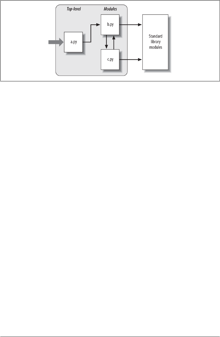
The first of these, a Python import statement, gives the file a.py access to everything
defined by top-level code in the file b.py. The code import b roughly means:
Load the file b.py (unless it’s already loaded), and give me access to all its attributes
through the name b.
To satisfy such goals, import (and, as you’ll see later, from) statements execute and load
other files on request. More formally, in Python, cross-file module linking is not re-
solved until such import statements are executed at runtime; their net effect is to assign
module names—simple variables like b—to loaded module objects. In fact, the module
name used in an import statement serves two purposes: it identifies the external file to
be loaded, but it also becomes a variable assigned to the loaded module.
Similarly, objects defined by a module are also created at runtime, as the import is
executing: import literally runs statements in the target file one at a time to create its
contents. Along the way, every name assigned at the top-level of the file becomes an
attribute of the module, accessible to importers. For example, the second of the state-
ments in a.py calls the function spam defined in the module b—created by running its
def statement during the import—using object attribute notation. The code b.spam
means:
Fetch the value of the name spam that lives within the object b.
This happens to be a callable function in our example, so we pass a string in parentheses
('gumby'). If you actually type these files, save them, and run a.py, the words “gumby
spam” will be printed.
As we’ve seen, the object.attribute notation appears throughout Python code—most
objects have useful attributes that are fetched with the “.” operator. Some reference
callable objects like functions that take action (e.g., a salary computer), and others are
Figure 22-1. Program architecture in Python. A program is a system of modules. It has one top-level
script file (launched to run the program), and multiple module files (imported libraries of tools). Scripts
and modules are both text files containing Python statements, though the statements in modules
usually just create objects to be used later. Python’s standard library provides a collection of precoded
modules.
672 | Chapter 22: Modules: The Big Picture
www.it-ebooks.info

simple data values that denote more static objects and properties (e.g., a person’s
name).
The notion of importing is also completely general throughout Python. Any file can
import tools from any other file. For instance, the file a.py may import b.py to call its
function, but b.py might also import c.py to leverage different tools defined there. Im-
port chains can go as deep as you like: in this example, the module a can import b,
which can import c, which can import b again, and so on.
Besides serving as the highest organizational structure, modules (and module packages,
described in Chapter 24) are also the highest level of code reuse in Python. Coding
components in module files makes them useful in your original program, and in any
other programs you may write later. For instance, if after coding the program in Fig-
ure 22-1 we discover that the function b.spam is a general-purpose tool, we can reuse
it in a completely different program; all we have to do is import the file b.py again from
the other program’s files.
Standard Library Modules
Notice the rightmost portion of Figure 22-1. Some of the modules that your programs
will import are provided by Python itself and are not files you will code.
Python automatically comes with a large collection of utility modules known as the
standard library. This collection, over 200 modules large at last count, contains plat-
form-independent support for common programming tasks: operating system inter-
faces, object persistence, text pattern matching, network and Internet scripting, GUI
construction, and much more. None of these tools are part of the Python language
itself, but you can use them by importing the appropriate modules on any standard
Python installation. Because they are standard library modules, you can also be rea-
sonably sure that they will be available and will work portably on most platforms on
which you will run Python.
This book’s examples employ a few of the standard library’s modules—timeit, sys,
and os in last chapter’s code, for instance—but we’ll really only scratch the surface of
the libraries story here. For a complete look, you should browse the standard Python
library reference manual, available either online at http://www.python.org, or with your
Python installation (via IDLE or Python’s Start button menu on some Windows). The
PyDoc tool discussed in Chapter 15 is another way to explore standard library modules.
Because there are so many modules, this is really the only way to get a feel for what
tools are available. You can also find tutorials on Python library tools in commercial
books that cover application-level programming, such as O’Reilly’s Programming
Python, but the manuals are free, viewable in any web browser (in HTML format),
viewable in other formats (e.g., Windows help), and updated each time Python is re-
released. See Chapter 15 for more pointers.
Python Program Architecture | 673
www.it-ebooks.info

How Imports Work
The prior section talked about importing modules without really explaining what hap-
pens when you do so. Because imports are at the heart of program structure in Python,
this section goes into more formal detail on the import operation to make this process
less abstract.
Some C programmers like to compare the Python module import operation to a C
#include, but they really shouldn’t—in Python, imports are not just textual insertions
of one file into another. They are really runtime operations that perform three distinct
steps the first time a program imports a given file:
1. Find the module’s file.
2. Compile it to byte code (if needed).
3. Run the module’s code to build the objects it defines.
To better understand module imports, we’ll explore these steps in turn. Bear in mind
that all three of these steps are carried out only the first time a module is imported
during a program’s execution; later imports of the same module in a program run
bypass all of these steps and simply fetch the already loaded module object in memory.
Technically, Python does this by storing loaded modules in a table named sys.mod
ules and checking there at the start of an import operation. If the module is not present,
a three-step process begins.
1. Find It
First, Python must locate the module file referenced by an import statement. Notice
that the import statement in the prior section’s example names the file without a .py
extension and without its directory path: it just says import b, instead of something
like import c:\dir1\b.py. Path and extension details are omitted on purpose; instead,
Python uses a standard module search path and known file types to locate the module
file corresponding to an import statement.1 Because this is the main part of the import
operation that programmers must know about, we’ll return to this topic in a moment.
1. It’s syntactically illegal to include path and extension details in a standard import. However, package
imports, which we’ll discuss in Chapter 24, allow import statements to include part of the directory path
leading to a file as a set of period-separated names. Package imports, though, still rely on the normal
module search path to locate the leftmost directory in a package path (i.e., they are relative to a directory
in the search path). They also cannot make use of any platform-specific directory syntax in the import
statements; such syntax only works on the search path. Also, note that module file search path issues are
not as relevant when you run frozen executables (discussed in Chapter 2), which typically embed byte
code in the binary image.
674 | Chapter 22: Modules: The Big Picture
www.it-ebooks.info

2. Compile It (Maybe)
After finding a source code file that matches an import statement by traversing the
module search path, Python next compiles it to byte code, if necessary. We discussed
byte code briefly in Chapter 2, but it’s a bit richer than explained there. During an
import operation Python checks both file modification times and the byte code’s Python
version number to decide how to proceed. The former uses file “timestamps,” and the
latter uses either a “magic” number embedded in the byte code or a filename, depending
on the Python release being used. This step chooses an action as follows:
Compile
If the byte code file is older than the source file (i.e., if you’ve changed the source)
or was created by a different Python version, Python automatically regenerates the
byte code when the program is run.
As discussed ahead, this model is modified somewhat in Python 3.2 and later—
byte code files are segregated in a __pycache__ subdirectory and named with their
Python version to avoid contention and recompiles when multiple Pythons are
installed. This obviates the need to check version numbers in the byte code, but
the timestamp check is still used to detect changes in the source.
Don’t compile
If, on the other hand, Python finds a .pyc byte code file that is not older than the
corresponding .py source file and was created by the same Python version, it skips
the source-to-byte-code compile step.
In addition, if Python finds only a byte code file on the search path and no source,
it simply loads the byte code directly; this means you can ship a program as just
byte code files and avoid sending source. In other words, the compile step is by-
passed if possible to speed program startup.
Notice that compilation happens when a file is being imported. Because of this, you
will not usually see a .pyc byte code file for the top-level file of your program, unless it
is also imported elsewhere—only imported files leave behind .pyc files on your ma-
chine. The byte code of top-level files is used internally and discarded; byte code of
imported files is saved in files to speed future imports.
Top-level files are often designed to be executed directly and not imported at all. Later,
we’ll see that it is possible to design a file that serves both as the top-level code of a
program and as a module of tools to be imported. Such a file may be both executed
and imported, and thus does generate a .pyc. To learn how this works, watch for the
discussion of the special __name__ attribute and __main__ in Chapter 25.
3. Run It
The final step of an import operation executes the byte code of the module. All state-
ments in the file are run in turn, from top to bottom, and any assignments made to
names during this step generate attributes of the resulting module object. This is how
How Imports Work | 675
www.it-ebooks.info

the tools defined by the module’s code are created. For instance, def statements in a
file are run at import time to create functions and assign attributes within the module
to those functions. The functions can then be called later in the program by the file’s
importers.
Because this last import step actually runs the file’s code, if any top-level code in a
module file does real work, you’ll see its results at import time. For example, top-level
print statements in a module show output when the file is imported. Function def
statements simply define objects for later use.
As you can see, import operations involve quite a bit of work—they search for files,
possibly run a compiler, and run Python code. Because of this, any given module is
imported only once per process by default. Future imports skip all three import steps
and reuse the already loaded module in memory. If you need to import a file again after
it has already been loaded (for example, to support dynamic end-user customizations),
you have to force the issue with an imp.reload call—a tool we’ll meet in the next
chapter.2
Byte Code Files: __pycache__ in Python 3.2+
As mentioned briefly, the way that Python stores files to retain the byte code that results
from compiling your source has changed in Python 3.2 and later. First of all, if Python
cannot write a file to save this on your computer for any reason, your program still runs
fine—Python simply creates and uses the byte code in memory and discards it on exit.
To speed startups, though, it will try to save byte code in a file in order to skip the
compile step next time around. The way it does this varies per Python version:
In Python 3.1 and earlier (including all of Python 2.X)
Byte code is stored in files in the same directory as the corresponding source files,
normally with the filename extension .pyc (e.g., module.pyc). Byte code files are
also stamped internally with the version of Python that created them (known as a
“magic” field to developers) so Python knows to recompile when this differs in the
version of Python running your program. For instance, if you upgrade to a new
Python whose byte code differs, all your byte code files will be recompiled auto-
matically due to a version number mismatch, even if you haven’t changed your
source code.
In Python 3.2 and later
Byte code is instead stored in files in a subdirectory named __pycache__, which
Python creates if needed, and which is located in the directory containing the cor-
responding source files. This helps avoid clutter in your source directories by seg-
regating the byte code files in their own directory. In addition, although byte code
2. As described earlier, Python keeps already imported modules in the built-in sys.modules dictionary so it
can keep track of what’s been loaded. In fact, if you want to see which modules are loaded, you can import
sys and print list(sys.modules.keys()). There’s more on other uses for this internal table in Chapter 25.
676 | Chapter 22: Modules: The Big Picture
www.it-ebooks.info

files still get the .pyc extension as before, they are given more descriptive names
that include text identifying the version of Python that created them (e.g., mod-
ule.cpython-32.pyc). This avoids contention and recompiles: because each version
of Python installed can have its own uniquely named version of byte code files in
the __pycache__ subdirectory, running under a given version doesn’t overwrite the
byte code of another, and doesn’t require recompiles. Technically, byte code file-
names also include the name of the Python that created them, so CPython, Jython,
and other implementations mentioned in the preface and Chapter 2 can coexist on
the same machine without stepping on each other’s work (once they support this
model).
In both models, Python always recreates the byte code file if you’ve changed the source
code file since the last compile, but version differences are handled differently—by
magic numbers and replacement prior to 3.2, and by filenames that allow for multiple
copies in 3.2 and later.
Byte Code File Models in Action
The following is a quick example of these two models in action under 2.X and 3.3. I’ve
omitted much of the text displayed by the dir directory listing on Windows here to
save space, and the script used here isn’t listed because it is not relevant to this discus-
sion (it’s from Chapter 2, and simply prints two values). Prior to 3.2, byte code files
show up alongside their source files after being created by import operations:
c:\code\py2x> dir
10/31/2012 10:58 AM 39 script0.py
c:\code\py2x> C:\python27\python
>>> import script0
hello world
1267650600228229401496703205376
>>> ^Z
c:\code\py2x> dir
10/31/2012 10:58 AM 39 script0.py
10/31/2012 11:00 AM 154 script0.pyc
However, in 3.2 and later byte code files are saved in the __pycache__ subdirectory and
include versions and Python implementation details in their names to avoid clutter and
contention among the Pythons on your computer:
c:\code\py2x> cd ..\py3x
c:\code\py3x> dir
10/31/2012 10:58 AM 39 script0.py
c:\code\py3x> C:\python33\python
>>> import script0
hello world
1267650600228229401496703205376
>>> ^Z
Byte Code Files: __pycache__ in Python 3.2+ | 677
www.it-ebooks.info

c:\code\py3x> dir
10/31/2012 10:58 AM 39 script0.py
10/31/2012 11:00 AM <DIR> __pycache__
c:\code\py3x> dir __pycache__
10/31/2012 11:00 AM 184 script0.cpython-33.pyc
Crucially, under the model used in 3.2 and later, importing the same file with a different
Python creates a different byte code file, instead of overwriting the single file as done
by the pre-3.2 model—in the newer model, each Python version and implementation
has its own byte code files, ready to be loaded on the next program run (earlier Pythons
will happily continue using their scheme on the same machine):
c:\code\py3x> C:\python32\python
>>> import script0
hello world
1267650600228229401496703205376
>>> ^Z
c:\code\py3x> dir __pycache__
10/31/2012 12:28 PM 178 script0.cpython-32.pyc
10/31/2012 11:00 AM 184 script0.cpython-33.pyc
Python 3.2’s newer byte code file model is probably superior, as it avoids recompiles
when there is more than one Python on your machine—a common case in today’s
mixed 2.X/3.X world. On the other hand, it is not without potential incompatibilities
in programs that rely on the prior file and directory structure. This may be a compati-
bility issue in some tools programs, for instance, though most well-behaved tools
should work as before. See Python 3.2’s “What’s New?” document for details on po-
tential impacts.
Also keep in mind that this process is completely automatic—it’s a side effect of running
programs—and most programmers probably won’t care about or even notice the dif-
ference, apart from faster startups due to fewer recompiles.
The Module Search Path
As mentioned earlier, the part of the import procedure that most programmers will
need to care about is usually the first—locating the file to be imported (the “find it”
part). Because you may need to tell Python where to look to find files to import, you
need to know how to tap into its search path in order to extend it.
In many cases, you can rely on the automatic nature of the module import search path
and won’t need to configure this path at all. If you want to be able to import user-
defined files across directory boundaries, though, you will need to know how the search
path works in order to customize it. Roughly, Python’s module search path is composed
of the concatenation of these major components, some of which are preset for you and
some of which you can tailor to tell Python where to look:
678 | Chapter 22: Modules: The Big Picture
www.it-ebooks.info

1. The home directory of the program
2. PYTHONPATH directories (if set)
3. Standard library directories
4. The contents of any .pth files (if present)
5. The site-packages home of third-party extensions
Ultimately, the concatenation of these four components becomes sys.path, a mutable
list of directory name strings that I’ll expand upon later in this section. The first and
third elements of the search path are defined automatically. Because Python searches
the concatenation of these components from first to last, though, the second and
fourth elements can be used to extend the path to include your own source code di-
rectories. Here is how Python uses each of these path components:
Home directory (automatic)
Python first looks for the imported file in the home directory. The meaning of this
entry depends on how you are running the code. When you’re running a pro-
gram, this entry is the directory containing your program’s top-level script file.
When you’re working interactively, this entry is the directory in which you are
working (i.e., the current working directory).
Because this directory is always searched first, if a program is located entirely in a
single directory, all of its imports will work automatically with no path configura-
tion required. On the other hand, because this directory is searched first, its files
will also override modules of the same name in directories elsewhere on the path;
be careful not to accidentally hide library modules this way if you need them in
your program, or use package tools we’ll meet later that can partially sidestep this
issue.
PYTHONPATH directories (configurable)
Next, Python searches all directories listed in your PYTHONPATH environment vari-
able setting, from left to right (assuming you have set this at all: it’s not preset for
you). In brief, PYTHONPATH is simply a list of user-defined and platform-specific
names of directories that contain Python code files. You can add all the directories
from which you wish to be able to import, and Python will extend the module
search path to include all the directories your PYTHONPATH lists.
Because Python searches the home directory first, this setting is only important
when importing files across directory boundaries—that is, if you need to import a
file that is stored in a different directory from the file that imports it. You’ll probably
want to set your PYTHONPATH variable once you start writing substantial programs,
but when you’re first starting out, as long as you save all your module files in the
directory in which you’re working (i.e., the home directory, like the C:\code used
in this book) your imports will work without you needing to worry about this
setting at all.
The Module Search Path | 679
www.it-ebooks.info

Standard library directories (automatic)
Next, Python automatically searches the directories where the standard library
modules are installed on your machine. Because these are always searched, they
normally do not need to be added to your PYTHONPATH or included in path files
(discussed next).
.pth path file directories (configurable)
Next, a lesser-used feature of Python allows users to add directories to the module
search path by simply listing them, one per line, in a text file whose name ends
with a .pth suffix (for “path”). These path configuration files are a somewhat ad-
vanced installation-related feature; we won’t cover them fully here, but they pro-
vide an alternative to PYTHONPATH settings.
In short, text files of directory names dropped in an appropriate directory can serve
roughly the same role as the PYTHONPATH environment variable setting. For instance,
if you’re running Windows and Python 3.3, a file named myconfig.pth may be
placed at the top level of the Python install directory (C:\Python33) or in the site-
packages subdirectory of the standard library there (C:\Python33\Lib\site-pack-
ages) to extend the module search path. On Unix-like systems, this file might be
located in usr/local/lib/python3.3/site-packages or /usr/local/lib/site-python instead.
When such a file is present, Python will add the directories listed on each line of
the file, from first to last, near the end of the module search path list—currently,
after PYTHONPATH and standard libraries, but before the site-packages directory
where third-party extensions are often installed. In fact, Python will collect the
directory names in all the .pth path files it finds and will filter out any duplicates
and nonexistent directories. Because they are files rather than shell settings, path
files can apply to all users of an installation, instead of just one user or shell. More-
over, for some users and applications, text files may be simpler to code than envi-
ronment settings.
This feature is more sophisticated than I’ve described here. For more details, con-
sult the Python library manual, and especially its documentation for the standard
library module site—this module allows the locations of Python libraries and path
files to be configured, and its documentation describes the expected locations of
path files in general. I recommend that beginners use PYTHONPATH or perhaps a sin-
gle .pth file, and then only if you must import across directories. Path files are used
more often by third-party libraries, which commonly install a path file in Python’s
site-packages, described next.
The Lib\site-packages directory of third-party extensions (automatic)
Finally, Python automatically adds the site-packages subdirectory of its standard
library to the module search path. By convention, this is the place that most third-
party extensions are installed, often automatically by the distutils utility de-
scribed in an upcoming sidebar. Because their install directory is always part of the
module search path, clients can import the modules of such extensions without
any path settings.
680 | Chapter 22: Modules: The Big Picture
www.it-ebooks.info

Configuring the Search Path
The net effect of all of this is that both the PYTHONPATH and path file components of the
search path allow you to tailor the places where imports look for files. The way you set
environment variables and where you store path files varies per platform. For instance,
on Windows, you might use your Control Panel’s System icon to set PYTHONPATH to a
list of directories separated by semicolons, like this:
c:\pycode\utilities;d:\pycode\package1
Or you might instead create a text file called C:\Python33\pydirs.pth, which looks like
this:
c:\pycode\utilities
d:\pycode\package1
These settings are analogous on other platforms, but the details can vary too widely for
us to cover in this chapter. See Appendix A for pointers on extending your module
search path with PYTHONPATH or .pth files on various platforms.
Search Path Variations
This description of the module search path is accurate, but generic; the exact config-
uration of the search path is prone to changing across platforms, Python releases, and
even Python implementations. Depending on your platform, additional directories may
automatically be added to the module search path as well.
For instance, some Pythons may add an entry for the current working directory—the
directory from which you launched your program—in the search path before the
PYTHONPATH directories. When you’re launching from a command line, the current
working directory may not be the same as the home directory of your top-level file (i.e.,
the directory where your program file resides), which is always added. Because the
current working directory can vary each time your program runs, you normally
shouldn’t depend on its value for import purposes. See Chapter 3 for more on launching
programs from command lines.3
To see how your Python configures the module search path on your platform, you can
always inspect sys.path—the topic of the next section.
The sys.path List
If you want to see how the module search path is truly configured on your machine,
you can always inspect the path as Python knows it by printing the built-in sys.path
3. Also watch for Chapter 24’s discussion of the new relative import syntax and search rules in Python 3.X;
they modify the search path for from statements in files inside packages when “.” characters are used (e.g.,
from . import string). By default, a package’s own directory is not automatically searched by imports
in Python 3.X, unless such relative imports are used by files in the package itself.
The Module Search Path | 681
www.it-ebooks.info

list (that is, the path attribute of the standard library module sys). This list of directory
name strings is the actual search path within Python; on imports, Python searches each
directory in this list from left to right, and uses the first file match it finds.
Really, sys.path is the module search path. Python configures it at program startup,
automatically merging the home directory of the top-level file (or an empty string to
designate the current working directory), any PYTHONPATH directories, the contents of
any .pth file paths you’ve created, and all the standard library directories. The result is
a list of directory name strings that Python searches on each import of a new file.
Python exposes this list for two good reasons. First, it provides a way to verify the search
path settings you’ve made—if you don’t see your settings somewhere in this list, you
need to recheck your work. For example, here is what my module search path looks
like on Windows under Python 3.3, with my PYTHONPATH set to C:\code and a C:
\Python33\mypath.pth path file that lists C:\Users\mark. The empty string at the front
means current directory, and my two settings are merged in; the rest are standard library
directories and files and the site-packages home for third-party extensions:
>>> import sys
>>> sys.path
['', 'C:\\code', 'C:\\Windows\\system32\\python33.zip', 'C:\\Python33\\DLLs',
'C:\\Python33\\lib', 'C:\\Python33', 'C:\\Users\\mark',
'C:\\Python33\\lib\\site-packages']
Second, if you know what you’re doing, this list provides a way for scripts to tailor their
search paths manually. As you’ll see by example later in this part of the book, by
modifying the sys.path list, you can modify the search path for all future imports made
in a program’s run. Such changes last only for the duration of the script, however;
PYTHONPATH and .pth files offer more permanent ways to modify the path—the first per
user, and the second per installation.
On the other hand, some programs really do need to change sys.path. Scripts that run
on web servers, for example, often run as the user “nobody” to limit machine access.
Because such scripts cannot usually depend on “nobody” to have set PYTHONPATH in any
particular way, they often set sys.path manually to include required source directories,
prior to running any import statements. A sys.path.append or sys.path.insert will
often suffice, though will endure for a single program run only.
Module File Selection
Keep in mind that filename extensions (e.g., .py) are omitted from import statements
intentionally. Python chooses the first file it can find on the search path that matches
the imported name. In fact, imports are the point of interface to a host of external
components—source code, multiple flavors of byte code, compiled extensions, and
more. Python automatically selects any type that matches a module’s name.
682 | Chapter 22: Modules: The Big Picture
www.it-ebooks.info

Module sources
For example, an import statement of the form import b might today load or resolve to:
• A source code file named b.py
• A byte code file named b.pyc
• An optimized byte code file named b.pyo (a less common format)
• A directory named b, for package imports (described in Chapter 24)
• A compiled extension module, coded in C, C++, or another language, and dy-
namically linked when imported (e.g., b.so on Linux, or b.dll or b.pyd on Cygwin
and Windows)
• A compiled built-in module coded in C and statically linked into Python
• A ZIP file component that is automatically extracted when imported
• An in-memory image, for frozen executables
• A Java class, in the Jython version of Python
• A .NET component, in the IronPython version of Python
C extensions, Jython, and package imports all extend imports beyond simple files. To
importers, though, differences in the loaded file type are completely irrelevant, both
when importing and when fetching module attributes. Saying import b gets whatever
module b is, according to your module search path, and b.attr fetches an item in the
module, be it a Python variable or a linked-in C function. Some standard modules we
will use in this book are actually coded in C, not Python; because they look just like
Python-coded module files, their clients don’t have to care.
Selection priorities
If you have both a b.py and a b.so in different directories, Python will always load the
one found in the first (leftmost) directory of your module search path during the left-
to-right search of sys.path. But what happens if it finds both a b.py and a b.so in the
same directory? In this case, Python follows a standard picking order, though this order
is not guaranteed to stay the same over time or across implementations. In general, you
should not depend on which type of file Python will choose within a given directory—
make your module names distinct, or configure your module search path to make your
module selection preferences explicit.
Import hooks and ZIP files
Normally, imports work as described in this section—they find and load files on your
machine. However, it is possible to redefine much of what an import operation does
in Python, using what are known as import hooks. These hooks can be used to make
imports do various useful things, such as loading files from archives, performing de-
cryption, and so on.
The Module Search Path | 683
www.it-ebooks.info
In fact, Python itself makes use of these hooks to enable files to be directly imported
from ZIP archives: archived files are automatically extracted at import time when
a .zip file is selected from the module import search path. One of the standard library
directories in the earlier sys.path display, for example, is a .zip file today. For more
details, see the Python standard library manual’s description of the built-in
__import__ function, the customizable tool that import statements actually run.
Also see Python 3.3’s “What’s New?” document for updates on this
front that we’ll mostly omit here for space. In short, in this version and
later, the __import__ function is now implemented by impor
tlib.__import__, in part to unify and more clearly expose its imple-
mentation.
The latter of these calls is also wrapped by importlib.import_module—
a tool that, per Python’s current manuals, is generally preferred over
__import__ for direct calls to import by name string, a technique dis-
cussed in Chapter 25. Both calls still work today, though the
__import__ function supports customizing imports by replacement in
the built-in scope (see Chapter 17), and other techniques support similar
roles. See the Python library manuals for more details.
Optimized byte code files
Finally, Python also supports the notion of .pyo optimized byte code files, created and
run with the -O Python command-line flag, and automatically generated by some install
tools. Because these run only slightly faster than normal .pyc files (typically 5 percent
faster), however, they are infrequently used. The PyPy system (see Chapter 2 and
Chapter 21), for example, provides more substantial speedups. See Appendix A and
Chapter 36 for more on .pyo files.
Third-Party Software: distutils
This chapter’s description of module search path settings is targeted mainly at user-
defined source code that you write on your own. Third-party extensions for Python
typically use the distutils tools in the standard library to automatically install them-
selves, so no path configuration is required to use their code.
Systems that use distutils generally come with a setup.py script, which is run to install
them; this script imports and uses distutils modules to place such systems in a direc-
tory that is automatically part of the module search path (usually in the Lib\site-pack-
ages subdirectory of the Python install tree, wherever that resides on the target ma-
chine).
For more details on distributing and installing with distutils, see the Python standard
manual set; its use is beyond the scope of this book (for instance, it also provides ways
to automatically compile C-coded extensions on the target machine). Also check out
the third-party open source eggs system, which adds dependency checking for installed
Python software.
684 | Chapter 22: Modules: The Big Picture
www.it-ebooks.info

Note: as this fifth edition is being written, there is some talk of deprecating distutils
and replacing it with a newer distutils2 package in the Python standard library. The
status of this is unclear—it was anticipated in 3.3 but did not appear—so be sure to
see Python’s “What’s New” documents for updates on this front that may emerge after
this book is released.
Chapter Summary
In this chapter, we covered the basics of modules, attributes, and imports and explored
the operation of import statements. We learned that imports find the designated file on
the module search path, compile it to byte code, and execute all of its statements to
generate its contents. We also learned how to configure the search path to be able to
import from directories other than the home directory and the standard library direc-
tories, primarily with PYTHONPATH settings.
As this chapter demonstrated, the import operation and modules are at the heart of
program architecture in Python. Larger programs are divided into multiple files, which
are linked together at runtime by imports. Imports in turn use the module search path
to locate files, and modules define attributes for external use.
Of course, the whole point of imports and modules is to provide a structure to your
program, which divides its logic into self-contained software components. Code in one
module is isolated from code in another; in fact, no file can ever see the names defined
in another, unless explicit import statements are run. Because of this, modules minimize
name collisions between different parts of your program.
You’ll see what this all means in terms of actual statements and code in the next chapter.
Before we move on, though, let’s run through the chapter quiz.
Test Your Knowledge: Quiz
1. How does a module source code file become a module object?
2. Why might you have to set your PYTHONPATH environment variable?
3. Name the five major components of the module import search path.
4. Name four file types that Python might load in response to an import operation.
5. What is a namespace, and what does a module’s namespace contain?
Test Your Knowledge: Answers
1. A module’s source code file automatically becomes a module object when that
module is imported. Technically, the module’s source code is run during the im-
Test Your Knowledge: Answers | 685
www.it-ebooks.info

port, one statement at a time, and all the names assigned in the process become
attributes of the module object.
2. You only need to set PYTHONPATH to import from directories other than the one in
which you are working (i.e., the current directory when working interactively, or
the directory containing your top-level file). In practice, this will be a common case
for nontrivial programs.
3. The five major components of the module import search path are the top-level
script’s home directory (the directory containing it), all directories listed in the
PYTHONPATH environment variable, the standard library directories, all directories
listed in .pth path files located in standard places, and the site-packages root di-
rectory for third-party extension installs. Of these, programmers can customize
PYTHONPATH and .pth files.
4. Python might load a source code (.py) file, a byte code (.pyc or .pyo) file, a C ex-
tension module (e.g., a .so file on Linux or a .dll or .pyd file on Windows), or a
directory of the same name for package imports. Imports may also load more exotic
things such as ZIP file components, Java classes under the Jython version of
Python, .NET components under IronPython, and statically linked C extensions
that have no files present at all. In fact, with import hooks, imports can load arbi-
trary items.
5. A namespace is a self-contained package of variables, which are known as the
attributes of the namespace object. A module’s namespace contains all the names
assigned by code at the top level of the module file (i.e., not nested in def or
class statements). Technically, a module’s global scope morphs into the module
object’s attributes namespace. A module’s namespace may also be altered by as-
signments from other files that import it, though this is generally frowned upon
(see Chapter 17 for more on the downsides of cross-file changes).
686 | Chapter 22: Modules: The Big Picture
www.it-ebooks.info

CHAPTER 23
Module Coding Basics
Now that we’ve looked at the larger ideas behind modules, let’s turn to some examples
of modules in action. Although some of the early topics in this chapter will be review
for linear readers who have already applied them in previous chapters’ examples, we’ll
find that they quickly lead us to further details surrounding Python’s modules that we
haven’t yet met, such as nesting, reloads, scopes, and more.
Python modules are easy to create; they’re just files of Python program code created
with a text editor. You don’t need to write special syntax to tell Python you’re making
a module; almost any text file will do. Because Python handles all the details of finding
and loading modules, modules are also easy to use; clients simply import a module, or
specific names a module defines, and use the objects they reference.
Module Creation
To define a module, simply use your text editor to type some Python code into a text
file, and save it with a “.py” extension; any such file is automatically considered a
Python module. All the names assigned at the top level of the module become its
attributes (names associated with the module object) and are exported for clients to use
—they morph from variable to module object attribute automatically.
For instance, if you type the following def into a file called module1.py and import it,
you create a module object with one attribute—the name printer, which happens to
be a reference to a function object:
def printer(x): # Module attribute
print(x)
Module Filenames
Before we go on, I should say a few more words about module filenames. You can call
modules just about anything you like, but module filenames should end in a .py suffix
if you plan to import them. The .py is technically optional for top-level files that will
687
www.it-ebooks.info

be run but not imported, but adding it in all cases makes your files’ types more obvious
and allows you to import any of your files in the future.
Because module names become variable names inside a Python program (without
the .py), they should also follow the normal variable name rules outlined in Chap-
ter 11. For instance, you can create a module file named if.py, but you cannot import
it because if is a reserved word—when you try to run import if, you’ll get a syntax
error. In fact, both the names of module files and the names of directories used in
package imports (discussed in the next chapter) must conform to the rules for variable
names presented in Chapter 11; they may, for instance, contain only letters, digits, and
underscores. Package directories also cannot contain platform-specific syntax such as
spaces in their names.
When a module is imported, Python maps the internal module name to an external
filename by adding a directory path from the module search path to the front, and
a .py or other extension at the end. For instance, a module named M ultimately maps
to some external file <directory>\M.<extension> that contains the module’s code.
Other Kinds of Modules
As mentioned in the preceding chapter, it is also possible to create a Python module by
writing code in an external language such as C, C++, and others (e.g., Java, in the
Jython implementation of the language). Such modules are called extension modules,
and they are generally used to wrap up external libraries for use in Python scripts. When
imported by Python code, extension modules look and feel the same as modules coded
as Python source code files—they are accessed with import statements, and they provide
functions and objects as module attributes. Extension modules are beyond the scope
of this book; see Python’s standard manuals or advanced texts such as Programming
Python for more details.
Module Usage
Clients can use the simple module file we just wrote by running an import or from
statement. Both statements find, compile, and run a module file’s code, if it hasn’t yet
been loaded. The chief difference is that import fetches the module as a whole, so you
must qualify to fetch its names; in contrast, from fetches (or copies) specific names out
of the module.
Let’s see what this means in terms of code. All of the following examples wind up calling
the printer function defined in the prior section’s module1.py module file, but in dif-
ferent ways.
688 | Chapter 23: Module Coding Basics
www.it-ebooks.info

The import Statement
In the first example, the name module1 serves two different purposes—it identifies an
external file to be loaded, and it becomes a variable in the script, which references the
module object after the file is loaded:
>>> import module1 # Get module as a whole (one or more)
>>> module1.printer('Hello world!') # Qualify to get names
Hello world!
The import statement simply lists one or more names of modules to load, separated by
commas. Because it gives a name that refers to the whole module object, we must go
through the module name to fetch its attributes (e.g., module1.printer).
The from Statement
By contrast, because from copies specific names from one file over to another scope, it
allows us to use the copied names directly in the script without going through the
module (e.g., printer):
>>> from module1 import printer # Copy out a variable (one or more)
>>> printer('Hello world!') # No need to qualify name
Hello world!
This form of from allows us to list one or more names to be copied out, separated by
commas. Here, it has the same effect as the prior example, but because the imported
name is copied into the scope where the from statement appears, using that name in
the script requires less typing—we can use it directly instead of naming the enclosing
module. In fact, we must; from doesn’t assign the name of the module itself.
As you’ll see in more detail later, the from statement is really just a minor extension to
the import statement—it imports the module file as usual (running the full three-step
procedure of the preceding chapter), but adds an extra step that copies one or more
names (not objects) out of the file. The entire file is loaded, but you’re given names for
more direct access to its parts.
The from * Statement
Finally, the next example uses a special form of from: when we use a * instead of specific
names, we get copies of all names assigned at the top level of the referenced module.
Here again, we can then use the copied name printer in our script without going
through the module name:
>>> from module1 import * # Copy out _all_ variables
>>> printer('Hello world!')
Hello world!
Technically, both import and from statements invoke the same import operation; the
from * form simply adds an extra step that copies all the names in the module into the
importing scope. It essentially collapses one module’s namespace into another; again,
Module Usage | 689
www.it-ebooks.info

the net effect is less typing for us. Note that only * works in this context; you can’t use
pattern matching to select a subset of names (though you could with more work and
a loop through a module’s __dict__, discussed ahead).
And that’s it—modules really are simple to use. To give you a better understanding of
what really happens when you define and use modules, though, let’s move on to look
at some of their properties in more detail.
In Python 3.X, the from ...* statement form described here can be used
only at the top level of a module file, not within a function. Python 2.X
allows it to be used within a function, but issues a warning anyhow. It’s
rare to see this statement used inside a function in practice; when
present, it makes it impossible for Python to detect variables statically,
before the function runs. Best practice in all Pythons recommends listing
all your imports at the top of a module file; it’s not required, but makes
them easier to spot.
Imports Happen Only Once
One of the most common questions people seem to ask when they start using modules
is, “Why won’t my imports keep working?” They often report that the first import
works fine, but later imports during an interactive session (or program run) seem to
have no effect. In fact, they’re not supposed to. This section explains why.
Modules are loaded and run on the first import or from, and only the first. This is on
purpose—because importing is an expensive operation, by default Python does it just
once per file, per process. Later import operations simply fetch the already loaded
module object.
Initialization code
As one consequence, because top-level code in a module file is usually executed only
once, you can use it to initialize variables. Consider the file simple.py, for example:
print('hello')
spam = 1 # Initialize variable
In this example, the print and = statements run the first time the module is imported,
and the variable spam is initialized at import time:
% python
>>> import simple # First import: loads and runs file's code
hello
>>> simple.spam # Assignment makes an attribute
1
Second and later imports don’t rerun the module’s code; they just fetch the already
created module object from Python’s internal modules table. Thus, the variable spam
is not reinitialized:
690 | Chapter 23: Module Coding Basics
www.it-ebooks.info

>>> simple.spam = 2 # Change attribute in module
>>> import simple # Just fetches already loaded module
>>> simple.spam # Code wasn't rerun: attribute unchanged
2
Of course, sometimes you really want a module’s code to be rerun on a subsequent
import. We’ll see how to do this with Python’s reload function later in this chapter.
import and from Are Assignments
Just like def, import and from are executable statements, not compile-time declarations.
They may be nested in if tests, to select among options; appear in function defs, to be
loaded only on calls (subject to the preceding note); be used in try statements, to pro-
vide defaults; and so on. They are not resolved or run until Python reaches them while
executing your program. In other words, imported modules and names are not available
until their associated import or from statements run.
Changing mutables in modules
Also, like def, the import and from are implicit assignments:
•import assigns an entire module object to a single name.
•from assigns one or more names to objects of the same names in another module.
All the things we’ve already discussed about assignment apply to module access, too.
For instance, names copied with a from become references to shared objects; as with
function arguments, reassigning a copied name has no effect on the module from which
it was copied, but changing a shared mutable object through a copied name can also
change it in the module from which it was imported. To illustrate, consider the fol-
lowing file, small.py:
x = 1
y = [1, 2]
When importing with from, we copy names to the importer’s scope that initially share
objects referenced by the module’s names:
% python
>>> from small import x, y # Copy two names out
>>> x = 42 # Changes local x only
>>> y[0] = 42 # Changes shared mutable in place
Here, x is not a shared mutable object, but y is. The names y in the importer and the
importee both reference the same list object, so changing it from one place changes it
in the other:
>>> import small # Get module name (from doesn't)
>>> small.x # Small's x is not my x
1
>>> small.y # But we share a changed mutable
[42, 2]
Module Usage | 691
www.it-ebooks.info

For more background on this, see Chapter 6. And for a graphical picture of what
from assignments do with references, flip back to Figure 18-1 (function argument pass-
ing), and mentally replace “caller” and “function” with “imported” and “importer.”
The effect is the same, except that here we’re dealing with names in modules, not
functions. Assignment works the same everywhere in Python.
Cross-file name changes
Recall from the preceding example that the assignment to x in the interactive session
changed the name x in that scope only, not the x in the file—there is no link from a
name copied with from back to the file it came from. To really change a global name in
another file, you must use import:
% python
>>> from small import x, y # Copy two names out
>>> x = 42 # Changes my x only
>>> import small # Get module name
>>> small.x = 42 # Changes x in other module
This phenomenon was introduced in Chapter 17. Because changing variables in other
modules like this is a common source of confusion (and often a bad design choice),
we’ll revisit this technique again later in this part of the book. Note that the change to
y[0] in the prior session is different; it changes an object, not a name, and the name in
both modules references the same, changed object.
import and from Equivalence
Notice in the prior example that we have to execute an import statement after the
from to access the small module name at all. from only copies names from one module
to another; it does not assign the module name itself. At least conceptually, a from
statement like this one:
from module import name1, name2 # Copy these two names out (only)
is equivalent to this statement sequence:
import module # Fetch the module object
name1 = module.name1 # Copy names out by assignment
name2 = module.name2
del module # Get rid of the module name
Like all assignments, the from statement creates new variables in the importer, which
initially refer to objects of the same names in the imported file. Only the names are
copied out, though, not the objects they reference, and not the name of the module
itself. When we use the from * form of this statement (from module import *), the
equivalence is the same, but all the top-level names in the module are copied over to
the importing scope this way.
692 | Chapter 23: Module Coding Basics
www.it-ebooks.info

Notice that the first step of the from runs a normal import operation, with all the se-
mantics outlined in the preceding chapter. Because of this, the from always imports the
entire module into memory if it has not yet been imported, regardless of how many
names it copies out of the file. There is no way to load just part of a module file (e.g.,
just one function), but because modules are byte code in Python instead of machine
code, the performance implications are generally negligible.
Potential Pitfalls of the from Statement
Because the from statement makes the location of a variable more implicit and obscure
(name is less meaningful to the reader than module.name), some Python users recommend
using import instead of from most of the time. I’m not sure this advice is warranted,
though; from is commonly and widely used, without too many dire consequences. In
practice, in realistic programs, it’s often convenient not to have to type a module’s name
every time you wish to use one of its tools. This is especially true for large modules that
provide many attributes—the standard library’s tkinter GUI module, for example.
It is true that the from statement has the potential to corrupt namespaces, at least in
principle—if you use it to import variables that happen to have the same names as
existing variables in your scope, your variables will be silently overwritten. This prob-
lem doesn’t occur with the simple import statement because you must always go
through a module’s name to get to its contents (module.attr will not clash with a vari-
able named attr in your scope). As long as you understand and expect that this can
happen when using from, though, this isn’t a major concern in practice, especially if
you list the imported names explicitly (e.g., from module import x, y, z).
On the other hand, the from statement has more serious issues when used in conjunc-
tion with the reload call, as imported names might reference prior versions of objects.
Moreover, the from module import * form really can corrupt namespaces and make
names difficult to understand, especially when applied to more than one file—in this
case, there is no way to tell which module a name came from, short of searching the
external source files. In effect, the from * form collapses one namespace into another,
and so defeats the namespace partitioning feature of modules. We will explore these
issues in more detail in the section “Module Gotchas” on page 770 (see Chapter 25).
Probably the best real-world advice here is to generally prefer import to from for simple
modules, to explicitly list the variables you want in most from statements, and to limit
the from * form to just one import per file. That way, any undefined names can be
assumed to live in the module referenced with the from *. Some care is required when
using the from statement, but armed with a little knowledge, most programmers find
it to be a convenient way to access modules.
Module Usage | 693
www.it-ebooks.info

When import is required
The only time you really must use import instead of from is when you must use the same
name defined in two different modules. For example, if two files define the same name
differently:
# M.py
def func():
...do something...
# N.py
def func():
...do something else...
and you must use both versions of the name in your program, the from statement will
fail—you can have only one assignment to the name in your scope:
# O.py
from M import func
from N import func # This overwrites the one we fetched from M
func() # Calls N.func only!
An import will work here, though, because including the name of the enclosing module
makes the two names unique:
# O.py
import M, N # Get the whole modules, not their names
M.func() # We can call both names now
N.func() # The module names make them unique
This case is unusual enough that you’re unlikely to encounter it very often in practice.
If you do, though, import allows you to avoid the name collision. Another way out of
this dilemma is using the as extension, which we’ll cover in Chapter 25 but is simple
enough to introduce here:
# O.py
from M import func as mfunc # Rename uniquely with "as"
from N import func as nfunc
mfunc(); nfunc() # Calls one or the other
The as extension works in both import and from as a simple renaming tool (it can also
be used to give a shorter synonym for a long module name in import); more on this
form in Chapter 25.
Module Namespaces
Modules are probably best understood as simply packages of names—i.e., places to
define names you want to make visible to the rest of a system. Technically, modules
usually correspond to files, and Python creates a module object to contain all the names
assigned in a module file. But in simple terms, modules are just namespaces (places
where names are created), and the names that live in a module are called its at-
tributes. This section expands on the details behind this model.
694 | Chapter 23: Module Coding Basics
www.it-ebooks.info

Files Generate Namespaces
I’ve mentioned that files morph into namespaces, but how does this actually happen?
The short answer is that every name that is assigned a value at the top level of a module
file (i.e., not nested in a function or class body) becomes an attribute of that module.
For instance, given an assignment statement such as X = 1 at the top level of a module
file M.py, the name X becomes an attribute of M, which we can refer to from outside the
module as M.X. The name X also becomes a global variable to other code inside M.py,
but we need to consider the notion of module loading and scopes a bit more formally
to understand why:
•Module statements run on the first import. The first time a module is imported
anywhere in a system, Python creates an empty module object and executes the
statements in the module file one after another, from the top of the file to the
bottom.
•Top-level assignments create module attributes. During an import, statements
at the top level of the file not nested in a def or class that assign names (e.g., =,
def) create attributes of the module object; assigned names are stored in the mod-
ule’s namespace.
•Module namespaces can be accessed via the attribute__dict__ or dir(M).
Module namespaces created by imports are dictionaries; they may be accessed
through the built-in __dict__ attribute associated with module objects and may be
inspected with the dir function. The dir function is roughly equivalent to the sorted
keys list of an object’s __dict__ attribute, but it includes inherited names for classes,
may not be complete, and is prone to changing from release to release.
•Modules are a single scope (local is global). As we saw in Chapter 17, names
at the top level of a module follow the same reference/assignment rules as names
in a function, but the local and global scopes are the same—or, more formally,
they follow the LEGB scope rule we met in Chapter 17, but without the L and E
lookup layers.
Crucially, though, the module’s global scope becomes an attribute dictionary of a
module object after the module has been loaded. Unlike function scopes, where
the local namespace exists only while the function runs, a module file’s scope be-
comes a module object’s attribute namespace and lives on after the import, pro-
viding a source of tools to importers.
Here’s a demonstration of these ideas. Suppose we create the following module file in
a text editor and call it module2.py:
print('starting to load...')
import sys
name = 42
def func(): pass
Module Namespaces | 695
www.it-ebooks.info

class klass: pass
print('done loading.')
The first time this module is imported (or run as a program), Python executes its state-
ments from top to bottom. Some statements create names in the module’s namespace
as a side effect, but others do actual work while the import is going on. For instance,
the two print statements in this file execute at import time:
>>> import module2
starting to load...
done loading.
Once the module is loaded, its scope becomes an attribute namespace in the module
object we get back from import. We can then access attributes in this namespace by
qualifying them with the name of the enclosing module:
>>> module2.sys
<module 'sys' (built-in)>
>>> module2.name
42
>>> module2.func
<function func at 0x000000000222E7B8>
>>> module2.klass
<class 'module2.klass'>
Here, sys, name, func, and klass were all assigned while the module’s statements were
being run, so they are attributes after the import. We’ll talk about classes in Part VI,
but notice the sys attribute—import statements really assign module objects to names,
and any type of assignment to a name at the top level of a file generates a module
attribute.
Namespace Dictionaries: __dict__
In fact, internally, module namespaces are stored as dictionary objects. These are just
normal dictionaries with all the usual methods. When needed—for instance, to write
tools that list module content generically as we will in Chapter 25—we can access a
module’s namespace dictionary through the module’s __dict__ attribute. Continuing
the prior section’s example (remember to wrap this in a list call in Python 3.X—it’s a
view object there, and contents may vary outside 3.3 used here):
>>> list(module2.__dict__.keys())
['__loader__', 'func', 'klass', '__builtins__', '__doc__', '__file__', '__name__',
'name', '__package__', 'sys', '__initializing__', '__cached__']
The names we assigned in the module file become dictionary keys internally, so some
of the names here reflect top-level assignments in our file. However, Python also adds
some names in the module’s namespace for us; for instance, __file__ gives the name
696 | Chapter 23: Module Coding Basics
www.it-ebooks.info

of the file the module was loaded from, and __name__ gives its name as known to im-
porters (without the .py extension and directory path). To see just the names your code
assigns, filter out the double-underscore names as we’ve done before, in Chapter 15’s
dir coverage and Chapter 17’s built-in scope coverage:
>>> list(name for name in module2.__dict__.keys() if not name.startswith('__'))
['func', 'klass', 'name', 'sys']
>>> list(name for name in module2.__dict__ if not name.startswith('__'))
['func', 'sys', 'name', 'klass']
This time we’re filtering with a generator instead of a list comprehension, and can omit
the .keys() because dictionaries generate their keys automatically though implicitly;
the effect is the same. We’ll see similar __dict__ dictionaries on class-related objects in
Part VI too. In both cases, attribute fetch is similar to dictionary indexing, though only
the former kicks off inheritance in classes:
>>> module2.name, module2.__dict__['name']
(42, 42)
Attribute Name Qualification
Speaking of attribute fetch, now that you’re becoming more familiar with modules, we
should firm up the notion of name qualification more formally too. In Python, you can
access the attributes of any object that has attributes using the qualification (a.k.a.
attribute fetch) syntax object.attribute.
Qualification is really an expression that returns the value assigned to an attribute name
associated with an object. For example, the expression module2.sys in the previous
example fetches the value assigned to sys in module2. Similarly, if we have a built-in list
object L, L.append returns the append method object associated with that list.
It’s important to keep in mind that attribute qualification has nothing to do with the
scope rules we studied in Chapter 17; it’s an independent concept. When you use
qualification to access names, you give Python an explicit object from which to fetch
the specified names. The LEGB scope rule applies only to bare, unqualified names—it
may be used for the leftmost name in a name path, but later names after dots search
specific objects instead. Here are the rules:
Simple variables
X means search for the name X in the current scopes (following the LEGB rule of
Chapter 17).
Qualification
X.Y means find X in the current scopes, then search for the attribute Y in the object
X (not in scopes).
Qualification paths
X.Y.Z means look up the name Y in the object X, then look up Z in the object X.Y.
Module Namespaces | 697
www.it-ebooks.info

Generality
Qualification works on all objects with attributes: modules, classes, C extension
types, etc.
In Part VI, we’ll see that attribute qualification means a bit more for classes—it’s also
the place where something called inheritance happens—but in general, the rules out-
lined here apply to all names in Python.
Imports Versus Scopes
As we’ve learned, it is never possible to access names defined in another module file
without first importing that file. That is, you never automatically get to see names in
another file, regardless of the structure of imports or function calls in your program. A
variable’s meaning is always determined by the locations of assignments in your source
code, and attributes are always requested of an object explicitly.
For example, consider the following two simple modules. The first, moda.py, defines
a variable X global to code in its file only, along with a function that changes the global
X in this file:
X = 88 # My X: global to this file only
def f():
global X # Change this file's X
X = 99 # Cannot see names in other modules
The second module, modb.py, defines its own global variable X and imports and calls
the function in the first module:
X = 11 # My X: global to this file only
import moda # Gain access to names in moda
moda.f() # Sets moda.X, not this file's X
print(X, moda.X)
When run, moda.f changes the X in moda, not the X in modb. The global scope for
moda.f is always the file enclosing it, regardless of which module it is ultimately called
from:
% python modb.py
11 99
In other words, import operations never give upward visibility to code in imported files
—an imported file cannot see names in the importing file. More formally:
• Functions can never see names in other functions, unless they are physically en-
closing.
• Module code can never see names in other modules, unless they are explicitly im-
ported.
698 | Chapter 23: Module Coding Basics
www.it-ebooks.info

Such behavior is part of the lexical scoping notion—in Python, the scopes surrounding
a piece of code are completely determined by the code’s physical position in your file.
Scopes are never influenced by function calls or module imports.1
Namespace Nesting
In some sense, although imports do not nest namespaces upward, they do nest down-
ward. That is, although an imported module never has direct access to names in a file
that imports it, using attribute qualification paths it is possible to descend into arbi-
trarily nested modules and access their attributes. For example, consider the next three
files. mod3.py defines a single global name and attribute by assignment:
X = 3
mod2.py in turn defines its own X, then imports mod3 and uses qualification to access
the imported module’s attribute:
X = 2
import mod3
print(X, end=' ') # My global X
print(mod3.X) # mod3's X
mod1.py also defines its own X, then imports mod2, and fetches attributes in both the
first and second files:
X = 1
import mod2
print(X, end=' ') # My global X
print(mod2.X, end=' ') # mod2's X
print(mod2.mod3.X) # Nested mod3's X
Really, when mod1 imports mod2 here, it sets up a two-level namespace nesting. By using
the path of names mod2.mod3.X, it can descend into mod3, which is nested in the imported
mod2. The net effect is that mod1 can see the Xs in all three files, and hence has access to
all three global scopes:
% python mod1.py
2 3
1 2 3
The reverse, however, is not true: mod3 cannot see names in mod2, and mod2 cannot see
names in mod1. This example may be easier to grasp if you don’t think in terms of
namespaces and scopes, but instead focus on the objects involved. Within mod1, mod2
is just a name that refers to an object with attributes, some of which may refer to other
1. Some languages act differently and provide for dynamic scoping, where scopes really may depend on
runtime calls. This tends to make code trickier, though, because the meaning of a variable can differ over
time. In Python, scopes more simply correspond to the text of your program.
Module Namespaces | 699
www.it-ebooks.info

objects with attributes (import is an assignment). For paths like mod2.mod3.X, Python
simply evaluates from left to right, fetching attributes from objects along the way.
Note that mod1 can say import mod2, and then mod2.mod3.X, but it cannot say import
mod2.mod3—this syntax invokes something called package (directory) imports, de-
scribed in the next chapter. Package imports also create module namespace nesting,
but their import statements are taken to reflect directory trees, not simple file import
chains.
Reloading Modules
As we’ve seen, a module’s code is run only once per process by default. To force a
module’s code to be reloaded and rerun, you need to ask Python to do so explicitly by
calling the reload built-in function. In this section, we’ll explore how to use reloads to
make your systems more dynamic. In a nutshell:
• Imports (via both import and from statements) load and run a module’s code only
the first time the module is imported in a process.
• Later imports use the already loaded module object without reloading or rerunning
the file’s code.
• The reload function forces an already loaded module’s code to be reloaded and
rerun. Assignments in the file’s new code change the existing module object in
place.
Why care about reloading modules? In short, dynamic customization: the reload func-
tion allows parts of a program to be changed without stopping the whole program.
With reload, the effects of changes in components can be observed immediately. Re-
loading doesn’t help in every situation, but where it does, it makes for a much shorter
development cycle. For instance, imagine a database program that must connect to a
server on startup; because program changes or customizations can be tested immedi-
ately after reloads, you need to connect only once while debugging. Long-running
servers can update themselves this way, too.
Because Python is interpreted (more or less), it already gets rid of the compile/link steps
you need to go through to get a C program to run: modules are loaded dynamically
when imported by a running program. Reloading offers a further performance advan-
tage by allowing you to also change parts of running programs without stopping.
Though beyond this book’s scope, note that reload currently only works on modules
written in Python; compiled extension modules coded in a language such as C can be
dynamically loaded at runtime, too, but they can’t be reloaded (though most users
probably prefer to code customizations in Python anyhow!).
700 | Chapter 23: Module Coding Basics
www.it-ebooks.info

Version skew note: In Python 2.X, reload is available as a built-in func-
tion. In Python 3.X, it has been moved to the imp standard library mod-
ule—it’s known as imp.reload in 3.X. This simply means that an extra
import or from statement is required to load this tool in 3.X only. Readers
using 2.X can ignore these imports in this book’s examples, or use them
anyhow—2.X also has a reload in its imp module to ease migration to
3.X. Reloading works the same regardless of its packaging.
reload Basics
Unlike import and from:
•reload is a function in Python, not a statement.
•reload is passed an existing module object, not a new name.
•reload lives in a module in Python 3.X and must be imported itself.
Because reload expects an object, a module must have been previously imported suc-
cessfully before you can reload it (if the import was unsuccessful due to a syntax or
other error, you may need to repeat it before you can reload the module). Furthermore,
the syntax of import statements and reload calls differs: as a function reloads require
parentheses, but import statements do not. Abstractly, reloading looks like this:
import module # Initial import
...use module.attributes...
... # Now, go change the module file
...
from imp import reload # Get reload itself (in 3.X)
reload(module) # Get updated exports
...use module.attributes...
The typical usage pattern is that you import a module, then change its source code in
a text editor, and then reload it. This can occur when working interactively, but also
in larger programs that reload periodically.
When you call reload, Python rereads the module file’s source code and reruns its top-
level statements. Perhaps the most important thing to know about reload is that it
changes a module object in place; it does not delete and re-create the module object.
Because of that, every reference to an entire module object anywhere in your program
is automatically affected by a reload. Here are the details:
•reload runs a module file’s new code in the module’s current namespace.
Rerunning a module file’s code overwrites its existing namespace, rather than de-
leting and re-creating it.
•Top-level assignments in the file replace names with new values. For instance,
rerunning a def statement replaces the prior version of the function in the module’s
namespace by reassigning the function name.
Reloading Modules | 701
www.it-ebooks.info

•Reloads impact all clients that use import to fetch modules. Because clients
that use import qualify to fetch attributes, they’ll find new values in the module
object after a reload.
•Reloads impact future from clients only. Clients that used from to fetch attributes
in the past won’t be affected by a reload; they’ll still have references to the old
objects fetched before the reload.
•Reloads apply to a single module only. You must run them on each module you
wish to update, unless you use code or tools that apply reloads transitively.
reload Example
To demonstrate, here’s a more concrete example of reload in action. In the following,
we’ll change and reload a module file without stopping the interactive Python session.
Reloads are used in many other scenarios, too (see the sidebar “Why You Will Care:
Module Reloads” on page 703), but we’ll keep things simple for illustration here.
First, in the text editor of your choice, write a module file named changer.py with the
following contents:
message = "First version"
def printer():
print(message)
This module creates and exports two names—one bound to a string, and another to a
function. Now, start the Python interpreter, import the module, and call the function
it exports. The function will print the value of the global message variable:
% python
>>> import changer
>>> changer.printer()
First version
Keeping the interpreter active, now edit the module file in another window:
...modify changer.py without stopping Python...
% notepad changer.py
Change the global message variable, as well as the printer function body:
message = "After editing"
def printer():
print('reloaded:', message)
Then, return to the Python window and reload the module to fetch the new code. Notice
in the following interaction that importing the module again has no effect; we get the
original message, even though the file’s been changed. We have to call reload in order
to get the new version:
...back to the Python interpreter...
>>> import changer
>>> changer.printer() # No effect: uses loaded module
First version
>>> from imp import reload
702 | Chapter 23: Module Coding Basics
www.it-ebooks.info

>>> reload(changer) # Forces new code to load/run
<module 'changer' from '.\\changer.py'>
>>> changer.printer() # Runs the new version now
reloaded: After editing
Notice that reload actually returns the module object for us—its result is usually ig-
nored, but because expression results are printed at the interactive prompt, Python
shows a default <module 'name'...> representation.
Two final notes here: first, if you use reload, you’ll probably want to pair it with
import instead of from, as the latter isn’t updated by reload operations—leaving your
names in a state that’s strange enough to warrant postponing further elaboration until
this part’s “gotchas” at the end of Chapter 25. Second, reload by itself updates only a
single module, but it’s straightforward to code a function that applies it transitively to
related modules—an extension we’ll save for a case study near the end of Chapter 25.
Why You Will Care: Module Reloads
Besides allowing you to reload (and hence rerun) modules at the interactive prompt,
module reloads are also useful in larger systems, especially when the cost of restarting
the entire application is prohibitive. For instance, game servers and systems that must
connect to servers over a network on startup are prime candidates for dynamic reloads.
They’re also useful in GUI work (a widget’s callback action can be changed while the
GUI remains active), and when Python is used as an embedded language in a C or C+
+ program (the enclosing program can request a reload of the Python code it runs,
without having to stop). See Programming Python for more on reloading GUI callbacks
and embedded Python code.
More generally, reloads allow programs to provide highly dynamic interfaces. For in-
stance, Python is often used as a customization language for larger systems—users can
customize products by coding bits of Python code onsite, without having to recompile
the entire product (or even having its source code at all). In such worlds, the Python
code already adds a dynamic flavor by itself.
To be even more dynamic, though, such systems can automatically reload the Python
customization code periodically at runtime. That way, users’ changes are picked up
while the system is running; there is no need to stop and restart each time the Python
code is modified. Not all systems require such a dynamic approach, but for those that
do, module reloads provide an easy-to-use dynamic customization tool.
Chapter Summary
This chapter delved into the essentials of module coding tools—the import and from
statements, and the reload call. We learned how the from statement simply adds an
extra step that copies names out of a file after it has been imported, and how reload
forces a file to be imported again without stopping and restarting Python. We also
surveyed namespace concepts, saw what happens when imports are nested, explored
Chapter Summary | 703
www.it-ebooks.info

the way files become module namespaces, and learned about some potential pitfalls of
the from statement.
Although we’ve already seen enough to handle module files in our programs, the next
chapter extends our coverage of the import model by presenting package imports—a
way for our import statements to specify part of the directory path leading to the desired
module. As we’ll see, package imports give us a hierarchy that is useful in larger systems
and allow us to break conflicts between same-named modules. Before we move on,
though, here’s a quick quiz on the concepts presented here.
Test Your Knowledge: Quiz
1. How do you make a module?
2. How is the from statement related to the import statement?
3. How is the reload function related to imports?
4. When must you use import instead of from?
5. Name three potential pitfalls of the from statement.
6. What...is the airspeed velocity of an unladen swallow?
Test Your Knowledge: Answers
1. To create a module, you simply write a text file containing Python statements; every
source code file is automatically a module, and there is no syntax for declaring one.
Import operations load module files into module objects in memory. You can also
make a module by writing code in an external language like C or Java, but such
extension modules are beyond the scope of this book.
2. The from statement imports an entire module, like the import statement, but as an
extra step it also copies one or more variables from the imported module into the
scope where the from appears. This enables you to use the imported names directly
(name) instead of having to go through the module (module.name).
3. By default, a module is imported only once per process. The reload function forces
a module to be imported again. It is mostly used to pick up new versions of a
module’s source code during development, and in dynamic customization scenar-
ios.
4. You must use import instead of from only when you need to access the same name
in two different modules; because you’ll have to specify the names of the enclosing
modules, the two names will be unique. The as extension can render from usable
in this context as well.
5. The from statement can obscure the meaning of a variable (which module it is
defined in), can have problems with the reload call (names may reference prior
versions of objects), and can corrupt namespaces (it might silently overwrite names
704 | Chapter 23: Module Coding Basics
www.it-ebooks.info


CHAPTER 24
Module Packages
So far, when we’ve imported modules, we’ve been loading files. This represents typical
module usage, and it’s probably the technique you’ll use for most imports you’ll code
early on in your Python career. However, the module import story is a bit richer than
I have thus far implied.
In addition to a module name, an import can name a directory path. A directory of
Python code is said to be a package, so such imports are known as package imports. In
effect, a package import turns a directory on your computer into another Python name-
space, with attributes corresponding to the subdirectories and module files that the
directory contains.
This is a somewhat advanced feature, but the hierarchy it provides turns out to be handy
for organizing the files in a large system and tends to simplify module search path
settings. As we’ll see, package imports are also sometimes required to resolve import
ambiguities when multiple program files of the same name are installed on a single
machine.
Because it is relevant to code in packages only, we’ll also introduce Python’s recent
relative imports model and syntax here. As we’ll see, this model modifies search paths
in 3.X, and extends the from statement for imports within packages in both 2.X and
3.X. This model can make such intrapackage imports more explicit and succinct, but
comes with some tradeoffs that can impact your programs.
Finally, for readers using Python 3.3 and later, its new namespace package model—
which allows packages to span multiple directories and requires no initialization file—
is also introduced here. This new-style package model is optional and can be used in
concert with the original (now known as “regular”) package model, but it upends some
of the original model’s basic ideas and rules. Because of that, we’ll explore regular
packages here first for all readers, and present namespace packages last as an optional
topic.
707
www.it-ebooks.info

Package Import Basics
At a base level, package imports are straightforward—in the place where you have been
naming a simple file in your import statements, you can instead list a path of names
separated by periods:
import dir1.dir2.mod
The same goes for from statements:
from dir1.dir2.mod import x
The “dotted” path in these statements is assumed to correspond to a path through the
directory hierarchy on your computer, leading to the file mod.py (or similar; the ex-
tension may vary). That is, the preceding statements indicate that on your machine
there is a directory dir1, which has a subdirectory dir2, which contains a module file
mod.py (or similar).
Furthermore, these imports imply that dir1 resides within some container directory
dir0, which is a component of the normal Python module search path. In other words,
these two import statements imply a directory structure that looks something like this
(shown with Windows backslash separators):
dir0\dir1\dir2\mod.py # Or mod.pyc, mod.so, etc.
The container directory dir0 needs to be added to your module search path unless it’s
the home directory of the top-level file, exactly as if dir1 were a simple module file.
More formally, the leftmost component in a package import path is still relative to a
directory included in the sys.path module search path list we explored in Chap-
ter 22. From there down, though, the import statements in your script explicitly give
the directory paths leading to modules in packages.
Packages and Search Path Settings
If you use this feature, keep in mind that the directory paths in your import statements
can be only variables separated by periods. You cannot use any platform-specific path
syntax in your import statements, such as C:\dir1, My Documents.dir2, or ../dir1—
these do not work syntactically. Instead, use any such platform-specific syntax in your
module search path settings to name the container directories.
For instance, in the prior example, dir0—the directory name you add to your module
search path—can be an arbitrarily long and platform-specific directory path leading up
to dir1. You cannot use an invalid statement like this:
import C:\mycode\dir1\dir2\mod # Error: illegal syntax
But you can add C:\mycode to your PYTHONPATH variable or a .pth file, and say this in
your script:
import dir1.dir2.mod
708 | Chapter 24: Module Packages
www.it-ebooks.info

In effect, entries on the module search path provide platform-specific directory path
prefixes, which lead to the leftmost names in import and from statements. These import
statements themselves provide the remainder of the directory path in a platform-neutral
fashion.1
As for simple file imports, you don’t need to add the container directory dir0 to your
module search path if it’s already there—per Chapter 22, it will be if it’s the home
directory of the top-level file, the directory you’re working in interactively, a standard
library directory, or the site-packages third-party install root. One way or another,
though, your module search path must include all the directories containing leftmost
components in your code’s package import statements.
Package __init__.py Files
If you choose to use package imports, there is one more constraint you must follow: at
least until Python 3.3, each directory named within the path of a package import state-
ment must contain a file named __init__.py, or your package imports will fail. That is,
in the example we’ve been using, both dir1 and dir2 must contain a file called
__init__.py; the container directory dir0 does not require such a file because it’s not
listed in the import statement itself.
More formally, for a directory structure such as this:
dir0\dir1\dir2\mod.py
and an import statement of the form:
import dir1.dir2.mod
the following rules apply:
•dir1 and dir2 both must contain an __init__.py file.
•dir0, the container, does not require an __init__.py file; this file will simply be
ignored if present.
•dir0, not dir0\dir1, must be listed on the module search path sys.path.
To satisfy the first two of these rules, package creators must create files of the sort we’ll
explore here. To satisfy the latter of these, dir0 must be an automatic path component
(the home, libraries, or site-packages directories), or be given in PYTHONPATH or .pth file
settings or manual sys.path changes.
1. The dot path syntax was chosen partly for platform neutrality, but also because paths in import statements
become real nested object paths. This syntax also means that you may get odd error messages if you forget
to omit the .py in your import statements. For example, import mod.py is assumed to be a directory path
import—it loads mod.py, then tries to load a mod\py.py, and ultimately issues a potentially confusing
“No module named py” error message. As of Python 3.3 this error message has been improved to say
“No module named 'm.py'; m is not a package.”
Package Import Basics | 709
www.it-ebooks.info

The net effect is that this example’s directory structure should be as follows, with in-
dentation designating directory nesting:
dir0\ # Container on module search path
dir1\
__init__.py
dir2\
__init__.py
mod.py
The __init__.py files can contain Python code, just like normal module files. Their
names are special because their code is run automatically the first time a Python pro-
gram imports a directory, and thus serves primarily as a hook for performing initiali-
zation steps required by the package. These files can also be completely empty, though,
and sometimes have additional roles—as the next section explains.
As we’ll see near the end of this chapter, the requirement of packages
to have a file named __init__.py has been lifted as of Python 3.3. In that
release and later, directories of modules with no such file may be im-
ported as single-directory namespace packages, which work the same
but run no initialization-time code file. Prior to Python 3.3, though, and
in all of Python 2.X, packages still require __init__.py files. As described
ahead, in 3.3 and later these files also provide a performance advantage
when used.
Package initialization file roles
In more detail, the __init__.py file serves as a hook for package initialization-time ac-
tions, declares a directory as a Python package, generates a module namespace for a
directory, and implements the behavior of from * (i.e., from .. import *) statements
when used with directory imports:
Package initialization
The first time a Python program imports through a directory, it automatically runs
all the code in the directory’s __init__.py file. Because of that, these files are a
natural place to put code to initialize the state required by files in a package. For
instance, a package might use its initialization file to create required data files, open
connections to databases, and so on. Typically, __init__.py files are not meant to
be useful if executed directly; they are run automatically when a package is first
accessed.
Module usability declarations
Package __init__.py files are also partly present to declare that a directory is a
Python package. In this role, these files serve to prevent directories with common
names from unintentionally hiding true modules that appear later on the module
search path. Without this safeguard, Python might pick a directory that has nothing
to do with your code, just because it appears nested in an earlier directory on the
search path. As we’ll see later, Python 3.3’s namespace packages obviate much of
710 | Chapter 24: Module Packages
www.it-ebooks.info

this role, but achieve a similar effect algorithmically by scanning ahead on the path
to find later files.
Module namespace initialization
In the package import model, the directory paths in your script become real nested
object paths after an import. For instance, in the preceding example, after the im-
port the expression dir1.dir2 works and returns a module object whose namespace
contains all the names assigned by dir2’s __init__.py initialization file. Such files
provide a namespace for module objects created for directories, which would
otherwise have no real associated module file.
from * statement behavior
As an advanced feature, you can use __all__ lists in __init__.py files to define what
is exported when a directory is imported with the from * statement form. In an
__init__.py file, the __all__ list is taken to be the list of submodule names that
should be automatically imported when from * is used on the package (directory)
name. If __all__ is not set, the from * statement does not automatically load sub-
modules nested in the directory; instead, it loads just names defined by assignments
in the directory’s __init__.py file, including any submodules explicitly imported by
code in this file. For instance, the statement from submodule import X in a direc-
tory’s __init__.py makes the name X available in that directory’s namespace. (We’ll
see additional roles for __all__ in Chapter 25: it serves to declare from * exports
of simple files as well.)
You can also simply leave these files empty, if their roles are beyond your needs (and
frankly, they are often empty in practice). They must exist, though, for your directory
imports to work at all.
Don’t confuse package __init__.py files with the class __init__ con-
structor methods we’ll meet in the next part of the book. The former
are files of code run when imports first step through a package directory
in a program run, while the latter are called when an instance is created.
Both have initialization roles, but they are otherwise very different.
Package Import Example
Let’s actually code the example we’ve been talking about to show how initialization
files and paths come into play. The following three files are coded in a directory dir1
and its subdirectory dir2—comments give the pathnames of these files:
# dir1\__init__.py
print('dir1 init')
x = 1
# dir1\dir2\__init__.py
print('dir2 init')
y = 2
Package Import Example | 711
www.it-ebooks.info

# dir1\dir2\mod.py
print('in mod.py')
z = 3
Here, dir1 will be either an immediate subdirectory of the one we’re working in (i.e.,
the home directory), or an immediate subdirectory of a directory that is listed on the
module search path (technically, on sys.path). Either way, dir1’s container does not
need an __init__.py file.
import statements run each directory’s initialization file the first time that directory is
traversed, as Python descends the path; print statements are included here to trace
their execution:
C:\code> python # Run in dir1's container directory
>>> import dir1.dir2.mod # First imports run init files
dir1 init
dir2 init
in mod.py
>>>
>>> import dir1.dir2.mod # Later imports do not
Just like module files, an already imported directory may be passed to reload to force
reexecution of that single item. As shown here, reload accepts a dotted pathname to
reload nested directories and files:
>>> from imp import reload # from needed in 3.X only
>>> reload(dir1)
dir1 init
<module 'dir1' from '.\\dir1\\__init__.py'>
>>>
>>> reload(dir1.dir2)
dir2 init
<module 'dir1.dir2' from '.\\dir1\\dir2\\__init__.py'>
Once imported, the path in your import statement becomes a nested object path in your
script. Here, mod is an object nested in the object dir2, which in turn is nested in the
object dir1:
>>> dir1
<module 'dir1' from '.\\dir1\\__init__.py'>
>>> dir1.dir2
<module 'dir1.dir2' from '.\\dir1\\dir2\\__init__.py'>
>>> dir1.dir2.mod
<module 'dir1.dir2.mod' from '.\\dir1\\dir2\\mod.py'>
In fact, each directory name in the path becomes a variable assigned to a module object
whose namespace is initialized by all the assignments in that directory’s __init__.py
file. dir1.x refers to the variable x assigned in dir1\__init__.py, much as mod.z refers to
the variable z assigned in mod.py:
>>> dir1.x
1
>>> dir1.dir2.y
2
712 | Chapter 24: Module Packages
www.it-ebooks.info

>>> dir1.dir2.mod.z
3
from Versus import with Packages
import statements can be somewhat inconvenient to use with packages, because you
may have to retype the paths frequently in your program. In the prior section’s example,
for instance, you must retype and rerun the full path from dir1 each time you want to
reach z. If you try to access dir2 or mod directly, you’ll get an error:
>>> dir2.mod
NameError: name 'dir2' is not defined
>>> mod.z
NameError: name 'mod' is not defined
It’s often more convenient, therefore, to use the from statement with packages to avoid
retyping the paths at each access. Perhaps more importantly, if you ever restructure
your directory tree, the from statement requires just one path update in your code,
whereas imports may require many. The import as extension, discussed formally in the
next chapter, can also help here by providing a shorter synonym for the full path, and
a renaming tool when the same name appears in multiple modules:
C:\code> python
>>> from dir1.dir2 import mod # Code path here only
dir1 init
dir2 init
in mod.py
>>> mod.z # Don't repeat path
3
>>> from dir1.dir2.mod import z
>>> z
3
>>> import dir1.dir2.mod as mod # Use shorter name (see Chapter 25)
>>> mod.z
3
>>> from dir1.dir2.mod import z as modz # Ditto if names clash (see Chapter 25)
>>> modz
3
Why Use Package Imports?
If you’re new to Python, make sure that you’ve mastered simple modules before step-
ping up to packages, as they are a somewhat more advanced feature. They do serve
useful roles, though, especially in larger programs: they make imports more informa-
tive, serve as an organizational tool, simplify your module search path, and can resolve
ambiguities.
First of all, because package imports give some directory information in program files,
they both make it easier to locate your files and serve as an organizational tool. Without
package paths, you must often resort to consulting the module search path to find files.
Why Use Package Imports? | 713
www.it-ebooks.info

Moreover, if you organize your files into subdirectories for functional areas, package
imports make it more obvious what role a module plays, and so make your code more
readable. For example, a normal import of a file in a directory somewhere on the module
search path, like this:
import utilities
offers much less information than an import that includes the path:
import database.client.utilities
Package imports can also greatly simplify your PYTHONPATH and .pth file search path
settings. In fact, if you use explicit package imports for all your cross-directory imports,
and you make those package imports relative to a common root directory where all
your Python code is stored, you really only need a single entry on your search path: the
common root. Finally, package imports serve to resolve ambiguities by making explicit
exactly which files you want to import—and resolve conflicts when the same module
name appears in more than one place. The next section explores this role in more detail.
A Tale of Three Systems
The only time package imports are actually required is to resolve ambiguities that may
arise when multiple programs with same-named files are installed on a single machine.
This is something of an install issue, but it can also become a concern in general practice
—especially given the tendency of developers to use simple and similar names for
module files. Let’s turn to a hypothetical scenario to illustrate.
Suppose that a programmer develops a Python program that contains a file called
utilities.py for common utility code, and a top-level file named main.py that users launch
to start the program. All over this program, its files say import utilities to load and
use the common code. When the program is shipped, it arrives as a single .tar or .zip
file containing all the program’s files, and when it is installed, it unpacks all its files into
a single directory named system1 on the target machine:
system1\
utilities.py # Common utility functions, classes
main.py # Launch this to start the program
other.py # Import utilities to load my tools
Now, suppose that a second programmer develops a different program with files also
called utilities.py and main.py, and again uses import utilities throughout the pro-
gram to load the common code file. When this second system is fetched and installed
on the same computer as the first system, its files will unpack into a new directory called
system2 somewhere on the receiving machine—ensuring that they do not overwrite
same-named files from the first system:
system2\
utilities.py # Common utilities
main.py # Launch this to run
other.py # Imports utilities
714 | Chapter 24: Module Packages
www.it-ebooks.info

So far, there’s no problem: both systems can coexist and run on the same computer.
In fact, you won’t even need to configure the module search path to use these programs
on your computer—because Python always searches the home directory first (that is,
the directory containing the top-level file), imports in either system’s files will auto-
matically see all the files in that system’s directory. For instance, if you click on sys-
tem1\main.py, all imports will search system1 first. Similarly, if you launch sys-
tem2\main.py, system2 will be searched first instead. Remember, module search path
settings are only needed to import across directory boundaries.
However, suppose that after you’ve installed these two programs on your machine, you
decide that you’d like to use some of the code in each of the utilities.py files in a system
of your own. It’s common utility code, after all, and Python code by nature “wants” to
be reused. In this case, you’d like to be able to say the following from code that you’re
writing in a third directory to load one of the two files:
import utilities
utilities.func('spam')
Now the problem starts to materialize. To make this work at all, you’ll have to set the
module search path to include the directories containing the utilities.py files. But which
directory do you put first in the path—system1 or system2?
The problem is the linear nature of the search path. It is always scanned from left to
right, so no matter how long you ponder this dilemma, you will always get just one
utilities.py—from the directory listed first (leftmost) on the search path. As is, you’ll
never be able to import it from the other directory at all.
You could try changing sys.path within your script before each import operation, but
that’s both extra work and highly error prone. And changing PYTHONPATH before each
Python program run is too tedious, and won’t allow you to use both versions in a single
file in an event. By default, you’re stuck.
This is the issue that packages actually fix. Rather than installing programs in inde-
pendent directories listed on the module search path individually, you can package and
install them as subdirectories under a common root. For instance, you might organize
all the code in this example as an install hierarchy that looks like this:
root\
system1\
__init__.py
utilities.py
main.py
other.py
system2\
__init__.py
utilities.py
main.py
other.py
system3\ # Here or elsewhere
__init__.py # Need __init__.py here only if imported elsewhere
myfile.py # Your new code here
Why Use Package Imports? | 715
www.it-ebooks.info

Now, add just the common root directory to your search path. If your code’s imports
are all relative to this common root, you can import either system’s utility file with a
package import—the enclosing directory name makes the path (and hence, the module
reference) unique. In fact, you can import both utility files in the same module, as long
as you use an import statement and repeat the full path each time you reference the
utility modules:
import system1.utilities
import system2.utilities
system1.utilities.function('spam')
system2.utilities.function('eggs')
The names of the enclosing directories here make the module references unique.
Note that you have to use import instead of from with packages only if you need to
access the same attribute name in two or more paths. If the name of the called function
here were different in each path, you could use from statements to avoid repeating the
full package path whenever you call one of the functions, as described earlier; the as
extension in from can also be used to provide unique synonyms.
Also, notice in the install hierarchy shown earlier that __init__.py files were added to
the system1 and system2 directories to make this work, but not to the root directory.
Only directories listed within import statements in your code require these files; as
we’ve seen, they are run automatically the first time the Python process imports through
a package directory.
Technically, in this case the system3 directory doesn’t have to be under root—just the
packages of code from which you will import. However, because you never know when
your own modules might be useful in other programs, you might as well place them
under the common root directory as well to avoid similar name-collision problems in
the future.
Finally, notice that both of the two original systems’ imports will keep working un-
changed. Because their home directories are searched first, the addition of the common
root on the search path is irrelevant to code in system1 and system2; they can keep
saying just import utilities and expect to find their own files when run as programs
—though not when used as packages in 3.X, as the next section explains. If you’re
careful to unpack all your Python systems under a common root like this, path con-
figuration also becomes simple: you’ll only need to add the common root directory
once.
Why You Will Care: Module Packages
Because packages are a standard part of Python, it’s common to see larger third-party
extensions shipped as sets of package directories, rather than flat lists of modules. The
win32all Windows extensions package for Python, for instance, was one of the first to
jump on the package bandwagon. Many of its utility modules reside in packages im-
ported with paths. For instance, to load client-side COM tools, you use a statement
like this:
716 | Chapter 24: Module Packages
www.it-ebooks.info
from win32com.client import constants, Dispatch
This line fetches names from the client module of the win32com package—an install
subdirectory.
Package imports are also pervasive in code run under the Jython Java-based imple-
mentation of Python, because Java libraries are organized into hierarchies as well. In
recent Python releases, the email and XML tools are likewise organized into package
subdirectories in the standard library, and Python 3.X groups even more related mod-
ules into packages—including tkinter GUI tools, HTTP networking tools, and more.
The following imports access various standard library tools in 3.X (2.X usage may vary):
from email.message import Message
from tkinter.filedialog import askopenfilename
from http.server import CGIHTTPRequestHandler
Whether you create package directories or not, you will probably import from them
eventually.
Package Relative Imports
The coverage of package imports so far has focused mostly on importing package files
from outside the package. Within the package itself, imports of same-package files can
use the same full path syntax as imports from outside the package—and as we’ll see,
sometimes should. However, package files can also make use of special intrapackage
search rules to simplify import statements. That is, rather than listing package import
paths, imports within the package can be relative to the package.
The way this works is version-dependent: Python 2.X implicitly searches package di-
rectories first on imports, while 3.X requires explicit relative import syntax in order to
import from the package directory. This 3.X change can enhance code readability by
making same-package imports more obvious, but it’s also incompatible with 2.X and
may break some programs.
If you’re starting out in Python with version 3.X, your focus in this section will likely
be on its new import syntax and model. If you’ve used other Python packages in the
past, though, you’ll probably also be interested in how the 3.X model differs. Let’s
begin our tour with the latter perspective on this topic.
As we’ll learn in this section, use of package relative imports can actually
limit your files’ roles. In short, they can no longer be used as executable
program files in both 2.X and 3.X. Because of this, normal package im-
port paths may be a better option in many cases. Still, this feature has
found its way into many a Python file, and merits a review by most
Python programmers to better understand both its tradeoffs and moti-
vation.
Package Relative Imports | 717
www.it-ebooks.info

Changes in Python 3.X
The way import operations in packages work has changed slightly in Python 3.X. This
change applies only to imports within files when files are used as part of a package
directory; imports in other usage modes work as before. For imports in packages,
though, Python 3.X introduces two changes:
• It modifies the module import search path semantics to skip the package’s own
directory by default. Imports check only paths on the sys.path search path. These
are known as absolute imports.
• It extends the syntax of from statements to allow them to explicitly request that
imports search the package’s directory only, with leading dots. This is known as
relative import syntax.
These changes are fully present in Python 3.X. The new from statement relative syntax
is also available in Python 2.X, but the default absolute search path change must be
enabled as an option there. Enabling this can break 2.X programs, but is available for
3.X forward compatibility.
The impact of this change is that in 3.X (and optionally in 2.X), you must generally use
special from dotted syntax to import modules located in the same package as the im-
porter, unless your imports list a complete path relative to a package root on
sys.path, or your imports are relative to the always-searched home directory of the
program’s top-level file (which is usually the current working directory).
By default, though, your package directory is not automatically searched, and intra-
package imports made by files in a directory used as a package will fail without the
special from syntax. As we’ll see, in 3.X this can affect the way you will structure imports
or directories for modules meant for use in both top-level programs and importable
packages. First, though, let’s take a more detailed look at how this all works.
Relative Import Basics
In both Python 3.X and 2.X, from statements can now use leading dots (“.”) to specify
that they require modules located within the same package (known as package relative
imports), instead of modules located elsewhere on the module import search path
(called absolute imports). That is:
•Imports with dots: In both Python 3.X and 2.X, you can use leading dots in from
statements’ module names to indicate that imports should be relative-only to the
containing package—such imports will search for modules inside the package di-
rectory only and will not look for same-named modules located elsewhere on the
import search path (sys.path). The net effect is that package modules override
outside modules.
•Imports without dots: In Python 2.X, normal imports in a package’s code without
leading dots currently default to a relative-then-absolute search path order—that
718 | Chapter 24: Module Packages
www.it-ebooks.info

is, they search the package’s own directory first. However, in Python 3.X, normal
imports within a package are absolute-only by default—in the absence of any spe-
cial dot syntax, imports skip the containing package itself and look elsewhere on
the sys.path search path.
For example, in both Python 3.X and 2.X a statement of the form:
from . import spam # Relative to this package
instructs Python to import a module named spam located in the same package directory
as the file in which this statement appears. Similarly, this statement:
from .spam import name
means “from a module named spam located in the same package as the file that contains
this statement, import the variable name.”
The behavior of a statement without the leading dot depends on which version of
Python you use. In 2.X, such an import will still default to the original relative-then-
absolute search path order (i.e., searching the package’s directory first), unless a state-
ment of the following form is included at the top of the importing file (as its first exe-
cutable statement):
from __future__ import absolute_import # Use 3.X relative import model in 2.X
If present, this statement enables the Python 3.X absolute-only search path change. In
3.X, and in 2.X when enabled, an import without a leading dot in the module name
always causes Python to skip the relative components of the module import search path
and look instead in the absolute directories that sys.path contains. For instance, in
3.X’s model, a statement of the following form will always find a string module some-
where on sys.path, instead of a module of the same name in the package:
import string # Skip this package's version
By contrast, without the from __future__ statement in 2.X, if there’s a local string
module in the package, it will be imported instead. To get the same behavior in 3.X,
and in 2.X when the absolute import change is enabled, run a statement of the following
form to force a relative import:
from . import string # Searches this package only
This statement works in both Python 2.X and 3.X today. The only difference in the 3.X
model is that it is required in order to load a module that is located in the same package
directory as the file in which this appears, when the file is being used as part of a package
(and unless full package paths are spelled out).
Notice that leading dots can be used to force relative imports only with the from state-
ment, not with the import statement. In Python 3.X, the import modname statement is
always absolute-only, skipping the containing package’s directory. In 2.X, this state-
ment form still performs relative imports, searching the package’s directory first. from
statements without leading dots behave the same as import statements—absolute-only
Package Relative Imports | 719
www.it-ebooks.info

in 3.X (skipping the package directory), and relative-then-absolute in 2.X (searching
the package directory first).
Other dot-based relative reference patterns are possible, too. Within a module file lo-
cated in a package directory named mypkg, the following alternative import forms work
as described:
from .string import name1, name2 # Imports names from mypkg.string
from . import string # Imports mypkg.string
from .. import string # Imports string sibling of mypkg
To understand these latter forms better, and to justify all this added complexity, we
need to take a short detour to explore the rationale behind this change.
Why Relative Imports?
Besides making intrapackage imports more explicit, this feature is designed in part to
allow scripts to resolve ambiguities that can arise when a same-named file appears in
multiple places on the module search path. Consider the following package directory:
mypkg\
__init__.py
main.py
string.py
This defines a package named mypkg containing modules named mypkg.main and
mypkg.string. Now, suppose that the main module tries to import a module named
string. In Python 2.X and earlier, Python will first look in the mypkg directory to per-
form a relative import. It will find and import the string.py file located there, assigning
it to the name string in the mypkg.main module’s namespace.
It could be, though, that the intent of this import was to load the Python standard
library’s string module instead. Unfortunately, in these versions of Python, there’s no
straightforward way to ignore mypkg.string and look for the standard library’s string
module located on the module search path. Moreover, we cannot resolve this with full
package import paths, because we cannot depend on any extra package directory
structure above the standard library being present on every machine.
In other words, simple imports in packages can be both ambiguous and error-prone.
Within a package, it’s not clear whether an import spam statement refers to a module
within or outside the package. As one consequence, a local module or package can hide
another hanging directly off of sys.path, whether intentionally or not.
In practice, Python users can avoid reusing the names of standard library modules they
need for modules of their own (if you need the standard string, don’t name a new
module string!). But this doesn’t help if a package accidentally hides a standard mod-
ule; moreover, Python might add a new standard library module in the future that has
the same name as a module of your own. Code that relies on relative imports is also
720 | Chapter 24: Module Packages
www.it-ebooks.info

less easy to understand, because the reader may be confused about which module is
intended to be used. It’s better if the resolution can be made explicit in code.
The relative imports solution in 3.X
To address this dilemma, imports run within packages have changed in Python 3.X to
be absolute-only (and can be made so as an option in 2.X). Under this model, an
import statement of the following form in our example file mypkg/main.py will always
find a string module outside the package, via an absolute import search of sys.path:
import string # Imports string outside package (absolute)
A from import without leading-dot syntax is considered absolute as well:
from string import name # Imports name from string outside package
If you really want to import a module from your package without giving its full path
from the package root, though, relative imports are still possible if you use the dot
syntax in the from statement:
from . import string # Imports mypkg.string here (relative)
This form imports the string module relative to the current package only and is the
relative equivalent to the prior import example’s absolute form (both load a module as
a whole). When this special relative syntax is used, the package’s directory is the only
directory searched.
We can also copy specific names from a module with relative syntax:
from .string import name1, name2 # Imports names from mypkg.string
This statement again refers to the string module relative to the current package. If this
code appears in our mypkg.main module, for example, it will import name1 and name2
from mypkg.string.
In effect, the “.” in a relative import is taken to stand for the package directory con-
taining the file in which the import appears. An additional leading dot performs the
relative import starting from the parent of the current package. For example, this state-
ment:
from .. import spam # Imports a sibling of mypkg
will load a sibling of mypkg—i.e., the spam module located in the package’s own con-
tainer directory, next to mypkg. More generally, code located in some module A.B.C can
use any of these forms:
from . import D # Imports A.B.D (. means A.B)
from .. import E # Imports A.E (.. means A)
from .D import X # Imports A.B.D.X (. means A.B)
from ..E import X # Imports A.E.X (.. means A)
Package Relative Imports | 721
www.it-ebooks.info

Relative imports versus absolute package paths
Alternatively, a file can sometimes name its own package explicitly in an absolute im-
port statement, relative to a directory on sys.path. For example, in the following,
mypkg will be found in an absolute directory on sys.path:
from mypkg import string # Imports mypkg.string (absolute)
However, this relies on both the configuration and the order of the module search path
settings, while relative import dot syntax does not. In fact, this form requires that the
directory immediately containing mypkg be included in the module search path. It prob-
ably is if mypkg is the package root (or else the package couldn’t be used from the outside
in the first place!), but this directory may be nested in a much larger package tree. If
mypkg isn’t the package’s root, absolute import statements must list all the directories
below the package’s root entry in sys.path when naming packages explicitly like this:
from system.section.mypkg import string # system container on sys.path only
In large or deep packages, that could be substantially more work to code than a dot:
from . import string # Relative import syntax
With this latter form, the containing package is searched automatically, regardless of
the search path settings, search path order, and directory nesting. On the other hand,
the full-path absolute form will work regardless of how the file is being used—as part
of a program or package—as we’ll explore ahead.
The Scope of Relative Imports
Relative imports can seem a bit perplexing on first encounter, but it helps if you re-
member a few key points about them:
•Relative imports apply to imports within packages only. Keep in mind that
this feature’s module search path change applies only to import statements within
module files used as part of a package—that is, intrapackage imports. Normal
imports in files not used as part of a package still work exactly as described earlier,
automatically searching the directory containing the top-level script first.
•Relative imports apply to the from statement only. Also remember that this
feature’s new syntax applies only to from statements, not import statements. It’s
detected by the fact that the module name in a from begins with one or more dots
(periods). Module names that contain embedded dots but don’t have a leading dot
are package imports, not relative imports.
In other words, package relative imports in 3.X really boil down to just the removal of
2.X’s inclusive search path behavior for packages, along with the addition of special
from syntax to explicitly request that relative package-only behavior be used. If you
coded your package imports in the past so that they did not depend upon 2.X’s implicit
relative lookup (e.g., by always spelling out full paths from a package root), this change
722 | Chapter 24: Module Packages
www.it-ebooks.info

is largely a moot point. If you didn’t, you’ll need to update your package files to use
the new from syntax for local package files, or full absolute paths.
Module Lookup Rules Summary
With packages and relative imports, the module search story in Python 3.X that we
have seen so far can be summarized as follows:
• Basic modules with simple names (e.g., A) are located by searching each directory
on the sys.path list, from left to right. This list is constructed from both system
defaults and user-configurable settings described in Chapter 22.
• Packages are simply directories of Python modules with a special __init__.py file,
which enables A.B.C directory path syntax in imports. In an import of A.B.C, for
example, the directory named A is located relative to the normal module import
search of sys.path, B is another package subdirectory within A, and C is a module
or other importable item within B.
• Within a package’s files, normal import and from statements use the same
sys.path search rule as imports elsewhere. Imports in packages using from state-
ments and leading dots, however, are relative to the package; that is, only the
package directory is checked, and the normal sys.path lookup is not used. In from .
import A, for example, the module search is restricted to the directory containing
the file in which this statement appears.
Python 2.X works the same, except that normal imports without dots also automatically
search the package directory first before proceeding on to sys.path.
In sum, Python imports select between relative (in the containing directory) and abso-
lute (in a directory on sys.path) resolutions as follows:
Dotted imports: from . import m
Are relative-only in both 2.X and 3.X
Nondotted imports: import m, from m import x
Are relative-then-absolute in 2.X, and absolute-only in 3.X
As we’ll see later, Python 3.3 adds another flavor to modules—namespace packages—
which is largely disjointed from the package-relative story we’re covering here. This
newer model supports package-relative imports too, and is simply a different way to
construct a package. It augments the import search procedure to allow package content
to be spread across multiple simple directories as a last-resort resolution. Thereafter,
though, the composite package behaves the same in terms of relative import rules.
Relative Imports in Action
But enough theory: let’s run some simple code to demonstrate the concepts behind
relative imports.
Package Relative Imports | 723
www.it-ebooks.info

Imports outside packages
First of all, as mentioned previously, this feature does not impact imports outside a
package. Thus, the following finds the standard library string module as expected:
C:\code> c:\Python33\python
>>> import string
>>> string
<module 'string' from 'C:\\Python33\\lib\\string.py'>
But if we add a module of the same name in the directory we’re working in, it is selected
instead, because the first entry on the module search path is the current working di-
rectory (CWD):
# code\string.py
print('string' * 8)
C:\code> c:\Python33\python
>>> import string
stringstringstringstringstringstringstringstring
>>> string
<module 'string' from '.\\string.py'>
In other words, normal imports are still relative to the “home” directory (the top-level
script’s container, or the directory you’re working in). In fact, package relative import
syntax is not even allowed in code that is not in a file being used as part of a package:
>>> from . import string
SystemError: Parent module '' not loaded, cannot perform relative import
In this section, code entered at the interactive prompt behaves the same as it would if
run in a top-level script, because the first entry on sys.path is either the interactive
working directory or the directory containing the top-level file. The only difference is
that the start of sys.path is an absolute directory, not an empty string:
# code\main.py
import string # Same code but in a file
print(string)
C:\code> C:\python33\python main.py # Equivalent results in 2.X
stringstringstringstringstringstringstringstring
<module 'string' from 'c:\\code\\string.py'>
Similarly, a from . import string in this nonpackage file fails the same as it does at the
interactive prompt—programs and packages are different file usage modes.
Imports within packages
Now, let’s get rid of the local string module we coded in the CWD and build a package
directory there with two modules, including the required but empty test\pkg
\__init__.py file. Package roots in this section are located in the CWD added automat-
ically to sys.path, so we don’t need to set PYTHONPATH. I’ll also largely omit empty
724 | Chapter 24: Module Packages
www.it-ebooks.info

__init__.py files and most error message text for space (and non-Windows readers will
have to pardon the shell commands here, and translate for your platform):
C:\code> del string* # del __pycache__\string* for bytecode in 3.2+
C:\code> mkdir pkg
c:\code> notepad pkg\__init__.py
# code\pkg\spam.py
import eggs # <== Works in 2.X but not 3.X!
print(eggs.X)
# code\pkg\eggs.py
X = 99999
import string
print(string)
The first file in this package tries to import the second with a normal import statement.
Because this is taken to be relative in 2.X but absolute in 3.X, it fails in the latter. That
is, 2.X searches the containing package first, but 3.X does not. This is the incompatible
behavior you have to be aware of in 3.X:
C:\code> c:\Python27\python
>>> import pkg.spam
<module 'string' from 'C:\Python27\lib\string.pyc'>
99999
C:\code> c:\Python33\python
>>> import pkg.spam
ImportError: No module named 'eggs'
To make this work in both 2.X and 3.X, change the first file to use the special relative
import syntax, so that its import searches the package directory in 3.X too:
# code\pkg\spam.py
from . import eggs # <== Use package relative import in 2.X or 3.X
print(eggs.X)
# code\pkg\eggs.py
X = 99999
import string
print(string)
C:\code> c:\Python27\python
>>> import pkg.spam
<module 'string' from 'C:\Python27\lib\string.pyc'>
99999
C:\code> c:\Python33\python
>>> import pkg.spam
<module 'string' from 'C:\\Python33\\lib\\string.py'>
99999
Package Relative Imports | 725
www.it-ebooks.info

Imports are still relative to the CWD
Notice in the preceding example that the package modules still have access to standard
library modules like string—their normal imports are still relative to the entries on the
module search path. In fact, if you add a string module to the CWD again, imports in
a package will find it there instead of in the standard library. Although you can skip
the package directory with an absolute import in 3.X, you still can’t skip the home
directory of the program that imports the package:
# code\string.py
print('string' * 8)
# code\pkg\spam.py
from . import eggs
print(eggs.X)
# code\pkg\eggs.py
X = 99999
import string # <== Gets string in CWD, not Python lib!
print(string)
C:\code> c:\Python33\python # Same result in 2.X
>>> import pkg.spam
stringstringstringstringstringstringstringstring
<module 'string' from '.\\string.py'>
99999
Selecting modules with relative and absolute imports
To show how this applies to imports of standard library modules, reset the package
again. Get rid of the local string module, and define a new one inside the package itself:
C:\code> del string* # del __pycache__\string* for bytecode in 3.2+
# code\pkg\spam.py
import string # <== Relative in 2.X, absolute in 3.X
print(string)
# code\pkg\string.py
print('Ni' * 8)
Now, which version of the string module you get depends on which Python you use.
As before, 3.X interprets the import in the first file as absolute and skips the package,
but 2.X does not—another example of the incompatible behavior in 3.X:
C:\code> c:\Python33\python
>>> import pkg.spam
<module 'string' from 'C:\\Python33\\lib\\string.py'>
C:\code> c:\Python27\python
>>> import pkg.spam
NiNiNiNiNiNiNiNi
<module 'pkg.string' from 'pkg\string.py'>
726 | Chapter 24: Module Packages
www.it-ebooks.info

Using relative import syntax in 3.X forces the package to be searched again, as it is in
2.X—by using absolute or relative import syntax in 3.X, you can either skip or select
the package directory explicitly. In fact, this is the use case that the 3.X model addresses:
# code\pkg\spam.py
from . import string # <== Relative in both 2.X and 3.X
print(string)
# code\pkg\string.py
print('Ni' * 8)
C:\code> c:\Python33\python
>>> import pkg.spam
NiNiNiNiNiNiNiNi
<module 'pkg.string' from '.\\pkg\\string.py'>
C:\code> c:\Python27\python
>>> import pkg.spam
NiNiNiNiNiNiNiNi
<module 'pkg.string' from 'pkg\string.py'>
Relative imports search packages only
It’s also important to note that relative import syntax is really a binding declaration, not
just a preference. If we delete the string.py file and any associated byte code in this
example now, the relative import in spam.py fails in both 3.X and 2.X, instead of falling
back on the standard library (or any other) version of this module:
# code\pkg\spam.py
from . import string # <== Fails in both 2.X and 3.X if no string.py here!
C:\code> del pkg\string*
C:\code> C:\python33\python
>>> import pkg.spam
ImportError: cannot import name string
C:\code> C:\python27\python
>>> import pkg.spam
ImportError: cannot import name string
Modules referenced by relative imports must exist in the package directory.
Imports are still relative to the CWD, again
Although absolute imports let you skip package modules this way, they still rely on
other components of sys.path. For one last test, let’s define two string modules of our
own. In the following, there is one module by that name in the CWD, one in the pack-
age, and another in the standard library:
# code\string.py
print('string' * 8)
# code\pkg\spam.py
Package Relative Imports | 727
www.it-ebooks.info

from . import string # <== Relative in both 2.X and 3.X
print(string)
# code\pkg\string.py
print('Ni' * 8)
When we import the string module with relative import syntax like this, we get the
version in the package in both 2.X and 3.X, as desired:
C:\code> c:\Python33\python # Same result in 2.X
>>> import pkg.spam
NiNiNiNiNiNiNiNi
<module 'pkg.string' from '.\\pkg\\string.py'>
When absolute syntax is used, though, the module we get varies per version again. 2.X
interprets this as relative to the package first, but 3.X makes it “absolute,” which in this
case really just means it skips the package and loads the version relative to the CWD
—not the version in the standard library:
# code\string.py
print('string' * 8)
# code\pkg\spam.py
import string # <== Relative in 2.X, "absolute" in 3.X: CWD!
print(string)
# code\pkg\string.py
print('Ni' * 8)
C:\code> c:\Python33\python
>>> import pkg.spam
stringstringstringstringstringstringstringstring
<module 'string' from '.\\string.py'>
C:\code> c:\Python27\python
>>> import pkg.spam
NiNiNiNiNiNiNiNi
<module 'pkg.string' from 'pkg\string.pyc'>
As you can see, although packages can explicitly request modules within their own
directories with dots, their “absolute” imports are otherwise still relative to the rest of
the normal module search path. In this case, a file in the program using the package
hides the standard library module the package may want. The change in 3.X simply
allows package code to select files either inside or outside the package (i.e., relatively
or absolutely). Because import resolution can depend on an enclosing context that may
not be foreseen, though, absolute imports in 3.X are not a guarantee of finding a module
in the standard library.
Experiment with these examples on your own for more insight. In practice, this is not
usually as ad hoc as it might seem: you can generally structure your imports, search
paths, and module names to work the way you wish during development. You should
keep in mind, though, that imports in larger systems may depend upon context of use,
and the module import protocol is part of a successful library’s design.
728 | Chapter 24: Module Packages
www.it-ebooks.info

Pitfalls of Package-Relative Imports: Mixed Use
Now that you’ve learned about package-relative imports, you should also keep in mind
that they may not always be your best option. Absolute package imports, with a com-
plete directory path relative to a directory on sys.path, are still sometimes preferred
over both implicit package-relative imports in Python 2.X, and explicit package-relative
import dot syntax in both Python 2.X and 3.X. This issue may seem obscure, but will
likely become important fairly soon after you start coding packages of your own.
As we’ve seen, Python 3.X’s relative import syntax and absolute search rule default
make intrapackage imports explicit and thus easier to notice and maintain, and allow
explicit choice in some name conflict scenarios. However, there are also two major
ramifications of this model that you should be aware of:
• In both Python 3.X and 2.X, use of package-relative import statements implicitly
binds a file to a package directory and role, and precludes it from being used in
other ways.
• In Python 3.X, the new relative search rule change means that a file can no longer
serve as both script and package module as easily as it could in 2.X.
These constraint’s causes are a bit subtle, but because the following are simultaneously
true:
• Python 3.X and 2.X do not allow from . relative syntax to be used unless the im-
porter is being used as part of a package (i.e., is being imported from somewhere
else).
• Python 3.X does not search a package module’s own directory for imports, unless
from . relative syntax is used (or the module is in the current working directory or
main script’s home directory).
Use of relative imports prevents you from creating directories that serve as both exe-
cutable programs and externally importable packages in 3.X and 2.X. Moreover, some
files can no longer serve as both script and package module in 3.X as they could in 2.X.
In terms of import statements, the rules pan out as follows—the first is for package
mode only in both Pythons, and the second is for program mode only in 3.X:
from . import mod # Not allowed in nonpackage mode in both 2.X and 3.X
import mod # Does not search file's own directory in package mode in 3.X
The net effect is that for files to be used in either 2.X or 3.X, you may need to choose a
single usage mode—package (with relative imports) or program (with simple imports),
and isolate true package module files in a subdirectory apart from top-level script files.
Alternatively, you can attempt manual sys.path changes (a generally brittle and error-
prone task), or always use full package paths in absolute imports instead of either
package-relative syntax or simple imports, and assume the package root is on the mod-
ule search path:
from system.section.mypkg import mod # Works in both program and package mode
Package Relative Imports | 729
www.it-ebooks.info

Of all these schemes, the last—full package path imports—may be the most portable
and functional, but we need to turn to more concrete code to see why.
The issue
For example, in Python 2.X it’s common to use the same single directory as both pro-
gram and package, using normal undotted imports. This relies on the script’s home
directory to resolve imports when used as a program, and the 2.X relative-then-absolute
rule to resolve intrapackage imports when used as a package. This won’t quite work in
3.X, though—in package mode, plain imports do not load modules in the same direc-
tory anymore, unless that directory also happens to be the same as the main file’s con-
tainer or the current working directory (and hence, be on sys.path).
Here’s what this looks like in action, stripped to a bare minimum of code (for brevity
in this section I again omit __init__.py package directory files required prior to Python
3.3, and for variety use the 3.3 Windows launcher covered in Appendix B):
# code\pkg\main.py
import spam
# code\pkg\spam.py
import eggs # <== Works if in "." = home of main script file
# code\pkg\eggs.py
print('Eggs' * 4) # But won't load this file when used as pkg in 3.X!
c:\code> python pkg\main.py # OK as program, in both 2.X and 3.X
EggsEggsEggsEggs
c:\code> python pkg\spam.py
EggsEggsEggsEggs
c:\code> py −2 # OK as package in 2.X: relative-then-absolute
>>> import pkg.spam # 2.X: plain imports search package directory first
EggsEggsEggsEggs
C:\code> py −3 # But 3.X fails to find file here: absolute only
>>> import pkg.spam # 3.X: plain imports search only CWD plus sys.path
ImportError: No module named 'eggs'
Your next step might be to add the required relative import syntax for 3.X use, but it
won’t help here. The following retains the single directory for both a main top-level
script and package modules, and adds the required dots—in both 2.X and 3.X this now
works when the directory is imported as a package, but fails when it is used as a program
directory (including attempts to run a module as a script directly):
# code\pkg\main.py
import spam
# code\pkg\spam.py
from . import eggs # <== Not a package if main file here (even if me)!
# code\pkg\eggs.py
730 | Chapter 24: Module Packages
www.it-ebooks.info

print('Eggs' * 4)
c:\code> python # OK as package but not program in both 3.X and 2.X
>>> import pkg.spam
EggsEggsEggsEggs
c:\code> python pkg\main.py
SystemError: ... cannot perform relative import
c:\code> python pkg\spam.py
SystemError: ... cannot perform relative import
Fix 1: Package subdirectories
In a mixed-use case like this, one solution is to isolate all but the main files used only
by the program in a subdirectory—this way, your intrapackage imports still work in all
Pythons, you can use the top directory as a standalone program, and the nested direc-
tory still serves as a package for use from other programs:
# code\pkg\main.py
import sub.spam # <== Works if move modules to pkg below main file
# code\pkg\sub\spam.py
from . import eggs # Package relative works now: in subdirectory
# code\pkg\sub\eggs.py
print('Eggs' * 4)
c:\code> python pkg\main.py # From main script: same result in 2.X and 3.X
EggsEggsEggsEggs
c:\code> python # From elsewhere: same result in 2.X and 3.X
>>> import pkg.sub.spam
EggsEggsEggsEggs
The potential downside of this scheme is that you won’t be able to run package modules
directly to test them with embedded self-test code, though tests can be coded separately
in their parent directory instead:
c:\code> py −3 pkg\sub\spam.py # But individual modules can't be run to test
SystemError: ... cannot perform relative import
Fix 2: Full path absolute import
Alternatively, full path package import syntax would address this case too—it requires
the directory above the package root to be in your path, though this is probably not an
extra requirement for a realistic software package. Most Python packages will either
require this setting, or arrange for it to be handled automatically with install tools (such
as distutils, which may store a package’s code in a directory on the default module
search path such as the site-packages root; see Chapter 22 for more details):
# code\pkg\main.py
import spam
Package Relative Imports | 731
www.it-ebooks.info

# code\pkg\spam.py
import pkg.eggs # <== Full package paths work in all cases, 2.X+3.X
# code\pkg\eggs.py
print('Eggs' * 4)
c:\code> set PYTHONPATH=C:\code
c:\code> python pkg\main.py # From main script: Same result in 2.X and 3.X
EggsEggsEggsEggs
c:\code> python # From elsewhere: Same result in 2.X and 3.X
>>> import pkg.spam
EggsEggsEggsEggs
Unlike the subdirectory fix, full path absolute imports like these also allow you to run
your modules standalone to test:
c:\code> python pkg\spam.py # Individual modules are runnable too in 2.X and 3.X
EggsEggsEggsEggs
Example: Application to module self-test code (preview)
To summarize, here’s another typical example of the issue and its full path resolution.
This uses a common technique we’ll expand on in the next chapter, but the idea is
simple enough to include as a preview here (though you may want to review this again
later—the coverage makes more sense here).
Consider the following two modules in a package directory, the second of which in-
cludes self-test code. In short, a module’s __name__ attribute is the string “__main__”
when it is being run as a top-level script, but not when it is being imported, which
allows it to be used as both module and script:
# code\dualpkg\m1.py
def somefunc():
print('m1.somefunc')
# code\dualpkg\m2.py
...import m1 here... # Replace me with a real import statement
def somefunc():
m1.somefunc()
print('m2.somefunc')
if __name__ == '__main__':
somefunc() # Self-test or top-level script usage mode code
The second of these needs to import the first where the “...import m1 here...” place-
holder appears. Replacing this line with a relative import statement works when the
file is used as a package, but is not allowed in nonpackage mode by either 2.X or 3.X
(results and error messages are omitted here for space; see the file dualpkg\results.txt
in the book’s examples for the full listing):
# code\dualpkg\m2.py
from . import m1
732 | Chapter 24: Module Packages
www.it-ebooks.info

c:\code> py −3
>>> import dualpkg.m2 # OK
C:\code> py −2
>>> import dualpkg.m2 # OK
c:\code> py −3 dualpkg\m2.py # Fails!
c:\code> py −2 dualpkg\m2.py # Fails!
Conversely, a simple import statement works in nonpackage mode in both 2.X and
3.X, but fails in package mode in 3.X only, because such statements do not search the
package directory in 3.X:
# code\dualpkg\m2.py
import m1
c:\code> py −3
>>> import dualpkg.m2 # Fails!
c:\code> py −2
>>> import dualpkg.m2 # OK
c:\code> py −3 dualpkg\m2.py # OK
c:\code> py −2 dualpkg\m2.py # OK
And finally, using full package paths works again in both usage modes and Pythons, as
long as the package’s root is on the module search path (as it must be to be used
elsewhere):
# code\dualpkg\m2.py
import dualpkg.m1 as m1 # And: set PYTHONPATH=c:\code
c:\code> py −3
>>> import dualpkg.m2 # OK
C:\code> py −2
>>> import dualpkg.m2 # OK
c:\code> py −3 dualpkg\m2.py # OK
c:\code> py −2 dualpkg\m2.py # OK
In sum, unless you’re willing and able to isolate your modules in subdirectories below
scripts, full package path imports are probably preferable to package-relative imports
—though they’re more typing, they handle all cases, and they work the same in 2.X
and 3.X. There may be additional workarounds that involve extra tasks (e.g., manually
setting sys.path in your code), but we’ll skip them here because they are more obscure
and rely on import semantics, which is error-prone; full package imports rely only on
the basic package mechanism.
Naturally, the extent to which this may impact your modules can vary per package;
absolute imports may also require changes when directories are reorganized, and rel-
ative imports may become invalid if a local module is relocated.
Package Relative Imports | 733
www.it-ebooks.info

Be sure to also watch for future Python changes on this front. Although
this book covers Python up to 3.3 only, at this writing, there is talk in a
PEP of possibly addressing some package issues in Python 3.4, perhaps
even allowing relative imports to be used in program mode. On the other
hand, this initiative’s scope and outcome is uncertain and would work
only on 3.4 and later; the full path solution given here is version-neutral;
and 3.4 is more than a year away in any event. That is, you can wait for
a change to a 3.X change that limited functionality, or simply use tried-
and-true full package paths.
Python 3.3 Namespace Packages
Now that you’ve learned all about package and package-relative imports, I need to
explain that there’s a new option that modifies some of the ideas we just covered. At
least abstractly, as of release 3.3 Python has four import models. From original to new-
est:
Basic module imports: import mod, from mod import attr
The original model: imports of files and their contents, relative to the sys.path
module search path
Package imports: import dir1.dir2.mod, from dir1.mod import attr
Imports that give directory path extensions relative to the sys.path module search
path, where each package is contained in a single directory and has an initialization
file, in Python 2.X and 3.X
Package-relative imports: from . import mod (relative), import mod (absolute)
The model used for intrapackage imports of the prior section, with its relative or
absolute lookup schemes for dotted and nondotted imports, available but differing
in Python 2.X and 3.X
Namespace packages: import splitdir.mod
The new namespace package model that we’ll survey here, which allows packages
to span multiple directories, and requires no initialization file, introduced in Python
3.3
The first two of these are self-contained, but the third tightens up the search order and
extends syntax for intrapackage imports, and the fourth upends some of the core no-
tions and requirements of the prior package model. In fact, Python 3.3 (and later) now
has two flavors of packages:
• The original model, now known as regular packages
• The alternative model, known as namespace packages
This is similar in spirit to the “classic” and “new style” class model dichotomy we’ll
meet in the next part of this book, though the new is more an addition to the old here.
The original and new package models are not mutually exclusive, and can be used
734 | Chapter 24: Module Packages
www.it-ebooks.info

simultaneously in the same program. In fact, the new namespace package model works
as something of a fallback option, recognized only if normal modules and regular pack-
ages of the same name are not present on the module search path.
The rationale for namespace packages is rooted in package installation goals that may
seem obscure unless you are responsible for such tasks, and is better addressed by this
feature’s PEP document. In short, though, they resolve a potential for collision of mul-
tiple __init__.py files when package parts are merged, by removing this file completely.
Moreover, by providing standard support for packages that can be split across multiple
directories and located in multiple sys.path entries, namespace packages both enhance
install flexibility and provide a common mechanism to replace the multiple incompat-
ible solutions that have arisen to address this goal.
Though too early to judge their uptake, average Python users may find namespace
packages to be a useful and alternative extension to the regular package model—one
that does not require initialization files, and allows any directory of code to be used as
an importable package. To see why, let’s move on to the details.
Namespace Package Semantics
A namespace package is not fundamentally different from a regular package; it is just
a different way of creating packages. Moreover, they are still relative to sys.path at the
top level: the leftmost component of a dotted namespace package path must still be
located in an entry on the normal module search path.
In terms of physical structure, though, the two can differ substantially. Regular pack-
ages still must have an __init__.py file that is run automatically, and reside in a single
directory as before. By contrast, new-style namespace packages cannot contain an
__init__.py, and may span multiple directories that are collected at import time. In fact,
none of the directories that make up a namespace package can have an __init__.py, but
the content nested within each of them is treated as a single package.
The import algorithm
To truly understand namespace packages, we have to look under the hood to see how
the import operation works in 3.3. During imports, Python still iterates over each di-
rectory in the module search path, sys.path, just as in 3.2 and earlier. In 3.3, though,
while looking for an imported module or package named spam, for each directory in
the module search path, Python tests for a wider variety of matching criteria, in the
following order:
1. If directory\spam\__init__.py is found, a regular package is imported and re-
turned.
2. If directory\spam.{py, pyc, or other module extension} is found, a simple module
is imported and returned.
Python 3.3 Namespace Packages | 735
www.it-ebooks.info

3. If directory\spam is found and is a directory, it is recorded and the scan continues
with the next directory in the search path.
4. If none of the above was found, the scan continues with the next directory in the
search path.
If the search path scan completes without returning a module or package by steps 1 or
2, and at least one directory was recorded by step 3, then a namespace package is created.
The creation of the namespace package happens immediately, and is not deferred until
a sublevel import occurs. The new namespace package has a __path__ attribute set to
an iterable of the directory path strings that were found and recorded during the scan
by step 3, but does not have a __file__.
The __path__ attribute is then used in later, deeper accesses to search all package com-
ponents—each recorded entry on a namespace package’s __path__ is searched when-
ever further nested items are requested, much like the sole directory of a regular pack-
age.
Viewed another way, the __path__ attribute of a namespace package serves the same
role for lower-level components that sys.path does at the top for the leftmost compo-
nent of package import paths; it becomes the “parent path” for accessing lower items
using the same four-step procedure just sketched.
The net result is that a namespace package is a sort of virtual concatenation of directories
located via multiple sys.path entries. Once a namespace package is created, though,
there is no functional difference between it and a regular package; it supports everything
we’ve learned for regular packages, including package-relative import syntax.
Impacts on Regular Packages: Optional __init__.py
As one consequence of this new import procedure, as of Python 3.3 packages no longer
require __init__.py files—when a single-directory package does not have this file, it will
be treated as a single-directory namespace package, and no warning will be issued. This
is a major relaxation of prior rules, but a commonly requested change; many packages
require no initialization code, and it seemed extraneous to have to create an empty
initialization file in such cases. This is finally no longer required as of 3.3.
At the same time, the original regular package model is still fully supported, and au-
tomatically runs code in __init__.py as before as an initialization hook. Moreover, when
it’s known that a package will never be a portion of a split namespace package, there
is a performance advantage to coding it as a regular package with an __init__.py. Cre-
ation and loading of a regular package occurs immediately when it is located along the
path. With namespace packages, all entries in the path must be scanned before the
package is created. More formally, regular packages stop the prior section’s algorithm
at step 1; namespace packages do not.
736 | Chapter 24: Module Packages
www.it-ebooks.info

Per this change’s PEP, there is no plan to remove support of regular packages—at least,
that’s the story today; change is always a possibility in open source projects (indeed,
the prior edition quoted plans on string formatting and relative imports in 2.X that were
later abandoned), so as usual, be sure to watch for future developments on this front.
Given the performance advantage and auto-initialization code of regular packages,
though, it seems unlikely that they would be removed altogether.
Namespace Packages in Action
To see how namespace packages work, consider the following two modules and nested
directory structure—with two subdirectories named sub located in different parent
directories, dir1 and dir2:
C:\code\ns\dir1\sub\mod1.py
C:\code\ns\dir2\sub\mod2.py
If we add both dir1 and dir2 to the module search path, sub becomes a namespace
package spanning both, with the two module files available under that name even
though they live in separate physical directories. Here’s the files’ contents and the re-
quired path settings on Windows: there are no __init__.py files here—in fact there
cannot be in namespace packages, as this is their chief physical differentiation:
c:\code> mkdir ns\dir1\sub # Two dirs of same name in different dirs
c:\code> mkdir ns\dir2\sub # And similar outside Windows
c:\code> type ns\dir1\sub\mod1.py # Module files in different directories
print(r'dir1\sub\mod1')
c:\code> type ns\dir2\sub\mod2.py
print(r'dir2\sub\mod2')
c:\code> set PYTHONPATH=C:\code\ns\dir1;C:\code\ns\dir2
Now, when imported directly in 3.3 and later, the namespace package is the virtual
concatenation of its individual directory components, and allows further nested parts
to be accessed through its single, composite name with normal imports:
c:\code> C:\Python33\python
>>> import sub
>>> sub # Namespace packages: nested search paths
<module 'sub' (namespace)>
>>> sub.__path__
_NamespacePath(['C:\\code\\ns\\dir1\\sub', 'C:\\code\\ns\\dir2\\sub'])
>>> from sub import mod1
dir1\sub\mod1
>>> import sub.mod2 # Content from two different directories
dir2\sub\mod2
>>> mod1
<module 'sub.mod1' from 'C:\\code\\ns\\dir1\\sub\\mod1.py'>
Python 3.3 Namespace Packages | 737
www.it-ebooks.info

>>> sub.mod2
<module 'sub.mod2' from 'C:\\code\\ns\\dir2\\sub\\mod2.py'>
This is also true if we import through the namespace package name immediately—
because the namespace package is made when first reached, the timing of path exten-
sions is irrelevant:
c:\code> C:\Python33\python
>>> import sub.mod1
dir1\sub\mod1
>>> import sub.mod2 # One package spanning two directories
dir2\sub\mod2
>>> sub.mod1
<module 'sub.mod1' from 'C:\\code\\ns\\dir1\\sub\\mod1.py'>
>>> sub.mod2
<module 'sub.mod2' from 'C:\\code\\ns\\dir2\\sub\\mod2.py'>
>>> sub
<module 'sub' (namespace)>
>>> sub.__path__
_NamespacePath(['C:\\code\\ns\\dir1\\sub', 'C:\\code\\ns\\dir2\\sub'])
Interestingly, relative imports work in namespace packages too—in the following, the
relative import statement references a file in the package, even though the referenced
file resides in a different directory:
c:\code> type ns\dir1\sub\mod1.py
from . import mod2 # And "from . import string" still fails
print(r'dir1\sub\mod1')
c:\code> C:\Python33\python
>>> import sub.mod1 # Relative import of mod2 in another dir
dir2\sub\mod2
dir1\sub\mod1
>>> import sub.mod2 # Already imported module not rerun
>>> sub.mod2
<module 'sub.mod2' from 'C:\\code\\ns\\dir2\\sub\\mod2.py'>
As you can see, namespace packages are like ordinary single-directory packages in every
way, except for having a split physical storage—which is why single directory name-
spaces packages without __init__.py files are exactly like regular packages, but with no
initialization logic to be run.
Namespace Package Nesting
Namespace packages even support arbitrary nesting—once a package namespace pack-
age is created, it serves essentially the same role at its level that sys.path does at the
top, becoming the “parent path” for lower levels. Continuing the prior section’s ex-
ample:
c:\code> mkdir ns\dir2\sub\lower # Further nested components
c:\code> type ns\dir2\sub\lower\mod3.py
738 | Chapter 24: Module Packages
www.it-ebooks.info

print(r'dir2\sub\lower\mod3')
c:\code> C:\Python33\python
>>> import sub.lower.mod3 # Namespace pkg nested in namespace pkg
dir2\sub\lower\mod3
c:\code> C:\Python33\python
>>> import sub # Same effect if accessed incrementally
>>> import sub.mod2
dir2\sub\mod2
>>> import sub.lower.mod3
dir2\sub\lower\mod3
>>> sub.lower # A single-directory namespace pkg
<module 'sub.lower' (namespace)>
>>> sub.lower.__path__
_NamespacePath(['C:\\code\\ns\\dir2\\sub\\lower'])
In the preceding, sub is a namespace package split across two directories, and
sub.lower is a single-directory namespace package nested within the portion of sub
physically located in dir2. sub.lower is also the namespace package equivalent of a
regular package with no __init__.py.
This nesting behavior holds true whether the lower component is a module, regular
package, or another namespace package—by serving as new import search paths,
namespace packages allow all three to be nested within them freely:
c:\code> mkdir ns\dir1\sub\pkg
C:\code> type ns\dir1\sub\pkg\__init__.py
print(r'dir1\sub\pkg\__init__.py')
c:\code> C:\Python33\python
>>> import sub.mod2 # Nested module
dir2\sub\mod2
>>> import sub.pkg # Nested regular package
dir1\sub\pkg\__init__.py
>>> import sub.lower.mod3 # Nested namespace package
dir2\sub\lower\mod3
>>> sub # Modules, packages,and namespaces
<module 'sub' (namespace)>
>>> sub.mod2
<module 'sub.mod2' from 'C:\\code\\ns\\dir2\\sub\\mod2.py'>
>>> sub.pkg
<module 'sub.pkg' from 'C:\\code\\ns\\dir1\\sub\\pkg\\__init__.py'>
>>> sub.lower
<module 'sub.lower' (namespace)>
>>> sub.lower.mod3
<module 'sub.lower.mod3' from 'C:\\code\\ns\\dir2\\sub\\lower\\mod3.py'>
Trace through this example’s files and directories for more insight. As you can see,
namespace packages integrate seamlessly into the former import models, and extend
it with new functionality.
Python 3.3 Namespace Packages | 739
www.it-ebooks.info

Files Still Have Precedence over Directories
As explained earlier, part of the purpose of __init___.py files in regular packages is to
declare the directory as a package—it tells Python to use the directory, rather than
skipping ahead to a possible file of the same name later on the path. This avoids inad-
vertently choosing a noncode subdirectory that accidentally appears early on the path,
over a desired module of the same name.
Because namespace packages do not require these special files, they would seem to
invalidate this safeguard. This isn’t the case, though—because the namespace algo-
rithm outlined earlier continues scanning the path after a namespace directory has been
found, files later on the path still have priority over earlier directories with no
__init__.py. For example, consider the following directories and modules:
c:\code> mkdir ns2
c:\code> mkdir ns3
c:\code> mkdir ns3\dir
c:\code> notepad ns3\dir\ns2.py
c:\code> type ns3\dir\ns2.py
print(r'ns3\dir\ns2.py!')
The ns2 directory here cannot be imported in Python 3.2 and earlier—it’s not a regular
package, as it lacks an __init__.py initialization file. This directory can be imported
under 3.3, though—it’s a namespace package directory in the current working direc-
tory, which is always the first item on the sys.path module search path irrespective of
PYTHONPATH settings:
c:\code> set PYTHONPATH=
c:\code> py −3.2
>>> import ns2
ImportError: No module named ns2
c:\code> py −3.3
>>> import ns2
>>> ns2 # A single-directory namespace package in CWD
<module 'ns2' (namespace)>
>>> ns2.__path__
_NamespacePath(['.\\ns2'])
But watch what happens when the directory containing a file of the same name as a
namespace directory is added later on the search path, via PYTHONPATH settings—the file
is used instead, because Python keeps searching later path entries after a namespace
package directory is found. It stops searching only when a module or regular package
is located, or the path has been completely scanned. Namespace packages are returned
only if nothing else was found along the way:
c:\code> set PYTHONPATH=C:\code\ns3\dir
c:\code> py −3.3
>>> import ns2 # Use later module file, not same-named directory!
ns3\dir\ns2.py!
>>> ns2
<module 'ns2' from 'C:\\code\\ns3\\dir\\ns2.py'>
740 | Chapter 24: Module Packages
www.it-ebooks.info

>>> import sys
>>> sys.path[:2] # First '' means current working directory, CWD
['', 'C:\\code\\ns3\\dir']
In fact, setting the path to include a module works the same as it does in earlier Pythons,
even if a same-named namespace directory appears earlier on the path; namespace
packages are used in 3.3 only in cases that would be errors in earlier Pythons:
c:\code> py −3.2
>>> import ns2
ns3\dir\ns2.py!
>>> ns2
<module 'ns2' from 'C:\code\ns3\dir\ns2.py'>
This is also why none of the directories in a namespace package is allowed to have a
__init__.py file: as soon as the import algorithm finds one that does, it returns a regular
package immediately, and abandons the path search and the namespace package. Put
more formally, the import algorithm chooses a namespace package only at the end of
the path scan, and stops at steps 1 or 2 if either a regular package or module file is found
sooner.
The net effect is that both module files and regular packages anywhere on the module
search path have precedence over namespace package directories. In the following, for
example, a namespace package called sub exists as the concatenation of same-named
directories under dir1 and dir2 on the path:
c:\code> mkdir ns4\dir1\sub
c:\code> mkdir ns4\dir2\sub
c:\code> set PYTHONPATH=c:\code\ns4\dir1;c:\code\ns4\dir2
c:\code> py −3
>>> import sub
>>> sub
<module 'sub' (namespace)>
>>> sub.__path__
_NamespacePath(['c:\\code\\ns4\\dir1\\sub', 'c:\\code\\ns4\\dir2\\sub'])
Much like a module file, though, a regular package added in the rightmost path entry
takes priority over same-named namespace package directories too—the import path
scan starts recording a namespace package tentatively in dir1 as before, but abandons
it when the regular package is detected in dir2:
c:\code> notepad ns4\dir2\sub\__init__.py
c:\code> py −3
>>> import sub # Use later reg. package, not same-named directory!
>>> sub
<module 'sub' from 'c:\\code\\ns4\\dir2\\sub\\__init__.py'>
Though a useful extension, because namespace packages are available only to readers
using Python 3.3 (and later) I’m going to defer to Python’s manuals for more details on
the subject. See especially this change’s PEP document for this change’s rationale, ad-
ditional details, and more comprehensive examples.
Python 3.3 Namespace Packages | 741
www.it-ebooks.info

Chapter Summary
This chapter introduced Python’s package import model—an optional but useful way
to explicitly list part of the directory path leading up to your modules. Package imports
are still relative to a directory on your module import search path, but your script gives
the rest of the path to the module explicitly.
As we’ve seen, packages not only make imports more meaningful in larger systems, but
also simplify import search path settings if all cross-directory imports are relative to a
common root directory, and resolve ambiguities when there is more than one module
of the same name—including the name of the enclosing directory in a package import
helps distinguish between them.
Because it’s relevant only to code in packages, we also explored the newer relative
import model here—a way for imports in package files to select modules in the same
package explicitly using leading dots in a from, instead of relying on an older and error-
prone implicit package search rule. Finally, we surveyed Python 3.3 namespace pack-
ages, which allow a logical package to span multiple physical directories as a fallback
option of import searches, and remove the initialization file requirements of the prior
model.
In the next chapter, we will survey a handful of more advanced module-related topics,
such as the __name__ usage mode variable and name-string imports. As usual, though,
let’s close out this chapter first with a short quiz to review what you’ve learned here.
Test Your Knowledge: Quiz
1. What is the purpose of an __init__.py file in a module package directory?
2. How can you avoid repeating the full package path every time you reference a
package’s content?
3. Which directories require __init__.py files?
4. When must you use import instead of from with packages?
5. What is the difference between from mypkg import spam and from . import spam?
6. What is a namespace package?
Test Your Knowledge: Answers
1. The __init__.py file serves to declare and initialize a regular module package;
Python automatically runs its code the first time you import through a directory
in a process. Its assigned variables become the attributes of the module object
created in memory to correspond to that directory. It is also not optional until 3.3
and later—you can’t import through a directory with package syntax unless it
contains this file.
742 | Chapter 24: Module Packages
www.it-ebooks.info

2. Use the from statement with a package to copy names out of the package directly,
or use the as extension with the import statement to rename the path to a shorter
synonym. In both cases, the path is listed in only one place, in the from or import
statement.
3. In Python 3.2 and earlier, each directory listed in an executed import or from state-
ment must contain an __init__.py file. Other directories, including the directory
that contains the leftmost component of a package path, do not need to include
this file.
4. You must use import instead of from with packages only if you need to access the
same name defined in more than one path. With import, the path makes the ref-
erences unique, but from allows only one version of any given name (unless you
also use the as extension to rename).
5. In Python 3.X, from mypkg import spam is an absolute import—the search for
mypkg skips the package directory and the module is located in an absolute directory
in sys.path. A statement from . import spam, on the other hand, is a relative import
—spam is looked up relative to the package in which this statement is contained
only. In Python 2.X, the absolute import searches the package directory first before
proceeding to sys.path; relative imports work as described.
6. A namespace package is an extension to the import model, available in Python 3.3
and later, that corresponds to one or more directories that do not have
__init__.py files. When Python finds these during an import search, and does not
find a simple module or regular package first, it creates a namespace package that
is the virtual concatenation of all found directories having the requested module
name. Further nested components are looked up in all the namespace package’s
directories. The effect is similar to a regular package, but content may be split across
multiple directories.
Test Your Knowledge: Answers | 743
www.it-ebooks.info

CHAPTER 25
Advanced Module Topics
This chapter concludes this part of the book with a collection of more advanced mod-
ule-related topics—data hiding, the __future__ module, the __name__ variable,
sys.path changes, listing tools, importing modules by name string, transitive reloads,
and so on—along with the standard set of gotchas and exercises related to what we’ve
covered in this part of the book.
Along the way, we’ll build some larger and more useful tools than we have so far that
combine functions and modules. Like functions, modules are more effective when their
interfaces are well defined, so this chapter also briefly reviews module design concepts,
some of which we have explored in prior chapters.
Despite the word “advanced” used in this chapter’s title for symmetry, this is mostly a
grab-bag assortment of additional module topics. Because some of the topics discussed
here are widely used—especially the __name__ trick—be sure to browse here before
moving on to classes in the next part of the book.
Module Design Concepts
Like functions, modules present design tradeoffs: you have to think about which func-
tions go in which modules, module communication mechanisms, and so on. All of this
will become clearer when you start writing bigger Python systems, but here are a few
general ideas to keep in mind:
•You’re always in a module in Python. There’s no way to write code that doesn’t
live in some module. As mentioned briefly in Chapter 17 and Chapter 21, even
code typed at the interactive prompt really goes in a built-in module called
__main__; the only unique things about the interactive prompt are that code runs
and is discarded immediately, and expression results are printed automatically.
•Minimize module coupling: global variables. Like functions, modules work
best if they’re written to be closed boxes. As a rule of thumb, they should be as
independent of global variables used within other modules as possible, except for
745
www.it-ebooks.info
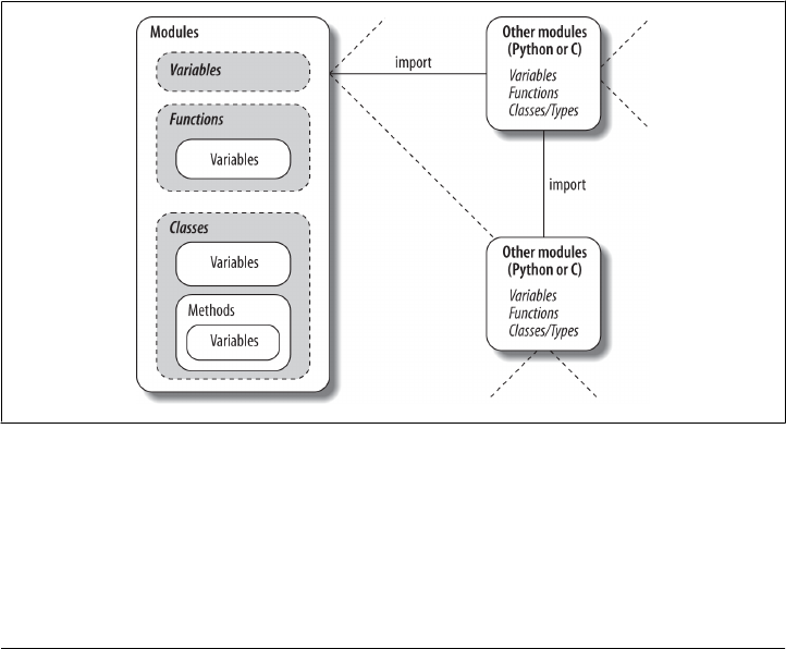
functions and classes imported from them. The only things a module should share
with the outside world are the tools it uses, and the tools it defines.
•Maximize module cohesion: unified purpose. You can minimize a module’s
couplings by maximizing its cohesion; if all the components of a module share a
general purpose, you’re less likely to depend on external names.
•Modules should rarely change other modules’ variables. We illustrated this
with code in Chapter 17, but it’s worth repeating here: it’s perfectly OK to use
globals defined in another module (that’s how clients import services, after all),
but changing globals in another module is often a symptom of a design problem.
There are exceptions, of course, but you should try to communicate results through
devices such as function arguments and return values, not cross-module changes.
Otherwise, your globals’ values become dependent on the order of arbitrarily re-
mote assignments in other files, and your modules become harder to understand
and reuse.
As a summary, Figure 25-1 sketches the environment in which modules operate. Mod-
ules contain variables, functions, classes, and other modules (if imported). Functions
have local variables of their own, as do classes—objects that live within modules and
which we’ll begin studying in the next chapter. As we saw in Part IV, functions can
nest, too, but all are ultimately contained by modules at the top.
Figure 25-1. Module execution environment. Modules are imported, but modules also import and use
other modules, which may be coded in Python or another language such as C. Modules in turn contain
variables, functions, and classes to do their work, and their functions and classes may contain variables
and other items of their own. At the top, though, programs are just sets of modules.
746 | Chapter 25: Advanced Module Topics
www.it-ebooks.info

Data Hiding in Modules
As we’ve seen, a Python module exports all the names assigned at the top level of its
file. There is no notion of declaring which names should and shouldn’t be visible out-
side the module. In fact, there’s no way to prevent a client from changing names inside
a module if it wants to.
In Python, data hiding in modules is a convention, not a syntactical constraint. If you
want to break a module by trashing its names, you can, but fortunately, I’ve yet to meet
a programmer for whom this was a life goal. Some purists object to this liberal attitude
toward data hiding, claiming that it means Python can’t implement encapsulation.
However, encapsulation in Python is more about packaging than about restricting.
We’ll expand this idea in the next part in relation to classes, which also have no privacy
syntax but can often emulate its effect in code.
Minimizing from * Damage: _X and __all__
As a special case, you can prefix names with a single underscore (e.g., _X) to prevent
them from being copied out when a client imports a module’s names with a from *
statement. This really is intended only to minimize namespace pollution; because from
* copies out all names, the importer may get more than it’s bargained for (including
names that overwrite names in the importer). Underscores aren’t “private” declara-
tions: you can still see and change such names with other import forms, such as the
import statement:
# unders.py
a, _b, c, _d = 1, 2, 3, 4
>>> from unders import * # Load non _X names only
>>> a, c
(1, 3)
>>> _b
NameError: name '_b' is not defined
>>> import unders # But other importers get every name
>>> unders._b
2
Alternatively, you can achieve a hiding effect similar to the _X naming convention by
assigning a list of variable name strings to the variable __all__ at the top level of the
module. When this feature is used, the from * statement will copy out only those names
listed in the __all__ list. In effect, this is the converse of the _X convention: __all__
identifies names to be copied, while _X identifies names not to be copied. Python looks
for an __all__ list in the module first and copies its names irrespective of any under-
scores; if __all__ is not defined, from * copies all names without a single leading un-
derscore:
# alls.py
__all__ = ['a', '_c'] # __all__ has precedence over _X
Data Hiding in Modules | 747
www.it-ebooks.info

a, b, _c, _d = 1, 2, 3, 4
>>> from alls import * # Load __all__ names only
>>> a, _c
(1, 3)
>>> b
NameError: name 'b' is not defined
>>> from alls import a, b, _c, _d # But other importers get every name
>>> a, b, _c, _d
(1, 2, 3, 4)
>>> import alls
>>> alls.a, alls.b, alls._c, alls._d
(1, 2, 3, 4)
Like the _X convention, the __all__ list has meaning only to the from * statement form
and does not amount to a privacy declaration: other import statements can still access
all names, as the last two tests show. Still, module writers can use either technique to
implement modules that are well behaved when used with from *. See also the discus-
sion of __all__ lists in package __init__.py files in Chapter 24; there, these lists declare
submodules to be automatically loaded for a from * on their container.
Enabling Future Language Features: __future__
Changes to the language that may potentially break existing code are usually introduced
gradually in Python. They often initially appear as optional extensions, which are dis-
abled by default. To turn on such extensions, use a special import statement of this form:
from __future__ import featurename
When used in a script, this statement must appear as the first executable statement in
the file (possibly following a docstring or comment), because it enables special com-
pilation of code on a per-module basis. It’s also possible to submit this statement at the
interactive prompt to experiment with upcoming language changes; the feature will
then be available for the remainder of the interactive session.
For example, in this book we’ve seen how to use this statement in Python 2.X to activate
3.X true division in Chapter 5, 3.X print calls in Chapter 11, and 3.X absolute imports
for packages in Chapter 24. Prior editions of this book used this statement form to
demonstrate generator functions, which required a keyword that was not yet enabled
by default (they use a featurename of generators).
All of these changes have the potential to break existing code in Python 2.X, so they
were phased in gradually or offered as optional extensions, enabled with this special
import. At the same time, some are available to allow you to write code that is forward
compatible with later releases you may port to someday.
For a list of futurisms you may import and turn on this way, run a dir call on the
__future__ module after importing it, or see its library manual entry. Per its documen-
748 | Chapter 25: Advanced Module Topics
www.it-ebooks.info

tation, none of its feature names will ever be removed, so it’s safe to leave in a
__future__ import even in code run by a version of Python where the feature is present
normally.
Mixed Usage Modes: __name__ and __main__
Our next module-related trick lets you both import a file as a module and run it as a
standalone program, and is widely used in Python files. It’s actually so simple that some
miss the point at first: each module has a built-in attribute called __name__, which
Python creates and assigns automatically as follows:
• If the file is being run as a top-level program file, __name__ is set to the string
"__main__" when it starts.
• If the file is being imported instead, __name__ is set to the module’s name as known
by its clients.
The upshot is that a module can test its own __name__ to determine whether it’s being
run or imported. For example, suppose we create the following module file, named
runme.py, to export a single function called tester:
def tester():
print("It's Christmas in Heaven...")
if __name__ == '__main__': # Only when run
tester() # Not when imported
This module defines a function for clients to import and use as usual:
c:\code> python
>>> import runme
>>> runme.tester()
It's Christmas in Heaven...
But the module also includes code at the bottom that is set up to call the function
automatically when this file is run as a program:
c:\code> python runme.py
It's Christmas in Heaven...
In effect, a module’s __name__ variable serves as a usage mode flag, allowing its code to
be leveraged as both an importable library and a top-level script. Though simple, you’ll
see this hook used in the majority of the Python program files you are likely to encounter
in the wild—both for testing and dual usage.
For instance, perhaps the most common way you’ll see the __name__ test applied is for
self-test code. In short, you can package code that tests a module’s exports in the module
itself by wrapping it in a __name__ test at the bottom of the file. This way, you can use
the file in clients by importing it, but also test its logic by running it from the system
shell or via another launching scheme.
Mixed Usage Modes: __name__ and __main__ | 749
www.it-ebooks.info

Coding self-test code at the bottom of a file under the __name__ test is probably the most
common and simplest unit-testing protocol in Python. It’s much more convenient than
retyping all your tests at the interactive prompt. (Chapter 36 will discuss other com-
monly used options for testing Python code—as you’ll see, the unittest and doctest
standard library modules provide more advanced testing tools.)
In addition, the __name__ trick is also commonly used when you’re writing files that
can be used both as command-line utilities and as tool libraries. For instance, suppose
you write a file-finder script in Python. You can get more mileage out of your code if
you package it in functions and add a __name__ test in the file to automatically call those
functions when the file is run standalone. That way, the script’s code becomes reusable
in other programs.
Unit Tests with __name__
In fact, we’ve already seen a prime example in this book of an instance where the
__name__ check could be useful. In the section on arguments in Chapter 18, we coded
a script that computed the minimum value from the set of arguments sent in (this was
the file minmax.py in “The min Wakeup Call!”):
def minmax(test, *args):
res = args[0]
for arg in args[1:]:
if test(arg, res):
res = arg
return res
def lessthan(x, y): return x < y
def grtrthan(x, y): return x > y
print(minmax(lessthan, 4, 2, 1, 5, 6, 3)) # Self-test code
print(minmax(grtrthan, 4, 2, 1, 5, 6, 3))
This script includes self-test code at the bottom, so we can test it without having to
retype everything at the interactive command line each time we run it. The problem
with the way it is currently coded, however, is that the output of the self-test call will
appear every time this file is imported from another file to be used as a tool—not exactly
a user-friendly feature! To improve it, we can wrap up the self-test call in a __name__
check, so that it will be launched only when the file is run as a top-level script, not when
it is imported (this new version of the module file is renamed minmax2.py here):
print('I am:', __name__)
def minmax(test, *args):
res = args[0]
for arg in args[1:]:
if test(arg, res):
res = arg
return res
750 | Chapter 25: Advanced Module Topics
www.it-ebooks.info

def lessthan(x, y): return x < y
def grtrthan(x, y): return x > y
if __name__ == '__main__':
print(minmax(lessthan, 4, 2, 1, 5, 6, 3)) # Self-test code
print(minmax(grtrthan, 4, 2, 1, 5, 6, 3))
We’re also printing the value of __name__ at the top here to trace its value. Python creates
and assigns this usage-mode variable as soon as it starts loading a file. When we run
this file as a top-level script, its name is set to __main__, so its self-test code kicks in
automatically:
c:\code> python minmax2.py
I am: __main__
1
6
If we import the file, though, its name is not __main__, so we must explicitly call the
function to make it run:
c:\code> python
>>> import minmax2
I am: minmax2
>>> minmax2.minmax(minmax2.lessthan, 's', 'p', 'a', 'a')
'a'
Again, regardless of whether this is used for testing, the net effect is that we get to use
our code in two different roles—as a library module of tools, or as an executable pro-
gram.
Per Chapter 24’s discussion of package relative imports, this section’s
technique can also have some implications for imports run by files that
are also used as package components in 3.X, but can still be leveraged
with absolute package path imports and other techniques. See the prior
chapter’s discussion and example for more details.
Example: Dual Mode Code
Here’s a more substantial module example that demonstrates another way that the
prior section’s __name__ trick is commonly employed. The following module, for-
mats.py, defines string formatting utilities for importers, but also checks its name to
see if it is being run as a top-level script; if so, it tests and uses arguments listed on the
system command line to run a canned or passed-in test. In Python, the sys.argv list
contains command-line arguments—it is a list of strings reflecting words typed on the
command line, where the first item is always the name of the script being run. We used
this in Chapter 21’s benchmark tool as switches, but leverage it as a general input
mechanism here:
#!python
"""
Example: Dual Mode Code | 751
www.it-ebooks.info

File: formats.py (2.X and 3.X)
Various specialized string display formatting utilities.
Test me with canned self-test or command-line arguments.
To do: add parens for negative money, add more features.
"""
def commas(N):
"""
Format positive integer-like N for display with
commas between digit groupings: "xxx,yyy,zzz".
"""
digits = str(N)
assert(digits.isdigit())
result = ''
while digits:
digits, last3 = digits[:-3], digits[-3:]
result = (last3 + ',' + result) if result else last3
return result
def money(N, numwidth=0, currency='$'):
"""
Format number N for display with commas, 2 decimal digits,
leading $ and sign, and optional padding: "$ -xxx,yyy.zz".
numwidth=0 for no space padding, currency='' to omit symbol,
and non-ASCII for others (e.g., pound=u'\xA3' or u'\u00A3').
"""
sign = '-' if N < 0 else ''
N = abs(N)
whole = commas(int(N))
fract = ('%.2f' % N)[-2:]
number = '%s%s.%s' % (sign, whole, fract)
return '%s%*s' % (currency, numwidth, number)
if __name__ == '__main__':
def selftest():
tests = 0, 1 # fails: −1, 1.23
tests += 12, 123, 1234, 12345, 123456, 1234567
tests += 2 ** 32, 2 ** 100
for test in tests:
print(commas(test))
print('')
tests = 0, 1, −1, 1.23, 1., 1.2, 3.14159
tests += 12.34, 12.344, 12.345, 12.346
tests += 2 ** 32, (2 ** 32 + .2345)
tests += 1.2345, 1.2, 0.2345
tests += −1.2345, −1.2, −0.2345
tests += −(2 ** 32), −(2**32 + .2345)
tests += (2 ** 100), −(2 ** 100)
for test in tests:
print('%s [%s]' % (money(test, 17), test))
import sys
if len(sys.argv) == 1:
selftest()
752 | Chapter 25: Advanced Module Topics
www.it-ebooks.info

else:
print(money(float(sys.argv[1]), int(sys.argv[2])))
This file works identically in Python 2.X and 3.X. When run directly, it tests itself as
before, but it uses options on the command line to control the test behavior. Run this
file directly with no command-line arguments on your own to see what its self-test code
prints—it’s too extensive to list in full here:
c:\code> python formats.py
0
1
12
123
1,234
12,345
123,456
1,234,567
...etc...
To test specific strings, pass them in on the command line along with a minimum field
width; the script’s __main__ code passes them on to its money function, which in turn
runs commas:
C:\code> python formats.py 999999999 0
$999,999,999.00
C:\code> python formats.py −999999999 0
$-999,999,999.00
C:\code> python formats.py 123456789012345 0
$123,456,789,012,345.00
C:\code> python formats.py −123456789012345 25
$ −123,456,789,012,345.00
C:\code> python formats.py 123.456 0
$123.46
C:\code> python formats.py −123.454 0
$-123.45
As before, because this code is instrumented for dual-mode usage, we can also import
its tools normally to reuse them as library components in scripts, modules, and the
interactive prompt:
>>> from formats import money, commas
>>> money(123.456)
'$123.46'
>>> money(-9999999.99, 15)
'$ −9,999,999.99'
>>> X = 99999999999999999999
>>> '%s (%s)' % (commas(X), X)
'99,999,999,999,999,999,999 (99999999999999999999)'
You can use command-line arguments in ways similar to this example to provide gen-
eral inputs to scripts that may also package their code as functions and classes for reuse
by importers. For more advanced command-line processing, see “Python Command-
Example: Dual Mode Code | 753
www.it-ebooks.info

Line Arguments” on page 1432 in Appendix A, and the getopt, optparse, and arg
parse modules’ documentation in Python’s standard library manual. In some scenarios,
you might also use the built-in input function, used in Chapter 3 and Chapter 10, to
prompt the shell user for test inputs instead of pulling them from the command line.
Also see Chapter 7’s discussion of the new {,d} string format method
syntax added in Python 2.7 and 3.1; this formatting extension separates
thousands groups with commas much like the code here. The module
listed here, though, adds money formatting, can be changed, and serves
as a manual alternative for comma insertions in earlier Pythons.
Currency Symbols: Unicode in Action
This module’s money function defaults to dollars, but supports other currency symbols
by allowing you to pass in non-ASCII Unicode characters. The Unicode ordinal with
hexadecimal value 00A3, for example, is the pound symbol, and 00A5 is the yen. You
can code these in a variety of forms, as:
• The character’s decoded Unicode code point ordinal (integer) in a text string, with
either Unicode or hex escapes (for 2.X compatibility, use a leading u in such string
literals in Python 3.3)
• The character’s raw encoded form in a byte string that is decoded before passed,
with hex escapes (for 3.X compatibility, use a leading b in such string literals in
Python 2.X)
• The actual character itself in your program’s text, along with a source code en-
coding declaration
We previewed Unicode in Chapter 4 and will get into more details in Chapter 37, but
its basic requirements here are fairly simple, and serve as a decent use case. To test
alternative currencies, I typed the following in a file, formats_currency.py, because it
was too much to reenter interactively on changes:
from __future__ import print_function # 2.X
from formats import money
X = 54321.987
print(money(X), money(X, 0, ''))
print(money(X, currency=u'\xA3'), money(X, currency=u'\u00A5'))
print(money(X, currency=b'\xA3'.decode('latin-1')))
print(money(X, currency=u'\u20AC'), money(X, 0, b'\xA4'.decode('iso-8859-15')))
print(money(X, currency=b'\xA4'.decode('latin-1')))
The following gives this test file’s output in Python 3.3 in IDLE, and in other contexts
configured properly. It works the same in 2.X because it prints and codes strings port-
ably. Per Chapter 11, a __future__ import enables 3.X print calls in 2.X. And as intro-
754 | Chapter 25: Advanced Module Topics
www.it-ebooks.info

duced in Chapter 4, 3.X b'...' bytes literals are taken as simple strings in 2.X, and 2.X
u'...' Unicode literals as treated as normal strings in 3.X as of 3.3.
$54,321.99 54,321.99
£54,321.99 ¥54,321.99
£54,321.99
€54,321.99 €54,321.99
¤54,321.99
If this works on your computer, you can probably skip the next few paragraphs. De-
pending on your interface and system settings, though, getting this to run and display
properly may require additional steps. On my machine, it behaves correctly when
Python and the display medium are in sync, but the euro and generic currency symbols
in the last two lines fail with errors in a basic Command Prompt on Windows.
Specifically, this test script always runs and produces the output shown in the IDLE
GUI in both 3.X and 2.X, because Unicode-to-glyph mappings are handled well. It also
works as advertised in 3.X on Windows if you redirect the output to a file and open it
with Notepad, because 3.X encodes content on this platform in a default Windows
format that Notepad understands:
c:\code> formats_currency.py > temp
c:\code> notepad temp
However, this doesn’t work in 2.X, because Python tries to encode printed text as ASCII
by default. To show all the non-ASCII characters in a Windows Command Prompt
window directly, on some computers you may need to change the Windows code
page (used to render characters) as well as Python’s PYTHONIOENCODING environment
variable (used as the encoding of text in standard streams, including the translation of
characters to bytes when they are printed) to a common Unicode format such as UTF-8:
c:\code> chcp 65001 # Console matches Python
c:\code> set PYTHONIOENCODING=utf-8 # Python matches console
c:\code> formats_currency.py > temp # Both 3.X and 2.X write UTF-8 text
c:\code> type temp # Console displays it properly
c:\code> notepad temp # Notepad recognizes UTF-8 too
You may not need to take these steps on some platforms and even on some Windows
distributions. I did because my laptop’s code page is set to 437 (U.S. characters), but
your code pages may vary.
Subtly, the only reason this test works on Python 2.X at all is because 2.X allows normal
and Unicode strings to be mixed, as long as the normal string is all 7-bit ASCII char-
acters. On 3.3, the 2.X u'...' Unicode literal is supported for compatibility, but taken
the same as normal '...' strings, which are always Unicode (removing the leading u
makes the test work in 3.0 through 3.2 too, but breaks 2.X compatibility):
c:\code> py −2
>>> print u'\xA5' + '1', '%s2' % u'\u00A3' # 2.X: unicode/str mix for ASCII str
¥1 £2
c:\code> py −3
Example: Dual Mode Code | 755
www.it-ebooks.info

>>> print(u'\xA5' + '1', '%s2' % u'\u00A3') # 3.X: str is Unicode, u'' optional
¥1 £2
>>> print('\xA5' + '1', '%s2' % '\u00A3')
¥1 £2
Again, there’s much more on Unicode in Chapter 37—a topic many see as peripheral,
but which can crop up even in relatively simple contexts like this! The takeaway point
here is that, operational issues aside, a carefully coded script can often manage to sup-
port Unicode in both 3.X and 2.X.
Docstrings: Module Documentation at Work
Finally, because this example’s main file uses the docstring feature introduced in Chap-
ter 15, we can use the help function or PyDoc’s GUI/browser modes to explore its tools
as well—modules are almost automatically general-purpose tools. Here’s help at work;
Figure 25-2 gives the PyDoc view on our file.
>>> import formats
>>> help(formats)
Help on module formats:
NAME
formats
DESCRIPTION
File: formats.py (2.X and 3.X)
Various specialized string display formatting utilities.
Test me with canned self-test or command-line arguments.
To do: add parens for negative money, add more features.
FUNCTIONS
commas(N)
Format positive integer-like N for display with
commas between digit groupings: "xxx,yyy,zzz".
money(N, numwidth=0, currency='$')
Format number N for display with commas, 2 decimal digits,
leading $ and sign, and optional padding: "$ -xxx,yyy.zz".
numwidth=0 for no space padding, currency='' to omit symbol,
and non-ASCII for others (e.g., pound=u'£' or u'£').
FILE
c:\code\formats.py
Changing the Module Search Path
Let’s return to more general module topics. In Chapter 22, we learned that the module
search path is a list of directories that can be customized via the environment variable
PYTHONPATH, and possibly via .pth files. What I haven’t shown you until now is how a
Python program itself can actually change the search path by changing the built-in
756 | Chapter 25: Advanced Module Topics
www.it-ebooks.info
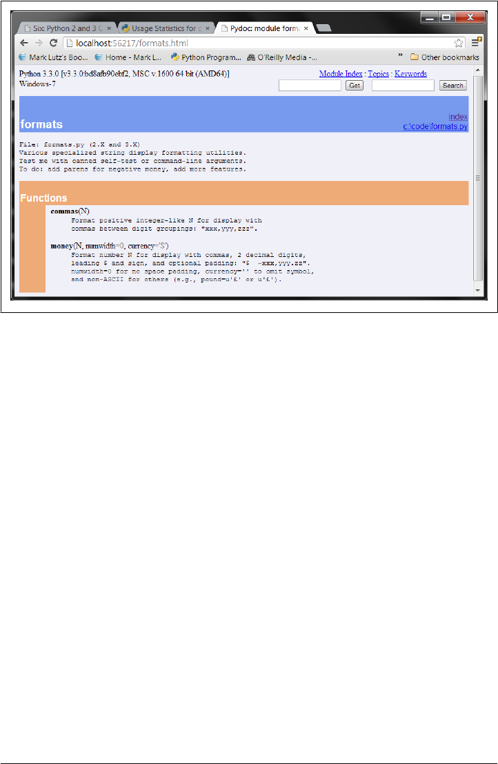
sys.path list. Per Chapter 22, sys.path is initialized on startup, but thereafter you can
delete, append, and reset its components however you like:
>>> import sys
>>> sys.path
['', 'c:\\temp', 'C:\\Windows\\system32\\python33.zip', ...more deleted...]
>>> sys.path.append('C:\\sourcedir') # Extend module search path
>>> import string # All imports search the new dir last
Once you’ve made such a change, it will impact all future imports anywhere while a
Python program runs, as all importers share the same single sys.path list (there’s only
one copy of a given module in memory during a program’s run—that’s why reload
exists). In fact, this list may be changed arbitrarily:
>>> sys.path = [r'd:\temp'] # Change module search path
>>> sys.path.append('c:\\lp5e\\examples') # For this run (process) only
>>> sys.path.insert(0, '..')
>>> sys.path
['..', 'd:\\temp', 'c:\\lp5e\\examples']
>>> import string
Traceback (most recent call last):
File "<stdin>", line 1, in <module>
ImportError: No module named 'string'
Thus, you can use this technique to dynamically configure a search path inside a Python
program. Be careful, though: if you delete a critical directory from the path, you may
lose access to critical utilities. In the prior example, for instance, we no longer have
Figure 25-2. PyDoc’s view of formats.py, obtained by running a “py −3 -m pydoc –b” command line
in 3.2 and later and clicking on the file’s index entry (see Chapter 15)
Changing the Module Search Path | 757
www.it-ebooks.info

access to the string module because we deleted the Python source library’s directory
from the path!
Also, remember that such sys.path settings endure for only as long as the Python ses-
sion or program (technically, process) that made them runs; they are not retained after
Python exits. By contrast, PYTHONPATH and .pth file path configurations live in the op-
erating system instead of a running Python program, and so are more global: they are
picked up by every program on your machine and live on after a program completes.
On some systems, the former can be per-user and the latter can be installation-wide.
The as Extension for import and from
Both the import and from statements were eventually extended to allow an imported
name to be given a different name in your script. We’ve used this extension earlier, but
here are some additional details: the following import statement:
import modulename as name # And use name, not modulename
is equivalent to the following, which renames the module in the importer’s scope only
(it’s still known by its original name to other files):
import modulename
name = modulename
del modulename # Don't keep original name
After such an import, you can—and in fact must—use the name listed after the as to
refer to the module. This works in a from statement, too, to assign a name imported
from a file to a different name in the importer’s scope; as before you get only the new
name you provide, not its original:
from modulename import attrname as name # And use name, not attrname
As discussed in Chapter 23, this extension is commonly used to provide short syno-
nyms for longer names, and to avoid name clashes when you are already using a name
in your script that would otherwise be overwritten by a normal import statement:
import reallylongmodulename as name # Use shorter nickname
name.func()
from module1 import utility as util1 # Can have only 1 "utility"
from module2 import utility as util2
util1(); util2()
It also comes in handy for providing a short, simple name for an entire directory path
and avoiding name collisions when using the package import feature described in
Chapter 24:
import dir1.dir2.mod as mod # Only list full path once
mod.func()
from dir1.dir2.mod import func as modfunc # Rename to make unique if needed
modfunc()
758 | Chapter 25: Advanced Module Topics
www.it-ebooks.info

This is also something of a hedge against name changes: if a new release of a library
renames a module or tool your code uses extensively, or provides a new alternative
you’d rather use instead, you can simply rename it to its prior name on import to avoid
breaking your code:
import newname as oldname
from library import newname as oldname
...and keep happily using oldname until you have time to update all your code...
For example, this approach can address some 3.X library changes (e.g., 3.X’s tkinter
versus 2.X’s Tkinter), though they’re often substantially more than just a new name!
Example: Modules Are Objects
Because modules expose most of their interesting properties as built-in attributes, it’s
easy to write programs that manage other programs. We usually call such manager
programs metaprograms because they work on top of other systems. This is also referred
to as introspection, because programs can see and process object internals. Introspec-
tion is a somewhat advanced feature, but it can be useful for building programming
tools.
For instance, to get to an attribute called name in a module called M, we can use attribute
qualification or index the module’s attribute dictionary, exposed in the built-in
__dict__ attribute we met in Chapter 23. Python also exports the list of all loaded
modules as the sys.modules dictionary and provides a built-in called getattr that lets
us fetch attributes from their string names—it’s like saying object.attr, but attr is an
expression that yields a string at runtime. Because of that, all the following expressions
reach the same attribute and object:1
M.name # Qualify object by attribute
M.__dict__['name'] # Index namespace dictionary manually
sys.modules['M'].name # Index loaded-modules table manually
getattr(M, 'name') # Call built-in fetch function
By exposing module internals like this, Python helps you build programs about pro-
grams. For example, here is a module named mydir.py that puts these ideas to work to
implement a customized version of the built-in dir function. It defines and exports a
function called listing, which takes a module object as an argument and prints a for-
matted listing of the module’s namespace sorted by name:
1. As we saw briefly in “Other Ways to Access Globals” in Chapter 17, because a function can access its
enclosing module by going through the sys.modules table like this, it can also be used to emulate the effect
of the global statement. For instance, the effect of global X; X=0 can be simulated (albeit with much
more typing!) by saying this inside a function: import sys; glob=sys.modules[__name__]; glob.X=0.
Remember, each module gets a __name__ attribute for free; it’s visible as a global name inside the functions
within the module. This trick provides another way to change both local and global variables of the same
name inside a function.
Example: Modules Are Objects | 759
www.it-ebooks.info

#!python
"""
mydir.py: a module that lists the namespaces of other modules
"""
from __future__ import print_function # 2.X compatibility
seplen = 60
sepchr = '-'
def listing(module, verbose=True):
sepline = sepchr * seplen
if verbose:
print(sepline)
print('name:', module.__name__, 'file:', module.__file__)
print(sepline)
count = 0
for attr in sorted(module.__dict__): # Scan namespace keys (or enumerate)
print('%02d) %s' % (count, attr), end = ' ')
if attr.startswith('__'):
print('<built-in name>') # Skip __file__, etc.
else:
print(getattr(module, attr)) # Same as .__dict__[attr]
count += 1
if verbose:
print(sepline)
print(module.__name__, 'has %d names' % count)
print(sepline)
if __name__ == '__main__':
import mydir
listing(mydir) # Self-test code: list myself
Notice the docstring at the top; as in the prior formats.py example, because we may
want to use this as a general tool, the docstring provides functional information acces-
sible via help and GUI/browser mode of PyDoc—a tool that uses similar introspection
tools to do its job. A self-test is also provided at the bottom of this module, which
narcissistically imports and lists itself. Here’s the sort of output produced in Python
3.3; this script works on 2.X too (where it may list fewer names) because it prints from
the __future__:
c:\code> py −3 mydir.py
------------------------------------------------------------
name: mydir file: c:\code\mydir.py
------------------------------------------------------------
00) __builtins__ <built-in name>
01) __cached__ <built-in name>
02) __doc__ <built-in name>
03) __file__ <built-in name>
04) __initializing__ <built-in name>
05) __loader__ <built-in name>
06) __name__ <built-in name>
07) __package__ <built-in name>
760 | Chapter 25: Advanced Module Topics
www.it-ebooks.info

08) listing <function listing at 0x000000000295B488>
09) print_function _Feature((2, 6, 0, 'alpha', 2), (3, 0, 0, 'alpha', 0), 65536)
10) sepchr -
11) seplen 60
------------------------------------------------------------
mydir has 12 names
------------------------------------------------------------
To use this as a tool for listing other modules, simply pass the modules in as objects to
this file’s function. Here it is listing attributes in the tkinter GUI module in the standard
library (a.k.a. Tkinter in Python 2.X); it will technically work on any object with
__name__, __file__, and __dict__ attributes:
>>> import mydir
>>> import tkinter
>>> mydir.listing(tkinter)
------------------------------------------------------------
name: tkinter file: C:\Python33\lib\tkinter\__init__.py
------------------------------------------------------------
00) ACTIVE active
01) ALL all
02) ANCHOR anchor
03) ARC arc
04) At <function At at 0x0000000002BD41E0>
...many more names omitted...
156) image_types <function image_types at 0x0000000002BE2378>
157) mainloop <function mainloop at 0x0000000002BCBBF8>
158) sys <module 'sys' (built-in)>
159) wantobjects 1
160) warnings <module 'warnings' from 'C:\\Python33\\lib\\warnings.py'>
------------------------------------------------------------
tkinter has 161 names
------------------------------------------------------------
We’ll meet getattr and its relatives again later. The point to notice here is that mydir
is a program that lets you browse other programs. Because Python exposes its internals,
you can process objects generically.2
Importing Modules by Name String
The module name in an import or from statement is a hardcoded variable name. Some-
times, though, your program will get the name of a module to be imported as a string
at runtime—from a user selection in a GUI, or a parse of an XML document, for in-
stance. Unfortunately, you can’t use import statements directly to load a module given
its name as a string—Python expects a variable name that’s taken literally and not
evaluated, not a string or expression. For instance:
2. You can preload tools such as mydir.listing and the reloader we’ll meet in a moment into the interactive
namespace by importing them in the file referenced by the PYTHONSTARTUP environment variable. Because
code in the startup file runs in the interactive namespace (module __main__), importing common tools in
the startup file can save you some typing. See Appendix A for more details.
Importing Modules by Name String | 761
www.it-ebooks.info

>>> import 'string'
File "<stdin>", line 1
import "string"
^
SyntaxError: invalid syntax
It also won’t work to simply assign the string to a variable name:
x = 'string'
import x
Here, Python will try to import a file x.py, not the string module—the name in an
import statement both becomes a variable assigned to the loaded module and identifies
the external file literally.
Running Code Strings
To get around this, you need to use special tools to load a module dynamically from a
string that is generated at runtime. The most general approach is to construct an
import statement as a string of Python code and pass it to the exec built-in function to
run (exec is a statement in Python 2.X, but it can be used exactly as shown here—the
parentheses are simply ignored):
>>> modname = 'string'
>>> exec('import ' + modname) # Run a string of code
>>> string # Imported in this namespace
<module 'string' from 'C:\\Python33\\lib\\string.py'>
We met the exec function (and its cousin for expressions, eval) earlier, in Chapter 3
and Chapter 10. It compiles a string of code and passes it to the Python interpreter to
be executed. In Python, the byte code compiler is available at runtime, so you can write
programs that construct and run other programs like this. By default, exec runs the
code in the current scope, but you can get more specific by passing in optional name-
space dictionaries if needed. It also has security issues noted earlier in the book, which
may be minor in a code string you are building yourself.
Direct Calls: Two Options
The only real drawback to exec here is that it must compile the import statement each
time it runs, and compiling can be slow. Precompiling to byte code with the compile
built-in may help for code strings run many times, but in most cases it’s probably
simpler and may run quicker to use the built-in __import__ function to load from a
name string instead, as noted in Chapter 22. The effect is similar, but __import__ returns
the module object, so assign it to a name here to keep it:
>>> modname = 'string'
>>> string = __import__(modname)
>>> string
<module 'string' from 'C:\\Python33\\lib\\string.py'>
762 | Chapter 25: Advanced Module Topics
www.it-ebooks.info

As also noted in Chapter 22, the newer call importlib.import_module does the same
work, and is generally preferred in more recent Pythons for direct calls to import by
name string—at least per the current “official” policy stated in Python’s manuals:
>>> import importlib
>>> modname = 'string'
>>> string = importlib.import_module(modname)
>>> string
<module 'string' from 'C:\\Python33\\lib\\string.py'>
The import_module call takes a module name string, and an optional second argument
that gives the package used as the anchor point for resolving relative imports, which
defaults to None. This call works the same as __import__ in its basic roles, but see
Python’s manuals for more details.
Though both calls still work, in Pythons where both are available, the original
__import__ is generally intended for customizing import operations by reassignment in
the built-in scope (and any future changes in “official” policy are beyond the scope of
this book!).
Example: Transitive Module Reloads
This section develops a module tool that ties together and applies some earlier topics,
and serves as a larger case study to close out this chapter and part. We studied module
reloads in Chapter 23, as a way to pick up changes in code without stopping and re-
starting a program. When you reload a module, though, Python reloads only that par-
ticular module’s file; it doesn’t automatically reload modules that the file being reloaded
happens to import.
For example, if you reload some module A, and A imports modules B and C, the reload
applies only to A, not to B and C. The statements inside A that import B and C are rerun
during the reload, but they just fetch the already loaded B and C module objects (as-
suming they’ve been imported before). In actual yet abstract code, here’s the file A.py:
# A.py
import B # Not reloaded when A is!
import C # Just an import of an already loaded module: no-ops
% python
>>> . . .
>>> from imp import reload
>>> reload(A)
By default, this means that you cannot depend on reloads to pick up changes in all the
modules in your program transitively—instead, you must use multiple reload calls to
update the subcomponents independently. This can require substantial work for large
systems you’re testing interactively. You can design your systems to reload their sub-
components automatically by adding reload calls in parent modules like A, but this
complicates the modules’ code.
Example: Transitive Module Reloads | 763
www.it-ebooks.info

A Recursive Reloader
A better approach is to write a general tool to do transitive reloads automatically by
scanning modules’ __dict__ namespace attributes and checking each item’s type to
find nested modules to reload. Such a utility function could call itself recursively to
navigate arbitrarily shaped and deep import dependency chains. Module __dict__ at-
tributes were introduced in Chapter 23 and employed earlier in this chapter, and the
type call was presented in Chapter 9; we just need to combine the two tools.
The module reloadall.py listed next defines a reload_all function that automatically
reloads a module, every module that the module imports, and so on, all the way to the
bottom of each import chain. It uses a dictionary to keep track of already reloaded
modules, recursion to walk the import chains, and the standard library’s types module,
which simply predefines type results for built-in types. The visited dictionary techni-
que works to avoid cycles here when imports are recursive or redundant, because mod-
ule objects are immutable and so can be dictionary keys; as we learned in Chapter 5
and Chapter 8, a set would offer similar functionality if we use visited.add(module) to
insert:
#!python
"""
reloadall.py: transitively reload nested modules (2.X + 3.X).
Call reload_all with one or more imported module module objects.
"""
import types
from imp import reload # from required in 3.X
def status(module):
print('reloading ' + module.__name__)
def tryreload(module):
try:
reload(module) # 3.3 (only?) fails on some
except:
print('FAILED: %s' % module)
def transitive_reload(module, visited):
if not module in visited: # Trap cycles, duplicates
status(module) # Reload this module
tryreload(module) # And visit children
visited[module] = True
for attrobj in module.__dict__.values(): # For all attrs
if type(attrobj) == types.ModuleType: # Recur if module
transitive_reload(attrobj, visited)
def reload_all(*args):
visited = {} # Main entry point
for arg in args: # For all passed in
if type(arg) == types.ModuleType:
transitive_reload(arg, visited)
764 | Chapter 25: Advanced Module Topics
www.it-ebooks.info

def tester(reloader, modname): # Self-test code
import importlib, sys # Import on tests only
if len(sys.argv) > 1: modname = sys.argv[1] # command line (or passed)
module = importlib.import_module(modname) # Import by name string
reloader(module) # Test passed-in reloader
if __name__ == '__main__':
tester(reload_all, 'reloadall') # Test: reload myself?
Besides namespace dictionaries, this script makes use of other tools we’ve studied here:
it includes a __name__ test to launch self-test code when run as a top-level script only,
and its tester function uses sys.argv to inspect command-line arguments and impor
tlib to import a module by name string passed in as a function or command-line ar-
gument. One curious bit: notice how this code must wrap the basic reload call in a
try statement to catch exceptions—in Python 3.3, reloads sometimes fail due to a re-
write of the import machinery. The try was previewed in Chapter 10, and is covered
in full in Part VII.
Testing recursive reloads
Now, to leverage this utility for normal use, import its reload_all function and pass it
an already loaded module object—just as you would for the built-in reload function.
When the file runs standalone, its self-test code calls reload_all automatically, reload-
ing its own module by default if no command-line arguments are used. In this mode,
the module must import itself because its own name is not defined in the file without
an import. This code works in both 3.X and 2.X because we’ve used + and % instead of
a comma in the prints, though the set of modules used and thus reloaded may vary
across lines:
C:\code> c:\Python33\python reloadall.py
reloading reloadall
reloading types
c:\code> C:\Python27\python reloadall.py
reloading reloadall
reloading types
With a command-line argument, the tester instead reloads the given module by its name
string—here, the benchmark module we coded in Chapter 21. Note that we give a
module name in this mode, not a filename (as for import statements, don’t include
the .py extension); the script ultimately imports the module using the module search
path as usual:
c:\code> reloadall.py pybench
reloading pybench
reloading timeit
reloading itertools
reloading sys
reloading time
reloading gc
reloading os
Example: Transitive Module Reloads | 765
www.it-ebooks.info

reloading errno
reloading ntpath
reloading stat
reloading genericpath
reloading copyreg
Perhaps most commonly, we can also deploy this module at the interactive prompt—
here, in 3.3 for some standard library modules. Notice how os is imported by
tkinter, but tkinter reaches sys before os can (if you want to test this on Python 2.X,
substitute Tkinter for tkinter):
>>> from reloadall import reload_all
>>> import os, tkinter
>>> reload_all(os) # Normal usage mode
reloading os
reloading ntpath
reloading stat
reloading sys
reloading genericpath
reloading errno
reloading copyreg
>>> reload_all(tkinter)
reloading tkinter
reloading _tkinter
reloading warnings
reloading sys
reloading linecache
reloading tokenize
reloading builtins
FAILED: <module 'builtins'>
reloading re
...etc...
reloading os
reloading ntpath
reloading stat
reloading genericpath
reloading errno
...etc...
And finally here is a session that shows the effect of normal versus transitive reloads—
changes made to the two nested files are not picked up by reloads, unless the transitive
utility is used:
import b # File a.py
X = 1
import c # File b.py
Y = 2
Z = 3 # File c.py
C:\code> py −3
>>> import a
>>> a.X, a.b.Y, a.b.c.Z
766 | Chapter 25: Advanced Module Topics
www.it-ebooks.info

(1, 2, 3)
# Without stopping Python, change all three files' assignment values and save
>>> from imp import reload
>>> reload(a) # Built-in reload is top level only
<module 'a' from '.\\a.py'>
>>> a.X, a.b.Y, a.b.c.Z
(111, 2, 3)
>>> from reloadall import reload_all
>>> reload_all(a) # Normal usage mode
reloading a
reloading b
reloading c
>>> a.X, a.b.Y, a.b.c.Z # Reloads all nested modules too
(111, 222, 333)
Study the reloader’s code and results for more on its operation. The next section exer-
cises its tools further.
Alternative Codings
For all the recursion fans in the audience, the following lists an alternative recursive
coding for the function in the prior section—it uses a set instead of a dictionary to detect
cycles, is marginally more direct because it eliminates a top-level loop, and serves to
illustrate recursive function techniques in general (compare with the original to see how
this differs). This version also gets some of its work for free from the original, though
the order in which it reloads modules might vary if namespace dictionary order does
too:
"""
reloadall2.py: transitively reload nested modules (alternative coding)
"""
import types
from imp import reload # from required in 3.X
from reloadall import status, tryreload, tester
def transitive_reload(objects, visited):
for obj in objects:
if type(obj) == types.ModuleType and obj not in visited:
status(obj)
tryreload(obj) # Reload this, recur to attrs
visited.add(obj)
transitive_reload(obj.__dict__.values(), visited)
def reload_all(*args):
transitive_reload(args, set())
if __name__ == '__main__':
tester(reload_all, 'reloadall2') # Test code: reload myself?
Example: Transitive Module Reloads | 767
www.it-ebooks.info

As we saw in Chapter 19, there is usually an explicit stack or queue equivalent to most
recursive functions, which may be preferable in some contexts. The following is one
such transitive reloader; it uses a generator expression to filter out nonmodules and
modules already visited in the current module’s namespace. Because it both pops and
adds items at the end of its list, it is stack based, though the order of both pushes and
dictionary values influences the order in which it reaches and reloads modules—it visits
submodules in namespace dictionaries from right to left, unlike the left-to-right order
of the recursive versions (trace through the code to see how). We could change this,
but dictionary order is arbitrary anyhow.
"""
reloadall3.py: transitively reload nested modules (explicit stack)
"""
import types
from imp import reload # from required in 3.X
from reloadall import status, tryreload, tester
def transitive_reload(modules, visited):
while modules:
next = modules.pop() # Delete next item at end
status(next) # Reload this, push attrs
tryreload(next)
visited.add(next)
modules.extend(x for x in next.__dict__.values()
if type(x) == types.ModuleType and x not in visited)
def reload_all(*modules):
transitive_reload(list(modules), set())
if __name__ == '__main__':
tester(reload_all, 'reloadall3') # Test code: reload myself?
If the recursion and nonrecursion used in this example is confusing, see the discussion
of recursive functions in Chapter 19 for background on the subject.
Testing reload variants
To prove that these work the same, let’s test all three of our reloader variants. Thanks
to their common testing function, we can run all three from a command line both with
no arguments to test the module reloading itself, and with the name of a module to be
reloaded listed on the command line (in sys.argv):
c:\code> reloadall.py
reloading reloadall
reloading types
c:\code> reloadall2.py
reloading reloadall2
reloading types
c:\code> reloadall3.py
768 | Chapter 25: Advanced Module Topics
www.it-ebooks.info

reloading reloadall3
reloading types
Though it’s hard to see here, we really are testing the individual reloader alternatives
—each of these tests shares a common tester function, but passes it the reload_all
from its own file. Here are the variants reloading the 3.X tkinter GUI module and all
the modules its imports reach:
c:\code> reloadall.py tkinter
reloading tkinter
reloading _tkinter
reloading tkinter._fix
...etc...
c:\code> reloadall2.py tkinter
reloading tkinter
reloading tkinter.constants
reloading tkinter._fix
...etc...
c:\code> reloadall3.py tkinter
reloading tkinter
reloading sys
reloading tkinter.constants
...etc...
All three work on both Python 3.X and 2.X too—they’re careful to unify prints with
formatting, and avoid using version-specific tools (though you must use 2.X module
names like Tkinter, and I’m using the 3.3 Windows launcher here to run per Appen-
dix B):
c:\code> py −2 reloadall.py
reloading reloadall
reloading types
c:\code> py −2 reloadall2.py Tkinter
reloading Tkinter
reloading _tkinter
reloading FixTk
...etc...
As usual we can test interactively, too, by importing and calling either a module’s main
reload entry point with a module object, or the testing function with a reloader function
and module name string:
C:\code> py −3
>>> import reloadall, reloadall2, reloadall3
>>> import tkinter
>>> reloadall.reload_all(tkinter) # Normal use case
reloading tkinter
reloading tkinter._fix
reloading os
...etc...
>>> reloadall.tester(reloadall2.reload_all, 'tkinter') # Testing utility
reloading tkinter
reloading tkinter._fix
reloading os
Example: Transitive Module Reloads | 769
www.it-ebooks.info

...etc...
>>> reloadall.tester(reloadall3.reload_all, 'reloadall3') # Mimic self-test code
reloading reloadall3
reloading types
Finally, if you look at the output of tkinter reloads earlier, you may notice that each
of the three variants may produce results in a different order; they all depend on name-
space dictionary ordering, and the last also relies on the order in which items are added
to its stack. In fact, under Python 3.3, the reload order for a given reloader can vary
from run to run. To ensure that all three are reloading the same modules irrespective
of the order in which they do so, we can use sets (or sorts) to test for order-neutral
equality of their printed messages—obtained here by running shell commands with the
os.popen utility we met in Chapter 13 and used in Chapter 21:
>>> import os
>>> res1 = os.popen('reloadall.py tkinter').read()
>>> res2 = os.popen('reloadall2.py tkinter').read()
>>> res3 = os.popen('reloadall3.py tkinter').read()
>>> res1[:75]
'reloading tkinter\nreloading tkinter.constants\nreloading tkinter._fix\nreload'
>>> res1 == res2, res2 == res3
(False, False)
>>> set(res1) == set(res2), set(res2) == set(res3)
(True, True)
Run these scripts, study their code, and experiment on your own for more insight; these
are the sort of importable tools you might want to add to your own source code library.
Watch for a similar testing technique in the coverage of class tree listers in Chap-
ter 31, where we’ll apply it to passed class objects and extend it further.
Also keep in mind that all three variants reload only modules that were loaded with
import statements—since names copied with from statements do not cause a module
to be nested and referenced in the importer’s namespace, their containing module is
not reloaded. More fundamentally, the transitive reloaders rely on the fact that module
reloads update module objects in place, such that all references to those modules in any
scope will see the updated version automatically. Because they copy names out, from
importers are not updated by reloads—transitive or not—and supporting this may
require either source code analysis, or customization of the import operation (see
Chapter 22 for pointers).
Tool impacts like this are perhaps another reason to prefer import to from—which
brings us to the end of this chapter and part, and the standard set of warnings for this
part’s topic.
Module Gotchas
In this section, we’ll take a look at the usual collection of boundary cases that can make
life interesting for Python beginners. Some are review here, and a few are so obscure
770 | Chapter 25: Advanced Module Topics
www.it-ebooks.info

that coming up with representative examples can be a challenge, but most illustrate
something important about the language.
Module Name Clashes: Package and Package-Relative Imports
If you have two modules of the same name, you may only be able to import one of them
—by default, the one whose directory is leftmost in the sys.path module search path
will always be chosen. This isn’t an issue if the module you prefer is in your top-level
script’s directory; since that is always first in the module path, its contents will be
located first automatically. For cross-directory imports, however, the linear nature of
the module search path means that same-named files can clash.
To fix, either avoid same-named files or use the package imports feature of Chap-
ter 24. If you need to get to both same-named files, structure your source files in sub-
directories, such that package import directory names make the module references
unique. As long as the enclosing package directory names are unique, you’ll be able to
access either or both of the same-named modules.
Note that this issue can also crop up if you accidentally use a name for a module of
your own that happens to be the same as a standard library module you need—your
local module in the program’s home directory (or another directory early in the module
path) can hide and replace the library module.
To fix, either avoid using the same name as another module you need or store your
modules in a package directory and use Python 3.X’s package-relative import model,
available in 2.X as an option. In this model, normal imports skip the package directory
(so you’ll get the library’s version), but special dotted import statements can still select
the local version of the module if needed.
Statement Order Matters in Top-Level Code
As we’ve seen, when a module is first imported (or reloaded), Python executes its
statements one by one, from the top of the file to the bottom. This has a few subtle
implications regarding forward references that are worth underscoring here:
• Code at the top level of a module file (not nested in a function) runs as soon as
Python reaches it during an import; because of that, it cannot reference names
assigned lower in the file.
• Code inside a function body doesn’t run until the function is called; because names
in a function aren’t resolved until the function actually runs, they can usually ref-
erence names anywhere in the file.
Generally, forward references are only a concern in top-level module code that executes
immediately; functions can reference names arbitrarily. Here’s a file that illustrates
forward reference dos and don’ts:
Module Gotchas | 771
www.it-ebooks.info

func1() # Error: "func1" not yet assigned
def func1():
print(func2()) # OK: "func2" looked up later
func1() # Error: "func2" not yet assigned
def func2():
return "Hello"
func1() # OK: "func1" and "func2" assigned
When this file is imported (or run as a standalone program), Python executes its state-
ments from top to bottom. The first call to func1 fails because the func1 def hasn’t run
yet. The call to func2 inside func1 works as long as func2’s def has been reached by the
time func1 is called—and it hasn’t when the second top-level func1 call is run. The last
call to func1 at the bottom of the file works because func1 and func2 have both been
assigned.
Mixing defs with top-level code is not only difficult to read, it’s also dependent on
statement ordering. As a rule of thumb, if you need to mix immediate code with defs,
put your defs at the top of the file and your top-level code at the bottom. That way,
your functions are guaranteed to be defined and assigned by the time Python runs the
code that uses them.
from Copies Names but Doesn’t Link
Although it’s commonly used, the from statement is the source of a variety of potential
gotchas in Python. As we’ve learned, the from statement is really an assignment to names
in the importer’s scope—a name-copy operation, not a name aliasing. The implications
of this are the same as for all assignments in Python, but they’re subtle, especially given
that the code that shares the objects lives in different files. For instance, suppose we
define the following module, nested1.py:
# nested1.py
X = 99
def printer(): print(X)
If we import its two names using from in another module, nested2.py, we get copies of
those names, not links to them. Changing a name in the importer resets only the binding
of the local version of that name, not the name in nested1.py:
# nested2.py
from nested1 import X, printer # Copy names out
X = 88 # Changes my "X" only!
printer() # nested1's X is still 99
% python nested2.py
99
772 | Chapter 25: Advanced Module Topics
www.it-ebooks.info

If we use import to get the whole module and then assign to a qualified name, however,
we change the name in nested1.py. Attribute qualification directs Python to a name in
the module object, rather than a name in the importer, nested3.py:
# nested3.py
import nested1 # Get module as a whole
nested1.X = 88 # OK: change nested1's X
nested1.printer()
% python nested3.py
88
from * Can Obscure the Meaning of Variables
I mentioned this earlier but saved the details for here. Because you don’t list the vari-
ables you want when using the from module import * statement form, it can accidentally
overwrite names you’re already using in your scope. Worse, it can make it difficult to
determine where a variable comes from. This is especially true if the from * form is used
on more than one imported file.
For example, if you use from * on three modules in the following, you’ll have no way
of knowing what a raw function call really means, short of searching all three external
module files—all of which may be in other directories:
>>> from module1 import * # Bad: may overwrite my names silently
>>> from module2 import * # Worse: no way to tell what we get!
>>> from module3 import *
>>> . . .
>>> func() # Huh???
The solution again is not to do this: try to explicitly list the attributes you want in your
from statements, and restrict the from * form to at most one imported module per file.
That way, any undefined names must by deduction be in the module named in the
single from *. You can avoid the issue altogether if you always use import instead of
from, but that advice is too harsh; like much else in programming, from is a convenient
tool if used wisely. Even this example isn’t an absolute evil—it’s OK for a program to
use this technique to collect names in a single space for convenience, as long as it’s well
known.
reload May Not Impact from Imports
Here’s another from-related gotcha: as discussed previously, because from copies (as-
signs) names when run, there’s no link back to the modules where the names came
from. Names imported with from simply become references to objects, which happen
to have been referenced by the same names in the importee when the from ran.
Module Gotchas | 773
www.it-ebooks.info

Because of this behavior, reloading the importee has no effect on clients that import its
names using from. That is, the client’s names will still reference the original objects
fetched with from, even if the names in the original module are later reset:
from module import X # X may not reflect any module reloads!
. . .
from imp import reload
reload(module) # Changes module, but not my names
X # Still references old object
To make reloads more effective, use import and name qualification instead of from.
Because qualifications always go back to the module, they will find the new bindings
of module names after reloading has updated the module’s content in place:
import module # Get module, not names
. . .
from imp import reload
reload(module) # Changes module in place
module.X # Get current X: reflects module reloads
As a related consequence, our transitive reloader earlier in this chapter doesn’t apply
to names fetched with from, only import; again, if you’re going to use reloads, you’re
probably better off with import.
reload, from, and Interactive Testing
In fact, the prior gotcha is even more subtle than it appears. Chapter 3 warned that it’s
usually better not to launch programs with imports and reloads because of the com-
plexities involved. Things get even worse when from is brought into the mix. Python
beginners most often stumble onto its issues in scenarios like this—imagine that after
opening a module file in a text edit window, you launch an interactive session to load
and test your module with from:
from module import function
function(1, 2, 3)
Finding a bug, you jump back to the edit window, make a change, and try to reload
the module this way:
from imp import reload
reload(module)
This doesn’t work, because the from statement assigned only the name function, not
module. To refer to the module in a reload, you have to first bind its name with an
import statement at least once:
from imp import reload
import module
reload(module)
function(1, 2, 3)
However, this doesn’t quite work either—reload updates the module object in place,
but as discussed in the preceding section, names like function that were copied out of
774 | Chapter 25: Advanced Module Topics
www.it-ebooks.info

the module in the past still refer to the old objects; in this instance, function is still the
original version of the function. To really get the new function, you must refer to it as
module.function after the reload, or rerun the from:
from imp import reload
import module
reload(module)
from module import function # Or give up and use module.function()
function(1, 2, 3)
Now, the new version of the function will finally run, but it seems an awful lot of work
to get there.
As you can see, there are problems inherent in using reload with from: not only do you
have to remember to reload after imports, but you also have to remember to rerun your
from statements after reloads. This is complex enough to trip up even an expert once
in a while. In fact, the situation has gotten even worse in Python 3.X, because you must
also remember to import reload itself!
The short story is that you should not expect reload and from to play together nicely.
Again, the best policy is not to combine them at all—use reload with import, or launch
your programs other ways, as suggested in Chapter 3: using the Run→Run Module
menu option in IDLE, file icon clicks, system command lines, or the exec built-in
function.
Recursive from Imports May Not Work
I saved the most bizarre (and, thankfully, obscure) gotcha for last. Because imports
execute a file’s statements from top to bottom, you need to be careful when using
modules that import each other. This is often called recursive imports, but the recursion
doesn’t really occur (in fact, circular may be a better term here)—such imports won’t
get stuck in infinite importing loops. Still, because the statements in a module may not
all have been run when it imports another module, some of its names may not yet exist.
If you use import to fetch the module as a whole, this probably doesn’t matter; the
module’s names won’t be accessed until you later use qualification to fetch their values,
and by that time the module is likely complete. But if you use from to fetch specific
names, you must bear in mind that you will only have access to names in that module
that have already been assigned when a recursive import is kicked off.
For instance, consider the following modules, recur1 and recur2. recur1 assigns a name
X, and then imports recur2 before assigning the name Y. At this point, recur2 can fetch
recur1 as a whole with an import—it already exists in Python’s internal modules table,
which makes it importable, and also prevents the imports from looping. But if recur2
uses from, it will be able to see only the name X; the name Y, which is assigned below
the import in recur1, doesn’t yet exist, so you get an error:
# recur1.py
X = 1
Module Gotchas | 775
www.it-ebooks.info

import recur2 # Run recur2 now if it doesn't exist
Y = 2
# recur2.py
from recur1 import X # OK: "X" already assigned
from recur1 import Y # Error: "Y" not yet assigned
C:\code> py −3
>>> import recur1
Traceback (most recent call last):
File "<stdin>", line 1, in <module>
File ".\recur1.py", line 2, in <module>
import recur2
File ".\recur2.py", line 2, in <module>
from recur1 import Y
ImportError: cannot import name Y
Python avoids rerunning recur1’s statements when they are imported recursively from
recur2 (otherwise the imports would send the script into an infinite loop that might
require a Ctrl-C solution or worse), but recur1’s namespace is incomplete when it’s
imported by recur2.
The solution? Don’t use from in recursive imports (no, really!). Python won’t get stuck
in a cycle if you do, but your programs will once again be dependent on the order of
the statements in the modules. In fact, there are two ways out of this gotcha:
• You can usually eliminate import cycles like this by careful design—maximizing
cohesion and minimizing coupling are good first steps.
• If you can’t break the cycles completely, postpone module name accesses by using
import and attribute qualification (instead of from and direct names), or by running
your froms either inside functions (instead of at the top level of the module) or near
the bottom of your file to defer their execution.
There is additional perspective on this issue in the exercises at the end of this chapter
—which we’ve officially reached.
Chapter Summary
This chapter surveyed some more advanced module-related concepts. We studied data
hiding techniques, enabling new language features with the __future__ module, the
__name__ usage mode variable, transitive reloads, importing by name strings, and more.
We also explored and summarized module design issues, wrote some more substantial
programs, and looked at common mistakes related to modules to help you avoid them
in your code.
The next chapter begins our look at Python’s class—its object-oriented programming
tool. Much of what we’ve covered in the last few chapters will apply there, too: classes
live in modules and are namespaces as well, but they add an extra component to at-
tribute lookup called inheritance search. As this is the last chapter in this part of the
776 | Chapter 25: Advanced Module Topics
www.it-ebooks.info

book, however, before we dive into that topic, be sure to work through this part’s set
of lab exercises. And before that, here is this chapter’s quiz to review the topics covered
here.
Test Your Knowledge: Quiz
1. What is significant about variables at the top level of a module whose names begin
with a single underscore?
2. What does it mean when a module’s __name__ variable is the string "__main__"?
3. If the user interactively types the name of a module to test, how can your code
import it?
4. How is changing sys.path different from setting PYTHONPATH to modify the module
search path?
5. If the module __future__ allows us to import from the future, can we also import
from the past?
Test Your Knowledge: Answers
1. Variables at the top level of a module whose names begin with a single underscore
are not copied out to the importing scope when the from * statement form is used.
They can still be accessed by an import or the normal from statement form, though.
The __all__ list is similar, but the logical converse; its contents are the only names
that are copied out on a from *.
2. If a module’s __name__ variable is the string "__main__", it means that the file is
being executed as a top-level script instead of being imported from another file in
the program. That is, the file is being used as a program, not a library. This usage
mode variable supports dual-mode code and tests.
3. User input usually comes into a script as a string; to import the referenced module
given its string name, you can build and run an import statement with exec, or pass
the string name in a call to the __import__ or importlib.import_module.
4. Changing sys.path only affects one running program (process), and is temporary
—the change goes away when the program ends. PYTHONPATH settings live in the
operating system—they are picked up globally by all your programs on a machine,
and changes to these settings endure after programs exit.
5. No, we can’t import from the past in Python. We can install (or stubbornly use)
an older version of the language, but the latest Python is generally the best Python
(at least within lines—see 2.X longevity!).
Test Your Knowledge: Answers | 777
www.it-ebooks.info

Test Your Knowledge: Part V Exercises
See Part V in Appendix D for the solutions.
1. Import basics. Write a program that counts the lines and characters in a file (similar
in spirit to part of what wc does on Unix). With your text editor, code a Python
module called mymod.py that exports three top-level names:
• A countLines(name) function that reads an input file and counts the number
of lines in it (hint: file.readlines does most of the work for you, and len does
the rest, though you could count with for and file iterators to support massive
files too).
• A countChars(name) function that reads an input file and counts the number
of characters in it (hint: file.read returns a single string, which may be used
in similar ways).
• A test(name) function that calls both counting functions with a given input
filename. Such a filename generally might be passed in, hardcoded, input with
the input built-in function, or pulled from a command line via the sys.argv
list shown in this chapter’s formats.py and reloadall.py examples; for now, you
can assume it’s a passed-in function argument.
All three mymod functions should expect a filename string to be passed in. If you
type more than two or three lines per function, you’re working much too hard—
use the hints I just gave!
Next, test your module interactively, using import and attribute references to fetch
your exports. Does your PYTHONPATH need to include the directory where you created
mymod.py? Try running your module on itself: for example, test("mymod.py").
Note that test opens the file twice; if you’re feeling ambitious, you may be able to
improve this by passing an open file object into the two count functions (hint:
file.seek(0) is a file rewind).
2. from/from *. Test your mymod module from exercise 1 interactively by using from to
load the exports directly, first by name, then using the from * variant to fetch
everything.
3. __main__. Add a line in your mymod module that calls the test function automati-
cally only when the module is run as a script, not when it is imported. The line you
add will probably test the value of __name__ for the string "__main__", as shown in
this chapter. Try running your module from the system command line; then, im-
port the module and test its functions interactively. Does it still work in both
modes?
4. Nested imports. Write a second module, myclient.py, that imports mymod and tests
its functions; then run myclient from the system command line. If myclient uses
from to fetch from mymod, will mymod’s functions be accessible from the top level of
myclient? What if it imports with import instead? Try coding both variations in
778 | Chapter 25: Advanced Module Topics
www.it-ebooks.info

myclient and test interactively by importing myclient and inspecting its __dict__
attribute.
5. Package imports. Import your file from a package. Create a subdirectory called
mypkg nested in a directory on your module import search path, copy or move the
mymod.py module file you created in exercise 1 or 3 into the new directory, and
try to import it with a package import of the form import mypkg.mymod and call its
functions. Try to fetch your counter functions with a from too.
You’ll need to add an __init__.py file in the directory your module was moved to
make this go, but it should work on all major Python platforms (that’s part of the
reason Python uses “.” as a path separator). The package directory you create can
be simply a subdirectory of the one you’re working in; if it is, it will be found via
the home directory component of the search path, and you won’t have to configure
your path. Add some code to your __init__.py, and see if it runs on each import.
6. Reloads. Experiment with module reloads: perform the tests in Chapter 23’s
changer.py example, changing the called function’s message and/or behavior re-
peatedly, without stopping the Python interpreter. Depending on your system, you
might be able to edit changer in another window, or suspend the Python interpreter
and edit in the same window (on Unix, a Ctrl-Z key combination usually suspends
the current process, and an fg command later resumes it, though a text edit window
probably works just as well).
7. Circular imports. In the section on recursive (a.k.a. circular) import gotchas, im-
porting recur1 raised an error. But if you restart Python and import recur2 inter-
actively, the error doesn’t occur—test this and see for yourself. Why do you think
it works to import recur2, but not recur1? (Hint: Python stores new modules in
the built-in sys.modules table—a dictionary—before running their code; later im-
ports fetch the module from this table first, whether the module is “complete” yet
or not.) Now, try running recur1 as a top-level script file: python recur1.py. Do
you get the same error that occurs when recur1 is imported interactively? Why?
(Hint: when modules are run as programs, they aren’t imported, so this case has
the same effect as importing recur2 interactively; recur2 is the first module impor-
ted.) What happens when you run recur2 as a script? Circular imports are uncom-
mon and rarely this bizarre in practice. On the other hand, if you can understand
why they are a potential problem, you know a lot about Python’s import semantics.
Test Your Knowledge: Part V Exercises | 779
www.it-ebooks.info


CHAPTER 26
OOP: The Big Picture
So far in this book, we’ve been using the term “object” generically. Really, the code
written up to this point has been object-based—we’ve passed objects around our scripts,
used them in expressions, called their methods, and so on. For our code to qualify as
being truly object-oriented (OO), though, our objects will generally need to also par-
ticipate in something called an inheritance hierarchy.
This chapter begins our exploration of the Python class—a coding structure and device
used to implement new kinds of objects in Python that support inheritance. Classes are
Python’s main object-oriented programming (OOP) tool, so we’ll also look at OOP
basics along the way in this part of the book. OOP offers a different and often more
effective way of programming, in which we factor code to minimize redundancy, and
write new programs by customizing existing code instead of changing it in place.
In Python, classes are created with a new statement: the class. As you’ll see, the objects
defined with classes can look a lot like the built-in types we studied earlier in the book.
In fact, classes really just apply and extend the ideas we’ve already covered; roughly,
they are packages of functions that use and process built-in object types. Classes,
though, are designed to create and manage new objects, and support inheritance—a
mechanism of code customization and reuse above and beyond anything we’ve seen
so far.
One note up front: in Python, OOP is entirely optional, and you don’t need to use
classes just to get started. You can get plenty of work done with simpler constructs such
as functions, or even simple top-level script code. Because using classes well requires
some up-front planning, they tend to be of more interest to people who work in stra-
tegic mode (doing long-term product development) than to people who work in tacti-
cal mode (where time is in very short supply).
Still, as you’ll see in this part of the book, classes turn out to be one of the most useful
tools Python provides. When used well, classes can actually cut development time
radically. They’re also employed in popular Python tools like the tkinter GUI API, so
most Python programmers will usually find at least a working knowledge of class basics
helpful.
783
www.it-ebooks.info

Why Use Classes?
Remember when I told you that programs “do things with stuff” in Chapter 4 and
Chapter 10? In simple terms, classes are just a way to define new sorts of stuff, reflecting
real objects in a program’s domain. For instance, suppose we decide to implement that
hypothetical pizza-making robot we used as an example in Chapter 16. If we implement
it using classes, we can model more of its real-world structure and relationships. Two
aspects of OOP prove useful here:
Inheritance
Pizza-making robots are kinds of robots, so they possess the usual robot-y prop-
erties. In OOP terms, we say they “inherit” properties from the general category
of all robots. These common properties need to be implemented only once for the
general case and can be reused in part or in full by all types of robots we may build
in the future.
Composition
Pizza-making robots are really collections of components that work together as a
team. For instance, for our robot to be successful, it might need arms to roll dough,
motors to maneuver to the oven, and so on. In OOP parlance, our robot is an
example of composition; it contains other objects that it activates to do its bidding.
Each component might be coded as a class, which defines its own behavior and
relationships.
General OOP ideas like inheritance and composition apply to any application that can
be decomposed into a set of objects. For example, in typical GUI systems, interfaces
are written as collections of widgets—buttons, labels, and so on—which are all drawn
when their container is drawn (composition). Moreover, we may be able to write our
own custom widgets—buttons with unique fonts, labels with new color schemes, and
the like—which are specialized versions of more general interface devices (inheritance).
From a more concrete programming perspective, classes are Python program units, just
like functions and modules: they are another compartment for packaging logic and
data. In fact, classes also define new namespaces, much like modules. But, compared
to other program units we’ve already seen, classes have three critical distinctions that
make them more useful when it comes to building new objects:
Multiple instances
Classes are essentially factories for generating one or more objects. Every time we
call a class, we generate a new object with a distinct namespace. Each object gen-
erated from a class has access to the class’s attributes and gets a namespace of its
own for data that varies per object. This is similar to the per-call state retention of
Chapter 17’s closure functions, but is explicit and natural in classes, and is just one
of the things that classes do. Classes offer a complete programming solution.
784 | Chapter 26: OOP: The Big Picture
www.it-ebooks.info

Customization via inheritance
Classes also support the OOP notion of inheritance; we can extend a class by re-
defining its attributes outside the class itself in new software components coded
as subclasses. More generally, classes can build up namespace hierarchies, which
define names to be used by objects created from classes in the hierarchy. This
supports multiple customizable behaviors more directly than other tools.
Operator overloading
By providing special protocol methods, classes can define objects that respond to
the sorts of operations we saw at work on built-in types. For instance, objects made
with classes can be sliced, concatenated, indexed, and so on. Python provides
hooks that classes can use to intercept and implement any built-in type operation.
At its base, the mechanism of OOP in Python is largely just two bits of magic: a special
first argument in functions (to receive the subject of a call) and inheritance attribute
search (to support programming by customization). Other than this, the model is
largely just functions that ultimately process built-in types. While not radically new,
though, OOP adds an extra layer of structure that supports better programming than
flat procedural models. Along with the functional tools we met earlier, it represents a
major abstraction step above computer hardware that helps us build more sophisticated
programs.
OOP from 30,000 Feet
Before we see what this all means in terms of code, I’d like to say a few words about
the general ideas behind OOP. If you’ve never done anything object-oriented in your
life before now, some of the terminology in this chapter may seem a bit perplexing on
the first pass. Moreover, the motivation for these terms may be elusive until you’ve had
a chance to study the ways that programmers apply them in larger systems. OOP is as
much an experience as a technology.
Attribute Inheritance Search
The good news is that OOP is much simpler to understand and use in Python than in
other languages, such as C++ or Java. As a dynamically typed scripting language,
Python removes much of the syntactic clutter and complexity that clouds OOP in other
tools. In fact, much of the OOP story in Python boils down to this expression:
object.attribute
We’ve been using this expression throughout the book to access module attributes, call
methods of objects, and so on. When we say this to an object that is derived from a
class statement, however, the expression kicks off a search in Python—it searches a
tree of linked objects, looking for the first appearance of attribute that it can find.
When classes are involved, the preceding Python expression effectively translates to
the following in natural language:
OOP from 30,000 Feet | 785
www.it-ebooks.info
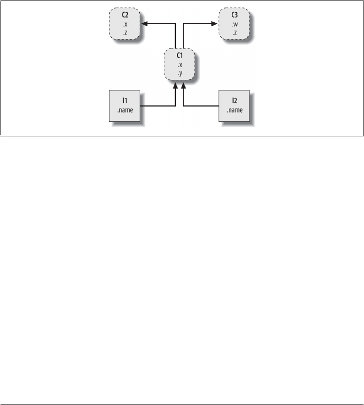
Find the first occurrence of attribute by looking in object, then in all classes above it,
from bottom to top and left to right.
In other words, attribute fetches are simply tree searches. The term inheritance is ap-
plied because objects lower in a tree inherit attributes attached to objects higher in that
tree. As the search proceeds from the bottom up, in a sense, the objects linked into a
tree are the union of all the attributes defined in all their tree parents, all the way up
the tree.
In Python, this is all very literal: we really do build up trees of linked objects with code,
and Python really does climb this tree at runtime searching for attributes every time we
use the object.attribute expression. To make this more concrete, Figure 26-1 sketches
an example of one of these trees.
Figure 26-1. A class tree, with two instances at the bottom (I1 and I2), a class above them (C1), and
two superclasses at the top (C2 and C3). All of these objects are namespaces (packages of variables),
and the inheritance search is simply a search of the tree from bottom to top looking for the lowest
occurrence of an attribute name. Code implies the shape of such trees.
In this figure, there is a tree of five objects labeled with variables, all of which have
attached attributes, ready to be searched. More specifically, this tree links together three
class objects (the ovals C1, C2, and C3) and two instance objects (the rectangles I1 and
I2) into an inheritance search tree. Notice that in the Python object model, classes and
the instances you generate from them are two distinct object types:
Classes
Serve as instance factories. Their attributes provide behavior—data and functions
—that is inherited by all the instances generated from them (e.g., a function to
compute an employee’s salary from pay and hours).
Instances
Represent the concrete items in a program’s domain. Their attributes record data
that varies per specific object (e.g., an employee’s Social Security number).
In terms of search trees, an instance inherits attributes from its class, and a class inherits
attributes from all classes above it in the tree.
786 | Chapter 26: OOP: The Big Picture
www.it-ebooks.info

In Figure 26-1, we can further categorize the ovals by their relative positions in the tree.
We usually call classes higher in the tree (like C2 and C3) superclasses; classes lower in
the tree (like C1) are known as subclasses. These terms refer to both relative tree positions
and roles. Superclasses provide behavior shared by all their subclasses, but because the
search proceeds from the bottom up, subclasses may override behavior defined in their
superclasses by redefining superclass names lower in the tree.1
As these last few words are really the crux of the matter of software customization in
OOP, let’s expand on this concept. Suppose we build up the tree in Figure 26-1, and
then say this:
I2.w
Right away, this code invokes inheritance. Because this is an object.attribute expres-
sion, it triggers a search of the tree in Figure 26-1—Python will search for the attribute
w by looking in I2 and above. Specifically, it will search the linked objects in this order:
I2, C1, C2, C3
and stop at the first attached w it finds (or raise an error if w isn’t found at all). In this
case, w won’t be found until C3 is searched because it appears only in that object. In
other words, I2.w resolves to C3.w by virtue of the automatic search. In OOP termi-
nology, I2 “inherits” the attribute w from C3.
Ultimately, the two instances inherit four attributes from their classes: w, x, y, and z.
Other attribute references will wind up following different paths in the tree. For ex-
ample:
•I1.x and I2.x both find x in C1 and stop because C1 is lower than C2.
•I1.y and I2.y both find y in C1 because that’s the only place y appears.
•I1.z and I2.z both find z in C2 because C2 is further to the left than C3.
•I2.name finds name in I2 without climbing the tree at all.
Trace these searches through the tree in Figure 26-1 to get a feel for how inheritance
searches work in Python.
The first item in the preceding list is perhaps the most important to notice—because
C1 redefines the attribute x lower in the tree, it effectively replaces the version above it
in C2. As you’ll see in a moment, such redefinitions are at the heart of software cus-
tomization in OOP—by redefining and replacing the attribute, C1 effectively customizes
what it inherits from its superclasses.
1. In other literature and circles, you may also occasionally see the terms base classes and derived classes
used to describe superclasses and subclasses, respectively. Python people and this book tend to use the
latter terms.
OOP from 30,000 Feet | 787
www.it-ebooks.info

Classes and Instances
Although they are technically two separate object types in the Python model, the classes
and instances we put in these trees are almost identical—each type’s main purpose is
to serve as another kind of namespace—a package of variables, and a place where we
can attach attributes. If classes and instances therefore sound like modules, they should;
however, the objects in class trees also have automatically searched links to other
namespace objects, and classes correspond to statements, not entire files.
The primary difference between classes and instances is that classes are a kind of fac-
tory for generating instances. For example, in a realistic application, we might have an
Employee class that defines what it means to be an employee; from that class, we generate
actual Employee instances. This is another difference between classes and modules—
we only ever have one instance of a given module in memory (that’s why we have to
reload a module to get its new code), but with classes, we can make as many instances
as we need.
Operationally, classes will usually have functions attached to them (e.g., computeSa
lary), and the instances will have more basic data items used by the class’s functions
(e.g., hoursWorked). In fact, the object-oriented model is not that different from the
classic data-processing model of programs plus records—in OOP, instances are like
records with “data,” and classes are the “programs” for processing those records. In
OOP, though, we also have the notion of an inheritance hierarchy, which supports
software customization better than earlier models.
Method Calls
In the prior section, we saw how the attribute reference I2.w in our example class tree
was translated to C3.w by the inheritance search procedure in Python. Perhaps just as
important to understand as the inheritance of attributes, though, is what happens when
we try to call methods—functions attached to classes as attributes.
If this I2.w reference is a function call, what it really means is “call the C3.w function to
process I2.” That is, Python will automatically map the call I2.w() into the call
C3.w(I2), passing in the instance as the first argument to the inherited function.
In fact, whenever we call a function attached to a class in this fashion, an instance of
the class is always implied. This implied subject or context is part of the reason we refer
to this as an object-oriented model—there is always a subject object when an operation
is run. In a more realistic example, we might invoke a method called giveRaise attached
as an attribute to an Employee class; such a call has no meaning unless qualified with
the employee to whom the raise should be given.
As we’ll see later, Python passes in the implied instance to a special first argument in
the method, called self by convention. Methods go through this argument to process
the subject of the call. As we’ll also learn, methods can be called through either an
instance—bob.giveRaise()—or a class—Employee.giveRaise(bob)—and both forms
788 | Chapter 26: OOP: The Big Picture
www.it-ebooks.info

serve purposes in our scripts. These calls also illustrate both of the key ideas in OOP:
to run a bob.giveRaise() method call, Python:
1. Looks up giveRaise from bob, by inheritance search
2. Passes bob to the located giveRaise function, in the special self argument
When you call Employee.giveRaise(bob), you’re just performing both steps yourself.
This description is technically the default case (Python has additional method types
we’ll meet later), but it applies to the vast majority of the OOP code written in the
language. To see how methods receive their subjects, though, we need to move on to
some code.
Coding Class Trees
Although we are speaking in the abstract here, there is tangible code behind all these
ideas, of course. We construct trees and their objects with class statements and class
calls, which we’ll meet in more detail later. In short:
• Each class statement generates a new class object.
• Each time a class is called, it generates a new instance object.
• Instances are automatically linked to the classes from which they are created.
• Classes are automatically linked to their superclasses according to the way we list
them in parentheses in a class header line; the left-to-right order there gives the
order in the tree.
To build the tree in Figure 26-1, for example, we would run Python code of the following
form. Like function definition, classes are normally coded in module files and are run
during an import (I’ve omitted the guts of the class statements here for brevity):
class C2: ... # Make class objects (ovals)
class C3: ...
class C1(C2, C3): ... # Linked to superclasses (in this order)
I1 = C1() # Make instance objects (rectangles)
I2 = C1() # Linked to their classes
Here, we build the three class objects by running three class statements, and make the
two instance objects by calling the class C1 twice, as though it were a function. The
instances remember the class they were made from, and the class C1 remembers its listed
superclasses.
Technically, this example is using something called multiple inheritance, which simply
means that a class has more than one superclass above it in the class tree—a useful
technique when you wish to combine multiple tools. In Python, if there is more than
one superclass listed in parentheses in a class statement (like C1’s here), their left-to-
right order gives the order in which those superclasses will be searched for attributes
OOP from 30,000 Feet | 789
www.it-ebooks.info

by inheritance. The leftmost version of a name is used by default, though you can always
choose a name by asking for it from the class it lives in (e.g., C3.z).
Because of the way inheritance searches proceed, the object to which you attach an
attribute turns out to be crucial—it determines the name’s scope. Attributes attached
to instances pertain only to those single instances, but attributes attached to classes are
shared by all their subclasses and instances. Later, we’ll study the code that hangs
attributes on these objects in depth. As we’ll find:
• Attributes are usually attached to classes by assignments made at the top level in
class statement blocks, and not nested inside function def statements there.
• Attributes are usually attached to instances by assignments to the special argument
passed to functions coded inside classes, called self.
For example, classes provide behavior for their instances with method functions we
create by coding def statements inside class statements. Because such nested defs as-
sign names within the class, they wind up attaching attributes to the class object that
will be inherited by all instances and subclasses:
class C2: ... # Make superclass objects
class C3: ...
class C1(C2, C3): # Make and link class C1
def setname(self, who): # Assign name: C1.setname
self.name = who # Self is either I1 or I2
I1 = C1() # Make two instances
I2 = C1()
I1.setname('bob') # Sets I1.name to 'bob'
I2.setname('sue') # Sets I2.name to 'sue'
print(I1.name) # Prints 'bob'
There’s nothing syntactically unique about def in this context. Operationally, though,
when a def appears inside a class like this, it is usually known as a method, and it
automatically receives a special first argument—called self by convention—that pro-
vides a handle back to the instance to be processed. Any values you pass to the method
yourself go to arguments after self (here, to who).2
Because classes are factories for multiple instances, their methods usually go through
this automatically passed-in self argument whenever they need to fetch or set attributes
of the particular instance being processed by a method call. In the preceding code,
self is used to store a name in one of two instances.
Like simple variables, attributes of classes and instances are not declared ahead of time,
but spring into existence the first time they are assigned values. When a method assigns
to a self attribute, it creates or changes an attribute in an instance at the bottom of the
2. If you’ve ever used C++ or Java, you’ll recognize that Python’s self is the same as the this pointer, but
self is always explicit in both headers and bodies of Python methods to make attribute accesses more
obvious: a name has fewer possible meanings.
790 | Chapter 26: OOP: The Big Picture
www.it-ebooks.info

class tree (i.e., one of the rectangles in Figure 26-1) because self automatically refers
to the instance being processed—the subject of the call.
In fact, because all the objects in class trees are just namespace objects, we can fetch or
set any of their attributes by going through the appropriate names. Saying C1.setname
is as valid as saying I1.setname, as long as the names C1 and I1 are in your code’s scopes.
Operator Overloading
As currently coded, our C1 class doesn’t attach a name attribute to an instance until the
setname method is called. Indeed, referencing I1.name before calling I1.setname would
produce an undefined name error. If a class wants to guarantee that an attribute like
name is always set in its instances, it more typically will fill out the attribute at con-
struction time, like this:
class C2: ... # Make superclass objects
class C3: ...
class C1(C2, C3):
def __init__(self, who): # Set name when constructed
self.name = who # Self is either I1 or I2
I1 = C1('bob') # Sets I1.name to 'bob'
I2 = C1('sue') # Sets I2.name to 'sue'
print(I1.name) # Prints 'bob'
If it’s coded or inherited, Python automatically calls a method named __init__ each
time an instance is generated from a class. The new instance is passed in to the self
argument of __init__ as usual, and any values listed in parentheses in the class call go
to arguments two and beyond. The effect here is to initialize instances when they are
made, without requiring extra method calls.
The __init__ method is known as the constructor because of when it is run. It’s the
most commonly used representative of a larger class of methods called operator over-
loading methods, which we’ll discuss in more detail in the chapters that follow. Such
methods are inherited in class trees as usual and have double underscores at the start
and end of their names to make them distinct. Python runs them automatically when
instances that support them appear in the corresponding operations, and they are
mostly an alternative to using simple method calls. They’re also optional: if omitted,
the operations are not supported. If no __init__ is present, class calls return an empty
instance, without initializing it.
For example, to implement set intersection, a class might either provide a method
named intersect, or overload the & expression operator to dispatch to the required
logic by coding a method named __and__. Because the operator scheme makes instances
look and feel more like built-in types, it allows some classes to provide a consistent and
natural interface, and be compatible with code that expects a built-in type. Still, apart
from the __init__ constructor—which appears in most realistic classes—many pro-
OOP from 30,000 Feet | 791
www.it-ebooks.info

grams may be better off with simpler named methods unless their objects are similar
to built-ins. A giveRaise may make sense for an Employee, but a & might not.
OOP Is About Code Reuse
And that, along with a few syntax details, is most of the OOP story in Python. Of course,
there’s a bit more to it than just inheritance. For example, operator overloading is much
more general than I’ve described so far—classes may also provide their own imple-
mentations of operations such as indexing, fetching attributes, printing, and more. By
and large, though, OOP is about looking up attributes in trees with a special first ar-
gument in functions.
So why would we be interested in building and searching trees of objects? Although it
takes some experience to see how, when used well, classes support code reuse in ways
that other Python program components cannot. In fact, this is their highest purpose.
With classes, we code by customizing existing software, instead of either changing
existing code in place or starting from scratch for each new project. This turns out to
be a powerful paradigm in realistic programming.
At a fundamental level, classes are really just packages of functions and other names,
much like modules. However, the automatic attribute inheritance search that we get
with classes supports customization of software above and beyond what we can do
with modules and functions. Moreover, classes provide a natural structure for code
that packages and localizes logic and names, and so aids in debugging.
For instance, because methods are simply functions with a special first argument, we
can mimic some of their behavior by manually passing objects to be processed to simple
functions. The participation of methods in class inheritance, though, allows us to nat-
urally customize existing software by coding subclasses with new method definitions,
rather than changing existing code in place. There is really no such concept with mod-
ules and functions.
Polymorphism and classes
As an example, suppose you’re assigned the task of implementing an employee database
application. As a Python OOP programmer, you might begin by coding a general su-
perclass that defines default behaviors common to all the kinds of employees in your
organization:
class Employee: # General superclass
def computeSalary(self): ... # Common or default behaviors
def giveRaise(self): ...
def promote(self): ...
def retire(self): ...
Once you’ve coded this general behavior, you can specialize it for each specific kind of
employee to reflect how the various types differ from the norm. That is, you can code
subclasses that customize just the bits of behavior that differ per employee type; the
792 | Chapter 26: OOP: The Big Picture
www.it-ebooks.info

rest of the employee types’ behavior will be inherited from the more general class. For
example, if engineers have a unique salary computation rule (perhaps it’s not hours
times rate), you can replace just that one method in a subclass:
class Engineer(Employee): # Specialized subclass
def computeSalary(self): ... # Something custom here
Because the computeSalary version here appears lower in the class tree, it will replace
(override) the general version in Employee. You then create instances of the kinds of
employee classes that the real employees belong to, to get the correct behavior:
bob = Employee() # Default behavior
sue = Employee() # Default behavior
tom = Engineer() # Custom salary calculator
Notice that you can make instances of any class in a tree, not just the ones at the bottom
—the class you make an instance from determines the level at which the attribute search
will begin, and thus which versions of the methods it will employ.
Ultimately, these three instance objects might wind up embedded in a larger container
object—for instance, a list, or an instance of another class—that represents a depart-
ment or company using the composition idea mentioned at the start of this chapter.
When you later ask for these employees’ salaries, they will be computed according to
the classes from which the objects were made, due to the principles of the inheritance
search:
company = [bob, sue, tom] # A composite object
for emp in company:
print(emp.computeSalary()) # Run this object's version: default or custom
This is yet another instance of the idea of polymorphism introduced in Chapter 4 and
expanded in Chapter 16. Recall that polymorphism means that the meaning of an op-
eration depends on the object being operated on. That is, code shouldn’t care about
what an object is, only about what it does. Here, the method computeSalary is located
by inheritance search in each object before it is called. The net effect is that we auto-
matically run the correct version for the object being processed. Trace the code to see
why.3
In other applications, polymorphism might also be used to hide (i.e., encapsulate) in-
terface differences. For example, a program that processes data streams might be coded
to expect objects with input and output methods, without caring what those methods
actually do:
def processor(reader, converter, writer):
while True:
data = reader.read()
3. The company list in this example could be a database if stored in a file with Python object pickling,
introduced in Chapter 9, to make the employees persistent. Python also comes with a module named
shelve, which allows the pickled representation of class instances to be stored in an access-by-key
filesystem; we’ll deploy it in Chapter 28.
OOP from 30,000 Feet | 793
www.it-ebooks.info

if not data: break
data = converter(data)
writer.write(data)
By passing in instances of subclasses that specialize the required read and write method
interfaces for various data sources, we can reuse the processor function for any data
source we need to use, both now and in the future:
class Reader:
def read(self): ... # Default behavior and tools
def other(self): ...
class FileReader(Reader):
def read(self): ... # Read from a local file
class SocketReader(Reader):
def read(self): ... # Read from a network socket
...
processor(FileReader(...), Converter, FileWriter(...))
processor(SocketReader(...), Converter, TapeWriter(...))
processor(FtpReader(...), Converter, XmlWriter(...))
Moreover, because the internal implementations of those read and write methods have
been factored into single locations, they can be changed without impacting code such
as this that uses them. The processor function might even be a class itself to allow the
conversion logic of converter to be filled in by inheritance, and to allow readers and
writers to be embedded by composition (we’ll see how this works later in this part of
the book).
Programming by customization
Once you get used to programming this way (by software customization), you’ll find
that when it’s time to write a new program, much of your work may already be done
—your task largely becomes one of mixing together existing superclasses that already
implement the behavior required by your program. For example, someone else might
have written the Employee, Reader, and Writer classes in this section’s examples for use
in completely different programs. If so, you get all of that person’s code “for free.”
In fact, in many application domains, you can fetch or purchase collections of super-
classes, known as frameworks, that implement common programming tasks as classes,
ready to be mixed into your applications. These frameworks might provide database
interfaces, testing protocols, GUI toolkits, and so on. With frameworks, you often
simply code a subclass that fills in an expected method or two; the framework classes
higher in the tree do most of the work for you. Programming in such an OOP world is
just a matter of combining and specializing already debugged code by writing subclasses
of your own.
Of course, it takes a while to learn how to leverage classes to achieve such OOP utopia.
In practice, object-oriented work also entails substantial design work to fully realize
the code reuse benefits of classes—to this end, programmers have begun cataloging
common OOP structures, known as design patterns, to help with design issues. The
actual code you write to do OOP in Python, though, is so simple that it will not in itself
794 | Chapter 26: OOP: The Big Picture
www.it-ebooks.info

pose an additional obstacle to your OOP quest. To see why, you’ll have to move on to
Chapter 27.
Chapter Summary
We took an abstract look at classes and OOP in this chapter, taking in the big picture
before we dive into syntax details. As we’ve seen, OOP is mostly about an argument
named self, and a search for attributes in trees of linked objects called inheritance.
Objects at the bottom of the tree inherit attributes from objects higher up in the tree
—a feature that enables us to program by customizing code, rather than changing it or
starting from scratch. When used well, this model of programming can cut develop-
ment time radically.
The next chapter will begin to fill in the coding details behind the picture painted here.
As we get deeper into Python classes, though, keep in mind that the OOP model in
Python is very simple; as we’ve seen here, it’s really just about looking up attributes in
object trees and a special function argument. Before we move on, here’s a quick quiz
to review what we’ve covered here.
Test Your Knowledge: Quiz
1. What is the main point of OOP in Python?
2. Where does an inheritance search look for an attribute?
3. What is the difference between a class object and an instance object?
4. Why is the first argument in a class’s method function special?
5. What is the __init__ method used for?
6. How do you create a class instance?
7. How do you create a class?
8. How do you specify a class’s superclasses?
Test Your Knowledge: Answers
1. OOP is about code reuse—you factor code to minimize redundancy and program
by customizing what already exists instead of changing code in place or starting
from scratch.
2. An inheritance search looks for an attribute first in the instance object, then in the
class the instance was created from, then in all higher superclasses, progressing
from the bottom to the top of the object tree, and from left to right (by default).
The search stops at the first place the attribute is found. Because the lowest version
of a name found along the way wins, class hierarchies naturally support customi-
zation by extension in new subclasses.
Test Your Knowledge: Answers | 795
www.it-ebooks.info

3. Both class and instance objects are namespaces (packages of variables that appear
as attributes). The main difference between them is that classes are a kind of factory
for creating multiple instances. Classes also support operator overloading meth-
ods, which instances inherit, and treat any functions nested in the class as methods
for processing instances.
4. The first argument in a class’s method function is special because it always receives
the instance object that is the implied subject of the method call. It’s usually called
self by convention. Because method functions always have this implied subject
and object context by default, we say they are “object-oriented” (i.e., designed to
process or change objects).
5. If the __init__ method is coded or inherited in a class, Python calls it automatically
each time an instance of that class is created. It’s known as the constructor method;
it is passed the new instance implicitly, as well as any arguments passed explicitly
to the class name. It’s also the most commonly used operator overloading method.
If no __init__ method is present, instances simply begin life as empty namespaces.
6. You create a class instance by calling the class name as though it were a function;
any arguments passed into the class name show up as arguments two and beyond
in the __init__ constructor method. The new instance remembers the class it was
created from for inheritance purposes.
7. You create a class by running a class statement; like function definitions, these
statements normally run when the enclosing module file is imported (more on this
in the next chapter).
8. You specify a class’s superclasses by listing them in parentheses in the class state-
ment, after the new class’s name. The left-to-right order in which the classes are
listed in the parentheses gives the left-to-right inheritance search order in the class
tree.
796 | Chapter 26: OOP: The Big Picture
www.it-ebooks.info

CHAPTER 27
Class Coding Basics
Now that we’ve talked about OOP in the abstract, it’s time to see how this translates
to actual code. This chapter begins to fill in the syntax details behind the class model
in Python.
If you’ve never been exposed to OOP in the past, classes can seem somewhat compli-
cated if taken in a single dose. To make class coding easier to absorb, we’ll begin our
detailed exploration of OOP by taking a first look at some basic classes in action in this
chapter. We’ll expand on the details introduced here in later chapters of this part of
the book, but in their basic form, Python classes are easy to understand.
In fact, classes have just three primary distinctions. At a base level, they are mostly just
namespaces, much like the modules we studied in Part V. Unlike modules, though,
classes also have support for generating multiple objects, for namespace inheritance,
and for operator overloading. Let’s begin our class statement tour by exploring each
of these three distinctions in turn.
Classes Generate Multiple Instance Objects
To understand how the multiple objects idea works, you have to first understand that
there are two kinds of objects in Python’s OOP model: class objects and instance ob-
jects. Class objects provide default behavior and serve as factories for instance objects.
Instance objects are the real objects your programs process—each is a namespace in
its own right, but inherits (i.e., has automatic access to) names in the class from which
it was created. Class objects come from statements, and instances come from calls; each
time you call a class, you get a new instance of that class.
This object-generation concept is very different from most of the other program con-
structs we’ve seen so far in this book. In effect, classes are essentially factories for gen-
erating multiple instances. By contrast, only one copy of each module is ever imported
into a single program. In fact, this is why reload works as it does, updating a single-
instance shared object in place. With classes, each instance can have its own, inde-
pendent data, supporting multiple versions of the object that the class models.
797
www.it-ebooks.info

In this role, class instances are similar to the per-call state of the closure (a.k.a. factory)
functions of Chapter 17, but this is a natural part of the class model, and state in classes
is explicit attributes instead of implicit scope references. Moreover, this is just part of
what classes do—they also support customization by inheritance, operator overload-
ing, and multiple behaviors via methods. Generally speaking, classes are a more com-
plete programming tool, though OOP and function programming are not mutually ex-
clusive paradigms. We may combine them by using functional tools in methods, by
coding methods that are themselves generators, by writing user-defined iterators (as
we’ll see in Chapter 30), and so on.
The following is a quick summary of the bare essentials of Python OOP in terms of its
two object types. As you’ll see, Python classes are in some ways similar to both defs
and modules, but they may be quite different from what you’re used to in other lan-
guages.
Class Objects Provide Default Behavior
When we run a class statement, we get a class object. Here’s a rundown of the main
properties of Python classes:
•The class statement creates a class object and assigns it a name. Just like the
function def statement, the Python class statement is an executable statement.
When reached and run, it generates a new class object and assigns it to the name
in the class header. Also, like defs, class statements typically run when the files
they are coded in are first imported.
•Assignments inside class statements make class attributes. Just like in module
files, top-level assignments within a class statement (not nested in a def) generate
attributes in a class object. Technically, the class statement defines a local scope
that morphs into the attribute namespace of the class object, just like a module’s
global scope. After running a class statement, class attributes are accessed by name
qualification: object.name.
•Class attributes provide object state and behavior. Attributes of a class object
record state information and behavior to be shared by all instances created from
the class; function def statements nested inside a class generate methods, which
process instances.
Instance Objects Are Concrete Items
When we call a class object, we get an instance object. Here’s an overview of the key
points behind class instances:
•Calling a class object like a function makes a new instance object. Each time
a class is called, it creates and returns a new instance object. Instances represent
concrete items in your program’s domain.
798 | Chapter 27: Class Coding Basics
www.it-ebooks.info

•Each instance object inherits class attributes and gets its own namespace.
Instance objects created from classes are new namespaces; they start out empty
but inherit attributes that live in the class objects from which they were generated.
•Assignments to attributes of self in methods make per-instance attributes.
Inside a class’s method functions, the first argument (called self by convention)
references the instance object being processed; assignments to attributes of self
create or change data in the instance, not the class.
The end result is that classes define common, shared data and behavior, and generate
instances. Instances reflect concrete application entities, and record per-instance data
that may vary per object.
A First Example
Let’s turn to a real example to show how these ideas work in practice. To begin, let’s
define a class named FirstClass by running a Python class statement interactively:
>>> class FirstClass: # Define a class object
def setdata(self, value): # Define class's methods
self.data = value # self is the instance
def display(self):
print(self.data) # self.data: per instance
We’re working interactively here, but typically, such a statement would be run when
the module file it is coded in is imported. Like functions created with defs, this class
won’t even exist until Python reaches and runs this statement.
Like all compound statements, the class starts with a header line that lists the class
name, followed by a body of one or more nested and (usually) indented statements.
Here, the nested statements are defs; they define functions that implement the behavior
the class means to export.
As we learned in Part IV, def is really an assignment. Here, it assigns function objects
to the names setdata and display in the class statement’s scope, and so generates
attributes attached to the class—FirstClass.setdata and FirstClass.display. In fact,
any name assigned at the top level of the class’s nested block becomes an attribute of
the class.
Functions inside a class are usually called methods. They’re coded with normal defs,
and they support everything we’ve learned about functions already (they can have de-
faults, return values, yield items on request, and so on). But in a method function, the
first argument automatically receives an implied instance object when called—the sub-
ject of the call. We need to create a couple of instances to see how this works:
>>> x = FirstClass() # Make two instances
>>> y = FirstClass() # Each is a new namespace
By calling the class this way (notice the parentheses), we generate instance objects,
which are just namespaces that have access to their classes’ attributes. Properly speak-
Classes Generate Multiple Instance Objects | 799
www.it-ebooks.info

ing, at this point, we have three objects: two instances and a class. Really, we have three
linked namespaces, as sketched in Figure 27-1. In OOP terms, we say that x “is a”
FirstClass, as is y—they both inherit names attached to the class.
The two instances start out empty but have links back to the class from which they
were generated. If we qualify an instance with the name of an attribute that lives in the
class object, Python fetches the name from the class by inheritance search (unless it
also lives in the instance):
>>> x.setdata("King Arthur") # Call methods: self is x
>>> y.setdata(3.14159) # Runs: FirstClass.setdata(y, 3.14159)
Neither x nor y has a setdata attribute of its own, so to find it, Python follows the link
from instance to class. And that’s about all there is to inheritance in Python: it happens
at attribute qualification time, and it just involves looking up names in linked objects
—here, by following the is-a links in Figure 27-1.
In the setdata function inside FirstClass, the value passed in is assigned to
self.data. Within a method, self—the name given to the leftmost argument by con-
vention—automatically refers to the instance being processed (x or y), so the assign-
ments store values in the instances’ namespaces, not the class’s; that’s how the data
names in Figure 27-1 are created.
Because classes can generate multiple instances, methods must go through the self
argument to get to the instance to be processed. When we call the class’s display
method to print self.data, we see that it’s different in each instance; on the other hand,
the name display itself is the same in x and y, as it comes (is inherited) from the class:
>>> x.display() # self.data differs in each instance
King Arthur
>>> y.display() # Runs: FirstClass.display(y)
3.14159
Notice that we stored different object types in the data member in each instance—a
string and a floating-point number. As with everything else in Python, there are no
declarations for instance attributes (sometimes called members); they spring into exis-
tence the first time they are assigned values, just like simple variables. In fact, if we were
Figure 27-1. Classes and instances are linked namespace objects in a class tree that is searched by
inheritance. Here, the “data” attribute is found in instances, but “setdata” and “display” are in the
class above them.
800 | Chapter 27: Class Coding Basics
www.it-ebooks.info

to call display on one of our instances before calling setdata, we would trigger an
undefined name error—the attribute named data doesn’t even exist in memory until it
is assigned within the setdata method.
As another way to appreciate how dynamic this model is, consider that we can change
instance attributes in the class itself, by assigning to self in methods, or outside the
class, by assigning to an explicit instance object:
>>> x.data = "New value" # Can get/set attributes
>>> x.display() # Outside the class too
New value
Although less common, we could even generate an entirely new attribute in the in-
stance’s namespace by assigning to its name outside the class’s method functions:
>>> x.anothername = "spam" # Can set new attributes here too!
This would attach a new attribute called anothername, which may or may not be used
by any of the class’s methods, to the instance object x. Classes usually create all of the
instance’s attributes by assignment to the self argument, but they don’t have to—
programs can fetch, change, or create attributes on any objects to which they have
references.
It usually doesn’t make sense to add data that the class cannot use, and it’s possible to
prevent this with extra “privacy” code based on attribute access operator overloading,
as we’ll discuss later in this book (see Chapter 30 and Chapter 39). Still, free attribute
access translates to less syntax, and there are cases where it’s even useful—for example,
in coding data records of the sort we’ll see later in this chapter.
Classes Are Customized by Inheritance
Let’s move on to the second major distinction of classes. Besides serving as factories
for generating multiple instance objects, classes also allow us to make changes by in-
troducing new components (called subclasses), instead of changing existing compo-
nents in place.
As we’ve seen, instance objects generated from a class inherit the class’s attributes.
Python also allows classes to inherit from other classes, opening the door to coding
hierarchies of classes that specialize behavior—by redefining attributes in subclasses
that appear lower in the hierarchy, we override the more general definitions of those
attributes higher in the tree. In effect, the further down the hierarchy we go, the more
specific the software becomes. Here, too, there is no parallel with modules, whose
attributes live in a single, flat namespace that is not as amenable to customization.
In Python, instances inherit from classes, and classes inherit from superclasses. Here
are the key ideas behind the machinery of attribute inheritance:
•Superclasses are listed in parentheses in a class header. To make a class inherit
attributes from another class, just list the other class in parentheses in the new
Classes Are Customized by Inheritance | 801
www.it-ebooks.info
class statement’s header line. The class that inherits is usually called a subclass,
and the class that is inherited from is its superclass.
•Classes inherit attributes from their superclasses. Just as instances inherit the
attribute names defined in their classes, classes inherit all of the attribute names
defined in their superclasses; Python finds them automatically when they’re ac-
cessed, if they don’t exist in the subclasses.
•Instances inherit attributes from all accessible classes. Each instance gets
names from the class it’s generated from, as well as all of that class’s superclasses.
When looking for a name, Python checks the instance, then its class, then all su-
perclasses.
•Each object.attribute reference invokes a new, independent search. Python
performs an independent search of the class tree for each attribute fetch expression.
This includes references to instances and classes made outside class statements
(e.g., X.attr), as well as references to attributes of the self instance argument in a
class’s method functions. Each self.attr expression in a method invokes a new
search for attr in self and above.
•Logic changes are made by subclassing, not by changing superclasses. By
redefining superclass names in subclasses lower in the hierarchy (class tree), sub-
classes replace and thus customize inherited behavior.
The net effect—and the main purpose of all this searching—is that classes support
factoring and customization of code better than any other language tool we’ve seen so
far. On the one hand, they allow us to minimize code redundancy (and so reduce
maintenance costs) by factoring operations into a single, shared implementation; on
the other, they allow us to program by customizing what already exists, rather than
changing it in place or starting from scratch.
Strictly speaking, Python’s inheritance is a bit richer than described here,
when we factor in new-style descriptors and metaclasses—advanced
topics we’ll study later—but we can safely restrict our scope to instances
and their classes, both at this point in the book and in most Python
application code. We’ll define inheritance formally in Chapter 40.
A Second Example
To illustrate the role of inheritance, this next example builds on the previous one. First,
we’ll define a new class, SecondClass, that inherits all of FirstClass’s names and pro-
vides one of its own:
>>> class SecondClass(FirstClass): # Inherits setdata
def display(self): # Changes display
print('Current value = "%s"' % self.data)
802 | Chapter 27: Class Coding Basics
www.it-ebooks.info
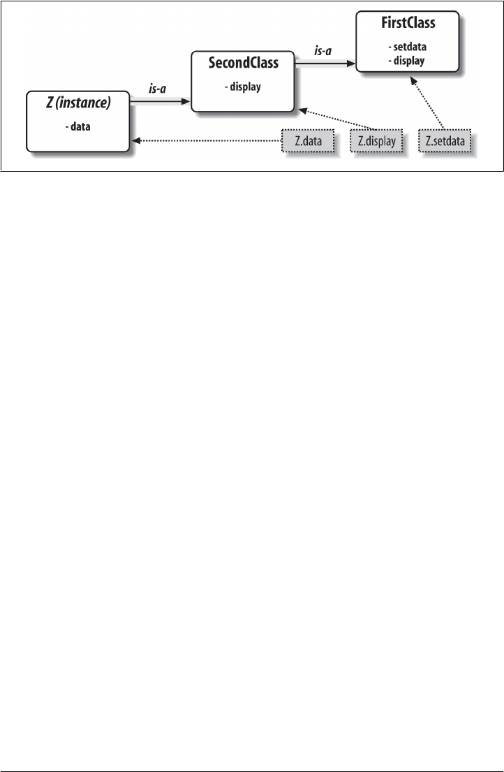
SecondClass defines the display method to print with a different format. By defining
an attribute with the same name as an attribute in FirstClass, SecondClass effectively
replaces the display attribute in its superclass.
Recall that inheritance searches proceed upward from instances to subclasses to su-
perclasses, stopping at the first appearance of the attribute name that it finds. In this
case, since the display name in SecondClass will be found before the one in First
Class, we say that SecondClass overrides FirstClass’s display. Sometimes we call this
act of replacing attributes by redefining them lower in the tree overloading.
The net effect here is that SecondClass specializes FirstClass by changing the behavior
of the display method. On the other hand, SecondClass (and any instances created from
it) still inherits the setdata method in FirstClass verbatim. Let’s make an instance to
demonstrate:
>>> z = SecondClass()
>>> z.setdata(42) # Finds setdata in FirstClass
>>> z.display() # Finds overridden method in SecondClass
Current value = "42"
As before, we make a SecondClass instance object by calling it. The setdata call still
runs the version in FirstClass, but this time the display attribute comes from Second
Class and prints a custom message. Figure 27-2 sketches the namespaces involved.
Now, here’s a crucial thing to notice about OOP: the specialization introduced in
SecondClass is completely external to FirstClass. That is, it doesn’t affect existing or
future FirstClass objects, like the x from the prior example:
>>> x.display() # x is still a FirstClass instance (old message)
New value
Rather than changing FirstClass, we customized it. Naturally, this is an artificial ex-
ample, but as a rule, because inheritance allows us to make changes like this in external
components (i.e., in subclasses), classes often support extension and reuse better than
functions or modules can.
Figure 27-2. Specialization: overriding inherited names by redefining them in extensions lower in the
class tree. Here, SecondClass redefines and so customizes the “display” method for its instances.
Classes Are Customized by Inheritance | 803
www.it-ebooks.info

Classes Are Attributes in Modules
Before we move on, remember that there’s nothing magic about a class name. It’s just
a variable assigned to an object when the class statement runs, and the object can be
referenced with any normal expression. For instance, if our FirstClass were coded in
a module file instead of being typed interactively, we could import it and use its name
normally in a class header line:
from modulename import FirstClass # Copy name into my scope
class SecondClass(FirstClass): # Use class name directly
def display(self): ...
Or, equivalently:
import modulename # Access the whole module
class SecondClass(modulename.FirstClass): # Qualify to reference
def display(self): ...
Like everything else, class names always live within a module, so they must follow all
the rules we studied in Part V. For example, more than one class can be coded in a
single module file—like other statements in a module, class statements are run during
imports to define names, and these names become distinct module attributes. More
generally, each module may arbitrarily mix any number of variables, functions, and
classes, and all names in a module behave the same way. The file food.py demonstrates:
# food.py
var = 1 # food.var
def func(): ... # food.func
class spam: ... # food.spam
class ham: ... # food.ham
class eggs: ... # food.eggs
This holds true even if the module and class happen to have the same name. For ex-
ample, given the following file, person.py:
class person: ...
we need to go through the module to fetch the class as usual:
import person # Import module
x = person.person() # Class within module
Although this path may look redundant, it’s required: person.person refers to the per
son class inside the person module. Saying just person gets the module, not the class,
unless the from statement is used:
from person import person # Get class from module
x = person() # Use class name
As with any other variable, we can never see a class in a file without first importing and
somehow fetching it from its enclosing file. If this seems confusing, don’t use the same
name for a module and a class within it. In fact, common convention in Python dictates
that class names should begin with an uppercase letter, to help make them more distinct:
804 | Chapter 27: Class Coding Basics
www.it-ebooks.info

import person # Lowercase for modules
x = person.Person() # Uppercase for classes
Also, keep in mind that although classes and modules are both namespaces for attach-
ing attributes, they correspond to very different source code structures: a module re-
flects an entire file, but a class is a statement within a file. We’ll say more about such
distinctions later in this part of the book.
Classes Can Intercept Python Operators
Let’s move on to the third and final major difference between classes and modules:
operator overloading. In simple terms, operator overloading lets objects coded with
classes intercept and respond to operations that work on built-in types: addition, slic-
ing, printing, qualification, and so on. It’s mostly just an automatic dispatch mechanism
—expressions and other built-in operations route control to implementations in
classes. Here, too, there is nothing similar in modules: modules can implement function
calls, but not the behavior of expressions.
Although we could implement all class behavior as method functions, operator over-
loading lets objects be more tightly integrated with Python’s object model. Moreover,
because operator overloading makes our own objects act like built-ins, it tends to foster
object interfaces that are more consistent and easier to learn, and it allows class-based
objects to be processed by code written to expect a built-in type’s interface. Here is a
quick rundown of the main ideas behind overloading operators:
•Methods named with double underscores (__X__) are special hooks. In Python
classes we implement operator overloading by providing specially named methods
to intercept operations. The Python language defines a fixed and unchangeable
mapping from each of these operations to a specially named method.
•Such methods are called automatically when instances appear in built-in
operations. For instance, if an instance object inherits an __add__ method, that
method is called whenever the object appears in a + expression. The method’s
return value becomes the result of the corresponding expression.
•Classes may override most built-in type operations. There are dozens of special
operator overloading method names for intercepting and implementing nearly
every operation available for built-in types. This includes expressions, but also
basic operations like printing and object creation.
•There are no defaults for operator overloading methods, and none are re-
quired. If a class does not define or inherit an operator overloading method, it just
means that the corresponding operation is not supported for the class’s instances.
If there is no __add__, for example, + expressions raise exceptions.
•New-style classes have some defaults, but not for common operations. In
Python 3.X, and so-called “new style” classes in 2.X that we’ll define later, a root
Classes Can Intercept Python Operators | 805
www.it-ebooks.info

class named object does provide defaults for some __X__ methods, but not for
many, and not for most commonly used operations.
•Operators allow classes to integrate with Python’s object model. By over-
loading type operations, the user-defined objects we implement with classes can
act just like built-ins, and so provide consistency as well as compatibility with
expected interfaces.
Operator overloading is an optional feature; it’s used primarily by people developing
tools for other Python programmers, not by application developers. And, candidly, you
probably shouldn’t use it just because it seems clever or “cool.” Unless a class needs to
mimic built-in type interfaces, it should usually stick to simpler named methods. Why
would an employee database application support expressions like * and +, for example?
Named methods like giveRaise and promote would usually make more sense.
Because of this, we won’t go into details on every operator overloading method available
in Python in this book. Still, there is one operator overloading method you are likely
to see in almost every realistic Python class: the __init__ method, which is known as
the constructor method and is used to initialize objects’ state. You should pay special
attention to this method, because __init__, along with the self argument, turns out
to be a key requirement to reading and understanding most OOP code in Python.
A Third Example
On to another example. This time, we’ll define a subclass of the prior section’s Second
Class that implements three specially named attributes that Python will call automat-
ically:
•__init__ is run when a new instance object is created: self is the new ThirdClass
object.1
•__add__ is run when a ThirdClass instance appears in a + expression.
•__str__ is run when an object is printed (technically, when it’s converted to its
print string by the str built-in function or its Python internals equivalent).
Our new subclass also defines a normally named method called mul, which changes the
instance object in place. Here’s the new subclass:
>>> class ThirdClass(SecondClass): # Inherit from SecondClass
def __init__(self, value): # On "ThirdClass(value)"
self.data = value
def __add__(self, other): # On "self + other"
return ThirdClass(self.data + other)
def __str__(self): # On "print(self)", "str()"
return '[ThirdClass: %s]' % self.data
1. Not to be confused with the __init__.py files in module packages! The method here is a class constructor
function used to initialize the newly created instance, not a module package. See Chapter 24 for more
details.
806 | Chapter 27: Class Coding Basics
www.it-ebooks.info
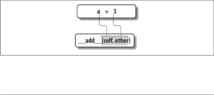
def mul(self, other): # In-place change: named
self.data *= other
>>> a = ThirdClass('abc') # __init__ called
>>> a.display() # Inherited method called
Current value = "abc"
>>> print(a) # __str__: returns display string
[ThirdClass: abc]
>>> b = a + 'xyz' # __add__: makes a new instance
>>> b.display() # b has all ThirdClass methods
Current value = "abcxyz"
>>> print(b) # __str__: returns display string
[ThirdClass: abcxyz]
>>> a.mul(3) # mul: changes instance in place
>>> print(a)
[ThirdClass: abcabcabc]
ThirdClass “is a” SecondClass, so its instances inherit the customized display method
from SecondClass of the preceding section. This time, though, ThirdClass creation calls
pass an argument (e.g., “abc”). This argument is passed to the value argument in the
__init__ constructor and assigned to self.data there. The net effect is that Third
Class arranges to set the data attribute automatically at construction time, instead of
requiring setdata calls after the fact.
Further, ThirdClass objects can now show up in + expressions and print calls. For +,
Python passes the instance object on the left to the self argument in __add__ and the
value on the right to other, as illustrated in Figure 27-3; whatever __add__ returns be-
comes the result of the + expression (more on its result in a moment).
For print, Python passes the object being printed to self in __str__; whatever string
this method returns is taken to be the print string for the object. With __str__ (or its
more broadly relevant twin __repr__, which we’ll meet and use in the next chapter),
we can use a normal print to display objects of this class, instead of calling the special
display method.
Figure 27-3. In operator overloading, expression operators and other built-in operations performed
on class instances are mapped back to specially named methods in the class. These special methods
are optional and may be inherited as usual. Here, a + expression triggers the __add__ method.
Classes Can Intercept Python Operators | 807
www.it-ebooks.info

Specially named methods such as __init__, __add__, and __str__ are inherited by sub-
classes and instances, just like any other names assigned in a class. If they’re not coded
in a class, Python looks for such names in all its superclasses, as usual. Operator over-
loading method names are also not built-in or reserved words; they are just attributes
that Python looks for when objects appear in various contexts. Python usually calls
them automatically, but they may occasionally be called by your code as well. For
example, the __init__ method is often called manually to trigger initialization steps in
a superclass, as we’ll see in the next chapter.
Returning results, or not
Some operator overloading methods like __str__ require results, but others are more
flexible. For example, notice how the __add__ method makes and returns a new instance
object of its class, by calling ThirdClass with the result value—which in turn triggers
__init__ to initialize the result. This is a common convention, and explains why b in
the listing has a display method; it’s a ThirdClass object too, because that’s what +
returns for this class’s objects. This essentially propagates the type.
By contrast, mul changes the current instance object in place, by reassigning the self
attribute. We could overload the * expression to do the latter, but this would be too
different from the behavior of * for built-in types such as numbers and strings, for which
it always makes new objects. Common practice dictates that overloaded operators
should work the same way that built-in operator implementations do. Because operator
overloading is really just an expression-to-method dispatch mechanism, though, you
can interpret operators any way you like in your own class objects.
Why Use Operator Overloading?
As a class designer, you can choose to use operator overloading or not. Your choice
simply depends on how much you want your object to look and feel like built-in types.
As mentioned earlier, if you omit an operator overloading method and do not inherit
it from a superclass, the corresponding operation will not be supported for your in-
stances; if it’s attempted, an exception will be raised (or, in some cases like printing, a
standard default will be used).
Frankly, many operator overloading methods tend to be used only when you are im-
plementing objects that are mathematical in nature; a vector or matrix class may over-
load the addition operator, for example, but an employee class likely would not. For
simpler classes, you might not use overloading at all, and would rely instead on explicit
method calls to implement your objects’ behavior.
On the other hand, you might decide to use operator overloading if you need to pass
a user-defined object to a function that was coded to expect the operators available on
a built-in type like a list or a dictionary. Implementing the same operator set in your
class will ensure that your objects support the same expected object interface and so
are compatible with the function. Although we won’t cover every operator overloading
808 | Chapter 27: Class Coding Basics
www.it-ebooks.info

method in this book, we’ll survey additional common operator overloading techniques
in action in Chapter 30.
One overloading method we will use often here is the __init__ constructor method,
used to initialize newly created instance objects, and present in almost every realistic
class. Because it allows classes to fill out the attributes in their new instances immedi-
ately, the constructor is useful for almost every kind of class you might code. In fact,
even though instance attributes are not declared in Python, you can usually find out
which attributes an instance will have by inspecting its class’s __init__ method.
Of course, there’s nothing wrong with experimenting with interesting language tools,
but they don’t always translate to production code. With time and experience, you’ll
find these programming patterns and guidelines to be natural and nearly automatic.
The World’s Simplest Python Class
We’ve begun studying class statement syntax in detail in this chapter, but I’d again
like to remind you that the basic inheritance model that classes produce is very simple
—all it really involves is searching for attributes in trees of linked objects. In fact, we
can create a class with nothing in it at all. The following statement makes a class with
no attributes attached, an empty namespace object:
>>> class rec: pass # Empty namespace object
We need the no-operation pass placeholder statement (discussed in Chapter 13) here
because we don’t have any methods to code. After we make the class by running this
statement interactively, we can start attaching attributes to the class by assigning names
to it completely outside of the original class statement:
>>> rec.name = 'Bob' # Just objects with attributes
>>> rec.age = 40
And, after we’ve created these attributes by assignment, we can fetch them with the
usual syntax. When used this way, a class is roughly similar to a “struct” in C, or a
“record” in Pascal. It’s basically an object with field names attached to it (as we’ll see
ahead, doing similar with dictionary keys requires extra characters):
>>> print(rec.name) # Like a C struct or a record
Bob
Notice that this works even though there are no instances of the class yet; classes are
objects in their own right, even without instances. In fact, they are just self-contained
namespaces; as long as we have a reference to a class, we can set or change its attributes
anytime we wish. Watch what happens when we do create two instances, though:
>>> x = rec() # Instances inherit class names
>>> y = rec()
The World’s Simplest Python Class | 809
www.it-ebooks.info

These instances begin their lives as completely empty namespace objects. Because they
remember the class from which they were made, though, they will obtain the attributes
we attached to the class by inheritance:
>>> x.name, y.name # name is stored on the class only
('Bob', 'Bob')
Really, these instances have no attributes of their own; they simply fetch the name at-
tribute from the class object where it is stored. If we do assign an attribute to an instance,
though, it creates (or changes) the attribute in that object, and no other—crucially,
attribute references kick off inheritance searches, but attribute assignments affect only
the objects in which the assignments are made. Here, this means that x gets its own
name, but y still inherits the name attached to the class above it:
>>> x.name = 'Sue' # But assignment changes x only
>>> rec.name, x.name, y.name
('Bob', 'Sue', 'Bob')
In fact, as we’ll explore in more detail in Chapter 29, the attributes of a namespace
object are usually implemented as dictionaries, and class inheritance trees are (generally
speaking) just dictionaries with links to other dictionaries. If you know where to look,
you can see this explicitly.
For example, the __dict__ attribute is the namespace dictionary for most class-based
objects. Some classes may also (or instead) define attributes in __slots__, an advanced
and seldom-used feature that we’ll note in Chapter 28, but largely postpone until
Chapter 31 and Chapter 32. Normally, __dict__ literally is an instance’s attribute
namespace.
To illustrate, the following was run in Python 3.3; the order of names and set of
__X__ internal names present can vary from release to release, and we filter out built-
ins with a generator expression as we’ve done before, but the names we assigned are
present in all:
>>> list(rec.__dict__.keys())
['age', '__module__', '__qualname__', '__weakref__', 'name', '__dict__', '__doc__']
>>> list(name for name in rec.__dict__ if not name.startswith('__'))
['age', 'name']
>>> list(x.__dict__.keys())
['name']
>>> list(y.__dict__.keys()) # list() not required in Python 2.X
[]
Here, the class’s namespace dictionary shows the name and age attributes we assigned
to it, x has its own name, and y is still empty. Because of this model, an attribute can
often be fetched by either dictionary indexing or attribute notation, but only if it’s
present on the object in question—attribute notation kicks off inheritance search, but
indexing looks in the single object only (as we’ll see later, both have valid roles):
>>> x.name, x.__dict__['name'] # Attributes present here are dict keys
('Sue', 'Sue')
810 | Chapter 27: Class Coding Basics
www.it-ebooks.info

>>> x.age # But attribute fetch checks classes too
40
>>> x.__dict__['age'] # Indexing dict does not do inheritance
KeyError: 'age'
To facilitate inheritance search on attribute fetches, each instance has a link to its class
that Python creates for us—it’s called __class__, if you want to inspect it:
>>> x.__class__ # Instance to class link
<class '__main__.rec'>
Classes also have a __bases__ attribute, which is a tuple of references to their superclass
objects—in this example just the implied object root class in Python 3.X we’ll explore
later (you’ll get an empty tuple in 2.X instead):
>>> rec.__bases__ # Class to superclasses link, () in 2.X
(<class 'object'>,)
These two attributes are how class trees are literally represented in memory by Python.
Internal details like these are not required knowledge—class trees are implied by the
code you run, and their search is normally automatic—but they can often help demys-
tify the model.
The main point to take away from this look under the hood is that Python’s class model
is extremely dynamic. Classes and instances are just namespace objects, with attributes
created on the fly by assignment. Those assignments usually happen within the class
statements you code, but they can occur anywhere you have a reference to one of the
objects in the tree.
Even methods, normally created by a def nested in a class, can be created completely
independently of any class object. The following, for example, defines a simple function
outside of any class that takes one argument:
>>> def uppername(obj):
return obj.name.upper() # Still needs a self argument (obj)
There is nothing about a class here yet—it’s a simple function, and it can be called as
such at this point, provided we pass in an object obj with a name attribute, whose value
in turn has an upper method—our class instances happen to fit the expected interface,
and kick off string uppercase conversion:
>>> uppername(x) # Call as a simple function
'SUE'
If we assign this simple function to an attribute of our class, though, it becomes a
method, callable through any instance, as well as through the class name itself as long
as we pass in an instance manually—a technique we’ll leverage further in the next
chapter:2
>>> rec.method = uppername # Now it's a class's method!
>>> x.method() # Run method to process x
'SUE'
The World’s Simplest Python Class | 811
www.it-ebooks.info

>>> y.method() # Same, but pass y to self
'BOB'
>>> rec.method(x) # Can call through instance or class
'SUE'
Normally, classes are filled out by class statements, and instance attributes are created
by assignments to self attributes in method functions. The point again, though, is that
they don’t have to be; OOP in Python really is mostly about looking up attributes in
linked namespace objects.
Records Revisited: Classes Versus Dictionaries
Although the simple classes of the prior section are meant to illustrate class model
basics, the techniques they employ can also be used for real work. For example, Chap-
ter 8 and Chapter 9 showed how to use dictionaries, tuples, and lists to record properties
of entities in our programs, generically called records. It turns out that classes can often
serve better in this role—they package information like dictionaries, but can also bun-
dle processing logic in the form of methods. For reference, here is an example for tuple-
and dictionary-based records we used earlier in the book (using one of many dictionary
coding techniques):
>>> rec = ('Bob', 40.5, ['dev', 'mgr']) # Tuple-based record
>>> print(rec[0])
Bob
>>> rec = {}
>>> rec['name'] = 'Bob' # Dictionary-based record
>>> rec['age'] = 40.5 # Or {...}, dict(n=v), etc.
>>> rec['jobs'] = ['dev', 'mgr']
>>>
>>> print(rec['name'])
Bob
This code emulates tools like records in other languages. As we just saw, though, there
are also multiple ways to do the same with classes. Perhaps the simplest is this—trading
keys for attributes:
>>> class rec: pass
>>> rec.name = 'Bob' # Class-based record
>>> rec.age = 40.5
>>> rec.jobs = ['dev', 'mgr']
2. In fact, this is one of the reasons the self argument must always be explicit in Python methods—because
methods can be created as simple functions independent of a class, they need to make the implied instance
argument explicit. They can be called as either functions or methods, and Python can neither guess nor
assume that a simple function might eventually become a class’s method. The main reason for the explicit
self argument, though, is to make the meanings of names more obvious: names not referenced through
self are simple variables mapped to scopes, while names referenced through self with attribute notation
are obviously instance attributes.
812 | Chapter 27: Class Coding Basics
www.it-ebooks.info

>>>
>>> print(rec.name)
Bob
This code has substantially less syntax than the dictionary equivalent. It uses an empty
class statement to generate an empty namespace object. Once we make the empty
class, we fill it out by assigning class attributes over time, as before.
This works, but a new class statement will be required for each distinct record we will
need. Perhaps more typically, we can instead generate instances of an empty class to
represent each distinct entity:
>>> class rec: pass
>>> pers1 = rec() # Instance-based records
>>> pers1.name = 'Bob'
>>> pers1.jobs = ['dev', 'mgr']
>>> pers1.age = 40.5
>>>
>>> pers2 = rec()
>>> pers2.name = 'Sue'
>>> pers2.jobs = ['dev', 'cto']
>>>
>>> pers1.name, pers2.name
('Bob', 'Sue')
Here, we make two records from the same class. Instances start out life empty, just like
classes. We then fill in the records by assigning to attributes. This time, though, there
are two separate objects, and hence two separate name attributes. In fact, instances of
the same class don’t even have to have the same set of attribute names; in this example,
one has a unique age name. Instances really are distinct namespaces, so each has a
distinct attribute dictionary. Although they are normally filled out consistently by a
class’s methods, they are more flexible than you might expect.
Finally, we might instead code a more full-blown class to implement the record and its
processing—something that data-oriented dictionaries do not directly support:
>>> class Person:
def __init__(self, name, jobs, age=None): # class = data + logic
self.name = name
self.jobs = jobs
self.age = age
def info(self):
return (self.name, self.jobs)
>>> rec1 = Person('Bob', ['dev', 'mgr'], 40.5) # Construction calls
>>> rec2 = Person('Sue', ['dev', 'cto'])
>>>
>>> rec1.jobs, rec2.info() # Attributes + methods
(['dev', 'mgr'], ('Sue', ['dev', 'cto']))
This scheme also makes multiple instances, but the class is not empty this time: we’ve
added logic (methods) to initialize instances at construction time and collect attributes
The World’s Simplest Python Class | 813
www.it-ebooks.info

into a tuple on request. The constructor imposes some consistency on instances here
by always setting the name, job, and age attributes, even though the latter can be omitted
when an object is made. Together, the class’s methods and instance attributes create a
package, which combines both data and logic.
We could further extend this code by adding logic to compute salaries, parse names,
and so on. Ultimately, we might link the class into a larger hierarchy to inherit and
customize an existing set of methods via the automatic attribute search of classes, or
perhaps even store instances of the class in a file with Python object pickling to make
them persistent. In fact, we will—in the next chapter, we’ll expand on this analogy
between classes and records with a more realistic running example that demonstrates
class basics in action.
To be fair to other tools, in this form, the two class construction calls above more closely
resemble dictionaries made all at once, but still seem less cluttered and provide extra
processing methods. In fact, the class’s construction calls more closely resemble Chap-
ter 9’s named tuples—which makes sense, given that named tuples really are classes
with extra logic to map attributes to tuple offsets:
>>> rec = dict(name='Bob', age=40.5, jobs=['dev', 'mgr']) # Dictionaries
>>> rec = {'name': 'Bob', 'age': 40.5, 'jobs': ['dev', 'mgr']}
>>> rec = Rec('Bob', 40.5, ['dev', 'mgr']) # Named tuples
In the end, although types like dictionaries and tuples are flexible, classes allow us to
add behavior to objects in ways that built-in types and simple functions do not directly
support. Although we can store functions in dictionaries, too, using them to process
implied instances is nowhere near as natural and structured as it is in classes. To see
this more clearly, let’s move ahead to the next chapter.
Chapter Summary
This chapter introduced the basics of coding classes in Python. We studied the syntax
of the class statement, and we saw how to use it to build up a class inheritance tree.
We also studied how Python automatically fills in the first argument in method func-
tions, how attributes are attached to objects in a class tree by simple assignment, and
how specially named operator overloading methods intercept and implement built-in
operations for our instances (e.g., expressions and printing).
Now that we’ve learned all about the mechanics of coding classes in Python, the next
chapter turns to a larger and more realistic example that ties together much of what
we’ve learned about OOP so far, and introduces some new topics. After that, we’ll
continue our look at class coding, taking a second pass over the model to fill in some
of the details that were omitted here to keep things simple. First, though, let’s work
through a quiz to review the basics we’ve covered so far.
814 | Chapter 27: Class Coding Basics
www.it-ebooks.info

Test Your Knowledge: Quiz
1. How are classes related to modules?
2. How are instances and classes created?
3. Where and how are class attributes created?
4. Where and how are instance attributes created?
5. What does self mean in a Python class?
6. How is operator overloading coded in a Python class?
7. When might you want to support operator overloading in your classes?
8. Which operator overloading method is most commonly used?
9. What are two key concepts required to understand Python OOP code?
Test Your Knowledge: Answers
1. Classes are always nested inside a module; they are attributes of a module object.
Classes and modules are both namespaces, but classes correspond to statements
(not entire files) and support the OOP notions of multiple instances, inheritance,
and operator overloading (modules do not). In a sense, a module is like a single-
instance class, without inheritance, which corresponds to an entire file of code.
2. Classes are made by running class statements; instances are created by calling a
class as though it were a function.
3. Class attributes are created by assigning attributes to a class object. They are nor-
mally generated by top-level assignments nested in a class statement—each name
assigned in the class statement block becomes an attribute of the class object
(technically, the class statement’s local scope morphs into the class object’s at-
tribute namespace, much like a module). Class attributes can also be created,
though, by assigning attributes to the class anywhere a reference to the class object
exists—even outside the class statement.
4. Instance attributes are created by assigning attributes to an instance object. They
are normally created within a class’s method functions coded inside the class
statement, by assigning attributes to the self argument (which is always the im-
plied instance). Again, though, they may be created by assignment anywhere a
reference to the instance appears, even outside the class statement. Normally, all
instance attributes are initialized in the __init__ constructor method; that way,
later method calls can assume the attributes already exist.
5. self is the name commonly given to the first (leftmost) argument in a class’s
method function; Python automatically fills it in with the instance object that is
the implied subject of the method call. This argument need not be called self
(though this is a very strong convention); its position is what is significant. (Ex-
C++ or Java programmers might prefer to call it this because in those languages
Test Your Knowledge: Answers | 815
www.it-ebooks.info

that name reflects the same idea; in Python, though, this argument must always be
explicit.)
6. Operator overloading is coded in a Python class with specially named methods;
they all begin and end with double underscores to make them unique. These are
not built-in or reserved names; Python just runs them automatically when an in-
stance appears in the corresponding operation. Python itself defines the mappings
from operations to special method names.
7. Operator overloading is useful to implement objects that resemble built-in types
(e.g., sequences or numeric objects such as matrixes), and to mimic the built-in
type interface expected by a piece of code. Mimicking built-in type interfaces en-
ables you to pass in class instances that also have state information (i.e., attributes
that remember data between operation calls). You shouldn’t use operator over-
loading when a simple named method will suffice, though.
8. The __init__ constructor method is the most commonly used; almost every class
uses this method to set initial values for instance attributes and perform other
startup tasks.
9. The special self argument in method functions and the __init__ constructor
method are the two cornerstones of OOP code in Python; if you get these, you
should be able to read the text of most OOP Python code—apart from these, it’s
largely just packages of functions. The inheritance search matters too, of course,
but self represents the automatic object argument, and __init__ is widespread.
816 | Chapter 27: Class Coding Basics
www.it-ebooks.info

CHAPTER 28
A More Realistic Example
We’ll dig into more class syntax details in the next chapter. Before we do, though, I’d
like to show you a more realistic example of classes in action that’s more practical than
what we’ve seen so far. In this chapter, we’re going to build a set of classes that do
something more concrete—recording and processing information about people. As
you’ll see, what we call instances and classes in Python programming can often serve
the same roles as records and programs in more traditional terms.
Specifically, in this chapter we’re going to code two classes:
•Person—a class that creates and processes information about people
•Manager—a customization of Person that modifies inherited behavior
Along the way, we’ll make instances of both classes and test out their functionality.
When we’re done, I’ll show you a nice example use case for classes—we’ll store our
instances in a shelve object-oriented database, to make them permanent. That way, you
can use this code as a template for fleshing out a full-blown personal database written
entirely in Python.
Besides actual utility, though, our aim here is also educational: this chapter provides a
tutorial on object-oriented programming in Python. Often, people grasp the last chap-
ter’s class syntax on paper, but have trouble seeing how to get started when confronted
with having to code a new class from scratch. Toward this end, we’ll take it one step
at a time here, to help you learn the basics; we’ll build up the classes gradually, so you
can see how their features come together in complete programs.
In the end, our classes will still be relatively small in terms of code, but they will
demonstrate all of the main ideas in Python’s OOP model. Despite its syntax details,
Python’s class system really is largely just a matter of searching for an attribute in a tree
of objects, along with a special first argument for functions.
817
www.it-ebooks.info

Step 1: Making Instances
OK, so much for the design phase—let’s move on to implementation. Our first task is
to start coding the main class, Person. In your favorite text editor, open a new file for
the code we’ll be writing. It’s a fairly strong convention in Python to begin module
names with a lowercase letter and class names with an uppercase letter; like the name
of self arguments in methods, this is not required by the language, but it’s so common
that deviating might be confusing to people who later read your code. To conform,
we’ll call our new module file person.py and our class within it Person, like this:
# File person.py (start)
class Person: # Start a class
All our work will be done in this file until later in this chapter. We can code any number
of functions and classes in a single module file in Python, and this one’s person.py name
might not make much sense if we add unrelated components to it later. For now, we’ll
assume everything in it will be Person-related. It probably should be anyhow—as we’ve
learned, modules tend to work best when they have a single, cohesive purpose.
Coding Constructors
Now, the first thing we want to do with our Person class is record basic information
about people—to fill out record fields, if you will. Of course, these are known as in-
stance object attributes in Python-speak, and they generally are created by assignment
to self attributes in a class’s method functions. The normal way to give instance at-
tributes their first values is to assign them to self in the __init__ constructor method,
which contains code run automatically by Python each time an instance is created. Let’s
add one to our class:
# Add record field initialization
class Person:
def __init__(self, name, job, pay): # Constructor takes three arguments
self.name = name # Fill out fields when created
self.job = job # self is the new instance object
self.pay = pay
This is a very common coding pattern: we pass in the data to be attached to an instance
as arguments to the constructor method and assign them to self to retain them per-
manently. In OO terms, self is the newly created instance object, and name, job, and
pay become state information—descriptive data saved on an object for later use. Al-
though other techniques (such as enclosing scope reference closures) can save details,
too, instance attributes make this very explicit and easy to understand.
Notice that the argument names appear twice here. This code might even seem a bit
redundant at first, but it’s not. The job argument, for example, is a local variable in the
scope of the __init__ function, but self.job is an attribute of the instance that’s the
818 | Chapter 28: A More Realistic Example
www.it-ebooks.info

implied subject of the method call. They are two different variables, which happen to
have the same name. By assigning the job local to the self.job attribute with
self.job=job, we save the passed-in job on the instance for later use. As usual in Python,
where a name is assigned, or what object it is assigned to, determines what it means.
Speaking of arguments, there’s really nothing magical about __init__, apart from the
fact that it’s called automatically when an instance is made and has a special first ar-
gument. Despite its weird name, it’s a normal function and supports all the features of
functions we’ve already covered. We can, for example, provide defaults for some of its
arguments, so they need not be provided in cases where their values aren’t available or
useful.
To demonstrate, let’s make the job argument optional—it will default to None, meaning
the person being created is not (currently) employed. If job defaults to None, we’ll
probably want to default pay to 0, too, for consistency (unless some of the people you
know manage to get paid without having jobs!). In fact, we have to specify a default
for pay because according to Python’s syntax rules and Chapter 18, any arguments in
a function’s header after the first default must all have defaults, too:
# Add defaults for constructor arguments
class Person:
def __init__(self, name, job=None, pay=0): # Normal function args
self.name = name
self.job = job
self.pay = pay
What this code means is that we’ll need to pass in a name when making Persons, but
job and pay are now optional; they’ll default to None and 0 if omitted. The self argu-
ment, as usual, is filled in by Python automatically to refer to the instance object—
assigning values to attributes of self attaches them to the new instance.
Testing As You Go
This class doesn’t do much yet—it essentially just fills out the fields of a new record—
but it’s a real working class. At this point we could add more code to it for more features,
but we won’t do that yet. As you’ve probably begun to appreciate already, programming
in Python is really a matter of incremental prototyping—you write some code, test it,
write more code, test again, and so on. Because Python provides both an interactive
session and nearly immediate turnaround after code changes, it’s more natural to test
as you go than to write a huge amount of code to test all at once.
Before adding more features, then, let’s test what we’ve got so far by making a few
instances of our class and displaying their attributes as created by the constructor. We
could do this interactively, but as you’ve also probably surmised by now, interactive
testing has its limits—it gets tedious to have to reimport modules and retype test cases
each time you start a new testing session. More commonly, Python programmers use
Step 1: Making Instances | 819
www.it-ebooks.info

the interactive prompt for simple one-off tests but do more substantial testing by writing
code at the bottom of the file that contains the objects to be tested, like this:
# Add incremental self-test code
class Person:
def __init__(self, name, job=None, pay=0):
self.name = name
self.job = job
self.pay = pay
bob = Person('Bob Smith') # Test the class
sue = Person('Sue Jones', job='dev', pay=100000) # Runs __init__ automatically
print(bob.name, bob.pay) # Fetch attached attributes
print(sue.name, sue.pay) # sue's and bob's attrs differ
Notice here that the bob object accepts the defaults for job and pay, but sue provides
values explicitly. Also note how we use keyword arguments when making sue; we could
pass by position instead, but the keywords may help remind us later what the data is,
and they allow us to pass the arguments in any left-to-right order we like. Again, despite
its unusual name, __init__ is a normal function, supporting everything you already
know about functions—including both defaults and pass-by-name keyword argu-
ments.
When this file runs as a script, the test code at the bottom makes two instances of our
class and prints two attributes of each (name and pay):
C:\code> person.py
Bob Smith 0
Sue Jones 100000
You can also type this file’s test code at Python’s interactive prompt (assuming you
import the Person class there first), but coding canned tests inside the module file like
this makes it much easier to rerun them in the future.
Although this is fairly simple code, it’s already demonstrating something important.
Notice that bob’s name is not sue’s, and sue’s pay is not bob’s. Each is an independent
record of information. Technically, bob and sue are both namespace objects—like all
class instances, they each have their own independent copy of the state information
created by the class. Because each instance of a class has its own set of self attributes,
classes are a natural for recording information for multiple objects this way; just like
built-in types such as lists and dictionaries, classes serve as a sort of object factory.
Other Python program structures, such as functions and modules, have no such con-
cept. Chapter 17’s closure functions come close in terms of per-call state, but don’t
have the multiple methods, inheritance, and larger structure we get from classes.
Using Code Two Ways
As is, the test code at the bottom of the file works, but there’s a big catch—its top-level
print statements run both when the file is run as a script and when it is imported as a
820 | Chapter 28: A More Realistic Example
www.it-ebooks.info
module. This means if we ever decide to import the class in this file in order to use it
somewhere else (and we will soon in this chapter), we’ll see the output of its test code
every time the file is imported. That’s not very good software citizenship, though: client
programs probably don’t care about our internal tests and won’t want to see our output
mixed in with their own.
Although we could split the test code off into a separate file, it’s often more convenient
to code tests in the same file as the items to be tested. It would be better to arrange to
run the test statements at the bottom only when the file is run for testing, not when the
file is imported. That’s exactly what the module __name__ check is designed for, as you
learned in the preceding part of this book. Here’s what this addition looks like—add
the require test and indent your self-test code:
# Allow this file to be imported as well as run/tested
class Person:
def __init__(self, name, job=None, pay=0):
self.name = name
self.job = job
self.pay = pay
if __name__ == '__main__': # When run for testing only
# self-test code
bob = Person('Bob Smith')
sue = Person('Sue Jones', job='dev', pay=100000)
print(bob.name, bob.pay)
print(sue.name, sue.pay)
Now, we get exactly the behavior we’re after—running the file as a top-level script tests
it because its __name__ is __main__, but importing it as a library of classes later does not:
C:\code> person.py
Bob Smith 0
Sue Jones 100000
C:\code> python
Python 3.3.0 (v3.3.0:bd8afb90ebf2, Sep 29 2012, 10:57:17) ...
>>> import person
>>>
When imported, the file now defines the class, but does not use it. When run directly,
this file creates two instances of our class as before, and prints two attributes of each;
again, because each instance is an independent namespace object, the values of their
attributes differ.
Version Portability: Prints
All of this chapter’s code works on both Python 2.X and 3.X, but I’m running it under
Python 3.X, and a few of its outputs use 3.X print function calls with multiple argu-
ments. As explained in Chapter 11, this means that some of its outputs may vary slightly
under Python 2.X. If you run under 2.X the code will work as is, but you’ll notice
Step 1: Making Instances | 821
www.it-ebooks.info

parentheses around some output lines because the extra parentheses in a print turn
multiple items into a tuple in 2.X only:
C:\code> c:\python27\python person.py
('Bob Smith', 0)
('Sue Jones', 100000)
If this difference is the sort of detail that might keep you awake at nights, simply remove
the parentheses to use 2.X print statements, or add an import of Python 3.X’s print
function at the top of your script, as shown in Chapter 11 (I’d add this everywhere here,
but it’s a bit distracting):
from __future__ import print_function
You can also avoid the extra parentheses portably by using formatting to yield a single
object to print. Either of the following works in both 2.X and 3.X, though the method
form is newer:
print('{0} {1}'.format(bob.name, bob.pay)) # Format method
print('%s %s' % (bob.name, bob.pay)) # Format expression
As also described in Chapter 11, such formatting may be required in some cases, be-
cause objects nested in a tuple may print differently than those printed as top-level
objects—the former prints with __repr__ and the latter with __str__ (operator over-
loading methods discussed further in this chapter as well as Chapter 30).
To sidestep this issue, this edition codes displays with __repr__ (the fallback in all cases,
including nesting and the interactive prompt) instead of __str__ (the default for prints)
so that all object appearances print the same in 3.X and 2.X, even those in superfluous
tuple parentheses!
Step 2: Adding Behavior Methods
Everything looks good so far—at this point, our class is essentially a record factory; it
creates and fills out fields of records (attributes of instances, in more Pythonic terms).
Even as limited as it is, though, we can still run some operations on its objects. Although
classes add an extra layer of structure, they ultimately do most of their work by em-
bedding and processing basic core data types like lists and strings. In other words, if
you already know how to use Python’s simple core types, you already know much of
the Python class story; classes are really just a minor structural extension.
For example, the name field of our objects is a simple string, so we can extract last names
from our objects by splitting on spaces and indexing. These are all core data type op-
erations, which work whether their subjects are embedded in class instances or not:
>>> name = 'Bob Smith' # Simple string, outside class
>>> name.split() # Extract last name
['Bob', 'Smith']
>>> name.split()[-1] # Or [1], if always just two parts
'Smith'
822 | Chapter 28: A More Realistic Example
www.it-ebooks.info

Similarly, we can give an object a pay raise by updating its pay field—that is, by changing
its state information in place with an assignment. This task also involves basic opera-
tions that work on Python’s core objects, regardless of whether they are standalone or
embedded in a class structure (I’m formatting the result in the following to mask the
fact that different Pythons print a different number of decimal digits):
>>> pay = 100000 # Simple variable, outside class
>>> pay *= 1.10 # Give a 10% raise
>>> print('%.2f' % pay) # Or: pay = pay * 1.10, if you like to type
110000.00 # Or: pay = pay + (pay * .10), if you _really_ do!
To apply these operations to the Person objects created by our script, simply do to
bob.name and sue.pay what we just did to name and pay. The operations are the same,
but the subjects are attached as attributes to objects created from our class:
# Process embedded built-in types: strings, mutability
class Person:
def __init__(self, name, job=None, pay=0):
self.name = name
self.job = job
self.pay = pay
if __name__ == '__main__':
bob = Person('Bob Smith')
sue = Person('Sue Jones', job='dev', pay=100000)
print(bob.name, bob.pay)
print(sue.name, sue.pay)
print(bob.name.split()[-1]) # Extract object's last name
sue.pay *= 1.10 # Give this object a raise
print('%.2f' % sue.pay)
We’ve added the last three lines here; when they’re run, we extract bob’s last name by
using basic string and list operations on his name field, and give sue a pay raise by
modifying her pay attribute in place with basic number operations. In a sense, sue is
also a mutable object—her state changes in place just like a list after an append call.
Here’s the new version’s output:
Bob Smith 0
Sue Jones 100000
Smith
110000.00
The preceding code works as planned, but if you show it to a veteran software developer
he or she will probably tell you that its general approach is not a great idea in practice.
Hardcoding operations like these outside of the class can lead to maintenance problems
in the future.
For example, what if you’ve hardcoded the last-name-extraction formula at many dif-
ferent places in your program? If you ever need to change the way it works (to support
a new name structure, for instance), you’ll need to hunt down and update every oc-
currence. Similarly, if the pay-raise code ever changes (e.g., to require approval or da-
Step 2: Adding Behavior Methods | 823
www.it-ebooks.info

tabase updates), you may have multiple copies to modify. Just finding all the appear-
ances of such code may be problematic in larger programs—they may be scattered
across many files, split into individual steps, and so on. In a prototype like this, frequent
change is almost guaranteed.
Coding Methods
What we really want to do here is employ a software design concept known as encap-
sulation—wrapping up operation logic behind interfaces, such that each operation is
coded only once in our program. That way, if our needs change in the future, there is
just one copy to update. Moreover, we’re free to change the single copy’s internals
almost arbitrarily, without breaking the code that uses it.
In Python terms, we want to code operations on objects in a class’s methods, instead
of littering them throughout our program. In fact, this is one of the things that classes
are very good at—factoring code to remove redundancy and thus optimize maintaina-
bility. As an added bonus, turning operations into methods enables them to be applied
to any instance of the class, not just those that they’ve been hardcoded to process.
This is all simpler in code than it may sound in theory. The following achieves encap-
sulation by moving the two operations from code outside the class to methods inside
the class. While we’re at it, let’s change our self-test code at the bottom to use the new
methods we’re creating, instead of hardcoding operations:
# Add methods to encapsulate operations for maintainability
class Person:
def __init__(self, name, job=None, pay=0):
self.name = name
self.job = job
self.pay = pay
def lastName(self): # Behavior methods
return self.name.split()[-1] # self is implied subject
def giveRaise(self, percent):
self.pay = int(self.pay * (1 + percent)) # Must change here only
if __name__ == '__main__':
bob = Person('Bob Smith')
sue = Person('Sue Jones', job='dev', pay=100000)
print(bob.name, bob.pay)
print(sue.name, sue.pay)
print(bob.lastName(), sue.lastName()) # Use the new methods
sue.giveRaise(.10) # instead of hardcoding
print(sue.pay)
As we’ve learned, methods are simply normal functions that are attached to classes and
designed to process instances of those classes. The instance is the subject of the method
call and is passed to the method’s self argument automatically.
The transformation to the methods in this version is straightforward. The new last
Name method, for example, simply does to self what the previous version hardcoded
824 | Chapter 28: A More Realistic Example
www.it-ebooks.info

for bob, because self is the implied subject when the method is called. lastName also
returns the result, because this operation is a called function now; it computes a value
for its caller to use arbitrarily, even if it is just to be printed. Similarly, the new
giveRaise method just does to self what we did to sue before.
When run now, our file’s output is similar to before—we’ve mostly just refactored the
code to allow for easier changes in the future, not altered its behavior:
Bob Smith 0
Sue Jones 100000
Smith Jones
110000
A few coding details are worth pointing out here. First, notice that sue’s pay is now still
an integer after a pay raise—we convert the math result back to an integer by calling
the int built-in within the method. Changing the value to either int or float is probably
not a significant concern for this demo: integer and floating-point objects have the same
interfaces and can be mixed within expressions. Still, we may need to address truncation
and rounding issues in a real system—money probably is significant to Persons!
As we learned in Chapter 5, we might handle this by using the round(N, 2) built-in to
round and retain cents, using the decimal type to fix precision, or storing monetary
values as full floating-point numbers and displaying them with a %.2f or {0:.2f} for-
matting string to show cents as we did earlier. For now, we’ll simply truncate any cents
with int. For another idea, also see the money function in the formats.py module of
Chapter 25; you could import this tool to show pay with commas, cents, and currency
signs.
Second, notice that we’re also printing sue’s last name this time—because the last-name
logic has been encapsulated in a method, we get to use it on any instance of the class.
As we’ve seen, Python tells a method which instance to process by automatically pass-
ing it in to the first argument, usually called self. Specifically:
• In the first call, bob.lastName(), bob is the implied subject passed to self.
• In the second call, sue.lastName(), sue goes to self instead.
Trace through these calls to see how the instance winds up in self—it’s a key concept.
The net effect is that the method fetches the name of the implied subject each time.
The same happens for giveRaise. We could, for example, give bob a raise by calling
giveRaise for both instances this way, too. Unfortunately for bob, though, his zero
starting pay will prevent him from getting a raise as the program is currently coded—
nothing times anything is nothing, something we may want to address in a future 2.0
release of our software.
Finally, notice that the giveRaise method assumes that percent is passed in as a floating-
point number between zero and one. That may be too radical an assumption in the real
world (a 1000% raise would probably be a bug for most of us!); we’ll let it pass for this
prototype, but we might want to test or at least document this in a future iteration of
Step 2: Adding Behavior Methods | 825
www.it-ebooks.info

this code. Stay tuned for a rehash of this idea in a later chapter in this book, where we’ll
code something called function decorators and explore Python’s assert statement—
alternatives that can do the validity test for us automatically during development. In
Chapter 39, for example, we’ll write a tool that lets us validate with strange incantations
like the following:
@rangetest(percent=(0.0, 1.0)) # Use decorator to validate
def giveRaise(self, percent):
self.pay = int(self.pay * (1 + percent))
Step 3: Operator Overloading
At this point, we have a fairly full-featured class that generates and initializes instances,
along with two new bits of behavior for processing instances in the form of methods.
So far, so good.
As it stands, though, testing is still a bit less convenient than it needs to be—to trace
our objects, we have to manually fetch and print individual attributes (e.g., bob.name,
sue.pay). It would be nice if displaying an instance all at once actually gave us some
useful information. Unfortunately, the default display format for an instance object
isn’t very good—it displays the object’s class name, and its address in memory (which
is essentially useless in Python, except as a unique identifier).
To see this, change the last line in the script to print(sue) so it displays the object as a
whole. Here’s what you’ll get—the output says that sue is an “object” in 3.X, and an
“instance” in 2.X as coded:
Bob Smith 0
Sue Jones 100000
Smith Jones
<__main__.Person object at 0x00000000029A0668>
Providing Print Displays
Fortunately, it’s easy to do better by employing operator overloading—coding methods
in a class that intercept and process built-in operations when run on the class’s instan-
ces. Specifically, we can make use of what are probably the second most commonly
used operator overloading methods in Python, after __init__: the __repr__ method
we’ll deploy here, and its __str__ twin introduced in the preceding chapter.
These methods are run automatically every time an instance is converted to its print
string. Because that’s what printing an object does, the net transitive effect is that
printing an object displays whatever is returned by the object’s __str__ or __repr__
method, if the object either defines one itself or inherits one from a superclass. Double-
underscored names are inherited just like any other.
Technically, __str__ is preferred by print and str, and __repr__ is used as a fallback
for these roles and in all other contexts. Although the two can be used to implement
826 | Chapter 28: A More Realistic Example
www.it-ebooks.info

different displays in different contexts, coding just __repr__ alone suffices to give a
single display in all cases—prints, nested appearances, and interactive echoes. This still
allows clients to provide an alternative display with __str__, but for limited contexts
only; since this is a self-contained example, this is a moot point here.
The __init__ constructor method we’ve already coded is, strictly speaking, operator
overloading too—it is run automatically at construction time to initialize a newly cre-
ated instance. Constructors are so common, though, that they almost seem like a special
case. More focused methods like __repr__ allow us to tap into specific operations and
provide specialized behavior when our objects are used in those contexts.
Let’s put this into code. The following extends our class to give a custom display that
lists attributes when our class’s instances are displayed as a whole, instead of relying
on the less useful default display:
# Add __repr__ overload method for printing objects
class Person:
def __init__(self, name, job=None, pay=0):
self.name = name
self.job = job
self.pay = pay
def lastName(self):
return self.name.split()[-1]
def giveRaise(self, percent):
self.pay = int(self.pay * (1 + percent))
def __repr__(self): # Added method
return '[Person: %s, %s]' % (self.name, self.pay) # String to print
if __name__ == '__main__':
bob = Person('Bob Smith')
sue = Person('Sue Jones', job='dev', pay=100000)
print(bob)
print(sue)
print(bob.lastName(), sue.lastName())
sue.giveRaise(.10)
print(sue)
Notice that we’re doing string % formatting to build the display string in __repr__ here;
at the bottom, classes use built-in type objects and operations like these to get their
work done. Again, everything you’ve already learned about both built-in types and
functions applies to class-based code. Classes largely just add an additional layer of
structure that packages functions and data together and supports extensions.
We’ve also changed our self-test code to print objects directly, instead of printing in-
dividual attributes. When run, the output is more coherent and meaningful now; the
“[...]” lines are returned by our new __repr__, run automatically by print operations:
[Person: Bob Smith, 0]
[Person: Sue Jones, 100000]
Smith Jones
[Person: Sue Jones, 110000]
Step 3: Operator Overloading | 827
www.it-ebooks.info

Design note: as we’ll learn in Chapter 30, the __repr__ method is often used to provide
an as-code low-level display of an object when present, and __str__ is reserved for more
user-friendly informational displays like ours here. Sometimes classes provide both a
__str__ for user-friendly displays and a __repr__ with extra details for developers to
view. Because printing runs __str__ and the interactive prompt echoes results with
__repr__, this can provide both target audiences with an appropriate display.
Since __repr__ applies to more display cases, including nested appearances, and be-
cause we’re not interested in displaying two different formats, the all-inclusive
__repr__ is sufficient for our class. Here, this also means that our custom display will
be used in 2.X if we list both bob and sue in a 3.X print call—a technically nested
appearance, per the sidebar in “Version Portability: Prints” on page 821.
Step 4: Customizing Behavior by Subclassing
At this point, our class captures much of the OOP machinery in Python: it makes
instances, provides behavior in methods, and even does a bit of operator overloading
now to intercept print operations in __repr__. It effectively packages our data and logic
together into a single, self-contained software component, making it easy to locate code
and straightforward to change it in the future. By allowing us to encapsulate behavior,
it also allows us to factor that code to avoid redundancy and its associated maintenance
headaches.
The only major OOP concept it does not yet capture is customization by inheritance.
In some sense, we’re already doing inheritance, because instances inherit methods from
their classes. To demonstrate the real power of OOP, though, we need to define a
superclass/subclass relationship that allows us to extend our software and replace bits
of inherited behavior. That’s the main idea behind OOP, after all; by fostering a coding
model based upon customization of work already done, it can dramatically cut devel-
opment time.
Coding Subclasses
As a next step, then, let’s put OOP’s methodology to use and customize our Person
class by extending our software hierarchy. For the purpose of this tutorial, we’ll define
a subclass of Person called Manager that replaces the inherited giveRaise method with
a more specialized version. Our new class begins as follows:
class Manager(Person): # Define a subclass of Person
This code means that we’re defining a new class named Manager, which inherits from
and may add customizations to the superclass Person. In plain terms, a Manager is almost
like a Person (admittedly, a very long journey for a very small joke...), but Manager has
a custom way to give raises.
828 | Chapter 28: A More Realistic Example
www.it-ebooks.info

For the sake of argument, let’s assume that when a Manager gets a raise, it receives the
passed-in percentage as usual, but also gets an extra bonus that defaults to 10%. For
instance, if a Manager’s raise is specified as 10%, it will really get 20%. (Any relation to
Persons living or dead is, of course, strictly coincidental.) Our new method begins as
follows; because this redefinition of giveRaise will be closer in the class tree to Man
ager instances than the original version in Person, it effectively replaces, and thereby
customizes, the operation. Recall that according to the inheritance search rules, the
lowest version of the name wins:1
class Manager(Person): # Inherit Person attrs
def giveRaise(self, percent, bonus=.10): # Redefine to customize
Augmenting Methods: The Bad Way
Now, there are two ways we might code this Manager customization: a good way and a
bad way. Let’s start with the bad way, since it might be a bit easier to understand. The
bad way is to cut and paste the code of giveRaise in Person and modify it for Manager,
like this:
class Manager(Person):
def giveRaise(self, percent, bonus=.10):
self.pay = int(self.pay * (1 + percent + bonus)) # Bad: cut and paste
This works as advertised—when we later call the giveRaise method of a Manager in-
stance, it will run this custom version, which tacks on the extra bonus. So what’s wrong
with something that runs correctly?
The problem here is a very general one: anytime you copy code with cut and paste, you
essentially double your maintenance effort in the future. Think about it: because we
copied the original version, if we ever have to change the way raises are given (and we
probably will), we’ll have to change the code in two places, not one. Although this is a
small and artificial example, it’s also representative of a universal issue—anytime you’re
tempted to program by copying code this way, you probably want to look for a better
approach.
Augmenting Methods: The Good Way
What we really want to do here is somehow augment the original giveRaise, instead of
replacing it altogether. The good way to do that in Python is by calling to the original
version directly, with augmented arguments, like this:
class Manager(Person):
def giveRaise(self, percent, bonus=.10):
Person.giveRaise(self, percent + bonus) # Good: augment original
1. And no offense to any managers in the audience, of course. I once taught a Python class in New Jersey,
and nobody laughed at this joke, among others. The organizers later told me it was a group of managers
evaluating Python.
Step 4: Customizing Behavior by Subclassing | 829
www.it-ebooks.info

This code leverages the fact that a class’s method can always be called either through
an instance (the usual way, where Python sends the instance to the self argument
automatically) or through the class (the less common scheme, where you must pass the
instance manually). In more symbolic terms, recall that a normal method call of this
form:
instance.method(args...)
is automatically translated by Python into this equivalent form:
class.method(instance, args...)
where the class containing the method to be run is determined by the inheritance search
rule applied to the method’s name. You can code either form in your script, but there
is a slight asymmetry between the two—you must remember to pass along the instance
manually if you call through the class directly. The method always needs a subject
instance one way or another, and Python provides it automatically only for calls made
through an instance. For calls through the class name, you need to send an instance to
self yourself; for code inside a method like giveRaise, self already is the subject of the
call, and hence the instance to pass along.
Calling through the class directly effectively subverts inheritance and kicks the call
higher up the class tree to run a specific version. In our case, we can use this technique
to invoke the default giveRaise in Person, even though it’s been redefined at the Man
ager level. In some sense, we must call through Person this way, because a self.giveR
aise() inside Manager’s giveRaise code would loop—since self already is a Manager,
self.giveRaise() would resolve again to Manager.giveRaise, and so on and so forth
recursively until available memory is exhausted.
This “good” version may seem like a small difference in code, but it can make a huge
difference for future code maintenance—because the giveRaise logic lives in just one
place now (Person’s method), we have only one version to change in the future as needs
evolve. And really, this form captures our intent more directly anyhow—we want to
perform the standard giveRaise operation, but simply tack on an extra bonus. Here’s
our entire module file with this step applied:
# Add customization of one behavior in a subclass
class Person:
def __init__(self, name, job=None, pay=0):
self.name = name
self.job = job
self.pay = pay
def lastName(self):
return self.name.split()[-1]
def giveRaise(self, percent):
self.pay = int(self.pay * (1 + percent))
def __repr__(self):
return '[Person: %s, %s]' % (self.name, self.pay)
class Manager(Person):
830 | Chapter 28: A More Realistic Example
www.it-ebooks.info

def giveRaise(self, percent, bonus=.10): # Redefine at this level
Person.giveRaise(self, percent + bonus) # Call Person's version
if __name__ == '__main__':
bob = Person('Bob Smith')
sue = Person('Sue Jones', job='dev', pay=100000)
print(bob)
print(sue)
print(bob.lastName(), sue.lastName())
sue.giveRaise(.10)
print(sue)
tom = Manager('Tom Jones', 'mgr', 50000) # Make a Manager: __init__
tom.giveRaise(.10) # Runs custom version
print(tom.lastName()) # Runs inherited method
print(tom) # Runs inherited __repr__
To test our Manager subclass customization, we’ve also added self-test code that makes
a Manager, calls its methods, and prints it. When we make a Manager, we pass in a name,
and an optional job and pay as before—because Manager had no __init__ constructor,
it inherits that in Person. Here’s the new version’s output:
[Person: Bob Smith, 0]
[Person: Sue Jones, 100000]
Smith Jones
[Person: Sue Jones, 110000]
Jones
[Person: Tom Jones, 60000]
Everything looks good here: bob and sue are as before, and when tom the Manager is
given a 10% raise, he really gets 20% (his pay goes from $50K to $60K), because the
customized giveRaise in Manager is run for him only. Also notice how printing tom as a
whole at the end of the test code displays the nice format defined in Person’s __repr__:
Manager objects get this, lastName, and the __init__ constructor method’s code “for
free” from Person, by inheritance.
What About super?
To extend inherited methods, the examples in this chapter simply call the original
through the superclass name: Person.giveRaise(...). This is the traditional and sim-
plest scheme in Python, and the one used in most of this book.
Java programmers may especially be interested to know that Python also has a super
built-in function that allows calling back to a superclass’s methods more generically—
but it’s cumbersome to use in 2.X; differs in form between 2.X and 3.X; relies on unusual
semantics in 3.X; works unevenly with Python’s operator overloading; and does not
always mesh well with traditionally coded multiple inheritance, where a single super-
class call won’t suffice.
In its defense, the super call has a valid use case too—cooperative same-named method
dispatch in multiple inheritance trees—but it relies on the “MRO” ordering of classes,
which many find esoteric and artificial; unrealistically assumes universal deployment
to be used reliably; does not fully support method replacement and varying argument
Step 4: Customizing Behavior by Subclassing | 831
www.it-ebooks.info

lists; and to many observers seems an obscure solution to a use case that is rare in real
Python code.
Because of these downsides, this book prefers to call superclasses by explicit name
instead of super, recommends the same policy for newcomers, and defers presenting
super until Chapter 32. It’s usually best judged after you learn the simpler, and generally
more traditional and “Pythonic” ways of achieving the same goals, especially if you’re
new to OOP. Topics like MROs and cooperative multiple inheritance dispatch seem a
lot to ask of beginners—and others.
And to any Java programmers in the audience: I suggest resisting the temptation to use
Python’s super until you’ve had a chance to study its subtle implications. Once you
step up to multiple inheritance, it’s not what you think it is, and more than you probably
expect. The class it invokes may not be the superclass at all, and can even vary per
context. Or to paraphrase a movie line: Python’s super is like a box of chocolates—you
never know what you’re going to get!
Polymorphism in Action
To make this acquisition of inherited behavior even more striking, we can add the
following code at the end of our file temporarily:
if __name__ == '__main__':
...
print('--All three--')
for obj in (bob, sue, tom): # Process objects generically
obj.giveRaise(.10) # Run this object's giveRaise
print(obj) # Run the common __repr__
Here’s the resulting output, with its new parts highlighted in bold:
[Person: Bob Smith, 0]
[Person: Sue Jones, 100000]
Smith Jones
[Person: Sue Jones, 110000]
Jones
[Person: Tom Jones, 60000]
--All three--
[Person: Bob Smith, 0]
[Person: Sue Jones, 121000]
[Person: Tom Jones, 72000]
In the added code, object is either a Person or a Manager, and Python runs the appro-
priate giveRaise automatically—our original version in Person for bob and sue, and our
customized version in Manager for tom. Trace the method calls yourself to see how
Python selects the right giveRaise method for each object.
This is just Python’s notion of polymorphism, which we met earlier in the book, at work
again—what giveRaise does depends on what you do it to. Here, it’s made all the more
obvious when it selects from code we’ve written ourselves in classes. The practical effect
in this code is that sue gets another 10% but tom gets another 20%, because
832 | Chapter 28: A More Realistic Example
www.it-ebooks.info

giveRaise is dispatched based upon the object’s type. As we’ve learned, polymorphism
is at the heart of Python’s flexibility. Passing any of our three objects to a function that
calls a giveRaise method, for example, would have the same effect: the appropriate
version would be run automatically, depending on which type of object was passed.
On the other hand, printing runs the same __repr__ for all three objects, because it’s
coded just once in Person. Manager both specializes and applies the code we originally
wrote in Person. Although this example is small, it’s already leveraging OOP’s talent
for code customization and reuse; with classes, this almost seems automatic at times.
Inherit, Customize, and Extend
In fact, classes can be even more flexible than our example implies. In general, classes
can inherit, customize, or extend existing code in superclasses. For example, although
we’re focused on customization here, we can also add unique methods to Manager that
are not present in Person, if Managers require something completely different (Python
namesake reference intended). The following snippet illustrates. Here, giveRaise re-
defines a superclass’s method to customize it, but someThingElse defines something
new to extend:
class Person:
def lastName(self): ...
def giveRaise(self): ...
def __repr__(self): ...
class Manager(Person): # Inherit
def giveRaise(self, ...): ... # Customize
def someThingElse(self, ...): ... # Extend
tom = Manager()
tom.lastName() # Inherited verbatim
tom.giveRaise() # Customized version
tom.someThingElse() # Extension here
print(tom) # Inherited overload method
Extra methods like this code’s someThingElse extend the existing software and are avail-
able on Manager objects only, not on Persons. For the purposes of this tutorial, however,
we’ll limit our scope to customizing some of Person’s behavior by redefining it, not
adding to it.
OOP: The Big Idea
As is, our code may be small, but it’s fairly functional. And really, it already illustrates
the main point behind OOP in general: in OOP, we program by customizing what has
already been done, rather than copying or changing existing code. This isn’t always an
obvious win to newcomers at first glance, especially given the extra coding requirements
of classes. But overall, the programming style implied by classes can cut development
time radically compared to other approaches.
Step 4: Customizing Behavior by Subclassing | 833
www.it-ebooks.info

For instance, in our example we could theoretically have implemented a custom giv
eRaise operation without subclassing, but none of the other options yield code as op-
timal as ours:
• Although we could have simply coded Manager from scratch as new, independent
code, we would have had to reimplement all the behaviors in Person that are the
same for Managers.
• Although we could have simply changed the existing Person class in place for the
requirements of Manager’s giveRaise, doing so would probably break the places
where we still need the original Person behavior.
• Although we could have simply copied the Person class in its entirety, renamed the
copy to Manager, and changed its giveRaise, doing so would introduce code re-
dundancy that would double our work in the future—changes made to Person in
the future would not be picked up automatically, but would have to be manually
propagated to Manager’s code. As usual, the cut-and-paste approach may seem
quick now, but it doubles your work in the future.
The customizable hierarchies we can build with classes provide a much better solution
for software that will evolve over time. No other tools in Python support this develop-
ment mode. Because we can tailor and extend our prior work by coding new subclasses,
we can leverage what we’ve already done, rather than starting from scratch each time,
breaking what already works, or introducing multiple copies of code that may all have
to be updated in the future. When done right, OOP is a powerful programmer’s ally.
Step 5: Customizing Constructors, Too
Our code works as it is, but if you study the current version closely, you may be struck
by something a bit odd—it seems pointless to have to provide a mgr job name for
Manager objects when we create them: this is already implied by the class itself. It would
be better if we could somehow fill in this value automatically when a Manager is made.
The trick we need to improve on this turns out to be the same as the one we employed
in the prior section: we want to customize the constructor logic for Managers in such a
way as to provide a job name automatically. In terms of code, we want to redefine an
__init__ method in Manager that provides the mgr string for us. And as in giveRaise
customization, we also want to run the original __init__ in Person by calling through
the class name, so it still initializes our objects’ state information attributes.
The following extension to person.py will do the job—we’ve coded the new Manager
constructor and changed the call that creates tom to not pass in the mgr job name:
# File person.py
# Add customization of constructor in a subclass
class Person:
def __init__(self, name, job=None, pay=0):
self.name = name
834 | Chapter 28: A More Realistic Example
www.it-ebooks.info

self.job = job
self.pay = pay
def lastName(self):
return self.name.split()[-1]
def giveRaise(self, percent):
self.pay = int(self.pay * (1 + percent))
def __repr__(self):
return '[Person: %s, %s]' % (self.name, self.pay)
class Manager(Person):
def __init__(self, name, pay): # Redefine constructor
Person.__init__(self, name, 'mgr', pay) # Run original with 'mgr'
def giveRaise(self, percent, bonus=.10):
Person.giveRaise(self, percent + bonus)
if __name__ == '__main__':
bob = Person('Bob Smith')
sue = Person('Sue Jones', job='dev', pay=100000)
print(bob)
print(sue)
print(bob.lastName(), sue.lastName())
sue.giveRaise(.10)
print(sue)
tom = Manager('Tom Jones', 50000) # Job name not needed:
tom.giveRaise(.10) # Implied/set by class
print(tom.lastName())
print(tom)
Again, we’re using the same technique to augment the __init__ constructor here that
we used for giveRaise earlier—running the superclass version by calling through the
class name directly and passing the self instance along explicitly. Although the con-
structor has a strange name, the effect is identical. Because we need Person’s construc-
tion logic to run too (to initialize instance attributes), we really have to call it this way;
otherwise, instances would not have any attributes attached.
Calling superclass constructors from redefinitions this way turns out to be a very com-
mon coding pattern in Python. By itself, Python uses inheritance to look for and call
only one __init__ method at construction time—the lowest one in the class tree. If you
need higher __init__ methods to be run at construction time (and you usually do), you
must call them manually, and usually through the superclass’s name. The upside to
this is that you can be explicit about which argument to pass up to the superclass’s
constructor and can choose to not call it at all: not calling the superclass constructor
allows you to replace its logic altogether, rather than augmenting it.
The output of this file’s self-test code is the same as before—we haven’t changed what
it does, we’ve simply restructured to get rid of some logical redundancy:
[Person: Bob Smith, 0]
[Person: Sue Jones, 100000]
Smith Jones
[Person: Sue Jones, 110000]
Jones
[Person: Tom Jones, 60000]
Step 5: Customizing Constructors, Too | 835
www.it-ebooks.info

OOP Is Simpler Than You May Think
In this complete form, and despite their relatively small sizes, our classes capture nearly
all the important concepts in Python’s OOP machinery:
• Instance creation—filling out instance attributes
• Behavior methods—encapsulating logic in a class’s methods
• Operator overloading—providing behavior for built-in operations like printing
• Customizing behavior—redefining methods in subclasses to specialize them
• Customizing constructors—adding initialization logic to superclass steps
Most of these concepts are based upon just three simple ideas: the inheritance search
for attributes in object trees, the special self argument in methods, and operator over-
loading’s automatic dispatch to methods.
Along the way, we’ve also made our code easy to change in the future, by harnessing
the class’s propensity for factoring code to reduce redundancy. For example, we wrap-
ped up logic in methods and called back to superclass methods from extensions to
avoid having multiple copies of the same code. Most of these steps were a natural
outgrowth of the structuring power of classes.
By and large, that’s all there is to OOP in Python. Classes certainly can become larger
than this, and there are some more advanced class concepts, such as decorators and
metaclasses, which we will meet in later chapters. In terms of the basics, though, our
classes already do it all. In fact, if you’ve grasped the workings of the classes we’ve
written, most OOP Python code should now be within your reach.
Other Ways to Combine Classes
Having said that, I should also tell you that although the basic mechanics of OOP are
simple in Python, some of the art in larger programs lies in the way that classes are put
together. We’re focusing on inheritance in this tutorial because that’s the mechanism
the Python language provides, but programmers sometimes combine classes in other
ways, too.
For example, a common coding pattern involves nesting objects inside each other to
build up composites. We’ll explore this pattern in more detail in Chapter 31, which is
really more about design than about Python. As a quick example, though, we could
use this composition idea to code our Manager extension by embedding a Person, instead
of inheriting from it.
The following alternative, coded in file person-composite.py, does so by using the __get
attr__ operator overloading method to intercept undefined attribute fetches and del-
egate them to the embedded object with the getattr built-in. The getattr call was
introduced in Chapter 25—it’s the same as X.Y attribute fetch notation and thus per-
836 | Chapter 28: A More Realistic Example
www.it-ebooks.info

forms inheritance, but the attribute name Y is a runtime string—and __getattr__ is
covered in full in Chapter 30, but its basic usage is simple enough to leverage here.
By combining these tools, the giveRaise method here still achieves customization, by
changing the argument passed along to the embedded object. In effect, Manager becomes
a controller layer that passes calls down to the embedded object, rather than up to
superclass methods:
# File person-composite.py
# Embedding-based Manager alternative
class Person:
...same...
class Manager:
def __init__(self, name, pay):
self.person = Person(name, 'mgr', pay) # Embed a Person object
def giveRaise(self, percent, bonus=.10):
self.person.giveRaise(percent + bonus) # Intercept and delegate
def __getattr__(self, attr):
return getattr(self.person, attr) # Delegate all other attrs
def __repr__(self):
return str(self.person) # Must overload again (in 3.X)
if __name__ == '__main__':
...same...
The output of this version is the same as the prior, so I won’t list it again. The more
important point here is that this Manager alternative is representative of a general coding
pattern usually known as delegation—a composite-based structure that manages a
wrapped object and propagates method calls to it.
This pattern works in our example, but it requires about twice as much code and is less
well suited than inheritance to the kinds of direct customizations we meant to express
(in fact, no reasonable Python programmer would code this example this way in prac-
tice, except perhaps those writing general tutorials!). Manager isn’t really a Person here,
so we need extra code to manually dispatch method calls to the embedded object;
operator overloading methods like __repr__ must be redefined (in 3.X, at least, as noted
in the upcoming sidebar “Catching Built-in Attributes in 3.X” on page 839); and
adding new Manager behavior is less straightforward since state information is one level
removed.
Still, object embedding, and design patterns based upon it, can be a very good fit when
embedded objects require more limited interaction with the container than direct cus-
tomization implies. A controller layer, or proxy, like this alternative Manager, for ex-
ample, might come in handy if we want to adapt a class to an expected interface it does
not support, or trace or validate calls to another object’s methods (indeed, we will use
a nearly identical coding pattern when we study class decorators later in the book).
Moreover, a hypothetical Department class like the following could aggregate other ob-
jects in order to treat them as a set. Replace the self-test code at the bottom of the
Step 5: Customizing Constructors, Too | 837
www.it-ebooks.info

person.py file temporarily to try this on your own; the file person-department.py in the
book’s examples does:
# File person-department.py
# Aggregate embedded objects into a composite
class Person:
...same...
class Manager(Person):
...same...
class Department:
def __init__(self, *args):
self.members = list(args)
def addMember(self, person):
self.members.append(person)
def giveRaises(self, percent):
for person in self.members:
person.giveRaise(percent)
def showAll(self):
for person in self.members:
print(person)
if __name__ == '__main__':
bob = Person('Bob Smith')
sue = Person('Sue Jones', job='dev', pay=100000)
tom = Manager('Tom Jones', 50000)
development = Department(bob, sue) # Embed objects in a composite
development.addMember(tom)
development.giveRaises(.10) # Runs embedded objects' giveRaise
development.showAll() # Runs embedded objects' __repr__
When run, the department’s showAll method lists all of its contained objects after up-
dating their state in true polymorphic fashion with giveRaises:
[Person: Bob Smith, 0]
[Person: Sue Jones, 110000]
[Person: Tom Jones, 60000]
Interestingly, this code uses both inheritance and composition—Department is a com-
posite that embeds and controls other objects to aggregate, but the embedded Person
and Manager objects themselves use inheritance to customize. As another example, a
GUI might similarly use inheritance to customize the behavior or appearance of labels
and buttons, but also composition to build up larger packages of embedded widgets,
such as input forms, calculators, and text editors. The class structure to use depends
on the objects you are trying to model—in fact, the ability to model real-world entities
this way is one of OOP’s strengths.
Design issues like composition are explored in Chapter 31, so we’ll postpone further
investigations for now. But again, in terms of the basic mechanics of OOP in Python,
our Person and Manager classes already tell the entire story. Now that you’ve mastered
838 | Chapter 28: A More Realistic Example
www.it-ebooks.info

the basics of OOP, though, developing general tools for applying it more easily in your
scripts is often a natural next step—and the topic of the next section.
Catching Built-in Attributes in 3.X
An implementation note: in Python 3.X—and in 2.X when 3.X’s “new style” classes
are enabled—the alternative delegation-based Manager class of the file person-compo-
site.py that we coded in this chapter will not be able to intercept and delegate operator
overloading method attributes like __repr__ without redefining them itself. Although
we know that __repr__ is the only such name used in our specific example, this is a
general issue for delegation-based classes.
Recall that built-in operations like printing and addition implicitly invoke operator
overloading methods such as __repr__ and __add__. In 3.X’s new-style classes, built-in
operations like these do not route their implicit attribute fetches through generic at-
tribute managers: neither __getattr__ (run for undefined attributes) nor its cousin
__getattribute__ (run for all attributes) is invoked. This is why we have to redefine
__repr__ redundantly in the alternative Manager, in order to ensure that printing is
routed to the embedded Person object in 3.X.
Comment out this method to see this live—the Manager instance prints with a default
in 3.X, but still uses Person’s __repr__ in 2.X. In fact, the __repr__ in Manager isn’t
required in 2.X at all, as it’s coded to use 2.X normal and default (a.k.a. “classic”)
classes:
c:\code> py −3 person-composite.py
[Person: Bob Smith, 0]
...etc...
<__main__.Manager object at 0x00000000029AA8D0>
c:\code> py −2 person-composite.py
[Person: Bob Smith, 0]
...etc...
[Person: Tom Jones, 60000]
Technically, this happens because built-in operations begin their implicit search for
method names at the instance in 2.X’s default classic classes, but start at the class in
3.X’s mandated new-style classes, skipping the instance entirely. By contrast, explicit
by-name attribute fetches are always routed to the instance first in both models. In 2.X
classic classes, built-ins route attributes this way too—printing, for example, routes
__repr__ through __getattr__. This is why commenting out Manager’s __repr__ has no
effect in 2.X: the call is delegated to Person. New-style classes also inherit a default for
__repr__ from their automatic object superclass that would foil __getattr__, but the
new-style __getattribute__ doesn’t intercept the name either.
This is a change, but isn’t a show-stopper—delegation-based new-style classes can
generally redefine operator overloading methods to delegate them to wrapped objects,
either manually or via tools or superclasses. This topic is too advanced to explore further
in this tutorial, though, so don’t sweat the details too much here. Watch for it to be
revisited in Chapter 31 and Chapter 32 (the latter of which defines new-style classes
more formally); to impact examples again in the attribute management coverage of
Step 5: Customizing Constructors, Too | 839
www.it-ebooks.info

Chapter 38 and the Private class decorator in Chapter 39 (the last of these also codes
workarounds); and to be a special-case factor in a nearly formal inheritance definition
in Chapter 40. In a language like Python that supports both attribute interception and
operator overloading, the impacts of this change can be as broad as this spread implies!
Step 6: Using Introspection Tools
Let’s make one final tweak before we throw our objects onto a database. As they are,
our classes are complete and demonstrate most of the basics of OOP in Python. They
still have two remaining issues we probably should iron out, though, before we go live
with them:
• First, if you look at the display of the objects as they are right now, you’ll notice
that when you print tom the Manager, the display labels him as a Person. That’s not
technically incorrect, since Manager is a kind of customized and specialized Per
son. Still, it would be more accurate to display an object with the most specific (that
is, lowest) class possible: the one an object is made from.
• Second, and perhaps more importantly, the current display format shows only the
attributes we include in our __repr__, and that might not account for future goals.
For example, we can’t yet verify that tom’s job name has been set to mgr correctly
by Manager’s constructor, because the __repr__ we coded for Person does not print
this field. Worse, if we ever expand or otherwise change the set of attributes as-
signed to our objects in __init__, we’ll have to remember to also update
__repr__ for new names to be displayed, or it will become out of sync over time.
The last point means that, yet again, we’ve made potential extra work for ourselves in
the future by introducing redundancy in our code. Because any disparity in __repr__
will be reflected in the program’s output, this redundancy may be more obvious than
the other forms we addressed earlier; still, avoiding extra work in the future is generally
a good thing.
Special Class Attributes
We can address both issues with Python’s introspection tools—special attributes and
functions that give us access to some of the internals of objects’ implementations. These
tools are somewhat advanced and generally used more by people writing tools for other
programmers to use than by programmers developing applications. Even so, a basic
knowledge of some of these tools is useful because they allow us to write code that
processes classes in generic ways. In our code, for example, there are two hooks that
can help us out, both of which were introduced near the end of the preceding chapter
and used in earlier examples:
• The built-in instance.__class__ attribute provides a link from an instance to the
class from which it was created. Classes in turn have a __name__, just like modules,
840 | Chapter 28: A More Realistic Example
www.it-ebooks.info

and a __bases__ sequence that provides access to superclasses. We can use these
here to print the name of the class from which an instance is made rather than one
we’ve hardcoded.
• The built-in object.__dict__ attribute provides a dictionary with one key/value
pair for every attribute attached to a namespace object (including modules, classes,
and instances). Because it is a dictionary, we can fetch its keys list, index by key,
iterate over its keys, and so on, to process all attributes generically. We can use this
here to print every attribute in any instance, not just those we hardcode in custom
displays, much as we did in Chapter 25’s module tools.
We met the first of these categories in the prior chapter, but here’s a quick review at
Python’s interactive prompt with the latest versions of our person.py classes. Notice
how we load Person at the interactive prompt with a from statement here—class names
live in and are imported from modules, exactly like function names and other variables:
>>> from person import Person
>>> bob = Person('Bob Smith')
>>> bob # Show bob's __repr__ (not __str__)
[Person: Bob Smith, 0]
>>> print(bob) # Ditto: print => __str__ or __repr__
[Person: Bob Smith, 0]
>>> bob.__class__ # Show bob's class and its name
<class 'person.Person'>
>>> bob.__class__.__name__
'Person'
>>> list(bob.__dict__.keys()) # Attributes are really dict keys
['pay', 'job', 'name'] # Use list to force list in 3.X
>>> for key in bob.__dict__:
print(key, '=>', bob.__dict__[key]) # Index manually
pay => 0
job => None
name => Bob Smith
>>> for key in bob.__dict__:
print(key, '=>', getattr(bob, key)) # obj.attr, but attr is a var
pay => 0
job => None
name => Bob Smith
As noted briefly in the prior chapter, some attributes accessible from an instance might
not be stored in the __dict__ dictionary if the instance’s class defines __slots__: an
optional and relatively obscure feature of new-style classes (and hence all classes in
Python 3.X) that stores attributes sequentially in the instance; may preclude an instance
__dict__ altogether; and which we won’t study in full until Chapter 31 and Chap-
ter 32. Since slots really belong to classes instead of instances, and since they are rarely
Step 6: Using Introspection Tools | 841
www.it-ebooks.info

used in any event, we can reasonably ignore them here and focus on the normal
__dict__.
As we do, though, keep in mind that some programs may need to catch exceptions for
a missing __dict__, or use hasattr to test or getattr with a default if its users might
deploy slots. As we’ll see in Chapter 32, the next section’s code won’t fail if used by a
class with slots (its lack of them is enough to guarantee a __dict__) but slots—and other
“virtual” attributes—won’t be reported as instance data.
A Generic Display Tool
We can put these interfaces to work in a superclass that displays accurate class names
and formats all attributes of an instance of any class. Open a new file in your text editor
to code the following—it’s a new, independent module named classtools.py that im-
plements just such a class. Because its __repr__ display overload uses generic intro-
spection tools, it will work on any instance, regardless of the instance’s attributes set.
And because this is a class, it automatically becomes a general formatting tool: thanks
to inheritance, it can be mixed into any class that wishes to use its display format. As
an added bonus, if we ever want to change how instances are displayed we need only
change this class, as every class that inherits its __repr__ will automatically pick up the
new format when it’s next run:
# File classtools.py (new)
"Assorted class utilities and tools"
class AttrDisplay:
"""
Provides an inheritable display overload method that shows
instances with their class names and a name=value pair for
each attribute stored on the instance itself (but not attrs
inherited from its classes). Can be mixed into any class,
and will work on any instance.
"""
def gatherAttrs(self):
attrs = []
for key in sorted(self.__dict__):
attrs.append('%s=%s' % (key, getattr(self, key)))
return ', '.join(attrs)
def __repr__(self):
return '[%s: %s]' % (self.__class__.__name__, self.gatherAttrs())
if __name__ == '__main__':
class TopTest(AttrDisplay):
count = 0
def __init__(self):
self.attr1 = TopTest.count
self.attr2 = TopTest.count+1
TopTest.count += 2
842 | Chapter 28: A More Realistic Example
www.it-ebooks.info

class SubTest(TopTest):
pass
X, Y = TopTest(), SubTest() # Make two instances
print(X) # Show all instance attrs
print(Y) # Show lowest class name
Notice the docstrings here—because this is a general-purpose tool, we want to add
some functional documentation for potential users to read. As we saw in Chapter 15,
docstrings can be placed at the top of simple functions and modules, and also at the
start of classes and any of their methods; the help function and the PyDoc tool extract
and display these automatically. We’ll revisit docstrings for classes in Chapter 29.
When run directly, this module’s self-test makes two instances and prints them; the
__repr__ defined here shows the instance’s class, and all its attributes names and values,
in sorted attribute name order. This output is the same in Python 3.X and 2.X because
each object’s display is a single constructed string:
C:\code> classtools.py
[TopTest: attr1=0, attr2=1]
[SubTest: attr1=2, attr2=3]
Another design note here: because this class uses __repr__ instead of __str__ its displays
are used in all contexts, but its clients also won’t have the option of providing an al-
ternative low-level display—they can still add a __str__, but this applies to print and
str only. In a more general tool, using __str__ instead limits a display’s scope, but
leaves clients the option of adding a __repr__ for a secondary display at interactive
prompts and nested appearances. We’ll follow this alternative policy when we code
expanded versions of this class in Chapter 31; for this demo, we’ll stick with the all-
inclusive __repr__.
Instance Versus Class Attributes
If you study the classtools module’s self-test code long enough, you’ll notice that its
class displays only instance attributes, attached to the self object at the bottom of the
inheritance tree; that’s what self’s __dict__ contains. As an intended consequence, we
don’t see attributes inherited by the instance from classes above it in the tree (e.g.,
count in this file’s self-test code—a class attribute used as an instance counter). Inher-
ited class attributes are attached to the class only, not copied down to instances.
If you ever do wish to include inherited attributes too, you can climb the __class__ link
to the instance’s class, use the __dict__ there to fetch class attributes, and then iterate
through the class’s __bases__ attribute to climb to even higher superclasses, repeating
as necessary. If you’re a fan of simple code, running a built-in dir call on the instance
instead of using __dict__ and climbing would have much the same effect, since dir
results include inherited names in the sorted results list. In Python 2.7:
>>> from person import Person # 2.X: keys is list, dir shows less
>>> bob = Person('Bob Smith')
Step 6: Using Introspection Tools | 843
www.it-ebooks.info

>>> bob.__dict__.keys() # Instance attrs only
['pay', 'job', 'name']
>>> dir(bob) # Plus inherited attrs in classes
['__doc__', '__init__', '__module__', '__repr__', 'giveRaise', 'job', 'lastName',
'name', 'pay']
If you’re using Python 3.X, your output will vary, and may be more than you bargained
for; here’s the 3.3 result for the last two statements (keys list order can vary per run):
>>> list(bob.__dict__.keys()) # 3.X keys is a view, not a list
['name', 'job', 'pay']
>>> dir(bob) # 3.X includes class type methods
['__class__', '__delattr__', '__dict__', '__dir__', '__doc__', '__eq__',
'__format__', '__ge__', '__getattribute__', '__gt__', '__hash__', '__init__',
...more omitted: 31 attrs...
'__setattr__', '__sizeof__', '__str__', '__subclasshook__', '__weakref__',
'giveRaise', 'job', 'lastName', 'name', 'pay']
The code and output here varies between Python 2.X and 3.X, because 3.X’s
dict.keys is not a list, and 3.X’s dir returns extra class-type implementation attributes.
Technically, dir returns more in 3.X because classes are all “new style” and inherit a
large set of operator overloading names from the class type. In fact, as usual you’ll
probably want to filter out most of the __X__ names in the 3.X dir result, since they are
internal implementation details and not something you’d normally want to display:
>>> len(dir(bob))
31
>>> list(name for name in dir(bob) if not name.startswith('__'))
['giveRaise', 'job', 'lastName', 'name', 'pay']
In the interest of space, we’ll leave optional display of inherited class attributes with
either tree climbs or dir as suggested experiments for now. For more hints on this front,
though, watch for the classtree.py inheritance tree climber we will write in Chap-
ter 29, and the lister.py attribute listers and climbers we’ll code in Chapter 31.
Name Considerations in Tool Classes
One last subtlety here: because our AttrDisplay class in the classtools module is a
general tool designed to be mixed into other arbitrary classes, we have to be aware of
the potential for unintended name collisions with client classes. As is, I’ve assumed that
client subclasses may want to use both its __repr__ and gatherAttrs, but the latter of
these may be more than a subclass expects—if a subclass innocently defines a gather
Attrs name of its own, it will likely break our class, because the lower version in the
subclass will be used instead of ours.
To see this for yourself, add a gatherAttrs to TopTest in the file’s self-test code; unless
the new method is identical, or intentionally customizes the original, our tool class will
844 | Chapter 28: A More Realistic Example
www.it-ebooks.info

no longer work as planned—self.gatherAttrs within AttrDisplay searches anew from
the TopTest instance:
class TopTest(AttrDisplay):
....
def gatherAttrs(self): # Replaces method in AttrDisplay!
return 'Spam'
This isn’t necessarily bad—sometimes we want other methods to be available to sub-
classes, either for direct calls or for customization this way. If we really meant to provide
a __repr__ only, though, this is less than ideal.
To minimize the chances of name collisions like this, Python programmers often prefix
methods not meant for external use with a single underscore: _gatherAttrs in our case.
This isn’t foolproof (what if another class defines _gatherAttrs, too?), but it’s usually
sufficient, and it’s a common Python naming convention for methods internal to a class.
A better and less commonly used solution would be to use two underscores at the front
of the method name only: __gatherAttrs for us. Python automatically expands such
names to include the enclosing class’s name, which makes them truly unique when
looked up by the inheritance search. This is a feature usually called pseudoprivate class
attributes, which we’ll expand on in Chapter 31 and deploy in an expanded version of
this class there. For now, we’ll make both our methods available.
Our Classes’ Final Form
Now, to use this generic tool in our classes, all we need to do is import it from its
module, mix it in by inheritance in our top-level class, and get rid of the more specific
__repr__ we coded before. The new display overload method will be inherited by in-
stances of Person, as well as Manager; Manager gets __repr__ from Person, which now
obtains it from the AttrDisplay coded in another module. Here is the final version of
our person.py file with these changes applied:
# File classtools.py (new)
...as listed earlier...
# File person.py (final)
"""
Record and process information about people.
Run this file directly to test its classes.
"""
from classtools import AttrDisplay # Use generic display tool
class Person(AttrDisplay): # Mix in a repr at this level
"""
Create and process person records
"""
def __init__(self, name, job=None, pay=0):
self.name = name
self.job = job
self.pay = pay
Step 6: Using Introspection Tools | 845
www.it-ebooks.info

def lastName(self): # Assumes last is last
return self.name.split()[-1]
def giveRaise(self, percent): # Percent must be 0..1
self.pay = int(self.pay * (1 + percent))
class Manager(Person):
"""
A customized Person with special requirements
"""
def __init__(self, name, pay):
Person.__init__(self, name, 'mgr', pay) # Job name is implied
def giveRaise(self, percent, bonus=.10):
Person.giveRaise(self, percent + bonus)
if __name__ == '__main__':
bob = Person('Bob Smith')
sue = Person('Sue Jones', job='dev', pay=100000)
print(bob)
print(sue)
print(bob.lastName(), sue.lastName())
sue.giveRaise(.10)
print(sue)
tom = Manager('Tom Jones', 50000)
tom.giveRaise(.10)
print(tom.lastName())
print(tom)
As this is the final revision, we’ve added a few comments here to document our work
—docstrings for functional descriptions and # for smaller notes, per best-practice con-
ventions, as well as blank lines between methods for readability—a generally good style
choice when classes or methods grow large, which I resisted earlier for these small
classes, in part to save space and keep the code more compact.
When we run this code now, we see all the attributes of our objects, not just the ones
we hardcoded in the original __repr__. And our final issue is resolved: because AttrDis
play takes class names off the self instance directly, each object is shown with the name
of its closest (lowest) class—tom displays as a Manager now, not a Person, and we can
finally verify that his job name has been correctly filled in by the Manager constructor:
C:\code> person.py
[Person: job=None, name=Bob Smith, pay=0]
[Person: job=dev, name=Sue Jones, pay=100000]
Smith Jones
[Person: job=dev, name=Sue Jones, pay=110000]
Jones
[Manager: job=mgr, name=Tom Jones, pay=60000]
This is the more useful display we were after. From a larger perspective, though, our
attribute display class has become a general tool, which we can mix into any class by
inheritance to leverage the display format it defines. Further, all its clients will auto-
846 | Chapter 28: A More Realistic Example
www.it-ebooks.info

matically pick up future changes in our tool. Later in the book, we’ll meet even more
powerful class tool concepts, such as decorators and metaclasses; along with Python’s
many introspection tools, they allow us to write code that augments and manages
classes in structured and maintainable ways.
Step 7 (Final): Storing Objects in a Database
At this point, our work is almost complete. We now have a two-module system that not
only implements our original design goals for representing people, but also provides a
general attribute display tool we can use in other programs in the future. By coding
functions and classes in module files, we’ve ensured that they naturally support reuse.
And by coding our software as classes, we’ve ensured that it naturally supports exten-
sion.
Although our classes work as planned, though, the objects they create are not real
database records. That is, if we kill Python, our instances will disappear—they’re tran-
sient objects in memory and are not stored in a more permanent medium like a file, so
they won’t be available in future program runs. It turns out that it’s easy to make
instance objects more permanent, with a Python feature called object persistence—
making objects live on after the program that creates them exits. As a final step in this
tutorial, let’s make our objects permanent.
Pickles and Shelves
Object persistence is implemented by three standard library modules, available in every
Python:
pickle
Serializes arbitrary Python objects to and from a string of bytes
dbm (named anydbm in Python 2.X)
Implements an access-by-key filesystem for storing strings
shelve
Uses the other two modules to store Python objects on a file by key
We met these modules very briefly in Chapter 9 when we studied file basics. They
provide powerful data storage options. Although we can’t do them complete justice in
this tutorial or book, they are simple enough that a brief introduction is enough to get
you started.
The pickle module
The pickle module is a sort of super-general object formatting and deformatting tool:
given a nearly arbitrary Python object in memory, it’s clever enough to convert the
object to a string of bytes, which it can use later to reconstruct the original object in
memory. The pickle module can handle almost any object you can create—lists, dic-
Step 7 (Final): Storing Objects in a Database | 847
www.it-ebooks.info

tionaries, nested combinations thereof, and class instances. The latter are especially
useful things to pickle, because they provide both data (attributes) and behavior (meth-
ods); in fact, the combination is roughly equivalent to “records” and “programs.” Be-
cause pickle is so general, it can replace extra code you might otherwise write to create
and parse custom text file representations for your objects. By storing an object’s pickle
string on a file, you effectively make it permanent and persistent: simply load and un-
pickle it later to re-create the original object.
The shelve module
Although it’s easy to use pickle by itself to store objects in simple flat files and load
them from there later, the shelve module provides an extra layer of structure that allows
you to store pickled objects by key. shelve translates an object to its pickled string with
pickle and stores that string under a key in a dbm file; when later loading, shelve fetches
the pickled string by key and re-creates the original object in memory with pickle. This
is all quite a trick, but to your script a shelve2 of pickled objects looks just like a
dictionary—you index by key to fetch, assign to keys to store, and use dictionary tools
such as len, in, and dict.keys to get information. Shelves automatically map dictionary
operations to objects stored in a file.
In fact, to your script the only coding difference between a shelve and a normal dictio-
nary is that you must open shelves initially and must close them after making changes.
The net effect is that a shelve provides a simple database for storing and fetching native
Python objects by keys, and thus makes them persistent across program runs. It does
not support query tools such as SQL, and it lacks some advanced features found in
enterprise-level databases (such as true transaction processing), but native Python ob-
jects stored on a shelve may be processed with the full power of the Python language
once they are fetched back by key.
Storing Objects on a Shelve Database
Pickling and shelves are somewhat advanced topics, and we won’t go into all their
details here; you can read more about them in the standard library manuals, as well as
application-focused books such as the Programming Python follow-up text. This is all
simpler in Python than in English, though, so let’s jump into some code.
Let’s write a new script that throws objects of our classes onto a shelve. In your text
editor, open a new file we’ll call makedb.py. Since this is a new file, we’ll need to import
our classes in order to create a few instances to store. We used from to load a class at
the interactive prompt earlier, but really, as with functions and other variables, there
are two ways to load a class from a file (class names are variables like any other, and
not at all magic in this context):
2. Yes, we use “shelve” as a noun in Python, much to the chagrin of a variety of editors I’ve worked with
over the years, both electronic and human.
848 | Chapter 28: A More Realistic Example
www.it-ebooks.info

import person # Load class with import
bob = person.Person(...) # Go through module name
from person import Person # Load class with from
bob = Person(...) # Use name directly
We’ll use from to load in our script, just because it’s a bit less to type. To keep this
simple, copy or retype in our new script the self-test lines from person.py that make
instances of our classes, so we have something to store (this is a simple demo, so we
won’t worry about the test-code redundancy here). Once we have some instances, it’s
almost trivial to store them on a shelve. We simply import the shelve module, open a
new shelve with an external filename, assign the objects to keys in the shelve, and close
the shelve when we’re done because we’ve made changes:
# File makedb.py: store Person objects on a shelve database
from person import Person, Manager # Load our classes
bob = Person('Bob Smith') # Re-create objects to be stored
sue = Person('Sue Jones', job='dev', pay=100000)
tom = Manager('Tom Jones', 50000)
import shelve
db = shelve.open('persondb') # Filename where objects are stored
for obj in (bob, sue, tom): # Use object's name attr as key
db[obj.name] = obj # Store object on shelve by key
db.close() # Close after making changes
Notice how we assign objects to the shelve using their own names as keys. This is just
for convenience; in a shelve, the key can be any string, including one we might create
to be unique using tools such as process IDs and timestamps (available in the os and
time standard library modules). The only rule is that the keys must be strings and should
be unique, since we can store just one object per key, though that object can be a list,
dictionary, or other object containing many objects itself.
In fact, the values we store under keys can be Python objects of almost any sort—built-
in types like strings, lists, and dictionaries, as well as user-defined class instances, and
nested combinations of all of these and more. For example, the name and job attributes
of our objects could be nested dictionaries and lists as in earlier incarnations in this
book (though this would require a bit of redesign to the current code).
That’s all there is to it—if this script has no output when run, it means it probably
worked; we’re not printing anything, just creating and storing objects in a file-based
database.
C:\code> makedb.py
Exploring Shelves Interactively
At this point, there are one or more real files in the current directory whose names all
start with “persondb”. The actual files created can vary per platform, and just as in the
built-in open function, the filename in shelve.open() is relative to the current working
Step 7 (Final): Storing Objects in a Database | 849
www.it-ebooks.info

directory unless it includes a directory path. Wherever they are stored, these files im-
plement a keyed-access file that contains the pickled representation of our three Python
objects. Don’t delete these files—they are your database, and are what you’ll need to
copy or transfer when you back up or move your storage.
You can look at the shelve’s files if you want to, either from Windows Explorer or the
Python shell, but they are binary hash files, and most of their content makes little sense
outside the context of the shelve module. With Python 3.X and no extra software
installed, our database is stored in three files (in 2.X, it’s just one file, persondb, because
the bsddb extension module is preinstalled with Python for shelves; in 3.X, bsddb is an
optional third-party open source add-on).
For example, Python’s standard library glob module allows us to get directory listings
in Python code to verify the files here, and we can open the files in text or binary mode
to explore strings and bytes:
>>> import glob
>>> glob.glob('person*')
['person-composite.py', 'person-department.py', 'person.py', 'person.pyc',
'persondb.bak', 'persondb.dat', 'persondb.dir']
>>> print(open('persondb.dir').read())
'Sue Jones', (512, 92)
'Tom Jones', (1024, 91)
'Bob Smith', (0, 80)
>>> print(open('persondb.dat','rb').read())
b'\x80\x03cperson\nPerson\nq\x00)\x81q\x01}q\x02(X\x03\x00\x00\x00jobq\x03NX\x03\x00
...more omitted...
This content isn’t impossible to decipher, but it can vary on different platforms and
doesn’t exactly qualify as a user-friendly database interface! To verify our work better,
we can write another script, or poke around our shelve at the interactive prompt. Be-
cause shelves are Python objects containing Python objects, we can process them with
normal Python syntax and development modes. Here, the interactive prompt effectively
becomes a database client:
>>> import shelve
>>> db = shelve.open('persondb') # Reopen the shelve
>>> len(db) # Three 'records' stored
3
>>> list(db.keys()) # keys is the index
['Sue Jones', 'Tom Jones', 'Bob Smith'] # list() to make a list in 3.X
>>> bob = db['Bob Smith'] # Fetch bob by key
>>> bob # Runs __repr__ from AttrDisplay
[Person: job=None, name=Bob Smith, pay=0]
>>> bob.lastName() # Runs lastName from Person
'Smith'
850 | Chapter 28: A More Realistic Example
www.it-ebooks.info

>>> for key in db: # Iterate, fetch, print
print(key, '=>', db[key])
Sue Jones => [Person: job=dev, name=Sue Jones, pay=100000]
Tom Jones => [Manager: job=mgr, name=Tom Jones, pay=50000]
Bob Smith => [Person: job=None, name=Bob Smith, pay=0]
>>> for key in sorted(db):
print(key, '=>', db[key]) # Iterate by sorted keys
Bob Smith => [Person: job=None, name=Bob Smith, pay=0]
Sue Jones => [Person: job=dev, name=Sue Jones, pay=100000]
Tom Jones => [Manager: job=mgr, name=Tom Jones, pay=50000]
Notice that we don’t have to import our Person or Manager classes here in order to load
or use our stored objects. For example, we can call bob’s lastName method freely, and
get his custom print display format automatically, even though we don’t have his
Person class in our scope here. This works because when Python pickles a class instance,
it records its self instance attributes, along with the name of the class it was created
from and the module where the class lives. When bob is later fetched from the shelve
and unpickled, Python will automatically reimport the class and link bob to it.
The upshot of this scheme is that class instances automatically acquire all their class
behavior when they are loaded in the future. We have to import our classes only to
make new instances, not to process existing ones. Although a deliberate feature, this
scheme has somewhat mixed consequences:
• The downside is that classes and their module’s files must be importable when an
instance is later loaded. More formally, pickleable classes must be coded at the top
level of a module file accessible from a directory listed on the sys.path module
search path (and shouldn’t live in the topmost script files’ module __main__ unless
they’re always in that module when used). Because of this external module file
requirement, some applications choose to pickle simpler objects such as diction-
aries or lists, especially if they are to be transferred across the Internet.
• The upside is that changes in a class’s source code file are automatically picked up
when instances of the class are loaded again; there is often no need to update stored
objects themselves, since updating their class’s code changes their behavior.
Shelves also have well-known limitations (the database suggestions at the end of this
chapter mention a few of these). For simple object storage, though, shelves and pickles
are remarkably easy-to-use tools.
Updating Objects on a Shelve
Now for one last script: let’s write a program that updates an instance (record) each
time it runs, to prove the point that our objects really are persistent—that their current
values are available every time a Python program runs. The following file, upda-
tedb.py, prints the database and gives a raise to one of our stored objects each time. If
Step 7 (Final): Storing Objects in a Database | 851
www.it-ebooks.info

you trace through what’s going on here, you’ll notice that we’re getting a lot of utility
“for free”—printing our objects automatically employs the general __repr__ overload-
ing method, and we give raises by calling the giveRaise method we wrote earlier. This
all “just works” for objects based on OOP’s inheritance model, even when they live in
a file:
# File updatedb.py: update Person object on database
import shelve
db = shelve.open('persondb') # Reopen shelve with same filename
for key in sorted(db): # Iterate to display database objects
print(key, '\t=>', db[key]) # Prints with custom format
sue = db['Sue Jones'] # Index by key to fetch
sue.giveRaise(.10) # Update in memory using class's method
db['Sue Jones'] = sue # Assign to key to update in shelve
db.close() # Close after making changes
Because this script prints the database when it starts up, we have to run it at least twice
to see our objects change. Here it is in action, displaying all records and increasing
sue’s pay each time it is run (it’s a pretty good script for sue...something to schedule to
run regularly as a cron job perhaps?):
C:\code> updatedb.py
Bob Smith => [Person: job=None, name=Bob Smith, pay=0]
Sue Jones => [Person: job=dev, name=Sue Jones, pay=100000]
Tom Jones => [Manager: job=mgr, name=Tom Jones, pay=50000]
C:\code> updatedb.py
Bob Smith => [Person: job=None, name=Bob Smith, pay=0]
Sue Jones => [Person: job=dev, name=Sue Jones, pay=110000]
Tom Jones => [Manager: job=mgr, name=Tom Jones, pay=50000]
C:\code> updatedb.py
Bob Smith => [Person: job=None, name=Bob Smith, pay=0]
Sue Jones => [Person: job=dev, name=Sue Jones, pay=121000]
Tom Jones => [Manager: job=mgr, name=Tom Jones, pay=50000]
C:\code> updatedb.py
Bob Smith => [Person: job=None, name=Bob Smith, pay=0]
Sue Jones => [Person: job=dev, name=Sue Jones, pay=133100]
Tom Jones => [Manager: job=mgr, name=Tom Jones, pay=50000]
Again, what we see here is a product of the shelve and pickle tools we get from Python,
and of the behavior we coded in our classes ourselves. And once again, we can verify
our script’s work at the interactive prompt—the shelve’s equivalent of a database client:
C:\code> python
>>> import shelve
>>> db = shelve.open('persondb') # Reopen database
>>> rec = db['Sue Jones'] # Fetch object by key
>>> rec
[Person: job=dev, name=Sue Jones, pay=146410]
852 | Chapter 28: A More Realistic Example
www.it-ebooks.info

>>> rec.lastName()
'Jones'
>>> rec.pay
146410
For another example of object persistence in this book, see the sidebar in Chapter 31
titled “Why You Will Care: Classes and Persistence” on page 941. It stores a some-
what larger composite object in a flat file with pickle instead of shelve, but the effect
is similar. For more details and examples for both pickles and shelves, see also Chap-
ter 9 (file basics) and Chapter 37 (3.X string tool changes), other books, and Python’s
manuals.
Future Directions
And that’s a wrap for this tutorial. At this point, you’ve seen all the basics of Python’s
OOP machinery in action, and you’ve learned ways to avoid redundancy and its asso-
ciated maintenance issues in your code. You’ve built full-featured classes that do real
work. As an added bonus, you’ve made them real database records by storing them in
a Python shelve, so their information lives on persistently.
There is much more we could explore here, of course. For example, we could extend
our classes to make them more realistic, add new kinds of behavior to them, and so on.
Giving a raise, for instance, should in practice verify that pay increase rates are between
zero and one—an extension we’ll add when we meet decorators later in this book. You
might also mutate this example into a personal contacts database, by changing the state
information stored on objects, as well as the classes’ methods used to process it. We’ll
leave this a suggested exercise open to your imagination.
We could also expand our scope to use tools that either come with Python or are freely
available in the open source world:
GUIs
As is, we can only process our database with the interactive prompt’s command-
based interface, and scripts. We could also work on expanding our object data-
base’s usability by adding a desktop graphical user interface for browsing and up-
dating its records. GUIs can be built portably with either Python’s tkinter
(Tkinter in 2.X) standard library support, or third-party toolkits such as WxPython
and PyQt. tkinter ships with Python, lets you build simple GUIs quickly, and is
ideal for learning GUI programming techniques; WxPython and PyQt tend to be
more complex to use but often produce higher-grade GUIs in the end.
Websites
Although GUIs are convenient and fast, the Web is hard to beat in terms of acces-
sibility. We might also implement a website for browsing and updating records,
instead of or in addition to GUIs and the interactive prompt. Websites can be
constructed with either basic CGI scripting tools that come with Python, or full-
featured third-party web frameworks such as Django, TurboGears, Pylons,
Future Directions | 853
www.it-ebooks.info

web2Py, Zope, or Google’s App Engine. On the Web, your data can still be stored
in a shelve, pickle file, or other Python-based medium; the scripts that process it
are simply run automatically on a server in response to requests from web browsers
and other clients, and they produce HTML to interact with a user, either directly
or by interfacing with framework APIs. Rich Internet application (RIA) systems
such as Silverlight and pyjamas also attempt to combine GUI-like interactivity with
web-based deployment.
Web services
Although web clients can often parse information in the replies from websites (a
technique colorfully known as “screen scraping”), we might go further and provide
a more direct way to fetch records on the Web via a web services interface such as
SOAP or XML-RPC calls—APIs supported by either Python itself or the third-party
open source domain, which generally map data to and from XML format for trans-
mission. To Python scripts, such APIs return data more directly than text embed-
ded in the HTML of a reply page.
Databases
If our database becomes higher-volume or critical, we might eventually move it
from shelves to a more full-featured storage mechanism such as the open source
ZODB object-oriented database system (OODB), or a more traditional SQL-based
relational database system such as MySQL, Oracle, or PostgreSQL. Python itself
comes with the in-process SQLite database system built-in, but other open source
options are freely available on the Web. ZODB, for example, is similar to Python’s
shelve but addresses many of its limitations, better supporting larger databases,
concurrent updates, transaction processing, and automatic write-through on in-
memory changes (shelves can cache objects and flush to disk at close time with
their writeback option, but this has limitations: see other resources). SQL-based
systems like MySQL offer enterprise-level tools for database storage and may be
directly used from a Python script. As we saw in Chapter 9, MongoDB offers an
alternative approach that stores JSON documents, which closely parallel Python
dictionaries and lists, and are language neutral, unlike pickle data.
ORMs
If we do migrate to a relational database system for storage, we don’t have to sac-
rifice Python’s OOP tools. Object-relational mappers (ORMs) like SQLObject and
SQLAlchemy can automatically map relational tables and rows to and from Python
classes and instances, such that we can process the stored data using normal Python
class syntax. This approach provides an alternative to OODBs like shelve and
ZODB and leverages the power of both relational databases and Python’s class
model.
While I hope this introduction whets your appetite for future exploration, all of these
topics are of course far beyond the scope of this tutorial and this book at large. If you
want to explore any of them on your own, see the Web, Python’s standard library
manuals, and application-focused books such as Programming Python. In the latter I
854 | Chapter 28: A More Realistic Example
www.it-ebooks.info

pick up this example where we’ve stopped here, showing how to add both a GUI and
a website on top of the database to allow for browsing and updating instance records.
I hope to see you there eventually, but first, let’s return to class fundamentals and finish
up the rest of the core Python language story.
Chapter Summary
In this chapter, we explored all the fundamentals of Python classes and OOP in action,
by building upon a simple but real example, step by step. We added constructors,
methods, operator overloading, customization with subclasses, and introspection-
based tools, and we met other concepts such as composition, delegation, and poly-
morphism along the way.
In the end, we took objects created by our classes and made them persistent by storing
them on a shelve object database—an easy-to-use system for saving and retrieving na-
tive Python objects by key. While exploring class basics, we also encountered multiple
ways to factor our code to reduce redundancy and minimize future maintenance costs.
Finally, we briefly previewed ways to extend our code with application-programming
tools such as GUIs and databases, covered in follow-up books.
In the next chapters of this part of the book, we’ll return to our study of the details
behind Python’s class model and investigate its application to some of the design con-
cepts used to combine classes in larger programs. Before we move ahead, though, let’s
work through this chapter’s quiz to review what we covered here. Since we’ve already
done a lot of hands-on work in this chapter, we’ll close with a set of mostly theory-
oriented questions designed to make you trace through some of the code and ponder
some of the bigger ideas behind it.
Test Your Knowledge: Quiz
1. When we fetch a Manager object from the shelve and print it, where does the display
format logic come from?
2. When we fetch a Person object from a shelve without importing its module, how
does the object know that it has a giveRaise method that we can call?
3. Why is it so important to move processing into methods, instead of hardcoding it
outside the class?
4. Why is it better to customize by subclassing rather than copying the original and
modifying?
5. Why is it better to call back to a superclass method to run default actions, instead
of copying and modifying its code in a subclass?
6. Why is it better to use tools like __dict__ that allow objects to be processed ge-
nerically than to write more custom code for each type of class?
Test Your Knowledge: Quiz | 855
www.it-ebooks.info

7. In general terms, when might you choose to use object embedding and composition
instead of inheritance?
8. What would you have to change if the objects coded in this chapter used a dictio-
nary for names and a list for jobs, as in similar examples earlier in this book?
9. How might you modify the classes in this chapter to implement a personal contacts
database in Python?
Test Your Knowledge: Answers
1. In the final version of our classes, Manager ultimately inherits its __repr__ printing
method from AttrDisplay in the separate classtools module and two levels up in
the class tree. Manager doesn’t have one itself, so the inheritance search climbs to
its Person superclass; because there is no __repr__ there either, the search climbs
higher and finds it in AttrDisplay. The class names listed in parentheses in a
class statement’s header line provide the links to higher superclasses.
2. Shelves (really, the pickle module they use) automatically relink an instance to the
class it was created from when that instance is later loaded back into memory.
Python reimports the class from its module internally, creates an instance with its
stored attributes, and sets the instance’s __class__ link to point to its original class.
This way, loaded instances automatically obtain all their original methods (like
lastName, giveRaise, and __repr__), even if we have not imported the instance’s
class into our scope.
3. It’s important to move processing into methods so that there is only one copy to
change in the future, and so that the methods can be run on any instance. This is
Python’s notion of encapsulation—wrapping up logic behind interfaces, to better
support future code maintenance. If you don’t do so, you create code redundancy
that can multiply your work effort as the code evolves in the future.
4. Customizing with subclasses reduces development effort. In OOP, we code by
customizing what has already been done, rather than copying or changing existing
code. This is the real “big idea” in OOP—because we can easily extend our prior
work by coding new subclasses, we can leverage what we’ve already done. This is
much better than either starting from scratch each time, or introducing multiple
redundant copies of code that may all have to be updated in the future.
5. Copying and modifying code doubles your potential work effort in the future, re-
gardless of the context. If a subclass needs to perform default actions coded in a
superclass method, it’s much better to call back to the original through the super-
class’s name than to copy its code. This also holds true for superclass constructors.
Again, copying code creates redundancy, which is a major issue as code evolves.
6. Generic tools can avoid hardcoded solutions that must be kept in sync with the
rest of the class as it evolves over time. A generic __repr__ print method, for ex-
ample, need not be updated each time a new attribute is added to instances in an
856 | Chapter 28: A More Realistic Example
www.it-ebooks.info

__init__ constructor. In addition, a generic print method inherited by all classes
appears and need be modified in only one place—changes in the generic version
are picked up by all classes that inherit from the generic class. Again, eliminating
code redundancy cuts future development effort; that’s one of the primary assets
classes bring to the table.
7. Inheritance is best at coding extensions based on direct customization (like our
Manager specialization of Person). Composition is well suited to scenarios where
multiple objects are aggregated into a whole and directed by a controller layer class.
Inheritance passes calls up to reuse, and composition passes down to delegate.
Inheritance and composition are not mutually exclusive; often, the objects em-
bedded in a controller are themselves customizations based upon inheritance.
8. Not much since this was really a first-cut prototype, but the lastName method
would need to be updated for the new name format; the Person constructor would
have change the job default to an empty list; and the Manager class would probably
need to pass along a job list in its constructor instead of a single string (self-test
code would change as well, of course). The good news is that these changes would
need to be made in just one place—in our classes, where such details are encap-
sulated. The database scripts should work as is, as shelves support arbitrarily nes-
ted data.
9. The classes in this chapter could be used as boilerplate “template” code to imple-
ment a variety of types of databases. Essentially, you can repurpose them by mod-
ifying the constructors to record different attributes and providing whatever meth-
ods are appropriate for the target application. For instance, you might use at-
tributes such as name, address, birthday, phone, email, and so on for a contacts
database, and methods appropriate for this purpose. A method named sendmail,
for example, might use Python’s standard library smptlib module to send an email
to one of the contacts automatically when called (see Python’s manuals or appli-
cation-level books for more details on such tools). The AttrDisplay tool we wrote
here could be used verbatim to print your objects, because it is intentionally
generic. Most of the shelve database code here can be used to store your objects,
too, with minor changes.
Test Your Knowledge: Answers | 857
www.it-ebooks.info

CHAPTER 29
Class Coding Details
If you haven’t quite gotten all of Python OOP yet, don’t worry; now that we’ve had a
first tour, we’re going to dig a bit deeper and study the concepts introduced earlier in
further detail. In this and the following chapter, we’ll take another look at class me-
chanics. Here, we’re going to study classes, methods, and inheritance, formalizing and
expanding on some of the coding ideas introduced in Chapter 27. Because the class is
our last namespace tool, we’ll summarize Python’s namespace and scope concepts as
well.
The next chapter continues this in-depth second pass over class mechanics by covering
one specific aspect: operator overloading. Besides presenting additional details, this
chapter and the next also give us an opportunity to explore some larger classes than
those we have studied so far.
Content note: if you’ve been reading linearly, some of this chapter will be review and
summary of topics introduced in the preceding chapter’s case study, revisited here by
language topics with smaller and more self-contained examples for readers new to
OOP. Others may be tempted to skip some of this chapter, but be sure to see the
namespace coverage here, as it explains some subtleties in Python’s class model.
The class Statement
Although the Python class statement may seem similar to tools in other OOP languages
on the surface, on closer inspection, it is quite different from what some programmers
are used to. For example, as in C++, the class statement is Python’s main OOP tool,
but unlike in C++, Python’s class is not a declaration. Like a def, a class statement is
an object builder, and an implicit assignment—when run, it generates a class object
and stores a reference to it in the name used in the header. Also like a def, a class
statement is true executable code—your class doesn’t exist until Python reaches and
runs the class statement that defines it. This typically occurs while importing the
module it is coded in, but not before.
859
www.it-ebooks.info

General Form
class is a compound statement, with a body of statements typically indented appearing
under the header. In the header, superclasses are listed in parentheses after the class
name, separated by commas. Listing more than one superclass leads to multiple in-
heritance, which we’ll discuss more formally in Chapter 31. Here is the statement’s
general form:
class name(superclass,...): # Assign to name
attr = value # Shared class data
def method(self,...): # Methods
self.attr = value # Per-instance data
Within the class statement, any assignments generate class attributes, and specially
named methods overload operators; for instance, a function called __init__ is called
at instance object construction time, if defined.
Example
As we’ve seen, classes are mostly just namespaces—that is, tools for defining names
(i.e., attributes) that export data and logic to clients. A class statement effectively de-
fines a namespace. Just as in a module file, the statements nested in a class statement
body create its attributes. When Python executes a class statement (not a call to a
class), it runs all the statements in its body, from top to bottom. Assignments that
happen during this process create names in the class’s local scope, which become at-
tributes in the associated class object. Because of this, classes resemble both modules
and functions:
• Like functions, class statements are local scopes where names created by nested
assignments live.
• Like names in a module, names assigned in a class statement become attributes
in a class object.
The main distinction for classes is that their namespaces are also the basis of inheri-
tance in Python; reference attributes that are not found in a class or instance object are
fetched from other classes.
Because class is a compound statement, any sort of statement can be nested inside its
body—print, assignments, if, def, and so on. All the statements inside the class state-
ment run when the class statement itself runs (not when the class is later called to make
an instance). Typically, assignment statements inside the class statement make data
attributes, and nested defs make method attributes. In general, though, any type of
name assignment at the top level of a class statement creates a same-named attribute
of the resulting class object.
For example, assignments of simple nonfunction objects to class attributes produce
data attributes, shared by all instances:
860 | Chapter 29: Class Coding Details
www.it-ebooks.info

>>> class SharedData:
spam = 42 # Generates a class data attribute
>>> x = SharedData() # Make two instances
>>> y = SharedData()
>>> x.spam, y.spam # They inherit and share 'spam' (a.k.a. SharedData.spam)
(42, 42)
Here, because the name spam is assigned at the top level of a class statement, it is
attached to the class and so will be shared by all instances. We can change it by going
through the class name, and we can refer to it through either instances or the class:1
>>> SharedData.spam = 99
>>> x.spam, y.spam, SharedData.spam
(99, 99, 99)
Such class attributes can be used to manage information that spans all the instances—
a counter of the number of instances generated, for example (we’ll expand on this idea
by example in Chapter 32). Now, watch what happens if we assign the name spam
through an instance instead of the class:
>>> x.spam = 88
>>> x.spam, y.spam, SharedData.spam
(88, 99, 99)
Assignments to instance attributes create or change the names in the instance, rather
than in the shared class. More generally, inheritance searches occur only on attribute
references, not on assignment: assigning to an object’s attribute always changes that
object, and no other.2 For example, y.spam is looked up in the class by inheritance, but
the assignment to x.spam attaches a name to x itself.
Here’s a more comprehensive example of this behavior that stores the same name in
two places. Suppose we run the following class:
class MixedNames: # Define class
data = 'spam' # Assign class attr
def __init__(self, value): # Assign method name
self.data = value # Assign instance attr
def display(self):
print(self.data, MixedNames.data) # Instance attr, class attr
1. If you’ve used C++ you may recognize this as similar to the notion of C++’s “static” data members—
members that are stored in the class, independent of instances. In Python, it’s nothing special: all class
attributes are just names assigned in the class statement, whether they happen to reference functions
(C++’s “methods”) or something else (C++’s “members”). In Chapter 32, we’ll also meet Python static
methods (akin to those in C++), which are just self-less functions that usually process class attributes.
2. Unless the class has redefined the attribute assignment operation to do something unique with the
__setattr__ operator overloading method (discussed in Chapter 30), or uses advanced attribute tools
such as properties and descriptors (discussed in Chapter 32 and Chapter 38). Much of this chapter presents
the normal case, which suffices at this point in the book, but as we’ll see later, Python hooks allow
programs to deviate from the norm often.
The class Statement | 861
www.it-ebooks.info

This class contains two defs, which bind class attributes to method functions. It also
contains an = assignment statement; because this assignment assigns the name data
inside the class, it lives in the class’s local scope and becomes an attribute of the class
object. Like all class attributes, this data is inherited and shared by all instances of the
class that don’t have data attributes of their own.
When we make instances of this class, the name data is attached to those instances by
the assignment to self.data in the constructor method:
>>> x = MixedNames(1) # Make two instance objects
>>> y = MixedNames(2) # Each has its own data
>>> x.display(); y.display() # self.data differs, MixedNames.data is the same
1 spam
2 spam
The net result is that data lives in two places: in the instance objects (created by the
self.data assignment in __init__), and in the class from which they inherit names
(created by the data assignment in the class). The class’s display method prints both
versions, by first qualifying the self instance, and then the class.
By using these techniques to store attributes in different objects, we determine their
scope of visibility. When attached to classes, names are shared; in instances, names
record per-instance data, not shared behavior or data. Although inheritance searches
look up names for us, we can always get to an attribute anywhere in a tree by accessing
the desired object directly.
In the preceding example, for instance, specifying x.data or self.data will return an
instance name, which normally hides the same name in the class; however, Mixed
Names.data grabs the class’s version of the name explicitly. The next section describes
one of the most common roles for such coding patterns, and explains more about the
way we deployed it in the prior chapter.
Methods
Because you already know about functions, you also know about methods in classes.
Methods are just function objects created by def statements nested in a class state-
ment’s body. From an abstract perspective, methods provide behavior for instance
objects to inherit. From a programming perspective, methods work in exactly the same
way as simple functions, with one crucial exception: a method’s first argument always
receives the instance object that is the implied subject of the method call.
In other words, Python automatically maps instance method calls to a class’s method
functions as follows. Method calls made through an instance, like this:
instance.method(args...)
are automatically translated to class method function calls of this form:
class.method(instance, args...)
862 | Chapter 29: Class Coding Details
www.it-ebooks.info

where Python determines the class by locating the method name using the inheritance
search procedure. In fact, both call forms are valid in Python.
Besides the normal inheritance of method attribute names, the special first argument
is the only real magic behind method calls. In a class’s method, the first argument is
usually called self by convention (technically, only its position is significant, not its
name). This argument provides methods with a hook back to the instance that is the
subject of the call—because classes generate many instance objects, they need to use
this argument to manage data that varies per instance.
C++ programmers may recognize Python’s self argument as being similar to C++’s
this pointer. In Python, though, self is always explicit in your code: methods must
always go through self to fetch or change attributes of the instance being processed
by the current method call. This explicit nature of self is by design—the presence of
this name makes it obvious that you are using instance attribute names in your script,
not names in the local or global scope.
Method Example
To clarify these concepts, let’s turn to an example. Suppose we define the following
class:
class NextClass: # Define class
def printer(self, text): # Define method
self.message = text # Change instance
print(self.message) # Access instance
The name printer references a function object; because it’s assigned in the class state-
ment’s scope, it becomes a class object attribute and is inherited by every instance made
from the class. Normally, because methods like printer are designed to process in-
stances, we call them through instances:
>>> x = NextClass() # Make instance
>>> x.printer('instance call') # Call its method
instance call
>>> x.message # Instance changed
'instance call'
When we call the method by qualifying an instance like this, printer is first located by
inheritance, and then its self argument is automatically assigned the instance object
(x); the text argument gets the string passed at the call ('instance call'). Notice that
because Python automatically passes the first argument to self for us, we only actually
have to pass in one argument. Inside printer, the name self is used to access or set
per-instance data because it refers back to the instance currently being processed.
As we’ve seen, though, methods may be called in one of two ways—through an in-
stance, or through the class itself. For example, we can also call printer by going
through the class name, provided we pass an instance to the self argument explicitly:
Methods | 863
www.it-ebooks.info

>>> NextClass.printer(x, 'class call') # Direct class call
class call
>>> x.message # Instance changed again
'class call'
Calls routed through the instance and the class have the exact same effect, as long as
we pass the same instance object ourselves in the class form. By default, in fact, you get
an error message if you try to call a method without any instance:
>>> NextClass.printer('bad call')
TypeError: unbound method printer() must be called with NextClass instance...
Calling Superclass Constructors
Methods are normally called through instances. Calls to methods through a class,
though, do show up in a variety of special roles. One common scenario involves the
constructor method. The __init__ method, like all attributes, is looked up by inheri-
tance. This means that at construction time, Python locates and calls just one
__init__. If subclass constructors need to guarantee that superclass construction-time
logic runs, too, they generally must call the superclass’s __init__ method explicitly
through the class:
class Super:
def __init__(self, x):
...default code...
class Sub(Super):
def __init__(self, x, y):
Super.__init__(self, x) # Run superclass __init__
...custom code... # Do my init actions
I = Sub(1, 2)
This is one of the few contexts in which your code is likely to call an operator over-
loading method directly. Naturally, you should call the superclass constructor this way
only if you really want it to run—without the call, the subclass replaces it completely.
For a more realistic illustration of this technique in action, see the Manager class example
in the prior chapter’s tutorial.3
Other Method Call Possibilities
This pattern of calling methods through a class is the general basis of extending—
instead of completely replacing—inherited method behavior. It requires an explicit
instance to be passed because all methods do by default. Technically, this is because
methods are instance methods in the absence of any special code.
3. On a related note, you can also code multiple __init__ methods within the same class, but only the last
definition will be used; see Chapter 31 for more details on multiple method definitions.
864 | Chapter 29: Class Coding Details
www.it-ebooks.info

In Chapter 32, we’ll also meet a newer option added in Python 2.2, static methods, that
allow you to code methods that do not expect instance objects in their first arguments.
Such methods can act like simple instanceless functions, with names that are local to
the classes in which they are coded, and may be used to manage class data. A related
concept we’ll meet in the same chapter, the class method, receives a class when called
instead of an instance and can be used to manage per-class data, and is implied in
metaclasses.
These are both advanced and usually optional extensions, though. Normally, an in-
stance must always be passed to a method—whether automatically when it is called
through an instance, or manually when you call through a class.
Per the sidebar “What About super?” on page 831 in Chapter 28, Python
also has a super built-in function that allows calling back to a super-
class’s methods more generically, but we’ll defer its presentation until
Chapter 32 due to its downsides and complexities. See the aforemen-
tioned sidebar for more details; this call has well-known tradeoffs in
basic usage, and an esoteric advanced use case that requires universal
deployment to be most effective. Because of these issues, this book pre-
fers to call superclasses by explicit name instead of super as a policy; if
you’re new to Python, I recommend the same approach for now, espe-
cially for your first pass over OOP. Learn the simple way now, so you
can compare it to others later.
Inheritance
Of course, the whole point of the namespace created by the class statement is to sup-
port name inheritance. This section expands on some of the mechanisms and roles of
attribute inheritance in Python.
As we’ve seen, in Python, inheritance happens when an object is qualified, and it in-
volves searching an attribute definition tree—one or more namespaces. Every time you
use an expression of the form object.attr where object is an instance or class object,
Python searches the namespace tree from bottom to top, beginning with object, looking
for the first attr it can find. This includes references to self attributes in your methods.
Because lower definitions in the tree override higher ones, inheritance forms the basis
of specialization.
Attribute Tree Construction
Figure 29-1 summarizes the way namespace trees are constructed and populated with
names. Generally:
• Instance attributes are generated by assignments to self attributes in methods.
• Class attributes are created by statements (assignments) in class statements.
Inheritance | 865
www.it-ebooks.info
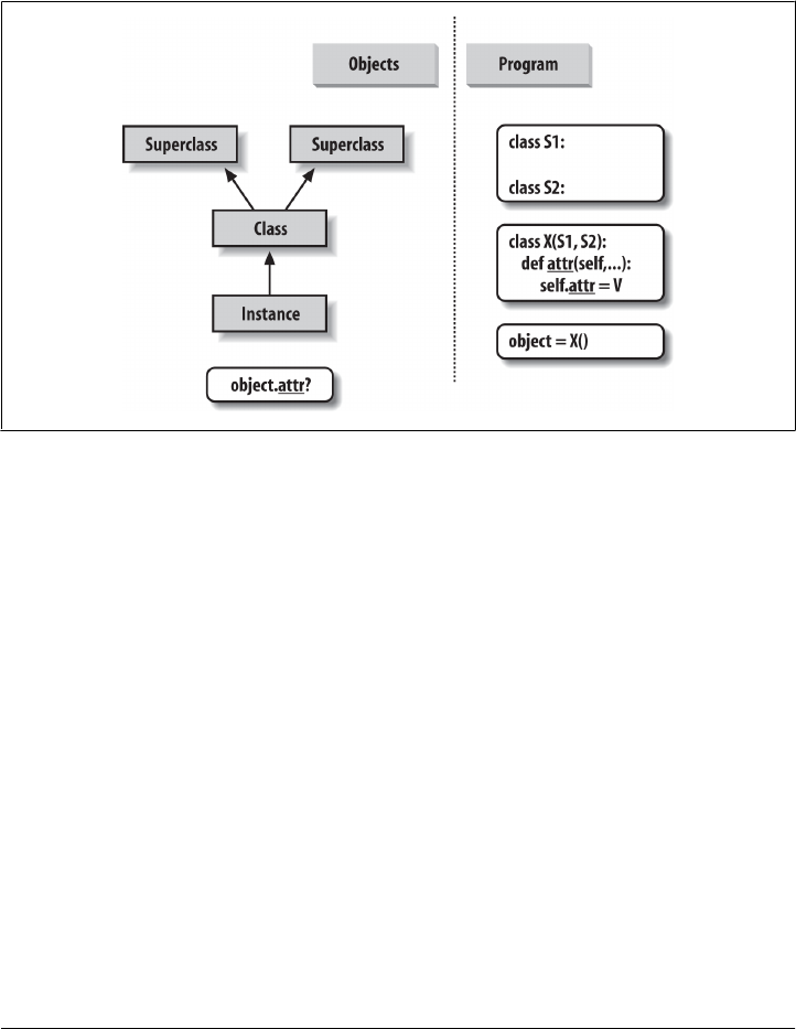
• Superclass links are made by listing classes in parentheses in a class statement
header.
The net result is a tree of attribute namespaces that leads from an instance, to the class
it was generated from, to all the superclasses listed in the class header. Python searches
upward in this tree, from instances to superclasses, each time you use qualification to
fetch an attribute name from an instance object.4
Figure 29-1. Program code creates a tree of objects in memory to be searched by attribute inheritance.
Calling a class creates a new instance that remembers its class, running a class statement creates a
new class, and superclasses are listed in parentheses in the class statement header. Each attribute
reference triggers a new bottom-up tree search—even references to self attributes within a class’s
methods.
Specializing Inherited Methods
The tree-searching model of inheritance just described turns out to be a great way to
specialize systems. Because inheritance finds names in subclasses before it checks su-
perclasses, subclasses can replace default behavior by redefining their superclasses’
4. Two fine points here: first, this description isn’t 100% complete, because we can also create instance and
class attributes by assigning them to objects outside class statements—but that’s a much less common
and sometimes more error-prone approach (changes aren’t isolated to class statements). In Python, all
attributes are always accessible by default. We’ll talk more about attribute name privacy in Chapter 30
when we study __setattr__, in Chapter 31 when we meet __X names, and again in Chapter 39, where
we’ll implement it with a class decorator.
Second, as also noted in Chapter 27, the full inheritance story grows more convoluted when advanced
topics such as metaclasses and descriptors are added to the mix—and we’re deferring a formal definition
until Chapter 40 for this reason. In common usage, though, it’s simply a way to redefine, and hence
customize, behavior coded in classes.
866 | Chapter 29: Class Coding Details
www.it-ebooks.info

attributes. In fact, you can build entire systems as hierarchies of classes, which you
extend by adding new external subclasses rather than changing existing logic in place.
The idea of redefining inherited names leads to a variety of specialization techniques.
For instance, subclasses may replace inherited attributes completely, provide attributes
that a superclass expects to find, and extend superclass methods by calling back to the
superclass from an overridden method. We’ve already seen some of these patterns in
action; here’s a self-contained example of extension at work:
>>> class Super:
def method(self):
print('in Super.method')
>>> class Sub(Super):
def method(self): # Override method
print('starting Sub.method') # Add actions here
Super.method(self) # Run default action
print('ending Sub.method')
Direct superclass method calls are the crux of the matter here. The Sub class replaces
Super’s method function with its own specialized version, but within the replacement,
Sub calls back to the version exported by Super to carry out the default behavior. In
other words, Sub.method just extends Super.method’s behavior, rather than replacing it
completely:
>>> x = Super() # Make a Super instance
>>> x.method() # Runs Super.method
in Super.method
>>> x = Sub() # Make a Sub instance
>>> x.method() # Runs Sub.method, calls Super.method
starting Sub.method
in Super.method
ending Sub.method
This extension coding pattern is also commonly used with constructors; see the section
“Methods” on page 862 for an example.
Class Interface Techniques
Extension is only one way to interface with a superclass. The file shown in this section,
specialize.py, defines multiple classes that illustrate a variety of common techniques:
Super
Defines a method function and a delegate that expects an action in a subclass.
Inheritor
Doesn’t provide any new names, so it gets everything defined in Super.
Replacer
Overrides Super’s method with a version of its own.
Inheritance | 867
www.it-ebooks.info

Extender
Customizes Super’s method by overriding and calling back to run the default.
Provider
Implements the action method expected by Super’s delegate method.
Study each of these subclasses to get a feel for the various ways they customize their
common superclass. Here’s the file:
class Super:
def method(self):
print('in Super.method') # Default behavior
def delegate(self):
self.action() # Expected to be defined
class Inheritor(Super): # Inherit method verbatim
pass
class Replacer(Super): # Replace method completely
def method(self):
print('in Replacer.method')
class Extender(Super): # Extend method behavior
def method(self):
print('starting Extender.method')
Super.method(self)
print('ending Extender.method')
class Provider(Super): # Fill in a required method
def action(self):
print('in Provider.action')
if __name__ == '__main__':
for klass in (Inheritor, Replacer, Extender):
print('\n' + klass.__name__ + '...')
klass().method()
print('\nProvider...')
x = Provider()
x.delegate()
A few things are worth pointing out here. First, notice how the self-test code at the end
of this example creates instances of three different classes in a for loop. Because classes
are objects, you can store them in a tuple and create instances generically with no extra
syntax (more on this idea later). Classes also have the special __name__ attribute, like
modules; it’s preset to a string containing the name in the class header. Here’s what
happens when we run the file:
% python specialize.py
Inheritor...
in Super.method
Replacer...
in Replacer.method
868 | Chapter 29: Class Coding Details
www.it-ebooks.info

Extender...
starting Extender.method
in Super.method
ending Extender.method
Provider...
in Provider.action
Abstract Superclasses
Of the prior example’s classes, Provider may be the most crucial to understand. When
we call the delegate method through a Provider instance, two independent inheritance
searches occur:
1. On the initial x.delegate call, Python finds the delegate method in Super by
searching the Provider instance and above. The instance x is passed into the
method’s self argument as usual.
2. Inside the Super.delegate method, self.action invokes a new, independent in-
heritance search of self and above. Because self references a Provider instance,
the action method is located in the Provider subclass.
This “filling in the blanks” sort of coding structure is typical of OOP frameworks. In a
more realistic context, the method filled in this way might handle an event in a GUI,
provide data to be rendered as part of a web page, process a tag’s text in an XML file,
and so on—your subclass provides specific actions, but the framework handles the rest
of the overall job.
At least in terms of the delegate method, the superclass in this example is what is
sometimes called an abstract superclass—a class that expects parts of its behavior to be
provided by its subclasses. If an expected method is not defined in a subclass, Python
raises an undefined name exception when the inheritance search fails.
Class coders sometimes make such subclass requirements more obvious with assert
statements, or by raising the built-in NotImplementedError exception with raise state-
ments. We’ll study statements that may trigger exceptions in depth in the next part of
this book; as a quick preview, here’s the assert scheme in action:
class Super:
def delegate(self):
self.action()
def action(self):
assert False, 'action must be defined!' # If this version is called
>>> X = Super()
>>> X.delegate()
AssertionError: action must be defined!
We’ll meet assert in Chapter 33 and Chapter 34; in short, if its first expression evaluates
to false, it raises an exception with the provided error message. Here, the expression is
Inheritance | 869
www.it-ebooks.info

always false so as to trigger an error message if a method is not redefined, and inheri-
tance locates the version here. Alternatively, some classes simply raise a NotImplemen
tedError exception directly in such method stubs to signal the mistake:
class Super:
def delegate(self):
self.action()
def action(self):
raise NotImplementedError('action must be defined!')
>>> X = Super()
>>> X.delegate()
NotImplementedError: action must be defined!
For instances of subclasses, we still get the exception unless the subclass provides the
expected method to replace the default in the superclass:
>>> class Sub(Super): pass
>>> X = Sub()
>>> X.delegate()
NotImplementedError: action must be defined!
>>> class Sub(Super):
def action(self): print('spam')
>>> X = Sub()
>>> X.delegate()
spam
For a somewhat more realistic example of this section’s concepts in action, see the “Zoo
animal hierarchy” exercise (Exercise 8) at the end of Chapter 32, and its solution in
“Part VI, Classes and OOP” in Appendix D. Such taxonomies are a traditional way to
introduce OOP, but they’re a bit removed from most developers’ job descriptions (with
apologies to any readers who happen to work at the zoo!).
Abstract superclasses in Python 3.X and 2.6+: Preview
As of Python 2.6 and 3.0, the prior section’s abstract superclasses (a.k.a. “abstract base
classes”), which require methods to be filled in by subclasses, may also be implemented
with special class syntax. The way we code this varies slightly depending on the version.
In Python 3.X, we use a keyword argument in a class header, along with special @
decorator syntax, both of which we’ll study in detail later in this book:
from abc import ABCMeta, abstractmethod
class Super(metaclass=ABCMeta):
@abstractmethod
def method(self, ...):
pass
But in Python 2.6 and 2.7, we use a class attribute instead:
870 | Chapter 29: Class Coding Details
www.it-ebooks.info

class Super:
__metaclass__ = ABCMeta
@abstractmethod
def method(self, ...):
pass
Either way, the effect is the same—we can’t make an instance unless the method is
defined lower in the class tree. In 3.X, for example, here is the special syntax equivalent
of the prior section’s example:
>>> from abc import ABCMeta, abstractmethod
>>>
>>> class Super(metaclass=ABCMeta):
def delegate(self):
self.action()
@abstractmethod
def action(self):
pass
>>> X = Super()
TypeError: Can't instantiate abstract class Super with abstract methods action
>>> class Sub(Super): pass
>>> X = Sub()
TypeError: Can't instantiate abstract class Sub with abstract methods action
>>> class Sub(Super):
def action(self): print('spam')
>>> X = Sub()
>>> X.delegate()
spam
Coded this way, a class with an abstract method cannot be instantiated (that is, we
cannot create an instance by calling it) unless all of its abstract methods have been
defined in subclasses. Although this requires more code and extra knowledge, the po-
tential advantage of this approach is that errors for missing methods are issued when
we attempt to make an instance of the class, not later when we try to call a missing
method. This feature may also be used to define an expected interface, automatically
verified in client classes.
Unfortunately, this scheme also relies on two advanced language tools we have not met
yet—function decorators, introduced in Chapter 32 and covered in depth in Chap-
ter 39, as well as metaclass declarations, mentioned in Chapter 32 and covered in
Chapter 40—so we will finesse other facets of this option here. See Python’s standard
manuals for more on this, as well as precoded abstract superclasses Python provides.
Inheritance | 871
www.it-ebooks.info

Namespaces: The Conclusion
Now that we’ve examined class and instance objects, the Python namespace story is
complete. For reference, I’ll quickly summarize all the rules used to resolve names here.
The first things you need to remember are that qualified and unqualified names are
treated differently, and that some scopes serve to initialize object namespaces:
• Unqualified names (e.g., X) deal with scopes.
• Qualified attribute names (e.g., object.X) use object namespaces.
• Some scopes initialize object namespaces (for modules and classes).
These concepts sometimes interact—in object.X, for example, object is looked up per
scopes, and then X is looked up in the result objects. Since scopes and namespaces are
essential to understanding Python code, let’s summarize the rules in more detail.
Simple Names: Global Unless Assigned
As we’ve learned, unqualified simple names follow the LEGB lexical scoping rule out-
lined when we explored functions in Chapter 17:
Assignment (X = value)
Makes names local by default: creates or changes the name X in the current local
scope, unless declared global (or nonlocal in 3.X).
Reference (X)
Looks for the name X in the current local scope, then any and all enclosing func-
tions, then the current global scope, then the built-in scope, per the LEGB rule.
Enclosing classes are not searched: class names are fetched as object attributes
instead.
Also per Chapter 17, some special-case constructs localize names further (e.g., variables
in some comprehensions and try statement clauses), but the vast majority of names
follow the LEGB rule.
Attribute Names: Object Namespaces
We’ve also seen that qualified attribute names refer to attributes of specific objects and
obey the rules for modules and classes. For class and instance objects, the reference
rules are augmented to include the inheritance search procedure:
Assignment (object.X = value)
Creates or alters the attribute name X in the namespace of the object being quali-
fied, and none other. Inheritance-tree climbing happens only on attribute refer-
ence, not on attribute assignment.
872 | Chapter 29: Class Coding Details
www.it-ebooks.info

Reference (object.X)
For class-based objects, searches for the attribute name X in object, then in all
accessible classes above it, using the inheritance search procedure. For nonclass
objects such as modules, fetches X from object directly.
As noted earlier, the preceding captures the normal and typical case. These attribute
rules can vary in classes that utilize more advanced tools, especially for new-style classes
—an option in 2.X and the standard in 3.X, which we’ll explore in Chapter 32. For
example, reference inheritance can be richer than implied here when metaclasses are
deployed, and classes which leverage attribute management tools such as properties,
descriptors, and __setattr__ can intercept and route attribute assignments arbitrarily.
In fact, some inheritance is run on assignment too, to locate descriptors with a
__set__ method in new-style classes; such tools override the normal rules for both
reference and assignment. We’ll explore attribute management tools in depth in Chap-
ter 38, and formalize inheritance and its use of descriptors in Chapter 40. For now,
most readers should focus on the normal rules given here, which cover most Python
application code.
The “Zen” of Namespaces: Assignments Classify Names
With distinct search procedures for qualified and unqualified names, and multiple
lookup layers for both, it can sometimes be difficult to tell where a name will wind up
going. In Python, the place where you assign a name is crucial—it fully determines the
scope or object in which a name will reside. The file manynames.py illustrates how this
principle translates to code and summarizes the namespace ideas we have seen through-
out this book (sans obscure special-case scopes like comprehensions):
# File manynames.py
X = 11 # Global (module) name/attribute (X, or manynames.X)
def f():
print(X) # Access global X (11)
def g():
X = 22 # Local (function) variable (X, hides module X)
print(X)
class C:
X = 33 # Class attribute (C.X)
def m(self):
X = 44 # Local variable in method (X)
self.X = 55 # Instance attribute (instance.X)
This file assigns the same name, X, five times—illustrative, though not exactly best
practice! Because this name is assigned in five different locations, though, all five Xs in
this program are completely different variables. From top to bottom, the assignments
to X here generate: a module attribute (11), a local variable in a function (22), a class
Namespaces: The Conclusion | 873
www.it-ebooks.info

attribute (33), a local variable in a method (44), and an instance attribute (55). Although
all five are named X, the fact that they are all assigned at different places in the source
code or to different objects makes all of these unique variables.
You should take the time to study this example carefully because it collects ideas we’ve
been exploring throughout the last few parts of this book. When it makes sense to you,
you will have achieved Python namespace enlightenment. Or, you can run the code
and see what happens—here’s the remainder of this source file, which makes an in-
stance and prints all the Xs that it can fetch:
# manynames.py, continued
if __name__ == '__main__':
print(X) # 11: module (a.k.a. manynames.X outside file)
f() # 11: global
g() # 22: local
print(X) # 11: module name unchanged
obj = C() # Make instance
print(obj.X) # 33: class name inherited by instance
obj.m() # Attach attribute name X to instance now
print(obj.X) # 55: instance
print(C.X) # 33: class (a.k.a. obj.X if no X in instance)
#print(C.m.X) # FAILS: only visible in method
#print(g.X) # FAILS: only visible in function
The outputs that are printed when the file is run are noted in the comments in the code;
trace through them to see which variable named X is being accessed each time. Notice
in particular that we can go through the class to fetch its attribute (C.X), but we can
never fetch local variables in functions or methods from outside their def statements.
Locals are visible only to other code within the def, and in fact only live in memory
while a call to the function or method is executing.
Some of the names defined by this file are visible outside the file to other modules too,
but recall that we must always import before we can access names in another file—
name segregation is the main point of modules, after all:
# otherfile.py
import manynames
X = 66
print(X) # 66: the global here
print(manynames.X) # 11: globals become attributes after imports
manynames.f() # 11: manynames's X, not the one here!
manynames.g() # 22: local in other file's function
print(manynames.C.X) # 33: attribute of class in other module
I = manynames.C()
print(I.X) # 33: still from class here
874 | Chapter 29: Class Coding Details
www.it-ebooks.info

I.m()
print(I.X) # 55: now from instance!
Notice here how manynames.f() prints the X in manynames, not the X assigned in this file
—scopes are always determined by the position of assignments in your source code
(i.e., lexically) and are never influenced by what imports what or who imports whom.
Also, notice that the instance’s own X is not created until we call I.m()—attributes, like
all variables, spring into existence when assigned, and not before. Normally we create
instance attributes by assigning them in class __init__ constructor methods, but this
isn’t the only option.
Finally, as we learned in Chapter 17, it’s also possible for a function to change names
outside itself, with global and (in Python 3.X) nonlocal statements—these statements
provide write access, but also modify assignment’s namespace binding rules:
X = 11 # Global in module
def g1():
print(X) # Reference global in module (11)
def g2():
global X
X = 22 # Change global in module
def h1():
X = 33 # Local in function
def nested():
print(X) # Reference local in enclosing scope (33)
def h2():
X = 33 # Local in function
def nested():
nonlocal X # Python 3.X statement
X = 44 # Change local in enclosing scope
Of course, you generally shouldn’t use the same name for every variable in your script
—but as this example demonstrates, even if you do, Python’s namespaces will work to
keep names used in one context from accidentally clashing with those used in another.
Nested Classes: The LEGB Scopes Rule Revisited
The preceding example summarized the effect of nested functions on scopes, which we
studied in Chapter 17. It turns out that classes can be nested too—a useful coding
pattern in some types of programs, with scope implications that follow naturally from
what you already know, but that may not be obvious on first encounter. This section
illustrates the concept by example.
Though they are normally coded at the top level of a module, classes also sometimes
appear nested in functions that generate them—a variation on the “factory function”
(a.k.a. closure) theme in Chapter 17, with similar state retention roles. There we noted
Namespaces: The Conclusion | 875
www.it-ebooks.info

that class statements introduce new local scopes much like function def statements,
which follow the same LEGB scope lookup rule as function definitions.
This rule applies both to the top level of the class itself, as well as to the top level of
method functions nested within it. Both form the L layer in this rule—they are normal
local scopes, with access to their names, names in any enclosing functions, globals in
the enclosing module, and built-ins. Like modules, the class’s local scope morphs into
an attribute namespace after the class statement is run.
Although classes have access to enclosing functions’ scopes, though, they do not act
as enclosing scopes to code nested within the class: Python searches enclosing functions
for referenced names, but never any enclosing classes. That is, a class is a local scope
and has access to enclosing local scopes, but it does not serve as an enclosing local scope
to further nested code. Because the search for names used in method functions skips
the enclosing class, class attributes must be fetched as object attributes using inheri-
tance.
For example, in the following nester function, all references to X are routed to the global
scope except the last, which picks up a local scope redefinition (the section’s code is in
file classscope.py, and the output of each example is described in its last two comments):
X = 1
def nester():
print(X) # Global: 1
class C:
print(X) # Global: 1
def method1(self):
print(X) # Global: 1
def method2(self):
X = 3 # Hides global
print(X) # Local: 3
I = C()
I.method1()
I.method2()
print(X) # Global: 1
nester() # Rest: 1, 1, 1, 3
print('-'*40)
Watch what happens, though, when we reassign the same name in nested function
layers: the redefinitions of X create locals that hide those in enclosing scopes, just as for
simple nested functions; the enclosing class layer does not change this rule, and in fact
is irrelevant to it:
X = 1
def nester():
X = 2 # Hides global
print(X) # Local: 2
class C:
print(X) # In enclosing def (nester): 2
876 | Chapter 29: Class Coding Details
www.it-ebooks.info

def method1(self):
print(X) # In enclosing def (nester): 2
def method2(self):
X = 3 # Hides enclosing (nester)
print(X) # Local: 3
I = C()
I.method1()
I.method2()
print(X) # Global: 1
nester() # Rest: 2, 2, 2, 3
print('-'*40)
And here’s what happens when we reassign the same name at multiple stops along the
way: assignments in the local scopes of both functions and classes hide globals or en-
closing function locals of the same name, regardless of the nesting involved:
X = 1
def nester():
X = 2 # Hides global
print(X) # Local: 2
class C:
X = 3 # Class local hides nester's: C.X or I.X (not scoped)
print(X) # Local: 3
def method1(self):
print(X) # In enclosing def (not 3 in class!): 2
print(self.X) # Inherited class local: 3
def method2(self):
X = 4 # Hides enclosing (nester, not class)
print(X) # Local: 4
self.X = 5 # Hides class
print(self.X) # Located in instance: 5
I = C()
I.method1()
I.method2()
print(X) # Global: 1
nester() # Rest: 2, 3, 2, 3, 4, 5
print('-'*40)
Most importantly, the lookup rules for simple names like X never search enclosing
class statements—just defs, modules, and built-ins (it’s the LEGB rule, not CLEGB!).
In method1, for example, X is found in a def outside the enclosing class that has the same
name in its local scope. To get to names assigned in the class (e.g., methods), we must
fetch them as class or instance object attributes, via self.X in this case.
Believe it or not, we’ll see use cases for this nested classes coding pattern later in this
book, especially in some of Chapter 39’s decorators. In this role, the enclosing function
usually both serves as a class factory and provides retained state for later use in the
enclosed class or its methods.
Namespaces: The Conclusion | 877
www.it-ebooks.info

Namespace Dictionaries: Review
In Chapter 23, we learned that module namespaces have a concrete implementation as
dictionaries, exposed with the built-in __dict__ attribute. In Chapter 27 and Chap-
ter 28, we learned that the same holds true for class and instance objects—attribute
qualification is mostly a dictionary indexing operation internally, and attribute inher-
itance is largely a matter of searching linked dictionaries. In fact, within Python, in-
stance and class objects are mostly just dictionaries with links between them. Python
exposes these dictionaries, as well as their links, for use in advanced roles (e.g., for
coding tools).
We put some of these tools to work in the prior chapter, but to summarize and help
you better understand how attributes work internally, let’s work through an interactive
session that traces the way namespace dictionaries grow when classes are involved.
Now that we know more about methods and superclasses, we can also embellish the
coverage here for a better look. First, let’s define a superclass and a subclass with meth-
ods that will store data in their instances:
>>> class Super:
def hello(self):
self.data1 = 'spam'
>>> class Sub(Super):
def hola(self):
self.data2 = 'eggs'
When we make an instance of the subclass, the instance starts out with an empty
namespace dictionary, but it has links back to the class for the inheritance search to
follow. In fact, the inheritance tree is explicitly available in special attributes, which
you can inspect. Instances have a __class__ attribute that links to their class, and classes
have a __bases__ attribute that is a tuple containing links to higher superclasses (I’m
running this on Python 3.3; your name formats, internal attributes, and key orders may
vary):
>>> X = Sub()
>>> X.__dict__ # Instance namespace dict
{}
>>> X.__class__ # Class of instance
<class '__main__.Sub'>
>>> Sub.__bases__ # Superclasses of class
(<class '__main__.Super'>,)
>>> Super.__bases__ # () empty tuple in Python 2.X
(<class 'object'>,)
As classes assign to self attributes, they populate the instance objects—that is, at-
tributes wind up in the instances’ attribute namespace dictionaries, not in the classes’.
An instance object’s namespace records data that can vary from instance to instance,
and self is a hook into that namespace:
>>> Y = Sub()
878 | Chapter 29: Class Coding Details
www.it-ebooks.info

>>> X.hello()
>>> X.__dict__
{'data1': 'spam'}
>>> X.hola()
>>> X.__dict__
{'data2': 'eggs', 'data1': 'spam'}
>>> list(Sub.__dict__.keys())
['__qualname__', '__module__', '__doc__', 'hola']
>>> list(Super.__dict__.keys())
['__module__', 'hello', '__dict__', '__qualname__', '__doc__', '__weakref__']
>>> Y.__dict__
{}
Notice the extra underscore names in the class dictionaries; Python sets these auto-
matically, and we can filter them out with the generator expressions we saw in Chap-
ter 27 and Chapter 28 that we won’t repeat here. Most are not used in typical programs,
but there are tools that use some of them (e.g., __doc__ holds the docstrings discussed
in Chapter 15).
Also, observe that Y, a second instance made at the start of this series, still has an empty
namespace dictionary at the end, even though X’s dictionary has been populated by
assignments in methods. Again, each instance has an independent namespace dictio-
nary, which starts out empty and can record completely different attributes than those
recorded by the namespace dictionaries of other instances of the same class.
Because attributes are actually dictionary keys inside Python, there are really two ways
to fetch and assign their values—by qualification, or by key indexing:
>>> X.data1, X.__dict__['data1']
('spam', 'spam')
>>> X.data3 = 'toast'
>>> X.__dict__
{'data2': 'eggs', 'data3': 'toast', 'data1': 'spam'}
>>> X.__dict__['data3'] = 'ham'
>>> X.data3
'ham'
This equivalence applies only to attributes actually attached to the instance, though.
Because attribute fetch qualification also performs an inheritance search, it can access
inherited attributes that namespace dictionary indexing cannot. The inherited attribute
X.hello, for instance, cannot be accessed by X.__dict__['hello'].
Experiment with these special attributes on your own to get a better feel for how name-
spaces actually do their attribute business. Also try running these objects through the
dir function we met in the prior two chapters—dir(X) is similar to
X.__dict__.keys(), but dir sorts its list and includes some inherited and built-in at-
Namespaces: The Conclusion | 879
www.it-ebooks.info

tributes. Even if you will never use these in the kinds of programs you write, seeing that
they are just normal dictionaries can help solidify namespaces in general.
In Chapter 32, we’ll learn also about slots, a somewhat advanced new-
style class feature that stores attributes in instances, but not in their
namespace dictionaries. It’s tempting to treat these as class attributes,
and indeed, they appear in class namespaces where they manage the
per-instance values. As we’ll see, though, slots may prevent a __dict__
from being created in the instance entirely—a potential that generic
tools must sometimes account for by using storage-neutral tools such
as dir and getattr.
Namespace Links: A Tree Climber
The prior section demonstrated the special __class__ and __bases__ instance and class
attributes, without really explaining why you might care about them. In short, these
attributes allow you to inspect inheritance hierarchies within your own code. For ex-
ample, they can be used to display a class tree, as in the following Python 3.X and 2.X
example:
#!python
"""
classtree.py: Climb inheritance trees using namespace links,
displaying higher superclasses with indentation for height
"""
def classtree(cls, indent):
print('.' * indent + cls.__name__) # Print class name here
for supercls in cls.__bases__: # Recur to all superclasses
classtree(supercls, indent+3) # May visit super > once
def instancetree(inst):
print('Tree of %s' % inst) # Show instance
classtree(inst.__class__, 3) # Climb to its class
def selftest():
class A: pass
class B(A): pass
class C(A): pass
class D(B,C): pass
class E: pass
class F(D,E): pass
instancetree(B())
instancetree(F())
if __name__ == '__main__': selftest()
The classtree function in this script is recursive—it prints a class’s name using
__name__, then climbs up to the superclasses by calling itself. This allows the function
to traverse arbitrarily shaped class trees; the recursion climbs to the top, and stops at
880 | Chapter 29: Class Coding Details
www.it-ebooks.info

root superclasses that have empty __bases__ attributes. When using recursion, each
active level of a function gets its own copy of the local scope; here, this means that
cls and indent are different at each classtree level.
Most of this file is self-test code. When run standalone in Python 2.X, it builds an empty
class tree, makes two instances from it, and prints their class tree structures:
C:\code> c:\python27\python classtree.py
Tree of <__main__.B instance at 0x00000000022C3A88>
...B
......A
Tree of <__main__.F instance at 0x00000000022C3A88>
...F
......D
.........B
............A
.........C
............A
......E
When run by Python 3.X, the tree includes the implied object superclass that is auto-
matically added above standalone root (i.e., topmost) classes, because all classes are
“new style” in 3.X—more on this change in Chapter 32:
C:\code> c:\python33\python classtree.py
Tree of <__main__.selftest.<locals>.B object at 0x00000000029216A0>
...B
......A
.........object
Tree of <__main__.selftest.<locals>.F object at 0x00000000029216A0>
...F
......D
.........B
............A
...............object
.........C
............A
...............object
......E
.........object
Here, indentation marked by periods is used to denote class tree height. Of course, we
could improve on this output format, and perhaps even sketch it in a GUI display. Even
as is, though, we can import these functions anywhere we want a quick display of a
physical class tree:
C:\code> c:\python33\python
>>> class Emp: pass
>>> class Person(Emp): pass
>>> bob = Person()
>>> import classtree
>>> classtree.instancetree(bob)
Namespaces: The Conclusion | 881
www.it-ebooks.info

Tree of <__main__.Person object at 0x000000000298B6D8>
...Person
......Emp
.........object
Regardless of whether you will ever code or use such tools, this example demonstrates
one of the many ways that you can make use of special attributes that expose interpreter
internals. You’ll see another when we code the lister.py general-purpose class display
tools in Chapter 31’s section “Multiple Inheritance: “Mix-in” Classes” on page 956
—there, we will extend this technique to also display attributes in each object in a class
tree and function as a common superclass.
In the last part of this book, we’ll revisit such tools in the context of Python tool building
at large, to code tools that implement attribute privacy, argument validation, and more.
While not in every Python programmer’s job description, access to internals enables
powerful development tools.
Documentation Strings Revisited
The last section’s example includes a docstring for its module, but remember that doc-
strings can be used for class components as well. Docstrings, which we covered in detail
in Chapter 15, are string literals that show up at the top of various structures and are
automatically saved by Python in the corresponding objects’ __doc__ attributes. This
works for module files, function defs, and classes and methods.
Now that we know more about classes and methods, the following file, docstr.py, pro-
vides a quick but comprehensive example that summarizes the places where docstrings
can show up in your code. All of these can be triple-quoted blocks or simpler one-liner
literals like those here:
"I am: docstr.__doc__"
def func(args):
"I am: docstr.func.__doc__"
pass
class spam:
"I am: spam.__doc__ or docstr.spam.__doc__ or self.__doc__"
def method(self):
"I am: spam.method.__doc__ or self.method.__doc__"
print(self.__doc__)
print(self.method.__doc__)
The main advantage of documentation strings is that they stick around at runtime.
Thus, if it’s been coded as a docstring, you can qualify an object with its __doc__ at-
tribute to fetch its documentation (printing the result interprets line breaks if it’s a
multiline string):
>>> import docstr
>>> docstr.__doc__
882 | Chapter 29: Class Coding Details
www.it-ebooks.info

'I am: docstr.__doc__'
>>> docstr.func.__doc__
'I am: docstr.func.__doc__'
>>> docstr.spam.__doc__
'I am: spam.__doc__ or docstr.spam.__doc__ or self.__doc__'
>>> docstr.spam.method.__doc__
'I am: spam.method.__doc__ or self.method.__doc__'
>>> x = docstr.spam()
>>> x.method()
I am: spam.__doc__ or docstr.spam.__doc__ or self.__doc__
I am: spam.method.__doc__ or self.method.__doc__
A discussion of the PyDoc tool, which knows how to format all these strings in reports
and web pages, appears in Chapter 15. Here it is running its help function on our code
under Python 2.X (Python 3.X shows additional attributes inherited from the implied
object superclass in the new-style class model—run this on your own to see the 3.X
extras, and watch for more about this difference in Chapter 32):
>>> help(docstr)
Help on module docstr:
NAME
docstr - I am: docstr.__doc__
FILE
c:\code\docstr.py
CLASSES
spam
class spam
| I am: spam.__doc__ or docstr.spam.__doc__ or self.__doc__
|
| Methods defined here:
|
| method(self)
| I am: spam.method.__doc__ or self.method.__doc__
FUNCTIONS
func(args)
I am: docstr.func.__doc__
Documentation strings are available at runtime, but they are less flexible syntactically
than # comments, which can appear anywhere in a program. Both forms are useful
tools, and any program documentation is good (as long as it’s accurate, of course!). As
stated before, the Python “best practice” rule of thumb is to use docstrings for func-
tional documentation (what your objects do) and hash-mark comments for more mi-
cro-level documentation (how arcane bits of code work).
Documentation Strings Revisited | 883
www.it-ebooks.info

Classes Versus Modules
Finally, let’s wrap up this chapter by briefly comparing the topics of this book’s last
two parts: modules and classes. Because they’re both about namespaces, the distinction
can be confusing. In short:
• Modules
— Implement data/logic packages
— Are created with Python files or other-language extensions
— Are used by being imported
— Form the top-level in Python program structure
• Classes
— Implement new full-featured objects
— Are created with class statements
— Are used by being called
— Always live within a module
Classes also support extra features that modules don’t, such as operator overloading,
multiple instance generation, and inheritance. Although both classes and modules are
namespaces, you should be able to tell by now that they are very different things. We
need to move ahead to see just how different classes can be.
Chapter Summary
This chapter took us on a second, more in-depth tour of the OOP mechanisms of the
Python language. We learned more about classes, methods, and inheritance, and we
wrapped up the namespaces and scopes story in Python by extending it to cover its
application to classes. Along the way, we looked at some more advanced concepts,
such as abstract superclasses, class data attributes, namespace dictionaries and links,
and manual calls to superclass methods and constructors.
Now that we’ve learned all about the mechanics of coding classes in Python, Chap-
ter 30 turns to a specific facet of those mechanics: operator overloading. After that we’ll
explore common design patterns, looking at some of the ways that classes are com-
monly used and combined to optimize code reuse. Before you read ahead, though, be
sure to work through the usual chapter quiz to review what we’ve covered here.
Test Your Knowledge: Quiz
1. What is an abstract superclass?
2. What happens when a simple assignment statement appears at the top level of a
class statement?
884 | Chapter 29: Class Coding Details
www.it-ebooks.info

3. Why might a class need to manually call the __init__ method in a superclass?
4. How can you augment, instead of completely replacing, an inherited method?
5. How does a class’s local scope differ from that of a function?
6. What...was the capital of Assyria?
Test Your Knowledge: Answers
1. An abstract superclass is a class that calls a method, but does not inherit or define
it—it expects the method to be filled in by a subclass. This is often used as a way
to generalize classes when behavior cannot be predicted until a more specific sub-
class is coded. OOP frameworks also use this as a way to dispatch to client-defined,
customizable operations.
2. When a simple assignment statement (X = Y) appears at the top level of a class
statement, it attaches a data attribute to the class (Class.X). Like all class attributes,
this will be shared by all instances; data attributes are not callable method func-
tions, though.
3. A class must manually call the __init__ method in a superclass if it defines an
__init__ constructor of its own and still wants the superclass’s construction code
to run. Python itself automatically runs just one constructor—the lowest one in
the tree. Superclass constructors are usually called through the class name, passing
in the self instance manually: Superclass.__init__(self, ...).
4. To augment instead of completely replacing an inherited method, redefine it in a
subclass, but call back to the superclass’s version of the method manually from the
new version of the method in the subclass. That is, pass the self instance to the
superclass’s version of the method manually: Superclass.method(self, ...).
5. A class is a local scope and has access to enclosing local scopes, but it does not
serve as an enclosing local scope to further nested code. Like modules, the class
local scope morphs into an attribute namespace after the class statement is run.
6. Ashur (or Qalat Sherqat), Calah (or Nimrud), the short-lived Dur Sharrukin (or
Khorsabad), and finally Nineveh.
Test Your Knowledge: Answers | 885
www.it-ebooks.info

CHAPTER 30
Operator Overloading
This chapter continues our in-depth survey of class mechanics by focusing on operator
overloading. We looked briefly at operator overloading in prior chapters; here, we’ll
fill in more details and look at a handful of commonly used overloading methods.
Although we won’t demonstrate each of the many operator overloading methods avail-
able, those we will code here are a representative sample large enough to uncover the
possibilities of this Python class feature.
The Basics
Really “operator overloading” simply means intercepting built-in operations in a class’s
methods—Python automatically invokes your methods when instances of the class
appear in built-in operations, and your method’s return value becomes the result of the
corresponding operation. Here’s a review of the key ideas behind overloading:
• Operator overloading lets classes intercept normal Python operations.
• Classes can overload all Python expression operators.
• Classes can also overload built-in operations such as printing, function calls, at-
tribute access, etc.
• Overloading makes class instances act more like built-in types.
• Overloading is implemented by providing specially named methods in a class.
In other words, when certain specially named methods are provided in a class, Python
automatically calls them when instances of the class appear in their associated expres-
sions. Your class provides the behavior of the corresponding operation for instance
objects created from it.
As we’ve learned, operator overloading methods are never required and generally don’t
have defaults (apart from a handful that some classes get from object); if you don’t
code or inherit one, it just means that your class does not support the corresponding
operation. When used, though, these methods allow classes to emulate the interfaces
of built-in objects, and so appear more consistent.
887
www.it-ebooks.info
Constructors and Expressions: __init__ and __sub__
As a review, consider the following simple example: its Number class, coded in the file
number.py, provides a method to intercept instance construction (__init__), as well as
one for catching subtraction expressions (__sub__). Special methods such as these are
the hooks that let you tie into built-in operations:
# File number.py
class Number:
def __init__(self, start): # On Number(start)
self.data = start
def __sub__(self, other): # On instance - other
return Number(self.data - other) # Result is a new instance
>>> from number import Number # Fetch class from module
>>> X = Number(5) # Number.__init__(X, 5)
>>> Y = X - 2 # Number.__sub__(X, 2)
>>> Y.data # Y is new Number instance
3
As we’ve already learned, the __init__ constructor method seen in this code is the most
commonly used operator overloading method in Python; it’s present in most classes,
and used to initialize the newly created instance object using any arguments passed to
the class name. The __sub__ method plays the binary operator role that __add__ did in
Chapter 27’s introduction, intercepting subtraction expressions and returning a new
instance of the class as its result (and running __init__ along the way).
We’ve already studied __init__ and basic binary operators like __sub__ in some depth,
so we won’t rehash their usage further here. In this chapter, we will tour some of the
other tools available in this domain and look at example code that applies them in
common use cases.
Technically, instance creation first triggers the __new__ method, which
creates and returns the new instance object, which is then passed into
__init__ for initialization. Since __new__ has a built-in implementation
and is redefined in only very limited roles, though, nearly all Python
classes initialize by defining an __init__ method. We’ll see one use case
for __new__ when we study metaclasses in Chapter 40; though rare, it is
sometimes also used to customize creation of instances of mutable
types.
Common Operator Overloading Methods
Just about everything you can do to built-in objects such as integers and lists has a
corresponding specially named method for overloading in classes. Table 30-1 lists a
few of the most common; there are many more. In fact, many overloading methods
come in multiple versions (e.g., __add__, __radd__, and __iadd__ for addition), which
888 | Chapter 30: Operator Overloading
www.it-ebooks.info

is one reason there are so many. See other Python books, or the Python language ref-
erence manual, for an exhaustive list of the special method names available.
Table 30-1. Common operator overloading methods
Method Implements Called for
__init__ Constructor Object creation: X = Class(args)
__del__ Destructor Object reclamation of X
__add__ Operator + X + Y, X += Y if no __iadd__
__or__ Operator | (bitwise OR) X | Y, X |= Y if no __ior__
__repr__, __str__ Printing, conversions print(X), repr(X), str(X)
__call__ Function calls X(*args, **kargs)
__getattr__ Attribute fetch X.undefined
__setattr__ Attribute assignment X.any = value
__delattr__ Attribute deletion del X.any
__getattribute__ Attribute fetch X.any
__getitem__ Indexing, slicing, iteration X[key], X[i:j], for loops and other iterations if no
__iter__
__setitem__ Index and slice assignment X[key] = value, X[i:j] = iterable
__delitem__ Index and slice deletion del X[key], del X[i:j]
__len__ Length len(X), truth tests if no __bool__
__bool__ Boolean tests bool(X), truth tests (named __nonzero__ in 2.X)
__lt__, __gt__,
__le__, __ge__,
__eq__, __ne__
Comparisons X < Y, X > Y, X <= Y, X >= Y, X == Y, X != Y
(or else __cmp__ in 2.X only)
__radd__ Right-side operators Other + X
__iadd__ In-place augmented operators X += Y (or else __add__)
__iter__, __next__ Iteration contexts I=iter(X), next(I); for loops, in if no __con
tains__, all comprehensions, map(F,X), others
(__next__ is named next in 2.X)
__contains__ Membership test item in X (any iterable)
__index__ Integer value hex(X), bin(X), oct(X), O[X], O[X:] (replaces 2.X
__oct__, __hex__)
__enter__, __exit__ Context manager (Chapter 34)with obj as var:
__get__, __set__,
__delete__
Descriptor attributes (Chapter 38)X.attr, X.attr = value, del X.attr
__new__ Creation (Chapter 40) Object creation, before __init__
All overloading methods have names that start and end with two underscores to keep
them distinct from other names you define in your classes. The mappings from special
The Basics | 889
www.it-ebooks.info

method names to expressions or operations are predefined by the Python language,
and documented in full in the standard language manual and other reference resources.
For example, the name __add__ always maps to + expressions by Python language def-
inition, regardless of what an __add__ method’s code actually does.
Operator overloading methods may be inherited from superclasses if not defined, just
like any other methods. Operator overloading methods are also all optional—if you
don’t code or inherit one, that operation is simply unsupported by your class, and
attempting it will raise an exception. Some built-in operations, like printing, have de-
faults (inherited from the implied object class in Python 3.X), but most built-ins fail
for class instances if no corresponding operator overloading method is present.
Most overloading methods are used only in advanced programs that require objects to
behave like built-ins, though the __init__ constructor we’ve already met tends to ap-
pear in most classes. Let’s explore some of the additional methods in Table 30-1 by
example.
Although expressions trigger operator methods, be careful not to as-
sume that there is a speed advantage to cutting out the middleman and
calling the operator method directly. In fact, calling the operator method
directly might be twice as slow, presumably because of the overhead of
a function call, which Python avoids or optimizes in built-in cases.
Here’s the story for len and __len__ using Appendix B’s Windows
launcher and Chapter 21’s timing techniques on Python 3.3 and 2.7: in
both, calling __len__ directly takes twice as long:
c:\code> py −3 -m timeit -n 1000 -r 5
-s "L = list(range(100))" "x = L.__len__()"
1000 loops, best of 5: 0.134 usec per loop
c:\code> py −3 -m timeit -n 1000 -r 5
-s "L = list(range(100))" "x = len(L)"
1000 loops, best of 5: 0.063 usec per loop
c:\code> py −2 -m timeit -n 1000 -r 5
-s "L = list(range(100))" "x = L.__len__()"
1000 loops, best of 5: 0.117 usec per loop
c:\code> py −2 -m timeit -n 1000 -r 5
-s "L = list(range(100))" "x = len(L)"
1000 loops, best of 5: 0.0596 usec per loop
This is not as artificial as it may seem—I’ve actually come across rec-
ommendations for using the slower alternative in the name of speed at
a noted research institution!
Indexing and Slicing: __getitem__ and __setitem__
Our first method set allows your classes to mimic some of the behaviors of sequences
and mappings. If defined in a class (or inherited by it), the __getitem__ method is called
890 | Chapter 30: Operator Overloading
www.it-ebooks.info

automatically for instance-indexing operations. When an instance X appears in an in-
dexing expression like X[i], Python calls the __getitem__ method inherited by the in-
stance, passing X to the first argument and the index in brackets to the second argument.
For example, the following class returns the square of an index value—atypical perhaps,
but illustrative of the mechanism in general:
>>> class Indexer:
def __getitem__(self, index):
return index ** 2
>>> X = Indexer()
>>> X[2] # X[i] calls X.__getitem__(i)
4
>>> for i in range(5):
print(X[i], end=' ') # Runs __getitem__(X, i) each time
0 1 4 9 16
Intercepting Slices
Interestingly, in addition to indexing, __getitem__ is also called for slice expressions—
always in 3.X, and conditionally in 2.X if you don’t provide more specific slicing meth-
ods. Formally speaking, built-in types handle slicing the same way. Here, for example,
is slicing at work on a built-in list, using upper and lower bounds and a stride (see
Chapter 7 if you need a refresher on slicing):
>>> L = [5, 6, 7, 8, 9]
>>> L[2:4] # Slice with slice syntax: 2..(4-1)
[7, 8]
>>> L[1:]
[6, 7, 8, 9]
>>> L[:-1]
[5, 6, 7, 8]
>>> L[::2]
[5, 7, 9]
Really, though, slicing bounds are bundled up into a slice object and passed to the list’s
implementation of indexing. In fact, you can always pass a slice object manually—slice
syntax is mostly syntactic sugar for indexing with a slice object:
>>> L[slice(2, 4)] # Slice with slice objects
[7, 8]
>>> L[slice(1, None)]
[6, 7, 8, 9]
>>> L[slice(None, −1)]
[5, 6, 7, 8]
>>> L[slice(None, None, 2)]
[5, 7, 9]
This matters in classes with a __getitem__ method—in 3.X, the method will be called
both for basic indexing (with an index) and for slicing (with a slice object). Our previous
Indexing and Slicing: __getitem__ and __setitem__ | 891
www.it-ebooks.info

class won’t handle slicing because its math assumes integer indexes are passed, but the
following class will. When called for indexing, the argument is an integer as before:
>>> class Indexer:
data = [5, 6, 7, 8, 9]
def __getitem__(self, index): # Called for index or slice
print('getitem:', index)
return self.data[index] # Perform index or slice
>>> X = Indexer()
>>> X[0] # Indexing sends __getitem__ an integer
getitem: 0
5
>>> X[1]
getitem: 1
6
>>> X[-1]
getitem: −1
9
When called for slicing, though, the method receives a slice object, which is simply
passed along to the embedded list indexer in a new index expression:
>>> X[2:4] # Slicing sends __getitem__ a slice object
getitem: slice(2, 4, None)
[7, 8]
>>> X[1:]
getitem: slice(1, None, None)
[6, 7, 8, 9]
>>> X[:-1]
getitem: slice(None, −1, None)
[5, 6, 7, 8]
>>> X[::2]
getitem: slice(None, None, 2)
[5, 7, 9]
Where needed, __getitem__ can test the type of its argument, and extract slice object
bounds—slice objects have attributes start, stop, and step, any of which can be None
if omitted:
>>> class Indexer:
def __getitem__(self, index):
if isinstance(index, int): # Test usage mode
print('indexing', index)
else:
print('slicing', index.start, index.stop, index.step)
>>> X = Indexer()
>>> X[99]
indexing 99
>>> X[1:99:2]
slicing 1 99 2
>>> X[1:]
slicing 1 None None
892 | Chapter 30: Operator Overloading
www.it-ebooks.info

If used, the __setitem__ index assignment method similarly intercepts both index and
slice assignments—in 3.X (and usually in 2.X) it receives a slice object for the latter,
which may be passed along in another index assignment or used directly in the same
way:
class IndexSetter:
def __setitem__(self, index, value): # Intercept index or slice assignment
...
self.data[index] = value # Assign index or slice
In fact, __getitem__ may be called automatically in even more contexts than indexing
and slicing—it’s also an iteration fallback option, as we’ll see in a moment. First,
though, let’s take a quick look at 2.X’s flavor of these operations for 2.X readers, and
clarify a potential point of confusion in this category.
Slicing and Indexing in Python 2.X
In Python 2.X only, classes can also define __getslice__ and __setslice__ methods to
intercept slice fetches and assignments specifically. If defined, these methods are passed
the bounds of the slice expression, and are preferred over __getitem__ and __seti
tem__ for two-limit slices. In all other cases, though, this context works the same as in
3.X; for example, a slice object is still created and passed to __getitem__ if no __get
slice__ is found or a three-limit extended slice form is used:
C:\code> c:\python27\python
>>> class Slicer:
def __getitem__(self, index): print index
def __getslice__(self, i, j): print i, j
def __setslice__(self, i, j,seq): print i, j,seq
>>> Slicer()[1] # Runs __getitem__ with int, like 3.X
1
>>> Slicer()[1:9] # Runs __getslice__ if present, else __getitem__
1 9
>>> Slicer()[1:9:2] # Runs __getitem__ with slice(), like 3.X!
slice(1, 9, 2)
These slice-specific methods are removed in 3.X, so even in 2.X you should generally
use __getitem__ and __setitem__ instead and allow for both indexes and slice objects
as arguments—both for forward compatibility, and to avoid having to handle two- and
three-limit slices differently. In most classes, this works without any special code, be-
cause indexing methods can manually pass along the slice object in the square brackets
of another index expression, as in the prior section’s example. See the section “Mem-
bership: __contains__, __iter__, and __getitem__” on page 906 for another example
of slice interception at work.
Indexing and Slicing: __getitem__ and __setitem__ | 893
www.it-ebooks.info

But 3.X’s __index__ Is Not Indexing!
On a related note, don’t confuse the (perhaps unfortunately named) __index__ method
in Python 3.X for index interception—this method returns an integer value for an in-
stance when needed and is used by built-ins that convert to digit strings (and in retro-
spect, might have been better named __asindex__):
>>> class C:
def __index__(self):
return 255
>>> X = C()
>>> hex(X) # Integer value
'0xff'
>>> bin(X)
'0b11111111'
>>> oct(X)
'0o377'
Although this method does not intercept instance indexing like __getitem__, it is also
used in contexts that require an integer—including indexing:
>>> ('C' * 256)[255]
'C'
>>> ('C' * 256)[X] # As index (not X[i])
'C'
>>> ('C' * 256)[X:] # As index (not X[i:])
'C'
This method works the same way in Python 2.X, except that it is not called for the
hex and oct built-in functions; use __hex__ and __oct__ in 2.X (only) instead to intercept
these calls.
Index Iteration: __getitem__
Here’s a hook that isn’t always obvious to beginners, but turns out to be surprisingly
useful. In the absence of more-specific iteration methods we’ll get to in the next section,
the for statement works by repeatedly indexing a sequence from zero to higher indexes,
until an out-of-bounds IndexError exception is detected. Because of that, __geti
tem__ also turns out to be one way to overload iteration in Python—if this method is
defined, for loops call the class’s __getitem__ each time through, with successively
higher offsets.
It’s a case of “code one, get one free”—any built-in or user-defined object that responds
to indexing also responds to for loop iteration:
>>> class StepperIndex:
def __getitem__(self, i):
return self.data[i]
>>> X = StepperIndex() # X is a StepperIndex object
>>> X.data = "Spam"
894 | Chapter 30: Operator Overloading
www.it-ebooks.info

>>>
>>> X[1] # Indexing calls __getitem__
'p'
>>> for item in X: # for loops call __getitem__
print(item, end=' ') # for indexes items 0..N
S p a m
In fact, it’s really a case of “code one, get a bunch free.” Any class that supports for
loops automatically supports all iteration contexts in Python, many of which we’ve seen
in earlier chapters (iteration contexts were presented in Chapter 14). For example, the
in membership test, list comprehensions, the map built-in, list and tuple assignments,
and type constructors will also call __getitem__ automatically, if it’s defined:
>>> 'p' in X # All call __getitem__ too
True
>>> [c for c in X] # List comprehension
['S', 'p', 'a', 'm']
>>> list(map(str.upper, X)) # map calls (use list() in 3.X)
['S', 'P', 'A', 'M']
>>> (a, b, c, d) = X # Sequence assignments
>>> a, c, d
('S', 'a', 'm')
>>> list(X), tuple(X), ''.join(X) # And so on...
(['S', 'p', 'a', 'm'], ('S', 'p', 'a', 'm'), 'Spam')
>>> X
<__main__.StepperIndex object at 0x000000000297B630>
In practice, this technique can be used to create objects that provide a sequence interface
and to add logic to built-in sequence type operations; we’ll revisit this idea when ex-
tending built-in types in Chapter 32.
Iterable Objects: __iter__ and __next__
Although the __getitem__ technique of the prior section works, it’s really just a fallback
for iteration. Today, all iteration contexts in Python will try the __iter__ method first,
before trying __getitem__. That is, they prefer the iteration protocol we learned about
in Chapter 14 to repeatedly indexing an object; only if the object does not support the
iteration protocol is indexing attempted instead. Generally speaking, you should prefer
__iter__ too—it supports general iteration contexts better than __getitem__ can.
Technically, iteration contexts work by passing an iterable object to the iter built-in
function to invoke an __iter__ method, which is expected to return an iterator object.
If it’s provided, Python then repeatedly calls this iterator object’s __next__ method to
produce items until a StopIteration exception is raised. A next built-in function is also
Iterable Objects: __iter__ and __next__ | 895
www.it-ebooks.info

available as a convenience for manual iterations—next(I) is the same as
I.__next__(). For a review of this model’s essentials, see Figure 14-1 in Chapter 14.
This iterable object interface is given priority and attempted first. Only if no such
__iter__ method is found, Python falls back on the __getitem__ scheme and repeatedly
indexes by offsets as before, until an IndexError exception is raised.
Version skew note: As described in Chapter 14, if you are using Python
2.X, the I.__next__() iterator method just described is named
I.next() in your Python, and the next(I) built-in is present for porta-
bility—it calls I.next() in 2.X and I.__next__() in 3.X. Iteration works
the same in 2.X in all other respects.
User-Defined Iterables
In the __iter__ scheme, classes implement user-defined iterables by simply imple-
menting the iteration protocol introduced in Chapter 14 and elaborated in Chap-
ter 20. For example, the following file uses a class to define a user-defined iterable that
generates squares on demand, instead of all at once (per the preceding note, in Python
2.X define next instead of __next__, and print with a trailing comma as usual):
# File squares.py
class Squares:
def __init__(self, start, stop): # Save state when created
self.value = start - 1
self.stop = stop
def __iter__(self): # Get iterator object on iter
return self
def __next__(self): # Return a square on each iteration
if self.value == self.stop: # Also called by next built-in
raise StopIteration
self.value += 1
return self.value ** 2
When imported, its instances can appear in iteration contexts just like built-ins:
% python
>>> from squares import Squares
>>> for i in Squares(1, 5): # for calls iter, which calls __iter__
print(i, end=' ') # Each iteration calls __next__
1 4 9 16 25
Here, the iterator object returned by __iter__ is simply the instance self, because the
__next__ method is part of this class itself. In more complex scenarios, the iterator
object may be defined as a separate class and object with its own state information to
support multiple active iterations over the same data (we’ll see an example of this in a
moment). The end of the iteration is signaled with a Python raise statement—intro-
duced in Chapter 29 and covered in full in the next part of this book, but which simply
896 | Chapter 30: Operator Overloading
www.it-ebooks.info

raises an exception as if Python itself had done so. Manual iterations work the same on
user-defined iterables as they do on built-in types as well:
>>> X = Squares(1, 5) # Iterate manually: what loops do
>>> I = iter(X) # iter calls __iter__
>>> next(I) # next calls __next__ (in 3.X)
1
>>> next(I)
4
...more omitted...
>>> next(I)
25
>>> next(I) # Can catch this in try statement
StopIteration
An equivalent coding of this iterable with __getitem__ might be less natural, because
the for would then iterate through all offsets zero and higher; the offsets passed in
would be only indirectly related to the range of values produced (0..N would need to
map to start..stop). Because __iter__ objects retain explicitly managed state between
next calls, they can be more general than __getitem__.
On the other hand, iterables based on __iter__ can sometimes be more complex and
less functional than those based on __getitem__. They are really designed for iteration,
not random indexing—in fact, they don’t overload the indexing expression at all,
though you can collect their items in a sequence such as a list to enable other operations:
>>> X = Squares(1, 5)
>>> X[1]
TypeError: 'Squares' object does not support indexing
>>> list(X)[1]
4
Single versus multiple scans
The __iter__ scheme is also the implementation for all the other iteration contexts we
saw in action for the __getitem__ method—membership tests, type constructors, se-
quence assignment, and so on. Unlike our prior __getitem__ example, though, we also
need to be aware that a class’s __iter__ may be designed for a single traversal only, not
many. Classes choose scan behavior explicitly in their code.
For example, because the current Squares class’s __iter__ always returns self with just
one copy of iteration state, it is a one-shot iteration; once you’ve iterated over an in-
stance of that class, it’s empty. Calling __iter__ again on the same instance returns
self again, in whatever state it may have been left. You generally need to make a new
iterable instance object for each new iteration:
>>> X = Squares(1, 5) # Make an iterable with state
>>> [n for n in X] # Exhausts items: __iter__ returns self
[1, 4, 9, 16, 25]
>>> [n for n in X] # Now it's empty: __iter__ returns same self
[]
Iterable Objects: __iter__ and __next__ | 897
www.it-ebooks.info

>>> [n for n in Squares(1, 5)] # Make a new iterable object
[1, 4, 9, 16, 25]
>>> list(Squares(1, 3)) # A new object for each new __iter__ call
[1, 4, 9]
To support multiple iterations more directly, we could also recode this example with
an extra class or other technique, as we will in a moment. As is, though, by creating a
new instance for each iteration, you get a fresh copy of iteration state:
>>> 36 in Squares(1, 10) # Other iteration contexts
True
>>> a, b, c = Squares(1, 3) # Each calls __iter__ and then __next__
>>> a, b, c
(1, 4, 9)
>>> ':'.join(map(str, Squares(1, 5)))
'1:4:9:16:25'
Just like single-scan built-ins such as map, converting to a list supports multiple scans
as well, but adds time and space performance costs, which may or may not be significant
to a given program:
>>> X = Squares(1, 5)
>>> tuple(X), tuple(X) # Iterator exhausted in second tuple()
((1, 4, 9, 16, 25), ())
>>> X = list(Squares(1, 5))
>>> tuple(X), tuple(X)
((1, 4, 9, 16, 25), (1, 4, 9, 16, 25))
We’ll improve this to support multiple scans more directly ahead, after a bit of compare-
and-contrast.
Classes versus generators
Notice that the preceding example would probably be simpler if it was coded with
generator functions or expressions—tools introduced in Chapter 20 that automatically
produce iterable objects and retain local variable state between iterations:
>>> def gsquares(start, stop):
for i in range(start, stop + 1):
yield i ** 2
>>> for i in gsquares(1, 5):
print(i, end=' ')
1 4 9 16 25
>>> for i in (x ** 2 for x in range(1, 6)):
print(i, end=' ')
1 4 9 16 25
Unlike classes, generator functions and expressions implicitly save their state and create
the methods required to conform to the iteration protocol—with obvious advantages
898 | Chapter 30: Operator Overloading
www.it-ebooks.info

in code conciseness for simpler examples like these. On the other hand, the class’s more
explicit attributes and methods, extra structure, inheritance hierarchies, and support
for multiple behaviors may be better suited for richer use cases.
Of course, for this artificial example, you could in fact skip both techniques and simply
use a for loop, map, or a list comprehension to build the list all at once. Barring perfor-
mance data to the contrary, the best and fastest way to accomplish a task in Python is
often also the simplest:
>>> [x ** 2 for x in range(1, 6)]
[1, 4, 9, 16, 25]
However, classes may be better at modeling more complex iterations, especially when
they can benefit from the assets of classes in general. An iterable that produces items
in a complex database or web service result, for example, might be able to take fuller
advantage of classes. The next section explores another use case for classes in user-
defined iterables.
Multiple Iterators on One Object
Earlier, I mentioned that the iterator object (with a __next__) produced by an iterable
may be defined as a separate class with its own state information to more directly
support multiple active iterations over the same data. Consider what happens when
we step across a built-in type like a string:
>>> S = 'ace'
>>> for x in S:
for y in S:
print(x + y, end=' ')
aa ac ae ca cc ce ea ec ee
Here, the outer loop grabs an iterator from the string by calling iter, and each nested
loop does the same to get an independent iterator. Because each active iterator has its
own state information, each loop can maintain its own position in the string, regardless
of any other active loops. Moreover, we’re not required to make a new string or convert
to a list each time; the single string object itself supports multiple scans.
We saw related examples earlier, in Chapter 14 and Chapter 20. For instance, generator
functions and expressions, as well as built-ins like map and zip, proved to be single-
iterator objects, thus supporting a single active scan. By contrast, the range built-in,
and other built-in types like lists, support multiple active iterators with independent
positions.
When we code user-defined iterables with classes, it’s up to us to decide whether we
will support a single active iteration or many. To achieve the multiple-iterator effect,
__iter__ simply needs to define a new stateful object for the iterator, instead of re-
turning self for each iterator request.
Iterable Objects: __iter__ and __next__ | 899
www.it-ebooks.info

The following SkipObject class, for example, defines an iterable object that skips every
other item on iterations. Because its iterator object is created anew from a supplemental
class for each iteration, it supports multiple active loops directly (this is file skip-
per.py in the book’s examples):
#!python3
# File skipper.py
class SkipObject:
def __init__(self, wrapped): # Save item to be used
self.wrapped = wrapped
def __iter__(self):
return SkipIterator(self.wrapped) # New iterator each time
class SkipIterator:
def __init__(self, wrapped):
self.wrapped = wrapped # Iterator state information
self.offset = 0
def __next__(self):
if self.offset >= len(self.wrapped): # Terminate iterations
raise StopIteration
else:
item = self.wrapped[self.offset] # else return and skip
self.offset += 2
return item
if __name__ == '__main__':
alpha = 'abcdef'
skipper = SkipObject(alpha) # Make container object
I = iter(skipper) # Make an iterator on it
print(next(I), next(I), next(I)) # Visit offsets 0, 2, 4
for x in skipper: # for calls __iter__ automatically
for y in skipper: # Nested fors call __iter__ again each time
print(x + y, end=' ') # Each iterator has its own state, offset
A quick portability note: as is, this is 3.X-only code. To make it 2.X compatible, import
the 3.X print function, and either use next instead of __next__ for 2.X-only use, or alias
the two names in the class’s scope for dual 2.X/3.X usage (file skipper_2x.py in the
book’s examples does):
#!python
from __future__ import print_function # 2.X/3.X compatibility
...
class SkipIterator:
...
def __next__(self):
...
next = __next__ # 2.X/3.X compatibility
When the appropriate version is run in either Python, this example works like the nested
loops with built-in strings. Each active loop has its own position in the string because
each obtains an independent iterator object that records its own state information:
900 | Chapter 30: Operator Overloading
www.it-ebooks.info

% python skipper.py
a c e
aa ac ae ca cc ce ea ec ee
By contrast, our earlier Squares example supports just one active iteration, unless we
call Squares again in nested loops to obtain new objects. Here, there is just one SkipOb
ject iterable, with multiple iterator objects created from it.
Classes versus slices
As before, we could achieve similar results with built-in tools—for example, slicing
with a third bound to skip items:
>>> S = 'abcdef'
>>> for x in S[::2]:
for y in S[::2]: # New objects on each iteration
print(x + y, end=' ')
aa ac ae ca cc ce ea ec ee
This isn’t quite the same, though, for two reasons. First, each slice expression here will
physically store the result list all at once in memory; iterables, on the other hand, pro-
duce just one value at a time, which can save substantial space for large result lists.
Second, slices produce new objects, so we’re not really iterating over the same object in
multiple places here. To be closer to the class, we would need to make a single object
to step across by slicing ahead of time:
>>> S = 'abcdef'
>>> S = S[::2]
>>> S
'ace'
>>> for x in S:
for y in S: # Same object, new iterators
print(x + y, end=' ')
aa ac ae ca cc ce ea ec ee
This is more similar to our class-based solution, but it still stores the slice result in
memory all at once (there is no generator form of built-in slicing today), and it’s only
equivalent for this particular case of skipping every other item.
Because user-defined iterables coded with classes can do anything a class can do, they
are much more general than this example may imply. Though such generality is not
required in all applications, user-defined iterables are a powerful tool—they allow us
to make arbitrary objects look and feel like the other sequences and iterables we have
met in this book. We could use this technique with a database object, for example, to
support iterations over large database fetches, with multiple cursors into the same query
result.
Iterable Objects: __iter__ and __next__ | 901
www.it-ebooks.info

Coding Alternative: __iter__ plus yield
And now, for something completely implicit—but potentially useful nonetheless. In
some applications, it’s possible to minimize coding requirements for user-defined itera-
bles by combining the __iter__ method we’re exploring here and the yield generator
function statement we studied in Chapter 20. Because generator functions automati-
cally save local variable state and create required iterator methods, they fit this role
well, and complement the state retention and other utility we get from classes.
As a review, recall that any function that contains a yield statement is turned into a
generator function. When called, it returns a new generator object with automatic re-
tention of local scope and code position, an automatically created __iter__ method
that simply returns itself, and an automatically created __next__ method (next in 2.X)
that starts the function or resumes it where it last left off:
>>> def gen(x):
for i in range(x): yield i ** 2
>>> G = gen(5) # Create a generator with __iter__ and __next__
>>> G.__iter__() == G # Both methods exist on the same object
True
>>> I = iter(G) # Runs __iter__: generator returns itself
>>> next(I), next(I) # Runs __next__ (next in 2.X)
(0, 1)
>>> list(gen(5)) # Iteration contexts automatically run iter and next
[0, 1, 4, 9, 16]
This is still true even if the generator function with a yield happens to be a method
named __iter__: whenever invoked by an iteration context tool, such a method will
return a new generator object with the requisite __next__. As an added bonus, generator
functions coded as methods in classes have access to saved state in both instance at-
tributes and local scope variables.
For example, the following class is equivalent to the initial Squares user-defined iterable
we coded earlier in squares.py.
# File squares_yield.py
class Squares: # __iter__ + yield generator
def __init__(self, start, stop): # __next__ is automatic/implied
self.start = start
self.stop = stop
def __iter__(self):
for value in range(self.start, self.stop + 1):
yield value ** 2
There’s no need to alias next to __next__ for 2.X compatibility here, because this
method is now automated and implied by the use of yield. As before, for loops and
other iteration tools iterate through instances of this class automatically:
% python
>>> from squares_yield import Squares
>>> for i in Squares(1, 5): print(i, end=' ')
902 | Chapter 30: Operator Overloading
www.it-ebooks.info

1 4 9 16 25
And as usual, we can look under the hood to see how this actually works in iteration
contexts. Running our class instance through iter obtains the result of calling
__iter__ as usual, but in this case the result is a generator object with an automatically
created __next__ of the same sort we always get when calling a generator function that
contains a yield. The only difference here is that the generator function is automatically
called on iter. Invoking the result object’s next interface produces results on demand:
>>> S = Squares(1, 5) # Runs __init__: class saves instance state
>>> S
<squares_yield.Squares object at 0x000000000294B630>
>>> I = iter(S) # Runs __iter__: returns a generator
>>> I
<generator object __iter__ at 0x00000000029A8CF0>
>>> next(I)
1
>>> next(I) # Runs generator's __next__
4
...etc...
>>> next(I) # Generator has both instance and local scope state
StopIteration
It may also help to notice that we could name the generator method something other
than __iter__ and call manually to iterate—Squares(1,5).gen(), for example. Using
the __iter__ name invoked automatically by iteration tools simply skips a manual at-
tribute fetch and call step:
class Squares: # Non __iter__ equivalent (squares_manual.py)
def __init__(...):
...
def gen(self):
for value in range(self.start, self.stop + 1):
yield value ** 2
% python
>>> from squares_manual import Squares
>>> for i in Squares(1, 5).gen(): print(i, end=' ')
...same results...
>>> S = Squares(1, 5)
>>> I = iter(S.gen()) # Call generator manually for iterable/iterator
>>> next(I)
...same results...
Coding the generator as __iter__ instead cuts out the middleman in your code, though
both schemes ultimately wind up creating a new generator object for each iteration:
• With __iter__, iteration triggers __iter__, which returns a new generator with
__next__.
Iterable Objects: __iter__ and __next__ | 903
www.it-ebooks.info

• Without __iter__, your code calls to make a generator, which returns itself for
__iter__.
See Chapter 20 for more on yield and generators if this is puzzling, and compare it
with the more explicit __next__ version in squares.py earlier. You’ll notice that this new
squares_yield.py version is 4 lines shorter (7 versus 11). In a sense, this scheme reduces
class coding requirements much like the closure functions of Chapter 17, but in this
case does so with a combination of functional and OOP techniques, instead of an al-
ternative to classes. For example, the generator method still leverages self attributes.
This may also very well seem like one too many levels of magic to some observers—it
relies on both the iteration protocol and the object creation of generators, both of which
are highly implicit (in contradiction of longstanding Python themes: see import this).
Opinions aside, it’s important to understand the non-yield flavor of class iterables too,
because it’s explicit, general, and sometimes broader in scope.
Still, the __iter__/yield technique may prove effective in cases where it applies. It also
comes with a substantial advantage—as the next section explains.
Multiple iterators with yield
Besides its code conciseness, the user-defined class iterable of the prior section based
upon the __iter__/yield combination has an important added bonus—it also supports
multiple active iterators automatically. This naturally follows from the fact that each
call to __iter__ is a call to a generator function, which returns a new generator with its
own copy of the local scope for state retention:
% python
>>> from squares_yield import Squares # Using the __iter__/yield Squares
>>> S = Squares(1, 5)
>>> I = iter(S)
>>> next(I); next(I)
1
4
>>> J = iter(S) # With yield, multiple iterators automatic
>>> next(J)
1
>>> next(I) # I is independent of J: own local state
9
Although generator functions are single-scan iterables, the implicit calls to __iter__ in
iteration contexts make new generators supporting new independent scans:
>>> S = Squares(1, 3)
>>> for i in S: # Each for calls __iter__
for j in S:
print('%s:%s' % (i, j), end=' ')
1:1 1:4 1:9 4:1 4:4 4:9 9:1 9:4 9:9
904 | Chapter 30: Operator Overloading
www.it-ebooks.info

To do the same without yield requires a supplemental class that stores iterator state
explicitly and manually, using techniques of the preceding section (and grows to 15
lines: 8 more than with yield):
# File squares_nonyield.py
class Squares:
def __init__(self, start, stop): # Non-yield generator
self.start = start # Multiscans: extra object
self.stop = stop
def __iter__(self):
return SquaresIter(self.start, self.stop)
class SquaresIter:
def __init__(self, start, stop):
self.value = start - 1
self.stop = stop
def __next__(self):
if self.value == self.stop:
raise StopIteration
self.value += 1
return self.value ** 2
This works the same as the yield multiscan version, but with more, and more explicit,
code:
% python
>>> from squares_nonyield import Squares
>>> for i in Squares(1, 5): print(i, end=' ')
1 4 9 16 25
>>>
>>> S = Squares(1, 5)
>>> I = iter(S)
>>> next(I); next(I)
1
4
>>> J = iter(S) # Multiple iterators without yield
>>> next(J)
1
>>> next(I)
9
>>> S = Squares(1, 3)
>>> for i in S: # Each for calls __iter___
for j in S:
print('%s:%s' % (i, j), end=' ')
1:1 1:4 1:9 4:1 4:4 4:9 9:1 9:4 9:9
Finally, the generator-based approach could similarly remove the need for an extra
iterator class in the prior item-skipper example of file skipper.py, thanks to its automatic
methods and local variable state retention (and checks in at 9 lines versus the original’s
16):
Iterable Objects: __iter__ and __next__ | 905
www.it-ebooks.info

# File skipper_yield.py
class SkipObject: # Another __iter__ + yield generator
def __init__(self, wrapped): # Instance scope retained normally
self.wrapped = wrapped # Local scope state saved auto
def __iter__(self):
offset = 0
while offset < len(self.wrapped):
item = self.wrapped[offset]
offset += 2
yield item
This works the same as the non-yield multiscan version, but with less, and less explicit,
code:
% python
>>> from skipper_yield import SkipObject
>>> skipper = SkipObject('abcdef')
>>> I = iter(skipper)
>>> next(I); next(I); next(I)
'a'
'c'
'e'
>>> for x in skipper: # Each for calls __iter__: new auto generator
for y in skipper:
print(x + y, end=' ')
aa ac ae ca cc ce ea ec ee
Of course, these are all artificial examples that could be replaced with simpler tools like
comprehensions, and their code may or may not scale up in kind to more realistic tasks.
Study these alternatives to see how they compare. As so often in programming, the best
tool for the job will likely be the best tool for your job!
Membership: __contains__, __iter__, and __getitem__
The iteration story is even richer than we’ve seen thus far. Operator overloading is often
layered: classes may provide specific methods, or more general alternatives used as
fallback options. For example:
• Comparisons in Python 2.X use specific methods such as __lt__ for “less than” if
present, or else the general __cmp__. Python 3.X uses only specific methods, not
__cmp__, as discussed later in this chapter.
• Boolean tests similarly try a specific __bool__ first (to give an explicit True/False
result), and if it’s absent fall back on the more general __len__ (a nonzero length
means True). As we’ll also see later in this chapter, Python 2.X works the same but
uses the name __nonzero__ instead of __bool__.
In the iterations domain, classes can implement the in membership operator as an
iteration, using either the __iter__ or __getitem__ methods. To support more specific
membership, though, classes may code a __contains__ method—when present, this
906 | Chapter 30: Operator Overloading
www.it-ebooks.info

method is preferred over __iter__, which is preferred over __getitem__. The __con
tains__ method should define membership as applying to keys for a mapping (and can
use quick lookups), and as a search for sequences.
Consider the following class, whose file has been instrumented for dual 2.X/3.X usage
using the techniques described earlier. It codes all three methods and tests membership
and various iteration contexts applied to an instance. Its methods print trace messages
when called:
# File contains.py
from __future__ import print_function # 2.X/3.X compatibility
class Iters:
def __init__(self, value):
self.data = value
def __getitem__(self, i): # Fallback for iteration
print('get[%s]:' % i, end='') # Also for index, slice
return self.data[i]
def __iter__(self): # Preferred for iteration
print('iter=> ', end='') # Allows only one active iterator
self.ix = 0
return self
def __next__(self):
print('next:', end='')
if self.ix == len(self.data): raise StopIteration
item = self.data[self.ix]
self.ix += 1
return item
def __contains__(self, x): # Preferred for 'in'
print('contains: ', end='')
return x in self.data
next = __next__ # 2.X/3.X compatibility
if __name__ == '__main__':
X = Iters([1, 2, 3, 4, 5]) # Make instance
print(3 in X) # Membership
for i in X: # for loops
print(i, end=' | ')
print()
print([i ** 2 for i in X]) # Other iteration contexts
print( list(map(bin, X)) )
I = iter(X) # Manual iteration (what other contexts do)
while True:
try:
print(next(I), end=' @ ')
except StopIteration:
break
Membership: __contains__, __iter__, and __getitem__ | 907
www.it-ebooks.info

As is, the class in this file has an __iter__ that supports multiple scans, but only a single
scan can be active at any point in time (e.g., nested loops won’t work), because each
iteration attempt resets the scan cursor to the front. Now that you know about yield
in iteration methods, you should be able to tell that the following is equivalent but
allows multiple active scans—and judge for yourself whether its more implicit nature
is worth the nested-scan support and six lines shaved (this is in file contains_yield.py):
class Iters:
def __init__(self, value):
self.data = value
def __getitem__(self, i): # Fallback for iteration
print('get[%s]:' % i, end='') # Also for index, slice
return self.data[i]
def __iter__(self): # Preferred for iteration
print('iter=> next:', end='') # Allows multiple active iterators
for x in self.data: # no __next__ to alias to next
yield x
print('next:', end='')
def __contains__(self, x): # Preferred for 'in'
print('contains: ', end='')
return x in self.data
On both Python 3.X and 2.X, when either version of this file runs its output is as follows
—the specific __contains__ intercepts membership, the general __iter__ catches other
iteration contexts such that __next__ (whether explicitly coded or implied by yield) is
called repeatedly, and __getitem__ is never called:
contains: True
iter=> next:1 | next:2 | next:3 | next:4 | next:5 | next:
iter=> next:next:next:next:next:next:[1, 4, 9, 16, 25]
iter=> next:next:next:next:next:next:['0b1', '0b10', '0b11', '0b100', '0b101']
iter=> next:1 @ next:2 @ next:3 @ next:4 @ next:5 @ next:
Watch what happens to this code’s output if we comment out its __contains__ method,
though—membership is now routed to the general __iter__ instead:
iter=> next:next:next:True
iter=> next:1 | next:2 | next:3 | next:4 | next:5 | next:
iter=> next:next:next:next:next:next:[1, 4, 9, 16, 25]
iter=> next:next:next:next:next:next:['0b1', '0b10', '0b11', '0b100', '0b101']
iter=> next:1 @ next:2 @ next:3 @ next:4 @ next:5 @ next:
And finally, here is the output if both __contains__ and __iter__ are commented out
—the indexing __getitem__ fallback is called with successively higher indexes until it
raises IndexError, for membership and other iteration contexts:
get[0]:get[1]:get[2]:True
get[0]:1 | get[1]:2 | get[2]:3 | get[3]:4 | get[4]:5 | get[5]:
get[0]:get[1]:get[2]:get[3]:get[4]:get[5]:[1, 4, 9, 16, 25]
get[0]:get[1]:get[2]:get[3]:get[4]:get[5]:['0b1', '0b10', '0b11', '0b100','0b101']
get[0]:1 @ get[1]:2 @ get[2]:3 @ get[3]:4 @ get[4]:5 @ get[5]:
908 | Chapter 30: Operator Overloading
www.it-ebooks.info

As we’ve seen, the __getitem__ method is even more general: besides iterations, it also
intercepts explicit indexing as well as slicing. Slice expressions trigger __getitem__ with
a slice object containing bounds, both for built-in types and user-defined classes, so
slicing is automatic in our class:
>>> from contains import Iters
>>> X = Iters('spam') # Indexing
>>> X[0] # __getitem__(0)
get[0]:'s'
>>> 'spam'[1:] # Slice syntax
'pam'
>>> 'spam'[slice(1, None)] # Slice object
'pam'
>>> X[1:] # __getitem__(slice(..))
get[slice(1, None, None)]:'pam'
>>> X[:-1]
get[slice(None, −1, None)]:'spa'
>>> list(X) # And iteration too!
iter=> next:next:next:next:next:['s', 'p', 'a', 'm']
In more realistic iteration use cases that are not sequence-oriented, though, the
__iter__ method may be easier to write since it must not manage an integer index, and
__contains__ allows for membership optimization as a special case.
Attribute Access: __getattr__ and __setattr__
In Python, classes can also intercept basic attribute access (a.k.a. qualification) when
needed or useful. Specifically, for an object created from a class, the dot operator ex-
pression object.attribute can be implemented by your code too, for reference, as-
signment, and deletion contexts. We saw a limited example in this category in Chap-
ter 28, but will review and expand on the topic here.
Attribute Reference
The __getattr__ method intercepts attribute references. It’s called with the attribute
name as a string whenever you try to qualify an instance with an undefined (nonexistent)
attribute name. It is not called if Python can find the attribute using its inheritance tree
search procedure.
Because of its behavior, __getattr__ is useful as a hook for responding to attribute
requests in a generic fashion. It’s commonly used to delegate calls to embedded (or
“wrapped”) objects from a proxy controller object—of the sort introduced in Chap-
ter 28’s introduction to delegation. This method can also be used to adapt classes to an
interface, or add accessors for data attributes after the fact—logic in a method that
validates or computes an attribute after it’s already being used with simple dot notation.
Attribute Access: __getattr__ and __setattr__ | 909
www.it-ebooks.info

The basic mechanism underlying these goals is straightforward—the following class
catches attribute references, computing the value for one dynamically, and triggering
an error for others unsupported with the raise statement described earlier in this chap-
ter for iterators (and fully covered in Part VII):
>>> class Empty:
def __getattr__(self, attrname): # On self.undefined
if attrname == 'age':
return 40
else:
raise AttributeError(attrname)
>>> X = Empty()
>>> X.age
40
>>> X.name
...error text omitted...
AttributeError: name
Here, the Empty class and its instance X have no real attributes of their own, so the access
to X.age gets routed to the __getattr__ method; self is assigned the instance (X), and
attrname is assigned the undefined attribute name string ('age'). The class makes age
look like a real attribute by returning a real value as the result of the X.age qualification
expression (40). In effect, age becomes a dynamically computed attribute—its value is
formed by running code, not fetching an object.
For attributes that the class doesn’t know how to handle, __getattr__ raises the built-
in AttributeError exception to tell Python that these are bona fide undefined names;
asking for X.name triggers the error. You’ll see __getattr__ again when we see delegation
and properties at work in the next two chapters; let’s move on to related tools here.
Attribute Assignment and Deletion
In the same department, the __setattr__ intercepts all attribute assignments. If this
method is defined or inherited, self.attr = value becomes self.__setattr__('attr',
value). Like __getattr__, this allows your class to catch attribute changes, and validate
or transform as desired.
This method is a bit trickier to use, though, because assigning to any self attributes
within __setattr__ calls __setattr__ again, potentially causing an infinite recursion
loop (and a fairly quick stack overflow exception!). In fact, this applies to all self at-
tribute assignments anywhere in the class—all are routed to __setattr__, even those
in other methods, and those to names other than that which may have triggered
__setattr__ in the first place. Remember, this catches all attribute assignments.
If you wish to use this method, you can avoid loops by coding instance attribute as-
signments as assignments to attribute dictionary keys. That is, use
self.__dict__['name'] = x, not self.name = x; because you’re not assigning to
__dict__ itself, this avoids the loop:
910 | Chapter 30: Operator Overloading
www.it-ebooks.info
>>> class Accesscontrol:
def __setattr__(self, attr, value):
if attr == 'age':
self.__dict__[attr] = value + 10 # Not self.name=val or setattr
else:
raise AttributeError(attr + ' not allowed')
>>> X = Accesscontrol()
>>> X.age = 40 # Calls __setattr__
>>> X.age
50
>>> X.name = 'Bob'
...text omitted...
AttributeError: name not allowed
If you change the __dict__ assignment in this to either of the following, it triggers the
infinite recursion loop and exception—both dot notation and its setattr built-in func-
tion equivalent (the assignment analog of getattr) fail when age is assigned outside the
class:
self.age = value + 10 # Loops
setattr(self, attr, value + 10) # Loops (attr is 'age')
An assignment to another name within the class triggers a recursive __setattr__ call
too, though in this class ends less dramatically in the manual AttributeError exception:
self.other = 99 # Recurs but doesn't loop: fails
It’s also possible to avoid recursive loops in a class that uses __setattr__ by routing
any attribute assignments to a higher superclass with a call, instead of assigning keys
in __dict__:
self.__dict__[attr] = value + 10 # OK: doesn't loop
object.__setattr__(self, attr, value + 10) # OK: doesn't loop (new-style only)
Because the object form requires use of new-style classes in 2.X, though, we’ll postpone
details on this form until Chapter 38’s deeper look at attribute management at large.
A third attribute management method, __delattr__, is passed the attribute name string
and invoked on all attribute deletions (i.e., del object.attr). Like __setattr__, it must
avoid recursive loops by routing attribute deletions with the using class through
__dict__ or a superclass.
As we’ll learn in Chapter 32, attributes implemented with new-style
class features such as slots and properties are not physically stored in the
instance’s __dict__ namespace dictionary (and slots may even preclude
its existence entirely!). Because of this, code that wishes to support such
attributes should code __setattr__ to assign with the
object.__setattr__ scheme shown here, not by self.__dict__ indexing
unless it’s known that subject classes store all their data in the instance
itself. In Chapter 38 we’ll also see that the new-style __getattribute__
Attribute Access: __getattr__ and __setattr__ | 911
www.it-ebooks.info

has similar requirements. This change is mandated in Python 3.X, but
also applies to 2.X if new-style classes are used.
Other Attribute Management Tools
These three attribute-access overloading methods allow you to control or specialize
access to attributes in your objects. They tend to play highly specialized roles, some of
which we’ll explore later in this book. For another example of __getattr__ at work, see
Chapter 28’s person-composite.py. And for future reference, keep in mind that there are
other ways to manage attribute access in Python:
• The __getattribute__ method intercepts all attribute fetches, not just those that
are undefined, but when using it you must be more cautious than with __get
attr__ to avoid loops.
• The property built-in function allows us to associate methods with fetch and set
operations on a specific class attribute.
•Descriptors provide a protocol for associating __get__ and __set__ methods of a
class with accesses to a specific class attribute.
•Slots attributes are declared in classes but create implicit storage in each instance.
Because these are somewhat advanced tools not of interest to every Python program-
mer, we’ll defer a look at properties until Chapter 32 and detailed coverage of all the
attribute management techniques until Chapter 38.
Emulating Privacy for Instance Attributes: Part 1
As another use case for such tools, the following code—file private0.py—generalizes
the previous example, to allow each subclass to have its own list of private names that
cannot be assigned to its instances (and uses a user-defined exception class, which you’ll
have to take on faith until Part VII):
class PrivateExc(Exception): pass # More on exceptions in Part VII
class Privacy:
def __setattr__(self, attrname, value): # On self.attrname = value
if attrname in self.privates:
raise PrivateExc(attrname, self) # Make, raise user-define except
else:
self.__dict__[attrname] = value # Avoid loops by using dict key
class Test1(Privacy):
privates = ['age']
class Test2(Privacy):
privates = ['name', 'pay']
def __init__(self):
self.__dict__['name'] = 'Tom' # To do better, see Chapter 39!
912 | Chapter 30: Operator Overloading
www.it-ebooks.info

if __name__ == '__main__':
x = Test1()
y = Test2()
x.name = 'Bob' # Works
#y.name = 'Sue' # Fails
print(x.name)
y.age = 30 # Works
#x.age = 40 # Fails
print(y.age)
In fact, this is a first-cut solution for an implementation of attribute privacy in Python
—disallowing changes to attribute names outside a class. Although Python doesn’t
support private declarations per se, techniques like this can emulate much of their
purpose.
This is a partial—and even clumsy—solution, though; to make it more effective, we
must augment it to allow classes to set their private attributes more naturally, without
having to go through __dict__ each time, as the constructor must do here to avoid
triggering __setattr__ and an exception. A better and more complete approach might
require a wrapper (“proxy”) class to check for private attribute accesses made outside
the class only, and a __getattr__ to validate attribute fetches too.
We’ll postpone a more complete solution to attribute privacy until Chapter 39, where
we’ll use class decorators to intercept and validate attributes more generally. Even
though privacy can be emulated this way, though, it almost never is in practice. Python
programmers are able to write large OOP frameworks and applications without private
declarations—an interesting finding about access controls in general that is beyond the
scope of our purposes here.
Still, catching attribute references and assignments is generally a useful technique; it
supports delegation, a design technique that allows controller objects to wrap up em-
bedded objects, add new behaviors, and route other operations back to the wrapped
objects. Because they involve design topics, we’ll revisit delegation and wrapper classes
in the next chapter.
String Representation: __repr__ and __str__
Our next methods deal with display formats—a topic we’ve already explored in prior
chapters, but will summarize and formalize here. As a review, the following code ex-
ercises the __init__ constructor and the __add__ overload method, both of which we’ve
already seen (+ is an in-place operation here, just to show that it can be; per Chap-
ter 27, a named method may be preferred). As we’ve learned, the default display of
instance objects for a class like this is neither generally useful nor aesthetically pretty:
>>> class adder:
def __init__(self, value=0):
self.data = value # Initialize data
String Representation: __repr__ and __str__ | 913
www.it-ebooks.info

def __add__(self, other):
self.data += other # Add other in place (bad form?)
>>> x = adder() # Default displays
>>> print(x)
<__main__.adder object at 0x00000000029736D8>
>>> x
<__main__.adder object at 0x00000000029736D8>
But coding or inheriting string representation methods allows us to customize the dis-
play—as in the following, which defines a __repr__ method in a subclass that returns
a string representation for its instances.
>>> class addrepr(adder): # Inherit __init__, __add__
def __repr__(self): # Add string representation
return 'addrepr(%s)' % self.data # Convert to as-code string
>>> x = addrepr(2) # Runs __init__
>>> x + 1 # Runs __add__ (x.add() better?)
>>> x # Runs __repr__
addrepr(3)
>>> print(x) # Runs __repr__
addrepr(3)
>>> str(x), repr(x) # Runs __repr__ for both
('addrepr(3)', 'addrepr(3)')
If defined, __repr__ (or its close relative, __str__) is called automatically when class
instances are printed or converted to strings. These methods allow you to define a better
display format for your objects than the default instance display. Here, __repr__ uses
basic string formatting to convert the managed self.data object to a more human-
friendly string for display.
Why Two Display Methods?
So far, what we’ve seen is largely review. But while these methods are generally straight-
forward to use, their roles and behavior have some subtle implications both for design
and coding. In particular, Python provides two display methods to support alternative
displays for different audiences:
•__str__ is tried first for the print operation and the str built-in function (the in-
ternal equivalent of which print runs). It generally should return a user-friendly
display.
•__repr__ is used in all other contexts: for interactive echoes, the repr function, and
nested appearances, as well as by print and str if no __str__ is present. It should
generally return an as-code string that could be used to re-create the object, or a
detailed display for developers.
That is, __repr__ is used everywhere, except by print and str when a __str__ is defined.
This means you can code a __repr__ to define a single display format used everywhere,
914 | Chapter 30: Operator Overloading
www.it-ebooks.info

and may code a __str__ to either support print and str exclusively, or to provide an
alternative display for them.
As noted in Chapter 28, general tools may also prefer __str__ to leave other classes the
option of adding an alternative __repr__ display for use in other contexts, as long as
print and str displays suffice for the tool. Conversely, a general tool that codes a
__repr__ still leaves clients the option of adding alternative displays with a __str__ for
print and str. In other words, if you code either, the other is available for an additional
display. In cases where the choice isn’t clear, __str__ is generally preferred for larger
user-friendly displays, and __repr__ for lower-level or as-code displays and all-inclusive
roles.
Let’s write some code to illustrate these two methods’ distinctions in more concrete
terms. The prior example in this section showed how __repr__ is used as the fallback
option in many contexts. However, while printing falls back on __repr__ if no
__str__ is defined, the inverse is not true—other contexts, such as interactive echoes,
use __repr__ only and don’t try __str__ at all:
>>> class addstr(adder):
def __str__(self): # __str__ but no __repr__
return '[Value: %s]' % self.data # Convert to nice string
>>> x = addstr(3)
>>> x + 1
>>> x # Default __repr__
<__main__.addstr object at 0x00000000029738D0>
>>> print(x) # Runs __str__
[Value: 4]
>>> str(x), repr(x)
('[Value: 4]', '<__main__.addstr object at 0x00000000029738D0>')
Because of this, __repr__ may be best if you want a single display for all contexts. By
defining both methods, though, you can support different displays in different contexts
—for example, an end-user display with __str__, and a low-level display for program-
mers to use during development with __repr__. In effect, __str__ simply overrides
__repr__ for more user-friendly display contexts:
>>> class addboth(adder):
def __str__(self):
return '[Value: %s]' % self.data # User-friendly string
def __repr__(self):
return 'addboth(%s)' % self.data # As-code string
>>> x = addboth(4)
>>> x + 1
>>> x # Runs __repr__
addboth(5)
>>> print(x) # Runs __str__
[Value: 5]
>>> str(x), repr(x)
('[Value: 5]', 'addboth(5)')
String Representation: __repr__ and __str__ | 915
www.it-ebooks.info

Display Usage Notes
Though generally simple to use, I should mention three usage notes regarding these
methods here. First, keep in mind that __str__ and __repr__ must both return strings;
other result types are not converted and raise errors, so be sure to run them through a
to-string converter (e.g., str or %) if needed.
Second, depending on a container’s string-conversion logic, the user-friendly display
of __str__ might only apply when objects appear at the top level of a print operation;
objects nested in larger objects might still print with their __repr__ or its default. The
following illustrates both of these points:
>>> class Printer:
def __init__(self, val):
self.val = val
def __str__(self): # Used for instance itself
return str(self.val) # Convert to a string result
>>> objs = [Printer(2), Printer(3)]
>>> for x in objs: print(x) # __str__ run when instance printed
# But not when instance is in a list!
2
3
>>> print(objs)
[<__main__.Printer object at 0x000000000297AB38>, <__main__.Printer obj...etc...>]
>>> objs
[<__main__.Printer object at 0x000000000297AB38>, <__main__.Printer obj...etc...>]
To ensure that a custom display is run in all contexts regardless of the container, code
__repr__, not __str__; the former is run in all cases if the latter doesn’t apply, including
nested appearances:
>>> class Printer:
def __init__(self, val):
self.val = val
def __repr__(self): # __repr__ used by print if no __str__
return str(self.val) # __repr__ used if echoed or nested
>>> objs = [Printer(2), Printer(3)]
>>> for x in objs: print(x) # No __str__: runs __repr__
2
3
>>> print(objs) # Runs __repr__, not ___str__
[2, 3]
>>> objs
[2, 3]
Third, and perhaps most subtle, the display methods also have the potential to trigger
infinite recursion loops in rare contexts—because some objects’ displays include dis-
plays of other objects, it’s not impossible that a display may trigger a display of an object
being displayed, and thus loop. This is rare and obscure enough to skip here, but watch
916 | Chapter 30: Operator Overloading
www.it-ebooks.info

for an example of this looping potential to appear for these methods in a note near the
end of the next chapter in its listinherited.py example’s class, where __repr__ can loop.
In practice, __str__, and its more inclusive relative __repr__, seem to be the second
most commonly used operator overloading methods in Python scripts, behind
__init__. Anytime you can print an object and see a custom display, one of these two
tools is probably in use. For additional examples of these tools at work and the design
tradeoffs they imply, see Chapter 28’s case study and Chapter 31’s class lister mix-ins,
as well as their role in Chapter 35’s exception classes, where __str__ is required over
__repr__.
Right-Side and In-Place Uses: __radd__ and __iadd__
Our next group of overloading methods extends the functionality of binary operator
methods such as __add__ and __sub__ (called for + and -), which we’ve already seen.
As mentioned earlier, part of the reason there are so many operator overloading meth-
ods is because they come in multiple flavors—for every binary expression, we can im-
plement a left, right, and in-place variant. Though defaults are also applied if you don’t
code all three, your objects’ roles dictate how many variants you’ll need to code.
Right-Side Addition
For instance, the __add__ methods coded so far technically do not support the use of
instance objects on the right side of the + operator:
>>> class Adder:
def __init__(self, value=0):
self.data = value
def __add__(self, other):
return self.data + other
>>> x = Adder(5)
>>> x + 2
7
>>> 2 + x
TypeError: unsupported operand type(s) for +: 'int' and 'Adder'
To implement more general expressions, and hence support commutative-style opera-
tors, code the __radd__ method as well. Python calls __radd__ only when the object on
the right side of the + is your class instance, but the object on the left is not an instance
of your class. The __add__ method for the object on the left is called instead in all other
cases (all of this section’s five Commuter classes are coded in file commuter.py in the
book’s examples, along with a self-test):
class Commuter1:
def __init__(self, val):
self.val = val
def __add__(self, other):
print('add', self.val, other)
Right-Side and In-Place Uses: __radd__ and __iadd__ | 917
www.it-ebooks.info

return self.val + other
def __radd__(self, other):
print('radd', self.val, other)
return other + self.val
>>> from commuter import Commuter1
>>> x = Commuter1(88)
>>> y = Commuter1(99)
>>> x + 1 # __add__: instance + noninstance
add 88 1
89
>>> 1 + y # __radd__: noninstance + instance
radd 99 1
100
>>> x + y # __add__: instance + instance, triggers __radd__
add 88 <commuter.Commuter1 object at 0x00000000029B39E8>
radd 99 88
187
Notice how the order is reversed in __radd__: self is really on the right of the +, and
other is on the left. Also note that x and y are instances of the same class here; when
instances of different classes appear mixed in an expression, Python prefers the class
of the one on the left. When we add the two instances together, Python runs __add__,
which in turn triggers __radd__ by simplifying the left operand.
Reusing __add__ in __radd__
For truly commutative operations that do not require special-casing by position, it is
also sometimes sufficient to reuse __add__ for __radd__: either by calling __add__ di-
rectly; by swapping order and re-adding to trigger __add__ indirectly; or by simply
assigning __radd__ to be an alias for __add__ at the top level of the class statement (i.e.,
in the class’s scope). The following alternatives implement all three of these schemes,
and return the same results as the original—though the last saves an extra call or dis-
patch and hence may be quicker (in all, __radd__ is run when self is on the right side
of a +):
class Commuter2:
def __init__(self, val):
self.val = val
def __add__(self, other):
print('add', self.val, other)
return self.val + other
def __radd__(self, other):
return self.__add__(other) # Call __add__ explicitly
class Commuter3:
def __init__(self, val):
self.val = val
def __add__(self, other):
print('add', self.val, other)
return self.val + other
def __radd__(self, other):
918 | Chapter 30: Operator Overloading
www.it-ebooks.info

return self + other # Swap order and re-add
class Commuter4:
def __init__(self, val):
self.val = val
def __add__(self, other):
print('add', self.val, other)
return self.val + other
__radd__ = __add__ # Alias: cut out the middleman
In all these, right-side instance appearances trigger the single, shared __add__ method,
passing the right operand to self, to be treated the same as a left-side appearance. Run
these on your own for more insight; their returned values are the same as the original.
Propagating class type
In more realistic classes where the class type may need to be propagated in results,
things can become trickier: type testing may be required to tell whether it’s safe to
convert and thus avoid nesting. For instance, without the isinstance test in the fol-
lowing, we could wind up with a Commuter5 whose val is another Commuter5 when two
instances are added and __add__ triggers __radd__:
class Commuter5: # Propagate class type in results
def __init__(self, val):
self.val = val
def __add__(self, other):
if isinstance(other, Commuter5): # Type test to avoid object nesting
other = other.val
return Commuter5(self.val + other) # Else + result is another Commuter
def __radd__(self, other):
return Commuter5(other + self.val)
def __str__(self):
return '<Commuter5: %s>' % self.val
>>> from commuter import Commuter5
>>> x = Commuter5(88)
>>> y = Commuter5(99)
>>> print(x + 10) # Result is another Commuter instance
<Commuter5: 98>
>>> print(10 + y)
<Commuter5: 109>
>>> z = x + y # Not nested: doesn't recur to __radd__
>>> print(z)
<Commuter5: 187>
>>> print(z + 10)
<Commuter5: 197>
>>> print(z + z)
<Commuter5: 374>
>>> print(z + z + 1)
<Commuter5: 375>
The need for the isinstance type test here is very subtle—uncomment, run, and trace
to see why it’s required. If you do, you’ll see that the last part of the preceding test
Right-Side and In-Place Uses: __radd__ and __iadd__ | 919
www.it-ebooks.info

winds up differing and nesting objects—which still do the math correctly, but kick off
pointless recursive calls to simplify their values, and extra constructor calls build re-
sults:
>>> z = x + y # With isinstance test commented-out
>>> print(z)
<Commuter5: <Commuter5: 187>>
>>> print(z + 10)
<Commuter5: <Commuter5: 197>>
>>> print(z + z)
<Commuter5: <Commuter5: <Commuter5: <Commuter5: 374>>>>
>>> print(z + z + 1)
<Commuter5: <Commuter5: <Commuter5: <Commuter5: 375>>>>
To test, the rest of commuter.py looks and runs like this—classes can appear in tuples
naturally:
#!python
from __future__ import print_function # 2.X/3.X compatibility
...classes defined here...
if __name__ == '__main__':
for klass in (Commuter1, Commuter2, Commuter3, Commuter4, Commuter5):
print('-' * 60)
x = klass(88)
y = klass(99)
print(x + 1)
print(1 + y)
print(x + y)
c:\code> commuter.py
------------------------------------------------------------
add 88 1
89
radd 99 1
100
add 88 <__main__.Commuter1 object at 0x000000000297F2B0>
radd 99 88
187
------------------------------------------------------------
...etc...
There are too many coding variations to explore here, so experiment with these classes
on your own for more insight; aliasing __radd__ to __add__ in Commuter5, for example,
saves a line, but doesn’t prevent object nesting without isinstance. See also Python’s
manuals for a discussion of other options in this domain; for example, classes may also
return the special NotImplemented object for unsupported operands to influence method
selection (this is treated as though the method were not defined).
In-Place Addition
To also implement += in-place augmented addition, code either an __iadd__ or an
__add__. The latter is used if the former is absent. In fact, the prior section’s Commuter
920 | Chapter 30: Operator Overloading
www.it-ebooks.info

classes already support += for this reason—Python runs __add__ and assigns the result
manually. The __iadd__ method, though, allows for more efficient in-place changes to
be coded where applicable:
>>> class Number:
def __init__(self, val):
self.val = val
def __iadd__(self, other): # __iadd__ explicit: x += y
self.val += other # Usually returns self
return self
>>> x = Number(5)
>>> x += 1
>>> x += 1
>>> x.val
7
For mutable objects, this method can often specialize for quicker in-place changes:
>>> y = Number([1]) # In-place change faster than +
>>> y += [2]
>>> y += [3]
>>> y.val
[1, 2, 3]
The normal __add__ method is run as a fallback, but may not be able optimize in-place
cases:
>>> class Number:
def __init__(self, val):
self.val = val
def __add__(self, other): # __add__ fallback: x = (x + y)
return Number(self.val + other) # Propagates class type
>>> x = Number(5)
>>> x += 1
>>> x += 1 # And += does concatenation here
>>> x.val
7
Though we’ve focused on + here, keep in mind that every binary operator has similar
right-side and in-place overloading methods that work the same (e.g., __mul__,
__rmul__, and __imul__). Still, right-side methods are an advanced topic and tend to be
fairly uncommon in practice; you only code them when you need operators to be com-
mutative, and then only if you need to support such operators at all. For instance, a
Vector class may use these tools, but an Employee or Button class probably would not.
Call Expressions: __call__
On to our next overloading method: the __call__ method is called when your instance
is called. No, this isn’t a circular definition—if defined, Python runs a __call__ method
for function call expressions applied to your instances, passing along whatever posi-
Call Expressions: __call__ | 921
www.it-ebooks.info

tional or keyword arguments were sent. This allows instances to conform to a function-
based API:
>>> class Callee:
def __call__(self, *pargs, **kargs): # Intercept instance calls
print('Called:', pargs, kargs) # Accept arbitrary arguments
>>> C = Callee()
>>> C(1, 2, 3) # C is a callable object
Called: (1, 2, 3) {}
>>> C(1, 2, 3, x=4, y=5)
Called: (1, 2, 3) {'y': 5, 'x': 4}
More formally, all the argument-passing modes we explored in Chapter 18 are sup-
ported by the __call__ method—whatever is passed to the instance is passed to this
method, along with the usual implied instance argument. For example, the method
definitions:
class C:
def __call__(self, a, b, c=5, d=6): ... # Normals and defaults
class C:
def __call__(self, *pargs, **kargs): ... # Collect arbitrary arguments
class C:
def __call__(self, *pargs, d=6, **kargs): ... # 3.X keyword-only argument
all match all the following instance calls:
X = C()
X(1, 2) # Omit defaults
X(1, 2, 3, 4) # Positionals
X(a=1, b=2, d=4) # Keywords
X(*[1, 2], **dict(c=3, d=4)) # Unpack arbitrary arguments
X(1, *(2,), c=3, **dict(d=4)) # Mixed modes
See Chapter 18 for a refresher on function arguments. The net effect is that classes and
instances with a __call__ support the exact same argument syntax and semantics as
normal functions and methods.
Intercepting call expression like this allows class instances to emulate the look and feel
of things like functions, but also retain state information for use during calls. We saw
an example similar to the following while exploring scopes in Chapter 17, but you
should now be familiar enough with operator overloading to understand this pattern
better:
>>> class Prod:
def __init__(self, value): # Accept just one argument
self.value = value
def __call__(self, other):
return self.value * other
>>> x = Prod(2) # "Remembers" 2 in state
>>> x(3) # 3 (passed) * 2 (state)
6
922 | Chapter 30: Operator Overloading
www.it-ebooks.info

>>> x(4)
8
In this example, the __call__ may seem a bit gratuitous at first glance. A simple method
can provide similar utility:
>>> class Prod:
def __init__(self, value):
self.value = value
def comp(self, other):
return self.value * other
>>> x = Prod(3)
>>> x.comp(3)
9
>>> x.comp(4)
12
However, __call__ can become more useful when interfacing with APIs (i.e., libraries)
that expect functions—it allows us to code objects that conform to an expected func-
tion call interface, but also retain state information, and other class assets such as in-
heritance. In fact, it may be the third most commonly used operator overloading
method, behind the __init__ constructor and the __str__ and __repr__ display-format
alternatives.
Function Interfaces and Callback-Based Code
As an example, the tkinter GUI toolkit (named Tkinter in Python 2.X) allows you to
register functions as event handlers (a.k.a. callbacks)—when events occur, tkinter calls
the registered objects. If you want an event handler to retain state between events, you
can register either a class’s bound method, or an instance that conforms to the expected
interface with __call__.
In the prior section’s code, for example, both x.comp from the second example and x
from the first can pass as function-like objects this way. Chapter 17’s closure func-
tions with state in enclosing scopes can achieve similar effects, but don’t provide as
much support for multiple operations or customization.
I’ll have more to say about bound methods in the next chapter, but for now, here’s a
hypothetical example of __call__ applied to the GUI domain. The following class de-
fines an object that supports a function-call interface, but also has state information
that remembers the color a button should change to when it is later pressed:
class Callback:
def __init__(self, color): # Function + state information
self.color = color
def __call__(self): # Support calls with no arguments
print('turn', self.color)
Call Expressions: __call__ | 923
www.it-ebooks.info

Now, in the context of a GUI, we can register instances of this class as event handlers
for buttons, even though the GUI expects to be able to invoke event handlers as simple
functions with no arguments:
# Handlers
cb1 = Callback('blue') # Remember blue
cb2 = Callback('green') # Remember green
B1 = Button(command=cb1) # Register handlers
B2 = Button(command=cb2)
When the button is later pressed, the instance object is called as a simple function with
no arguments, exactly like in the following calls. Because it retains state as instance
attributes, though, it remembers what to do—it becomes a stateful function object:
# Events
cb1() # Prints 'turn blue'
cb2() # Prints 'turn green'
In fact, many consider such classes to be the best way to retain state information in the
Python language (per generally accepted Pythonic principles, at least). With OOP, the
state remembered is made explicit with attribute assignments. This is different than
other state retention techniques (e.g., global variables, enclosing function scope refer-
ences, and default mutable arguments), which rely on more limited or implicit behavior.
Moreover, the added structure and customization in classes goes beyond state reten-
tion.
On the other hand, tools such as closure functions are useful in basic state retention
roles too, and 3.X’s nonlocal statement makes enclosing scopes a viable alternative in
more programs. We’ll revisit such tradeoffs when we start coding substantial decorators
in Chapter 39, but here’s a quick closure equivalent:
def callback(color): # Enclosing scope versus attrs
def oncall():
print('turn', color)
return oncall
cb3 = callback('yellow') # Handler to be registered
cb3() # On event: prints 'turn yellow'
Before we move on, there are two other ways that Python programmers sometimes tie
information to a callback function like this. One option is to use default arguments in
lambda functions:
cb4 = (lambda color='red': 'turn ' + color) # Defaults retain state too
print(cb4())
The other is to use bound methods of a class— a bit of a preview, but simple enough to
introduce here. A bound method object is a kind of object that remembers both the
self instance and the referenced function. This object may therefore be called later as
a simple function without an instance:
924 | Chapter 30: Operator Overloading
www.it-ebooks.info

class Callback:
def __init__(self, color): # Class with state information
self.color = color
def changeColor(self): # A normal named method
print('turn', self.color)
cb1 = Callback('blue')
cb2 = Callback('yellow')
B1 = Button(command=cb1.changeColor) # Bound method: reference, don't call
B2 = Button(command=cb2.changeColor) # Remembers function + self pair
In this case, when this button is later pressed it’s as if the GUI does this, which invokes
the instance’s changeColor method to process the object’s state information, instead of
the instance itself:
cb1 = Callback('blue')
obj = cb1.changeColor # Registered event handler
obj() # On event prints 'turn blue'
Note that a lambda is not required here, because a bound method reference by itself
already defers a call until later. This technique is simpler, but perhaps less general than
overloading calls with __call__. Again, watch for more about bound methods in the
next chapter.
You’ll also see another __call__ example in Chapter 32, where we will use it to imple-
ment something known as a function decorator—a callable object often used to add a
layer of logic on top of an embedded function. Because __call__ allows us to attach
state information to a callable object, it’s a natural implementation technique for a
function that must remember to call another function when called itself. For more
__call__ examples, see the state retention preview examples in Chapter 17, and the
more advanced decorators and metaclasses of Chapter 39 and Chapter 40.
Comparisons: __lt__, __gt__, and Others
Our next batch of overloading methods supports comparisons. As suggested in Ta-
ble 30-1, classes can define methods to catch all six comparison operators: <, >, <=, >=,
==, and !=. These methods are generally straightforward to use, but keep the following
qualifications in mind:
• Unlike the __add__/__radd__ pairings discussed earlier, there are no right-side var-
iants of comparison methods. Instead, reflective methods are used when only one
operand supports comparison (e.g., __lt__ and __gt__ are each other’s reflection).
• There are no implicit relationships among the comparison operators. The truth of
== does not imply that != is false, for example, so both __eq__ and __ne__ should
be defined to ensure that both operators behave correctly.
• In Python 2.X, a __cmp__ method is used by all comparisons if no more specific
comparison methods are defined; it returns a number that is less than, equal to, or
Comparisons: __lt__, __gt__, and Others | 925
www.it-ebooks.info

greater than zero, to signal less than, equal, and greater than results for the com-
parison of its two arguments (self and another operand). This method often uses
the cmp(x, y) built-in to compute its result. Both the __cmp__ method and the
cmp built-in function are removed in Python 3.X: use the more specific methods
instead.
We don’t have space for an in-depth exploration of comparison methods, but as a quick
introduction, consider the following class and test code:
class C:
data = 'spam'
def __gt__(self, other): # 3.X and 2.X version
return self.data > other
def __lt__(self, other):
return self.data < other
X = C()
print(X > 'ham') # True (runs __gt__)
print(X < 'ham') # False (runs __lt__)
When run under Python 3.X or 2.X, the prints at the end display the expected results
noted in their comments, because the class’s methods intercept and implement com-
parison expressions. Consult Python’s manuals and other reference resources for more
details in this category; for example, __lt__ is used for sorts in Python3.X, and as for
binary expression operators, these methods can also return NotImplemented for unsup-
ported arguments.
The __cmp__ Method in Python 2.X
In Python 2.X only, the __cmp__ method is used as a fallback if more specific methods
are not defined: its integer result is used to evaluate the operator being run. The fol-
lowing produces the same result as the prior section’s code under 2.X, for example, but
fails in 3.X because __cmp__ is no longer used:
class C:
data = 'spam' # 2.X only
def __cmp__(self, other): # __cmp__ not used in 3.X
return cmp(self.data, other) # cmp not defined in 3.X
X = C()
print(X > 'ham') # True (runs __cmp__)
print(X < 'ham') # False (runs __cmp__)
Notice that this fails in 3.X because __cmp__ is no longer special, not because the cmp
built-in function is no longer present. If we change the prior class to the following to
try to simulate the cmp call, the code still works in 2.X but fails in 3.X:
class C:
data = 'spam'
def __cmp__(self, other):
return (self.data > other) - (self.data < other)
926 | Chapter 30: Operator Overloading
www.it-ebooks.info

So why, you might be asking, did I just show you a comparison method that is no longer
supported in 3.X? While it would be easier to erase history entirely, this book is designed
to support both 2.X and 3.X readers. Because __cmp__ may appear in code 2.X readers
must reuse or maintain, it’s fair game in this book. Moreover, __cmp__ was removed
more abruptly than the __getslice__ method described earlier, and so may endure
longer. If you use 3.X, though, or care about running your code under 3.X in the future,
don’t use __cmp__ anymore: use the more specific comparison methods instead.
Boolean Tests: __bool__ and __len__
The next set of methods is truly useful (yes, pun intended!). As we’ve learned, every
object is inherently true or false in Python. When you code classes, you can define what
this means for your objects by coding methods that give the True or False values of
instances on request. The names of these methods differ per Python line; this section
starts with the 3.X story, then shows 2.X’s equivalent.
As mentioned briefly earlier, in Boolean contexts, Python first tries __bool__ to obtain
a direct Boolean value; if that method is missing, Python tries __len__ to infer a truth
value from the object’s length. The first of these generally uses object state or other
information to produce a Boolean result. In 3.X:
>>> class Truth:
def __bool__(self): return True
>>> X = Truth()
>>> if X: print('yes!')
yes!
>>> class Truth:
def __bool__(self): return False
>>> X = Truth()
>>> bool(X)
False
If this method is missing, Python falls back on length because a nonempty object is
considered true (i.e., a nonzero length is taken to mean the object is true, and a zero
length means it is false):
>>> class Truth:
def __len__(self): return 0
>>> X = Truth()
>>> if not X: print('no!')
no!
If both methods are present Python prefers __bool__ over __len__, because it is more
specific:
Boolean Tests: __bool__ and __len__ | 927
www.it-ebooks.info

>>> class Truth:
def __bool__(self): return True # 3.X tries __bool__ first
def __len__(self): return 0 # 2.X tries __len__ first
>>> X = Truth()
>>> if X: print('yes!')
yes!
If neither truth method is defined, the object is vacuously considered true (though any
potential implications for more metaphysically inclined readers are strictly coinciden-
tal):
>>> class Truth:
pass
>>> X = Truth()
>>> bool(X)
True
At least that’s the Truth in 3.X. These examples won’t generate exceptions in 2.X, but
some of their results there may look a bit odd (and trigger an existential crisis or two)
unless you read the next section.
Boolean Methods in Python 2.X
Alas, it’s not nearly as dramatic as billed—Python 2.X users simply use __nonzero__
instead of __bool__ in all of the preceding section’s code. Python 3.X renamed the 2.X
__nonzero__ method to __bool__, but Boolean tests work the same otherwise; both 3.X
and 2.X use __len__ as a fallback.
Subtly, if you don’t use the 2.X name, the first test in the prior section will work the
same for you anyhow, but only because __bool__ is not recognized as a special method
name in 2.X, and objects are considered true by default! To witness this version dif-
ference live, you need to return False:
C:\code> c:\python33\python
>>> class C:
def __bool__(self):
print('in bool')
return False
>>> X = C()
>>> bool(X)
in bool
False
>>> if X: print(99)
in bool
This works as advertised in 3.X. In 2.X, though, __bool__ is ignored and the object is
always considered true by default:
928 | Chapter 30: Operator Overloading
www.it-ebooks.info

C:\code> c:\python27\python
>>> class C:
def __bool__(self):
print('in bool')
return False
>>> X = C()
>>> bool(X)
True
>>> if X: print(99)
99
The short story here: in 2.X, use __nonzero__ for Boolean values, or return 0 from the
__len__ fallback method to designate false:
C:\code> c:\python27\python
>>> class C:
def __nonzero__(self):
print('in nonzero')
return False # Returns int (or True/False, same as 1/0)
>>> X = C()
>>> bool(X)
in nonzero
False
>>> if X: print(99)
in nonzero
But keep in mind that __nonzero__ works in 2.X only; if used in 3.X it will be silently
ignored and the object will be classified as true by default—just like using 3.X’s
__bool__ in 2.X!
And now that we’ve managed to cross over into the realm of philosophy, let’s move on
to look at one last overloading context: object demise.
Object Destruction: __del__
It’s time to close out this chapter—and learn how to do the same for our class objects.
We’ve seen how the __init__ constructor is called whenever an instance is generated
(and noted how __new__ is run first to make the object). Its counterpart, the destruc-
tor method __del__, is run automatically when an instance’s space is being reclaimed
(i.e., at “garbage collection” time):
>>> class Life:
def __init__(self, name='unknown'):
print('Hello ' + name)
self.name = name
def live(self):
print(self.name)
def __del__(self):
print('Goodbye ' + self.name)
Object Destruction: __del__ | 929
www.it-ebooks.info

>>> brian = Life('Brian')
Hello Brian
>>> brian.live()
Brian
>>> brian = 'loretta'
Goodbye Brian
Here, when brian is assigned a string, we lose the last reference to the Life instance
and so trigger its destructor method. This works, and it may be useful for implementing
some cleanup activities, such as terminating a server connection. However, destructors
are not as commonly used in Python as in some OOP languages, for a number of reasons
that the next section describes.
Destructor Usage Notes
The destructor method works as documented, but it has some well-known caveats and
a few outright dark corners that make it somewhat rare to see in Python code:
•Need: For one thing, destructors may not be as useful in Python as they are in some
other OOP languages. Because Python automatically reclaims all memory space
held by an instance when the instance is reclaimed, destructors are not necessary
for space management. In the current CPython implementation of Python, you
also don’t need to close file objects held by the instance in destructors because they
are automatically closed when reclaimed. As mentioned in Chapter 9, though, it’s
still sometimes best to run file close methods anyhow, because this autoclose be-
havior may vary in alternative Python implementations (e.g., Jython).
•Predictability: For another, you cannot always easily predict when an instance will
be reclaimed. In some cases, there may be lingering references to your objects in
system tables that prevent destructors from running when your program expects
them to be triggered. Python also does not guarantee that destructor methods will
be called for objects that still exist when the interpreter exits.
•Exceptions: In fact, __del__ can be tricky to use for even more subtle reasons. Ex-
ceptions raised within it, for example, simply print a warning message to
sys.stderr (the standard error stream) rather than triggering an exception event,
because of the unpredictable context under which it is run by the garbage collector
—it’s not always possible to know where such an exception should be delivered.
•Cycles: In addition, cyclic (a.k.a. circular) references among objects may prevent
garbage collection from happening when you expect it to. An optional cycle de-
tector, enabled by default, can automatically collect such objects eventually, but
only if they do not have __del__ methods. Since this is relatively obscure, we’ll
ignore further details here; see Python’s standard manuals’ coverage of both
__del__ and the gc garbage collector module for more information.
Because of these downsides, it’s often better to code termination activities in an ex-
plicitly called method (e.g., shutdown). As described in the next part of the book, the
930 | Chapter 30: Operator Overloading
www.it-ebooks.info

try/finally statement also supports termination actions, as does the with statement
for objects that support its context manager model.
Chapter Summary
That’s as many overloading examples as we have space for here. Most of the other
operator overloading methods work similarly to the ones we’ve explored, and all are
just hooks for intercepting built-in type operations. Some overloading methods, for
example, have unique argument lists or return values, but the general usage pattern is
the same. We’ll see a few others in action later in the book:
•Chapter 34 uses __enter__ and __exit__ in with statement context managers.
•Chapter 38 uses the __get__ and __set__ class descriptor fetch/set methods.
•Chapter 40 uses the __new__ object creation method in the context of metaclasses.
In addition, some of the methods we’ve studied here, such as __call__ and __str__,
will be employed by later examples in this book. For complete coverage, though, I’ll
defer to other documentation sources—see Python’s standard language manual or ref-
erence books for details on additional overloading methods.
In the next chapter, we leave the realm of class mechanics behind to explore common
design patterns—the ways that classes are commonly used and combined to optimize
code reuse. After that, we’ll survey a handful of advanced topics and move on to ex-
ceptions, the last core subject of this book. Before you read on, though, take a moment
to work through the chapter quiz below to review the concepts we’ve covered.
Test Your Knowledge: Quiz
1. What two operator overloading methods can you use to support iteration in your
classes?
2. What two operator overloading methods handle printing, and in what contexts?
3. How can you intercept slice operations in a class?
4. How can you catch in-place addition in a class?
5. When should you provide operator overloading?
Test Your Knowledge: Answers
1. Classes can support iteration by defining (or inheriting) __getitem__ or __iter__.
In all iteration contexts, Python tries to use __iter__ first, which returns an object
that supports the iteration protocol with a __next__ method: if no __iter__ is found
by inheritance search, Python falls back on the __getitem__ indexing method,
Test Your Knowledge: Answers | 931
www.it-ebooks.info

which is called repeatedly, with successively higher indexes. If used, the yield
statement can create the __next__ method automatically.
2. The __str__ and __repr__ methods implement object print displays. The former is
called by the print and str built-in functions; the latter is called by print and str
if there is no __str__, and always by the repr built-in, interactive echoes, and nested
appearances. That is, __repr__ is used everywhere, except by print and str when
a __str__ is defined. A __str__ is usually used for user-friendly displays;
__repr__ gives extra details or the object’s as-code form.
3. Slicing is caught by the __getitem__ indexing method: it is called with a slice object,
instead of a simple integer index, and slice objects may be passed on or inspected
as needed. In Python 2.X, __getslice__ (defunct in 3.X) may be used for two-limit
slices as well.
4. In-place addition tries __iadd__ first, and __add__ with an assignment second. The
same pattern holds true for all binary operators. The __radd__ method is also avail-
able for right-side addition.
5. When a class naturally matches, or needs to emulate, a built-in type’s interfaces.
For example, collections might imitate sequence or mapping interfaces, and call-
ables might be coded for use with an API that expects a function. You generally
shouldn’t implement expression operators if they don’t naturally map to your ob-
jects naturally and logically, though—use normally named methods instead.
932 | Chapter 30: Operator Overloading
www.it-ebooks.info

CHAPTER 31
Designing with Classes
So far in this part of the book, we’ve concentrated on using Python’s OOP tool, the
class. But OOP is also about design issues—that is, how to use classes to model useful
objects. This chapter will touch on a few core OOP ideas and present some additional
examples that are more realistic than many shown so far.
Along the way, we’ll code some common OOP design patterns in Python, such as
inheritance, composition, delegation, and factories. We’ll also investigate some design-
focused class concepts, such as pseudoprivate attributes, multiple inheritance, and
bound methods.
One note up front: some of the design terms mentioned here require more explanation
than I can provide in this book. If this material sparks your curiosity, I suggest exploring
a text on OOP design or design patterns as a next step. As we’ll see, the good news is
that Python makes many traditional design patterns trivial.
Python and OOP
Let’s begin with a review—Python’s implementation of OOP can be summarized by
three ideas:
Inheritance
Inheritance is based on attribute lookup in Python (in X.name expressions).
Polymorphism
In X.method, the meaning of method depends on the type (class) of subject object X.
Encapsulation
Methods and operators implement behavior, though data hiding is a convention
by default.
By now, you should have a good feel for what inheritance is all about in Python. We’ve
also talked about Python’s polymorphism a few times already; it flows from Python’s
lack of type declarations. Because attributes are always resolved at runtime, objects that
933
www.it-ebooks.info

implement the same interfaces are automatically interchangeable; clients don’t need to
know what sorts of objects are implementing the methods they call.
Encapsulation means packaging in Python—that is, hiding implementation details be-
hind an object’s interface. It does not mean enforced privacy, though that can be im-
plemented with code, as we’ll see in Chapter 39. Encapsulation is available and useful
in Python nonetheless: it allows the implementation of an object’s interface to be
changed without impacting the users of that object.
Polymorphism Means Interfaces, Not Call Signatures
Some OOP languages also define polymorphism to mean overloading functions based
on the type signatures of their arguments—the number passed and/or their types. Be-
cause there are no type declarations in Python, this concept doesn’t really apply; as
we’ve seen, polymorphism in Python is based on object interfaces, not types.
If you’re pining for your C++ days, you can try to overload methods by their argument
lists, like this:
class C:
def meth(self, x):
...
def meth(self, x, y, z):
...
This code will run, but because the def simply assigns an object to a name in the class’s
scope, the last definition of the method function is the only one that will be retained.
Put another way, it’s just as if you say X = 1 and then X = 2; X will be 2. Hence, there
can be only one definition of a method name.
If they are truly required, you can always code type-based selections using the type-
testing ideas we met in Chapter 4 and Chapter 9, or the argument list tools introduced
in Chapter 18:
class C:
def meth(self, *args):
if len(args) == 1: # Branch on number arguments
...
elif type(arg[0]) == int: # Branch on argument types (or isinstance())
...
You normally shouldn’t do this, though—it’s not the Python way. As described in
Chapter 16, you should write your code to expect only an object interface, not a specific
data type. That way, it will be useful for a broader category of types and applications,
both now and in the future:
class C:
def meth(self, x):
x.operation() # Assume x does the right thing
934 | Chapter 31: Designing with Classes
www.it-ebooks.info

It’s also generally considered better to use distinct method names for distinct opera-
tions, rather than relying on call signatures (no matter what language you code in).
Although Python’s object model is straightforward, much of the art in OOP is in the
way we combine classes to achieve a program’s goals. The next section begins a tour
of some of the ways larger programs use classes to their advantage.
OOP and Inheritance: “Is-a” Relationships
We’ve explored the mechanics of inheritance in depth already, but I’d now like to show
you an example of how it can be used to model real-world relationships. From a pro-
grammer’s point of view, inheritance is kicked off by attribute qualifications, which
trigger searches for names in instances, their classes, and then any superclasses. From
a designer’s point of view, inheritance is a way to specify set membership: a class defines
a set of properties that may be inherited and customized by more specific sets (i.e.,
subclasses).
To illustrate, let’s put that pizza-making robot we talked about at the start of this part
of the book to work. Suppose we’ve decided to explore alternative career paths and
open a pizza restaurant (not bad, as career paths go). One of the first things we’ll need
to do is hire employees to serve customers, prepare the food, and so on. Being engineers
at heart, we’ve decided to build a robot to make the pizzas; but being politically and
cybernetically correct, we’ve also decided to make our robot a full-fledged employee
with a salary.
Our pizza shop team can be defined by the four classes in the following Python 3.X and
2.X example file, employees.py. The most general class, Employee, provides common
behavior such as bumping up salaries (giveRaise) and printing (__repr__). There are
two kinds of employees, and so two subclasses of Employee—Chef and Server. Both
override the inherited work method to print more specific messages. Finally, our pizza
robot is modeled by an even more specific class—PizzaRobot is a kind of Chef, which
is a kind of Employee. In OOP terms, we call these relationships “is-a” links: a robot is
a chef, which is an employee. Here’s the employees.py file:
# File employees.py (2.X + 3.X)
from __future__ import print_function
class Employee:
def __init__(self, name, salary=0):
self.name = name
self.salary = salary
def giveRaise(self, percent):
self.salary = self.salary + (self.salary * percent)
def work(self):
print(self.name, "does stuff")
def __repr__(self):
return "<Employee: name=%s, salary=%s>" % (self.name, self.salary)
class Chef(Employee):
OOP and Inheritance: “Is-a” Relationships | 935
www.it-ebooks.info

def __init__(self, name):
Employee.__init__(self, name, 50000)
def work(self):
print(self.name, "makes food")
class Server(Employee):
def __init__(self, name):
Employee.__init__(self, name, 40000)
def work(self):
print(self.name, "interfaces with customer")
class PizzaRobot(Chef):
def __init__(self, name):
Chef.__init__(self, name)
def work(self):
print(self.name, "makes pizza")
if __name__ == "__main__":
bob = PizzaRobot('bob') # Make a robot named bob
print(bob) # Run inherited __repr__
bob.work() # Run type-specific action
bob.giveRaise(0.20) # Give bob a 20% raise
print(bob); print()
for klass in Employee, Chef, Server, PizzaRobot:
obj = klass(klass.__name__)
obj.work()
When we run the self-test code included in this module, we create a pizza-making robot
named bob, which inherits names from three classes: PizzaRobot, Chef, and Employee.
For instance, printing bob runs the Employee.__repr__ method, and giving bob a raise
invokes Employee.giveRaise because that’s where the inheritance search finds that
method:
c:\code> python employees.py
<Employee: name=bob, salary=50000>
bob makes pizza
<Employee: name=bob, salary=60000.0>
Employee does stuff
Chef makes food
Server interfaces with customer
PizzaRobot makes pizza
In a class hierarchy like this, you can usually make instances of any of the classes, not
just the ones at the bottom. For instance, the for loop in this module’s self-test code
creates instances of all four classes; each responds differently when asked to work be-
cause the work method is different in each. bob the robot, for example, gets work from
the most specific (i.e., lowest) PizzaRobot class.
Of course, these classes just simulate real-world objects; work prints a message for the
time being, but it could be expanded to do real work later (see Python’s interfaces to
936 | Chapter 31: Designing with Classes
www.it-ebooks.info

devices such as serial ports, Arduino boards, and the Raspberry Pi if you’re taking this
section much too literally!).
OOP and Composition: “Has-a” Relationships
The notion of composition was introduced in Chapter 26 and Chapter 28. From a
programmer’s point of view, composition involves embedding other objects in a con-
tainer object, and activating them to implement container methods. To a designer,
composition is another way to represent relationships in a problem domain. But, rather
than set membership, composition has to do with components—parts of a whole.
Composition also reflects the relationships between parts, called “has-a” relationships.
Some OOP design texts refer to composition as aggregation, or distinguish between the
two terms by using aggregation to describe a weaker dependency between container
and contained. In this text, a “composition” simply refers to a collection of embedded
objects. The composite class generally provides an interface all its own and implements
it by directing the embedded objects.
Now that we’ve implemented our employees, let’s put them in the pizza shop and let
them get busy. Our pizza shop is a composite object: it has an oven, and it has employees
like servers and chefs. When a customer enters and places an order, the components
of the shop spring into action—the server takes the order, the chef makes the pizza,
and so on. The following example—file pizzashop.py—runs the same on Python 3.X
and 2.X and simulates all the objects and relationships in this scenario:
# File pizzashop.py (2.X + 3.X)
from __future__ import print_function
from employees import PizzaRobot, Server
class Customer:
def __init__(self, name):
self.name = name
def order(self, server):
print(self.name, "orders from", server)
def pay(self, server):
print(self.name, "pays for item to", server)
class Oven:
def bake(self):
print("oven bakes")
class PizzaShop:
def __init__(self):
self.server = Server('Pat') # Embed other objects
self.chef = PizzaRobot('Bob') # A robot named bob
self.oven = Oven()
def order(self, name):
customer = Customer(name) # Activate other objects
customer.order(self.server) # Customer orders from server
OOP and Composition: “Has-a” Relationships | 937
www.it-ebooks.info

self.chef.work()
self.oven.bake()
customer.pay(self.server)
if __name__ == "__main__":
scene = PizzaShop() # Make the composite
scene.order('Homer') # Simulate Homer's order
print('...')
scene.order('Shaggy') # Simulate Shaggy's order
The PizzaShop class is a container and controller; its constructor makes and embeds
instances of the employee classes we wrote in the prior section, as well as an Oven class
defined here. When this module’s self-test code calls the PizzaShop order method, the
embedded objects are asked to carry out their actions in turn. Notice that we make a
new Customer object for each order, and we pass on the embedded Server object to
Customer methods; customers come and go, but the server is part of the pizza shop
composite. Also notice that employees are still involved in an inheritance relationship;
composition and inheritance are complementary tools.
When we run this module, our pizza shop handles two orders—one from Homer, and
then one from Shaggy:
c:\code> python pizzashop.py
Homer orders from <Employee: name=Pat, salary=40000>
Bob makes pizza
oven bakes
Homer pays for item to <Employee: name=Pat, salary=40000>
...
Shaggy orders from <Employee: name=Pat, salary=40000>
Bob makes pizza
oven bakes
Shaggy pays for item to <Employee: name=Pat, salary=40000>
Again, this is mostly just a toy simulation, but the objects and interactions are repre-
sentative of composites at work. As a rule of thumb, classes can represent just about
any objects and relationships you can express in a sentence; just replace nouns with
classes (e.g., Oven), and verbs with methods (e.g., bake), and you’ll have a first cut at a
design.
Stream Processors Revisited
For a composition example that may be a bit more tangible than pizza-making robots,
recall the generic data stream processor function we partially coded in the introduction
to OOP in Chapter 26:
def processor(reader, converter, writer):
while True:
data = reader.read()
if not data: break
data = converter(data)
writer.write(data)
938 | Chapter 31: Designing with Classes
www.it-ebooks.info

Rather than using a simple function here, we might code this as a class that uses com-
position to do its work in order to provide more structure and support inheritance. The
following 3.X/2.X file, streams.py, demonstrates one way to code the class:
class Processor:
def __init__(self, reader, writer):
self.reader = reader
self.writer = writer
def process(self):
while True:
data = self.reader.readline()
if not data: break
data = self.converter(data)
self.writer.write(data)
def converter(self, data):
assert False, 'converter must be defined' # Or raise exception
This class defines a converter method that it expects subclasses to fill in; it’s an example
of the abstract superclass model we outlined in Chapter 29 (more on assert in Part VII—
it simply raises an exception if its test is false). Coded this way, reader and writer objects
are embedded within the class instance (composition), and we supply the conversion
logic in a subclass rather than passing in a converter function (inheritance). The file
converters.py shows how:
from streams import Processor
class Uppercase(Processor):
def converter(self, data):
return data.upper()
if __name__ == '__main__':
import sys
obj = Uppercase(open('trispam.txt'), sys.stdout)
obj.process()
Here, the Uppercase class inherits the stream-processing loop logic (and anything else
that may be coded in its superclasses). It needs to define only what is unique about it
—the data conversion logic. When this file is run, it makes and runs an instance that
reads from the file trispam.txt and writes the uppercase equivalent of that file to the
stdout stream:
c:\code> type trispam.txt
spam
Spam
SPAM!
c:\code> python converters.py
SPAM
SPAM
SPAM!
OOP and Composition: “Has-a” Relationships | 939
www.it-ebooks.info

To process different sorts of streams, pass in different sorts of objects to the class con-
struction call. Here, we use an output file instead of a stream:
C:\code> python
>>> import converters
>>> prog = converters.Uppercase(open('trispam.txt'), open('trispamup.txt', 'w'))
>>> prog.process()
C:\code> type trispamup.txt
SPAM
SPAM
SPAM!
But, as suggested earlier, we could also pass in arbitrary objects coded as classes that
define the required input and output method interfaces. Here’s a simple example that
passes in a writer class that wraps up the text inside HTML tags:
C:\code> python
>>> from converters import Uppercase
>>>
>>> class HTMLize:
def write(self, line):
print('<PRE>%s</PRE>' % line.rstrip())
>>> Uppercase(open('trispam.txt'), HTMLize()).process()
<PRE>SPAM</PRE>
<PRE>SPAM</PRE>
<PRE>SPAM!</PRE>
If you trace through this example’s control flow, you’ll see that we get both uppercase
conversion (by inheritance) and HTML formatting (by composition), even though the
core processing logic in the original Processor superclass knows nothing about either
step. The processing code only cares that writers have a write method and that a method
named convert is defined; it doesn’t care what those methods do when they are called.
Such polymorphism and encapsulation of logic is behind much of the power of classes
in Python.
As is, the Processor superclass only provides a file-scanning loop. In more realistic
work, we might extend it to support additional programming tools for its subclasses,
and, in the process, turn it into a full-blown application framework. Coding such a tool
once in a superclass enables you to reuse it in all of your programs. Even in this simple
example, because so much is packaged and inherited with classes, all we had to code
was the HTML formatting step; the rest was free.
For another example of composition at work, see exercise 9 at the end of Chapter 32
and its solution in Appendix D; it’s similar to the pizza shop example. We’ve focused
on inheritance in this book because that is the main tool that the Python language itself
provides for OOP. But, in practice, composition may be used as much as inheritance
as a way to structure classes, especially in larger systems. As we’ve seen, inheritance
and composition are often complementary (and sometimes alternative) techniques.
940 | Chapter 31: Designing with Classes
www.it-ebooks.info

Because composition is a design issue outside the scope of the Python language and
this book, though, I’ll defer to other resources for more on this topic.
Why You Will Care: Classes and Persistence
I’ve mentioned Python’s pickle and shelve object persistence support a few times in
this part of the book because it works especially well with class instances. In fact, these
tools are often compelling enough to motivate the use of classes in general—by pickling
or shelving a class instance, we get data storage that contains both data and logic com-
bined.
For example, besides allowing us to simulate real-world interactions, the pizza shop
classes developed in this chapter could also be used as the basis of a persistent restaurant
database. Instances of classes can be stored away on disk in a single step using Python’s
pickle or shelve modules. We used shelves to store instances of classes in the OOP
tutorial in Chapter 28, but the object pickling interface is remarkably easy to use as well:
import pickle
object = SomeClass()
file = open(filename, 'wb') # Create external file
pickle.dump(object, file) # Save object in file
import pickle
file = open(filename, 'rb')
object = pickle.load(file) # Fetch it back later
Pickling converts in-memory objects to serialized byte streams (in Python, strings),
which may be stored in files, sent across a network, and so on; unpickling converts
back from byte streams to identical in-memory objects. Shelves are similar, but they
automatically pickle objects to an access-by-key database, which exports a dictionary-
like interface:
import shelve
object = SomeClass()
dbase = shelve.open(filename)
dbase['key'] = object # Save under key
import shelve
dbase = shelve.open(filename)
object = dbase['key'] # Fetch it back later
In our pizza shop example, using classes to model employees means we can get a simple
database of employees and shops with little extra work—pickling such instance objects
to a file makes them persistent across Python program executions:
>>> from pizzashop import PizzaShop
>>> shop = PizzaShop()
>>> shop.server, shop.chef
(<Employee: name=Pat, salary=40000>, <Employee: name=Bob, salary=50000>)
>>> import pickle
>>> pickle.dump(shop, open('shopfile.pkl', 'wb'))
This stores an entire composite shop object in a file all at once. To bring it back later in
another session or program, a single step suffices as well. In fact, objects restored this
way retain both state and behavior:
OOP and Composition: “Has-a” Relationships | 941
www.it-ebooks.info

>>> import pickle
>>> obj = pickle.load(open('shopfile.pkl', 'rb'))
>>> obj.server, obj.chef
(<Employee: name=Pat, salary=40000>, <Employee: name=Bob, salary=50000>)
>>> obj.order('LSP')
LSP orders from <Employee: name=Pat, salary=40000>
Bob makes pizza
oven bakes
LSP pays for item to <Employee: name=Pat, salary=40000>
This just runs a simulation as is, but we might extend the shop to keep track of inven-
tory, revenue, and so on—saving it to its file after changes would retain its updated
state. See the standard library manual and related coverage in Chapter 9, Chapter 28,
and Chapter 37 for more on pickles and shelves.
OOP and Delegation: “Wrapper” Proxy Objects
Beside inheritance and composition, object-oriented programmers often speak of del-
egation, which usually implies controller objects that embed other objects to which
they pass off operation requests. The controllers can take care of administrative activ-
ities, such as logging or validating accesses, adding extra steps to interface components,
or monitoring active instances.
In a sense, delegation is a special form of composition, with a single embedded object
managed by a wrapper (sometimes called a proxy) class that retains most or all of the
embedded object’s interface. The notion of proxies sometimes applies to other mech-
anisms too, such as function calls; in delegation, we’re concerned with proxies for all
of an object’s behavior, including method calls and other operations.
This concept was introduced by example in Chapter 28, and in Python is often imple-
mented with the __getattr__ method hook we studied in Chapter 30. Because this
operator overloading method intercepts accesses to nonexistent attributes, a wrapper
class can use __getattr__ to route arbitrary accesses to a wrapped object. Because this
method allows attribute requests to be routed generically, the wrapper class retains the
interface of the wrapped object and may add additional operations of its own.
By way of review, consider the file trace.py (which runs the same in 2.X and 3.X):
class Wrapper:
def __init__(self, object):
self.wrapped = object # Save object
def __getattr__(self, attrname):
print('Trace: ' + attrname) # Trace fetch
return getattr(self.wrapped, attrname) # Delegate fetch
Recall from Chapter 30 that __getattr__ gets the attribute name as a string. This code
makes use of the getattr built-in function to fetch an attribute from the wrapped object
by name string—getattr(X,N) is like X.N, except that N is an expression that evaluates
to a string at runtime, not a variable. In fact, getattr(X,N) is similar to X.__dict__[N],
942 | Chapter 31: Designing with Classes
www.it-ebooks.info

but the former also performs an inheritance search, like X.N, while the latter does not
(see Chapter 22 and Chapter 29 for more on the __dict__ attribute).
You can use the approach of this module’s wrapper class to manage access to any object
with attributes—lists, dictionaries, and even classes and instances. Here, the Wrapper
class simply prints a trace message on each attribute access and delegates the attribute
request to the embedded wrapped object:
>>> from trace import Wrapper
>>> x = Wrapper([1, 2, 3]) # Wrap a list
>>> x.append(4) # Delegate to list method
Trace: append
>>> x.wrapped # Print my member
[1, 2, 3, 4]
>>> x = Wrapper({'a': 1, 'b': 2}) # Wrap a dictionary
>>> list(x.keys()) # Delegate to dictionary method
Trace: keys
['a', 'b']
The net effect is to augment the entire interface of the wrapped object, with additional
code in the Wrapper class. We can use this to log our method calls, route method calls
to extra or custom logic, adapt a class to a new interface, and so on.
We’ll revive the notions of wrapped objects and delegated operations as one way to
extend built-in types in the next chapter. If you are interested in the delegation design
pattern, also watch for the discussions in Chapter 32 and Chapter 39 of function dec-
orators, a strongly related concept designed to augment a specific function or method
call rather than the entire interface of an object, and class decorators, which serve as a
way to automatically add such delegation-based wrappers to all instances of a class.
Version skew note: As we saw by example in Chapter 28, delegation of
object interfaces by general proxies has changed substantially in 3.X
when wrapped objects implement operator overloading methods. Tech-
nically, this is a new-style class difference, and can appear in 2.X code
too if it enables this option; per the next chapter, it’s mandatory in 3.X
and thus often considered a 3.X change.
In Python 2.X’s default classes, operator overloading methods run by
built-in operations are routed through generic attribute interception
methods like __getattr__. Printing a wrapped object directly, for ex-
ample, calls this method for __repr__ or __str__, which then passes the
call on to the wrapped object. This pattern holds for __iter__,
__add__, and the other operator methods of the prior chapter.
In Python 3.X, this no longer happens: printing does not trigger __get
attr__ (or its __getattribute__ cousin we’ll study in the next chapter)
and a default display is used instead. In 3.X, new-style classes look up
methods invoked implicitly by built-in operations in classes and skip
the normal instance lookup entirely. Explicit name attribute fetches are
routed to __getattr__ the same way in both 2.X and 3.X, but built-in
OOP and Delegation: “Wrapper” Proxy Objects | 943
www.it-ebooks.info

operation method lookup differs in ways that may impact some dele-
gation-based tools.
We’ll return to this issue in the next chapter as a new-style class change,
and see it live in Chapter 38 and Chapter 39, in the context of managed
attributes and decorators. For now, keep in mind that for delegation
coding patterns, you may need to redefine operator overloading meth-
ods in wrapper classes (either by hand, by tools, or by superclasses) if
they are used by embedded objects and you want them to be intercepted
in new-style classes.
Pseudoprivate Class Attributes
Besides larger structuring goals, class designs often must address name usage too. In
Chapter 28’s case study, for example, we noted that methods defined within a general
tool class might be modified by subclasses if exposed, and noted the tradeoffs of this
policy—while it supports method customization and direct calls, it’s also open to ac-
cidental replacements.
In Part V, we learned that every name assigned at the top level of a module file is
exported. By default, the same holds for classes—data hiding is a convention, and
clients may fetch or change attributes in any class or instance to which they have a
reference. In fact, attributes are all “public” and “virtual,” in C++ terms; they’re all
accessible everywhere and are looked up dynamically at runtime.1
That said, Python today does support the notion of name “mangling” (i.e., expansion)
to localize some names in classes. Mangled names are sometimes misleadingly called
“private attributes,” but really this is just a way to localize a name to the class that
created it—name mangling does not prevent access by code outside the class. This
feature is mostly intended to avoid namespace collisions in instances, not to restrict
access to names in general; mangled names are therefore better called “pseudoprivate”
than “private.”
Pseudoprivate names are an advanced and entirely optional feature, and you probably
won’t find them very useful until you start writing general tools or larger class hierar-
chies for use in multiprogrammer projects. In fact, they are not always used even when
they probably should be—more commonly, Python programmers code internal names
with a single underscore (e.g., _X), which is just an informal convention to let you know
that a name shouldn’t generally be changed (it means nothing to Python itself).
1. This tends to scare people with a C++ background disproportionately. In Python, it’s even possible to
change or completely delete a class’s method at runtime. On the other hand, almost nobody ever does
this in practical programs. As a scripting language, Python is more about enabling than restricting. Also,
recall from our discussion of operator overloading in Chapter 30 that __getattr__ and __setattr__ can
be used to emulate privacy, but are generally not used for this purpose in practice. More on this when we
code a more realistic privacy decorator in Chapter 39.
944 | Chapter 31: Designing with Classes
www.it-ebooks.info

Because you may see this feature in other people’s code, though, you need to be some-
what aware of it, even if you don’t use it yourself. And once you learn its advantages
and contexts of use, you may find this feature to be more useful in your own code than
some programmers realize.
Name Mangling Overview
Here’s how name mangling works: within a class statement only, any names that
start with two underscores but don’t end with two underscores are automatically ex-
panded to include the name of the enclosing class at their front. For instance, a name
like __X within a class named Spam is changed to _Spam__X automatically: the original
name is prefixed with a single underscore and the enclosing class’s name. Because the
modified name contains the name of the enclosing class, it’s generally unique; it won’t
clash with similar names created by other classes in a hierarchy.
Name mangling happens only for names that appear inside a class statement’s code,
and then only for names that begin with two leading underscores. It works for every
name preceded with double underscores, though—both class attributes (including
method names) and instance attribute names assigned to self. For example, in a class
named Spam, a method named __meth is mangled to _Spam__meth, and an instance at-
tribute reference self.__X is transformed to self._Spam__X.
Despite the mangling, as long as the class uses the double underscore version every-
where it refers to the name, all its references will still work. Because more than one class
may add attributes to an instance, though, this mangling helps avoid clashes—but we
need to move on to an example to see how.
Why Use Pseudoprivate Attributes?
One of the main issues that the pseudoprivate attribute feature is meant to alleviate has
to do with the way instance attributes are stored. In Python, all instance attributes wind
up in the single instance object at the bottom of the class tree, and are shared by all
class-level method functions the instance is passed into. This is different from the
C++ model, where each class gets its own space for data members it defines.
Within a class’s method in Python, whenever a method assigns to a self attribute (e.g.,
self.attr = value), it changes or creates an attribute in the instance (recall that inher-
itance searches happen only on reference, not on assignment). Because this is true even
if multiple classes in a hierarchy assign to the same attribute, collisions are possible.
For example, suppose that when a programmer codes a class, it is assumed that the
class owns the attribute name X in the instance. In this class’s methods, the name is set,
and later fetched:
class C1:
def meth1(self): self.X = 88 # I assume X is mine
def meth2(self): print(self.X)
Pseudoprivate Class Attributes | 945
www.it-ebooks.info

Suppose further that another programmer, working in isolation, makes the same as-
sumption in another class:
class C2:
def metha(self): self.X = 99 # Me too
def methb(self): print(self.X)
Both of these classes work by themselves. The problem arises if the two classes are ever
mixed together in the same class tree:
class C3(C1, C2): ...
I = C3() # Only 1 X in I!
Now, the value that each class gets back when it says self.X will depend on which class
assigned it last. Because all assignments to self.X refer to the same single instance,
there is only one X attribute—I.X—no matter how many classes use that attribute name.
This isn’t a problem if it’s expected, and indeed, this is how classes communicate—the
instance is shared memory. To guarantee that an attribute belongs to the class that uses
it, though, prefix the name with double underscores everywhere it is used in the class,
as in this 2.X/3.X file, pseudoprivate.py:
class C1:
def meth1(self): self.__X = 88 # Now X is mine
def meth2(self): print(self.__X) # Becomes _C1__X in I
class C2:
def metha(self): self.__X = 99 # Me too
def methb(self): print(self.__X) # Becomes _C2__X in I
class C3(C1, C2): pass
I = C3() # Two X names in I
I.meth1(); I.metha()
print(I.__dict__)
I.meth2(); I.methb()
When thus prefixed, the X attributes will be expanded to include the names of their
classes before being added to the instance. If you run a dir call on I or inspect its
namespace dictionary after the attributes have been assigned, you’ll see the expanded
names, _C1__X and _C2__X, but not X. Because the expansion makes the names more
unique within the instance, the class coders can be fairly safe in assuming that they
truly own any names that they prefix with two underscores:
% python pseudoprivate.py
{'_C2__X': 99, '_C1__X': 88}
88
99
This trick can avoid potential name collisions in the instance, but note that it does not
amount to true privacy. If you know the name of the enclosing class, you can still access
either of these attributes anywhere you have a reference to the instance by using the
fully expanded name (e.g., I._C1__X = 77). Moreover, names could still collide if un-
knowing programmers use the expanded naming pattern explicitly (unlikely, but not
946 | Chapter 31: Designing with Classes
www.it-ebooks.info

impossible). On the other hand, this feature makes it less likely that you will acciden-
tally step on a class’s names.
Pseudoprivate attributes are also useful in larger frameworks or tools, both to avoid
introducing new method names that might accidentally hide definitions elsewhere in
the class tree and to reduce the chance of internal methods being replaced by names
defined lower in the tree. If a method is intended for use only within a class that may
be mixed into other classes, the double underscore prefix virtually ensures that the
method won’t interfere with other names in the tree, especially in multiple-inheritance
scenarios:
class Super:
def method(self): ... # A real application method
class Tool:
def __method(self): ... # Becomes _Tool__method
def other(self): self.__method() # Use my internal method
class Sub1(Tool, Super): ...
def actions(self): self.method() # Runs Super.method as expected
class Sub2(Tool):
def __init__(self): self.method = 99 # Doesn't break Tool.__method
We met multiple inheritance briefly in Chapter 26 and will explore it in more detail
later in this chapter. Recall that superclasses are searched according to their left-to-right
order in class header lines. Here, this means Sub1 prefers Tool attributes to those in
Super. Although in this example we could force Python to pick the application class’s
methods first by switching the order of the superclasses listed in the Sub1 class header,
pseudoprivate attributes resolve the issue altogether. Pseudoprivate names also prevent
subclasses from accidentally redefining the internal method’s names, as in Sub2.
Again, I should note that this feature tends to be of use primarily for larger, multiprog-
rammer projects, and then only for selected names. Don’t be tempted to clutter your
code unnecessarily; only use this feature for names that truly need to be controlled by
a single class. Although useful in some general class-based tools, for simpler programs,
it’s probably overkill.
For more examples that make use of the __X naming feature, see the lister.py mix-in
classes introduced later in this chapter in the multiple inheritance section, as well as
the discussion of Private class decorators in Chapter 39.
If you care about privacy in general, you might want to review the emulation of private
instance attributes sketched in the section “Attribute Access: __getattr__ and __se-
tattr__” on page 909 in Chapter 30, and watch for the more complete Private class
decorator we’ll build with delegation in Chapter 39. Although it’s possible to emulate
true access controls in Python classes, this is rarely done in practice, even for large
systems.
Pseudoprivate Class Attributes | 947
www.it-ebooks.info

Methods Are Objects: Bound or Unbound
Methods in general, and bound methods in particular, simplify the implementation of
many design goals in Python. We met bound methods briefly while studying __call__ in
Chapter 30. The full story, which we’ll flesh out here, turns out to be more general and
flexible than you might expect.
In Chapter 19, we learned how functions can be processed as normal objects. Methods
are a kind of object too, and can be used generically in much the same way as other
objects—they can be assigned to names, passed to functions, stored in data structures,
and so on—and like simple functions, qualify as “first class” objects. Because a class’s
methods can be accessed from an instance or a class, though, they actually come in two
flavors in Python:
Unbound (class) method objects: no self
Accessing a function attribute of a class by qualifying the class returns an unbound
method object. To call the method, you must provide an instance object explicitly
as the first argument. In Python 3.X, an unbound method is the same as a simple
function and can be called through the class’s name; in 2.X it’s a distinct type and
cannot be called without providing an instance.
Bound (instance) method objects: self + function pairs
Accessing a function attribute of a class by qualifying an instance returns a bound
method object. Python automatically packages the instance with the function in
the bound method object, so you don’t need to pass an instance to call the method.
Both kinds of methods are full-fledged objects; they can be transferred around a pro-
gram at will, just like strings and numbers. Both also require an instance in their first
argument when run (i.e., a value for self). This is why we’ve had to pass in an instance
explicitly when calling superclass methods from subclass methods in previous exam-
ples (including this chapter’s employees.py); technically, such calls produce unbound
method objects along the way.
When calling a bound method object, Python provides an instance for you automati-
cally—the instance used to create the bound method object. This means that bound
method objects are usually interchangeable with simple function objects, and makes
them especially useful for interfaces originally written for functions (see the sidebar
“Why You Will Care: Bound Method Callbacks” on page 953 for a realistic use case
in GUIs).
To illustrate in simple terms, suppose we define the following class:
class Spam:
def doit(self, message):
print(message)
Now, in normal operation, we make an instance and call its method in a single step to
print the passed-in argument:
948 | Chapter 31: Designing with Classes
www.it-ebooks.info

object1 = Spam()
object1.doit('hello world')
Really, though, a bound method object is generated along the way, just before the
method call’s parentheses. In fact, we can fetch a bound method without actually call-
ing it. An object.name expression evaluates to an object as all expressions do. In the
following, it returns a bound method object that packages the instance (object1) with
the method function (Spam.doit). We can assign this bound method pair to another
name and then call it as though it were a simple function:
object1 = Spam()
x = object1.doit # Bound method object: instance+function
x('hello world') # Same effect as object1.doit('...')
On the other hand, if we qualify the class to get to doit, we get back an unbound method
object, which is simply a reference to the function object. To call this type of method,
we must pass in an instance as the leftmost argument—there isn’t one in the expression
otherwise, and the method expects it:
object1 = Spam()
t = Spam.doit # Unbound method object (a function in 3.X: see ahead)
t(object1, 'howdy') # Pass in instance (if the method expects one in 3.X)
By extension, the same rules apply within a class’s method if we reference self attributes
that refer to functions in the class. A self.method expression is a bound method object
because self is an instance object:
class Eggs:
def m1(self, n):
print(n)
def m2(self):
x = self.m1 # Another bound method object
x(42) # Looks like a simple function
Eggs().m2() # Prints 42
Most of the time, you call methods immediately after fetching them with attribute
qualification, so you don’t always notice the method objects generated along the way.
But if you start writing code that calls objects generically, you need to be careful to treat
unbound methods specially—they normally require an explicit instance object to be
passed in.
For an optional exception to this rule, see the discussion of static and
class methods in the next chapter, and the brief mention of one in the
next section. Like bound methods, static methods can masquerade as
basic functions because they do not expect instances when called. For-
mally speaking, Python supports three kinds of class-level methods—
instance, static, and class—and 3.X allows simple functions in classes,
too. Chapter 40’s metaclass methods are distinct too, but they are es-
sentially class methods with less scope.
Methods Are Objects: Bound or Unbound | 949
www.it-ebooks.info

Unbound Methods Are Functions in 3.X
In Python 3.X, the language has dropped the notion of unbound methods. What we
describe as an unbound method here is treated as a simple function in 3.X. For most
purposes, this makes no difference to your code; either way, an instance will be passed
to a method’s first argument when it’s called through an instance.
Programs that do explicit type testing might be impacted, though—if you print the type
of an instance-less class-level method, it displays “unbound method” in 2.X, and
“function” in 3.X.
Moreover, in 3.X it is OK to call a method without an instance, as long as the method
does not expect one and you call it only through the class and never through an instance.
That is, Python 3.X will pass along an instance to methods only for through-instance
calls. When calling through a class, you must pass an instance manually only if the
method expects one:
C:\code> c:\python33\python
>>> class Selfless:
def __init__(self, data):
self.data = data
def selfless(arg1, arg2): # A simple function in 3.X
return arg1 + arg2
def normal(self, arg1, arg2): # Instance expected when called
return self.data + arg1 + arg2
>>> X = Selfless(2)
>>> X.normal(3, 4) # Instance passed to self automatically: 2+(3+4)
9
>>> Selfless.normal(X, 3, 4) # self expected by method: pass manually
9
>>> Selfless.selfless(3, 4) # No instance: works in 3.X, fails in 2.X!
7
The last test in this fails in 2.X, because unbound methods require an instance to be
passed by default; it works in 3.X because such methods are treated as simple functions
not requiring an instance. Although this removes some potential error trapping in 3.X
(what if a programmer accidentally forgets to pass an instance?), it allows a class’s
methods to be used as simple functions as long as they are not passed and do not expect
a “self” instance argument.
The following two calls still fail in both 3.X and 2.X, though—the first (calling through
an instance) automatically passes an instance to a method that does not expect one,
while the second (calling through a class) does not pass an instance to a method that
does expect one (error message text here is per 3.3):
>>> X.selfless(3, 4)
TypeError: selfless() takes 2 positional arguments but 3 were given
>>> Selfless.normal(3, 4)
TypeError: normal() missing 1 required positional argument: 'arg2'
950 | Chapter 31: Designing with Classes
www.it-ebooks.info

Because of this change, the staticmethod built-in function and decorator described in
the next chapter is not needed in 3.X for methods without a self argument that are
called only through the class name, and never through an instance—such methods are
run as simple functions, without receiving an instance argument. In 2.X, such calls are
errors unless an instance is passed manually or the method is marked as being static
(more on static methods in the next chapter).
It’s important to be aware of the differences in behavior in 3.X, but bound methods are
generally more important from a practical perspective anyway. Because they pair to-
gether the instance and function in a single object, they can be treated as callables
generically. The next section demonstrates what this means in code.
For a more visual illustration of unbound method treatment in Python
3.X and 2.X, see also the lister.py example in the multiple inheritance
section later in this chapter. Its classes print the value of methods fetched
from both instances and classes, in both versions of Python—as un-
bound methods in 2.X and simple functions in 3.X. Also note that this
change is inherent in 3.X itself, not the new-style class model it man-
dates.
Bound Methods and Other Callable Objects
As mentioned earlier, bound methods can be processed as generic objects, just like
simple functions—they can be passed around a program arbitrarily. Moreover, because
bound methods combine both a function and an instance in a single package, they can
be treated like any other callable object and require no special syntax when invoked.
The following, for example, stores four bound method objects in a list and calls them
later with normal call expressions:
>>> class Number:
def __init__(self, base):
self.base = base
def double(self):
return self.base * 2
def triple(self):
return self.base * 3
>>> x = Number(2) # Class instance objects
>>> y = Number(3) # State + methods
>>> z = Number(4)
>>> x.double() # Normal immediate calls
4
>>> acts = [x.double, y.double, y.triple, z.double] # List of bound methods
>>> for act in acts: # Calls are deferred
print(act()) # Call as though functions
4
6
Methods Are Objects: Bound or Unbound | 951
www.it-ebooks.info

9
8
Like simple functions, bound method objects have introspection information of their
own, including attributes that give access to the instance object and method function
they pair. Calling the bound method simply dispatches the pair:
>>> bound = x.double
>>> bound.__self__, bound.__func__
(<__main__.Number object at 0x...etc...>, <function Number.double at 0x...etc...>)
>>> bound.__self__.base
2
>>> bound() # Calls bound.__func__(bound.__self__, ...)
4
Other callables
In fact, bound methods are just one of a handful of callable object types in Python. As
the following demonstrates, simple functions coded with a def or lambda, instances that
inherit a __call__, and bound instance methods can all be treated and called the same
way:
>>> def square(arg):
return arg ** 2 # Simple functions (def or lambda)
>>> class Sum:
def __init__(self, val): # Callable instances
self.val = val
def __call__(self, arg):
return self.val + arg
>>> class Product:
def __init__(self, val): # Bound methods
self.val = val
def method(self, arg):
return self.val * arg
>>> sobject = Sum(2)
>>> pobject = Product(3)
>>> actions = [square, sobject, pobject.method] # Function, instance, method
>>> for act in actions: # All three called same way
print(act(5)) # Call any one-arg callable
25
7
15
>>> actions[-1](5) # Index, comprehensions, maps
15
>>> [act(5) for act in actions]
[25, 7, 15]
>>> list(map(lambda act: act(5), actions))
[25, 7, 15]
952 | Chapter 31: Designing with Classes
www.it-ebooks.info

Technically speaking, classes belong in the callable objects category too, but we nor-
mally call them to generate instances rather than to do actual work—a single action is
better coded as a simple function than a class with a constructor, but the class here
serves to illustrate its callable nature:
>>> class Negate:
def __init__(self, val): # Classes are callables too
self.val = -val # But called for object, not work
def __repr__(self): # Instance print format
return str(self.val)
>>> actions = [square, sobject, pobject.method, Negate] # Call a class too
>>> for act in actions:
print(act(5))
25
7
15
-5
>>> [act(5) for act in actions] # Runs __repr__ not __str__!
[25, 7, 15, −5]
>>> table = {act(5): act for act in actions} # 3.X/2.7 dict comprehension
>>> for (key, value) in table.items():
print('{0:2} => {1}'.format(key, value)) # 2.6+/3.X str.format
25 => <function square at 0x0000000002987400>
15 => <bound method Product.method of <__main__.Product object at ...etc...>>
-5 => <class '__main__.Negate'>
7 => <__main__.Sum object at 0x000000000298BE48>
As you can see, bound methods, and Python’s callable objects model in general, are
some of the many ways that Python’s design makes for an incredibly flexible language.
You should now understand the method object model. For other examples of bound
methods at work, see the upcoming sidebar “Why You Will Care: Bound Method
Callbacks” on page 953 as well as the prior chapter’s discussion of callback handlers
in the section on the method __call__.
Why You Will Care: Bound Method Callbacks
Because bound methods automatically pair an instance with a class’s method function,
you can use them anywhere a simple function is expected. One of the most common
places you’ll see this idea put to work is in code that registers methods as event callback
handlers in the tkinter GUI interface (named Tkinter in Python 2.X) we’ve met before.
As review, here’s the simple case:
def handler():
...use globals or closure scopes for state...
...
widget = Button(text='spam', command=handler)
To register a handler for button click events, we usually pass a callable object that takes
no arguments to the command keyword argument. Function names (and lambdas) work
Methods Are Objects: Bound or Unbound | 953
www.it-ebooks.info

here, and so do class-level methods—though they must be bound methods if they ex-
pect an instance when called:
class MyGui:
def handler(self):
...use self.attr for state...
def makewidgets(self):
b = Button(text='spam', command=self.handler)
Here, the event handler is self.handler—a bound method object that remembers both
self and MyGui.handler. Because self will refer to the original instance when handler
is later invoked on events, the method will have access to instance attributes that can
retain state between events, as well as class-level methods. With simple functions, state
normally must be retained in global variables or enclosing function scopes instead.
See also the discussion of __call__ operator overloading in Chapter 30 for another way
to make classes compatible with function-based APIs, and lambda in Chapter 19 for
another tool often used in callback roles. As noted in the former of these, you don’t
generally need to wrap a bound method in a lambda; the bound method in the preceding
example already defers the call (note that there are no parentheses to trigger one), so
adding a lambda here would be pointless!
Classes Are Objects: Generic Object Factories
Sometimes, class-based designs require objects to be created in response to conditions
that can’t be predicted when a program is written. The factory design pattern allows
such a deferred approach. Due in large part to Python’s flexibility, factories can take
multiple forms, some of which don’t seem special at all.
Because classes are also “first class” objects, it’s easy to pass them around a program,
store them in data structures, and so on. You can also pass classes to functions that
generate arbitrary kinds of objects; such functions are sometimes called factories in
OOP design circles. Factories can be a major undertaking in a strongly typed language
such as C++ but are almost trivial to implement in Python.
For example, the call syntax we met in Chapter 18 can call any class with any number
of positional or keyword constructor arguments in one step to generate any sort of
instance:2
def factory(aClass, *pargs, **kargs): # Varargs tuple, dict
return aClass(*pargs, **kargs) # Call aClass (or apply in 2.X only)
class Spam:
2. Actually, this syntax can invoke any callable object, including functions, classes, and methods. Hence,
the factory function here can also run any callable object, not just a class (despite the argument name).
Also, as we learned in Chapter 18, Python 2.X has an alternative to aClass(*pargs, **kargs): the
apply(aClass, pargs, kargs) built-in call, which has been removed in Python 3.X because of its
redundancy and limitations.
954 | Chapter 31: Designing with Classes
www.it-ebooks.info

def doit(self, message):
print(message)
class Person:
def __init__(self, name, job=None):
self.name = name
self.job = job
object1 = factory(Spam) # Make a Spam object
object2 = factory(Person, "Arthur", "King") # Make a Person object
object3 = factory(Person, name='Brian') # Ditto, with keywords and default
In this code, we define an object generator function called factory. It expects to be
passed a class object (any class will do) along with one or more arguments for the class’s
constructor. The function uses special “varargs” call syntax to call the function and
return an instance.
The rest of the example simply defines two classes and generates instances of both by
passing them to the factory function. And that’s the only factory function you’ll ever
need to write in Python; it works for any class and any constructor arguments. If you
run this live (factory.py), your objects will look like this:
>>> object1.doit(99)
99
>>> object2.name, object2.job
('Arthur', 'King')
>>> object3.name, object3.job
('Brian', None)
By now, you should know that everything is a “first class” object in Python—including
classes, which are usually just compiler input in languages like C++. It’s natural to pass
them around this way. As mentioned at the start of this part of the book, though, only
objects derived from classes do full OOP in Python.
Why Factories?
So what good is the factory function (besides providing an excuse to illustrate first-
class class objects in this book)? Unfortunately, it’s difficult to show applications of
this design pattern without listing much more code than we have space for here. In
general, though, such a factory might allow code to be insulated from the details of
dynamically configured object construction.
For instance, recall the processor example presented in the abstract in Chapter 26, and
then again as a composition example earlier in this chapter. It accepts reader and writer
objects for processing arbitrary data streams. The original version of this example
manually passed in instances of specialized classes like FileWriter and SocketReader to
customize the data streams being processed; later, we passed in hardcoded file, stream,
and formatter objects. In a more dynamic scenario, external devices such as configu-
ration files or GUIs might be used to configure the streams.
Classes Are Objects: Generic Object Factories | 955
www.it-ebooks.info

In such a dynamic world, we might not be able to hardcode the creation of stream
interface objects in our scripts, but might instead create them at runtime according to
the contents of a configuration file.
Such a file might simply give the string name of a stream class to be imported from a
module, plus an optional constructor call argument. Factory-style functions or code
might come in handy here because they would allow us to fetch and pass in classes that
are not hardcoded in our program ahead of time. Indeed, those classes might not even
have existed at all when we wrote our code:
classname = ...parse from config file...
classarg = ...parse from config file...
import streamtypes # Customizable code
aclass = getattr(streamtypes, classname) # Fetch from module
reader = factory(aclass, classarg) # Or aclass(classarg)
processor(reader, ...)
Here, the getattr built-in is again used to fetch a module attribute given a string name
(it’s like saying obj.attr, but attr is a string). Because this code snippet assumes a
single constructor argument, it doesn’t strictly need factory—we could make an in-
stance with just aclass(classarg). The factory function may prove more useful in the
presence of unknown argument lists, however, and the general factory coding pattern
can improve the code’s flexibility.
Multiple Inheritance: “Mix-in” Classes
Our last design pattern is one of the most useful, and will serve as a subject for a more
realistic example to wrap up this chapter and point toward the next. As a bonus, the
code we’ll write here may be a useful tool.
Many class-based designs call for combining disparate sets of methods. As we’ve seen,
in a class statement, more than one superclass can be listed in parentheses in the header
line. When you do this, you leverage multiple inheritance—the class and its instances
inherit names from all the listed superclasses.
When searching for an attribute, Python’s inheritance search traverses all superclasses
in the class header from left to right until a match is found. Technically, because any
of the superclasses may have superclasses of its own, this search can be a bit more
complex for larger class trees:
• In classic classes (the default until Python 3.0), the attribute search in all cases
proceeds depth-first all the way to the top of the inheritance tree, and then from
left to right. This order is usually called DFLR, for its depth-first, left-to-right path.
• In new-style classes (optional in 2.X and standard in 3.X), the attribute search is
usually as before, but in diamond patterns proceeds across by tree levels before
moving up, in a more breadth-first fashion. This order is usually called the new-
956 | Chapter 31: Designing with Classes
www.it-ebooks.info

style MRO, for method resolution order, though it’s used for all attributes, not just
methods.
The second of these search rules is explained fully in the new-style class discussion in
the next chapter. Though difficult to understand without the next chapter’s code (and
somewhat rare to create yourself), diamond patterns appear when multiple classes in a
tree share a common superclass; the new-style search order is designed to visit such a
shared superclass just once, and after all its subclasses. In either model, though, when
a class has multiple superclasses, they are searched from left to right according to the
order listed in the class statement header lines.
In general, multiple inheritance is good for modeling objects that belong to more than
one set. For instance, a person may be an engineer, a writer, a musician, and so on, and
inherit properties from all such sets. With multiple inheritance, objects obtain the un-
ion of the behavior in all their superclasses. As we’ll see ahead, multiple inheritance
also allows classes to function as general packages of mixable attributes.
Though a useful pattern, multiple inheritance’s chief downside is that it can pose a
conflict when the same method (or other attribute) name is defined in more than one
superclass. When this occurs, the conflict is resolved either automatically by the in-
heritance search order, or manually in your code:
•Default: By default, inheritance chooses the first occurrence of an attribute it finds
when an attribute is referenced normally—by self.method(), for example. In this
mode, Python chooses the lowest and leftmost in classic classes, and in nondia-
mond patterns in all classes; new-style classes may choose an option to the right
before one above in diamonds.
•Explicit: In some class models, you may sometimes need to select an attribute ex-
plicitly by referencing it through its class name—with superclass.method(self),
for instance. Your code breaks the conflict and overrides the search’s default—to
select an option to the right of or above the inheritance search’s default.
This is an issue only when the same name appears in multiple superclasses, and you do
not wish to use the first one inherited. Because this isn’t as common an issue in typical
Python code as it may sound, we’ll defer details on this topic until we study new-style
classes and their MRO and super tools in the next chapter, and revisit this as a “gotcha”
at the end of that chapter. First, though, the next section demonstrates a practical use
case for multiple inheritance-based tools.
Coding Mix-in Display Classes
Perhaps the most common way multiple inheritance is used is to “mix in” general-
purpose methods from superclasses. Such superclasses are usually called mix-in classes
—they provide methods you add to application classes by inheritance. In a sense, mix-
in classes are similar to modules: they provide packages of methods for use in their
client subclasses. Unlike simple functions in modules, though, methods in mix-in
Multiple Inheritance: “Mix-in” Classes | 957
www.it-ebooks.info

classes also can participate in inheritance hierarchies, and have access to the self in-
stance for using state information and other methods in their trees.
For example, as we’ve seen, Python’s default way to print a class instance object isn’t
incredibly useful:
>>> class Spam:
def __init__(self): # No __repr__ or __str__
self.data1 = "food"
>>> X = Spam()
>>> print(X) # Default: class name + address (id)
<__main__.Spam object at 0x00000000029CA908> # Same in 2.X, but says "instance"
As you saw in both Chapter 28’s case study and Chapter 30’s operator overloading
coverage, you can provide a __str__ or __repr__ method to implement a custom string
representation of your own. But, rather than coding one of these in each and every class
you wish to print, why not code it once in a general-purpose tool class and inherit it in
all your classes?
That’s what mix-ins are for. Defining a display method in a mix-in superclass once
enables us to reuse it anywhere we want to see a custom display format—even in classes
that may already have another superclass. We’ve already seen tools that do related
work:
•Chapter 28’s AttrDisplay class formatted instance attributes in a generic
__repr__ method, but it did not climb class trees and was utilized in single-inher-
itance mode only.
•Chapter 29’s classtree.py module defined functions for climbing and sketching
class trees, but it did not display object attributes along the way and was not ar-
chitected as an inheritable class.
Here, we’re going to revisit these examples’ techniques and expand upon them to code
a set of three mix-in classes that serve as generic display tools for listing instance at-
tributes, inherited attributes, and attributes on all objects in a class tree. We’ll also use
our tools in multiple-inheritance mode and deploy coding techniques that make classes
better suited to use as generic tools.
Unlike Chapter 28, we’ll also code this with a __str__ instead of a __repr__. This is
partially a style issue and limits their role to print and str, but the displays we’ll be
developing will be rich enough to be categorized as more user-friendly than as-code.
This policy also leaves client classes the option of coding an alternative lower-level
display for interactive echoes and nested appearances with a __repr__. Using
__repr__ here would still allow an alternative __str__, but the nature of the displays
we’ll be implementing more strongly suggests a __str__ role. See Chapter 30 for a review
of these distinctions.
958 | Chapter 31: Designing with Classes
www.it-ebooks.info

Listing instance attributes with __dict__
Let’s get started with the simple case—listing attributes attached to an instance. The
following class, coded in the file listinstance.py, defines a mix-in called ListInstance
that overloads the __str__ method for all classes that include it in their header lines.
Because this is coded as a class, ListInstance is a generic tool whose formatting logic
can be used for instances of any subclass client:
#!python
# File listinstance.py (2.X + 3.X)
class ListInstance:
"""
Mix-in class that provides a formatted print() or str() of instances via
inheritance of __str__ coded here; displays instance attrs only; self is
instance of lowest class; __X names avoid clashing with client's attrs
"""
def __attrnames(self):
result = ''
for attr in sorted(self.__dict__):
result += '\t%s=%s\n' % (attr, self.__dict__[attr])
return result
def __str__(self):
return '<Instance of %s, address %s:\n%s>' % (
self.__class__.__name__, # My class's name
id(self), # My address
self.__attrnames()) # name=value list
if __name__ == '__main__':
import testmixin
testmixin.tester(ListInstance)
All the code in this section runs in both Python 2.X and 3.X. A coding note: this code
exhibits a classic comprehension pattern, and you could save some program real estate
by implementing the __attrnames method here more concisely with a generator ex-
pression that is triggered by the string join method, but it’s arguably less clear—ex-
pressions that wrap lines like this should generally make you consider simpler coding
alternatives:
def __attrnames(self):
return ''.join('\t%s=%s\n' % (attr, self.__dict__ [attr])
for attr in sorted(self.__dict__))
ListInstance uses some previously explored tricks to extract the instance’s class name
and attributes:
• Each instance has a built-in __class__ attribute that references the class from which
it was created, and each class has a __name__ attribute that references the name in
the header, so the expression self.__class__.__name__ fetches the name of an in-
stance’s class.
Multiple Inheritance: “Mix-in” Classes | 959
www.it-ebooks.info

• This class does most of its work by simply scanning the instance’s attribute dic-
tionary (remember, it’s exported in __dict__) to build up a string showing the
names and values of all instance attributes. The dictionary’s keys are sorted to
finesse any ordering differences across Python releases.
In these respects, ListInstance is similar to Chapter 28’s attribute display; in fact, it’s
largely just a variation on a theme. Our class here uses two additional techniques,
though:
• It displays the instance’s memory address by calling the id built-function, which
returns any object’s address (by definition, a unique object identifier, which will
be useful in later mutations of this code).
• It uses the pseudoprivate naming pattern for its worker method: __attrnames. As
we learned earlier in this chapter, Python automatically localizes any such name
to its enclosing class by expanding the attribute name to include the class name (in
this case, it becomes _ListInstance__attrnames). This holds true for both class
attributes (like methods) and instance attributes attached to self. As noted in
Chapter 28’s first-cut version, this behavior is useful in a general tool like this, as
it ensures that its names don’t clash with any names used in its client subclasses.
Because ListInstance defines a __str__ operator overloading method, instances de-
rived from this class display their attributes automatically when printed, giving a bit
more information than a simple address. Here is the class in action, in single-inheritance
mode, mixed in to the previous section’s class (this code works the same in both Python
3.X and 2.X, though 2.X default repr displays use the label “instance” instead of “ob-
ject”):
>>> from listinstance import ListInstance
>>> class Spam(ListInstance): # Inherit a __str__ method
def __init__(self):
self.data1 = 'food'
>>> x = Spam()
>>> print(x) # print() and str() run __str__
<Instance of Spam, address 43034496:
data1=food
>
You can also fetch and save the listing output as a string without printing it with str,
and interactive echoes still use the default format because we’re left __repr__ as an
option for clients:
>>> display = str(x) # Print this to interpret escapes
>>> display
'<Instance of Spam, address 43034496:\n\tdata1=food\n>'
>>> x # The __repr__ still is a default
<__main__.Spam object at 0x000000000290A780>
960 | Chapter 31: Designing with Classes
www.it-ebooks.info

The ListInstance class is useful for any classes you write—even classes that already
have one or more superclasses. This is where multiple inheritance comes in handy: by
adding ListInstance to the list of superclasses in a class header (i.e., mixing it in), you
get its __str__ “for free” while still inheriting from the existing superclass(es). The file
testmixin0.py demonstrates with a first-cut testing script:
# File testmixin0.py
from listinstance import ListInstance # Get lister tool class
class Super:
def __init__(self): # Superclass __init__
self.data1 = 'spam' # Create instance attrs
def ham(self):
pass
class Sub(Super, ListInstance): # Mix in ham and a __str__
def __init__(self): # Listers have access to self
Super.__init__(self)
self.data2 = 'eggs' # More instance attrs
self.data3 = 42
def spam(self): # Define another method here
pass
if __name__ == '__main__':
X = Sub()
print(X) # Run mixed-in __str__
Here, Sub inherits names from both Super and ListInstance; it’s a composite of its own
names and names in both its superclasses. When you make a Sub instance and print it,
you automatically get the custom representation mixed in from ListInstance (in this
case, this script’s output is the same under both Python 3.X and 2.X, except for object
addresses, which can naturally vary per process):
c:\code> python testmixin0.py
<Instance of Sub, address 44304144:
data1=spam
data2=eggs
data3=42
>
This testmixin0 testing script works, but it hardcodes the tested class’s name in the
code, and makes it difficult to experiment with alternatives—as we will in a moment.
To be more flexible, we can borrow a page from Chapter 25’s module reloaders, and
pass in the object to be tested, as in the following improved test script, testmixin—the
one actually used by all the lister class modules’ self-test code. In this context the object
passed in to the tester is a mix-in class instead of a function, but the principle is similar:
everything qualifies as a passable “first class” object in Python:
#!python
# File testmixin.py (2.X + 3.X)
"""
Generic lister mixin tester: similar to transitive reloader in
Chapter 25, but passes a class object to tester (not function),
Multiple Inheritance: “Mix-in” Classes | 961
www.it-ebooks.info

and testByNames adds loading of both module and class by name
strings here, in keeping with Chapter 31's factories pattern.
"""
import importlib
def tester(listerclass, sept=False):
class Super:
def __init__(self): # Superclass __init__
self.data1 = 'spam' # Create instance attrs
def ham(self):
pass
class Sub(Super, listerclass): # Mix in ham and a __str__
def __init__(self): # Listers have access to self
Super.__init__(self)
self.data2 = 'eggs' # More instance attrs
self.data3 = 42
def spam(self): # Define another method here
pass
instance = Sub() # Return instance with lister's __str__
print(instance) # Run mixed-in __str__ (or via str(x))
if sept: print('-' * 80)
def testByNames(modname, classname, sept=False):
modobject = importlib.import_module(modname) # Import by namestring
listerclass = getattr(modobject, classname) # Fetch attr by namestring
tester(listerclass, sept)
if __name__ == '__main__':
testByNames('listinstance', 'ListInstance', True) # Test all three here
testByNames('listinherited', 'ListInherited', True)
testByNames('listtree', 'ListTree', False)
While it’s at it, this script also adds the ability to specify test module and class by name
string, and leverages this in its self-test code—an application of the factory pattern’s
mechanics described earlier. Here is the new script in action, being run by the lister
module that imports it to test its own class (with the same results in 2.X and 3.X again);
we can run the test script itself too, but that mode tests the two lister variants, which
we have yet to see (or code!):
c:\code> python listinstance.py
<Instance of Sub, address 43256968:
data1=spam
data2=eggs
data3=42
>
c:\code> python testmixin.py
<Instance of Sub, address 43977584:
data1=spam
data2=eggs
data3=42
962 | Chapter 31: Designing with Classes
www.it-ebooks.info

>
...and tests of two other lister classes coming up...
The ListInstance class we’ve coded so far works in any class it’s mixed into because
self refers to an instance of the subclass that pulls this class in, whatever that may be.
Again, in a sense, mix-in classes are the class equivalent of modules—packages of
methods useful in a variety of clients. For example, here is ListInstance working again
in single-inheritance mode on a different class’s instances, loaded with import, and
displaying attributes assigned outside the class:
>>> import listinstance
>>> class C(listinstance.ListInstance): pass
>>> x = C()
>>> x.a, x.b, x.c = 1, 2, 3
>>> print(x)
<Instance of C, address 43230824:
a=1
b=2
c=3
>
Besides the utility they provide, mix-ins optimize code maintenance, like all classes do.
For example, if you later decide to extend ListInstance’s __str__ to also print all the
class attributes that an instance inherits, you’re safe; because it’s an inherited method,
changing __str__ automatically updates the display of each subclass that imports the
class and mixes it in. And since it’s now officially “later,” let’s move on to the next
section to see what such an extension might look like.
Listing inherited attributes with dir
As it is, our ListerInstance mix-in displays instance attributes only (i.e., names at-
tached to the instance object itself). It’s trivial to extend the class to display all the
attributes accessible from an instance, though—both its own and those it inherits from
its classes. The trick is to use the dir built-in function instead of scanning the instance’s
__dict__ dictionary; the latter holds instance attributes only, but the former also col-
lects all inherited attributes in Python 2.2 and later.
The following mutation codes this scheme; I’ve coded this in its own module to facil-
itate simple testing, but if existing clients were to use this version instead they would
pick up the new display automatically (and recall from Chapter 25 that an import’s
as clause can rename a new version to a prior name being used):
#!python
# File listinherited.py (2.X + 3.X)
class ListInherited:
"""
Use dir() to collect both instance attrs and names inherited from
its classes; Python 3.X shows more names than 2.X because of the
implied object superclass in the new-style class model; getattr()
Multiple Inheritance: “Mix-in” Classes | 963
www.it-ebooks.info

fetches inherited names not in self.__dict__; use __str__, not
__repr__, or else this loops when printing bound methods!
"""
def __attrnames(self):
result = ''
for attr in dir(self): # Instance dir()
if attr[:2] == '__' and attr[-2:] == '__': # Skip internals
result += '\t%s\n' % attr
else:
result += '\t%s=%s\n' % (attr, getattr(self, attr))
return result
def __str__(self):
return '<Instance of %s, address %s:\n%s>' % (
self.__class__.__name__, # My class's name
id(self), # My address
self.__attrnames()) # name=value list
if __name__ == '__main__':
import testmixin
testmixin.tester(ListInherited)
Notice that this code skips __X__ names’ values; most of these are internal names that
we don’t generally care about in a generic listing like this. This version also must use
the getattr built-in function to fetch attributes by name string instead of using instance
attribute dictionary indexing—getattr employs the inheritance search protocol, and
some of the names we’re listing here are not stored on the instance itself.
To test the new version, run its file directly—it passes the class it defines to the test-
mixin.py file’s test function to be used as a mix-in in a subclass. This output of this test
and lister class varies per release, though, because dir results differ. In Python 2.X, we
get the following; notice the name mangling at work in the lister’s method name (I
truncated some of the full value displays to fit on this page):
c:\code> c:\python27\python listinherited.py
<Instance of Sub, address 35161352:
_ListInherited__attrnames=<bound method Sub.__attrnames of <test...more...>>
__doc__
__init__
__module__
__str__
data1=spam
data2=eggs
data3=42
ham=<bound method Sub.ham of <testmixin.Sub instance at 0x00000...more...>>
spam=<bound method Sub.spam of <testmixin.Sub instance at 0x00000...more...>>
>
In Python 3.X, more attributes are displayed because all classes are “new style” and
inherit names from the implied object superclass; more on this in Chapter 32. Because
so many names are inherited from the default superclass, I’ve omitted many here—
there are 32 in total in 3.3. Run this on your own for the full listing:
964 | Chapter 31: Designing with Classes
www.it-ebooks.info

c:\code> c:\python33\python listinherited.py
<Instance of Sub, address 43253152:
_ListInherited__attrnames=<bound method Sub.__attrnames of <test...more...>>
__class__
__delattr__
__dict__
__dir__
__doc__
__eq__
...more names omitted 32 total...
__repr__
__setattr__
__sizeof__
__str__
__subclasshook__
__weakref__
data1=spam
data2=eggs
data3=42
ham=<bound method Sub.ham of <testmixin.tester.<locals>.Sub ...more...>>
spam=<bound method Sub.spam of <testmixin.tester.<locals>.Sub ...more...>>
>
As one possible improvement to address the proliferation of inherited built-in names
and long values here, the following alternative for ___attrnames in file listinheri-
ted2.py of the book example’s package groups the double-underscore names separately,
and minimizes line wrapping for large attribute values; notice how it escapes a % with
%% so that just one remains for the final formatting operation at the end:
def __attrnames(self, indent=' '*4):
result = 'Unders%s\n%s%%s\nOthers%s\n' % ('-'*77, indent, '-'*77)
unders = []
for attr in dir(self): # Instance dir()
if attr[:2] == '__' and attr[-2:] == '__': # Skip internals
unders.append(attr)
else:
display = str(getattr(self, attr))[:82-(len(indent) + len(attr))]
result += '%s%s=%s\n' % (indent, attr, display)
return result % ', '.join(unders)
With this change, the class’s test output is a bit more sophisticated, but also more
concise and usable:
c:\code> c:\python27\python listinherited2.py
<Instance of Sub, address 36299208:
Unders-----------------------------------------------------------------------------
__doc__, __init__, __module__, __str__
Others-----------------------------------------------------------------------------
_ListInherited__attrnames=<bound method Sub.__attrnames of <testmixin.Sub insta
data1=spam
data2=eggs
data3=42
ham=<bound method Sub.ham of <testmixin.Sub instance at 0x000000000229E1C8>>
spam=<bound method Sub.spam of <testmixin.Sub instance at 0x000000000229E1C8>>
>
Multiple Inheritance: “Mix-in” Classes | 965
www.it-ebooks.info

c:\code> c:\python33\python listinherited2.py
<Instance of Sub, address 43318912:
Unders-----------------------------------------------------------------------------
__class__, __delattr__, __dict__, __dir__, __doc__, __eq__, __format__, __ge__,
__getattribute__, __gt__, __hash__, __init__, __le__, __lt__, __module__, __ne__,
__new__, __qualname__, __reduce__, __reduce_ex__, __repr__, __setattr__, __sizeof__,
__str__, __subclasshook__, __weakref__
Others-----------------------------------------------------------------------------
_ListInherited__attrnames=<bound method Sub.__attrnames of <testmixin.tester.<l
data1=spam
data2=eggs
data3=42
ham=<bound method Sub.ham of <testmixin.tester.<locals>.Sub object at 0x0000000
spam=<bound method Sub.spam of <testmixin.tester.<locals>.Sub object at 0x00000
>
Display format is an open-ended problem (e.g., Python’s standard pprint “pretty
printer” module may offer options here too), so we’ll leave further polishing as a sug-
gested exercise. The tree lister of the next section may be more useful in any event.
Looping in __repr__: One caution here—now that we’re displaying in-
herited methods too, we have to use __str__ instead of __repr__ to
overload printing. With __repr__, this code will fall into recursive loops
—displaying the value of a method triggers the __repr__ of the method’s
class, in order to display the class. That is, if the lister’s __repr__ tries
to display a method, displaying the method’s class will trigger the lister’s
__repr__ again. Subtle, but true! Change __str__ to __repr__ here to see
this for yourself. If you must use __repr__ in such a context, you can
avoid the loops by using isinstance to compare the type of attribute
values against types.MethodType in the standard library, to know which
items to skip.
Listing attributes per object in class trees
Let’s code one last extension. As it is, our latest lister includes inherited names, but
doesn’t give any sort of designation of the classes from which the names are acquired.
As we saw in the classtree.py example near the end of Chapter 29, though, it’s straight-
forward to climb class inheritance trees in code. The following mix-in class, coded in
the file listtree.py, makes use of this same technique to display attributes grouped by
the classes they live in—it sketches the full physical class tree, displaying attributes
attached to each object along the way. The reader must still infer attribute inheritance,
but this gives substantially more detail than a simple flat list:
#!python
# File listtree.py (2.X + 3.X)
class ListTree:
"""
Mix-in that returns an __str__ trace of the entire class tree and all
966 | Chapter 31: Designing with Classes
www.it-ebooks.info

its objects' attrs at and above self; run by print(), str() returns
constructed string; uses __X attr names to avoid impacting clients;
recurses to superclasses explicitly, uses str.format() for clarity;
"""
def __attrnames(self, obj, indent):
spaces = ' ' * (indent + 1)
result = ''
for attr in sorted(obj.__dict__):
if attr.startswith('__') and attr.endswith('__'):
result += spaces + '{0}\n'.format(attr)
else:
result += spaces + '{0}={1}\n'.format(attr, getattr(obj, attr))
return result
def __listclass(self, aClass, indent):
dots = '.' * indent
if aClass in self.__visited:
return '\n{0}<Class {1}:, address {2}: (see above)>\n'.format(
dots,
aClass.__name__,
id(aClass))
else:
self.__visited[aClass] = True
here = self.__attrnames(aClass, indent)
above = ''
for super in aClass.__bases__:
above += self.__listclass(super, indent+4)
return '\n{0}<Class {1}, address {2}:\n{3}{4}{5}>\n'.format(
dots,
aClass.__name__,
id(aClass),
here, above,
dots)
def __str__(self):
self.__visited = {}
here = self.__attrnames(self, 0)
above = self.__listclass(self.__class__, 4)
return '<Instance of {0}, address {1}:\n{2}{3}>'.format(
self.__class__.__name__,
id(self),
here, above)
if __name__ == '__main__':
import testmixin
testmixin.tester(ListTree)
This class achieves its goal by traversing the inheritance tree—from an instance’s
__class__ to its class, and then from the class’s __bases__ to all superclasses recursively,
scanning each object’s attribute __dict__ along the way. Ultimately, it concatenates
each tree portion’s string as the recursion unwinds.
It can take a while to understand recursive programs like this, but given the arbitrary
shape and depth of class trees, we really have no choice here (apart from explicit stack
Multiple Inheritance: “Mix-in” Classes | 967
www.it-ebooks.info

equivalents of the sorts we met in Chapter 19 and Chapter 25, which tend to be no
simpler, and which we’ll omit here for space and time). This class is coded to keep its
business as explicit as possible, though, to maximize clarity.
For example, you could replace the __listclass method’s loop statement in the first
of the following with the implicitly run generator expression in the second, but the
second seems unnecessarily convoluted in this context—recursive calls embedded in a
generator expression—and has no obvious performance advantage, especially given this
program’s limited scope (neither alternative makes a temporary list, though the first
may create more temporary results depending on the internal implementation of
strings, concatenation, and join—something you’d need to time with Chapter 21’s
tools to determine):
above = ''
for super in aClass.__bases__:
above += self.__listclass(super, indent+4)
...or...
above = ''.join(
self.__listclass(super, indent+4) for super in aClass.__bases__)
You could also code the else clause in __listclass like the following, as in the prior
edition of this book—an alternative that embeds everything in the format arguments
list; relies on the fact that the join call kicks off the generator expression and its recursive
calls before the format operation even begins building up the result text; and seems
more difficult to understand, despite the fact that I wrote it (never a good sign!):
self.__visited[aClass] = True
genabove = (self.__listclass(c, indent+4) for c in aClass.__bases__)
return '\n{0}<Class {1}, address {2}:\n{3}{4}{5}>\n'.format(
dots,
aClass.__name__,
id(aClass),
self.__attrnames(aClass, indent), # Runs before format!
''.join(genabove),
dots)
As always, explicit is better than implicit, and your code can be as big a factor in this
as the tools it uses.
Also notice how this version uses the Python 3.X and 2.6/2.7 string format method
instead of % formatting expressions, in an effort to make substitutions arguably clearer;
when many substitutions are applied like this, explicit argument numbers may make
the code easier to decipher. In short, in this version we exchange the first of the fol-
lowing lines for the second:
return '<Instance of %s, address %s:\n%s%s>' % (...) # Expression
return '<Instance of {0}, address {1}:\n{2}{3}>'.format(...) # Method
This policy has an unfortunate downside in 3.2 and 3.3 too, but we have to run the
code to see why.
968 | Chapter 31: Designing with Classes
www.it-ebooks.info

Running the tree lister
Now, to test, run this class’s module file as before; it passes the ListTree class to
testmixin.py to be mixed in with a subclass in the test function. The file’s tree-sketcher
output in Python 2.X is as follows:
c:\code> c:\python27\python listtree.py
<Instance of Sub, address 36690632:
_ListTree__visited={}
data1=spam
data2=eggs
data3=42
....<Class Sub, address 36652616:
__doc__
__init__
__module__
spam=<unbound method Sub.spam>
........<Class Super, address 36652712:
__doc__
__init__
__module__
ham=<unbound method Super.ham>
........>
........<Class ListTree, address 30795816:
_ListTree__attrnames=<unbound method ListTree.__attrnames>
_ListTree__listclass=<unbound method ListTree.__listclass>
__doc__
__module__
__str__
........>
....>
>
Notice in this output how methods are unbound now under 2.X, because we fetch them
from classes directly. In the previous section’s version they displayed as bound methods,
because ListInherited fetched these from instances with getattr instead (the first ver-
sion indexed the instance __dict__ and did not display inherited methods on classes at
all). Also observe how the lister’s __visited table has its name mangled in the instance’s
attribute dictionary; unless we’re very unlucky, this won’t clash with other data there.
Some of the lister class’s methods are mangled for pseudoprivacy as well.
Under Python 3.X in the following, we again get extra attributes which may vary within
the 3.X line, and extra superclasses—as we’ll learn in the next chapter, all top-level
classes inherit from the built-in object class automatically in 3.X; Python 2.X classes
do so manually if they desire new-style class behavior. Also notice that the attributes
that were unbound methods in 2.X are simple functions in 3.X, as described earlier in
this chapter (and that again, I’ve deleted most built-in attributes in object to save space
here; run this on your own for the complete listing):
Multiple Inheritance: “Mix-in” Classes | 969
www.it-ebooks.info

c:\code> c:\python33\python listtree.py
<Instance of Sub, address 44277488:
_ListTree__visited={}
data1=spam
data2=eggs
data3=42
....<Class Sub, address 36990264:
__doc__
__init__
__module__
__qualname__
spam=<function tester.<locals>.Sub.spam at 0x0000000002A3C840>
........<Class Super, address 36989352:
__dict__
__doc__
__init__
__module__
__qualname__
__weakref__
ham=<function tester.<locals>.Super.ham at 0x0000000002A3C730>
............<Class object, address 506770624:
__class__
__delattr__
__dir__
__doc__
__eq__
...more omitted: 22 total...
__repr__
__setattr__
__sizeof__
__str__
__subclasshook__
............>
........>
........<Class ListTree, address 36988440:
_ListTree__attrnames=<function ListTree.__attrnames at 0x0000000002A3C158>
_ListTree__listclass=<function ListTree.__listclass at 0x0000000002A3C1E0>
__dict__
__doc__
__module__
__qualname__
__str__
__weakref__
............<Class object:, address 506770624: (see above)>
........>
....>
>
This version avoids listing the same class object twice by keeping a table of classes
visited so far (this is why an object’s id is included—to serve as a key for a previously
970 | Chapter 31: Designing with Classes
www.it-ebooks.info

displayed item in the report). Like the transitive module reloader of Chapter 25, a
dictionary works to avoid repeats in the output because class objects are hashable and
thus may be dictionary keys; a set would provide similar functionality.
Technically, cycles are not generally possible in class inheritance trees—a class must
already have been defined to be named as a superclass, and Python raises an exception
as it should if you attempt to create a cycle later by __bases__ changes—but the visited
mechanism here avoids relisting a class twice:
>>> class C: pass
>>> class B(C): pass
>>> C.__bases__ = (B,) # Deep, dark magic!
TypeError: a __bases__ item causes an inheritance cycle
Usage variation: Showing underscore name values
This version also takes care to avoid displaying large internal objects by skipping
__X__ names again. If you comment out the code that treats these names specially:
for attr in sorted(obj.__dict__):
# if attr.startswith('__') and attr.endswith('__'):
# result += spaces + '{0}\n'.format(attr)
# else:
result += spaces + '{0}={1}\n'.format(attr, getattr(obj, attr))
then their values will display normally. Here’s the output in 2.X with this temporary
change made, giving the values of every attribute in the class tree:
c:\code> c:\python27\python listtree.py
<Instance of Sub, address 35750408:
_ListTree__visited={}
data1=spam
data2=eggs
data3=42
....<Class Sub, address 36353608:
__doc__=None
__init__=<unbound method Sub.__init__>
__module__=testmixin
spam=<unbound method Sub.spam>
........<Class Super, address 36353704:
__doc__=None
__init__=<unbound method Super.__init__>
__module__=testmixin
ham=<unbound method Super.ham>
........>
........<Class ListTree, address 31254568:
_ListTree__attrnames=<unbound method ListTree.__attrnames>
_ListTree__listclass=<unbound method ListTree.__listclass>
__doc__=
Mix-in that returns an __str__ trace of the entire class tree and all
its objects' attrs at and above self; run by print(), str() returns
Multiple Inheritance: “Mix-in” Classes | 971
www.it-ebooks.info

constructed string; uses __X attr names to avoid impacting clients;
recurses to superclasses explicitly, uses str.format() for clarity;
__module__=__main__
__str__=<unbound method ListTree.__str__>
........>
....>
>
This test’s output is much larger in 3.X and may justify isolating underscore names in
general as we did earlier. In fact, this test may not even work in some currently recent
3.X releases as is:
c:\code> c:\python33\python listtree.py
...etc...
File "listtree.py", line 18, in __attrnames
result += spaces + '{0}={1}\n'.format(attr, getattr(obj, attr))
TypeError: Type method_descriptor doesn't define __format__
I debated recoding to work around this issue, but it serves as a fair example of debugging
requirements and techniques in a dynamic open source project like Python. Per the
following note, the str.format call no longer supports certain object types that are the
values of built-in attribute names—yet another reason these names are probably better
skipped.
Debugging a str.format issue: In 3.X, running the commented-out ver-
sion works in 3.0 and 3.1, but there seems to be a bug, or at least a
regression, here in 3.2 and 3.3—these Pythons fail with an exception
because five built-in methods in object do not define a __format__ ex-
pected by str.format, and the default in object is apparently no longer
applied correctly in such cases with empty and generic formatting tar-
gets. To see this live, it’s enough to run simplified code that isolates the
problem:
c:\code> py −3.1
>>> '{0}'.format(object.__reduce__)
"<method '__reduce__' of 'object' objects>"
c:\code> py −3.3
>>> '{0}'.format(object.__reduce__)
TypeError: Type method_descriptor doesn't define __format__
Per both prior behavior and current Python documentation, empty tar-
gets like this are supposed to convert the object to its str print string
(see both the original PEP 3101 and the 3.3 language reference manual).
Oddly, the {0} and {0:s} string targets both now fail, but the {0!s}
forced str conversion target works, as does manual str preconversion
—apparently reflecting a change for a type-specific case that neglected
perhaps more common generic usage modes:
c:\code> py −3.3
>>> '{0:s}'.format(object.__reduce__)
TypeError: Type method_descriptor doesn't define __format__
>>> '{0!s}'.format(object.__reduce__)
"<method '__reduce__' of 'object' objects>"
972 | Chapter 31: Designing with Classes
www.it-ebooks.info

>>> '{0}'.format(str(object.__reduce__))
"<method '__reduce__' of 'object' objects>"
To fix, wrap the format call in a try statement to catch the exception;
use % formatting expressions instead of the str.format method; use one
of the aforementioned still-working str.format usage modes and hope
it does not change too; or wait for a repair of this in a later 3.X release.
Here’s the recommended workaround using the tried-and-true % (it’s
also noticeably shorter, but I won’t repeat Chapter 7’s comparisons
here):
c:\code> py −3.3
>>> '%s' % object.__reduce__
"<method '__reduce__' of 'object' objects>"
To apply this in the tree lister’s code, change the first of these to its
follower:
result += spaces + '{0}={1}\n'.format(attr, getattr(obj, attr))
result += spaces + '%s=%s\n' % (attr, getattr(obj, attr))
Python 2.X has the same regression in 2.7 but not 2.6—inherited from
the 3.2 change, apparently—but does not show object methods in this
chapter’s example. Since this example generates too much output in 3.X
anyhow, it’s a moot point here, but is a decent example of real-world
coding. Unfortunately, using newer features like str.format sometimes
puts your code in the awkward position of beta tester in the current 3.X
line!
Usage variation: Running on larger modules
For more fun, uncomment the underscore handler lines to enable them again, and try
mixing this class into something more substantial, like the Button class of Python’s
tkinter GUI toolkit module. In general, you’ll want to name ListTree first (leftmost)
in a class header, so its __str__ is picked up; Button has one, too, and the leftmost
superclass is always searched first in multiple inheritance.
The output of the following is fairly massive (20K characters and 330 lines in 3.X—and
38K if you forget to uncomment the underscore detection!), so run this code on your
own to see the full listing. Notice how our lister’s __visited dictionary attribute mixes
harmlessly with those created by tkinter itself. If you’re using Python 2.X, also recall
that you should use Tkinter for the module name instead of tkinter:
>>> from listtree import ListTree
>>> from tkinter import Button # Both classes have a __str__
>>> class MyButton(ListTree, Button): pass # ListTree first: use its __str__
>>> B = MyButton(text='spam')
>>> open('savetree.txt', 'w').write(str(B)) # Save to a file for later viewing
20513
>>> len(open('savetree.txt').readlines()) # Lines in the file
330
>>> print(B) # Print the display here
<Instance of MyButton, address 43363688:
Multiple Inheritance: “Mix-in” Classes | 973
www.it-ebooks.info

_ListTree__visited={}
_name=43363688
_tclCommands=[]
_w=.43363688
children={}
master=.
...much more omitted...
>
>>> S = str(B) # Or print just the first part
>>> print(S[:1000])
Experiment arbitrarily on your own. The main point here is that OOP is all about code
reuse, and mix-in classes are a powerful example. Like almost everything else in pro-
gramming, multiple inheritance can be a useful device when applied well. In practice,
though, it is an advanced feature and can become complicated if used carelessly or
excessively. We’ll revisit this topic as a gotcha at the end of the next chapter.
Collector module
Finally, to make importing our tools even easier, we can provide a collector module
that combines them in a single namespace—importing just the following gives access
to all three lister mix-ins at once:
# File lister.py
# Collect all three listers in one module for convenience
from listinstance import ListInstance
from listinherited import ListInherited
from listtree import ListTree
Lister = ListTree # Choose a default lister
Importers can use the individual class names as is, or alias them to a common name
used in subclasses that can be modified in the import statement:
>>> import lister
>>> lister.ListInstance # Use a specific lister
<class 'listinstance.ListInstance'>
>>> lister.Lister # Use Lister default
<class 'listtree.ListTree'>
>>> from lister import Lister # Use Lister default
>>> Lister
<class 'listtree.ListTree'>
>>> from lister import ListInstance as Lister # Use Lister alias
>>> Lister
<class 'listinstance.ListInstance'>
Python often makes flexible tool APIs nearly automatic.
974 | Chapter 31: Designing with Classes
www.it-ebooks.info

Room for improvement: MRO, slots, GUIs
Like most software, there’s much more we could do here. The following gives some
pointers on extensions you may wish to explore. Some are interesting projects, and two
serve as segue to the next chapter, but for space will have to remain in the suggested
exercise category here.
General ideas: GUIs, built-ins
Grouping double-underscore names as we did earlier may help reduce the size of
the tree display, though some like __init__ are user-defined and may merit special
treatment. Sketching the tree in a GUI might be a natural next step too—the
tkinter toolkit that we utilized in the prior section’s lister examples ships with
Python and provides basic but easy support, and others offer richer but more com-
plex alternatives. See the notes at the end of Chapter 28’s case study for more
pointers in this department.
Physical trees versus inheritance: using the MRO (preview)
In the next chapter, we’ll also meet the new-style class model, which modifies the
search order for one special multiple inheritance case (diamonds). There, we’ll also
study the class.__mro__ new-style class object attribute—a tuple giving the class
tree search order used by inheritance, known as the new-style MRO.
As is, our ListTree tree lister sketches the physical shape of the inheritance tree,
and expects the viewer to infer from this where an attribute is inherited from. This
was its goal, but a general object viewer might also use the MRO tuple to auto-
matically associate an attribute with the class from which it is inherited—by scan-
ning the new-style MRO (or the classic classes’ DFLR ordering) for each inherited
attribute in a dir result, we can simulate Python’s inheritance search, and map
attributes to their source objects in the physical class tree displayed.
In fact, we will write code that comes very close to this idea in the next chapter’s
mapattrs module, and reuse this example’s test classes there to demonstrate the
idea, so stay tuned for an epilogue to this story. This might be used instead of or
in addition to displaying attribute physical locations in __attrnames here; both
forms might be useful data for programmers to see. This approach is also one way
to deal with slots, the topic of the next note.
Virtual data: slots, properties, and more (preview)
Because they scan instance __dict__ namespace dictionaries, the ListInstance and
ListTree classes presented here raise some subtle design issues. In Python classes,
some names associated with instance data may not be stored at the instance itself.
This includes topics presented in the next chapter such as new-style properties,
slots, and descriptors, but also attributes dynamically computed in all classes with
tools like __getattr__. None of these “virtual” attributes’ names are stored in an
instance’s namespace dictionary, so none will be displayed as part of an instance’s
own data.
Multiple Inheritance: “Mix-in” Classes | 975
www.it-ebooks.info

Of these, slots seem the most strongly associated with an instance; they store data
on instances, even though their names don’t appear in instance namespace dic-
tionaries. Properties and descriptors are associated with instances too, but they
don’t reserve space in the instance, their computed nature is much more explicit,
and they may seem closer to class-level methods than instance data.
As we’ll see in the next chapter, slots function like instance attributes, but are
created and managed by automatically created items in classes. They are a relatively
infrequently used new-style class option, where instance attributes are declared in
a __slots__ class attribute, and not physically stored in an instance’s __dict__; in
fact, slots may suppress a __dict__ entirely. Because of this, tools that display in-
stances by scanning their namespaces alone won’t directly associate the instance
with attributes stored in slots. As is, ListTree displays slots as class attributes
wherever they appear (though not at the instance), and ListInstance doesn’t dis-
play them at all.
Though this will make more sense after we study this feature in the next chapter,
it impacts code here and similar tools. For example, if in textmixin.py we assign
__slots__=['data1'] in Super and __slots__=['data3'] in Sub, only the data2 at-
tribute is displayed in the instance by these two lister classes. ListTree also displays
data1 and data3, but as attributes of the Super and Sub class objects and with a
special format for their values (technically, they are class-level descriptors, another
new-style tool introduced in the next chapter).
As the next chapter will explain, to show slot attributes as instance names, tools
generally need to use dir to get a list of all attributes—both physically present and
inherited—and then use either getattr to fetch their values from the instance, or
fetch values from their inheritance source via __dict__ in tree scans and accept the
display of the implementations of some at classes. Because dir includes the names
of inherited “virtual” attributes—including both slots and properties—they would
be included in the instance set. As we’ll also find, the MRO might assist here to
map dir attribute to their sources, or restrict instance displays to names coded in
user-defined classes by filtering out names inherited from the built-in object.
ListInherited is immune to most of this, because it already displays the full dir
results set, which include both __dict__ names and all classes’ __slots__ names,
though its display is of marginal use as is. A ListTree variant using the dir technique
along with the MRO sequence to map attributes to classes would apply to slots
too, because slots-based names appear in class’s __dict__ results individually as
slot management tools, though not in the instance __dict__.
Alternatively, as a policy we could simply let our code handle slot-based attributes
as it currently does, rather than complicating it for a rarely used, advanced feature
that’s even questionable practice today. Slots and normal instance attributes are
different kinds of names. In fact, displaying slots names as attributes of classes
instead of instances is technically more accurate—as we’ll see in the next chapter
their implementation is at classes, though their space is at instances.
976 | Chapter 31: Designing with Classes
www.it-ebooks.info

Ultimately, attempting to collect all the “virtual” attributes associated with a class
may be a bit of a pipe dream anyhow. Techniques like those outlined here may
address slots and properties, but some attributes are entirely dynamic, with no
physical basis at all: those computed on fetch by generic method such as __get
attr__ are not data in the classic sense. Tools that attempt to display data in a
wildly dynamic language Python must come with the caveat that some data is
ethereal at best!
We’ll also make a minor extension to this section’s code in the exercises at the end of
this part of the book, to list superclass names in parentheses at the start of instance
displays, so keep it filed for future reference for now. To better understand the last of
the preceding two points, we need to wrap up this chapter and move on to the next
and last in this part of the book.
Other Design-Related Topics
In this chapter, we’ve studied inheritance, composition, delegation, multiple inheri-
tance, bound methods, and factories—all common patterns used to combine classes
in Python programs. We’ve really only scratched the surface here in the design patterns
domain, though. Elsewhere in this book you’ll find coverage of other design-related
topics, such as:
•Abstract superclasses (Chapter 29)
•Decorators (Chapter 32 and Chapter 39)
•Type subclasses (Chapter 32)
•Static and class methods (Chapter 32)
•Managed attributes (Chapter 32 and Chapter 38)
•Metaclasses (Chapter 32 and Chapter 40)
For more details on design patterns, though, we’ll delegate to other resources on OOP
at large. Although patterns are important in OOP work and are often more natural in
Python than other languages, they are not specific to Python itself, and a subject that’s
often best acquired by experience.
Chapter Summary
In this chapter, we sampled common ways to use and combine classes to optimize their
reusability and factoring benefits—what are usually considered design issues that are
often independent of any particular programming language (though Python can make
them easier to implement). We studied delegation (wrapping objects in proxy classes),
composition (controlling embedded objects), and inheritance (acquiring behavior from
other classes), as well as some more esoteric concepts such as pseudoprivate attributes,
multiple inheritance, bound methods, and factories.
Chapter Summary | 977
www.it-ebooks.info

The next chapter ends our look at classes and OOP by surveying more advanced class-
related topics. Some of its material may be of more interest to tool writers than appli-
cation programmers, but it still merits a review by most people who will do OOP in
Python—if not for your code, then for the code of others you may need to understand.
First, though, here’s another quick chapter quiz to review.
Test Your Knowledge: Quiz
1. What is multiple inheritance?
2. What is delegation?
3. What is composition?
4. What are bound methods?
5. What are pseudoprivate attributes used for?
Test Your Knowledge: Answers
1. Multiple inheritance occurs when a class inherits from more than one superclass;
it’s useful for mixing together multiple packages of class-based code. The left-to-
right order in class statement headers determines the general order of attribute
searches.
2. Delegation involves wrapping an object in a proxy class, which adds extra behavior
and passes other operations to the wrapped object. The proxy retains the interface
of the wrapped object.
3. Composition is a technique whereby a controller class embeds and directs a num-
ber of objects, and provides an interface all its own; it’s a way to build up larger
structures with classes.
4. Bound methods combine an instance and a method function; you can call them
without passing in an instance object explicitly because the original instance is still
available.
5. Pseudoprivate attributes (whose names begin but do not end with two leading
underscores: __X) are used to localize names to the enclosing class. This includes
both class attributes like methods defined inside the class, and self instance at-
tributes assigned inside the class’s methods. Such names are expanded to include
the class name, which makes them generally unique.
978 | Chapter 31: Designing with Classes
www.it-ebooks.info
CHAPTER 32
Advanced Class Topics
This chapter concludes our look at OOP in Python by presenting a few more advanced
class-related topics: we will survey subclassing built-in types, “new style” class changes
and extensions, static and class methods, slots and properties, function and class dec-
orators, the MRO and the super call, and more.
As we’ve seen, Python’s OOP model is, at its core, relatively simple, and some of the
topics presented in this chapter are so advanced and optional that you may not en-
counter them very often in your Python applications-programming career. In the in-
terest of completeness, though—and because you never know when an “advanced”
topic may crop up in code you use—we’ll round out our discussion of classes with a
brief look at these advanced tools for OOP work.
As usual, because this is the last chapter in this part of the book, it ends with a section
on class-related “gotchas,” and the set of lab exercises for this part. I encourage you to
work through the exercises to help cement the ideas we’ve studied here. I also suggest
working on or studying larger OOP Python projects as a supplement to this book. As
with much in computing, the benefits of OOP tend to become more apparent with
practice.
Content notes: This chapter collects advanced class topics, but some are
too large for this chapter to cover well. Topics such as properties, de-
scriptors, decorators, and metaclasses are mentioned only briefly here,
and given a fuller treatment in the final part of this book, after excep-
tions. Be sure to look ahead for more complete examples and extended
coverage of some of the subjects that fall into this chapter’s category.
You’ll also notice that this is the largest chapter in this book—I’m as-
suming that readers courageous enough to take on this chapter’s topics
are ready to roll up their sleeves and explore its in-depth coverage. If
you’re not looking for advanced OOP topics, you may wish to skip
ahead to chapter-end materials, and come back here when you confront
these tools in the code of your programming future.
979
www.it-ebooks.info

Extending Built-in Types
Besides implementing new kinds of objects, classes are sometimes used to extend the
functionality of Python’s built-in types to support more exotic data structures. For
instance, to add queue insert and delete methods to lists, you can code classes that wrap
(embed) a list object and export insert and delete methods that process the list specially,
like the delegation technique we studied in Chapter 31. As of Python 2.2, you can also
use inheritance to specialize built-in types. The next two sections show both techniques
in action.
Extending Types by Embedding
Do you remember those set functions we wrote in Chapter 16 and Chapter 18? Here’s
what they look like brought back to life as a Python class. The following example (the
file setwrapper.py) implements a new set object type by moving some of the set func-
tions to methods and adding some basic operator overloading. For the most part, this
class just wraps a Python list with extra set operations. But because it’s a class, it also
supports multiple instances and customization by inheritance in subclasses. Unlike our
earlier functions, using classes here allows us to make multiple self-contained set ob-
jects with preset data and behavior, rather than passing lists into functions manually:
class Set:
def __init__(self, value = []): # Constructor
self.data = [] # Manages a list
self.concat(value)
def intersect(self, other): # other is any sequence
res = [] # self is the subject
for x in self.data:
if x in other: # Pick common items
res.append(x)
return Set(res) # Return a new Set
def union(self, other): # other is any sequence
res = self.data[:] # Copy of my list
for x in other: # Add items in other
if not x in res:
res.append(x)
return Set(res)
def concat(self, value): # value: list, Set...
for x in value: # Removes duplicates
if not x in self.data:
self.data.append(x)
def __len__(self): return len(self.data) # len(self), if self
def __getitem__(self, key): return self.data[key] # self[i], self[i:j]
def __and__(self, other): return self.intersect(other) # self & other
def __or__(self, other): return self.union(other) # self | other
980 | Chapter 32: Advanced Class Topics
www.it-ebooks.info

def __repr__(self): return 'Set:' + repr(self.data) # print(self),...
def __iter__(self): return iter(self.data) # for x in self,...
To use this class, we make instances, call methods, and run defined operators as usual:
from setwrapper import Set
x = Set([1, 3, 5, 7])
print(x.union(Set([1, 4, 7]))) # prints Set:[1, 3, 5, 7, 4]
print(x | Set([1, 4, 6])) # prints Set:[1, 3, 5, 7, 4, 6]
Overloading operations such as indexing and iteration also enables instances of our
Set class to often masquerade as real lists. Because you will interact with and extend
this class in an exercise at the end of this chapter, I won’t say much more about this
code until Appendix D.
Extending Types by Subclassing
Beginning with Python 2.2, all the built-in types in the language can now be subclassed
directly. Type-conversion functions such as list, str, dict, and tuple have become
built-in type names—although transparent to your script, a type-conversion call (e.g.,
list('spam')) is now really an invocation of a type’s object constructor.
This change allows you to customize or extend the behavior of built-in types with user-
defined class statements: simply subclass the new type names to customize them. In-
stances of your type subclasses can generally be used anywhere that the original built-
in type can appear. For example, suppose you have trouble getting used to the fact that
Python list offsets begin at 0 instead of 1. Not to worry—you can always code your
own subclass that customizes this core behavior of lists. The file typesubclass.py shows
how:
# Subclass built-in list type/class
# Map 1..N to 0..N-1; call back to built-in version.
class MyList(list):
def __getitem__(self, offset):
print('(indexing %s at %s)' % (self, offset))
return list.__getitem__(self, offset - 1)
if __name__ == '__main__':
print(list('abc'))
x = MyList('abc') # __init__ inherited from list
print(x) # __repr__ inherited from list
print(x[1]) # MyList.__getitem__
print(x[3]) # Customizes list superclass method
x.append('spam'); print(x) # Attributes from list superclass
x.reverse(); print(x)
In this file, the MyList subclass extends the built-in list’s __getitem__ indexing method
only, to map indexes 1 to N back to the required 0 to N−1. All it really does is decrement
Extending Built-in Types | 981
www.it-ebooks.info

the submitted index and call back to the superclass’s version of indexing, but it’s
enough to do the trick:
% python typesubclass.py
['a', 'b', 'c']
['a', 'b', 'c']
(indexing ['a', 'b', 'c'] at 1)
a
(indexing ['a', 'b', 'c'] at 3)
c
['a', 'b', 'c', 'spam']
['spam', 'c', 'b', 'a']
This output also includes tracing text the class prints on indexing. Of course, whether
changing indexing this way is a good idea in general is another issue—users of your
MyList class may very well be confused by such a core departure from Python sequence
behavior! The ability to customize built-in types this way can be a powerful asset,
though.
For instance, this coding pattern gives rise to an alternative way to code a set—as a
subclass of the built-in list type, rather than a standalone class that manages an em-
bedded list object as shown in the prior section. As we learned in Chapter 5, Python
today comes with a powerful built-in set object, along with literal and comprehension
syntax for making new sets. Coding one yourself, though, is still a great way to learn
about type subclassing in general.
The following class, coded in the file setsubclass.py, customizes lists to add just methods
and operators related to set processing. Because all other behavior is inherited from the
built-in list superclass, this makes for a shorter and simpler alternative—everything
not defined here is routed to list directly:
from __future__ import print_function # 2.X compatibility
class Set(list):
def __init__(self, value = []): # Constructor
list.__init__([]) # Customizes list
self.concat(value) # Copies mutable defaults
def intersect(self, other): # other is any sequence
res = [] # self is the subject
for x in self:
if x in other: # Pick common items
res.append(x)
return Set(res) # Return a new Set
def union(self, other): # other is any sequence
res = Set(self) # Copy me and my list
res.concat(other)
return res
def concat(self, value): # value: list, Set, etc.
for x in value: # Removes duplicates
if not x in self:
982 | Chapter 32: Advanced Class Topics
www.it-ebooks.info

self.append(x)
def __and__(self, other): return self.intersect(other)
def __or__(self, other): return self.union(other)
def __repr__(self): return 'Set:' + list.__repr__(self)
if __name__ == '__main__':
x = Set([1,3,5,7])
y = Set([2,1,4,5,6])
print(x, y, len(x))
print(x.intersect(y), y.union(x))
print(x & y, x | y)
x.reverse(); print(x)
Here is the output of the self-test code at the end of this file. Because subclassing core
types is a somewhat advanced feature with a limited target audience, I’ll omit further
details here, but I invite you to trace through these results in the code to study its
behavior (which is the same on Python 3.X and 2.X):
% python setsubclass.py
Set:[1, 3, 5, 7] Set:[2, 1, 4, 5, 6] 4
Set:[1, 5] Set:[2, 1, 4, 5, 6, 3, 7]
Set:[1, 5] Set:[1, 3, 5, 7, 2, 4, 6]
Set:[7, 5, 3, 1]
There are more efficient ways to implement sets with dictionaries in Python, which
replace the nested linear search scans in the set implementations shown here with more
direct dictionary index operations (hashing) and so run much quicker. For more details,
see the continuation of this thread in the follow-up book Programming Python. Again,
if you’re interested in sets, also take another look at the set object type we explored in
Chapter 5; this type provides extensive set operations as built-in tools. Set implemen-
tations are fun to experiment with, but they are no longer strictly required in Python
today.
For another type subclassing example, explore the implementation of the bool type in
Python 2.3 and later. As mentioned earlier in the book, bool is a subclass of int with
two instances (True and False) that behave like the integers 1 and 0 but inherit custom
string-representation methods that display their names.
The “New Style” Class Model
In release 2.2, Python introduced a new flavor of classes, known as new-style classes;
classes following the original and traditional model became known as classic classes
when compared to the new kind. In 3.X the class story has merged, but it remains split
for Python 2.X users and code:
• In Python 3.X, all classes are automatically what were formerly called “new style,”
whether they explicitly inherit from object or not. Coding the object superclass is
optional and implied.
The “New Style” Class Model | 983
www.it-ebooks.info

• In Python 2.X, classes must explicitly inherit from object (or another built-in type)
to be considered “new style” and enable and obtain all new-style behavior. Classes
without this are “classic.”
Because all classes are automatically new-style in 3.X, the features of new-style classes
are simply normal class features in that line. I’ve opted to keep their descriptions in this
section separate, however, in deference to users of Python 2.X code—classes in such
code acquire new-style features and behavior only when they are derived from object.
In other words, when Python 3.X users see descriptions of “new style” topics in this
book, they should take them to be descriptions of existing properties of their classes.
For 2.X readers, these are a set of optional changes and extensions that you may choose
to enable or not, unless the code you must use already employs them.
In Python 2.X, the identifying syntactic difference for new-style classes is that they are
derived from either a built-in type, such as list, or a special built-in class known as
object. The built-in name object is provided to serve as a superclass for new-style
classes if no other built-in type is appropriate to use:
class newstyle(object): # 2.X explicit new-style derivation
...normal class code... # Not required in 3.X: automatic
Any class derived from object, or any other built-in type, is automatically treated as a
new-style class. That is, as long as a built-in type is somewhere in its superclass tree, a
2.X class acquires new-style class behavior and extensions. Classes not derived from
built-ins such as object are considered classic.
Just How New Is New-Style?
As we’ll see, new-style classes come with profound differences that impact programs
broadly, especially when code leverages their added advanced features. In fact, at least
in terms of its OOP support, these changes on some levels transform Python into a
different language altogether—one that’s mandated in the 3.X line, one that’s optional
in 2.X only if ignored by every programmer, and one that borrows much more from
(and is often as complex as) other languages in this domain.
New-style classes stem in part from an attempt to merge the notion of class with that
of type around the time of Python 2.2, though they went unnoticed by many until they
were escalated to required knowledge in 3.X. You’ll need to judge the success of that
merging for yourself, but as we’ll see, there are still distinctions in the model—now
between class and metaclass—and one of its side effects is to make normal classes more
powerful but also substantially more complex. The new-style inheritance algorithm
formalized in Chapter 40, for example, grows in complexity by at least a factor of 2.
Still, some programmers using straightforward application code may notice only slight
divergence from traditional “classic” classes. After all, we’ve managed to get to this
point in this book writing substantial class examples, with mostly just passing mentions
984 | Chapter 32: Advanced Class Topics
www.it-ebooks.info

of this change. Moreover, the classic class model still available in 2.X works exactly as
it has for some two decades.1
However, because they modify core class behaviors, new-style classes had to be intro-
duced in Python 2.X as a distinct tool so as to avoid impacting any existing code that
depends on the prior model. For example, some subtle differences, such as diamond
pattern inheritance search and the interaction of built-in operations and managed at-
tribute methods such as __getattr__ can cause some existing code to fail if left un-
changed. Using optional extensions in the new model such as slots can have the same
effect.
The class model split is removed in Python 3.X, which mandates new-style classes, but
it still exists for readers using 2.X, or reusing the vast amount of existing 2.X code in
production use. Because this has been an optional extension in 2.X, code written for
that line may use either class model.
The next two top-level sections provide overviews of the ways in which new-style
classes differ and the new tools they provide. These topics represent potential changes
to some Python 2.X readers, but simply additional advanced class topics to many
Python 3.X readers. If you’re in the latter group, you’ll find full coverage here, though
some of it is presented in the context of changes—which you can accept as features,
but only if you never must deal with any of the millions of lines of existing 2.X code.
New-Style Class Changes
New-style classes differ from classic classes in a number of ways, some of which are
subtle but can impact both existing 2.X code and common coding styles. As preview
and summary, here are some of the most prominent ways they differ:
Attribute fetch for built-ins: instance skipped
The __getattr__ and __getattribute__ generic attribute interception methods are
still run for attributes accessed by explicit name, but no longer for attributes im-
plicitly fetched by built-in operations. They are not called for __X__ operator over-
loading method names in built-in contexts only—the search for such names begins
at classes, not instances. This breaks or complicates objects that serve as proxies
for another object’s interface, if wrapped objects implement operator overloading.
1. As a data point, the book Programming Python, a 1,600-page applications programming follow-up to this
book that uses 3.X exclusively, neither uses nor needs to accommodate any of the new-style class tools
of this chapter, and still manages to build significant programs for GUIs, websites, systems programming,
databases, and text. It’s mostly straightforward code that leverages built-in types and libraries to do its
work, not obscure and esoteric OOP extensions. When it does use classes, they are relatively simple,
providing structure and code factoring. That book’s code is also probably more representative of real-
world programming than some in this language tutorial text—which suggests that many of Python’s
advanced OOP tools may be artificial, having more to do with language design than practical program
goals. Then again, that book has the luxury of restricting its toolset to such code; as soon as your coworker
finds a way to use an arcane language feature, all bets are off!
New-Style Class Changes | 985
www.it-ebooks.info

Such methods must be redefined for the sake of differing built-ins dispatch in new-
style classes.
Classes and types merged: type testing
Classes are now types, and types are now classes. In fact, the two are essentially
synonyms, though the metaclasses that now subsume types are still somewhat dis-
tinct from normal classes. The type(I) built-in returns the class an instance is made
from, instead of a generic instance type, and is normally the same as I.__class__.
Moreover, classes are instances of the type class, and type may be subclassed to
customize class creation with metaclasses coded with class statements. This can
impact code that tests types or otherwise relies on the prior type model.
Automatic object root class: defaults
All new-style classes (and hence types) inherit from object, which comes with a
small set of default operator overloading methods (e.g., __repr__). In 3.X, this class
is added automatically above the user-defined root (i.e., topmost) classes in a tree,
and need not be listed as a superclass explicitly. This can affect code that assumes
the absence of method defaults and root classes.
Inheritance search order: MRO and diamonds
Diamond patterns of multiple inheritance have a slightly different search order—
roughly, at diamonds they are searched across before up, and more breadth-first
than depth-first. This attribute search order, known as the MRO, can be traced
with a new __mro__ attribute available on new-style classes. The new search order
largely applies only to diamond class trees, though the new model’s implied
object root itself forms a diamond in all multiple inheritance trees. Code that relies
on the prior order will not work the same.
Inheritance algorithm: Chapter 40
The algorithm used for inheritance in new-style classes is substantially more com-
plex than the depth-first model of classic classes, incorporating special cases for
descriptors, metaclasses, and built-ins. We won’t be able to formalize this until
Chapter 40 after we’ve studied metaclasses and descriptors in more depth, but it
can impact code that does not anticipate its extra convolutions.
New advanced tools: code impacts
New-style classes have a set of new class tools, including slots, properties, descrip-
tors, super, and the __getattribute__ method. Most of these have very specific
tool-building purposes. Their use can also impact or break existing code, though;
slots, for example, sometimes prevent creation of an instance namespace dictionary
altogether, and generic attribute handlers may require different coding.
We’ll explore the extensions noted in the last of these items in a later top-level section
of its own, and will defer formal inheritance algorithm coverage until Chapter 40 as
noted. Because the other items on this list have the potential to break traditional Python
code, though, let’s take a closer look at each in turn here.
986 | Chapter 32: Advanced Class Topics
www.it-ebooks.info
Content note: Keep in mind that new-style class changes apply to both
3.X and 2.X, even though they are an option in the latter. This chapter
and book sometimes label features as 3.X changes to contrast with tra-
ditional 2.X code, but some are technically introduced by new-style
classes—which are mandated in 3.X, but can show up in 2.X code too.
For space, this distinction is called out often but not dogmatically here.
Complicating this distinction, some 3.X class-related changes owe to
new-style classes (e.g., skipping __getattr__ for operator methods) but
some do not (e.g., replacing unbound methods with functions). More-
over, many 2.X programmers stick to classic classes, ignoring what they
view as a 3.X feature. New-style classes are not new, though, and apply
to both Pythons—if they appear in 2.X code, they’re required reading
for 2.X users too.
Attribute Fetch for Built-ins Skips Instances
We introduced this new-style class change in sidebars in both Chapter 28 and Chap-
ter 31 because of their impact on prior examples and topics. In new-style classes (and
hence all classes in 3.X), the generic instance attribute interception methods __get
attr__ and __getattribute__ are no longer called by built-in operations for __X__ op-
erator overloading method names—the search for such names begins at classes, not
instances. Attributes accessed by explicit name, however, are routed through these
methods, even if they are __X__ names. Hence, this is primarily a change to the behavior
of built-in operations.
More formally, if a class defines a __getitem__ index overload method and X is an in-
stance of this class, then an index expression like X[I] is roughly equivalent to X.__geti
tem__(I) for classic classes, but type(X).__getitem__(X, I) for new-style classes—the
latter beginning its search in the class, and thus skipping a __getattr__ step from the
instance for an undefined name.
Technically, this method search for built-in operations like X[I] uses normal inheri-
tance beginning at the class level, and inspects only the namespace dictionaries of all
the classes from which X derives—a distinction that can matter in the metaclass model
we’ll meet later in this chapter and focus on in Chapter 40, where classes may acquire
behavior differently. The instance, however, is omitted by built-ins’ search.
Why the lookup change?
You can find formal rationales for this change elsewhere; this book is disinclined to
parrot justifications for a change that breaks many working programs. But this is im-
agined as both an optimization path and a solution to a seemingly obscure call pat-
tern issue. The former rationale is supported by the frequency of built-in operations. If
every +, for example, requires extra steps at the instance, it can degrade program speed
—especially so given the new-style model’s many attribute-level extensions.
New-Style Class Changes | 987
www.it-ebooks.info

The latter rationale is more obscure, and is described in Python manuals; in short, it
reflects a conundrum introduced by the metaclass model. Because classes are now in-
stances of metaclasses, and because metaclasses can define built-in operator methods
to process the classes they generate, a method call run for a class must skip the class
itself and look one level higher to pick up a method that processes the class, rather than
selecting the class’s own version. Its own version would result in an unbound method
call, because the class’s own method processes lower instances. This is just the usual
unbound method model we discussed in the prior chapter, but is potentially aggravated
by the fact that classes can acquire type behavior from metaclasses too.
As a result, because classes are both types and instances in their own right, all instances
are skipped for built-in operation method lookup. This is supposedly applied to normal
instances for uniformity and consistency, but both non-built-in names and direct and
explicit calls to built-in names still check the instance anyhow. Though perhaps a con-
sequence of the new-style class model, to some this may seem a solution arrived at for
the sake of a usage pattern that was more artificial and obscure than the widely used
one it broke. Its role as optimization path seems more defensible, but also not without
repercussions.
In particular, this has potentially broad implications for the delegation-based classes,
often known as proxy classes, when embedded objects implement operator overload-
ing. In new-style classes, such a proxy object’s class must generally redefine any such
names to catch and delegate, either manually or with tools. The net effect is to either
significantly complicate or wholly obviate an entire category of programs. We explored
delegation in Chapter 28 and Chapter 31; it’s a common pattern used to augment or
adapt another class’s interface—to add validation, tracing, timing, and many other
sorts of logic. Though proxies may be more the exception than the rule in typical Python
code, many Python programs depend upon them.
Implications for attribute interception
In simple terms, and run in Python 2.X to show how new-style classes differ, indexing
and prints are routed to __getattr__ in traditional classes, but not for new-style classes,
where printing uses a default:2
>>> class C:
data = 'spam'
def __getattr__(self, name): # Classic in 2.X: catches built-ins
print(name)
return getattr(self.data, name)
>>> X = C()
>>> X[0]
__getitem__
2. As of this chapter’s interaction listings, I’ve started omitting some blank lines and shortening some hex
addresses to 32 bits in object displays, to reduce size and clutter. I’m going to assume that by this point
in the book, you’ll find such small details irrelevant.
988 | Chapter 32: Advanced Class Topics
www.it-ebooks.info

's'
>>> print(X) # Classic doesn't inherit default
__str__
spam
>>> class C(object): # New-style in 2.X and 3.X
...rest of class unchanged...
>>> X = C() # Built-ins not routed to getattr
>>> X[0]
TypeError: 'C' object does not support indexing
>>> print(X)
<__main__.C object at 0x02205780>
Though apparently rationalized in the name of class metaclass methods and optimizing
built-in operations, this divergence is not addressed by special-casing normal instances
having a __getattr__, and applies only to built-in operations—not to normally named
methods, or explicit calls to built-in methods by name:
>>> class C: pass # 2.X classic class
>>> X = C()
>>> X.normal = lambda: 99
>>> X.normal()
99
>>> X.__add__ = lambda(y): 88 + y
>>> X.__add__(1)
89
>>> X + 1
89
>>> class C(object): pass # 2.X/3.X new-style class
>>> X = C()
>>> X.normal = lambda: 99
>>> X.normal() # Normals still from instance
99
>>> X.__add__ = lambda(y): 88 + y
>>> X.__add__(1) # Ditto for explicit built-in names
89
>>> X + 1
TypeError: unsupported operand type(s) for +: 'C' and 'int'
This behavior winds up being inherited by the __getattr__ attribute interception
method:
>>> class C(object):
def __getattr__(self, name): print(name)
>>> X = C()
>>> X.normal # Normal names are still routed to getattr
normal
>>> X.__add__ # Direct calls by name are too, but expressions are not!
__add__
>>> X + 1
TypeError: unsupported operand type(s) for +: 'C' and 'int'
New-Style Class Changes | 989
www.it-ebooks.info

Proxy coding requirements
In a more realistic delegation scenario, this means that built-in operations like expres-
sions no longer work the same as their traditional direct-call equivalent. Asymmetri-
cally, direct calls to built-in method names still work, but equivalent expressions do
not because through-type calls fail for names not at the class level and above. In other
words, this distinction arises in built-in operations only; explicit fetches run correctly:
>>> class C(object):
data = 'spam'
def __getattr__(self, name):
print('getattr: ' + name)
return getattr(self.data, name)
>>> X = C()
>>> X.__getitem__(1) # Traditional mapping works but new-style's does not
getattr: __getitem__
'p'
>>> X[1]
TypeError: 'C' object does not support indexing
>>> type(X).__getitem__(X, 1)
AttributeError: type object 'C' has no attribute '__getitem__'
>>> X.__add__('eggs') # Ditto for +: instance skipped for expression only
getattr: __add__
'spameggs'
>>> X + 'eggs'
TypeError: unsupported operand type(s) for +: 'C' and 'str'
>>> type(X).__add__(X, 'eggs')
AttributeError: type object 'C' has no attribute '__add__'
The net effect: to code a proxy of an object whose interface may in part be invoked by
built-in operations, new-style classes require both __getattr__ for normal names, as
well as method redefinitions for all names accessed by built-in operations—whether
coded manually, obtained from superclasses, or generated by tools. When redefinitions
are so incorporated, calls through both instances and types are equivalent to built-in
operations, though redefined names are no longer routed to the generic __getattr__
undefined name handler, even for explicit name calls:
>>> class C(object): # New-style: 3.X and 2.X
data = 'spam'
def __getattr__(self, name): # Catch normal names
print('getattr: ' + name)
return getattr(self.data, name)
def __getitem__(self, i): # Redefine built-ins
print('getitem: ' + str(i))
return self.data[i] # Run expr or getattr
def __add__(self, other):
print('add: ' + other)
return getattr(self.data, '__add__')(other)
>>> X = C()
990 | Chapter 32: Advanced Class Topics
www.it-ebooks.info

>>> X.upper
getattr: upper
<built-in method upper of str object at 0x0233D670>
>>> X.upper()
getattr: upper
'SPAM'
>>> X[1] # Built-in operation (implicit)
getitem: 1
'p'
>>> X.__getitem__(1) # Traditional equivalence (explicit)
getitem: 1
'p'
>>> type(X).__getitem__(X, 1) # New-style equivalence
getitem: 1
'p'
>>> X + 'eggs' # Ditto for + and others
add: eggs
'spameggs'
>>> X.__add__('eggs')
add: eggs
'spameggs'
>>> type(X).__add__(X, 'eggs')
add: eggs
'spameggs'
For more details
We will revisit this change in Chapter 40 on metaclasses, and by example in the contexts
of attribute management in Chapter 38 and privacy decorators in Chapter 39. In the
latter of these, we’ll also explore coding structures for providing proxies with the re-
quired operator methods generically—it’s not an impossible task, and may need to be
coded just once if done well. For more of the sort of code influenced by this issue, see
those later chapters, as well as the earlier examples in Chapter 28 and Chapter 31.
Because we’ll expand on this issue later in the book, we’ll cut the coverage short here.
For external links and pointers on this issue, though, see the following (along with your
local search engine):
•Python Issue 643841: this issue has been discussed widely, but its most official
history seems to be documented at http://bugs.python.org/issue643841. There, it
was raised as a concern for real programs and escalated to be addressed, but a
proposed library remedy or broader change in Python was struck down in favor of
a simple documentation change to describe the new mandated behavior.
•Tool recipes: also see http://code.activestate.com/recipes/252151, an Active State
Python recipe that describes a tool that automatically fills in special method names
as generic call dispatchers in a proxy class created with metaclass techniques in-
troduced later in this chapter. This tool still must ask you to pass in the operator
New-Style Class Changes | 991
www.it-ebooks.info

method names that a wrapped object may implement, though (it must, as interface
components of a wrapped object may be inherited from arbitrary sources).
•Other approaches: a web search today will uncover numerous additional tools that
similarly populate proxy classes with overloading methods; it’s a widespread con-
cern! Again, in Chapter 39, we’ll also see how to code straightforward and general
superclasses once that provide the required methods or attributes as mix-ins,
without metaclasses, redundant code generation, or similarly complex techniques.
This story may evolve over time, of course, but has been an issue for many years. As
this stands today, classic class proxies for objects that do any operator overloading are
effectively broken as new-style classes. Such classes in both 2.X and 3.X require coding
or generating wrappers for all the implicitly invoked operator methods a wrapped ob-
ject may support. This is not ideal for such programs—some proxies may require doz-
ens of wrapper methods (potentially over 50!)—but reflects, or is at least an artifact of,
the design goals of new-style class developers.
Be sure to see Chapter 40’s metaclass coverage for an additional illus-
tration of this issue and its rationale. We’ll also see there that this be-
havior of built-ins qualifies as a special case in new-style inheritance.
Understanding this well requires more background on metaclasses than
the current chapter can provide, a regrettable byproduct of metaclasses
in general—they’ve become prerequisite to more usage than their orig-
inators may have foreseen.
Type Model Changes
On to our next new-style change: depending on your assessment, in new-style classes
the distinction between type and class has either been greatly muted or has vanished
entirely. Specifically:
Classes are types
The type object generates classes as its instances, and classes generate instances of
themselves. Both are considered types, because they generate instances. In fact,
there is no real difference between built-in types like lists and strings and user-
defined types coded as classes. This is why we can subclass built-in types, as shown
earlier in this chapter—a subclass of a built-in type such as list qualifies as a new-
style class and becomes a new user-defined type.
Types are classes
New class-generating types may be coded in Python as the metaclasses we’ll meet
later in this chapter—user-defined type subclasses that are coded with normal
class statements, and control creation of the classes that are their instances. As
we’ll see, metaclasses are both class and type, though they are distinct enough to
support a reasonable argument that the prior type/class dichotomy has become
one of metaclass/class, perhaps at the cost of added complexity in normal classes.
992 | Chapter 32: Advanced Class Topics
www.it-ebooks.info

Besides allowing us to subclass built-in types and code metaclasses, one of the most
practical contexts where this type/class merging becomes most obvious is when we do
explicit type testing. With Python 2.X’s classic classes, the type of a class instance is a
generic “instance,” but the types of built-in objects are more specific:
C:\code> c:\python27\python
>>> class C: pass # Classic classes in 2.X
>>> I = C() # Instances are made from classes
>>> type(I), I.__class__
(<type 'instance'>, <class __main__.C at 0x02399768>)
>>> type(C) # But classes are not the same as types
<type 'classobj'>
>>> C.__class__
AttributeError: class C has no attribute '__class__'
>>> type([1, 2, 3]), [1, 2, 3].__class__
(<type 'list'>, <type 'list'>)
>>> type(list), list.__class__
(<type 'type'>, <type 'type'>)
But with new-style classes in 2.X, the type of a class instance is the class it’s created
from, since classes are simply user-defined types—the type of an instance is its class,
and the type of a user-defined class is the same as the type of a built-in object type.
Classes have a __class__ attribute now, too, because they are instances of type:
C:\code> c:\python27\python
>>> class C(object): pass # New-style classes in 2.X
>>> I = C() # Type of instance is class it's made from
>>> type(I), I.__class__
(<class '__main__.C'>, <class '__main__.C'>)
>>> type(C), C.__class__ # Classes are user-defined types
(<type 'type'>, <type 'type'>)
The same is true for all classes in Python 3.X, since all classes are automatically new-
style, even if they have no explicit superclasses. In fact, the distinction between built-
in types and user-defined class types seems to melt away altogether in 3.X:
C:\code> c:\python33\python
>>> class C: pass
>>> I = C() # All classes are new-style in 3.X
>>> type(I), I.__class__ # Type of instance is class it's made from
(<class '__main__.C'>, <class '__main__.C'>)
>>> type(C), C.__class__ # Class is a type, and type is a class
(<class 'type'>, <class 'type'>)
>>> type([1, 2, 3]), [1, 2, 3].__class__
(<class 'list'>, <class 'list'>)
New-Style Class Changes | 993
www.it-ebooks.info

>>> type(list), list.__class__ # Classes and built-in types work the same
(<class 'type'>, <class 'type'>)
As you can see, in 3.X classes are types, but types are also classes. Technically, each
class is generated by a metaclass—a class that is normally either type itself, or a subclass
of it customized to augment or manage generated classes. Besides impacting code that
does type testing, this turns out to be an important hook for tool developers. We’ll talk
more about metaclasses later in this chapter, and again in more detail in Chapter 40.
Implications for type testing
Besides providing for built-in type customization and metaclass hooks, the merging of
classes and types in the new-style class model can impact code that does type testing.
In Python 3.X, for example, the types of class instances compare directly and mean-
ingfully, and in the same way as built-in type objects. This follows from the fact that
classes are now types, and an instance’s type is the instance’s class:
C:\code> c:\python33\python
>>> class C: pass
>>> class D: pass
>>> c, d = C(), D()
>>> type(c) == type(d) # 3.X: compares the instances' classes
False
>>> type(c), type(d)
(<class '__main__.C'>, <class '__main__.D'>)
>>> c.__class__, d.__class__
(<class '__main__.C'>, <class '__main__.D'>)
>>> c1, c2 = C(), C()
>>> type(c1) == type(c2)
True
With classic classes in 2.X, though, comparing instance types is almost useless, because
all instances have the same “instance” type. To truly compare types, the instance
__class__ attributes must be compared (if you care about portability, this works in 3.X,
too, but it’s not required there):
C:\code> c:\python27\python
>>> class C: pass
>>> class D: pass
>>> c, d = C(), D()
>>> type(c) == type(d) # 2.X: all instances are same type!
True
>>> c.__class__ == d.__class__ # Compare classes explicitly if needed
False
>>> type(c), type(d)
(<type 'instance'>, <type 'instance'>)
>>> c.__class__, d.__class__
(<class __main__.C at 0x024585A0>, <class __main__.D at 0x024588D0>)
994 | Chapter 32: Advanced Class Topics
www.it-ebooks.info

And as you should expect by now, new-style classes in 2.X work the same as all classes
in 3.X in this regard—comparing instance types compares the instances’ classes auto-
matically:
C:\code> c:\python27\python
>>> class C(object): pass
>>> class D(object): pass
>>> c, d = C(), D()
>>> type(c) == type(d) # 2.X new-style: same as all in 3.X
False
>>> type(c), type(d)
(<class '__main__.C'>, <class '__main__.D'>)
>>> c.__class__, d.__class__
(<class '__main__.C'>, <class '__main__.D'>)
Of course, as I’ve pointed out numerous times in this book, type checking is usually
the wrong thing to do in Python programs (we code to object interfaces, not object
types), and the more general isinstance built-in is more likely what you’ll want to use
in the rare cases where instance class types must be queried. However, knowledge of
Python’s type model can help clarify the class model in general.
All Classes Derive from “object”
Another ramification of the type change in the new-style class model is that because all
classes derive (inherit) from the class object either implicitly or explicitly, and because
all types are now classes, every object derives from the object built-in class, whether
directly or through a superclass. Consider the following interaction in Python 3.X:
>>> class C: pass # For new-style classes
>>> X = C()
>>> type(X), type(C) # Type is class instance was created from
(<class '__main__.C'>, <class 'type'>)
As before, the type of a class instance is the class it was made from, and the type of a
class is the type class because classes and types have merged. It is also true, though,
that the instance and class are both derived from the built-in object class and type, an
implicit or explicit superclass of every class:
>>> isinstance(X, object)
True
>>> isinstance(C, object) # Classes always inherit from object
True
The preceding returns the same results for both new-style and classic classes in 2.X
today, though 2.X type results differ. More importantly, as we’ll see ahead, object is
not added to or present in a 2.X classic class’s __bases__ tuple, and so is not a true
superclass.
New-Style Class Changes | 995
www.it-ebooks.info

The same relationship holds true for built-in types like lists and strings, because types
are classes in the new-style model—built-in types are now classes, and their instances
derive from object, too:
>>> type('spam'), type(str)
(<class 'str'>, <class 'type'>)
>>> isinstance('spam', object) # Same for built-in types (classes)
True
>>> isinstance(str, object)
True
In fact, type itself derives from object, and object derives from type, even though the
two are different objects—a circular relationship that caps the object model and stems
from the fact that types are classes that generate classes:
>>> type(type) # All classes are types, and vice versa
<class 'type'>
>>> type(object)
<class 'type'>
>>> isinstance(type, object) # All classes derive from object, even type
True
>>> isinstance(object, type) # Types make classes, and type is a class
True
>>> type is object
False
Implications for defaults
The preceding may seem obscure, but this model has a number of practical implica-
tions. For one thing, it means that we sometimes must be aware of the method defaults
that come with the explicit or implicit object root class in new-style classes only:
c:\code> py −2
>>> dir(object)
['__class__', '__delattr__', '__doc__', '__format__', '__getattribute__', '__hash__'
, '__init__', '__new__', '__reduce__', '__reduce_ex__', '__repr__', '__setattr__', '
__sizeof__', '__str__', '__subclasshook__']
>>> class C: pass
>>> C.__bases__ # Classic classes do not inherit from object
()
>>> X = C()
>>> X.__repr__
AttributeError: C instance has no attribute '__repr__'
>>> class C(object): pass # New-style classes inherit object defaults
>>> C.__bases__
(<type 'object'>,)
>>> X = C()
>>> X.__repr__
<method-wrapper '__repr__' of C object at 0x00000000020B5978>
c:\code> py −3
996 | Chapter 32: Advanced Class Topics
www.it-ebooks.info

>>> class C: pass # This means all classes get defaults in 3.X
>>> C.__bases__
(<class 'object'>,)
>>> C().__repr__
<method-wrapper '__repr__' of C object at 0x0000000002955630>
This model also makes for fewer special cases than the prior type/class distinction of
classic classes, and it allows us to write code that can safely assume and use an
object superclass (e.g., by assuming it as an “anchor” in some super built-in roles de-
scribed ahead, and by passing it method calls to invoke default behavior). We’ll see
examples of the latter later in the book; for now, let’s move on to explore the last major
new-style change.
Diamond Inheritance Change
Our final new-style class model change is also one of its most visible: its slightly different
inheritance search order for so-called diamond pattern multiple inheritance trees—a
tree pattern in which more than one superclass leads to the same higher superclass
further above (and whose name comes from the diamond shape of the tree if you sketch
out—a square resting on one of its corners).
The diamond pattern is a fairly advanced design concept, only occurs in multiple in-
heritance trees, and tends to be coded rarely in Python practice, so we won’t cover this
topic in full depth. In short, though, the differing search orders were introduced briefly
in the prior chapter’s multiple inheritance coverage:
For classic classes (the default in 2.X): DFLR
The inheritance search path is strictly depth first, and then left to right—Python
climbs all the way to the top, hugging the left side of the tree, before it backs up
and begins to look further to the right. This search order is known as DFLR for the
first letters in its path’s directions.
For new-style classes (optional in 2.X and automatic in 3.X): MRO
The inheritance search path is more breadth-first in diamond cases—Python first
looks in any superclasses to the right of the one just searched before ascending to
the common superclass at the top. In other words, this search proceeds across by
levels before moving up. This search order is called the new-style MRO for “method
resolution order” (and often just MRO for short when used in contrast with the
DFLR order). Despite the name, this is used for all attributes in Python, not just
methods.
The new-style MRO algorithm is a bit more complex than just described—and we’ll
expand on it a bit more formally later—but this is as much as many programmers need
to know. Still, it has both important benefits for new-style class code, as well as pro-
gram-breaking potential for existing classic class code.
For example, the new-style MRO allows lower superclasses to overload attributes of
higher superclasses, regardless of the sort of multiple inheritance trees they are mixed
New-Style Class Changes | 997
www.it-ebooks.info

into. Moreover, the new-style search rule avoids visiting the same superclass more than
once when it is accessible from multiple subclasses. It’s arguably better than DFLR, but
applies to a small subset of Python user code; as we’ll see, though, the new-style class
model itself makes diamonds much more common, and the MRO more important.
At the same time, the new MRO will locate attributes differently, creating a potential
incompatibility for 2.X classic classes. Let’s move on to some code to see how its dif-
ferences pan out in practice.
Implications for diamond inheritance trees
To illustrate how the new-style MRO search differs, consider this simplistic incarnation
of the diamond multiple inheritance pattern for classic classes. Here, D’s superclasses
B and C both lead to the same common ancestor, A:
>>> class A: attr = 1 # Classic (Python 2.X)
>>> class B(A): pass # B and C both lead to A
>>> class C(A): attr = 2
>>> class D(B, C): pass # Tries A before C
>>> x = D()
>>> x.attr # Searches x, D, B, A
1
The attribute x.attr here is found in superclass A, because with classic classes, the
inheritance search climbs as high as it can before backing up and moving right. The
full DFLR search order would visit x, D, B, A, C, and then A. For this attribute, the search
stops as soon as attr is found in A, above B.
However, with new-style classes derived from a built-in like object (and all classes in
3.X), the search order is different: Python looks in C to the right of B, before trying A
above B. The full MRO search order would visit x, D, B, C, and then A. For this attribute,
the search stops as soon as attr is found in C:
>>> class A(object): attr = 1 # New-style ("object" not required in 3.X)
>>> class B(A): pass
>>> class C(A): attr = 2
>>> class D(B, C): pass # Tries C before A
>>> x = D()
>>> x.attr # Searches x, D, B, C
2
This change in the inheritance search procedure is based upon the assumption that if
you mix in C lower in the tree, you probably intend to grab its attributes in preference
to A’s. It also assumes that C is always intended to override A’s attributes in all contexts,
which is probably true when it’s used standalone but may not be when it’s mixed into
a diamond with classic classes—you might not even know that C may be mixed in like
this when you code it.
998 | Chapter 32: Advanced Class Topics
www.it-ebooks.info

Since it is most likely that the programmer meant that C should override A in this case,
though, new-style classes visit C first. Otherwise, C could be essentially pointless in a
diamond context for any names in A too—it could not customize A and would be used
only for names unique to C.
Explicit conflict resolution
Of course, the problem with assumptions is that they assume things! If this search order
deviation seems too subtle to remember, or if you want more control over the search
process, you can always force the selection of an attribute from anywhere in the tree
by assigning or otherwise naming the one you want at the place where the classes are
mixed together. The following, for example, chooses new-style order in a classic class
by resolving the choice explicitly:
>>> class A: attr = 1 # Classic
>>> class B(A): pass
>>> class C(A): attr = 2
>>> class D(B, C): attr = C.attr # <== Choose C, to the right
>>> x = D()
>>> x.attr # Works like new-style (all 3.X)
2
Here, a tree of classic classes is emulating the search order of new-style classes for a
specific attribute: the assignment to the attribute in D picks the version in C, thereby
subverting the normal inheritance search path (D.attr will be lowest in the tree). New-
style classes can similarly emulate classic classes by choosing the higher version of the
target attribute at the place where the classes are mixed together:
>>> class A(object): attr = 1 # New-style
>>> class B(A): pass
>>> class C(A): attr = 2
>>> class D(B, C): attr = B.attr # <== Choose A.attr, above
>>> x = D()
>>> x.attr # Works like classic (default 2.X)
1
If you are willing to always resolve conflicts like this, you may be able to largely ignore
the search order difference and not rely on assumptions about what you meant when
you coded your classes.
Naturally, attributes picked this way can also be method functions—methods are nor-
mal, assignable attributes that happen to reference callable function objects:
>>> class A:
def meth(s): print('A.meth')
>>> class C(A):
def meth(s): print('C.meth')
>>> class B(A):
New-Style Class Changes | 999
www.it-ebooks.info
pass
>>> class D(B, C): pass # Use default search order
>>> x = D() # Will vary per class type
>>> x.meth() # Defaults to classic order in 2.X
A.meth
>>> class D(B, C): meth = C.meth # <== Pick C's method: new-style (and 3.X)
>>> x = D()
>>> x.meth()
C.meth
>>> class D(B, C): meth = B.meth # <== Pick B's method: classic
>>> x = D()
>>> x.meth()
A.meth
Here, we select methods by explicitly assigning to names lower in the tree. We might
also simply call the desired class explicitly; in practice, this pattern might be more
common, especially for things like constructors:
class D(B, C):
def meth(self): # Redefine lower
...
C.meth(self) # <== Pick C's method by calling
Such selections by assignment or call at mix-in points can effectively insulate your code
from this difference in class flavors. This applies only to the attributes you handle this
way, of course, but explicitly resolving the conflicts ensures that your code won’t vary
per Python version, at least in terms of attribute conflict selection. In other words, this
can serve as a portability technique for classes that may need to be run under both the
new-style and classic class models.
Explicit is better than implicit—for method resolution too: Even without
the classic/new-style class divergence, the explicit method resolution
technique shown here may come in handy in multiple inheritance sce-
narios in general. For instance, if you want part of a superclass on the
left and part of a superclass on the right, you might need to tell Python
which same-named attributes to choose by using explicit assignments
or calls in subclasses. We’ll revisit this notion in a “gotcha” at the end
of this chapter.
Also note that diamond inheritance patterns might be more problematic
in some cases than I’ve implied here (e.g., what if B and C both have
required constructors that call to the constructor in A?). Since such con-
texts are rare in real-world Python, we’ll defer this topic until we explore
the super built-in function near the end of this chapter; besides provid-
ing generic access to superclasses in single inheritance trees, super sup-
ports a cooperative mode for resolving conflicts in multiple inheritance
trees by ordering method calls per the MRO—assuming this order
makes sense in this context too!
1000 | Chapter 32: Advanced Class Topics
www.it-ebooks.info

Scope of search order change
In sum, by default, the diamond pattern is searched differently for classic and new-style
classes, and this is a non-backward-compatible change. Keep in mind, though, that this
change primarily affects diamond pattern cases of multiple inheritance; new-style class
inheritance works the same for most other inheritance tree structures. Further, it’s not
impossible that this entire issue may be of more theoretical than practical importance
—because the new-style search wasn’t significant enough to address until Python 2.2
and didn’t become standard until 3.0, it seems unlikely to impact most Python code.
Having said that, I should also note that even though you might not code diamond
patterns in classes you write yourself, because the implied object superclass is above
every root class in 3.X as we saw earlier, every case of multiple inheritance exhibits the
diamond pattern today. That is, in new-style classes, object automatically plays the
role that the class A does in the example we just considered. Hence the new-style MRO
search rule not only modifies logical semantics, but is also an important performance
optimization—it avoids visiting and searching the same class more than once, even the
automatic object.
Just as important, we’ve also seen that the implied object superclass in the new-style
model provides default methods for a variety of built-in operations, including the
__str__ and __repr__ display format methods. Run a dir(object) to see which methods
are provided. Without the new-style MRO search order, in multiple inheritance cases
the defaults in object would always override redefinitions in user-coded classes, unless
they were always made in the leftmost superclass. In other words, the new-style class
model itself makes using the new-style search order more critical!
For a more visual example of the implied object superclass in 3.X, and other examples
of diamond patterns created by it, see the ListTree class’s output in the lister.py example
in the preceding chapter, as well as the classtree.py tree walker example in Chapter 29—
and the next section.
More on the MRO: Method Resolution Order
To trace how new-style inheritance works by default, we can also use the new
class.__mro__ attribute mentioned in the preceding chapter’s class lister examples—
technically a new-style extension, but useful here to explore a change. This attribute
returns a class’s MRO—the order in which inheritance searches classes in a new-style
class tree. This MRO is based on the C3 superclass linearization algorithm initially
developed in the Dylan programming language, but later adopted by other languages
including Python 2.3 and Perl 6.
The MRO algorithm
This book avoids a full description of the MRO algorithm deliberately, because many
Python programmers don’t need to care (this only impacts diamonds, which are rela-
New-Style Class Changes | 1001
www.it-ebooks.info

tively rare in real-world code); because it differs between 2.X and 3.X; and because the
details of the MRO are a bit too arcane and academic for this text. As a rule, this book
avoids formal algorithms and prefers to teach informally by example.
On the other hand, some readers may still have an interest in the formal theory behind
new-style MRO. If this set includes you, it’s described in full detail online; search
Python’s manuals and the Web for current MRO links. In short, though, the MRO
essentially works like this:
1. List all the classes that an instance inherits from using the classic class’s DFLR
lookup rule, and include a class multiple times if it’s visited more than once.
2. Scan the resulting list for duplicate classes, removing all but the last occurrence of
duplicates in the list.
The resulting MRO list for a given class includes the class, its superclasses, and all
higher superclasses up to the object root class at the top of the tree. It’s ordered such
that each class appears before its parents, and multiple parents retain the order in which
they appear in the __bases__ superclass tuple.
Crucially, though, because common parents in diamonds appear only at the position
of their last visitation, lower classes are searched first when the MRO list is later used
by attribute inheritance. Moreover, each class is included and thus visited just once,
no matter how many classes lead to it.
We’ll see applications of this algorithm later in this chapter, including that in super—
a built-in that elevates the MRO to required reading if you wish to fully understand
how methods are dispatched by this call, should you choose to use it. As we’ll see,
despite its name, this call invokes the next class on the MRO, which might not be a
superclass at all.
Tracing the MRO
If you just want to see how Python’s new-style inheritance orders superclasses in gen-
eral, though, new-style classes (and hence all classes in 3.X) have a class.__mro__ at-
tribute, which is a tuple giving the linear search order Python uses to look up attributes
in superclasses. Really, this attribute is the inheritance order in new-style classes, and
is often as much MRO detail as many Python users need.
Here are some illustrative examples, run in 3.X; for diamond inheritance patterns only,
the search is the new order we’ve been studying—across before up, per the MRO for
new-style classes always used in 3.X, and available as an option in 2.X:
>>> class A: pass
>>> class B(A): pass # Diamonds: order differs for newstyle
>>> class C(A): pass # Breadth-first across lower levels
>>> class D(B, C): pass
>>> D.__mro__
(<class '__main__.D'>, <class '__main__.B'>, <class '__main__.C'>,
<class '__main__.A'>, <class 'object'>)
1002 | Chapter 32: Advanced Class Topics
www.it-ebooks.info

For nondiamonds, though, the search is still as it has always been (albeit with an extra
object root)—to the top, and then to the right (a.k.a. DFLR, depth first and left to
right, the model used for all classic classes in 2.X):
>>> class A: pass
>>> class B(A): pass # Nondiamonds: order same as classic
>>> class C: pass # Depth first, then left to right
>>> class D(B, C): pass
>>> D.__mro__
(<class '__main__.D'>, <class '__main__.B'>, <class '__main__.A'>,
<class '__main__.C'>, <class 'object'>)
The MRO of the following tree, for example, is the same as the earlier diamond, per
DFLR:
>>> class A: pass
>>> class B: pass # Another nondiamond: DFLR
>>> class C(A): pass
>>> class D(B, C): pass
>>> D.__mro__
(<class '__main__.D'>, <class '__main__.B'>, <class '__main__.C'>,
<class '__main__.A'>, <class 'object'>)
Notice how the implied object superclass always shows up at the end of the MRO; as
we’ve seen, it’s added automatically above root (topmost) classes in new-style class trees
in 3.X (and optionally in 2.X):
>>> A.__bases__ # Superclass links: object at two roots
(<class 'object'>,)
>>> B.__bases__
(<class 'object'>,)
>>> C.__bases__
(<class '__main__.A'>,)
>>> D.__bases__
(<class '__main__.B'>, <class '__main__.C'>)
Technically, the implied object superclass always creates a diamond in multiple in-
heritance even if your classes do not—your classes are searched as before, but the new-
style MRO ensures that object is visited last, so your classes can override its defaults:
>>> class X: pass
>>> class Y: pass
>>> class A(X): pass # Nondiamond: depth first then left to right
>>> class B(Y): pass # Though implied "object" always forms a diamond
>>> class D(A, B): pass
>>> D.mro()
[<class '__main__.D'>, <class '__main__.A'>, <class '__main__.X'>,
<class '__main__.B'>, <class '__main__.Y'>, <class 'object'>]
>>> X.__bases__, Y.__bases__
((<class 'object'>,), (<class 'object'>,))
>>> A.__bases__, B.__bases__
((<class '__main__.X'>,), (<class '__main__.Y'>,))
New-Style Class Changes | 1003
www.it-ebooks.info

The class.__mro__ attribute is available only on new-style classes; it’s not present in
2.X unless classes derive from object. Strictly speaking, new-style classes also have a
class.mro() method used in the prior example for variety; it’s called at class instantia-
tion time and its return value is a list used to initialize the __mro__ attribute when the
class is created (the method is available for customization in metaclasses, described
later). You can also select MRO names if classes’ object displays are too detailed, though
this book usually shows the objects to remind you of their true form:
>>> D.mro() == list(D.__mro__)
True
>>> [cls.__name__ for cls in D.__mro__]
['D', 'A', 'X', 'B', 'Y', 'object']
However you access or display them, class MRO paths might be useful to resolve con-
fusion, and in tools that must imitate Python’s inheritance search order. The next sec-
tion shows the latter role in action.
Example: Mapping Attributes to Inheritance Sources
As a prime MRO use case, we noted at the end of the prior chapter that class tree
climbers—such as the class tree lister mix-in we wrote there—might benefit from the
MRO. As coded, the tree lister gave the physical locations of attributes in a class tree.
However, by mapping the list of inherited attributes in a dir result to the linear MRO
sequence (or DFLR order for classic classes), such tools can more directly associate
attributes with the classes from which they are inherited—also a useful relationship for
programmers.
We won’t recode our tree lister here, but as a first major step, the following file,
mapattrs.py, implements tools that can be used to associate attributes with their in-
heritance source; as an added bonus, its mapattrs function demonstrates how inheri-
tance actually searches for attributes in class tree objects, though the new-style MRO
is largely automated for us:
"""
File mapattrs.py (3.X + 2.X)
Main tool: mapattrs() maps all attributes on or inherited by an
instance to the instance or class from which they are inherited.
Assumes dir() gives all attributes of an instance. To simulate
inheritance, uses either the class's MRO tuple, which gives the
search order for new-style classes (and all in 3.X), or a recursive
traversal to infer the DFLR order of classic classes in 2.X.
Also here: inheritance() gives version-neutral class ordering;
assorted dictionary tools using 3.X/2.7 comprehensions.
"""
import pprint
def trace(X, label='', end='\n'):
1004 | Chapter 32: Advanced Class Topics
www.it-ebooks.info

print(label + pprint.pformat(X) + end) # Print nicely
def filterdictvals(D, V):
"""
dict D with entries for value V removed.
filterdictvals(dict(a=1, b=2, c=1), 1) => {'b': 2}
"""
return {K: V2 for (K, V2) in D.items() if V2 != V}
def invertdict(D):
"""
dict D with values changed to keys (grouped by values).
Values must all be hashable to work as dict/set keys.
invertdict(dict(a=1, b=2, c=1)) => {1: ['a', 'c'], 2: ['b']}
"""
def keysof(V):
return sorted(K for K in D.keys() if D[K] == V)
return {V: keysof(V) for V in set(D.values())}
def dflr(cls):
"""
Classic depth-first left-to-right order of class tree at cls.
Cycles not possible: Python disallows on __bases__ changes.
"""
here = [cls]
for sup in cls.__bases__:
here += dflr(sup)
return here
def inheritance(instance):
"""
Inheritance order sequence: new-style (MRO) or classic (DFLR)
"""
if hasattr(instance.__class__, '__mro__'):
return (instance,) + instance.__class__.__mro__
else:
return [instance] + dflr(instance.__class__)
def mapattrs(instance, withobject=False, bysource=False):
"""
dict with keys giving all inherited attributes of instance,
with values giving the object that each is inherited from.
withobject: False=remove object built-in class attributes.
bysource: True=group result by objects instead of attributes.
Supports classes with slots that preclude __dict__ in instances.
"""
attr2obj = {}
inherits = inheritance(instance)
for attr in dir(instance):
for obj in inherits:
if hasattr(obj, '__dict__') and attr in obj.__dict__: # See slots
attr2obj[attr] = obj
break
if not withobject:
New-Style Class Changes | 1005
www.it-ebooks.info

attr2obj = filterdictvals(attr2obj, object)
return attr2obj if not bysource else invertdict(attr2obj)
if __name__ == '__main__':
print('Classic classes in 2.X, new-style in 3.X')
class A: attr1 = 1
class B(A): attr2 = 2
class C(A): attr1 = 3
class D(B, C): pass
I = D()
print('Py=>%s' % I.attr1) # Python's search == ours?
trace(inheritance(I), 'INH\n') # [Inheritance order]
trace(mapattrs(I), 'ATTRS\n') # Attrs => Source
trace(mapattrs(I, bysource=True), 'OBJS\n') # Source => [Attrs]
print('New-style classes in 2.X and 3.X')
class A(object): attr1 = 1 # "(object)" optional in 3.X
class B(A): attr2 = 2
class C(A): attr1 = 3
class D(B, C): pass
I = D()
print('Py=>%s' % I.attr1)
trace(inheritance(I), 'INH\n')
trace(mapattrs(I), 'ATTRS\n')
trace(mapattrs(I, bysource=True), 'OBJS\n')
This file assumes dir gives all an instance’s attributes. It maps each attribute in a dir
result to its source by scanning either the MRO order for new-style classes, or the DFLR
order for classic classes, searching each object’s namespace __dict__ along the way.
For classic classes, the DFLR order is computed with a simple recursive scan. The net
effect is to simulate Python’s inheritance search in both class models.
This file’s self-test code applies its tools to the diamond multiple-inheritance trees we
saw earlier. It uses Python’s pprint library module to display lists and dictionaries nicely
—pprint.pprint is its basic call, and its pformat returns a print string. Run this on
Python 2.7 to see both classic DFLR and new-style MRO search orders; on Python 3.3,
the object derivation is unnecessary, and both tests give the same, new-style results.
Importantly, attr1, whose value is labeled with “Py=>” and whose name appears in
the results lists, is inherited from class A in classic search, but from class C in new-style
search:
c:\code> py −2 mapattrs.py
Classic classes in 2.X, new-style in 3.X
Py=>1
INH
[<__main__.D instance at 0x000000000225A688>,
<class __main__.D at 0x0000000002248828>,
<class __main__.B at 0x0000000002248768>,
<class __main__.A at 0x0000000002248708>,
<class __main__.C at 0x00000000022487C8>,
<class __main__.A at 0x0000000002248708>]
ATTRS
1006 | Chapter 32: Advanced Class Topics
www.it-ebooks.info

{'__doc__': <class __main__.D at 0x0000000002248828>,
'__module__': <class __main__.D at 0x0000000002248828>,
'attr1': <class __main__.A at 0x0000000002248708>,
'attr2': <class __main__.B at 0x0000000002248768>}
OBJS
{<class __main__.A at 0x0000000002248708>: ['attr1'],
<class __main__.B at 0x0000000002248768>: ['attr2'],
<class __main__.D at 0x0000000002248828>: ['__doc__', '__module__']}
New-style classes in 2.X and 3.X
Py=>3
INH
(<__main__.D object at 0x0000000002257B38>,
<class '__main__.D'>,
<class '__main__.B'>,
<class '__main__.C'>,
<class '__main__.A'>,
<type 'object'>)
ATTRS
{'__dict__': <class '__main__.A'>,
'__doc__': <class '__main__.D'>,
'__module__': <class '__main__.D'>,
'__weakref__': <class '__main__.A'>,
'attr1': <class '__main__.C'>,
'attr2': <class '__main__.B'>}
OBJS
{<class '__main__.A'>: ['__dict__', '__weakref__'],
<class '__main__.B'>: ['attr2'],
<class '__main__.C'>: ['attr1'],
<class '__main__.D'>: ['__doc__', '__module__']}
As a larger application of these tools, the following is our inheritance simulator at work
in 3.3 on the preceding chapter’s testmixin0.py file’s test classes (I’ve deleted some built-
in names here for space; as usual, run live for the whole list). Notice how __X pseudo-
private names are mapped to their defining classes, and how ListInstance appears in
the MRO before object, which has a __str__ that would otherwise be chosen first—as
you’ll recall, mixing this method in was the whole point of the lister classes!
c:\code> py −3
>>> from mapattrs import trace, dflr, inheritance, mapattrs
>>> from testmixin0 import Sub
>>> I = Sub() # Sub inherits from Super and ListInstance roots
>>> trace(dflr(I.__class__)) # 2.X search order: implied object before lister!
[<class 'testmixin0.Sub'>,
<class 'testmixin0.Super'>,
<class 'object'>,
<class 'listinstance.ListInstance'>,
<class 'object'>]
>>> trace(inheritance(I)) # 3.X (+ 2.X newstyle) search order: lister first
(<testmixin0.Sub object at 0x0000000002974630>,
<class 'testmixin0.Sub'>,
New-Style Class Changes | 1007
www.it-ebooks.info

<class 'testmixin0.Super'>,
<class 'listinstance.ListInstance'>,
<class 'object'>)
>>> trace(mapattrs(I))
{'_ListInstance__attrnames': <class 'listinstance.ListInstance'>,
'__init__': <class 'testmixin0.Sub'>,
'__str__': <class 'listinstance.ListInstance'>,
...etc...
'data1': <testmixin0.Sub object at 0x0000000002974630>,
'data2': <testmixin0.Sub object at 0x0000000002974630>,
'data3': <testmixin0.Sub object at 0x0000000002974630>,
'ham': <class 'testmixin0.Super'>,
'spam': <class 'testmixin0.Sub'>}
>>> trace(mapattrs(I, bysource=True))
{<testmixin0.Sub object at 0x0000000002974630>: ['data1', 'data2', 'data3'],
<class 'listinstance.ListInstance'>: ['_ListInstance__attrnames', '__str__'],
<class 'testmixin0.Super'>: ['__dict__', '__weakref__', 'ham'],
<class 'testmixin0.Sub'>: ['__doc__',
'__init__',
'__module__',
'__qualname__',
'spam']}
>>> trace(mapattrs(I, withobject=True))
{'_ListInstance__attrnames': <class 'listinstance.ListInstance'>,
'__class__': <class 'object'>,
'__delattr__': <class 'object'>,
...etc...
Here’s the bit you might run if you want to label class objects with names inherited by
an instance, though you may want to filter out some built-in double-underscore names
for the sake of users’ eyesight!
>>> amap = mapattrs(I, withobject=True, bysource=True)
>>> trace(amap)
{<testmixin0.Sub object at 0x0000000002974630>: ['data1', 'data2', 'data3'],
<class 'listinstance.ListInstance'>: ['_ListInstance__attrnames', '__str__'],
<class 'testmixin0.Super'>: ['__dict__', '__weakref__', 'ham'],
<class 'testmixin0.Sub'>: ['__doc__',
'__init__',
'__module__',
'__qualname__',
'spam'],
<class 'object'>: ['__class__',
'__delattr__',
...etc...
'__sizeof__',
'__subclasshook__']}
Finally, and as both a follow-up to the prior chapter’s ruminations and segue to the
next section here, the following shows how this scheme works for class-based slots
attributes too. Because a class’s __dict__ includes both normal class attributes and
individual entries for the instance attributes defined by its __slots__ list, the slots at-
1008 | Chapter 32: Advanced Class Topics
www.it-ebooks.info

tributes inherited by an instance will be correctly associated with the implementing
class from which they are acquired, even though they are not physically stored in the
instance’s __dict__ itself:
# mapattrs-slots.py: test __slots__ attribute inheritance
from mapattrs import mapattrs, trace
class A(object): __slots__ = ['a', 'b']; x = 1; y = 2
class B(A): __slots__ = ['b', 'c']
class C(A): x = 2
class D(B, C):
z = 3
def __init__(self): self.name = 'Bob';
I = D()
trace(mapattrs(I, bysource=True)) # Also: trace(mapattrs(I))
For explicitly new-style classes like those in this file, the results are the same under both
2.7 and 3.3, though 3.3 adds an extra built-in name to the set. The attribute names here
reflect all those inherited by the instance from user-defined classes, even those imple-
mented by slots defined at classes and stored in space allocated in the instance:
c:\code> py −3 mapattrs-slots.py
{<__main__.D object at 0x00000000028988E0>: ['name'],
<class '__main__.C'>: ['x'],
<class '__main__.D'>: ['__dict__',
'__doc__',
'__init__',
'__module__',
'__qualname__',
'__weakref__',
'z'],
<class '__main__.A'>: ['a', 'y'],
<class '__main__.B'>: ['__slots__', 'b', 'c']}
But we need to move ahead to understand the role of slots better—and understand why
mapattrs must be careful to check to see if a __dict__ is present before fetching it!
Study this code for more insight. For the prior chapter’s tree lister, your next step might
be to index the mapattrs function’s bysource=True dictionary result to obtain an object’s
attributes during the tree sketch traversal, instead of (or perhaps in addition to?) its
current physical __dict__ scan. You’ll probably need to use getattr on the instance to
fetch attribute values, because some may be implemented as slots or other “virtual”
attributes at their source classes, and fetching these at the class directly won’t return
the instance’s value. If I code anymore here, though, I’ll deprive readers of the remaining
fun, and the next section of its subject matter.
New-Style Class Changes | 1009
www.it-ebooks.info

Python’s pprint module used in this example works as shown in Pythons
3.3 and 2.7, but appears to have an issue in Pythons 3.2 and 3.1 where
it raises a wrong-number-arguments exception internally for the objects
displayed here. Since I’ve already devoted too much space to covering
transitory Python defects, and since this has been repaired in the ver-
sions of Python used in this edition, we’ll leave working around this in
the suggested exercises column for readers running this on the infected
Pythons; change trace to simple prints as needed, and mind the note
on battery dependence in Chapter 1!
New-Style Class Extensions
Beyond the changes described in the prior section (some of which, frankly, may seem
too academic and obscure to matter to many readers of this book), new-style classes
provide a handful of more advanced class tools that have more direct and practical
application—slots, properties, descriptors, and more. The following sections provide an
overview of each of these additional features, available for new-style class in Python
2.X and all classes in Python 3.X. Also in this extensions category are the __mro__ at-
tribute and the super call, both covered elsewhere—the former in the previous section
to explore a change, and the latter postponed until chapter end to serve as a larger case
study.
Slots: Attribute Declarations
By assigning a sequence of string attribute names to a special __slots__ class attribute,
we can enable a new-style class to both limit the set of legal attributes that instances of
the class will have, and optimize memory usage and possibly program speed. As we’ll
find, though, slots should be used only in applications that clearly warrant the added
complexity. They will complicate your code, may complicate or break code you may
use, and require universal deployment to be effective.
Slot basics
To use slots, assign a sequence of string names to the special __slots__ variable and
attribute at the top level of a class statement: only those names in the __slots__ list
can be assigned as instance attributes. However, like all names in Python, instance
attribute names must still be assigned before they can be referenced, even if they’re
listed in __slots__:
>>> class limiter(object):
__slots__ = ['age', 'name', 'job']
>>> x = limiter()
>>> x.age # Must assign before use
AttributeError: age
1010 | Chapter 32: Advanced Class Topics
www.it-ebooks.info

>>> x.age = 40 # Looks like instance data
>>> x.age
40
>>> x.ape = 1000 # Illegal: not in __slots__
AttributeError: 'limiter' object has no attribute 'ape'
This feature is envisioned as both a way to catch typo errors like this (assignments to
illegal attribute names not in __slots__ are detected) as well as an optimization mech-
anism.
Allocating a namespace dictionary for every instance object can be expensive in terms
of memory if many instances are created and only a few attributes are required. To save
space, instead of allocating a dictionary for each instance, Python reserves just enough
space in each instance to hold a value for each slot attribute, along with inherited at-
tributes in the common class to manage slot access. This might additionally speed
execution, though this benefit is less clear and might vary per program, platform, and
Python.
Slots are also something of a major break with Python’s core dynamic nature, which
dictates that any name may be created by assignment. In fact, they imitate C++ for
efficiency at the expense of flexibility, and even have the potential to break some pro-
grams. As we’ll see, slots also come with a plethora of special-case usage rules. Per
Python’s own manual, they should not be used except in clearly warranted cases—they
are difficult to use correctly, and are, to quote the manual:
best reserved for rare cases where there are large numbers of instances in a memory-
critical application.
In other words, this is yet another feature that should be used only if clearly warranted.
Unfortunately, slots seem to be showing up in Python code much more often than they
should; their obscurity seems to be a draw in itself. As usual, knowledge is your best
ally in such things, so let’s take a quick look here.
In Python 3.3, non-slots attribute space requirements have been reduced
with a key-sharing dictionary model, where the __dict__ dictionaries
used for objects’ attributes may share part of their internal storage, in-
cluding that of their keys. This may lessen some of the value of
__slots__ as an optimization tool; per benchmark reports, this change
reduces memory use by 10% to 20% for object-oriented programs, gives
a small improvement in speed for programs that create many similar
objects, and may be optimized further in the future. On the other hand,
this won’t negate the presence of __slots__ in existing code you may
need to understand!
Slots and namespace dictionaries
Potential benefits aside, slots can complicate the class model—and code that relies on
it—substantially. In fact, some instances with slots may not have a __dict__ attribute
New-Style Class Extensions | 1011
www.it-ebooks.info

namespace dictionary at all, and others will have data attributes that this dictionary
does not include. To be clear: this is a major incompatibility with the traditional class
model—one that can complicate any code that accesses attributes generically, and may
even cause some programs to fail altogether.
For instance, programs that list or access instance attributes by name string may need
to use more storage-neutral interfaces than __dict__ if slots may be used. Because an
instance’s data may include class-level names such as slots—either in addition to or
instead of namespace dictionary storage—both attribute sources may need to be quer-
ied for completeness.
Let’s see what this means in terms of code, and explore more about slots along the way.
First off, when slots are used, instances do not normally have an attribute dictionary
—instead, Python uses the class descriptors feature introduced ahead to allocate and
manage space reserved for slot attributes in the instance. In Python 3.X, and in 2.X for
new-style classes derived from object:
>>> class C: # Requires "(object)" in 2.X only
__slots__ = ['a', 'b'] # __slots__ means no __dict__ by default
>>> X = C()
>>> X.a = 1
>>> X.a
1
>>> X.__dict__
AttributeError: 'C' object has no attribute '__dict__'
However, we can still fetch and set slot-based attributes by name string using storage-
neutral tools such as getattr and setattr (which look beyond the instance __dict__
and thus include class-level names like slots) and dir (which collects all inherited names
throughout a class tree):
>>> getattr(X, 'a')
1
>>> setattr(X, 'b', 2) # But getattr() and setattr() still work
>>> X.b
2
>>> 'a' in dir(X) # And dir() finds slot attributes too
True
>>> 'b' in dir(X)
True
Also keep in mind that without an attribute namespace dictionary, it’s not possible to
assign new names to instances that are not names in the slots list:
>>> class D: # Use D(object) for same result in 2.X
__slots__ = ['a', 'b']
def __init__(self):
self.d = 4 # Cannot add new names if no __dict__
>>> X = D()
AttributeError: 'D' object has no attribute 'd'
1012 | Chapter 32: Advanced Class Topics
www.it-ebooks.info

We can still accommodate extra attributes, though, by including __dict__ explicitly in
__slots__, in order to create an attribute namespace dictionary too:
>>> class D:
__slots__ = ['a', 'b', '__dict__'] # Name __dict__ to include one too
c = 3 # Class attrs work normally
def __init__(self):
self.d = 4 # d stored in __dict__, a is a slot
>>> X = D()
>>> X.d
4
>>> X.c
3
>>> X.a # All instance attrs undefined until assigned
AttributeError: a
>>> X.a = 1
>>> X.b = 2
In this case, both storage mechanisms are used. This renders __dict__ too limited for
code that wishes to treat slots as instance data, but generic tools such as getattr still
allow us to process both storage forms as a single set of attributes:
>>> X.__dict__ # Some objects have both __dict__ and slot names
{'d': 4} # getattr() can fetch either type of attr
>>> X.__slots__
['a', 'b', '__dict__']
>>> getattr(X, 'a'), getattr(X, 'c'), getattr(X, 'd') # Fetches all 3 forms
(1, 3, 4)
Because dir also returns all inherited attributes, though, it might be too broad in some
contexts; it also includes class-level methods, and even all object defaults. Code that
wishes to list just instance attributes may in principle still need to allow for both storage
forms explicitly. We might at first naively code this as follows:
>>> for attr in list(X.__dict__) + X.__slots__: # Wrong...
print(attr, '=>', getattr(X, attr))
Since either can be omitted, we may more correctly code this as follows, using get
attr to allow for defaults—a noble but nonetheless inaccurate approach, as the next
section will explain:
>>> for attr in list(getattr(X, '__dict__', [])) + getattr(X, '__slots__', []):
print(attr, '=>', getattr(X, attr))
d => 4
a => 1 # Less wrong...
b => 2
__dict__ => {'d': 4}
Multiple __slot__ lists in superclasses
The preceding code works in this specific case, but in general it’s not entirely accu-
rate. Specifically, this code addresses only slot names in the lowest __slots__ attribute
New-Style Class Extensions | 1013
www.it-ebooks.info

inherited by an instance, but slot lists may appear more than once in a class tree. That
is, a name’s absence in the lowest __slots__ list does not preclude its existence in a
higher __slots__. Because slot names become class-level attributes, instances acquire
the union of all slot names anywhere in the tree, by the normal inheritance rule:
>>> class E:
__slots__ = ['c', 'd'] # Superclass has slots
>>> class D(E):
__slots__ = ['a', '__dict__'] # But so does its subclass
>>> X = D()
>>> X.a = 1; X.b = 2; X.c = 3 # The instance is the union (slots: a, c)
>>> X.a, X.c
(1, 3)
Inspecting just the inherited slots list won’t pick up slots defined higher in a class tree:
>>> E.__slots__ # But slots are not concatenated
['c', 'd']
>>> D.__slots__
['a', '__dict__']
>>> X.__slots__ # Instance inherits *lowest* __slots__
['a', '__dict__']
>>> X.__dict__ # And has its own an attr dict
{'b': 2}
>>> for attr in list(getattr(X, '__dict__', [])) + getattr(X, '__slots__', []):
print(attr, '=>', getattr(X, attr))
b => 2 # Other superclass slots missed!
a => 1
__dict__ => {'b': 2}
>>> dir(X) # But dir() includes all slot names
[...many names omitted... 'a', 'b', 'c', 'd']
In other words, in terms of listing instance attributes generically, one __slots__ isn’t
always enough—they are potentially subject to the full inheritance search procedure.
See the earlier mapattrs-slots.py for another example of slots appearing in multiple
superclasses. If multiple classes in a class tree have their own __slots__ attributes,
generic programs must develop other policies for listing attributes—as the next section
explains.
Handling slots and other “virtual” attributes generically
At this point, you may wish to review the discussion of slots policy options at the
coverage of the lister.py display mix-in classes near the end of the preceding chapter—
a prime example of why generic programs may need to care about slots. Such tools that
attempt to list instance data attributes generically must account for slots, and perhaps
other such “virtual” instance attributes like properties and descriptors discussed ahead
—names that similarly reside in classes but may provide attribute values for instances
1014 | Chapter 32: Advanced Class Topics
www.it-ebooks.info

on request. Slots are the most data-centric of these, but are representative of a larger
category.
Such attributes require inclusive approaches, special handling, or general avoidance—
the latter of which becomes unsatisfactory as soon as any programmer uses slots in
subject code. Really, class-level instance attributes like slots probably necessitate a re-
definition of the term instance data—as locally stored attributes, the union of all in-
herited attributes, or some subset thereof.
For example, some programs might classify slot names as attributes of classes instead
of instances; these attributes do not exist in instance namespace dictionaries, after all.
Alternatively, as shown earlier, programs can be more inclusive by relying on dir to
fetch all inherited attribute names and getattr to fetch their corresponding values for
the instance—without regard to their physical location or implementation. If you must
support slots as instance data, this is likely the most robust way to proceed:
>>> class Slotful:
__slots__ = ['a', 'b', '__dict__']
def __init__(self, data):
self.c = data
>>> I = Slotful(3)
>>> I.a, I.b = 1, 2
>>> I.a, I.b, I.c # Normal attribute fetch
(1, 2, 3)
>>> I.__dict__ # Both __dict__ and slots storage
{'c': 3}
>>> [x for x in dir(I) if not x.startswith('__')]
['a', 'b', 'c']
>>> I.__dict__['c'] # __dict__ is only one attr source
3
>>> getattr(I, 'c'), getattr(I, 'a') # dir+getattr is broader than __dict__
(3, 1) # applies to slots, properties, descrip
>>> for a in (x for x in dir(I) if not x.startswith('__')):
print(a, getattr(I, a))
a 1
b 2
c 3
Under this dir/getattr model, you can still map attributes to their inheritance sources,
and filter them more selectively by source or type if needed, by scanning the MRO—
as we did earlier in both mapattrs.py and its application to slots in mapattrs-slots.py.
As an added bonus, such tools and policies for handling slots will potentially apply
automatically to properties and descriptors too, though these attributes are more ex-
plicitly computed values, and less obviously instance-related data than slots.
Also keep in mind that this is not just a tools issue. Class-based instance attributes like
slots also impact the traditional coding of the __setattr__ operator overloading method
New-Style Class Extensions | 1015
www.it-ebooks.info

we met in Chapter 30. Because slots and some other attributes are not stored in the
instance __dict__, and may even imply its absence, new-style classes must instead gen-
erally run attribute assignments by routing them to the object superclass. In practice,
this may make this method fundamentally different in some classic and new-style
classes.
Slot usage rules
Slot declarations can appear in multiple classes in a class tree, but when they do they
are subject to a number of constraints that are somewhat difficult to rationalize unless
you understand the implementation of slots as class-level descriptors for each slot name
that are inherited by the instances where the managed space is reserved (descriptors
are an advanced tool we’ll study in detail in the last part of this book):
•Slots in subs are pointless when absent in supers: If a subclass inherits from a su-
perclass without a __slots__, the instance __dict__ attribute created for the su-
perclass will always be accessible, making a __slots__ in the subclass largely point-
less. The subclass still manages its slots, but doesn’t compute their values in any
way, and doesn’t avoid a dictionary—the main reason to use slots.
•Slots in supers are pointless when absent in subs: Similarly, because the meaning of
a __slots__ declaration is limited to the class in which it appears, subclasses will
produce an instance __dict__ if they do not define a __slots__, rendering a
__slots__ in a superclass largely pointless.
•Redefinition renders super slots pointless: If a class defines the same slot name as a
superclass, its redefinition hides the slot in the superclass per normal inheritance.
You can access the version of the name defined by the superclass slot only by
fetching its descriptor directly from the superclass.
•Slots prevent class-level defaults: Because slots are implemented as class-level de-
scriptors (along with per-instance space), you cannot use class attributes of the
same name to provide defaults as you can for normal instance attributes: assigning
the same name in the class overwrites the slot descriptor.
•Slots and __dict__: As shown earlier, __slots__ preclude both an instance
__dict__ and assigning names not listed, unless __dict__ is listed explicitly too.
We’ve already seen the last of these in action, and the earlier mapattrs-slots.py illustrates
the third. It’s easy to demonstrate how the new rules here translate to actual code—
most crucially, a namespace dictionary is created when any class in a tree omits slots,
thereby negating the memory optimization benefit:
>>> class C: pass # Bullet 1: slots in sub but not super
>>> class D(C): __slots__ = ['a'] # Makes instance dict for nonslots
>>> X = D() # But slot name still managed in class
>>> X.a = 1; X.b = 2
>>> X.__dict__
{'b': 2}
>>> D.__dict__.keys()
1016 | Chapter 32: Advanced Class Topics
www.it-ebooks.info

dict_keys([... 'a', '__slots__', ...])
>>> class C: __slots__ = ['a'] # Bullet 2: slots in super but not sub
>>> class D(C): pass # Makes instance dict for nonslots
>>> X = D() # But slot name still managed in class
>>> X.a = 1; X.b = 2
>>> X.__dict__
{'b': 2}
>>> C.__dict__.keys()
dict_keys([... 'a', '__slots__', ...])
>>> class C: __slots__ = ['a'] # Bullet 3: only lowest slot accessible
>>> class D(C): __slots__ = ['a']
>>> class C: __slots__ = ['a']; a = 99 # Bullet 4: no class-level defaults
ValueError: 'a' in __slots__ conflicts with class variable
In other words, besides their program-breaking potential, slots essentially require both
universal and careful deployment to be effective—because slots do not compute values
dynamically like properties (coming up in the next section), they are largely pointless
unless each class in a tree uses them and is cautious to define only new slot names not
defined by other classes. It’s an all-or-nothing feature—an unfortunate property shared
by the super call discussed ahead:
>>> class C: __slots__ = ['a'] # Assumes universal use, differing names
>>> class D(C): __slots__ = ['b']
>>> X = D()
>>> X.a = 1; X.b = 2
>>> X.__dict__
AttributeError: 'D' object has no attribute '__dict__'
>>> C.__dict__.keys(), D.__dict__.keys()
(dict_keys([... 'a', '__slots__', ...]), dict_keys([... 'b', '__slots__', ...]))
Such rules—among others regarding weak references omitted here for space—are part
of the reason slots are not generally recommended, except in pathological cases where
their space reduction is significant. Even then, their potential to complicate or break
code should be ample cause to carefully consider the tradeoffs. Not only must they be
spread almost neurotically throughout a framework, they may also break tools you rely
on.
Example impacts of slots: ListTree and mapattrs
As a more realistic example of slots’ effects, due to the first bullet in the prior section,
Chapter 31’s ListTree class does not fail when mixed in to a class that defines
__slots__, even though it scans instance namespace dictionaries. The lister class’s own
lack of slots is enough to ensure that the instance will still have a __dict__, and hence
not trigger an exception when fetched or indexed. For example, both of the following
display without error—the second also allows names not in the slots list to be assigned
as instances attributes, including any required by the superclass:
class C(ListTree): pass
X = C() # OK: no __slots__ used
New-Style Class Extensions | 1017
www.it-ebooks.info

print(X)
class C(ListTree): __slots__ = ['a', 'b'] # OK: superclass produces __dict__
X = C()
X.c = 3
print(X) # Displays c at X, a and b at C
The following classes display correctly as well—any nonslot class like ListTree gener-
ates an instance __dict__, and can thus safely assume its presence:
class A: __slots__ = ['a'] # Both OK by bullet 1 above
class B(A, ListTree): pass
class A: __slots__ = ['a']
class B(A, ListTree): __slots__ = ['b'] # Displays b at B, a at A
Although it renders subclass slots pointless, this is a positive side effect for tools classes
like ListTree (and its Chapter 28 predecessor). In general, though, some tools might
need to catch exceptions when __dict__ is absent or use a hasattr or getattr to test or
provide defaults if slot usage may preclude a namespace dictionary in instance objects
inspected.
For example, you should now be able to understand why the mapattrs.py program
earlier in this chapter must check for the presence of a __dict__ before fetching it—
instance objects created from classes with __slots__ won’t have one. In fact, if we use
the highlighted alternative line in the following, the mapattrs function fails with an
exception when attempting to look for an attribute name in the instance at the front of
the inheritance path sequence:
def mapattrs(instance, withobject=False, bysource=False):
for attr in dir(instance):
for obj in inherits:
if attr in obj.__dict__: # May fail if __slots__ used
>>> class C: __slots__ = ['a']
>>> X = C()
>>> mapattrs(X)
AttributeError: 'C' object has no attribute '__dict__'
Either of the following works around the issue, and allows the tool to support slots—
the first provides a default, and the second is more verbose but seems marginally more
explicit in its intent:
if attr in getattr(obj, '__dict__', {}):
if hasattr(obj, '__dict__') and attr in obj.__dict__:
As mentioned earlier, some tools may benefit from mapping dir results to objects in
the MRO this way, instead of scanning an instance __dict__ in general—without this
more inclusive approach, attributes implemented by class-level tools like slots won’t
be reported as instance data. Even so, this doesn’t necessarily excuse such tools from
allowing for a missing __dict__ in the instance too!
1018 | Chapter 32: Advanced Class Topics
www.it-ebooks.info

What about slots speed?
Finally, while slots primarily optimize memory use, their speed impact is less clear-cut.
Here’s a simple test script using the timeit techniques we studied in Chapter 21. For
both the slots and nonslots (instance dictionary) storage models, it makes 1,000 in-
stances, assigns and fetches 4 attributes on each, and repeats 1,000 times—for both
models taking the best of 3 runs that each exercise a total of 8M attribute operations:
# File slots-test.py
from __future__ import print_function
import timeit
base = """
Is = []
for i in range(1000):
X = C()
X.a = 1; X.b = 2; X.c = 3; X.d = 4
t = X.a + X.b + X.c + X.d
Is.append(X)
"""
stmt = """
class C:
__slots__ = ['a', 'b', 'c', 'd']
""" + base
print('Slots =>', end=' ')
print(min(timeit.repeat(stmt, number=1000, repeat=3)))
stmt = """
class C:
pass
""" + base
print('Nonslots=>', end=' ')
print(min(timeit.repeat(stmt, number=1000, repeat=3)))
At least on this code, on my laptop, and in my installed versions (Python 3.3 and 2.7),
the best times imply that slots are slightly quicker in 3.X and a wash in 2.X, though this
says little about memory space, and is prone to change arbitrarily in the future:
c:\code> py −3 slots-test.py
Slots => 0.7780903942045899
Nonslots=> 0.9888108080898417
c:\code> py −2 slots-test.py
Slots => 0.80868754371
Nonslots=> 0.802224740747
For more on slots in general, see the Python standard manual set. Also watch for the
Private decorator case study of Chapter 39—an example that naturally allows for at-
tributes based on both __slots__ and __dict__ storage, by using delegation and storage-
neutral accessor tools like getattr.
New-Style Class Extensions | 1019
www.it-ebooks.info

Properties: Attribute Accessors
Our next new-style extension is properties—a mechanism that provides another way
for new-style classes to define methods called automatically for access or assignment
to instance attributes. This feature is similar to properties (a.k.a. “getters” and “setters”)
in languages like Java and C#, but in Python is generally best used sparingly, as a way
to add accessors to attributes after the fact as needs evolve and warrant. Where needed,
though, properties allow attribute values to be computed dynamically without requir-
ing method calls at the point of access.
Though properties cannot support generic attribute routing goals, at least for specific
attributes they are an alternative to some traditional uses of the __getattr__ and
__setattr__ overloading methods we first studied in Chapter 30. Properties have a
similar effect to these two methods, but by contrast incur an extra method call only for
accesses to names that require dynamic computation—other nonproperty names are
accessed normally with no extra calls. Although __getattr__ is invoked only for unde-
fined names, the __setattr__ method is instead called for assignment to every attribute.
Properties and slots are related too, but serve different goals. Both implement instance
attributes that are not physically stored in instance namespace dictionaries—a sort of
“virtual” attribute—and both are based on the notion of class-level attribute descrip-
tors. In contrast, slots manage instance storage, while properties intercept access and
compute values arbitrarily. Because their underlying descriptor implementation tool is
too advanced for us to cover here, properties and descriptors both get full treatment in
Chapter 38.
Property basics
As a brief introduction, though, a property is a type of object assigned to a class attribute
name. You generate a property by calling the property built-in function, passing in up
to three accessor methods—handlers for get, set, and delete operations—as well as an
optional docstring for the property. If any argument is passed as None or omitted, that
operation is not supported.
The resulting property object is typically assigned to a name at the top level of a
class statement (e.g., name=property()), and a special @ syntax we’ll meet later is avail-
able to automate this step. When thus assigned, later accesses to the class property
name itself as an object attribute (e.g., obj.name) are automatically routed to one of the
accessor methods passed into the property call.
For example, we’ve seen how the __getattr__ operator overloading method allows
classes to intercept undefined attribute references in both classic and new-style classes:
>>> class operators:
def __getattr__(self, name):
if name == 'age':
return 40
else:
1020 | Chapter 32: Advanced Class Topics
www.it-ebooks.info

raise AttributeError(name)
>>> x = operators()
>>> x.age # Runs __getattr__
40
>>> x.name # Runs __getattr__
AttributeError: name
Here is the same example, coded with properties instead; note that properties are
available for all classes but require the new-style object derivation in 2.X to work prop-
erly for intercepting attribute assignments (and won’t complain if you forget this—but
will silently overwrite your property with the new data!):
>>> class properties(object): # Need object in 2.X for setters
def getage(self):
return 40
age = property(getage, None, None, None) # (get, set, del, docs), or use @
>>> x = properties()
>>> x.age # Runs getage
40
>>> x.name # Normal fetch
AttributeError: 'properties' object has no attribute 'name'
For some coding tasks, properties can be less complex and quicker to run than the
traditional techniques. For example, when we add attribute assignment support, prop-
erties become more attractive—there’s less code to type, and no extra method calls are
incurred for assignments to attributes we don’t wish to compute dynamically:
>>> class properties(object): # Need object in 2.X for setters
def getage(self):
return 40
def setage(self, value):
print('set age: %s' % value)
self._age = value
age = property(getage, setage, None, None)
>>> x = properties()
>>> x.age # Runs getage
40
>>> x.age = 42 # Runs setage
set age: 42
>>> x._age # Normal fetch: no getage call
42
>>> x.age # Runs getage
40
>>> x.job = 'trainer' # Normal assign: no setage call
>>> x.job # Normal fetch: no getage call
'trainer'
The equivalent class based on operator overloading incurs extra method calls for as-
signments to attributes not being managed and needs to route attribute assignments
through the attribute dictionary to avoid loops (or, for new-style classes, to the
New-Style Class Extensions | 1021
www.it-ebooks.info

object superclass’s __setattr__ to better support “virtual” attributes such as slots and
properties coded in other classes):
>>> class operators:
def __getattr__(self, name): # On undefined reference
if name == 'age':
return 40
else:
raise AttributeError(name)
def __setattr__(self, name, value): # On all assignments
print('set: %s %s' % (name, value))
if name == 'age':
self.__dict__['_age'] = value # Or object.__setattr__()
else:
self.__dict__[name] = value
>>> x = operators()
>>> x.age # Runs __getattr__
40
>>> x.age = 41 # Runs __setattr__
set: age 41
>>> x._age # Defined: no __getattr__ call
41
>>> x.age # Runs __getattr__
40
>>> x.job = 'trainer' # Runs __setattr__ again
set: job trainer
>>> x.job # Defined: no __getattr__ call
'trainer'
Properties seem like a win for this simple example. However, some applications of
__getattr__ and __setattr__ still require more dynamic or generic interfaces than
properties directly provide.
For example, in many cases the set of attributes to be supported cannot be determined
when the class is coded, and may not even exist in any tangible form (e.g., when
delegating arbitrary attribute references to a wrapped/embedded object generically). In
such contexts, a generic __getattr__ or a __setattr__ attribute handler with a passed-
in attribute name is usually preferable. Because such generic handlers can also support
simpler cases, properties are often an optional and redundant extension—albeit one
that may avoid extra calls on assignments, and one that some programmers may prefer
when applicable.
For more details on both options, stay tuned for Chapter 38 in the final part of this
book. As we’ll see there, it’s also possible to code properties using the @ symbol function
decorator syntax—a topic introduced later in this chapter, and an equivalent and au-
tomatic alternative to manual assignment in the class scope:
class properties(object):
@property # Coding properties with decorators: ahead
def age(self):
...
@age.setter
1022 | Chapter 32: Advanced Class Topics
www.it-ebooks.info

def age(self, value):
...
To make sense of this decorator syntax, though, we must move ahead.
__getattribute__ and Descriptors: Attribute Tools
Also in the class extensions department, the __getattribute__ operator overloading
method, available for new-style classes only, allows a class to intercept all attribute
references, not just undefined references. This makes it more potent than its __get
attr__ cousin we used in the prior section, but also trickier to use—it’s prone to loops
much like __setattr__, but in different ways.
For more specialized attribute interception goals, in addition to properties and operator
overloading methods, Python supports the notion of attribute descriptors—classes with
__get__ and __set__ methods, assigned to class attributes and inherited by instances,
that intercept read and write accesses to specific attributes. As a preview, here’s one of
the simplest descriptors you’re likely to encounter:
>>> class AgeDesc(object):
def __get__(self, instance, owner): return 40
def __set__(self, instance, value): instance._age = value
>>> class descriptors(object):
age = AgeDesc()
>>> x = descriptors()
>>> x.age # Runs AgeDesc.__get__
40
>>> x.age = 42 # Runs AgeDesc.__set__
>>> x._age # Normal fetch: no AgeDesc call
42
Descriptors have access to state in instances of themselves as well as their client class,
and are in a sense a more general form of properties; in fact, properties are a simplified
way to define a specific type of descriptor—one that runs functions on access. De-
scriptors are also used to implement the slots feature we met earlier, and other Python
tools.
Because __getattribute__ and descriptors are too substantial to cover well here, we’ll
defer the rest of their coverage, as well as much more on properties, to Chapter 38 in
the final part of this book. We’ll also employ them in examples in Chapter 39 and study
how they factor into inheritance in Chapter 40.
Other Class Changes and Extensions
As mentioned, we’re also postponing coverage of the super built-in—an additional
major new-style class extension that relies on its MRO—until the end of this chapter.
Before we get there, though, we’re going to explore additional class-related changes
New-Style Class Extensions | 1023
www.it-ebooks.info

and extensions that are not necessarily bound to new-style classes, but were introduced
at roughly the same time: static and class methods, decorators, and more.
Many of the changes and feature additions of new-style classes integrate with the notion
of subclassable types mentioned earlier in this chapter, because subclassable types and
new-style classes were introduced in conjunction with a merging of the type/class di-
chotomy in Python 2.2 and beyond. As we’ve seen, in 3.X, this merging is complete:
classes are now types, and types are classes, and Python classes today still reflect both
that conceptual merging and its implementation.
Along with these changes, Python also grew a more coherent and generalized protocol
for coding metaclasses—classes that subclass the type object, intercept class creation
calls, and may provide behavior acquired by classes. Accordingly, they provide a well-
defined hook for management and augmentation of class objects. They are also an
advanced topic that is optional for most Python programmers, so we’ll postpone further
details here. We’ll glimpse metaclasses again later in this chapter in conjunction with
class decorators—a feature whose roles often overlap—but we’ll postpone their full
coverage until Chapter 40, in the final part of this book. For our purpose here, let’s
move on to a handful of additional class-related extensions.
Static and Class Methods
As of Python 2.2, it is possible to define two kinds of methods within a class that can
be called without an instance: static methods work roughly like simple instance-less
functions inside a class, and class methods are passed a class instead of an instance.
Both are similar to tools in other languages (e.g., C++ static methods). Although this
feature was added in conjunction with the new-style classes discussed in the prior sec-
tions, static and class methods work for classic classes too.
To enable these method modes, you must call special built-in functions named
staticmethod and classmethod within the class, or invoke them with the special @name
decoration syntax we’ll meet later in this chapter. These functions are required to enable
these special method modes in Python 2.X, and are generally needed in 3.X. In Python
3.X, a staticmethod declaration is not required for instance-less methods called only
through a class name, but is still required if such methods are called through instances.
Why the Special Methods?
As we’ve learned, a class’s method is normally passed an instance object in its first
argument, to serve as the implied subject of the method call—that’s the “object” in
“object-oriented programming.” Today, though, there are two ways to modify this
model. Before I explain what they are, I should explain why this might matter to you.
Sometimes, programs need to process data associated with classes instead of instances.
Consider keeping track of the number of instances created from a class, or maintaining
1024 | Chapter 32: Advanced Class Topics
www.it-ebooks.info

a list of all of a class’s instances that are currently in memory. This type of information
and its processing are associated with the class rather than its instances. That is, the
information is usually stored on the class itself and processed apart from any instance.
For such tasks, simple functions coded outside a class can often suffice—because they
can access class attributes through the class name, they have access to class data and
never require access to an instance. However, to better associate such code with a class,
and to allow such processing to be customized with inheritance as usual, it would be
better to code these types of functions inside the class itself. To make this work, we
need methods in a class that are not passed, and do not expect, a self instance argu-
ment.
Python supports such goals with the notion of static methods—simple functions with
no self argument that are nested in a class and are designed to work on class attributes
instead of instance attributes. Static methods never receive an automatic self argument,
whether called through a class or an instance. They usually keep track of information
that spans all instances, rather than providing behavior for instances.
Although less commonly used, Python also supports the notion of class methods—
methods of a class that are passed a class object in their first argument instead of an
instance, regardless of whether they are called through an instance or a class. Such
methods can access class data through their class argument—what we’ve called self
thus far—even if called through an instance. Normal methods, now known in formal
circles as instance methods, still receive a subject instance when called; static and class
methods do not.
Static Methods in 2.X and 3.X
The concept of static methods is the same in both Python 2.X and 3.X, but its imple-
mentation requirements have evolved somewhat in Python 3.X. Since this book covers
both versions, I need to explain the differences in the two underlying models before we
get to the code.
Really, we already began this story in the preceding chapter, when we explored the
notion of unbound methods. Recall that both Python 2.X and 3.X always pass an in-
stance to a method that is called through an instance. However, Python 3.X treats
methods fetched directly from a class differently than 2.X—a difference in Python lines
that has nothing to do with new-style classes:
• Both Python 2.X and 3.X produce a bound method when a method is fetched
through an instance.
• In Python 2.X, fetching a method from a class produces an unbound method, which
cannot be called without manually passing an instance.
• In Python 3.X, fetching a method from a class produces a simple function, which
can be called normally with no instance present.
Static and Class Methods | 1025
www.it-ebooks.info

In other words, Python 2.X class methods always require an instance to be passed in,
whether they are called through an instance or a class. By contrast, in Python 3.X we
are required to pass an instance to a method only if the method expects one—methods
that do not include an instance argument can be called through the class without pass-
ing an instance. That is, 3.X allows simple functions in a class, as long as they do not
expect and are not passed an instance argument. The net effect is that:
• In Python 2.X, we must always declare a method as static in order to call it without
an instance, whether it is called through a class or an instance.
• In Python 3.X, we need not declare such methods as static if they will be called
through a class only, but we must do so in order to call them through an instance.
To illustrate, suppose we want to use class attributes to count how many instances are
generated from a class. The following file, spam.py, makes a first attempt—its class has
a counter stored as a class attribute, a constructor that bumps up the counter by one
each time a new instance is created, and a method that displays the counter’s value.
Remember, class attributes are shared by all instances. Therefore, storing the counter
in the class object itself ensures that it effectively spans all instances:
class Spam:
numInstances = 0
def __init__(self):
Spam.numInstances = Spam.numInstances + 1
def printNumInstances():
print("Number of instances created: %s" % Spam.numInstances)
The printNumInstances method is designed to process class data, not instance data—
it’s about all the instances, not any one in particular. Because of that, we want to be
able to call it without having to pass an instance. Indeed, we don’t want to make an
instance to fetch the number of instances, because this would change the number of
instances we’re trying to fetch! In other words, we want a self-less “static” method.
Whether this code’s printNumInstances works or not, though, depends on which
Python you use, and which way you call the method—through the class or through an
instance. In 2.X, calls to a self-less method function through both the class and in-
stances fail (as usual, I’ve omitted some error text here for space):
C:\code> c:\python27\python
>>> from spam import Spam
>>> a = Spam() # Cannot call unbound class methods in 2.X
>>> b = Spam() # Methods expect a self object by default
>>> c = Spam()
>>> Spam.printNumInstances()
TypeError: unbound method printNumInstances() must be called with Spam instance
as first argument (got nothing instead)
>>> a.printNumInstances()
TypeError: printNumInstances() takes no arguments (1 given)
The problem here is that unbound instance methods aren’t exactly the same as simple
functions in 2.X. Even though there are no arguments in the def header, the method
1026 | Chapter 32: Advanced Class Topics
www.it-ebooks.info

still expects an instance to be passed in when it’s called, because the function is asso-
ciated with a class. In Python 3.X, calls to self-less methods made through classes
work, but calls from instances fail:
C:\code> c:\python33\python
>>> from spam import Spam
>>> a = Spam() # Can call functions in class in 3.X
>>> b = Spam() # Calls through instances still pass a self
>>> c = Spam()
>>> Spam.printNumInstances() # Differs in 3.X
Number of instances created: 3
>>> a.printNumInstances()
TypeError: printNumInstances() takes 0 positional arguments but 1 was given
That is, calls to instance-less methods like printNumInstances made through the class
fail in Python 2.X but work in Python 3.X. On the other hand, calls made through an
instance fail in both Pythons, because an instance is automatically passed to a method
that does not have an argument to receive it:
Spam.printNumInstances() # Fails in 2.X, works in 3.X
instance.printNumInstances() # Fails in both 2.X and 3.X (unless static)
If you’re able to use 3.X and stick with calling self-less methods through classes only,
you already have a static method feature. However, to allow self-less methods to be
called through classes in 2.X and through instances in both 2.X and 3.X, you need to
either adopt other designs or be able to somehow mark such methods as special. Let’s
look at both options in turn.
Static Method Alternatives
Short of marking a self-less method as special, you can sometimes achieve similar
results with different coding structures. For example, if you just want to call functions
that access class members without an instance, perhaps the simplest idea is to use
normal functions outside the class, not class methods. This way, an instance isn’t ex-
pected in the call. The following mutation of spam.py illustrates, and works the same
in Python 3.X and 2.X:
def printNumInstances():
print("Number of instances created: %s" % Spam.numInstances)
class Spam:
numInstances = 0
def __init__(self):
Spam.numInstances = Spam.numInstances + 1
C:\code> c:\python33\python
>>> import spam
>>> a = spam.Spam()
>>> b = spam.Spam()
>>> c = spam.Spam()
>>> spam.printNumInstances() # But function may be too far removed
Static and Class Methods | 1027
www.it-ebooks.info

Number of instances created: 3 # And cannot be changed via inheritance
>>> spam.Spam.numInstances
3
Because the class name is accessible to the simple function as a global variable, this
works fine. Also, note that the name of the function becomes global, but only to this
single module; it will not clash with names in other files of the program.
Prior to static methods in Python, this structure was the general prescription. Because
Python already provides modules as a namespace-partitioning tool, one could argue
that there’s not typically any need to package functions in classes unless they implement
object behavior. Simple functions within modules like the one here do much of what
instance-less class methods could, and are already associated with the class because
they live in the same module.
Unfortunately, this approach is still less than ideal. For one thing, it adds to this file’s
scope an extra name that is used only for processing a single class. For another, the
function is much less directly associated with the class by structure; in fact, its definition
could be hundreds of lines away. Perhaps worse, simple functions like this cannot be
customized by inheritance, since they live outside a class’s namespace: subclasses can-
not directly replace or extend such a function by redefining it.
We might try to make this example work in a version-neutral way by using a normal
method and always calling it through (or with) an instance, as usual:
class Spam:
numInstances = 0
def __init__(self):
Spam.numInstances = Spam.numInstances + 1
def printNumInstances(self):
print("Number of instances created: %s" % Spam.numInstances)
C:\code> c:\python33\python
>>> from spam import Spam
>>> a, b, c = Spam(), Spam(), Spam()
>>> a.printNumInstances()
Number of instances created: 3
>>> Spam.printNumInstances(a)
Number of instances created: 3
>>> Spam().printNumInstances() # But fetching counter changes counter!
Number of instances created: 4
Unfortunately, as mentioned earlier, such an approach is completely unworkable if we
don’t have an instance available, and making an instance changes the class data, as
illustrated in the last line here. A better solution would be to somehow mark a method
inside a class as never requiring an instance. The next section shows how.
Using Static and Class Methods
Today, there is another option for coding simple functions associated with a class that
may be called through either the class or its instances. As of Python 2.2, we can code
1028 | Chapter 32: Advanced Class Topics
www.it-ebooks.info

classes with static and class methods, neither of which requires an instance argument
to be passed in when invoked. To designate such methods, classes call the built-in
functions staticmethod and classmethod, as hinted in the earlier discussion of new-style
classes. Both mark a function object as special—that is, as requiring no instance if static
and requiring a class argument if a class method. For example, in the file bothme-
thods.py (which unifies 2.X and 3.X printing with lists, though displays still vary slightly
for 2.X classic classes):
# File bothmethods.py
class Methods:
def imeth(self, x): # Normal instance method: passed a self
print([self, x])
def smeth(x): # Static: no instance passed
print([x])
def cmeth(cls, x): # Class: gets class, not instance
print([cls, x])
smeth = staticmethod(smeth) # Make smeth a static method (or @: ahead)
cmeth = classmethod(cmeth) # Make cmeth a class method (or @: ahead)
Notice how the last two assignments in this code simply reassign (a.k.a. rebind) the
method names smeth and cmeth. Attributes are created and changed by any assignment
in a class statement, so these final assignments simply overwrite the assignments made
earlier by the defs. As we’ll see in a few moments, the special @ syntax works here as
an alternative to this just as it does for properties—but makes little sense unless you
first understand the assignment form here that it automates.
Technically, Python now supports three kinds of class-related methods, with differing
argument protocols:
•Instance methods, passed a self instance object (the default)
•Static methods, passed no extra object (via staticmethod)
•Class methods, passed a class object (via classmethod, and inherent in metaclasses)
Moreover, Python 3.X extends this model by also allowing simple functions in a class
to serve the role of static methods without extra protocol, when called through a class
object only. Despite its name, the bothmethods.py module illustrates all three method
types, so let’s expand on these in turn.
Instance methods are the normal and default case that we’ve seen in this book. An
instance method must always be called with an instance object. When you call it
through an instance, Python passes the instance to the first (leftmost) argument auto-
matically; when you call it through a class, you must pass along the instance manually:
>>> from bothmethods import Methods # Normal instance methods
>>> obj = Methods() # Callable through instance or class
>>> obj.imeth(1)
[<bothmethods.Methods object at 0x0000000002A15710>, 1]
Static and Class Methods | 1029
www.it-ebooks.info

>>> Methods.imeth(obj, 2)
[<bothmethods.Methods object at 0x0000000002A15710>, 2]
Static methods, by contrast, are called without an instance argument. Unlike simple
functions outside a class, their names are local to the scopes of the classes in which they
are defined, and they may be looked up by inheritance. Instance-less functions can be
called through a class normally in Python 3.X, but never by default in 2.X. Using the
staticmethod built-in allows such methods to also be called through an instance in 3.X
and through both a class and an instance in Python 2.X (that is, the first of the following
works in 3.X without staticmethod, but the second does not):
>>> Methods.smeth(3) # Static method: call through class
[3] # No instance passed or expected
>>> obj.smeth(4) # Static method: call through instance
[4] # Instance not passed
Class methods are similar, but Python automatically passes the class (not an instance)
in to a class method’s first (leftmost) argument, whether it is called through a class or
an instance:
>>> Methods.cmeth(5) # Class method: call through class
[<class 'bothmethods.Methods'>, 5] # Becomes cmeth(Methods, 5)
>>> obj.cmeth(6) # Class method: call through instance
[<class 'bothmethods.Methods'>, 6] # Becomes cmeth(Methods, 6)
In Chapter 40, we’ll also find that metaclass methods—a unique, advanced, and tech-
nically distinct method type—behave similarly to the explicitly-declared class methods
we’re exploring here.
Counting Instances with Static Methods
Now, given these built-ins, here is the static method equivalent of this section’s in-
stance-counting example—it marks the method as special, so it will never be passed
an instance automatically:
class Spam:
numInstances = 0 # Use static method for class data
def __init__(self):
Spam.numInstances += 1
def printNumInstances():
print("Number of instances: %s" % Spam.numInstances)
printNumInstances = staticmethod(printNumInstances)
Using the static method built-in, our code now allows the self-less method to be called
through the class or any instance of it, in both Python 2.X and 3.X:
>>> from spam_static import Spam
>>> a = Spam()
>>> b = Spam()
>>> c = Spam()
>>> Spam.printNumInstances() # Call as simple function
Number of instances: 3
1030 | Chapter 32: Advanced Class Topics
www.it-ebooks.info

>>> a.printNumInstances() # Instance argument not passed
Number of instances: 3
Compared to simply moving printNumInstances outside the class, as prescribed earlier,
this version requires an extra staticmethod call (or an @ line we’ll see ahead). However,
it also localizes the function name in the class scope (so it won’t clash with other names
in the module); moves the function code closer to where it is used (inside the class
statement); and allows subclasses to customize the static method with inheritance—a
more convenient and powerful approach than importing functions from the files in
which superclasses are coded. The following subclass and new testing session illustrate
(be sure to start a new session after changing files, so that your from imports load the
latest version of the file):
class Sub(Spam):
def printNumInstances(): # Override a static method
print("Extra stuff...") # But call back to original
Spam.printNumInstances()
printNumInstances = staticmethod(printNumInstances)
>>> from spam_static import Spam, Sub
>>> a = Sub()
>>> b = Sub()
>>> a.printNumInstances() # Call from subclass instance
Extra stuff...
Number of instances: 2
>>> Sub.printNumInstances() # Call from subclass itself
Extra stuff...
Number of instances: 2
>>> Spam.printNumInstances() # Call original version
Number of instances: 2
Moreover, classes can inherit the static method without redefining it—it is run without
an instance, regardless of where it is defined in a class tree:
>>> class Other(Spam): pass # Inherit static method verbatim
>>> c = Other()
>>> c.printNumInstances()
Number of instances: 3
Notice how this also bumps up the superclass’s instance counter, because its construc-
tor is inherited and run—a behavior that begins to encroach on the next section’s sub-
ject.
Counting Instances with Class Methods
Interestingly, a class method can do similar work here—the following has the same
behavior as the static method version listed earlier, but it uses a class method that
receives the instance’s class in its first argument. Rather than hardcoding the class
name, the class method uses the automatically passed class object generically:
Static and Class Methods | 1031
www.it-ebooks.info

class Spam:
numInstances = 0 # Use class method instead of static
def __init__(self):
Spam.numInstances += 1
def printNumInstances(cls):
print("Number of instances: %s" % cls.numInstances)
printNumInstances = classmethod(printNumInstances)
This class is used in the same way as the prior versions, but its printNumInstances
method receives the Spam class, not the instance, when called from both the class and
an instance:
>>> from spam_class import Spam
>>> a, b = Spam(), Spam()
>>> a.printNumInstances() # Passes class to first argument
Number of instances: 2
>>> Spam.printNumInstances() # Also passes class to first argument
Number of instances: 2
When using class methods, though, keep in mind that they receive the most specific
(i.e., lowest) class of the call’s subject. This has some subtle implications when trying
to update class data through the passed-in class. For example, if in module
spam_class.py we subclass to customize as before, augment Spam.printNumInstances to
also display its cls argument, and start a new testing session:
class Spam:
numInstances = 0 # Trace class passed in
def __init__(self):
Spam.numInstances += 1
def printNumInstances(cls):
print("Number of instances: %s %s" % (cls.numInstances, cls))
printNumInstances = classmethod(printNumInstances)
class Sub(Spam):
def printNumInstances(cls): # Override a class method
print("Extra stuff...", cls) # But call back to original
Spam.printNumInstances()
printNumInstances = classmethod(printNumInstances)
class Other(Spam): pass # Inherit class method verbatim
The lowest class is passed in whenever a class method is run, even for subclasses that
have no class methods of their own:
>>> from spam_class import Spam, Sub, Other
>>> x = Sub()
>>> y = Spam()
>>> x.printNumInstances() # Call from subclass instance
Extra stuff... <class 'spam_class.Sub'>
Number of instances: 2 <class 'spam_class.Spam'>
>>> Sub.printNumInstances() # Call from subclass itself
Extra stuff... <class 'spam_class.Sub'>
Number of instances: 2 <class 'spam_class.Spam'>
>>> y.printNumInstances() # Call from superclass instance
Number of instances: 2 <class 'spam_class.Spam'>
1032 | Chapter 32: Advanced Class Topics
www.it-ebooks.info

In the first call here, a class method call is made through an instance of the Sub subclass,
and Python passes the lowest class, Sub, to the class method. All is well in this case—
since Sub’s redefinition of the method calls the Spam superclass’s version explicitly, the
superclass method in Spam receives its own class in its first argument. But watch what
happens for an object that inherits the class method verbatim:
>>> z = Other() # Call from lower sub's instance
>>> z.printNumInstances()
Number of instances: 3 <class 'spam_class.Other'>
This last call here passes Other to Spam’s class method. This works in this example
because fetching the counter finds it in Spam by inheritance. If this method tried to
assign to the passed class’s data, though, it would update Other, not Spam! In this specific
case, Spam is probably better off hardcoding its own class name to update its data if it
means to count instances of all its subclasses too, rather than relying on the passed-in
class argument.
Counting instances per class with class methods
In fact, because class methods always receive the lowest class in an instance’s tree:
•Static methods and explicit class names may be a better solution for processing
data local to a class.
•Class methods may be better suited to processing data that may differ for each class
in a hierarchy.
Code that needs to manage per-class instance counters, for example, might be best off
leveraging class methods. In the following, the top-level superclass uses a class method
to manage state information that varies for and is stored on each class in the tree—
similar in spirit to the way instance methods manage state information that varies per
class instance:
class Spam:
numInstances = 0
def count(cls): # Per-class instance counters
cls.numInstances += 1 # cls is lowest class above instance
def __init__(self):
self.count() # Passes self.__class__ to count
count = classmethod(count)
class Sub(Spam):
numInstances = 0
def __init__(self): # Redefines __init__
Spam.__init__(self)
class Other(Spam): # Inherits __init__
numInstances = 0
>>> from spam_class2 import Spam, Sub, Other
>>> x = Spam()
>>> y1, y2 = Sub(), Sub()
Static and Class Methods | 1033
www.it-ebooks.info
>>> z1, z2, z3 = Other(), Other(), Other()
>>> x.numInstances, y1.numInstances, z1.numInstances # Per-class data!
(1, 2, 3)
>>> Spam.numInstances, Sub.numInstances, Other.numInstances
(1, 2, 3)
Static and class methods have additional advanced roles, which we will finesse here;
see other resources for more use cases. In recent Python versions, though, the static
and class method designations have become even simpler with the advent of function
decoration syntax—a way to apply one function to another that has roles well beyond
the static method use case that was its initial motivation. This syntax also allows us to
augment classes in Python 2.X and 3.X—to initialize data like the numInstances counter
in the last example, for instance. The next section explains how.
For a postscript on Python’s method types, be sure to watch for coverage
of metaclass methods in Chapter 40—because these are designed to pro-
cess a class that is an instance of a metaclass, they turn out to be very
similar to the class methods defined here, but require no classmethod
declaration, and apply only to the shadowy metaclass realm.
Decorators and Metaclasses: Part 1
Because the staticmethod and classmethod call technique described in the prior section
initially seemed obscure to some observers, a device was eventually added to make the
operation simpler. Python decorators—similar to the notion and syntax of annotations
in Java—both addressed this specific need and provided a general tool for adding logic
that manages both functions and classes, or later calls to them.
This is called a “decoration,” but in more concrete terms is really just a way to run extra
processing steps at function and class definition time with explicit syntax. It comes in
two flavors:
•Function decorators—the initial entry in this set, added in Python 2.4—augment
function definitions. They specify special operation modes for both simple func-
tions and classes’ methods by wrapping them in an extra layer of logic implemented
as another function, usually called a metafunction.
•Class decorators—a later extension, added in Python 2.6 and 3.0—augment class
definitions. They do the same for classes, adding support for management of whole
objects and their interfaces. Though perhaps simpler, they often overlap in roles
with metaclasses.
Function decorators turn out to be very general tools: they are useful for adding many
types of logic to functions besides the static and class method use cases. For instance,
they may be used to augment functions with code that logs calls made to them, checks
the types of passed arguments during debugging, and so on. Function decorators can
be used to manage either functions themselves or later calls to them. In the latter mode,
1034 | Chapter 32: Advanced Class Topics
www.it-ebooks.info

function decorators are similar to the delegation design pattern we explored in Chap-
ter 31, but they are designed to augment a specific function or method call, not an entire
object interface.
Python provides a few built-in function decorators for operations such as marking static
and class methods and defining properties (as sketched earlier, the property built-in
works as a decorator automatically), but programmers can also code arbitrary decora-
tors of their own. Although they are not strictly tied to classes, user-defined function
decorators often are coded as classes to save the original functions for later dispatch,
along with other data as state information.
This proved such a useful hook that it was extended in Python 2.6, 2.7, and 3.X—class
decorators bring augmentation to classes too, and are more directly tied to the class
model. Like their function cohorts, class decorators may manage classes themselves or
later instance creation calls, and often employ delegation in the latter mode. As we’ll
find, their roles also often overlap with metaclasses; when they do, the newer class
decorators may offer a more lightweight way to achieve the same goals.
Function Decorator Basics
Syntactically, a function decorator is a sort of runtime declaration about the function
that follows. A function decorator is coded on a line by itself just before the def state-
ment that defines a function or method. It consists of the @ symbol, followed by what
we call a metafunction—a function (or other callable object) that manages another
function. Static methods since Python 2.4, for example, may be coded with decorator
syntax like this:
class C:
@staticmethod # Function decoration syntax
def meth():
...
Internally, this syntax has the same effect as the following—passing the function
through the decorator and assigning the result back to the original name:
class C:
def meth():
...
meth = staticmethod(meth) # Name rebinding equivalent
Decoration rebinds the method name to the decorator’s result. The net effect is that
calling the method function’s name later actually triggers the result of its staticme
thod decorator first. Because a decorator can return any sort of object, this allows the
decorator to insert a layer of logic to be run on every call. The decorator function is free
to return either the original function itself, or a new proxy object that saves the original
function passed to the decorator to be invoked indirectly after the extra logic layer runs.
With this addition, here’s a better way to code our static method example from the
prior section in either Python 2.X or 3.X:
Decorators and Metaclasses: Part 1 | 1035
www.it-ebooks.info

class Spam:
numInstances = 0
def __init__(self):
Spam.numInstances = Spam.numInstances + 1
@staticmethod
def printNumInstances():
print("Number of instances created: %s" % Spam.numInstances)
>>> from spam_static_deco import Spam
>>> a = Spam()
>>> b = Spam()
>>> c = Spam()
>>> Spam.printNumInstances() # Calls from classes and instances work
Number of instances created: 3
>>> a.printNumInstances()
Number of instances created: 3
Because they also accept and return functions, the classmethod and property built-in
functions may be used as decorators in the same way—as in the following mutation of
the prior bothmethods.py:
# File bothmethods_decorators.py
class Methods(object): # object needed in 2.X for property setters
def imeth(self, x): # Normal instance method: passed a self
print([self, x])
@staticmethod
def smeth(x): # Static: no instance passed
print([x])
@classmethod
def cmeth(cls, x): # Class: gets class, not instance
print([cls, x])
@property # Property: computed on fetch
def name(self):
return 'Bob ' + self.__class__.__name__
>>> from bothmethods_decorators import Methods
>>> obj = Methods()
>>> obj.imeth(1)
[<bothmethods_decorators.Methods object at 0x0000000002A256A0>, 1]
>>> obj.smeth(2)
[2]
>>> obj.cmeth(3)
[<class 'bothmethods_decorators.Methods'>, 3]
>>> obj.name
'Bob Methods'
Keep in mind that staticmethod and its kin here are still built-in functions; they may
be used in decoration syntax, just because they take a function as an argument and
return a callable to which the original function name can be rebound. In fact, any such
1036 | Chapter 32: Advanced Class Topics
www.it-ebooks.info

function can be used in this way—even user-defined functions we code ourselves, as
the next section explains.
A First Look at User-Defined Function Decorators
Although Python provides a handful of built-in functions that can be used as decorators,
we can also write custom decorators of our own. Because of their wide utility, we’re
going to devote an entire chapter to coding decorators in the final part of this book. As
a quick example, though, let’s look at a simple user-defined decorator at work.
Recall from Chapter 30 that the __call__ operator overloading method implements a
function-call interface for class instances. The following code uses this to define a call
proxy class that saves the decorated function in the instance and catches calls to the
original name. Because this is a class, it also has state information—a counter of calls
made:
class tracer:
def __init__(self, func): # Remember original, init counter
self.calls = 0
self.func = func
def __call__(self, *args): # On later calls: add logic, run original
self.calls += 1
print('call %s to %s' % (self.calls, self.func.__name__))
return self.func(*args)
@tracer # Same as spam = tracer(spam)
def spam(a, b, c): # Wrap spam in a decorator object
return a + b + c
print(spam(1, 2, 3)) # Really calls the tracer wrapper object
print(spam('a', 'b', 'c')) # Invokes __call__ in class
Because the spam function is run through the tracer decorator, when the original
spam name is called it actually triggers the __call__ method in the class. This method
counts and logs the call, and then dispatches it to the original wrapped function. Note
how the *name argument syntax is used to pack and unpack the passed-in arguments;
because of this, this decorator can be used to wrap any function with any number of
positional arguments.
The net effect, again, is to add a layer of logic to the original spam function. Here is the
script’s 3.X and 2.X output—the first line comes from the tracer class, and the second
gives the return value of the spam function itself:
c:\code> python tracer1.py
call 1 to spam
6
call 2 to spam
abc
Trace through this example’s code for more insight. As it is, this decorator works for
any function that takes positional arguments, but it does not handle keyword argu-
Decorators and Metaclasses: Part 1 | 1037
www.it-ebooks.info

ments, and cannot decorate class-level method functions (in short, for methods its
__call__ would be passed a tracer instance only). As we’ll see in Part VIII, there are a
variety of ways to code function decorators, including nested def statements; some of
the alternatives are better suited to methods than the version shown here.
For example, by using nested functions with enclosing scopes for state, instead of call-
able class instances with attributes, function decorators often become more broadly
applicable to class-level methods too. We’ll postpone the full details on this, but here’s
a brief look at this closure based coding model; it uses function attributes for counter
state for portability, but could leverage variables and nonlocal instead in 3.X only:
def tracer(func): # Remember original
def oncall(*args): # On later calls
oncall.calls += 1
print('call %s to %s' % (oncall.calls, func.__name__))
return func(*args)
oncall.calls = 0
return oncall
class C:
@tracer
def spam(self,a, b, c): return a + b + c
x = C()
print(x.spam(1, 2, 3))
print(x.spam('a', 'b', 'c')) # Same output as tracer1 (in tracer2.py)
A First Look at Class Decorators and Metaclasses
Function decorators turned out to be so useful that Python 2.6 and 3.0 expanded the
model, allowing decorators to be applied to classes as well as functions. In short, class
decorators are similar to function decorators, but they are run at the end of a class
statement to rebind a class name to a callable. As such, they can be used to either
manage classes just after they are created, or insert a layer of wrapper logic to manage
instances when they are later created. Symbolically, the code structure:
def decorator(aClass): ...
@decorator # Class decoration syntax
class C: ...
is mapped to the following equivalent:
def decorator(aClass): ...
class C: ... # Name rebinding equivalent
C = decorator(C)
The class decorator is free to augment the class itself, or return a proxy object that
intercepts later instance construction calls. For example, in the code of the section
“Counting instances per class with class methods” on page 1033, we could use this
1038 | Chapter 32: Advanced Class Topics
www.it-ebooks.info

hook to automatically augment the classes with instance counters and any other data
required:
def count(aClass):
aClass.numInstances = 0
return aClass # Return class itself, instead of a wrapper
@count
class Spam: ... # Same as Spam = count(Spam)
@count
class Sub(Spam): ... # numInstances = 0 not needed here
@count
class Other(Spam): ...
In fact, as coded, this decorator can be applied to class or functions—it happily returns
the object being defined in either context after initializing the object’s attribute:
@count
def spam(): pass # Like spam = count(spam)
@count
class Other: pass # Like Other = count(Other)
spam.numInstances # Both are set to zero
Other.numInstances
Though this decorator manages a function or class itself, as we’ll see later in this book,
class decorators can also manage an object’s entire interface by intercepting construc-
tion calls, and wrapping the new instance object in a proxy that deploys attribute ac-
cessor tools to intercept later requests—a multilevel coding technique we’ll use to im-
plement class attribute privacy in Chapter 39. Here’s a preview of the model:
def decorator(cls): # On @ decoration
class Proxy:
def __init__(self, *args): # On instance creation: make a cls
self.wrapped = cls(*args)
def __getattr__(self, name): # On attribute fetch: extra ops here
return getattr(self.wrapped, name)
return Proxy
@decorator
class C: ... # Like C = decorator(C)
X = C() # Makes a Proxy that wraps a C, and catches later X.attr
Metaclasses, mentioned briefly earlier, are a similarly advanced class-based tool whose
roles often intersect with those of class decorators. They provide an alternate model,
which routes the creation of a class object to a subclass of the top-level type class, at
the conclusion of a class statement:
class Meta(type):
def __new__(meta, classname, supers, classdict):
...extra logic + class creation via type call...
Decorators and Metaclasses: Part 1 | 1039
www.it-ebooks.info

class C(metaclass=Meta):
...my creation routed to Meta... # Like C = Meta('C', (), {...})
In Python 2.X, the effect is the same, but the coding differs—use a class attribute instead
of a keyword argument in the class header:
class C:
__metaclass__ = Meta
... my creation routed to Meta...
In either line, Python calls a class’s metaclass to create the new class object, passing in
the data defined during the class statement’s run; in 2.X, the metaclass simply defaults
to the classic class creator:
classname = Meta(classname, superclasses, attributedict)
To assume control of the creation or initialization of a new class object, a metaclass
generally redefines the __new__ or __init__ method of the type class that normally
intercepts this call. The net effect, as with class decorators, is to define code to be run
automatically at class creation time. Here, this step binds the class name to the result
of a call to a user-defined metaclass. In fact, a metaclass need not be a class at all—a
possibility we’ll explore later that blurs some of the distinction between this tool and
decorators, and may even qualify the two as functionally equivalent in many roles.
Both schemes, class decorators and metaclasses, are free to augment a class or return
an arbitrary object to replace it—a protocol with almost limitless class-based custom-
ization possibilities. As we’ll see later, metaclasses may also define methods that process
their instance classes, rather than normal instances of them—a technique that’s similar
to class methods, and might be emulated in spirit by methods and data in class deco-
rator proxies, or even a class decorator that returns a metaclass instance. Such mind-
binding concepts will require Chapter 40’s conceptual groundwork (and quite possibly
sedation!).
For More Details
Naturally, there’s much more to the decorator and metaclass stories than I’ve shown
here. Although they are a general mechanism whose usage may be required by some
packages, coding new user-defined decorators and metaclasses is an advanced topic of
interest primarily to tool writers, not application programmers. Because of this, we’ll
defer additional coverage until the final and optional part of this book:
•Chapter 38 shows how to code properties using function decorator syntax in more
depth.
•Chapter 39 has much more on decorators, including more comprehensive exam-
ples.
•Chapter 40 covers metaclasses, and more on the class and instance management
story.
1040 | Chapter 32: Advanced Class Topics
www.it-ebooks.info

Although these chapters cover advanced topics, they’ll also provide us with a chance
to see Python at work in more substantial examples than much of the rest of the book
was able to provide. For now, let’s move on to our final class-related topic.
The super Built-in Function: For Better or Worse?
So far, I’ve mentioned Python’s super built-in function only briefly in passing because
it is relatively uncommon and may even be controversial to use. Given this call’s in-
creased visibility in recent years, though, it merits some further elaboration in this
edition. Besides introducing super, this section also serves as a language design case
study to close out a chapter on so many tools whose presence may to some seem curious
in a scripting language like Python.
Some of this section calls this proliferation of tools into question, and I encourage you
to judge any subjective content here for yourself (and we’ll return to such things at the
end of this book after we’ve expanded on other advanced tools such as metaclasses and
descriptors). Still, Python’s rapid growth rate in recent years represents a strategic de-
cision point for its community going forward, and super seems as good a representative
example as any.
The Great super Debate
As noted in Chapter 28 and Chapter 29, Python has a super built-in function that can
be used to invoke superclass methods generically, but was deferred until this point of
the book. This was deliberate—because super has substantial downsides in typical
code, and a sole use case that seems obscure and complex to many observers, most
beginners are better served by the traditional explicit-name call scheme used so far. See
the sidebar “What About super?” on page 831 in Chapter 28 for a brief summary of
the rationale for this policy.
The Python community itself seems split on this subject, with online articles about it
running the gamut from “Python’s Super Considered Harmful” to “Python’s super()
considered super!”3 Frankly, in my live classes this call seems to be most often of interest
to Java programmers starting to use Python anew, because of its conceptual similarity
to a tool in that language (many a new Python feature ultimately owes its existence to
programmers of other languages bringing their old habits to a new model). Python’s
super is not Java’s—it translates differently to Python’s multiple inheritance, and has
3. Both are opinion pieces in part, but are suggested reading. The first was eventually retitled “Python’s
Super is nifty, but you can’t use it,” and is today at https://fuhm.net/super-harmful. Oddly—and despite
its subjective tone—the second article (“Python’s super() considered super!”) alone somehow found its
way into Python’s official library manual; see its link in the manual’s super section...and consider
demanding that differing opinions be represented more evenly in your tools’ documentation, or omitted
altogether. Python’s manuals are not the place for personal opinion and one-sided propaganda!
The super Built-in Function: For Better or Worse? | 1041
www.it-ebooks.info

a use case beyond Java’s—but it has managed to generate both controversy and mis-
understanding since its conception.
This book postponed the super call until now (and omitted it almost entirely in prior
editions) because it has significant issues—it’s prohibitively cumbersome to use in 2.X,
differs in form between 2.X and 3.X, is based upon unusual semantics in 3.X, and mixes
poorly with Python’s multiple inheritance and operator overloading in typical Python
code. In fact, as we’ll see, in some code super can actually mask problems, and dis-
courage a more explicit coding style that offers better control.
In its defense, this call does have a valid use case too—cooperative same-named method
dispatch in diamond multiple inheritance trees—but it seems to ask a lot of newcomers.
It requires that super be used universally and consistently (if not neurotically), much
like __slots__ discussed earlier; relies on the arguably obscure MRO algorithm to order
calls; and addresses a use case that seems far more the exception than the norm in
Python programs. In this role, super seems an advanced tool based upon esoteric prin-
ciples, which may be beyond much of Python’s audience, and seems artificial to real
program goals. That aside, its expectation of universal use seems unrealistic for the vast
amount of existing Python code.
Because of all these factors, this introductory-level book has preferred the traditional
explicit-name call scheme thus far and recommends the same for newcomers. You’re
better off learning the traditional scheme first, and might be better off sticking with
that in general, rather than using an extra special-case tool that may not work in some
contexts, and relies on arcane magic in the valid but atypical use case it addresses. This
is not just your author’s opinion; despite its advocate’s best intentions, super is not
widely recognized as “best practice” in Python today, for completely valid reasons.
On the other hand, just as for other tools the increasing use of this call in Python code
in recent years makes it no longer optional for many Python programmers—the first
time you see it, it’s officially mandatory! For readers who may wish to experiment with
super, and for other readers who may have it imposed upon them, this section provides
a brief look at this tool and its rationale—beginning with alternatives to it.
Traditional Superclass Call Form: Portable, General
In general, this book’s examples prefer to call back to superclass methods when needed
by naming the superclass explicitly, because this technique is traditional in Python,
because it works the same in both Python 2.X and 3.X, and because it sidesteps limi-
tations and complexities related to this call in both 2.X and 3.X. As shown earlier, the
traditional superclass method call scheme to augment a superclass method works as
follows:
>>> class C: # In Python 2.X and 3.X
def act(self):
print('spam')
1042 | Chapter 32: Advanced Class Topics
www.it-ebooks.info

>>> class D(C):
def act(self):
C.act(self) # Name superclass explicitly, pass self
print('eggs')
>>> X = D()
>>> X.act()
spam
eggs
This form works the same in 2.X and 3.X, follows Python’s normal method call map-
ping model, applies to all inheritance tree forms, and does not lead to confusing be-
havior when operator overloading is used. To see why these distinctions matter, let’s
see how super compares.
Basic super Usage and Its Tradeoffs
In this section, we’ll both introduce super in basic, single-inheritance mode, and look
at its perceived downsides in this role. As we’ll find, in this context super does work as
advertised, but is not much different from traditional calls, relies on unusual semantics,
and is cumbersome to deploy in 2.X. More critically, as soon as your classes grow to
use multiple inheritance, this super usage mode can both mask problems in your code
and route calls in ways you may not expect.
Odd semantics: A magic proxy in Python 3.X
The super built-in actually has two intended roles. The more esoteric of these—coop-
erative multiple inheritance dispatch protocols in diamond multiple-inheritance trees
(yes, a mouthful!)—relies on the 3.X MRO, was borrowed from the Dylan language,
and will be covered later in this section.
The role we’re interested in here is more commonly used, and more frequently reques-
ted by people with Java backgrounds—to allow superclasses to be named generically
in inheritance trees. This is intended to promote simpler code maintenance, and to
avoid having to type long superclass reference paths in calls. In Python 3.X, this call
seems at least at first glance to achieve this purpose well:
>>> class C: # In Python 3.X (only: see 2.X super form ahead)
def act(self):
print('spam')
>>> class D(C):
def act(self):
super().act() # Reference superclass generically, omit self
print('eggs')
>>> X = D()
>>> X.act()
spam
eggs
The super Built-in Function: For Better or Worse? | 1043
www.it-ebooks.info

This works, and minimizes code changes—you don’t need to update the call if D’s
superclass changes in the future. One of the biggest downsides of this call in 3.X,
though, is its reliance on deep magic: though prone to change, it operates today by
inspecting the call stack in order to automatically locate the self argument and find
the superclass, and pairs the two in a special proxy object that routes the later call to
the superclass version of the method. If that sounds complicated and strange, it’s be-
cause it is. In fact, this call form doesn’t work at all outside the context of a class’s
method:
>>> super # A "magic" proxy object that routes later calls
<class 'super'>
>>> super()
SystemError: super(): no arguments
>>> class E(C):
def method(self): # self is implicit in super...only!
proxy = super() # This form has no meaning outside a method
print(proxy) # Show the normally hidden proxy object
proxy.act() # No arguments: implicitly calls superclass method!
>>> E().method()
<super: <class 'E'>, <E object>>
spam
Really, this call’s semantics resembles nothing else in Python—it’s neither a bound nor
unbound method, and somehow finds a self even though you omit one in the call. In
single inheritance trees, a superclass is available from self via the path
self.__class__.__bases__[0], but the heavily implicit nature of this call makes this
difficult to see, and even flies in the face of Python’s explicit self policy that holds true
everywhere else. That is, this call violates a fundamental Python idiom for a single use
case. It also soundly contradicts Python’s longstanding EIBTI design rule (run an “im-
port this” for more on this rule).
Pitfall: Adding multiple inheritance naively
Besides its unusual semantics, even in 3.X this super role applies most directly to single
inheritance trees, and can become problematic as soon as classes employ multiple in-
heritance with traditionally coded classes. This seems a major limitation of scope; due
to the utility of mix-in classes in Python, multiple inheritance from disjoint and inde-
pendent superclasses is probably more the norm than the exception in realistic code.
The super call seems a recipe for disaster in classes coded to naively use its basic mode,
without allowing for its much more subtle implications in multiple inheritance trees.
The following illustrates the trap. This code begins its life happily deploying super in
single-inheritance mode to invoke a method one level up from C:
>>> class A: # In Python 3.X
def act(self): print('A')
>>> class B:
def act(self): print('B')
1044 | Chapter 32: Advanced Class Topics
www.it-ebooks.info

>>> class C(A):
def act(self):
super().act() # super applied to a single-inheritance tree
>>> X = C()
>>> X.act()
A
If such classes later grow to use more than one superclass, though, super can become
error-prone, and even unusable—it does not raise an exception for multiple inheritance
trees, but will naively pick just the leftmost superclass having the method being run
(technically, the first per the MRO), which may or may not be the one that you want:
>>> class C(A, B): # Add a B mix-in class with the same method
def act(self):
super().act() # Doesn't fail on multi-inher, but picks just one!
>>> X = C()
>>> X.act()
A
>>> class C(B, A):
def act(self):
super().act() # If B is listed first, A.act() is no longer run!
>>> X = C()
>>> X.act()
B
Perhaps worse, this silently masks the fact that you should probably be selecting su-
perclasses explicitly in this case, as we learned earlier in both this chapter and its pred-
ecessor. In other words, super usage may obscure a common source of errors in Python
—one so common that it shows up again in this part’s “Gotchas.” If you may need to
use direct calls later, why not use them earlier too?
>>> class C(A, B): # Traditional form
def act(self): # You probably need to be more explicit here
A.act(self) # This form handles both single and multiple inher
B.act(self) # And works the same in both Python 3.X and 2.X
>>> X = C() # So why use the super() special case at all?
>>> X.act()
A
B
As we’ll see in a few moments, you might also be able to address such cases by deploying
super calls in every class of the tree. But that’s also one of the biggest downsides of
super—why code it in every class, when it’s usually not needed, and when using the
preceding simpler traditional form in a single class will usually suffice? Especially in
existing code—and new code that uses existing code—this super requirement seems
harsh, if not unrealistic.
Much more subtly, as we’ll also see ahead, once you step up to multiple inheritance
calls this way, the super calls in your code might not invoke the class you expect them
to. They’ll be routed per the MRO order, which, depending on where else super might
be used, may invoke a method in a class that is not the caller’s superclass at all—an
The super Built-in Function: For Better or Worse? | 1045
www.it-ebooks.info

implicit ordering that might make for interesting debugging sessions! Unless you com-
pletely understand what super means once multiple inheritance is introduced, you may
be better off not deploying it in single-inheritance mode either.
This coding situation isn’t nearly as abstract as it may seem. Here’s a real-world example
of such a case, taken from the PyMailGUI case study in Programming Python—the
following very typical Python classes use multiple inheritance to mix in both application
logic and window tools from independent, standalone classes, and hence must invoke
both superclass constructors explicitly with direct calls by name. As coded, a
super().__init__() here would run only one constructor, and adding super throughout
this example’s disjoint class trees would be more work, would be no simpler, and
wouldn’t make sense in tools meant for arbitrary deployment in clients that may use
super or not:
class PyMailServerWindow(PyMailServer, windows.MainWindow):
"a Tk, with extra protocol and mixed-in methods"
def __init__(self):
windows.MainWindow.__init__(self, appname, srvrname)
PyMailServer.__init__(self)
class PyMailFileWindow(PyMailFile, windows.PopupWindow):
"a Toplevel, with extra protocol and mixed-in methods"
def __init__(self, filename):
windows.PopupWindow.__init__(self, appname, filename)
PyMailFile.__init__(self, filename)
The crucial point here is that using super for just the single inheritance cases where it
applies most clearly is a potential source of error and confusion, and means that pro-
grammers must remember two ways to accomplish the same goal, when just one—
explicit direct calls—could suffice for all cases.
In other words, unless you can be sure that you will never add a second superclass to
a class in a tree over your software’s entire lifespan, you cannot use super in single-
inheritance mode without understanding and allowing for its much more sophisticated
role in multiple-inheritance trees. We’ll discuss the latter ahead, but it’s not optional
if you deploy super at all.
From a more practical view, it’s also not clear that the trivial amount of code mainte-
nance that this super role is envisioned to avoid fully justifies its presence. In Python
practice, superclass names in headers are rarely changed; when they are, there are usu-
ally at most a very small number of superclass calls to update within the class. And
consider this: if you add a new superclass in the future that doesn’t use super (as in the
preceding example), you’ll have to either wrap it in an adaptor proxy or augment all
the super calls in your class to use the traditional explicit-name call scheme anyhow—
a maintenance task that seems just as likely, but perhaps more error-prone if you’ve
grown to rely on super magic.
1046 | Chapter 32: Advanced Class Topics
www.it-ebooks.info

Limitation: Operator overloading
As briefly noted in Python’s library manual, super also doesn’t fully work in the pres-
ence of __X__ operator overloading methods. If you study the following code, you’ll see
that direct named calls to overload methods in the superclass operate normally, but
using the super result in an expression fails to dispatch to the superclass’s overload
method:
>>> class C: # In Python 3.X
def __getitem__(self, ix): # Indexing overload method
print('C index')
>>> class D(C):
def __getitem__(self, ix): # Redefine to extend here
print('D index')
C.__getitem__(self, ix) # Traditional call form works
super().__getitem__(ix) # Direct name calls work too
super()[ix] # But operators do not! (__getattribute__)
>>> X = C()
>>> X[99]
C index
>>> X = D()
>>> X[99]
D index
C index
C index
Traceback (most recent call last):
File "", line 1, in
File "", line 6, in __getitem__
TypeError: 'super' object is not subscriptable
This behavior is due to the very same new-style (and 3.X) class change described earlier
in this chapter (see “Attribute Fetch for Built-ins Skips Instances” on page 987)—be-
cause the proxy object returned by super uses __getattribute__ to catch and dispatch
later method calls, it fails to intercept the automatic __X__ method invocations run by
built-in operations including expressions, as these begin their search in the class instead
of the instance. This may seem less severe than the multiple-inheritance limitation, but
operators should generally work the same as the equivalent method call, especially for
a built-in like this. Not supporting this adds another exception for super users to con-
front and remember.
Other languages’ mileage may vary, but in Python, self is explicit, multiple-inheritance
mix-ins and operator overloading are common, and superclass name updates are rare.
Because super adds an odd special case to the language—one with strange semantics,
limited scope, rigid requirements, and questionable reward—most Python program-
mers may be better served by the more broadly applicable traditional call scheme. While
super has some advanced applications too that we’ll study ahead, they may be too
obscure to warrant making it a mandatory part of every Python programmer’s toolbox.
The super Built-in Function: For Better or Worse? | 1047
www.it-ebooks.info

Use differs in Python 2.X: Verbose calls
If you are a Python 2.X user reading this dual-version book, you should also know that
the super technique is not portable between Python lines. Its form differs between 2.X
and 3.X—and not just between classic and new-style classes. It’s really a different tool
in 2.X, which cannot run 3.X’s simpler form.
To make this call work in Python 2.X, you must first use new-style classes. Even then,
you must also explicitly pass in the immediate class name and self to super, making
this call so complex and verbose that in most cases it’s probably easier to avoid it
completely, and simply name the superclass explicitly per the previous traditional code
pattern (for brevity, I’ll leave it to readers to consider what changing a class’s own name
means for code maintenance when using the 2.X super form!):
>>> class C(object): # In Python 2.X: for new-style classes only
def act(self):
print('spam')
>>> class D(C):
def act(self):
super(D, self).act() # 2.X: different call format - seems too complex
print('eggs') # "D" may be just as much to type/change as "C"!
>>> X = D()
>>> X.act()
spam
eggs
Although you can use the 2.X call form in 3.X for backward compatibility, it’s too
cumbersome to deploy in 3.X-only code, and the more reasonable 3.X form is not usable
in 2.X:
>>> class D(C):
def act(self):
super().act() # Simpler 3.X call format fails in 2.X
print('eggs')
>>> X = D()
>>> X.act()
TypeError: super() takes at least 1 argument (0 given)
On the other hand, the traditional call form with explicit class names works in 2.X in
both classic and new-style classes, and exactly as it does in 3.X:
>>> class D(C):
def act(self):
C.act(self) # But traditional pattern works portably
print('eggs') # And may often be simpler in 2.X code
>>> X = D()
>>> X.act()
spam
eggs
1048 | Chapter 32: Advanced Class Topics
www.it-ebooks.info

So why use a technique that works in only limited contexts instead of one that works
in many more? Though its basis is complex, the next sections attempt to rally support
for the super cause.
The super Upsides: Tree Changes and Dispatch
Having just shown you the downsides of super, I should also confess that I’ve been
tempted to use this call in code that would only ever run on 3.X, and which used a very
long superclass reference path through a module package (that is, mostly for laziness,
but coding brevity can matter too). To be fair, super may still be useful in some use
cases, the chief among which merit a brief introduction here:
•Changing class trees at runtime: When a superclass may be changed at runtime, it’s
not possible to hardcode its name in a call expression, but it is possible to dispatch
calls via super.
On the other hand, this case is extremely rare in Python programming, and other
techniques can often be used in this context as well.
•Cooperative multiple inheritance method dispatch: When multiple inheritance trees
must dispatch to the same-named method in multiple classes, super can provide a
protocol for orderly call routing.
On the other hand, the class tree must rely upon the ordering of classes by the
MRO—a complex tool in its own right that is artificial to the problem a program
is meant to address—and must be coded or augmented to use super in each version
of the method in the tree to be effective. Such dispatch can also often be imple-
mented in other ways (e.g., via instance state).
As discussed earlier, super can also be used to select a superclass generically as long as
the MRO’s default makes sense, though in traditional code naming a superclass ex-
plicitly is often preferable, and may even be required. Moreover, even valid super use
cases tend to be uncommon in many Python programs—to the point of seeming aca-
demic curiosity to some. The two cases just listed, however, are most often cited as
super rationales, so let’s take a quick look at each.
Runtime Class Changes and super
Superclass that might be changed at runtime dynamically preclude hardcoding their
names in a subclass’s methods, while super will happily look up the current superclass
dynamically. Still, this case may be too rare in practice to warrant the super model by
itself, and can often be implemented in other ways in the exceptional cases where it is
needed. To illustrate, the following changes the superclass of C dynamically by changing
the subclass’s __bases__ tuple in 3.X:
>>> class X:
def m(self): print('X.m')
>>> class Y:
The super Built-in Function: For Better or Worse? | 1049
www.it-ebooks.info

def m(self): print('Y.m')
>>> class C(X): # Start out inheriting from X
def m(self): super().m() # Can't hardcode class name here
>>> i = C()
>>> i.m()
X.m
>>> C.__bases__ = (Y,) # Change superclass at runtime!
>>> i.m()
Y.m
This works (and shares behavior-morphing goals with other deep magic, such as
changing an instance’s __class__), but seems rare in the extreme. Moreover, there may
be other ways to achieve the same effect—perhaps most simply, calling through the
current superclass tuple’s value indirectly: special code to be sure, but only for a very
special case (and perhaps not any more special than implicit routing by MROs):
>>> class C(X):
def m(self): C.__bases__[0].m(self) # Special code for a special case
>>> i = C()
>>> i.m()
X.m
>>> C.__bases__ = (Y,) # Same effect, without super()
>>> i.m()
Y.m
Given the preexisting alternatives, this case alone doesn’t seem to justify super, though
in more complex trees, the next rationale—based on the tree’s MRO order instead of
physical superclass links—may apply here as well.
Cooperative Multiple Inheritance Method Dispatch
The second of the use cases listed earlier is the main rationale commonly given for
super, and also borrows from other programming languages (most notably, Dylan),
where its use case may be more common than it is in typical Python code. It generally
applies to diamond pattern multiple inheritance trees, discussed earlier in this chapter,
and allows for cooperative and conformant classes to route calls to a same-named
method coherently among multiple class implementations. Especially for constructors,
which have multiple implementations normally, this can simplify call routing protocol
when used consistently.
In this mode, each super call selects the method from a next class following it in the
MRO ordering of the class of the self subject of a method call. The MRO was intro-
duced earlier; it’s the path Python follows for inheritance in new-style classes. Because
the MRO’s linear ordering depends on which class self was made from, the order of
method dispatch orchestrated by super can vary per class tree, and visits each class just
once as long as all classes use super to dispatch.
1050 | Chapter 32: Advanced Class Topics
www.it-ebooks.info

Since every class participates in a diamond under object in 3.X (and 2.X new-style
classes), the applications are broader than you might expect. In fact, some of the earlier
examples that demonstrated super shortcomings in multiple inheritance trees could
use this call to achieve their dispatch goals. To do so, however, super must be used
universally in the class tree to ensure that method call chains are passed on—a fairly
major requirement that may be difficult to enforce in much existing and new code.
The basics: Cooperative super call in action
Let’s take a look at what this role means in code. In this and the following sections,
we’ll both learn how super works, and explore the tradeoffs it implies along the way.
To get started, consider the following traditionally coded Python classes (condensed
somewhat here as usual for space):
>>> class B:
def __init__(self): print('B.__init__') # Disjoint class tree branches
>>> class C:
def __init__(self): print('C.__init__')
>>> class D(B, C): pass
>>> x = D() # Runs leftmost only by default
B.__init__
In this case, superclass tree branches are disjoint (they don’t share a common explicit
ancestor), so subclasses that combine them must call through each superclass by name
—a common situation in much existing Python code that super cannot address directly
without code changes:
>>> class D(B, C):
def __init__(self): # Traditional form
B.__init__(self) # Invoke supers by name
C.__init__(self)
>>> x = D()
B.__init__
C.__init__
In diamond class tree patterns, though, explicit-name calls may by default trigger the
top-level class’s method more than once, though this might be subverted with addi-
tional protocols (e.g., status markers in the instance):
>>> class A:
def __init__(self): print('A.__init__')
>>> class B(A):
def __init__(self): print('B.__init__'); A.__init__(self)
>>> class C(A):
def __init__(self): print('C.__init__'); A.__init__(self)
>>> x = B()
B.__init__
A.__init__
>>> x = C() # Each super works by itself
C.__init__
The super Built-in Function: For Better or Worse? | 1051
www.it-ebooks.info

A.__init__
>>> class D(B, C): pass # Still runs leftmost only
>>> x = D()
B.__init__
A.__init__
>>> class D(B, C):
def __init__(self): # Traditional form
B.__init__(self) # Invoke both supers by name
C.__init__(self)
>>> x = D() # But this now invokes A twice!
B.__init__
A.__init__
C.__init__
A.__init__
By contrast, if all classes use super, or are appropriately coerced by proxies to behave
as if they do, the method calls are dispatched according to class order in the MRO, such
that the top-level class’s method is run just once:
>>> class A:
def __init__(self): print('A.__init__')
>>> class B(A):
def __init__(self): print('B.__init__'); super().__init__()
>>> class C(A):
def __init__(self): print('C.__init__'); super().__init__()
>>> x = B() # Runs B.__init__, A is next super in self's B MRO
B.__init__
A.__init__
>>> x = C()
C.__init__
A.__init__
>>> class D(B, C): pass
>>> x = D() # Runs B.__init__, C is next super in self's D MRO!
B.__init__
C.__init__
A.__init__
The real magic behind this is the linear MRO list constructed for the class of self—
because each class appears just once on this list, and because super dispatches to the
next class on this list, it ensures an orderly invocation chain that visits each class just
once. Crucially, the next class following B in the MRO differs depending on the class
of self—it’s A for a B instance, but C for a D instance, accounting for the order of con-
structors run:
>>> B.__mro__
(<class '__main__.B'>, <class '__main__.A'>, <class 'object'>)
>>> D.__mro__
(<class '__main__.D'>, <class '__main__.B'>, <class '__main__.C'>,
<class '__main__.A'>, <class 'object'>)
1052 | Chapter 32: Advanced Class Topics
www.it-ebooks.info

The MRO and its algorithm were presented earlier in this chapter. By selecting a next
class in the MRO sequence, a super call in a class’s method propagates the call through
the tree, so long as all classes do the same. In this mode super does not necessarily
choose a superclass at all; it picks the next in the linearized MRO, which might be a
sibling—or even a lower relative—in the class tree of a given instance. See “Tracing the
MRO” on page 1002 for other examples of the path super dispatch would follow, es-
pecially for nondiamonds.
The preceding works—and may even seem clever at first glance—but its scope may
also appear limited to some. Most Python programs do not rely on the nuances of
diamond pattern multiple inheritance trees (in fact, many Python programmers I’ve
met do not know what the term means!). Moreover, super applies most directly to single
inheritance and cooperative diamond cases, and may seem superfluous for disjoint
nondiamond cases, where we might want to invoke superclass methods selectively or
independently. Even cooperative diamonds can be managed in other ways that may
afford programmers more control than an automatic MRO ordering can. To evaluate
this tool objectively, though, we need to look deeper.
Constraint: Call chain anchor requirement
The super call comes with complexities that may not be apparent on first encounter,
and may even seem initially like features. For example, because all classes inherit from
object in 3.X automatically (and explicitly in 2.X new-style classes), the MRO ordering
can be used even in cases where the diamond is only implicit—in the following, trig-
gering constructors in independent classes automatically:
>>> class B:
def __init__(self): print('B.__init__'); super().__init__()
>>> class C:
def __init__(self): print('C.__init__'); super().__init__()
>>> x = B() # object is an implied super at the end of MRO
B.__init__
>>> x = C()
C.__init__
>>> class D(B, C): pass # Inherits B.__init__ but B's MRO differs for D
>>> x = D() # Runs B.__init__, C is next super in self's D MRO!
B.__init__
C.__init__
Technically, this dispatch model generally requires that the method being called by
super must exist, and must have the same argument signature across the class tree, and
every appearance of the method but the last must use super itself. This prior example
works only because the implied object superclass at the end of the MRO of all three
classes happens to have a compatible __init__ that satisfies these rules:
>>> B.__mro__
(<class '__main__.B'>, <class 'object'>)
The super Built-in Function: For Better or Worse? | 1053
www.it-ebooks.info

>>> D.__mro__
(<class '__main__.D'>, <class '__main__.B'>, <class '__main__.C'>, <class 'object'>)
Here, for a D instance, the next class in the MRO after B is C, which is followed by
object whose __init__ silently accepts the call from C and ends the chain. Thus, B’s
method calls C’s, which ends in object’s version, even though C is not a superclass to B.
Really, though, this example is atypical—and perhaps even lucky. In most cases, no
such suitable default will exist in object, and it may be less trivial to satisfy this model’s
expectations. Most trees will require an explicit—and possibly extra—superclass to
serve the anchoring role that object does here, to accept but not forward the call. Other
trees may require careful design to adhere to this requirement. Moreover, unless Python
optimizes it away, the call to object (or other anchor) defaults at the end of the chain
may also add extra performance costs.
By contrast, in such cases direct calls incur neither extra coding requirements nor added
performance cost, and make dispatch more explicit and direct:
>>> class B:
def __init__(self): print('B.__init__')
>>> class C:
def __init__(self): print('C.__init__')
>>> class D(B, C):
def __init__(self): B.__init__(self); C.__init__(self)
>>> x = D()
B.__init__
C.__init__
Scope: An all-or-nothing model
Also keep in mind that traditional classes that were not written to use super in this role
cannot be directly used in such cooperative dispatch trees, as they will not forward calls
along the MRO chain. It’s possible to incorporate such classes with proxies that wrap
the original object and add the requisite super calls, but this imposes both additional
coding requirements and performance costs on the model. Given that there are many
millions of lines of existing Python code that do not use super, this seems a major
detriment.
Watch what happens, for example, if any one class fails to pass along the call chain by
omitting a super, ending the call chain prematurely—like __slots__, super is generally
an all-or-nothing feature:
>>> class B:
def __init__(self): print('B.__init__'); super().__init__()
>>> class C:
def __init__(self): print('C.__init__'); super().__init__()
>>> class D(B, C):
def __init__(self): print('D.__init__'); super().__init__()
>>> X = D()
D.__init__
B.__init__
1054 | Chapter 32: Advanced Class Topics
www.it-ebooks.info

C.__init__
>>> D.__mro__
(<class '__main__.D'>, <class '__main__.B'>, <class '__main__.C'>, <class 'object'>)
# What if you must use a class that doesn't call super?
>>> class B:
def __init__(self): print('B.__init__')
>>> class D(B, C):
def __init__(self): print('D.__init__'); super().__init__()
>>> X = D()
D.__init__
B.__init__ # It's an all-or-nothing tool...
Satisfying this mandatory propagation requirement may be no simpler than direct by-
name calls—which you might still forget, but which you won’t need to require of all
the code your classes employ. As mentioned, it’s possible to adapt a class like B by
inheriting from a proxy class that embeds B instances, but that seems artificial to pro-
gram goals, adds an extra call to each wrapped method, is subject to the new-style class
problems we met earlier regarding interface proxies and built-ins, and seems an extra-
ordinary and even stunning added coding requirement inherent in a model intended to
simplify code.
Flexibility: Call ordering assumptions
Routing with super also assumes that you really mean to pass method calls throughout
all your classes per the MRO, which may or may not match your call ordering require-
ments. For example, imagine that—irrespective of other inheritance ordering needs—
the following requires that the class C’s version of a given method be run before B’s in
some contexts. If the MRO says otherwise, you’re back to traditional calls, which may
conflict with super usage—in the following, invoking C’s method twice:
# What if method call ordering needs differ from the MRO?
>>> class B:
def __init__(self): print('B.__init__'); super().__init__()
>>> class C:
def __init__(self): print('C.__init__'); super().__init__()
>>> class D(B, C):
def __init__(self): print('D.__init__'); C.__init__(self); B.__init__(self)
>>> X = D()
D.__init__
C.__init__
B.__init__
C.__init__ # It's the MRO xor explicit calls...
Similarly, if you want some methods to not run at all, the super automatic path won’t
apply as directly as explicit calls may, and will make it difficult to take more explicit
control of the dispatch process. In realistic programs with many methods, resources,
and state variables, these seem entirely plausible scenarios. While you could reorder
superclasses in D for this method, that may break other expectations.
The super Built-in Function: For Better or Worse? | 1055
www.it-ebooks.info

Customization: Method replacement
On a related note, the universal deployment expectations of super may make it difficult
for a single class to replace (override) an inherited method altogether. Not passing the
call higher with super—intentionally in this case—works fine for the class itself, but
may break the call chain of trees it’s mixed into, thereby preventing methods elsewhere
in the tree from running. Consider the following tree:
>>> class A:
def method(self): print('A.method'); super().method()
>>> class B(A):
def method(self): print('B.method'); super().method()
>>> class C:
def method(self): print('C.method') # No super: must anchor the chain!
>>> class D(B, C):
def method(self): print('D.method'); super().method()
>>> X = D()
>>> X.method()
D.method
B.method
A.method # Dispatch to all per the MRO automatically
C.method
Method replacement here breaks the super model, and probably leads us back to the
traditional form:
# What if a class needs to replace a super's default entirely?
>>> class B(A):
def method(self): print('B.method') # Drop super to replace A's method
>>> class D(B, C):
def method(self): print('D.method'); super().method()
>>> X = D()
>>> X.method()
D.method
B.method # But replacement also breaks the call chain...
>>> class D(B, C):
def method(self): print('D.method'); B.method(self); C.method(self)
>>> D().method()
D.method
B.method
C.method # It's back to explicit calls...
Once again, the problem with assumptions is that they assume things! Although the
assumption of universal routing might be reasonable for constructors, it would also
seem to conflict with one of the core tenets of OOP—unrestricted subclass customiza-
tion. This might suggest restricting super usage to constructors, but even these might
sometimes warrant replacement, and this adds an odd special-case requirement for one
specific context. A tool that can be used only for certain categories of methods might
be seen by some as redundant—and even spurious, given the extra complexity it im-
plies.
1056 | Chapter 32: Advanced Class Topics
www.it-ebooks.info

Coupling: Application to mix-in classes
Subtly, when we say super selects the next class in the MRO, we really mean the next
class in the MRO that implements the requested method—it technically skips ahead until
it finds a class with the requested name. This matters for independent mix-in classes,
which might be added to arbitrary client trees. Without this skipping-ahead behavior,
such mix-ins wouldn’t work at all—they would otherwise drop the call chain of their
clients’ arbitrary methods, and couldn’t rely on their own super calls to work as ex-
pected.
In the following independent branches, for example, C’s call to method is passed on,
even though Mixin, the next class in the C instance’s MRO, doesn’t define that method’s
name. As long as method name sets are disjoint, this just works—the call chains of each
branch can exist independently:
# Mix-ins work for disjoint method sets
>>> class A:
def other(self): print('A.other')
>>> class Mixin(A):
def other(self): print('Mixin.other'); super().other()
>>> class B:
def method(self): print('B.method')
>>> class C(Mixin, B):
def method(self): print('C.method'); super().other(); super().method()
>>> C().method()
C.method
Mixin.other
A.other
B.method
>>> C.__mro__
(<class '__main__.C'>, <class '__main__.Mixin'>, <class '__main__.A'>,
<class '__main__.B'>, <class 'object'>)
Similarly, mixing the other way doesn’t break call chains of the mix-in either. For in-
stance, in the following, even though B doesn’t define other when called in C, classes
do later in the MRO. In fact, the call chains work even if one of the branches doesn’t
use super at all—as long as a method is defined somewhere ahead on the MRO, its call
works:
>>> class C(B, Mixin):
def method(self): print('C.method'); super().other(); super().method()
>>> C().method()
C.method
Mixin.other
A.other
B.method
>>> C.__mro__
The super Built-in Function: For Better or Worse? | 1057
www.it-ebooks.info

(<class '__main__.C'>, <class '__main__.B'>, <class '__main__.Mixin'>,
<class '__main__.A'>, <class 'object'>)
This is also true in the presence of diamonds—disjoint method sets are dispatched as
expected, even if not implemented by each disjoint branch, because we select the next
on the MRO with the method. Really, because the MRO contains the same classes in
these cases, and because a subclass always appears before its superclass in the MRO,
they are equivalent contexts. For example, the call in Mixin to other in the following
still finds it in A, even though the next class after Mixin on the MRO is B (the call to
method in C works again for similar reasons):
# Explicit diamonds work too
>>> class A:
def other(self): print('A.other')
>>> class Mixin(A):
def other(self): print('Mixin.other'); super().other()
>>> class B(A):
def method(self): print('B.method')
>>> class C(Mixin, B):
def method(self): print('C.method'); super().other(); super().method()
>>> C().method()
C.method
Mixin.other
A.other
B.method
>>> C.__mro__
(<class '__main__.C'>, <class '__main__.Mixin'>, <class '__main__.B'>,
<class '__main__.A'>, <class 'object'>)
# Other mix-in orderings work too
>>> class C(B, Mixin):
def method(self): print('C.method'); super().other(); super().method()
>>> C().method()
C.method
Mixin.other
A.other
B.method
>>> C.__mro__
(<class '__main__.C'>, <class '__main__.B'>, <class '__main__.Mixin'>,
<class '__main__.A'>, <class 'object'>)
Still, this has an effect that is no different—but may seem wildly more implicit—than
direct by-name calls, which also work the same in this case regardless of superclass
ordering, and whether there is a diamond or not. In this case, the motivation for relying
on MRO ordering seems on shaky ground, if the traditional form is both simpler and
more explicit, and offers more control and flexibility:
1058 | Chapter 32: Advanced Class Topics
www.it-ebooks.info

# But direct calls work here too: explicit is better than implicit
>>> class C(Mixin, B):
def method(self): print('C.method'); Mixin.other(self); B.method(self)
>>> X = C()
>>> X.method()
C.method
Mixin.other
A.other
B.method
More crucially, this example so far assumes that method names are disjoint in its
branches; the dispatch order for same-named methods in diamonds like this may be
much less fortuitous. In a diamond like the preceding, for example, it’s not impossible
that a client class could invalidate a super call’s intent—the call to method in Mixin in
the following works to run A’s version as expected, unless it’s mixed into a tree that
drops the call chain:
# But for nondisjoint methods: super creates overly strong coupling
>>> class A:
def method(self): print('A.method')
>>> class Mixin(A):
def method(self): print('Mixin.method'); super().method()
>>> Mixin().method()
Mixin.method
A.method
>>> class B(A):
def method(self): print('B.method') # super here would invoke A after B
>>> class C(Mixin, B):
def method(self): print('C.method'); super().method()
>>> C().method()
C.method
Mixin.method
B.method # We miss A in this context only!
It may be that B shouldn’t redefine this method anyhow (and frankly, we may be en-
croaching on problems inherent in multiple inheritance in general), but this need not
also break the mix-in—direct calls give you more control in such cases, and allow mix-
in classes to be much more independent of usage contexts:
# And direct calls do not: they are immune to context of use
>>> class A:
def method(self): print('A.method')
>>> class Mixin(A):
def method(self): print('Mixin.method'); A.method(self) # C irrelevant
>>> class C(Mixin, B):
def method(self): print('C.method'); Mixin.method(self)
>>> C().method()
C.method
The super Built-in Function: For Better or Worse? | 1059
www.it-ebooks.info

Mixin.method
A.method
More to the point, by making mix-ins more self-contained, direct calls minimize com-
ponent coupling that always skews program complexity higher—a fundamental soft-
ware principle that seems neglected by super’s variable and context-specific dispatch
model.
Customization: Same-argument constraints
As a final note, you should also consider the consequences of using super when method
arguments differ per class—because a class coder can’t be sure which version of a
method super might invoke (indeed, this may vary per tree!), every version of the
method must generally accept the same arguments list, or choose its inputs with anal-
ysis of generic argument lists—either of which imposes additional requirements on
your code. In realistic programs, this constraint may in fact be a true showstopper for
many potential super applications, precluding its use entirely.
To illustrate why this can matter, recall the pizza shop employee classes we wrote in
Chapter 31. As coded there, both subclasses use direct by-name calls to invoke the
superclass constructor, filling in an expected salary argument automatically—the logic
being that the subclass implies the pay grade:
>>> class Employee:
def __init__(self, name, salary): # Common superclass
self.name = name
self.salary = salary
>>> class Chef1(Employee):
def __init__(self, name): # Differing arguments
Employee.__init__(self, name, 50000) # Dispatch by direct call
>>> class Server1(Employee):
def __init__(self, name):
Employee.__init__(self, name, 40000)
>>> bob = Chef1('Bob')
>>> sue = Server1('Sue')
>>> bob.salary, sue.salary
(50000, 40000)
This works, but since this is a single-inheritance tree, we might be tempted to deploy
super here to route the constructor calls generically. Doing so works for either subclass
in isolation, since its MRO includes just itself and its actual superclass:
>>> class Chef2(Employee):
def __init__(self, name):
super().__init__(name, 50000) # Dispatch by super()
>>> class Server2(Employee):
def __init__(self, name):
super().__init__(name, 40000)
1060 | Chapter 32: Advanced Class Topics
www.it-ebooks.info

>>> bob = Chef2('Bob')
>>> sue = Server2('Sue')
>>> bob.salary, sue.salary
(50000, 40000)
Watch what happens, though, when an employee is a member of both categories. Be-
cause the constructors in the tree have differing argument lists, we’re in trouble:
>>> class TwoJobs(Chef2, Server2): pass
>>> tom = TwoJobs('Tom')
TypeError: __init__() takes 2 positional arguments but 3 were given
The problem here is that the super call in Chef2 no longer invokes its Employee super-
class, but instead invokes its sibling class and follower on the MRO, Server2. Since this
sibling has a differing argument list than the true superclass—expecting just self and
name—the code breaks. This is inherent in super use: because the MRO can differ per
tree, it might call different versions of a method in different trees—even some you may
not be able to anticipate when coding a class by itself:
>>> TwoJobs.__mro__
(<class '__main__.TwoJobs'>, <class '__main__.Chef2'>, <class '__main__.Server2'>
<class '__main__.Employee'>, <class 'object'>)
>>> Chef2.__mro__
(<class '__main__.Chef2'>, <class '__main__.Employee'>, <class 'object'>)
By contrast, the direct by-name call scheme still works when the classes are mixed,
though the results are a bit dubious—the combined category gets the pay of the leftmost
superclass:
>>> class TwoJobs(Chef1, Server1): pass
>>> tom = TwoJobs('Tom')
>>> tom.salary
50000
Really, we probably want to route the call to the top-level class in this event with a new
salary—a model that is possible with direct calls but not with super alone. Moreover,
calling Employee directly in this one class means our code uses two dispatch techniques
when just one—direct calls—would suffice:
>>> class TwoJobs(Chef1, Server1):
def __init__(self, name): Employee.__init__(self, name, 70000)
>>> tom = TwoJobs('Tom')
>>> tom.salary
70000
>>> class TwoJobs(Chef2, Server2):
def __init__(self, name): super().__init__(name, 70000)
>>> tom = TwoJobs('Tom')
TypeError: __init__() takes 2 positional arguments but 3 were given
The super Built-in Function: For Better or Worse? | 1061
www.it-ebooks.info

This example may warrant redesign in general—splitting off shareable parts of Chef
and Server to mix-in classes without a constructor, for example. It’s also true that
polymorphism in general assumes that the methods in an object’s external interface
have the same argument signature, though this doesn’t quite apply to customization
of superclass methods—an internal implementation technique that should by nature
support variation, especially in constructors.
But the crucial point here is that because direct calls do not make code dependent on
a magic ordering that can vary per tree, they more directly support argument list flex-
ibility. More broadly, the questionable (or weak) performances super turns in on
method replacement, mix-in coupling, call ordering, and argument constraints should
make you evaluate its deployment carefully. Even in single-inheritance mode, its po-
tential for later impacts as trees grow is considerable.
In sum, the three requirements of super in this role are also the source of most of its
usability issues:
• The method called by super must exist—which requires extra code if no anchor is
present.
• The method called by super must have the same argument signature across the
class tree—which impairs flexibility, especially for implementation-level methods
like constructors.
• Every appearance of the method called by super but the last must use super itself
—which makes it difficult to use existing code, change call ordering, override
methods, and code self-contained classes.
Taken together, these seem to make for a tool with both substantial complexity and
significant tradeoffs—downsides that will assert themselves the moment the code
grows to incorporate multiple inheritance.
Naturally, there may be creative workarounds for the super dilemmas just posed, but
additional coding steps would further dilute the call’s benefits—and we’ve run out of
space here in any event. There are also alternative non-super solutions to some diamond
method dispatch problems, but these will have to be left as a user exercise for space
reasons too. In general, when superclass methods are called by explicit name, root
classes of diamonds might check state in instances to avoid firing twice—a similarly
complex coding pattern, but required rarely in most code, and which to some may seem
no more difficult than using super itself.
The super Summary
So there it is—the bad and the good. As with all Python extensions, you should be the
judge on this one too. I’ve tried to give both sides of the debate a fair shake here to help
you decide. But because the super call:
• Differs in form between 2.X and 3.X
1062 | Chapter 32: Advanced Class Topics
www.it-ebooks.info

• In 3.X, relies on arguably non-Pythonic magic, and does not fully apply to operator
overloading or traditionally coded multiple-inheritance trees
• In 2.X, seems so verbose in this intended role that it may make code more complex
instead of less
• Claims code maintenance benefits that may be more hypothetical than real in
Python practice
even ex–Java programmers should also consider this book’s preferred traditional tech-
nique of explicit-name superclass calls to be at least as valid a solution as Python’s super
—a call that on some levels seems an unusual and limited answer to a question that
was not being asked by most Python programmers, and was not deemed important for
much of Python’s history.
At the same time, the super call offers one solution to the difficult problem of same-
named method dispatch in multiple inheritance trees, for programs that choose to use
it universally and consistently. But therein lies one of its largest obstacles: it requires
universal deployment to address a problem most programmers probably do not have.
Moreover, at this point in Python’s history, asking programmers to change their exist-
ing code to use this call widely enough to make it reliable seems highly unrealistic.
Perhaps the chief problem of this role, though, is the role itself—same-named method
dispatch in multiple inheritance trees is relatively rare in real Python programs, and
obscure enough to have generated both much controversy and much misunderstanding
surrounding this role. People don’t use Python the same way they use C++, Java, or
Dylan, and lessons from other such languages do not necessarily apply.
Also keep in mind that using super makes your program’s behavior dependent on the
MRO algorithm—a procedure that we’ve covered only informally here due to its com-
plexity, that is artificial to your program’s purpose, and that seems tersely documented
and understood in the Python world. As we’ve seen, even if you understand the MRO,
its implications on customization, coupling, and flexibility are remarkably subtle. If you
don’t completely understand this algorithm—or have goals that its application does
not address—you may be better served not relying on it to implicitly trigger actions in
your code.
Or, to quote a Python motto from its import this creed:
If the implementation is hard to explain, it’s a bad idea.
The super call seems firmly in this category. Most programmers won’t use an arcane
tool aimed at a rare use case, no matter how clever it may be. This is especially true in
a scripting language that bills itself as friendly to nonspecialists. Regrettably, use by any
programmer can impose such a tool on others anyhow—the real reason I’ve covered it
here, and a theme we’ll revisit at the end of this book.
As usual, time and user base will tell if this call’s tradeoffs or momentum lead to broader
adoption or not. At the least, it behooves you to also know about the traditional explicit-
name superclass call technique, as it is still commonly used and often either simpler or
The super Built-in Function: For Better or Worse? | 1063
www.it-ebooks.info

required in today’s real-world Python programming. If you do choose to use this tool,
my own advice to readers is to remember that using super:
• In single-inheritance mode can mask later problems and lead to unexpected be-
havior as trees grow
• In multiple-inheritance mode brings with it substantial complexity for an atypical
Python use case
For other opinions on Python’s super that go into further details both good and bad,
search the Web for related articles. You can find plenty of additional positions, though
in the end, Python’s future relies as much on yours as any other.
Class Gotchas
We’ve reached the end of the primary OOP coverage in this book. After exceptions,
we’ll explore additional class-related examples and topics in the last part of the book,
but that part mostly just gives expanded coverage to concepts introduced here. As
usual, let’s wrap up this part with the standard warnings about pitfalls to avoid.
Most class issues can be boiled down to namespace issues—which makes sense, given
that classes are just namespaces with a handful of extra tricks. Some of the items in this
section are more like class usage pointers than problems, but even experienced class
coders have been known to stumble on a few.
Changing Class Attributes Can Have Side Effects
Theoretically speaking, classes (and class instances) are mutable objects. As with built-
in lists and dictionaries, you can change them in place by assigning to their attributes
—and as with lists and dictionaries, this means that changing a class or instance object
may impact multiple references to it.
That’s usually what we want, and is how objects change their state in general, but
awareness of this issue becomes especially critical when changing class attributes. Be-
cause all instances generated from a class share the class’s namespace, any changes at
the class level are reflected in all instances, unless they have their own versions of the
changed class attributes.
Because classes, modules, and instances are all just objects with attribute namespaces,
you can normally change their attributes at runtime by assignments. Consider the fol-
lowing class. Inside the class body, the assignment to the name a generates an attribute
X.a, which lives in the class object at runtime and will be inherited by all of X’s instances:
>>> class X:
a = 1 # Class attribute
>>> I = X()
>>> I.a # Inherited by instance
1064 | Chapter 32: Advanced Class Topics
www.it-ebooks.info

1
>>> X.a
1
So far, so good—this is the normal case. But notice what happens when we change the
class attribute dynamically outside the class statement: it also changes the attribute in
every object that inherits from the class. Moreover, new instances created from the class
during this session or program run also get the dynamically set value, regardless of what
the class’s source code says:
>>> X.a = 2 # May change more than X
>>> I.a # I changes too
2
>>> J = X() # J inherits from X's runtime values
>>> J.a # (but assigning to J.a changes a in J, not X or I)
2
Is this a useful feature or a dangerous trap? You be the judge. As we learned in Chap-
ter 27, you can actually get work done by changing class attributes without ever making
a single instance—a technique that can simulate the use of “records” or “structs” in
other languages. As a refresher, consider the following unusual but legal Python pro-
gram:
class X: pass # Make a few attribute namespaces
class Y: pass
X.a = 1 # Use class attributes as variables
X.b = 2 # No instances anywhere to be found
X.c = 3
Y.a = X.a + X.b + X.c
for X.i in range(Y.a): print(X.i) # Prints 0..5
Here, the classes X and Y work like “fileless” modules—namespaces for storing variables
we don’t want to clash. This is a perfectly legal Python programming trick, but it’s less
appropriate when applied to classes written by others; you can’t always be sure that
class attributes you change aren’t critical to the class’s internal behavior. If you’re out
to simulate a C struct, you may be better off changing instances than classes, as that
way only one object is affected:
class Record: pass
X = Record()
X.name = 'bob'
X.job = 'Pizza maker'
Changing Mutable Class Attributes Can Have Side Effects, Too
This gotcha is really an extension of the prior. Because class attributes are shared by all
instances, if a class attribute references a mutable object, changing that object in place
from any instance impacts all instances at once:
Class Gotchas | 1065
www.it-ebooks.info

>>> class C:
shared = [] # Class attribute
def __init__(self):
self.perobj = [] # Instance attribute
>>> x = C() # Two instances
>>> y = C() # Implicitly share class attrs
>>> y.shared, y.perobj
([], [])
>>> x.shared.append('spam') # Impacts y's view too!
>>> x.perobj.append('spam') # Impacts x's data only
>>> x.shared, x.perobj
(['spam'], ['spam'])
>>> y.shared, y.perobj # y sees change made through x
(['spam'], [])
>>> C.shared # Stored on class and shared
['spam']
This effect is no different than many we’ve seen in this book already: mutable objects
are shared by simple variables, globals are shared by functions, module-level objects
are shared by multiple importers, and mutable function arguments are shared by the
caller and the callee. All of these are cases of general behavior—multiple references to
a mutable object—and all are impacted if the shared object is changed in place from
any reference. Here, this occurs in class attributes shared by all instances via inheri-
tance, but it’s the same phenomenon at work. It may be made more subtle by the
different behavior of assignments to instance attributes themselves:
x.shared.append('spam') # Changes shared object attached to class in place
x.shared = 'spam' # Changed or creates instance attribute attached to x
But again, this is not a problem, it’s just something to be aware of; shared mutable class
attributes can have many valid uses in Python programs.
Multiple Inheritance: Order Matters
This may be obvious by now, but it’s worth underscoring: if you use multiple inheri-
tance, the order in which superclasses are listed in the class statement header can be
critical. Python always searches superclasses from left to right, according to their order
in the header line.
For instance, in the multiple inheritance example we studied in Chapter 31, suppose
that the Super class implemented a __str__ method, too:
class ListTree:
def __str__(self): ...
class Super:
def __str__(self): ...
class Sub(ListTree, Super): # Get ListTree's __str__ by listing it first
1066 | Chapter 32: Advanced Class Topics
www.it-ebooks.info

x = Sub() # Inheritance searches ListTree before Super
Which class would we inherit it from—ListTree or Super? As inheritance searches pro-
ceed from left to right, we would get the method from whichever class is listed first
(leftmost) in Sub’s class header. Presumably, we would list ListTree first because its
whole purpose is its custom __str__ (indeed, we had to do this in Chapter 31 when
mixing this class with a tkinter.Button that had a __str__ of its own).
But now suppose Super and ListTree have their own versions of other same-named
attributes, too. If we want one name from Super and another from ListTree, the order
in which we list them in the class header won’t help—we will have to override inher-
itance by manually assigning to the attribute name in the Sub class:
class ListTree:
def __str__(self): ...
def other(self): ...
class Super:
def __str__(self): ...
def other(self): ...
class Sub(ListTree, Super): # Get ListTree's __str__ by listing it first
other = Super.other # But explicitly pick Super's version of other
def __init__(self):
...
x = Sub() # Inheritance searches Sub before ListTree/Super
Here, the assignment to other within the Sub class creates Sub.other—a reference back
to the Super.other object. Because it is lower in the tree, Sub.other effectively hides
ListTree.other, the attribute that the inheritance search would normally find. Simi-
larly, if we listed Super first in the class header to pick up its other, we would need to
select ListTree’s method explicitly:
class Sub(Super, ListTree): # Get Super's other by order
__str__ = Lister.__str__ # Explicitly pick Lister.__str__
Multiple inheritance is an advanced tool. Even if you understood the last paragraph,
it’s still a good idea to use it sparingly and carefully. Otherwise, the meaning of a name
may come to depend on the order in which classes are mixed in an arbitrarily far-
removed subclass. (For another example of the technique shown here in action, see the
discussion of explicit conflict resolution in “The ‘New-Style’ Class Model”, as well as
the earlier super coverage.)
As a rule of thumb, multiple inheritance works best when your mix-in classes are as
self-contained as possible—because they may be used in a variety of contexts, they
should not make assumptions about names related to other classes in a tree. The pseu-
doprivate __X attributes feature we studied in Chapter 31 can help by localizing names
that a class relies on owning and limiting the names that your mix-in classes add to the
mix. In this example, for instance, if ListTree only means to export its custom
Class Gotchas | 1067
www.it-ebooks.info

__str__, it can name its other method __other to avoid clashing with like-named classes
in the tree.
Scopes in Methods and Classes
When working out the meaning of names in class-based code, it helps to remember
that classes introduce local scopes, just as functions do, and methods are simply further
nested functions. In the following example, the generate function returns an instance
of the nested Spam class. Within its code, the class name Spam is assigned in the gener
ate function’s local scope, and hence is visible to any further nested functions, including
code inside method; it’s the E in the “LEGB” scope lookup rule:
def generate():
class Spam: # Spam is a name in generate's local scope
count = 1
def method(self):
print(Spam.count) # Visible in generate's scope, per LEGB rule (E)
return Spam()
generate().method()
This example works in Python since version 2.2 because the local scopes of all enclosing
function defs are automatically visible to nested defs (including nested method defs,
as in this example).
Even so, keep in mind that method defs cannot see the local scope of the enclosing
class; they can see only the local scopes of enclosing defs. That’s why methods must
go through the self instance or the class name to reference methods and other attributes
defined in the enclosing class statement. For example, code in the method must use
self.count or Spam.count, not just count.
To avoid nesting, we could restructure this code such that the class Spam is defined at
the top level of the module: the nested method function and the top-level generate will
then both find Spam in their global scopes; it’s not localized to a function’s scope, but
is still local to a single module:
def generate():
return Spam()
class Spam: # Define at top level of module
count = 1
def method(self):
print(Spam.count) # Works: in global (enclosing module)
generate().method()
In fact, this approach is recommended for all Python releases—code tends to be simpler
in general if you avoid nesting classes and functions. On the other hand, class nesting
is useful in closure contexts, where the enclosing function’s scope retains state used by
the class or its methods. In the following, the nested method has access to its own scope,
1068 | Chapter 32: Advanced Class Topics
www.it-ebooks.info

the enclosing function’s scope (for label), the enclosing module’s global scope, any-
thing saved in the self instance by the class, and the class itself via its nonlocal name:
>>> def generate(label): # Returns a class instead of an instance
class Spam:
count = 1
def method(self):
print("%s=%s" % (label, Spam.count))
return Spam
>>> aclass = generate('Gotchas')
>>> I = aclass()
>>> I.method()
Gotchas=1
Miscellaneous Class Gotchas
Here’s a handful of additional class-related warnings, mostly as review.
Choose per-instance or class storage wisely
On a similar note, be careful when you decide whether an attribute should be stored
on a class or its instances: the former is shared by all instances, and the latter will differ
per instance. This can be a crucial design issue in practice. In a GUI program, for
instance, if you want information to be shared by all of the window class objects your
application will create (e.g., the last directory used for a Save operation, or an already
entered password), it must be stored as class-level data; if stored in the instance as
self attributes, it will vary per window or be missing entirely when looked up by in-
heritance.
You usually want to call superclass constructors
Remember that Python runs only one __init__ constructor method when an instance
is made—the lowest in the class inheritance tree. It does not automatically run the
constructors of all superclasses higher up. Because constructors normally perform re-
quired startup work, you’ll usually need to run a superclass constructor from a subclass
constructor—using a manual call through the superclass’s name (or super), passing
along whatever arguments are required—unless you mean to replace the super’s con-
structor altogether, or the superclass doesn’t have or inherit a constructor at all.
Delegation-based classes in 3.X: __getattr__ and built-ins
Another reminder: as described earlier in this chapter and elsewhere, classes that use
the __getattr__ operator overloading method to delegate attribute fetches to wrapped
objects may fail in Python 3.X (and 2.X when new-style classes are used) unless operator
overloading methods are redefined in the wrapper class. The names of operator over-
loading methods implicitly fetched by built-in operations are not routed through
generic attribute-interception methods. To work around this, you must redefine such
Class Gotchas | 1069
www.it-ebooks.info

methods in wrapper classes, either manually, with tools, or by definition in super-
classes; we’ll see how in Chapter 40.
KISS Revisited: “Overwrapping-itis”
When used well, the code reuse features of OOP make it excel at cutting development
time. Sometimes, though, OOP’s abstraction potential can be abused to the point of
making code difficult to understand. If classes are layered too deeply, code can become
obscure; you may have to search through many classes to discover what an operation
does.
For example, I once worked in a C++ shop with thousands of classes (some machine-
generated), and up to 15 levels of inheritance. Deciphering method calls in such a
complex system was often a monumental task: multiple classes had to be consulted for
even the most basic of operations. In fact, the logic of the system was so deeply wrapped
that understanding a piece of code in some cases required days of wading through
related files. This obviously isn’t ideal for programmer productivity!
The most general rule of thumb of Python programming applies here, too: don’t make
things complicated unless they truly must be. Wrapping your code in multiple layers of
classes to the point of incomprehensibility is always a bad idea. Abstraction is the basis
of polymorphism and encapsulation, and it can be a very effective tool when used well.
However, you’ll simplify debugging and aid maintainability if you make your class
interfaces intuitive, avoid making your code overly abstract, and keep your class hier-
archies short and flat unless there is a good reason to do otherwise. Remember: code
you write is generally code that others must read. See Chapter 20 for more on KISS.
Chapter Summary
This chapter presented an assortment of advanced class-related topics, including sub-
classing built-in types, new-style classes, static methods, and decorators. Most of these
are optional extensions to the OOP model in Python, but they may become more useful
as you start writing larger object-oriented programs, and are fair game if they appear
in code you must understand. As mentioned earlier, our discussion of some of the more
advanced class tools continues in the final part of this book; be sure to look ahead if
you need more details on properties, descriptors, decorators, and metaclasses.
This is the end of the class part of this book, so you’ll find the usual lab exercises at the
end of the chapter: be sure to work through them to get some practice coding real
classes. In the next chapter, we’ll begin our look at our last core language topic, ex-
ceptions—Python’s mechanism for communicating errors and other conditions to your
code. This is a relatively lightweight topic, but I’ve saved it for last because new ex-
ceptions are supposed to be coded as classes today. Before we tackle that final core
subject, though, take a look at this chapter’s quiz and the lab exercises.
1070 | Chapter 32: Advanced Class Topics
www.it-ebooks.info

Test Your Knowledge: Quiz
1. Name two ways to extend a built-in object type.
2. What are function and class decorators used for?
3. How do you code a new-style class?
4. How are new-style and classic classes different?
5. How are normal and static methods different?
6. Are tools like __slots__ and super valid to use in your code?
7. How long should you wait before lobbing a “Holy Hand Grenade”?
Test Your Knowledge: Answers
1. You can embed a built-in object in a wrapper class, or subclass the built-in type
directly. The latter approach tends to be simpler, as most original behavior is au-
tomatically inherited.
2. Function decorators are generally used to manage a function or method, or add to
it a layer of logic that is run each time the function or method is called. They can
be used to log or count calls to a function, check its argument types, and so on.
They are also used to “declare” static methods (simple functions in a class that are
not passed an instance when called), as well as class methods and properties. Class
decorators are similar, but manage whole objects and their interfaces instead of a
function call.
3. New-style classes are coded by inheriting from the object built-in class (or any
other built-in type). In Python 3.X, all classes are new-style automatically, so this
derivation is not required (but doesn’t hurt); in 2.X, classes with this explicit der-
ivation are new-style and those without it are “classic.”
4. New-style classes search the diamond pattern of multiple inheritance trees differ-
ently—they essentially search breadth-first (across), instead of depth-first (up) in
diamond trees. New-style classes also change the result of the type built-in for
instances and classes, do not run generic attribute fetch methods such as __get
attr__ for built-in operation methods, and support a set of advanced extra tools
including properties, descriptors, super, and __slots__ instance attribute lists.
5. Normal (instance) methods receive a self argument (the implied instance), but
static methods do not. Static methods are simple functions nested in class objects.
To make a method static, it must either be run through a special built-in function
or be decorated with decorator syntax. Python 3.X allows simple functions in a
class to be called through the class without this step, but calls through instances
still require static method declaration.
6. Of course, but you shouldn’t use advanced tools automatically without carefully
considering their implications. Slots, for example, can break code; super can mask
Test Your Knowledge: Answers | 1071
www.it-ebooks.info

later problems when used for single inheritance, and in multiple inheritance brings
with it substantial complexity for an isolated use case; and both require universal
deployment to be most useful. Evaluating new or advanced tools is a primary task
of any engineer, and is why we explored tradeoffs so carefully in this chapter. This
book’s goal is not to tell you which tools to use, but to underscore the importance
of objectively analyzing them—a task often given too low a priority in the software
field.
7. Three seconds. (Or, more accurately: “And the Lord spake, saying, ‘First shalt thou
take out the Holy Pin. Then, shalt thou count to three, no more, no less. Three
shalt be the number thou shalt count, and the number of the counting shall be
three. Four shalt thou not count, nor either count thou two, excepting that thou
then proceed to three. Five is right out. Once the number three, being the third
number, be reached, then lobbest thou thy Holy Hand Grenade of Antioch towards
thy foe, who, being naughty in my sight, shall snuff it.’”)4
Test Your Knowledge: Part VI Exercises
These exercises ask you to write a few classes and experiment with some existing code.
Of course, the problem with existing code is that it must be existing. To work with the
set class in exercise 5, either pull the class source code off this book’s website (see the
preface for a pointer) or type it up by hand (it’s fairly brief). These programs are starting
to get more sophisticated, so be sure to check the solutions at the end of the book for
pointers. You’ll find them in Appendix D, under Part VI.
1. Inheritance. Write a class called Adder that exports a method add(self, x, y) that
prints a “Not Implemented” message. Then, define two subclasses of Adder that
implement the add method:
ListAdder
With an add method that returns the concatenation of its two list arguments
DictAdder
With an add method that returns a new dictionary containing the items in both
its two dictionary arguments (any definition of dictionary addition will do)
Experiment by making instances of all three of your classes interactively and calling
their add methods.
Now, extend your Adder superclass to save an object in the instance with a con-
structor (e.g., assign self.data a list or a dictionary), and overload the + operator
with an __add__ method to automatically dispatch to your add methods (e.g., X +
Y triggers X.add(X.data,Y)). Where is the best place to put the constructors and
4. This quote is from Monty Python and the Holy Grail (and if you didn’t know that, it may be time to find
a copy!).
1072 | Chapter 32: Advanced Class Topics
www.it-ebooks.info

operator overloading methods (i.e., in which classes)? What sorts of objects can
you add to your class instances?
In practice, you might find it easier to code your add methods to accept just one
real argument (e.g., add(self,y)), and add that one argument to the instance’s
current data (e.g., self.data + y). Does this make more sense than passing two
arguments to add? Would you say this makes your classes more “object-oriented”?
2. Operator overloading. Write a class called MyList that shadows (“wraps”) a Python
list: it should overload most list operators and operations, including +, indexing,
iteration, slicing, and list methods such as append and sort. See the Python reference
manual or other documentation for a list of all possible methods to support. Also,
provide a constructor for your class that takes an existing list (or a MyList instance)
and copies its components into an instance attribute. Experiment with your class
interactively. Things to explore:
a. Why is copying the initial value important here?
b. Can you use an empty slice (e.g., start[:]) to copy the initial value if it’s a
MyList instance?
c. Is there a general way to route list method calls to the wrapped list?
d. Can you add a MyList and a regular list? How about a list and a MyList instance?
e. What type of object should operations like + and slicing return? What about
indexing operations?
f. If you are working with a reasonably recent Python release (version 2.2 or
later), you may implement this sort of wrapper class by embedding a real list
in a standalone class, or by extending the built-in list type with a subclass.
Which is easier, and why?
3. Subclassing. Make a subclass of MyList from exercise 2 called MyListSub, which
extends MyList to print a message to stdout before each call to the + overloaded
operation and counts the number of such calls. MyListSub should inherit basic
method behavior from MyList. Adding a sequence to a MyListSub should print a
message, increment the counter for + calls, and perform the superclass’s method.
Also, introduce a new method that prints the operation counters to stdout, and
experiment with your class interactively. Do your counters count calls per instance,
or per class (for all instances of the class)? How would you program the other
option? (Hint: it depends on which object the count members are assigned to: class
members are shared by instances, but self members are per-instance data.)
4. Attribute methods. Write a class called Attrs with methods that intercept every
attribute qualification (both fetches and assignments), and print messages listing
their arguments to stdout. Create an Attrs instance, and experiment with quali-
fying it interactively. What happens when you try to use the instance in expres-
sions? Try adding, indexing, and slicing the instance of your class. (Note: a fully
generic approach based upon __getattr__ will work in 2.X’s classic classes but not
in 3.X’s new-style classes—which are optional in 2.X—for reasons noted in Chap-
Test Your Knowledge: Part VI Exercises | 1073
www.it-ebooks.info

ter 28, Chapter 31, and Chapter 32, and summarized in the solution to this exer-
cise.)
5. Set objects. Experiment with the set class described in “Extending Types by Em-
bedding”. Run commands to do the following sorts of operations:
a. Create two sets of integers, and compute their intersection and union by using
& and | operator expressions.
b. Create a set from a string, and experiment with indexing your set. Which
methods in the class are called?
c. Try iterating through the items in your string set using a for loop. Which
methods run this time?
d. Try computing the intersection and union of your string set and a simple
Python string. Does it work?
e. Now, extend your set by subclassing to handle arbitrarily many operands using
the *args argument form. (Hint: see the function versions of these algorithms
in Chapter 18.) Compute intersections and unions of multiple operands with
your set subclass. How can you intersect three or more sets, given that & has
only two sides?
f. How would you go about emulating other list operations in the set class? (Hint:
__add__ can catch concatenation, and __getattr__ can pass most named list
method calls like append to the wrapped list.)
6. Class tree links. In “Namespaces: The Whole Story” in Chapter 29 and in “Multiple
Inheritance: ‘Mix-in’ Classes” in Chapter 31, we learned that classes have a
__bases__ attribute that returns a tuple of their superclass objects (the ones listed
in parentheses in the class header). Use __bases__ to extend the lister.py mix-in
classes we wrote in Chapter 31 so that they print the names of the immediate
superclasses of the instance’s class. When you’re done, the first line of the string
representation should look like this (your address will almost certainly vary):
<Instance of Sub(Super, Lister), address 7841200:
7. Composition. Simulate a fast-food ordering scenario by defining four classes:
Lunch
A container and controller class
Customer
The actor who buys food
Employee
The actor from whom a customer orders
Food
What the customer buys
To get you started, here are the classes and methods you’ll be defining:
class Lunch:
def __init__(self) # Make/embed Customer and Employee
1074 | Chapter 32: Advanced Class Topics
www.it-ebooks.info

def order(self, foodName) # Start a Customer order simulation
def result(self) # Ask the Customer what Food it has
class Customer:
def __init__(self) # Initialize my food to None
def placeOrder(self, foodName, employee) # Place order with an Employee
def printFood(self) # Print the name of my food
class Employee:
def takeOrder(self, foodName) # Return a Food, with requested name
class Food:
def __init__(self, name) # Store food name
The order simulation should work as follows:
a. The Lunch class’s constructor should make and embed an instance of Cus
tomer and an instance of Employee, and it should export a method called
order. When called, this order method should ask the Customer to place an
order by calling its placeOrder method. The Customer’s placeOrder method
should in turn ask the Employee object for a new Food object by calling
Employee’s takeOrder method.
b. Food objects should store a food name string (e.g., “burritos”), passed down
from Lunch.order, to Customer.placeOrder, to Employee.takeOrder, and finally
to Food’s constructor. The top-level Lunch class should also export a method
called result, which asks the customer to print the name of the food it received
from the Employee via the order (this can be used to test your simulation).
Note that Lunch needs to pass either the Employee or itself to the Customer to allow
the Customer to call Employee methods.
Experiment with your classes interactively by importing the Lunch class, calling its
order method to run an interaction, and then calling its result method to verify
that the Customer got what he or she ordered. If you prefer, you can also simply
code test cases as self-test code in the file where your classes are defined, using the
module __name__ trick of Chapter 25. In this simulation, the Customer is the active
agent; how would your classes change if Employee were the object that initiated
customer/employee interaction instead?
8. Zoo animal hierarchy. Consider the class tree shown in Figure 32-1.
Code a set of six class statements to model this taxonomy with Python inheri-
tance. Then, add a speak method to each of your classes that prints a unique mes-
sage, and a reply method in your top-level Animal superclass that simply calls
self.speak to invoke the category-specific message printer in a subclass below (this
will kick off an independent inheritance search from self). Finally, remove the
speak method from your Hacker class so that it picks up the default above it. When
you’re finished, your classes should work this way:
% python
>>> from zoo import Cat, Hacker
Test Your Knowledge: Part VI Exercises | 1075
www.it-ebooks.info
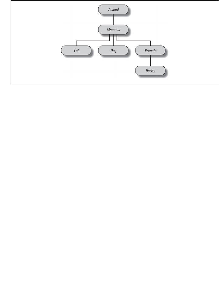
>>> spot = Cat()
>>> spot.reply() # Animal.reply: calls Cat.speak
meow
>>> data = Hacker() # Animal.reply: calls Primate.speak
>>> data.reply()
Hello world!
Figure 32-1. A zoo hierarchy composed of classes linked into a tree to be searched by attribute
inheritance. Animal has a common “reply” method, but each class may have its own custom
“speak” method called by “reply”.
9. The Dead Parrot Sketch. Consider the object embedding structure captured in
Figure 32-2.
Code a set of Python classes to implement this structure with composition. Code
your Scene object to define an action method, and embed instances of the Cus
tomer, Clerk, and Parrot classes (each of which should define a line method that
prints a unique message). The embedded objects may either inherit from a common
superclass that defines line and simply provide message text, or define line them-
selves. In the end, your classes should operate like this:
% python
>>> import parrot
>>> parrot.Scene().action() # Activate nested objects
customer: "that's one ex-bird!"
clerk: "no it isn't..."
parrot: None
1076 | Chapter 32: Advanced Class Topics
www.it-ebooks.info
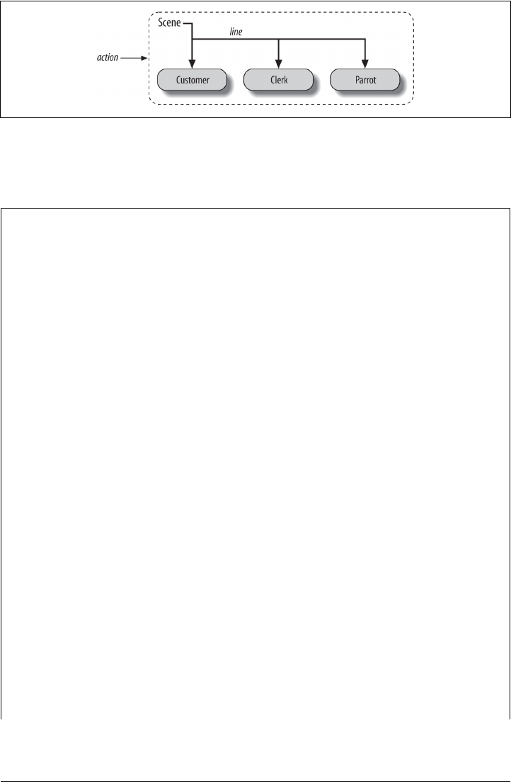
Figure 32-2. A scene composite with a controller class (Scene) that embeds and directs instances of
three other classes (Customer, Clerk, Parrot). The embedded instance’s classes may also participate
in an inheritance hierarchy; composition and inheritance are often equally useful ways to structure
classes for code reuse.
Why You Will Care: OOP by the Masters
When I teach Python classes, I invariably find that about halfway through the class,
people who have used OOP in the past are following along intensely, while people who
have not are beginning to glaze over (or nod off completely). The point behind the
technology just isn’t apparent.
In a book like this, I have the luxury of including material like the new Big Picture
overview in Chapter 26, and the gradual tutorial of Chapter 28—in fact, you should
probably review that section if you’re starting to feel like OOP is just some computer
science mumbo-jumbo. Though it adds much more structure than the generators we
met earlier, OOP similarly relies on some magic (inheritance search and a special first
argument) that beginners can find difficult to rationalize.
In real classes, however, to help get the newcomers on board (and keep them awake),
I have been known to stop and ask the experts in the audience why they use OOP. The
answers they’ve given might help shed some light on the purpose of OOP, if you’re new
to the subject.
Here, then, with only a few embellishments, are the most common reasons to use OOP,
as cited by my students over the years:
Code reuse
This one’s easy (and is the main reason for using OOP). By supporting inheritance,
classes allow you to program by customization instead of starting each project from
scratch.
Encapsulation
Wrapping up implementation details behind object interfaces insulates users of a
class from code changes.
Structure
Classes provide new local scopes, which minimizes name clashes. They also pro-
vide a natural place to write and look for implementation code, and to manage
object state.
Test Your Knowledge: Part VI Exercises | 1077
www.it-ebooks.info

Maintenance
Classes naturally promote code factoring, which allows us to minimize redun-
dancy. Thanks both to the structure and code reuse support of classes, usually only
one copy of the code needs to be changed.
Consistency
Classes and inheritance allow you to implement common interfaces, and hence
create a common look and feel in your code; this eases debugging, comprehension,
and maintenance.
Polymorphism
This is more a property of OOP than a reason for using it, but by supporting code
generality, polymorphism makes code more flexible and widely applicable, and
hence more reusable.
Other
And, of course, the number one reason students gave for using OOP: it looks good
on a résumé! (OK, I threw this one in as a joke, but it is important to be familiar
with OOP if you plan to work in the software field today.)
Finally, keep in mind what I said at the beginning of this part of the book: you won’t
fully appreciate OOP until you’ve used it for a while. Pick a project, study larger ex-
amples, work through the exercises—do whatever it takes to get your feet wet with OO
code; it’s worth the effort.
1078 | Chapter 32: Advanced Class Topics
www.it-ebooks.info


CHAPTER 33
Exception Basics
This part of the book deals with exceptions, which are events that can modify the flow
of control through a program. In Python, exceptions are triggered automatically on
errors, and they can be triggered and intercepted by your code. They are processed by
four statements we’ll study in this part, the first of which has two variations (listed
separately here) and the last of which was an optional extension until Python 2.6 and
3.0:
try/except
Catch and recover from exceptions raised by Python, or by you.
try/finally
Perform cleanup actions, whether exceptions occur or not.
raise
Trigger an exception manually in your code.
assert
Conditionally trigger an exception in your code.
with/as
Implement context managers in Python 2.6, 3.0, and later (optional in 2.5).
This topic was saved until nearly the end of the book because you need to know about
classes to code exceptions of your own. With a few exceptions (pun intended), though,
you’ll find that exception handling is simple in Python because it’s integrated into the
language itself as another high-level tool.
Why Use Exceptions?
In a nutshell, exceptions let us jump out of arbitrarily large chunks of a program. Con-
sider the hypothetical pizza-making robot we discussed earlier in the book. Suppose
we took the idea seriously and actually built such a machine. To make a pizza, our
culinary automaton would need to execute a plan, which we would implement as a
1081
www.it-ebooks.info

Python program: it would take an order, prepare the dough, add toppings, bake the
pie, and so on.
Now, suppose that something goes very wrong during the “bake the pie” step. Perhaps
the oven is broken, or perhaps our robot miscalculates its reach and spontaneously
combusts. Clearly, we want to be able to jump to code that handles such states quickly.
As we have no hope of finishing the pizza task in such unusual cases, we might as well
abandon the entire plan.
That’s exactly what exceptions let you do: you can jump to an exception handler in a
single step, abandoning all function calls begun since the exception handler was en-
tered. Code in the exception handler can then respond to the raised exception as ap-
propriate (by calling the fire department, for instance!).
One way to think of an exception is as a sort of structured “super go to.” An exception
handler (try statement) leaves a marker and executes some code. Somewhere further
ahead in the program, an exception is raised that makes Python jump back to that
marker, abandoning any active functions that were called after the marker was left.
This protocol provides a coherent way to respond to unusual events. Moreover, because
Python jumps to the handler statement immediately, your code is simpler—there is
usually no need to check status codes after every call to a function that could possibly
fail.
Exception Roles
In Python programs, exceptions are typically used for a variety of purposes. Here are
some of their most common roles:
Error handling
Python raises exceptions whenever it detects errors in programs at runtime. You
can catch and respond to the errors in your code, or ignore the exceptions that are
raised. If an error is ignored, Python’s default exception-handling behavior kicks
in: it stops the program and prints an error message. If you don’t want this default
behavior, code a try statement to catch and recover from the exception—Python
will jump to your try handler when the error is detected, and your program will
resume execution after the try.
Event notification
Exceptions can also be used to signal valid conditions without you having to pass
result flags around a program or test them explicitly. For instance, a search routine
might raise an exception on failure, rather than returning an integer result code—
and hoping that the code will never be a valid result!
Special-case handling
Sometimes a condition may occur so rarely that it’s hard to justify convoluting your
code to handle it in multiple places. You can often eliminate special-case code by
handling unusual cases in exception handlers in higher levels of your program. An
1082 | Chapter 33: Exception Basics
www.it-ebooks.info

assert can similarly be used to check that conditions are as expected during de-
velopment.
Termination actions
As you’ll see, the try/finally statement allows you to guarantee that required
closing-time operations will be performed, regardless of the presence or absence
of exceptions in your programs. The newer with statement offers an alternative in
this department for objects that support it.
Unusual control flows
Finally, because exceptions are a sort of high-level and structured “go to,” you can
use them as the basis for implementing exotic control flows. For instance, although
the language does not explicitly support backtracking, you can implement it in
Python by using exceptions and a bit of support logic to unwind assignments.1
There is no “go to” statement in Python (thankfully!), but exceptions can some-
times serve similar roles; a raise, for instance, can be used to jump out of multiple
loops.
We saw some of these roles briefly earlier, and will study typical exception use cases
in action later in this part of the book. For now, let’s get started with a look at Python’s
exception-processing tools.
Exceptions: The Short Story
Compared to some other core language topics we’ve met in this book, exceptions are
a fairly lightweight tool in Python. Because they are so simple, let’s jump right into
some code.
Default Exception Handler
Suppose we write the following function:
>>> def fetcher(obj, index):
return obj[index]
There’s not much to this function—it simply indexes an object on a passed-in index.
In normal operation, it returns the result of a legal index:
>>> x = 'spam'
>>> fetcher(x, 3) # Like x[3]
'm'
1. But true backtracking is not part of the Python language. Backtracking undoes all computations before
it jumps, but Python exceptions do not: variables assigned between the time a try statement is entered
and the time an exception is raised are not reset to their prior values. Even the generator functions and
expressions we met in Chapter 20 don’t do full backtracking—they simply respond to next(G) requests
by restoring state and resuming. For more on backtracking, see books on artificial intelligence or the
Prolog or Icon programming languages.
Exceptions: The Short Story | 1083
www.it-ebooks.info

However, if we ask this function to index off the end of the string, an exception will be
triggered when the function tries to run obj[index]. Python detects out-of-bounds in-
dexing for sequences and reports it by raising (triggering) the built-in IndexError ex-
ception:
>>> fetcher(x, 4) # Default handler - shell interface
Traceback (most recent call last):
File "<stdin>", line 1, in <module>
File "<stdin>", line 2, in fetcher
IndexError: string index out of range
Because our code does not explicitly catch this exception, it filters back up to the top
level of the program and invokes the default exception handler, which simply prints the
standard error message. By this point in the book, you’ve probably seen your share of
standard error messages. They include the exception that was raised, along with a stack
trace—a list of all the lines and functions that were active when the exception occurred.
The error message text here was printed by Python 3.3; it can vary slightly per release,
and even per interactive shell, so you shouldn’t rely upon its exact form—in either this
book or your code. When you’re coding interactively in the basic shell interface, the
filename is just “<stdin>,” meaning the standard input stream.
When working in the IDLE GUI’s interactive shell, the filename is “<pyshell>,” and
source lines are displayed, too. Either way, file line numbers are not very meaningful
when there is no file (we’ll see more interesting error messages later in this part of the
book):
>>> fetcher(x, 4) # Default handler - IDLE GUI interface
Traceback (most recent call last):
File "<pyshell#6>", line 1, in <module>
fetcher(x, 4)
File "<pyshell#3>", line 2, in fetcher
return obj[index]
IndexError: string index out of range
In a more realistic program launched outside the interactive prompt, after printing an
error message the default handler at the top also terminates the program immediately.
That course of action makes sense for simple scripts; errors often should be fatal, and
the best you can do when they occur is inspect the standard error message.
Catching Exceptions
Sometimes, this isn’t what you want, though. Server programs, for instance, typically
need to remain active even after internal errors. If you don’t want the default exception
behavior, wrap the call in a try statement to catch exceptions yourself:
>>> try:
... fetcher(x, 4)
... except IndexError: # Catch and recover
... print('got exception')
...
1084 | Chapter 33: Exception Basics
www.it-ebooks.info

got exception
>>>
Now, Python jumps to your handler—the block under the except clause that names
the exception raised—automatically when an exception is triggered while the try block
is running. The net effect is to wrap a nested block of code in an error handler that
intercepts the block’s exceptions.
When working interactively like this, after the except clause runs, we wind up back at
the Python prompt. In a more realistic program, try statements not only catch excep-
tions, but also recover from them:
>>> def catcher():
try:
fetcher(x, 4)
except IndexError:
print('got exception')
print('continuing')
>>> catcher()
got exception
continuing
>>>
This time, after the exception is caught and handled, the program resumes execution
after the entire try statement that caught it—which is why we get the “continuing”
message here. We don’t see the standard error message, and the program continues on
its way normally.
Notice that there’s no way in Python to go back to the code that triggered the exception
(short of rerunning the code that reached that point all over again, of course). Once
you’ve caught the exception, control continues after the entire try that caught the
exception, not after the statement that kicked it off. In fact, Python clears the memory
of any functions that were exited as a result of the exception, like fetcher in our ex-
ample; they’re not resumable. The try both catches exceptions, and is where the pro-
gram resumes.
Presentation note: The interactive prompt’s “...” reappears in this part
for some top-level try statements, because their code won’t work if cut
and pasted unless nested in a function or class (the except and other
lines must align with the try, and not have extra preceding spaces that
are needed to illustrate their indentation structure). To run, simply type
or paste statements with “...” prompts one line at a time.
Raising Exceptions
So far, we’ve been letting Python raise exceptions for us by making mistakes (on pur-
pose this time!), but our scripts can raise exceptions too—that is, exceptions can be
raised by Python or by your program, and can be caught or not. To trigger an exception
Exceptions: The Short Story | 1085
www.it-ebooks.info

manually, simply run a raise statement. User-triggered exceptions are caught the same
way as those Python raises. The following may not be the most useful Python code ever
penned, but it makes the point—raising the built-in IndexError exception:
>>> try:
... raise IndexError # Trigger exception manually
... except IndexError:
... print('got exception')
...
got exception
As usual, if they’re not caught, user-triggered exceptions are propagated up to the top-
level default exception handler and terminate the program with a standard error mes-
sage:
>>> raise IndexError
Traceback (most recent call last):
File "<stdin>", line 1, in <module>
IndexError
As we’ll see in the next chapter, the assert statement can be used to trigger exceptions,
too—it’s a conditional raise, used mostly for debugging purposes during development:
>>> assert False, 'Nobody expects the Spanish Inquisition!'
Traceback (most recent call last):
File "<stdin>", line 1, in <module>
AssertionError: Nobody expects the Spanish Inquisition!
User-Defined Exceptions
The raise statement introduced in the prior section raises a built-in exception defined
in Python’s built-in scope. As you’ll learn later in this part of the book, you can also
define new exceptions of your own that are specific to your programs. User-defined
exceptions are coded with classes, which inherit from a built-in exception class: usually
the class named Exception:
>>> class AlreadyGotOne(Exception): pass # User-defined exception
>>> def grail():
raise AlreadyGotOne() # Raise an instance
>>> try:
... grail()
... except AlreadyGotOne: # Catch class name
... print('got exception')
...
got exception
>>>
As we’ll see in the next chapter, an as clause on an except can gain access to the ex-
ception object itself. Class-based exceptions allow scripts to build exception categories,
which can inherit behavior, and have attached state information and methods. They
can also customize their error message text displayed if they’re not caught:
1086 | Chapter 33: Exception Basics
www.it-ebooks.info

>>> class Career(Exception):
def __str__(self): return 'So I became a waiter...'
>>> raise Career()
Traceback (most recent call last):
File "<stdin>", line 1, in <module>
__main__.Career: So I became a waiter...
>>>
Termination Actions
Finally, try statements can say “finally”—that is, they may include finally blocks.
These look like except handlers for exceptions, but the try/finally combination speci-
fies termination actions that always execute “on the way out,” regardless of whether
an exception occurs in the try block or not;
>>> try:
... fetcher(x, 3)
... finally: # Termination actions
... print('after fetch')
...
'm'
after fetch
>>>
Here, if the try block finishes without an exception, the finally block will run, and
the program will resume after the entire try. In this case, this statement seems a bit silly
—we might as well have simply typed the print right after a call to the function, and
skipped the try altogether:
fetcher(x, 3)
print('after fetch')
There is a problem with coding this way, though: if the function call raises an exception,
the print will never be reached. The try/finally combination avoids this pitfall—when
an exception does occur in a try block, finally blocks are executed while the program
is being unwound:
>>> def after():
try:
fetcher(x, 4)
finally:
print('after fetch')
print('after try?')
>>> after()
after fetch
Traceback (most recent call last):
File "<stdin>", line 1, in <module>
File "<stdin>", line 3, in after
File "<stdin>", line 2, in fetcher
IndexError: string index out of range
>>>
Exceptions: The Short Story | 1087
www.it-ebooks.info
Here, we don’t get the “after try?” message because control does not resume after the
try/finally block when an exception occurs. Instead, Python jumps back to run the
finally action, and then propagates the exception up to a prior handler (in this case,
to the default handler at the top). If we change the call inside this function so as not to
trigger an exception, the finally code still runs, but the program continues after the try:
>>> def after():
try:
fetcher(x, 3)
finally:
print('after fetch')
print('after try?')
>>> after()
after fetch
after try?
>>>
In practice, try/except combinations are useful for catching and recovering from ex-
ceptions, and try/finally combinations come in handy to guarantee that termination
actions will fire regardless of any exceptions that may occur in the try block’s code.
For instance, you might use try/except to catch errors raised by code that you import
from a third-party library, and try/finally to ensure that calls to close files or terminate
server connections are always run. We’ll see some such practical examples later in this
part of the book.
Although they serve conceptually distinct purposes, as of Python 2.5, we can mix
except and finally clauses in the same try statement—the finally is run on the way
out regardless of whether an exception was raised, and regardless of whether the ex-
ception was caught by an except clause.
As we’ll learn in the next chapter, Python 2.X and 3.X both provide an alternative to
try/finally when using some types of objects. The with/as statement runs an object’s
context management logic to guarantee that termination actions occur, irrespective of
any exceptions in its nested block:
>>> with open('lumberjack.txt', 'w') as file: # Always close file on exit
file.write('The larch!\n')
Although this option requires fewer lines of code, it’s applicable only when processing
certain object types, so try/finally is a more general termination structure, and is often
simpler than coding a class in cases where with is not already supported. On the other
hand, with/as may also run startup actions too, and supports user-defined context
management code with access to Python’s full OOP toolset.
Why You Will Care: Error Checks
One way to see how exceptions are useful is to compare coding styles in Python and
languages without exceptions. For instance, if you want to write robust programs in
the C language, you generally have to test return values or status codes after every
1088 | Chapter 33: Exception Basics
www.it-ebooks.info

operation that could possibly go astray, and propagate the results of the tests as your
programs run:
doStuff()
{ # C program
if (doFirstThing() == ERROR) # Detect errors everywhere
return ERROR; # even if not handled here
if (doNextThing() == ERROR)
return ERROR;
...
return doLastThing();
}
main()
{
if (doStuff() == ERROR)
badEnding();
else
goodEnding();
}
In fact, realistic C programs often have as much code devoted to error detection as to
doing actual work. But in Python, you don’t have to be so methodical (and neurotic!).
You can instead wrap arbitrarily vast pieces of a program in exception handlers and
simply write the parts that do the actual work, assuming all is normally well:
def doStuff(): # Python code
doFirstThing() # We don't care about exceptions here,
doNextThing() # so we don't need to detect them
...
doLastThing()
if __name__ == '__main__':
try:
doStuff() # This is where we care about results,
except: # so it's the only place we must check
badEnding()
else:
goodEnding()
Because control jumps immediately to a handler when an exception occurs, there’s no
need to instrument all your code to guard for errors, and there’s no extra performance
overhead to run all the tests. Moreover, because Python detects errors automatically,
your code often doesn’t need to check for errors in the first place. The upshot is that
exceptions let you largely ignore the unusual cases and avoid error-checking code that
can distract from your program’s goals.
Chapter Summary
And that is the majority of the exception story; exceptions really are a simple tool.
To summarize, Python exceptions are a high-level control flow device. They may be
raised by Python, or by your own programs. In both cases, they may be ignored (to
trigger the default error message), or caught by try statements (to be processed by your
Chapter Summary | 1089
www.it-ebooks.info

code). The try statement comes in two logical formats that, as of Python 2.5, can be
combined—one that handles exceptions, and one that executes finalization code re-
gardless of whether exceptions occur or not. Python’s raise and assert statements
trigger exceptions on demand—both built-ins and new exceptions we define with
classes—and the with/as statement is an alternative way to ensure that termination
actions are carried out for objects that support it.
In the rest of this part of the book, we’ll fill in some of the details about the statements
involved, examine the other sorts of clauses that can appear under a try, and discuss
class-based exception objects. The next chapter begins our tour by taking a closer look
at the statements we introduced here. Before you turn the page, though, here are a few
quiz questions to review.
Test Your Knowledge: Quiz
1. Name three things that exception processing is good for.
2. What happens to an exception if you don’t do anything special to handle it?
3. How can your script recover from an exception?
4. Name two ways to trigger exceptions in your script.
5. Name two ways to specify actions to be run at termination time, whether an ex-
ception occurs or not.
Test Your Knowledge: Answers
1. Exception processing is useful for error handling, termination actions, and event
notification. It can also simplify the handling of special cases and can be used to
implement alternative control flows as a sort of structured “go to” operation. In
general, exception processing also cuts down on the amount of error-checking code
your program may require—because all errors filter up to handlers, you may not
need to test the outcome of every operation.
2. Any uncaught exception eventually filters up to the default exception handler
Python provides at the top of your program. This handler prints the familiar error
message and shuts down your program.
3. If you don’t want the default message and shutdown, you can code try/except
statements to catch and recover from exceptions that are raised within its nested
code block. Once an exception is caught, the exception is terminated and your
program continues after the try.
4. The raise and assert statements can be used to trigger an exception, exactly as if
it had been raised by Python itself. In principle, you can also raise an exception by
making a programming mistake, but that’s not usually an explicit goal!
1090 | Chapter 33: Exception Basics
www.it-ebooks.info

5. The try/finally statement can be used to ensure actions are run after a block of
code exits, regardless of whether the block raises an exception or not. The with/
as statement can also be used to ensure termination actions are run, but only when
processing object types that support it.
Test Your Knowledge: Answers | 1091
www.it-ebooks.info
CHAPTER 34
Exception Coding Details
In the prior chapter we took a quick look at exception-related statements in action.
Here, we’re going to dig a bit deeper—this chapter provides a more formal introduction
to exception processing syntax in Python. Specifically, we’ll explore the details behind
the try, raise, assert, and with statements. As we’ll see, although these statements are
mostly straightforward, they offer powerful tools for dealing with exceptional condi-
tions in Python code.
One procedural note up front: The exception story has changed in major
ways in recent years. As of Python 2.5, the finally clause can appear in
the same try statement as except and else clauses (previously, they
could not be combined). Also, as of Python 3.0 and 2.6, the new with
context manager statement has become official, and user-defined ex-
ceptions must now be coded as class instances, which should inherit
from a built-in exception superclass. Moreover, 3.X sports slightly
modified syntax for the raise statement and except clauses, some of
which is available in 2.6 and 2.7.
I will focus on the state of exceptions in recent Python 2.X and 3.X
releases in this edition, but because you are still very likely to see the
original techniques in code for some time to come, along the way I’ll
point out how things have evolved in this domain.
The try/except/else Statement
Now that we’ve seen the basics, it’s time for the details. In the following discussion,
I’ll first present try/except/else and try/finally as separate statements, because in
versions of Python prior to 2.5 they serve distinct roles and cannot be combined, and
still are at least logically distinct today. Per the preceding note, in Python 2.5 and later
except and finally can be mixed in a single try statement; we’ll see the implications
of that merging after we’ve explored the two original forms in isolation.
1093
www.it-ebooks.info

Syntactically, the try is a compound, multipart statement. It starts with a try header
line, followed by a block of (usually) indented statements; then one or more except
clauses that identify exceptions to be caught and blocks to process them; and an op-
tional else clause and block at the end. You associate the words try, except, and
else by indenting them to the same level (i.e., lining them up vertically). For reference,
here’s the general and most complete format in Python 3.X:
try:
statements # Run this main action first
except name1:
statements # Run if name1 is raised during try block
except (name2, name3):
statements # Run if any of these exceptions occur
except name4 as var:
statements # Run if name4 is raised, assign instance raised to var
except:
statements # Run for all other exceptions raised
else:
statements # Run if no exception was raised during try block
Semantically, the block under the try header in this statement represents the main
action of the statement—the code you’re trying to run and wrap in error processing
logic. The except clauses define handlers for exceptions raised during the try block,
and the else clause (if coded) provides a handler to be run if no exceptions occur. The
var entry here has to do with a feature of raise statements and exception classes, which
we will discuss in full later in this chapter.
How try Statements Work
Operationally, here’s how try statements are run. When a try statement is entered,
Python marks the current program context so it can return to it if an exception occurs.
The statements nested under the try header are run first. What happens next depends
on whether exceptions are raised while the try block’s statements are running, and
whether they match those that the try is watching for:
• If an exception occurs while the try block’s statements are running, and the ex-
ception matches one that the statement names, Python jumps back to the try and
runs the statements under the first except clause that matches the raised exception,
after assigning the raised exception object to the variable named after the as key-
word in the clause (if present). After the except block runs, control then resumes
below the entire try statement (unless the except block itself raises another ex-
ception, in which case the process is started anew from this point in the code).
• If an exception occurs while the try block’s statements are running, but the ex-
ception does not match one that the statement names, the exception is propagated
up to the next most recently entered try statement that matches the exception; if
no such matching try statement can be found and the search reaches the top level
of the process, Python kills the program and prints a default error message.
1094 | Chapter 34: Exception Coding Details
www.it-ebooks.info

• If an exception does not occur while the try block’s statements are running, Python
runs the statements under the else line (if present), and control then resumes below
the entire try statement.
In other words, except clauses catch any matching exceptions that happen while the
try block is running, and the else clause runs only if no exceptions happen while the
try block runs. Exceptions raised are matched to exceptions named in except clauses
by superclass relationships we’ll explore in the next chapter, and the empty except clause
(with no exception name) matches all (or all other) exceptions.
The except clauses are focused exception handlers—they catch exceptions that occur
only within the statements in the associated try block. However, as the try block’s
statements can call functions coded elsewhere in a program, the source of an exception
may be outside the try statement itself.
In fact, a try block might invoke arbitrarily large amounts of program code—including
code that may have try statements of its own, which will be searched first when ex-
ceptions occur. That is, try statements can nest at runtime, a topic I’ll have more to say
about in Chapter 36.
try Statement Clauses
When you write a try statement, a variety of clauses can appear after the try header.
Table 34-1 summarizes all the possible forms—you must use at least one. We’ve already
met some of these: as you know, except clauses catch exceptions, finally clauses run
on the way out, and else clauses run if no exceptions are encountered.
Formally, there may be any number of except clauses, but you can code else only if
there is at least one except, and there can be only one else and one finally. Through
Python 2.4, the finally clause must appear alone (without else or except); the try/
finally is really a different statement. As of Python 2.5, however, a finally can appear
in the same statement as except and else (more on the ordering rules later in this chapter
when we meet the unified try statement).
Table 34-1. try statement clause forms
Clause form Interpretation
except: Catch all (or all other) exception types.
except name:Catch a specific exception only.
except name as value:Catch the listed exception and assign its instance.
except (name1, name2): Catch any of the listed exceptions.
except (name1, name2) as value:Catch any listed exception and assign its instance.
else: Run if no exceptions are raised in the try block.
finally: Always perform this block on exit.
The try/except/else Statement | 1095
www.it-ebooks.info

We’ll explore the entries with the extra as value part in more detail when we meet the
raise statement later in this chapter. They provide access to the objects that are raised
as exceptions.
Catching any and all exceptions
The first and fourth entries in Table 34-1 are new here:
•except clauses that list no exception name (except:) catch all exceptions not pre-
viously listed in the try statement.
•except clauses that list a set of exceptions in parentheses (except (e1, e2, e3):)
catch any of the listed exceptions.
Because Python looks for a match within a given try by inspecting the except clauses
from top to bottom, the parenthesized version has the same effect as listing each ex-
ception in its own except clause, but you have to code the statement body associated
with each only once. Here’s an example of multiple except clauses at work, which
demonstrates just how specific your handlers can be:
try:
action()
except NameError:
...
except IndexError:
...
except KeyError:
...
except (AttributeError, TypeError, SyntaxError):
...
else:
...
In this example, if an exception is raised while the call to the action function is running,
Python returns to the try and searches for the first except that names the exception
raised. It inspects the except clauses from top to bottom and left to right, and runs the
statements under the first one that matches. If none match, the exception is propagated
past this try. Note that the else runs only when no exception occurs in action—it does
not run when an exception without a matching except is raised.
Catching all: The empty except and Exception
If you really want a general “catchall” clause, an empty except does the trick:
try:
action()
except NameError:
... # Handle NameError
except IndexError:
... # Handle IndexError
except:
... # Handle all other exceptions
1096 | Chapter 34: Exception Coding Details
www.it-ebooks.info

else:
... # Handle the no-exception case
The empty except clause is a sort of wildcard feature—because it catches everything, it
allows your handlers to be as general or specific as you like. In some scenarios, this
form may be more convenient than listing all possible exceptions in a try. For example,
the following catches everything without listing anything:
try:
action()
except:
... # Catch all possible exceptions
Empty excepts also raise some design issues, though. Although convenient, they may
catch unexpected system exceptions unrelated to your code, and they may inadver-
tently intercept exceptions meant for another handler. For example, even system exit
calls and Ctrl-C key combinations in Python trigger exceptions, and you usually want
these to pass. Even worse, the empty except may also catch genuine programming
mistakes for which you probably want to see an error message. We’ll revisit this as a
gotcha at the end of this part of the book. For now, I’ll just say, “use with care.”
Python 3.X more strongly supports an alternative that solves one of these problems—
catching an exception named Exception has almost the same effect as an empty
except, but ignores exceptions related to system exits:
try:
action()
except Exception:
... # Catch all possible exceptions, except exits
We’ll explore how this form works its voodoo formally in the next chapter when we
study exception classes. In short, it works because exceptions match if they are a sub-
class of one named in an except clause, and Exception is a superclass of all the exceptions
you should generally catch this way. This form has most of the same convenience of
the empty except, without the risk of catching exit events. Though better, it also has
some of the same dangers—especially with regard to masking programming errors.
Version skew note: See also the raise statement ahead for more on the
as portion of except clauses in try. Syntactically, Python 3.X requires
the except E as V: handler clause form listed in Table 34-1 and used in
this book, rather than the older except E, V: form. The latter form is
still available (but not recommended) in Python 2.6 and 2.7: if used, it’s
converted to the former.
The change was made to eliminate confusion regarding the dual role of
commas in the older form. In this form, two alternate exceptions are
properly coded as except (E1, E2):. Because 3.X supports the as form
only, commas in a handler clause are always taken to mean a tuple,
regardless of whether parentheses are used or not, and the values are
interpreted as alternative exceptions to be caught.
The try/except/else Statement | 1097
www.it-ebooks.info

As we’ll see ahead, though, this option does not modify the scoping
rules in 2.X: even with the new as syntax, the variable V is still available
after the except block in 2.X. In 3.X, V is not available later, and is in
fact forcibly deleted.
The try else Clause
The purpose of the else clause is not always immediately obvious to Python newcom-
ers. Without it, though, there is no direct way to tell (without setting and checking
Boolean flags) whether the flow of control has proceeded past a try statement because
no exception was raised, or because an exception occurred and was handled. Either
way, we wind up after the try:
try:
...run code...
except IndexError:
...handle exception...
# Did we get here because the try failed or not?
Much like the way else clauses in loops make the exit cause more apparent, the else
clause provides syntax in a try that makes what has happened obvious and unambig-
uous:
try:
...run code...
except IndexError:
...handle exception...
else:
...no exception occurred...
You can almost emulate an else clause by moving its code into the try block:
try:
...run code...
...no exception occurred...
except IndexError:
...handle exception...
This can lead to incorrect exception classifications, though. If the “no exception oc-
curred” action triggers an IndexError, it will register as a failure of the try block and
erroneously trigger the exception handler below the try (subtle, but true!). By using an
explicit else clause instead, you make the logic more obvious and guarantee that
except handlers will run only for real failures in the code you’re wrapping in a try, not
for failures in the else no-exception case’s action.
Example: Default Behavior
Because the control flow through a program is easier to capture in Python than in
English, let’s run some examples that further illustrate exception basics in the context
of larger code samples in files.
1098 | Chapter 34: Exception Coding Details
www.it-ebooks.info

I’ve mentioned that exceptions not caught by try statements percolate up to the top
level of the Python process and run Python’s default exception-handling logic (i.e.,
Python terminates the running program and prints a standard error message). To il-
lustrate, running the following module file, bad.py, generates a divide-by-zero excep-
tion:
def gobad(x, y):
return x / y
def gosouth(x):
print(gobad(x, 0))
gosouth(1)
Because the program ignores the exception it triggers, Python kills the program and
prints a message:
% python bad.py
Traceback (most recent call last):
File "bad.py", line 7, in <module>
gosouth(1)
File "bad.py", line 5, in gosouth
print(gobad(x, 0))
File "bad.py", line 2, in gobad
return x / y
ZeroDivisionError: division by zero
I ran this in a shell window with Python 3.X. The message consists of a stack trace
(“Traceback”) and the name of and details about the exception that was raised. The
stack trace lists all lines active when the exception occurred, from oldest to newest.
Note that because we’re not working at the interactive prompt, in this case the file and
line number information is more useful. For example, here we can see that the bad
divide happens at the last entry in the trace—line 2 of the file bad.py, a return state-
ment.1
Because Python detects and reports all errors at runtime by raising exceptions, excep-
tions are intimately bound up with the ideas of error handling and debugging in general.
If you’ve worked through this book’s examples, you’ve undoubtedly seen an exception
or two along the way—even typos usually generate a SyntaxError or other exception
when a file is imported or executed (that’s when the compiler is run). By default, you
get a useful error display like the one just shown, which helps you track down the
problem.
Often, this standard error message is all you need to resolve problems in your code.
For more heavy-duty debugging jobs, you can catch exceptions with try statements,
1. As mentioned in the prior chapter, the text of error messages and stack traces tends to vary slightly over
time and shells. Don’t be alarmed if your error messages don’t exactly match mine. When I ran this
example in Python 3.3’s IDLE GUI, for instance, its error message text showed filenames with full absolute
directory paths.
The try/except/else Statement | 1099
www.it-ebooks.info

or use one of the debugging tools that I introduced in Chapter 3 and will summarize
again in Chapter 36, such as the pdb standard library module.
Example: Catching Built-in Exceptions
Python’s default exception handling is often exactly what you want—especially for
code in a top-level script file, an error often should terminate your program immedi-
ately. For many programs, there is no need to be more specific about errors in your code.
Sometimes, though, you’ll want to catch errors and recover from them instead. If you
don’t want your program terminated when Python raises an exception, simply catch it
by wrapping the program logic in a try. This is an important capability for programs
such as network servers, which must keep running persistently. For example, the fol-
lowing code, in the file kaboom.py, catches and recovers from the TypeError Python
raises immediately when you try to concatenate a list and a string (remember, the +
operator expects the same sequence type on both sides):
def kaboom(x, y):
print(x + y) # Trigger TypeError
try:
kaboom([0, 1, 2], 'spam')
except TypeError: # Catch and recover here
print('Hello world!')
print('resuming here') # Continue here if exception or not
When the exception occurs in the function kaboom, control jumps to the try statement’s
except clause, which prints a message. Since an exception is “dead” after it’s been
caught like this, the program continues executing below the try rather than being ter-
minated by Python. In effect, the code processes and clears the error, and your script
recovers:
% python kaboom.py
Hello world!
resuming here
Keep in mind that once you’ve caught an error, control resumes at the place where you
caught it (i.e., after the try); there is no direct way to go back to the place where the
exception occurred (here, in the function kaboom). In a sense, this makes exceptions
more like simple jumps than function calls—there is no way to return to the code that
triggered the error.
The try/finally Statement
The other flavor of the try statement is a specialization that has to do with finalization
(a.k.a. termination) actions. If a finally clause is included in a try, Python will always
run its block of statements “on the way out” of the try statement, whether an exception
occurred while the try block was running or not. Its general form is:
1100 | Chapter 34: Exception Coding Details
www.it-ebooks.info

try:
statements # Run this action first
finally:
statements # Always run this code on the way out
With this variant, Python begins by running the statement block associated with the
try header line as usual. What happens next depends on whether an exception occurs
during the try block:
• If an exception does not occur while the try block is running, Python continues on
to run the finally block, and then continues execution past the try statement.
• If an exception does occur during the try block’s run, Python still comes back and
runs the finally block, but it then propagates the exception up to a previously
entered try or the top-level default handler; the program does not resume execution
below the finally clause’s try statement. That is, the finally block is run even if
an exception is raised, but unlike an except, the finally does not terminate the
exception—it continues being raised after the finally block runs.
The try/finally form is useful when you want to be completely sure that an action will
happen after some code runs, regardless of the exception behavior of the program. In
practice, it allows you to specify cleanup actions that always must occur, such as file
closes and server disconnects where required.
Note that the finally clause cannot be used in the same try statement as except and
else in Python 2.4 and earlier, so the try/finally is best thought of as a distinct state-
ment form if you are using an older release. In Python 2.5, and later, however,
finally can appear in the same statement as except and else, so today there is really a
single try statement with many optional clauses (more about this shortly). Whichever
version you use, though, the finally clause still serves the same purpose—to specify
“cleanup” actions that must always be run, regardless of any exceptions.
As we’ll also see later in this chapter, as of Python 2.6 and 3.0, the new
with statement and its context managers provide an object-based way
to do similar work for exit actions. Unlike finally, this new statement
also supports entry actions, but it is limited in scope to objects that
implement the context manager protocol it leverages.
Example: Coding Termination Actions with try/finally
We saw some simple try/finally examples in the prior chapter. Here’s a more realistic
example that illustrates a typical role for this statement:
class MyError(Exception): pass
def stuff(file):
raise MyError()
file = open('data', 'w') # Open an output file (this can fail too)
The try/finally Statement | 1101
www.it-ebooks.info

try:
stuff(file) # Raises exception
finally:
file.close() # Always close file to flush output buffers
print('not reached') # Continue here only if no exception
When the function in this code raises its exception, the control flow jumps back and
runs the finally block to close the file. The exception is then propagated on to either
another try or the default top-level handler, which prints the standard error message
and shuts down the program. Hence, the statement after this try is never reached. If
the function here did not raise an exception, the program would still execute the
finally block to close the file, but it would then continue below the entire try state-
ment.
In this specific case, we’ve wrapped a call to a file-processing function in a try with a
finally clause to make sure that the file is always closed, and thus finalized, whether
the function triggers an exception or not. This way, later code can be sure that the file’s
output buffer’s content has been flushed from memory to disk. A similar code structure
can guarantee that server connections are closed, and so on.
As we learned in Chapter 9, file objects are automatically closed on garbage collection
in standard Python (CPython); this is especially useful for temporary files that we don’t
assign to variables. However, it’s not always easy to predict when garbage collection
will occur, especially in larger programs or alternative Python implementations with
differing garbage collection policies (e.g., Jython, PyPy). The try statement makes file
closes more explicit and predictable and pertains to a specific block of code. It ensures
that the file will be closed on block exit, regardless of whether an exception occurs or
not.
This particular example’s function isn’t all that useful (it just raises an exception), but
wrapping calls in try/finally statements is a good way to ensure that your closing-time
termination activities always run. Again, Python always runs the code in your
finally blocks, regardless of whether an exception happens in the try block.2
Notice how the user-defined exception here is again defined with a class—as we’ll see
more formally in the next chapter, exceptions today must all be class instances in 2.6,
3.0, and later releases in both lines.
Unified try/except/finally
In all versions of Python prior to release 2.5 (for its first 15 years of life, more or less),
the try statement came in two flavors and was really two separate statements—we
could either use a finally to ensure that cleanup code was always run, or write
2. Unless Python crashes completely, of course. It does a good job of avoiding this, though, by checking all
possible errors as a program runs. When a program does crash hard, it is usually due to a bug in linked-
in C extension code, outside of Python’s scope.
1102 | Chapter 34: Exception Coding Details
www.it-ebooks.info

except blocks to catch and recover from specific exceptions and optionally specify an
else clause to be run if no exceptions occurred.
That is, the finally clause could not be mixed with except and else. This was partly
because of implementation issues, and partly because the meaning of mixing the two
seemed obscure—catching and recovering from exceptions seemed a disjoint concept
from performing cleanup actions.
In Python 2.5 and later, though, the two statements have merged. Today, we can mix
finally, except, and else clauses in the same statement—in part because of similar
utility in the Java language. That is, we can now write a statement of this form:
try: # Merged form
main-action
except Exception1:
handler1
except Exception2: # Catch exceptions
handler2
...
else: # No-exception handler
else-block
finally: # The finally encloses all else
finally-block
The code in this statement’s main-action block is executed first, as usual. If that code
raises an exception, all the except blocks are tested, one after another, looking for a
match to the exception raised. If the exception raised is Exception1, the handler1 block
is executed; if it’s Exception2, handler2 is run, and so on. If no exception is raised, the
else-block is executed.
No matter what’s happened previously, the finally-block is executed once the main
action block is complete and any raised exceptions have been handled. In fact, the code
in the finally-block will be run even if there is an error in an exception handler or the
else-block and a new exception is raised.
As always, the finally clause does not end the exception—if an exception is active
when the finally-block is executed, it continues to be propagated after the finally-
block runs, and control jumps somewhere else in the program (to another try, or to
the default top-level handler). If no exception is active when the finally is run, control
resumes after the entire try statement.
The net effect is that the finally is always run, regardless of whether:
• An exception occurred in the main action and was handled.
• An exception occurred in the main action and was not handled.
• No exceptions occurred in the main action.
• A new exception was triggered in one of the handlers.
Again, the finally serves to specify cleanup actions that must always occur on the way
out of the try, regardless of what exceptions have been raised or handled.
Unified try/except/finally | 1103
www.it-ebooks.info

Unified try Statement Syntax
When combined like this, the try statement must have either an except or a finally,
and the order of its parts must be like this:
try -> except -> else -> finally
where the else and finally are optional, and there may be zero or more excepts, but
there must be at least one except if an else appears. Really, the try statement consists
of two parts: excepts with an optional else, and/or the finally.
In fact, it’s more accurate to describe the merged statement’s syntactic form this way
(square brackets mean optional and star means zero-or-more here):
try: # Format 1
statements
except [type [as value]]: # [type [, value]] in Python 2.X
statements
[except [type [as value]]:
statements]*
[else:
statements]
[finally:
statements]
try: # Format 2
statements
finally:
statements
Because of these rules, the else can appear only if there is at least one except, and it’s
always possible to mix except and finally, regardless of whether an else appears or
not. It’s also possible to mix finally and else, but only if an except appears too (though
the except can omit an exception name to catch everything and run a raise statement,
described later, to reraise the current exception). If you violate any of these ordering
rules, Python will raise a syntax error exception before your code runs.
Combining finally and except by Nesting
Prior to Python 2.5, it is actually possible to combine finally and except clauses in a
try by syntactically nesting a try/except in the try block of a try/finally statement.
We’ll explore this technique more fully in Chapter 36, but the basics may help clarify
the meaning of a combined try—the following has the same effect as the new merged
form shown at the start of this section:
try: # Nested equivalent to merged form
try:
main-action
except Exception1:
handler1
except Exception2:
handler2
1104 | Chapter 34: Exception Coding Details
www.it-ebooks.info

...
else:
no-error
finally:
cleanup
Again, the finally block is always run on the way out, regardless of what happened in
the main action and regardless of any exception handlers run in the nested try (trace
through the four cases listed previously to see how this works the same). Since an
else always requires an except, this nested form even sports the same mixing con-
straints of the unified statement form outlined in the preceding section.
However, this nested equivalent seems more obscure to some, and requires more code
than the new merged form—though just one four-character line plus extra indentation.
Mixing finally into the same statement makes your code arguably easier to write and
read, and is a generally preferred technique today.
Unified try Example
Here’s a demonstration of the merged try statement form at work. The following file,
mergedexc.py, codes four common scenarios, with print statements that describe the
meaning of each:
# File mergedexc.py (Python 3.X + 2.X)
sep = '-' * 45 + '\n'
print(sep + 'EXCEPTION RAISED AND CAUGHT')
try:
x = 'spam'[99]
except IndexError:
print('except run')
finally:
print('finally run')
print('after run')
print(sep + 'NO EXCEPTION RAISED')
try:
x = 'spam'[3]
except IndexError:
print('except run')
finally:
print('finally run')
print('after run')
print(sep + 'NO EXCEPTION RAISED, WITH ELSE')
try:
x = 'spam'[3]
except IndexError:
print('except run')
else:
Unified try/except/finally | 1105
www.it-ebooks.info

print('else run')
finally:
print('finally run')
print('after run')
print(sep + 'EXCEPTION RAISED BUT NOT CAUGHT')
try:
x = 1 / 0
except IndexError:
print('except run')
finally:
print('finally run')
print('after run')
When this code is run, the following output is produced in Python 3.3; in 2.X, its
behavior and output are the same because the print calls each print a single item,
though the error message text varies slightly. Trace through the code to see how ex-
ception handling produces the output of each of the four tests here:
c:\code> py −3 mergedexc.py
---------------------------------------------
EXCEPTION RAISED AND CAUGHT
except run
finally run
after run
---------------------------------------------
NO EXCEPTION RAISED
finally run
after run
---------------------------------------------
NO EXCEPTION RAISED, WITH ELSE
else run
finally run
after run
---------------------------------------------
EXCEPTION RAISED BUT NOT CAUGHT
finally run
Traceback (most recent call last):
File "mergedexc.py", line 39, in <module>
x = 1 / 0
ZeroDivisionError: division by zero
This example uses built-in operations in the main action to trigger exceptions (or not),
and it relies on the fact that Python always checks for errors as code is running. The
next section shows how to raise exceptions manually instead.
The raise Statement
To trigger exceptions explicitly, you can code raise statements. Their general form is
simple—a raise statement consists of the word raise, optionally followed by the class
to be raised or an instance of it:
1106 | Chapter 34: Exception Coding Details
www.it-ebooks.info

raise instance # Raise instance of class
raise class # Make and raise instance of class: makes an instance
raise # Reraise the most recent exception
As mentioned earlier, exceptions are always instances of classes in Python 2.6, 3.0, and
later. Hence, the first raise form here is the most common—we provide an instance
directly, either created before the raise or within the raise statement itself. If we pass
a class instead, Python calls the class with no constructor arguments, to create an in-
stance to be raised; this form is equivalent to adding parentheses after the class refer-
ence. The last form reraises the most recently raised exception; it’s commonly used
in exception handlers to propagate exceptions that have been caught.
Version skew note: Python 3.X no longer supports the raise Exc, Args
form that is still available in Python 2.X. In 3.X, use the raise
Exc(Args) instance-creation call form described in this book instead.
The equivalent comma form in 2.X is legacy syntax provided for com-
patibility with the now-defunct string-based exceptions model, and it’s
deprecated in 2.X. If used, it is converted to the 3.X call form.
As in earlier releases, a raise Exc form is also allowed to name a class—
it is converted to raise Exc() in both versions, calling the class con-
structor with no arguments. Besides its defunct comma syntax, Python
2.X’s raise also allowed for either string or class exceptions, but the
former is removed in 2.6, deprecated in 2.5, and not covered here except
for a brief mention in the next chapter. Use classes for new exceptions
today.
Raising Exceptions
To make this clearer, let’s look at some examples. With built-in exceptions, the fol-
lowing two forms are equivalent—both raise an instance of the exception class named,
but the first creates the instance implicitly:
raise IndexError # Class (instance created)
raise IndexError() # Instance (created in statement)
We can also create the instance ahead of time—because the raise statement accepts
any kind of object reference, the following two examples raise IndexError just like the
prior two:
exc = IndexError() # Create instance ahead of time
raise exc
excs = [IndexError, TypeError]
raise excs[0]
When an exception is raised, Python sends the raised instance along with the exception.
If a try includes an except name as X: clause, the variable X will be assigned the instance
provided in the raise:
The raise Statement | 1107
www.it-ebooks.info

try:
...
except IndexError as X: # X assigned the raised instance object
...
The as is optional in a try handler (if it’s omitted, the instance is simply not assigned
to a name), but including it allows the handler to access both data in the instance and
methods in the exception class.
This model works the same for user-defined exceptions we code with classes—the
following, for example, passes to the exception class constructor arguments that be-
come available in the handler through the assigned instance:
class MyExc(Exception): pass
...
raise MyExc('spam') # Exception class with constructor args
...
try:
...
except MyExc as X: # Instance attributes available in handler
print(X.args)
Because this encroaches on the next chapter’s topic, though, I’ll defer further details
until then.
Regardless of how you name them, exceptions are always identified by class instance
objects, and at most one is active at any given time. Once caught by an except clause
anywhere in the program, an exception dies (i.e., won’t propagate to another try),
unless it’s reraised by another raise statement or error.
Scopes and try except Variables
We’ll study exception objects in more detail in the next chapter. Now that we’ve seen
the as variable in action, though, we can finally clarify the related version-specific scope
issue summarized in Chapter 17. In Python 2.X, the exception reference variable name
in an except clause is not localized to the clause itself, and is available after the associated
block runs:
c:\code> py −2
>>> try:
... 1 / 0
... except Exception as X: # 2.X does not localize X either way
... print X
...
integer division or modulo by zero
>>> X
ZeroDivisionError('integer division or modulo by zero',)
This is true in 2.X whether we use the 3.X-style as or the earlier comma syntax:
>>> try:
... 1 / 0
... except Exception, X:
1108 | Chapter 34: Exception Coding Details
www.it-ebooks.info

... print X
...
integer division or modulo by zero
>>> X
ZeroDivisionError('integer division or modulo by zero',)
By contrast, Python 3.X localizes the exception reference name to the except block—
the variable is not available after the block exits, much like a temporary loop variable
in 3.X comprehension expressions (3.X also doesn’t accept 2.X’s except comma syntax,
as noted earlier):
c:\code> py −3
>>> try:
... 1 / 0
... except Exception, X:
SyntaxError: invalid syntax
>>> try:
... 1 / 0
... except Exception as X: # 3.X localizes 'as' names to except block
... print(X)
...
division by zero
>>> X
NameError: name 'X' is not defined
Unlike compression loop variables, though, this variable is removed after the except
block exits in 3.X. It does so because it would otherwise retain a reference to the runtime
call stack, which would defer garbage collection and thus retain excess memory space.
This removal occurs, though, even if you’re using the name elsewhere, and is more
extreme policy than that used for comprehensions:
>>> X = 99
>>> try:
... 1 / 0
... except Exception as X: # 3.X localizes _and_ removes on exit!
... print(X)
...
division by zero
>>> X
NameError: name 'X' is not defined
>>> X = 99
>>> {X for X in 'spam'} # 2.X/3.X localizes only: not removed
{'s', 'a', 'p', 'm'}
>>> X
99
Because of this, you should generally use unique variable names in your try statement’s
except clauses, even if they are localized by scope. If you do need to reference the
exception instance after the try statement, simply assign it to another name that won’t
be automatically removed:
The raise Statement | 1109
www.it-ebooks.info

>>> try:
... 1 / 0
... except Exception as X: # Python removes this reference
... print(X)
... Saveit = X # Assign exc to retain exc if needed
...
division by zero
>>> X
NameError: name 'X' is not defined
>>> Saveit
ZeroDivisionError('division by zero',)
Propagating Exceptions with raise
The raise statement is a bit more feature-rich than we’ve seen thus far. For example,
a raise that does not include an exception name or extra data value simply reraises the
current exception. This form is typically used if you need to catch and handle an ex-
ception but don’t want the exception to die in your code:
>>> try:
... raise IndexError('spam') # Exceptions remember arguments
... except IndexError:
... print('propagating')
... raise # Reraise most recent exception
...
propagating
Traceback (most recent call last):
File "<stdin>", line 2, in <module>
IndexError: spam
Running a raise this way reraises the exception and propagates it to a higher handler
(or the default handler at the top, which stops the program with a standard error mes-
sage). Notice how the argument we passed to the exception class shows up in the error
messages; you’ll learn why this happens in the next chapter.
Python 3.X Exception Chaining: raise from
Exceptions can sometimes be triggered in response to other exceptions—both delib-
erately and by new program errors. To support full disclosure in such cases, Python
3.X (but not 2.X) also allows raise statements to have an optional from clause:
raise newexception from otherexception
When the from is used in an explicit raise request, the expression following from speci-
fies another exception class or instance to attach to the __cause__ attribute of the new
exception being raised. If the raised exception is not caught, Python prints both ex-
ceptions as part of the standard error message:
>>> try:
... 1 / 0
... except Exception as E:
... raise TypeError('Bad') from E # Explicitly chained exceptions
1110 | Chapter 34: Exception Coding Details
www.it-ebooks.info

...
Traceback (most recent call last):
File "<stdin>", line 2, in <module>
ZeroDivisionError: division by zero
The above exception was the direct cause of the following exception:
Traceback (most recent call last):
File "<stdin>", line 4, in <module>
TypeError: Bad
When an exception is raised implicitly by a program error inside an exception handler,
a similar procedure is followed automatically: the previous exception is attached to the
new exception’s __context__ attribute and is again displayed in the standard error
message if the exception goes uncaught:
>>> try:
... 1 / 0
... except:
... badname # Implicitly chained exceptions
...
Traceback (most recent call last):
File "<stdin>", line 2, in <module>
ZeroDivisionError: division by zero
During handling of the above exception, another exception occurred:
Traceback (most recent call last):
File "<stdin>", line 4, in <module>
NameError: name 'badname' is not defined
In both cases, because the original exception objects thus attached to new exception
objects may themselves have attached causes, the causality chain can be arbitrary
long, and is displayed in full in error messages. That is, error messages might give more
than two exceptions. The net effect in both explicit and implicit contexts is to allow
programmers to know all exceptions involved, when one exception triggers another:
>>> try:
... try:
... raise IndexError()
... except Exception as E:
... raise TypeError() from E
... except Exception as E:
... raise SyntaxError() from E
...
Traceback (most recent call last):
File "<stdin>", line 3, in <module>
IndexError
The above exception was the direct cause of the following exception:
Traceback (most recent call last):
File "<stdin>", line 5, in <module>
TypeError
The raise Statement | 1111
www.it-ebooks.info

The above exception was the direct cause of the following exception:
Traceback (most recent call last):
File "<stdin>", line 7, in <module>
SyntaxError: None
Code like the following would similarly display three exceptions, though implicitly
triggered here:
try:
try:
1 / 0
except:
badname
except:
open('nonesuch')
Like the unified try, chained exceptions are similar to utility in other languages (in-
cluding Java and C#) though it’s not clear which languages were borrowers. In Python,
it’s a still somewhat obscure extension, so we’ll defer to Python’s manuals for more
details. In fact, Python 3.3 adds a way to stop exceptions from chaining, per the fol-
lowing note.
Python 3.3 chained exception suppression: raise from None. Python 3.3
introduces a new syntax form—using None as the exception name in the
raise from statement:
raise newexception from None
This allows the display of the chained exception context described in
the preceding section to be disabled. This makes for less cluttered error
messages in applications that convert between exception types while
processing exception chains.
The assert Statement
As a somewhat special case for debugging purposes, Python includes the assert state-
ment. It is mostly just syntactic shorthand for a common raise usage pattern, and an
assert can be thought of as a conditional raise statement. A statement of the form:
assert test, data # The data part is optional
works like the following code:
if __debug__:
if not test:
raise AssertionError(data)
In other words, if the test evaluates to false, Python raises an exception: the data item
(if it’s provided) is used as the exception’s constructor argument. Like all exceptions,
the AssertionError exception will kill your program if it’s not caught with a try, in
which case the data item shows up as part of the standard error message.
1112 | Chapter 34: Exception Coding Details
www.it-ebooks.info

As an added feature, assert statements may be removed from a compiled program’s
byte code if the -O Python command-line flag is used, thereby optimizing the program.
AssertionError is a built-in exception, and the __debug__ flag is a built-in name that is
automatically set to True unless the -O flag is used. Use a command line like python –O
main.py to run in optimized mode and disable (and hence skip) asserts.
Example: Trapping Constraints (but Not Errors!)
Assertions are typically used to verify program conditions during development. When
displayed, their error message text automatically includes source code line information
and the value listed in the assert statement. Consider the file asserter.py:
def f(x):
assert x < 0, 'x must be negative'
return x ** 2
% python
>>> import asserter
>>> asserter.f(1)
Traceback (most recent call last):
File "<stdin>", line 1, in <module>
File ".\asserter.py", line 2, in f
assert x < 0, 'x must be negative'
AssertionError: x must be negative
It’s important to keep in mind that assert is mostly intended for trapping user-defined
constraints, not for catching genuine programming errors. Because Python traps pro-
gramming errors itself, there is usually no need to code assert to catch things like out-
of-bounds indexes, type mismatches, and zero divides:
def reciprocal(x):
assert x != 0 # A generally useless assert!
return 1 / x # Python checks for zero automatically
Such assert use cases are usually superfluous—because Python raises exceptions on
errors automatically, you might as well let it do the job for you. As a rule, you don’t
need to do error checking explicitly in your own code.
Of course, there are exceptions for most rules—as suggested earlier in the book, if a
function has to perform long-running or unrecoverable actions before it reaches the
place where an exception will be triggered, you still might want to test for errors. Even
in this case, though, be careful not to make your tests overly specific or restrictive, or
you will limit your code’s utility.
For another example of common assert usage, see the abstract superclass example in
Chapter 29; there, we used assert to make calls to undefined methods fail with a mes-
sage. It’s a rare but useful tool.
The assert Statement | 1113
www.it-ebooks.info

with/as Context Managers
Python 2.6 and 3.0 introduced a new exception-related statement—the with, and its
optional as clause. This statement is designed to work with context manager objects,
which support a new method-based protocol, similar in spirit to the way that iteration
tools work with methods of the iteration protocol. This feature is also available as an
option in 2.5, but must be enabled there with an import of this form:
from __future__ import with_statement
The with statement is also similar to a “using” statement in the C# language. Although
a somewhat optional and advanced tools-oriented topic (and once a candidate for the
next part of the book), context managers are lightweight and useful enough to group
with the rest of the exception toolset here.
In short, the with/as statement is designed to be an alternative to a common try/
finally usage idiom; like that statement, with is in large part intended for specifying
termination-time or “cleanup” activities that must run regardless of whether an excep-
tion occurs during a processing step.
Unlike try/finally, the with statement is based upon an object protocol for specifying
actions to be run around a block of code. This makes with less general, qualifies it as
redundant in termination roles, and requires coding classes for objects that do not
support its protocol. On the other hand, with also handles entry actions, can reduce
code size, and allows code contexts to be managed with full OOP.
Python enhances some built-in tools with context managers, such as files that auto-
matically close themselves and thread locks that automatically lock and unlock, but
programmers can code context managers of their own with classes, too. Let’s take a
brief look at the statement and its implicit protocol.
Basic Usage
The basic format of the with statement looks like this, with an optional part in square
brackets here:
with expression [as variable]:
with-block
The expression here is assumed to return an object that supports the context manage-
ment protocol (more on this protocol in a moment). This object may also return a value
that will be assigned to the name variable if the optional as clause is present.
Note that the variable is not necessarily assigned the result of the expression; the result
of the expression is the object that supports the context protocol, and the variable may
be assigned something else intended to be used inside the statement. The object re-
turned by the expression may then run startup code before the with-block is started,
as well as termination code after the block is done, regardless of whether the block
raised an exception or not.
1114 | Chapter 34: Exception Coding Details
www.it-ebooks.info

Some built-in Python objects have been augmented to support the context management
protocol, and so can be used with the with statement. For example, file objects (covered
in Chapter 9) have a context manager that automatically closes the file after the with
block regardless of whether an exception is raised, and regardless of if or when the
version of Python running the code may close automatically:
with open(r'C:\misc\data') as myfile:
for line in myfile:
print(line)
...more code here...
Here, the call to open returns a simple file object that is assigned to the name myfile.
We can use myfile with the usual file tools—in this case, the file iterator reads line by
line in the for loop.
However, this object also supports the context management protocol used by the
with statement. After this with statement has run, the context management machinery
guarantees that the file object referenced by myfile is automatically closed, even if the
for loop raised an exception while processing the file.
Although file objects may be automatically closed on garbage collection, it’s not always
straightforward to know when that will occur, especially when using alternative Python
implementations. The with statement in this role is an alternative that allows us to be
sure that the close will occur after execution of a specific block of code.
As we saw earlier, we can achieve a similar effect with the more general and explicit
try/finally statement, but it requires three more lines of administrative code in this
case (four instead of just one):
myfile = open(r'C:\misc\data')
try:
for line in myfile:
print(line)
...more code here...
finally:
myfile.close()
We won’t cover Python’s multithreading modules in this book (for more on that topic,
see follow-up application-level texts such as Programming Python) but the lock and
condition synchronization objects they define may also be used with the with statement,
because they support the context management protocol—in this case adding both entry
and exit actions around a block:
lock = threading.Lock() # After: import threading
with lock:
# critical section of code
...access shared resources...
Here, the context management machinery guarantees that the lock is automatically
acquired before the block is executed and released once the block is complete, regard-
less of exception outcomes.
with/as Context Managers | 1115
www.it-ebooks.info

As introduced in Chapter 5, the decimal module also uses context managers to simplify
saving and restoring the current decimal context, which specifies the precision and
rounding characteristics for calculations:
with decimal.localcontext() as ctx: # After: import decimal
ctx.prec = 2
x = decimal.Decimal('1.00') / decimal.Decimal('3.00')
After this statement runs, the current thread’s context manager state is automatically
restored to what it was before the statement began. To do the same with a try/
finally, we would need to save the context before and restore it manually after the
nested block.
The Context Management Protocol
Although some built-in types come with context managers, we can also write new ones
of our own. To implement context managers, classes use special methods that fall into
the operator overloading category to tap into the with statement. The interface expected
of objects used in with statements is somewhat complex, and most programmers only
need to know how to use existing context managers. For tool builders who might want
to write new application-specific context managers, though, let’s take a quick look at
what’s involved.
Here’s how the with statement actually works:
1. The expression is evaluated, resulting in an object known as a context manager that
must have __enter__ and __exit__ methods.
2. The context manager’s __enter__ method is called. The value it returns is assigned
to the variable in the as clause if present, or simply discarded otherwise.
3. The code in the nested with block is executed.
4. If the with block raises an exception, the __exit__(type, value, traceback) method
is called with the exception details. These are the same three values returned by
sys.exc_info, described in the Python manuals and later in this part of the book.
If this method returns a false value, the exception is reraised; otherwise, the ex-
ception is terminated. The exception should normally be reraised so that it is
propagated outside the with statement.
5. If the with block does not raise an exception, the __exit__ method is still called,
but its type, value, and traceback arguments are all passed in as None.
Let’s look at a quick demo of the protocol in action. The following, file withas.py,
defines a context manager object that traces the entry and exit of the with block in any
with statement it is used for:
class TraceBlock:
def message(self, arg):
print('running ' + arg)
def __enter__(self):
1116 | Chapter 34: Exception Coding Details
www.it-ebooks.info

print('starting with block')
return self
def __exit__(self, exc_type, exc_value, exc_tb):
if exc_type is None:
print('exited normally\n')
else:
print('raise an exception! ' + str(exc_type))
return False # Propagate
if __name__ == '__main__':
with TraceBlock() as action:
action.message('test 1')
print('reached')
with TraceBlock() as action:
action.message('test 2')
raise TypeError
print('not reached')
Notice that this class’s __exit__ method returns False to propagate the exception;
deleting the return statement would have the same effect, as the default None return
value of functions is False by definition. Also notice that the __enter__ method returns
self as the object to assign to the as variable; in other use cases, this might return a
completely different object instead.
When run, the context manager traces the entry and exit of the with statement block
with its __enter__ and __exit__ methods. Here’s the script in action being run under
either Python 3.X or 2.X (as usual, mileage varies slightly in some 2.X displays, and this
runs on 2.6, 2.7, and 2.5 if enabled):
c:\code> py −3 withas.py
starting with block
running test 1
reached
exited normally
starting with block
running test 2
raise an exception! <class 'TypeError'>
Traceback (most recent call last):
File "withas.py", line 22, in <module>
raise TypeError
TypeError
Context managers can also utilize OOP state information and inheritance, but are
somewhat advanced devices for tool builders, so we’ll skip additional details here (see
Python’s standard manuals for the full story—for example, there’s a new contextlib
standard module that provides additional tools for coding context managers). For sim-
pler purposes, the try/finally statement provides sufficient support for termination-
time activities without coding classes.
with/as Context Managers | 1117
www.it-ebooks.info

Multiple Context Managers in 3.1, 2.7, and Later
Python 3.1 introduced a with extension that eventually appeared in Python 2.7 as well.
In these and later Pythons, the with statement may also specify multiple (sometimes
referred to as “nested”) context managers with new comma syntax. In the following,
for example, both files’ exit actions are automatically run when the statement block
exits, regardless of exception outcomes:
with open('data') as fin, open('res', 'w') as fout:
for line in fin:
if 'some key' in line:
fout.write(line)
Any number of context manager items may be listed, and multiple items work the same
as nested with statements. In Pythons that support this, the following code:
with A() as a, B() as b:
...statements...
is equivalent to the following, which also works in 3.0 and 2.6:
with A() as a:
with B() as b:
...statements...
Python 3.1’s release notes have additional details, but here’s a quick look at the exten-
sion in action—to implement a parallel lines scan of two files, the following uses
with to open two files at once and zip together their lines, without having to manually
close when finished (assuming manual closes are required):
>>> with open('script1.py') as f1, open('script2.py') as f2:
... for pair in zip(f1, f2):
... print(pair)
...
('# A first Python script\n', 'import sys\n')
('import sys # Load a library module\n', 'print(sys.path)\n')
('print(sys.platform)\n', 'x = 2\n')
('print(2 ** 32) # Raise 2 to a power\n', 'print(x ** 32)\n')
You might use this coding structure to do a line-by-line comparison of two text files,
for example—replace the print with an if for a simple file comparison operation, and
use enumerate for line numbers:
with open('script1.py') as f1, open('script2.py') as f2:
for (linenum, (line1, line2)) in enumerate(zip(f1, f2)):
if line1 != line2:
print('%s\n%r\n%r' % (linenum, line1, line2))
Still, the preceding technique isn’t all that useful in CPython, because input file objects
don’t require a buffer flush, and file objects are closed automatically when reclaimed
if still open. In CPython, the files would be reclaimed immediately if the parallel scan
were coded the following simpler way:
for pair in zip(open('script1.py'), open('script2.py')): # Same effect, auto close
print(pair)
1118 | Chapter 34: Exception Coding Details
www.it-ebooks.info

On the other hand, alternative implementations such as PyPy and Jython may require
more direct closure inside loops to avoid taxing system resources, due to differing
garbage collectors. Even more usefully, the following automatically closes the output
file on statement exit, to ensure that any buffered text is transferred to disk immediately:
>>> with open('script2.py') as fin, open('upper.py', 'w') as fout:
... for line in fin:
... fout.write(line.upper())
...
>>> print(open('upper.py').read())
IMPORT SYS
PRINT(SYS.PATH)
X = 2
PRINT(X ** 32)
In both cases, we can instead simply open files in individual statements and close after
processing if needed, and in some scripts we probably should—there’s no point in using
statements that catch an exception if it means your program is out of business anyhow!
fin = open('script2.py')
fout = open('upper.py', 'w')
for line in fin: # Same effect as preceding code, auto close
fout.write(line.upper())
However, in cases where programs must continue after exceptions, the with forms also
implicitly catch exceptions, and thereby also avoid a try/finally in cases where close
is required. The equivalent without with is more explicit, but requires noticeably more
code:
fin = open('script2.py')
fout = open('upper.py', 'w')
try: # Same effect but explicit close on error
for line in fin:
fout.write(line.upper())
finally:
fin.close()
fout.close()
On the other hand, the try/finally is a single tool that applies to all finalization cases,
whereas the with adds a second tool that can be more concise, but applies to only certain
objects types, and doubles the required knowledge base of programmers. As usual,
you’ll have to weigh the tradeoffs for yourself.
Chapter Summary
In this chapter, we took a more detailed look at exception processing by exploring the
statements related to exceptions in Python: try to catch them, raise to trigger them,
assert to raise them conditionally, and with to wrap code blocks in context managers
that specify entry and exit actions.
Chapter Summary | 1119
www.it-ebooks.info

Up to this point, exceptions probably seem like a fairly lightweight tool, and in fact,
they are; the only substantially complex thing about them is how they are identified.
The next chapter continues our exploration by describing how to implement exception
objects of your own; as you’ll see, classes allow you to code new exceptions specific to
your programs. Before we move ahead, though, let’s work through the following short
quiz on the basics covered here.
Test Your Knowledge: Quiz
1. What is the try statement for?
2. What are the two common variations of the try statement?
3. What is the raise statement for?
4. What is the assert statement designed to do, and what other statement is it like?
5. What is the with/as statement designed to do, and what other statement is it like?
Test Your Knowledge: Answers
1. The try statement catches and recovers from exceptions—it specifies a block of
code to run, and one or more handlers for exceptions that may be raised during
the block’s execution.
2. The two common variations on the try statement are try/except/else (for catching
exceptions) and try/finally (for specifying cleanup actions that must occur
whether an exception is raised or not). Through Python 2.4, these were separate
statements that could be combined by syntactic nesting; in 2.5 and later, except
and finally blocks may be mixed in the same statement, so the two statement
forms are merged. In the merged form, the finally is still run on the way out of
the try, regardless of what exceptions may have been raised or handled. In fact,
the merged form is equivalent to nesting a try/except/else in a try/finally, and
the two still have logically distinct roles.
3. The raise statement raises (triggers) an exception. Python raises built-in excep-
tions on errors internally, but your scripts can trigger built-in or user-defined ex-
ceptions with raise, too.
4. The assert statement raises an AssertionError exception if a condition is false. It
works like a conditional raise statement wrapped up in an if statement, and can
be disabled with a –O switch.
5. The with/as statement is designed to automate startup and termination activities
that must occur around a block of code. It is roughly like a try/finally statement
in that its exit actions run whether an exception occurred or not, but it allows a
richer object-based protocol for specifying entry and exit actions, and may reduce
1120 | Chapter 34: Exception Coding Details
www.it-ebooks.info


CHAPTER 35
Exception Objects
So far, I’ve been deliberately vague about what an exception actually is. As suggested
in the prior chapter, as of Python 2.6 and 3.0 both built-in and user-defined exceptions
are identified by class instance objects. This is what is raised and propagated along by
exception processing, and the source of the class matched against exceptions named
in try statements.
Although this means you must use object-oriented programming to define new excep-
tions in your programs—and introduces a knowledge dependency that deferred full
exception coverage to this part of the book—basing exceptions on classes and OOP
offers a number of benefits. Among them, class-based exceptions:
•Can be organized into categories. Exceptions coded as classes support future
changes by providing categories—adding new exceptions in the future won’t gen-
erally require changes in try statements.
•Have state information and behavior. Exception classes provide a natural place
for us to store context information and tools for use in the try handler—instances
have access to both attached state information and callable methods.
•Support inheritance. Class-based exceptions can participate in inheritance hier-
archies to obtain and customize common behavior—inherited display methods,
for example, can provide a common look and feel for error messages.
Because of these advantages, class-based exceptions support program evolution and
larger systems well. As we’ll find, all built-in exceptions are identified by classes and
are organized into an inheritance tree, for the reasons just listed. You can do the same
with user-defined exceptions of your own.
In fact, in Python 3.X the built-in exceptions we’ll study here turn out to be integral to
new exceptions you define. Because 3.X requires user-defined exceptions to inherit
from built-in exception superclasses that provide useful defaults for printing and state
retention, the task of coding user-defined exceptions also involves understanding the
roles of these built-ins.
1123
www.it-ebooks.info

Version skew note: Python 2.6, 3.0, and later require exceptions to be
defined by classes. In addition, 3.X requires exception classes to be de-
rived from the BaseException built-in exception superclass, either di-
rectly or indirectly. As we’ll see, most programs inherit from this class’s
Exception subclass, to support catchall handlers for normal exception
types—naming it in a handler will thus catch everything most programs
should. Python 2.X allows standalone classic classes to serve as excep-
tions, too, but it requires new-style classes to be derived from built-in
exception classes, the same as 3.X.
Exceptions: Back to the Future
Once upon a time (well, prior to Python 2.6 and 3.0), it was possible to define excep-
tions in two different ways. This complicated try statements, raise statements, and
Python in general. Today, there is only one way to do it. This is a good thing: it removes
from the language substantial cruft accumulated for the sake of backward compatibil-
ity. Because the old way helps explain why exceptions are as they are today, though,
and because it’s not really possible to completely erase the history of something that
has been used by on the order of a million people over the course of nearly two decades,
let’s begin our exploration of the present with a brief look at the past.
String Exceptions Are Right Out!
Prior to Python 2.6 and 3.0, it was possible to define exceptions with both class in-
stances and string objects. String-based exceptions began issuing deprecation warnings
in 2.5 and were removed in 2.6 and 3.0, so today you should use class-based exceptions,
as shown in this book. If you work with legacy code, though, you might still come
across string exceptions. They might also appear in books, tutorials, and web resources
written a few years ago (which qualifies as an eternity in Python years!).
String exceptions were straightforward to use—any string would do, and they matched
by object identity, not value (that is, using is, not ==):
C:\code> C:\Python25\python
>>> myexc = "My exception string" # Were we ever this young?...
>>> try:
... raise myexc
... except myexc:
... print('caught')
...
caught
This form of exception was removed because it was not as good as classes for larger
programs and code maintenance. In modern Pythons, string exceptions trigger excep-
tions instead:
C:\code> py −3
>>> raise 'spam'
1124 | Chapter 35: Exception Objects
www.it-ebooks.info

TypeError: exceptions must derive from BaseException
C:\code> py −2
>>> raise 'spam'
TypeError: exceptions must be old-style classes or derived from BaseException, ...etc
Although you can’t use string exceptions today, they actually provide a natural vehicle
for introducing the class-based exceptions model.
Class-Based Exceptions
Strings were a simple way to define exceptions. As described earlier, however, classes
have some added advantages that merit a quick look. Most prominently, they allow us
to identify exception categories that are more flexible to use and maintain than simple
strings. Moreover, classes naturally allow for attached exception details and support
inheritance. Because they are seen by many as the better approach, they are now re-
quired.
Coding details aside, the chief difference between string and class exceptions has to do
with the way that exceptions raised are matched against except clauses in try state-
ments:
• String exceptions were matched by simple object identity: the raised exception was
matched to except clauses by Python’s is test.
• Class exceptions are matched by superclass relationships: the raised exception
matches an except clause if that except clause names the exception instance’s class
or any superclass of it.
That is, when a try statement’s except clause lists a superclass, it catches instances of
that superclass, as well as instances of all its subclasses lower in the class tree. The net
effect is that class exceptions naturally support the construction of exception hierar-
chies: superclasses become category names, and subclasses become specific kinds of
exceptions within a category. By naming a general exception superclass, an except
clause can catch an entire category of exceptions—any more specific subclass will
match.
String exceptions had no such concept: because they were matched by simple object
identity, there was no direct way to organize exceptions into more flexible categories
or groups. The net result was that exception handlers were coupled with exception sets
in a way that made changes difficult.
In addition to this category idea, class-based exceptions better support exception state
information (attached to instances) and allow exceptions to participate in inheritance
hierarchies (to obtain common behaviors). Because they offer all the benefits of classes
and OOP in general, they provide a more powerful alternative to the now-defunct
string-based exceptions model in exchange for a small amount of additional code.
Exceptions: Back to the Future | 1125
www.it-ebooks.info

Coding Exceptions Classes
Let’s look at an example to see how class exceptions translate to code. In the following
file, classexc.py, we define a superclass called General and two subclasses called Spe
cific1 and Specific2. This example illustrates the notion of exception categories—
General is a category name, and its two subclasses are specific types of exceptions within
the category. Handlers that catch General will also catch any subclasses of it, including
Specific1 and Specific2:
class General(Exception): pass
class Specific1(General): pass
class Specific2(General): pass
def raiser0():
X = General() # Raise superclass instance
raise X
def raiser1():
X = Specific1() # Raise subclass instance
raise X
def raiser2():
X = Specific2() # Raise different subclass instance
raise X
for func in (raiser0, raiser1, raiser2):
try:
func()
except General: # Match General or any subclass of it
import sys
print('caught: %s' % sys.exc_info()[0])
C:\code> python classexc.py
caught: <class '__main__.General'>
caught: <class '__main__.Specific1'>
caught: <class '__main__.Specific2'>
This code is mostly straightforward, but here are a few points to notice:
Exception superclass
Classes used to build exception category trees have very few requirements—in fact,
in this example they are mostly empty, with bodies that do nothing but pass. No-
tice, though, how the top-level class here inherits from the built-in Exception class.
This is required in Python 3.X; Python 2.X allows standalone classic classes to serve
as exceptions too, but it requires new-style classes to be derived from built-in ex-
ception classes just as in 3.X. Although we don’t employ it here, because Excep
tion provides some useful behavior we’ll meet later, it’s a good idea to inherit from
it in either Python.
Raising instances
In this code, we call classes to make instances for the raise statements. In the class
exception model, we always raise and catch a class instance object. If we list a class
1126 | Chapter 35: Exception Objects
www.it-ebooks.info

name without parentheses in a raise, Python calls the class with no constructor
argument to make an instance for us. Exception instances can be created before
the raise, as done here, or within the raise statement itself.
Catching categories
This code includes functions that raise instances of all three of our classes as ex-
ceptions, as well as a top-level try that calls the functions and catches General
exceptions. The same try also catches the two specific exceptions, because they
are subclasses of General—members of its category.
Exception details
The exception handler here uses the sys.exc_info call—as we’ll see in more detail
in the next chapter, it’s how we can grab hold of the most recently raised exception
in a generic fashion. Briefly, the first item in its result is the class of the exception
raised, and the second is the actual instance raised. In a general except clause like
the one here that catches all classes in a category, sys.exc_info is one way to de-
termine exactly what’s occurred. In this particular case, it’s equivalent to fetching
the instance’s __class__ attribute. As we’ll see in the next chapter, the
sys.exc_info scheme is also commonly used with empty except clauses that catch
everything.
The last point merits further explanation. When an exception is caught, we can be sure
that the instance raised is an instance of the class listed in the except, or one of its more
specific subclasses. Because of this, the __class__ attribute of the instance also gives
the exception type. The following variant in classexc2.py, for example, works the same
as the prior example—it uses the as extension in its except clause to assign a variable
to the instance actually raised:
class General(Exception): pass
class Specific1(General): pass
class Specific2(General): pass
def raiser0(): raise General()
def raiser1(): raise Specific1()
def raiser2(): raise Specific2()
for func in (raiser0, raiser1, raiser2):
try:
func()
except General as X: # X is the raised instance
print('caught: %s' % X.__class__) # Same as sys.exc_info()[0]
Because __class__ can be used like this to determine the specific type of exception
raised, sys.exc_info is more useful for empty except clauses that do not otherwise have
a way to access the instance or its class. Furthermore, more realistic programs usually
should not have to care about which specific exception was raised at all—by calling
methods of the exception class instance generically, we automatically dispatch to be-
havior tailored for the exception raised.
Exceptions: Back to the Future | 1127
www.it-ebooks.info

More on this and sys.exc_info in the next chapter; also see Chapter 29 and Part VI at
large if you’ve forgotten what __class__ means in an instance, and the prior chapter
for a review of the as used here.
Why Exception Hierarchies?
Because there are only three possible exceptions in the prior section’s example, it
doesn’t really do justice to the utility of class exceptions. In fact, we could achieve the
same effects by coding a list of exception names in parentheses within the except clause:
try:
func()
except (General, Specific1, Specific2): # Catch any of these
...
This approach worked for the defunct string exception model too. For large or high
exception hierarchies, however, it may be easier to catch categories using class-based
categories than to list every member of a category in a single except clause. Perhaps
more importantly, you can extend exception hierarchies as software needs evolve by
adding new subclasses without breaking existing code.
Suppose, for example, you code a numeric programming library in Python, to be used
by a large number of people. While you are writing your library, you identify two things
that can go wrong with numbers in your code—division by zero, and numeric overflow.
You document these as the two standalone exceptions that your library may raise:
# mathlib.py
class Divzero(Exception): pass
class Oflow(Exception): pass
def func():
...
raise Divzero()
...and so on...
Now, when people use your library, they typically wrap calls to your functions or classes
in try statements that catch your two exceptions; after all, if they do not catch your
exceptions, exceptions from your library will kill their code:
# client.py
import mathlib
try:
mathlib.func(...)
except (mathlib.Divzero, mathlib.Oflow):
...handle and recover...
1128 | Chapter 35: Exception Objects
www.it-ebooks.info

This works fine, and lots of people start using your library. Six months down the road,
though, you revise it (as programmers are prone to do!). Along the way, you identify a
new thing that can go wrong—underflow, perhaps—and add that as a new exception:
# mathlib.py
class Divzero(Exception): pass
class Oflow(Exception): pass
class Uflow(Exception): pass
Unfortunately, when you re-release your code, you create a maintenance problem for
your users. If they’ve listed your exceptions explicitly, they now have to go back and
change every place they call your library to include the newly added exception name:
# client.py
try:
mathlib.func(...)
except (mathlib.Divzero, mathlib.Oflow, mathlib.Uflow):
...handle and recover...
This may not be the end of the world. If your library is used only in-house, you can
make the changes yourself. You might also ship a Python script that tries to fix such
code automatically (it would probably be only a few dozen lines, and it would guess
right at least some of the time). If many people have to change all their try statements
each time you alter your exception set, though, this is not exactly the most polite of
upgrade policies.
Your users might try to avoid this pitfall by coding empty except clauses to catch all
possible exceptions:
# client.py
try:
mathlib.func(...)
except: # Catch everything here (or catch Exception super)
...handle and recover...
But this workaround might catch more than they bargained for—things like running
out of memory, keyboard interrupts (Ctrl-C), system exits, and even typos in their own
try block’s code will all trigger exceptions, and such things should pass, not be caught
and erroneously classified as library errors. Catching the Exception super class improves
on this, but still intercepts—and thus may mask—program errors.
And really, in this scenario users want to catch and recover from only the specific ex-
ceptions the library is defined and documented to raise. If any other exception occurs
during a library call, it’s likely a genuine bug in the library (and probably time to contact
the vendor!). As a rule of thumb, it’s usually better to be specific than general in ex-
ception handlers—an idea we’ll revisit as a “gotcha” in the next chapter.1
Why Exception Hierarchies? | 1129
www.it-ebooks.info

So what to do, then? Class exception hierarchies fix this dilemma completely. Rather
than defining your library’s exceptions as a set of autonomous classes, arrange them
into a class tree with a common superclass to encompass the entire category:
# mathlib.py
class NumErr(Exception): pass
class Divzero(NumErr): pass
class Oflow(NumErr): pass
def func():
...
raise DivZero()
...and so on...
This way, users of your library simply need to list the common superclass (i.e., category)
to catch all of your library’s exceptions, both now and in the future:
# client.py
import mathlib
try:
mathlib.func(...)
except mathlib.NumErr:
...report and recover...
When you go back and hack (update) your code again, you can add new exceptions as
new subclasses of the common superclass:
# mathlib.py
...
class Uflow(NumErr): pass
The end result is that user code that catches your library’s exceptions will keep working,
unchanged. In fact, you are free to add, delete, and change exceptions arbitrarily in the
future—as long as clients name the superclass, and that superclass remains intact, they
are insulated from changes in your exceptions set. In other words, class exceptions
provide a better answer to maintenance issues than strings could.
Class-based exception hierarchies also support state retention and inheritance in ways
that make them ideal in larger programs. To understand these roles, though, we first
1. As a clever student of mine suggested, the library module could also provide a tuple object that contains
all the exceptions the library can possibly raise—the client could then import the tuple and name it in an
except clause to catch all the library’s exceptions (recall that including a tuple in an except means catch
any of its exceptions). When new exceptions are added later, the library can just expand the exported
tuple. This would work, but you’d still need to keep the tuple up-to-date with raised exceptions inside
the library module. Also, class hierarchies offer more benefits than just categories—they also support
inherited state and methods and a customization model that individual exceptions do not.
1130 | Chapter 35: Exception Objects
www.it-ebooks.info

need to see how user-defined exception classes relate to the built-in exceptions from
which they inherit.
Built-in Exception Classes
I didn’t really pull the prior section’s examples out of thin air. All built-in exceptions
that Python itself may raise are predefined class objects. Moreover, they are organized
into a shallow hierarchy with general superclass categories and specific subclass types,
much like the prior section’s exceptions class tree.
In Python 3.X, all the familiar exceptions you’ve seen (e.g., SyntaxError) are really just
predefined classes, available as built-in names in the module named builtins; in Python
2.X, they instead live in __builtin__ and are also attributes of the standard library
module exceptions. In addition, Python organizes the built-in exceptions into a hier-
archy, to support a variety of catching modes. For example:
BaseException: topmost root, printing and constructor defaults
The top-level root superclass of exceptions. This class is not supposed to be directly
inherited by user-defined classes (use Exception instead). It provides default print-
ing and state retention behavior inherited by subclasses. If the str built-in is called
on an instance of this class (e.g., by print), the class returns the display strings of
the constructor arguments passed when the instance was created (or an empty
string if there were no arguments). In addition, unless subclasses replace this class’s
constructor, all of the arguments passed to this class at instance construction time
are stored in its args attribute as a tuple.
Exception: root of user-defined exceptions
The top-level root superclass of application-related exceptions. This is an imme-
diate subclass of BaseException and is a superclass to every other built-in exception,
except the system exit event classes (SystemExit, KeyboardInterrupt, and Genera
torExit). Nearly all user-defined classes should inherit from this class, not BaseEx
ception. When this convention is followed, naming Exception in a try statement’s
handler ensures that your program will catch everything but system exit events,
which should normally be allowed to pass. In effect, Exception becomes a catchall
in try statements and is more accurate than an empty except.
ArithmeticError: root of numeric errors
A subclass of Exception, and the superclass of all numeric errors. Its subclasses
identify specific numeric errors: OverflowError, ZeroDivisionError, and Floating
PointError.
LookupError: root of indexing errors
A subclass of Exception, and the superclass category for indexing errors for both
sequences and mappings—IndexError and KeyError—as well as some Unicode
lookup errors.
Built-in Exception Classes | 1131
www.it-ebooks.info

And so on—because the built-in exception set is prone to frequent changes, this book
doesn’t document it exhaustively. You can read further about this structure in reference
texts such as Python Pocket Reference or the Python library manual. In fact, the excep-
tions class tree differs slightly between Python 3.X and 2.X in ways we’ll omit here,
because they are not relevant to examples.
You can also see the built-in exceptions class tree in the help text of the exceptions
module in Python 2.X only (see Chapter 4 and Chapter 15 for help on help):
>>> import exceptions
>>> help(exceptions)
...lots of text omitted...
This module is removed in 3.X, where you’ll find up-to-date help in the other resources
mentioned.
Built-in Exception Categories
The built-in class tree allows you to choose how specific or general your handlers will
be. For example, because the built-in exception ArithmeticError is a superclass for
more specific exceptions such as OverflowError and ZeroDivisionError:
• By listing ArithmeticError in a try, you will catch any kind of numeric error raised.
• By listing ZeroDivisionError, you will intercept just that specific type of error, and
no others.
Similarly, because Exception is the superclass of all application-level exceptions in
Python 3.X, you can generally use it as a catchall—the effect is much like an empty
except, but it allows system exit exceptions to pass and propagate as they usually
should:
try:
action()
except Exception: # Exits not caught here
...handle all application exceptions...
else:
...handle no-exception case...
This doesn’t quite work universally in Python 2.X, however, because standalone user-
defined exceptions coded as classic classes are not required to be subclasses of the
Exception root class. This technique is more reliable in Python 3.X, since it requires all
classes to derive from built-in exceptions. Even in Python 3.X, though, this scheme
suffers most of the same potential pitfalls as the empty except, as described in the prior
chapter—it might intercept exceptions intended for elsewhere, and it might mask gen-
uine programming errors. Since this is such a common issue, we’ll revisit it as a “gotcha”
in the next chapter.
1132 | Chapter 35: Exception Objects
www.it-ebooks.info
Whether or not you will leverage the categories in the built-in class tree, it serves as a
good example; by using similar techniques for class exceptions in your own code, you
can provide exception sets that are flexible and easily modified.
Python 3.3 reworks the built-in IO and OS exception hierarchies. It adds
new specific exception classes corresponding to common file and system
error numbers, and groups these and others related to operating system
calls under the OSError category superclass. Former exception names
are retained for backward compatibility.
Prior to this, programs inspect the data attached to the exception in-
stance to see what specific error occurred, and possibly reraise others to
be propagated (the errno module has names preset to the error codes
for convenience, and the error number is available in both the generic
tuple as V.args[0] and attribute V.errno):
c:\temp> py −3.2
>>> try:
... f = open('nonesuch.txt')
... except IOError as V:
... if V.errno == 2: # Or errno.N, V.args[0]
... print('No such file')
... else:
... raise # Propagate others
...
No such file
This code still works in 3.3, but with the new classes, programs in 3.3
and later can be more specific about the exceptions they mean to pro-
cess, and ignore others:
c:\temp> py −3.3
>>> try:
... f = open('nonesuch.txt')
... except FileNotFoundError:
... print('No such file')
...
No such file
For full details on this extension and its classes, see the other resources
listed earlier.
Default Printing and State
Built-in exceptions also provide default print displays and state retention, which is often
as much logic as user-defined classes require. Unless you redefine the constructors your
classes inherit from them, any constructor arguments you pass to these classes are
automatically saved in the instance’s args tuple attribute, and are automatically dis-
played when the instance is printed. An empty tuple and display string are used if no
constructor arguments are passed, and a single argument displays as itself (not as a
tuple).
Built-in Exception Classes | 1133
www.it-ebooks.info

This explains why arguments passed to built-in exception classes show up in error
messages—any constructor arguments are attached to the instance and displayed when
the instance is printed:
>>> raise IndexError # Same as IndexError(): no arguments
Traceback (most recent call last):
File "<stdin>", line 1, in <module>
IndexError
>>> raise IndexError('spam') # Constructor argument attached, printed
Traceback (most recent call last):
File "<stdin>", line 1, in <module>
IndexError: spam
>>> I = IndexError('spam') # Available in object attribute
>>> I.args
('spam',)
>>> print(I) # Displays args when printed manually
spam
The same holds true for user-defined exceptions in Python 3.X (and for new-style classes
in 2.X), because they inherit the constructor and display methods present in their built-
in superclasses:
>>> class E(Exception): pass
...
>>> raise E
Traceback (most recent call last):
File "<stdin>", line 1, in <module>
__main__.E
>>> raise E('spam')
Traceback (most recent call last):
File "<stdin>", line 1, in <module>
__main__.E: spam
>>> I = E('spam')
>>> I.args
('spam',)
>>> print(I)
spam
When intercepted in a try statement, the exception instance object gives access to both
the original constructor arguments and the display method:
>>> try:
... raise E('spam')
... except E as X:
... print(X) # Displays and saves constructor arguments
... print(X.args)
... print(repr(X))
...
spam
('spam',)
E('spam',)
1134 | Chapter 35: Exception Objects
www.it-ebooks.info

>>> try: # Multiple arguments save/display a tuple
... raise E('spam', 'eggs', 'ham')
... except E as X:
... print('%s %s' % (X, X.args))
...
('spam', 'eggs', 'ham') ('spam', 'eggs', 'ham')
Note that exception instance objects are not strings themselves, but use the __str__
operator overloading protocol we studied in Chapter 30 to provide display strings when
printed; to concatenate with real strings, perform manual conversions: str(X) + 'as
tr', '%s' % X, and the like.
Although this automatic state and display support is useful by itself, for more specific
display and state retention needs you can always redefine inherited methods such as
__str__ and __init__ in Exception subclasses—as the next section shows.
Custom Print Displays
As we saw in the preceding section, by default, instances of class-based exceptions
display whatever you passed to the class constructor when they are caught and printed:
>>> class MyBad(Exception): pass
...
>>> try:
... raise MyBad('Sorry--my mistake!')
... except MyBad as X:
... print(X)
...
Sorry--my mistake!
This inherited default display model is also used if the exception is displayed as part of
an error message when the exception is not caught:
>>> raise MyBad('Sorry--my mistake!')
Traceback (most recent call last):
File "<stdin>", line 1, in <module>
__main__.MyBad: Sorry--my mistake!
For many roles, this is sufficient. To provide a more custom display, though, you can
define one of two string-representation overloading methods in your class (__repr__ or
__str__) to return the string you want to display for your exception. The string the
method returns will be displayed if the exception either is caught and printed or reaches
the default handler:
>>> class MyBad(Exception):
... def __str__(self):
... return 'Always look on the bright side of life...'
...
>>> try:
... raise MyBad()
... except MyBad as X:
... print(X)
Custom Print Displays | 1135
www.it-ebooks.info

...
Always look on the bright side of life...
>>> raise MyBad()
Traceback (most recent call last):
File "<stdin>", line 1, in <module>
__main__.MyBad: Always look on the bright side of life...
Whatever your method returns is included in error messages for uncaught exceptions
and used when exceptions are printed explicitly. The method returns a hardcoded
string here to illustrate, but it can also perform arbitrary text processing, possibly using
state information attached to the instance object. The next section looks at state in-
formation options.
A subtle point here: you generally must redefine __str__ for exception
display purposes, because the built-in exception superclasses already
have a __str__ method, and __str__ is preferred to __repr__ in some
contexts—including error message displays. If you define a __repr__,
printing will happily call the built-in superclass’s __str__ instead!
>>> class E(Exception):
def __repr__(self): return 'Not called!'
>>> raise E('spam')
...
__main__.E: spam
>>> class E(Exception):
def __str__(self): return 'Called!'
>>> raise E('spam')
...
__main__.E: Called!
See Chapter 30 for more details on these special operator overloading
methods.
Custom Data and Behavior
Besides supporting flexible hierarchies, exception classes also provide storage for extra
state information as instance attributes. As we saw earlier, built-in exception super-
classes provide a default constructor that automatically saves constructor arguments
in an instance tuple attribute named args. Although the default constructor is adequate
for many cases, for more custom needs we can provide a constructor of our own. In
addition, classes may define methods for use in handlers that provide precoded excep-
tion processing logic.
Providing Exception Details
When an exception is raised, it may cross arbitrary file boundaries—the raise state-
ment that triggers an exception and the try statement that catches it may be in com-
pletely different module files. It is not generally feasible to store extra details in global
1136 | Chapter 35: Exception Objects
www.it-ebooks.info

variables because the try statement might not know which file the globals reside in.
Passing extra state information along in the exception itself allows the try statement
to access it more reliably.
With classes, this is nearly automatic. As we’ve seen, when an exception is raised,
Python passes the class instance object along with the exception. Code in try statements
can access the raised instance by listing an extra variable after the as keyword in an
except handler. This provides a natural hook for supplying data and behavior to the
handler.
For example, a program that parses data files might signal a formatting error by raising
an exception instance that is filled out with extra details about the error:
>>> class FormatError(Exception):
def __init__(self, line, file):
self.line = line
self.file = file
>>> def parser():
raise FormatError(42, file='spam.txt') # When error found
>>> try:
... parser()
... except FormatError as X:
... print('Error at: %s %s' % (X.file, X.line))
...
Error at: spam.txt 42
In the except clause here, the variable X is assigned a reference to the instance that was
generated when the exception was raised. This gives access to the attributes attached
to the instance by the custom constructor. Although we could rely on the default state
retention of built-in superclasses, it’s less relevant to our application (and doesn’t sup-
port the keyword arguments used in the prior example):
>>> class FormatError(Exception): pass # Inherited constructor
>>> def parser():
raise FormatError(42, 'spam.txt') # No keywords allowed!
>>> try:
... parser()
... except FormatError as X:
... print('Error at:', X.args[0], X.args[1]) # Not specific to this app
...
Error at: 42 spam.txt
Providing Exception Methods
Besides enabling application-specific state information, custom constructors also better
support extra behavior for exception objects. That is, the exception class can also define
methods to be called in the handler. The following code in excparse.py, for example,
adds a method that uses exception state information to log errors to a file automatically:
Custom Data and Behavior | 1137
www.it-ebooks.info

from __future__ import print_function # 2.X compatibility
class FormatError(Exception):
logfile = 'formaterror.txt'
def __init__(self, line, file):
self.line = line
self.file = file
def logerror(self):
log = open(self.logfile, 'a')
print('Error at:', self.file, self.line, file=log)
def parser():
raise FormatError(40, 'spam.txt')
if __name__ == '__main__':
try:
parser()
except FormatError as exc:
exc.logerror()
When run, this script writes its error message to a file in response to method calls in
the exception handler:
c:\code> del formaterror.txt
c:\code> py −3 excparse.py
c:\code> py −2 excparse.py
c:\code> type formaterror.txt
Error at: spam.txt 40
Error at: spam.txt 40
In such a class, methods (like logerror) may also be inherited from superclasses, and
instance attributes (like line and file) provide a place to save state information that
provides extra context for use in later method calls. Moreover, exception classes are
free to customize and extend inherited behavior:
class CustomFormatError(FormatError):
def logerror(self):
...something unique here...
raise CustomFormatError(...)
In other words, because they are defined with classes, all the benefits of OOP that we
studied in Part VI are available for use with exceptions in Python.
Two final notes here: first, the raised instance object assigned to exc in this code is also
available generically as the second item in the result tuple of the sys.exc_info() call—
a tool that returns information about the most recently raised exception. This interface
must be used if you do not list an exception name in an except clause but still need
access to the exception that occurred, or to any of its attached state information or
methods. Second, although our class’s logerror method appends a custom message to
a logfile, it could also generate Python’s standard error message with stack trace using
tools in the traceback standard library module, which uses traceback objects.
1138 | Chapter 35: Exception Objects
www.it-ebooks.info

To learn more about sys.exc_info and tracebacks, though, we need to move ahead to
the next chapter.
Chapter Summary
In this chapter, we explored coding user-defined exceptions. As we learned, exceptions
are implemented as class instance objects as of Python 2.6 and 3.0 (an earlier string-
based exception model alternative was available in earlier releases but has now been
deprecated). Exception classes support the concept of exception hierarchies that ease
maintenance, allow data and behavior to be attached to exceptions as instance at-
tributes and methods, and allow exceptions to inherit data and behavior from super-
classes.
We saw that in a try statement, catching a superclass catches that class as well as all
subclasses below it in the class tree—superclasses become exception category names,
and subclasses become more specific exception types within those categories. We also
saw that the built-in exception superclasses we must inherit from provide usable de-
faults for printing and state retention, which we can override if desired.
The next chapter wraps up this part of the book by exploring some common use cases
for exceptions and surveying tools commonly used by Python programmers. Before we
get there, though, here’s this chapter’s quiz.
Test Your Knowledge: Quiz
1. What are the two new constraints on user-defined exceptions in Python 3.X?
2. How are raised class-based exceptions matched to handlers?
3. Name two ways that you can attach context information to exception objects.
4. Name two ways that you can specify the error message text for exception objects.
5. Why should you not use string-based exceptions anymore today?
Test Your Knowledge: Answers
1. In 3.X, exceptions must be defined by classes (that is, a class instance object is
raised and caught). In addition, exception classes must be derived from the built-
in class BaseException; most programs inherit from its Exception subclass, to sup-
port catchall handlers for normal kinds of exceptions.
2. Class-based exceptions match by superclass relationships: naming a superclass in
an exception handler will catch instances of that class, as well as instances of any
of its subclasses lower in the class tree. Because of this, you can think of superclasses
as general exception categories and subclasses as more specific types of exceptions
within those categories.
Test Your Knowledge: Answers | 1139
www.it-ebooks.info

3. You can attach context information to class-based exceptions by filling out instance
attributes in the instance object raised, usually in a custom class constructor. For
simpler needs, built-in exception superclasses provide a constructor that stores its
arguments on the instance automatically (as a tuple in the attribute args). In ex-
ception handlers, you list a variable to be assigned to the raised instance, then go
through this name to access attached state information and call any methods de-
fined in the class.
4. The error message text in class-based exceptions can be specified with a custom
__str__ operator overloading method. For simpler needs, built-in exception su-
perclasses automatically display anything you pass to the class constructor. Oper-
ations like print and str automatically fetch the display string of an exception
object when it is printed either explicitly or as part of an error message.
5. Because Guido said so—they have been removed as of both Python 2.6 and 3.0.
There are arguably good reasons for this: string-based exceptions did not support
categories, state information, or behavior inheritance in the way class-based ex-
ceptions do. In practice, this made string-based exceptions easier to use at first
when programs were small, but more complex to use as programs grew larger.
The downsides of requiring exceptions to be classes are to break existing code, and
create a forward knowledge dependency—beginners must first learn classes and
OOP before they can code new exceptions, or even truly understand exceptions at
all. In fact, this is why this relatively straightforward topic was largely postponed
until this point in the book. For better or worse, such dependencies are not un-
common in Python today (see the preface and conclusion for more on such things).
1140 | Chapter 35: Exception Objects
www.it-ebooks.info

CHAPTER 36
Designing with Exceptions
This chapter rounds out this part of the book with a collection of exception design
topics and common use case examples, followed by this part’s gotchas and exercises.
Because this chapter also closes out the fundamentals portion of the book at large, it
includes a brief overview of development tools as well to help you as you make the
migration from Python beginner to Python application developer.
Nesting Exception Handlers
Most of our examples so far have used only a single try to catch exceptions, but what
happens if one try is physically nested inside another? For that matter, what does it
mean if a try calls a function that runs another try? Technically, try statements can
nest, in terms of both syntax and the runtime control flow through your code. I’ve
mentioned this briefly, but let’s clarify the idea here.
Both of these cases can be understood if you realize that Python stacks try statements
at runtime. When an exception is raised, Python returns to the most recently entered
try statement with a matching except clause. Because each try statement leaves a
marker, Python can jump back to earlier trys by inspecting the stacked markers. This
nesting of active handlers is what we mean when we talk about propagating exceptions
up to “higher” handlers—such handlers are simply try statements entered earlier in
the program’s execution flow.
Figure 36-1 illustrates what occurs when try statements with except clauses nest at
runtime. The amount of code that goes into a try block can be substantial, and it may
contain function calls that invoke other code watching for the same exceptions. When
an exception is eventually raised, Python jumps back to the most recently entered
try statement that names that exception, runs that statement’s except clause, and then
resumes execution after that try.
Once the exception is caught, its life is over—control does not jump back to all match-
ing trys that name the exception; only the first (i.e., most recent) one is given the
opportunity to handle it. In Figure 36-1, for instance, the raise statement in the func-
1141
www.it-ebooks.info
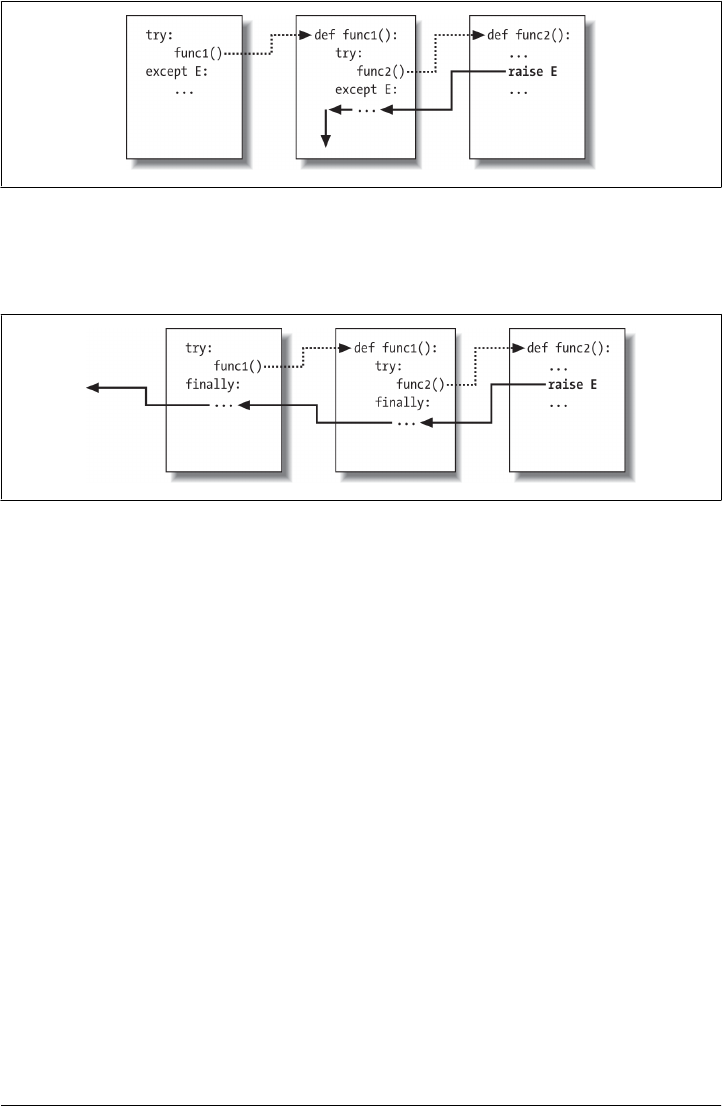
tion func2 sends control back to the handler in func1, and then the program continues
within func1.
By contrast, when try statements that contain only finally clauses are nested, each
finally block is run in turn when an exception occurs—Python continues propagating
the exception up to other trys, and eventually perhaps to the top-level default handler
(the standard error message printer). As Figure 36-2 illustrates, the finally clauses do
not kill the exception—they just specify code to be run on the way out of each try
during the exception propagation process. If there are many try/finally clauses active
when an exception occurs, they will all be run, unless a try/except catches the exception
somewhere along the way.
In other words, where the program goes when an exception is raised depends entirely
upon where it has been—it’s a function of the runtime flow of control through the script,
not just its syntax. The propagation of an exception essentially proceeds backward
through time to try statements that have been entered but not yet exited. This propa-
gation stops as soon as control is unwound to a matching except clause, but not as it
passes through finally clauses on the way.
Figure 36-1. Nested try/except statements: when an exception is raised (by you or by Python), control
jumps back to the most recently entered try statement with a matching except clause, and the program
resumes after that try statement. except clauses intercept and stop the exception—they are where you
process and recover from exceptions.
Figure 36-2. Nested try/finally statements: when an exception is raised here, control returns to the
most recently entered try to run its finally statement, but then the exception keeps propagating to all
finallys in all active try statements and eventually reaches the default top-level handler, where an
error message is printed. finally clauses intercept (but do not stop) an exception—they are for actions
to be performed “on the way out.”
1142 | Chapter 36: Designing with Exceptions
www.it-ebooks.info

Example: Control-Flow Nesting
Let’s turn to an example to make this nesting concept more concrete. The following
module file, nestexc.py, defines two functions. action2 is coded to trigger an exception
(you can’t add numbers and sequences), and action1 wraps a call to action2 in a try
handler, to catch the exception:
def action2():
print(1 + []) # Generate TypeError
def action1():
try:
action2()
except TypeError: # Most recent matching try
print('inner try')
try:
action1()
except TypeError: # Here, only if action1 re-raises
print('outer try')
% python nestexc.py
inner try
Notice, though, that the top-level module code at the bottom of the file wraps a call to
action1 in a try handler, too. When action2 triggers the TypeError exception, there will
be two active try statements—the one in action1, and the one at the top level of the
module file. Python picks and runs just the most recent try with a matching except—
which in this case is the try inside action1.
Again, the place where an exception winds up jumping to depends on the control flow
through the program at runtime. Because of this, to know where you will go, you need
to know where you’ve been. In this case, where exceptions are handled is more a func-
tion of control flow than of statement syntax. However, we can also nest exception
handlers syntactically—an equivalent case we turn to next.
Example: Syntactic Nesting
As I mentioned when we looked at the new unified try/except/finally statement in
Chapter 34, it is possible to nest try statements syntactically by their position in your
source code:
try:
try:
action2()
except TypeError: # Most recent matching try
print('inner try')
except TypeError: # Here, only if nested handler re-raises
print('outer try')
Nesting Exception Handlers | 1143
www.it-ebooks.info

Really, though, this code just sets up the same handler-nesting structure as (and behaves
identically to) the prior example. In fact, syntactic nesting works just like the cases
sketched in Figure 36-1 and Figure 36-2. The only difference is that the nested handlers
are physically embedded in a try block, not coded elsewhere in functions that are called
from the try block. For example, nested finally handlers all fire on an exception,
whether they are nested syntactically or by means of the runtime flow through physi-
cally separated parts of your code:
>>> try:
... try:
... raise IndexError
... finally:
... print('spam')
... finally:
... print('SPAM')
...
spam
SPAM
Traceback (most recent call last):
File "<stdin>", line 3, in <module>
IndexError
See Figure 36-2 for a graphic illustration of this code’s operation; the effect is the same,
but the function logic has been inlined as nested statements here. For a more useful
example of syntactic nesting at work, consider the following file, except-finally.py:
def raise1(): raise IndexError
def noraise(): return
def raise2(): raise SyntaxError
for func in (raise1, noraise, raise2):
print('<%s>' % func.__name__)
try:
try:
func()
except IndexError:
print('caught IndexError')
finally:
print('finally run')
print('...')
This code catches an exception if one is raised and performs a finally termination-
time action regardless of whether an exception occurs. This may take a few moments
to digest, but the effect is the same as combining an except and a finally clause in a
single try statement in Python 2.5 and later:
% python except-finally.py
<raise1>
caught IndexError
finally run
...
<noraise>
finally run
...
1144 | Chapter 36: Designing with Exceptions
www.it-ebooks.info

<raise2>
finally run
Traceback (most recent call last):
File "except-finally.py", line 9, in <module>
func()
File "except-finally.py", line 3, in raise2
def raise2(): raise SyntaxError
SyntaxError: None
As we saw in Chapter 34, as of Python 2.5, except and finally clauses can be mixed
in the same try statement. This, along with multiple except clause support, makes some
of the syntactic nesting described in this section unnecessary, though the equivalent
runtime nesting is common in larger Python programs. Moreover, syntactic nesting still
works today, may still appear in code written prior to Python 2.5 that you may en-
counter, can make the disjoint roles of except and finally more explicit, and can be
used as a technique for implementing alternative exception-handling behaviors in gen-
eral.
Exception Idioms
We’ve seen the mechanics behind exceptions. Now let’s take a look at some of the other
ways they are typically used.
Breaking Out of Multiple Nested Loops: “go to”
As mentioned at the start of this part of the book, exceptions can often be used to serve
the same roles as other languages’ “go to” statements to implement more arbitrary
control transfers. Exceptions, however, provide a more structured option that localizes
the jump to a specific block of nested code.
In this role, raise is like “go to,” and except clauses and exception names take the place
of program labels. You can jump only out of code wrapped in a try this way, but that’s
a crucial feature—truly arbitrary “go to” statements can make code extraordinarily
difficult to understand and maintain.
For example, Python’s break statement exits just the single closest enclosing loop, but
we can always use exceptions to break out of more than one loop level if needed:
>>> class Exitloop(Exception): pass
...
>>> try:
... while True:
... while True:
... for i in range(10):
... if i > 3: raise Exitloop # break exits just one level
... print('loop3: %s' % i)
... print('loop2')
... print('loop1')
... except Exitloop:
... print('continuing') # Or just pass, to move on
Exception Idioms | 1145
www.it-ebooks.info

...
loop3: 0
loop3: 1
loop3: 2
loop3: 3
continuing
>>> i
4
If you change the raise in this to break, you’ll get an infinite loop, because you’ll break
only out of the most deeply nested for loop, and wind up in the second-level loop
nesting. The code would then print “loop2” and start the for again.
Also notice that variable i is still what it was after the try statement exits. Variable
assignments made in a try are not undone in general, though as we’ve seen, exception
instance variables listed in except clause headers are localized to that clause, and the
local variables of any functions that are exited as a result of a raise are discarded.
Technically, active functions’ local variables are popped off the call stack and the ob-
jects they reference may be garbage-collected as a result, but this is an automatic step.
Exceptions Aren’t Always Errors
In Python, all errors are exceptions, but not all exceptions are errors. For instance, we
saw in Chapter 9 that file object read methods return an empty string at the end of a
file. In contrast, the built-in input function—which we first met in Chapter 3, deployed
in an interactive loop in Chapter 10, and learned is named raw_input in 2.X—reads a
line of text from the standard input stream, sys.stdin, at each call and raises the built-
in EOFError at end-of-file.
Unlike file methods, this function does not return an empty string—an empty string
from input means an empty line. Despite its name, though, the EOFError exception is
just a signal in this context, not an error. Because of this behavior, unless the end-of-
file should terminate a script, input often appears wrapped in a try handler and nested
in a loop, as in the following code:
while True:
try:
line = input() # Read line from stdin (raw_input in 2.X)
except EOFError:
break # Exit loop at end-of-file
else:
...process next line here...
Several other built-in exceptions are similarly signals, not errors—for example, calling
sys.exit() and pressing Ctrl-C on your keyboard raise SystemExit and KeyboardInter
rupt, respectively.
Python also has a set of built-in exceptions that represent warnings rather than errors;
some of these are used to signal use of deprecated (phased out) language features. See
the standard library manual’s description of built-in exceptions for more information,
1146 | Chapter 36: Designing with Exceptions
www.it-ebooks.info

and consult the warnings module’s documentation for more on exceptions raised as
warnings.
Functions Can Signal Conditions with raise
User-defined exceptions can also signal nonerror conditions. For instance, a search
routine can be coded to raise an exception when a match is found instead of returning
a status flag for the caller to interpret. In the following, the try/except/else exception
handler does the work of an if/else return-value tester:
class Found(Exception): pass
def searcher():
if ...success...:
raise Found() # Raise exceptions instead of returning flags
else:
return
try:
searcher()
except Found: # Exception if item was found
...success...
else: # else returned: not found
...failure...
More generally, such a coding structure may also be useful for any function that cannot
return a sentinel value to designate success or failure. In a widely applicable function,
for instance, if all objects are potentially valid return values, it’s impossible for any
return value to signal a failure condition. Exceptions provide a way to signal results
without a return value:
class Failure(Exception): pass
def searcher():
if ...success...:
return ...founditem...
else:
raise Failure()
try:
item = searcher()
except Failure:
...not found...
else:
...use item here...
Because Python is dynamically typed and polymorphic to the core, exceptions, rather
than sentinel return values, are the generally preferred way to signal such conditions.
Exception Idioms | 1147
www.it-ebooks.info

Closing Files and Server Connections
We encountered examples in this category in Chapter 34. As a summary, though, ex-
ception processing tools are also commonly used to ensure that system resources are
finalized, regardless of whether an error occurs during processing or not.
For example, some servers require connections to be closed in order to terminate a
session. Similarly, output files may require close calls to flush their buffers to disk for
waiting consumers, and input files may consume file descriptors if not closed; although
file objects are automatically closed when garbage-collected if still open, in some Py-
thons it may be difficult to be sure when that will occur.
As we saw in Chapter 34, the most general and explicit way to guarantee termination
actions for a specific block of code is the try/finally statement:
myfile = open(r'C:\code\textdata', 'w')
try:
...process myfile...
finally:
myfile.close()
As we also saw, some objects make this potentially easier in Python 2.6, 3.0, and later
by providing context managers that terminate or close the objects for us automatically
when run by the with/as statement:
with open(r'C:\code\textdata', 'w') as myfile:
...process myfile...
So which option is better here? As usual, it depends on your programs. Compared to
the traditional try/finally, context managers are more implicit, which runs contrary
to Python’s general design philosophy. Context managers are also arguably less general
—they are available only for select objects, and writing user-defined context managers
to handle general termination requirements is more complex than coding a try/finally.
On the other hand, using existing context managers requires less code than using try/
finally, as shown by the preceding examples. Moreover, the context manager protocol
supports entry actions in addition to exit actions. In fact, it can save a line of code when
no exceptions are expected at all (albeit at the expense of further nesting and indenting
file processing logic):
myfile = open(filename, 'w') # Traditional form
...process myfile...
myfile.close()
with open(filename) as myfile: # Context manager form
...process myfile...
Still, the implicit exception processing of with makes it more directly comparable to
the explicit exception handling of try/finally. Although try/finally is the more widely
applicable technique, context managers may be preferable where they are already
available, or where their extra complexity is warranted.
1148 | Chapter 36: Designing with Exceptions
www.it-ebooks.info
Debugging with Outer try Statements
You can also make use of exception handlers to replace Python’s default top-level ex-
ception-handling behavior. By wrapping an entire program (or a call to it) in an outer
try in your top-level code, you can catch any exception that may occur while your
program runs, thereby subverting the default program termination.
In the following, the empty except clause catches any uncaught exception raised while
the program runs. To get hold of the actual exception that occurred in this mode, fetch
the sys.exc_info function call result from the built-in sys module; it returns a tuple
whose first two items contain the current exception’s class and the instance object
raised (more on sys.exc_info in a moment):
try:
...run program...
except: # All uncaught exceptions come here
import sys
print('uncaught!', sys.exc_info()[0], sys.exc_info()[1])
This structure is commonly used during development, to keep programs active even
after errors occur—within a loop, it allows you to run additional tests without having
to restart. It’s also used when testing other program code, as described in the next
section.
On a related note, for more about handling program shutdowns
without recovery from them, see also Python’s atexit standard library
module. It’s also possible to customize what the top-level exception
handler does with sys.excepthook. These and other related tools are
described in Python’s library manual.
Running In-Process Tests
Some of the coding patterns we’ve just looked at can be combined in a test-driver
application that tests other code within the same process. The following partial code
sketches the general model:
import sys
log = open('testlog', 'a')
from testapi import moreTests, runNextTest, testName
def testdriver():
while moreTests():
try:
runNextTest()
except:
print('FAILED', testName(), sys.exc_info()[:2], file=log)
else:
print('PASSED', testName(), file=log)
testdriver()
Exception Idioms | 1149
www.it-ebooks.info

The testdriver function here cycles through a series of test calls (the module testapi
is left abstract in this example). Because an uncaught exception in a test case would
normally kill this test driver, you need to wrap test case calls in a try if you want to
continue the testing process after a test fails. The empty except catches any uncaught
exception generated by a test case as usual, and it uses sys.exc_info to log the exception
to a file. The else clause is run when no exception occurs—the test success case.
Such boilerplate code is typical of systems that test functions, modules, and classes by
running them in the same process as the test driver. In practice, however, testing can
be much more sophisticated than this. For instance, to test external programs, you could
instead check status codes or outputs generated by program-launching tools such as
os.system and os.popen, used earlier in this book and covered in the standard library
manual. Such tools do not generally raise exceptions for errors in the external programs
—in fact, the test cases may run in parallel with the test driver.
At the end of this chapter, we’ll also briefly meet more complete testing frameworks
provided by Python, such as doctest and PyUnit, which provide tools for comparing
expected outputs with actual results.
More on sys.exc_info
The sys.exc_info result used in the last two sections allows an exception handler to
gain access to the most recently raised exception generically. This is especially useful
when using the empty except clause to catch everything blindly, to determine what was
raised:
try:
...
except:
# sys.exc_info()[0:2] are the exception class and instance
If no exception is being handled, this call returns a tuple containing three None values.
Otherwise, the values returned are (type, value, traceback), where:
•type is the exception class of the exception being handled.
•value is the exception class instance that was raised.
•traceback is a traceback object that represents the call stack at the point where the
exception originally occurred, and used by the traceback module to generate error
messages.
As we saw in the prior chapter, sys.exc_info can also sometimes be useful to determine
the specific exception type when catching exception category superclasses. As we’ve
also learned, though, because in this case you can also get the exception type by fetching
the __class__ attribute of the instance obtained with the as clause, sys.exc_info is often
redundant apart from the empty except:
try:
...
1150 | Chapter 36: Designing with Exceptions
www.it-ebooks.info

except General as instance:
# instance.__class__ is the exception class
As we’ve seen, using Exception for the General exception name here would catch all
nonexit exceptions, similar to an empty except but less extreme, and still giving access
to the exception instance and its class. Even so, using the instance object’s interfaces
and polymorphism is often a better approach than testing exception types—exception
methods can be defined per class and run generically:
try:
...
except General as instance:
# instance.method() does the right thing for this instance
As usual, being too specific in Python can limit your code’s flexibility. A polymorphic
approach like the last example here generally supports future evolution better than
explicitly type-specific tests or actions.
Displaying Errors and Tracebacks
Finally, the exception traceback object available in the prior section’s sys.exc_info
result is also used by the standard library’s traceback module to generate the standard
error message and stack display manually. This file has a handful of interfaces that
support wide customization, which we don’t have space to cover usefully here, but the
basics are simple. Consider the following aptly named file, badly.py:
import traceback
def inverse(x):
return 1 / x
try:
inverse(0)
except Exception:
traceback.print_exc(file=open('badly.exc', 'w'))
print('Bye')
This code uses the print_exc convenience function in the traceback module, which
uses sys.exc_info data by default; when run, the script prints the error message to a
file—handy in testing programs that need to catch errors but still record them in full:
c:\code> python badly.py
Bye
c:\code> type badly.exc
Traceback (most recent call last):
File "badly.py", line 7, in <module>
inverse(0)
File "badly.py", line 4, in inverse
return 1 / x
ZeroDivisionError: division by zero
Exception Idioms | 1151
www.it-ebooks.info

For much more on traceback objects, the traceback module that uses them, and related
topics, consult other reference resources and manuals.
Version skew note: In Python 2.X, the older tools sys.exc_type and
sys.exc_value still work to fetch the most recent exception type and
value, but they can manage only a single, global exception for the entire
process. These two names have been removed in Python 3.X. The newer
and preferred sys.exc_info() call available in both 2.X and 3.X instead
keeps track of each thread’s exception information, and so is thread-
specific. Of course, this distinction matters only when using multiple
threads in Python programs (a subject beyond this book’s scope), but
3.X forces the issue. See other resources for more details.
Exception Design Tips and Gotchas
I’m lumping design tips and gotchas together in this chapter, because it turns out that
the most common gotchas largely stem from design issues. By and large, exceptions
are easy to use in Python. The real art behind them is in deciding how specific or general
your except clauses should be and how much code to wrap up in try statements. Let’s
address the second of these concerns first.
What Should Be Wrapped
In principle, you could wrap every statement in your script in its own try, but that
would just be silly (the try statements would then need to be wrapped in try state-
ments!). What to wrap is really a design issue that goes beyond the language itself, and
it will become more apparent with use. But for now, here are a few rules of thumb:
• Operations that commonly fail should generally be wrapped in try statements. For
example, operations that interface with system state (file opens, socket calls, and
the like) are prime candidates for try.
• However, there are exceptions to the prior rule—in a simple script, you may
want failures of such operations to kill your program instead of being caught and
ignored. This is especially true if the failure is a showstopper. Failures in Python
typically result in useful error messages (not hard crashes), and this is the best
outcome some programs could hope for.
• You should implement termination actions in try/finally statements to guarantee
their execution, unless a context manager is available as a with/as option. The try/
finally statement form allows you to run code whether exceptions occur or not
in arbitrary scenarios.
• It is sometimes more convenient to wrap the call to a large function in a single
try statement, rather than littering the function itself with many try statements.
1152 | Chapter 36: Designing with Exceptions
www.it-ebooks.info

That way, all exceptions in the function percolate up to the try around the call,
and you reduce the amount of code within the function.
The types of programs you write will probably influence the amount of exception han-
dling you code as well. Servers, for instance, must generally keep running persistently
and so will likely require try statements to catch and recover from exceptions. In-
process testing programs of the kind we saw in this chapter will probably handle ex-
ceptions as well. Simpler one-shot scripts, though, will often ignore exception handling
completely because failure at any step requires script shutdown.
Catching Too Much: Avoid Empty except and Exception
As mentioned, exception handler generality is a key design choice. Python lets you pick
and choose which exceptions to catch, but you sometimes have to be careful to not be
too inclusive. For example, you’ve seen that an empty except clause catches every ex-
ception that might be raised while the code in the try block runs.
That’s easy to code, and sometimes desirable, but you may also wind up intercepting
an error that’s expected by a try handler higher up in the exception nesting structure.
For example, an exception handler such as the following catches and stops every ex-
ception that reaches it, regardless of whether another handler is waiting for it:
def func():
try:
... # IndexError is raised in here
except:
... # But everything comes here and dies!
try:
func()
except IndexError: # Exception should be processed here
...
Perhaps worse, such code might also catch unrelated system exceptions. Even things
like memory errors, genuine programming mistakes, iteration stops, keyboard inter-
rupts, and system exits raise exceptions in Python. Unless you’re writing a debugger or
similar tool, such exceptions should not usually be intercepted in your code.
For example, scripts normally exit when control falls off the end of the top-level file.
However, Python also provides a built-in sys.exit(statuscode) call to allow early ter-
minations. This actually works by raising a built-in SystemExit exception to end the
program, so that try/finally handlers run on the way out and special types of programs
can intercept the event.1 Because of this, a try with an empty except might unknowingly
prevent a crucial exit, as in the following file (exiter.py):
1. A related call, os._exit, also ends a program, but via an immediate termination—it skips cleanup actions,
including any registered with the atexit module noted earlier, and cannot be intercepted with try/
except or try/finally blocks. It is usually used only in spawned child processes, a topic beyond this book’s
scope. See the library manual or follow-up texts for details.
Exception Design Tips and Gotchas | 1153
www.it-ebooks.info

import sys
def bye():
sys.exit(40) # Crucial error: abort now!
try:
bye()
except:
print('got it') # Oops--we ignored the exit
print('continuing...')
% python exiter.py
got it
continuing...
You simply might not expect all the kinds of exceptions that could occur during an
operation. Using the built-in exception classes of the prior chapter can help in this
particular case, because the Exception superclass is not a superclass of SystemExit:
try:
bye()
except Exception: # Won't catch exits, but _will_ catch many others
...
In other cases, though, this scheme is no better than an empty except clause—because
Exception is a superclass above all built-in exceptions except system-exit events, it still
has the potential to catch exceptions meant for elsewhere in the program.
Probably worst of all, both using an empty except and catching the Exception superclass
will also catch genuine programming errors, which should be allowed to pass most of
the time. In fact, these two techniques can effectively turn off Python’s error-reporting
machinery, making it difficult to notice mistakes in your code. Consider this code, for
example:
mydictionary = {...}
...
try:
x = myditctionary['spam'] # Oops: misspelled
except:
x = None # Assume we got KeyError
...continue here with x...
The coder here assumes that the only sort of error that can happen when indexing a
dictionary is a missing key error. But because the name myditctionary is misspelled (it
should say mydictionary), Python raises a NameError instead for the undefined name
reference, which the handler will silently catch and ignore. The event handler will in-
correctly fill in a None default for the dictionary access, masking the program error.
Moreover, catching Exception here will not help—it would have the exact same effect
as an empty except, happily and silently filling in a default and masking a genuine
program error you will probably want to know about. If this happens in code that is
far removed from the place where the fetched values are used, it might make for a very
interesting debugging task!
1154 | Chapter 36: Designing with Exceptions
www.it-ebooks.info

As a rule of thumb, be as specific in your handlers as you can be—empty except clauses
and Exception catchers are handy, but potentially error-prone. In the last example, for
instance, you would be better off saying except KeyError: to make your intentions
explicit and avoid intercepting unrelated events. In simpler scripts, the potential for
problems might not be significant enough to outweigh the convenience of a catchall,
but in general, general handlers are generally trouble.
Catching Too Little: Use Class-Based Categories
On the other hand, neither should handlers be too specific. When you list specific
exceptions in a try, you catch only what you actually list. This isn’t necessarily a bad
thing, but if a system evolves to raise other exceptions in the future, you may need to
go back and add them to exception lists elsewhere in your code.
We saw this phenomenon at work in the prior chapter. For instance, the following
handler is written to treat MyExcept1 and MyExcept2 as normal cases and everything else
as an error. If you add a MyExcept3 in the future, though, it will be processed as an error
unless you update the exception list:
try:
...
except (MyExcept1, MyExcept2): # Breaks if you add a MyExcept3 later
... # Nonerrors
else:
... # Assumed to be an error
Luckily, careful use of the class-based exceptions we discussed in Chapter 34 can make
this code maintenance trap go away completely. As we saw, if you catch a general
superclass, you can add and raise more specific subclasses in the future without having
to extend except clause lists manually—the superclass becomes an extendible excep-
tions category:
try:
...
except SuccessCategoryName: # OK if you add a MyExcept3 subclass later
... # Nonerrors
else:
... # Assumed to be an error
In other words, a little design goes a long way. The moral of the story is to be careful
to be neither too general nor too specific in exception handlers, and to pick the gran-
ularity of your try statement wrappings wisely. Especially in larger systems, exception
policies should be a part of the overall design.
Core Language Summary
Congratulations! This concludes your look at the fundamentals of the Python pro-
gramming language. If you’ve gotten this far, you’ve become a fully operational Python
Core Language Summary | 1155
www.it-ebooks.info

programmer. There’s more optional reading in the advanced topics part ahead that I’ll
describe in a moment. In terms of the essentials, though, the Python story—and this
book’s main journey—is now complete.
Along the way, you’ve seen just about everything there is to see in the language itself,
and in enough depth to apply to most of the code you are likely to encounter in the
open source “wild.” You’ve studied built-in types, statements, and exceptions, as well
as tools used to build up the larger program units of functions, modules, and classes.
You’ve also explored important software design issues, the complete OOP paradigm,
functional programing tools, program architecture concepts, alternative tool tradeoffs,
and more—compiling a skill set now qualified to be turned loose on the task of devel-
oping real applications.
The Python Toolset
From this point forward, your future Python career will largely consist of becoming
proficient with the toolset available for application-level Python programming. You’ll
find this to be an ongoing task. The standard library, for example, contains hundreds
of modules, and the public domain offers still more tools. It’s possible to spend decades
seeking proficiency with all these tools, especially as new ones are constantly appearing
to address new technologies (trust me on this—I’m at 20 years and counting!).
Speaking generally, Python provides a hierarchy of toolsets:
Built-ins
Built-in types like strings, lists, and dictionaries make it easy to write simple pro-
grams fast.
Python extensions
For more demanding tasks, you can extend Python by writing your own functions,
modules, and classes.
Compiled extensions
Although we don’t cover this topic in this book, Python can also be extended with
modules written in an external language like C or C++.
Because Python layers its toolsets, you can decide how deeply your programs need to
delve into this hierarchy for any given task—you can use built-ins for simple scripts,
add Python-coded extensions for larger systems, and code compiled extensions for
advanced work. We’ve only covered the first two of these categories in this book, and
that’s plenty to get you started doing substantial programming in Python.
Beyond this, there are tools, resources, or precedents for using Python in nearly any
computer domain you can imagine. For pointers on where to go next, see Chapter 1’s
overview of Python applications and users. You’ll likely find that with a powerful open
source language like Python, common tasks are often much easier, and even enjoyable,
than you might expect.
1156 | Chapter 36: Designing with Exceptions
www.it-ebooks.info

Development Tools for Larger Projects
Most of the examples in this book have been fairly small and self-contained. They were
written that way on purpose, to help you master the basics. But now that you know all
about the core language, it’s time to start learning how to use Python’s built-in and
third-party interfaces to do real work.
In practice, Python programs can become substantially larger than the examples you’ve
experimented with so far in this book. Even in Python, thousands of lines of code are
not uncommon for nontrivial and useful programs, once you add up all the individual
modules in the system. Though Python basic program structuring tools such as mod-
ules and classes help much to manage this complexity, other tools can sometimes offer
additional support.
For developing larger systems, you’ll find such support available in both Python and
the public domain. You’ve seen some of these in action, and I’ve mentioned a few
others. To help you on your next steps, here is a quick tour and summary of some of
the most commonly used tools in this domain:
PyDoc and docstrings
PyDoc’s help function and HTML interfaces were introduced in Chapter 15. PyDoc
provides a documentation system for your modules and objects, integrates with
Python’s docstrings syntax, and is a standard part of the Python system. See Chap-
ter 15 and Chapter 4 for more documentation source hints.
PyChecker and PyLint
Because Python is such a dynamic language, some programming errors are not
reported until your program runs (even syntax errors are not caught until a file is
run or imported). This isn’t a big drawback—as with most languages, it just means
that you have to test your Python code before shipping it. At worst, with Python
you essentially trade a compile phase for an initial testing phase. Furthermore,
Python’s dynamic nature, automatic error messages, and exception model make it
easier and quicker to find and fix errors than it is in some other languages. Unlike
C, for example, Python does not crash completely on errors.
Still, tools can help here too. The PyChecker and PyLint systems provide support
for catching common errors ahead of time, before your script runs. They serve
similar roles to the lint program in C development. Some Python developers run
their code through PyChecker prior to testing or delivery, to catch any lurking
potential problems. In fact, it’s not a bad idea to try this when you’re first starting
out—some of these tools’ warnings may help you learn to spot and avoid common
Python mistakes. PyChecker and PyLint are third-party open source packages,
available at the PyPI website or your friendly neighborhood web search engine.
They may appear in IDE GUIs as well.
PyUnit (a.k.a. unittest)
In Chapter 25, we learned how to add self-test code to a Python file by using the
__name__ == '__main__' trick at the bottom of the file—a simple unit-testing pro-
Core Language Summary | 1157
www.it-ebooks.info

tocol. For more advanced testing purposes, Python comes with two testing support
tools. The first, PyUnit (called unittest in the library manual), provides an object-
oriented class framework for specifying and customizing test cases and expected
results. It mimics the JUnit framework for Java. This is a sophisticated class-based
unit testing system; see the Python library manual for details.
doctest
The doctest standard library module provides a second and simpler approach to
regression testing, based upon Python’s docstrings feature. Roughly, to use doct
est, you cut and paste a log of an interactive testing session into the docstrings of
your source files. doctest then extracts your docstrings, parses out the test cases
and results, and reruns the tests to verify the expected results. doctest’s operation
can be tailored in a variety of ways; see the library manual for more details.
IDEs
We discussed IDEs for Python in Chapter 3. IDEs such as IDLE provide a graphical
environment for editing, running, debugging, and browsing your Python pro-
grams. Some advanced IDEs—such as Eclipse, Komodo, NetBeans, and others
listed in Chapter 3—may support additional development tasks, including source
control integration, code refactoring, project management tools, and more. See
Chapter 3, the text editors page at http://www.python.org, and your favorite web
search engine for more on available IDEs and GUI builders for Python.
Profilers
Because Python is so high-level and dynamic, intuitions about performance
gleaned from experience with other languages usually don’t apply to Python code.
To truly isolate performance bottlenecks in your code, you need to add timing logic
with clock tools in the time or timeit modules, or run your code under the pro
file module. We saw an example of the timing modules at work when comparing
the speed of iteration tools and Pythons in Chapter 21.
Profiling is usually your first optimization step—code for clarity, then profile to
isolate bottlenecks, and then time alternative codings of the slow parts of your
program. For the second of these steps, profile is a standard library module that
implements a source code profiler for Python. It runs a string of code you provide
(e.g., a script file import, or a call to a function) and then, by default, prints a report
to the standard output stream that gives performance statistics—number of calls
to each function, time spent in each function, and more.
The profile module can be run as a script or imported, and it may be customized
in various ways; for example, it can save run statistics to a file to be analyzed later
with the pstats module. To profile interactively, import the profile module and
call profile.run('code'), passing in the code you wish to profile as a string (e.g.,
a call to a function, an import of a file, or code read from a file). To profile from a
system shell command line, use a command of the form python -m profile
main.py args (see Appendix A for more on this format). Also see Python’s standard
library manuals for other profiling options; the cProfile module, for example, has
1158 | Chapter 36: Designing with Exceptions
www.it-ebooks.info

identical interfaces to profile but runs with less overhead, so it may be better suited
to profiling long-running programs.
Debuggers
We also discussed debugging options in Chapter 3 (see its sidebar “Debugging
Python Code” on page 83). As a review, most development IDEs for Python support
GUI-based debugging, and the Python standard library also includes a source code
debugger module called pdb. This module provides a command-line interface and
works much like common C language debuggers (e.g., dbx, gdb).
Much like the profiler, the pdb debugger can be run either interactively or from a
command line and can be imported and called from a Python program. To use it
interactively, import the module, start running code by calling a pdb function (e.g.,
pdb.run('main()')), and then type debugging commands from pdb’s interactive
prompt. To launch pdb from a system shell command line, use a command of the
form python -m pdb main.py args. pdb also includes a useful postmortem analysis
call, pdb.pm(), which starts the debugger after an exception has been encountered,
possibly in conjunction with Python’s -i flag. See Appendix A for more on these
tools.
Because IDEs such as IDLE also include point-and-click debugging interfaces,
pdb isn’t as critical a tool today, except when a GUI isn’t available or when more
control is desired. See Chapter 3 for tips on using IDLE’s debugging GUI interfaces.
Really, neither pdb nor IDEs seem to be used much in practice—as noted in Chap-
ter 3, most programmers either insert print statements or simply read Python’s
error messages: perhaps not the most high-tech of approaches, but the practical
tends to win the day in the Python world!
Shipping options
In Chapter 2, we introduced common tools for packaging Python programs.
py2exe, PyInstaller, and others listed in that chapter can package byte code and
the Python Virtual Machine into “frozen binary” standalone executables, which
don’t require that Python be installed on the target machine and hide your system’s
code. In addition, we learned in Chapter 2 that Python programs may be shipped
in their source (.py) or byte code (.pyc) forms, and that import hooks support
special packaging techniques such as automatic extraction of .zip files and byte
code encryption.
We also briefly met the standard library’s distutils modules, which provide pack-
aging options for Python modules and packages, and C-coded extensions; see the
Python manuals for more details. The emerging Python “eggs” third-party pack-
aging system provides another alternative that also accounts for dependencies;
search the Web for more details.
Optimization options
When speed counts, there are a handful of options for optimizing your programs.
The PyPy system described in Chapter 2 provides a just-in-time compiler for trans-
lating Python byte code to binary machine code, and Shed Skin offers a Python-to-
Core Language Summary | 1159
www.it-ebooks.info

C++ translator. You may also occasionally see .pyo optimized byte code files, gen-
erated and run with the -O Python command-line flag discussed in Chapter 22 and
Chapter 34, and to be deployed in Chapter 39; because this provides a very modest
performance boost, however, it is not commonly used except to remove debugging
code.
As a last resort, you can also move parts of your program to a compiled language
such as C to boost performance. See the book Programming Python and the Python
standard manuals for more on C extensions. In general, Python’s speed tends to
also improve over time, so upgrading to later releases may improve speed too—
once you verify that they are faster for your code, that is (though largely repaired
since, Python 3.0’s initial release was up to 1000X slower than 2.X on some IO
operations!).
Other hints for larger projects
We’ve met a variety of core language features in this text that will also tend to
become more useful once you start coding larger projects. These include module
packages (Chapter 24), class-based exceptions (Chapter 34), class pseudoprivate
attributes (Chapter 31), documentation strings (Chapter 15), module path con-
figuration files (Chapter 22), hiding names from from * with __all__ lists and _X-
style names (Chapter 25), adding self-test code with the __name__ == '__main__'
trick (Chapter 25), using common design rules for functions and modules (Chap-
ter 17, Chapter 19, and Chapter 25), using object-oriented design patterns (Chap-
ter 31 and others), and so on.
To learn about other large-scale Python development tools available in the public do-
main, be sure to browse the pages at the PyPI website at http://www.python.org, and
the Web at large. Applying Python is actually a larger topic than learning Python, and
one we’ll have to delegate to follow-up resources here.
Chapter Summary
This chapter wrapped up the exceptions part of the book with a survey of design con-
cepts, a look at common exception use cases, and a brief summary of commonly used
development tools.
This chapter also wrapped up the core material of this book. At this point, you’ve been
exposed to the full subset of Python that most programmers use—and probably more.
In fact, if you have read this far, you should feel free to consider yourself an official
Python programmer. Be sure to pick up a t-shirt or laptop sticker the next time you’re
online (and don’t forget to add Python to your résumé the next time you dig it out).
The next and final part of this book is a collection of chapters dealing with topics that
are advanced, but still in the core language category. These chapters are all optional
reading, or at least deferrable reading, because not every Python programmer must delve
into their subjects, and others can postpone these chapters’ topics until they are needed.
1160 | Chapter 36: Designing with Exceptions
www.it-ebooks.info

Indeed, many of you can stop here and begin exploring Python’s roles in your appli-
cation domains. Frankly, application libraries tend to be more important in practice
than advanced—and to some, esoteric—language features.
On the other hand, if you do need to care about things like Unicode or binary data,
have to deal with API-building tools such as descriptors, decorators, and metaclasses,
or just want to dig a bit further in general, the next part of the book will help you get
started. The larger examples in the final part will also give you a chance to see the
concepts you’ve already learned being applied in more realistic ways.
As this is the end of the core material of this book, though, you get a break on the
chapter quiz—just one question this time. As always, be sure to work through this
part’s closing exercises to cement what you’ve learned in the past few chapters; because
the next part is optional reading, this is the final end-of-part exercises session. If you
want to see some examples of how what you’ve learned comes together in real scripts
drawn from common applications, be sure to check out the “solution” to exercise 4 in
Appendix D.
And if this is the end of your journey in this book, be sure to also see the “Bonus” section
at the end of Chapter 41, the very last chapter in this book (for the sake of readers
continuing on to the Advanced Topics part, I won’t spill the beans here).
Test Your Knowledge: Quiz
1. (This question is a repeat from the first quiz in Chapter 1—see, I told you it would
be easy! :-) Why does “spam” show up in so many Python examples in books and
on the Web?
Test Your Knowledge: Answers
1. Because Python is named after the British comedy group Monty Python (based on
surveys I’ve conducted in classes, this is a much-too-well-kept secret in the Python
world!). The spam reference comes from a Monty Python skit, set in a cafeteria
whose menu items all seem to come with Spam. A couple trying to order food there
keeps getting drowned out by a chorus of Vikings singing a song about Spam. No,
really. And if I could insert an audio clip of that song here, I would...
Test Your Knowledge: Part VII Exercises
As we’ve reached the end of this part of the book, it’s time for a few exception exercises
to give you a chance to practice the basics. Exceptions really are simple tools; if you get
these, you’ve probably mastered the exceptions domain. See Part VII in Appendix D
for the solutions.
Test Your Knowledge: Part VII Exercises | 1161
www.it-ebooks.info

1. try/except. Write a function called oops that explicitly raises an IndexError excep-
tion when called. Then write another function that calls oops inside a try/except
statement to catch the error. What happens if you change oops to raise a
KeyError instead of an IndexError? Where do the names KeyError and IndexError
come from? (Hint: recall that all unqualified names generally come from one of
four scopes.)
2. Exception objects and lists. Change the oops function you just wrote to raise an
exception you define yourself, called MyError. Identify your exception with a class
(unless you’re using Python 2.5 or earlier, you must). Then, extend the try state-
ment in the catcher function to catch this exception and its instance in addition to
IndexError, and print the instance you catch.
3. Error handling. Write a function called safe(func, *pargs, **kargs) that runs any
function with any number of positional and/or keyword arguments by using the
* arbitrary arguments header and call syntax, catches any exception raised while
the function runs, and prints the exception using the exc_info call in the sys mod-
ule. Then use your safe function to run your oops function from exercise 1 or 2.
Put safe in a module file called exctools.py, and pass it the oops function interac-
tively. What kind of error messages do you get? Finally, expand safe to also print
a Python stack trace when an error occurs by calling the built-in print_exc function
in the standard traceback module; see earlier in this chapter, and consult the
Python library reference manual for usage details. We could probably code safe as
a function decorator using Chapter 32 techniques, but we’ll have to move on to the
next part of the book to learn fully how (see the solutions for a preview).
4. Self-study examples. At the end of Appendix D, I’ve included a handful of example
scripts developed as group exercises in live Python classes for you to study and run
on your own in conjunction with Python’s standard manual set. These are not
described, and they use tools in the Python standard library that you’ll have to
research on your own. Still, for many readers, it helps to see how the concepts
we’ve discussed in this book come together in real programs. If these whet your
appetite for more, you can find a wealth of larger and more realistic application-
level Python program examples in follow-up books like Programming Python and
on the Web.
1162 | Chapter 36: Designing with Exceptions
www.it-ebooks.info


CHAPTER 37
Unicode and Byte Strings
So far, our exploration of strings in this book has been deliberately incomplete. Chap-
ter 4’s types preview briefly introduced Python’s Unicode strings and files without
giving many details, and the strings chapter in the core types part of this book (Chap-
ter 7) deliberately limited its scope to the subset of string topics that most Python
programmers need to know about.
This was by design: because many programmers, including most beginners, deal with
simple forms of text like ASCII, they can happily work with Python’s basic str string
type and its associated operations and don’t need to come to grips with more advanced
string concepts. In fact, such programmers can often ignore the string changes in Python
3.X and continue to use strings as they may have in the past.
On the other hand, many other programmers deal with more specialized types of data:
non-ASCII character sets, image file contents, and so on. For those programmers, and
others who may someday join them, in this chapter we’re going to fill in the rest of the
Python string story and look at some more advanced concepts in Python’s string model.
Specifically, we’ll explore the basics of Python’s support for Unicode text—rich char-
acter strings used in internationalized applications—as well as binary data—strings
that represent absolute byte values. As we’ll see, the advanced string representation
story has diverged in recent versions of Python:
•Python 3.X provides an alternative string type for binary data, and supports Uni-
code text (including ASCII) in its normal string type.
•Python 2.X provides an alternative string type for non-ASCII Unicode text, and
supports both simple text and binary data in its normal string type.
In addition, because Python’s string model has a direct impact on how you process
non-ASCII files, we’ll explore the fundamentals of that related topic here as well. Fi-
nally, we’ll take a brief look at some advanced string and binary tools, such as pattern
matching, object pickling, binary data packing, and XML parsing, and the ways in
which they are impacted by 3.X’s string changes.
1165
www.it-ebooks.info

This is officially an advanced topics chapter, because not all programmers will need to
delve into the worlds of Unicode encodings or binary data. For some readers, Chap-
ter 4’s preview may suffice, and others may wish to file this chapter away for future
reference. If you ever need to care about processing either of these, though, you’ll find
that Python’s string models provide the support you need.
String Changes in 3.X
One of the most noticeable changes in the Python 3.X line is the mutation of string
object types. In a nutshell, 2.X’s str and unicode types have morphed into 3.X’s
bytes and str types, and a new mutable bytearray type has been added. The bytear
ray type is technically available in Python 2.6 and 2.7 too (though not earlier), but it’s
a back-port from 3.X and does not as clearly distinguish between text and binary con-
tent in 2.X.
Especially if you process data that is either Unicode or binary in nature, these changes
can have substantial impacts on your code. As a general rule of thumb, how much you
need to care about this topic depends in large part upon which of the following cate-
gories you fall into:
• If you deal with non-ASCII Unicode text—for instance, in the context of interna-
tionalized domains like the Web, or the results of some XML and JSON parsers
and databases—you will find support for text encodings to be different in 3.X, but
also probably more direct, accessible, and seamless than in 2.X.
• If you deal with binary data—for example, in the form of image or audio files or
packed data processed with the struct module—you will need to understand 3.X’s
new bytes object and 3.X’s different and sharper distinction between text and bi-
nary data and files.
• If you fall into neither of the prior two categories, you can generally use strings in
3.X much as you would in 2.X, with the general str string type, text files, and all
the familiar string operations we studied earlier. Your strings will be encoded and
decoded by 3.X using your platform’s default encoding (e.g., ASCII, or UTF-8 on
Windows in the U.S.—sys.getdefaultencoding gives your default if you care to
check), but you probably won’t notice.
In other words, if your text is always ASCII, you can get by with normal string objects
and text files and can avoid most of the following story for now. As we’ll see in a
moment, ASCII is a simple kind of Unicode and a subset of other encodings, so string
operations and files generally “just work” if your programs process only ASCII text.
Even if you fall into the last of the three categories just mentioned, though, a basic
understanding of Unicode and 3.X’s string model can help both to demystify some of
the underlying behavior now, and to make mastering Unicode or binary data issues
easier if they impact you later.
1166 | Chapter 37: Unicode and Byte Strings
www.it-ebooks.info

To put that more strongly: like it or not, Unicode will be part of most software devel-
opment in the interconnected future we’ve sown, and will probably impact you even-
tually. Though applications are beyond our scope here, if you work with the Internet,
files, directories, network interfaces, databases, pipes, JSON, XML, and even GUIs,
Unicode may no longer be an optional topic for you in Python 3.X.
Python 3.X’s support for Unicode and binary data is also available in 2.X, albeit in
different forms. Although our main focus in this chapter is on string types in 3.X, we’ll
also explore how 2.X’s equivalent support differs along the way for readers using 2.X.
Regardless of which version you use, the tools we’ll explore here can become important
in many types of programs.
String Basics
Before we look at any code, let’s begin with a general overview of Python’s string model.
To understand why 3.X changed the way it did on this front, we have to start with a
brief look at how characters are actually represented in computers—both when enco-
ded in files and when stored in memory.
Character Encoding Schemes
Most programmers think of strings as series of characters used to represent textual data.
While that’s accurate, the way characters are stored can vary, depending on what sort
of character set must be recorded. When text is stored on files, for example, its character
set determines its format.
Character sets are standards that assign integer codes to individual characters so they
can be represented in computer memory. The ASCII standard, for example, was created
in the U.S., and it defines many U.S. programmers’ notion of text strings. ASCII defines
character codes from 0 through 127 and allows each character to be stored in one 8-
bit byte, only 7 bits of which are actually used.
For example, the ASCII standard maps the character 'a' to the integer value 97 (0x61
in hex), which can be stored in a single byte in memory and files. If you wish to see
how this works, Python’s ord built-in function gives the binary identifying value for a
character, and chr returns the character for a given integer code value:
>>> ord('a') # 'a' is a byte with binary value 97 in ASCII (and others)
97
>>> hex(97)
'0x61'
>>> chr(97) # Binary value 97 stands for character 'a'
'a'
Sometimes one byte per character isn’t enough, though. Various symbols and accented
characters, for instance, do not fit into the range of possible characters defined by
ASCII. To accommodate special characters, some standards use all the possible values
String Basics | 1167
www.it-ebooks.info

in an 8-bit byte, 0 through 255, to represent characters, and assign the values 128
through 255 (outside ASCII’s range) to special characters.
One such standard, known as the Latin-1 character set, is widely used in Western
Europe. In Latin-1, character codes above 127 are assigned to accented and otherwise
special characters. The character assigned to byte value 196, for example, is a specially
marked non-ASCII character:
>>> 0xC4
196
>>> chr(196) # Python 3.X result form shown
'Ä'
This standard allows for a wide array of extra special characters, but still supports ASCII
as a 7-bit subset of its 8-bit representation.
Still, some alphabets define so many characters that it is impossible to represent each
of them as one byte. Unicode allows more flexibility. Unicode text is sometimes referred
to as “wide-character” strings, because characters may be represented with multiple
bytes if needed. Unicode is typically used in internationalized programs, to represent
European, Asian, and other non-English character sets that have more characters than
8-bit bytes can represent.
To store such rich text in computer memory, we say that characters are translated to
and from raw bytes using an encoding—the rules for translating a string of Unicode
characters to a sequence of bytes, and extracting a string from a sequence of bytes.
More procedurally, this translation back and forth between bytes and strings is defined
by two terms:
•Encoding is the process of translating a string of characters into its raw bytes form,
according to a desired encoding name.
•Decoding is the process of translating a raw string of bytes into its character string
form, according to its encoding name.
That is, we encode from string to raw bytes, and decode from raw bytes to string. To
scripts, decoded strings are just characters in memory, but may be encoded into a
variety of byte string representations when stored on files, transferred over networks,
embedded in documents and databases, and so on.
For some encodings, the translation process is trivial—ASCII and Latin-1, for instance,
map each character to a fixed-size single byte, so no translation work is required. For
other encodings, the mapping can be more complex and yield multiple bytes per char-
acter, even for simple 8-bit forms of text.
The widely used UTF-8 encoding, for example, allows a wide range of characters to be
represented by employing a variable-sized number of bytes scheme. Character codes
less than 128 are represented as a single byte; codes between 128 and 0x7ff (2047) are
turned into 2 bytes, where each byte has a value between 128 and 255; and codes above
0x7ff are turned into 3- or 4-byte sequences having values between 128 and 255. This
1168 | Chapter 37: Unicode and Byte Strings
www.it-ebooks.info

keeps simple ASCII strings compact, sidesteps byte ordering issues, and avoids null
(zero value) bytes that can cause problems for C libraries and networking.
Because their encodings’ character maps assign characters to the same codes for com-
patibility, ASCII is a subset of both Latin-1 and UTF-8. That is, a valid ASCII character
string is also a valid Latin-1- and UTF-8-encoded string. For example, every ASCII file
is a valid UTF-8 file, because the ASCII character set is a 7-bit subset of UTF-8.
Conversely, the UTF-8 encoding is binary compatible with ASCII, but only for character
codes less than 128. Latin-1 and UTF-8 simply allow for additional characters: Latin-1
for characters mapped to values 128 through 255 within a byte, and UTF-8 for char-
acters that may be represented with multiple bytes.
Other encodings allow for richer character sets in different ways. UTF-16 and
UTF-32, for example, format text with a fixed-size 2 and 4 bytes per each character
scheme, respectively, even for characters that could otherwise fit in a single byte. Some
encodings may also insert prefixes that identify byte ordering.
To see this for yourself, run a string’s encode method, which gives its encoded byte-
string format under a named scheme—a two-character ASCII string is 2 bytes in ASCII,
Latin-1, and UTF-8, but it’s much wider in UTF-16 and UTF-32, and includes header
bytes:
>>> S = 'ni'
>>> S.encode('ascii'), S.encode('latin1'), S.encode('utf8')
(b'ni', b'ni', b'ni')
>>> S.encode('utf16'), len(S.encode('utf16'))
(b'\xff\xfen\x00i\x00', 6)
>>> S.encode('utf32'), len(S.encode('utf32'))
(b'\xff\xfe\x00\x00n\x00\x00\x00i\x00\x00\x00', 12)
These results differ slightly in Python 2.X (you won’t get the leading b for byte strings).
But all of these encoding schemes—ASCII, Latin-1, UTF-8, and many others—are
considered to be Unicode.
To Python programmers, encodings are specified as strings containing the encoding’s
name. Python comes with roughly 100 different encodings; see the Python library ref-
erence for a complete list. Importing the module encodings and running help(encod
ings) shows you many encoding names as well; some are implemented in Python, and
some in C. Some encodings have multiple names, too; for example, latin-1,
iso_8859_1, and 8859 are all synonyms for the same encoding, Latin-1. We’ll revisit
encodings later in this chapter, when we study techniques for writing Unicode strings
in a script.
For more on the underlying Unicode story, see the Python standard manual set. It
includes a “Unicode HOWTO” in its “Python HOWTOs” section, which provides
additional background that we will skip here in the interest of space.
String Basics | 1169
www.it-ebooks.info

How Python Stores Strings in Memory
The prior section’s encodings really only apply when text is stored or transferred ex-
ternally, in files and other mediums. In memory, Python always stores decoded text
strings in an encoding-neutral format, which may or may not use multiple bytes for each
character. All text processing occurs in this uniform internal format. Text is translated
to and from an encoding-specific format only when it is transferred to or from external
text files, byte strings, or APIs with specific encoding requirements. Once in memory,
though, strings have no encoding. They are just the string object presented in this book.
Though irrelevant to your code, it may help some readers to make this more tangible.
The way Python actually stores text in memory is prone to change over time, and in
fact mutated substantially as of 3.3:
Python 3.2 and earlier
Through Python 3.2, strings are stored internally in fixed-length UTF-16 (roughly,
UCS-2) format with 2 bytes per character, unless Python is configured to use 4
bytes per character (UCS-4).
Python 3.3 and later
Python 3.3 and later instead use a variable-length scheme with 1, 2, or 4 bytes per
character, depending on a string’s content. The size is chosen based upon the
character with the largest Unicode ordinal value in the represented string. This
scheme allows a space-efficient representation in common cases, but also allows
for full UCS-4 on all platforms.
Python 3.3’s new scheme is an optimization, especially compared to former wide Uni-
code builds. Per Python documentation: memory footprint is divided by 2 to 4 de-
pending on the text; encoding an ASCII string to UTF-8 doesn’t need to encode char-
acters anymore, because its ASCII and UTF-8 representations are the same; repeating
a single ASCII letter and getting a substring of an ASCII strings is 4 times faster; UTF-8
is 2 to 4 times faster; and UTF-16 encoding is up to 10 times faster. On some bench-
marks, Python 3.3’s overall memory usage is 2 to 3 times smaller than 3.2, and similar
to the less Unicode-centric 2.7.
Regardless of the storage scheme used, as noted in Chapter 6 Unicode clearly requires
us to think of strings in terms of characters, instead of bytes. This may be a bigger hurdle
for programmers accustomed to the simpler ASCII-only world where each character
mapped to a single byte, but that idea no longer applies, in terms of both the results of
text string tools and physical character size:
Text tools
Today, both string content and length really correspond to Unicode code points—
identifying ordinal numbers for characters. For instance, the built-in ord function
now returns a character’s Unicode code point ordinal, which is not necessarily an
ASCII code, and which may or may not fit in a single 8-bit byte’s value. Similarly,
1170 | Chapter 37: Unicode and Byte Strings
www.it-ebooks.info

len returns the number of characters, not bytes; the string is probably larger in
memory, and its characters may not fit in bytes anyhow.
Text size
As we saw by example in Chapter 4, under Unicode a single character does not
necessarily map directly to a single byte, either when encoded in a file or when
stored in memory. Even characters in simple 7-bit ASCII text may not map to bytes
—UTF-16 uses multiple bytes per character in files, and Python may allocate 1, 2,
or 4 bytes per character in memory. Thinking in terms of characters allows us to
abstract away the details of external and internal storage.
The key point here, though, is that encoding pertains mostly to files and transfers. Once
loaded into a Python string, text in memory has no notion of an “encoding,” and is
simply a sequence of Unicode characters (a.k.a. code points) stored generically. In your
script, that string is accessed as a Python string object—the next section’s topic.
Python’s String Types
At a more concrete level, the Python language provides string data types to represent
character text in your scripts. The string types you will use in your scripts depend upon
the version of Python you’re using. Python 2.X has a general string type for representing
binary data and simple 8-bit text like ASCII, along with a specific type for representing
richer Unicode text:
•str for representing 8-bit text and binary data
•unicode for representing decoded Unicode text
Python 2.X’s two string types are different (unicode allows for the extra size of some
Unicode characters and has extra support for encoding and decoding), but their oper-
ation sets largely overlap. The str string type in 2.X is used for text that can be repre-
sented with 8-bit bytes (including ASCII and Latin-1), as well as binary data that rep-
resents absolute byte values.
By contrast, Python 3.X comes with three string object types—one for textual data and
two for binary data:
•str for representing decoded Unicode text (including ASCII)
•bytes for representing binary data (including encoded text)
•bytearray, a mutable flavor of the bytes type
As mentioned earlier, bytearray is also available in Python 2.6 and 2.7, but it’s simply
a back-port from 3.X with less content-specific behavior and is generally considered a
3.X type.
String Basics | 1171
www.it-ebooks.info

Why the different string types?
All three string types in 3.X support similar operation sets, but they have different roles.
The main goal behind this change in 3.X was to merge the normal and Unicode string
types of 2.X into a single string type that supports both simple and Unicode text: de-
velopers wanted to remove the 2.X string dichotomy and make Unicode processing
more natural. Given that ASCII and other 8-bit text is really a simple kind of Unicode,
this convergence seems logically sound.
To achieve this, 3.X stores text in a redefined str type—an immutable sequence of
characters (not necessarily bytes), which may contain either simple text such as ASCII
whose character values fit in single bytes, or richer character set text such as UTF-8
whose character values may require multiple bytes. Strings processed by your script
with this type are stored generically in memory, and are encoded to and decoded from
byte strings per either the platform Unicode default or an explicit encoding name. This
allows scripts to translate text to different encoding schemes, both in memory and when
transferring to and from files.
While 3.X’s new str type does achieve the desired string/unicode merging, many pro-
grams still need to process raw binary data that is not encoded per any text format.
Image and audio files, as well as packed data used to interface with devices or C pro-
grams you might process with Python’s struct module, fall into this category. Because
Unicode strings are decoded from bytes, they cannot be used to represent bytes.
To support processing of such truly binary data, a new string type, bytes, also was
introduced—an immutable sequence of 8-bit integers representing absolute byte values,
which prints as ASCII characters when possible. Though a distinct object type, bytes
supports almost all the same operations that the str type does; this includes string
methods, sequence operations, and even re module pattern matching, but not string
formatting. In 2.X, the general str type fills this binary data role, because its strings are
just sequences of bytes; the separate unicode type handles richer text strings.
In more detail, a 3.X bytes object really is a sequence of small integers, each of which
is in the range 0 through 255; indexing a bytes returns an int, slicing one returns
another bytes, and running the list built-in on one returns a list of integers, not char-
acters. When processed with operations that assume characters, though, the contents
of bytes objects are assumed to be ASCII-encoded bytes (e.g., the isalpha method
assumes each byte is an ASCII character code). Further, bytes objects are printed as
character strings instead of integers for convenience.
While they were at it, Python developers also added a bytearray type in 3.X. bytear
ray is a variant of bytes that is mutable and so supports in-place changes. It supports
the usual string operations that str and bytes do, as well as many of the same in-place
change operations as lists (e.g., the append and extend methods, and assignment to
indexes). This can be useful both for truly binary data and simple types of text. As-
suming your text strings can be treated as raw 8-bit bytes (e.g., ASCII or Latin-1 text),
bytearray finally adds direct in-place mutability for text data—something not possible
1172 | Chapter 37: Unicode and Byte Strings
www.it-ebooks.info

without conversion to a mutable type in Python 2.X, and not supported by Python 3.X’s
str or bytes.
Although Python 2.X and 3.X offer much the same functionality, they package it dif-
ferently. In fact, the mapping from 2.X to 3.X string types is not completely direct—
2.X’s str equates to both str and bytes in 3.X, and 3.X’s str equates to both str and
unicode in 2.X. Moreover, the mutability of 3.X’s bytearray is unique.
In practice, though, this asymmetry is not as daunting as it might sound. It boils down
to the following: in 2.X, you will use str for simple text and binary data and unicode
for advanced forms of text whose character sets don’t map to 8-bit bytes; in 3.X, you’ll
use str for any kind of text (ASCII, Latin-1, and all other kinds of Unicode) and bytes or
bytearray for binary data. In practice, the choice is often made for you by the tools you
use—especially in the case of file processing tools, the topic of the next section.
Text and Binary Files
File I/O (input and output) was also revamped in 3.X to reflect the str/bytes distinction
and automatically support encoding Unicode text on transfers. Python now makes a
sharp platform-independent distinction between text files and binary files; in 3.X:
Text files
When a file is opened in text mode, reading its data automatically decodes its con-
tent and returns it as a str; writing takes a str and automatically encodes it before
transferring it to the file. Both reads and writes translate per a platform default or
a provided encoding name. Text-mode files also support universal end-of-line
translation and additional encoding specification arguments. Depending on the
encoding name, text files may also automatically process the byte order mark se-
quence at the start of a file (more on this momentarily).
Binary files
When a file is opened in binary mode by adding a b (lowercase only) to the mode-
string argument in the built-in open call, reading its data does not decode it in any
way but simply returns its content raw and unchanged, as a bytes object; writing
similarly takes a bytes object and transfers it to the file unchanged. Binary-mode
files also accept a bytearray object for the content to be written to the file.
Because the language sharply differentiates between str and bytes, you must decide
whether your data is text or binary in nature and use either str or bytes objects to
represent its content in your script, as appropriate. Ultimately, the mode in which you
open a file will dictate which type of object your script will use to represent its content:
• If you are processing image files, data transferred over networks, packed binary
data whose content you must extract, or some device data streams, chances are
good that you will want to deal with it using bytes and binary-mode files. You might
also opt for bytearray if you wish to update the data without making copies of it
in memory.
String Basics | 1173
www.it-ebooks.info

• If instead you are processing something that is textual in nature, such as program
output, HTML, email content, or CSV or XML files, you’ll probably want to use
str and text-mode files.
Notice that the mode string argument to built-in function open (its second argument)
becomes fairly crucial in Python 3.X—its content not only specifies a file processing
mode, but also implies a Python object type. By adding a b to the mode string, you specify
binary mode and will receive, or must provide, a bytes object to represent the file’s
content when reading or writing. Without the b, your file is processed in text mode,
and you’ll use str objects to represent its content in your script. For example, the modes
rb, wb, and rb+ imply bytes; r, w+, and rt (the default) imply str.
Text-mode files also handle the byte order marker (BOM) sequence that may appear at
the start of files under some encoding schemes. In the UTF-16 and UTF-32 encodings,
for example, the BOM specifies big- or little-endian format (essentially, which end of
a bit-string is most significant)—see the leading bytes in the results of the UTF-16 and
UTF-32 encoding calls we ran earlier for examples. A UTF-8 text file might also include
a BOM to declare that it is UTF-8 in general. When reading and writing data using
these encoding schemes, Python skips or writes the BOM according to rules we’ll study
later in this chapter.
In Python 2.X, the same behavior is supported, but normal files created by open are
used to access bytes-based data, and Unicode files opened with the codecs.open call are
used to process Unicode text data. The latter of these also encode and decode on trans-
fer, as we’ll see later in this chapter. First, let’s explore Python’s Unicode string model
live.
Coding Basic Strings
Let’s step through a few examples that demonstrate how the 3.X string types are used.
One note up front: the code in this section was run with and applies to 3.X only. Still,
basic string operations are generally portable across Python versions. Simple ASCII
strings represented with the str type work the same in 2.X and 3.X (and exactly as we
saw in Chapter 7 of this book).
Moreover, although there is no bytes type in Python 2.X (it has just the general str), it
can usually run code that thinks there is—in 2.6 and 2.7, the call bytes(X) is present
as a synonym for str(X), and the new literal form b'...' is taken to be the same as the
normal string literal '...'. You may still run into version skew in some isolated cases,
though; the 2.6/2.7 bytes call, for instance, does not require or allow the second argu-
ment (encoding name) that is required by 3.X’s bytes.
1174 | Chapter 37: Unicode and Byte Strings
www.it-ebooks.info

Python 3.X String Literals
Python 3.X string objects originate when you call a built-in function such as str or
bytes, read a file created by calling open (described in the next section), or code literal
syntax in your script. For the latter, a new literal form, b'xxx' (and equivalently,
B'xxx') is used to create bytes objects in 3.X, and you may create bytearray objects by
calling the bytearray function, with a variety of possible arguments.
More formally, in 3.X all the current string literal forms—'xxx', "xxx", and triple-
quoted blocks—generate a str; adding a b or B just before any of them creates a
bytes instead. This new b'...' bytes literal is similar in form to the r'...' raw string
used to suppress backslash escapes. Consider the following, run in 3.X:
C:\code> C:\python33\python
>>> B = b'spam' # 3.X bytes literal make a bytes object (8-bit bytes)
>>> S = 'eggs' # 3.X str literal makes a Unicode text string
>>> type(B), type(S)
(<class 'bytes'>, <class 'str'>)
>>> B # bytes: sequence of int, prints as character string
b'spam'
>>> S
'eggs'
The 3.X bytes object is actually a sequence of short integers, though it prints its content
as characters whenever possible:
>>> B[0], S[0] # Indexing returns an int for bytes, str for str
(115, 'e')
>>> B[1:], S[1:] # Slicing makes another bytes or str object
(b'pam', 'ggs')
>>> list(B), list(S)
([115, 112, 97, 109], ['e', 'g', 'g', 's']) # bytes is really 8-bit small ints
The bytes object is also immutable, just like str (though bytearray, described later, is
not); you cannot assign a str, bytes, or integer to an offset of a bytes object.
>>> B[0] = 'x' # Both are immutable
TypeError: 'bytes' object does not support item assignment
>>> S[0] = 'x'
TypeError: 'str' object does not support item assignment
Finally, note that the bytes literal’s b or B prefix also works for any string literal form,
including triple-quoted blocks, though you get back a string of raw bytes that may or
may not map to characters:
>>> # bytes prefix works on single, double, triple quotes, raw
>>> B = B"""
... xxxx
... yyyy
... """
>>> B
b'\nxxxx\nyyyy\n'
Coding Basic Strings | 1175
www.it-ebooks.info

Python 2.X Unicode literals in Python 3.3
Python 2.X’s u'xxx' and U'xxx' Unicode string literal forms were removed in Python
3.0 because they were deemed redundant—normal strings are Unicode in 3.X. To aid
both forward and backward compatibility, though, they are available again as of 3.3,
where they are treated as normal str strings:
C:\code> C:\python33\python
>>> U = u'spam' # 2.X Unicode literal accepted in 3.3+
>>> type(U) # It is just str, but is backward compatible
<class 'str'>
>>> U
'spam'
>>> U[0]
's'
>>> list(U)
['s', 'p', 'a', 'm']
These literals are gone in 3.0 through 3.2, where you must use 'xxx' instead. You should
generally use 3.X 'xxx' text literals in new 3.X-only code, because the 2.X form is
superfluous. However, in 3.3 and later, using the 2.X literal form can ease the task of
porting 2.X code, and boost 2.X code compatibility (for a case in point, see Chap-
ter 25’s currency example, described in an upcoming note). Regardless of how text
strings are coded in 3.X, though, they are all Unicode, even if they contain only ASCII
characters (more on writing non-ASCII Unicode text in the section “Coding Non-ASCII
Text” on page 1179).
Python 2.X String Literals
All three of the 3.X string forms of the prior section can be coded in 2.X, but their
meaning differs. As mentioned earlier, in Python 2.6 and 2.7 the b'xxx' bytes literal is
present for forward compatibility with 3.X, but is the same as 'xxx' and makes a str
(the b is ignored), and bytes is just a synonym for str; as you’ve seen, in 3.X both of
these address the distinct bytes type:
C:\code> C:\python27\python
>>> B = b'spam' # 3.X bytes literal is just str in 2.6/2.7
>>> S = 'eggs' # str is a bytes/character sequence
>>> type(B), type(S)
(<type 'str'>, <type 'str'>)
>>> B, S
('spam', 'eggs')
>>> B[0], S[0]
('s', 'e')
>>> list(B), list(S)
(['s', 'p', 'a', 'm'], ['e', 'g', 'g', 's'])
In 2.X the special Unicode literal and type accommodates richer forms of text:
>>> U = u'spam' # 2.X Unicode literal makes a distinct type
>>> type(U) # Works in 3.3 too, but is just a str there
1176 | Chapter 37: Unicode and Byte Strings
www.it-ebooks.info

<type 'unicode'>
>>> U
u'spam'
>>> U[0]
u's'
>>> list(U)
[u's', u'p', u'a', u'm']
As we saw, for compatibility this form works in 3.3 and later too, but it simply makes
a normal str there (the u is ignored).
String Type Conversions
Although Python 2.X allowed str and unicode type objects to be mixed in expressions
(when the str contained only 7-bit ASCII text), 3.X draws a much sharper distinction
—str and bytes type objects never mix automatically in expressions and never are
converted to one another automatically when passed to functions. A function that ex-
pects an argument to be a str object won’t generally accept a bytes, and vice versa.
Because of this, Python 3.X basically requires that you commit to one type or the other,
or perform manual, explicit conversions when needed:
•str.encode() and bytes(S, encoding) translate a string to its raw bytes form and
create an encoded bytes from a decoded str in the process.
•bytes.decode() and str(B, encoding) translate raw bytes into its string form and
create a decoded str from an encoded bytes in the process.
These encode and decode methods (as well as file objects, described in the next section)
use either a default encoding for your platform or an explicitly passed-in encoding
name. For example, in Python 3.X:
>>> S = 'eggs'
>>> S.encode() # str->bytes: encode text into raw bytes
b'eggs'
>>> bytes(S, encoding='ascii') # str->bytes, alternative
b'eggs'
>>> B = b'spam'
>>> B.decode() # bytes->str: decode raw bytes into text
'spam'
>>> str(B, encoding='ascii') # bytes->str, alternative
'spam'
Two cautions here. First of all, your platform’s default encoding is available in the
sys module, but the encoding argument to bytes is not optional, even though it is in
str.encode (and bytes.decode).
Second, although calls to str do not require the encoding argument like bytes does,
leaving it off in str calls does not mean that it defaults—instead, a str call without an
encoding returns the bytes object’s print string, not its str converted form (this is usu-
ally not what you’ll want!). Assuming B and S are still as in the prior listing:
Coding Basic Strings | 1177
www.it-ebooks.info

>>> import sys
>>> sys.platform # Underlying platform
'win32'
>>> sys.getdefaultencoding() # Default encoding for str here
'utf-8'
>>> bytes(S)
TypeError: string argument without an encoding
>>> str(B) # str without encoding
"b'spam'" # A print string, not conversion!
>>> len(str(B))
7
>>> len(str(B, encoding='ascii')) # Use encoding to convert to str
4
When in doubt, pass in an encoding name argument in 3.X, even if it may have a default.
Conversions are similar in Python 2.X, though 2.X’s support for mixing string types in
expressions makes conversions optional for ASCII text, and the tool names differ for
the different string type model—conversions in 2.X occur between encoded str and
decoded unicode, rather than 3.X’s encoded bytes and decoded str:
>>> S = 'spam' # 2.X type string conversion tools
>>> U = u'eggs'
>>> S, U
('spam', u'eggs')
>>> unicode(S), str(U) # 2.X converts str->uni, uni->str
(u'spam', 'eggs')
>>> S.decode(), U.encode() # versus 3.X byte->str, str->bytes
(u'spam', 'eggs')
Coding Unicode Strings
Encoding and decoding become more meaningful when you start dealing with non-
ASCII Unicode text. To code arbitrary Unicode characters in your strings, some of
which you might not even be able to type on your keyboard, Python string literals
support both "\xNN" hex byte value escapes and "\uNNNN" and "\UNNNNNNNN" Unicode
escapes in string literals. In Unicode escapes, the first form gives four hex digits to
encode a 2-byte (16-bit) character code point, and the second gives eight hex digits for
a 4-byte (32-bit) code point. Byte strings support only hex escapes for encoded text and
other forms of byte-based data.
Coding ASCII Text
Let’s step through some examples that demonstrate text coding basics. As we’ve seen,
ASCII text is a simple type of Unicode, stored as a sequence of byte values that represent
characters:
C:\code> C:\python33\python
>>> ord('X') # 'X' is binary code point value 88 in the default encoding
1178 | Chapter 37: Unicode and Byte Strings
www.it-ebooks.info

88
>>> chr(88) # 88 stands for character 'X'
'X'
>>> S = 'XYZ' # A Unicode string of ASCII text
>>> S
'XYZ'
>>> len(S) # Three characters long
3
>>> [ord(c) for c in S] # Three characters with integer ordinal values
[88, 89, 90]
Normal 7-bit ASCII text like this is represented with one character per byte under each
of the Unicode encoding schemes described earlier in this chapter:
>>> S.encode('ascii') # Values 0..127 in 1 byte (7 bits) each
b'XYZ'
>>> S.encode('latin-1') # Values 0..255 in 1 byte (8 bits) each
b'XYZ'
>>> S.encode('utf-8') # Values 0..127 in 1 byte, 128..2047 in 2, others 3 or 4
b'XYZ'
In fact, the bytes objects returned by encoding ASCII text this way are really a sequence
of short integers, which just happen to print as ASCII characters when possible:
>>> S.encode('latin-1')
b'XYZ'
>>> S.encode('latin-1')[0]
88
>>> list(S.encode('latin-1'))
[88, 89, 90]
Coding Non-ASCII Text
Formally, to code non-ASCII characters, we can use:
•Hex or Unicode escapes to embed Unicode code point ordinal values in text strings
—normal string literals in 3.X, and Unicode string literals in 2.X (and in 3.3 for
compatibility).
•Hex escapes to embed the encoded representation of characters in byte strings—
normal string literals in 2.X, and bytes string literals in 3.X (and in 2.X for com-
patibility).
Note that text strings embed actual code point values, while byte strings embed their
encoded form. The value of a character’s encoded representation in a byte string is the
same as its decoded Unicode code point value in a text string for only certain characters
and encodings. In any event, hex escapes are limited to coding a single byte’s value,
but Unicode escapes can name characters with values 2 and 4 bytes wide. The chr
function can also be used to create a single non-ASCII character from its code point
value, and as we’ll see later, source code declarations apply to such characters embed-
ded in your script.
Coding Unicode Strings | 1179
www.it-ebooks.info

For instance, the hex values 0xCD and 0xE8 are codes for two special accented characters
outside the 7-bit range of ASCII, but we can embed them in 3.X str objects because
str supports Unicode:
>>> chr(0xc4) # 0xC4, 0xE8: characters outside ASCII's range
'Ä'
>>> chr(0xe8)
'è'
>>> S = '\xc4\xe8' # Single 8-bit value hex escapes: two digits
>>> S
'Äè'
>>> S = '\u00c4\u00e8' # 16-bit Unicode escapes: four digits each
>>> S
'Äè'
>>> len(S) # Two characters long (not number of bytes!)
2
Note that in Unicode text string literals like these, hex and Unicode escapes denote a
Unicode code point value, not byte values. The x hex escapes require exactly two digits
(for 8-bit code point values), and u and U Unicode escapes require exactly four and eight
hexadecimal digits, respectively, for denoting code point values that can be as big as
16 and 32 bits will allow:
>>> S = '\U000000c4\U000000e8' # 32-bit Unicode escapes: eight digits each
>>> S
'Äè'
As shown later, Python 2.X works similarly in this regard, but Unicode escapes are
allowed only in its Unicode literal form. They work in normal string literals in 3.X here
simply because its normal strings are always Unicode.
Encoding and Decoding Non-ASCII text
Now, if we try to encode the prior section’s non-ASCII text string into raw bytes using
as ASCII, we’ll get an error, because its characters are outside ASCII’s 7-bit code point
value range:
>>> S = '\u00c4\u00e8' # Non-ASCII text string, two characters long
>>> S
'Äè'
>>> len(S)
2
>>> S.encode('ascii')
UnicodeEncodeError: 'ascii' codec can't encode characters in position 0-1:
ordinal not in range(128)
Encoding this as Latin-1 works, though, because each character falls into that encod-
ing’s 8-bit range, and we get 1 byte per character allocated in the encoded byte string.
Encoding as UTF-8 also works: this encoding supports a wide range of Unicode code
1180 | Chapter 37: Unicode and Byte Strings
www.it-ebooks.info

points, but allocates 2 bytes per non-ASCII character instead. If these encoded strings
are written to a file, the raw bytes shown here for encoding results are what is actually
stored on the file for the encoding types given:
>>> S.encode('latin-1') # 1 byte per character when encoded
b'\xc4\xe8'
>>> S.encode('utf-8') # 2 bytes per character when encoded
b'\xc3\x84\xc3\xa8'
>>> len(S.encode('latin-1')) # 2 bytes in latin-1, 4 in utf-8
2
>>> len(S.encode('utf-8'))
4
Note that you can also go the other way, reading raw bytes from a file and decoding
them back to a Unicode string. However, as we’ll see later, the encoding mode you give
to the open call causes this decoding to be done for you automatically on input (and
avoids issues that may arise from reading partial character sequences when reading by
blocks of bytes):
>>> B = b'\xc4\xe8' # Text encoded per Latin-1
>>> B
b'\xc4\xe8'
>>> len(B) # 2 raw bytes, two encoded characters
2
>>> B.decode('latin-1') # Decode to text per Latin-1
'Äè'
>>> B = b'\xc3\x84\xc3\xa8' # Text encoded per UTF-8
>>> len(B) # 4 raw bytes, two encoded characters
4
>>> B.decode('utf-8') # Decode to text per UTF-8
'Äè'
>>> len(B.decode('utf-8')) # Two Unicode characters in memory
2
Other Encoding Schemes
Some encodings use even larger byte sequences to represent characters. When needed,
you can specify both 16- and 32-bit Unicode code point values for characters in your
strings—as shown earlier, we can use "\u..." with four hex digits for the former, and
"\U..." with eight hex digits for the latter, and can mix these in literals with simpler
ASCII characters freely:
>>> S = 'A\u00c4B\U000000e8C'
>>> S # A, B, C, and 2 non-ASCII characters
'AÄBèC'
>>> len(S) # Five characters long
5
>>> S.encode('latin-1')
b'A\xc4B\xe8C'
Coding Unicode Strings | 1181
www.it-ebooks.info

>>> len(S.encode('latin-1')) # 5 bytes when encoded per latin-1
5
>>> S.encode('utf-8')
b'A\xc3\x84B\xc3\xa8C'
>>> len(S.encode('utf-8')) # 7 bytes when encoded per utf-8
7
Technically speaking, you can also build Unicode strings piecemeal using chr instead
of Unicode or hex escapes, but this might become tedious for large strings:
>>> S = 'A' + chr(0xC4) + 'B' + chr(0xE8) + 'C'
>>> S
'AÄBèC'
Some other encodings may use very different byte formats, though. The cp500 EBCDIC
encoding, for example, doesn’t even encode ASCII the same way as the encodings we’ve
been using so far; since Python encodes and decodes for us, we only generally need to
care about this when providing encoding names for data sources:
>>> S
'AÄBèC'
>>> S.encode('cp500') # Two other Western European encodings
b'\xc1c\xc2T\xc3'
>>> S.encode('cp850') # 5 bytes each, different encoded values
b'A\x8eB\x8aC'
>>> S = 'spam' # ASCII text is the same in most
>>> S.encode('latin-1')
b'spam'
>>> S.encode('utf-8')
b'spam'
>>> S.encode('cp500') # But not in cp500: IBM EBCDIC!
b'\xa2\x97\x81\x94'
>>> S.encode('cp850')
b'spam'
The same holds true for the UTF-16 and UTF-32 encodings, which use fixed 2- and 4-
byte-per-character schemes with same-sized headers—non-ASCII encodes differently,
and ASCII is not 1 byte per character:
>>> S = 'A\u00c4B\U000000e8C'
>>> S.encode('utf-16')
b'\xff\xfeA\x00\xc4\x00B\x00\xe8\x00C\x00'
>>> S = 'spam'
>>> S.encode('utf-16')
b'\xff\xfes\x00p\x00a\x00m\x00'
>>> S.encode('utf-32')
b'\xff\xfe\x00\x00s\x00\x00\x00p\x00\x00\x00a\x00\x00\x00m\x00\x00\x00'
1182 | Chapter 37: Unicode and Byte Strings
www.it-ebooks.info

Byte String Literals: Encoded Text
Two cautions here too. First, Python 3.X allows special characters to be coded with
both hex and Unicode escapes in str strings, but only with hex escapes in bytes strings
—Unicode escape sequences are silently taken verbatim in bytes literals, not as escapes.
In fact, bytes must be decoded to str strings to print their non-ASCII characters prop-
erly:
>>> S = 'A\xC4B\xE8C' # 3.X: str recognizes hex and Unicode escapes
>>> S
'AÄBèC'
>>> S = 'A\u00C4B\U000000E8C'
>>> S
'AÄBèC'
>>> B = b'A\xC4B\xE8C' # bytes recognizes hex but not Unicode
>>> B
b'A\xc4B\xe8C'
>>> B = b'A\u00C4B\U000000E8C' # Escape sequences taken literally!
>>> B
b'A\\u00C4B\\U000000E8C'
>>> B = b'A\xC4B\xE8C' # Use hex escapes for bytes
>>> B # Prints non-ASCII as hex
b'A\xc4B\xe8C'
>>> print(B)
b'A\xc4B\xe8C'
>>> B.decode('latin-1') # Decode as latin-1 to interpret as text
'AÄBèC'
Second, bytes literals require characters either to be ASCII characters or, if their values
are greater than 127, to be escaped; str stings, on the other hand, allow literals con-
taining any character in the source character set—which, as discussed later, defaults
to UTF-8 unless an encoding declaration is given in the source file:
>>> S = 'AÄBèC' # Chars from UTF-8 if no encoding declaration
>>> S
'AÄBèC'
>>> B = b'AÄBèC'
SyntaxError: bytes can only contain ASCII literal characters.
>>> B = b'A\xC4B\xE8C' # Chars must be ASCII, or escapes
>>> B
b'A\xc4B\xe8C'
>>> B.decode('latin-1')
'AÄBèC'
>>> S.encode() # Source code encoded per UTF-8 by default
b'A\xc3\x84B\xc3\xa8C' # Uses system default to encode, unless passed
>>> S.encode('utf-8')
b'A\xc3\x84B\xc3\xa8C'
Coding Unicode Strings | 1183
www.it-ebooks.info

>>> B.decode() # Raw bytes do not correspond to utf-8
UnicodeDecodeError: 'utf8' codec can't decode bytes in position 1-2: ...
Both these constraints make sense if you remember that byte strings hold bytes-based
data, not decoded Unicode code point ordinals; while they may contain the encoded
form of text, decoded code point values don’t quite apply to byte strings unless the
characters are first encoded.
Converting Encodings
So far, we’ve been encoding and decoding strings to inspect their structure. It’s also
possible to convert a string to a different encoding than its original, but we must provide
an explicit encoding name to encode to and decode from. This is true whether the
original text string originated in a file or a literal.
The term conversion may be a misnomer here—it really just means encoding a text
string to raw bytes per a different encoding scheme than the one it was decoded from.
As stressed earlier, decoded text in memory has no encoding type, and is simply a string
of Unicode code points (a.k.a. characters); there is no concept of changing its encoding
in this form. Still, this scheme allows scripts to read data in one encoding and store it
in another, to support multiple clients of the same data:
>>> B = b'A\xc3\x84B\xc3\xa8C' # Text encoded in UTF-8 format originally
>>> S = B.decode('utf-8') # Decode to Unicode text per UTF-8
>>> S
'AÄBèC'
>>> T = S.encode('cp500') # Convert to encoded bytes per EBCDIC
>>> T
b'\xc1c\xc2T\xc3'
>>> U = T.decode('cp500') # Convert back to Unicode per EBCDIC
>>> U
'AÄBèC'
>>> U.encode() # Per default utf-8 encoding again
b'A\xc3\x84B\xc3\xa8C'
Keep in mind that the special Unicode and hex character escapes are only necessary
when you code non-ASCII Unicode strings manually. In practice, you’ll often load such
text from files instead. As we’ll see later in this chapter, 3.X’s file object (created with
the open built-in function) automatically decodes text strings as they are read and enc-
odes them when they are written; because of this, your script can often deal with strings
generically, without having to code special characters directly.
Later in this chapter we’ll also see that it’s possible to convert between encodings when
transferring strings to and from files, using a technique very similar to that in the last
example; although you’ll still need to provide explicit encoding names when opening
a file, the file interface does most of the conversion work for you automatically.
1184 | Chapter 37: Unicode and Byte Strings
www.it-ebooks.info

Coding Unicode Strings in Python 2.X
I stress Python 3.X Unicode support in this chapter because it’s new. But now that I’ve
shown you the basics of Unicode strings in 3.X, I need to explain more fully how you
can do much the same in 2.X, though the tools differ. unicode is available in Python
2.X, but is a distinct type from str, supports most of the same operations, and allows
mixing of normal and Unicode strings when the str is all ASCII.
In fact, you can essentially pretend 2.X’s str is 3.X’s bytes when it comes to decoding
raw bytes into a Unicode string, as long as it’s in the proper form. Here is 2.X in action;
Unicode characters display in hex in 2.X unless you explicitly print, and non-ASCII
displays can vary per shell (most of this section ran outside IDLE, which sometimes
detects and prints Latin-1 characters in encoded byte strings—see ahead for more on
PYTHONIOENCODING and Windows Command Prompt display issues):
C:\code> C:\python27\python
>>> S = 'A\xC4B\xE8C' # String of 8-bit bytes
>>> S # Text encoded per Latin-1, some non-ASCII
'A\xc4B\xe8C'
>>> print S # Nonprintable characters (IDLE may differ)
A─BΦC
>>> U = S.decode('latin1') # Decode bytes to Unicode text per latin-1
>>> U
u'A\xc4B\xe8C'
>>> print U
AÄBèC
>>> S.decode('utf-8') # Encoded form not compatible with utf-8
UnicodeDecodeError: 'utf8' codec can't decode byte 0xc4 in position 1: invalid c
ontinuation byte
>>> S.decode('ascii') # Encoded bytes are also outside ASCII range
UnicodeDecodeError: 'ascii' codec can't decode byte 0xc4 in position 1: ordinal
not in range(128)
To code Unicode text, make a unicode object with the u'xxx' literal form (as mentioned,
this literal is available again in 3.3, but superfluous in 3.X in general, since its normal
strings support Unicode):
>>> U = u'A\xC4B\xE8C' # Make Unicode string, hex escapes
>>> U
u'A\xc4B\xe8C'
>>> print U
AÄBèC
Once you’ve created it, you can convert Unicode text to different raw byte encodings,
similar to encoding str objects into bytes objects in 3.X:
>>> U.encode('latin-1') # Encode per latin-1: 8-bit bytes
'A\xc4B\xe8C'
Coding Unicode Strings | 1185
www.it-ebooks.info

>>> U.encode('utf-8') # Encode per utf-8: multibyte
'A\xc3\x84B\xc3\xa8C'
Non-ASCII characters can be coded with hex or Unicode escapes in string literals in
2.X, just as in 3.X. However, as with bytes in 3.X, the "\u..." and "\U..." escapes are
recognized only for unicode strings in 2.X, not 8-bit str strings—again, these are used
to give the values of decoded Unicode ordinal integers, which don’t make sense in a
raw byte string:
C:\code> C:\python27\python
>>> U = u'A\xC4B\xE8C' # Hex escapes for non-ASCII
>>> U
u'A\xc4B\xe8C'
>>> print U
AÄBèC
>>> U = u'A\u00C4B\U000000E8C' # Unicode escapes for non-ASCII
>>> U # u'' = 16 bits, U'' = 32 bits
u'A\xc4B\xe8C'
>>> print U
AÄBèC
>>> S = 'A\xC4B\xE8C' # Hex escapes work
>>> S
'A\xc4B\xe8C'
>>> print S # But some may print oddly, unless decoded
A─BΦC
>>> print S.decode('latin-1')
AÄBèC
>>> S = 'A\u00C4B\U000000E8C' # Not Unicode escapes: taken literally!
>>> S
'A\\u00C4B\\U000000E8C'
>>> print S
A\u00C4B\U000000E8C
>>> len(S)
19
Mixing string types in 2.X
Like 3.X’s str and bytes, 2.X’s unicode and str share nearly identical operation sets,
so unless you need to convert to other encodings you can often treat unicode as though
it were str. One of the primary differences between 2.X and 3.X, though, is that uni
code and non-Unicode str objects can be freely mixed in 2.X expressions—as long as
the str is compatible with the unicode object, Python will automatically convert it up
to unicode:
>>> u'ab' + 'cd' # Can mix if compatible in 2.X
u'abcd' # But 'ab' + b'cd' not allowed in 3.X
However, this liberal approach to mixing string types in 2.X works only if the 8-bit
string happens to contain only 7-bit (ASCII) bytes:
1186 | Chapter 37: Unicode and Byte Strings
www.it-ebooks.info

>>> S = 'A\xC4B\xE8C' # Can't mix in 2.X if str is non-ASCII!
>>> U = u'A\xC4B\xE8C'
>>> S + U
UnicodeDecodeError: 'ascii' codec can't decode byte 0xc4 in position 1: ordinal
not in range(128)
>>> 'abc' + U # Can mix only if str is all 7-bit ASCII
u'abcA\xc4B\xe8C'
>>> print 'abc' + U # Use print to display characters
abcAÄBèC
>>> S.decode('latin-1') + U # Manual conversion may be required in 2.X too
u'A\xc4B\xe8CA\xc4B\xe8C'
>>> print S.decode('latin-1') + U
AÄBèCAÄBèC
>>> print u'\xA3' + '999.99' # Also see Chapter 25's currency example
£999.99
By contrast, in 3.X, str and bytes never mix automatically and require manual con-
versions—the preceding code actually runs in 3.3, but only because 2.X’s Unicode
literal is taken to be the same as a normal string by 3.X (the u is ignored); the 3.X
equivalent would be a str added to a bytes (i.e., 'ab' + b'cd') which fails in 3.X, unless
objects are converted to a common type.
In 2.X, though, the difference in types is often trivial to your code. Like normal strings,
Unicode strings may be concatenated, indexed, sliced, matched with the re module,
and so on, and they cannot be changed in place. If you ever need to convert between
the two types explicitly, you can use the built-in str and unicode functions as shown
earlier:
>>> str(u'spam') # Unicode to normal
'spam'
>>> unicode('spam') # Normal to Unicode
u'spam'
If you are using Python 2.X, also watch for an example of your different file interface
later in this chapter. Your open call supports only files of 8-bit bytes, returning their
contents as str strings, and it’s up to you to interpret the contents as text or binary data
and decode if needed. To read and write Unicode files and encode or decode their
content automatically, use 2.X’s codecs.open call we’ll see in action later in this chapter.
This call provides much the same functionality as 3.X’s open and uses 2.X unicode
objects to represent file content—reading a file translates encoded bytes into decoded
Unicode characters, and writing translates strings to the desired encoding specified
when the file is opened.
Source File Character Set Encoding Declarations
Finally, Unicode escape codes are fine for the occasional Unicode character in string
literals, but they can become tedious if you need to embed non-ASCII text in your
Coding Unicode Strings | 1187
www.it-ebooks.info

strings frequently. To interpret the content of strings you code and hence embed within
the text of your script files, Python uses the UTF-8 encoding by default, but it allows
you to change this to support arbitrary character sets by including a comment that
names your desired encoding. The comment must be of this form and must appear as
either the first or second line in your script in either Python 2.X or 3.X:
# -*- coding: latin-1 -*-
When a comment of this form is present, Python will recognize strings represented
natively in the given encoding. This means you can edit your script file in a text editor
that accepts and displays accented and other non-ASCII characters correctly, and
Python will decode them correctly in your string literals. For example, notice how the
comment at the top of the following file, text.py, allows Latin-1 characters to be em-
bedded in strings, which are themselves embedded in the script file’s text:
# -*- coding: latin-1 -*-
# Any of the following string literal forms work in latin-1.
# Changing the encoding above to either ascii or utf-8 fails,
# because the 0xc4 and 0xe8 in myStr1 are not valid in either.
myStr1 = 'aÄBèC'
myStr2 = 'A\u00c4B\U000000e8C'
myStr3 = 'A' + chr(0xC4) + 'B' + chr(0xE8) + 'C'
import sys
print('Default encoding:', sys.getdefaultencoding())
for aStr in myStr1, myStr2, myStr3:
print('{0}, strlen={1}, '.format(aStr, len(aStr)), end='')
bytes1 = aStr.encode() # Per default utf-8: 2 bytes for non-ASCII
bytes2 = aStr.encode('latin-1') # One byte per char
#bytes3 = aStr.encode('ascii') # ASCII fails: outside 0..127 range
print('byteslen1={0}, byteslen2={1}'.format(len(bytes1), len(bytes2)))
When run, this script produces the following output, giving, for each of three coding
techniques, the string, its length, and the lengths of its UTF-8 and Latin-1 encoded byte
string forms.
C:\code> C:\python33\python text.py
Default encoding: utf-8
aÄBèC, strlen=5, byteslen1=7, byteslen2=5
AÄBèC, strlen=5, byteslen1=7, byteslen2=5
AÄBèC, strlen=5, byteslen1=7, byteslen2=5
Since many programmers are likely to fall back on the standard UTF-8 encoding, I’ll
defer to Python’s standard manual set for more details on this option and other ad-
vanced Unicode support topics, such as properties and character name escapes in
strings I’m omitting here. For this chapter, let’s take a quick look at the new byte string
object types in Python 3.X, before moving on to its file and tool changes.
1188 | Chapter 37: Unicode and Byte Strings
www.it-ebooks.info

For an additional example of non-ASCII character coding and source
file declarations, see the currency symbols used in the money formatting
example of Chapter 25, as well as its associated file in this book’s ex-
amples package, formats_currency2.py. The latter requires a source-file
declaration to be usable by Python, because it embeds non-ASCII cur-
rency symbol characters. This example also illustrates the portability
gains possible when using 2.X’s Unicode literal in 3.X code in 3.3 and
later.
Using 3.X bytes Objects
We studied a wide variety of operations available for Python 3.X’s general str string
type in Chapter 7; the basic string type works identically in 2.X and 3.X, so we won’t
rehash this topic. Instead, let’s dig a bit deeper into the operation sets provided by the
new bytes type in 3.X.
As mentioned previously, the 3.X bytes object is a sequence of small integers, each of
which is in the range 0 through 255, that happens to print as ASCII characters when
displayed. It supports sequence operations and most of the same methods available on
str objects (and present in 2.X’s str type). However, bytes does not support the for
mat method or the % formatting expression, and you cannot mix and match bytes and
str type objects without explicit conversions—you generally will use all str type objects
and text files for text data, and all bytes type objects and binary files for binary data.
Method Calls
If you really want to see what attributes str has that bytes doesn’t, you can always
check their dir built-in function results. The output can also tell you something about
the expression operators they support (e.g., __mod__ and __rmod__ implement the %
operator):
C:\code> C:\python33\python
# Attributes in str but not bytes
>>> set(dir('abc')) - set(dir(b'abc'))
{'isdecimal', '__mod__', '__rmod__', 'format_map', 'isprintable',
'casefold', 'format', 'isnumeric', 'isidentifier', 'encode'}
# Attributes in bytes but not str
>>> set(dir(b'abc')) - set(dir('abc'))
{'decode', 'fromhex'}
As you can see, str and bytes have almost identical functionality. Their unique at-
tributes are generally methods that don’t apply to the other; for instance, decode trans-
lates a raw bytes into its str representation, and encode translates a string into its raw
bytes representation. Most of the methods are the same, though bytes methods require
bytes arguments (again, 3.X string types don’t mix). Also recall that bytes objects are
Using 3.X bytes Objects | 1189
www.it-ebooks.info

immutable, just like str objects in both 2.X and 3.X (error messages here have been
shortened for brevity):
>>> B = b'spam' # b'...' bytes literal
>>> B.find(b'pa')
1
>>> B.replace(b'pa', b'XY') # bytes methods expect bytes arguments
b'sXYm'
>>> B.split(b'pa') # bytes methods return bytes results
[b's', b'm']
>>> B
b'spam'
>>> B[0] = 'x'
TypeError: 'bytes' object does not support item assignment
One notable difference is that string formatting works only on str objects in 3.X, not
on bytes objects (see Chapter 7 for more on string formatting expressions and meth-
ods):
>>> '%s' % 99
'99'
>>> b'%s' % 99
TypeError: unsupported operand type(s) for %: 'bytes' and 'int'
>>> '{0}'.format(99)
'99'
>>> b'{0}'.format(99)
AttributeError: 'bytes' object has no attribute 'format'
Sequence Operations
Besides method calls, all the usual generic sequence operations you know (and possibly
love) from Python 2.X strings and lists work as expected on both str and bytes in 3.X;
this includes indexing, slicing, concatenation, and so on. Notice in the following that
indexing a bytes object returns an integer giving the byte’s binary value; bytes really is
a sequence of 8-bit integers, but for convenience prints as a string of ASCII-coded char-
acters where possible when displayed as a whole. To check a given byte’s value, use
the chr built-in to convert it back to its character, as in the following:
>>> B = b'spam' # A sequence of small ints
>>> B # Prints as ASCII characters (and/or hex escapes)
b'spam'
>>> B[0] # Indexing yields an int
115
>>> B[-1]
109
>>> chr(B[0]) # Show character for int
's'
1190 | Chapter 37: Unicode and Byte Strings
www.it-ebooks.info

>>> list(B) # Show all the byte's int values
[115, 112, 97, 109]
>>> B[1:], B[:-1]
(b'pam', b'spa')
>>> len(B)
4
>>> B + b'lmn'
b'spamlmn'
>>> B * 4
b'spamspamspamspam'
Other Ways to Make bytes Objects
So far, we’ve been mostly making bytes objects with the b'...' literal syntax. We can
also create them by calling the bytes constructor with a str and an encoding name,
calling the bytes constructor with an iterable of integers representing byte values, or
encoding a str object per the default (or passed-in) encoding. As we’ve seen, encoding
takes a text str and returns the raw encoded byte values of the string per the encoding
specified; conversely, decoding takes a raw bytes sequence and translates it to its str
text string representation—a series of Unicode characters. Both operations create new
string objects:
>>> B = b'abc' # Literal
>>> B
b'abc'
>>> B = bytes('abc', 'ascii') # Constructor with encoding name
>>> B
b'abc'
>>> ord('a')
97
>>> B = bytes([97, 98, 99]) # Integer iterable
>>> B
b'abc'
>>> B = 'spam'.encode() # str.encode() (or bytes())
>>> B
b'spam'
>>>
>>> S = B.decode() # bytes.decode() (or str())
>>> S
'spam'
From a functional perspective, the last two of these operations are really tools for
converting between str and bytes, a topic introduced earlier and expanded upon in the
next section.
Using 3.X bytes Objects | 1191
www.it-ebooks.info

Mixing String Types
In the replace call of the section “Method Calls” on page 1189, we had to pass in two
bytes objects—str types won’t work there. Although Python 2.X automatically con-
verts str to and from unicode when possible (i.e., when the str is 7-bit ASCII text),
Python 3.X requires specific string types in some contexts and expects manual conver-
sions if needed:
# Must pass expected types to function and method calls
>>> B = b'spam'
>>> B.replace('pa', 'XY')
TypeError: expected an object with the buffer interface
>>> B.replace(b'pa', b'XY')
b'sXYm'
>>> B = B'spam'
>>> B.replace(bytes('pa'), bytes('xy'))
TypeError: string argument without an encoding
>>> B.replace(bytes('pa', 'ascii'), bytes('xy', 'utf-8'))
b'sxym'
# Must convert manually in 3.X mixed-type expressions
>>> b'ab' + 'cd'
TypeError: can't concat bytes to str
>>> b'ab'.decode() + 'cd' # bytes to str
'abcd'
>>> b'ab' + 'cd'.encode() # str to bytes
b'abcd'
>>> b'ab' + bytes('cd', 'ascii') # str to bytes
b'abcd'
Although you can create bytes objects yourself to represent packed binary data, they
can also be made automatically by reading files opened in binary mode, as we’ll see in
more detail later in this chapter. First, though, let’s introduce bytes’s very close, and
mutable, cousin.
Using 3.X/2.6+ bytearray Objects
So far we’ve focused on str and bytes, because they subsume Python 2’s unicode and
str. Python 3.X grew a third string type, though—bytearray, a mutable sequence of
integers in the range 0 through 255, which is a mutable variant of bytes. As such, it
supports the same string methods and sequence operations as bytes, as well as many
of the mutable in-place-change operations supported by lists.
1192 | Chapter 37: Unicode and Byte Strings
www.it-ebooks.info

Bytearrays support in-place changes to both truly binary data as well as simple forms
of text such as ASCII, which can be represented with 1 byte per character (richer Uni-
code text generally requires Unicode strings, which are still immutable). The bytear
ray type is also available in Python 2.6 and 2.7 as a back-port from 3.X, but it does not
enforce the strict text/binary distinction there that it does in 3.X.
bytearrays in Action
Let’s take a quick tour. We can create bytearray objects by calling the bytearray built-
in. In Python 2.X, any string may be used to initialize:
# Creation in 2.6/2.7: a mutable sequence of small (0..255) ints
>>> S = 'spam'
>>> C = bytearray(S) # A back-port from 3.X in 2.6+
>>> C # b'..' == '..' in 2.6+ (str)
bytearray(b'spam')
In Python 3.X, an encoding name or byte string is required, because text and binary
strings do not mix (though byte strings may reflect encoded Unicode text):
# Creation in 3.X: text/binary do not mix
>>> S = 'spam'
>>> C = bytearray(S)
TypeError: string argument without an encoding
>>> C = bytearray(S, 'latin1') # A content-specific type in 3.X
>>> C
bytearray(b'spam')
>>> B = b'spam' # b'..' != '..' in 3.X (bytes/str)
>>> C = bytearray(B)
>>> C
bytearray(b'spam')
Once created, bytearray objects are sequences of small integers like bytes and are mu-
table like lists, though they require an integer for index assignments, not a string (all
of the following is a continuation of this session and is run under Python 3.X unless
otherwise noted—see comments for 2.X usage notes):
# Mutable, but must assign ints, not strings
>>> C[0]
115
>>> C[0] = 'x' # This and the next work in 2.6/2.7
TypeError: an integer is required
>>> C[0] = b'x'
TypeError: an integer is required
>>> C[0] = ord('x') # Use ord() to get a character's ordinal
>>> C
Using 3.X/2.6+ bytearray Objects | 1193
www.it-ebooks.info

bytearray(b'xpam')
>>> C[1] = b'Y'[0] # Or index a byte string
>>> C
bytearray(b'xYam')
Processing bytearray objects borrows from both strings and lists, since they are mutable
byte strings. While the byterrray’s methods overlap with both str and bytes, it also
has many of the list’s mutable methods. Besides named methods, the __iadd__ and
__setitem__ methods in bytearray implement += in-place concatenation and index as-
signment, respectively:
# in bytes but not bytearray
>>> set(dir(b'abc')) - set(dir(bytearray(b'abc')))
{'__getnewargs__'}
# in bytearray but not bytes
>>> set(dir(bytearray(b'abc'))) - set(dir(b'abc'))
{'__iadd__', 'reverse', '__setitem__', 'extend', 'copy', '__alloc__',
'__delitem__', '__imul__', 'remove', 'clear', 'insert', 'append', 'pop'}
You can change a bytearray in place with both index assignment, as you’ve just seen,
and list-like methods like those shown here (to change text in place prior to 2.6, you
would need to convert to and then from a list, with list(str) and ''.join(list)—see
Chapter 4 and Chapter 6 for examples):
# Mutable method calls
>>> C
bytearray(b'xYam')
>>> C.append(b'LMN') # 2.X requires string of size 1
TypeError: an integer is required
>>> C.append(ord('L'))
>>> C
bytearray(b'xYamL')
>>> C.extend(b'MNO')
>>> C
bytearray(b'xYamLMNO')
All the usual sequence operations and string methods work on bytearrays, as you would
expect (notice that like bytes objects, their expressions and methods expect bytes ar-
guments, not str arguments):
# Sequence operations and string methods
>>> C
bytearray(b'xYamLMNO')
>>> C + b'!#'
bytearray(b'xYamLMNO!#')
>>> C[0]
120
1194 | Chapter 37: Unicode and Byte Strings
www.it-ebooks.info

>>> C[1:]
bytearray(b'YamLMNO')
>>> len(C)
8
>>> C.replace('xY', 'sp') # This works in 2.X
TypeError: Type str doesn't support the buffer API
>>> C.replace(b'xY', b'sp')
bytearray(b'spamLMNO')
>>> C
bytearray(b'xYamLMNO')
>>> C * 4
bytearray(b'xYamLMNOxYamLMNOxYamLMNOxYamLMNO')
Python 3.X String Types Summary
Finally, by way of summary, the following examples demonstrate how bytes and byte
array objects are sequences of ints, and str objects are sequences of characters:
# Binary versus text
>>> B # B is same as S in 2.6/2.7
b'spam'
>>> list(B)
[115, 112, 97, 109]
>>> C
bytearray(b'xYamLMNO')
>>> list(C)
[120, 89, 97, 109, 76, 77, 78, 79]
>>> S
'spam'
>>> list(S)
['s', 'p', 'a', 'm']
Although all three Python 3.X string types can contain character values and support
many of the same operations, again, you should always:
• Use str for textual data.
• Use bytes for binary data.
• Use bytearray for binary data you wish to change in place.
Related tools such as files, the next section’s topic, often make the choice for you.
Using Text and Binary Files
This section expands on the impact of Python 3.X’s string model on the file processing
basics introduced earlier in the book. As mentioned earlier, the mode in which you
open a file is crucial—it determines which object type you will use to represent the file’s
Using Text and Binary Files | 1195
www.it-ebooks.info

content in your script. Text mode implies str objects, and binary mode implies bytes
objects:
•Text-mode files interpret file contents according to a Unicode encoding—either the
default for your platform, or one whose name you pass in. By passing in an encoding
name to open, you can force conversions for various types of Unicode files. Text-
mode files also perform universal line-end translations: by default, all line-end
forms map to the single '\n' character in your script, regardless of the platform on
which you run it. As described earlier, text files also handle reading and writing
the byte order mark (BOM) stored at the start-of-file in some Unicode encoding
schemes.
•Binary-mode files instead return file content to you raw, as a sequence of integers
representing byte values, with no encoding or decoding and no line-end transla-
tions.
The second argument to open determines whether you want text or binary processing,
just as it does in 2.X Python—adding a b to this string implies binary mode (e.g.,
"rb" to read binary data files). The default mode is "rt"; this is the same as "r", which
means text input (just as in 2.X).
In 3.X, though, this mode argument to open also implies an object type for file content
representation, regardless of the underlying platform—text files return a str for reads
and expect one for writes, but binary files return a bytes for reads and expect one (or
a bytearray) for writes.
Text File Basics
To demonstrate, let’s begin with basic file I/O. As long as you’re processing basic text
files (e.g., ASCII) and don’t care about circumventing the platform-default encoding of
strings, files in 3.X look and feel much as they do in 2.X (for that matter, so do strings
in general). The following, for instance, writes one line of text to a file and reads it back
in 3.X, exactly as it would in 2.X (note that file is no longer a built-in name in 3.X, so
it’s perfectly OK to use it as a variable here):
C:\code> C:\python33\python
# Basic text files (and strings) work the same as in 2.X
>>> file = open('temp', 'w')
>>> size = file.write('abc\n') # Returns number of characters written
>>> file.close() # Manual close to flush output buffer
>>> file = open('temp') # Default mode is "r" (== "rt"): text input
>>> text = file.read()
>>> text
'abc\n'
>>> print(text)
abc
1196 | Chapter 37: Unicode and Byte Strings
www.it-ebooks.info

Text and Binary Modes in 2.X and 3.X
In Python 2.X, there is no major distinction between text and binary files—both accept
and return content as str strings. The only major difference is that text files automat-
ically map \n end-of-line characters to and from \r\n on Windows, while binary files
do not (I’m stringing operations together into one-liners here just for brevity):
C:\code> C:\python27\python
>>> open('temp', 'w').write('abd\n') # Write in text mode: adds \r
>>> open('temp', 'r').read() # Read in text mode: drops \r
'abd\n'
>>> open('temp', 'rb').read() # Read in binary mode: verbatim
'abd\r\n'
>>> open('temp', 'wb').write('abc\n') # Write in binary mode
>>> open('temp', 'r').read() # \n not expanded to \r\n
'abc\n'
>>> open('temp', 'rb').read()
'abc\n'
In Python 3.X, things are a bit more complex because of the distinction between str
for text data and bytes for binary data. To demonstrate, let’s write a text file and read
it back in both modes in 3.X. Notice that we are required to provide a str for writing,
but reading gives us a str or a bytes, depending on the open mode:
C:\code> C:\python33\python
# Write and read a text file
>>> open('temp', 'w').write('abc\n') # Text mode output, provide a str
4
>>> open('temp', 'r').read() # Text mode input, returns a str
'abc\n'
>>> open('temp', 'rb').read() # Binary mode input, returns a bytes
b'abc\r\n'
Notice how on Windows text-mode files translate the \n end-of-line character to \r\n
on output; on input, text mode translates the \r\n back to \n, but binary-mode files do
not. This is the same in 2.X, and it’s normally what we want—text files should for
portability map end-of-line markers to and from \n (which is what is actually present
in files in Linux, where no mapping occurs), and such translations should never occur
for binary data (where end-of-line bytes are irrelevant). Although you can control this
behavior with extra open arguments in 3.X if desired, the default usually works well.
Now let’s do the same again, but with a binary file. We provide a bytes to write in this
case, and we still get back a str or a bytes, depending on the input mode:
# Write and read a binary file
>>> open('temp', 'wb').write(b'abc\n') # Binary mode output, provide a bytes
4
>>> open('temp', 'r').read() # Text mode input, returns a str
'abc\n'
>>> open('temp', 'rb').read() # Binary mode input, returns a bytes
b'abc\n'
Using Text and Binary Files | 1197
www.it-ebooks.info

Note that the \n end-of-line character is not expanded to \r\n in binary-mode output
—again, a desired result for binary data. Type requirements and file behavior are the
same even if the data we’re writing to the binary file is truly binary in nature. In the
following, for example, the "\x00" is a binary zero byte and not a printable character:
# Write and read truly binary data
>>> open('temp', 'wb').write(b'a\x00c') # Provide a bytes
3
>>> open('temp', 'r').read() # Receive a str
'a\x00c'
>>> open('temp', 'rb').read() # Receive a bytes
b'a\x00c'
Binary-mode files always return contents as a bytes object, but accept either a bytes or
bytearray object for writing; this naturally follows, given that bytearray is basically just
a mutable variant of bytes. In fact, most APIs in Python 3.X that accept a bytes also
allow a bytearray:
# bytearrays work too
>>> BA = bytearray(b'\x01\x02\x03')
>>> open('temp', 'wb').write(BA)
3
>>> open('temp', 'r').read()
'\x01\x02\x03'
>>> open('temp', 'rb').read()
b'\x01\x02\x03'
Type and Content Mismatches in 3.X
Notice that you cannot get away with violating Python’s str/bytes type distinction
when it comes to files. As the following examples illustrate, we get errors (shortened
here) if we try to write a bytes to a text file or a str to a binary file (the exact text of the
error messages here is prone to change):
# Types are not flexible for file content
>>> open('temp', 'w').write('abc\n') # Text mode makes and requires str
4
>>> open('temp', 'w').write(b'abc\n')
TypeError: must be str, not bytes
>>> open('temp', 'wb').write(b'abc\n') # Binary mode makes and requires bytes
4
>>> open('temp', 'wb').write('abc\n')
TypeError: 'str' does not support the buffer interface
This makes sense: text has no meaning in binary terms, before it is encoded. Although
it is often possible to convert between the types by encoding str and decoding bytes,
as described earlier in this chapter, you will usually want to stick to either str for text
data or bytes for binary data. Because the str and bytes operation sets largely intersect,
the choice won’t be much of a dilemma for most programs (see the string tools coverage
in the final section of this chapter for some prime examples of this).
1198 | Chapter 37: Unicode and Byte Strings
www.it-ebooks.info

In addition to type constraints, file content can matter in 3.X. Text-mode output files
require a str instead of a bytes for content, so there is no way in 3.X to write truly
binary data to a text-mode file. Depending on the encoding rules, bytes outside the
default character set can sometimes be embedded in a normal string, and they can
always be written in binary mode (some of the following raise errors when displaying
their string results in Pythons prior to 3.3, but the file operations work successfully):
# Can't read truly binary data in text mode
>>> chr(0xFF) # FF is a valid char, FE is not
'ÿ'
>>> chr(0xFE) # An error in some Pythons
'\xfe'
>>> open('temp', 'w').write(b'\xFF\xFE\xFD') # Can't use arbitrary bytes!
TypeError: must be str, not bytes
>>> open('temp', 'w').write('\xFF\xFE\xFD') # Can write if embeddable in str
3
>>> open('temp', 'wb').write(b'\xFF\xFE\xFD') # Can also write in binary mode
3
>>> open('temp', 'rb').read() # Can always read as binary bytes
b'\xff\xfe\xfd'
>>> open('temp', 'r').read() # Can't read text unless decodable!
'ÿ\xfe\xfd' # An error in some Pythons
In general, however, because text-mode input files in 3.X must be able to decode con-
tent per a Unicode encoding, there is no way to read truly binary data in text mode, as
the next section explains.
Using Unicode Files
So far, we’ve been reading and writing basic text and binary files. It turns out to be easy
to read and write Unicode text stored in files too, because the 3.X open call accepts an
encoding for text files, and arranges to run the required encoding and decoding for us
automatically as data is transferred. This allows us to process a variety of Unicode text
created with different encodings than the default for the platform, and store the same
text in different encodings for different purposes.
Reading and Writing Unicode in 3.X
In fact, we can effectively convert a string to different encoded forms both manually
with method calls as we did earlier, and automatically on file input and output. We’ll
use the following Unicode string in this section to demonstrate:
C:\code> C:\python33\python
>>> S = 'A\xc4B\xe8C' # Five-character decoded string, non-ASCII
>>> S
'AÄBèC'
Using Unicode Files | 1199
www.it-ebooks.info

>>> len(S)
5
Manual encoding
As we’ve already learned, we can always encode such a string to raw bytes according
to the target encoding name:
# Encode manually with methods
>>> L = S.encode('latin-1') # 5 bytes when encoded as latin-1
>>> L
b'A\xc4B\xe8C'
>>> len(L)
5
>>> U = S.encode('utf-8') # 7 bytes when encoded as utf-8
>>> U
b'A\xc3\x84B\xc3\xa8C'
>>> len(U)
7
File output encoding
Now, to write our string to a text file in a particular encoding, we can simply pass the
desired encoding name to open—although we could manually encode first and write in
binary mode, there’s no need to:
# Encoding automatically when written
>>> open('latindata', 'w', encoding='latin-1').write(S) # Write as latin-1
5
>>> open('utf8data', 'w', encoding='utf-8').write(S) # Write as utf-8
5
>>> open('latindata', 'rb').read() # Read raw bytes
b'A\xc4B\xe8C'
>>> open('utf8data', 'rb').read() # Different in files
b'A\xc3\x84B\xc3\xa8C'
File input decoding
Similarly, to read arbitrary Unicode data, we simply pass in the file’s encoding type
name to open, and it decodes from raw bytes to strings automatically; we could read
raw bytes and decode manually too, but that can be tricky when reading in blocks (we
might read an incomplete character), and it isn’t necessary:
# Decoding automatically when read
>>> open('latindata', 'r', encoding='latin-1').read() # Decoded on input
'AÄBèC'
>>> open('utf8data', 'r', encoding='utf-8').read() # Per encoding type
'AÄBèC'
>>> X = open('latindata', 'rb').read() # Manual decoding:
>>> X.decode('latin-1') # Not necessary
1200 | Chapter 37: Unicode and Byte Strings
www.it-ebooks.info

'AÄBèC'
>>> X = open('utf8data', 'rb').read()
>>> X.decode() # UTF-8 is default
'AÄBèC'
Decoding mismatches
Finally, keep in mind that this behavior of files in 3.X limits the kind of content you
can load as text. As suggested in the prior section, Python 3.X really must be able to
decode the data in text files into a str string, according to either the default or a passed-
in Unicode encoding name. Trying to open a truly binary data file in text mode, for
example, is unlikely to work in 3.X even if you use the correct object types:
>>> file = open(r'C:\Python33\python.exe', 'r')
>>> text = file.read()
UnicodeDecodeError: 'charmap' codec can't decode byte 0x90 in position 2: ...
>>> file = open(r'C:\Python33\python.exe', 'rb')
>>> data = file.read()
>>> data[:20]
b'MZ\x90\x00\x03\x00\x00\x00\x04\x00\x00\x00\xff\xff\x00\x00\xb8\x00\x00\x00'
The first of these examples might not fail in Python 2.X (normal files do not decode
text), even though it probably should: reading the file may return corrupted data in the
string, due to automatic end-of-line translations in text mode (any embedded \r\n bytes
will be translated to \n on Windows when read). To treat file content as Unicode text
in 2.X, we need to use special tools instead of the general open built-in function, as we’ll
see in a moment. First, though, let’s turn to a more explosive topic.
Handling the BOM in 3.X
As described earlier in this chapter, some encoding schemes store a special byte order
marker (BOM) sequence at the start of files, to specify data endianness (which end of
a string of bits is most significant to its value) or declare the encoding type. Python both
skips this marker on input and writes it on output if the encoding name implies it, but
we sometimes must use a specific encoding name to force BOM processing explicitly.
For example, in the UTF-16 and UTF-32 encodings, the BOM specifies big- or little-
endian format. A UTF-8 text file may also include a BOM, but this isn’t guaranteed,
and serves only to declare that it is UTF-8 in general. When reading and writing data
using these encoding schemes, Python automatically skips or writes the BOM if it is
either implied by a general encoding name, or if you provide a more specific encoding
name to force the issue. For instance:
• In UTF-16, the BOM is always processed for “utf-16,” and the more specific en-
coding name “utf-16-le” denotes little-endian format.
• In UTF-8, the more specific encoding “utf-8-sig” forces Python to both skip and
write a BOM on input and output, respectively, but the general “utf-8” does not.
Using Unicode Files | 1201
www.it-ebooks.info

Dropping the BOM in Notepad
Let’s make some files with BOMs to see how this works in practice. When you save a
text file in Windows Notepad, you can specify its encoding type in a drop-down list—
simple ASCII text, UTF-8, or little- or big-endian UTF-16. If a two-line text file named
spam.txt is saved in Notepad as the encoding type ANSI, for instance, it’s written as
simple ASCII text without a BOM. When this file is read in binary mode in Python, we
can see the actual bytes stored in the file. When it’s read as text, Python performs end-
of-line translation by default; we can also decode it as explicit UTF-8 text since ASCII
is a subset of this scheme (and UTF-8 is Python 3.X’s default encoding):
C:\code> C:\python33\python # File saved in Notepad
>>> import sys
>>> sys.getdefaultencoding()
'utf-8'
>>> open('spam.txt', 'rb').read() # ASCII (UTF-8) text file
b'spam\r\nSPAM\r\n'
>>> open('spam.txt', 'r').read() # Text mode translates line end
'spam\nSPAM\n'
>>> open('spam.txt', 'r', encoding='utf-8').read()
'spam\nSPAM\n'
If this file is instead saved as UTF-8 in Notepad, it is prepended with a 3-byte UTF-8
BOM sequence, and we need to give a more specific encoding name (“utf-8-sig”) to
force Python to skip the marker:
>>> open('spam.txt', 'rb').read() # UTF-8 with 3-byte BOM
b'\xef\xbb\xbfspam\r\nSPAM\r\n'
>>> open('spam.txt', 'r').read()
'spam\nSPAM\n'
>>> open('spam.txt', 'r', encoding='utf-8').read()
'\ufeffspam\nSPAM\n'
>>> open('spam.txt', 'r', encoding='utf-8-sig').read()
'spam\nSPAM\n'
If the file is stored as Unicode big endian in Notepad, we get UTF-16-format data in the
file, with 2-byte (16-bit) characters prepended with a 2-byte BOM sequence—the en-
coding name “utf-16” in Python skips the BOM because it is implied (since all UTF-16
files have a BOM), and “utf-16-be” handles the big-endian format but does not skip
the BOM (the second of the following fails to print on older Pythons):
>>> open('spam.txt', 'rb').read()
b'\xfe\xff\x00s\x00p\x00a\x00m\x00\r\x00\n\x00S\x00P\x00A\x00M\x00\r\x00\n'
>>> open('spam.txt', 'r').read()
'\xfeÿ\x00s\x00p\x00a\x00m\x00\n\x00\n\x00S\x00P\x00A\x00M\x00\n\x00\n'
>>> open('spam.txt', 'r', encoding='utf-16').read()
'spam\nSPAM\n'
>>> open('spam.txt', 'r', encoding='utf-16-be').read()
'\ufeffspam\nSPAM\n'
Notepad’s “Unicode,” by the way, is UTF-16 little endian (which, of course, is one of
very many kinds of Unicode encoding!).
1202 | Chapter 37: Unicode and Byte Strings
www.it-ebooks.info

Dropping the BOM in Python
The same patterns generally hold true for output. When writing a Unicode file in Python
code, we need a more explicit encoding name to force the BOM in UTF-8—“utf-8”
does not write (or skip) the BOM, but “utf-8-sig” does:
>>> open('temp.txt', 'w', encoding='utf-8').write('spam\nSPAM\n')
10
>>> open('temp.txt', 'rb').read() # No BOM
b'spam\r\nSPAM\r\n'
>>> open('temp.txt', 'w', encoding='utf-8-sig').write('spam\nSPAM\n')
10
>>> open('temp.txt', 'rb').read() # Wrote BOM
b'\xef\xbb\xbfspam\r\nSPAM\r\n'
>>> open('temp.txt', 'r').read()
'spam\nSPAM\n'
>>> open('temp.txt', 'r', encoding='utf-8').read() # Keeps BOM
'\ufeffspam\nSPAM\n'
>>> open('temp.txt', 'r', encoding='utf-8-sig').read() # Skips BOM
'spam\nSPAM\n'
Notice that although “utf-8” does not drop the BOM, data without a BOM can be read
with both “utf-8” and “utf-8-sig”—use the latter for input if you’re not sure whether a
BOM is present in a file (and don’t read this paragraph out loud in an airport security
line!):
>>> open('temp.txt', 'w').write('spam\nSPAM\n')
10
>>> open('temp.txt', 'rb').read() # Data without BOM
b'spam\r\nSPAM\r\n'
>>> open('temp.txt', 'r').read() # Either utf-8 works
'spam\nSPAM\n'
>>> open('temp.txt', 'r', encoding='utf-8').read()
'spam\nSPAM\n'
>>> open('temp.txt', 'r', encoding='utf-8-sig').read()
'spam\nSPAM\n'
Finally, for the encoding name “utf-16,” the BOM is handled automatically: on out-
put, data is written in the platform’s native endianness, and the BOM is always written;
on input, data is decoded per the BOM, and the BOM is always stripped because it’s
standard in this scheme:
>>> sys.byteorder
'little'
>>> open('temp.txt', 'w', encoding='utf-16').write('spam\nSPAM\n')
10
>>> open('temp.txt', 'rb').read()
b'\xff\xfes\x00p\x00a\x00m\x00\r\x00\n\x00S\x00P\x00A\x00M\x00\r\x00\n\x00'
>>> open('temp.txt', 'r', encoding='utf-16').read()
'spam\nSPAM\n'
Using Unicode Files | 1203
www.it-ebooks.info

More specific UTF-16 encoding names can specify different endianness, though you
may have to manually write and skip the BOM yourself in some scenarios if it is required
or present—study the following examples for more BOM-making instructions:
>>> open('temp.txt', 'w', encoding='utf-16-be').write('\ufeffspam\nSPAM\n')
11
>>> open('spam.txt', 'rb').read()
b'\xfe\xff\x00s\x00p\x00a\x00m\x00\r\x00\n\x00S\x00P\x00A\x00M\x00\r\x00\n'
>>> open('temp.txt', 'r', encoding='utf-16').read()
'spam\nSPAM\n'
>>> open('temp.txt', 'r', encoding='utf-16-be').read()
'\ufeffspam\nSPAM\n'
The more specific UTF-16 encoding names work fine with BOM-less files, though
“utf-16” requires one on input in order to determine byte order:
>>> open('temp.txt', 'w', encoding='utf-16-le').write('SPAM')
4
>>> open('temp.txt', 'rb').read() # OK if BOM not present or expected
b'S\x00P\x00A\x00M\x00'
>>> open('temp.txt', 'r', encoding='utf-16-le').read()
'SPAM'
>>> open('temp.txt', 'r', encoding='utf-16').read()
UnicodeError: UTF-16 stream does not start with BOM
Experiment with these encodings yourself or see Python’s library manuals for more
details on the BOM.
Unicode Files in 2.X
The preceding discussion applies to Python 3.X’s string types and files. You can achieve
similar effects for Unicode files in 2.X, but the interface is different. However, if you
replace str with unicode and open with codecs.open, the result is essentially the same
in 3.X:
C:\code> C:\python27\python
>>> S = u'A\xc4B\xe8C' # 2.X type
>>> print S
AÄBèC
>>> len(S)
5
>>> S.encode('latin-1') # Manual calls
'A\xc4B\xe8C'
>>> S.encode('utf-8')
'A\xc3\x84B\xc3\xa8C'
>>> import codecs # 2.X files
>>> codecs.open('latindata', 'w', encoding='latin-1').write(S) # Writes encode
>>> codecs.open('utfdata', 'w', encoding='utf-8').write(S)
>>> open('latindata', 'rb').read()
'A\xc4B\xe8C'
>>> open('utfdata', 'rb').read()
'A\xc3\x84B\xc3\xa8C'
1204 | Chapter 37: Unicode and Byte Strings
www.it-ebooks.info

>>> codecs.open('latindata', 'r', encoding='latin-1').read() # Reads decode
u'A\xc4B\xe8C'
>>> codecs.open('utfdata', 'r', encoding='utf-8').read()
u'A\xc4B\xe8C'
>>> print codecs.open('utfdata', 'r', encoding='utf-8').read() # Print to view
AÄBèC
For more 2.X Unicode details, see earlier sections of this chapter and Python 2.X man-
uals.
Unicode Filenames and Streams
In closing, this section has focused on the encoding and decoding of Unicode text file
content, but Python also supports the notion of non-ASCII file names. In fact, they are
independent settings in sys, which can vary per Python version and platform (2.X re-
turns ASCII for the first of the following on Windows):
>>> import sys
>>> sys.getdefaultencoding(), sys.getfilesystemencoding() # File content, names
('utf-8', 'mbcs')
Filenames: Text versus bytes
Filename encoding is often a nonissue. In short, for filenames given as Unicode text
strings, the open call encodes automatically to and from the underlying platform’s file-
name conventions. Passing arbitrarily pre-encoded filenames as byte strings to file tools
(including open and directory walkers and listers) overrides automatic encodings, and
forces filename results to be returned in encoded byte string form too—useful if file-
names are undecodable per the underlying platform’s conventions (I’m using Win-
dows, but some of the following may fail on other platforms):
>>> f = open('xxx\u00A5', 'w') # Non-ASCII filename
>>> f.write('\xA5999\n') # Writes five characters
>>> f.close()
>>> print(open('xxx\u00A5').read()) # Text: auto-encoded
¥999
>>> print(open(b'xxx\xA5').read()) # Bytes: pre-encoded
¥999
>>> import glob # Filename expansion tool
>>> glob.glob('*\u00A5*') # Get decoded text for decoded text
['xxx¥']
>>> glob.glob(b'*\xA5*') # Get encoded bytes for encoded bytes
[b'xxx\xa5']
Stream content: PYTHONIOENCODING
In addition, the environment variable PYTHONIOENCODING can be used to set the encoding
used for text in the standard streams—input, output, and error. This setting overrides
Python’s default encoding for printed text, which on Windows currently uses a Win-
Using Unicode Files | 1205
www.it-ebooks.info

dows format on 3.X and ASCII on 2.X. Setting this to a general Unicode format like
UTF-8 may sometimes be required to print non-ASCII text, and to display such text in
shell windows (possibly in conjunction with code page changes on some Windows
machines). A script that prints non-ASCII filenames, for example, may fail unless this
setting is made.
For more background on this subject, see also “Currency Symbols: Unicode in Action”
in Chapter 25. There, we work through an example that demonstrates the essentials of
portable Unicode coding, as well as the roles and requirements of PYTHONIOENCODING
settings, which we won’t rehash here.
For more on these topics in general, see Python manuals or books such as Programming
Python, 4th Edition (or later, if later may be). The latter of these digs deeper into streams
and files from an applications-level perspective.
Other String Tool Changes in 3.X
Many of the other popular string-processing tools in Python’s standard library have
also been revamped for the new str/bytes type dichotomy. We won’t cover any of these
application-focused tools in much detail in this core language book, but to wrap up
this chapter, here’s a quick look at four of the major tools impacted: the re pattern-
matching module, the struct binary data module, the pickle object serialization mod-
ule, and the xml package for parsing XML text. As noted ahead, other Python tools,
such as its json module, differ in ways similar to those presented here.
The re Pattern-Matching Module
Python’s re pattern-matching module supports text processing that is more general
than that afforded by simple string method calls such as find, split, and replace. With
re, strings that designate searching and splitting targets can be described by general
patterns, instead of absolute text. This module has been generalized to work on objects
of any string type in 3.X—str, bytes, and bytearray—and returns result substrings of
the same type as the subject string. In 2.X it supports both unicode and str.
Here it is at work in 3.X, extracting substrings from a line of text—borrowed, of course,
from Monty Python’s The Meaning of Life. Within pattern strings, (.*) means any
character (the .), zero or more times (the *), saved away as a matched substring (the
()). Parts of the string matched by the parts of a pattern enclosed in parentheses are
available after a successful match, via the group or groups method:
C:\code> C:\python33\python
>>> import re
>>> S = 'Bugger all down here on earth!' # Line of text
>>> B = b'Bugger all down here on earth!' # Usually from a file
>>> re.match('(.*) down (.*) on (.*)', S).groups() # Match line to pattern
('Bugger all', 'here', 'earth!') # Matched substrings
1206 | Chapter 37: Unicode and Byte Strings
www.it-ebooks.info

>>> re.match(b'(.*) down (.*) on (.*)', B).groups() # bytes substrings
(b'Bugger all', b'here', b'earth!')
In Python 2.X results are similar, but the unicode type is used for non-ASCII text, and
str handles both 8-bit and binary text:
C:\code> C:\python27\python
>>> import re
>>> S = 'Bugger all down here on earth!' # Simple text and binary
>>> U = u'Bugger all down here on earth!' # Unicode text
>>> re.match('(.*) down (.*) on (.*)', S).groups()
('Bugger all', 'here', 'earth!')
>>> re.match('(.*) down (.*) on (.*)', U).groups()
(u'Bugger all', u'here', u'earth!')
Since bytes and str support essentially the same operation sets, this type distinction is
largely transparent. But note that, like in other APIs, you can’t mix str and bytes types
in its calls’ arguments in 3.X (although if you don’t plan to do pattern matching on
binary data, you probably don’t need to care):
C:\code> C:\python33\python
>>> import re
>>> S = 'Bugger all down here on earth!'
>>> B = b'Bugger all down here on earth!'
>>> re.match('(.*) down (.*) on (.*)', B).groups()
TypeError: can't use a string pattern on a bytes-like object
>>> re.match(b'(.*) down (.*) on (.*)', S).groups()
TypeError: can't use a bytes pattern on a string-like object
>>> re.match(b'(.*) down (.*) on (.*)', bytearray(B)).groups()
(bytearray(b'Bugger all'), bytearray(b'here'), bytearray(b'earth!'))
>>> re.match('(.*) down (.*) on (.*)', bytearray(B)).groups()
TypeError: can't use a string pattern on a bytes-like object
The struct Binary Data Module
The Python struct module, used to create and extract packed binary data from strings,
also works the same in 3.X as it does in 2.X, but in 3.X packed data is represented as
bytes and bytearray objects only, not str objects (which makes sense, given that it’s
intended for processing binary data, not decoded text); and “s” data code values must
be bytes as of 3.2 (the former str UTF-8 auto-encode is dropped).
Here are both Pythons in action, packing three objects into a string according to a binary
type specification (they create a 4-byte integer, a 4-byte string, and a 2-byte integer):
C:\code> C:\python33\python
>>> from struct import pack
>>> pack('>i4sh', 7, b'spam', 8) # bytes in 3.X (8-bit strings)
Other String Tool Changes in 3.X | 1207
www.it-ebooks.info

b'\x00\x00\x00\x07spam\x00\x08'
C:\code> C:\python27\python
>>> from struct import pack
>>> pack('>i4sh', 7, 'spam', 8) # str in 2.X (8-bit strings)
'\x00\x00\x00\x07spam\x00\x08'
Since bytes has an almost identical interface to that of str in 3.X and 2.X, though, most
programmers probably won’t need to care—the change is irrelevant to most existing
code, especially since reading from a binary file creates a bytes automatically. Although
the last test in the following example fails on a type mismatch, most scripts will read
binary data from a file, not create it as a string as we do here:
C:\code> C:\python33\python
>>> import struct
>>> B = struct.pack('>i4sh', 7, b'spam', 8)
>>> B
b'\x00\x00\x00\x07spam\x00\x08'
>>> vals = struct.unpack('>i4sh', B)
>>> vals
(7, b'spam', 8)
>>> vals = struct.unpack('>i4sh', B.decode())
TypeError: 'str' does not support the buffer interface
Apart from the new syntax for bytes, creating and reading binary files works almost the
same in 3.X as it does in 2.X. Still, code like this is one of the main places where pro-
grammers will notice the bytes object type:
C:\code> C:\python33\python
# Write values to a packed binary file
>>> F = open('data.bin', 'wb') # Open binary output file
>>> import struct
>>> data = struct.pack('>i4sh', 7, b'spam', 8) # Create packed binary data
>>> data # bytes in 3.X, not str
b'\x00\x00\x00\x07spam\x00\x08'
>>> F.write(data) # Write to the file
10
>>> F.close()
# Read values from a packed binary file
>>> F = open('data.bin', 'rb') # Open binary input file
>>> data = F.read() # Read bytes
>>> data
b'\x00\x00\x00\x07spam\x00\x08'
>>> values = struct.unpack('>i4sh', data) # Extract packed binary data
>>> values # Back to Python objects
(7, b'spam', 8)
Once you’ve extracted packed binary data into Python objects like this, you can dig
even further into the binary world if you have to—strings can be indexed and sliced to
get individual bytes’ values, individual bits can be extracted from integers with bitwise
operators, and so on (see earlier in this book for more on the operations applied here):
1208 | Chapter 37: Unicode and Byte Strings
www.it-ebooks.info

>>> values # Result of struct.unpack
(7, b'spam', 8)
# Accessing bits of parsed integers
>>> bin(values[0]) # Can get to bits in ints
'0b111'
>>> values[0] & 0x01 # Test first (lowest) bit in int
1
>>> values[0] | 0b1010 # Bitwise or: turn bits on
15
>>> bin(values[0] | 0b1010) # 15 decimal is 1111 binary
'0b1111'
>>> bin(values[0] ^ 0b1010) # Bitwise xor: off if both true
'0b1101'
>>> bool(values[0] & 0b100) # Test if bit 3 is on
True
>>> bool(values[0] & 0b1000) # Test if bit 4 is set
False
Since parsed bytes strings are sequences of small integers, we can do similar processing
with their individual bytes:
# Accessing bytes of parsed strings and bits within them
>>> values[1]
b'spam'
>>> values[1][0] # bytes string: sequence of ints
115
>>> values[1][1:] # Prints as ASCII characters
b'pam'
>>> bin(values[1][0]) # Can get to bits of bytes in strings
'0b1110011'
>>> bin(values[1][0] | 0b1100) # Turn bits on
'0b1111111'
>>> values[1][0] | 0b1100
127
Of course, most Python programmers don’t deal with binary bits; Python has higher-
level object types, like lists and dictionaries that are generally a better choice for rep-
resenting information in Python scripts. However, if you must use or produce lower-
level data used by C programs, networking libraries, or other interfaces, Python has
tools to assist.
The pickle Object Serialization Module
We met the pickle module briefly in Chapter 9, Chapter 28, and Chapter 31. In Chap-
ter 28, we also used the shelve module, which uses pickle internally. For completeness
here, keep in mind that the Python 3.X version of the pickle module always creates a
bytes object, regardless of the default or passed-in “protocol” (data format level). You
can see this by using the module’s dumps call to return an object’s pickle string:
C:\code> C:\python33\python
>>> import pickle # dumps() returns pickle string
Other String Tool Changes in 3.X | 1209
www.it-ebooks.info

>>> pickle.dumps([1, 2, 3]) # Python 3.X default protocol=3=binary
b'\x80\x03]q\x00(K\x01K\x02K\x03e.'
>>> pickle.dumps([1, 2, 3], protocol=0) # ASCII protocol 0, but still bytes!
b'(lp0\nL1L\naL2L\naL3L\na.'
This implies that files used to store pickled objects must always be opened in binary
mode in Python 3.X, since text files use str strings to represent data, not bytes—the
dump call simply attempts to write the pickle string to an open output file:
>>> pickle.dump([1, 2, 3], open('temp', 'w')) # Text files fail on bytes!
TypeError: must be str, not bytes # Despite protocol value
>>> pickle.dump([1, 2, 3], open('temp', 'w'), protocol=0)
TypeError: must be str, not bytes
>>> pickle.dump([1, 2, 3], open('temp', 'wb')) # Always use binary in 3.X
>>> open('temp', 'r').read() # This works, but just by luck
'\u20ac\x03]q\x00(K\x01K\x02K\x03e.'
Notice the last result here didn’t issue an error in text mode only because the stored
binary data was compatible with the Windows platform’s UTF-8 default decoder; this
was really just luck (and in fact, this command failed when printing in older Pythons,
and may fail on other platforms). Because pickle data is not generally decodable Uni-
code text, the same rule holds on input—correct usage in 3.X requires always both
writing and reading pickle data in binary modes, whether unpickling or not:
>>> pickle.dump([1, 2, 3], open('temp', 'wb'))
>>> pickle.load(open('temp', 'rb'))
[1, 2, 3]
>>> open('temp', 'rb').read()
b'\x80\x03]q\x00(K\x01K\x02K\x03e.'
In Python 2.X, we can get by with text-mode files for pickled data, as long as the pro-
tocol is level 0 (the default in 2.X) and we use text mode consistently to convert line
ends:
C:\code> C:\python27\python
>>> import pickle
>>> pickle.dumps([1, 2, 3]) # Python 2.X default=0=ASCII
'(lp0\nI1\naI2\naI3\na.'
>>> pickle.dumps([1, 2, 3], protocol=1)
']q\x00(K\x01K\x02K\x03e.'
>>> pickle.dump([1, 2, 3], open('temp', 'w')) # Text mode works in 2.X
>>> pickle.load(open('temp'))
[1, 2, 3]
>>> open('temp').read()
'(lp0\nI1\naI2\naI3\na.'
1210 | Chapter 37: Unicode and Byte Strings
www.it-ebooks.info

If you care about version neutrality, though, or don’t want to care about protocols or
their version-specific defaults, always use binary-mode files for pickled data—the fol-
lowing works the same in Python 3.X and 2.X:
>>> import pickle
>>> pickle.dump([1, 2, 3], open('temp', 'wb')) # Version neutral
>>> pickle.load(open('temp', 'rb')) # And required in 3.X
[1, 2, 3]
Because almost all programs let Python pickle and unpickle objects automatically and
do not deal with the content of pickled data itself, the requirement to always use binary
file modes is the only significant incompatibility in Python 3.X’s newer pickling model.
See reference books or Python’s manuals for more details on object pickling.
XML Parsing Tools
XML is a tag-based language for defining structured information, commonly used to
define documents and data shipped over the Web. Although some information can be
extracted from XML text with basic string methods or the re pattern module, XML’s
nesting of constructs and arbitrary attribute text tend to make full parsing more accu-
rate.
Because XML is such a pervasive format, Python itself comes with an entire package of
XML parsing tools that support the SAX and DOM parsing models, as well as a package
known as ElementTree—a Python-specific API for parsing and constructing XML. Be-
yond basic parsing, the open source domain provides support for additional XML tools,
such as XPath, Xquery, XSLT, and more.
XML by definition represents text in Unicode form, to support internationalization.
Although most of Python’s XML parsing tools have always returned Unicode strings,
in Python 3.X their results have mutated from the 2.X unicode type to the 3.X general
str string type—which makes sense, given that 3.X’s str string is Unicode, whether
the encoding is ASCII or other.
We can’t go into many details here, but to sample the flavor of this domain, suppose
we have a simple XML text file, mybooks.xml:
<books>
<date>1995~2013</date>
<title>Learning Python</title>
<title>Programming Python</title>
<title>Python Pocket Reference</title>
<publisher>O'Reilly Media</publisher>
</books>
and we want to run a script to extract and display the content of all the nested title
tags, as follows:
Learning Python
Programming Python
Python Pocket Reference
Other String Tool Changes in 3.X | 1211
www.it-ebooks.info

There are at least four basic ways to accomplish this (not counting more advanced tools
like XPath). First, we could run basic pattern matching on the file’s text, though this
tends to be inaccurate if the text is unpredictable. Where applicable, the re module we
met earlier does the job—its match method looks for a match at the start of a string,
search scans ahead for a match, and the findall method used here locates all places
where the pattern matches in the string (the result comes back as a list of matched
substrings corresponding to parenthesized pattern groups, or tuples of such for mul-
tiple groups):
# File patternparse.py
import re
text = open('mybooks.xml').read()
found = re.findall('<title>(.*)</title>', text)
for title in found: print(title)
Second, to be more robust, we could perform complete XML parsing with the standard
library’s DOM parsing support. DOM parses XML text into a tree of objects and pro-
vides an interface for navigating the tree to extract tag attributes and values; the inter-
face is a formal specification, independent of Python:
# File domparse.py
from xml.dom.minidom import parse, Node
xmltree = parse('mybooks.xml')
for node1 in xmltree.getElementsByTagName('title'):
for node2 in node1.childNodes:
if node2.nodeType == Node.TEXT_NODE:
print(node2.data)
As a third option, Python’s standard library supports SAX parsing for XML. Under the
SAX model, a class’s methods receive callbacks as a parse progresses and use state
information to keep track of where they are in the document and collect its data:
# File saxparse.py
import xml.sax.handler
class BookHandler(xml.sax.handler.ContentHandler):
def __init__(self):
self.inTitle = False
def startElement(self, name, attributes):
if name == 'title':
self.inTitle = True
def characters(self, data):
if self.inTitle:
print(data)
def endElement(self, name):
if name == 'title':
self.inTitle = False
import xml.sax
parser = xml.sax.make_parser()
handler = BookHandler()
1212 | Chapter 37: Unicode and Byte Strings
www.it-ebooks.info

parser.setContentHandler(handler)
parser.parse('mybooks.xml')
Finally, the ElementTree system available in the etree package of the standard library
can often achieve the same effects as XML DOM parsers, but with remarkably less code.
It’s a Python-specific way to both parse and generate XML text; after a parse, its API
gives access to components of the document:
# File etreeparse.py
from xml.etree.ElementTree import parse
tree = parse('mybooks.xml')
for E in tree.findall('title'):
print(E.text)
When run in either 2.X or 3.X, all four of these scripts display the same printed result:
C:\code> C:\python27\python domparse.py
Learning Python
Programming Python
Python Pocket Reference
C:\code> C:\python33\python domparse.py
Learning Python
Programming Python
Python Pocket Reference
Technically, though, in 2.X some of these scripts produce unicode string objects, while
in 3.X all produce str strings, since that type includes Unicode text (whether ASCII or
other):
C:\code> C:\python33\python
>>> from xml.dom.minidom import parse, Node
>>> xmltree = parse('mybooks.xml')
>>> for node in xmltree.getElementsByTagName('title'):
for node2 in node.childNodes:
if node2.nodeType == Node.TEXT_NODE:
node2.data
'Learning Python'
'Programming Python'
'Python Pocket Reference'
C:\code> C:\python27\python
>>> ...same code...
u'Learning Python'
u'Programming Python'
u'Python Pocket Reference'
Programs that must deal with XML parsing results in nontrivial ways will need to ac-
count for the different object type in 3.X. Again, though, because all strings have nearly
identical interfaces in both 2.X and 3.X, most scripts won’t be affected by the change;
tools available on unicode in 2.X are generally available on str in 3.X. The major feat,
Other String Tool Changes in 3.X | 1213
www.it-ebooks.info

if there is one, is likely in getting the encoding names right when transferring the parsed-
out data to and from files, network connections, GUIs, and so on.
Regrettably, going into further XML parsing details is beyond this book’s scope. If you
are interested in text or XML parsing, it is covered in more detail in the applications-
focused follow-up book Programming Python. For more details on re, struct, pickle,
and XML, as well as the additional impacts of Unicode on other library tools such as
filename expansion and directory walkers, consult the Web, the aforementioned book
and others, and Python’s standard library manual.
For a related topic, see also the JSON example in Chapter 9—a language-neutral data
exchange format, whose structure is very similar to Python dictionaries and lists, and
whose strings are all Unicode that differs in type between Pythons 2.X and 3.X much
the same as shown for XML here.
Why You Will Care: Inspecting Files, and Much More
As I was updating this chapter, I stumbled onto a use case for some of its tools. After
saving a formerly ASCII HTML file in Notepad as “UTF8,” I found that it had grown
a mystery non-ASCII character along the way due to an apparent keyboard operator
error, and would no longer work as ASCII in text tools. To find the bad character, I
simply started Python, decoded the file’s content from its UTF-8 format via a text
mode file, and scanned character by character looking for the first byte that was not a
valid ASCII character too:
>>> f = open('py33-windows-launcher.html', encoding='utf8')
>>> t = f.read()
>>> for (i, c) in enumerate(t):
try:
x = c.encode(encoding='ascii')
except:
print(i, sys.exc_info()[0])
9886 <class 'UnicodeEncodeError'>
With the bad character’s index in hand, it’s easy to slice the Unicode string for more
details:
>>> len(t)
31021
>>> t[9880:9890]
'ugh. \u206cThi'
>>> t[9870:9890]
'trace through. \u206cThi'
After fixing, I could also open in binary mode to verify and explore actual undecoded
file content further:
>>> f = open('py33-windows-launcher.html', 'rb')
>>> b = f.read()
>>> b[0]
60
>>> b[:10]
b'<HTML>\r\n<T'
1214 | Chapter 37: Unicode and Byte Strings
www.it-ebooks.info

Not rocket science, perhaps, and there are other approaches, but Python makes for a
convenient tactical tool in such cases, and its file objects give you a tangible window
on your data when needed, both in scripts and interactive mode.
For more realistically scaled examples of Unicode at work, I suggest my other book
Programming Python, 4th Edition (or later). That book develops much larger programs
than we can here, and has numerous up close and personal encounters with Unicode
along the way, in the context of files, directory walkers, network sockets, GUIs, email
content and headers, web page content, databases, and more. Though clearly an im-
portant topic in today’s global software world, Unicode is more mandatory than you
might expect, especially in a language like Python 3.X, which elevates it to its core string
and file types, thus bringing all its users into the Unicode fold—ready or not!
Chapter Summary
This chapter explored in-depth the advanced string types available in Python 3.X and
2.X for processing Unicode text and binary data. As we saw, many programmers use
ASCII text and can get by with the basic string type and its operations. For more ad-
vanced applications, Python’s string models fully support both richer Unicode text (via
the normal string type in 3.X and a special type in 2.X) and byte-oriented data (repre-
sented with a bytes type in 3.X and normal strings in 2.X).
In addition, we learned how Python’s file object has mutated in 3.X to automatically
encode and decode Unicode text and deal with byte strings for binary-mode files, and
saw similar utility for 2.X. Finally, we briefly met some text and binary data tools in
Python’s library, and sampled their behavior in 3.X and 2.X.
In the next chapter, we’ll shift our focus to tool-builder topics, with a look at ways to
manage access to object attributes by inserting automatically run code. Before we move
on, though, here’s a set of questions to review what we’ve learned here. This has been
a substantial chapter, so be sure to read the quiz answers eventually for a more in-depth
summary.
Test Your Knowledge: Quiz
1. What are the names and roles of string object types in Python 3.X?
2. What are the names and roles of string object types in Python 2.X?
3. What is the mapping between 2.X and 3.X string types?
4. How do Python 3.X’s string types differ in terms of operations?
5. How can you code non-ASCII Unicode characters in a string in 3.X?
6. What are the main differences between text- and binary-mode files in Python 3.X?
7. How would you read a Unicode text file that contains text in a different encoding
than the default for your platform?
Test Your Knowledge: Quiz | 1215
www.it-ebooks.info

8. How can you create a Unicode text file in a specific encoding format?
9. Why is ASCII text considered to be a kind of Unicode text?
10. How large an impact does Python 3.X’s string types change have on your code?
Test Your Knowledge: Answers
1. Python 3.X has three string types: str (for Unicode text, including ASCII), bytes
(for binary data with absolute byte values), and bytearray (a mutable flavor of
bytes). The str type usually represents content stored on a text file, and the other
two types generally represent content stored on binary files.
2. Python 2.X has two main string types: str (for 8-bit text and binary data) and
unicode (for possibly wider character Unicode text). The str type is used for both
text and binary file content; unicode is used for text file content that is generally
more complex than 8-bit characters. Python 2.6 (but not earlier) also has 3.X’s
bytearray type, but it’s mostly a back-port and doesn’t exhibit the sharp text/binary
distinction that it does in 3.X.
3. The mapping from 2.X to 3.X string types is not direct, because 2.X’s str equates
to both str and bytes in 3.X, and 3.X’s str equates to both str and unicode in 2.X.
The mutability of bytearray in 3.X is also unique. In general, though: Unicode text
is handled by 3.X str and 2.X unicode, byte-based data is handled by 3.X bytes
and 2.X str, and 3.X bytes and 2.X str can both handle some simpler types of text.
4. Python 3.X’s string types share almost all the same operations: method calls, se-
quence operations, and even larger tools like pattern matching work the same way.
On the other hand, only str supports string formatting operations, and bytear
ray has an additional set of operations that perform in-place changes. The str and
bytes types also have methods for encoding and decoding text, respectively.
5. Non-ASCII Unicode characters can be coded in a string with both hex (\xNN) and
Unicode (\uNNNN, \UNNNNNNNN) escapes. On some machines, some non-ASCII char-
acters—certain Latin-1 characters, for example—can also be typed or pasted di-
rectly into code, and are interpreted per the UTF-8 default or a source code en-
coding directive comment.
6. In 3.X, text-mode files assume their file content is Unicode text (even if it’s all
ASCII) and automatically decode when reading and encode when writing. With
binary-mode files, bytes are transferred to and from the file unchanged. The con-
tents of text-mode files are usually represented as str objects in your script, and
the contents of binary files are represented as bytes (or bytearray) objects. Text-
mode files also handle the BOM for certain encoding types and automatically
translate end-of-line sequences to and from the single \n character on input and
output unless this is explicitly disabled; binary-mode files do not perform either of
these steps. Python 2.X uses codecs.open for Unicode files, which encodes and
decodes similarly; 2.X’s open only translates line ends in text mode.
1216 | Chapter 37: Unicode and Byte Strings
www.it-ebooks.info

7. To read files encoded in a different encoding than the default for your platform,
simply pass the name of the file’s encoding to the open built-in in 3.X
(codecs.open() in 2.X); data will be decoded per the specified encoding when it is
read from the file. You can also read in binary mode and manually decode the bytes
to a string by giving an encoding name, but this involves extra work and is some-
what error-prone for multibyte characters (you may accidentally read a partial
character sequence).
8. To create a Unicode text file in a specific encoding format, pass the desired en-
coding name to open in 3.X (codecs.open() in 2.X); strings will be encoded per the
desired encoding when they are written to the file. You can also manually encode
a string to bytes and write it in binary mode, but this is usually extra work.
9. ASCII text is considered to be a kind of Unicode text, because its 7-bit range of
values is a subset of most Unicode encodings. For example, valid ASCII text is also
valid Latin-1 text (Latin-1 simply assigns the remaining possible values in an 8-bit
byte to additional characters) and valid UTF-8 text (UTF-8 defines a variable-byte
scheme for representing more characters, but ASCII characters are still represented
with the same codes, in a single byte). This makes Unicode backward-compatible
with the mass of ASCII text data in the world (though it also may have limited its
options—self-identifying text, for instance, may have been difficult (though BOMs
serve much the same role).
10. The impact of Python 3.X’s string types change depends upon the types of strings
you use. For scripts that use simple ASCII text on platforms with ASCII-compatible
default encodings, the impact is probably minor: the str string type works the same
in 2.X and 3.X in this case. Moreover, although string-related tools in the standard
library such as re, struct, pickle, and xml may technically use different types in
3.X than in 2.X, the changes are largely irrelevant to most programs because 3.X’s
str and bytes and 2.X’s str support almost identical interfaces. If you process
Unicode data, the toolset you need has simply moved from 2.X’s unicode and
codecs.open() to 3.X’s str and open. If you deal with binary data files, you’ll need
to deal with content as bytes objects; since they have a similar interface to 2.X
strings, though, the impact should again be minimal. That said, the update of the
book Programming Python for 3.X ran across numerous cases where Unicode’s
mandatory status in 3.X implied changes in standard library APIs—from network-
ing and GUIs, to databases and email. In general, Unicode will probably impact
most 3.X users eventually.
Test Your Knowledge: Answers | 1217
www.it-ebooks.info

CHAPTER 38
Managed Attributes
This chapter expands on the attribute interception techniques introduced earlier, in-
troduces another, and employs them in a handful of larger examples. Like everything
in this part of the book, this chapter is classified as an advanced topic and optional
reading, because most applications programmers don’t need to care about the material
discussed here—they can fetch and set attributes on objects without concern for at-
tribute implementations.
Especially for tools builders, though, managing attribute access can be an important
part of flexible APIs. Moreover, an understanding of the descriptor model covered here
can make related tools such as slots and properties more tangible, and may even be
required reading if it appears in code you must use.
Why Manage Attributes?
Object attributes are central to most Python programs—they are where we often store
information about the entities our scripts process. Normally, attributes are simply
names for objects; a person’s name attribute, for example, might be a simple string,
fetched and set with basic attribute syntax:
person.name # Fetch attribute value
person.name = value # Change attribute value
In most cases, the attribute lives in the object itself, or is inherited from a class from
which it derives. That basic model suffices for most programs you will write in your
Python career.
Sometimes, though, more flexibility is required. Suppose you’ve written a program to
use a name attribute directly, but then your requirements change—for example, you
decide that names should be validated with logic when set or mutated in some way
when fetched. It’s straightforward to code methods to manage access to the attribute’s
value (valid and transform are abstract here):
class Person:
def getName(self):
1219
www.it-ebooks.info

if not valid():
raise TypeError('cannot fetch name')
else:
return self.name.transform()
def setName(self, value):
if not valid(value):
raise TypeError('cannot change name')
else:
self.name = transform(value)
person = Person()
person.getName()
person.setName('value')
However, this also requires changing all the places where names are used in the entire
program—a possibly nontrivial task. Moreover, this approach requires the program to
be aware of how values are exported: as simple names or called methods. If you begin
with a method-based interface to data, clients are immune to changes; if you do not,
they can become problematic.
This issue can crop up more often than you might expect. The value of a cell in a
spreadsheet-like program, for instance, might begin its life as a simple discrete value,
but later mutate into an arbitrary calculation. Since an object’s interface should be
flexible enough to support such future changes without breaking existing code, switch-
ing to methods later is less than ideal.
Inserting Code to Run on Attribute Access
A better solution would allow you to run code automatically on attribute access, if
needed. That’s one of the main roles of managed attributes—they provide ways to add
attribute accessor logic after the fact. More generally, they support arbitrary attribute
usage modes that go beyond simple data storage.
At various points in this book, we’ve met Python tools that allow our scripts to dy-
namically compute attribute values when fetching them and validate or change at-
tribute values when storing them. In this chapter, we’re going to expand on the tools
already introduced, explore other available tools, and study some larger use-case ex-
amples in this domain. Specifically, this chapter presents four accessor techniques:
• The __getattr__ and __setattr__ methods, for routing undefined attribute fetches
and all attribute assignments to generic handler methods.
• The __getattribute__ method, for routing all attribute fetches to a generic handler
method.
• The property built-in, for routing specific attribute access to get and set handler
functions.
1220 | Chapter 38: Managed Attributes
www.it-ebooks.info

• The descriptor protocol, for routing specific attribute accesses to instances of classes
with arbitrary get and set handler methods, and the basis for other tools such as
properties and slots.
The tools in the first of these bullets are available in all Pythons. The last three bullets’
tools are available in Python 3.X and new-style classes in 2.X—they first appeared in
Python 2.2, along with many of the other advanced tools of Chapter 32 such as slots
and super. We briefly met the first and third of these in Chapter 30 and Chapter 32,
respectively; the second and fourth are largely new topics we’ll explore in full here.
As we’ll see, all four techniques share goals to some degree, and it’s usually possible to
code a given problem using any one of them. They do differ in some important ways,
though. For example, the last two techniques listed here apply to specific attributes,
whereas the first two are generic enough to be used by delegation-based proxy classes
that must route arbitrary attributes to wrapped objects. As we’ll see, all four schemes
also differ in both complexity and aesthetics, in ways you must see in action to judge
for yourself.
Besides studying the specifics behind the four attribute interception techniques listed
in this section, this chapter also presents an opportunity to explore larger programs
than we’ve seen elsewhere in this book. The CardHolder case study at the end, for ex-
ample, should serve as a self-study example of larger classes in action. We’ll also be
using some of the techniques outlined here in the next chapter to code decorators, so
be sure you have at least a general understanding of these topics before you move on.
Properties
The property protocol allows us to route a specific attribute’s get, set, and delete op-
erations to functions or methods we provide, enabling us to insert code to be run au-
tomatically on attribute access, intercept attribute deletions, and provide documenta-
tion for the attributes if desired.
Properties are created with the property built-in and are assigned to class attributes,
just like method functions. Accordingly, they are inherited by subclasses and instances,
like any other class attributes. Their access-interception functions are provided with
the self instance argument, which grants access to state information and class at-
tributes available on the subject instance.
A property manages a single, specific attribute; although it can’t catch all attribute
accesses generically, it allows us to control both fetch and assignment accesses and
enables us to change an attribute from simple data to a computation freely, without
breaking existing code. As we’ll see, properties are strongly related to descriptors; in
fact, they are essentially a restricted form of them.
Properties | 1221
www.it-ebooks.info

The Basics
A property is created by assigning the result of a built-in function to a class attribute:
attribute = property(fget, fset, fdel, doc)
None of this built-in’s arguments are required, and all default to None if not passed. For
the first three, this None means that the corresponding operation is not supported, and
attempting it will raise an AttributeError exception automatically.
When these arguments are used, we pass fget a function for intercepting attribute
fetches, fset a function for assignments, and fdel a function for attribute deletions.
Technically, all three of these arguments accept any callable, including a class’s method,
having a first argument to receive the instance being qualified. When later invoked, the
fget function returns the computed attribute value, fset and fdel return nothing
(really, None), and all three may raise exceptions to reject access requests.
The doc argument receives a documentation string for the attribute, if desired; other-
wise, the property copies the docstring of the fget function, which as usual defaults to
None.
This built-in property call returns a property object, which we assign to the name of
the attribute to be managed in the class scope, where it will be inherited by every in-
stance.
A First Example
To demonstrate how this translates to working code, the following class uses a property
to trace access to an attribute named name; the actual stored data is named _name so it
does not clash with the property (if you’re working along with the book examples
package, some filenames in this chapter are implied by the command-lines that run
them following their listings):
class Person: # Add (object) in 2.X
def __init__(self, name):
self._name = name
def getName(self):
print('fetch...')
return self._name
def setName(self, value):
print('change...')
self._name = value
def delName(self):
print('remove...')
del self._name
name = property(getName, setName, delName, "name property docs")
bob = Person('Bob Smith') # bob has a managed attribute
print(bob.name) # Runs getName
bob.name = 'Robert Smith' # Runs setName
print(bob.name)
1222 | Chapter 38: Managed Attributes
www.it-ebooks.info

del bob.name # Runs delName
print('-'*20)
sue = Person('Sue Jones') # sue inherits property too
print(sue.name)
print(Person.name.__doc__) # Or help(Person.name)
Properties are available in both 2.X and 3.X, but they require new-style object deriva-
tion in 2.X to work correctly for assignments—add object as a superclass here to run
this in 2.X. You can list the superclass in 3.X too, but it’s implied and not required, and
is sometimes omitted in this book to reduce clutter.
This particular property doesn’t do much—it simply intercepts and traces an attribute
—but it serves to demonstrate the protocol. When this code is run, two instances inherit
the property, just as they would any other attribute attached to their class. However,
their attribute accesses are caught:
c:\code> py −3 prop-person.py
fetch...
Bob Smith
change...
fetch...
Robert Smith
remove...
--------------------
fetch...
Sue Jones
name property docs
Like all class attributes, properties are inherited by both instances and lower subclasses.
If we change our example as follows, for instance:
class Super:
...the original Person class code...
name = property(getName, setName, delName, 'name property docs')
class Person(Super):
pass # Properties are inherited (class attrs)
bob = Person('Bob Smith')
...rest unchanged...
the output is the same—the Person subclass inherits the name property from Super, and
the bob instance gets it from Person. In terms of inheritance, properties work the same
as normal methods; because they have access to the self instance argument, they can
access instance state information and methods irrespective of subclass depth, as the
next section further demonstrates.
Properties | 1223
www.it-ebooks.info

Computed Attributes
The example in the prior section simply traces attribute accesses. Usually, though,
properties do much more—computing the value of an attribute dynamically when
fetched, for example. The following example illustrates:
class PropSquare:
def __init__(self, start):
self.value = start
def getX(self): # On attr fetch
return self.value ** 2
def setX(self, value): # On attr assign
self.value = value
X = property(getX, setX) # No delete or docs
P = PropSquare(3) # Two instances of class with property
Q = PropSquare(32) # Each has different state information
print(P.X) # 3 ** 2
P.X = 4
print(P.X) # 4 ** 2
print(Q.X) # 32 ** 2 (1024)
This class defines an attribute X that is accessed as though it were static data, but really
runs code to compute its value when fetched. The effect is much like an implicit method
call. When the code is run, the value is stored in the instance as state information, but
each time we fetch it via the managed attribute, its value is automatically squared:
c:\code> py −3 prop-computed.py
9
16
1024
Notice that we’ve made two different instances—because property methods automat-
ically receive a self argument, they have access to the state information stored in in-
stances. In our case, this means the fetch computes the square of the subject instance’s
own data.
Coding Properties with Decorators
Although we’re saving additional details until the next chapter, we introduced function
decorator basics earlier, in Chapter 32. Recall that the function decorator syntax:
@decorator
def func(args): ...
is automatically translated to this equivalent by Python, to rebind the function name
to the result of the decorator callable:
def func(args): ...
func = decorator(func)
1224 | Chapter 38: Managed Attributes
www.it-ebooks.info

Because of this mapping, it turns out that the property built-in can serve as a decorator,
to define a function that will run automatically when an attribute is fetched:
class Person:
@property
def name(self): ... # Rebinds: name = property(name)
When run, the decorated method is automatically passed to the first argument of the
property built-in. This is really just alternative syntax for creating a property and re-
binding the attribute name manually, but may be seen as more explicit in this role:
class Person:
def name(self): ...
name = property(name)
Setter and deleter decorators
As of Python 2.6 and 3.0, property objects also have getter, setter, and deleter meth-
ods that assign the corresponding property accessor methods and return a copy of the
property itself. We can use these to specify components of properties by decorating
normal methods too, though the getter component is usually filled in automatically
by the act of creating the property itself:
class Person:
def __init__(self, name):
self._name = name
@property
def name(self): # name = property(name)
"name property docs"
print('fetch...')
return self._name
@name.setter
def name(self, value): # name = name.setter(name)
print('change...')
self._name = value
@name.deleter
def name(self): # name = name.deleter(name)
print('remove...')
del self._name
bob = Person('Bob Smith') # bob has a managed attribute
print(bob.name) # Runs name getter (name 1)
bob.name = 'Robert Smith' # Runs name setter (name 2)
print(bob.name)
del bob.name # Runs name deleter (name 3)
print('-'*20)
sue = Person('Sue Jones') # sue inherits property too
print(sue.name)
print(Person.name.__doc__) # Or help(Person.name)
Properties | 1225
www.it-ebooks.info

In fact, this code is equivalent to the first example in this section—decoration is just
an alternative way to code properties in this case. When it’s run, the results are the same:
c:\code> py −3 prop-person-deco.py
fetch...
Bob Smith
change...
fetch...
Robert Smith
remove...
--------------------
fetch...
Sue Jones
name property docs
Compared to manual assignment of property results, in this case using decorators to
code properties requires just three extra lines of code—a seemingly negligible differ-
ence. As is so often the case with alternative tools, though, the choice between the two
techniques is largely subjective.
Descriptors
Descriptors provide an alternative way to intercept attribute access; they are strongly
related to the properties discussed in the prior section. Really, a property is a kind of
descriptor—technically speaking, the property built-in is just a simplified way to create
a specific type of descriptor that runs method functions on attribute accesses. In fact,
descriptors are the underlying implementation mechanism for a variety of class tools,
including both properties and slots.
Functionally speaking, the descriptor protocol allows us to route a specific attribute’s
get, set, and delete operations to methods of a separate class’s instance object that we
provide. This allows us to insert code to be run automatically on attribute fetches and
assignments, intercept attribute deletions, and provide documentation for the at-
tributes if desired.
Descriptors are created as independent classes, and they are assigned to class attributes
just like method functions. Like any other class attribute, they are inherited by sub-
classes and instances. Their access-interception methods are provided with both a
self for the descriptor instance itself, as well as the instance of the client class whose
attribute references the descriptor object. Because of this, they can retain and use state
information of their own, as well as state information of the subject instance. For ex-
ample, a descriptor may call methods available in the client class, as well as descriptor-
specific methods it defines.
Like a property, a descriptor manages a single, specific attribute; although it can’t catch
all attribute accesses generically, it provides control over both fetch and assignment
accesses and allows us to change an attribute name freely from simple data to a com-
putation without breaking existing code. Properties really are just a convenient way to
1226 | Chapter 38: Managed Attributes
www.it-ebooks.info

create a specific kind of descriptor, and as we shall see, they can be coded as descriptors
directly.
Unlike properties, descriptors are broader in scope, and provide a more general tool.
For instance, because they are coded as normal classes, descriptors have their own state,
may participate in descriptor inheritance hierarchies, can use composition to aggregate
objects, and provide a natural structure for coding internal methods and attribute doc-
umentation strings.
The Basics
As mentioned previously, descriptors are coded as separate classes and provide spe-
cially named accessor methods for the attribute access operations they wish to intercept
—get, set, and deletion methods in the descriptor class are automatically run when the
attribute assigned to the descriptor class instance is accessed in the corresponding way:
class Descriptor:
"docstring goes here"
def __get__(self, instance, owner): ... # Return attr value
def __set__(self, instance, value): ... # Return nothing (None)
def __delete__(self, instance): ... # Return nothing (None)
Classes with any of these methods are considered descriptors, and their methods are
special when one of their instances is assigned to another class’s attribute—when the
attribute is accessed, they are automatically invoked. If any of these methods are absent,
it generally means that the corresponding type of access is not supported. Unlike prop-
erties, however, omitting a __set__ allows the descriptor attribute’s name to be assigned
and thus redefined in an instance, thereby hiding the descriptor—to make an attribute
read-only, you must define __set__ to catch assignments and raise an exception.
Descriptors with __set__ methods also have some special-case implications for inher-
itance that we’ll largely defer until Chapter 40’s coverage of metaclasses and the com-
plete inheritance specification. In short, a descriptor with a __set__ is known formally
as data descriptor, and is given precedence over other names located by normal inher-
itance rules. The inherited descriptor for name __class__, for example, overrides the
same name in an instance’s namespace dictionary. This also works to ensure that data
descriptors you code in your own classes take precedence over others.
Descriptor method arguments
Before we code anything realistic, let’s take a brief look at some fundamentals. All three
descriptor methods outlined in the prior section are passed both the descriptor class
instance (self), and the instance of the client class to which the descriptor instance is
attached (instance).
The __get__ access method additionally receives an owner argument, specifying the class
to which the descriptor instance is attached. Its instance argument is either the instance
through which the attribute was accessed (for instance.attr), or None when the at-
Descriptors | 1227
www.it-ebooks.info

tribute is accessed through the owner class directly (for class.attr). The former of
these generally computes a value for instance access, and the latter usually returns
self if descriptor object access is supported.
For example, in the following 3.X session, when X.attr is fetched, Python automatically
runs the __get__ method of the Descriptor class instance to which the Subject.attr
class attribute is assigned. In 2.X, use the print statement equivalent, and derive both
classes here from object, as descriptors are a new-style class tool; in 3.X this derivation
is implied and can be omitted, but doesn’t hurt:
>>> class Descriptor: # Add "(object)" in 2.X
def __get__(self, instance, owner):
print(self, instance, owner, sep='\n')
>>> class Subject: # Add "(object)" in 2.X
attr = Descriptor() # Descriptor instance is class attr
>>> X = Subject()
>>> X.attr
<__main__.Descriptor object at 0x0281E690>
<__main__.Subject object at 0x028289B0>
<class '__main__.Subject'>
>>> Subject.attr
<__main__.Descriptor object at 0x0281E690>
None
<class '__main__.Subject'>
Notice the arguments automatically passed in to the __get__ method in the first at-
tribute fetch—when X.attr is fetched, it’s as though the following translation occurs
(though the Subject.attr here doesn’t invoke __get__ again):
X.attr -> Descriptor.__get__(Subject.attr, X, Subject)
The descriptor knows it is being accessed directly when its instance argument is None.
Read-only descriptors
As mentioned earlier, unlike properties, simply omitting the __set__ method in a de-
scriptor isn’t enough to make an attribute read-only, because the descriptor name can
be assigned to an instance. In the following, the attribute assignment to X.a stores a in
the instance object X, thereby hiding the descriptor stored in class C:
>>> class D:
def __get__(*args): print('get')
>>> class C:
a = D() # Attribute a is a descriptor instance
>>> X = C()
>>> X.a # Runs inherited descriptor __get__
get
>>> C.a
1228 | Chapter 38: Managed Attributes
www.it-ebooks.info
get
>>> X.a = 99 # Stored on X, hiding C.a!
>>> X.a
99
>>> list(X.__dict__.keys())
['a']
>>> Y = C()
>>> Y.a # Y still inherits descriptor
get
>>> C.a
get
This is the way all instance attribute assignments work in Python, and it allows classes
to selectively override class-level defaults in their instances. To make a descriptor-based
attribute read-only, catch the assignment in the descriptor class and raise an exception
to prevent attribute assignment—when assigning an attribute that is a descriptor,
Python effectively bypasses the normal instance-level assignment behavior and routes
the operation to the descriptor object:
>>> class D:
def __get__(*args): print('get')
def __set__(*args): raise AttributeError('cannot set')
>>> class C:
a = D()
>>> X = C()
>>> X.a # Routed to C.a.__get__
get
>>> X.a = 99 # Routed to C.a.__set__
AttributeError: cannot set
Also be careful not to confuse the descriptor __delete__ method with
the general __del__ method. The former is called on attempts to delete
the managed attribute name on an instance of the owner class; the latter
is the general instance destructor method, run when an instance of any
kind of class is about to be garbage-collected. __delete__ is more closely
related to the __delattr__ generic attribute deletion method we’ll meet
later in this chapter. See Chapter 30 for more on operator overloading
methods.
A First Example
To see how this all comes together in more realistic code, let’s get started with the same
first example we wrote for properties. The following defines a descriptor that intercepts
access to an attribute named name in its clients. Its methods use their instance argument
to access state information in the subject instance, where the name string is actually
stored. Like properties, descriptors work properly only for new-style classes, so be sure
to derive both classes in the following from object if you’re using 2.X—it’s not enough
to derive just the descriptor, or just its client:
Descriptors | 1229
www.it-ebooks.info

class Name: # Use (object) in 2.X
"name descriptor docs"
def __get__(self, instance, owner):
print('fetch...')
return instance._name
def __set__(self, instance, value):
print('change...')
instance._name = value
def __delete__(self, instance):
print('remove...')
del instance._name
class Person: # Use (object) in 2.X
def __init__(self, name):
self._name = name
name = Name() # Assign descriptor to attr
bob = Person('Bob Smith') # bob has a managed attribute
print(bob.name) # Runs Name.__get__
bob.name = 'Robert Smith' # Runs Name.__set__
print(bob.name)
del bob.name # Runs Name.__delete__
print('-'*20)
sue = Person('Sue Jones') # sue inherits descriptor too
print(sue.name)
print(Name.__doc__) # Or help(Name)
Notice in this code how we assign an instance of our descriptor class to a class at-
tribute in the client class; because of this, it is inherited by all instances of the class, just
like a class’s methods. Really, we must assign the descriptor to a class attribute like this
—it won’t work if assigned to a self instance attribute instead. When the descriptor’s
__get__ method is run, it is passed three objects to define its context:
•self is the Name class instance.
•instance is the Person class instance.
•owner is the Person class.
When this code is run the descriptor’s methods intercept accesses to the attribute, much
like the property version. In fact, the output is the same again:
c:\code> py −3 desc-person.py
fetch...
Bob Smith
change...
fetch...
Robert Smith
remove...
--------------------
fetch...
Sue Jones
name descriptor docs
1230 | Chapter 38: Managed Attributes
www.it-ebooks.info

Also like in the property example, our descriptor class instance is a class attribute and
thus is inherited by all instances of the client class and any subclasses. If we change the
Person class in our example to the following, for instance, the output of our script is
the same:
...
class Super:
def __init__(self, name):
self._name = name
name = Name()
class Person(Super): # Descriptors are inherited (class attrs)
pass
...
Also note that when a descriptor class is not useful outside the client class, it’s perfectly
reasonable to embed the descriptor’s definition inside its client syntactically. Here’s
what our example looks like if we use a nested class:
class Person:
def __init__(self, name):
self._name = name
class Name: # Using a nested class
"name descriptor docs"
def __get__(self, instance, owner):
print('fetch...')
return instance._name
def __set__(self, instance, value):
print('change...')
instance._name = value
def __delete__(self, instance):
print('remove...')
del instance._name
name = Name()
When coded this way, Name becomes a local variable in the scope of the Person class
statement, such that it won’t clash with any names outside the class. This version works
the same as the original—we’ve simply moved the descriptor class definition into the
client class’s scope—but the last line of the testing code must change to fetch the doc-
string from its new location (per the example file desc-person-nested.py):
...
print(Person.Name.__doc__) # Differs: not Name.__doc__ outside class
Computed Attributes
As was the case when using properties, our first descriptor example of the prior section
didn’t do much—it simply printed trace messages for attribute accesses. In practice,
descriptors can also be used to compute attribute values each time they are fetched.
The following illustrates—it’s a rehash of the same example we coded for properties,
Descriptors | 1231
www.it-ebooks.info

which uses a descriptor to automatically square an attribute’s value each time it is
fetched:
class DescSquare:
def __init__(self, start): # Each desc has own state
self.value = start
def __get__(self, instance, owner): # On attr fetch
return self.value ** 2
def __set__(self, instance, value): # On attr assign
self.value = value # No delete or docs
class Client1:
X = DescSquare(3) # Assign descriptor instance to class attr
class Client2:
X = DescSquare(32) # Another instance in another client class
# Could also code two instances in same class
c1 = Client1()
c2 = Client2()
print(c1.X) # 3 ** 2
c1.X = 4
print(c1.X) # 4 ** 2
print(c2.X) # 32 ** 2 (1024)
When run, the output of this example is the same as that of the original property-based
version, but here a descriptor class object is intercepting the attribute accesses:
c:\code> py −3 desc-computed.py
9
16
1024
Using State Information in Descriptors
If you study the two descriptor examples we’ve written so far, you might notice that
they get their information from different places—the first (the name attribute example)
uses data stored on the client instance, and the second (the attribute squaring example)
uses data attached to the descriptor object itself (a.k.a. self). In fact, descriptors can
use both instance state and descriptor state, or any combination thereof:
•Descriptor state is used to manage either data internal to the workings of the de-
scriptor, or data that spans all instances. It can vary per attribute appearance (often,
per client class).
•Instance state records information related to and possibly created by the client class.
It can vary per client class instance (that is, per application object).
In other words, descriptor state is per-descriptor data and instance state is per-client-
instance data. As usual in OOP, you must choose state carefully. For instance, you
would not normally use descriptor state to record employee names, since each client
instance requires its own value—if stored in the descriptor, each client class instance
1232 | Chapter 38: Managed Attributes
www.it-ebooks.info

will effectively share the same single copy. On the other hand, you would not usually
use instance state to record data pertaining to descriptor implementation internals—if
stored in each instance, there would be multiple varying copies.
Descriptor methods may use either state form, but descriptor state often makes it un-
necessary to use special naming conventions to avoid name collisions in the instance
for data that is not instance-specific. For example, the following descriptor attaches
information to its own instance, so it doesn’t clash with that on the client class’s in-
stance—but also shares that information between two client instances:
class DescState: # Use descriptor state, (object) in 2.X
def __init__(self, value):
self.value = value
def __get__(self, instance, owner): # On attr fetch
print('DescState get')
return self.value * 10
def __set__(self, instance, value): # On attr assign
print('DescState set')
self.value = value
# Client class
class CalcAttrs:
X = DescState(2) # Descriptor class attr
Y = 3 # Class attr
def __init__(self):
self.Z = 4 # Instance attr
obj = CalcAttrs()
print(obj.X, obj.Y, obj.Z) # X is computed, others are not
obj.X = 5 # X assignment is intercepted
CalcAttrs.Y = 6 # Y reassigned in class
obj.Z = 7 # Z assigned in instance
print(obj.X, obj.Y, obj.Z)
obj2 = CalcAttrs() # But X uses shared data, like Y!
print(obj2.X, obj2.Y, obj2.Z)
This code’s internal value information lives only in the descriptor, so there won’t be a
collision if the same name is used in the client’s instance. Notice that only the descriptor
attribute is managed here—get and set accesses to X are intercepted, but accesses to Y
and Z are not (Y is attached to the client class and Z to the instance). When this code is
run, X is computed when fetched, but its value is also the same for all client instances
because it uses descriptor-level state:
c:\code> py −3 desc-state-desc.py
DescState get
20 3 4
DescState set
DescState get
50 6 7
DescState get
50 6 4
Descriptors | 1233
www.it-ebooks.info

It’s also feasible for a descriptor to store or use an attribute attached to the client class’s
instance, instead of itself. Crucially, unlike data stored in the descriptor itself, this allows
for data that can vary per client class instance. The descriptor in the following example
assumes the instance has an attribute _X attached by the client class, and uses it to
compute the value of the attribute it represents:
class InstState: # Using instance state, (object) in 2.X
def __get__(self, instance, owner):
print('InstState get') # Assume set by client class
return instance._X * 10
def __set__(self, instance, value):
print('InstState set')
instance._X = value
# Client class
class CalcAttrs:
X = InstState() # Descriptor class attr
Y = 3 # Class attr
def __init__(self):
self._X = 2 # Instance attr
self.Z = 4 # Instance attr
obj = CalcAttrs()
print(obj.X, obj.Y, obj.Z) # X is computed, others are not
obj.X = 5 # X assignment is intercepted
CalcAttrs.Y = 6 # Y reassigned in class
obj.Z = 7 # Z assigned in instance
print(obj.X, obj.Y, obj.Z)
obj2 = CalcAttrs() # But X differs now, like Z!
print(obj2.X, obj2.Y, obj2.Z)
Here, X is assigned to a descriptor as before that manages accesses. The new descriptor
here, though, has no information itself, but it uses an attribute assumed to exist in the
instance—that attribute is named _X, to avoid collisions with the name of the descriptor
itself. When this version is run the results are similar, but the value of the descriptor
attribute can vary per client instance due to the differing state policy:
c:\code> py −3 desc-state-inst.py
InstState get
20 3 4
InstState set
InstState get
50 6 7
InstState get
20 6 4
Both descriptor and instance state have roles. In fact, this is a general advantage that
descriptors have over properties—because they have state of their own, they can easily
retain data internally, without adding it to the namespace of the client instance object.
As a summary, the following uses both state sources—its self.data retains per-attribute
information, while its instance.data can vary per client instance:
1234 | Chapter 38: Managed Attributes
www.it-ebooks.info

>>> class DescBoth:
def __init__(self, data):
self.data = data
def __get__(self, instance, owner):
return '%s, %s' % (self.data, instance.data)
def __set__(self, instance, value):
instance.data = value
>>> class Client:
def __init__(self, data):
self.data = data
managed = DescBoth('spam')
>>> I = Client('eggs')
>>> I.managed # Show both data sources
'spam, eggs'
>>> I.managed = 'SPAM' # Change instance data
>>> I.managed
'spam, SPAM'
We’ll revisit the implications of this choice in a larger case study later in this chapter.
Before we move on, recall from Chapter 32’s coverage of slots that we can access “vir-
tual” attributes like properties and descriptors with tools like dir and getattr, even
though they don’t exist in the instance’s namespace dictionary. Whether you should
access these this way probably varies per program—properties and descriptors may
run arbitrary computation, and may be less obviously instance “data” than slots:
>>> I.__dict__
{'data': 'SPAM'}
>>> [x for x in dir(I) if not x.startswith('__')]
['data', 'managed']
>>> getattr(I, 'data')
'SPAM'
>>> getattr(I, 'managed')
'spam, SPAM'
>>> for attr in (x for x in dir(I) if not x.startswith('__')):
print('%s => %s' % (attr, getattr(I, attr)))
data => SPAM
managed => spam, SPAM
The more generic __getattr__ and __getattribute__ tools we’ll meet later are not de-
signed to support this functionality—because they have no class-level attributes, their
“virtual” attribute names do not appear in dir results. In exchange, they are also not
limited to specific attribute names coded as properties or descriptors: tools that share
even more than this behavior, as the next section explains.
Descriptors | 1235
www.it-ebooks.info

How Properties and Descriptors Relate
As mentioned earlier, properties and descriptors are strongly related—the property
built-in is just a convenient way to create a descriptor. Now that you know how both
work, you should also be able to see that it’s possible to simulate the property built-in
with a descriptor class like the following:
class Property:
def __init__(self, fget=None, fset=None, fdel=None, doc=None):
self.fget = fget
self.fset = fset
self.fdel = fdel # Save unbound methods
self.__doc__ = doc # or other callables
def __get__(self, instance, instancetype=None):
if instance is None:
return self
if self.fget is None:
raise AttributeError("can't get attribute")
return self.fget(instance) # Pass instance to self
# in property accessors
def __set__(self, instance, value):
if self.fset is None:
raise AttributeError("can't set attribute")
self.fset(instance, value)
def __delete__(self, instance):
if self.fdel is None:
raise AttributeError("can't delete attribute")
self.fdel(instance)
class Person:
def getName(self): print('getName...')
def setName(self, value): print('setName...')
name = Property(getName, setName) # Use like property()
x = Person()
x.name
x.name = 'Bob'
del x.name
This Property class catches attribute accesses with the descriptor protocol and routes
requests to functions or methods passed in and saved in descriptor state when the class
is created. Attribute fetches, for example, are routed from the Person class, to the
Property class’s __get__ method, and back to the Person class’s getName. With descrip-
tors, this “just works”:
c:\code> py −3 prop-desc-equiv.py
getName...
setName...
AttributeError: can't delete attribute
Note that this descriptor class equivalent only handles basic property usage, though;
to use @ decorator syntax to also specify set and delete operations, we’d have to extend
1236 | Chapter 38: Managed Attributes
www.it-ebooks.info

our Property class with setter and deleter methods, which would save the decorated
accessor function and return the property object (self should suffice). Since the prop
erty built-in already does this, we’ll omit a formal coding of this extension here.
Descriptors and slots and more
You can also probably now at least in part imagine how descriptors are used to imple-
ment Python’s slots extension: instance attribute dictionaries are avoided by creating
class-level descriptors that intercept slot name access, and map those names to se-
quential storage space in the instance. Unlike the explicit property call, though, much
of the magic behind slots is orchestrated at class creation time both automatically and
implicitly, when a __slots__ attribute is present in a class.
See Chapter 32 for more on slots (and why they’re not recommended except in patho-
logical use cases). Descriptors are also used for other class tools, but we’ll omit further
internals details here; see Python’s manuals and source code for more details.
In Chapter 39, we’ll also make use of descriptors to implement function
decorators that apply to both functions and methods. As you’ll see there,
because descriptors receive both descriptor and subject class instances
they work well in this role, though nested functions are usually a con-
ceptually much simpler solution. We’ll also deploy descriptors as one
way to intercept built-in operation method fetches in Chapter 39.
Be sure to also see Chapter 40’s coverage of data descriptors’ precedence
in the full inheritance model mentioned earlier: with a __set__, descrip-
tors override other names, and are thus fairly binding—they cannot be
hidden by names in instance dictionaries.
__getattr__ and __getattribute__
So far, we’ve studied properties and descriptors—tools for managing specific attributes.
The __getattr__ and __getattribute__ operator overloading methods provide still
other ways to intercept attribute fetches for class instances. Like properties and de-
scriptors, they allow us to insert code to be run automatically when attributes are ac-
cessed. As we’ll see, though, these two methods can also be used in more general ways.
Because they intercept arbitrary names, they apply in broader roles such as delegation,
but may also incur extra calls in some contexts, and are too dynamic to register in
dir results.
Attribute fetch interception comes in two flavors, coded with two different methods:
•__getattr__ is run for undefined attributes—because it is run only for attributes
not stored on an instance or inherited from one of its classes, its use is straightfor-
ward.
__getattr__ and __getattribute__ | 1237
www.it-ebooks.info

•__getattribute__ is run for every attribute—because it is all-inclusive, you must
be cautious when using this method to avoid recursive loops by passing attribute
accesses to a superclass.
We met the former of these in Chapter 30; it’s available for all Python versions. The
latter of these is available for new-style classes in 2.X, and for all (implicitly new-style)
classes in 3.X. These two methods are representatives of a set of attribute interception
methods that also includes __setattr__ and __delattr_. Because these methods have
similar roles, though, we will generally treat them all as a single topic here.
Unlike properties and descriptors, these methods are part of Python’s general operator
overloading protocol—specially named methods of a class, inherited by subclasses, and
run automatically when instances are used in the implied built-in operation. Like all
normal methods of a class, they each receive a first self argument when called, giving
access to any required instance state information as well as other methods of the class
in which they appear.
The __getattr__ and __getattribute__ methods are also more generic than properties
and descriptors—they can be used to intercept access to any (or even all) instance
attribute fetches, not just a single specific name. Because of this, these two methods
are well suited to general delegation-based coding patterns—they can be used to im-
plement wrapper (a.k.a. proxy) objects that manage all attribute accesses for an em-
bedded object. By contrast, we must define one property or descriptor for every at-
tribute we wish to intercept. As we’ll see ahead, this role is impaired somewhat in new-
style classes for built-in operations, but still applies to all named methods in a wrapped
object’s interface.
Finally, these two methods are more narrowly focused than the alternatives we consid-
ered earlier: they intercept attribute fetches only, not assignments. To also catch at-
tribute changes by assignment, we must code a __setattr__ method—an operator
overloading method run for every attribute fetch, which must take care to avoid recur-
sive loops by routing attribute assignments through the instance namespace dictionary
or a superclass method. Although less common, we can also code a __delattr__ over-
loading method (which must avoid looping in the same way) to intercept attribute
deletions. By contrast, properties and descriptors catch get, set, and delete operations
by design.
Most of these operator overloading methods were introduced earlier in the book; here,
we’ll expand on their usage and study their roles in larger contexts.
The Basics
__getattr__ and __setattr__ were introduced in Chapter 30 and Chapter 32, and
__getattribute__ was mentioned briefly in Chapter 32. In short, if a class defines or
inherits the following methods, they will be run automatically when an instance is used
in the context described by the comments to the right:
1238 | Chapter 38: Managed Attributes
www.it-ebooks.info

def __getattr__(self, name): # On undefined attribute fetch [obj.name]
def __getattribute__(self, name): # On all attribute fetch [obj.name]
def __setattr__(self, name, value): # On all attribute assignment [obj.name=value]
def __delattr__(self, name): # On all attribute deletion [del obj.name]
In all of these, self is the subject instance object as usual, name is the string name of the
attribute being accessed, and value is the object being assigned to the attribute. The
two get methods normally return an attribute’s value, and the other two return nothing
(None). All can raise exceptions to signal prohibited access.
For example, to catch every attribute fetch, we can use either of the first two previous
methods, and to catch every attribute assignment we can use the third. The following
uses __getattr__ and works portably on both Python 2.X and 3.X, not requiring new-
style object derivation in 2.X:
class Catcher:
def __getattr__(self, name):
print('Get: %s' % name)
def __setattr__(self, name, value):
print('Set: %s %s' % (name, value))
X = Catcher()
X.job # Prints "Get: job"
X.pay # Prints "Get: pay"
X.pay = 99 # Prints "Set: pay 99"
Using __getattribute__ works exactly the same in this specific case, but requires
object derivation in 2.X (only), and has subtle looping potential, which we’ll take up
in the next section:
class Catcher(object): # Need (object) in 2.X only
def __getattribute__(self, name): # Works same as getattr here
print('Get: %s' % name) # But prone to loops on general
...rest unchanged...
Such a coding structure can be used to implement the delegation design pattern we met
earlier, in Chapter 31. Because all attributes are routed to our interception methods
generically, we can validate and pass them along to embedded, managed objects. The
following class (borrowed from Chapter 31), for example, traces every attribute fetch
made to another object passed to the wrapper (proxy) class:
class Wrapper:
def __init__(self, object):
self.wrapped = object # Save object
def __getattr__(self, attrname):
print('Trace: ' + attrname) # Trace fetch
return getattr(self.wrapped, attrname) # Delegate fetch
X = Wrapper([1, 2, 3])
X.append(4) # Prints "Trace: append"
print(X.wrapped) # Prints "[1, 2, 3, 4]"
There is no such analog for properties and descriptors, short of coding accessors for
every possible attribute in every possibly wrapped object. On the other hand, when
__getattr__ and __getattribute__ | 1239
www.it-ebooks.info

such generality is not required, generic accessor methods may incur additional calls for
assignments in some contexts—a tradeoff described in Chapter 30 and mentioned in
the context of the case study example we’ll explore at the end of this chapter.
Avoiding loops in attribute interception methods
These methods are generally straightforward to use; their only substantially complex
aspect is the potential for looping (a.k.a. recursing). Because __getattr__ is called for
undefined attributes only, it can freely fetch other attributes within its own code. How-
ever, because __getattribute__ and __setattr__ are run for all attributes, their code
needs to be careful when accessing other attributes to avoid calling themselves again
and triggering a recursive loop.
For example, another attribute fetch run inside a __getattribute__ method’s code will
trigger __getattribute__ again, and the code will usually loop until memory is exhaus-
ted:
def __getattribute__(self, name):
x = self.other # LOOPS!
Technically, this method is even more loop-prone than this may imply—a self attribute
reference run anywhere in a class that defines this method will trigger __getattri
bute__, and also has the potential to loop depending on the class’s logic. This is nor-
mally desired behavior—intercepting every attribute fetch is this method’s purpose,
after all—but you should be aware that this method catches all attribute fetches wher-
ever they are coded. When coded within __getattribute__ itself, this almost always
causes a loop. To avoid this loop, route the fetch through a higher superclass instead
to skip this level’s version—because the object class is always a new-style superclass,
it serves well in this role:
def __getattribute__(self, name):
x = object.__getattribute__(self, 'other') # Force higher to avoid me
For __setattr__, the situation is similar, as summarized in Chapter 30—assigning
any attribute inside this method triggers __setattr__ again and may create a similar
loop:
def __setattr__(self, name, value):
self.other = value # Recurs (and might LOOP!)
Here too, self attribute assignments anywhere in a class defining this method trigger
__setattr__ as well, though the potential for looping is much stronger when they show
up in __setattr__ itself. To work around this problem, you can assign the attribute as
a key in the instance’s __dict__ namespace dictionary instead. This avoids direct at-
tribute assignment:
def __setattr__(self, name, value):
self.__dict__['other'] = value # Use attr dict to avoid me
1240 | Chapter 38: Managed Attributes
www.it-ebooks.info
Although it’s a less traditional approach, __setattr__ can also pass its own attribute
assignments to a higher superclass to avoid looping, just like __getattribute__ (and
per the upcoming note, this scheme is sometimes preferred):
def __setattr__(self, name, value):
object.__setattr__(self, 'other', value) # Force higher to avoid me
By contrast, though, we cannot use the __dict__ trick to avoid loops in __getattri
bute__:
def __getattribute__(self, name):
x = self.__dict__['other'] # Loops!
Fetching the __dict__ attribute itself triggers __getattribute__ again, causing a recur-
sive loop. Strange but true!
The __delattr__ method is less commonly used in practice, but when it is, it is called
for every attribute deletion (just as __setattr__ is called for every attribute assignment).
When using this method, you must take care to avoid loops when deleting attributes,
by using the same techniques: namespace dictionaries operations or superclass method
calls.
As noted in Chapter 30, attributes implemented with new-style class
features such as slots and properties are not physically stored in the in-
stance’s __dict__ namespace dictionary (and slots may even preclude
its existence entirely). Because of this, code that wishes to support such
attributes should code __setattr__ to assign with the
object.__setattr__ scheme shown here, not by self.__dict__ index-
ing. Namespace __dict__ operations suffice for classes known to store
data in instances, like this chapter’s self-contained examples; general
tools, though, should prefer object.
A First Example
Generic attribute management is not nearly as complicated as the prior section may
have implied. To see how to put these ideas to work, here is the same first example we
used for properties and descriptors in action again, this time implemented with at-
tribute operator overloading methods. Because these methods are so generic, we test
attribute names here to know when a managed attribute is being accessed; others are
allowed to pass normally:
class Person: # Portable: 2.X or 3.X
def __init__(self, name): # On [Person()]
self._name = name # Triggers __setattr__!
def __getattr__(self, attr): # On [obj.undefined]
print('get: ' + attr)
if attr == 'name': # Intercept name: not stored
return self._name # Does not loop: real attr
else: # Others are errors
__getattr__ and __getattribute__ | 1241
www.it-ebooks.info

raise AttributeError(attr)
def __setattr__(self, attr, value): # On [obj.any = value]
print('set: ' + attr)
if attr == 'name':
attr = '_name' # Set internal name
self.__dict__[attr] = value # Avoid looping here
def __delattr__(self, attr): # On [del obj.any]
print('del: ' + attr)
if attr == 'name':
attr = '_name' # Avoid looping here too
del self.__dict__[attr] # but much less common
bob = Person('Bob Smith') # bob has a managed attribute
print(bob.name) # Runs __getattr__
bob.name = 'Robert Smith' # Runs __setattr__
print(bob.name)
del bob.name # Runs __delattr__
print('-'*20)
sue = Person('Sue Jones') # sue inherits property too
print(sue.name)
#print(Person.name.__doc__) # No equivalent here
Notice that the attribute assignment in the __init__ constructor triggers __setattr__
too—this method catches every attribute assignment, even those anywhere within the
class itself. When this code is run, the same output is produced, but this time it’s the
result of Python’s normal operator overloading mechanism and our attribute intercep-
tion methods:
c:\code> py −3 getattr-person.py
set: _name
get: name
Bob Smith
set: name
get: name
Robert Smith
del: name
--------------------
set: _name
get: name
Sue Jones
Also note that, unlike with properties and descriptors, there’s no direct notion of spec-
ifying documentation for our attribute here; managed attributes exist within the code
of our interception methods, not as distinct objects.
Using __getattribute__
To achieve exactly the same results with __getattribute__, replace __getattr__ in the
example with the following; because it catches all attribute fetches, this version must
1242 | Chapter 38: Managed Attributes
www.it-ebooks.info

be careful to avoid looping by passing new fetches to a superclass, and it can’t generally
assume unknown names are errors:
# Replace __getattr__ with this
def __getattribute__(self, attr): # On [obj.any]
print('get: ' + attr)
if attr == 'name': # Intercept all names
attr = '_name' # Map to internal name
return object.__getattribute__(self, attr) # Avoid looping here
When run with this change, the output is similar, but we get an extra __getattri
bute__ call for the fetch in __setattr__ (the first time originating in __init__):
c:\code> py −3 getattribute-person.py
set: _name
get: __dict__
get: name
Bob Smith
set: name
get: __dict__
get: name
Robert Smith
del: name
get: __dict__
--------------------
set: _name
get: __dict__
get: name
Sue Jones
This example is equivalent to that coded for properties and descriptors, but it’s a bit
artificial, and it doesn’t really highlight these tools’ assets. Because they are generic,
__getattr__ and __getattribute__ are probably more commonly used in delegation-
base code (as sketched earlier), where attribute access is validated and routed to an
embedded object. Where just a single attribute must be managed, properties and de-
scriptors might do as well or better.
Computed Attributes
As before, our prior example doesn’t really do anything but trace attribute fetches; it’s
not much more work to compute an attribute’s value when fetched. As for properties
and descriptors, the following creates a virtual attribute X that runs a calculation when
fetched:
class AttrSquare:
def __init__(self, start):
self.value = start # Triggers __setattr__!
def __getattr__(self, attr): # On undefined attr fetch
if attr == 'X':
return self.value ** 2 # value is not undefined
else:
__getattr__ and __getattribute__ | 1243
www.it-ebooks.info

raise AttributeError(attr)
def __setattr__(self, attr, value): # On all attr assignments
if attr == 'X':
attr = 'value'
self.__dict__[attr] = value
A = AttrSquare(3) # 2 instances of class with overloading
B = AttrSquare(32) # Each has different state information
print(A.X) # 3 ** 2
A.X = 4
print(A.X) # 4 ** 2
print(B.X) # 32 ** 2 (1024)
Running this code results in the same output that we got earlier when using properties
and descriptors, but this script’s mechanics are based on generic attribute interception
methods:
c:\code> py −3 getattr-computed.py
9
16
1024
Using __getattribute__
As before, we can achieve the same effect with __getattribute__ instead of __get
attr__; the following replaces the fetch method with a __getattribute__ and changes
the __setattr__ assignment method to avoid looping by using direct superclass method
calls instead of __dict__ keys:
class AttrSquare: # Add (object) for 2.X
def __init__(self, start):
self.value = start # Triggers __setattr__!
def __getattribute__(self, attr): # On all attr fetches
if attr == 'X':
return self.value ** 2 # Triggers __getattribute__ again!
else:
return object.__getattribute__(self, attr)
def __setattr__(self, attr, value): # On all attr assignments
if attr == 'X':
attr = 'value'
object.__setattr__(self, attr, value)
When this version, getattribute-computed.py, is run, the results are the same again.
Notice, though, the implicit routing going on inside this class’s methods:
•self.value=start inside the constructor triggers __setattr__
•self.value inside __getattribute__ triggers __getattribute__ again
In fact, __getattribute__ is run twice each time we fetch attribute X. This doesn’t hap-
pen in the __getattr__ version, because the value attribute is not undefined. If you care
1244 | Chapter 38: Managed Attributes
www.it-ebooks.info

about speed and want to avoid this, change __getattribute__ to use the superclass to
fetch value as well:
def __getattribute__(self, attr):
if attr == 'X':
return object.__getattribute__(self, 'value') ** 2
Of course, this still incurs a call to the superclass method, but not an additional recur-
sive call before we get there. Add print calls to these methods to trace how and when
they run.
__getattr__ and __getattribute__ Compared
To summarize the coding differences between __getattr__ and __getattribute__, the
following example uses both to implement three attributes—attr1 is a class attribute,
attr2 is an instance attribute, and attr3 is a virtual managed attribute computed when
fetched:
class GetAttr:
attr1 = 1
def __init__(self):
self.attr2 = 2
def __getattr__(self, attr): # On undefined attrs only
print('get: ' + attr) # Not on attr1: inherited from class
if attr == 'attr3': # Not on attr2: stored on instance
return 3
else:
raise AttributeError(attr)
X = GetAttr()
print(X.attr1)
print(X.attr2)
print(X.attr3)
print('-'*20)
class GetAttribute(object): # (object) needed in 2.X only
attr1 = 1
def __init__(self):
self.attr2 = 2
def __getattribute__(self, attr): # On all attr fetches
print('get: ' + attr) # Use superclass to avoid looping here
if attr == 'attr3':
return 3
else:
return object.__getattribute__(self, attr)
X = GetAttribute()
print(X.attr1)
print(X.attr2)
print(X.attr3)
__getattr__ and __getattribute__ | 1245
www.it-ebooks.info

When run, the __getattr__ version intercepts only attr3 accesses, because it is unde-
fined. The __getattribute__ version, on the other hand, intercepts all attribute fetches
and must route those it does not manage to the superclass fetcher to avoid loops:
c:\code> py −3 getattr-v-getattr.py
1
2
get: attr3
3
--------------------
get: attr1
1
get: attr2
2
get: attr3
3
Although __getattribute__ can catch more attribute fetches than __getattr__, in prac-
tice they are often just variations on a theme—if attributes are not physically stored,
the two have the same effect.
Management Techniques Compared
To summarize the coding differences in all four attribute management schemes we’ve
seen in this chapter, let’s quickly step through a somewhat more comprehensive com-
puted-attribute example using each technique, coded to run in either Python 3.X or
2.X. The following first version uses properties to intercept and calculate attributes
named square and cube. Notice how their base values are stored in names that begin
with an underscore, so they don’t clash with the names of the properties themselves:
# Two dynamically computed attributes with properties
class Powers(object): # Need (object) in 2.X only
def __init__(self, square, cube):
self._square = square # _square is the base value
self._cube = cube # square is the property name
def getSquare(self):
return self._square ** 2
def setSquare(self, value):
self._square = value
square = property(getSquare, setSquare)
def getCube(self):
return self._cube ** 3
cube = property(getCube)
X = Powers(3, 4)
print(X.square) # 3 ** 2 = 9
print(X.cube) # 4 ** 3 = 64
X.square = 5
print(X.square) # 5 ** 2 = 25
1246 | Chapter 38: Managed Attributes
www.it-ebooks.info

To do the same with descriptors, we define the attributes with complete classes. Note
that these descriptors store base values as instance state, so they must use leading un-
derscores again so as not to clash with the names of descriptors; as we’ll see in the final
example of this chapter, we could avoid this renaming requirement by storing base
values as descriptor state instead, but that doesn’t as directly address data that must
vary per client class instance:
# Same, but with descriptors (per-instance state)
class DescSquare(object):
def __get__(self, instance, owner):
return instance._square ** 2
def __set__(self, instance, value):
instance._square = value
class DescCube(object):
def __get__(self, instance, owner):
return instance._cube ** 3
class Powers(object): # Need all (object) in 2.X only
square = DescSquare()
cube = DescCube()
def __init__(self, square, cube):
self._square = square # "self.square = square" works too,
self._cube = cube # because it triggers desc __set__!
X = Powers(3, 4)
print(X.square) # 3 ** 2 = 9
print(X.cube) # 4 ** 3 = 64
X.square = 5
print(X.square) # 5 ** 2 = 25
To achieve the same result with __getattr__ fetch interception, we again store base
values with underscore-prefixed names so that accesses to managed names are unde-
fined and thus invoke our method; we also need to code a __setattr__ to intercept
assignments, and take care to avoid its potential for looping:
# Same, but with generic __getattr__ undefined attribute interception
class Powers:
def __init__(self, square, cube):
self._square = square
self._cube = cube
def __getattr__(self, name):
if name == 'square':
return self._square ** 2
elif name == 'cube':
return self._cube ** 3
else:
raise TypeError('unknown attr:' + name)
def __setattr__(self, name, value):
if name == 'square':
__getattr__ and __getattribute__ | 1247
www.it-ebooks.info

self.__dict__['_square'] = value # Or use object
else:
self.__dict__[name] = value
X = Powers(3, 4)
print(X.square) # 3 ** 2 = 9
print(X.cube) # 4 ** 3 = 64
X.square = 5
print(X.square) # 5 ** 2 = 25
The final option, coding this with __getattribute__, is similar to the prior version.
Because we catch every attribute now, though, we must also route base value fetches
to a superclass to avoid looping or extra calls—fetching self._square directly works
too, but runs a second __getattribute__ call:
# Same, but with generic __getattribute__ all attribute interception
class Powers(object): # Need (object) in 2.X only
def __init__(self, square, cube):
self._square = square
self._cube = cube
def __getattribute__(self, name):
if name == 'square':
return object.__getattribute__(self, '_square') ** 2
elif name == 'cube':
return object.__getattribute__(self, '_cube') ** 3
else:
return object.__getattribute__(self, name)
def __setattr__(self, name, value):
if name == 'square':
object.__setattr__(self, '_square', value) # Or use __dict__
else:
object.__setattr__(self, name , value)
X = Powers(3, 4)
print(X.square) # 3 ** 2 = 9
print(X.cube) # 4 ** 3 = 64
X.square = 5
print(X.square) # 5 ** 2 = 25
As you can see, each technique takes a different form in code, but all four produce the
same result when run:
9
64
25
For more on how these alternatives compare, and other coding options, stay tuned for
a more realistic application of them in the attribute validation example in the section
“Example: Attribute Validations” on page 1256. First, though, we need to take a short
side trip to study a new-style-class pitfall associated with two of these tools—the generic
attribute interceptors presented in this section.
1248 | Chapter 38: Managed Attributes
www.it-ebooks.info

Intercepting Built-in Operation Attributes
If you’ve been reading this book linearly, some of this section is review and elaboration
on material covered earlier, especially in Chapter 32. For others, this topic is presented
in this chapter’s context here.
When I introduced __getattr__ and __getattribute__, I stated that they intercept un-
defined and all attribute fetches, respectively, which makes them ideal for delegation-
based coding patterns. While this is true for both normally named and explicitly
called attributes, their behavior needs some additional clarification: for method-name
attributes implicitly fetched by built-in operations, these methods may not be run at
all. This means that operator overloading method calls cannot be delegated to wrapped
objects unless wrapper classes somehow redefine these methods themselves.
For example, attribute fetches for the __str__, __add__, and __getitem__ methods run
implicitly by printing, + expressions, and indexing, respectively, are not routed to the
generic attribute interception methods in 3.X. Specifically:
• In Python 3.X, neither __getattr__ nor __getattribute__ is run for such attributes.
• In Python 2.X classic classes, __getattr__ is run for such attributes if they are un-
defined in the class.
• In Python 2.X, __getattribute__ is available for new-style classes only and works
as it does in 3.X.
In other words, in all Python 3.X classes (and 2.X new-style classes), there is no direct
way to generically intercept built-in operations like printing and addition. In Python
2.X’s default classic classes, the methods such operations invoke are looked up at run-
time in instances, like all other attributes; in Python 3.X’s new-style classes such meth-
ods are looked up in classes instead. Since 3.X mandates new-style classes and 2.X
defaults to classic, this is understandably attributed to 3.X, but it can happen in 2.X
new-style code too. In 2.X, though, you at least have a way to avoid this change; in 3.X,
you do not.
Per Chapter 32, the official (though tersely documented) rationale for this change ap-
pears to revolve around metaclassses and optimization of built-in operations. Regard-
less, given that all attributes—both normally named and others—still dispatch gener-
ically through the instance and these methods when accessed explicitly by name, this
does not seem meant to preclude delegation in general; it seems more an optimization
step for built-in operations’ implicit behavior. This does, however, make delegation-
based coding patterns more complex in 3.X, because object interface proxies cannot
generically intercept operator overloading method calls and route them to an embedded
object.
This is an inconvenience, but is not necessarily a showstopper—wrapper classes can
work around this constraint by redefining all relevant operator overloading methods
in the wrapper itself, in order to delegate calls. These extra methods can be added either
__getattr__ and __getattribute__ | 1249
www.it-ebooks.info

manually, with tools, or by definition in and inheritance from common superclasses.
This does, however, make object wrappers more work than they used to be when op-
erator overloading methods are a part of a wrapped object’s interface.
Keep in mind that this issue applies only to __getattr__ and __getattribute__. Because
properties and descriptors are defined for specific attributes only, they don’t really
apply to delegation-based classes at all—a single property or descriptor cannot be used
to intercept arbitrary attributes. Moreover, a class that defines both operator overload-
ing methods and attribute interception will work correctly, regardless of the type of
attribute interception defined. Our concern here is only with classes that do not have
operator overloading methods defined, but try to intercept them generically.
Consider the following example, the file getattr-bultins.py, which tests various attribute
types and built-in operations on instances of classes containing __getattr__ and __get
attribute__ methods:
class GetAttr:
eggs = 88 # eggs stored on class, spam on instance
def __init__(self):
self.spam = 77
def __len__(self): # len here, else __getattr__ called with __len__
print('__len__: 42')
return 42
def __getattr__(self, attr): # Provide __str__ if asked, else dummy func
print('getattr: ' + attr)
if attr == '__str__':
return lambda *args: '[Getattr str]'
else:
return lambda *args: None
class GetAttribute(object): # object required in 2.X, implied in 3.X
eggs = 88 # In 2.X all are isinstance(object) auto
def __init__(self): # But must derive to get new-style tools,
self.spam = 77 # incl __getattribute__, some __X__ defaults
def __len__(self):
print('__len__: 42')
return 42
def __getattribute__(self, attr):
print('getattribute: ' + attr)
if attr == '__str__':
return lambda *args: '[GetAttribute str]'
else:
return lambda *args: None
for Class in GetAttr, GetAttribute:
print('\n' + Class.__name__.ljust(50, '='))
X = Class()
X.eggs # Class attr
X.spam # Instance attr
X.other # Missing attr
len(X) # __len__ defined explicitly
1250 | Chapter 38: Managed Attributes
www.it-ebooks.info

# New-styles must support [], +, call directly: redefine
try: X[0] # __getitem__?
except: print('fail []')
try: X + 99 # __add__?
except: print('fail +')
try: X() # __call__? (implicit via built-in)
except: print('fail ()')
X.__call__() # __call__? (explicit, not inherited)
print(X.__str__()) # __str__? (explicit, inherited from type)
print(X) # __str__? (implicit via built-in)
When run under Python 2.X as coded, __getattr__ does receive a variety of implicit
attribute fetches for built-in operations, because Python looks up such attributes in
instances normally. Conversely, __getattribute__ is not run for any of the operator
overloading names invoked by built-in operations, because such names are looked up
in classes only in the new-style class model:
c:\code> py −2 getattr-builtins.py
GetAttr===========================================
getattr: other
__len__: 42
getattr: __getitem__
getattr: __coerce__
getattr: __add__
getattr: __call__
getattr: __call__
getattr: __str__
[Getattr str]
getattr: __str__
[Getattr str]
GetAttribute======================================
getattribute: eggs
getattribute: spam
getattribute: other
__len__: 42
fail []
fail +
fail ()
getattribute: __call__
getattribute: __str__
[GetAttribute str]
<__main__.GetAttribute object at 0x02287898>
Note how __getattr__ intercepts both implicit and explicit fetches of __call__ and
__str__ in 2.X here. By contrast, __getattribute__ fails to catch implicit fetches of either
attribute name for built-in operations.
__getattr__ and __getattribute__ | 1251
www.it-ebooks.info

Really, the __getattribute__ case is the same in 2.X as it is in 3.X, because in 2.X classes
must be made new-style by deriving from object to use this method. This code’s
object derivation is optional in 3.X because all classes are new-style.
When run under Python 3.X, though, results for __getattr__ differ—none of the im-
plicitly run operator overloading methods trigger either attribute interception method
when their attributes are fetched by built-in operations. Python 3.X (and new-style
classes in general) skips the normal instance lookup mechanism when resolving such
names, though normally named methods are still intercepted as before:
c:\code> py −3 getattr-builtins.py
GetAttr===========================================
getattr: other
__len__: 42
fail []
fail +
fail ()
getattr: __call__
<__main__.GetAttr object at 0x02987CC0>
<__main__.GetAttr object at 0x02987CC0>
GetAttribute======================================
getattribute: eggs
getattribute: spam
getattribute: other
__len__: 42
fail []
fail +
fail ()
getattribute: __call__
getattribute: __str__
[GetAttribute str]
<__main__.GetAttribute object at 0x02987CF8>
Trace these outputs back to prints in the script to see how this works. Some highlights:
•__str__ access fails to be caught twice by __getattr__ in 3.X: once for the built-in
print, and once for explicit fetches because a default is inherited from the class
(really, from the built-in object, which is an automatic superclass to every class in
3.X).
•__str__ fails to be caught only once by the __getattribute__ catchall, during the
built-in print operation; explicit fetches bypass the inherited version.
•__call__ fails to be caught in both schemes in 3.X for built-in call expressions, but
it is intercepted by both when fetched explicitly; unlike __str__, there is no inher-
ited __call__ default for object instances to defeat __getattr__.
•__len__ is caught by both classes, simply because it is an explicitly defined method
in the classes themselves—though its name it is not routed to either __getattr__
or __getattribute__ in 3.X if we delete the class’s __len__ methods.
• All other built-in operations fail to be intercepted by both schemes in 3.X.
1252 | Chapter 38: Managed Attributes
www.it-ebooks.info

Again, the net effect is that operator overloading methods implicitly run by built-in
operations are never routed through either attribute interception method in 3.X: Python
3.X’s new-style classes search for such attributes in classes and skip instance lookup
entirely. Normally named attributes do not.
This makes delegation-based wrapper classes more difficult to code in 3.X’s new-style
classes—if wrapped classes may contain operator overloading methods, those methods
must be redefined redundantly in the wrapper class in order to delegate to the wrapped
object. In general delegation tools, this can add dozens of extra methods.
Of course, the addition of such methods can be partly automated by tools that augment
classes with new methods (the class decorators and metaclasses of the next two chapters
might help here). Moreover, a superclass might be able to define all these extra methods
once, for inheritance in delegation-based classes. Still, delegation coding patterns re-
quire extra work in 3.X’s classes.
For a more realistic illustration of this phenomenon as well as its workaround, see the
Private decorator example in the following chapter. There, we’ll explore alternatives
for coding the operator methods required of proxies in 3.X’s classes—including reus-
able mix-in superclass models. We’ll also see there that it’s possible to insert a __getat
tribute__ in the client class to retain its original type, although this method still won’t
be called for operator overloading methods; printing still runs a __str__ defined in such
a class directly, for example, instead of routing the request through __getattribute__.
As a more realistic example of this, the next section resurrects our class tutorial exam-
ple. Now that you understand how attribute interception works, I’ll be able to explain
one of its stranger bits.
Delegation-based managers revisited
The object-oriented tutorial of Chapter 28 presented a Manager class that used object
embedding and method delegation to customize its superclass, rather than inheritance.
Here is the code again for reference, with some irrelevant testing removed:
class Person:
def __init__(self, name, job=None, pay=0):
self.name = name
self.job = job
self.pay = pay
def lastName(self):
return self.name.split()[-1]
def giveRaise(self, percent):
self.pay = int(self.pay * (1 + percent))
def __repr__(self):
return '[Person: %s, %s]' % (self.name, self.pay)
class Manager:
def __init__(self, name, pay):
self.person = Person(name, 'mgr', pay) # Embed a Person object
def giveRaise(self, percent, bonus=.10):
__getattr__ and __getattribute__ | 1253
www.it-ebooks.info

self.person.giveRaise(percent + bonus) # Intercept and delegate
def __getattr__(self, attr):
return getattr(self.person, attr) # Delegate all other attrs
def __repr__(self):
return str(self.person) # Must overload again (in 3.X)
if __name__ == '__main__':
sue = Person('Sue Jones', job='dev', pay=100000)
print(sue.lastName())
sue.giveRaise(.10)
print(sue)
tom = Manager('Tom Jones', 50000) # Manager.__init__
print(tom.lastName()) # Manager.__getattr__ -> Person.lastName
tom.giveRaise(.10) # Manager.giveRaise -> Person.giveRaise
print(tom) # Manager.__repr__ -> Person.__repr__
Comments at the end of this file show which methods are invoked for a line’s operation.
In particular, notice how lastName calls are undefined in Manager, and thus are routed
into the generic __getattr__ and from there on to the embedded Person object. Here
is the script’s output—Sue receives a 10% raise from Person, but Tom gets 20% because
giveRaise is customized in Manager:
c:\code> py −3 getattr-delegate.py
Jones
[Person: Sue Jones, 110000]
Jones
[Person: Tom Jones, 60000]
By contrast, though, notice what occurs when we print a Manager at the end of the script:
the wrapper class’s __repr__ is invoked, and it delegates to the embedded Person ob-
ject’s __repr__. With that in mind, watch what happens if we delete the Man
ager.__repr__ method in this code:
# Delete the Manager __str__ method
class Manager:
def __init__(self, name, pay):
self.person = Person(name, 'mgr', pay) # Embed a Person object
def giveRaise(self, percent, bonus=.10):
self.person.giveRaise(percent + bonus) # Intercept and delegate
def __getattr__(self, attr):
return getattr(self.person, attr) # Delegate all other attrs
Now printing does not route its attribute fetch through the generic __getattr__ inter-
ceptor under Python 3.X’s new-style classes for Manager objects. Instead, a default
__repr__ display method inherited from the class’s implicit object superclass is looked
up and run (sue still prints correctly, because Person has an explicit __repr__):
c:\code> py −3 getattr-delegate.py
Jones
[Person: Sue Jones, 110000]
Jones
<__main__.Manager object at 0x029E7B70>
1254 | Chapter 38: Managed Attributes
www.it-ebooks.info

As coded, running without a __repr__ like this does trigger __getattr__ in Python 2.X’s
default classic classes, because operator overloading attributes are routed through this
method, and such classes do not inherit a default for __repr__:
c:\code> py −2 getattr-delegate.py
Jones
[Person: Sue Jones, 110000]
Jones
[Person: Tom Jones, 60000]
Switching to __getattribute__ won’t help 3.X here either—like __getattr__, it is not
run for operator overloading attributes implied by built-in operations in either Python
2.X or 3.X:
# Replace __getattr_ with __getattribute__
class Manager(object): # Use "(object)" in 2.X
def __init__(self, name, pay):
self.person = Person(name, 'mgr', pay) # Embed a Person object
def giveRaise(self, percent, bonus=.10):
self.person.giveRaise(percent + bonus) # Intercept and delegate
def __getattribute__(self, attr):
print('**', attr)
if attr in ['person', 'giveRaise']:
return object.__getattribute__(self, attr) # Fetch my attrs
else:
return getattr(self.person, attr) # Delegate all others
Regardless of which attribute interception method is used in 3.X, we still must include
a redefined __repr__ in Manager (as shown previously) in order to intercept printing
operations and route them to the embedded Person object:
C:\code> py −3 getattr-delegate.py
Jones
[Person: Sue Jones, 110000]
** lastName
** person
Jones
** giveRaise
** person
<__main__.Manager object at 0x028E0590>
Notice that __getattribute__ gets called twice here for methods—once for the method
name, and again for the self.person embedded object fetch. We could avoid that with
a different coding, but we would still have to redefine __repr__ to catch printing, albeit
differently here (self.person would cause this __getattribute__ to fail):
# Code __getattribute__ differently to minimize extra calls
class Manager:
def __init__(self, name, pay):
self.person = Person(name, 'mgr', pay)
def __getattribute__(self, attr):
print('**', attr)
person = object.__getattribute__(self, 'person')
__getattr__ and __getattribute__ | 1255
www.it-ebooks.info

if attr == 'giveRaise':
return lambda percent: person.giveRaise(percent+.10)
else:
return getattr(person, attr)
def __repr__(self):
person = object.__getattribute__(self, 'person')
return str(person)
When this alternative runs, our object prints properly, but only because we’ve added
an explicit __repr__ in the wrapper—this attribute is still not routed to our generic
attribute interception method:
Jones
[Person: Sue Jones, 110000]
** lastName
Jones
** giveRaise
[Person: Tom Jones, 60000]
That short story here is that delegation-based classes like Manager must redefine some
operator overloading methods (like __repr__ and __str__) to route them to embedded
objects in Python 3.X, but not in Python 2.X unless new-style classes are used. Our
only direct options seem to be using __getattr__ and Python 2.X, or redefining operator
overloading methods in wrapper classes redundantly in 3.X.
Again, this isn’t an impossible task; many wrappers can predict the set of operator
overloading methods required, and tools and superclasses can automate part of this
task—in fact, we’ll study coding patterns that can fill this need in the next chapter.
Moreover, not all classes use operator overloading methods (indeed, most application
classes usually should not). It is, however, something to keep in mind for delegation
coding models used in Python 3.X; when operator overloading methods are part of an
object’s interface, wrappers must accommodate them portably by redefining them lo-
cally.
Example: Attribute Validations
To close out this chapter, let’s turn to a more realistic example, coded in all four of our
attribute management schemes. The example we will use defines a CardHolder object
with four attributes, three of which are managed. The managed attributes validate or
transform values when fetched or stored. All four versions produce the same results for
the same test code, but they implement their attributes in very different ways. The
examples are included largely for self-study; although I won’t go through their code in
detail, they all use concepts we’ve already explored in this chapter.
Using Properties to Validate
Our first coding in the file that follows uses properties to manage three attributes. As
usual, we could use simple methods instead of managed attributes, but properties help
1256 | Chapter 38: Managed Attributes
www.it-ebooks.info

if we have been using attributes in existing code already. Properties run code automat-
ically on attribute access, but are focused on a specific set of attributes; they cannot be
used to intercept all attributes generically.
To understand this code, it’s crucial to notice that the attribute assignments inside the
__init__ constructor method trigger property setter methods too. When this method
assigns to self.name, for example, it automatically invokes the setName method, which
transforms the value and assigns it to an instance attribute called __name so it won’t
clash with the property’s name.
This renaming (sometimes called name mangling) is necessary because properties use
common instance state and have none of their own. Data is stored in an attribute called
__name, and the attribute called name is always a property, not data. As we saw in
Chapter 31, names like __name are known as pseudoprivate attributes, and are changed
by Python to include the enclosing class’s name when stored in the instance’s name-
space; here, this helps keep the implementation-specific attributes distinct from others,
including that of the property that manages them.
In the end, this class manages attributes called name, age, and acct; allows the attribute
addr to be accessed directly; and provides a read-only attribute called remain that is
entirely virtual and computed on demand. For comparison purposes, this property-
based coding weighs in at 39 lines of code, not counting its two initial lines, and includes
the object derivation required in 2.X but optional in 3.X:
# File validate_properties.py
class CardHolder(object): # Need "(object)" for setter in 2.X
acctlen = 8 # Class data
retireage = 59.5
def __init__(self, acct, name, age, addr):
self.acct = acct # Instance data
self.name = name # These trigger prop setters too!
self.age = age # __X mangled to have class name
self.addr = addr # addr is not managed
# remain has no data
def getName(self):
return self.__name
def setName(self, value):
value = value.lower().replace(' ', '_')
self.__name = value
name = property(getName, setName)
def getAge(self):
return self.__age
def setAge(self, value):
if value < 0 or value > 150:
raise ValueError('invalid age')
else:
self.__age = value
age = property(getAge, setAge)
Example: Attribute Validations | 1257
www.it-ebooks.info

def getAcct(self):
return self.__acct[:-3] + '***'
def setAcct(self, value):
value = value.replace('-', '')
if len(value) != self.acctlen:
raise TypeError('invald acct number')
else:
self.__acct = value
acct = property(getAcct, setAcct)
def remainGet(self): # Could be a method, not attr
return self.retireage - self.age # Unless already using as attr
remain = property(remainGet)
Testing code
The following code, validate_tester.py, tests our class; run this script with the name of
the class’s module (sans “.py”) as a single command-line argument (you could also add
most of its test code to the bottom of each file, or interactively import it from a module
after importing the class). We’ll use this same testing code for all four versions of this
example. When it runs, it makes two instances of our managed-attribute class and
fetches and changes their various attributes. Operations expected to fail are wrapped
in try statements, and identical behavior on 2.X is supported by enabling the 3.X
print function:
# File validate_tester.py
from __future__ import print_function # 2.X
def loadclass():
import sys, importlib
modulename = sys.argv[1] # Module name in command line
module = importlib.import_module(modulename) # Import module by name string
print('[Using: %s]' % module.CardHolder) # No need for getattr() here
return module.CardHolder
def printholder(who):
print(who.acct, who.name, who.age, who.remain, who.addr, sep=' / ')
if __name__ == '__main__':
CardHolder = loadclass()
bob = CardHolder('1234-5678', 'Bob Smith', 40, '123 main st')
printholder(bob)
bob.name = 'Bob Q. Smith'
bob.age = 50
bob.acct = '23-45-67-89'
printholder(bob)
sue = CardHolder('5678-12-34', 'Sue Jones', 35, '124 main st')
printholder(sue)
try:
sue.age = 200
except:
print('Bad age for Sue')
1258 | Chapter 38: Managed Attributes
www.it-ebooks.info

try:
sue.remain = 5
except:
print("Can't set sue.remain")
try:
sue.acct = '1234567'
except:
print('Bad acct for Sue')
Here is the output of our self-test code on both Python 3.X and 2.X; again, this is the
same for all versions of this example, except for the tested class’s name. Trace through
this code to see how the class’s methods are invoked; accounts are displayed with some
digits hidden, names are converted to a standard format, and time remaining until
retirement is computed when fetched using a class attribute cutoff:
c:\code> py −3 validate_tester.py validate_properties
[Using: <class 'validate_properties.CardHolder'>]
12345*** / bob_smith / 40 / 19.5 / 123 main st
23456*** / bob_q._smith / 50 / 9.5 / 123 main st
56781*** / sue_jones / 35 / 24.5 / 124 main st
Bad age for Sue
Can't set sue.remain
Bad acct for Sue
Using Descriptors to Validate
Now, let’s recode our example using descriptors instead of properties. As we’ve seen,
descriptors are very similar to properties in terms of functionality and roles; in fact,
properties are basically a restricted form of descriptor. Like properties, descriptors are
designed to handle specific attributes, not generic attribute access. Unlike properties,
descriptors can also have their own state, and are a more general scheme.
Option 1: Validating with shared descriptor instance state
To understand the following code, it’s again important to notice that the attribute
assignments inside the __init__ constructor method trigger descriptor __set__ meth-
ods. When the constructor method assigns to self.name, for example, it automatically
invokes the Name.__set__() method, which transforms the value and assigns it to a
descriptor attribute called name.
In the end, this class implements the same attributes as the prior version: it manages
attributes called name, age, and acct; allows the attribute addr to be accessed directly;
and provides a read-only attribute called remain that is entirely virtual and computed
on demand. Notice how we must catch assignments to the remain name in its descriptor
and raise an exception; as we learned earlier, if we did not do this, assigning to this
attribute of an instance would silently create an instance attribute that hides the class
attribute descriptor.
Example: Attribute Validations | 1259
www.it-ebooks.info

For comparison purposes, this descriptor-based coding takes 45 lines of code; I’ve
added the required object derivation to the main descriptor classes for 2.X compati-
bility (they can be omitted for code to be run in 3.X only, but don’t hurt in 3.X, and
aid portability if present):
# File validate_descriptors1.py: using shared descriptor state
class CardHolder(object): # Need all "(object)" in 2.X only
acctlen = 8 # Class data
retireage = 59.5
def __init__(self, acct, name, age, addr):
self.acct = acct # Instance data
self.name = name # These trigger __set__ calls too!
self.age = age # __X not needed: in descriptor
self.addr = addr # addr is not managed
# remain has no data
class Name(object):
def __get__(self, instance, owner): # Class names: CardHolder locals
return self.name
def __set__(self, instance, value):
value = value.lower().replace(' ', '_')
self.name = value
name = Name()
class Age(object):
def __get__(self, instance, owner):
return self.age # Use descriptor data
def __set__(self, instance, value):
if value < 0 or value > 150:
raise ValueError('invalid age')
else:
self.age = value
age = Age()
class Acct(object):
def __get__(self, instance, owner):
return self.acct[:-3] + '***'
def __set__(self, instance, value):
value = value.replace('-', '')
if len(value) != instance.acctlen: # Use instance class data
raise TypeError('invald acct number')
else:
self.acct = value
acct = Acct()
class Remain(object):
def __get__(self, instance, owner):
return instance.retireage - instance.age # Triggers Age.__get__
def __set__(self, instance, value):
raise TypeError('cannot set remain') # Else set allowed here
remain = Remain()
1260 | Chapter 38: Managed Attributes
www.it-ebooks.info

When run with the prior testing script, all examples in this section produce the same
output as shown for properties earlier, except that the name of the class in the first line
varies:
C:\code> python validate_tester.py validate_descriptors1
...same output as properties, except class name...
Option 2: Validating with per-client-instance state
Unlike in the prior property-based variant, though, in this case the actual name value is
attached to the descriptor object, not the client class instance. Although we could store
this value in either instance or descriptor state, the latter avoids the need to mangle
names with underscores to avoid collisions. In the CardHolder client class, the attribute
called name is always a descriptor object, not data.
Importantly, the downside of this scheme is that state stored inside a descriptor itself
is class-level data that is effectively shared by all client class instances, and so cannot
vary between them. That is, storing state in the descriptor instance instead of the
owner (client) class instance means that the state will be the same in all owner class
instances. Descriptor state can vary only per attribute appearance.
To see this at work, in the preceding descriptor-based CardHolder example, try printing
attributes of the bob instance after creating the second instance, sue. The values of
sue’s managed attributes (name, age, and acct) overwrite those of the earlier object
bob, because both share the same, single descriptor instance attached to their class:
# File validate_tester2.py
from __future__ import print_function # 2.X
from validate_tester import loadclass
CardHolder = loadclass()
bob = CardHolder('1234-5678', 'Bob Smith', 40, '123 main st')
print('bob:', bob.name, bob.acct, bob.age, bob.addr)
sue = CardHolder('5678-12-34', 'Sue Jones', 35, '124 main st')
print('sue:', sue.name, sue.acct, sue.age, sue.addr) # addr differs: client data
print('bob:', bob.name, bob.acct, bob.age, bob.addr) # name,acct,age overwritten?
The results confirm the suspicion—in terms of managed attributes, bob has morphed
into sue!
c:\code> py −3 validate_tester2.py validate_descriptors1
[Using: <class 'validate_descriptors1.CardHolder'>]
bob: bob_smith 12345*** 40 123 main st
sue: sue_jones 56781*** 35 124 main st
bob: sue_jones 56781*** 35 123 main st
There are valid uses for descriptor state, of course—to manage descriptor implemen-
tation and data that spans all instance—and this code was implemented to illustrate
the technique. Moreover, the state scope implications of class versus instance attributes
should be more or less a given at this point in the book.
Example: Attribute Validations | 1261
www.it-ebooks.info

However, in this particular use case, attributes of CardHolder objects are probably better
stored as per-instance data instead of descriptor instance data, perhaps using the same
__X naming convention as the property-based equivalent to avoid name clashes in the
instance—a more important factor this time, as the client is a different class with its
own state attributes. Here are the required coding changes; it doesn’t change line counts
(we’re still at 45):
# File validate_descriptors2.py: using per-client-instance state
class CardHolder(object): # Need all "(object)" in 2.X only
acctlen = 8 # Class data
retireage = 59.5
def __init__(self, acct, name, age, addr):
self.acct = acct # Client instance data
self.name = name # These trigger __set__ calls too!
self.age = age # __X needed: in client instance
self.addr = addr # addr is not managed
# remain managed but has no data
class Name(object):
def __get__(self, instance, owner): # Class names: CardHolder locals
return instance.__name
def __set__(self, instance, value):
value = value.lower().replace(' ', '_')
instance.__name = value
name = Name() # class.name vs mangled attr
class Age(object):
def __get__(self, instance, owner):
return instance.__age # Use descriptor data
def __set__(self, instance, value):
if value < 0 or value > 150:
raise ValueError('invalid age')
else:
instance.__age = value
age = Age() # class.age vs mangled attr
class Acct(object):
def __get__(self, instance, owner):
return instance.__acct[:-3] + '***'
def __set__(self, instance, value):
value = value.replace('-', '')
if len(value) != instance.acctlen: # Use instance class data
raise TypeError('invald acct number')
else:
instance.__acct = value
acct = Acct() # class.acct vs mangled name
class Remain(object):
def __get__(self, instance, owner):
return instance.retireage - instance.age # Triggers Age.__get__
def __set__(self, instance, value):
raise TypeError('cannot set remain') # Else set allowed here
remain = Remain()
1262 | Chapter 38: Managed Attributes
www.it-ebooks.info

This supports per-instance data for the name, age, and acct managed fields as expected
(bob remains bob), and other tests work as before:
c:\code> py −3 validate_tester2.py validate_descriptors2
[Using: <class 'validate_descriptors2.CardHolder'>]
bob: bob_smith 12345*** 40 123 main st
sue: sue_jones 56781*** 35 124 main st
bob: bob_smith 12345*** 40 123 main st
c:\code> py −3 validate_tester.py validate_descriptors2
...same output as properties, except class name...
One small caveat here: as coded, this version doesn’t support through-class descriptor
access, because such access passes a None to the instance argument (also notice the
attribute __X name mangling to _Name__name in the error message when the fetch attempt
is made):
>>> from validate_descriptors1 import CardHolder
>>> bob = CardHolder('1234-5678', 'Bob Smith', 40, '123 main st')
>>> bob.name
'bob_smith'
>>> CardHolder.name
'bob_smith'
>>> from validate_descriptors2 import CardHolder
>>> bob = CardHolder('1234-5678', 'Bob Smith', 40, '123 main st')
>>> bob.name
'bob_smith'
>>> CardHolder.name
AttributeError: 'NoneType' object has no attribute '_Name__name'
We could detect this with a minor amount of additional code to trigger the error more
explicitly, but there’s probably no point—because this version stores data in the client
instance, there’s no meaning to its descriptors unless they’re accompanied by a client
instance (much like a normal unbound instance method). In fact, that’s really the entire
point of this version’s change!
Because they are classes, descriptors are a useful and powerful tool, but they present
choices that can deeply impact a program’s behavior. As always in OOP, choose your
state retention policies carefully.
Using __getattr__ to Validate
As we’ve seen, the __getattr__ method intercepts all undefined attributes, so it can be
more generic than using properties or descriptors. For our example, we simply test the
attribute name to know when a managed attribute is being fetched; others are stored
physically on the instance and so never reach __getattr__. Although this approach is
more general than using properties or descriptors, extra work may be required to imitate
the specific-attribute focus of other tools. We need to check names at runtime, and we
must code a __setattr__ in order to intercept and validate attribute assignments.
Example: Attribute Validations | 1263
www.it-ebooks.info

As for the property and descriptor versions of this example, it’s critical to notice that
the attribute assignments inside the __init__ constructor method trigger the class’s
__setattr__ method too. When this method assigns to self.name, for example, it au-
tomatically invokes the __setattr__ method, which transforms the value and assigns
it to an instance attribute called name. By storing name on the instance, it ensures that
future accesses will not trigger __getattr__. In contrast, acct is stored as _acct, so that
later accesses to acct do invoke __getattr__.
In the end, this class, like the prior two, manages attributes called name, age, and
acct; allows the attribute addr to be accessed directly; and provides a read-only attribute
called remain that is entirely virtual and is computed on demand.
For comparison purposes, this alternative comes in at 32 lines of code—7 fewer than
the property-based version, and 13 fewer than the version using descriptors. Clarity
matters more than code size, of course, but extra code can sometimes imply extra
development and maintenance work. Probably more important here are roles: generic
tools like __getattr__ may be better suited to generic delegation, while properties and
descriptors are more directly designed to manage specific attributes.
Also note that the code here incurs extra calls when setting unmanaged attributes (e.g.,
addr), although no extra calls are incurred for fetching unmanaged attributes, since they
are defined. Though this will likely result in negligible overhead for most programs, the
more narrowly focused properties and descriptors incur an extra call only when man-
aged attributes are accessed, and also appear in dir results when needed by generic
tools.
Here’s the __getattr__ version of our validations code:
# File validate_getattr.py
class CardHolder:
acctlen = 8 # Class data
retireage = 59.5
def __init__(self, acct, name, age, addr):
self.acct = acct # Instance data
self.name = name # These trigger __setattr__ too
self.age = age # _acct not mangled: name tested
self.addr = addr # addr is not managed
# remain has no data
def __getattr__(self, name):
if name == 'acct': # On undefined attr fetches
return self._acct[:-3] + '***' # name, age, addr are defined
elif name == 'remain':
return self.retireage - self.age # Doesn't trigger __getattr__
else:
raise AttributeError(name)
def __setattr__(self, name, value):
if name == 'name': # On all attr assignments
value = value.lower().replace(' ', '_') # addr stored directly
1264 | Chapter 38: Managed Attributes
www.it-ebooks.info

elif name == 'age': # acct mangled to _acct
if value < 0 or value > 150:
raise ValueError('invalid age')
elif name == 'acct':
name = '_acct'
value = value.replace('-', '')
if len(value) != self.acctlen:
raise TypeError('invald acct number')
elif name == 'remain':
raise TypeError('cannot set remain')
self.__dict__[name] = value # Avoid looping (or via object)
When this code is run with either test script, it produces the same output (with a dif-
ferent class name):
c:\code> py −3 validate_tester.py validate_getattr
...same output as properties, except class name...
c:\code> py −3 validate_tester2.py validate_getattr
...same output as instance-state descriptors, except class name...
Using __getattribute__ to Validate
Our final variant uses the __getattribute__ catchall to intercept attribute fetches and
manage them as needed. Every attribute fetch is caught here, so we test the attribute
names to detect managed attributes and route all others to the superclass for normal
fetch processing. This version uses the same __setattr__ to catch assignments as the
prior version.
The code works very much like the __getattr__ version, so I won’t repeat the full
description here. Note, though, that because every attribute fetch is routed to __getat
tribute__, we don’t need to mangle names to intercept them here (acct is stored as
acct). On the other hand, this code must take care to route nonmanaged attribute
fetches to a superclass to avoid looping or extra calls.
Also notice that this version incurs extra calls for both setting and fetching unmanaged
attributes (e.g., addr); if speed is paramount, this alternative may be the slowest of the
bunch. For comparison purposes, this version amounts to 32 lines of code, just like the
prior version, and includes the requisite object derivation for 2.X compatibility; like
properties and descriptors, __getattribute__ is a new-style class tool:
# File validate_getattribute.py
class CardHolder(object): # Need "(object)" in 2.X only
acctlen = 8 # Class data
retireage = 59.5
def __init__(self, acct, name, age, addr):
self.acct = acct # Instance data
self.name = name # These trigger __setattr__ too
self.age = age # acct not mangled: name tested
self.addr = addr # addr is not managed
Example: Attribute Validations | 1265
www.it-ebooks.info

# remain has no data
def __getattribute__(self, name):
superget = object.__getattribute__ # Don't loop: one level up
if name == 'acct': # On all attr fetches
return superget(self, 'acct')[:-3] + '***'
elif name == 'remain':
return superget(self, 'retireage') - superget(self, 'age')
else:
return superget(self, name) # name, age, addr: stored
def __setattr__(self, name, value):
if name == 'name': # On all attr assignments
value = value.lower().replace(' ', '_') # addr stored directly
elif name == 'age':
if value < 0 or value > 150:
raise ValueError('invalid age')
elif name == 'acct':
value = value.replace('-', '')
if len(value) != self.acctlen:
raise TypeError('invald acct number')
elif name == 'remain':
raise TypeError('cannot set remain')
self.__dict__[name] = value # Avoid loops, orig names
Both the getattr and getattribute scripts work the same as the property and per-client-
instance descriptor versions, when run by both tester scripts on either 2.X or 3.X.—
four ways to achieve the same goal in Python, though they vary in structure, and are
perhaps less redundant in some other roles. Be sure to study and run this section’s code
on your own for more pointers on managed attribute coding techniques.
Chapter Summary
This chapter covered the various techniques for managing access to attributes in
Python, including the __getattr__ and __getattribute__ operator overloading meth-
ods, class properties, and class attribute descriptors. Along the way, it compared and
contrasted these tools and presented a handful of use cases to demonstrate their be-
havior.
Chapter 39 continues our tool-building survey with a look at decorators—code run
automatically at function and class creation time, rather than on attribute access. Before
we continue, though, let’s work through a set of questions to review what we’ve covered
here.
Test Your Knowledge: Quiz
1. How do __getattr__ and __getattribute__ differ?
2. How do properties and descriptors differ?
3. How are properties and decorators related?
1266 | Chapter 38: Managed Attributes
www.it-ebooks.info

4. What are the main functional differences between __getattr__ and __getattri
bute__ and properties and descriptors?
5. Isn’t all this feature comparison just a kind of argument?
Test Your Knowledge: Answers
1. The __getattr__ method is run for fetches of undefined attributes only (i.e., those
not present on an instance and not inherited from any of its classes). By contrast,
the __getattribute__ method is called for every attribute fetch, whether the at-
tribute is defined or not. Because of this, code inside a __getattr__ can freely fetch
other attributes if they are defined, whereas __getattribute__ must use special code
for all such attribute fetches to avoid looping or extra calls (it must route fetches
to a superclass to skip itself).
2. Properties serve a specific role, while descriptors are more general. Properties define
get, set, and delete functions for a specific attribute; descriptors provide a class
with methods for these actions, too, but they provide extra flexibility to support
more arbitrary actions. In fact, properties are really a simple way to create a specific
kind of descriptor—one that runs functions on attribute accesses. Coding differs
too: a property is created with a built-in function, and a descriptor is coded with
a class; thus, descriptors can leverage all the usual OOP features of classes, such
as inheritance. Moreover, in addition to the instance’s state information, descrip-
tors have local state of their own, so they can sometimes avoid name collisions in
the instance.
3. Properties can be coded with decorator syntax. Because the property built-in ac-
cepts a single function argument, it can be used directly as a function decorator to
define a fetch access property. Due to the name rebinding behavior of decorators,
the name of the decorated function is assigned to a property whose get accessor is
set to the original function decorated (name = property(name)). Property setter
and deleter attributes allow us to further add set and delete accessors with deco-
ration syntax—they set the accessor to the decorated function and return the aug-
mented property.
4. The __getattr__ and __getattribute__ methods are more generic: they can be used
to catch arbitrarily many attributes. In contrast, each property or descriptor pro-
vides access interception for only one specific attribute—we can’t catch every at-
tribute fetch with a single property or descriptor. On the other hand, properties
and descriptors handle both attribute fetch and assignment by design: __get
attr__ and __getattribute__ handle fetches only; to intercept assignments as well,
__setattr__ must also be coded. The implementation is also different: __get
attr__ and __getattribute__ are operator overloading methods, whereas proper-
ties and descriptors are objects manually assigned to class attributes. Unlike the
others, properties and descriptors can also sometimes avoid extra calls on assign-
ment to unmanaged names, and show up in dir results automatically, but are also
Test Your Knowledge: Quiz | 1267
www.it-ebooks.info

narrower in scope—they can’t address generic dispatch goals. In Python evolution,
new features tend to offer alternatives, but do not fully subsume what came before.
5. No it isn’t. To quote from Python namesake Monty Python’s Flying Circus:
An argument is a connected series of statements intended to establish a
proposition.
No it isn't.
Yes it is! It's not just contradiction.
Look, if I argue with you, I must take up a contrary position.
Yes, but that's not just saying "No it isn't."
Yes it is!
No it isn't!
Yes it is!
No it isn't. Argument is an intellectual process. Contradiction is just
the automatic gainsaying of any statement the other person makes.
(short pause) No it isn't.
It is.
Not at all.
Now look...
1268 | Chapter 38: Managed Attributes
www.it-ebooks.info

CHAPTER 39
Decorators
In the advanced class topics chapter of this book (Chapter 32), we met static and class
methods, took a quick look at the @ decorator syntax Python offers for declaring them,
and previewed decorator coding techniques. We also met function decorators briefly
in Chapter 38, while exploring the property built-in’s ability to serve as one, and in
Chapter 29 while studying the notion of abstract superclasses.
This chapter picks up where this previous decorator coverage left off. Here, we’ll dig
deeper into the inner workings of decorators and study more advanced ways to code
new decorators ourselves. As we’ll see, many of the concepts we studied earlier—es-
pecially state retention—show up regularly in decorators.
This is a somewhat advanced topic, and decorator construction tends to be of more
interest to tool builders than to application programmers. Still, given that decorators
are becoming increasingly common in popular Python frameworks, a basic under-
standing can help demystify their role, even if you’re just a decorator user.
Besides covering decorator construction details, this chapter serves as a more realistic
case study of Python in action. Because its examples grow somewhat larger than most
of the others we’ve seen in this book, they better illustrate how code comes together
into more complete systems and tools. As an extra perk, some of the code we’ll write
here may be used as general-purpose tools in your day-to-day programs.
What’s a Decorator?
Decoration is a way to specify management or augmentation code for functions and
classes. Decorators themselves take the form of callable objects (e.g., functions) that
process other callable objects. As we saw earlier in this book, Python decorators come
in two related flavors, neither of which requires 3.X or new-style classes:
•Function decorators, added in Python 2.4, do name rebinding at function definition
time, providing a layer of logic that can manage functions and methods, or later
calls to them.
1269
www.it-ebooks.info

•Class decorators, added in Python 2.6 and 3.0, do name rebinding at class definition
time, providing a layer of logic that can manage classes, or the instances created
by later calls to them.
In short, decorators provide a way to insert automatically run code at the end of function
and class definition statements—at the end of a def for function decorators, and at the
end of a class for class decorators. Such code can play a variety of roles, as described
in the following sections.
Managing Calls and Instances
In typical use, this automatically run code may be used to augment calls to functions
and classes. It arranges this by installing wrapper (a.k.a. proxy) objects to be invoked
later:
Call proxies
Function decorators install wrapper objects to intercept later function calls and
process them as needed, usually passing the call on to the original function to run
the managed action.
Interface proxies
Class decorators install wrapper objects to intercept later instance creation calls
and process them as required, usually passing the call on to the original class to
create a managed instance.
Decorators achieve these effects by automatically rebinding function and class names
to other callables, at the end of def and class statements. When later invoked, these
callables can perform tasks such as tracing and timing function calls, managing access
to class instance attributes, and so on.
Managing Functions and Classes
Although most examples in this chapter deal with using wrappers to intercept later
calls to functions and classes, this is not the only way decorators can be used:
Function managers
Function decorators can also be used to manage function objects, instead of or in
addition to later calls to them—to register a function to an API, for instance. Our
primary focus here, though, will be on their more commonly used call wrapper
application.
Class managers
Class decorators can also be used to manage class objects directly, instead of or in
addition to instance creation calls—to augment a class with new methods, for
example. Because this role intersects strongly with that of metaclasses, we’ll see
additional use cases in the next chapter. As we’ll find, both tools run at the end of
the class creation process, but class decorators often offer a lighter-weight solution.
1270 | Chapter 39: Decorators
www.it-ebooks.info

In other words, function decorators can be used to manage both function calls and
function objects, and class decorators can be used to manage both class instances and
classes themselves. By returning the decorated object itself instead of a wrapper, dec-
orators become a simple post-creation step for functions and classes.
Regardless of the role they play, decorators provide a convenient and explicit way to
code tools useful both during program development and in live production systems.
Using and Defining Decorators
Depending on your job description, you might encounter decorators as a user or a
provider (you might also be a maintainer, but that just means you straddle the fence).
As we’ve seen, Python itself comes with built-in decorators that have specialized roles
—static and class method declaration, property creation, and more. In addition, many
popular Python toolkits include decorators to perform tasks such as managing database
or user-interface logic. In such cases, we can get by without knowing how the decorators
are coded.
For more general tasks, programmers can code arbitrary decorators of their own. For
example, function decorators may be used to augment functions with code that adds
call tracing or logging, performs argument validity testing during debugging, automat-
ically acquires and releases thread locks, times calls made to functions for optimization,
and so on. Any behavior you can imagine adding to—really, wrapping around—a
function call is a candidate for custom function decorators.
On the other hand, function decorators are designed to augment only a specific function
or method call, not an entire object interface. Class decorators fill the latter role better
—because they can intercept instance creation calls, they can be used to implement
arbitrary object interface augmentation or management tasks. For example, custom
class decorators can trace, validate, or otherwise augment every attribute reference
made for an object. They can also be used to implement proxy objects, singleton classes,
and other common coding patterns. In fact, we’ll find that many class decorators bear
a strong resemblance to—and in fact are a prime application of—the delegation coding
pattern we met in Chapter 31.
Why Decorators?
Like many advanced Python tools, decorators are never strictly required from a purely
technical perspective: we can often implement their functionality instead using simple
helper function calls or other techniques. And at a base level, we can always manually
code the name rebinding that decorators perform automatically.
That said, decorators provide an explicit syntax for such tasks, which makes intent
clearer, can minimize augmentation code redundancy, and may help ensure correct
API usage:
What’s a Decorator? | 1271
www.it-ebooks.info
• Decorators have a very explicit syntax, which makes them easier to spot than helper
function calls that may be arbitrarily far-removed from the subject functions or
classes.
• Decorators are applied once, when the subject function or class is defined; it’s not
necessary to add extra code at every call to the class or function, which may have
to be changed in the future.
• Because of both of the prior points, decorators make it less likely that a user of an
API will forget to augment a function or class according to API requirements.
In other words, beyond their technical model, decorators offer some advantages in
terms of both code maintenance and consistency. Moreover, as structuring tools, dec-
orators naturally foster encapsulation of code, which reduces redundancy and makes
future changes easier.
Decorators do have some potential drawbacks, too—when they insert wrapper logic,
they can alter the types of the decorated objects, and they may incur extra calls when
used as call or interface proxies. On the other hand, the same considerations apply to
any technique that adds wrapping logic to objects.
We’ll explore these tradeoffs in the context of real code later in this chapter. Although
the choice to use decorators is still somewhat subjective, their advantages are compel-
ling enough that they are quickly becoming best practice in the Python world. To help
you decide for yourself, let’s turn to the details.
Decorators versus macros: Python’s decorators bear similarities to what
some call aspect-oriented programming in other languages—code inser-
ted to run automatically before or after a function call runs. Their syntax
also very closely resembles (and is likely borrowed from) Java’s anno-
tations, though Python’s model is usually considered more flexible and
general.
Some liken decorators to macros too, but this isn’t entirely apt, and
might even be misleading. Macros (e.g., C’s #define preprocessor di-
rective) are typically associated with textual replacement and expan-
sion, and designed for generating code. By contrast, Python’s decorators
are a runtime operation, based upon name rebinding, callable objects,
and often, proxies. While the two may have use cases that sometimes
overlap, decorators and macros are fundamentally different in scope,
implementation, and coding patterns. Comparing the two seems akin
to comparing Python’s import with a C #include, which similarly con-
fuses a runtime object-based operation with text insertion.
Of course, the term macro has been a bit diluted over time—to some,
it now can also refer to any canned series of steps or procedure—and
users of other languages might find the analogy to descriptors useful
anyhow. But they should probably also keep in mind that decorators
are about callable objects managing callable objects, not text expansion.
Python tends to be best understood and used in terms of Python idioms.
1272 | Chapter 39: Decorators
www.it-ebooks.info

The Basics
Let’s get started with a first-pass look at decoration behavior from a symbolic perspec-
tive. We’ll write real and more substantial code soon, but since most of the magic of
decorators boils down to an automatic rebinding operation, it’s important to under-
stand this mapping first.
Function Decorators
Function decorators have been available in Python since version 2.4. As we saw earlier
in this book, they are largely just syntactic sugar that runs one function through another
at the end of a def statement, and rebinds the original function name to the result.
Usage
A function decorator is a kind of runtime declaration about the function whose defini-
tion follows. The decorator is coded on a line just before the def statement that defines
a function or method, and it consists of the @ symbol followed by a reference to a
metafunction—a function (or other callable object) that manages another function.
In terms of code, function decorators automatically map the following syntax:
@decorator # Decorate function
def F(arg):
...
F(99) # Call function
into this equivalent form, where decorator is a one-argument callable object that re-
turns a callable object with the same number of arguments as F (in not F itself):
def F(arg):
...
F = decorator(F) # Rebind function name to decorator result
F(99) # Essentially calls decorator(F)(99)
This automatic name rebinding works on any def statement, whether it’s for a simple
function or a method within a class. When the function F is later called, it’s actually
calling the object returned by the decorator, which may be either another object that
implements required wrapping logic, or the original function itself.
In other words, decoration essentially maps the first of the following into the second
—though the decorator is really run only once, at decoration time:
func(6, 7)
decorator(func)(6, 7)
This automatic name rebinding accounts for the static method and property decoration
syntax we met earlier in the book:
The Basics | 1273
www.it-ebooks.info

class C:
@staticmethod
def meth(...): ... # meth = staticmethod(meth)
class C:
@property
def name(self): ... # name = property(name)
In both cases, the method name is rebound to the result of a built-in function decorator,
at the end of the def statement. Calling the original name later invokes whatever object
the decorator returns. In these specific cases, the original names are rebound to a static
method router and property descriptor, but the process is much more general than this
—as the next section explains.
Implementation
A decorator itself is a callable that returns a callable. That is, it returns the object to be
called later when the decorated function is invoked through its original name—either
a wrapper object to intercept later calls, or the original function augmented in some
way. In fact, decorators can be any type of callable and return any type of callable: any
combination of functions and classes may be used, though some are better suited to
certain contexts.
For example, to tap into the decoration protocol in order to manage a function just
after it is created, we might code a decorator of this form:
def decorator(F):
# Process function F
return F
@decorator
def func(): ... # func = decorator(func)
Because the original decorated function is assigned back to its name, this simply adds
a post-creation step to function definition. Such a structure might be used to register a
function to an API, assign function attributes, and so on.
In more typical use, to insert logic that intercepts later calls to a function, we might
code a decorator to return a different object than the original function—a proxy for
later calls:
def decorator(F):
# Save or use function F
# Return a different callable: nested def, class with __call__, etc.
@decorator
def func(): ... # func = decorator(func)
This decorator is invoked at decoration time, and the callable it returns is invoked when
the original function name is later called. The decorator itself receives the decorated
function; the callable returned receives whatever arguments are later passed to the
decorated function’s name. When coded properly, this works the same for class-level
1274 | Chapter 39: Decorators
www.it-ebooks.info

methods: the implied instance object simply shows up in the first argument of the re-
turned callable.
In skeleton terms, here’s one common coding pattern that captures this idea—the dec-
orator returns a wrapper that retains the original function in an enclosing scope:
def decorator(F): # On @ decoration
def wrapper(*args): # On wrapped function call
# Use F and args
# F(*args) calls original function
return wrapper
@decorator # func = decorator(func)
def func(x, y): # func is passed to decorator's F
...
func(6, 7) # 6, 7 are passed to wrapper's *args
When the name func is later called, it really invokes the wrapper function returned by
decorator; the wrapper function can then run the original func because it is still available
in an enclosing scope. When coded this way, each decorated function produces a new
scope to retain state.
To do the same with classes, we can overload the call operation and use instance at-
tributes instead of enclosing scopes:
class decorator:
def __init__(self, func): # On @ decoration
self.func = func
def __call__(self, *args): # On wrapped function call
# Use self.func and args
# self.func(*args) calls original function
@decorator
def func(x, y): # func = decorator(func)
... # func is passed to __init__
func(6, 7) # 6, 7 are passed to __call__'s *args
When the name func is later called now, it really invokes the __call__ operator over-
loading method of the instance created by decorator; the __call__ method can then
run the original func because it is still available in an instance attribute. When coded
this way, each decorated function produces a new instance to retain state.
Supporting method decoration
One subtle point about the prior class-based coding is that while it works to intercept
simple function calls, it does not quite work when applied to class-level method func-
tions:
class decorator:
def __init__(self, func): # func is method without instance
self.func = func
def __call__(self, *args): # self is decorator instance
The Basics | 1275
www.it-ebooks.info

# self.func(*args) fails! # C instance not in args!
class C:
@decorator
def method(self, x, y): # method = decorator(method)
... # Rebound to decorator instance
When coded this way, the decorated method is rebound to an instance of the decorator
class, instead of a simple function.
The problem with this is that the self in the decorator’s __call__ receives the decora
tor class instance when the method is later run, and the instance of class C is never
included in *args. This makes it impossible to dispatch the call to the original method
—the decorator object retains the original method function, but it has no instance to
pass to it.
To support both functions and methods, the nested function alternative works better:
def decorator(F): # F is func or method without instance
def wrapper(*args): # class instance in args[0] for method
# F(*args) runs func or method
return wrapper
@decorator
def func(x, y): # func = decorator(func)
...
func(6, 7) # Really calls wrapper(6, 7)
class C:
@decorator
def method(self, x, y): # method = decorator(method)
... # Rebound to simple function
X = C()
X.method(6, 7) # Really calls wrapper(X, 6, 7)
When coded this way wrapper receives the C class instance in its first argument, so it
can dispatch to the original method and access state information.
Technically, this nested-function version works because Python creates a bound
method object and thus passes the subject class instance to the self argument only
when a method attribute references a simple function; when it references an instance
of a callable class instead, the callable class’s instance is passed to self to give the
callable class access to its own state information. We’ll see how this subtle difference
can matter in more realistic examples later in this chapter.
Also note that nested functions are perhaps the most straightforward way to support
decoration of both functions and methods, but not necessarily the only way. The prior
chapter’s descriptors, for example, receive both the descriptor and subject class instance
when called. Though more complex, later in this chapter we’ll see how this tool can be
leveraged in this context as well.
1276 | Chapter 39: Decorators
www.it-ebooks.info

Class Decorators
Function decorators proved so useful that the model was extended to allow class dec-
oration as of Python 2.6 and 3.0. They were initially resisted because of role overlap
with metaclasses; in the end, though, they were adopted because they provide a simpler
way to achieve many of the same goals.
Class decorators are strongly related to function decorators; in fact, they use the same
syntax and very similar coding patterns. Rather than wrapping individual functions or
methods, though, class decorators are a way to manage classes, or wrap up instance
construction calls with extra logic that manages or augments instances created from a
class. In the latter role, they may manage full object interfaces.
Usage
Syntactically, class decorators appear just before class statements, in the same way that
function decorators appear just before def statements. In symbolic terms, for a decora
tor that must be a one-argument callable that returns a callable, the class decorator
syntax:
@decorator # Decorate class
class C:
...
x = C(99) # Make an instance
is equivalent to the following—the class is automatically passed to the decorator func-
tion, and the decorator’s result is assigned back to the class name:
class C:
...
C = decorator(C) # Rebind class name to decorator result
x = C(99) # Essentially calls decorator(C)(99)
The net effect is that calling the class name later to create an instance winds up triggering
the callable returned by the decorator, which may or may not call the original class itself.
Implementation
New class decorators are coded with many of the same techniques used for function
decorators, though some may involve two levels of augmentation—to manage both
instance construction calls, as well as instance interface access. Because a class deco-
rator is also a callable that returns a callable, most combinations of functions and classes
suffice.
However it’s coded, the decorator’s result is what runs when an instance is later created.
For example, to simply manage a class just after it is created, return the original class
itself:
The Basics | 1277
www.it-ebooks.info

def decorator(C):
# Process class C
return C
@decorator
class C: ... # C = decorator(C)
To instead insert a wrapper layer that intercepts later instance creation calls, return a
different callable object:
def decorator(C):
# Save or use class C
# Return a different callable: nested def, class with __call__, etc.
@decorator
class C: ... # C = decorator(C)
The callable returned by such a class decorator typically creates and returns a new
instance of the original class, augmented in some way to manage its interface. For
example, the following inserts an object that intercepts undefined attributes of a class
instance:
def decorator(cls): # On @ decoration
class Wrapper:
def __init__(self, *args): # On instance creation
self.wrapped = cls(*args)
def __getattr__(self, name): # On attribute fetch
return getattr(self.wrapped, name)
return Wrapper
@decorator
class C: # C = decorator(C)
def __init__(self, x, y): # Run by Wrapper.__init__
self.attr = 'spam'
x = C(6, 7) # Really calls Wrapper(6, 7)
print(x.attr) # Runs Wrapper.__getattr__, prints "spam"
In this example, the decorator rebinds the class name to another class, which retains
the original class in an enclosing scope and creates and embeds an instance of the
original class when it’s called. When an attribute is later fetched from the instance, it
is intercepted by the wrapper’s __getattr__ and delegated to the embedded instance
of the original class. Moreover, each decorated class creates a new scope, which re-
members the original class. We’ll flesh out this example into some more useful code
later in this chapter.
Like function decorators, class decorators are commonly coded as either “factory”
functions that create and return callables, classes that use __init__ or __call__ methods
to intercept call operations, or some combination thereof. Factory functions typically
retain state in enclosing scope references, and classes in attributes.
1278 | Chapter 39: Decorators
www.it-ebooks.info

Supporting multiple instances
As for function decorators, some callable type combinations work better for class dec-
orators than others. Consider the following invalid alternative to the class decorator of
the prior example:
class Decorator:
def __init__(self, C): # On @ decoration
self.C = C
def __call__(self, *args): # On instance creation
self.wrapped = self.C(*args)
return self
def __getattr__(self, attrname): # On atrribute fetch
return getattr(self.wrapped, attrname)
@Decorator
class C: ... # C = Decorator(C)
x = C()
y = C() # Overwrites x!
This code handles multiple decorated classes (each makes a new Decorator instance)
and will intercept instance creation calls (each runs __call__). Unlike the prior version,
however, this version fails to handle multiple instances of a given class—each instance
creation call overwrites the prior saved instance. The original version does support
multiple instances, because each instance creation call makes a new independent wrap-
per object. More generally, either of the following patterns supports multiple wrapped
instances:
def decorator(C): # On @ decoration
class Wrapper:
def __init__(self, *args): # On instance creation: new Wrapper
self.wrapped = C(*args) # Embed instance in instance
return Wrapper
class Wrapper: ...
def decorator(C): # On @ decoration
def onCall(*args): # On instance creation: new Wrapper
return Wrapper(C(*args)) # Embed instance in instance
return onCall
We’ll study this phenomenon in a more realistic context later in the chapter too; in
practice, though, we must be careful to combine callable types properly to support our
intent, and choose state policies wisely.
Decorator Nesting
Sometimes one decorator isn’t enough. For instance, suppose you’ve coded two func-
tion decorators to be used during development—one to test argument types before
function calls, and another to test return value types after function calls. You can use
either independently, but what to do if you want to employ both on a single function?
What you really need is a way to nest the two, such that the result of one decorator is
The Basics | 1279
www.it-ebooks.info

the function decorated by the other. It’s irrelevant which is nested, as long as both steps
run on later calls.
To support multiple nested steps of augmentation this way, decorator syntax allows
you to add multiple layers of wrapper logic to a decorated function or method. When
this feature is used, each decorator must appear on a line of its own. Decorator syntax
of this form:
@A
@B
@C
def f(...):
...
runs the same as the following:
def f(...):
...
f = A(B(C(f)))
Here, the original function is passed through three different decorators, and the re-
sulting callable object is assigned back to the original name. Each decorator processes
the result of the prior, which may be the original function or an inserted wrapper.
If all the decorators insert wrappers, the net effect is that when the original function
name is called, three different layers of wrapping object logic will be invoked, to aug-
ment the original function in three different ways. The last decorator listed is the first
applied, and is the most deeply nested when the original function name is later called
(insert joke about Python “interior decorators” here).
Just as for functions, multiple class decorators result in multiple nested function calls,
and possibly multiple levels and steps of wrapper logic around instance creation calls.
For example, the following code:
@spam
@eggs
class C:
...
X = C()
is equivalent to the following:
class C:
...
C = spam(eggs(C))
X = C()
Again, each decorator is free to return either the original class or an inserted wrapper
object. With wrappers, when an instance of the original C class is finally requested, the
call is redirected to the wrapping layer objects provided by both the spam and eggs
decorators, which may have arbitrarily different roles—they might trace and validate
attribute access, for example, and both steps would be run on later requests.
1280 | Chapter 39: Decorators
www.it-ebooks.info

For instance, the following do-nothing decorators simply return the decorated func-
tion:
def d1(F): return F
def d2(F): return F
def d3(F): return F
@d1
@d2
@d3
def func(): # func = d1(d2(d3(func)))
print('spam')
func() # Prints "spam"
The same syntax works on classes, as do these same do-nothing decorators.
When decorators insert wrapper function objects, though, they may augment the orig-
inal function when called—the following concatenates to its result in the decorator
layers, as it runs the layers from inner to outer:
def d1(F): return lambda: 'X' + F()
def d2(F): return lambda: 'Y' + F()
def d3(F): return lambda: 'Z' + F()
@d1
@d2
@d3
def func(): # func = d1(d2(d3(func)))
return 'spam'
print(func()) # Prints "XYZspam"
We use lambda functions to implement wrapper layers here (each retains the wrapped
function in an enclosing scope); in practice, wrappers can take the form of functions,
callable classes, and more. When designed well, decorator nesting allows us to combine
augmentation steps in a wide variety of ways.
Decorator Arguments
Both function and class decorators can also seem to take arguments, although really
these arguments are passed to a callable that in effect returns the decorator, which in
turn returns a callable. By nature, this usually sets up multiple levels of state retention.
The following, for instance:
@decorator(A, B)
def F(arg):
...
F(99)
The Basics | 1281
www.it-ebooks.info

is automatically mapped into this equivalent form, where decorator is a callable that
returns the actual decorator. The returned decorator in turn returns the callable run
later for calls to the original function name:
def F(arg):
...
F = decorator(A, B)(F) # Rebind F to result of decorator's return value
F(99) # Essentially calls decorator(A, B)(F)(99)
Decorator arguments are resolved before decoration ever occurs, and they are usually
used to retain state information for use in later calls. The decorator function in this
example, for instance, might take a form like the following:
def decorator(A, B):
# Save or use A, B
def actualDecorator(F):
# Save or use function F
# Return a callable: nested def, class with __call__, etc.
return callable
return actualDecorator
The outer function in this structure generally saves the decorator arguments away as
state information, for use in the actual decorator, the callable it returns, or both. This
code snippet retains the state information argument in enclosing function scope refer-
ences, but class attributes are commonly used as well.
In other words, decorator arguments often imply three levels of callables: a callable to
accept decorator arguments, which returns a callable to serve as decorator, which re-
turns a callable to handle calls to the original function or class. Each of the three levels
may be a function or class and may retain state in the form of scopes or class attributes.
Decorator arguments can be used to provide attribute initialization values, call trace
message labels, attribute names to be validated, and much more—any sort of config-
uration parameter for objects or their proxies is a candidate. We’ll see concrete exam-
ples of decorator arguments employed later in this chapter.
Decorators Manage Functions and Classes, Too
Although much of the rest of this chapter focuses on wrapping later calls to functions
and classes, it’s important to remember that the decorator mechanism is more general
than this—it is a protocol for passing functions and classes through any callable im-
mediately after they are created. As such, it can also be used to invoke arbitrary post-
creation processing:
def decorator(O):
# Save or augment function or class O
return O
@decorator
def F(): ... # F = decorator(F)
1282 | Chapter 39: Decorators
www.it-ebooks.info

@decorator
class C: ... # C = decorator(C)
As long as we return the original decorated object this way instead of a proxy, we can
manage functions and classes themselves, not just later calls to them. We’ll see more
realistic examples later in this chapter that use this idea to register callable objects to
an API with decoration and assign attributes to functions when they are created.
Coding Function Decorators
On to the code—in the rest of this chapter, we are going to study working examples
that demonstrate the decorator concepts we just explored. This section presents a
handful of function decorators at work, and the next shows class decorators in action.
Following that, we’ll close out with some larger case studies of class and function dec-
orator usage—complete implementations of class privacy and argument range tests.
Tracing Calls
To get started, let’s revive the call tracer example we met in Chapter 32. The following
defines and applies a function decorator that counts the number of calls made to the
decorated function and prints a trace message for each call:
# File decorator1.py
class tracer:
def __init__(self, func): # On @ decoration: save original func
self.calls = 0
self.func = func
def __call__(self, *args): # On later calls: run original func
self.calls += 1
print('call %s to %s' % (self.calls, self.func.__name__))
self.func(*args)
@tracer
def spam(a, b, c): # spam = tracer(spam)
print(a + b + c) # Wraps spam in a decorator object
Notice how each function decorated with this class will create a new instance, with its
own saved function object and calls counter. Also observe how the *args argument
syntax is used to pack and unpack arbitrarily many passed-in arguments. This gener-
ality enables this decorator to be used to wrap any function with any number of posi-
tional arguments; this version doesn’t yet work on keyword arguments or class-level
methods, and doesn’t return results, but we’ll fix these shortcomings later in this sec-
tion.
Now, if we import this module’s function and test it interactively, we get the following
sort of behavior—each call generates a trace message initially, because the decorator
class intercepts it. This code runs as is under both Python 2.X and 3.X, as does all code
Coding Function Decorators | 1283
www.it-ebooks.info

in this chapter unless otherwise noted (I’ve made prints version-neutral, and decorators
do not require new-style classes; some hex addresses have also been shortened to pro-
tect the sighted):
>>> from decorator1 import spam
>>> spam(1, 2, 3) # Really calls the tracer wrapper object
call 1 to spam
6
>>> spam('a', 'b', 'c') # Invokes __call__ in class
call 2 to spam
abc
>>> spam.calls # Number calls in wrapper state information
2
>>> spam
<decorator1.tracer object at 0x02D9A730>
When run, the tracer class saves away the decorated function, and intercepts later calls
to it, in order to add a layer of logic that counts and prints each call. Notice how the
total number of calls shows up as an attribute of the decorated function—spam is really
an instance of the tracer class when decorated, a finding that may have ramifications
for programs that do type checking, but is generally benign (decorators might copy the
original function’s __name__, but such forgery is limited, and could lead to confusion).
For function calls, the @ decoration syntax can be more convenient than modifying each
call to account for the extra logic level, and it avoids accidentally calling the original
function directly. Consider a nondecorator equivalent such as the following:
calls = 0
def tracer(func, *args):
global calls
calls += 1
print('call %s to %s' % (calls, func.__name__))
func(*args)
def spam(a, b, c):
print(a, b, c)
>>> spam(1, 2, 3) # Normal nontraced call: accidental?
1 2 3
>>> tracer(spam, 1, 2, 3) # Special traced call without decorators
call 1 to spam
1 2 3
This alternative can be used on any function without the special @ syntax, but unlike
the decorator version, it requires extra syntax at every place where the function is called
in your code. Furthermore, its intent may not be as obvious, and it does not ensure that
the extra layer will be invoked for normal calls. Although decorators are never re-
quired (we can always rebind names manually), they are often the most convenient and
uniform option.
1284 | Chapter 39: Decorators
www.it-ebooks.info

Decorator State Retention Options
The last example of the prior section raises an important issue. Function decorators
have a variety of options for retaining state information provided at decoration time,
for use during the actual function call. They generally need to support multiple deco-
rated objects and multiple calls, but there are a number of ways to implement these
goals: instance attributes, global variables, nonlocal closure variables, and function
attributes can all be used for retaining state.
Class instance attributes
For example, here is an augmented version of the prior example, which adds support
for keyword arguments with ** syntax, and returns the wrapped function’s result to
support more use cases (for nonlinear readers, we first studied keyword arguments in
Chapter 18, and for readers working with the book examples package, some filenames
in this chapter are again implied by the command-lines that follow their listings):
class tracer: # State via instance attributes
def __init__(self, func): # On @ decorator
self.calls = 0 # Save func for later call
self.func = func
def __call__(self, *args, **kwargs): # On call to original function
self.calls += 1
print('call %s to %s' % (self.calls, self.func.__name__))
return self.func(*args, **kwargs)
@tracer
def spam(a, b, c): # Same as: spam = tracer(spam)
print(a + b + c) # Triggers tracer.__init__
@tracer
def eggs(x, y): # Same as: eggs = tracer(eggs)
print(x ** y) # Wraps eggs in a tracer object
spam(1, 2, 3) # Really calls tracer instance: runs tracer.__call__
spam(a=4, b=5, c=6) # spam is an instance attribute
eggs(2, 16) # Really calls tracer instance, self.func is eggs
eggs(4, y=4) # self.calls is per-decoration here
Like the original, this uses class instance attributes to save state explicitly. Both the
wrapped function and the calls counter are per-instance information—each decoration
gets its own copy. When run as a script under either 2.X or 3.X, the output of this
version is as follows; notice how the spam and eggs functions each have their own calls
counter, because each decoration creates a new class instance:
c:\code> python decorator2.py
call 1 to spam
6
call 2 to spam
15
call 1 to eggs
Coding Function Decorators | 1285
www.it-ebooks.info

65536
call 2 to eggs
256
While useful for decorating functions, this coding scheme still has issues when applied
to methods—a shortcoming we’ll address in a later revision.
Enclosing scopes and globals
Closure functions—with enclosing def scope references and nested defs—can often
achieve the same effect, especially for static data like the decorated original function.
In this example, though, we would also need a counter in the enclosing scope that
changes on each call, and that’s not possible in Python 2.X (recall from Chapter 17 that
the nonlocal statement is 3.X-only).
In 2.X, we can still use either classes and attributes per the prior section, or other
options. Moving state variables out to the global scope with declarations is one candi-
date, and works in both 2.X and 3.X:
calls = 0
def tracer(func): # State via enclosing scope and global
def wrapper(*args, **kwargs): # Instead of class attributes
global calls # calls is global, not per-function
calls += 1
print('call %s to %s' % (calls, func.__name__))
return func(*args, **kwargs)
return wrapper
@tracer
def spam(a, b, c): # Same as: spam = tracer(spam)
print(a + b + c)
@tracer
def eggs(x, y): # Same as: eggs = tracer(eggs)
print(x ** y)
spam(1, 2, 3) # Really calls wrapper, assigned to spam
spam(a=4, b=5, c=6) # wrapper calls spam
eggs(2, 16) # Really calls wrapper, assigned to eggs
eggs(4, y=4) # Global calls is not per-decoration here!
Unfortunately, moving the counter out to the common global scope to allow it to be
changed like this also means that it will be shared by every wrapped function. Unlike
class instance attributes, global counters are cross-program, not per-function—the
counter is incremented for any traced function call. You can tell the difference if you
compare this version’s output with the prior version’s—the single, shared global call
counter is incorrectly updated by calls to every decorated function:
c:\code> python decorator3.py
call 1 to spam
6
call 2 to spam
1286 | Chapter 39: Decorators
www.it-ebooks.info

15
call 3 to eggs
65536
call 4 to eggs
256
Enclosing scopes and nonlocals
Shared global state may be what we want in some cases. If we really want a per-func-
tion counter, though, we can either use classes as before, or make use of closure (a.k.a.
factory) functions and the nonlocal statement in Python 3.X, described in Chap-
ter 17. Because this new statement allows enclosing function scope variables to be
changed, they can serve as per-decoration and changeable data. In 3.X only:
def tracer(func): # State via enclosing scope and nonlocal
calls = 0 # Instead of class attrs or global
def wrapper(*args, **kwargs): # calls is per-function, not global
nonlocal calls
calls += 1
print('call %s to %s' % (calls, func.__name__))
return func(*args, **kwargs)
return wrapper
@tracer
def spam(a, b, c): # Same as: spam = tracer(spam)
print(a + b + c)
@tracer
def eggs(x, y): # Same as: eggs = tracer(eggs)
print(x ** y)
spam(1, 2, 3) # Really calls wrapper, bound to func
spam(a=4, b=5, c=6) # wrapper calls spam
eggs(2, 16) # Really calls wrapper, bound to eggs
eggs(4, y=4) # Nonlocal calls _is_ per-decoration here
Now, because enclosing scope variables are not cross-program globals, each wrapped
function gets its own counter again, just as for classes and attributes. Here’s the new
output when run under 3.X:
c:\code> py −3 decorator4.py
call 1 to spam
6
call 2 to spam
15
call 1 to eggs
65536
call 2 to eggs
256
Coding Function Decorators | 1287
www.it-ebooks.info

Function attributes
Finally, if you are not using Python 3.X and don’t have a nonlocal statement—or you
want your code to work portably on both 3.X and 2.X—you may still be able to avoid
globals and classes by making use of function attributes for some changeable state in-
stead. In all Pythons since 2.1, we can assign arbitrary attributes to functions to attach
them, with func.attr=value. Because a factory function makes a new function on each
call, its attributes become per-call state. Moreover, you need to use this technique only
for state variables that must change; enclosing scope references are still retained and
work normally.
In our example, we can simply use wrapper.calls for state. The following works the
same as the preceding nonlocal version because the counter is again per-decorated-
function, but it also runs in Python 2.X:
def tracer(func): # State via enclosing scope and func attr
def wrapper(*args, **kwargs): # calls is per-function, not global
wrapper.calls += 1
print('call %s to %s' % (wrapper.calls, func.__name__))
return func(*args, **kwargs)
wrapper.calls = 0
return wrapper
@tracer
def spam(a, b, c): # Same as: spam = tracer(spam)
print(a + b + c)
@tracer
def eggs(x, y): # Same as: eggs = tracer(eggs)
print(x ** y)
spam(1, 2, 3) # Really calls wrapper, assigned to spam
spam(a=4, b=5, c=6) # wrapper calls spam
eggs(2, 16) # Really calls wrapper, assigned to eggs
eggs(4, y=4) # wrapper.calls _is_ per-decoration here
As we learned in Chapter 17, this works only because the name wrapper is retained in
the enclosing tracer function’s scope. When we later increment wrapper.calls, we are
not changing the name wrapper itself, so no nonlocal declaration is required. This ver-
sion runs in either Python line:
c:\code> py −2 decorator5.py
...same output as prior version, but works on 2.X too...
This scheme was almost relegated to a footnote, because it may be more obscure than
nonlocal in 3.X and might be better saved for cases where other schemes don’t help.
However, function attributes also have substantial advantages. For one, they allow
access to the saved state from outside the decorator’s code; nonlocals can only be seen
inside the nested function itself, but function attributes have wider visibility. For an-
other, they are far more portable; this scheme also works in 2.X, making it version-
neutral.
1288 | Chapter 39: Decorators
www.it-ebooks.info

We will employ function attributes again in an answer to one of the end-of-chapter
questions, where their visibility outside callables becomes an asset. As changeable state
associated with a context of use, they are equivalent to enclosing scope nonlocals. As
usual, choosing from multiple tools is an inherent part of the programming task.
Because decorators often imply multiple levels of callables, you can combine functions
with enclosing scopes, classes with attributes, and function attributes to achieve a va-
riety of coding structures. As we’ll see later, though, this sometimes may be subtler
than you expect—each decorated function should have its own state, and each deco-
rated class may require state both for itself and for each generated instance.
In fact, as the next section will explain in more detail, if we want to apply function
decorators to class-level methods, too, we also have to be careful about the distinction
Python makes between decorators coded as callable class instance objects and deco-
rators coded as functions.
Class Blunders I: Decorating Methods
When I wrote the first class-based tracer function decorator in decorator1.py earlier,
I naively assumed that it could also be applied to any method—decorated methods
should work the same, I reasoned, but the automatic self instance argument would
simply be included at the front of *args. The only real downside to this assumption is
that it is completely wrong! When applied to a class’s method, the first version of the
tracer fails, because self is the instance of the decorator class and the instance of the
decorated subject class is not included in *args at all. This is true in both Python 3.X
and 2.X.
I introduced this phenomenon earlier in this chapter, but now we can see it in the
context of realistic working code. Given the class-based tracing decorator:
class tracer:
def __init__(self, func): # On @ decorator
self.calls = 0 # Save func for later call
self.func = func
def __call__(self, *args, **kwargs): # On call to original function
self.calls += 1
print('call %s to %s' % (self.calls, self.func.__name__))
return self.func(*args, **kwargs)
decoration of simple functions works as advertised earlier:
@tracer
def spam(a, b, c): # spam = tracer(spam)
print(a + b + c) # Triggers tracer.__init__
>>> spam(1, 2, 3) # Runs tracer.__call__
call 1 to spam
6
>>> spam(a=4, b=5, c=6) # spam saved in an instance attribute
call 2 to spam
15
Coding Function Decorators | 1289
www.it-ebooks.info

However, decoration of class-level methods fails (more lucid sequential readers might
recognize this as an adaptation of our Person class resurrected from the object-oriented
tutorial in Chapter 28):
class Person:
def __init__(self, name, pay):
self.name = name
self.pay = pay
@tracer
def giveRaise(self, percent): # giveRaise = tracer(giveRaise)
self.pay *= (1.0 + percent)
@tracer
def lastName(self): # lastName = tracer(lastName)
return self.name.split()[-1]
>>> bob = Person('Bob Smith', 50000) # tracer remembers method funcs
>>> bob.giveRaise(.25) # Runs tracer.__call__(???, .25)
call 1 to giveRaise
TypeError: giveRaise() missing 1 required positional argument: 'percent'
>>> print(bob.lastName()) # Runs tracer.__call__(???)
call 1 to lastName
TypeError: lastName() missing 1 required positional argument: 'self'
The root of the problem here is in the self argument of the tracer class’s __call__
method—is it a tracer instance or a Person instance? We really need both as it’s coded:
the tracer for decorator state, and the Person for routing on to the original method.
Really, self must be the tracer object, to provide access to tracer’s state information
(its calls and func); this is true whether decorating a simple function or a method.
Unfortunately, when our decorated method name is rebound to a class instance object
with a __call__, Python passes only the tracer instance to self; it doesn’t pass along
the Person subject in the arguments list at all. Moreover, because the tracer knows
nothing about the Person instance we are trying to process with method calls, there’s
no way to create a bound method with an instance, and thus no way to correctly dis-
patch the call. This isn’t a bug, but it’s wildly subtle.
In the end, the prior listing winds up passing too few arguments to the decorated
method, and results in an error. Add a line to the decorator’s __call__ to print all its
arguments to verify this—as you can see, self is the tracer instance, and the Person
instance is entirely absent:
>>> bob.giveRaise(.25)
<__main__.tracer object at 0x02A486D8> (0.25,) {}
call 1 to giveRaise
Traceback (most recent call last):
File "<stdin>", line 1, in <module>
File "<stdin>", line 9, in __call__
TypeError: giveRaise() missing 1 required positional argument: 'percent'
1290 | Chapter 39: Decorators
www.it-ebooks.info

As mentioned earlier, this happens because Python passes the implied subject instance
to self when a method name is bound to a simple function only; when it is an instance
of a callable class, that class’s instance is passed instead. Technically, Python makes a
bound method object containing the subject instance only when the method is a simple
function, not when it is a callable instance of another class.
Using nested functions to decorate methods
If you want your function decorators to work on both simple functions and class-level
methods, the most straightforward solution lies in using one of the other state retention
solutions described earlier—code your function decorator as nested defs, so that you
don’t depend on a single self instance argument to be both the wrapper class instance
and the subject class instance.
The following alternative applies this fix using Python 3.X nonlocals; recode this to use
function attributes for the changeable calls to use in 2.X. Because decorated methods
are rebound to simple functions instead of instance objects, Python correctly passes
the Person object as the first argument, and the decorator propagates it on in the first
item of *args to the self argument of the real, decorated methods:
# A call tracer decorator for both functions and methods
def tracer(func): # Use function, not class with __call__
calls = 0 # Else "self" is decorator instance only!
def onCall(*args, **kwargs): # Or in 2.X+3.X: use [onCall.calls += 1]
nonlocal calls
calls += 1
print('call %s to %s' % (calls, func.__name__))
return func(*args, **kwargs)
return onCall
if __name__ == '__main__':
# Applies to simple functions
@tracer
def spam(a, b, c): # spam = tracer(spam)
print(a + b + c) # onCall remembers spam
@tracer
def eggs(N):
return 2 ** N
spam(1, 2, 3) # Runs onCall(1, 2, 3)
spam(a=4, b=5, c=6)
print(eggs(32))
# Applies to class-level method functions too!
class Person:
def __init__(self, name, pay):
self.name = name
self.pay = pay
Coding Function Decorators | 1291
www.it-ebooks.info

@tracer
def giveRaise(self, percent): # giveRaise = tracer(giveRaise)
self.pay *= (1.0 + percent) # onCall remembers giveRaise
@tracer
def lastName(self): # lastName = tracer(lastName)
return self.name.split()[-1]
print('methods...')
bob = Person('Bob Smith', 50000)
sue = Person('Sue Jones', 100000)
print(bob.name, sue.name)
sue.giveRaise(.10) # Runs onCall(sue, .10)
print(int(sue.pay))
print(bob.lastName(), sue.lastName()) # Runs onCall(bob), lastName in scopes
We’ve also indented the file’s self-test code under a __name__ test so the decorator can
be imported and used elsewhere. This version works the same on both functions and
methods, but runs in 3.X only due to its nonlocal:
c:\code> py −3 calltracer.py
call 1 to spam
6
call 2 to spam
15
call 1 to eggs
4294967296
methods...
Bob Smith Sue Jones
call 1 to giveRaise
110000
call 1 to lastName
call 2 to lastName
Smith Jones
Trace through these results to make sure you have a handle on this model; the next
section provides an alternative to it that supports classes, but is also substantially more
complex.
Using descriptors to decorate methods
Although the nested function solution illustrated in the prior section is the most
straightforward way to support decorators that apply to both functions and class-level
methods, other schemes are possible. The descriptor feature we explored in the prior
chapter, for example, can help here as well.
Recall from our discussion in that chapter that a descriptor is normally a class attribute
assigned to an object with a __get__ method run automatically whenever that attribute
is referenced and fetched; new-style class object derivation is required for descriptors
in Python 2.X, but not 3.X:
class Descriptor(object):
def __get__(self, instance, owner): ...
1292 | Chapter 39: Decorators
www.it-ebooks.info

class Subject:
attr = Descriptor()
X = Subject()
X.attr # Roughly runs Descriptor.__get__(Subject.attr, X, Subject)
Descriptors may also have __set__ and __del__ access methods, but we don’t need
them here. More relevant to this chapter’s topic, because the descriptor’s __get__
method receives both the descriptor class instance and subject class instance when
invoked, it’s well suited to decorating methods when we need both the decorator’s state
and the original class instance for dispatching calls. Consider the following alternative
tracing decorator, which also happens to be a descriptor when used for a class-level
method:
class tracer(object): # A decorator+descriptor
def __init__(self, func): # On @ decorator
self.calls = 0 # Save func for later call
self.func = func
def __call__(self, *args, **kwargs): # On call to original func
self.calls += 1
print('call %s to %s' % (self.calls, self.func.__name__))
return self.func(*args, **kwargs)
def __get__(self, instance, owner): # On method attribute fetch
return wrapper(self, instance)
class wrapper:
def __init__(self, desc, subj): # Save both instances
self.desc = desc # Route calls back to deco/desc
self.subj = subj
def __call__(self, *args, **kwargs):
return self.desc(self.subj, *args, **kwargs) # Runs tracer.__call__
@tracer
def spam(a, b, c): # spam = tracer(spam)
...same as prior... # Uses __call__ only
class Person:
@tracer
def giveRaise(self, percent): # giveRaise = tracer(giveRaise)
...same as prior... # Makes giveRaise a descriptor
This works the same as the preceding nested function coding. Its operation varies by
usage context:
• Decorated functions invoke only its __call__, and never invoke its __get__.
• Decorated methods invoke its __get__ first to resolve the method name fetch (on
I.method); the object returned by __get__ retains the subject class instance and is
then invoked to complete the call expression, thereby triggering the decorator’s
__call__ (on ()).
For example, the test code’s call to:
Coding Function Decorators | 1293
www.it-ebooks.info

sue.giveRaise(.10) # Runs __get__ then __call__
runs tracer.__get__ first, because the giveRaise attribute in the Person class has been
rebound to a descriptor by the method function decorator. The call expression then
triggers the __call__ method of the returned wrapper object, which in turn invokes
tracer.__call__. In other words, decorated method calls trigger a four-step process:
tracer.__get__, followed by three call operations— wrapper.__call__,
tracer.__call__, and finally the original wrapped method.
The wrapper object retains both descriptor and subject instances, so it can route control
back to the original decorator/descriptor class instance. In effect, the wrapper object
saves the subject class instance available during method attribute fetch and adds it to
the later call’s arguments list, which is passed to the decorator__call__. Routing the
call back to the descriptor class instance this way is required in this application so that
all calls to a wrapped method use the same calls counter state information in the
descriptor instance object.
Alternatively, we could use a nested function and enclosing scope references to achieve
the same effect—the following version works the same as the preceding one, by swap-
ping a class and object attributes for a nested function and scope references. It requires
noticeably less code, but follows the same four-step process on each decorated method
call:
class tracer(object):
def __init__(self, func): # On @ decorator
self.calls = 0 # Save func for later call
self.func = func
def __call__(self, *args, **kwargs): # On call to original func
self.calls += 1
print('call %s to %s' % (self.calls, self.func.__name__))
return self.func(*args, **kwargs)
def __get__(self, instance, owner): # On method fetch
def wrapper(*args, **kwargs): # Retain both inst
return self(instance, *args, **kwargs) # Runs __call__
return wrapper
Add print statements to these alternatives’ methods to trace the multistep get/call pro-
cess on your own, and run them with the same test code as in the nested function
alternative shown earlier (see file calltracer-descr.py for their source). In either coding,
this descriptor-based scheme is also substantially subtler than the nested function op-
tion, and so is probably a second choice here. To be more blunt, if its complexity doesn’t
send you screaming into the night, its performance costs probably should! Still, this
may be a useful coding pattern in other contexts.
It’s also worth noting that we might code this descriptor-based decorator more simply
as follows, but it would then apply only to methods, not to simple functions—an in-
trinsic limitation of attribute descriptors (and just the inverse of the problem we’re
trying to solve: application to both functions and methods)
class tracer(object): # For methods, but not functions!
def __init__(self, meth): # On @ decorator
1294 | Chapter 39: Decorators
www.it-ebooks.info

self.calls = 0
self.meth = meth
def __get__(self, instance, owner): # On method fetch
def wrapper(*args, **kwargs): # On method call: proxy with self+inst
self.calls += 1
print('call %s to %s' % (self.calls, self.meth.__name__))
return self.meth(instance, *args, **kwargs)
return wrapper
class Person:
@tracer # Applies to class methods
def giveRaise(self, percent): # giveRaise = tracer(giveRaise)
... # Makes giveRaise a descriptor
@tracer # But fails for simple functions
def spam(a, b, c): # spam = tracer(spam)
... # No attribute fetch occurs here
In the rest of this chapter we’re going to be fairly casual about using classes or functions
to code our function decorators, as long as they are applied only to functions. Some
decorators may not require the instance of the original class, and will still work on both
functions and methods if coded as a class—something like Python’s own staticme
thod decorator, for example, wouldn’t require an instance of the subject class (indeed,
its whole point is to remove the instance from the call).
The moral of this story, though, is that if you want your decorators to work on both
simple functions and methods, you’re probably better off using the nested-function-
based coding pattern outlined here instead of a class with call interception.
Timing Calls
To sample the fuller flavor of what function decorators are capable of, let’s turn to a
different use case. Our next decorator times calls made to a decorated function—both
the time for one call, and the total time among all calls. The decorator is applied to two
functions, in order to compare the relative speed of list comprehensions and the map
built-in call:
# File timerdeco1.py
# Caveat: range still differs - a list in 2.X, an iterable in 3.X
# Caveat: timer won't work on methods as coded (see quiz solution)
import time, sys
force = list if sys.version_info[0] == 3 else (lambda X: X)
class timer:
def __init__(self, func):
self.func = func
self.alltime = 0
def __call__(self, *args, **kargs):
start = time.clock()
result = self.func(*args, **kargs)
Coding Function Decorators | 1295
www.it-ebooks.info

elapsed = time.clock() - start
self.alltime += elapsed
print('%s: %.5f, %.5f' % (self.func.__name__, elapsed, self.alltime))
return result
@timer
def listcomp(N):
return [x * 2 for x in range(N)]
@timer
def mapcall(N):
return force(map((lambda x: x * 2), range(N)))
result = listcomp(5) # Time for this call, all calls, return value
listcomp(50000)
listcomp(500000)
listcomp(1000000)
print(result)
print('allTime = %s' % listcomp.alltime) # Total time for all listcomp calls
print('')
result = mapcall(5)
mapcall(50000)
mapcall(500000)
mapcall(1000000)
print(result)
print('allTime = %s' % mapcall.alltime) # Total time for all mapcall calls
print('\n**map/comp = %s' % round(mapcall.alltime / listcomp.alltime, 3))
When run in either Python 3.X or 2.X, the output of this file’s self-test code is as follows
—giving for each function call the function name, time for this call, and time for all
calls so far, along with the first call’s return value, cumulative time for each function,
and the map-to-comprehension time ratio at the end:
c:\code> py −3 timerdeco1.py
listcomp: 0.00001, 0.00001
listcomp: 0.00499, 0.00499
listcomp: 0.05716, 0.06215
listcomp: 0.11565, 0.17781
[0, 2, 4, 6, 8]
allTime = 0.17780527629411225
mapcall: 0.00002, 0.00002
mapcall: 0.00988, 0.00990
mapcall: 0.10601, 0.11591
mapcall: 0.21690, 0.33281
[0, 2, 4, 6, 8]
allTime = 0.3328064956447921
**map/comp = 1.872
Times vary per Python line and test machine, of course, and cumulative time is available
as a class instance attribute here. As usual, map calls are almost twice as slow as list
1296 | Chapter 39: Decorators
www.it-ebooks.info
comprehensions when the latter can avoid a function call (or equivalently, its require-
ment of function calls can make map slower).
Decorators versus per-call timing
For comparison, see Chapter 21 for a nondecorator approach to timing iteration alter-
natives like these. As a review, we saw two per-call timing techniques there, homegrown
and library—here deployed to time the 1M list comprehension case of the decorator’s
test code, though incurring extra costs for management code including an outer loop
and function calls:
>>> def listcomp(N): [x * 2 for x in range(N)]
>>> import timer # Chapter 21 techniques
>>> timer.total(1, listcomp, 1000000)
(0.1461295268088542, None)
>>> import timeit
>>> timeit.timeit(number=1, stmt=lambda: listcomp(1000000))
0.14964829430189397
In this specific case, a nondecorator approach would allow the subject functions to be
used with or without timing, but it would also complicate the call signature when timing
is desired—we’d need to add code at every call instead of once at the def. Moreover,
in the nondecorator scheme there would be no direct way to guarantee that all list
builder calls in a program are routed through timer logic, short of finding and poten-
tially changing them all. This may make it difficult to collect cumulative data for all calls.
In general, decorators may be preferred when functions are already deployed as part of
a larger system, and may not be easily passed to analysis functions at calls. On the other
hand, because decorators charge each call to a function with augmentation logic, a
nondecorator approach may be better if you wish to augment calls more selectively. As
usual, different tools serve different roles.
Timer call portability and new options in 3.3: Also see Chapter 21’s more
complete handling and selection of time module functions, as well as its
sidebar concerning the new and improved timer functions in this mod-
ule available as of Python 3.3 (e.g., perf_counter). We’re taking a sim-
plistic approach here for both brevity and version neutrality, but
time.clock may not be best on some platforms even prior to 3.3, and
platform or version tests may be required outside Windows.
Testing subtleties
Notice how this script uses its force setting to make it portable between 2.X and 3.X.
As described in Chapter 14, the map built-in returns an iterable that generates results
on demand in 3.X, but an actual list in 2.X. Hence, 3.X’s map by itself doesn’t compare
directly to a list comprehension’s work. In fact, without wrapping it in a list call to
Coding Function Decorators | 1297
www.it-ebooks.info

force results production, the map test takes virtually no time at all in 3.X—it returns an
iterable without iterating!
At the same time, adding this list call in 2.X too charges map with an unfair penalty—
the map test’s results would include the time required to build two lists, not one. To
work around this, the script selects a map enclosing function per the Python version
number in sys: in 3.X, picking list, and in 2.X using a no-op function that simply
returns its input argument unchanged. This adds a very minor constant time in 2.X,
which is probably fully overshadowed by the cost of the inner loop iterations in the
timed function.
While this makes the comparison between list comprehensions and map more fair in
either 2.X or 3.X, because range is also an iterator in 3.X, the results for 2.X and 3.X
won’t compare directly unless you also hoist this call out of the timed code. They’ll be
relatively comparable—and will reflect best practice code in each line anyhow—but a
range iteration adds extra time in 3.X only. For more on all such things, see Chap-
ter 21’s benchmark recreations; producing comparable numbers is often a nontrivial
task.
Finally, as we did for the tracer decorator earlier, we could make this timing decorator
reusable in other modules by indenting the self-test code at the bottom of the file under
a __name__ test so it runs only when the file is run, not when it’s imported. We won’t
do this here, though, because we’re about to add another feature to our code.
Adding Decorator Arguments
The timer decorator of the prior section works, but it would be nice if it were more
configurable—providing an output label and turning trace messages on and off, for
instance, might be useful in a general-purpose tool like this. Decorator arguments come
in handy here: when they’re coded properly, we can use them to specify configuration
options that can vary for each decorated function. A label, for instance, might be added
as follows:
def timer(label=''):
def decorator(func):
def onCall(*args): # Multilevel state retention:
... # args passed to function
func(*args) # func retained in enclosing scope
print(label, ... # label retained in enclosing scope
return onCall
return decorator # Returns the actual decorator
@timer('==>') # Like listcomp = timer('==>')(listcomp)
def listcomp(N): ... # listcomp is rebound to new onCall
listcomp(...) # Really calls onCall
This code adds an enclosing scope to retain a decorator argument for use on a later
actual call. When the listcomp function is defined, Python really invokes decorator—
1298 | Chapter 39: Decorators
www.it-ebooks.info

the result of timer, run before decoration actually occurs—with the label value avail-
able in its enclosing scope. That is, timer returns the decorator, which remembers both
the decorator argument and the original function, and returns the callable onCall,
which ultimately invokes the original function on later calls. Because this structure
creates new decorator and onCall functions, their enclosing scopes are per-decoration
state retention.
We can put this structure to use in our timer to allow a label and a trace control flag to
be passed in at decoration time. Here’s an example that does just that, coded in a
module file named timerdeco2.py so it can be imported as a general tool; it uses a class
for the second state retention level instead of a nested function, but the net result is
similar:
import time
def timer(label='', trace=True): # On decorator args: retain args
class Timer:
def __init__(self, func): # On @: retain decorated func
self.func = func
self.alltime = 0
def __call__(self, *args, **kargs): # On calls: call original
start = time.clock()
result = self.func(*args, **kargs)
elapsed = time.clock() - start
self.alltime += elapsed
if trace:
format = '%s %s: %.5f, %.5f'
values = (label, self.func.__name__, elapsed, self.alltime)
print(format % values)
return result
return Timer
Mostly all we’ve done here is embed the original Timer class in an enclosing function,
in order to create a scope that retains the decorator arguments per deployment. The
outer timer function is called before decoration occurs, and it simply returns the
Timer class to serve as the actual decorator. On decoration, an instance of Timer is made
that remembers the decorated function itself, but also has access to the decorator ar-
guments in the enclosing function scope.
Timing with decorator arguments
This time, rather than embedding self-test code in this file, we’ll run the decorator in
a different file. Here’s a client of our timer decorator, the module file testseqs.py, ap-
plying it to sequence iteration alternatives again:
import sys
from timerdeco2 import timer
force = list if sys.version_info[0] == 3 else (lambda X: X)
@timer(label='[CCC]==>')
def listcomp(N): # Like listcomp = timer(...)(listcomp)
return [x * 2 for x in range(N)] # listcomp(...) triggers Timer.__call__
Coding Function Decorators | 1299
www.it-ebooks.info

@timer(trace=True, label='[MMM]==>')
def mapcall(N):
return force(map((lambda x: x * 2), range(N)))
for func in (listcomp, mapcall):
result = func(5) # Time for this call, all calls, return value
func(50000)
func(500000)
func(1000000)
print(result)
print('allTime = %s\n' % func.alltime) # Total time for all calls
print('**map/comp = %s' % round(mapcall.alltime / listcomp.alltime, 3))
Again, to make this fair, map is wrapped in a list call in 3.X only. When run as is in 3.X
or 2.X, this file prints the following—each decorated function now has a label of its
own defined by decorator arguments, which will be more useful when we need to find
trace displays mixed in with a larger program’s output:
c:\code> py −3 testseqs.py
[CCC]==> listcomp: 0.00001, 0.00001
[CCC]==> listcomp: 0.00504, 0.00505
[CCC]==> listcomp: 0.05839, 0.06344
[CCC]==> listcomp: 0.12001, 0.18344
[0, 2, 4, 6, 8]
allTime = 0.1834406801777564
[MMM]==> mapcall: 0.00003, 0.00003
[MMM]==> mapcall: 0.00961, 0.00964
[MMM]==> mapcall: 0.10929, 0.11892
[MMM]==> mapcall: 0.22143, 0.34035
[0, 2, 4, 6, 8]
allTime = 0.3403542519173618
**map/comp = 1.855
As usual, we can also test interactively to see how the decorator’s configuration argu-
ments come into play:
>>> from timerdeco2 import timer
>>> @timer(trace=False) # No tracing, collect total time
... def listcomp(N):
... return [x * 2 for x in range(N)]
...
>>> x = listcomp(5000)
>>> x = listcomp(5000)
>>> x = listcomp(5000)
>>> listcomp.alltime
0.0037191417530599152
>>> listcomp
<timerdeco2.timer.<locals>.Timer object at 0x02957518>
>>> @timer(trace=True, label='\t=>') # Turn on tracing, custom label
... def listcomp(N):
1300 | Chapter 39: Decorators
www.it-ebooks.info

... return [x * 2 for x in range(N)]
...
>>> x = listcomp(5000)
=> listcomp: 0.00106, 0.00106
>>> x = listcomp(5000)
=> listcomp: 0.00108, 0.00214
>>> x = listcomp(5000)
=> listcomp: 0.00107, 0.00321
>>> listcomp.alltime
0.003208920466562404
As is, this timing function decorator can be used for any function, both in modules and
interactively. In other words, it automatically qualifies as a general-purpose tool for
timing code in our scripts. Watch for another example of decorator arguments in the
section “Implementing Private Attributes” on page 1314, and again in “A Basic Range-
Testing Decorator for Positional Arguments”.
Supporting methods: This section’s timer decorator works on any func-
tion, but a minor rewrite is required to be able to apply it to class-level
methods too. In short, as our earlier section “Class Blunders I: Decorat-
ing Methods” on page 1289 illustrated, it must avoid using a nested
class. Because this mutation was deliberately reserved to be a subject of
one of our end-of-chapter quiz questions, though, I’ll avoid giving away
the answer completely here.
Coding Class Decorators
So far we’ve been coding function decorators to manage function calls, but as we’ve
seen, decorators have been extended to work on classes too as of Python 2.6 and 3.0.
As described earlier, while similar in concept to function decorators, class decorators
are applied to classes instead—they may be used either to manage classes themselves,
or to intercept instance creation calls in order to manage instances. Also like function
decorators, class decorators are really just optional syntactic sugar, though many be-
lieve that they make a programmer’s intent more obvious and minimize erroneous or
missed calls.
Singleton Classes
Because class decorators may intercept instance creation calls, they can be used to either
manage all the instances of a class, or augment the interfaces of those instances. To
demonstrate, here’s a first class decorator example that does the former—managing all
instances of a class. This code implements the classic singleton coding pattern, where
at most one instance of a class ever exists. Its singleton function defines and returns a
function for managing instances, and the @ syntax automatically wraps up a subject
class in this function:
Coding Class Decorators | 1301
www.it-ebooks.info

# 3.X and 2.X: global table
instances = {}
def singleton(aClass): # On @ decoration
def onCall(*args, **kwargs): # On instance creation
if aClass not in instances: # One dict entry per class
instances[aClass] = aClass(*args, **kwargs)
return instances[aClass]
return onCall
To use this, decorate the classes for which you want to enforce a single-instance model
(for reference, all the code in this section is in the file singletons.py):
@singleton # Person = singleton(Person)
class Person: # Rebinds Person to onCall
def __init__(self, name, hours, rate): # onCall remembers Person
self.name = name
self.hours = hours
self.rate = rate
def pay(self):
return self.hours * self.rate
@singleton # Spam = singleton(Spam)
class Spam: # Rebinds Spam to onCall
def __init__(self, val): # onCall remembers Spam
self.attr = val
bob = Person('Bob', 40, 10) # Really calls onCall
print(bob.name, bob.pay())
sue = Person('Sue', 50, 20) # Same, single object
print(sue.name, sue.pay())
X = Spam(val=42) # One Person, one Spam
Y = Spam(99)
print(X.attr, Y.attr)
Now, when the Person or Spam class is later used to create an instance, the wrapping
logic layer provided by the decorator routes instance construction calls to onCall, which
in turn ensures a single instance per class, regardless of how many construction calls
are made. Here’s this code’s output (2.X prints extra tuple parentheses):
c:\code> python singletons.py
Bob 400
Bob 400
42 42
Coding alternatives
Interestingly, you can code a more self-contained solution here if you’re able to use the
nonlocal statement (available in Python 3.X only) to change enclosing scope names, as
described earlier—the following alternative achieves an identical effect, by using one
enclosing scope per class, instead of one global table entry per class. It works the same,
1302 | Chapter 39: Decorators
www.it-ebooks.info

but it does not depend on names in the global scope outside the decorator (note that
the None check could use is instead of == here, but it’s a trivial test either way):
# 3.X only: nonlocal
def singleton(aClass): # On @ decoration
instance = None
def onCall(*args, **kwargs): # On instance creation
nonlocal instance # 3.X and later nonlocal
if instance == None:
instance = aClass(*args, **kwargs) # One scope per class
return instance
return onCall
In either Python 3.X or 2.X (2.6 and later), you can also code a self-contained solution
with either function attributes or a class instead. The first of the following codes the
former, leveraging the fact that there will be one onCall function per decoration—the
object namespace serves the same role as an enclosing scope. The second uses one
instance per decoration, rather than an enclosing scope, function object, or global table.
In fact, the second relies on the same coding pattern that we will later see is a common
decorator class blunder—here we want just one instance, but that’s not usually the case:
# 3.X and 2.X: func attrs, classes (alternative codings)
def singleton(aClass): # On @ decoration
def onCall(*args, **kwargs): # On instance creation
if onCall.instance == None:
onCall.instance = aClass(*args, **kwargs) # One function per class
return onCall.instance
onCall.instance = None
return onCall
class singleton:
def __init__(self, aClass): # On @ decoration
self.aClass = aClass
self.instance = None
def __call__(self, *args, **kwargs): # On instance creation
if self.instance == None:
self.instance = self.aClass(*args, **kwargs) # One instance per class
return self.instance
To make this decorator a fully general-purpose tool, choose one, store it in an import-
able module file, and indent the self-test code under a __name__ check—steps we’ll leave
as suggested exercise. The final class-based version offers a portability and explicit
option, with extra structure that may better support later evolution, but OOP might
not be warranted in all contexts.
Tracing Object Interfaces
The singleton example of the prior section illustrated using class decorators to manage
all the instances of a class. Another common use case for class decorators augments
the interface of each generated instance. Class decorators can essentially install on in-
Coding Class Decorators | 1303
www.it-ebooks.info

stances a wrapper or “proxy” logic layer that manages access to their interfaces in some
way.
For example, in Chapter 31, the __getattr__ operator overloading method is shown as
a way to wrap up entire object interfaces of embedded instances, in order to implement
the delegation coding pattern. We saw similar examples in the managed attribute cov-
erage of the prior chapter. Recall that __getattr__ is run when an undefined attribute
name is fetched; we can use this hook to intercept method calls in a controller class
and propagate them to an embedded object.
For reference, here’s the original nondecorator delegation example, working on two
built-in type objects:
class Wrapper:
def __init__(self, object):
self.wrapped = object # Save object
def __getattr__(self, attrname):
print('Trace:', attrname) # Trace fetch
return getattr(self.wrapped, attrname) # Delegate fetch
>>> x = Wrapper([1,2,3]) # Wrap a list
>>> x.append(4) # Delegate to list method
Trace: append
>>> x.wrapped # Print my member
[1, 2, 3, 4]
>>> x = Wrapper({"a": 1, "b": 2}) # Wrap a dictionary
>>> list(x.keys()) # Delegate to dictionary method
Trace: keys # Use list() in 3.X
['a', 'b']
In this code, the Wrapper class intercepts access to any of the wrapped object’s named
attributes, prints a trace message, and uses the getattr built-in to pass off the request
to the wrapped object. Specifically, it traces attribute accesses made outside the wrap-
ped object’s class; accesses inside the wrapped object’s methods are not caught and
run normally by design. This whole-interface model differs from the behavior of func-
tion decorators, which wrap up just one specific method.
Tracing interfaces with class decorators
Class decorators provide an alternative and convenient way to code this __getattr__
technique to wrap an entire interface. As of both 2.6 and 3.0, for example, the prior
class example can be coded as a class decorator that triggers wrapped instance creation,
instead of passing a premade instance into the wrapper’s constructor (also augmented
here to support keyword arguments with **kargs and to count the number of accesses
made to illustrate changeable state):
def Tracer(aClass): # On @ decorator
class Wrapper:
def __init__(self, *args, **kargs): # On instance creation
self.fetches = 0
1304 | Chapter 39: Decorators
www.it-ebooks.info

self.wrapped = aClass(*args, **kargs) # Use enclosing scope name
def __getattr__(self, attrname):
print('Trace: ' + attrname) # Catches all but own attrs
self.fetches += 1
return getattr(self.wrapped, attrname) # Delegate to wrapped obj
return Wrapper
if __name__ == '__main__':
@Tracer
class Spam: # Spam = Tracer(Spam)
def display(self): # Spam is rebound to Wrapper
print('Spam!' * 8)
@Tracer
class Person: # Person = Tracer(Person)
def __init__(self, name, hours, rate): # Wrapper remembers Person
self.name = name
self.hours = hours
self.rate = rate
def pay(self): # Accesses outside class traced
return self.hours * self.rate # In-method accesses not traced
food = Spam() # Triggers Wrapper()
food.display() # Triggers __getattr__
print([food.fetches])
bob = Person('Bob', 40, 50) # bob is really a Wrapper
print(bob.name) # Wrapper embeds a Person
print(bob.pay())
print('')
sue = Person('Sue', rate=100, hours=60) # sue is a different Wrapper
print(sue.name) # with a different Person
print(sue.pay())
print(bob.name) # bob has different state
print(bob.pay())
print([bob.fetches, sue.fetches]) # Wrapper attrs not traced
It’s important to note that this is very different from the tracer decorator we met earlier
(despite the name!). In “Coding Function Decorators”, we looked at decorators that
enabled us to trace and time calls to a given function or method. In contrast, by inter-
cepting instance creation calls, the class decorator here allows us to trace an entire
object interface—that is, accesses to any of the instance’s attributes.
The following is the output produced by this code under both 3.X and 2.X (2.6 and
later): attribute fetches on instances of both the Spam and Person classes invoke the
__getattr__ logic in the Wrapper class, because food and bob are really instances of
Wrapper, thanks to the decorator’s redirection of instance creation calls:
c:\code> python interfacetracer.py
Trace: display
Coding Class Decorators | 1305
www.it-ebooks.info

Spam!Spam!Spam!Spam!Spam!Spam!Spam!Spam!
[1]
Trace: name
Bob
Trace: pay
2000
Trace: name
Sue
Trace: pay
6000
Trace: name
Bob
Trace: pay
2000
[4, 2]
Notice how there is one Wrapper class with state retention per decoration, generated by
the nested class statement in the Tracer function, and how each instance gets its own
fetches counter by virtue of generating a new Wrapper instance. As we’ll see ahead,
orchestrating this is trickier than you may expect.
Applying class decorators to built-in types
Also notice that the preceding decorates a user-defined class. Just like in the original
example in Chapter 31, we can also use the decorator to wrap up a built-in type such
as a list, as long as we either subclass to allow decoration syntax or perform the deco-
ration manually—decorator syntax requires a class statement for the @ line. In the
following, x is really a Wrapper again due to the indirection of decoration:
>>> from interfacetracer import Tracer
>>> @Tracer
... class MyList(list): pass # MyList = Tracer(MyList)
>>> x = MyList([1, 2, 3]) # Triggers Wrapper()
>>> x.append(4) # Triggers __getattr__, append
Trace: append
>>> x.wrapped
[1, 2, 3, 4]
>>> WrapList = Tracer(list) # Or perform decoration manually
>>> x = WrapList([4, 5, 6]) # Else subclass statement required
>>> x.append(7)
Trace: append
>>> x.wrapped
[4, 5, 6, 7]
The decorator approach allows us to move instance creation into the decorator itself,
instead of requiring a premade object to be passed in. Although this seems like a minor
difference, it lets us retain normal instance creation syntax and realize all the benefits
of decorators in general. Rather than requiring all instance creation calls to route objects
1306 | Chapter 39: Decorators
www.it-ebooks.info

through a wrapper manually, we need only augment class definitions with decorator
syntax:
@Tracer # Decorator approach
class Person: ...
bob = Person('Bob', 40, 50)
sue = Person('Sue', rate=100, hours=60)
class Person: ... # Nondecorator approach
bob = Wrapper(Person('Bob', 40, 50))
sue = Wrapper(Person('Sue', rate=100, hours=60))
Assuming you will make more than one instance of a class, and want to apply the
augmentation to every instance of a class, decorators will generally be a net win in terms
of both code size and code maintenance.
Attribute version skew note: The preceding tracer decorator works for
explicitly accessed attribute names on all Pythons. As we learned in
Chapter 38, Chapter 32, and elsewhere, though, __getattr__ intercepts
built-ins’ implicit accesses to operator overloading methods like
__str__ and __repr__ in Python 2.X’s default classic classes, but not in
3.X’s new-style classes.
In Python 3.X’s classes, instances inherit defaults for some, but not all
of these names from the class (really, from the object superclass). More-
over, in 3.X, implicitly invoked attributes for built-in operations like
printing and + are not routed through __getattr__, or its cousin, __get
attribute__. In new-style classes, built-ins start such searches at
classes and skip the normal instance lookup entirely.
Here, this means that the __getattr__ based tracing wrapper will auto-
matically trace and propagate operator overloading calls for built-ins in
2.X as coded, but not in 3.X. To see this, display “x” directly at the end
of the preceding interactive session—in 2.X the attribute __repr__ is
traced and the list prints as expected, but in 3.X no trace occurs and the
list prints using a default display for the Wrapper class:
>>> x # 2.X
Trace: __repr__
[4, 5, 6, 7]
>>> x # 3.X
<interfacetracer.Tracer.<locals>.Wrapper object at 0x02946358>
To work the same in 3.X, operator overloading methods generally must
be redefined redundantly in the wrapper class, either by hand, by tools,
or by definition in superclasses. We’ll see this at work again in a Pri
vate decorator later in this chapter—where we’ll also study ways to add
the methods required of such code in 3.X.
Coding Class Decorators | 1307
www.it-ebooks.info

Class Blunders II: Retaining Multiple Instances
Curiously, the decorator function in this example can almost be coded as a class instead
of a function, with the proper operator overloading protocol. The following slightly
simplified alternative works similarly because its __init__ is triggered when the @ dec-
orator is applied to the class, and its __call__ is triggered when a subject class instance
is created. Our objects are really instances of Tracer this time, and we essentially just
trade an enclosing scope reference for an instance attribute here:
class Tracer:
def __init__(self, aClass): # On @decorator
self.aClass = aClass # Use instance attribute
def __call__(self, *args): # On instance creation
self.wrapped = self.aClass(*args) # ONE (LAST) INSTANCE PER CLASS!
return self
def __getattr__(self, attrname):
print('Trace: ' + attrname)
return getattr(self.wrapped, attrname)
@Tracer # Triggers __init__
class Spam: # Like: Spam = Tracer(Spam)
def display(self):
print('Spam!' * 8)
...
food = Spam() # Triggers __call__
food.display() # Triggers __getattr__
As we saw in the abstract earlier, though, this class-only alternative handles multiple
classes as before, but it won’t quite work for multiple instances of a given class: each
instance construction call triggers __call__, which overwrites the prior instance. The
net effect is that Tracer saves just one instance—the last one created. Experiment with
this yourself to see how, but here’s an example of the problem:
@Tracer
class Person: # Person = Tracer(Person)
def __init__(self, name): # Wrapper bound to Person
self.name = name
bob = Person('Bob') # bob is really a Wrapper
print(bob.name) # Wrapper embeds a Person
Sue = Person('Sue')
print(sue.name) # sue overwrites bob
print(bob.name) # OOPS: now bob's name is 'Sue'!
This code’s output follows—because this tracer only has a single shared instance, the
second overwrites the first:
Trace: name
Bob
Trace: name
Sue
Trace: name
Sue
1308 | Chapter 39: Decorators
www.it-ebooks.info

The problem here is bad state retention—we make one decorator instance per class,
but not per class instance, such that only the last instance is retained. The solution, as
in our prior class blunder for decorating methods, lies in abandoning class-based dec-
orators.
The earlier function-based Tracer version does work for multiple instances, because
each instance construction call makes a new Wrapper instance, instead of overwriting
the state of a single shared Tracer instance; the original nondecorator version handles
multiple instances correctly for the same reason. The moral here: decorators are not
only arguably magical, they can also be incredibly subtle!
Decorators Versus Manager Functions
Regardless of such subtleties, the Tracer class decorator example ultimately still relies
on __getattr__ to intercept fetches on a wrapped and embedded instance object. As
we saw earlier, all we’ve really accomplished is moving the instance creation call inside
a class, instead of passing the instance into a manager function. With the original non-
decorator tracing example, we would simply code instance creation differently:
class Spam: # Nondecorator version
... # Any class will do
food = Wrapper(Spam()) # Special creation syntax
@Tracer
class Spam: # Decorator version
... # Requires @ syntax at class
food = Spam() # Normal creation syntax
Essentially, class decorators shift special syntax requirements from the instance creation
call to the class statement itself. This is also true for the singleton example earlier in
this section—rather than decorating a class and using normal instance creation calls,
we could simply pass the class and its construction arguments into a manager function:
instances = {}
def getInstance(aClass, *args, **kwargs):
if aClass not in instances:
instances[aClass] = aClass(*args, **kwargs)
return instances[aClass]
bob = getInstance(Person, 'Bob', 40, 10) # Versus: bob = Person('Bob', 40, 10)
Alternatively, we could use Python’s introspection facilities to fetch the class from an
already created instance (assuming creating an initial instance is acceptable):
instances = {}
def getInstance(object):
aClass = object.__class__
if aClass not in instances:
instances[aClass] = object
return instances[aClass]
bob = getInstance(Person('Bob', 40, 10)) # Versus: bob = Person('Bob', 40, 10)
Coding Class Decorators | 1309
www.it-ebooks.info

The same holds true for function decorators like the tracer we wrote earlier: rather than
decorating a function with logic that intercepts later calls, we could simply pass the
function and its arguments into a manager that dispatches the call:
def func(x, y): # Nondecorator version
... # def tracer(func, args): ... func(*args)
result = tracer(func, (1, 2)) # Special call syntax
@tracer
def func(x, y): # Decorator version
... # Rebinds name: func = tracer(func)
result = func(1, 2) # Normal call syntax
Manager function approaches like this place the burden of using special syntax on
calls, instead of expecting decoration syntax at function and class definitions, but also
allow you to selectively apply augmentation on a call-by-call basis.
Why Decorators? (Revisited)
So why did I just show you ways to not use decorators to implement singletons? As I
mentioned at the start of this chapter, decorators present us with tradeoffs. Although
syntax matters, we all too often forget to ask the “why” questions when confronted
with new tools. Now that we’ve seen how decorators actually work, let’s step back for
a minute to glimpse the big picture here before moving on to more code.
Like most language features, decorators have both pros and cons. For example, in the
negatives column, decorators may suffer from three potential drawbacks, which can
vary per decorator type:
Type changes
As we’ve seen, when wrappers are inserted, a decorated function or class does not
retain its original type—it is rebound to a wrapper (proxy) object, which might
matter in programs that use object names or test object types. In the singleton
example, both the decorator and manager function approaches retain the original
class type for instances; in the tracer code, neither approach does, because wrap-
pers are required. Of course, you should avoid type checks in a polymorphic lan-
guage like Python anyhow, but there are exceptions to most rules.
Extra calls
A wrapping layer added by decoration incurs the additional performance cost of
an extra call each time the decorated object is invoked—calls are relatively time-
expensive operations, so decoration wrappers can make a program slower. In the
tracer code, both approaches require each attribute to be routed through a wrapper
layer; the singleton example avoids extra calls by retaining the original class type.
All or nothing
Because decorators augment a function or class, they generally apply to every later
call to the decorated object. That ensures uniform deployment, but can also be a
1310 | Chapter 39: Decorators
www.it-ebooks.info

negative if you’d rather apply an augmentation more selectively on a call-by-call
basis.
That said, none of these is a very serious issue. For most programs, decorations’ uni-
formity is an asset, the type difference is unlikely to matter, and the speed hit of the
extra calls will be insignificant. Furthermore, the latter of these occurs only when
wrappers are used, can often be negated if we simply remove the decorator when op-
timal performance is required, and is also incurred by nondecorator solutions that add
wrapping logic (including metaclasses, as we’ll see in Chapter 40).
Conversely, as we saw at the start of this chapter, decorators have three main advan-
tages. Compared to the manager (a.k.a. “helper”) function solutions of the prior sec-
tion, decorators offer:
Explicit syntax
Decorators make augmentation explicit and obvious. Their @ syntax is easier to
recognize than special code in calls that may appear anywhere in a source file—in
our singleton and tracer examples, for instance, the decorator lines seem more
likely to be noticed than extra code at calls would be. Moreover, decorators allow
function and instance creation calls to use normal syntax familiar to all Python
programmers.
Code maintenance
Decorators avoid repeated augmentation code at each function or class call. Be-
cause they appear just once, at the definition of the class or function itself, they
obviate redundancy and simplify future code maintenance. For our singleton and
tracer cases, we need to use special code at each call to use a manager function
approach—extra work is required both initially and for any modifications that
must be made in the future.
Consistency
Decorators make it less likely that a programmer will forget to use required wrap-
ping logic. This derives mostly from the two prior advantages—because decoration
is explicit and appears only once, at the decorated objects themselves, decorators
promote more consistent and uniform API usage than special code that must be
included at each call. In the singleton example, for instance, it would be easy to
forget to route all class creation calls through special code, which would subvert
the singleton management altogether.
Decorators also promote code encapsulation to reduce redundancy and minimize future
maintenance effort; although other code structuring tools do too, decorators add ex-
plicit structure that makes this natural for augmentation tasks.
None of these benefits completely requires decorator syntax to be achieved, though,
and decorator usage is ultimately a stylistic choice. That said, most programmers find
them to be a net win, especially as a tool for using libraries and APIs correctly.
Coding Class Decorators | 1311
www.it-ebooks.info

Historic anecdote: I can recall similar arguments being made both for
and against constructor functions in classes—prior to the introduction
of __init__ methods, programmers achieved the same effect by running
an instance through a method manually when creating it (e.g.,
X=Class().init()). Over time, though, despite being fundamentally a
stylistic choice, the __init__ syntax came to be universally preferred
because it was more explicit, consistent, and maintainable. Although
you should be the judge, decorators seem to bring many of the same
assets to the table.
Managing Functions and Classes Directly
Most of our examples in this chapter have been designed to intercept function and
instance creation calls. Although this is typical for decorators, they are not limited to
this role. Because decorators work by running new functions and classes through dec-
orator code, they can also be used to manage function and class objects themselves,
not just later calls made to them.
Imagine, for example, that you require methods or classes used by an application to be
registered to an API for later processing (perhaps that API will call the objects later, in
response to events). Although you could provide a registration function to be called
manually after the objects are defined, decorators make your intent more explicit.
The following simple implementation of this idea defines a decorator that can be ap-
plied to both functions and classes, to add the object to a dictionary-based registry.
Because it returns the object itself instead of a wrapper, it does not intercept later calls:
# Registering decorated objects to an API
from __future__ import print_function # 2.X
registry = {}
def register(obj): # Both class and func decorator
registry[obj.__name__] = obj # Add to registry
return obj # Return obj itself, not a wrapper
@register
def spam(x):
return(x ** 2) # spam = register(spam)
@register
def ham(x):
return(x ** 3)
@register
class Eggs: # Eggs = register(Eggs)
def __init__(self, x):
self.data = x ** 4
def __str__(self):
return str(self.data)
1312 | Chapter 39: Decorators
www.it-ebooks.info

print('Registry:')
for name in registry:
print(name, '=>', registry[name], type(registry[name]))
print('\nManual calls:')
print(spam(2)) # Invoke objects manually
print(ham(2)) # Later calls not intercepted
X = Eggs(2)
print(X)
print('\nRegistry calls:')
for name in registry:
print(name, '=>', registry[name](2)) # Invoke from registry
When this code is run the decorated objects are added to the registry by name, but they
still work as originally coded when they’re called later, without being routed through
a wrapper layer. In fact, our objects can be run both manually and from inside the
registry table:
c:\code> py −3 registry-deco.py
Registry:
spam => <function spam at 0x02969158> <class 'function'>
ham => <function ham at 0x02969400> <class 'function'>
Eggs => <class '__main__.Eggs'> <class 'type'>
Manual calls:
4
8
16
Registry calls:
spam => 4
ham => 8
Eggs => 16
A user interface might use this technique, for example, to register callback handlers for
user actions. Handlers might be registered by function or class name, as done here, or
decorator arguments could be used to specify the subject event; an extra def statement
enclosing our decorator could be used to retain such arguments for use on decoration.
This example is artificial, but its technique is very general. For example, function dec-
orators might also be used to process function attributes, and class decorators might
insert new class attributes, or even new methods, dynamically. Consider the following
function decorators—they assign function attributes to record information for later use
by an API, but they do not insert a wrapper layer to intercept later calls:
# Augmenting decorated objects directly
>>> def decorate(func):
func.marked = True # Assign function attribute for later use
return func
>>> @decorate
def spam(a, b):
Managing Functions and Classes Directly | 1313
www.it-ebooks.info

return a + b
>>> spam.marked
True
>>> def annotate(text): # Same, but value is decorator argument
def decorate(func):
func.label = text
return func
return decorate
>>> @annotate('spam data')
def spam(a, b): # spam = annotate(...)(spam)
return a + b
>>> spam(1, 2), spam.label
(3, 'spam data')
Such decorators augment functions and classes directly, without catching later calls to
them. We’ll see more examples of class decorations managing classes directly in the
next chapter, because this turns out to encroach on the domain of metaclasses; for the
remainder of this chapter, let’s turn to two larger case studies of decorators at work.
Example: “Private” and “Public” Attributes
The final two sections of this chapter present larger examples of decorator use. Both
are presented with minimal description, partly because this chapter has hit its size
limits, but mostly because you should already understand decorator basics well enough
to study these on your own. Being general-purpose tools, these examples give us a
chance to see how decorator concepts come together in more useful code.
Implementing Private Attributes
The following class decorator implements a Private declaration for class instance at-
tributes—that is, attributes stored on an instance, or inherited from one of its classes.
It disallows fetch and change access to such attributes from outside the decorated class,
but still allows the class itself to access those names freely within its own methods. It’s
not exactly C++ or Java, but it provides similar access control as an option in Python.
We saw an incomplete first-cut implementation of instance attribute privacy for
changes only in Chapter 30. The version here extends this concept to validate attribute
fetches too, and it uses delegation instead of inheritance to implement the model. In
fact, in a sense this is just an extension to the attribute tracer class decorator we met
earlier.
Although this example utilizes the new syntactic sugar of class decorators to code at-
tribute privacy, its attribute interception is ultimately still based upon the __get
attr__ and __setattr__ operator overloading methods we met in prior chapters. When
1314 | Chapter 39: Decorators
www.it-ebooks.info

a private attribute access is detected, this version uses the raise statement to raise an
exception, along with an error message; the exception may be caught in a try or allowed
to terminate the script.
Here is the code, along with a self test at the bottom of the file. It will work under both
Python 3.X and 2.X (2.6 and later) because it employs version-neutral print and
raise syntax, though as coded it catches built-ins’ dispatch to operator overloading
method attributes in 2.X only (more on this in a moment):
"""
File access1.py (3.X + 2.X)
Privacy for attributes fetched from class instances.
See self-test code at end of file for a usage example.
Decorator same as: Doubler = Private('data', 'size')(Doubler).
Private returns onDecorator, onDecorator returns onInstance,
and each onInstance instance embeds a Doubler instance.
"""
traceMe = False
def trace(*args):
if traceMe: print('[' + ' '.join(map(str, args)) + ']')
def Private(*privates): # privates in enclosing scope
def onDecorator(aClass): # aClass in enclosing scope
class onInstance: # wrapped in instance attribute
def __init__(self, *args, **kargs):
self.wrapped = aClass(*args, **kargs)
def __getattr__(self, attr): # My attrs don't call getattr
trace('get:', attr) # Others assumed in wrapped
if attr in privates:
raise TypeError('private attribute fetch: ' + attr)
else:
return getattr(self.wrapped, attr)
def __setattr__(self, attr, value): # Outside accesses
trace('set:', attr, value) # Others run normally
if attr == 'wrapped': # Allow my attrs
self.__dict__[attr] = value # Avoid looping
elif attr in privates:
raise TypeError('private attribute change: ' + attr)
else:
setattr(self.wrapped, attr, value) # Wrapped obj attrs
return onInstance # Or use __dict__
return onDecorator
if __name__ == '__main__':
traceMe = True
@Private('data', 'size') # Doubler = Private(...)(Doubler)
class Doubler:
Example: “Private” and “Public” Attributes | 1315
www.it-ebooks.info

def __init__(self, label, start):
self.label = label # Accesses inside the subject class
self.data = start # Not intercepted: run normally
def size(self):
return len(self.data) # Methods run with no checking
def double(self): # Because privacy not inherited
for i in range(self.size()):
self.data[i] = self.data[i] * 2
def display(self):
print('%s => %s' % (self.label, self.data))
X = Doubler('X is', [1, 2, 3])
Y = Doubler('Y is', [-10, −20, −30])
# The following all succeed
print(X.label) # Accesses outside subject class
X.display(); X.double(); X.display() # Intercepted: validated, delegated
print(Y.label)
Y.display(); Y.double()
Y.label = 'Spam'
Y.display()
# The following all fail properly
"""
print(X.size()) # prints "TypeError: private attribute fetch: size"
print(X.data)
X.data = [1, 1, 1]
X.size = lambda S: 0
print(Y.data)
print(Y.size())
"""
When traceMe is True, the module file’s self-test code produces the following output.
Notice how the decorator catches and validates both attribute fetches and assignments
run outside of the wrapped class, but does not catch attribute accesses inside the class
itself:
c:\code> py −3 access1.py
[set: wrapped <__main__.Doubler object at 0x00000000029769B0>]
[set: wrapped <__main__.Doubler object at 0x00000000029769E8>]
[get: label]
X is
[get: display]
X is => [1, 2, 3]
[get: double]
[get: display]
X is => [2, 4, 6]
[get: label]
Y is
[get: display]
Y is => [-10, −20, −30]
[get: double]
[set: label Spam]
[get: display]
Spam => [−20, −40, −60]
1316 | Chapter 39: Decorators
www.it-ebooks.info

Implementation Details I
This code is a bit complex, and you’re probably best off tracing through it on your own
to see how it works. To help you study, though, here are a few highlights worth men-
tioning.
Inheritance versus delegation
The first-cut privacy example shown in Chapter 30 used inheritance to mix in a
__setattr__ to catch accesses. Inheritance makes this difficult, however, because dif-
ferentiating between accesses from inside or outside the class is not straightforward
(inside access should be allowed to run normally, and outside access should be restric-
ted). To work around this, the Chapter 30 example requires inheriting classes to use
__dict__ assignments to set attributes—an incomplete solution at best.
The version here uses delegation (embedding one object inside another) instead of in-
heritance; this pattern is better suited to our task, as it makes it much easier to distin-
guish between accesses inside and outside of the subject class. Attribute accesses from
outside the subject class are intercepted by the wrapper layer’s overloading methods
and delegated to the class if valid. Accesses inside the class itself (i.e., through self
within its methods’ code) are not intercepted and are allowed to run normally without
checks, because privacy is not inherited in this version.
Decorator arguments
The class decorator used here accepts any number of arguments, to name private at-
tributes. What really happens, though, is that the arguments are passed to the Pri
vate function, and Private returns the decorator function to be applied to the subject
class. That is, the arguments are used before decoration ever occurs; Private returns
the decorator, which in turn “remembers” the privates list as an enclosing scope ref-
erence.
State retention and enclosing scopes
Speaking of enclosing scopes, there are actually three levels of state retention at work
in this code:
• The arguments to Private are used before decoration occurs and are retained as
an enclosing scope reference for use in both onDecorator and onInstance.
• The class argument to onDecorator is used at decoration time and is retained as an
enclosing scope reference for use at instance construction time.
• The wrapped instance object is retained as an instance attribute in the onIn
stance proxy object, for use when attributes are later accessed from outside the
class.
This all works fairly naturally, given Python’s scope and namespace rules.
Example: “Private” and “Public” Attributes | 1317
www.it-ebooks.info

Using __dict__ and __slots__ (and other virtual names)
The __setattr__ method in this code relies on an instance object’s __dict__ attribute
namespace dictionary in order to set onInstance’s own wrapped attribute. As we learned
in the prior chapter, this method cannot assign an attribute directly without looping.
However, it uses the setattr built-in instead of __dict__ to set attributes in the wrap-
ped object itself. Moreover, getattr is used to fetch attributes in the wrapped object,
since they may be stored in the object itself or inherited by it.
Because of that, this code will work for most classes—including those with “virtual”
class-level attributes based on slots, properties, descriptors, and even __getattr__ and
its ilk. By assuming a namespace dictionary for itself only and using storage-neutral
tools for the wrapped object, the wrapper class avoids limitations inherent in other
tools.
For example, you may recall from Chapter 32 that new-style classes with __slots__
may not store attributes in a __dict__ (and in fact may not even have one of these at
all). However, because we rely on a __dict__ only at the onInstance level here, and not
in the wrapped instance, this concern does not apply. In addition, because setattr and
getattr apply to attributes based on both __dict__ and __slots__, our decorator applies
to classes using either storage scheme. By the same reasoning, the decorator also applies
to new-style properties and similar tools: delegated names will be looked up anew in
the wrapped instance, irrespective of attributes of the decorator proxy object itself.
Generalizing for Public Declarations, Too
Now that we have a Private implementation, it’s straightforward to generalize the code
to allow for Public declarations too—they are essentially the inverse of Private decla-
rations, so we need only negate the inner test. The example listed in this section allows
a class to use decorators to define a set of either Private or Public instance attributes
—attributes of any kind stored on an instance or inherited from its classes—with the
following semantics:
•Private declares attributes of a class’s instances that cannot be fetched or assigned,
except from within the code of the class’s methods. That is, any name declared
Private cannot be accessed from outside the class, while any name not declared
Private can be freely fetched or assigned from outside the class.
•Public declares attributes of a class’s instances that can be fetched or assigned from
both outside the class and within the class’s methods. That is, any name declared
Public can be freely accessed anywhere, while any name not declared Public cannot
be accessed from outside the class.
Private and Public declarations are intended to be mutually exclusive: when using
Private, all undeclared names are considered Public, and when using Public, all un-
declared names are considered Private. They are essentially inverses, though unde-
clared names not created by a class’s methods behave slightly differently—new names
1318 | Chapter 39: Decorators
www.it-ebooks.info

can be assigned and thus created outside the class under Private (all undeclared names
are accessible), but not under Public (all undeclared names are inaccessible).
Again, study this code on your own to get a feel for how this works. Notice that this
scheme adds an additional fourth level of state retention at the top, beyond that de-
scribed in the preceding section: the test functions used by the lambdas are saved in an
extra enclosing scope. This example is coded to run under either Python 3.X or 2.X
(2.6 or later), though it comes with a caveat when run under 3.X (explained briefly in
the file’s docstring and expanded on after the code):
"""
File access2.py (3.X + 2.X)
Class decorator with Private and Public attribute declarations.
Controls external access to attributes stored on an instance, or
Inherited by it from its classes. Private declares attribute names
that cannot be fetched or assigned outside the decorated class,
and Public declares all the names that can.
Caveat: this works in 3.X for explicitly named attributes only: __X__
operator overloading methods implicitly run for built-in operations
do not trigger either __getattr__ or __getattribute__ in new-style
classes. Add __X__ methods here to intercept and delegate built-ins.
"""
traceMe = False
def trace(*args):
if traceMe: print('[' + ' '.join(map(str, args)) + ']')
def accessControl(failIf):
def onDecorator(aClass):
class onInstance:
def __init__(self, *args, **kargs):
self.__wrapped = aClass(*args, **kargs)
def __getattr__(self, attr):
trace('get:', attr)
if failIf(attr):
raise TypeError('private attribute fetch: ' + attr)
else:
return getattr(self.__wrapped, attr)
def __setattr__(self, attr, value):
trace('set:', attr, value)
if attr == '_onInstance__wrapped':
self.__dict__[attr] = value
elif failIf(attr):
raise TypeError('private attribute change: ' + attr)
else:
setattr(self.__wrapped, attr, value)
return onInstance
return onDecorator
def Private(*attributes):
Example: “Private” and “Public” Attributes | 1319
www.it-ebooks.info

return accessControl(failIf=(lambda attr: attr in attributes))
def Public(*attributes):
return accessControl(failIf=(lambda attr: attr not in attributes))
See the prior example’s self-test code for a usage example. Here’s a quick look at these
class decorators in action at the interactive prompt; they work the same in 2.X and 3.X
for attributes referenced by explicit name like those tested here. As advertised, non-
Private or Public names can be fetched and changed from outside the subject class,
but Private or non-Public names cannot:
>>> from access2 import Private, Public
>>> @Private('age') # Person = Private('age')(Person)
class Person: # Person = onInstance with state
def __init__(self, name, age):
self.name = name
self.age = age # Inside accesses run normally
>>> X = Person('Bob', 40)
>>> X.name # Outside accesses validated
'Bob'
>>> X.name = 'Sue'
>>> X.name
'Sue'
>>> X.age
TypeError: private attribute fetch: age
>>> X.age = 'Tom'
TypeError: private attribute change: age
>>> @Public('name')
class Person:
def __init__(self, name, age):
self.name = name
self.age = age
>>> X = Person('bob', 40) # X is an onInstance
>>> X.name # onInstance embeds Person
'bob'
>>> X.name = 'Sue'
>>> X.name
'Sue'
>>> X.age
TypeError: private attribute fetch: age
>>> X.age = 'Tom'
TypeError: private attribute change: age
Implementation Details II
To help you analyze the code, here are a few final notes on this version. Since this is
just a generalization of the preceding section’s version, the implementation notes there
apply here as well.
1320 | Chapter 39: Decorators
www.it-ebooks.info

Using __X pseudoprivate names
Besides generalizing, this version also makes use of Python’s __X pseudoprivate name
mangling feature (which we met in Chapter 31) to localize the wrapped attribute to the
proxy control class, by automatically prefixing it with this class’s name. This avoids
the prior version’s risk for collisions with a wrapped attribute that may be used by the
real, wrapped class, and it’s useful in a general tool like this. It’s not quite “privacy,”
though, because the mangled version of the name can be used freely outside the class.
Notice that we also have to use the fully expanded name string—'_onInstance__wrap
ped'— as a test value in __setattr__, because that’s what Python changes it to.
Breaking privacy
Although this example does implement access controls for attributes of an instance and
its classes, it is possible to subvert these controls in various ways—for instance, by
going through the expanded version of the wrapped attribute explicitly (bob.pay might
not work, but the fully mangled bob._onInstance__wrapped.pay could!). If you have to
explicitly try to do so, though, these controls are probably sufficient for normal in-
tended use. Of course, privacy controls can generally be subverted in other languages
if you try hard enough (#define private public may work in some C++ implementa-
tions, too). Although access controls can reduce accidental changes, much of this is up
to programmers in any language; whenever source code may be changed, airtight access
control will always be a bit of a pipe dream.
Decorator tradeoffs
We could again achieve the same results without decorators, by using manager func-
tions or coding the name rebinding of decorators manually; the decorator syntax, how-
ever, makes this consistent and a bit more obvious in the code. The chief potential
downsides of this and any other wrapper-based approach are that attribute access in-
curs an extra call, and instances of decorated classes are not really instances of the
original decorated class—if you test their type with X.__class__ or isinstance(X, C),
for example, you’ll find that they are instances of the wrapper class. Unless you plan
to do introspection on objects’ types, though, the type issue is probably irrelevant, and
the extra call may apply mostly to development time; as we’ll see later, there are ways
to remove decorations automatically if desired.
Open Issues
As is, this example works as planned under both Python 2.X and 3.X for methods called
explicitly by name. As with most software, though, there is always room for improve-
ment. Most notably, this tool turns in mixed performance on operator overloading
methods if they are used by client classes.
As coded, the proxy class is a classic class when run under 2.X, but a new-style class
when run by 3.X. As such, the code supports any client class in 2.X, but in 3.X fails to
Example: “Private” and “Public” Attributes | 1321
www.it-ebooks.info

validate or delegate operator overloading methods dispatched implicitly by built-in
operations, unless they are redefined in the proxy. Clients that do not use operator
overloading are fully supported, but others may require additional code in 3.X.
Importantly, this is not a new-style class issue here, it’s a Python version issue—the
same code runs differently and fails in 3.X only. Because the nature of the wrapped
object’s class is irrelevant to the proxy, we are concerned only with the proxy’s own
code, which works under 2.X but not 3.X.
We’ve met this issue a few times already in this book, but let’s take a quick look at its
impact on the very realistic code we’ve written here, and explore a workaround to it.
Caveat: Implicitly run operator overloading methods fail to delegate under 3.X
Like all delegation-based classes that use __getattr__, this decorator works cross-ver-
sion for normally named or explicitly called attributes only. When run implicitly by
built-in operations, operator overloading methods like __str__ and __add__ work dif-
ferently for new-style classes. Because this code is interpreted as a new-style class in
3.X only, such operations fail to reach an embedded object that defines them when run
under this Python line as currently coded.
As we learned in the prior chapter, built-in operations look for operator overloading
names in instances for classic classes, but not for new-style classes—for the latter, they
skip the instance entirely and begin the search for such methods in classes (technically,
in the namespace dictionaries of all classes in the instance’s tree). Hence, the __X__
operator overloading methods implicitly run for built-in operations do not trigger either
__getattr__ or __getattribute__ in new-style classes; because such attribute fetches
skip our onInstance class’s __getattr__ altogether, they cannot be validated or dele-
gated.
Our decorator’s class is not coded as explicitly new-style (by deriving from object), so
it will catch operator overloading methods if run under 2.X as a default classic class.
In 3.X, though, because all classes are new-style automatically (and by mandate), such
methods will fail if they are implemented by the embedded object—because they are
not caught by the proxy, they won’t be passed on.
The most direct workaround in 3.X is to redefine redundantly in onInstance all the
operator overloading methods that can possibly be used in wrapped objects. Such extra
methods can be added by hand, by tools that partly automate the task (e.g., with class
decorators or the metaclasses discussed in the next chapter), or by definition in reusable
superclasses. Though tedious—and code-intensive enough to largely omit here—we’ll
explore approaches to satisfying this 3.X-only requirement in a moment.
First, though, to see the difference for yourself, try applying the decorator to a class
that uses operator overloading methods under 2.X; validations work as before, and
both the __str__ method used by printing and the __add__ method run for + invoke the
1322 | Chapter 39: Decorators
www.it-ebooks.info

decorator’s __getattr__ and hence wind up being validated and delegated to the subject
Person object correctly:
C:\code> c:\python27\python
>>> from access2 import Private
>>> @Private('age')
class Person:
def __init__(self):
self.age = 42
def __str__(self):
return 'Person: ' + str(self.age)
def __add__(self, yrs):
self.age += yrs
>>> X = Person()
>>> X.age # Name validations fail correctly
TypeError: private attribute fetch: age
>>> print(X) # __getattr__ => runs Person.__str__
Person: 42
>>> X + 10 # __getattr__ => runs Person.__add__
>>> print(X) # __getattr__ => runs Person.__str__
Person: 52
When the same code is run under Python 3.X, though, the implicitly invoked
__str__ and __add__ skip the decorator’s __getattr__ and look for definitions in or
above the decorator class itself; print winds up finding the default display inherited
from the class type (technically, from the implied object superclass in 3.X), and + gen-
erates an error because no default is inherited:
C:\code> c:\python33\python
>>> from access2 import Private
>>> @Private('age')
class Person:
def __init__(self):
self.age = 42
def __str__(self):
return 'Person: ' + str(self.age)
def __add__(self, yrs):
self.age += yrs
>>> X = Person() # Name validations still work
>>> X.age # But 3.X fails to delegate built-ins!
TypeError: private attribute fetch: age
>>> print(X)
<access2.accessControl.<locals>.onDecorator.<locals>.onInstance object at ...etc>
>>> X + 10
TypeError: unsupported operand type(s) for +: 'onInstance' and 'int'
>>> print(X)
<access2.accessControl.<locals>.onDecorator.<locals>.onInstance object at ...etc>
Strangely, this occurs only for dispatch from built-in operations; explicit direct calls to
overload methods are routed to __getattr__, though clients using operator overloading
can’t be expected to do the same:
Example: “Private” and “Public” Attributes | 1323
www.it-ebooks.info

>>> X.__add__(10) # Though calls by name work normally
>>> X._onInstance__wrapped.age # Break privacy to view result...
52
In other words, this is a matter of built-in operations versus explicit calls; it has little to
do with the actual names of the methods involved. Just for built-in operations, Python
skips a step for 3.X’s new-style classes.
Using the alternative __getattribute__ method won’t help here—although it is defined
to catch every attribute reference (not just undefined names), it is also not run by built-
in operations. Python’s property feature, which we met in Chapter 38, won’t help di-
rectly here either; recall that properties are automatically run code associated with
specific attributes defined when a class is written, and are not designed to handle arbi-
trary attributes in wrapped objects.
Approaches to redefining operator overloading methods for 3.X
As mentioned earlier, the most straightforward solution under 3.X is to redundantly
redefine operator overloading names that may appear in embedded objects in delega-
tion-based classes like our decorator. This isn’t ideal because it creates some code re-
dundancy, especially compared to 2.X solutions. However, it isn’t an impossibly major
coding effort; can be automated to some extent with tools or superclasses; suffices to
make our decorator work in 3.X; and may allow operator overloading names to be
declared Private or Public too, assuming overloading methods trigger the failIf test
internally.
For instance, the following is an inline redefinition approach—add
method redefinitions to the proxy for every operator overloading method a wrapped
object may define itself, to catch and delegate. We’re adding just four operation inter-
ceptors to illustrate, but others are similar (new code is in bold font here):
def accessControl(failIf):
def onDecorator(aClass):
class onInstance:
def __init__(self, *args, **kargs):
self.__wrapped = aClass(*args, **kargs)
# Intercept and delegate built-in operations specifically
def __str__(self):
return str(self.__wrapped)
def __add__(self, other):
return self.__wrapped + other # Or getattr(x, '__add__')(y)
def __getitem__(self, index):
return self.__wrapped[index] # If needed
def __call__(self, *args, **kargs):
return self.__wrapped(*args, **kargs) # If needed
# plus any others needed
# Intercept and delegate by-name attribute access generically
def __getattr__(self, attr): ...
def __setattr__(self, attr, value): ...
Inline definition.
1324 | Chapter 39: Decorators
www.it-ebooks.info

return onInstance
return onDecorator
Alternatively, these methods can be inserted by a common superclass
—given that there are dozens of such methods, an external class may be better suited
to the task, especially if it is general enough to be used in any such interface proxy class.
Either of the following mix-in class schemes (among likely others) suffice to catch and
delegate built-ins operations:
• The first catches built-ins and forcibly reroutes down to the subclass __get
attr__. It requires that operator overloading names be public per the decorator’s
specifications, but built-in operation calls will work the same as both explicit name
calls and 2.X’s classic classes.
• The second catches built-ins and reroutes to the wrapped object directly. It requires
access to and assumes a proxy attribute named _wrapped giving access to the em-
bedded object—which is less than ideal because it precludes wrapped objects from
using the same name and creates a subclass dependency, but better than using the
mangled and class-specific _onInstance__wrapped, and no worse than a similarly
named method.
Like the inline approach, both of these mix-ins also require one method per built-in
operation in general tools that proxy arbitrary objects’ interfaces. Notice how these
classes catch operation calls rather than operation attribute fetches, and thus must per-
form the actual operation by delegating a call or expression:
class BuiltinsMixin:
def __add__(self, other):
return self.__class__.__getattr__(self, '__add__')(other)
def __str__(self):
return self.__class__.__getattr__(self, '__str__')()
def __getitem__(self, index):
return self.__class__.__getattr__(self, '__getitem__')(index)
def __call__(self, *args, **kargs):
return self.__class__.__getattr__(self, '__call__')(*args, **kargs)
# plus any others needed
def accessControl(failIf):
def onDecorator(aClass):
class onInstance(BuiltinsMixin):
...rest unchanged...
def __getattr__(self, attr): ...
def __setattr__(self, attr, value): ...
class BuiltinsMixin:
def __add__(self, other):
return self._wrapped + other # Assume a _wrapped
def __str__(self): # Bypass __getattr__
return str(self._wrapped)
def __getitem__(self, index):
return self._wrapped[index]
Mix-in superclasses.
Example: “Private” and “Public” Attributes | 1325
www.it-ebooks.info

def __call__(self, *args, **kargs):
return self._wrapped(*args, **kargs)
# plus any others needed
def accessControl(failIf):
def onDecorator(aClass):
class onInstance(BuiltinsMixin):
...and use self._wrapped instead of self.__wrapped...
def __getattr__(self, attr): ...
def __setattr__(self, attr, value): ...
Either one of these superclass mix-ins will be extraneous code, but must be imple-
mented only once, and seem much more straightforward than the various metaclass-
or decorator-based tool approaches you’ll find online that populate each proxy class
with the requisite methods redundantly (see the class augmentation examples in Chap-
ter 40 for the principles behind such tools).
Naturally, both of the prior section’s mix-
in superclasses might be improved with additional code changes we’ll largely pass on
here, except for two variations worth noting briefly. First, compare the following mu-
tation of the first mix-in—which uses a simpler coding structure but will incur an extra
call per built-in operation, making it slower (though perhaps not significantly so in a
proxy context):
class BuiltinsMixin:
def reroute(self, attr, *args, **kargs):
return self.__class__.__getattr__(self, attr)(*args, **kargs)
def __add__(self, other):
return self.reroute('__add__', other)
def __str__(self):
return self.reroute('__str__')
def __getitem__(self, index):
return self.reroute('__getitem__', index)
def __call__(self, *args, **kargs):
return self.reroute('__call__', *args, **kargs)
# plus any others needed
Second, all the preceding built-in mix-in classes code each operator overloading
method explicitly, and intercept the call issued for the operation. With an alternative
coding, we could instead generate methods from a list of names mechanically, and
intercept only the attribute fetch preceding the call by creating class-level descriptors of
the prior chapter—as in the following, which, like the second mix-in alternative, as-
sumes the proxied object is named _wrapped in the proxy instance itself:
class BuiltinsMixin:
class ProxyDesc(object): # object for 2.X
def __init__(self, attrname):
self.attrname = attrname
def __get__(self, instance, owner):
return getattr(instance._wrapped, self.attrname) # Assume a _wrapped
builtins = ['add', 'str', 'getitem', 'call'] # Plus any others
Coding variations: Routers, descriptors, automation.
1326 | Chapter 39: Decorators
www.it-ebooks.info

for attr in builtins:
exec('__%s__ = ProxyDesc("__%s__")' % (attr, attr))
This coding may be the most concise, but also the most implicit and complex, and is
fairly tightly coupled with its subclasses by the shared name. The loop at the end of
this class is equivalent to the following, run in the mix-in class’s local scope—it creates
descriptors that respond to initial name lookups by fetching from the wrapped object
in __get__, rather than catching the later operation call itself:
__add__ = ProxyDesc("__add__")
__str__ = ProxyDesc("__str__")
...etc...
With such operator overloading methods added—either inline or by mix-in inheritance
—the prior Private example client that overloaded + and print with __str__ and
__add__ works correctly under 2.X and 3.X, as do subclasses that overload indexing
and calls. If you care to experiment further, see files access2_builtins*.py in the book
examples package for complete codings of these options; we’ll also employ that third
of the mix-in options in a solution to an end-of-chapter quiz.
Should operator methods be validated?
Adding support for operator overloading methods is required of interface proxies in
general, to delegate calls correctly. In our specific privacy application, though, it also
raises some additional design choices. In particular, privacy of operator overloading
methods differs per implementation:
• Because they invoke __getattr__, the rerouter mix-ins require either that all
__X__ names accessed be listed in Public decorations, or that Private be used in-
stead when operator overloading is present in clients. In classes that use overload-
ing heavily, Public may be impractical.
• Because they bypass __getattr__ entirely, as coded here both the inline scheme
and self._wrapped mix-ins do not have these constraints, but they preclude built-
in operations from being made private, and cause built-in operation dispatch to
work asymmetrically from both explicit __X__ calls by-name and 2.X’s default
classic classes.
• Python 2.X classic classes have the first bullet’s constraints, simply because all
__X__ names are routed through __getattr__ automatically.
• Operator overloading names and protocols differ between 2.X and 3.X, making
truly cross-version decoration less than trivial (e.g., Public decorators may need to
list names from both lines).
We’ll leave final policy here a TBD, but some interface proxies might prefer to allow
__X__ operator names to always pass unchecked when delegated.
In the general case, though, a substantial amount of extra code is required to accom-
modate 3.X’s new-style classes as delegation proxies—in principle, every operator
Example: “Private” and “Public” Attributes | 1327
www.it-ebooks.info

overloading method that is no longer dispatched as a normal instance attribute auto-
matically will need to be defined redundantly in a general tool class like this privacy
decorator. This is why this extension is omitted in our code: there are potentially more
than 50 such methods! Because all its classes are new-style, delegation-based code is
more difficult—though not necessarily impossible—in Python 3.X.
Implementation alternatives: __getattribute__ inserts, call stack inspection
Although redundantly defining operator overloading methods in wrappers is probably
the most straightforward workaround to Python 3.X dilemma outlined in the prior
section, it’s not necessarily the only one. We don’t have space to explore this issue
much further here, so deeper investigation will have to be relegated to suggested exer-
cise. Because one dead-end alternative illustrates class concepts well, though, it merits
a brief mention.
One downside of the privacy example is that instance objects are not truly instances of
the original class—they are instances of the wrapper instead. In some programs that
rely on type testing, this might matter. To support such cases, we might try to achieve
similar effects by inserting a __getattribute__ and a __setattr__ method into the orig-
inal class, to catch every attribute reference and assignment made on its instances. These
inserted methods would pass valid requests up to their superclass to avoid loops, using
the techniques we studied in the prior chapter. Here is the potential change to our class
decorator’s code:
# Method insertion: rest of access2.py code as before
def accessControl(failIf):
def onDecorator(aClass):
def getattributes(self, attr):
trace('get:', attr)
if failIf(attr):
raise TypeError('private attribute fetch: ' + attr)
else:
return object.__getattribute__(self, attr)
def setattributes(self, attr, value):
trace('set:', attr)
if failIf(attr):
raise TypeError('private attribute change: ' + attr)
else:
return object.__setattr__(self, attr, value)
aClass.__getattribute__ = getattributes
aClass.__setattr__ = setattributes # Insert accessors
return aClass # Return original class
return onDecorator
This alternative addresses the type-testing issue but suffers from others. For one thing,
this decorator can be used by new-style class clients only: because __getattribute__ is
a new-style-only tool (as is this __setattr__ coding), decorated classes in 2.X must use
1328 | Chapter 39: Decorators
www.it-ebooks.info

new-style derivation, which may or may not be appropriate for their goals. In fact, the
set of classes supported is even further limited: inserting methods will break clients that
are already using a __setattr__ or __getattribute__ of their own.
Worse, this scheme does not address the built-in operation attributes issue described
in the prior section, because __getattribute__ is also not run in these contexts. In our
case, if Person had a __str__ it would be run by print operations, but only because it
was actually present in that class. As before, the __str__ attribute would not be routed
to the inserted __getattribute__ method generically—printing would bypass this
method altogether and call the class’s __str__ directly.
Although this is probably better than not supporting operator overloading methods in
a wrapped object at all (barring redefinition, at least), this scheme still cannot intercept
and validate __X__ methods, making it impossible for any of them to be private.
Whether operator overloading methods should be private is another matter, but this
structure precludes the possibility.
Much worse, because this nonwrapper approach works by adding a __getattribute__
and __setattr__ to the decorated class, it also intercepts attribute accesses made by the
class itself and validates them the same as accesses made from outside. In other words,
the class’s own method won’t be able to use its private names either! This is a show-
stopper for the insertion approach.
In fact, inserting these methods this way is functionally equivalent to inheriting them,
and implies the same constraints as our original Chapter 30 privacy code. To know
whether an attribute access originated inside or outside the class, our methods might
need to inspect frame objects on the Python call stack. This might ultimately yield a
solution—implementing private attributes as properties or descriptors that check the
stack and validate for outside accesses only, for example—but it would slow access
further, and is far too dark a magic for us to explore here. (Descriptors seem to make
all things possible, even when they shouldn’t!)
While interesting, and possibly relevant for some other use cases, this method insertion
technique doesn’t meet our goals. We won’t explore this option’s coding pattern fur-
ther here because we will study class augmentation techniques in the next chapter, in
conjunction with metaclasses. As we’ll see there, metaclasses are not strictly required
for changing classes this way, because class decorators can often serve the same role.
Python Isn’t About Control
Now that I’ve gone to such great lengths to implement Private and Public attribute
declarations for Python code, I must again remind you that it is not entirely Pythonic
to add access controls to your classes like this. In fact, most Python programmers will
probably find this example to be largely or totally irrelevant, apart from serving as a
demonstration of decorators in action. Most large Python programs get by successfully
without any such controls at all.
Example: “Private” and “Public” Attributes | 1329
www.it-ebooks.info

That said, you might find this tool useful in limited scopes during development. If you
do wish to regulate attribute access in order to eliminate coding mistakes, or happen
to be a soon-to-be-ex-C++-or-Java programmer, most things are possible with Python’s
operator overloading and introspection tools.
Example: Validating Function Arguments
As a final example of the utility of decorators, this section develops a function decora-
tor that automatically tests whether arguments passed to a function or method are
within a valid numeric range. It’s designed to be used during either development or
production, and it can be used as a template for similar tasks (e.g., argument type
testing, if you must). Because this chapter’s size limits have been broached, this exam-
ple’s code is largely self-study material, with limited narrative; as usual, browse the
code for more details.
The Goal
In the object-oriented tutorial of Chapter 28, we wrote a class that gave a pay raise to
objects representing people based upon a passed-in percentage:
class Person:
...
def giveRaise(self, percent):
self.pay = int(self.pay * (1 + percent))
There, we noted that if we wanted the code to be robust it would be a good idea to
check the percentage to make sure it’s not too large or too small. We could implement
such a check with either if or assert statements in the method itself, using inline tests:
class Person:
def giveRaise(self, percent): # Validate with inline code
if percent < 0.0 or percent > 1.0:
raise TypeError, 'percent invalid'
self.pay = int(self.pay * (1 + percent))
class Person: # Validate with asserts
def giveRaise(self, percent):
assert percent >= 0.0 and percent <= 1.0, 'percent invalid'
self.pay = int(self.pay * (1 + percent))
However, this approach clutters up the method with inline tests that will probably be
useful only during development. For more complex cases, this can become tedious
(imagine trying to inline the code needed to implement the attribute privacy provided
by the last section’s decorator). Perhaps worse, if the validation logic ever needs to
change, there may be arbitrarily many inline copies to find and update.
A more useful and interesting alternative would be to develop a general tool that can
perform range tests for us automatically, for the arguments of any function or method
1330 | Chapter 39: Decorators
www.it-ebooks.info

we might code now or in the future. A decorator approach makes this explicit and
convenient:
class Person:
@rangetest(percent=(0.0, 1.0)) # Use decorator to validate
def giveRaise(self, percent):
self.pay = int(self.pay * (1 + percent))
Isolating validation logic in a decorator simplifies both clients and future maintenance.
Notice that our goal here is different than the attribute validations coded in the prior
chapter’s final example. Here, we mean to validate the values of function arguments
when passed, rather than attribute values when set. Python’s decorator and introspec-
tion tools allow us to code this new task just as easily.
A Basic Range-Testing Decorator for Positional Arguments
Let’s start with a basic range test implementation. To keep things simple, we’ll begin
by coding a decorator that works only for positional arguments and assumes they al-
ways appear at the same position in every call; they cannot be passed by keyword name,
and we don’t support additional **args keywords in calls because this can invalidate
the positions declared in the decorator. Code the following in a file called rangetest1.py:
def rangetest(*argchecks): # Validate positional arg ranges
def onDecorator(func):
if not __debug__: # True if "python -O main.py args..."
return func # No-op: call original directly
else: # Else wrapper while debugging
def onCall(*args):
for (ix, low, high) in argchecks:
if args[ix] < low or args[ix] > high:
errmsg = 'Argument %s not in %s..%s' % (ix, low, high)
raise TypeError(errmsg)
return func(*args)
return onCall
return onDecorator
As is, this code is mostly a rehash of the coding patterns we explored earlier: we use
decorator arguments, nested scopes for state retention, and so on.
We also use nested def statements to ensure that this works for both simple functions
and methods, as we learned earlier. When used for a class’s method, onCall receives the
subject class’s instance in the first item in *args and passes this along to self in the
original method function; argument numbers in range tests start at 1 in this case, not 0.
New here, notice this code’s use of the __debug__ built-in variable—Python sets this to
True, unless it’s being run with the –O optimize command-line flag (e.g., python –O
main.py). When __debug__ is False, the decorator returns the origin function un-
changed, to avoid extra later calls and their associated performance penalty. In other
words, the decorator automatically removes its augmentation logic when –O is used,
without requiring you to physically remove the decoration lines in your code.
Example: Validating Function Arguments | 1331
www.it-ebooks.info

This first iteration solution is used as follows:
# File rangetest1_test.py
from __future__ import print_function # 2.X
from rangetest1 import rangetest
print(__debug__) # False if "python -O main.py"
@rangetest((1, 0, 120)) # persinfo = rangetest(...)(persinfo)
def persinfo(name, age): # age must be in 0..120
print('%s is %s years old' % (name, age))
@rangetest([0, 1, 12], [1, 1, 31], [2, 0, 2009])
def birthday(M, D, Y):
print('birthday = {0}/{1}/{2}'.format(M, D, Y))
class Person:
def __init__(self, name, job, pay):
self.job = job
self.pay = pay
@rangetest([1, 0.0, 1.0]) # giveRaise = rangetest(...)(giveRaise)
def giveRaise(self, percent): # Arg 0 is the self instance here
self.pay = int(self.pay * (1 + percent))
# Comment lines raise TypeError unless "python -O" used on shell command line
persinfo('Bob Smith', 45) # Really runs onCall(...) with state
#persinfo('Bob Smith', 200) # Or person if -O cmd line argument
birthday(5, 31, 1963)
#birthday(5, 32, 1963)
sue = Person('Sue Jones', 'dev', 100000)
sue.giveRaise(.10) # Really runs onCall(self, .10)
print(sue.pay) # Or giveRaise(self, .10) if -O
#sue.giveRaise(1.10)
#print(sue.pay)
When run, valid calls in this code produce the following output (all the code in this
section works the same under Python 2.X and 3.X, because function decorators are
supported in both, we’re not using attribute delegation, and we use version-neutral
exception construction and printing techniques):
C:\code> python rangetest1_test.py
True
Bob Smith is 45 years old
birthday = 5/31/1963
110000
Uncommenting any of the invalid calls causes a TypeError to be raised by the decorator.
Here’s the result when the last two lines are allowed to run (as usual, I’ve omitted some
of the error message text here to save space):
C:\code> python rangetest1_test.py
True
1332 | Chapter 39: Decorators
www.it-ebooks.info

Bob Smith is 45 years old
birthday = 5/31/1963
110000
TypeError: Argument 1 not in 0.0..1.0
Running Python with its -O flag at a system command line will disable range testing,
but also avoid the performance overhead of the wrapping layer—we wind up calling
the original undecorated function directly. Assuming this is a debugging tool only, you
can use this flag to optimize your program for production use:
C:\code> python -O rangetest1_test.py
False
Bob Smith is 45 years old
birthday = 5/31/1963
110000
231000
Generalizing for Keywords and Defaults, Too
The prior version illustrates the basics we need to employ, but it’s fairly limited—it
supports validating arguments passed by position only, and it does not validate key-
word arguments (in fact, it assumes that no keywords are passed in a way that makes
argument position numbers incorrect). Additionally, it does nothing about arguments
with defaults that may be omitted in a given call. That’s fine if all your arguments are
passed by position and never defaulted, but less than ideal in a general tool. Python
supports much more flexible argument-passing modes, which we’re not yet addressing.
The mutation of our example shown next does better. By matching the wrapped func-
tion’s expected arguments against the actual arguments passed in a call, it supports
range validations for arguments passed by either position or keyword name, and it skips
testing for default arguments omitted in the call. In short, arguments to be validated
are specified by keyword arguments to the decorator, which later steps through both
the *pargs positionals tuple and the **kargs keywords dictionary to validate.
"""
File rangetest.py: function decorator that performs range-test
validation for arguments passed to any function or method.
Arguments are specified by keyword to the decorator. In the actual
call, arguments may be passed by position or keyword, and defaults
may be omitted. See rangetest_test.py for example use cases.
"""
trace = True
def rangetest(**argchecks): # Validate ranges for both+defaults
def onDecorator(func): # onCall remembers func and argchecks
if not __debug__: # True if "python -O main.py args..."
return func # Wrap if debugging; else use original
else:
code = func.__code__
allargs = code.co_varnames[:code.co_argcount]
funcname = func.__name__
Example: Validating Function Arguments | 1333
www.it-ebooks.info

def onCall(*pargs, **kargs):
# All pargs match first N expected args by position
# The rest must be in kargs or be omitted defaults
expected = list(allargs)
positionals = expected[:len(pargs)]
for (argname, (low, high)) in argchecks.items():
# For all args to be checked
if argname in kargs:
# Was passed by name
if kargs[argname] < low or kargs[argname] > high:
errmsg = '{0} argument "{1}" not in {2}..{3}'
errmsg = errmsg.format(funcname, argname, low, high)
raise TypeError(errmsg)
elif argname in positionals:
# Was passed by position
position = positionals.index(argname)
if pargs[position] < low or pargs[position] > high:
errmsg = '{0} argument "{1}" not in {2}..{3}'
errmsg = errmsg.format(funcname, argname, low, high)
raise TypeError(errmsg)
else:
# Assume not passed: default
if trace:
print('Argument "{0}" defaulted'.format(argname))
return func(*pargs, **kargs) # OK: run original call
return onCall
return onDecorator
The following test script shows how the decorator is used—arguments to be validated
are given by keyword decorator arguments, and at actual calls we can pass by name or
position and omit arguments with defaults even if they are to be validated otherwise:
"""
File rangetest_test.py (3.X + 2.X)
Comment lines raise TypeError unless "python -O" used on shell command line
"""
from __future__ import print_function # 2.X
from rangetest import rangetest
# Test functions, positional and keyword
@rangetest(age=(0, 120)) # persinfo = rangetest(...)(persinfo)
def persinfo(name, age):
print('%s is %s years old' % (name, age))
@rangetest(M=(1, 12), D=(1, 31), Y=(0, 2013))
def birthday(M, D, Y):
print('birthday = {0}/{1}/{2}'.format(M, D, Y))
persinfo('Bob', 40)
persinfo(age=40, name='Bob')
1334 | Chapter 39: Decorators
www.it-ebooks.info

birthday(5, D=1, Y=1963)
#persinfo('Bob', 150)
#persinfo(age=150, name='Bob')
#birthday(5, D=40, Y=1963)
# Test methods, positional and keyword
class Person:
def __init__(self, name, job, pay):
self.job = job
self.pay = pay
# giveRaise = rangetest(...)(giveRaise)
@rangetest(percent=(0.0, 1.0)) # percent passed by name or position
def giveRaise(self, percent):
self.pay = int(self.pay * (1 + percent))
bob = Person('Bob Smith', 'dev', 100000)
sue = Person('Sue Jones', 'dev', 100000)
bob.giveRaise(.10)
sue.giveRaise(percent=.20)
print(bob.pay, sue.pay)
#bob.giveRaise(1.10)
#bob.giveRaise(percent=1.20)
# Test omitted defaults: skipped
@rangetest(a=(1, 10), b=(1, 10), c=(1, 10), d=(1, 10))
def omitargs(a, b=7, c=8, d=9):
print(a, b, c, d)
omitargs(1, 2, 3, 4)
omitargs(1, 2, 3)
omitargs(1, 2, 3, d=4)
omitargs(1, d=4)
omitargs(d=4, a=1)
omitargs(1, b=2, d=4)
omitargs(d=8, c=7, a=1)
#omitargs(1, 2, 3, 11) # Bad d
#omitargs(1, 2, 11) # Bad c
#omitargs(1, 2, 3, d=11) # Bad d
#omitargs(11, d=4) # Bad a
#omitargs(d=4, a=11) # Bad a
#omitargs(1, b=11, d=4) # Bad b
#omitargs(d=8, c=7, a=11) # Bad a
When this script is run, out-of-range arguments raise an exception as before, but ar-
guments may be passed by either name or position, and omitted defaults are not vali-
dated. This code runs on both 2.X and 3.X. Trace its output and test this further on
your own to experiment; it works as before, but its scope has been broadened:
C:\code> python rangetest_test.py
Bob is 40 years old
Bob is 40 years old
birthday = 5/1/1963
Example: Validating Function Arguments | 1335
www.it-ebooks.info

110000 120000
1 2 3 4
Argument "d" defaulted
1 2 3 9
1 2 3 4
Argument "c" defaulted
Argument "b" defaulted
1 7 8 4
Argument "c" defaulted
Argument "b" defaulted
1 7 8 4
Argument "c" defaulted
1 2 8 4
Argument "b" defaulted
1 7 7 8
On validation errors, we get an exception as before when one of the method test lines
is uncommented, unless the -O command-line argument is passed to Python to disable
the decorator’s logic:
TypeError: giveRaise argument "percent" not in 0.0..1.0
Implementation Details
This decorator’s code relies on both introspection APIs and subtle constraints of ar-
gument passing. To be fully general we could in principle try to mimic Python’s argu-
ment matching logic in its entirety to see which names have been passed in which
modes, but that’s far too much complexity for our tool. It would be better if we could
somehow match arguments passed by name against the set of all expected arguments’
names, in order to determine which position arguments actually appear in during a
given call.
Function introspection
It turns out that the introspection API available on function objects and their associated
code objects has exactly the tool we need. This API was briefly introduced in Chap-
ter 19, but we’ll actually put it to use here. The set of expected argument names is
simply the first N variable names attached to a function’s code object:
# In Python 3.X (and 2.6+ for compatibility)
>>> def func(a, b, c, e=True, f=None): # Args: three required, two defaults
x = 1 # Plus two more local variables
y = 2
>>> code = func.__code__ # Code object of function object
>>> code.co_nlocals
7
>>> code.co_varnames # All local variable names
('a', 'b', 'c', 'e', 'f', 'x', 'y')
>>> code.co_varnames[:code.co_argcount] # <== First N locals are expected args
('a', 'b', 'c', 'e', 'f')
1336 | Chapter 39: Decorators
www.it-ebooks.info

And as usual, starred-argument names in the call proxy allow it to collect arbitrarily
many arguments to be matched against the expected arguments so obtained from the
function’s introspection API:
>>> def catcher(*pargs, **kargs): print('%s, %s' % (pargs, kargs))
>>> catcher(1, 2, 3, 4, 5)
(1, 2, 3, 4, 5), {}
>>> catcher(1, 2, c=3, d=4, e=5) # Arguments at calls
(1, 2), {'d': 4, 'e': 5, 'c': 3}
The function object’s API is available in older Pythons, but the func.__code__ attribute
is named func.func_code in 2.5 and earlier; the newer __code__ attribute is also redun-
dantly available in 2.6 and later for portability. Run a dir call on function and code
objects for more details. Code like the following would support 2.5 and earlier, though
the sys.version_info result itself is similarly nonportable—it’s a named tuple in recent
Pythons, but we can use offsets on newer and older Pythons alike:
>>> import sys # For backward compatibility
>>> tuple(sys.version_info) # [0] is major release number
(3, 3, 0, 'final', 0)
>>> code = func.__code__ if sys.version_info[0] == 3 else func.func_code
Argument assumptions
Given the decorated function’s set of expected argument names, the solution relies
upon two constraints on argument passing order imposed by Python (these still hold
true in both 2.X and 3.X current releases):
• At the call, all positional arguments appear before all keyword arguments.
• In the def, all nondefault arguments appear before all default arguments.
That is, a nonkeyword argument cannot generally follow a keyword argument at a
call, and a nondefault argument cannot follow a default argument at a definition. All
“name=value” syntax must appear after any simple “name” in both places. As we’ve
also learned, Python matches argument values passed by position to argument names
in function headers from left to right, such that these values always match the left-
most names in headers. Keywords match by name instead, and a given argument can
receive only one value.
To simplify our work, we can also make the assumption that a call is valid in general
—that is, that all arguments either will receive values (by name or position), or will be
omitted intentionally to pick up defaults. This assumption won’t necessarily hold, be-
cause the function has not yet actually been called when the wrapper logic tests validity
—the call may still fail later when invoked by the wrapper layer, due to incorrect ar-
gument passing. As long as that doesn’t cause the wrapper to fail any more badly,
though, we can finesse the validity of the call. This helps, because validating calls before
they are actually made would require us to emulate Python’s argument-matching al-
gorithm in full—again, too complex a procedure for our tool.
Example: Validating Function Arguments | 1337
www.it-ebooks.info

Matching algorithm
Now, given these constraints and assumptions, we can allow for both keywords and
omitted default arguments in the call with this algorithm. When a call is intercepted,
we can make the following assumptions and deductions:
1. Let N be the number of passed positional arguments, obtained from the length of
the *pargs tuple.
2. All N positional arguments in *pargs must match the first N expected arguments
obtained from the function’s code object. This is true per Python’s call ordering
rules, outlined earlier, since all positionals precede all keywords in a call.
3. To obtain the names of arguments actually passed by position, we can slice the list
of all expected arguments up to the length N of the *pargs passed positionals tuple.
4. Any arguments after the first N expected arguments either were passed by keyword
or were defaulted by omission at the call.
5. For each argument name to be validated by the decorator:
a. If the name is in **kargs, it was passed by name—indexing **kargs gives its
passed value.
b. If the name is in the first N expected arguments, it was passed by position—
its relative position in the expected list gives its relative position in *pargs.
c. Otherwise, we can assume it was omitted in the call and defaulted, and need
not be checked.
In other words, we can skip tests for arguments that were omitted in a call by assuming
that the first N actually passed positional arguments in *pargs must match the first N
argument names in the list of all expected arguments, and that any others must either
have been passed by keyword and thus be in **kargs, or have been defaulted. Under
this scheme, the decorator will simply skip any argument to be checked that was omit-
ted between the rightmost positional argument and the leftmost keyword argument;
between keyword arguments; or after the rightmost positional in general. Trace
through the decorator and its test script to see how this is realized in code.
Open Issues
Although our range-testing tool works as planned, three caveats remain—it doesn’t
detect invalid calls, doesn’t handle some arbitrary-argument signatures, and doesn’t
fully support nesting. Improvements may require extension or altogether different ap-
proaches. Here’s a quick rundown of the issues.
Invalid calls
First, as mentioned earlier, calls to the original function that are not valid still fail in
our final decorator. The following both trigger exceptions, for example:
1338 | Chapter 39: Decorators
www.it-ebooks.info

omitargs()
omitargs(d=8, c=7, b=6)
These only fail, though, where we try to invoke the original function, at the end of the
wrapper. While we could try to imitate Python’s argument matching to avoid this,
there’s not much reason to do so—since the call would fail at this point anyhow, we
might as well let Python’s own argument-matching logic detect the problem for us.
Arbitrary arguments
Second, although our final version handles positional arguments, keyword arguments,
and omitted defaults, it still doesn’t do anything explicit about *pargs and **kargs
starred-argument names that may be used in a decorated function that accepts arbi-
trarily many arguments itself. We probably don’t need to care for our purposes, though:
• If an extra keyword argument is passed, its name will show up in **kargs and can
be tested normally if mentioned to the decorator.
• If an extra keyword argument is not passed, its name won’t be in either **kargs or
the sliced expected positionals list, and it will thus not be checked—it is treated as
though it were defaulted, even though it is really an optional extra argument.
• If an extra positional argument is passed, there’s no way to reference it in the dec-
orator anyhow—its name won’t be in either **kargs or the sliced expected argu-
ments list, so it will simply be skipped. Because such arguments are not listed in
the function’s definition, there’s no way to map a name given to the decorator back
to an expected relative position.
In other words, as it is the code supports testing arbitrary keyword arguments by name,
but not arbitrary positionals that are unnamed and hence have no set position in the
function’s argument signature. In terms of the function object’s API, here’s the effect
of these tools in decorated functions:
>>> def func(*kargs, **pargs): pass
>>> code = func.__code__
>>> code.co_nlocals, code.co_varnames
(2, ('kargs', 'pargs'))
>>> code.co_argcount, code.co_varnames[:code.co_argcount]
(0, ())
>>> def func(a, b, *kargs, **pargs): pass
>>> code = func.__code__
>>> code.co_argcount, code.co_varnames[:code.co_argcount]
(2, ('a', 'b'))
Because starred-argument names show up as locals but not as expected arguments, they
won’t be a factor in our matching algorithm—names preceding them in function head-
ers can be validated as usual, but not any extra positional arguments passed. In prin-
ciple, we could extend the decorator’s interface to support *pargs in the decorated
function, too, for the rare cases where this might be useful (e.g., a special argument
Example: Validating Function Arguments | 1339
www.it-ebooks.info

name with a test to apply to all arguments in the wrapper’s *pargs beyond the length
of the expected arguments list), but we’ll pass on such an extension here.
Decorator nesting
Finally, and perhaps most subtly, this code’s approach does not fully support use of
decorator nesting to combine steps. Because it analyzes arguments using names in func-
tion definitions, and the names of the call proxy function returned by a nested deco-
ration won’t correspond to argument names in either the original function or decorator
arguments, it does not fully support use in nested mode.
Technically, when nested, only the most deeply nested appearance’s validations are
run in full; all other nesting levels run tests on arguments passed by keyword only.
Trace the code to see why; because the onCall proxy’s call signature expects no named
positional arguments, any to-be-validated arguments passed to it by position are treated
as if they were omitted and hence defaulted, and are thus skipped.
This may be inherent in this tool’s approach—proxies change the argument name sig-
natures at their levels, making it impossible to directly map names in decorator argu-
ments to positions in passed argument sequences. When proxies are present, argument
names ultimately apply to keywords only; by contrast, the first-cut solution’s argument
positions may support proxies better, but do not fully support keywords.
In lieu of this nesting capability, we’ll generalize this decorator to support multiple
types of validations in a single decoration in an end-of-chapter quiz solution, which
also gives examples of the nesting limitation in action. Since we’ve already neared the
space allocation for this example, though, if you care about these or any other further
improvements, you’ve officially crossed over into the realm of suggested exercises.
Decorator Arguments Versus Function Annotations
Interestingly, the function annotation feature introduced in Python 3.X (3.0 and later)
could provide an alternative to the decorator arguments used by our example to specify
range tests. As we learned in Chapter 19, annotations allow us to associate expressions
with arguments and return values, by coding them in the def header line itself; Python
collects annotations in a dictionary and attaches it to the annotated function.
We could use this in our example to code range limits in the header line, instead of in
decorator arguments. We would still need a function decorator to wrap the function
in order to intercept later calls, but we would essentially trade decorator argument
syntax:
@rangetest(a=(1, 5), c=(0.0, 1.0))
def func(a, b, c): # func = rangetest(...)(func)
print(a + b + c)
for annotation syntax like this:
1340 | Chapter 39: Decorators
www.it-ebooks.info

@rangetest
def func(a:(1, 5), b, c:(0.0, 1.0)):
print(a + b + c)
That is, the range constraints would be moved into the function itself, instead of being
coded externally. The following script illustrates the structure of the resulting decora-
tors under both schemes, in incomplete skeleton code for brevity. The decorator ar-
guments code pattern is that of our complete solution shown earlier; the annotation
alternative requires one less level of nesting, because it doesn’t need to retain decorator
arguments as state:
# Using decorator arguments (3.X + 2.X)
def rangetest(**argchecks):
def onDecorator(func):
def onCall(*pargs, **kargs):
print(argchecks)
for check in argchecks:
pass # Add validation code here
return func(*pargs, **kargs)
return onCall
return onDecorator
@rangetest(a=(1, 5), c=(0.0, 1.0))
def func(a, b, c): # func = rangetest(...)(func)
print(a + b + c)
func(1, 2, c=3) # Runs onCall, argchecks in scope
# Using function annotations (3.X only)
def rangetest(func):
def onCall(*pargs, **kargs):
argchecks = func.__annotations__
print(argchecks)
for check in argchecks:
pass # Add validation code here
return func(*pargs, **kargs)
return onCall
@rangetest
def func(a:(1, 5), b, c:(0.0, 1.0)): # func = rangetest(func)
print(a + b + c)
func(1, 2, c=3) # Runs onCall, annotations on func
When run, both schemes have access to the same validation test information, but in
different forms—the decorator argument version’s information is retained in an argu-
ment in an enclosing scope, and the annotation version’s information is retained in an
attribute of the function itself. In 3.X only, due to the use of function annotations:
C:\code> py −3 decoargs-vs-annotation.py
{'a': (1, 5), 'c': (0.0, 1.0)}
6
Example: Validating Function Arguments | 1341
www.it-ebooks.info

{'a': (1, 5), 'c': (0.0, 1.0)}
6
I’ll leave fleshing out the rest of the annotation-based version as a suggested exercise;
its code would be identical to that of our complete solution shown earlier, because
range-test information is simply on the function instead of in an enclosing scope. Really,
all this buys us is a different user interface for our tool—it will still need to match
argument names against expected argument names to obtain relative positions as be-
fore.
In fact, using annotation instead of decorator arguments in this example actually limits
its utility. For one thing, annotation only works under Python 3.X, so 2.X is no longer
supported; function decorators with arguments, on the other hand, work in both ver-
sions.
More importantly, by moving the validation specifications into the def header, we es-
sentially commit the function to a single role—since annotation allows us to code only
one expression per argument, it can have only one purpose. For instance, we cannot
use range-test annotations for any other role.
By contrast, because decorator arguments are coded outside the function itself, they
are both easier to remove and more general—the code of the function itself does not
imply a single decoration purpose. Crucially, by nesting decorators with arguments, we
can apply multiple augmentation steps to the same function; annotation directly sup-
ports only one. With decorator arguments, the function itself also retains a simpler,
normal appearance.
Still, if you have a single purpose in mind, and you can commit to supporting 3.X only,
the choice between annotation and decorator arguments is largely stylistic and subjec-
tive. As is so often true in life, one person’s decoration or annotation may well be
another’s syntactic clutter!
Other Applications: Type Testing (If You Insist!)
The coding pattern we’ve arrived at for processing arguments in decorators could be
applied in other contexts. Checking argument data types at development time, for ex-
ample, is a straightforward extension:
def typetest(**argchecks):
def onDecorator(func):
...
def onCall(*pargs, **kargs):
positionals = list(allargs)[:len(pargs)]
for (argname, type) in argchecks.items():
if argname in kargs:
if not isinstance(kargs[argname], type):
...
raise TypeError(errmsg)
elif argname in positionals:
position = positionals.index(argname)
1342 | Chapter 39: Decorators
www.it-ebooks.info

if not isinstance(pargs[position], type):
...
raise TypeError(errmsg)
else:
# Assume not passed: default
return func(*pargs, **kargs)
return onCall
return onDecorator
@typetest(a=int, c=float)
def func(a, b, c, d): # func = typetest(...)(func)
...
func(1, 2, 3.0, 4) # OK
func('spam', 2, 99, 4) # Triggers exception correctly
Using function annotations instead of decorator arguments for such a decorator, as
described in the prior section, would make this look even more like type declarations
in other languages:
@typetest
def func(a: int, b, c: float, d): # func = typetest(func)
... # Gasp!...
But we’re getting dangerously close to triggering a “flag on the play” here. As you should
have learned in this book, this particular role is generally a bad idea in working code,
and, much like private declarations, is not at all Pythonic (and is often a symptom of
an ex-C++ programmer’s first attempts to use Python).
Type testing restricts your function to work on specific types only, instead of allowing
it to operate on any types with compatible interfaces. In effect, it limits your code and
breaks its flexibility. On the other hand, every rule has exceptions; type checking may
come in handy in isolated cases while debugging and when interfacing with code writ-
ten in more restrictive languages, such as C++.
Still, this general pattern of argument processing might also be applicable in a variety
of less controversial roles. We might even generalize further by passing in a test func-
tion, much as we did to add Public decorations earlier; a single copy of this sort of code
would then suffice for both range and type testing, and perhaps other similar goals. In
fact, we will generalize this way in the end-of-chapter quiz coming up, so we’ll leave
this extension as a cliffhanger here.
Chapter Summary
In this chapter, we explored decorators—both the function and class varieties. As we
learned, decorators are a way to insert code to be run automatically when a function
or class is defined. When a decorator is used, Python rebinds a function or class name
to the callable object it returns. This hook allows us to manage functions and classes
themselves, or later calls to them—by adding a layer of wrapper logic to catch later
calls, we can augment both function calls and instance interfaces. As we also saw,
Chapter Summary | 1343
www.it-ebooks.info

manager functions and manual name rebinding can achieve the same effect, but dec-
orators provide a more explicit and uniform solution.
As we also learned, class decorators can be used to manage classes themselves, rather
than just their instances. Because this functionality overlaps with metaclasses—the
topic of the next and final technical chapter— you’ll have to read ahead for the con-
clusion to this story, and that of this book at large. First, though, let’s work through
the following quiz. Because this chapter was mostly focused on its examples, its quiz
will ask you to modify some of its code in order to review. You can find the original
versions’ code in the book’s examples package (see the preface for access pointers). If
you’re pressed for time, study the modifications listed in the answers instead—pro-
gramming is as much about reading code as writing it.
Test Your Knowledge: Quiz
1. Method decorators: As mentioned in one of this chapter’s notes, the time-
rdeco2.py module’s timer function decorator with decorator arguments that we
wrote in the section “Adding Decorator Arguments” on page 1298 can be applied
only to simple functions, because it uses a nested class with a __call__ operator
overloading method to catch calls. This structure does not work for a class’s meth-
ods because the decorator instance is passed to self, not the subject class instance.
Rewrite this decorator so that it can be applied to both simple functions and meth-
ods in classes, and test it on both functions and methods. (Hint: see the section
“Class Blunders I: Decorating Methods” on page 1289 for pointers.) Note that you
will probably need to use function object attributes to keep track of total time, since
you won’t have a nested class for state retention and can’t access nonlocals from
outside the decorator code. As an added bonus, this makes your decorator usable
on both Python 3.X and 2.X.
2. Class decorators: The Public/Private class decorators we wrote in module ac-
cess2.py in this chapter’s first case study example will add performance costs to
every attribute fetch in a decorated class. Although we could simply delete the @
decoration line to gain speed, we could also augment the decorator itself to check
the __debug__ switch and perform no wrapping at all when the –O Python flag is
passed on the command line—just as we did for the argument range-test decora-
tors. That way, we can speed our program without changing its source, via com-
mand-line arguments (python –O main.py...). While we’re at it, we could also use
one of the mix-in superclass techniques we studied to catch a few built-in opera-
tions in Python 3.X too. Code and test these two extensions.
3. Generalized argument validations: The function and method decorator we wrote
in rangetest.py checks that passed arguments are in a valid range, but we also saw
that the same pattern could apply to similar goals such as argument type testing,
and possibly more. Generalize the range tester so that its single code base can be
used for multiple argument validations. Passed-in functions may be the simplest
1344 | Chapter 39: Decorators
www.it-ebooks.info

solution given the coding structure here, though in more OOP-based contexts,
subclasses that provide expected methods can often provide similar generalization
routes as well.
Test Your Knowledge: Answers
1. Here’s one way to code the first question’s solution, and its output (though some
methods may run too fast to register reported time). The trick lies in replacing
nested classes with nested functions, so the self argument is not the decorator’s
instance, and assigning the total time to the decorator function itself so it can be
fetched later through the original rebound name (see the section “State Information
Retention Options” of this chapter for details—functions support arbitrary at-
tribute attachment, and the function name is an enclosing scope reference in this
context). If you wish to expand this further, it might be useful to also record the
best (minimum) call time in addition to the total time, as we did in Chapter 21’s
timer examples.
"""
File timerdeco.py (3.X + 2.X)
Call timer decorator for both functions and methods.
"""
import time
def timer(label='', trace=True): # On decorator args: retain args
def onDecorator(func): # On @: retain decorated func
def onCall(*args, **kargs): # On calls: call original
start = time.clock() # State is scopes + func attr
result = func(*args, **kargs)
elapsed = time.clock() - start
onCall.alltime += elapsed
if trace:
format = '%s%s: %.5f, %.5f'
values = (label, func.__name__, elapsed, onCall.alltime)
print(format % values)
return result
onCall.alltime = 0
return onCall
return onDecorator
I’ve coded tests in a separate file here to allow the decorator to be easily reused:
"""
File timerdeco-test.py
"""
from __future__ import print_function # 2.X
from timerdeco import timer
import sys
force = list if sys.version_info[0] == 3 else (lambda X: X)
print('---------------------------------------------------')
# Test on functions
Test Your Knowledge: Answers | 1345
www.it-ebooks.info

@timer(trace=True, label='[CCC]==>')
def listcomp(N): # Like listcomp = timer(...)(listcomp)
return [x * 2 for x in range(N)] # listcomp(...) triggers onCall
@timer('[MMM]==>')
def mapcall(N):
return force(map((lambda x: x * 2), range(N))) # list() for 3.X views
for func in (listcomp, mapcall):
result = func(5) # Time for this call, all calls, return value
func(5000000)
print(result)
print('allTime = %s\n' % func.alltime) # Total time for all calls
print('---------------------------------------------------')
# Test on methods
class Person:
def __init__(self, name, pay):
self.name = name
self.pay = pay
@timer()
def giveRaise(self, percent): # giveRaise = timer()(giveRaise)
self.pay *= (1.0 + percent) # tracer remembers giveRaise
@timer(label='**')
def lastName(self): # lastName = timer(...)(lastName)
return self.name.split()[-1] # alltime per class, not instance
bob = Person('Bob Smith', 50000)
sue = Person('Sue Jones', 100000)
bob.giveRaise(.10)
sue.giveRaise(.20) # runs onCall(sue, .10)
print(int(bob.pay), int(sue.pay))
print(bob.lastName(), sue.lastName()) # runs onCall(bob), remembers lastName
print('%.5f %.5f' % (Person.giveRaise.alltime, Person.lastName.alltime))
If all goes according to plan, you’ll see the following output in both Python 3.X
and 2.X, albeit with timing results that will vary per Python and machine:
c:\code> py −3 timerdeco-test.py
---------------------------------------------------
[CCC]==>listcomp: 0.00001, 0.00001
[CCC]==>listcomp: 0.57930, 0.57930
[0, 2, 4, 6, 8]
allTime = 0.5793010457092784
[MMM]==>mapcall: 0.00002, 0.00002
[MMM]==>mapcall: 1.08609, 1.08611
[0, 2, 4, 6, 8]
allTime = 1.0861149923442373
---------------------------------------------------
giveRaise: 0.00001, 0.00001
1346 | Chapter 39: Decorators
www.it-ebooks.info

giveRaise: 0.00000, 0.00001
55000 120000
**lastName: 0.00001, 0.00001
**lastName: 0.00000, 0.00001
Smith Jones
0.00001 0.00001
2. The following three files satisfy the second question. The first gives the decorator
—it’s been augmented to return the original class in optimized mode (–O), so at-
tribute accesses don’t incur a speed hit. Mostly, it just adds the debug mode test
statements and indents the class further to the right:
"""
File access.py (3.X + 2.X)
Class decorator with Private and Public attribute declarations.
Controls external access to attributes stored on an instance, or
inherited by it from its classes in any fashion.
Private declares attribute names that cannot be fetched or assigned
outside the decorated class, and Public declares all the names that can.
Caveats: in 3.X catches built-ins coded in BuiltinMixins only (expand me);
as coded, Public may be less useful than Private for operator overloading.
"""
from access_builtins import BuiltinsMixin # A partial set!
traceMe = False
def trace(*args):
if traceMe: print('[' + ' '.join(map(str, args)) + ']')
def accessControl(failIf):
def onDecorator(aClass):
if not __debug__:
return aClass
else:
class onInstance(BuiltinsMixin):
def __init__(self, *args, **kargs):
self.__wrapped = aClass(*args, **kargs)
def __getattr__(self, attr):
trace('get:', attr)
if failIf(attr):
raise TypeError('private attribute fetch: ' + attr)
else:
return getattr(self.__wrapped, attr)
def __setattr__(self, attr, value):
trace('set:', attr, value)
if attr == '_onInstance__wrapped':
self.__dict__[attr] = value
elif failIf(attr):
raise TypeError('private attribute change: ' + attr)
else:
setattr(self.__wrapped, attr, value)
return onInstance
Test Your Knowledge: Answers | 1347
www.it-ebooks.info

return onDecorator
def Private(*attributes):
return accessControl(failIf=(lambda attr: attr in attributes))
def Public(*attributes):
return accessControl(failIf=(lambda attr: attr not in attributes))
I’ve also used one of our mix-in techniques to add some operator overloading
method redefinitions to the wrapper class, so that in 3.X it correctly delegates built-
in operations to subject classes that use these methods. As coded, the proxy is a
default classic class in 2.X that routes these through __getattr__ already, but in
3.X is a new-style class that does not. The mix-in used here requires listing such
methods in Public decorators; see earlier for alternatives that do not (but that also
do not allow built-ins to be made private), and expand this class as needed:
"""
File access_builtins.py (from access2_builtins2b.py)
Route some built-in operations back to proxy class __getattr__, so they
work the same in 3.X as direct by-name calls and 2.X's default classic classes.
Expand me as needed to include other __X__ names used by proxied objects.
"""
class BuiltinsMixin:
def reroute(self, attr, *args, **kargs):
return self.__class__.__getattr__(self, attr)(*args, **kargs)
def __add__(self, other):
return self.reroute('__add__', other)
def __str__(self):
return self.reroute('__str__')
def __getitem__(self, index):
return self.reroute('__getitem__', index)
def __call__(self, *args, **kargs):
return self.reroute('__call__', *args, **kargs)
# Plus any others used by wrapped objects in 3.X only
Here too I split the self-test code off to a separate file, so the decorator could be
imported elsewhere without triggering the tests, and without requiring a
__name__ test and indenting:
"""
File: access-test.py
Test code: separate file to allow decorator reuse.
"""
import sys
from access import Private, Public
print('---------------------------------------------------------')
# Test 1: names are public if not private
@Private('age') # Person = Private('age')(Person)
class Person: # Person = onInstance with state
1348 | Chapter 39: Decorators
www.it-ebooks.info

def __init__(self, name, age):
self.name = name
self.age = age # Inside accesses run normally
def __add__(self, N):
self.age += N # Built-ins caught by mix-in in 3.X
def __str__(self):
return '%s: %s' % (self.name, self.age)
X = Person('Bob', 40)
print(X.name) # Outside accesses validated
X.name = 'Sue'
print(X.name)
X + 10
print(X)
try: t = X.age # FAILS unless "python -O"
except: print(sys.exc_info()[1])
try: X.age = 999 # ditto
except: print(sys.exc_info()[1])
print('---------------------------------------------------------')
# Test 2: names are private if not public
# Operators must be non-Private or Public in BuiltinMixin used
@Public('name', '__add__', '__str__', '__coerce__')
class Person:
def __init__(self, name, age):
self.name = name
self.age = age
def __add__(self, N):
self.age += N # Built-ins caught by mix-in in 3.X
def __str__(self):
return '%s: %s' % (self.name, self.age)
X = Person('bob', 40) # X is an onInstance
print(X.name) # onInstance embeds Person
X.name = 'sue'
print(X.name)
X + 10
print(X)
try: t = X.age # FAILS unless "python -O"
except: print(sys.exc_info()[1])
try: X.age = 999 # ditto
except: print(sys.exc_info()[1])
Finally, if all works as expected, this test’s output is as follows in both Python 3.X
and 2.X—the same code applied to the same class decorated with Private and then
with Public:
c:\code> py −3 access-test.py
---------------------------------------------------------
Bob
Sue
Sue: 50
Test Your Knowledge: Answers | 1349
www.it-ebooks.info

private attribute fetch: age
private attribute change: age
---------------------------------------------------------
bob
sue
sue: 50
private attribute fetch: age
private attribute change: age
c:\code> py −3 -O access-test.py # Suppresses the four access error messages
3. Here’s a generalized argument validator for you to study on your own. It uses a
passed-in validation function, to which it passes the test’s criteria value coded for
the argument in the decorator. This handles ranges, type tests, value testers, and
almost anything else you can dream up in an expressive language like Python. I’ve
also refactored the code a bit to remove some redundancy, and automated test
failure processing. See this module’s self-test for usage examples and expected
output. Per this example’s caveats described earlier, this decorator doesn’t fully
work in nested mode as is—only the most deeply nested validation is run for po-
sitional arguments—but its arbitrary valuetest can be used to combine differing
types of tests in a single decoration (though the amount of code needed in this
mode may negate much of its benefits over a simple assert!).
"""
File argtest.py: (3.X + 2.X) function decorator that performs
arbitrary passed-in validations for arguments passed to any
function method. Range and type tests are two example uses;
valuetest handles more arbitrary tests on an argument's value.
Arguments are specified by keyword to the decorator. In the actual
call, arguments may be passed by position or keyword, and defaults
may be omitted. See self-test code below for example use cases.
Caveats: doesn't fully support nesting because call proxy args
differ; doesn't validate extra args passed to a decoratee's *args;
and may be no easier than an assert except for canned use cases.
"""
trace = False
def rangetest(**argchecks):
return argtest(argchecks, lambda arg, vals: arg < vals[0] or arg > vals[1])
def typetest(**argchecks):
return argtest(argchecks, lambda arg, type: not isinstance(arg, type))
def valuetest(**argchecks):
return argtest(argchecks, lambda arg, tester: not tester(arg))
def argtest(argchecks, failif): # Validate args per failif + criteria
def onDecorator(func): # onCall retains func, argchecks, failif
if not __debug__: # No-op if "python -O main.py args..."
1350 | Chapter 39: Decorators
www.it-ebooks.info

return func
else:
code = func.__code__
expected = list(code.co_varnames[:code.co_argcount])
def onError(argname, criteria):
errfmt = '%s argument "%s" not %s'
raise TypeError(errfmt % (func.__name__, argname, criteria))
def onCall(*pargs, **kargs):
positionals = expected[:len(pargs)]
for (argname, criteria) in argchecks.items(): # For all to test
if argname in kargs: # Passed by name
if failif(kargs[argname], criteria):
onError(argname, criteria)
elif argname in positionals: # Passed by posit
position = positionals.index(argname)
if failif(pargs[position], criteria):
onError(argname, criteria)
else: # Not passed-dflt
if trace:
print('Argument "%s" defaulted' % argname)
return func(*pargs, **kargs) # OK: run original call
return onCall
return onDecorator
if __name__ == '__main__':
import sys
def fails(test):
try: result = test()
except: print('[%s]' % sys.exc_info()[1])
else: print('?%s?' % result)
print('--------------------------------------------------------------------')
# Canned use cases: ranges, types
@rangetest(m=(1, 12), d=(1, 31), y=(1900, 2013))
def date(m, d, y):
print('date = %s/%s/%s' % (m, d, y))
date(1, 2, 1960)
fails(lambda: date(1, 2, 3))
@typetest(a=int, c=float)
def sum(a, b, c, d):
print(a + b + c + d)
sum(1, 2, 3.0, 4)
sum(1, d=4, b=2, c=3.0)
fails(lambda: sum('spam', 2, 99, 4))
fails(lambda: sum(1, d=4, b=2, c=99))
print('--------------------------------------------------------------------')
# Arbitrary/mixed tests
Test Your Knowledge: Answers | 1351
www.it-ebooks.info

@valuetest(word1=str.islower, word2=(lambda x: x[0].isupper()))
def msg(word1='mighty', word2='Larch', label='The'):
print('%s %s %s' % (label, word1, word2))
msg() # word1 and word2 defaulted
msg('majestic', 'Moose')
fails(lambda: msg('Giant', 'Redwood'))
fails(lambda: msg('great', word2='elm'))
print('--------------------------------------------------------------------')
# Manual type and range tests
@valuetest(A=lambda x: isinstance(x, int), B=lambda x: x > 0 and x < 10)
def manual(A, B):
print(A + B)
manual(100, 2)
fails(lambda: manual(1.99, 2))
fails(lambda: manual(100, 20))
print('--------------------------------------------------------------------')
# Nesting: runs both, by nesting proxies on original.
# Open issue: outer levels do not validate positionals due
# to call proxy function's differing argument signature;
# when trace=True, in all but the last of these "X" is
# classified as defaulted due to the proxy's signature.
@rangetest(X=(1, 10))
@typetest(Z=str) # Only innermost validates positional args
def nester(X, Y, Z):
return('%s-%s-%s' % (X, Y, Z))
print(nester(1, 2, 'spam')) # Original function runs properly
fails(lambda: nester(1, 2, 3)) # Nested typetest is run: positional
fails(lambda: nester(1, 2, Z=3)) # Nested typetest is run: keyword
fails(lambda: nester(0, 2, 'spam')) # <==Outer rangetest not run: posit.
fails(lambda: nester(X=0, Y=2, Z='spam')) # Outer rangetest is run: keyword
This module’s self-test output in both 3.X and 2.X follows (some 2.X object dis-
plays vary slightly): as usual, correlate with the source for more insights.
c:\code> py −3 argtest.py
--------------------------------------------------------------------
date = 1/2/1960
[date argument "y" not (1900, 2013)]
10.0
10.0
[sum argument "a" not <class 'int'>]
[sum argument "c" not <class 'float'>]
--------------------------------------------------------------------
The mighty Larch
The majestic Moose
[msg argument "word1" not <method 'islower' of 'str' objects>]
[msg argument "word2" not <function <lambda> at 0x0000000002A096A8>]
--------------------------------------------------------------------
1352 | Chapter 39: Decorators
www.it-ebooks.info

102
[manual argument "A" not <function <lambda> at 0x0000000002A09950>]
[manual argument "B" not <function <lambda> at 0x0000000002A09B70>]
--------------------------------------------------------------------
1-2-spam
[nester argument "Z" not <class 'str'>]
[nester argument "Z" not <class 'str'>]
?0-2-spam?
[onCall argument "X" not (1, 10)]
Finally, as we’ve learned, this decorator’s coding structure works for both functions
and methods:
# File argtest_testmeth.py
from argtest import rangetest, typetest
class C:
@rangetest(a=(1, 10))
def meth1(self, a):
return a * 1000
@typetest(a=int)
def meth2(self, a):
return a * 1000
>>> from argtest_testmeth import C
>>> X = C()
>>> X.meth1(5)
5000
>>> X.meth1(20)
TypeError: meth1 argument "a" not (1, 10)
>>> X.meth2(20)
20000
>>> X.meth2(20.9)
TypeError: meth2 argument "a" not <class 'int'>
Test Your Knowledge: Answers | 1353
www.it-ebooks.info

CHAPTER 40
Metaclasses
In the prior chapter, we explored decorators and studied various examples of their use.
In this final technical chapter of the book, we’re going to continue our tool-builders
focus and investigate another advanced topic: metaclasses.
In a sense, metaclasses simply extend the code-insertion model of decorators. As we
learned in the prior chapter, function and class decorators allow us to intercept and
augment function calls and class instance creation calls. In a similar spirit, metaclasses
allow us to intercept and augment class creation—they provide an API for inserting
extra logic to be run at the conclusion of a class statement, albeit in different ways than
decorators. Accordingly, they provide a general protocol for managing class objects in
a program.
Like all the subjects dealt with in this part of the book, this is an advanced topic that
can be investigated on an as-needed basis. In practice, metaclasses allow us to gain a
high level of control over how a set of classes works. This is a powerful concept, and
metaclasses are not intended for most application programmers. Nor, frankly, is this a
topic for the faint of heart—some parts of this chapter may warrant extra focus (and
others might even owe attribution to Dr. Seuss!).
On the other hand, metaclasses open the door to a variety of coding patterns that may
be difficult or impossible to achieve otherwise, and they are especially of interest to
programmers seeking to write flexible APIs or programming tools for others to use.
Even if you don’t fall into that category, though, metaclasses can teach you much about
Python’s class model in general (as we’ll see, they even impact inheritance), and are
prerequisite to understanding code that employs them. Like other advanced tools,
metaclasses have begun appearing in Python programs more often than their creators
may have intended.
As in the prior chapter, part of our goal here is also to show more realistic code examples
than we did earlier in this book. Although metaclasses are a core language topic and
not themselves an application domain, part of this chapter’s agenda is to spark your
interest in exploring larger application-programming examples after you finish this
book.
1355
www.it-ebooks.info

Because this is the final technical chapter in this book, it also begins to wrap up some
threads concerning Python itself that we’ve met often along the way and will finalize
in the conclusion that follows. Where you go after this book is up to you, of course,
but in an open source project it’s important to keep the big picture in mind while
hacking the small details.
To Metaclass or Not to Metaclass
Metaclasses are perhaps the most advanced topic in this book, if not the Python lan-
guage as a whole. To borrow a quote from the comp.lang.python newsgroup by veteran
Python core developer Tim Peters (who is also the author of the famous “import this”
Python motto):
[Metaclasses] are deeper magic than 99% of users should ever worry about. If you wonder
whether you need them, you don’t (the people who actually need them know with cer-
tainty that they need them, and don’t need an explanation about why).
In other words, metaclasses are primarily intended for a subset of programmers build-
ing APIs and tools for others to use. In many (if not most) cases, they are probably not
the best choice in applications work. This is especially true if you’re developing code
that other people will use in the future. Coding something “because it seems cool” is
not generally a reasonable justification, unless you are experimenting or learning.
Still, metaclasses have a wide variety of potential roles, and it’s important to know when
they can be useful. For example, they can be used to enhance classes with features like
tracing, object persistence, exception logging, and more. They can also be used to con-
struct portions of a class at runtime based upon configuration files, apply function
decorators to every method of a class generically, verify conformance to expected in-
terfaces, and so on.
In their more grandiose incarnations, metaclasses can even be used to implement al-
ternative coding patterns such as aspect-oriented programming, object/relational map-
pers (ORMs) for databases, and more. Although there are often alternative ways to
achieve such results—as we’ll see, the roles of class decorators and metaclasses often
intersect—metaclasses provide a formal model tailored to those tasks. We don’t have
space to explore all such applications first-hand in this chapter, of course, but you
should feel free to search the Web for additional use cases after studying the basics here.
Probably the reason for studying metaclasses most relevant to this book is that this
topic can help demystify Python’s class mechanics in general. For instance, we’ll see
that they are an intrinsic part of the language’s new-style inheritance model finally
formalized in full here. Although you may or may not code or reuse them in your work,
a cursory understanding of metaclasses can impart a deeper understanding of Python
at large.1
1356 | Chapter 40: Metaclasses
www.it-ebooks.info

Increasing Levels of “Magic”
Most of this book has focused on straightforward application-coding techniques—the
modules, functions, and classes that most programmers spend their time writing to
achieve real-world goals. The majority of Python’s users may use classes and make
instances, and might even do a bit of operator overloading, but they probably won’t
get too deep into the details of how their classes actually work.
However, in this book we’ve also seen a variety of tools that allow us to control Python’s
behavior in generic ways, and that often have more to do with Python internals or tool
building than with application-programming domains. As a review, and to help us place
metaclasses in the tools spectrum:
Introspection attributes and tools
Special attributes like __class__ and __dict__ allow us to inspect internal imple-
mentation aspects of Python objects, in order to process them generically—to list
all attributes of an object, display a class’s name, and so on. As we’ve also seen,
tools such as dir and getattr can serve similar roles when “virtual” attributes such
as slots must be supported.
Operator overloading methods
Specially named methods such as __str__ and __add__ coded in classes intercept
and provide behavior for built-in operations applied to class instances, such as
printing, expression operators, and so on. They are run automatically in response
to built-in operations and allow classes to conform to expected interfaces.
Attribute interception methods
A special category of operator overloading methods provides a way to intercept
attribute accesses on instances generically: __getattr__, __setattr__,
__delattr__, and __getattribute__ allow wrapper (a.k.a. proxy) classes to insert
automatically run code that may validate attribute requests and delegate them to
embedded objects. They allow any number of attributes of an object to be com-
puted when accessed—either selected attributes, or all of them.
Class properties
The property built-in allows us to associate code with a specific class attribute that
is automatically run when the attribute is fetched, assigned, or deleted. Though
not as generic as the prior paragraph’s tools, properties allow for automatic code
invocation on access to specific attributes.
Class attribute descriptors
Really, property is a succinct way to define an attribute descriptor that runs func-
tions on access automatically. Descriptors allow us to code in a separate class
1. And to quote a Python 3.3 error message I just came across: “TypeError: metaclass conflict: the metaclass
of a derived class must be a (non-strict) subclass of the metaclasses of all its bases” (!). This reflects an
erroneous use of a module as a superclass, but metaclasses may not be as optional as developers imply
—a theme we’ll revisit in the next chapter’s conclusion to this book.
To Metaclass or Not to Metaclass | 1357
www.it-ebooks.info

__get__, __set__, and __delete__ handler methods that are run automatically when
an attribute assigned to an instance of that class is accessed. They provide a general
way to insert arbitrary code that is run implicitly when a specific attribute is ac-
cessed as part of the normal attribute lookup procedure.
Function and class decorators
As we saw in Chapter 39, the special @callable syntax for decorators allows us to
add logic to be automatically run when a function is called or a class instance is
created. This wrapper logic can trace or time calls, validate arguments, manage all
instances of a class, augment instances with extra behavior such as attribute fetch
validation, and more. Decorator syntax inserts name-rebinding logic to be run at
the end of function and class definition statements—decorated function and class
names may be rebound to either augmented original objects, or to object proxies
that intercept later calls.
Metaclasses
The last topic of magic introduced in Chapter 32, which we take up here.
As mentioned in this chapter’s introduction, metaclasses are a continuation of this story
—they allow us to insert logic to be run automatically at the end of a class statement,
when a class object is being created. Though strongly reminiscent of class decorators,
the metaclass mechanism doesn’t rebind the class name to a decorator callable’s result,
but rather routes creation of the class itself to specialized logic.
A Language of Hooks
In other words, metaclasses are ultimately just another way to define automatically run
code. With the tools listed in the prior section, Python provides ways for us to interject
logic in a variety of contexts—at operator evaluation, attribute access, function calls,
class instance creation, and now class object creation. It’s a language with hooks galore
—a feature open to abuse like any other, but one that also offers the flexibility that
some programmers desire, and that some programs may require.
As we’ve also seen, many of these advanced Python tools have intersecting roles. For
example, attributes can often be managed with properties, descriptors, or attribute
interception methods. As we’ll see in this chapter, class decorators and metaclasses can
often be used interchangeably as well. By way of preview:
• Although class decorators are often used to manage instances, they can also be used
to manage classes instead, much like metaclasses.
• Similarly, while metaclasses are designed to augment class construction, they can
also insert proxies to manage instances instead, much like class decorators.
In fact, the main functional difference between these two tools is simply their place in
the timing of class creation. As we saw in the prior chapter, class decorators run after
the decorated class has already been created. Thus, they are often used to add logic to
1358 | Chapter 40: Metaclasses
www.it-ebooks.info

be run at instance creation time. When they do provide behavior for a class, it is typically
through changes or proxies, instead of a more direct relationship.
As we’ll see here, metaclasses, by contrast, run during class creation to make and return
the new client class. Therefore, they are often used for managing or augmenting
classes themselves, and can even provide methods to process the classes that are created
from them, via a direct instance relationship.
For example, metaclasses can be used to add decoration to all methods of classes au-
tomatically, register all classes in use to an API, add user-interface logic to classes au-
tomatically, create or extend classes from simplified specifications in text files, and so
on. Because they can control how classes are made—and by proxy the behavior their
instances acquire—metaclass applicability is potentially very wide.
As we’ll also see here, though, these two tools are more similar than different in many
common roles. Since tool choices are sometimes partly subjective, knowledge of the
alternatives can help you pick the right tool for a given task. To understand the options
better, let’s see how metaclasses stack up.
The Downside of “Helper” Functions
Also like the decorators of the prior chapter, metaclasses are often optional from a
theoretical perspective. We can usually achieve the same effect by passing class objects
through manager functions—sometimes known as helper functions—much as we can
achieve the goals of decorators by passing functions and instances through manager
code. Just like decorators, though, metaclasses:
• Provide a more formal and explicit structure
• Help ensure that application programmers won’t forget to augment their classes
according to an API’s requirements
• Avoid code redundancy and its associated maintenance costs by factoring class
customization logic into a single location, the metaclass
To illustrate, suppose we want to automatically insert a method into a set of classes.
Of course, we could do this with simple inheritance, if the subject method is known
when we code the classes. In that case, we can simply code the method in a superclass
and have all the classes in question inherit from it:
class Extras:
def extra(self, args): # Normal inheritance: too static
...
class Client1(Extras): ... # Clients inherit extra methods
class Client2(Extras): ...
class Client3(Extras): ...
X = Client1() # Make an instance
X.extra() # Run the extra methods
To Metaclass or Not to Metaclass | 1359
www.it-ebooks.info

Sometimes, though, it’s impossible to predict such augmentation when classes are co-
ded. Consider the case where classes are augmented in response to choices made in a
user interface at runtime, or to specifications typed in a configuration file. Although
we could code every class in our imaginary set to manually check these, too, it’s a lot
to ask of clients (required is abstract here—it’s something to be filled in):
def extra(self, arg): ...
class Client1: ... # Client augments: too distributed
if required():
Client1.extra = extra
class Client2: ...
if required():
Client2.extra = extra
class Client3: ...
if required():
Client3.extra = extra
X = Client1()
X.extra()
We can add methods to a class after the class statement like this because a class-level
method is just a function that is associated with a class and has a first argument to
receive the self instance. Although this works, it might become untenable for larger
method sets, and puts all the burden of augmentation on client classes (and assumes
they’ll remember to do this at all!).
It would be better from a maintenance perspective to isolate the choice logic in a single
place. We might encapsulate some of this extra work by routing classes through a
manager function—such a manager function would extend the class as required and
handle all the work of runtime testing and configuration:
def extra(self, arg): ...
def extras(Class): # Manager function: too manual
if required():
Class.extra = extra
class Client1: ...
extras(Client1)
class Client2: ...
extras(Client2)
class Client3: ...
extras(Client3)
X = Client1()
X.extra()
1360 | Chapter 40: Metaclasses
www.it-ebooks.info

This code runs the class through a manager function immediately after it is created.
Although manager functions like this one can achieve our goal here, they still put a
fairly heavy burden on class coders, who must understand the requirements and adhere
to them in their code. It would be better if there was a simple way to enforce the aug-
mentation in the subject classes, so that they don’t need to deal with the augmentation
so explicitly, and would be less likely to forget to use it altogether. In other words, we’d
like to be able to insert some code to run automatically at the end of a class statement,
to augment the class.
This is exactly what metaclasses do—by declaring a metaclass, we tell Python to route
the creation of the class object to another class we provide:
def extra(self, arg): ...
class Extras(type):
def __init__(Class, classname, superclasses, attributedict):
if required():
Class.extra = extra
class Client1(metaclass=Extras): ... # Metaclass declaration only (3.X form)
class Client2(metaclass=Extras): ... # Client class is instance of meta
class Client3(metaclass=Extras): ...
X = Client1() # X is instance of Client1
X.extra()
Because Python invokes the metaclass automatically at the end of the class statement
when the new class is created, it can augment, register, or otherwise manage the class
as needed. Moreover, the only requirement for the client classes is that they declare the
metaclass; every class that does so will automatically acquire whatever augmentation
the metaclass provides, both now and in the future if the metaclass changes.
Of course, this is the standard rationale, which you’ll need to judge for yourself—in
truth, clients might forget to list a metaclass just as easily as they could forget to call a
manager function! Still, the explicit nature of metaclasses may make this less likely.
Moreover, metaclasses have additional potentials we haven’t yet seen. Although it may
be difficult to glean from this small example, metaclasses generally handle such tasks
better than more manual approaches.
Metaclasses Versus Class Decorators: Round 1
Having said that, it’s also important to note that the class decorators described in the
preceding chapter sometimes overlap with metaclasses—in terms of both utility and
benefit. Although they are often used for managing instances, class decorators can also
augment classes, independent of any created instances. Their syntax makes their usage
similarly explicit, and arguably more obvious than manager function calls.
For example, suppose we coded our manager function to return the augmented class,
instead of simply modifying it in place. This would allow a greater degree of flexibility,
To Metaclass or Not to Metaclass | 1361
www.it-ebooks.info

because the manager would be free to return any type of object that implements the
class’s expected interface:
def extra(self, arg): ...
def extras(Class):
if required():
Class.extra = extra
return Class
class Client1: ...
Client1 = extras(Client1)
class Client2: ...
Client2 = extras(Client2)
class Client3: ...
Client3 = extras(Client3)
X = Client1()
X.extra()
If you think this is starting to look reminiscent of class decorators, you’re right. In the
prior chapter we emphasized class decorators’ role in augmenting instance creation
calls. Because they work by automatically rebinding a class name to the result of a
function, though, there’s no reason that we can’t use them to augment the class by
changing it before any instances are ever created. That is, class decorators can apply
extra logic to classes, not just instances, at class creation time:
def extra(self, arg): ...
def extras(Class):
if required():
Class.extra = extra
return Class
@extras
class Client1: ... # Client1 = extras(Client1)
@extras
class Client2: ... # Rebinds class independent of instances
@extras
class Client3: ...
X = Client1() # Makes instance of augmented class
X.extra() # X is instance of original Client1
Decorators essentially automate the prior example’s manual name rebinding here. Just
as for metaclasses, because this decorator returns the original class, instances are made
from it, not from a wrapper object. In fact, instance creation is not intercepted at all in
this example.
1362 | Chapter 40: Metaclasses
www.it-ebooks.info

In this specific case—adding methods to a class when it’s created—the choice between
metaclasses and decorators is somewhat arbitrary. Decorators can be used to manage
both instances and classes, and intersect most strongly with metaclasses in the second
of these roles, but this discrimination is not absolute. In fact, the roles of each are
determined in part by their mechanics.
As we’ll see ahead, decorators technically correspond to metaclass __init__ methods,
used to initialize newly created classes. Metaclasses have additional customization
hooks beyond class initialization, though, and may perform arbitrary class construction
tasks that might be more difficult with decorators. This can make them more complex,
but also better suited for augmenting classes as they are being formed.
For example, metaclasses also have a __new__ method used to create a class, which has
no analogy in decorators; making a new class in a decorator would incur an extra step.
Moreover, metaclasses may also provide behavior acquired by classes in the form of
methods, which have no direct counterpart in decorators either; decorators must pro-
vide class behavior is less direct ways.
Conversely, because metaclasses are designed to manage classes, applying them to
managing instances alone is less optimal. Because they are also responsible for making
the class itself, metaclasses incur this as an extra step in instance management roles.
We’ll explore these differences in code later in this chapter, and will flesh out this
section’s partial code into a real working example later in this chapter. To understand
how metaclasses do their work, though, we first need to get a clearer picture of their
underlying model.
There’s Magic, and Then There’s Magic
This chapter’s “Increasing Levels of Magic” list deals with types of magic beyond those
widely seen as beneficial by programmers. Some might add Python’s functional tools
like closures and generators, and even its basic OOP support, to this list—the former
relying on scope retention and automatic generator object creation, and the latter on
inheritance attribute search and a special first function argument. Though based on
magic too, these represent paradigms that ease the task of programming by providing
abstractions above and beyond the underlying hardware architecture.
For example, OOP—Python’s earlier paradigm—is broadly accepted in the software
world. It provides a model for writing programs that is more complete, explicit, and
richly structured than functional tools. That is, some levels of magic are considered
more warranted than others; after all, if it were not for some magic, programs would
still consist of machine code (or physical switches).
It’s usually the accumulation of new magic that puts systems at risk of breaching a
complexity threshold—such as adding a functional paradigm to what was always an
OO language, or adding redundant or advanced ways to achieve goals that are rarely
pursued in the common practice of most users. Such magic can set the entry bar far too
high for a large part of your tool’s audience.
To Metaclass or Not to Metaclass | 1363
www.it-ebooks.info

Moreover, some magic is imposed on its users more than others. The translation step
of a compiler, for instance, does not generally require its users to be compiler devel-
opers. By contrast, Python’s super assumes full mastery and deployment of the arguably
obscure and artificial MRO algorithm. The new-style inheritance algorithm presented
in this chapter similarly assumes descriptors, metaclasses, and the MRO as its prereq-
uisites—all advanced tools in their own right. Even implicit “hooks” like descriptors
remain implicit only until their first failure or maintenance cycle. Such magic exposed
escalates a tool’s prerequisites and downgrades its usability.
In open source systems, only time and downloads can determine where such thresholds
may lie. Finding the proper balance of power and complexity depends as much on
shifting opinion as on technology. Subjective factors aside, though, new magic that
imposes itself on users inevitably skews a system’s learning curve higher—a topic we’ll
return to in the next chapter’s final words.
The Metaclass Model
To understand metaclasses, you first need to understand a bit more about Python’s
type model and what happens at the end of a class statement. As we’ll see here, the
two are intimately related.
Classes Are Instances of type
So far in this book, we’ve done most of our work by making instances of built-in types
like lists and strings, as well as instances of classes we code ourselves. As we’ve seen,
instances of classes have some state information attributes of their own, but they also
inherit behavioral attributes from the classes from which they are made. The same holds
true for built-in types; list instances, for example, have values of their own, but they
inherit methods from the list type.
While we can get a lot done with such instance objects, Python’s type model turns out
to be a bit richer than I’ve formally described. Really, there’s a hole in the model we’ve
seen thus far: if instances are created from classes, what is it that creates our classes? It
turns out that classes are instances of something, too:
• In Python 3.X, user-defined class objects are instances of the object named type,
which is itself a class.
• In Python 2.X, new-style classes inherit from object, which is a subclass of type;
classic classes are instances of type and are not created from a class.
We explored the notion of types in Chapter 9 and the relationship of classes to types
in Chapter 32, but let’s review the basics here so we can see how they apply to meta-
classes.
Recall that the type built-in returns the type of any object (which is itself an object)
when called with a single argument. For built-in types like lists, the type of the instance
1364 | Chapter 40: Metaclasses
www.it-ebooks.info

is the built-in list type, but the type of the list type is the type type itself—the type object
at the top of the hierarchy creates specific types, and specific types create instances.
You can see this for yourself at the interactive prompt. In Python 3.X, for example, the
type of a list instance is the list class, and the type of the list class is the type class:
C:\code> py −3 # In 3.X:
>>> type([]), type(type([])) # List instance is created from list class
(<class 'list'>, <class 'type'>) # List class is created from type class
>>> type(list), type(type) # Same, but with type names
(<class 'type'>, <class 'type'>) # Type of type is type: top of hierarchy
As we learned when studying new-style class changes in Chapter 32, the same is gen-
erally true in Python 2.X, but types are not quite the same as classes—type is a unique
kind of built-in object that caps the type hierarchy and is used to construct types:
C:\code> py −2
>>> type([]), type(type([])) # In 2.X, type is a bit different
(<type 'list'>, <type 'type'>)
>>> type(list), type(type)
(<type 'type'>, <type 'type'>)
As it happens, the type/instance relationship holds true for user-defined classes as well:
instances are created from classes, and classes are created from type. In Python 3.X,
though, the notion of a “type” is merged with the notion of a “class.” In fact, the two
are essentially synonyms—classes are types, and types are classes. That is:
• Types are defined by classes that derive from type.
• User-defined classes are instances of type classes.
• User-defined classes are types that generate instances of their own.
As we saw earlier, this equivalence affects code that tests the type of instances: the type
of an instance is the class from which it was generated. It also has implications for the
way that classes are created that turn out to be the key to this chapter’s subject. Because
classes are normally created from a root type class by default, most programmers don’t
need to think about this type/class equivalence. However, it opens up new possibilities
for customizing both classes and their instances.
For example, all user-defined classes in 3.X (and new-style classes in 2.X) are instances
of the type class, and instance objects are instances of their classes; in fact, classes now
have a __class__ that links to type, just as an instance has a __class__ that links to the
class from which it was made:
C:\code> py −3
>>> class C: pass # 3.X class object (new-style)
>>> X = C() # Class instance object
>>> type(X) # Instance is instance of class
<class '__main__.C'>
>>> X.__class__ # Instance's class
<class '__main__.C'>
>>> type(C) # Class is instance of type
The Metaclass Model | 1365
www.it-ebooks.info

<class 'type'>
>>> C.__class__ # Class's class is type
<class 'type'>
Notice especially the last two lines here—classes are instances of the type class, just as
normal instances are instances of a user-defined class. This works the same for both
built-ins and user-defined class types in 3.X. In fact, classes are not really a separate
concept at all: they are simply user-defined types, and type itself is defined by a class.
In Python 2.X, things work similarly for new-style classes derived from object, because
this enables 3.X class behavior (as we’ve seen, 3.X adds object to the __bases__ super-
class tuple of top-level root classes automatically to qualify them as new-style):
C:\code> py −2
>>> class C(object): pass # In 2.X new-style classes,
>>> X = C() # classes have a class too
>>> type(X)
<class '__main__.C'>
>>> X.__class__
<class '__main__.C'>
>>> type(C)
<type 'type'>
>>> C.__class__
<type 'type'>
Classic classes in 2.X are a bit different, though—because they reflect the original class
model in older Pythons, they do not have a __class__ link, and like built-in types in
2.X they are instances of type, not a type class (I’ve shortened some of the hex addresses
in object displays in this chapter for clarity):
C:\code> py −2
>>> class C: pass # In 2.X classic classes,
>>> X = C() # classes have no class themselves
>>> type(X)
<type 'instance'>
>>> X.__class__
<class __main__.C at 0x005F85A0>
>>> type(C)
<type 'classobj'>
>>> C.__class__
AttributeError: class C has no attribute '__class__'
Metaclasses Are Subclasses of Type
Why would we care that classes are instances of a type class in 3.X? It turns out that
this is the hook that allows us to code metaclasses. Because the notion of type is the
same as class today, we can subclass type with normal object-oriented techniques and
class syntax to customize it. And because classes are really instances of the type class,
1366 | Chapter 40: Metaclasses
www.it-ebooks.info

creating classes from customized subclasses of type allows us to implement custom
kinds of classes. In full detail, this all works out quite naturally—in 3.X, and in 2.X
new-style classes:
•type is a class that generates user-defined classes.
• Metaclasses are subclasses of the type class.
• Class objects are instances of the type class, or a subclass thereof.
• Instance objects are generated from a class.
In other words, to control the way classes are created and augment their behavior, all
we need to do is specify that a user-defined class be created from a user-defined meta-
class instead of the normal type class.
Notice that this type instance relationship is not quite the same as normal inheritance.
User-defined classes may also have superclasses from which they and their instances
inherit attributes as usual. As we’ve seen, inheritance superclasses are listed in paren-
theses in the class statement and show up in a class’s __bases__ tuple. The type from
which a class is created, though, and of which it is an instance, is a different relationship.
Inheritance searches instance and class namespace dictionaries, but classes may also
acquire behavior from their type that is not exposed to the normal inheritance search.
To lay the groundwork for understanding this distinction, the next section describes
the procedure Python follows to implement this instance-of type relationship.
Class Statement Protocol
Subclassing the type class to customize it is really only half of the magic behind meta-
classes. We still need to somehow route a class’s creation to the metaclass, instead of
the default type. To fully understand how this is arranged, we also need to know how
class statements do their business.
We’ve already learned that when Python reaches a class statement, it runs its nested
block of code to create its attributes—all the names assigned at the top level of the
nested code block generate attributes in the resulting class object. These names are
usually method functions created by nested defs, but they can also be arbitrary at-
tributes assigned to create class data shared by all instances.
Technically speaking, Python follows a standard protocol to make this happen: at the
end of a class statement, and after running all its nested code in a namespace dictionary
corresponding to the class’s local scope, Python calls the type object to create the
class object like this:
class = type(classname, superclasses, attributedict)
The type object in turn defines a __call__ operator overloading method that runs two
other methods when the type object is called:
The Metaclass Model | 1367
www.it-ebooks.info

type.__new__(typeclass, classname, superclasses, attributedict)
type.__init__(class, classname, superclasses, attributedict)
The __new__ method creates and returns the new class object, and then the __init__
method initializes the newly created object. As we’ll see in a moment, these are the
hooks that metaclass subclasses of type generally use to customize classes.
For example, given a class definition like the following for Spam:
class Eggs: ... # Inherited names here
class Spam(Eggs): # Inherits from Eggs
data = 1 # Class data attribute
def meth(self, arg): # Class method attribute
return self.data + arg
Python will internally run the nested code block to create two attributes of the class
(data and meth), and then call the type object to generate the class object at the end of
the class statement:
Spam = type('Spam', (Eggs,), {'data': 1, 'meth': meth, '__module__': '__main__'})
In fact, you can call type this way yourself to create a class dynamically—albeit here
with a fabricated method function and empty superclasses tuple (Python adds object
automatically in both 3.X and 2.X):
>>> x = type('Spam', (), {'data': 1, 'meth': (lambda x, y: x.data + y)})
>>> i = x()
>>> x, i
(<class '__main__.Spam'>, <__main__.Spam object at 0x029E7780>)
>>> i.data, i.meth(2)
(1, 3)
The class produced is exactly like that you’d get from running a class statement:
>>> x.__bases__
(<class 'object'>,)
>>> [(a, v) for (a, v) in x.__dict__.items() if not a.startswith('__')]
[('data', 1), ('meth', <function <lambda> at 0x0297A158>)]
Because this type call is made automatically at the end of the class statement, though,
it’s an ideal hook for augmenting or otherwise processing a class. The trick lies in
replacing the default type with a custom subclass that will intercept this call. The next
section shows how.
Declaring Metaclasses
As we’ve just seen, classes are created by the type class by default. To tell Python to
create a class with a custom metaclass instead, you simply need to declare a metaclass
to intercept the normal instance creation call in a user-defined class. How you do so
depends on which Python version you are using.
1368 | Chapter 40: Metaclasses
www.it-ebooks.info

Declaration in 3.X
In Python 3.X, list the desired metaclass as a keyword argument in the class header:
class Spam(metaclass=Meta): # 3.X version (only)
Inheritance superclasses can be listed in the header as well. In the following, for ex-
ample, the new class Spam inherits from superclass Eggs, but is also an instance of and
is created by metaclass Meta:
class Spam(Eggs, metaclass=Meta): # Normal supers OK: must list first
In this form, superclasses must be listed before the metaclass; in effect, the ordering
rules used for keyword arguments in function calls apply here.
Declaration in 2.X
We can get the same effect in Python 2.X, but we must specify the metaclass differently
—using a class attribute instead of a keyword argument:
class Spam(object): # 2.X version (only), object optional?
__metaclass__ = Meta
class Spam(Eggs, object): # Normal supers OK: object suggested
__metaclass__ = Meta
Technically, some classes in 2.X do not have to derive from object explicitly to make
use of metaclasses. The generalized metaclass dispatch mechanism was added at the
same time as new-style classes, but is not itself bound to them. It does, however,
produce them—in the presence of a __metaclass__ declaration, 2.X makes the resulting
class new-style automatically, adding object to its __bases__ sequence. In the absence
of this declaration, 2.X simply uses the classic class creator as the metaclass default.
Because of this, some classes in 2.X require only the __metaclass__ attribute.
On the other hand, notice that metaclasses imply that your class will be new-style in
2.X even without an explicit object. They’ll behave somewhat differently as outlined
in Chapter 32, and as we’ll see ahead 2.X may require that they or their superclasses
derive from object explicitly, because a new-style class cannot have only classic super-
classes in this context. Given this, deriving from object doesn’t hurt as a sort of warning
about the class’s nature, and may be required to avoid potential problems.
Also in 2.X, a module level __metaclass__ global variable is available to link all classes
in the module to a metaclass. This is no longer supported in 3.X, as it was intended as
a temporary measure to make it easier to default to new-style classes without deriving
every class from object. Python 3.X also ignores the 2.X class attribute, and the 3.X
keyword form is a syntax error in 2.X, so there is no simple portability route. Apart
from differing syntax, though, metaclass declaration in 2.X and 3.X has the same effect,
which we turn to next.
Declaring Metaclasses | 1369
www.it-ebooks.info
Metaclass Dispatch in Both 3.X and 2.X
When a specific metaclass is declared per the prior sections’ syntax, the call to create
the class object run at the end of the class statement is modified to invoke the meta-
class instead of the type default:
class = Meta(classname, superclasses, attributedict)
And because the metaclass is a subclass of type, the type class’s __call__ delegates the
calls to create and initialize the new class object to the metaclass, if it defines custom
versions of these methods:
Meta.__new__(Meta, classname, superclasses, attributedict)
Meta.__init__(class, classname, superclasses, attributedict)
To demonstrate, here’s the prior section’s example again, augmented with a 3.X met-
aclass specification:
class Spam(Eggs, metaclass=Meta): # Inherits from Eggs, instance of Meta
data = 1 # Class data attribute
def meth(self, arg): # Class method attribute
return self.data + arg
At the end of this class statement, Python internally runs the following to create the
class object—again, a call you could make manually too, but automatically run by
Python’s class machinery:
Spam = Meta('Spam', (Eggs,), {'data': 1, 'meth': meth, '__module__': '__main__'})
If the metaclass defines its own versions of __new__ or __init__, they will be invoked
in turn during this call by the inherited type class’s __call__ method, to create and
initialize the new class. The net effect is to automatically run methods the metaclass
provides, as part of the class construction process. The next section shows how we
might go about coding this final piece of the metaclass puzzle.
This chapter uses Python 3.X metaclass keyword argument syntax, not
the 2.X class attribute. 2.X readers will need to translate, but version
neutrality is not straightforward here—3.X doesn’t recognize the at-
tribute and 2.X doesn’t allow keyword syntax—and listing examples
twice doesn’t address portability (or chapter size!).
Coding Metaclasses
So far, we’ve seen how Python routes class creation calls to a metaclass, if one is speci-
fied and provided. How, though, do we actually code a metaclass that customizes type?
It turns out that you already know most of the story—metaclasses are coded with
normal Python class statements and semantics. By definition, they are simply classes
that inherit from type. Their only substantial distinctions are that Python calls them
1370 | Chapter 40: Metaclasses
www.it-ebooks.info

automatically at the end of a class statement, and that they must adhere to the inter-
face expected by the type superclass.
A Basic Metaclass
Perhaps the simplest metaclass you can code is simply a subclass of type with a
__new__ method that creates the class object by running the default version in type. A
metaclass __new__ like this is run by the __call__ method inherited from type; it typi-
cally performs whatever customization is required and calls the type superclass’s
__new__ method to create and return the new class object:
class Meta(type):
def __new__(meta, classname, supers, classdict):
# Run by inherited type.__call__
return type.__new__(meta, classname, supers, classdict)
This metaclass doesn’t really do anything (we might as well let the default type class
create the class), but it demonstrates the way a metaclass taps into the metaclass hook
to customize—because the metaclass is called at the end of a class statement, and
because the type object’s __call__ dispatches to the __new__ and __init__ methods,
code we provide in these methods can manage all the classes created from the metaclass.
Here’s our example in action again, with prints added to the metaclass and the file at
large to trace (again, some filenames are implied by later command-lines in this chap-
ter):
class MetaOne(type):
def __new__(meta, classname, supers, classdict):
print('In MetaOne.new:', meta, classname, supers, classdict, sep='\n...')
return type.__new__(meta, classname, supers, classdict)
class Eggs:
pass
print('making class')
class Spam(Eggs, metaclass=MetaOne): # Inherits from Eggs, instance of MetaOne
data = 1 # Class data attribute
def meth(self, arg): # Class method attribute
return self.data + arg
print('making instance')
X = Spam()
print('data:', X.data, X.meth(2))
Here, Spam inherits from Eggs and is an instance of MetaOne, but X is an instance of and
inherits from Spam. When this code is run with Python 3.X, notice how the metaclass
is invoked at the end of the class statement, before we ever make an instance—meta-
classes are for processing classes, and classes are for processing normal instances:
c:\code> py −3 metaclass1.py
making class
In MetaOne.new:
Coding Metaclasses | 1371
www.it-ebooks.info

...<class '__main__.MetaOne'>
...Spam
...(<class '__main__.Eggs'>,)
...{'data': 1, 'meth': <function Spam.meth at 0x02A191E0>, '__module__': '__main__'}
making instance
data: 1 3
Presentation note: I’m truncating addresses and omitting some irrelevant built-in
__X__ names in namespace dictionaries in this chapter for brevity, and as noted earlier
am forgoing 2.X portability due to differing declaration syntax. To run in 2.X, use the
class attribute form, and change print operations as desired. This example works in 2.X
with the following modifications, in the file metaclass1-2x.py; notice that either Eggs
or Spam must be derived from object explicitly, or else 2.X issues a warning because
new-style class can’t have only classic bases here—when in doubt, use object in 2.X
metaclasses clients:
from __future__ import print_function # To run the same in 2.X (only)
class Eggs(object): # One of the "object" optional
class Spam(Eggs, object):
__metaclass__ = MetaOne
Customizing Construction and Initialization
Metaclasses can also tap into the __init__ protocol invoked by the type object’s
__call__. In general, __new__ creates and returns the class object, and __init__ initial-
izes the already created class passed in as an argument. Metaclasses can use either or
both hooks to manage the class at creation time:
class MetaTwo(type):
def __new__(meta, classname, supers, classdict):
print('In MetaTwo.new: ', classname, supers, classdict, sep='\n...')
return type.__new__(meta, classname, supers, classdict)
def __init__(Class, classname, supers, classdict):
print('In MetaTwo.init:', classname, supers, classdict, sep='\n...')
print('...init class object:', list(Class.__dict__.keys()))
class Eggs:
pass
print('making class')
class Spam(Eggs, metaclass=MetaTwo): # Inherits from Eggs, instance of MetaTwo
data = 1 # Class data attribute
def meth(self, arg): # Class method attribute
return self.data + arg
print('making instance')
X = Spam()
print('data:', X.data, X.meth(2))
In this case, the class initialization method is run after the class construction method,
but both run at the end of the class statement before any instances are made. Con-
1372 | Chapter 40: Metaclasses
www.it-ebooks.info

versely, an __init__ in Spam would run at instance creation time, and is not affected or
run by the metaclass’s __init__:
c:\code> py −3 metaclass2.py
making class
In MetaTwo.new:
...Spam
...(<class '__main__.Eggs'>,)
...{'data': 1, 'meth': <function Spam.meth at 0x02967268>, '__module__': '__main__'}
In MetaTwo.init:
...Spam
...(<class '__main__.Eggs'>,)
...{'data': 1, 'meth': <function Spam.meth at 0x02967268>, '__module__': '__main__'}
...init class object: ['__qualname__', 'data', '__module__', 'meth', '__doc__']
making instance
data: 1 3
Other Metaclass Coding Techniques
Although redefining the type superclass’s __new__ and __init__ methods is the most
common way to insert logic into the class object creation process with the metaclass
hook, other schemes are possible.
Using simple factory functions
For example, metaclasses need not really be classes at all. As we’ve learned, the class
statement issues a simple call to create a class at the conclusion of its processing. Be-
cause of this, any callable object can in principle be used as a metaclass, provided it
accepts the arguments passed and returns an object compatible with the intended class.
In fact, a simple object factory function may serve just as well as a type subclass:
# A simple function can serve as a metaclass too
def MetaFunc(classname, supers, classdict):
print('In MetaFunc: ', classname, supers, classdict, sep='\n...')
return type(classname, supers, classdict)
class Eggs:
pass
print('making class')
class Spam(Eggs, metaclass=MetaFunc): # Run simple function at end
data = 1 # Function returns class
def meth(self, arg):
return self.data + arg
print('making instance')
X = Spam()
print('data:', X.data, X.meth(2))
Coding Metaclasses | 1373
www.it-ebooks.info

When run, the function is called at the end of the declaring class statement, and it
returns the expected new class object. The function is simply catching the call that the
type object’s __call__ normally intercepts by default:
c:\code> py −3 metaclass3.py
making class
In MetaFunc:
...Spam
...(<class '__main__.Eggs'>,)
...{'data': 1, 'meth': <function Spam.meth at 0x029471E0>, '__module__': '__main__'}
making instance
data: 1 3
Overloading class creation calls with normal classes
Because normal class instances can respond to call operations with operator overload-
ing, they can serve in some metaclass roles too, much like the preceding function. The
output of the following is similar to the prior class-based versions, but it’s based on a
simple class—one that doesn’t inherit from type at all, and provides a __call__ for its
instances that catches the metaclass call using normal operator overloading. Note that
__new__ and __init__ must have different names here, or else they will run when the
Meta instance is created, not when it is later called in the role of metaclass:
# A normal class instance can serve as a metaclass too
class MetaObj:
def __call__(self, classname, supers, classdict):
print('In MetaObj.call: ', classname, supers, classdict, sep='\n...')
Class = self.__New__(classname, supers, classdict)
self.__Init__(Class, classname, supers, classdict)
return Class
def __New__(self, classname, supers, classdict):
print('In MetaObj.new: ', classname, supers, classdict, sep='\n...')
return type(classname, supers, classdict)
def __Init__(self, Class, classname, supers, classdict):
print('In MetaObj.init:', classname, supers, classdict, sep='\n...')
print('...init class object:', list(Class.__dict__.keys()))
class Eggs:
pass
print('making class')
class Spam(Eggs, metaclass=MetaObj()): # MetaObj is normal class instance
data = 1 # Called at end of statement
def meth(self, arg):
return self.data + arg
print('making instance')
X = Spam()
print('data:', X.data, X.meth(2))
1374 | Chapter 40: Metaclasses
www.it-ebooks.info

When run, the three methods are dispatched via the normal instance’s __call__ inher-
ited from its normal class, but without any dependence on type dispatch mechanics or
semantics:
c:\code> py −3 metaclass4.py
making class
In MetaObj.call:
...Spam
...(<class '__main__.Eggs'>,)
...{'data': 1, 'meth': <function Spam.meth at 0x029492F0>, '__module__': '__main__'}
In MetaObj.new:
...Spam
...(<class '__main__.Eggs'>,)
...{'data': 1, 'meth': <function Spam.meth at 0x029492F0>, '__module__': '__main__'}
In MetaObj.init:
...Spam
...(<class '__main__.Eggs'>,)
...{'data': 1, 'meth': <function Spam.meth at 0x029492F0>, '__module__': '__main__'}
...init class object: ['__module__', '__doc__', 'data', '__qualname__', 'meth']
making instance
data: 1 3
In fact, we can use normal superclass inheritance to acquire the call interceptor in this
coding model—the superclass here is serving essentially the same role as type, at least
in terms of metaclass dispatch:
# Instances inherit from classes and their supers normally
class SuperMetaObj:
def __call__(self, classname, supers, classdict):
print('In SuperMetaObj.call: ', classname, supers, classdict, sep='\n...')
Class = self.__New__(classname, supers, classdict)
self.__Init__(Class, classname, supers, classdict)
return Class
class SubMetaObj(SuperMetaObj):
def __New__(self, classname, supers, classdict):
print('In SubMetaObj.new: ', classname, supers, classdict, sep='\n...')
return type(classname, supers, classdict)
def __Init__(self, Class, classname, supers, classdict):
print('In SubMetaObj.init:', classname, supers, classdict, sep='\n...')
print('...init class object:', list(Class.__dict__.keys()))
class Spam(Eggs, metaclass=SubMetaObj()): # Invoke Sub instance via Super.__call__
...rest of file unchanged...
c:\code> py −3 metaclass4-super.py
making class
In SuperMetaObj.call:
...as before...
In SubMetaObj.new:
...as before...
In SubMetaObj.init:
...as before...
Coding Metaclasses | 1375
www.it-ebooks.info

making instance
data: 1 3
Although such alternative forms work, most metaclasses get their work done by rede-
fining the type superclass’s __new__ and __init__; in practice, this is usually as much
control as is required, and it’s often simpler than other schemes. Moreover, metaclasses
have access to additional tools, such as class methods we’ll explore ahead, which can
influence class behavior more directly than some other schemes.
Still, we’ll see later that a simple callable-based metaclass can often work much like a
class decorator, which allows the metaclasses to manage instances as well as classes.
First, though, the next section presents an example drawn from the Python “Twilight
Zone” to introduce metaclass name resolution concepts.
Overloading class creation calls with metaclasses
Since they participate in normal OOP mechanics, it’s also possible for metaclasses to
catch the creation call at the end of a class statement directly, by redefining the type
object’s __call__. The redefinitions of both __new__ and __call__ must be careful to
call back to their defaults in type if they mean to make a class in the end, and
__call__ must invoke type to kick off the other two here:
# Classes can catch calls too (but built-ins look in metas, not supers!)
class SuperMeta(type):
def __call__(meta, classname, supers, classdict):
print('In SuperMeta.call: ', classname, supers, classdict, sep='\n...')
return type.__call__(meta, classname, supers, classdict)
def __init__(Class, classname, supers, classdict):
print('In SuperMeta init:', classname, supers, classdict, sep='\n...')
print('...init class object:', list(Class.__dict__.keys()))
print('making metaclass')
class SubMeta(type, metaclass=SuperMeta):
def __new__(meta, classname, supers, classdict):
print('In SubMeta.new: ', classname, supers, classdict, sep='\n...')
return type.__new__(meta, classname, supers, classdict)
def __init__(Class, classname, supers, classdict):
print('In SubMeta init:', classname, supers, classdict, sep='\n...')
print('...init class object:', list(Class.__dict__.keys()))
class Eggs:
pass
print('making class')
class Spam(Eggs, metaclass=SubMeta): # Invoke SubMeta, via SuperMeta.__call__
data = 1
def meth(self, arg):
return self.data + arg
print('making instance')
1376 | Chapter 40: Metaclasses
www.it-ebooks.info

X = Spam()
print('data:', X.data, X.meth(2))
This code has some oddities I’ll explain in a moment. When run, though, all three
redefined methods run in turn for Spam as in the prior section. This is again essentially
what the type object does by default, but there’s an additional metaclass call for the
metaclass subclass (metasubclass?):
c:\code> py −3 metaclass5.py
making metaclass
In SuperMeta init:
...SubMeta
...(<class 'type'>,)
...{'__init__': <function SubMeta.__init__ at 0x028F92F0>, ...}
...init class object: ['__doc__', '__module__', '__new__', '__init__, ...]
making class
In SuperMeta.call:
...Spam
...(<class '__main__.Eggs'>,)
...{'data': 1, 'meth': <function Spam.meth at 0x028F9378>, '__module__': '__main__'}
In SubMeta.new:
...Spam
...(<class '__main__.Eggs'>,)
...{'data': 1, 'meth': <function Spam.meth at 0x028F9378>, '__module__': '__main__'}
In SubMeta init:
...Spam
...(<class '__main__.Eggs'>,)
...{'data': 1, 'meth': <function Spam.meth at 0x028F9378>, '__module__': '__main__'}
...init class object: ['__qualname__', '__module__', '__doc__', 'data', 'meth']
making instance
data: 1 3
This example is complicated by the fact that it overrides a method invoked by a built-
in operation—in this case, the call run automatically to create a class. Metaclasses are
used to create class objects, but only generate instances of themselves when called in a
metaclass role. Because of this, name lookup with metaclasses may be somewhat dif-
ferent than what we are accustomed to. The __call__ method, for example, is looked
up by built-ins in the class (a.k.a. type) of an object; for metaclasses, this means the
metaclass of a metaclass!
As we’ll see ahead, metaclasses also inherit names from other metaclasses normally,
but as for normal classes, this seems to apply to explicit name fetches only, not to the
implicit lookup of names for built-in operations such as calls. The latter appears to look
in the metaclass’s class, available in its __class__ link—which is either the default
type or a metaclass. This is the same built-ins routing issue we’ve seen so often in this
book for normal class instances. The metaclass in SubMeta is required to set this link,
though this also kicks off a metaclass construction step for the metaclass itself.
Trace the invocations in the output. SuperMeta’s __call__ method is not run for the call
to SuperMeta when making SubMeta (this goes to type instead), but is run for the Sub
Meta call when making Spam. Inheriting normally from SuperMeta does not suffice to
Coding Metaclasses | 1377
www.it-ebooks.info

catch SubMeta calls, and for reasons we’ll see later is actually the wrong thing to do for
operator overloading methods: SuperMeta’s __call__ is then acquired by Spam, causing
Spam instance creation calls to fail before any instance is ever created. Subtle but true!
Here’s an illustration of the issue in simpler terms—a normal superclass is skipped for
built-ins, but not for explicit fetches and calls, the latter relying on normal attribute
name inheritance:
class SuperMeta(type):
def __call__(meta, classname, supers, classdict): # By name, not built-in
print('In SuperMeta.call:', classname)
return type.__call__(meta, classname, supers, classdict)
class SubMeta(SuperMeta): # Created by type default
def __init__(Class, classname, supers, classdict): # Overrides type.__init__
print('In SubMeta init:', classname)
print(SubMeta.__class__)
print([n.__name__ for n in SubMeta.__mro__])
print()
print(SubMeta.__call__) # Not a data descriptor if found by name
print()
SubMeta.__call__(SubMeta, 'xxx', (), {}) # Explicit calls work: class inheritance
print()
SubMeta('yyy', (), {}) # But implicit built-in calls do not: type
c:\code> py −3 metaclass5b.py
<class 'type'>
['SubMeta', 'SuperMeta', 'type', 'object']
<function SuperMeta.__call__ at 0x029B9158>
In SuperMeta.call: xxx
In SubMeta init: xxx
In SubMeta init: yyy
Of course, this specific example is a special case: catching a built-in run on a metaclass,
a likely rare usage related to __call__ here. But it underscores a core asymmetry and
apparent inconsistency: normal attribute inheritance is not fully used for built-in dispatch
—for both instances and classes.
To truly understand this example’s subtleties, though, we need to get more formal
about what metaclasses mean for Python name resolution in general.
Inheritance and Instance
Because metaclasses are specified in similar ways to inheritance superclasses, they can
be a bit confusing at first glance. A few key points should help summarize and clarify
the model:
1378 | Chapter 40: Metaclasses
www.it-ebooks.info

Metaclasses inherit from the type class (usually)
Although they have a special role, metaclasses are coded with class statements and
follow the usual OOP model in Python. For example, as subclasses of type, they
can redefine the type object’s methods, overriding and customizing them as
needed. Metaclasses typically redefine the type class’s __new__ and __init__ to
customize class creation and initialization. Although it’s less common, they can
also redefine __call__ if they wish to catch the end-of-class creation call directly
(albeit with the complexities we saw in the prior section), and can even be simple
functions or other callables that return arbitrary objects, instead of type subclasses.
Metaclass declarations are inherited by subclasses
The metaclass=M declaration in a user-defined class is inherited by the class’s normal
subclasses, too, so the metaclass will run for the construction of each class that
inherits this specification in a superclass inheritance chain.
Metaclass attributes are not inherited by class instances
Metaclass declarations specify an instance relationship, which is not the same as
what we’ve called inheritance thus far. Because classes are instances of metaclasses,
the behavior defined in a metaclass applies to the class, but not the class’s later
instances. Instances obtain behavior from their classes and superclasses, but not
from any metaclasses. Technically, attribute inheritance for normal instances usu-
ally searches only the __dict__ dictionaries of the instance, its class, and all its
superclasses; metaclasses are not included in inheritance lookup for normal in-
stances.
Metaclass attributes are acquired by classes
By contrast, classes do acquire methods of their metaclasses by virtue of the in-
stance relationship. This is a source of class behavior that processes classes them-
selves. Technically, classes acquire metaclass attributes through the class’s
__class__ link just as normal instances acquire names from their class, but inher-
itance via __dict__ search is attempted first: when the same name is available to a
class in both a metaclass and a superclass, the superclass (inheritance) version is
used instead of that on a metaclass (instance). The class’s __class__, however, is
not followed for its own instances: metaclass attributes are made available to their
instance classes, but not to instances of those instance classes (and see the earlier
reference to Dr. Seuss...).
This may be easier to understand in code than in prose. To illustrate all these points,
consider the following example:
# File metainstance.py
class MetaOne(type):
def __new__(meta, classname, supers, classdict): # Redefine type method
print('In MetaOne.new:', classname)
return type.__new__(meta, classname, supers, classdict)
def toast(self):
return 'toast'
Inheritance and Instance | 1379
www.it-ebooks.info

class Super(metaclass=MetaOne): # Metaclass inherited by subs too
def spam(self): # MetaOne run twice for two classes
return 'spam'
class Sub(Super): # Superclass: inheritance versus instance
def eggs(self): # Classes inherit from superclasses
return 'eggs' # But not from metaclasses
When this code is run (as a script or module), the metaclass handles construction of
both client classes, and instances inherit class attributes but not metaclass attributes:
>>> from metainstance import * # Runs class statements: metaclass run twice
In MetaOne.new: Super
In MetaOne.new: Sub
>>> X = Sub() # Normal instance of user-defined class
>>> X.eggs() # Inherited from Sub
'eggs'
>>> X.spam() # Inherited from Super
'spam'
>>> X.toast() # Not inherited from metaclass
AttributeError: 'Sub' object has no attribute 'toast'
By contrast, classes both inherit names from their superclasses, and acquire names from
their metaclass (which in this example is itself inherited from a superclass):
>>> Sub.eggs(X) # Own method
'eggs'
>>> Sub.spam(X) # Inherited from Super
'spam'
>>> Sub.toast() # Acquired from metaclass
'toast'
>>> Sub.toast(X) # Not a normal class method
TypeError: toast() takes 1 positional argument but 2 were given
Notice how the last of the preceding calls fails when we pass in an instance, because
the name resolves to a metaclass method, not a normal class method. In fact, both the
object you fetch a name from and its source become crucial here. Methods acquired
from metaclasses are bound to the subject class, while methods from normal classes
are unbound if fetched through the class but bound when fetched through the instance:
>>> Sub.toast
<bound method MetaOne.toast of <class 'metainstance.Sub'>>
>>> Sub.spam
<function Super.spam at 0x0298A2F0>
>>> X.spam
<bound method Sub.spam of <metainstance.Sub object at 0x02987438>>
We’ve studied the last two of these rules before in Chapter 31’s bound method cover-
age; the first is new, but reminiscent of class methods. To understand why this works
the way it does, we need to explore the metaclass instance relationship further.
1380 | Chapter 40: Metaclasses
www.it-ebooks.info

Metaclass Versus Superclass
In even simpler terms, watch what happens in the following: as an instance of the A
metaclass type, class B acquires A’s attribute, but this attribute is not made available for
inheritance by B’s own instances—the acquisition of names by metaclass instances is
distinct from the normal inheritance used for class instances:
>>> class A(type): attr = 1
>>> class B(metaclass=A): pass # B is meta instance and acquires meta attr
>>> I = B() # I inherits from class but not meta!
>>> B.attr
1
>>> I.attr
AttributeError: 'B' object has no attribute 'attr'
>>> 'attr' in B.__dict__, 'attr' in A.__dict__
(False, True)
By contrast, if A morphs from metaclass to superclass, then names inherited from an A
superclass become available to later instances of B, and are located by searching name-
space dictionaries in classes in the tree—that is, by checking the __dict__ of objects in
the method resolution order (MRO), much like the mapattrs example we coded back
in Chapter 32:
>>> class A: attr = 1
>>> class B(A): pass # I inherits from class and supers
>>> I = B()
>>> B.attr
1
>>> I.attr
1
>>> 'attr' in B.__dict__, 'attr' in A.__dict__
(False, True)
This is why metaclasses often do their work by manipulating a new class’s namespace
dictionary, if they wish to influence the behavior of later instance objects—instances
will see names in a class, but not its metaclass. Watch what happens, though, if the
same name is available in both attribute sources—the inheritance name is used instead
of instance acquisition:
>>> class M(type): attr = 1
>>> class A: attr = 2
>>> class B(A, metaclass=M): pass # Supers have precedence over metas
>>> I = B()
>>> B.attr, I.attr
(2, 2)
>>> 'attr' in B.__dict__, 'attr' in A.__dict__, 'attr' in M.__dict__
(False, True, True)
This is true regardless of the relative height of the inheritance and instance sources—
Python checks the __dict__ of each class on the MRO (inheritance), before falling back
on metaclass acquisition (instance):
>>> class M(type): attr = 1
>>> class A: attr = 2
Inheritance and Instance | 1381
www.it-ebooks.info

>>> class B(A): pass
>>> class C(B, metaclass=M): pass # Super two levels above meta: still wins
>>> I = C()
>>> I.attr, C.attr
(2, 2)
>>> [x.__name__ for x in C.__mro__] # See Chapter 32 for all things MRO
['C', 'B', 'A', 'object']
In fact, classes acquire metaclass attributes through their __class__ link, in the same
way that normal instances inherit from classes through their __class__, which makes
sense, given that classes are also instances of metaclasses. The chief distinction is that
instance inheritance does not follow a class’s __class__, but instead restricts its scope
to the __dict__ of each class in a tree per the MRO—following __bases__ at each class
only, and using only the instance’s __class__ link once:
>>> I.__class__ # Followed by inheritance: instance's class
<class '__main__.C'>
>>> C.__bases__ # Followed by inheritance: class's supers
(<class '__main__.B'>,)
>>> C.__class__ # Followed by instance acquisition: metaclass
<class '__main__.M'>
>>> C.__class__.attr # Another way to get to metaclass attributes
1
If you study this, you’ll probably notice a nearly glaring symmetry here, which leads us
to the next section.
Inheritance: The Full Story
As it turns out, instance inheritance works in similar ways, whether the “instance” is
created from a normal class, or is a class created from a metaclass subclass of type—a
single attribute search rule, which fosters the grander and parallel notion of metaclass
inheritance hierarchies. To illustrate the basics of this conceptual merger, in the fol-
lowing, the instance inherits from all its classes; the class inherits from both classes and
metaclasses; and metaclasses inherit from higher metaclasses (supermetaclasses?):
>>> class M1(type): attr1 = 1 # Metaclass inheritance tree
>>> class M2(M1): attr2 = 2 # Gets __bases__, __class__, __mro__
>>> class C1: attr3 = 3 # Superclass inheritance tree
>>> class C2(C1,metaclass=M2): attr4 = 4 # Gets __bases__, __class__, __mro__
>>> I = C2() # I gets __class__ but not others
>>> I.attr3, I.attr4 # Instance inherits from super tree
(3, 4)
>>> C2.attr1, C2.attr2, C2.attr3, C2.attr4 # Class gets names from both trees!
(1, 2, 3, 4)
>>> M2.attr1, M2.attr2 # Metaclass inherits names too!
(1, 2)
1382 | Chapter 40: Metaclasses
www.it-ebooks.info

Both inheritance paths—class and metaclass—employ the same links, though not re-
cursively: instances do not inherit their class’s metaclass names, but may request them
explicitly:
>>> I.__class__ # Links followed at instance with no __bases__
<class '__main__.C2'>
>>> C2.__bases__
(<class '__main__.C1'>,)
>>> C2.__class__ # Links followed at class after __bases__
<class '__main__.M2'>
>>> M2.__bases__
(<class '__main__.M1'>,)
>>> I.__class__.attr1 # Route inheritance to the class's meta tree
1
>>> I.attr1 # Though class's __class__ not followed normally
AttributeError: 'C2' object has no attribute 'attr1'
>>> M2.__class__ # Both trees have MROs and instance links
<class 'type'>
>>> [x.__name__ for x in C2.__mro__] # __bases__ tree from I.__class__
['C2', 'C1', 'object']
>>> [x.__name__ for x in M2.__mro__] # __bases__ tree from C2.__class__
['M2', 'M1', 'type', 'object']
If you care about metaclasses, or must use code that does, study these examples, and
then study them again. In effect, inheritance follows __bases__ before following a single
__class__; normal instances have no __bases__; and classes have both—whether nor-
mal or metaclass. In fact, understanding this example is important to Python name
resolution in general, as the next section explains.
Python’s inheritance algorithm: The simple version
Now that we know about metaclass acquisition, we’re finally able to formalize the
inheritance rules that they augment. Technically, inheritance deploys two distinct but
similar lookup routines, and is based on MROs. Because __bases__ are used to con-
struct the __mro__ ordering at class creation time, and because a class’s __mro__ includes
itself, the prior section’s generalization is the same as the following—a first-cut defi-
nition of Python’s new-style inheritance algorithm:
To look up an explicit attribute name:
1. From an instance I, search the instance, then its class, and then all its superclasses,
using:
a. The __dict__ of the instance I
b. The __dict__ of all classes on the __mro__ found at I’s __class__, from left to
right
2. From a class C, search the class, then all its superclasses, and then its metaclasses
tree, using:
Inheritance and Instance | 1383
www.it-ebooks.info

a. The __dict__ of all classes on the __mro__ found at C itself, from left to right
b. The __dict__ of all metaclasses on the __mro__ found at C’s __class__, from
left to right
3. In both rule 1 and 2, give precedence to data descriptors located in step b sources
(see ahead).
4. In both rule 1 and 2, skip step a and begin the search at step b for built-in operations
(see ahead).
The first two steps are followed for normal, explicit attribute fetch only. There are
exceptions for both built-ins and descriptors, both of which we’ll clarify in a moment.
In addition, a __getattr__ or __getattribute__ may also be used for missing or all
names, respectively, per Chapter 38.
Most programmers need only be aware of the first of these rules, and perhaps the first
step of the second—which taken together correspond to 2.X classic class inheritance.
There’s an extra acquisition step added for metaclasses (2b), but it’s essentially the
same as others—a fairly subtle equivalence to be sure, but metaclass acquisition is not
as novel as it may seem. In fact, it’s just one component of the larger model.
The descriptors special case
At least that’s the normal—and simplistic—case. I listed step 3 in the prior section
specially, because it doesn’t apply to most code, and complicates the algorithm sub-
stantially. It turns out, though, that inheritance also has a special case interaction with
Chapter 38’s attribute descriptors. In short, some descriptors known as data descriptors
—those that define __set__ methods to intercept assignments—are given precedence,
such that their names override other inheritance sources.
This exception serves some practical roles. For example, it is used to ensure that the
special __class__ and __dict__ attributes cannot be redefined by the same names in an
instance’s own __dict__:
>>> class C: pass # Inheritance special case #1...
>>> I = C() # Class data descriptors have precedence
>>> I.__class__, I.__dict__
(<class '__main__.C'>, {})
>>> I.__dict__['name'] = 'bob' # Dynamic data in the instance
>>> I.__dict__['__class__'] = 'spam' # Assign keys, not attributes
>>> I.__dict__['__dict__'] = {}
>>> I.name # I.name comes from I.__dict__ as usual
'bob' # But I.__class__ and I.__dict__ do not!
>>> I.__class__, I.__dict__
(<class '__main__.C'>, {'__class__': 'spam', '__dict__': {}, 'name': 'bob'})
This data descriptor exception is tested before the preceding two inheritance rules as
a preliminary step, may be more important to Python implementers than Python pro-
grammers, and can be reasonably ignored by most application code in any event—that
1384 | Chapter 40: Metaclasses
www.it-ebooks.info

is, unless you code data descriptors of your own, which follow the same inheritance
special case precedence rule:
>>> class D:
def __get__(self, instance, owner): print('__get__')
def __set__(self, instance, value): print('__set__')
>>> class C: d = D() # Data descriptor attribute
>>> I = C()
>>> I.d # Inherited data descriptor access
__get__
>>> I.d = 1
__set__
>>> I.__dict__['d'] = 'spam' # Define same name in instance namespace dict
>>> I.d # But doesn't hide data descriptor in class!
__get__
Conversely, if this descriptor did not define a __set__, the name in the instance’s dic-
tionary would hide the name in its class instead, per normal inheritance:
>>> class D:
def __get__(self, instance, owner): print('__get__')
>>> class C: d = D()
>>> I = C()
>>> I.d # Inherited nondata descriptor access
__get__
>>> I.__dict__['d'] = 'spam' # Hides class names per normal inheritance rules
>>> I.d
'spam'
In both cases, Python automatically runs the descriptor’s __get__ when it’s found by
inheritance, rather than returning the descriptor object itself—part of the attribute
magic we met earlier in the book. The special status afforded to data descriptors, how-
ever, also modifies the meaning of attribute inheritance, and thus the meaning of names
in your code.
Python’s inheritance algorithm: The somewhat-more-complete version
With both the data descriptor special case and general descriptor invocation factored
in with class and metaclass trees, Python’s full new-style inheritance algorithm can be
stated as follows—a complex procedure, which assumes knowledge of descriptors,
metaclasses, and MROs, but is the final arbiter of attribute names nonetheless (in the
following, items are attempted in sequence either as numbered, or per their left-to-right
order in “or” conjunctions):
To look up an explicit attribute name:
1. From an instance I, search the instance, its class, and its superclasses, as follows:
a. Search the __dict__ of all classes on the __mro__ found at I’s __class__
b. If a data descriptor was found in step a, call it and exit
Inheritance and Instance | 1385
www.it-ebooks.info

c. Else, return a value in the __dict__ of the instance I
d. Else, call a nondata descriptor or return a value found in step a
2. From a class C, search the class, its superclasses, and its metaclasses tree, as follows:
a. Search the __dict__ of all metaclasses on the __mro__ found at C’s __class__
b. If a data descriptor was found in step a, call it and exit
c. Else, call a descriptor or return a value in the __dict__ of a class on C’s own
__mro__
d. Else, call a nondata descriptor or return a value found in step a
3. In both rule 1 and 2, built-in operations essentially use just step a sources (see
ahead)
Note here again that this applies to normal, explicit attribute fetch only. The implicit
lookup of method names for built-ins doesn’t follow these rules, and essentially uses
just step a sources in both cases, as the next section will demonstrate.
On top of all this, method __getattr__ may be run if defined when an attribute is not
found, and method __getattribute__ may be run for every attribute fetch, though they
are special-case extensions to the name lookup model. See Chapter 38 for more on
these tools and descriptors.
Assignment inheritance
Also note that the prior section defines inheritance in terms of attribute reference
(lookup), but parts of it apply to attribute assignment as well. As we’ve learned, as-
signment normally changes attributes in the subject object itself, but inheritance is also
invoked on assignment to test first for some of Chapter 38’s attribute management
tools, including descriptors and properties. When present, such tools intercept at-
tribute assignment, and may route it arbitrarily.
For example, when an attribute assignment is run for new-style classes, a data descrip-
tor with a __set__ method is acquired from a class by inheritance using the MRO, and
has precedence over the normal storage model. In terms of the prior section’s rules:
• When applied to an instance, such assignments essentially follow steps a through
c of rule 1, searching the instance’s class tree, though step b calls __set__ instead
of __get__, and step c stops and stores in the instance instead of attempting a fetch.
• When applied to a class, such assignments run the same procedure on the class’s
metaclass tree: roughly the same as rule 2, but step c stops and stores in the class.
Because descriptors are also the basis for other advanced attribute tools such as prop-
erties and slots, this inheritance pre-check on assignment is utilized in multiple con-
texts. The net effect is that descriptors are treated as an inheritance special case in new-
style classes, for both reference and assignment.
1386 | Chapter 40: Metaclasses
www.it-ebooks.info

The built-ins special case
At least that’s almost the full story. As we’ve seen, built-ins don’t follow these rules.
Instances and classes may both be skipped for built-in operations only, as a special case
that differs from normal or explicit name inheritance. Because this is a context-spe-
cific divergence, it’s easier to demonstrate in code than to weave into a single algorithm.
In the following, str is the built-in, __str__ is its explicit name equivalent, and the
instance is skipped for the built-in only:
>>> class C: # Inheritance special case #2...
attr = 1 # Built-ins skip a step
def __str__(self): return('class')
>>> I = C()
>>> I.__str__(), str(I) # Both from class if not in instance
('class', 'class')
>>> I.__str__ = lambda: 'instance'
>>> I.__str__(), str(I) # Explicit=>instance, built-in=>class!
('instance', 'class')
>>> I.attr # Asymmetric with normal or explicit names
1
>>> I.attr = 2; I.attr
2
As we saw in metaclass5.py earlier, the same holds true for classes: explicit names start
at the class, but built-ins start at the class’s class, which is its metaclass, and defaults
to type:
>>> class D(type):
def __str__(self): return('D class')
>>> class C(D):
pass
>>> C.__str__(C), str(C) # Explicit=>super, built-in=>metaclass!
('D class', "<class '__main__.C'>")
>>> class C(D):
def __str__(self): return('C class')
>>> C.__str__(C), str(C) # Explicit=>class, built-in=>metaclass!
('C class', "<class '__main__.C'>")
>>> class C(metaclass=D):
def __str__(self): return('C class')
>>> C.__str__(C), str(C) # Built-in=>user-defined metaclass
('C class', 'D class')
In fact, it can sometimes be nontrivial to know where a name comes from in this model,
since all classes also inherit from object—including the default type metaclass. In the
following’s explicit call, C appears to get a default __str__ from object instead of the
metaclass, per the first source of class inheritance (the class’s own MRO); by contrast,
the built-in skips ahead to the metaclass as before:
Inheritance and Instance | 1387
www.it-ebooks.info

>>> class C(metaclass=D):
pass
>>> C.__str__(C), str(C) # Explicit=>object, built-in=>metaclass
("<class '__main__.C'>", 'D class')
>>> C.__str__
<slot wrapper '__str__' of 'object' objects>
>>> for k in (C, C.__class__, type): print([x.__name__ for x in k.__mro__])
['C', 'object']
['D', 'type', 'object']
['type', 'object']
All of which leads us to this book’s final import this quote—a tenet that seems to
conflict with the status given to descriptors and built-ins in the attribute inheritance
mechanism of new-style classes:
Special cases aren’t special enough to break the rules.
Some practical needs warrant exceptions, of course. We’ll forgo rationales here, but
you should carefully consider the implications of an object-oriented language that ap-
plies inheritance—its foundational operation—in such an uneven and inconsistent
fashion. At a minimum, this should underscore the importance of keeping your code
simple, to avoid making it dependent on such convoluted rules. As always, your code’s
users and maintainers will be glad you did.
For more fidelity on this story, see Python’s internal implementation of inheritance—
a complete saga chronicled today in its object.c and typeobject.c, the former for normal
instances, and the latter for classes. Delving into internals shouldn’t be required to use
Python, of course, but it’s the ultimate source of truth in a complex and evolving system,
and sometimes the best you’ll find. This is especially true in boundary cases born of
accrued exceptions. For our purposes here, let’s move on to the last bit of metaclass
magic.
Metaclass Methods
Just as important as the inheritance of names, methods in metaclasses process their
instance classes—not the normal instance objects we’ve known as “self,” but classes
themselves. This makes them similar in spirit and form to the class methods we studied
in Chapter 32, though they again are available in the metaclasses instance realm only,
not to normal instance inheritance. The failure at the end of the following, for example,
stems from the explicit name inheritance rules of the prior section:
>>> class A(type):
def x(cls): print('ax', cls) # A metaclass (instances=classes)
def y(cls): print('ay', cls) # y is overridden by instance B
>>> class B(metaclass=A):
def y(self): print('by', self) # A normal class (normal instances)
def z(self): print('bz', self) # Namespace dict holds y and z
1388 | Chapter 40: Metaclasses
www.it-ebooks.info

>>> B.x # x acquired from metaclass
<bound method A.x of <class '__main__.B'>>
>>> B.y # y and z defined in class itself
<function B.y at 0x0295F1E0>
>>> B.z
<function B.z at 0x0295F378>
>>> B.x() # Metaclass method call: gets cls
ax <class '__main__.B'>
>>> I = B() # Instance method calls: get inst
>>> I.y()
by <__main__.B object at 0x02963BE0>
>>> I.z()
bz <__main__.B object at 0x02963BE0>
>>> I.x() # Instance doesn't see meta names
AttributeError: 'B' object has no attribute 'x'
Metaclass Methods Versus Class Methods
Though they differ in inheritance visibility, much like class methods, metaclass meth-
ods are designed to manage class-level data. In fact, their roles can overlap—much as
metaclasses do in general with class decorators—but metaclass methods are not ac-
cessible except through the class, and do not require an explicit classmethod class-level
data declaration in order to be bound with the class. In other words, metaclass methods
can be thought of as implicit class methods, with limited visibility:
>>> class A(type):
def a(cls): # Metaclass method: gets class
cls.x = cls.y + cls.z
>>> class B(metaclass=A):
y, z = 11, 22
@classmethod # Class method: gets class
def b(cls):
return cls.x
>>> B.a() # Call metaclass method; visible to class only
>>> B.x # Creates class data on B, accessible to normal instances
33
>>> I = B()
>>> I.x, I.y, I.z
(33, 11, 22)
>>> I.b() # Class method: sends class, not instance; visible to instance
33
>>> I.a() # Metaclass methods: accessible through class only
AttributeError: 'B' object has no attribute 'a'
Metaclass Methods | 1389
www.it-ebooks.info

Operator Overloading in Metaclass Methods
Just like normal classes, metaclasses may also employ operator overloading to make
built-in operations applicable to their instance classes. The __getitem__ indexing
method in the following metaclass, for example, is a metaclass method designed to
process classes themselves—the classes that are instances of the metaclass, not those
classes’ own later instances. In fact, per the inheritance algorithms sketched earlier,
normal class instances don’t inherit names acquired via the metaclass instance rela-
tionship at all, though they can access names present on their own classes:
>>> class A(type):
def __getitem__(cls, i): # Meta method for processing classes:
return cls.data[i] # Built-ins skip class, use meta
# Explicit names search class + meta
>>> class B(metaclass=A): # Data descriptors in meta used first
data = 'spam'
>>> B[0] # Metaclass instance names: visible to class only
's'
>>> B.__getitem__
<bound method A.__getitem__ of <class '__main__.B'>>
>>> I = B()
>>> I.data, B.data # Normal inheritance names: visible to instance and class
('spam', 'spam')
>>> I[0]
TypeError: 'B' object does not support indexing
It’s possible to define a __getattr__ on a metaclass too, but it can be used to process
its instance classes only, not their normal instances—as usual, it’s not even acquired
by a class’s instances:
>>> class A(type):
def __getattr__(cls, name): # Acquired by class B getitem
return getattr(cls.data, name) # But not run same by built-ins
>>> class B(metaclass=A):
data = 'spam'
>>> B.upper()
'SPAM'
>>> B.upper
<built-in method upper of str object at 0x029E7420>
>>> B.__getattr__
<bound method A.__getattr__ of <class '__main__.B'>>
>>> I = B()
>>> I.upper
AttributeError: 'B' object has no attribute 'upper'
>>> I.__getattr__
AttributeError: 'B' object has no attribute '__getattr__'
Moving the __getattr__ to a metaclass doesn’t help with its built-in interception short-
comings, though. In the following continuation, explicit attributes are routed to the
1390 | Chapter 40: Metaclasses
www.it-ebooks.info

metaclass’s __getattr__, but built-ins are not, despite that fact the indexing is routed
to a metaclass’s __getitem__ in the first example of the section—strongly suggesting
that new-style __getattr__ is a special case of a special case, and further recommending
code simplicity that avoids dependence on such boundary cases:
>>> B.data = [1, 2, 3]
>>> B.append(4) # Explicit normal names routed to meta's getattr
>>> B.data
[1, 2, 3, 4]
>>> B.__getitem__(0) # Explicit special names routed to meta's gettarr
1
>>> B[0] # But built-ins skip meta's gettatr too?!
TypeError: 'A' object does not support indexing
As you can probably tell, metaclasses are interesting to explore, but it’s easy to lose
track of their big picture. In the interest of space, we’ll omit additional fine points here.
For the purposes of this chapter, it’s more important to show why you’d care to use
such a tool in the first place. Let’s move on to some larger examples to sample the roles
of metaclasses in action. As we’ll find, like so many tools in Python, metaclasses are
first and foremost about easing maintenance work by eliminating redundancy.
Example: Adding Methods to Classes
In this and the following section, we’re going to study examples of two common use
cases for metaclasses: adding methods to a class, and decorating all methods automat-
ically. These are just two of the many metaclass roles, which unfortunately will consume
the space we have left for this chapter; again, you should consult the Web for more
advanced applications. These examples are representative of metaclasses in action,
though, and they suffice to illustrate their application.
Moreover, both give us an opportunity to contrast class decorators and metaclasses—
our first example compares metaclass- and decorator-based implementations of class
augmentation and instance wrapping, and the second applies a decorator with a met-
aclass first and then with another decorator. As you’ll see, the two tools are often in-
terchangeable, and even complementary.
Manual Augmentation
Earlier in this chapter, we looked at skeleton code that augmented classes by adding
methods to them in various ways. As we saw, simple class-based inheritance suffices if
the extra methods are statically known when the class is coded. Composition via object
embedding can often achieve the same effect too. For more dynamic scenarios, though,
other techniques are sometimes required—helper functions can usually suffice, but
metaclasses provide an explicit structure and minimize the maintenance costs of
changes in the future.
Example: Adding Methods to Classes | 1391
www.it-ebooks.info

Let’s put these ideas in action here with working code. Consider the following example
of manual class augmentation—it adds two methods to two classes, after they have
been created:
# Extend manually - adding new methods to classes
class Client1:
def __init__(self, value):
self.value = value
def spam(self):
return self.value * 2
class Client2:
value = 'ni?'
def eggsfunc(obj):
return obj.value * 4
def hamfunc(obj, value):
return value + 'ham'
Client1.eggs = eggsfunc
Client1.ham = hamfunc
Client2.eggs = eggsfunc
Client2.ham = hamfunc
X = Client1('Ni!')
print(X.spam())
print(X.eggs())
print(X.ham('bacon'))
Y = Client2()
print(Y.eggs())
print(Y.ham('bacon'))
This works because methods can always be assigned to a class after it’s been created,
as long as the methods assigned are functions with an extra first argument to receive
the subject self instance—this argument can be used to access state information ac-
cessible from the class instance, even though the function is defined independently of
the class.
When this code runs, we receive the output of a method coded inside the first class, as
well as the two methods added to the classes after the fact:
c:\code> py −3 extend-manual.py
Ni!Ni!
Ni!Ni!Ni!Ni!
baconham
ni?ni?ni?ni?
baconham
This scheme works well in isolated cases and can be used to fill out a class arbitrarily
at runtime. It suffers from a potentially major downside, though: we have to repeat the
1392 | Chapter 40: Metaclasses
www.it-ebooks.info

augmentation code for every class that needs these methods. In our case, it wasn’t too
onerous to add the two methods to both classes, but in more complex scenarios this
approach can be time-consuming and error-prone. If we ever forget to do this consis-
tently, or we ever need to change the augmentation, we can run into problems.
Metaclass-Based Augmentation
Although manual augmentation works, in larger programs it would be better if we could
apply such changes to an entire set of classes automatically. That way, we’d avoid the
chance of the augmentation being botched for any given class. Moreover, coding the
augmentation in a single location better supports future changes—all classes in the set
will pick up changes automatically.
One way to meet this goal is to use metaclasses. If we code the augmentation in a
metaclass, every class that declares that metaclass will be augmented uniformly and
correctly and will automatically pick up any changes made in the future. The following
code demonstrates:
# Extend with a metaclass - supports future changes better
def eggsfunc(obj):
return obj.value * 4
def hamfunc(obj, value):
return value + 'ham'
class Extender(type):
def __new__(meta, classname, supers, classdict):
classdict['eggs'] = eggsfunc
classdict['ham'] = hamfunc
return type.__new__(meta, classname, supers, classdict)
class Client1(metaclass=Extender):
def __init__(self, value):
self.value = value
def spam(self):
return self.value * 2
class Client2(metaclass=Extender):
value = 'ni?'
X = Client1('Ni!')
print(X.spam())
print(X.eggs())
print(X.ham('bacon'))
Y = Client2()
print(Y.eggs())
print(Y.ham('bacon'))
This time, both of the client classes are extended with the new methods because they
are instances of a metaclass that performs the augmentation. When run, this version’s
Example: Adding Methods to Classes | 1393
www.it-ebooks.info

output is the same as before—we haven’t changed what the code does, we’ve just re-
factored it to encapsulate the augmentation more cleanly:
c:\code> py −3 extend-meta.py
Ni!Ni!
Ni!Ni!Ni!Ni!
baconham
ni?ni?ni?ni?
baconham
Notice that the metaclass in this example still performs a fairly static task: adding two
known methods to every class that declares it. In fact, if all we need to do is always add
the same two methods to a set of classes, we might as well code them in a normal
superclass and inherit in subclasses. In practice, though, the metaclass structure sup-
ports much more dynamic behavior. For instance, the subject class might also be con-
figured based upon arbitrary logic at runtime:
# Can also configure class based on runtime tests
class MetaExtend(type):
def __new__(meta, classname, supers, classdict):
if sometest():
classdict['eggs'] = eggsfunc1
else:
classdict['eggs'] = eggsfunc2
if someothertest():
classdict['ham'] = hamfunc
else:
classdict['ham'] = lambda *args: 'Not supported'
return type.__new__(meta, classname, supers, classdict)
Metaclasses Versus Class Decorators: Round 2
Keep in mind again that the prior chapter’s class decorators often overlap with this
chapter’s metaclasses in terms of functionality. This derives from the fact that:
•Class decorators rebind class names to the result of a function at the end of a
class statement, after the new class has been created.
•Metaclasses work by routing class object creation through an object at the end of
a class statement, in order to create the new class.
Although these are slightly different models, in practice they can often achieve the same
goals, albeit in different ways. As you’ve now seen, class decorators correspond directly
to metaclass __init__ methods called to initialize newly created classes. Decorators
have no direct analog to the metaclass __new__ (called to make classes in the first place)
or to metaclass methods (used to process instance classes), but many or most use cases
for these tools do not require these extra steps.
Because of this, both tools in principle can be used to manage both instances of a class
and the class itself. In practice, though, metaclasses incur extra steps to manage in-
stances, and decorators incur extra steps to create new classes. Hence, while their roles
1394 | Chapter 40: Metaclasses
www.it-ebooks.info

often overlap, metaclasses are probably best used for class object management. Let’s
translate these ideas to code.
Decorator-based augmentation
In pure augmentation cases, decorators can often stand in for metaclasses. For example,
the prior section’s metaclass example, which adds methods to a class on creation, can
also be coded as a class decorator; in this mode, decorators roughly correspond to the
__init__ method of metaclasses, since the class object has already been created by the
time the decorator is invoked. Also as for metaclasses, the original class type is retained,
since no wrapper object layer is inserted. The output of the following, file extend-
deco.py, is the same as that of the prior metaclass code:
# Extend with a decorator: same as providing __init__ in a metaclass
def eggsfunc(obj):
return obj.value * 4
def hamfunc(obj, value):
return value + 'ham'
def Extender(aClass):
aClass.eggs = eggsfunc # Manages class, not instance
aClass.ham = hamfunc # Equiv to metaclass __init__
return aClass
@Extender
class Client1: # Client1 = Extender(Client1)
def __init__(self, value): # Rebound at end of class stmt
self.value = value
def spam(self):
return self.value * 2
@Extender
class Client2:
value = 'ni?'
X = Client1('Ni!') # X is a Client1 instance
print(X.spam())
print(X.eggs())
print(X.ham('bacon'))
Y = Client2()
print(Y.eggs())
print(Y.ham('bacon'))
In other words, at least in certain cases, decorators can manage classes as easily as
metaclasses. The converse isn’t quite so straightforward, though; metaclasses can be
used to manage instances, but only with a certain amount of extra magic. The next
section demonstrates.
Example: Adding Methods to Classes | 1395
www.it-ebooks.info

Managing instances instead of classes
As we’ve just seen, class decorators can often serve the same class-management role as
metaclasses. Metaclasses can often serve the same instance-management role as deco-
rators, too, but this requires extra code and may seem less natural. That is:
•Class decorators can manage both classes and instances, but don’t create classes
normally.
•Metaclasses can manage both classes and instances, but instances require extra
work.
That said, certain applications may be better coded in one or the other. For example,
consider the following class decorator example from the prior chapter; it’s used to print
a trace message whenever any normally named attribute of a class instance is fetched:
# Class decorator to trace external instance attribute fetches
def Tracer(aClass): # On @ decorator
class Wrapper:
def __init__(self, *args, **kargs): # On instance creation
self.wrapped = aClass(*args, **kargs) # Use enclosing scope name
def __getattr__(self, attrname):
print('Trace:', attrname) # Catches all but .wrapped
return getattr(self.wrapped, attrname) # Delegate to wrapped object
return Wrapper
@Tracer
class Person: # Person = Tracer(Person)
def __init__(self, name, hours, rate): # Wrapper remembers Person
self.name = name
self.hours = hours
self.rate = rate # In-method fetch not traced
def pay(self):
return self.hours * self.rate
bob = Person('Bob', 40, 50) # bob is really a Wrapper
print(bob.name) # Wrapper embeds a Person
print(bob.pay()) # Triggers __getattr__
When this code is run, the decorator uses class name rebinding to wrap instance objects
in an object that produces the trace lines in the following output:
c:\code> py −3 manage-inst-deco.py
Trace: name
Bob
Trace: pay
2000
Although it’s possible for a metaclass to achieve the same effect, it seems less straight-
forward conceptually. Metaclasses are designed explicitly to manage class object cre-
ation, and they have an interface tailored for this purpose. To use a metaclass just to
manage instances, we have to also take on responsibility for creating the class too—an
1396 | Chapter 40: Metaclasses
www.it-ebooks.info

extra step if normal class creation would otherwise suffice. The following metaclass, in
file manage-inst-meta.py, has the same effect as the prior decorator:
# Manage instances like the prior example, but with a metaclass
def Tracer(classname, supers, classdict): # On class creation call
aClass = type(classname, supers, classdict) # Make client class
class Wrapper:
def __init__(self, *args, **kargs): # On instance creation
self.wrapped = aClass(*args, **kargs)
def __getattr__(self, attrname):
print('Trace:', attrname) # Catches all but .wrapped
return getattr(self.wrapped, attrname) # Delegate to wrapped object
return Wrapper
class Person(metaclass=Tracer): # Make Person with Tracer
def __init__(self, name, hours, rate): # Wrapper remembers Person
self.name = name
self.hours = hours
self.rate = rate # In-method fetch not traced
def pay(self):
return self.hours * self.rate
bob = Person('Bob', 40, 50) # bob is really a Wrapper
print(bob.name) # Wrapper embeds a Person
print(bob.pay()) # Triggers __getattr__
This works, but it relies on two tricks. First, it must use a simple function instead of a
class, because type subclasses must adhere to object creation protocols. Second, it must
manually create the subject class by calling type manually; it needs to return an instance
wrapper, but metaclasses are also responsible for creating and returning the subject
class. Really, we’re using the metaclass protocol to imitate decorators in this example,
rather than vice versa; because both run at the conclusion of a class statement, in many
roles they are just variations on a theme. This metaclass version produces the same
output as the decorator when run live:
c:\code> py −3 manage-inst-meta.py
Trace: name
Bob
Trace: pay
2000
You should study both versions of these examples for yourself to weigh their tradeoffs.
In general, though, metaclasses are probably best suited to class management, due to
their design; class decorators can manage either instances or classes, though they may
not be the best option for more advanced metaclass roles that we don’t have space to
cover in this book. See the Web for more metaclass examples, but keep in mind that
some are more appropriate than others (and some of their authors may know less of
Python than you do!).
Example: Adding Methods to Classes | 1397
www.it-ebooks.info

Metaclass and class decorator equivalence?
The preceding section illustrated that metaclasses incur an extra step to create the class
when used in instance management roles, and hence can’t quite subsume decorators
in all use cases. But what about the inverse—are decorators a replacement for meta-
classes?
Just in case this chapter has not yet managed to make your head explode, consider the
following metaclass coding alternative too—a class decorator that returns a metaclass
instance:
# A decorator can call a metaclass, though not vice versa without type()
>>> class Metaclass(type):
def __new__(meta, clsname, supers, attrdict):
print('In M.__new__:')
print([clsname, supers, list(attrdict.keys())])
return type.__new__(meta, clsname, supers, attrdict)
>>> def decorator(cls):
return Metaclass(cls.__name__, cls.__bases__, dict(cls.__dict__))
>>> class A:
x = 1
>>> @decorator
class B(A):
y = 2
def m(self): return self.x + self.y
In M.__new__:
['B', (<class '__main__.A'>,), ['__qualname__', '__doc__', 'm', 'y', '__module__']]
>>> B.x, B.y
(1, 2)
>>> I = B()
>>> I.x, I.y, I.m()
(1, 2, 3)
This nearly proves the equivalence of the two tools, but really just in terms of dis-
patch at class construction time. Again, decorators essentially serve the same role as
metaclass __init__ methods. Because this decorator returns a metaclass instance, met-
aclasses—or at least their type superclass—are still assumed here. Moreover, this winds
up triggering an additional metaclass call after the class is created, and isn’t an ideal
scheme in real code—you might as well move this metaclass to the first creation step:
>>> class B(A, metaclass=Metaclass): ... # Same effect, but makes just one class
Still, there is some tool redundancy here, and decorator and metaclass roles often over-
lap in practice. And although decorators don’t directly support the notion of class-level
methods in metaclasses discussed earlier, methods and state in proxy objects created
by decorators can achieve similar effects, though for space we’ll leave this last obser-
vation in the suggested explorations column.
1398 | Chapter 40: Metaclasses
www.it-ebooks.info

The inverse may not seem applicable—a metaclass can’t generally defer to a nonme-
taclass decorator, because the class doesn’t yet exist until the metaclass call completes
—although a metaclass can take the form of a simple callable that invokes type to create
the class directly and passes it on to the decorator. In other words, the crucial hook in
the model is the type call issued for class construction. Given that, metaclasses and
class decorators are often functionally equivalent, with varying dispatch protocol mod-
els:
>>> def Metaclass(clsname, supers, attrdict):
return decorator(type(clsname, supers, attrdict))
>>> def decorator(cls): ...
>>> class B(A, metaclass=Metaclass): ... # Metas can call decos and vice versa
In fact, metaclasses need not necessarily return a type instance either—any object
compatible with the class coder’s expectations will do—and this further blurs the dec-
orator/metaclass distinction:
>>> def func(name, supers, attrs):
return 'spam'
>>> class C(metaclass=func): # A class whose metaclass makes it a string!
attr = 'huh?'
>>> C, C.upper()
('spam', 'SPAM')
>>> def func(cls):
return 'spam'
>>> @func
class C: # A class whose decorator makes it a string!
attr = 'huh?'
>>> C, C.upper()
('spam', 'SPAM')
Odd metaclass and decorator tricks like these aside, timing often determines roles in
practice, as stated earlier:
• Because decorators run after a class is created, they incur an extra runtime step in
class creation roles.
• Because metaclasses must create classes, they incur an extra coding step in instance
management roles.
In other words, neither completely subsumes the other. Strictly speaking, metaclasses
might be a functional superset, as they can call decorators during class creation; but
metaclasses can also be substantially heavier to understand and code, and many roles
intersect completely. In practice, the need to take over class creation entirely is probably
much less important than tapping into the process in general.
Example: Adding Methods to Classes | 1399
www.it-ebooks.info

Rather than follow this rabbit hole further, though, let’s move on to explore metaclass
roles that may be a bit more typical and practical. The next section concludes this
chapter with one more common use case—applying operations to a class’s methods
automatically at class creation time.
Example: Applying Decorators to Methods
As we saw in the prior section, because they are both run at the end of a class statement,
metaclasses and decorators can often be used interchangeably, albeit with different
syntax. The choice between the two is arbitrary in many contexts. It’s also possible to
use them in combination, as complementary tools. In this section, we’ll explore an
example of just such a combination—applying a function decorator to all the methods
of a class.
Tracing with Decoration Manually
In the prior chapter we coded two function decorators, one that traced and counted all
calls made to a decorated function and another that timed such calls. They took various
forms there, some of which were applicable to both functions and methods and some
of which were not. The following collects both decorators’ final forms into a module
file for reuse and reference here:
# File decotools.py: assorted decorator tools
import time
def tracer(func): # Use function, not class with __call__
calls = 0 # Else self is decorator instance only
def onCall(*args, **kwargs):
nonlocal calls
calls += 1
print('call %s to %s' % (calls, func.__name__))
return func(*args, **kwargs)
return onCall
def timer(label='', trace=True): # On decorator args: retain args
def onDecorator(func): # On @: retain decorated func
def onCall(*args, **kargs): # On calls: call original
start = time.clock() # State is scopes + func attr
result = func(*args, **kargs)
elapsed = time.clock() - start
onCall.alltime += elapsed
if trace:
format = '%s%s: %.5f, %.5f'
values = (label, func.__name__, elapsed, onCall.alltime)
print(format % values)
return result
onCall.alltime = 0
return onCall
return onDecorator
1400 | Chapter 40: Metaclasses
www.it-ebooks.info

As we learned in the prior chapter, to use these decorators manually, we simply import
them from the module and code the decoration @ syntax before each method we wish
to trace or time:
from decotools import tracer
class Person:
@tracer
def __init__(self, name, pay):
self.name = name
self.pay = pay
@tracer
def giveRaise(self, percent): # giveRaise = tracer(giverRaise)
self.pay *= (1.0 + percent) # onCall remembers giveRaise
@tracer
def lastName(self): # lastName = tracer(lastName)
return self.name.split()[-1]
bob = Person('Bob Smith', 50000)
sue = Person('Sue Jones', 100000)
print(bob.name, sue.name)
sue.giveRaise(.10) # Runs onCall(sue, .10)
print('%.2f' % sue.pay)
print(bob.lastName(), sue.lastName()) # Runs onCall(bob), remembers lastName
When this code is run, we get the following output—calls to decorated methods are
routed to logic that intercepts and then delegates the call, because the original method
names have been bound to the decorator:
c:\code> py −3 decoall-manual.py
call 1 to __init__
call 2 to __init__
Bob Smith Sue Jones
call 1 to giveRaise
110000.00
call 1 to lastName
call 2 to lastName
Smith Jones
Tracing with Metaclasses and Decorators
The manual decoration scheme of the prior section works, but it requires us to add
decoration syntax before each method we wish to trace and to later remove that syntax
when we no longer desire tracing. If we want to trace every method of a class, this can
become tedious in larger programs. In more dynamic contexts where augmentations
depend upon runtime parameters, it may not be possible at all. It would be better if we
could somehow apply the tracer decorator to all of a class’s methods automatically.
With metaclasses, we can do exactly that—because they are run when a class is con-
structed, they are a natural place to add decoration wrappers to a class’s methods. By
Example: Applying Decorators to Methods | 1401
www.it-ebooks.info

scanning the class’s attribute dictionary and testing for function objects there, we can
automatically run methods through the decorator and rebind the original names to the
results. The effect is the same as the automatic method name rebinding of decorators,
but we can apply it more globally:
# Metaclass that adds tracing decorator to every method of a client class
from types import FunctionType
from decotools import tracer
class MetaTrace(type):
def __new__(meta, classname, supers, classdict):
for attr, attrval in classdict.items():
if type(attrval) is FunctionType: # Method?
classdict[attr] = tracer(attrval) # Decorate it
return type.__new__(meta, classname, supers, classdict) # Make class
class Person(metaclass=MetaTrace):
def __init__(self, name, pay):
self.name = name
self.pay = pay
def giveRaise(self, percent):
self.pay *= (1.0 + percent)
def lastName(self):
return self.name.split()[-1]
bob = Person('Bob Smith', 50000)
sue = Person('Sue Jones', 100000)
print(bob.name, sue.name)
sue.giveRaise(.10)
print('%.2f' % sue.pay)
print(bob.lastName(), sue.lastName())
When this code is run, the results are the same as before—calls to methods are routed
to the tracing decorator first for tracing, and then propagated on to the original method:
c:\code> py −3 decoall-meta.py
call 1 to __init__
call 2 to __init__
Bob Smith Sue Jones
call 1 to giveRaise
110000.00
call 1 to lastName
call 2 to lastName
Smith Jones
The result you see here is a combination of decorator and metaclass work—the meta-
class automatically applies the function decorator to every method at class creation
time, and the function decorator automatically intercepts method calls in order to print
the trace messages in this output. The combination “just works,” thanks to the gener-
ality of both tools.
1402 | Chapter 40: Metaclasses
www.it-ebooks.info

Applying Any Decorator to Methods
The prior metaclass example works for just one specific function decorator—tracing.
However, it’s trivial to generalize this to apply any decorator to all the methods of a
class. All we have to do is add an outer scope layer to retain the desired decorator, much
like we did for decorators in the prior chapter. The following, for example, codes such
a generalization and then uses it to apply the tracer decorator again:
# Metaclass factory: apply any decorator to all methods of a class
from types import FunctionType
from decotools import tracer, timer
def decorateAll(decorator):
class MetaDecorate(type):
def __new__(meta, classname, supers, classdict):
for attr, attrval in classdict.items():
if type(attrval) is FunctionType:
classdict[attr] = decorator(attrval)
return type.__new__(meta, classname, supers, classdict)
return MetaDecorate
class Person(metaclass=decorateAll(tracer)): # Apply a decorator to all
def __init__(self, name, pay):
self.name = name
self.pay = pay
def giveRaise(self, percent):
self.pay *= (1.0 + percent)
def lastName(self):
return self.name.split()[-1]
bob = Person('Bob Smith', 50000)
sue = Person('Sue Jones', 100000)
print(bob.name, sue.name)
sue.giveRaise(.10)
print('%.2f' % sue.pay)
print(bob.lastName(), sue.lastName())
When this code is run as it is, the output is again the same as that of the previous
examples—we’re still ultimately decorating every method in a client class with the
tracer function decorator, but we’re doing so in a more generic fashion:
c:\code> py −3 decoall-meta-any.py
call 1 to __init__
call 2 to __init__
Bob Smith Sue Jones
call 1 to giveRaise
110000.00
call 1 to lastName
call 2 to lastName
Smith Jones
Now, to apply a different decorator to the methods, we can simply replace the decorator
name in the class header line. To use the timer function decorator shown earlier, for
Example: Applying Decorators to Methods | 1403
www.it-ebooks.info

example, we could use either of the last two header lines in the following when defining
our class—the first accepts the timer’s default arguments, and the second specifies label
text:
class Person(metaclass=decorateAll(tracer)): # Apply tracer
class Person(metaclass=decorateAll(timer())): # Apply timer, defaults
class Person(metaclass=decorateAll(timer(label='**'))): # Decorator arguments
Notice that this scheme cannot support nondefault decorator arguments differing per
method in the client class, but it can pass in decorator arguments that apply to all such
methods, as done here. To test, use the last of these metaclass declarations to apply the
timer, and add the following lines at the end of the script to see the timer’s extra in-
formational attributes:
# If using timer: total time per method
print('-'*40)
print('%.5f' % Person.__init__.alltime)
print('%.5f' % Person.giveRaise.alltime)
print('%.5f' % Person.lastName.alltime)
The new output is as follows—the metaclass wraps methods in timer decorators now,
so we can tell how long each and every call takes, for every method of the class:
c:\code> py −3 decoall-meta-any2.py
**__init__: 0.00001, 0.00001
**__init__: 0.00001, 0.00001
Bob Smith Sue Jones
**giveRaise: 0.00002, 0.00002
110000.00
**lastName: 0.00002, 0.00002
**lastName: 0.00002, 0.00004
Smith Jones
----------------------------------------
0.00001
0.00002
0.00004
Metaclasses Versus Class Decorators: Round 3 (and Last)
As you might expect, class decorators intersect with metaclasses here, too. The fol-
lowing version replaces the preceding example’s metaclass with a class decorator. That
is, it defines and uses a class decorator that applies a function decorator to all methods
of a class. Although the prior sentence may sound more like a Zen statement than a
technical description, this all works quite naturally—Python’s decorators support ar-
bitrary nesting and combinations:
# Class decorator factory: apply any decorator to all methods of a class
from types import FunctionType
from decotools import tracer, timer
1404 | Chapter 40: Metaclasses
www.it-ebooks.info

def decorateAll(decorator):
def DecoDecorate(aClass):
for attr, attrval in aClass.__dict__.items():
if type(attrval) is FunctionType:
setattr(aClass, attr, decorator(attrval)) # Not __dict__
return aClass
return DecoDecorate
@decorateAll(tracer) # Use a class decorator
class Person: # Applies func decorator to methods
def __init__(self, name, pay): # Person = decorateAll(..)(Person)
self.name = name # Person = DecoDecorate(Person)
self.pay = pay
def giveRaise(self, percent):
self.pay *= (1.0 + percent)
def lastName(self):
return self.name.split()[-1]
bob = Person('Bob Smith', 50000)
sue = Person('Sue Jones', 100000)
print(bob.name, sue.name)
sue.giveRaise(.10)
print('%.2f' % sue.pay)
print(bob.lastName(), sue.lastName())
When this code is run as it is, the class decorator applies the tracer function decorator
to every method and produces a trace message on calls (the output is the same as that
of the preceding metaclass version of this example):
c:\code> py −3 decoall-deco-any.py
call 1 to __init__
call 2 to __init__
Bob Smith Sue Jones
call 1 to giveRaise
110000.00
call 1 to lastName
call 2 to lastName
Smith Jones
Notice that the class decorator returns the original, augmented class, not a wrapper
layer for it (as is common when wrapping instance objects instead). As for the metaclass
version, we retain the type of the original class—an instance of Person is an instance of
Person, not of some wrapper class. In fact, this class decorator deals with class creation
only; instance creation calls are not intercepted at all.
This distinction can matter in programs that require type testing for instances to yield
the original class, not a wrapper. When augmenting a class instead of an instance, class
decorators can retain the original class type. The class’s methods are not their original
functions because they are rebound to decorators, but this is likely less important in
practice, and it’s true in the metaclass alternative as well.
Also note that, like the metaclass version, this structure cannot support function dec-
orator arguments that differ per method in the decorated class, but it can handle such
Example: Applying Decorators to Methods | 1405
www.it-ebooks.info

arguments if they apply to all such methods. To use this scheme to apply the timer
decorator, for example, either of the last two decoration lines in the following will
suffice if coded just before our class definition—the first uses decorator argument de-
faults, and the second provides one explicitly:
@decorateAll(tracer) # Decorate all with tracer
@decorateAll(timer()) # Decorate all with timer, defaults
@decorateAll(timer(label='@@')) # Same but pass a decorator argument
As before, let’s use the last of these decorator lines and add the following at the end of
the script to test our example with a different decorator (better schemes are possible
on both the testing and timing fronts here, of course, but we’re at chapter end; improve
as desired):
# If using timer: total time per method
print('-'*40)
print('%.5f' % Person.__init__.alltime)
print('%.5f' % Person.giveRaise.alltime)
print('%.5f' % Person.lastName.alltime)
The same sort of output appears—for every method we get timing data for each and
all calls, but we’ve passed a different label argument to the timer decorator:
c:\code> py −3 decoall-deco-any2.py
@@__init__: 0.00001, 0.00001
@@__init__: 0.00001, 0.00001
Bob Smith Sue Jones
@@giveRaise: 0.00002, 0.00002
110000.00
@@lastName: 0.00002, 0.00002
@@lastName: 0.00002, 0.00004
Smith Jones
----------------------------------------
0.00001
0.00002
0.00004
Finally, it’s possible to combine decorators such that each runs per method call, but it
will likely require changes to those we’ve coded here. As is, nesting calls to them directly
winds up tracing or timing the other’s creation-time application, listing the two on
separate lines results in tracing or timing the other’s wrapper before running the original
method, and metaclasses seem to fare no better on this front:
@decorateAll(tracer(timer(label='@@'))) # Traces applying the timer
class Person:
@decorateAll(tracer) # Traces onCall wrapper, times methods
@decorateAll(timer(label='@@'))
class Person:
@decorateAll(timer(label='@@'))
1406 | Chapter 40: Metaclasses
www.it-ebooks.info

@decorateAll(tracer) # Times onCall wrapper, traces methods
class Person:
Pondering this further will have to remain suggested study—both because we’re out of
space and time, and because this may quite possibly be illegal in some states!
As you can see, metaclasses and class decorators are not only often interchangeable,
but also commonly complementary. Both provide advanced but powerful ways to cus-
tomize and manage both class and instance objects, because both ultimately allow you
to insert code into the class creation process. Although some more advanced applica-
tions may be better coded with one or the other, the way you choose or combine these
two tools in many cases is largely up to you.
Chapter Summary
In this chapter, we studied metaclasses and explored examples of them in action.
Metaclasses allow us to tap into the class creation protocol of Python, in order to man-
age or augment user-defined classes. Because they automate this process, they may
provide better solutions for API writers than manual code or helper functions; because
they encapsulate such code, they may minimize maintenance costs better than some
other approaches.
Along the way, we also saw how the roles of class decorators and metaclasses often
intersect: because both run at the conclusion of a class statement, they can sometimes
be used interchangeably. Class decorators and metaclasses can both be used to manage
both class and instance objects, though each tool may present tradeoffs in some use
cases.
Since this chapter covered an advanced topic, we’ll work through just a few quiz ques-
tions to review the basics (candidly, if you’ve made it this far in a chapter on metaclasses,
you probably already deserve extra credit!). Because this is the last part of the book,
we’ll forgo the end-of-part exercises. Be sure to see the appendixes that follow for
Python changes, the solutions to the prior parts’ exercises, and more; the last of these
includes a sampling of typical application-level programs for self-study.
Once you finish the quiz, you’ve officially reached the end of this book’s technical
material. The next and final chapter offers some brief closing thoughts to wrap up the
book at large. I’ll see you there in the Python benediction after you work through this
final quiz.
Test Your Knowledge: Quiz
1. What is a metaclass?
2. How do you declare the metaclass of a class?
3. How do class decorators overlap with metaclasses for managing classes?
Test Your Knowledge: Quiz | 1407
www.it-ebooks.info

4. How do class decorators overlap with metaclasses for managing instances?
5. Would you rather count decorators or metaclasses amongst your weaponry? (And
please phrase your answer in terms of a popular Monty Python skit.)
Test Your Knowledge: Answers
1. A metaclass is a class used to create a class. Normal new-style classes are instances
of the type class by default. Metaclasses are usually subclasses of the type class,
which redefines class creation protocol methods in order to customize the class
creation call issued at the end of a class statement; they typically redefine the
methods __new__ and __init__ to tap into the class creation protocol. Metaclasses
can also be coded other ways—as simple functions, for example—but they are
always responsible for making and returning an object for the new class. Meta-
classes may have methods and data to provide behavior for their classes too—and
constitute a secondary pathway for inheritance search—but their attributes are
accessible only to their class instances, not to their instance’s instances.
2. In Python 3.X, use a keyword argument in the class header line: class C(meta
class=M). In Python 2.X, use a class attribute instead: __metaclass__ = M. In 3.X,
the class header line can also name normal superclasses before the metaclass key-
word argument; in 2.X you generally should derive from object too, though this
is sometimes optional.
3. Because both are automatically triggered at the end of a class statement, class
decorators and metaclasses can both be used to manage classes. Decorators rebind
a class name to a callable’s result and metaclasses route class creation through a
callable, but both hooks can be used for similar purposes. To manage classes,
decorators simply augment and return the original class objects. Metaclasses aug-
ment a class after they create it. Decorators may have a slight disadvantage in this
role if a new class must be defined, because the original class has already been
created.
4. Because both are automatically triggered at the end of a class statement, we can
use both class decorators and metaclasses to manage class instances, by inserting
a wrapper (proxy) object to catch instance creation calls. Decorators may rebind
the class name to a callable run on instance creation that retains the original class
object. Metaclasses can do the same, but may have a slight disadvantage in this
role, because they must also create the class object.
5. Our chief weapon is decorators...decorators and metaclasses...metaclasses and
decorators... Our two weapons are metaclasses and decorators...and ruthless effi-
ciency... Our three weapons are metaclasses, decorators, and ruthless effi-
ciency...and an almost fanatical devotion to Python... Our four...no... Amongst our
weapons... Amongst our weaponry...are such elements as metaclasses, decora-
tors... I’ll come in again...
1408 | Chapter 40: Metaclasses
www.it-ebooks.info

CHAPTER 41
All Good Things
Welcome to the end of the book! Now that you’ve made it this far, I want to say a few
words in closing about Python’s evolution before turning you loose on the software
field. This topic is subjective by nature, of course, but vital to all Python users none-
theless.
You’ve now had a chance to see the entire language yourself—including some advanced
features that may seem at odds with its scripting paradigm. Though many will under-
standably accept this as status quo, in an open source project it’s crucial that some ask
the “why” questions too. Ultimately, the trajectory of the Python story—and its true
conclusion—is at least in part up to you.
The Python Paradox
If you’ve read this book, or reasonable subsets of it, you should now be able to weigh
Python’s tradeoffs fairly. As you’ve seen, Python is a powerful, expressive, and even
fun programming language, which will serve as an enabling technology for wherever
you choose to go next. At the same time, you’ve also seen that today’s Python is some-
thing of a paradox: it has expanded to incorporate tools that many consider both need-
lessly redundant and curiously advanced—and at a rate that appears to be only accel-
erating.
For my part, as one of Python’s earliest advocates, I’ve watched it morph over the years
from simple to sophisticated tool, with a steadily shifting scope. By most measures, it
seems to have grown at least as complex as other languages that drove many of us to
Python in the first place. And just as in those other languages, this has inevitably fos-
tered a growing culture in which obscurity is a badge of honor.
That’s as contrary to Python’s original goals as it could be. Run an import this in any
Python interactive session to see what I mean—the creed I’ve quoted from repeatedly
in this book in contexts where it was clearly violated. On many levels, its core ideals of
explicitness, simplicity, and lack of redundancy have been either naively forgotten or
carelessly abandoned.
1409
www.it-ebooks.info

The end result is a language and community that could in part be described today in
some of the same terms I used in the Perl sidebar of Chapter 1. While Python still has
much to offer, this trend threatens to negate much of its perceived advantage, as the
next section explains.
On “Optional” Language Features
I included a quote near the start of the prior chapter about metaclasses not being of
interest to 99% of Python programmers, to underscore their perceived obscurity. That
statement is not quite accurate, though, and not just numerically so. The quote’s author
is a noted Python contributor and friend from the early days of Python, and I don’t
mean to pick on anyone unfairly. Moreover, I’ve often made such statements about
language feature obscurity myself—in the various editions of this very book, in fact.
The problem, though, is that such statements really apply only to people who work
alone and only ever use code that they’ve written themselves. As soon as an “optional”
advanced language feature is used by anyone in an organization, it is no longer optional
—it is effectively imposed on everyone in the organization. The same holds true for
externally developed software you use in your systems—if the software’s author uses
an advanced or extraneous language feature, it’s no longer entirely optional for you,
because you have to understand the feature to reuse or change the code.
This observation applies to all the advanced topics covered in this book, including those
listed as “magic” hooks near the beginning of the prior chapter, and many others:
Generators, decorators, slots, properties, descriptors, metaclasses, context managers,
closures, super, namespace packages, Unicode, function annotations, relative imports,
keyword-only arguments, class and static methods, and even obscure applications of
comprehensions and operator overloading
If any person or program you need to work with uses such tools, they automatically
become part of your required knowledge base too.
To see just how daunting this can be, one need only consider Chapter 40’s new-style
inheritance procedure—a horrifically convoluted model that can make descriptors and
metaclasses prerequisite to understanding even basic name resolution. Chapter 32’s
super similarly ups the intellectual ante—imposing an obscenely implicit and artificial
MRO algorithm on readers of any code that uses this tool.
The net effect of such over-engineering is to either escalate learning requirements rad-
ically, or foster a user base that only partially understands the tools they employ. This
is obviously less than ideal for those hoping to use Python in simpler ways, and con-
tradictory to the scripting motif.
1410 | Chapter 41: All Good Things
www.it-ebooks.info

Against Disquieting Improvements
This observation also applies to the many redundant features we’ve seen, such as
Chapter 7’s str.format method and Chapter 34’s with statement—tools borrowed
from other languages, and overlapping with others long present in Python. When pro-
grammers use multiple ways to achieve the same goal, all become required knowledge.
Let’s be honest: Python has grown rife with redundancy in recent years. As I suggested
in the preface—and as you’ve now seen first-hand—today’s Python world comes re-
plete with all the functional duplications and expansions chronicled in Table 41-1,
among others we’ve seen in this book.
Table 41-1. A sampling of redundancy and feature explosion in Python
Category Specifics
3 major paradigms Procedural, functional, object-oriented
2 incompatible lines 2.X and 3.X, with new-style classes in both
3 string formatting tools % expression, str.format, string.Template
4 attribute accessor tools __getattr__, __getattribute__, properties, descriptors
2 finalization statements try/finally, with
4 varieties of comprehension List, generator, set, dictionary
3 class augmentation tools Function calls, decorators, metaclasses
4 kinds of methods Instance, static, class, metaclass
2 attribute storage systems Dictionaries, slots
4 flavors of imports Module, package, package relative, namespace package
2 superclass dispatch protocols Direct calls, super + MRO
5 assignment statement forms Basic, multiname, augmented, sequence, starred
2 types of functions Normal, generator
5 function argument forms Basic, name=value, *pargs, **kargs, keyword-only
2 class behavior sources Superclasses, metaclasses
4 state retention options Classes, closures, function attributes, mutables
2 class models Classic + new-style in 2.X, mandated new-style in 3.X
2 Unicode models Optional in 2.X, mandated in 3.X
2 PyDoc modes GUI client, required all-browser in recent 3.X
2 byte code storage schemes Original, __pycache__ only in recent 3.X
If you care about Python, you should take a moment to browse this table. It reflects a
virtual explosion in functionality and toolbox size—59 concepts that are all fair game
for newcomers. Most of its categories began with just one original member in Python;
many were expanded in part to imitate other languages; and only the last few can be
The Python Paradox | 1411
www.it-ebooks.info

simplified by pretending that the latest Python is the only Python that matters to its
programmers.
I’ve stressed avoiding unwarranted complexity in this book, but in practice, both ad-
vanced and new tools tend to encourage their own adoption—often for no better reason
than a programmer’s personal desire to demonstrate prowess. The net result is that
much Python code today is littered with these complex and extraneous tools. That is,
nothing is truly “optional” if nothing is truly optional.
Complexity Versus Power
This is why some Python old-timers (myself included) sometimes worry that Python
seems to have grown larger and more complex over time. New features added by vet-
erans, converts, and even amateurs may have raised the intellectual bar for newcomers.
Although Python’s core ideas, like dynamic typing and built-in types, have remained
essentially the same, its advanced additions can become required reading for any
Python programmer. I chose to cover these topics here for this reason, despite their
omission in early editions. It’s not possible to skip the advanced stuff if it’s in code you
have to understand.
On the other hand, as mentioned in Chapter 1, to most observers Python is still no-
ticeably simpler than most of its contemporaries, and perhaps only as complex as its
many roles require. Though it’s acquired many of the same tools as Java, C#, and
C++, they tend to be lighter weight in the context of a dynamically typed scripting
language. For all its growth over the years, Python is still relatively easy to learn and
use when compared to the alternatives, and new learners can often pick up advanced
topics as needed.
And frankly, application programmers tend to spend most of their time dealing with
libraries and extensions, not advanced and sometimes-arcane language features. For
instance, the book Programming Python—a follow-up to this one—deals mostly with
the marriage of Python to application libraries for tasks such as GUIs, databases, and
the Web, not with esoteric language tools (though Unicode still forces itself onto many
stages, and the odd generator expression and yield crop up along the way).
Moreover, the flipside of this growth is that Python has become more powerful. When
used well, tools like decorators and metaclasses are not only arguably “cool,” but allow
creative programmers to build more flexible and useful APIs for other programmers to
use. As we’ve seen, they can also provide good solutions to problems of encapsulation
and maintenance.
Simplicity Versus Elitism
Whether this justifies the potential expansion of required Python knowledge is up to
you to decide. For better or worse, a person’s skill level often decides this issue by
default—more advanced programmers like more advanced tools and tend to forget
1412 | Chapter 41: All Good Things
www.it-ebooks.info

about their impact on other camps. Fortunately, though, this isn’t an absolute; good
programmers also understand that simplicity is good engineering, and advanced tools
should be used only when warranted. This is true in any programming language, but
especially in one like Python that is frequently exposed to new or novice programmers
as an extension tool.
And if you’re still not buying this, keep in mind that many people using Python are not
comfortable with even basic OOP. Trust me on this; I’ve met thousands of them. Al-
though Python was never a trivial subject, the reports from the software trenches are
very clear on this point: unwarranted added complexity is never a welcome feature,
especially when it is driven by the personal preferences of an unrepresentative few.
Whether intended or not, this is often understandably perceived as elitism—a mindset
that is both unproductive and rude, and has no place in a tool as widely used as Python.
This is also a social issue, of course, and pertains as much to individual programmers
as to language designers. In the “real world” where open source software is measured,
though, Python-based systems that require their users to master the nuances of meta-
classes, descriptors, and the like should probably scale their market expectations ac-
cordingly. Hopefully, if this book has done its job, you’ll find the importance of sim-
plicity in programming to be one of its most important and lasting takeaways.
Closing Thoughts
So there you have it—some observations from someone who has been using, teaching,
and advocating Python for two decades, and still wishes nothing but the best for its
future. None of these concerns are entirely new, of course. Indeed, the growth of this
very book over the years seems testament to the effect of Python’s own growth—if not
an ironic eulogy to its original conception as a tool that would simplify programming
and be accessible to both experts and nonspecialists alike. Judging by language heft
alone, that dream seems to have been either neglected or abandoned entirely.
That said, Python’s present rise in popularity seems to show no signs of abating—a
powerful counterargument to complexity concerns. Today’s Python world may be un-
derstandably less concerned with its original and perhaps idealistic goals than with
applying its present form in their work. Python gets many a job done in the practical
world of complex programming requirements, and this is still ample cause to recom-
mend it for many tasks. Original goals aside, mass appeal does qualify as one form of
success, though one whose significance will have to await the verdict of time.
If you’re interested in musing further over Python’s evolution and learning curve, I
wrote a more in-depth article in 2012 on such things: Answer Me These Questions
Three..., available online at http://learning-python.com/pyquestions3.html. These are
important pragmatic questions that are crucial to Python’s future, and deserve more
attention than I’ve given here. But these are highly subjective issues; this is not a phi-
losophy text; and this book has already exceeded its page-count targets.
The Python Paradox | 1413
www.it-ebooks.info

More importantly, in an open source project like Python the answers to such questions
must be formed anew by each wave of newcomers. I hope the wave you ride in will
have as much common sense as fun while plotting Python’s future.
Where to Go From Here
And that’s a wrap, folks. You’ve officially reached the end of this book. Now that you
know Python inside and out, your next step, should you choose to take it, is to explore
the libraries, techniques, and tools available in the application domains in which you
work.
Because Python is so widely used, you’ll find ample resources for using it in almost any
application you can think of—from GUIs, the Web, and databases to numeric pro-
gramming, robotics, and system administration. See Chapter 1 and your favorite web
browser for pointers to popular tools and topics.
This is where Python starts to become truly fun, but this is also where this book’s story
ends, and others’ begin. For pointers on where to turn after this book, see the recom-
mended follow-up texts mentioned in the preface. I hope to see you in an applications
programming domain soon.
Good luck with your journey. And of course, “Always look on the bright side of Life!”
Encore: Print Your Own Completion Certificate!
And one last thing: in lieu of exercises for this part of the book, I’m going to post a
bonus script here for you to study and run on your own. I can’t provide completion
certificates for readers of this book (and the certificates would be worthless if I could),
but I can include an arguably cheesy Python script that does—the following file, cer-
tificate.py, is a Python 2.X and 3.X script that creates a simple book completion certif-
icate in both text and HTML file forms, and pops them up in a web browser on your
machine by default.
#!/usr/bin/python
"""
File certificate.py: a Python 2.X and 3.X script.
Generate a bare-bones class completion certificate: printed,
and saved in text and html files displayed in a web browser.
"""
from __future__ import print_function # 2.X compatibility
import time, sys, webbrowser
if sys.version_info[0] == 2: # 2.X compatibility
input = raw_input
import cgi
htmlescape = cgi.escape
else:
import html
1414 | Chapter 41: All Good Things
www.it-ebooks.info

htmlescape = html.escape
maxline = 60 # For seperator lines
browser = True # Display in a browser
saveto = 'Certificate.txt' # Output filenames
template = """
%s
===> Official Certificate <===
Date: %s
This certifies that:
\t%s
has survived the massive tome:
\t%s
and is now entitled to all privileges thereof, including
the right to proceed on to learning how to develop Web
sites, desktop GUIs, scientific models, and assorted apps,
with the possible assistance of follow-up applications
books such as Programming Python (shameless plug intended).
--Mark Lutz, Instructor
(Note: certificate void where obtained by skipping ahead.)
%s
"""
# Interact, setup
for c in 'Congratulations!'.upper():
print(c, end=' ')
sys.stdout.flush() # Else some shells wait for \n
time.sleep(0.25)
print()
date = time.asctime()
name = input('Enter your name: ').strip() or 'An unknown reader'
sept = '*' * maxline
book = 'Learning Python 5th Edition'
# Make text file version
file = open(saveto, 'w')
text = template % (sept, date, name, book, sept)
print(text, file=file)
file.close()
# Make html file version
htmlto = saveto.replace('.txt', '.html')
file = open(htmlto, 'w')
Encore: Print Your Own Completion Certificate! | 1415
www.it-ebooks.info

tags = text.replace(sept, '<hr>') # Insert a few tags
tags = tags.replace('===>', '<h1 align=center>')
tags = tags.replace('<===', '</h1>')
tags = tags.split('\n') # Line-by-line mods
tags = ['<p>' if line == ''
else line for line in tags]
tags = ['<i>%s</i>' % htmlescape(line) if line[:1] == '\t'
else line for line in tags]
tags = '\n'.join(tags)
link = '<i><a href="http://www.rmi.net/~lutz">Book support site</a></i>\n'
foot = '<table>\n<td><img src="ora-lp.jpg" hspace=5>\n<td>%s</table>\n' % link
tags = '<html><body bgcolor=beige>' + tags + foot + '</body></html>'
print(tags, file=file)
file.close()
# Display results
print('[File: %s]' % saveto, end='')
print('\n' * 2, open(saveto).read())
if browser:
webbrowser.open(saveto, new=True)
webbrowser.open(htmlto, new=False)
if sys.platform.startswith('win'):
input('[Press Enter]') # Keep window open if clicked on Windows
Run this script on your own, and study its code for a summary of some of the ideas
we’ve covered in this book. Fetch it from this book’s website described in the preface
if you wish. You won’t find any descriptors, decorators, metaclasses, or super calls in
this code, but it’s typical Python nonetheless.
When run, it generates the web page captured in the fully gratuitous Figure 41-1. This
could be much more grandiose, of course; see the Web for pointers to Python support
for PDFs and other document tools such as Sphinx surveyed in Chapter 15. But hey: if
you’ve made it to the end of this book, you deserve another joke or two...
1416 | Chapter 41: All Good Things
www.it-ebooks.info
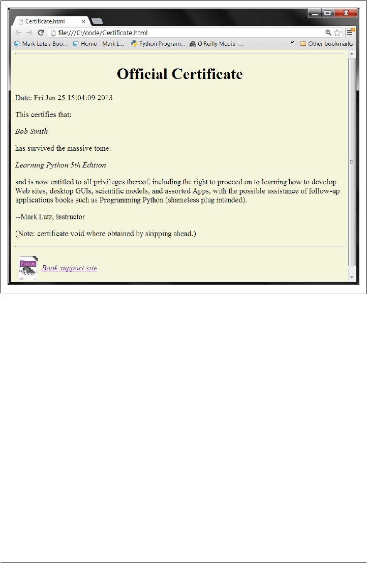


APPENDIX A
Installation and Configuration
This appendix provides additional installation and configuration details as a resource
for people new to these topics. It’s located here because not all readers will need to deal
with these subjects up front. Because it covers some peripheral topics such as environ-
ment variables and command-line arguments, though, this material probably merits at
least a quick scan for most readers.
Installing the Python Interpreter
Because you need the Python interpreter to run Python scripts, the first step in using
Python is usually installing Python. Unless one is already available on your machine,
you’ll need to fetch, install, and possibly configure a recent version of Python on your
computer. You’ll only need to do this once per machine, and if you will be running a
frozen binary (described in Chapter 2) or self-installing system, your setup tasks may
be trivial or null.
Is Python Already Present?
Before you do anything else, check whether you already have a recent Python on your
machine. If you are working on Linux, Mac OS X, or some Unix systems, Python is
probably already installed on your computer, though it may be one or two releases
behind the cutting edge. Here’s how to check:
• On Windows 7 and earlier, check whether there is a Python entry in the Start but-
ton’s All Programs menu (at the bottom left of the screen). On Windows 8, look
for Python in a Start screen tile, your Search tool, the “All apps” display on your
Start screen, or a File Explorer in desktop mode (more on Windows 8 in an up-
coming sidebar).
• On Mac OS X, open a Terminal window (Applications→Utilities→Terminal) and
type python at the prompt. Python, IDLE, and its tkinter GUI toolkit are standard
components of this system.
1421
www.it-ebooks.info

• On Linux and Unix, type python at a shell prompt (a.k.a. terminal window), and
see what happens. Alternatively, try searching for “python” in the usual places
—/usr/bin, /usr/local/bin, etc. As on Macs, Python is a standard part of Linux sys-
tems.
If you find a Python, make sure it’s a recent version. Although any recent Python will
do for most of this text, this edition focuses on Python 3.3 and 2.7 specifically, so you
may want to install one of these to run some of the examples in this book.
Speaking of versions, per the preface, I recommend starting out with Python 3.3 or later
if you’re learning Python anew and don’t need to deal with existing 2.X code; otherwise,
you should generally use Python 2.7. Some popular Python-based systems still use older
releases, though (2.6 and even 2.5 are still widespread), so if you’re working with ex-
isting systems be sure to use a version relevant to your needs; the next section describes
locations where you can fetch a variety of Python versions.
Where to Get Python
If there is no Python on your machine, you will need to install one yourself. The good
news is that Python is an open source system that is freely available on the Web and
very easy to install on most platforms.
You can always fetch the latest and greatest standard Python release from http://www
.python.org, Python’s official website. Look for the Downloads link on that page, and
choose a release for the platform on which you will be working. You’ll find prebuilt
self-installer files for Windows (run to install), Installer Disk Images for Mac OS X
(installed per Mac conventions), the full source code distribution (typically compiled
on Linux, Unix, or OS X machines to generate an interpreter), and more.
Although Python is standard on Linux these days, you can also find RPMs for Linux
on the Web (unpack them with rpm). Python’s website also has links to pages where
versions for other platforms are maintained, either at Python.org (http://www.python
.org) itself or offsite. For example, you can find third-party Python installers for Goo-
gle’s Android, as well as apps to install Python on Apple’s iOS.
A Google web search is another great way to find Python installation packages. Among
other platforms, you can find Python prebuilt for iPods, Palm handhelds, Nokia cell
phones, PlayStation and PSP, Solaris, AS/400, and Windows Mobile, though some of
these are typically a few releases behind the curve.
If you find yourself pining for a Unix environment on a Windows machine, you might
also be interested in installing Cygwin and its version of Python (see http://www.cygwin
.com). Cygwin is a GPL-licensed library and toolset that provides full Unix functionality
on Windows machines, and it includes a prebuilt Python that makes use of all the Unix
tools provided.
1422 | Appendix A: Installation and Configuration
www.it-ebooks.info

You can also find Python on CD-ROMs supplied with Linux distributions, included
with some products and computer systems, and enclosed with some other Python
books. These tend to lag behind the current release somewhat, but usually not seriously
so.
In addition, you can find Python in some free and commercial development bundles.
At this writing, this alternative distributions category includes:
ActiveState ActivePython
A package that combines Python with extensions for scientific, Windows, and
other development needs, including PyWin32 and the PythonWin IDE
Enthought Python Distribution
A combination of Python and a host of additional libraries and tools oriented to-
ward scientific computing needs
Portable Python
A blend of Python and add-on packages configured to run directly from a portable
device
Pythonxy
A scientific-oriented Python distribution based on Qt and Spyder
Conceptive Python SDK
A bundle targeted at business, desktop, and database applications
PyIMSL Studio
A commercial distribution for numerical analysis
Anaconda Python
A distribution for analysis and visualization of large data sets
This set is prone to change, so search the Web for details on all of the above, and others.
Some of these are free, some are not, and some have both free and nonfree versions.
All combine the standard Python freely available at http://www.python.org with addi-
tional tools, but can simplify install tasks for many.
Finally, if you are interested in alternative Python implementations, run a web search
to check out Jython (the Python port to the Java environment) and IronPython (Python
for the C#/.NET world), both of which are described in Chapter 2. Installation of these
systems is beyond the scope of this book.
Installation Steps
Once you’ve downloaded Python, you need to install it. Installation steps are very
platform-specific, but here are a few pointers for the major Python platforms (biased
in volume toward Windows, only because that is the platform where most Python
newcomers are likely to encounter the language first):
Installing the Python Interpreter | 1423
www.it-ebooks.info

Windows
For Windows (including XP, Vista, 7, and 8), Python comes as a self-installer MSI
program file—simply double-click on its file icon, and answer Yes or Next at every
prompt to perform a default install. The default install includes Python’s docu-
mentation set and support for tkinter (Tkinter in Python 2.X) GUIs, shelve data-
bases, and the IDLE development GUI. Python 3.3 and 2.7 are normally installed
in the directories C:\Python33 and C:\Python27 though this can be changed at
install time.
For convenience, on Windows 7 and earlier Python shows up after the install in
the Start button’s All Programs menu (see ahead for Windows 8 notes). Python’s
menu there has five entries that give quick access to common tasks: starting the
IDLE user interface, reading module documentation, starting an interactive ses-
sion, reading Python’s standard manuals, and uninstalling. Most of these options
involve concepts explored in detail elsewhere in this text.
When installed on Windows, Python also automatically uses filename associa-
tions to register itself to be the program that opens Python files when their icons
are clicked (a program launch technique described in Chapter 3). It is also possible
to build Python from its source code on Windows, but this is not commonly done
so we’ll skip the details here (see python.org).
Three additional install-related notes for Windows users: first, be sure to see the
next appendix for an introduction to the new Windows launcher shipped with 3.3;
it changes some of the rules for installation, file associations, and command lines,
but can be an asset if you have multiple Python versions on your computer (e.g.,
both 2.X and 3.X). Per Appendix B, Python 3.3’s MSI installer also has an option
to set your PATH variable to include Python’s directory.
Second, Windows 8 users should see the sidebar in this appendix “Using Python
on Windows 8” on page 1425. Standard Python installs and works the same on
Windows 8, where it runs in desktop mode, but you won’t get the Start button
menu described earlier, and the tablet interface on top is not yet directly supported.
Finally, some Windows Vista users may run into install issues related to security
features. This seems to have been resolved over time (and Vista is relatively rare
these days), but if running the MSI installer file directly doesn’t work as expected,
it’s probably because MSI files are not true executables and do not correctly inherit
administrator permissions (they run per the registry). To fix, run the installer from
a command line with appropriate permissions: Select Command Prompt, choose
“Run as administrator,” cd to the directory where your Python MSI file resides,
and run the MSI installer with a command line of the form: msiexec /i
python-2.5.1.msi.
Linux
For Linux, if Python or your desired flavor of it is not already present, you can
probably obtain it as one or more RPM files, which you unpack in the usual way
(consult the RPM manpage for details). Depending on which RPMs you download,
1424 | Appendix A: Installation and Configuration
www.it-ebooks.info

there may be one for Python itself, and another that adds support for tkinter GUIs
and the IDLE environment. Because Linux is a Unix-like system, the next para-
graph applies as well.
Unix
For Unix systems, Python is usually compiled from its full C source code distri-
bution. This usually only requires you to unpack the file and run simple config
and make commands; Python configures its own build procedure automatically,
according to the system on which it is being compiled. However, be sure to see the
package’s README file for more details on this process. Because Python is open
source, its source code may be used and distributed free of charge.
On other platforms the installation details can differ widely, but they generally follow
the platform’s normal conventions. For example, installing the “Pippy” port of Python
for PalmOS required a hotsync operation with your PDA, and Python for the Sharp
Zaurus Linux-based PDA was one or more .ipk files, which you simply ran to install
(these likely still work, though finding the devices today may be a logistical challenge!).
More recently, Python can be installed and used on Android and iOS platforms too,
but installation and usage techniques are too platform-specific to cover here. For ad-
ditional install procedures and the latest on available ports, try both Python’s website
and a web search.
Using Python on Windows 8
Windows 8 was released as this edition was being written. As mentioned in the preface,
this book was developed on both Windows 7 and 8, but mostly under Windows 7
because the choice is irrelevant to almost everything in this book—both Python 2.X
and 3.X presently work only in desktop mode on Windows 8, but install and run there
the same as in Windows 7, Vista, XP, and others. Once you navigate past the tablet-
like layer at the top, usage is almost entirely as before.
The only notable exception to this is Windows 8’s lack of a Start button menu in desktop
mode. You don’t get the nice menu of Python options automatically, though you can
simulate it manually. Although this story is prone to change (and you should take this
sidebar as an early report), here are a few Windows 8 usage notes.
At this writing, the standard Python Windows MSI installer program installs Python
on Windows 8 correctly, and exactly as in the past: you get the same filename associ-
ations for icon clicks, access from command lines, and so on. The installer also creates
a Start screen button on Windows 8, but Python itself runs in Windows 8’s desktop
mode, which is essentially the same as Windows 7 without a Start button menu. For
example, the Windows 8 Start screen button created by the Python install simply
switches control to desktop mode to open a Python interactive shell.
The upside to this is that all existing Python software works on Windows 8’s desktop
just as before. One downside is that you’ll need to create shortcuts for the user-friendly
Start button menu items created automatically on former Windows versions. This in-
Installing the Python Interpreter | 1425
www.it-ebooks.info

cludes the former menu’s links to the IDLE GUI, PyDoc, Python’s command-line in-
terface, and Python’s manuals set.
This isn’t a showstopper—you can emulate the former Start button menu’s items with
either tiles on the Start screen or shortcuts on the desktop taskbar. To do so, you might
look up these tools in a variety of ways:
• By navigating to their corresponding filename in a File Explorer, opened by right-
clicking the screen’s lower-left corner.
• By searching for their name in the Search “charm,” opened by pulling down the
screen’s top-right corner.
• By finding their entry after right-clicking on the Start screen to open the All apps
display, which is reminiscent of the former Start button menus.
• By locating their tiles on your Start screen, if they have any.
For example, you can locate IDLE by navigating to the file idle.py in C:\Python33\Lib,
by searching on “idle,” by finding IDLE in “All apps,” or by clicking a Start screen tile
if one exists. You can find Python itself in the same ways (and probably others). This
isn’t quite as nice as the original Start button menus out of the box, but it suffices.
Probably the bigger potential downside on Windows 8 is that while Python runs fine in
desktop mode, it doesn’t yet have an official port to run as a Start screen style “app.”
That is, standard Python does not yet run programs in the WinRT (formerly known as
Metro) environment—the tile-based media consumption layer that appears first when
you start Windows 8, and before you can click your way to the desktop. This may be
a temporary state, though, as a number of options either already exist or are being
actively explored.
On one front, it’s not impossible that Python’s installer may be enhanced for Windows
8’s nondesktop mode. There has already been work on porting Python to run as a Start
screen “app,” though this may appear as a separate installer package due to differences
in the underlying libraries (in short, WinRT runs programs in a classic “sandbox”
model, with a restricted subset of the libraries available normally).
On other fronts, the C#/.NET-based IronPython system may offer additional Windows
8 “app” development options, and some of Python’s major GUI toolkits such as tkinter,
wxPython, and PyQt could eventually provide portability to the Windows 8 “apps”
environment as well. The Qt library underlying the latter of these seems to have already
showed some progress in this department.
For now, existing Python software runs fine in Windows 8’s desktop mode unchanged.
Developing or running Python code in the Start screen “apps” environment will likely
require special handling and platform-specific APIs not unlike those required to run
Python on other tablet- and phone-oriented platforms based on Google’s Android and
Apple’s iOS (iPhone and iPad) operating systems.
Also note that much of this sidebar applies to Window 8, but not Windows RT. The
latter does not run third-party desktop mode applications directly, and may need to
await a sanctioned Python installer that supports the WinRT “app” API in general.
1426 | Appendix A: Installation and Configuration
www.it-ebooks.info

Then again, the Windows 8 story remains to be told. Be sure to watch for developments
in both Windows and Python’s installer for it. For now, a simple tile click or Windows-
key press to hop into desktop mode will allow most Python programmers on Windows
to safely ignore the tablet-like interface on top—at least until “apps” trounce “pro-
grams” altogether.1
Configuring Python
After you’ve installed Python, you may want to configure some system settings that
impact the way Python runs your code. (If you are just getting started with the language,
you can probably skip this section completely; there is usually no need to specify any
system settings for basic programs.)
Generally speaking, parts of the Python interpreter’s behavior can be configured with
environment variable settings and command-line options. In this section, we’ll take a
brief look at both, but be sure to see other documentation sources for more details on
the topics we introduce here.
Python Environment Variables
Environment variables—known to some as shell variables, or DOS variables—are sys-
tem-wide settings that live outside Python and thus can be used to customize the in-
terpreter’s behavior each time it is run on a given computer. Python recognizes a handful
of environment variable settings, but only a few are used often enough to warrant ex-
planation here. Table A-1 summarizes the main Python-related environment variable
settings (you’ll find information on others in Python reference resources).
Table A-1. Important environment variables
Variable Role
PATH (or path) System shell search path (for finding “python”)
PYTHONPATH Python module search path (for imports)
PYTHONSTARTUP Path to Python interactive startup file
TCL_LIBRARY, TK_LIBRARY GUI extension variables (tkinter)
PY_PYTHON, PY_PYTHON3, PY_PYTHON2 Windows launcher defaults (see Appendix B)
These variables are straightforward to use, but here are a few pointers:
1. Lest that seem too sarcastic, I should note that Windows 8.1 may address some launch screen and
Start button (if not menu) concerns per late-breaking rumors, and this edition's new Windows 8
sidebar replaces one in prior editions that discussed a Windows Vista issue. Any similarities you might
deduce from that are officially coincidental.
Configuring Python | 1427
www.it-ebooks.info

PATH
The PATH setting lists a set of directories that the operating system searches for
executable programs, when they are invoked without a full directory path. It should
normally include the directory where your Python interpreter lives (the python
program on Unix, or the python.exe file on Windows).
You don’t need to set this variable at all if you are willing to work in the directory
where Python resides, or type the full path to Python in command lines. On Win-
dows, for instance, the PATH is irrelevant if you run a cd C:\Python33 before running
any code (to change to the directory where Python lives—though you shouldn’t
generally store your own code in this directory per Chapter 3), or always type
C:\Python33\python instead of just python (giving a full path).
Also note that PATH settings are mostly for launching programs from command
lines; they are usually irrelevant when launching via icon clicks and IDEs—the
former uses filename associations, and the latter uses built-in mechanisms, and
doesn’t generally require this configuration step. See also Appendix B for details
on 3.3’s automatic PATH setting option at install time.
PYTHONPATH
The PYTHONPATH setting serves a role similar to PATH: the Python interpreter consults
the PYTHONPATH variable to locate module files when you import them in a program.
If used, this variable is set to a platform-dependent list of directory names, sepa-
rated by colons on Unix and semicolons on Windows. This list normally includes
just your own source code directories. Its content is merged into the sys.path
module import search path, along with the script’s container directory, any .pth
path file settings, and standard library directories.
You don’t need to set this variable unless you will be performing cross-directory
imports—because Python always searches the home directory of the program’s top-
level file automatically, this setting is required only if a module needs to import
another module that lives in a different directory. See also the discussion of .pth
path files later in this appendix for an alternative to PYTHONPATH. For more on the
module search path, refer to Chapter 22.
PYTHONSTARTUP
If PYTHONSTARTUP is set to the pathname of a file of Python code, Python executes
the file’s code automatically whenever you start the interactive interpreter, as
though you had typed it at the interactive command line. This is a rarely used but
handy way to make sure you always load certain utilities when working interac-
tively; it saves an import each time you start a Python session.
tkinter settings
If you wish to use the tkinter GUI toolkit (named Tkinter in 2.X), you might have
to set the two GUI variables in the last line of Table A-1 to the names of the source
library directories of the Tcl and Tk systems (much like PYTHONPATH). However,
these settings are not required on Windows systems (where tkinter support is
installed alongside Python), and are usually not required on Mac OS X and Linux
1428 | Appendix A: Installation and Configuration
www.it-ebooks.info

systems, unless the underlying Tcl and Tk libraries are either invalid or reside in
nonstandard directories (see python.org’s Download page for more details).
PY_PYTHON, PY_PYTHON3, PY_PYTHON2
These settings are used to specify default Pythons when you are using the new (at
this writing) Windows launcher that ships with Python 3.3 and is available sepa-
rately for other versions. Since we’ll be exploring the launcher in Appendix B, I’ll
postpone further details here.
Note that because these environment settings are external to Python itself, when you
set them is usually irrelevant: this can be done before or after Python is installed, as
long as they are set the way you require before Python is actually run—be sure to restart
your Python IDEs and interactive sessions after making such changes if you want them
to apply.
tkinter and IDLE GUIs on Linux and Macs
The IDLE interface described in Chapter 3 is a Python tkinter GUI program. The
tkinter module (named Tkinter in 2.X) is a GUI toolkit that is automatically installed
with standard Python on Windows, and is an inherent part of Mac OS X and most
Linux installations.
On some Linux systems, though, the underlying GUI library may not be a standard
installed component. To add GUI support to your Python on Linux if needed, try run-
ning a command line of the form yum tkinter to automatically install tkinter’s under-
lying libraries. This should work on Linux distributions (and some other systems) on
which the yum installation program is available; for others, see your platform’s instal-
lation documentation.
As also discussed in Chapter 3, on Mac OS X IDLE probably lives in the MacPython
(or Python N.M) folder of your Applications folder (along with PythonLauncher, used
for starting programs with clicks in Finder), but be sure to see the Download page at
python.org if IDLE has problems; you may need to install an update on some OS X
versions (see Chapter 3).
How to Set Configuration Options
The way to set Python-related environment variables, and what to set them to, depends
on the type of computer you’re working on. And again, remember that you won’t
necessarily have to set these at all right away; especially if you’re working in IDLE
(described in Chapter 3) and save all your files in the same directory, configuration is
probably not required up front.
But suppose, for illustration, that you have generally useful module files in directories
called utilities and package1 somewhere on your machine, and you want to be able to
import these modules from files located in other directories. That is, to load a file called
Configuring Python | 1429
www.it-ebooks.info

spam.py in either the utilities or package1 directories, you want to be able to say this in
another file in another directory:
import spam
To make this work, you’ll have to configure your module search path one way or an-
other to include the directory containing spam.py. Here are a few tips on this process
using PYTHONPATH as an example; do the same for other settings like PATH as needed
(though 3.3 can set PATH automatically: see Appendix B).
Unix/Linux shell variables
On Unix systems, the way to set environment variables depends on the shell you use.
Under the csh shell, you might add a line like the following in your .cshrc or .login file
to set the Python module search path:
setenv PYTHONPATH /usr/home/pycode/utilities:/usr/lib/pycode/package1
This tells Python to look for imported modules in two user-defined directories. Alter-
natively, if you’re using the ksh shell, the setting might instead appear in your .kshrc
file and look like this:
export PYTHONPATH="/usr/home/pycode/utilities:/usr/lib/pycode/package1"
Other shells may use different (but analogous) syntax.
DOS variables (and older Windows)
If you are using MS-DOS or some now fairly old flavors of Windows, you may need to
add an environment variable configuration command to your C:\autoexec.bat file, and
reboot your machine for the changes to take effect. The configuration command on
such machines has a syntax unique to DOS:
set PYTHONPATH=c:\pycode\utilities;d:\pycode\package1
You can type such a command in a DOS console window, too, but the setting will then
be active only for that one console window. Changing your .bat file makes the change
permanent and global to all programs, though this technique has been superseded in
recent years by that described in the next section.
Windows environment variable GUI
On all recent versions of Windows (including XP, Vista, 7, and 8), you can instead set
PYTHONPATH and other variables via the system environment variable GUI without having
to edit files, type command lines, or reboot. Select the Control Panel (in your Start
button in Windows 7 and earlier, and in the desktop mode’s Settings “charm” on
Windows 8), choose the System icon, pick the Advanced settings tab or link, and click
the Environment Variables button at the bottom to edit or add new variables (PYTHON
PATH is usually a new user variable). Use the same variable name and values syntax
1430 | Appendix A: Installation and Configuration
www.it-ebooks.info

shown in the DOS set command in the preceding section. On Vista you may have to
verify operations along the way.
You do not need to reboot your machine after this, but be sure to restart Python if it’s
open so that it picks up your changes—it configures its import search path at startup
time only. If you’re working in a Windows Command Prompt window, you’ll probably
need to restart that to pick up your changes as well.
Windows registry
If you are an experienced Windows user, you may also be able to configure the module
search path by using the Windows Registry Editor. To open this tool, type regedit in
the Start→Run... interface on some Windows, in the search field at the bottom of the
Start button display on Windows 7, and in a Command Prompt window on Windows
8 and others (among other routes). Assuming the typical registry tool is available on
your machine, you can then navigate to Python’s entries and make your changes. This
is a delicate and error-prone procedure, though, so unless you’re familiar with the
registry, I suggest using other options (indeed, this is akin to performing brain surgery
on your computer, so be careful!).
Path files
Finally, if you choose to extend the module search path with a .pth path file instead of
the PYTHONPATH variable, you might instead code a text file that looks like the following
on Windows (e.g., file C:\Python33\mypath.pth):
c:\pycode\utilities
d:\pycode\package1
Its contents will differ per platform, and its container directory may differ per both
platform and Python release. Python locates this file automatically when it starts up.
Directory names in path files may be absolute, or relative to the directory containing
the path file; multiple .pth files can be used (all their directories are added), and .pth
files may appear in various automatically checked directories that are platform- and
version-specific. In general, a Python release numbered Python N.M typically looks for
path files in C:\PythonNM and C:\PythonNM\Lib\site-packages on Windows, and in /
usr/local/lib/pythonN.M/site-packages and /usr/local/lib/site-python on Unix and Linux.
See Chapter 22 for more on using path files to configure the sys.path import search
path.
Because environment settings are often optional, and because this isn’t a book on op-
erating system shells, I’ll defer to other sources for further details. Consult your system
shell’s manpages or other documentation for more information, and if you have trouble
figuring out what your settings should be, ask your system administrator or another
local expert for help.
Configuring Python | 1431
www.it-ebooks.info

Python Command-Line Arguments
When you start Python from a system command line (a.k.a. a shell prompt, or Com-
mand Prompt window), you can pass in a variety of option flags to control how Python
runs your code. Unlike the system-wide environment variables of the prior section,
command-line arguments can be different each time you run a script. The complete
form of a Python command-line invocation in 3.3 looks like this (2.7 is roughly the
same, with a few differences described ahead):
python [-bBdEhiOqsSuvVWxX] [-c command | -m module-name | script | - ] [args]
The rest of this section briefly demonstrates some of Python’s most commonly used
arguments. For more details on available command-line options not covered here, see
the Python manuals or reference texts. Or better yet, ask Python itself—run a command
line form like this:
C:\code> python -h
to request Python’s help display, which documents all available command-line options.
If you deal with complex command lines, be sure to also check out the standard library
modules in this domain: the original getop, the newer argparse, and the now-depre-
cated (since 3.2) optparse, which support more sophisticated command-line process-
ing. Also see Python’s library manuals and other references for more on the pdb and
profile modules the following tour deploys.
Running script files with arguments
Most command lines make use of only the script and args parts of the last section’s
Python command-line format, to run a program’s source file with arguments to be used
by the program itself. To illustrate, consider the following script—a text file named
showargs.py, created in directory C:\code or another of your choosing—which prints
the command-line arguments made available to the script as sys.argv, a Python list of
Python strings (if you don’t yet know how to create or run Python script files, see the
full coverage in Chapter 2 and Chapter 3; we’re interested only in command-line ar-
guments here):
# File showargs.py
import sys
print(sys.argv)
In the following command line, both python and showargs.py can also be complete
directory paths—the former is assumed to be on your PATH here, and the latter is as-
sumed to be in the current directory. The three arguments (a b –c) meant for the script
show up in the sys.argv list and can be inspected by your script’s code there; the first
item in sys.argv is always the script file’s name, when it is known:
C:\code> python showargs.py a b -c # Most common: run a script file
['showargs.py', 'a', 'b', '-c']
1432 | Appendix A: Installation and Configuration
www.it-ebooks.info

As covered elsewhere in this book, Python lists print in square brackets and strings
display in quotes.
Running code given in arguments and standard input
Other code format specification options allow you to give Python code to be run on
the command line itself (-c), and accept code to run from the standard input stream (a
– means read from a pipe or redirected input stream file, terms also defined in full
elsewhere in this text):
C:\code> python -c "print(2 ** 100)" # Read code from command argument
1267650600228229401496703205376
C:\code> python -c "import showargs" # Import a file to run its code
['-c']
C:\code> python - < showargs.py a b -c # Read code from standard input
['-', 'a', 'b', '-c']
C:\code> python - a b -c < showargs.py # Same effect as prior line
['-', 'a', 'b', '-c']
Running modules on the search path
The –m code specification locates a module on Python’s module search path and then
runs it as a top-level script (as module __main__). That is, it looks up a script the same
way import operations do, using the directory list normally known as sys.path, which
includes the current directory, PYTHONPATH settings, and standard libraries. Leave off the
“.py” suffix here, as the filename is treated as a module.
C:\code> python -m showargs a b -c # Locate/run module as script
['c:\\code\\showargs.py', 'a', 'b', '-c']
The –m option also supports running tools, modules in packages with and without
relative import syntax, and modules located in .zip archives. For instance, this switch
is commonly used to run the pdb debugger and profile profiler modules from a com-
mand line for a script invocation, rather than interactively:
C:\code> python # Interactve debugger session
>>> import pdb
>>> pdb.run('import showargs')
...more omitted: see pdb docs
C:\code> python -m pdb showargs.py a b -c # Debugging a script (c=continue)
> C:\code\showargs.py(2)<module>()
-> import sys
(Pdb) c
['showargs.py', 'a', 'b', '-c']
...more omitted: q to exit
The profiler runs and times your code; its output can vary per Python, operating system,
and computer:
Configuring Python | 1433
www.it-ebooks.info

C:\code> python -m profile showargs.py a b -c # Profiling a script
['showargs.py', 'a', 'b', '-c']
9 function calls in 0.016 seconds
Ordered by: standard name
ncalls tottime percall cumtime percall filename:lineno(function)
2 0.000 0.000 0.000 0.000 :0(charmap_encode)
1 0.000 0.000 0.000 0.000 :0(exec)
...more omitted: see profile docs
You might also use the -m switch to spawn Chapter 3’s IDLE GUI program located in
the standard library from any other directory, and to start the pydoc and timeit tools
modules with command lines as we do in this book in Chapter 15 and Chapter 21 (see
those chapters for more details on the tools launched here):
c:\code> python -m idlelib.idle -n # Run IDLE in package, no subprocess
c:\code> python -m pydoc -b # Run pydoc and timeit tools modules
c:\code> python -m timeit -n 1000 -r 3 -s "L = [1,2,3,4,5]" "M = [x + 1 for x in L]"
Optimized and unbuffered modes
Immediately after the “python” and before the designation of code to be run, Python
accepts additional arguments that control its own behavior. These arguments are con-
sumed by Python itself and are not meant for the script being run. For example, -O runs
Python in optimized mode and -u forces standard streams to be unbuffered—with the
latter, any printed text will be finalized immediately, and won’t be delayed in a buffer:
C:\code> python -O showargs.py a b -c # Optimized: make/run ".pyo" byte code
C:\code> python -u showargs.py a b -c # Unbuffered standard output stream
Post-run interactive mode
Finally, the –i flag enters interactive mode after running a script—especially useful as
a debugging tool, because you can print variables’ final values after a successful run to
get more details:
C:\code> python -i showargs.py a b -c # Go to interactive mode on script exit
['showargs.py', 'a', 'b', '-c']
>>> sys # Final value of sys: imported module
<module 'sys' (built-in)>
>>> ^Z
You can also print variables this way after an exception shuts down your script to see
what they looked like when the exception occurred, even if not running in debug mode
—though you can start the debugger’s postmortem tool here as well (type is the Win-
dows file display command; try a cat or other elsewhere):
C:\code> type divbad.py
X = 0
1434 | Appendix A: Installation and Configuration
www.it-ebooks.info

print(1 / X)
C:\code> python divbad.py # Run the buggy script
...error text omitted
ZeroDivisionError: division by zero
C:\code> python -i divbad.py # Print variable values at error
...error text omitted
ZeroDivisionError: division by zero
>>> X
0
>>> import pdb # Start full debugger session now
>>> pdb.pm()
> C:\code\divbad.py(2)<module>()
-> print(1 / X)
(Pdb) quit
Python 2.X command-line arguments
Besides those just mentioned, Python 2.7 supports additional options that promote 3.X
compatibility (−3 to warn about incompatibilities, and –Q to control division operator
models) and detecting inconsistent tab indentation usage, which is always detected and
reported in 3.X (-t; see Chapter 12). Again, you can always ask Python 2.X itself for
more on the subject as needed:
C:\code> c:\python27\python -h
Python 3.3 Windows Launcher Command Lines
Technically, the preceding section described the arguments you can pass to the Python
interpreter itself—the program usually named python.exe on Windows, and python on
Linux (the .exe is normally omitted on Windows). As we’ll see in the next appendix,
the Windows launcher shipped with Python 3.3 augments this story for users of 3.3
and later or the standalone launcher package. It adds new executables that accept
Python version numbers as arguments in command lines used to start Python and your
scripts (file what.py is listed and described in the next appendix, and simply prints the
Python version number):
C:\code> py what.py # Windows launcher command lines
3.3.0
C:\code> py −2 what.py # Version number switch
2.7.3
C:\code> py −3.3 -i what.py -a -b -c # Arguments for all 3: py, python, script
3.3.0
>>> ^Z
In fact, as the last run of the preceding example shows, command lines using the
launcher can give arguments for the launcher itself (−3.3), Python itself (-i), and your
script (-a, -b, and -c). The launcher can also parse version numbers out of #! Unix lines
Configuring Python | 1435
www.it-ebooks.info

at the top of script files instead. Because the next appendix is devoted to this launcher
entirely, though, you’ll have to read on for the rest of this story.
For More Help
Python’s standard manual set today includes valuable pointers for usage on various
platforms. The standard manual set is available in your Start button on Windows 7 and
earlier after Python is installed (option “Python Manuals”), and online at http://www
.python.org. Look for the manual set’s top-level section titled “Using Python” for more
platform-specific pointers and hints, as well as up-to-date cross-platform environment
and command-line details.
As always, the Web is your ally, too, especially in a field that often evolves faster than
books like this can be updated. Given Python’s widespread adoption, chances are good
that answers to any high-level usage questions you may have can be found with a web
search.
1436 | Appendix A: Installation and Configuration
www.it-ebooks.info

APPENDIX B
The Python 3.3 Windows Launcher
This appendix describes the new Windows launcher for Python, installed with Python
3.3 automatically, and available separately on the Web for use with older versions.
Though the new launcher comes with some pitfalls, it provides some much-needed
coherence for program execution when multiple Pythons coexist on the same com-
puter.
I’ve written this page for programmers using Python on Windows. Though it is plat-
form-specific by nature, it’s targeted at both Python beginners (most of whom get
started on this platform), as well as Python developers who write code to work portably
between Windows and Unix. As we will see, the new launcher changes the rules on
Windows radically enough to impact everyone who uses Python on Windows, or may
in the future.
The Unix Legacy
To fully understand the launcher’s protocols, we have to begin with a short history
lesson. Unix developers long ago devised a protocol for designating a program to run
a script’s code. On Unix systems (including Linux and Mac OS X), the first line in a
script’s text file is special if it begins with a two-character sequence: #!, sometimes
called a shebang (an arguably silly phrase I promise not to repeat from here on).
Chapter 3 gives a brief overview of this topic, but here’s another look. In Unix scripts,
such lines designate a program to run the rest of the script’s contents, by coding it after
the #!—using either the directory path to the desired program itself, or an invocation
of the env Unix utility that looks up the target per your PATH setting, the customizable
system environment variable that lists directories to be searched for executables:
#!/usr/local/bin/python
...script's code # Run under this specific program
#!/usr/bin/env python
...script's code # Run under "python" found on PATH
1437
www.it-ebooks.info

By making such a script executable (e.g., via chmod +x script.py), you can run it by
giving just its filename in a command line; the #! line at the top then directs the Unix
shell to a program that will run the rest of the file’s code. Depending on the platform’s
install structure, the python that these #! lines name might be a real executable, or a
symbolic link to a version-specific executable located elsewhere. These lines might also
name a more specific executable explicitly, such as python3. Either way, by changing
#! lines, symbolic links, or PATH settings, Unix developers can route a script to the
appropriate installed Python.
None of this applies to Windows itself, of course, where #! lines have no inherent
meaning. Python itself has historically ignored such lines as comments if present on
Windows (“#” starts a comment in the language). Still, the idea of selecting Python
executables on a per-file basis is a compelling feature in a world where Python 2.X and
3.X often coexist on the same machine. Given that many programmers coded #! lines
for portability to Unix anyhow, the idea seemed ripe for emulating.
The Windows Legacy
The install model has been very different on the other side of the fence. In the past (well,
in every Python until 3.3), the Windows installer updated the global Windows registry
such that the latest Python version installed on your computer was the version that
opened Python files when they were clicked or run by direct filename in command lines.
Some Windows users may know this registry as filename associations, configurable in
Control Panel’s Default Programs dialog. You do not need to give files executable priv-
ileges for this to work, as you do for Unix scripts. In fact, there’s no such concept on
Windows—filename associations and commands suffice to launch files as programs.
Under this install model, if you wished to open a file with a different version than the
latest install, you had to run a command line giving the full path to the Python you
wanted, or update your filename associations manually to use the desired version. You
could also point generic python command lines to a specific Python by setting or chang-
ing your PATH setting, but Python didn’t set this for you, and this wouldn’t apply to
scripts launched by icon clicks and other contexts.
This reflects the natural order on Windows (when you click on a .doc file, Windows
usually opens it in the latest Word installed), and has been the state of things ever since
there was a Python on Windows. It’s less ideal if you have Python scripts that require
different versions on the same machine, though—a situation that has become increas-
ingly common, and perhaps even normal in the dual Python 2.X/3.X era. Running
multiple Pythons on Windows prior to 3.3 can be tedious for developers, and discour-
aging for newcomers.
1438 | Appendix B: The Python 3.3 Windows Launcher
www.it-ebooks.info

Introducing the New Windows Launcher
The new Windows launcher, shipped and installed automatically with Python 3.3 (and
presumably later), and available as a standalone package for use with other versions,
addresses these deficits in the former install model by providing two new executables:
•py.exe for console programs
•pyw.exe for nonconsole (typically GUI) programs
These two programs are registered to open .py and .pyw files, respectively, via Windows
filename associations. Like Python’s original python.exe main program (which they do
not deprecate but can largely subsume), these new executables are also registered to
open byte code files launched directly. Amongst their weapons, these two new execut-
ables:
• Automatically open Python source and byte-code files launched by icon clicks or
filename commands, via Windows associations
• Are normally installed on your system search path and do not require a directory
path or PATH settings when used as command lines
• Allow Python version numbers to be passed in easily as command-line arguments,
when starting both scripts and interactive sessions
• Attempt to parse Unix-style #! comment lines at the top of scripts to determine
which Python version should be used to run a file’s code
The net effect is that under the new launcher, when multiple Pythons are installed on
Windows, you are no longer limited to either the latest version installed or explicit/full
command lines. Instead, you can now select versions explicitly on both a per-file and
per-command basis, and specify versions in either partial or full form in both contexts.
Here’s how this works:
1. To select versions per file, use Unix-style top-of-script comments like these:
#!python2
#!/usr/bin/python2.7
#!/usr/bin/env python3
2. To select versions per command, use command lines of the following forms:
py −2 m.py
py −2.7 m.py
py −3 m.py
For example, the first of these techniques can serve as a sort of directive to declare which
Python version the script depends upon, and will be applied by the launcher whenever
the script is run by command line or icon click (these are variants of a file named
script.py):
Introducing the New Windows Launcher | 1439
www.it-ebooks.info

#!python3
...
...a 3.X script # Runs under latest 3.X installed
...
#!python2
...
...a 2.X script # Runs under latest 2.X installed
...
#!python2.6
...
...a 2.6 script # Runs under 2.6 (only)
...
On Windows, command lines are typed in a Command Prompt window, designated
by its C:\code> prompt in this appendix. The first of the following is the same as both
the second and an icon click, because of filename associations:
C:\code> script.py # Run per file's #! line if present, else per default
C:\code> py script.py # Ditto, but py.exe is run explicitly
Alternatively, the second technique just listed can select versions with argument
switches in command lines instead:
C:\code> py −3 script.py # Runs under latest 3.X
C:\code> py −2 script.py # Runs under latest 2.X
C:\code> py −2.6 script.py # Runs under 2.6 (only)
This works both when launching scripts and starting the interactive interpreter (when
no script is named):
C:\code> py −3 # Starts latest 3.X, interactive
C:\code> py −2 # Starts latest 2.X, interactive
C:\code> py −3.1 # Starts 3.1 (only), interactive
C:\code> py # Starts default Python (initially 2.X: see ahead)
If there are both #! lines in the file and a version number switch in the command line
used to start it, the command line’s version overrides that in the file’s directive:
#! python3.2
...
...a 3.X script
...
C\code> py script.py # Runs under 3.2, per file directive
C\code> py −3.1 script.py # Runs under 3.1, even if 3.2 present
The launcher also applies heuristics to select a specific Python version when it is missing
or only partly described. For instance, the latest 2.X is run when only a 2 is specified,
and a 2.X is preferred for files that do not name a version in a #! line when launched
by icon click or generic command lines (e.g., py m.py, m.py), unless you configure the
default to use 3.X instead by setting PY_PYTHON or a configuration file entry (more on
this ahead).
1440 | Appendix B: The Python 3.3 Windows Launcher
www.it-ebooks.info

Especially in the current dual 2.X/3.X Python world, explicit version selection seems a
useful addition for Windows, where many (and probably most) newcomers get their
first exposure to the language. Although it is not without potential pitfalls—including
failures on unrecognized Unix #! lines and a puzzling 2.X default—it does allow for a
more graceful coexistence of 2.X and 3.X files on the same machine, and provides a
rational approach to version control in command lines.
For the complete story on the Windows launcher, including more advanced features
and use cases I’ll either condense or largely omit here, see Python’s release notes and
try a web search to find the PEP (the proposal document). Among other things, the
launcher also allows selecting between 32- and 64-bit installs, specifying defaults in
configuration files, and defining custom #! command string expansion.
A Windows Launcher Tutorial
Some readers familiar with Unix scripting may find the prior section enough to get
started. For others, this section provides additional context in the form of a tutorial,
which gives concrete examples of the launcher in action for you to trace through. This
section also discloses additional launcher details along the way, though, so even well-
seasoned Unix veterans may benefit from a quick scan here before FTPing all their
Python scripts to the local Windows box.
To get started, we’ll be using the following simple script, what.py, which can be run
under both 2.X and 3.X to echo the version number of the Python that runs its code.
It uses sys.version—a string whose first component after splitting on whitespace is
Python’s version number:
#!python3
import sys
print(sys.version.split()[0]) # First part of string
If you want to work along, type this script’s code in your favorite text file editor, open
a Command Prompt window for typing the command lines we’ll be running, and cd to
the directory where you’ve save the script (C:\code is where I’m working, but feel free
to save this wherever you wish, and see Chapter 3 for more Windows usage pointers).
This script’s first-line comment serves to designate the required Python version; it must
begin with #! per Unix convention, and allows for a space before the python3 or not.
On my machine I currently have Pythons 2.7, 3,1, 3.2, and 3.3 all installed; let’s watch
which version is invoked as the script’s first line is modified in the following sections,
exploring file directives, command lines, and defaults along the way.
Step 1: Using Version Directives in Files
As this script is coded, when run by icon click or command line, the first line directs
the registered py.exe launcher to run using the latest 3.X installed:
A Windows Launcher Tutorial | 1441
www.it-ebooks.info

#! python3
import sys
print(sys.version.split()[0])
C:\code> what.py # Run per file directive
3.3.0
C:\code> py what.py # Ditto: latest 3.X
3.3.0
Again, the space after #! is optional; I added a space to demonstrate the point here.
Note that the first what.py command here is equivalent to both an icon click and a full
py what.py, because the py.exe program is registered to open .py files automatically in
the Windows filename associations registry when the launcher is installed.
Also note that when launcher documentation (including this appendix) talks about the
latest version, it means the highest-numbered version. That is, it refers to the latest
released, not the latest installed on your computer (e.g., if you install 3.1 after 3.3, #!
python3 selects the latter). The launcher cycles through the Pythons on your computer
to find the highest-numbered version that matches your specification or defaults; this
differs from the former last-installed-wins model.
Now, changing the first line name to python2 triggers the latest (really, highest-num-
bered) 2.X installed instead. Here’s this change at work; I’ll omit the last two lines of
our script from this point on because they won’t be altered:
#! python2
...rest of script unchanged
C:\code> what.py # Run with latest 2.X per #!
2.7.3
And you can request a more specific version if needed—for example, if you don’t want
the latest in a Python line:
#! python3.1
...
C:\code> what.py # Run with 3.1 per #!
3.1.4
This is true even if the requested version is not installed—which is treated as an error
case by the launcher:
#! python2.6
...
C:\code> what.py
Requested Python version (2.6) is not installed
Unrecognized Unix #! lines are also treated as errors, unless you give a version number
as a command-line switch to compensate, as the next section describes in more detail
(and as the section on launcher issues will revisit as a pitfall):
1442 | Appendix B: The Python 3.3 Windows Launcher
www.it-ebooks.info

#!/bin/python
...
C:\code> what.py
Unable to create process using '/bin/python "C:\code\what.py" '
C:\code> py what.py
Unable to create process using '/bin/python what.py'
C:\code> py −3 what.py
3.3.0
Technically, the launcher recognizes Unix-style #! lines at the top of script files that
follow one of the following four patterns:
#!/usr/bin/env python*
#!/usr/bin/python*
#!/usr/local/bin/python*
#!python*
Any #! line that does not take one of these recognized and parseable forms is assumed
to be a fully specified command line to start a process to run the file, which is passed
to Windows as is, and generates the error message we saw previously if it is not a valid
Windows command. (The launcher also supports “customized” command expansions
via its configuration files, which are attempted before passing unrecognized commands
on to Windows, but we’ll gloss over these here.)
In recognizable #! lines, directory paths are coded per Unix convention, for portability
to that platform. The * part at the end of the four preceding recognized patterns denotes
an optional Python version number, in one of three forms:
Partial (e.g., python3)
To run the version installed with the highest minor release number among those
with the major release number given
Full (e.g., python3.1)
To run that specific version only, optionally suffixed by −32 to prefer a 32-bit ver-
sion (e.g., python3.1-32)
Omitted (e.g., python)
To run the launcher’s default version, which is 2 unless changed (e.g., by setting
the PY_PYTHON environment variable to 3), another pitfall described ahead
Files with no #! line at all behave the same as those that name just a generic python—
the aforementioned omitted case—and are influenced by PY_PYTHON default settings.
The first case, partials, may also be affected by version-specific environment settings
(e.g., set PY_PYTHON3 to 3.1 to select 3.1 for python3, and set PY_PYTHON2 to 2.6 to pick
2.6 for python2). We'll revisit defaults later in this tutorial.
First, though, note that anything after the * part in a #! line’s format is assumed to be
command-line arguments to Python itself (i.e., program python.exe), unless you also
A Windows Launcher Tutorial | 1443
www.it-ebooks.info

give arguments in a py command line that are deemed to supersede #! line arguments
by the launcher:
#!python3 [any python.exe arguments go here]
...
These include all the Python command-line arguments we met in Appendix A. But this
leads us to launcher command lines in general, and will suffice as a natural segue to
the next section.
Step 2: Using Command-Line Version Switches
As mentioned, version switches on command lines can be used to select a Python ver-
sion if one isn’t present in the file. You run a py or pyw command line to pass them a
switch this way, instead of relying on filename associations in the registry, and instead
of (or in addition to) giving versions in #! lines in files. In the following, we modify our
script so that it has no #! directive:
# not a launcher directive
...
C:\code> py −3 what.py # Run per command-line switch
3.3.0
C:\code> py −2 what.py # Ditto: latest 2.X installed
2.7.3
C:\code> py −3.2 what.py # Ditto: 3.2 specifically (and only)
3.2.3
C:\code> py what.py # Run per launcher's default (ahead)
2.7.3
But command-line switches also take precedence over a version designation in a file’s
directive:
#! python3.1
...
C:\code> what.py # Run per file directive
3.1.4
C:\code> py what.py # Ditto
3.1.4
C:\code> py −3.2 what.py # Switches override directives
3.2.3
C:\code> py −2 what.py # Ditto
2.7.3
Formally, the launcher accepts the following command-line argument types (which
exactly mirror the * part at the end of a file’s #! line described in the prior section):
1444 | Appendix B: The Python 3.3 Windows Launcher
www.it-ebooks.info

−2 Launch the latest Python 2.X version
-3 Launch the latest Python 3.X version
-X.Y Launch the specified Python version (X is 2 or 3)
-X.Y−32 Launch the specified 32-bit Python version
And the launcher’s command lines take the following general form:
py [py.exe arg] [python.exe args] script.py [script.py args]
Anything following the launcher’s own argument (if present) is treated as though it
were passed to the python.exe program—typically, this includes any arguments for
Python itself, followed by the script filename, followed by any arguments meant for the
script.
The usual -m mod, -c cmd, and - program specification forms work in a py command
line too, as do all the other Python command-line arguments covered in Appendix A.
As mentioned earlier, arguments to python.exe can also appear at the end of the #!
directive line in a file, if used, though arguments in py command lines override them.
To see how this works, let’s write a new script that extends the prior to display com-
mand-line arguments; sys.argv is the script’s own arguments, and I’m using the Python
(python.exe) -i switch, which directs it to the interactive prompt (>>>) after a script
runs:
# args.py, show my arguments too
import sys
print(sys.version.split()[0])
print(sys.argv)
C:\code> py −3 -i args.py -a 1 -b -c # −3: py, -i: python, rest: script
3.3.0
['args.py', '-a', '1', '-b', '-c']
>>> ^Z
C:\code> py -i args.py -a 1 -b -c # Args to python, script
2.7.3
['args.py', '-a', '1', '-b', '-c']
>>> ^Z
C:\code> py −3 -c print(99) # −3 to py, rest to python: "-c cmd"
99
C:\code> py −2 -c "print 99"
99
Notice how the first two launches run the default Python unless a version is given in
the command line, because no #! line appears in the script itself. Somewhat coinci-
dentally, that leads us to the last topic of this tutorial.
Step 3: Using and Changing Defaults
As also mentioned, the launcher defaults to 2.X for a generic python in a #! directive
with no specific version number. This is true whether this generic form appears in a
A Windows Launcher Tutorial | 1445
www.it-ebooks.info

full Unix path (e.g., #!/usr/bin/python) or not (#!python). Here’s the latter case in
action, coded in our original what.py script:
#!python
... # Same as #!/usr/bin/python
C:\code> what.py # Run per launcher default
2.7.3
The default is also applied when no directive is present at all—perhaps the most com-
mon case for code written to be used on Windows primarily or exclusively:
# not a launcher directive
...
C:\code> what.py # Also run per default
2.7.3
C:\code> py what.py # Ditto
2.7.3
But you can set the launcher’s default to 3.X with initialization file or environment
variable settings, which will apply to both files run from command lines and by icon
clicks via their name’s association with py.exe or pyw.exe in the Windows registry:
# not a launcher directive
...
C:\code> what.py # Run per default
2.7.3
C:\code> set PY_PYTHON=3 # Or via Control Panel/System
C:\code> what.py # Run per changed default
3.3.0
As suggested earlier, for more fine-grained control you can also set version-specific
environment variables to direct partial selections to a specific release, instead of falling
back on the installed release with the highest minor number:
#!python3
...
C:\code> py what.py # Runs "latest" 3.X
3.3.0
C:\code> set PY_PYTHON3=3.1 # Use PY_PYTHON2 for 2.X
C:\code> py what.py # Override highest-minor choice
3.1.4
The set used in these interactions applies to its Command Prompt window only; mak-
ing such settings in the Control Panel’s System window will make them apply globally
across your machine (see Appendix A for help with these settings). You may or may
not want to set defaults this way depending on the majority of the Python code you’ll
1446 | Appendix B: The Python 3.3 Windows Launcher
www.it-ebooks.info

be running. Many Python 2.X users can probably rely on defaults unchanged, and
override them in #! lines or py command lines as needed.
However, the setting used for directive-less files, PY_PYTHON, seems fairly crucial. Most
programmers who have used Python on Windows in the past will probably expect 3.X
to be the default after installing 3.3, especially given that the launcher is installed by
3.3 in the first place—a seeming paradox, which leads us to the next section.
Pitfalls of the New Windows Launcher
Though the new Windows launcher in 3.3 is a nice addition, like much in 3.X it may
have been nicer had it appeared years ago. Unfortunately, it comes with some backward
incompatibilities, which may be an inevitable byproduct of today’s multiversion Python
world, but which may also break some existing programs. This includes examples in
books I’ve written, and probably many others. While porting code to 3.3, I’ve come
across three launcher issues worth noting:
• Unrecognized Unix !# lines now make scripts fail on Windows.
• The launcher defaults to using 2.X unless told otherwise.
• The new PATH extension is off by default and seems contradictory.
The rest of this section gives a rundown of each of these three issues in turn. In the
following, I use the programs in my book Programming Python, 4th Edition, as an
example to illustrate the impacts of launcher incompatibilities, because porting these
3.1/3.2 examples to 3.3 was my first exposure to the new launcher. In my specific case,
installing 3.3 broke numerous book examples that worked formerly under 3.2 and 3.1.
The causes for these failures outlined here may break your code too.
Pitfall 1: Unrecognized Unix !# Lines Fail
The new Windows launcher recognizes Unix #! lines that begin with #!/usr/bin/env
python but not the other common Unix form #!/bin/env python (which is actually
mandated on some Unixes). Scripts that use the latter of these, including some of my
book examples, worked on Windows in the past because their #! lines coded for Unix
compatibility have been ignored as comments by all Windows Pythons to date. These
scripts now fail to run in 3.3 because the new launcher doesn’t recognize their directive’s
format and posts an error message.
More generally, scripts with any #! Unix line not recognized will now fail to run on
Windows. This includes scripts having any first line that begins with a #! that is not
followed by one of the four recognized patterns described earlier: /usr/bin/env
python*, /usr/bin/python*, /usr/local/bin/python*, or python*. Anything else won’t
work, and requires code changes. For instance, a somewhat common #!/bin/python
line also causes a script to now fail on Windows, unless a version number is given in
command-line switches.
Pitfalls of the New Windows Launcher | 1447
www.it-ebooks.info

Unix-style #! lines probably aren’t present in Windows-only programs, but can be
common in programs meant to be run on Unix too. Treating unrecognized Unix di-
rectives as errors on Windows seems a bit extreme, especially given that this is new
behavior in 3.3, and will likely be unexpected. Why not just ignore unrecognized #!
lines and run the file with the default Python—like every Windows Python to date has?
It’s possible that this might be improved in a future 3.X release (there may be some
pushback on this), but today you must change any files using a #!/bin/env or other
unrecognized pattern, if you want them to run under the launcher installed with Python
3.3 on Windows.
Book examples impact and fix
With respect to the book examples I ported to 3.3, this broke roughly a dozen scripts
that started with #!/bin/env python. Regrettably, this includes some of the book’s user-
friendly and top-level demo launcher scripts (PyGadgets and PyDemos). To fix, I
changed these to use the accepted #!/usr/bin/env python form instead. Altering your
Windows file associations to omit the launcher altogether may be another option (e.g.,
associating .py files with python.exe instead of py.exe), but this negates the launcher’s
benefits, and seems a bit much to ask of users, especially newcomers.
One open issue here: strangely, passing any command-line switch to the launcher, even
a python.exe argument, seems to negate this effect and fall back on the default Python
—m.py and py m.py both issue errors on unrecognized #! lines, but py -i m.py runs
such a file with the default Python. This seems a possible launcher bug, but also relies
on the default, the subject of the next issue.
Pitfall 2: The Launcher Defaults to 2.X
Oddly, the Windows 3.3 launcher defaults to using an installed Python 2.X when run-
ning scripts that don’t select 3.X explicitly. That is, scripts that either have no #! di-
rective or use one that names python generically will be run by a 2.X Python by default
when launched by icon clicks, direct filename command lines (m.py), or launcher com-
mand lines that give no version switch (py m.py). This is true even if 3.3 is installed after
a 2.X on your machine, and has the potential to make many 3.X scripts fail initially.
The implications of this are potentially broad. As one example, clicking the icon of a
directive-less 3.X file just after installing 3.3 may now fail, because the associated
launcher assumes you mean to use 2.X by default. This probably won’t be a pleasant
first encounter for some Python newcomers! This assumes the 3.X file has no #! direc-
tive that provides an explicit python3 version number, but most scripts meant to run
on Windows won’t have a #! line at all, and many files coded before the launcher came
online won’t accommodate its version number expectations. Most 3.X users will be
basically compelled to set PY_PYTHON after installing 3.3—hardly a usability win.
Program launches that don’t give an explicit version number might be arguably am-
biguous on Unix too, and often rely on symbolic links from python to a specific version
1448 | Appendix B: The Python 3.3 Windows Launcher
www.it-ebooks.info

(which is most likely 2.X today—a state the new Windows launcher seems to emulate).
But as for the prior issue, this probably shouldn’t trigger a new error on Windows in
3.3 for scripts that worked there formerly. Most programmers wouldn’t expect Unix
comment lines to matter on Windows, and wouldn’t expect 2.X to be used by default
just after installing 3.X.
Book examples impact and fix
In terms of my book examples port, this 2.X default caused multiple 3.X script failures
after installing 3.3, for both scripts with no #! line, as well as scripts with a Unix-
compatible #!/usr/bin/python line. To fix just the latter, change all scripts in this cat-
egory to name python3 explicitly instead of just python. To fix both the former and the
latter in a single step, set the Windows launcher’s default to be 3.X globally with either
a py.ini configuration file (see the launcher’s documentation for details) or a
PY_PYTHON environment variable setting as shown in the earlier examples (e.g., set
PY_PYTHON=3). As mentioned in the prior point, manually changing your file associations
is another solution, but none of these options seem simpler than those imposed by prior
install schemes.
Pitfall 3: The New PATH Extension Option
Besides installing the new launcher, the Windows Python 3.3 installer can automati-
cally add the directory containing 3.3’s python.exe executable to your system PATH set-
ting. The reasoning behind this is that it might make life easier for some Windows
beginners—they can type just python instead of the full directory path to it. This isn’t
a feature of the launcher per se, and shouldn’t cause scripts to fail in general. It had no
impact on the book examples. But it seems to clash with the launcher’s operation and
goals, and may be best avoided. This is a bit subtle, but I’ll explain why.
As described, the new launcher’s py and pyw executables are by default installed on your
system search path, and running them requires neither directory paths nor PATH settings.
If you start scripts with py instead of python command lines, the new PATH feature is
irrelevant. In fact, py completely subsumes python in most contexts. Given that file
associations will launch py or pyw instead of python anyhow, you probably should too
—using python instead of py may prove redundant and inconsistent, and might even
launch a version different than that used in launcher contexts should the two schemes’
settings grow out of sync. In short, adding python to PATH seems contradictory to the
new launcher’s worldview, and potentially error-prone.
Also note that updating your PATH assumes you want a python command to run 3.3
normally, and this feature is disabled by default; be sure to select this in the install screen
if you want this to work (but not if you don’t!). Due to the second pitfall mentioned
earlier, many users may still need to set PY_PYTHON to 3 for programs run by icon clicks
that invoke the new launcher, which seems no simpler than setting PATH, a step that the
Pitfalls of the New Windows Launcher | 1449
www.it-ebooks.info

launcher was meant to remove. You may be better served by using just the launcher’s
executables, and changing just PY_PYTHON as needed.
Conclusions: A Net Win for Windows
To be fair, some of the prior section’s pitfalls may be an inevitable consequence of trying
to simultaneously support a Unix feature on Windows and multiple installed versions.
In exchange, it provides a coherent way to manage mixed-version scripts and installa-
tions. You’ll probably find the Windows launcher shipped with 3.3 and later to be a
major asset once you start using it, and get past any initial incompatibilities you may
encounter.
In fact, you may also want to start getting into the habit of coding compatible Unix-
style #! lines in your Windows scripts, with explicit version numbers (e.g., #!/usr/bin/
python3). Not only does this declare your code’s requirements and arrange for its proper
execution on Windows, it will also subvert the launcher’s defaults, and may also make
your script usable as a Unix executable in the future.
But you should be aware that the launcher may break some formerly valid scripts having
#! lines, may choose a default version that you don’t expect and your scripts can’t use,
and may require configuration and code changes on the order of those it was intended
to obviate. The new boss is better than the old boss, but seems to have gone to the same
school.
For more on Windows usage, see Appendix A for installation and configuration, Chap-
ter 3 for general concepts, and platform-specific documents in Python’s manuals set.
1450 | Appendix B: The Python 3.3 Windows Launcher
www.it-ebooks.info

APPENDIX C
Python Changes and This Book
This appendix briefly summarizes changes made in recent releases of Python organized
by the book editions where they first appeared, and gives links to their coverage in this
book. It is intended as a reference for both readers of prior editions, as well as developers
migrating from prior Python releases.
Here’s how changes in Python relate to this book’s recent editions:
• This fifth edition of 2013 covers Python 3.3 and 2.7.
• The fourth edition of 2009 covered Python 2.6 and 3.0 (with some 3.1 features).
• The third edition of 2007 covered Python 2.5.
• The first and second editions of 1999 and 2003 covered Pythons 2.0 and 2.2.
• The predecessor of this book, 1996’s Programming Python, covered Python 1.3.
Hence, to see changes made in just this fifth edition, see the Python 2.7, 3.2, and 3.3
changes listed ahead. For changes incorporated into both the fourth and fifth editions
(that is, since the third), also see Python 2.6, 3.0, and 3.1 changes here. Third edition
language changes are listed very briefly too, though this seems of only historical value
today.
Also note that this appendix focuses on major changes and book impacts, and is not
intended as a complete guide to Python’s evolution. For the fuller story on changes
applied in each new Python release, consult the “What’s New” documents that are part
of its standard documentation set, and available at the Documentation page of
python.org. Chapter 15 covers Python documentation and its manuals set.
Major 2.X/3.X Differences
Much of this appendix relates Python changes to book coverage. If you’re instead
looking for a quick summary of the most prominent 2.X/3.X distinctions, the following
may suffice. Note that this section primarily compares the latest 3.X and 2.X releases
—3.3 and 2.7. Many 3.X features are not listed here because they were either also added
1451
www.it-ebooks.info

to 2.6 (e.g., the with statement and class decorators), or back-ported later to 2.7 (e.g.,
set and dictionary comprehensions), but are not available in earlier 2.X releases. See
later sections for more fine-grained information about changes in earlier versions, and
see Python’s “What’s New” documents for changes that may appear in future releases.
3.X Differences
The following summarizes tools that differ across Python lines.
•Unicode string model: In 3.X, normal str strings support all Unicode text including
ASCII, and the separate bytes type represents raw 8-bit byte sequences. In 2.X,
normal str strings support both 8-bit text including ASCII, and a separate uni
code type represents richer Unicode text as an option.
•File model: In 3.X, files created by open are specialized by content—text files im-
plement Unicode encodings and represent content as str strings, and binary files
represent content as bytes strings. In 2.X, files use distinct interfaces—files created
by open represent content as str strings for content that is either 8-bit text or bytes-
based data, and codecs.open implements Unicode text encodings.
•Class model: In 3.X, all classes derive from object automatically and acquire the
numerous changes and extensions of new-style classes, including their differing
inheritance algorithm, built-ins dispatch, and MRO search order for diamond-
pattern trees. In 2.X, normal classes follow the classic model, and explicit inheri-
tance from object or other built-in types enables the new-style model as an option.
•Built-in iterables: In 3.X, map, zip, range, filter, and dictionary keys, values, and
items are all iterable objects that generate values on request. In 2.X, these calls
create physical lists.
•Printing: 3.X provides a built-in function with keyword arguments for configura-
tion, while 2.X provides a statement with special syntax for configuration.
•Relative imports: Both 2.X and 3.X support from . relative import statements, but
3.X changes the search rule to skip a package’s own directory for normal imports.
•True division: Both 2.X and 3.X support the // floor division operator, but the / is
true division in 3.X and retains fractional remainders, while / is type-specific in 2.X.
•Integer types: 3.X has a single integer type that supports extended precision. 2.X
has both normal int and extended long, and automatic conversion to long.
•Comprehension scopes: In 3.X, all comprehension forms—list, set, dictionary, gen-
erator—localize variables to the expression. In 2.X, list comprehensions do not.
•PyDoc: An all-browser pydoc –b interface is supported as of 3.2 and required as of
3.3. In 2.X, the original pydoc –g GUI client interface may be used instead.
•Byte code storage: As of 3.2, 3.X stores byte code files in a __pycache__ subdirectory
of the source directory, with version-identifying names. In 2.X, byte code is stored
in the source file directory with generic names.
1452 | Appendix C: Python Changes and This Book
www.it-ebooks.info

•Built-in system exceptions: As of 3.3, 3.X has a reworked exception hierarchy for
OS and IO classes that includes additional categories and granularity. In 2.X, ex-
ception attributes must sometimes be inspected on system errors.
•Comparisons and sorts: In 3.X, relative magnitude comparisons of both mixed-
types and dictionaries are errors, and sorts do not support mixed types or general
comparison functions (use key mappers instead). In 2.X all these forms work.
•String exceptions and module functions: String-based exceptions are fully removed
in 3.X, though they are also gone in 2.X as of 2.6 (use classes instead). string
module functions redundant with string object methods are also removed in 3.X.
•Language removals: Per Table C-2, 3.X removes, renames, or relocates many 2.X
language items: reload, apply, `x`, <>, 0177, 999L, dict.has_key, raw_input, xrange,
file, reduce, and file.xreadlines.
3.X-Only Extensions
The following summarizes tools available in 3.X only.
•Extended sequence assignment: 3.X allows a * in sequence assignment targets to
collect remaining unmatched iterable items in a list. 2.X can achieve similar effects
with slicing.
•Nonlocal: 3.X provides a nonlocal statement, which allows names in enclosing
function scopes to be changed from within nested functions. 2.X can achieve sim-
ilar effects with function attributes, mutable objects, and class state.
•Function annotations: 3.X allows function arguments and return types to be anno-
tated with objects that are retained in the function but not otherwise used. 2.X may
often achieve similar effects with extra objects or decorator arguments.
•Keyword-only arguments: 3.X allows specification of function arguments that must
be passed as keywords, typically used for extra configuration options. 2.X may
often achieve similar effects with argument analysis and dictionary pops.
•Chained exceptions: 3.X allows exceptions to be chained and thus appear in error
messages, with a raise from extension; 3.3 allows a None to cancel the chain.
•Yield from: As of 3.3, the yield statement may delegate to a nested generator with
from. 2.X can often achieve similar results with a for loop in simpler use cases.
•Namespace packages: As of 3.3, the package model is extended to allow packages
that span multiple directories with no initialization file, as a fallback option. 2.X
might achieve similar effects with import extensions.
•Windows launcher: As of 3.3, a launcher is shipped with Python for Windows,
though this is also available separately for use on other Pythons, including 2.X.
•Internals: As of 3.2, threading is implemented with time slices instead of virtual
machine instruction counts, and 3.3 stores Unicode text in a variable-length
Major 2.X/3.X Differences | 1453
www.it-ebooks.info

scheme instead of fixed-size bytes. 2.X’s string model minimizes Unicode use in
general.
General Remarks: 3.X Changes
Although the Python 3.X line covered in the two most recent editions of this book is
largely the same language as its 2.X predecessor, it differs in some crucial ways. As
discussed in the preface and summarized in the preceding section, 3.X’s nonoptional
Unicode model, mandatory new-style classes, and broader emphasis on generators and
other functional tools alone can make it a materially different experience.
On the whole, Python 3.X may be a cleaner language, but it is also in many ways a more
sophisticated language, relying upon concepts that are substantially more advanced. In
fact, some of its changes seem to assume you must already know Python in order to
learn Python. The preface mentioned some of the more prominent circular knowledge
dependencies in 3.X that imply forward topic dependencies.
As a random example, the rationale for wrapping dictionary views in a list call in 3.X
is incredibly subtle and requires substantial foreknowledge—of views, generators, and
the iteration protocol, at the least. Keyword arguments are similarly required in simple
tools (e.g., printing, string formatting, dictionary creation, and sorting) that crop up
long before a newcomer learns enough about functions to understand them fully. One
of this book’s goals is to help bridge this knowledge gap in today’s 2.X/3.X dual-version
world.
Changes in Libraries and Tools
There are additional changes in Python 3.X not listed in this appendix, simply because
they don’t affect this book. For example, some standard libraries and development
tools are outside this book’s core language scope, though some are mentioned along
the way (e.g., timeit), and others have always been covered here (e.g., PyDoc).
For completeness, the following sections note 3.X developments in these categories.
Some of the changes in these categories are also listed later in this appendix, in con-
junction with the book edition and Python version in which they were introduced.
Standard library changes
Formally speaking, the Python standard library is not a part of this book’s core language
subject, even though it’s always available with Python, and permeates realistic Python
programs. In fact, the libraries were not subject to the temporary 3.X language changes
moratorium enacted during 3.2’s development.
Because of this, changes in the standard library have a larger impact on applications-
focused books like Programming Python than they do here. Although most standard
1454 | Appendix C: Python Changes and This Book
www.it-ebooks.info

library functionality is still present, Python 3.X takes further liberties with renaming
modules, grouping them into packages, and changing API call patterns.
Some library changes are much broader, though. Python 3.X’s Unicode model, for ex-
ample, creates widespread differences in 3.X’s standard library—it potentially impacts
any program that processes file content, filenames, directory walkers, pipes, descriptor
files, sockets, text in GUIs, Internet protocols such as FTP and email, CGI scripts, web
content of many kinds, and even some persistence tools such as DBM files, shelves,
and pickles.
For a more comprehensive list of changes in 3.X’s standard libraries, see the “What’s
New” documents for 3.X releases (especially 3.0) in Python’s standard manual set.
Because it uses Python 3.X throughout, the aforementioned Programming Python can
also serve as a guide to 3.X library changes.
Tools changes
Though most development tools are the same between 2.X and 3.X (e.g., for debugging,
profiling, timing, and testing), a few have undergone changes in 3.X along with the
language and library. Among these, the PyDoc module documentation system has
moved away from its former GUI client model in 3.2 and earlier, replacing it with an
all web browser interface.
Other noteworthy changes in this category: the distutils package, used to distribute and
install third-party software, is to be subsumed by a new packaging system in 3.X; the
new __pycache__ byte code storage scheme described in this book, though an improve-
ment, potentially impacts many Python tools and programs; and the internal imple-
mentation of threading changed as of 3.2 to reduce contention by modifying the global
interpreter lock (GIL) to use absolute time slices instead of a virtual machine instruction
counter.
Migrating to 3.X
If you are migrating from Python 2.X to Python 3.X, be sure to also see the 2to3 auto-
matic code conversion script that is shipped with Python 3.X. It’s currently available
in Python’s Tools\Scripts install folder, or via a web search. This script cannot translate
everything, and attempts to translate core language code primarily—3.X standard li-
brary APIs may differ further. Still, it does a reasonable job of converting much 2.X
code to run under 3.X.
Conversely, the 3to2 back-conversion program, currently available in the third-party
domain, can also translate much Python 3.X code to run in 2.X environments. De-
pending on your goals and constraints, either 2to3 or 3to2 may prove useful if you must
maintain code for both Python lines; see the Web for details, and additional tools and
techniques.
General Remarks: 3.X Changes | 1455
www.it-ebooks.info

It’s also possible to write code that runs portably on both 2.X and 3.X using techniques
presented in this book—importing 3.X features from __future__, avoiding version-
specific tools, and so on. Many of the examples in this book are platform-neutral. For
examples, see the benchmarking tools in Chapter 21, the module reloaders and comma
formatter in Chapter 25, the class tree listers in Chapter 31, most of the larger decorator
examples in Chapter 38 and Chapter 39, the joke script at the end of Chapter 41, and
more. As long as you understand 2.X/3.X core language differences, coding around
them is often straightforward.
If you’re interested in writing code for both 2.X and 3.X, see also six—a library of cross-
version mapping and renaming tools, which currently lives at http://packages.python
.org/six. Naturally, this package can’t offset every difference in language semantics and
library APIs, and in many cases you must use its library tools instead of straight Python
to realize its portability gains. In exchange, though, your programs become much more
version-neutral when using this library’s tools.
Fifth Edition Python Changes: 2.7, 3.2, 3.3
The following specific changes were made in the Python 2.X and 3.X lines after the
fourth edition was published, and have been incorporated into this edition. Specifically,
this section documents Python book-related changes in Pythons 2.7, 3.2, and 3.3.
Changes in Python 2.7
On the technical front, Python 2.7 mostly incorporates as back-ports a handful of 3.X
features that were covered in the prior edition of this book, but formerly as 3.X-only
features. This new fifth edition presents these as 2.7 tools as well. Among these:
• Set literals:
{1, 4, 2, 3, 4}
• Set and dictionary comprehensions:
{c * 4 for c in 'spam'}, {c: c * 4 for c in 'spam'}
• Dictionary views, incorporated as optional methods:
dict.viewkeys(), dict.viewvalues(), dict.viewitems()
• Comma separators and field autonumbering in str.format (from 3.1):
'{:,.2f} {}'.format(1234567.891, 'spam')
• Nested with statement context managers (from 3.1):
with X() as x, Y() as y: ...
• Float object repr display improvements (back-ported from 3.1: see ahead)
1456 | Appendix C: Python Changes and This Book
www.it-ebooks.info

To see where these topics are covered in the book, look for their entries in the 3.0
changes list of Table C-1, or the Python 3.1 changes section, both ahead. They were
already present for 3.X, but have been updated to reflect their availability in 2.7 as well.
On the logistical front, per current plans 2.7 will be the last major 2.X series release,
but will have a long maintenance period in which it will continue to be used in pro-
duction work. After 2.7, new development is to shift to the Python 3.X line.
That said, it’s impossible to foresee how this official posture will stand the test of time,
given 2.X’s still very wide user base. See the preface for more on this; the optimized
PyPy implementation, for example, is still Python 2.X only. Or, to borrow a Monty
Python line, “I’m not dead yet...”—stay tuned for developments on the Python 2.X
story.
Changes in Python 3.3
Python 3.3 includes a surprisingly large number of changes for a point release. Some
of these are not entirely compatible with code written for prior release in the 3.X line.
Among these, the new Windows launcher, installed as a mandatory part of 3.3, has
broad potential to break existing 3.X scripts run on Windows.
Here’s a brief rundown of noteworthy 3.3 changes, along with their location in this
book where applicable. Python 3.3 comes with:
• A reduced memory footprint that is more in line with 2.X, thanks mainly to its new
variable-length string storage scheme, and also to its attribute name-sharing dic-
tionaries system (see Chapter 37 and Chapter 32)
• A new namespace package model, where new-style packages may span multiple
directories and require no __init__.py file (see Chapter 24)
• New syntax for delegating to subgenerators: yield from ... (see Chapter 20)
• New syntax for suppressing exception context: raise ... from None (see Chap-
ter 34)
• New syntax for accepting 2.X’s Unicode literal form to ease migration: 3.3 now
treats 2.X’s Unicode literal u'xxxx' the same as its normal string 'xxxx', similar to
the way 2.X treats 3.X’s bytes literal b'xxxx' the same as its normal string
'xxxx' (see Chapter 4, Chapter 7, and Chapter 37)
• Reworked OS and IO exception hierarchies, which provide more inclusive general
superclasses, as well as new subclasses for common errors that can obviate the need
to inspect exception object attributes (see Chapter 35)
• An all-web-browser-based interface to PyDoc documentation started via pydoc -b,
replacing its former standalone GUI client search interface, which was in the Win-
dows 7 and earlier Start button and invoked by pydoc –g (see Chapter 15)
Fifth Edition Python Changes: 2.7, 3.2, 3.3 | 1457
www.it-ebooks.info

• Changes to some longstanding standard library modules, including ftplib, time,
and email, and potentially distutils; impacts in this book: time has new portable
calls in 3.X (see Chapter 21 and Chapter 39)
• An implementation of the __import__ function in importlib.__import__, in part to
unify and more clearly expose its implementation (see Chapter 22 and Chapter 25)
• A new capability in the Windows 3.3 installer that extends the system PATH setting
to include 3.3’s directory as an install-time option to simplify some command lines
(see Appendixes A and B)
• A new Windows launcher, which attempts to interpret Unix-style #! lines for dis-
patching Python scripts on Windows, and allows both #! lines and new py com-
mand lines to select between Python 2.X and 3.X versions explicitly on both a per-
file and per-command basis (see the new Appendix B)
Changes in Python 3.2
Python 3.2 continued the 3.X line’s evolution. It was developed during a moratorium
on 3.X core language changes, so its relevant changes were minor. Here’s a quick review
of major 3.2 changes, and their location in this fifth edition where relevant:
• Byte-code files storage model change: __pycache__ (see Chapter 2 and Chapter 22)
• The struct module’s autoencoding for strings is gone (see Chapter 9 and Chap-
ter 37)
• 3.X str/bytes split supported better by Python itself (not relevant to this book)
• The cgi.escape call was to be moved in 3.2+ (not relevant to this book)
• Threading implementation change: time slices (not relevant to this book)
Fourth Edition Python Changes: 2.6, 3.0, 3.1
The fourth edition was updated to cover Python 3.0 and 2.6, and incorporated a small
number of major changes made in 3.1. Its 3.0 and 3.1 changes apply to all future releases
in the 3.X line including this fifth edition’s Python 3.3, and its 2.6 changes are also part
of this edition’s 2.7. As noted earlier, some of the changes described here as 3.X changes
also later found their way into Python 2.7 as back-ports (e.g., set literals, and set and
dictionary comprehensions).
Changes in Python 3.1
In addition to the 3.0 and 2.6 changes listed in upcoming sections, shortly before going
to press the fourth edition was also augmented with notes about prominent extensions
in the then upcoming Python 3.1 release, including:
1458 | Appendix C: Python Changes and This Book
www.it-ebooks.info

• Comma separators and automatic field numbering in string format method calls
(Chapter 7)
• Multiple context manager syntax in with statements (Chapter 34)
• New methods for number objects (Chapter 5)
• (Not added until this fifth edition) Floating-point display changes (Chapter 4 and
Chapter 5)
This fifth edition covers these topics in the chapters just noted. Because Python 3.1 was
targeted primarily at optimization and was released relatively soon after 3.0, the fourth
edition also applied directly to 3.1. In fact, because Python 3.1 superseded 3.0 entirely,
and because the latest Python is usually the best Python to fetch and use anyhow,
whenever that edition used the term “Python 3.0” it generally referred to the language
variations introduced by Python 3.0 but that are present in the entire 3.X line, including
this edition’s Python 3.3.
One notable exception: the fourth edition did not incorporate 3.1’s new repr display
scheme for floating-point numbers. The new display algorithm attempts to display
floating-point numbers more intelligently when possible, usually with fewer (but oc-
casionally with more) decimal digits—a change that is reflected in this fifth edition.
Changes in Python 3.0 and 2.6
The fourth edition’s language changes stem from Python 3.0 and 2.6. All of its 2.6 and
many of its 3.0 changes are shared by Python 2.7 and 3.3 today. Python 2.7 was ex-
tended with some 3.0 features not present in 2.6 (see earlier in this appendix), and
Python 3.3 inherits all the features introduced by 3.0.
Because there were so many changes in the initial 3.X release, they are noted only briefly
in tables here, with links to more details in this book. Table C-1 provides the first set
of 3.X changes, listing the most prominent new language features covered in the fourth
edition, along with the primary chapters in the current fifth edition in which they ap-
pear.
Table C-1. Extensions in Python 2.6 and 3.0
Extension Covered in chapter(s)
The print function in 3.0 11
The nonlocal x,y statement in 3.0 17
The str.format method in 2.6 and 3.0 7
String types in 3.0: str for Unicode text, bytes for binary data 7, 37
Text and binary file distinctions in 3.0 9, 37
Class decorators in 2.6 and 3.0: @private('age') 32, 39
New iterators in 3.0: range, map, zip 14, 20
Dictionary views in 3.0: D.keys, D.values, D.items 8, 14
Fourth Edition Python Changes: 2.6, 3.0, 3.1 | 1459
www.it-ebooks.info

Extension Covered in chapter(s)
Division operators in 3.0: remainders, / and // 5
Set literals in 3.0: {a, b, c} 5
Set comprehensions in 3.0: {x**2 for x in seq} 4, 5, 14, 20
Dictionary comprehensions in 3.0: {x: x**2 for x in seq} 4, 8, 14, 20
Binary digit-string support in 2.6 and 3.0: 0b0101, bin(I) 5
The fraction number type in 2.6 and 3.0: Fraction(1, 3) 5
Function annotations in 3.0: def f(a:99, b:str)->int 19
Keyword-only arguments in 3.0: def f(a, *b, c, **d) 18, 20
Extended sequence unpacking in 3.0: a, *b = seq 11, 13
Relative import syntax for packages enabled in 3.0: from . 24
Context managers enabled in 2.6 and 3.0: with/as 34, 36
Exception syntax changes in 3.0: raise, except/as, superclass 34, 35
Exception chaining in 3.0: raise e2 from e1 34
Reserved word changes in 2.6 and 3.0 11
New-style class cutover in 3.0 32
Property decorators in 2.6 and 3.0: @property 38
Descriptor use in 2.6 and 3.0 32, 38
Metaclass use in 2.6 and 3.0 32, 40
Abstract base classes support in 2.6 and 3.0 29
Specific Language Removals in 3.0
In addition to extensions, a number of 2.X language tools have been removed in 3.X in
an effort to clean up its design. Table C-2 summarizes the 3.X removals that impact
this book, covered in various chapters of this edition as noted. As also shown in this
table, many of the 3.X removals have direct replacements, some of which are also
available in 2.6 and 2.7 to support future migration to 3.X.
Table C-2. Removals in Python 3.0 that impact this book
Removed Replacement Covered in chapter(s)
reload(M) imp.reload(M) (or exec)3, 23
apply(f, ps, ks) f(*ps, **ks) 18
`X` repr(X) 5
X <> Y X != Y 5
long int 5
9999L 9999 5
D.has_key(K) K in D (or D.get(key) != None)8
1460 | Appendix C: Python Changes and This Book
www.it-ebooks.info

Removed Replacement Covered in chapter(s)
raw_input input 3, 10
old input eval(input()) 3
xrange range 13, 14
file open (and io module classes) 9
X.next X.__next__, called by next(X) 14, 20, 30
X.__getslice__ X.__getitem__ passed a slice ob-
ject
7, 30
X.__setslice__ X.__setitem__ passed a slice ob-
ject
7, 30
reduce functools.reduce (or loop code) 14, 19
execfile(filename) exec(open(file
name).read())
3
exec open(filename) exec(open(file
name).read())
3
0777 0o777 5
print x, y print(x, y) 11
print >> F, x, y print(x, y, file=F) 11
print x, y, print(x, y, end=' ') 11
u'ccc' (back in 3.3) 'ccc' 4, 7, 37
'bbb' for byte strings b'bbb' 4, 7, 9, 37
raise E, V raise E(V) 33, 34, 35
except E, X: except E as X: 33, 34, 35
def f((a, b)): def f(x): (a, b) = x 11, 18, 20
file.xreadlines for line in file: (or
X=iter(file))
13, 14
D.keys(), etc. as lists list(D.keys()) (dictionary views) 8, 14
map(), range(), etc. as lists list(map()), list(range())
(built-ins)
14
map(None, ...) zip (or manual code to pad results) 13, 20
X=D.keys(); X.sort() sorted(D) (or list(D.keys()))4, 8, 14
cmp(x, y) (x > y) - (x < y) 30
X.__cmp__(y) __lt__, __gt__, __eq__, etc. 30
X.__nonzero__ X.__bool__ 30
X.__hex__, X.__oct__ X.__index__ 30
Sort comparison functions Use key=transform or
reverse=True
8
Fourth Edition Python Changes: 2.6, 3.0, 3.1 | 1461
www.it-ebooks.info

Removed Replacement Covered in chapter(s)
Dictionary <, >, <=, >= Compare sorted(D.items()) (or
loop code)
8, 9
types.ListType list (types is for non-built-in names
only)
9
__metaclass__ = M class C(metaclass=M): 29, 32, 40
__builtin__ builtins (renamed) 17
Tkinter tkinter (renamed) 18, 19, 25, 30, 31
sys.exc_type, exc_value sys.exc_info()[0], [1] 35, 36
function.func_code function.__code__ 19, 39
__getattr__ run by built-ins Redefine __X__ methods in wrapper
classes
31, 38, 39
-t, –tt command-line switches Inconsistent tabs/spaces use is always an
error
10, 12
from ... *, within a function May only appear at the top level of a file 23
import mod, in same package from . import mod, package-rel-
ative form
24
class MyException: class MyException(Excep
tion):
35
exceptions module Built-in scope, library manual 35
thread, Queue modules _thread, queue (both renamed) 17
anydbm module dbm (renamed) 28
cPickle module _pickle (renamed, used automati-
cally)
9
os.popen2/3/4 subprocess.Popen (os.popen re-
tained)
14
String-based exceptions Class-based exceptions (also required in
2.6)
33, 34, 35
String module functions String object methods 7
Unbound methods Functions (staticmethod to call via
instance)
31, 32
Mixed type comparisons, sorts Nonnumeric mixed type magnitude
comparisons (and sorts) are errors
5, 9
Third Edition Python Changes: 2.3, 2.4, 2.5
The third edition of this book was thoroughly updated to reflect Python 2.5 and all
changes to the language made after the publication of the second edition in late 2003.
(The second edition was based largely on Python 2.2, with some 2.3 features grafted
on at the end of the project.) In addition, brief discussions of anticipated changes in
1462 | Appendix C: Python Changes and This Book
www.it-ebooks.info

the upcoming Python 3.0 release were incorporated where appropriate. Here are some
of the major language topics for which new or expanded coverage was provided (chap-
ter numbers here have been updated to reflect this fifth edition):
• The new B if A else C conditional expression (Chapter 12, Chapter 19)
•with/as context managers (Chapter 34)
•try/except/finally unification (Chapter 34)
• Relative import syntax (Chapter 24)
• Generator expressions (Chapter 20)
• New generator function features (Chapter 20)
• Function decorators (Chapter 32, Chapter 39)
• The set object type (Chapter 5)
• New built-in functions: sorted, sum, any, all, enumerate (Chapter 13 and Chap-
ter 14)
• The decimal fixed-precision object type (Chapter 5)
• Files, list comprehensions, and iterators (Chapter 14 and Chapter 20)
• New development tools: Eclipse, distutils, unittest and doctest, IDLE enhance-
ments, Shed Skin, and so on (Chapter 2 and Chapter 36)
Smaller language changes (for instance, the widespread use of True and False; the new
sys.exc_info for fetching exception details; and the demise of string-based exceptions,
string methods, and the apply and reduce built-ins) were incorporated throughout the
book. The third edition also expanded coverage of some of the features that were new
in the second edition, including three-limit slices and the arbitrary arguments call syn-
tax that subsumed apply.
Earlier and Later Python Changes
Each edition before the third also incorporated Python changes too—the first two ed-
itions from 1999 and 2003 covered Pythons 2.0 and 2.2, and their 1996 Programming
Python 1st Edition predecessor, from which my three later books were all derived, began
the process with Python 1.3—but I’ve omitted these here because they are now ancient
history (well, in computer field terms, at least).
See the first and second editions for more details, if you can manage to scare one up.
While it’s impossible to predict the future, given how much has stood the test of time,
it’s likely that the core ideas stressed in this book will likely apply to future Pythons as
well.
Earlier and Later Python Changes | 1463
www.it-ebooks.info

APPENDIX D
Solutions to End-of-Part Exercises
Part I, Getting Started
See “Test Your Knowledge: Part I Exercises” on page 87 in Chapter 3 for the exercises.
1. Interaction. Assuming Python is configured properly, the interaction should look
something like the following (you can run this any way you like (in IDLE, from a
shell prompt, and so on):
% python
...copyright information lines...
>>> "Hello World!"
'Hello World!'
>>> # Use Ctrl-D or Ctrl-Z to exit, or close window
2. Programs. Your code (i.e., module) file module1.py and the operating system shell
interactions should look like this:
print('Hello module world!')
% python module1.py
Hello module world!
Again, feel free to run this other ways—by clicking the file’s icon, by using IDLE’s
Run→Run Module menu option, and so on.
3. Modules. The following interaction listing illustrates running a module file by im-
porting it:
% python
>>> import module1
Hello module world!
>>>
Remember that you will need to reload the module to run it again without stopping
and restarting the interpreter. The question about moving the file to a different
directory and importing it again is a trick question: if Python generates a mod-
ule1.pyc file in the original directory, it uses that when you import the module,
even if the source code (.py) file has been moved to a directory not in Python’s
1465
www.it-ebooks.info

search path. The .pyc file is written automatically if Python has access to the source
file’s directory; it contains the compiled byte code version of a module. See Chap-
ter 3 for more on modules.
4. Scripts. Assuming your platform supports the #! trick, your solution will look like
the following (although your #! line may need to list another path on your ma-
chine). Note that these lines are significant under the Windows launcher shipped
and installed with Python 3.3, where they are parsed to select a version of Python
to run the script, along with a default setting; see Appendix B for details and ex-
amples.
#!/usr/local/bin/python (or #!/usr/bin/env python)
print('Hello module world!')
% chmod +x module1.py
% module1.py
Hello module world!
5. Errors. The following interaction (run in Python 3.X) demonstrates the sorts of
error messages you’ll get when you complete this exercise. Really, you’re triggering
Python exceptions; the default exception-handling behavior terminates the run-
ning Python program and prints an error message and stack trace on the screen.
The stack trace shows where you were in a program when the exception occurred
(if function calls are active when the error happens, the “Traceback” section dis-
plays all active call levels). In Chapter 10 and Part VII, you will learn that you can
catch exceptions using try statements and process them arbitrarily; you’ll also see
there that Python includes a full-blown source code debugger for special error-
detection requirements. For now, notice that Python gives meaningful messages
when programming errors occur, instead of crashing silently:
% python
>>> 2 ** 500
32733906078961418700131896968275991522166420460430647894832913680961337964046745
54883270092325904157150886684127560071009217256545885393053328527589376
>>>
>>> 1 / 0
Traceback (most recent call last):
File "<stdin>", line 1, in <module>
ZeroDivisionError: int division or modulo by zero
>>>
>>> spam
Traceback (most recent call last):
File "<stdin>", line 1, in <module>
NameError: name 'spam' is not defined
6. Breaks and cycles. When you type this code:
L = [1, 2]
L.append(L)
you create a cyclic data structure in Python. In Python releases before 1.5.1, the
Python printer wasn’t smart enough to detect cycles in objects, and it would print
1466 | Appendix D: Solutions to End-of-Part Exercises
www.it-ebooks.info
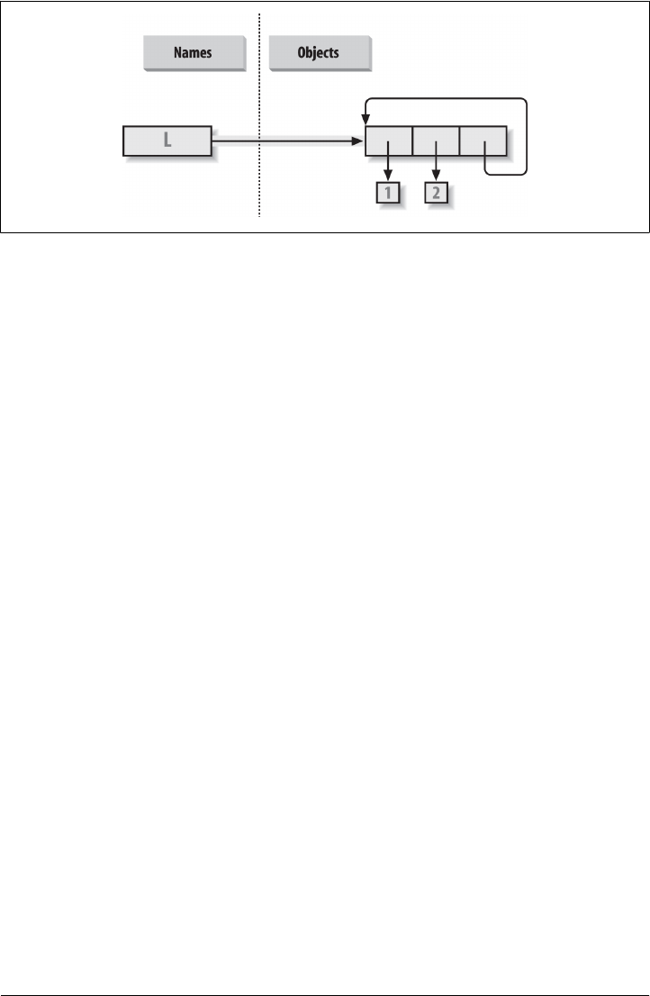
an unending stream of [1, 2, [1, 2, [1, 2, [1, 2, and so on, until you hit the
break-key combination on your machine (which, technically, raises a keyboard-
interrupt exception that prints a default message). Beginning with Python 1.5.1,
the printer is clever enough to detect cycles and prints [[...]] instead to let you
know that it has detected a loop in the object’s structure and avoided getting stuck
printing forever.
The reason for the cycle is subtle and requires information you will glean in
Part II, so this is something of a preview. But in short, assignments in Python always
generate references to objects, not copies of them. You can think of objects as
chunks of memory and of references as implicitly followed pointers. When you run
the first assignment above, the name L becomes a named reference to a two-item
list object—a pointer to a piece of memory. Python lists are really arrays of object
references, with an append method that changes the array in place by tacking on
another object reference at the end. Here, the append call adds a reference to the
front of L at the end of L, which leads to the cycle illustrated in Figure D-1: a pointer
at the end of the list that points back to the front of the list.
Besides being printed specially, as you’ll learn in Chapter 6 cyclic objects must also
be handled specially by Python’s garbage collector, or their space will remain un-
reclaimed even when they are no longer in use. Though rare in practice, in some
programs that traverse arbitrary objects or structures you might have to detect such
cycles yourself by keeping track of where you’ve been to avoid looping. Believe it
or not, cyclic data structures can sometimes be useful, despite their special-case
printing.
Part II, Types and Operations
See “Test Your Knowledge: Part II Exercises” on page 313 in Chapter 9 for the exercises.
Figure D-1. A cyclic object, created by appending a list to itself. By default, Python appends a reference
to the original list, not a copy of the list.
Part II, Types and Operations | 1467
www.it-ebooks.info

1. The basics. Here are the sorts of results you should get, along with a few comments
about their meaning. Again, note that ; is used in a few of these to squeeze more
than one statement onto a single line (the ; is a statement separator), and commas
build up tuples displayed in parentheses. Also keep in mind that the / division
result near the top differs in Python 2.X and 3.X (see Chapter 5 for details), and
the list wrapper around dictionary method calls is needed to display results in
3.X, but not 2.X (see Chapter 8):
# Numbers
>>> 2 ** 16 # 2 raised to the power 16
65536
>>> 2 / 5, 2 / 5.0 # Integer / truncates in 2.X, but not 3.X
(0.40000000000000002, 0.40000000000000002)
# Strings
>>> "spam" + "eggs" # Concatenation
'spameggs'
>>> S = "ham"
>>> "eggs " + S
'eggs ham'
>>> S * 5 # Repetition
'hamhamhamhamham'
>>> S[:0] # An empty slice at the front -- [0:0]
'' # Empty of same type as object sliced
>>> "green %s and %s" % ("eggs", S) # Formatting
'green eggs and ham'
>>> 'green {0} and {1}'.format('eggs', S)
'green eggs and ham'
# Tuples
>>> ('x',)[0] # Indexing a single-item tuple
'x'
>>> ('x', 'y')[1] # Indexing a two-item tuple
'y'
# Lists
>>> L = [1,2,3] + [4,5,6] # List operations
>>> L, L[:], L[:0], L[-2], L[-2:]
([1, 2, 3, 4, 5, 6], [1, 2, 3, 4, 5, 6], [], 5, [5, 6])
>>> ([1,2,3]+[4,5,6])[2:4]
[3, 4]
>>> [L[2], L[3]] # Fetch from offsets; store in a list
[3, 4]
>>> L.reverse(); L # Method: reverse list in place
[6, 5, 4, 3, 2, 1]
>>> L.sort(); L # Method: sort list in place
[1, 2, 3, 4, 5, 6]
>>> L.index(4) # Method: offset of first four (search)
3
1468 | Appendix D: Solutions to End-of-Part Exercises
www.it-ebooks.info

# Dictionaries
>>> {'a':1, 'b':2}['b'] # Index a dictionary by key
2
>>> D = {'x':1, 'y':2, 'z':3}
>>> D['w'] = 0 # Create a new entry
>>> D['x'] + D['w']
1
>>> D[(1,2,3)] = 4 # A tuple used as a key (immutable)
>>> D
{'w': 0, 'z': 3, 'y': 2, (1, 2, 3): 4, 'x': 1}
>>> list(D.keys()), list(D.values()), (1,2,3) in D # Methods, key test
(['w', 'z', 'y', (1, 2, 3), 'x'], [0, 3, 2, 4, 1], True)
# Empties
>>> [[]], ["",[],(),{},None] # Lots of nothings: empty objects
([[]], ['', [], (), {}, None])
2. Indexing and slicing. Indexing out of bounds (e.g., L[4]) raises an error; Python
always checks to make sure that all offsets are within the bounds of a sequence.
On the other hand, slicing out of bounds (e.g., L[-1000:100]) works because Python
scales out-of-bounds slices so that they always fit (the limits are set to zero and the
sequence length, if required).
Extracting a sequence in reverse, with the lower bound greater than the higher
bound (e.g., L[3:1]), doesn’t really work. You get back an empty slice ([ ]) because
Python scales the slice limits to make sure that the lower bound is always less than
or equal to the upper bound (e.g., L[3:1] is scaled to L[3:3], the empty insertion
point at offset 3). Python slices are always extracted from left to right, even if you
use negative indexes (they are first converted to positive indexes by adding the
sequence length). Note that Python 2.3’s three-limit slices modify this behavior
somewhat. For instance, L[3:1:-1] does extract from right to left:
>>> L = [1, 2, 3, 4]
>>> L[4]
Traceback (innermost last):
File "<stdin>", line 1, in ?
IndexError: list index out of range
>>> L[-1000:100]
[1, 2, 3, 4]
>>> L[3:1]
[]
>>> L
[1, 2, 3, 4]
>>> L[3:1] = ['?']
>>> L
[1, 2, 3, '?', 4]
Part II, Types and Operations | 1469
www.it-ebooks.info

3. Indexing, slicing, and del. Your interaction with the interpreter should look some-
thing like the following code. Note that assigning an empty list to an offset stores
an empty list object there, but assigning an empty list to a slice deletes the slice.
Slice assignment expects another sequence, or you’ll get a type error; it inserts items
inside the sequence assigned, not the sequence itself:
>>> L = [1,2,3,4]
>>> L[2] = []
>>> L
[1, 2, [], 4]
>>> L[2:3] = []
>>> L
[1, 2, 4]
>>> del L[0]
>>> L
[2, 4]
>>> del L[1:]
>>> L
[2]
>>> L[1:2] = 1
Traceback (innermost last):
File "<stdin>", line 1, in ?
TypeError: illegal argument type for built-in operation
4. Tuple assignment. The values of X and Y are swapped. When tuples appear on the
left and right of an assignment symbol (=), Python assigns objects on the right to
targets on the left according to their positions. This is probably easiest to under-
stand by noting that the targets on the left aren’t a real tuple, even though they
look like one; they are simply a set of independent assignment targets. The items
on the right are a tuple, which gets unpacked during the assignment (the tuple
provides the temporary assignment needed to achieve the swap effect):
>>> X = 'spam'
>>> Y = 'eggs'
>>> X, Y = Y, X
>>> X
'eggs'
>>> Y
'spam'
5. Dictionary keys. Any immutable object can be used as a dictionary key, including
integers, tuples, strings, and so on. This really is a dictionary, even though some
of its keys look like integer offsets. Mixed-type keys work fine, too:
>>> D = {}
>>> D[1] = 'a'
>>> D[2] = 'b'
>>> D[(1, 2, 3)] = 'c'
>>> D
{1: 'a', 2: 'b', (1, 2, 3): 'c'}
6. Dictionary indexing. Indexing a nonexistent key (D['d']) raises an error; assigning
to a nonexistent key (D['d']='spam') creates a new dictionary entry. On the other
hand, out-of-bounds indexing for lists raises an error too, but so do out-of-bounds
1470 | Appendix D: Solutions to End-of-Part Exercises
www.it-ebooks.info

assignments. Variable names work like dictionary keys; they must have already
been assigned when referenced, but they are created when first assigned. In fact,
variable names can be processed as dictionary keys if you wish (they’re made visible
in module namespace or stack-frame dictionaries):
>>> D = {'a':1, 'b':2, 'c':3}
>>> D['a']
1
>>> D['d']
Traceback (innermost last):
File "<stdin>", line 1, in ?
KeyError: d
>>> D['d'] = 4
>>> D
{'b': 2, 'd': 4, 'a': 1, 'c': 3}
>>>
>>> L = [0, 1]
>>> L[2]
Traceback (innermost last):
File "<stdin>", line 1, in ?
IndexError: list index out of range
>>> L[2] = 3
Traceback (innermost last):
File "<stdin>", line 1, in ?
IndexError: list assignment index out of range
7. Generic operations. Question answers:
• The + operator doesn’t work on different/mixed types (e.g., string + list, list
+ tuple).
•+ doesn’t work for dictionaries, as they aren’t sequences.
• The append method works only for lists, not strings, and keys works only on
dictionaries. append assumes its target is mutable, since it’s an in-place exten-
sion; strings are immutable.
• Slicing and concatenation always return a new object of the same type as the
objects processed:
>>> "x" + 1
Traceback (innermost last):
File "<stdin>", line 1, in ?
TypeError: illegal argument type for built-in operation
>>>
>>> {} + {}
Traceback (innermost last):
File "<stdin>", line 1, in ?
TypeError: bad operand type(s) for +
>>>
>>> [].append(9)
>>> "".append('s')
Traceback (innermost last):
File "<stdin>", line 1, in ?
AttributeError: attribute-less object
>>>
Part II, Types and Operations | 1471
www.it-ebooks.info

>>> list({}.keys()) # list() needed in 3.X, not 2.X
[]
>>> [].keys()
Traceback (innermost last):
File "<stdin>", line 1, in ?
AttributeError: keys
>>>
>>> [][:]
[]
>>> ""[:]
''
8. String indexing. This is a bit of a trick question—because strings are collections of
one-character strings, every time you index a string, you get back a string that can
be indexed again. S[0][0][0][0][0] just keeps indexing the first character over and
over. This generally doesn’t work for lists (lists can hold arbitrary objects) unless
the list contains strings:
>>> S = "spam"
>>> S[0][0][0][0][0]
's'
>>> L = ['s', 'p']
>>> L[0][0][0]
's'
9. Immutable types. Either of the following solutions works. Index assignment
doesn’t, because strings are immutable:
>>> S = "spam"
>>> S = S[0] + 'l' + S[2:]
>>> S
'slam'
>>> S = S[0] + 'l' + S[2] + S[3]
>>> S
'slam'
(See also the Python 3.X and 2.6+ bytearray string type in Chapter 37—it’s a mu-
table sequence of small integers that is essentially processed the same as a string.)
10. Nesting. Here is a sample:
>>> me = {'name':('John', 'Q', 'Doe'), 'age':'?', 'job':'engineer'}
>>> me['job']
'engineer'
>>> me['name'][2]
'Doe'
11. Files. Here’s one way to create and read back a text file in Python (ls is a Unix
command; use dir on Windows):
# File: maker.py
file = open('myfile.txt', 'w')
file.write('Hello file world!\n') # Or: open().write()
file.close() # close not always needed
# File: reader.py
file = open('myfile.txt') # 'r' is default open mode
1472 | Appendix D: Solutions to End-of-Part Exercises
www.it-ebooks.info

print(file.read()) # Or print(open().read())
% python maker.py
% python reader.py
Hello file world!
% ls -l myfile.txt
-rwxrwxrwa 1 0 0 19 Apr 13 16:33 myfile.txt
Part III, Statements and Syntax
See “Test Your Knowledge: Part III Exercises” on page 467 in Chapter 15 for the ex-
ercises.
1. Coding basic loops. As you work through this exercise, you’ll wind up with code
that looks like the following:
>>> S = 'spam'
>>> for c in S:
... print(ord(c))
...
115
112
97
109
>>> x = 0
>>> for c in S: x += ord(c) # Or: x = x + ord(c)
...
>>> x
433
>>> x = []
>>> for c in S: x.append(ord(c))
...
>>> x
[115, 112, 97, 109]
>>> list(map(ord, S)) # list() required in 3.X, not 2.X
[115, 112, 97, 109]
>>> [ord(c) for c in S] # map and listcomps automate list builders
[115, 112, 97, 109]
2. Backslash characters. The example prints the bell character (\a) 50 times; assuming
your machine can handle it, and when it’s run outside of IDLE, you may get a series
of beeps (or one sustained tone, if your machine is fast enough). Hey—I warned
you.
3. Sorting dictionaries. Here’s one way to work through this exercise (see Chapter 8
or Chapter 14 if this doesn’t make sense). Remember, you really do have to split
up the keys and sort calls like this because sort returns None. In Python 2.2 and
later, you can iterate through dictionary keys directly without calling keys (e.g.,
Part III, Statements and Syntax | 1473
www.it-ebooks.info

for key in D:), but the keys list will not be sorted like it is by this code. In more
recent Pythons, you can achieve the same effect with the sorted built-in, too:
>>> D = {'a':1, 'b':2, 'c':3, 'd':4, 'e':5, 'f':6, 'g':7}
>>> D
{'f': 6, 'c': 3, 'a': 1, 'g': 7, 'e': 5, 'd': 4, 'b': 2}
>>>
>>> keys = list(D.keys()) # list() required in 3.X, not in 2.X
>>> keys.sort()
>>> for key in keys:
... print(key, '=>', D[key])
...
a => 1
b => 2
c => 3
d => 4
e => 5
f => 6
g => 7
>>> for key in sorted(D): # Better, in more recent Pythons
... print(key, '=>', D[key])
4. Program logic alternatives. Here’s some sample code for the solutions. For step e,
assign the result of 2 ** X to a variable outside the loops of steps a and b, and use
it inside the loop. Your results may vary a bit; this exercise is mostly designed to
get you playing with code alternatives, so anything reasonable gets full credit:
# a
L = [1, 2, 4, 8, 16, 32, 64]
X = 5
i = 0
while i < len(L):
if 2 ** X == L[i]:
print('at index', i)
break
i += 1
else:
print(X, 'not found')
# b
L = [1, 2, 4, 8, 16, 32, 64]
X = 5
for p in L:
if (2 ** X) == p:
print((2 ** X), 'was found at', L.index(p))
break
else:
print(X, 'not found')
# c
1474 | Appendix D: Solutions to End-of-Part Exercises
www.it-ebooks.info

L = [1, 2, 4, 8, 16, 32, 64]
X = 5
if (2 ** X) in L:
print((2 ** X), 'was found at', L.index(2 ** X))
else:
print(X, 'not found')
# d
X = 5
L = []
for i in range(7): L.append(2 ** i)
print(L)
if (2 ** X) in L:
print((2 ** X), 'was found at', L.index(2 ** X))
else:
print(X, 'not found')
# f
X = 5
L = list(map(lambda x: 2**x, range(7))) # Or [2**x for x in range(7)]
print(L) # list() to print all in 3.X, not 2.X
if (2 ** X) in L:
print((2 ** X), 'was found at', L.index(2 ** X))
else:
print(X, 'not found')
5. Code maintenance. There is no fixed solution to show here; see mypydoc.py in the
book’s examples package for my edits on this code as one example.
Part IV, Functions and Generators
See “Test Your Knowledge: Part IV Exercises” on page 663 in Chapter 21 for the ex-
ercises.
1. The basics. There’s not much to this one, but notice that using print (and hence
your function) is technically a polymorphic operation, which does the right thing
for each type of object:
% python
>>> def func(x): print(x)
...
>>> func("spam")
spam
>>> func(42)
42
>>> func([1, 2, 3])
[1, 2, 3]
Part IV, Functions and Generators | 1475
www.it-ebooks.info

>>> func({'food': 'spam'})
{'food': 'spam'}
2. Arguments. Here’s a sample solution. Remember that you have to use print to see
results in the test calls because a file isn’t the same as code typed interactively;
Python doesn’t normally echo the results of expression statements in files:
def adder(x, y):
return x + y
print(adder(2, 3))
print(adder('spam', 'eggs'))
print(adder(['a', 'b'], ['c', 'd']))
% python mod.py
5
spameggs
['a', 'b', 'c', 'd']
3. varargs. Two alternative adder functions are shown in the following file, add-
ers.py. The hard part here is figuring out how to initialize an accumulator to an
empty value of whatever type is passed in. The first solution uses manual type
testing to look for an integer, and an empty slice of the first argument (assumed to
be a sequence) if the argument is determined not to be an integer. The second
solution uses the first argument to initialize and scan items 2 and beyond, much
like one of the min function variants shown in Chapter 18.
The second solution is better. Both of these assume all arguments are of the same
type, and neither works on dictionaries (as we saw in Part II, + doesn’t work on
mixed types or dictionaries). You could add a type test and special code to allow
dictionaries, too, but that’s extra credit.
def adder1(*args):
print('adder1', end=' ')
if type(args[0]) == type(0): # Integer?
sum = 0 # Init to zero
else: # else sequence:
sum = args[0][:0] # Use empty slice of arg1
for arg in args:
sum = sum + arg
return sum
def adder2(*args):
print('adder2', end=' ')
sum = args[0] # Init to arg1
for next in args[1:]:
sum += next # Add items 2..N
return sum
for func in (adder1, adder2):
print(func(2, 3, 4))
print(func('spam', 'eggs', 'toast'))
print(func(['a', 'b'], ['c', 'd'], ['e', 'f']))
1476 | Appendix D: Solutions to End-of-Part Exercises
www.it-ebooks.info

% python adders.py
adder1 9
adder1 spameggstoast
adder1 ['a', 'b', 'c', 'd', 'e', 'f']
adder2 9
adder2 spameggstoast
adder2 ['a', 'b', 'c', 'd', 'e', 'f']
4. Keywords. Here is my solution to the first and second parts of this exercise (coded
in the file mod.py). To iterate over keyword arguments, use the **args form in the
function header and use a loop (e.g., for x in args.keys(): use args[x]), or use
args.values() to make this the same as summing *args positionals:
def adder(good=1, bad=2, ugly=3):
return good + bad + ugly
print(adder())
print(adder(5))
print(adder(5, 6))
print(adder(5, 6, 7))
print(adder(ugly=7, good=6, bad=5))
% python mod.py
6
10
14
18
18
# Second part solutions
def adder1(*args): # Sum any number of positional args
tot = args[0]
for arg in args[1:]:
tot += arg
return tot
def adder2(**args): # Sum any number of keyword args
argskeys = list(args.keys()) # list needed in 3.X!
tot = args[argskeys[0]]
for key in argskeys[1:]:
tot += args[key]
return tot
def adder3(**args): # Same, but convert to list of values
args = list(args.values()) # list needed to index in 3.X!
tot = args[0]
for arg in args[1:]:
tot += arg
return tot
def adder4(**args): # Same, but reuse positional version
return adder1(*args.values())
print(adder1(1, 2, 3), adder1('aa', 'bb', 'cc'))
Part IV, Functions and Generators | 1477
www.it-ebooks.info

print(adder2(a=1, b=2, c=3), adder2(a='aa', b='bb', c='cc'))
print(adder3(a=1, b=2, c=3), adder3(a='aa', b='bb', c='cc'))
print(adder4(a=1, b=2, c=3), adder4(a='aa', b='bb', c='cc'))
5. (and 6.) Dictionary tools. Here are my solutions to exercises 5 and 6 (file dicts.py).
These are just coding exercises, though, because Python 1.5 added the dictionary
methods D.copy() and D1.update(D2) to handle things like copying and adding
(merging) dictionaries. See Chapter 8 for dict.update examples, and Python’s li-
brary manual or O’Reilly’s Python Pocket Reference for more details. X[:] doesn’t
work for dictionaries, as they’re not sequences (see Chapter 8 for details). Also,
remember that if you assign (e = d) rather than copying, you generate a reference
to a shared dictionary object; changing d changes e, too:
def copyDict(old):
new = {}
for key in old.keys():
new[key] = old[key]
return new
def addDict(d1, d2):
new = {}
for key in d1.keys():
new[key] = d1[key]
for key in d2.keys():
new[key] = d2[key]
return new
% python
>>> from dicts import *
>>> d = {1: 1, 2: 2}
>>> e = copyDict(d)
>>> d[2] = '?'
>>> d
{1: 1, 2: '?'}
>>> e
{1: 1, 2: 2}
>>> x = {1: 1}
>>> y = {2: 2}
>>> z = addDict(x, y)
>>> z
{1: 1, 2: 2}
6. See #5.
7. More argument-matching examples. Here is the sort of interaction you should get,
along with comments that explain the matching that goes on:
def f1(a, b): print(a, b) # Normal args
def f2(a, *b): print(a, b) # Positional varargs
def f3(a, **b): print(a, b) # Keyword varargs
def f4(a, *b, **c): print(a, b, c) # Mixed modes
1478 | Appendix D: Solutions to End-of-Part Exercises
www.it-ebooks.info

def f5(a, b=2, c=3): print(a, b, c) # Defaults
def f6(a, b=2, *c): print(a, b, c) # Defaults and positional varargs
% python
>>> f1(1, 2) # Matched by position (order matters)
1 2
>>> f1(b=2, a=1) # Matched by name (order doesn't matter)
1 2
>>> f2(1, 2, 3) # Extra positionals collected in a tuple
1 (2, 3)
>>> f3(1, x=2, y=3) # Extra keywords collected in a dictionary
1 {'x': 2, 'y': 3}
>>> f4(1, 2, 3, x=2, y=3) # Extra of both kinds
1 (2, 3) {'x': 2, 'y': 3}
>>> f5(1) # Both defaults kick in
1 2 3
>>> f5(1, 4) # Only one default used
1 4 3
>>> f6(1) # One argument: matches "a"
1 2 ()
>>> f6(1, 3, 4) # Extra positional collected
1 3 (4,)
8. Primes revisited. Here is the primes example, wrapped up in a function and a mod-
ule (file primes.py) so it can be run multiple times. I added an if test to trap neg-
atives, 0, and 1. I also changed / to // in this edition to make this solution immune
to the Python 3.X / true division changes we studied in Chapter 5, and to enable
it to support floating-point numbers (uncomment the from statement and
change // to / to see the differences in 2.X):
#from __future__ import division
def prime(y):
if y <= 1: # For some y > 1
print(y, 'not prime')
else:
x = y // 2 # 3.X / fails
while x > 1:
if y % x == 0: # No remainder?
print(y, 'has factor', x)
break # Skip else
x -= 1
else:
print(y, 'is prime')
prime(13); prime(13.0)
prime(15); prime(15.0)
Part IV, Functions and Generators | 1479
www.it-ebooks.info

prime(3); prime(2)
prime(1); prime(-3)
Here is the module in action; the // operator allows it to work for floating-point
numbers too, even though it perhaps should not:
% python primes.py
13 is prime
13.0 is prime
15 has factor 5
15.0 has factor 5.0
3 is prime
2 is prime
1 not prime
-3 not prime
This function still isn’t very reusable—it could return values, instead of printing
—but it’s enough to run experiments. It’s also not a strict mathematical prime
(floating points work), and it’s still inefficient. Improvements are left as exercises
for more mathematically minded readers. (Hint: a for loop over range(y, 1, −1)
may be a bit quicker than the while, but the algorithm is the real bottleneck here.)
To time alternatives, use the homegrown timer or standard library timeit modules
and coding patterns like those used in Chapter 21’s timing sections (and see Sol-
ution 10).
9. Iterations and comprehensions. Here is the sort of code you should write; I may
have a preference, but yours may vary:
>>> values = [2, 4, 9, 16, 25]
>>> import math
>>> res = []
>>> for x in values: res.append(math.sqrt(x))
...
>>> res
[1.4142135623730951, 2.0, 3.0, 4.0, 5.0]
>>> list(map(math.sqrt, values))
[1.4142135623730951, 2.0, 3.0, 4.0, 5.0]
>>> [math.sqrt(x) for x in values]
[1.4142135623730951, 2.0, 3.0, 4.0, 5.0]
>>> list(math.sqrt(x) for x in values)
[1.4142135623730951, 2.0, 3.0, 4.0, 5.0]
10. Timing tools. Here is some code I wrote to time the three square root options, along
with the results in CPythons 3.3 and 2.7 and PyPy 1.9 (which implements Python
2.7). Each test takes the best of three runs; each run takes the total time required
to call the test function 1,000 times; and each test function iterates 1,000 times.
The last result of each function is printed to verify that all three do the same work:
# File timer2.py (2.X and 3.X)
...same as listed in Chapter 21...
1480 | Appendix D: Solutions to End-of-Part Exercises
www.it-ebooks.info

# File timesqrt.py
import sys, timer2
reps = 10000
repslist = range(reps) # Pull out range list time for 2.X
from math import sqrt # Not math.sqrt: adds attr fetch time
def mathMod():
for i in repslist:
res = sqrt(i)
return res
def powCall():
for i in repslist:
res = pow(i, .5)
return res
def powExpr():
for i in repslist:
res = i ** .5
return res
print(sys.version)
for test in (mathMod, powCall, powExpr):
elapsed, result = timer2.bestoftotal(test, _reps1=3, _reps=1000)
print ('%s: %.5f => %s' % (test.__name__, elapsed, result))
Following are the test results for the three Pythons. The 3.3 and 2.7 results are
roughly twice as fast as 3.0 and 2.6 in the prior edition, due largely to a faster test
machine. For each Python tested, it looks like the math module is quicker than the
** expression, which is quicker than the pow call; however, you should try this with
your code and on your own machine and version of Python. Also, note that Python
3.3 is essentially twice as slow as 2.7 on this test, and PyPy is a rough order of
magnitude (10X) faster than both CPythons, despite the fact that this is running
floating-point math and iterations. Later versions of any of these Pythons might
differ, so time this in the future to see for yourself:
c:\code> py −3 timesqrt.py
3.3.0 (v3.3.0:bd8afb90ebf2, Sep 29 2012, 10:57:17) [MSC v.1600 64 bit (AMD64)]
mathMod: 2.04481 => 99.99499987499375
powCall: 3.40973 => 99.99499987499375
powExpr: 2.56458 => 99.99499987499375
c:\code> py −2 timesqrt.py
2.7.3 (default, Apr 10 2012, 23:24:47) [MSC v.1500 64 bit (AMD64)]
mathMod: 1.04337 => 99.994999875
powCall: 2.57516 => 99.994999875
powExpr: 1.89560 => 99.994999875
c:\code> c:\pypy\pypy-1.9\pypy timesqrt.py
2.7.2 (341e1e3821ff, Jun 07 2012, 15:43:00)
[PyPy 1.9.0 with MSC v.1500 32 bit]
mathMod: 0.07491 => 99.994999875
Part IV, Functions and Generators | 1481
www.it-ebooks.info

powCall: 0.85678 => 99.994999875
powExpr: 0.85453 => 99.994999875
To time the relative speeds of Python 3.X and 2.7 dictionary comprehensions and
equivalent for loops interactively, you can run a session like the following. It ap-
pears that the two are roughly the same in this regard under Python 3.3; unlike list
comprehensions, though, manual loops are slightly faster than dictionary com-
prehensions today (though the difference isn’t exactly earth-shattering—at the end
we save half a second when making 50 dictionaries of 1,000,000 items each). Again,
rather than taking these results as gospel you should investigate further on your
own, on your computer and with your Python:
C:\code> c:\python33\python
>>>
>>> def dictcomp(I):
return {i: i for i in range(I)}
>>> def dictloop(I):
new = {}
for i in range(I): new[i] = i
return new
>>> dictcomp(10)
{0: 0, 1: 1, 2: 2, 3: 3, 4: 4, 5: 5, 6: 6, 7: 7, 8: 8, 9: 9}
>>> dictloop(10)
{0: 0, 1: 1, 2: 2, 3: 3, 4: 4, 5: 5, 6: 6, 7: 7, 8: 8, 9: 9}
>>>
>>> from timer2 import total, bestof
>>> bestof(dictcomp, 10000)[0] # 10,000-item dict
0.0017095345403959072
>>> bestof(dictloop, 10000)[0]
0.002097576400046819
>>>
>>> bestof(dictcomp, 100000)[0] # 100,000-items: 10X slower
0.012716923463358398
>>> bestof(dictloop, 100000)[0]
0.014129806355413166
>>>
>>> bestof(dictcomp, 1000000)[0] # 1 of 1M-items: 10X time
0.11614425187337929
>>> bestof(dictloop, 1000000)[0]
0.1331144855439561
>>>
>>> total(dictcomp, 1000000, _reps=50)[0] # Total to make 50 1M-item dicts
5.8162020671780965
>>> total(dictloop, 1000000, _reps=50)[0]
6.626680761285343
11. Recursive functions. I coded this function as follows; a simple range, comprehen-
sion, or map will do the job here as well, but recursion is useful enough to experiment
with here (print is a function in 3.X only, unless you import it from __future__ or
code your own equivalent):
1482 | Appendix D: Solutions to End-of-Part Exercises
www.it-ebooks.info

def countdown(N):
if N == 0:
print('stop') # 2.X: print 'stop'
else:
print(N, end=' ') # 2.X: print N,
countdown(N-1)
>>> countdown(5)
5 4 3 2 1 stop
>>> countdown(20)
20 19 18 17 16 15 14 13 12 11 10 9 8 7 6 5 4 3 2 1 stop
# Nonrecursive options:
>>> list(range(5, 0, −1))
[5, 4, 3, 2, 1]
# On 3.X only:
>>> t = [print(i, end=' ') for i in range(5, 0, −1)]
5 4 3 2 1
>>> t = list(map(lambda x: print(x, end=' '), range(5, 0, −1)))
5 4 3 2 1
I didn’t include a generator-based solution in this exercise on the grounds of merit
(and humanity!), but one is listed below; all the other techniques seem much sim-
pler in this case—a good example of cases where generators should probably be
avoided. Remember that generators produce no results until iterated, so we need
a for or yield from here (yield from works in 3.3 and later only):
def countdown2(N): # Generator function, recursive
if N == 0:
yield 'stop'
else:
yield N
for x in countdown2(N-1): yield x # 3.3+: yield from countdown2(N-1)
>>> list(countdown2(5))
[5, 4, 3, 2, 1, 'stop']
# Nonrecursive options:
>>> def countdown3(): # Generator function, simpler
yield from range(5, 0, −1) # Pre 3.3: for x in range(): yield x
>>> list(countdown3())
[5, 4, 3, 2, 1]
>>> list(x for x in range(5, 0, −1)) # Equivalent generator expression
[5, 4, 3, 2, 1]
>>> list(range(5, 0, −1)) # Equivalent nongenerator form
[5, 4, 3, 2, 1]
12. Computing factorials. The following file shows how I coded this exercise; it runs
on Python 3.X and 2.X, and its output on 3.3 is given in a string literal at the end
of the file. Naturally, there are many possible variations on its code; its ranges, for
Part IV, Functions and Generators | 1483
www.it-ebooks.info

instance, could run from 2..N+1 to skip an iteration, and fact2 could use
reduce(operator.mul, range(N, 1, −1)) to avoid a lambda.
#!python
from __future__ import print_function # File factorials.py
from functools import reduce
from timeit import repeat
import math
def fact0(N): # Recursive
if N == 1: # Fails at 999 by default
return N
else:
return N * fact0(N-1)
def fact1(N):
return N if N == 1 else N * fact1(N-1) # Recursive, one-liner
def fact2(N): # Functional
return reduce(lambda x, y: x * y, range(1, N+1))
def fact3(N):
res = 1
for i in range(1, N+1): res *= i # Iterative
return res
def fact4(N):
return math.factorial(N) # Stdlib "batteries"
# Tests
print(fact0(6), fact1(6), fact2(6), fact3(6), fact4(6)) # 6*5*4*3*2*1: all 720
print(fact0(500) == fact1(500) == fact2(500) == fact3(500) == fact4(500)) # True
for test in (fact0, fact1, fact2, fact3, fact4):
print(test.__name__, min(repeat(stmt=lambda: test(500), number=20, repeat=3)))
r"""
C:\code> py −3 factorials.py
720 720 720 720 720
True
fact0 0.003990868798355564
fact1 0.003901433457907475
fact2 0.002732909419593966
fact3 0.002052614370939676
fact4 0.0003401475243271501
"""
Conclusions: recursion is slowest on my Python and machine, and fails once N
reaches 999 due to the default stack size setting in sys; per Chapter 19, this limit
can be increased, but simple loops or the standard library tool seem the best route
here in any event.
This general finding holds true often. For instance, ''.join(reversed(S)) may be
the preferred way to reverse a string, even though recursive solutions are possible.
1484 | Appendix D: Solutions to End-of-Part Exercises
www.it-ebooks.info

Time the following to see how: as for factorials in 3.X, recursion is today an order
of magnitude slower in CPython, though these results vary in PyPy:
def rev1(S):
if len(S) == 1:
return S
else:
return S[-1] + rev1(S[:-1]) # Recursive: 10x slower in CPython today
def rev2(S):
return ''.join(reversed(S)) # Nonrecursive iterable: simpler, faster
def rev3(S):
return S[::-1] # Even better?: sequence reversal by slice
Part V, Modules and Packages
See “Test Your Knowledge: Part V Exercises” on page 778 in Chapter 25 for the exer-
cises.
1. Import basics. When you’re done, your file (mymod.py) and interaction should look
similar to the following; remember that Python can read a whole file into a list of
line strings, and the len built-in returns the lengths of strings and lists:
def countLines(name):
file = open(name)
return len(file.readlines())
def countChars(name):
return len(open(name).read())
def test(name): # Or pass file object
return countLines(name), countChars(name) # Or return a dictionary
% python
>>> import mymod
>>> mymod.test('mymod.py')
(10, 291)
Your counts may vary, as mine may or may not include comments and an extra
line at the end. Note that these functions load the entire file in memory all at once,
so they won’t work for pathologically large files too big for your machine’s memory.
To be more robust, you could read line by line with iterators instead and count as
you go:
def countLines(name):
tot = 0
for line in open(name): tot += 1
return tot
def countChars(name):
tot = 0
Part V, Modules and Packages | 1485
www.it-ebooks.info

for line in open(name): tot += len(line)
return tot
A generator expression can have the same effect (though the instructor might take
off points for excessive magic!):
def countlines(name): return sum(+1 for line in open(name))
def countchars(name): return sum(len(line) for line in open(name))
On Unix, you can verify your output with a wc command; on Windows, right-click
on your file to view its properties. Note that your script may report fewer characters
than Windows does—for portability, Python converts Windows \r\n line-end
markers to \n, thereby dropping 1 byte (character) per line. To match byte counts
with Windows exactly, you must open in binary mode ('rb'), or add the number
of bytes corresponding to the number of lines. See Chapter 9 and Chapter 37 for
more on end-of-line translations in text files.
The “ambitious” part of this exercise (passing in a file object so you only open the
file once), will require you to use the seek method of the built-in file object. It works
like C’s fseek call (and may call it behind the scenes): seek resets the current po-
sition in the file to a passed-in offset. After a seek, future input/output operations
are relative to the new position. To rewind to the start of a file without closing and
reopening it, call file.seek(0); the file read methods all pick up at the current
position in the file, so you need to rewind to reread. Here’s what this tweak would
look like:
def countLines(file):
file.seek(0) # Rewind to start of file
return len(file.readlines())
def countChars(file):
file.seek(0) # Ditto (rewind if needed)
return len(file.read())
def test(name):
file = open(name) # Pass file object
return countLines(file), countChars(file) # Open file only once
>>> import mymod2
>>> mymod2.test("mymod2.py")
(11, 392)
2. from/from *. Here’s the from * part; replace * with countChars to do the rest:
% python
>>> from mymod import *
>>> countChars("mymod.py")
291
3. __main__. If you code it properly, this file works in either mode—program run or
module import:
def countLines(name):
file = open(name)
1486 | Appendix D: Solutions to End-of-Part Exercises
www.it-ebooks.info

return len(file.readlines())
def countChars(name):
return len(open(name).read())
def test(name): # Or pass file object
return countLines(name), countChars(name) # Or return a dictionary
if __name__ == '__main__':
print(test('mymod.py'))
% python mymod.py
(13, 346)
This is where I would probably begin to consider using command-line arguments
or user input to provide the filename to be counted, instead of hardcoding it in the
script (see Chapter 25 for more on sys.argv, and Chapter 10 for more on input—
and use raw_input instead in 2.X):
if __name__ == '__main__':
print(test(input('Enter file name:')) # Console (raw_input in 2.X)
if __name__ == '__main__':
import sys # Command line
print(test(sys.argv[1]))
4. Nested imports. Here is my solution (file myclient.py):
from mymod import countLines, countChars
print(countLines('mymod.py'), countChars('mymod.py'))
% python myclient.py
13 346
As for the rest of this one, mymod’s functions are accessible (that is, importable) from
the top level of myclient, since from simply assigns to names in the importer (it
works as if mymod’s defs appeared in myclient). For example, another file can say:
import myclient
myclient.countLines(...)
from myclient import countChars
countChars(...)
If myclient used import instead of from, you’d need to use a path to get to the
functions in mymod through myclient:
import myclient
myclient.mymod.countLines(...)
from myclient import mymod
mymod.countChars(...)
In general, you can define collector modules that import all the names from other
modules so they’re available in a single convenience module. The following partial
Part V, Modules and Packages | 1487
www.it-ebooks.info

code, for example, creates three different copies of the name somename—mod1.some
name, collector.somename, and __main__.somename; all three share the same integer
object initially, and only the name somename exists at the interactive prompt as is:
# File mod1.py
somename = 42
# File collector.py
from mod1 import * # Collect lots of names here
from mod2 import * # from assigns to my names
from mod3 import *
>>> from collector import somename
5. Package imports. For this, I put the mymod.py solution file listed for exercise 3 into
a directory package. The following is what I did in a Windows console interface to
set up the directory and the __init__.py file that it’s required to have until Python
3.3; you’ll need to interpolate for other platforms (e.g., use cp and vi instead of
copy and notepad). This works in any directory (I’m using my own code directory
here), and you can do some of this from a file explorer GUI, too.
When I was done, I had a mypkg subdirectory that contained the files
__init__.py and mymod.py. Until Python 3.3’s namespace package extension, you
need an __init__.py in the mypkg directory, but not in its parent; technically,
mypkg is located in the home directory component of the module search path.
Notice how a print statement coded in the directory’s initialization file fires only
the first time it is imported, not the second; raw strings are also used here to avoid
escape issues in the file paths:
C:\code> mkdir mypkg
C:\code> copy mymod.py mypkg\mymod.py
C:\code> notepad mypkg\__init__.py
...coded a print statement...
C:\code> python
>>> import mypkg.mymod
initializing mypkg
>>> mypkg.mymod.countLines(r'mypkg\mymod.py')
13
>>> from mypkg.mymod import countChars
>>> countChars(r'mypkg\mymod.py')
346
6. Reloads. This exercise just asks you to experiment with changing the changer.py
example in the book, so there’s nothing to show here.
7. Circular imports. The short story is that importing recur2 first works because the
recursive import then happens at the import in recur1, not at a from in recur2.
The long story goes like this: importing recur2 first works because the recursive
import from recur1 to recur2 fetches recur2 as a whole, instead of getting specific
names. recur2 is incomplete when it’s imported from recur1, but because it uses
import instead of from, you’re safe: Python finds and returns the already created
1488 | Appendix D: Solutions to End-of-Part Exercises
www.it-ebooks.info

recur2 module object and continues to run the rest of recur1 without a glitch.
When the recur2 import resumes, the second from finds the name Y in recur1 (it’s
been run completely), so no error is reported.
Running a file as a script is not the same as importing it as a module; these cases
are the same as running the first import or from in the script interactively. For
instance, running recur1 as a script works, because it is the same as importing
recur2 interactively, as recur2 is the first module imported in recur1. Running
recur2 as a script fails for the same reason—it’s the same as running its first import
interactively.
Part VI, Classes and OOP
See “Test Your Knowledge: Part VI Exercises” on page 1072 in Chapter 32 for the
exercises.
1. Inheritance. Here’s the solution code for this exercise (file adder.py), along with
some interactive tests. The __add__ overload has to appear only once, in the su-
perclass, as it invokes type-specific add methods in subclasses:
class Adder:
def add(self, x, y):
print('not implemented!')
def __init__(self, start=[]):
self.data = start
def __add__(self, other): # Or in subclasses?
return self.add(self.data, other) # Or return type?
class ListAdder(Adder):
def add(self, x, y):
return x + y
class DictAdder(Adder):
def add(self, x, y):
new = {}
for k in x.keys(): new[k] = x[k]
for k in y.keys(): new[k] = y[k]
return new
% python
>>> from adder import *
>>> x = Adder()
>>> x.add(1, 2)
not implemented!
>>> x = ListAdder()
>>> x.add([1], [2])
[1, 2]
>>> x = DictAdder()
>>> x.add({1:1}, {2:2})
{1: 1, 2: 2}
>>> x = Adder([1])
Part VI, Classes and OOP | 1489
www.it-ebooks.info

>>> x + [2]
not implemented!
>>>
>>> x = ListAdder([1])
>>> x + [2]
[1, 2]
>>> [2] + x
In 3.3: TypeError: can only concatenate list (not "ListAdder") to list
Earlier: TypeError: __add__ nor __radd__ defined for these operands
Notice in the last test that you get an error for expressions where a class instance
appears on the right of a +; if you want to fix this, use __radd__ methods, as de-
scribed in “Operator Overloading” in Chapter 30.
If you are saving a value in the instance anyhow, you might as well rewrite the
add method to take just one argument, in the spirit of other examples in this part
of the book (this is adder2.py):
class Adder:
def __init__(self, start=[]):
self.data = start
def __add__(self, other): # Pass a single argument
return self.add(other) # The left side is in self
def add(self, y):
print('not implemented!')
class ListAdder(Adder):
def add(self, y):
return self.data + y
class DictAdder(Adder):
def add(self, y):
d = self.data.copy() # Change to use self.data instead of x
d.update(y) # Or "cheat" by using quicker built-ins
return d
x = ListAdder([1, 2, 3])
y = x + [4, 5, 6]
print(y) # Prints [1, 2, 3, 4, 5, 6]
z = DictAdder(dict(name='Bob')) + {'a':1}
print(z) # Prints {'name': 'Bob', 'a': 1}
Because values are attached to objects rather than passed around, this version is
arguably more object-oriented. And, once you’ve gotten to this point, you’ll prob-
ably find that you can get rid of add altogether and simply define type-specific
__add__ methods in the two subclasses.
2. Operator overloading. The solution code (file mylist.py) uses a handful of operator
overloading methods we explored in Chapter 30. Copying the initial value in the
constructor is important because it may be mutable; you don’t want to change or
have a reference to an object that’s possibly shared somewhere outside the class.
The __getattr__ method routes calls to the wrapped list. For hints on an easier
1490 | Appendix D: Solutions to End-of-Part Exercises
www.it-ebooks.info

way to code this in Python 2.2 and later, see “Extending Types by Subclass-
ing” on page 981 in Chapter 32:
class MyList:
def __init__(self, start):
#self.wrapped = start[:] # Copy start: no side effects
self.wrapped = list(start) # Make sure it's a list here
def __add__(self, other):
return MyList(self.wrapped + other)
def __mul__(self, time):
return MyList(self.wrapped * time)
def __getitem__(self, offset): # Also passed a slice in 3.X
return self.wrapped[offset] # For iteration if no __iter__
def __len__(self):
return len(self.wrapped)
def __getslice__(self, low, high): # Ignored in 3.X: uses __getitem__
return MyList(self.wrapped[low:high])
def append(self, node):
self.wrapped.append(node)
def __getattr__(self, name): # Other methods: sort/reverse/etc
return getattr(self.wrapped, name)
def __repr__(self): # Catchall display method
return repr(self.wrapped)
if __name__ == '__main__':
x = MyList('spam')
print(x)
print(x[2])
print(x[1:])
print(x + ['eggs'])
print(x * 3)
x.append('a')
x.sort()
print(' '.join(c for c in x))
c:\code> python mylist.py
['s', 'p', 'a', 'm']
a
['p', 'a', 'm']
['s', 'p', 'a', 'm', 'eggs']
['s', 'p', 'a', 'm', 's', 'p', 'a', 'm', 's', 'p', 'a', 'm']
a a m p s
Note that it’s important to copy the start value by calling list instead of slicing
here, because otherwise the result may not be a true list and so will not respond to
expected list methods, such as append (e.g., slicing a string returns another string,
not a list). You would be able to copy a MyList start value by slicing because its
class overloads the slicing operation and provides the expected list interface; how-
ever, you need to avoid slice-based copying for objects such as strings.
3. Subclassing. My solution (mysub.py) appears as follows. Your solution should be
similar:
Part VI, Classes and OOP | 1491
www.it-ebooks.info

from mylist import MyList
class MyListSub(MyList):
calls = 0 # Shared by instances
def __init__(self, start):
self.adds = 0 # Varies in each instance
MyList.__init__(self, start)
def __add__(self, other):
print('add: ' + str(other))
MyListSub.calls += 1 # Class-wide counter
self.adds += 1 # Per-instance counts
return MyList.__add__(self, other)
def stats(self):
return self.calls, self.adds # All adds, my adds
if __name__ == '__main__':
x = MyListSub('spam')
y = MyListSub('foo')
print(x[2])
print(x[1:])
print(x + ['eggs'])
print(x + ['toast'])
print(y + ['bar'])
print(x.stats())
c:\code> python mysub.py
a
['p', 'a', 'm']
add: ['eggs']
['s', 'p', 'a', 'm', 'eggs']
add: ['toast']
['s', 'p', 'a', 'm', 'toast']
add: ['bar']
['f', 'o', 'o', 'bar']
(3, 2)
4. Attribute methods. I worked through this exercise as follows. Notice that in Python
2.X’s classic classes, operators try to fetch attributes through __getattr__, too; you
need to return a value to make them work. As noted in Chapter 32 and elsewhere,
__getattr__ is not called for built-in operations in Python 3.X (and in 2.X if new-
style classes are used), so the expressions aren’t intercepted at all here; in new-style
classes, a class like this must redefine __X__ operator overloading methods explic-
itly. More on this in Chapter 28, Chapter 31, Chapter 32, Chapter 38, and Chap-
ter 39: it can impact much code!
c:\code> py −2
>>> class Attrs:
def __getattr__(self, name):
print('get %s' % name)
def __setattr__(self, name, value):
print('set %s %s' % (name, value))
1492 | Appendix D: Solutions to End-of-Part Exercises
www.it-ebooks.info

>>> x = Attrs()
>>> x.append
get append
>>> x.spam = 'pork'
set spam pork
>>> x + 2
get __coerce__
TypeError: 'NoneType' object is not callable
>>> x[1]
get __getitem__
TypeError: 'NoneType' object is not callable
>>> x[1:5]
get __getslice__
TypeError: 'NoneType' object is not callable
c:\code> py −3
>>> ...same startup code...
>>> x + 2
TypeError: unsupported operand type(s) for +: 'Attrs' and 'int'
>>> x[1]
TypeError: 'Attrs' object does not support indexing
>>> x[1:5]
TypeError: 'Attrs' object is not subscriptable
5. Set objects. Here’s the sort of interaction you should get. Comments explain which
methods are called. Also, note that sets are a built-in type in Python today, so this
is largely just a coding exercise (see Chapter 5 for more on sets).
% python
>>> from setwrapper import Set
>>> x = Set([1, 2, 3, 4]) # Runs __init__
>>> y = Set([3, 4, 5])
>>> x & y # __and__, intersect, then __repr__
Set:[3, 4]
>>> x | y # __or__, union, then __repr__
Set:[1, 2, 3, 4, 5]
>>> z = Set("hello") # __init__ removes duplicates
>>> z[0], z[-1], z[2:] # __getitem__
('h', 'o', ['l', 'o'])
>>> for c in z: print(c, end=' ') # __iter__ (else __getitem__) [3.X print]
...
h e l o
>>> ''.join(c.upper() for c in z) # __iter__ (else __getitem__)
'HELO'
>>> len(z), z # __len__, __repr__
(4, Set:['h', 'e', 'l', 'o'])
>>> z & "mello", z | "mello"
(Set:['e', 'l', 'o'], Set:['h', 'e', 'l', 'o', 'm'])
Part VI, Classes and OOP | 1493
www.it-ebooks.info

My solution to the multiple-operand extension subclass looks like the following
class (file multiset.py). It needs to replace only two methods in the original set. The
class’s documentation string explains how it works:
from setwrapper import Set
class MultiSet(Set):
"""
Inherits all Set names, but extends intersect and union to support
multiple operands; note that "self" is still the first argument
(stored in the *args argument now); also note that the inherited
& and | operators call the new methods here with 2 arguments, but
processing more than 2 requires a method call, not an expression;
intersect doesn't remove duplicates here: the Set constructor does;
"""
def intersect(self, *others):
res = []
for x in self: # Scan first sequence
for other in others: # For all other args
if x not in other: break # Item in each one?
else: # No: break out of loop
res.append(x) # Yes: add item to end
return Set(res)
def union(*args): # self is args[0]
res = []
for seq in args: # For all args
for x in seq: # For all nodes
if not x in res:
res.append(x) # Add new items to result
return Set(res)
Your interaction with the extension will look something like the following. Note
that you can intersect by using & or calling intersect, but you must call inter
sect for three or more operands; & is a binary (two-sided) operator. Also, note that
we could have called MultiSet simply Set to make this change more transparent if
we used setwrapper.Set to refer to the original within multiset (the as clause in an
import could rename the class too if desired):
>>> from multiset import *
>>> x = MultiSet([1, 2, 3, 4])
>>> y = MultiSet([3, 4, 5])
>>> z = MultiSet([0, 1, 2])
>>> x & y, x | y # Two operands
(Set:[3, 4], Set:[1, 2, 3, 4, 5])
>>> x.intersect(y, z) # Three operands
Set:[]
>>> x.union(y, z)
Set:[1, 2, 3, 4, 5, 0]
>>> x.intersect([1,2,3], [2,3,4], [1,2,3]) # Four operands
Set:[2, 3]
>>> x.union(range(10)) # Non-MultiSets work, too
1494 | Appendix D: Solutions to End-of-Part Exercises
www.it-ebooks.info

Set:[1, 2, 3, 4, 0, 5, 6, 7, 8, 9]
>>> w = MultiSet('spam') # String sets
>>> w
Set:['s', 'p', 'a', 'm']
>>> ''.join(w | 'super')
'spamuer'
>>> (w | 'super') & MultiSet('slots')
Set:['s']
6. Class tree links. Here is the way I changed the lister classes, and a rerun of the test
to show its format. Do the same for the dir-based version, and also do this when
formatting class objects in the tree climber variant:
class ListInstance:
def __attrnames(self):
...unchanged...
def __str__(self):
return '<Instance of %s(%s), address %s:\n%s>' % (
self.__class__.__name__, # My class's name
self.__supers(), # My class's own supers
id(self), # My address
self.__attrnames()) # name=value list
def __supers(self):
names = []
for super in self.__class__.__bases__: # One level up from class
names.append(super.__name__) # name, not str(super)
return ', '.join(names)
# Or: ', '.join(super.__name__ for super in self.__class__.__bases__)
c:\code> py listinstance-exercise.py
<Instance of Sub(Super, ListInstance), address 43671000:
data1=spam
data2=eggs
data3=42
>
7. Composition. My solution is as follows (file lunch.py), with comments from the
description mixed in with the code. This is one case where it’s probably easier to
express a problem in Python than it is in English:
class Lunch:
def __init__(self): # Make/embed Customer, Employee
self.cust = Customer()
self.empl = Employee()
def order(self, foodName): # Start Customer order simulation
self.cust.placeOrder(foodName, self.empl)
def result(self): # Ask the Customer about its Food
self.cust.printFood()
class Customer:
def __init__(self): # Initialize my food to None
self.food = None
Part VI, Classes and OOP | 1495
www.it-ebooks.info

def placeOrder(self, foodName, employee): # Place order with Employee
self.food = employee.takeOrder(foodName)
def printFood(self): # Print the name of my food
print(self.food.name)
class Employee:
def takeOrder(self, foodName): # Return Food, with desired name
return Food(foodName)
class Food:
def __init__(self, name): # Store food name
self.name = name
if __name__ == '__main__':
x = Lunch() # Self-test code
x.order('burritos') # If run, not imported
x.result()
x.order('pizza')
x.result()
% python lunch.py
burritos
pizza
8. Zoo animal hierarchy. Here is the way I coded the taxonomy in Python (file
zoo.py); it’s artificial, but the general coding pattern applies to many real structures,
from GUIs to employee databases to spacecraft. Notice that the self.speak refer-
ence in Animal triggers an independent inheritance search, which finds speak in a
subclass. Test this interactively per the exercise description. Try extending this
hierarchy with new classes, and making instances of various classes in the tree:
class Animal:
def reply(self): self.speak() # Back to subclass
def speak(self): print('spam') # Custom message
class Mammal(Animal):
def speak(self): print('huh?')
class Cat(Mammal):
def speak(self): print('meow')
class Dog(Mammal):
def speak(self): print('bark')
class Primate(Mammal):
def speak(self): print('Hello world!')
class Hacker(Primate): pass # Inherit from Primate
9. The Dead Parrot Sketch. Here’s how I implemented this one (file parrot.py). Notice
how the line method in the Actor superclass works: by accessing self attributes
twice, it sends Python back to the instance twice, and hence invokes two inheritance
searches—self.name and self.says() find information in the specific subclasses:
1496 | Appendix D: Solutions to End-of-Part Exercises
www.it-ebooks.info

class Actor:
def line(self): print(self.name + ':', repr(self.says()))
class Customer(Actor):
name = 'customer'
def says(self): return "that's one ex-bird!"
class Clerk(Actor):
name = 'clerk'
def says(self): return "no it isn't..."
class Parrot(Actor):
name = 'parrot'
def says(self): return None
class Scene:
def __init__(self):
self.clerk = Clerk() # Embed some instances
self.customer = Customer() # Scene is a composite
self.subject = Parrot()
def action(self):
self.customer.line() # Delegate to embedded
self.clerk.line()
self.subject.line()
Part VII, Exceptions and Tools
See “Test Your Knowledge: Part VII Exercises” on page 1161 in Chapter 36 for the
exercises.
1. try/except. My version of the oops function (file oops.py) follows. As for the non-
coding questions, changing oops to raise a KeyError instead of an IndexError means
that the try handler won’t catch the exception—it “percolates” to the top level and
triggers Python’s default error message. The names KeyError and IndexError come
from the outermost built-in names scope (the B in “LEGB”). Import builtins in
3.X (and __builtin__ in Python 2.X) and pass it as an argument to the dir function
to see this for yourself.
def oops():
raise IndexError()
def doomed():
try:
oops()
except IndexError:
print('caught an index error!')
else:
print('no error caught...')
if __name__ == '__main__': doomed()
Part VII, Exceptions and Tools | 1497
www.it-ebooks.info

% python oops.py
caught an index error!
2. Exception objects and lists. Here’s the way I extended this module for an exception
of my own, file oops2.py:
from __future__ import print_function # 2.X
class MyError(Exception): pass
def oops():
raise MyError('Spam!')
def doomed():
try:
oops()
except IndexError:
print('caught an index error!')
except MyError as data:
print('caught error:', MyError, data)
else:
print('no error caught...')
if __name__ == '__main__':
doomed()
% python oops2.py
caught error: <class '__main__.MyError'> Spam!
Like all class exceptions, the instance is accessible via the as variable data; the error
message shows both the class (<...>) and its instance (Spam!). The instance must
be inheriting both an __init__ and a __repr__ or __str__ from Python’s Excep
tion class, or it would print much like the class does. See Chapter 35 for details on
how this works in built-in exception classes.
3. Error handling. Here’s one way to solve this one (file exctools.py). I did my tests in
a file, rather than interactively, but the results are similar enough for full credit.
Notice that the empty except and sys.exc_info approach used here will catch exit-
related exceptions that listing Exception with an as variable won’t; that’s probably
not ideal in most applications code, but might be useful in a tool like this designed
to work as a sort of exceptions firewall.
import sys, traceback
def safe(callee, *pargs, **kargs):
try:
callee(*pargs, **kargs) # Catch everything else
except: # Or "except Exception as E:"
traceback.print_exc()
print('Got %s %s' % (sys.exc_info()[0], sys.exc_info()[1]))
if __name__ == '__main__':
import oops2
safe(oops2.oops)
1498 | Appendix D: Solutions to End-of-Part Exercises
www.it-ebooks.info

c:\code> py −3 exctools.py
Traceback (most recent call last):
File "C:\code\exctools.py", line 5, in safe
callee(*pargs, **kargs) # Catch everything else
File "C:\code\oops2.py", line 6, in oops
raise MyError('Spam!')
oops2.MyError: Spam!
Got <class 'oops2.MyError'> Spam!
The following sort of code could turn this into a function decorator that could wrap
and catch exceptions raised by any function, using techniques introduced in
Chapter 32, but covered more fully in Chapter 39 in the next part of the book—it
augments a function, rather than expecting it to be passed in explicitly:
import sys, traceback
def safe(callee):
def callproxy(*pargs, **kargs):
try:
return callee(*pargs, **kargs)
except:
traceback.print_exc()
print('Got %s %s' % (sys.exc_info()[0], sys.exc_info()[1]))
raise
return callproxy
if __name__ == '__main__':
import oops2
@safe
def test():
oops2.oops()
test()
4. Self-study examples. Here are a few examples for you to study as time allows; for
more, see follow-up books—such as Programming Python, from which these ex-
amples were borrowed or derived—and the Web:
# Find the largest Python source file in a single directory
import os, glob
dirname = r'C:\Python33\Lib'
allsizes = []
allpy = glob.glob(dirname + os.sep + '*.py')
for filename in allpy:
filesize = os.path.getsize(filename)
allsizes.append((filesize, filename))
allsizes.sort()
print(allsizes[:2])
print(allsizes[-2:])
Part VII, Exceptions and Tools | 1499
www.it-ebooks.info

# Find the largest Python source file in an entire directory tree
import sys, os, pprint
if sys.platform[:3] == 'win':
dirname = r'C:\Python33\Lib'
else:
dirname = '/usr/lib/python'
allsizes = []
for (thisDir, subsHere, filesHere) in os.walk(dirname):
for filename in filesHere:
if filename.endswith('.py'):
fullname = os.path.join(thisDir, filename)
fullsize = os.path.getsize(fullname)
allsizes.append((fullsize, fullname))
allsizes.sort()
pprint.pprint(allsizes[:2])
pprint.pprint(allsizes[-2:])
# Find the largest Python source file on the module import search path
import sys, os, pprint
visited = {}
allsizes = []
for srcdir in sys.path:
for (thisDir, subsHere, filesHere) in os.walk(srcdir):
thisDir = os.path.normpath(thisDir)
if thisDir.upper() in visited:
continue
else:
visited[thisDir.upper()] = True
for filename in filesHere:
if filename.endswith('.py'):
pypath = os.path.join(thisDir, filename)
try:
pysize = os.path.getsize(pypath)
except:
print('skipping', pypath)
allsizes.append((pysize, pypath))
allsizes.sort()
pprint.pprint(allsizes[:3])
pprint.pprint(allsizes[-3:])
# Sum columns in a text file separated by commas
filename = 'data.txt'
sums = {}
for line in open(filename):
cols = line.split(',')
1500 | Appendix D: Solutions to End-of-Part Exercises
www.it-ebooks.info

nums = [int(col) for col in cols]
for (ix, num) in enumerate(nums):
sums[ix] = sums.get(ix, 0) + num
for key in sorted(sums):
print(key, '=', sums[key])
# Similar to prior, but using lists instead of dictionaries for sums
import sys
filename = sys.argv[1]
numcols = int(sys.argv[2])
totals = [0] * numcols
for line in open(filename):
cols = line.split(',')
nums = [int(x) for x in cols]
totals = [(x + y) for (x, y) in zip(totals, nums)]
print(totals)
# Test for regressions in the output of a set of scripts
import os
testscripts = [dict(script='test1.py', args=''), # Or glob script/args dir
dict(script='test2.py', args='spam')]
for testcase in testscripts:
commandline = '%(script)s %(args)s' % testcase
output = os.popen(commandline).read()
result = testcase['script'] + '.result'
if not os.path.exists(result):
open(result, 'w').write(output)
print('Created:', result)
else:
priorresult = open(result).read()
if output != priorresult:
print('FAILED:', testcase['script'])
print(output)
else:
print('Passed:', testcase['script'])
# Build GUI with tkinter (Tkinter in 2.X) with buttons that change color and grow
from tkinter import * # Use Tkinter in 2.X
import random
fontsize = 25
colors = ['red', 'green', 'blue', 'yellow', 'orange', 'white', 'cyan', 'purple']
def reply(text):
print(text)
popup = Toplevel()
Part VII, Exceptions and Tools | 1501
www.it-ebooks.info

color = random.choice(colors)
Label(popup, text='Popup', bg='black', fg=color).pack()
L.config(fg=color)
def timer():
L.config(fg=random.choice(colors))
win.after(250, timer)
def grow():
global fontsize
fontsize += 5
L.config(font=('arial', fontsize, 'italic'))
win.after(100, grow)
win = Tk()
L = Label(win, text='Spam',
font=('arial', fontsize, 'italic'), fg='yellow', bg='navy',
relief=RAISED)
L.pack(side=TOP, expand=YES, fill=BOTH)
Button(win, text='press', command=(lambda: reply('red'))).pack(side=BOTTOM, fill=X)
Button(win, text='timer', command=timer).pack(side=BOTTOM, fill=X)
Button(win, text='grow', command=grow).pack(side=BOTTOM, fill=X)
win.mainloop()
# Similar to prior, but use classes so each window has own state information
from tkinter import *
import random
class MyGui:
"""
A GUI with buttons that change color and make the label grow
"""
colors = ['blue', 'green', 'orange', 'red', 'brown', 'yellow']
def __init__(self, parent, title='popup'):
parent.title(title)
self.growing = False
self.fontsize = 10
self.lab = Label(parent, text='Gui1', fg='white', bg='navy')
self.lab.pack(expand=YES, fill=BOTH)
Button(parent, text='Spam', command=self.reply).pack(side=LEFT)
Button(parent, text='Grow', command=self.grow).pack(side=LEFT)
Button(parent, text='Stop', command=self.stop).pack(side=LEFT)
def reply(self):
"change the button's color at random on Spam presses"
self.fontsize += 5
color = random.choice(self.colors)
self.lab.config(bg=color,
font=('courier', self.fontsize, 'bold italic'))
def grow(self):
"start making the label grow on Grow presses"
1502 | Appendix D: Solutions to End-of-Part Exercises
www.it-ebooks.info

self.growing = True
self.grower()
def grower(self):
if self.growing:
self.fontsize += 5
self.lab.config(font=('courier', self.fontsize, 'bold'))
self.lab.after(500, self.grower)
def stop(self):
"stop the button growing on Stop presses"
self.growing = False
class MySubGui(MyGui):
colors = ['black', 'purple'] # Customize to change color choices
MyGui(Tk(), 'main')
MyGui(Toplevel())
MySubGui(Toplevel())
mainloop()
# Email inbox scanning and maintenance utility
"""
scan pop email box, fetching just headers, allowing
deletions without downloading the complete message
"""
import poplib, getpass, sys
mailserver = 'your pop email server name here' # pop.server.net
mailuser = 'your pop email user name here'
mailpasswd = getpass.getpass('Password for %s?' % mailserver)
print('Connecting...')
server = poplib.POP3(mailserver)
server.user(mailuser)
server.pass_(mailpasswd)
try:
print(server.getwelcome())
msgCount, mboxSize = server.stat()
print('There are', msgCount, 'mail messages, size ', mboxSize)
msginfo = server.list()
print(msginfo)
for i in range(msgCount):
msgnum = i+1
msgsize = msginfo[1][i].split()[1]
resp, hdrlines, octets = server.top(msgnum, 0) # Get hdrs only
print('-'*80)
print('[%d: octets=%d, size=%s]' % (msgnum, octets, msgsize))
for line in hdrlines: print(line)
if input('Print?') in ['y', 'Y']:
Part VII, Exceptions and Tools | 1503
www.it-ebooks.info

for line in server.retr(msgnum)[1]: print(line) # Get whole msg
if input('Delete?') in ['y', 'Y']:
print('deleting')
server.dele(msgnum) # Delete on srvr
else:
print('skipping')
finally:
server.quit() # Make sure we unlock mbox
input('Bye.') # Keep window up on Windows
# CGI server-side script to interact with a web browser
#!/usr/bin/python
import cgi
form = cgi.FieldStorage() # Parse form data
print("Content-type: text/html\n") # hdr plus blank line
print("<HTML>")
print("<title>Reply Page</title>") # HTML reply page
print("<BODY>")
if not 'user' in form:
print("<h1>Who are you?</h1>")
else:
print("<h1>Hello <i>%s</i>!</h1>" % cgi.escape(form['user'].value))
print("</BODY></HTML>")
# Database script to populate a shelve with Python objects
# see also Chapter 28 shelve and Chapter 31 pickle examples
rec1 = {'name': {'first': 'Bob', 'last': 'Smith'},
'job': ['dev', 'mgr'],
'age': 40.5}
rec2 = {'name': {'first': 'Sue', 'last': 'Jones'},
'job': ['mgr'],
'age': 35.0}
import shelve
db = shelve.open('dbfile')
db['bob'] = rec1
db['sue'] = rec2
db.close()
# Database script to print and update shelve created in prior script
import shelve
db = shelve.open('dbfile')
for key in db:
print(key, '=>', db[key])
bob = db['bob']
bob['age'] += 1
1504 | Appendix D: Solutions to End-of-Part Exercises
www.it-ebooks.info

db['bob'] = bob
db.close()
# Database script to populate and query a MySql database
from MySQLdb import Connect
conn = Connect(host='localhost', user='root', passwd='XXXXXXX')
curs = conn.cursor()
try:
curs.execute('drop database testpeopledb')
except:
pass # Did not exist
curs.execute('create database testpeopledb')
curs.execute('use testpeopledb')
curs.execute('create table people (name char(30), job char(10), pay int(4))')
curs.execute('insert people values (%s, %s, %s)', ('Bob', 'dev', 50000))
curs.execute('insert people values (%s, %s, %s)', ('Sue', 'dev', 60000))
curs.execute('insert people values (%s, %s, %s)', ('Ann', 'mgr', 40000))
curs.execute('select * from people')
for row in curs.fetchall():
print(row)
curs.execute('select * from people where name = %s', ('Bob',))
print(curs.description)
colnames = [desc[0] for desc in curs.description]
while True:
print('-' * 30)
row = curs.fetchone()
if not row: break
for (name, value) in zip(colnames, row):
print('%s => %s' % (name, value))
conn.commit() # Save inserted records
# Fetch and open/play a file by FTP
import webbrowser, sys
from ftplib import FTP # Socket-based FTP tools
from getpass import getpass # Hidden password input
if sys.version[0] == '2': input = raw_input # 2.X compatibility
nonpassive = False # Force active mode FTP for server?
filename = input('File?') # File to be downloaded
dirname = input('Dir? ') or '.' # Remote directory to fetch from
sitename = input('Site?') # FTP site to contact
user = input('User?') # Use () for anonymous
if not user:
userinofo = ()
else:
from getpass import getpass # Hidden password input
Part VII, Exceptions and Tools | 1505
www.it-ebooks.info

userinfo = (user, getpass('Pswd?'))
print('Connecting...')
connection = FTP(sitename) # Connect to FTP site
connection.login(*userinfo) # Default is anonymous login
connection.cwd(dirname) # Xfer 1k at a time to localfile
if nonpassive: # Force active FTP if server requires
connection.set_pasv(False)
print('Downloading...')
localfile = open(filename, 'wb') # Local file to store download
connection.retrbinary('RETR ' + filename, localfile.write, 1024)
connection.quit()
localfile.close()
print('Playing...')
webbrowser.open(filename)
1506 | Appendix D: Solutions to End-of-Part Exercises
www.it-ebooks.info
Index
Symbols
# character
comments, 48, 55, 141, 444
directives, 48
#! characters, 59, 60–62, 1441–1444
% (percent sign)
formatting expression operator, 217, 227–
229, 1189
system shell prompt, 44, 48, 56
( ) (parentheses)
comprehensions and, 112
expression operators and, 139
statements and, 323, 328
superclasses and, 801
tuples and, 277
* (multiplication) operator
multiplying numbers, 97
repeating lists, 242
repeating strings, 100, 200
+ (plus) operator
adding numbers, 97
concatenating lists, 242, 1100
concatenating strings, 100, 200, 1100
+= in-place addition, 920, 1194
, (comma), 277
/ / operator, 146–150
/ operator, 146–150
: (colon), 322
; (semicolon), 323, 327
<< (left-shift) operator, 207
== (equivalence) operator, 301
>>> prompt
about, 45, 49
common usage mistakes, 52
@ symbol
about, 1029, 1035
function decorators and, 1022, 1035, 1273
[ ] (square brackets), 96, 224, 328
\ (backslash)
escape sequences and, 105, 193–197
multiline statements and, 328, 378
_ (underscore)
class names, 845
module names, 70, 747
name mangling and, 945
operator overloading, 104, 805
showing name values, 971
{ } (curly braces), 114, 328
A
abs built-in function, 155
absolute imports, 718, 722, 726, 731
abstract superclasses, 869–871, 939
access-by-key databases and filesystems
dictionary interfaces, 848
exploring interactively, 849–851
iterations and, 423
object persistence and, 116, 847
pickle module, 290
storing objects on, 271, 848
updating objects, 851
accessor functions, 498, 554
__add__ method, 104, 808, 889, 918
addition operation, 97
all built-in function, 432
__all__ variable, 711, 747
Android platform, 1425
annotations, 565–567, 1340–1342
__annotations__ attribute, 565
We’d like to hear your suggestions for improving our indexes. Send email to index@oreilly.com.
1507
www.it-ebooks.info

anonymous functions (see lambda expressions)
any built-in function, 432
anydbm module, 847
apply built-in function, 538, 954
arbitrary arguments, 534–538, 1339
arbitrary expressions, 100
arbitrary structures, 558–561
argparse module, 754
arguments, 529
(see also keyword arguments)
about, 523
arbitrary, 534–538, 1339
avoiding changes, 526
calculating lengths of, 620
call expressions and, 209
coding functions, 476
decorator, 1281, 1298–1301, 1330–1343,
1340–1342
default values, 529, 532–534, 658–660
intersecting sequences example, 545–547
matching, 528–531, 547–549
positional, 529, 534, 1331–1343
quiz questions and answers, 551
running script files with, 1432
self, 554, 573, 811, 818, 1025
shared references and, 524–526
simulating multiple results, 527
simulating output parameters, 527
unpacking, 528, 535
usage example, 542–545
ArithmeticError class, 1131, 1132
arrays, lists and, 109
as extension for import/from statements, 758
ascii built-in function, 224
ASCII character set
about, 1167
character code conversions, 207
encoding, 1178
encoding and decoding, 194
usage example, 582
aspect-oriented programming, 1272
assert statement
about, 321, 1081, 1112
special-case handling, 1083
triggering exceptions, 1086
usage example, 1113
AssertionError exception, 1112
assignment statements
about, 320, 339, 500
augmented assignments, 341, 350–352
extended sequence unpacking, 341, 344–
348, 398
list-unpacking assignments, 340
multiple-target assignments, 341, 348–349
quiz questions and answers, 370
sequence assignments, 340–344
syntax patterns, 340–341
tuple-unpacking assignments, 340, 396–
398, 591
variable name rules, 352–355
asterisk (*), 97, 100, 200, 242
atexit module, 1149
attribute fetches
about, 209, 839
attribute name qualification and, 697
built-in types and, 985, 987–992
AttributeError exception, 910, 1222
attributes, 910
(see also specific types of attributes)
about, 68, 798
accessing, 1220
assigning and deleting, 910
attribute tools, 1023
built-in, 839, 1249–1256
data, 860
descriptors and, 1226–1237
handling generically, 1014–1016
inheritance and, 785–787, 802, 963–966
listing per object, 966–971
managing, 912, 1219–1221
mapping to inheritance sources, 1004–
1009
modules and, 68–71, 671–673, 804
name qualification for, 697
namespaces and, 872
operator overloading and, 909–913, 1237–
1256
privacy considerations, 913
properties for, 1221–1226
quiz questions and answers, 1266–1268
referencing, 909
special class, 840–842
string method calls and, 231
validating, 1256–1266
augmented assignments, 341, 350–352
augmented classes, 1391–1394, 1395
automatic memory management, 18
awk utility, 413
1508 | Index
www.it-ebooks.info

B
backslash (\)
escape sequences and, 105, 193–197
multiline statements and, 328, 378
backtracking, exception handlers and, 1083
base classes, 787
BaseException class, 1123, 1131
__bases__ attribute
about, 811, 878
inheritance and, 843, 967, 1383
BDFL (Benevolent Dictator for Life), 17
benchmarking
pystone.py program, 656
quiz questions and answers, 662
timeit module, 647–655
timing iteration, 629–655
usage examples, 651
Benevolent Dictator for Life (BDFL), 17
big-endian format, 1201–1204
bin built-in function, 135, 207
binary files
about, 107, 123, 1173–1174, 1196
escape sequences and, 196
frozen executables, 39, 82
storing data, 293
struct module and, 1207–1209
text files and, 123
version considerations, 287, 1197
binary formatting, 231
binary notation, 135, 151–153
binary operator methods, 917–921
bitwise operations, 137, 153–155
blank lines
common usage mistakes, 53
statements and, 53, 375
block strings, 198–199
blocks of code
delimiting, 376–378
indenting, 376–378
loop coding techniques, 402–411
nesting, 335, 376–378
special case rules, 329
BOM (byte order marker), 1174, 1201–1204
__bool__ method, 889, 927–929
Booleans (bool type)
about, 127, 384
operator overloading and, 927–929
truth test and, 171, 305, 380–382
version considerations, 928
bound methods, 573, 948–953, 1025
bounds checking for lists, 110
branching in if statements, 372–374
break statement
about, 320, 389
nested loops and, 391, 1145
bsddb extension module, 850
built-in attributes, 839, 1249–1256
built-in exception classes
about, 1131
built-in categories, 1132
default printing and state, 1133–1135
built-in exceptions, 1086, 1100
built-in object types
about, 19, 94, 295
attribute fetches for, 985, 987–992
class decorators and, 1306
common usage mistakes, 308–311
comparison operations, 300–303
core data types, 95, 295
dictionaries (see dictionaries)
equality and, 300–303
extending, 980–983
files (see files)
general type categories, 235–236
generation in, 606–609
iteration and, 422–424
lists (see lists)
metaclasses and, 1387–1388
numbers (see numbers)
object flexibility, 297
references versus copies, 297–300, 308
strings (see strings)
tuples (see tuples)
type hierarchies, 306–308
built-in scope
about, 487, 491–493
LEGB rule and, 488
__builtin__ module, 156, 493
builtins module, 156, 491–493
byte code
about, 30–31
modules and, 676–678
optimizing, 684
PVM and, 31
Python versions and, 31
source changes and, 31
byte order marker (BOM), 1174, 1201–1204
bytearray string type
Index | 1509
www.it-ebooks.info

about, 107, 190, 1166, 1171–1173, 1192–
1195
changing strings, 102, 209, 211
bytes built-in function, 306
bytes string type
about, 106, 287, 1171–1173, 1189
bytearray string type and, 190
encoded text, 1183
making bytes objects, 1191
method calls, 1189
mixing string types, 1192
pickle module and, 290
quiz questions and answers, 1215–1217
sequence operations, 1190
type and content mismatches, 1198
C
C language
argument-passing model, 524
#define directive, 1272
error checks, 1088
#include directive, 1272
memory address pointers, 177
while loops, 394
C++ language, 861, 863, 944
call expressions, 209, 921–925
__call__ method
about, 889, 921–925
bound methods and, 952–953
class decorators and, 1278, 1308
class objects and, 573
function decorators and, 1037, 1275, 1293
case considerations
case conversion for strings, 192
variable name rules, 352
certificate, completion, 1414–1416
cgi.FieldStorage class, 271
chaining
exceptions, 1110–1112
methods, 427
numeric comparisons, 144–146
character code conversions, 206
character sets, 1167
(see also ASCII character set; Unicode
character set)
chr built-in function, 206, 582, 1167, 1179
circular references, 179
__class__ attribute
about, 840, 878, 993
coding exception classes, 1127
comparing class instances, 306
exception type and, 1150
inheritance and, 843
listing attributes in class trees, 967
class attributes
about, 843
abstract superclasses and, 870
class gotchas, 1064–1066
creating, 865
function decorators and, 1285
instance attributes versus, 843
pseudoprivate, 845, 944–947, 1160, 1321
special, 840
usage examples, 878
class decorators
about, 943, 1034, 1270, 1277
built-in types and, 1306
coding, 1301–1311
implementing, 1277–1278
manager functions versus, 1309
metaclasses and, 1034, 1038–1040, 1361–
1363, 1394–1400, 1404–1407
multiple instances and, 1279, 1308
singleton classes, 1301–1303
state retention options, 1317
tracing object interfaces, 1303–1307
usage considerations, 1277, 1310
class methods
about, 1024
counting instances, 1031–1034
metaclass methods versus, 1389
usage considerations, 1028–1030
class statement
about, 321, 789–791, 798, 859
decorators and, 1270, 1277, 1306
general form, 860
inheritance and, 865–871
local scope and, 489
metaclasses and, 1367
methods and, 862–865
modules and, 804
objects and, 130
properties for, 798, 861, 1020
usage examples, 799–801, 802, 860
classes
about, 96, 784, 809–812
augmented, 1391–1394, 1395
class instances, 306
1510 | Index
www.it-ebooks.info

closures versus, 503
coding class trees, 789–791
coding gotchas, 1064–1070
combining, 836–839
customizing behavior, 828–834
customizing constructors, 834–839
decorators and, 1270, 1282, 1312–1314
descriptors and, 1226
dictionaries versus, 812–814
docstrings and, 882
exception, 1123–1140
explicit attributes and, 513
extending built-in types, 980–983
functions and, 788, 860
generators and, 606–609, 898
inheritance and, 789, 801–805, 802, 865–
871, 956–977
instances (see instances)
intercepting operators, 805–809, 826–828
introspection tools, 840–847
listing attributes in class trees, 966–971
methods and, 788, 822–826, 862–865
mix-in, 956–977, 1057–1060
modules and, 788, 804, 860, 884
MRO ordering, 831, 957
name considerations, 844
namespaces and, 860, 872–882
nesting, 875–877
new-style (see new-style classes)
objects and, 954–956, 983
operator overloading, 104
persistence and, 941
polymorphism and, 792–794, 832
proxy (see proxy classes)
quiz questions and answers, 815, 855–857,
884, 978, 1071
scopes in, 1068
singleton, 1301–1303
storing objects in databases, 847–853
subclasses (see subclasses)
superclasses (see superclasses)
type object and, 1364–1366
usage examples, 799–801, 802, 806–808,
845–847
user-defined, 129
version considerations, 983
classmethod built-in function, 1024, 1029–
1030
client module, 717
closures (see factory functions)
__cmp__ method, 925–927
code points, 106, 194, 206, 1170
codecs module
about, 108
open method, 125, 283, 287, 1204
coding (see development considerations)
cohesion
in functions, 553
in modules, 746
collections module
namedtuple function, 256, 281
OrderedDict subclass, 256
colon (:), 322
comma (,), 277
command lines and files (see system command
lines and files)
command-line arguments, 204, 751, 1432–
1435
comments
# character, 48, 55, 141, 444
#! characters, 60–62
statements and, 375
comparison operations
built-in object types, 300–303
dictionaries, 270, 302
lists, 302
numbers, 144–146, 302
operator overloading and, 925–927
recursive, 300
sets, 302
strings, 302
testing truth values, 380–382
tuples, 302
version considerations, 247, 302
compile built-in function, 762
compiled extensions, 7
completion certificate, 1414–1416
complex built-in function, 135, 306
complex numbers, 97, 151
component coupling, 1060
component integration, 12
composition
about, 784
combining classes, 836–839
OOP considerations, 937–941
compound object types, 297
compound statements, 371
(see also specific statements)
Index | 1511
www.it-ebooks.info

about, 371, 375
colon character, 322
common usage mistakes, 52, 53
special case rules, 327–328, 379–380
terminating, 375
timing, 645
comprehension variables, 490, 623
comprehensions, 441
(see also list comprehensions)
dictionary, 263, 265–266, 432, 624–626
iterables versus, 597–602
quiz questions and answers, 441, 626
set, 166, 168, 432, 624–626
syntax summary, 622–626
concatenating
lists, 242, 1100
strings, 100, 104, 200, 1100
tuples, 277
virtual concatenation, 737
conflict resolution, diamond inheritance trees,
999–1000
constants, 95
constructors
class gotchas, 1069
coding, 818
customizing, 834–839
__init__ method and, 818, 864
operator overloading and, 888
superclass, 864
__contains__ method, 482, 889, 906–909
__context__ attribute, 1111
context managers
about, 1114–1117
closing files and server connections, 1148
decimals, 159
files, 285, 294
implementing, 1081, 1088
multiple, 1118–1119
version considerations, 1118–1119
contextlib module, 1117
continuation lines in statements, 328, 378
continue statement, 320, 389, 391
control flows
exceptions and, 1083
nesting, 1143
control languages, 6, 7, 12
control-flow statements, 375
conversions
case, 192
for encodings, 1184
fraction, 162
hex, octal, binary notation, 151–153
integer, 152
mixed types, 139, 162
storing objects in files, 288–290
string, 152, 205–207
string types, 1192
3to2 converter, 367
tuple, 278–279
2to3 converter, 366
copy module, 299
core data types (see built-in object types)
coupling
component, 1060
functions, 553
modules, 745
super built-in function, 1057–1060
cPickle module, 290
CPython system
about, 33, 34
timeit module and, 643–645
CSV file format, 214, 292
csv module, 214, 292
curly braces { }, 114, 328
currency symbols, 754–756
current working directory (CWD), 724, 726,
727
CWD (current working directory), 724, 726,
727
cx_freeze tool, 39
cycles, recursive calls and, 560
cyclic data structures, 310
cyclic references, 179
Cygwin system, 45
Cython system, 33, 37
D
data attributes, 860
data structures
about, 94
arbitrary, 558–561
built-in object types and, 95
cyclic, 310
dictionaries and, 259
empty, 304
data types (see object types)
database programming, 12
1512 | Index
www.it-ebooks.info

databases, access-by-key (see access-by-key
databases and filesystems)
dbm module, 847
__debug__ built-in variable, 1113, 1331
debugging Python code
about, 83–85
IDLE debugger, 77
string issues, 972
tools supporting, 1159
with try statement, 1149
decimal module, 158
decimals (decimal object)
about, 97, 127, 157–158
context manager, 159
from_float method, 158
getcontext method, 159
localcontext method, 159
numeric accuracy in, 161
resetting precision temporarily, 159
setting precision globally, 158
decoding (see encoding and decoding)
decorators, 1034
(see also class decorators; function
decorators)
about, 1034, 1269
abstract superclasses and, 870
arguments and, 1281, 1298–1301, 1330–
1343, 1340–1342
coding properties, 1224–1226
defining, 1271
encapsulation and, 1311
macros versus, 1272
manager functions versus, 1309
managing calls and instances, 1270
managing functions and classes, 1270, 1282,
1312–1314
methods and, 1289–1295, 1400–1407
nesting, 1279–1281, 1340
private and public attributes, 1314–1330
quiz questions and answers, 1344–1353
range-testing for positional arguments,
1331–1343
timing alternatives, 635
usage considerations, 1271–1272, 1310
def statement
about, 320, 476
class statement and, 859
coding functions, 475
decorators and, 1270, 1273
lambda expressions and, 505
name resolution and, 488
nesting, 477, 506, 790
runtime execution, 477
scope and, 486, 487, 488
default exception handler, 1083
__del__ method
about, 889
descriptors and, 1293
managing attributes, 1229
object destruction and, 929–931
del statement, 249, 321
__delattr__ method, 889, 1238
delegation
about, 942
class gotchas, 1069
function decorators and, 1035
inheritance versus, 1317
OOP considerations, 942–943
operator overloading and, 1322–1329
proxy classes and, 988
__delete__ method, 889, 1229
deleting
dictionary items, 252
list items, 249
delimiters
blocks of code, 376–378
statement, 378
__delitem__ method, 889
deprecation protocol for Python, 354
depth-first, left-to-right (DFLR) path, 956, 997
derived classes, 787, 995–997
descriptors
about, 861, 1023, 1226–1237
attribute access and, 1221
builtins routing mixin, 1326
decorating methods with, 1292–1295
inheritance and, 866, 1384–1386
management techniques compared, 1246–
1248
managing attributes, 912
metaclasses and, 1384
properties and, 1236–1237
read-only, 1228
slots and, 1237
state information in, 1232–1235
validating with, 1259–1263
design patterns, 501–503
destructor method, 929–931
Index | 1513
www.it-ebooks.info

development considerations
built-in type gotchas, 308–311
class gotchas, 1064–1070
code reuse, 792–795
coding class decorators, 1301–1311
coding class trees, 789–791
coding constructors, 818
coding exception classes, 1126–1128
coding exception details, 1093–1121, 1141–
1162
coding function decorators, 1283–1301
coding functions, 475–478, 556, 571–572
coding metaclasses, 1370–1378
coding methods, 824–826
coding strings, 1174–1178
coding subclasses, 828
common coding gotchas, 463–465
database programming, 12
development community, 15
EIBTI acronym, 614–616
function gotchas, 656–661
improvement suggestions, 975–977
for larger projects, 1157–1160
minimizing cross-file changes, 497–498
minimizing global variables, 495
module coding, 687–705
program execution, 32
rapid development cycle, 6, 33
rapid prototyping, 13
DFLR (depth-first, left-to-right) path, 956, 997
diamond patterns
about, 957
attribute searches, 956
inheritance search order, 986, 997–1009
__dict__ attribute
about, 841, 843
listing attributes in class trees, 967
listing instance attributes, 959–963
metaprogram example, 761
namespace dictionaries and, 696
namespaces and, 572, 695
private attributes and, 1318
slots and, 1011–1013
usage example, 759, 810
wrapper classes and, 943
dict built-in function, 306, 432
dictionaries (dict object)
about, 96, 113, 250–251
adding keys, 223
alternate ways to make, 262
changing in place, 254
classes versus, 812–814
clear method, 252
common operations, 251, 253
comparison operations, 270, 302
copy method, 252, 299
data structures and, 259
deleting items, 252
dictionary views, 266–269, 439–440
empty dictionaries, 252
fromkeys method, 266
get method, 118, 252, 255, 260
has_key method, 118, 264, 270
indexing, 114, 252, 258
interface considerations, 271
items method, 138, 252, 254, 264, 266, 303,
397, 434
iteration in, 120, 253, 422, 439–440
keys method, 118, 252, 253, 254, 264, 266,
269, 422, 434
keyword arguments, 114
lists versus, 259, 263
literals, 96, 251
mapping operations, 114, 116–118, 257
missing keys, 116–118
movie database example, 256–258
mutable nature of, 113
nesting, 115, 252, 254, 260
optimization in, 120
OrderedDict subclass, 256
pop method, 252, 255, 549
popitem method, 252
quiz questions and answers, 272
sequence operations and, 258
setdefault method, 252
sorting keys, 118–119, 269
string formatting expressions, 221
type-specific methods, 252, 254–256
update method, 252, 255
usage considerations, 258–262
values method, 252, 254, 264, 266, 434,
608
version considerations, 264–271, 303
viewitems method, 264
viewkeys method, 252, 264
viewvalues method, 264
zip built-in function and, 409
1514 | Index
www.it-ebooks.info

dictionary comprehensions, 263, 265–266,
432, 624–626
dir built-in function
about, 104
customizing version of, 759
as documentation source, 444–446
inheritance and, 843, 963–966
inspecting namespaces, 695
directives, 48
directories, file precedence over, 740–741
diretory walkers, 607
display formats
generic display tool, 842
neutralizing difference with code, 367–368
numeric, 143
print operations, 826–828, 1135
distutils modules, 684, 731, 1159
division operations
about, 146
floor division, 146–150
truncating division, 146–150
version considerations, 146–148
__ doc__ attribute, 444, 446–449, 879, 882
doctest module, 750, 1158
documentation
# comments, 48, 55, 141, 444
about, 443
additional resources, 444, 461–463, 673
dir built-in function, 104, 444–446
docstrings, 199, 375, 444, 446–449
help built-in function, 104, 215, 444, 449–
451
PyDoc system, 105, 444, 449–460
quiz questions and answers, 466
Sphinx tool, 444, 461
documentation strings
about, 444, 446–449, 882, 1157
modules and, 756
triple-quoted strings, 199
usage considerations, 375
DOM parsing, 1212
dot path syntax, 709
duck typing, 480
dynamic typing
about, 18, 97, 175, 185
objects and, 176–179
quiz questions and answers, 186
references and, 176, 180–185
variables and, 176–178
E
Easter eggs, 5
EBCDIC encoding, 1182
Eclipse IDE, 80
EIBTI acronym, 614–616
ElementTree package, 1211, 1213
else clause (loop blocks), 389, 392–394
embedded programs, 81
empty data structures, 304
empty dictionaries, 252
empty lists, 240
empty strings, 191
empty tuples, 276
encapsulation
about, 933
decorators and, 1311
polymorphism and, 793
enclosing scope
about, 487
function-related gotchas, 661
LEGB rule and, 488
nonlocal statement and, 924, 1286–1287,
1302
retaining state with defaults, 504–508
state retention and, 1317
encoding and decoding
about, 1167–1169
additional schemes, 1181
ASCII, 194, 1178
byte string literals, 1183
character set declarations, 1187–1188
converting, 1184
EBCDIC, 1182
filenames, 1205
non-ASCII text, 1179–1181
Unicode, 123, 190, 192, 1178–1188, 1199–
1206
encodings module, 1169
endianness, 1201–1204
__enter__ method, 889, 1116
enumerate built-in function
about, 402, 410
iteration and, 430
usage example, 424
env program, 60
environment variables
about, 1427–1429
PATH, 45, 46, 57, 60, 1427, 1428
PYTHONIOENCODING, 1205
Index | 1515
www.it-ebooks.info

PYTHONPATH, 72, 458, 679, 708, 756,
1427, 1428, 1430
PYTHONSTARTUP, 1427, 1428
PY_PYTHON, 61, 1427, 1429
PY_PYTHON2, 1427, 1429
PY_PYTHON3, 1427, 1429
TCL_LIBRARY, 1427
TK_LIBRARY, 1427
EOFError exception, 1146
__eq__ method, 889, 925
equality
built-in object types, 300–303
shared references and, 183–185
testing truth values, 380–382
value equality operators, 137
equivalence (==) operator, 301
errno module, 1133
error handling
displaying errors and tracebacks, 1151
exceptions and, 1082, 1088
missing keys, 116–118, 260
scripts and, 66
testing inputs, 332
with try statements, 333–334
escape sequences, 105, 191, 193–197
etree package, 1213
eval built-in function
jump tables and, 571
strings and, 152, 206, 289
event notification, 1082
Exception class
about, 1126, 1131
as catchall, 1097, 1132, 1151
user-defined exceptions and, 1086
exception classes
about, 1123–1125
built-in, 1131–1135
coding, 1126–1128
custom data and behavior, 1136–1139
custom print displays, 1135
hierarchies in, 1128–1131
quiz questions and answers, 1139
version considerations, 1123
exception handlers, 1082
(see also specific statements)
about, 1082
backtracking and, 1083
default, 1083
defining methods for, 1137–1139
interactive prompt and, 1085
nesting, 1141–1145
termination actions and, 1084, 1088
exception variables, 490
exceptions, 1081
(see also specific exceptions and specific
statements)
about, 1081
built-in, 1086, 1100
catching, 1084, 1088, 1096–1097, 1100
catching too little, 1155
catching too much, 1153–1155
chaining, 1110–1112
class-based, 1123–1140
coding details, 1093–1121
common roles, 1082
design tips and gotchas, 1152–1155
errors versus, 1146
propagating, 1110
quiz questions and answers, 1090, 1120,
1161
raising, 549, 896, 1085, 1107
string-based, 1124
usage considerations, 1081, 1145–1152
user-defined, 1086, 1134, 1147
exceptions module, 1132
exec built-in function, 72–73
execfile built-in function, 73
executable scripts
#! comment in Windows, 60–62
about, 59
env program, 60
executing programs (see program execution)
exercises
part I, 87–89, 1465–1467
part II, 313–315, 1468–1472
part III, 467–469, 1473–1475
part IV, 663–665, 1475–1485
part V, 778–779, 1485–1489
part VI, 1072–1076, 1489–1496
part VII, 1161, 1497–1499
__exit__ method, 889, 1116
explicit attributes, 513
exponentiation operation, 97
expression operators
converting mixed types, 139
grouping with parentheses, 139
listed, 136
operator overloading, 141
1516 | Index
www.it-ebooks.info

operator precedence, 139
polymorphism and, 141
set operations and, 164
version considerations, 138
expressions, 136
(see also lambda expressions)
about, 136
arbitrary, 100
call, 209, 921–925
code examples, 50
expression operators, 136–141
functions versus, 234, 356
generator, 439, 440, 591, 597–604
indexing, 99
numbers in, 141–143
objects and, 93
operator overloading and, 888
quiz questions and answers, 370
slice, 891
statements and, 93, 356–357
string formatting, 216–222
variables and, 176
extended sequence unpacking
about, 341, 344–348
for loops and, 398
extending built-in types
about, 980
by embedding, 980
by subclassing, 981–983
extension modules, 688
F
factorials, 615, 665, 1483
factory functions
about, 501–503
generic, 954–956
gotchas, 661
metaclasses and, 1373
false value in Python
Booleans and, 171, 304–305, 380–382
built-in scope and, 494
operator overloading and, 927–929
FieldStorage class, 271
FIFO (first-in-first-out), 559
__file__ attribute, 761
files (file object), 286
(see also binary files; text files)
about, 122, 282
close method, 283, 285
closing, 1148
common operations, 282, 285
context manager, 285
context managers, 294
flush method, 283, 294
generating namespaces, 695
__init__.py files, 709–711
inspecting, 1214
iteration in, 286, 416–419, 590
list comprehensions and, 426
literals, 96
minimizing cross-file changes, 497–498
module filenames, 687
__next__ method, 417, 419, 426
open built-in function and, 122, 126, 283
precedence over directories, 740–741
print operations and, 358
quiz questions and answers, 311
read method, 123, 283, 286, 400
readline method, 123, 283, 285, 417
readlines method, 283, 401, 418, 426, 482
seek method, 123, 283, 482
storing objects in files, 288–290
tools supporting, 294
type-specific methods, 123, 285
usage considerations, 58, 284–285
write method, 283, 288
writelines method, 283
xreadlines method, 401
filesystems, access-by-key (see access-by-key
databases and filesystems)
filter built-in function
generator expressions versus, 601
iteration and, 430, 434, 437, 576
list comprehensions and, 112, 583–586
filtering test results, 427
first-class object model, 562, 574
first-in-first-out (FIFO), 559
float built-in function, 206, 306
floating-point numbers (float type)
about, 97, 127, 134
as_integer_ratio method, 136
is_integer method, 136
try statements and, 334
FloatingPointError exception, 1131
floor division, 146–150
for statement
about, 320, 395
extended sequence unpacking, 348
Index | 1517
www.it-ebooks.info

filter clauses, 427
general format, 395
iteration and, 416, 418, 420, 422
list comprehensions and, 400, 415, 425
nested loops, 428
nesting, 399–400
parallel traversals, 407–410
quiz questions and answers, 414
range built-in function and, 344
recursion versus, 558
sequence scans, 403
sorting keys, 118–119
terminating, 53
usage examples, 395–400
format built-in function, 225, 227
__format__ method, 225
formatting strings (see string formatting)
fractions (fraction object)
about, 127, 160
conversions and mixed types, 162
from_float method, 162
numeric accuracy in, 161
fractions module, 160
freeze tool, 39
from * statement
about, 689
modules and, 689
namespace pollution and, 747
package imports and, 710
variables and, 773
from statement
about, 69, 321, 669, 689, 691–694
as extension, 758
copying names, 772
exec built-in function and, 73
import statement versus, 692, 713, 775
package imports and, 708
potential pitfalls, 693–694
relative imports model and, 707
reload built-in function and, 773–775
testing and, 774
frozen binaries, 39, 82
frozenset built-in function, 168, 296
function attributes, 515–517, 564–565, 1288
function decorators
about, 943, 1034–1037, 1269
adding arguments, 1298–1301
coding, 1283–1301
implementing, 1274
manager functions versus, 1310
method blunders, 1289–1295
method declaration and, 1275
properties and, 1022
state retention options, 1285–1289
timing calls, 1295–1301
tracing calls, 1283–1284
usage considerations, 1273
user-defined, 1037
validating arguments, 1330–1343
functional programming
built-in functions for, 574–577
classes, 798
closures, 501–503
list comprehensions, 581–589
functions, 96
(see also specific functions)
about, 96, 473–475
accessor, 498, 554
annotations and, 565–567, 1340–1342
anonymous, 567–573
applying generically, 536–537
*arg form, 433, 534–538, 541
**args form, 531, 534–538, 541
calling, 478
classes and, 788, 860
coding, 475–478, 556, 571–572
cohesion in, 553
common pitfalls, 656–661
coupling, 553
decorators and, 1270, 1282, 1312–1314
defining, 478
design concepts, 553–554
expressions versus, 234, 356
factory, 501–503, 661, 954–956, 1373
first-class object model, 562, 574
generator, 439, 440, 591–597, 602–604
helper, 1309, 1359–1361
intersecting sequences, 480–483, 545–547
introspection tools, 563, 1336
**kargs form, 620, 1304, 1333, 1338
keyword arguments, 114
manager, 1309, 1359–1361
mapping operations, 574–576
metafunctions, 1034–1037, 1273
methods and, 799
nesting, 499–508, 572, 1291
*pargs form, 1333, 1338
polymorphism in, 479, 482
1518 | Index
www.it-ebooks.info

programming tools, 574–577
quiz questions and answers, 483, 578
recursive, 487, 555–561, 764–767, 775,
880
scope considerations, 486
signaling conditions with, 1147
unbound methods as, 950
functools module, 576
__future__ module, 148, 367, 748
G
garbage collection
about, 116, 208
exception variables and, 490
objects and, 178, 929–931
gc module, 179
__ge__ method, 889
generators
about, 112, 591
classes and, 606–609, 898
EIBTI acronym, 614–616
functions versus expressions, 602–604
generating scrambled sequences, 609–614
iterables versus comprehensions, 597–602
iteration and, 120, 439, 440, 592, 604–605,
617–621
multithreading and, 595
__next__ method, 593
quiz questions and answers, 626
recursive calls, 968
send method, 596
yield versus return statement, 592–597
__get__ method
about, 889
descriptors and, 912, 1292
managing attributes, 1228
getattr built-in function, 836, 942
__getattr__ method
about, 889, 909–913, 1220
attribute fetches and, 836
attribute interception and, 988
class decorators and, 1278, 1304–1307
emulating privacy, 944
__getattribute__ method comparison,
1245
implementation alternatives, 1328–1329
intercepting built-in operation attributes,
1249–1256
managing attributes, 1237–1256
metaclasses and, 1390
new-style classes and, 987
validating with, 1263–1265
wrapper classes and, 942
__getattribute__ method
about, 889, 912, 1023, 1220
attribute fetches and, 839
__getattr__ method comparison, 1245
intercepting built-in operation attributes,
1249–1256
managing attributes, 1237–1256
new-style classes and, 987
recursive looping and, 561
validating with, 1265
__getitem__ method
about, 889, 890–894
index iteration and, 894–895
membership and, 906–909
user defined class and, 441
user defined iterables and, 609
getopt module, 754
__getslice__ method, 893, 927
global scope
about, 487
LEGB rule and, 488, 872
state retention and, 513
global statement
about, 320, 487, 494, 509
coding functions, 476
global variables
alternatives for accessing, 498
minimizing, 495
modules and, 745
go to statements, 1145
Graphical User Interface (GUI), 11, 853
__gt__ method, 889, 925
GUI (Graphical User Interface), 11, 853
H
hash character (#)
comments, 48, 55, 141, 444
directives, 48
help built-in function
about, 104, 215, 444
PyDoc system and, 449–451, 883, 1157
helper functions, 1309, 1359–1361
hex built-in function, 135
__hex__ method, 894
hexadecimal notation
Index | 1519
www.it-ebooks.info

integers, 135, 151–153
string escape sequences, 105
HTML reports, 452–460
I
-i command-line argument, 84
__iadd__ method, 889, 917–921, 1194
icon clicks
about, 62
limitations, 63–66
Windows platform, 63–65
id built-in function, 960
IDEs (integrated development environments)
about, 74, 1158
alternative, 79–81
IDLE user interface
about, 73, 446, 1429
advanced tools, 77
basic usage, 75–76
common usage mistakes, 58, 78–79
multiline block strings, 198
startup details, 74
usability features, 76
if (elif/else) statement
about, 320, 322, 371
basic examples, 372
filter clauses, 427
general format, 371
interactive loops example, 330, 333
missing keys tests, 116–118
multiway branching, 372–374, 570
quiz questions and answers, 385
terminating, 53
if/else ternary expression, 137, 382–384
immutable objects
about, 101, 208
changing in place, 297, 311
constraints with, 167
immutable sequences, 191
imp.reload function, 66–71, 78, 669
implementation-related object types, 96
implicit assignments, 691
__import__ built-in function, 684, 762
import statement, 708
(see also package imports)
about, 66–71, 321, 669, 671–673, 689
as extension, 758
as one-time occurrence, 690
common usage mistakes, 71, 78
dot path syntax, 709
enabling context managers, 1114
as executable statement, 691
from statement versus, 692, 713, 775
importing modules by name string, 761–
763
packages and, 708
potential pitfalls, 693–694
process overview, 674–676
scopes versus, 698
import this command, 5, 589
importlib.import_module function, 684, 763
in operator
dictionaries and, 117, 253
sets and, 127
strings and, 214
in-place change operations
avoiding mutable argument changes, 526
dictionaries and, 254
expression statements and, 357
immutable objects and, 297, 311
lists and, 244–250, 357
scope and, 488
shared references and, 181–183
indenting
blocks of code, 376–378
common usage mistakes, 52
statements, 324–327
__index__ method, 889, 894
IndexError exception, 896, 1084, 1086
indexing
dictionaries, 114, 252, 258
lists, 243, 244–246
operator overloading and, 890–894
strings, 99, 201–204
tuples, 277
indirect function calls, 562
inheritance, 956
(see also multiple inheritance)
about, 783–785, 865, 933
abstract superclasses, 869–871
assignment and, 1386
attribute tree construction, 865
attributes and, 785–787, 802, 963–966
built-ins and, 1387
class interface techniques, 867–868
classes and, 801–805, 802, 956–977
delegation versus, 1317
descriptors and, 866, 1384–1386
1520 | Index
www.it-ebooks.info

formal definition and algorithm, 1382–
1388
instances and, 799
mapping attributes to sources, 1004–1009
metaclasses and, 866, 1378–1388
multiple, 789
namespaces and, 865
OOP considerations, 935–937
specializing inherited methods, 866
subclasses and, 808
type object and, 1379
usage examples, 802
__init__ method
about, 791, 889
attribute validation and, 1257
class decorators and, 1278, 1308
coding multiple, 864
constructors and, 818, 864, 888
inheritance and, 808
metaclasses and, 1371
__init__.py files, 709–711, 735–737
input built-in function
input trick on Windows, 64, 65
prompting for test inputs, 754
usage example, 330
installing Python, 28, 1421–1425
instance attributes, 843
class attributes versus, 843
creating, 865
emulating privacy for, 912
function decorators and, 1285
listing with __dict__, 959–963
usage examples, 878
instance methods, 864
instances
about, 784, 798
about and, 788
counting with class methods, 1031–1034
counting with static methods, 1030
creating, 798, 818–821
decorators managing, 1270
inheritance and, 799
metaclasses and, 1378–1388, 1396–1397
multiple, 797–801, 1279, 1308
namespaces and, 799
raising with raise statement, 1126
type object and, 1364–1366
usage examples, 799–801
int built-in function
about, 152, 205, 306
alternatives to, 207
interactive loops example, 332
integers (int type)
about, 97, 134
bit_length method, 154
converting to strings, 152
hex, octal, binary notation, 135, 151–153
integer keys, 259
precision in, 150
integrated development environments (IDEs)
about, 74, 1158
alternative, 79–81
interactive loops, 329–336
interactive prompt
about, 31, 43
code directories, 47
common usage mistakes, 52–54
exception handling and, 1085
as experimenting tool, 50
new Windows options, 46
printing values at, 356
prompts and comments and, 48
recursive reload example, 766
running code interactively, 49
scope and, 487
starting interactive sessions, 44
system path, 45
terminating compound statements, 53
as testing tool, 51
Internet scripting, 11
interpreters (see Python interpreter)
introspection tools
classes, 840–847
functions, 563, 1336
iOS platform, 1425
IronPython system, 34, 35
is operator, 136, 301
isinstance built-in function, 306, 919, 966
iter built-in function
about, 120, 419–422, 438
user defined iterables and, 608
__iter__ method
about, 608, 889
coding example, 902–906
iterable objects and, 895–906
membership and, 906–909
user defined classes and, 441
iteration
Index | 1521
www.it-ebooks.info

about, 120, 416
additional contexts, 429–434
additional information, 440
built-in functions and, 430, 434, 436, 574–
576, 617–621
built-in types supported, 422–424
comprehensions versus, 597–602
in dictionaries, 120, 253, 422, 439–440
in files, 286, 416–419, 590
generators and, 120, 439, 440, 592, 604–
605, 617–621
in lists, 242
loop coding techniques, 402–411, 416–424
manual, 419–422
multiple versus single pass, 438
one-shot, 621
operator overloading and, 894–906
quiz questions and answers, 441
timing iteration alternatives, 629–655
in tuples, 277
version considerations, 419, 434–440
J
JIT (just-in-time) compiler, 36, 38
JSON format
about, 116, 271
storing objects in, 291–292
json module, 13, 116, 271, 291
jump tables, 569, 571
just-in-time (JIT) compiler, 36, 38
Jython system, 34
K
KeyboardInterrupt exception, 1146
keys, 269
(see also access-by-key databases and
filesystems)
access-by-key databases and filesystems,
116
dictionary, 118, 223, 252, 253, 258, 269
integer-based, 259
mapping values to, 257
missing, 116–118, 260
sorting, 118–119, 256, 269
string method calls and, 231
tuple-based, 259
usage notes, 258
keyword arguments
about, 529, 532–534
abstract superclasses and, 870
decorators and, 1285
homegrown timing module, 641
mapping operations and, 114
modifying sort behavior, 247
printing example, 548
usage examples, 820
version considerations, 539–542
KISS principle, 588–589, 1070
Komodo IDE, 80
L
lambda expressions
about, 505, 567–572
callbacks and, 924
coding functions, 475, 571–572
def statement and, 505
inline callbacks, 573
multiway branching and, 374, 570
nesting, 506, 572
scope and, 487, 488, 572
unpacking arguments, 528
usage example, 137
language features, enabling in modules, 748
last-in-first-out (LIFO), 249, 559
Latin-1 character set, 1168
__le__ method, 889
left-shift (<<) operator, 207
LEGB rule
built-in scope and, 492
name resolution, 488–490
namespaces and, 872
nested classes, 875–877
len built-in function
dictionaries and, 253
sequence shufflers, 404
strings, 98
strings and, 194, 197, 200, 1171
__len__ method, 889, 927–929
lexical scoping, 486
LIFO (last-in-first-out), 249, 559
Linux platform
configuring Python, 1430
frozen binaries and, 39
GUI support, 11
icon clicks, 62
IDLE startup details, 75
installing Python, 28, 1424
1522 | Index
www.it-ebooks.info

system shell prompt, 44
working directory, 48
list built-in function
about, 212
converting objects to lists, 279
iteration protocol and, 267, 423, 430, 431,
434, 439
type customization and, 306
list comprehensions
about, 111–113, 424–425, 581
extended syntax, 427–429
files and, 426
filter built-in function and, 112, 583–586
for statement and, 400, 415, 425
functional tools, 581–589
generator expressions and, 440
map built-in function versus, 112, 243, 582,
590
matrixes and, 586–588
range built-in function and, 112, 242, 406
usage considerations, 588–589
list-unpacking assignments, 340
lists (list object)
about, 96, 109, 239–242
append method, 110, 246, 248, 344, 432
bounds checking, 110
changing in place, 244–250, 357
common operations, 240, 242, 249
comparison operations, 302
concatenating, 242, 1100
copy method, 250, 299
count method, 249
deleting items, 249
dictionaries versus, 259, 263
empty lists, 240
extend method, 110, 246, 248, 431
index method, 249
indexing, 243, 244–246
insert method, 110, 245, 249
iteration in, 242
literals, 96, 240
matrixes and, 243
mutable nature of, 109, 239
nesting, 110, 243
pop method, 110, 245, 249, 344
quiz questions and answers, 272
remove method, 110, 245, 249
repeating, 242
reverse method, 110, 247, 248
sequence operations, 109, 243
slicing, 243, 244–246
sort method, 110, 118, 246–248
tuples versus, 279
type-specific methods, 246–249
type-specific operations, 109
literals
about, 95
built-in object type examples, 95
byte string, 1183
dictionary, 96, 251
file, 96
hex, octal, binary notation, 151–153
integer objects, 134, 151–153
list, 96, 240
numeric, 96, 134–136
set, 96, 166
string, 96, 190–199, 378, 1175–1177
tuple, 96, 276
Unicode, 106, 190, 1176
little-endian format, 1201–1204
local scope
about, 487
class statement and, 489
LEGB rule and, 488, 872
local variables, 483
logical operations, 137
LookupError class, 1131
loops, 329
(see also specific statements)
attribute interception methods and, 1240
breaking out of, 1145
coding techniques for, 402–411
else clause, 389, 392–394
function-related gotchas, 661
interactive, 329–336
iterations and, 402–411, 416–424
nesting, 427–429, 506, 583–586, 1145
quiz questions and answers, 414
recursion versus, 557
__lt__ method, 889, 925
M
Mac OS X platform
frozen binaries and, 39
GUI support, 11
icon clicks, 62
IDLE startup details, 74
installing Python, 28
Index | 1523
www.it-ebooks.info

launch options, 82
system shell prompt, 44
working directory, 48
macros, decorators versus, 1272
__main__ module, 749–751, 851
manager functions, 1309, 1359–1361
map built-in function
benchmarking, 652
generator expressions versus, 599–601
homegrown timing module and, 635–638
iteration and, 430, 434, 436, 574–576, 617–
621
list comprehensions versus, 112, 243, 582,
590
loop coding techniques and, 402, 407–410
parallel traversals, 407–410
timing calls example, 1295
version considerations, 408
mapattrs module, 975
mapping operations
about, 113
dictionaries and, 114, 116–118, 257
functions and, 574–576
mapping attributes to inheritance sources,
1004–1009
mapping values to keys, 257
missing keys, 116–118
math module
about, 98
built-in numeric tools, 155
floor function, 148
trunc function, 149
mathematical operations
about, 97
division, 146–150
expression operators, 137
nesting, 98
Matlab numeric programming system, 4, 111
matrixes
list comprehensions and, 586–588
nested lists and, 243
max built-in function, 155, 433
membership
in operator and, 117, 127, 214, 253
operator overloading and, 906–909
memory management
automatic, 18
garbage collection, 116, 178, 208
generator expressions and, 599
storing strings, 1170
metaclasses
about, 1355
built-in object types and, 1387–1388
call pattern issues and, 988
class decorators and, 1034, 1038–1040,
1361–1363, 1394–1400, 1404–
1407
class statement and, 1367
coding, 1370–1378
customizing construction and initialization,
1372
declaring, 1368–1370
descriptors and, 1384
factory functions and, 1373
inheritance and, 866, 1378–1388
instances and, 1378–1388, 1396–1397
methods in, 1388–1407
model overview, 1364–1368
operator overloading and, 1374–1378,
1390
superclasses versus, 1381
type object and, 1366
usage considerations, 1356–1363
usage examples, 1391–1407
version considerations, 1369–1370
metafunctions, 1034–1037, 1273
metaprograms, 759–761
method resolution order (see MRO)
methods, 822
(see also operator overloading)
about, 788, 862
adding, 822–826, 1391–1400
attribute fetches, 209
augmenting, 829–831
binary operator, 917–921
bound, 573, 948–953, 1025
chaining, 427
coding, 824–826
decorators and, 1289–1295, 1400–1407
dictionary, 252, 254–256
exception handler, 1137–1139
expressions and, 356
file, 123, 285
functions and, 799
instance, 864
list, 110, 246–249
metaclass, 1388–1407
number-specific, 136
1524 | Index
www.it-ebooks.info

as objects, 948–953
scopes in, 1068
static, 865
string, 102, 191, 209–216, 215–216
string formatting, 222–234
superclass constructors, 864
tuple, 278–279
unbound, 948–953, 1025
underscores in, 805
usage examples, 863
microthreads, 35
min built-in function, 155, 433, 633
missing keys, 116–118, 260
mix-in classes, 956–977, 1057–1060
__mod__ method, 1189
module search path
about, 72, 678–684, 1431
changing, 756–758
lookup rules summary, 723
running modules, 1433
modules, 707
(see also from statement; import statement;
packages)
about, 54, 96, 98, 669–670
as extension for import/from statements,
758
attributes and, 68–71, 671–673, 804
byte code files, 676–678
classes and, 788, 804, 860, 884
common usage mistakes, 71, 78
copying names, 689, 691–694, 772
creating, 687–688
data hiding in, 747
design concepts, 745–746
dual mode code example, 751–756
embedding calls, 81
enabling future language features, 748
exec built-in function and, 72
extension, 688
importing, 707
mixed usage modes, 749–751
module search path, 72, 678–684, 723, 756–
758, 1431, 1433
name clashes, 771
namespaces and, 71, 669, 694–700
as objects, 759–761
potential gotchas, 770–776
programs and, 54, 93
Python program architecture and, 670–673
quiz questions and answers, 685, 704, 777
reloading, 66–71, 78, 700–703, 763–770
scope considerations, 486
statements and, 54, 93, 771
usage considerations, 688–694, 973
modulus operator, 217
mod_python package, 12
MongoDB database, 116
movie database example, 256–258
MRO (method resolution order)
about, 986, 997–1009
new-style classes and, 957, 975
super built-in function and, 831, 1050–
1058
__mro__ attribute
about, 975, 986, 1001–1004
inheritance and, 1383
multiline block strings, 198–199
multiline statements (see compound
statements)
multiple context managers, 1118–1119
multiple inheritance
about, 789
class gotchas, 1066–1068
diamond patterns of, 986, 997–1009
mix-in classes and, 956–977
super built-in function and, 1043–1046,
1050–1062
multiple instances, 797–801, 1279, 1308
multiple-target assignments, 341, 348–349
multiplication (*) operator
multiplying numbers, 97
repeating lists, 242
repeating strings, 100, 200
multithreading, 496, 595
multiway branching in if statements, 372–374,
570
mutable objects
avoiding argument changes, 526
changing in modules, 691
default values for arguments, 534
dictionaries as, 113
function gotchas, 658–660
lists as, 109, 239
N
__name__ attribute
about, 959
functions and, 537
Index | 1525
www.it-ebooks.info

inspecting inheritance hierarchies, 880
metaprogram example, 761
mixed usage modes, 749–751
modules and, 732, 759, 821
preset value, 868
name collisions, 71
name mangling, 944, 1321
name resolution, 488–490
named tuples, 122, 256, 277, 280–282
namespace declarations, 494
namespace dictionaries
about, 878–880
__dict__ attribute, 696
slots and, 1011–1013
namespace package model
about, 707, 723, 734
file precedence in, 740–741
nesting, 738
semantics, 735–737
usage examples, 737–738
namespaces
about, 68, 71, 485, 788, 872
assigning names, 873–875
attribute names and, 872
classes and, 860
__dict__ attribute, 572, 695, 810
files generating, 695
inheritance and, 865
instances and, 799
LEGB rule and, 872, 875–877
minimizing namespace pollution, 747
modules and, 71, 669, 694–700
nested classes and, 875–877
nesting, 699
scope and, 485
naming conventions and rules
classes, 844
LEGB rule, 488–490, 492, 872, 875–877
scope and, 485
for variables, 352–355
_x name prefix, 747
__ne__ method, 889, 925
nesting
blocks of code, 335, 376–378
classes, 875–877
control flows, 1143
decorators, 1279–1281, 1340
def statement, 477, 506, 790
dictionaries, 115, 252, 254, 260
exception handlers, 1141–1145
for statement, 399–400
functions, 499–508, 572, 1291
lambda expressions, 506, 572
lists, 110, 243
loops, 427–429, 506, 583–586, 1145
mathematical operations, 98
namespace packages, 738
namespaces, 699
string formatting, 225
try/except/finally statement, 1104, 1143–
1145
tuples, 277
NetBeans IDE, 80
__new__ method, 889, 929, 1371
new-style classes
about, 839, 983–985
attribute tools, 1023
changes in, 985–1009, 1023
class tools, 986, 1004–1009
extensions to, 1010–1024
MRO and, 957, 975
multiple inheritance in, 956
properties, 1020–1023
slots, 1008, 1010–1019
next built-in function, 120, 419–422, 608
__next__ method
about, 419, 889
file iterators and, 417
generator functions and, 593
iterable objects and, 895–906
user defined iterables and, 608
None object, 127, 304
nonlocal statement
about, 320, 487, 494, 508–512
boundary cases, 511
coding functions, 476
enclosing scope and, 924, 1286–1287,
1302
state retention options, 512–517
version considerations, 508–512
normal versus chained comparisons, 144–146
NotImplemented object, 920
NotImplementedError exception, 869
numbers
about, 97–99, 133
bitwise operations, 153–155
Booleans (see Booleans)
built-in tools, 136, 155–157
1526 | Index
www.it-ebooks.info

comparison operations, 144–146, 302
complex, 97, 151
decimals (see decimals)
division operation, 146–150
expression operators, 136–141
in expressions, 141–143
floating-point (see floating-point numbers)
fractions (see fractions)
integers (see integers)
numeric display formats, 143
numeric extensions, 172
numeric literals, 96, 134–136
quiz questions and answers, 173
rational, 97, 127
sequence operations, 98
sets (see sets)
in variables, 141–143
numeric programming, 13
NumPy numeric programming extension
about, 4, 7, 13
customer base, 172
matrix support, 111
O
object persistence, 116
(see also specific modules)
about, 116, 847
classes and, 941
database programming and, 13
implementing, 847
object relational mappers (ORMs), 13, 854
object serialization, 1209–1211
object superclass, 881, 986, 995–997
object types
built-in (see built-in object types)
compound, 297
dictionaries (see dictionaries)
dynamic typing, 18, 97, 175–187
files (see files)
general type categories, 235–236
implementation-related, 96
lists (see lists)
numbers (see numbers)
quiz questions and answers, 131
strings (see strings)
strong typing, 97
testing, 986, 992–995, 1342
tuples (see tuples)
object-oriented programming (see OOP)
objects, 93
(see also immutable objects; mutable
objects)
about, 93, 94, 177
attributes for, 785–787
classes and, 954–956, 983
dynamic typing, 18, 97, 175–187
expressions and, 93
garbage collection, 116, 178
iterable, 120, 416, 420, 423, 895–906
listing attributes per, 966–971
methods as, 948–953
modules as, 759–761
optimizing, 120
reference counters, 177, 179
shared references and, 180–185
slice, 891
strong typing, 97
type designators, 177
updating on shelves, 851
variables and, 176
oct built-in function, 135, 152
__oct__ method, 894
octal notation, 135, 151–153
OOP (object-oriented programming)
about, 833
attribute inheritance, 785–787
bound and unbound methods, 948–953
class gotchas, 1064–1070
classes and instances, 784, 788
code reuse, 792–795
coding class trees, 789–791
coding classes, 797–816, 859–885
composition and, 937–941
by customization, 794
decorators and metaclasses, 1034–1041
delegation and, 942–943
exception classes, 1123–1140
extending built-in types, 980–983
generic object factories, 954–956
important concepts in, 836
inheritance and, 935–937
KISS principle, 1070
metaclasses, 1376
method calls, 788
mix-in classes, 956–977
new-style classes, 983–1024
operator overloading, 791, 887–932
polymorphism and, 934
Index | 1527
www.it-ebooks.info

pseudoprivate class attributes, 944–947
Python and, 16, 129, 554, 933
quiz questions and answers, 795
realistic example of classes, 817–857
state information, 1232
static and class methods, 1024–1034
super built-in function, 1041–1064
open built-in function
customizing, 517–519
file processing and, 122, 126, 283
version considerations, 287
Windows platform and, 286
operations (see specific operations)
operator module, 577
operator overloading
about, 296, 785, 791, 805, 887, 1238
attributes and, 909–913, 1237–1256
binary operator methods, 917–921
Boolean tests and, 927–929
call expressions and, 921–925
common methods, 888–890
comparisons and, 925–927
constructors and expressions, 888
delegation and, 1322
display formats and, 368
double underscores and, 104
indexing and slicing, 890–894
iteration and, 894–906
membership and, 906–909
metaclasses and, 1374–1378, 1390
object destruction, 929–931
polymorphism and, 141
quiz questions and answers, 931
string representation and, 913–917
super built-in function and, 1047
usage considerations, 808
usage examples, 806–808, 826–828
validating methods, 1327
operator precedence, 139
optimizing objects
about, 120, 1159
byte code files, 684
execution optimization tools, 37–38
optparse module, 754
__or__ method, 889
or operator, 384
ord built-in function, 206, 582, 1167
OrderedDict subclass, 256
ordering (see sorting)
ORMs (object relational mappers), 13, 854
os module
descriptor files, 295
_exit function, 1153
popen function, 295, 402, 411, 423, 607,
650, 1150
system function, 412, 1150
walk function, 423, 607
OSError class, 1133
OverflowError exception, 1131, 1132
P
package imports
about, 707–711
__all__ variable, 711
from versus import statement, 713
__init__.py files, 709–711
relative imports model, 707, 717–733
search path settings, 708, 719
usage considerations, 713–716
usage example, 711–713
version considerations, 718
packages
about, 707, 716
__all__ variable, 711
namespace package model, 707, 723, 734–
741
package imports, 708–716
quiz questions and answers, 742
relative imports model, 707, 717–733
search path settings, 708, 719
parameters (see arguments)
parentheses ( )
comprehensions and, 112
expression operators and, 139
statements and, 323, 328
superclasses and, 801
tuples and, 277
Parrot project, 40
parsing text in strings, 213
pass statement, 320, 389–390
passing-arguments-by-pointer, 524
passing-arguments-by-value, 524
PATH environment variable
about, 1427, 1428
env program and, 60
new Windows options, 46
setting, 45, 57
paths
1528 | Index
www.it-ebooks.info

module search paths, 72, 678–684, 723,
756–758, 1431, 1433
package imports, 708
package search paths, 708, 719
recording for recursive calls, 561
pattern matching in strings
about, 108
re module and, 108, 215, 1206
pdb command-line debugger, 84, 1159
PEP (Python Enhancement Proposal), 15
percent sign (%)
formatting expression operator, 217, 227–
229, 1189
system shell prompt, 44, 48, 56
performance considerations, 589
(see also benchmarking)
list comprehensions, 589
MRO and, 1001
program execution, 32
Python alternatives, 35
slots, 1019
Perl programming language, 24
permutations, 612–614
persistence (see object persistence)
Peters, Tim, 543
pexpect system, 295
pickle module
about, 847
object persistence and, 13, 116
object serialization and, 1209–1211
persistence and, 941
storing objects, 290, 295
plus (+) operator
adding numbers, 97
concatenating lists, 242, 1100
concatenating strings, 100, 200, 1100
PMW extension package, 11
polymorphism
about, 101, 129, 933
classes and, 792–794, 832
in functions, 479, 482
OOP considerations, 934
operator overloading and, 141
testing exception types, 1151
portability, 17
positional arguments, 529, 534, 1331–1343
pow built-in function, 155
pprint module
pformat function, 1006
pprint function, 1006
usage considerations, 1009
precedence rules, 139
print built-in function, 49, 359–361, 547–549
print operations, 49
(see also print statement)
about, 358
built-in exception classes and, 1133–1135
completion certificate, 1414–1416
custom displays, 1135
display formats, 826–828
expression statements and, 356
file object methods and, 358
print built-in function, 49, 359–361, 547–
549
print stream redirection, 363–366
quiz questions and answers, 370
standard output stream, 295, 358, 368
version considerations, 359–363, 547–549,
821
version-neutral, 366–368
print statement
about, 49, 361–363
common usage mistakes, 52, 59
debugging code and, 84
numeric display formats and, 143
private attributes, 1314–1318
procedures (see functions)
profile module, 121, 642, 1158
program architecture
about, 67
conceptual hierarchy, 93, 319
modules and, 670–673
program execution
about, 27
alternative IDEs, 79–81
alternative launch options, 81–83
byte code compilation and, 30–31
clicking file icons, 62–66
debugging code, 83–85
development considerations, 32
embedding calls, 81
exec built-in function and, 72–73
frozen binaries, 39, 82
future possibilities, 40, 83
IDLE user interface, 73–79
interactive prompt, 31, 43–54
interpreters and, 27–28, 30
model variations in, 33–40
Index | 1529
www.it-ebooks.info

module imports and reloads, 66–72
optimization tools, 37–38
performance considerations, 32
programmer's perspective, 28–30
PVM and, 31
quiz questions and answers, 41, 85–87
selecting from options, 83
system command lines and files, 54–59
text editor launch options, 82
Unix-style scripts, 59–62
program units, 96
(see also classes; functions; modules)
Programming Python (Lutz), 985
programs
about, 54
metaprograms, 759–761
modules and, 54, 93
prompts (see interactive prompt; system
prompt)
properties
about, 1020–1023
attribute, 1221–1226
class statement, 798, 861, 1020
coding with decorators, 1224–1226
descriptors and, 1236–1237
validating with, 1256–1259
property built-in function, 1020, 1036, 1220,
1236
prototyping systems, 13
proxy classes (wrappers)
about, 942–943
decorators installing, 1270
delegation and, 988
pseudoprivate class attributes
about, 845, 944–947
larger projects and, 1160
public attributes and, 1321
PSF (Python Software Foundation), 15
pstats module, 1158
Psyco system, 36, 38
.pth file extension, 708
public attributes, 1318–1321
PVM (Python Virtual Machine), 31
.py file extension
about, 29, 675, 687
common usage mistakes, 78
imported files and, 55
py2app tool, 39
py2exe tool, 39
.pyc file extension, 30, 675, 676
__pycache__ subdirectory, 31, 63, 675, 676–
678
PyChecker tool, 661, 1157
PyDev IDE, 80
PyDoc system
about, 105, 444
changing colors in, 456
help function, 449–451, 883, 1157
HTML reports, 452–460
version considerations, 452–460
pydoc.py script, 458
pygame toolkit, 39
PyInstaller tool, 39, 1159
PyLint system, 1157
PyMongo interface, 116
.pyo file extension, 684
PyPy system
about, 7, 34
benchmarking, 652
performance considerations, 35
timeit module and, 643–645
Pyrolog interpreter, 36
PySerial extension, 295
PySolFC program, 15
pystone.py program, 656
Python Enhancement Proposal (PEP), 15
Python interpreter
about, 27, 30
additional information, 1436
alternatives to, 36
byte code and, 30–31
configuring, 1427–1436
development considerations, 32
installing, 28, 1421–1425
locating with env program, 60
performance considerations, 32
PVM and, 31
Python programming language
additional information, 1436
advantages of, 3–5
common applications of, 10–15
compared to other languages, 21–22
compared to Perl, 24
development community, 15
execution speed, 7
future directions, 853–855
implementation alternatives, 33–36
new Windows options, 46
1530 | Index
www.it-ebooks.info

paradox of, 1409–1414
pillars of programming, 94
portability, 17
quiz questions and answers, 23–24
scripting and, 5
technical strengths, 16–21
tools supporting, 10–15, 19, 1156
tradeoffs using, 8, 15
user base, 9–10, 35
version considerations (see version
considerations for Python)
Python Software Foundation (PSF), 15
Python Virtual Machine (PVM), 31
PYTHONIOENCODING environment
variable, 1205
PythonLauncher, 62
PYTHONPATH environment variable
about, 1427, 1428
module search paths, 72, 679, 756
package search paths, 708
PyDoc HTML reports, 458
Windows platform and, 1430
PYTHONSTARTUP environment variable,
1427, 1428
PythonWin IDE, 80
PyUnit tool, 1157
.pyw file extension, 46
PY_PYTHON environment variable, 61, 1427,
1429
PY_PYTHON2 environment variable, 1427,
1429
PY_PYTHON3 environment variable, 1427,
1429
Q
queue module, 496
queues
best-first searches, 560
FIFO, 559
recursion versus, 559, 768
quiz questions and answers
chapter 1: Python Q&A session, 23–24
chapter 2: program execution, 41
chapter 3: program execution, 85–87
chapter 4: object types, 131
chapter 5: numbers, 173
chapter 6: dynamic typing, 186
chapter 7: strings, 237
chapter 8: lists and dictionaries, 272
chapter 9: tuples, files, and everything else,
311
chapter 10: statements, 336
chapter 11: assignments, expressions, and
prints, 370
chapter 12: if tests and syntax rules, 385
chapter 13: while and for loops, 414
chapter 14: iterations and comprehensions,
441
chapter 15: documentation, 466
chapter 16: functions, 483
chapter 17: scopes, 519–521
chapter 18: arguments, 551
chapter 19: functions, 578
chapter 20: comprehensions and generators,
626
chapter 21: benchmarking, 662
chapter 22: modules, 685
chapter 23: modules, 704
chapter 24: module packages, 742
chapter 25: modules, 777
chapter 26: OOP, 795
chapter 27: classes, 815
chapter 28: classes, 855–857
chapter 29: classes, 884
chapter 30: operator overloading, 931
chapter 31: classes, 978
chapter 32: classes, 1071
chapter 33: exceptions, 1090
chapter 34: exceptions, 1120
chapter 35: exception classes, 1139
chapter 36: exceptions, 1161
chapter 37: Unicode and byte strings, 1215–
1217
chapter 38: attributes, 1266–1268
chapter 39: decorators, 1344–1353
quotation marks
interchangeable, 193
multiline block strings, 198–199
strings in, 105, 191
R
r file processing mode, 122, 283
__radd__ method, 889, 917–921
raise statement
about, 321, 1081, 1106
built-in exceptions and, 1086
chaining exceptions, 1110–1112
from clause, 1110–1112
Index | 1531
www.it-ebooks.info

propagating exceptions, 1110
raising exceptions, 549, 896, 1086, 1107
raising instances, 1126
signaling conditions with, 1147
version considerations, 1107
random module
about, 98, 156
generator example, 616
range built-in function
counter loops, 402
iteration and, 434, 435
list comprehensions and, 112, 242, 406
loop coding techniques and, 344, 402–407
nonexhaustive traversals, 405
sequence scans, 403
sequence shufflers, 404
timing calls example, 1298
rapid development cycle, 6, 33
rational numbers, 97, 127
raw_input built-in function, 64, 65, 330
re module
about, 96
findall function, 1212
match function, 192, 1212
pattern matching and, 108, 215, 1206
search function, 1212
read-only descriptors, 1228
recursive comparisons, 300
recursive functions
about, 487, 555, 880
coding alternatives, 556
from statement and, 775
generators and, 968
handling arbitrary structures, 558–561
loops versus, 557
reloaders, 764–767
summation with, 555
usage examples, 561
reduce built-in function, 430, 576
reference counters, 177, 179
references, 180
(see also shared references)
about, 177, 500
assignments and, 339
attribute, 909
circular, 179
copies versus, 297–300, 308
cyclic, 179
dynamic typing and, 176, 180–185
string method calls, 231
weak, 185
relative imports model
about, 707, 717–720
absolute imports versus, 722
lookup rules summary, 723
pitfalls of, 729–733
scope of, 722
usage considerations, 720–722
usage examples, 723–728
version considerations, 721
reload built-in function
about, 66–71, 700–703
common usage mistakes, 71, 78
from statement and, 773–775
usage examples, 763–770
repetition
as programming pillar, 94
in strings, 100, 200, 242
in tuples, 277
usage considerations, 309
repr built-in function
about, 205
display formats, 144
string formatting method calls and, 224
version considerations, 138
__repr__ method
about, 889, 913–917
custom print displays, 1135
inheritance and, 842, 966
print display example, 826–828
recursive looping and, 561
reserved words, 352
reStructuredText markup language, 461
return statement
about, 320, 477
coding functions, 475
function gotchas, 660
returning multiple values, 527
yield statement versus, 592–597
reversed built-in function, 248, 401
RIAs (rich Internet applications), 12
rich Internet applications (RIAs), 12
__rmod__ method, 1189
round built-in function, 149, 156
running programs (see program execution)
S
SAX parsing, 1212
1532 | Index
www.it-ebooks.info

ScientificPython programming extension, 14
SciPy programming extension, 14, 111
scopes
about, 485–488
accessing global variables, 498
builtins module, 491–493
comprehension variables and, 623
function-related gotchas, 661
global statement, 320, 476, 487, 494, 509
imports versus, 698
LEGB rule and, 488, 492, 872, 875–877
in methods and classes, 1068
minimizing cross-file changes, 497–498
minimizing global variables, 495
modules and, 695
name resolution and, 488–490
nested functions and, 499–508, 572
nonlocal statement, 320, 476, 487, 494,
508–517
quiz questions and answers, 519–521
relative imports model, 722
try/except statement and, 1108
usage example, 490
screen scraping technique, 854
scripts and scripting
about, 5
common usage mistakes, 78
error handling, 66
executable, 59–62
Internet, 11
launching scripts with icon clicks, 62–66
modules and, 54
Python support, 16
running with arguments, 1432
terminating compound statements, 53
timeit module and, 644, 647–651
timing script, 634
writing scripts, 55
search path
modules, 72, 678–684, 756–758, 1431,
1433
packages, 708, 719
selection as programming pillar, 94
self argument
about, 554, 863
coding constructors, 818
lambda callbacks and, 573
static methods and, 1025
usage considerations, 811
semicolon (;), 323, 327
sentinel value, 1147
sequence assignments
about, 340–342
advanced patterns, 342–344
sequence operations
bytes string type, 1190
dictionaries and, 258
generating scrambled sequences, 609–614
iteration and, 434
lists, 109
loop coding techniques, 403–405
numbers, 98
statement execution, 375
strings, 99–101
sequences
about, 99
escape, 105, 191, 193–197
intersecting, 480–483, 545–547
list, 109, 243
as programming pillar, 94
repeating, 309
string, 99
tuple, 121
server connections, closing, 1148
set built-in function, 126, 167, 306
set comprehensions, 166, 168, 432, 624–626
__set__ method
about, 889
descriptors and, 912, 1293
managing attributes, 1227
set notation, 111
setattr built-in function, 572
__setattr__ method
about, 889, 909–913, 1220, 1238
attribute assignments and, 861
emulating privacy, 944
private attributes and, 1318
recursive looping and, 561
__setitem__ method, 889, 890–894, 1194
sets
about, 97, 126, 163, 169–171, 547
comparison operations, 302
copy method, 299
creating, 126
dictionary views and, 268
frozen, 167
immutable constraints, 167
literals, 96, 166
Index | 1533
www.it-ebooks.info

version considerations, 164–169
__setslice__ method, 893
shadowing, 661
shared references
about, 180–181
arguments and, 524–526
augmented assignments and, 352
equality and, 183–185
in-place changes and, 181–183
multiple-target assignments and, 349
Shed Skin system, 33, 37
shell tools and commands, 6, 11, 411–413
(see also system command lines and files)
shelve module
about, 793, 847, 848
dictionary interfaces and, 271
exploring shelves interactively, 849–851
object persistence and, 116, 941
open function, 849
pickle module and, 1209–1211
storing objects on database, 848
updating objects, 851
shelves (see access-by-key databases and
filesystems)
singleton classes, 1301–1303
slice expressions, 891
slice objects, 891
slicing
lists, 243, 244–246
nonexhaustive traversals, 405
operator overloading and, 890–893
strings, 100, 201–204
tuples, 277
slots
about, 1008, 1010
descriptors and, 1237
example impacts of, 1017
handling generically, 1014–1016
managing attributes, 912
namespace dictionaries and, 1011–1013
private attributes and, 1318
speed considerations, 1019
superclasses and, 1013
usage rules, 1016
socket module, 96
sorted built-in function
about, 118
dictionaries and, 269, 303
iteration and, 430
lists and, 248
tuples and, 278
sorting
keys, 118–119, 256, 269
lists, 246–248
version considerations, 247, 302
source code
about, 30
timestamps in, 31
spaces versus tabs, 378
Sphinx tool, 444, 461
SQL database API, 590
square brackets [ ], 96, 224, 328
square roots, 156
stack traces, 1084, 1099
Stackless Python, 11, 35
stacks
inspecting, 1328–1329
LIFO, 249, 559
limiting depth of, 561
recursion versus, 559, 768
standard error stream (stderr), 366, 930
standard input stream (stdin), 369
standard library
about, 4
launch options, 82
standard output stream (stdout), 295, 358,
368
state information
about, 129
built-in exception classes and, 1133–1135
class decorators and, 1317
in descriptors, 1232–1235
factory functions and, 501
function attributes and, 565
function decorators and, 1285–1289
generator functions, 592
nonlocal statement and, 512–517
recursive functions and, 560
validating with descriptors and, 1259–1263
statements
about, 319
assignment, 320, 339–370
colon character and, 322
common usage mistakes, 53
compound (see compound statements)
continuation lines in, 328, 378
control-flow, 375
delimiting, 378
1534 | Index
www.it-ebooks.info

expressions and, 93, 356–357
indenting, 324–327
interactive loops example, 329–336
listed, 320–322
modules and, 54, 93, 771
parentheses and, 323, 328
Python syntax model, 322–329
quiz questions and answers, 336
semicolon and, 323
special case rules, 327–329, 379–380
syntax rules, 375–380
terminating, 323
version considerations, 321
static methods
about, 865, 1024
alternatives for, 1027
counting instances, 1030
usage considerations, 1028–1030
version considerations, 1025–1027
staticmethod built-in function, 951, 1024,
1029–1030
steps in slicing, 203
StopIteration exception, 417, 420, 593
storing objects and data
binary data, 293
class building example, 847–853
class gotchas, 1069
in files, 288–290
in JSON format, 291–292
pickle module, 290, 295
on shelve database, 848
strings, 1170
struct module, 293
str built-in function
about, 205, 306
display formats, 144
string formatting method calls and, 224
usage example, 98
version considerations, 138
__str__ method
about, 889, 913–917
custom print displays, 1135
inheritance and, 808, 966
print display example, 826–828, 843
str string type
about, 1171–1173
converting, 1192
encoded text, 1183
re module and, 1206
text files and, 287
Unicode literals, 106, 190, 1176
version considerations, 194
stream redirection, 57
strides in slicing, 203
string formatting
about, 103, 144, 1190
converting integers to strings, 152
expressions technique, 216–222
literals, 191
method calls technique, 222–234
nesting, 225
type codes, 218–220
string module
about, 215–216
relative imports examples, 719–722, 724–
728
strings (str object)
about, 96, 99, 189, 1167–1174
__add__ method, 104
alternate ways to code, 105
backslash characters, 193–197
casefold method, 247
changing, 102, 208, 211–213
coding, 1174–1178
common operations, 190–201
comparison operations, 302
concatenating, 100, 104, 200, 1100
converting, 152, 192, 205–207
debugging, 972
decode method, 192, 1177
documentation, 199, 375, 444, 446–449
empty strings, 191
encode method, 192, 1169, 1177
endswith method, 192, 214
exceptions based on, 1124
find method, 102, 191, 200, 212
format method, 222, 225, 227–234, 968
formatting (see string formatting)
garbage collection and, 208
immutable, 101, 191, 208
importing modules by name string, 761–
763
indexing, 99, 201–204
isdigit method, 192, 332
join method, 192, 213, 431, 598
literals, 96, 190–199, 378, 1175–1177
lower method, 192, 247
multiline block strings, 198–199
Index | 1535
www.it-ebooks.info

nonexhaustive traversals, 405
operator overloading and, 913–917
parsing text, 213
pattern matching, 108, 215
quiz questions and answers, 237, 1215–
1217
repeating, 100, 200
replace method, 102, 191, 208, 211
rstrip method, 191, 205, 289, 426
sequence operations, 99–101
slicing, 100, 201–204
split method, 191, 213, 289
tool changes, 1206–1214
type and content mismatches, 1198
type-specific methods, 102, 191, 209–216
Unicode, 106–108, 189, 754–756, 1178–
1188
upper method, 103, 632
version considerations, 190, 194, 215–216,
229, 968, 1165–1167, 1204
strong typing, 97
struct module, 124, 293, 1172, 1207–1209
__sub__ method, 888
subclasses
about, 787
class interface techniques, 867–868
coding, 828
customizing behavior, 802, 828–834
extending built-in types, 981–983
inheritance and, 808, 866
type object and, 1366
subprocess module, 295, 413
substitution operations in string formatting,
103
sum built-in function, 112, 155, 555
super built-in function
about, 831, 865, 1041
basic usage and tradeoffs, 1043–1049
debates about, 1041–1042
multiple inheritance and, 1043–1046,
1050–1062
operator overloading and, 1047
runtime class changes, 1049
summary of, 1062
version considerations, 1048
superclasses
about, 787
abstract, 869–871, 939
class gotchas, 1069
class interface techniques, 867–868
constructor methods, 864
customizing, 833
inheritance and, 866
metaclasses versus, 1381
multiple inheritance and, 956
operator overloading methods and, 1325
parentheses and, 801
slots and, 1013
traditional forms, 1042
sys module
argv attribute, 204, 650, 751
excepthook function, 1149
exc_info function, 1138, 1149, 1150–1152
exit function, 1146, 1153
file name settings, 1205
getrecursionlimit function, 561
modules dictionary, 498, 676, 759
path list, 72, 682, 719, 723, 756
platform attribute, 55, 223, 631
setrecursionlimit function, 561
stderr attribute, 366, 930
stdin attribute, 369
stdout attribute, 295, 358, 363–366, 368
system command lines and files
about, 54, 1432–1436
common usage mistakes, 58
running files with command lines, 56
running in Python, 294, 411–413, 423, 650,
770
starting interactive sessions, 44
system shell prompt, 44, 48
timeit module and, 644
usage variations, 57
writing scripts, 55
system shell prompt
about, 44, 48
running files, 56
SystemExit exception, 1146, 1153
systeminfo command, 412
systems programming, 11
T
-t command-line flag, 378
tabs versus spaces, 378
TCL_LIBRARY environment variable, 1427
termination actions
about, 1083, 1087–1088
default exception handler and, 1084
1536 | Index
www.it-ebooks.info

try/finally statement and, 1083, 1087–1088,
1100–1102, 1152
with/as statement and, 1083, 1088, 1152
testing
error handling, 332–334
filtering results, 427
from statement and, 774
interactive prompt and, 51
list comprehensions and, 583–586
for missing keys, 117
with __name__ attribute, 750
for positional arguments, 1331–1343
processes, 819–820, 1149
reloading variants, 769
timing calls example, 1297
truth values, 171, 305, 380–382, 927–929
type, 986, 992–995, 1342
text editor launch options, 82
text files
about, 107, 1173–1174, 1196
binary files and, 123
creating, 122
Unicode, 124–126, 190, 754–756
version considerations, 287, 1197
_thread module, 496
threading module, 496
3to2 converter, 367
time module
about, 121, 543
clock function, 631, 633, 644, 1297
homegrown timing module and, 630
perf_counter function, 633, 1297
process_time function, 633
time function, 631, 633
timeit module
about, 121, 543, 642–647
benchmark and script, 647–651
other examples, 890, 1019, 1297, 1434,
1484
repeat function, 643
setup code, 646, 654
timestamps in source code, 31
timing calls with function decorators, 1295–
1301
timing iterations
alternatives for, 629–642
timeit module, 642–655
timsort algorithm, 543
tkinter GUI toolkit
about, 11
callbacks and, 923, 953
common usage mistakes, 79
configuring Python and, 1428
IDLE and, 74
keyword arguments and, 550
lambda callbacks, 573
quit function, 79
testing reloading variants, 769
TK_LIBRARY environment variable, 1427
traceback module, 1151
traceback objects, 1150, 1151
translation (see encoding and decoding)
triple quotes, 198–199
true value in Python
Booleans and, 171, 304–305, 380–382
built-in scope and, 494
operator overloading and, 927–929
truncating division, 146–150
try statement
about, 1094–1095
catching built-in exceptions, 1100
clauses supported, 1095–1098
debugging with, 1149
default behavior, 1098
wrapping statements with, 1152
try/except statement
about, 321, 1081
catching exceptions, 1084, 1088, 1096–
1097, 1100
error handling, 333–334
nesting, 1141–1145
scopes and, 1108
try/except/else statement, 1093–1100, 1147,
1150
try/except/finally statement, 1102–1106,
1143–1145
try/finally statement
about, 321, 1081
closing files and server connections, 1148
closing files example, 294
termination actions, 1083, 1087–1088,
1100–1102, 1152
-tt command-line flag, 378
tuple built-in function, 279, 306, 431
tuple-unpacking assignments, 340, 396–398
tuples
about, 70, 121–122, 276
assignments and, 591
Index | 1537
www.it-ebooks.info

common operations, 276, 277–279
comparison operations, 302
concatenating, 277
converting, 278–279
count method, 277, 279
empty, 276
exception hierarchies and, 1129
immutable, 121, 278–279
index method, 277, 279
indexing, 277
iteration in, 277
lists versus, 279
literals, 96, 276
named, 122, 256, 277, 280–282
nesting, 277
quiz questions and answers, 311
repeating, 277
slicing, 277
tuple keys, 259
type-specific methods, 278–279
2to3 converter, 366
type built-in function, 128, 306, 986, 992–995
type designators, 177
type object
classes as instances of, 1364–1366
inheritance and, 1379
metaclasses as subclasses of, 1366
TypeError exception, 1100, 1356
types module, 306, 764
U
unbound methods, 948–953, 1025
underscore (_)
class names, 845
module names, 70, 747
name mangling and, 945
operator overloading, 104, 805
showing name values, 971
Unicode character set
character code conversions, 207
code points, 106, 194, 206, 1170
currency symbols, 754–756
encoding and decoding, 123, 190, 192,
1178–1188, 1199–1206
JSON format and, 292
literals and, 106, 190, 1176
quiz questions and answers, 1215–1217
strings and, 106–108, 189, 754–756, 1178–
1188
text files and, 124–126, 190, 754–756
unicode string type
about, 106, 190, 287, 1171–1173
coding strings with, 1185–1187
converting, 1192
re module and, 1206
unittest module, 750, 1158
Unix platform
awk utility, 413
configuring Python, 1430
env program, 60
executable scripts, 59–62
frozen binaries, 39
GUI support, 11
icon clicks, 62
IDLE startup details, 75
installing Python, 28, 1425
system shell prompt, 44
Windows launcher and, 1437
working directory, 48
Unladen Swallow project, 40
unpacking arguments, 528, 535
user-defined classes, 129
user-defined exceptions, 1086, 1134, 1147
UTF-16 encoding, 1170
UTF-8 encoding, 1168
V
validating
attributes, 1256–1266
function arguments, 1330–1343
operator overloading methods, 1327
value equality operators, 137
van Rossum, Guido, 17
varargs, 529, 536–537
variables
about, 177
assigning values to, 50, 99, 176, 177
attributes and, 68
comprehension, 490, 623
creating, 99, 176
dynamic typing and, 176–178
exception, 490
expressions and, 176
from * statement and, 773
function-related gotchas, 661
global, 495, 498, 745
local, 483
name collisions and, 71
1538 | Index
www.it-ebooks.info

name rules for, 352–355
numbers in, 141–143
objects and, 176
scope of, 486
shared references and, 180–185
try/except statement and, 1108
version considerations for Python
about, xxxvi–xxxix
abstract superclasses, 870
Booleans, 928
builtins module, 156, 493
classes, 983
comparisons and sorts, 247, 302
context managers, 1118–1119
dictionaries, 264–271, 303
division operations, 146–148
exception classes, 1123
expression operators, 138
files, 287, 1197
function attributes, 515–517
iteration, 419, 434–440, 896
keyword arguments, 539–542
map built-in function, 408
metaclasses, 1369–1370
next method, 593
nonlocal statement, 508–512
package imports, 718
printing, 359–363, 547–549, 821
PyDoc system, 452–460
raise statement, 1107
relative imports model, 721
sets, 164–169
statements, 321
static methods, 1025–1027
storing strings in memory, 1170
strings, 190, 194, 215–216, 229, 968, 1165–
1167, 1204
summarized, 1451–1463
super built-in function, 1048
threading, 496
unbound methods, 950
wrapper classes, 943
view objects, 266–269, 439–440
virtual attributes, 1014–1016
virtual concatenation, 737
W
w file processing mode, 122, 283
warnings module, 1147
weak references, 185
weakref module, 185
websites, 462, 853
while statement
about, 119, 320, 387
C language, 394
general format, 388
interactive loops example, 330
iteration and, 418
quiz questions and answers, 414
recursion versus, 557
sequence scans, 403
usage examples, 388
whitespace, 191
win32all package, 716
Windows launcher
#! comment support, 60–62
about, 46, 57, 1439–1441, 1450
command lines, 1435
icon clicks, 62
pitfalls, 1447–1450
tutorial on, 1441–1447
Unix legacy, 1437
Windows legacy, 1438
Windows platform
#! comment support, 60–62
command-line interface, 45, 57
common usage mistakes, 58
configuring Python, 1430
frozen binaries and, 39
GUI support, 11
icon clicks, 62, 63–65
IDLE startup details, 74
installing Python, 28, 1424, 1425–1427
new options, 46
open built-in function, 286
Python documentation, 461
system shell prompt, 44
systeminfo command, 412
win32all package, 716
working directory, 47
Windows Registry Editor, 1431
Wing IDE, 80
Winpdb system, 85
with/as statement
about, 321, 1081, 1114–1117
closing files and server connections, 1148
file objects and, 285, 294
resetting precision, 159
Index | 1539
www.it-ebooks.info

termination actions, 1083, 1088, 1152
version considerations, 1118–1119
working directory, 47
wrappers (proxy classes)
about, 942–943
decorators installing, 1270
delegation and, 988
writing scripts, 55
wxPython GUI API, 11
X
_x naming convention, 747, 1321
XML parsing tools, 1211–1214
xrange built-in function, 403, 435
Y
yield operator, 137
yield statement
about, 320
coding example, 902–906
coding functions, 475
extended syntax, 605
function gotchas, 660
generator functions and, 591
iteration and, 423, 440
return statement versus, 592–597
Z
ZeroDivisionError exception, 1131, 1132
zip built-in function
dictionary keys and, 262, 265
iteration and, 430, 433, 434, 437, 617–621
loop coding techniques and, 402, 407–410
parallel traversals, 407–410
.zip file extension, 684
ZODB object-oriented database system, 854
1540 | Index
www.it-ebooks.info

About the Author
Mark Lutz is a leading Python trainer, the author of Python’s earliest and best-selling
texts, and a pioneering figure in the Python world.
Mark is the author of the three O’Reilly books Learning Python, Programming
Python, and Python Pocket Reference, all currently in fourth or fifth editions. He has
been using and promoting Python since 1992, started writing Python books in 1995,
and began teaching Python classes in 1997. As of Spring 2013, Mark has instructed 260
Python training sessions, taught roughly 4,000 students in live classes, and written
Python books that have sold 400,000 units and been translated to at least a dozen
languages.
Together, his two decades of Python efforts have helped to establish it as one of the
most widely used programming languages in the world today. In addition, Mark has
been in the software field for 30 years. He holds BS and MS degrees in computer science
from the University of Wisconsin where he explored implementations of the Prolog
language, and over his career has worked as a professional software developer on com-
pilers, programming tools, scripting applications, and assorted client/server systems.
Mark maintains a training website and an additional book support site on the Web.
Colophon
The animal on the cover of Learning Python, Fifth Edition, is a wood rat (Neotoma
Muridae). The wood rat lives in a wide range of conditions (mostly rocky, scrub, and
desert areas) over much of North and Central America, generally at some distance from
humans. Wood rats are good climbers, nesting in trees or bushes up to six meters off
the ground; some species burrow underground or in rock crevices or inhabit other
species’ abandoned holes.
These grayish-beige, medium-size rodents are the original pack rats: they carry anything
and everything into their homes, whether or not it’s needed, and are especially attracted
to shiny objects such as tin cans, glass, and silverware.
The cover image is a 19th-century engraving from Cuvier’s Animals. The cover font is
Adobe ITC Garamond. The text font is Linotype Birka; the heading font is Adobe
Myriad Condensed; and the code font is LucasFont’s TheSansMonoCondensed.
www.it-ebooks.info
