Manual V1.0
User Manual:
Open the PDF directly: View PDF ![]() .
.
Page Count: 20
Manual
Brain Network Construction and Classification Toolbox
BrainNetClass (Version 1.0)
(Publishing date: 06-17-2019)
Copyright (C) 2019 IDEA Laboratory, Department of Radiology and Biomedical Research Imaging Center (BRIC)
University of North Carolina at Chapel Hill, Chapel Hill, NC 27599, USA
Table of Contents
1. Overview .................................................................................................................................. 3
2. Installation ............................................................................................................................... 4
3. Quick running ......................................................................................................................... 6
4. Inputs file preparation............................................................................................................ 7
5. Brain network construction ................................................................................................... 9
6. Feature extraction and selection .......................................................................................... 12
7. Classification and model evaluation .................................................................................... 13
8. Before hitting the ‘Run’ button ........................................................................................... 15
9. Result display and guidance of result interpretation ......................................................... 16
10. Exemplary data ................................................................................................................. 18
11. Batch mode ........................................................................................................................ 19
References ...................................................................................................................................... 20

1. Overview
Brain functional connectivity networks derived from resting-state functional MRI has become an
important and popular technique to understand normative and altered brain functions. Machine
learning on the brain functional networks for individualized classification, prediction, or diagnosis
is booming in recent years. On the pressing demand by the neuroscientists and clinical researchers
who would like to construct the brain functional networks for classification but with limited
knowledge of machine learning or coding, we developed BrainNetClass (v1.0).
The aim of BrainNetClass is to make it easier for neuroscientists, clinicians, and researchers from
other fields conduct state-of-the-art brain network construction and rigorous machine learning-
based classifications in a hassle-free, automatic, and interpretable way. It also helps to facilitate
clinical applications of neuroimaging-based machine learning. It is hoped that this toolbox could be
of help in standardization the methodology and boost reproducibility, generalizability, and
interpretability of the network-based classification.
This toolbox is developed by Zhen Zhou, Xiaobo Chen, Yu Zhang, Han Zhang, and Dinggang Shen.
The brain network construction algorithms were contributed by Lishan Qiao, Renping Yu, Xiaobo
Chen, Yu Zhang, and Han Zhang. This work was supported in part by NIH grants EB022880,
AG049371, AG042599, and AG041721.
For any issues and suggestions, please contact Zhen Zhou (zzstefan@email.unc.edu) and Han Zhang
(hanzhang@med.unc.edu) at UNC-CH. If writing papers using our toolbox, please cite the
following toolbox article [1]. It is also recommended to cite the corresponding methodological
papers [2-9].
[1] Toolbox article (to be added).
[2] Chen, X., Zhang, H., Gao, Y., Wee, C.Y., Li, G., Shen, D., Alzheimer's Disease Neuroimaging, I., 2016. High-order resting-
state functional connectivity network for MCI classification. Hum Brain Mapp 37, 3282-3296.
[3] Qiao, L., Zhang, H., Kim, M., Teng, S., Zhang, L., Shen, D., 2016. Estimating functional brain networks by incorporating a
modularity prior. NeuroImage 141, 399-407.
[4] Zhang, Y., Zhang, H., Chen, X., Liu, M., Zhu, X., Lee, S.-W., Shen, D., 2019. Strength and Similarity Guided Group-level
Brain Functional Network Construction for MCI Diagnosis. Pattern Recognition, 88, 421-430.
[5] Zhang, H., Chen, X., Zhang, Y., Shen, D., 2017. Test-retest reliability of “high-order” functional connectivity in young
healthy adults. Frontiers in Neuroscience, 11:439.
[6] Zhang, Y., Zhang, H., Chen, X., Lee, S.-W., Shen, D., 2017. Hybrid High-order Functional Connectivity Networks Using
Resting-state Functional MRI for Mild Cognitive Impairment Diagnosis, Scientific Reports, 7: 6530.
[7] Chen, X., Zhang, H., Shen, D., 2017. Hierarchical High-Order Functional Connectivity Networks and Selective Feature
Fusion for MCI Classification. Neuroinformatics, 15(3):271-284.
[8] Yu, R., Zhang, H., An, L., Chen, X., Wei, Z., Shen, D., 2017. Connectivity strength-weighted sparse group representation-
based brain network construction for MCI classification. Human Brain Mapping, 38(5): 2370-2383.
[9] Zhang, H., Chen, X., Shi, F., Li, G., Kim, M., Giannakopoulos, P., Haller, S., Shen, D., 2016. Topographic Information based
High-Order Functional Connectivity and its Application in Abnormality Detection for Mild Cognitive Impairment, Journal of
Alzheimer's Disease, 54(3): 1095-1112.
2. Installation
First, download BrainNetClass from the Github site:
https://github.com/zzstefan/BrainNetClass
Together with the toolbox are the manual and exemplary data sets.
The recommended environment for running BrainNetClass is:
MATLAB version 2016b and higher, running on Windows 10 and Ubuntu 16.04 (the two platforms
have been tested successfully but other platforms may also work well).
Warning: If running on a lower version MATLAB, there could be compatibility errors.
The installation of BrainNetClass is similar to setting up other MATLAB toolboxes. Simply
download and unzip the package and add its main folder by using addpath to the MATLAB working
path. There are two options to add path:
• Command line
Type the following command line in the MATLAB command window:
>> addpath(genpath(‘D:\BrainNetClass’));
Where the ‘D: \BrainNetClass’ is the exemplary path of BrainNetClass on your computer.
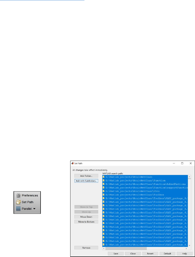
• Interface
Click ‘Set Path’ on the MATLAB panel, or type ‘pathtool’ in the MATLAB command window.
Click ‘Add with Subfolders…’ button, and select path, i.e., ‘D:\BrainNetClass’.
Click ‘Save’ to save your change. If you do not have permission to save your changes on your
computer (e.g., on the server), please save pathdef.m to another location where you will often launch
MATLAB.
Warning: Make sure the BrainNetClass path DOES NOT include any space or special character.
Note: BrainNetClass-v1.0 uses libsvm-3.23 and SLEP-4.1 toolboxes. To run the toolbox, we
sometimes need a compiled libsvm library and SLEP library. Although the compiled version of them
are included in the toolbox, we highly recommend user make a compiled version by themselves.
To compile libsvm, after adding path, please type the following in the command window:
>> cd ‘D:\BrainNetClass’;
>> cd ‘toolbox/libsvm-3.23’;
>> mex -setup
To compile SLEP:
>> cd ‘D:\BrainNetClass’;
>> cd ‘toolbox/SLEP_package_4.1’;
>> mex -setup
Note: Compiling of these two packages may require compilers, please refer to
https://www.mathworks.com/support/requirements/supported-compilers.html.
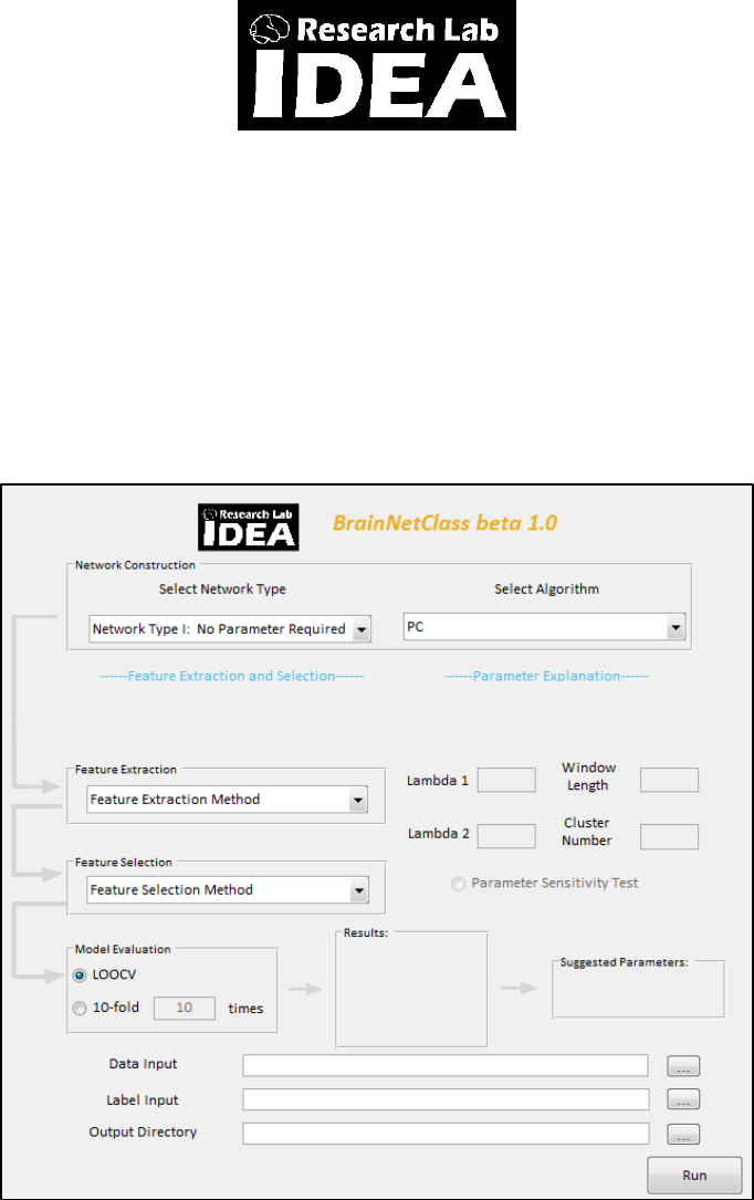
After installation, to run the toolbox, type ‘BrainNetClass’ in the MATLAB command window. The
following GUI window will pop-up.
3. Quick running
1. Specify the RS-fMRI time series data of all subjects by selecting the folder containing all the
text files (in each text file, the data is arranged as a matrix sized Time × Node). Also, specify a
text-formatted label file containing a column of labels for all subjects (e.g., -1 for patient and 1
for control) in the same order as what the Matlab takes when reading these time series data. The
output directory should be also specified.
2. Choose the network construction method by first selecting the type of brain construction
methods and then the specific method. When choosing a parameter required brain network
construction method, the user needs to specify the parameter range(s) if they do not want to use
the default settings. There are brief explanations of the meanings of the parameters on the panel
above parameter settings for users to check.
3. Select or use predefined feature extraction and feature selection methods. There are also
explanations on the panel above for users to check.
4. Choose model evaluation or cross-validation method. If choosing 10-fold cross-validation,
users might also want to specify how many times the 10-fold cross validation will be repeated.
5. After clicking the Run button and waiting for all the processes completing as an ‘All Jobs
Completed’ window will pop out, all the results will be printed out on the result panel and the
suggested parameters panel (if applicable).
6. A full log of results for a hassle-free report is also generated in the result folder.
7. The users may also want to test the performance of other baseline methods, such as PC and SR,
to compare with the state-of-the-art by repeating the above steps.
4. Inputs file preparation
First, the user should specify the input folder that contains ALL of the input data files from ALL
subjects. There are time series files and a label file, both of which should be in the *.txt file format.
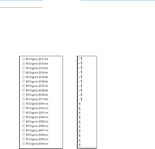
The format of the regional time series file (e.g., 001.txt, 002.txt …) should be the same as that of
the provided exemplary data (see the left panel of the figure below). For each subject, there should
be one *.txt file, which must be a matrix with rows denoting the time points and columns
representing the ROIs. Each subject’s data is in each file. The time series data can be obtained by
the DPABI toolbox (http://rfmri.org/dpabi), REST toolbox (http://restfmri.net/forum/REST_V1.8),
DPARSFA toolbox (http://rfmri.org/dpabi), or other software. For DPABI/REST/DPARSFA, using
‘extracting ROI time series’ function. For preprocessing of raw fMRI data, please see these
toolboxes’ manuals. The user should put all this extracted time series text files into a single folder
without any other files and set this folder as the input directory. The label text file should be prepared
like the following figure (right panel), with each label located in one line for each subject in an order
corresponding to the order of time series data. E.g., -1 represents patient and 1 represents control.
Warning: Make sure the order of two inputs is EXACTLY matched. If not sure, please check the
‘Current Folder’ window in MATLAB to get the idea of the ordering information for the time series
files. To avoid confusion, it is recommended to use the following naming convention:
ROISignals_sub0001.txt, ROISignals_sub0002.txt, … The label should be in the same order (and
should be only -1 and 1).
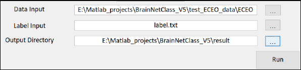
The output directory should also be specified at the beginning. The user may need to create an empty
folder and use it to store the final results. Remember every time you run the toolbox, all the old
result files in the result folder will be covered by new results. We suggest the user stores the saved
results elsewhere when setting up a new running process. Right after the inputs being specified, like
this:
5. Brain network construction
Then, the user should choose which brain construction method to use. The available methods can
be categorized into two types: those with No Parameter Required (Network Type I), e.g., PC,
aHOFC and tHOFC, and those with Parameter Required (Network Type II), e.g., SR, GSR, WSR,
WSGR, SGR, SSGSR, SLR, and dHOFC. For details, see below and please refer to the mentioned
original papers.
Tips: It is recommended that users select only one method that is assumed most appropriate for their
own study. In addition to the main method, the PC and SR can be used as baseline methods. Please
avoid blind selecting and testing all methods and only reporting the one with the best result, because
it violates the rule of machine learning, as the optimized model is determined based on the testing
data. If the sample size is large (e.g., > 200), better choose Network Type I, as parameter
optimization could be time-consuming. If physical memory is low (e.g., < 16GB), better choose
Network Type I. If the data is noising, Network Type II is better, as they may effectively reduce
noise.
Below is a brief explanation of all the available brain network construction methods. For more
details, please see the toolbox paper (to be added) and their respective original papers listed behind.
1. PC: Pearson’s correlation. The most conventional method. It can be used as a baseline
method. No parameter is required.
2. SR: Sparse representation with an L1-norm constraint. One parameter is required. When you
expect the network is sparse or there is heavy noise in the data, you may use it. It can also be
used as a baseline method.
3. GSR: Group sparse representation. It makes sure that all subjects have similar FC network
pattern. One parameter is required. (Wee et al., 2014)
4. SSGSR: Generate within-group similar networks but retain necessary between-group
difference. Two parameters are required. (Zhang et al., 2019)
5. SGR: Sparse group representation. Combining L1-norm and Lq,1-norm to preserve certain
structured information in the adjacency matrix. Two parameters are required. (Yu et al., 2017)
6. WSR: FC-weighted SR. SR-based network construction but with strong FC preserved. One
parameter is required. (Yu et al., 2017)
7. WSGR: Similar to SGR but with strong FC preserved. Two parameters are required. (Yu et
al., 2017)
8. LSR: Low-rank constraint-based SR. Make sure that the network is both sparse and structured
(having some modular structures). Two parameters are required. (Qiao et al., 2016)
9. tHOFC (topographical similarity-based HOFC): A high-order FC metric, the inter-regional
functional relationship is estimated by the FC topological similarity rather than the BOLD
signal similarity. No parameter is required. (Zhang et al., 2016)
10. aHOFC (associated HOFC): A further step from tHOFC measuring inter-level HOFC (the
similarity between HOFC and conventional FC topological profiles. No parameter is required.
(Zhang et al., 2016)

11. dHOFC: Dynamic FC-based HOFC that measures temporal synchronization of dynamic FC
time series. Two parameters are required. (Chen et al., 2016)
Tips: How to choose network construction methods
• If users want to use a simple yet reliable network construction method, PC, tHOFC, and aHOFC
are suggested. Compared to PC, tHOFC and aHOFC are more robust to noise yet interpretable, and
most importantly, they provide supplementary information to PC.
• By using the dynamic FC, dHOFC could capture more high-level complex interaction among brain
regions and perform better than the conventional low-order static FC. Therefore, for diseases (e.g.,
mental disorders) assumed to have little alterations in the brain network, dHOFC is suggested.
• Therefore, for data the potentially higher noise level, SR-based methods can be used. If the brain
networks generated too sparse, the user may choose WSR, WSGR, or SLR to make the estimated
network less sparse, contain more strong connections, or have certain structures. If the data look
quite heterogeneous across subjects and the PC-based networks show large variability (which might
be caused by the noise and artifacts), users may choose group-wise sparse representation, such as
GSR or SSGSR, to make the networks more topologically identical across individuals.
Note: It is not required to pre-specify parameters for the Network Type I, but when choosing a
method in Network Type II, the user needs to specify the related parameter(s) by entering the ranges
of it (them). Although the user could use the default parameter ranges given by the toolbox, it is
recommended to carefully choose them, as the parameters could significantly affect the constructed
brain networks and the classification results. The toolbox will provide default parameter range(s)
for users but they are allowed to change the default parameters based on their own preferences.
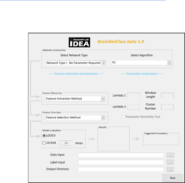
For example, as shown in the figure below, the default ranges for both parameters (λ1 and λ2) of
the SSGSR method are from 0.01 to 0.1 with the increment of 0.01, i.e., [0.01 0.02 0.03 0.04 0.05
0.06 0.07 0.08 0.09 0.1]. Also, it can be set as [2^-4 2^-3 2^-2 2^-1 2^0 2^1 2^2 2^3 2^4] (indicating
[2-4 2-3 2-2 2-1 20 21 22 23 24]). The roles or functions of the λ1 and λ2 are shown in the
panel below in blue.
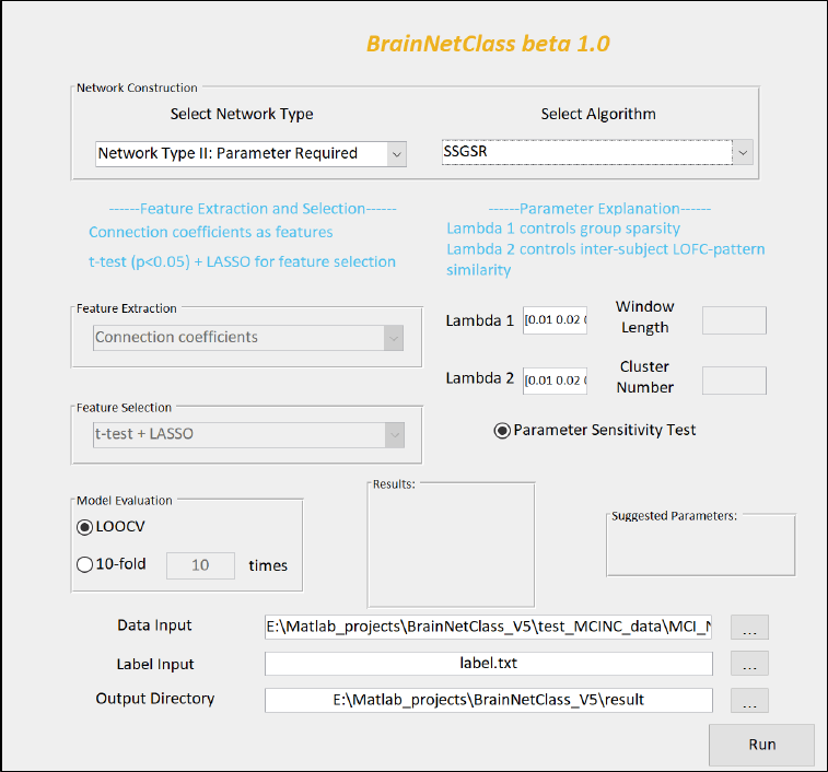
For all the SR-based methods, we have 𝜆1 (and 𝜆2) to be specified, while for the dHOFC method,
we have window length and number of clusters to be specified since it uses dynamic functional
connectivity.
Tips: The memory needed and computation time are related to the sample size, number of ROIs in
the template, brain network construction method, and parameter range (if applicable). We
recommend use computing clusters or servers with a good amount of memory.
6. Feature extraction and selection
After choosing a network construction method, the user needs to choose the methods for feature
extraction and selection. We provide two types of feature extraction methods: connection
coefficients (i.e., directly use the connectivity strength of each link as features) and local clustering
coefficient (i.e., one of the widely used nodal character calculated based on a weighted graph). For
more details, please see (Chen et al., 2016; Zhang et al., 2019).
If the user chooses a network construction method requiring no parameters, he/she will then choose
the method for feature extraction (i.e., connection coefficients and weighted local clustering
coefficients) and selection (i.e., t-test, LASSO, and t-test + LASSO).
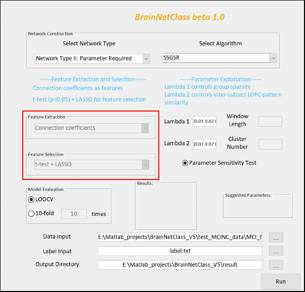
If the user chooses a network construction method requiring a parameter(s), specific feature
extraction/selection method will be automatically suggested to the user and it may be changed. For
example, for the SR-based methods, users are restricted to use the connection-based coefficients as
features combining with t-test+LASSO to perform feature selection (see the figure below). For the
dHOFC method, users are restricted to use weighted-graph local clustering coefficients as features
and LASSO to perform feature selection.
Note: The default threshold used for the t-test is p < 0.05. The hyper-parameter used for LASSO is
0.1. If the user wants to change these settings, please go to BrainNetClass.m file in the toolbox’s
path to change the settings. For example, one may change the value at the end of ‘[Line 119]
handles.default.lasso_lambda=0.1’ to any value. By decreasing it, the number of selected
parameters will be larger, and vice versa.
7. Classification and model evaluation
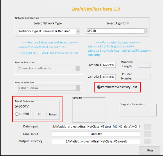
We provided two types of cross-validation strategies (see figure below). The first one is leave-one-
out cross-validation (LOOCV) and the other is 10-fold cross-validation. If the sample size is large,
we recommend the 10-fold cross-validation to save time. With a limited sample size, we recommend
LOOCV. Of note, Notably, 10-fold cross validation will be run for many times (default: 10 times,
the user may specify more than 10 times, e.g., 100, but it will increase the processing time). This is
because the result of 10-fold cross validation heavily depends on data partitioning.
There is a ‘Parameter Sensitivity Test’ function provided to assess the effects of the hyper-
parameters on classification accuracy using LOOCV with all the subjects. See (Zhang et al., 2019)
for the rationale for doing so. It is suggested to do so and include the result in the paper. When the
user chooses any parameter-required brain network construction method, the parameter sensitivity
test will be chosen automatically. While it is free to be de-selected, we still encourage the user to
choose the parameter sensitivity test, because it will not take too long time to run and will provide
a valuable result in terms of model sensitivity.
The toolbox also automatically counts the selection occurrence (%) of each combination of the
parameters. This information can be used to evaluate model robustness and is thus suggested to
include in the paper. For a robust model, there should be one value of the parameter (or one
combination of the parameters) significantly selected more than others.
In addition to the numeric classification performance evaluations and the ROC curve, the user may
also want to know which features contributed more (a.k.a., contributing features) or more important
to the disease classification. We thus provide the averaged weight derived from the SVM across all
the cross-validation runs for each feature as the feature importance measure. Another quantitative
measurement of feature importance, i.e., the selection occurrence of each feature being selected in feature
selection across all cross-validation runs, could also indicate feature importance. The more frequently a
feature has been selected, the more important this feature could be.
For dHOFC method, the resultant important features will be some clusters including some
nodes/edges and they will be saved in a different way. The saved result (‘result_features.mat’ in the
result folder) will be a cell array with four columns, representing the selection occurrence of each
feature (cluster), the indices of the involved nodes in each cluster, a matrix indicating the
connections in each cluster (nROI nROI, if there is a connection between two nodes, then the
value of this connection is set to 1), and the mean weight for each feature (cluster), respectively.
For other methods, if connection coefficients are used as features, the saved result will be a cell
array with two elements. One is a matrix (nROI nROI) with each connection set to the averaged
weight of the connection. The other is a matrix (nROI nROI) with each connection set to the
normalized occurrence (%) of the connection. If local clustering coefficients are used for features,
then the saved result will be a cell array with two elements. One is a vector (in a length of nROI)
with each element representing an averaged weight of this node. The other is also a vector at the
same length with each element representing the normalized occurrence (%) of this node.
Besides, we also show the group-averaged brain network (which is saved as
‘Mean_optimal_negativeLabel_network_.mat’ and ‘Mean_optimal_positiveLabel_network_.mat’
in the result folder) in a form of two weighted adjacency matrices for each group constructed by the
optimal parameter(s) if the user chooses the parameter needed brain network construction methods.
For methods requiring no parameter, we just averaged the constructed brain network within each
group.
Another unique feature of our toolbox is that it saves the optimal classification model
(‘saved_model.mat’ in the result folder). With new data coming, the saved model can be simply
applied on the new data to decide the type of the new data (i.e., patient or normal control), omitting
the training and testing process, which will highly improve the efficiency.
8. Before hitting the ‘Run’ button
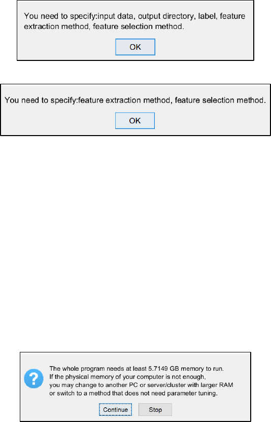
We have set up some reminders for the user to let them better use the toolbox. When the user chooses
a certain brain network construction method, if he/she forgets some settings (i.e., feature
extraction/selection method), a dialog box will pop out to remind the user, which are shown as below:
or
After all the settings are successfully set up, the user is ready to run the toolbox. There is also a
reminder of how much memory the toolbox could use when choosing one of the parameter-required
network construction methods (or Type II network construction methods; for Type I method,
memory usually is not a big concern). For example, when the user chooses dHOFC, a dialog box
will pop up showing the estimated memory that running the entire analysis will require as below. In
this example, at least 5.72 GB physical memory is needed. Note that it is just a rough estimation, it
may need more than 5.72 GB in reality. If the user feels that there is not enough memory left, he/she
may change to a computing cluster/server with more memory, or choose a network construction
method without parameter optimization (i.e., Type I method), or he/she can narrow down the range
of the parameters to be tuned (for example, by changing the parameter sampling strategy from [0.01
0.02 0.03 0.04 0.05 0.06 0.07 0.08 0.09 0.1] to [0.01 0.03 0.05 0.07 0.09]).
9. Result display and guidance of result interpretation
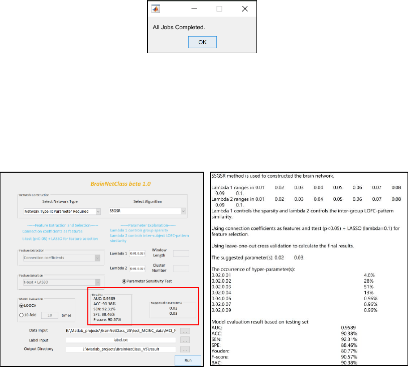
Once all the data analysis process has been finished, a dialog box pops out, as shown below. If not,
please wait for this dialog box before doing anything further, as the toolbox is still running.
When all the computational processes are finished, the model performance will be displayed on the
GUI panel (see the left panel of the figure below). The results are also recorded and saved in a log
file (in *.txt format). This log file records the method used to construct the brain network, the
parameters the user specified, feature extraction and selection methods, cross-validation methods,
suggested parameter(s), the occurrence of parameters, and the performance of the classifier (see the
right panel of the figure below).
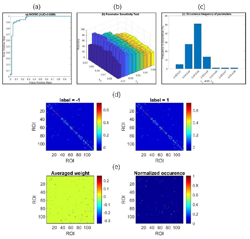
Furthermore, if the user chooses the parameter-required network construction methods and go
through the whole process (i.e., the parameter sensitivity test), the toolbox will generate five figures
in the result folder (see the figure below), which are:
a) Receiver Operating Characteristic (ROC) curve of the classification performance;
b) Classification accuracy from the parameter sensitivity test;
c) Parameter selection occurrence;
d) Averaged optimal network for each group;
e) Contributing features, showing as averaged weight and normalized occurrence.
The toolbox also generates four *.mat files in the result folder:
a) Mean_optimal_negativeLabel_network_.mat
b) Mean_optimal_positiveLabel_network_.mat
c) result_features.mat
d) saved_model.mat
For more interpretation of these generated results, please see the toolbox paper.

10. Exemplary data
We provide some exemplary data for the users to get familiar with the usage of the toolbox. The
data is from http://fcon_1000.projects.nitrc.org/indi/retro/BeijingEOEC.html (Beijing: Eyes Open
Eyes Closed Study). The goal is to use resting-state fMRI time series from 116 brain regions to
construct brain functional networks and predict whether the subject is in eyes closed state or eyes
open state. There is a full version (with longer running time but better classification result) and a
simplified version of the data (with shorter running time, for fast running). The labels (EC, EO) are
provided with two versions as well (see label.txt and label_simple.txt). For more details and more
experiments, please see the toolbox paper (to be added).
11. Batch mode
In addition to the GUI-based mode, BrainNetClass also offers a batch mode.
The batch mode is for advanced users.
The related functions can be found in ‘BatchExamples’ folder in the main folder of the toolbox,
which includes:
1. ‘param_select_demo.m’
This is a main batch-process function for all Type-II network-based classification, which requires
parameter optimization. It will be called by the provided demo function in 3 and generate some
results (ROC curve and other model evaluation metrics, parameter sensitivity test result). More
modules will be added in this demo in future versions.
2. ‘no_param_select_demo.m’
This is a main batch-process function for all Type-I network-based classification, which does not
require parameter optimization. It will be called by the provided demo function in 3 and generate
some results (ROC curve and other model evaluation metrics). More modules will be added in this
demo in future versions.
3. ‘run_EC_EO_demo.m’
This is an exemplary demo function for users to conduct a two-class classification using dHOFC
(the main method), SR (one of the baseline methods), and PC (one of the baseline methods). It
calls main functions in 1 and 2. Users may modify it according to their own preference. For details
of the inputs and outputs, please see ‘param_select_demo.m’ and ‘no_param_select_demo.m’.
Exemplar data inputs are provided in the ‘BatchExamples’ folder, which contain ‘ECEO_label.
mat’ and ‘ECEO.mat’. User can run ‘run_EC_EO_demo.m’ with these inputs.
References
Chen, X., Zhang, H., Gao, Y., Wee, C.Y., Li, G., Shen, D., Alzheimer's Disease Neuroimaging, I.,
2016. High-order resting-state functional connectivity network for MCI classification. Hum Brain
Mapp 37, 3282-3296.
Qiao, L., Zhang, H., Kim, M., Teng, S., Zhang, L., Shen, D., 2016. Estimating functional brain
networks by incorporating a modularity prior. Neuroimage 141, 399-407.
Wee, C.Y., Yap, P.T., Zhang, D., Wang, L., Shen, D., 2014. Group-constrained sparse fMRI
connectivity modeling for mild cognitive impairment identification. Brain Struct Funct 219, 641-
656.
Yu, R., Zhang, H., An, L., Chen, X., Wei, Z., Shen, D., 2017. Connectivity strength-weighted sparse
group representation-based brain network construction for MCI classification. Hum Brain Mapp 38,
2370-2383.
Zhang, H., Chen, X., Shi, F., Li, G., Kim, M., Giannakopoulos, P., Haller, S., Shen, D., 2016.
Topographical Information-Based High-Order Functional Connectivity and Its Application in
Abnormality Detection for Mild Cognitive Impairment. J Alzheimers Dis 54, 1095-1112.
Zhang, Y., Zhang, H., Chen, X., Liu, M., Zhu, X., Lee, S.-W., Shen, D., 2019. Strength and similarity
guided group-level brain functional network construction for MCI diagnosis. Pattern Recognition
88, 421-430.
