Mondrian Technical Guide 3.0

User Manual:

Open the PDF directly: View PDF .
Page Count: 254 [warning: Documents this large are best viewed by clicking the View PDF Link!]

License and Copyright
Introduction
JasperAnalysis and Mondrian
Mondrian and OLAP
- Online Analytical Processing
- Conclusion
Mondrian Architecture
- Layers of a Mondrian system
  - Storage and aggregation strategies
- API
How to Design a Mondrian Schema
MDX Specification
Configuration Guide
Optimizing Mondrian Performance
Aggregate Tables
Cache Control
Mondrian CmdRunner
Mondrian FAQs
Results Caching – The key to performance
Learning more about Mondrian
Appendix A – MDX Function List
Visual Basic for Applications (VBA) Function List

Mondrian 3.0.4

Technical Guide

Developing OLAP solutions with Mondrian/JasperAnalysis

March 2009

- 1 -

Table of Contents

License and Copyright ..........................................................................................................5

Introduction ........................................................................................................................9

JasperAnalysis and Mondrian................................................................................................. 9

Mondrian and OLAP............................................................................................................ 11

Online Analytical Processing............................................................................................. 11

Conclusion ..................................................................................................................... 12

Mondrian Architecture ........................................................................................................ 13

Layers of a Mondrian system ........................................................................................... 13

API................................................................................................................................15

How to Design a Mondrian Schema...................................................................................... 17

What is a schema?.......................................................................................................... 17

Schema files................................................................................................................... 17

Logical model................................................................................................................. 17

Cube.............................................................................................................................. 19

Measures ....................................................................................................................... 19

Dimensions, Hierarchies, Levels ....................................................................................... 20

Mapping dimensions and hierarchies onto tables ............................................................... 21

The 'all' member............................................................................................................. 22

Time dimensions............................................................................................................. 23

Order and display of levels .............................................................................................. 23

Multiple hierarchies......................................................................................................... 24

Degenerate dimensions................................................................................................... 25

Inline tables................................................................................................................... 26

Member properties and formatters ................................................................................... 27

Approximate level cardinality ........................................................................................... 27

Star and snowflake schemas............................................................................................ 27

Shared dimensions.......................................................................................................... 28

Join optimization............................................................................................................. 28

Advanced logical constructs............................................................................................. 29

Member properties.......................................................................................................... 33

Calculated members........................................................................................................ 34

Named sets.................................................................................................................... 36

Plug-ins ......................................................................................................................... 37

Member reader............................................................................................................... 40

Internationalization......................................................................................................... 45

Aggregate tables ............................................................................................................ 47

Access-control................................................................................................................ 48

XML elements................................................................................................................. 52

MDX Specification .............................................................................................................. 55

What is MDX?................................................................................................................. 55

What is the syntax of MDX?............................................................................................. 55

Mondrian-specific MDX.................................................................................................... 55

Configuration Guide............................................................................................................ 58

Properties ...................................................................................................................... 58

Property list.................................................................................................................... 59

Connect strings............................................................................................................... 66

Cache management........................................................................................................ 68

Memory management ..................................................................................................... 68

Logging ......................................................................................................................... 69

Optimizing Mondrian Performance....................................................................................... 70

Introduction................................................................................................................... 70

A generalized tuning process for Mondrian........................................................................ 70

- 2 -

Recommendations for database tuning............................................................................. 71

Aggregate Tables, Materialized Views and Mondrian .......................................................... 71

AggGen.......................................................................................................................... 72

Optimizing Calculations with the Expression Cache ............................................................ 72

Aggregate Tables............................................................................................................... 74

Introduction................................................................................................................... 74

What are aggregate tables?............................................................................................. 75

A simple aggregate table................................................................................................. 76

Another aggregate table.................................................................................................. 77

Defining aggregate tables................................................................................................ 78

Building aggregate tables ................................................................................................ 79

How Mondrian recognizes Aggregate Tables...................................................................... 85

Aggregate tables and parent-child hierarchies ................................................................... 90

How Mondrian uses aggregate tables ............................................................................... 93

Tools for designing and maintaining aggregate tables........................................................ 96

Properties that affect aggregates ..................................................................................... 97

Aggregate Table References............................................................................................ 99

Cache Control.................................................................................................................... 99

Note for JasperAnalysis................................................................................................... 99

Introduction................................................................................................................... 99

How Mondrian's cache works........................................................................................... 99

New CacheControl API ...................................................................................................100

Other cache control topics..............................................................................................104

Mondrian CmdRunner........................................................................................................108

What is CmdRunner?......................................................................................................108

Building ........................................................................................................................108

Usage...........................................................................................................................108

Properties File ...............................................................................................................109

Command line arguments...............................................................................................110

CmdRunner Commands..................................................................................................110

AggGen: Aggregate SQL Generator .................................................................................114

Mondrian FAQs .................................................................................................................118

Why doesn't Mondrian use a standard API?......................................................................118

How does Mondrian's dialect of MDX differ from Microsoft Analysis Services?......................118

How can Mondrian be extended?.....................................................................................118

Can Mondrian handle large datasets? ..............................................................................119

How do I enable tracing?................................................................................................119

How do I enable logging?...............................................................................................119

What is the syntax of a Mondrian connect string?.............................................................120

Where is Mondrian going in the future? ...........................................................................120

Where can I find out more?............................................................................................120

Mondrian is wonderful! How can I possibly thank you?......................................................120

Modeling.......................................................................................................................120

Build/install...................................................................................................................122

Performance..................................................................................................................122

Results Caching – The key to performance..........................................................................125

Segment.......................................................................................................................126

Member set...................................................................................................................126

Schema ........................................................................................................................126

Star schemas.................................................................................................................126

Learning more about Mondrian...........................................................................................127

How Mondrian generates SQL.........................................................................................127

Logging Levels and Information......................................................................................128

- 3 -

Default aggregate table recognition rules.........................................................................129

Snowflakes and the DimensionUsage level attribute..........................................................134

Appendix A – MDX Function List.........................................................................................138

Visual Basic for Applications (VBA) Function List ..................................................................177

- 4 -

License and Copyright

This manual is derived from content published as part of the Mondrian open source project at

http://mondrian.pentaho.org, https://sourceforge.net/projects/mondrian and

https://sourceforge.net/project/showfiles.php?group_id=35302.

This content is published under the Common Public License Agreement version 1.0 (the “CPL”,

available at the following URL: http://www.opensource.org/licenses/cpl.html) - the same license

as the the original content.

- 5 -

Common Public License - v 1.0

THE ACCOMPANYING PROGRAM IS PROVIDED UNDER THE TERMS OF THIS COMMON

PUBLIC LICENSE ("AGREEMENT"). ANY USE, REPRODUCTION OR DISTRIBUTION OF THE

PROGRAM CONSTITUTES RECIPIENT'S ACCEPTANCE OF THIS AGREEMENT.

1. DEFINITIONS

"Contribution" means:

a) in the case of the initial Contributor, the initial code and documentation distributed under this

Agreement, and

b) in the case of each subsequent Contributor:

i) changes to the Program, and

ii) additions to the Program;

where such changes and/or additions to the Program originate from and are distributed by that

particular Contributor. A Contribution 'originates' from a Contributor if it was added to the

Program by such Contributor itself or anyone acting on such Contributor's behalf. Contributions

do not include additions to the Program which: (i) are separate modules of software distributed in

conjunction with the Program under their own license agreement, and (ii) are not derivative works

of the Program.

"Contributor" means any person or entity that distributes the Program.

"Licensed Patents " mean patent claims licensable by a Contributor which are necessarily infringed by the

use or sale of its Contribution alone or when combined with the Program.

"Program" means the Contributions distributed in accordance with this Agreement.

"Recipient" means anyone who receives the Program under this Agreement, including all Contributors.

2. GRANT OF RIGHTS

a) Subject to the terms of this Agreement, each Contributor hereby grants Recipient a non-

exclusive, worldwide, royalty-free copyright license to reproduce, prepare derivative works of,

publicly display, publicly perform, distribute and sublicense the Contribution of such Contributor,

if any, and such derivative works, in source code and object code form.

b) Subject to the terms of this Agreement, each Contributor hereby grants Recipient a non-

exclusive, worldwide, royalty-free patent license under Licensed Patents to make, use, sell, offer

to sell, import and otherwise transfer the Contribution of such Contributor, if any, in source code

and object code form. This patent license shall apply to the combination of the Contribution and

the Program if, at the time the Contribution is added by the Contributor, such addition of the

Contribution causes such combination to be covered by the Licensed Patents. The patent license

shall not apply to any other combinations which include the Contribution. No hardware per se is

licensed hereunder.

c) Recipient understands that although each Contributor grants the licenses to its Contributions set

forth herein, no assurances are provided by any Contributor that the Program does not infringe the

patent or other intellectual property rights of any other entity. Each Contributor disclaims any

liability to Recipient for claims brought by any other entity based on infringement of intellectual

property rights or otherwise. As a condition to exercising the rights and licenses granted

hereunder, each Recipient hereby assumes sole responsibility to secure any other intellectual

property rights needed, if any. For example, if a third party patent license is required to allow

Recipient to distribute the Program, it is Recipient's responsibility to acquire that license before

distributing the Program.

d) Each Contributor represents that to its knowledge it has sufficient copyright rights in its

Contribution, if any, to grant the copyright license set forth in this Agreement.

- 6 -

3. REQUIREMENTS

A Contributor may choose to distribute the Program in object code form under its own license agreement,

provided that:

a) it complies with the terms and conditions of this Agreement; and

b) its license agreement:

i) effectively disclaims on behalf of all Contributors all warranties and conditions, express and

implied, including warranties or conditions of title and non-infringement, and implied warranties

or conditions of merchantability and fitness for a particular purpose;

ii) effectively excludes on behalf of all Contributors all liability for damages, including direct,

indirect, special, incidental and consequential damages, such as lost profits;

iii) states that any provisions which differ from this Agreement are offered by that Contributor

alone and not by any other party; and

iv) states that source code for the Program is available from such Contributor, and informs

licensees how to obtain it in a reasonable manner on or through a medium customarily used for

software exchange.

When the Program is made available in source code form:

a) it must be made available under this Agreement; and

b) a copy of this Agreement must be included with each copy of the Program.

Contributors may not remove or alter any copyright notices contained within the Program.

Each Contributor must identify itself as the originator of its Contribution, if any, in a manner that

reasonably allows subsequent Recipients to identify the originator of the Contribution.

4. COMMERCIAL DISTRIBUTION

Commercial distributors of software may accept certain responsibilities with respect to end users, business

partners and the like. While this license is intended to facilitate the commercial use of the Program, the

Contributor who includes the Program in a commercial product offering should do so in a manner which

does not create potential liability for other Contributors. Therefore, if a Contributor includes the Program in

a commercial product offering, such Contributor ("Commercial Contributor") hereby agrees to defend and

indemnify every other Contributor ("Indemnified Contributor") against any losses, damages and costs

(collectively "Losses") arising from claims, lawsuits and other legal actions brought by a third party against

the Indemnified Contributor to the extent caused by the acts or omissions of such Commercial Contributor

in connection with its distribution of the Program in a commercial product offering. The obligations in this

section do not apply to any claims or Losses relating to any actual or alleged intellectual property

infringement. In order to qualify, an Indemnified Contributor must: a) promptly notify the Commercial

Contributor in writing of such claim, and b) allow the Commercial Contributor to control, and cooperate

with the Commercial Contributor in, the defense and any related settlement negotiations. The Indemnified

Contributor may participate in any such claim at its own expense.

For example, a Contributor might include the Program in a commercial product offering, Product X. That

Contributor is then a Commercial Contributor. If that Commercial Contributor then makes performance

claims, or offers warranties related to Product X, those performance claims and warranties are such

Commercial Contributor's responsibility alone. Under this section, the Commercial Contributor would have

to defend claims against the other Contributors related to those performance claims and warranties, and if a

court requires any other Contributor to pay any damages as a result, the Commercial Contributor must pay

those damages.

5. NO WARRANTY

EXCEPT AS EXPRESSLY SET FORTH IN THIS AGREEMENT, THE PROGRAM IS PROVIDED ON

AN "AS IS" BASIS, WITHOUT WARRANTIES OR CONDITIONS OF ANY KIND, EITHER

EXPRESS OR IMPLIED INCLUDING, WITHOUT LIMITATION, ANY WARRANTIES OR

CONDITIONS OF TITLE, NON-INFRINGEMENT, MERCHANTABILITY OR FITNESS FOR A

PARTICULAR PURPOSE. Each Recipient is solely responsible for determining the appropriateness of

using and distributing the Program and assumes all risks associated with its exercise of rights under this

- 7 -

Agreement, including but not limited to the risks and costs of program errors, compliance with applicable

laws, damage to or loss of data, programs or equipment, and unavailability or interruption of operations.

6. DISCLAIMER OF LIABILITY

EXCEPT AS EXPRESSLY SET FORTH IN THIS AGREEMENT, NEITHER RECIPIENT NOR ANY

CONTRIBUTORS SHALL HAVE ANY LIABILITY FOR ANY DIRECT, INDIRECT, INCIDENTAL,

SPECIAL, EXEMPLARY, OR CONSEQUENTIAL DAMAGES (INCLUDING WITHOUT

LIMITATION LOST PROFITS), HOWEVER CAUSED AND ON ANY THEORY OF LIABILITY,

WHETHER IN CONTRACT, STRICT LIABILITY, OR TORT (INCLUDING NEGLIGENCE OR

OTHERWISE) ARISING IN ANY WAY OUT OF THE USE OR DISTRIBUTION OF THE PROGRAM

OR THE EXERCISE OF ANY RIGHTS GRANTED HEREUNDER, EVEN IF ADVISED OF THE

POSSIBILITY OF SUCH DAMAGES.

7. GENERAL

If any provision of this Agreement is invalid or unenforceable under applicable law, it shall not affect the

validity or enforceability of the remainder of the terms of this Agreement, and without further action by the

parties hereto, such provision shall be reformed to the minimum extent necessary to make such provision

valid and enforceable.

If Recipient institutes patent litigation against a Contributor with respect to a patent applicable to software

(including a cross-claim or counterclaim in a lawsuit), then any patent licenses granted by that Contributor

to such Recipient under this Agreement shall terminate as of the date such litigation is filed. In addition, if

Recipient institutes patent litigation against any entity (including a cross-claim or counterclaim in a

lawsuit) alleging that the Program itself (excluding combinations of the Program with other software or

hardware) infringes such Recipient's patent(s), then such Recipient's rights granted under Section 2(b) shall

terminate as of the date such litigation is filed.

All Recipient's rights under this Agreement shall terminate if it fails to comply with any of the material

terms or conditions of this Agreement and does not cure such failure in a reasonable period of time after

becoming aware of such noncompliance. If all Recipient's rights under this Agreement terminate, Recipient

agrees to cease use and distribution of the Program as soon as reasonably practicable. However, Recipient's

obligations under this Agreement and any licenses granted by Recipient relating to the Program shall

continue and survive.

Everyone is permitted to copy and distribute copies of this Agreement, but in order to avoid inconsistency

the Agreement is copyrighted and may only be modified in the following manner. The Agreement Steward

reserves the right to publish new versions (including revisions) of this Agreement from time to time. No

one other than the Agreement Steward has the right to modify this Agreement. IBM is the initial

Agreement Steward. IBM may assign the responsibility to serve as the Agreement Steward to a suitable

separate entity. Each new version of the Agreement will be given a distinguishing version number. The

Program (including Contributions) may always be distributed subject to the version of the Agreement under

which it was received. In addition, after a new version of the Agreement is published, Contributor may

elect to distribute the Program (including its Contributions) under the new version. Except as expressly

stated in Sections 2(a) and 2(b) above, Recipient receives no rights or licenses to the intellectual property of

any Contributor under this Agreement, whether expressly, by implication, estoppel or otherwise. All rights

in the Program not expressly granted under this Agreement are reserved.

This Agreement is governed by the laws of the State of New York and the intellectual property laws of the

United States of America. No party to this Agreement will bring a legal action under this Agreement more

than one year after the cause of action arose. Each party waives its rights to a jury trial in any resulting

litigation.

- 8 -

Introduction

This document summarizes in one place the available documentation from the Mondrian open

source project, version 3.0.4. The contents are derived from documentation in the Mondrian code

distribution.

The aim of this document is to provide a guide to the use of Mondrian, covering:

• Mondrian overview and architecture

• Developing OLAP schemas

• Querying cubes with MDX

• Tools and techniques for managing data and tuning query performance

• Integrating Mondrian into applications

The audience of this document is intended to be people creating and managing Mondrian based

OLAP environments and developers who are integrating Mondrian into their applications.

JasperAnalysis and Mondrian

JasperAnalysis in JasperServer 3.5 is based on Mondrian 3.0.4 and the corresponding version of

JPivot (the OLAP slice and dice user interface). JasperAnalysis modifies these base open source

projects in the following ways:

Extensive changes to the JPivot user interface

• Revised Look and feel

• Expand and Collapse All

• Additonal display and output options

• Performance improvements for drillthrough against Mondrian cubes

• Fully internationalized text

• Save/Save As View to the JasperServer repository

Mondrian Integration with JasperServer

• Integration with the JasperServer repository

o Schemas, Data Source definitions in JasperServer Repository

o Access to resources controlled by repository permissions for users and roles

• Maintenance screens for Mondrian and XML/A configuration

• Mondrian and XML/A data sources for JasperReports

• Configuration of JasperAnalysis as an XML/A server, providing services to XML/A client

such as Excel Pivot tables (Jaspersoft ODBO Connect) and other JasperAnalysis web

clients

• Display of current Mondrian configuration settings

JasperAnalysis Professional Features

JasperAnalysis Professional Edition has additional features beyond what is provided in

JasperAnalysis Community Edition.

- 9 -

• Performance Profiling Analysis and reports for SQL and MDX queries

• Data level security: user profile based fitering of OLAP results beyond simple roles

• Editing of current Mondrian configuration settings through the browser

• Excel Pivot Table ODBO driver: connects to JasperAnalysis and Mondrian to display and

interact with JasperAnalysis hosted cubes

JasperAnalysis is documented in separate User and Administration Guides. In this guide, there

are specific notes on where JasperAnalysis differs from standard Mondrian features.

- 10 -

Mondrian and OLAP

Mondrian is an OLAP engine written in Java. It executes queries written in the MDX language,

reading data from a relational database (RDBMS), and presents the results in a multidimensional

format via a Java API. Let's go into what that means.

Online Analytical Processing

OLAP (Online Analytical Processing) means analysing large quantities of data in real-time. Unlike

Online Transaction Processing (OLTP), where typical operations read and modify individual and

small numbers of records, OLAP deals with data in bulk, and operations are generally read-only.

The term 'online' implies that even though huge quantities of data are involved — typically many

millions of records, occupying several gigabytes — the system must respond to queries fast

enough to allow an interactive exploration of the data. As we shall see, that presents

considerable technical challenges.

OLAP employs a technique called Multidimensional Analysis. Whereas a relational database stores

all data in the form of rows and columns, a multidimensional dataset consists of axes and cells.

Consider the dataset

Year

2000 2001 Growth

Product

Dollar

sales Unit

sales Dollar

sales Unit

sales Dollar

sales Unit

sales

Total $7,073 2,693 $7,636 3,008 8% 12%

— Books $2,753 824 $3,331 966 21% 17%

—— Fiction $1,341 424 $1,202 380 -10% -10%

—— Non-fiction $1,412 400 $2,129 586 51% 47%

— Magazines $2,753 824 $2,426 766 -12% -7%

— Greetings

cards $1,567 1,045 $1,879 1,276 20% 22%

The rows axis consists of the members 'All products', 'Books', 'Fiction', and so forth, and the

columns axis consists of the cartesian product of the years '2000' and '2001', and the calculation

'Growth', and the measures 'Unit sales' and 'Dollar sales'. Each cell represents the sales of a

product category in a particular year; for example, the dollar sales of Magazines in 2001 were

$2,426.

This is a richer view of the data than would be presented by a relational database. The members

of a multidimensional dataset are not always values from a relational column. 'Total', 'Books' and

'Fiction' are members at successive levels in a hierarchy, each of which is rolled up to the next.

And even though it is alongside the years '2000' and '2001', 'Growth' is a calculated member,

which introduces a formula for computing cells from other cells.

The dimensions used here — products, time, and measures — are just three of many dimensions

by which the dataset can be categorized and filtered. The collection of dimensions, hierarchies

and measures is called a cube.

- 11 -

Conclusion

I hope I have demonstrated that multidimensional is above all a way of presenting data.

Although some multidimensional databases store the data in multidimensional format, I shall

argue that it is simpler to store the data in relational format.

Now it's time to look at the architecture of an OLAP system. See Mondrian architecture.

- 12 -

- 13 -

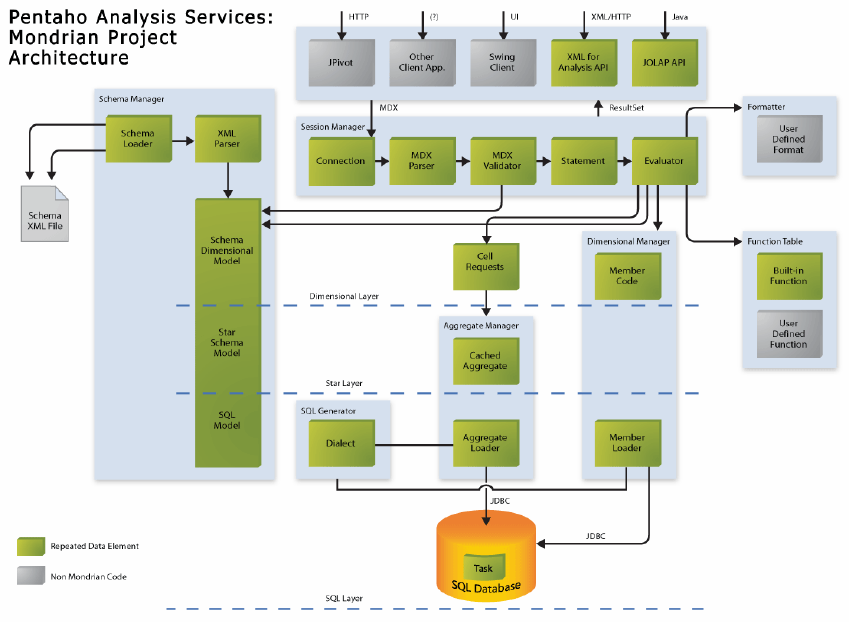
Mondrian Architecture

Layers of a Mondrian system

A Mondrian OLAP System consists of four layers; working from the eyes of the end-user to the

bowels of the data center, these are as follows: the presentation layer, the dimensional layer, the

star layer, and the storage layer. (See figure 1.)

The presentation layer determines what the end-user sees on his or her monitor, and how he or

she can interact to ask new questions. There are many ways to present multidimensional

datasets, including pivot tables (an interactive version of the table shown above), pie, line and

bar charts, and advanced visualization tools such as clickable maps and dynamic graphics. These

might be written in Swing or JSP, charts rendered in JPEG or GIF format, or transmitted to a

remote application via XML. What all of these forms of presentation have in common is the

multidimensional 'grammar' of dimensions, measures and cells in which the presentation layer

asks the question is asked, and OLAP server returns the answer.

The second layer is the dimensional layer. The dimensional layer parses, validates and executes

MDX queries. A query is evaluted in multiple phases. The axes are computed first, then the

values of the cells within the axes. For efficiency, the dimensional layer sends cell-requests to the

aggregation layer in batches. A query transformer allows the application to manipulate existing

queries, rather than building an MDX statement from scratch for each request. And metadata

describes the the dimensional model, and how it maps onto the relational model.

The third layer is the star layer, and is responsible for maintaining an aggregate cache. An

aggregation is a set of measure values ('cells') in memory, qualified by a set of dimension column

values. The dimensional layer sends requests for sets of cells. If the requested cells are not in the

cache, or derivable by rolling up an aggregation in the cache, the aggregation manager sends a

request to the storage layer.

The storage layer is an RDBMS. It is responsible for providing aggregated cell data, and members

from dimension tables. I describe below why I decided to use the features of the RDBMS rather

than developing a storage system optimized for multidimensional data.

These components can all exist on the same machine, or can be distributed between machines.

Layers 2 and 3, which comprise the Mondrian server, must be on the same machine. The storage

layer could be on another machine, accessed via remote JDBC connection. In a multi-user

system, the presentation layer would exist on each end-user's machine (except in the case of JSP

pages generated on the server).

Storage and aggregation strategies

OLAP Servers are generally categorized according to how they store their data:

• A MOLAP (multidimensional OLAP) server stores all of its data on disk in structures

optimized for multidimensional access. Typically, data is stored in dense arrays, requiring

only 4 or 8 bytes per cell value.

• A ROLAP (relational OLAP) server stores its data in a relational database. Each row in a

fact table has a column for each dimension and measure.

Three kinds of data need to be stored: fact table data (the transactional records), aggregates,

and dimensions.

MOLAP databases store fact data in multidimensional format, but if there are more than a few

dimensions, this data will be sparse, and the multidimensional format does not perform well. A

HOLAP (hybrid OLAP) system solves this problem by leaving the most granular data in the

relational database, but stores aggregates in multidimensional format.

Pre-computed aggregates are necessary for large data sets, otherwise certain queries could not

be answered without reading the entire contents of the fact table. MOLAP aggregates are often

an image of the in-memory data structure, broken up into pages and stored on disk. ROLAP

aggregates are stored in tables. In some ROLAP systems these are explicitly managed by the

OLAP server; in other systems, the tables are declared as materialized views, and they are

- 14 -

implicitly used when the OLAP server issues a query with the right combination of columns in the

group by clause.

The final component of the aggregation strategy is the cache. The cache holds pre-computed

aggregations in memory so subsequent queries can access cell values without going to disk. If

the cache holds the required data set at a lower level of aggregation, it can compute the required

data set by rolling up.

The cache is arguably the most important part of the aggregation strategy because it is adaptive.

It is difficult to choose a set of aggregations to pre-compute which speed up the system without

using huge amounts of disk, particularly those with a high dimensionality or if the users are

submitting unpredictable queries. And in a system where data is changing in real-time, it is

impractical to maintain pre-computed aggregates. A reasonably sized cache can allow a system

to perform adequately in the face of unpredictable queries, with few or no pre-computed

aggregates.

Mondrian's aggregation strategy is as follows:

• Fact data is stored in the RDBMS. Why develop a storage manager when the RDBMS

already has one?

• Read aggregate data into the cache by submitting group by queries. Again, why develop

an aggregator when the RDBMS has one?

• If the RDBMS supports materialized views, and the database administrator chooses to

create materialized views for particular aggregations, then Mondrian will use them

implicitly. Ideally, Mondrian's aggregation manager should be aware that these

materialized views exist and that those particular aggregations are cheap to compute. If

should even offer tuning suggestings to the database administrator.

The general idea is to delegate unto the database what is the database's. This places additional

burden on the database, but once those features are added to the database, all clients of the

database will benefit from them. Multidimensional storage would reduce I/O and result in faster

operation in some circumstances, but I don't think it warrants the complexity at this stage.

A wonderful side-effect is that because Mondrian requires no storage of its own, it can be

installed by adding a JAR file to the class path and be up and running immediately. Because there

are no redundant data sets to manage, the data-loading process is easier, and Mondrian is ideally

suited to do OLAP on data sets which change in real time.

API

Mondrian provides an API for client applications to execute queries.

Since there is no widely universally accepted API for executing OLAP queries, Mondrian's primary

API proprietary; however, anyone who has used JDBC should find it familiar. The main difference

is the query language: Mondrian uses a language called MDX ('Multi-Dimensional eXpressions')

to specify queries, where JDBC would use SQL. MDX is described in more detail below.

The following Java fragment connects to Mondrian, executes a query, and prints the results:

- 15 -

import mondrian.olap.*;

import java.io.PrintWriter;

Connection connection = DriverManager.getConnection(

"Provider=mondrian;" +

"Jdbc=jdbc:odbc:MondrianFoodMart;" +

"Catalog=/WEB-INF/FoodMart.xml;",

null,

false);

Query query = connection.parseQuery(

"SELECT {[Measures].[Unit Sales], [Measures].[Store Sales]} on columns," +

" {[Product].children} on rows " +

"FROM [Sales] " +

"WHERE ([Time].[1997].[Q1], [Store].[CA].[San Francisco])");

Result result = connection.execute(query);

result.print(new PrintWriter(System.out));

A Connection is created via a DriverManager, in a similar way to JDBC. A Query is analogous to a

JDBC Statement, and is created by parsing an MDX string. A Result is analogous to a JDBC

ResultSet; since we are dealing with multi-dimensional data, it consists of axes and cells, rather

than rows and columns. Since OLAP is intended for data exploration, you can modify the parse

tree contained in a query by operations such as drillDown and sort, then re-execute the query.

The API also presents the database schema as a set of objects: Schema, Cube, Dimension,

Hierarchy, Level, Member. For more information about the Mondrian API, see the javadoc.

To comply with emerging standards, we are adding two APIs to Mondrian:

• JOLAP is a standard emerging from the JSR process, and it will become part of J2EE

sometime in 2003. We have a few simple JOLAP queries running in class

mondrian.test.JolapTest.

• XML for Analysis is a standard for accessing OLAP servers via SOAP (Simple Object

Access Protocol). This will allow non-Java components like Microsoft Excel to run queries

against Mondrian.

- 16 -

How to Design a Mondrian Schema

What is a schema?

A schema defines a multi-dimensional database. It contains a logical model, consisting of cubes,

hierarchies, and members, and a mapping of this model onto a physical model.

The logical model consists of the constructs used to write queries in MDX language: cubes,

dimensions, hierarchies, levels, and members.

The physical model is the source of the data which is presented through the logical model. It is

typically a star schema, which is a set of tables in a relational database; later, we shall see

examples of other kinds of mappings.

Schema files

Mondrian schemas are represented in an XML file. An example schema, containing almost all of

the constructs we discuss here, is supplied as demo/FoodMart.xml in the mondrian

distribution. The dataset to populate this schema is also in the distribution.

Currently, the only way to create a schema is to edit a schema XML file in a text editor. The XML

syntax is not too complicated, so this is not as difficult as it sounds, particularly if you use the

FoodMart schema as a guiding example.

NOTE: The order of XML elements is important. For example, <UserDefinedFunction>

element has to occur inside the <Schema> element after all collections of <Cube>,

<VirtualCube>, <NamedSet> and <Role> elements. If you include it before the first <Cube>

element, the rest of the schema will be ignored.

Logical model

The most important components of a schema are cubes, measures, and dimensions:

• A

cube

is a collection of dimensions and measures in a particular subject area.

• A

measure

is a quantity that you are interested in measuring, for example, unit sales of a

product, or cost price of inventory items.

• A

dimension

is an attribute, or set of attributes, by which you can divide measures into

sub-categories. For example, you might wish to break down product sales by their color,

the gender of the customer, and the store in which the product was sold; color, gender,

and store are all dimensions.

Let's look at the XML definition of a simple schema.

- 17 -

<Hierarchy hasAll="true" allMemberName="All Genders"

primaryKey="customer_id">

</Hierarchy>

</Dimension>

<Level name="Year" column="the_year" type="Numeric"

uniqueMembers="true"/>

<Level name="Month" column="month_of_year" type="Numeric"

uniqueMembers="false"/>

</Hierarchy>

</Dimension>

<Measure name="Unit Sales" column="unit_sales" aggregator="sum"

formatString="#,###"/>

<Measure name="Store Sales" column="store_sales" aggregator="sum"

formatString="#,###.##"/>

<Measure name="Store Cost" column="store_cost" aggregator="sum"

formatString="#,###.00"/>

<CalculatedMember name="Profit" dimension="Measures"

formula="[Measures].

[Store Sales]-[Measures].[Store Cost]">

</CalculatedMember>

</Cube>

</Schema>

This schema contains a single cube, called "Sales". The Sales cube has two dimensions, "Time",

and "Gender", and two measures, "Unit Sales" and "Store Sales".

We can write an MDX query on this schema:

SELECT {[Measures].[Unit Sales], [Measures].[Store Sales]} ON COLUMNS,

{descendants([Time].[1997].[Q1])} ON ROWS

FROM [Sales]

WHERE [Gender].[F]

This query refers to the Sales cube ([Sales]), each of the dimensions [Measures], [Time],

[Gender], and various members of those dimensions. The results are as follows:

[Time] [Measures].[Unit Sales] [Measures].[Store Sales]

[1997].[Q1] 0 0

[1997].[Q1].[Jan] 0 0

[1997].[Q1].[Feb] 0 0

[1997].[Q1].[Mar] 0 0

Now let's look at the schema definition in more detail.

- 18 -

Cube

A cube (see <Cube>) is a named collection of measures and dimensions. The one thing the

measures and dimensions have in common is the fact table, here "sales_fact_1997". As we

shall see, the fact table holds the columns from which measures are calculated, and contains

references to the tables which hold the dimensions.

...

</Cube>

The fact table is defined using the <Table> element. If the fact table is not in the default

schema, you can provide an explicit schema using the "schema" attribute, for example

You can also use the <View> and <Join> constructs to build more complicated SQL statements.

Measures

The Sales cube defines several measures, including "Unit Sales" and "Store Sales".

<Measure name="Unit Sales" column="unit_sales"

aggregator="sum" datatype="Integer" formatString="#,###"/>

<Measure name="Store Sales" column="store_sales"

aggregator="sum" datatype="Numeric" formatString="#,###.00"/>

Each measure (see <Measure>) has a name, a column in the fact table, and an aggregator.

The aggregator is usually "sum", but "count", "mix", "max", "avg", and "distinct count" are also

allowed; "distinct count" has some limitations if your cube contains a parent-child hierarchy.

The optional datatype attribute specifies how cell values are represented in Mondrian's cache,

and how they are returned via XML for Analysis. The datatype attribute can have values

"String", "Integer", "Numeric" “Boolean”, “Date”, “Time”, and “Timestamp”. The default is

"Numeric", except for "count" and "distinct-count" measures, which are "Integer".

An optional formatString attribute specifies how the value is to be printed. Here, we have

chosen to output unit sales with no decimal places (since it is an integer), and store sales with

two decimal places (since it is a currency value). The ',' and '.' symbols are locale-sensitive, so if

you were running in Italian, store sales might appear as "48.123,45". You can achieve even more

wild effects using advanced format strings.

A measure can have a caption attribute to be returned by the Member.getCaption() method

instead of the name. Defining a specific caption does make sense if special letters (e.g. Σ or Π)

are to be displayed:

<Measure name="Sum X" column="sum_x" aggregator="sum" caption="Σ

X"/>

- 19 -

Rather than coming from a column, a measure can use a cell reader, or a measure can use a SQL

expression to calculate its value. The measure "Promotion Sales" is an example of this.

<Measure name="Promotion Sales" aggregator="sum"

formatString="#,###.00">

(case when sales_fact_1997.promotion_id =

0 then 0 else sales_fact_1997.store_sales end)

</SQL>

</MeasureExpression>

</Measure>

In this case, sales are only included in the summation if they correspond to a promotion sales.

Arbitrary SQL expressions can be used, including subqueries. However, the underlying database

must be able to support that SQL expression in the context of an aggregate. Variations in syntax

between different databases is handled by specifying the dialect in the SQL tag.

In order to provide a specific formatting of the cell values, a measure can use a cell formatter.

Dimensions, Hierarchies, Levels

Some more definitions:

• A

member

is a point within a dimension determined by a particular set of attribute

values. The gender hierarchy has the two members 'M' and 'F'. 'San Francisco',

'California' and 'USA' are all members of the store hierarchy.

• A

hierarchy

is a set of members organized into a structure for convenient analysis. For

example, the store hierarchy consists of the store name, city, state, and nation. The

hierarchy allows you form intermediate sub-totals: the sub-total for a state is the sum of

the sub-totals of all of the cities in that state, each of which is the sum of the sub-totals

of the stores in that city.

• A

level

is a collection of members which have the same distance from the root of the

hierarchy.

• A

dimension

is a collection of hierarchies which discriminate on the same fact table

attribute (say, the day that a sale occurred).

For reasons of uniformity, measures are treated as members of a special dimension, called

'Measures'.

An example

Let's look at a simple dimension.

</Hierarchy>

</Dimension>

- 20 -

This dimension consists of a single hierarchy, which consists of a single level called Gender. (As

we shall see later, there is also a special level called [(All)] containing a grand total.)

The values for the dimension come from the gender column in the customer table. The

"gender" column contains two values, 'F' and 'M', so the Gender dimension contains the members

[Gender].[F] and [Gender].[M].

For any given sale, the gender dimension is the gender of the customer who made that

purchase. This is expressed by joining from the fact table "sales_fact_1997.customer_id" to the

dimension table "customer.customer_id".

Mapping dimensions and hierarchies onto tables

A dimension is joined to a cube by means of a pair of columns, one in the fact table, the other in

the dimension table. The <Dimension> element has a foreignKey attribute, which is the

name of a column in the fact table; the <Hierarchy> element has primaryKey attribute.

If the hierarchy has more than one table, you can disambiguate using the primaryKeyTable

attribute.

The column attribute defines the key of the level. It must be the name of a column in the level's

table. If the key is an expression, you can instead use the <KeyExpression> element inside

the Level. The following is equivalent to the above example:

<SQL dialect="generic">customer.gender</SQL>

</KeyExpression>

</Level>

</Hierarchy>

</Dimension>

Other attributes of <Level>, <Measure> and <Property> have corresponding nested

elements:

Parent

element Attribute Equivalent

nested element Description

<Level> column <KeyExpression> Key of level.

<Level> nameColumn <NameExpression> Expression which defines the name of

members of this level. If not specified,

the level key is used.

<Level> ordinalColumn <OrdinalExpression> Expression which defines the order of

members. If not specified, the level key

is used.

<Level> captionColumn <CaptionExpression> Expression which forms the caption of

members. If not specified, the level

name is used.

- 21 -

<Level> parentColumn <ParentExpression> Expression by which child members

reference their parent member in a

parent-child hierarchy. Not specified in a

regular hierarchy.

<Measure> column <MeasureExpression>SQL expression to calculate the value of

the measure (the argument to the SQL

aggregate function).

<Property> column <PropertyExpression>SQL expression to calculate the value of

the property.

The uniqueMembers attribute is used to optimize SQL generation. If you know that the values

of a given level column in the dimension table are unique across all the other values in that

column across the parent levels, then set uniqueMembers="true", otherwise, set to

"false". For example, a time dimension like [Year].[Month] will have

uniqueMembers="false" at the Month level, as the same month appears in different years.

On the other hand, if you had a [Product Class].[Product Name] hierarchy, and you

were sure that [Product Name] was unique, then you can set uniqueMembers="true". If

you are not sure, then always set uniqueMembers="false". At the top level, this will always

be uniqueMembers="true", as there is no parent level.

The highCardinality attribute is used to notify Mondrian there are undefined and very high

number of elements for this dimension. Acceptable values are true or false (last one is default

value). Actions performed over the whole set of dimension elements cannot be performed when

using highCardinality="true".

The 'all' member

By default, every hierarchy contains a top level called '(All)', which contains a single member

called '(All {hierarchyName})'. This member is parent of all other members of the

hierarchy, and thus represents a grand total. It is also the default member of the hierarchy; that

is, the member which is used for calculating cell values when the hierarchy is not included on an

axis or in the slicer. The allMemberName and allLevelName attributes override the default

names of the all level and all member.

If the <Hierarchy> element has hasAll="false", the 'all' level is suppressed. The default

member of that dimension will now be the first member of the first level; for example, in a Time

hierarchy, it will be the first year in the hierarchy. Changing the default member can be

confusing, so you should generally use hasAll="true".

The <Hierarchy> element also has a defaultMember attribute, to override the default member of

the hierarchy:

<Hierarchy hasAll="false" primaryKey="time_id"

defaultMember="[Time].[1997].[Q1].[1]"/>

...

- 22 -

Time dimensions

Time dimensions based on year/month/week/day are coded differently in the Mondrian schema

due to the MDX time related functions such as:

• ParallelPeriod([level[, index[, member]]])

• PeriodsToDate([level[, member]])

• WTD([member])

• MTD([member])

• QTD([member])

• YTD([member])

• LastPeriod(index[, member])

Time dimensions have type="TimeDimension". The role of a level in a time dimension is

indicated by the level's levelType attribute, whose allowable values are as follows:

levelType value Meaning

TimeYears Level is a year

TimeQuarters Level is a quarter

TimeMonths Level is a month

TimeWeeks Level is a week

TimeDays Level represents days

Here is an example of a time dimension:

<Hierarchy hasAll="true" allMemberName="All Periods"

primaryKey="dateid">

<Level name="Year" column="year" uniqueMembers="true"

levelType="TimeYears" type="Numeric"/>

<Level name="Quarter" column="quarter"

uniqueMembers="false" levelType="TimeQuarters" />

<Level name="Month" column="month" uniqueMembers="false"

ordinalColumn="month" nameColumn="month_name"

levelType="TimeMonths" type="Numeric"/>

<Level name="Week" column="week_in_month"

uniqueMembers="false" levelType="TimeWeeks" />

<Level name="Day" column="day_in_month"

uniqueMembers="false" ordinalColumn="day_in_month"

nameColumn="day_name" levelType="TimeDays" type="Numeric"/>

</Hierarchy>

</Dimension>

Order and display of levels

Notice that in the time hierarchy example above the ordinalColumn and nameColumn

attributes on the <Level> element. These effect how levels are displayed in a result. The

- 23 -

ordinalColumn attribute specifies a column in the Hierarchy table that provides the order of

the members in a given Level, while the nameColumn specifies a column that will be displayed.

For example, in the Month Level above, the datehierarchy table has month (1 .. 12) and

month_name (January, February, ...) columns. The column value that will be used internally

within MDX is the month column, so valid member specifications will be of the form:

[Time].[2005].[Q1].[1]. Members of the [Month] level will displayed in the order

January, February, etc.

In a parent-child hierarchy, members are always sorted in hierarchical order. The

ordinalColumn attribute controls the order that siblings appear within their parent.

Ordinal columns may be of any datatype which can legally be used in an ORDER BY clause.

Scope of ordering is per-parent, so in the example above, the day_in_month column should cycle

for each month. Values returned by the JDBC driver should be non-null instances of

java.lang.Comparable which yield the desired ordering when their Comparable.compareTo

method is called.

Levels contain a type attribute, which can have values "String", "Integer", "Numeric",

"Boolean", "Date", "Time", and "Timestamp". The default value is "Numeric" because key

columns generally have a numeric type. If it is a different type, Mondrian needs to know this so it

can generate SQL statements correctly; for example, string values will be generated enclosed in

single quotes:

WHERE productSku = '123-455-AA'

Multiple hierarchies

A dimension can contain more than one hierarchy:

<Level name="Year" column="the_year" type="Numeric"

uniqueMembers="true"/>

<Level name="Quarter" column="quarter"

uniqueMembers="false"/>

<Level name="Month" column="month_of_year"

type="Numeric" uniqueMembers="false"/>

</Hierarchy>

<Hierarchy name="Time Weekly" hasAll="false"

primaryKey="time_id">

<Level name="Year" column="the_year" type="Numeric"

uniqueMembers="true"/>

<Level name="Week" column="week"

uniqueMembers="false"/>

<Level name="Day" column="day_of_week" type="String"

uniqueMembers="false"/>

</Hierarchy>

</Dimension>

- 24 -

Notice that the first hierarchy doesn't have a name. By default, a hierarchy has the same name

as its dimension, so the first hierarchy is called "Time".

These hierarchies don't have much in common — they don't even have the same table! — except

that they are joined from the same column in the fact table, "time_id". The main reason to

put two hierarchies in the same dimension is because it makes more sense to the end-user: end-

users know that it makes no sense to have the "Time" hierarchy on one axis and the "Time

Weekly" hierarchy on another axis. If two hierarchies are the same dimension, the MDX language

enforces common sense, and does not allow you to use them both in the same query.

Degenerate dimensions

degenerate dimension

is a dimension which is so simple that it isn't worth creating its own

dimension table. For example, consider following the fact table:

product_id time_id payment_method customer_id store_id item_count dollars

55 20040106 Credit 123 22 3 $3.54

78 20040106 Cash 89 22 1 $20.00

199 20040107 ATM 3 22 2 $2.99

55 20040106 Cash 122 22 1 $1.18

and suppose we created a dimension table for the values in the payment_method column:

payment_method

Credit

Cash

ATM

This dimension table is fairly pointless. It only has 3 values, adds no additional information, and

incurs the cost of an extra join.

Instead, you can create a degenerate dimension. To do this, declare a dimension without a table,

and Mondrian will assume that the columns come from the fact table.

<!-- No table element here.

Fact table is assumed. -->

<Level name="Payment method"

column="payment_method" uniqueMembers="true" />

</Hierarchy>

</Dimension>

</Cube>

Note that because there is no join, the foreignKey attribute of Dimension is not necessary,

and the Hierarchy element has no <Table> child element or primaryKey attribute.

- 25 -

Inline tables

The <InlineTable> construct allows you to define a dataset in the schema file. You must

declare the names of the columns, the column types ("String" or "Numeric"), and a set of rows.

As for <Table> and <View>, you must provide a unique alias with which to refer to the dataset.

Here is an example:

</ColumnDefs>

<Rows>

<Row>

</Row>

<Row>

<Value column="desc">Medium</Value>

</Row>

<Row>

</Row>

</Rows>

</InlineTable>

<Level name="Severity" column="id" nameColumn="desc"

uniqueMembers="true"/>

</Hierarchy>

</Dimension>

This has the same effect as if you had a table called 'severity' in your database:

id desc

1 High

2 Medium

3 Low

and the declaration

<Level name="Severity" column="id" nameColumn="desc"

uniqueMembers="true"/>

</Hierarchy>

</Dimension>

- 26 -

To specify a NULL value for a column, omit the <Value> for that column, and the column's value

will default to NULL.

Member properties and formatters

As we shall see later, a level definition can also define member properties and a member

formatter.

Approximate level cardinality

The <Level> element allows specifying the optional attribute "approxRowCount". Specifying

approxRowCount can improve performance by reducing the need to determine level, hierarchy,

and dimension cardinality. This can have a significant impact when connecting to Mondrian via

XMLA.

Star and snowflake schemas

We saw earlier how to build a cube based upon a fact table, and dimensions in the fact table

("Payment method") and in a table joined to the fact table ("Gender"). This is the most common

kind of mapping, and is known as a

star schema

But a dimension can be based upon more than one table, provided that there is a well-defined

path to join these tables to the fact table. This kind of dimension is known as a snowflake, and is

defined using the <Join> operator. For example:

...

<Hierarchy hasAll="true" primaryKey="product_id"

primaryKeyTable="product">

<Join leftKey="product_class_key" rightAlias="product_class"

rightKey="product_class_id">

</Join>

<!-- Level declarations ... ->

</Hierarchy>

</Dimension>

</Cube>

This defines a "Product" dimension consisting of three tables. The fact table joins to

"product" (via the foreign key "product_id"), which joins to "product_class" (via the

foreign key "product_class_id"), which joins to " product_type" (via the foreign key

"product_type_id"). We require a <Join> element nested within a <Join> element

because <Join> takes two operands; the operands can be tables, joins, or even queries.

The arrangement of the tables seems complex, the simple rule of thumb is to order the tables by

the number of rows they contain. The "product" table has the most rows, so it joins to the fact

- 27 -

table and appears first; "product_class" has fewer rows, and "product_type", at the tip

of the snowflake, has least of all.

Note that the outer <Join> element has a rightAlias attribute. This is necessary because the

right component of the join (the inner <Join> element) consists of more than one table. No

leftAlias attribute is necessary in this case, because the leftKey column unambiguously

comes from the "product" table.

Shared dimensions

When generating the SQL for a join, mondrian needs to know which column to join to. If you are

joining to a join, then you need to tell it which of the tables in the join that column belongs to

(usually it will be the first table in the join).

Because shared dimensions don't belong to a cube, you have to give them an explicit table (or

other data source). When you use them in a particular cube, you specify the foreign key. This

example shows the Store Type dimension being joined to the Sales cube using the

sales_fact_1997.store_id foreign key, and to the Warehouse cube using the

warehouse.warehouse_store_id foreign key:

</Hierarchy>

</Dimension>

...

<DimensionUsage name="Store Type" source="Store Type"

foreignKey="store_id"/>

</Cube>

...

<DimensionUsage name="Store Type" source="Store Type"

foreignKey="warehouse_store_id"/>

</Cube>

Join optimization

The table mapping in the schema tells Mondrian how to get the data, but Mondrian is smart

enough not to read the schema literally. It applies a number of optimizations when generating

queries:

• If a dimension has a small number of members, Mondrian reads it into a cache on first

use. See the mondrian.rolap.LargeDimensionThreshold property.

• If a dimension (or, more precisely, the level of the dimension being accessed) is in the

fact table, Mondrian does not perform a join.

- 28 -

• If two dimensions access the same table via the same join path, Mondrian only joins

them once. For example, [Gender] and [Age] might both be columns in the

customers table, joined via sales_1997.cust_id = customers.cust_id.

Advanced logical constructs

Virtual cubes

A virtual cube combines two regular cubes. It is defined by the <VirtualCube> element:

</CubeUsages>

<VirtualCubeMeasure cubeName="Sales" name="[Measures].[Sales

Count]"/>

<VirtualCubeMeasure cubeName="Sales" name="[Measures].[Store

Sales]"/>

<VirtualCubeMeasure cubeName="Sales" name="[Measures].[Profit

Growth]"/>

<VirtualCubeMeasure cubeName="Warehouse" name="[Measures].[Store

Invoice]"/>

<VirtualCubeMeasure cubeName="Warehouse" name="[Measures].[Supply

Time]"/>

<VirtualCubeMeasure cubeName="Warehouse" name="[Measures].[Units

Ordered]"/>

<VirtualCubeMeasure cubeName="Warehouse" name="[Measures].[Units

Shipped]"/>

<VirtualCubeMeasure cubeName="Warehouse" name="[Measures].[Warehouse

Cost]"/>

<VirtualCubeMeasure cubeName="Warehouse" name="[Measures].[Warehouse

Profit]"/>

<VirtualCubeMeasure cubeName="Warehouse" name="[Measures].[Warehouse

Sales]"/>

<VirtualCubeMeasure cubeName="Warehouse" name="[Measures].[Average

Warehouse Sale]"/>

<Formula>[Measures].[Profit] / [Measures].[Units Shipped]</Formula>

</CalculatedMember>

</VirtualCube>

- 29 -

The <CubeUsages> element is optional. It specifies the cubes that are imported into the virtual

cube. Holds CubeUsage elements.

The <CubeUsage> element is optional. It specifies the base cube that is imported into the virtual

cube. Currently it is possible to define a VirtualCubeMeasure and similar imports from base cube

without defining CubeUsage for the cube. The cubeName attribute specifies the base cube being

imported. The ignoreUnrelatedDimensions attribute specifies that the measures from this

base cube will have non joining dimension members pushed to the top level member. This

behaviour is currently supported for aggregation. This attribute is by default false.

ignoreUnrelatedDimensions is an experimental feature similar to the similarly named

feature in SSAS 2005. MSDN documentation mentions "When IgnoreUnrelatedDimensions is true,

unrelated dimensions are forced to their top level; when the value is false, dimensions are not

forced to their top level. This property is similar to the Multidimensional Expressions (MDX)

ValidMeasure function". Current mondrian implementation of ignoreUnrelatedDimensions

depends on use of ValidMeasure. E.g. If we want to apply this behaviour to "Unit Sales" measure

in the "Warehouse and Sales" virtual cube then we need to define a CubeUsage entry for "Sales"

cube as shown in the example above and also wrap this measure with ValidMeasure.

The <VirtualCubeDimension> element imports a dimension from one of the constituent

cubes. If you do not specify the cubeName attribute, this means you are importing a shared

dimension. (If a shared dimension is used more than once in a cube, there is no way, at present,

to disambiguate which usage of the shared dimension you intend to import.)

The <VirtualCubeDimension> element imports a measure from one of the constituent cubes.

It is imported with the same name. If you want to create a formula, or just to rename a measure

as you import it, use the <CalculatedMember> element.

Virtual cubes occur surprisingly frequently in real-world applications. They occur when you have

fact tables of different granularities (say one measured at the day level, another at the month

level), or fact tables of different dimensionalities (say one on Product, Time and Customer,

another on Product, Time and Warehouse), and want to present the results to an end-user who

doesn't know or care how the data is structured.

Any common dimensions -- shared dimensions which are used by both constituent cubes -- are

automatically synchronized. In this example, [Time] and [Product] are common dimensions.

So if the context is ([Time].[1997].[Q2], [Product].[Beer].[Miller Lite]),

measures from either cube will relate to this context.

Dimensions which only belong to one cube are called non-conforming dimensions. The

[Gender] dimension is an example of this: it exists in the Sales cube but not Warehouse. If the

context is ([Gender].[F], [Time].[1997].[Q1]), it makes sense to ask the value of the

[Unit Sales] measure (which comes from the [Sales] cube) but not the [Units

Ordered] measure (from [Warehouse]). In the context of [Gender].[F], [Units

Ordered] has value NULL.

Parent-child hierarchies

A conventional hierarchy has a rigid set of levels, and members which adhere to those levels. For

example, in the Product hierarchy, any member of the Product Name level has a parent in

the Brand Name level, which has a parent in the Product Subcategory level, and so forth.

This structure is sometimes too rigid to model real-world data.

- 30 -

parent-child hierarchy

has only one level (not counting the special 'all' level), but any member

can have parents in the same level. A classic example is the reporting structure in the

Employees hierarchy:

<Hierarchy hasAll="true" allMemberName="All Employees"

primaryKey="employee_id">

<Level name="Employee Id" uniqueMembers="true" type="Numeric"

column="employee_id" nameColumn="full_name"

parentColumn="supervisor_id" nullParentValue="0">

</Level>

</Hierarchy>

</Dimension>

The important attributes here are parentColumn and nullParentValue:

• The parentColumn attribute is the name of the column which links a member to its

parent member; in this case, it is the foreign key column which points to an employee's

supervisor. The <ParentExpression> child element of <Level> is equivalent to the

parentColumn attribute, but allows you to define an arbitrary SQL expression, just like

the <Expression> element. The parentColumn attribute (or <ParentExpression>

element) is the only indication to Mondrian that a hierarchy has a parent-child structure.

• The nullParentValue attribute is the value which indicates that a member has no

parent. The default is nullParentValue="null", but since many database don't

index null values, schema designers sometimes use values as the empty string, 0, and -1

instead.

Tuning parent-child hierarchies

There's one serious problem with the parent-child hierarchy defined above, and that is the

amount of work Mondrian has to do in order to compute cell-totals. Let's suppose that the

employee table contains the following data:

employee

supervisor_id employee_id full_name

null 1 Frank

1 2 Bill

2 3 Eric

1 4 Jane

3 5 Mark

2 6 Carla

If we want to compute the total salary budget for Bill, we need to add in the salaries of Eric and

Carla (who report to Bill) and Mark (who reports to Eric). Usually Mondrian generates a SQL

GROUP BY statement to compute these totals, but there is no (generally available) SQL construct

- 31 -

which can traverse hierarchies. So by default, Mondrian generates one SQL statement per

supervisor, to retrieve and total all of that supervisor's direct reports.

This approach has a couple of drawbacks. First, the performance is not very good if a hierarchy

contains more than a hundred members. Second, because Mondrian implements the "distinct

count" aggregator by generating SQL, you cannot define a "distinct count" member in any cube

which contains a parent-child hierarchy.

How can we solve these problems? The answer is to enhance the data so that Mondrian is able

to retrieve the information it needs using standard SQL. Mondrian supports a mechanism called a

closure table

for this purpose.

Closure tables

A closure table is a SQL table which contains a record for every employee/supervisor relationship,

regardless of depth. (In mathematical terms, this is called the 'reflexive transitive closure' of the

employee/supervisor relationship. The distance column is not strictly required, but it makes it

easier to populate the table.)

employee_closure

supervisor_id employee_id distance

1 1 0

1 2 1

1 3 2

1 4 1

1 5 3

1 6 2

2 2 0

2 3 1

2 5 2

2 6 1

3 3 0

3 5 1

4 4 0

5 5 0

6 6 0

In the catalog XML, the <Closure> element maps the level onto a <Table>:

<Hierarchy hasAll="true" allMemberName="All Employees"

primaryKey="employee_id">

<Level name="Employee Id" uniqueMembers="true" type="Numeric"

column="employee_id" nameColumn="full_name"

parentColumn="supervisor_id" nullParentValue="0">

</Closure>

- 32 -

</Hierarchy>

</Dimension>

This table allows totals to be evaluated in pure SQL. Even though this introduces an extra able

into the query, database optimizers are very good at handling joins. I recommend that you

declare both supervisor_id and employee_id NOT NULL, and index them as follows:

CREATE UNIQUE INDEX employee_closure_pk ON employee_closure (

supervisor_id,

employee_id

);

CREATE INDEX employee_closure_emp ON employee_closure (

employee_id

);

The table needs to be re-populated whenever the hierarchy changes, and it is the application's

responsibility to do so -- Mondrian does not do this! Here is an example of a stored procedure

that computes a closure table.

CREATE PROCEDURE close_employee()

BEGIN

DECLARE distance int;

TRUNCATE TABLE employee_closure;

SET distance = 0;

-- seed closure with self-pairs (distance 0)

INSERT INTO employee_closure (supervisor_id, employee_id, distance)

SELECT employee_id, employee_id, distance

FROM employee;

-- for each pair (root, leaf) in the closure,

-- add (root, leaf->child) from the base table

REPEAT

SET distance = distance + 1;

INSERT INTO employee_closure (supervisor_id, employee_id, distance)

SELECT employee_closure.supervisor_id, employee.employee_id,

distance

FROM employee_closure, employee

WHERE employee_closure.employee_id = employee.supervisor_id

AND employee_closure.distance = distance - 1;

UNTIL (ROW_COUNT() == 0))

END REPEAT

END

Member properties

Member properties are defined by the <Property> element within a <Level>, like this:

<Property name="MyProp" column="PropColumn"

formatter="com.acme.MyPropertyFormatter"/>

- 33 -

The formatter attribute defines a property formatter, which is explained later.

Once properties have been defined in the schema, you can use them in MDX statements via the

member.Properties("propertyName") function, for example:

SELECT {[Store Sales]} ON COLUMNS,

TopCount(Filter([Store].[Store Name].Members,

[Store].CurrentMember.Properties("Store Type") =

"Supermarket"),

10,

[Store Sales]) ON ROWS

FROM [Sales]

Mondrian deduces the type of the property expression, if it can. If the property name is a

constant string, the type is based upon the type attribute ("String", "Numeric" or "Boolean") of

the property definition. If the property name is an expression (for example

CurrentMember.Properties("Store " + "Type")), Mondrian will return an untyped

value.

Calculated members

Suppose you want to create a measure whose value comes not from a column of the fact table,

but from an MDX formula. One way to do this is to use a WITH MEMBER clause, like this:

WITH MEMBER [Measures].[Profit] AS '[Measures].[Store Sales]-

[Measures].[Store Cost]',

FORMAT_STRING = '$#,###'

SELECT {[Measures].[Store Sales], [Measures].[Profit]} ON COLUMNS,

{[Product].Children} ON ROWS

FROM [Sales]

WHERE [Time].[1997]

But rather than including this clause in every MDX query of your application, you can define the

member in your schema, as part of your cube definition:

<Formula>[Measures].[Store Sales] - [Measures].[Store Cost]</Formula>

</CalculatedMember>

You can also declare the formula as an XML attribute, if you prefer. The effect is just the same.

<CalculatedMember name="Profit" dimension="Measures"

formula="[Measures].[Store Sales]-[Measures].[Store Cost]">

</CalculatedMember>

Note that the <CalculatedMemberProperty > (not <Property>) element corresponds to

the FORMAT_STRING = '$#,###' fragment of the MDX statement. You can define other

properties here too, but FORMAT_STRING is by far the most useful in practice.

- 34 -

The FORMAT_STRING property value can also be evaluated using an expression. When

formatting a particular cell, first the expression is evaluated to yield a format string, then the

format string is applied to the cell value. Here is the same property with a conditional format

string:

<CalculatedMemberProperty name="FORMAT_STRING" expression="Iif(Value

< 0, '|($#,##0.00)|style=red', '|$#,##0.00|style=green')"/>

For more details about format strings, see the MDX specification.

One additional calculated member property that is worth mentioning is DATATYPE. As with

measures, setting datatype specifies how the calculated member is returned via XML for Analysis.

The DATATYPE property of a calculated member can have values "String", "Integer", or

"Numeric":

You can make a calculated member or a measure invisible. If you specify visible="false"

(the default is "true") in the <Measure> or <CalculatedMember> element, user-interfaces

such as JPivot will notice this property and hide the member. This is useful if you want to

perform calculations in a number of steps, and hide intermediate steps from end-users. For

example, here only "Margin per Sqft" is visible, and its factors "Store Cost", "Margin" and "Store

Sqft" are hidden:

<Measure

name="Store Cost"

column="store_cost"

aggregator="sum"

formatString="#,###.00"

visible="false"/>

<CalculatedMember

name="Margin"

dimension="Measures"

visible="false">

<Formula>([Measures].[Store Sales] - [Measures].[Store Cost]) /

[Measures].[Store Cost]</Formula>

<CalculatedMember

name="Store Sqft"

dimension="Measures"

visible="false">

<Formula>[Store].Properties("Sqft")</Formula>

<CalculatedMember

name="Margin per Sqft"

dimension="Measures"

visible="true">

<Formula>[Measures].[Margin] / [Measures].[Store Cost]</Formula>

</CalculatedMember>

- 35 -

Named sets

The WITH SET clause of an MDX statement allows you to declare a set expression which can be

used throughout that query. For example,

WITH SET [Top Sellers] AS

'TopCount([Warehouse].[Warehouse Name].MEMBERS, 5,

[Measures].[Warehouse Sales])'

SELECT

{[Measures].[Warehouse Sales]} ON COLUMNS,

{[Top Sellers]} ON ROWS

FROM [Warehouse]

WHERE [Time].[Year].[1997]

The WITH SET clause is very similar to the WITH MEMBER clause, and as you might expect, it

has a construct in schema analogous to < CalculatedMember>. The <NamedSet> element

allows you to define a named set in your schema as part of a cube definition. It is implicitly

available for any query against that cube:

...

<Formula>TopCount([Warehouse].[Warehouse Name].MEMBERS, 5,

[Measures].[Warehouse Sales])</Formula>

</NamedSet>

</Cube>

SELECT

{[Measures].[Warehouse Sales]} ON COLUMNS,

{[Top Sellers]} ON ROWS

FROM [Warehouse]

WHERE [Time].[Year].[1997]

Warehouse Warehouse Sales

Treehouse Distribution 31,116.37

Jorge Garcia, Inc. 30,743.77

Artesia Warehousing, Inc. 29,207.96

Jorgensen Service Storage 22,869.79

Destination, Inc. 22,187.42

A named set defined against a cube is not inherited by a virtual cubes defined against that cube.

(But you can define a named set against a virtual cube.)

You can also define a named set as global to a schema:

<Formula>TopCount([CA Cities], 2, [Measures].[Unit

Sales])</Formula>

- 36 -

</NamedSet>

</Schema>

A named set defined against a schema is available in all cubes and virtual cubes in that schema.

However, it is only valid if the cube contains dimensions with the names required to make the

formula valid. For example, it would be valid to use [CA Cities] in queries against the

[Sales] and [Warehouse and Sales] cubes, but if you used it in a query against the

[Warehouse] cube you would get an error, because [Warehouse] does not have a [Store]

dimension.

Plug-ins

Sometimes Mondrian's schema language isn't flexible enough, or the MDX language isn't powerful

enough, to solve the problem at hand. What you want to do is add a little of your own Java code

into the Mondrian application, and a

plug-in

is a way to do this.

Each of Mondrian's extensions is technically a Service Provider Interface (SPI); in short, a Java

interface which you write code to implement, and which Mondrian will call at runtime. You also

need to register an extension (usually somewhere in your schema.xml file) and to ensure that it

appears on the classpath.

Plug-ins include user-defined functions; cell, member and property formatters; dynamic schema

processors and Data source change listener. There is incomplete support for member readers

and cell readers, and in future we may support pluggable SQL dialects.

Other extenstions include Dynamic datasource xmla servlet

User-defined function

A user-defined function must have a public constructor and implement the

mondrian.spi.UserDefinedFunction interface. For example,

package com.acme;

import mondrian.olap.*;

import mondrian.olap.type.*;

import mondrian.spi.UserDefinedFunction;

/**

* A simple user-defined function which adds one to its argument.

public class PlusOneUdf implements UserDefinedFunction {

// public constructor

public PlusOneUdf() {

}

public String getName() {

return "PlusOne";

}

public String getDescription() {

return "Returns its argument plus one";

- 37 -

}

public Syntax getSyntax() {

return Syntax.Function;

}

public Type getReturnType(Type[] parameterTypes) {

return new NumericType();

}

public Type[] getParameterTypes() {

return new Type[] {new NumericType()};

}

public Object execute(Evaluator evaluator, Exp[] arguments) {

final Object argValue = arguments[0].evaluateScalar(evaluator);

if (argValue instanceof Number) {

return new Double(((Number) argValue).doubleValue() + 1);

} else {

// Argument might be a RuntimeException indicating that

// the cache does not yet have the required cell value. The

// function will be called again when the cache is loaded.

return null;

}

public String[] getReservedWords() {

return null;

}

Declare it in your schema:

...

</Schema>

And use it in any MDX statement:

WITH MEMBER [Measures].[Unit Sales Plus One]

AS 'PlusOne([Measures].[Unit Sales])'

SELECT

{[Measures].[Unit Sales]} ON COLUMNS,

{[Gender].MEMBERS} ON ROWS

FROM [Sales]

If a user-defined function has a public constructor with one string argument, Mondrian will pass

in the function's name. Why? This allows you to define two or more user-defined functions using

the same class:

package com.acme;

import mondrian.olap.*;

import mondrian.olap.type.*;

- 38 -

import mondrian.spi.UserDefinedFunction;

/**

* A user-defined function which either adds one to or

* subtracts one from its argument.

public class PlusOrMinusOneUdf implements UserDefinedFunction {

private final name;

private final isPlus;

// public constructor with one argument

public PlusOneUdf(String name) {

this.name = name;

if (name.equals("PlusOne")) {

isPlus = true;

} else if (name.equals("MinusOne")) {

isPlus = false;

} else {

throw new IllegalArgumentException("Unexpected name " +

name);

}

public String getName() {

return name;

}

public String getDescription() {

return "Returns its argument plus or minus one";

}

public Syntax getSyntax() {

return Syntax.Function;

}

public Type getReturnType(Type[] parameterTypes) {

return new NumericType();

}

public Type[] getParameterTypes() {

return new Type[] {new NumericType()};

}

public Object execute(Evaluator evaluator, Exp[] arguments) {

final Object argValue = arguments[0].evaluateScalar(evaluator);

if (argValue instanceof Number) {

if (isPlus) {

return new Double(((Number) argValue).doubleValue() +

1);

} else {

return new Double(((Number) argValue).doubleValue() -

1);

}

} else {

// Argument might be a RuntimeException indicating that

// the cache does not yet have the required cell value. The

// function will be called again when the cache is loaded.

- 39 -

return null;

}

public String[] getReservedWords() {

return null;

}

and register two the functions in your schema:

...

<UserDefinedFunction name="PlusOne"

class="com.acme.PlusOrMinusOneUdf">

<UserDefinedFunction name="MinusOne"

class="com.acme.PlusOrMinusOneUdf">

</Schema>

If you're tired of writing duplicated User-defined Function declarations in schema files, you can

pack your User-defined Function implemention classes into a jar file with a embedded resource

file META-INF/services/mondrian.spi.UserDefinedFunction. This resource file contains class names

of implementations of interface mondrian.spi.UserDefinedFunction, one name per line. For more

details, you may look into src/main/META-INF/services/mondrian.spi.UserDefinedFunction in

source ball and Service Provider. User-defined Functions declared by this means are available to

all mondrian schema in one JVM.

Caution: you can't define more than one User-defined Function implementations in one class

when you declare User-defined Functions in this way.

Member reader

member reader

is a means of accessing members. Hierarchies are usually based upon a

dimension table (an 'arm' of a star schema), and are therefore populated using SQL. But even if

your data doesn't reside in an RDBMS, you can make it appear as a hierarchy by writing a Java

class called a

custom member reader

Here are a couple of examples:

1. DateSource (to be written) generates a time hierarchy. Conventionally, data warehouse

implementors generate a table containing a row for every date their system is ever likely

to deal with. But the problem is that this table needs to be loaded, and as time goes by,

they will have to remember to add more rows. DateSource generates date members in

memory, and on demand.

2. FileSystemSource (to be written) presents the file system as a hierarchy of

directories and files. Since a directory can have a parent which is itself a directory, it is a

parent-child hierarchy. Like the time hierarchy created by DateSource, this is a virtual

hierarchy: the member for a particular file is only created when, and if, that file's parent

directory is expanded.

3. ExpressionMemberReader (to be written) creates a hierarchy based upon an

expression.

- 40 -

A custom member reader must implement the mondrian.rolap.MemberSource interface. If you

need to implement a larger set of member operations for fine-grained control, implement the

derived mondrian.rolap.MemberReader interface; otherwise, Mondrian wrap your reader in a

mondrian.rolap.CacheMemberReader object. Your member reader must have a public constructor

which takes ( RolapHierarchy, Properties) parameters, and throws no checked

exceptions.

Member readers are declared using the <Hierarchy> element's memberReaderClass

attribute; any <Parameter> child elements are passed via the properties constructor

parameter. Here is an example:

<Hierarchy hasAll="true"

memberReaderClass="mondrian.rolap.HasBoughtDairySource">

</Hierarchy>

</Dimension>

Cell reader

Not implemented yet. Syntax would be something like

</Measure>

For a calculated member that belongs to a cube or virtual cube, you can define a formatter by

setting the CELL_FORMATTER property of the member to the name of the formatter class:

<CalculatedMemberProperty name="CELL_FORMATTER"

value="com.acme.MyCellFormatter" />

</CalculatedMember>

For a calculated measure defined in the WITH MEMBER clause of an MDX query, you can set the

same property in the MDX to achieve the same effect:

WITH MEMBER [Measures].[Foo]

AS '[Measures].[Unit Sales] * 2',

CELL_FORMATTER='com.acme.MyCellFormatter'

SELECT {[Measures].[Unit Sales], [Measures].[Foo]} ON COLUMNS,

{[Store].Children} ON ROWS

FROM [Sales]

The cell formatter property is ignored if a member does not belong to the [Measures]

dimension.

Cell formatter

- 41 -

A cell formatter modifies the behavior of Cell.getFormattedValue(). The class must

implement the mondrian.olap.CellFormatter interface, and is specified like this:

Member formatter

A member formatter modifies the behavior of Member.getCaption(). The class must

implement the mondrian.olap.MemberFormatter interface, and is specified like this:

<Level column="column" name="name"

formatter="com.acme.MyMemberFormatter"/>

Property formatter

A property formatter modifies the behavior of Property.getPropertyFormattedValue().

The class must implement the mondrian.olap.PropertyFormatter interface, and is

specified like this:

<Property name="MyProp" column="PropColumn"

formatter="com.acme.MyPropertyFormatter"/>

Schema processor

A schema processor implements the mondrian.rolap.DynamicSchemaProcessor interface.

It is specified as part of the connection string, like this:

Jdbc=jdbc:odbc:MondrianFoodMart; JdbcUser=ziggy; JdbcPassword=stardust;

DynamicSchemaProcessor=com.acme.MySchemaProcessor

The effect is that when reading the contents of the schema from a URL, Mondrian turns to the

schema processor rather than Java's default URL handler. This gives the schema reader the

opportunity to run a schema through a filter, or even generate an entire schema on the fly.

When DynamicSchemaProcessor is specified, schema would be processed and reloaded on every

ROLAP connection request. Property UseContentChecksum should be used along with a schema

processor to enable caching of the schema:

DataSource=java:/jdbc/MyWarehouse;

DynamicSchemaProcessor=com.acme.MySchemaProcessor;

UseContentChecksum=true

In this case once loaded schema would be cached until it's change. If schema content has

changed, it would be reloaded (and processed).

Dynamic schemas are a very powerful construct. As we shall see, an important application for

them is internationalization.

- 42 -

Data source change listener

A data source change listener implements the mondrian.spi.DataSourceChangeListener interface.

It is specified as part of the connection string, like this:

Jdbc=jdbc:odbc:MondrianFoodMart; JdbcUser=ziggy; JdbcPassword=stardust;

DataSourceChangeListener=com.acme.MyChangeListener;

Everytime mondrian has to decide whether it will use data from cache, it will call the change

listener. When the change listener tells mondrian the datasource has changed for a dimension,

cube, ... then mondrian will flush the cache and read from database again.

This class should be called in mondrian before any data is read, so even before cache is build.

This way, the plugin is able to register the first timestamp mondrian tries to read the datasource.

Each time a query is started, aggregate cache is checked to see if it has changed. If so, cache

will be flushed and aggregates will be reloaded from the data source.

Here is an example of a data source change listener plugin class :

package com.acme;

//...

import javax.sql.DataSource;

import java.sql.Connection;

import java.sql.ResultSet;

import java.sql.SQLException;

import java.sql.Timestamp;

//...

import mondrian.olap.MondrianDef;

import mondrian.rolap.RolapHierarchy;

import mondrian.rolap.RolapUtil;

import mondrian.rolap.agg.Aggregation;

import mondrian.rolap.RolapStar;

import mondrian.spi.impl.DataSourceChangeListenerImpl;

//...

public class MyChangeListener extends DataSourceChangeListenerImpl {

public MyChangeListener() {

}

public synchronized boolean isHierarchyChanged(RolapHierarchy

hierarchy) {

// Since this function is called many times, it is a good idea

to not check the database every time

// And use some sort of time interval...

// Get name of the table (does not work if based on view)

String tableName = getTableName(hierarchy);

Connection jdbcConnection = null;

DataSource dataSource =

hierarchy.getRolapSchema().getInternalConnection().getDataSour

ce();

- 43 -

try {

jdbcConnection = dataSource.getConnection();

if (jdbcConnection != null) {

// Check database whether hierarchy data source has

changed

// ...

}

public synchronized boolean isAggregationChanged(Aggregation

aggregation) {

// The first time, register star and bitKey and remember first

time of access...

RolapStar star = aggregation.getStar();

BitKey bitKey = aggregation.getConstrainedColumnsBitKey();

// The first time this function is called, only the bitKey is

set,

// the columns are not filled up yet.

RolapStar.Column[] columns = aggregation.getColumns();

if (columns != null) {

// Check database...

}

Dynamic datasource xmla servlet

Note that JaspeAnalysis has its own implementation of a servlet to manage XML/A requests, and

does not use DynamicDatasourceXmlaServlet. Data sources and other catalog information are

stored in the JasperServer repository.

The DynamicDatasourceXmlaServlet Extends DefaultXmlaServlet to add dynamic datasource

loading capability. For every client request that it receives, it checks for updates to

datasources.xml content. It selectively clears cache for catalogs that have changed or no longer

exist in the datasources.xml. It considers a catalog as changed when either of its properties

(DataSourceInfo, definition properties on DataSourcesConfig.Catalog) are different. It identifies

catalog by name.

This servlet complements the dynamic catalog loading capability based on UseContentChecksum.

It does not check the catalog content for updates. There is no overlap in the functionality. Both

together will give full dynamic datasource and catalog configuration capability

Following change needs to be done in web.xml in the MondrianXmlaServlet configuration entry:

<servlet-name>MondrianXmlaServlet</servlet-name>

<servlet-

class>mondrian.xmla.impl.DynamicDatasourceXmlaServlet</servlet-class>

- 44 -

</servlet>

This implementation has a limitation. It requires catalog name to be unique across the

datasources and may not work correctly otherwise

Internationalization

JasperAnalysis does not allow this approach for dynamic internationalization of schemas. You will

need a schema per language.

An internationalized Mondrian application would have a schema for each language, where the

caption of each object appears in the local language. For example, the [Product] dimension

would have the caption "Product" in English and "Produit" in French.

It is unwise to translate the actual names of the schema objects, because then the MDX

statements would need to be changed also. All that you need to change is the caption. Every

schema object (schema, cube, dimension, level, measure) has a caption attribute, and user

interfaces such as JPivot display the caption rather than the real name. Additionally:

• A hierarchy can have an allMemberCaption attribute as display value of the "All"

member.

• For the schema we can set a display value of the "measures" dimension by the

measuresCaption attribute.

One way to create an internationalized application is to create a copy of the schema file for each

language, but these are difficult to maintain. A better way is to use the

LocalizingDynamicSchemaProcessor class to perform dynamic substitution on a single schema

file.

Localizing schema processor

First, write your schema using variables as values for caption, allMemberCaption and

measuresCaption attributes as follows:

<Dimension name="Store"

caption="%{foodmart.dimension.store.caption}">

<Hierarchy hasAll="true" allMemberName="All Stores"

allMemberCaption ="%{foodmart.dimension.store.allmember.caption =All

Stores}" primaryKey="store_id">

<Level name="Store Country" column="store_country"

uniqueMembers="true" caption=

"%{foodmart.dimension.store.country.caption}"/>

<Level name="Store State" column="store_state"

uniqueMembers="true" caption=

"%{foodmart.dimension.store.state.caption}"/>

<Level name="Store City" column="store_city"

uniqueMembers="false" caption=

- 45 -

"%{foodmart.dimension.store.city.caption}"/>

<Level name="Store Name" column="store_name" uniqueMembers="true"

caption= "%{foodmart.dimension.store.name.caption}">

<Property name="Store Type" column="store_type" caption=

"%{foodmart.dimension.store. name.property_type.caption}"/>

<Property name="Store Manager" column="store_manager" caption=

"%{foodmart.dimension.store. name.property_manager.caption}"/>

<Property name="Store Sqft" column="store_sqft" type="Numeric"

caption= "%{foodmart.dimension.store.

name.property_storesqft.caption}"/>

<Property name="Grocery Sqft" column="grocery_sqft"

type="Numeric"/>

<Property name="Frozen Sqft" column="frozen_sqft"

type="Numeric"/>

<Property name="Has coffee bar" column="coffee_bar"

type="Boolean"/>

<Property name="Street address" column="store_street_address"

type="String"/>

</Level>

</Hierarchy>

</Dimension>

...

...

<Measure name="Unit Sales" column="unit_sales"

caption="%{foodmart.cube.sales.measure.unitsales}">

As usual, the default caption for any cube, measure, dimension or level without a caption

attribute is the name of the element. A hierarchy's default caption is the caption of its dimension;

for example, the [Store] hierarchy has no caption defined, so it inherits the caption

attribute from its parent, the [Store] dimension.

Next, add the dynamic schema processor and locale to your connect string. For example,

Provider=mondrian; Locale=en_US; DynamicSchemaProcessor=

mondrian.i18n.LocalizingDynamicSchemaProcessor; Jdbc=

jdbc:odbc:MondrianFoodMart; Catalog= /WEB-INF/FoodMart.xml

Now, for each locale you wish to support, provide a resource file named

locale_{locale}.properties. For example,

# locale.properties: Default resources

foodmart.measures.caption=Measures

foodmart.dimension.store.country.caption=Store Country

foodmart.dimension.store.name.property_type.column= store_type

foodmart.dimension.store.country.member.caption= store_country

foodmart.dimension.store.name.property_type.caption =Store Type

foodmart.dimension.store.name.caption =Store Name

foodmart.dimension.store.state.caption =Store State

foodmart.dimension.store.name.property_manager.caption =Store Manager

foodmart.dimension.store.name.property_storesqft.caption =Store Sq. Ft.

foodmart.dimension.store.allmember.caption =All Stores

- 46 -

foodmart.dimension.store.caption =Store

foodmart.cube.sales.caption =Sales

foodmart.dimension.store.city.caption =Store City

foodmart.cube.sales.measure.unitsales =Unit Sales

and

# locale_hu.properties: Resources for the 'hu' locale.

foodmart.measures.caption=Hungarian Measures

foodmart.dimension.store.country.caption=Orsz\u00E1g

foodmart.dimension.store.name.property_manager.caption

=\u00C1ruh\u00E1z vezet\u0151

foodmart.dimension.store.country.member.caption

=store_country_caption_hu

foodmart.dimension.store.name.property_type.caption =Tipusa

foodmart.dimension.store.name.caption =Megnevez\u00E9s

foodmart.dimension.store.state.caption =\u00C1llam/Megye

foodmart.dimension.store.name.property_type.column

=store_type_caption_hu

foodmart.dimension.store.name.property_storesqft.caption =M\u00E9ret

n.l\u00E1b

foodmart.dimension.store.allmember.caption =Minden \u00C1ruh\u00E1z

foodmart.dimension.store.caption =\u00C1ruh\u00E1z

foodmart.cube.sales.caption =Forgalom

foodmart.dimension.store.city.caption =V\u00E1ros

foodmart.cube.sales.measure.unitsales =Eladott db

Aggregate tables

Aggregate tables are a way to improve Mondrian's performance when the fact table contains a

huge number of rows: a million or more. An aggregate table is essentially a pre-computed

summary of the data in the fact table.

Let's look at a simple aggregate table.

<AggMeasure name="[Measures].[Store Cost]"

column="STORE_COST_SUM"/>

<AggMeasure name="[Measures].[Store Sales]"

column="STORE_SALES_SUM"/>

<AggLevel name="[Product].[Product Family]"

column="PRODUCT_FAMILY"/>

</AggName>

</Table>

</Cube>

- 47 -

The <AggForeignKey> element, not shown here, allows you to reference a dimension table

directly, without including its columns in the aggregate table. It is described in the aggregate

tables guide.

In practice, a cube which is based upon a very large fact table may have several aggregate

tables. It is inconvenient to declare each aggregate table explicitly in the schema XML file, and

luckily there is a better way. In the following example, Mondrian locates aggregate tables by

pattern-matching.

Cube name="Sales">

<AggMeasure name="[Measures].[Store Cost]"

column="STORE_COST_SUM"/>

<AAggMeasure name="[Measures].[Store Sales]"

column="STORE_SALES_SUM"/>

<AggLevel name="[Product].[Product Family]"

column="PRODUCT_FAMILY"/>

</Table> </AggPattern>

</Table

</Cube>

It tells Mondrian to treat all tables which match the pattern "agg_.*_sales_fact_1997" as

aggregate tables, except "agg_c_14_sales_fact_1997" and

"agg_lc_100_sales_fact_1997". Mondrian uses rules to deduce the roles of the columns in

those tables, so it's important to adhere to strict naming conventions. The naming conventions

are described in the aggregate tables guide.

The performance guide has advice on choosing aggregate tables.

Access-control

Note that in JasperAnalysis Community Edition, roles are not set when connecting to Mondrian

and so roles as defined here are not operational.

In JasperAnalysis Professional, roles are dynamically defined based on the user profile and role

definitions. This goers beyond the simple role approach of standard Mondrian. See the

JasperAnalysis Professional User and Adminsitration Guides for more details.

- 48 -

OK, so now you've got all this great data, but you don't everyone to be able to read all of it. To

solve this, you can define an access-control profile, called a

Role

, as part of the schema, and set

this role when establishing a connection.

Defining a role

Roles are defined by <Role> elements, which occur as direct children of the <Schema> element,

after the last <Cube>. Here is an example of a role:

<HierarchyGrant hierarchy="[Store]" access="custom"

topLevel="[Store].[Store Country]">

<MemberGrant member="[Store].[USA].[CA].[Los Angeles]"

access="none"/>

</HierarchyGrant>

<HierarchyGrant hierarchy="[Customers]" access="custom"

topLevel="[Customers].[State Province]"

bottomLevel="[Customers].[City]">

<MemberGrant member="[Customers].[USA].[CA].[Los Angeles]"

access="none"/>

</HierarchyGrant>

</CubeGrant>

</SchemaGrant>

</Role>

A <SchemaGrant> defines the default access for objects in a schema. The access attribute can

be "all" or "none"; this access can be overridden for specific objects. In this case, because

access="none", a user would only be able to browse the "Sales" cube, because it is explicitly

granted.

A <CubeGrant> defines the access to a particular cube. As for <SchemaGrant>, the access

attribute can be "all" or "none", and can be overridden for specific sub-objects in the cube.

A <HierarchyGrant> defines access to a hierarchy. The access attribute can be "all", meaning

all members are visible; "none", meaning the hierarchy's very existence is hidden from the user;

and "custom". With custom access, you can use the topLevel attribute to define the top level

which is visible (preventing users from seeing too much of the 'big picture', such as viewing

revenues rolled up to the Store Country level); or use the bottomLevel attribute to define

the bottom level which is visible (here, preventing users from invading looking at individual

customers' details); or control which sets of members the user can see, by defining nested

<MemberGrant> elements.

You can only define a <MemberGrant> element if its enclosing <HierarchyGrant> has

access="custom". Member grants give (or remove) access to a given member, and all of its

children. Here are the rules:

- 49 -

1. Members inherit access from their parents. If you deny access to California, you

won't be able to see San Francisco.

2. Grants are order-dependent. If you grant access to USA, then deny access to

Oregon, then you won't be able to see Oregon, or Portland. But if you were to deny

access to Oregon, then grant access to USA, you can effectively see everything.

3. A member is visible if any of its children are visible. Suppose you deny access to

USA, then grant access to California. You will be able to see USA, and California, but

none of the other states. The totals against USA will still reflect all states, however.

4. Member grants don't override the hierarchy grant's top- and bottom-levels. If

you set topLevel="[Store].[Store State]", and grant access to California, you

won't be able to see USA.

In the example, the user will have access to California, and all of the cities in California except

Los Angeles. They will be able to see USA (because its child, California, is visible), but no other

nations, and not All Stores (because it is above the top level, Store Country).

Rollup policy

rollup policy

determines how Mondrian computes a member's total if the current role cannot

see all of that member's children. Under the default rollup policy, called 'full', the total for that

member includes contributions from the children that are not visible. For example, suppose that

Fred belongs to a role that can see [USA].[CA] and [USA].[OR] but not [USA].[WA]. If

Fred runs the query

SELECT {[Measures].[Unit Sales]} ON COLUMNS,

{[[Store].[USA], Store].[USA].Children} ON ROWS

FROM [Sales]

the query returns

[Customer] [Measures].[Unit Sales]

[USA] 266,773

[USA].[CA] 74,748

[USA].[OR] 67,659

Note that [USA].[WA] is not returned, per the access-control policy, but the total includes the

total from Washington (124,366) that Fred cannot see. For some applications, this is not

appropriate. In particular, if the dimension has a small number of members, the end-user may be

able to deduce the values of the members which they do not have access to.

To remedy this, a role can apply a different rollup policy to a hierarchy. The policy describes how

a total is calculated for a particular member if the current role can only see some of that

member's children:

• Full. The total for that member includes all children. This is the default policy if you don't

specify the rollupPolicy attribute.

• Partial. The total for that member includes only accessible children.

• Hidden. If any of the children are inaccessible, the total is hidden.

- 50 -

Note that the default rollup policy in JasperAnalysis is Partial.

Under the 'partial' policy, the [USA] total is the sum of the accessible children [CA] and [OR]:

[Customer] [Measures].[Unit Sales]

[USA] 142,407

[USA].[CA] 74,748

[USA].[OR] 67,659

Under 'hidden' policy, the [USA] total is hidden because one of its children is not accessible:

[Customer] [Measures].[Unit Sales]

[USA] -

[USA].[CA] 74,748

[USA].[OR] 67,659

The policy is specified per role and hierarchy. In the following example, the role sees partial

totals for the [Store] hierarchy but full totals for [Product].

<HierarchyGrant hierarchy="[Store]" access="custom"

rollupPolicy="partial" topLevel="[Store].[Store Country]">

<MemberGrant member="[Store].[USA].[CA].[Los Angeles]"

access="none"/>

</HierarchyGrant>

<HierarchyGrant hierarchy="[Customers]" access="custom"

rollupPolicy="full" topLevel="[Customers].[State Province]"

bottomLevel="[Customers].[City]">

<MemberGrant member="[Customers].[USA].[CA]"

access="all"/>

<MemberGrant member="[Customers].[USA].[CA].[Los

Angeles]" access="none"/>

</HierarchyGrant>

</CubeGrant>

</SchemaGrant>

</Role>

This example also shows existing features, such as how hierarchy grants can be restricted using

topLevel and/or bottomLevel attributes, and how a role can be prevented from seeing a

hierarchy using access="none".

Union roles

A union role combines several roles, and has the sum of their privileges.

- 51 -

A union role can see a particular schema object if one or more of its constituent roles can see it.

Similarly, the rollup policy of a union role with respect to a particular hierarchy is the least

restrictive of all of the roles' rollup policies.

Here is an example showing the syntax of a union role.

<Union>

</Union>

</Role>

The constituent roles "California manager" and "Eastern sales manager" may be regular roles,

user-defined roles or union roles, but they must be declared earlier in the schema file. The

"Coastal manager" role will be able to see any member that or a "California manager" and

"Eastern sales manager". It will be able to see all the cells at the intersection of these members,

plus it will be able to see cells that neither role can see: for example, if only "California manager"

can see [USA].[CA].[Fresno], and only "Eastern sales manager" see the [Sales Target]

measure, then "Coastal manager" will be able to see the sales target for Fresno, which neither of

the constituent roles have access to.

Setting a connection's role

A role only has effect when it is associated with a connection. By default, connections have a role

which gives them access to every cube in that connection's schema.

Most databases associate roles (or 'groups') with users, and automatically assign them when

users log in. However, Mondrian doesn't have the notion of users, so you have to establish the

role in a different way. There are two ways of doing this:

1. In the connect string. If you specify the Role keyword in the connect string, the

connection will adopt that role. You can specify multiple role names separated by

commas, and a union role will be created; if a role name contains a comma, escape it

with an extra comma. See class DriverManager for examples of connect string syntax.

2. Programmatically. Once your application has established a connection, call the method

Connection.setRole(Role). You can create a Role programmatically (see interface Role

and the developer's note link for more details), or look one up using the method

Schema.lookupRole(String).

XML elements

Element Description

<Schema> Collection of Cubes, Virtual cubes, Shared

dimensions, and Roles.

Logical elements

<Cube> A collection of dimensions and measures, all

centered on a fact table.

<VirtualCube> A cube defined by combining the dimensions

and measures of one or more cubes. A measure

- 52 -

originating from another cube can be a

<CalculatedMember>.

<VirtualCubeDimension> Usage of a dimension by a virtual cube.

<VirtualCubeMeasure> Usage of a measure by a virtual cube.

<DimensionUsage> Usage of a shared dimension by a cube.

<Hierarchy> Hierarchy.

<Level> Level of a hierarchy.

<KeyExpression> SQL expression used as key of the level, in lieu

of a column.

<NameExpression> SQL expression used to compute the name of a

member, in lieu of Level.nameColumn.

<CaptionExpression> SQL expression used to compute the caption of

a member, in lieu ofLevel.captionColumn.

<OrdinalExpression> SQL expression used to sort members of a

level, in lieu of Level.ordinalColumn.

<ParentExpression> SQL expression used to compute a measure, in

lieu of Level.parentColumn.

<Property> Member property. The definition is against a

hierarchy or level, but the property will be

available to all members.

<PropertyExpression> SQL expression used to compute the value of a

property, in lieu of Property.column.

<CalculatedMember> A member whose value is derived using a

formula, defined as part of a cube.

<NamedSet> A set whose value is derived using a formula,

defined as part of a cube.

Physical elements

<Table> Fact or dimension table.

<View> Defines a 'table' using a SQL query, which can

have different variants for different underlying

databases.

<Join> Defines a 'table' by joining a set of queries.

<InlineTable> Defines a table using an inline dataset.

<Closure> Maps a parent-child hierarchy onto a closure

table.

Aggregate Tables

<AggExclude> Exclude a candidate aggregate table by name

or pattern matching.

<AggName> Declares an aggregate table to be matched by

name.

<AggPattern> Declares a set of aggregate tables by regular

expression pattern.

<AggFactCount> Specifies name of the column in the candidate

aggregate table which contains the number of

fact table rows.

<AggIgnoreColumn> Tells Mondrian to ignore a column in an

- 53 -

aggregate table.

<AggForeignKey> Maps foreign key in the fact table to a foreign

key column in the candidate aggregate table.

<AggMeasure> Maps a measure to a column in the candidate

aggregate table.

<AggLevel> Maps a level to a column in the candidate

aggregate table.

Access control

<Role> An access-control profile.

<SchemaGrant> A set of rights to a schema.

<CubeGrant> A set of rights to a cube.

<CubeUsages> Base cubes that are imported into a virtual cube

<CubeUsage> Usage of a base cube by a virtual cube.

<HierarchyGrant> A set of rights to a hierarchy and levels within

that hierarchy.

<MemberGrant> A set of rights to a member and its children.

<Union> Definition of a set of ri

hts as the union of a set

of roles.

Extensions

<UserDefinedFunction> Imports a user-defined function.

Miscellaneous

<Parameter> Part of the definition of a Hierarchy; passed to a

MemberReader, if present.

<CalculatedMemberProperty> Property of a calculated member.

<Formula> Holds the formula text within a <NamedSet> or

<CalculatedMember>.

<ColumnDefs> Holder for <ColumnDef> elements.

<ColumnDef> Definition of a column in an <InlineTable>

dataset.

<Rows> Holder for <Row> elements.

<Row> Row in an <InlineTable> dataset.

<Value> Value of a column in an <InlineTable>

dataset.

<MeasureExpression> SQL expression used to compute a measure, in

lieu of a column.

<SQL> The SQL expression for a particular database

dialect.

- 54 -

MDX Specification

What is MDX?

MDX stands for 'multi-dimensional expressions'. It is the main query language implemented by

Mondrian.

MDX was introduced by Microsoft with Microsoft SQL Server OLAP Services in around 1998, as

the language component of the OLE DB for OLAP API. More recently, MDX has appeared as part

of the XML for Analysis API. Microsoft proposed MDX as a standard, and its adoption among

application writers and other OLAP providers is steadily increasing.

What is the syntax of MDX?

A basic MDX query looks like this:

SELECT {[Measures].[Unit Sales], [Measures].[Store Sales]} ON

COLUMNS,{[Product].members} ON ROWS

FROM [Sales] WHERE [Time].[1997].[Q2]

It looks a little like SQL, but don't be deceived! The structure of an MDX query is quite different

from SQL.

Since MDX is a standard language, we don't cover its syntax here. (The Microsoft SQL Server site

has an MDX specification; there's also a good tutorial in Database Journal.) This specification

describes the differences between Mondrian's dialect and the standard dialect of MDX.

Mondrian-specific MDX

StrToSet and StrToTuple

The StrToSet() and StrToTuple() functions take an extra parameter:

Parsing

Parsing is case-sensitive.

Parameters

Pseudo-functions Param() and ParamRef() allow you to create parameterized MDX statements.

Cast operator

The Cast operator converts scalar expressions to other types. The syntax is

- 55 -

Cast(<Expression> AS <Type>)

where <Type> is one of:

• BOOLEAN

• NUMERIC

• DECIMAL

• STRING

For example,

Cast([Store].CurrentMember.[Store Sqft], INTEGER)

returns the value of the [Store Sqft] property as an integer value.

IN and NOT IN

IN and NOT IN are Mondrian-specific functions. For example:

SELECT {[Measures].[Unit Sales]} ON COLUMNS,

FILTER([Product].[Product Family].MEMBERS,

[Product].[Product Family].CurrentMember NOT IN

{[Product].[All Products].firstChild,

[Product].[All Products].lastChild}) ON ROWS

FROM [Sales]

MATCHES and NOT MATCHES

MATCHES and NOT MATCHES are Mondrian-specific functions which compare a string with a Java

regular expression. For example, the following query finds all employees whose name starts with

'sam' (case-insensitive):

SELECT {[Measures].[Org Salary]} ON COLUMNS,

Filter({[Employees].MEMBERS},

[Employees].CurrentMember.Name MATCHES '(?i)sam.*') ON ROWS

FROM [HR]

Visual Basic for Applications (VBA) functions

Since the first implementation of MDX was as part of Microsoft SQL Server OLAP Services, the

language inherited the built-in functions available in that environment, namely the Visual Basic

for Applications (VBA) specification. This specification includes functions for conversion (CBool,

CInt, IsNumber), arithmetic (Tan, Exp), finance (NPer, NPV), and date/time (DatePart, Now).

Even though Mondrian cannot interface with Visual Basic, it includes a large number of VBA

functions to allow MDX queries written in a Microsoft environment to run unchanged.

This document describes which VBA functions are available in Mondrian; for more detailed

descriptions of all VBA functions, see Visual Basic Functions. Note that that document includes

some VBA functions which are not implemented in Mondrian.

- 56 -

Comments

MDX statements can contain comments. There are 3 syntactic forms for comments:

// End-of-line comment

-- End-of-line comment

/* Multi-line

comment */

Comments can be nested, for example

/* Multi-line

comment /* Comment within a comment */

Format Strings

Every member has a FORMAT_STRING property, which affects how its raw value is rendered into

text in the user interface. For example, the query

WITH MEMBER [Measures].[Profit] AS '([Measures].[Store Sales] -

[Measures].[Store Cost])',

FORMAT_STRING = "$#,###.00"

SELECT {[Measures].[Store Sales], [Measures].[Profit]} ON COLUMNS,

{[Product].CurrentMember.Children} ON ROWS

FROM [Sales]

yields cells formatted in dollar and cent amounts.

Members defined in a schema file can also have format strings. Measures use the formatString

attribute:

<Measure name="Store Sales" column="store_sales" aggregator="sum"

formatString="#,###.00"/>

and calculated members use the <CalculatedMemberProperty> sub-element:

<CalculatedMember name="Profit" dimension="Measures"

formula="[Measures].[Store Sales] - [Measures].[Store Cost]">

</CalculatedMember>

Format strings use Visual Basic formatting syntax; see class mondrian.olap.Format for more

details.

A measure's format string is usually a fixed string, but is really an expression, which is evaluated

in the same context as the cell. You can therefore change the formatting of a cell depending

upon the cell's value.

- 57 -

The format string can even contain 'style' attributes which are interpreted specially by JPivot. If

present, JPivot will render cells in color.

The following example combines a dynamic formula with style attributes. The result is that cells

are displayed with green background if they are less than $100,000, or a red background if they

are greater than $100,000:

WITH MEMBER [Measures].[Profit] AS

'([Measures].[Store Sales] - [Measures].[Store Cost])',

FORMAT_STRING = Iif([Measures].[Profit] < 100000, '|#|style=green',

'|#|style=red')

SELECT {[Measures].[Store Sales], [Measures].[Profit]} ON COLUMNS,

{[Product].CurrentMember.Children} ON ROWS

FROM [Sales]

Order of sets

MDX sets are ordered and may contain duplicates. (Both of these properties are at odds with the

mathematical definition of 'set', so it would have been better if they were called 'lists', but we're

stuck with the term 'set'.)

For most functions that return sets, Microsoft's documentation for SQL Server Analysis Services

2008 (the

de facto

MDX standard) does not specify the order of elements in the result set, and

one might assume that MDX server could return the results in any order and still comply with the

standard. However, Mondrian's implementation of MDX gives stronger guarantees: a function's

result set will be in the obvious order.

For most functions, the definition of 'obvious' is obvious, so we won't spell it out in detail. For

example, Filter returns elements in the same order as the set expression; Crossjoin returns

the results in the order of the first set expression, then within that, by the second second

expression. Similarly Generate, Union, Except. The sorting functions (Order, TopCount,

BottomCount, TopPercent, Hierarchize, etc.) use a stable sorting algorithm. Metadata

methods such as <Hierarchy>.Members return their results in natural order.

If you do not care about the order of results of a set expression (say because you are sorting the

results later), wrap the expression the Unorder function, and mondrian may be able to use a

more efficient algorithm that does not guarantee order.

Configuration Guide

Properties

Mondrian has a properties file to allow you to configure how it executes. The mondrian.properties

file is loaded when the executing Mondrian JAR detects it needs properties, but can also be done

explicitly in your code. It looks in several places, in the following order:

1. In the directory where you started your JVM (Current working directory for JVM process,

java.exe on Win32, java on *nix).

- 58 -

2. If there isn't mondrian.properties under current working directory of JVM process, Class

MondrianProperties's classloader will try to locate mondrian.properties in all of its

classpaths. So you may put mondrian.properties under /WEB-INF/classes when you

pack Mondrian into a Java web application. The demonstration web applications have this

configuration.

These properties are stored as system properties, so they can be set during JVM startup via -

D<property>=<value>.

Property list

The following properties in mondrian.properties effect the operations of Mondrian.

Not all of the properties in this table are of interest to the end-user. For example, those in the

'Testing' are only applicable if are running Mondrian's suite of regression tests.

Property Type Default

value Description

Miscellaneous

mondrian.foodmart .jdbcURL string "

dbc:odbc:

Mondrian

FoodMart"

Property containing the JDBC URL of the

FoodMart database. The default value is to

connect to an ODBC data source called

"MondrianFoodMart".

mondrian.query. limit int 40

Maximum number of simultaneous queries

the system will allow.

Oracle fails if you try to run more than the

'processes' parameter in init.ora, typically

150. The throughput of Oracle and other

databases will probably reduce long before

you get to their limit.

mondrian. jdbcDrivers string See

Description

A list of JDBC drivers to load automatically.

Must be a comma-separated list of class

names, and the classes must be on the

class path.

mondrian.result .limit int 0

If a query exceeds the limit, you will get an

error such as:

Mondrian result limit exceeded: Mondrian

Error: Size of CrossJoin result (53,463)

exceeded limit (50,000)

Number of members to be read exceeded

limit 50,000

and Mondrian throws a

mondrian.olap.ResourceLimitExceededExcep

tion. See also limit properties.

- 59 -

mondrian.rolap.

CachePool.costLimit int 10,000 Obsolete.

mondrian.rolap. evaluate.

MaxEvalDepth int 10

Maximum number of passes allowable while

evaluatin

an MDX expression. If evaluation

exceeds this depth (for example, while

evaluating a very complex calculated

member), Mondrian will throw an error.

mondrian.rolap.

LargeDimension Threshold int 100

Determines when a dimension is considered

"large". If a dimension has more than this

number of members, Mondrian uses a smart

member reader.

mondrian.rolap.

SparseSegment

ValueThreshold int 1,000

The values of the mondrian.rolap.

SparseSegment ValueThreshold

(

countThreshold

) and mondrian.rolap.

SparseSegment DensityThreshold

(

densityThreshold

) properties determine

whether to choose a sparse or dense

representation when storing collections of

cell values in memory.

When storing collections of cell values in

memory, Mondrian has to choose between

a sparse and a dense representation, based

upon the

possible

and

actual

number of

values. The density is defined by the

formula

density = actual / possible

Mondrian uses a sparse representation if

possible - (countThreshold *

actual) > densityThreshold

For example, at the default values

(

countThreshold

= 1000 and

densityThreshold

= 0.5), Mondrian use a

dense representation for

• (1000 possible, 0 actual), or

• (2000 possible, 500 actual), or

• (3000 possible, 1000 actual).

Any fewer actual values, or any more

possible values, and Mondrian will use a

sparse representation.

mondrian.rolap.

SparseSegment

DensityThreshold double 0.5 See

ondrian.rolap. SparseSegment

ValueThreshold.

mondrian.olap.

triggers.enable boolean true Whether to notify the Mondrian system

when a property value changes.

- 60 -

This allows objects dependent on Mondrian

properties to react (that is, reload), when a

given property changes via, say,

MondrianProperties .instance()

.populate(null);

MondrianProperties .instance()

.QueryLimit.set(50);

mondrian.olap.

case.sensitive boolean false Controls whether the MDX parser resolves

uses case-sensitive matching when looking

up identifiers.

mondrian.rolap.

localePropFile string null Name of locale property file.

Used for the

LocalizingDynamicSchemaProcessor; see

Internationalization for more details.

mondrian.rolap.queryTimeout int 0 If set to a value

reater than zero, limits the

number of seconds a query executes before

it is aborted.

mondrian.rolap.nonempty boolean false If true, each query axis implicit has the NON

EMPTY option set (and in fact there is no

way to display empty cells).

mondrian.rolap.ignoreInvali

dMembers boolean false

If set to true, during schema load, invalid

members are ignored and will be treated as

a null member if they are later referenced in

a query.

Testing

mondrian.test. Name string null

Property which determines which tests are

run. This is a Java regular expression. If this

property is specified, only tests whose

names match the pattern in its entirety will

be run.

mondrian.test. Class string -

Property which determines which test class

to run. This is the name of the class which

either implements interface junit

.framework.Test or has a method

public static

junit.framework.Test suite().

mondrian.test

.connectString string -

Property containing the connect string

which regresssion tests should use to

connect to the database.

See the connect string specification for

more details.

mondrian.test

.QueryFilePattern string - (not documented)

- 61 -

mondrian.test

.QueryFileDirectory string - (not documented)

mondrian.test .Iterations int 1 (not documented)

mondrian.test .VUsers int 1 (not documented)

mondrian.test .TimeLimit int 0 The time limit for the test run in seconds. If

the test is running after that time, it is

terminated.

mondrian.test .Warmup boolean false Whether this is a "warmup test".

mondrian. catalogURL string - The URL of the catalog to be used by

CmdRunner and XML/A Test.

mondrian.test

.ExpDependencies int 0

Whether to test operators' dependencies,

and how much time to spend doing it.

If this property is positive, Mondrian's test

framework allocates an expression evaluator

which evaluates each expression several

times, and makes sure that the results of

the expression are independent of

dimensions which the expression claims to

be independent of.

mondrian.test .random.seed int 1234

Seed for random number

enerator used by

some of the tests.

Any value besides 0 or -1 gives

deterministic behavior. The default value is

1234: most users should use this. Setting

the seed to a different value can increase

coverage, and therefore may uncover new

bugs.

If you set the value to 0, the system will

generate its own pseudo-random seed.

If you set the value to -1, Mondrian uses

the next seed from an internal random-

number generator. This is a little more

deterministic than setting the value to 0.

public final Inte

erProperty TestSeed = new

IntegerProperty(

this, "", 1234);

mondrian.test. jdbcURL string - Property containing the JDBC URL of a test

database. It does not default.

mondrian.test .jdbcUser string - Property containing the JDBC user of a test

database. The default value is null, to cope

with DBMSs that don't need this.

mondrian.test .jdbcPassword string - Property containing the JDBC password of a

test database. The default value is null, to

cope with DBMSs that don't need this.

Aggregate tables

mondrian.rolap boolean False, Whether to use aggregate tables.

- 62 -

.aggregates.Use True in

JasperAnaly

sis If true, then Mondrian uses aggregate

tables. This property is queried prior to each

aggregate query so that changing the value

of this property dynamically (not just at

startup) is meaningful.

Aggregates can be read from the database

using the mondrian.rolap.

aggregates.Read property but will not

be used unless this property is set to true.

mondrian.rolap

.aggregates.Read boolean

False,

True in

JasperAnaly

sis

Whether to read aggregate tables.

If set to true, then Mondrian scans the

database for aggregate tables. Unless

mondrian.rolap. aggregates.Use is

set to true, the a

ates found will not be

used.

mondrian.rolap. aggregates.

ChooseByVolume boolean False

Whether to choose an aggregate tables

based volume or row count.

If true, Mondrian uses the aggregate table

with the smallest volume (number of rows

multiplied by number of columns); if false,

Mondrian uses the aggregate table with the

fewest rows.

mondrian.rolap.

aggregates.rules string See

Description

Name of the file which defines the rules for

recognizing an aggregate table.

Can be either a resource in the Mondrian

or a URL. See aggregate table rules for

details.

Normally, this property is not set by a user.

Default: "/DefaultRules.xml"

(which is in the mondrian.rolap

.aggmatcher package in mondrian.jar)

mondrian.rolap.

aggregates.rule.tag string default The AggRule element's tag value.

Normally, this property is not set by a user.

mondrian.rolap. aggregates.

generateSql boolean false

Whether to print the SQL code generated

for aggregate tables.

If set, then as each aggregate request is

processed, both the lost and collapsed

dimension create and insert sql code is

printed. This is for use in the CmdRunner

allowing one to create aggregate table

generation sql.

- 63 -

Caching

mondrian.rolap.

star.disable Caching boolean false

Whether to clear a RolapStar's data cache

after each query.

If true, RolapStar does not cache aggregate

data from one query to the next: the cache

is cleared after each query.

mondrian.expCache .enable boolean true

Controls whether to use a cache for the

results of frequently evaluated expressions.

With the cache disabled, an expression like:

Rank([Product]. CurrentMember,

Order([Product] .MEMBERS,

[Measures].[Unit Sales]))

would perform many redundant sorts.

mondrian.rolap.

RolapResult. flushAfter

EachQuery boolean false Obsolete.

SQL generation

mondrian.native

.crossjoin.enable boolean true If enabled, some NON EMPTY CrossJoin

MDX statements will be computed in the

database and not within Mondrian/Java

mondrian.native

.topcount.enable boolean false If enabled, some TopCount MDX

statements will be computed in the

database and not within Mondrian/Java

mondrian.native

.filter.enable boolean false If enabled, some Filter() MDX

statements will be computed in the

database and not within Mondrian/Java

mondrian.native

.nonempty.enable boolean true If enabled, some NON EMPTY MDX set

operations like member.children,

level.members and

member.descendants will be computed

in the database and not within

Mondrian/Java

mondrian.rolap.

generate.formatted .sql boolean false

Whether to pretty-print SQL generated

statements.

If true, Mondrian generates SQL strings are

generated in the log or output in pretty-

print mode, formatted for ease of reading.

mondrian.rolap.

maxConstraints int 1,000 Max number of constraints in a single `IN'

SQL clause.

This value may be variant among database

products and their runtime settings. Oracle,

for example, gives the error "ORA-01795:

maximum number of expressions in a list is

1000".

- 64 -

Recommended values:

• Oracle: 1,000

• DB2: 2,500

• Other: 10,000

XML/A

mondrian.xmla. drillthrough

TotalCount.enable boolean true

If enabled, first row in the result of an

XML/A drill-through request will be filled

with the total count of rows in underlying

database.

mondrian.xmla. drillthrough

MaxRows int 1,000

Limit on the number of rows returned by

XML/A drill through request.

- 65 -

Connect strings

Connect string syntax

Mondrian connect strings are a connection of property/value pairs, of the form

'property=value;property=value;...'.

Values can be enclosed in single-quotes, which allows them to contain spaces and punctuation.

See the the OLE DB connect string syntax specification.

The supported properties are described below.

Connect string properties

Name Require

d? Description

Provider

es Must have the value "Mondrian".

Jdbc The URL of the JDBC database where the data is stored. You

must specify either DataSource or Jdbc.

DataSource

Exactly

one The name of a data source class. The class must implement the

avax.sql.DataSource interface. You must specify either

DataSource or Jdbc.

JdbcDrivers

es Comma-separated list of JDBC driver classes, for example,

JdbcDrivers=sun.jdbc.odbc.JdbcOdbcDriver,oracle

.jdbc.OracleDriver

JdbcUser No The name of the user to log on to the JDBC database. (If your

JDBC driver allows you to specify the user name in the JDBC

URL, you don't need to set this property.)

JdbcPassword No The name of the password to log on to the JDBC database. (If

your JDBC driver allows you to specify the password in the JDBC

URL, you don't need to set this property.)

Catalog

The URL of the catalog, an XML file which describes the schema:

cubes, hierarchies, and so forth. For example,

Catalog=file:demo/FoodMart.xml

Catalogs are described in the Schema Guide. See also

CatalogContent.

CatalogContent

Exactly

one

n XML strin

representin

the schema: cubes, hierarchies, and

so forth. For example,

CatalogContent=<Schema name="MySchema"><Cube

name="Cube1"> ... </Schema>

Catalogs are described in the Schema Guide. See also Catalog.

CatalogName No Not used. If, in future, Mondrian supports multiple catalogs, this

- 66 -

property will specify which catalog to use. See also Catalog.

PoolNeeded No

Tells Mondrian whether to add a layer of connection pooling.

If the value "true" is specified, or no value is specified, Mondrian

assumes that:

• connections created via the Jdbc property are not

pooled, and therefore need to be pooled;

• connections created via the DataSource are already

pooled.

If the value "false" is specified, Mondrian does not apply

connection-pooling to any connection.

Role No The name of the role to adopt for access-control purposes. If not

specified, the connection uses a role which has access to every

object in the schema.

dbc.* No

ny property whose name be

ins with "

dbc." will be added to

the JDBC connection properties, after removing this prefix. This

allows you to specify connection properties without a URL.

For example, given the properties

jdbc.Timeout=50; jdbc.CacheSize=1m

Mondrian will create a JDBC connection using the properties

{Timeout="50", CacheSize="1m"}.

UseContentChecksum No

llows mondrian to work with dynamically chan

schema. If

this property is set to true and schema content has changed

(previous checksum doesn't equal with current), schema would

be reloaded. The default is false.

Could be used in combination with DynamicSchemaProcessor

property.

UseSchemaPool No

Controls whether a new connection use a schema from the

schema cache. If true, the default, a connection shares a

schema definition (and hence also a cache of aggregate data

retrieved by previous queries) with other connections which

have a textually identical schema definition.

If false, the connection has a private schema definition and

cache.

DynamicSchemaProce

ssor No

he name of a class which is called at runtime in order to modify

the schema content. The class must implement the

mondrian.rolap.DynamicSchemaProcessor interface. For

example,

DynamicSchemaProcessor =

mondrian.i18n.LocalizingDynamicSchemaProcessor

uses the builtin schema processor class

mondrian.i18n.LocalizingDynamicSchemaProcessor to replace

variables in the schema file, according to resource files and the

- 67 -

current locale (see the Locale property).

Locale No

The requested Locale for the current session. The locale

determines the formattin

of numbers and date/time values, and

Mondrian's error messages.

Example values are "en" (English), "en_US" (United States

English), "hu" (Hungarian). If Locale is not specified, then the

name of system's default will be used, as per

ava.util.Locale#

etDefault().

Connect string properties are also documented in the RolapConnectionProperties class.

Cache management

Schema cache

To flush all schema definitions, use the mondrian.olap.MondrianServer.flushSchemaCache()

method:

import mondrian.olap.*;

Connection connection;

MondrianServer.forConnection(connection).flushSchemaCache();

The cache is only used when creating new connections; existing connections retain their

schemas.

Memory management

Out Of Memory

Java OutOfMemoryErrors have always been an issue with applications. When the JVM throws

an Error as opposed to an Exception it is telling the application that its world has ended and

it has no recourse but to die. Prior to Java5 there was not much one could do other than buy 64-

bit machines with lots of RAM and hope for the best. For a multi-user, Mondrian environment

with potentially very large data-sets and clients that can generate queries requesting arbitrarily

large amounts of that data, this can be an issue. This is especially the case when Mondrian is

being hosted on some corporate web-server; applications that kill web-servers are not looked

upon favorably by IT.

With Java5 (and Java6, etc.) there is alternative. An application cay take advantage of a new

feature in Java5 allowing the application to be notified when memory starts running low. This

allows the application to take preemptive action prior to an OutOfMemoryError being

generated by the Java runtime.

Mondrian takes advantage of this new feature. Rather than passing an OutOfMemoryError to

its client, it will now stop processing the present query, free up data structures associated with

the present query and return a MemoryLimitExceededException to the client. The

MemoryLimitExceededException is one of Mondrian's ResultLimitExceededException

- 68 -

which are used to communicate with clients that a limit has been exceeded, in this case, memory

usage.

By default, for Mondrian running under Java5, this feature is enabled and the "safety limit" is set

at 90 percent, when memory usage gets to with 90 percent of the maximum possible, the the

processing of the current query is stopped and a MemoryLimitExceededException is return

to the client. See the Memory monitoring properties above on this page for additional

information.

Lastly, the gorilla in the closet. Java5 in its wisdom only allows for one memory threshold

notification level to be registered with the JVM. What this means is if within the same JVM, some

code registers one level, say, at 80% (here I use percentages for ease of presentation rather

than number of bytes which is what the Java5 API actually supports) and some other code later

on registers a level of 90%, then it is the 90% that the JVM knows about - it knows nothing of

the previously registered 80%. What this means is that the code expecting to be notified when

the memory level crosses 80%, won't be notified!

For many applications that don't share their JVM with other applications, this is not a problem,

but for Mondrian is it potentially an issue. Mondrian can be running in a Webserver and

Webservers can have more than one independent applications. Each such application can register

a different memory threshold notification level. In general, application-containing applications

such as web-servers or application-servers are a problem with the current Java5 memory

threshold notification approach. At the current time, I do not know a way around this problem.

Logging

Mondrian uses log4j for all information and debug logging. When running within an application

server, Mondrian's log4j configuration is determined by the server's or web application's log4j

configuration. Please see log4j's documentation for a additional details.

Configuring log4j within Mondrian's test environment

When running outside an application server, log4j determines the location of the log4j.xml file via

the log4j.configuration java system property. log4j treats this string as a URL, so to have it detect

the log4j file on the file system, you must use the syntax "file:DIR/log4j.xml". Relative paths are

acceptible, so if you have your log4j.xml file in the root directory of mondrian, "file:log4j.xml" will

load the correct file. You may specify the log4j.configuration property in mondrian.properties,

because Mondrian's ant build file explicitly sets the property as a JVM system property when

running JUnit tests.

MDX and SQL Statement Logging

The default log4j.xml file is configured so that a separate log file is created for both MDX and

SQL statement logging. In the code, the MDX and SQL strings are logged at the debug level, so

to disable them you can set the log level to INFO or any other level above debug. Statement

logging occurs within the log4j categories "mondrian.mdx" ,"mondrian.sql" and

“jasperanalysis.drillThroughSQL”. These categories log the statements and how long they took to

execute. The SQL log also records the number of results returned in the result set.

- 69 -

Optimizing Mondrian Performance

Introduction

As with any data warehouse project, dealing with volumes is always the make or break issue.

Mondrian has its own issues, based on its architecture and goals of being cross platform. Here

are some experiences and comments.

From the Mondrian developer's mailing list in February, 2005 - an example of unoptimized

performance:

When Mondrian initializes and starts to process the first queries, it makes SQL calls to get

member lists and determine cardinality, and then to load segments into the cache. When

Mondrian is closed and restarted, it has to do that work again. This can be a significant chunk of

time depending on the cube size. For example in one test an 8GB cube (55M row fact table) took

15 minutes (mostly doing a group by) before it returned results from its first query, and absent

any caching on the database server would take another 15 minutes if you closed it and reopened

the application. Now, this cube was just one month of data; imagine the time if there was 5

years worth.

Since this time, Mondrian has been extended to use aggregate tables and materialized views,

which have a lot of performance benefits that address the above issue.

From Julian:

I'm surprised that people can run 10m+ row fact tables on Mondrian at all, without using

aggregate tables or materialized views.

From Sherman:

Our largest site has a cube with currently ~6M facts on a single low end Linux box running our

application with Mondrian and Postgres (not an ideal configuration), without aggregate tables,

and gets sub second response times for the user interface (JPivot). This was achieved by tuning

the database to support the queries being executed, modifying the OS configuration to best

support Postgres execution (thanks Josh!) and adding as much RAM as possible.

A generalized tuning process for Mondrian

The process for addressing performance of Mondrian is a combination of design, hardware,

database and other configuration tuning. For really large cubes, the performance issues are

driven more by the hardware, operating system and database tuning than anything Mondrian can

do.

• Have a reasonable physical design for requirements, such as a data warehouse and

specific data marts

• Architect the application effectively

o Separate the environment where Mondrian is executing from the DBMS

- 70 -

o If possible: separate UI processing from the environment where Mondrian is

caching

• Have adequate hardware for the DBMS

• Tune the operating system for the DBMS

• Add materialized views or aggregate tables to support specific MDX queries (see

Aggregate Tables and AggGen below)

• Tune the DBMS for the specific SQL queries being executed: that is, indexes on both the

dimensions and fact table

• Tune the Mondrian cache: the larger the better

Recommendations for database tuning

As part of database tuning process, enable SQL tracing and tail the log file. Run some

representative MDX queries and watch which SQL statements take a long time. Tune the

database to fix those statements and rerun.

• Indexes on primary and foreign keys

• Consider enabling foreign keys

• Ensure that columns are marked NOT NULL where possible

• If a table has a compound primary key, experiment with indexing subsets of the columns

with different leading edges. For example, for columns (a, b, c) create a unique index on

(a, b, c) and non-unique indexes on (b, c) and (c, a). Oracle can use such indexes to

speed up counts.

• On Oracle, consider using bitmap indexes for low-cardinality columns. (Julian

implemented the Oracle's bitmap index feature, and he's rather proud of them!)

• On Oracle, Postgres and other DBMSs, analyze tables, otherwise the cost-based

optimizers will not be used

Mondrian currently uses 'count(distinct ...)' queries to determine the cardinality of dimensions

and levels as it starts, and for your measures that are counts, that is, aggregator="count".

Indexes might speed up those queries -- although performance is likely to vary between

databases, because optimizing count-distinct queries is a tricky problem.

Aggregate Tables, Materialized Views and Mondrian

The best way to increase the performance of Mondrian is to build a set of aggregate (summary)

tables that coexist with the base fact table. These aggregate tables contain pre-aggregated

measures build from the fact table.

Some databases, particularly Oracle, can automatically create these aggregations through

materialized views, which are tables created and synchronized from views. Otherwise, you will

have to maintain the aggregation tables through your data warehouse load processes, usually by

clearing them and rerunning aggregating INSERTs.

Aggregate tables are introduced in the Schema Guide.

Choosing aggregate tables

- 71 -

It isn't easy to choose the right aggregate tables. For one thing, there are so many to choose

from: even a modest cube with six dimensions each with three levels has 64 = 1296 possible

aggregate tables! And aggregate tables interfere with each other. If you add a new aggregate

table, Mondrian may use an existing aggregate table less frequently.

Missing aggregate tables may not even be the problem. Choosing aggregate tables is part of a

wider performance tuning process, where finding the problem is more than half of the battle. The

real cause may be a missing index on your fact table, your cache isn't large enough, or (if you're

running Oracle) the fact that you forgot to compute statistics. (See recommendations, above.)

Performance tuning is an iterative process. The steps are something like this:

1. Choose a few queries which are typical for those the end-users will be executing.

2. Run your set of sample queries, and note how long they take. Now the cache has been

primed, run the queries again: has performance improved?

3. Is the performance good enough? If it is, stop tuning now! If your data set isn't very

large, you probably don't need any aggregate tables.

4. Decide which aggregate tables to create. If you turn on SQL tracing, looking at the

GROUP BY clauses of the long-running SQL statements will be a big clue here.

5. Register the aggregate tables in your catalog, create the tables in the database, populate

the tables, and add indexes.

6. Restart Mondrian, to flush the cache and re-read the schema, then go to step 2 to see if

things have improved.

AggGen

AggGen is a tool that generates SQL to support the creation and maintenance of aggregate

tables, and would give a template for the creation of materialized views for databases that

support those. Given an MDX query, the generated create/insert SQL is optimal for the given

query. The generated SQL covers both the "lost" and "collapsed" dimensions. For usage, see the

documentation for CmdRunner.

Optimizing Calculations with the Expression Cache

Mondrian may have performance issues if your schema makes intensive use of calculations.

Mondrian executes calculations very efficiently, so usually the time spent calculating expressions

is insignificant compared to the time spent executing SQL, but if you have many layers of

calculated members and sets, in particular set-oriented constructs like the Aggregate function, it

is possible that many thousands of calculations will be required for each cell.

To see whether calculations are causing your performance problem, turn on SQL tracing and

measure what proportion of the time is spent executing SQL. If SQL is less than 50% of the time,

it is possible that excessive calculations are responsible for the rest. (If the result set is very

large, and if you are using JPivot or XML/A, the cost of generating HTML or XML is also worth

investigating.)

It caches cell values retrieved from the database, but it does not generally cache the results of

calculations. (The sole case where mondrian caches expression results automatically is for the

- 72 -

second argument of the Rank(<Member>, <Set>[, <Expression>]) function, since this

function is typically evaluated many times for different members over the same set.)

Since calculations are very efficient, this is generally the best policy: it is better for mondrian to

use the available memory to cache values retrieved from the database, which are much slower to

re-create.

The expression cache only caches expression results for the duration of a single statement. The

results are not available for other statements. The expression cache also takes into account the

evaluation context, and the known dependencies of particular functions and operators. For

example, the expression

Filter([Store].[City].Members, ([Store].CurrentMember.Parent,

[Time].[1997].[Q1])) > 100)

depends on all dimensions besides [Store] and [Time], because the expression overrides the

value of the [Store] and [Time] dimensions inherited from the context, but the implicit evaluation

of a cell pulls in all other dimensions. If the expression result has been cached for the contexts

([Store].[USA], [Time].[1997].[Q2], [Gender].[M]), the cache knows that it will

return the same value for ([Store].[USA].[CA], [Time].[1997].[Q3],

[Gender].[M]); however, ([Store].[USA], [Time].[1997].[Q2], [Gender].[F])

will require a new cache value, because the dependent dimension [Gender] has a different value.

However, if your application is very calculation intensive, you can use the

Cache(<Expression>) function to tell mondrian to store the results of the expression in the

expression cache. The first time this function is called, it evaluates its argument and stores it in

the expression cache; subsequent calls within the an equivalent context will retrieve the value

from the cache. We recommend that you use this function sparingly. If you have cached a

frequently evaluated expression, then it will not be necessary to cache sub-expressions or super-

expressions; the sub-expressions will be evaluated less frequently, and the super-expressions will

evaluate more quickly because their expensive argument has been cached.

- 73 -

Aggregate Tables

Introduction

Unlike many OLAP servers, Mondrian does not store data on disk: it just works on the data in the

RDBMS, and once it has read a piece of data once, it stores that data in its cache. This greatly

simplifies the process of installing Mondrian, but it puts limits on Mondrian's performance when

Mondrian is applied to a huge dataset.

Consider what happens when the CEO runs her Sales Report first thing on a Monday morning.

This report contains a single number: the total sales of all products, in all regions, this year. In

order to get this number, Mondrian generates a query something like this:

SELECT sum(store_sales)

FROM sales_fact,

time

WHERE sales_fact.time_id = time.time_id

AND time.year = 2005

and sends it to the DBMS. The DBMS takes several minutes to execute it: which is

understandable because the DBMS has to read all of this year's records in the fact table (a few

million sales, say) and aggregate them into a single total. Clearly, what is needed in this case,

and in others like it, is a pre-computed summary of the data: an aggregate table.

aggregate table

coexists with the base fact table, and contains pre-aggregated measures

build from the fact table. It is registered in Mondrian's schema, so that Mondrian can choose to

use whether to use the aggregate table rather than the fact table, if it is applicable for a

particular query.

Designing aggregate tables is a fine art. There is extensive research, both empirical and

theoretical, available on the web concerning different ways to structure aggregate tables and we

will not attempt to duplicate any of it here.

- 74 -

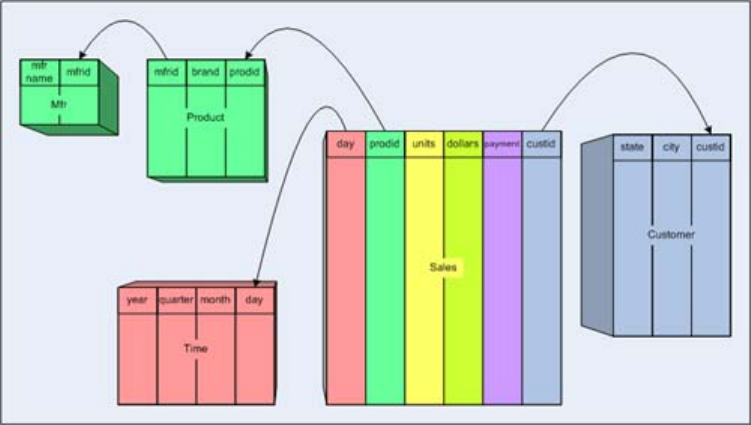
What are aggregate tables?

To explain what aggregate tables are, let's consider a simple star schema.

The star schema has a single fact table Sales, two measure columns (units and dollars)

and four dimension tables (Product, Mfr, Customer, Time, and Customer).

On top of this star schema, we create the following multidimensional model:

• Cube [Sales] has two measures [Unit sales] and [Dollar sales]

• Dimension [Product] has levels [All Products], [Manufacturer], [Brand],

[Prodid]

• Dimension [Time] has levels [All Time], [Year], [Quarter], [Month], [Day]

• Dimension [Customer] has levels [All Customers], [State], [City], [Custid]

• Dimension [Payment Method] has levels [All Payment Methods], [Payment

Method]

Most of the dimensions have a corresponding dimension table, but there are two exceptions. The

[Product] dimension is a

snowflake dimension

, which means that it is spread across more than

one table (in this case Product and Mfr). The [Payment Method] dimension is a

degenerate

dimension

; its sole attribute is the payment column in the fact table, and so it does not need a

dimension table.

- 75 -

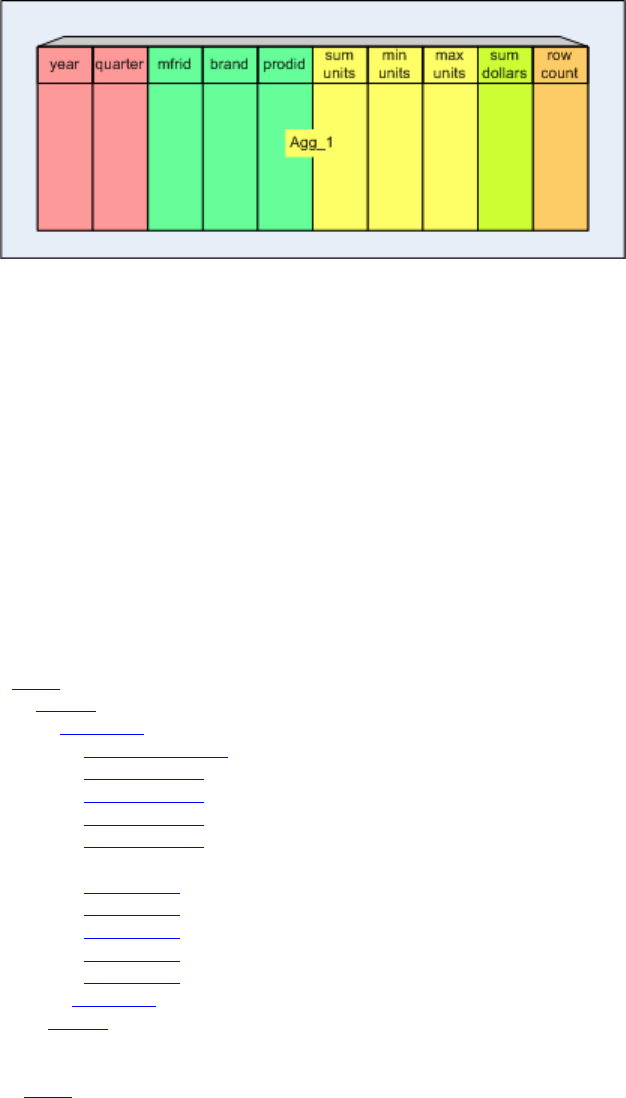
A simple aggregate table

Now let's create an aggregate table, Agg_1:

See how the original star schema columns have been combined into the table:

• The Time dimension has been "collapsed" into the aggregate table, omitting the month

and day columns.

• The two tables of the Product dimension has been "collapsed" into the aggregate table.

• The Customer dimension has been "lost".

• For each measure column in the fact table (units, dollars), there are one or more

measure columns in the aggregate table (sum units, min units, max units, sum

dollars).

• There is also a measure column, row count, representing the "count" measure.

Agg_1 would be declared like this:

<AggMeasure name="[Measures].[Dollar Sales]" column="sum

dollars"/>

</AggName>

</Table>

</Cube>

- 76 -

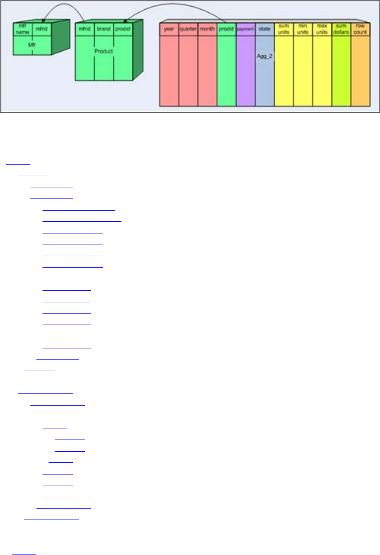
Another aggregate table

Another aggregate table, Agg_2:

and the corresponding XML:

<AggMeasure name="[Measures].[Dollar Sales]" column="sum

dollars"/>

<AggLevel name="[Payment Method].[Payment Method]"

column="payment"/>

</AggName>

</Table>

<Hierarchy hasAll="true" primaryKey="prodid"

primaryKeyTable="Product">

</Join>

</Hierarchy>

</Dimension>

</Cube>

- 77 -

Several dimensions have been collapsed: [Time] at the [Quarter] level; [Customer] at the

[State] level; and [Payment Method] at the [Payment Method] level. But the

[Product] dimension has been retained in its original snowflake form.

The <AggForeignKey> element is used to declare that the column prodid links to the

dimension table, but all other columns remain in the Product and Mfr dimension tables.

Defining aggregate tables

A fact table can have zero or more aggregate tables. Every aggregate table is associated with

just one fact table. It aggregates the fact table measures over one or more of the dimensions. As

an example, if a particular column in the fact table represents the number of sales of some

product on a given day by a given store, then an aggregate table might be created that sums the

information so that applies at a month level rather than by day. Such an aggregate might

reasonably be 1/30th the size of the fact table (assuming comparable sales for every day of a

month). Now, if one were to execute a MDX query that needed sales information at a month (or

quarter or year) level, running the query against the aggregate table is faster but yields the same

answer as if it were run against the base fact table.

Further, one might create an aggregate that not only aggregates at the month level but also,

rather than at the individual store level, aggregates at the state level. If there were, say, 20

stores per state, then this aggregate table would be 1/600th the size of the original fact table.

MDX queries interested only at the month or above and state or above levels would use this

table.

When a MDX query runs, what aggregate should be used? This comes down to what measures

are needed and with which dimension levels. The base fact table always has the correct

measures and dimension levels. But, it might also be true that there is one or more aggregate

tables that also have the measures and levels. Of these, the aggregate table with the lowest cost

to read, the smallest number of rows, should be the table used to fulfill the query.

Mondrian supports two aggregation techniques which are called "lost" dimension and "collapsed"

dimension. For the creation of any given aggregate table these can be applied independently to

any number of different dimensions.

A "lost" dimension is one which is completely missing from the aggregate table. The measures

that appear in the table have been aggregated across all values of the lost dimension. As an

example, in a fact table with dimensions of time, location, and product and measure sales, for an

aggregate table that did not have the location dimension that dimension would be "lost". Here,

the sales measure would be the aggregation over all locations. An aggregate table where all of

the dimensions are lost is possible - it would have a single row with the measure aggregated over

everything - sales for all time, all locations and all products.

fact table

time_id

product_id

location_id

measure

lost (time_id) dimension table

product_id

location_id

- 78 -

measure (aggregated over time)

fact_count

fully lost dimension table

measure (aggregated over everything)

fact_count

Note the "fact_count" column in the aggregate table. This additional column is a general feature

of aggregate tables. It is a count of how many fact table columns were aggregated into the one

aggregate table row. As an example, if for a particular choice of product_id and location_id, the

time_id occurred 5 times in the fact table, then in the aggregate table the fact_count column

would contain 5 for that product_id/location_id pair (a given product was sold at a given location

at 5 different times).

The second supported aggregation technique provides a finer level of control, the "collapsed"

dimension technique. Recall that the dimension key in the fact table refers (more or less) to the

lowest level in the dimension hierarchy. For a collapsed dimension, the dimension key in the

aggregate table is replaced with a set of dimension levels; the dimension key column is replaced

with a set of columns; a fully denormalized summary table for that dimension. As an example, if

the time dimension with base fact table foreign key time_id had the levels: day, month, quarter

and year, and in an aggregate it was collapsed to the month level, then the aggregate table

would not have a time_id column but rather columns for month, quarter and year. The SQL

generated for a MDX query for which this aggregate table can be used, would no longer refer to

the time dimension's table but rather all time related information would be gotten from the

aggregate table.

time dimension table

time_id

day

month

quarter

year

fact table

time_id

measure

collapsed dimension table

month

quarter

year

measure (aggregated to month level)

fact_count

In the literature, there are other ways of creating aggregate tables but they are not supported by

Mondrian at this time.

Building aggregate tables

Aggregate tables must be built. Generally, they not real-time; they are rebuilt, for example, every

night for use the following day by the analysts. Considering the lost and collapsed dimension

technique for aggregate table definition, one can estimate that for a dimension with N levels,

there are N+1 possible aggregate tables (N collapsed and 1 lost). Also, dimensions (with different

- 79 -

dimension tables) can be aggregated independently. For the FoodMart Sales cube there are 1400

different possible aggregate tables.

Clearly, one does not want to create all possible aggregate tables. Which ones to create depends

upon two considerations. The first consideration is application dependent: the nature of the MDX

queries that will be executed. If many of the queries deal with per month and per state

questions, then an aggregate at those levels might be created. The second consideration is

application independent: per dimension aggregating from the lowest level to the next lowest

generally gives greater bang for the buck than aggregating from the N to the N+1 (N>1) level.

This is because 1) a first level aggregation can be used for all queries at that level and above and

2) dimension fan-out tends to increase for the lower levels. Of course, your mileage may vary.

In a sense, picking which aggregate tables to build is analogous to picking which indexes to build

on a table; it is application dependent and experience helps.

The hardest part about the actually creation and population of aggregate tables is figuring out

how to create the first couple; what the SQL looks like. After that they are pretty much all the

same.

Four examples will be given. They all concern building aggregate tables for the sales_fact_1997

fact table. As a reminder, the sales_fact_1997 fact table looks like:

sales_fact_1997

product_id

time_id

customer_id

promotion_id

store_id

store_sales

store_cost

unit_sales

The first example is a lost time dimension aggregate table, the time_id foreign key is missing.

CREATE TABLE agg_l_05_sales_fact_1997 (

product_id INTEGER NOT NULL,

customer_id INTEGER NOT NULL,

promotion_id INTEGER NOT NULL,

store_id INTEGER NOT NULL,

store_sales DECIMAL(10,4) NOT NULL,

store_cost DECIMAL(10,4) NOT NULL,

unit_sales DECIMAL(10,4) NOT NULL,

fact_count INTEGER NOT NULL);

CREATE INDEX i_sls_97_cust_id ON agg_l_05_sales_fact_1997

(customer_id);

CREATE INDEX i_sls_97_prod_id ON agg_l_05_sales_fact_1997 (product_id);

CREATE INDEX i_sls_97_promo_id ON agg_l_05_sales_fact_1997

(promotion_id);

CREATE INDEX i_sls_97_store_id ON agg_l_05_sales_fact_1997 (store_id);

INSERT INTO agg_l_05_sales_fact_1997 (

product_id,

customer_id,

- 80 -

promotion_id,

store_id,

store_sales,

store_cost,

unit_sales,

fact_count)

SELECT

product_id,

customer_id,

promotion_id,

store_id,

SUM(store_sales) AS store_sales,

SUM(store_cost) AS store_cost,

SUM(unit_sales) AS unit_sales,

COUNT(*) AS fact_count

FROM

sales_fact_1997

GROUP BY

product_id,

customer_id,

promotion_id,

store_id;

A couple of things to note here.

The above is in MySQL's dialect of SQL, and may not work for your database - but I hope the

general idea is clear. The aggregate table "looks like" the base fact table except the time_id

column is missing and there is a new fact_count column. The insert statement populates the

aggregate table from the base fact table summing the measure columns and counting to

populate the fact_count column. This done while grouping by the remaining foreign keys to the

remaining dimension tables.

Next, some databases recognize star joins - Oracle for instance. For such database one should

not create indexes, not on the fact table and not on the aggregate tables. On the other hand,

databases that do not recognize star joins will require indexes on both the fact table and the

aggregate tables.

For our purposes here, the exact name of the aggregate table is not important; the "agg_l_05_"

preceding the base fact table's name sales_fact_1997. First, the aggregate table name must be

different from the base fact table name. Next, the aggregate table name ought to be related to

the base fact table name both for human eyeballing of what aggregate is associated with which

fact table, but also, as described below, Mondrian employs mechanism to automagically

recognize which tables are aggregates of others.

The following example is a collapsed dimension aggregate table where the time dimension has

been rolled up to the month level.

CREATE TABLE agg_c_14_sales_fact_1997 (

product_id INTEGER NOT NULL,

customer_id INTEGER NOT NULL,

promotion_id INTEGER NOT NULL,

store_id INTEGER NOT NULL,

month_of_year SMALLINT(6) NOT NULL,

quarter VARCHAR(30) NOT NULL,

- 81 -

the_year SMALLINT(6) NOT NULL,

store_sales DECIMAL(10,4) NOT NULL,

store_cost DECIMAL(10,4) NOT NULL,

unit_sales DECIMAL(10,4) NOT NULL,

fact_count INTEGER NOT NULL);

CREATE INDEX i_sls_97_cust_id ON agg_c_14_sales_fact_1997

(customer_id);

CREATE INDEX i_sls_97_prod_id ON agg_c_14_sales_fact_1997 (product_id);

CREATE INDEX i_sls_97_promo_id ON agg_c_14_sales_fact_1997

(promotion_id);

CREATE INDEX i_sls_97_store_id ON agg_c_14_sales_fact_1997 (store_id);

INSERT INTO agg_c_14_sales_fact_1997 (

product_id,

customer_id,

promotion_id,

store_id,

month_of_year,

quarter,

the_year,

store_sales,

store_cost,

unit_sales,

fact_count)

SELECT

BASE.product_id,

BASE.customer_id,

BASE.promotion_id,

BASE.store_id,

DIM.month_of_year,

DIM.quarter,

DIM.the_year,

SUM(BASE.store_sales) AS store_sales,

SUM(BASE.store_cost) AS store_cost,

SUM(BASE.unit_sales) AS unit_sales,

COUNT(*) AS fact_count

FROM

sales_fact_1997 AS BASE, time_by_day AS DIM

WHERE

BASE.time_id = DIM.time_id

GROUP BY

BASE.product_id,

BASE.customer_id,

BASE.promotion_id,

BASE.store_id,

DIM.month_of_year,

DIM.quarter,

DIM.the_year;

In this case, one can see that the time_id foreign key in the base fact table has been replaced

with the columns: month_of_year, quarter, and the_year in the aggregate table. There is, as

always, the fact_count column. The measures are inserted as sums. And, the group by clause is

over the remaining foreign keys as well as the imported time dimension levels.

- 82 -

When creating a collapsed dimension aggregate one might consider creating indexes for the

columns imported from the dimension that was collapsed.

Below is another aggregate table. This one has two lost dimensions (store_id and

promotion_id) as well as collapsed dimension on time to the quarter level. This shows how

aggregate techniques can be mixed.

CREATE TABLE agg_lc_100_sales_fact_1997 (

product_id INTEGER NOT NULL,

customer_id INTEGER NOT NULL,

quarter VARCHAR(30) NOT NULL,

the_year SMALLINT(6) NOT NULL,

store_sales DECIMAL(10,4) NOT NULL,

store_cost DECIMAL(10,4) NOT NULL,

unit_sales DECIMAL(10,4) NOT NULL,

fact_count INTEGER NOT NULL);

CREATE INDEX i_sls_97_cust_id ON agg_lc_100_sales_fact_1997

(customer_id);

CREATE INDEX i_sls_97_prod_id ON agg_lc_100_sales_fact_1997

(product_id);

INSERT INTO agg_lc_100_sales_fact_1997 (

product_id,

customer_id,

quarter,

the_year,

store_sales,

store_cost,

unit_sales,

fact_count)

SELECT

BASE.product_id,

BASE.customer_id,

DIM.quarter,

DIM.the_year,

SUM(BASE.store_sales) AS store_sales,

SUM(BASE.store_cost) AS store_cost,

SUM(BASE.unit_sales) AS unit_sales,

COUNT(*) AS fact_count

FROM sales_fact_1997 AS BASE,

time_by_day AS DIM

WHERE

BASE.time_id = DIM.time_id

GROUP BY

BASE.product_id,

BASE.customer_id,

DIM.quarter,

DIM.the_year;

In the above three examples, for the most part the column names in the aggregate are the same

column names that appear in the fact table and dimension tables. These tables would all be

recognized by the Mondrian default aggregate recognizer. It is possible to create an aggregate

table and name the columns arbitrarily. For such an aggregate, an explicit Mondrian recognizer

must be specified.

- 83 -

CREATE TABLE agg_c_special_sales_fact_1997 (

PRODUCT_ID INTEGER NOT NULL,

CUSTOMER_ID INTEGER NOT NULL,

PROMOTION_ID INTEGER NOT NULL,

STORE_ID INTEGER NOT NULL,

TIME_MONTH SMALLINT(6) NOT NULL,

TIME_QUARTER VARCHAR(30) NOT NULL,

TIME_YEAR SMALLINT(6) NOT NULL,

STORE_SALES_SUM DECIMAL(10,4) NOT NULL,

STORE_COST_SUM DECIMAL(10,4) NOT NULL,

UNIT_SALES_SUM DECIMAL(10,4) NOT NULL,

FACT_COUNT INTEGER NOT NULL);

CREATE INDEX i_sls_97_cust_id ON agg_c_special_sales_fact_1997

(CUSTOMER_ID);

CREATE INDEX i_sls_97_prod_id ON agg_c_special_sales_fact_1997

(PRODUCT_ID);

CREATE INDEX i_sls_97_promo_id ON agg_c_special_sales_fact_1997

(PROMOTION_ID);

CREATE INDEX i_sls_97_store_id ON agg_c_special_sales_fact_1997

(STORE_ID);

INSERT INTO agg_c_special_sales_fact_1997 (

PRODUCT_ID,

CUSTOMER_ID,

PROMOTION_ID,

STORE_ID,

TIME_MONTH,

TIME_QUARTER,

TIME_YEAR,

STORE_SALES_SUM,

STORE_COST_SUM,

UNIT_SALES_SUM,

FACT_COUNT)

SELECT

BASE.product_id,

BASE.customer_id,

BASE.promotion_id,

BASE.store_id,

DIM.month_of_year,

DIM.quarter,

DIM.the_year,

SUM(BASE.store_sales) AS STORE_SALES_SUM,

SUM(BASE.store_cost) AS STORE_COST_SUM,

SUM(BASE.unit_sales) AS UNIT_SALES_SUM,

COUNT(*) AS FACT_COUNT

FROM

sales_fact_1997 BASE, time_by_day DIM

WHERE

BASE.time_id = DIM.time_id

GROUP BY

BASE.product_id,

BASE.customer_id,

BASE.promotion_id,

BASE.store_id,

DIM.month_of_year,

- 84 -

DIM.quarter,

DIM.the_year;

This aggregate table has column names that are not identical to those found in the base fact

table and dimension table. It is still a valid aggregate but Mondrian has to be told how to map its

columns into those of the base fact table.

Sometimes with multiple aggregate tables, one aggregate table is an aggregate of not only the

base fact table but also another aggregate table; an aggregate table with lost time and product

dimensions (no time_id and product_id foreign keys) is an aggregate of the base fact table and

an aggregate which only has a lost time dimension (no time_id foreign key). In this case, one

might first build the aggregate with only the lost time dimension and then build the aggregate

with both lost time and product dimensions from that first aggregate - it will be faster (in some

cases, much faster) to populate the second aggregate from the first rather than from the base

fact table.

One last note, when creating aggregate tables from the base fact table pay attention to the size

of the numeric columns - what might be big enough in the base fact table might not be big

enough in an aggregate.

How Mondrian recognizes Aggregate Tables

Mondrian has to know about the aggregate tables in order to use them. You can either define an

aggregate explicitly, or set up rules to recognize several aggregate tables at the same time.

How Mondrian recognizes aggregate table names and columns pretty much dictates how one

must name those table names and columns when creating them in the first place!

Rules

Rules are templates, designed to work for all fact table names and their column names. These

rules are templates of regular expressions that are instantiated with the names of a fact table

and its columns. In order to describe the rule templates, a name that instantiate a rule are

represented in a rule by have the name bracketed by "${" and "}". As an example,

"abc_${name}_xyz" is a rule parameterized by "name". When name is "john" the template

becomes "abc_john_xyz".

The regular expression engine used here and a definition of the allowed regular expression

grammar is found in the Java regular expression Pattern class: java.util.regex.Pattern.

In order that a table be recognized as an aggregate table, Mondrian must be able to map from

the fact table foreign key columns and measure columns and those in the aggregate table. In

addition, Mondrian must identify the fact count column in the aggregate and possible level

columns (which would appear in an aggregate table if it had a "collapsed" dimension). What

follows is a description of the steps taken in the identification of aggregate tables by the default

recognizer. If at any step, a match fails, the table is rejected as an aggregate table.

Starting off, the candidate aggregate table's name must comply with the aggregate table name

rule. Represented as a template regular expression the rule is:

agg_.+_${fact_table_name}

- 85 -

which is parameterized with the fact table's name. (In addition, this rule is applied in "ignore

case" mode.) This means that an aggregate table's name must start with "agg_" (ignoring

character case), followed by at least one character, then the '_' character and, lastly, the name of

the fact table. The ".+" in the template has special meaning in a regular expression - it matches

one or more characters.

As an example of applying the aggregate table name rule, let the fact table be called

sales_fact_1997, the Sales cube's fact table from the FoodMart schema. Applying the

specific fact table name to the regular expression template creates the following regular

expression:

agg_.+_sales_fact_1997

This will match the following table names:

• agg_l_05_sales_fact_1997

• agg_c_14_sales_fact_1997

• agg_lc_100_sales_fact_1997

• agg_c_special_sales_fact_1997

• AGG_45_SALES_FACT_1997

• AGG_drop_time_id_sales_fact_1997

The aggregate table name recognition mechanism has one additional programatic feature, one

can specify that only a portion of the base fact table name be used as the basis of template

name. For instance, if the DBA demanded that all fact tables begin with the string "fact_", e.g.,

"fact_sales_fact_1997", one would certainly not want that string to have to be part of each

aggregate table's name. The aggregate table name recognition mechanism allows one to specify

a regular expression with one and only one group clause (a group clause is a pattern bracketed

by '(' and ')'). Whatever is matched by the contents of the group clause is taken to be the part of

the fact table name to be used in the matching template. This regular expression containing the

group clause is specified as the "basename" attribute. The default Mondrian aggregate table

recognizer does not use this feature. For more information see the associated developer's note

link.

After the default recognizer determines that a table's name matches the aggregate table

template regular expression for a given fact table, it then attempts to match columns. The first

column tested for is the "fact count" column. Here the candidate aggregate table must have a

column called "fact_count" (ignoring case) and this column's type must be numeric. The following

examples would match as "fact count" columns.

fact_count

FACT_COUNT

fact_COUNT

Following matching the "fact count" column, the candidate aggregate table's columns are

examined for possible foreign key matches. For each of the foreign key column names in the fact

table it is determined if there are any character case independent matches of the aggregate

table's columns. Those columns that match are noted. It is alright if no columns match; the

aggregate might be a "collapsed" dimension aggregate with no fact table foreign keys remaining.

- 86 -

If the fact table had foreign key columns "store_id" and "time_id", then the following aggregate

table columns (for example) would match:

• time_id

• store_id

• TIME_ID

• STORE_ID

• time_ID

• STORE_id

At this point, matches are looked for the level and measure columns. Both of these matching

rules are multi-part - has sub rules; each rule has more than one possible regular expression that

might match where a match on any one is a match.

There are three sub rules for matching level columns. Each is a template which is parameterized

with 1) the fact table's cube's dimension hierarchy's name, "hierarchy_name", 2) the fact table's

cube's dimension hierarchy's level name, "level_name", 3) the dimension table's level column

name, "level_column_name", and 4) a usage prefix, "usage_prefix", which in most cases is null":

• ${hierarchy_name}_${level_name}

• ${hierarchy_name}_${level_column_name}

• ${usage_prefix}${level_column_name}

• ${level_column_name}

The "usage_prefix" is the value of the DimensionUsage's or private Dimension's optional

usagePrefix attribute. It can be the case that a "level_column_name", the name of a

dimension's level column, is the same for more than one dimension. During aggregate

recognition for collapsed dimension aggregates where the base fact table has two or more

dimensions with common column names, the attempted recognition will fail unless in the schema

catalog the usagePrefix attribute is used to disambiguate those column names. Of course, one

must also remember to prefix the the column in the aggregate table with the same prefix.

As an example of usagePrefix, consider a fact table named ORDERS which has two

DimensionUsages, one for the CUSTOMER dimension and the other for the WHOLESALER

dimension where each dimension has a level column named CUST_NM. In this case, a collapsed

aggregate table could not include a column named CUST_NM because there would be no way to

tell which dimension to associate it with. But if in the CUSTOMER' DimensionUsage the

usagePrefix had the value "CU_", while the WHOLESALER's usagePrefix had the value

"WS_", and the aggregate table column was named WS_CUST_NM, then the recognizer could

associate the column with the WHOLESALER dimension.

In the case of a private Dimension, a usagePrefix need only be used if there is a public,

shared Dimension that has the same name and has a "level_column_name" that is also the

same. Without the usagePrefix there would be no way of disambiguating collapsed dimension

aggregate tables.

- 87 -

If any of these parameters have space characters, ' ', these are mapped to underscore

characters, '_', and, similarly, dot characters, '.', are also mapped to underscores. So, if the

hierarchy_name is "Time", level_name is "Month" and level_column_name is month_of_year, the

possible aggregate table column names are:

• time_month

• time_month_of_year

• month_of_year

For this rule, the "hierarchy_name" and "level_name" are converted to lower case while the

"level_column_name" must match exactly.

Lastly, there is the rule for measures. There are three parameters to matching aggregate

columns to measures: 1) the fact table's cube's measure name, "measure_name", 2) the fact

table's cube's measure column name, "measure_column_name", and 3) the fact table's cube's

measure's aggregator (sum, avg, max, etc.), "aggregate_name".

• ${measure_name}

• ${measure_column_name}

• ${measure_column_name}_${aggregate_name}

where the measure name is converted to lower case and both the measure column name and

aggregate name are matched as they appear. If the fact table's cube's measure name was, "Avg

Unit Sales", the fact table's measure column name is "unit_sales", and, lastly, the fact table's

cube's measure's aggregate name is "avg", then possible aggregate table column names that

would match are:

• avg_unit_sales

• unit_sales

• unit_sales_avg

For Mondrian developers there are additional notes describing the default rule recognition

schema.

Explicit aggregates

On a per cube basis, in a schema file a user can both include and exclude aggregate tables. A

table that would have been include as an aggregate by the default rules can be explicitly

excluded. A table that would not be include by the default rules can be explicitly included. A table

that would have only been partially recognized by the default rules and, therefore, resulted in a

warning or error message, can be explicitly include in rules specified in the cube's definition.

Below is an example for the FoodMart Sales cube with fact table sales_fact_1997. There

are child elements of the Table element that deal with aggregate table recognition.

- 88 -

<AggForeignKey factColumn="product_id" aggColumn="PRODUCT_ID"

<AggForeignKey factColumn="customer_id" aggColumn="CUSTOMER_ID"

<AggForeignKey factColumn="promotion_id"

aggColumn="PROMOTION_ID" />

<AggMeasure name="[Measures].[Unit Sales]"

column="UNIT_SALES_SUM" />

<AggMeasure name="[Measures].[Store Cost]"

column="STORE_COST_SUM" />

<AggMeasure name="[Measures].[Store Sales]"

column="STORE_SALES_SUM" />

</AggName>

....

</AggPattern>

</Table>

....

</Cube>

The AggExclude elements define tables that should not be considered aggregates of the fact

table. In this case Mondrian is instructed to ignore the tables agg_c_14_sales_fact_1997,

agg_lc_10_sales_fact_1997 and agg_pc_10_sales_fact_1997. Following the excludes

is the AggName element which identifies the name of an aggregate table table,

agg_c_special_sales_fact_1997, and rules for mapping names from the fact table and

cube to it. The two AggIgnoreColumn elements are used to specifically state to Mondrian that

the columns admin_one and admin_two are known and should be ignored. If these columns

were not so identified, Mondrian at the end of determining the fitness of the

agg_c_special_sales_fact_1997 table to be an aggregate of the sales_fact_1997 fact

table would complain that there were extra unidentified columns and that the mapping was

incomplete. The AggForeignKey elements define mappings from the sales_fact_1997 fact

table foreign key column names into the agg_c_special_sales_fact_1997 aggregate table

column names.

Both the AggMeasure and AggLevel elements map "logical" name, names defined in the

cube's schema, to the aggregate table's column names. An aggregate table does not have to

have all of the measures that are found in the base fact table, so it is not a requirement that all

- 89 -

of the fact table measures appear as AggMeasure mappings, though it will certainly be the most

common case. The most notable exception are distinct-count measures; such a measure

can be aggregated, but one can not in general aggregate further on the measure - the

"distinctness" of the measure has been lost during the first aggregation.

The AggLevel entries correspond to collapsed dimensions. For each collapsed dimension there

is a hierarchy of levels spanning from the top level down to some intermediate level (with no

gaps).

The AggName element is followed by an AggPattern element. This matches candidate

aggregate table names using a regular expression. Included as child elements of the

AggPattern element are two AggExclude elements. These specifically state what table names

should not be considered by this AggPattern element.

In a given Table element, all of the AggExclude are applied first, followed by the AggName

element rules and then the AggPattern rules. In the case where the same fact table is used by

multiple cubes, the above still applies, but its across all of the aggregation rules in all of the

multiple cube's Table elements. The first "Agg" element, name or pattern, that matches per

candidate aggregate table name has its associated rules applied.

Most of the time, the scope of these include/exclude statements apply only to the cube in

question, but not always. A cube has a fact table and it is the characteristics of the fact table (like

column names) against which some of the aggregate table rules are applied. But, a fact table can

actually be the basis of more than one cube. In the FoodMart schema the sales_fact_1997

fact table applies to both the Sales and the Sales Ragged cubes. What this means is that any

explicit rules defined in the Sales cube also applies to the Sales Ragged cube and visa versa.

One feature of the explicit recognizer is very useful. With a single line in the cubes definition in

the schema file, one can force Mondrian not to recognize any aggregate tables for the cube's fact

table. As an example, for the FoodMart Sales cube the following excludes all aggregate tables

because the regular expression pattern ".*" matches all candidate aggregate table names.

</Table>

During aggregate table recognition, rather than fail silently, Mondrian is rather noisy about things

it can not figure out.

Aggregate tables and parent-child hierarchies

A parent-child hierarchy is a special kind of hierarchy where members can have arbitrary depth.

The classic example of a parent-child hierarchy is an employee org-chart.

When dealing with parent-child hierarchies, the challenge is to roll up measures of child members

into parent members. For example, when considering an employee Bill who is head of a

department, we want to report not Bill's salary, but Bill's salary plus the sum of his direct and

indirect reports (Eric, Mark and Carla). It is difficult to generate efficient SQL to do this rollup, so

Mondrian provides a special structure called a closure table, which contains the expanded

contents of the hierarchy.

- 90 -

A closure table serves a similar purpose to an aggregate table: it contains a redundant copy of

the data in the database, organized in such a way that Mondrian can access the data efficiently.

An aggregate table speeds up aggregation, whereas a closure table makes it more efficient to

compute hierarchical rollups.

Supposing that a schema contains a large fact table, and one of the hierarchies is a parent-child

hierarchy. Is is possible to make aggregate tables and closure tables work together, to get better

performance? Let's consider a concrete example.

Cube:

[Salary]

Dimensions:

[Employee], with level [Employee]

[Time], with levels [Year], [Quarter], [Month], [Day]

Fact table:

salary (employee_id, time_id, dollars)

Parent-child dimension table:

employee (employee_id, supervisor_id, name)

employee

supervisor_id employee_id name

null 1 Frank

1 2 Bill

2 3 Eric

1 4 Jane

3 5 Mark

2 6 Carla

Closure table:

employee_closure (employee_id, supervisor_id, depth)

employee_closure

supervisor_id employee_id distance

1 1 0

1 2 1

1 3 2

1 4 1

1 5 3

1 6 2

2 2 0

2 3 1

2 5 2

2 6 1

3 3 0

3 5 1

4 4 0

5 5 0

6 6 0

Regular dimension table:

time (year, month, quarter, time_id)

- 91 -

Aggregate tables at the leaf level of a parent-child hierarchy

The simplest option is to create an aggregate table which joins at the leaf level of the parent-

child hierarchy. The following aggregate table is for leaf members of the [Employee] hierarchy,

and the [Year] level of the [Time] hierarchy.

Aggregate table:

agg_salary_Employee_Time_Year (employee_id, time_year, sum_dollars)

INSERT INTO agg_salary_Employee_Time_Year

SELECT

salary.employee_id,

time.year AS time_year,

sum(salary.dollars) AS sum_dollars

FROM salary,

time

WHERE time.time_id = salary.time_id

GROUP BY salary.employee_id, time.year

Mondrian can use the aggregate table to retrieve salaries of leaf employees (without rolling up

salaries of child employees). But because the aggregate table has the same foreign key as the

salary fact table, Mondrian is able to automatically join salary.employee_id to either

agg_salary_Employee_Time_Year.employee_id or

agg_salary_Employee_Time_Year.supervisor_id to rollup employees efficiently.

Combined closure and aggregate tables

A more advanced option is to combine the closure table and aggregate table into one:

Aggregate table:

agg_salary_Employee$Closure_Time_Year (supervisor_id, time_year,

sum_dollars)

INSERT INTO agg_salary_Employee$Closure_Time_Year

SELECT

ec.supervisor_id,

time.year AS time_year,

sum(salary.dollars) AS sum_dollars

FROM employee_closure AS ec,

salary,

time

WHERE ec.supervisor_id = salary.employee_id

AND ec.supervisor_id <> ec.employee_id

AND time.time_id = salary.time_id

GROUP BY ec.employee_id, ec.supervisor_id, time.year

The agg_salary_Employee$Closure_Time_Year aggregate table contains the salary of

every employee, rolled up to include their direct and indirect reports, aggregated to the [Year]

level of the [Time] dimension.

- 92 -

The trick: How combined closure and aggregate tables work

Incidentally, this works based upon a 'trick' in Mondrian's internals. Whenever Mondrian sees a

closure table, it creates a auxilliary dimension behind the scenes. In the case of the [Employee]

hierarchy and its employee_closure table, the auxilliary dimension is called

[Employee$Closure].

Dimension [Employee$Closure], levels [supervisor_id], [employee_id]

When an MDX query evaluates a cell which uses a rolled up salary measure, Mondrian translates

the coordinates of that cell in the [Employee] dimension into a corresponding coordinate in the

[Employee$Closure] dimension. This translation happens

before

Mondrian starts to search

for a suitable aggregate table, so if your aggregate table contains the name of the auxiliary

hierarchy (as agg_salary_Employee$Closure_Time_Year contains the name of the

[Employee$Closure] hierarchy) it find and use the aggregate table in the ordinary way.

How Mondrian uses aggregate tables

Choosing between aggregate tables

If more than one aggregate table matches a particular query, Mondrian needs to choose between

them.

If there is an aggregate table of the same granularity as the query, Mondrian will use it. If there

is no aggregate table at the desired granularity, Mondrian will pick an aggregate table of lower

granularity and roll up from it. In general, Mondrian chooses the aggregate table with the fewest

rows, which is typically the aggregate table with the fewest extra dimensions. See property

mondrian.rolap.aggregates.ChooseByVolume.

Distinct count

There is an important exception for distinct-count measures: they cannot in be rolled up over

arbitrary dimensions. To see why, consider the case of a supermarket chain which has two stores

in the same city. Suppose that Store A has 1000 visits from 800 distinct customers in the month

of July, while Store B has 1500 visits from 900 distinct customers. Clearly the two stores had a

total of 2500 customer visits between them, but how many distinct customers? We can say that

there were at least 900, and maybe as many as 1700, but assuming that some customers visit

both stores, and the real total will be somewhere in between. "Distinct customers" is an example

of a distinct-count measure, and cannot be deduced by rolling up subtotals. You have to go back

to the raw data in the fact table.

There is a special case where it is acceptable to roll up distinct count measures. Suppose that we

know that in July, this city's stores (Store A and B combined) have visits from 600 distinct female

customers and 700 distinct male customers. Can we say that the number of distinct customers in

July is 1300? Yes we can, because we know that the sets of male and female customers cannot

possibly overlap. In technical terms, gender is

functionally dependent on

customer id.

- 93 -

The rule for rolling up distinct measures can be stated as follows:

A distinct count measure over key

can be computed by rolling up more granular subtotals only

if the attributes which are being rolled up are functionally dependent on

Even with this special case, it is difficult to create enough aggregate tables to satisfy every

possible query. When evaluating a distinct-count measure, Mondrian can only use an aggregate

table if it has the same logical/level granularity as the cell being requested, or can be rolled up to

that granularity only by dropping functionally dependent attributes. If there is no aggregate table

of the desired granularity, Mondrian goes instead against the fact table.

This has implications for aggregate design. If your application makes extensive use of distinct-

count measures, you will need to create an aggregate table for each granularity where it is used.

That could be a lot of aggregate tables! (We hope to have a better solution for this problem in

future releases.)

That said, Mondrian will rollup measures in an aggregate table that contains one or more distinct-

count measures if none of the distinct-count measures are requested. In that respect an

aggregate table containing distinct-count measures are just like any other aggregate table as

long as the distinct-count measures are not needed. And once in memory, distinct-count

measures are cached like other measures, and can be used for future queries.

When building an aggregate table that will contain a distinct-count measure, the measure must

be rolled up to a logical dimension level, which is to say that the aggregate table must be a

collapsed dimension aggregate. If it is rolled up only to the dimension's foreign key, there is no

guarantee that the foreign key is at the same granularity as the lowest logical level, which is

what is used by MDX requests. So for an aggregate table that only rolls the distinct-count

measure to the foreign key granularity, a request of that distinct-count measure may result in

further rollup and, therefore, an error.

Consider the following aggregate table that has lost dimensions customer_id, product_id,

promotion_id and store_id.

INSERT INTO "agg_l_04_sales_fact_1997" (

"time_id",

"store_sales",

"store_cost",

"unit_sales",

"customer_count",

"fact_count"

) SELECT

"time_id",

SUM("store_sales") AS "store_sales",

SUM("store_cost") AS "store_cost",

SUM("unit_sales") AS "unit_sales",

COUNT(DISTINCT "customer_id") AS "customer_count",

COUNT(*) AS "fact_count"

FROM "sales_fact_1997"

GROUP BY "time_id";

This aggregate table is useless for computing the "customer_count" measure. Why? The

distinct-count measure is rolled up to the time_id granularity, the lowest level granularity of the

physical database table time_by_day. Even a query against the lowest level in the Time

- 94 -

dimension would require a rollup from time_id to month_of_year, and this is impossible to

perform.

Now consider this collapsed Time dimension aggregate table that has the same lost dimensions

customer_id, product_id, promotion_id and store_id. The time_id foreign key is no

longer present, rather it has been replaced with the logical levels the_year, quarter and

month_of_year.

INSERT INTO "agg_c_10_sales_fact_1997" (

"month_of_year",

"quarter",

"the_year",

"store_sales",

"store_cost",

"unit_sales",

"customer_count",

"fact_count"

) SELECT

"D"."month_of_year",

"D"."quarter",

"D"."the_year",

SUM("B"."store_sales") AS "store_sales",

SUM("B"."store_cost") AS "store_cost",

SUM("B"."unit_sales") AS "unit_sales",

COUNT(DISTINCT "customer_id") AS "customer_count",

COUNT(*) AS fact_count

FROM

"sales_fact_1997" "B",

"time_by_day" "D"

WHERE

"B"."time_id" = "D"."time_id"

GROUP BY

"D"."month_of_year",

"D"."quarter",

"D"."the_year";

This aggregate table of the distinct-count measure can be used to fulfill a query as long as the

query specifies the Time dimension down to the month_of_year level.

The general rule when building aggregate tables involving distinct-count measures is that there

can be NO foreign keys remaining in the aggregate table - for each base table foreign key, it

must either be dropped, a lost dimension aggregate, or it must be replaces with levels, a

collapsed dimension aggregate. In fact, this rule, though not required, is useful to follow when

creating any aggregate table; there is no value in maintaining foreign keys in aggregate tables.

They should be replaced by collapsing to levels unless the larger memory used by such

aggregate tables is too much for one's database system.

- 95 -

A better design for the aggregate table would include a few attributes which are functionally

dependent on customer_id, the key for the distinct-count measure:

INSERT INTO "agg_c_12_sales_fact_1997" (

"country",

"gender",

"marital_status",

"month_of_year",

"quarter",

"the_year",

"store_sales",

"store_cost",

"unit_sales",

"customer_count",

"fact_count"

) SELECT

"D"."month_of_year",

"D"."quarter",

"D"."the_year",

SUM("B"."store_sales") AS "store_sales",

SUM("B"."store_cost") AS "store_cost",

SUM("B"."unit_sales") AS "unit_sales",

COUNT(DISTINCT "customer_id") AS "customer_count",

COUNT(*) AS fact_count

FROM

"sales_fact_1997" "B",

"time_by_day" "D",

"customer" "C"

WHERE

"B"."time_id" = "D"."time_id"

AND "B".customer_id" = "C"."customer_id"

GROUP BY

"C"."country",

"C"."gender",

"C"."marital_status",

"D"."month_of_year",

"D"."quarter",

"D"."the_year";

The added attributes are "country", "gender" and "marital_status". This table has only

appoximately 12x the number of rows of the previous aggregate table (3 values of country x 2

values of gender x 2 values of marital_status) but can answer many more potential

queries.

Tools for designing and maintaining aggregate tables

Aggregate tables are difficult to design and maintain. We make no bones about it. But this is the

first release in which aggregate tables have been available, and we decided to get the internals

right rather than building a toolset to make them easy to use.

Unless your dataset is very large, Mondrian's performance will be just fine without aggregate

tables. If Mondrian isn't performing well, you should first check that your DBMS is well-tuned: see

our guide to optimizing performance). If decide to build aggregate tables anyway, we don't offer

- 96 -

any tools to help administrators design them, so unless you are blessed with superhuman

patience and intuition, using them won't be smooth sailing.

Here are some ideas for tools we'd like to build in the future. I'm thinking of these being utilities,

not part of the core runtime engine. There's plenty of room to wrap these utilities in nice

graphical interfaces, make them smarter.

AggGen (aggregate generator)

AggGen is a tool that generates SQL to support the creation and maintenance of aggregate

tables, and would give a template for the creation of materialized views for databases that

support those. Given an MDX query, the generated create/insert SQL is optimal for the given

query. The generated SQL covers both the "lost" and "collapsed" dimensions. For usage, see the

documentation for CmdRunner.

Aggregate table populater

This utility populates (or generates INSERT statements to populate) the agg tables.

For extra credit: populate the tables in topological order, so that higher level aggregations can be

built from lower level aggregations. (See [AAD+96]).

Script generator

This utility generates a script containing CREATE TABLE and CREATE INDEX statements all

possible aggregate tables (including indexes), XML for these tables, and comments indicating the

estimated number of rows in these tables. Clearly this will be a huge script, and it would be

ridiculous to create all of these tables. The person designing the schema could copy/paste from

this file to create their own schema.

Recommender

This utility (maybe graphical, maybe text-based) recommends a set of aggregate tables. This is

essentially an optimization algorithm, and it is described in the academic literature [AAD+96].

Constraints on the optimization process are the amount of storage required, the estimated time

to populate the agg tables.

The algorithm could also take into account usage information. A set of sample queries could be

an input to the utility, or the utility could run as a background task, consuming the query log and

dynamically making recommendations.

Online/offline control

This utility would allow agg tables to be taken offline/online while Mondrian is still running.

Properties that affect aggregates

Mondrian has properties that control the behavior of its aggregate table sub-system. (You can

find the full set of properties in the Configuration Guide.)

- 97 -

Property Type Default

Value Description

mondrian.

rolap.

aggregates. Use boolean false

If set to true, then Mondrian uses any

ate tables that have been read.

These tables are then candidates for

use in fulfilling MDX queries. If set to

false, then no aggregate table related

activity takes place in Mondrian.

mondrian.

rolap.

aggregates.

Read

boolean false

If set to true, then Mondrian reads

the database schema and recognizes

aggregate tables. These tables are

then candidates for use in fulfilling

MDX queries. If set to false, then

aggregate table will not be read from

the database. Of course, after

aggregate tables have been read,

they are read, so setting this property

false after starting with the property

being true, has no effect. Mondrian

will not actually use the aggregate

tables unless the

ondrian.rolap.

aggregates.Use property is set to

true.

mondrian.

rolap.

aggregates.

ChooseByVolume

boolean false

Currently, Mondrian support to

algorithms for selecting which

ate table to use: the a

ate

with smallest row count or the

aggregate with smallest volume (row

count * row size). If set to false, then

row count is used. If true, then

volume is used.

mondrian.

rolap.

aggregates.

rules

resource

or url /Default

Rules.xml

This is a developer property, not a

user property. Setting this to a url

(e.g., file://c:/myrules.xml)

allows one to use their own "default"

Mondrian aggregate table recognition

rules. In

eneral use this should never

be changed from the default value.

mondrian.

rolap.

aggregates.

rule. tag

string default

This is also a developer property. It

allows one to pick which named rule

in the default rule file to use. In

general use this should never be

changed from the default value.

- 98 -

Aggregate Table References

[AAD+96]

S. Agarwal, R. Agrawal, P. M. Deshpande, A. Gupta, J. F. Naughton,

R. Ramakrishnan, and S. Sarawagi. On the computation of

multidimensional aggregates. In Proc. 22nd VLDB, pages 506-521,

Mumbai, Sept. 1996. [pdf]

[ABDGHLS99]

J. Albrecht, A. Bauer, O. Deyerling, H. Gunze, W. Hummer, W.

Lehner, L. Schlesinger. Management of Multidimensional Aggregates

for Efficient Online Analytical Processing. Proceedings of

International Database Engineering and Applications Symposium,

1999, pp. 156–164. [pdf]

[GBLP96]

J. Gray, A. Bosworth, A. Layman, and H. Pirahesh. Data cube: A

relational aggregation operator generalizing group-by, cross-tab, and

sub-totals. In Proc. 12th ICDE, pages 152-159, New Orleans, March

1996. [pdf]

[HNSS95]

P.J. Haas, J.F. Naughton, S. Seshadri, and L. Stokes. Sampling-

based estimation of the number of distinct values of an attribute.

Proceedings of the Eighth International Conference on Very Large

Databases (VLDB), pages 311–322, Zurich, Switzerland, September

1995. [pdf]

[Rittman05] M. Rittman. Compressed Composites (Oracle 10g Compression)

Explained. Online article. [html]

[SDNR96] Amit Shukla, Prasad Deshpande, Jeffrey F. Naughton, Karthikeyan

Ramasamy. Storage Estimation for Multidimensional Aggregates in

the Presence of Hierarchies. VLDB 1996, pp. 522–531. [pdf]

Cache Control

Note for JasperAnalysis

The Mondrian cache control API is only used in it simplest form in JasperAnalysis 3.5. Only the

full cache can be flushed, in keeping with prior versions of Mondrian.

Introduction

One of the strengths of mondrian's design is that you don't need to do any processing to

populate special data structures before you start running OLAP queries. More than a few people

have observed that this makes mondrian an excellent choice for 'real-time OLAP' -- running multi-

dimensional queries on a database which is constantly changing. The problem is that mondrian's

cache gets in the way. Usually the cache is a great help, because it ensures that Mondrian only

goes to the DBMS once for a given piece of data, but the cache becomes out of date if the

underlying database is changing.

This is solved with a set of APIs for cache control. Before I explain the API, let's understand how

Mondrian caches data.

How Mondrian's cache works

Mondrian's cache ensures that once a multidimensional cell -- say the Unit Sales of Beer in Texas

in Q1, 1997 -- has been retrieved from the DBMS using an SQL query, it is retained in memory

for subsequent MDX calculations. That cell may be used later during the execution of the same

- 99 -

MDX query, and by future queries in the same session and in other sessions. The cache is a

major factor ensuring that Mondrian is responsive for speed-of-thought analysis.

The cache operates at a lower level of abstraction than access control. If the current role is only

permitted to see only sales of Dairy products, and the query asks for all sales in 1997, then the

request sent to Mondrian's cache will be for Dairy sales in 1997. This ensures that the cache can

safely be shared among users which have different permissions.

If the contents of the DBMS change while Mondrian is running, Mondrian's implementation must

overcome some challenges. The end-user expects a speed-of-thought query response time

yielding a more or less up-to-date view of the database. Response time necessitates a cache, but

this cache will tend to become out of date as the database is modified.

Mondrian cannot deduce when the database is being modified, so we introduce an API so that

the container can tell Mondrian which parts of the cache are out of date. Mondrian's

implementation must ensure that the changing database state does not yield inconsistent query

results.

Until now, control of the cache has been very crude: applications would typically call:

mondrian.rolap.RolapSchema.clearCache();

to flush the cache which maps connect string URLs to in-memory datasets. The effect of this call

is that a future connection will have to re-load metadata by parsing the schema XML file, and

then load the data afresh.

There are a few problems with this approach. Flushing all data and metadata is all appropriate if

the contents of a schema XML file has changed, but we have thrown out the proverbial baby with

the bath-water. If only the data has changed, we would like to use a cheaper operation.

The final problem with the clearCache() method is that it affects only new connections.

Existing connections will continue to use the same metadata and stale data, and will compete for

scarce memory with new connections.

New CacheControl API

The new CacheControl API solves all of the problems described above. It provides fine-grained

control over data in the cache, and the changes take place as soon as possible while retaining a

consistent view of the data.

When a connection uses the API to notify Mondrian that the database has changed, subsequent

queries will see the new state of the database. Queries in other connections which are in

progress when the notification is received will see the database state either before or after the

notification, but in any case, will see a consistent view of the world.

The cache control API uses the new concept of a cache region, an area of multidimensional

space defined by one or more members. To flush the cache, you first define a cache region, then

tell Mondrian to flush all cell values which relate to that region. To ensure consistency, Mondrian

automatically flushes all rollups of those cells.

A simple example

Suppose that a connection has executed a query:

- 100 -

import mondrian.olap.*;

Connection connection;

Query query = connection.parseQuery(

"SELECT" +

" {[Time].[1997]," +

" [Time].[1997].Children} ON COLUMNS," +

" {[Customer].[USA]," +

" [Customer].[USA].[OR]," +

" [Customer].[USA].[WA]} ON ROWS" +

"FROM [Sales]");

Result result = connection.execute(query);

and that this has populated the cache with the following segments:

Segment YN#1

Year Nation Unit Sales

1997 USA xxx

Predicates: Year=1997, Nation=USA

Segment YNS#1

Year Nation State Unit Sales

1997 USA OR xxx

1997 USA WA xxx

Predicates: Year=1997, Nation=USA, State={OR, WA}

Segment YQN#1

Year Quarter Nation Unit Sales

1997 Q1 USA xxx

1997 Q2 USA xxx

Predicates: Year=1997, Quarter=any, Nation=USA

Segment YQNS#1

Year Quarter Nation State Unit Sales

1997 Q1 USA OR xxx

1997 Q1 USA WA xxx

1997 Q2 USA OR xxx

1997 Q2 USA WA xxx

Predicates: Year=1997, Quarter=any, Nation=USA,

State={OR, WA}

Now suppose that the application knows that batch of rows from Oregon, Q2 have been updated

in the fact table. The application notifies Mondrian of the fact by defining a cache region:

// Lookup members

Cube salesCube =

connection.getSchema().lookupCube(

"Sales", true);

SchemaReader schemaReader =

salesCube.getSchemaReader(null);

Member memberTimeQ2 =

schemaReader.getMemberByUniqueName(

Id.Segment.toList("Time", "1997", "Q2"),

true);

Member memberCustomerOR =

schemaReader.getMemberByUniqueName(

Id.Segment.toList("Customer", "USA", "OR"),

- 101 -

true);

// Create an object for managing the cache

CacheControl cacheControl =

Connection.getCacheControl(null);

// Create a cache region defined by

// [Time].[1997].[Q2] cross join

// [Customer].[USA].[OR].

CacheControl.CellRegion measuresRegion =

cacheControl.createMeasuresRegion(

salesCube);

CacheControl.CellRegion regionTimeQ2 =

cacheControl.createMemberRegion(

memberTimeQ2, true);

CacheControl.CellRegion regionCustomerOR =

cacheControl.createMemberRegion(

memberCustomerOR, true);

CacheControl.CellRegion regionOregonQ2 =

cacheControl.createCrossjoinRegion(

measuresRegion,

regionCustomerOR,

regionTimeQ2);

and flushing that region:

cacheControl.flush(regionOregonQ2);

Now let's look at what segments are left in memory after the flush.

Segment YNS#1

Year Nation State Unit Sales

1997 USA OR xxx

1997 USA WA xxx

Predicates: Year=1997, Nation=USA, State={WA}

Segment YQN#1

Year Quarter Nation Unit Sales

1997 Q1 USA xxx

1997 Q2 USA xxx

Predicates: Year=1997, Quarter={any except Q2},

Nation=USA

Segment YQNS#1

Year Quarter Nation State Unit Sales

1997 Q1 USA OR xxx

1997 Q1 USA WA xxx

1997 Q2 USA OR xxx

1997 Q2 USA WA xxx

Predicates: Year=1997, Quarter=any, Nation=USA,

State={OR, WA}

The effects are:

Segment YN#1 has been deleted. All cells in the segment could contain values in

Oregon/1997/Q2.

- 102 -

The constraints in YNS#1 have been strengthened. The constraint on the State column is

modified from State={OR, WA} to State={WA} so that future requests for (1997, Q2, USA,

OR) will not consider this segment.

The constraints in YQN#1 have been strengthened. The constraint on the Quarter column is

modified from Quarter=any to Quarter={any except Q2}.

The constraints in YQNS#1 have been strengthened, similar to YNS#1.

More about cell regions

The previous example showed how to make a cell region consisting of a single member, and how

to combine these regions into a two-dimensional region using a crossjoin. The CacheControl API

supports several methods of creating regions:

createMemberRegion(Member, boolean) creates a region containing a

single member, optionally including its descendants.

createMemberRegion(boolean lowerInclusive, Member lowerMember, boolean

upperInclusive, Member upperMember, boolean descendants) creates a

region containing a range of members, optionally including their

descendants, and optionally including each endpoint. A range may be

either closed, or open at one end.

createCrossjoinRegion(CellRegion...) combines several regions into a

higher dimensionality region. The constituent regions must not have

any dimensions in common.

createUnionRegion(CellRegion...) unions several regions of the same

dimensionality.

createMeasuresRegion(Cube) creates a region containing all of the

measures of a given cube.

The second overloading of createMemberRegion() is interesting because it allows a range of

members to be flushed. Probably the most common use case for cache flush -- flushing all cells

since a given point in time -- is expressed as a member range. For example, to flush all cells

since February 15th, 2006, you would use the following code:

// Lookup members

Cube salesCube =

connection.getSchema().lookupCube(

"Sales", true);

SchemaReader schemaReader =

salesCube.getSchemaReader(null);

Member memberTimeOct15 =

schemaReader.getMemberByUniqueName(

Id.Segment.toList("Time", "2006", "Q1"", "2" ,"15”),

true);

// Create an object for managing the cache

CacheControl cacheControl =

Connection.getCacheControl(null);

// Create a cache region defined by

// [Time].[1997].[Q1].[2].[15] to +infinity.

CacheControl.CellRegion measuresRegion =

cacheControl.createMeasuresRegion(

salesCube);

CacheControl.CellRegion regionTimeFeb15 =

- 103 -

cacheControl.createMemberRegion(

true, memberTimeFeb15, false, null, true);

Recall that the cell cache is organized in terms of columns, not members. This makes member

ranges difficult for mondrian to implement. A range such as "February 15th 2007 onwards"

becomes

year > 2007

|| (year = 2007

&& (quarter > 'Q1'

|| (quarter = 'Q1'

&& (month > 2

|| (month = 2

&& day >= 15)))))

The region returned by createMeasuresRegion(Cube) effectively encompasses the whole

cube. To flush all cubes in the schema, use a loop:

Connection connection;

CacheControl cacheControl = connection.getCacheControl(null);

for (Cube cube : connection.getSchema().getCubes()) {

cacheControl.flush(

cacheControl.createMeasuresRegion(cube));

}

Merging and truncating segments

The current implementation does not actually remove the cells from memory. For instance, in

segment YNS#1 in the example above, the cell (1997, USA, OR) is still in the segment, even

though it will never be accessed. It doesn't seem worth the effort to rebuild the segment to save

a little memory, but we may revisit this decision.

In future, one possible strategy would be to remove a segment if more than a given percentage

of its cells are unreachable.

It might also be useful to be able to merge segments which have the same dimensionality, to

reduce fragmentation if the cache is flushed repeatedly over slightly different bounds. There are

some limitations on when this can be done, since predicates can only constrain one column: it

would not be possible to merge the segments {(State=TX, Quarter=Q2)} and

{(State=WA, Quarter=Q3)} into a single segment, for example. An alternative solution to

fragmentation would be to simply remove all segments of a particular dimensionality if

fragmentation is detected.

Other cache control topics

Flushing the dimension cache

An application might also want to make modifications to a dimension table. Mondrian does not

currently allow an application to control the cache of members, but we intend to do so in the

future. Here are some notes which will allow this to be implemented.

- 104 -

The main way that Mondrian caches dimensions in memory is via a cache of member children.

That is to say, for a given member, the cache holds the list of all children of that member.

If a dimension table row was inserted or deleted, or if its key attributes are updated, its parent's

child list would need to be modified, and perhaps other ancestors too. For example, if a customer

Zachary William is added in city Oakland, the children list of Oakland will need to be flushed. If

Zachary is the first customer in Oakland, California's children list will need to be flushed to

accommodate the new member Oakland.

There are a few other ways that members can be cached:

Each hierarchy has a list of root members, an 'all' member (which may or not be visible), and a

default member (which may or may not be the 'all' member).

Formulas defined against a cube may reference members.

All other references to members are ephemeral: they are built up during the execution of a

query, and are discarded when the query has finished executing and its result set is

forgotten.

Possible APIs might be flushMember(Member, boolean children) or

flushMembers(CellRegion).

Cache consistency

Mondrian's cache implementation must solve several challenges in order to prevent inconsistent

query results. Suppose, for example, a connection executes the query

SELECT {[Measures].[Unit Sales]} ON COLUMNS,

{[Gender].Members} ON ROWS

FROM [Sales]

It would be unacceptable if, due to updates to the underlying database, the query yielded a

result where the total for [All gender] did not equal the sum of [Female] and [Male], such as:

Unit Sales

All gender 100,000

Female 60,000

Male 55,000

We cannot guarantee that the query result is absolutely up to date, but the query must represent

the state of the database at some point in time. To do this, the implementation must ensure that

both cache flush and cache population are atomic operations.

First, Mondrian's implementation must provide atomic cache flush so that from the perspective of

any clients of the cache. Suppose that while the above query is being executed, another

connection issues a cache flush request. Since the flush request and query are simultaneous, it is

acceptable for the query to return the state of the database before the flush request or after, but

not a mixture of the two.

The query needs to use two aggregates: one containing total sales, and another containing sales

sliced by gender. To see a consistent view of the two aggregates, the implementation must

ensure that from the perspective of the query, both aggregates are flushed simultaneously. The

query evaluator will therefore either see both aggregates, or see none.

- 105 -

Second, Mondrian must provide atomic cache population, so that the database is read

consistently. Consider an example.

The end user runs a query asking for the total sales:

Unit Sales

All gender 100,000

After that query has completed, the cache contains the total sales but not the sales for each

gender.

New sales are added to the fact table.

The end user runs a query which shows total sales and sales for male and female customers. The

query uses the cached value for total sales, but issues a query to the fact table to find the

totals for male and female, and sees different data than when the cache was last populated.

As result, the query is inconsistent:

Unit Sales

All gender 100,000

Female 60,000

Male 55,000

Atomic cache population is difficult to ensure if the database is being modified without Mondrian's

knowledge. One solution, not currently implemented, would be for Mondrian to leverage the

DBMS' support for read-consistent views of the data. Read-consistent views are expensive for the

DBMS to implement (for example, in Oracle they yield the infamous 'Snapshot too old' error), so

we would not want Mondrian to use these by default, on a database which is known not to be

changing.

Another solution might be to extend the Cache Control API so that the application can say 'this

part of the database is currently undergoing modification'.

This scenario has not even considered aggregate tables. We have assumed that aggregate tables

do not exist, or if they do, they are updated in sync with the fact table. How to deal with

aggregate tables which are maintained asynchronously is still an open question.

Metadata cache control

The CacheControl API tidies up a raft of (mostly equivalent) methods which had grown up for

controlling metadata (schema XML files loaded into memory). The methods

mondrian.rolap.RolapSchema.clearCache()

mondrian.olap.MondrianServer.flushSchemaCache()

mondrian.rolap.cache.CachePool.flush()

mondrian.rolap.RolapSchema.flushRolapStarCaches(boolean)

mondrian.rolap.RolapSchema.flushAllRolapStarCachedAggregations()

mondrian.rolap.RolapSchema.flushSchema(String,String,String,String)

mondrian.rolap.RolapSchema.flushSchema(DataSource,String)

are all deprecated and are superseded by the CacheControl methods:

void flushSchemaCache();

- 106 -

void flushSchema( String catalogUrl, String connectionKey, String

jdbcUser, String dataSourceStr);

void flushSchema( String catalogUrl, DataSource dataSource);

- 107 -

Mondrian CmdRunner

What is CmdRunner?

CmdRunner is a command line interpreter for Mondrian. From within the command interpreter or

in a command file: properties can be set and values displayed, logging levels changed, built-in

function usages displayed, parameter values displayed and set, per-cube attributes displayed and

set, results and errors from the previous MDX command displayed and, of course, MDX queries

evaluated.

For Mondrian developers new features can be quickly tested with CmdRunner. As an example, to

test a new user-defined function all one need to is add it to the schema, add the location of the

function's java class to the class path, point CmdRunner at the schema and execute a MDX query

that uses the new function.

For MDX developers, CmdRunner lets one test a new MDX query or Mondrian schema without

having to run Mondrian in a Webserver using JPivot. Rather, one can have the new MDX query in

a file and point CmdRunner at it. Granted, the output is a list, possibly long, of row and column

entries; but sometimes all one needs from CmdRunner is to know that the query runs and other

times one can always post process the output into excel or gnuplot, etc.

Building

There are two ways to run the command interpreter. The first is to have a script create a class

path with all of the needed mondrian and support jars in it and then have java execute the

CmdRunner main method. The second is to build a jar that contains all of the needed classes and

simply have java reference the jar using the -jar argument.

To build the CmdRunner combined jar from the shell command line execute the following build

command:

mondrian> ./build.sh cmdrunner

This will create the jar cmdrunner.jar in the MONDRIAN_HOME/lib directory. For this build to

create a jar that can actually be used it is important that the

JDBC

jar for your database be

placed in the MONDRIAN_HOME/testlib directory prior to executing the build command.

What is useful about the cmdrunner.jar is that it can be executed without having to have the

MONDRIAN_HOME directory around since it bundles up everything that is needed (other than the

properties and schema files).

Usage

There are two ways to invoke CmdRunner: using the cmdrunner.jar or using a script that

builds a class path of the required jars and then executes java with that class path. The former is

an easy "canned" solution but requires building the cmdrunner.jar while the later is quicker if

you are in a code, compile and test cycle.

- 108 -

To run CmdRunner using the cmdrunner.jar from the shell prompt execute:

somedir> java -jar cmdrunner.jar -p foodmart.properties

In the MONDRIAN_HOME/bin directory there are the shell scripts cmdrunner.sh and

cmdrunner.cmd that can be used duplicating the above command:

mondrian> ./bin/cmdrunner.sh -p foodmart.properties

To run CmdRunner without first building the cmdrunner.jar there is the run.sh in the

MONDRIAN_HOME/bin directory. This script creates a class path and includes all jars in the

MONDRIAN_HOME/testlib directory where the jdbc jars are located.

mondrian> ./bin/run.sh -p foodmart.properties

Properties File

Below is an example properties file:

#######################################################################

#######

# Example properties file

# $Id: //open/mondrian/doc/cmdrunner.html#10 $

#######################################################################

#######

# Environment

mondrian.catalogURL=file:///home/madonna/mondrian/FoodMartSchema.xml

# mysql

mondrian.test.jdbcURL=jdbc:mysql://localhost/foodmart?user=foodmart&pas

sword=foodmart

# to specify the jdbc username and password:

# mondrian.test.jdbcUser=foodmart

# mondrian.test.jdbcPassword=foodmart

mondrian.jdbcDrivers=com.mysql.jdbc.Driver

# Use MD5 based caching for the RolapSchema instance

mondrian.catalog.content.cache.enabled=true

# both read and use aggregate tables

mondrian.rolap.aggregates.Use=true

mondrian.rolap.aggregates.Read=true

# generate aggregate sql (for every mdx query)

#mondrian.rolap.aggregates.generateSql=true

# pretty print sql (if log level for mondrian.rolap.RolapUtil is DEBUG)

mondrian.rolap.generate.formatted.sql=true

# by default the aggregate table with the smallest number of rows

# (rather than rows times size of each row) is used

#mondrian.rolap.aggregates.ChooseByVolume=true

- 109 -

Command line arguments

CmdRunner has the following command line options:

Option Description

-h Print help, the list of command line options.

-d Enable CmdRunner debugging. This does not change this log level.

-t Time each mdx query's execution.

-nocache Regardless of the settings in the Schema file, set each Cube to no in-

memory aggregate caching (caching is turned off so each query goes

to the database).

-rc Do not reload the connection after each query (the default is to

reload the connection. Its safe to just ignore this.

-p property-file Specify the Mondrian property file. This ar

ument is basically required

for any but the most trivial command interpreter commands. To

execute a MDX query or request information about a function, the

property file must be supplied. On the other hand, to have the

CmdRunner print out its internal help, then the property file is not

needed.

-f filename+ Specify the name of one or more files that contains CmdRunner

commands. If this argument is not supplied, then the interpreter

starting in the command entry mode. After the -f is seen, all

subsequent arguments are interpreted as filenames.

-x xmla_filename+ Specify the name of one or more files that contains XMAL request

that has no SOAP wrapper. After the -x is seen, all subsequent

arguments are interpreted as XMLA filenames.

-xs

soap_xmla_filename+ Specify the name of one or more files that contains XMAL request

with a SOAP wrapper. After the -xs is seen, all subsequent

arguments are interpreted as SOAP XMLA filenames.

-vt Validate the XMLA response using XSLT transform. This can only be

used with the -x or -xs flags.

-vx Validate the XMLA response using XPaths. This can only be used with

the -x or -xs flags.

mdx_command A string representing one or more CmdRunner commands.

CmdRunner Commands

The command interpreter has a fixed set of built in commands. When a line is read, if the first

word of the line matches one of the commands, then the rest of the line is assumed to be

arguments to that command. On the other hand, if the first word does not match a built in

command, then all text until a ';' is seen or until a '=' is entered by itself on a command

continuation line is seen will be passed to the Mondrian query engine.

help

> help <cr>

- 110 -

Prints help for all commands.

set

> set [ property[=value ] ] <cr>

With no args, prints all mondrian properties and values.

With "property" prints property's value.

With "property=value" set property to that value.

log

> log [ classname[=level ] ] <cr>

With no args, prints the current log level of all classes.

With "classname" prints the current log level of the class.

With "classname=level" set log level to new value.

file

> file [ filename | '=' ] <cr>

With no args, prints the last filename executed.

With "filename", read and execute filename.

With "=" character, re-read and re-execute previous filename.

list

> list [ cmd | result ] <cr>

With no arguments, list previous cmd and result

With "cmd" argument, list the last mdx query cmd.

With "result" argument, list the last mdx query result.

func

> func [ name ] <cr>

With no arguments, list all defined function names.

- 111 -

With "name" argument, display the functions: name, description, and syntax.

param

> param [ name[=value ] ] <cr>

With no arguments, all param name/value pairs are printed.

With "name" argument, the value of the param is printed.

With "name=value" sets the parameter with name to value. If name is null, then unsets all

parameters. If value is null, then unsets the parameter associated with value.

cube

> cube [ cubename [ name [=value | command] ] ] <cr>

With no arguments, all cubes are listed by name.

With "cubename" argument, cube attribute name/values for: fact table (readonly) aggregate

caching (readwrite) are printed.

With "cubename name=value", sets the readwrite attribute with name to value.

With "cubename command", executes the commands: clearCache.

error

> error [ msg | stack ] <cr>

With no arguments, both message and stack are printed.

With "msg" argument, the Error message is printed.

With "stack" argument, the Error stack trace is printed.

echo

> echo text <cr>

Prints text to standard out.

expr

> expr cubename expression <cr>

Evaluates an expression against a cube

- 112 -

> = <cr>

Re-executes previous MDX query.

> ~ <cr>

Clears any text entered so far for the current command.

exit

> exit <cr>

Exits the MDX command interpreter.

run an MDX query

> <mdx query> ( [ ';' ] <cr> | <cr> ( '=' | '~' ) <cr> )

Executes or cancels an MDX query.

An MDX query may span one or more lines. The continuation prompt is a '?'.

After the last line of the query has been entered, on the next line a single execute character, '=',

may be entered followed by a carriage return. The lone '=' informs the interpreter that the query

has has been entered and is ready to execute.

At anytime during the entry of a query the cancel character, '~', may be entered alone on a line.

This removes all of the query text from the the command interpreter.

Queries can also be ended by using a semicolon ';' at the end of a line.

During general operation, Mondrian Property triggers are disabled. If you enable Mondrian

Property triggers for a CmdRunner session, either in the property file read on starup or by

explicitly using the set property command

> set mondrian.olap.triggers.enable=true <cr>

then one can force a re-scanning of the database for aggregate tables by disabling and then re-

enabling the use of aggregates:

> set mondrian.olap.aggregates.Read=false <cr>

> set mondrian.olap.aggregates.Read=true <cr>

In fact, as long as one does not use the -rc command line argument so that a new connection is

gotten every time a query is executed, one can edit the Mondrian schema file between MDX

- 113 -

query execute. This allows one to not only change what aggregates tables are in seen by

Mondrian but also the definitions of the cubes within a given CmdRunner session.

Similarly, one can change between aggregate table partial ordering algorithm by changing the

value of the associated property, mondrian.olap.aggregates.ChooseByVolume thus

triggering internal code to reorder the aggregate table lookup order.

Within the command interpreter there is no ability to edit a previously entered MDX query. If you

wish to iteratively edit and run a MDX query, put the query in a file, tell the CmdRunner to

execute the file using the file command, re-execute the file using the = command, and in

separate window edit/save MDX in the file.

There is also no support for a command history (other than the '=' command).

AggGen: Aggregate SQL Generator

Mondrian release 1.2 introduced Aggregate Tables as a means of improving performance, but

aggregate tables are difficult to use without tools to support them.

CmdRunner includes a utility called AggGen, the Aggregate Table Generator. With it, you can

issue an MDX query, and generate a script to create and populate the appropriate aggregate

tables to support that MDX query. (The query does not actually return a result.)

In the property file provided to the CmdRunner at startup add the line:

mondrian.rolap.aggregates.generateSql=true

or from the CmdRunner command line enter:

> set mondrian.rolap.aggregates.generateSql=true <cr>

This instructs Mondrian whenever an MDX query is executed (and the cube associated with the

query is not virtual) to output to standard out the Sql associated with the creation and population

of both the "lost" dimension aggregate table and the "collapsed" dimension aggregate table

which would be best suited to optimize the given MDX query. This Sql has to be edited to change

the "l_XXX" in the "lost" dimension statements or "c_XXX" in the "collapsed" dimension

statements to more appropriate table names (remembering to make sure that the new names

can still be recognized by Mondrian as aggregates of the particular fact table).

As an example, if the following MDX is run against a MySql system:

WITH MEMBER

[Store].[Nat'l Avg] AS

'AVG( { [Store].[Store Country].Members}, [Measures].[Units

Shipped])'

SELECT

{ [Store].[Store Country].Members, [Store].[Nat'l Avg] } ON

COLUMNS,

{ [Product].[Product Family].[Non-Consumable].Children } ON ROWS

FROM

[Warehouse]

- 114 -

WHERE

[Measures].[Units Shipped];

Then the following is written to standard output:

WARN [main] AggGen For RolapStar: "inventory_fact_1997" measure with

name, "warehouse_sales"-"inventory_fact_1997"."warehouse_cost", is not

a column

name. The measure's column name may be an expression and currently

AggGen does

not handle expressions. You will have to add this measure to the

aggregate table

definition by hand.

CREATE TABLE agg_l_XXX_inventory_fact_1997 (

time_id INT,

product_id INT NOT NULL,

store_id INT,

store_invoice DECIMAL(10,4),

supply_time SMALLINT,

warehouse_cost DECIMAL(10,4),

warehouse_sales DECIMAL(10,4),

units_shipped INT,

units_ordered INT,

fact_count INTEGER NOT NULL);

INSERT INTO agg_l_XXX_inventory_fact_1997 (

time_id,

product_id,

store_id,

store_invoice,

supply_time,

warehouse_cost,

warehouse_sales,

units_shipped,

units_ordered,

fact_count)

SELECT

`inventory_fact_1997`.`time_id` AS `time_id`,

`inventory_fact_1997`.`product_id` AS `product_id`,

`inventory_fact_1997`.`store_id` AS `store_id`,

SUM(`inventory_fact_1997`.`store_invoice`) AS `store_invoice`,

SUM(`inventory_fact_1997`.`supply_time`) AS `supply_time`,

SUM(`inventory_fact_1997`.`warehouse_cost`) AS `warehouse_cost`,

SUM(`inventory_fact_1997`.`warehouse_sales`) AS `warehouse_sales`,

SUM(`inventory_fact_1997`.`units_shipped`) AS `units_shipped`,

SUM(`inventory_fact_1997`.`units_ordered`) AS `units_ordered`,

COUNT(*) AS `fact_count`

FROM

`inventory_fact_1997` AS `inventory_fact_1997`

GROUP BY

`inventory_fact_1997`.`time_id`,

`inventory_fact_1997`.`product_id`,

`inventory_fact_1997`.`store_id`;

CREATE TABLE agg_c_XXX_inventory_fact_1997 (

- 115 -

product_family VARCHAR(30),

product_department VARCHAR(30),

store_country VARCHAR(30),

the_year SMALLINT,

store_invoice DECIMAL(10,4),

supply_time SMALLINT,

warehouse_cost DECIMAL(10,4),

warehouse_sales DECIMAL(10,4),

units_shipped INT,

units_ordered INT,

fact_count INTEGER NOT NULL);

INSERT INTO agg_c_XXX_inventory_fact_1997 (

product_family,

product_department,

store_country,

the_year,

store_invoice,

supply_time,

warehouse_cost,

warehouse_sales,

units_shipped,

units_ordered,

fact_count)

SELECT

`product_class`.`product_family` AS `product_family`,

`product_class`.`product_department` AS `product_department`,

`store`.`store_country` AS `store_country`,

`time_by_day`.`the_year` AS `the_year`,

SUM(`inventory_fact_1997`.`store_invoice`) AS `store_invoice`,

SUM(`inventory_fact_1997`.`supply_time`) AS `supply_time`,

SUM(`inventory_fact_1997`.`warehouse_cost`) AS `warehouse_cost`,

SUM(`inventory_fact_1997`.`warehouse_sales`) AS `warehouse_sales`,

SUM(`inventory_fact_1997`.`units_shipped`) AS `units_shipped`,

SUM(`inventory_fact_1997`.`units_ordered`) AS `units_ordered`,

COUNT(*) AS `fact_count`

FROM

`inventory_fact_1997` AS `inventory_fact_1997`,

`product_class` AS `product_class`,

`product` AS `product`,

`store` AS `store`,

`time_by_day` AS `time_by_day`

WHERE

`product`.`product_class_id` = `product_class`.`product_class_id`

and

`inventory_fact_1997`.`product_id` = `product`.`product_id` and

`inventory_fact_1997`.`store_id` = `store`.`store_id` and

`inventory_fact_1997`.`time_id` = `time_by_day`.`time_id`

GROUP BY

`product_class`.`product_family`,

`product_class`.`product_department`,

`store`.`store_country`,

`time_by_day`.`the_year`;

There are a couple of things to notice about the output.

- 116 -

First, is the WARN log message. This appears because the inventory_fact_1997 table has a

measure with a column attribute "warehouse_sales"-

"inventory_fact_1997"."warehouse_cost" that is not a column name, its an

expression. The AggGen code does not currently know what to do with such an expression, so it

issues a warning. A user would have to take the generated aggregate table Sql scripts and alter

them to accommodate this measure.

There are two aggregate tables, agg_l_XXX_inventory_fact_1997 the "lost" dimension

case and agg_c_XXX_inventory_fact_1997 the "collapsed" dimension case. The "lost"

dimension table, keeps the foreign keys for those dimension used by the MDX query and discards

the other foreign keys, while the "collapsed" dimension table also discards the foreign keys that

are not needed but, in addition, rolls up or collapses the remaining dimensions to just those

levels needed by the query.

There are no indexes creation Sql statements for the aggregate tables. This is because not all

databases require indexes to achive good performance against star schemas - your mileage may

vary so do some testing. (With MySql indexes are a good idea).

If one is creating a set of aggregate tables, there are cases where it is more efficient to create

the set of aggregates that are just above the fact tables and then create each subsequent level

of aggregates from one of the preceeding aggregate tables rather than always going back to the

fact table.

There are many possible aggregate tables for a given set of fact tables. AggGen just provides

example Sql scripts based upon the MDX query run. Judgement has to be used when creating

aggregate tables. There are tradeoffs such as which are the MDX queries that are run the most

often? How much space does each aggregate table take? How long does it take to create the

aggregate tables? How often does the set of MDX queries change? etc.

During normal Mondrian operation, for instance, with JPivot, it is recommended that the above

AggGen property not be set to true as it will slow down Mondrian and generate a lot of text in

the log file.

- 117 -

Mondrian FAQs

How do I use Mondrian in my application?

There are several ways. If you have a fixed set of queries which you'd like to display as HTML

tables, use the tab library. webapp/taglib.jsp is an example of this.

The JPivot project (http://jpivot.sourceforge.net) is a JSP-based pivot table, and will allow you to

dynamically explore a dataset over the web. It replaces the prototype pivot table

webapp/morph.jsp.

You could also build a pivot table in a client technology such as Swing.

Why doesn't Mondrian use a standard API?

Because there isn't one. MDX is a component of Microsoft's OLE DB for OLAP standard which, as

the name implies, only runs on Windows. Mondrian's API is fairly similar in flavor to ADO MD

(ActiveX Data Objects for Multidimensional), a API which Microsoft built in order to make OLE DB

for OLAP easier to use.

XML for Analysis is pretty much OLE DB for OLAP expressed in Web Services rather than COM,

and therefore seems to offer a platform-neutral standard for OLAP, but take-up seems to be

limited to vendors who supported OLE DB for OLAP already.

The other query vendors failed to reach consensus several years ago with the OLAP Council API,

and are now encamped on the JOLAP specification.

We plan to provide a JOLAP API to Mondrian as soon as JOLAP is available.

How does Mondrian's dialect of MDX differ from Microsoft

Analysis Services?

See MDX language specification.

Not very much.

1. The StrToSet() and StrToTuple() functions take an extra parameter.

2. Parsing is case-sensitive.

3. Pseudo-functions Param() and ParamRef() allow you to create parameterized MDX

statements.

How can Mondrian be extended?

See User-defined function, Cell reader, Member reader

- 118 -

Can Mondrian handle large datasets?

Yes, if your RDBMS can. We delegate the aggregation to the RDBMS, and if your RDBMS happens

to have materialized group by views created, your query will fly. And the next time you run the

same or a similar query, that will really fly, because the results will be in the aggregation cache.

How do I enable tracing?

To enable tracing, set mondrian.trace.level to 1 in mondrian.properties. You will see

text and execution time of each SQL statement, like this:

SqlMemberSource.getLevelMemberCount: executing sql [select count(*) as

`c0` from (select distinct `store`.`store_country` as `c0` from `store`

as `store`) as `foo`], 110 ms

SqlMemberSource.getMembers: executing sql [select distinct

`store`.`store_sqft` as `c0` from `store` as `store` order by

`store`.`store_sqft`], 50 ms

Notes:

• If you are running mondrian from the command-line, or via Ant,

mondrian.properties should be in the current directory.

• If you are running in Tomcat, mondrian.properties should be in

TOMCAT_HOME/bin. Changes will only take effect when you re-start Tomcat. The output

goes to the console from which you started Tomcat.

How do I enable logging?

Mondrian uses the Apache Log4j logger. To build, test, and run Mondrian requires a log4j.jar file.

A log4j.jar file is provided as part of the Mondrian distribution.

Also provided is a log4j.properties file. Such a file is needed when running Mondrian in

standalone mode (such as when running the Mondrian junit tests or the CmdRunner utility).

Generally, Mondrian is embedded in an application, such as a webserver, which may have their

own log4j.properties file or some other mechanism for setting log4j properties. In such cases, the

user must use those for controlling Mondrian's logging.

Mondrian follows Apache's guidance on what type of information is logged at what level:

• FATAL: A very severe error event that will presumably lead the application to abort.

• ERROR: An error event that might still allow the application to continue running.

• WARN: A potentially harmful situation.

• INFO: An informational message that highlight the progress of the application at a

coarse-grained level.

• DEBUG: A fine-grained informational event that is most useful to debug an application.

It is recommended for general use that the Mondrian log level be set to WARN; arguably, its good

to know when things are going South.

- 119 -

What is the syntax of a Mondrian connect string?

The syntax of the connect string is described in the Javadoc for the method

mondrian.olap.DriverManager.getConnection(String connectString, boolean fresh).

What is the syntax of a Mondrian connect string?

The syntax of the connect string is described in the Javadoc for the method

mondrian.olap.DriverManager.getConnection(String connectString, boolean fresh).

Where is Mondrian going in the future?

1. Presentation layer (see JPivot for more details).

2. Complete implementation of MDX (not all of the functions implemented yet)

3. Tuning

Where can I find out more?

MDX Solutions with Microsoft SQL Server Analysis Services

by George Spofford is the best book I

have found on MDX. Despite the title, principles it describes can be applied to any RDBMS.

OLAP Solutions: Building Multidimensional Information Systems

by Erik Thomsen is a great

overview of multidimensional databases, but does not deal with MDX.

The reference work on data warehousing is

The Data Warehouse Toolkit: The Complete Guide to

Dimensional Modeling (Second Edition)

, by Ralph Kimball, Margy Ross. It covers the business

process well, but the focus is more on star schemas and ROLAP than OLAP.

The Microsoft Analysis Services online documentation has excellent online documentation of

MDX, including a list of MDX functions.

Mondrian is wonderful! How can I possibly thank you?

We'd love to hear what you liked and didn't like about it. If you can think of ways that Mondrian

can be improved, roll up your sleeves and help make it better. If you use Mondrian in your

application, consider sharing your work so that everyone can use it.

Modeling

Measures not stored in the fact table

I am trying to build a cube with measures from 2 different tables. I have tried a virtual cube, but

it does not seem to work - it only relates measures and dimensions from the same table. Is there

a way to specify that a measure is not coming from the fact table? Say using SQL select?

- 120 -

Virtual cubes sound like the right approach. The way to do it is to first create a dummy cube on

your lookup table, with dimensions for as many columns as are applicable. (A classic example of

this kind of cube is an 'ExchangeRate' cube, whose only dimensions are time and currency.)

Then create a virtual cube of the dummy cube and the real cube (onto your fact table).

Note that you will need to use shared dimensions for the cubes to join implicitly.

How can I define my fact table based on an arbitrary SQL

statement?

Use the <View> element INSTEAD OF the <Table> element. You need to specify the 'alias'

attribute, which Mondrian uses as a table alias.

The XML 'CDATA' construct is useful in case there are strange characters in your SQL, but isn't

essential.

<View alias="DFACD_filtered"> <SQL dialect="generic"> <![CDATA[select *

from DFACD where CSOC = '09']]> </SQL> </View>

Why can't Mondrian find my tables?

Consider this scenario. I have created some tables in Oracle, like this:

CREATE TABLE sales ( prodid INTEGER, day INTEGER, amount NUMBER);

and referenced it in my schema.xml like this:

<Cube name="Sales"> <Table name="sales"/> ... <Measure name="Sales"

column="amount" aggregator="sum"/> <Measure name="Sales count"

column="prodid" aggregator="count"/> </Cube>

Now I start up Mondrian and get an error ORA-00942: Table or view "sales" does

not exist while executing the SQL statement SELECT "prodid", count(*) FROM

"sales" GROUP BY "prodid". The query looks valid, and the table exists, so why is Oracle

giving an error?

The problem is that table and column names are case-sensitive. You told Mondrian to look for a

table called "sales", not "SALES" or "Sales".

Oracle's table and column names are case-sensitive too, provided that you enclose them in

double-quotes, like this:

CREATE TABLE "sales" ( "prodid" INTEGER, "day" INTEGER, "amount"

NUMBER);

If you omit the double-quotes, Oracle automatically converts the identifiers to upper-case, so the

first CREATE TABLE command actually created a table called "SALES". When the query gets run,

Mondrian is looking for a table called "sales" (because that's what you called it in your

schema.xml), yet Oracle only has a table called "SALES".

- 121 -

There are two possible solutions. The simplest is to change the objects to upper-case in your

schema.xml file:

<Cube name="Sales"> <Table name="SALES"/> ... <Measure name="Sales"

column="AMOUNT" aggregator="sum"/> <Measure name="Sales count"

column="PRODID" aggregator="count"/> </Cube>

Alternatively, if you decide you would like your table and column names to be in lower or mixed

case (or even, for that matter, to contain spaces), then you must double-quote object names

when you issue CREATE TABLE statements to Oracle.

Build/install

I get compilation errors? Why is this?

For example:

"SchemaTreeModel.java": Error #: 302 : cannot access class MondrianDef.Schema;

java.io.IOException: class not found: class MondrianDef.Schema at line 29, column 14

You can't just compile the source code using your IDE; you must build using ant, as described in

the build instructions. This is because several Java classes, such as mondrian.olap.MondrianDef

(as in this case), mondrian.olap.MondrianResource and mondrian.olap.Parser are generated from

other files. I recommend that you do ant clean before trying to build again.

Another example:

"NamedObject.java": Error #: 704 : cannot access directory javax\jmi\reflect at line 4, column

You don't have the correct JAR files (in this case, lib/jmi.jar) on your classpath. Again, you should

have followed the build instructions. This problem often happens when people try to build using

an IDE. You must use ant for the first ever build, but you may be able to setup your IDE to do

incremental builds.

Performance

When I change the data in the RDBMS, the result doesn't

change even if i refresh the browser. Why is this?

Mondrian uses a cache to improve performance. The first time you run a query, Mondrian will

execute various SQL statements to load the data (you can see these statements by turning on

tracing). The next time, it will use the information in the cache.

- 122 -

Cache control is primitive right now. If the data in the RDBMS is modified, Mondrian has no way

to know, and does not refresh its cache. If you are using the JPivot web ui and refresh the

browser, that will simply regenerate the web page, not flush the cache. The only way to refresh

the cache is to call the following piece of code, which flushes the entire contents:

mondrian.rolap.CachePool.instance().flush();

See caching design for more information.

Tuning the Aggregate function

I am using an MDX query with a calculated "aggregate" member. It aggregates the values

between Node A and Node B. The dimension that it is aggregating on is a Time dimension. This

Time dimension has a granularity of one minute. When executing this MDX query, the

performance seems to be fairly bad.

Here is the query:

WITH MEMBER [Time].[AggregateValues] AS

'Aggregate([Time].[2004].[October].[1].[12].[10] :

[Time].[2004].[October].[20].[12].[10])'

SELECT [Measures].[Volume] ON ROWS,

NON EMPTY {[Service].[Name]}

WHERE ([Time].[AggregateValues])

Is this normal behavior? Is there any way I can speed this up?

Answer:

The performance is bad because you are pulling 19 days * 1440 minutes per day = 27360 cells

from the database into memory per cell that you actually display. Mondrian is a lot less efficient

at crunching numbers than the database is, and uses a lot of memory.

The best way to improve performance is to push as much of the processing to the database as

possible. If you were asking for a whole month, it would be easy:

WITH MEMBER [Time].[AggregateValues]

AS 'Aggregate({[Time].[2004].[October]})'

SELECT [Measures].[Volume] ON ROWS,

NON EMPTY {[Service].[Name]}

WHERE ([Time].[AggregateValues])

But since you're working with time periods which are not aligned with the dimensional structure,

you'll have to chop up the interval:

WITH MEMBER [Time].[AggregateValues]

AS 'Aggregate({

[Time].[2004].[October].[1].[12].[10]

: [Time].[2004].[October].[1].[23].[59],

[Time].[2004].[October].[2]

: [Time].[2004].[October].[19],

[Time].[2004].[October].[20].[0].[00]

- 123 -

: [Time].[2004].[October].[20].[12].[10]})'

SELECT [Measures].[Volume] ON ROWS,

NON EMPTY {[Service].[Name]}

WHERE ([Time].[AggregateValues])

This will retrieve a much smaller number of cells from the database — 18 days + no more than

1440 minutes — and therefore do more of the heavy lifting using SQL's GROUP BY operator. If

you want to improve it still further, introduce hourly aggregates.

Q. I saw the perforce files, but a I couldn't find where to register and get new user, or the

instructions that you have mentioned above;

A. The project administrators (Julian) register you. I would suggest that you start with guest level

access and let's see if you need update access later.

Q. Do you have some model for development environment (e.g. eclipse 3.0 + ant 1.6 + jboss x.x

+ .....)?

A. Using Eclipse for Mondrian development works fine. There is an Eclipse Perforce plug-in, too,

but you can use the Perforce client outside of Eclipse. Some people use Intellij (which is free for

open-source use).

As a test web-server, most people use Tomcat 5.0.

Q. Are all the updated documentation in the perforce server? How could I get more materials,

howtos, etc. to reduce my learn curve?

A. As with any open source project, the documentation is the web site (which is source-controlled

in Perforce too), the forums and mailing lists, the test suite and the code.

Q. How could I enroll myself into mondrian source forge project?

A. Sign up as a SourceForge user and subscribe to the Mondrian mailing lists and forums. Also,

there are a lot of Mondrian related questions from the JPivot project - I suggest you subscribe to

JPivot too.

- 124 -

Results Caching – The key to performance

The various subsystems of Mondrian have different memory requirements. Some of them require

a fixed amount of memory to do their work, whereas others can exploit extra memory to increase

their performance. This is an overview of how the various subsystems use memory.

Caching

is a scheme whereby a component uses extra memory when it is available in order to

boost its performance, and when times are hard, it releases memory with loss of performance

but with no loss of correctness. A cache is the use of extra memory when times are good, use

varying amounts of memory.

Garbage collection

is carried out by the Java VM to reclaim objects which are unreachable from

'live' objects. A special construct called a

soft reference

allows objects to be garbage-collected in

hard times.

The garbage collector is not very discriminating in what it chooses to throw out, so mondrian has

its own caching strategy. There are several caches in the system (described below), but they all

of the objects in these caches are registered in the singleton instance of class

mondrian.rolap.CachePool (currently there is just a single instance). The cache pool doesn't

actually store the objects, but handles all of the events related to their life cycle in a cache. It

weighs objects' cost (some function involving their size in bytes and their usefulness, which is

based upon how recently they were used) and their benefit (the effort it would take to re-

compute them).

The cache pool is not infallible — in particular, it can not adapt to conditions where memory is in

short supply — so uses soft references, so that the garbage collector can overrule its wisdom.

Cached objects must obey the following contract:

1. They must implement interface mondrian.rolap.CachePool.Cacheable, which includes

methods to measure objects' cost, benefit, record each time they are used, and tell them

to remove themselves from their cache.

2. They must call CachePool.register(Cacheable) either in their constructor or, in any case,

before they are made visible in their cache.

3. They they must call CachePool.unregister(Cacheable) when they are removed from their

cache and in their finalize() method.

4. They must be despensable: if they disappear, their subsystem will continue to work

correctly, albeit slower. A subsystem can declare an object to be temporarily

indispensable by calling CachePool.pin(Cacheable, Collection) and then unpin it a short

time later.

5. Their cache must reference them via soft references, so that they are available for

garbage collection.

6. Thread safety. Their cache must be thread-safe.

If a cached object takes a significant time to initialize, it may not be possible to construct it,

concurrency. If this is the case, you should use phased construction. First construct and register

the object, but mark it 'under construction'. Then release the lock on the CachePool and the

- 125 -

object's cache, and continue initializing the object. Other threads will be able to see the object,

and should be able to wait until the object is constructed. The method

Segment.waitUntilLoaded() is an example of this.

The following objects are cached.

Segment

A Segment (class mondrian.rolap.agg.Segment) is a collection of cell values parameterized by a

measure, and a set of (column, value) pairs. An example of a segment is

(Unit sales, Gender = 'F', State in {'CA','OR'}, Marital Status =

anything

)

All segments over the same set of columns belong to an Aggregation, in this case

('Sales' Star, Gender, State, Marital Status)

Note that different measures (in the same Star) occupy the same Aggregation. Aggregations

belong to the AggregationManager, a singleton.

Segments are pinned during the evaluation of a single MDX query. The query evaluates the

expressions twice. The first pass, it finds which cell values it needs, pins the segments containing

the ones which are already present (one pin-count for each cell value used), and builds a cell

request (class mondrian.rolap.agg.CellRequest) for those which are not present. It executes the

cell request to bring the required cell values into the cache, again, pinned. Then it evalutes the

query a second time, knowing that all cell values are available. Finally, it releases the pins.

Member set

A member set (class mondrian.rolap.SmartMemberReader.ChildrenList) is a set of children of a

particular member. It belongs to a member reader (class mondrian.rolap.SmartMemberReader).

Schema

Schemas (class mondrian.rolap.RolapSchema) are cached in class

mondrian.rolap.RolapSchema.Pool, which is a singleton (todo: use soft references). The cache

key is the URL which the schema was loaded from.

Star schemas

Star schemas (class mondrian.rolap.RolapStar) are stored in the static member

RolapStar.stars (todo: use soft references), and accessed via

RolapStar.getOrCreateStar(RolapSchema, MondrianDef.Relation).

- 126 -

Learning more about Mondrian

How Mondrian generates SQL

If you're feeling mystified where the various SQL statements come from, here's a good way to

learn more. Give it a try, and if you have more questions I'll be glad to answer them.

In a debugger, put a break point in the RolapUtil.executeQuery() method, and run a

simple query. The easiest way to run a query is to run a junit testcase such as

BasicQueryTest.testSample0(). The debugger will stop every time a SQL statement is executed,

and you should be able to loop up the call stack to which component is executing the query.

I expect that you will see the following phases in the execution:

• One or two SQL queries will be executed as the schema.xml file is read (validating

calculated members and named sets, resolving default members of hierarchies, and

such)

• A few SQL queries will be executed to resolve members as the query is parsed. (For

example, if a query uses [Store].[USA].[CA], it will look all members of the [Store

Nation] level, then look up all children of the [USA] member.)

• When the query is executed, the axes (slicer, columns, rows) are executed first. Expect

to see more queries on dimension tables when expressions like [Product].children

are evaluated.

• Once the axes are populated, the cells are evaluated. Rather than executing a SQL query

per cell, Mondrian makes a pass over all cells building a list of cells which are not in the

cache. Then it builds and executes a SQL query to fetch all of those cells. If it didn't

manage to fetch all cell values, it will repeat this step until it does.

Remember that the purpose of these queries is to populate cache. There are two caches. The

dimension cache which maps a member to its children, e.g.

[Store].[All Stores] → { [Store].[USA], [Store].[Canada],

[Store].[Mexico]}

The aggregation cache maps a tuple a measure value, e.g.

([Store].[USA], [Gender].[F], [Measures].[Unit Sales]) → 123,456

Once the cache has been populated, the query won't be executed again. That's why I

recommend that you restart the process each time you run this in the debugger.

- 127 -

Logging Levels and Information

Some of the Mondrian classes are instrumented with Apache Log4J Loggers. For some of these

classes there are certain logging setting that provide information for not just the code developer

but also for someone setting up a Mondrian installation. The following is a list of some of those

log setting and the associated information.

Category Level Description

mondrian.rolap.aggmatcher.AggTab

leManager INFO A list of the RolapStar fact table names

(aliases) and for each fact table, a list of

all of its associated aggregate tables.

mondrian.rolap.aggmatcher.AggTab

leManager DEBUG A verbose output of all RolapStar fact

tables, their measures columns, and

dimension tables and columnns, along

with all of each fact table's aggregate

tables, columns and dimension tables.

mondrian.rolap.aggmatcher.Defaul

tDef DEBUG For each candidate aggregate table, the

Matcher regular expressions for matching:

table name and the fact count, foreign

key, level and measure columns. Helpful in

finding out why an aggregate table was

not recognized.

mondrian.rolap.agg.AggregationMa

nager DEBUG For each aggregate Sql query, if an

aggregate table can be used to fulfill the

query, which aggregate it was along with

bitKeys and column names.

mondrian.rolap.RolapUtil DEBUG Prints out all Sql statements and their

execution time. If one set the Mondrian

property,

mondrian.rolap.generate.formatt

ed.sql to true, then the Sql is pretty

printed (very nice).

mondrian.rolap.RolapConnection DEBUG Prints out each MDX query prior to its

execution. (No pretty printing, sigh.)

mondrian.rolap.RolapSchema DEBUG Prints out each Rolap Schema as it is

being loaded.

There are more classes with logging, but their logging is at a lower, more detailed level of more

use to code developers.

Log levels can be set in either a log4j.properties file or log4j.xml file. You have to make sure you

tell Mondrian which one to use. For the log4j.properties, entries might look like:

log4j.category.mondrian.rolap.RolapConnection=DEBUG

log4j.category.mondrian.rolap.RolapUtil=DEBUG

while for the log4.xml:

- 128 -

</category>

</category>

Default aggregate table recognition rules

The default Mondrian rules for recognizing aggregate tables are specified by creating an instance

of the rule schema found in the file:

MONDRIAN_HOME/src/main/rolap/aggmatcher/DefaultRulesSchema.xml. The

instance of this schema that is built into the mondrian.jar after a build is in the same

directory, MONDRIAN_HOME/src/main/rolap/aggmatcher/DefaultRules.xml.

There are six different default rules that are used to match and map a candidate aggregate table:

table name, ignore column, fact count column, foreign key column, level column and measure

column. All of these rules are defined by creating an instance of the DefaultRulesSchema.xml

grammar. The DefaultRulesSchema.xml instance, the DefaultRules.xml file mentioned above, that

by default is built as part of the mondrian.jar does not contain an ignore column rule. This

grammar has base/supporting classes that are common to the above rules. In XOM terms, these

are classes and super classes of the rule elements.

The first XOM class dealing with matching is the CaseMatcher class. This has an attribute

"charcase" that takes the legal values of

"ignore" (default)

"exact"

"upper"

"lower"

When the value of the attribute is "ignore", then the regular expression formed by an element

extending the CaseMatcher class will be case independent for both any parameters used to

instantiate the regular expression template as well as for the text in the post-instantiated regular

expression. On the other hand, when the "charcase" attribute take any of the other three values,

it is only the parameter values themselves that are "exact", unchanged, "lower", converted to

lower case, or "upper", converted to upper case.

The class NameMatcher extends the CaseMatcher class. This class has pre-template and

post-template attributes whose default values is the empty string. These attributes are

prepended/appended to a parameter to generate a regular expression. As an example, the

TableMatcher element extends NameMatcher class. The parameter in this case is the fact

table name and the regular expression would be:

pre-template-attribute${fact_table_name}post-template-attribute

For Mondrian, the builtin rule has the pre template value "agg_.+_" and the post template

attribute value is the default so the regular expression becomes:

agg_.+_${fact_table_name}

- 129 -

Also, the NameMatcher has an attribute called basename which is optional. If set, then its

value must be a regular expression with a single capture group. A capture group is an regular

expression component surrounded by "(" and ")". As an example, "(.*)" is a capture group and if

this was the total regular expression, then it would match anything and the single capture would

match the same. On the other hand if the total regular expression was "RF_(.*)_TBL", then a

name such as "RF_SHIPPMENTS_TBL" would match the regular expression while the capture

group would be "SHIPPMENTS". Now, if the basename attribute is defined, then it is applied to

each fact table name allowing one to strip away information and get to the "base" name. This

might be needed because a DBA might prepend or append a tag to all of your fact table names

and the DBA might wish to have a different tag prepend or append to all of your aggregate table

names (RF_SHIPPMENTS_TBL as the fact table and RA_SHIPPMENTS_AGG_14 as an example

aggregate name (the DBA prepended the "RA_" and you appended the "_AGG_14")).

Both the FactCountMatch and ForeignKeyMatch elements also extend the NameMatcher

class. In these cases, the builtin Mondrian rule has no pre or post template attribute values, no

regular expression, The FactCountMatch takes no other parameter from the fact table (the

fact table does not have a fact count column) rather it takes a fact count attribute with default

value "fact_count", and this is used to create the regular expression. For the ForeignKeyMatch

matcher, its the fact table's foreign key that is used as the regular expression.

The ignore, asdf level and measure column matching elements have one or more Regex child

elements. These allow for specifying multiple possible matches (if any match, then its a match).

The IgnoreMap, LevelMap and MeasureMap elements extend the RegexMapper which

holds an array of Regex elements. The Regex element extends CaseMatcher It has two

attributes, space with default value '_' which says how space characters should be mapped,

and dot with default value '_' which says how '.' characters should be mapped. If a name were

the string "Unit Sales.Case" then (with the default values for the space and dot attributes and

with CaseMatcher mapping to lower case ) this would become "unit_sales_case".

The IgnoreMap element has NO template parameter names. Each Regex value is simply a

regular expression. As an example (Mondrian by default does not include an IgnoreMap by

default), a regular expression that matches all aggregate table columns then end with

'_DO_NOT_USE' would be:

.*_DO_NOT_USE

One might want to use an IgnoreMap element to filter out aggregate columns if, for example,

the aggregate table is a materialized view, since with each "normal" column of such a

materialized view there is an associated support column used by the database which has no

significance to Mondrian. In the process of recognizing aggregate tables, Mondrian logs a

warning message for each column whose use can not be determined. Materialized views have so

many of these support columns that if, in fact, there was a column whose use was desired but

was not recognized (for instance, the column name is misspelt) all of the materialized view

column warning message mask the one warning message that one really needs to see.

The IgnoreMap regular expressions are applied before any of the other column matching

actions. If one sets the IgnoreMap regular expression to, for example,

- 130 -

then all columns are marked as "ignore" and there are no other columns left to match anything

else. One must be very careful when choosing IgnoreMap regular expressions not just for your

current columns but for columns that might be created in the future. Its best to document this

usage in your organization.

The following is what the element might look like in a DefaultRules.xml file:

.*_DO_NOT_USE

</Regex>

</IgnoreMap>

The LevelMap element has the four template parameter names (hardcoded):

hierarchy_name

level_name

level_column_name

usage_prefix

These are names that can be used in creating template regular expressions. The builtin Mondrian

default rules for level matching defines three Regex child elements for the LevelMap element.

These define the template regular expressions:

${hierarchy_name}_${level_name}

${hierarchy_name}_${level_column_name}

${usage_prefix}${level_column_name}

${level_column_name}

Mondrian while attempting to match a candidate aggregate table against a particular fact table,

iterates through the fact table's cube's hierarchy name, level name and level colum names

looking for matches.

The MeasureMap element has the three template parameter names (hardcoded):

measure_name

measure_column_name

aggregate_name

which can appear in template regular expressions. The builtin Mondrian default rules for measure

matching defines three Regex child elements for the MeasureMap element. These are

${measure_name}

${measure_column_name}

${measure_column_name}_${aggregate_name}

and Mondrian attempts to match a candidate aggregate table's column names against these as it

iterators over a fact table's measures.

A grouping of FactCountMatch , ForeignKeyMatch , TableMatcher , LevelMap , and

MeasureMap make up a AggRule element, a rule set. Each AggRule has a tag attribute

- 131 -

which is a unique identifier for the rule. There can be multiple AggRule elements in the outer

AggRules element. Each AggRule having its own tag attribute. When Mondrian runs, it

selects (via the mondrian.rolap.aggregates.rule.tag property) which rule set to use.

One last wrinkle, within a AggRule the FactCountMatch , ForeignKeyMatch ,

TableMatcher , LevelMap , and MeasureMap child elements can be either defined explicitly

within the AggRule element or by reference FactCountMatchRef , ForeignKeyMatchRef

, TableMatcherRef , LevelMapRef , and MeasureMapRef The references are defined as

child elements of the top level AggRules element. With references the same rule element can

be used by more than one AggRule (code reuse).

Below is an example of a default rule set with rather different matching rules.

<FactCountMatch id="fca" factCountName="FACT_TABLE_COUNT"

charcase="exact" />

${hierarchy_name}_${level_name}

</Regex>

${hierarchy_name}_${level_name}_${level_column_name}

</Regex>

${hierarchy_name}_${level_column_name}

</Regex>

${usage_prefix}${level_column_name}

</Regex>

${level_column_name}_.+

</Regex>

</LevelMap>

${measure_name}(_${measure_column_name}(_${aggregate_name})?)?

</Regex>

${measure_column_name}(_${aggregate_name})?

</Regex>

</MeasureMap>

</AggRule>

</AggRules>

First, all fact count columns must be called FACT_TABLE_COUNT exactly, no ignoring case.

Next, foreign key columns match the regular expression

agg_${foreign_key_name}

- 132 -

that is, the fact table foreign key column name with "agg_" prepened such as agg_time_id .

The aggregate table names match the regular expression

agg_${fact_table_name}_.+

For the FoodMart sales_fact_1997 fact table, an aggregate could be named,

agg_sales_fact_1997_01

agg_sales_fact_1997_lost_time_id

agg_sales_fact_1997_top

If the hierarchy, level and level column names were:

hierarchy_name="Sales Location"

level_name="State"

level_column_name="state_location"

usage_prefix=null

then the following aggregate table column names would be recognizing as level column names:

SALES_LOCATION_STATE

Sales_Location_State_state_location

state_location_level.

If in the schema file the DimensionUsage for the hierarchy had a usagePrefix attribute,

usage_prefix="foo_"

then with the above level and level column names and usage_prefix the following aggregate

table column names would be recognizing as level column names:

SALES_LOCATION_STATE

Sales_Location_State_state_location

state_location_level.

foo_state_location.

In the case of matching measure columns, if the measure template parameters have the

following values:

measure_name="Unit Sales"

measure_column_name="m1"

aggregate_name="Avg"

then possible aggregate columns that could match are:

unit_sales_m1

unit_sales_m1_avg

m1_avg

- 133 -

The intent of the above example default rule set is not that they are necessarily realistic or

usable, rather, it just shows what is possible.

Snowflakes and the DimensionUsage level attribute

Mondrian supports dimensions with all of their levels lumped into a single table (with all the

duplication of data that that entails), but also snowflakes. A snowflake dimension is one where

the fact table joins to one table (generally the lowest) and that table then joins to a table

representing the next highest level, and so on until the top level's table is reached. For each level

there is a separate table.

As an example snowflake, below is a set of Time levels and four possible join element blocks,

relationships between the tables making up the Time dimension. (In a schema file, the levels

must appear after the joins.)

<Level name="Calendar Year" table="TimeYear" column="YEAR_SID"

nameColumn="YEAR_NAME" levelType="TimeYears" uniqueMembers="true"/>

<Level name="Quarter" table="TimeQtr" column="QTR_SID"

nameColumn="QTR_NAME" levelType="TimeQuarters" uniqueMembers="true"/>

<Level name="Month" table="TimeMonth" column="MONTH_SID"

nameColumn="MONTH_ONLY_NAME" levelType="TimeMonths"

uniqueMembers="false"/>

<Level name="Day" table="TimeDay" column="DAY_SID"

nameColumn="DAY_NAME"

levelType="TimeDays" uniqueMembers="true"/>

<Join leftAlias="TimeYear" leftKey="YEAR_SID"

rightAlias="TimeQtr" rightKey="YEAR_SID" >

<Join leftAlias="TimeQtr" leftKey="QTR_SID"

rightAlias="TimeMonth" rightKey="QTR_SID" >

<Join leftAlias="TimeMonth" leftKey="MONTH_SID"

rightAlias="TimeDay" rightKey="MONTH_SID" >

</Join>

<Join leftAlias="TimeQtr" leftKey="YEAR_SID"

rightAlias="TimeYear" rightKey="YEAR_SID" >

<Join leftAlias="TimeMonth" leftKey="QTR_SID"

rightAlias="TimeQtr" rightKey="QTR_SID" >

<Join leftAlias="TimeDay" leftKey="MONTH_SID"

rightAlias="TimeMonth" rightKey="MONTH_SID" >

</Join>

</Join>

</Join>

- 134 -

<Join leftAlias="TimeMonth" leftKey="MONTH_SID"

rightAlias="TimeDay" rightKey="MONTH_SID" >

<Join leftAlias="TimeQtr" leftKey="QTR_SID"

rightAlias="TimeMonth" rightKey="QTR_SID" >

<Join leftAlias="TimeYear" leftKey="YEAR_SID"

rightAlias="TimeQtr" rightKey="YEAR_SID" >

</Join>

</Join>

</Join>

<Join leftAlias="TimeDay" leftKey="MONTH_SID"

rightAlias="TimeMonth" rightKey="MONTH_SID" >

<Join leftAlias="TimeMonth" leftKey="QTR_SID"

rightAlias="TimeQtr" rightKey="QTR_SID" >

<Join leftAlias="TimeQtr" leftKey="YEAR_SID"

rightAlias="TimeYear" rightKey="YEAR_SID" >

</Join>

- 135 -

Viewed as trees these can be represented as follows:

---------------

| |

Year --------------

| |

Quarter ---------

| |

Month Day

----------------

| |

-------------- Year

| |

--------- Quarter

| |

Day Month

----------------

| |

-------------- Day

| |

--------- Month

| |

Year Quarter

---------------

| |

Day --------------

| |

Month ---------

| |

Quarter Year

It turns out that these join block are equivalent; what table joins to what other table using what

keys. In addition, they are all (now) treated the same by Mondrian. The last join block is the

canonical representation; left side components are levels of greater depth than right side

components, and components of greater depth are higher in the join tree than those of lower

depth:

---------------

| |

Day --------------

| |

Month ---------

| |

Quarter Year

- 136 -

Mondrian reorders these join blocks into the canonical form and uses that to build subtables in

the RolapStar.

In addition, if a cube had a DimensionUsage of this Time dimension with, for example, its

level attribute set to Month, then the above tree is pruned

--------------

| |

Month ---------

| |

Quarter Year

and the pruned tree is what is used to create the subtables in the RolapStar. Of course, the fact

table must, in this case, have a MONTH_SID foreign key.

Note that the Level element's table attribute MUST use the table alias and NOT the table name.

- 137 -

Appendix A – MDX Function List

These are the functions implemented in the current Mondrian release.

Name Description

$AggregateChildren Equivalent to 'Aggregate(<Hierarchy>.CurrentMember.Children); for

internal use.

Syntax

<Numeric Expression> $AggregateChildren(<Hierarchy>)

() Syntax

* Multiplies two numbers.

Syntax

* Returns the cross product of two sets.

Syntax

+ Adds two numbers.

Syntax

- Subtracts two numbers.

Syntax

- Returns the negative of a number.

Syntax

- <Numeric Expression>

/ Divides two numbers.

Syntax

: Infix colon operator returns the set of members between a given pair

of members.

- 138 -

Syntax

< Returns whether an expression is less than another.

Syntax

< Returns whether an expression is less than another.

Syntax

<= Returns whether an expression is less than or equal to another.

Syntax

<= Returns whether an expression is less than or equal to another.

Syntax

<> Returns whether two expressions are not equal.

Syntax

<> Returns whether two expressions are not equal.

Syntax

= Returns whether two expressions are equal.

Syntax

= Returns whether two expressions are equal.

Syntax

> Returns whether an expression is greater than another.

Syntax

- 139 -

> Returns whether an expression is greater than another.

Syntax

>= Returns whether an expression is greater than or equal to another.

Syntax

>= Returns whether an expression is greater than or equal to another.

Syntax

AND Returns the conjunction of two conditions.

Syntax

Abs Returns a value of the same type that is passed to it specifying the

absolute value of a number.

Syntax

<Numeric Expression> Abs(<Numeric Expression>)

Acos Returns the arccosine, or inverse cosine, of a number. The arccosine is

the angle whose cosine is Arg1. The returned angle is given in radians

in the range 0 (zero) to pi.

Syntax

<Numeric Expression> Acos(<Numeric Expression>)

Acosh Returns the inverse hyperbolic cosine of a number. Number must be

greater than or equal to 1. The inverse hyperbolic cosine is the value

whose hyperbolic cosine is Ar

1, so Acosh(Cosh(number)) equals Ar

Syntax

<Numeric Expression> Acosh(<Numeric Expression>)

AddCalculatedMembers Adds calculated members to a set.

Syntax

<Set> AddCalculatedMembers(<Set>)

Aggregate Returns a calculated value using the appropriate aggregate function,

based on the context of the query.

Syntax

<Numeric Expression> Aggregate(<Set>)

<Numeric Expression> Aggregate(<Set>, <Numeric Expression>)

AllMembers Returns a set that contains all members, including calculated

members, of the specified dimension.

- 140 -

Syntax

<Dimension>.AllMembers

AllMembers Returns a set that contains all members, including calculated

members, of the specified hierarchy.

Syntax

<Hierarchy>.AllMembers

AllMembers Returns a set that contains all members, including calculated

members, of the specified level.

Syntax

<Level>.AllMembers

Ancestor Returns the ancestor of a member at a specified level.

Syntax

<Member> Ancestor(<Member>, <Level>)

<Member> Ancestor(<Member>, <Numeric Expression>)

Asc Returns an Integer representing the character code corresponding to

the first letter in a string.

Syntax

<Integer> Asc(<String>)

AscB See Asc.

Syntax

<Integer> AscB(<String>)

AscW See Asc.

Syntax

<Integer> AscW(<String>)

Ascendants Returns the set of the ascendants of a specified member.

Syntax

<Set> Ascendants(<Member>)

Asin Returns the arcsine, or inverse sine, of a number. The arcsine is the

angle whose sine is Arg1. The returned angle is given in radians in the

range -pi/2 to pi/2.

Syntax

<Numeric Expression> Asin(<Numeric Expression>)

Asinh Returns the inverse hyperbolic sine of a number. The inverse

hyperbolic sine is the value whose hyperbolic sine is Arg1, so

- 141 -

Asinh(Sinh(number)) equals Arg1.

Syntax

<Numeric Expression> Asinh(<Numeric Expression>)

Atan2 Returns the arctangent, or inverse tangent, of the specified x- and y-

coordinates. The arctangent is the angle from the x-axis to a line

containing the origin (0, 0) and a point with coordinates (x_num,

y_num). The angle is given in radians between -pi and pi, excluding -

pi.

Syntax

<Numeric Expression> Atan2(<Numeric Expression>, <Numeric

Expression>)

Atanh Returns the inverse hyperbolic tangent of a number. Number must be

between -1 and 1 (excluding -1 and 1).

Syntax

<Numeric Expression> Atanh(<Numeric Expression>)

Atn Returns a Double specifying the arctangent of a number.

Syntax

<Numeric Expression> Atn(<Numeric Expression>)

Avg Returns the average value of a numeric expression evaluated over a

set.

Syntax

<Numeric Expression> Avg(<Set>)

<Numeric Expression> Avg(<Set>, <Numeric Expression>)

BottomCount Returns a specified number of items from the bottom of a set,

optionally ordering the set first.

Syntax

<Set> BottomCount(<Set>, <Numeric Expression>, <Numeric

Expression>)

<Set> BottomCount(<Set>, <Numeric Expression>)

BottomPercent Sorts a set and returns the bottom N elements whose cumulative total

is at least a specified percentage.

Syntax

<Set> BottomPercent(<Set>, <Numeric Expression>, <Numeric

Expression>)

BottomSum Sorts a set and returns the bottom N elements whose cumulative total

is at least a specified value.

- 142 -

Syntax

<Set> BottomSum(<Set>, <Numeric Expression>, <Numeric

Expression>)

CBool Returns an expression that has been converted to a Variant of subtype

Boolean.

Syntax

<Logical Expression> CBool(<Value>)

CByte Returns an expression that has been converted to a Variant of subtype

Byte.

Syntax

<Integer> CByte(<Value>)

CDate Returns an expression that has been converted to a Variant of subtype

Date.

Syntax

<DateTime> CDate(<Value>)

CDbl Returns an expression that has been converted to a Variant of subtype

Double.

Syntax

<Numeric Expression> CDbl(<Value>)

CInt Returns an expression that has been converted to a Variant of subtype

Integer.

Syntax

<Integer> CInt(<Value>)

Cache Evaluates and returns its sole argument, applying statement-level

caching

Syntax

Cache(<<Exp>>)

CalculatedChild Returns an existing calculated child member with name <String> from

the specified <Member>.

Syntax

<Member> <Member>.CalculatedChild(<String>)

Caption Returns the caption of a dimension.

- 143 -

Syntax

<Dimension>.Caption

Caption Returns the caption of a hierarchy.

Syntax

<Hierarchy>.Caption

Caption Returns the caption of a level.

Syntax

<Level>.Caption

Caption Returns the caption of a member.

Syntax

<Member>.Caption

Cast Converts values to another type

Syntax

Cast(<Expression> AS <Type>)

Children Returns the children of a member.

Syntax

<Member>.Children

Chr Returns a String containing the character associated with the specified

character code.

Syntax

<String> Chr(<Integer>)

ChrB See Chr.

Syntax

<String> ChrB(<Integer>)

ChrW See Chr.

Syntax

<String> ChrW(<Integer>)

ClosingPeriod Returns the last descendant of a member at a level.

Syntax

<Member> ClosingPeriod()

<Member> ClosingPeriod(<Level>)

<Member> ClosingPeriod(<Level>, <Member>)

<Member> ClosingPeriod(<Member>)

CoalesceEmpty Coalesces an empty cell value to a different value. All of the

expressions must be of the same type (number or string).

- 144 -

Syntax

CoalesceEmpty(<Value Expression>[, <Value Expression>...])

Correlation Returns the correlation of two series evaluated over a set.

Syntax

<Numeric Expression> Correlation(<Set>, <Numeric Expression>)

<Numeric Expression> Correlation(<Set>, <Numeric Expression>,

<Numeric Expression>)

Cos Returns a Double specifying the cosine of an angle.

Syntax

<Numeric Expression> Cos(<Numeric Expression>)

Cosh Returns the hyperbolic cosine of a number.

Syntax

<Numeric Expression> Cosh(<Numeric Expression>)

Count Returns the number of tuples in a set, empty cells included unless the

optional EXCLUDEEMPTY flag is used.

Syntax

<Numeric Expression> Count(<Set>)

<Numeric Expression> Count(<Set>, <Symbol>)

Count Returns the number of tuples in a set including empty cells.

Syntax

<Set>.Count

Cousin Returns the member with the same relative position under <ancestor

member> as the member specified.

Syntax

<Member> Cousin(<Member>, <Ancestor Member>)

Covariance Returns the covariance of two series evaluated over a set (biased).

Syntax

<Numeric Expression> Covariance(<Set>, <Numeric Expression>)

<Numeric Expression> Covariance(<Set>, <Numeric Expression>,

<Numeric Expression>)

CovarianceN Returns the covariance of two series evaluated over a set (unbiased).

Syntax

<Numeric Expression> CovarianceN(<Set>, <Numeric Expression>)

<Numeric Expression> CovarianceN(<Set>, <Numeric Expression>,

<Numeric Expression>)

Crossjoin Returns the cross product of two sets.

- 145 -

Syntax

<Set> Crossjoin(<Set>, <Set>)

CurrentDateMember Returns the exact member within the specified dimension

corresponding to the current date, in the format specified by the

format parameter. If there is no such date, returns the NULL member.

Format strings are the same as used by the MDX Format function,

namely the Visual Basic format strings. See

http://www.apostate.com/programming/vb-format.html

Syntax

<Member> CurrentDateMember(<Hierarchy>, <String>)

CurrentDateMember Returns the closest or exact member within the specified dimension

corresponding to the current date, in the format specified by the

format parameter. Format strings are the same as used by the MDX

Format function, namely the Visual Basic format strings. See

http://www.apostate.com/programming/vb-format.html

Syntax

<Member> CurrentDateMember(<Hierarchy>, <String>, <Symbol>)

CurrentDateString Returns the current date formatted as specified by the format

parameter.

Syntax

<String> CurrentDateString(<String>)

CurrentMember Returns the current member along a dimension during an iteration.

Syntax

<Dimension>.CurrentMember

CurrentMember Returns the current member along a hierarchy during an iteration.

Syntax

<Hierarchy>.CurrentMember

DDB Returns a Double specifying the depreciation of an asset for a specific

time period using the double-declining balance method or some other

method you specify.

Syntax

<Numeric Expression> DDB(<Numeric Expression>, <Numeric

Expression>, <Numeric Expression>, <Numeric Expression>,

<Numeric Expression>)

DDB Returns a Double specifying the depreciation of an asset for a specific

time period using the double-declining balance method or some other

- 146 -

method you specify.

Syntax

<Numeric Expression> DDB(<Numeric Expression>, <Numeric

Expression>, <Numeric Expression>, <Numeric Expression>)

DataMember Returns the system-generated data member that is associated with a

nonleaf member of a dimension.

Syntax

<Member>.DataMember

Date Returns a Variant (Date) containing the current system date.

Syntax

<DateTime> Date()

DateAdd Returns a Variant (Date) containing a date to which a specified time

interval has been added.

Syntax

<DateTime> DateAdd(<String>, <Numeric Expression>,

<DateTime>)

DateDiff Returns a Variant (Long) specifying the number of time intervals

between two specified dates.

Syntax

<Numeric Expression> DateDiff(<Strin

>, <DateTime>, <DateTime>,

<Integer>, <Integer>)

DateDiff Returns a Variant (Long) specifying the number of time intervals

between two specified dates.

Syntax

<Numeric Expression> DateDiff(<Strin

>, <DateTime>, <DateTime>,

<Integer>)

DateDiff Returns a Variant (Long) specifying the number of time intervals

between two specified dates.

Syntax

<Numeric Expression> DateDiff(<Strin

>, <DateTime>, <DateTime>)

DatePart Returns a Variant (Integer) containing the specified part of a given

date.

Syntax

<Integer> DatePart(<String>, <DateTime>, <Integer>, <Integer>)

- 147 -

DatePart Returns a Variant (Integer) containing the specified part of a given

date.

Syntax

<Integer> DatePart(<String>, <DateTime>, <Integer>)

DatePart Returns a Variant (Integer) containing the specified part of a given

date.

Syntax

<Integer> DatePart(<String>, <DateTime>)

DateSerial Returns a Variant (Date) for a specified year, month, and day.

Syntax

<DateTime> DateSerial(<Integer>, <Integer>, <Integer>)

DateValue Returns a Variant (Date).

Syntax

<DateTime> DateValue(<DateTime>)

Day Returns a Variant (Integer) specifying a whole number between 1 and

31, inclusive, representing the day of the month.

Syntax

<Integer> Day(<DateTime>)

DefaultMember Returns the default member of a dimension.

Syntax

<Dimension>.DefaultMember

DefaultMember Returns the default member of a hierarchy.

Syntax

<Hierarchy>.DefaultMember

Degrees Converts radians to degrees.

Syntax

<Numeric Expression> Degrees(<Numeric Expression>)

Descendants Returns the set of descendants of a member at a specified level,

optionally including or excluding descendants in other levels.

Syntax

<Set> Descendants(<Member>)

<Set> Descendants(<Member>, <Level>)

<Set> Descendants(<Member>, <Level>, <Symbol>)

<Set> Descendants(<Member>, <Numeric Expression>, <Symbol>)

- 148 -

<Set> Descendants(<Member>, <Empty>, <Symbol>)

Dimension Returns the dimension that contains a specified hierarchy.

Syntax

<Dimension>.Dimension

Dimension Returns the dimension that contains a specified hierarchy.

Syntax

<Hierarchy>.Dimension

Dimension Returns the dimension that contains a specified level.

Syntax

<Level>.Dimension

Dimension Returns the dimension that contains a specified member.

Syntax

<Member>.Dimension

Dimensions Returns the dimension whose zero-based position within the cube is

specified by a numeric expression.

Syntax

<Dimension> Dimensions(<Numeric Expression>)

Dimensions Returns the dimension whose name is specified by a string.

Syntax

<Dimension> Dimensions(<String>)

Distinct Eliminates duplicate tuples from a set.

Syntax

<Set> Distinct(<Set>)

DrilldownLevel Drills down the members of a set, at a specified level, to one level

below. Alternatively, drills down on a specified dimension in the set.

Syntax

<Set> DrilldownLevel(<Set>)

<Set> DrilldownLevel(<Set>, <Level>)

<Set> DrilldownLevel(<Set>, <Empty>, <Numeric Expression>)

DrilldownLevelBottom Drills down the bottommost members of a set, at a specified level, to

one level below.

Syntax

<Set> DrilldownLevelBottom(<Set>, <Numeric Expression>)

<Set> DrilldownLevelBottom(<Set>, <Numeric Expression>, <Level>)

- 149 -

<Set> DrilldownLevelBottom(<Set>, <Numeric Expression>, <Level>,

<Numeric Expression>)

<Set> DrilldownLevelBottom(<Set>, <Numeric Expression>,

<Empty>, <Numeric Expression>)

DrilldownLevelTop Drills down the topmost members of a set, at a specified level, to one

level below.

Syntax

<Set> DrilldownLevelTop(<Set>, <Numeric Expression>)

<Set> DrilldownLevelTop(<Set>, <Numeric Expression>, <Level>)

<Set> DrilldownLevelTop(<Set>, <Numeric Expression>, <Level>,

<Numeric Expression>)

<Set> DrilldownLevelTop(<Set>, <Numeric Expression>, <Empty>,

<Numeric Expression>)

DrilldownMember Drills down the members in a set that are present in a second specified

set.

Syntax

<Set> DrilldownMember(<Set>, <Set>)

<Set> DrilldownMember(<Set>, <Set>, <Symbol>)

Except Finds the difference between two sets, optionally retaining duplicates.

Syntax

<Set> Except(<Set>, <Set>)

<Set> Except(<Set>, <Set>, <Symbol>)

Exists Returns the the set of tuples of the first set that exist with one or more

tuples of the second set.

Syntax

<Set> Exists(<Set>, <Set>)

Exp Returns a Double specifying e (the base of natural logarithms) raised

to a power.

Syntax

<Numeric Expression> Exp(<Numeric Expression>)

Extract Returns a set of tuples from extracted dimension elements. The

opposite of Crossjoin.

Syntax

Extract(<Set>, <Dimension>[, <Dimension>...])

FV Returns a Double specifying the future value of an annuity based on

periodic, fixed payments and a fixed interest rate.

- 150 -

Syntax

<Numeric Expression> FV(<Numeric Expression>, <Numeric

Expression>, <Numeric Expression>, <Numeric Expression>, <Lo

ical

Expression>)

FV Returns a Double specifying the future value of an annuity based on

periodic, fixed payments and a fixed interest rate.

Syntax

<Numeric Expression> FV(<Numeric Expression>, <Numeric

Expression>, <Numeric Expression>, <Numeric Expression>)

FV Returns a Double specifying the future value of an annuity based on

periodic, fixed payments and a fixed interest rate.

Syntax

<Numeric Expression> FV(<Numeric Expression>, <Numeric

Expression>, <Numeric Expression>)

Filter Returns the set resulting from filtering a set based on a search

condition.

Syntax

<Set> Filter(<Set>, <Logical Expression>)

FirstChild Returns the first child of a member.

Syntax

<Member>.FirstChild

FirstQ Returns the 1st quartile value of a numeric expression evaluated over

a set.

Syntax

<Numeric Expression> FirstQ(<Set>)

<Numeric Expression> FirstQ(<Set>, <Numeric Expression>)

FirstSibling Returns the first child of the parent of a member.

Syntax

<Member>.FirstSibling

Format Formats a number or date to a string.

Syntax

<String> Format(<Member>, <String>)

<String> Format(<Numeric Expression>, <String>)

<String> Format(<DateTime>, <String>)

- 151 -

FormatCurrency Returns an expression formatted as a currency value using the

currency symbol defined in the system control panel.

Syntax

<String> FormatCurrency(<Value>, <Integer>, <Integer>,

<Integer>, <Integer>)

FormatCurrency Returns an expression formatted as a currency value using the

currency symbol defined in the system control panel.

Syntax

<String> FormatCurrency(<Value>, <Integer>, <Integer>,

<Integer>)

FormatCurrency Returns an expression formatted as a currency value using the

currency symbol defined in the system control panel.

Syntax

<String> FormatCurrency(<Value>, <Integer>, <Integer>)

FormatCurrency Returns an expression formatted as a currency value using the

currency symbol defined in the system control panel.

Syntax

<String> FormatCurrency(<Value>, <Integer>)

FormatCurrency Returns an expression formatted as a currency value using the

currency symbol defined in the system control panel.

Syntax

<String> FormatCurrency(<Value>)

FormatDateTime Returns an expression formatted as a date or time.

Syntax

<String> FormatDateTime(<DateTime>, <Integer>)

FormatDateTime Returns an expression formatted as a date or time.

Syntax

<String> FormatDateTime(<DateTime>)

FormatNumber Returns an expression formatted as a number.

Syntax

<Strin

> FormatNumber(<Value>, <Inte

er>, <Inte

er>,

<Integer>)

FormatNumber Returns an expression formatted as a number.

- 152 -

Syntax

<String> FormatNumber(<Value>, <Integer>, <Integer>,

<Integer>)

FormatNumber Returns an expression formatted as a number.

Syntax

<String> FormatNumber(<Value>, <Integer>, <Integer>)

FormatNumber Returns an expression formatted as a number.

Syntax

<String> FormatNumber(<Value>, <Integer>)

FormatNumber Returns an expression formatted as a number.

Syntax

<String> FormatNumber(<Value>)

FormatPercent Returns an expression formatted as a percentage (multipled by 100)

with a trailing % character.

Syntax

<Strin

> FormatPercent(<Value>, <Inte

er>, <Inte

er>,

<Integer>)

FormatPercent Returns an expression formatted as a percentage (multipled by 100)

with a trailing % character.

Syntax

<String> FormatPercent(<Value>, <Inte

er>, <Inte

er>)

FormatPercent Returns an expression formatted as a percentage (multipled by 100)

with a trailing % character.

Syntax

<String> FormatPercent(<Value>, <Integer>, <Integer>)

FormatPercent Returns an expression formatted as a percentage (multipled by 100)

with a trailing % character.

Syntax

<String> FormatPercent(<Value>, <Integer>)

FormatPercent Returns an expression formatted as a percentage (multipled by 100)

with a trailing % character.

Syntax

<String> FormatPercent(<Value>)

Generate Applies a set to each member of another set and joins the resulting

- 153 -

sets by union.

Syntax

<Set> Generate(<Set>, <Set>)

<Set> Generate(<Set>, <Set>, <Symbol>)

Generate Applies a set to a string expression and joins resulting sets by string

concatenation.

Syntax

<String> Generate(<Set>, <String>)

<String> Generate(<Set>, <String>, <String>)

Head Returns the first specified number of elements in a set.

Syntax

<Set> Head(<Set>)

<Set> Head(<Set>, <Numeric Expression>)

Hex Returns a String representing the hexadecimal value of a number.

Syntax

<String> Hex(<Value>)

Hierarchize Orders the members of a set in a hierarchy.

Syntax

<Set> Hierarchize(<Set>)

<Set> Hierarchize(<Set>, <Symbol>)

Hierarchy Returns a level's hierarchy.

Syntax

<Level>.Hierarchy

Hierarchy Returns a member's hierarchy.

Syntax

<Member>.Hierarchy

Hour Returns a Variant (Integer) specifying a whole number between 0 and

23, inclusive, representing the hour of the day.

Syntax

<Integer> Hour(<DateTime>)

IIf Returns one of two tuples determined by a logical test.

Syntax

- 154 -

<Tuple> IIf(<Logical Expression>, <Tuple>, <Tuple>)

IIf Returns one of two dimension values determined by a logical test.

Syntax

<Dimension> IIf(<Logical Expression>, <Dimension>, <Dimension>)

IIf Returns one of two hierarchy values determined by a logical test.

Syntax

<Hierarchy> IIf(<Logical Expression>, <Hierarchy>, <Hierarchy>)

IIf Returns one of two level values determined by a logical test.

Syntax

<Level> IIf(<Logical Expression>, <Level>, <Level>)

IIf Returns boolean determined by a logical test.

Syntax

<Logical Expression> IIf(<Lo

ical Expression>, <Lo

ical Expression>,

<Logical Expression>)

IIf Returns one of two member values determined by a logical test.

Syntax

<Member> IIf(<Logical Expression>, <Member>, <Member>)

IIf Returns one of two numeric values determined by a logical test.

Syntax

<Numeric Expression> IIf(<Logical Expression>, <Numeric

Expression>, <Numeric Expression>)

IIf Returns one of two set values determined by a logical test.

Syntax

<Set> IIf(<Logical Expression>, <Set>, <Set>)

IIf Returns one of two string values determined by a logical test.

Syntax

<String> IIf(<Logical Expression>, <String>, <String>)

IPmt Returns a Double specifying the interest payment for a given period of

an annuity based on periodic, fixed payments and a fixed interest rate.

Syntax

<Numeric Expression> IPmt(<Numeric Expression>, <Numeric

Expression>, <Numeric Expression>, <Numeric Expression>,

- 155 -

<Numeric Expression>, <Logical Expression>)

IPmt Returns a Double specifying the interest payment for a given period of

an annuity based on periodic, fixed payments and a fixed interest rate.

Syntax

<Numeric Expression> IPmt(<Numeric Expression>, <Numeric

Expression>, <Numeric Expression>, <Numeric Expression>,

<Numeric Expression>)

IPmt Returns a Double specifying the interest payment for a given period of

an annuity based on periodic, fixed payments and a fixed interest rate.

Syntax

<Numeric Expression> IPmt(<Numeric Expression>, <Numeric

Expression>, <Numeric Expression>, <Numeric Expression>)

IRR Returns a Double specifying the internal rate of return for a series of

periodic cash flows (payments and receipts).

Syntax

<Numeric Expression> IRR(<Array>, <Numeric Expression>)

IRR Returns a Double specifying the internal rate of return for a series of

periodic cash flows (payments and receipts).

Syntax

<Numeric Expression> IRR(<Array>)

IS Returns whether two objects are the same

Syntax

IS EMPTY Determines if an expression evaluates to the empty cell value.

Syntax

<Member> IS EMPTY

<Tuple> IS EMPTY

IS NULL Returns whether an object is null

Syntax

<Member> IS NULL

<Level> IS NULL

<Hierarchy> IS NULL

- 156 -

<Dimension> IS NULL

InStr Returns the position of the first occurrence of one string within

another. Implements very basic form of InStr

Syntax

<Numeric Expression> InStr(<String>, <String>)

InStrRev Returns the position of an occurrence of one string within another,

from the end of string.

Syntax

<Integer> InStrRev(<String>, <String>, <Integer>, <Integer>)

InStrRev Returns the position of an occurrence of one string within another,

from the end of string.

Syntax

<Integer> InStrRev(<String>, <String>, <Integer>)

InStrRev Returns the position of an occurrence of one string within another,

from the end of string.

Syntax

<Integer> InStrRev(<String>, <String>)

Int Returns the integer portion of a number. If negative, returns the

negative number less than or equal to the number.

Syntax

<Integer> Int(<Value>)

Intersect Returns the intersection of two input sets, optionally retaining

duplicates.

Syntax

<Set> Intersect(<Set>, <Set>, <Symbol>)

<Set> Intersect(<Set>, <Set>)

IsDate Returns a Boolean value indicating whether an expression can be

converted to a date..

Syntax

<Logical Expression> IsDate(<Value>)

IsEmpty Determines if an expression evaluates to the empty cell value.

Syntax

<Logical Expression> IsEmpty(<String>)

<Logical Expression> IsEmpty(<Numeric Expression>)

- 157 -

Item Returns a member from the tuple specified in <Tuple>. The member

to be returned is specified by the zero-based position of the member in

the set in <Index>.

Syntax

<Member> <Tuple>.Item(<Numeric Expression>)

Item Returns a tuple from the set specified in <Set>. The tuple to be

returned is specified by the zero-based position of the tuple in the set

in <Index>.

Syntax

<Member> <Set>.Item(<Numeric Expression>)

Item Returns a tuple from the set specified in <Set>. The tuple to be

returned is specified by the member name (or names) in <String>.

Syntax

<Set>.Item(<String> [, ...])

LCase Returns a String that has been converted to lowercase.

Syntax

<String> LCase(<String>)

LTrim Returns a Variant (String) containing a copy of a specified string

without leading spaces.

Syntax

<String> LTrim(<String>)

Lag Returns a member further along the specified member's dimension.

Syntax

<Member> <Member>.Lag(<Numeric Expression>)

LastChild Returns the last child of a member.

Syntax

<Member>.LastChild

LastPeriods Returns a set of members prior to and including a specified member.

Syntax

<Set> LastPeriods(<Numeric Expression>)

<Set> LastPeriods(<Numeric Expression>, <Member>)

LastSibling Returns the last child of the parent of a member.

- 158 -

Syntax

<Member>.LastSibling

Lead Returns a member further along the specified member's dimension.

Syntax

<Member> <Member>.Lead(<Numeric Expression>)

Left Returns a specified number of characters from the left side of a string.

Syntax

<String> Left(<String>, <Integer>)

Len Returns the number of characters in a string

Syntax

<Numeric Expression> Len(<String>)

Level Returns a member's level.

Syntax

<Member>.Level

Levels Returns the level whose position in a hierarchy is specified by a

numeric expression.

Syntax

<Level> <Hierarchy>.Levels(<Numeric Expression>)

Levels Returns the level whose name is specified by a string expression.

Syntax

<Level> <Hierarchy>.Levels(<String>)

Levels Returns the level whose name is specified by a string expression.

Syntax

<Level> Levels(<String>)

LinRegIntercept Calculates the linear regression of a set and returns the value of b in

the regression line y = ax + b.

Syntax

<Numeric Expression> LinRegIntercept(<Set>, <Numeric

Expression>)

<Numeric Expression> LinRegIntercept(<Set>, <Numeric

Expression>, <Numeric Expression>)

LinRegPoint Calculates the linear regression of a set and returns the value of y in

- 159 -

the regression line y = ax + b.

Syntax

<Numeric Expression> LinRegPoint(<Numeric Expression>, <Set>,

<Numeric Expression>)

<Numeric Expression> LinRegPoint(<Numeric Expression>, <Set>,

<Numeric Expression>, <Numeric Expression>)

LinRegR2 Calculates the linear regression of a set and returns R2 (the coefficient

of determination).

Syntax

<Numeric Expression> LinRegR2(<Set>, <Numeric Expression>)

<Numeric Expression> LinRegR2(<Set>, <Numeric Expression>,

<Numeric Expression>)

LinRegSlope Calculates the linear regression of a set and returns the value of a in

the regression line y = ax + b.

Syntax

<Numeric Expression> LinRegSlope(<Set>, <Numeric Expression>)

<Numeric Expression> LinRegSlope(<Set>, <Numeric Expression>,

<Numeric Expression>)

LinRegVariance Calculates the linear regression of a set and returns the variance

associated with the regression line y = ax + b.

Syntax

<Numeric Expression> LinRegVariance(<Set>, <Numeric

Expression>)

<Numeric Expression> LinRegVariance(<Set>, <Numeric

Expression>, <Numeric Expression>)

Log Returns a Double specifying the natural logarithm of a number.

Syntax

<Numeric Expression> Log(<Numeric Expression>)

Log10 Returns the base-10 logarithm of a number.

Syntax

<Numeric Expression> Log10(<Numeric Expression>)

MIRR Returns a Double specifying the modified internal rate of return for a

series of periodic cash flows (payments and receipts).

Syntax

<Numeric Expression> MIRR(<Array>, <Numeric Expression>,

<Numeric Expression>)

- 160 -

Max Returns the maximum value of a numeric expression evaluated over a

set.

Syntax

<Numeric Expression> Max(<Set>)

<Numeric Expression> Max(<Set>, <Numeric Expression>)

Median Returns the median value of a numeric expression evaluated over a

set.

Syntax

<Numeric Expression> Median(<Set>)

<Numeric Expression> Median(<Set>, <Numeric Expression>)

Members Returns the set of members in a dimension.

Syntax

<Dimension>.Members

Members Returns the set of members in a hierarchy.

Syntax

<Hierarchy>.Members

Members Returns the set of members in a level.

Syntax

<Level>.Members

Members Returns the member whose name is specified by a string expression.

Syntax

<Member> Members(<String>)

Mid Returns a specified number of characters from a string.

Syntax

<String> Mid(<String>, <Integer>, <Integer>)

Mid Returns a specified number of characters from a string.

Syntax

<String> Mid(<String>, <Integer>)

Min Returns the minimum value of a numeric expression evaluated over a

set.

Syntax

<Numeric Expression> Min(<Set>)

- 161 -

<Numeric Expression> Min(<Set>, <Numeric Expression>)

Minute Returns a Variant (Integer) specifying a whole number between 0 and

59, inclusive, representing the minute of the hour.

Syntax

<Integer> Minute(<DateTime>)

Month Returns a Variant (Integer) specifying a whole number between 1 and

12, inclusive, representing the month of the year.

Syntax

<Integer> Month(<DateTime>)

MonthName Returns a string indicating the specified month.

Syntax

<String> MonthName(<Integer>, <Logical Expression>)

Mtd A shortcut function for the PeriodsToDate function that specifies the

level to be Month.

Syntax

<Set> Mtd()

<Set> Mtd(<Member>)

NOT Returns the negation of a condition.

Syntax

NOT <Logical Expression>

NPV Returns a Double specifying the net present value of an investment

based on a series of periodic cash flows (payments and receipts) and a

discount rate.

Syntax

<Numeric Expression> NPV(<Numeric Expression>, <Array>)

NPer Returns a Double specifying the number of periods for an annuity

based on periodic, fixed payments and a fixed interest rate.

Syntax

<Numeric Expression> NPer(<Numeric Expression>, <Numeric

Expression>, <Numeric Expression>, <Numeric Expression>, <Logical

Expression>)

Name Returns the name of a dimension.

Syntax

<Dimension>.Name

- 162 -

Name Returns the name of a hierarchy.

Syntax

<Hierarchy>.Name

Name Returns the name of a level.

Syntax

<Level>.Name

Name Returns the name of a member.

Syntax

<Member>.Name

NextMember Returns the next member in the level that contains a specified

member.

Syntax

<Member>.NextMember

NonEmptyCrossJoin Returns the cross product of two sets, excluding empty tuples and

tuples without associated fact table data.

Syntax

<Set> NonEmptyCrossJoin(<Set>, <Set>)

Now Returns a Variant (Date) specifying the current date and time

according your computer's system date and time.

Syntax

<DateTime> Now()

OR Returns the disjunction of two conditions.

Syntax

Oct Returns a Variant (String) representing the octal value of a number.

Syntax

<String> Oct(<Value>)

OpeningPeriod Returns the first descendant of a member at a level.

Syntax

<Member> OpeningPeriod()

<Member> OpeningPeriod(<Level>)

<Member> OpeningPeriod(<Level>, <Member>)

- 163 -

Order Arranges members of a set, optionally preserving or breaking the

hierarchy.

Syntax

<Set> Order(<Set>, <Value>, <Symbol>)

<Set> Order(<Set>, <Value>)

Ordinal Returns the zero-based ordinal value associated with a level.

Syntax

<Level>.Ordinal

PPmt Returns a Double specifying the principal payment for a given period

of an annuity based on periodic, fixed payments and a fixed interest

rate.

Syntax

<Numeric Expression> PPmt(<Numeric Expression>, <Numeric

Expression>, <Numeric Expression>, <Numeric Expression>,

<Numeric Expression>, <Logical Expression>)

PPmt Returns a Double specifying the principal payment for a given period

of an annuity based on periodic, fixed payments and a fixed interest

rate.

Syntax

<Numeric Expression> PPmt(<Numeric Expression>, <Numeric

Expression>, <Numeric Expression>, <Numeric Expression>,

<Numeric Expression>)

PPmt Returns a Double specifying the principal payment for a given period

of an annuity based on periodic, fixed payments and a fixed interest

rate.

Syntax

<Numeric Expression> PPmt(<Numeric Expression>, <Numeric

Expression>, <Numeric Expression>, <Numeric Expression>)

PV Returns a Double specifying the present value of an annuity based on

periodic, fixed payments to be paid in the future and a fixed interest

rate.

Syntax

<Numeric Expression> PV(<Numeric Expression>, <Numeric

Expression>, <Numeric Expression>, <Numeric Expression>, <Lo

ical

Expression>)

ParallelPeriod Returns a member from a prior period in the same relative position as

a specified member.

- 164 -

Syntax

<Member> ParallelPeriod()

<Member> ParallelPeriod(<Level>)

<Member> ParallelPeriod(<Level>, <Numeric Expression>)

<Member> ParallelPeriod(<Level>, <Numeric Expression>,

<Member>)

ParamRef Returns the current value of this parameter. If it is null, returns the

default value.

Syntax

<Value> ParamRef(<String>)

Parameter Returns default value of parameter.

Syntax

<String> Parameter(<String>, <Symbol>, <String>, <String>)

<String> Parameter(<String>, <Symbol>, <String>)

<Numeric Expression> Parameter(<String>, <Symbol>, <Numeric

Expression>, <String>)

<Numeric Expression> Parameter(<String>, <Symbol>, <Numeric

Expression>)

<Member> Parameter(<String>, <Hierarchy>, <Member>, <String>)

<Member> Parameter(<String>, <Hierarchy>, <Member>)

Parent Returns the parent of a member.

Syntax

<Member>.Parent

Percentile Returns the value of the tuple that is at a given percentile of a set.

Syntax

<Numeric Expression> Percentile(<Set>, <Numeric Expression>,

<Numeric Expression>)

PeriodsToDate Returns a set of periods (members) from a specified level startin

with

the first period and ending with a specified member.

Syntax

<Set> PeriodsToDate()

<Set> PeriodsToDate(<Level>)

<Set> PeriodsToDate(<Level>, <Member>)

Pi Returns the number 3.14159265358979, the mathematical constant pi,

accurate to 15 digits.

Syntax

- 165 -

<Numeric Expression> Pi()

Pmt Returns a Double specifying the payment for an annuity based on

periodic, fixed payments and a fixed interest rate.

Syntax

<Numeric Expression> Pmt(<Numeric Expression>, <Numeric

Expression>, <Numeric Expression>, <Numeric Expression>, <Lo

ical

Expression>)

Power Returns the result of a number raised to a power.

Syntax

<Numeric Expression> Power(<Numeric Expression>, <Numeric

Expression>)

PrevMember Returns the previous member in the level that contains a specified

member.

Syntax

<Member>.PrevMember

Properties Returns the value of a member property.

Syntax

<Member>.Properties(<String Expression>)

Qtd A shortcut function for the PeriodsToDate function that specifies the

level to be Quarter.

Syntax

<Set> Qtd()

<Set> Qtd(<Member>)

RTrim Returns a Variant (String) containing a copy of a specified string

without trailing spaces.

Syntax

<String> RTrim(<String>)

Radians Converts degrees to radians.

Syntax

<Numeric Expression> Radians(<Numeric Expression>)

Rank Returns the one-based rank of a tuple in a set.

Syntax

<Integer> Rank(<Tuple>, <Set>)

<Integer> Rank(<Tuple>, <Set>, <Numeric Expression>)

- 166 -

<Integer> Rank(<Member>, <Set>)

<Integer> Rank(<Member>, <Set>, <Numeric Expression>)

Rate Returns a Double specifyin

the interest rate per period for an annuity.

Syntax

<Numeric Expression> Rate(<Numeric Expression>, <Numeric

Expression>, <Numeric Expression>, <Numeric Expression>, <Lo

ical

Expression>, <Numeric Expression>)

Rate Returns a Double specifyin

the interest rate per period for an annuity.

Syntax

<Numeric Expression> Rate(<Numeric Expression>, <Numeric

Expression>, <Numeric Expression>, <Numeric Expression>, <Lo

ical

Expression>)

Rate Returns a Double specifyin

the interest rate per period for an annuity.

Syntax

<Numeric Expression> Rate(<Numeric Expression>, <Numeric

Expression>, <Numeric Expression>, <Numeric Expression>)

Rate Returns a Double specifyin

the interest rate per period for an annuity.

Syntax

<Numeric Expression> Rate(<Numeric Expression>, <Numeric

Expression>, <Numeric Expression>)

Replace Returns a string in which a specified substring has been replaced with

another substring a specified number of times.

Syntax

<String> Replace(<String>, <String>, <String>, <Integer>,

<Integer>, <Integer>)

Replace Returns a string in which a specified substring has been replaced with

another substring a specified number of times.

Syntax

<String> Replace(<String>, <String>, <String>, <Integer>,

<Integer>)

Replace Returns a string in which a specified substring has been replaced with

another substring a specified number of times.

Syntax

<String> Replace(<String>, <String>, <String>, <Integer>)

Replace Returns a string in which a specified substring has been replaced with

another substring once.

- 167 -

Syntax

<String> Replace(<String>, <String>, <String>)

Right Returns a Variant (String) containing a specified number of characters

from the right side of a string.

Syntax

<String> Right(<String>, <Integer>)

Round Returns a number rounded to a specified number of decimal places.

Syntax

<Numeric Expression> Round(<Numeric Expression>, <Integer>)

Round Returns a number rounded to a specified number of decimal places.

Syntax

<Numeric Expression> Round(<Numeric Expression>)

SLN Returns a Double specifying the straight-line depreciation of an asset

for a single period.

Syntax

<Numeric Expression> SLN(<Numeric Expression>, <Numeric

Expression>, <Numeric Expression>)

SYD Returns a Double specifying the sum-of-years' di

its depreciation of an

asset for a specified period.

Syntax

<Numeric Expression> SYD(<Numeric Expression>, <Numeric

Expression>, <Numeric Expression>, <Numeric Expression>)

Second Returns a Variant (Integer) specifying a whole number between 0 and

59, inclusive, representing the second of the minute.

Syntax

<Integer> Second(<DateTime>)

SetToStr Constructs a string from a set.

Syntax

<String> SetToStr(<Set>)

Sgn Returns a Variant (Integer) indicating the sign of a number.

Syntax

<Integer> Sgn(<Numeric Expression>)

- 168 -

Siblings Returns the siblings of a specified member, including the member

itself.

Syntax

<Member>.Siblings

Sin Returns a Double specifying the sine of an angle.

Syntax

<Numeric Expression> Sin(<Numeric Expression>)

Sinh Returns the hyperbolic sine of a number.

Syntax

<Numeric Expression> Sinh(<Numeric Expression>)

Space Returns a Variant (String) consisting of the specified number of

spaces.

Syntax

<String> Space(<Integer>)

Sqr Returns a Double specifying the square root of a number.

Syntax

<Numeric Expression> Sqr(<Numeric Expression>)

SqrtPi Returns the square root of (number * pi).

Syntax

<Numeric Expression> SqrtPi(<Numeric Expression>)

Stddev Alias for Stdev.

Syntax

<Numeric Expression> Stddev(<Set>)

<Numeric Expression> Stddev(<Set>, <Numeric Expression>)

StddevP Alias for StdevP.

Syntax

<Numeric Expression> StddevP(<Set>)

<Numeric Expression> StddevP(<Set>, <Numeric Expression>)

Stdev Returns the standard deviation of a numeric expression evaluated over

a set (unbiased).

Syntax

<Numeric Expression> Stdev(<Set>)

<Numeric Expression> Stdev(<Set>, <Numeric Expression>)

StdevP Returns the standard deviation of a numeric expression evaluated over

- 169 -

a set (biased).

Syntax

<Numeric Expression> StdevP(<Set>)

<Numeric Expression> StdevP(<Set>, <Numeric Expression>)

Str Returns a Variant (String) representation of a number.

Syntax

<String> Str(<Value>)

StrComp Returns a Variant (Integer) indicating the result of a string

comparison.

Syntax

<Integer> StrComp(<String>, <String>, <Integer>)

StrComp Returns a Variant (Integer) indicating the result of a string

comparison.

Syntax

<Integer> StrComp(<String>, <String>)

StrReverse Returns a string in which the character order of a specified string is

reversed.

Syntax

<String> StrReverse(<String>)

StrToMember Returns a member from a unique name String in MDX format.

Syntax

<Member> StrToMember(<String>)

StrToSet Constructs a set from a string expression.

Syntax

<Set> StrToSet(<String>[, <Dimension>...])

StrToTuple Constructs a tuple from a string.

Syntax

<Tuple> StrToTuple(<String>)

String Constructs a string containing <number> of the same <character>.

Syntax

<String> String(<Integer> number, <Integer> character)

StripCalculatedMembers Removes calculated members from a set.

- 170 -

Syntax

<Set> StripCalculatedMembers(<Set>)

Subset Returns a subset of elements from a set.

Syntax

<Set> Subset(<Set>, <Numeric Expression>)

<Set> Subset(<Set>, <Numeric Expression>, <Numeric Expression>)

Sum Returns the sum of a numeric expression evaluated over a set.

Syntax

<Numeric Expression> Sum(<Set>)

<Numeric Expression> Sum(<Set>, <Numeric Expression>)

Tail Returns a subset from the end of a set.

Syntax

<Set> Tail(<Set>)

<Set> Tail(<Set>, <Numeric Expression>)

Tan Returns a Double specifying the tangent of an angle.

Syntax

<Numeric Expression> Tan(<Numeric Expression>)

Tanh Returns the hyperbolic tangent of a number.

Syntax

<Numeric Expression> Tanh(<Numeric Expression>)

ThirdQ Returns the 3rd quartile value of a numeric expression evaluated over

a set.

Syntax

<Numeric Expression> ThirdQ(<Set>)

<Numeric Expression> ThirdQ(<Set>, <Numeric Expression>)

Time Returns a Variant (Date) indicating the current system time.

Syntax

<DateTime> Time()

TimeSerial Returns a Variant (Date) containing the time for a specific hour,

minute, and second.

Syntax

<DateTime> TimeSerial(<Integer>, <Integer>, <Integer>)

- 171 -

TimeValue Returns a Variant (Date) containing the time.

Syntax

<DateTime> TimeValue(<DateTime>)

Timer Returns a Single representing the number of seconds elapsed since

midnight.

Syntax

<Numeric Expression> Timer()

ToggleDrillState Toggles the drill state of members. This function is a combination of

DrillupMember and DrilldownMember.

Syntax

<Set> ToggleDrillState(<Set>, <Set>)

<Set> ToggleDrillState(<Set>, <Set>, <Symbol>)

TopCount Returns a specified number of items from the top of a set, optionally

ordering the set first.

Syntax

<Set> TopCount(<Set>, <Numeric Expression>, <Numeric

Expression>)

<Set> TopCount(<Set>, <Numeric Expression>)

TopPercent Sorts a set and returns the top N elements whose cumulative total is at

least a specified percentage.

Syntax

<Set> TopPercent(<Set>, <Numeric Expression>, <Numeric

Expression>)

TopSum Sorts a set and returns the top N elements whose cumulative total is at

least a specified value.

Syntax

<Set> TopSum(<Set>, <Numeric Expression>, <Numeric

Expression>)

Trim Returns a Variant (String) containing a copy of a specified string

without leading and trailing spaces.

Syntax

<String> Trim(<String>)

TupleToStr Constructs a string from a tuple.

Syntax

- 172 -

<String> TupleToStr(<Tuple>)

TypeName Returns a String that provides information about a variable.

Syntax

<String> TypeName(<Value>)

UCase Returns a string that has been converted to uppercase

Syntax

<String> UCase(<String>)

Union Returns the union of two sets, optionally retaining duplicates.

Syntax

<Set> Union(<Set>, <Set>)

<Set> Union(<Set>, <Set>, <Symbol>)

UniqueName Returns the unique name of a dimension.

Syntax

<Dimension>.UniqueName

UniqueName Returns the unique name of a hierarchy.

Syntax

<Hierarchy>.UniqueName

UniqueName Returns the unique name of a level.

Syntax

<Level>.UniqueName

UniqueName Returns the unique name of a member.

Syntax

<Member>.UniqueName

Unorder Removes any enforced ordering from a specified set.

Syntax

<Set> Unorder(<Set>)

Val Returns the numbers contained in a string as a numeric value of

appropriate type.

Syntax

<Numeric Expression> Val(<String>)

ValidMeasure Returns a valid measure in a virtual cube by forcing inapplicable

dimensions to their top level.

- 173 -

Syntax

<Numeric Expression> ValidMeasure(<Tuple>)

Value Returns the value of a measure.

Syntax

<Member>.Value

Var Returns the variance of a numeric expression evaluated over a set

(unbiased).

Syntax

<Numeric Expression> Var(<Set>)

<Numeric Expression> Var(<Set>, <Numeric Expression>)

VarP Returns the variance of a numeric expression evaluated over a set

(biased).

Syntax

<Numeric Expression> VarP(<Set>)

<Numeric Expression> VarP(<Set>, <Numeric Expression>)

Variance Alias for Var.

Syntax

<Numeric Expression> Variance(<Set>)

<Numeric Expression> Variance(<Set>, <Numeric Expression>)

VarianceP Alias for VarP.

Syntax

<Numeric Expression> VarianceP(<Set>)

<Numeric Expression> VarianceP(<Set>, <Numeric Expression>)

VisualTotals Dynamically totals child members specified in a set using a pattern for

the total label in the result set.

Syntax

<Set> VisualTotals(<Set>)

<Set> VisualTotals(<Set>, <String>)

Weekday Returns a Variant (Integer) containing a whole number representing

the day of the week.

Syntax

<Integer> Weekday(<DateTime>, <Integer>)

Weekday Returns a Variant (Integer) containing a whole number representing

the day of the week.

- 174 -

Syntax

<Integer> Weekday(<DateTime>)

WeekdayName Returns a string indicating the specified day of the week.

Syntax

<String> WeekdayName(<Integer>, <Logical Expression>,

<Integer>)

Wtd A shortcut function for the PeriodsToDate function that specifies the

level to be Week.

Syntax

<Set> Wtd()

<Set> Wtd(<Member>)

XOR Returns whether two conditions are mutually exclusive.

Syntax

Year Returns a Variant (Integer) containing a whole number representing

the year.

Syntax

<Integer> Year(<DateTime>)

Ytd A shortcut function for the PeriodsToDate function that specifies the

level to be Year.

Syntax

<Set> Ytd()

<Set> Ytd(<Member>)

_CaseMatch Evaluates various expressions, and returns the corresponding

expression for the first which matches a particular value.

Syntax

Case <Expression> When <Expression> Then <Expression> [...] [Else

<Expression>] End

_CaseTest Evaluates various conditions, and returns the correspondin

expression

for the first which evaluates to true.

Syntax

Case When <Logical Expression> Then <Expression> [...] [Else

<Expression>] End

{} Brace operator constructs a set.

- 175 -

Syntax

{<Member> [, <Member>...]}

|| Concatenates two strings.

Syntax

- 176 -

Visual Basic for Applications (VBA) Function List

following table describes the functions in the Visual Basic for Applications (VBA) specification,

which are implicitly part of the MDX language specification.

Some of the functions are not implemented in mondrian, but are included for completeness. The

'Mondrian version/priority' column indicates which functions are implemented in mondrian, and if

not, priority of the development team for adding them. Some functions, such as Beep, will never

be implemented in Mondrian MDX.

The MDX language implemented by mondrian, including a list of set of functions implemented, is

described in the MDX specification.

Name Description Mondrian

version /

priority

Abs

Returns a value of the same type that is passed to it

specifying the absolute value of a number.

Syntax

Abs(number)

The required number argument can be any valid numeric

expression. If number contains Null, Null is returned; if it is an

uninitialized variable, zero is returned.

Remarks

The absolute value of a number is its unsigned magnitude.

For example, ABS(-1) and ABS(1) both return 1.

Add -

AppActivate -

Array

Returns a Variant containing an array.

Syntax

Array(arglist)

The required arglist argument is a comma-delimited list of

values that are assigned to the elements of the array

contained within the Variant. If no arguments are specified,

an array of zero length is created.

Remarks

Not applicable -

mondrian has no

array data type

- 177 -

The notation used to refer to an element of an array consists

of the variable name followed by parentheses containing an

index number indicating the desired element. In the following

example, the first statement creates a variable named

as a Variant. The second statement assigns an array to

variable

. The last statement assigns the value contained in the

second array element to another variable.

Dim A As Variant

A = Array(10,20,30)

B = A(2)

The lower bound of an array created using the Array function

is determined by the lower bound specified with the Option

Base statement, unless Array is qualified with the name of the

type library (for example VBA.Array). If qualified with the

type-library name, Array is unaffected by Option Base.

Note A Variant that is not declared as an array can still

contain an array. A Variant variable can contain an array of

any type, except fixed-length strings and user-defined types.

Although a Variant containing an array is conceptually

different from an array whose elements are of type Variant,

the array elements are accessed in the same way.

Asc

Returns an Integer representing the character code

corresponding to the first letter in a string.

Syntax

Asc(string)

he required strin

ument is any valid strin

expression. If

the string contains no characters, a run-time error occurs.

Remarks

The range for returns is 0 255 on non-DBCS systems, but

32768 32767 on DBCS systems.

Note The AscB function is used with byte data contained in a

string. Instead of returning the character code for the first

character, AscB returns the first byte. The AscW function

returns the Unicode character code except on platforms

where Unicode is not supported, in which case, the behavior

is identical to the Asc function.

AscB See Asc N/A

AscW See Asc 1

Atn Returns a Double specifying the arctangent of a number.

Syntax

- 178 -

Atn(number)

The required number argument is a Double or any valid

numeric expression.

Remarks

The Atn function takes the ratio of two sides of a right

triangle (number) and returns the corresponding angle in

radians. The ratio is the length of the side opposite the angle

divided by the length of the side adjacent to the angle.

The range of the result is -pi/2 to pi/2 radians.

o convert de

rees to radians, multiply de

rees by pi/180. To

convert radians to degrees, multiply radians by 180/pi.

Note Atn is the inverse trigonometric function of Tan, which

takes an angle as its argument and returns the ratio of two

sides of a right triangle. Do not confuse Atn with the

cotangent, which is the simple inverse of a tangent

(1/tangent).

Beep Not applicable in

server

Calendar -

CallByName

Executes a method of an object, or sets or returns a property

of an object.

Syntax

CallByName(object, procname, calltype,[args()])

The CallByName function syntax has these named arguments:

Part Description

object Required; Variant (Object). The name of the object on

which the function will be executed.

procname Required; Variant (String). A string expression

containing the name of a property or method of the object.

calltype Required; Constant. A constant of type vbCallType

representing the type of procedure being called.

args() Optional: Variant (Array).

Remarks

The CallByName function is used to get or set a property, or

invoke a method at run time using a string name.

In the followin

example, the first line uses CallByName to set

the MousePointer property of a text box, the second line gets

the value of the MousePointer property, and the third line

- 179 -

invokes the Move method to move the text box:

CallByName Text1, "MousePointer", vbLet, vbCrosshair

Result = CallByName (Text1, "MousePointer", vbGet)

CallByName Text1, "Move", vbMethod, 100, 100

CBool

Returns an expression that has been converted to a Variant of

subtype Boolean.

CBool(expression)

The expression argument is any valid expression.

If expression is zero, False is returned; otherwise, True is

returned. If expression can't be interpreted as a numeric

value, a run-time error occurs.

The following example uses the CBool function to convert an

expression to a Boolean. If the expression evaluates to a

nonzero value, CBool returns True; otherwise, it returns

False.

CByte

Returns an expression that has been converted to a Variant of

subtype Byte.

CByte(expression)

The expression argument is any valid expression.

In general, you can document your code using the subtype

conversion functions to show that the result of some

operation should be expressed as a particular data type

rather than the default data type. For example, use CByte to

force byte arithmetic in cases where currency, single-

precision, double-precision, or integer arithmetic normally

would occur.

Use the CByte function to provide internationally aware

conversions from any other data type to a Byte subtype. For

example, different decimal separators are properly reco

nized

depending on the locale setting of your system, as are

different thousand separators.

If expression lies outside the acceptable range for the byte

subtype, an error occurs.

N/A; mondrian

has no byte

datatype

CCur

Returns an expression that has been converted to a Variant of

subtype Currency.

CCur(expression)

The expression argument is any valid expression.

In general, you can document your code using the subtype

conversion functions to show that the result of some

- 180 -

operation should be expressed as a particular data type

rather than the default data type. For example, use CCur to

force currency arithmetic in cases where integer arithmetic

normally would occur.

You should use the CCur function to provide internationally

aware conversions from any other data type to a Currency

subtype. For example, different decimal separators and

thousands separators are properly recognized depending on

the locale setting of your system.

CDate

Returns an expression that has been converted to a Variant of

subtype Date.

CDate(date)

The date argument is any valid date expression.

Use the IsDate function to determine if date can be converted

to a date or time. CDate recognizes date literals and time

literals as well as some numbers that fall within the range of

acceptable dates. When converting a number to a date, the

whole number portion is converted to a date. Any fractional

part of the number is converted to a time of day, starting at

midnight.

CDate recognizes date formats according to the locale setting

of your system. The correct order of day, month, and year

may not be determined if it is provided in a format other than

one of the recognized date settings. In addition, a long date

format is not recognized if it also contains the day-of-the-

week string.

CDbl

Returns an expression that has been converted to a Variant of

subtype Double.

CDbl(expression)

The expression argument is any valid expression.

In general, you can document your code using the subtype

conversion functions to show that the result of some

operation should be expressed as a particular data type

rather than the default data type. For example, use CDbl or

CSng to force double-precision or single-precision arithmetic

in cases where currency or integer arithmetic normally would

occur.

Use the CDbl function to provide internationally aware

conversions from any other data type to a Double subtype.

For example, different decimal separators and thousands

separators are properly recognized depending on the locale

setting of your system.

CDec

- 181 -

ChDir

ChDrive

Choose

Chr

Returns a String containing the character associated with the

specified character code.

Syntax

Chr(charcode)

The required charcode argument is a Long that identifies a

character.

Remarks

Numbers from 0 31 are the same as standard, nonprintable

ASCII codes. For example, Chr(10) returns a linefeed

character. The normal range for charcode is 0 255. However,

on DBCS systems, the actual range for charcode is -32768 to

65535.

Note The ChrB function is used with byte data contained in a

String. Instead of returning a character, which may be one or

two bytes, ChrB always returns a single byte. The ChrW

function returns a String containing the Unicode character

except on platforms where Unicode is not supported, in which

case, the behavior is identical to the Chr function.

ChrB See Chr. -

ChrW See Chr. 1

CInt

Returns an expression that has been converted to a Variant of

subtype Integer.

CInt(expression)

The expression argument is any valid expression.

In general, you can document your code using the subtype

conversion functions to show that the result of some

operation should be expressed as a particular data type

rather than the default data type. For example, use CInt or

CLng to force integer arithmetic in cases where currency,

single-precision, or double-precision arithmetic normally

would occur.

Use the CInt function to provide internationally aware

conversions from any other data type to an Integer subtype.

For example, different decimal separators are properly

reco

nized dependin

on the locale settin

of your system, as

are different thousand separators.

If expression lies outside the acceptable ran

e for the Inte

subtype, an error occurs.

- 182 -

The following example uses the CInt function to convert a

value to an Integer:

Dim MyDouble, MyInt

MyDouble = 2345.5678 ' MyDouble is a Double.

MyInt = CInt(MyDouble) ' MyInt contains 2346.

Note. CInt differs from the Fix and Int functions, which

truncate, rather than round, the fractional part of a number.

When the fractional part is exactly 0.5, the CInt function

always rounds it to the nearest even number. For example,

0.5 rounds to 0, and 1.5 rounds to 2.

Clear

CLng

Returns an expression that has been converted to a Variant of

subtype Long.

CLng(expression)

The expression argument is any valid expression.

In general, you can document your code using the subtype

conversion functions to show that the result of some

operation should be expressed as a particular data type

rather than the default data type. For example, use CInt or

CLng to force integer arithmetic in cases where currency,

single-precision, or double-precision arithmetic normally

would occur.

Use the CLng function to provide internationally aware

conversions from any other data type to a Long subtype. For

example, different decimal separators are properly reco

nized

depending on the locale setting of your system, as are

different thousand separators.

If expression lies outside the acceptable range for the Long

subtype, an error occurs.

The following example uses the CLng function to convert a

value to a Long:

Dim MyVal1, MyVal2, MyLong1, MyLong2

MyVal1 = 25427.45: MyVal2 = 25427.55 ' MyVal1, MyVal2 are

Doubles.

MyLong1 = CLng(MyVal1) ' MyLong1 contains 25427.

MyLong2 = CLng(MyVal2) ' MyLong2 contains 25428.

Note. CLng differs from the Fix and Int functions, which

truncate, rather than round, the fractional part of a number.

When the fractional part is exactly 0.5, the CLng function

always rounds it to the nearest even number. For example,

0.5 rounds to 0, and 1.5 rounds to 2.

- 183 -

Command

Returns the argument portion of the command line used to

launch Microsoft Visual Basic or an executable program

developed with Visual Basic.

Syntax

Command

Remarks

When Visual Basic is launched from the command line, any

portion of the command line that follows

/cmd

is passed to the program as the command-line argument. In

the following example,

cmdlineargs

represents the argument information returned by the

Command function.

VB /cmd cmdlineargs

For applications developed with Visual Basic and compiled to

an .exe file, Command returns any arguments that appear

after the name of the application on the command line. For

example:

MyApp cmdlineargs

To find how command line arguments can be changed in the

user interface of the application you're using, search Help for

"command line arguments."

Cos

Returns a Double specifying the cosine of an angle.

Syntax

Cos(number)

The required number argument is a Double or any valid

numeric expression that expresses an angle in radians.

Remarks

The Cos function takes an angle and returns the ratio of two

sides of a right triangle. The ratio is the length of the side

adjacent to the angle divided by the length of the

hypotenuse.

The result lies in the range -1 to 1.

o convert de

rees to radians, multiply de

rees by pi/180. To

convert radians to degrees, multiply radians by 180/pi.

Count ?

CreateObject Creates and returns a reference to an ActiveX object.

- 184 -

Syntax

CreateObject(class,[servername])

The CreateObject function syntax has these parts:

Part Description

class Required; Variant (String). The application name and

class of the object to create.

servername Optional; Variant (String). The name of the

network server where the object will be created. If

servername is an empty strin

(""), the local machine is used.

The class argument uses the syntax appname.objecttype and

has these parts:

Part Description

appname Required; Variant (String). The name of the

application providing the object.

objecttype Required; Variant (String). The type or class of

object to create.

Remarks

Every application that supports Automation provides at least

one type of object. For example, a word processing

application may provide an Application object, a Document

object, and a Toolbar object.

CSng ?

CStr ?

CurDir

Returns a Variant (String) representing the current path.

Syntax

CurDir[(drive)]

The optional drive argument is a string expression that

specifies an existing drive. If no drive is specified or if drive is

a zero-length string (""), CurDir returns the path for the

current drive.

Cvar

CVDate

CVErr

Returns a Variant of subtype Error containing an error

number specified by the user.

Syntax

CVErr(errornumber)

The required errornumber argument is any valid error

number.

- 185 -

Remarks

Use the CVErr function to create user-defined errors in user-

created procedures. For example, if you create a function that

accepts several arguments and normally returns a string, you

can have your function evaluate the input arguments to

ensure they are within acceptable range. If they are not, it is

likely your function will not return what you expect. In this

event, CVErr allows you to return an error number that tells

you what action to take.

Note that implicit conversion of an Error is not allowed. For

example, you can't directly assi

n the return value of CVErr to

a variable that is not a Variant. However, you can perform an

explicit conversion (using CInt, CDbl, and so on) of the value

returned by CVErr and assign that to a variable of the

appropriate data type.

Date

Returns a Variant (Date) containing the current system date.

Syntax

Date

Remarks

To set the system date, use the Date statement.

Date, and if the calendar is Gregorian, Date$ behavior is

unchanged by the Calendar property setting. If the calendar

is Hijri, Date$ returns a 10-character string of the form mm-

dd-yyyy, where mm (01-12), dd (01-30) and yyyy (1400-

1523) are the Hijri month, day and year. The equivalent

Gregorian range is Jan 1, 1980 through Dec 31, 2099.

DateAdd

Returns a Variant (Date) containing a date to which a

specified time interval has been added.

Syntax

DateAdd(interval, number, date)

The DateAdd function syntax has these named arguments:

Part Description

interval Required. Strin

expression that is the interval of time

you want to add.

number Required. Numeric expression that is the number of

intervals you want to add. It can be positive (to get dates in

the future) or negative (to get dates in the past).

date Required. Variant (Date) or literal representing date to

which the interval is added.

Settings

- 186 -

The interval argument has these settings:

Setting Description

yyyy Year

q Quarter

m Month

y Day of year

d Day

w Weekday

ww Week

h Hour

n Minute

s Second

Remarks

You can use the DateAdd function to add or subtract a

specified time interval from a date. For example, you can use

DateAdd to calculate a date 30 days from today or a time 45

minutes from now.

To add days to date, you can use Day of Year ("y"), Day

("d"), or Weekday ("w").

The DateAdd function won't return an invalid date. The

following example adds one month to January 31:

DateAdd("m", 1, "31-Jan-95")

In this case, DateAdd returns 28-Feb-95, not 31-Feb-95. If

date is 31-Jan-96, it returns 29-Feb-96 because 1996 is a leap

year.

If the calculated date would precede the year 100 (that is,

you subtract more years than are in date), an error occurs.

If number isn't a Long value, it is rounded to the nearest

whole number before being evaluated.

Note The format of the return value for DateAdd is

determined by Control Panel settings, not by the format that

is passed in date argument.

Note For date, if the Calendar property setting is Gregorian,

the supplied date must be Gregorian. If the calendar is Hijri,

the supplied date must be Hijri. If month values are names,

the name must be consistent with the current Calendar

property setting. To minimize the possibility of month names

conflicting with the current Calendar property setting, enter

numeric month values (Short Date format).

DateDiff Returns a Variant (Long) specifying the number of time

intervals between two specified dates.

Syntax

- 187 -

DateDiff(interval, date1, date2[, firstdayofweek[,

firstweekofyear]])

The DateDiff function syntax has these named arguments:

Part Description

interval Required. Strin

expression that is the interval of time

you use to calculate the difference between date1 and date2.

date1, date2 Required; Variant (Date). Two dates you want

to use in the calculation.

firstdayofweek Optional. A constant that specifies the first day

of the week. If not specified, Sunday is assumed.

firstweekofyear Optional. A constant that specifies the first

week of the year. If not specified, the first week is assumed

to be the week in which January 1 occurs.

Settings

The interval argument has these settings:

Setting Description

yyyy Year

q Quarter

m Month

y Day of year

d Day

w Weekday

ww Week

h Hour

n Minute

s Second

The firstdayofweek argument has these settings:

Constant Value Description

vbUseSystem 0 Use the NLS API setting.

vbSunday 1 Sunday (default)

vbMonday 2 Monday

vbTuesday 3 Tuesday

vbWednesday 4 Wednesday

vbThursday 5 Thursday

vbFriday 6 Friday

vbSaturday 7 Saturday

Constant Value Description

vbUseSystem 0 Use the NLS API setting.

vbFirstJan1 1 Start with week in which January 1 occurs

(default).

vbFirstFourDays 2 Start with the first week that has at least

four days in the new year.

vbFirstFullWeek 3 Start with first full week of the year.

- 188 -

Remarks

You can use the DateDiff function to determine how many

specified time intervals exist between two dates. For example,

you might use DateDiff to calculate the number of days

between two dates, or the number of weeks between today

and the end of the year.

To calculate the number of days between date1 and date2,

you can use either Day of year ("y") or Day ("d"). When

interval is Weekday ("w"), DateDiff returns the number of

weeks between the two dates. If date1 falls on a Monday,

DateDiff counts the number of Mondays until date2. It counts

date2 but not date1. If interval is Week ("ww"), however, the

DateDiff function returns the number of calendar weeks

between the two dates. It counts the number of Sundays

between date1 and date2. DateDiff counts date2 if it falls on

a Sunday; but it doesn't count date1, even if it does fall on a

Sunday.

If date1 refers to a later point in time than date2, the

DateDiff function returns a negative number.

he firstdayofweek ar

ument affects calculations that use the

"w" and "ww" interval symbols.

If date1 or date2 is a date literal, the specified year becomes

a permanent part of that date. However, if date1 or date2 is

enclosed in double quotation marks (" "), and you omit the

year, the current year is inserted in your code each time the

date1 or date2 expression is evaluated. This makes it possible

to write code that can be used in different years.

When comparing December 31 to January 1 of the

immediately succeeding year, DateDiff for Year ("yyyy")

returns 1 even though only a day has elapsed.

Note For date1 and date2, if the Calendar property setting is

Gregorian, the supplied date must be Gregorian. If the

calendar is Hijri, the supplied date must be Hijri.

DatePart

Returns a Variant (Integer) containing the specified part of a

given date.

Syntax

DatePart(interval, date[,firstdayofweek[, firstweekofyear]])

The DatePart function syntax has these named arguments:

Part Description

interval Required. Strin

expression that is the interval of time

- 189 -

you want to return.

date Required. Variant (Date) value that you want to

evaluate.

firstdayofweek Optional. A constant that specifies the first day

of the week. If not specified, Sunday is assumed.

firstweekofyear Optional. A constant that specifies the first

week of the year. If not specified, the first week is assumed

to be the week in which January 1 occurs.

Settings

The interval argument has these settings:

Setting Description

yyyy Year

q Quarter

m Month

y Day of year

d Day

w Weekday

ww Week

h Hour

n Minute

s Second

The firstdayofweek argument has these settings:

Constant Value Description

vbUseSystem 0 Use the NLS API setting.

vbSunday 1 Sunday (default)

vbMonday 2 Monday

vbTuesday 3 Tuesday

vbWednesday 4 Wednesday

vbThursday 5 Thursday

vbFriday 6 Friday

vbSaturday 7 Saturday

The firstweekofyear argument has these settings:

Constant Value Description

vbUseSystem 0 Use the NLS API setting.

vbFirstJan1 1 Start with week in which January 1 occurs

(default).

vbFirstFourDays 2 Start with the first week that has at least

four days in the new year.

vbFirstFullWeek 3 Start with first full week of the year.

Remarks

You can use the DatePart function to evaluate a date and

return a specific interval of time. For example, you might use

DatePart to calculate the day of the week or the current hour.

- 190 -

he firstdayofweek ar

ument affects calculations that use the

"w" and "ww" interval symbols.

If date is a date literal, the specified year becomes a

permanent part of that date. However, if date is enclosed in

double quotation marks (" "), and you omit the year, the

current year is inserted in your code each time the date

expression is evaluated. This makes it possible to write code

that can be used in different years.

Note For date, if the Calendar property setting is Gregorian,

the supplied date must be Gregorian. If the calendar is Hijri,

the supplied date must be Hijri.

The returned date part is in the time period units of the

current Arabic calendar. For example, if the current calendar

is Hijri and the date part to be returned is the year, the year

value is a Hijri year.

DateSerial

Returns a Variant (Date) for a specified year, month, and day.

Syntax

DateSerial(year, month, day)

The DateSerial function syntax has these named arguments:

Part Description

year Required; Integer. Number between 100 and 9999,

inclusive, or a numeric expression.

month Required; Integer. Any numeric expression.

day Required; Integer. Any numeric expression.

Remarks

To specify a date, such as December 31, 1991, the range of

numbers for each DateSerial argument should be in the

accepted range for the unit; that is, 131 for days and 112 for

months. However, you can also specify relative dates for each

ument usin

any numeric expression that represents some

number of days, months, or years before or after a certain

date.

The following example uses numeric expressions instead of

absolute date numbers. Here the DateSerial function returns

a date that is the day before the first day (

1 - 1

), two months before August (

8 - 2

), 10 years before 1990 (

1990 - 10

); in other words, May 31, 1980.

- 191 -

DateSerial(1990 - 10, 8 - 2, 1 - 1)

Under Windows 98 or Windows 2000, two digit years for the

year argument are interpreted based on user-defined

machine settings. The default settings are that values

between 0 and 29, inclusive, are interpreted as the years

20002029. The default values between 30 and 99 are

interpreted as the years 19301999. For all other year

arguments, use a four-digit year (for example, 1800).

Earlier versions of Windows interpret two-di

it years based on

the defaults described above. To be sure the function returns

the proper value, use a four-digit year.

When any argument exceeds the accepted range for that

argument, it increments to the next larger unit as

appropriate. For example, if you specify 35 days, it is

evaluated as one month and some number of days,

depending on where in the year it is applied. If any single

argument is outside the range -32,768 to 32,767, an error

occurs. If the date specified by the three arguments falls

outside the acceptable range of dates, an error occurs.

Note For year, month, and day, if the Calendar property

setting is Gregorian, the supplied value is assumed to be

Gregorian. If the Calendar property setting is Hijri, the

supplied value is assumed to be Hijri.

The returned date part is in the time period units of the

current Visual Basic calendar. For example, if the current

calendar is Hijri and the date part to be returned is the year,

the year value is a Hijri year. For the argument year, values

between 0 and 99, inclusive, are interpreted as the years

1400-1499. For all other year values, use the complete four-

digit year (for example, 1520).

DateValue

Returns a Variant (Date).

Syntax

DateValue(date)

The required date argument is normally a string expression

representing a date from January 1, 100 through December

31, 9999. However, date can also be any expression that can

represent a date, a time, or both a date and time, in that

range.

Remarks

If date is a string that includes only numbers separated by

valid date separators, DateValue recognizes the order for

month, day, and year according to the Short Date format you

specified for your system. DateValue also recognizes

unambiguous dates that contain month names, either in long

- 192 -

or abbreviated form. For example, in addition to recognizing

12/30/1991 and 12/30/91, DateValue also recognizes

December 30, 1991 and Dec 30, 1991.

If the year part of date is omitted, DateValue uses the current

year from your computer's system date.

If the date argument includes time information, DateValue

doesn't return it. However, if date includes invalid time

information (such as "89:98"), an error occurs.

Note For date, if the Calendar property setting is Gregorian,

the supplied date must be Gregorian. If the calendar is Hijri,

the supplied date must be Hijri. If the supplied date is Hijri,

the argument date is a String representing a date from

1/1/100 (Gregorian Aug 2, 718) through 4/3/9666 (Gregorian

Dec 31, 9999).

Day

Returns a Variant (Integer) specifying a whole number

between 1 and 31, inclusive, representing the day of the

month.

Syntax

Day(date)

The required date argument is any Variant, numeric

expression, string expression, or any combination, that can

represent a date. If date contains Null, Null is returned.

Note If the Calendar property setting is Gregorian, the

returned integer represents the Gregorian day of the month

for the date argument. If the calendar is Hijri, the returned

integer represents the Hijri day of the month for the date

argument.

DDB

Returns a Double specifyin

the depreciation of an asset for a

specific time period using the double-declining balance

method or some other method you specify.

Syntax

DDB(cost, salvage, life, period[, factor])

The DDB function has these named arguments:

Part Description

cost Required. Double specifying initial cost of the asset.

salvage Required. Double specifying value of the asset at the

end of its useful life.

life Required. Double specifying length of useful life of the

asset.

period Required. Double specifying period for which asset

depreciation is calculated.

factor Optional. Variant specifying rate at which the balance

- 193 -

declines. If omitted, 2 (double-declining method) is assumed.

Remarks

The double-declining balance method computes depreciation

at an accelerated rate. Depreciation is highest in the first

period and decreases in successive periods.

he life and period ar

uments must be expressed in the same

units. For example, if life is given in months, period must also

be given in months. All arguments must be positive numbers.

The DDB function uses the following formula to calculate

depreciation for a given period:

Depreciation / period = ((cost salvage) * factor) / life

Dir

Returns a String representing the name of a file, directory, or

folder that matches a specified pattern or file attribute, or the

volume label of a drive.

Syntax

Dir[(pathname[, attributes])]

The Dir function syntax has these parts:

Part Description

pathname Optional. String expression that specifies a file

name may include directory or folder, and drive. A zero-

length string ("") is returned if pathname is not found.

attributes Optional. Constant or numeric expression, whose

sum specifies file attributes. If omitted, returns files that

match pathname but have no attributes.

Settings

The attributes argument settings are:

Constant Value Description

vbNormal 0 (Default) Specifies files with no attributes.

vbReadOnly 1 Specifies read-only files in addition to files with

no attributes.

vbHidden 2 Specifies hidden files in addition to files with no

attributes.

VbSystem 4 Specifies system files in addition to files with no

attributes.

vbVolume 8 Specifies volume label; if any other attributed is

specified, vbVolume is ignored.

vbDirectory 16 Specifies directories or folders in addition to

files with no attributes.

Note These constants are specified by Visual Basic for

- 194 -

Applications and can be used anywhere in your code in place

of the actual values..

Remarks

Dir supports the use of multiple character (*) and single

character (?) wildcards to specify multiple files.

DoEvents

Yields execution so that the operating system can process

other events.

Syntax

DoEvents( )

Remarks

The DoEvents function returns an Integer representing the

number of open forms in stand-alone versions of Visual Basic,

such as Visual Basic, Professional Edition. DoEvents returns

zero in all other applications.

DoEvents passes control to the operating system. Control is

returned after the operating system has finished processing

the events in its queue and all keys in the SendKeys queue

have been sent.

DoEvents is most useful for simple things like allowing a user

to cancel a process after it has started, for example a search

for a file. For long-running processes, yielding the processor

is better accomplished by using a Timer or delegating the

task to an ActiveX EXE component.. In the latter case, the

task can continue completely independent of your application,

and the operating system takes case of multitasking and time

slicing.

Caution Any time you temporarily yield the processor within

an event procedure, make sure the procedure is not executed

again from a different part of your code before the first call

returns; this could cause unpredictable results. In addition, do

not use DoEvents if other applications could possibly interact

with your procedure in unforeseen ways during the time you

have yielded control.

DeleteSetting

Description

Environ

Returns the String associated with an operating system

environment variable.

Syntax

Environ({envstring | number})

The Environ function syntax has these named arguments:

- 195 -

Part Description

envstring Optional. String expression containing the name of

an environment variable.

number Optional. Numeric expression corresponding to the

numeric order of the environment string in the environment-

string table. The number argument can be any numeric

expression, but is rounded to a whole number before it is

evaluated.

Remarks

If envstring can't be found in the environment-string table, a

zero-length string ("") is returned. Otherwise, Environ returns

the text assigned to the specified envstring; that is, the text

following the equal sign (=) in the environment-string table

for that environment variable.

If you specify number, the string occupying that numeric

position in the environment-string table is returned. In this

case, Environ returns all of the text, including envstring. If

there is no environment string in the specified position,

Environ returns a zero-length string.

EOF

Returns an Integer containing the Boolean value True when

the end of a file opened for Random or sequential Input has

been reached.

Syntax

EOF(filenumber)

The required filenumber argument is an Integer containing

any valid file number.

Remarks

Use EOF to avoid the error generated by attempting to get

input past the end of a file.

The EOF function returns False until the end of the file has

been reached. With files opened for Random or Binary

access, EOF returns False until the last executed Get

statement is unable to read an entire record.

With files opened for Binary access, an attempt to read

through the file using the Input function until EOF returns

True generates an error. Use the LOF and Loc functions

instead of EOF when reading binary files with Input, or use

Get when using the EOF function. With files opened for

Output, EOF always returns True.

Err Contains information about run-time errors.

- 196 -

Remarks

The properties of the Err object are set by the generator of

an error Visual Basic, an object, or the programmer.

he default property of the Err ob

ect is Number. Because the

default property can be represented by the object name Err,

earlier code written using the Err function or Err statement

doesn't have to be modified.

When a run-time error occurs, the properties of the Err ob

ect

are filled with information that uniquely identifies the error

and information that can be used to handle it. To generate a

run-time error in your code, use the Raise method.

The Err object's properties are reset to zero or zero-length

strings ("") after an Exit Sub, Exit Function, Exit Property or

Resume Next statement within an error-handling routine.

Using any form of the Resume statement outside of an error-

handling routine will not reset the Err object's properties. The

Clear method can be used to explicitly reset Err.

Use the Raise method, rather than the Error statement, to

generate run-time errors for system errors and class modules.

Using the Raise method in other code depends on the

richness of the information you want to return.

he Err ob

ect is an intrinsic ob

ect with

lobal scope. There is

no need to create an instance of it in your code.

Error

Returns the error message that corresponds to a given error

number.

Syntax

Error[(errornumber)]

The optional errornumber argument can be any valid error

number. If errornumber is a valid error number, but is not

defined, Error returns the string "Application-defined or

object-defined error." If errornumber is not valid, an error

occurs. If errornumber is omitted, the message correspondin

to the most recent run-time error is returned. If no run-time

error has occurred, or errornumber is 0, Error returns a zero-

length string ("").

Remarks

Examine the property settings of the Err object to identify the

most recent run-time error. The return value of the Error

function corresponds to the Description property of the Err

object.

Exp Returns a Double specifying e (the base of natural

logarithms) raised to a power.

- 197 -

Syntax

Exp(number)

The required number argument is a Double or any valid

numeric expression.

Remarks

If the value of number exceeds 709.782712893, an error

occurs. The constant e is approximately 2.718282.

Note The Exp function complements the action of the Log

function and is sometimes referred to as the antilogarithm.

FileAttr

Returns a Long representing the file mode for files opened

using the Open statement.

Syntax

FileAttr(filenumber, returntype)

The FileAttr function syntax has these named arguments:

Part Description

filenumber Required; Integer. Any valid file number.

returntype Required; Integer. Number indicating the type of

information to return. Specify 1 to return a value indicating

the file mode. On 16-bit systems only, specify 2 to retrieve an

operating system file handle. Returntype 2 is not supported in

32-bit systems and causes an error.

Return Values

When the returntype argument is 1, the following return

values indicate the file access mode:

Mode Value

Input 1

Output 2

Random 4

Append 8

Binary 32

FileCopy -

FileDateTime

Returns a Variant (Date) that indicates the date and time

when a file was created or last modified.

Syntax

FileDateTime(pathname)

The required pathname argument is a string expression that

- 198 -

specifies a file name. The pathname may include the directory

or folder, and the drive.

FileLen

Returns a Long specifying the length of a file in bytes.

Syntax

FileLen(pathname)

The required pathname argument is a string expression that

specifies a file. The pathname may include the directory or

folder, and the drive.

Remarks

If the specified file is open when the FileLen function is called,

the value returned represents the size of the file immediately

before it was opened.

Note To obtain the length of an open file, use the LOF

function.

Filter

Returns a zero-based array containin

subset of a strin

array

based on a specified filter criteria.

Syntax

Filter(sourcesrray, match[, include[, compare]])

The Filter function syntax has these named argument:

Part Description

sourcearray Required. One-dimensional array of strings to be

searched.

match Required. String to search for.

include Optional. Boolean value indicating whether to return

substrings that include or exclude match. If include is True,

Filter returns the subset of the array that contains match as a

substring. If include is False, Filter returns the subset of the

array that does not contain match as a substring.

compare Optional. Numeric value indicating the kind of string

comparison to use. See Settings section for values.

Settings

The compare argument can have the following values:

Constant Value Description

vbUseCompareOption 1 Performs a comparison using the

setting of the Option Compare statement.

vbBinaryCompare 0 Performs a binary comparison.

vbTextCompare 1 Performs a textual comparison.

vbDatabaseCompare 2 Microsoft Access only. Performs a

comparison based on information in your database.

- 199 -

Remarks

If no matches of match are found within sourcearray, Filter

returns an empty array. An error occurs if sourcearray is Null

or is not a one-dimensional array.

The array returned by the Filter function contains only

enough elements to contain the number of matched items.

Fix See Int 1

Format

Returns a Variant (Strin

) containin

an expression formatted

according to instructions contained in a format expression.

Syntax

Format(expression[, format[, firstdayofweek[,

firstweekofyear]]])

The Format function syntax has these parts:

Part Description

expression Required. Any valid expression.

format Optional. A valid named or user-defined format

expression.

firstdayofweek Optional. A constant that specifies the first day

of the week.

firstweekofyear Optional. A constant that specifies the first

week of the year.

Settings

The firstdayofweek argument has these settings:

Constant Value Description

vbUseSystem 0 Use NLS API setting.

VbSunday 1 Sunday (default)

vbMonday 2 Monday

vbTuesday 3 Tuesday

vbWednesday 4 Wednesday

vbThursday 5 Thursday

vbFriday 6 Friday

vbSaturday 7 Saturday

The firstweekofyear argument has these settings:

Constant Value Description

vbUseSystem 0 Use NLS API setting.

vbFirstJan1 1 Start with week in which January 1 occurs

(default).

vbFirstFourDays 2 Start with the first week that has at least

- 200 -

four days in the year.

vbFirstFullWeek 3 Start with the first full week of the year.

Remarks

To Format Do This

Numbers Use predefined named numeric formats or create

user-defined numeric formats.

Dates and times Use predefined named date/time formats or

create user-defined date/time formats.

Date and time serial numbers Use date and time formats or

numeric formats.

Strings Create your own user-defined string formats.

If you try to format a number without specifying format,

Format provides functionality similar to the Str function,

although it is internationally aware. However, positive

numbers formatted as strings using Format dont include a

leading space reserved for the sign of the value; those

converted using Str retain the leading space.

If you are formatting a non-localized numeric string, you

should use a user-defined numeric format to ensure that you

get the look you want.

Note If the Calendar property setting is Gregorian and format

specifies date formatting, the supplied expression must be

Gregorian. If the Visual Basic Calendar property setting is

Hijri, the supplied expression must be Hijri.

If the calendar is Gregorian, the meaning of format

expression symbols is unchanged. If the calendar is Hijri, all

date format symbols (for example, dddd, mmmm, yyyy) have

the same meaning but apply to the Hijri calendar. Format

symbols remain in English; symbols that result in text display

(for example, AM and PM) display the string (English or

Arabic) associated with that symbol. The range of certain

symbols changes when the calendar is Hijri.

Symbol Range

d 1-30

dd 1-30

ww 1-51

mmm Displays full month names (Hijri month names have no

abbreviations).

y 1-355

yyyy 100-9666

FormatCurrency Returns an expression formatted as a currency value using

the currency symbol defined in the system control panel.

Syntax

- 201 -

FormatCurrency(Expression[,NumDigitsAfterDecimal

[,IncludeLeadingDigit [,UseParensForNegativeNumbers

[,GroupDigits]]]])

The FormatCurrency function syntax has these parts:

Part Description

Expression Required. Expression to be formatted.

NumDigitsAfterDecimal Optional. Numeric value indicating

how many places to the right of the decimal are displayed.

Default value is 1, which indicates that the computer's

regional settings are used.

IncludeLeadingDigit Optional. Tristate constant that indicates

whether or not a leading zero is displayed for fractional

values. See Settings section for values.

UseParensForNegativeNumbers Optional. Tristate constant

that indicates whether or not to place negative values within

parentheses. See Settings section for values.

GroupDi

its Optional. Tristate constant that indicates whether

or not numbers are grouped using the group delimiter

specified in the computer's regional settings. See Settings

section for values.

Settings

he IncludeLeadin

it, UseParensForNe

ativeNumbers, and

GroupDigits arguments have the following settings:

Constant Value Description

vbTrue 1 True

vbFalse 0 False

vbUseDefault 2 Use the setting from the computer's regional

settings.

Remarks

When one or more optional arguments are omitted, the

values for omitted arguments are provided by the computer's

regional settings.

The position of the currency symbol relative to the currency

value is determined by the system's regional settings.

Note All settings information comes from the Regional

Settings Currency tab, except leading zero which comes from

the Number tab.

FormatDateTime Returns an expression formatted as a date or time.

Syntax

- 202 -

FormatDateTime(Date[,NamedFormat])

The FormatDateTime function syntax has these parts:

Part Description

Date Required. Date expression to be formatted.

NamedFormat Optional. Numeric value that indicates the

date/time format used. If omitted, vbGeneralDate is used.

Settings

The NamedFormat argument has the following settings:

Constant Value Description

vbGeneralDate 0 Display a date and/or time. If there is a date

part, display it as a short date. If there is a time part, display

it as a long time. If present, both parts are displayed.

vbLongDate 1 Display a date using the long date format

specified in your computer's regional settings.

vbShortDate 2 Display a date using the short date format

specified in your computer's regional settings.

vbLongTime 3 Display a time using the time format specified

in your computer's regional settings.

vbShortTime 4 Display a time using the 24-hour format

(hh:mm).

FormatNumber

Returns an expression formatted as a number.

Syntax

FormatNumber(Expression[,NumDigitsAfterDecimal

[,IncludeLeadingDigit [,UseParensForNegativeNumbers

[,GroupDigits]]]])

The FormatNumber function syntax has these parts:

Part Description

Expression Required. Expression to be formatted.

NumDigitsAfterDecimal Optional. Numeric value indicating

how many places to the right of the decimal are displayed.

Default value is 1, which indicates that the computer's

regional settings are used.

IncludeLeadingDigit Optional. Tristate constant that indicates

whether or not a leading zero is displayed for fractional

values. See Settings section for values.

UseParensForNegativeNumbers Optional. Tristate constant

that indicates whether or not to place negative values within

parentheses. See Settings section for values.

GroupDigits Optional. Tristate constant that indicates whether

or not numbers are grouped using the group delimiter

specified in the computer's regional settings. See Settings

section for values.

- 203 -

Settings

he IncludeLeadin

it, UseParensForNe

ativeNumbers, and

GroupDigits arguments have the following settings:

Constant Value Description

vbTrue 1 True

vbFalse 0 False

vbUseDefault 2 Use the setting from the computer's regional

settings.

Remarks

When one or more optional arguments are omitted, the

values for omitted arguments are provided by the computer's

regional settings.

Note All settings information comes from the Regional

Settings Number tab.

FormatPercent

Returns an expression formatted as a percentage (multipled

by 100) with a trailing % character.

Syntax

FormatPercent(Expression[,NumDigitsAfterDecimal

[,IncludeLeadingDigit [,UseParensForNegativeNumbers

[,GroupDigits]]]])

The FormatPercent function syntax has these parts:

Part Description

Expression Required. Expression to be formatted.

NumDigitsAfterDecimal Optional. Numeric value indicating

how many places to the right of the decimal are displayed.

Default value is 1, which indicates that the computer's

regional settings are used.

IncludeLeadingDigit Optional. Tristate constant that indicates

whether or not a leading zero is displayed for fractional

values. See Settings section for values.

UseParensForNegativeNumbers Optional. Tristate constant

that indicates whether or not to place negative values within

parentheses. See Settings section for values.

GroupDi

its Optional. Tristate constant that indicates whether

or not numbers are grouped using the group delimiter

specified in the computer's regional settings. See Settings

section for values.

Settings

The IncludeLeadingDigit, UseParensForNegativeNumbers, and

GroupDigits arguments have the following settings:

Constant Value Description

- 204 -

vbTrue 1 True

vbFalse 0 False

vbUseDefault 2 Use the setting from the computer's regional

settings.

Remarks

When one or more optional arguments are omitted, the

values for omitted arguments are provided by the computer's

regional settings.

Note All settings information comes from the Regional

Settings Number tab.

FreeFile

Returns an Integer representing the next file number

available for use by the Open statement.

Syntax

FreeFile[(rangenumber)]

The optional rangenumber argument is a Variant that

specifies the range from which the next free file number is to

be returned. Specify a 0 (default) to return a file number in

the range 1 255, inclusive. Specify a 1 to return a file number

in the range 256 511.

Remarks

Use FreeFile to supply a file number that is not already in use.

Returns a Double specifying the future value of an annuity

based on periodic, fixed payments and a fixed interest rate.

Syntax

FV(rate, nper, pmt[, pv[, type]])

The FV function has these named arguments:

Part Description

rate Required. Double specifying interest rate per period. For

example, if you get a car loan at an annual percentage rate

(APR) of 10 percent and make monthly payments, the rate

per period is 0.1/12, or 0.0083.

nper Required. Integer specifying total number of payment

periods in the annuity. For example, if you make monthly

payments on a four-year car loan, your loan has a total of 4 *

12 (or 48) payment periods.

pmt Required. Double specifying payment to be made each

period. Payments usually contain principal and interest that

doesn't change over the life of the annuity.

pv Optional. Variant specifying present value (or lump sum)

of a series of future payments. For example, when you

borrow money to buy a car, the loan amount is the present

- 205 -

value to the lender of the monthly car payments you will

make. If omitted, 0 is assumed.

type Optional. Variant specifying when payments are due.

Use 0 if payments are due at the end of the payment period,

or use 1 if payments are due at the beginning of the period.

If omitted, 0 is assumed.

Remarks

An annuity is a series of fixed cash payments made over a

period of time. An annuity can be a loan (such as a home

mortgage) or an investment (such as a monthly savings

plan).

The rate and nper arguments must be calculated using

payment periods expressed in the same units. For example, if

rate is calculated using months, nper must also be calculated

using months.

For all ar

uments, cash paid out (such as deposits to savin

is represented by negative numbers; cash received (such as

dividend checks) is represented by positive numbers.

GetAllSettings

Returns a list of key settings and their respective values

(originally created with SaveSetting) from an application's

entry in the Windows registry.

Syntax

GetAllSettings(appname, section)

The GetAllSettings function syntax has these named

arguments:

Part Description

appname Required. String expression containing the name of

the application or project whose key settings are requested.

section Required. String expression containing the name of

the section whose key settings are requested. GetAllSettings

returns a Variant whose contents is a two-dimensional array

of strings containing all the key settings in the specified

section and their corresponding values.

Remarks

GetAllSettings returns an uninitialized Variant if either

appname or section does not exist.

GetAttr

Returns an Integer representing the attributes of a file,

directory, or folder.

Syntax

- 206 -

GetAttr(pathname)

The required pathname argument is a string expression that

specifies a file name. The pathname may include the directory

or folder, and the drive.

Return Values

The value returned by GetAttr is the sum of the following

attribute values:

Constant Value Description

vbNormal 0 Normal.

vbReadOnly 1 Read-only.

vbHidden 2 Hidden.

vbSystem 4 System file.

vbDirectory 16 Directory or folder.

vbArchive 32 File has changed since last backup.

Note These constants are specified by Visual Basic for

Applications. The names can be used anywhere in your code

in place of the actual values.

Remarks

To determine which attributes are set, use the And operator

to perform a bitwise comparison of the value returned by the

GetAttr function and the value of the individual file attribute

you want. If the result is not zero, that attribute is set for the

named file. For example, the return value of the following

And expression is zero if the Archive attribute is not set:

Result = GetAttr(FName) And vbArchive

A nonzero value is returned if the Archive attribute is set.

GetObject

Returns a reference to an object provided by an ActiveX

component.

Syntax

GetObject([pathname] [, class])

The GetObject function syntax has these named arguments:

Part Description

pathname Optional; Variant (String). The full path and name

of the file containing the object to retrieve. If pathname is

omitted, class is required.

class Optional; Variant (String). A string representing the

class of the object.

The class argument uses the syntax appname.objecttype and

- 207 -

has these parts:

Part Description

appname Required; Variant (String). The name of the

application providing the object.

objecttype Required; Variant (String). The type or class of

object to create.

Remarks

Use the GetOb

ect function to access an ActiveX ob

ect from a

file and assign the object to an object variable. Use the Set

statement to assign the object returned by GetObject to the

object variable. For example:

Dim CADObject As Object

Set CADObject = GetObject("C:\CAD\SCHEMA.CAD")

When this code is executed, the application associated with

the specified pathname is started and the object in the

specified file is activated.

If pathname is a zero-length string (""), GetObject returns a

new object instance of the specified type. If the pathname

argument is omitted, GetObject returns a currently active

object of the specified type. If no object of the specified type

exists, an error occurs.

Some applications allow you to activate part of a file. Add an

exclamation point (!) to the end of the file name and follow it

with a string that identifies the part of the file you want to

activate. For information on how to create this string, see the

documentation for the application that created the object.

For example, in a drawing application you might have

multiple layers to a drawin

stored in a file. You could use the

following code to activate a layer within a drawing called

SCHEMA.CAD

Set LayerObject = GetObject("C:\CAD\SCHEMA.CAD!Layer3")

If you don't specify the object's class, Automation determines

the application to start and the object to activate, based on

the file name you provide. Some files, however, may support

more than one class of object. For example, a drawing might

support three different types of ob

ects: an Application ob

ect,

a Drawing object, and a Toolbar object, all of which are part

of the same file. To specify which object in a file you want to

activate, use the optional class argument. For example:

Dim MyObject As Object

Set MyObject = GetObject("C:\DRAWINGS\SAMPLE.DRW",

"FIGMENT.DRAWING")

- 208 -

In the example,

FIGMENT

is the name of a drawing application and

DRAWING

is one of the object types it supports.

Once an ob

ect is activated, you reference it in code usin

the

object variable you defined. In the preceding example, you

access properties and methods of the new object using the

object variable

MyObject

. For example:

MyObject.Line 9, 90

MyObject.InsertText 9, 100, "Hello, world."

MyObject.SaveAs "C:\DRAWINGS\SAMPLE.DRW"

Note Use the GetObject function when there is a current

instance of the object or if you want to create the object with

a file already loaded. If there is no current instance, and you

don't want the object started with a file loaded, use the

CreateObject function.

If an object has registered itself as a single-instance object,

only one instance of the object is created, no matter how

many times CreateObject is executed. With a single-instance

object, GetObject always returns the same instance when

called with the zero-len

th strin

("") syntax, and it causes an

error if the pathname argument is omitted. You can't use

GetObject to obtain a reference to a class created with Visual

Basic.

GetSetting

Returns a key setting value from an application's entry in the

Windows registry.

Syntax

GetSetting(appname, section, key[, default])

The GetSetting function syntax has these named arguments:

Part Description

appname Required. String expression containing the name of

the application or project whose key setting is requested.

section Required. String expression containing the name of

the section where the key setting is found.

key Required. String expression containing the name of the

key setting to return.

default Optional. Expression containing the value to return if

no value is set in the key setting. If omitted, default is

assumed to be a zero-length string ("").

Remarks

If any of the items named in the GetSetting arguments do not

- 209 -

exist, GetSetting returns the value of default.

HelpContext

HelpFile

Hex

Returns a String representing the hexadecimal value of a

number.

Syntax

Hex(number)

The required number argument is any valid numeric

expression or string expression.

Remarks

If number is not already a whole number, it is rounded to the

nearest whole number before being evaluated.

If number is Hex returns

Null Null

Empty Zero (0)

Any other number Up to eight hexadecimal characters

You can represent hexadecimal numbers directly by precedin

numbers in the proper range with

&H.

For example,

&H10

represents decimal 16 in hexadecimal notation.

Hour

Returns a Variant (Integer) specifying a whole number

between 0 and 23, inclusive, representing the hour of the

day.

Syntax

Hour(time)

The required time argument is any Variant, numeric

expression, string expression, or any combination, that can

represent a time. If time contains Null, Null is returned.

IIf

Returns one of two parts, depending on the evaluation of an

expression.

Syntax

IIf(expr, truepart, falsepart)

The IIf function syntax has these named arguments:

Part Description

expr Required. Expression you want to evaluate.

- 210 -

truepart Required. Value or expression returned if expr is

True.

falsepart Required. Value or expression returned if expr is

False.

Remarks

IIf always evaluates both truepart and falsepart, even though

it returns only one of them. Because of this, you should watch

for undesirable side effects. For example, if evaluating

falsepart results in a division by zero error, an error occurs

even if expr is True.

IMEStatus

Returns an Inte

er specifyin

the current Input Method Editor

(IME) mode of Microsoft Windows; available in East Asian

versions only.

Syntax

IMEStatus

Return Values

The return values for the Japanese locale are as follows:

Constant Value Description

vbIMEModeNoControl 0 Don't control IME (default)

vbIMEModeOn 1 IME on

vbIMEModeOff 2 IME off

vbIMEModeDisable 3 IME disabled

vbIMEModeHiragana 4 Full-width Hiragana mode

vbIMEModeKatakana 5 Full-width Katakana mode

vbIMEModeKatakanaHalf 6 Half-width Katakana mode

vbIMEModeAlphaFull 7 Full-width Alphanumeric mode

vbIMEModeAlpha 8 Half-width Alphanumeric mode

The return values for the Korean locale are as follows:

Constant Value Description

vbIMEModeNoControl 0 Don't control IME(default)

vbIMEModeAlphaFull 7 Full-width Alphanumeric mode

vbIMEModeAlpha 8 Half-width Alphanumeric mode

vbIMEModeHangulFull 9 Full-width Hangul mode

vbIMEModeHangul 10 Half-width Hangul mode

The return values for the Chinese locale are as follows:

Constant Value Description

vbIMEModeNoControl 0 Don't control IME (default)

vbIMEModeOn 1 IME on

vbIMEModeOff 2 IME off

- 211 -

Input

Returns String containing characters from a file opened in

Input or Binary mode.

Syntax

Input(number, [#]filenumber)

The Input function syntax has these parts:

Part Description

number Required. Any valid numeric expression specifyin

the

number of characters to return.

filenumber Required. Any valid file number.

Remarks

Data read with the Input function is usually written to a file

with Print # or Put. Use this function only with files opened in

Input or Binary mode.

Unlike the Input # statement, the Input function returns all of

the characters it reads, including commas, carriage returns,

linefeeds, quotation marks, and leading spaces.

With files opened for Binary access, an attempt to read

through the file using the Input function until EOF returns

True generates an error. Use the LOF and Loc functions

instead of EOF when reading binary files with Input, or use

Get when using the EOF function.

Security Note When reading from files, do not make decisions

about the contents of the file based on the file name

extension. For example, a file named Form1.vb may not be a

Visual Basic source file.

Note Use the InputB function for byte data contained within

text files. With InputB, number specifies the number of bytes

to return rather than the number of characters to return.

InputB -

InputBox

Displays a prompt in a dialog box, waits for the user to input

text or click a button, and returns a String containing the

contents of the text box.

Syntax

InputBox(prompt[, title] [, default] [, xpos] [, ypos] [,

helpfile, context])

The InputBox function syntax has these named arguments:

Part Description

prompt Required. Strin

expression displayed as the messa

in the dialog box. The maximum length of prompt is

- 212 -

approximately 1024 characters, depending on the width of

the characters used. If prompt consists of more than one line,

you can separate the lines using a carriage return character

(Chr(13)), a linefeed character (Chr(10)), or carriage

returnlinefeed character combination (Chr(13) & Chr(10))

between each line.

title Optional. String expression displayed in the title bar of

the dialog box. If you omit title, the application name is

placed in the title bar.

default Optional. String expression displayed in the text box

as the default response if no other input is provided. If you

omit default, the text box is displayed empty.

xpos Optional. Numeric expression that specifies, in twips, the

horizontal distance of the left edge of the dialog box from the

left edge of the screen. If xpos is omitted, the dialog box is

horizontally centered.

ypos Optional. Numeric expression that specifies, in twips, the

vertical distance of the upper edge of the dialog box from the

top of the screen. If ypos is omitted, the dialog box is

vertically positioned approximately one-third of the way down

the screen.

helpfile Optional. Strin

expression that identifies the Help file

to use to provide context-sensitive Help for the dialog box. If

helpfile is provided, context must also be provided.

context Optional. Numeric expression that is the Help context

number assigned to the appropriate Help topic by the Help

author. If context is provided, helpfile must also be provided.

Remarks

When both helpfile and context are provided, the user can

press F1 to view the Help topic corresponding to the context.

Some host applications, for example, Microsoft Excel, also

automatically add a Help button to the dialog box. If the user

clicks OK or presses ENTER , the InputBox function returns

whatever is in the text box. If the user clicks Cancel, the

function returns a zero-length string ("").

Note To specify more than the first named argument, you

must use InputBox in an expression. To omit some positional

arguments, you must include the corresponding comma

delimiter.

InStr

Returns a Variant (Long) specifying the position of the first

occurrence of one string within another.

Syntax

InStr([start, ]string1, string2[, compare])

The InStr function syntax has these arguments:

Part Description

mondrian 2.4

- 213 -

start Optional. Numeric expression that sets the starting

position for each search. If omitted, search begins at the first

character position. If start contains Null, an error occurs. The

start argument is required if compare is specified.

string1 Required. String expression being searched.

string2 Required. String expression sought.

compare Optional. Specifies the type of string comparison. If

compare is Null, an error occurs. If compare is omitted, the

Option Compare setting determines the type of comparison.

Specify a valid LCID (LocaleID) to use locale-specific rules in

the comparison.

Settings

The compare argument settings are:

Constant Value Description

vbUseCompareOption -1 Performs a comparison using the

setting of the Option Compare statement.

vbBinaryCompare 0 Performs a binary comparison.

vbTextCompare 1 Performs a textual comparison.

vbDatabaseCompare 2 Microsoft Access only. Performs a

comparison based on information in your database.

Return Values

If InStr returns

string1 is zero-length 0

string1 is Null Null

string2 is zero-length start

string2 is Null Null

string2 is not found 0

string2 is found within string1 Position at which match is

found

start > string2 0

Remarks

The InStrB function is used with byte data contained in a

string. Instead of returning the character position of the first

occurrence of one string within another, InStrB returns the

byte position.

InStrB See InStr. -

InStrRev

Returns the position of an occurrence of one string within

another, from the end of string.

Syntax

InstrRev(stringcheck, stringmatch[, start[, compare]])

- 214 -

The InstrRev function syntax has these named arguments:

Part Description

stringcheck Required. String expression being searched.

stringmatch Required. String expression being searched for.

start Optional. Numeric expression that sets the starting

position for each search. If omitted, 1 is used, which means

that the search begins at the last character position. If start

contains Null, an error occurs.

compare Optional. Numeric value indicating the kind of

comparison to use when evaluating substrings. If omitted, a

binary comparison is performed. See Settings section for

values.

Settings

The compare argument can have the following values:

Constant Value Description

vbUseCompareOption 1 Performs a comparison using the

setting of the Option Compare statement.

vbBinaryCompare 0 Performs a binary comparison.

vbTextCompare 1 Performs a textual comparison.

vbDatabaseCompare 2 Microsoft Access only. Performs a

comparison based on information in your database.

Return Values

InStrRev returns the following values:

If InStrRev returns

stringcheck is zero-length 0

stringcheck is Null Null

stringmatch is zero-length start

stringmatch is Null Null

stringmatch is not found 0

stringmatch is found within stringcheck Position at which

match is found

start > Len(stringmatch) 0

Remarks

Note that the syntax for the InstrRev function is not the same

as the syntax for the Instr function.

Int

Returns the integer portion of a number.

Syntax

Int(number)

Fix(number)

- 215 -

The required number argument is a Double or any valid

numeric expression. If number contains Null, Null is returned.

Remarks

Both Int and Fix remove the fractional part of number and

return the resulting integer value.

The difference between Int and Fix is that if number is

negative, Int returns the first negative integer less than or

equal to number, whereas Fix returns the first negative

integer greater than or equal to number. For example, Int

converts -8.4 to -9, and Fix converts -8.4 to -8.

Fix(number) is equivalent to:

Sgn(number) * Int(Abs(number))

IPmt

Returns a Double specifying the interest payment for a given

period of an annuity based on periodic, fixed payments and a

fixed interest rate.

Syntax

IPmt(rate, per, nper, pv[, fv[, type]])

The IPmt function has these named arguments:

Part Description

rate Required. Double specifying interest rate per period. For

example, if you get a car loan at an annual percentage rate

(APR) of 10 percent and make monthly payments, the rate

per period is 0.1/12, or 0.0083.

per Required. Double specifying payment period in the range

1 through nper.

nper Required. Double specifying total number of payment

periods in the annuity. For example, if you make monthly

payments on a four-year car loan, your loan has a total of 4 *

12 (or 48) payment periods.

pv Required. Double specifying present value, or value today,

of a series of future payments or receipts. For example, when

you borrow money to buy a car, the loan amount is the

present value to the lender of the monthly car payments you

will make.

fv Optional. Variant specifying future value or cash balance

you want after you've made the final payment. For example,

the future value of a loan is $0 because that's its value after

the final payment. However, if you want to save $50,000 over

18 years for your child's education, then $50,000 is the future

value. If omitted, 0 is assumed.

type Optional. Variant specifying when payments are due.

Use 0 if payments are due at the end of the payment period,

or use 1 if payments are due at the beginning of the period.

If omitted, 0 is assumed.

- 216 -

Remarks

An annuity is a series of fixed cash payments made over a

period of time. An annuity can be a loan (such as a home

mortgage) or an investment (such as a monthly savings

plan).

The rate and nper arguments must be calculated using

payment periods expressed in the same units. For example, if

rate is calculated using months, nper must also be calculated

using months.

For all ar

uments, cash paid out (such as deposits to savin

is represented by negative numbers; cash received (such as

dividend checks) is represented by positive numbers.

IRR

Returns a Double specifying the internal rate of return for a

series of periodic cash flows (payments and receipts).

Syntax

IRR(values()[, guess])

The IRR function has these named arguments:

Part Description

values() Required. Array of Double specifying cash flow

values. The array must contain at least one negative value (a

payment) and one positive value (a receipt).

guess Optional. Variant specifying value you estimate will be

returned by IRR. If omitted, guess is 0.1 (10 percent).

Remarks

The internal rate of return is the interest rate received for an

investment consisting of payments and receipts that occur at

regular intervals.

The IRR function uses the order of values within the array to

interpret the order of payments and receipts. Be sure to enter

your payment and receipt values in the correct sequence. The

cash flow for each period doesn't have to be fixed, as it is for

an annuity.

IRR is calculated by iteration. Starting with the value of

guess, IRR cycles through the calculation until the result is

accurate to within 0.00001 percent. If IRR can't find a result

after 20 tries, it fails.

IsArray Returns a Boolean value indicating whether a variable is an

array.

- 217 -

Syntax

IsArray(varname)

The required varname argument is an identifier specifying a

variable.

Remarks

IsArray returns True if the variable is an array; otherwise, it

returns False. IsArray is especially useful with variants

containing arrays.

IsDate

Returns a Boolean value indicatin

whether an expression can

be converted to a date.

Syntax

IsDate(expression)

The required expression argument is a Variant containing a

date expression or strin

expression reco

nizable as a date or

time.

Remarks

IsDate returns True if the expression is a date or is

recognizable as a valid date; otherwise, it returns False. In

Microsoft Windows, the range of valid dates is January 1, 100

A.D. through December 31, 9999 A.D.; the ranges vary

among operating systems.

IsEmpty

Returns a Boolean value indicating whether a variable has

been initialized.

Syntax

IsEmpty(expression)

The required expression argument is a Variant containing a

numeric or string expression. However, because IsEmpty is

used to determine if individual variables are initialized, the

expression argument is most often a single variable name.

Remarks

IsEmpty returns True if the variable is uninitialized, or is

explicitly set to Empty; otherwise, it returns False. False is

always returned if expression contains more than one

variable. IsEmpty only returns meaningful information for

variants.

since mondrian

0.6

IsError Returns a Boolean value indicating whether an expression is

an error value.

- 218 -

Syntax

IsError(expression)

The required expression argument can be any valid

expression.

Remarks

Error values are created by converting real numbers to error

values using the CVErr function. The IsError function is used

to determine if a numeric expression represents an error.

IsError returns True if the expression argument indicates an

error; otherwise, it returns False.

IsMissing

Returns a Boolean value indicating whether an optional

Variant argument has been passed to a procedure.

Syntax

IsMissing(argname)

The required argname argument contains the name of an

optional Variant procedure argument.

Remarks

Use the IsMissing function to detect whether or not optional

Variant ar

uments have been provided in callin

a procedure.

IsMissing returns True if no value has been passed for the

specified argument; otherwise, it returns False. If IsMissing

returns True for an ar

ument, use of the missin

ument in

other code may cause a user-defined error. If IsMissing is

used on a ParamArray argument, it always returns False. To

detect an empty ParamArray, test to see if the arrays upper

bound is less than its lower bound.

Note IsMissing does not work on simple data types (such as

Integer or Double) because, unlike Variants, they don't have

a provision for a "missing" flag bit. Because of this, the syntax

for typed optional arguments allows you to specify a default

value. If the argument is omitted when the procedure is

called, then the argument will have this default value, as in

the example below:

Sub MySub(Optional MyVar As String = "specialvalue")

If MyVar = "specialvalue" Then

' MyVar was omitted.

Else

...

End Sub

In many cases you can omit the

If MyVar

test entirely by making the default value equal to the value

- 219 -

you want

MyVar

to contain if the user omits it from the function call. This

makes your code more concise and efficient.

IsNull

Returns a Boolean value that indicates whether an expression

contains no valid data (Null).

Syntax

IsNull(expression)

The required expression argument is a Variant containing a

numeric expression or string expression.

Remarks

IsNull returns True if expression is Null; otherwise, IsNull

returns False. If expression consists of more than one

variable, Null in any constituent variable causes True to be

returned for the entire expression.

The Null value indicates that the Variant contains no valid

data. Null is not the same as Empty, which indicates that a

variable has not yet been initialized. It is also not the same as

a zero-length string (""), which is sometimes referred to as a

null string.

Important Use the IsNull function to determine whether an

expression contains a Null value. Expressions that you might

expect to evaluate to True under some circumstances, such

If Var = Null

and

If Var <> Null

, are always False. This is because any expression containing

a Null is itself Null and, therefore, False.

IsNumeric

Returns a Boolean value indicatin

whether an expression can

be evaluated as a number.

Syntax

IsNumeric(expression)

The required expression argument is a Variant containing a

numeric expression or string expression.

Remarks

IsNumeric returns True if the entire expression is recognized

as a number; otherwise, it returns False.

IsNumeric returns False if expression is a date expression.

- 220 -

IsObject

Returns a Boolean value indicating whether an identifier

represents an object variable.

Syntax

IsObject(identifier)

The required identifier argument is a variable name.

Remarks

IsObject is useful only in determining whether a Variant is of

VarType vbObject. This could occur if the Variant actually

references (or once referenced) an object, or if it contains

Nothing.

IsObject returns True if identifier is a variable declared with

Object type or any valid class type, or if identifier is a Variant

of VarType vbObject, or a user-defined object; otherwise, it

returns False. IsObject returns True even if the variable has

been set to Nothing.

Use error trapping to be sure that an object reference is valid.

Item ?

Join

Returns a string created by joining a number of substrings

contained in an array.

Syntax

Join(sourcearray[, delimiter])

The Join function syntax has these named arguments:

Part Description

sourcearray Required. One-dimensional array containing

substrings to be joined.

delimiter Optional. String character used to separate the

substrings in the returned string. If omitted, the space

character (" ") is used. If delimiter is a zero-len

th strin

(""),

all items in the list are concatenated with no delimiters.

Kill

LastDllError

LCase

Returns a String that has been converted to lowercase.

Syntax

LCase(string)

he required strin

ument is any valid strin

expression. If

string contains Null, Null is returned.

Remarks

- 221 -

Only uppercase letters are converted to lowercase; all

lowercase letters and nonletter characters remain unchanged.

Left

Returns a Variant (String) containing a specified number of

characters from the left side of a string.

Syntax

Left(string, length)

The Left function syntax has these named arguments:

Part Description

string Required. String expression from which the leftmost

characters are returned. If string contains Null, Null is

returned.

length Required; Variant (Long). Numeric expression

indicating how many characters to return. If 0, a zero-length

string ("") is returned. If greater than or equal to the number

of characters in string, the entire string is returned.

Remarks

To determine the number of characters in string, use the Len

function.

Note Use the LeftB function with byte data contained in a

string. Instead of specifying the number of characters to

return, length specifies the number of bytes.

mondrian 2.4

LeftB See Left.

Len

Returns a Long containing the number of characters in a

string or the number of bytes required to store a variable.

Syntax

Len(string | varname)

The Len function syntax has these parts:

Part Description

string Any valid string expression. If string contains Null, Null

is returned.

Varname Any valid variable name. If varname contains Null,

Null is returned. If varname is a Variant, Len treats it the

same as a String and always returns the number of

characters it contains.

Remarks

One (and only one) of the two possible arguments must be

mondrian 2.4

- 222 -

specified. With user-defined types, Len returns the size as it

will be written to the file.

Note Use the LenB function with byte data contained in a

string, as in double-byte character set (DBCS) languages.

Instead of returning the number of characters in a string,

LenB returns the number of bytes used to represent that

string. With user-defined types, LenB returns the in-memory

size, including any padding between elements. For sample

code that uses LenB, see the second example in the example

topic.

Note Len may not be able to determine the actual number of

storage bytes required when used with variable-len

th strin

in user-defined data types.

LenB See Len.

Loc

Returns a Long specifying the current read/write position

within an open file.

Syntax

Loc(filenumber)

The required filenumber argument is any valid Integer file

number.

Remarks

The following describes the return value for each file access

mode:

Mode Return Value

Random Number of the last record read from or written to

the file.

Sequential Current byte position in the file divided by 128.

However, information returned by Loc for sequential files is

neither used nor required.

Binary Position of the last byte read or written.

LOF

Returns a Long representing the size, in bytes, of a file

opened using the Open statement.

Syntax

LOF(filenumber)

The required filenumber argument is an Integer containing a

valid file number.

Note Use the FileLen function to obtain the length of a file

that is not open.

Log Returns a Double specifying the natural logarithm of a

number. 1

- 223 -

Syntax

Log(number)

The required number argument is a Double or any valid

numeric expression greater than zero.

Remarks

The natural logarithm is the logarithm to the base e. The

constant e is approximately 2.718282.

You can calculate base-n logarithms for any number x by

dividing the natural logarithm of x by the natural logarithm of

n as follows:

Logn(x) = Log(x) / Log(n)

The following example illustrates a custom Function that

calculates base-10 logarithms:

Static Function Log10(X)

Log10 = Log(X) / Log(10#)

End Function

LTrim

Returns a Variant (String) containing a copy of a specified

strin

without leadin

spaces (LTrim), trailin

spaces (RTrim),

or both leading and trailing spaces (Trim).

Syntax

LTrim(string)

RTrim(string)

Trim(string)

The required string argument is any valid strin

expression. If

string contains Null, Null is returned.

Mid

Returns a Variant (String) containing a specified number of

characters from a string.

Syntax

Mid(string, start[, length])

The Mid function syntax has these named arguments:

Part Description

string Required. String expression from which characters are

returned. If string contains Null, Null is returned.

start Required; Lon

. Character position in strin

at which the

part to be taken be

ins. If start is

reater than the number of

characters in string, Mid returns a zero-length string ("").

length Optional; Variant (Long). Number of characters to

mondrian 2.4

- 224 -

return. If omitted or if there are fewer than length characters

in the text (including the character at start), all characters

from the start position to the end of the string are returned.

Remarks

To determine the number of characters in string, use the Len

function.

Note Use the MidB function with byte data contained in a

string, as in double-byte character set languages. Instead of

specifying the number of characters, the arguments specify

numbers of bytes. For sample code that uses MidB, see the

second example in the example topic.

MidB See Mid. -

Minute

Returns a Variant (Integer) specifying a whole number

between 0 and 59, inclusive, representing the minute of the

hour.

Syntax

Minute(time)

The required time argument is any Variant, numeric

expression, string expression, or any combination, that can

represent a time. If time contains Null, Null is returned.

MIRR

Returns a Double specifying the modified internal rate of

return for a series of periodic cash flows (payments and

receipts).

Syntax

MIRR(values(), finance_rate, reinvest_rate)

The MIRR function has these named arguments:

Part Description

values() Required. Array of Double specifying cash flow

values. The array must contain at least one negative value (a

payment) and one positive value (a receipt).

finance_rate Required. Double specifying interest rate paid as

the cost of financing.

reinvest_rate Required. Double specifying interest rate

received on gains from cash reinvestment.

Remarks

The modified internal rate of return is the internal rate of

return when payments and receipts are financed at different

rates. The MIRR function takes into account both the cost of

the investment (finance_rate) and the interest rate received

- 225 -

on reinvestment of cash (reinvest_rate).

The finance_rate and reinvest_rate arguments are

percentages expressed as decimal values. For example, 12

percent is expressed as 0.12.

The MIRR function uses the order of values within the array

to interpret the order of payments and receipts. Be sure to

enter your payment and receipt values in the correct

sequence.

MkDir -

Month

Returns a Variant (Integer) specifying a whole number

between 1 and 12, inclusive, representing the month of the

year.

Syntax

Month(date)

The required date argument is any Variant, numeric

expression, string expression, or any combination, that can

represent a date. If date contains Null, Null is returned.

Note If the Calendar property setting is Gregorian, the

returned inte

er represents the Gre

orian day of the week for

the date argument. If the calendar is Hijri, the returned

integer represents the Hijri day of the week for the date

argument. For Hijri dates, the argument number is any

numeric expression that can represent a date and/or time

from 1/1/100 (Gregorian Aug 2, 718) through 4/3/9666

(Gregorian Dec 31, 9999).

MonthName

Returns a string indicating the specified month.

Syntax

MonthName(month[, abbreviate])

The MonthName function syntax has these parts:

Part Description

month Required. The numeric designation of the month. For

example, January is 1, February is 2, and so on.

abbreviate Optional. Boolean value that indicates if the month

name is to be abbreviated. If omitted, the default is False,

which means that the month name is not abbreviated.

MsgBox

Displays a message in a dialog box, waits for the user to click

a button, and returns an Integer indicating which button the

user clicked.

Syntax

MsgBox(prompt[, buttons] [, title] [, helpfile, context])

- 226 -

The MsgBox function syntax has these named arguments:

Part Description

prompt Required. String expression displayed as the messa

in the dialog box. The maximum length of prompt is

approximately 1024 characters, depending on the width of

the characters used. If prompt consists of more than one line,

you can separate the lines using a carriage return character

(Chr(13)), a linefeed character (Chr(10)), or carriage return

linefeed character combination (Chr(13) & Chr(10)) between

each line.

buttons Optional. Numeric expression that is the sum of

values specifying the number and type of buttons to display,

the icon style to use, the identity of the default button, and

the modality of the messa

e box. If omitted, the default value

for buttons is 0.

title Optional. String expression displayed in the title bar of

the dialog box. If you omit title, the application name is

placed in the title bar.

helpfile Optional. Strin

expression that identifies the Help file

to use to provide context-sensitive Help for the dialog box. If

helpfile is provided, context must also be provided.

context Optional. Numeric expression that is the Help context

number assigned to the appropriate Help topic by the Help

author. If context is provided, helpfile must also be provided.

Settings

The buttons argument settings are:

Constant Value Description

vbOKOnly 0 Display OK button only.

vbOKCancel 1 Display OK and Cancel buttons.

vbAbortRetryIgnore 2 Display Abort, Retry, and Ignore

buttons.

vbYesNoCancel 3 Display Yes, No, and Cancel buttons.

vbYesNo 4 Display Yes and No buttons.

vbRetryCancel 5 Display Retry and Cancel buttons.

vbCritical 16 Display Critical Message icon.

vbQuestion 32 Display Warning Query icon.

vbExclamation 48 Display Warning Message icon.

vbInformation 64 Display Information Message icon.

vbDefaultButton1 0 First button is default.

vbDefaultButton2 256 Second button is default.

vbDefaultButton3 512 Third button is default.

vbDefaultButton4 768 Fourth button is default.

vbApplicationModal 0 Application modal; the user must

respond to the message box before continuing work in the

current application.

vbSystemModal 4096 System modal; all applications are

suspended until the user responds to the message box.

- 227 -

vbMs

BoxHelpButton 16384 Adds Help button to the messa

box

VbMsgBoxSetForeground 65536 Specifies the message box

window as the foreground window

vbMsgBoxRight 524288 Text is right aligned

vbMs

BoxRtlReadin

1048576 Specifies text should appear as

right-to-left reading on Hebrew and Arabic systems

The first group of values (05) describes the number and type

of buttons displayed in the dialog box; the second group (16,

32, 48, 64) describes the icon style; the third group (0, 256,

512) determines which button is the default; and the fourth

roup (0, 4096) determines the modality of the messa

e box.

When adding numbers to create a final value for the buttons

argument, use only one number from each group.

Note These constants are specified by Visual Basic for

Applications. As a result, the names can be used anywhere in

your code in place of the actual values.

Return Values

Constant Value Description

vbOK 1 OK

vbCancel 2 Cancel

vbAbort 3 Abort

vbRetry 4 Retry

vbIgnore 5 Ignore

vbYes 6 Yes

vbNo 7 No

Remarks

When both helpfile and context are provided, the user can

press F1 to view the Help topic corresponding to the context.

Some host applications, for example, Microsoft Excel, also

automatically add a Help button to the dialog box.

If the dialog box displays a Cancel button, pressing the ESC

key has the same effect as clicking Cancel. If the dialog box

contains a Help button, context-sensitive Help is provided for

the dialo

box. However, no value is returned until one of the

other buttons is clicked.

Note To specify more than the first named argument, you

must use MsgBox in an expression. To omit some positional

arguments, you must include the corresponding comma

delimiter.

Now Returns a Variant (Date) specifying the current date and time

according your computer's system date and time.

- 228 -

Syntax

Now

NPer

Returns a Double specifying the number of periods for an

annuity based on periodic, fixed payments and a fixed

interest rate.

Syntax

NPer(rate, pmt, pv[, fv[, type]])

The NPer function has these named arguments:

Part Description

rate Required. Double specifying interest rate per period. For

example, if you get a car loan at an annual percentage rate

(APR) of 10 percent and make monthly payments, the rate

per period is 0.1/12, or 0.0083.

pmt Required. Double specifying payment to be made each

period. Payments usually contain principal and interest that

doesn't change over the life of the annuity.

pv Required. Double specifying present value, or value today,

of a series of future payments or receipts. For example, when

you borrow money to buy a car, the loan amount is the

present value to the lender of the monthly car payments you

will make.

fv Optional. Variant specifying future value or cash balance

you want after you've made the final payment. For example,

the future value of a loan is $0 because that's its value after

the final payment. However, if you want to save $50,000 over

18 years for your child's education, then $50,000 is the future

value. If omitted, 0 is assumed.

type Optional. Variant specifying when payments are due.

Use 0 if payments are due at the end of the payment period,

or use 1 if payments are due at the beginning of the period.

If omitted, 0 is assumed.

Remarks

An annuity is a series of fixed cash payments made over a

period of time. An annuity can be a loan (such as a home

mortgage) or an investment (such as a monthly savings

plan).

For all ar

uments, cash paid out (such as deposits to savin

is represented by negative numbers; cash received (such as

dividend checks) is represented by positive numbers.

NPV

Returns a Double specifying the net present value of an

investment based on a series of periodic cash flows

(payments and receipts) and a discount rate.

Syntax

- 229 -

NPV(rate, values())

The NPV function has these named arguments:

Part Description

rate Required. Double specifyin

discount rate over the len

of the period, expressed as a decimal.

values() Required. Array of Double specifying cash flow

values. The array must contain at least one negative value (a

payment) and one positive value (a receipt).

Remarks

The net present value of an investment is the current value of

a future series of payments and receipts.

The NPV function uses the order of values within the array to

interpret the order of payments and receipts. Be sure to enter

your payment and receipt values in the correct sequence.

The NPV investment begins one period before the date of the

first cash flow value and ends with the last cash flow value in

the array.

The net present value calculation is based on future cash

flows. If your first cash flow occurs at the beginning of the

first period, the first value must be added to the value

returned by NPV and must not be included in the cash flow

values of values( ).

The NPV function is similar to the PV function (present value)

except that the PV function allows cash flows to begin either

at the end or the beginning of a period. Unlike the variable

NPV cash flow values, PV cash flows must be fixed

throughout the investment.

Number ?

Oct

Returns a Variant (String) representing the octal value of a

number.

Syntax

Oct(number)

The required number argument is any valid numeric

expression or string expression.

Remarks

If number is not already a whole number, it is rounded to the

nearest whole number before being evaluated.

- 230 -

If number is Oct returns

Null Null

Empty Zero (0)

Any other number Up to 11 octal characters

You can represent octal numbers directly by preceding

numbers in the proper range with

. For example,

&O10

is the octal notation for decimal 8.

Partition

Returns a Variant (String) indicating where a number occurs

within a calculated series of ranges.

Syntax

Partition(number, start, stop, interval)

The Partition function syntax has these named arguments:

Part Description

number Required. Whole number that you want to evaluate

against the ranges.

start Required. Whole number that is the start of the overall

range of numbers. The number can't be less than 0.

stop Required. Whole number that is the end of the overall

range of numbers. The number can't be equal to or less than

start.

Remarks

The Partition function identifies the particular range in which

number falls and returns a Variant (String) describing that

range. The Partition function is most useful in queries. You

can create a select query that shows how many orders fall

within various ranges, for example, order values from 1 to

1000, 1001 to 2000, and so on.

The following table shows how the ranges are determined

using three sets of start, stop, and interval parts. The First

Range and Last Range columns show what Partition returns.

The ranges are represented by lowervalue:uppervalue, where

the low end (lowervalue) of the range is separated from the

high end (uppervalue) of the range with a colon (:).

start stop interval Before First First Range Last Range After

Last

0 99 5 " :-1" " 0: 4" " 95: 99" " 100: "

20 199 10 " : 19" " 20: 29" " 190: 199" " 200: "

100 1010 20 " : 99" " 100: 119" " 1000: 1010" " 1011: "

- 231 -

In the table shown above, the third line shows the result

when start and stop define a set of numbers that can't be

evenly divided by interval. The last range extends to stop (11

numbers) even though interval is 20.

If necessary, Partition returns a range with enough leading

spaces so that there are the same number of characters to

the left and right of the colon as there are characters in stop,

plus one. This ensures that if you use Partition with other

numbers, the resulting text will be handled properly during

any subsequent sort operation.

If interval is 1, the ran

e is number:number, re

ardless of the

start and stop arguments. For example, if interval is 1,

number is 100 and stop is 1000, Partition returns " 100: 100".

If any of the parts is Null, Partition returns a Null.

Pmt

Returns a Double specifying the payment for an annuity

based on periodic, fixed payments and a fixed interest rate.

Syntax

Pmt(rate, nper, pv[, fv[, type]])

The Pmt function has these named arguments:

Part Description

rate Required. Double specifying interest rate per period. For

example, if you get a car loan at an annual percentage rate

(APR) of 10 percent and make monthly payments, the rate

per period is 0.1/12, or 0.0083.

nper Required. Integer specifying total number of payment

periods in the annuity. For example, if you make monthly

payments on a four-year car loan, your loan has a total of 4 *

12 (or 48) payment periods.

pv Required. Double specifying present value (or lump sum)

that a series of payments to be paid in the future is worth

now. For example, when you borrow money to buy a car, the

loan amount is the present value to the lender of the monthly

car payments you will make.

fv Optional. Variant specifying future value or cash balance

you want after you've made the final payment. For example,

the future value of a loan is $0 because that's its value after

the final payment. However, if you want to save $50,000 over

18 years for your child's education, then $50,000 is the future

value. If omitted, 0 is assumed.

type Optional. Variant specifying when payments are due.

Use 0 if payments are due at the end of the payment period,

or use 1 if payments are due at the beginning of the period.

If omitted, 0 is assumed.

- 232 -

Remarks

An annuity is a series of fixed cash payments made over a

period of time. An annuity can be a loan (such as a home

mortgage) or an investment (such as a monthly savings

plan).

The rate and nper arguments must be calculated using

payment periods expressed in the same units. For example, if

rate is calculated using months, nper must also be calculated

using months.

For all ar

uments, cash paid out (such as deposits to savin

is represented by negative numbers; cash received (such as

dividend checks) is represented by positive numbers.

PPmt

Returns a Double specifying the principal payment for a

iven

period of an annuity based on periodic, fixed payments and a

fixed interest rate.

Syntax

PPmt(rate, per, nper, pv[, fv[, type]])

The PPmt function has these named arguments:

Part Description

rate Required. Double specifying interest rate per period. For

example, if you get a car loan at an annual percentage rate

(APR) of 10 percent and make monthly payments, the rate

per period is 0.1/12, or 0.0083.

per Required. Integer specifying payment period in the range

1 through nper.

nper Required. Integer specifying total number of payment

periods in the annuity. For example, if you make monthly

payments on a four-year car loan, your loan has a total of 4 *

12 (or 48) payment periods.

pv Required. Double specifying present value, or value today,

of a series of future payments or receipts. For example, when

you borrow money to buy a car, the loan amount is the

present value to the lender of the monthly car payments you

will make.

fv Optional. Variant specifying future value or cash balance

you want after you've made the final payment. For example,

the future value of a loan is $0 because that's its value after

the final payment. However, if you want to save $50,000 over

18 years for your child's education, then $50,000 is the future

value. If omitted, 0 is assumed.

type Optional. Variant specifying when payments are due.

Use 0 if payments are due at the end of the payment period,

or use 1 if payments are due at the beginning of the period.

If omitted, 0 is assumed.

- 233 -

Remarks

An annuity is a series of fixed cash payments made over a

period of time. An annuity can be a loan (such as a home

mortgage) or an investment (such as a monthly savings

plan).

The rate and nper arguments must be calculated using

payment periods expressed in the same units. For example, if

rate is calculated using months, nper must also be calculated

using months.

For all ar

uments, cash paid out (such as deposits to savin

is represented by negative numbers; cash received (such as

dividend checks) is represented by positive numbers.

Returns a Double specifying the present value of an annuity

based on periodic, fixed payments to be paid in the future

and a fixed interest rate.

Syntax

PV(rate, nper, pmt[, fv[, type]])

The PV function has these named arguments:

Part Description

rate Required. Double specifying interest rate per period. For

example, if you get a car loan at an annual percentage rate

(APR) of 10 percent and make monthly payments, the rate

per period is 0.1/12, or 0.0083.

nper Required. Integer specifying total number of payment

periods in the annuity. For example, if you make monthly

payments on a four-year car loan, your loan has a total of 4 *

12 (or 48) payment periods.

pmt Required. Double specifying payment to be made each

period. Payments usually contain principal and interest that

doesn't change over the life of the annuity.

fv Optional. Variant specifying future value or cash balance

you want after you've made the final payment. For example,

the future value of a loan is $0 because that's its value after

the final payment. However, if you want to save $50,000 over

18 years for your child's education, then $50,000 is the future

value. If omitted, 0 is assumed.

type Optional. Variant specifying when payments are due.

Use 0 if payments are due at the end of the payment period,

or use 1 if payments are due at the beginning of the period.

If omitted, 0 is assumed.

Remarks

An annuity is a series of fixed cash payments made over a

period of time. An annuity can be a loan (such as a home

- 234 -

mortgage) or an investment (such as a monthly savings

plan).

The rate and nper arguments must be calculated using

payment periods expressed in the same units. For example, if

rate is calculated using months, nper must also be calculated

using months.

For all ar

uments, cash paid out (such as deposits to savin

is represented by negative numbers; cash received (such as

dividend checks) is represented by positive numbers.

QBColor

Returns a Long representing the RGB color code

corresponding to the specified color number.

Syntax

QBColor(color)

The required color argument is a whole number in the range

015.

Settings

The color argument has these settings:

Number Color Number Color

0 Black 8 Gray

1 Blue 9 Light Blue

2 Green 10 Light Green

3 Cyan 11 Light Cyan

4 Red 12 Light Red

5 Magenta 13 Light Magenta

6 Yellow 14 Light Yellow

7 White 15 Bright White

Remarks

The color argument represents color values used by earlier

versions of Basic (such as Microsoft Visual Basic for MS-DOS

and the Basic Compiler). Starting with the least-significant

byte, the returned value specifies the red, green, and blue

values used to set the appropriate color in the RGB system

used by Visual Basic for Applications.

Raise

Randomize See Rnd. 2

Rate

Returns a Double specifyin

the interest rate per period for an

annuity.

Syntax

Rate(nper, pmt, pv[, fv[, type[, guess]]])

- 235 -

The Rate function has these named arguments:

Part Description

nper Required. Double specifying total number of payment

periods in the annuity. For example, if you make monthly

payments on a four-year car loan, your loan has a total of 4 *

12 (or 48) payment periods.

pmt Required. Double specifying payment to be made each

period. Payments usually contain principal and interest that

doesn't change over the life of the annuity.

pv Required. Double specifying present value, or value today,

of a series of future payments or receipts. For example, when

you borrow money to buy a car, the loan amount is the

present value to the lender of the monthly car payments you

will make.

fv Optional. Variant specifying future value or cash balance

you want after you make the final payment. For example, the

future value of a loan is $0 because that's its value after the

final payment. However, if you want to save $50,000 over 18

years for your child's education, then $50,000 is the future

value. If omitted, 0 is assumed.

type Optional. Variant specifying a number indicating when

payments are due. Use 0 if payments are due at the end of

the payment period, or use 1 if payments are due at the

beginning of the period. If omitted, 0 is assumed.

guess Optional. Variant specifying value you estimate will be

returned by Rate. If omitted, guess is 0.1 (10 percent).

Remarks

An annuity is a series of fixed cash payments made over a

period of time. An annuity can be a loan (such as a home

mortgage) or an investment (such as a monthly savings

plan).

For all ar

uments, cash paid out (such as deposits to savin

is represented by negative numbers; cash received (such as

dividend checks) is represented by positive numbers.

Rate is calculated by iteration. Starting with the value of

guess, Rate cycles through the calculation until the result is

accurate to within 0.00001 percent. If Rate can't find a result

after 20 tries, it fails. If your guess is 10 percent and Rate

fails, try a different value for guess.

Remove

Replace

Returns a string in which a specified substring has been

replaced with another substring a specified number of times.

Syntax

Replace(expression, find, replace[, start[, count[, compare]]])

- 236 -

The Replace function syntax has these named arguments:

Part Description

expression Required. String expression containing substring

to replace.

find Required. Substring being searched for.

replace Required. Replacement substring.

start Optional. Position within expression where substring

search is to begin. If omitted, 1 is assumed.

count Optional. Number of substrin

substitutions to perform.

If omitted, the default value is 1, which means make all

possible substitutions.

compare Optional. Numeric value indicating the kind of

comparison to use when evaluating substrings. See Settings

section for values.

Settings

The compare argument can have the following values:

Constant Value Description

vbUseCompareOption 1 Performs a comparison using the

setting of the Option Compare statement.

vbBinaryCompare 0 Performs a binary comparison.

vbTextCompare 1 Performs a textual comparison.

vbDatabaseCompare 2 Microsoft Access only. Performs a

comparison based on information in your database.

Return Values

Replace returns the following values:

If Replace returns

expression is zero-length Zero-length string ("")

expression is Null An error.

find is zero-length Copy of expression.

replace is zero-length Copy of expression with all occurences

of find removed.

start > Len(expression) Zero-length string.

count is 0 Copy of expression.

Remarks

The return value of the Replace function is a string, with

substitutions made, that begins at the position specified by

start and and concludes at the end of the expression strin

. It

is not a copy of the original string from start to finish.

Reset

RGB Returns a Long whole number representing an RGB color 2

- 237 -

value.

Syntax

RGB(red, green, blue)

The RGB function syntax has these named arguments:

Part Description

red Required; Variant (Integer). Number in the range 0255,

inclusive, that represents the red component of the color.

reen Required; Variant (Inte

er). Number in the ran

e 0255,

inclusive, that represents the green component of the color.

blue Required; Variant (Integer). Number in the range 0255,

inclusive, that represents the blue component of the color.

Remarks

Application methods and properties that accept a color

specification expect that specification to be a number

representin

an RGB color value. An RGB color value specifies

the relative intensity of red, green, and blue to cause a

specific color to be displayed.

The value for any argument to RGB that exceeds 255 is

assumed to be 255.

The following table lists some standard colors and the red,

green, and blue values they include:

Color Red Value Green Value Blue Value

Black 0 0 0

Blue 0 0 255

Green 0 255 0

Cyan 0 255 255

Red 255 0 0

Magenta 255 0 255

Yellow 255 255 0

White 255 255 255

Right

Returns a Variant (String) containing a specified number of

characters from the right side of a string.

Syntax

Right(string, length)

The Right function syntax has these named arguments:

Part Description

string Required. String expression from which the rightmost

characters are returned. If string contains Null, Null is

returned.

- 238 -

length Required; Variant (Long). Numeric expression

indicating how many characters to return. If 0, a zero-length

string ("") is returned. If greater than or equal to the number

of characters in string, the entire string is returned.

Remarks

To determine the number of characters in string, use the Len

function.

Note Use the RightB function with byte data contained in a

string. Instead of specifying the number of characters to

return, length specifies the number of bytes.

RightB See Right. -

RmDir -

Rnd

Returns a Single containing a random number.

Syntax

Rnd[(number)]

The optional number argument is a Single or any valid

numeric expression.

Return Values

If number is Rnd generates

Less than zero The same number every time, using number

as the seed.

Greater than zero The next random number in the sequence.

Equal to zero The most recently generated number.

Not supplied The next random number in the sequence.

Remarks

The Rnd function returns a value less than 1 but greater than

or equal to zero.

The value of number determines how Rnd generates a

random number:

For any given initial seed, the same number sequence is

generated because each successive call to the Rnd function

uses the previous number as a seed for the next number in

the sequence.

Before calling Rnd, use the Randomize statement without an

argument to initialize the random-number generator with a

seed based on the system timer.

- 239 -

To produce random integers in a given range, use this

formula:

Int((upperbound - lowerbound + 1) * Rnd + lowerbound)

Here, upperbound is the highest number in the range, and

lowerbound is the lowest number in the range.

Note To repeat sequences of random numbers, call Rnd with

a negative argument immediately before using Randomize

with a numeric argument. Using Randomize with the same

value for number does not repeat the previous sequence.

Security Note Because the Random statement and the Rnd

function start with a seed value and generate numbers that

fall within a finite range, the results may be predictable by

someone who knows the algorithm used to generate them.

Consequently, the Random statement and the Rnd function

should not be used to generate random numbers for use in

cryptography.

Round

Returns a number rounded to a specified number of decimal

places.

Syntax

Round(expression [,numdecimalplaces])

The Round function syntax has these parts:

Part Description

expression Required. Numeric expression being rounded.

numdecimalplaces Optional. Number indicating how many

places to the right of the decimal are included in the

rounding. If omitted, integers are returned by the Round

function.

RTrim See LTrim. 1

SaveSetting -

Second

Returns a Variant (Integer) specifying a whole number

between 0 and 59, inclusive, representing the second of the

minute.

Syntax

Second(time)

The required time argument is any Variant, numeric

expression, string expression, or any combination, that can

represent a time. If time contains Null, Null is returned.

Seek

Returns a Long specifying the current read/write position

within a file opened using the Open statement.

Syntax

- 240 -

Seek(filenumber)

The required filenumber argument is an Integer containing a

valid file number.

Remarks

Seek returns a value between 1 and 2,147,483,647

(equivalent to 2^31 1), inclusive.

The following describes the return values for each file access

mode.

Mode Return Value

Random Number of the next record read or written

Binary,

Output,

Append,

Input Byte position at which the next operation takes place.

The first byte in a file is at position 1, the second byte is at

position 2, and so on.

SendKeys

SetAttr

Sgn

Returns a Variant (Integer) indicating the sign of a number.

Syntax

Sgn(number)

The required number argument can be any valid numeric

expression.

Return Values

If number is Sgn returns

Greater than zero 1

Equal to zero 0

Less than zero -1

Remarks

The sign of the number argument determines the return

value of the Sgn function.

Shell

Runs an executable program and returns a Variant (Double)

representing the program's task ID if successful, otherwise it

returns zero.

Syntax

Shell(pathname[,windowstyle])

The Shell function syntax has these named arguments:

- 241 -

Part Description

pathname Required; Variant (Strin

). Name of the pro

ram to

execute and any required arguments or command-line

switches; may include directory or folder and drive.

windowstyle Optional. Variant (Integer) corresponding to the

style of the window in which the program is to be run. If

windowstyle is omitted, the pro

ram is started minimized with

focus.

The windowstyle named argument has these values:

Constant Value Description

vbHide 0 Window is hidden and focus is passed to the hidden

window.

vbNormalFocus 1 Window has focus and is restored to its

original size and position.

vbMinimizedFocus 2 Window is displayed as an icon with

focus.

vbMaximizedFocus 3 Window is maximized with focus.

vbNormalNoFocus 4 Window is restored to its most recent

size and position. The currently active window remains active.

vbMinimizedNoFocus 6 Window is displayed as an icon. The

currently active window remains active.

Remarks

If the Shell function successfully executes the named file, it

returns the task ID of the started program. The task ID is a

unique number that identifies the running program. If the

Shell function can't start the named program, an error occurs.

Note By default, the Shell function runs other programs

asynchronously. This means that a pro

ram started with Shell

ht not finish executin

before the statements followin

the

Shell function are executed.

Security Note If you do not enclose the path and file

specification in quotes, there is a security risk if the file name

or a path node contains spaces. If the path node specification

is not inside quotes, for example

\Program Files

and a program named

Program.exe

had been installed in C:\, for example by illicit tampering,

Windows would execute it instead of

MyFile.exe

Sin Returns a Double specifying the sine of an angle.

Syntax

- 242 -

Sin(number)

The required number argument is a Double or any valid

numeric expression that expresses an angle in radians.

Remarks

The Sin function takes an angle and returns the ratio of two

sides of a right triangle. The ratio is the length of the side

opposite the angle divided by the length of the hypotenuse.

The result lies in the range -1 to 1.

To convert degrees to radians, multiply de

rees by pi/180. To

convert radians to degrees, multiply radians by 180/pi.

SLN

Returns a Double specifying the straight-line depreciation of

an asset for a single period.

Syntax

SLN(cost, salvage, life)

The SLN function has these named arguments:

Part Description

cost Required. Double specifying initial cost of the asset.

salvage Required. Double specifying value of the asset at the

end of its useful life.

life Required. Double specifyin

len

th of the useful life of the

asset.

Remarks

The depreciation period must be expressed in the same unit

as the life argument. All arguments must be positive

numbers.

Source

Space

Returns a Variant (String) consisting of the specified number

of spaces.

Syntax

Space(number)

The required number argument is the number of spaces you

want in the string.

Remarks

The Space function is useful for formatting output and

clearing data in fixed-length strings.

- 243 -

Split

Returns a zero-based, one-dimensional array containing a

specified number of substrings.

Syntax

Split(expression[, delimiter[, limit[, compare]]])

The Split function syntax has these named arguments:

Part Description

expression Required. String expression containing substrings

and delimiters. If expression is a zero-length string(""), Split

returns an empty array, that is, an array with no elements

and no data.

delimiter Optional. String character used to identify substring

limits. If omitted, the space character (" ") is assumed to be

the delimiter. If delimiter is a zero-length string, a single-

element array containing the entire expression string is

returned.

limit Optional. Number of substrings to be returned; 1

indicates that all substrings are returned.

compare Optional. Numeric value indicating the kind of

comparison to use when evaluating substrings. See Settings

section for values.

Settings

The compare argument can have the following values:

Constant Value Description

vbUseCompareOption 1 Performs a comparison using the

setting of the Option Compare statement.

vbBinaryCompare 0 Performs a binary comparison.

vbTextCompare 1 Performs a textual comparison.

vbDatabaseCompare 2 Microsoft Access only. Performs a

comparison based on information in your database.

Sqr

Returns a Double specifying the square root of a number.

Syntax

Sqr(number)

The required number argument is a Double or any valid

numeric expression greater than or equal to zero.

Str

Returns a Variant (String) representation of a number.

Syntax

Str(number)

he required number ar

ument is a Lon

containin

any valid

numeric expression.

- 244 -

Remarks

When numbers are converted to strings, a leading space is

always reserved for the si

n of number. If number is positive,

the returned strin

contains a leadin

space and the plus si

is implied.

Use the Format function to convert numeric values you want

formatted as dates, times, or currency or in other user-

defined formats. Unlike Str, the Format function doesn't

include a leading space for the sign of number.

Note The Str function reco

nizes only the period (.) as a valid

decimal separator. When different decimal separators may be

used (for example, in international applications), use CStr to

convert a number to a string.

StrComp

Returns a Variant (Integer) indicating the result of a string

comparison.

Syntax

StrComp(string1, string2[, compare])

The StrComp function syntax has these named arguments:

Part Description

string1 Required. Any valid string expression.

string2 Required. Any valid string expression.

compare Optional. Specifies the type of string comparison. If

the compare argument is Null, an error occurs. If compare is

omitted, the Option Compare setting determines the type of

comparison.

Settings

The compare argument settings are:

Constant Value Description

vbUseCompareOption -1 Performs a comparison using the

setting of the Option Compare statement.

vbBinaryCompare 0 Performs a binary comparison.

vbTextCompare 1 Performs a textual comparison.

vbDatabaseCompare 2 Microsoft Access only. Performs a

comparison based on information in your database.

Return Values

The StrComp function has the following return values:

If StrComp returns

- 245 -

string1 is less than string2 -1

string1 is equal to string2 0

string1 is greater than string2 1

string1 or string2 is Null Null

String

Returns a Variant (String) containing a repeating character

string of the length specified.

Syntax

String(number, character)

The String function syntax has these named arguments:

Part Description

number Required; Long. Length of the returned string. If

number contains Null, Null is returned.

character Required; Variant. Character code specifying the

character or string expression whose first character is used to

build the return string. If character contains Null, Null is

returned.

Remarks

If you specify a number for character

reater than 255, Strin

converts the number to a valid character code using the

formula:

character Mod 256

StrReverse

Returns a string in which the character order of a specified

string is reversed.

Syntax

StrReverse(expression)

The expression argument is the string whose characters are

to be reversed. If expression is a zero-length string (""), a

zero-length string is returned. If expression is Null, an error

occurs.

Switch

Evaluates a list of expressions and returns a Variant value or

an expression associated with the first expression in the list

that is True.

Syntax

Switch(expr-1, value-1[, expr-2, value-2 [, expr-n,value-n]])

The Switch function syntax has these parts:

Part Description

expr Required. Variant expression you want to evaluate.

- 246 -

value Required. Value or expression to be returned if the

corresponding expression is True.

Remarks

The Switch function argument list consists of pairs of

expressions and values. The expressions are evaluated from

left to ri

ht, and the value associated with the first expression

to evaluate to True is returned. If the parts aren't properly

paired, a run-time error occurs. For example, if expr-1 is

True, Switch returns value-1. If expr-1 is False, but expr-2 is

True, Switch returns value-2, and so on.

Switch returns a Null value if:

None of the expressions is True.

The first True expression has a corresponding value that is

Null.

Switch evaluates all of the expressions, even thou

h it returns

only one of them. For this reason, you should watch for

undesirable side effects. For example, if the evaluation of any

expression results in a division by zero error, an error occurs.

SYD

Returns a Double specifying the sum-of-years' digits

depreciation of an asset for a specified period.

Syntax

SYD(cost, salvage, life, period)

The SYD function has these named arguments:

Part Description

cost Required. Double specifying initial cost of the asset.

salvage Required. Double specifying value of the asset at the

end of its useful life.

life Required. Double specifyin

len

th of the useful life of the

asset.

period Required. Double specifying period for which asset

depreciation is calculated.

Remarks

he life and period ar

uments must be expressed in the same

units. For example, if life is given in months, period must also

be given in months. All arguments must be positive numbers.

Tan Returns a Double specifying the tangent of an angle.

Syntax

- 247 -

Tan(number)

The required number argument is a Double or any valid

numeric expression that expresses an angle in radians.

Remarks

Tan takes an angle and returns the ratio of two sides of a

right triangle. The ratio is the length of the side opposite the

angle divided by the length of the side adjacent to the angle.

o convert de

rees to radians, multiply de

rees by pi/180. To

convert radians to degrees, multiply radians by 180/pi.

Time

Returns a Variant (Date) indicating the current system time.

Syntax

Time

Remarks

To set the system time, use the Time statement.

Timer

Returns a Single representing the number of seconds elapsed

since midnight.

Syntax

Timer

Remarks

In Microsoft Windows the Timer function returns fractional

portions of a second.

TimeSerial

Returns a Variant (Date) containing the time for a specific

hour, minute, and second.

Syntax

TimeSerial(hour, minute, second)

The TimeSerial function syntax has these named arguments:

Part Description

hour Required; Variant (Integer). Number between 0 (12:00

A.M.) and 23 (11:00 P.M.), inclusive, or a numeric expression.

minute Required; Variant (Integer). Any numeric expression.

second Required; Variant (Integer). Any numeric expression.

Remarks

o specify a time, such as 11:59:59, the ran

e of numbers for

- 248 -

each TimeSerial argument should be in the normal range for

the unit; that is, 023 for hours and 059 for minutes and

seconds. However, you can also specify relative times for

each argument using any numeric expression that represents

some number of hours, minutes, or seconds before or after a

certain time. The following example uses expressions instead

of absolute time numbers. The TimeSerial function returns a

time for 15 minutes before (

-15

) six hours before noon (

12 - 6

), or 5:45:00 A.M.

TimeSerial(12 - 6, -15, 0)

When any argument exceeds the normal range for that

argument, it increments to the next larger unit as

appropriate. For example, if you specify 75 minutes, it is

evaluated as one hour and 15 minutes. If any single

argument is outside the range -32,768 to 32,767, an error

occurs. If the time specified by the three arguments causes

the date to fall outside the acceptable range of dates, an

error occurs.

TimeValue

Returns a Variant (Date) containing the time.

Syntax

TimeValue(time)

The required time argument is normally a string expression

representing a time from 0:00:00 (12:00:00 A.M.) to

23:59:59 (11:59:59 P.M.), inclusive. However, time can also

be any expression that represents a time in that range. If

time contains Null, Null is returned.

Remarks

You can enter valid times using a 12-hour or 24-hour clock.

For example,

"2:24PM"

and

"14:24"

are both valid time arguments.

If the time argument contains date information, TimeValue

doesn't return it. However, if time includes invalid date

information, an error occurs.

Trim See LTrim. 1

TypeName

Returns a String that provides information about a variable.

Syntax

TypeName(varname)

- 249 -

The required varname argument is a Variant containing any

variable except a variable of a user-defined type.

Remarks

The string returned by TypeName can be any one of the

following:

String returned Variable

object type An object whose type is objecttype

Byte Byte value

Integer Integer

Long Long integer

Single Single-precision floating-point number

Double Double-precision floating-point number

Currency Currency value

Decimal Decimal value

Date Date value

String String

Boolean Boolean value

Error An error value

Empty Uninitialized

Null No valid data

Object An object

Unknown An object whose type is unknown

Nothing Object variable that doesn't refer to an object

If varname is an array, the returned string can be any one of

the possible returned strings (or Variant) with empty

parentheses appended. For example, if varname is an array

of integers, TypeName returns "

Integer()

UCase

Returns a Variant (String) containing the specified string,

converted to uppercase.

Syntax

UCase(string)

he required strin

ument is any valid strin

expression. If

string contains Null, Null is returned.

Remarks

Only lowercase letters are converted to uppercase; all

uppercase letters and nonletter characters remain unchanged.

mondrian 2.4

Val Returns the numbers contained in a string as a numeric value

of appropriate type.

Syntax

- 250 -

Val(string)

The required string argument is any valid string expression.

Remarks

he Val function stops readin

the strin

at the first character

it can't recognize as part of a number. Symbols and

characters that are often considered parts of numeric values,

such as dollar signs and commas, are not recognized.

However, the function recognizes the radix prefixes

(for octal) and

(for hexadecimal). Blanks, tabs, and linefeed characters are

stripped from the argument.

The following returns the value 1615198:

Val(" 1615 198th Street N.E.")

In the code below, Val returns the decimal value -1 for the

hexadecimal value shown:

Val("&HFFFF")

Note The Val function recognizes only the period (.) as a valid

decimal separator. When different decimal separators are

used, as in international applications, use CDbl instead to

convert a string to a number.

VarType

Returns an Integer indicating the subtype of a variable.

Syntax

VarType(varname)

The required varname argument is a Variant containing any

variable except a variable of a user-defined type.

Return Values

Constant Value Description

vbEmpty 0 Empty (uninitialized)

vbNull 1 Null (no valid data)

vbInteger 2 Integer

vbLong 3 Long integer

vbSingle 4 Single-precision floating-point number

vbDouble 5 Double-precision floating-point number

vbCurrency 6 Currency value

vbDate 7 Date value

vbString 8 String

vbObject 9 Object

vbError 10 Error value

vbBoolean 11 Boolean value

- 251 -

vbVariant 12 Variant (used only with arrays of variants)

vbDataObject 13 A data access object

vbDecimal 14 Decimal value

vbByte 17 Byte value

vbUserDefinedType 36 Variants that contain user-defined

types

vbArray 8192 Array

Note These constants are specified by Visual Basic for

Applications. The names can be used anywhere in your code

in place of the actual values.

Remarks

The VarType function never returns the value for vbArray by

itself. It is always added to some other value to indicate an

array of a particular type. The constant vbVariant is only

returned in conjunction with vbArray to indicate that the

argument to the VarType function is an array of type Variant.

For example, the value returned for an array of integers is

calculated as vbInte

er + vbArray, or 8194. If an ob

ect has a

default property, VarType (object) returns the type of the

object's default property.

Weekday

Returns a Variant (Integer) containing a whole number

representing the day of the week.

Syntax

Weekday(date, [firstdayofweek])

The Weekday function syntax has these named arguments:

Part Description

date Required. Variant, numeric expression, strin

expression,

or any combination, that can represent a date. If date

contains Null, Null is returned.

firstdayofweek Optional. A constant that specifies the first day

of the week. If not specified, vbSunday is assumed.

Settings

The firstdayofweek argument has these settings:

Constant Value Description

vbUseSystem 0 Use the NLS API setting.

vbSunday 1 Sunday (default)

vbMonday 2 Monday

vbTuesday 3 Tuesday

vbWednesday 4 Wednesday

vbThursday 5 Thursday

vbFriday 6 Friday

- 252 -

vbSaturday 7 Saturday

Return Values

The Weekday function can return any of these values:

Constant Value Description

vbSunday 1 Sunday

vbMonday 2 Monday

vbTuesday 3 Tuesday

vbWednesday 4 Wednesday

vbThursday 5 Thursday

vbFriday 6 Friday

vbSaturday 7 Saturday

Remarks

If the Calendar property setting is Gregorian, the returned

integer represents the Gregorian day of the week for the date

argument. If the calendar is Hijri, the returned integer

represents the Hijri day of the week for the date argument.

For Hijri dates, the argument number is any numeric

expression that can represent a date and/or time from

1/1/100 (Gregorian Aug 2, 718) through 4/3/9666 (Gregorian

Dec 31, 9999).

WeekdayName

Returns a string indicating the specified day of the week.

Syntax

WeekdayName(weekday, abbreviate, firstdayofweek)

The WeekdayName function syntax has these parts:

Part Description

weekday Required. The numeric designation for the day of

the week. Numeric value of each day depends on setting of

the firstdayofweek setting.

abbreviate Optional. Boolean value that indicates if the

weekday name is to be abbreviated. If omitted, the default is

False, which means that the weekday name is not

abbreviated.

firstdayofweek Optional. Numeric value indicatin

the first day

of the week. See Settings section for values.

Settings

The firstdayofweek argument can have the following values:

Constant Value Description

vbUseSystem 0 Use National Language Support (NLS) API

- 253 -

setting.

vbSunday 1 Sunday (default)

vbMonday 2 Monday

vbTuesday 3 Tuesday

vbWednesday 4 Wednesday

vbThursday 5 Thursday

vbFriday 6 Friday

vbSaturday 7 Saturday

Width

Year

Returns a Variant (Integer) containing a whole number

representing the year.

Syntax

Year(date)

The required date argument is any Variant, numeric

expression, string expression, or any combination, that can

represent a date. If date contains Null, Null is returned.

Note If the Calendar property setting is Gregorian, the

returned integer represents the Gregorian year for the date

argument. If the calendar is Hijri, the returned integer

represents the Hijri year for the date argument. For Hijri

dates, the argument number is any numeric expression that

can represent a date and/or time from 1/1/100 (Gregorian

Aug 2, 718) through 4/3/9666 (Gregorian Dec 31, 9999).

- 254 -

Mondrian Technical Guide 3.0

Navigation menu

Versions of this User Manual:

Views

Navigation