Motion Mapper User Guide
User Manual:
Open the PDF directly: View PDF ![]() .
.
Page Count: 26

Motion Mapper Framework User Guide
The motion mapper framework can be used to process 1) kinematic data of robot/animal motion and 2)
videos of robot/animal motion. The result of the framework would be a 2d embedding space that
represents the robot motion. The regions with high point’s density in the space probably represent
stereotyped behaviors of the robot. The followings are the instruction of the framework processing the
two different kinds of inputs.
Contents
Directory Structure: ............................................................................................................. 2
I. Analysis of kinematic data of the robot motion ........................................................... 2
Methods ........................................................................................................................... 2
Matlab Codes .................................................................................................................. 7
How to Run the Codes .................................................................................................... 10
Results ............................................................................................................................ 12
II. Analysis of cockroach self-righting videos .................................................................. 16
Methods ......................................................................................................................... 16
Matlab Codes ................................................................................................................. 18
How to Run the Codes .................................................................................................... 20
Results ............................................................................................................................ 24
Directory Structure:
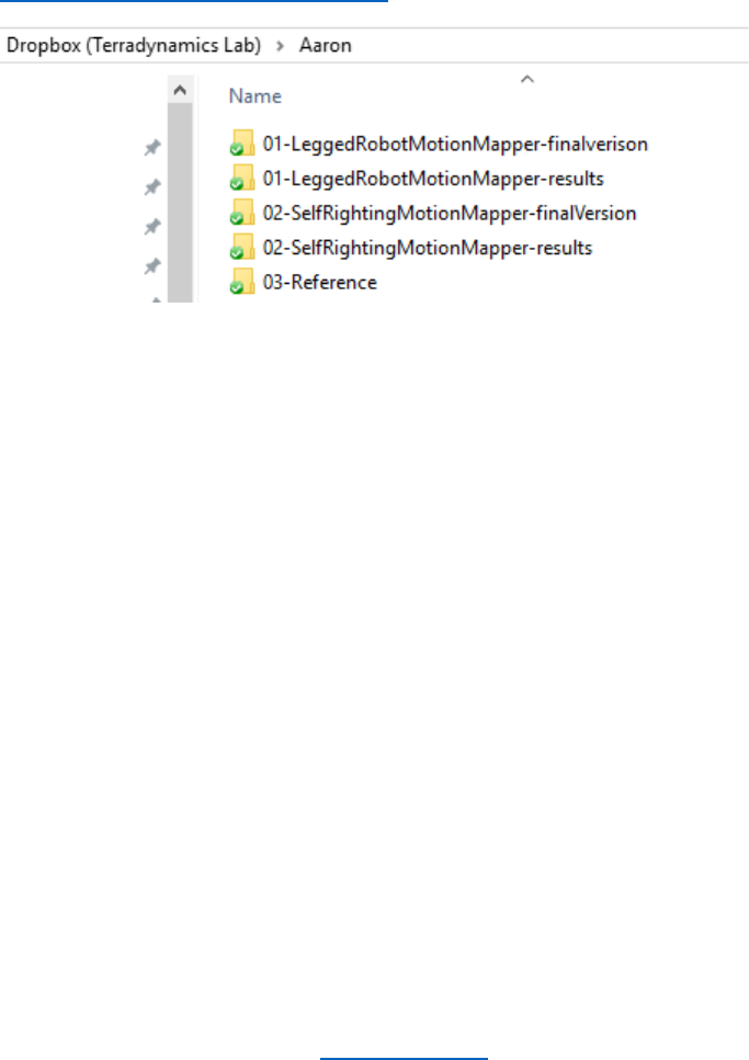
D:\Dropbox (Terradynamics Lab)\Aaron
1) ./01-LeggedRobotMotionMapper-finalversion/: Stores the matlab codes of the first section of this
manual – analysis of kinematic data of the robot motion
2) ./01-LeggedRobotMotionMapper-results/: Stores the results of the legged robot motion mapper
3) ./02-SelfRightingMotionMapper-finalVersion/: Stores the matlab codes of the second section of
this manual – analysis of cockroach self-righting videos
4) ./02-SelfRightingMotionMapper-results/: Stores the results of the self righting motion mapper
5) ./03-Reference/: The folder in which all study materials and resources mentioned in this manual are
stored.
I. Analysis of kinematic data of the robot motion
This project represents a sample implementation of the motion mapper behavioral analysis by using the
kinematic data of the robot crossing the beam. User can easily change the dimension of input data by
randomly combining the data of velocity, orientation and position.
Methods
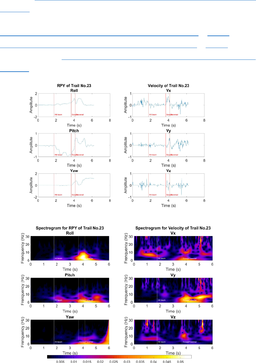
1. Spectrogram generation (Interface paper - 3.3)
We compute the amplitudes of the Morlet continuous wavelet transform for each time series.
Although similar to a Fourier spectrogram, wavelets possess a multi-resolution time–frequency
trade-off, allowing for a more complete description of postural dynamics occurring at several time
scales. For the results presented here, we look at 30 frequency channels, dyadically spaced between
1 and 30 Hz. Here is an example of spectrogram for the trial no.23.
Study materials:
1) Study notes: D:\Dropbox (Terradynamics Lab)\Aaron\03-Reference\Wavelet Transform Notes by
Aaron.pptx
2) The wavelet tutorial:
D:\Dropbox (Terradynamics Lab)\Aaron\03-Reference\WaveletTutorial.pdf or web link
D:\Dropbox (Terradynamics Lab)\Aaron\03-Reference\Wavelets_2010.pdf or web link
3) The Fourier transform: https://betterexplained.com/articles/an-interactive-guide-to-the-fourier-
transform/
2. Spatial embedding (Interface paper - 3.4)
The generated spectrogram comprises 30 frequency channels for each of the six dimensions
(R,P,Y,Vx,Vy,Vz), making each point in time represented by a 180 dimensional feature vector. We
would like to find a low-dimensional representation that captures the important features of the
dataset. t-SNE is used to take data from a high-dimensional space and embed it into a space of much
smaller dimensionality.
Study materials:
1) Comprehensive Guide on t-SNE: https://www.analyticsvidhya.com/blog/2017/01/t-sne-
implementation-r-python/
2) Study notes: D:\Dropbox (Terradynamics Lab)\Aaron\03-Reference\t-SNE Study Notes.pdf
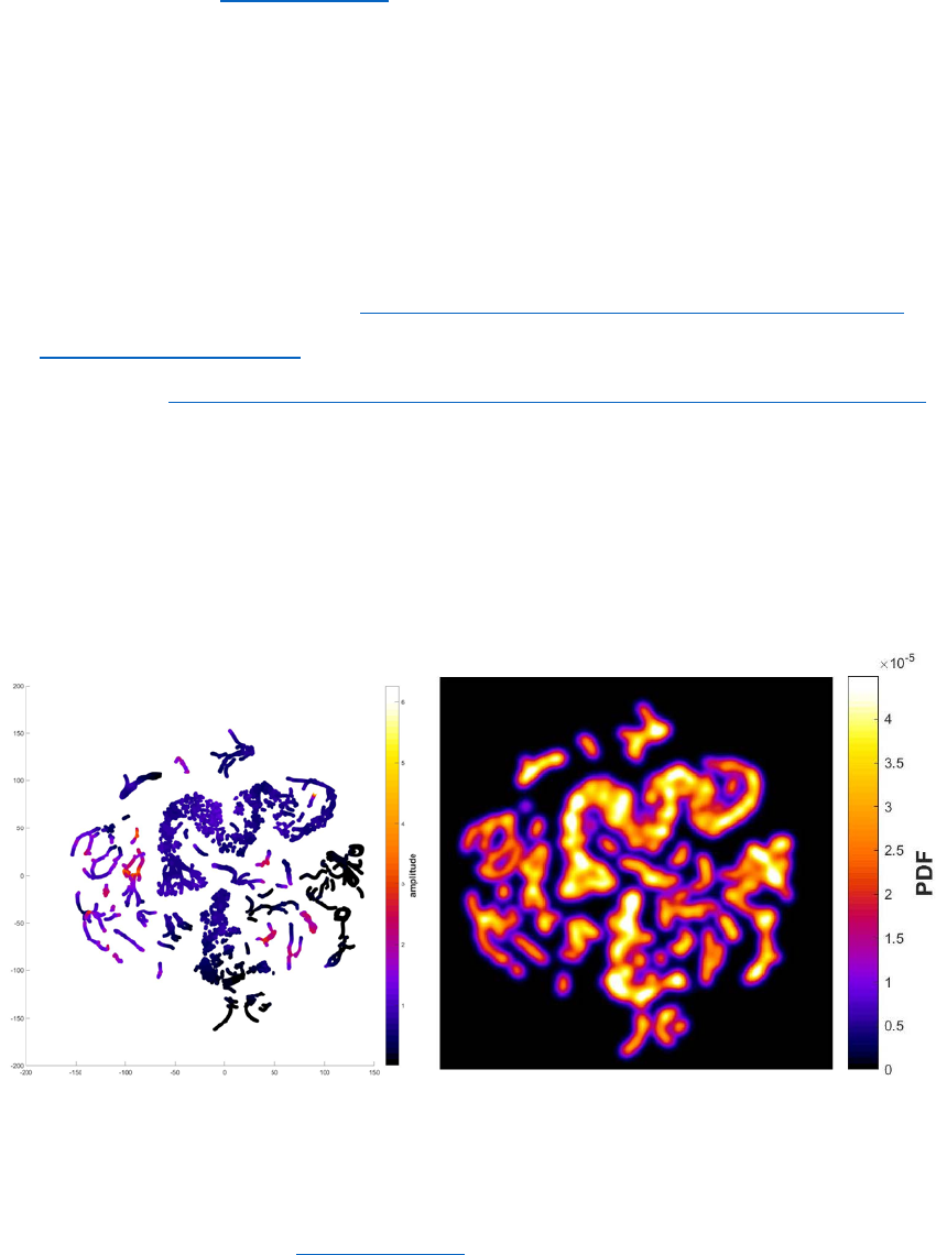
After we got the embedding of our spectral feature vectors into two dimensions, we generated an
estimate of the probability density by convolving each point in the embedded map with a Gaussian
of relatively small width. The locations of local maxima provide a potential representation for the
stereotyped behaviors that the files perform.
Figure left: spectral points embedded into two dimensions via t-SNE
Figure right: Probability density function (PDF) generated from convolving with a Gaussian
3. Behavior states definition (Interface paper - 4.1, 4.2)
The embedded space comprises peaks surrounded by valleys. Finding connected areas in the
embedding plane such that climbing up the gradient of probability density always leads to some
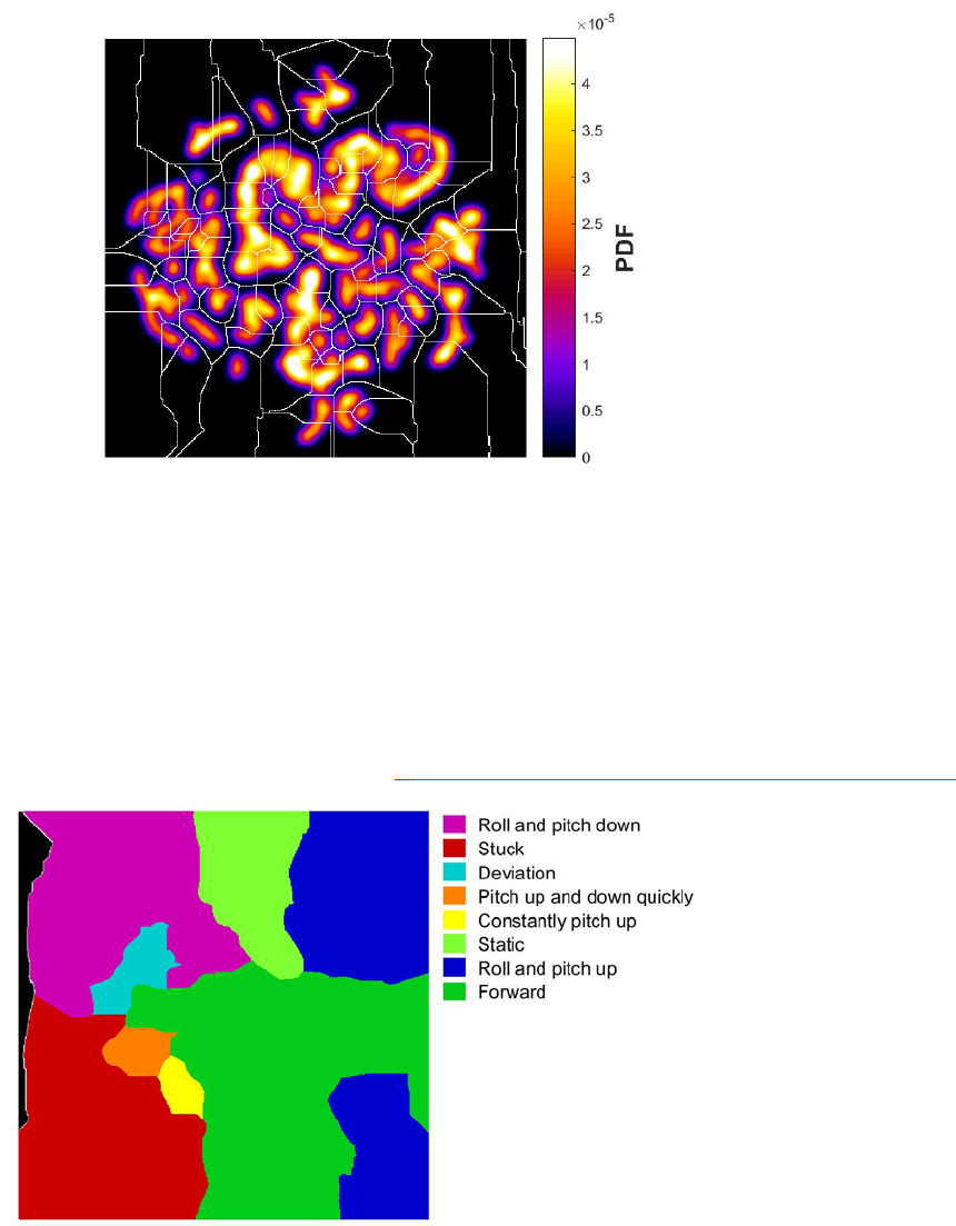
local maximum, often referred to as a watershed transform, we delineate 116 regions of the
embedded space. Each of these contains a single local maximum of probability density.
Figure: Boundary lines obtained from performing a watershed transform on the PDF.
Observing the original movies corresponding to pauses in one of the regions, we consistently
observe the robot performing a distinct action that corresponds to a recognizable behavior when
viewed by eye.
All the mapped videos can be found in: D:\Dropbox (Terradynamics Lab)\Aaron\Videos\Mapped
Figure: The organization of behavioral space into regions of similar movement types. Definition of
regions is performed through visual assessment of movies
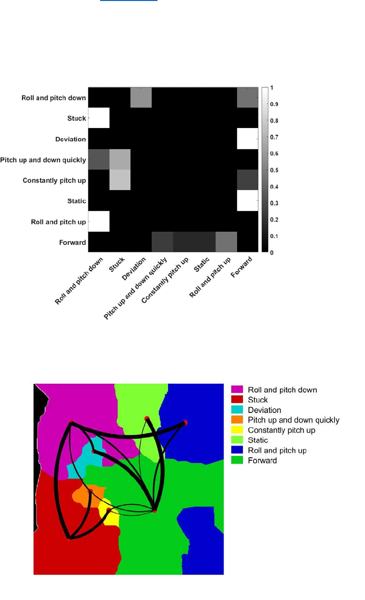
4. Transition matrices (PNAS paper - Transition Matrices)
To investigate the temporal pattern of behaviors, we first calculated the behavioral Markov
transition matrix over different time scales, which describes the probability that the animal will go
from state j to state i.
Plotting this matrix on the behavioral map itself, we can see the transition distribution on the
behavioral map. All transition probabilities less than 0.05 are omitted.
Study materials:
1) MIT open course on Markov Matrics: https://youtu.be/nnssRe5DewE
2) Markov Chains: https://nlp.stanford.edu/IR-book/html/htmledition/markov-chains-1.html
Matlab Codes
IMPORTANT: the path of the final version codes that implement the above-mentioned
methods: D:\Dropbox (Terradynamics Lab)\Aaron\01-LeggedRobotMotionMapper-finalverison.
1) To run this code, you will first have to compile the associated mex files contained in this repository.
In order to do this, type compile_mex_files in the MATLAB command prompt from the main
directory.
2) An example run-through of all the portions of the algorithm can be found in run.m. Given a mat file
storing the kinematic data, this will run through each of the steps in the algorithm.
3) All default parameters can be adjusted within setRunParameters.m. Additionally, parameters can
be set by inputting a struct containing the desired parameter name and value into the function (see
code for details).
4) The major sub-routines for the method are named as coherently as possible:
a) dataProcess.m: Process the data of RPY, XYZ and velocity.
1. Input:
• robotData -> the raw kinematic data got from robot experiment.
• shellTagID -> the corresponding tag for robot.
• position -> boolean variable to decide whether select the position data (true/false).
• orientation -> boolean variable to decide whether select the orientation data
(true/false).
• velocity -> Boolean variable to decide whether select the velocity data (true/false)
2. Output:
• RobData -> the processed kinematic data. It can be 3d, 6d or 9d depending on user
selection.
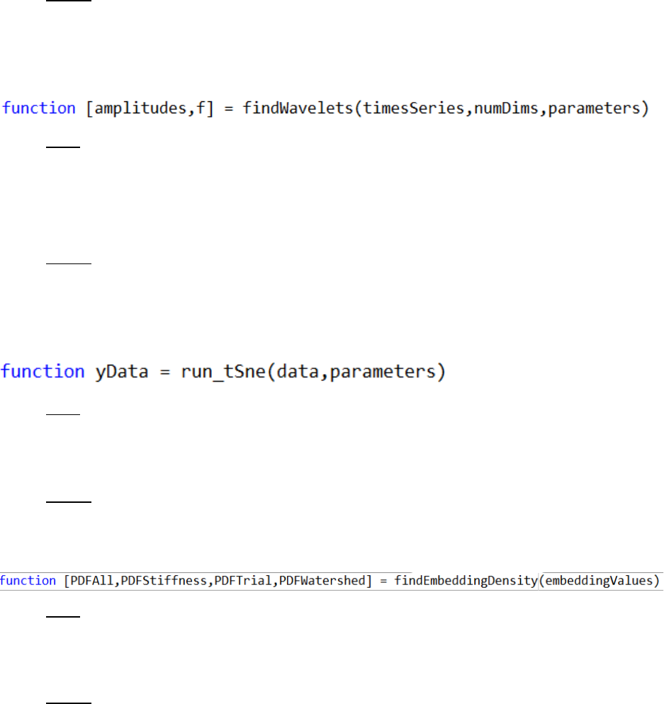
b) findWavelets.m: Computes the Morlet wavelet transform for the input kinematic data
1. Input:
• timeSeries -> the n(time) x d(dimension) kinematic time series.
• numDims -> the number of dimension of time series.
• parameters -> struct containing non-default choices for parameters.
2. Output:
• amplitudes -> wavelet amplitudes.
• f -> frequencies used in wavelet transforms (Hz).
c) run_tSne.m: Runs the t-SNE algorithm
1. Input:
• data -> Nxd array of wavelet amplitudes
• parameters -> struct containing non-default choices for parameters.
2. Output:
• yData -> Nx2 array of embedding results
d) findEmbeddingDensity.m: Calculates and plots the density on the embedding space
1. Input:
• embeddingValues -> 1x 30(no. of trials) cell arrays, each cell contains Nx2 array of
embedding results.
2. Output:
• PDFAll -> embedding density figure for all the trials.
• PDFStiffness -> embedding density figure for each stiffness (low, stiffness, and high).
• PDFTrial -> embedding density figure for each trails.
• PDFWatershed -> watershed embedding density figure for all the trials.
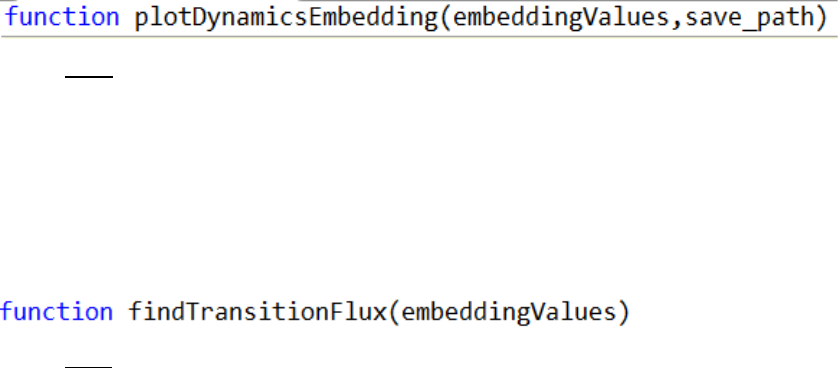
e) plotDynamicsEmbedding.m: Plots the trajectories of each trial on the embedding space.
1. Input:
• embeddingValues -> 1x 30(no. of trials) cell arrays, each cell contains Nx2 array of
embedding results.
• Save_path -> the path to save the figures.
f) findTransitionFlux.m: Plots the transition flux for all clusters on the watershed embedding
space.
1. Input:
• embeddingValues -> 1x 30(no. of trials) cell arrays, each cell contains Nx2 array of
embedding results.
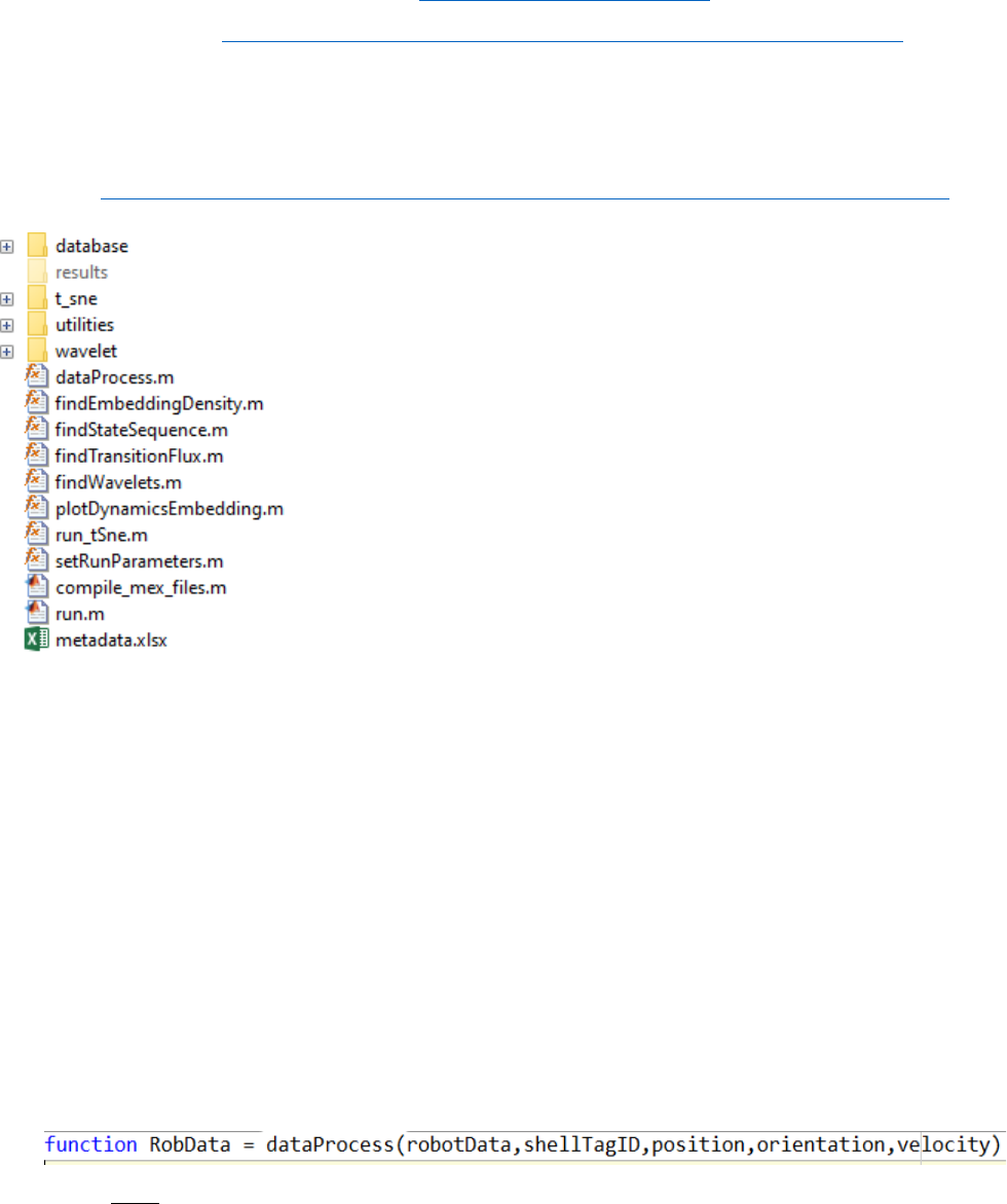
5) The function of the folders in the directory:
./Database/ -> The folder saves all the .mat files
./results/ -> The folder saves all the results, including the figures and embedding dynamics. User
can change the result destination in the code.
./t-sne/ -> Saves the function files for t-SNE
./utilities/ -> Saves any other utility function files
./wavelet/ -> Saves the function files for Morlet wavelet transform
How to Run the Codes
Open the run.m at: D:\Dropbox (Terradynamics Lab)\Aaron\01-LeggedRobotMotionMapper-
finalverison\run.m
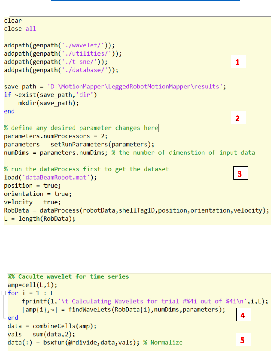
1. Change the save path
2. Define any desired parameters
3. Run the dataProcess.m with the selection of position/orientation/velocity
4. Run the findWavelets.m to find the wavelets for the data generated by dataProcess.m
5. Normalize the wavelet amplitude.
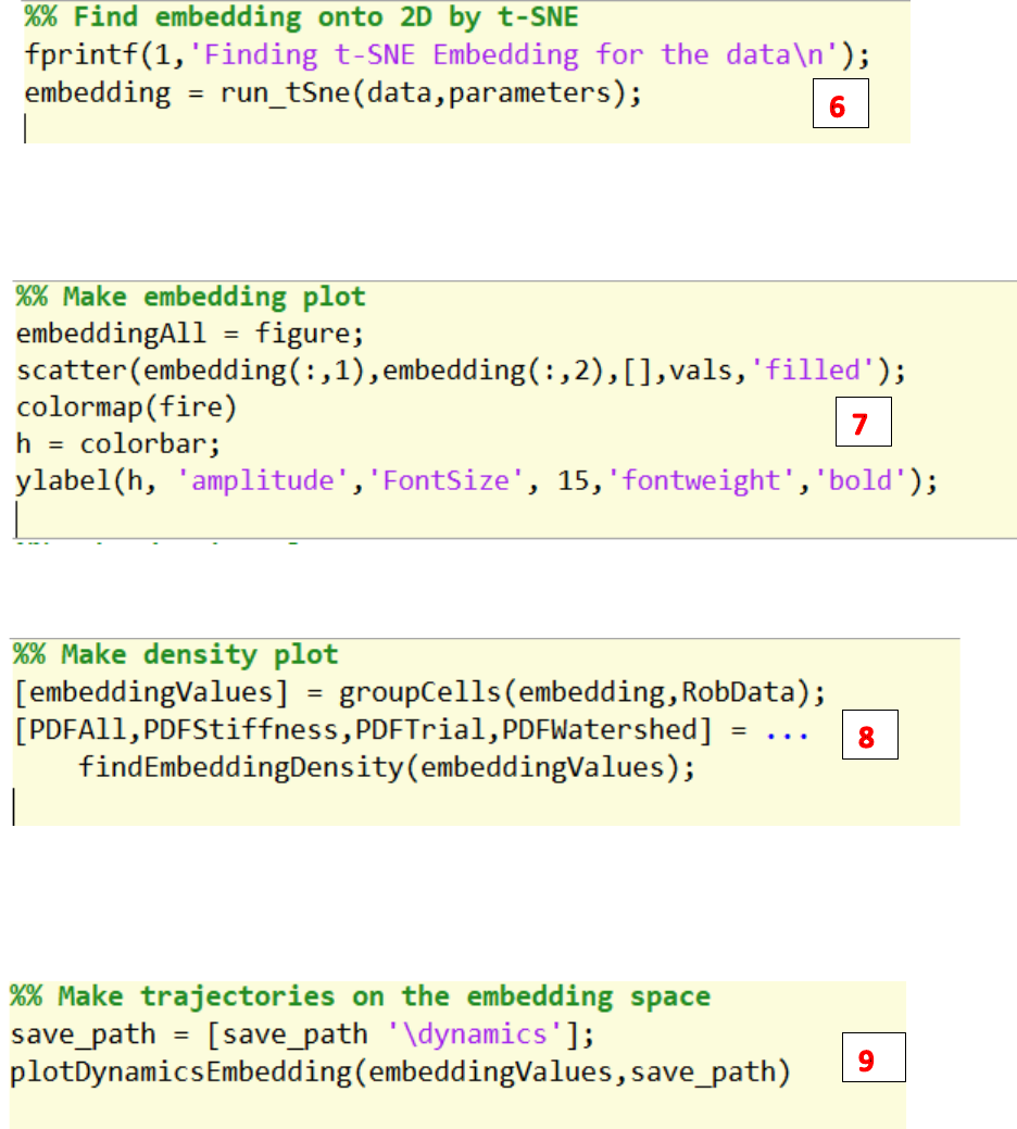
6. Run the run_tSne.m to find the 2d embedding of the wavelet amplitude generated by
findWavelets.m
7. Plot the embedding results.
8. Run findEmbeddingDensity.m to plot the points’ density on the embedding space.
9. Run plotDynamicsEmbedding.m to plot trajectories of each trial on the embedding space.
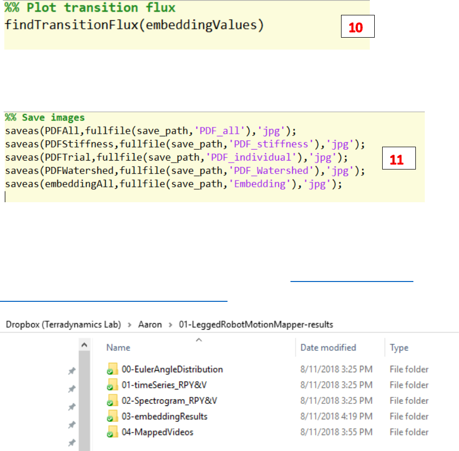
10. Run findTransitionFlux.m to plot the transition flux for all clusters on the watershed embedding
space.
11. Save the above-mentioned figures to the save path.
Results
IMPORTANT: all the figures and the mapped videos are stored at D:\Dropbox (Terradynamics
Lab)\Aaron\01-LeggedRobotMotionMapper-results
1) ./00-EulerAngleDistribution/ contains the euler angle distribution of roll, pitch and yaw for the
robot motion
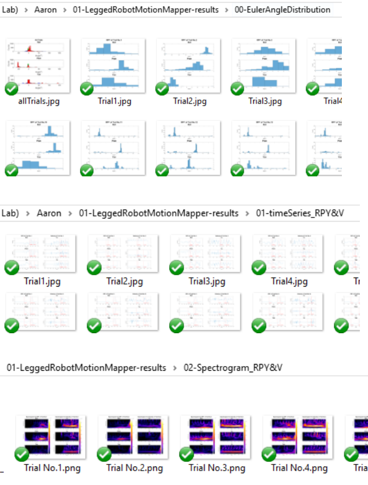
2) ./01-timeSeries_RPY&V/ contains the figures of input time series
3) ./02-Spectrogram_RPY&V/ contains the figures of sepectrogram generated by wavelet transform
4) ./03-embeddingResults/ contains the 2d embedding results for the kinematic data
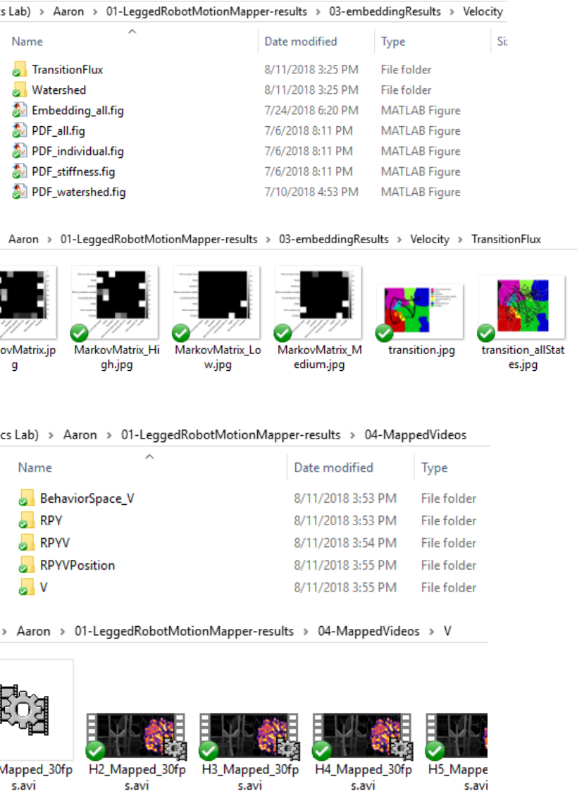
5) ./04-MappedVideos/ contains the videos mapped with trajectories on embedding space
II. Analysis of cockroach self-righting videos
This is a sample implementation of the motion mapper behavioral analysis by using videos of the robot
motion. The framework can process single video or multiple videos. The methods of processing videos
are pretty similar to that of processing kinematic data. The difference between these two methods is the
part of data processing. Here I will introduce the methods that are different from the above-mentioned
ones.
Methods
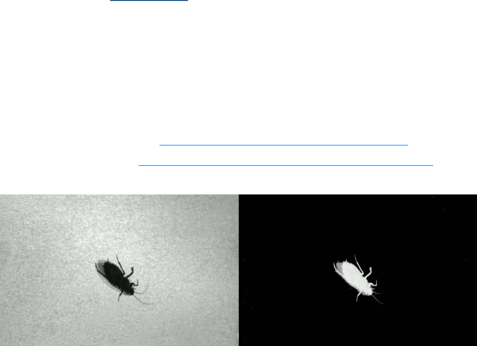
1. Video Segmentation (Interface paper - 3.1)
To isolate the fly from the background, we apply Canny Edge Detection method for edge detection,
resulting in a binary image containing the edge positions. In order to achieve good segmentation,
the contrast between the animal and background should be high. One way we can do is using
translucent background and adding a light at the bottom to improve the contrast when doing
experiment in the future.
Study materials:
1) Canny edge detection tutorial: http://www.aishack.in/tutorials/canny-edge-detector/
2) Edge detection in Matlab: https://www.mathworks.com/help/images/edge-detection.html
a) The raw videos: b) The videos after being segmented:
2. Crop Video / Find Bounding Box
Because the animal goes around in the videos, the center of the fly within the frame vary over time.
In order to make sure the animal can locate in the center of each frames, the framework will find
the center of the animal body and then crop the frame with a 450 x 450 square window whose
center locates at the center of the animal body.
b) The videos after being segmented: b) The videos after being cropped:
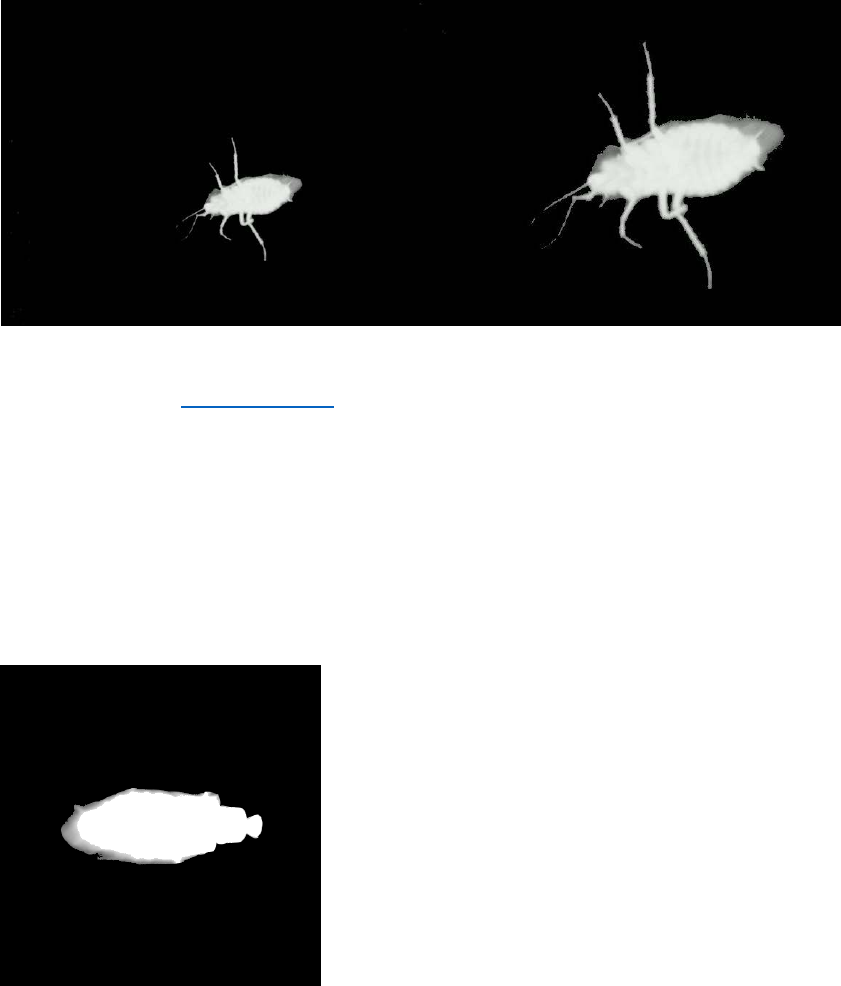
3. Video Alignment (Interface paper – Appendix A)
To keep the orientation of the animal within the frame same over time, we next register each frame
rotationally with respect to a template image. The template image is generated by taking a typical
image of the animal and then manually ablating the wings and legs digitally. In Photoshop, use the
magnetic lasso tool and select the outline of the animal body, then delete the regions outside the
selection region, which finally remains the template image.
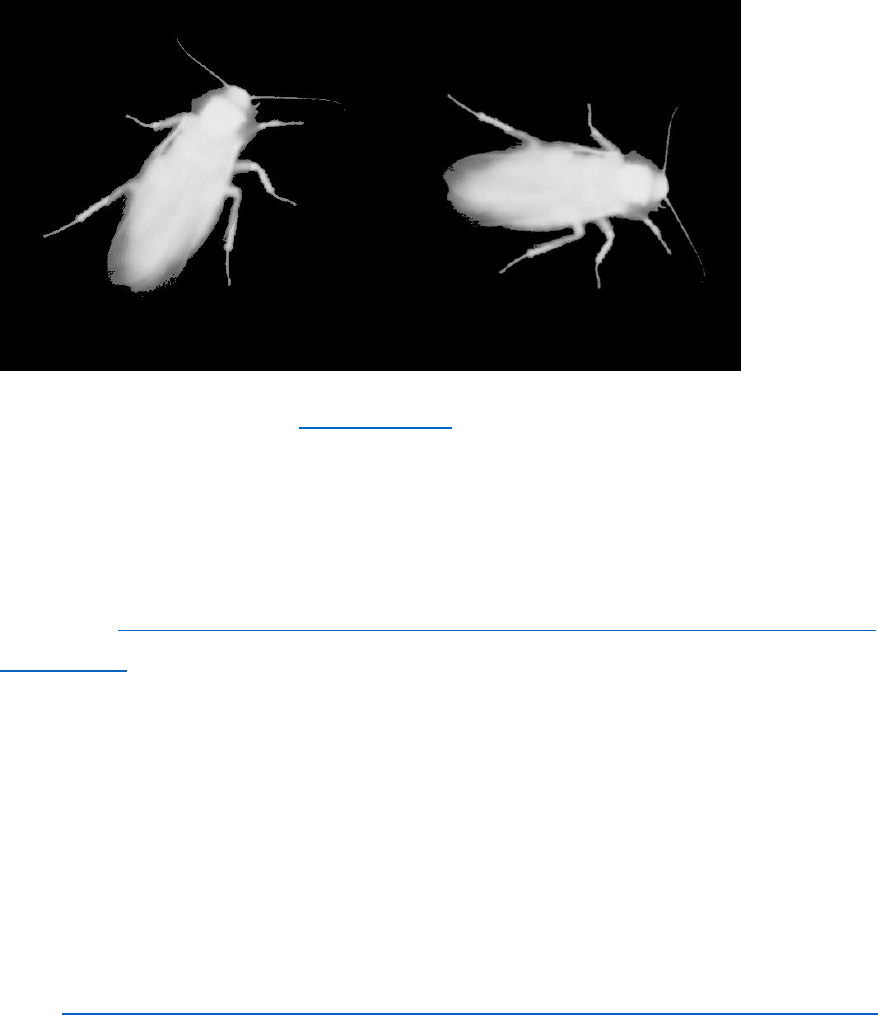
a) Template:
b) The videos after being cropped: c) The aligned videos:
4. Generate Time Series by PCA (Interface paper - 3.2)
The framework will apply principal component analysis (PCA) to the videos and then project
individual images onto these principal components, which convert a movie of animal behavior into
time series. User can change the number of principal components in the codes.
Study materials:
PCA tutorial: https://towardsdatascience.com/a-one-stop-shop-for-principal-component-analysis-
5582fb7e0a9c
After generating the time series, the framework then computes the Morlet wavelet and find the
embedding space by t-SNE, which are the same as the methods of processing kinematic data. (See
above)
Matlab Codes
IMPORTANT: the path of the final version codes that implement the above-mentioned
methods: D:\Dropbox (Terradynamics Lab)\Aaron\02-SelfRightingMotionMapper-finalVersion.

1) An example run-through of all the portions of the algorithm can be found in run.m. Given single
video or multiple videos, this will run through each of the steps in the algorithm.
2) All default parameters can be adjusted within setRunParameters.m. Additionally, parameters can
be set by inputting a struct containing the desired parameter name and value into the function (see
code for details).
3) The major sub-routines for the method are named as coherently as possible:
a) runPreprocess.m: Runs the alignment and segmentation routines on a .avi file
b) findBoundingBox.m : Finds the bounding box of the image and crop it
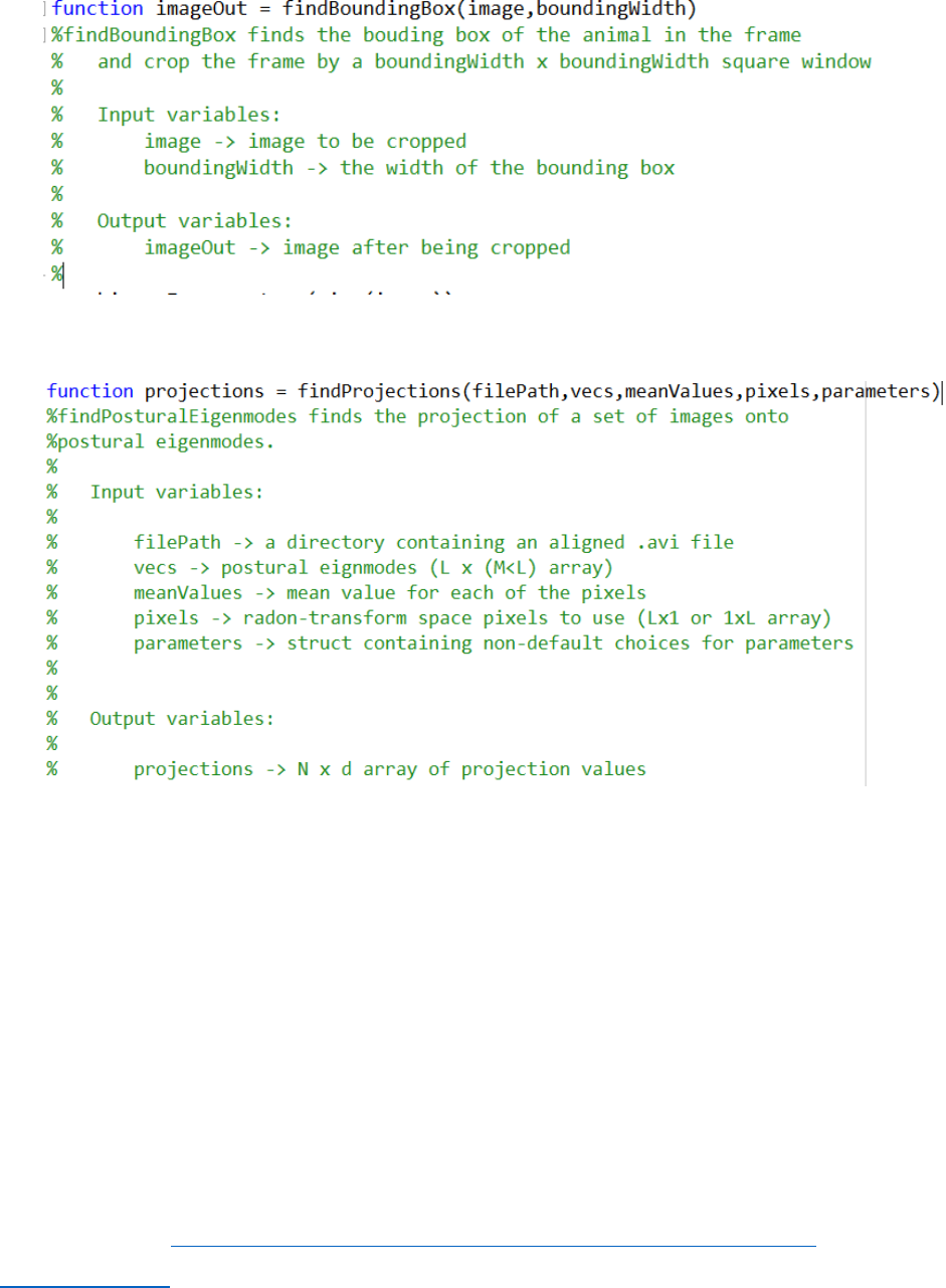
c) findProjections.m: Finds the time series of videos by PCA
All other routine are the same as those in the analysis of kinematic data.
4) The function of the folders in the directory:
./PCA/ -> Saves the function files for PCA
./segmentation_alignment/ -> Saves the function files for registering videos
./t-sne/ -> Saves the function files for t-SNE
./utilities/ -> Saves any other utility function files
./wavelet/ -> Saves the function files for Morlet wavelet transform
How to Run the Codes
Open the run.m at D:\Dropbox (Terradynamics Lab)\Aaron\02-SelfRightingMotionMapper-
finalVersion\run.m
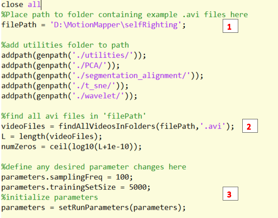
1. Change the path to the folder containing the .avi videos
2. Find all the .avi videos in the path.
3. Define any desired parameters.
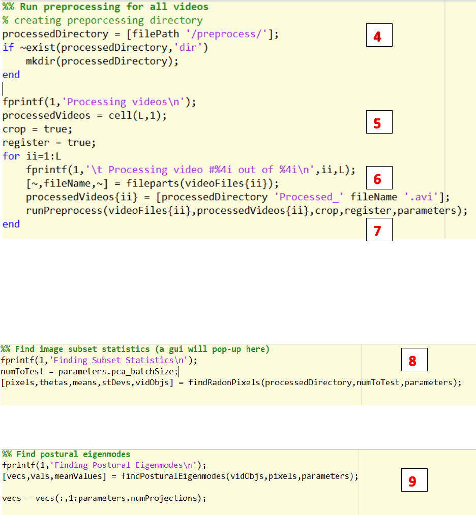
4. Change the path to save the processed videos.
5. Decide whether crop and align the videos.
6. Change the name of the video to be saved.
7. Run runPreprocess.m to process the videos and save the videos to the path.
8. Run findRadonPixels.m to run randon transform to find subset pixels of images
9. Run findPosturalEigenmodes.m to find the principal components / postural eigenmodes.
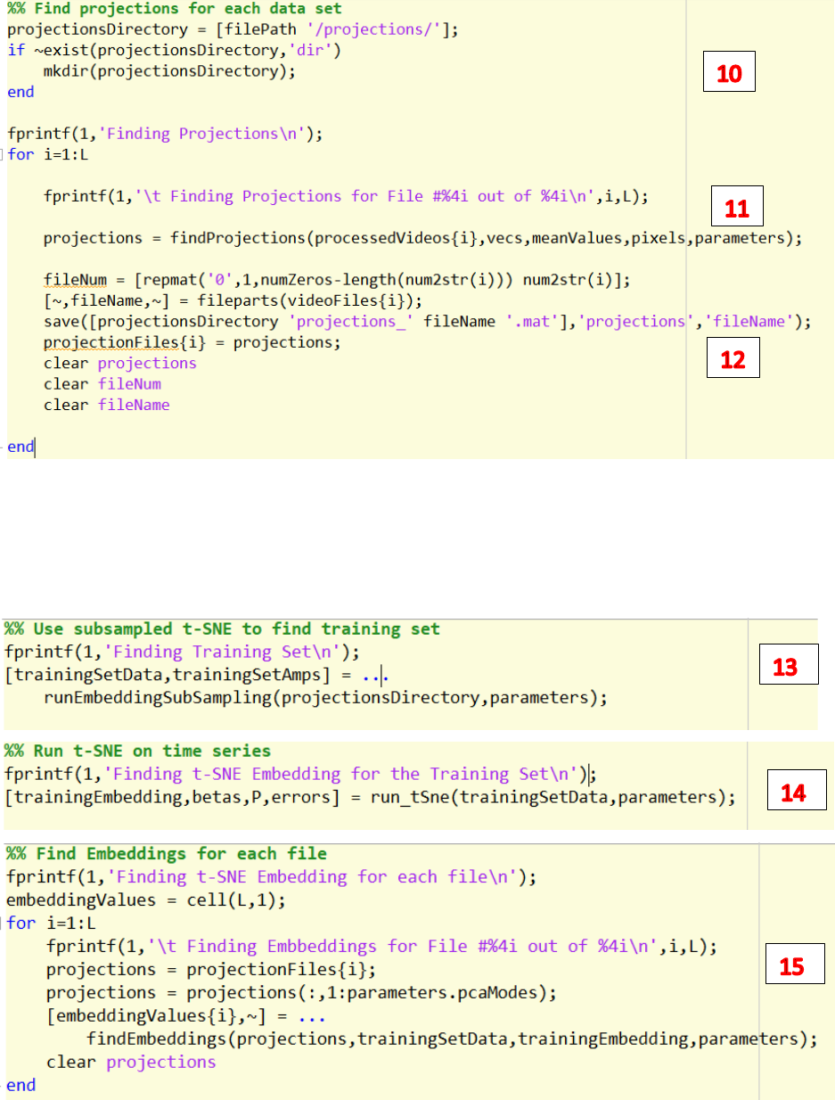
10. Change the path to save the time series generated by PCA
11. Run findProjections.m to run PCA and generate time series.
12. Save the time series to the path.
13. Run runEmbeddingSubSampling.m to find training set of time series.
14. Run run_tSne.m to find the training embeddings on the training set.
15. Run findEmbeddings.m to find the 2d embeddings space for all videos
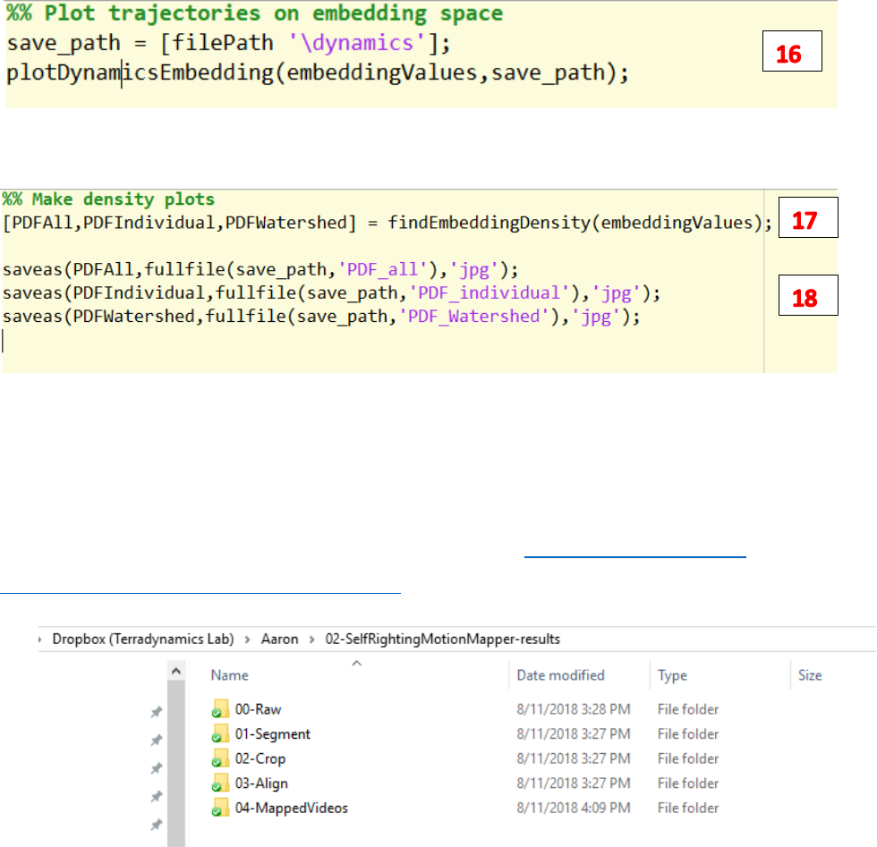
16. Run plotDynamicsEmbedding.m to plot trajectories of each file on the embedding space.
17. Run findEmbeddingDensity plot the points’ density on the embedding space.
18. Save the above-mentioned figures.
Results
IMPORTANT: all the figures and the mapped videos are stored at D:\Dropbox (Terradynamics
Lab)\Aaron\02-SelfRightingMotionMapper-results
1) ./00-Raw/ contains the raw videos of the cockroach self-righting
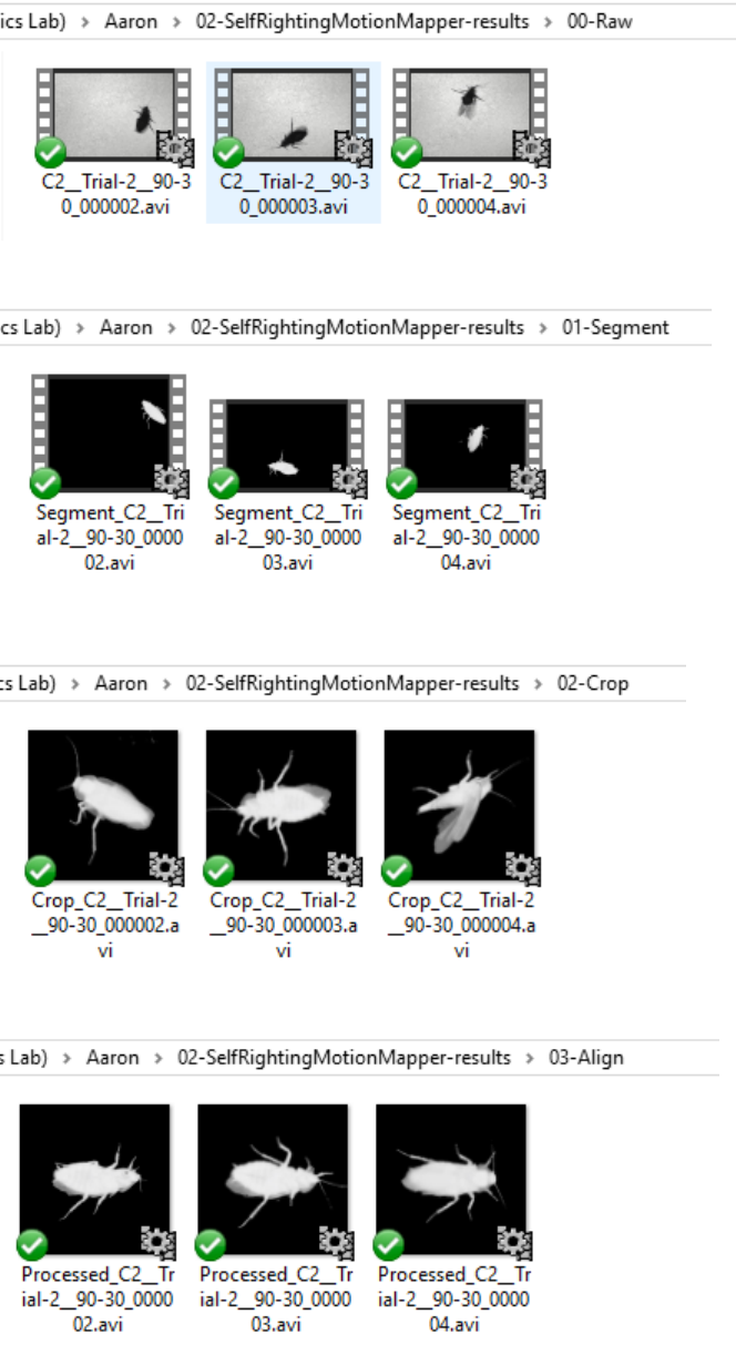
2) ./01-Segment/ contains the videos after being segmented
3) ./02-Crop/ contains the video after being cropped by a square window
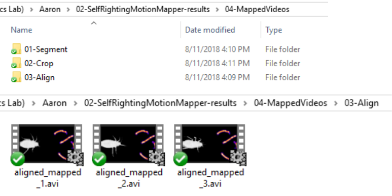
4) ./03-Align/ contains the alignment videos
5) ./04-MappedVideos/ contains the videos mapped with trajectories on the embedding space