NCAR Graphics Manual
User Manual:
Open the PDF directly: View PDF ![]() .
.
Page Count: 41

1
NCAR Command Language (NCL)
Mini Graphics Manual
Document Version 1.3, NCL Version 6.0.0 March 2011
The NCAR Command Language (NCL) is an open source, free, interpreted programming
language, specifically designed for the access, analysis, and visualization of data.
http://www.ncl.ucar.edu/
NCL has many features common to modern programming languages, including types, variables,
operators, expressions, conditional statements, loops, and functions and procedures. An NCL
Mini Reference Manual describing basic language features may be downloaded at:
http://www.ncl.ucar.edu/Document/Manuals/
This Mini Graphics Manual includes topics on setting up your NCL environment, high-level
graphical interfaces, color, vectors, contours, workstations, page maximization, maps and more.
Contributors: Sylvia Murphy, Mary Haley, and Dennis Shea. Send comments about this manual
to ncl-talk@ucar.edu.
For actual script examples and sample plots, please visit one of the following sites:
http://www.ncl.ucar.edu/Applications/
http://www.ncl.ucar.edu/Document/Manuals/Getting_Started/
keyword courier-bold
built-in functions courier-bold blue
contributed functions courier-bold green
shea_util functions courier-bold purple
symbols bold
operators bold
plot templates courier-bold green
plot resources courier-bold
user variables italics
WWW links underline
© Copyright, 2011, National Center for Atmospheric Research,1850 Table Mesa Drive, Boulder CO 80305.
NCL is sponsored by the National Science Foundation.
2
Section 1: Overview ........................................................................................................................ 4!
Section 1.1 Sample script ........................................................................................................... 4!
Section 2: High-Level Graphical Interfaces .................................................................................... 4!
Section 2.1 gsn generic interfaces .............................................................................................. 5!
Section 2.2 gsn_csm interfaces .................................................................................................. 5!
Section 2.3 Which should I use? ................................................................................................. 5!
Section 2.4 gsn special interfaces ............................................................................................... 6!
Section 2.5 Loading the interfaces .............................................................................................. 6!
Section 2.6 gsn_csm expectations .............................................................................................. 6!
Section 3: Getting Started ............................................................................................................... 7!
Section 3.1 $NCARG_ROOT ...................................................................................................... 7!
Section 3.2 .hluresfile .................................................................................................................. 7!
Section 3.3 Running NCL ............................................................................................................ 8!
Section 4: Workstations .................................................................................................................. 8!
Section 5: Plot Mods via Resources ............................................................................................... 8!
Section 5.1 Resource types ........................................................................................................ 8!
Section 5.2 Setting resources ..................................................................................................... 9!
Section 5.3 Some common resources ........................................................................................ 9!
Section 5.4 Drawing a plot and gsnDraw ................................................................................... 9!
Section 5.5 Advancing the frame and gsnFrame ....................................................................... 9!
Section 5.6 Special string resources, gsnLeftString, gsnCenterString, gsnRightString ............ 10!
Section 6: Color ............................................................................................................................ 10!
Section 6.1 Turning on color ..................................................................................................... 10!
Section 6.2 The default colormap ............................................................................................. 10!
Section 6.3 Built-in colormaps ................................................................................................... 11!
Section 6.4 Using RBG triplets .................................................................................................. 11!
Section 6.5 Named colors ......................................................................................................... 12!
Section 6.6 gsnSpreadColors ................................................................................................... 12!
Section 6.7 CMYK ..................................................................................................................... 13!
Section 7: Vectors ......................................................................................................................... 13!
Section 7.1 Types of vectors ..................................................................................................... 13!
Section 7.2 Controlling vectors ................................................................................................. 13!
Section 7.3 Vectors colored by a scalar field or on a scalar field .............................................. 14!
Section 8: Map Tickmarks ............................................................................................................ 16!
Section 9: Page Maximization ...................................................................................................... 16!
Section 10: Contours .................................................................................................................... 17!
Section 10.1 Manually setting contour levels ............................................................................ 17!
Section 10.2 Contour effects ..................................................................................................... 17!
Section 10.3 Explicitly setting contour levels ............................................................................ 18!
Section 10.4 Contour labels ...................................................................................................... 18!
Section 11: Two-Dimensional Lat/Lon Arrays ............................................................................... 18!
Section 11.1 Native grid projections .......................................................................................... 19!
Section 12: Aspect Ratio Changes ............................................................................................... 20!
Section 13: Paneling ..................................................................................................................... 20!
Section 13.1 Sample script ....................................................................................................... 20!
Section 13.2 Orienting plots on a page ..................................................................................... 21!
Section 13.3 Important panel resources ................................................................................... 21!
Section 13.4 Paneling plots of different sizes ........................................................................... 22!
Section 14: Font Heights .............................................................................................................. 23!
Section 15: Titles .......................................................................................................................... 23!
Section 16: Legends ..................................................................................................................... 23!
Section 17: Label Bars .................................................................................................................. 23!
Section 18: Function Codes .......................................................................................................... 24!
Section 18.1 Superscripting/subscripting .................................................................................. 24!
Section 18.2 Carriage return ..................................................................................................... 24!
Section 18.3 Greek or mathematical characters ....................................................................... 24!
3
Section 19: Primitives ................................................................................................................... 24!
Section 19.1 Polygons .............................................................................................................. 24!
Section 19.2 Polylines ............................................................................................................... 25!
Section 19.3 Polymarkers ......................................................................................................... 26!
Section 20: Adding Text ................................................................................................................ 26!
Section 21: X-Y Plots .................................................................................................................... 26!
Section 22: Explicit Tickmark Labeling ......................................................................................... 28!
Appendix A: Common Resources ................................................................................................. 29!
Axis - http://www.ncl.ucar.edu/Document/Graphics/Resources/tr.shtml ................................... 29!
Contour - http://www.ncl.ucar.edu/Document/Graphics/Resources/cn.shtml ........................... 29!
Labelbars - http://www.ncl.ucar.edu/Document/Graphics/Resources/lb.shtml ......................... 30!
GSN - http://www.ncl.ucar.edu/Document/Graphics/Resources/gsn.shtml .............................. 31!
Legends - http://www.ncl.ucar.edu/Document/Graphics/Resources/lg.shtml ........................... 32!
XY curves - http://www.ncl.ucar.edu/Document/Graphics/Resources/xy.shtml ........................ 32!
Maps - http://www.ncl.ucar.edu/Document/Graphics/Resources/mp.shtml .............................. 32!
Polygons, polylines, polymarkers -
http://www.ncl.ucar.edu/Document/Graphics/Resources/gs.shtml ........................................... 34!
Appendix B: High-level Graphical Interfaces ................................................................................ 35!
gsn generic interfaces ............................................................................................................... 35!
gsn_csm interfaces ................................................................................................................... 35!
gsn special interfaces ................................................................................................................ 36!
Appendix C: List of Named Colors ................................................................................................ 37!
Appendix D: Common Error Messages ........................................................................................ 39!
Appendix E: Glossary ................................................................................................................... 41!

4
Section 1: Overview
This document describes how to use high-level graphical interfaces to generate plots. The
following section contains a script example that illustrates the framework used to create a plot.
This manual assumes the reader is familiar with the data model used by NCL (a netCDF data
model). Please refer to the Mini-Reference Manual if necessary.
Section 1.1 Sample script
In general, a script has the following characteristics: (1) load the libraries containing the high-level
graphical interfaces with the load command. By convention, this occurs before the begin
statement. (2) Read in the data. (3) Conduct data processing (optional). (4) Open a workstation.
(5) Choose a color table (optional). (6) Create a resource variable to which various graphical
options (resources) may be assigned as attributes (if plot modifications are desired). (7) Invoke
the appropriate graphical interface passing in the workstation, data, and resources.
;*******************************************
load "$NCARG_ROOT/lib/ncarg/nclscripts/csm/gsn_code.ncl"
load "$NCARG_ROOT/lib/ncarg/nclscripts/csm/gsn_csm.ncl"
;*******************************************
begin
;*******************************************
in = addfile("myfile.nc","r"); pointer to file
t = in->T ; read in data
;*******************************************
; create plot
;*******************************************
wks = gsn_open_wks("ps","ce") ; open ce.ps file
; choose colormap
gsn_define_colormap(wks,"BlAqGrYeOrRe")
res = True ; resource varb
res@cnFillOn = True ; turn on color
res@cnLinesOn = False ; no cn lines
res@cnLevelSpacingF = 0.5 ; cn spacing
res@gsnSpreadColors = True ; full colors
res@lbAutoLabelStride = True ; nice lb labels
plot = gsn_csm_contour_map(wks,t,res)
end
The default behavior of the graphical interfaces is to draw the plot and advance the frame. These
terms will be described in greater detail in sections 5.4 and 5.5. This default can be changed.
An entire library of example scripts exists on the web at:
http://www.ncl.ucar.edu/Applications/
Section 2: High-Level Graphical Interfaces
NCL's graphics are based upon object-oriented (OO) methods. This approach provides
considerable flexibility and power but can be tedious. To aid users, two suites of high-level
graphical interfaces have been developed. These interfaces facilitate the visualization process
while retaining the benefits of the OO approach. For historical reasons, all plot interfaces begin
5
with gsn_ which stands for "Getting Started with NCL".
The graphical interfaces may be a function, which will return a graphical object, or a procedure,
which will modify or perform a specific task on a graphical object.
Section 2.1 gsn generic interfaces
The generic interfaces are functions and procedures that create basic x-y, contour, streamline,
and vector plots. Generally, default settings are used, but the user may readily change these
settings. A list of these interfaces is listed in Appendix B. Example plots and a tutorial on how to
use these interfaces is at:
http://www.ncl.ucar.edu/Document/Manuals/Getting_Started/
The examples on this site contain a line-by-line description of various graphical options.
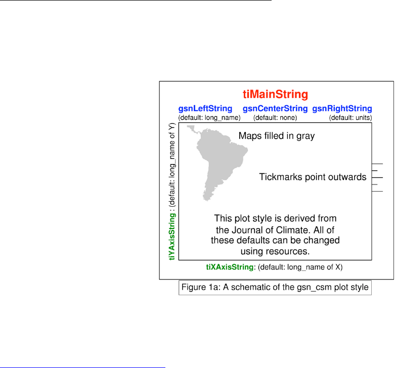
Section 2.2 gsn_csm interfaces
These high-level interfaces emulate the
graphical style of figures appearing in the
J. of Climate (June, 1998) special issue
focusing on the Climate System Model
(CSM). While the gsn_csm interfaces
were designed for a specific purpose,
many users prefer them over the generic
interfaces. The reason is that they
automatically perform tasks like adding
color label bars, which must be explicitly
added when using the generic gsn
interfaces. They also will use a variable's
long_name and units attributes (if
available) to label a plot (figure 1a). The
long_name will be placed in the upper
left corner and the units in the upper right
corner. Other features include the
addition of lat/lon labels of the form
“30N/120E” on cylindrical equidistant and
polar projection plots, and special labels on pressure height plots. Appendix B contains a list of
these interfaces.
You can view many examples produced by these interfaces at:
http://www.ncl.ucar.edu/Applications/
Section 2.3 Which should I use?
Most frequently, users prefer the gsn_csm interfaces over the generic gsn interfaces. Here are
some specific reasons to do so:
• Your data has attributes and you want your plot automatically labeled.
• You want as much done for you as possible.
• You like the general style.

6
• You want to put your data on a map, and your data has geophysical coordinates.
Section 2.4 gsn special interfaces
These interfaces perform special tasks, like drawing markers and text. They should not be
confused with the gsn generic interfaces which are limited to those in part one of Appendix B.
Section 2.5 Loading the interfaces
The gsn generic and gsn_csm plot interfaces and routines are located in two NCL scripts that are
distributed with the NCL software. Though the functions and procedures included in the libraries
can be loaded at any time prior to use, they are most frequently loaded at the top of the script
before the begin statement.
load "$NCARG_ROOT/lib/ncarg/nclscripts/csm/gsn_code.ncl"
load "$NCARG_ROOT/lib/ncarg/nclscripts/csm/gsn_csm.ncl"
Section 2.6 gsn_csm expectations
Labeling:
The gsn_csm plot interfaces may access information required by the CCSM netCDF convention.
For example, if the data has a “units” or “long_name” attribute, it will be used to automatically
label the plot. (figure 1a).
Units attribute of coordinate variable:
The latitude and longitude coordinate variables should have (but not limited to) attributes in one of
the following forms:
"degrees_north" "degrees_east"
"degrees-north" "degrees-east"
"degree_north" "degree_east"
"degrees north" "degrees east"
"degrees_N" "degrees_E"
"Degrees_north" "Degrees_east"
If the coordinate variable does not conform to one of the above names, you will receive an
annoying error message in the form of:
(0) is_valid_lat_ycoord: Warning: The units attribute of the Y
coordinate array is not set to one of the allowable units values
(i.e. 'degrees_north'). Your latitude labels may not be correct.
As with non-conforming named dimensions, it is simple to add the appropriate attribute to the
coordinate variable:
x&lat@units = "degrees_north"
The & symbol is used to access the coordinate variable, and the @ symbol is used to access the
attribute. These symbols are described in greater detail in the Mini-Reference Manual (see front
cover for download location).

7
Section 3: Getting Started
Section 3.1 $NCARG_ROOT
To execute NCL, you need to set this environment variable. The specific UNIX file which contains
the NCARG_ROOT specification is system dependent. For csh or tcsh, it can be set in your
".cshrc" file or your ".login" file. Do it in the file which initializes your $path variable. If you are
running ksh, bash, or sh, it will be placed in your ".profile". Here are some examples:
tcsh/csh bash/sh
setenv NCARG_ROOT /contrib export NCARG_ROOT=/contrib
path = ($NCARG_ROOT/bin $path) export PATH=$NCARG_ROOT:$PATH
NCARG_ROOT should be set to the parent directory of the “bin” directory that contains the ncl
executable. This will vary from system to system. If you are unsure, ask your local system
administrator where it is installed.
Section 3.2 .hluresfile
NCL has a default graphical environment that most users prefer to alter. This is accomplished
through the .hluresfile. Upon execution, NCL looks for this file in the user's home directory. The
following lists the most common usage of this file:
! White background/black foreground
*wkForegroundColor : (/0.,0.,0./)
*wkBackgroundColor : (/1.,1.,1./)
! Color map
*wkColorMap : rainbow+gray
! Font stuff
*Font : helvetica
! Function Codes [Default is a colon]
*TextFuncCode : ~
! X11 window size
*wkWidth : 800
*wkHeight: 800
Placing this file in your home directory would result in a large X11 window size, a common font,
and plots that have white as the background color and black as the foreground color.
You can download a sample .hluresfile at:
http://www.ncl.ucar.edu/Document/Graphics/hlures.shtml
8
Section 3.3 Running NCL
NCL can be run in two modes, script mode and interactive mode. To initiate the latter, simply type
"ncl" at the prompt. In interactive mode you are required to type each command separately. In
script mode, you create a separate NCL script which you send to the interpreter via the following
commands:
prompt> ncl [space] script
There is no required extension for an ncl script, but by convention the suffix "*.ncl" is used. NCL
scripts can have a begin and end statement, with a carriage return after the end statement. You
can optionally include options and command line arguments when you run NCL. See the Mini-
Reference Manual, whose location is mentioned on the first page of this document.
Section 4: Workstations
Opening a workstation is required prior to the creation of one or more plots. The workstation is
simply the location where the graphical instructions are sent (e.g. to a window or postscript file).
The workstation is given a name. This name becomes part of the output filename or title of X11
window. Users may have many workstations opened at the same time, although most only open
one. Only one colormap can be associated with each workstation.
There are six types of workstations: ncgm (NCAR computer graphics metafile), ps (postscript),
eps (encapsulated postscript, contains a bounding box), epsi (encapsulated postscript with a
bitmap preview), pdf, and X11 window. Examples:
wks = gsn_open_wks(“pdf”,”34_x_45”)
wks_2 = gsn_open_wks(“ps”,”myfile”)
The text to the left of the equal sign is a variable and can therefore be arbitrarily named.
Section 5: Plot Mods via Resources
Resources are the means by which we modify the default NCL plot. They may be strings, floats,
integers, doubles, etc. depending on the type of resource. The first two (or three) letters are lower
case, and the remaining letters are words of which the first letter is capitalized (e.g. cnFillOn).
If the resource is expecting a float value, an F is appended to the resource name (e.g.
txFontHeightF, mpMinLatF etc).
Section 5.1 Resource types
The first two letters of a resource identify what type of resource it is:
9
The
complet
e list of
resourc
es
under
these
categori
es may be accessed at:
http://www.ncl.ucar.edu/Document/Graphics/Resources/
Additionally, there is a unique set of gsn resources that were created specifically for the gsn
interfaces, and these resources can be found at the above URL as well.
Section 5.2 Setting resources
Resources are passed to the high-level graphpical interfaces as attributes to a logical variable.
Attributes are assigned using the @ symbol. Note that res is a user-defined variable. It is wise to
create separate variables for resources to be passed to different types of interfaces (e.g. con_res,
vec_res, xy_res). Vector resources sent to a contour routine will cause warning messages. The
following code snippet creates the variable res which is of type logical. Attributes associated with
res are then assigned.
res = True
res@tiMainString = “my title”
res@cnFillOn = True
The resource variable is always the last argument in the graphical interface calling sequence.
plot = gsn_csm_contour(wks,data,res)
plot2 = gsn_xy(wks,data,res)
The variable to the left of the equal sign is of type graphic. The name is arbitrary.
Section 5.3 Some common resources
It is impossible in the space provided here to give a complete description of each resource and its
options. Appendix A contains a list of some of the most commonly used resources.
Section 5.4 Drawing a plot and gsnDraw
By default, the high-level graphical interfaces create and draw graphical objects. This behavior
can be changed by setting the resource gsnDraw = False.
Section 5.5 Advancing the frame and gsnFrame
By default, the high-level graphical interfaces advance the frame after the graphical object has
been drawn. One analogy for the frame is that of a page in a book. The workstation is the book,
and advancing the frame is equivalent of turning the page in the book. A book or workstation can
am
annotation manager
pm
plot manager
vf
vector field
cn
contour
pr
primitive
vc
vectors
ca
coordinate arrays
sf
scalar field
vp
viewport
gs
graphical style
ti
title
wk
workstation
lb
labelbar
tm
tickmarks
ws
workspace
lg
legend
tx
text
xy
xy plot
mp
maps
tr
transform

10
have one or multiple frames (pages). The default behavior (turning to a new page) can be
changed by setting gsnFrame = False.
Section 5.6 Special string resources, gsnLeftString,
gsnCenterString, gsnRightString
The default behavior of the gsn_csm graphical interfaces is to place the long_name of the data (if
available) on the upper left corner of the plot, and the units of the data (if available) in the upper
right corner of the plot (figure 1a). This behavior can be changed through the use of the
gsnLeftString and gsnRightString resources. The following would remove the string:
res = True
res@gsnLeftString = ""
The following would set the right string to a user specified value, and also set the center string
which is not set by default:
res = True
res@gsnRightString = "my string"
res@gsnCenterString = "center"
Section 6: Color
Section 6.1 Turning on color
The resource cnFillOn = True will turn on the color fill of contours. Additionally, cnFillMode
= “RasterFill” will turn on raster contours.
Only one colormap is associated with a workstation (think page or group of pages) and not an
individual plot. This means that you cannot put plots with different colormaps onto the same
workstation, unless you merge the colormaps. The following URL contains an example of this
procedure:
http://www.ncl.ucar.edu/Applications/color.shtml
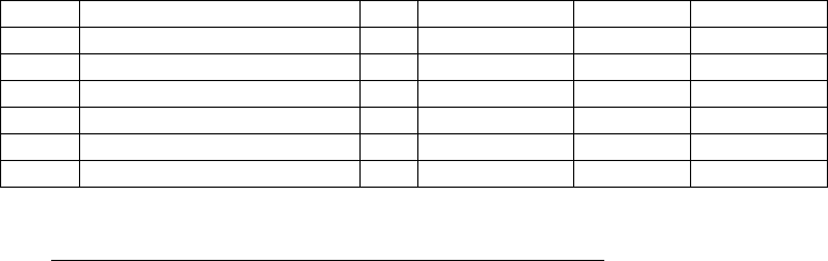
Section 6.2 The default colormap
NCL's default colormap (figure 5a) consists of a series of very distinct colors. Most users find that
it is not well suited to scientific applications. There are three ways to change the colormap:
selecting a built-in colormap (section 6.3), specifying an array of RBG triplets (section 6.4), or
specifying an array of named colors (section 6.5).
11
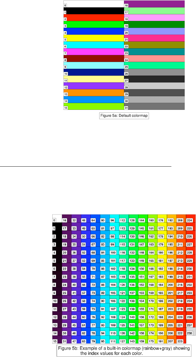
Section 6.3 Built-in colormaps
There are numerous pre-defined colormaps. A list of available maps can be found at:
http://www.ncl.ucar.edu/Document/Graphics/color_tables.shtml
The user can select a particular colormap via the following procedure:
gsn_define_colormap(wks,"gui_default")
Section 6.4 Using RBG triplets

12
The user can define a custom colormap by using RGB (red, green, blue) triplets. This is
illustrated via the following code snippet.
;divide by 225.0 (type float) to
;normalize and convert colors to a
;float variable.
colors = (/ (/255,255,255/),\
(/0,0,0/),\
(/255,255,255/),\
(/244,255,244/), \
(/217,255,217/), \
(/163,255,163/),\
(/106,255,106/),
(/43,255,106/),\
(/255,127,0/) /) /255.0
; generate new color map
gsn_define_colormap(wks,colors)
The first two triplets (colors) are black and white. These are used for the foreground and
background. If you are creating your own colormap, you must make sure these colors are present
in the first two triplets.
Section 6.5 Named colors
There is a large list of named colors that all correspond to specific RBG values. See Appendix C
for a text list, or the following URL for a visual list:
http://www.ncl.ucar.edu/Document/Graphics/named_colors.shtml
The following code snippet would create a color map using an array of named colors:
colors = (/ "white", "black", "white", "RoyalBlue",
"LightSkyBlue", "PowderBlue", "LightGreen",\
"PaleGreen", "wheat", "brown","pink"/)
gsn_define_colormap(wks,colors)
Section 6.6 gsnSpreadColors
When creating a color contour or vector plot, the default behavior of NCL is to select the first N
sequential colors from a colormap, where N is the number of contour or vector levels. Consider a
colormap that contains 200 colors and spans the colors dark blue to dark red. The default
behavior is use the first N colors (all dark blue). This behavior can be overridden by setting
gsnSpreadColors = True. This gsn resource forces the use of all the colors in a colormap by
subsampling across it. For example, if there were 10 contour levels and 200 colors, then every
20th color would be used. The user may also force the use of only a portion of a colormap with
the resources gsnSpreadColorStart and gsnSpreadColorEnd. The values given to these
resources are the numerical indices of the current colormap. All the images of the built-in
colormap contain indices (figure 5b).
13
Section 6.7 CMYK
Some scientific journals require that submitted figures be in CMYK format. CMYK is an alternative
color model preferred by commercial printers. The following NCL code snippet creates a CMYK
plot.
; create variable to hold info
type = "ps"
type@wkColorModel = "cmyk"
; pass this to the workstation
wks = gsn_open_wks(type,"color")
; select a colormap
gsn_define_colormap(wks,"BlWhRe")
Note that the colormap is not being changed to CMYK; the postscript file is being converted on
output.
Section 7: Vectors
Section 7.1 Types of vectors
There are four types of vectors in NCL. The types may be changed by setting the resource
vcGlyphStyle = "type":
• “LineArrow”: a polyline and arrowhead. This is the default
• “FillArrow”: is a filled polygon and arrowhead.
• “WindBarb”: uses the standard wind barb glyph seen on weather maps.
• “CurlyVector”: a curved polyline tangent to the instantaneous flow in the
neighborhood of the grid point.
Section 7.2 Controlling vectors
There are three resources that most vector plots will require. These control the size of the vectors
through a reference vector, and thin the vectors for presentation (figure 5c).
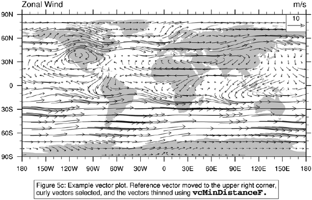
14
The following code snippet demonstrates the use of these resources.
res = True
; set the reference vector mag and size
res@vcRefMagnitude = 10.0
res@vcRefLengthF = 0.045
; thin the vectors
res@vcMinDistanceF = 0.017
plot = gsn_csm_vector(wks,u,v,res)
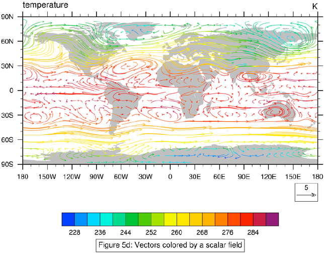
Section 7.3 Vectors colored by a scalar field or on a scalar field
There are four interfaces that draw vectors and a scalar field (contours) on the same plot:
• gsn_csm_vector_scalar_map_ce
• gsn_csm_vector_scalar_map_polar
• gsn_csm_vector_scalar_map
• gsn_csm_pres_hgt_vector
The default behavior of these interfaces is to color the vectors by the magnitude of the scalar field
(Fig 5d). In order to change this default behavior, it is necessary to pass the resource
gsnScalarContour = True to the interface via a resource variable.
15
If a different type of plot is desired, it may be necessary to create separate contour and vector
plots and use the overlay procedure to combine them.
Below is part of a script that creates two graphical objects (plots). overlay is used to combine
them into one object. Note that the gsnDraw and gsnFrame resources are set to False. The
order in which the two plots is created does not matter. overlay has two arguments, each is a
graphical object. The overlay procedure adds (superimposes) the second object onto the first
object. After the overlay is complete, it is necessary to manually draw the combined object and
advance the frame.
In the resource list of one of the plots, the gsnLeftString and gsnRightString should be
turned off. Otherwise you will have two label strings from the two plots overlapping each other.
; create vector plot
res = True
res@vcRefMagnitudeF = 30.0
res@vcRefLengthF = 0.045
res@vcMinDistanceF = .019
res@vcGlyphStyle = "CurlyVector"
res@gsnDraw = False
res@gsnFrame = False
res@gsnLeftString = ""
res@gsnRightString = ""
plot = gsn_csm_vector(wks,u,v,res)
; create contour plot
resCN = True
resCN@cnFillOn = True
resCN@cnLinesOn = False
resCN@gsnSpreadColors = True
resCN@gsnDraw = False
16
base = gsn_csm_contour(wks,data,resCN)
;overlay vector plot onto contour plot
overlay(base,plot)
draw(base) ; draw the combined obj
frame(wks) ; advance the frame
The most important aspect of successfully creating an overlay is to ensure that the coordinates
variables for the data in the two plots are the same. If they are not, the overlay may produce
incorrect results.
Section 8: Map Tickmarks
There are two type of map tickmarks in NCL. The first type (figure 5e) is the default appearance
for the *_ce and *_polar plot interfaces. The second type (figure 5f) were added to NCL in
version 4.2.0.a023. You can turn on the latter by setting the resource
pmTickMarkDisplayMode = "Always".
Section 9: Page Maximization
The resource gsnMaximize will automatically resize a plot and rotate it as necessary to fill the
page. Note that if you are creating a panel plot (see section 13), this should be associated with
the variable being sent to gsn_panel and not in the resource variable for the individual plots.
There is another resource gsnPaperOrientation that can be set to "automatic" (default),
"landscape", or "portrait", to force the rotation of a page.
Figure 5e: The default tickmarks in the *_ce
and *_polar gsn_csm plot interfaces.
Figure 5f: Map tickmarks built into NCL in
version 4.2.0.a023. You turn on these tick-
marks by setting
pmTickMarkDisplayMode = "Always"
17
Section 10: Contours
Section 10.1 Manually setting contour levels
Requires the use of four resources:
res@cnLevelSelectionMode = "ManualLevels”
res@cnMinLevelValF = -30
res@cnMaxLevelValF = 30
res@cnLevelSpacingF = 5
Section 10.2 Contour effects
Numerous functions and gsn resources have been developed to create special contour effects
(figure 5g).
Figure 5g: Example of a special contour ef-
fect. This plot uses the resource
gsnZeroLineContourThicknessF to make
the zero line thicker, and then uses various
contour fill patterns to shade different areas.
For example, there is a resource that allows you to specify the zero line thickness
(gsnContourZeroLineThicknessF) and to set the dash pattern of the negative contours
(gsnContourNegLineDashPattern). There’s a function for shading different parts of a contour
plot (gsn_contour_shade). This function is located in the special library script shea_util.ncl,
which comes bundled with NCL. This library script must be loaded before the begin statement
just like the plot interface library scripts:
load "$NCARG_ROOT/lib/ncarg/nclscripts/csm/shea_util.ncl"
For a listing of shea_util.ncl functions, see:
http://www.ncl.ucar.edu/Document/Functions/list_shea_util.shtml
The following code snippet calls one of these functions:
res = True
res@gsnDraw = False
res@gsnFrame = False
res@cnFillOn = True
res@gsnSpreadColors = True
plot = gsn_csm_contour_map(wks,chi,res)
sres = True
sres@gsnShadeLow = 14
sres@gsnShadeHigh = “red”

18
plot = gsn_contour_shade(plot,-5.,10.,sres)
ShadeLtContour requires plot as an argument. This is why gsnDraw and gsnFrame are set to
False. After the call, it is necessary to manually draw and advance the frame.
Section 10.3 Explicitly setting contour levels
Requires only two resources:
res@cnLevelSelectionMode = "Explicit"
res@cnLevels = (/.01,4,7.2/)
Section 10.4 Contour labels
There are three contour label placement modes, randomized (default), computed, and constant.
Only the constant method makes the label part of the line (figure 5h.b). The other two draw the
line through the label (figure 5h.a). To avoid this, it is necessary to turn on the label masking with
cnLabelMasking = True. Then a background color or a transparent background can be
chosen with cnLineLabelBackgroundColor (figure 5h.c).
The density of the labels is controlled by cnLineDashSegLenF if the constant method is in effect
and by cnLineLabelDensityF when the randomized or computed methods are in effect.
Section 11: Two-Dimensional Lat/Lon Arrays
Data that has two-dimensional lat/lon information associated with it comes in two types.
The first type is data that has already been projected onto the sphere of the earth. We call this a
native grid projection. A common example is a native Lambert Conformal projection.
The second type is data from an irregular grid in which each grid point must be expressed via a
unique location, but it is not already pre-projected. There are many grids that fall into this

19
category including curvilinear and finite element grids.
Each of these cases requires its own special technique. If you have data with two-dimensional
lat/lon information, you MUST know in advance if it is on a native grid projection or not.
Section 11.1 Native grid projections
How do you know if you have a native grid projection? Some GRIB and netCDF files will contain
attributes such as “grid type” in which they indicate a specific projection. For those files with no
information, the user may have to ask the data source for more information.
The first technique required for a native grid projection is to turn off the transformation of the data
onto the map projection by setting:
res@tfDoNDCOverlay = True
The second technique is to correctly limit the map using the corners method. This method
requires that the user know the lower left and upper right corner of their grid.
res@mpLimitMode = "Corners"
res@mpLeftCornerLatF = 16
res@mpLeftCornerLonF = 135
res@mpRightCornerLatF = 54
res@mpRightCornerLonF = 79
Some netCDF and GRIB files will contain an array "corners" that contains this information.
The final technique is grid specific. The grid itself must be specified and several resources that
define the grid must be set. For instance, a Lambert Conformal projection requires the setting of
two latitude values and one longitude value:
res@mpProjection="LambertConformal"
res@mpLambertParallel1F = 30.
res@mpLambertParallel2F = 55.
res@mpLambertMeridianF = 45.
Again, some files contain this information.
http://wwww.ncl.ucar.edu/Applications/native.shtml
http://www.ncl.ucar.edu/Applications/lcnative.shtml
Section 11.2 Irregular grids
The special attributes lon2d and lat2d are used to correctly plot this type of data on a map.
Consider a data file with the following characteristics:
time = 1
nlat = 345
nlon = 567
20
float TLONG (nlat,nlon)
float TLAT (nlat,nlon)
float ROFF (time,nlat,nlon)
The following code snippet demonstrates the required technique:
tlat = f->TLAT
tlong = f->TLONG
roff = f->ROFF
roff@lon2d = tlat
roff@lat2d = tlon
While tlat and tlong are variable names and can therefore be called anything, the attributes
lon2d and lat2d are reserved and cannot be changed.
The explicit setting of these two attributes is the only action required to plot data with two-
dimensional lat/lon information (that is not on a native grid) on a map using the high-level
graphical interfaces. For a contour plot, you may also want to consider changing the fill mode with
the cnFillMode resource.
Plot creation is slower than the plotting of data with one-dimensional coordinates.
Section 12: Aspect Ratio Changes
Two resources, vpWidthF and vpHeightF allow the user to change the aspect ratio of a plot.
Note that if the plot is a map, the resource mpShapeMode = "FreeAspect" must also be
added.
Section 13: Paneling
A panel plot contains two or more graphical objects (plots) rendered on the same page. The most
common approach to paneling is through the special gsn interface gsn_panel. This interface
assumes that all plots are the same size. It uses the size and shape of the first plot to determine
the orientation on the page of the panel.
Section 13.1 Sample script
The following code snippet demonstrates a basic paneling technique:
plot = new(2,graphic)
res = True
res@cnFillOn = True
res@gsnSpreadColors = True
res@gsnDraw = False
res@gsnFrame = False
plot(0) = gsn_csm_contour(wks,u,res)
plot(1) = gsn_csm_contour(wks,v,res)
;*************************************
21
; create panel plot
;**************************************
resP = True
resP@txString = "common title"
gsn_panel(wks,plot,(/3,1/),resP)
In this script, (1) A graphical array is created. plot is a variable which is created to contain multiple
graphical objects. (2) The resource gsnDraw is set to False so that the individual plots are not
drawn as they are created. (3) The resource gsnFrame is set to False to suppress the automatic
frame/page advance. (4) The individual graphical objects are created. (5) A separate panel
resource variable is created. (6) gsn_panel is invoked. The arguments are the workstation, the
plot array, the plot orientation on the page (section 13.2), and the panel resource variable.
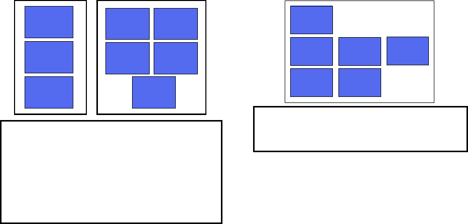
Section 13.2 Orienting plots on a page
The third argument to gsn_panel is an array indicating how plots should be oriented on the
page. The simplest manifestation of this array is an indication of the number of rows and columns
desired (figure 13a).
A greater degree of control can be attained, however, through the setting of the special panel
resource gsnPanelRowSpec = True. If this resource is used, the plot orientation refers to the
number of plots per row.
Section 13.3 Important panel resources
The following resources are commonly used in the creation of a panel plot. They are to be passed
to gsn_panel, and not the individual plots in the graphical array.
• txString: common title
(/3,1/)(/3,1/)
(/3,2/)(/3,2/)
Figure 13a: Example plot orientations created
by gsn_panel. The (/3,1/) orientation used on
an array containing three graphical objects re-
sults in a panel plot that is three rows by one
column. The (/3,2/) orientation used on an ar-
ray of five graphical objects results in a plot
that is three rows by two columns with the last
object being centered below the others.
Figure 13b: The result plot a plot orientation of
(/1,3,2/). This type of orientation can only be
used if gsnPanelRowSpec = True.

22
• gsnPanelLabelBar: common label bar
• gsnPanelBottom: space at bottom
• gsnPanelTop: space at top
• gsnPanelFigureStrings: puts strings of your choice in the upper left
corners of each plot in the panel. Which corner to place the strings can be controlled.
For examples on the use and effect of these resources, go to the web site:
http://www.ncl.ucar.edu/Applications/panel.shtml
Section 13.4 Paneling plots of different sizes
gsn_panel expects plots to be of the same size. Sending plots of different sizes to the
procedure can produce unexpected results.
The user can manually create a frame containing plots of different sizes by specifying where on
the page they should be located, and what size they should be. The following code snippet
demonstrates this technique (Fig 13a):
; create first plot
res = True ; plot mods
res@gsnFrame = False ; don’t advance
res@vpXF = 0.2 ; x location
res@vpYF = 0.83 ; y location
res@vpWidthF = 0.6 ; width
res@vpHeightF = 0.465 ; height
plot1 = gsn_csm_contour_map_polar(wks,d,res)
; create second plot
sres = True
sres@gsnFrame = False
sres@vpXF = 0.15
sres@vpYF = 0.3
sres@vpWidthF = 0.7
sres@vpHeightF = 0.18
plot2 = gsn_csm_xy(wks,x,y,sres)
frame(wks)
23
Figure 13a: Demonstrates the paneling of different sized plots.
Section 14: Font Heights
There are numerous labels and titles in NCL. Each of these are controlled by their own resources.
For instance, the font height for the tickmark labels of the bottom x-axis is controlled by
tmXBFontHeightF while the font height for label bar labels is controlled by
lbLabelFontHeightF, etc. Appendix A contains a list of some of the more common font height
resources.
Section 15: Titles
There are three primary plots titles and three additional titles created exclusively in the gsn_csm
high-level graphical interfaces. The main title is controlled through the tiMainString resource,
and the x and y axis titles are controlled through the tiXAxisString and tiYAxisString
respectively. Section 5.6 discusses the additional title resources gsnLeftString,
gsnRightString, and gsnCenterString.
Section 16: Legends
By default, an x-y plot contains no legend. To turn a legend on, it is necessary to set
pmLegendDisplayMode = "Always". See Appendix A for a list of other legend resources.
Section 17: Label Bars
In the gsn_csm high-level graphical interfaces, a label is automatically created when the user
turns on color by setting cnFillOn = True. The default orientation and location for this label
bar is horizontal, below the plot, with the labels being set to the edge of each color. Appendix A
contains a list of resources that can be used to modify this default behavior. A label bar can also

24
be created from scratch for those using the gsn generic interfaces. The following web site
contains an example of this technique:
http://www.ncl.ucar.edu/Applications/labelbar.shtml
Section 18: Function Codes
NCL uses a function code to force font changes, superscripting, subscripting etc in the middle of
a text string. The default function code in NCL is a colon (:). Many users prefer to reserve the
colon for possible use in a string. You can change the default function code to another character
in your ".hluresfile". In our example (section 3.2), the default function code has been changed to a
tilde (~). All the examples in this section will use this function code.
Section 18.1 Superscripting/subscripting
"10~S~2~N~x" 102 x
"T~B~K" TK
Section 18.2 Carriage return
"carriage return~C~here" carriage return
here
Section 18.3 Greek or mathematical characters
"~F33~helas~F21~Chars" ηελασChars
Section 19: Primitives
Section 19.1 Polygons
A polygon is an enclosed region with a minimum of three points. The last point should be a
duplicate of the first point in order to close the polygon.
A polygon can be added to a plot in either plot coordinates (gsn_polygon), or page/NDC
coordinates (gsn_polygon_ndc). Neither of these procedures makes the polygon part of the
plot. This means that if the plot is paneled, the polygon will not stay with the plot. If paneling is
desired, then gsn_add_polygon should be used.
The following code snippet demonstrates how to draw or add a polygon on or to a plot:
; plot created above with gsnFrame and gsnDraw set to false.
; add polygon to plot
y = (/30.,30.,0.0,0.,30./)
x = (/-90.,-45.,-45.,-90.,-90./)
25
resp = True ; mods yes
resp@gsFillColor = "red" ; color
; this technique can not be used with
; paneling
gsn_polygon(wks,x,y,resp)
; this method CAN be used with paneling. Must be set to dummy variable
d = gsn_add_polyline(wks,plot,x,y,resp)
draw(plot)
frame(wks)
Observe the difference between gsn_polygon and gsn_add_polygon. The latter is a function
that is set to a unique dummy variable. This variable should not be deleted. If multiple polygons
are being added in a loop, then an array of dummy variables needs to be created (see section
19.2 for example).
There are numerous resources that control the color and style of polygons (see Appendix A for
the most common).
Section 19.2 Polylines
There are three interfaces that will add/draw polylines to/on a plot: gsn_polyline (plot
coordinates), gsn_polyline_ndc (page/NDC coordinates), and gsn_add_polyline.
The following is a code snippet demonstrating how to draw a box on a plot using polylines:
; plot created above with gsnFrame and gsnDraw set to false.
; add polylines to plot
y = (/30.,30.,0.0,0.,30./)
x = (/-90.,-45.,-45.,-90.,-90./)
resp = True
resp@gsFillColor = "red" ; color
resp@gsLineThicknessF = 2.0
; create array of dummy graphic
; variables. This is required, b/c
; each line must be associated with a
; unique dummy variable.
d = new(4,graphic)
; draw each line separately. Each line must contain two points.
do i=0,3
d(i)= gsn_add_polyline(wks,plot,x(i:i+1),y(i:i+1),resp)
end do
draw(plot)
frame(wks)
There are numerous resources that control the style of polylines (Appendix A).
26
Section 19.3 Polymarkers
There are seventeen marker styles that can be used (figure 19a) when adding polymarkers to a
plot. The three interfaces available are gsn_polymarker (plot coordinates),
gsn_polymarker_ndc (page coordinates), and gsn_add_polymarker. You can create your
own markers using the NhlNewMarker function:
http://www.ncl.ucar.edu/Document/Functions/Built-in/NhlNewMarker.shtml
Section 20: Adding Text
There are three high-level interfaces that will additional text to a plot, gsn_text (plot
coordinates), gsn_text_ndc (page coordinates), and gsn_add_text. Only the latter function
makes the text part of the plot so that it can be paneled together with other plots. The following
code snippet demonstrates how to add additional text to a plot:
; plot created above with gsnDraw and gsnFrame set to false
add_T = "text here"
x = 0.5 ; middle of x
y = 0.85 ; towards top of page
txres = True
txres@txFontHeightF = 0.03
gsn_text_ndc(wks,plot,add_T,x,y,txres)
draw(plot)
Section 21: X-Y Plots
The following code snippet demonstrates the creation of an X-Y (line) plot using the high-level
graphical interface gsn_csm_xy:
27
; read in data
f = addfile("./uv300.nc","r")
u = f->U
x = u&lat
y = u
; open workstation
wks = gsn_open_wks("ps","xy")
; create plot
res = True
res@tiMainString = "Basic XY plot"
plot = gsn_csm_xy(wks,x,y,res)
In order to place more than one line on the page, it is necessary to create a new array that is
large enough to hold all the lines:
; read in data
f = addfile("./uv300.nc","r")
u = f->U
x = u&lat
y = u
; create array to hold multiple lines
data = new((/2,dimsizes(x)/),float)
; use coordinate subscripting to select
; two lines from u
data(0,:) = u(0,:,{82})
data(1,:) = u(0,:,{-69})
; open workstation
wks = gsn_open_wks("ps","xy")
; create plot
res = True
res@xyLineThicknesses = (/1.0,2.0/)
res@xyLineColors = (/"blue"/)
plot = gsn_csm_xy(wks,y,data,res)
There are many resources that can be used to modify the style of x-y plots (Appendix A),
including gsnXYBarChart which will turn an x-y plot into a bar chart (figure 21a).
28
Figure 21a: Example of a bar chart. gsnXYBarChart = True
Other x-y plot examples are available at:
http://www.ncl.ucar.edu/Applications/xy.shtml
It is easy to change a line plot to a scatter plot by setting xyMarkLineMode to "Marker".
Available marker styles are listed in figure 21a. Other resources that effect scatter plots are
located in Appendix A.
Section 22: Explicit Tickmark Labeling
It is possible for the user to replace the default tickmark labels provided by the high-level
graphical interface with custom labels. The following code snippet demonstrates this technique:
custom_labs = (/"Jan","Feb","Mar"/)
x_values = x&time
res = True
res@tmXBMode = "Explicit"
res@tmXBValues = x_values
res@tmXBLabels = custom_labs
res@tmLabelAutoStride = True
plot = gsn_csm_xy(wks,x,y,res)
The values assigned to the tmXBValues attribute must equal in part to the values determined by
the graphical interface. For instance, if the x-axis was time, in increments of seconds, then the
user could not assign tmXBValues numbers that were unrelated integers such as the number of
tickmarks desired.
29
Appendix A: Common Resources
These are a list of some common resources by topic. They are by no means exhaustive. The
term dynamic means that the value is determined by NCL. For an exhaustive list of resources,
see:
http://www.ncl.ucar.edu/Document/Graphics/Resources/
Axis - http://www.ncl.ucar.edu/Document/Graphics/Resources/tr.shtml
Name
Function
Default
Example
trYReverse
trXReverse
reverse x or y axis
False
True
trYMinF
trXMinF
set minimum of x or y
axis
0.0
3
trYMaxF
trXMaxF
set maximum of x or
y axis
1.0
900
trYLog
trXLog
turn on/off log axis
False
True
Contour - http://www.ncl.ucar.edu/Document/Graphics/Resources/cn.shtml
Name
Function
Default
Example
cnFillOn
turn on/off color filled
contours
False
True
cnLinesOn
turn on/off contour
lines
True
False
cnFillMode
set type of contour fill
“AreaFill”
“RasterFill”
cnLevelSelectionMode
control contour levels
“AutomaticLevels”
“ExplicitLevels”
“ManualLevels”
cnMinLevelValF
cnMaxLevelValF
set minimum or
maximum contour
level
dynamic
5
35
cnLevelSpacingF
set contour spacing
dynamic
2
cnLevels
set contour elvels
when
cnLevelSelectionMode
is “ExplicitLevels”
dynamic
(/3,5,7,9,10,45/)
cnLineThicknessF
set thickness of
contour lines
1.0
2.0
cnFillPatterns
set pattern fills
“SolidFill”
(/1,3,-1/)
(-1 is transparent)
cnInfoLabelOn
turn on/off the contour
info label
True
False
30
Labelbars - http://www.ncl.ucar.edu/Document/Graphics/Resources/lb.shtml
Name
Function
Default
Example
cnFillOn
turn contour fill
on/off
False
True
cnFillMode
set contour fill
mode
“AreaFill”
“RasterFill”
cnLabelBarEndStyle
set style for end
labels
“IncludeOuterBoxes”
“ExcludeOuterBoxes”
gsnSpreadColors
span full range of
colormap
False
True
gsnSpreadColorStart
begin colormap at
particular index
2
46
gsnSpreadColorEnd
end colormap at
particular index
ncolors-1
89
lbLabelBarOn
turn on/off the
labelbar
True for gsn_csm
interfaces
False
lbOrientation
set orientation of
labelbar
horizontal for
gsn_csm interfaces
“vertical”
lbLabelAutoStride
automatically pick
nice labelbar
label stride
False
True
lbTitleOn
turn on/off a
labelbar title
False
True
lbTitleString
set labelbar title
Null
“m/s”
lbLabelAlignment
st where the
labelbar label is
oriented wrt to
the color boxes
“ExternalEdges”
“BoxCenters”
pmLabelBarOrthogonalPosF
moves the
labelbar
orthogonally to its
position. For a
horizontal
labelbar, this is
up and down.
N/A
-0.03
pmLabelBarParallalPosF
moves the
labelbar
perpendicularly to
its position. For a
vertical labelbar,
this is left and
right.
N/A
-0.01
pmLabelBarWidthF
set the width of
the labelbar
set for the user in the
gsn_csm interfaces
pmLabelBarHeightF
set the height of
the labelbar
set for the user in the
gsn_csm interfaces
31
GSN - http://www.ncl.ucar.edu/Document/Graphics/Resources/gsn.shtml
Name
Function
Default
Example
gsnAddCyclic
turn on/off the
addition of a cyclic
point to the
longitude coordinate
values
True for data that
has 1D coordinate
variables
False
gsnCenterString
see figure 1a
N/A
“string here”
gsnDraw
draw the plot
True
False
gsnFrame
advanced the frame
(page)
True
False
gsnLeftString
see figure 1a
long_name (if
exists) in gsn_csm
interfaces
“Salinity”
gsnMaximize
maximizes plot and
rotates to landscape
if necessary
False
True
gsnPanelFigureStrings
add a series of
strings to the upper
left corner of each
plot in a panel
N/A
(/”a”,”b”,”c”/)
gsnPanelLabelBar
turn on/off a
common labelbar in
a panel plot
False
True
gsnRightString
see figure 1a
units (if exists) in
gsn_csm interfaces
“ppm”
gsnScalarContour
force vector/scalar
gsn_csm interfaces
to draw vectors over
the scalar field
False
True
gsnSpreadColors
span full range of
colormap
False
True
gsnSpreadColorStart
begin colormap at
particular index
2
46
gsnSpreadColorEnd
end colormap at
particular index
ncolors-1
89
gsnXYBarChart
changes an x-y line
into a bar chart
False
True
gsnXRefLine
add a vertical
reference line to a
plot
None
1.0
gsnXRefLineColor
change color of X
reference line
foreground color
“green”
gsnYRefLine
add a horizontal
reference line to a
plot
None
0.0
gsnYRefLineColor
change color of Y
reference line
foreground color
“blue”
32
Legends - http://www.ncl.ucar.edu/Document/Graphics/Resources/lg.shtml
Name
Function
Default
Example
pmLegendWidthF
set width of a
legend
dynamic
0.6
pmLegendHeightF
set height of a
legend
dynamic
0.3
lgTitleOn
turn on legend title
False
True
lgTitleString
set title string
N/A
“Profiles”
lgOrientation
set orientation of
the legend
“horizontal”
“vertical”
lgPerimOn
turn the legend
perimeter on/off
True
False
xyExplicitLegendLabels
change default
legend labels
N/A
(/“a”,”b”/)
pmLegendOrthgonalPosF
adjust the legend
orthogonally
N/A
-0.03
pmLegendParallelPosF
adjust the legend
perpendicularly
N/A
0.2
XY curves - http://www.ncl.ucar.edu/Document/Graphics/Resources/xy.shtml
Name
Function
Default
Example
xyDashPatterns
set line pattern
solid
(/0,2/)
(/“solid”, “dash”/)
xyLineThicknesses
set line thicknesses
1.0
(/2.0,3.0,4.0/)
xyLineColors
set line colors
foreground color
(/“red”,”blue”/)
xyMarkLineModes
set whether lines
contain markers,
lines, or both
markers and lines
“Lines”
“Lines”
“Markers”
“MarkLines”
xyMarkers
set marker styles
asterisk
5
xyMarkerColor
set marker colors
foreground color
“green”
xyMarkerSizeF
set marker size
0.01
0.03
Maps - http://www.ncl.ucar.edu/Document/Graphics/Resources/mp.shtml
The second through fifth resources are to be used when zooming in on a cylindrical equidistant or
polar stereographic projection. They are the limits set when using mpLimitMode = “LatLon”. This
resource is set for the user by the high-level plot interfaces. Other projections, such as lambert
conformal, require a different limit mode (mpLimitMode = “Corners”).
33
Name
Function
Default
Example
mpLimitMode
determine
how a map is
zoomed in
depends on
projection
“LatLon”
“Corners”
mpMinLatF
set minimum
latitude for
map zoom
dynamic
30.
mpMaxLafF
set maximum
latitude for
map zoom
dynamic
60.
mpMinLonF
set minimum
longitude for
map zoom
dynamic
-70.
mpMaxLonF
set maximum
longitude for
map zoom
dynamic
89.
mpFillOn
turn on/off
map fill
True for
gsn_csm
interfaces
False
mpCenterLonF
set center
longitude of
projection
0
180.
mpDataBaseVersion
set map
database
resolution
“LowRes”
“MediumRes”
“HighRes”
(must be
downloaded)
mpLandFillColor
set color of
land areas
“gray” for
gsn_csm
interfaces
“brown”
mpOceanFillColor
set color of
ocean areas
“transparent”
“SkyBlue”
mpInlandWaterFillColor
set color of
inland water
areas
“transparent”
“blue”
mpOutlineOn
turn on/off
the map
outlines
True
False
mpOutlineBoundarySets
set various
continental
outlines on
and off
“Geophysical”
“Geosphysica
lAndUSState
s”
“National”
mpGeophysicalLineThicknessF
set line
thickness of
map outlines
1.0
2.0
mpGeophysicalLinColor
set color of
map outlines
foreground
“red”
mpUSStateLineColor
set color of
US state
boundaries
foreground
“blue”
34
Polygons, polylines, polymarkers -
http://www.ncl.ucar.edu/Document/Graphics/Resources/gs.shtml
Name
Function
Default
Example
gsFillColor
set fill color for inside
of polygon
transparent
“red”
gsEdgeColor
set color of the outline
of a polygon
none
“black”
gsEdgesOn
turn on/off polygon
edge
False
True
gsLineColor
set polyline color
foreground color
“orange”
gsLineThicknessF
set polyline thickness
1.0
2.5
gsMarkerIndex
set marker style
asterisk (0)
5
gsMarkerColor
set marker color
foreground color
“purple”
gsMarkerSizeF
set marker size
0.007
0.014
35
Appendix B: High-level Graphical Interfaces
gsn generic interfaces
gsn_xy gsn_vector_map
gsn_y gsn_vector_scalar_map
gsn_contour gsn_streamline
gsn_contour_map gsn_streamline_map
gsn_vector gsn_map
gsn_vector_scalar
As an example, the following line of code will contour the two-dimensional array data:
plot = gsn_contour(wks,data,res)
gsn_csm interfaces
In the list below, an _ce stands for cylindrical equidistant projection. An _hov stands for hovmuller diagram.
All other interface names are self-explanatory. As with the gsn generic interfaces, the gsn_csm interfaces
are functions and return a graphical object. Note: many of the interfaces listed below could be placed into
more than one category.
Contour:
gsn_contour_shade (nice customization of contour filling)
gsn_csm_contour
gsn_csm_contour_map (choose your projection)
gsn_csm_contour_map_ce
gsn_csm_contour_map_polar
gsn_csm_contour_map_overlay (overlay additional contours)
plot = gsn_csm_contour(wks,data,res)
Streamline:
gsn_csm_streamline
gsn_csm_streamline_map (choose your projection)
gsn_csm_streamline_map_ce
gsn_csm_streamline_map_polar
gsn_csm_streamline_contour_map
gsn_csm_streamline_contour_map_ce
gsn_csm_streamline_contour_map_polar
plot = gsn_csm_streamline(wks,u,v,res)
Vector:
gsn_csm_vector
gsn_csm_vector_map
gsn_csm_vector_map_ce
gsn_csm_vector_scalar_map
gsn_csm_vector_scalar_map_ce
gsn_csm_vector_scalar_map_polar
plot = gsn_csm_vector(wks,u,v,res)
Pressure/Height:
gsn_csm_pres_hgt
gsn_csm_pres_hgt_streamline
gsn_csm_pres_hgt_vector

36
Misc:
gsn_csm_lat_time
gsn_csm_time_lat
gsn_csm_hov
gsn_csm_xy
gsn_csm_y
gsn special interfaces
Polylines: These interfaces add a polyline to an existing plot:
gsn_polyline (plot coordinates)
gsn_polyline_ndc (page coordinates)
gsn_add_polyline (can be paneled, plot coords)
Polymarkers: These interfaces add polymarkers to an existing plot:
gsn_polymarker (plot coordinates)
gsn_polymarker_ndc (page coordinates)
gsn_add_polymarker (can be paneled, plot coords)
Polygons: These interfaces add a polygon to an existing plot:
gsn_polygon (plot coordinates)
gsn_polygon_ndc (page coordinates)
gsn_add_polygon (can be paneled, plot coords)
Text: These interfaces add text to an existing plot:
gsn_text (plot coordinates)
gsn_text_ndc (page coordinates)
gsn_add_text (can be paneled, plot coords)
gsn_create_text (no coords, use in conjunction with gsn_add_annotation)
Colormaps: These interfaces are used for manipulating color maps. You can view the built-in color maps
at:
http://www.ncl.ucar.edu/Document/Graphics/color_table_gallery.shtml
gsn_define_colormap gsn_merge_colormaps gsn_draw_colormap
gsn_retrieve_colormap gsn_draw_named_colors gsn_reverse_colormap
hlsrgb hsvrgb rgbhls
rgbhsv rgbyiq yiqrgb
Miscellaneous: These interfaces perform a variety of functions:
gsn_add_annotation gsn_open_wks
gsn_attach_plots gsn_panel
gsn_blank_plot gsn_table
gsn_create_labelbar
gsn_create_legend
gsn_histogram
gsn_labelbar_ndc
gsn_legend_ndc

37
Appendix C: List of Named Colors
The full list of colors and their RGB triplets are available at:
http://www.ncl.ucar.edu/Applications/Scripts/rgb.txt
http://www.ncl.ucar.edu/Document/Graphics/named_colors.shtml
All of these colors have multiple spelling with the non-capitalized versions having a space
between the words and the capitalized versions containing no space (e.g. ghost white,
GhostWhite). For the sake of brevity only one version per RGB triplet is listed here. There are
also numerous variations on each named color (e.g. snow, snow1, snow2, snow3 etc.). These
variations are also not listed.
255 250 250 snow
248 248 255 ghost white
245 245 245 white smoke
220 220 220 gainsboro
255 250 240 floral white
253 245 230 old lace
250 240 230 linen
250 235 215 antique white
255 239 213 papaya whip
255 235 205 blanched almond
255 228 196 bisque
255 218 185 peach puff
255 222 173 navajo white
255 228 181 moccasin
255 248 220 cornsilk
255 255 240 ivory
255 250 205 lemon chiffon
255 245 238 seashell
240 255 240 honeydew
245 255 250 mint cream
240 255 255 azure
240 248 255 alice blue
230 230 250 lavender
255 240 245 lavender blush
255 228 225 misty rose
255 255 255 white
0 0 0 black
47 79 79 dark slate gray
105 105 105 dim gray
112 128 144 slate gray
119 136 153 light slate gray
190 190 190 gray
211 211 211 light grey
25 25 112 midnight blue
0 0 128 navy blue
100 149 237 cornflower blue
72 61 139 dark slate blue
106 90 205 slate blue
123 104 238 medium slate blue
132 112 255 light slate blue
0 0 205 medium blue
65 105 225 royal blue
0 0 255 blue
30 144 255 dodger blue
0 191 255 deep sky blue
135 206 235 sky blue
135 206 250 light sky blue
70 130 180 steel blue
176 196 222 light steel blue
173 216 230 light blue
176 224 230 powder blue
175 238 238 pale turquoise
0 206 209 dark turquoise
72 209 204 medium turquoise
64 224 208 turquoise
0 255 255 cyan
224 255 255 light cyan
95 158 160 cadet blue
102 205 170 medium aquamarine
127 255 212 aquamarine
0 100 0 dark green
85 107 47 dark olive green
143 188 143 dark sea green
46 139 87 sea green
60 179 113 medium sea green
32 178 170 light sea green
152 251 152 pale green
0 255 127 spring green
124 252 0 lawn green
0 255 0 green
127 255 0 chartreuse
0 250 154 medium spring green
173 255 47 green yellow
50 205 50 lime green
154 205 50 yellow green
34 139 34 forest green
107 142 35 olive drab
189 183 107 dark khaki
240 230 140 khaki
238 232 170 pale goldenrod
250 250 210 light goldenrod yellow
255 255 224 light yellow
255 255 0 yellow
255 215 0 gold
238 221 130 light goldenrod
218 165 32 goldenrod 1
84 134 11 dark goldenrod
188 143 143 rosy brown
205 92 92 indian red
139 69 19 saddle brown
160 82 45 sienna
205 133 63 peru
38
222 184 135 burlywood
245 245 220 beige
245 222 179 wheat
244 164 96 sandy brown
210 180 140 tan
210 105 30 chocolate
178 34 34 firebrick
165 42 42 brown
233 150 122 dark salmon
250 128 114 salmon
255 160 122 light salmon
255 165 0 orange
255 140 0 dark orange
255 127 80 coral
240 128 128 light coral
255 99 71 tomato
255 69 0 orange red
255 0 0 red
255 105 180 hot pink
255 20 147 deep pink
255 192 203 pink
255 182 193 light pink
219 112 147 pale violet red
176 48 96 maroon
199 21 133 medium violet red
208 32 144 violet red
255 0 255 magenta
238 130 238 violet
221 160 221 plum
218 112 214 orchid
186 85 211 medium orchid
153 50 204 dark orchid
148 0 211 dark violet
138 43 226 blue violet
160 32 240 purple
147 112 219 medium purple
216 191 216 thistle
You can use the following code to draw a test set of named colors for debugging purposes:
load "$NCARG_ROOT/lib/ncarg/nclscripts/csm/gsn_code.ncl"
begin
wks = gsn_open_wks("x11","gsn_draw_named_colors")
colors = (/"white", "black", "PeachPuff", "MintCream", "SlateBlue", \
"Khaki", "OliveDrab","BurlyWood", "LightSalmon", "Coral", \
"HotPink", "LemonChiffon", "AliceBlue", "LightGrey", \
"MediumTurquoise", "DarkSeaGreen", "Peru", "Tomato", \
"Orchid","PapayaWhip"/)
rows = 4
cols = 5
gsn_draw_named_colors(wks,colors,(/rows,cols/)) ; Draw these
; named colors.
end

39
Appendix D: Common Error Messages
Message:
(0) check_for_y_lat_coord: Warning: Data either does not contain a
valid latitude coordinate array or doesn't contain one at all
(0) check_for_lon_coord: Warning: Data either does not contain a valid
longitude coordinate array or doesn't contain one at all
Solution:
Need to rename x and y dimensions to one of those listed in section 2.6.
Message:
(0) is_valid_lat_ycoord: Warning: The units attribute of the Y
coordinate array is not set to one of the allowable units values (i.e.
'degrees_north'). Your latitude labels may not be correct.
(0) is_valid_lat_xcoord: Warning: The units attribute of the X
coordinate array is not set to one of the allowable units values (i.e.
'degrees_east'). Your longitude labels may not be correct.
Solution:
Need to add or change the units attributes for the latitude/longitude coordinate arrays (see
section 2.6)
Message:
(0) gsn_add_cyclic: Warning: The range of your longitude data is not
360. You may want to set gsnAddCyclic to False to avoid a warning
message from the Spline function.
Solution:
A cyclic point is added to the data in all gsn_csm high-level map interfaces. If this is inappropriate
(e.g. a regional plot), then it is necessary to set gsnAddCyclic = False
Message:
(0) warning:_NhlCreateSplineCoordApprox: Attempt to create spline
approximation for Y axis failed: consider adjusting trYTensionF value
warning:IrTransInitialize: error creating spline approximation for
trYCoordPoints; defaulting to linear
Solution:
Chances are this has occurred because of an error in the longitude coordinate variable. It is either
incorrect or there is a gap in the data.

40
Message:
fatal:ContourPlotDraw: Workspace reallocation would exceed maximum size
16777216 fatal:ContourPlotDraw: draw error fatal:PlotManagerDraw: error
in plot draw fatal:_NhlPlotManagerDraw: Draw error
Solution:
The plot of your data is too large for NCL’s default 16MB size. You must increase the size by
setting:
setvalues NhlGetWorkspaceObjectId()
"wsMaximumSize": 33554432
end setvalues

41
Appendix E: Glossary
attribute: datum of any type that is assigned to an NCL variable using the '@' operator. An
attribute of a variable can contain descriptive information about the variable. Attributes are used
to set plot options for the gsn and gsn_csm suite of plotting functions.
color index: An integer value that represents an index into the current color table. Index 0 is the
background color and 1 is the foreground color. Color index values can be used with any
graphical resource that defines the color of a plot attribute (like a line color or a polygon fill color).
See also “named color”.
coordinate variable: value associated with a named dimension of a variable or file variable that
contains numerical coordinate information for each index of the dimension. Coordinate variables
must be singly-dimensioned values. They are recognized and used by the gsn_csm suite of
plotting scripts to define the X and Y axes values.
named color: a string representing a predefined color. Named colors can be used with just about
any graphical resource that defines the color of a plot attribute (like a line color or a polygon fill
color). In order to use a named color, that color must be part of your current color table. See also
“color index”.
named dimension: a dimension of a variable or file variable that has been assigned a name
using the '!' operator.
NDC coordinates: (normalized page coordinates) the lower left corner of a page is (0,0), the
lower right corner is (0,1), the upper left corner is (1,0), and the upper right corner is (1,1). There
are several special interfaces that function in NDC space (e.g. gsn_text_ndc,
gsn_polyline_ndc).
panel/paneling: putting more than one plot onto a page. Note that gsn_panel expects plots of
the same size. Plots of different sizes can be paneled using the viewport resources vpXF and
vpYF to manually place the plots on a page. See section 13 for details.
plot coordinates: unlike NDC coordinates which refer to the page and never change, the plot
coordinates are plot dependent. A map plot would have plot coordinates in latitude and longitude.
A time series plot would have plot coordinates in time and whatever the other coordinate is. There
are many interfaces that work in plot coordinate space (e.g. gsn_polyline, gsn_add_text).
resources: values that will modify the default behavior of a plot. The first two (or three) letters of
a resource are lower case and tell the user what type of resource it is (section 4.1). The
remaining part of the resource describes what it does (e.g. cnFillOn turns on color fill for
contour plots, txFontHeightF sets the font height for a text string).
viewport: the viewport is a rectangular subregion of NDC space that specifies where plot objects
will be drawn. The precise meaning of the viewport depends on the plot object. For example, for
XyPlot objects, the viewport specifies where the grid containing the curves will be placed, and the
labeling (if any) will be drawn outside of the viewport. On the other hand, for TextItem objects, the
viewport will be a rectangle surrounding the text string.
workstation: a valid output device such as an X Window System display, a PostScript file, a PDF file, a
PNG file, or an NCGM.
