NCAR Language Manual
User Manual:
Open the PDF directly: View PDF ![]() .
.
Page Count: 43

NCAR Command Language
(NCL)
Mini-Language
Reference Manual
Document Version 1.1.10, NCL Version 6.1.2 September, 2014
This manual includes a brief description of the NCL language, file IO, printing, data
processing, command line options, and using external codes. Direct comments about
this manual to ncl-talk@ucar.edu.
http://www.ncl.ucar.edu/Document/Manuals/
keyword courier-bold
built-in functions courier-bold blue
contributed functions courier-bold green
symbols bold
plot templates courier-bold green
plot resources courier-bold
user variables italics
WWW links underline
© Copyright, 2013, National Center for Atmospheric Research, 1850 Table Mesa Drive, Boulder CO 80305.
The use of NCL is governed by separate Binary and Source Code License Agreements
i
Section 1: Introduction..................................................................................................................... 1!
Section 1.1 Setting the user path................................................................................................. 1!
Section 1.2 Executing..................................................................................................................1!
Section 2: Language ....................................................................................................................... 2!
Section 2.1 Symbols ....................................................................................................................2!
Section 2.2 Data types................................................................................................................. 3!
Section 2.3 Reserved keywords ..................................................................................................3!
Section 2.4 Expressions ..............................................................................................................3!
Section 2.5 Variables...................................................................................................................4!
Section 2.6 Statements................................................................................................................ 4!
Section 2.7 Loops........................................................................................................................ 4!
Section 2.8 Blocks and if statements...........................................................................................5!
Section 2.9 Dimensions and subscripting....................................................................................6!
Section 2.10 Dimension reduction ...............................................................................................6!
Section 2.11 Named dimensions ................................................................................................. 7!
Section 2.12 Coordinate variables...............................................................................................7!
Section 2.13 Attributes.................................................................................................................8!
Section 2.14 _Fill Value ...............................................................................................................8!
Section 2.15 Coercion ................................................................................................................. 8!
Section 2.16 Variables and metadata.......................................................................................... 9!
Section 2.17 Variable Reassignment.........................................................................................10!
Section 2.18 Variable of Type List (Container variable) ............................................................ 10!
Section 3: NCL File input/output.................................................................................................... 11!
Section 3.1 Supported formats ..................................................................................................11!
Section 3.1.1 Creation of a file reference ..................................................................................11!
Section 3.1.2 Reading variables................................................................................................ 12!
Section 3.1.3 When to use the $ syntax ....................................................................................13!
Section 3.1.4 Printing the contents of a supported file ..............................................................13!
Section 3.1.5 Reordering a variable on input.............................................................................13!
Section 3.1.6 Importing byte or short data with conversion to float ...........................................13!
Section 3.1.7 Spanning multiple files.........................................................................................14!
Section 3.1.8 Altering the default behavior of addfile(s) ....................................................14!
Section 3.1.9 ncl_filedump........................................................................................................ 14!
Section 3.1.10 ncl_convert2nc................................................................................................... 15!
Section 3.2 Binary data files ......................................................................................................15!
Section 3.3 ASCII ......................................................................................................................16!
Section 3.4 Writing netCDF/HDF............................................................................................... 17!
Section 3.5 Remote file access: OPeNDAP ..............................................................................19!
Section 4: Printing .........................................................................................................................20!
Section 4.1 printVarSummary.................................................................................................... 20!
Section 4.2 print......................................................................................................................... 20!
Section 4.3 sprintf, sprinti ..........................................................................................................21!
Section 4.4 Pretty Print: write_matrix, print_table....................................................................21!
Section 5: Data analysis and Arrays ............................................................................................. 22!
Section 5.1 Array ordering and syntax....................................................................................... 22!
Section 5.2 Array conformance .................................................................................................23!
Section 5.3 Array memory allocation .........................................................................................23!
Section 5.4 Functions and procedures ......................................................................................24!
Section 5.5 Built-in functions and procedures ...........................................................................25!
Section 5.6 contributed.ncl ........................................................................................................ 27!
Section 5.7 User-defined functions and procedures..................................................................28!
Section 5.8 System interaction ..................................................................................................30!
Section 6: Command line options and assignments ..................................................................... 31!
Section 6.1 Options altering behavior when NCL is invoked..................................................... 31!
Section 6.2 Specifying variable assignments on command line................................................ 32!
ii
Section 7: Using external codes....................................................................................................33!
Section 7.1 NCL/Fortran interface .............................................................................................33!
Section 7.2 f77 subroutines .......................................................................................................34!
Section 7.3 f90 subroutines .......................................................................................................34!
Section 7.4 Accessing the LAPACK library distributed with NCL ..............................................36!
Section 7.5 Using commercial libraries...................................................................................... 36!
Section 7.6 What WRAPIT does................................................................................................ 37!
Section 7.7 NCL/Fortran array mapping .................................................................................... 38!
Section 7.8 NCL and Fortran (or C) in Unix shell script............................................................. 38!
Section 7.9 Using NCL as a scripting language ........................................................................ 39!

1
Section 1: Introduction
The NCAR Command Language (NCL) is an interpreted programming language,
specifically designed for the access, analysis, and visualization of data. NCL has many
features common to modern programming languages: variables (numeric and non-
numeric types), operators, expressions, conditional statements, loops, and functions and
procedures. The most complete and current documentation for NCL is the Reference
Manual located at:
http://www.ncl.ucar.edu/Document/Manuals/Ref_Manual/
NCL may already be installed on your local system. If not, NCL binaries and source
code are free and are available for the most common Linux/Unix, MacOSX and Cygwin
(Windows) operating systems. Click “Download” at:
http://www.ncl.ucar.edu/
Section 1.1 Setting the user path
In order to run NCL, you must set your NCARG_ROOT environment variable to the
parent directory where the NCL executables and accompanying files were installed. You
also need to make sure that the directory where the NCL executables reside is in your
search path. It is best to do this from one of your .* files in your home directory. If you
are not sure which shell you are running, you can do an "echo $SHELL".
If NCL resides in (say) /usr/local, the following setting would be appropriate:
From C-shell (csh):
setenv NCARG_ROOT /usr/local
setenv PATH $NCARG_ROOT:${PATH}
From bash, ksh:
export NCARG_ROOT=/usr/local
export PATH=/usr/local/bin:$PATH
See your local system administrator for information about your local system.
Section 1.2 Executing
NCL may be executed interactively. NCL is case sensitive, and all statements require a
return to terminate a statement. NCL’s interactive environment is not as sophisticated as
some other tools but it is adequate for simple tasks. Note that it is possible to save the
statements entered using the optional record and stop record statements (Section
2.6).
2
Interactive mode:
ncl <return>
record "savefile" ; optional (this is not commonly used)
statement(s)
stop record ; only if record is present
quit
Batch mode: When a script containing a sequence of prewritten NCL statements is
executed it is called batch-mode. Batch-mode scripts often have a “.ncl” suffix. However,
this is a convention only and is not required. The batch-mode script may be invoked at
the command line via:
ncl foo.ncl
ncl foo.ncl>&! foo.out [C-Shell; output sent to foo.out]
ncl foo.ncl>&! foo.out & [C-Shell; run in background]
ncl < foo.ncl [also acceptable]
NCL allows several options to be specified on the command line. Invoking “ncl –h” will
display currently supported options. Command line variable assignment is discussed in
Section 6.
External NCL functions/procedures (Section 5) and shared objects (Section 7) can be
accessed in interactive or batch mode via:
load "myfoo.ncl"
load "$HOME/myscripts/funct.ncl"
external DEMO "/tmp/Path/myfoo.so"
Section 2: Language
Section 2.1 Symbols
NCL has a suite of syntax symbols that facilitate assorted tasks. Commonly used syntax
symbols include:
; begins a comment. Text to the right of ; is ignored.
= assignment
:= reassignment (available in version 6.1.2)
@ create or reference attributes
! create or reference named dimensions
& create or reference a coordinate variable
{...} used for coordinate subscripting
$ enclose strings when importing/exporting variables via addfile
[...] subscript variables of type list
(/.../) construct an array
: used in array syntax
| used as a separator for named dimensions

3
\ continue statement for spanning multiple lines
:: used as separator when calling external codes
-> used for variable input/output with supported data formats
=> used to access netCDF-4/HDF5 groups
Section 2.2 Data types
Numeric: double (64 bit), float (32 bit), long (32 or 64 bit), integer (32 bit), short (16 bit),
byte (8 bits), complex is not supported. NCL version 6.0.0 was expanded to include
many additional numeric types. This was done to be consistent with the numeric types
supported by netCDF4. Please see a complete description of NCL’s numeric types a
Non-numeric: string, character, graphic, file, logical, list.
Section 2.3 Reserved keywords
begin, break, byte, character, continue, create, defaultapp, do,
double, else, end, enumeric, external, False, file, float,
function, getvalues, graphic, if, integer, int64, list, load,
local, logical, long, _Missing, Missing, new, noparent, numeric,
procedure, quit, Quit, QUIT, record, return, setvalues, short,
string, then, True, undef, while and all built-in function and procedure
names. A current list of all NCL keywords is at:
http://www.ncl.ucar.edu/Document/Manuals/Ref_Manual/NclKeywords.shtml
Section 2.4 Expressions
Precedence rules can be circumvented by use of parentheses "(...)" around expressions.
NCL does not operate on any array element set to _FillValue (see section 2.13).
Algebraic operators:
+ addition (+ is an overloaded operator; also used for string concatenation)
- subtraction
* multiplication
^ exponent
% modulus, integers only
# matrix multiply
>, < greater than, less than (sometimes called “clipping” operators)
Logical:
.lt. less than
http://www.ncl.ucar.edu/Document/Manuals/Ref_Manual/NclDataTypes.shtm
l
4
.le. less than or equal to
.gt. greater than
.ne. not equal to
.eq. equal to
.and. and
.or. or
.xor. exclusive or
.not. not
Section 2.5 Variables
Variable names must begin with an alphabetic character but can contain any mix of
numeric and alphabetic characters. The underscore "_" is also allowed. NCL variables
are based upon the netCDF variable model. As such, variables may have ancillary
information (called metadata) attached to the variable. Metadata may be accessed,
created, changed and deleted via NCL functions and syntax (see sections 2.11-2.13).
Variables imported via NCL’s addfile or addfiles functions (Section 3) will have all
available metadata automatically attached to the variable. This greatly simplifies coding
and access to each variable’s metadata.
Section 2.6 Statements
Statements are the fundamental element of NCL. Everything NCL does happens only
after a statement is entered. Statements are case sensitive and are not restricted to
being a single line of source, and statements can be nested within statements. There are
17 different kinds of statements: assignment, procedure call, function definition,
procedure definition, block, do, if-then, if-then-else, break, continue, setvalues,
getvalues, return, record, new, stop, and quit.
Section 2.7 Loops
NCL provides two kinds of do loops: a while loop that repeats until its
scalar_logical_expression evaluates to False, and a traditional do loop that loops from a
start value through an end value incrementing or decrementing a loop variable either by
one or by a specified stride.
do n=start,end,optional_stride
[statement(s)]
end do ; space is required
do while (scalar_logical_expression)
[statement(s)]
end do
With each kind of loop, the keywords break and continue can be used.
5
break: jump to first statement after end do
continue: proceed directly to the next iteration
Use of loops should be minimized in any interpreted language. Often, loops can be
replaced by array syntax or a built-in function. If multiple do loops are required and
execution speed is a concern, linking codes written in Fortran or C may be the best
approach. (Section 7.)
Section 2.8 Blocks and if statements
Blocks provide a way to group a list of statements. Since blocks are statements, the
statements within the begin and end do not get executed until the end statement is
parsed and the source is determined to be free of syntax errors. The use of begin and
end is optional.
begin ; optional
[statement(s)]
end ; required if begin present
There are two kinds of if statements: the if-then statement and the if-then-else
statement. These function like if statements in other popular programming languages.
if (scalar_logical_expression) then
[statement(s)]
end if
if (scalar_logical_expression) then
[statement(s)]
else
[statement(s)]
end if
Technically, there is no explicit else if statement in NCL. However, nested if
statements can be used. Each if must have a corresponding end if.
if (scalar_logical_expression) then
[A_statement(s)]
else if (scalar_logical_expression) then
[B_statement(s)]
else if (scalar_logical_expression) then
[C_statement(s)]
else
[D_statement(s)]
end if ; C & D
end if ; B
end if ; A
Logical expressions are evaluated left to right, so in multiple expression statements,
place the expression most likely to fail on the left:

6
if (z.eq.3 .and. all(x.gt.0)) then
[statement(s)]
end if
Section 2.9 Dimensions and subscripting
There are two types of array subscripting in NCL: standard and coordinate. Standard
subscripting features are similar to the array subscripting available in F90, Matlab, and
IDL. In addition, NCL dimensions may have names associated with them (Section 2.10).
NCL subscript indices start at 0 and end at N-1. Like the C computer language, NCL is
row major. For multidimensional arrays this means that the rightmost subscript varies
fastest and the leftmost subscript varies slowest. Subscripts have the form:
start_index : end_index : optional_stride
Omission of start_index defaults to 0; omission of end_index defaults to N-1; the default
optional_stride is 1. Therefore, a “:” without a start or end index means all elements.
Section 2.9.1 Standard subscripting may be used to index any array variable. For the
following examples, assume variable T is a 3D array of size (nt, ny, nx) with named
dimensions (time, lat, lon).
Index
T ; entire array [don’t need T(:,:,:)]
T(0,:,::5) ; 1st time, all lat, every 5th lon
T(0,::-1,4:50) ; 1st time, reverse lat, lon index values 4-50
T(:1,45,10:20) ; 1st two time, 46th lat, 10-20 lon
Section 2.9.2 Coordinate subscripting may be used for any dimension conforming to
the netCDF coordinate variable data model. By definition, coordinate variables must be
one-dimensional arrays of monotonically increasing or decreasing values where the
variable’s name and associated dimension name are the same (e.g. time(time), lat(lat),
p(p), etc.). Coordinate subscripting is invoked by enclosing the natural coordinates
between curly braces "{...}".
X = T(:,{-20:20},{90:290:2})
Select all time, -20 to 20 latitude inclusive, 90 to 290 longitude with a stride of 2.
Section 2.10 Dimension reduction
When a constant subscript is specified, dimension reduction occurs. This means the
rank of the array is reduced (ie., fewer dimensions). Assume T is dimensioned (nt, nz,
ny, nx), then:
T1 = T(5,:,12,:) ; yields T1(nz,nx); the 5 and 12 are degenerate
T2 = T(:,:,:,0) ; yields T2(nt,nz,ny); the 0 is degenerate
7
NCL ignores the degenerate dimension but all appropriate metadata are copied. The
user may force retention of the degenerate dimension via:
T3 = T(5:5,:,12,:) ; T3(1,nz,nx)
T4 = T(5:5,:,12:12,:) ; T4(1,nz,1,nx)
Section 2.11 Named dimensions
All variables read from netCDF, GRIB and HDF files have named dimensions. In
addition, users may name or rename a dimension. Named dimensions are only used to
reshape an array (e.g. transpose). The ! symbol is used to create a named dimension or
to retrieve a dimension name. Dimension numbering proceeds from left-to-right with the
leftmost dimension equal to 0. Assume T is 3D array with size (ntime, nlat, nlon):
Assignment of named dimensions via ! syntax:
T!0 = "time"
T!1 = "lat"
T!2 = "lon"
Retrieval of named dimensions:
LAT = T!1 ; LAT = "lat"
Section 2.11.1 Dimension reordering: Named dimensions should only be used when
dimension reordering is required.
reordered_T = T(lon|:,lat|:,time|:) ; (lon,lat,time)
Named dimensions are not subscripts. However, named dimensions can be used with
coordinate and standard subscripting.
X = T({lat|-20:20}, lon|30:42, time|:)
(Reorder to (lat,lon,time) and select latitudes –20 to 20, longitude indices 30 through 42,
all time values.)
Section 2.12 Coordinate variables
By netCDF definition, a coordinate variable is a one-dimensional array containing
monotonically increasing or decreasing values that has the same name and size as the
dimension to which they are assigned (e.g. time(time), level(level),
lat(lat), etc.). Coordinate variables represent the data coordinates for each index
in a named dimension and can be used in coordinate subscripting. The & operator is
used to reference and assign coordinate variables. In order to assign a coordinate
variable to a dimension, the dimension must first have a name associated with it:
T!0 = "lat" ; name a dimension
8
T!1 = "lon"
T&lat = (/-90.,-85.,...,85.,90./) ; assign values to named dim
T&lon = fspan(0.,355.,72)
(See section 5.3 for a description of the array constructors (/…/).)
Section 2.13 Attributes
Attributes are descriptive information that may be associated with an existing variable.
They are very useful for communicating information to the user about specific data.
Variable attributes are referenced by entering the variable name, followed by the symbol
@ and the attribute name:
T@units = "Degrees C" ; assign attribute
T@_FillValue = -9999.0 ; assign scalar float
T@wgt = (/.25,.50,.25/) ; assign 1D array
W = T@wgt ; retrieve attribute
Attributes can be used in expressions and subscripted in the same fashion as variables:
T = TS * TS@scale_factor + TS@add_offset
Note this equation uses array syntax (see section 5.1).
Section 2.14 _Fill Value
The attribute _FillValue is a netCDF and NCL reserved attribute name that indicates
missing values. Some graphics and algebraic operations treat _FillValue in a special
way. Note that the attribute "missing_value" has no special status in NCL. If your data
has a "missing_value" attribute but no _FillValue attribute, you can assign it:
x@_FillValue = x@missing_value
Section 2.15 Coercion
Coercion is the implicit conversion of data from one data type to another. This occurs
when two or more values of different vaiable types are operands to the same operator. A
simple example is:
X = 5.2 + 9
Here 5.2 is of type float while 9 is of type integer. In this case, the 9 is silently coerced
(promoted) to float prior to the addition. NCL will automatically coerce when no
information is lost. If K is of type integer and X is of type float (or double) then the
following statement would result in a fatal error (no coercion because information is
possibly lost):

9
K = X
When information may be lost, explicit conversion functions must be used.
K = toint(X)
Variables of type double may be explicity created using the "d" format:
x = 23431234.0d
Other type conversion functions and qualifiers may be found at:
http://www.ncl.ucar.edu/Document/Functions/type_convert.shtml
Section 2.16 Variables and metadata
There are two types of assignments in NCL, value-only assignments and variable-to-
variable assignments. Only the latter copies metadata.
Value-only assignments occur when the right side of the assignment is not a variable.
The right side can be a constant, the result of an expression, or the result of the array
constructor syntax (/…/). No dimension names, coordinate variables or attributes other
than _FillValue are assigned. If the right side of the expression does not contain any
missing values, then _FillValue is not assigned. Examples:
a = (/1,2,3,4,5,6,7,8,9,10/)
b = ispan(1,10,1)
q = w * sin(z) + 5
b = 19911231.5d ; double
If the left side was defined prior to the assignment statement, then the value on the left
side is assigned the value of the right side. If the left side is a subscripted reference to a
variable, then the right side elements are mapped to the appropriate location in the left
side variable. If the left side has any attributes, dimension names, or coordinate
variables, they will be left unchanged since only values are being assigned to the left
side variable. For example, assume T is a variable which has named dimensions,
coordinate arrays, and attributes. Further, T contains temperature data and has a units
attribute such that:
T@units = "degC"
indicating that the units are degrees Celsius. Converting to degrees Kelvin would be a
value-only assignment (no metadata transferred) because the right side is an
expression:
T = T + 273.15
T would retain its original metadata including the units attribute. In this case, it is the
10
user’s responsibility to update the units attribute:
T@units = "degK"
Variable-to-variable assignments means all attributes, coordinate variables, and
dimension names, in addition to the actual values, are assigned. Assignment occurs
when both the left side and the right side are variables. If y did not exist, then y=x
would result in y being an exact copy of x including any metadata. If y was previously
defined, then x must be of the same type (or be coercible to the type of y), and x must
have the same dimensionality as y. Further, if y had metadata then the metadata
associated with x would replace those associated with y. It is important to note that the
array constructor characters (/…/) can be used to assign one variable to another so that
only values are assigned while attributes, dimensions, and coordinates variables are
ignored. This is the same as a value-to-variable assignment. For example:
x = (/ y /)
Section 2.17 Variable Reassignment
NCL is a strongly typed language. By default, it will not allow a variable to be
dynamically reassigned like (say) Matlab or IDL. For example, let
k = (/1,2,3,8/) ; type integer, size 4
NCL will allow the following (rhs means ‘right hand side’):
k = (/4,5,6,9/) ; rhs is same type and size
NCL will not allow the following:
k = (/1,2,3,8/)*1.0 ; rhs is float (different type)
k = (/1,2,3,8,9/) ; rhs is size 5 (different size)
Prior to v6.1.2, the user would have to delete(k) prior to the assignment. NCL v6.1.2
introduced a new reassignment operator invoked by the := syntax. This allows dynamic
reassignment (no need to explicitly delete the variable prior to assignment):
k := (/1,2,3,8/)*1.0
k := (/1,2,3,8,9/)
Section 2.18 Variable of Type List (Container variable)
A variable of type list can contain multiple variables. Consider, three variables
a = ... ; may have meta data (type double)
b = ... ; " " " " (type string)
c = ... ; " " " " (type integer)

11
A list variable can be created via the [/…/] syntax
myList = [/ a,b,c /] ; create a variable of type list
A more complete description may be found (search for ‘List variables’) at:
http://www.ncl.ucar.edu/Document/Manuals/Ref_Manual/NclVariables.shtml
Section 3: NCL File input/output
NCL has excellent file support for a variety of common data formats.
Section 3.1 Supported formats
File formats that are known to NCL are called supported formats. These formats include
netCDF3/4, HDF4 (Scientific Data Set), HDF4-EOS, HDF5, HDF5-EOS, GRIB-1, GRIB-
2, shapefile, and CCM History Tape format (Cray only). For a detailed online
discussion:
http://www.ncl.ucar.edu/Document/Manuals/Ref_Manual/NclFormatSupport.shtml
Section 3.1.1 Creation of a file reference
The function, addfile, can be used to import all supported formats:
f = addfile (fname.ext, status)
f is a reference or pointer to a file. It can be any valid variable name. fname is the full or
relative path of the data file. Supported formats have different (case insensitive) file
extensions. NCL recognizes all common file extensions.
status: "r" [read: all supported formats]
"c" [create: netCDF or HDF only]
"w" [read/write: netCDF or HDF only ]
Examples:
f = addfile("foo.nc", "r")
grb = addfile("/my/grib/foo.grb", "r")
hdf = addfile("/your/hdf/foo.hdf","c")
h = addfile("foo.hdfeos", "r")
diri = "/some/path/"
fili = "space.h5"
sat = addfile(diri+fili, "r")
12
The file on the disk need not have the file extension attached to the file. E.g., if a grib file
is named "foo " then, addfile("foo.grb", "r")will initially search for a file named
foo.grb. If the file does not exist under the specified name, addfile will search for a
file named "foo" and treat it as a GRIB file.
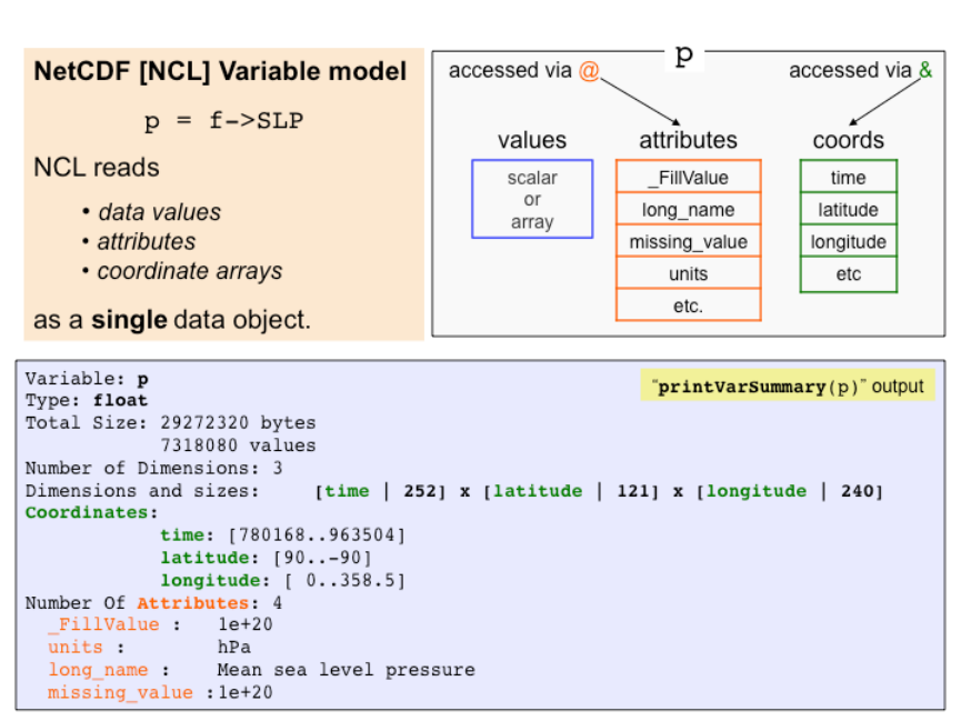
Section 3.1.2 Reading variables
Importing (reading) variables from any supported format is simple. If X is a variable on a
file referenced (pointed-to) by f, then:
x = f->X
If variable metadata (attributes and/or coordinate variables) are available they will
automatically be attached to the variable x. The user need not explicitly read any
attributes or coordinate variables because NCL automatically associates all the
information with the variable.
An important feature is that when a variable is imported, it is placed into a consistent
variable model regardless of the original source file format (netCDF-3/4, HDF-4/5, GRIB-
1/2, shapefile). This facilitates data processing and the creation of generic functions.
The following figure illustrates NCL’s netCDF-based variable model including a printed
overview of the variable.

13
Section 3.1.3 When to use the $ syntax
In some instances, the variable name must be enclosed by the $ symbol. This is
necessary if the variable on the file has a non-alphanumeric character (e.g., space, "+"
or "-") embedded in the name:
x = f->$"ice cream+oreo-cookies…yummy!"$
or the item on the right hand side of the pointer (->) is itself a variable of type string:
vars = (/"T","U","V"/)
x = f->$vars(n)$ ; n=0,1,2
Section 3.1.4 Printing the contents of a supported file
print can be used to view the contents of any supported format or variable. When used
on a file the printed information will be similar to that produced by "ncdump –h foo.nc".
(Note: ncdump is a netCDF/Unidata application; it is not part of NCL.) For example:
f = addfile ("foo.grb","r")
print(f) ; looks like ncdump –h
Note: The NCL command line utility ncl_filedump can produce an overview of any
supported file’s contents from the command line. See:
http://www.ncl.ucar.edu/Document/Tools/ncl_filedump.shtml
ncl_filedump foo.grb ; netCDF, GRIB of HDF
Section 3.1.5 Reordering a variable on input
Assume X is a 3D variable with dimension sizes (ntime, nlat, nlon). To reverse the
latitude ordering of the array:
X = f->X(:,::-1,:) ; use NCL array syntax
Section 3.1.6 Importing byte or short data with conversion to float
Distributed with NCL is a suite of user-contributed functions. Several functions in this
library will convert variables of type short and byte to type float:
x = short2flt(f->X) ; also, x = short2flt_hdf(f->X)
y = byte2flt(f->Y)
To use these functions, the "contributed.ncl" library must be loaded prior to use:

14
load "$NCARG_ROOT/lib/ncarg/nclscripts/csm/contributed.ncl"
Section 3.1.7 Spanning multiple files
The function addfiles (note the trailing ‘s’) provides the user with the ability to access
data spanning multiple files. This function can concatenate records (default; “cat”) or
"join" variables from different files by adding an extra dimension. In this example, we use
systemfunc (see section 5.8) to get a listing of all the ann* netCDF files in the current
directory.
fils = systemfunc("ls ann*.nc")
f = addfiles(fils,"r")
T = f[:]->T
or use coordinate subscripting if appropriate
T = f[:]->T(:,{500},{-30:30},: )
The resultant variable, T, will span all the files.
For more detail, see:
http://www.ncl.ucar.edu/Document/Functions/Built-in/addfiles.shtml
Section 3.1.8 Altering the default behavior of addfile(s)
The setfileoption procedure can be used to alter the default settings of addfile
and addfiles. See details at:
http://www.ncl.ucar.edu/Document/Functions/Built-in/setfileoption.shtml
Section 3.1.9 ncl_filedump
This command line operator will generate a text description of a specified file. The file
may be in any supported file format: netCDF, GRIB, HDF or HDF-EOS. The default
output is to the standard output [screen] but it may be redirected to a file. Regardless of
the input file format, the textual form of the output is similar to that produced by ‘ncdump
–h’.
ncl_filedump [options] fname.ext
The file name on the disk is not required to have the file extension. E.g., if the specified
file is "foo.grb" then, ncl_filedump will initially search for that file. If the file does not
exist under the specified name, ncl_filedump will search for a file named "foo" and treat
it as a GRIB file.
The options are may be seen by entering ‘ncl_filedump –h’ or, for more details, consult

15
http://www.ncl.ucar.edu/Document/Tools/ncl_filedump.shtml
Section 3.1.10 ncl_convert2nc
This command line operator will convert any GRIB, HDF or HDF-EOS file to netCDF
format.
ncl_convert2nc fname(s) [options]
Note that the options are specified after the file name(s). The options may be seen by
entering ‘ncl_convert2nc –h’ or, for more details and extensive examples, consult
http://www.ncl.ucar.edu/Document/Tools/ncl_convert2nc.shtml
Section 3.2 Binary data files
Binary data are not necessarily portable. Most machines write IEEE binary. Notable
exceptions include the CRAY native binary. Even IEEE binaries are not necessarily
portable. IEEE binaries are in two different flavors: big endian and little endian.
Depending on the machine, a binary file may have to reorder the bytes (byte swap). NCL
allows for dynamic byte swapping via the setfileoption procedure.
Reading binary files:
Several functions read binary data files. Most read IEEE binary and several read CRAY
binary. There is no standard file extension for binary files. The ".bin" is arbitrary.
fbinrecread(path:string,recnum:integer,dims[*]:integer,type:string) can be used to
read a Fortran unformatted sequential file. Records, which start at 0, can be of varying
type and length.
x = fbinrecread("a.bin",0,(/64,128/),"float")
fbindirread(path:string,rnum:integer,dims[*]:integer,type:string) can be used to read
binary records of fixed record length (direct access). All records in the file must be the
same dimensionality and type. To read the (n+1)th record:
x = fbindirread("b.bin",n,(/73,144/),"float")
Other functions for reading binary data include: cbinread, fbinread, and
craybinrecread.
Writing binary files:
Several procedures write IEEE binary data files.
fbinrecwrite(path:string,recnum:integer,value) can be used to write a Fortran
unformatted sequential file. Records can be of varying type and length.
16
Assume you have the following five variables: time(ntime), lat(nlat), lon(nlon),
y(ntime,nlat,nlon), z(nlat,nlon). Note that using a –1 as a record number means to
append.
fbinrecwrite("f.bin",-1, time)
fbinrecwrite("f.bin",-1, lat)
fbinrecwrite("f.bin",-1, lon)
fbinrecwrite("f.bin",-1, y)
fbinrecwrite("f.bin",-1, z)
fbindirwrite(path:string,value) can be used to write a Fortran direct access file. All
records must be of the same length and type.
do n=0,ntim-1
fbindirwrite("/my/path/f.bin",y(nt,:,:))
end do
Other procedures for writing IEEE binary data include: cbinwrite and fbinwrite.
Reading/writing big endian and little endian files:
The default behavior of NCL’s binary read/write functions and procedures is to assume
the files are compatible with the endian type for the system. The setfileoption
procedure can be used to dynamically perform byte swapping, if needed.
Section 3.3 ASCII
Reading ASCII files:
asciiread(filepath:string,dims[*]:integer,datatype:string), allows the data to be shaped
upon input. Complicated ASCII files (e.g., multiple variable types or differing numbers of
columns) should be read by importing the file as type string and using the string and
conversion functions to parse the data. Alternatively, C or Fortran subroutines could be
used.
z = asciiread("data.asc",(/100,13/),"float")
z will be a float variable with 100 rows and 13 columns, e.g. (100,13). Also see Section
5.8.
NCL is distributed with several functions in contributed.ncl that facilitate access to ascii
files that are partitioned into header and tabular numbers. These functions are called
readAsciiHeader and readAsciiTable, respectively.
Writing ASCII files:
asciiwrite(filepath:string, value) writes one column of values and the user has no
control over format.
17
asciiwrite("foo.ascii",x) ; one element per row
write_matrix(data[*][*]:numeric, fmtf:string, option) can write multiple columns and
the user has format control (also see section 4.4).
fmtf ="15f7.2" ; format string using fortran notation
opt = True
opt@fout = "foo.ascii"
write_matrix(x,fmtf,opt)
write_table(filepath:string, option:string, alist:list, fmtf:string), introduced in v6.1.0, is
the most flexible of the procedures that write ascii files. It can write or append all
elements of a list variable to a user specified file.
alist = [/a,b,c,d,f/] ; list with different variables
write_table("foo.ascii", "w", alist, "%d%16.2f%s%d%ld")
Section 3.4 Writing netCDF/HDF
There are two approaches for creating netCDF (or HDF) files. The first method is called
the "simple method" while the second method follows the "traditional approach" of
explicitly predefining the file’s contents before writing any values to the file.
Simple method:
This method is straightforward. One could substitute ".hdf" for the ".nc" to create an HDF
file.
fo = addfile("foo.nc","c")
fo->X = x
fo->Y = y
To create an UNLIMITED dimension, which is usually time, it is necessary to add the
following line of code prior to writing any values:
filedimdef(fo,"time",-1,True)
Traditional method:
Sometimes the "simple method" to netCDF file creation can be slow, particularly if there
are many variables or the resulting output file is large. The "traditional method" is more
efficient. This approach requires the user to explicitly define the content of the entire file,
prior to writing.
NCL functions that predefine a netCDF file:
filevardef: define name of one or more variables
filevarattdef: copy attributes from a variable to one or more file variables
18
filedimdef: define dimensions including unlimited dimension
fileattdef: copy attributes from a variable to a file as global attributes
setfileoption some options can dramatically improve performance
For the following example, assume that the variables time,lat,lon and T reside in
memory. When written to the netCDF file, the variable T is to be named TMP.
fout = addfile("out.nc","c")
; create global attributes
fileAtt = True
fileAtt@title = "Sample"
fileAtt@Conventions = "None"
fileAtt@creation_date = systemfunc("date")
setfileoption(fout,“DefineMode”,True) ; optional
fileattdef(fout,fileAtt)
; predefine coordinate variables
dimNames = (/"time","lat","lon"/)
dimSizes = (/-1,nlat,nlon/) ; -1 means unspecified
dimUnlim = (/True,False,False/)
; predefine names, type, dimensions
; explicit dimension naming or getvardims can be used
filedimdef(fout,dimNames,dimSizes,dimUnlim)
filevardef(fout,"time",typeof(time),getvardims(time))
filevardef(fout,"lat" ,typeof(lat) ,"lat")
filevardef(fout,"lon" ,typeof(lon) ,"lon")
filevardef(fout,"TMP" ,typeof(T) , getvardims(T) )
; predefine each variable’s attributes
filevarattdef(fout,"time",time)
filevarattdef(fout,"lat" ,lat)
filevarattdef(fout,"lon" ,lon)
filevarattdef(fout,"TMP" ,T)
setfileoption(fout,”SuppressDefineMode”,False) ; optional
; output values only [use (/… /) to strip metadata]
fout->time = (/time/)
fout->lat = (/lat/)
fout->lon = (/lon/)
fout->TMP = (/T/) ; T in script; TMP on file
Writing scalars to netCDF:
NCL uses the reserved dimension name "ncl_scalar" to identify scalar values that are to
be written to netCDF.
; simple method
fo = addfile("simple.nc","c")

19
con = 5
con!0 = "ncl_scalar"
fo->constant = con
; traditional method
re = 6.37122e06
re@long_name = "radius of earth"
re@units = "m"
fout = addfile("traditional.nc", "c")
filevardef(fout,"re",typeof(re),"ncl_scalar")
filevarattdef(fout,"re",re)
fout->re = (/re/)
Writing compressed files:
Writing compressed files can result in considerable reduction in file size. The
setfileoption procedure has an option called "CompressionLevel". This can be used
to specify the compression-level for data written to a NetCDF4 classic file. Prior to
opening the file , the following file options should be set:
setfileoption ("nc", "Format","NetCDF4Classic")
setfileoption ("nc", "CompressionLevel", 1) ; 0 through 9 possible
All data written to the file will be compressed. Currently, there is no way to selectively
activate compression on a per-variable basis. A “CompressionLevel” of one is best.
Contents of a well-written netCDF/HDF File:
Global file attributes that should be in any file include title, conventions (if any) and
source. Other file attributes may include history, references, etc.
Command line conversion of supported formats to netCDF:
NCL has a command line utility, ncl_convert2nc, that will convert any supported
format [GRIB-1, GRIB-2, HDF4, HDF4-EOS] to netCDF. For details see:
http://www.ncl.ucar.edu/Document/Tools/ncl_convert2nc.shtml
Section 3.5 Remote file access: OPeNDAP
Some (not all!) data servers allow remote data access via OPeNDAP: Open Source
Project for Network Data Access Protocol. OPeNDAP-enabled NCL is available on
some UNIX systems. File access is via a URL that is running an OPeNDAP server:
f = addfile ("http://path/foo.nc", "r")
or
fils = "http://path/" + (/ "foo1.nc", "foo2.nc", "foo3.nc"/)
20
f = addfiles(fils, "r")
Users can test for file availability using isfilepresent. Please note that if you are
behind a firewall, you may not be able to access data in this manner. Also, some
OPeNDAP servers require user registration prior to access.
Section 4: Printing
NCL provides limited printing capabilities. In some instances, it may be better to invoke
Fortran or C routines to have better format control. Available functions and procedures
include:
printVarSummary provides and overview of a variable including all metadata
print same as printVarSummary + each value of the variable
sprinti, sprintf provides some format control
write_matrix prints one variable in tabular form
print_table prints multiple variables of different types
Section 4.1 printVarSummary
Usage: printVarSummary(u)
Variable: u
Type: double
Total Size: bytes
147456 values
Number of Dimensions: 4
Dimensions / Sizes: [time | 1] x [lev | 18] x
[lat | 64] x [lon | 128]
Coordinates:
time: [4046..4046]
lev: [4.809 .. 992.5282]
lat: [-87.86379 .. 87.86379]
lon: [ 0. 0 .. 357.1875]
Number of Attributes: 2
long_name: zonal wind component
units: m/s
Section 4.2 print
Usage: print(u)
This will print the same information as printVarSummary followed by each individual
value and the associated subscript:
(0,0,0,0) 31.7
(0,0,0,1) 31.4
21
(0,0,0,2) 32.3 [snip]
The printing of the subscripts may be avoided by invoking NCL via: ncl –n foo.ncl.
print(u(0,{500},:,{100}))
would print u for all latitudes at time index 0, the level closest to 500 and the longitude
closest to 100.
print("min(u)="+min(u)+" max(u)="+max(u))
results in the following string:
min(u)= -53.8125 max(u)=55.9736
Section 4.3 sprintf, sprinti
print("min(u)="+sprintf("%5.2f",min(u)))
results in:
min(u) = -53.81
ii=(/-47,3579,24680/)
print(sprinti("%+7.5i",ii))
results in the following (on different lines):
-00047, +03579, +24680
Section 4.4 Pretty Print: write_matrix, print_table
If T(nrow,ncol), where nrow = 3 and ncol = 5 then
write_matrix(T,"5f7.2",False):
4.36 4.66 3.77 -1.66 4.06
9.73 -5.84 0.89 8.46 10.39
4.91 4.59 -3.09 7.55 4.56
Note: although write_matrix is prototyped for 2D arrays, arrays of higher
dimensionality can be printed using ndtooned and onedtond. Assume
X(nt,nz,ny,nx):
dimx = (/nt,nz*ny*nx/) or
dimx = (/nt*nz,ny*nx/)
write_matrix(onedtond(ndtooned(X),dimx),"12f8.3",False)

22
A more flexible procedure was introduced in v6.1.0: print_table. This allows
multiple variables of mixed data types to be printed with different formats.
alist = [/a,b,c,d,f/] ; variables of different types
print_table(alist, "%d,%16.2f,%s,%d,%ld")
Section 5: Data analysis and Arrays
NCL offers different approaches to analyzing data: (1) array syntax and operations, (2)
hundreds of built-in functions, (3) many user contributed functions and, (4) invoking
Fortran or C language routines. Tips on coding efficiently can be found at:
http://www.ncl.ucar.edu/Document/Manuals/Ref_Manual/NclUsage.shtml
Section 5.1 Array ordering and syntax
NCL arrays are row major and use zero-based indexing similar to that used by the
Python, C and C++ languages and the ordering of arrays within netCDF files. By
comparison, other common processing languages (eg., fortran, MATLAB, R) are column
major and use one-based indexing while the IDL language is column major but uses
zero-based indexing. Row major means that for each row all the columns are grouped
together. In practice, this means that in row major languages the leftmost dimension
varies slowest while the rightmost varies fastest. A simple is example is in Section 7.6.
NCL's algebra, like Fortran 90, MATLAB and IDL supports operations on scalars and
arrays rather than single scalar values like C, C++ and PASCAL. For array operations to
work, both operands must have the same number of dimensions and same size
dimensions, otherwise an error condition occurs. Furthermore, the data types of each
operand must be equivalent, or one operand must be coercible to the type of the other
operand. Let A and B be (10,30,64,128):
C = A+B ; element-by-element addition
D = A-B ; element-by-element subtraction
E = A*B ; element-by-element multiplication
C, D and E will be created automatically if they did not previously exist. If they did exist
then the result of the operation on the right hand side must be coercible to the type of left
hand side.
Scalar values are special cases when considering array operations. When scalar values
appear in an expression with a multi-dimensional value (i.e., an array), the scalar value
is applied to each element of the array. Consider
F = 2*E + 5
Here, each element of array E will be multiplied by 2 and then 5 will be added to each
element. The result will be assigned to F.

23
NCL’s < and > array operators (sometimes called “clipping operators”) are not commonly
used in other languages. Assume sst is (100,72,144) and sice = -1.8 (a scalar). The
statement:
sst = sst > sice
means that any values of sst less than sice will be replaced by sice.
All array expressions automatically ignore any operation involving values set to
_FillValue.
Section 5.2 Array conformance
Array expressions require that all operands have the same number of dimensions and
same size dimensions. In this case, the arrays are said to "conform" to each other.
Scalars conform to the shape of any array. Assume T and P are dimensioned
(10,30,64,128):
theta = T*( 1000/P )^0.286
This results in theta being dimensioned (10,30,64,128). conform or conform_dims
can be used to generate arrays that conform to another array. Assume T is
dimensioned (10,30,64,128) and P is dimensioned (30):
theta = T*(1000/conform(T,P,1))^0.286
conform expands P, which matches dimension "1" of T. For more details see:
http://www.ncl.ucar.edu/Document/Functions/Built-in/conform.shtml
http://www.ncl.ucar.edu/Document/Functions/Built-in/conform_dims.shtml
Section 5.3 Array memory allocation
Memory can be explicitly allocated/created for arrays in two ways:
1) Use of the array constructor (/.../)
a_integer = (/1,2,3/)
a_float = (/1.0, 2.0, 3.0/)
a_double = (/4d0,5d-5,1d30/)
a_string = (/"a","b","c"/)
a_logical = (/True,False,True/)
a_2darray = (/(/1,2/),(/5,6/),(/8,9/)/) ; 3 rows x 2 cols
2) Use the new(array_size,shape,type,[_FillValue]) statement: The inclusion of
_FillValue is optional. If it is not present, a default value will be assigned. Specifying
“No_FillValue” will result in no default _FillValue being assigned.
24
; _FillValue
a = new(3,float) ; 9.96921e+36
b = new(10,float,1e20) ; 1e20
c = new((/5,6,7/),integer) ; -2147483647
d = new(dimsizes(U),double) ; 9.969209968386869e+36
e = new(dimsizes(ndtooned(U)),logical); Missing
s = new(100,string) ; “missing”
q = new(3,float,”No_FillValue”) ; no _FillValue
Memory is automatically created by functions for returned variables; thus, use of the new
statement is not often needed or recommended.
Section 5.4 Functions and procedures
Like most languages, NCL has both functions and procedures. There are differences of
which users should be aware:
(a) Functions are expressions because they return one or more values and can therefore
be used as part of an expression. E.g., max, sin and exp are all standard mathematical
functions:
z = exp(sin(max(q))) + 12.345
Functions are not required to return the same type or size array every time they are
called.
(b) Procedures (analogous to Fortran subroutines) cannot be part of an expression
because they do not return values. NCL procedures are used in a way similar to those
used other programming languages. They perform a specific task and/or are used to
modify one or more of the input arguments.
Arguments to NCL functions and procedures:
Arguments are passed by reference. This means that changes to their values, attributes,
dimension names, and coordinate variables within a function or procedure will change
their values in the main program. By convention, arguments to functions should not be
changed by a function although this is not required. In the following discussion, it will be
assumed that arguments to functions follow this convention.
Argument prototyping:
In NCL, function and procedure arguments can be specified to be very constrained and
require a specific type, number of dimensions, and a dimension size for each dimension,
or arguments can have no type or dimension constraints. This is called argument
prototyping.
(a) Constrained argument specification means arguments are required to have a specific
type, size and dimension shape.
procedure ex (x[*][*]:float,y[2]:byte,\

25
res:logical,text:string)
The argument x must be a two-dimensional array of type float, y must be a one-
dimensional array of length 2, res and text must be of type logical and string
respectively, but can be of any dimensionality.
(b) Generic type prototyping: type only
function xy_interp(x:numeric,y:numeric)
Here numeric means any numeric data type listed in section 2.2.
(c) No type, no size, no dimension shape specification:
procedure foo(a,b,c)
(d) Combination:
function ex(d[*]:float,x:numeric,wks:graphic,y[2],a)
There is one very important feature which users should be aware of when passing
arguments to procedures. This is an issue only when the procedure is expected to
modify the input arguments. When an input argument must be coerced to the correct
type for the procedure, NCL is not able to coerce data in the reverse direction so the
argument is not affected by changes made to it within the procedure. NCL does
generate a WARNING message.
Section 5.5 Built-in functions and procedures
NCL contains hundreds of built-in functions and procedures from the simple to the
complex:
http://www.ncl.ucar.edu/Document/Functions/
Functions can return scalars or arrays and there is no need to preallocate array memory.
For example, let G be a 4D array with dimension sizes (ntime, nlev, 73, 144) To
interpolate G to a Gaussian grid with 128 longitudes and 64 latitudes with a triangular
truncation at wave 42, the following built-in function may be used:
g = f2gsh(G,(/64,128/),42)
f2gsh will perform the interpolation at all times and levels. The return array g will be
dynamically created and will be of size (ntime, nlev, 64, 128)
Generally, built-in functions do not return, create or change metadata. However, many of
the more commonly used built-in functions have "_Wrap" versions located in a script of
user contributed functions named “contributed.ncl”. These wrappers will handle the
metadata appropriately.

26
http://ww.ncl.ucar.edu/Document/Functions/Contributed/
NCL has many functions for performing operations on multidimensional arrays.
These include the dim_*_n suite of functions plus numerous other *_n functions (eg,
center_finite_diff_n, detrend_n). When an appropriate *_n function is
available, it should be utilized. The *_n functions require the user to specify the
dimension number(s) upon which an operation is to be performed. As a simple example,
consider the variable X(ntim,klev,nlat,mlon). NCL’s dimension numbering is left-to-right
and begins with zero: time => 0, lev => 1, lat => 2, and lon => 3. To compute zonal and
time averages,
Xzon = dim_avg_n(T, 3) ; Xzon(ntim,klev,nlat)
Xtim = dim_avg_n(T, 0) ; Xtim(klev,nlat,mlon)
Some functions and procedures may require that the dimensions of a particular
argument appear in a specific order. In these cases, the dimensions of the arguments
may have to be reordered using named dimensions. Consider the eofunc function
used to compute empirical orthogonal functions. Assume T is a 3D variable with size
(ntime,nlat,nlon) and with named dimensions (time,lat, lon). Most commonly the
eofunc function is used to derive orthogonal spatial patterns which vary in importance
over time (principal components; eofunc_ts). To accomplish this partitioning the
eofunc function requires that the rightmost dimension be time. Hence, dimension
reordering must be used:
eof = eofunc(T(lat|:,lon|:,time|:), 3, option) ; 3 EOFs
This results in a variable (eof) dimensioned (3, nlat, nlon).
In general, functions do not require memory to be explicitly allocated. The filling of an
array as part of a loop is an example of when it may be required. Assume T contains 10
years of monthly means (ntim=120). To compute the monthly climatology and standard
deviation for each of the twelve months, memory for returned values must be
preallocated because the calculation occurs in a loop.
; preallocate array
nmos = 12
Tclm = new((/nmos,klev,nlat,nlon /),typeof(T),T@_FillValue)
Tstd = Tclm ; same size/shape
ntim = dimsizes(time) ; get size of time (120)
do n=0,nmos-1
Tclm(n,:,:,:) = dim_avg_n (T(n:ntim-1:nmos,:,:,:) , 0)
Tstd(n,:,:,:) = dim_stddev_n(T(n:ntim-1:nmos,:,:,:), 0)
end do
Preallocation of arrays for procedures:
If a procedure is to return one or more arguments, memory for the returned variables
must be preallocated. Consider uv2sfvpg, which takes as input the zonal (u) and
meridional (v) velocity components and returns the stream function (psi) and velocity

27
potential (chi). The returned arrays must be the same size and type as the velocity
components:
psi = new(dimsizes(u),typeof(u))
chi = new(dimsizes(u),typeof(u))
uv2sfvp(u,v,psi,chi)
Function embedding:
Functions are themselves expressions so they can form parts of larger expressions,
which can reduce the number of lines of code. The readability of embedded functions is
subjective, however. Consider:
X = f2gsh(fo2fsh(fbinrecread(f,6,(/72,144/),"float")),(/nlat,lon/),42)
More lines of code may make the sequence easier to follow:
G = fbinrecread(f,6,(/72,144/),"float")
X = f2gsh(fo2fsh(G),(/nlat,mlon/),42)
Built-in utility functions:
Learning how to use NCL’s built-in utility functions can make processing simpler and
cleaner. The most commonly used are: all, any, conform, conform_dims,
ind, ind_resolve, dimsizes, fspan, ispan, ndtooned, onedtond,
mask, ismissing, system, systemfunc, print, printVarSummary and
where.
See these URLs for more details:
http://www.ncl.ucar.edu/Document/Functions/array_manip.shtml
http://www.ncl.ucar.edu/Document/Functions/array_query.shtml
Section 5.6 contributed.ncl
The NCL distribution includes a library of user-contributed functions that can facilitate
analyses. To access this library, you must load contributed.ncl at top of your script:
load "$NCARG_ROOT/lib/ncarg/nclscripts/csm/contributed.ncl"
Brief descriptions of the functions and procedures contained in contributed.ncl are at:
http://www.ncl.ucar.edu/Document/Functions/Contributed/
While not required, most NCL users prefer to have a variable’s metadata readily
available. This information is particularly useful when using certain high-level graphical
interfaces or when creating netCDF or HDF files. Since NCL’s built-in functions do not
create, change, or copy metadata, it becomes the user’s responsibility to maintain or
create metadata. Many of the functions in “contributed.ncl” can be grouped by how they

28
handle metadata.
Section 5.6.1 Wrap functions
The "contributed.ncl" script contains many functions that contain code to create or
maintain all appropriate meta data for built-in functions. The are called ‘wrap” functions.
The purpose of the wrap functions is to associate metadata with the returned variable.
The wrappers have the same calling sequence as the corresponding function, and the
name of the wrapper is the same as the function with an appended suffix ("_Wrap").
The use of dim_avg_n would result in the loss of T’s metadata:
Tzon = dim_avg_n(T, 0)
The use of dim_avg_n_Wrap would retain the metadata:
Tzon = dim_avg_n_Wrap (T, 0)
For a complete list of available wrap functions see:
http://www.ncl.ucar.edu/Document/Functions/Contributed/
copy_VarAtts, copy_VarCoords, copy_VarMeta, and copyatt are a few of the
functions that users have added to the contributed library for the purpose of explicitly
copying coordinate variables, attributes or both. Each performs this function in a slightly
different way.
Section 5.6.2 Type conversion
Assorted "contributed.ncl" functions that convert one type to another while retaining
metadata include short2flt , byte2flt, short2flt_hdf, numeric2int and
dble2flt.
Section 5.6.3 Climatology functions:
contributed.ncl has several climatology and anomaly functions that also create the
appropriate metadata: clmMon*(), stdMon*(), and month_to_month are just a few
of the examples.
Users are encouraged to peruse contributed.ncl to learn about various functions. The
functions can be taken and modified for your own purposes.
Section 5.7 User-defined functions and procedures
Users may create their own functions and procedures to accomplish repetitive tasks.
The general structure is:
undef("function_name")
function function_name(argument declaration)
29
local local_variable_list
begin
[statement(s)]
return (return_value) ; individual variable (any type)
end
undef("procedure_name")
procedure procedure_name(argument declaration)
local local_variable_list
begin
[statement(s)]
end
The undef procedure causes any previously defined user function or procedure to be
deleted. (Note: Built-in functions can not be deleted or redefined.) The local statement
lists variables local to the current function or procedure. The use of undef or local is
not required, but is recommended.
One frequently asked question is: What is the difference between a function and
procedure? A function returns a variable which may be used in subsequent code. A
procedure performs a task. Two common tasks are the creation of plots and files. Users
often establish personal libraries of functions and procedures. This allows for the
creation of cleaner and more compact scripts.
A second frequently asked question is : Can NCL user defined functions return multiple
variables? The answer is “yes”. However, it is not as convenient as (say) Matlab
which allows : [a,b,c] = foo(…)
.
Consider the following simple example:
undef("foo")
function foo(argument declaration)
local a,b,c [other local variables]
begin
[statements]
a = … ; may have meta data (type double)
b = … ; “ “ “ “ (type string)
c = … ; “ “ “ “ (type graphic)
return ( [/ a,b,c /] ) ; return as a ‘list’ variable
end
Use the function via
q = foo(…) ; q is a variable of type list
There is NCL syntax to access each variable within the list variable. However, it may be
clearer to explicitly extract the individual variables from the list variable via the list [..]
syntax
aa = q[0] ; aa will include any meta data
bb = q[1] ; bb “ “ “ “ “
30
cc = q[2] ; cc “ “ “ “ “
delete(q) ; list variable ‘q’ no longer needed
Important Note: All user created functions/procedures must be loaded prior to use.
They can be in the same script or located elsewhere.
load "/path/to/myLibrary.ncl"
Optional arguments:
Users may input optional arguments to procedures and functions. By convention, this is
accomplished by attaching attributes to a variable prototyped as logical. The high-
level graphical functions and procedures all use optional arguments in this manner. This
argument can then be queried using NCL’s built-in suite of is* functions (e.g. isatt).
opt = True
opt@scale = 0.01
opt@add = 1000
opt@wgts = (/0.25,0.50,0.25/)
opt@a3d = array_3D
undef ("foo")
function foo(x:numeric,opt:logical)
local dimx,rankx,xx
begin
dimx = dimsizes(x)
rankx = dimsizes(dimx)
if(typeof(x).eq."short")then
if(opt.and.isatt(opt,"scale"))then
xx = x*opt@scale
else
xx = x
end if
else
return(x)
end if
end
Section 5.8 System interaction
Users may interact with the system via systemfunc and system. Basically, the user
creates a string containing the Unix command to be executed. The semicolon can
separate multiple Unix commands. Options to Unix commands can be included by using
single quotes within the string.
systemfunc allows system commands to be executed and information is returned to an
NCL variable.
files_full_path = systemfunc("ls /my/data/*.nc")
files_names = systemfunc("cd /my/data ; ls *.nc")
date = systemfunc("date")

31
Use the Unix "cut" command to extract columns 14-19 of an ASCII file (sample.txt),
return as a one-dimensional array of type string, and convert to type float.
x = tofloat(systemfunc("cut –c14-19 sample.txt"))
system allows the user to execute an action. This is different than systemfunc in that
no information is returned to NCL. Some examples:
system("cp 10.nc /ptmp/user/") ; copy a file
system("sed ‘s/NaN/-999./g’ "+asc_input+" > asc_output")
In the following, all of the netCDF files for 1995 are acquired from NCAR’s High
Performance storage System (HPSS) system and put into the directory /ptmp/user/.
HPSS = "/USER/Data/Path"
dir = "/ptmp/user/"
year = 1995
system("hsi -q ’cd "+HPSS+" ; prompt ; lcd "+dir \
+" ; mget "+ nyear+ "-*.nc’ ")
By default, NCL invokes the Bourne shell when it passes commands to the system. The
following uses Bourne shell syntax to create a directory if it does not already exist:
DIR = "SAMPLE"
system("if ! test -d "+DIR+" ; then mkdir "+DIR+" ; fi")
Users may be more familiar with other UNIX shells. The following uses C-shell syntax to
accomplish the same task.:
system("csh -c 'if (! -d "+DIR+") then ; mkdir "+DIR+" ; endif'")
To prevent the Bourne shell from attempting to interpret csh syntax, the commands are
enclosed by single quotes ('). If the csh command contains single quotes they would
need to be escaped with a backslash ( \ ).
Section 6: Command line options and assignments
NCL supports a limited number of options and the setting and execution of simple NCL
statements at the command line, in either interactive or batch mode. Details with
examples are described at:
http://www.ncl.ucar.edu/Document/Manuals/Ref_Manual/NclCLO.shtml
Section 6.1 Options altering behavior when NCL is invoked
The following is a list of the predefined options and what they do:
32
-h display command line options usage
-f use New File Structure, and NetCDF4 features
-n don't enumerate values in print()
-o retain former behavior for certain backwards-incompatible changes
-p don't page output from the system() command
-x echo NCL statements as encountered
-V print the NCL version and exit
Here’s a simple example of using the –x option:
% ncl -x
Copyright (C) 1995-2005 - All Rights Reserved
University Corporation for Atmospheric Research
NCAR Command Language Version 4.2.0.a033
The use of this software is governed by a License Agreement.
See http://www.ncl.ucar.edu/ for more details.
ncl 0> a = 5
+ a = 5
ncl 1> exit
+ exit
Section 6.2 Specifying variable assignments on command line
Creating variables on the command line when NCL is invoked can facilitate data
processing tasks. Some simple examples of command line arguments (CLAs):
ncl nyrStrt=1800 nyrLast=2005 foo.ncl
ncl ‘f=”test.nc”’ p=(/850,500,200/) ‘v=(/”T”,”Q”/)’ foo.ncl
Spaces are not allowed. Statements containing strings must be enclosed with single
quotes.
The script may contain default settings for variables that are optional:
ncl a=5 c=3.14d0 foo3.ncl
The foo3.ncl script could check the command line for a variable via the isvar function:
if(.not.isvar(“a”)) then
a = 10 ; set to 10 if a not defined
end if
if(.not.isvar(“b”) then
b = 72.5 ; set to 72.5 if not defined.
end if
Invoking CLAs within a Unix shell script can be a nuisance. The shell script must be
escaped by using special shell characters. The NCL command line

33
ncl ‘filName=”foo.nc”’ test.ncl
would be the following in C-shell syntax:
#!/bin/csh –f
set a=foo.nc
eval ncl filName=\\\”$a\\\” test.ncl
This is rather obscure and it requires knowledge of Unix shell syntax. It is often cleaner
and easier to use an NCL script for typical shell script tasks. (See Section 7.8)
Section 7: Using external codes
NCL, which is written in C, has been designed to allow users to invoke external codes
(e.g., Fortran, C, or other libraries). The primary focus here is the use of Fortran (f77,
f90) subroutines. To use external C-language functions see:
http://www.ncl.ucar.edu/Document/Manuals/Ref_Manual/NclExtend.shtml
Section 7.1 NCL/Fortran interface
The use of Fortran subroutines is greatly facilitated by the WRAPIT utility, which is
distributed with NCL. Options available may be viewed by entering “WRAPIT –h” on the
command line. WRAPIT compiles the external code and generates a file that, by
convention, is called a "shared object". This object is identified by a ".so" extension.
The only information that WRAPIT requires is the interface between Fortran and NCL
including the subroutine declaration statement and arguments. Explicit specification of
the argument types is not necessary since WRAPIT is aware of Fortran’s default typing.
Of course, users can override the default typing by explicitly specifying the type in the
Fortran declarations. NCL uses the interface delimiter pair:
C NCLFORTSTART
C NCLEND
to identify the interface section. Note that the delimiters are in the form of f77
comments and, thus, have no affect on the code. The C NCLFORTSTART precedes the
subroutine statement while C NCLEND follows the last declaration of arguments
pertaining to the interface.
C NCLFORTSTART
subroutine demo(xin,xout,mlon,nlat,text)
integer mlon, nlat
real xin(mlon,nlat), xout(mlon,nlat)
character*(*) text
C NCLEND
34
Section 7.2 f77 subroutines
The four-step process to create and call shared objects is best illustrated by an example.
Consider an existing file called foo.f. This file may contain one or more f77 subroutines.
1) Bracket each subroutine being called with interface delimiters:
C NCLFORTSTART
subroutine demo(xin,xout,mlon,nlat,text)
integer mlon, nlat
real xin(mlon,nlat), xout(mlon,nlat)
character*(*) text
C NCLEND
The rest of Fortran code may include many subroutines.
2) Create a shared object using WRAPIT. The default behaviour is for WRAPIT to name
the .so file the same as the Fortran file name (e.g. foo.so):
WRAPIT foo.f
3) Add an external statement to the NCL script. The external statement consists of
an arbitrary identifier, which NCL uses to dynamically select the correct shared object
(most commonly, this is the name of the Fortran file) and the location of the shared
object. The default location is the current directory.
external FOO "./foo.so"
4) Invoke the specific subroutine(s) from NCL. There is a special three-part syntax that
must be used which includes (a) the name by which NCL identifies the target shared
object, (b) the :: separator syntax, and (c) the Fortran subroutine interface.
FOO::demo(xin,xout,nlon,nlat,text)
A schematic NCL script would be:
external FOO "./foo.so"
begin
[statement(s)]
xout = new((/nlat,nlon/),typeof(xin)
FOO::demo(xin,xout,mlon,nlat,text)
[statement(s)]
end
Section 7.3 f90 subroutines
35
Invoking f90 subroutines is essentially the same process used for f77 subroutines except
for step (1). In f77, the NCL interface delimiters are inserted directly into the f77
subroutines. Unfortunately, the Fortran parser used by WRAPIT does not understand f90
syntax. Thus, the user must create a "stub" interface for each subroutine called by NCL.
These stub files are a repeat of the f90 declaration list in f77 syntax. There is no need for
the stub files to be complete subroutines. Remember, WRAPIT only cares about the
subroutine call and its arguments. Consider the following f90 subroutines contained in a
file called "quad.f90":
subroutine cquad(a,b,c,nq,x,quad)
implicit none
integer, intent(in) :: nq
real, intent(in) :: a, b, c, x(nq)
real, intent(out) :: quad(nq)
integer :: i ! local
quad = a*x**2 + b*x + c ! f90 array syntax
return
end subroutine cquad
subroutine prntq(x,q,nq)
implicit none
integer, intent(in) :: nq
real, intent(in) :: x(nq),q(nq)
integer :: i ! local
do i = 1,nq
write(*,'(I5, 2F10.3)')i,x(i),q(i)
end do
return
end subroutine prntq
1) Create interface stubs using f77 syntax and store in file quad90.stub. Each stub file
requires a set of C NCLFORTSTART and C NCLEND delimiters.
C NCLFORTSTART
subroutine cquad (a,b,c,nq,x,quad)
dimension x(nq),quad(nq) ! ftn default
C NCLEND
C NCLFORTSTART
subroutine prntq(x,q,nq)
integer nq
real x(nq),q(nq)
C NCLEND
2) Create the shared object using WRAPIT. If f90 modules were present, they should be
compiled prior to the routines that use them. The user must specify the compiler to be
used on the command line. Enter WRAPIT –h for a list of command line options.
WRAPIT quad90.stub quad.f90
36
3-4) Same as section 7.2.
A sample NCL script would be:
external QUPR "./quad90.so"
begin
a = 2.5
b = -.5
c = 100.
nx = 10
x = fspan(1.,10.,10)
q = new(nx,float)
QUPR::cquad(a,b,c,nx,x,q)
QUPR::prntq(x,q,nx)
end
Section 7.4 Accessing the LAPACK library distributed with NCL
NCL is distributed with a ‘double precision’ version of LAPACK. Users can access this
library by creating a stub (interface) subroutine and then using WRAPIT to create a
shared object. For example, let’s say a user wants to use LAPACK’s DGELS subroutine
to solve an overdetermined or underdetermined real linear system. The stub/interface
subroutine, here name DGELSI located in the file ‘dgels_interface.f’ , would look like
C NCLFORTSTART
SUBROUTINE DGELSI( M, N, NRHS, A, B, LWORK, WORK )
IMPLICIT NONE
INTEGER M, N, NRHS, LWORK
DOUBLE PRECISION A( M, N ), B( M, NRHS), WORK(LWORK)
C NCLEND
C declare local variables
INTEGER INFO
CHARACTER*1 TRANS
TRANS = "N”
CALL DGELS(TRANS, M,N,NRHS,A,LDA,B,LDB,WORK,LWORK,INFO)
RETURN
END
Use WRAPIT to compile the wrapper subroutine and to specify the location of the
LAPACK library for the local system.
WRAPIT -L $NCARG_ROOT/lib -l lapack_ncl dgels_interface.f
The sample script in the next section illustrates how one can invoke the shared object
from within an NCL script.
Section 7.5 Using commercial libraries
The process is similar to using f90 codes because the user must create a stub file to
explicitly specify the required calling sequence and argument types. Let’s assume we
want to use IMSL’s rcurv subroutine. For convenience, f77 syntax will be used.
37
1) Create a wrapper program arbitrarily named rcurvwWap.f
C NCLFORTSTART
subroutine rcurvwrap(n,x,y,nd,b,s,st,n1)
integer n, nd, n1
real x(n),y(n),st(10),b(n1),s(n1)
C NCLEND
call rcurv (n,x,y,nd,b,s,st) ! IMSL name
return
end
2) Use WRAPIT to compile the wrapper subroutine and to specify the location of the
IMSL library for the local system.
WRAPIT –l mp –L /usr/local/lib64/r4i4 –l imsl_mp rcurvWrap.f
3-4) Same as section 7.2 and 7.3
Sample script:
external IMSL "./rcurvWrap.so"
begin
x = (/0,0,1,1,2,2,4,4,5,5,6,6,7,7/)
y = (/508.1,498.4,568.2,577.3,651.7,657.0,\
755.3,758.9,787.6,792.1.841.4,831.8,854.7,\
871.4/)
nobs = dimsizes(y)
nd = 2
n1 = nd+1
b = new(n1,typeof(y)) ; create return arrays
s = new(n1,typeof(y))
st = new(10,typeof(y))
; call IMSL routine
IMSL::rcurvwrap(nobs,x,y,nd,b,s,st,n1)
print(b)
print(s)
print(st)
end
Section 7.6 What WRAPIT does
WRAPIT is a UNIX script that performs a number of tasks including using Fortran
compilation and linking that creates the shared object (.so). It provides users with many
options:
WRAPIT –h <return>
38
WRAPIT performs the following tasks:
1) Uses an NCL utility wrapit77, a C-language program, to create a C wrapper
program that invokes the f77 parser and creates the required C code to interface
between NCL and Fortran.
wrapit77 < foo.f >! foo_W.c
2) Compiles and creates object modules for the C and Fortran codes:
cc -c foo_W.c ; foo_W.o
f77 -c foo.f ; foo.o
3) Creates a dynamic shared object (.so) using the local ld.
4) Cleans up temporary files so that only the shared object file (*.so) remains.
Section 7.7 NCL/Fortran array mapping
In Fortran, the leftmost array dimension varies fastest while in NCL the rightmost array
dimension varies fastest. Sometimes this causes confusion. Rarely is reordering an
array required when invoking a Fortran subroutine from an NCL script. Thus, even
though the array dimension names appear in reverse order the individual array elements
directly map. The rule “fastest varying dimesnsions in one language map to fastest
varying dimension in another language” applies here.
NCL Fortran
x(time,lev,lat,lon) <=map=> x(lon,lat,lev,time)
Consider the following two arrays where N=2 and M=3:
ncl: x(N,M) <==> x(M,N) :Fortran
x(0,0) <==> x(1,1)
x(0,1) <==> x(2,1)
x(0,2) <==> x(3,1)
x(1,0) <==> x(1,2)
x(1,1) <==> x(2,2)
x(1,2) <==> x(3,2)
Section 7.8 NCL and Fortran (or C) in Unix shell script
When working on an NCL script that is invoking one or more Fortran (or C) shared
objects, it is convenient to combine all the various steps into a single Unix shell script.
The following outlines the components via a C-shell script.
#!/usr/bin/csh
# =========== Edit NCL Code ============

39
cat >! main.ncl << "END_NCL"
load ”$NCARG_ROOT/lib/ncarg/nclscripts/csm/gsn_code.ncl"
load ”$NCARG_ROOT/lib/ncarg/nclscripts/csm/gsn_csm.ncl“
load "$NCARG_ROOT/lib/ncarg/nclscripts/csm/contributed.ncl“
external SUB "./sub.so"
begin
...NCL code…
end
"END_NCL"
# ===========Edit Fortran Code ========
cat >! sub.f << "END_SUBF"
C NCLFORTSTART
...
C NCLEND
"END_SUBF"
# =========== Invoke WRAPIT ==========
WRAPIT sub.f
# =========== EXECUTE ========
ncl main.ncl >&! main.out
exit
Section 7.9 Using NCL as a scripting language
NCL can be used like a scripting language. Often, it is cleaner and easier then using a
Unix shell. The following uses an NCL do loop to (a) access files from NCAR’s High
Performance Storage System (HPSS); (b) invoke a netCDF operator (ncrcat) to create a
new netCDF file; and, (c) remove (rm) the files created in step (a). The general
procedure is to create a string that is passed to the system for execution via the system
procedure. The print statements are included to track the state of the script. Note
thesingle ‘ in the hpsscmd.
hpss = “/Model/Sample/” ; HPSS path
diri = “/ptmp/user/” ; dir containing input files
fili = “b20.007.pop.h.0” ; prefix of input files
diro = “/ptmp/user/out/” ; dir containing output files
filo = “b20.TEMP.” ; prefix of output files
nyrStrt = 300 ; 1st year
nyrLast = 999 ; last year
do nyear=nyrStrt,nyrLast
print (“---- “+nyear+” ----”)
; acquire 12 MSS files for year
hpsscmd = "hsi -q 'cd "+ hpssi +" ; lcd "+diri+ \
" ; prompt; mget "+fili+nyear+"-[0-1][0-9].nc'"
print ("hpsscmd= "+ hpsscmd)
print (“hpsscmd=“+hpsscmd)
40
system (hpsscmd)
; strip off the TEMP variable
ncocmd = “ncrcat –v TEMP “ +diri+fili+”*.nc “+ \
diro+filo+nyear+”.nc”
print (“ncocmd=“+ncocmd)
system (ncocmd)
; remove the monthly files
rmcmd = “’rm’ “+diri+fili+nyear+ ”.nc”
print (“rmcmd=“+rmcmd)
system (rmcmd)
end do
