NCPA User Guide

User Manual:

Open the PDF directly: View PDF .
Page Count: 28

ANeCA: User Guide

Author: Mahesh Panchal

This software was

Developed during my PhD

Supervisor: Dr. M. A. Beaumont

Funding: BBSRC, 10/02-10/05

July 22, 2008

Contents

1 Software Documentation 3

1.0.1 Updates from v1.0 . . . . . . . . . . . . . . . . . . . . 3

1.0.2 Updates from v1.1 . . . . . . . . . . . . . . . . . . . . 3

1.1 Basic’sofNCPA ......................... 4

1.1.1 Summary of the Method. . . . . . . . . . . . . . . . . . 4

1.1.2 Contraversy of NCPA . . . . . . . . . . . . . . . . . . . 5

1.2 Programcitation ......................... 5

1.3 TheInputFiles .......................... 6

1.3.1 The Nexus or Phylip DNA sequence ﬁle . . . . . . . . 6

1.3.2 Geographic information ﬁle . . . . . . . . . . . . . . . 7

1.4 TheOutputFiles......................... 7

1.4.1 TheGraphFile...................... 8

1.4.2 The Geodis Input ﬁle . . . . . . . . . . . . . . . . . . . 8

1.4.3 TheGMLﬁle ....................... 8

1.4.4 TheNestﬁle ....................... 8

1.4.5 The NANOVA ﬁle . . . . . . . . . . . . . . . . . . . . 8

1.4.6 The GeoDis Output ﬁle . . . . . . . . . . . . . . . . . 9

1.4.7 The GeoDis Summary ﬁle . . . . . . . . . . . . . . . . 9

1.4.8 The Inference File . . . . . . . . . . . . . . . . . . . . 9

1.5 Using the software for NCPA . . . . . . . . . . . . . . . . . . 9

1.5.1 Using the Graphical Interface . . . . . . . . . . . . . . 9

1.5.2 Using the Command Line . . . . . . . . . . . . . . . . 14

1.5.3 Drawing the nested design . . . . . . . . . . . . . . . . 14

1.6 AWorkedexample ........................ 15

1.6.1 Creating the Geographic information ﬁle . . . . . . . . 15

1.6.2 Creating the Nexus ﬁle . . . . . . . . . . . . . . . . . . 16

1.6.3 Create the haplotype network . . . . . . . . . . . . . . 16

1.6.4 Creating the Nested Design . . . . . . . . . . . . . . . 17

1.6.5 Drawing the Nested Design . . . . . . . . . . . . . . . 18

1.6.6 Performing the Permutation Analysis . . . . . . . . . . 18

1.6.7 Applying the Automated Inference Key. . . . . . . . . 18

1.7 Using the software for genotype-phenotype studies . . . . . . . 19

1.7.1 File simpliﬁcations . . . . . . . . . . . . . . . . . . . . 19

1.7.2 Using the Graphical Interface . . . . . . . . . . . . . . 20

1.7.3 Using the Command line . . . . . . . . . . . . . . . . . 20

1.8 Limitations of Software . . . . . . . . . . . . . . . . . . . . . . 20

1.9 Common Exceptions thrown . . . . . . . . . . . . . . . . . . . 21

1.10KnownIssues ........................... 21

1.11 Frequently Asked Questions . . . . . . . . . . . . . . . . . . . 22

1.12Disclaimer............................. 24

1.13 Acknowledgements . . . . . . . . . . . . . . . . . . . . . . . . 25

Chapter 1

Software Documentation

This software is a basic fully automated implementation of Nested Clade

Phylogeographic Analysis (NCPA). NCPA is a method of phylogeographic

inference developed by Alan Templeton and colleagues.

Please become familiar with this manual. It will solve a lot of

the common problems encountered using this software. Also please

check your results. This software is not intended to be a black box,

and is still in early stages of development.

1.0.1 Updates from v1.0

1. The inference key implemented has been updated from 14th July 2004

to the inference key dated 11th November 2005.

Unfortunately I have not had the time to work on including updates of TCS

or GeoDis.

1.0.2 Updates from v1.1

1. There has been a change in implementation of Question 19 and 20

on the inference key. These questions will no longer regard popula-

tions (sampled or unsampled) within the convex hull of all the clades

as within the clade boundary if they are within the convex hull of a

subclade.

2. ANeCA now uses TCS v1.21.

3. ANeCA now uses GeoDis v2.5.

1.1 Basic’s of NCPA

This is a summary of the method only and my opinion of the state of NCPA.

Please familiarise yourself with the literature surrounding the method includ-

ing criticisms and their replies. If you are unfamiliar with NCPA please use

the references within as a guide to familiarise yourself with the method.

1.1.1 Summary of the Method.

Many researchers use NCPA in various ways augmenting the method with

various results and techniques. The basic methodology is to generate a hap-

lotype network from your data, nest the haplotype network, calculate statis-

tics, and use an inference key. This is normally applied to a single locus, for

example, the Cytochrome b region in mtDNA.

Note that NCPA is a method that has evolved over the years. As such

there is some discrepancy as to how NCPA should be applied. The cur-

rent method of applying NCPA suggested by Templeton et al. (2005) is the

following:

1. Generate a haplotype network.

2. Use the nesting algorithm provided in the original literature (Templeton

et al. 1987; Templeton and Sing 1993).

3. Calculate the Dnand Dcstatistics using GeoDis (Posada et al. 2000).

4. Apply the key either by hand, using AUTOINFER (Zhang et al. 2006)1,

or this software (Check the diﬀerences).

5. Validate these inferences using other loci (Templeton et al. 2005).

However in practice many of the articles published by Templeton use the

following steps:

1. Generate a haplotype network.

2. Use the criteria in Crandall and Templeton (1993) to ﬁnd the best

resolution of the network.

3. If there are still loops, enumerate all possible trees within the network.

4. Nest all trees (This program is adequate for that purpose).

1This software has recently been withdrawn, but may become available in the near

future.

5. Calculate the Dnand Dcstatistics using GeoDis (Posada et al. 2000).

6. Apply the key either by hand, using AUTOINFER (Zhang et al. 2006),

or this software (Check the diﬀerences).

7. Check that all the trees provide inferences that are concordant. Discard

inferences that do not match.

8. Validate these inferences using other loci (Templeton et al. 2005).

1.1.2 Contraversy of NCPA

The ﬁeld of phylogeography is currently split as to whether the method works

or not. Much of the reasoning behind NCPA is as yet not explained in the lit-

erature. Simulations by Knowles and Maddison (2002) indicated that NCPA

did not work when they simulated fragmentation. These simulations were

criticised by Templeton (2004), however they still provide valuable insights

into the performance of NCPA and its usage. Moreover, Templeton (2004)

is often considered proof that NCPA is not prone to false positives, and is

actually conservative, however it is not the entire story. Much of NCPA is

in fact untested. What has been tested is the performance of NCPA under

fragmentation, and range expansion, using real data sets with strong a priori

expectations on a single loci, using steps 2. and 3. above. NCPA has also

been tested using simulations under the scenario of panmixia without using

steps 2. and 3. on single loci. These simulations shows that NCPA is prone

to false positives on a single locus when there is no signal, but remember that

this is not the full story. Multi-locus NCPA may still provide the answer to

the false positives from multiple testing, but it still needs to be tested.

There is still the question of what eﬀect the criteria of Crandall and

Templeton (1993) have on the performance of NCPA. The features used in

the criteria are also used later in the calculation of Dcand Dn. How exactly

(what is the algorithm) does one say that inferences are concordant? When

enumerating all trees in a haplotype network, can a missing intermediate

be a tip? If a rooted and unrooted haplotype network both give diﬀerent

inferences in the same clade, is the inference from the unrooted haplotype

network false?

1.2 Program citation

This is the citation for this software.

M. Panchal. 2007. The automation of Nested Clade Phylogeographic Anal-

ysis. Bioinformatics,23:509-510.

Please include the citations for TCS and GeoDis as well, as this software

relies heavily upon it.

M. Clement, D. Posada, and K. A. Crandall. 2000. TCS: A computer pro-

gram to estimate gene genealogies. Molecular Ecology,9(10):1657-1659.

D. Posada, K. A. Crandall, A. R. Templeton. 2000. GeoDis: A program

for the cladistic nested analysis of the geographical distribution of genetic

haplotypes. Molecular Ecology,9(4):487-488.

1.3 The Input Files

This section gives a description of the input ﬁles required to generate the

output ﬁles. Each ﬁle is a plain text ﬁle (do not save the ﬁles as RTF or

DOC ﬁles; they are not plain text).

1.3.1 The Nexus or Phylip DNA sequence ﬁle

This software uses a modiﬁed version of the Nexus ﬁle. Labels for each

DNA sequence must start with a letter and only contain letters or digits

(no whitespace). Each label should also have a period followed by a number

indicating which location (see 1.3.2) the sequence came from. Here is an

example of a Nexus ﬁle.

#NEXUS

begin data;

dimensions ntax=11 nchar=38;

format datatype=dna missing=? gap=-;

matrix

mxh1.1 CGTAAAGTTATACCCGAAAGGGAGAGAGTGAGAGTGTG

mxh2.1 CGTAAAGTTTTACCCGAAAGGGAGAGAGTGAGAGTGTG

mxs1.1 CGTAAAGTTATACCCGAAAGGGAGAGAGTGAGAGTGTG

mxs2.1 CGTAAAGTTATAGGCGAAAGGGAGAGAGTGAGAGTGTG

mxs3.2 CGTAAAGTTATAGGGGAAAGGGAGAGAGTGAGAGTGTG

mxs4.2 CGTAAAGTAATAGCCGAAAGGGAGAGAGTGAGAGTGTG

mxs5.2 CGTAAAGTAATAGCCGAAAGGGAGAGAGTGAGAGTGTG

txl1.3 CGTAATGTTATACCCGAAAGGCAGAGAGTGAGAGTGTG

txl2.3 CGTAATGTTATACCCGAAAGGCTCAGAGTGAGAGTGTG

txl3.4 CGTAATGTTATACCCGAAAGGCTCAGAGTGAGAGTGTG

txl4.4 CGTAAAGTTATAGCCGAAAGGCTGAGAGTGAGAGTGTG

;

end;

Note: Although not in the speciﬁcation of the NEXUS ﬁle format, each label

and its corresponding DNA sequence should be on a single line (NEXUS

sequential). Also the nexus ﬁle should not contain any other information

other than that which can be seen in the example.

1.3.2 Geographic information ﬁle

The ﬁrst line of the ﬁle should contain an identiﬁer for the data set. The

second line is a number nthat indicates the number of locations sampled

(this does not include the unsampled locations speciﬁed). The next 2nlines

contain the entries for each sampled location. Each geographic location spec-

iﬁed is written on two lines. The ﬁrst line of the entry contains the number

(id) of the geographic location, followed by the name of the location (letter

followed by letters or digits and no whitespace). The second line speciﬁes

the sample size, the location in decimal degrees, and the radius (spread) of

the sample location (in Km). Further habitable unsampled locations (where

prior knowledge indicates the species is present, or there is no prior knowledge

about the area) should also be speciﬁed after the sampled locations (This is

IMPORTANT information that is used to detect sampling inadequacies).

This is an example of a geographic information ﬁle.

mydataset // Name of the data set

2 // Number of sampled geographic locations

1 pop1 // Population number and name

7 10.50 -0.23 3 // Sample size, latitude, longitude, radius

2 pop2

5 -5.60 4.50 5.0

3 pop3 // This is an unsampled habitable location

0 -4.50 -3.50 5.4

Note: The number for each geographic location should be unique, sequential

and start from 1. Furthermore if a geographic region is not included, the

assumption made is that the area was sampled and the species was absent

in that area, or that the area is uninhabitable for that species.

1.4 The Output Files

This section describes the ﬁles that are given as output to the analysis.

1.4.1 The Graph File

TCS automatically writes out a *.graph ﬁle when it constructs a haplotype

network from the nexus ﬁle. The graph ﬁle is written in the GML format, and

speciﬁes the structure of the haplotype network. It also contains haplotype

frequency data and outgroup weights for each sampled haplotype.

1.4.2 The Geodis Input ﬁle

This is produced from the *.graph ﬁle and the geographic information ﬁle.

The geodis input ﬁle (*.gdin) can be written in two formats. The ﬁrst format

speciﬁes the geographic information as decimal degrees, and is automatically

written out. The second format writes the geographic information as a dis-

tance matrix where the distances are the great circle distances between each

geographic location. The clade information written for both formats are

exactly the same.

1.4.3 The GML ﬁle

A *.gml ﬁle is also written. This contains the structure of the nested clado-

gram. The ﬁle contains a graph in the GML format for each level of the

nested cladogram. This ﬁle was not intended to be used to construct the

nested cladogram design manually. It was intended to be used by the soft-

ware only. To see what the nested cladogram design looks like please use the

*.nest ﬁle.

1.4.4 The Nest ﬁle

An optional ﬁle (*.nest) that can be written so the user can manually recon-

struct the nested cladogram design on a diagram of the haplotype network

(which can be obtained through TCS). This contains the id of each clade in

the nested design. For the 0-step clades, the frequency data is included as

well as the label for the clade, and which clades it is connected to. For n-step

clades (n≥1), the information available is the label, the subclades within

the clade and the clades that are connected to it. The subclades are speci-

ﬁed in the order of tip clades, interior clades, followed by the symmetrically

stranded clades.

1.4.5 The NANOVA ﬁle

An optional ﬁle (*.nanova) can also be written which will provide nested in-

formation for each individual in the analysis. The data is provided as partial

data (as Comma Separated Values) that can be combined with individuals’

phenotype data for analysis with a Nested Analysis of Variance. The ﬁle is

primarily produced for users that wish to perform genotype-phenotype stud-

ies rather than geographic association studies of a species. See 1.7 for more

information.

1.4.6 The GeoDis Output ﬁle

This ﬁle (*.gdout) is written by GeoDis and contains the Dcand Dnproba-

bilities for each clade.

1.4.7 The GeoDis Summary ﬁle

This ﬁle can be produced by the automated inference key. The input ﬁles

required for this and the inference ﬁle are the geographic information ﬁle,

the Geodis Input (decimal degrees format), the GeoDis Output ﬁle, and the

GML ﬁle. The GeoDis input ﬁle needs to be in the decimal degrees format

even if the distance matrix format was analysed by GeoDis. The ﬁle contains

a summary of the information contained in the GeoDis Output ﬁle and marks

statistically signiﬁcant values with a star (and s or l if it is statistically small

or statistically large). It also contains geographic locations and their spread.

The geographic distribution is also given for each clade.

1.4.8 The Inference File

This ﬁle contains the inference made for each clade and the chain of inference

showing which questions were answered to reach that conclusion.

1.5 Using the software for NCPA

This is a basic guide to using the software for geographic association studies

of a species.

1.5.1 Using the Graphical Interface

To run the software either select NCPA.jar in your ﬁle explorer or type

java -jar NCPA.jar

from the command line.

To create the haplotype network using TCS v1.18, select

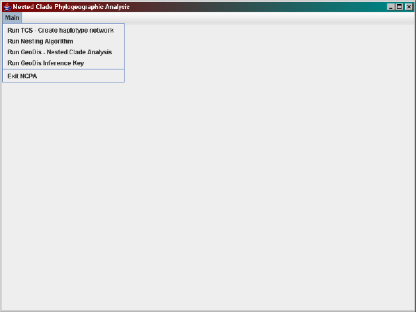
Figure 1.1: How to start TCS.

Main > Run TCS - Create haplotype network

from the menu.

Then select your nexus ﬁle from the menu using the following command,

File > Select NEXUS/PHYLIP Sequence file

and then click RUN, which will automatically save a *.graph ﬁle. Once the

haplotype network is created it is a good idea to save a picture of the haplo-

type network as well, although this can also be done at a later stage. Click

File > Save network as postscript

to save the image as a postscript ﬁle. Please refer to the TCS documentation

for further information about its functionality.

The next step is to nest the haplotype network and is done by either

selecting

Main > Run Nesting Algorithm

from the menu or by clicking the Run Nesting Algorithm button.

The following interface is displayed, and if TCS was used before, the

textﬁelds should be automatically completed providing the ﬁles can be found.

The user must provide the locations of the TCS graph ﬁle and the ﬁle con-

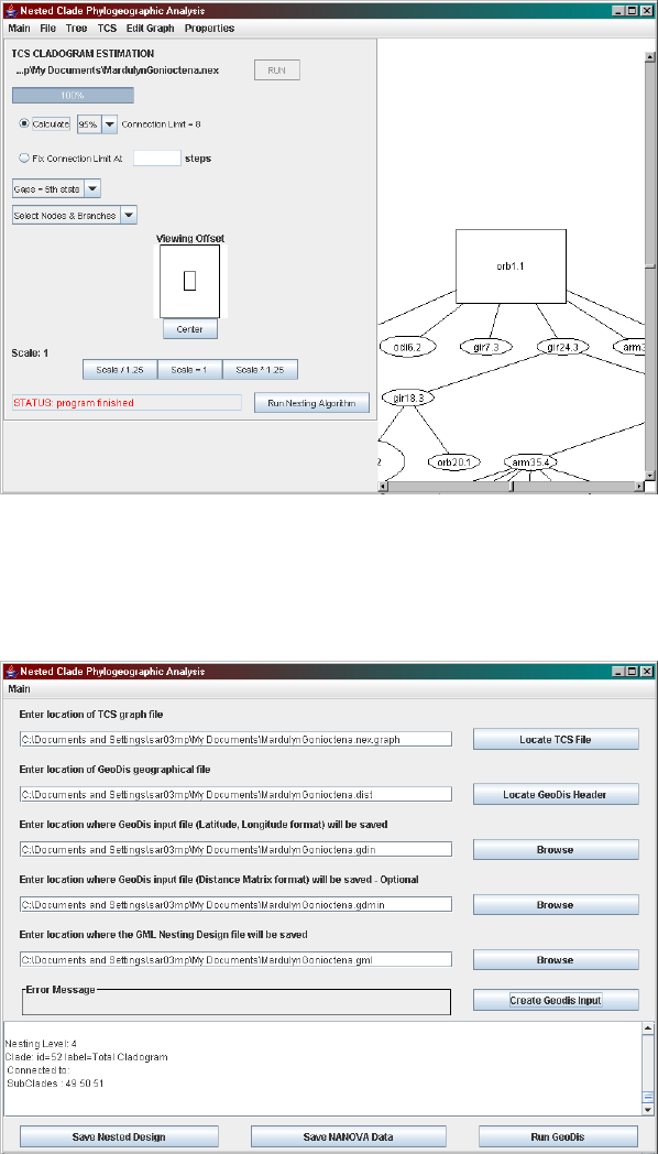
Figure 1.2: A screen shot of TCS.

Figure 1.3: A screen shot of the nesting software.

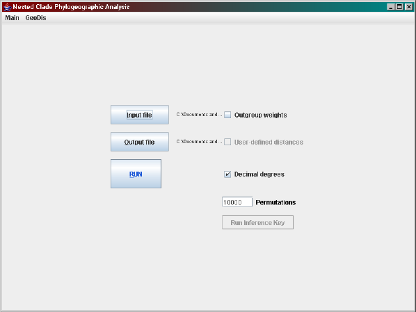
Figure 1.4: A screen shot of GeoDis.

taining the geographic information. The names of the GeoDis input ﬁles and

the name of the GML nested design ﬁle also need to be speciﬁed as they

will be required later on. Although the Distance Matrix format form of the

GeoDis ﬁle is optional it might be a good idea to compare the analyses from

both forms of input.

By clicking the Create GeoDis Input button, a summary of the nested

design will be shown in the text area that can be used to reconstruct it on the

haplotype network. This can also be saved by clicking Save Nested Design.

To move on to GeoDis select,

Main > Run GeoDis - Nested Clade Analysis

from the menu or click on the button Run GeoDis, which displays the GeoDis

interface.

If the nesting algorithm has just been run, the default input and output

ﬁles speciﬁed will be for the latitude-longitude format. Select the Decimal

degrees checkbox and then click RUN. If you want to analyse the distance ma-

trix format, then the input and output ﬁles need to be reselected. Following

that select the user-defined distances checkbox and then click RUN.

The automated inference key is then run by selecting

Main > Run GeoDis Inference Key

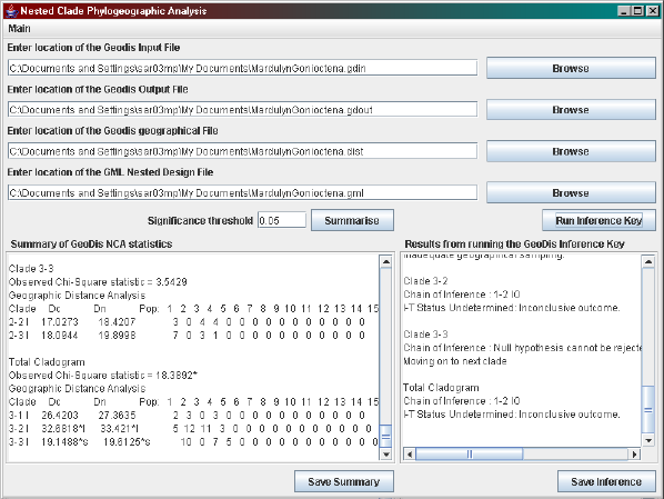
Figure 1.5: A screen shot of the automated inference key.

from the menu or clicking on the Run Inference Key button. Again the

textﬁelds are automatically ﬁlled in if GeoDis was used before. The ﬁles

required are the GeoDis input ﬁle in latitude-longitude format (even if you

are analysing the distance matrix format output from GeoDis), the GeoDis

output (in either latitude-longitude or distance matrix format; the default is

latitude-longitude format), the geographic information and the GML nested

design. By clicking Summarise, a summary of the geodis statistics are cre-

ated. The summary contains the location of the sample sites and the clades

analysed. For each clade analysed the summary marks which distances are

signiﬁcant at the 5% level with a *s or a *l (signiﬁcantly small or large re-

spectively), and also the sample location distribution. Click Run inference

key to run the automated inference key. This will analyse each clade and

give the chain of inference and the ﬁnal outcome, but nothing more. To ﬁnd

out which locations were involved in which inferences, the automated infer-

ence key must be traced manually using the summary ﬁle and the chain of

inference.

Note: GeoDis and the automated inference key may take a long time to run

for large data sets. Please be patient (To be sure an error has not occured it

may be better to run the graphical interface from the command line).

1.5.2 Using the Command Line

By using the command line all the ﬁles described above are written to disk

with the same name stem as the DNA sequence ﬁle (i.e., the NEXUS or

PHYLIP ﬁle), including the analyses with the distance matrix form (these

are tagged with an m before the ﬁle ending e.g., ﬁlename.minfer or ﬁle-

name.mgdin). To execute the software, type on the command line,

java -jar NCPA.jar [dnaSeqFile] [geographicfile]

e.g.,

java -jar NCPA.jar mydataset.nex mydataset.dist

Currently there is no provision to run individual components of the au-

tomated software, and so if you want to conduct a portion of the analysis, it

must be done from the graphical interface (or you can modify the code).

Additional options are available that must be speciﬁed in the given order.

These are the number of permutations that GeoDis uses (default is 10,000),

whether to use the distance matrix format (0 - false, 1 - true), and the signif-

icance threshold to use (default is 0.05). Again this is run on the command

line as follows.

java -jar NCPA.jar [dnaSeqFile] [geographicfile]

[numberOfPermutations] 0 [significanceThreshold]

All ﬁve parameters must be included even if you only wish to change one of

them.

1.5.3 Drawing the nested design

When the nesting software has ﬁnished writing the GeoDis Input ﬁle, you

have the option of saving a summary of the nested design that can be used

to draw it out. The ﬁrst step is to print out a picture of the haplotype tree

from TCS. If you have disjoint networks present TCS will only draw out one

of them, but by using the options from the menu the other networks can be

drawn out separately as well.

The summary of the nesting design contains all the levels of nesting start-

ing from the haplotype network. Each clade, including missing intermediates,

have a corresponding id with which to identify them. By using the labels of

the clades, haplotypes on the picture of the network can be assigned their ids.

Each clade also indicates which clade it was connected to allowing missing

intermediates to be assigned their ids. 1-step and higher level clades also

specify the ids of their subclades, and so the nesting design can be gradually

built up. The subclade ids are speciﬁed in the order of tip clades, interior

clades, and symmetrically stranded clades, which is helpful to determine how

the network was nested.

1.6 A Worked example

The ﬁles in this example are provided in the directory WorkedExample. The

data set provided is a real data set from (Mardulyn 2001). This example uses

the decimal degrees notation, however it is still possible to analyse distances

in GeoDis using the distance matrix format. I explain how this is done at

the appropriate point in the example.

1.6.1 Creating the Geographic information ﬁle

Here is a step by step guide to creating the Geographic information ﬁle.

1. Type the name of the dataset on the ﬁrst line of the ﬁle.

2. On the second line of the ﬁle type the number of populations sampled.

3. On the following lines we then type the information for each sampled

area. The information for each sampled area takes 2 lines. On the

ﬁrst is the population identiﬁcation number (starting at 1) followed by

the name of the area (at least 3 characters long, consisting of letters

and numbers and no white space). The second line of the information

contains the sample size, latitude (in decimal degrees), longitude (in

decimal degrees), and the radius (in Km) of the sample size.

4. After the sampled areas are the unsampled habitable areas. These are

locations where the species is known to be but was unsampled (e.g.

inaccessable areas), or where the area is habitable but the presence

of the species is unknown. This information takes 2 lines for each

area. The ﬁrst line is the population identiﬁcation number (continuing

numbering from the last sampled population), followed by the location

name. The second line is the sample size (which is 0), the latitude

(decimal degrees), the longitude (decimal degrees), and the area radius

(Km).

5. Save the ﬁle as a plain text ﬁle.

See GonioctenaPallida.dist for the example ﬁle.

1.6.2 Creating the Nexus ﬁle

This is a step by step guide to creating the Nexus ﬁle in sequential NEXUS

format.

1. On the ﬁrst line of the ﬁle type #NEXUS and then leave a line.

2. Type begin data;.

3. Following this type dimensions ntax= followed by the number of in-

dividuals in your data set. On the same line type nchar= followed by

the length (number of bases) of the DNA sequences and a semicolon.

(including insertions and missing characters represented by a -and ?

respectively).

4. On the next line type format datatype=dna missing=? gap=-;.

5. Then matrix on the next line.

6. On the next ntax lines enter a label for each of your dna sequences.

Ensure the labels start with a letter and contain only letters or digits

(no whitespace or special characters).

7. At the end of each label type a period followed by the identiﬁcation

number of the population/deme it came from.

8. Follow each label with a space or tab followed by the DNA sequence.

9. Once all the DNA sequences are written, on a new line type ;.

10. On the new line type end;.

11. Then save the ﬁle as a plain text ﬁle with the ﬁle ending .nex.

See GonioctenaPallida.nex for the example ﬁle.

1.6.3 Create the haplotype network

Open ANeCA, and select Main > Run TCS (or the latest version of TCS).

Open the Nexus ﬁle and click Run. At this stage it is your choice how you wish

to resolve loops, if they are present. In this example we follow the steps of

Mardulyn (2001) and resolve loops using two criteria suggested by Crandall

and Templeton (1993): (i) rare haplotypes are more likely to be found at

the tip, and more common haplotypes at interior nodes, of a cladogram;

and (ii) a singleton is more likely to be connected to haplotypes from the

same population than to haplotypes from diﬀerent populations (However,

note warning above about resolving loops). Once we have identiﬁed which

edges/branches and missing intermediate haplotypes need to be removed,

we need to identify the identiﬁcation numbers of the missing intermediate

haplotypes and the haplotypes which the branches connect to in order to

modify the *.graph ﬁle. To do this, visually locate the nodes and edges which

need to be removed. By double-clicking on a node that needs to be removed

or is connected to edge that needs to be removed, a dialog box will popup. In

the title bar will be the words Node x, where xis the identiﬁcation number of

the node. For each node that needs to be removed, record this number. For

each edge that needs to be removed, record both nodes the edge is connected

to. Open the graph ﬁle (in this case GonioctenaPallida.nex.graph) written

by TCS in a plain text editor. Using the search function, search for the string

id xwhere xis the identiﬁcation number of the node to be removed. This

string (id x) will be nested in a node [ ...] block. Delete this block to

remove the node. For each edge to be removed, search for the string source

x. This will identify edge [ ...] blocks where one of the haplotypes is

connected to the edge to be removed. Check that the target ycorresponds

to the other haplotype the edge is connected to. If this is true, then remove

that edge [ ...] block. Repeat this, searching for target xand checking

the source y, to ensure the edges that need to be removed have been. Save

this ﬁle as plain text and then continue with the nesting. Note that although

it is possible to modify visually the haplotype network within TCS, this

cannot be saved as a graph ﬁle. However please take the opportunity to save

a picture of the haplotype network.

1.6.4 Creating the Nested Design

Click Run Nesting Algorithm from TCS or from the menu. Select the

graph ﬁle and the geographic information ﬁle to be used in nesting. Select

the location to save the GeoDis input ﬁle (GonioctenaPallida.gdin) and the

GML nested design (GonioctenaPallida.gml), and then click Create GeoDis

Input. In order to draw and check the nested design you will need to save

the summary of the nested design (GonoictenaPallida.nest), by clicking Save

Nested Design. If you wish to write out the GeoDis input with geographic

information as a distance matrix then specify the name of that ﬁle too (Go-

nioctenaPallida.gdmin).

1.6.5 Drawing the Nested Design

Print out a picture of the haplotype network, and open the nest ﬁle (Go-

nioctenaPallida.nest) in a plain text editor. At the start of the ﬁle will be

a count of the number of edges in the graph and a count of how many are

part of loops. Next is the clade information at Nesting Level: 0, the

haplotype network level. Each Clade: gives the identiﬁcation number of

the haplotype/clade and the label it has on the diagram of the haplotype

network. Clades with label=" " indicate the clade is a missing interme-

diate haplotype. On the diagram of the haplotype network label each node

with the id of the clade, including missing intermediate haplotypes. Labeling

missing intermediate clades may be diﬃcult, however each Clade: shows the

id’s of the clades it is connected to. Using this information it is possible to

deduce which id’s belong to which missing intermediate clades. When all the

haplotypes on the diagram have been labeled, move onto Nesting Level:

1. For each Clade: in this level use SubClades : identify which group of

haplotypes/clades have been nested, and draw the clade onto the diagram.

Mark the clade id next to each clade drawn onto the diagram. Continue

this for each nesting level, checking that clades are connected to the correct

clades.

1.6.6 Performing the Permutation Analysis

Click Run GeoDis, and select the GeoDis input ﬁle to be analysed (either Go-

nioctenaPallida.gdin or GonioctenaPallida.gdmin), and select either Decimal

degrees or User-defined distances depending on the input ﬁle chosen.

Both input ﬁles have been analysed here (GonioctenaPallida.gdout corre-

sponds to the input ﬁle GonioctenaPallida.gdin, and GonioctenaPallida.gdmout

corresponds to the input ﬁle GonioctenaPallida.gdmin).

1.6.7 Applying the Automated Inference Key.

Click Run Inference Key to open the automated inference key. Select the

GeoDis input ﬁle in decimal degree format (GonioctenaPallida.gdin), the

GeoDis output ﬁle from either format (GonioctenaPallida.gdout or Goniocte-

naPallida.gdmout) depending on the statistics you wish to analyse, the ge-

ographical information ﬁle (GonioctenaPallida.dist), and the GML ﬁle (Go-

nioctenaPallida.gml). Then click Summarise and Run Inference Key. This

will summarise the information required to apply the key, and present the

inferences made for each clade using the automated key. To check each in-

ference (GonioctenaPallida.infer for the analysis using decimal degrees, and

GonioctenaPallida.minfer for the analysis using the user-deﬁned distances)

follow the inference key using the summary ﬁle (GonioctenaPallida.gdsum

for the analysis using decimal degrees format, GonioctenaPallida.gdmsum

for the analysis using the user-deﬁned distances). For each clade the sum-

mary ﬁle contains the Dcand Dnvalues and their signiﬁcance, and also

the number of individuals at each location. This allows the user to mark

out a clades geographic boundaries on a map and see which individuals and

locations are involved in an inference.

1.7 Using the software for genotype-phenotype

studies

Nested Clade Analysis was originally designed for genotype-phenotype asso-

ciation studies (although this software was initially designed only for NCPA).

A short guide is provided for using the software for genotype-phenotype as-

sociation studies.

Note: NCA for genotype-phenotype association studies has been superceded

by TreeScan (Posada et al. 2006), in particular to address the multiple testing

problem.

1.7.1 File simpliﬁcations

Although some users may also want to look at geographic associations, the

data speciﬁed for NCPA is more than is required for genotype-phenotype

association studies. If the user is not concerned about geographic location

then the distance information ﬁle need only contain the following few lines.

data_set_name

1 pop_1

1 0.0 0.0 0

The DNA sequence ﬁle normally would include the geographic location

in the label of each individual, however this should be replaced by the index

1 (corresponding to the dummy location in the geographic information ﬁle).

#NEXUS

begin data;

dimensions ntax=11 nchar=38;

format datatype=dna missing=? gap=-;

matrix

mxh1.1 CGTAAAGTTATACCCGAAAGGGAGAGAGTGAGAGTGTG

mxh2.1 CGTAAAGTTTTACCCGAAAGGGAGAGAGTGAGAGTGTG

mxs1.1 CGTAAAGTTATACCCGAAAGGGAGACAGTGAGTGTGTG

mxs2.1 CGTAAAGTTATAGGCGAAAGGGAGACAGTGAGAGTGTG

mxs3.1 CGTAAAGTTTTAGGGGAAAGGGAGACAGTGAGAGTGTG

mxs4.1 CGTAAAGTAATAGCCGAAAGGGAGAGAGTGAGAGTGTG

mxs5.1 CGTAAAGTAATAGCCGAAAGGGAGAGAGTGAGAGTGTG

1.7.2 Using the Graphical Interface

TCS and the automated nesting algorithm is used in the same way as for

NCPA. The only diﬀerence is that an extra ﬁle needs to be saved. Once the

nesting is complete, Click on Save NANOVA Data. This saves the data for

each individual, row by row specifying which clade the individual is in at

each step of the nested design. Note that TCS does not necessarily produce

a haplotype tree, and therefore the graph ﬁle will need to be modiﬁed before

nesting is performed. Often techniques from Coalescent Theory are used to

resolve loops (see Crandall and Templeton (1993) and Pfenninger and Posada

(2002)), or all possible trees are explored.

1.7.3 Using the Command line

To run NCA from the command line type:

java -jar NCPA.jar [dnaSeqFile] [geographicfile] -NANOVA

This causes the software to omit the GeoDis and automated inference key

stages of a normal NCPA run.

1.8 Limitations of Software

Careful consideration needs to be given to regions crossing the +180/-180 line

of longitude. For smaller areas of coverage all the geographic co-ordinates

can be oﬀset such that the area does not lie over the line. This assumes the

species cannot migrate in both directions around the globe to reach locations

either side of the +180/-180 line of longitude.

The automated inference key uses spherical geometry to some extent and

great circle distances between locations, and so is unsuitable for use in situ-

ations in which the distance matrix format in GeoDis would traditionally be

used (e.g., for riparian species).

Lastly, if NCPA appears not to respond then it is likely that an ex-

ception has been thrown. Please run the application from the command

line using java -jar NCPA.jar. Then duplicate the problem and note the

full output from the command line (redirect the output to a ﬁle is you

area able to using java -jar NCPA.jar > output.txt). Then send this

to m.panchal@rdg.ac.uk explaining how the bug occurred, how to replicate

it, the input ﬁles, and the output from the command line.

Note: If the Exception thrown is an OutOfMemoryException you can try

the following solution. Type the following on the command line.

java -Xms256m -Xmx256m -jar NCPA.jar ([additional arguments])

Lastly please consult the developers documentation for further informa-

tion regarding the software, such as the design and implementation details.

1.9 Common Exceptions thrown

We have attempted to make this software as easy to use as possible however

you may encounter certain exceptions while running ANeCA. Most excep-

tions generally note the problem and not the cause. We try to explain the

cause here and how they can be corrected.

OutOfMemoryException This exception indicates that the Java Virtual

Machine (JVM) has used up the memory allocated to this process. To

correct this the amount of memory the JVM uses must be increased,

using the ﬂags -Xms and -Xmx. Type the following on the command

line.

java -Xms256m -Xmx256m -jar NCPA.jar ([additional arguments])

This exception most often occurs in large datasets.

NumberFormatException:”unable to parse number” This indicates that

the geographic information ﬁle has been incorrectly written. Please

check this against the examples given.

1.10 Known Issues

Random exceptions thrown for Mac users Various exceptions have been

thrown running this software on Mac Operating Systems. Often the

exception cannot be reliably replicated and therefore the source of these

seemingly random exceptions is unknown.

Rerunning GeoDis After GeoDis has been run once, under certain cir-

cumstances it does not run again unless the software is restarted. The

circumstances are as yet unknown.

1.11 Frequently Asked Questions

How do I specify the radius of a sample location?

The radius of a sample location in eﬀect describes the approximate movement

range of individuals in that location, and also how far the sampled individuals

were spread out. For example, plants may be sampled from a large area, or

insects may be caught using a single trap but will have traveled to it within a

general radius. This parameter is slightly subjective, however it means that

the sample location covers a certain area rather than a point location.

How do I specify the unsampled locations?

This is done in the same way as for the sampled locations. These locations

are important because you either don’t know if something is there or you

know something is there but haven’t been able to sample it. Here the radius

can be used to describe the approximate size of the unknown area. It is up

to the user to determine how many of these location need to be speciﬁed and

to what granularity.

Why should I include unsampled locations?

If no unsampled locations are included, the software assumes that the species

is absent in that area. This also means the safeguards introduced in the in-

ference key to guard against sampling inadequacies are bypassed.

My study area is too small/large to specify the radius in Km.

What do I do?

NCPA is insensitive to scale, and so geographic co-ordinates can be safely

scaled, translated, and rotated to make radius distances in Km more sensible.

I want to resolve loops. How can I do this?

This software currently oﬀers no option of resolving loops. It is still possi-

ble to resolve them though and continue to use the software. First run the

nesting software on the reticulate network and save the *.nest ﬁle. Print a

picture of the haplotype network, and then use the *.nest ﬁle to assign the

ids to the haplotypes. Use your favoured method of breaking/resolving loops

to determine which edges should be removed. Open up a plain text editor

and open up the *.graph ﬁle automatically written by TCS (should be in the

same directory as your nexus ﬁle). In front of you now will be what looks

nonsensical information. Scroll down until you reach lines that looks like

this.

edge [

source 3

target 5

]

This is a representation of an edge. The numbers after source and target

are the ids of the haplotypes. Find the edges that you want to remove and

delete those four lines corresponding to each edge. For example if there is an

edge that links haplotype with id 4 to a haplotype with id 7 then the code

will look either like this,

edge [

source 4

target 7

]

or like this.

edge [

source 7

target 4

]

By removing these lines you have removed the edge connecting haplotype 4

to haplotype 7. Make sure you save this ﬁle as a plain text ﬁle. Open up the

nesting software and specify the ﬁle you just saved as the TCS graph ﬁle.

You can then continue using the software and nest the modiﬁed haplotype

network.

I have external information that makes some of the clades inte-

rior clades rather than tip clades. How do I change this in the

program?

Changing the tip/interior status of a clade is not currently possible within

the program. Once the GeoDis input ﬁle has been written, it can be changed

manually in a plain text editor. See the GeoDis documentation for further

information regarding the GeoDis input speciﬁcation. Once editing of the

ﬁles is complete, it can be read into GeoDis.

I want to use another haplotype network estimation method in-

stead of Statistical Parsimony. How do I use it with this software?

The software currently nests haplotype networks that have been written in

the GML format that is written as standard by the TCS software. To use a

haplotype network that is produced by another haplotype network estima-

tion method, it must ﬁrst be converted/written in the GML format. Unfor-

tunately there is no software that currently does this, and so the graph ﬁle

must be written by hand.

I have found a bug in the software. Who do I contact?

Please check if it is a bug, and there is no solution mentioned in the manuals

(either this or the TCS or GeoDis manuals). If it is a problem regarding the

correctness of TCS output or GeoDis output, please use the latest version of

the program available on David Posada’s website. If the problem persists,

please contact David Posada. If the problem is to do with the graphical

interface not functioning correctly (in TCS or GeoDis as well), or regarding

the nesting software or the automated inference key, please contact me.

A newer version of TCS/GeoDis is available. Why is it not in-

cluded?

I haven’t had the time to incorporate the new versions yet.

The software has stopped responding. What happened?

If it is a large data set please be patient with the software. If you have made

modiﬁcations to the input ﬁles then it is possible that there may be an error

reading the ﬁles. If you think a problem has occured, close the software, and

run it again from the command line using java -jar NCPA.jar from where

the NCPA.jar ﬁle is located.

1.12 Disclaimer

This software is provided free of charge. This program is distributed in the

hope that it will be useful, but without any warranty; without even the

implied warranty of merchantability or ﬁtness for a particular purpose. The

utmost eﬀort has been made to ensure the program is correct and free from

bugs, however problems may arise.

1.13 Acknowledgements

I would like to thank Mario Pulqu´erio, Oscar Moya, Jesus G´omez-Zurita,

Samantha O’Loughlin, and Gernot Segelbacher, for testing and providing

feedback regarding the software. I’m also grateful to the Biotechnology and

Biological Sciences Research Council for funding my PhD during which this

software was developed. I would also like to thank Keith Crandall, David

Posada, and an anonymous reviewer for comments and suggestions on the

software and its documentation.

Bibliography

K. A. Crandall. Multiple interspecies transmissions of human and simian

t-cell leukemia/lymphoma virus type i sequences. Molecular Biology and

Evolution, 13(1):115–131, 1996.

K. A. Crandall and A. R. Templeton. Empirical tests of some predictions

from coalescent theory with applications to intraspeciﬁc phylogeny recon-

struction. Genetics, 134(3):959–969, 1993.

L. L. Knowles and W. P. Maddison. Statistical phylogeography. Molecular

Ecology, 11(12):2623–2635, 2002.

P. Mardulyn. Phylogeography of the vosges mountains populations of go-

nioctena pallida (coleoptera : Chrysomelidae): a nested clade analysis of

mitochondrial dna haplotypes. Molecular Ecology, 10(7):1751–1763, 2001.

M. Pfenninger and D. Posada. Phylogeographic history of the land snail can-

didula unifasciata (helicellinae, stylommatophora): Fragmentation, corri-

dor migration, and secondary contact. Evolution, 56(9):1776–1788, 2002.

D. Posada, K. A. Crandall, and A. R. Templeton. Geodis: a program for

the cladistic nested analysis of the geographical distribution of genetic

haplotypes. Molecular Ecology, 9(4):487–488, 2000.

D. Posada, K. A. Crandall, and A. R. Templeton. Nested clade analysis

statistics. Molecular Ecology Notes, 0(0):Published before print., 2006.

A. R. Templeton. Statistical phylogeography: methods of evaluating and

minimizing inference errors. Molecular Ecology, 13(4):789–809, 2004.

A. R. Templeton and C. F. Sing. A cladistic analysis of phenotypic associ-

ations with haplotypes inferred from restriction endonuclease mapping .4.

nested analyses with cladogram uncertainty and recombination. Genetics,

134(2):659–669, 1993.

A. R. Templeton, E. Boerwinkle, and C. F. Sing. A cladistic analysis of

phenotypic associations with haplotypes inferred from restriction endonu-

clease mapping .1. basic theory and an analysis of alcohol dehydrogenase

activity in drosophila. Genetics, 117(2):343–351, 1987.

A. R. Templeton, E. Routman, and C. A. Phillips. Separating population

structure from population history : a cladistic analysis of the geographi-

cal distribution of mitochondrial dna haplotypes in the tiger salamander,

ambystoma tigrinum. Genetics, 140(2):767–782, 1995.

A. R. Templeton, T. Maxwell, D. Posada, J. H. Stengard, E. Boerwinkle,

and C. F. Sing. Tree scanning: A method for using haplotype trees in

phenotype/genotype association studies. Genetics, 169:441–453, 2005.

A.-B. Zhang, S. Tan, and T. Sota. Autoinfer 1.0: a computer program to

infer biogeographical events automatically. Molecular Ecology Notes, 6:

597–599, 2006.

NCPA User Guide

Navigation menu

Versions of this User Manual:

Views

Navigation