PDAnalyzer Software_engl, V0030112x NEW Manual PDAnalyze Software, V0030112
User Manual:
Open the PDF directly: View PDF ![]() .
.
Page Count: 35

User manual
PDAnalyze Software
F o r u s e w i t h t h e :
Prom o® serie s
Fida s ® s erie s
UF-C PC
U-S M P S
U-R AN GE
Phone +49 (0)721 96213-0
Fax +49 (0)721 96213-33
mail@palas.de
www.palas.de
PALAS GmbH
Partikel- und Lasermesstechnik
Greschbachstrasse 3b
76229 Karlsruhe

MANUAL PDANALYZE SOFTWARE
PALAS® GMBH, VERSION V0030112
2
Index:
INDEX: ............................................................................................................................................. 2
1 START OF THE PDANALYZE SOFTWARE ................................................................................ 4
2 MENU-ITEM: FILES .................................................................................................................. 4
2.1 Noticeable differences when importing data from the U-SMPS, U-RANGE ............. 6
3 MENU-ITEM: OVERALL DATA ................................................................................................. 7
3.1 Particle size time chart: ............................................................................................. 7
3.2 Weather station – time chart .................................................................................... 9
4 MENU-ITEM: SELECTED INTERVALS ....................................................................... 11
4.1 particle size distribution/statistics: ......................................................................... 11
4.1.1 particle size distribution/statistics: differential ............................................. 13
4.1.2 particle size distribution/statistics: cumulative ............................................. 14
4.1.3 particle size distribution/statistics: statistics .................................................. 15
4.1.4 particle size distribution/statistics: table ........................................................ 16
4.2 „particle size distribution color plot (sensor #1)“ .................................................... 17
4.3 fractional efficiency: ................................................................................................ 17
4.3.1 Fractional efficiency - Timechart ....................................................................... 18
4.3.2 Fractional efficiency – Timechart table............................................................. 19
4.3.3 Fractional efficiency - efficiency ..................................................................... 20
5 PROMO, FIDAS .................................................................................................................. 21
5.1 „Fine dust –time chart“ ........................................................................................... 21
5.1.1 “atmospheric PM fine dust” .............................................................................. 22
5.1.2 “classic PM fine dust” ........................................................................................ 23
5.1.3 “health related fine dust” ................................................................................. 23
5.2 „absolut filter system (sensor #1)“........................................................................... 24
5.3 “air sensor – time chart (sensor #1)” ....................................................................... 25
5.4 Operating parameters – time chart ......................................................................... 26
5.5 “heating units –time chart (sensor #1)” ................................................................... 27
5.6 “settings (sensor #1)“................................................................................................ 28
5.7 “raw data distribution (sensor #1)“ ......................................................................... 29
6 MENU-ITEM: U-SMPS/U-RANGE .................................................................................. 30
6.1 “UP-/DOWN-scan comparison (sensor #1)” ............................................................ 30
6.2 “settings (sensor #1)”................................................................................................ 31
6.3 “operating parameters (sensor #1)” ........................................................................ 31
7 MENU-ITEM: MISCELLANEOUS ................................................................................. 33
7.1 Comments ................................................................................................................. 33
7.2 Annotations .............................................................................................................. 34
8 APPENDIX .............................................................................................................................. 35

MANUAL PDANALYZE SOFTWARE
PALAS® GMBH, VERSION V0030112
3
8.1 Steps to display a particle size distribution that was measured with the U-SMPS 35
8.2 Steps to display PM values vs. time measured with the Fidas® ............................. 35
MANUAL PDANALYZE SOFTWARE
PALAS® GMBH, VERSION V0030112
4
1 Start of the PDAnalyze Software
Please start Promo®_Logger.exe to open the data evaluation software.
PDAnalyze is the designated data evaluation software for most of the Palas® particle
measurement systems, i.e.
Promo®, Fidas® optical aerosol spectrometers
UF-CPC universal fluid condensation particle counter for nanoparticles
U-SMPS universal scanning mobility particle sizer
U-RANGE combination of U-SMPS with Fidas®
The PDAnalyzer user interface with the following submenus is first visible on the screen:
1 „files“
2 „overall data“
3 „selected intervals“
4 „PROMO, FIDAS
5 „U–SMPS/U-RANGE“
6 „miscellaneous“
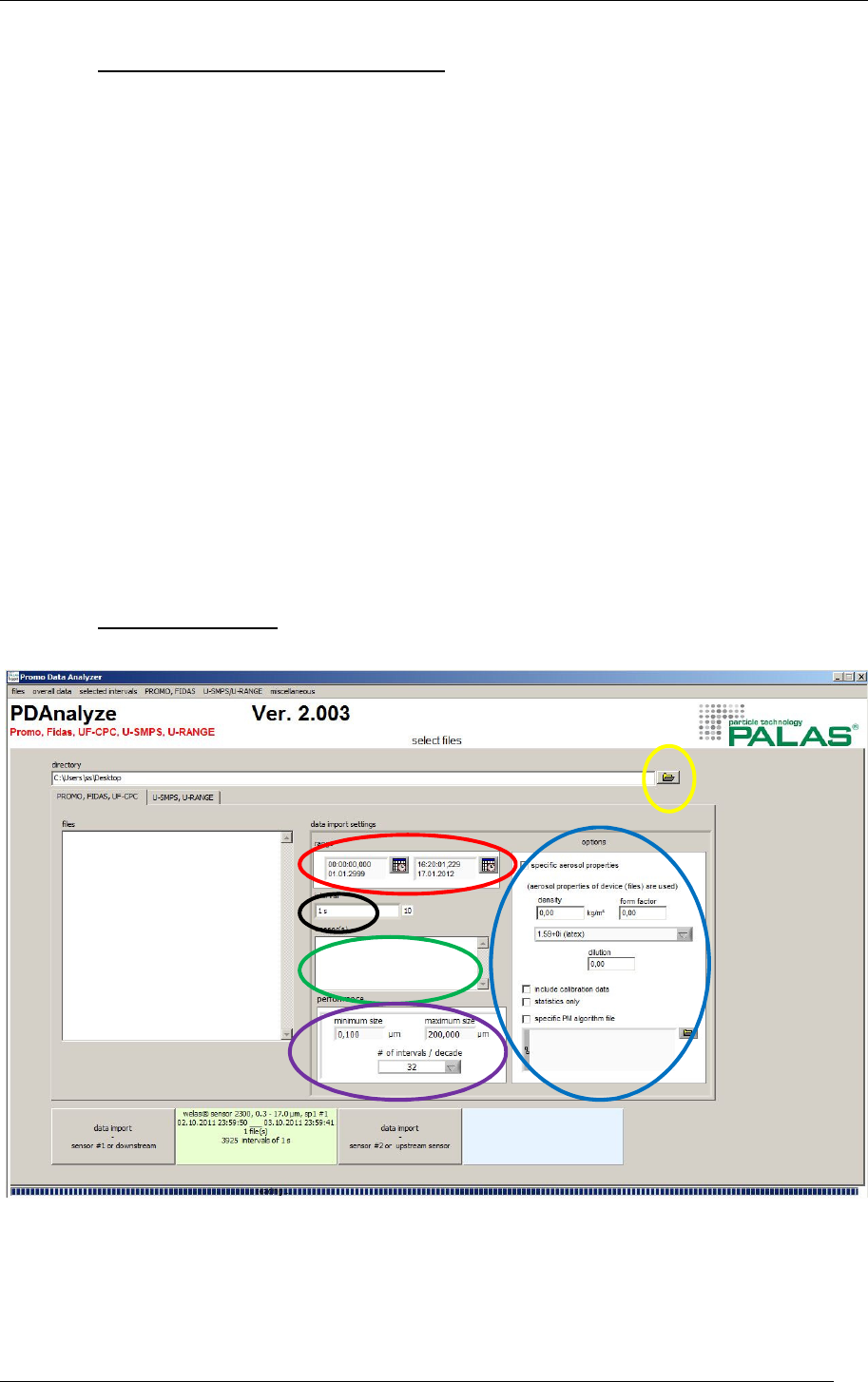
2 Menu-Item: files
Figure 1: Display of the submenu „files“
When loading data files into the software please pay attention that the appropriate tab
“PROMO, FIDAS, UF-CPC” or “U-SMPS, U-RANGE” is selected.
MANUAL PDANALYZE SOFTWARE
PALAS® GMBH, VERSION V0030112
5
For the loading of one or several files the yellow file symbols (yellow circle) are used.
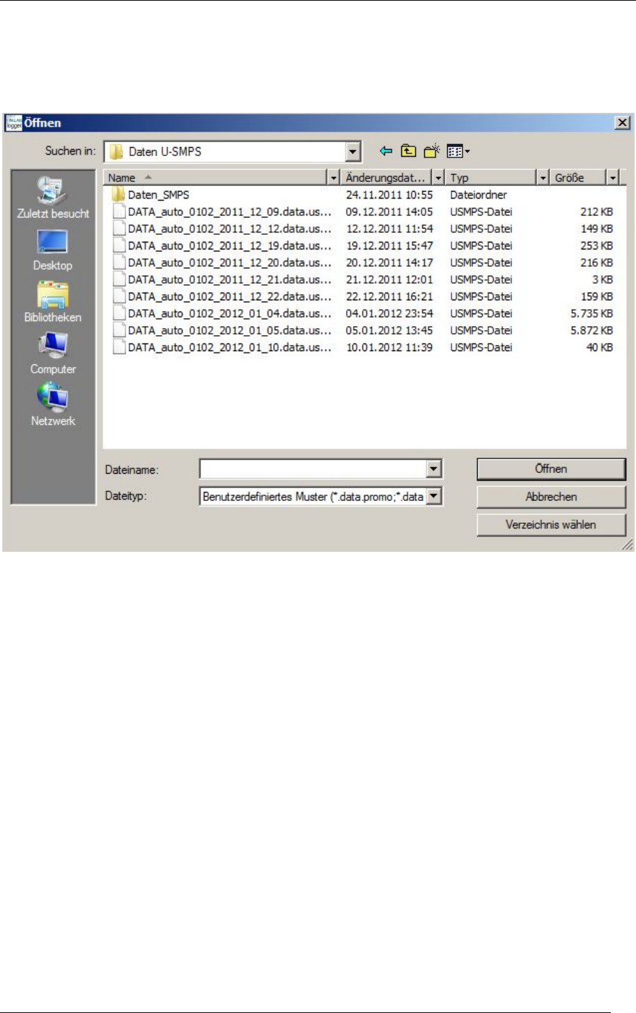
By selecting the yellow file symbol you open a window in which you need to select the path
to the folder in which the data files are stored.
Figure 1a: Selecting the folder in which the data files are stored
Please close this window by selecting “select folder” (bottom choice, called “Verzeichnis
wählen” in figure 1a). The data files in this folder will then be automatically shown in the
software (red circle in figure 2)
The currently used type of sensor is mentioned under sensor (green circle in figure 1).
Whenever it is measured with two sensors in an alternating way only the data of the
selected sensor are displayed.
With specific range distribution (red circle) a defined record can be analyzed more precisely.
Therefore the corresponding entry of time and date must be made. A further possibility can
be found in „selected intervals“ (see item 3).
With used aerosol properties (blue circle) the required data for concentration and shape
factor can be changed for the calculation of the mass concentration.
The data are saved during a measurement with a temporal resolution of 1 s, 10 s, 60 s or
120 s. With interval (black circle) these data can be displayed in correspondingly larger
intervals, e. g. 600 s.
MANUAL PDANALYZE SOFTWARE
PALAS® GMBH, VERSION V0030112
6
With performance the minimal and maximal value for the display and additionally the
resolution, e.g. 32 channels per decade can be selected. (purple circle).
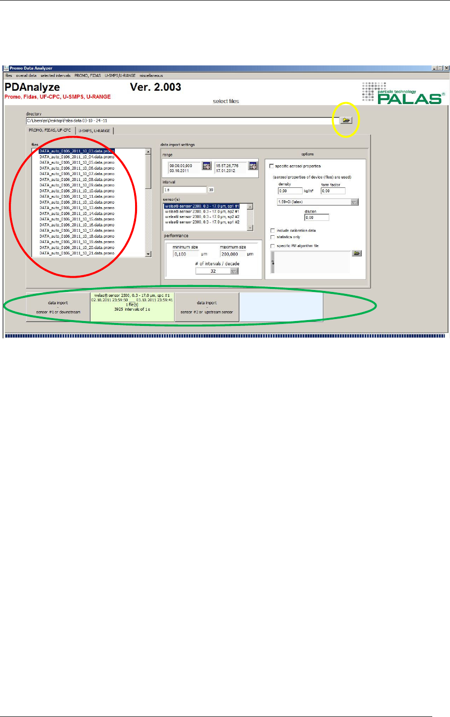
Figure 2: Loading of several data files
After selecting the yellow path symbol (yellow circle) all data files in this path automatically
get displayed in window below (red circle). The corresponding data can also be available on
a network drive. Via a click on the mouse button the correspondent data sets can be
selected.
With the button data import sensor # 1 or downstream data import sensor # 2 or upstream
the data are transferred to the evaluation software and displayed with a time stamp on the
left side. (green circle)
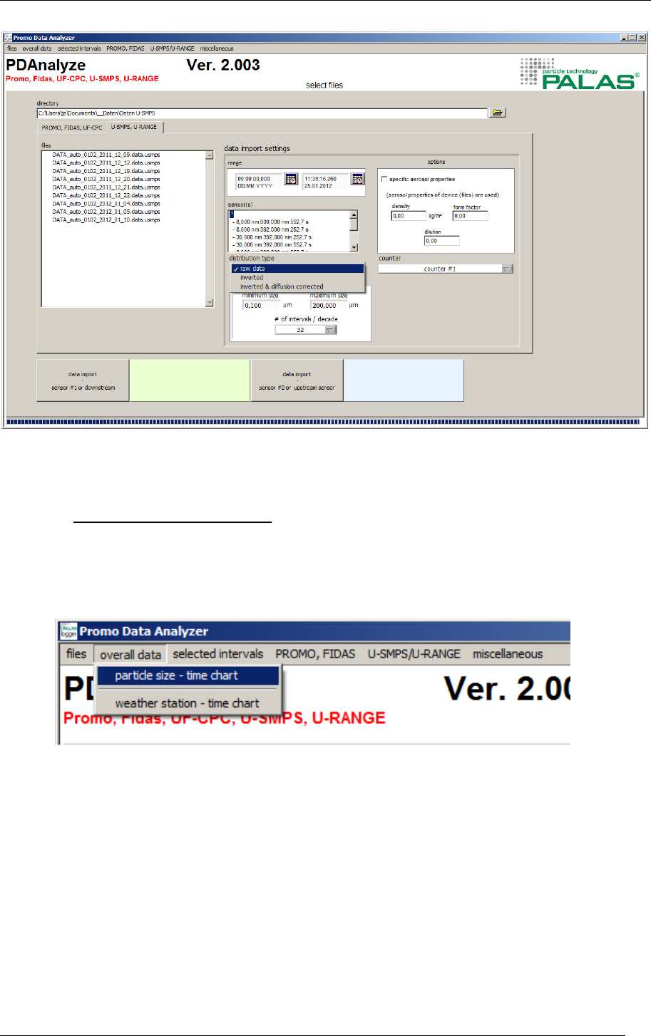
2.1 Noticeable differences when importing data from the U-SMPS, U-RANGE
Under “distribution type” you can select whether you want to analyse and display the raw
data, the inverted data or the inverted & diffusion corrected data (figure 2a). You need to
select this before importing the data to e.g. sensor #1 and this is then used throughout the
following description.
It is also possible to import for example the inverted and diffusion corrected data under
sensor #1 and the raw data under sensor #2. In the now following analysis and display of the
data it is then possible to switch quickly between raw and inverted data.
MANUAL PDANALYZE SOFTWARE
PALAS® GMBH, VERSION V0030112
7
Figure 2a: Selecting the data (raw, inverted, etc.) for the following evaluation
3 Menu-Item: overall data
The menu item „overall data“ has two submenu items:
• „particle size - time chart“
• „weather station - time chart“
Figure 3: „overall data“
3.1 Particle size time chart:
Please select in the menu „overall data“ the submenu „particle size – time chart“.
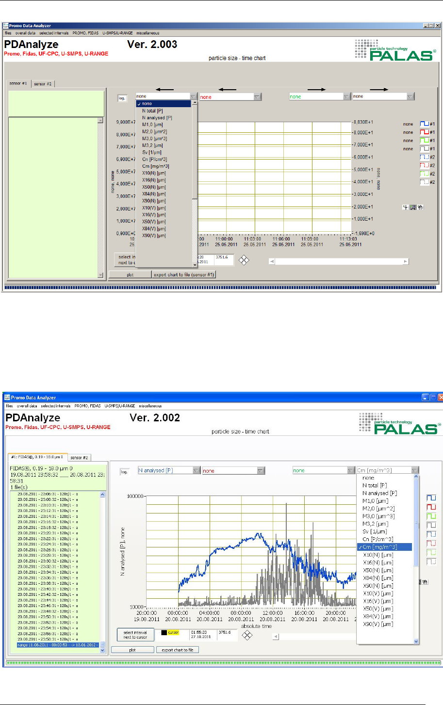
When starting the submenu „particle size –time chart“ the display of „overall data particle
size - time chart“ appears. In this display different data and statistical displays can be
compared against each other.
MANUAL PDANALYZE SOFTWARE
PALAS® GMBH, VERSION V0030112
8
Figure 4: Display“overall data: particle size - time chart” without selection
The two selection options on the left refer to the left vertical axis, the two on the right refer
to an additional right vertical axis if a selection is made.
All selection options are the same and include for example total number N analyzed and
total mass concentration Cm. (see figure 5)
Figure 5: Selection N analyzed and Cm at „overall data“
MANUAL PDANALYZE SOFTWARE
PALAS® GMBH, VERSION V0030112
9
It is possible to display other statistical values (see above). With the button Plot the two
chosen displays are assumed into the chart.
With the button export chart to file those displayed distributions can be saved as txt-file for
further import into software, e. g. Excel.
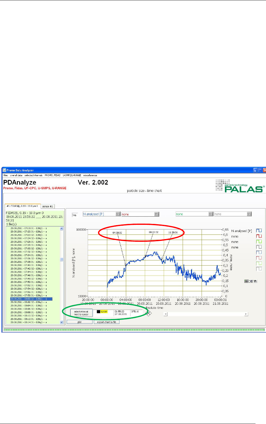
The devices remark the time of filter in and filter out with arrows in the chart automatically
as the button show annotations is marked and the button plot will be used (see red circle in
figure 6).
If one or more distributions will be marked on the left side below distribution those
distributions will be also highlighted in the chart as soon as the button show annotations are
marked and the button plot will be used (see 5. Menu-Item: miscellaneous).
With the cursor display also a specific time can be highlighted in the chart. Therefore the
time and the date have to be inserted (see green circle in figure 6).
Figure 6: Display of several points at „overall data: particle size – time chart“ view
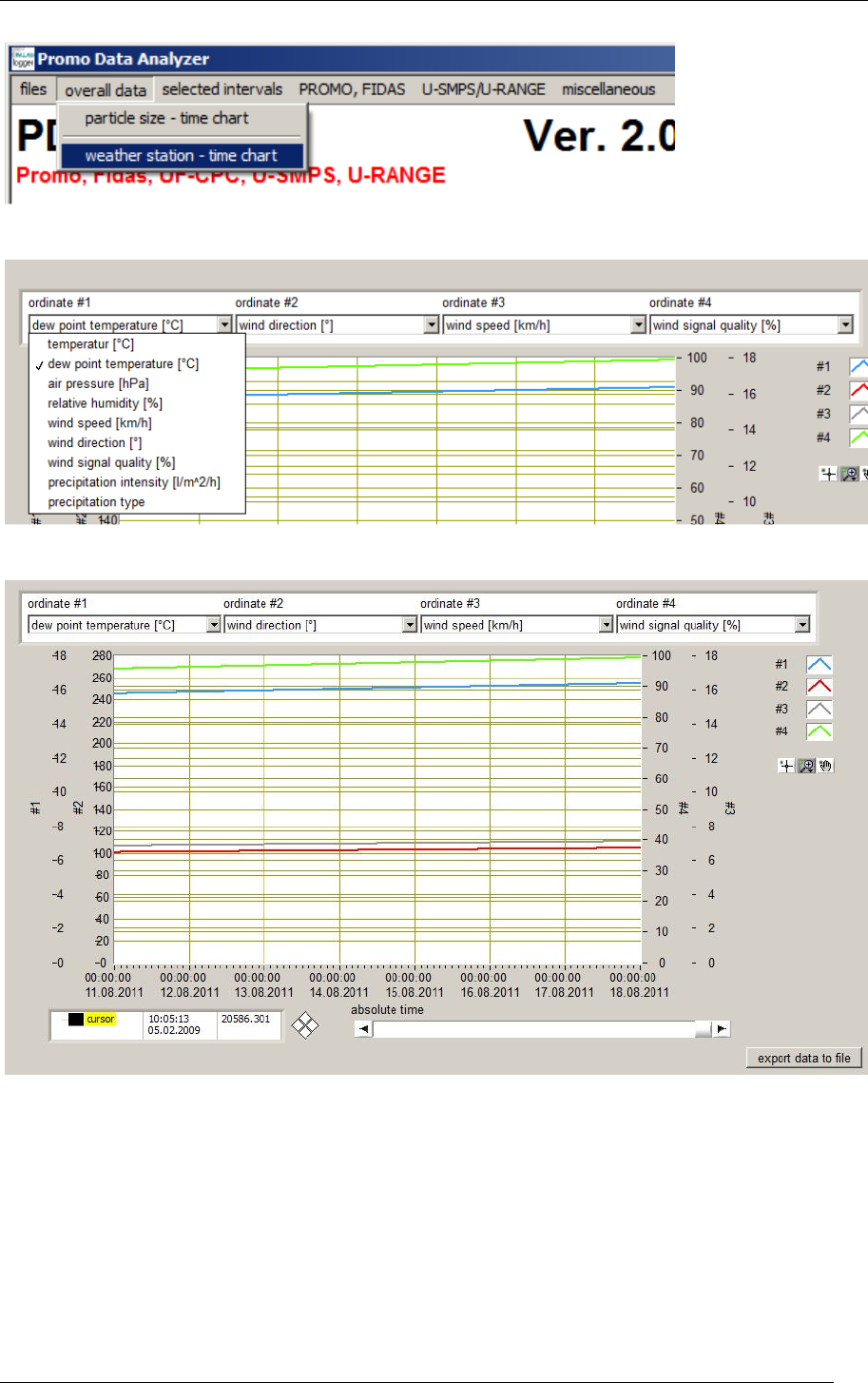
3.2 Weather station – time chart
When starting the submenu „overall data: weather station – time chart“ the values of the
weather station will be displayed, e.g. precipitation intensity.
MANUAL PDANALYZE SOFTWARE
PALAS® GMBH, VERSION V0030112
10
Bild 7: “overall data: weather station -time chart”
Figure 8: “overall data: weather station -time chart” selection of possible parameters
Figure 9: „overall data: weather station - time chart“ Display of several parameters
With the blue curve the dew point temperature in °C is displayed.
With the red curve the wind direction in ° is displayed.
With the gray curve the wind speed in km/h is displayed.
With the green curve the wind signal quality in % is displayed.
MANUAL PDANALYZE SOFTWARE
PALAS® GMBH, VERSION V0030112
11
4 Menu-Item: selected intervals
The menue item „selected intervals“ offers three sub-menues:
• „particle size distribution/statistics“
• „particle size distribution color plot (sensor #1)“
• “fractional efficiency”
In opposition to the display „overall data“, the menu-point „selected intervals“ displays a
distribution in a given time interval, the comparison of serveral marked distributions or of a
single distribution.
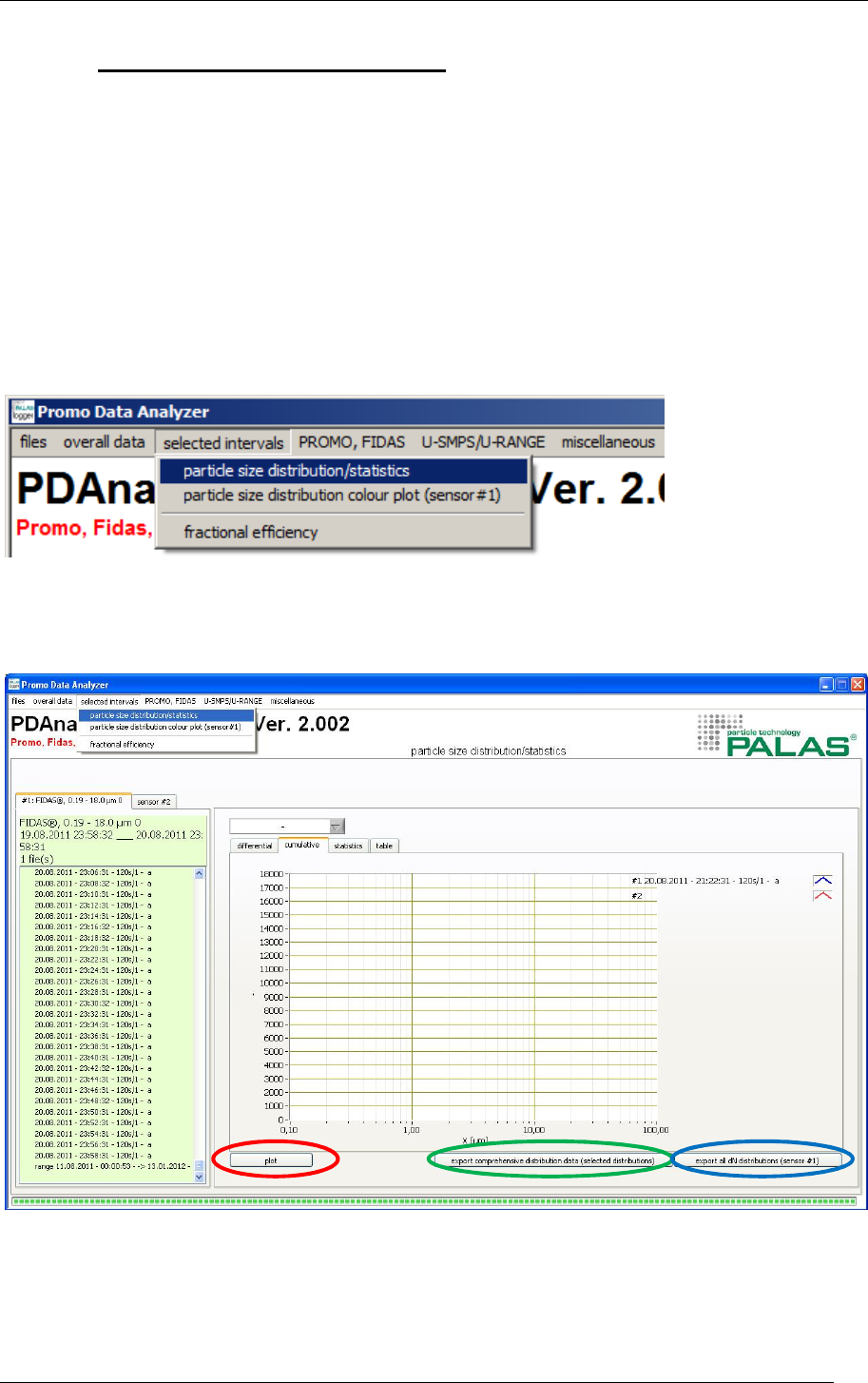
Figure10: “selected intervals: particle size distribution/statistics”
4.1 particle size distribution/statistics:
Figure11: Start screen of the menu item „selected intervals – particle size
distribution/statistics“
In the following examples three distributions were marked out of two whole days’
distribution with a time resolution of 600s and were compared against each other.
MANUAL PDANALYZE SOFTWARE
PALAS® GMBH, VERSION V0030112
12
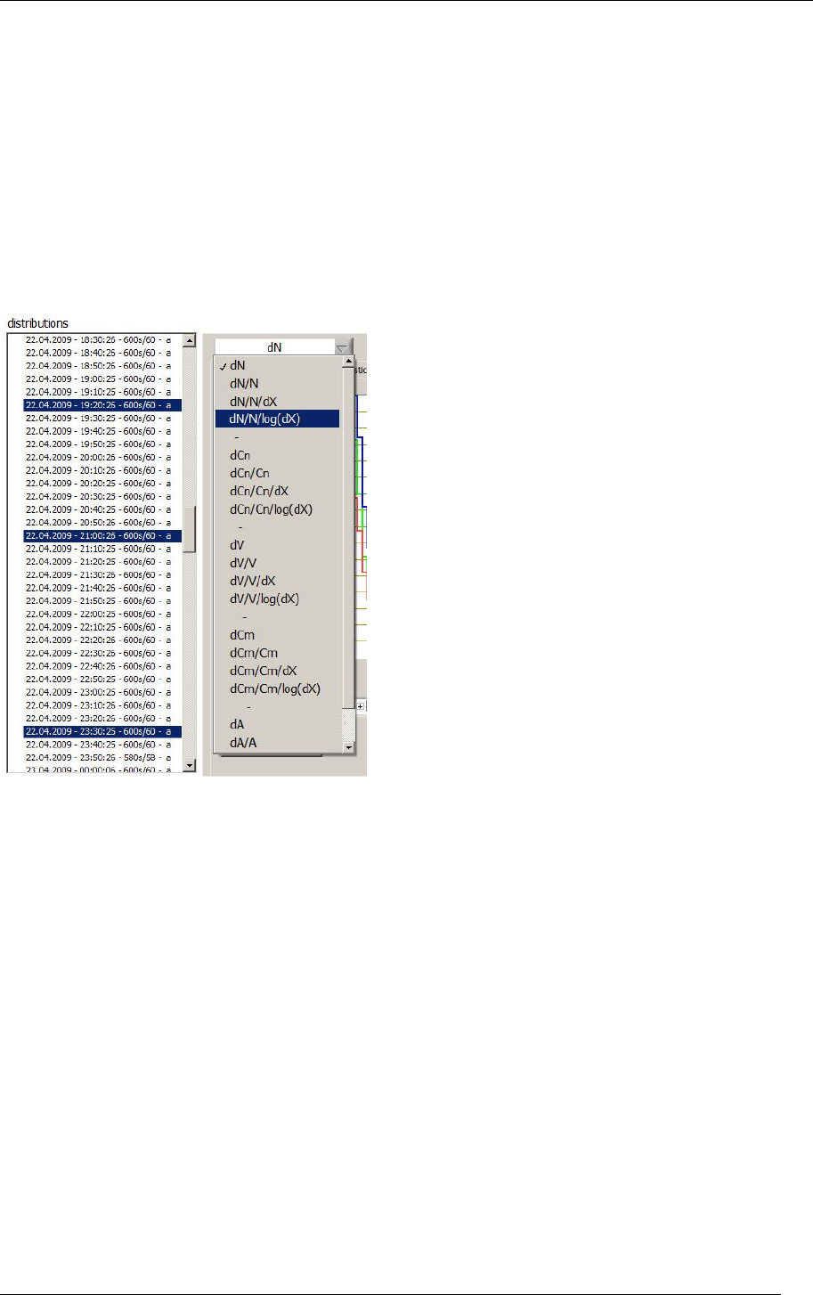
Therefore the three corresponding files were marked with control key on the left side under
distribution. After this, the kind of display has to be chosen, e. g. dN (Particle number) (see
figure 11) and the plot-Taste has to be activated (red circle).
With the button export comprehensive distribution data (selected distribution) (green
circle) or with the button export all dN distributions (sensor #1) (blue circle) the values are
save das a txt-file and can be used with other programs, e.g. Excel.
Figure 12: Drop down menu with different kinds of display for „selected intervals –particle
size distributions/statistics“
Within the submenu „selected intervals: particle size distributions/statistics“ it is possible
to chose between two graphical displays:
• „differential“
• „cumulative“
As well as two additional kind of displays of statistics and table:
• „statistics“
• „table“
The selected files will be shown with the corresponding color on the legend on the right side
(blue circle). With the button plot-button (red circle) the marked files will be assumed and
compared against each other and shown in a chart.
MANUAL PDANALYZE SOFTWARE
PALAS® GMBH, VERSION V0030112
13
The previous selected kind of display of the data, e. g. dN (green circle) will then be retained
for the graphical display („differential“, „cumulative“, „statistics” and “table”). The kind of
display can always be changed in the pull down menu (see figure 11) and will be effective by
using the plot-button.
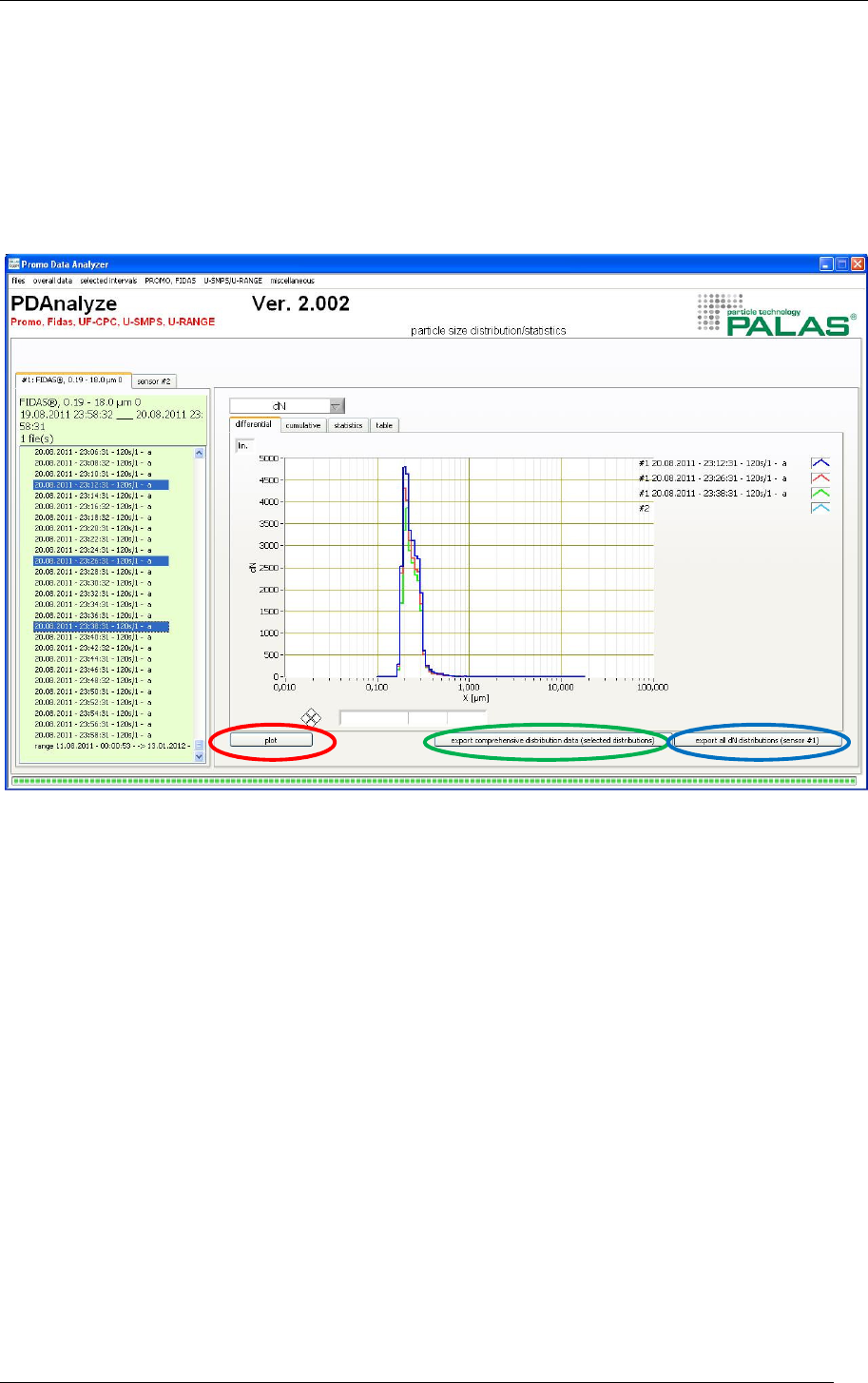
4.1.1 particle size distribution/statistics: differential
Figure 13: „differential“ display of the comparison of three distributions
With the button export comprehensive distribution data (selected distribution) (green
circle) or with the button export all dN distributions (sensor #1) (blue circle) the values are
save das a txt-file and can be used with other programs, e.g. Excel.
MANUAL PDANALYZE SOFTWARE
PALAS® GMBH, VERSION V0030112
14
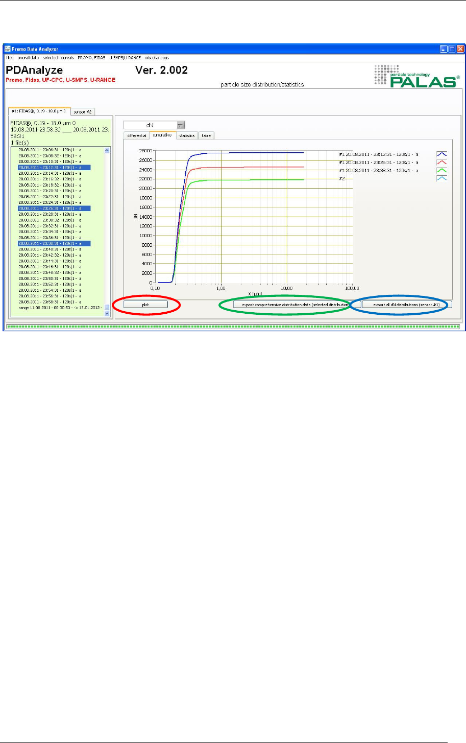
4.1.2 particle size distribution/statistics: cumulative
Figure 14: „cumulative“ display of the comparison of three distributions
With the button export comprehensive distribution data (selected distribution) (green
circle) or with the button export all dN distributions (sensor #1) (blue circle) the values are
save das a txt-file and can be used with other programs, e.g. Excel.
MANUAL PDANALYZE SOFTWARE
PALAS® GMBH, VERSION V0030112
15
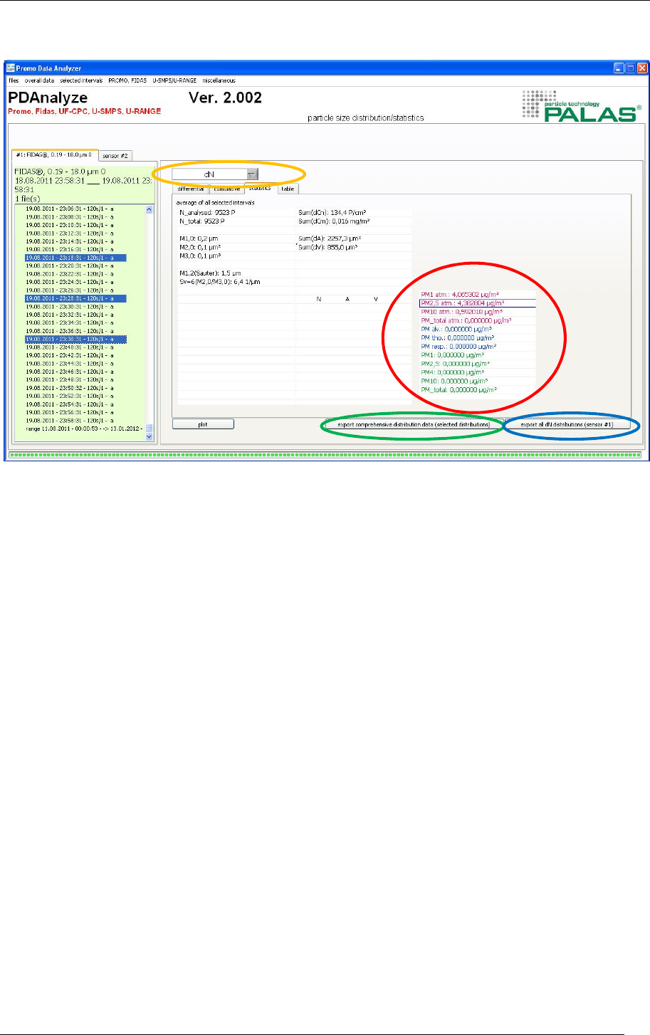
4.1.3 particle size distribution/statistics: statistics
Figure 15: „statistic“ display of the comparison of three distributions
Within the statistics always the mean value of the selected files is displayed. If you measure
with the Fidas® device the PM values will be also shown (red circle).
Always the statistical values of the selected distribution are sown. The kind of display in the
above figure is dN; it can be changed at any time (see yellow circle).
With the button export comprehensive distribution data (selected distribution) (green
circle) or with the button export all dN distributions (sensor #1) (blue circle) the values are
save das a txt-file and can be used with other programs, e.g. Excel.
MANUAL PDANALYZE SOFTWARE
PALAS® GMBH, VERSION V0030112
16
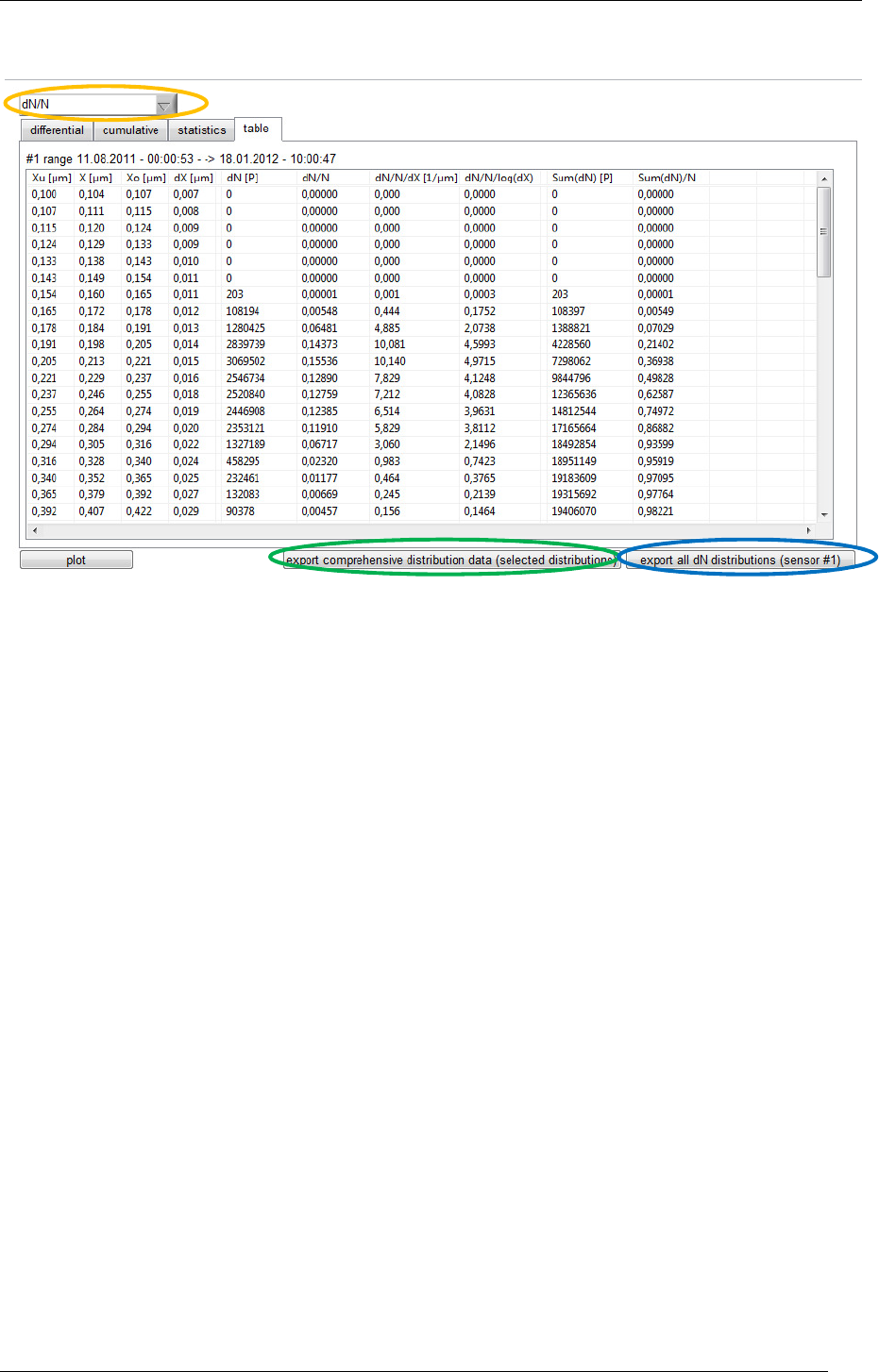
4.1.4 particle size distribution/statistics: table
Figure 16 „table“ display of the comparison of three distributions
With this kind of display always the mean value of the selected files will be sown. The table
of the selected kind of display will be sown. In this case it is dN/N; it can be changed at any
time (see yellow circle).
With the button export comprehensive distribution data (selected distribution) (green
circle) or with the button export all dN distributions (sensor #1) (blue circle) the values are
save das a txt-file and can be used with other programs, e.g. Excel.
MANUAL PDANALYZE SOFTWARE
PALAS® GMBH, VERSION V0030112
17
4.2 „particle size distribution color plot (sensor #1)“
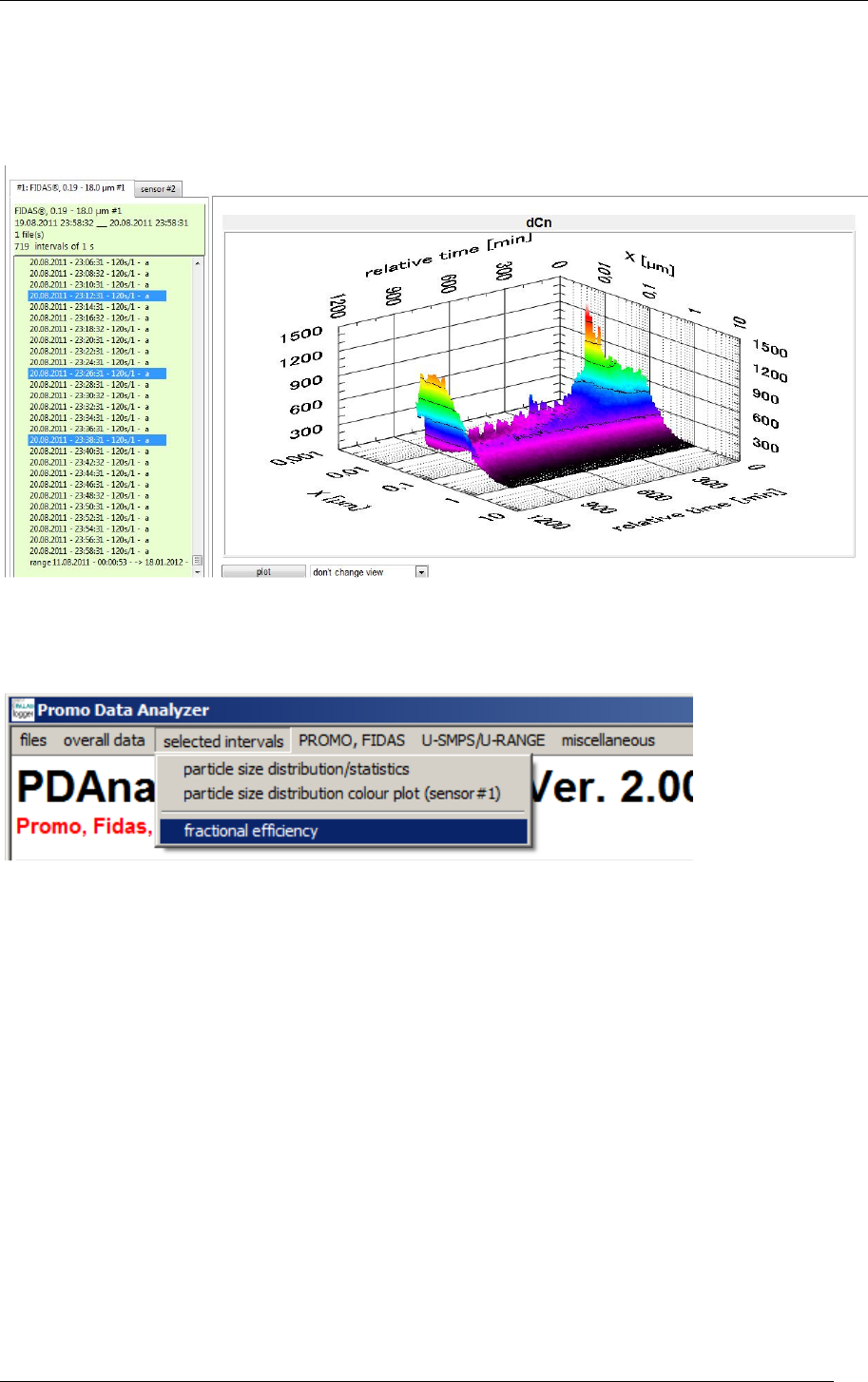
The menu item „particle size distribution color plot (sensor #1)“ shows the 3D graph of the
distribution:
Figure 17: „selected intervals: particle size distribution – color plot (sensor #1)“
4.3 fractional efficiency:
Figure 18: „selected intervals: fractional efficiency“
The menu item „selected intervals: fractional efficiency“ display the fractional efficiency
curve (the efficiency over the particle size).
Selection between:
Fractional efficiency - Timechart
Fractional efficiency – Timechart table
Fractional efficiency - efficiency
MANUAL PDANALYZE SOFTWARE
PALAS® GMBH, VERSION V0030112
18
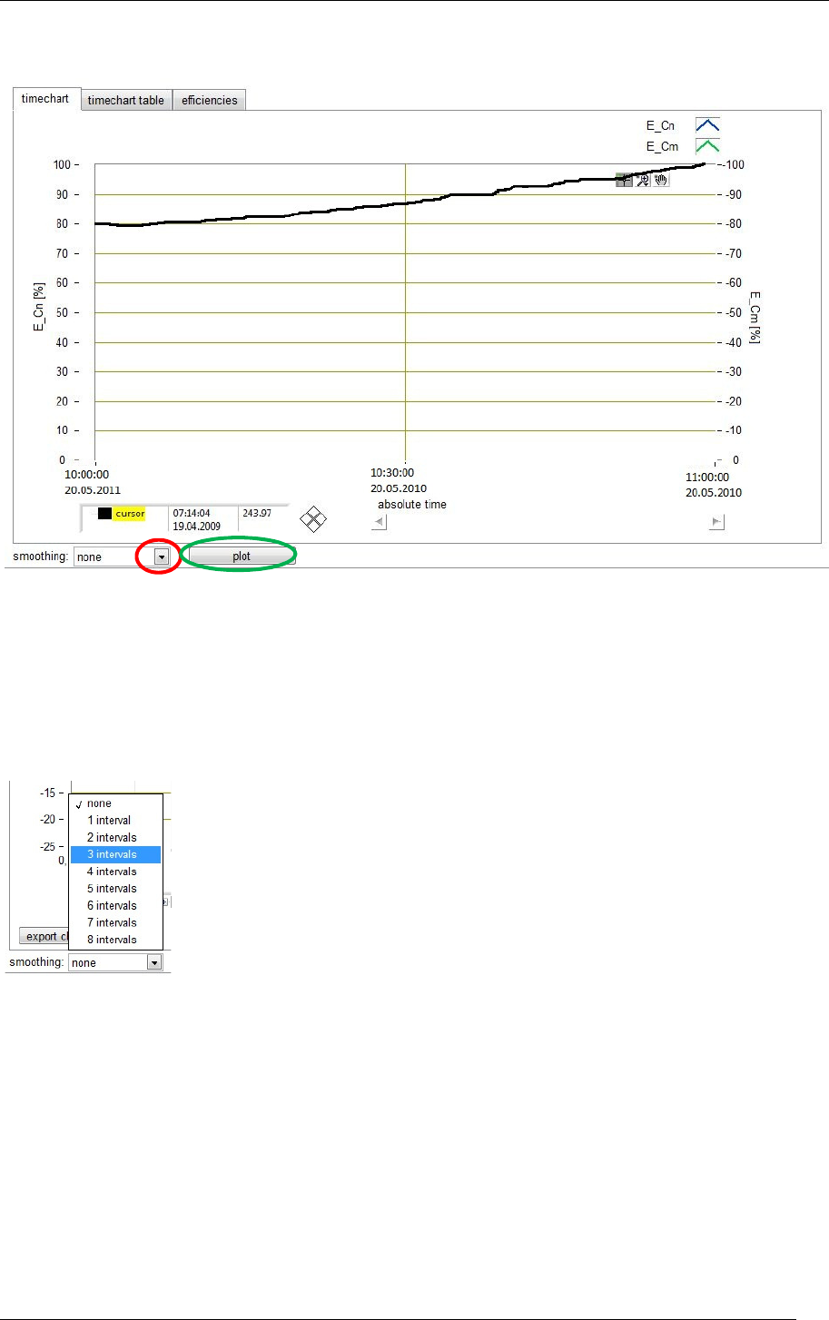
4.3.1 Fractional efficiency - Timechart
Figure 19: Display of the „fractional efficiency – time chart“
With the Plot-button (green circle) the fractional efficiency of the previous selected files will
be displayed in a time chart.
With the smoothing dropdown menu (red circle), the smoothing factor can be selected (see
figure 20).
Figure 20: Smoothing factor selection
MANUAL PDANALYZE SOFTWARE
PALAS® GMBH, VERSION V0030112
19
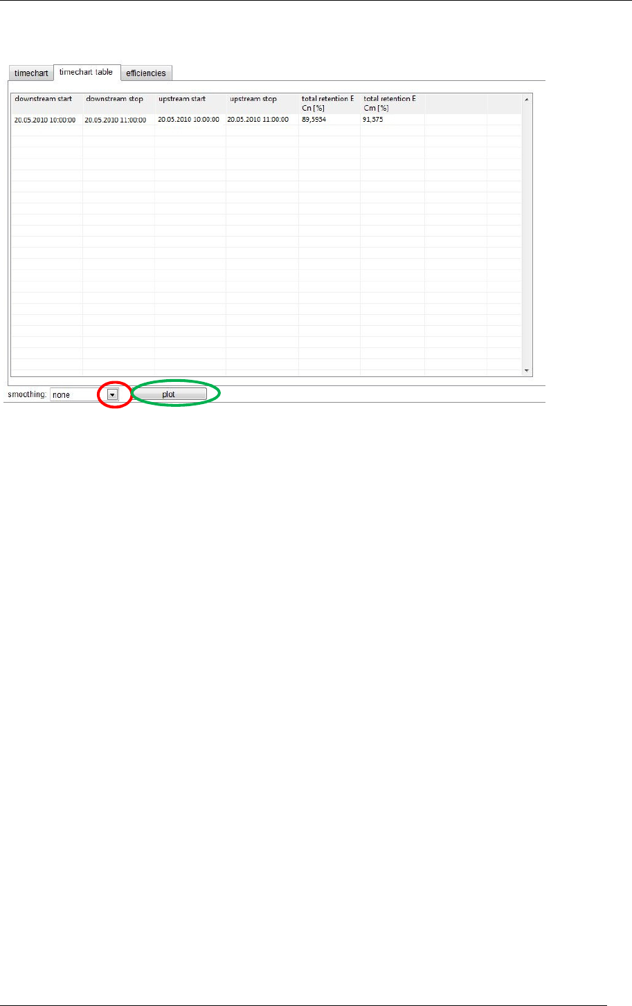
4.3.2 Fractional efficiency – Timechart table
Figure 21: Display of the „fractional efficiency – time chart table“
With the Plot-button (green circle) the fractional efficiency table of the previous selected
files will be displayed in a time chart.
With the smoothing dropdown menu (red circle), the smoothing factor can be selected (see
figure 20).
MANUAL PDANALYZE SOFTWARE
PALAS® GMBH, VERSION V0030112
20
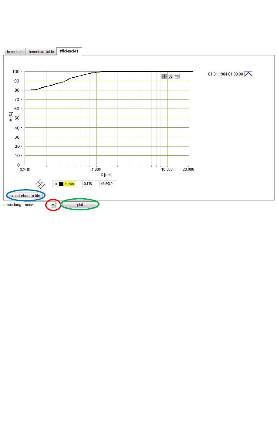
4.3.3 Fractional efficiency - efficiency
Figure 22: Display of the „fractional efficiency – efficiency“
With the Plot-button (green circle) the fractional efficiency of the previous selected files will
be displayed.
With the smoothing dropdown menu (red circle), the smoothing factor can be selected (see
figure 20).
With the button export chart to file the data are saved as a txt-file and can be used with
other programs, e.g. Excel.
MANUAL PDANALYZE SOFTWARE
PALAS® GMBH, VERSION V0030112
21
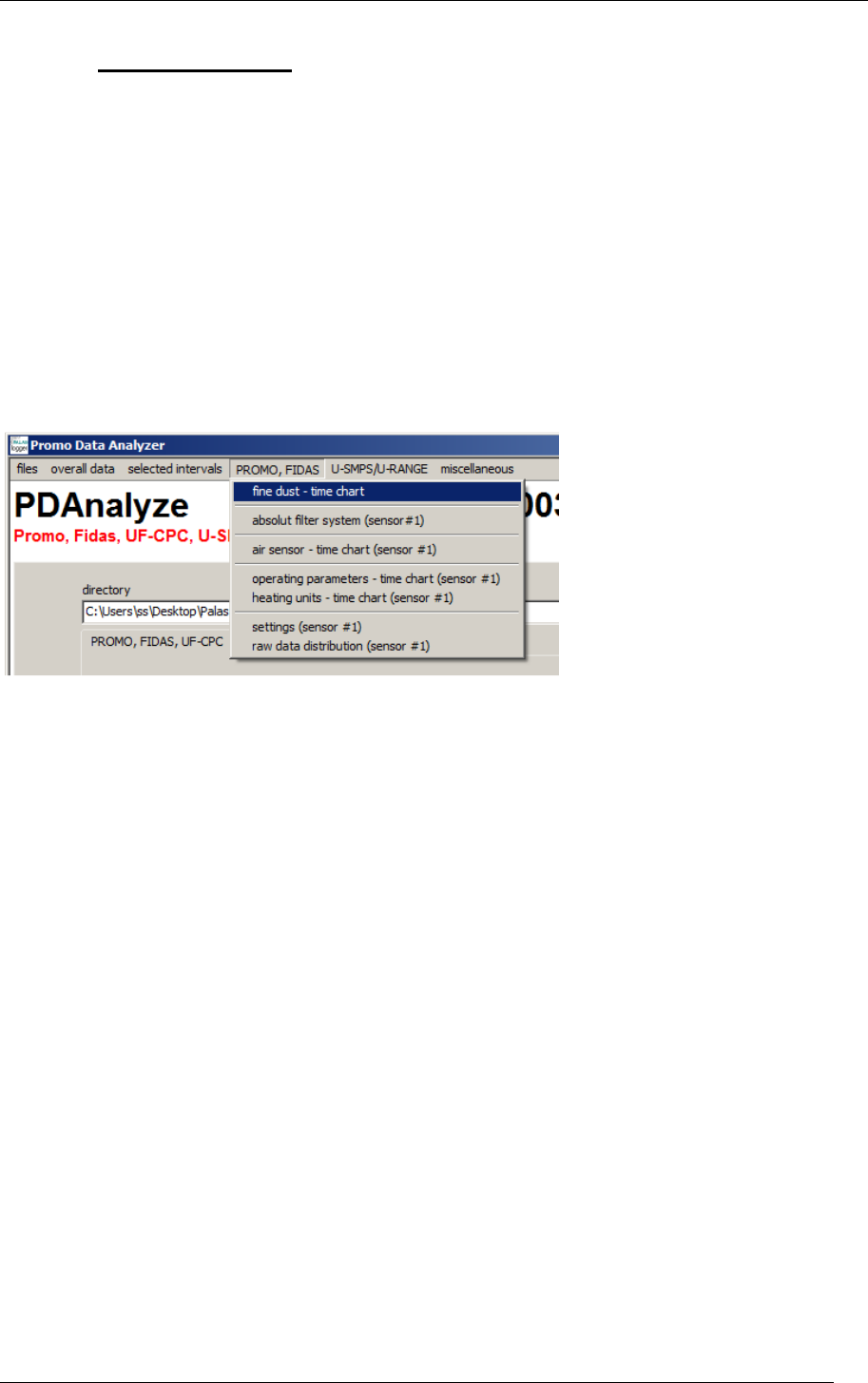
5 PROMO, FIDAS
“Promo, Fidas” offers the following sub-menus:
• „Fine dust –time chart“
• „absolut filter system (sensor #1)“
• “air sensor – time chart (sensor #1)”
• “operating parameters – time chart (sensor #1)”
• “heating units –time chart (sensor #1)”
• “settings (sensor #1)“
• “raw data distribution (sensor #1)“
5.1 „Fine dust –time chart“
The user gets the display of the PM1, PM2,5 and PM10 values over the time.
Figure 23: Promo, Fidas “fine dust – time chart”
Possibility to select between three different kinds of displays:
• “atmospheric PM fine dust”
• “classic PM fine dust”
• “health related fine dust”
The point of time of the deposit of the filter and the taking out of the filter will be marked in
the chart, as a filter was inserted (therefore also see point absolute filter) and this was also
inserted accordingly into the software. The identification of the filters is always FID
(Year/Month/Day)_time(Hour/Minute)(number of sample)_In/Out, e. g.
FID20090421_092223_to mean, that the Filter No. 23 on 21.04.2009 was deposited at 9.22
AM.
MANUAL PDANALYZE SOFTWARE
PALAS® GMBH, VERSION V0030112
22
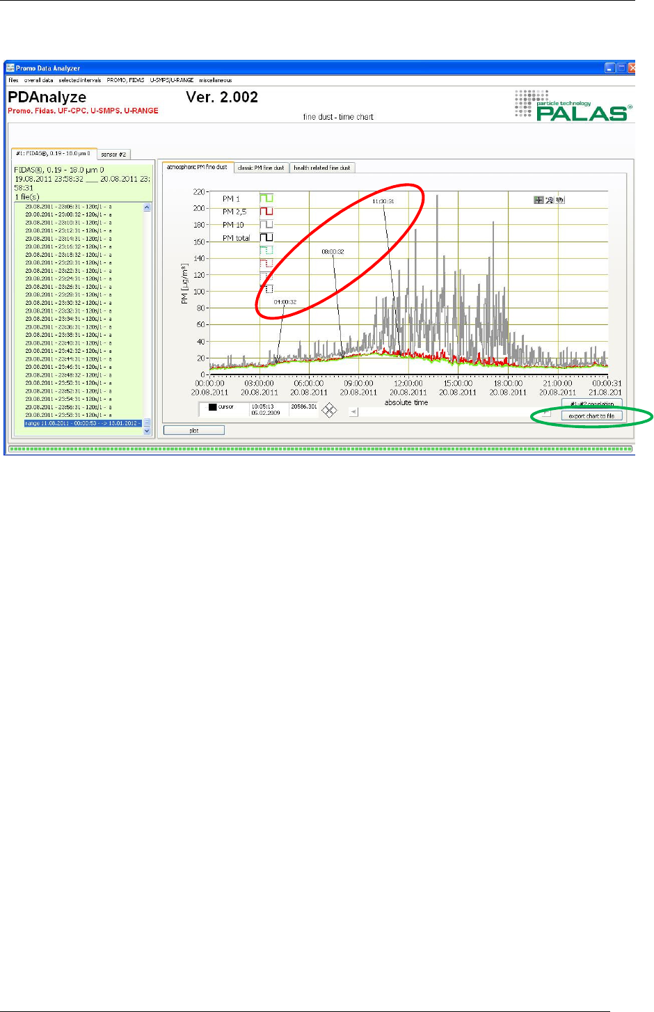
5.1.1 “atmospheric PM fine dust”
Figure 24: Display of “fine dust - time chart - atmospheric PM fine dust”
Display of the PM1, PM2,5 , PM10 and PM total values over the time according to atmospheric
PM fine dust evaluation algorithm, as well as the annotations (red circle) if available.
With the button “export chart to file (green circle) the graphic will be saved as a txt-file and
can further be used with other programs, e.g. Excel.
MANUAL PDANALYZE SOFTWARE
PALAS® GMBH, VERSION V0030112
23
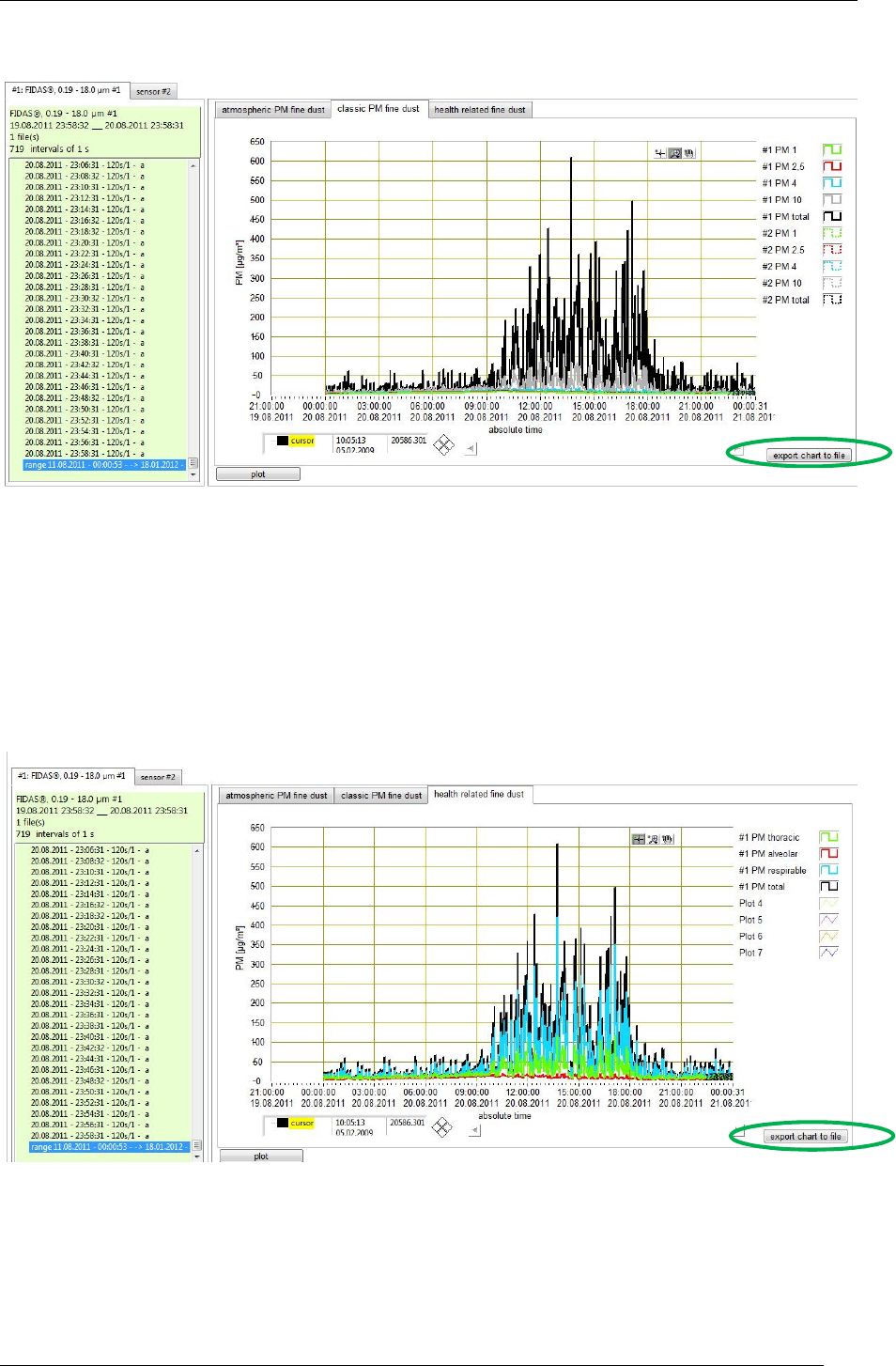
5.1.2 “classic PM fine dust”
Figure 25: Display of “fine dust - time chart - classic PM fine dust”
Display of the PM1, PM2,5 , PM10 and PM total values over the time according to classic PM
fine dust evaluation algorithm.
With the button “export chart to file (green circle) the graphic will be save das a txt-file and
can further be used with other programs, e.g. Excel.
5.1.3 “health related fine dust”
Figure 26: Display of “fine dust - time chart - classic PM fine dust”
Display of the PM1, PM2,5 , PM10 and PM total values over the time according to health related
PM fine dust evaluation algorithm.
With the button “export chart to file (green circle) the graphic will be save das a txt-file and
can further be used with other programs, e.g. Excel.
MANUAL PDANALYZE SOFTWARE
PALAS® GMBH, VERSION V0030112
24
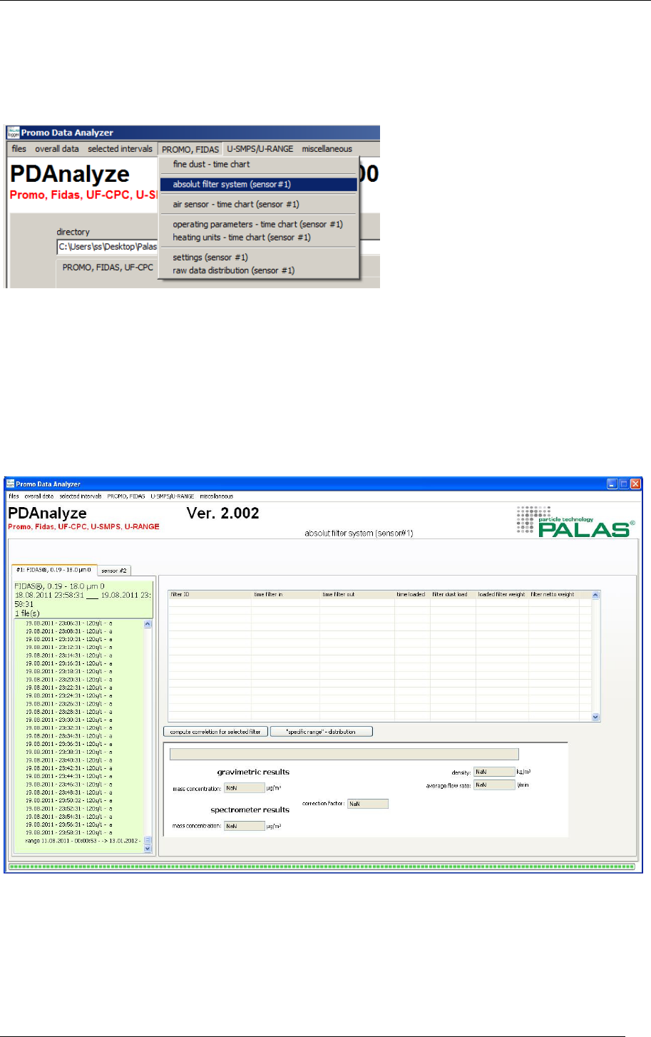
5.2 „absolut filter system (sensor #1)“
The Fidas® systems are equipped with a „total filter“ for the gravimetrical evaluation of the
total mass. With the PDAnalyze software the comparison can be done between the
gravimetrical collected mass value and the optical measured value.
Figure 27: Selection „PROMO, FIDAS - absolute filter system (sensor #1)“
In order to compute the correlation between gravimetric and optical measurement, please
select the appropriate files with a filter change (in/out).
After pressing the button compute correlation for selected filter the statistical values to the
corresponding files, which are marked under distribution, are then calculated.
This computed correlation factor can then be entered in the Fidas® firmware (please see
Fidas® firmware manual for details) for successive measurements.
Figure 28: start screen of the menu item „absolute filter system“
MANUAL PDANALYZE SOFTWARE
PALAS® GMBH, VERSION V0030112
25
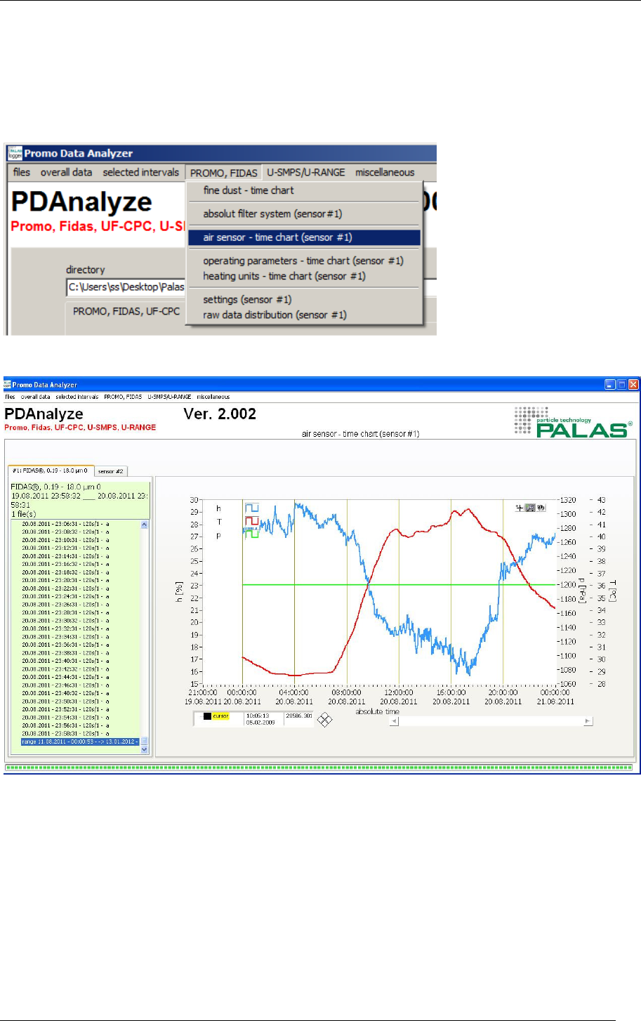
5.3 “air sensor – time chart (sensor #1)”
At the submenu „PROMO, FIDAS: air sensor – time chart (sensor #1)“ the value of rel.
humidity h in [%], the temperature T in [°C] and the barometrical atmospheric pressure p in
[Pa] over the time will be shown in the chart.
Figure 29: Selection “PROMO, FIDAS: air sensor - time chart (sensor #1)”
Figure 30: „PROMO, FIDAS: air sensor - time chart“ Display of sensor data for h, T and p
Graphical display of the chronological sequence of the relative humidity h in [%] (blue curve),
the temperature T in [°C] (red curve) and the barometric atmospheric pressure p in [Pa]
(green curve).
MANUAL PDANALYZE SOFTWARE
PALAS® GMBH, VERSION V0030112
26
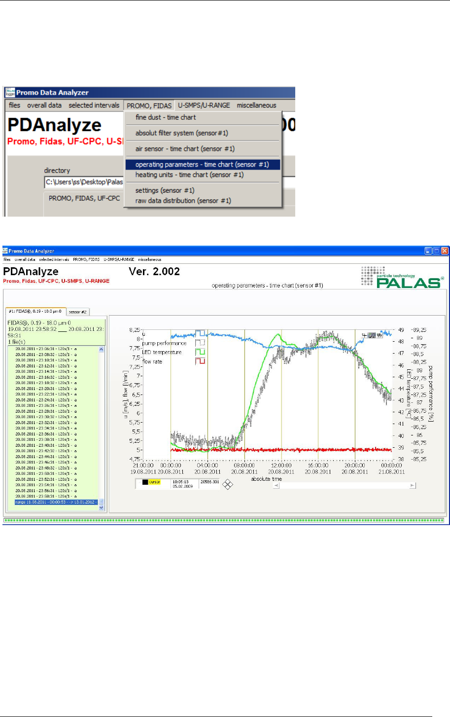
5.4 Operating parameters – time chart
The menu item „PROMO, FIDAS: operating parameters – time chart“ displays the values of
external sensors, e. g. particle speed.
Figure 31: Selection “PROMO, FIDAS operating parameters -time chart (sensor #1)”
Figure 32: “PROMO, FIDAS: operating parameters - time chart (sensor #1)”
With this kind of display there was an external sensor for the particle speed connected. The
particle speed is displayed in the blue curve aver the time. The values of the suction pump
are displayed in the grey curve over the time. The LED temperature is displayed in the green
curve over the time. The value of the volume flow is displayed in the red curve over the
time.
MANUAL PDANALYZE SOFTWARE
PALAS® GMBH, VERSION V0030112
27
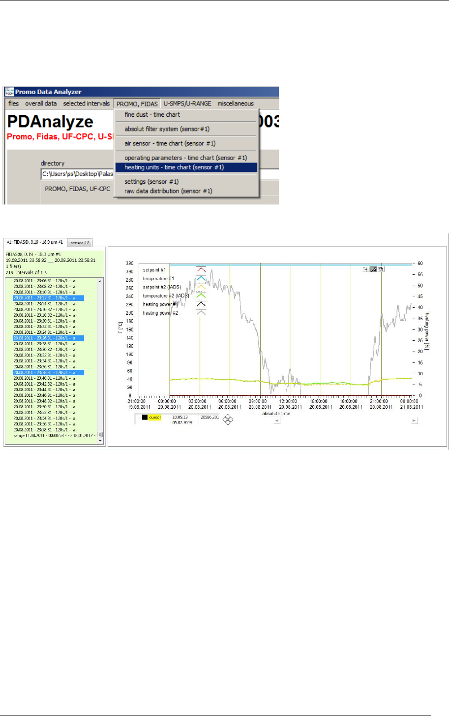
5.5 “heating units –time chart (sensor #1)”
The menu item „PROMO, FIDAS: heating units – time chart (sensor #1)“ displays the value
of any external heating, for example also the IADS (Intelligent Aerosol Drying System).
Figure 33: Selection “PROMO, FIDAS: heating units - time chart (sensor #1)”
Figure 34: “PROMO, FIDAS: heating units - time chart (sensor #1)”
Display of the selected and the current value of temperature sensor #1, temperature #2
(IADS) and the correspondent heating temperature as a time chart.
MANUAL PDANALYZE SOFTWARE
PALAS® GMBH, VERSION V0030112
28
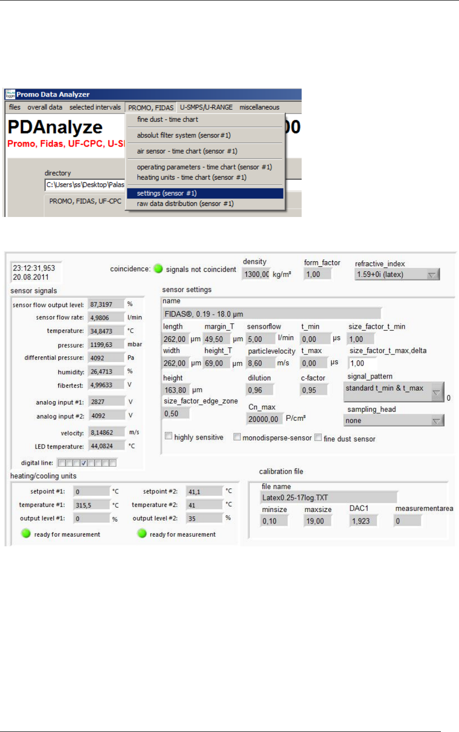
5.6 “settings (sensor #1)“
The menu item „PROMO, FIDAS: settings (sensor #1)“ shows all parameters that were set
and used during the measurement.
Figure 35: Selection “PROMO, FIDAS: settings (sensor #1)”
Figure 36: “PROMO, FIDAS: settings (sensor #1)”
Display of all parameters on one view, which are used for the calculation, e.g. measurement
volume, temperature, volume flow and so on.
Important in this case is that the LED for the coincidence value is always green, that means
the measurement is not done with coincidence error.
MANUAL PDANALYZE SOFTWARE
PALAS® GMBH, VERSION V0030112
29
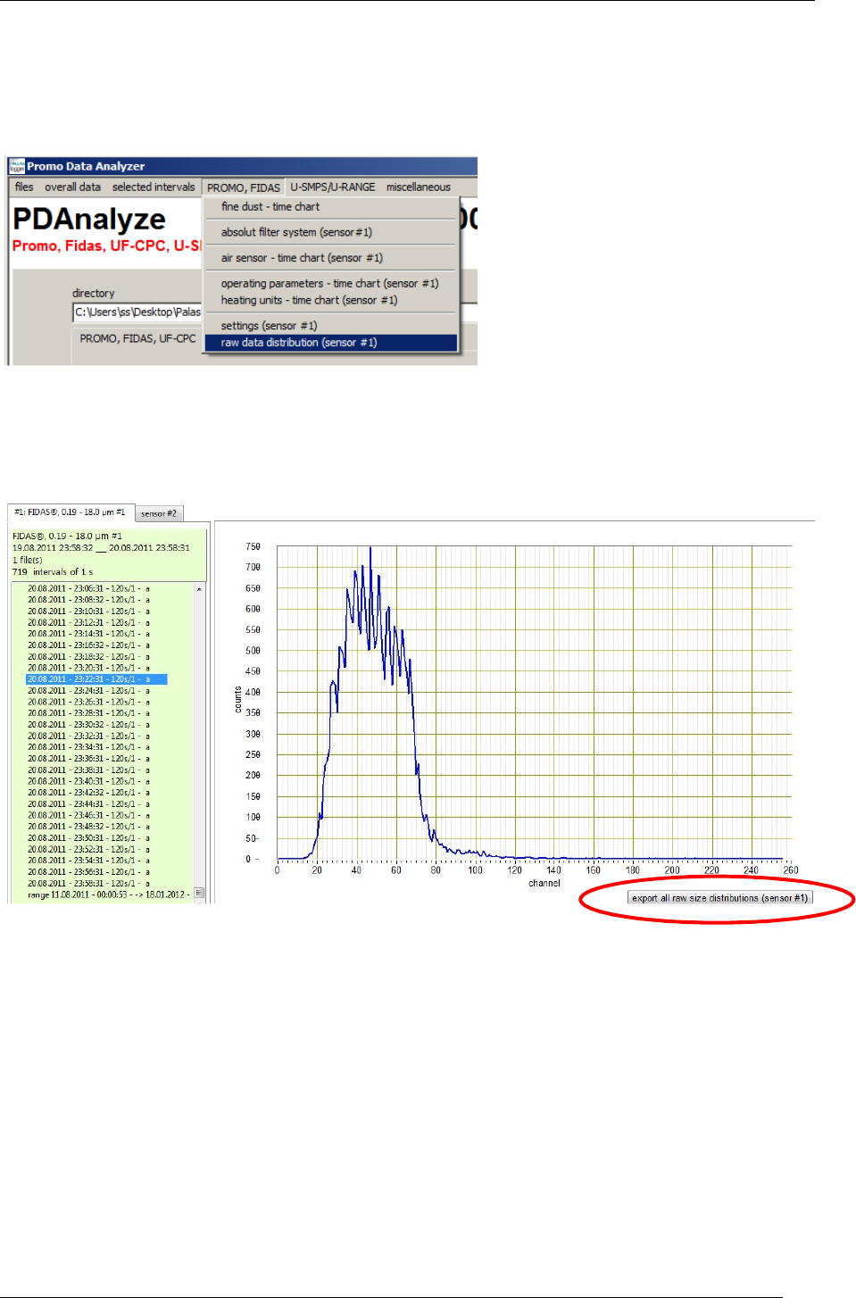
5.7 “raw data distribution (sensor #1)“
The menu item „PROMO, FIDAS: raw data distribution (sensor #1)“ display the raw data of
the measurement, e.g. the particle number of the raw data channels.
Figure 37: Selection “PROMO, FIDAS: raw data distribution (sensor #1)”
First of all the data has to be loaded as overall data or selected intervals and shown by
pressing the plot-button. After that the raw data distribution can be shown.
Figure 38: “PROMO, FIDAS: raw data distribution (sensor #1)”
With the button “export all raw size distributions (sensor #1)“ (red circle)all the raw data
values can be save das a txt-file and further be used with other programs, e.g. excel.
MANUAL PDANALYZE SOFTWARE
PALAS® GMBH, VERSION V0030112
30
6 Menu-Item: U-SMPS/U-RANGE
This menu item provides extended information about the scan process of the U-SMPS. This
information is only accessible if the measurement was performed with a U-SMPS or the U-
RANGE.
Note: This extended information is only available for data that are imported under sensor #1
(see 2. Menu-Item: files -> select files for more information).
This extended information is categorized as follows:
UP-/DOWN-scan comparison if an up-/down-scan (averaging) was performed the two
scans are averaged to yield one particle size distribution.
Here both scans as well as the averaged particle size
distribution are shown. If only an up-scan (scan from
smallest to largest particle size) or down-scan was
performed only this is shown.
Settings This lists parameters that were used during the scan,
especially “aerosol properties”, “scanning procedure”,
“DEMC properties” and an optional comment.
Operating parameters This is a graphical display of the sheath air flow rate,
temperature, and relative humidity, the impactor
pressure, and the sample air temperature and flow rate.
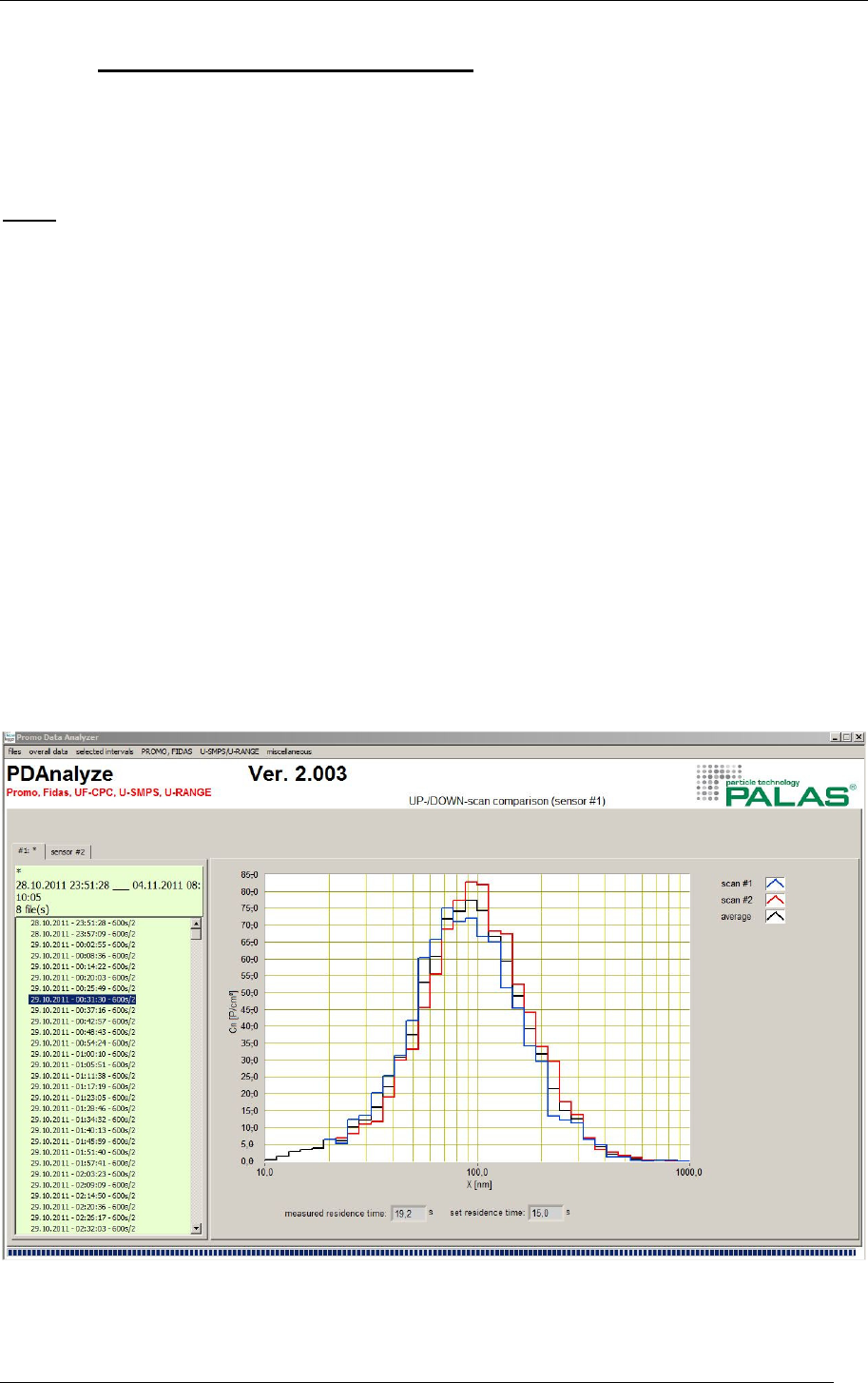
6.1 “UP-/DOWN-scan comparison (sensor #1)”
Figure 39: “UP-/DOWN-scan comparison (sensor #1)”
MANUAL PDANALYZE SOFTWARE
PALAS® GMBH, VERSION V0030112
31
If a measurement was performed with the setting “Up- and DOWNSCAN (averaging) - which
is also indicated by the /2 in the file list – this screen shows the combined (black) as well as
the single up-scan (blue) and single down-scan (red). At the bottom it also shows the
measured residence time and the set and used residence time.
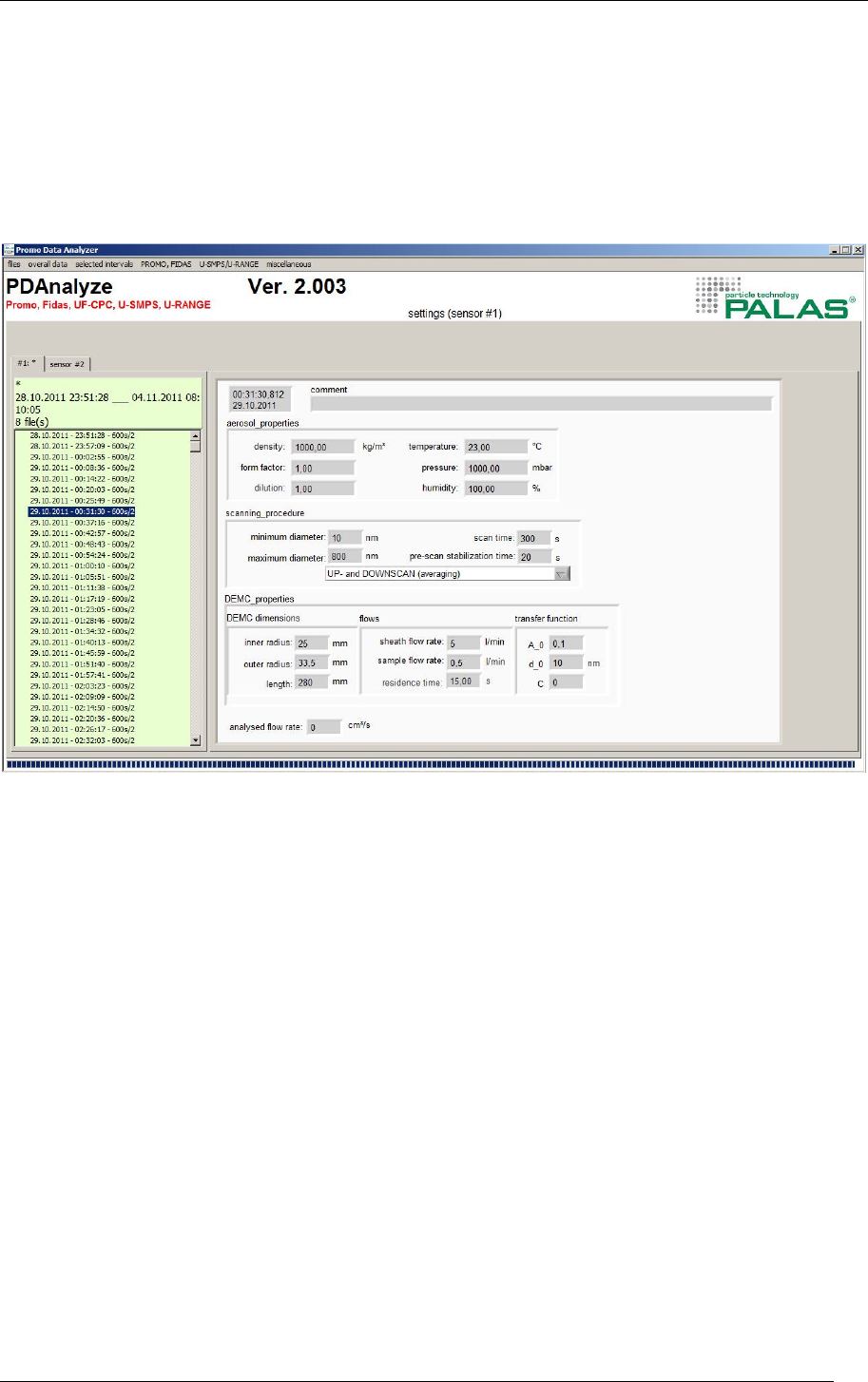
6.2 “settings (sensor #1)”
Figure 40: “settings (sensor #1)” – list of parameters
Here you see a list of parameters that were used during the scan, especially “aerosol
properties”, “scanning procedure”, “DEMC properties” and an optional comment.
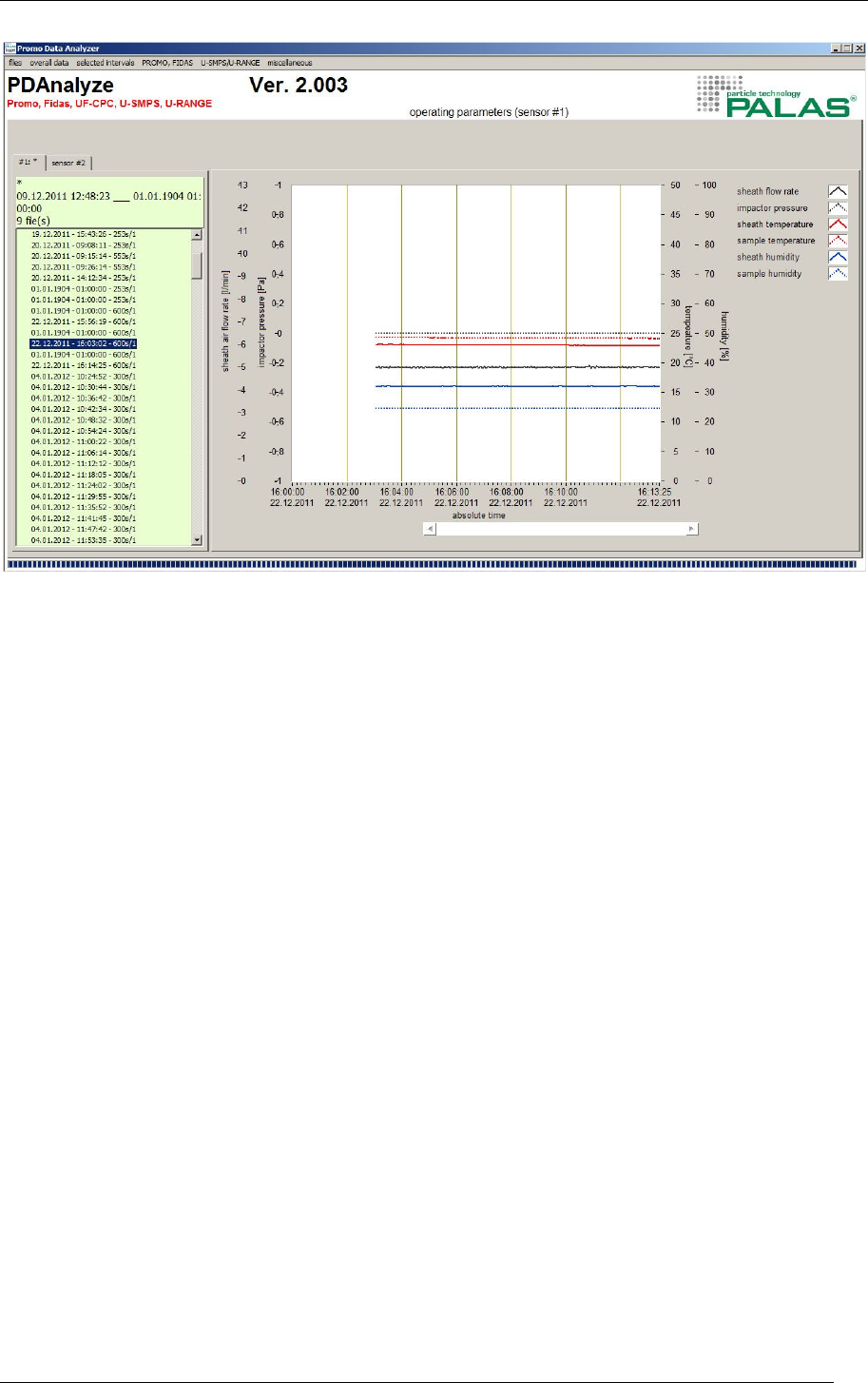
6.3 “operating parameters (sensor #1)”
This is a graphical display of the sheath air flow rate, temperature, and relative humidity, the
impactor pressure, and the sample air temperature and flow rate.
MANUAL PDANALYZE SOFTWARE
PALAS® GMBH, VERSION V0030112
32
Figure 41: “operating parameters (sensor #1)”
MANUAL PDANALYZE SOFTWARE
PALAS® GMBH, VERSION V0030112
33
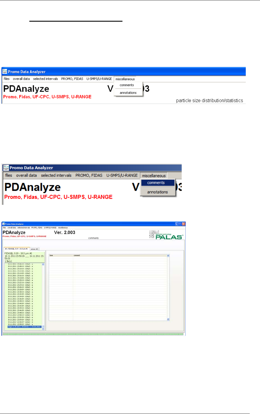
7 Menu-Item: miscellaneous
The menu item „miscellaneous“ has two sub-menus:
- „comment“
- „annotations“
Figure 42: „miscellaneous“
7.1 Comments
With „comments“ it is possible to write comments during a measurement, e. g. the time
when a filter was inserted or something like that.
Figure 43: Selection “miscellaneous: comments“
Figure 44: Selection “miscellaneous: comments“ (without comments)
MANUAL PDANALYZE SOFTWARE
PALAS® GMBH, VERSION V0030112
34
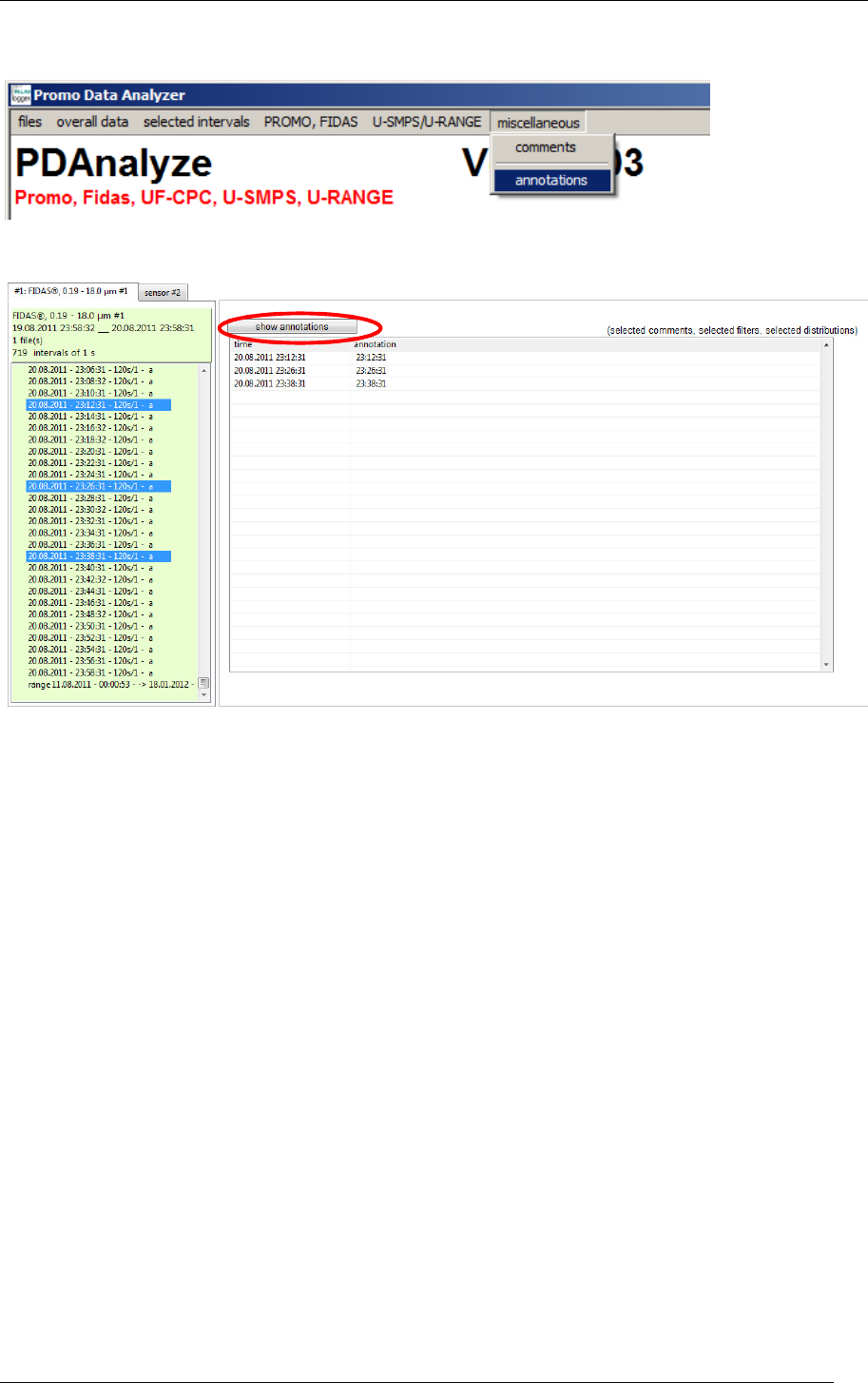
7.2 Annotations
Figure 45: Selection “miscellaneous: annotations“
Figure 46: “miscellaneous: annotations“
By pressing the button annotations (red circle), all the explanations with date and time
stamp are shown in the e table below, as well as in the graphical displays of the different
time charts (see for example figure 6 and figure 23).

MANUAL PDANALYZE SOFTWARE
PALAS® GMBH, VERSION V0030112
35
8 Appendix
8.1 Steps to display a particle size distribution that was measured with the U-SMPS
1. Files -> select files click on the yellow folder symbol to define the folder in which the
data files reside
2. Files -> select files select the “distribution type” i.e. the data you want to use, e.g.
the “inverted & diffusion corrected” data or the “raw data”
3. Files -> select files select the data files you want to analyze under “files”
4. Files -> select files import the data into the software using e.g. “data import sensor
#1 or downstream”
5. Selected intervals -> particle size distribution/statistics select the measurement(s)
for analysis and display in the list of measurements on the left (Note: the last entry in
this list covers the full range of listed measurements)
6. Selected intervals -> particle size distribution/statistics select the desired plot (e.g.
dCn/Cn) that is then shown. After any changes press “plot” to redraw the graph.
8.2 Steps to display PM values vs. time measured with the Fidas®
1. Files -> select files click on the yellow folder symbol to define the folder in which the
data files reside
2. Files -> select files select the data files you want to analyze under “files”
3. Files -> select files select the sensor (e.g. Fidas® 0.19 – 18.0 µm #1) under sensor(s)!
4. Files -> select files import the data into the software using e.g. “data import sensor
#1 or downstream”
5. PROMO, FIDAS -> fine dust – time chart statistics select the measurement(s) for
analysis and display in the list of measurements on the left (Note: the last entry in
this list covers the full range of listed measurements)
6. PROMO, FIDAS -> fine dust – time chart statistics after any changes press “plot” to
redraw the graph.
TIP: non-wanted PM-fractions can be turned invisible by clicking on the square
showing the colour of the plot and selecting the colour transparent (T).
