Natural Language Annotation For Machine Learning A Guide To Corpus ... [Pustejovsky & Stubbs 2012
User Manual:
Open the PDF directly: View PDF ![]() .
.
Page Count: 343 [warning: Documents this large are best viewed by clicking the View PDF Link!]
- Copyright
- Table of Contents
- Preface
- Chapter 1. The Basics
- Chapter 2. Defining Your Goal and Dataset
- Chapter 3. Corpus Analytics
- Chapter 4. Building Your Model and Specification
- Chapter 5. Applying and Adopting Annotation Standards
- Chapter 6. Annotation and Adjudication
- Chapter 7. Training: Machine Learning
- Chapter 8. Testing and Evaluation
- Chapter 9. Revising and Reporting
- Chapter 10. Annotation: TimeML
- Chapter 11. Automatic Annotation: Generating TimeML
- Chapter 12. Afterword: The Future of Annotation
- Appendix A. List of Available Corpora and Specifications
- Appendix B. List of Software Resources
- Appendix C. MAE User Guide
- Appendix D. MAI User Guide
- Appendix E. Bibliography
- Index
- About the Authors

James Pustejovsky and Amber Stubbs
Natural Language Annotation for
Machine Learning
ISBN: 978-1-449-30666-3
[LSI]
Natural Language Annotation for Machine Learning
by James Pustejovsky and Amber Stubbs
Copyright © 2013 James Pustejovsky and Amber Stubbs. All rights reserved.
Printed in the United States of America.
Published by O’Reilly Media, Inc., 1005 Gravenstein Highway North, Sebastopol, CA 95472.
O’Reilly books may be purchased for educational, business, or sales promotional use. Online editions are
also available for most titles (http://my.safaribooksonline.com). For more information, contact our corporate/
institutional sales department: 800-998-9938 or corporate@oreilly.com.
Editors: Julie Steele and Meghan Blanchette
Production Editor: Kristen Borg
Copyeditor: Audrey Doyle
Proofreader: Linley Dolby
Indexer: WordCo Indexing Services
Cover Designer: Randy Comer
Interior Designer: David Futato
Illustrator: Rebecca Demarest
October 2012: First Edition
Revision History for the First Edition:
2012-10-10 First release
See http://oreilly.com/catalog/errata.csp?isbn=9781449306663 for release details.
Nutshell Handbook, the Nutshell Handbook logo, and the O’Reilly logo are registered trademarks of O’Reilly
Media, Inc. Natural Language Annotation for Machine Learning, the image of a cockatiel, and related trade
dress are trademarks of O’Reilly Media, Inc.
Many of the designations used by manufacturers and sellers to distinguish their products are claimed as
trademarks. Where those designations appear in this book, and O’Reilly Media, Inc., was aware of a trade
mark claim, the designations have been printed in caps or initial caps.
While every precaution has been taken in the preparation of this book, the publisher and authors assume
no responsibility for errors or omissions, or for damages resulting from the use of the information contained
herein.

Table of Contents
Preface. . . . . . . . . . . . . . . . . . . . . . . . . . . . . . . . . . . . . . . . . . . . . . . . . . . . . . . . . . . . . . . . . . . . . . . ix
1. The Basics. . . . . . . . . . . . . . . . . . . . . . . . . . . . . . . . . . . . . . . . . . . . . . . . . . . . . . . . . . . . . . . . . . 1
The Importance of Language Annotation 1
The Layers of Linguistic Description 3
What Is Natural Language Processing? 4
A Brief History of Corpus Linguistics 5
What Is a Corpus? 8
Early Use of Corpora 10
Corpora Today 13
Kinds of Annotation 14
Language Data and Machine Learning 21
Classification 22
Clustering 22
Structured Pattern Induction 22
The Annotation Development Cycle 23
Model the Phenomenon 24
Annotate with the Specification 27
Train and Test the Algorithms over the Corpus 29
Evaluate the Results 30
Revise the Model and Algorithms 31
Summary 31
2. Defining Your Goal and Dataset. . . . . . . . . . . . . . . . . . . . . . . . . . . . . . . . . . . . . . . . . . . . . . . 33
Defining Your Goal 33
The Statement of Purpose 34
Refining Your Goal: Informativity Versus Correctness 35
Background Research 41
Language Resources 41
Organizations and Conferences 42
iii

NLP Challenges 43
Assembling Your Dataset 43
The Ideal Corpus: Representative and Balanced 45
Collecting Data from the Internet 46
Eliciting Data from People 46
The Size of Your Corpus 48
Existing Corpora 48
Distributions Within Corpora 49
Summary 51
3. Corpus Analytics. . . . . . . . . . . . . . . . . . . . . . . . . . . . . . . . . . . . . . . . . . . . . . . . . . . . . . . . . . . . 53
Basic Probability for Corpus Analytics 54
Joint Probability Distributions 55
Bayes Rule 57
Counting Occurrences 58
Zipf’s Law 61
N-grams 61
Language Models 63
Summary 65
4. Building Your Model and Specification. . . . . . . . . . . . . . . . . . . . . . . . . . . . . . . . . . . . . . . . . 67
Some Example Models and Specs 68
Film Genre Classification 70
Adding Named Entities 71
Semantic Roles 72
Adopting (or Not Adopting) Existing Models 75
Creating Your Own Model and Specification: Generality Versus Specificity 76
Using Existing Models and Specifications 78
Using Models Without Specifications 79
Different Kinds of Standards 80
ISO Standards 80
Community-Driven Standards 83
Other Standards Affecting Annotation 83
Summary 84
5. Applying and Adopting Annotation Standards. . . . . . . . . . . . . . . . . . . . . . . . . . . . . . . . . . 87
Metadata Annotation: Document Classification 88
Unique Labels: Movie Reviews 88
Multiple Labels: Film Genres 90
Text Extent Annotation: Named Entities 94
Inline Annotation 94
Stand-off Annotation by Tokens 96
iv | Table of Contents

Stand-off Annotation by Character Location 99
Linked Extent Annotation: Semantic Roles 101
ISO Standards and You 102
Summary 103
6. Annotation and Adjudication. . . . . . . . . . . . . . . . . . . . . . . . . . . . . . . . . . . . . . . . . . . . . . . 105
The Infrastructure of an Annotation Project 105
Specification Versus Guidelines 108
Be Prepared to Revise 109
Preparing Your Data for Annotation 110
Metadata 110
Preprocessed Data 110
Splitting Up the Files for Annotation 111
Writing the Annotation Guidelines 112
Example 1: Single Labels—Movie Reviews 113
Example 2: Multiple Labels—Film Genres 115
Example 3: Extent Annotations—Named Entities 119
Example 4: Link Tags—Semantic Roles 120
Annotators 122
Choosing an Annotation Environment 124
Evaluating the Annotations 126
Cohen’s Kappa (κ) 127
Fleiss’s Kappa (κ) 128
Interpreting Kappa Coefficients 131
Calculating κ in Other Contexts 132
Creating the Gold Standard (Adjudication) 134
Summary 135
7. Training: Machine Learning. . . . . . . . . . . . . . . . . . . . . . . . . . . . . . . . . . . . . . . . . . . . . . . . . 139
What Is Learning? 140
Defining Our Learning Task 142
Classifier Algorithms 144
Decision Tree Learning 145
Gender Identification 147
Naïve Bayes Learning 151
Maximum Entropy Classifiers 157
Other Classifiers to Know About 158
Sequence Induction Algorithms 160
Clustering and Unsupervised Learning 162
Semi-Supervised Learning 163
Matching Annotation to Algorithms 165
Table of Contents | v

Summary 166
8. Testing and Evaluation. . . . . . . . . . . . . . . . . . . . . . . . . . . . . . . . . . . . . . . . . . . . . . . . . . . . . 169
Testing Your Algorithm 170
Evaluating Your Algorithm 170
Confusion Matrices 171
Calculating Evaluation Scores 172
Interpreting Evaluation Scores 177
Problems That Can Affect Evaluation 178
Dataset Is Too Small 178
Algorithm Fits the Development Data Too Well 180
Too Much Information in the Annotation 181
Final Testing Scores 181
Summary 182
9. Revising and Reporting. . . . . . . . . . . . . . . . . . . . . . . . . . . . . . . . . . . . . . . . . . . . . . . . . . . . 185
Revising Your Project 186
Corpus Distributions and Content 186
Model and Specification 187
Annotation 188
Training and Testing 189
Reporting About Your Work 189
About Your Corpus 191
About Your Model and Specifications 192
About Your Annotation Task and Annotators 192
About Your ML Algorithm 193
About Your Revisions 194
Summary 194
10. Annotation: TimeML. . . . . . . . . . . . . . . . . . . . . . . . . . . . . . . . . . . . . . . . . . . . . . . . . . . . . . . 197
The Goal of TimeML 198
Related Research 199
Building the Corpus 201
Model: Preliminary Specifications 201
Times 202
Signals 202
Events 203
Links 203
Annotation: First Attempts 204
Model: The TimeML Specification Used in TimeBank 204
Time Expressions 204
Events 205
vi | Table of Contents

Signals 206
Links 207
Confidence 208
Annotation: The Creation of TimeBank 209
TimeML Becomes ISO-TimeML 211
Modeling the Future: Directions for TimeML 213
Narrative Containers 213
Expanding TimeML to Other Domains 215
Event Structures 216
Summary 217
11. Automatic Annotation: Generating TimeML. . . . . . . . . . . . . . . . . . . . . . . . . . . . . . . . . . . 219
The TARSQI Components 220
GUTime: Temporal Marker Identification 221
EVITA: Event Recognition and Classification 222
GUTenLINK 223
Slinket 224
SputLink 225
Machine Learning in the TARSQI Components 226
Improvements to the TTK 226
Structural Changes 227
Improvements to Temporal Entity Recognition: BTime 227
Temporal Relation Identification 228
Temporal Relation Validation 229
Temporal Relation Visualization 229
TimeML Challenges: TempEval-2 230
TempEval-2: System Summaries 231
Overview of Results 234
Future of the TTK 234
New Input Formats 234
Narrative Containers/Narrative Times 235
Medical Documents 236
Cross-Document Analysis 237
Summary 238
12. Afterword: The Future of Annotation. . . . . . . . . . . . . . . . . . . . . . . . . . . . . . . . . . . . . . . . . 239
Crowdsourcing Annotation 239
Amazon’s Mechanical Turk 240
Games with a Purpose (GWAP) 241
User-Generated Content 242
Handling Big Data 243
Boosting 243
Table of Contents | vii

Active Learning 244
Semi-Supervised Learning 245
NLP Online and in the Cloud 246
Distributed Computing 246
Shared Language Resources 247
Shared Language Applications 247
And Finally... 248
A. List of Available Corpora and Specifications. . . . . . . . . . . . . . . . . . . . . . . . . . . . . . . . . . . . 249
B. List of Software Resources. . . . . . . . . . . . . . . . . . . . . . . . . . . . . . . . . . . . . . . . . . . . . . . . . . 271
C. MAE User Guide. . . . . . . . . . . . . . . . . . . . . . . . . . . . . . . . . . . . . . . . . . . . . . . . . . . . . . . . . . . . 291
D. MAI User Guide. . . . . . . . . . . . . . . . . . . . . . . . . . . . . . . . . . . . . . . . . . . . . . . . . . . . . . . . . . . . 299
E. Bibliography. . . . . . . . . . . . . . . . . . . . . . . . . . . . . . . . . . . . . . . . . . . . . . . . . . . . . . . . . . . . . . 305
Index. . . . . . . . . . . . . . . . . . . . . . . . . . . . . . . . . . . . . . . . . . . . . . . . . . . . . . . . . . . . . . . . . . . . . . . 317
viii | Table of Contents

Preface
This book is intended as a resource for people who are interested in using computers to
help process natural language. A natural language refers to any language spoken by
humans, either currently (e.g., English, Chinese, Spanish) or in the past (e.g., Latin,
ancient Greek, Sanskrit). Annotation refers to the process of adding metadata informa
tion to the text in order to augment a computer’s capability to perform Natural Language
Processing (NLP). In particular, we examine how information can be added to natural
language text through annotation in order to increase the performance of machine
learning algorithms—computer programs designed to extrapolate rules from the infor
mation provided over texts in order to apply those rules to unannotated texts later on.
Natural Language Annotation for Machine Learning
This book details the multistage process for building your own annotated natural lan
guage dataset (known as a corpus) in order to train machine learning (ML) algorithms
for language-based data and knowledge discovery. The overall goal of this book is to
show readers how to create their own corpus, starting with selecting an annotation task,
creating the annotation specification, designing the guidelines, creating a “gold stan
dard” corpus, and then beginning the actual data creation with the annotation process.
Because the annotation process is not linear, multiple iterations can be required for
defining the tasks, annotations, and evaluations, in order to achieve the best results for
a particular goal. The process can be summed up in terms of the MATTER Annotation
Development Process: Model, Annotate, Train, Test, Evaluate, Revise. This book guides
the reader through the cycle, and provides detailed examples and discussion for different
types of annotation tasks throughout. These tasks are examined in depth to provide
context for readers and to help provide a foundation for their own ML goals.
ix

Additionally, this book provides access to and usage guidelines for lightweight, user-
friendly software that can be used for annotating texts and adjudicating the annotations.
While a variety of annotation tools are available to the community, the Multipurpose
Annotation Environment (MAE) adopted in this book (and available to readers as a free
download) was specifically designed to be easy to set up and get running, so that con
fusing documentation would not distract readers from their goals. MAE is paired with
the Multidocument Adjudication Interface (MAI), a tool that allows for quick compar
ison of annotated documents.
Audience
This book is written for anyone interested in using computers to explore aspects of the
information content conveyed by natural language. It is not necessary to have a pro
gramming or linguistics background to use this book, although a basic understanding
of a scripting language such as Python can make the MATTER cycle easier to follow,
and some sample Python code is provided in the book. If you don’t have any Python
experience, we highly recommend Natural Language Processing with Python by Steven
Bird, Ewan Klein, and Edward Loper (O’Reilly), which provides an excellent introduc
tion both to Python and to aspects of NLP that are not addressed in this book.
It is helpful to have a basic understanding of markup languages such as XML (or even
HTML) in order to get the most out of this book. While one doesn’t need to be an expert
in the theory behind an XML schema, most annotation projects use some form of XML
to encode the tags, and therefore we use that standard in this book when providing
annotation examples. Although you don’t need to be a web designer to understand the
book, it does help to have a working knowledge of tags and attributes in order to un
derstand how an idea for an annotation gets implemented.
Organization of This Book
Chapter 1 of this book provides a brief overview of the history of annotation and ma
chine learning, as well as short discussions of some of the different ways that annotation
tasks have been used to investigate different layers of linguistic research. The rest of the
book guides the reader through the MATTER cycle, from tips on creating a reasonable
annotation goal in Chapter 2, all the way through evaluating the results of the annotation
and ML stages, as well as a discussion of revising your project and reporting on your
work in Chapter 9. The last two chapters give a complete walkthrough of a single an
notation project and how it was recreated with machine learning and rule-based algo
rithms. Appendixes at the back of the book provide lists of resources that readers will
find useful for their own annotation tasks.
x | Preface
Software Requirements
While it’s possible to work through this book without running any of the code examples
provided, we do recommend having at least the Natural Language Toolkit (NLTK) in
stalled for easy reference to some of the ML techniques discussed. The NLTK currently
runs on Python versions from 2.4 to 2.7. (Python 3.0 is not supported at the time of this
writing.) For more information, see http://www.nltk.org.
The code examples in this book are written as though they are in the interactive Python
shell programming environment. For information on how to use this environment,
please see: http://docs.python.org/tutorial/interpreter.html. If not specifically stated in
the examples, it should be assumed that the command import nltk was used prior to
all sample code.
Conventions Used in This Book
The following typographical conventions are used in this book:
Italic
Indicates new terms, URLs, email addresses, filenames, and file extensions.
Constant width
Used for program listings, as well as within paragraphs to refer to program elements
such as variable or function names, databases, data types, environment variables,
statements, and keywords.
This icon signifies a tip, suggestion, or general note.
This icon indicates a warning or caution.
Using Code Examples
This book is here to help you get your job done. In general, you may use the code in this
book in your programs and documentation. You do not need to contact us for permis
sion unless you’re reproducing a significant portion of the code. For example, writing a
program that uses several chunks of code from this book does not require permission.
Preface | xi

Selling or distributing a CD-ROM of examples from O’Reilly books does require per
mission. Answering a question by citing this book and quoting example code does not
require permission. Incorporating a significant amount of example code from this book
into your product’s documentation does require permission.
We appreciate, but do not require, attribution. An attribution usually includes the title,
author, publisher, and ISBN. For example: “Natural Language Annotation for Machine
Learning by James Pustejovsky and Amber Stubbs (O’Reilly). Copyright 2013 James
Pustejovsky and Amber Stubbs, 978-1-449-30666-3.”
If you feel your use of code examples falls outside fair use or the permission given above,
feel free to contact us at permissions@oreilly.com.
Safari® Books Online
Safari Books Online (www.safaribooksonline.com) is an on-demand
digital library that delivers expert content in both book and video
form from the world’s leading authors in technology and business.
Technology professionals, software developers, web designers, and business and creative
professionals use Safari Books Online as their primary resource for research, problem
solving, learning, and certification training.
Safari Books Online offers a range of product mixes and pricing programs for organi
zations, government agencies, and individuals. Subscribers have access to thousands of
books, training videos, and prepublication manuscripts in one fully searchable database
from publishers like O’Reilly Media, Prentice Hall Professional, Addison-Wesley Pro
fessional, Microsoft Press, Sams, Que, Peachpit Press, Focal Press, Cisco Press, John
Wiley & Sons, Syngress, Morgan Kaufmann, IBM Redbooks, Packt, Adobe Press, FT
Press, Apress, Manning, New Riders, McGraw-Hill, Jones & Bartlett, Course Technol
ogy, and dozens more. For more information about Safari Books Online, please visit us
online.
How to Contact Us
Please address comments and questions concerning this book to the publisher:
O’Reilly Media, Inc.
1005 Gravenstein Highway North
Sebastopol, CA 95472
800-998-9938 (in the United States or Canada)
707-829-0515 (international or local)
707-829-0104 (fax)
xii | Preface

We have a web page for this book, where we list errata, examples, and any additional
information. You can access this page at http://oreil.ly/nat-lang-annotation-ML.
To comment or ask technical questions about this book, send email to bookques
tions@oreilly.com.
For more information about our books, courses, conferences, and news, see our website
at http://www.oreilly.com.
Find us on Facebook: http://facebook.com/oreilly
Follow us on Twitter: http://twitter.com/oreillymedia
Watch us on YouTube: http://www.youtube.com/oreillymedia
Acknowledgments
We would like thank everyone at O’Reilly who helped us create this book, in particular
Meghan Blanchette, Julie Steele, Sarah Schneider, Kristen Borg, Audrey Doyle, and ev
eryone else who helped to guide us through the process of producing it. We would also
like to thank the students who participated in the Brandeis COSI 216 class during the
spring 2011 semester for bearing with us as we worked through the MATTER cycle with
them: Karina Baeza Grossmann-Siegert, Elizabeth Baran, Bensiin Borukhov, Nicholas
Botchan, Richard Brutti, Olga Cherenina, Russell Entrikin, Livnat Herzig, Sophie Kush
kuley, Theodore Margolis, Alexandra Nunes, Lin Pan, Batia Snir, John Vogel, and Yaqin
Yang.
We would also like to thank our technical reviewers, who provided us with such excellent
feedback: Arvind S. Gautam, Catherine Havasi, Anna Rumshisky, and Ben Wellner, as
well as everyone who read the Early Release version of the book and let us know that
we were going in the right direction.
We would like to thank members of the ISO community with whom we have discussed
portions of the material in this book: Kiyong Lee, Harry Bunt, Nancy Ide, Nicoletta
Calzolari, Bran Boguraev, Annie Zaenen, and Laurent Romary.
Additional thanks to the members of the Brandeis Computer Science and Linguistics
departments, who listened to us brainstorm, kept us encouraged, and made sure ev
erything kept running while we were writing, especially Marc Verhagen, Lotus Gold
berg, Jessica Moszkowicz, and Alex Plotnick.
This book could not exist without everyone in the linguistics and computational lin
guistics communities who have created corpora and annotations, and, more impor
tantly, shared their experiences with the rest of the research community.
Preface | xiii

James Adds:
I would like to thank my wife, Cathie, for her patience and support during this project.
I would also like to thank my children, Zac and Sophie, for putting up with me while
the book was being finished. And thanks, Amber, for taking on this crazy effort with
me.
Amber Adds:
I would like to thank my husband, BJ, for encouraging me to undertake this project and
for his patience while I worked through it. Thanks also to my family, especially my
parents, for their enthusiasm toward this book. And, of course, thanks to my advisor
and coauthor, James, for having this crazy idea in the first place.
xiv | Preface

CHAPTER 1
The Basics
It seems as though every day there are new and exciting problems that people have
taught computers to solve, from how to win at chess or Jeopardy to determining shortest-
path driving directions. But there are still many tasks that computers cannot perform,
particularly in the realm of understanding human language. Statistical methods have
proven to be an effective way to approach these problems, but machine learning (ML)
techniques often work better when the algorithms are provided with pointers to what
is relevant about a dataset, rather than just massive amounts of data. When discussing
natural language, these pointers often come in the form of annotations—metadata that
provides additional information about the text. However, in order to teach a computer
effectively, it’s important to give it the right data, and for it to have enough data to learn
from. The purpose of this book is to provide you with the tools to create good data for
your own ML task. In this chapter we will cover:
• Why annotation is an important tool for linguists and computer scientists alike
• How corpus linguistics became the field that it is today
• The different areas of linguistics and how they relate to annotation and ML tasks
• What a corpus is, and what makes a corpus balanced
• How some classic ML problems are represented with annotations
• The basics of the annotation development cycle
The Importance of Language Annotation
Everyone knows that the Internet is an amazing resource for all sorts of information
that can teach you just about anything: juggling, programming, playing an instrument,
and so on. However, there is another layer of information that the Internet contains,
1

and that is how all those lessons (and blogs, forums, tweets, etc.) are being communi
cated. The Web contains information in all forms of media—including texts, images,
movies, and sounds—and language is the communication medium that allows people
to understand the content, and to link the content to other media. However, while com
puters are excellent at delivering this information to interested users, they are much less
adept at understanding language itself.
Theoretical and computational linguistics are focused on unraveling the deeper nature
of language and capturing the computational properties of linguistic structures. Human
language technologies (HLTs) attempt to adopt these insights and algorithms and turn
them into functioning, high-performance programs that can impact the ways we in
teract with computers using language. With more and more people using the Internet
every day, the amount of linguistic data available to researchers has increased signifi
cantly, allowing linguistic modeling problems to be viewed as ML tasks, rather than
limited to the relatively small amounts of data that humans are able to process on their
own.
However, it is not enough to simply provide a computer with a large amount of data and
expect it to learn to speak—the data has to be prepared in such a way that the computer
can more easily find patterns and inferences. This is usually done by adding relevant
metadata to a dataset. Any metadata tag used to mark up elements of the dataset is called
an annotation over the input. However, in order for the algorithms to learn efficiently
and effectively, the annotation done on the data must be accurate, and relevant to the
task the machine is being asked to perform. For this reason, the discipline of language
annotation is a critical link in developing intelligent human language technologies.
Giving an ML algorithm too much information can slow it down and
lead to inaccurate results, or result in the algorithm being so molded to
the training data that it becomes “overfit” and provides less accurate
results than it might otherwise on new data. It’s important to think
carefully about what you are trying to accomplish, and what informa
tion is most relevant to that goal. Later in the book we will give examples
of how to find that information, and how to determine how well your
algorithm is performing at the task you’ve set for it.
Datasets of natural language are referred to as corpora, and a single set of data annotated
with the same specification is called an annotated corpus. Annotated corpora can be
used to train ML algorithms. In this chapter we will define what a corpus is, explain
what is meant by an annotation, and describe the methodology used for enriching a
linguistic data collection with annotations for machine learning.
2 | Chapter 1: The Basics

The Layers of Linguistic Description
While it is not necessary to have formal linguistic training in order to create an annotated
corpus, we will be drawing on examples of many different types of annotation tasks, and
you will find this book more helpful if you have a basic understanding of the different
aspects of language that are studied and used for annotations. Grammar is the name
typically given to the mechanisms responsible for creating well-formed structures in
language. Most linguists view grammar as itself consisting of distinct modules or sys
tems, either by cognitive design or for descriptive convenience. These areas usually
include syntax, semantics, morphology, phonology (and phonetics), and the lexicon.
Areas beyond grammar that relate to how language is embedded in human activity
include discourse, pragmatics, and text theory. The following list provides more detailed
descriptions of these areas:
Syntax
The study of how words are combined to form sentences. This includes examining
parts of speech and how they combine to make larger constructions.
Semantics
The study of meaning in language. Semantics examines the relations between words
and what they are being used to represent.
Morphology
The study of units of meaning in a language. A morpheme is the smallest unit of
language that has meaning or function, a definition that includes words, prefixes,
affixes, and other word structures that impart meaning.
Phonology
The study of the sound patterns of a particular language. Aspects of study include
determining which phones are significant and have meaning (i.e., the phonemes);
how syllables are structured and combined; and what features are needed to describe
the discrete units (segments) in the language, and how they are interpreted.
Phonetics
The study of the sounds of human speech, and how they are made and perceived.
A phoneme is the term for an individual sound, and is essentially the smallest unit
of human speech.
Lexicon
The study of the words and phrases used in a language, that is, a language’s
vocabulary.
Discourse analysis
The study of exchanges of information, usually in the form of conversations, and
particularly the flow of information across sentence boundaries.
The Importance of Language Annotation | 3

Pragmatics
The study of how the context of text affects the meaning of an expression, and what
information is necessary to infer a hidden or presupposed meaning.
Text structure analysis
The study of how narratives and other textual styles are constructed to make larger
textual compositions.
Throughout this book we will present examples of annotation projects that make use of
various combinations of the different concepts outlined in the preceding list.
What Is Natural Language Processing?
Natural Language Processing (NLP) is a field of computer science and engineering that
has developed from the study of language and computational linguistics within the field
of Artificial Intelligence. The goals of NLP are to design and build applications that
facilitate human interaction with machines and other devices through the use of natural
language. Some of the major areas of NLP include:
Question Answering Systems (QAS)
Imagine being able to actually ask your computer or your phone what time your
favorite restaurant in New York stops serving dinner on Friday nights. Rather than
typing in the (still) clumsy set of keywords into a search browser window, you could
simply ask in plain, natural language—your own, whether it’s English, Mandarin,
or Spanish. (While systems such as Siri for the iPhone are a good start to this process,
it’s clear that Siri doesn’t fully understand all of natural language, just a subset of
key phrases.)
Summarization
This area includes applications that can take a collection of documents or emails
and produce a coherent summary of their content. Such programs also aim to pro
vide snap “elevator summaries” of longer documents, and possibly even turn them
into slide presentations.
Machine Translation
The holy grail of NLP applications, this was the first major area of research and
engineering in the field. Programs such as Google Translate are getting better and
better, but the real killer app will be the BabelFish that translates in real time when
you’re looking for the right train to catch in Beijing.
Speech Recognition
This is one of the most difficult problems in NLP. There has been great progress in
building models that can be used on your phone or computer to recognize spoken
4 | Chapter 1: The Basics

language utterances that are questions and commands. Unfortunately, while these
Automatic Speech Recognition (ASR) systems are ubiquitous, they work best in
narrowly defined domains and don’t allow the speaker to stray from the expected
scripted input (“Please say or type your card number now”).
Document classification
This is one of the most successful areas of NLP, wherein the task is to identify in
which category (or bin) a document should be placed. This has proved to be enor
mously useful for applications such as spam filtering, news article classification,
and movie reviews, among others. One reason this has had such a big impact is the
relative simplicity of the learning models needed for training the algorithms that
do the classification.
As we mentioned in the Preface, the Natural Language Toolkit (NLTK), described in
the O’Reilly book Natural Language Processing with Python, is a wonderful introduction
to the techniques necessary to build many of the applications described in the preceding
list. One of the goals of this book is to give you the knowledge to build specialized
language corpora (i.e., training and test datasets) that are necessary for developing such
applications.
A Brief History of Corpus Linguistics
In the mid-20th century, linguistics was practiced primarily as a descriptive field, used
to study structural properties within a language and typological variations between
languages. This work resulted in fairly sophisticated models of the different informa
tional components comprising linguistic utterances. As in the other social sciences, the
collection and analysis of data was also being subjected to quantitative techniques from
statistics. In the 1940s, linguists such as Bloomfield were starting to think that language
could be explained in probabilistic and behaviorist terms. Empirical and statistical
methods became popular in the 1950s, and Shannon’s information-theoretic view to
language analysis appeared to provide a solid quantitative approach for modeling qual
itative descriptions of linguistic structure.
Unfortunately, the development of statistical and quantitative methods for linguistic
analysis hit a brick wall in the 1950s. This was due primarily to two factors. First, there
was the problem of data availability. One of the problems with applying statistical meth
ods to the language data at the time was that the datasets were generally so small that it
was not possible to make interesting statistical generalizations over large numbers of
linguistic phenomena. Second, and perhaps more important, there was a general shift
in the social sciences from data-oriented descriptions of human behavior to introspec
tive modeling of cognitive functions.
A Brief History of Corpus Linguistics | 5

As part of this new attitude toward human activity, the linguist Noam Chomsky focused
on both a formal methodology and a theory of linguistics that not only ignored quan
titative language data, but also claimed that it was misleading for formulating models
of language behavior (Chomsky 1957).
This view was very influential throughout the 1960s and 1970s, largely because the
formal approach was able to develop extremely sophisticated rule-based language mod
els using mostly introspective (or self-generated) data. This was a very attractive alter
native to trying to create statistical language models on the basis of still relatively small
datasets of linguistic utterances from the existing corpora in the field. Formal modeling
and rule-based generalizations, in fact, have always been an integral step in theory for
mation, and in this respect, Chomsky’s approach on how to do linguistics has yielded
rich and elaborate models of language.
Timeline of Corpus Linguistics
Here’s a quick overview of some of the milestones in the field, leading up to where we are
now.
•1950s: Descriptive linguists compile collections of spoken and written utterances of
various languages from field research. Literary researchers begin compiling system
atic collections of the complete works of different authors. Key Word in Context
(KWIC) is invented as a means of indexing documents and creating concordances.
•1960s: Kucera and Francis publish A Standard Corpus of Present-Day American
English (the Brown Corpus), the first broadly available large corpus of language texts.
Work in Information Retrieval (IR) develops techniques for statistical similarity of
document content.
•1970s: Stochastic models developed from speech corpora make Speech Recognition
systems possible. The vector space model is developed for document indexing. The
London-Lund Corpus (LLC) is developed through the work of the Survey of English
Usage.
•1980s: The Lancaster-Oslo-Bergen (LOB) Corpus, designed to match the Brown
Corpus in terms of size and genres, is compiled. The COBUILD (Collins Birmingham
University International Language Database) dictionary is published, the first based
on examining usage from a large English corpus, the Bank of English. The Survey of
English Usage Corpus inspires the creation of a comprehensive corpus-based gram
mar, Grammar of English. The Child Language Data Exchange System (CHILDES)
Corpus is released as a repository for first language acquisition data.
•1990s: The Penn TreeBank is released. This is a corpus of tagged and parsed sentences
of naturally occurring English (4.5 million words). The British National Corpus
(BNC) is compiled and released as the largest corpus of English to date (100 million
words). The Text Encoding Initiative (TEI) is established to develop and maintain a
standard for the representation of texts in digital form.
6 | Chapter 1: The Basics
•2000s: As the World Wide Web grows, more data is available for statistical models
for Machine Translation and other applications. The American National Corpus
(ANC) project releases a 22-million-word subcorpus, and the Corpus of Contem
porary American English (COCA) is released (400 million words). Google releases
its Google N-gram Corpus of 1 trillion word tokens from public web pages. The
corpus holds up to five n-grams for each word token, along with their frequencies .
•2010s: International standards organizations, such as ISO, begin to recognize and co-
develop text encoding formats that are being used for corpus annotation efforts. The
Web continues to make enough data available to build models for a whole new range
of linguistic phenomena. Entirely new forms of text corpora, such as Twitter, Face
book, and blogs, become available as a resource.
Theory construction, however, also involves testing and evaluating your hypotheses
against observed phenomena. As more linguistic data has gradually become available,
something significant has changed in the way linguists look at data. The phenomena
are now observable in millions of texts and billions of sentences over the Web, and this
has left little doubt that quantitative techniques can be meaningfully applied to both test
and create the language models correlated with the datasets. This has given rise to the
modern age of corpus linguistics. As a result, the corpus is the entry point from which
all linguistic analysis will be done in the future.
You gotta have data! As philosopher of science Thomas Kuhn said:
“When measurement departs from theory, it is likely to yield mere
numbers, and their very neutrality makes them particularly sterile as a
source of remedial suggestions. But numbers register the departure
from theory with an authority and finesse that no qualitative technique
can duplicate, and that departure is often enough to start a search”
(Kuhn 1961).
The assembly and collection of texts into more coherent datasets that we can call corpora
started in the 1960s.
Some of the most important corpora are listed in Table 1-1.
A Brief History of Corpus Linguistics | 7

Table 1-1. A sampling of important corpora
Name of corpus Year published Size Collection contents
British National Corpus (BNC) 1991–1994 100 million words Cross section of British English, spoken and
written
American National Corpus (ANC) 2003 22 million words Spoken and written texts
Corpus of Contemporary American
English (COCA)
2008 425 million words Spoken, fiction, popular magazine, and
academic texts
What Is a Corpus?
A corpus is a collection of machine-readable texts that have been produced in a natural
communicative setting. They have been sampled to be representative and balanced with
respect to particular factors; for example, by genre—newspaper articles, literary fiction,
spoken speech, blogs and diaries, and legal documents. A corpus is said to be “repre
sentative of a language variety” if the content of the corpus can be generalized to that
variety (Leech 1991).
This is not as circular as it may sound. Basically, if the content of the corpus, defined by
specifications of linguistic phenomena examined or studied, reflects that of the larger
population from which it is taken, then we can say that it “represents that language
variety.”
The notion of a corpus being balanced is an idea that has been around since the 1980s,
but it is still a rather fuzzy notion and difficult to define strictly. Atkins and Ostler
(1992) propose a formulation of attributes that can be used to define the types of text,
and thereby contribute to creating a balanced corpus.
Two well-known corpora can be compared for their effort to balance the content of the
texts. The Penn TreeBank (Marcus et al. 1993) is a 4.5-million-word corpus that contains
texts from four sources: the Wall Street Journal, the Brown Corpus, ATIS, and the
Switchboard Corpus. By contrast, the BNC is a 100-million-word corpus that contains
texts from a broad range of genres, domains, and media.
The most diverse subcorpus within the Penn TreeBank is the Brown Corpus, which is
a 1-million-word corpus consisting of 500 English text samples, each one approximately
2,000 words. It was collected and compiled by Henry Kucera and W. Nelson Francis of
Brown University (hence its name) from a broad range of contemporary American
English in 1961. In 1967, they released a fairly extensive statistical analysis of the word
frequencies and behavior within the corpus, the first of its kind in print, as well as the
Brown Corpus Manual (Francis and Kucera 1964).
8 | Chapter 1: The Basics

There has never been any doubt that all linguistic analysis must be
grounded on specific datasets. What has recently emerged is the reali
zation that all linguistics will be bound to corpus-oriented techniques,
one way or the other. Corpora are becoming the standard data exchange
format for discussing linguistic observations and theoretical generali
zations, and certainly for evaluation of systems, both statistical and rule-
based.
Table 1-2 shows how the Brown Corpus compares to other corpora that are also still
in use.
Table 1-2. Comparing the Brown Corpus to other corpora
Corpus Size Use
Brown Corpus 500 English text samples; 1 million words Part-of-speech tagged data; 80 different tags used
Child Language Data
Exchange System
(CHILDES)
20 languages represented; thousands of
texts
Phonetic transcriptions of conversations with children
from around the world
Lancaster-Oslo-Bergen
Corpus
500 British English text samples, around
2,000 words each
Part-of-speech tagged data; a British version of the
Brown Corpus
Looking at the way the files of the Brown Corpus can be categorized gives us an idea of
what sorts of data were used to represent the English language. The top two general data
categories are informative, with 374 samples, and imaginative, with 126 samples.
These two domains are further distinguished into the following topic areas:
Informative
Press: reportage (44), Press: editorial (27), Press: reviews (17), Religion (17), Skills
and Hobbies (36), Popular Lore (48), Belles Lettres, Biography, Memoirs (75), Mis
cellaneous (30), Natural Sciences (12), Medicine (5), Mathematics (4), Social and
Behavioral Sciences (14), Political Science, Law, Education (15), Humanities (18),
Technology and Engineering (12)
Imaginative
General Fiction (29), Mystery and Detective Fiction (24), Science Fiction (6), Ad
venture and Western Fiction (29), Romance and Love Story (29) Humor (9)
Similarly, the BNC can be categorized into informative and imaginative prose, and
further into subdomains such as educational, public, business, and so on. A further
discussion of how the BNC can be categorized can be found in “Distributions Within
Corpora” (page 49).
As you can see from the numbers given for the Brown Corpus, not every category is
equally represented, which seems to be a violation of the rule of “representative and
balanced” that we discussed before. However, these corpora were not assembled with a
A Brief History of Corpus Linguistics | 9
specific task in mind; rather, they were meant to represent written and spoken language
as a whole. Because of this, they attempt to embody a large cross section of existing texts,
though whether they succeed in representing percentages of texts in the world is de
batable (but also not terribly important).
For your own corpus, you may find yourself wanting to cover a wide variety of text, but
it is likely that you will have a more specific task domain, and so your potential corpus
will not need to include the full range of human expression. The Switchboard Corpus
is an example of a corpus that was collected for a very specific purpose—Speech Rec
ognition for phone operation—and so was balanced and representative of the different
sexes and all different dialects in the United States.
Early Use of Corpora
One of the most common uses of corpora from the early days was the construction of
concordances. These are alphabetical listings of the words in an article or text collection
with references given to the passages in which they occur. Concordances position a word
within its context, and thereby make it much easier to study how it is used in a language,
both syntactically and semantically. In the 1950s and 1960s, programs were written to
automatically create concordances for the contents of a collection, and the results of
these automatically created indexes were called “Key Word in Context” indexes, or
KWIC indexes. A KWIC index is an index created by sorting the words in an article or
a larger collection such as a corpus, and aligning them in a format so that they can be
searched alphabetically in the index. This was a relatively efficient means for searching
a collection before full-text document search became available.
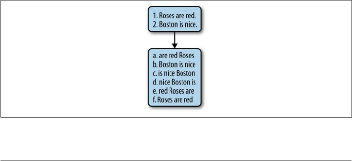
The way a KWIC index works is as follows. The input to a KWIC system is a file or
collection structured as a sequence of lines. The output is a sequence of lines, circularly
shifted and presented in alphabetical order of the first word. For an example, consider
a short article of two sentences, shown in Figure 1-1 with the KWIC index output that
is generated.
Figure 1-1. Example of a KWIC index
10 | Chapter 1: The Basics
Another benefit of concordancing is that, by displaying the keyword in its context, you
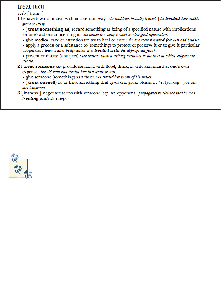
can visually inspect how the word is being used in a given sentence. To take a specific
example, consider the different meanings of the English verb treat. Specifically, let’s look
at the first two senses within sense (1) from the dictionary entry shown in Figure 1-2.
Figure 1-2. Senses of the word “treat”
Now let’s look at the concordances compiled for this verb from the BNC, as differentiated
by these two senses.
These concordances were compiled using the Word Sketch Engine, by
the lexicographer Patrick Hanks, and are part of a large resource of
sentence patterns using a technique called Corpus Pattern Analysis
(Pustejovsky et al. 2004; Hanks and Pustejovsky 2005).
What is striking when one examines the concordance entries for each of these senses is
the fact that the contexts are so distinct. These are presented in Figures 1-3 and 1-4.
A Brief History of Corpus Linguistics | 11
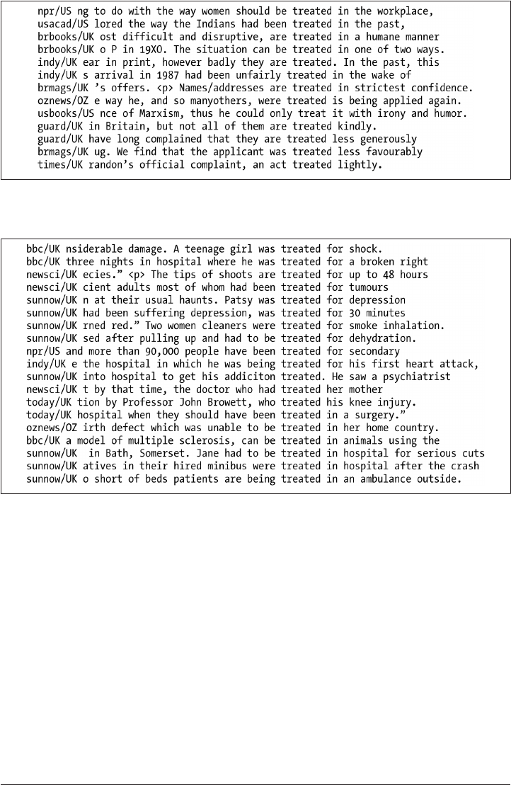
Figure 1-3. Sense (1a) for the verb “treat”
Figure 1-4. Sense (1b) for the verb “treat”
12 | Chapter 1: The Basics

The NLTK provides functionality for creating concordances. The easiest way
to make a concordance is to simply load the preprocessed texts into the NLTK
and then use the concordance function, like this:
>>> import NLTK
>>> from nltk.book import *
>>> text6.concordance("Ni")
If you have your own set of data for which you would like to create a con
cordance, then the process is a little more involved: you will need to read in
your files and use the NLTK functions to process them before you can create
your own concordance. Here is some sample code for a corpus of text files
(replace the directory location with your own folder of text files):
>>> corpus_loc = '/home/me/corpus/'
>>> docs = nltk.corpus.PlaintextCorpusReader(corpus_loc,'.*\.txt')
You can see if the files were read by checking what file IDs are present:
>>> print docs.fileids()
Next, process the words in the files and then use the concordance function
to examine the data:
>>> docs_processed = nltk.Text(docs.words())
>>> docs_processed.concordance("treat")
Corpora Today
When did researchers start to actually use corpora for modeling language phenomena
and training algorithms? Beginning in the 1980s, researchers in Speech Recognition
began to compile enough spoken language data to create language models (from tran
scriptions using n-grams and Hidden Markov Models [HMMS]) that worked well
enough to recognize a limited vocabulary of words in a very narrow domain. In the
1990s, work in Machine Translation began to see the influence of larger and larger
datasets, and with this, the rise of statistical language modeling for translation.
Eventually, both memory and computer hardware became sophisticated enough to col
lect and analyze increasingly larger datasets of language fragments. This entailed being
able to create statistical language models that actually performed with some reasonable
accuracy for different natural language tasks.
As one example of the increasing availability of data, Google has recently released the
Google Ngram Corpus. The Google Ngram dataset allows users to search for single words
(unigrams) or collocations of up to five words (5-grams). The dataset is available for
download from the Linguistic Data Consortium, and directly from Google. It is also
viewable online through the Google Ngram Viewer. The Ngram dataset consists of more
than one trillion tokens (words, numbers, etc.) taken from publicly available websites
and sorted by year, making it easy to view trends in language use. In addition to English,
Google provides n-grams for Chinese, French, German, Hebrew, Russian, and Spanish,
as well as subsets of the English corpus such as American English and English Fiction.
A Brief History of Corpus Linguistics | 13
N-grams are sets of items (often words, but they can be letters, pho
nemes, etc.) that are part of a sequence. By examining how often the
items occur together we can learn about their usage in a language, and
predict what would likely follow a given sequence (using n-grams for
this purpose is called n-gram modeling).
N-grams are applied in a variety of ways every day, such as in websites
that provide search suggestions once a few letters are typed in, and for
determining likely substitutions for spelling errors. They are also used
in speech disambiguation—if a person speaks unclearly but utters a
sequence that does not commonly (or ever) occur in the language being
spoken, an n-gram model can help recognize that problem and find the
words that the speaker probably intended to say.
Another modern corpus is ClueWeb09 (http://lemurproject.org/clueweb09.php/), a
dataset “created to support research on information retrieval and related human lan
guage technologies. It consists of about 1 billion web pages in ten languages that were
collected in January and February 2009.” This corpus is too large to use for an annotation
project (it’s about 25 terabytes uncompressed), but some projects have taken parts of the
dataset (such as a subset of the English websites) and used them for research (Pomikálek
et al. 2012). Data collection from the Internet is an increasingly common way to create
corpora, as new and varied content is always being created.
Kinds of Annotation
Consider the different parts of a language’s syntax that can be annotated. These include
part of speech (POS), phrase structure, and dependency structure. Table 1-3 shows ex
amples of each of these. There are many different tagsets for the parts of speech of a
language that you can choose from.
Table 1-3. Number of POS tags in different corpora
Tagset Size Date
Brown 77 1964
LOB 132 1980s
London-Lund Corpus 197 1982
Penn 36 1992
The tagset in Figure 1-5 is taken from the Penn TreeBank, and is the basis for all sub
sequent annotation over that corpus.
14 | Chapter 1: The Basics
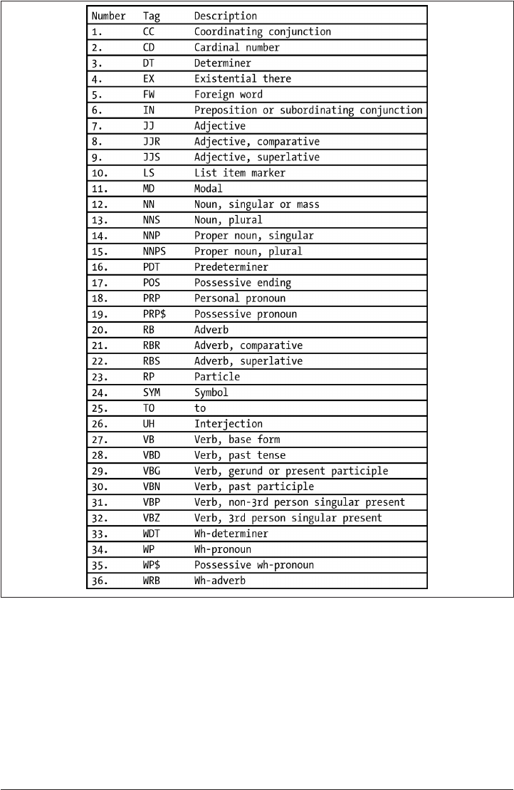
Figure 1-5. The Penn TreeBank tagset
The POS tagging process involves assigning the right lexical class marker(s) to all the
words in a sentence (or corpus). This is illustrated in a simple example, “The waiter
cleared the plates from the table.” (See Figure 1-6.)
A Brief History of Corpus Linguistics | 15
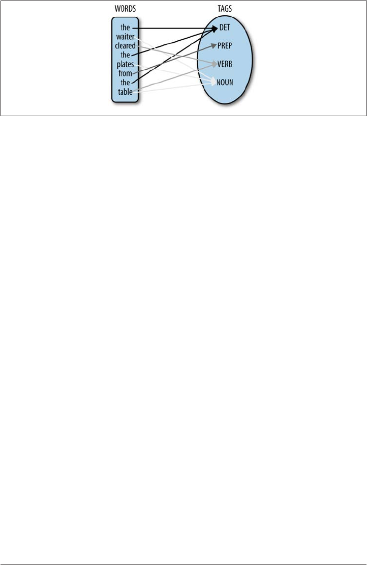
Figure 1-6. POS tagging sample
POS tagging is a critical step in many NLP applications, since it is important to know
what category a word is assigned to in order to perform subsequent analysis on it, such
as the following:
Speech Synthesis
Is the word a noun or a verb? Examples include object, overflow, insult, and sus
pect. Without context, each of these words could be either a noun or a verb.
Parsing
You need POS tags in order to make larger syntactic units. For example, in the
following sentences, is “clean dishes” a noun phrase or an imperative verb phrase?
Clean dishes are in the cabinet.
Clean dishes before going to work!
Machine Translation
Getting the POS tags and the subsequent parse right makes all the difference when
translating the expressions in the preceding list item into another language, such as
French: “Des assiettes propres” (Clean dishes) versus “Fais la vaisselle!” (Clean the
dishes!).
Consider how these tags are used in the following sentence, from the Penn TreeBank
(Marcus et al. 1993):
“From the beginning, it took a man with extraordinary qualities to succeed in Mexico,” says Kimihide Takimura, president of
Mitsui group’s Kensetsu Engineering Inc. unit.
“/” From/IN the/DT beginning/NN ,/, it/PRP took/VBD a/DT man/NN with/IN extraordinary/JJ qualities/NNS to/TO succeed/VB
in/IN Mexico/NNP ,/, “/” says/VBZ Kimihide/NNP Takimura/NNP ,/, president/NN of/IN Mitsui/NNS group/NN ’s/POS
Kensetsu/NNP Engineering/NNP Inc./NNP unit/NN ./.
16 | Chapter 1: The Basics
Identifying the correct parts of speech in a sentence is a necessary step in building many
natural language applications, such as parsers, Named Entity Recognizers, QAS, and
Machine Translation systems. It is also an important step toward identifying larger
structural units such as phrase structure.
Use the NLTK tagger to assign POS tags to the example sentence shown
here, and then with other sentences that might be more ambiguous:
>>> from nltk import pos_tag, word_tokenize
>>> pos_tag(word_tokenize("This is a test."))
Look for places where the tagger doesn’t work, and think about what
rules might be causing these errors. For example, what happens when
you try “Clean dishes are in the cabinet.” and “Clean dishes before going
to work!”?
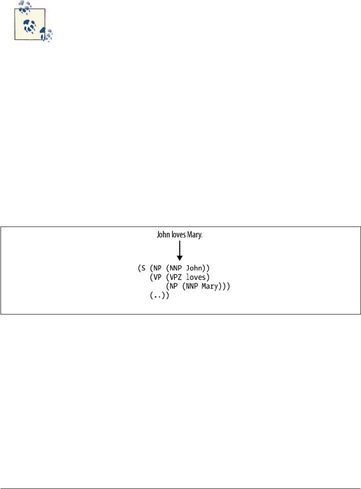
While words have labels associated with them (the POS tags mentioned earlier), specific
sequences of words also have labels that can be associated with them. This is called
syntactic bracketing (or labeling) and is the structure that organizes all the words we hear
into coherent phrases. As mentioned earlier, syntax is the name given to the structure
associated with a sentence. The Penn TreeBank is an annotated corpus with syntactic
bracketing explicitly marked over the text. An example annotation is shown in
Figure 1-7.
Figure 1-7. Syntactic bracketing
This is a bracketed representation of the syntactic tree structure, which is shown in
Figure 1-8.
A Brief History of Corpus Linguistics | 17
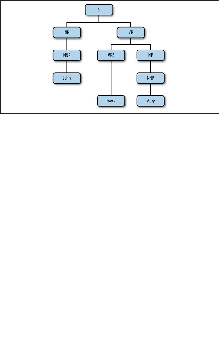
Figure 1-8. Syntactic tree structure
Notice that syntactic bracketing introduces two relations between the words in a sen
tence: order (precedence) and hierarchy (dominance). For example, the tree structure
in Figure 1-8 encodes these relations by the very nature of a tree as a directed acyclic
graph (DAG). In a very compact form, the tree captures the precedence and dominance
relations given in the following list:
{Dom(NNP1,John), Dom(VPZ,loves), Dom(NNP2,Mary), Dom(NP1,NNP1),
Dom(NP2,NNP2), Dom(S,NP1), Dom(VP,VPZ), Dom(VP,NP2), Dom(S,VP),
Prec(NP1,VP), Prec(VPZ,NP2)}
Any sophisticated natural language application requires some level of syntactic analysis,
including Machine Translation. If the resources for full parsing (such as that shown
earlier) are not available, then some sort of shallow parsing can be used. This is when
partial syntactic bracketing is applied to sequences of words, without worrying about
the details of the structure inside a phrase. We will return to this idea in later chapters.
In addition to POS tagging and syntactic bracketing, it is useful to annotate texts in a
corpus for their semantic value, that is, what the words mean in the sentence. We can
distinguish two kinds of annotation for semantic content within a sentence: what some
thing is, and what role something plays. Here is a more detailed explanation of each:
Semantic typing
A word or phrase in the sentence is labeled with a type identifier (from a reserved
vocabulary or ontology), indicating what it denotes.
18 | Chapter 1: The Basics
Semantic role labeling
A word or phrase in the sentence is identified as playing a specific semantic role
relative to a role assigner, such as a verb.
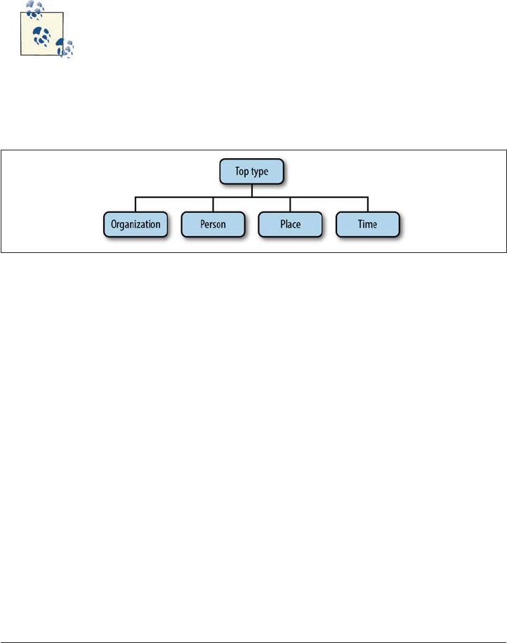
Let’s consider what annotation using these two strategies would look like, starting with
semantic types. Types are commonly defined using an ontology, such as that shown in
Figure 1-9.
The word ontology has its roots in philosophy, but ontologies also have
a place in computational linguistics, where they are used to create cate
gorized hierarchies that group similar concepts and objects. By assign
ing words semantic types in an ontology, we can create relationships
between different branches of the ontology, and determine whether
linguistic rules hold true when applied to all the words in a category.
Figure 1-9. A simple ontology
The ontology in Figure 1-9 is rather simple, with a small set of categories. However, even
this small ontology can be used to illustrate some interesting features of language. Con
sider the following example, with semantic types marked:
[Ms. Ramirez]Person of [QBC Productions]Organization visited [Boston]Place on [Satur
day]Time, where she had lunch with [Mr. Harris]Person of [STU Enterprises]Organization at
[1:15 pm]Time.
From this small example, we can start to make observations about how these objects
interact with one other. People can visit places, people have “of” relationships with
organizations, and lunch can happen on Saturday at 1:15 p.m. Given a large enough
corpus of similarly labeled sentences, we can start to detect patterns in usage that will
tell us more about how these labels do and do not interact.
A corpus of these examples can also tell us where our categories might need to be ex
panded. There are two “times” in this sentence: Saturday and 1:15 p.m. We can see that
events can occur “on” Saturday, but “at” 1:15 p.m. A larger corpus would show that this
A Brief History of Corpus Linguistics | 19

pattern remains true with other days of the week and hour designations—there is a
difference in usage here that cannot be inferred from the semantic types. However, not
all ontologies will capture all information—the applications of the ontology will deter
mine whether it is important to capture the difference between Saturday and 1:15 p.m.
The annotation strategy we just described marks up what a linguistic expression refers
to. But let’s say we want to know the basics for Question Answering, namely, the who,
what, where, and when of a sentence. This involves identifying what are called the
semantic role labels associated with a verb. What are semantic roles? Although there is
no complete agreement on what roles exist in language (there rarely is with linguists),
the following list is a fair representation of the kinds of semantic labels associated with
different verbs:
Agent
The event participant that is doing or causing the event to occur
Theme/figure
The event participant who undergoes a change in position or state
Experiencer
The event participant who experiences or perceives something
Source
The location or place from which the motion begins; the person from whom the
theme is given
GoalThe location or place to which the motion is directed or terminates
Recipient
The person who comes into possession of the theme
Patient
The event participant who is affected by the event
Instrument
The event participant used by the agent to do or cause the event
Location/ground
The location or place associated with the event itself
The annotated data that results explicitly identifies entity extents and the target relations
between the entities:
• [The man]agent painted [the wall]patient with [a paint brush]instrument.
• [Mary]figure walked to [the cafe]goal from [her house]source.
• [John]agent gave [his mother]recipient [a necklace]theme.
20 | Chapter 1: The Basics

• [My brother]theme lives in [Milwaukee]location.
Language Data and Machine Learning
Now that we have reviewed the methodology of language annotation along with some
examples of annotation formats over linguistic data, we will describe the computational
framework within which such annotated corpora are used, namely, that of machine
learning. Machine learning is the name given to the area of Artificial Intelligence con
cerned with the development of algorithms that learn or improve their performance
from experience or previous encounters with data. They are said to learn (or generate)
a function that maps particular input data to the desired output. For our purposes, the
“data” that an ML algorithm encounters is natural language, most often in the form of
text, and typically annotated with tags that highlight the specific features that are rele
vant to the learning task. As we will see, the annotation schemas discussed earlier, for
example, provide rich starting points as the input data source for the ML process (the
training phase).
When working with annotated datasets in NLP, three major types of ML algorithms are
typically used:
Supervised learning
Any technique that generates a function mapping from inputs to a fixed set of labels
(the desired output). The labels are typically metadata tags provided by humans
who annotate the corpus for training purposes.
Unsupervised learning
Any technique that tries to find structure from an input set of unlabeled data.
Semi-supervised learning
Any technique that generates a function mapping from inputs of both labeled data
and unlabeled data; a combination of both supervised and unsupervised learning.
Table 1-4 shows a general overview of ML algorithms and some of the annotation tasks
they are frequently used to emulate. We’ll talk more about why these algorithms are used
for these different tasks in Chapter 7.
Table 1-4. Annotation tasks and their accompanying ML algorithms
Algorithms Tasks
Clustering Genre classification, spam labeling
Decision trees Semantic type or ontological class assignment, coreference resolution
Naïve Bayes Sentiment classification, semantic type or ontological class assignment
Maximum Entropy (MaxEnt) Sentiment classification, semantic type, or ontological class assignment
Structured pattern induction (HMMs, CRFs, etc.) POS tagging, sentiment classification, word sense disambiguation
Language Data and Machine Learning | 21

You’ll notice that some of the tasks appear with more than one algorithm. That’s because
different approaches have been tried successfully for different types of annotation tasks,
and depending on the most relevant features of your own corpus, different algorithms
may prove to be more or less effective. Just to give you an idea of what the algorithms
listed in that table mean, the rest of this section gives an overview of the main types of
ML algorithms.
Classification
Classification is the task of identifying the labeling for a single entity from a set of data.
For example, in order to distinguish spam from not-spam in your email inbox, an algo
rithm called a classifier is trained on a set of labeled data, where individual emails have
been assigned the label [+spam] or [-spam]. It is the presence of certain (known) words
or phrases in an email that helps to identify an email as spam. These words are essentially
treated as features that the classifier will use to model the positive instances of spam as
compared to not-spam. Another example of a classification problem is patient diagnosis,
from the presence of known symptoms and other attributes. Here we would identify a
patient as having a particular disease, A, and label the patient record as [+disease-A] or
[-disease-A], based on specific features from the record or text. This might include blood
pressure, weight, gender, age, existence of symptoms, and so forth. The most common
algorithms used in classification tasks are Maximum Entropy (MaxEnt), Naïve Bayes,
decision trees, and Support Vector Machines (SVMs).
Clustering
Clustering is the name given to ML algorithms that find natural groupings and patterns
from the input data, without any labeling or training at all. The problem is generally
viewed as an unsupervised learning task, where either the dataset is unlabeled or the
labels are ignored in the process of making clusters. The clusters that are formed are
“similar in some respect,” and the other clusters formed are “dissimilar to the objects”
in other clusters. Some of the more common algorithms used for this task include k-
means, hierarchical clustering, Kernel Principle Component Analysis, and Fuzzy C-
Means (FCM).
Structured Pattern Induction
Structured pattern induction involves learning not only the label or category of a single
entity, but rather learning a sequence of labels, or other structural dependencies between
the labeled items. For example, a sequence of labels might be a stream of phonemes in
a speech signal (in Speech Recognition); a sequence of POS tags in a sentence corre
sponding to a syntactic unit (phrase); a sequence of dialog moves in a phone
22 | Chapter 1: The Basics

conversation; or steps in a task such as parsing, coreference resolution, or grammar
induction. Algorithms used for such problems include Hidden Markov Models
(HMMs), Conditional Random Fields (CRFs), and Maximum Entropy Markov Models
(MEMMs).
We will return to these approaches in more detail when we discuss machine learning in
greater depth in Chapter 7.
The Annotation Development Cycle
The features we use for encoding a specific linguistic phenomenon must be rich enough
to capture the desired behavior in the algorithm that we are training. These linguistic
descriptions are typically distilled from extensive theoretical modeling of the phenom
enon. The descriptions in turn form the basis for the annotation values of the specifi
cation language, which are themselves the features used in a development cycle for
training and testing an identification or labeling algorithm over text. Finally, based on
an analysis and evaluation of the performance of a system, the model of the phenomenon
may be revised for retraining and testing.
We call this particular cycle of development the MATTER methodology, as detailed here
and shown in Figure 1-10 (Pustejovsky 2006):
Model
Structural descriptions provide theoretically informed attributes derived from em
pirical observations over the data.
Annotate
An annotation scheme assumes a feature set that encodes specific structural de
scriptions and properties of the input data.
Train
The algorithm is trained over a corpus annotated with the target feature set.
Test The algorithm is tested against held-out data.
Evaluate
A standardized evaluation of results is conducted.
Revise
The model and the annotation specification are revisited in order to make the an
notation more robust and reliable with use in the algorithm.
The Annotation Development Cycle | 23
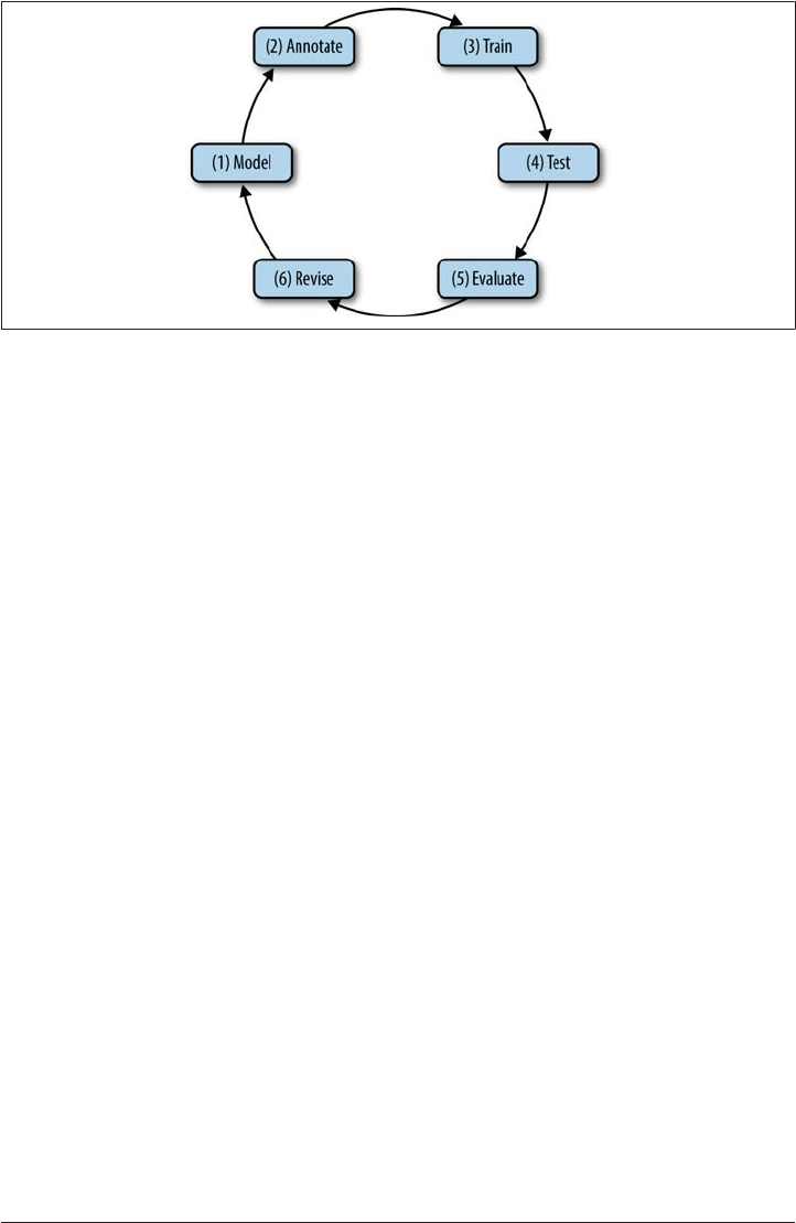
Figure 1-10. The MATTER cycle
We assume some particular problem or phenomenon has sparked your interest, for
which you will need to label natural language data for training for machine learning.
Consider two kinds of problems. First imagine a direct text classification task. It might
be that you are interested in classifying your email according to its content or with a
particular interest in filtering out spam. Or perhaps you are interested in rating your
incoming mail on a scale of what emotional content is being expressed in the message.
Now let’s consider a more involved task, performed over this same email corpus: iden
tifying what are known as Named Entities (NEs). These are references to everyday things
in our world that have proper names associated with them; for example, people, coun
tries, products, holidays, companies, sports, religions, and so on.
Finally, imagine an even more complicated task, that of identifying all the different
events that have been mentioned in your mail (birthdays, parties, concerts, classes,
airline reservations, upcoming meetings, etc.). Once this has been done, you will need
to “timestamp” them and order them, that is, identify when they happened, if in fact
they did happen. This is called the temporal awareness problem, and is one of the most
difficult in the field.
We will use these different tasks throughout this section to help us clarify what is in
volved with the different steps in the annotation development cycle.
Model the Phenomenon
The first step in the MATTER development cycle is “Model the Phenomenon.” The steps
involved in modeling, however, vary greatly, depending on the nature of the task you
have defined for yourself. In this section, we will look at what modeling entails and how
you know when you have an adequate first approximation of a model for your task.
24 | Chapter 1: The Basics

The parameters associated with creating a model are quite diverse, and it is difficult to
get different communities to agree on just what a model is. In this section we will be
pragmatic and discuss a number of approaches to modeling and show how they provide
the basis from which to created annotated datasets. Briefly, a model is a characterization
of a certain phenomenon in terms that are more abstract than the elements in the domain
being modeled. For the following discussion, we will define a model as consisting of a
vocabulary of terms, T, the relations between these terms, R, and their interpretation,
I. So, a model, M, can be seen as a triple, M = <T,R,I>. To better understand this notion
of a model, let us consider the scenarios introduced earlier. For spam detection, we can
treat it as a binary text classification task, requiring the simplest model with the cate
gories (terms) spam and not-spam associated with the entire email document. Hence,
our model is simply:
• T = {Document_type, Spam, Not-Spam}
• R = {Document_type ::= Spam | Not-Spam}
• I = {Spam = “something we don’t want!”, Not-Spam = “something we do want!"}
The document itself is labeled as being a member of one of these categories. This is
called document annotation and is the simplest (and most coarse-grained) annotation
possible. Now, when we say that the model contains only the label names for the cate
gories (e.g., sports, finance, news, editorials, fashion, etc.), this means there is no other
annotation involved. This does not mean the content of the files is not subject to further
scrutiny, however. A document that is labeled as a category, A, for example, is actually
analyzed as a large-feature vector containing at least the words in the document. A more
fine-grained annotation for the same task would be to identify specific words or phrases
in the document and label them as also being associated with the category directly. We’ll
return to this strategy in Chapter 4. Essentially, the goal of designing a good model of
the phenomenon (task) is that this is where you start for designing the features that go
into your learning algorithm. The better the features, the better the performance of the
ML algorithm!
Preparing a corpus with annotations of NEs, as mentioned earlier, involves a richer
model than the spam-filter application just discussed. We introduced a four-category
ontology for NEs in the previous section, and this will be the basis for our model to
identify NEs in text. The model is illustrated as follows:
• T = {Named_Entity, Organization, Person, Place, Time}
• R = {Named_Entity ::= Organization | Person | Place | Time}
•I = {Organization = “list of organizations in a database”, Person = “list of people in
a database”, Place = “list of countries, geographic locations, etc.”, Time = “all possible
dates on the calendar”}
The Annotation Development Cycle | 25

This model is necessarily more detailed, because we are actually annotating spans of
natural language text, rather than simply labeling documents (e.g., emails) as spam or
not-spam. That is, within the document, we are recognizing mentions of companies,
actors, countries, and dates.
Finally, what about an even more involved task, that of recognizing all temporal infor
mation in a document? That is, questions such as the following:
•When did that meeting take place?
•How long was John on vacation?
• Did Jill get promoted before or after she went on maternity leave?
We won’t go into the full model for this domain, but let’s see what is minimally necessary
in order to create annotation features to understand such questions. First we need to
distinguish between Time expressions (“yesterday,” “January 27,” “Monday”), Events
(“promoted,” “meeting,” “vacation”), and Temporal relations (“before,” “after,” “during”).
Because our model is so much more detailed, let’s divide the descriptive content by
domain:
• Time_Expression ::= TIME | DATE | DURATION | SET
— TIME: 10:15 a.m., 3 o’clock, etc.
— DATE: Monday, April 2011
— DURATION: 30 minutes, two years, four days
— SET: every hour, every other month
• Event: Meeting, vacation, promotion, maternity leave, etc.
• Temporal_Relations ::= BEFORE | AFTER | DURING | EQUAL | OVERLAP | ...
We will come back to this problem in a later chapter, when we discuss the impact of the
initial model on the subsequent performance of the algorithms you are trying to train
over your labeled data.
In later chapters, we will see that there are actually several models that
might be appropriate for describing a phenomenon, each providing a
different view of the data. We will call this multimodel annotation of the
phenomenon. A common scenario for multimodel annotation involves
annotators who have domain expertise in an area (such as biomedical
knowledge). They are told to identify specific entities, events, attributes,
or facts from documents, given their knowledge and interpretation of
a specific area. From this annotation, nonexperts can be used to mark
up the structural (syntactic) aspects of these same phenomena, thereby
making it possible to gain domain expert understanding without forc
ing the domain experts to learn linguistic theory as well.
26 | Chapter 1: The Basics

Once you have an initial model for the phenomena associated with the problem task
you are trying to solve, you effectively have the first tag specification, or spec, for the
annotation. This is the document from which you will create the blueprint for how to
annotate the corpus with the features in the model. This is called the annotation guide
line, and we talk about this in the next section.
Annotate with the Specification
Now that you have a model of the phenomenon encoded as a specification document,
you will need to train human annotators to mark up the dataset according to the tags
that are important to you. This is easier said than done, and in fact often requires multiple
iterations of modeling and annotating, as shown in Figure 1-11. This process is called
the MAMA (Model-Annotate-Model-Annotate) cycle, or the “babeling” phase of MAT
TER. The annotation guideline helps direct the annotators in the task of identifying the
elements and then associating the appropriate features with them, when they are
identified.
Two kinds of tags will concern us when annotating natural language data: consuming
tags and nonconsuming tags. A consuming tag refers to a metadata tag that has real
content from the dataset associated with it (e.g., it “consumes” some text); a noncon
suming tag, on the other hand, is a metadata tag that is inserted into the file but is not
associated with any actual part of the text. An example will help make this distinction
clear. Say that we want to annotate text for temporal information, as discussed earlier.
Namely, we want to annotate for three kinds of tags: times (called Timex tags), temporal
relations (TempRels), and Events. In the first sentence in the following example, each
tag is expressed directly as real text. That is, they are all consuming tags (“promoted” is
marked as an Event, “before” is marked as a TempRel, and “the summer” is marked as
a Timex). Notice, however, that in the second sentence, there is no explicit temporal
relation in the text, even though we know that it’s something like “on”. So, we actually
insert a TempRel with the value of “on” in our corpus, but the tag is flagged as a “non
consuming” tag.
• John was [promoted]Event [before]TempRel [the summer]Timex.
• John was [promoted]Event [Monday]Timex.
An important factor when creating an annotated corpus of your text is, of course, con
sistency in the way the annotators mark up the text with the different tags. One of the
most seemingly trivial problems is the most problematic when comparing annotations:
namely, the extent or the span of the tag. Compare the three annotations that follow. In
the first, the Organization tag spans “QBC Productions,” leaving out the company iden
tifier “Inc.” and the location “of East Anglia,” while these are included in varying spans
in the next two annotations.
The Annotation Development Cycle | 27
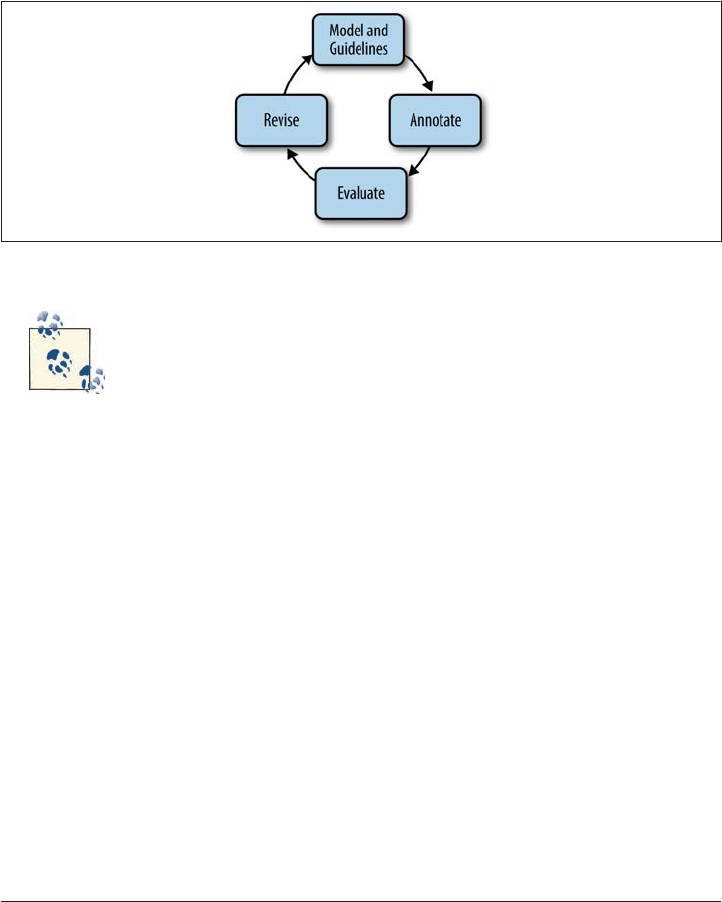
• [QBC Productions]Organization Inc. of East Anglia
• [QBC Productions Inc.]Organization of East Anglia
• [QBC Productions Inc. of East Anglia]Organization
Each of these might look correct to an annotator, but only one actually corresponds to
the correct markup in the annotation guideline. How are these compared and resolved?
Figure 1-11. The inner workings of the MAMA portion of the MATTER cycle
In order to assess how well an annotation task is defined, we use Inter-
Annotator Agreement (IAA) scores to show how individual annotators
compare to one another. If an IAA score is high, that is an indication
that the task is well defined and other annotators will be able to continue
the work. This is typically defined using a statistical measure called a
Kappa Statistic. For comparing two annotations against each other, the
Cohen Kappa is usually used, while when comparing more than two
annotations, a Fleiss Kappa measure is used. These will be defined in
Chapter 8.
Note that having a high IAA score doesn’t necessarily mean the anno
tations are correct; it simply means the annotators are all interpreting
your instructions consistently in the same way. Your task may still need
to be revised even if your IAA scores are high. This will be discussed
further in Chapter 9.
Once you have your corpus annotated by at least two people (more is preferable, but not
always practical), it’s time to create the gold standard corpus. The gold standard is the
final version of your annotated data. It uses the most up-to-date specification that you
created during the annotation process, and it has everything tagged correctly according
to the most recent guidelines. This is the corpus that you will use for machine learning,
28 | Chapter 1: The Basics

and it is created through the process of adjudication. At this point in the process, you
(or someone equally familiar with all the tasks) will compare the annotations and de
termine which tags in the annotations are correct and should be included in the gold
standard.
Train and Test the Algorithms over the Corpus
Now that you have adjudicated your corpus, you can use your newly created gold stan
dard for machine learning. The most common way to do this is to divide your corpus
into two parts: the development corpus and the test corpus. The development corpus is
then further divided into two parts: the training set and the development-test set.
Figure 1-12 shows a standard breakdown of a corpus, though different distributions
might be used for different tasks. The files are normally distributed randomly into the
different sets.
Figure 1-12. Corpus divisions for machine learning
The training set is used to train the algorithm that you will use for your task. The
development-test (dev-test) set is used for error analysis. Once the algorithm is trained,
it is run on the dev-test set and a list of errors can be generated to find where the
algorithm is failing to correctly label the corpus. Once sources of error are found, the
algorithm can be adjusted and retrained, then tested against the dev-test set again. This
procedure can be repeated until satisfactory results are obtained.
Once the training portion is completed, the algorithm is run against the held-out test
corpus, which until this point has not been involved in training or dev-testing. By hold
ing out the data, we can show how well the algorithm will perform on new data, which
gives an expectation of how it would perform on data that someone else creates as well.
Figure 1-13 shows the “TTER” portion of the MATTER cycle, with the different corpus
divisions and steps.
The Annotation Development Cycle | 29
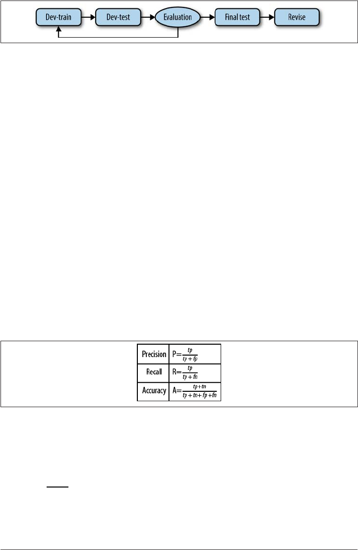
Figure 1-13. The Training–Evaluation cycle
Evaluate the Results
The most common method for evaluating the performance of your algorithm is to cal‐
culate how accurately it labels your dataset. This can be done by measuring the fraction
of the results from the dataset that are labeled correctly using a standard technique of
“relevance judgment” called the Precision and Recall metric.
Here’s how it works. For each label you are using to identify elements in the data, the
dataset is divided into two subsets: one that is labeled “relevant” to the label, and one
that is not relevant. Precision is a metric that is computed as the fraction of the correct
instances from those that the algorithm labeled as being in the relevant subset. Recall is
computed as the fraction of correct items among those that actually belong to the rele‐
vant subset. The following confusion matrix helps illustrate how this works:
Predicted Labeling
positive negative
Gold positive true positive (tp) false negative (fn)
Labeling negative false positive (fp) true negative (tn)
Given this matrix, we can define both precision and recall as shown in Figure 1-14, along
with a conventional definition of accuracy.
Figure 1-14. Precision and recall equations
The values of P and R are typically combined into a single metric called the F-measure,
which is the harmonic mean of the two.
F= 2* P*R
P+R
30 | Chapter 1: The Basics

This creates an overall score used for evaluation where precision and recall are measured
equally, though depending on the purpose of your corpus and algorithm, a variation of
this measure, such as one that rates precision higher than recall, may be more useful to
you. We will give more detail about how these equations are used for evaluation in
Chapter 8.
Revise the Model and Algorithms
Once you have evaluated the results of training and testing your algorithm on the data,
you will want to do an error analysis to see where it performed well and where it made
mistakes. This can be done with various packages and formulas, which we will discuss
in Chapter 8, including the creation of what are called confusion matrices. These will
help you go back to the design of the model, in order to create better tags and features
that will subsequently improve your gold standard, and consequently result in better
performance of your learning algorithm.
A brief example of model revision will help make this point. Recall the model for NE
extraction from the previous section, where we distinguished between four types of
entities: Organization, Place, Time, and Person. Depending on the corpus you have
assembled, it might be the case that you are missing a major category, or that you would
be better off making some subclassifications within one of the existing tags. For example,
you may find that the annotators are having a hard time knowing what to do with named
occurrences or events, such as Easter, 9-11, or Thanksgiving. These denote more than
simply Times, and suggest that perhaps a new category should be added to the model:
Event. Additionally, it might be the case that there is reason to distinguish geopolitical
Places from nongeopolitical Places. As with the “Model-Annotate” and “Train-Test”
cycles, once such additions and modifications are made to the model, the MATTER
cycle begins all over again, and revisions will typically bring improved performance.
Summary
In this chapter, we have provided an overview of the history of corpus and computational
linguistics, and the general methodology for creating an annotated corpus. Specifically,
we have covered the following points:
•Natural language annotation is an important step in the process of training com
puters to understand human speech for tasks such as Question Answering, Machine
Translation, and summarization.
•All of the layers of linguistic research, from phonetics to semantics to discourse
analysis, are used in different combinations for different ML tasks.
•In order for annotation to provide statistically useful results, it must be done on a
sufficiently large dataset, called a corpus. The study of language using corpora is
corpus linguistics.
Summary | 31

•Corpus linguistics began in the 1940s, but did not become a feasible way to study
language until decades later, when the technology caught up to the demands of the
theory.
•A corpus is a collection of machine-readable texts that are representative of natural
human language. Good corpora are representative and balanced with respect to the
genre or language that they seek to represent.
•The uses of computers with corpora have developed over the years from simple key-
word-in-context (KWIC) indexes and concordances that allowed full-text docu
ments to be searched easily, to modern, statistically based ML techniques.
•Annotation is the process of augmenting a corpus with higher-level information,
such as part-of-speech tagging, syntactic bracketing, anaphora resolution, and word
senses. Adding this information to a corpus allows the computer to find features
that can make a defined task easier and more accurate.
•Once a corpus is annotated, the data can be used in conjunction with ML algorithms
that perform classification, clustering, and pattern induction tasks.
•Having a good annotation scheme and accurate annotations is critical for machine
learning that relies on data outside of the text itself. The process of developing the
annotated corpus is often cyclical, with changes made to the tagsets and tasks as the
data is studied further.
•Here we refer to the annotation development cycle as the MATTER cycle—Model,
Annotate, Train, Test, Evaluate, Revise.
•Often before reaching the Test step of the process, the annotation scheme has already
gone through several revisions of the Model and Annotate stages.
•This book will show you how to create an accurate and effective annotation scheme
for a task of your choosing, apply the scheme to your corpus, and then use ML
techniques to train a computer to perform the task you designed.
32 | Chapter 1: The Basics

CHAPTER 2
Defining Your Goal and Dataset
Creating a clear definition of your annotation goal is vital for any project aiming to
incorporate machine learning. When you are designing your annotation tagsets, writing
guidelines, working with annotators, and training algorithms, it can be easy to become
sidetracked by details and lose sight of what you want to achieve. Having a clear goal to
refer back to can help, and in this chapter we will go over what you need to create a good
definition of your goal, and discuss how your goal can influence your dataset. In par
ticular, we will look at:
• What makes a good annotation goal
• Where to find related research
• How your dataset reflects your annotation goals
• Preparing the data for annotators to use
• How much data you will need for your task
What you should be able to take away from this chapter is a clear answer to the questions
“What am I trying to do?”, “How am I trying to do it?”, and “Which resources best fit
my needs?”. As you progress through the MATTER cycle, the answers to these questions
will probably change—corpus creation is an iterative process—but having a stated goal
will help keep you from getting off track.
Defining Your Goal
In terms of the MATTER cycle, at this point we’re right at the start of “M”—being able
to clearly explain what you hope to accomplish with your corpus is the first step in
creating your model. While you probably already have a good idea about what you want
to do, in this section we’ll give you some pointers on how to create a goal definition that
is useful and will help keep you focused in the later stages of the MATTER cycle.
33

We have found it useful to split the goal definition into two steps: first, write a statement
of purpose that covers the very basics of your task, and second, use that sentence to
expand on the “how”s of your goal. In the rest of this section, we’ll give some pointers
on how to make sure each of these parts will help you with your corpus task.
The Statement of Purpose
At this point we’re assuming that you already have some question pertaining to natural
language that you want to explore. (If you don’t really have a project in mind yet, check
the appendixes for lists of existing corpora, and read the proceedings from related con
ferences to see if there’s anything that catches your eye, or consider participating in
Natural Language Process [NLP] challenges, which are discussed later in this chapter.)
But how clearly can you explain what you intend to do? If you can’t come up with a one-
or two-sentence summary describing your intended line of research, then you’re going
to have a very hard time with the rest of this task. Keep in mind that we are not talking
about a sentence like “Genres are interesting”—that’s an opinion, not a starting point
for an annotation task. Instead, try to have a statement more like this:
I want to use keywords to detect the genre of a newspaper article in order to create da
tabases of categorized texts.
This statement is still going to need a lot of refinement before it can be turned into an
annotation model, but it answers the basic questions. Specifically, it says:
• What the annotation will be used for (databases)
• What the overall outcome of the annotation will be (genre classification)
• Where the corpus will come from (news articles)
• How the outcome will be achieved (keywords)
Be aware that you may have a task in mind that will require multiple annotation efforts.
For example, say you’re interested in exploring humor. Even if you have the time, money,
and people to do a comprehensive study of all aspects of humor, you will still need to
break down the task into manageable segments in order to create annotation tasks for
different types of humor. If you want to look at the effects of sarcasm and puns, you will
likely need different vocabularies for each task, or be willing to spend the time to create
one overarching annotation spec that will encompass all annotations, but we suggest
that you start small and then merge annotations later, if possible.
If you do have a broad task that you will need to break down into large subtasks, then
make that clear in your summary: “I want to create a program that can generate jokes
34 | Chapter 2: Defining Your Goal and Dataset

in text and audio formats, including puns, sarcasm, and exaggeration.” Each of the items
in that list will require a separate annotation and machine learning (ML) task. Grouping
them together, at least at first, would create such a massively complicated task that it
would be difficult to complete, let alone learn from.
To provide some more context, Table 2-1 shows a few examples of one-sentence sum
maries, representative of the diverse range of annotation projects and corpora that exist
in the field.
Table 2-1. Some corpora and their uses
Corpus Summary sentence
PropBank For annotating verbal propositions and their arguments for examining semantic roles
Manually Annotated Sub-Corpus
(MASC)
For annotating sentence boundaries, tokens, lemma, and part of speech (POS), noun and
verb chunks, and Named Entities (NEs); a subset of the Open American National Corpus
(OANC)
Penn Discourse TreeBank For annotating discourse relations between eventualities and propositions in newswires for
learning about discourse in natural language
MPQA Opinion Corpus For annotating opinions for use in evaluating emotional language
TimeBank For labeling times, events, and their relationships in news texts for use in temporal reasoning
i2b2 2008 Challenge, Task 1C For identifying patient smoking status from medical records for use in medical studies
2012 SemEval Task 7—COPA:
Choice of Plausible Alternatives
Provides alternative answers to questions; annotation focuses on finding the most likely
answer based on reasoning
Naturally, this isn’t a complete list of corpora, but it does cover a wide range of different
focuses for annotation tasks. These are not high-level descriptions of what these corpora
are about, but they answer the basic questions necessary for moving forward with an
annotation task. In the next section, we’ll look at how to turn this one sentence into an
annotation model.
Refining Your Goal: Informativity Versus Correctness
Now that you have a statement of purpose for your corpus, you need to turn it into a
task description that can be used to create your model—that is, your corpus, annotation
scheme, and guidelines.
When annotating corpora, there is a fine line between having an annotation that will
be the most useful for your task (having high informativity) and having an annotation
that is not too difficult for annotators to complete accurately (which results in high levels
of correctness).
A clear example of where this trade-off comes into play is temporal annotation. Imagine
that you want to capture all the relationships between times and events in this simple
narrative:
Defining Your Goal | 35
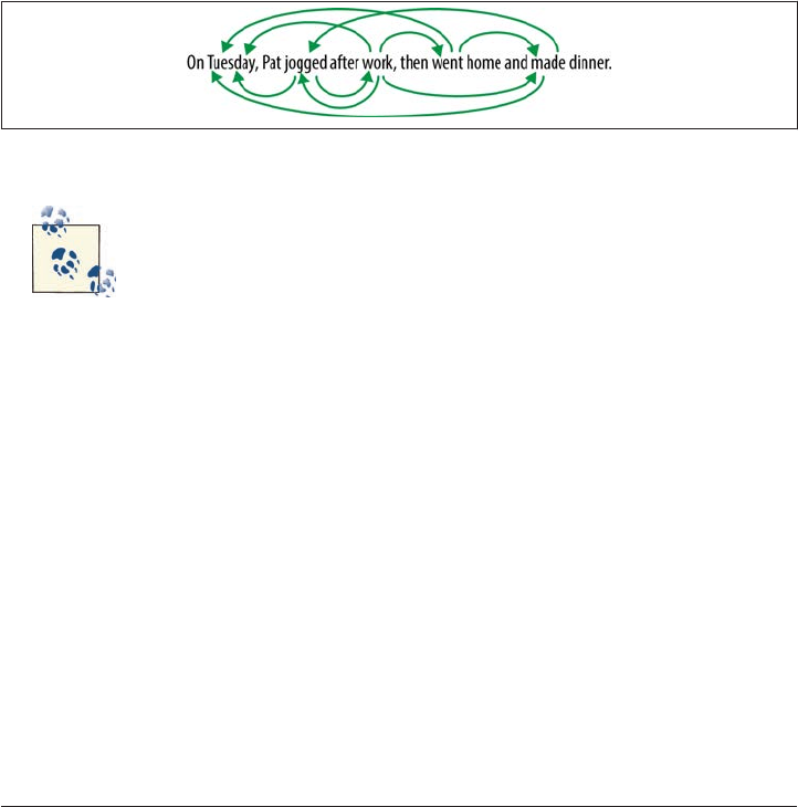
On Tuesday, Pat jogged after work, then went home and made dinner.
Figure 2-1 shows what it would look like to actually create all of those relationships, and
you can see that a large number of connections are necessary in order to capture all the
relationships between events and times. In such tasks, the number of relationships is
almost quadratic to the number of times and events [here we have 10, because the links
only go in one direction—if we captured both directions, there would be 20 links: x
⁕
(x – 1)], where x is the number of events/times in the sentence. It wouldn’t be very
practical to ask an annotator to do all that work by hand; such a task would take an
incredibly long time to complete, and an annotation that complex will lead to a lot of
errors and omissions—in other words, low correctness. However, asking for a limited
set of relations may lead to lower levels of informativity, especially if your annotation
guidelines are not very carefully written. We’ll discuss annotation guidelines further in
Chapter 6.
Figure 2-1. All temporal relations over events and times
You have probably realized that with this particular example it’s not
necessary to have a human create all those links—if A occurs before B
and B occurs before C, a computer could use closure rules to determine
that A occurs before C, and annotators would not have to capture that
information themselves. It’s always a good idea to consider what parts
of your task can be done automatically, especially when it can make your
annotator’s job easier without necessarily sacrificing accuracy.
The considerations surrounding informativity and correctness are very much inter
twined with one of the biggest factors affecting your annotation task: the scope of your
project. There are two main aspects of project scope that you need to consider: (1) how
far-reaching the goal is (the scope of the annotation), and (2) how much of your chosen
field you plan to cover (the scope of the corpus). We already touched on (2) a little in
the preceding section, and we will have more to say about it later, so for now let’s look
at (1).
The scope of the annotation task
At this point you have already begun to address the question of your task’s scope by
answering the four questions from the preceding section—at the very least you’ve
36 | Chapter 2: Defining Your Goal and Dataset
narrowed down what category of features you’ll be using (by answering the “means by
which the goal will be achieved” question), and what the overall goal of the annotation
will be. However, having a general class that your task can be slotted into may still leave
you with a lot of variables that you will need to consider.
As always, remember that the MATTER cycle is, in fact, a cycle, and as
you go through the steps, you may find new information that causes
your scope to widen or shrink.
It’s a bit difficult to discuss scope in general terms, so let’s look at some specific examples,
and then see how the principles can be applied to other projects. In the temporal relation
annotation task discussed previously, the scope of the project has to do with exactly
what relations are important to the annotation. Are only the main events in each sen
tence and their relationships important? Do you want to be able to capture only relations
inside a sentence, or do you want to capture relations between sentences as well? Maybe
you only care about the events that have clear temporal anchors, such as “Jay ran on
Sunday.” Do you think it’s important to differentiate between different types of links?
Similar questions can be asked about the newspaper genre classification example. In
that task, the relevant question is “How specific do you want your categories to be?” Is
it enough to divide articles into broad categories, such as “news” and “sports,” or do you
want a more detailed system that specifies “news:global” and “sports:baseball” (or even
“sports:baseball:Yankees”)?
If this is your first excursion into annotation and corpus building, start
with broader categories or simpler tasks—as you learn the ins and outs
of your dataset and annotation tags, you’ll be able to refine your project
in more meaningful and useful ways.
As you can see, the questions being asked about the two examples so far essentially
become questions about classification—in the newspaper example this is a much more
obvious correlation, but even the temporal relation example touches on this subject. By
defining different possible categories of relationships (inter- and intra-sentential, main
verbs versus other verbs), it’s much easier to identify what parts you feel will be most
relevant to your task.
This book is about annotation, and it’s necessarily true that if you have an annotation
project, classification is some part of your task. This could involve document-level tags,
as in the newspaper example; labels that are associated with each word (or a subset of
words), as in a POS tagging task; or labeling relationships between existing tags. If you
can think of your annotation task in terms of a classification task, then that will provide
Defining Your Goal | 37

a stable framework for you to start considering the scope of your task. You most likely
already have intuitions about what the relevant features of your data and task are, so use
those (at least at first) to determine the scope of your task. This intuition can also help
you determine what level of informativity you will need for good classification results,
and how accurate you can expect an annotator to be.
Linguistic intuition is an extremely useful way to get started in thinking
about a topic, but it can be misleading and even wrong. Once you’ve
started gathering texts and doing some annotation, if you find that the
data does not match your expectations, don’t hesitate to reevaluate your
approach.
Let’s go back to our four questions from the previous section and see how informativity
and correctness come into effect when elaborating on these aspects of your annotation
task. Now that you have a better idea of the scope of your project, it should be fairly easy
to see what sorts of things you will want to take into account when answering these
questions. (Notice that we didn’t say the questions would be easy to answer—the trade-
off between informativity and correctness is a consideration at all levels, and can make
it difficult to decide where to draw the line on a project.)
What will the annotation be used for?
It’s likely that the answer to this question hasn’t really changed based on the discussion
questions we’ve provided so far—the end product of the annotation, training, and testing
is why you’re taking on this project in the first place, and is what ultimately informs the
answers to the rest of the questions and the project as a whole. However, it’s helpful to
remind yourself of what you’re trying to do before you start expanding your answers to
the other questions.
If you have some idea of what ML techniques you’ll be using, then that can be a con
sideration as well at this point, but it’s not required, especially if this is your first turn
around the MATTER cycle.
What will the overall outcome be?
Thinking about the scope of your project in terms of a classification task, now is the
time to start describing the outcome in terms of specific categories. Instead of saying
“Classify newspaper articles into genres,” try to decide on the number of genres that you
think you’ll need to encompass all the types of articles you’re interested in.
38 | Chapter 2: Defining Your Goal and Dataset

The more categories that your task uses, the harder it will probably be
to train an ML algorithm to accurately label your corpus. This doesn’t
necessarily mean you should limit your project right from the start, but
you may find that in later iterations of the MATTER cycle you need to
merge some categories.
For the temporal relation annotation, accuracy versus informativity is a huge consid
eration, for the reasons described earlier (refer back to Figure 2-1 for a refresher on how
complicated this task can be). In this case, and in the case of tasks of similar complexity,
the specifics of how detailed your task will be will almost certainly have to be worked
out through multiple iterations of annotation and evaluation.
For both of these tasks, considering the desired outcome will help you to determine the
answer to this question. In the genre case, the use of the database is the main consid
eration point—who will be using it, and for what? Temporal annotation can be used for
a number of things, such as summarization, timeline creation, Question Answering,
and so on. The granularity of the task will also inform what needs to be captured in the
annotation: if, for example, you are only interested in summarizing the major events in
a text, then it might be sufficient to only annotate the relationships of the main event in
each sentence.
Where will the corpus come from?
Now that you’ve thought about the scope of your task, it should be much easier to answer
more specific questions about the scope of your corpus. Specifically, it’s time to start
thinking about the distribution of sources; that is, exactly where all your data will come
from and how different aspects of it will be balanced.
Returning to our newspaper classification example, consider whether different news
venues have sufficiently different styles that you would need to train an algorithm over
all of them, or if a single source is similar enough to the others for the algorithm to be
easily generalizable. Are the writing and topics in the New York Times similar enough
to the Wall Street Journal that you don’t need examples from each? What about news
papers and magazines that publish exclusively online? Do you consider blogs to be news
sources? Will you include only written articles, or will you also include transcripts of
broadcasts?
For temporal annotation, our experience has been that different publication styles and
genres can have a huge impact on how times are used in text. (Consider a children’s
story compared to a newspaper article, and how linear [or not] the narration in each
tends to be.) If you want your end product to cover all types of sources, this might be
another splitting point for your tasks—you may need to have different annotation
guidelines for different narrative genres, so consider carefully how far-reaching you want
your task to be.
Defining Your Goal | 39

Clearly, these considerations are tied into the scope of your task—the bigger the scope,
the more sources you will need to include in your annotation in order to maximize
informativity. However, the more disparate sources you include, the more likely it is that
you will need to consider having slightly different annotation tasks for each source,
which could lower correctness if the tasks are not fully thought out for each genre.
It’s also a good idea to check out existing corpora for texts that might be suitable for the
task you are working on. Using a preassembled corpus (or a subset of one) has the
obvious benefit of lessening the work that you will have to do, but it also means you will
have access to any other annotations that have been done on those files. See “Background
Research” (page 41) for more information on linguistic resources.
Don’t get too caught up in the beginning with creating the perfect cor
pus—remember that this process is cyclical, and if you find you’re miss
ing something, you can always go back and add it later.
How will the result be achieved?
In Chapter 1 we discussed the levels of linguistics—phonology, syntax, semantics, and
so on—and gave examples of annotation tasks for each of those levels. Consider at this
point, if you haven’t already, which of these levels your task fits into. However, don’t try
to force your task to only deal with a single linguistic level! Annotations and corpora do
not always fit neatly into one category or another, and the same is probably true of your
own task.
For instance, while the temporal relation task that we have been using as an example so
far fits fairly solidly into the discourse and text structure level, it relies on having events
and times already annotated. But what is an event? Often events are verbs (“He ran down
the street.”) but they can also be nouns (“The election was fiercely contested.”) or even
adjectives, depending on whether they represent a state that has changed (“The volcano
was dormant for centuries before the eruption.”). But labeling events is not a purely
syntactic task, because (1) not all nouns, verbs, and adjectives are events, and (2) the
context in which a word is used will determine whether a word is an event or not.
Consider “The party lasted until 10” versus “The political party solicited funds for the
campaign.” These examples add a semantic component to the event annotation.
It’s very likely that your own task will benefit from bringing in information from different
levels of linguistics. POS tagging is the most obvious example of additional information
that can have a huge impact on how well an algorithm performs an NLP task: knowing
the part of speech of a word can help with word sense disambiguation (“call the police”
versus “police the neighborhood”), determining how the syllables of a word are pro
nounced (consider the verb present versus the noun present—this is a common pattern
in American English), and so on.
40 | Chapter 2: Defining Your Goal and Dataset

Of course, there is always a trade-off: the more levels (or partial levels—it might not be
necessary to have POS labels for all your data; they might only be used on words that
are determined to be interesting in some other way) that your annotation includes, the
more informative it’s likely to be. But the other side of that is that the more complex
your task is, the more likely it is that your annotators will become confused, thereby
lowering your accuracy. Again, the important thing to remember is that MATTER is a
cycle, so you will need to experiment to determine what works best for your task.
Background Research
Now that you’ve considered what linguistic levels are appropriate for your task, it’s time
to do some research into related work. Creating an annotated corpus can take a lot of
effort, and while it’s possible to create a good annotation task completely on your own,
checking the state of the industry can save you a lot of time and effort. Chances are
there’s some research that’s relevant to what you’ve been doing, and it helps to not have
to reinvent the wheel.
For example, if you are interested in temporal annotation, you know by now that
ISO-TimeML is the ISO standard for time and event annotation, including temporal
relationships. But this fact doesn’t require that all temporal annotations use the ISO-
TimeML schema as-is. Different domains, such as medical and biomedical text analysis,
have found that TimeML is a useful starting place, but in some cases provides too many
options for annotators, or in other cases does not cover a particular case relevant to the
area being explored. Looking at what other people have done with existing annotation
schemes, particularly in fields related to those you are planning to annotate, can make
your own annotation task much easier to plan.
While the library and, of course, Google usually provide good starting places, those
sources might not have the latest information on annotation projects, particularly be
cause the primary publishing grounds in computational linguistics are conferences and
their related workshops. In the following sections we’ll give you some pointers to or
ganizations and workshops that may prove useful.
Language Resources
Currently there are a few different resources for locating preassembled corpora. The
Linguistic Data Consortium (LDC), for example, has a collection of hundreds of corpora
in both text and speech, from a variety of languages. While most of the corpora
are available to nonmembers (sometimes for a fee), some of them do require LDC
membership. The LDC is run by the University of Pennsylvania, and details about
membership and the cost of corpora are available on the LDC website.
Background Research | 41

The European Language Resources Association (ELRA) is another repository of both
spoken and written corpora from many different languages. As with the LDC, it is pos
sible to become a member of the ELRA in order to gain access to the entire database, or
access to individual corpora can be sought. More information is available at the ELRA
website.
Another useful resource is the LRE (Linguistic Resources and Evaluation) Map, which
provides a listing of all the resources used by researchers who submitted papers to the
LRE Conference (LREC) for the past few years. However, the list is not curated and so
not all the entries are guaranteed to be correct. A shortened version of the corpus and
annotation resources in the Map can be found in the appendixes of this book.
With both the LDC and the ELRA, it’s possible that while you would need to pay to gain
access to the most up-to-date version of a corpus, an older version may be available for
download from the group that created the corpus, so it’s worth checking around for
availability options if you are short of funds. And, of course, check the license on any
corpus you plan to use to ensure that it’s available for your purposes, no matter where
you obtain it from.
Organizations and Conferences
Much of the work on annotation that is available to the public is being done at univer
sities, making conference proceedings the best place to start looking for information
about tasks that might be related to your own. Here is a list of some of the bigger con
ferences that examine annotation and corpora, as well as some organizations that are
interested in the same topic:
• Association for Computational Linguistics (ACL)
• Institute of Electrical and Electronics Engineers (IEEE)
• Language Resources and Evaluation Conference (LREC)
• European Language Resources Association (ELRA)
• Conference on Computational Linguistics (COLING)
• American Medical Informatics Association (AMIA)
The LINGUIST List is not an organization that sponsors conferences and workshops
itself, but it does keep an excellent up-to-date list of calls for papers and dates of up
coming conferences. It also provides a list of linguistic organizations that can be sorted
by linguistic level.
42 | Chapter 2: Defining Your Goal and Dataset

NLP Challenges
In the past few years, NLP challenges hosted through conference workshops have be
come increasingly common. These challenges usually present a linguistic problem, a
training and testing dataset, and a limited amount of time during which teams or indi
viduals can attempt to create an algorithm or ruleset that can achieve good results on
the test data.
The topics of these challenges vary widely, from POS tagging to word sense disambig
uation to text analysis over biomedical data, and they are not limited to English. Some
workshops that you may want to look into are:
SemEval
This is a workshop held every three years as part of the Association for Computa
tional Linguistics. It involves a variety of challenges including word sense disam
biguation, temporal and spatial reasoning, and Machine Translation.
Conference on Natural Language Learning (CoNLL) Shared Task
This is a yearly NLP challenge held as part of the Special Interest Group on Natural
Language Learning of the Association for Computational Linguistics. Each year
a new NLP task is chosen for the challenge. Past challenges include uncertainty
detection, extracting syntactic and semantic dependencies, and multilingual
processing.
i2b2 NLP Shared Tasks
The i2b2 group is focused on using NLP in the medical domain, and each year it
holds a challenge involving reasoning over patient documents. Past challenges have
focused on comorbidity, smoking status, and identification of medication infor
mation.
A large number of other shared tasks and challenges are available for participation: the
NIST TREC Tracks are held every year, the BioNLP workshop frequently hosts a shared
task, and each year there are more. If you would like to be involved in an ML task but
don’t want to necessarily create a dataset and annotation yourself, signing up for one of
these challenges is an excellent way to get involved in the NLP community. NLP chal
lenges are also useful in that they are a good reference for tasks that might not have a
lot of time or funding. However, it should be noted that the time constraints on NLP
challenges often mean the obtained results are not the best possible overall, simply the
best possible given the time and data.
Assembling Your Dataset
We’ve already discussed some aspects that you will need to consider when assembling
your dataset: the scope of your task, whether existing corpora contain documents and
annotations that would be useful to you, and how varied your sources will be.
Assembling Your Dataset | 43

If you are planning to make your dataset public, make very sure that you have permission
to redistribute the information you are annotating. In some cases it is possible to release
only the stand-off annotations and a piece of code that will collect the data from websites,
but it’s best and easiest to simply ask permission of the content provider, particularly if
your corpus and annotation is for business rather than purely educational purposes.
Guidelines for Corpus Creation
Corpus linguist John Sinclair developed guidelines for the creation of linguistic corpora
(Sinclair 2005). While these guidelines are primarily directed at corpora designed to study
linguistic phenomena, they will be useful for anyone interested in building a corpus. The
full paper can be read at http://www.ahds.ac.uk/creating/guides/linguistic-corpora/chap
ter1.htm, but the guidelines are presented here for convenience:
1. The contents of a corpus should be selected without regard for the language they
contain, but according to their communicative function in the community in which
they arise.
2. Corpus builders should strive to make their corpus as representative as possible of
the language from which it is chosen.
3. Only those components of corpora that have been designed to be independently
contrastive should be contrasted.
4. Criteria for determining the structure of a corpus should be small in number, clearly
separate from each other, and efficient as a group in delineating a corpus that is
representative of the language or variety under examination.
5. Any information about a text other than the alphanumeric string of its words and
punctuation should be stored separately from the plain text and merged when re
quired in applications.
6. Samples of language for a corpus should, wherever possible, consist of entire docu
ments or transcriptions of complete speech events, or should get as close to this target
as possible. This means that samples will differ substantially in size.
7. The design and composition of a corpus should be documented fully with informa
tion about the contents and arguments in justification of the decisions taken.
8. The corpus builder should retain, as target notions, representativeness and balance.
While these are not precisely definable and attainable goals, they must be used to
guide the design of a corpus and the selection of its components.
9. Any control of subject matter in a corpus should be imposed by the use of external,
and not internal, criteria.
10. A corpus should aim for homogeneity in its components while maintaining adequate
coverage, and rogue texts should be avoided.
44 | Chapter 2: Defining Your Goal and Dataset

The Ideal Corpus: Representative and Balanced
In corpus linguistics, the phrase “representative and balanced” is often used to describe
the traits that should be targeted when building a corpus. Because a corpus must always
be a selected subset of any chosen language, it cannot contain all examples of the lan
guage’s possible uses. Therefore, a corpus must be created by sampling the existing texts
of a language. Since any sampling procedure inherently contains the possibility of skew
ing the dataset, care should be taken to ensure that the corpus is representative of the
“full range of variability in a population” (Biber 1993). The “population” being sampled
will be determined by the goal and scope of your annotation task. For example, if you
want to study movie reviews, you don’t need to worry about including other types of
reviews or writing in your corpus. You do, however, want to make sure you have examples
of different types of reviews in your dataset. McEnery et al. (2006:19–22) provide an
excellent discussion of considerations for sampling a language.
The other important concept in corpus creation is that of balance. Sinclair (2005) de
scribes a corpus as balanced this way: “the proportions of different kinds of text it con
tains should correspond with informed and intuitive judgments.” This applies predom
inantly to corpora that are taking samples from different types of text: for example, a
corpus that wants to represent “American English” would have to include all types of
written and spoken texts, from newspaper articles to chat room discussions to television
transcripts, book samples, and so on. A corpus that has been predefined to require a
smaller sample will be easier to balance, simply because there will be fewer directions
in which the scope of the corpus can be expanded, but the utility of the corpus for general
research purposes will be correspondingly decreased.
Admittedly, the concepts of “representativeness and balance” are not easy to define, and
whether or not any corpus can be considered truly representative is an issue that corpus
linguists have been debating for years. However, considering what aspects of your corpus
and the world may impact whether your dataset can be considered “representative and
balanced” is an excellent way to gauge how useful it will be for other annotation and
ML tasks, and can help ensure that your results are maximally applicable to other
datasets as well.
The important thing to look out for is whether or not your corpus
matches the goal of your task. If your goal is to be able to process any
movie review, then you’ll want your corpus to be an accurate represen
tation of how reviews are distributed in the real world. This will help to
train your algorithms to more accurately label reviews that you give it
later on.
Assembling Your Dataset | 45

Collecting Data from the Internet
If you are doing textual annotation, you will probably be collecting your corpus from
the Internet. There are a number of excellent books that will provide specifics for how
to gather URLs and string HTML tags from websites, as well as Twitter streams, forums,
and other Internet resources. We will discuss a few of them here.
Natural Language Processing with Python by Steven Bird, Ewan Klein, and Edward Loper
(O’Reilly) provides some basic instructions for importing text and web data straight
from the Internet. For example, if you are interested in collecting the text from a book
in the Project Gutenberg library, the process is quite simple (as the book describes):
>>> from urllib import urlopen
>>> url = "http://www.gutenberg.org/files/2554/2554.txt"
>>> raw = urlopen(url).read()
However, you should be aware that some websites block such programs from down
loading their content, and so you may need to find other ways to download your corpus.
If you are interested in taking the raw text from an HTML page, the NLTK includes a
package that will clean that input for you:
>>> url = "http://www.bbc.co.uk/news/world-us-canada-18963939"
>>> html = urlopen(url).read()
>>> raw = nltk.clean_html(html)
Chapter 11 of Natural Language Processing with Python provides information and re
sources for compiling data from other sources, such as from word processor files, da
tabases, and spreadsheets.
In terms of mining information from other web sources, such as Twitter and blogs,
Mining the Social Web by Matthew A. Russell (O’Reilly) provides detailed information
for using the Twitter API, as well as resources for mining information from email,
LinkedIn, and blogs.
Eliciting Data from People
So far we have assumed you will be annotating texts or recordings that already exist.
But for some tasks, the data just isn’t there, or at least it doesn’t exist in a form that’s
going to be of any use.
This applies, we think, more to tasks requiring annotation of spoken or visual phenom
ena than written work—unless you are looking for something very particular when it
comes to text, it’s rarely necessary to have people generate writing samples for you.
However, it’s very common to need spoken samples, or recordings of people performing
particular actions for speech or motion recognition projects.
46 | Chapter 2: Defining Your Goal and Dataset
If you do need to elicit data from humans and are affiliated with a uni
versity or business, you will probably have to seek permission from
lawyers, or even an Internal Review Board (IRB). Even if you are doing
your own research project, be very clear with your volunteers about
what you’re asking them to do and why you’re asking them to do it.
When it comes to eliciting data (as opposed to just collecting it), there are a few things
you need to consider: in particular, do you want your data to be spontaneous, or read?
Do you want each person to say the same thing, or not? Let’s take a look at what some
of the differences are and how they might affect your data.
Read speech
Read speech means that, while collecting data, you have each person read the same set
of sentences or words. If, for example, you wanted to compare different dialects or ac
cents, or train a Speech Recognition program to detect when people are saying the same
thing, then this is probably the paradigm you will want to use.
The VoxForge corpus uses this method—it provides a series of prompts that speakers
can record on their own and submit with a user profile describing their language back
ground.
If you do decide to have people read text from a prompt, be aware that
how the text is presented (font, bold, italics) can greatly affect how the
text is read. You may need to do some testing to make sure your readers
are giving you useful sound bites.
Recordings of news broadcasts can also be considered “read speech,” but be careful—
the cadence of news anchors is often very different from “standard” speech, so these
recordings might not be useful, depending on your goal.
A detailed description of the data collection process for the WSJCAM0 Corpus can be
found at http://www.ldc.upenn.edu/Catalog/readme_files/wsjcam0/wsjcam0.html.
Spontaneous speech
Naturally, spontaneous speech is collected without telling people what to say. This can
be done by asking people open-ended questions and recording their responses, or simply
recording conversations (with permission, of course!).
Assembling Your Dataset | 47

The Size of Your Corpus
Now that you know what kind of data you’re looking for and how you’re going to present
it, you have to decide how much data you’re actually going to collect and annotate. If
you’re planning to use a corpus that already exists, then the overall size of the corpus is
decided for you, but you still might have to determine how much of that corpus you
want to annotate.
Generally speaking, no matter what your annotation goal is, the more data you collect
and annotate, the closer you’ll get to achieving that goal. However, most of the time
“bigger is better” isn’t a very practical mantra when discussing annotation tasks—time,
money, limited resources, and attention span are all factors that can limit how much
annotation you and your annotators can complete.
If this is your first pass at data collection, the most important thing is
to have a sample corpus that has examples of all the phenomena that
you are expecting to be relevant to your task.
That being said, we recommend starting small when it comes to your first attempts at
annotating documents—select a handful of documents for your annotators first, and
see how well your annotation task and guidelines work (annotation guidelines will be
discussed further in Chapter 6). Once you have some of the problems worked out, then
you can go back and add to your corpus as needed.
Unfortunately, there’s no magic number that we can give you for deciding how big your
corpus will need to be in order to get good results. How big your corpus needs to be will
depend largely on how complex your annotation task is, but even having a way to quan
tify “complexity” in an annotation scheme won’t solve all the problems. However, cor
pora that are in use can provide a rule of thumb for how big you can expect your own
corpus to be.
Existing Corpora
A rule of thumb for gauging how big your corpus may need to be is to examine existing
corpora that are being used for tasks similar to yours. Table 2-2 shows sizes of some of
the different corpora that we have been discussing so far. As you can see, they do not
all use the same metric for evaluating size. This is largely a function of the purpose of
the corpus—corpora designed for evaluation at a document level, such as the movie
review corpus included in the Natural Language Toolkit (NLTK), will provide the num
ber of documents as a reference, while annotation tasks that are done at a word or phrase
level will report on the number of words or tokens for their metric.
48 | Chapter 2: Defining Your Goal and Dataset

Table 2-2. Existing corpora ranked in terms of estimated size
Corpus Estimated size
ClueWeb09 1,040,809,705 web pages
British National Corpus 100 million words
American National Corpus 22 million words (as of the time of this writing)
TempEval 2 (part of SemEval 2010) 10,000 to 60,000 tokens per language dataset
Penn Discourse TreeBank 1 million words
i2b2 2008 Challenge—smoking status 502 hospital discharge summaries
TimeBank 1.2 183 documents; 61,000 tokens
Disambiguating Sentiment Ambiguous Adjectives
(Chinese language data, part of SemEval 2010)
4,000 sentences
You will notice that the last three corpora are generally smaller in size than the other
corpora listed—this is because those three were used in NLP challenges as part of ex
isting workshops, and part of the challenge is to perform an NLP ML task in a limited
amount of time. This limit includes the time spent creating the training and testing
datasets, and so the corpora have to be much smaller in order to be feasible to annotate,
and in some cases the annotation schemes are simplified as well. However, results from
these challenges are often not as good as they would be if more time could have been
put into creating larger and more thoroughly annotated datasets.
Distributions Within Corpora
Previously we discussed including different types of sources in your corpus in order to
increase informativity. Here we will show examples of some of the source distributions
in existing corpora.
For example, TimeBank is a selection of 183 news articles that have been annotated with
time and event information. However, not all the articles in TimeBank were produced
the same way: some are broadcast transcripts, some are articles from a daily newspaper,
and some were written for broadcast over the newswire. The breakdown of this distri
bution is shown in Figure 2-2.
As you can see, while the corpus trends heavily toward daily published newspapers,
other sources are also represented. Having those different sources has provided insight
into how time and events are reported in similar, but not identical, media.
The Size of Your Corpus | 49

Figure 2-2. Production circumstances in TimeBank
The British National Corpus (BNC) is another example of a corpus that draws from
many sources—sources even more disparate than those in TimeBank. Figure 2-3 shows
the breakdown of text types in the BNC, as described in the Reference Guide for the BNC.
Figure 2-3. Distribution of text types in the BNC
Naturally, other distribution aspects can be considered when evaluating how balanced
a corpus is. The BNC also provides analysis of its corpus based on publication dates,
domain, medium, and analysis of subgroups, including information about authors and
intended audiences (see Figure 2-4).
50 | Chapter 2: Defining Your Goal and Dataset
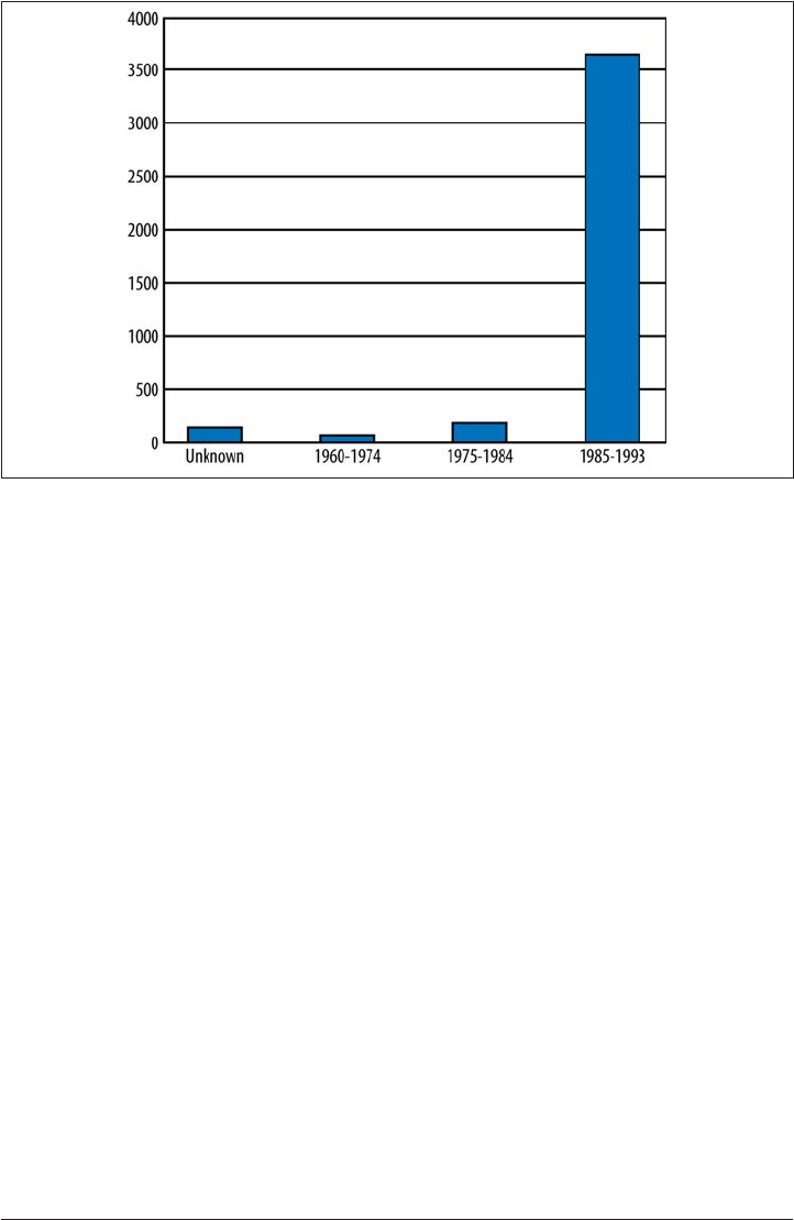
Figure 2-4. Publication dates in the BNC
For your corpus it’s unlikely that you will need to be concerned with having represen
tative samples of all of these possible segmentations. That being said, minimizing the
number of factors that could potentially make a difference is a good strategy, particularly
when you’re in the first few rounds of annotations. So, for example, making sure that all
of your texts come from the same time period, or checking that all of your speakers are
native to the language you are asking them to speak in, is something you may want to
take into account even if you ultimately decide to not include that type of diversity in
your corpus.
Summary
In this chapter we discussed what you need to create a good definition of your goal, and
how your goal can influence your dataset. In particular, we looked at the following
points:
• Having a clear definition of your annotation task will help you stay on track when
you start creating task definitions and writing annotation guidelines.
•There is often a trade-off in annotation tasks between informativity and accuracy
—be careful that you aren’t sacrificing too much of one in favor of another.
•Clearly defining the scope of your task will make it much easier to decide on the
sources of your corpus—and later, the annotation tags and guidelines.
Summary | 51

•Doing some background research can help keep you from reinventing the wheel
when it comes to your own annotation task.
•Using an existing corpus for your dataset can make it easier to do other analyses if
necessary.
•If an existing corpus doesn’t suit your needs, you can build your own, but consider
carefully what data you need and what might become a confounding factor.
•There are a variety of existing tools and programming languages that can help you
to collect data from the Internet.
•What information you intend to show to your annotators is an important factor
that can influence annotation, particularly in tasks that rely on opinion or annota
tors’ interpretations of texts, rather than objective facts.
52 | Chapter 2: Defining Your Goal and Dataset

CHAPTER 3
Corpus Analytics
Now that you have successfully created a corpus for your defined goal, it is important
to know what it contains. The goal of this chapter is to equip you with tools for analyzing
the linguistic content of this corpus. Hence, we will introduce you to the kinds of tech
niques and tools you will need in order to perform a variety of statistical analytics over
your corpus.
To this end, we will cover the aspects of statistics and probability that you need in order
to understand, from a linguistic perspective, just what is in the corpus we are building.
This is an area called corpus analytics. Topics will include the following:
• How to measure basic frequencies of word occurrence, by lemma and by token
• How to normalize the data you want to analyze
•How to measure the relatedness between words and phrases in a corpus (i.e., dis
tributions)
Knowing what is in your corpus will help you build your model for automatically iden
tifying the tags you will be creating in the next chapter. We will introduce these concepts
using linguistic examples whenever possible. Throughout the chapter, we will reference
a corpus of movie reviews, assembled from IMDb.com (IMDb). This will prove to be a
useful platform from which we can introduce these concepts.
Statistics is important for several reasons, but mostly it gives us two important abilities:
Data analysis
Discovering latent properties in the dataset
Significance for inferential statistics
Allowing us to make judgments and derive information regarding the content of
our corpus
53

This chapter does provide an overview of the statistics used to analyze corpora, but it
doesn’t provide a full course in statistics or probability. If you’re interested in reading
more about those topics, especially as they relate to corpus linguistics, we recommend
the following books/papers:
•Probability for Linguists. John Goldsmith. Math. & Sci. hum. / Mathematics and
Social Sciences (45e année, no. 180, 2007(4)). http://hum.uchicago.edu/~jagoldsm/
Papers/probabilityProofs.pdf.
•Analyzing Linguistic Data: A Practical Introduction to Statistics using R. R.H. Baayen.
Cambridge University Press; 1st edition, 2008.
•Statistics for Linguistics with R: A Practical Introduction. Stefan Th. Gries. De Gruyter
Mouton; 1st edition, 2010.
Basic Probability for Corpus Analytics
First let’s review some of the basic principles of probability.
State/sample space
When we perform an experiment or consider the possible values that can be as
signed to an attribute, such as an email being identified as spam or not-spam, we
are referring to the state space for that attribute: that is, {spam, not_spam}. Similarly,
the possible outcome for a coin toss is heads or tails, giving rise to the state space of
{heads, tails}.
Random variable
This is a variable that refers not to a fixed value, but to any possible outcome within
the defined domain; for example, the state space mentioned in the preceding list
item.
Probability
The probability of a specific outcome from the state space, x, is expressed as a func
tion, P(x). We say that P(x) refers to the “probability of x,” where x is some value of
the random variable X, x
∈
X.
Probabilities have two important properties:
• They must have values between 0 and 1, expressed as:
∀
x : 0 ≤ p(x) ≤ 1
54 | Chapter 3: Corpus Analytics

• The sum of the probabilities of all possible events must add up to 1:
∑
xϵXP(x) = 1
Let’s say you are interested in looking at movie reviews. Perhaps your goal is to collect
a corpus in order to train an algorithm to identify the genre of a movie, based on the
text from the plot summary, as found on IMDb.com, for example. In order to train an
algorithm to classify and label elements of the text, you need to know the nature of the
corpus.
Assume that we have 500 movie descriptions involving five genres, evenly balanced over
each genre, as follows:
• Action: 100 documents
• Comedy: 100 documents
• Drama: 100 documents
• Sci-fi: 100 documents
• Family: 100 documents
Given this corpus, we can define the random variable G (Genre), where the genre values
in the preceding list constitute the state space (sample space) for G. Because this is a
balanced corpus, any g
∈
G will have the same probability: for example, P(Drama) = .
20, P(Action) = .20, and so on.
If you want to find the probability of a particular variable in a corpus
using Python, you can do it quite easily using lists. If you have a list of
all the reviews, and a list of the comedies, you can use the length of the
respective lists to get the probability of randomly selecting a review with
a particular attribute. Let’s say that all is a list of the filenames for all
the reviews, and comedy is a list of the filenames that are comedies:
>>> p_com = float(len(comedy))/float(len(all))
Because the len() function returns an int, in order to get a probability,
you need to convert the int to a float; otherwise, you get a probability
of 0.
Joint Probability Distributions
Usually the kinds of questions we will want to ask about a corpus involve not just one
random variable, but multiple random variables at the same time. Returning to our
Basic Probability for Corpus Analytics | 55

IMDb corpus, we notice that there are two kinds of plot summaries: short and long. We
can define the random variable S (Summary) with the sample space of {short, long}. If
each genre has 50 short summaries and 50 long summaries, then P(short) = .5 and
P(long) = .5.
Now we have two random variables, G (Genre) and S (Summary). We denote the joint
probability distribution of these variables as P(G,S). If G and S are independent variables,
then we can define P(G,S) as follows:
P(G
∩
S) = P(G) × P(S)
So, assuming they are independent, the probability of randomly picking a “short com
edy” article is:
P(Comedy
∩
short) = P(Comedy) × P(short)
= 0.20 × 0.50
= 0.10
But are these two random variables independent of each other? Intuitively, two events
are independent if one event occurring does not alter the likelihood of the other event
occurring.
So, we can imagine separating out the short articles, and then picking a comedy from
those, or vice versa. There are 250 short articles, composed of five genres, each con
taining 50 articles. Alternatively, the comedy genre is composed of 100 articles, con
taining 50 short and 50 long articles. Looking at it this way is equivalent to determining
the conditional probability. This is the probability of outcome A, given that B has oc
curred (read “the probability of A given B”), and is defined as follows:
P(A|B) = P
(
A∩B
)
P(B)
This is the fraction of B results that are also A results. For our example, the probability
of picking a comedy, given that we have already determined that the article is short, is
as follows:
P(comedy |short) = P
(
Comedy ∩short
)
P(short)
We can quickly see that this returns 0.20, which is the same as P(Comedy). The property
of independence in fact tells us that, if G and S are independent, then:
P(G | S) = P(G)
56 | Chapter 3: Corpus Analytics
Similarly, since P(S | G) = P(S), P(short | Comedy) = P(short), which is 0.50.
Notice that from the preceding formula we have the following equivalent formula, which
is called the multiplication rule in probability:
P
(
A∩B
)
=P(B)P(A|B) = P(A)P(B|A)
When we need to compute the joint probability distribution for more than two random
variables, this equation generalizes to something known as the chain rule:
P
(
A1∩A2... ∩An
)
=P
(
A1
)
P
(
A2
|
A1
)
P
(
A3
|
A1∩A2
)
…P
(
An
|
∩i=1
n–1 Ai
)
This rule will become important when we build some of our first language models over
our annotated corpora.
The calculation of the conditional probability is important for the machine learning
(ML) algorithms we will encounter in Chapter 7. In particular, the Naïve Bayes Classifier
relies on the computation of conditional probabilities from the corpus.
Understanding how different attributes are connected in your corpus
can help you to discover aspects of your dataset that should be included
in your annotation task. If it turned out that the probability of a review
being short was correlated with one or more movie genres, then in
cluding that information in your annotation task (or later on when you
are building a feature set for your ML algorithm) could be very helpful.
At the same time, it may turn out that the connection between the length
of the review and the genre is purely coincidental, or is a result of your
corpus being unbalanced in some way. So checking your corpus for
significant joint probability distributions can also ensure that your cor
pus accurately represents the data you are working with.
Bayes Rule
Once we have the definition for computing a conditional probability, we can recast the
rule in terms of an equivalent formula called Bayes Theorem, stated as follows:
P(A|B) = P(B|A)P(A)
P(B)
This rule allows us to switch the order of dependence between events. This formulates
the conditional probability, P(A | B), into three other probabilities, that are hopefully
easier to find estimates for. This is important because when we want to design an ML
Basic Probability for Corpus Analytics | 57

algorithm for automatically classifying the different entities in our corpus, we need
training data, and this involves being able to easily access statistics for the probabilities
associated with the different judgments being used in the algorithm. We return to this
in Chapter 7.
Counting Occurrences
When putting together a corpus of linguistic texts, you most likely will not know the
probability distribution of a particular phenomenon before you examine the corpus. We
could not have known, for example, what the probability of encountering an action film
would be in the IMDb corpus, without counting the members associated with each value
of the Genre random variable. In reality, no corpus will be so conveniently balanced.
Such information constitutes the statistics over the corpus by counting occurrences of
the relevant objects in the dataset—in this case, movies that are labeled as action films,
comedy films, and so on. Similarly, when examining the linguistic content of a corpus,
we cannot know what the frequency distribution of the different words in the corpus
will be beforehand.
One of the most important things to know about your corpus before you apply any sort
of ML algorithm to it is the basic statistical profile of the words contained in it. The
corpus is essentially like a textbook that your learning algorithm is going to use as a
supply of examples (positive instances) for training. If you don’t know the distribution
of words (or whatever constitutes the objects of interest), then you don’t know what the
textbook is supplying for learning. A language corpus typically has an uneven distribu
tion of word types, as illustrated in Figure 3-1. Instructions for how to create this graph
for your own corpus can be found in Madnani 2012.
First, a note of clarification. When we say we are counting the “words” in a corpus, we
need to be clear about what that means. Word frequencies refer to the number of word
tokens that are instances of a word type (or lemma). So we are correct in saying that the
following sentence has 8 words in it, or that it has 11 words in it. It depends on what we
mean by “word”!
“The cat chased the mouse down the street in the dark.”
You can perform word counts over corpora directly with the NLTK. Figure 3-2 shows
some examples over the IMDb corpus. Determining what words or phrases are most
common in your dataset can help you get a grasp of what kind of text you’re looking at.
Here, we show some sample code that could be used to find the 50 most frequently used
words in a corpus of plain text.
58 | Chapter 3: Corpus Analytics
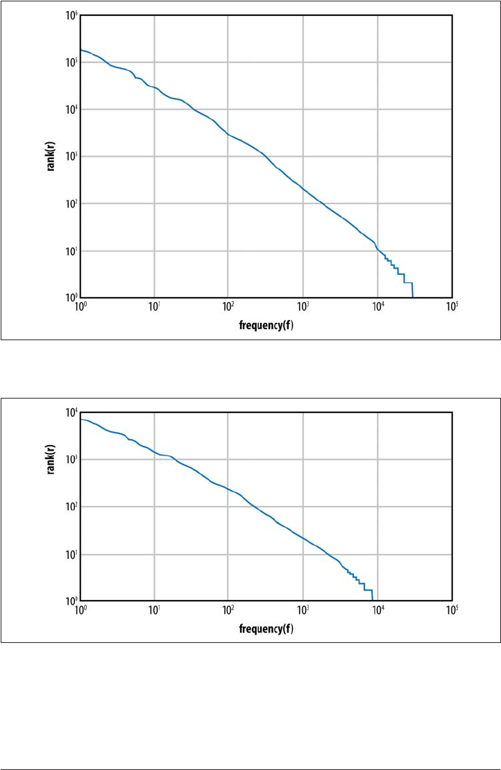
Figure 3-1. Frequency distribution in the NLTK Gutenburg corpus
Figure 3-2. Frequency distribution in the IMDb corpus
Counting Occurrences | 59

>>> import nltk
>>> from nltk.corpus import PlaintextCorpusReader
>>> imdbcorpus = PlaintextCorpusReader('./training','.*')
>>> from nltk import FreqDist
>>> fd1 = FreqDist(imdbcorpus.words())
>>> fd1.N() #total number of sample outcomes. Same as len(imdbcorpus.words())
160035
>>> fd1.B() #total number of sample values that have counts greater than zero
16715
>>> len(fd1.hapaxes()) #total number of all samples that occur once
7933
>>> frequentwords = fd1.keys() #automatically sorts based on frequency
>>> frequentwords[:50]
[',', 'the', '.', 'and', 'to', 'a', 'of', 'is', 'in', "'", 'his',
's', 'he', 'that', 'with', '-', 'her', '(', 'for', 'by', 'him',
'who', 'on', 'as', 'The', 'has', ')', '"', 'from', 'are', 'they',
'but', 'an', 'she', 'their', 'at', 'it', 'be', 'out', 'up', 'will',
'He', 'when', 'was', 'one', 'this', 'not', 'into', 'them', 'have']
Instructions for using the NLTK’s collocation functions are availabled at http://
nltk.googlecode.com/svn/trunk/doc/howto/collocations.html.
Here are two of the basic concepts you need for performing lexical statistics over a
corpus:
Corpus size (N)
The number of tokens in the corpus
Vocabulary size (V)
The number of types in the corpus
For any tokenized corpus, you can map each token to a type; for example, how many
times the appears (the number of tokens of the type the), and so on. Once we have the
word frequency distributions over a corpus, we can calculate two metrics: the rank/
frequency profile and the frequency spectrum of the word frequencies.
To get the rank/frequency profile, you take the type from the frequency list and replace
it with its rank, where the most frequent type is given rank 1, and so forth. To build a
frequency spectrum, you simply calculate the number of types that have a specific fre
quency. The first thing one notices with these metrics is that the top few frequency ranks
are taken up by function words (i.e., words such as the, a, and and; prepositions; etc.).
In the Brown Corpus, the 10 top-ranked words make up 23% of the total corpus size
(Baroni 2009). Another observation is that the bottom-ranked words display lots of ties
in frequency. For example, in the frequency table for the IMDb corpus, the number of
hapax legomena (words appearing only once in the corpus) is over 8,000. In the Brown
Corpus, about half of the vocabulary size is made up of words that occur only once.The
mean or average frequency hides huge deviations. In Brown, the average frequency of
a type is 19 tokens, but the mean is increased because of a few very frequent types.
60 | Chapter 3: Corpus Analytics

We also notice that most of the words in the corpus have a frequency well below the
mean. The mean will therefore be higher than the median, while the mode is usually 1.
So, the mean is not a very meaningful indicator of “central tendency,” and this is typical
of most large corpora.
Recall the distinctions between the following notions in statistics:
•Mean (or average): The sum of the values divided by the number
of values
x
¯
=1
n∑
i=4
nxi
• Mode: The most frequent value in the population (or dataset)
•Median: The numerical value that separates the higher half of a
population (or sample) from the lower half
Zipf’s Law
The uneven distribution of word types shown in the preceding section was first pointed
out over a variety of datasets by George Zipf in 1949. He noticed that frequency of a
word, f(w), appears as a nonlinearly decreasing function of the rank of the word, r(w),
in a corpus, and formulated the following relationship between these two variables:
f(w) = C
r(w)a
C is a constant that is determined by the particulars of the corpus, but for now, let’s say
that it’s the frequency of the most frequent word in the corpus. Let’s assume that a is 1;
then we can quickly see how frequency decreases with rank. Notice that the law is a
power law: frequency is a function of the negative power of rank, –a. So the first word
in the ranking occurs about twice as often as the second word in the ranking, and three
times as often as the third word in the ranking, and so on.
N-grams
In this section we introduce the notion of an n-gram. N-grams are important for a wide
range of applications in Natural Language Processing (NLP), because fairly straight
forward language models can be built using them, for speech, Machine Translation,
indexing, Information Retrieval (IR), and, as we will see, classification.
Counting Occurrences | 61

Imagine that we have a string of tokens, W, consisting of the elements w1, w2, … , wn.
Now consider a sliding window over W. If the sliding window consists of one cell (wi),
then the collection of one-cell substrings is called the unigram profile of the string; there
will be as many unigram profiles as there are elements in the string. Consider now all
two-cell substrings, where we look at w1 w2, w2 w3, and so forth, to the end of the string,
wn–1 wn. These are called bigram profiles, and we have n–1 bigrams for a string of
length n.
Using the definition of conditional probability mentioned earlier, we can define a prob
ability for a token, having seen the previous token, as a bigram probability. Thus the
conditional probability of an element, wi, given the previous element, wi–1:
P(wi | wi−1)
Extending this to bigger sliding windows, we an define an n-gram probability as simply
the conditional probability of an element given the previous n–1 elements. That is:
P(wi | wi−N−1 … wi−1)
The most common bigrams in any corpus will most likely not be very interesting to you,
however. They involve the most frequent words in word pairs. This happens to usually
be boring function word pairs, such as the following:
• of the
• in the
• on the
• in a
If you want to get a more meaningful set of bigrams (and trigrams), you can run the
corpus through a part-of-speech (POS) tagger, such as one of those provided by the
NLTK. This would filter the bigrams to more content-related pairs involving, for ex
ample, adjectives and nouns:
• Star Trek
• Bull Run
• Sidekick Brainiac
This can be a useful way to filter the meaningless n-grams from your results. A better
solution, however, is to take advantage of the “natural affinity” that the words in an n-
gram have for one another. This includes what are called collocations. A collocation is
the string created when two or more words co-occur in a language more frequently than
by chance. A convenient way to do this over a corpus is through a concept known as
pointwise mutual information (PMI). Basically, the intuition behind PMI is as follows.
62 | Chapter 3: Corpus Analytics

For two words, X and Y, we would like to know how much one word tells us about the
other. For example, given an occurrence of X, x, and an occurrence of Y, y, how much
does their joint probability differ from the expected value of assuming that they are
independent? This can be expressed as follows:
pmi(x;y) = ln P(x,y)
P(x)P(y)
In fact, the collocation function provided in the NLTK uses this relation to build bigram
collocations. Applying this function to the bigrams from the IMDb corpus, we can see
the following results:
>>> bigram_measures = nltk.collocations.BigramAssocMeasures()
>>> finder1 = BigramCollocationFinder.from_words(imdbcorpus.words())
>>> finder1.nbest(bigram_measures.pmi, 10)
[('".(', 'Check'), ('10th', 'Sarajevo'), ('16100', 'Patranis'),
('1st', 'Avenue'), ('317', 'Riverside'), ('5000', 'Reward'),
('6310', 'Willoughby'), ('750hp', 'tire'), ('ALEX', 'MILLER'),
('Aasoo', 'Bane')]
>>> finder1.apply_freq_filter(10) #look only at collocations that occur
10 times or more
>>> finder1.nbest(bigram_measures.pmi, 10)
[('United', 'States'), ('Los', 'Angeles'), ('Bhagwan', 'Shri'),
('martial', 'arts'), ('Lan', 'Yu'), ('Devi', 'Maa'),
('New', 'York'), ('qv', ')),'), ('qv', '))'), ('I', ")'")]
>>> finder1.apply_freq_filter(15)
>>> finder1.nbest(bigram_measures.pmi, 10)
[('Bhagwan', 'Shri'), ('Devi', 'Maa'), ('New', 'York'),
('qv', ')),'), ('qv', '))'), ('I', ")'"), ('no', 'longer'),
('years', 'ago'), ('none', 'other'), ('each', 'other')]
One issue with using this simple formula, however, involves the problem of sparse data.
That is, the probabilities of observed rare events are overestimated, and the probabilities
of unobserved rare events are underestimated. Researchers in computational linguistics
have found ways to get around this problem to a certain extent, and we will return to
this issue when we discuss ML algorithms in more detail in Chapter 7.
Language Models
So, what good are n-grams? NLP has used n-grams for many years to develop statistical
language models that predict sequence behaviors. Sequence behavior is involved in rec
ognizing the next X in a sequence of Xs; for example, Speech Recognition, Machine
Translation, and so forth. Language modeling predicts the next element in a sequence,
given the previously encountered elements.
Language Models | 63
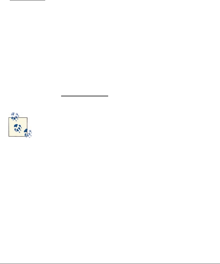
Let’s see more precisely just how this works, and how it makes use of the tools we dis
cussed in the previous sections. Imagine a sequence of words, w1, w2, … , wn. Predicting
any “next word” wi in this sequence is essentially expressed by the following probability
function:
P(wi | w1, …, wi−1)
which is equivalent to:
P
(
w1, ..., wi
)
P
(
w1, ..., wi–1
)
Notice what’s involved with computing these two joint probability distributions. We will
assume that the frequency of a word sequence in the corpus will estimate its probability.
That is:
P(w1, …, wi−1) = Count(w1, …, wi–1)
P(w1, …, wi) = Count(w1, …, wi)
giving us the ratio known as the relative frequency, shown here:
P
(
wi
|
w1, ..., wi–1
)
=Count
(
w1, ..., wi
)
Count
(
w1, ..., wi–1
)
As we just saw, the joint probabilities in the n-gram example can be
expressed as conditional probabilities, using the chain rule for sequence
behavior, illustrated as follows:
P
(
w1,w2..., wn
)
=P
(
w1
)
P
(
w2
|
w1
)
P
(
w3
|
w1,w2
)
...P
(
wn
|
w1n–1
)
which can be expressed as:
Π
k=1
nP
(
wk
|
w1k–1
)
Even though we can, in principle, estimate the probabilities that we need for making
our predictive model, there is little chance that we are going to have a lot of data to work
with, if we take the joint probability of the entire sequence of words. That is, there are
sequences of words that may never have occurred in our corpus, but we still want to be
able to predict the behavior associated with the elements contained in them. To solve
64 | Chapter 3: Corpus Analytics

this problem, we can make some simplifying assumptions regarding the contribution
of the elements in the sequence. That is, if we approximate the behavior of a word in a
sequence as being dependent on only the word before it, then we have reduced the n-
gram probability of:
P
(
wi
|
w1i-1
)
to this bigram probability:
P(wi | wi−1)
This is known as the Markov assumption, and using it, we can actually get some rea
sonable statistics for the bigrams in a corpus. These can be used to estimate the bigram
probabilities by using the concept of relative frequency mentioned earlier. That is, as
before, we take the ratio of the occurrences of the bigram in the corpus to the number
of occurrences of the prefix (the single word, in this case) in the corpus, as shown here:
P
(
wi
|
wi–1
)
=Count
(
wi–1,wi
)
Count
(
wi– 1
)
This procedure is known as a maximum likelihood estimation (MLE), and it provides a
fairly direct way to collect statistics that can be used for creating a language model. We
will return to these themes in Chapter 7.
Summary
In this chapter we introduced you to the tools you need to analyze the linguistic content
of a corpus as well as the kinds of techniques and tools you will need to perform a variety
of statistical analytics. In particular, we discussed the following:
•Corpus analytics comprises statistical and probabilistic tools that provide data
analysis over your corpus and information for performing inferential statistics. This
will be necessary information when you take your annotated corpus and train an
ML algorithm on it.
•It is necessary to distinguish between the occurrence of a word in a corpus (the
token) and the word itself (the type).
• The total number of tokens in a corpus gives us the corpus size.
• The total number of types in a corpus gives us the vocabulary size.
•The rank/frequency profile of the words in a corpus assigns a ranking to the words,
according to how many tokens there are of that word.
Summary | 65

•The frequency spectrum of the word gives the number of word types that have a
given frequency.
•Zipf’s law is a power law stating that the frequency of any word is inversely pro
portional to its rank.
•Constructing n-grams over the tokens in a corpus is the first step in building lan
guage models for many NLP applications.
•Pointwise mutual information is a measure of how dependent one word is on an
other in a text. This can be used to identify bigrams that are true collocations in a
corpus.
•Language models for predicting sequence behavior can be simplified by making the
Markov assumption, namely, when predicting a word, only pay attention to the
word before it.
66 | Chapter 3: Corpus Analytics

CHAPTER 4
Building Your Model and Specification
Now that you’ve defined your goal and collected a relevant dataset, you need to create
the model for your task. But what do we mean by “model”? Basically, the model is the
practical representation of your goal: a description of your task that defines the classi
fications and terms that are relevant to your project. You can also think of it as the aspects
of your task that you want to capture within your dataset. These classifications can be
represented by metadata, labels that are applied to the text of your corpus, and/or rela
tionships between labels or metadata. In this chapter, we will address the following
questions:
• The model is captured by a specification, or spec. But what does a spec look like?
•You have the goals for your annotation project. Where do you start? How do you
turn a goal into a model?
•What form should your model take? Are there standardized ways to structure the
phenomena?
• How do you take someone else’s standard and use it to create a specification?
•What do you do if there are no existing specifications, definitions, or standards for
the kinds of phenomena you are trying to identify and model?
•How do you determine when a feature in your description is an element in the spec
versus an attribute on an element?
The spec is the concrete representation of your model. So, whereas the model is an
abstract idea of what information you want your annotation to capture, and the inter
pretation of that information, the spec turns those abstract ideas into tags and attributes
that will be applied to your corpus.
67

Some Example Models and Specs
Recall from Chapter 1 that the first part in the MATTER cycle involves creating a model
for the task at hand. We introduced a model as a triple, M = <T,R,I>, consisting of a
vocabulary of terms, T, the relations between these terms, R, and their interpretation,
I. However, this is a pretty high-level description of what a model is. So, before we discuss
more theoretical aspects of models, let’s look at some examples of annotation tasks and
see what the models for those look like.
For the most part, we’ll be using XML DTD (Document Type Definition) representa
tions. XML is becoming the standard for representing annotation data, and DTDs are
the simplest way to show an overview of the type of information that will be marked up
in a document. The next few sections will go through what the DTDs for different models
will look like, so you can see how the different elements of an annotation task can be
translated into XML-compliant forms.
What Is a DTD?
A DTD is a set of declarations containing the basic building blocks that allow an XML
document to be validated. DTDs have been covered in depth in other books (O’Reilly’s
Learning XML and XML in a Nutshell) and websites (W3schools.com), so we’ll give a short
overview here.
Essentially, the DTD defines what the structure of an XML document will be by defining
what tags will be used inside the document and what attributes those tags will have. By
having a DTD, the XML in a file can be validated to ensure that the formatting is correct.
So what do we mean by tags and attributes? Let’s take a really basic example: web pages
and HTML. If you’ve ever made a website and edited some code by hand, you’re familiar
with elements such as <b> and <br />. These are tags that tell a program reading the
HTML that the text in between <b> and </b> should be bold, and that <br /> indicates
a newline should be included when the text is displayed. Annotation tasks use similar
formatting, but they define their own tags based on what information is considered im
portant for the goal being pursued. So an annotation task that is based on marking the
parts of speech in a text might have tags such as <noun>, <verb>, <adj>, and so on. In a
DTD, these tags would be defined like this:
<!ELEMENT noun ( #PCDATA ) >
<!ELEMENT verb ( #PCDATA ) >
<!ELEMENT adj ( #PCDATA ) >
The string !ELEMENT indicates that the information contained between the < and > is about
an element (also known as a “tag”), and the word following it is the name of that tag (noun,
verb, adj). The ( #PCDATA ) indicates that the information between the <noun> and
</noun> tags will be parsable character data (other flags instead of #PCDATA can be used
to provide other information about a tag, but for this book, we’re not going to worry about
them).
68 | Chapter 4: Building Your Model and Specification

By declaring the three tags in a DTD, we can have a valid XML document that has nouns,
verbs, and adjectives all marked up. However, annotation tasks often require more infor
mation about a piece of text than just its type. This is where attributes come in. For example,
knowing that a word is a verb is useful, but it’s even more useful to know the tense of the
verb—past, present, or future. This can be done by adding an attribute to a tag, which
looks like this:
<!ELEMENT verb ( #PCDATA ) >
<!ATTLIST verb tense ( past | present | future | none ) #IMPLIED >
The !ATTLIST line declares that an attribute called tense is being added to the verb
element, and that it has four possible values: past, present, future, and none. The
#IMPLIED shows that the information in the attribute isn’t required for the XML to be valid
(again, don’t worry too much about this for now). Now you can have a verb tag that looks
like this:
<verb tense="present">
You can also create attributes that allow annotators to put in their own information, by
declaring the attribute’s type to be CDATA instead of a list of options, like this:
<!ELEMENT verb ( #PCDATA ) >
<!ATTLIST verb tense CDATA #IMPLIED >
One last type of element that is commonly used in annotation is a linking element, or a
link tag. These tags are used to show relationships between other parts of the data that
have been marked up with tags. For instance, if the part-of-speech (POS) task also wanted
to show the relationship between a verb and the noun that performed the action described
by the verb, the annotation model might include a link tag called performs, like so:
<!ELEMENT performs EMPTY >
<!ATTLIST performs fromID IDREF >
<!ATTLIST performs toID IDREF >
The EMPTY in this element tag indicates that the tag will not be applied to any of the text
itself, but rather is being used to provide other information about the text. Normally in
HTML an empty tag would be something like the <br /> tag, or another tag that stands
on its own. In annotation tasks, an empty tag is used to create paths between other, con
tentful tags.
In a model, it is almost always important to keep track of the order (or arity) of the elements
involved in the linking relationship. We do this here by using two elements that have the
type IDREF, meaning they will refer to other annotated extents or elements in the text by
identifiable elements.
We’ll talk more about the IDs and the relationship between DTDs and annotated data in
Chapter 5, but for now, this should give you enough information to understand the ex
amples provided in this chapter.
Some Example Models and Specs | 69

There are other formats that can be used to specify specs for a model.
XML schema are sometimes used to create a more complex represen
tation of the tags being used, as is the Backus–Naur Form. However,
these formats are more complex than DTDs, and aren’t generally nec
essary to use unless you are using a particular piece of annotation soft
ware, or want to have a more restrictive spec. For the sake of simplicity,
we will use only DTD examples in this book.
Film Genre Classification
A common task in Natural Language Processing (NLP) and machine learning is clas
sifying documents into categories; for example, using film reviews or summaries to
determine the genre of the film being described. If you have a goal of being able to use
machine learning to identify the genre of a movie from the movie summary or review,
then a corresponding model could be that you want to label the summary with all the
genres that the movie applies to, in order to feed those labels into a classifier and train
it to identify relevant parts of the document. To turn that model into a spec, you need
to think about what that sort of label would look like, presumably in a DTD format.
The easiest way to create a spec for a classification task is to simply create a tag that
captures the information you need for your goal and model. In this case, you could create
a tag called genre that has an attribute called label, where label holds the values that
can be assigned to the movie summary. The simplest incarnation of this spec would be
this:
<!ELEMENT genre ( #PCDATA ) >
<!ATTLIST genre label CDATA #IMPLIED >
This DTD has the required tag and attribute, and allows for any information to be added
to the label attribute. Functionally for annotation purposes, this means the annotator
would be responsible for filling in the genres that she thinks apply to the text. Of course,
a large number of genre terms have been used, and not everyone will agree on what a
“standard” list of genres should be—for example, are “fantasy” and “sci-fi” different
genres, or should they be grouped into the same category? Are “mystery” films different
from “noir”? Because the list of genres will vary from person to person, it might be better
if your DTD specified a list of genres that annotators could choose from, like this:
<!ELEMENT genre ( #PCDATA ) >
<!ATTLIST genre label ( Action | Adventure | Animation | Biography | Comedy |
Crime | Documentary | Drama | Family | Fantasy | Film-Noir | Game-Show |
History | Horror | Music | Musical | Mystery | News | Reality-TV | Romance |
Sci-Fi | Sport | Talk-Show | Thriller | War | Western ) >
The list in the label attribute is taken from IMDb’s list of genres. Naturally, since other
genre lists exist (e.g., Netflix also has a list of genres), you would want to choose the one
that best matches your task, or create your own list. As you go through the process of
70 | Chapter 4: Building Your Model and Specification

annotation and the rest of the MATTER cycle, you’ll find places where your model/spec
needs to be revised in order to get the results you want. This is perfectly normal, even
for tasks that seem as straightforward as putting genre labels on movie summaries—
annotator opinions can vary, even when the task is as clearly defined as you can make
it. And computer algorithms don’t really think and interpret the way that people do, so
even when you get past the annotation phase, you may still find places where, in order
to maximize the correctness of the algorithm, you would have to change your model.
For example, looking at the genre list from IMDb we see that “romance” and “comedy”
are two separate genres, and so the summary of a romantic comedy would have to have
two labels: romance and comedy. But if, in a significant portion of reviews, those two
tags appear together, an algorithm may learn to always associate the two, even when the
summary being classified is really a romantic drama or musical comedy. So, you might
find it necessary to create a rom-com label to keep your classifier from creating false
associations.
In the other direction, there are many historical action movies that take place over very
different periods in history, and a machine learning (ML) algorithm may have trouble
finding enough common ground between a summary of 300, Braveheart, and Pearl
Harbor to create an accurate association with the history genre. In that case, you might
find it necessary to add different levels of historical genres, ones that reflect different
periods in history, to train a classifier in the most accurate way possible.
If you’re unclear on how the different components of the ML algorithm
can be affected by the spec, or why you might need to adapt a model to
get better results, don’t worry! For now, just focus on turning your goal
into a set of tags, and the rest will come later. But if you really want to
know how this works, Chapter 7 has an overview of all the different
ways that ML algorithms “learn,” and what it means to train each one.
Adding Named Entities
Of course, reworking the list of genres isn’t the only way to change a model to better fit
a task. Another way is to add tags and attributes that will more closely reflect the in
formation that’s relevant to your goal. In the case of the movie summaries, it might be
useful to keep track of some of the Named Entities (NEs) that appear in the summaries
that may give insight into the genre of the film. An NE is an entity (an object in the
world) that has a name which uniquely identifies it by name, nickname, abbreviation,
and so on. “O’Reilly,” “Brandeis University,” “Mount Hood,” “IBM,” and “Vice President”
are all examples of NEs. In the movie genre task, it might be helpful to keep track of NEs
such as film titles, directors, writers, actors, and characters that are mentioned in the
summaries.
Some Example Models and Specs | 71

You can see from the list in the preceding paragraph that there are many different NEs
in the model that we would like to capture. Because the model is abstract, the practical
application of these NEs to a spec or DTD has to be decided upon. There are often many
ways in which a model can be represented in a DTD, due to the categorical nature of
annotation tasks and of XML itself. In this case there are two primary ways in which
the spec could be created. We could have a single tag called named_entity with an
attribute that would have each of the items from the previous list, like this:
<!ELEMENT named_entity ( #PCDATA ) >
<!ATTLIST named_entity role (film_title | director |
writer | actor | character ) >
Or each role could be given its own tag, like this:
<!ELEMENT film_title ( #PCDATA ) >
<!ELEMENT director ( #PCDATA ) >
<!ELEMENT writer ( #PCDATA ) >
<!ELEMENT actor ( #PCDATA ) >
<!ELEMENT character ( #PCDATA ) >
While these two specs seem to be very different, in many ways they are interchangeable.
It would not be difficult to take an XML file with the first DTD and change it to one that
is compliant with the second. Often the choices that you’ll make about how your spec
will represent your model will be influenced by other factors, such as what format is
easier for your annotators, or what works better with the annotation software you are
using. We’ll talk more about the considerations that go into which formats to use in
Chapter 5 and Chapter 6.
By giving ML algorithms more information about the words in the document that are
being classified, such as by annotating the NEs, it’s possible to create more accurate
representations of what’s going on in the text, and to help the classifier pick out markers
that might make the classifications better.
Semantic Roles
Another layer of information that might be useful in examining movie summaries is to
annotate the relationships between the NEs that are marked up in the text. These rela
tionships are called semantic roles, and they are used to explicitly show the connections
between the elements in a sentence. In this case, it could be helpful to annotate the
relationships between actors and characters, and the staff of the movie and which movie
they worked on. Consider the following example summary/review:
In Love, Actually, writer/director Richard Curtis weaves a convoluted tale about charac
ters and their relationships. Of particular note is Liam Neeson (Schindler’s List, Star
Wars) as Daniel, a man struggling to deal with the death of his wife and the relationship
with his young stepson, Sam (Thomas Sangster). Emma Thompson (Sense and Sensibil
ity, Henry V) shines as a middle-aged housewife whose marriage with her husband (played
by Alan Rickman) is under siege by a beautiful secretary. While this movie does have its
72 | Chapter 4: Building Your Model and Specification

purely comedic moments (primarily presented by Bill Nighy as out-of-date rock star Billy
Mack), this movie avoids the more in-your-face comedy that Curtis has presented before
as a writer for Blackadder and Mr. Bean, presenting instead a remarkable, gently humorous
insight into what love, actually, is.
Using one of the NE DTDs from the preceding section would lead to a number of
annotated extents, but due to the density, an algorithm may have difficulty determining
who goes with what. By adding semantic role labels such as acts_in, acts_as, di
rects, writes, and character_in, the relationships between all the NEs will become
much clearer.
As with the DTD for the NEs, we are faced with a choice between using a single tag with
multiple attribute options:
<!ELEMENT sem_role ( EMPTY ) >
<!ATTLIST sem_role from IDREF >
<!ATTLIST sem_role to IDREF >
<!ATTLIST sem_role label (acts_in |
acts_as | directs | writes | character_in ) >
or a tag for each semantic role we wish to capture:
<!ELEMENT acts_in ( EMPTY ) >
<!ATTLIST acts_in from IDREF >
<!ATTLIST acts_in to IDREF >
<!ELEMENT acts_as ( EMPTY ) >
<!ATTLIST acts_as from IDREF >
<!ATTLIST acts_as to IDREF >
<!ELEMENT directs ( EMPTY ) >
<!ATTLIST directs from IDREF >
<!ATTLIST directs to IDREF >
<!ELEMENT writes ( EMPTY ) >
<!ATTLIST writes from IDREF >
<!ATTLIST writes to IDREF >
<!ELEMENT character_in ( EMPTY ) >
<!ATTLIST character_in from IDREF >
<!ATTLIST character_in to IDREF >
You’ll notice that this time, the DTD specifies that each of these elements is EMPTY,
meaning that no character data is associated directly with the tag. Remember that link
ing tags in annotation are usually defined by EMPTY tags specifically because links be
tween elements do not generally have text associated with them in particular, but rather
clarify a relationship between two or more other extents. We’ll discuss the application
of linking and other types of tags in Chapter 5.
Some Example Models and Specs | 73

Multimodel Annotations
It may be the case that your annotation task requires more than one model to fully capture
the data you need. This happens most frequently when a task requires information from
two or more very different levels of linguistics, or if information from two different do
mains needs to be captured. For example, an annotation over a corpus that’s made up of
documents that require training to understand, such as clinical notes, scientific papers,
or legal documents, may require that annotators have training in those fields, and that the
annotation task be tailored to the domain.
In general, employing different annotation models in the same task simply means that
more than one MATTER cycle is being worked through at the same time, and that the
different models will likely be focused on different aspects of the corpus or language being
explored. In these cases, it is important that all the models be coordinated, however, and
that changes made to one model during the MATTER cycle don’t cause conflict with the
others.
If your corpus is made up of domain-specific documents (such as the clinical notes that
we mentioned before), and your annotation task requires that your annotators be able to
interpret these documents (e.g., if you are trying to determine which patients have a par
ticular disease), then one of your models may need to be a light annotation task (Stubbs
2012).
A light annotation task is essentially a way to formulate an annotation model that allows
a domain expert (such as a doctor) to provide her insight into a text without being required
to link her knowledge to one of the layers of linguistic understanding. Such an annotation
task might be as simple as having the domain expert indicate whether a file has a particular
property (such as whether or not a patient is at risk for diabetes), or it may involve an
notating the parts of the text associated with a disease state. However, the domain expert
won’t be asked to mark POS tags or map every noun in the text to a semantic interpretation:
those aspects of the text would be handled in a different model altogether, and merged at
the end.
There is a slightly different philosophy behind the creation of light annotation tasks than
that of more “traditional” annotations: light annotations focus on encoding an answer to
a particular question about a text, rather than creating a complete record of a particular
linguistic phenomenon, with the purpose of later merging all the different models into a
single annotation. However, aside from the difference in goal, light annotation tasks still
follow the MATTER and MAMA cycles. Because of this, we aren’t going to use them as
examples in this book, and instead will stick to more traditional linguistic annotations.
If you are interested in performing an annotation task that requires domain-specific
knowledge, and therefore would benefit from using a light annotation task, a methodology
for creating a light annotation and incorporating it into the MATTER cycle is developed
and presented in Stubbs 2012.
74 | Chapter 4: Building Your Model and Specification

Adopting (or Not Adopting) Existing Models
Now that you have an idea of how specs can represent a model, let’s look a little more
closely at some of the details we just presented. You might recall from Chapter 1 that
when we discussed semantic roles we presented a very different list from acts_in,
acts_as, directs, writes, and character_in. Here’s what the list looked like:
Agent
The event participant that is doing or causing the event to occur
Theme/figure
The event participant who undergoes a change in position or state
Experiencer
The event participant who experiences or perceives something
Source
The location or place from which the motion begins; the person from whom the
theme is given
GoalThe location or place to which the motion is directed or terminates
Recipient
The person who comes into possession of the theme
Patient
The event participant who is affected by the event
Instrument
The event participant used by the agent to do or cause the event
Location/ground
The location or place associated with the event itself
Similarly, we also presented an ontology that defined the categories Organization, Per
son, Place, and Time. This set of labels can be viewed as a simple model of NE types that
are commonly used in other annotation tasks.
So, if these models exist, why didn’t we just use them for our film genre annotation task?
Why did we create our own sets of labels for our spec? Just as when defining the goal of
your annotation you need to think about the trade-off between informativity and cor
rectness, when creating the model and spec for your annotation task, you need to con
sider the trade-off between generality and specificity.
Adopting (or Not Adopting) Existing Models | 75

Creating Your Own Model and Specification: Generality Versus
Specificity
The ontology consisting of Organization, Person, Place, and Time is clearly a very gen
eral model for entities in a text, but for the film genre annotation task, it is much too
general to be useful for the kinds of distinctions we want to be able to make. Of the NE
labels that we identified earlier, four of them (“director,” “writer,” “actor,” and “character”)
would fall under the label “Person,” and “film title” doesn’t clearly fit under any of them.
Using these labels would lead to unhelpful annotations in two respects: first, the labels
used would be so generic as to be useless for the task (labeling everyone as “Person”
won’t help distinguish one movie review from another); and second, it would be difficult
to explain to the annotators that, while you’ve given them a set of labels, you don’t want
every instance of those types of entities labeled, but rather only those that are relevant
to the film (so, for example, a mention of another reviewer would not be labeled as a
“Person”). Clearly, overly general tags in a spec can lead to confusion during annotation.
On the other hand, we could have made the tags in the spec even more specific, such as
actor_star, actor_minor_character, character_main, character_minor, writ
er_film, writer_book, writer_book_and_film, and so on. But what would be gained
from such a complicated spec? While it’s possible to think of an annotation task where
it might be necessary to label all that information (perhaps one that was looking at how
these different people are described in movie reviews), remember that the task we de
fined was, first, simply labeling the genres of films as they are described in summaries
and reviews, and then expanding it to include some other information that might be
relevant to making that determination. Using overly specific tags in this case would
decrease how useful the annotations would be, and also increase the amount of work
done by the annotators for no obvious benefit. Figure 4-1 shows the different levels of
the hierarchy we are discussing. The top two levels are too vague, while the bottom is
too specific to be useful. The third level is just right for this task.
We face the same dichotomy when examining the list of semantic roles. The list given
in linguistic textbooks is a very general list of roles that can be applied to the nouns in
a sentence, but any annotation task trying to use them for film-related roles would have
to have a way to limit which nouns were assigned roles by the annotator, and most of
the roles related to the NEs we’re interested in would simply be “agent”—a label that is
neither helpful nor interesting for this task. So, in order to create a task that was in the
right place regarding generality and specificity, we developed our own list of roles that
were particular to this task.
76 | Chapter 4: Building Your Model and Specification
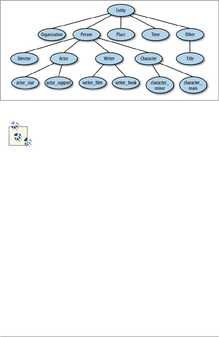
Figure 4-1. A hierarchy of named entities
We haven’t really gotten into the details of NE and semantic role anno
tation using existing models, but these are not trivial annotation tasks.
If you’re interested in learning more about annotation efforts that use
these models, check out FrameNet for semantic roles, and the Message
Understanding Conferences (MUCs) for examples of NE and corefer
ence annotation.
Overall, there are a few things that you want to make sure your model and specification
have in order to proceed with your task. They should:
•Contain a representation of all the tags and links relevant to completing your goal.
•Be relevant to the implementation stated in your goal (if your purpose is to classify
documents by genre, spending a lot of time annotating temporal information is
probably not going to be of immediate help).
•Be grounded in existing research as much as possible. Even if there’s no existing
annotation spec that meets your goal completely, you can still take advantage of
research that’s been done on related topics, which will make your own research
much easier.
Specifically to the last point on the list, even though the specs we’ve described for the
film genre annotation task use sets of tags that we created for this purpose, it’s difficult
to say that they weren’t based on an existing model to some extent. Obviously some
knowledge about NEs and semantic roles helped to inform how we described the an
notation task, and helped us to decide whether annotating those parts of the document
would be useful. But you don’t need to be a linguist to know that nouns can be assigned
to different groups, and that the relationships between different nouns and verbs can
Adopting (or Not Adopting) Existing Models | 77

be important to keep track of. Ultimately, while it’s entirely possible that your annotation
task is completely innovative and new, it’s still worth taking a look at some related re
search and resources and seeing if any of them are helpful for getting your model and
spec put together.
The best way to find out if a spec exists for your task is to do a search for existing
annotated datasets. If you aren’t sure where to start, or Google results seem overwhelm
ing, check Appendix A for the list of corpora and their annotations.
Using Existing Models and Specifications
While the examples we discussed thus far had fairly clear-cut reasons for us to create
our own tags for the spec, there are some advantages to basing your annotation task on
existing models. Interoperability is a big concern in the computer world, and it’s actually
a pretty big concern in linguistics as well—if you have an annotation that you want to
share with other people, there are a few things that make it easier to share, such as using
existing annotation standards (e.g., standardized formats for your annotation files),
using software to create the annotation that other people can also use, making your
annotation guidelines available to other people, and using models or specifications that
have already been vetted in similar tasks. We’ll talk more about standards and formats
later in this chapter and in the next one; for now, we’ll focus just on models and specs.
Using models or specs that other people have used can benefit your project in a few
ways. First of all, if you use the specification from an annotation project that’s already
been done, you have the advantage of using a system that’s already been vetted, and one
that may also come with an annotated corpus, which you can use to train your own
algorithms or use to augment your own dataset (assuming that the usage restrictions
on the corpus allow for that, of course).
In “Background Research” (page 41), we mentioned some places to start looking for
information that would be useful with defining your goal, so presumably you’ve already
done some research into the topics you’re interested in (if you haven’t, now is a good
time to go back and do so). Even if there’s no existing spec for your topic, you might
find a descriptive model similar to the one we provided for semantic roles.
Not all annotation and linguistic models live in semantic textbooks! The
list of film genres that we used was taken from IMDb.com, and there
are many other places where you can get insight into how to frame your
model and specification. A recent paper on annotating bias used the
Wikipedia standards for editing pages as the standard for developing a
spec and annotation guidelines for an annotation project (Herzig et al.
2011). Having a solid linguistic basis for your task can certainly help,
but don’t limit yourself to only linguistic resources!
78 | Chapter 4: Building Your Model and Specification

If you are lucky enough to find both a model and a specification that are suitable for
your task, you still might need to make some changes for them to fit your goal. For
example, if you are doing temporal annotation, you can start with the TimeML speci
fication, but you may find that the TIMEX3 tag is simply too much information for your
purposes, or too overwhelming for your annotators. The TIMEX3 DTD description is
as follows:
<!ELEMENT TIMEX3 ( #PCDATA ) >
<!ATTLIST TIMEX3 start #IMPLIED >
<!ATTLIST TIMEX3 tid ID #REQUIRED >
<!ATTLIST TIMEX3 type ( DATE | DURATION | SET | TIME ) #REQUIRED >
<!ATTLIST TIMEX3 value NMTOKEN #REQUIRED >
<!ATTLIST TIMEX3 anchorTimeID IDREF #IMPLIED >
<!ATTLIST TIMEX3 beginPoint IDREF #IMPLIED >
<!ATTLIST TIMEX3 endPoint IDREF #IMPLIED >
<!ATTLIST TIMEX3 freq NMTOKEN #IMPLIED >
<!ATTLIST TIMEX3 functionInDocument ( CREATION_TIME | EXPIRATION_TIME |
MODIFICATION_TIME | PUBLICATION_TIME | RELEASE_TIME | RECEPTION_TIME |
NONE ) #IMPLIED >
<!ATTLIST TIMEX3 mod ( BEFORE | AFTER | ON_OR_BEFORE | ON_OR_AFTER | LESS_THAN |
MORE_THAN | EQUAL_OR_LESS | EQUAL_OR_MORE | START | MID | END |
APPROX ) #IMPLIED >
<!ATTLIST TIMEX3 quant CDATA #IMPLIED >
<!ATTLIST TIMEX3 temporalFunction ( false | true ) #IMPLIED >
<!ATTLIST TIMEX3 valueFromFunction IDREF #IMPLIED >
<!ATTLIST TIMEX3 comment CDATA #IMPLIED >
A lot of information is encoded in a TIMEX3 tag. While the information is there for a
reason—years of debate and modification took place to create this description of a tem
poral reference—there are certainly annotation tasks where this level of detail will be
unhelpful, or even detrimental. If this is the case, other temporal annotation tasks have
been done over the years that have specs that you may find more suitable for your goal
and model.
Using Models Without Specifications
It’s entirely possible—even likely—that your annotation task may be based on a linguistic
(or psychological or sociological) phenomenon that has been clearly explained in the
literature, but has not yet been turned into a specification. In that case, you will have to
decide the form the specification will take, in much the same way that we discussed in
the first section of this chapter. Depending on how fleshed out the model is, you may
have to make decisions about what parts of the model become tags, what become at
tributes, and what become links. In some ways this can be harder than simply creating
your own model and spec, because you will be somewhat constrained by someone else’s
description of the phenomenon. However, having a specification that is grounded in an
established theory will make your own work easier to explain and distribute, so there
are advantages to this approach as well.
Adopting (or Not Adopting) Existing Models | 79

Many (if not all) of the annotation specifications that are currently in wide use are based
on theories of language that were created prior to the annotation task being created. For
example, the TLINK tag in ISO-TimeML is based largely on James Allen’s work in tem
poral reasoning (Allen 1984; Pustejovsky et al. 2003), and ISO-Space has been influenced
by the qualitative spatial reasoning work of Randell et al. (1992) and others. Similarly,
syntactic bracketing and POS labeling work, as well as existing semantic role labeling,
are all based on models developed over years of linguistic research and then applied
through the creation of syntactic specifications.
Different Kinds of Standards
Previously we mentioned that one of the aspects of having an interoperable annotation
project is using a standardized format for your annotation files, as well as using existing
models and specs. However, file specifications are not the only kind of standards that
exist in annotation: there are also annotation specifications that have been accepted by
the community as go-to (or de facto) standards for certain tasks. While there are no
mandated (a.k.a. de jure) standards in the annotation community, there are varying
levels and types of de facto standards that we will discuss here.
ISO Standards
The International Organization for Standardization (ISO) is the body responsible for
creating standards that are used around the world for ensuring compatibility of systems
between businesses and government, and across borders. ISO is the organization that
helps determine what the consensus will be for many different aspects of daily life, such
as the size of DVDs, representation of dates and times, and so on. There are even ISO
standards for representing linguistic annotations in general and for certain types of
specifications, in particular ISO-TimeML and ISO-Space. Of course, you aren’t re
quired to use ISO standards (there’s no Annotation Committee that enforces use of these
standards), but they do represent a good starting point for most annotation tasks, par
ticularly those standards related to representation.
ISO standards are created with the intent of interoperability, which sets
them apart from other de facto standards, as those often become the
go-to representation simply because they were there first, or were used
by a large community at the outset and gradually became ingrained in
the literature. While this doesn’t mean that non-ISO standards are in
herently problematic, it does mean that they may not have been created
with interoperability in mind.
80 | Chapter 4: Building Your Model and Specification

Annotation format standards
Linguistic annotation projects are being done all over the world for many different, but
often complementary, reasons. Because of this, in the past few years ISO has been de
veloping the Linguistic Annotation Framework (LAF), a model for annotation projects
that is abstract enough to apply to any level of linguistic annotation.
How can a model be flexible enough to encompass all of the different types of annotation
tasks? LAF takes a two-pronged approach to standardization. First, it focuses on the
structure of the data, rather than the content. Specifically, the LAF standard allows for
annotations to be represented in any format that the task organizers like, so long as it
can be transmuted into LAF’s XML-based “dump format,” which acts as an interface for
all manner of annotations. The dump format has the following qualities (Ide and Romary
2006):
•The annotation is kept separate from the text it is based on, and annotations are
associated with character or element offsets derived from the text.
• Each level of annotation is stored in a separate document.
•Annotations that represent hierarchical information (e.g., syntax trees) must be
either represented with embedding in the XML dump format, or use a flat structure
that symbolically represents relationships.
•When different annotations are merged, the dump format must be able to integrate
overlapping annotations in a way that is compatible with XML.
The first bullet point—keeping annotation separate from the text—now usually takes
the form of stand-off annotation (as opposed to inline annotation, where the tags and
text are intermingled). We’ll go through all the forms that annotation can take and the
pros and cons in Chapter 5.
The other side of the approach that LAF takes toward standardization is encouraging
researchers to use established labels for linguistic annotation. This means that instead
of just creating your own set of POS or NE tags, you can go to the Data Category Registry
(DCR) for definitions of existing tags, and use those to model your own annotation task.
Alternatively, you can name your tag whatever you want, but when transmuting to the
dump format, you would provide information about what tags in the DCR your own
tags are equivalent to. This will help other people merge existing annotations, because
it will be known whether two annotations are equivalent despite naming differences.
The DCR is currently under development (it’s not an easy task to create a repository of
all annotation tags and levels, and so progress has been made very carefully). You can
see the information as it currently exists at www.isocat.org.
Different Kinds of Standards | 81

Timeline of Standardization
LAF didn’t emerge as an ISO standard from out of nowhere. Here’s a quick rundown of
where the standards composing the LAF model originated:
•1987: The Text Encoding Initiative (TEI) is founded “to develop guidelines for en
coding machine-readable texts in the humanities and social sciences.” The TEI is still
an active organization today. See http://www.tei-c.org.
•1990: The TEI releases its first set of Guidelines for the Encoding and Interchange of
Machine Readable Texts. It recommends that encoding be done using SGML (Stan
dard Generalized Markup Language), the precursor to XML and HTML.
•1993: The Expert Advisory Group on Language Engineering Standards (EAGLES) is
formed to provide standards for large-scale language resources (ex, corpora), as well
as standards for manipulating and evaluating those resources. See http://
www.ilc.cnr.it/EAGLES/home.html.
•1998: The Corpus Encoding Standard (CES), also based on SGML, is released. The
CES is a corpus-specific application of the standards laid out in the TEI’s Guide
lines and was developed by the EAGLES group. See http://www.cs.vassar.edu/CES/.
•2000: The Corpus Encoding Standard for XML (XCES) is released, again under the
EAGLES group. See http://www.xces.org/.
•2002: The TEI releases version P4 of its Guidelines, the first version to implement
XML. See http://www.tei-c.org/Guidelines/P4/.
•2004: The first document describing the Linguistic Annotation Framework is released
(Ide and Romary 2004).
•2007: The most recent version (P5) of the TEI Guidelines is released. See http://
www.tei-c.org/Guidelines/P5/.
•2012: LAF and the TEI Guidelines are still being updated and improved to reflect
progress made in corpus and computational linguistics.
Annotation specification standards
In addition to helping create standards for annotation formats, ISO is working on de
veloping standards for specific annotation tasks. We mentioned ISO-TimeML already,
which is the standard for representing temporal information in a document. There is
also ISO-Space, the standard for representing locations, spatial configurations, and
movement in natural language. The area of ISO that is charged with looking at anno
tation standards for all areas of natural language is called TC 37/SC 4. Other projects
82 | Chapter 4: Building Your Model and Specification

involve the development of standards for how to encode syntactic categories and mor
phological information in different languages, semantic role labeling, dialogue act la
beling, discourse relation annotation, and many others. For more information, you can
visit the ISO web page or check out Appendix A of this book.
Community-Driven Standards
In addition to the committee-based standards provided by ISO, a number of de facto
standards have been developed in the annotation community simply through wide use.
These standards are created when an annotated resource is formed and made available
for general use. Because corpora and related resources can be very time-consuming to
create, once a corpus is made available it will usually quickly become part of the litera
ture. By extension, whatever annotation scheme was used for that corpus will also tend
to become a standard.
If there is a spec that is relevant to your project, taking advantage of community-driven
standards can provide some very useful benefit. Any existing corpora that are related
to your effort will be relevant, since they are developed using the spec you want to adopt.
Additionally, because resources such as these are often in wide use, searching the liter
ature for mentions of the corpus will often lead you to papers that are relevant to your
own research goals, and will help you identify any problems that might be associated
with the dataset or specification. Finally, datasets that have been around long enough
often have tools and interfaces built around them that will make the datasets easier for
you to use.
Community-driven standards don’t necessarily follow LAF guidelines,
or make use of other ISO standards. This doesn’t mean they should be
disregarded, but if interoperability is important to you, you may have
to do a little extra work to make your corpus fit the LAF guidelines.
We have a list of existing corpora in Appendix C to help you get started in finding
resources that are related to your own annotation task. While the list is as complete as
we could make it, it is not exhaustive, and you should still check online for resources
that would be useful to you. The list that we have was compiled from the LRE Map, a
database of NLP resources maintained by the European Language Resources Associa
tion (ELRA).
Other Standards Affecting Annotation
While the ISO and community-driven standards are generally the only standards di
rectly related to annotation and NLP, there are many standards in day-to-day life that
can affect your annotation project. For example, the format that you choose to store
your data in (Unicode, UTF-8, UTF-16, ASCII, etc.) will affect how easily other people
Different Kinds of Standards | 83

will be able to use your texts on their own computers. This becomes especially tricky if
you are annotating in a language other than English, where the alphabet uses different
sets of characters. Even languages with characters that overlap with English (French,
Spanish, Italian, etc.) can be problematic when accented vowels are used. We recom
mend using UTF-8 for encoding most languages, as it is an encoding that captures most
characters that you will encounter, and it is available for nearly all computing platforms.
Other standards that can affect a project are those that vary by region, such as the
representation of dates and times. If you have a project in which it is relevant to know
when the document was created, or how to interpret the dates in the text, it’s often
necessary to know where the document originated. In the United States, dates are often
represented as MM-DD-YYYY, whereas in other countries dates are written in the for
mat DD-MM-YYYY. So if you see the date 01-03-1999 in a text, knowing where it’s from
might help you determine whether the date is January 3 or March 1. Adding to the
confusion, most computers will store dates as YYYY-MM-DD so that the dates can be
easily sorted.
Similarly, naming conventions can also cause confusion. When annotating NEs, if you’re
making a distinction between given names and family names, again the origin of the
text can be a factor in how the names should be annotated. This can be especially con
fusing, because while it might be a convention in a country for people to be referred to
by their family name first (as in Hungary, South Korea, or Japan), if the text you are
annotating has been translated, the names may have been (or may not have been)
swapped by the translator to follow the convention of the language being translated to.
None of the issues we’ve mentioned should be deal breakers for your project, but they
are definitely things to be aware of. Depending on your task, you may also run into
regional variations in language or pronunciation, which can be factors that you should
take into account when creating your corpus. Additionally, you may need to modify
your model or specification to allow for annotating different formats of things such as
dates and names if you find that your corpus has more diversity in it than you initially
thought.
Summary
In this chapter we defined what models and specifications are, and looked at some of
the factors that should be taken into account when creating a model and spec for your
own annotation task. Specifically, we discussed the following:
•The model of your annotation project is the abstract representation of your goal,
and the specification is the concrete representation of it.
•XML DTDs are a handy way to represent a specification; they can be applied directly
to an annotation task.
84 | Chapter 4: Building Your Model and Specification

•Most models and specifications can be represented using three types of tags:
document-level labels, extent tags, and link tags.
• When creating your specification, you will need to consider the trade-off between
generality and specificity. Going too far in either direction can make your task
confusing and unmanageable.
•Searching existing datasets, annotation guidelines, and related publications and
conferences is a good way to find existing models and specifications for your task.
• Even if no existing task is a perfect fit for your goal, modifying an existing specifi
cation can be a good way to keep your project grounded in linguistic theories.
•Interoperability and standardization are concerns if you want to be able to share
your projects with other people. In particular, text encoding and annotation format
can have a big impact on how easily other people can use your corpus and anno
tations.
•Both ISO standards and community-driven standards are useful bases for creating
your model and specification.
•Regional differences in standards of writing, text representation, and other natural
language conventions can have an effect on your task, and may need to be repre
sented in your specification.
Summary | 85

CHAPTER 5
Applying and Adopting Annotation
Standards
Now that you’ve created the spec for your annotation goal, you’re almost ready to actually
start annotating your corpus. However, before you get to annotating you need to con
sider what form your annotated data will take—that is to say, you know what you want
your annotators to do, but you have to decide how you want them to do it. In this chapter
we’ll examine the different formats annotation can take, and discuss the pros and cons
of each one by answering the following questions:
• What does annotation look like?
• Are different types of tasks represented differently? If so, how?
•How can you ensure that your annotation can be used by other people and in con
junction with other tasks?
•What considerations go into deciding on an annotation environment and data for
mat, both for the annotators and for machine learning?
Before getting into the details of how to apply your spec to your corpus, you need to
understand what annotation actually looks like when it has been applied to a document
or text. So now let’s look at the spec examples from Chapter 4 and see how they can be
applied to an actual corpus.
There are many different ways to represent information about a corpus. The examples
we show you won’t be exhaustive, but they will give you an overview of some of the
different formats that annotated data can take.
87

Keep your data accessible. Your annotation project will be much easier
to manage if you choose a format for your data that’s easy for you to
modify and access. Using intricate database systems or complicated
XML schemas to define your data is fine if you’re used to them, but if
you aren’t you’ll be better off keeping things simple.
Annotation tasks range from simple document labeling to text extent tagging and tag
linking. As specs and tasks grow in complexity, more information needs to be contained
within the annotation. In the following sections we’ll discuss the most common ways
that these tasks are represented in data, and the pros and cons of each style.
Metadata Annotation: Document Classification
In Chapter 4 we discussed one example of a document classification task, that of labeling
the genres of a movie based on a summary or review by using nonexclusive category
labels (a movie can be both a comedy and a Western, for example). However, before we
get to multiple category labels for a document, let’s look at a slightly simpler example:
labeling movie reviews as positive, negative, or neutral toward the movie they are re
viewing. This is a simpler categorization exercise because the labels will not overlap;
each document will have only a single classification.
Unique Labels: Movie Reviews
Let’s say you have a corpus of 100 movie reviews, with roughly equal amounts of positive,
negative, and neutral documents. By reading each document, you (or your annotators)
can determine which category each document should be labeled as, but how are you
going to represent that information? Here are a few suggestions for what you can do:
•Have a text file or other simple file format (e.g., comma-separated) containing a list
of filenames, and its associated label.
•Create a database file and have your annotators enter SQL commands to add files
to the appropriate table.
•Create a folder for each label on your computer, and as each review is classified,
move the file into the appropriate folder.
•Have the annotators change the filename to add the word positive, negative, or
neutral, as in review0056-positive.txt.
• Add the classification inside the file containing the review.
88 | Chapter 5: Applying and Adopting Annotation Standards

Notice that these options run the gamut from completely external representations of the
annotation data, where the information is stored in completely different files, to entirely
internal, where the information is kept inside the same document. They also cover the
middle ground, where the information is kept in the filesystem—near the corpus but
not completely part of it.
So which of these systems is best? In Chapter 4, we discussed the importance of the LAF
standard, and explained why stand-off annotation is preferable to making changes to
the actual text of the corpus. So the last option on the list isn’t one that’s preferable.
But how do you choose between the other four options? They are all recording the
annotation information while still preserving the format of the data; is one really better
than the other? In terms of applying the model to the data, we would argue that no,
there’s no real difference between any of the remaining options. Each representation
could be turned into any of the others without loss of data or too much effort (assuming
that you or someone you know can do some basic programming, or is willing to do some
reformatting by hand).
So the actual decision here is going to be based on other factors, such as what will be
easiest for your annotators and what will result in the most accurate annotations. Asking
your annotators to learn SQL commands in order to create tables might be the best
option from your perspective, but unless your annotators are already familiar with that
language and an accompanying interface, chances are that using such a system will
greatly slow the annotation process, and possibly result in inaccurate annotations or
even loss of data if someone manages to delete your database.
Be aware of sources of error! Annotation tasks are often labor-intensive
and require attention to detail, so any source of confusion or mistakes
will probably crop up at least a few times.
Having your annotators type information can also be problematic, even with a simple
labeling task such as this one. Consider giving your annotators a folder of text files and
a spreadsheet containing a list of all the filenames. If you ask your annotators to fill in
the spreadsheet slots next to each filename with the label, what if they are using a pro
gram that will “helpfully” suggest options for autofilling each box? If you are using the
labels positive, negative, or neutral, the last two both start with “ne”, and if an annotator
gets tired or doesn’t pay attention, she may find herself accidentally filling in the wrong
label. Figure 5-1 shows how easily this could happen in a standard spreadsheet editor.
In a situation like that, you might want to consider using a different set of words, such
as likes, dislikes, and indifferent.
Metadata Annotation: Document Classification | 89
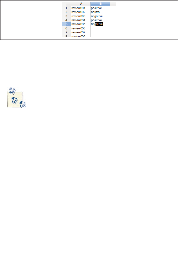
Figure 5-1. A possible source of error in annotation
Of course, this doesn’t mean it’s impossible to complete a task by using a spreadsheet
and classifications that are a bit similar. In some cases, such circumstances are impossible
to avoid. However, it’s never a bad idea to keep an eye out for places where mistakes can
easily slip in.
While we didn’t discuss the movie review annotation scenario in Chap
ter 4, we have assumed here that we have a schema that contains three
categories. However, that is by no means the only way to frame this task
and to categorize movie reviews. In the Movie Review Corpus that
comes with the Natural Language Toolkit (NLTK), reviews are divided
into only positive and negative (based on the scores provided in the
reviews themselves), and RottenTomatoes.com also uses a binary clas
sification. On the other hand, Metacritic.com rates everything on a scale
from 0 to 100.
Both of these websites provide annotation guidelines for reviews that
don’t give preassigned numeric ratings, and each of those websites has
its editors assign ratings based on their own systems (Metacritic.com;
RottenTomatoes.com).
Multiple Labels: Film Genres
As your tasks grow in complexity, there are more limiting factors for how to structure
your annotations. For example, there are a number of ways to approach the task of
labeling movie reviews that only allow one label per document, but what happens if it’s
possible for a document to have more than one label? In Chapter 4 we started discussing
a spec for a task involving labeling movie summaries with their associated genres. Let’s
expand on that example now, to see how we can handle more complex annotation tasks.
While it might be tempting to simply say, “Well, we’ll only give a single label to each
movie,” attempting to follow that guideline becomes difficult quickly. Are romantic
comedies considered romances, or comedies? You could add “romantic comedy” as a
genre label, but will you create a new label for every movie that crosses over a genre line?
90 | Chapter 5: Applying and Adopting Annotation Standards

Such a task quickly becomes ridiculous, simply due to the number of possible combi
nations. So, define your genres and allow annotators to put as many labels as necessary
on each movie (in Chapter 6 we’ll discuss in more detail possible approaches to guide
lines for such a task).
So how should this information be captured? Of the options listed for the movie review
task, some of them can be immediately discarded. Having your annotators change
the names of the files to contain the labels is likely to be cumbersome for both the
annotators and you: Casablanca-drama.txt is easy enough, but Spaceballs-
sciencefiction_comedy_action_parody.txt would be annoying for an annotator to create,
and equally annoying for you to parse into a more usable form (especially if spelling
errors start to sneak in).
Moving files into appropriately labeled folders is also more difficult with this task; a
copy of the file would have to be created for each label, and it would be much harder to
gather basic information such as how many labels, on average, each movie was given.
It would also be much, much harder for annotators to determine if they missed a label.
In Figure 5-1 we showed a sample spreadsheet with filenames and positive/negative/
neutral labels in different columns, with a different row for each review. While it would
certainly be possible to create a spreadsheet set up the same way to give to your anno
tators, it’s not hard to imagine how error-prone that sort of input would be for a task
with even more category options and more potential columns per movie.
So where does that leave us? If none of the simpler ways of labeling data are available,
then it’s probably time to look at annotation tools and XML representations of annota
tion data.
In this case, since the information you want to capture is metadata that’s relevant to the
entire document, you probably don’t need to worry about character offsets, so you can
have tags that look like this:
<GenreXML>
<FILM fid = "f1" title = "Cowboys and Aliens" file_name = "film01.txt" />
<GENRE gid = "g1" filmid = "f01" label = "western" />
<GENRE gid = "g2" filmid = = "f01" label = "sci-fi" />
<GENRE gid = "g3" filmid= "f01" label = "action" />
</GENREXML>
This is a very simple annotation, with an equally simple DTD or Document Type Def
inition [if you aren’t sure how to read this DTD, refer back to the sidebar “What Is a
DTD?” (page 68)]:
<!ENTITY name "GenreXML">
<!ELEMENT FILM (#PCDATA) >
<!ATTLIST FILM id ID >
<!ATTLIST FILM title CDATA >
<!ATTLIST FILM file_name CDATA >
Metadata Annotation: Document Classification | 91

<!ELEMENT GENRE (#PCDATA) >
<!ATTLIST GENRE id ID >
<!ATTLIST GENRE filmid CDATA >
<!ATTLIST GENRE label ( action | adventure | classic | ... ) >
This representation of the genre labeling task is not the only way to approach the problem
(in Chapter 4 we showed you a slightly different spec for the same task). Here, we have
two elements, film and genre, each with an ID number and relevant attributes; the
genre element is linked to the film it represents by the filmid attribute.
Don’t fall into the trap of thinking there is One True Spec for your task.
If you find that it’s easier to structure your data in a certain way, or to
add or remove elements or attributes, do it! Don’t let your spec get in
the way of your goal.
By having the filename stored in the XML for the genre listing, it’s possible to keep the
annotation completely separate from the text of the file being annotated. However,
clearly the file_name attribute is not one that is required, and probably not one that
you would want an annotator to fill in by hand. But it is useful, and would be easy to
generate automatically during pre- or postprocessing of the annotation data.
Giving each tag an ID number (rather than only the FILM tags) may not seem very
important right now, but it’s a good habit to get into because it makes discussing and
modifying the data much easier, and can also make it easier to expand your annotation
task later if you need to.
At this point you may be wondering how all this extra information is going to help with
your task. There are a few reasons why you should be willing to take on this extra
overhead:
•Having an element that contains the film information allows the annotation to be
kept either in the same file as the movie summary, or elsewhere without losing track
of the data.
•Keeping data in a structured format allows you to more easily manipulate it later.
Having annotation take the form of well-formated XML can make it much easier
to analyze later.
•Being able to create a structured representation of your spec helps cement your task,
and can show you where problems are in how you are thinking about your goal.
•Representing your spec as a DTD (or other format) means you can use annotation
tools to create your annotations. This can help cut down on spelling and other user-
input errors.
92 | Chapter 5: Applying and Adopting Annotation Standards

Figure 5-2 shows what the film genre annotation task looks like in the Multipurpose
Annotation Environment (MAE), an annotation tool that requires only a DTD-like
document to set up and get running. As you can see, by having the genre options supplied
in the DTD, an annotator has only to create a new instance of the GENRE element and
select the attribute he wants from the list.
Figure 5-2. Genre annotation in MAE
The output from this annotation process would look like this:
<FILM id="f0" start="-1" end="-1" text="" title="Cowboys and Aliens" />
<GENRE id="g0" start="-1" end="-1" text="" label="action" />
<GENRE id="g1" start="-1" end="-1" text="" label="sci-fi" />
<GENRE id="g2" start="-1" end="-1" text="" label="western" />
There are a few more elements here than the ones specified in the DTD shown earlier
—most tools will require that certain parameters be met in order to work with a task,
but in most cases those changes are superficial. In this case, since MAE is usually used
to annotate parts of the text rather than create metatags, the DTD had to be changed to
allow MAE to make GENRE and FILM nonconsuming tags. That’s why the start and end
elements are set to –1, to indicate that the scope of the tag isn’t limited to certain char
acters in the text. You’ll notice that here, the filmid attribute in the GENRE tag is not
present, and neither is the file_name attribute in the FILM tag. While it wouldn’t be
unreasonable to ask your annotators to assign that information themselves, it would be
easier—as well as both faster and more accurate—to do so with a program.
If you plan to keep the stand-off annotation in the same file as the text that’s being
annotated, then you might not need to add the file information to each tag. However,
annotation data can be a lot easier to analyze/manipulate if it doesn’t have to be extracted
from the text it’s referring to, so keeping your tag information in different files that refer
back to the originals is generally a best practice.
Metadata Annotation: Document Classification | 93

Text Extent Annotation: Named Entities
The review classification and genre identification tasks are examples of annotation labels
that refer to the entirety of a document. However, many annotation tasks require a finer-
grained approach, where tags are applied to specific areas of the text, rather than all of
it at once. We already discussed many examples of this type of task: part-of-speech (POS)
tagging, Named Entity (NE) recognition, the time and event identification parts of
TimeML, and so on. Basically, any annotation project that requires sections of the text
to be given distinct labels falls into this category. We will refer to this as extent annota
tion, because it’s annotating a text extent in the data that can be associated with character
locations.
In Chapter 4 we discussed the differences between stand-off and inline annotation, and
text extents are where the differences become important. The metadata-type tags used
for the document classification task could contain start and end indicators or could
leave them out; their presence in the annotation software was an artifact of the software
itself, rather than a statement of best practice. However, with stand-off annotation, it is
required that locational indicators are present in each tag. Naturally, there are multiple
ways to store this information, such as:
• Inline annotation
• Stand-off annotation by location in a sentence or paragraph
• Stand-off annotation by character location
In the following sections we will discuss the practical applications of each of these
methods, using Named Entity annotation as a case study.
As we discussed previously, NE annotation concerns marking up what you probably
think of as proper nouns—objects in the real world that have specific designators, not
just generic labels. So, “The Empire State Building” is an NE, while “the building over
there” is not. For now, we will use the following spec to describe the NE task:
<!ENTITY name "NamedEntityXML">
<!ELEMENT NE (#PCDATA) >
<!ATTLIST NE id ID >
<!ATTLIST NE type ( person | title | country | building | business |...) >
<!ATTLIST NE note CDATA >
Inline Annotation
While we still strongly recommend not using this form of data storage for your anno
tation project, the fact remains that it is a common way to store data. The phrase “inline
annotation” refers to the annotation XML tags being present in the text that is being
annotated, and physically surrounding the extent that the tag refers to, like this:
94 | Chapter 5: Applying and Adopting Annotation Standards

<NE id="i0” type="building">The Massachusetts State House</NE> in <NE id="i1” type="city">Boston, MA</NE> houses
the offices of many important state figures, including <NE id="i2” type="title">Governor</NE> <NE id="i3”
type="person">Deval Patrick</NE> and those of the <NE id="i4” type="organization">Massachusetts General Court</
NE>.
If nothing else, this format for annotation is extremely difficult to read. But more im
portant, it changes the formatting of the original text. While in this small example there
may not be anything special about the text’s format, the physical structure of other
documents may well be important for later analysis, and inline annotation makes that
difficult to preserve or reconstruct. Additionally, if this annotation were to later be
merged with, for example, POS tagging, the headache of getting the two different tagsets
to overlap could be enormous.
Not all forms of inline annotation are in XML format. There are other ways to mark up
data that is inside the text, such as using parentheses to mark syntactic groups, as was
done in the following Penn TreeBank II example, taken from “The Penn TreeBank:
Annotating Predicate Argument Structure” (Marcus et al. 1994):
(S (NP-SUBJ I
(VP consider
(S (NP-SUBJ Kris)
(NP-PRD a fool))))
There are still many programs that provide output in this or a similar format (the
Stanford Dependency Parser is one example), and if you want to use tools that do this,
you may have to find a way to convert information in this format to stand-off annotation
to make it maximally portable to other applications.
Of course, there are some benefits to inline annotation: it becomes unnecessary to keep
special track of the location of the tags or the text that the tags are surrounding, because
those things are inseparable. Still, these benefits are fairly shortsighted, and we strongly
recommend not using this paradigm for annotation.
Another kind of inline annotation is commonly seen in POS tagging, or other tasks
where a label is assigned to only one word (rather than spanning many words). In fact,
you already saw an example of it in Chapter 1, in the discussion of the Penn TreeBank.
“/” From/IN the/DT beginning/NN ,/, it/PRP took/VBD a/DT man/NN with/IN extraordinary/JJ qualities/NNS to/TO succeed/VB
in/IN Mexico/NNP ,/, “/” says/VBZ Kimihide/NNP Takimura/NNP ,/, president/NN of/IN Mitsui/NNS group/NN ’s/POS
Kensetsu/NNP Engineering/NNP Inc./NNP unit/NN ./.
Here, each POS tag is appended as a suffix directly to the word it is referring to, without
any XML tags separating the extent from its label. Not only does this form of annotation
make the data difficult to read, but it also changes the composition of the words them
selves. Consider how “group’s” becomes “group/NN ’s/POS”—the possessive “’s” has
Text Extent Annotation: Named Entities | 95

been separated from “group”, now making it even more difficult to reconstruct the orig
inal text. Or imagine trying to reconcile an annotation like this one with the NE example
in the previous example! It would not be impossible, but it could certainly cause
headaches.
While we don’t generally recommend using this format either, many existing POS tag
gers and other tools were originally written to provide output in this way, so it is some
thing you should be aware of, as you may need to realign the original text with the new
POS tags.
We are not, of course, suggesting that you should never use tools that
output information in formats other than some variant stand-off an
notation. Many of these tools are extremely useful and provide very
accurate output. However, you should be aware of problems that might
arise from trying to use them.
Another problem with this annotation format is that if it is applied to the NE task, there
is the immediate problem that the NE task requires that a single tag apply to more than
one word at the same time. There is an important distinction between applying the same
tag more than once in a document (as there is more than one NN tag in the Penn TreeBank
example), and applying one tag across a span of words. Grouping a set of words together
by using a single tag tells the reader something about that group that having the same
tag applied to each word individually does not. Consider these two examples:
<NE id="i0” type="building">The Massachusetts State
House</NE> in <NE id="i1” type="city">Boston, MA</NE>
…
The/NE_building Massachusetts/NE_building State/
NE_building House/NE_building in Boston/NE_city ,/
NE_city MA/NE_city …
In the example on the left, it is clear that the phrase “The Massachusetts State House”
is one unit as far as the annotation is concerned—the NE tag applies to the entire group.
On the other hand, in the example on the right, the same tag is applied individually to
each token, which makes it much harder to determine if each token is an NE on its own,
or if there is a connection between them. In fact, we end up tagging some tokens with
the wrong tag! Notice that the state “MA” has to be identified as “/NE_city” for the span
to be recognized as a city.
Stand-off Annotation by Tokens
One method that is sometimes used for stand-off annotation is tokenizing (i.e., sepa
rating) the text input and giving each token a number. The tokenization process is usually
based on whitespace and punctuation, though the specific process can vary by program
(e.g., some programs will split “’s” or “n’t” from “Meg’s” and “don’t”, and others will not).
The text in the appended annotation example has been tokenized—each word and
punctuation mark has been pulled apart.
96 | Chapter 5: Applying and Adopting Annotation Standards
Taking the preceding text as an example, there are a few different ways to identify the
text by assigning numbers to the tokens. One way is to simply number every token in
order, starting at 1 (or 0, if you prefer) and going until there are no more tokens left, as
shown in Table 5-1.
Table 5-1. Word labeling by token
TOKEN TOKEN_ID
“ 1
From 2
the 3
beginning 4
, 5
… …
unit 31
. 32
This data could be stored in a tab-separated file or in a spreadsheet, as it’s necessary to
keep the IDs associated with each token. Another way is to assign numbers to each
sentence, and identify each token by sentence number and its place in that sentence, as
shown in Table 5-2.
Table 5-2. Word labeling by sentence and token
TOKEN SENT_ID TOKEN_ID
“ 1 1
From 1 2
the 1 3
beginning 1 4
, 1 5
…
unit 1 31
. 1 32
Then 2 1
…
Naturally, more identifying features could be added, such as paragraph number, docu
ment number, and so on. The advantage of having additional information (such as
sentence number) to identify tokens is that this information can be used later to help
define features for the machine learning (ML) algorithms (while sentence number could
be inferred again later, if it’s known to be important, then it’s easier to have that infor
mation up front).
Text Extent Annotation: Named Entities | 97
Annotation data using this format could look something like Table 5-3.
Table 5-3. POS annotation in tokenized text
POS_TAG SENT_ID TOKEN_ID
“ 1 1
IN 1 2
DT 1 3
NN 1 4
…
There are some advantages to using this format: because the annotation is removed from
the text, it’s unnecessary to worry about overlapping tags when trying to merge anno
tations done on the same data. Also, this form of annotation would be relatively easy to
set up with a tokenizer program and any text that you want to give it.
However, there are some problems with this form of annotation as well. As you can see,
because the text is split on whitespace and punctuation, the original format of the data
cannot be recovered, so the maxim of “do no harm” to the data has been violated. If the
structure of the document that this text appeared in later became important when cre
ating features for a classifier, it could be difficult to merge this annotation with the
original text format.
It is possible to use token-based annotation without damaging the data,
though it would require running the tokenizer each time the annotation
needed to be paired with the text, and the same tokenizer would always
have to be used. This is the suggested way for dealing with token-based
stand-off annotation.
Additionally, this format has a similar problem to the appended annotation, in that it
appears to assume that each tag applies to only one token. While it’s not impossible to
apply a tag to a set of tokens, the overhead does become greater. Consider again our NE
example, this time tokenized, as shown in Table 5-4.
98 | Chapter 5: Applying and Adopting Annotation Standards
Table 5-4. Token-based corpus labels
TOKEN SENT_ID TOKEN_ID
The 1 1
Massachusetts 1 2
State 1 3
House 1 4
in 1 5
Boston 1 6
, 1 7
MA 1 8
houses 1 9
…
Table 5-5 shows how we would apply a tag spanning multiple tokens.
Table 5-5. Sample stand-off annotation using token IDs
TAG START_SENT_ID START_TOKEN_ID END_SENT_ID END_TOKEN_ID
NE_building 1 1 1 4
NE_city 1 6 1 8
The other flaw in this method is that it doesn’t easily allow for annotating parts of a
word. Annotation projects focusing on morphemes or verb roots would require anno
tating partial tokens, which would be difficult with this method. It isn’t impossible to
do—another set of attributes for each token could be used to indicate which characters
of the token are being labeled. However, at that point, one might as well move to
character-based stand-off annotation, which we will discuss in the next section.
Stand-off Annotation by Character Location
Using character locations to define what part of the document a tag applies to is a reliable
way to generate a stand-off annotation that can be used across different systems.
Character-based annotations use the character offset information to place tags in a
document, like this:
The Massachusetts State House in Boston, MA houses the offices
of many important state figures, including Governor Deval Patrick
and those of the Massachusetts General Court.
<NE id="N0" start="5" end="31" text="Massachussetts State House"
type="building" />
<NE id="N1" start="35" end="45" text="Boston, MA" type="city" />
Text Extent Annotation: Named Entities | 99
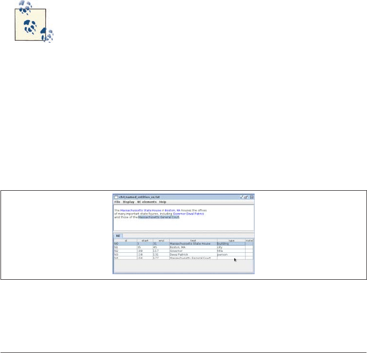
<NE id="N2" start="109" end="117" text="Governor" type="title" />
<NE id="N3" start="118" end="131" text="Deval Patrick" type="person" />
<NE id="N4" start="150" end="177" text="Massachusetts General Court"
type="organization" />
At first glance it is difficult to see the benefits to this format for annotation—the start
and end numbers don’t mean much to someone just looking at the tags, and the tags are
so far from the text as to be almost unrelated. However, this distance is precisely why
stand-off annotation is important, even necessary. By separating the tags from the text,
it becomes possible to have many different annotations pointing to the same document
without interfering with one another, and more important, without changing the orig
inal text of the document.
As for the start and end numbers, while it is difficult for a human to determine what
they are referring to, it’s very easy for computers to count the offsets to accomplish that
task. And the easier it is for the computer to find the important parts of text, the easier
it is to use that text and annotation for machine learning later.
Using start and end as attribute names to indicate where the tags
should be placed in the text is a convention that we use here, but is not
one that is a standard in annotation—different annotation tools and
systems will use different terms for this information. Similarly, the text
attribute does not have any special meaning either. What the attributes
are called is not important; what’s important is the information that they
hold.
Technically, all that’s needed for these tags to work are the start and end offset locations
and the tag attributes—here, the tags also contain the text that the tag applies to, because
it makes the annotation easier to evaluate. Even if that information was not there, the
tag would still be functional. Figure 5-3 shows what it might look like to create this
annotation in an annotation tool.
Figure 5-3. NE annotation
100 | Chapter 5: Applying and Adopting Annotation Standards

Naturally, some preparation is necessary to make stand-off annotation work well. For
starters, it’s important to decide early in the process what character encoding you will
use for your corpus, and to stick with that throughout the annotation process. The
character encoding that you choose will determine how different computers and pro
grams count where the characters are in your data, and changing encodings partway
through can cause a lot of work to be lost. We recommend using UTF-8 encoding for
your data.
Encoding problems can cause a lot of headaches, especially if your data
will be transferred between computers using different operating sys
tems. Using Windows can make this particularly difficult, as it seems
that Windows does not default to using UTF-8 encoding, while most
other operating systems (Mac and most flavors of Unix/Linux that we’re
aware of) do. It’s not impossible to use UTF-8 on Windows, but it does
require a little extra effort.
Linked Extent Annotation: Semantic Roles
Sometimes in annotation tasks, it is necessary to represent the connection between two
different tagged extents. For example, in temporal annotation, it is not enough to an
notate “Monday” and “ran” in the sentence “John ran on Monday”; to fully represent
the information presented in the sentence, we must also indicate that there is a con
nection between the day and the event. This is done by using relationship tags, also
called link tags.
Let’s look again at our example sentence about Boston. If we were to want to add loca
tional information to this annotation, we would want a way to indicate that there is a
relationship between places. We could do that by adding a tag to our DTD that would
look something like this:
<!ELEMENT L_LINK EMPTY >
<!ATTLIST L-LINK fromID IDREF >
<!ATTLIST L-LINK toID IDREF >
<!ATTLIST L-LINK relationship ( inside | outside | same | other ) >
Obviously, this is a very limited set of location relationships, but it will work for now.
How would this be applied to the annotation that we already have?
This is where the tag IDs that we mentioned in “Multiple Labels: Film Genres” (page
90) become very important. Because link tags do not refer directly to extents in the text,
they need to represent the connection between two annotated objects. The most com
mon way to represent this information is to use the ID numbers from the extent tags to
anchor the links. This new information will look like this:
Linked Extent Annotation: Semantic Roles | 101

The Massachusetts State House in Boston, MA houses the offices
of many important state figures, including Governor Deval Patrick
and those of the Massachusetts General Court.
<NE id="N0" start="5" end="31" text="Massachusetts State House"
type="building" />
<NE id="N1" start="35" end="45" text="Boston, MA" type="city" />
<NE id="N2" start="109" end="117" text="Governor" type="title" />
<NE id="N3" start="118" end="131" text="Deval Patrick" type="person" />
<NE id="N4" start="150" end="177" text="Massachusetts General Court"
type="organization" />
<L-LINK id="L0" fromID="N0" toID="N1" relationship="inside" />
<L-LINK id="L0" fromID="N4" toID="N0" relationship="inside" />
By referring to the IDs of the NE tags, we can easily encode information about the rela
tionships between them. And because the L-LINK tags also have ID numbers, it is pos
sible to create connections between them as well—perhaps a higher level of annotation
could indicate that two L-LINKs represent the same location information, which could
be useful for a different project.
Once again, the names of the attributes here are not particularly im
portant. We use fromID and toID as names for the link anchors, because
that is what the annotation tool MAE does, but other software uses
different conventions. The intent, however, is the same.
ISO Standards and You
In “ISO Standards” (page 80) we discussed the LAF (Linguistic Annotation Framework)
standard for representing annotated data. It might have sounded pretty formal, but don’t
worry! If you’re following along with our recommendations in this book and using XML-
based stand-off annotation, chances are that your annotation structure is already LAF-
compliant, and that you would just need to convert it to the LAF dump format. Also
keep in mind that LAF is a great foundation for linguistic researchers who want to share
their data, but if your annotation is only meant for you, or is proprietary to a company,
this might not be something you will need to worry about at all.
102 | Chapter 5: Applying and Adopting Annotation Standards

Summary
In this chapter we discussed some of the different methods for representing annotations
for a corpus annotation task. In particular, we noted the following:
•Annotations can be stored in many different ways, but it’s important to choose a
format that will be flexible and easy to change later if you need to. We recommend
stand-off, XML-based formats.
•In some cases, such as single-label document classification tasks, there are many
ways to store annotation data, but these techniques are essentially isomorphic. In
such cases, choose which method to use by considering how you plan to use the
data, and what methods work best for your annotators.
•For most annotation tasks, such as those requiring multiple labels on a document,
and especially those requiring extent annotation and linking, it will be useful to
have annotation software for your annotators to use. See Appendix B for a list of
available software.
•Extent annotation can take many forms, but character-based stand-off annotation
is the format that will make it easier to make any necessary changes to the annota
tions later, and also make it easier to merge with other annotations.
•If you do choose to use character-based stand-off annotation, be careful about what
encodings you use for your data, especially when you create the corpus in the first
place. Different programming languages and operating systems have different de
fault settings for character encoding, and it’s vital that you use a format that will
work for all your annotators (or at least be willing to dictate what resources your
annotators use).
•Using industry standards such as XML and annotation standards such as LAF for
your annotations will make it much easier for you to interact with other annotated
corpora, and make it easier for you to share your own work.
Summary | 103

CHAPTER 6
Annotation and Adjudication
Now that you have a corpus and a model, it’s time to start looking at the actual annotation
process—the “A” in the MATTER cycle. Here is where you define the method by which
your model is applied to your texts, both in theory (how your task is described to an
notators) and in practice (what software and other tools are used to create the annota
tions). A critical part of this stage is adjudication—where you take your annotators’ work
and use it to create the gold standard corpus that you will use for machine learning. In
this chapter we will answer the following questions:
• What are the components of an annotation task?
• What is the difference between a model specification and annotation guidelines?
• How do you create guidelines that fit your task?
• What annotation tool should you use for your annotation task?
• What skills do your annotators need to create your annotations?
•How can you tell (qualitatively) if your annotation guidelines are good for your
task?
• What is involved in adjudicating the annotations?
The Infrastructure of an Annotation Project
It’s much easier to write annotation guidelines when you understand how annotation
projects are usually run, so before getting into the details of guideline writing, we’re
going to go over a few different ways that you can structure your annotation effort.
Currently, what we would call the “traditional” approach goes like this. Once a schema
is developed and a corpus is collected, an investigator writes up guidelines, finds anno
tators, and distributes the guidelines and corpus to the annotators, who go off, annotate,
105
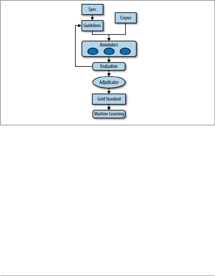
and then come back with a marked-up corpus. The researcher then collects the data
from each of the annotators, and calculates Inter-Annotator Agreement (IAA) scores.
If these scores are low, the guidelines (and sometimes the model) are revised, and the
annotation is redone. If the scores are good, adjudication is performed over the data to
create a gold standard, which is then used to train and test a machine learning (ML)
algorithm. Figure 6-1 visually depicts the annotation process.
Figure 6-1. The annotation process
So why do researchers use this distributed method of annotation, rather than doing it
themselves? There are two main reasons. First, there is a purely practical concern: most
annotation tasks now are performed with the end goal of training an ML system, and
to do that, there needs to be sufficient data to train the algorithm. Since for most tasks
this requires hundreds or even thousands of annotated articles or examples, it would be
completely impractical for only one or two people to create the required corpus.
The second reason for distributed annotation is that by having other people do the bulk
of the tagging, and then using that data to calculate agreement scores, the researcher
gets a sense of whether the task is sufficiently well defined to provide consistent data
should a bigger corpus be needed. If there is little agreement among annotators as to
how each tag and attribute should be used, it may be a sign that the guidelines are simply
not well written, but it may also be a sign that the task itself is flawed, or goes against
the way people generally understand language.
106 | Chapter 6: Annotation and Adjudication

Before computers were as fast as they are now, researchers wanting to examine language
data did so by hand, and usually by themselves or with the help of a student in the field.
However, annotated corpora from before the 1980s tended to be relatively small, simply
because of the infeasibility of creating and cataloging a large amount of data. While large
corpora were being put together in the 1970s and 1980s (such as the Brown Corpus), it
wasn’t until later that large, computer-based annotation efforts became common.
However, even with larger datasets becoming more available, it’s still sometimes neces
sary to return to an existing task and create a larger annotated corpus for it. This is why
it is important to have well-defined guidelines and good IAA scores; if a task is clear,
then it can be reproduced later by other groups of people. In Chapter 4 we discussed
interoperability and reproducibility as it applies to data formats, but the concept applies
to the annotation task as well.
Crowdsourcing
Crowdsourcing is another approach that is being used more frequently in the annotation
community. Essentially, instead of asking a small number of annotators to tag a large
number of extents, the task is broken down into a large number of smaller tasks, and a
large number of annotators are asked to tag only a few examples each. One popular
crowdsourcing platform is Amazon’s Mechanical Turk (MTurk), a resource where people
who have tasks that require human intelligence to perform can place requests that are
then fulfilled by people across the country and around the world. These HITs (human
intelligence tasks) are generally formatted to be very quick and relatively easy to perform,
so workers are usually paid in cents rather than dollars. Because of the availability of
annotators and how inexpensive each HIT is, many researchers have looked into using
crowdsourcing as a resource for annotation.
Generally, MTurk will only be useful for tasks that don’t require any special linguistic or
other domain knowledge. Additionally, due to the restricted nature of the HIT interface,
workers can’t be given pages and pages of annotation guidelines—aside from the imprac
ticality of the layout, it’s generally not worth a worker’s time to read that many instructions
for only a few cents. So, if you have an annotation task that can be broken down into simple
steps and explained easily in a few sentences, then MTurk may be a good resource for you
to look into. Because such tasks do have to be given a different format and broken down
into smaller pieces, we’re not going to go into the details of creating good annotation HITs
in this book, but Appendix E has a list of MTurk-related resources that you may find useful
if you decide to use MTurk.
The Infrastructure of an Annotation Project | 107

Specification Versus Guidelines
In the previous chapters we explored how models are created, and we looked at different
ways to define your task in terms of tags and XML. These tags encapsulate what your
schema is capable of capturing: they are an abstraction of what you want your data to
represent. The annotation guidelines represent the application of the schema to the data:
they are the guidebook for how the schema is used on your data.
If it helps, think of the distinction between schema and guidelines as
the difference between a list of ingredients and the actual baking in
structions. The guidelines determine how the ingredients (the schema:
tags, attributes, and data) are mixed together, and what they make when
you’re done. In baking, the same ingredients can be used to make bread
or cake, and in annotation, the same specification can sometimes be
used for different annotation projects.
The distinction between schema and guidelines is important, because it’s possible for a
single schema to be used for different annotation tasks, or for the same basic task but
with different data than has been used in the past. If you have decided to use or modify
an existing schema for your annotation task, then this distinction is one that you will
probably need to pay particular attention to, as existing guidelines for your task may
not fit your specific goal or corpus.
For example, the original TimeML annotation guidelines were written to be applied to
newspaper articles, which led to specific examples and notes in the guidelines that did
not apply to other genres. Specifically, when TimeML was applied to medical data, a few
changes were made to the schema, but for the most part, it was the annotation guidelines
that needed to be modified to give relevant examples to the annotators. While you might
feel that it’s reasonable to expect that an annotator could extrapolate the events and
relationships from “The president is hopeful that reconciliation can be reached” to “The
patient is feverish and may experience nausea,” it is better to provide genre-relevant
examples than to rely too much on your annotators’ intuitions.
Another example of a guideline changing the use of a spec would be having a task that
limits the application of the spec. Consider the Named Entity (NE) relations that we
discussed in “Adding Named Entities” (page 71). These relation sets were derived from
an existing specification relating to semantic role labels. However, rather than use the
entire set of semantic role relationships defined in that task, we used only a subset of
those that relate to movies and the roles that people play in creating them.
Finally, you may be in a situation where you have one spec that defines your task, but
you find it necessary to split the task into different steps. Sometimes this is useful if you
have a complicated model, and want to maximize accuracy by performing annotations
108 | Chapter 6: Annotation and Adjudication
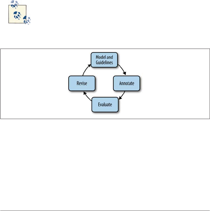
on only a few tags at a time, then adjudicating those tags, then moving on to the next
set of tags or relations. You may also find this approach necessary if your task requires
both general knowledge of the language and more specific knowledge that would require
a domain expert to provide. In those cases, you can have two tasks being performed
simultaneously by different groups of people on the same corpus, and then merge the
annotations later for ML purposes.
Be Prepared to Revise
While it is true that the entire MATTER process is a cycle, it is important to remember
that there is a smaller cycle of revision between the Model and Annotation stages. We
discussed in Chapter 4 how you may find it necessary to reformulate the spec as you
develop your model, but chances are good that once you start writing your annotation
guidelines, you will quickly find places where your data and spec don’t quite meet up.
Revising the spec while working on the guidelines and doing the an
notation occurs frequently enough that we refer to it as the MAMA
cycle: Model-Annotate-Model-Annotate (the Annotate step includes
writing the guidelines). See Figure 6-2.
Figure 6-2. The inner workings of the MAMA cycle
Once the guidelines are written and given to your annotators, the annotators themselves
will probably have questions about the spec and guidelines that may lead to more revi
sions. This is completely normal! To have an annotation task that can be reused in the
future, it’s important to take the time to make sure the spec and guidelines are clear and
well written.
Be Prepared to Revise | 109

Preparing Your Data for Annotation
Data preparation falls into two main tasks: the more theoretical act of deciding how to
present your documents to your annotators, and the very practical matter of coercing
those documents into a form that will work with the annotation tool that you choose.
A discussion of annotation tools will take place later in this chapter, so for now, we’ll
just focus on deciding what information to present to your annotators.
Metadata
Deciding what information to give to your annotators can be trickier than it seems. You
have the text files that you want annotated, but how much do you want your annotators
to know about the source of those files? For example, should they know where the files
came from and who produced them?
This may seem like a trivial problem, but information about a document can influence
annotators in sometimes unexpected ways. Opinion annotation in particular can be
susceptible to this problem. An obvious example would be, in examining the polarity
of movie reviews, informing the annotators of the star rating that the reviewer gave the
movie. If you want an annotator to look for both positive and negative adjectives, in
forming the annotator that the reviewer gave the movie 10 stars can prime her to look
only for positive adjectives.
In the same vein, if annotators are examining newspaper or Wikipedia articles for fac
tuality, informing them of the source of the article, or if the Wikipedia page was flagged
for being biased, could influence the annotators, particularly if a source is, to them,
associated with biased reporting, or if they tend to believe that Wikipedia flags are ac
curate.
As another example, say you are working on creating a phonetic transcription of recor
ded data; informing your annotators of the birthplace of a speaker could potentially bias
them to hear pronunciations in a particular way, especially if they are new to phonetic
transcription.
Bias can appear in unexpected ways—it’s useful to try a few variations
on the data presentation to eliminate different biasing factors.
Preprocessed Data
Another consideration in data presentation is giving your annotators data that already
has some information marked up.
There are two things to consider before doing that, however:
110 | Chapter 6: Annotation and Adjudication

•Is this information necessary for a human annotator, or would it be more useful for
an algorithm?
•Is this information going to be correct, or is it something that the annotator will
have to fix/examine for errors?
Part-of-speech (POS) is a great example of information that would be useful for a ma
chine to have, but that might not be necessary to give to an annotator (especially if the
annotator is a native speaker of the language he is evaluating). Presenting an annotator
with too much information can make the task confusing, and it could lower accuracy
without necessarily increasing informativity.
Whether or not your preprocessed information is correct will have a huge impact on
your annotation project. Certainly, it saves time to do part of your annotation auto
matically if the tools exist, but people in general tend to like simple instructions, and so
“Label all the Named Entities/times/events, then create links between them” might be
an easier rule to follow (especially since it could be done as two different tasks) than
“We have marked up most of the entities/times/events for you, but they might not be
correct, so we’d like you to fix any errors while creating links.”
If the provided annotations are of poor quality, asking annotators to correct partial
annotations can lead to mistakes not being fixed, especially when combined with other
instructions at the same time. Splitting the annotation into related tasks, such as cor
recting the generated labels and then later on adding more tags or creating links between
the corrected extents, is probably the best way to deal with this. It is more time-
consuming, but it will result in higher-quality annotations.
Splitting Up the Files for Annotation
We already told you about how you’ll need to divide your files into training and testing
datasets, but you will also want to set aside some documents for testing your annotation
guidelines on as well. As you work your way through the MAMA cycle, you’ll find that
(especially in the beginning) it won’t take long for you and your annotators to spot errors
and/or gaps in your model or guidelines. Because of this, we suggest having a set of 10–
20 files that you can use as a training set on which your annotators can test changes to
the guidelines. You can use these files in your gold standard later if you want or need
to, but because of how many times your annotators will have gone over those files in
particular, you probably won’t want to include them in your IAA calculations, because
they will be so heavily discussed and dissected.
Also, if you find that your guidelines have gone through many revisions, you’ll probably
want to switch out the training annotation files. That way, your annotators won’t become
so familiar with the expected annotations that they stop thinking about the guidelines.
As a rule of thumb, switch out your training files every two or three times you revise
your guidelines.
Preparing Your Data for Annotation | 111

Writing the Annotation Guidelines
The annotation guidelines are the instructions for how you want your annotators to
apply the model (your schema) to the data (your corpus) for a specific task. Opinions
vary on how much information should be included in the annotation guidelines—Dip
per et al. (2004), for example, believe that annotation guidelines should include a de
scription of the corpus, linguistic theories underlying the model, and so on. However,
we recommend that the annotation guidelines contain only the information needed for
the annotators to apply the tagsets to annotate the corpus for your particular annotation
task (remember: the same spec can be used for different goals).
Just because we say the annotation guidelines are only for creating an
notations doesn’t mean it’s not important to keep track of other infor
mation and make it available later! It’s just that when it comes to creating
an annotated corpus, including too much extra information can make
it harder for the annotators to figure out what parts of the document
are relevant to their task. Information about where the corpus came
from and how it was selected, what linguistic theories were used to
create your tagset, and how the corpus can be read and accessed should
absolutely be monitored and made available as part of the entire anno
tated corpus package—just don’t put it in the guidelines unless it’s di
rectly relevant to how you want the text annotated. We’ll talk more about
what information you should report on in Chapter 9.
So, to make the clearest guidelines you can, there are a few basics that your annotation
guidelines should cover. The guidelines should answer, at a minimum, the following
questions:
• What is the goal of the project?
•What is each tag called and how is it used? (Be specific: provide examples, and
discuss gray areas.)
• What parts of the text do you want annotated, and what should be left alone?
•How will the annotation be created? (For example, explain which tags or documents
to annotate first, how to use the annotation tools, etc.)
These bullets points provide a starting place for most tasks, and in the rest of this section
we’re going to go over what the answers to these questions for a few different tasks might
look like, as well as discuss how the questions need to be modified for different types of
tasks. Specifically, we’re going to look at single label classifications (movie reviews),
112 | Chapter 6: Annotation and Adjudication

multiple label classifications (film genres), extent annotations (NEs), and linked anno
tations (semantic roles). Before you begin writing your own guidelines, you may find it
helpful to look at the published guidelines for existing tasks. Check Appendix B for some
links to existing annotation tasks.
Make sure you write down your guidelines! Annotated corpora are most
useful when the guidelines used to create them are complete and avail
able for download with the corpus. Having the guidelines around will
make it easier for other people to recreate or expand your task later if
they need to.
Example 1: Single Labels—Movie Reviews
A classic example of a classification task is sorting movie reviews into positive and
negative categories to train a classifier to determine whether someone likes or dislikes
a movie based on what she says about it. A Movie Review Corpus (MRC) already exists
(it is available for download from http://www.cs.cornell.edu/people/pabo/movie-review-
data/, and is included in the Natural Language Toolkit [NLTK] dataset), and the creators
describe creating the corpus based on reviews from IMDb.com and selecting only those
reviews that gave numerical or star ratings in order to automatically categorize whether
the reviews were positive or negative (Pang and Lee 2004). So the initial labeling for this
task was actually done, in a sense, by the author of the review, and no annotation guide
lines were required.
But let’s say that you want to create a larger dataset, and to have humans create the labels
for the reviews. Let’s also say that your goal is to train an algorithm to be able to take
any review and label it as being positive or negative, like the creators of the MRC did.
However, if you go to IMDb.com right now and look at the reviews of nearly any movie,
you’ll find that not all reviews make clear good/bad distinctions. What would you do
with a review such as the following?
This movie was all right. The special effects were good, but the plot didn’t make a lot of
sense. The actors were funny, which helped, but the music was really distracting.
Now, this review doesn’t include a star rating, and it’s not (to our minds, anyway) clearly
positive or negative. It seems to give the movie a resounding “meh.” So how does that
fit in with your goal, or the goals of the MRC? Well, in the case of the MRC researchers,
they were only looking at the differences between positive and negative reviews, and so
they specifically collected only those that were clearly one or the other. However, if your
goal is to train an algorithm to work on any review selected at random, then you won’t
want to limit your corpus in that way.
Writing the Annotation Guidelines | 113

Make sure that your corpus matches your goal! We discussed this in
Chapter 2, but now is a good time to check to make sure any changes
that the MAMA cycle has made to your task are reflected in your corpus.
Otherwise, it will be difficult to train an ML algorithm later on.
So what should an annotator be told to do with the aforementioned review? One way
to help make that determination is to look at how other people handle the same problem.
The websites RottenTomatoes.com and Metacritic.com both have their editors assign
labels to reviews that do not provide specific categories or ratings themselves. Let’s take
a look at what they say about how these ratings are assigned:
… Our staffers will go through every publication on our Movies Publications list […]
looking for reviews for Iron Chef vs. Godzilla. For each review found, we will take the
score given by the critic and convert it to a 0–100 point scale. (For those critics who do
not provide a score, we’ll assign a score from 0–100 based on the general impression given
by the review.) […]
—Metacritic Help and Support
Unfortunately, that doesn’t really give guidelines for how to rate a review. Let’s look at
RottenTomatoes:
How do you determine whether a review with no stars is Rotten or Fresh? Most critics
from the Online Film Critics Society (OFCS) enter their own quotes and ratings. For
critics who don’t enter in their own quotes and ratings, it’s basically up to the judgment
of the editors. They take into account word choice, rating (if any), tone, and who the critic
is in their determination of whether a review is positive or not. If an editor is not certain
about a review, it is sent to another editor for a second opinion. “Wishy-washy” reviews,
reviews that are really difficult to determine if the critic recommends the film or not, are
usually given a Rotten because if the critic is not confident enough to give the movie even
an implied recommendation, then we shouldn’t either.
—RottenTomatoes Help Center
That’s a clear explanation for how to assign a label to a neutral review, with a good reason
for how the decision should be made. It also fits in with the stated goal of the corpus,
though it may not fit in with your own view of movie reviews. Assuming that you’re
satisfied with using that line of reasoning, let’s see where the project stands with regard
to the questions posed earlier.
What is the goal of the project?
To label movie reviews as being positive or negative.
What is each tag called and how is it used?
We have two labels, “positive” and “negative,” and each review will be labeled with
one of them, based on the tone of the review. Reviews that are not specifically pos
itive or negative will be labeled as “negative.”
114 | Chapter 6: Annotation and Adjudication

What parts of the text do you want annotated, and what should be left alone?
Each review will be given a single label, which will be applied to the entire document.
How should the annotation be created?
In Chapter 5 we discussed the different formats that can be used for capturing this
type of data. In this situation we would probably use a spreadsheet prepopulated
with the names of the files that are being examined, but this decision depends largely
on who your annotators are and what works best for them and you.
Keep in mind that we’re not going to provide a complete guideline in this chapter for
any of the tasks, just a high-level overview of the important points that need to be covered
for a good annotation guideline. As we mentioned before, check Appendix A for a list
of existing annotation tasks, and see Chapter 10 for a worked-through example of an
annotation task.
Example 2: Multiple Labels—Film Genres
A more complicated example of classification is identifying film genres. This type of
classification is an excellent example of a task where the annotation guidelines can
completely change the outcome of the annotation, and trying to apply the guidelines
may lead to changes in the spec.
Remember that within the MATTER cycle there is also the MAMA
(Model-Annotate-Model-Annotate) cycle. Chances are good (especial
ly if you are starting your annotation project from scratch) that you will
need to revise your model and guidelines at least a few times before you
will be able to annotate your entire corpus. But don’t be discouraged;
the more you refine your annotation, the easier it will be to define fea
tures for your ML algorithms later on.
If you recall from “Film Genre Classification” (page 70), when discussing the spec for a
film genre classification task we used IMDb’s list of film genres, which included the
following 26 genres:
Action Adventure Animation Biography Comedy
Crime Documentary Drama Family Fantasy
Film-Noir Game-Show History Horror Music
Musical Mystery News Reality-TV Romance
Sci-Fi Sport Talk-Show Thriller War
Western
Writing the Annotation Guidelines | 115

This certainly seems like a reasonable list, and it comes from one of the most (if not the
most) popular movie reference websites on the Internet, so at the very least it’s a good
starting point for your spec. So let’s look at the list of questions to be answered for the
guidelines.
What is the goal of the project?
To label film summaries with genre notations.
What is each tag called and how is it used?
We have 26 tags that can be applied to each summary as needed.
What parts of the text do you want annotated, and what should be left alone?
Each label will apply to the entire document.
How should the annotation be created?
Annotation software is probably the best way to apply multiple labels to a document.
Well, that was easy! Except…the answer to the second question, particularly the “how
is it used” part, is quite underspecified. When labeling movie reviews as positive or
negative it’s probably enough to say (as a starting point, at least) that the label will be
based on tone, and neutral reviews will be labeled as “negative.” However, genre labels
are not all mutually exclusive, so annotators are going to need clearer guidelines for how
and when to apply each one. One basic question that needs to be answered is: “Is there
a maximum number of labels that can be applied to a document?” The answer to this
question alone can completely differentiate one annotation task from another, even if
each one is using the same spec; guidelines that specify a maximum of, say, two labels
per document are likely going to return a vastly different corpus than guidelines that
have no such limit. For the imaginary task we are describing here, our guidelines will
not specify a limit to the number of tags.
However, while knowing how many labels can be applied partly answers the question
of “how” the tags are used, it doesn’t address all of the aspects of “how” the tags are used.
Another aspect that has to be considered is when each tag will be used. In the positive/
negative review task, each document was assigned a single label, and if a document
wasn’t positive, it was negative: a dichotomy that’s fairly straightforward. Since there’s
no limit to the number of genre tags (or even if there were a limit), annotators will need
some clarification about when to apply which tags.
At first, the question of when to use each label seems straightforward. But consider the
first two tags in the previous list: action and adventure. What, your annotators will want
to know, is the difference? A quick Google search shows that this is hardly the first time
this question has been asked, and the general consensus appears to be that action movies
tend to be more violent, while adventure movies generally require that the protagonist
116 | Chapter 6: Annotation and Adjudication
be going on some sort of journey to a place or situation he has not dealt with previously.
However, the same Google search also reveals that other genre lists (such as the one
Netflix uses) simply have one genre label called “Action-Adventure,” presumably due to
a high level of overlap between the two labels.
Let’s assume that you’re satisfied with the aforementioned distinction between action
and adventure, and you put them in your guidelines as definitions for your annotators
to refer back to. So now they’ll (hopefully) label Die Hard as an action movie and Around
the World in 80 Days as an adventure. But wait a minute, one of the first summaries for
Die Hard on IMDb.com starts with “New York City Detective John McClane has just
arrived in Los Angeles to spend Christmas with his wife. Unfortunately….” So is there
a journey involved? The character does go to a different location, but a cop who is used
to dealing with criminals going to a different city to deal with criminals doesn’t really
meet the “new situation” clause of the adventure definition given earlier, so we can
probably safely say that Die Hard doesn’t qualify as an adventure movie.
OK, that’s a good start. But what about Eat, Pray, Love? The main character clearly goes
on a journey to new places and situations, but we suspect that most people wouldn’t
consider it to be an adventure movie. So, maybe adventure movies also have to have
some element of danger? Better amend the definition in your guidelines. Or maybe at
this point you feel like trying to differentiate between the two is a bit tedious and/or
pointless, and you’d rather amend your spec to have a single action-adventure category.
Believe it or not, we didn’t include the preceding few paragraphs simply
because we enjoy nitpicking about movie genres. Rather, we included
them because this discussion illustrates the kinds of questions you will
need to answer for your annotators when you give them the guidelines
for their task. The simplest approach to the task is to just give your
annotators a pile of texts and tell them to put on whatever labels seem
right to them, but don’t forget that an important part of an annotation
task is reproducibility. If you simply tell annotators to label what they
want, it’s unlikely that a different set of annotators will be able to give
you the same (or even similar) results at a later date.
If you aren’t entirely sure what definition to give to each label, now would be a really
good time to take another piece of advice that we’ve repeated a number of times (and
will continue to repeat): do some research! One excellent book that we found on the
subject is Barry Keith Grant’s Film Genre: From Iconography to Ideology (Wallflower
Press, 2007). While not all of the theory in the book can necessarily be applied to an
annotation task, looking at the different genres in terms of themes rather than simply
looking at surface details can help clarify what makes a movie fit into a genre. For
Writing the Annotation Guidelines | 117

example, Western movies often are, in part, about exploring new frontiers and the pio
neer spirit, a definition that might be more effective and relevant than one that specifies
a Western has horses, people wearing cowboy hats, and at least one person who says
“pardner” very slowly.
A closer look at the film genres also reveals that not all of the genres in the list are
describing the same aspects of the film. While labels such as “Action,” “Adventure,”
“Crime,” and “Romance” tell the reader something about the events that will take place
in the film, the labels “Historical,” “Sci-Fi,” and “Fantasy” refer to the setting, and “Ani
mation,” “Talk-Show,” and “Reality-TV” all describe the production circumstances.
Therefore, an altogether different approach to this task would be to break up these genres
into categories (production, setting, etc.) and ask annotators to assign at least one label
from each category. Assuming that the categories and labels are sufficiently well defined
(which is not necessarily an easy task), the specific requirement of “at least X number
of labels” may greatly improve the IAA and reproducibility of your task. If you were to
take this approach, you might create a DTD (Document Type Definition) that looks
something like this:
<!ELEMENT setting ( EMPTY ) >
<!ATTLIST setting description ( historical | sci-fi | fantasy ) >
<!ELEMENT production ( EMPTY ) >
<!ATTLIST production circumstances ( animation | documentary |
game-show | musical | news | reality-tv | talk-show | ) >
<!ELEMENT content ( EMPTY ) >
<!ATTLIST content type ( action | adventure | biography |
crime | drama | mystery | romance ) >
Of course, this reorganized DTD is only a start: if you want to mandate that every movie
be assigned a setting, then you’ll need at least one that can describe a movie set in the
present with no particular augmentations to reality. But this is another way to frame the
genre task that might prove more useful, depending on the goal you’ve set.
Overall, it’s important to realize that if you have a task with many different labels that
you want to use, it’s vital that you create clear definitions for each label and to provide
examples of when you want your annotators to use each of them (and equally as im
portant, when you don’t want your annotators to use them). While this might seem more
important when you are creating your own labels rather than relying on existing terms,
you also want to make sure that your annotators’ judgments aren’t clouded by their own
preconceptions about what a term means.
118 | Chapter 6: Annotation and Adjudication

Another potential cause of confusion for annotators, aside from their
knowledge about a term in the spec, is their knowledge of the material
being annotated. If you are asking an annotator to create labels that
describe a movie based on a written summary, but the annotator has
seen the movie and feels that the summary is inaccurate, you will need
to address whether he can use his own world knowledge to augment
the information in the document he is labeling. Though for reprodu
cibility and ML purposes, we strongly recommend against using outside
knowledge or intuition as a source for annotation data.
Example 3: Extent Annotations—Named Entities
In “Adding Named Entities” (page 71), we gave a sample specification for film-related
NEs: film title, director, writer, actor, and character. While the definitions of each of
these roles should be a little easier to define than the genres discussed in the preceding
section, NE tags are extent tags, meaning that they are applied to specific text spans
inside a document, rather than to the document as a whole. Extent tags bring with them
a new set of considerations, such as the following:
•How should the annotators decide how long each tagged span should be? How many
words get included in each tag? For example, should descriptive phrases be includ
ed? What about titles, honorifics, or determiners? “A white house” is clearly different
from “the White House,” but is the determiner really the important part of that
phrase?
•What about names that get split up? While it’s reasonable to label “The Wachowskis”
as a single entity, what if the text says “Lana and Andy Wachowski”? Will that entire
phrase be tagged together, or do you want your annotators to do something different
in that case?
•Should your annotators annotate every mention of an NE, or only the first time that
it’s mentioned?
•What if an entity seems to be filling two different roles? In a standard NE annotation,
you might see “Boston City Hall”—should “Boston” be marked in the same extent
as “City Hall,” or are they different? Does one overlap the other?
•What about possessive constructions, such as “John Hughes’ The Breakfast Club”?
And if you do decide that “John Hughes” should be tagged separately from “The
Breakfast Club,” does the annotation include the apostrophe?
The preceding questions will need to be addressed for pretty much any NE task, and
more largely, for any task involving extent annotation, and most of them boil down to
this: What is the scope of each tag? That is, what are the limitations and guidelines for
where each tag should be placed, and how many times should it be used?
Writing the Annotation Guidelines | 119

Fortunately, NEs have been part of natural language annotations for years, so if you’re
willing to do a little research, you’ll find the answers to these questions that other re
searchers have found useful. One notable NE task took place at the Message Under
standing Conference (MUC) 6 in 1995. The guidelines for NE annotation that were
formed there have been modified for various other annotations over the years, and the
Linguistic Data Consortium (LDC) currently has a few good guidelines for doing NE
annotation, which you can find at http://projects.ldc.upenn.edu/LCTL/Specifications/.
While these guidelines are listed as being for languages other than English, the guidelines
themselves are in English and provide English-language examples.
You’ll notice that the Simple Named Entity Guidelines V6.5 document from the LDC
contains a section called “Difficult cases,” which addresses the questions about NE an
notation that we posed earlier. This is an excellent way to structure your guidelines—
having the first part provide clear examples of how a tag is used, and later on keeping
the tricky examples in one place. This will make it much easier for your annotators to
find what they need quickly while creating their annotations, and will be much less
frustrating for them.
Of course, many of the points that we made about annotations in the other guideline
examples also apply (What if someone is both a director and a writer? Does she get two
labels? If you’re performing a more general NE task, are each of the different types of
entities clearly defined so that your annotator knows when to use each one?), but we’re
not going to go over all of them again here. When it comes to extent tags, it’s important
for the guidelines to explain the scope of the tag—where the tag should (and shouldn’t)
be applied, and what to do when a relevant piece of text appears in different contexts.
This is particularly important, because, depending on how you calculate IAA, differ
ences in where the annotations start and end can have massive effects on the agreement
scores. Low agreement will also make adjudicating more difficult, so save yourself some
effort and make the guidelines as clear as you can.
Example 4: Link Tags—Semantic Roles
While the addition of extent tags to an annotation task requires clear guidelines on where
those tags should start and end, link tags bring two new questions to the guidelines that
need to be answered:
• What are the links connecting?
• When should a link be created?
These questions may seem quite straightforward, but recall our example of a temporal
link annotation from the discussion of informativity and correctness in “Refining Your
Goal: Informativity Versus Correctness” (page 35). Admittedly, that was a somewhat
extreme example of how an annotation task can get out of hand, but it does illustrate
the importance of having clear guidelines about when links are needed and when they
120 | Chapter 6: Annotation and Adjudication

should be created. Fortunately, most annotation tasks have much clearer boundaries
when it comes to linking extents than our sample temporal annotation did. For example,
the semantic role task for films that we discussed in “Semantic Roles” (page 72) doesn’t
have as much potential for getting completely blown out of proportion, although it too
has potential for confusion. Remember that the task specified that semantic relation
ships between actors, characters, writers, directors, and movies would be annotated with
the roles acts_in, acts_as, directs, writes, and character_in. So, for example, in
the sentence “James Cameron directed Avatar” we would have a link between “James
Cameron” (who would be tagged as a director) and “Avatar” (which would be tagged
as a film_title), and the link would have the semantic role directs.
But even this straightforward example has a few places where the task could become
more complicated. Let’s look at the sample review we saw in the preceiding chapter (here
the actors, writers, and directors are in bold, film titles are in italics, and characters are
in constant width:
In Love, Actually, writer/director Richard Curtis weaves a convoluted tale about charac
ters and their relationships. Of particular note is Liam Neeson (Schindler’s List, Star
Wars) as Daniel, a man struggling to deal with the death of his wife and the relationship
with his young stepson, Sam (Thomas Sangster). Emma Thompson (Sense and Sensibil
ity, Henry V) shines as a middle-aged housewife whose marriage with her hus
band (played by Alan Rickman) is under siege by a beautiful secretary. While this
movie does have its purely comedic moments (primarily presented by Bill Nighy as out-
of-date rock star Billy Mack), this movie avoids the more in-your-face comedy that
Curtis has presented before as a writer for Blackadder and Mr. Bean, presenting instead
a remarkable, gently humorous insight into what love, actually, is.
While most of the semantic role annotations here are quite straightforward, there are a
few pieces that might trip up conscientious annotators. For example, when creating
writes links for Black Adder and Mr. Bean, should those film titles be linked to the
Curtis that appears in the same sentence, or should they be linked back to the Richard
Curtis in the first sentence, because that’s his full name? Similarly, should every act_in
and character_in relationship for the movie being reviewed be linked back to the
mention of the title in the first sentence, or should they be linked to (currently unan
notated) phrases such as “this movie”? If Love, Actually were mentioned more than once
in the review, should the annotators link actors and characters to the closest mention
of the title, only to the first one, or to all of them?
We aren’t going to provide you with the answers to these questions, because there is no
One True Answer to them. How you approach the annotation will depend on your goal
and model, and simple trial and error with your guidelines and annotators will help
determine what the most reasonable and useful answer to these questions is for your
task. However, don’t forget to check out guidelines for similar tasks for suggestions on
what has worked for other people!
Writing the Annotation Guidelines | 121

Annotators
A key component of any annotation project is, of course, the people who perform the
annotation task. Clearly, this means that some thought needs to be put into who you
find to create your annotations. To that end, we suggest being able to answer the fol
lowing questions:
•What language or languages do your annotators need to know to perform your
annotation task?
•Does your annotation task require any specialized knowledge to understand or
perform?
•What are the practical considerations that need to be taken into account (money,
time, size of the dataset, etc.)?
Let’s go through these one at a time.
What language or languages do your annotators need to know to perform your annota
tion task? And furthermore, how well do they need to know them?
Chances are, the answer to this question is pretty obvious, but it’s still worth spec
ifying. If your task requires close reading of a text (e.g., anaphoric relationships,
word sense disambiguation, or semantic roles), you may want to limit your anno
tators to native speakers of the language that you are annotating. For some anno
tations, you may be able to use nonnative speakers, however, and for some tasks
they might even be preferred (e.g., if the purpose of the task is to learn about the
second-language learner’s perceptions of his new language). Regardless of what you
decide, be sure to make any language preferences clear in any job postings or de
scriptions.
Does your annotation task require any specialized knowledge to understand or perform?
Aside from the language(s) the texts are in, is there any other outside knowledge
that your annotators need to have to perform well on this task? If your task is one
of POS tagging, finding annotators who are familiar with those concepts (perhaps
people who have taken a syntax course or two) will probably lessen the time needed
to train your annotators and increase IAA.
There are other factors that can affect what your annotators need to know to per
form well at your annotation task, such as the actual source material. Biomedical
and clinical annotations are areas that more and more Natural Language Processing
(NLP) researchers are looking into, but it’s much easier for an annotator to identify
and label gene expressions in scientific papers if she is already familiar with the
concepts and vocabulary. Clinical documents such as hospital notes and discharge
summaries can be even trickier, because chances are, you will need someone trained
as an RN (if not an MD) to interpret any medical information you might be inter
ested in due to how dense and jargon-filled the text is.
122 | Chapter 6: Annotation and Adjudication
If you do decide that you will be selecting annotators with certain
skills or knowledge, be sure to keep track of that information and
make it available to other people who use your corpus and guide
lines. An annotation task’s reproducibility is increased when all the
variables are accounted for, just like any other experiment!
What are the practical considerations that need to be taken into account?
One thing you need to consider when planning your annotation project and where
to find annotators is that annotation takes time. Obviously, tasks that have a high
density of tags, such as POS tagging, are time-consuming simply because there is a
one-to-one ratio of tags to words. But more than that, most annotation tasks can
only be done for a few hours at a time by most people. Annotation requires a lot of
concentration and attention to detail, and if you expect your annotators to do it
from 9:00 to 5:00 for days in a row, you will likely get very inconsistent annotations.
Annotation will speed up as your workers get used to the task, but make sure you
allow enough time in your schedule for your annotators to do good work.
If you are expanding on an annotation task/guideline that already
exists, it’s worth the time to train your annotators on data from the
previous dataset. That way, you have a solid way to evaluate wheth
er your annotators understand the given task, and you can make
necessary adjustments to the guidelines without compromising
your own dataset.
In theory, if you were on a tight schedule, you could simply hire and train more
annotators to all work at the same time. However, as we will discuss further in
“Evaluating the Annotations” (page 126), you need to make sure each file gets anno
tated at least twice (so that you can calculate IAA scores), and these things are
generally easier to manage when you aren’t overwhelmed with annotators.
Also, even if your annotation guidelines have been repeatedly modified and per
fected, the longer that an annotator has to adjust to a task, the better he will be at
it, and the more time you allocate to getting the annotation done, the better your
annotators will be able to acclimate to the task and thereby generate more accurate
annotations.
Annotators | 123

Where to Look for Annotators
Assuming that you don’t have coworkers who you use to annotate your texts, you will need
to actually hire annotators at some point. While it’s certainly possible to post an ad on
Craigslist for annotators, for annotation tasks that don’t require any special training other
than knowing the language of the text, we recommend first checking to see if there are
any local colleges or universities that have linguistics or computational linguistics pro
grams. Depending on the task, it might not even be necessary to require that an annotator
be a linguist, but if your task involves something that has some linguistic complexity to it
(such as POS tagging), it’s helpful to look for annotators who will already be familiar with
the basic concepts.
On the other hand, for tasks that rely primarily on simply being able to interpret the text
(e.g., determining if a film review is positive or negative), a background in linguistics is
probably not necessary.
Finally, if your task does require some sort of special training to interpret (perhaps you
are interested in texts from a specific field, such as physics or biostatistics), then you will
almost certainly benefit from hiring annotators who have the necessary training to un
derstand your task. Again, local colleges or universities are usually a good place to start.
The LINGUIST List maintains a database of linguistics and linguistics-related programs
around the world. You can access it at http://linguistlist.org/teach/programs/.
Choosing an Annotation Environment
Many different annotation environments are available for use, ranging from free, stand
alone tools, such as the Multipurpose Annotation Environment (MAE) and Callisto, to
workbenches that provide annotation task management and adjudication options all
packaged together (such as SLATE and the Brandeis Annotation Tool [BAT]). A user
guide for MAE is provided in Appendix C, and MAE is a good tool to start with if you’ve
never annotated before, but annotation projects are not one-tool-fits-all. We aren’t going
to go through the entire list of tools here (a list in Appendix B gives an overview of what’s
available and some of the basic features of each piece of software), but there are a few
questions that you should be able to answer about your task, and that will help narrow
down what annotation software will be best for you.
Don’t forget that you will need to also give your annotators instructions
for how you want them to use the annotation tool you choose for the
annotation task, and probably provide at least one in-person tutorial as
well. Picking an annotation tool with a very steep learning curve for
annotators, or one that is easy to make mistakes in, can also cause errors
in annotation and lower resultant agreement scores.
124 | Chapter 6: Annotation and Adjudication

There are always basic considerations that you need to think about when it comes to
choosing software. For example, is it currently being supported, so if you have questions
about it there will be a way to find an answer? Will it work on all the computers and
operating systems that you and your annotators will be using? If the software is open
source and you want to make a change, do you have someone who can change the code
to make the adjustments you want? (This isn’t required in order to use open source
software, of course, but it can be a good way to get the annotation that you want.)
However, these questions are all fairly generic, so here are some annotation-specific
questions that will affect your choice of software.
What parts of your task does the annotation software need to support?
If you are annotating extents in a text and want your annotators to be able to easily
modify attributes associated with the tags they create, you’ll want to make sure the
tool you choose makes that functionality easy to access. Not all (or even most)
annotation software was built to be completely all-purpose: some software doesn’t
allow users to create links between annotated extents, and if you want to be able to
give your annotators access to ontologies or other existing resources while they
work, you’ll have to choose software that has that built in.
What are the units of your annotation task?
In “Text Extent Annotation: Named Entities” (page 94), we discussed the different
ways that extent annotation can be represented, as token-based or character-based.
The current standards favor character-based, stand-off annotations, but not all tools
use that system for their annotation representation. This isn’t necessarily a problem
if you aren’t committed to the stand-off paradigm, or if you are able to convert from
one format to another later on. However, as we discussed before, some tasks require
that partial words be annotated, and tools that only annotate at a token level, so if
you have one of those tasks, you will want to avoid software with that restriction.
Do you want your annotators to do all parts of the annotation task at once, or should
the task be divided into layers?
Some annotation tools (such as BAT), enforce a layered annotation process, which
means that each type of tag is annotated separately, with extent tags being annotated
and adjudicated first, and then link tags created on top of the adjudicated extents.
This format means that links will inherently have higher adjudication scores, be
cause the annotators will be working from the same set of annotated extents. How
ever, if you are still working out the kinks in your annotation task, this might not
be the best format to use, because it requires that large portions of the annotation
and adjudication be done before moving on to the rest of the annotation, which
means that if there is an error in your guidelines relating to extent tags that affect
how links are created, you’ll have to redo a lot of work to fix the error. However,
layered annotation can be an excellent way to break down a task into manageable
pieces, and the paradigm can be used even if you aren’t using a tool that enforces
that format.
Choosing an Annotation Environment | 125

What other features do you want to be able to incorporate?
As we mentioned at the beginning of this section, some tools provide task man
agement features (for managing which annotators get which files, keeping track of
accuracy, etc.), while others provide simple annotation interfaces. However, some
tools (such as GATE) also integrate POS taggers, tokenizers, and ML algorithms.
These features certainly aren’t mandatory for annotation tasks, but they can provide
some helpful tools for annotators (and for you, of course).
Evaluating the Annotations
Before you actually start creating the gold standard by adjudicating the annotations,
you’ll want to evaluate the annotation task, especially if you’re still working through the
MAMA cycle with your test set of annotation files. We’ve talked a lot so far about IAA
scores (sometimes called inter-coder or inter-tagger agreement scores), and how it’s im
portant to have good IAA scores to make sure your task is reproducible. IAA scores
provide a way to evaluate how accurately your annotation task can be done by two or
more annotators.
Good IAA scores don’t necessarily mean that your corpus will produce
good results when used to train an ML algorithm. However, the more
data that you can get annotated, the better your ML results are likely to
be, so it’s still worth your time to make a task reproducible—the easier
your task is for others to do, the more annotators you can train, so you
can have a bigger corpus for testing and training.
At first it might seem that calculating IAA is just a matter of counting up how many tags
there are in the dataset and calculating how many times the annotators agree on whether
each tag should be there. However, using straight percentages like that doesn’t take into
account random chance agreements that are likely to occur when people annotate texts.
If, for example, you want a set of movie reviews to be labeled as positive or negative, if
your annotators simply pick the label for each document without reading the text, there’s
a 50% chance that they will agree on the label they assign, which means that agreement
scores will seem artificially high.
To create numbers that can be compared across studies, various metrics have been de
veloped and used over the years for calculating IAA. The two most commonly used in
computational and corpus linguistics are Cohen’s Kappa (and its variation, Fleiss’s Kap
pa) and Krippendorff’s Alpha. Whether or not these metrics appropriately measure all
aspects of agreement in an annotation task is still being debated (for excellent reviews
of the topic, see Artstein and Poesio 2008 and Bayerl and Paul 2011), but here we’ll just
cover the basics of the kappa metrics, as they apply to most annotation tasks.
126 | Chapter 6: Annotation and Adjudication
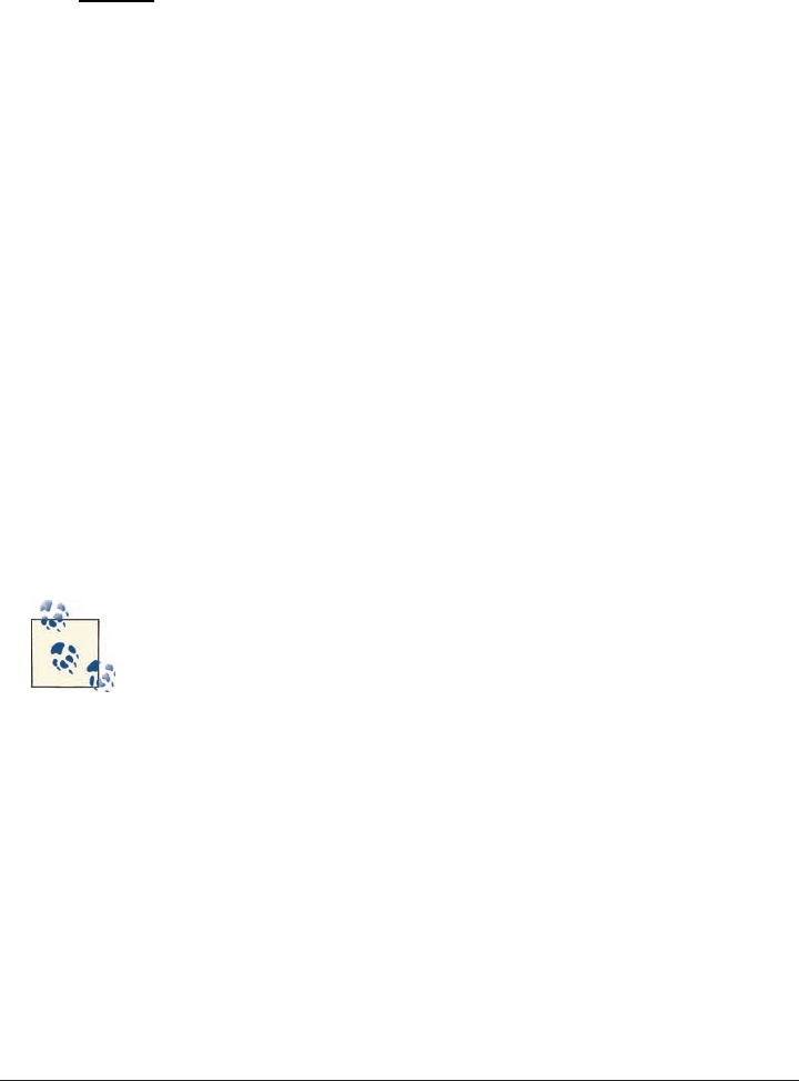
Cohen’s Kappa (κ)
Cohen’s Kappa (κ) measures the agreement between two annotators, while taking into
account the possibility of chance agreement. The equation is:
K=Pr(a) - Pr(e)
1 - Pr(e)
In the equation, Pr(a) is the relative observed agreement between annotators, and Pr(e)
is the expected agreement between annotators, if each annotator was to randomly pick
a category for each annotation. Let’s take a look at a specific example.
Going back to one of the examples we’ve been discussing, assume that we had an an
notation task where two annotators, A and B, were asked to assign the labels “positive,”
“neutral,” and “negative” to a set of 250 movie reviews, and that the resultant annotations
looked like this:
B B B
positive neutral negative
A positive 54 28 3
A neutral 31 18 23
A negative 0 21 72
The preceding table shows that while the annotators rarely had situations where one
labeled a review as “positive” and the other labeled it as “negative,” the “neutral” label
contributed a lot to the level of disagreement. But how do we turn these numbers into
an evaluation metric?
This table is essentially a confusion matrix, which is a table that’s used
to compare the output of an algorithm to a gold standard. We’ll talk
more about confusion matrices in Chapter 8.
First, we calculate Pr(a), the actual agreement between the annotators. Out of 250 docu
ments, A and B both said “positive” 54 times, both said “neutral” 18 times, and both said
“negative” 72 times. So the percentage of observed agreement is:
Pr(a)= (54 + 18 + 72) / 250 = .576 (57.6%)
Next we calculate Pr(e), the expected chance agreement, for each label. To do that, we
determine the percentage of the time that each annotator used each label and multiply
those percentages to determine how often the two annotators would use the same label
on the same document at the same time, then add each of those together to get Pr(e). If
that sounds confusing, just watch:
Evaluating the Annotations | 127

A used the label “positive” 85 times (54 + 28 + 3), or .425% of the time. B also used the
“positive” label 85 times (54 + 31), which is also .425. Multiplied together, .425 × .425
= .180, so A and B have a .180 chance of both randomly choosing “positive” as a label.
Now we do the same calculations for “neutral” and “negative.” A used “neutral” 72 times,
or .288%, and B used the tag 67 times, or .268%. Combined, (.268 × .288), there is a .077
chance of them both using the “neutral” tag. Finally, A used “negative” 93 times (.372)
and B used “negative” 98 times (.392), giving a .146 chance of agreement on the “neg
ative” tag.
Adding those three chance agreement scores together gives us:
Pr(e) = .180 + .077 + .146 = .403
Putting Pr(a) and Pr(e) into the equation gives us:
κ = (.576 – .403) / (1 – .403) = .173 / .597 = .29
We’ll discuss how to interpret the scores in “Interpreting Kappa Coefficients” (page 131);
for now, let’s move on to another example.
Fleiss’s Kappa (κ)
Cohen’s Kappa can determine the agreement between two annotators, but what if you
have three or more people annotating the same document? In that case, you’ll need to
use Fleiss’s Kappa instead. Fleiss’s Kappa isn’t actually based on Cohen’s Kappa; rather,
it’s an extension of Scott’s pi (π), but for most contexts, they are similar enough that it’s
OK to compare them.
The base equation for Fleiss’s κ is essentially the same as for Cohen’s κ, with the actual
agreement and expected agreement due to chance being calculated and compared.
However, the manner in which these are calculated differs, so we will use slightly dif
ferent symbols here to avoid confusion:
k=P-Pe
1 - Pe
In the preceding equation, P is the actual agreement and Pe is the expected agreement.
Fleiss’s Kappa differs from Cohen’s Kappa, however, in the way that these values are
calculated. The table used to represent annotator values for Fleiss’s Kappa, rather than
having one axis per annotator, has one axis for the possible values an annotator could
assign, and the other axis for each of the annotators. If we redid our movie review
annotation task with five annotators (250 documents, 3 categories), we would represent
their annotations like this:
128 | Chapter 6: Annotation and Adjudication

positive neutral negative
Annotator A 85 72 93
Annotator B 85 67 98
Annotator C 68 99 83
Annotator D 88 88 74
Annotator E 58 120 72
total 384 446 420
In this table, the categories are across the top, the annotators are down the side, and the
content of each cell represents how many times that annotator assigned that tag to a
document.
First, we need to calculate how many assignments went (proportionally) to each cate
gory. This is represented by Pc, where c stands for the category being evaluated. We do
this by summing up the contents of each row and dividing by the total number of an
notations. In the following equation, A is the number of annotators, a is the number of
annotations per annotator, k is the number of categories, and i represents the current
annotator:
Pc=1
Aa ∑
i=1
Aaic, 1 = 1
a∑
c=1
kaic
This looks a bit complicated, but basically all it says is that Pc (in this case, c will stand
for positive, neutral, and negative) will equal the sum of the values in its column divided
by the number of annotators times the number of annotations each annotator created.
The second part of the equation simply says that if you add up all the annotations that
an annotator made and divide by the number of annotations each annotator made in
dividually, you will get 1, because both numbers should be the same.
So, if we apply the Pc equation to the first annotation category, we get the following
equation:
P(positive) = (85 + 85 + 68 + 88 + 58) / (5 × 250)
= 384 / 1250
= .3072
If we apply this calculation to the rest of the table, we can fill in the bottom row of the
table, like so:
positive neutral negative
Annotator A 85 72 93
Annotator B 85 67 98
Evaluating the Annotations | 129

Annotator C 68 99 83
Annotator D 88 88 74
Annotator E 58 120 72
total 384 446 420
Pc.3072 .3568 .336
Next, we need to calculate Pi, which represents each annotator’s agreement with other
annotators, compared to all possible agreement values. As before, a is the number of
annotations per annotator, k is the number of categories, c is the current category, and
i is the current annotator.
Pi=
(
∑c=1
kaic
2
)
– (a)
a(a– 1)
Again, this isn’t as difficult to apply as it seems: for each row, we’re just summing up the
squares of the values in each column and moderating the output by the number of total
annotations by each annotator. So for Annotator A, we would calculate this:
P(Annotator A) = ( (852 + 722 + 932) - 250 ) / 250(250–1)
= 21058 - 250 / 62250
= 20808/62250
= .3343
By performing this calculation for each Annotator row in the table, we can fill out the
last column, like this:
positive neutral negative Pi
Annotator A 85 72 93 .3343
Annotator B 85 67 98 .3384
Annotator C 68 99 83 .3384
Annotator D 88 88 74 .3328
Annotator E 58 120 72 .3646
total 384 446 420
Pc.3072 .3568 .336
We’re almost done. P in the original Fleiss equation is the average of the Pi values, so we
calculate that by summing the Pi column and dividing by the number of annotators:
P( = (.3343 + .3384 + .3384 + .3328 + .3646) / 5
= 1.7085 / 5
= .3417
130 | Chapter 6: Annotation and Adjudication

Then we calculate P(e) by summing the squares of the Pc values, like so:
P(e) = .30722 + .35682 + .3362 = .335
Now we can finally plug these values into Fleiss’s Kappa equation and calculate our IAA
score:
κ = (.3417 – .335) / (1 – .335)
= .0067 / .665
= .004
Interpreting Kappa Coefficients
In the two preceding sections we came up with two different values of κ for two different
annotation tasks, .29 and .004.
But how are these scores actually interpreted? In many cases, the interpretation of the
kappa depends on the complexity and objectivity of the annotation task, so there’s no
hard-and-fast rule that can always be used to determine whether scores are good or not.
For example, a task such as POS tagging, even though it requires a lot of effort, would
be expected to get a κ score close to 1.0, due to how well defined the terms and underlying
theories are. On the other hand, tasks that require more interpretation of the text, such
as semantic role labeling or temporal annotation (where the text may actually have
multiple valid interpretations), are not generally held to such a high standard.
Landis and Koch 1977 provide these guidelines for interpreting κ and other agreement
metrics:
κ Agreement level
< 0 poor
0.01–0.20 slight
0.21–0.40 fair
0.41–0.60 moderate
0.61–0.80 substantial
0.81–1.00 perfect
There has been some debate about how strictly these numbers should be interpreted,
but they provide a good place to start. Another way to determine how your IAA scores
should be interpreted is to do some research and find out what kind of IAA scores other,
similar annotation tasks are getting. Naturally you should always strive to do well, but
some tasks are simply harder than others.
So what can we say about the IAA scores from the examples in the previous sections?
From our Cohen κ example, we obtained an agreement score of .29, which according to
this chart is only “fair.” And really, considering how few categories were included in the
Evaluating the Annotations | 131

task (the more categories a task includes, the more room there is for ambiguity between
labels), a score of .29 is pretty bad. Looking at the table of annotations, it’s clear that
there was a lot of confusion over how to spot a neutral review, so that part of the guideline
would definitely need to be revised. Also, the fact that Annotator B labeled a few reviews
as negative when Annotator A labeled them as positive—a fairly unusual error, consid
ering the presence of the “neutral” tag—could indicate that Annotator B is having some
trouble with the software as well as the guidelines.
As for the Fleiss’s Kappa score…well, that’s definitely one that would have to be revisited.
But why, and what should be changed to get better agreement? Looking at the chart
again, we can see that there’s a lot of variation in all of the columns—while Annotators
A, B, and D all have nearly the same number of positive reviews, those are the only values
that come anywhere close to grouping. Annotator E is so far off from everyone else that
if this were a real task, we’d be wondering if she got hold of a completely different set of
guidelines!
However, don’t be discouraged by low agreement scores, especially when you’re just
starting a new MAMA cycle. Poor initial results are normal, which is why we encourage
use of a small test set for annotation, just like you’ll do later for training your ML algo
rithm—it’s the best way to work out the kinks in your annotation task.
Calculating κ in Other Contexts
Both of the sample calculations we provided were only about annotators applying a set
number of labels to a document, which made determining percent agreements much
easier, because the divisor for calculating percentages was the same as the number of
documents. However, what happens if you are trying to calculate agreement for tags
that are applied to the words/tokens in a document, such as for POS tagging or for the
example of annotating actors, characters, directors, and so on in movie reviews that we
have been discussing?
For the POS tagging example, assuming that every token receives a tag, then the set of
items being annotated is the same as the number of words in each document (or in all
the documents at once, if you prefer). So your agreement table for two annotators would
still look much the same as it did in our example of positive, negative, and neutral movie
reviews, only the numbers in the table would be much bigger because they would reflect
the number of words in the document or corpus, rather than just the number of docu
ments.
However, what about annotation tasks where every token isn’t annotated, particularly
if the annotation is rather sparse? Let’s say, for example, that you ask two annotators to
only annotate the creature names and pronouns in Lewis Carroll’s “Jabberwocky”.
132 | Chapter 6: Annotation and Adjudication

“Jabberwocky” has 216 tokens (with punctuation marks considered individual tokens),
but most of them aren’t creature names or pronouns. So how should the nonannotated
words be counted? If we consider “untagged” to be a tag, then we might end up with a
comparison table that looks like this:
B B B
creature pronoun untagged
A creature 5 0 2
A pronoun 0 10 2
A untagged 1 7 189
Apparently our imaginary annotators were a bit confused about our guidelines for pro
nouns, and whether some of the made-up words were creatures or something else. Re
gardless, if we calculate Cohen’s Kappa for this table, we end up with a coefficient
of .691, which isn’t really bad considering that most of the poem’s nouns are made up
anyway. However, it’s clear that the IAA score is being heavily influenced by the fact that
there are so few tags in the text—the majority of the tokens go untagged, so the agreement
over the lack of tags may be skewing the results.
Pr(a) = .944
a(creature) = .032, b(creature) = .028 —> creature = .0009
a(pronoun) = .056, b(pronoun) = .079 —> pronoun = .0044
a(untagged) = .912, b(untagged) = .893 —> untagged = .814
Pr(e) = .009 + .0044 + .814 = .819
k = (.944 – .819) / (1 – .819)
= .125 / .181
= .691
It can be argued that in cases of sparse annotation, the set of items being examined
should be limited to only the items that were tagged by one or both annotators. In this
case, the number of items being investigated for agreement drops to 27.
B B B
creature pronoun untagged
A creature 5 0 2
A pronoun 0 10 2
A untagged 1 7 0
Pr(a) = .556
a(creature) = .259, b(creature) = .222 —> creature = .057
a(pronoun) = .444, b(pronoun) = .629 —> pronoun = .279
a(untagged) = .269, b(untagged) = .148 —> untagged = .039
Pr(e) = .057 + .279 + .039 = .355
Evaluating the Annotations | 133

k = (.556 – .355) / (1 – .355)
= .201 / .645
= .312
Clearly, the IAA score drops dramatically from “substantial” agreement at .691 to merely
“fair” agreement at .312 when the investigation space is limited to only those tokens that
were tagged by one or more annotators. You can imagine how much more complicated
the discussion of IAA scores can become when evaluating a task that involves character-
level rather than token-level annotations, where the length of the word being annotated
can also affect IAA scores!
Compelling arguments can be made for both sides of these IAA calculation discussions
(some would argue that, since annotation guidelines must also specify what not to an
notate, discounting agreement on that score is foolish; others would say that using more
rigorous agreement metrics increases the value of the calculations). We are not taking
a side on which metric is better, but whatever method you use for these calculations, be
sure to fully report on how you calculated the agreement. Regardless of how you calculate
your IAA score, remember that it indicates relative agreement, and for our “Jabber
wocky” example, both sets of scores would indicate that the guidelines will need to be
revised and another round of annotation done—back to the MAMA cycle!
If your tags have attributes, don’t forget to calculate IAA scores for those
too! In those cases, it’s fine to only compare attributes for a tag where
the annotators agree that a tag should exist (since comparing tags when
the annotators don’t agree on the existence of a tag won’t give you any
useful information), but if you only compare the attributes for matching
tags (extents that are identical or that at least overlap, links with the
same anchors, etc.), make sure you report that information with the
scores.
Creating the Gold Standard (Adjudication)
Once you’ve created a set of annotation guidelines that is getting you IAA scores that
you are satisfied with and you’ve had your annotators apply those guidelines to your
entire corpus, it’s time to actually adjudicate their annotations and create your gold
standard dataset, which is what you will use to train and test your ML algorithm. Gen
erally it’s best to have adjudicators who were involved in creating the annotation guide
lines, as they will have the best understanding of the purpose of the annotation. Hiring
new adjudicators means that you’ll have the same problem you did with annotators.
134 | Chapter 6: Annotation and Adjudication

Since you’re already familiar with the annotation task, you should find the adjudication
process to be fairly straightforward. You’ll need software to perform the adjudication in
(see Appendix B again for a list of what’s available), and after that, it’s just a matter of
taking the time to do a careful job. There are a few things to think about, however:
•It will take you just as long, possibly longer, to do a careful job of adjudicating your
corpus as it took one of your annotators to annotate it. Don’t forget to allocate
sufficient time to get this done.
•Consider breaking up the adjudication task into layers: first adjudicate each extent
tag or label individually, then each link tag. This will make it much easier to pay
attention to how each tag is being used, and will make link tags much more accurate
(because they’ll be connecting accurate extents).
•Just because two (or more) of your annotators agree about the presence of attributes
of a tag at a location doesn’t mean they’re right! Remember that annotators can
randomly be in agreement (which is why we spent so much time calculating kappa
scores). So don’t take for granted that annotators agreeing means they’re right, at
least until you have a good sense of your annotators’ abilities.
•If you do use more than one adjudicator, consider giving them all some of the same
documents so that you can also calculate IAA scores for them—that way, you’ll be
able to make sure they’re all on the same page.
Once you have all your files adjudicated, you’ll be ready to move on to the ML parts of
the MATTER cycle.
Summary
In this chapter we discussed how to apply your model and spec to your corpus through
the process of annotation, and how to create a gold standard corpus that can be used to
train and test your ML algorithms. Some of the important points are summarized here:
•The “A” in the MATTER cycle is composed of a lot of different parts, including
creating annotation guidelines, finding annotators, choosing an annotation tool,
training annotators, checking for IAA scores, revising guidelines, and finally, ad
judicating. Don’t be put off by the number of steps outlined in this chapter; just take
your time and take good notes.
•Guidelines and specifications are related, but they are not the same thing. The
guidelines will determine how the model is applied to the text—even if you are using
the same model, if the guidelines are different, they can result in a very different set
of annotations.
Summary | 135

•Creating a good set of annotation guidelines and an accurate and useful annotation
won’t happen on the first try. You will need to revise your guidelines and retrain
your annotators, probably more than once. That’s fine; just remember to allow
yourself time when planning your annotation task. Within the MATTER cycle is
the MAMA cycle, and no task is perfect straight off the bat.
•One of the things you will have to consider about the annotation process is what
information you want to present to your annotators—giving them preprocessed
data could ease the annotation process, but it could also bias your annotators, so
consider what information you want to present to your annotators.
•Because you’ll need to go through the MAMA cycle multiple times, it’s a good idea
to set aside a portion of your corpus on which to test your annotation guidelines
while you work out the kinks. This set can be used in your gold standard later, but
shouldn’t be given to your annotators right away once the guidelines are finalized.
•When you’re writing your annotation guidelines, there are a few questions that you’ll
find it necessary to answer for your annotators in the document. But the most
important thing is to keep your guidelines clear and to the point, and provide plenty
of examples for your annotators to follow.
•When finding annotators for a task, you need to consider what type of knowledge
they will need to complete your annotation task accurately (and, if possible, quick
ly), what language they should speak natively, and how much time you have to
annotate. The last consideration may play a role in how many annotators you need
to hire to complete your task on schedule.
•The annotation software that you give to your annotators to create the annotations
will have an effect on how easily and accurately the annotations are created, so keep
that in mind when choosing what tool you will use. Using more than one piece of
software for the same task could cause confusion and irregularities in the annota
tion, so it’s better to pick one and stick with it.
•Once your annotators have annotated your sample set of texts, it’s time to evaluate
the IAA scores. While there are many different ways to determine agreement, the
two most common in computational linguistics are Cohen’s Kappa and Fleiss’s
Kappa. Cohen’s Kappa is used if you have only two annotators annotating a docu
ment, while Fleiss’s Kappa is used for situations where more than two annotators
are used on a dataset.
•Based on how good your agreement scores are, you can decide whether or not your
task is ready to go past the test set and on to the full corpus. You will probably need
to revise your task at least once, so don’t be discouraged by low IAA scores.
•Interpreting IAA scores isn’t an exact science—a number of factors can influence
whether a score indicates that an annotation task is well defined, including
the number of tags, the subjectivity of the annotation task, and the number of
annotators.
136 | Chapter 6: Annotation and Adjudication

•Additionally, the items being annotated can have an effect on how you calculate
IAA. While it’s easy to calculate agreement when applying a single label to an entire
document, there is some debate about how IAA scores should be calculated when
applying tags to text extents. Regardless of what method you decide to apply for
calculating IAA scores, keep track of the decisions you make so that other people
can understand how you came up with your numbers.
•Having high IAA scores mean your task is likely to be reproducible, which is helpful
when creating a sufficiently large corpus. However, just because a task is reprodu
cible doesn’t necessarily mean it will be suitable for feeding to ML algorithms. Sim
ilarly, just because a task doesn’t have great agreement scores doesn’t mean it will
not be good for ML tasks. However, a reproducible task will be easier to create a
large corpus for, and the bigger your corpus, the more likely you are to get good ML
results, so putting some effort into creating your annotation guidelines will pay off
in the end.
•Once you’ve reached acceptable IAA scores on your annotation test set, you can set
your annotators loose on the full corpus. When you have the full corpus, it’s time
to adjudicate the annotations and create the gold standard corpus that you will use
to train your ML algorithms.
•Adjudication is best performed by people who helped create the annotation guide
lines. Bringing in new people to perform the adjudication can cause more confusion
and noise in your dataset.
•Calculating IAA agreement scores between adjudicators can be a good way to ensure
that your adjudicated corpus is consistent. The more consistent your corpus is, the
more accurate your ML results will be.
Summary | 137

CHAPTER 7
Training: Machine Learning
In this chapter we finally come to the topic of designing machine learning (ML) algo
rithms that will be run over our annotated text data. That is, we describe the task of
taking linguistic data (annotated and unannotated) to train ML algorithms to auto
matically classify, tag, and mark up the text for specific purposes. We will present the
goals and techniques of machine learning, and review the different algorithms that you
will want to consider using for your annotated corpus. Here are the questions we will
answer in this chapter:
•How do we define the learning problem formally? Learning as distinguishing or
classifying objects into different categories? Learning as problem solving or plan
ning?
•How does the design of a specification and annotation improve a learning algo
rithm?
•What kinds of features are in the dataset that you can exploit with your algorithm?
• What kinds of learning algorithms are there?
• When should you use one algorithm over another?
The purpose of this chapter is to give you an overview of the different types of algorithms
and approaches that are used for machine learning, and help you figure out which kind
will best suit your own annotation task. It is not meant to provide an in-depth discussion
of the math underlying all the different algorithms, or any of the details for using them.
There are a number of other books that provide that information in much more depth
than we intend to provide here. If you are interested in learning more about ML algo
rithms, we recommend the following books:
•Natural Language Processing with Python by Steven Bird, Ewan Klein, and Edward
Loper (O’Reilly, 2009)
139

•Foundations of Statistical Natural Language Processing by Chris Manning and
Hinrich Schütze (MIT Press, 1999)
•Speech and Language Processing by Daniel Jurafsky and James H. Martin (Prentice
Hall, 2008)
•Machine Learning by Tom Mitchell (McGraw-Hill/Science/Engineering/Math,
1997)
What Is Learning?
Machine learning refers to the area of computer science focusing on the development
and implementation of systems that improve as they encounter more data. To quote the
Nobel Prize-winning economist Herbert Simon:
Learning is any process by which a system improves its performance from experience.
For areas in language technology and computational linguistics, the most important
topics for learning include the following:
• Assigning categories to words (part-of-speech [POS] tagging)
• Assigning topics to articles, emails, or web pages
• Mood, affect, or sentiment classification of a text or utterance
• Assigning a semantic type or ontological class to a word or phrase
• Language identification
• Spoken word recognition
• Handwriting recognition
• Syntactic structure (sentence parsing)
• Timestamping of events or articles
• Temporal ordering of historical events
• Semantic roles for participants of events in a sentence
• Named Entity (NE) identification
• Coreference resolution
• Discourse structure identification
Although the preceding list presents a broad range of things to learn, you really only
need to study a few strategies to approach these problems computationally. We will
discuss three types of ML algorithms in this chapter:
140 | Chapter 7: Training: Machine Learning

Supervised learning
Any technique that generates a function mapping from inputs to a fixed set of labels
(the desired output). The labels are typically metadata tags provided by humans
who annotate the corpus for training purposes.
Unsupervised learning
Any technique that tries to find structure from an input set of unlabeled data.
Semi-supervised learning
Any technique that generates a function mapping from inputs of both labeled data
and unlabeled data; a combination of both supervised and unsupervised learning.
Because our focus is on how annotated data can improve a system’s performance, we
will focus our discussion on supervised learning first, and address semi-supervised and
unsupervised learning later in the chapter.
As we mentioned in Chapter 1, machine learning involves the development of algo
rithms that acquire new concepts or generally improve their performance from expe
rience or previous encounters with data. The algorithm learns an approximation of the
target function, mapping input data to the desired output. The annotation process dis
cussed in this book can be used to provide a richer source of material as the input data
for the ML training phase. From this chapter we will see that annotation is relevant to
machine learning because it allows us to ask two questions:
• How does the annotation give us a richer idea of what’s in the dataset?
• How can we leverage this knowledge as new features for training our algorithms?
When discussing the role of annotation in the application of training ML algorithms, it
is important to know what is involved in the process known as feature selection. This is
the process of finding which features in your dataset are most helpful in solving your
learning task. In this chapter we will discuss three types of features in the text that ML
algorithms can exploit for learning. They are as follows:
N-gram features
This is the classic “bag of words” approach to modeling a text document. Each word
in the document is treated as a feature for the learning algorithm. If single words
are used as features, then we call the resultant approach a unigram word model.
Term frequency—the number of occurrences of a word in a document—is an im
portant component of this model, along with document frequency—the frequency
of a word throughout the entire corpus. We can also take bigram, trigram, and
higher n-gram statistics into account if we want to capture some of the “larger
window” around a word.
Structure-dependent features (SD features)
These are features that can be identified and manipulated by virtue of the properties
of the data structure itself. For example, the features associated with a “word” treated
What Is Learning? | 141

1. Mitchell’s book, Machine Learning (1997), is still a valuable and very relevant introduction to the field of
machine learning. Read it today!
as an ASCII string will include any and all properties that can be derived from
examining the string; we can talk about a word’s “length,” its “first_character” (pre
fix), its “last_character” (suffix), and so on. Similarly, if a “sentence” is analyzed as
a string of tokens (occurring between sentence boundaries, <S> and </S>), then we
can refer to the “first_word” and “last_word” features for the structure.
Annotation-dependent features (AD features)
This includes any features that are associated with an annotation specification that
reflects a model of the data. For example, labels marking the type of an entity as
Person, Organization, or Place within an NE specification (as discussed earlier), are
features that reflect the model denoted by the annotations. Annotation-dependent
features introduce new dimensions for discrimination, classification, or clustering
that are not present in a unigram feature model (although they may be covered by
some n-gram models, as we’ll see shortly!).
We will learn when to use each of these classes, as well as which algorithms are most
appropriate for each feature type. In particular, we will answer the following question:
when does annotation actually help in a learning algorithm?
Defining Our Learning Task
To develop an algorithm, we need to have a precise representation of what we are trying
to learn. We’ll start with Tom Mitchell’s 1 definition of a learning task:
Learning involves improving on a task, T, with respect to a performance metric, P, based
on experience, E.
Given this statement of the problem (inspired by Simon’s concise phrasing shown ear
lier), Mitchell then discusses the five steps involved in the design of a learning system.
Consider what the role of a specification and the associated annotated data will be for
each of the following steps for designing a learning system:
1. Choose the “training experience.” For our purposes, this is the corpus that you just
built. The way we encode the “experience” surrounding our training samples reflects
how much we know about the dataset. The model we arrived at in Chapter 4 can
be used to mark up the dataset with annotations that might prove fruitful in rep
resenting the target function. Hence, we can think of annotation as enriching the
available feature space for the domain.
2. Identify the target function (what is the system going to learn?). A model and an
notation can help to define the class of target functions.
142 | Chapter 7: Training: Machine Learning

3. Choose how to represent the target function. Since annotations provide richer rep
resentations of the data than n-gram or structure-dependent features permit, the
target function can be formulated in a more general and possibly more broadly
applicable form.
4. Choose a learning algorithm to infer the target function from the experience you
provide it with.
5. Evaluate the results according to the performance metric you have chosen.
Rule-based Systems
It is important to point out that the design of a model and the creation of a specifi
cation can serve as the starting point for many different types of algorithms. In fact,
a good way to start off is to take the model for the annotation that you have developed
and convert it directly to a rule-based system. This involves converting the features
from the model to rules using the basic pattern of a condition-action pair. This is a
general template that can be used to label a single token or a sequence of tokens, and
it is at the core of most programs that parse sentences or programs, as well as verify
the content of Web-based applications, from email to Web-based queries and trans
actions.
The condition-action paradigm is the general term that includes parsing, and with
that, compiling, and other applications. For our purposes here, we are interested in
the more mundane problem of recognizing a token or sequence of tokens (the con
dition), and then applying some sort of tag or performing some sort of labeling (the
action).
In many areas of computational linguistics, in fact, rule-based systems will perform
as well as if not better than statistically trained ML algorithms. Rules are connections
between the condition and the resultant action. As we discuss in Chapter 11, rule-
based systems have been successfully applied to domain-constrained recognition
tasks such as the following:
•Finding event expressions across parts of speech (e.g., wedding, have eaten, hungry)
•Identifying times, dates, and temporal expressions (e.g., June 11, 1989; yesterday;
early March; three weeks from tomorrow)
• NEs, such as People, Organizations, and Locations (e.g., Bill Clinton; 10 Downing
Street; Apple Corporation; Paris, France)
Defining Our Learning Task | 143

Classifier Algorithms
In its most basic form, a classifier is a function that takes input in the form of a bundle
of features and outputs class labels associated with these features. The goal in classifier
learning is to learn this function from a labeled training set of input-output pairs (the
annotated training corpus). Because we are actively engaged in directing the algorithm
toward discovery of the function, this is called a supervised learning technique.
From the perspective of this book, the goal of supervised learning is to train an algorithm
with the most informative and representative examples you can find or create, for the
learning task at hand.
The goal of a classification task is to correctly sort a collection of things into the proper
category. If there are only two categories, then the task is called a binary classification
task, and the learner is called a binary classifier. We encountered annotations providing
this kind of problem in previous chapters. For example, if you are teaching a classifier
to recognize spam in your email, then you have two categories: spam and not-spam. As
with other text classification problems, the tag can be assigned to the text at the docu
ment level, upon inspection of the contents of the document. In this sense, there is no
linguistic annotation at all, but merely document-level annotation. Nevertheless, it still
falls within the general characterization of a classification problem: you have a training
set, d1, … ,dn, that has been labeled with the tags associated with annotations from the
(rather trivial) model, M, Spam (S), or Ham (H); {(d1,S),(d2,H), … (dn,S)}.
How the different types of features described in the preceding paragraph contribute to
solving such classifications is one of the topics of this chapter. Using n-gram features is
the simplest place to start when the label is associated with a document-level tag. Sur
prisingly, however, as you quickly discover with your own tweaking (feature engineer
ing), unigrams are often the best of all, beating out even bigram and trigram features
on certain tasks. This is counterintuitive at first, since it would always seem that “more
is better” when it comes to finding features for solving a task such as classification. But
the problem immediately emerges that, with too many features, most of the learning
algorithms we describe in this chapter get “confused” since the properties associated
with these features are distributional values over the corpus. So the challenge is somehow
to select which features do the best job.
When is one algorithm better than another? This depends on the scope
of the classification task relative to the data being used to create the
features for the classifiers.
When is one set or type of feature better than another? This depends
on what the target function is for the learning task.
144 | Chapter 7: Training: Machine Learning

This is where annotation comes in. The point of linguistic annotation is to identify
textual components of your document that can be associated with particular features
for the phenomena for which you want to develop learning algorithms. Let’s take some
examples beyond the spam-ham distinction. Consider sentiment analysis applied to
movie reviews or hotel ratings. The most expedient method for classifying movie reviews
is to set up the learning problem with n-gram features. The words in the reviews are
taken as independent features (lexical clues), and thrown into a description of the target
function. While this works remarkably well in general, this approach will fail to capture
properties that show up as nonlocal dependencies, such as the ways that negation and
modality are often expressed in language. Having an annotation that captures such
properties can provide additional features for learning algorithms that would otherwise
be unavailable.
Imagine that you’re trying to distinguish negative opinions of a product from positive
ones, such as for a digital camera. Think about how we express ourselves:
• The Plandex J45 is a terrible camera.
• This is not a good camera.
In these cases, we can readily identify a negative judgment (terrible), but even a simple
negation (not) may be difficult to recognize, unless we know how to place the positive
judgment (good camera) within the scope of the negation, assuming they’re all treated
as lexical clues.
Things get harder, however, with other cases. What happens when we have negative
judgments such as these?
• I don’t think this is a good camera.
• I cannot recommend this as a great camera.
It’s not clear whether learners trained with just n-gram features will be able to catch such
cases. These won’t present a problem if the annotation scheme we’ve created can identify
negation, regardless of where it appears in the sentence.
In the rest of this section, we review the basic learning algorithms used in the field, and
the advantages and disadvantages of each approach.
Decision Tree Learning
This is the most intuitive of all classifier algorithms, and is essentially a formal way of
asking “20 questions” of a corpus. For any annotation task you have defined, there will
be basic categories that are amenable to this approach. A decision tree is an upside-down
Classifier Algorithms | 145
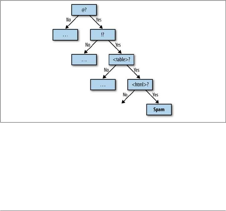
tree, which classifies instances of the dataset by sorting them “down the tree” from the
root question to a leaf node, at which point there is a specific classification of the instance.
Along the way, the nodes of the tree each represent a question that is answered by the
branches that shoot out of the node, “down the tree.”
The questions that are “asked” can pertain to any information available that is from the
dataset, but they are typically typed according to one of the three classes mentioned
earlier: n-gram features, structure-dependent features, or annotation-dependent fea
tures.
Let’s take, as an example, our old friend the spam filter. We mentioned before what the
annotation model for such a simple binary classifier would be, so now let’s see how we
can build the actual classifier that goes with the model. For example, for classifying texts
into spam or not-spam, we can make use of the logical structure of a decision tree by
asking about unigram or n-gram properties of the document, that is, lexical features.
For spam, this might include words or characters such as html, !, @, and <table>, which
are n-gram features (see Figure 7-1).
Figure 7-1. Decision tree over lexical triggers
We can, of course, ask questions regarding quantitative values associated with n-gram
(or lexical) features, such as the following, which are structure-dependent features:
• What percentage of the document is HTML tags?
• How many tables are there in the document?
146 | Chapter 7: Training: Machine Learning
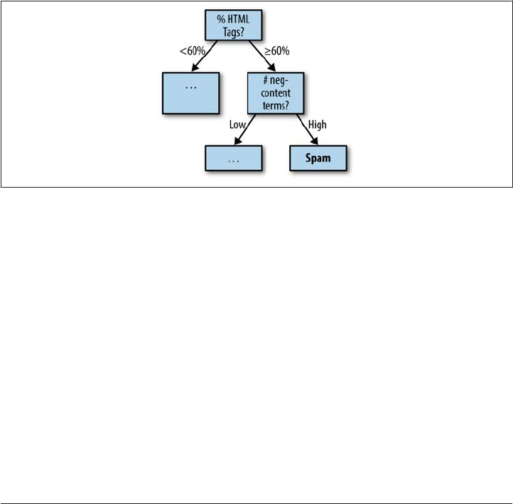
These questions are structure-dependent features that exploit the nature of the token
(word) and its distribution in the document.
We can also ask questions that assume a more sophisticated model of the data, such as
that associated with a specification and annotation schema. For example, our model of
spam may have a schema element called neg-content-term, which is a label that iden
tifies stereotypical spam-related vocabulary, be it pornography, physical dysfunction,
or unbelievably good financial offers. This type of question exploits an annotation-
dependent feature that we have made or abstracted over the dataset.
<!ELEMENT neg-content-term ( #PCDATA ) >
<!ATTLIST neg-content-term label ( viagra | bank | inheritance | transfer |
sex | dysfunction | performance | ... ) >
Any of these feature types can be combined into the same decision tree structure, as
illustrated in Figure 7-2.
Figure 7-2. Decision tree over mixed feature types
Gender Identification
Now let’s get our hands dirty with decision trees. We’ll start with the “first name gender”
classification problem described in Natural Language Processing with Python. This is the
problem of automatically recognizing whether a (first) name is male or female, as il
lustrated in Figure 7-3.
Classifier Algorithms | 147
Figure 7-3. Gender target function
The approach the authors of the aforementioned book describe is to look at properties
of the name as a token to determine how these properties can contribute to discrimi
nating between male and female. This is a great example of what we have called structure-
dependent (SD) features for learning. Essentially, the name is analyzed in terms of its
structure as a token, that is, a string of characters. That’s why the features that will be
used for training a gender classifier are structure-dependent, and not n-gram or
annotation-dependent features.
What would n-gram features for the first name gender problem look
like? It wouldn’t be pretty, since we would have to train on individual
full-token first name instances, where the corpus would be token-based.
No generalizations would be possible, since there is only one feature
associated with the target function values: for example, (female, male).
So, the algorithm can only correlate a tag with a known token, which
means it can only use this pairing in the future on tokens that it has
already identified.
What would an annotation-based feature be for this problem? Well, you
might have an annotation of the context around the name; for example,
words occurring within a window of the token. This might help in
identifying names from the syntactic or semantic context. This would
be particularly useful in a language that carried morphological marking
for gender on the verb or on modifiers that might accompany the name:
La belle Mary (Fr.), Le beau Peter (Fr.).
Upon examination of the corpus of first names, finding the most relevant structure-
dependent features for this problem turns out to be quite straightforward. Gender seems
to be reflected in values of two basic properties of the token:
•The value of characters in specific positions; for example, last, first, next to last, and
so on
• Other character properties, such as whether it’s a vowel, a consonant, and so on
148 | Chapter 7: Training: Machine Learning

2. We could also define an approximation to the target function, F’, as follows:
F' = w1F1 + w2F2 + w3F3 + w4F4 + w5F5 + w6F6
Namely, F' is a linear combination of the SD features shown in the preceding bulleted list, where wi refers to
the numerical coefficients that are chosen by the learning algorithm to optimize the value returned by F’,
which approximates F.
Once we have an inventory of features (in this case, they’re all structure-dependent
features), then we can get started. Recall the steps in the creation of a learning algorithm:
1. Choose the training experience, E. In this case, the experience is a list of SD features
for each name viewed as a token. More specifically, the instances are attribute-value
pairs, where the attributes are chosen from a fixed set along with their values.
2. Identify the target function (what is the system going to learn?). We are making a
binary choice of whether the token is male or female. So the target function is a
discrete Boolean classification (yes or no) over each example (e.g., Is “Nancy” fe
male? → yes; Is “Peter” female? → no). Formally, we can say that our function, f,
maps from word tokens to the binary classification associated with the gender pair,
{female, male}. We will define this as a Boolean value function, and simply refer to
the function as F, which returns true when the token is a female name and false
when the token is a male name.
3. Choose how to represent the target function: this will be some functional combi
nation of the SD features that we identified earlier. Again, using some of the features
that are identified in Natural Language Processing with Python, we have:2
•F1: last_letter = “a”
•F2: last_letter = “k”
•F3: last_letter = “f”
•F4: last_letter = “r”
•F5: last_letter = “y”
•F6: last_2_letters = “yn”
4. Choose a learning algorithm to infer the target function from the experience you
provide it with. We will start with the decision tree method.
5. Evaluate the results according to the performance metric you have chosen. We will
use accuracy over the resultant classifications as a performance metric.
Classifier Algorithms | 149

But, now, where do we start? That is, which feature do we use to start building our tree?
When using a decision tree to partition your data, this is one of the most difficult ques
tions to answer. Fortunately, there is a very nice way to assess the impact of choosing
one feature over another. It is called information gain and is based on the notion of
entropy from information theory. Here’s how it works.
In information theory, entropy measures the average uncertainty involved in choosing
an outcome from the set of possible outcomes. In our case, entropy is a measure over a
collection of data (the examples to classify) that characterizes how much order exists
between the items relative to a particular classification, C. Given our corpus, S, of train
ing data, the entropy is the sum of probabilities of each class value ci (pi), times the log
probability for that class value:
log21
pi
So, we can state the entropy of the corpus (as the random variable S) as follows:
H(S) = ∑
i=1
cpilog21
pi= - ∑
i=1
cpilog2pi
With the concept of entropy given here, we now define the information gain associated
with choosing a particular feature to create a partition over the dataset. Assume that
through examining the data or through the MATTER cycle, we’ve come up with a set
of features (or attributes) that we want to use for classifying our data. These can be
n-gram, structure-dependent, or annotation-dependent features. Let the features that
we’ve come up with for our task be the set, {A1, A2, … , An}. To judge the usefulness of a
feature as a “separation” between the data points, let’s define the information gain, G,
associated with an attribute, Ai, as the expected reduction in entropy that results from
using this attribute to partition the examples. Here’s the formal statement for informa
tion gain as just described, where G(S,A) stands for the “information gain” using at
tribute A relative to the set S:
G(S,A)=df H(S) – ∑
υ∈Val (A)
|
Sυ
|
|S|H
(
Sυ
)
Notice what this says. The measure of how effective an attribute A is in reducing the
entropy of a set is computed by taking the difference between the current value before
the partitioning, H(S), and the sum of the entropies of each subset Sv, weighted by the
fraction belonging to Sv.
150 | Chapter 7: Training: Machine Learning

Using information gain, let’s put the “20 questions” in the most effective order for par
titioning the dataset.
One of the problems we have when integrating a lot of features into our learning algo
rithm, as we saw earlier with decision tree learning, is that features are checked (the
questions are asked) in a fixed order in the tree. This ordering is not able to reflect the
fact that many features are independent of one another.
Another problem, as pointed out in Natural Language Processing with Python, is that
decision trees are bad at exploiting “weak predicates” of the correct category value, since
they usually show up so far down in the decision tree. The Naïve Bayes method can get
around many of these problems, as we will see in the next section.
Naïve Bayes Learning
As described in the preceding section, the classification task is defined as the association
of a category or class to an input. The learner tries to approximate this assignment
function, as shown here:
f:X → C
This function can be equivalently viewed as a conditional probability statement:
P(C | X)
where we are hoping to find the probability of assigning category C, given that we are
presented with X (where both are viewed as random variables).
Given that we have been thinking of the input in terms of features (n-gram, structure-
dependent, annotation-dependent), we can rephrase this formula using reference to
features instead. That is, we want to justify the assignment of a class C, given a set of
features associated with the training instance, F1, … , Fn. This is stated as:
p(C | XF1, …, XFn)
Essentially, the idea behind a probabilistic Bayesian classifier is a simple one, and one
that takes advantage of the correspondence between conditionals from the Bayes
Theorem, which we encountered in Chapter 3. There we saw that:
P(A|B) = P(B|A)P(A)
P(B)
This is often thought of in terms of the nominal probabilities of prior, likelihood, and
posterior, as shown here:
Classifier Algorithms | 151

posterior = likelihood × prior
evidence
With this equivalence, our classifier function can now be restated as follows:
P
(
C
|
XF1, ..., XFn
)
=P
(
XF1, ..., XFn
|
C
)
P(C)
P
(
XF1, ..., XFn
)
A common and reasonable move when training a classifier is to assume that the evidence
available to the approximation procedure (i.e., the learner) stays constant. If that’s the
case, then we can ignore the evidence completely and work with the unnormalized
conditional probability:
P(C | XF1, …, XFn) ∝ P(XF1, …, XFn | C)P(C)
So this is somewhat better, and the assumption here is that we can train the classifier by
estimating the two values, P(XF1, … , XFn | C) and P(C). Now, this is all well and good,
but notice that the number of instances we will need to have at hand to calculate such
estimates is exponentially large compared to the number of features! Fortunately, the
“naïve” in “Naïve Bayes” learning is not just a value judgment but a functional design
choice. If we make the assumption that all of the features, F1, … , Fn, are conditionally
independent of one another, then we have the following:
P
(
XF1, ..., XFn
|
C
)
= Π
i=1
nP
(
XFi
|
C
)
Plugging this back into the previous equation, we have a much simpler foundation from
which to calculate estimates of the probabilities, namely:
P
(
C
|
XF1, ..., XFn
)
∝P(C)Π
i=1
nP
(
XFi
|
C
)
Now that we have reformulated the approximation function of the learner in terms that
are amenable to realistic calculations over the dataset, we need to institute a policy for
how to compare our hypotheses regarding category assignment, given the data. That is,
the learning algorithm will need to consider a large number of candidate hypotheses for
what category to assign to the data, and we want to choose the most probable one from
this set. This hypothesis is called the maximum a posteriori (MAP) hypothesis, and it is
simply the maximized probability resulting from the application of the Bayes classifier
we just built. So now we can identify the learner as the Bayesian classifier from earlier,
making the conditional independence assumptions over the feature set, where the result
returns the maximum a posteriori probability:
152 | Chapter 7: Training: Machine Learning

Classify
(
f1, ..., fn
)
= argmaxcϵCP(C=c)ΠP
(
XFi=fi
|
C=c
)
Don’t worry about the details of the math; for now, just know that we want the function
to return the classification with the highest probability, based on the features provided
in the evidence to the learner. Namely, you provide the features; the counts from the
corpus create the estimates; and the algorithm provides the probabilities.
We should point out that Naïve Bayes is referred to as a generative classifier, since we
can view the distribution P(X|C) as describing how random instances of X can be gen
erated, conditioned on the target C.
Where Do Parameter Estimates Come From?
The estimates for the parameters being used in the model need to come from somewhere.
But how do we get them? In Chapter 3 we talked about calculating the prior probability
of a given category by using the relative frequencies of the data. Using relative frequencies
is a kind of Maximum Likelihood Estimation (MLE). We can do that for Naïve Bayes as
well. Namely, divide the number of samples in the category, C, by the total number of
samples, X, to estimate the probability distribution P(X|C). The Maximum Likelihood
Estimation is so called because it is this selection of the values of the parameters that will
give the highest probability for the training corpus.
The problem with this approach for a lot of problems in Natural Language Processing
(NLP), however, is that there simply isn’t enough data to calculate such values! This is
called the data sparseness problem. Consider what happens for data that the model hasn’t
encountered in the training corpus. The MLE will assign a zero probability to any unseen
events, which is a very unhelpful value for predicting behavior on a new corpus. To solve
this problem, statisticians have developed a number of methods to “discount” the prob
abilities of known events in order to assign small (but nonzero) values to the events not
seen in the corpus. One such technique is smoothing. For example, additive smoothing is
a common technique that takes the existing MLE for a known event and then discounts
by a factor dependent on the size of the corpus and the vocabulary (the set of categories
being used to bin the data). For a good review of smoothing techniques as used in NLP,
check out Jurafsky and Martin (2008), and Manning and Schuetze (1999).
Movie genre identification
Let’s take the classifier we just built out for a test drive. Recall the IMDb movie corpus
we discussed in Chapter 3. This corpus consists of 500 movie descriptions, evenly bal
anced over five genres: Action, Comedy, Drama, Sci-fi, and Family. Let’s assume our
training corpus to be 400 labeled movie summaries, consisting of 80 reviews from each
of the five genres. The learner’s task is to choose, from the 400 articles, which genre the
summary should belong to. The first question we need to confront is, what are the
features we can use as input for this classifier? Recall that, generally, the task of making
Classifier Algorithms | 153

document-level categorizations is best handled with n-gram features, while annotation
of NEs, events, or other text within the summary is not particularly helpful. This is easy
to see by simply inspecting a couple of movie summaries. Here are two of the movies
from the IMDb corpus, the drama Blowup, from 1966; and the family movie Chitty
Chitty Bang Bang, from 1968.
Blowup (1966): Thomas is a London-based photographer who leads the life of excess
typical of late 1960s mod London. He is primarily a highly sought-after studio fashion
photographer, although he is somewhat tiring of the vacuousness associated with it. He
is also working on a book, a photographic collection of primarily darker images of human
life, which is why he spent a night in a flophouse where he secretly took some photos.
While he is out one day, Thomas spies a couple being affectionate with each other in a
park. From a distance, he clandestinely starts to photograph them, hoping to use the
photographs as the final ones for his book. The female eventually sees what he is doing
and rushes over wanting him to stop and to give her the roll of film. She states that the
photographs will make her already complicated life more complicated. Following him
back to his studio, she does whatever she needs to to get the film. He eventually complies,
however in reality he has provided her with a different roll. After he develops the photo
graphs, he notices something further in the background of the shots. Blowing them up,
he believes he either photographed an attempted murder or an actual murder. The photos
begin a quest for Thomas to match his perception to reality.
Chitty Chitty Bang Bang (1968): In the early 20th century England, eccentric Caractacus
Potts works as an inventor, a job which barely supports himself, his equally eccentric
father, and his two adolescent children, Jeremy and Jemima. But they’re all happy. When
the children beg their father to buy for them their favorite plaything - a broken down
jalopy of a car sitting at a local junk yard - Caractacus does whatever he can to make some
money to buy it. One scheme to raise money involves the unexpected assistance of a pretty
and wealthy young woman they have just met named Truly Scrumptious, the daughter
of a candy factory owner. But Caractacus eventually comes into another one time only
windfall of money, enough to buy the car. Using his inventing skills, Caractacus trans
forms the piece of junk into a beautiful working machine, which they name Chitty Chitty
Bang Bang because of the noise the engine makes. At a seaside picnic with his children
and Truly, Caractacus spins a fanciful tale of an eccentric inventor, his pretty girlfriend
(who is the daughter of a candy factory owner), his two children, and a magical car named
Chitty all in the faraway land of Vulgaria. The ruthless Baron Bomburst, the ruler of
Vulgaria, will do whatever he can to get his hands on the magical car. But because of
Baroness Bomburst’s disdain for them, what are outlawed in Vulgaria are children, in
cluding the unsuspecting children of a foreign inventor of a magical car.
As you can see, while it might be possible to annotate characters, events, and specific
linguistic phrases, their contribution will be covered by the appropriate unigram or
bigram feature from the text. Selecting just the right set of features, of course, is still very
difficult for any particular learning task. Now let’s return to the five-step procedure for
creating our learning algorithm, and fill in the specifics for this task.
154 | Chapter 7: Training: Machine Learning

1. Choose the training experience, E. In this case, we start with the movie corpus and
take the list of n-gram features for each word in the summary.
2. Identify the target function (what is the system going to learn?). We are making an
n-ary choice of whether the summary is Drama, Action, Family, Sci-fi, or Comedy.
3. Choose how to represent the target function. We will assume that target function
is represented as the MAP of the Bayesian classifier over the features.
4. Choose a learning algorithm to infer the target function from the experience you
provide it with. This is tied to the way we chose to represent the function, namely:
Classify
(
f1, ..., fn
)
= argmaxcϵCP(C=c)ΠP
(
XFi=fi
|
C=c
)
5. Evaluate the results according to the performance metric you have chosen. We will
use accuracy over the resultant classifications as a performance metric.
Sentiment classification
Now let’s look at some classification tasks where different feature sets resulting from
richer annotation have proved to be helpful for improving results. We begin with
sentiment or opinion classification of texts. This is really two classification tasks: first,
distinguishing fact from opinion in language; and second, if a text is an opinion, deter
mining the sentiment conveyed by the opinion holder, and what object it is directed
toward. A simple example of this is the movie-review corpus included in the NLTK
corpus package, where movies are judged positively or negatively in a textual review.
Here are some examples:
•Positive:
jaws is a rare film that grabs your attention before it shows you a single image on
screen . the movie opens with blackness , and only distant , alien-like underwater
sounds . then it comes , the first ominous bars of composer john williams’ now
infamous score . dah-dum . there , director steven spielberg wastes no time , taking
us into the water on a midnight swim with a beautiful girl that turns deadly .
•Positive:
... and while the film , like all romantic comedies , takes a hiatus from laughs towards
the end because the plot has to finish up , there are more than enough truly hilarious
moments in the first hour that make up for any slumps in progress during the second
half . my formal complaints for the wedding singer aren’t very important . the film
is predicable , but who cares ? the characters are extremely likable , the movie is
ridiculously funny , and the experience is simply enjoyable .
Classifier Algorithms | 155

•Negative:
synopsis : a mentally unstable man undergoing psychotherapy saves a boy from a
potentially fatal accident and then falls in love with the boy’s mother , a fledgling
restauranteur . unsuccessfully attempting to gain the woman’s favor , he takes pic
tures of her and kills a number of people in his way . comments : stalked is yet
another in a seemingly endless string of spurned-psychos-getting-their-revenge
type movies which are a stable category in the 1990s film industry , both theatrical
and direct-to-video .
•Negative:
sean connery stars as a harvard law professor who heads back into the courtroom ,
by way of the everglades , to defend a young , educated black man ( blair under
wood ) . the guy is on death row for the murder of a white girl , and says that his
confession was coerced from the region’s tough , black cop ( lawrence fishburne ) .
watching connery and fishburne bump heads for two hours is amusing enough ,
but the plot’s a joke . there’s no logic at work here . tone is also an issue--there is
none . director arne glimcher never establishes exactly what his film is trying to
say . is it a statement on human rights ? is it a knock-off of silence of the lambs ?
More complicated cases emerge when we look at product reviews, or more nuanced
reviews, where the text is conveying a number of different opinions, not all of them
negative or positive. Consider the following review, for example:
I received my Kindle Fire this morning and it is pretty amazing. The size, screen quality,
and form factor are excellent. Books and magazines look amazing on the tablet and it
checks email and surfs the web quickly. (Kindle Fire review on Amazon.com)
This has been a growing area since around 2002 (Pang et al. 2002), and has also been
an area where corpora have been developed, including the MPQA Opinion Corpus
(Wiebe et al. 2005), described in Appendix A. There are some early classifiers based
entirely on n-gram models (mostly unigram) that perform quite well, so we will not
explore those here. Instead, we will look at whether annotation based on model criteria
can improve the results seen from n-gram-based models. If we take a model-based
approach, as developed in this book, then we are hoping to characterize the text and the
learning task with an annotation that reflects a deeper appreciation of the linguistic
phenomena being studied (and learned). To handle more nuanced review texts, re
searchers have proposed model-based schemas that reflect the dependencies between
the opinion holder and the product, as well as the type of sentiment. There are a couple
of annotation schemas that we can consider for sentiment annotation. For example,
following Liu (2012), we can define an opinion as a tuple consisting of the following
elements:
Opinion = <h, e, a, so, t>
156 | Chapter 7: Training: Machine Learning

where h is an opinion holder; e is the target entity of the opinion; a is a feature of the
target; so is the sentiment orientation; and t is the time of the opinion event. Using such
a description of opinions gives us an annotation language that picks out a much finer-
grained set of entities and properties regarding sentiment toward different kinds of
objects.
For example, the “orientation of the sentiment” will include values such as negative,
positive, neutral, or sarcastic. Furthermore, we may identify the intensity of the opinion
as low, medium, or high. Now consider what such an annotation gives us. Rather than
creating classifiers based only on n-gram features, we can make references to features
that have several advantages. First, they generalize over n-gram values and capture this
generalization as an abstraction, captured by the value of an attribute. Second, this at
tribute can be manipulated as a feature independent of whatever n-grams might be
associated with the values. Finally, the elements in the annotation can be associated by
relations that are explicitly annotated in the text, or they can be more readily discovered
as nonindependent by some algorithms, such as MaxEnt, which we will discuss next.
Maximum Entropy Classifiers
Now we will turn to another important classifer for ML tasks in NLP, called Maximum
Entropy (MaxEnt, for short). This is known as “logistic regression” in statistics. It is
similar in some respects to the Naïve Bayes model we just presented, and the features
that we identified and used for defining the target function earlier can be easily adapted
for this algorithm as well. The major difference is that the independence assumption
made for Naïve Bayes learning is not necessary for MaxEnt. Learning in a Naïve Bayes
Classifier involves counting up the number of co-occurrences of features and classes,
all in one go. In MaxEnt, on the other hand, the weights are learned using an iterative
procedure.
MaxEnt is a way to combine a wide range of pieces of evidence to classify a token or
sequence into a category, given some context. Because of data sparseness, a training
corpus may not have enough data to determine the probability of a class occurring with
all the contextual options. MaxEnt is a strategy for doing just this: namely, it estimates
probability distributions from the data. It starts from the assumption (giving it its name)
that, when there is no particular information about the data, we should assume that it
has a uniform distribution, meaning it has maximum entropy.
We use labeled training data to arrive at the constraints that are used for characterizing
the “class-specific” expectations for the distribution. These are essentially the features
that we encountered earlier with Naïve Bayes. Then, an iterative procedure applies to
these features and finds the MaxEnt distribution consistent with these constraints. On
this view, the correct distribution of a class a (a label) occurring in a context b (a feature),
p(a,b), is that which maximizes the entropy. This is shown in the following equation,
where class-context (label-feature) pairs are notated as (a,b):
Classifier Algorithms | 157

H(p) = - ∑
(
a,b
)
ϵA×Bp
(
a,b
)
log2p
(
a,b
)
MaxEnt works by keeping the entropy at a maximum while remaining consistent with
the partial information that we have available to us, that is, the evidence. We will define
any real-valued function of the context and the class to be a feature, fi(b,a)—these label-
feature combinations are often called joint-features (as in Natural Language Processing
with Python).
When using MaxEnt, first we need to identify the set of feature functions that will be
most useful in our classification task. For each of these, we measure the expected value
over our training data, and this becomes the constraint for the model distribution as
seen in the following equation (see Nigam et al. 1999 for a good discussion of this).
When the constraints are estimated in this manner, the distribution will always be of
the form shown in the following equation:
P(a|b) = - 1
Z(b)exp
(
∑
iλifi
(
b,a
))
This states that the probability of a class a given some context b is provided by the
exponential of the sum of all the parameterized (λi) features, fi(b,a); Z is a normalizing
factor to make sure the probability behaves correctly.
We’re not going to work through a whole new example for the MaxEnt model (there are
plenty of other books that do that), but put simply, MaxEnt uses the training data avail
able to directly estimate P(C|X), where we are hoping to find the probability of assigning
category C, given that we are presented with X, in contrast to Naïve Bayes. Because of
this, it is often called a discriminative classifier since the distribution P(X|C) directly
discriminates the target value C for any instance X.
Other Classifiers to Know About
In this chapter we have tried to cover the major topics in defining the target function
for your ML task. To this end, we have looked at several of the most popular supervised
learning algorithms in the field today; decision trees, Naïve Bayes, and MaxEnt. many
other algorithms can also be used for corpus annotation tasks, and a few of them are
listed here:
•K-nearest neighbor is a method for classifying objects based on the closed training
example in the feature space, which is dependent on the annotation features you
are providing the algorithm. It is a kind of instance-based (memory-based) learning
and is the simplest of all ML algorithms. kNN learning does not necessarily require
158 | Chapter 7: Training: Machine Learning

any annotation over the text at all, but rather can take immediate advantage of the
features of the text as individual tokens. kNN techniques have been applied to work
in Machine Translation and a number of other NLP problems, including semantic
relation extraction (Panchenko et al. 2012).
•Support Vector Machine (SVM) is a binary classifier that takes a set of input data
represented as points in space, and predicts what category each element should be
assigned to. SVMs are important because they can handle a very large number of
variables (features) and operate with a small number of samples. They have been
applied to both simple and quite complex classification tasks (Manning et al.
2008). The main idea behind SVMs is to find the best-fitting decision boundary
between two classes, one that is maximally far from any point in the training data.
Nonlinearly separable data can be handled elegantly by using a technique called the
kernel trick, which maps the data into a higher dimension where it behaves in a
linear fashion. SVMs have been applied very successfully to sentiment analysis
(Pang et al. 2002).
We won’t be going into detail about these, however; other books on machine learning
(see the list at the start of the chapter) provide excellent guides for how these classifiers
work, and the ones we’ve already discussed are enough to get you started in training
algorithms on your annotated data.
Micro Versus Macro
Classifiers are evaluated using the results of a simple table that sums up how often the tags
were correctly assigned. From this table we can compute the accuracy of the classifier.
Recall from “Evaluate the Results” (page 30) that we use four measures:
• Accuracy
• Precision
• Recall
• F-measure
If we have only two categories, then we can choose one of these measures. If we have a
problem that involves classifying objects into more than two categories, however, we can
focus on the classification accuracy for each category, and then average the evaluation
over all the categories to get an overall measure of the accuracy. This is called macro-
averaging. The other option is called micro-averaging, and it involves making one big
contingency table for all the data from all the categories. Then, we compute evaluation
measures from this table. The advantage of this is that it measures the overall performance
of the classification for all the categories, as opposed to what micro-averaging does, which
is to focus on the individual category performances rather than the overall averaging.
Classifier Algorithms | 159

Sequence Induction Algorithms
So far we have been discussing algorithms that classify a set of objects into distinct (and
possibly several) categories, separating emails that are spam from those that are not,
movies worth seeing from those that are rotten tomatoes, and so on. These are all ex
amples of simple individual classifiers. An equally important task in machine learning,
however, is learning sequences of specific categories. This is handled by a class of algo
rithms called sequence classifiers. In this section, we will briefly describe the problem
and the major algorithms used for this task.
First let’s define the problem. In many areas of language processing, we are presented
with data composed of sequences of units; for example, letters, morphemes, words, sen
tences, paragraphs, and so on. In fact, we already encountered sequence prediction
briefly in Chapter 3 with n-grams. While language modeling predicts the next element
in a sequence, given the previously encountered elements, sequence labeling picks the
best label for each element in a sequence. One of the most successful algorithms solving
this problem is the Hidden Markov Model (HMM). Given a sequence of elements (words,
letters, etc.), this algorithm computes a probability distribution over the possible labels
associated with them, and then computes the best label sequence.
We can identify two basic methods for sequence classification:
Feature-based classification
A sequence is tranformed into a feature vector. The vector is then classified ac
cording to conventional classifier methods.
Model-based classification
An inherent model of the probability distribution of the sequence is built. HMMs
and other statistical models are examples of this method.
Included in feature-based methods are n-gram models of sequences, where an n-gram
is selected as a feature. Given a set of such n-grams, we can represent a sequence as a
binary vector of the occurrence of the n-grams, or as a vector containing frequency
counts of the n-grams. With this sort of encoding, we can apply conventional methods
to model sequences (Manning and Schütze 1999). For example, SVMs have been used
for sequence data (Leslie et al. 2002), as have decision trees (Chuzhanova et al. 1998).
One additional measure that can improve feature-based classification is the use of a
distance measure, which can be applied to measure the similarity between sequences.
This can contribute to the performance of sequence labeling when using conventional
methods, such as k-nearest neighbor or SVMs. It should be noted that Euclidean metrics
for determining distance will typically not benefit from richer annotation encodings,
unless they are captured in the n-gram feature directly.
The most commonly used model-based classifier for sequence labeling is the HMM.
This is a technique that assigns a label to each element in a sequence, and computes the
160 | Chapter 7: Training: Machine Learning

score for the most likely label sequence by finding the probability distribution over all
possible labels. It has been used successfully in Speech Recognition, handwriting rec
ognition, POS tagging, and many other NLP tasks. Because the number of possible label
sequences gets unmanageable with long sequences, the model makes the same assump
tion that the sequence predictor from Chapter 3 did; namely, look at only the previous
n labels for calculating the probability (see “Language Models”). The underlying as
sumption is that the elements transition from state to state via a finite-state automaton
behavior, with probabilistic transitions between states. Then, this can be transformed
into a new model, with hidden states, where all observation tokens are emitted from
each state with a finite probability.
Of particular interest to us is the fact that the richer the encoding of features (e.g., from
annotations) the better one can calculate the transition probabilities from state to state
in the model. For further information on how HMMs are built, see Jurafsky and Martin
2008.
Finally, there are two other important sequence induction models that we must mention
briefly:
Maximum Entropy Markov Models (MEMMs)
This classifier was first proposed by McCallum et al. 2000 as an alternative to
HMMs. In this model, the transition and observation probability matrices are re
placed by MaxEnt classifiers for each state. This allows the encoding of the proba
bility distribution to make a state-to-state transition, having seen the observed data.
Such models have been used for information extraction (McCallum et al. 2000),
and identifying semantic role labels (Blunsom 2004).
Conditional Random Field (CRF) models
This classifier is introduced in Lafferty et al. 2001 as a new way to segment sequential
data. One advantage over HMMs is that CRFs can relax the strong independence
assumptions made in HMMs and stochastic models for sequence labeling. This
model overcomes the label bias problem, which MEMMs and other classifiers have.
This is a property of the network that causes a bias toward states with fewer outgoing
transitions, which can distort the calculation of the probability distribution of a
sequence. In a CRF, the weights of different features at different states can be traded
off against one another.
The examples for classifier algorithms and the discussions of other types of supervised
learning techniques should have given you a good basis for understanding how your
own annotation task can fit into the Training part of the MATTER cycle. The next
sections of this chapter address other types of learning methodologies: unsupervised
and semi-supervised.
Sequence Induction Algorithms | 161

Clustering and Unsupervised Learning
In this section we will briefly review ML algorithms that do not require any annotated
data to run, a process called unsupervised learning. Because there is not an explicit role
for annotated data, we will only review these techniques and not explore them in depth.
What kinds of problems are solved by clustering and what sort of algorithm is useful
for clustering?
Be sure to understand the distinction between clustering and classifi
cation! Clustering takes a body of data that has not been tagged or
labeled with any additional information. The goal of clustering is to
identify natural groupings (or clusters) that exist in the dataset. These
groupings do not correspond to any preconceived categories or labels
that you might be looking for, however, since they emerge from the data
without any prelabeling over the input.
The goal of classification, on the other hand, is to predict what class or
category a data element will belong to, after having trained it over a
dataset. This requires that the data is labeled with particular classes (the
labels you want on the data elements), with positive examples and neg
ative examples for the desired classification.
First, it is important to be clear about what is being learned, and what about the algorithm
is unsupervised. The goal of a clustering task is to find natural groupings in the data,
based entirely on the properties of the data elements themselves. Hence there is no role
for a “teacher,” who helps the learning algorithm assign the correct features to the pos
itive instances in the dataset.
It should be pointed out that, even though the dataset is unlabeled, the data being an
alyzed has intrinsic object properties that might be thought of as “labels,” but this is not
how we are using the term here. It is these properties that are exploited for making
comparisons of similarity and difference to create a cluster over the data elements.
As we just saw, clustering algorithms determine whether one element in a dataset is
similar to or different from another element. They can be classified according to the
way they treat the data after making this comparison. For example, if a clustering is
performed such that, if an item appears in one cluster it cannot appear in any other
cluster, then we have what is called an exclusive clustering. In exclusive clusterings, we
create an n-way partition of the dataset (with n clusters). Overlapping clustering, on the
other hand, allows clusters to be nonexclusive, where elements can appear in multiple
classes. If the similar elements can form clusters that can themselves combine with
similar elements to make new clusters, then we have what is called hierarchical cluster
ing. Finally, there is a family of clustering algorithms based entirely on probabilistic
methods, and these are called, not surprisingly, probabilistic clustering approaches.
162 | Chapter 7: Training: Machine Learning
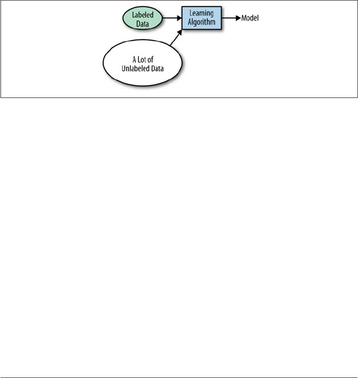
Semi-Supervised Learning
Semi-supervised learning (SSL) is a method of learning that employs both labeled data
as well as unlabeled data. It is an attractive idea for language-based tasks in particular,
because of two reasons: there is an enormous amount of unlabeled data available as
input to such an algorithm; and the cost of providing labeled training data can prove to
be prohibitively expensive in many cases.
While supervised learning algorithms require enough labeled training data to learn
reasonably accurate classifiers, and unsupervised learning methods can be used to dis
cover hidden structures in the unlabeled dataset, semi-supervised learning algorithms
combine aspects of both techniques. Figure 7-4 shows how SSL takes both labeled and
unlabeled data and puts them in an ML algorithm.
Figure 7-4. Semi-supervised learning
There are reasons why this might be useful to do, independent of the two reasons just
mentioned, however. Consider how this might work. In many learning scenarios, we
may or may not have a rich and descriptive model with which to create an annotation
of the dataset. That is, the phenomena may be quite complex and there may be dimen
sions that are not well captured, or dependencies among elements in the data that are
not identified, simply because you haven’t thought about them.
In other words, by first applying an unsupervised learning technique, such as k-means,
it might be possible to find clusters in the data that reflect meaningful representations
of complex or high dimensional data. The results of this step can then be taken as input
for a supervised phase of learning, using these clusters as soft labels. Figure 7-5 shows
how the SSL methodology fits into the MATTER cycle.
Statisticians have been using a type of SSL technique since the 1970s, iteratively using
the Expectation-Maximization (EM) algorithm to train classifiers by estimating pa
rameters of a generative model.
Semi-Supervised Learning | 163
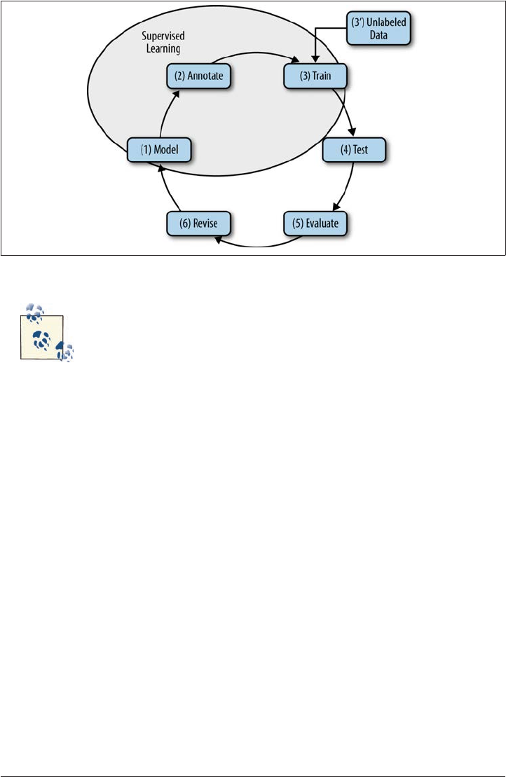
Figure 7-5. Semi-supervised learning in the MATTER cycle
Expectation-Maximization (EM) is a technique that allows you to find
Maximum Likelihood Estimations (MLEs) in circumstances where the
data would not normally seem to provide it easily; that is, some of the
random variables involved are not observed (see Chapter 3). The basic
idea behind EM is to make parameter estimates, given the missing data:
1. Replace missing values with estimates.
2. Estimate the parameters.
3. Repeat (1) using estimated values as correct, and (2) using estima
ted values as “observed.”
For details, see McLachlan and Krishnan 1996.
Several kinds of learning tasks are typically referred to as semi-supervised learning.
These include:
Transductive learning
This is where no general rule for determining a classifier is inferred, only where the
labels on the unlabeled data are predicted given the training phase.
Inductive learning
This is where a general rule for defining the classifier is inferred from the data, and
it is this rule (classifier) that is used to label the unlabled data.
164 | Chapter 7: Training: Machine Learning

Using SSL in a particular task without thinking through the nature of the unlabeled data
relative to the labeled training data can bring about a degradation in performance rather
than an improvement. However, for many tasks, SSL can actually perform better than
using labeled data alone (Singh et al. 2008), depending on the nature of the domain to
be explored, as well as the type of labeling task involved.
A particularly interesting kind of SSL is co-training. This is a technique that takes ad
vantage of two “views” of the data being examined for learning a concept. That is, each
perspective or view has an independent set of features that are used to describe the
example instance. Basically, it works when one classifier is able to correctly categorize
the instance where the other one could not. The correct assignment of the instance is
now added as positive data for the poorly performing classifier, and then is used for
iteratively training the classifier to perform better (Blum and Mitchell 1998).
Finally, there is another SSL technique that has recently been used to encouraging effect,
namely coupled training (Carlson et al. 2010). Given that the limited number of initial
labeled examples can be insufficient to reliably constrain the learning process, this
method proposes “coupling” the simultaneous training of many extractors over the data.
The effect is that more informative constraints can be identified with coupling that are
not possible with simple SSL training.
Matching Annotation to Algorithms
One of the difficult tasks when it comes to training an algorithm is actually picking
which algorithm matches best with your goal and annotation. Table 7-1 lists some com
mon tasks, as well as recommendations for what algorithms to use if you’re not sure
where to start. Keep in mind that we’re not suggesting these are the only algorithms that
can be used for these tasks, though! A lot of that decision rests on the corpus that you
chose and how you structured your annotation.
Table 7-1. Suggested ML algorithms for sample tasks
Task Suggested algorithm
Assigning categories to
words (POS tagging)
This is a sequence labeling task over annotation-dependent features and is usually seen as a
supervised learning task, using labeled training data of token sequences. This suggests one of the
following: HMMs, CRFs, or possibly SVMs (e.g., SVM-HMM). Efficient (transformational) rule-based
techniques also exist, such as the Brill tagger technique (Brill 1995).
Assigning topics to
articles, emails, or web
pages
This is a clustering problem usually viewed as an unsupervised learning task. It is a problem best
handled as an n-gram feature classification task creating a generative model. Some of the best
algorithms are Latent Dirichlet Allocation (LDA), where some number of topics (distributions over
words) exist for a document collection; Probabilistic Latent Semantic Analysis (PLSA); and other
“bag of words” algorithms.
Matching Annotation to Algorithms | 165

Task Suggested algorithm
Mood, affect, or
sentiment classification
of a text or utterance
This is a classification task using both n-gram and annotation-dependent features. This suggests
Naïve Bayes, MaxEnt, and SVM. In any of these approaches, n-grams can be used where
appropriate, but as mentioned earlier, unigrams often perform better because of the overfitting
problem. Overfitting occurs when you include too many features, causing the learning algorithm to
model the training data too precisely, which prevents it from generalizing well.
Assigning a semantic
type or ontological class
to a word or phrase
This is a classification task using both n-gram and annnotation-dependent features. As above, good
choices are Naïve Bayes, MaxEnt, decision trees (e.g., C4.5), and SVMs.
Word sense
disambiguation
This is a classification task that can take advantage of a wide variety of feature types. As a purely
supervised learning task, both SVMs and memory-based learning (MBL) approaches have been
used with both n-gram and annotation features. Viewed as an SSL problem, a classifier is trained
and then iteratively bootstrapped over unlabeled data. Pairwise similarity clustering (Rumshisky
2008) can be embedded in an SSL strategy to good effect as well.
Temporal and event
recognition
This is a classification task using both n-gram and annotation-dependent features. This suggests
Naïve Bayes, decision trees, or MaxEnt. Very good rule-based systems have also been developed,
including HeidelTime (Strötgen and Gertz 2010) and Evita (Saurí et al. 2005).
Semantic roles for
participants of events in a
sentence
This is a classification task that can build either a discriminative model or a generative model,
depending on what features are chosen and what dependencies are chosen between them. Models
exist using SVMs (Pradhan et al. 2003) and MaxEnt (Lim et al. 2004). SSL techniques have also been
used.
NE identification This is a fairly straightforward classification problem, using both n-gram and annotation-
dependent features. Approaches include Naïve Bayes, MaxEnt, SVMs, CRFs, MEMMs, and even MBLs.
Coreference resolution This can be viewed as a classification task, using mostly annotation-dependent features. Algorithms
include decision tree induction (C4.5) (Ng and Cardie 2002), co-training (Goldman and Zhou 2000),
CRFs (Wellner et al. 2004), and boosting (Ng and Cardie 2003), and first-order probabilistic models
(Culotta et al. 2007).
Summary
In this chapter we looked at how the model and annotation you have been developing
are able to feed into the ML algorithm that you will use for approximating the target
function you are interested in learning. We discussed the differences between the dif
ferent feature types: n-gram features, structure-dependent features, and annotation-
dependent features. We reviewed how these features are deployed in several important
learning algorithms, focusing on decision tree learning and Naïve Bayes learning. Here
is a summary of what you learned:
•ML algorithms are programs that get better as they are exposed to more data. ML
algorithms have been used in a variety of computational linguistic tasks, from POS
tagging to discourse structure recognition.
•There are three main types of ML algorithms: supervised, unsupervised, and semi-
supervised.
166 | Chapter 7: Training: Machine Learning

•Supervised learning uses annotated data to train an algorithm to identify features
in the data that are relevant to the intended function of the algorithm.
•N-gram features allow algorithms to take information about the words that are in
a document and examine aspects of the data such as term frequency to create as
sociations with different types of classifications.
•Structure-dependent features are defined by the properties of the data, such as
strings of characters, HTML or other types of markup tags, or other ways a docu
ment can be organized.
•Annotation-dependent features are associated with the annotation and reflect the
model of the annotation task.
•A learning task is defined in five steps: choose the corpus that will be trained on,
identify the target function of the algorithm, choose how the target function will
be represented (the features), select an ML algorithm to train, and evaluate the
results.
•Another way to use an annotated corpus in a software system is to design a rule-
based system: a program or set of programs that does not rely on an ML algorithm
being trained to do a task, but rather has a set of rules that encode the features that
an algorithm could be trained to identify.
•Rule-based systems are a good way to identify features that may be useful in a
document without having to take the time to train an algorithm. For some tasks
(e.g., temporal expression recognition), rule-based systems outperform ML
algorithms.
•Classification algorithms are used to apply the most likely label (or classification)
to a collection. They can be applied at a document, sentence, phrase, word, or any
other level of language that is appropriate for your task.
•Using n-gram features is the simplest way to start with a classification system, but
structure-dependent features and annotation-dependent features will help with
more complex tasks such as event recognition or sentiment analysis.
•Decision trees are a type of ML algorithm that essentially ask “20 questions” of a
corpus to determine what label should be applied to each item. The hierarchy of
the tree determines the order in which the classifications are applied.
•The “questions” asked at each branch of a decision tree can be structure-dependent,
annotation-dependent, or any other type of feature that can be discovered about
the data.
•A Naïve Bayes learning algorithm tries to assign the probability that an item will be
assigned a particular classification, based on the association between what features
are associated with each item, and how strongly those features are associated with
a particular label as determined by the Bayes Theorem.
Summary | 167

•The K-nearest neighbor algorithm uses much simpler rules than the Naïve Bayes
methods, with simple associations between features and classifications.
•Unsupervised learning is the process of “teaching” an algorithm without giving it
any starting information about the classifications that exist in the dataset.
•Classic examples of unsupervised learning are clustering algorithms, which find
natural groupings in the data in order to create sets of similar items. Essentially,
clustering algorithms find their own features for the datasets.
•Because clustering algorithms don’t take features from the users but instead discover
their own, the groups that a classifier creates may not be the ones that you have in
mind for your task.
•Semi-supervised learning techniques allow you to use a small amount of labeled
data to generate labels for larger sets of data, and are an effective way to deal with
very large datasets.
•If you aren’t sure where to start with your algorithm training, try to find a task or
annotation similar to your own and see what algorithms are commonly used for
those projects. If there aren’t any projects just like yours, try to find ones that have
similar features or feature types.
168 | Chapter 7: Training: Machine Learning

CHAPTER 8
Testing and Evaluation
Once you’ve selected an algorithm and started picking out your features, then you can
actually start testing your algorithm against your gold standard corpus and evaluating
the results—the “Training through Evaluation” (TE) portion of the MATTER cycle. Like
other parts of MATTER, the training, testing, and evaluation phases form their own,
smaller cycle. After you train your algorithm on the features you select, then you can
start the testing and evaluation processes.
In this chapter we’ll answer the following questions:
• When is testing performed?
• Why is there both a dev-test corpus and another test corpus?
• What’s being evaluated once the algorithm is run?
• How do you obtain an evaluation score?
• What do the evaluation scores mean?
• What should evaluators be aware of during these phases of the MATTER cycle?
• Which scores get reported at the end of these phases?
Keep in mind that the purpose of evaluating your algorithm is not just to get a good
score on your own data! The purpose is to provide testing conditions that convincingly
suggest that your algorithm will perform well on other people’s data, out in the real world.
So it’s important to keep track of the testing conditions, any modifications you make to
your algorithm, and places in your annotation scheme that you think could be changed
to improve performance later. Your algorithm getting a good “score” on your test doesn’t
really matter if no one else can take the same exam!
169
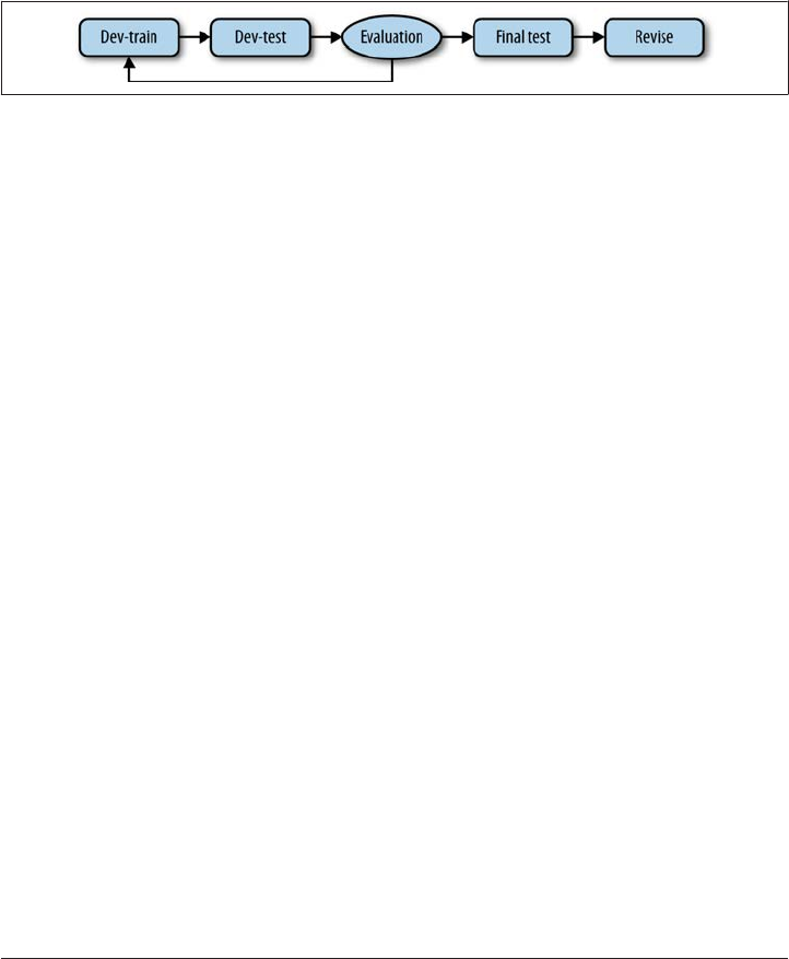
Testing Your Algorithm
Your algorithm will be tested multiple times during this phase of the MATTER cycle
(see Figure 8-1): after being trained on the dev-training set, it is tested on the dev-test
set. After evaluating the algorithm’s output, either you can go back to the dev-training
set and retrain your algorithm with new or modified features, or, if you’re satisfied with
your algorithm’s output, you can run your algorithm on your test corpus and report on
the results.
Figure 8-1. The training–evaluation cycle
Remember that the test set (as opposed to the dev-test set) is not used for testing until
you are ready to get “official” numbers for your algorithm’s performance over your cor
pus. Think of the test set as a final exam: the best way to determine if your algorithm
has learned the material is to give it one last test on material that’s similar to what was
used for training, but is not exactly the same. The last part is important: test data is kept
separate from the development set, and you never train your algorithm on your testing
data. You need to have an idea of how your algorithm would perform “in the wild,” which
you can’t do if you use the test data to train on, or run your algorithm multiple times on
your final test set—that’s why there’s a dev-test set that’s also separate from both the final
test set and the dev-training set.
For the rest of this chapter, we will simply refer to the data being evaluated as the
evaluation set, because the same evaluations are run on the results from the dev-test set
and the final test set. Keep in mind that although evaluations are run on the results of
both the dev-test and the final test sets, only the evaluation from the dev-test set is used
to tweak the features used for training. We’ll talk more about why this is in “Problems
That Can Affect Evaluation” (page 178).
Evaluating Your Algorithm
Once you’ve selected your features, trained your algorithm, and tested it, it’s time to
evaluate how the output from your algorithm compares to the gold standard annotations
on the evaluation set. First you need to calculate and interpret your evaluation scores,
after which it can be helpful to create a confusion matrix to help determine on what parts
of your task the algorithm is failing (or succeeding!).
170 | Chapter 8: Testing and Evaluation

Confusion Matrices
An extremely useful way to examine the results of your algorithm is to create a confusion
matrix—you may recall from “Cohen’s Kappa (κ)” (page 127) that we created one to
compare the annotations of two annotators. A confusion matrix allows us to look at
what labels the algorithm is using (and to a certain extent, where it’s putting them)
compared to the labels in the gold standard.
Because we already saw a similar example when calculating Cohen’s Kappa, it’s easy to
see how a confusion matrix can be used for other tasks where labels are being applied
to a document:
test test test
positive neutral negative
gold standard positive 96 4 0
gold standard neutral 13 87 0
gold standard negative 0 0 100
Correct annotations are identified by the numbers on the diagonal, shown here in bold.
In this example, the algorithm performed very well on identifying negative reviews, but
it had a harder time telling positive reviews from neutral ones. Specifically, the algorithm
tended to err by labeling entries that are “neutral” in the gold standard as “positive”
(though it labeled four as neutral when they should have been positive as well). So we
can see here that the algorithm will need to have better features for distinguishing pos
itive reviews from neutral ones.
The Natural Language Toolkit (NLTK) has a built-in function for cre
ating confusion matrices. Once you have a gold standard loaded and
have run your algorithm on an unlabeled test set, just run:
>>> matrix = nltk.ConfusionMatrix(gs,test)
where gs is a list of the gold standard annotation of the test set, and test
is a list of the output of the algorithm, although the NLTK table displays
percents instead of whole numbers. See the NLTK 2.0 metrics docu
mentation for more information.
It is also possible to create confusion matrices for tasks where labels are being applied
to words in the texts. The setup for the table is essentially the same: the test annotations
are on one axis, the gold standard annotations are on the other, and each tag is given a
column and a row. Here’s a partial example for what a part-of-speech (POS) tagging task
might look like:
Evaluating Your Algorithm | 171

test test test test test test
noun conjunction determiner adjective adverb …
gold noun 12951 0 0 211 0
gold conjunction 0 2664 0 0 0
gold determiner 0 0 589 0 0
gold adjective 184 0 0 4133 75
gold adverb 5 0 0 91 2166
gold …
This is very similar to the previous table for the movie review classification, except that
each unit in this table is a word rather than an entire document.
So if that is how you create a confusion matrix for a task where every word has a tag,
what do you do with an annotation task that results in sparser annotations? We actually
showed you the answer to this question before, in the example for calculating Inter-
Annotator Agreement (IAA) scores for sparse annotations [“Calculating κ in Other
Contexts” (page 132)]: just add an “untagged” category to the table, as we did in the table
for the “Jabberwocky” annotation task:
test test test
creature pronoun untagged
gold creature 5 0 2
gold pronoun 0 19 0
gold untagged 1 0 189
Creating a confusion matrix isn’t mandatory for evaluating an algorithm, but it can help
you (and anyone reading about your results) to understand where common sources of
error are. Also, they can be useful when calculating evaluation scores for your algorithm,
which we will address in the next section.
Calculating Evaluation Scores
Much like IAA scoring, there are a few different methods for evaluating your algorithm’s
performance. In this section we’ll go through how to calculate the most common eval
uation metrics, specifically percentage accuracy, precision and recall, and F-measures,
and how to apply these to different types of annotation tasks.
Percentage accuracy
The first metric that most people think of as an evaluation score for your algorithm is
to grade the output of the algorithm the way that you would grade an exam: simply look
at the generated annotations; mark off which ones are wrong and which are right; and
figure out what percentage of the total annotations are correct.
172 | Chapter 8: Testing and Evaluation

If you have a confusion matrix, the percentage accuracy is the sum of the diagonal (top
left to bottom right) of the table divided by the sum of all the cells of the table. So in the
movie review table from the previous section, we have a total accuracy of:
(96 + 87 + 100) / 300 = .943, or 94.3%
Unfortunately, while accuracy is easy to calculate, it can only give us a general idea of
how well an algorithm performed at a task: it can’t show specifically where the task went
wrong, or what aspects of the features need to be fixed. There are other ways to obtain
and assign scores to those attributes of a machine learning (ML) task, however, which
we will examine next.
Precision and recall
The biggest problem with calculating overall accuracy is that the resultant score doesn’t
address the two different kinds of mistakes that need to be examined for evaluating an
annotation task: places where it put the wrong tag on an item, and places where it failed
to put the right tag. These values are calculated by examining the precision and recall
for each tag/label in a task, and they help form a clearer picture of what aspects of an
algorithm need to be adjusted.
Precision and recall are traditionally associated with Information Retrieval (IR) tasks
such as those related to search algorithms. Let’s say there was a database of scientific
papers, and you wanted the computer to return all of the articles related to string theory.
If there are 50 relevant documents in the database and the search returns 75, then it’s
clear that the search has falsely identified some documents as being related to string
theory when they actually weren’t. When an item is given a label that it should not have,
that is called a false positive. On the other hand, if the same database were queried for
“string theory” and only 25 documents were returned, there would be multiple cases of
false negatives, where items were rejected for a label that they should have actually been
given. Documents that are returned accurately are called true positives, and documents
that are correctly ignored when they are irrelevant are true negatives.
By applying the idea of false negative and false positive to the results of an ML algorithm,
we can compute useful evaluation metrics that will help us to more accurately identify
sources of error in the system. However, unlike overall accuracy calculations where all
the tags are evaluated together, false positives and false negatives have to be evaluated
one tag at a time. If we think about it, this makes sense, particularly in annotation tasks
where only one tag (or no tag) is being applied to an item, as a false positive for one tag
is a false negative for another.
So how do we calculate the number of false positives and false negatives? With a con
fusion matrix, it’s quite easy. If we look at the matrix for movie review labels again, we
Evaluating Your Algorithm | 173

see that to evaluate the accuracy of the “positive” label we need to look at the first column,
which shows the number of documents the classifier labeled as “positive,” and the first
row, which shows how many documents in the gold standard were given the “positive”
label:
test test test
positive neutral negative
gold standard positive 96 4 0
gold standard neutral 13 87 0
gold standard negative 0 0 100
In all confusion matrices, the true positives are located at the intersection of the row
and column we are examining. In this case, the number of true positives is 96. False
positives are calculated by summing up the column “test—>positive” (minus the number
of true positives): here that number is 13 (13 + 0). Similarly, false negatives are calculated
by summing across the row for “gold standard—>positive” (again, without counting the
true positives), which is 4 (4 + 0). (The number of true negatives is the sum of the rest
of the table [187], but we won’t be needing that here.)
With the confusion matrix, calculating the true and false positives and negatives is simple
enough, but what do we do with them now? The answer is that we calculate precision
and recall values, which provide more nuanced information about our algorithm test.
Precision is the measure of how many items were accurately identified, and is defined
as:
p=true positive
true positive +false positive
For the “positive” tag, p = 96 / (96 + 13)
= 96 / 109
= .881
Recall is the measure of how many relevant items were identified (in other words, how
many of the documents that should have been labeled “positive” were actually given that
label):
r=true positive
true positive +false negative
r = 96 / (96 + 4 )
= 96 / 100
= .96
174 | Chapter 8: Testing and Evaluation

We can see from these numbers that for the “positive” label our algorithm has high recall,
which means it found most of the documents it should have, but lower precision, which
means it’s giving too many documents the “positive” label when they should be labeled
as something else.
If we perform these calculations with the rest of the matrix, we can make a table that
looks like this:
tag precision recall
positive .881 .96
neutral .95 .87
negative 1 1
In this case, the precision and recall numbers for positive and neutral are very close to
being each other’s opposite, because here, the “negative” tag isn’t influencing the other
two. In tables with more variation, such reciprocity is not the norm.
While it’s fairly standard to report the precision and recall numbers for each tag (and
tag attribute), papers about ML algorithms often mention another number, called the
F-measure, which we will discuss in the next section.
You can also se the NLTK to generate accuracy, precision, recall, F-
measure, and a number of other analysis metrics for you using the
nltk.metrics package. Like the confusion matrix, the accuracy metric
uses lists to calculate the numbers, while precision, recall, and F-
measure use sets of data instead. A good overview of how to create these
sets is available at http://bit.ly/QViUTB.
F-measure
The F-measure (also called the F-score or the F1 score) is an accuracy measure calculated
by finding the harmonic mean of the precision and recall of an algorithm’s performance
over a tag. The formula for F-measure is as follows (where p is precision and r is recall):
F= 2 ×
(
p×r
p+r
)
We see that the F-measure for the “positive” tag is 2 * (.881*.96) / (.881 + .96) = 1.692 /
1.841 = .919.
While the F-measure won’t tell you specifically where your algorithm is producing in
correct results, it does provide a handy way for someone to tell at a glance how your
Evaluating Your Algorithm | 175

algorithm is performing in general. This is why F-measure is commonly reported in
computational linguistics papers: not because it’s inherently useful to people trying to
find ways to improve their algorithm, but because it’s easier on the reader than pro
cessing an entire table of precision and recall scores for each tag used.
You may be wondering why we don’t use kappa coefficients for evalu
ating algorithms. The equations for kappa coefficients are designed to
take into account that annotators always bring in some level of random
chance, and also that when IAA scores are being calculated, the right
answer isn’t yet known. While gold standard corpora can certainly have
errors in them, they are considered correct for the purpose of training
and testing algorithms, and therefore are a mark to be evaluated against,
like the answer key on an exam.
Notice that this number is not the same as the overall accuracy from “Percentage accu
racy” (page 172), because this is the accuracy measure for only one tag. Again, we can
create a table of all the F-scores as shown here:
tag precision recall F-measure
positive .881 .96 .919
neutral .95 .87 .908
negative 1 1 1
F-measures, precision and recall, and accuracy are all commonly used metrics for eval
uating how an algorithm is performing during development, and are also often discussed
in articles and at conferences to report on how well an algorithm does on an annotation
task. We will discuss how to interpret these scores in the next section.
Other evaluation metrics
There are many other ways to analyze the various features, distributions, and problems
with your dataset, algorithms, and feature selection. Here’s an overview of some other
methods that you can use to check out how your system is performing:
T-test
Determines whether the means of two distributions are different in a statistically
significant way. Useful for comparing the results of two different algorithms over
your training and test sets.
Analysis of variance (ANOVA) test
Like a t-test, but allows multiple distributions to be compared at the same time.
176 | Chapter 8: Testing and Evaluation

Χ-squared (chi-squared) test
Can be used to test if two variables are independent. Useful for determining if an
attribute of a dataset (or a feature in the model) is contributing to part of the data
being mislabeled.
Receiver Operator Characteristic (ROC) curves
Used to compare true positive and false positive rates between classifiers or classifier
thresholds.
Also, don’t forget about the methods we showed you in Chapter 3. Some of those tests
can also be applied here.
For more information on how to apply these tests to your corpus and algorithm, please
check a statistics textbook. If you’re interested specifically in how statistics can be done
in Python, we suggest looking at Think Stats: Probability and Statistics for Program
mers, Allen B. Downey (O’Reilly, 2011).
Interpreting Evaluation Scores
Unlike IAA scores, there is no table that is used for determining, even roughly, how an
evaluation score should be interpreted. Clearly, you want to get your algorithm’s results
to be as close to 1 as possible, but the accuracy of an algorithm will depend greatly on
how difficult the task is, how appropriate the corpus is, and what the state of the art
currently is for that task or type of task. Ultimately, your own algorithm needs to be
evaluated in the context of other algorithms that have been trained to do similar tasks.
It’s especially important to consider how your task differs from other, similar tasks when
considering how your algorithm stacks up against other algorithms. For example, POS
taggers trained on the Penn TreeBank and used on corpora with similar texts usually
obtain accuracies in the upper 90s. However, when the same taggers are tested on bio
medical corpora, they get results that are much lower until they are also trained on
tagged biomedical data (see Tsuruoka et al. 2005 and Fan et al. 2011 for more information
on this topic). Using a different type of data for testing than training will probably cause
a drop in performance, which can then lead to the annotation of a more relevant set of
documents. But if you are the first person to explore a task in a different genre or subject,
it’s reasonable to expect that your scores will be lower than others who are working on
improving their own scores with the same sets of data.
Don’t get too caught up on the word test. While we’ve compared the
final evaluation scores to final exams for classes, there’s no scale that
determines if you “fail.” Due to the huge variation in task difficulty,
algorithm evaluation is more like being graded on a curve than on a
line.
Evaluating Your Algorithm | 177

However, while POS tagging results are generally quite good (once appropriate data is
being used for training), other tasks have accuracy numbers that are much lower, but
that are still considered good for that task. Consider the TempEval-2 challenge, held as
part of the 2010 SemEval (Verhagen et al. 2010). TempEval contains three main tasks:
event recognition, temporal expression recognition, and temporal relation annotation
(which is further divided into subtasks). Because identifying temporal and event infor
mation in text requires much more interpretation of the data, most algorithms designed
for this task had F-measures in the 80s for event recognition, and lower for relation
annotation. But despite being comparatively lower than POS tasks, these scores are still
considered good for the type of annotation they were working on. Thus, the evaluation
of your algorithm must be done in the context of similar tasks, rather than on a strict
scale from 0 to 100.
Problems That Can Affect Evaluation
While the methods of evaluation for algorithm accuracy are fairly straightforward to
calculate, the numbers that you end up with won’t necessarily show you all the sources
of error that might be affecting your results. In this section we’ll look at two of the
common problems that affect algorithm evaluation and what to do about them.
Dataset Is Too Small
So far in this chapter we’ve talked about dividing the corpus into three sets: dev-training,
dev-test, and final test. However, splitting up a corpus in this manner can be difficult if
the corpus isn’t very big. You want to make sure you have enough data to train on, but
if your testing sets are too small, then even a few errors can make it seem as though your
algorithm is doing a very poor job.
Fortunately, there is an approach you can use if you simply don’t have enough data to
properly train and test your algorithm. K-fold cross-validation is an analysis method
that allows you to split your data into k different partitions (or folds), then train your
algorithm on all the sections but one, and test it on the held-out section. You then choose
a different partition to hold out and repeat the process, until all the partitions have been
used as the test set. For example, if you divided your corpus into five partitions, (k = 5),
you would take four of those in which to train your algorithm, and test it on the fifth.
See Figure 8-2 for a visual representation of this method.
178 | Chapter 8: Testing and Evaluation
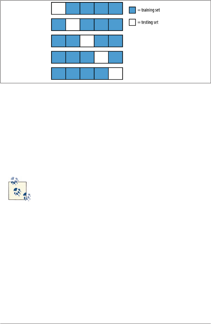
Figure 8-2. K-fold cross-validation
Once you have run your algorithm on all the subset variations of your testing and train
ing data, you can evaluate the accuracy of each round of testing and give the average of
all the results. There are other methods of dividing your test and training sets as well,
such as performing a fixed number of tests but randomly selecting what documents will
be in the training and testing sets each time. While the random selection method does
help take care of some problems that can still be found using the k-fold method (e.g., if
one of your folds randomly ended up with a set of documents that’s very different from
the rest of the folds), randomly selecting files means you can’t be sure that every file will
end up in both the testing and training sets at some point.
You can use Python to randomize your list of inputs and to select your
folds. Assuming you have a list of files, f, you can call Python’s shuf
fle function over the list to randomize the order:
>>> import random
>>> random.shuffle(f)
If you’re performing k-fold cross-validation and you want to use Python
to select each fold, you can do that in a loop to create a list of the set of
files in each fold:
>>> k = 20
>>> i=0
>>> folds = []
>>> while i<len(f):
>>> folds.append(f[i:i+k])
>>> i = i+k
Of course, you’ll want to make sure you pick a k that doesn’t leave your
last set too small to use, so make sure the k you pick either divides the
size of your list perfectly, or at least leaves a high enough remainder for
the algorithm to be trained on.
Problems That Can Affect Evaluation | 179

Cross-validation is an excellent way to determine how consistent your dataset is and
how stable your features are. If each round of testing and evaluation is returning roughly
the same numbers, then you can infer that your corpus is consistent and that your
evaluation results are accurate. However, if the results display a large amount of varia
tion, then it could indicate a larger problem with your dataset or feature selection, and
the results will not be very good if you use your algorithm on other datasets.
Algorithm Fits the Development Data Too Well
You might be wondering what we mean by the algorithm fitting the data too well: isn’t
that the whole point of selecting features and training an algorithm? While it’s true that
you want to have a feature set that does a good job of representing your corpus, it’s
possible to end up selecting features that exist disproportionately in your dev-training
and dev-testing sets, which will mean your algorithm will not work as well on your final
test set as it might otherwise. This problem is referred to as overfitting, and it generally
occurs when you have too many features in your algorithm’s model. Remember that the
purpose of training an algorithm is to create a tool that can be used on new data, not
only on your annotated corpus.
This is where the representativeness and balance of your corpus can really come into
play, but it’s also where the problem of attaining true representativeness and balance is
brought to light. A corpus that can claim to be representative and balanced for the types
of data it was created to represent will, in theory, lead to better ML results in the testing
phase of the MATTER cycle, because there will be less variation in features between the
training and testing datasets. However, in practice it will rarely be the case that all the
features you are using to train with will appear in the same proportion as in the test data,
simply from random chance in distributions.
So, how can you tell if your algorithm is overfit? Basically, if a feature adds accuracy
during the test–eval phases, but is introducing errors during the final test phase, then
your model is overfit to your training set. It’s that simple, but overfitting your training
data is a very easy trap to fall into, so watch out for it.
180 | Chapter 8: Testing and Evaluation

Keep track of your choices! The determination of how representative and
balanced your corpus is will be highly influenced by what your corpus
is intended to represent in the first place. This is why it’s important to
keep track of the methods you use to create your corpus and report them
to those who might use your corpus or your algorithm. Let’s say, for
example, that you created a movie review corpus but only included re
views containing 200 words or more, and then took precautions to make
sure the reviews were balanced across movie genres, polarity, and so on.
You can claim that your corpus is representative of reviews over a certain
length, but not that it’s representative of all reviews—and that’s fine!
There can be good reasons for putting limits on what gets included in
your corpus; the important thing is to be upfront about them so that
others will understand what they’re getting into when they use the re
sources you create.
Too Much Information in the Annotation
Sometimes your annotation task contains more information than a classifier actually
needs. One way to test this is to remove features from your algorithm and see if the
accuracy of the results changes significantly. Being able to achieve the same results with
a smaller set of features helps you to focus in on what’s really going on in the text, and
how to best represent that to a computer. You can also examine each feature one at a
time to help determine how much each one is adding to the accuracy of the overall
results.
Final Testing Scores
To get the final accuracy numbers that you will report to other people for your algorithm,
corpus, and annotation, you must run the trained algorithm over the final test set.
However, there is a danger in evaluating over the test data too many times. First, the
more times you run your algorithm over your final test data, the lower the statistical
significance of your results becomes—running too many tests means that you’re fishing
for features and tweaks that will improve your final testing scores, but the act of fishing
increases the likelihood that you’ll stumble upon something that just happens to improve
your scores, but doesn’t actually reflect a true feature in the real world.
A second (but related) issue is that the more you tweak your features for your test data,
the more danger you are in of overfitting your algorithm to your test data, which itself
will be no more representative of data in the real world than the rest of your corpus.
Final Testing Scores | 181

Ideally, you would only run your algorithm on your final test data once. If you do run
it more than once, be upfront about how many times it was run and what adjustments
were made between runs. This not only keeps you honest (and safer from stats-savvy
reviewers), but it also helps other people understand what problems they might en
counter using similar datasets or systems.
Summary
In this chapter we discussed how to test and evaluate your ML algorithm’s performance
on your dev-test and final-test data. Some of the key points in this process are sum
marized here:
•Algorithms are tested multiple times over the development-training and
development-testing sets of your corpus. After each run of the algorithm on the
dev-test data, evaluation of the results is performed and the algorithm/features are
adjusted as necessary.
•Creating a confusion matrix of your results is an excellent way to identify problems
with your algorithm’s performance, and also makes calculating accuracy scores
much easier.
•Calculating the percentage accuracy for your algorithm provides a baseline level
of evaluation, but it doesn’t tell the whole story about how your algorithm is
performing.
•Precision and recall are metrics used to compare the number of true positives, false
positives, and false negatives that your algorithm is producing. A high precision
score indicates that your algorithm is not returning many false positives; a high
recall score indicates that it is not producing a lot of false negatives.
•Depending on the purpose of your algorithm, you may want to favor high recall
over high precision, or vice versa.
•An F-measure is the harmonic mean of the precision and recall scores, and provides
a more robust overall metric of your results.
•Other evaluation metrics such as ROC, chi-squared, t-tests, and ANOVA can be
used to identify discrepancies and variables in your algorithm as well.
• The interpretation of evaluation scores is highly dependent on the current state of
the art in research areas similar to what you are working on—you’ll need to see how
other, similar algorithms are performing to determine how yours stacks up.
•If your dataset is too small to divide into training and testing sets, you can use cross-
validation to evaluate your algorithm.
• Beware of overfitting your algorithm to your training set!
182 | Chapter 8: Testing and Evaluation

•Run your algorithm over your final testing set as few times as possible (ideally, once),
and make sure to report the evaluation metrics for that run, as well as any changes
that you made between runs.
Summary | 183

CHAPTER 9
Revising and Reporting
Finally, we’re at the “R” of the MATTER cycle—revising your project. Of course, you’ve
probably been revising your project all along, as you worked your way through the
MAMA cycle, and refit your algorithms through the training, testing, and evaluation
stages of machine learning. However, while making adjustments at each step of the way,
you may have focused only on the steps at hand, so in the first part of this chapter, we
are going to take a step back and examine some of the “big picture” items that you may
want to reconsider about your project. To that end, we’ll discuss:
• Corpus modification
• Model and specs
• Annotation task and annotators
• Algorithm implementation
In the second part of the chapter we will discuss what information you should include
about your task when you are writing papers, giving presentations, or just putting to
gether a website so that people can learn about your project. Creating annotated corpora
and leveraging those corpora into good machine learning (ML) algorithms are difficult
tasks, and because so many variables affect the outcome of a project, the more open you
are about the choices you made, the more other people will be able to learn based on
your example. Some of the aspects of your project you need to consider reporting on
are:
• Corpus size, content, and creation
• Annotation methods and annotator qualifications
• ML modifications and training adjustments
• Revisions to your project, both implemented and planned
185

Revising Your Project
Now that you’ve made it to the end of the MATTER cycle, it’s a good time to step back
and look at the big picture of your entire annotation and ML task. In this section we’ll
go over some of the aspects of your project that you might want to consider revisiting
later.
Just because you identify something you want to change doesn’t mean
it has to be changed immediately! We’ll talk more about this in “Re
porting About Your Work” (page 189), but when telling other people about
your work, it’s perfectly acceptable to say there are aspects of your
project you are planning to change, and then report on what you have
so far.
As you go through the first half of this chapter, it’s a good idea to note the things that
you want to revise, and the aspects of your project you did revise while working through
the MATTER cycle. It will be much easier to report accurately on your annotation and
ML task if you have a clear outline of everything that you actually changed as you worked,
and everything that you would like to change in the future.
Corpus Distributions and Content
At this point we suggest going back and checking to see if your corpus is still represen
tative and balanced with regard to your task. It’s possible that your annotation model
has changed enough that you need to collect some new data samples, or that during the
training and testing phases you discovered some new features that you hadn’t considered
before and that are not well represented in your corpus.
However, don’t forget the “balanced” part of “representative and balanced.” If something
is a useful feature for correctly creating an annotation but it doesn’t appear in the wild
with any frequency, you don’t want to create an unbalanced corpus by having that feature
over-represented in your corpus, because that will skew the balance of any ML algorithm
trained on it.
Another task you may want to consider is testing your algorithm on a completely new
corpus, to see how it performs on other data. This will be easiest if you can find a corpus
that uses the same (or a similar) annotation scheme to the one that you are using. It’s
by no means required for you to do this, but it’s always good to have an idea of new
directions that your annotation and algorithm could go in the future.
186 | Chapter 9: Revising and Reporting

Model and Specification
Now that you have the results of both the annotation and ML parts of your task, you
can go back and examine the annotation model and specification in terms of the ML
results. We’re not suggesting that you completely change your annotation task to fit
exactly with what your algorithm performed best at, of course—a corpus with linguistic
subtleties is always a valuable resource, even if some of the aspects cannot be recreated
reliably through machine learning or other computer systems. However, now is a good
time to reevaluate how the features you used for machine learning tie in with the an
notation you devised, and whether your corpus might benefit from reflecting more of
those features.
At the same time, you can put some thought into whether all of the different tags and
attributes truly form their own distinct categories, and whether it might be more sensible
to conflate some of the information in your corpus. Sometimes during the MAMA cycle,
when you’ve been looking closely at the texts, tags, and attributes, it’s easy to become
too wrapped up in minutiae, and once you’ve reached the end of the MATTER cycle,
it’s easier to see what parts of your annotation task may need to be culled. If, for example,
you have a tag or attribute value that only gets used a handful of times in your corpus,
it might be time to consider whether it’s worth having annotators look for those specif
ically, or if they could be grouped in with something else.
Just because a tag is rarely used doesn’t necessarily mean you should get
rid of it! It’s also possible that something appears rarely simply because
your corpus accurately represents distributions in the real world, and
some things really do appear less frequently than others. For example,
in the IMDb database of genres (as of April 20, 2012), there are 1,344,395
genre labels applied to all the titles in the database. Of those, “news”
only appears 5,868 times—0.4% of all the labels used. But news is cer
tainly distinct from all of the other genres that IMDb uses, so it wouldn’t
make a lot of sense to decide that the label shouldn’t be used just because
it only appears rarely. On the other hand, the “lifestyle” genre label is
only used once, so it’s probably fair to say that either that label should
be phased out, or perhaps it’s already being removed and there’s just an
artifact in the file somewhere.
Please note that we aren’t suggesting there is a superior format for models or specs!
Whether your task needs to add categories or take them away will depend greatly on
your goal, data, and performance in the annotation and ML tasks, and there’s no ideal
number of categories, tags, attributes, or links that will apply to every task.
Revising Your Project | 187

Annotation
When reviewing this stage of the MATTER cycle, we strongly recommend going back
and writing down what you did, as well as what you want to change. While we recom
mend this for all aspects of the revision process, it is particularly important for this one
because papers on annotation tasks tend to under-report details on the implementation
of the annotation. But those details are some of the most important when it comes to
giving readers a sufficient understanding of your annotation task, so it’s important to
have them available to others who will be using your data or trying to replicate your
results.
Guidelines
Chances are you already fixed most of the problems with your annotation guidelines
during the MAMA cycle, so don’t worry too much about making corrections at this
point. Definitely don’t change your guidelines if you are planning to release the corpus
and/or publish about the process—releasing a set of guidelines that are different from
the ones used to annotate will only cause confusion. However, if you haven’t already,
you can always go back and poll your annotators to find out what aspects of the guide
lines they found confusing, and make notes about that for future projects.
Also, if you’ve decided to move your annotation to a new corpus, or you’ve discovered
aspects of your model that need to be changed, now is a good time to start making notes
about parts of your guidelines that will need to be changed as well. Remember that if
you are changing the type of documents in your corpus you will need to rework the
examples to better reflect the new data, and any changes to the spec will need to be
included as well.
Annotators
Another aspect of your task that you’ll want to think about is who you hired to annotate
your corpus. If you had a task requiring specialized knowledge to fully understand, did
you hire people who had that knowledge already (e.g., did you hire people with training
in linguistics to do a part-of-speech [POS] annotation task), or did you hire inexper
ienced people and train them? If you trained people from the beginning, were they able
to pick up the task quickly and make a minimum of mistakes, and finally, was the training
process ongoing throughout the annotation task? If you used Amazon’s Mechanical
Turk, were you able to obtain sufficiently high-quality annotations for your project, or
did you have to spend a lot of time weeding out bad data?
Annotators are probably the most variable aspect of an annotation task, and it’s worth
taking the time to make sure your annotators can do the job you want them to do with
a minimal amount of trouble. So when you’re revising your project, take the time to
consider whether there was anything about the annotators themselves (training, previ
ous experience, etc.) that might have affected the quality of the annotation.
188 | Chapter 9: Revising and Reporting

Tools
Finally, it’s worth checking in with your annotators and adjudicators to see if the software
you had them use to create your corpus is one that helped or hindered them in their
task. While most annotation software has some limitations, it always helps to pick soft
ware that will support your annotation task rather than get in the way of it. But it’s really
up to your annotators, who spend the most time working with the software, to decide
what the pros and cons are after they’ve finished their part of the MATTER cycle.
Training and Testing
If you’re following the MATTER cycle in order, then you’ve reached the Revision stage
right after going through a few turns of the Training–Evaluation cycle, so you’re probably
wondering what’s left to evaluate. There’s always more information to be found in a
corpus, and now could be a good time to go back and examine more linguistic aspects
of your corpus that could be useful for training and testing. In particular, if you focused
on annotation-based features in your algorithm, maybe it’s time to check to see if there
are any structure-based aspects of your corpus that you can take advantage of. For ex
ample, do certain phrases that you’re looking for tend to appear in noun groups or verb
groups? If you don’t know, try using a POS tagger or chunker or parser and then look
for correlations in your annotation to different linguistic aspects of the text. If you do
find correlations, you can make a note to add those aspects into future annotation tasks,
or into the ML algorithms later on.
Other aspects of the texts that you can take into consideration are the structure of the
document (are there section headers, or are important phrases more likely to appear at
the beginning or end of paragraphs?), any meta-information such as genre or register
(assuming that isn’t what you’re trying to figure out in the first place), the influence of
prepositional phrases, and so on.
Now is also a good time to reconsider whether you’re using the right algorithm—if you’ve
found more features that would be useful, it’s possible that you’ll want to switch from
one type of ML system to one that’s better suited to the new aspects of your corpus that
you’re exploring.
Reporting About Your Work
Considering how much work goes into creating an annotated corpus and subsequently
training an ML algorithm, you are probably going to want to tell people about what you
did. You can submit papers to the same conferences and journals that you used for
sources of inspiration for your annotation goal, or you can simply make the corpus,
Reporting About Your Work | 189

annotations, and your notes available on a website and let people know that the infor
mation is there. No matter how you decide to advertise the work you did, however, there
are some basic pieces of information that will make it easier for other researchers to
understand and make use of your materials.
At the moment there’s no gold standard or ISO list of what information should be in
cluded about an annotated corpus, but in this chapter we’re going to provide an overview
of the information most people generally agree is helpful to have when using a new
corpus or trying to understand how an ML algorithm was trained. In “Writing the
Annotation Guidelines” (page 112), we mentioned a paper by Dipper et al. 2004 that
examined annotation guidelines through the eyes of the different people who might be
using the corpus and guidelines later. While we objected to the idea that all the infor
mation they suggested should be put in the annotation guidelines themselves, their
suggestions for what information should be made available are excellent, and their cat
egories of corpus users provide a useful overview of the types of people who might be
interested in your work. These categories (summarized from Dipper et al. 2004) are:
Annotators
These are the people who applied your model to the data and created your annotated
corpus, and are interested mostly in the guidelines.
Corpus explorers
These people are interested in using the collection of texts to explore linguistic
hypotheses, and are most interested in how to find specific examples of linguistic
phenomena and how to interpret the annotations.
Language engineers
Language engineers are interested in using the corpus annotations to train their
own ML algorithm.
Guideline explorers
Theoretical linguists will want to know about the theory behind your annotation
tasks, to understand the underlying assumptions in your guidelines, and other peo
ple looking to write annotation guidelines will also want to understand how you
created the guidelines you used.
Guideline authors
During the annotation process you probably referred to your own guidelines re
peatedly to keep track of what you covered (or didn’t cover) for your annotators.
While some of these categories may not seem extremely relevant at this point in the
MATTER cycle (presumably you’re already familiar with your own guidelines and the
annotators have already put them away), remember that not only will people want to
look at your work for inspiration, at some point you might want to go back to it as well,
so the more carefully you compile and log your notes, the easier it will be to go back and
start making revisions.
190 | Chapter 9: Revising and Reporting

Other people who will be interested in your work are people who actually study factors
that affect annotation and Inter-Annotator Agreement (IAA) scores: the science of an
notation contains a lot of variables and unknowns, and the more information you share
about your own task and process, the more others can learn about what works and what
doesn’t regarding annotation and ML projects. Bayerl and Paul 2011 recently published
a journal article where they examined the factors that affect IAA scores (though they
refer to them as inter-coder agreement scores) in which they identify several potential
factors that will affect agreement. However, they also note that in many cases the in
formation they need was not reported, which makes it difficult to make general state
ments about annotation tasks in general. In “About Your Annotation Task and Anno
tators” (page 192), we’ll talk about the factors they identified as being relevant, so you’ll
know what to report on.
This part of the chapter isn’t meant to be a how-to guide for writing articles for confer
ences or journals, so we’re not going to go over when to cite your sources or how to
structure a report about your work. If you’re planning to publish a paper about your
work, the best thing to do is to read other papers from the same source to get an idea of
the expected tone and work from there. The rest of this section is intended as a guide
for what information other people will find most useful and relevant for understanding
the scope and implementation of your annotation and ML goal.
About Your Corpus
Ideally, you’ll be able to make your corpus available for download—after all, you put a
lot of work into collecting and annotating the data, so you should try to maximize the
utility of it by sharing it with other researchers. However, be sure that you won’t be
violating any copyright or privacy laws if you give people the actual texts that you
annotated.
Stand-off annotation is ideal for situations where you are unable to dis
tribute a corpus yourself, but you have the ability to inform other people
where to obtain the same texts—some websites, for example, don’t want
people to distribute portions of their databases without permission, but
it would probably be acceptable for you to release the stand-off anno
tations and instructions for how to recreate the corpus that you used.
If in doubt, however, ask permission first!
Even if you can make your corpus available, however, people will want to know what
criteria you used to select what was included in your corpus, and what criteria you used
to filter out unwanted texts. Furthermore, be sure to mention any changes that you made
to the texts—if you changed the encodings or the formatting, or if you added or removed
any information for your annotators. If you automated the corpus collection process,
Reporting About Your Work | 191

consider providing the code that you used as well—that way, if anyone wants to add
more data or annotations to your corpus later, there won’t be any discrepancies between
the new and old files. Otherwise, consider posting a template for the data that other
people can emulate.
If you used an existing corpus as a basis for your annotation, be sure to provide citation
information and an explanation of why you chose that dataset.
About Your Model and Specifications
When we talk about providing the model and specs for your annotation task, we don’t
just mean posting the DTD (Document Type Definition) with the tag information and
leaving it at that—although that’s very important too! This is the information the “corpus
explorers” want—not just the tags and attributes that you used, but the reasoning behind
why you chose them, and what (if any) linguistic theories they were based on. If you
performed a POS tagging task, what set of POS tags did you use? Did you make any
modifications to those tags? If so, why? If you had to create your own set of tags, how
did you divide the task into the categories that the tags represent? You should already
know the answers to these questions—they’re the same ones we asked you to think about
in Chapter 4—but being able to explain your model and specs to other people so that
they understand your reasoning will make your corpus significantly more useful to
them, even if they disagree with your decisions or reasoning.
Remember that we previously described an annotation model as M = <T,R,I>, where T
is a vocabulary of terms, R is the relations between these terms, and I is their interpre
tation. A lot of the information about these parts of the model will already be described
in your annotation guidelines, but the reasoning behind them probably isn’t, and that
information is what people interested in the model and spec will want to know.
About Your Annotation Task and Annotators
Because so many variables can affect annotation tasks, it’s important to be as clear as
possible when reporting on how you created the annotations and gold standards. Pub
lishing your annotation guidelines on your website or including them with the corpus
will definitely help, but there are many other pieces of information that other researchers
will consider important when evaluating your corpus. Bayerl and Paul 2011 in particular
identified the following list of information that they believe should be included in any
paper reporting on an annotation task:
• Number of annotators
• Type and amount of material annotated
• Number of categories in the scheme
• Criteria for selecting annotators
192 | Chapter 9: Revising and Reporting

•Annotators’ expert status (novices, domain experts, schema developers, native
speakers, etc.)
• Type and intensity of training
• Type and computation of agreement index
•Purpose for calculating the agreement index (including whether the goal was to
reach a certain threshold or achieve “highest-possible” agreement)
Everything on this list should be familiar to you, as they are aspects of the corpus,
annotation, and evaluation that we encouraged you to consider throughout the MAT
TER cycle, so it should come as no surprise that other people will find this information
useful as well. However, the list does not include all the factors that should be reported
about your annotation task—there’s lots of other information that other researchers will
find useful when planning their own annotation task, such as:
• Annotation/adjudication tools that you used
• How the gold standard was adjudicated, and information about the adjudicators
•Any major revisions that your model or guidelines had to undergo during the MA
MA cycle
•Information about the corpus, model, or other aspect of the annotation that may
have affected agreement scores or annotation quality
• Major sources of confusion or disagreement among annotators or adjudicators
Naturally, neither of these lists covers everything that someone may find important to
know about how your corpus was annotated, but providing this information offers a
base of knowledge that people can use to understand your annotation task. If you’re
wondering what else you may want to include, think about things that you wish you’d
known when you started the MATTER cycle yourself.
About Your ML Algorithm
Just as there are a lot of factors that can affect how your annotation task works out, there
are a lot of factors that can affect how your ML algorithm is evaluated. At a minimum,
we recommend reporting on:
• What type of algorithm you used (Naïve Bayes, decision tree, MaxEnt, etc.)
•The size of your training and testing corpus (or information about any cross-
validation technique that you used)
• How you calculated accuracy scores
• The number of times you ran the algorithm on your final-evaluation test set
Reporting About Your Work | 193

•What annotation-specific and structure-specific features you found most useful for
training your algorithm
•Any other resources that you used (such as WordNet, other corpora, POS taggers,
etc.)
Without this information, it will be difficult for other people to evaluate how well your
algorithm actually performed or how it can be expected to perform on new data. If
possible, we also encourage you to make your system available for download for other
people to use—you went through all that work to create it, so you might as well get the
credit for creating it!
About Your Revisions
Generally speaking, if you’re writing a paper about your annotation task and ML results,
any revisions that you made while working through the MATTER cycle would have
been reported in the appropriate sections—they don’t need to be reported in a separate
section. However, if you have ideas for revisions that you would like to make in the future
(such as ones you came up with during the Revision part of the MATTER cycle), it’s
common to put some notes about those in a “Future Work” section of a paper or website
for the resource. Including this information both shows that your work has future ap
plications and provides pointers for someone who might want to pick up where you left
off once you’ve moved on to other projects.
Summary
In this chapter we discussed some of the important considerations that should be taken
into account when revising your annotation task, or reporting the results to other re
searchers. In particular, we suggested the following:
•Once you’ve reached the Revision stage of the MATTER cycle, it’s time to look back
and consider what you could do differently, and how your annotations and algo
rithm can be used in the future.
•Consider whether there are any changes that you would make to the corpus, or
whether the domain of the corpus could be expanded.
•If there were aspects of your model or specifications that annotators found difficult
to implement or that weren’t useful for machine learning, how would you change
them? Or would you remove them entirely?
•Similarly, are there any tags or classes that you would add to your model or
specification?
194 | Chapter 9: Revising and Reporting

•Many different factors can affect annotation tasks, including annotation software,
the guidelines, and the annotators themselves: is there anything about those aspects
of your task that you would change?
•If you focused on annotation-based features during your ML training and testing,
are there any structure-based features that you could look at adding next time? Or
vice versa?
•As for reporting about your work, the more details that you make available to other
researchers, the more useful they will find your corpus and annotations. If an an
notation task is difficult to understand, it’s unlikely to be used in other research.
•You don’t have to publish a journal article or conference paper to make your corpus
available—making your data available on a website is good too!
•When you’re writing up the details of your annotation and ML task, consider all the
different types of people who might be interested in your work: people looking to
create their own annotation based on yours, people who want to do theoretical
research on your corpus, people who want to train their own ML algorithms, and
so on. Try to make available the relevant information that each of those groups will
want to know about.
•Let people know how you created your corpus and what criteria you used to include
(or exclude) certain texts.
•When explaining your model and specifications, don’t just publish the DTD—make
sure you explain where those tags and attributes came from and what theories they
are grounded in.
•Because so many factors can affect an annotation task, it’s important to report on
as many details as you can, including information about the annotators, the soft
ware, how the IAA scores were calculated, and so on. That will allow readers to
better compare your work to other corpora and annotations.
•Similarly, let people know how you trained your ML algorithm and which features
were useful for you (and which ones weren’t), as well as how you calculated the
accuracy scores.
• If you have ideas about how you would revise your annotation or algorithm in the
future, let people know! Ideas for expanding your corpus or annotation are always
welcome, but it’s also important to acknowledge places where you might have made
a mistake that can be fixed later.
•Most important, the more information you share about your task, the more useful
your task will be to other people, even if they don’t always agree with the decisions
you made.
Summary | 195

CHAPTER 10
Annotation: TimeML
Thus far in this book, we have been using TimeML as an example for annotation and
machine learning (ML) tasks. In this chapter, we will discuss the development of
TimeML as an annotation task, and guide you through the MAMA cycle, from its first
conception to its application to the TimeBank corpus, to the ISO standard that it is today.
We hope that by fully working through the MAMA cycle of a task as complex as TimeML,
we will be able to give you a clear understanding of some of the decisions, problems,
and successes that accompany a full-scale annotation task. Much of the content of this
chapter has been discussed in other papers (particularly Pustejovsky et al. 2005 and
Pustejovsky et al. 2003), but this is the first time a review of mistakes that were made
and problems that were discovered in the development of the model and guidelines will
be discussed in detail. In this chapter we’ll go over:
• The goal of TimeML
• Some of the related research and theories that influenced the project
• The MAMA cycle that led to the TimeML specification
• The creation of TimeBank
• The changes that TimeML underwent to become an ISO standard
• Changes that will be applied to TimeML in the future
The ideas for TimeML stem from an ARDA workshop based on a proposal for a work
shop to start thinking in terms of community standards for temporal expression and an
accompanying corpus (Pustejovsky 2001).
197

At this point we need to acknowledge that the TimeML annotation task
is clearly one that we are both deeply involved in. We didn’t decide to
focus on TimeML simply because we wanted to boast, however; these
chapters detail many of the mistakes that were made in the creation of
both TimeML and the TARSQI Toolkit, and they show just how messy
an implementation of the MATTER cycle can be. While any annotation
project will have similar problems and errors, we didn’t want to air any
one else’s dirty laundry by writing about their errors, so we decided to
stick with ones we made ourselves. However, we hope that a discussion
of some of the changes that had to be made to TimeML provides a useful
perspective for any problems you might encounter with your own an
notation task.
Many different people participated in the workshop, and many others have since con
tributed to TimeML and the accompanying corpus, TimeBank. For the sake of conve
nience, we will simply refer to the participants and contributors as the “working group.”
The following people contributed to the creation of TimeML and TimeBank: James
Allan, James Allen, Luc Belanger, Bran Boguraev, Michael Bukatin, Jose Castano, David
Day, Lisa Ferro, John Fran, Rob Gaizauskas, Patrick Hanks, Jerry Hobbs, Robert Ingria,
Graham Katz, Bob Knippen, Andrew Latto, Marcia Lazo, Penny Lehtola, Inderjeet Mani,
Mark Maybury, Jessica (Littman) Moszkowicz, Bev Nunan, Jean Michel Pomareda,
James Pustejovsky, Dragomir Radev, Erik Rauch, Anna Rumshisky, Antonio Sanfilippo,
Roser Saurí, Len Schubert, Andrew See, Andrea Setzer, Amber Stubbs, Beth Sundheim,
Svetlana Symonenko, Marc Verhagen, George Wilson, and Harris Wu.
The Goal of TimeML
The initial proposal for the workshop that created TimeML stated the following goals
and research questions:
Goals:
(a) to examine how to formally distinguish events and their temporal anchoring in text
(news articles); and (b) to evaluate and develop algorithms for identifying and extracting
events and temporal expressions from texts.
Research questions:
1. Time stamping events (identifying an event and anchoring it in time);
2. Ordering events with respect to each other (relating more than one event in terms
of precedence, overlap, and inclusion);
3. Reasoning about the ramifications of an event (what is changed by virtue of an event);
198 | Chapter 10: Annotation: TimeML

4. Reasoning about the persistence of an event (how long an event or the outcome of
an event persists).
The proposal also stated that the working group would create a corpus, TimeBank, that
would have 300–500 gold standard annotated documents.
If you go to http://timeml.org and check out the document that was used
to propose the workshop, you’ll notice that it (and a few others) state
the name of the project as “TenseML,” which was the original name of
the annotation language being created. However, the name was changed
to TimeML because “tense” is an attribute that only verbs have, whereas
events can also be nouns (and sometimes even adjectives). Also,
“TenseML” sounded a bit like a treatment for anxiety, so it wasn’t the
best name, and “TimeML” was quickly adopted instead.
Related Research
With the stated goals in mind, the working group began looking into research that was
related to their project. Specifically, they looked at existing computational linguistics
research and projects to determine what aspects of their goals had already been imple
mented in some form, and then they looked at more theoretical treatments of the same
problems to fill in the gaps of the existing research.
There was no completed version of anything like TimeML or TimeBank, but some as
pects of the goals had been implemented in other annotation projects; for example, the
TIMEX2 specification for marking times in texts had been developed the previous year
as part of a DARPA program (http://www.timexportal.info/timex2), the work done on
assigning timestamps to events in a document (Filatova and Hovy 2001), and Andrea
Setzer’s PhD dissertation work on annotating temporal information in newswire articles
(Setzer 2001).
However, none of these annotation projects satisfied all the desiderata of the goal of
TimeML, so the working group started to look at linguistic and temporal logic as well
as quantitative temporal reasoning models. The working group wasn’t looking only for
the most famous theories, but rather for frameworks that lent themselves to being turned
into models and annotations—work that could be represented consistently as tags and
attributes.
For example, Reichenbach (1947) created a three-point system for describing the im
portant times surrounding a statement of an event: the time of the event, E; the time of
the statement, S; and the reference point of the statement, R. This provides a way to
capture and reason with all the important information in a statement such as “By 9 p.m.,
everyone will have left the party.” The statement about everyone leaving is being made
Related Research | 199

prior to the event of their leaving, but the reference point of the event (9 p.m.) occurs
after everyone has left (assuming that the speaker is correct). So we can interpret from
this sentence that the speaking event, S, occurred before the action event, E, and that
both of those occurred before the reference time, R. By providing clear reference points
for each of the different times that influence how to interpret the events, each of these
times can be tied neatly into an annotation system.
Some other theories that proved useful to the working group were event ontologies that
distinguish between different types of events, such as activities, processes, and transi
tions (Vendler 1957; Kenny 1963); identifying linguistic features that determine what
class an event belongs to (Dowty 1991; Jackendoff 1983); viewing events as grammatical
objects (Tenny 2000); and subevent structures of identified events (Parsons 1990; Pus
tejovsky 1991). Some of these theories did not make it into TimeML—subevent struc
ture, for example, wasn’t included in the specification, and only now are people looking
at including that information in a formal way.
The working group was also looking at the big-picture repercussions of the annotation
scheme, and they were interested in making sure the logic of their system was consistent
so that the annotations could be used for temporal reasoning. To that end, they examined
linguistic theories of consistency and grammar (Montague 1970 ; Kamp 1988), as well
as how the relations between events and times were being represented. The temporal
interval problem was one that had received quite a bit of attention over the years, and
the working group had a number of different proposals and implementations from early
quantitative reasoning research to choose from (Allen 1984; Prior 1968; McDermott
1923; McCarthy and Hayes 1969). Eventually, the working group chose to use Allen’s
temporal interval logic, because the work has been consistently cited in the literature,
so it was well known to all the participants, and Allen and his colleagues had made
composition tables for the relations, so much of the work needed to turn the logic into
an annotation-friendly format had already been done.
One aspect of representing time and events that the working group chose not to imple
ment was the concept of branching futures (Belnap 1992), where events that may or may
not happen in the future (“The class president candidate promised everyone would get
free candy every day”) are tracked in a separate timeline from events that are being
discussed as already having happened. This type of modal representation was deemed
to be outside the scope of the goals of the working group, and the task was set aside (or,
perhaps, will be handled in a different branch in the future).
Once the working group had determined what theories and implementations were most
useful to incorporate into TimeML, they were able to select a corpus and start working
on the model and specification for the tasks, and begin working through the MAMA
cycle.
200 | Chapter 10: Annotation: TimeML

Building the Corpus
The initial proposal for TimeML and TimeBank specified that TimeBank would be a
gold standard corpus annotated with TimeML, and would contain “at least 300–500
articles, taken from either Reuters, the Factiva Media Base, or existing corpora such as
TDT and TREC” (Pustejovsky 2001). During the course of the workshop, a second
corpus was agreed upon—one of temporal queries. The effort to collect that corpus was
spearheaded by Dragomir Radev, although in the end, this set of texts did not end up
as part of TimeBank.
For the TimeBank corpus, the working group first planned to take 100 documents from
the Automatic Content Extraction (ACE) corpus, 100 articles from the Document Un
derstanding Conferences (DUC), 100 articles from PropBank, and 100 articles from the
Reuters-21578 text collection.
However, throughout the course of the workshop and various annotation tasks, the
working group found that 300–500 documents was far too much data to be annotated
with a specification like TimeML, which not only usually identified multiple events and/
or times per sentence, but required detailed attribute information for each tag, as well
as links between the annotated extents. As a result, the TimeBank corpus became smaller
than was originally planned.
The current version of TimeBank (version 1.2) has 183 news reports collected from the
ACE program and PropBank (TreeBank2) corpora. The articles from ACE are tran
scribed broadcast news articles from ABC, CNN, and other sources; ACE also supplied
newswire texts from AP and the New York Times. Articles from the Wall Street Journal
included in TimeBank come from PropBank. TimeBank is annotated with TimeML
specification version 1.2.1 and is available for download at http://www.timeml.org/site/
timebank/timebank.html.
Model: Preliminary Specifications
The work that came closest to achieving the goals of the TimeML working group was
that of Andrea Setzer (2001), whose dissertation research into annotating times and
events provided a platform from which the TimeML group was able to work. Setzer’s
work came to be known as STAG (Sheffield Temporal Annotation Guidelines) by the
working group, and it specified four types of extent tags: EVENT, Timex, SIGNAL, and DOA
(Date of Article). The very first version of a TimeML specification is contained in the
TimeML Historical Specification (version 0.2), which we will describe here.
It should be noted that even though the document we are referring to is the “historical
specification,” it is still the result of more than one preliminary specification and
Building the Corpus | 201

annotation attempt. The modifications to the existing annotation guidelines weren’t just
made by people sitting around a table thinking very hard (though there was some of
that too—and a lot of debating), but a lot of the modifications were made when the
preliminary specifications were applied to a few articles to see how they worked.
Times
When the working group began looking into this problem, two existing tags were used
for temporal annotation: the Timex tag, as described in STAG, and the TIMEX2 tag, which
was the result of another workshop. However, neither of these tags contained as much
information as the working group thought was needed, and so the working group pro
posed the creation of the TIMEX3 tag, which would be able to fully represent the temporal
information in a phrase such as “the week before last,” which is something that the Timex
and TIMEX2 tags left underspecified.
For example, with the TIMEX2 specification the phrase “two days before the party” would
be annotated as a single extent with an attribute that contained the calendar date being
represented. The TimeML group, on the other hand, wanted to capture the different
parts of that expression and recognize the “party” as an event, “two days” as a temporal
expression, “before” as a temporal signal, and a relationship between “two days” and
“party.”
However, the full specifications for the TIMEX3 tag were not completed when the his
torical specification was released, and so it took a few more runs through the MAMA
cycle before the tag really started to take shape, as we’ll see later in this chapter.
Another temporal tag that was in STAG was the DOA or Date of Article tag, which was
used to encode the date and time that the article was written, as that has special signif
icance when interpreting a news article. However, the TimeML working group decided
that rather than having a completely separate tag type for that temporal expression, it
would be included in the TIMEX3 tag and be given a special attribute that designated the
date as the DCT (Document Creation Time).
Signals
A temporal signal is a word in text that specifies a temporal relationship between two
events, or a time and an event. As we mentioned in the preceding section, in the phrase
“two days before the party,” the word “before” is a temporal signal, because it indicates
how two objects relate to each other. A SIGNAL tag existed in STAG, and the tag wasn’t
changed when it was adapted into TimeML. The only attribute was an ID that could be
referenced by other tags.
202 | Chapter 10: Annotation: TimeML

Events
The EVENT tag in STAG contained a lot of attributes that captured the information about
an event: there was a class attribute that denoted the type of event (occurrence,
perception, etc.), tense and aspect attributes that denoted the verb form, a related
ToEvent and relatedToTime attribute that designated what other event and/or time in
the text the extent being annotated was related to, and eventRelType and timeRel
Type attributes that indicated how the marked event was related to the indicated event
or time (“before,” “after,” etc.).
However, the TimeML working group felt that too much information was being stored
in an EVENT tag, and it was difficult to write guidelines that specified when the related
ToEvent/relatedToTime and their accompanying relType tags should be filled out—if
two events are connected in a sentence, which one should have that attribute information
filled out? The first one? The second? Both of them? How would a system where only
one event contained information that connected it to another event be programatically
evaluated? Because of these concerns, the working group proposed that a new LINK tag
be created to capture the relationship information between events and times without
associating the relationship information with an extent in the text, which we will discuss
in the next section.
At one point, the working group also proposed the creation of a STATE tag, for extents
that indicated phrases that described an object or event, but that changed over the course
of the document. The STATE tag was later folded into the EVENT tag, and state was added
to the list of possible values for the class attribute.
Links
The LINK tag was given attributes that allowed it to represent the temporal relationship
between two events, events and times, or two times (those attributes were removed from
the EVENT tag, as they were no longer needed there). The LINK had three ID attributes:
eventID, timeID, and signalID. It also had two attributes to indicate what type of object
was being linked to: relatedToEvent and relatedToTime; and a relType attribute that
contained an expanded set of relationships (based on Allen’s work in temporal reason
ing).
Not only did the LINK tag take the burden of expressing information about temporal
relationships off of the EVENT tag, but it also made it possible for a (theoretically) un
limited number of relationships to be expressed in connection to a single event or time:
this allowed for much more expressive temporal relations, and far more complete rea
soning about the relationships between time and events.
Model: Preliminary Specifications | 203

Annotation: First Attempts
During the course of the workshop, a series of “annotation fests” were held, where par
ticipants in the working group annotated a small set of documents based on the current
version of the specification. This proved to be an effective way to quickly find places
where the theory outlined in the specification didn’t quite line up with the reality of how
times and events were actually expressed in the documents. While we don’t have Inter-
Annotator Agreement (IAA) scores to report from those annotation attempts, a few
problems with the specifications did come to light as a result of the scores.
One thing the annotators noticed is that having one type of LINK tag didn’t differentiate
the different types of temporal relations: while it did allow for information about signals,
the information in phrases such as “The boat began to sink” didn’t really fit the LINK
specification, and “began” isn’t really a signal—it doesn’t indicate a relationship between
two different events, but rather where in the process of the “sinking” event the narrative
takes place.
Another issue that was raised was how to indicate that a single text event might actually
denote two events: in the sentence “John teaches on Monday and so does Mary,” the
“teaches” event is actually two events (in theory John and Mary could be teaching to
gether, but that’s not the standard interpretation of that phrasing), but it only has one
instance in the text. Something needed to be done in the annotation that allowed an
interpretive distinction of the two different events.
Not all of the problems discovered were with the specification—it was discovered that
the software being used to create the annotation was making it difficult for the anno
tators to see the information in the LINK tags, and so the program itself had to be modi
fied before a full annotation of the entire corpus could be completed.
Model: The TimeML Specification Used in TimeBank
TimeML 1.2.1 is the version of the specification that was used to annotate TimeBank,
and is the most recent published version of the guidelines. Don’t be fooled by the number,
though: there were at least four “official” versions of the specifications through the years,
and countless other interim versions, and more than one version of TimeBank. However,
for this discussion we’re going to roll up all those iterations of the MAMA cycle and just
talk about the most recent version of TimeML and TimeBank. You can see the specifi
cations at http://bit.ly/SDblyF.
Time Expressions
The TIMEX3 tag has been fleshed out to have many more attributes than the original
Timex and TIMEX2 tags. The full set of attributes looks like this:
204 | Chapter 10: Annotation: TimeML

tid ::= ID
{tid ::= TimeID
TimeID ::= t<integer>}
type ::= 'DATE' | 'TIME' | 'DURATION' | 'SET'
beginPoint ::= IDREF
{beginPoint ::= TimeID}
endPoint ::= IDREF
{endPoint ::= TimeID}
quant ::= CDATA
freq ::= Duration
functionInDocument ::= 'CREATION_TIME' | 'EXPIRATION_TIME' |
'MODIFICATION_TIME' | PUBLICATION_TIME' |
''RELEASE_TIME'| 'RECEPTION_TIME' |
'NONE' {default, if absent, is 'NONE'}
temporalFunction ::= 'true' | 'false' {default, if absent, is 'false'}
{temporalFunction ::= boolean}
value ::= Duration | Date | Time | WeekDate | WeekTime | Season |
PartOfYear | PaPrFu
valueFromFunction ::= IDREF
{valueFromFunction ::= TemporalFunctionID
TemporalFunctionID ::= tf<integer>}
mod ::= 'BEFORE' | 'AFTER' | 'ON_OR_BEFORE' | 'ON_OR_AFTER' |
'LESS_THAN' | 'MORE_THAN' |'EQUAL_OR_LESS' |
'EQUAL_OR_MORE' | 'START' | 'MID' | 'END' | 'APPROX'
anchorTimeID ::= IDREF
{anchorTimeID ::= TimeID}
comment ::= CDATA
As you can see, a lot of attributes help capture specific information about the time being
annotated: when it begins, when it ends, how often it happens, as well as the actual value.
The attribute functionInDocument helps encode a number of different ways that a
temporal expression could affect the interpretation of the document, such as when it’s
created, published, released, or expires.
This is a much more complicated structure than other temporal expression represen
tations, but the complexity of the information allows for the information to be used in
much more robust temporal reasoning systems.
Events
Unlike the TIMEX3 tag, the EVENT tag became much simpler as compared to the STAG
version. In this version of TimeML, it only has a few attributes: an ID, an event ID, a
class, and an optional comment attribute (actually, all the tags have places to put com
ments—that has less to do with the semantics of representing time and events, and more
to do with the fact that sometimes annotators need to explain why they made a particular
decision).
Model: The TimeML Specification Used in TimeBank | 205

eid ::= ID
{eid ::= EventID
EventID ::= e<integer>}
class ::= 'OCCURRENCE' | 'PERCEPTION' | 'REPORTING' | 'ASPECTUAL' |
'STATE' | 'I_STATE' | 'I_ACTION'
comment ::= CDATA
Now, you’ve probably noticed that there’s no way to annotate information such as verb
tense and aspect, or other parts of an event that would be good to have available. That’s
because of the solution that the working group came up with to address the problem of
single extents in text that actually encompass multiple events—the “John teaches on
Monday and so does Mary” problem.
The solution to that problem was to create a tag called MAKEINSTANCE, as a way to dis
tinguish between the linguistic mention of an event and how it was being used refer
entially. Every EVENT tag has at least one associated MAKEINSTANCE tag, or more if the
semantics of the sentence call for it. The attributes for the MAKEINSTANCE tag look like
this:
eiid ::= ID
{eiid ::= EventInstanceID
EventInstanceID ::= ei<integer>}
eventID ::= IDREF
{eventID ::= EventID}
signalID ::= IDREF
{signalID ::= SignalID}
pos ::= 'ADJECTIVE' | 'NOUN' | 'VERB' | 'PREPOSITION' | 'OTHER'
tense ::= 'FUTURE' | 'INFINITIVE' | 'PAST' | 'PASTPART' | 'PRESENT' |
'PRESPART' | 'NONE'
aspect ::= 'PROGRESSIVE' | 'PERFECTIVE' | 'PERFECTIVE_PROGRESSIVE' | 'NONE'
cardinality ::= CDATA
polarity ::= 'NEG' | 'POS' {default, if absent, is 'POS'}
modality ::= CDATA
comment ::= CDATA
Not only does this tag encompass all the information needed for a verbal event, such as
tense and aspect, but it also allows for the annotation of events that are nouns, adjectives,
and prepositions. It also encodes the polarity of an event (in “did not go,” the “go” event
has a polarity of “neg” because the event is negated). When creating link tags, links are
created between the IDs of the MAKEINSTANCE tags (called “event instance IDs”) to keep
the temporal relations as clear as possible.
Signals
Signal tags didn’t actually change from the very first implementation in STAG (aside
from the addition of a comment tag):
206 | Chapter 10: Annotation: TimeML

sid ::= ID
{sid ::= SignalID
SignalID ::= s<integer>}
comment ::= CDATA
What can we say? When something works, it works.
Links
Probably the biggest change from the starting STAG guidelines is how relationships
between events and times are handled. The incorporation of the LINK tag at the very
beginning was a pretty big change, but in this version of the TimeML specification, there
are actually three different types of link tags: TLINKs, ALINKs, and SLINKs.
TLINKs encode relationships between temporal objects: event-event links, time-event
links, event-time links, and time-time links.
attributes ::= [lid] [origin] (eventInstanceID | timeID) [signalID]
(relatedToEventInstance | relatedToTime) relType [comment]
[syntax]
lid ::= ID
{lid ::= LinkID
LinkID ::= l<integer>}
origin ::= CDATA
eventInstanceID ::= IDREF
{eventInstanceID ::= EventInstanceID}
timeID ::= IDREF
{timeID ::= TimeID}
signalID ::= IDREF
{signalID ::= SignalID}
relatedToEventInstance ::= IDREF
{relatedToEventInstance ::= EventInstanceID}
relatedToTime ::= IDREF
{relatedToTime ::= TimeID}
relType ::= 'BEFORE' | 'AFTER' | 'INCLUDES' | 'IS_INCLUDED' | 'DURING' |
'SIMULTANEOUS' | 'IAFTER' | 'IBEFORE' | 'IDENTITY' |
'BEGINS' | 'ENDS' | 'BEGUN_BY' | 'ENDED_BY' | 'DURING_INV'
comment ::= CDATA
syntax ::= CDATA
TLINKs are the most general-purpose of the links, and they also incorporate information
about any signals that are influencing the relationship between the two objects. The
relTypes are based on the temporal relationships defined by Allen (1984).
SLINKs don’t actually have anything to do with the SIGNAL tag, which you might guess
from the name. In fact, the S stands for “subordination,” and these links are most com
monly used to indicate that one verb takes a complement where another verb is subor
dinated. This usually happens with reporting verbs, as in “Harry said Sally went to the
store.” The “went” event is based on the “said” event—we can’t know for sure that the
Model: The TimeML Specification Used in TimeBank | 207

“went” event actually happened. Similarly, events such as “want,” “hope,” “enjoy,”
“promise,” and so on all introduce subordinating relationships. These types of relation
ships are marked specially to help keep track of the relationships that mark modality
and intentionality. SLINKs have the following attributes:
lid ::= ID
{lid ::= LinkID
LinkID ::= l<integer>}
origin ::= CDATA
eventInstanceID ::= IDREF
{eventInstanceID ::= EventInstanceID}
subordinatedEventInstance ::= IDREF
{subordinatedEventInstance ::= EventInstanceID}
signalID ::= IDREF
{signalID ::= SignalID}
relType ::= 'MODAL' | 'EVIDENTIAL' | 'NEG_EVIDENTIAL' |
'FACTIVE' | 'COUNTER_FACTIVE' | 'CONDITIONAL'
comment::= CDATA
syntax ::= CDATA
Initially, SLINKs were also used to mark modals and negatives, but sentences such as
“John may not want to teach on Monday” would have had three SLINKs and proved far
too difficult to annotate effectively or accurately.
The final new type of link tag is the ALINK, or aspectual link tag. These are used to take
care of sentences such as “The boat began to sink” that we discussed before: they mark
that the link being annotated has a temporal relationship, but they also mark what phase
of the event is being discussed.
lid ::= ID
{lid ::= LinkID
LinkID ::= l<integer>}
eventInstanceID ::= ID
{eventInstanceID ::= EventInstanceID}
signalID ::= IDREF
{signalID ::= SignalID}
relatedToEventInstance ::= IDREF
{relatedToEventInstance ::= EventInstanceID}
relType ::= 'INITIATES' | 'CULMINATES' | 'TERMINATES' |
'CONTINUES' | 'REINITIATES'
comment::= CDATA
syntax ::= CDATA
Confidence
A final addition to the TimeML specification is the CONFIDENCE tag, which is a noncon
suming tag that was used to modify other tags. This, like the comment attribute on the
other tags, was largely added as a way for the annotators to express their certainty about
their annotations, and to indicate places where they weren’t sure about an entire tag, or
a specific attribute of an indicated tag.
208 | Chapter 10: Annotation: TimeML

tagType ::= CDATA
tagID ::= IDREF
attributeName ::= CDATA
confidenceValue ::= CDATA
{confidenceValue ::= 0 < x < 1}
comment ::= CDATA
The CONFIDENCE tag isn’t a required part of the TimeML annotation, and since it’s used
to mark annotator’s opinions about their own work, it’s not included in IAA scoring.
Annotation: The Creation of TimeBank
Some of the articles in TimeBank have been annotated multiple times as the spec
changed over the years; this is normal in a MAMA cycle, especially one where there
have been multiple “official” specifications and guidelines. While we don’t have agree
ment numbers on all of the different times each document was annotated, we do have
numbers for the current TimeBank, version 1.2, annotated with TimeML specification
version 1.2.1.
In “Reporting About Your Work” (page 189), we talked about the different parts of your
annotation project that should be reported on to other people, and TimeML and Time
Bank are no exception. We’ve already discussed the makeup and size of the corpus, and
the specification has been gone over in a fair amount of detail here (and more detail is
available online if you’re interested). For annotators, the discussion gets a little bit com
plicated, as it says in the TimeBank documentation:
The annotation of TimeBank has been a multi-step process. In the first phase, five an
notators with varying backgrounds in linguistics took part. In addition to their annotation
work, each participated in the development of the TimeML annotation scheme. This
phase of the annotation took place during several annotation-intensive weeks. Through
out this time, the annotators met to discuss their work so that they could achieve a high
level of annotator agreement.
The annotation of each document during this phase of the effort began with a prepro
cessing step. This involved the tagging of some events and signals. When possible, pre
processing also attempted to supply the class, tense, and aspect of the tagged events. After
preprocessing, one of the five annotators completed the annotation of the document
including a check of the output from the preprocessing step.
During this phase of the annotation effort, TimeML was still under development. Sub
sequent phases of annotation involved updating this early version of TimeBank to the
current TimeML specification, version 1.2.1. This has been done automatically where
possible and manually where needed.
The most recent phase of the TimeBank development involved four annotators who have
all previously participated in some TimeML annotation and are intimately familiar with
the latest specification. Each annotator focused on a specific set of TimeML tags and used
the TimeBank browser to check whether the annotation of his or her tags is accurate and
complete. This current release of TimeBank reflects this work.
Annotation: The Creation of TimeBank | 209
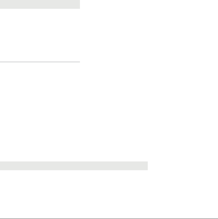
Because TimeML has been changed so many times, this partial-annotation approach is
much more sensible than starting from scratch every time the specification is updated.
However, taking this tack means that it is impossible to calculate IAA scores, because
the additions to the corpus were made piecemeal. To obtain IAA scores, then, the work
ing group tasked two annotators with experience in TimeML to annotate a subset of the
TimeBank documents, and scores were computed by comparing one annotator’s docu
ments to the other to obtain accuracy scores.
One of the problems with comparing extent tags is determining how to compare tags
that overlap but don’t match perfectly. For example, if a sentence has the phrase “will
have gone,” and one annotator marks the entire phrase as an EVENT and another anno
tator marks only “gone” as an event, should they be counted as a match, or not? It’s fairly
common to report both sets of statistics, and that’s what’s done in the TimeBank docu
mentation (see Table 10-1).
Table 10-1. IAA scores for TimeBank tags
TimeML tag Exact match Partial match
TIMEX3 .83 .96
SIGNAL .77 .77
EVENT .78 .81
ALINK .81
SLINK .85
TLINK .55
Partial matches can’t be calculated for link tags, since it wouldn’t make sense to consider
two links to be a partial match if they share a single anchor, which is why those values
are not provided in the table. The agreement for TLINKs is lower than for the other link
tags because of the same problem we’ve been discussing regarding linking events and
times: there are so many options for where links can be created, which makes creating
such links very problematic.
Don’t forget that when reporting on accuracy for tags, you also need to report on ac
curacy of attributes. Of course, you don’t include the attributes of tags that don’t match:
only compare the attributes of tags that have matching extents (for extent tags) or
matching anchors (for link tags). For TimeBank, these scores look like Table 10-2.
Table 10-2. IAA scores for TimeBank tag attributes
TimeML tag and attribute Average precision and recall Cohen’s Kappa
TIMEX3.type 1.00 1.00
TIMEX3.value .90 .89
TIMEX3.temporalFunction .95 .87
TIMEX3.mod .95 .73
210 | Chapter 10: Annotation: TimeML

TimeML tag and attribute Average precision and recall Cohen’s Kappa
EVENT.class .77 .67
EVENT.pos .99 .96
EVENT.tense .96 .93
EVENT.aspect 1.00 1.00
EVENT.polarity 1.00 1.00
EVENT.modality 1.00 1.00
ALINK.relType .80 .63
SLINK.relType .98 .96
TLINK.relType .77 .71
As would be expected, the kappa scores for the attributes are lower than the average
precision and recall scores, because kappa functions try to take into account the prob
ability that annotators are agreeing by chance, rather than by choice.
Overall, however, these scores are good, especially considering how complex TimeML
is (in terms of the number of tags and attributes) and how difficult temporal information
in a document can be to interpret, even for native speakers.
TimeML Becomes ISO-TimeML
The transformation of TimeML into an ISO standard didn’t happen overnight—in fact,
the process actually took several months to get going, and several years for the specifi
cation to be approved. We won’t go through all the gritty details of the process, but we
will give an overview of some of the major changes as described in Pustejovsky et al.
(forthcoming, 2010).
The first, and probably biggest, change for the specification was that it had to be made
more abstract: the model for the original TimeML was rooted in the idea that all anno
tations using the TimeML specification would be using an XML format for their data,
but that assumption couldn’t be made for an international standard. Therefore, the ISO-
TimeML model had to be expanded so that it could be represented in any number of
formats, even very different ones such as a UML (Unified Modeling Language) diagram,
or in different programming languages such as Lisp or Prolog. Doing this meant that
the ISO-TimeML working group had to be able to clearly express the relationships be
tween tags and their attributes, and how they could be connected to one another, so that
those relationships could be modeled in other representations.
TimeML Becomes ISO-TimeML | 211

Don’t worry if your own model isn’t quite as abstract as ISO-TimeML!
While having a model that can be represented in many different ways
without losing any data is definitely a perk that can make your anno
tation task more accessible to other people, it’s not required—TimeBank
was annotated before the ISO-TimeML abstraction was created, and it’s
still a very useful resource.
The next change that needed to be made was to make ISO-TimeML compliant with
other ISO standards, such as the Linguistic Annotation Framework (LAF). Since the
heavy lifting of creating a more abstract model had already been done, this primarily
involved modifying the tags so that they could be used in a stand-off annotion format.
The one used for ISO-TimeML is a token-based (rather than character-based)
annotation.
Also, in terms of the tags and their attributes for ISO-TimeML, the ways that temporal
relationships were handled had to be expanded so that the specification provided more
coverage for three different characteristics:
Order
How an event or time is positioned in a timeline relative to other events or times
Measurement
The size of a temporal entity, such as an event’s duration or the length of a temporal
interval
Quantity
The number of events being described in a phrase
The original versions of TimeML actually handled the “order” characteristic quite well:
TimeML already had a full set of temporal relations in the relType of the different link
tags, so those remained unchanged in the ISO specification.
However, the “measure” characteristic of the text wasn’t so fully covered. The original
TimeML had a type='DURATION' option for the TIMEX3 tag, but that didn’t fully capture
the different types of meanings that a “duration” could imply. Consider the different
interpretations of these two sentences: “Before leaving the house, I slept for two hours”
and “Before getting my pilot’s license, I flew for 300 hours.” In the first sentence, we can
reasonably interpret that the speaker slept for the full two-hour span, without any breaks.
However, the same assumption decidedly cannot be made for the second sentence, de
spite the fact that both sentences have the same basic syntax. To more fully express the
differences, a new type of link tag, the MLINK (measure link), was introduced in ISO-
TimeML. Essentially, the MLINK is used to explicitly state that a Timex expression is used
to “measure” the duration of an event.
212 | Chapter 10: Annotation: TimeML

The “quantity” characteristic was also somewhat underspecified in TimeML: as we
mentioned in previous discussions, phrases where a single extent indicated that multiple
events were taking place, such as “teach every Tuesday,” are difficult to annotate. This
is solved in ISO-TimeML by adding a “scopes” attribute to the TIMEX3 tag. This allows
the tag to have a relationship with the “teaches” event that is not limited to the relType
of the link, but rather provides a more open (but still semantically clear) interpretation
of the expression.
One other major change from TimeML to ISO-TimeML is the removal of the MAKEIN
STANCE tag. Annotators found the MAKEINSTANCE tag difficult to annotate, and so the
attributes from that tag were placed back into the EVENT tag, which allowed for easier
annotation, and the other additions to ISO-TimeML made up for the difference in how
the different expressions were annotated.
Finally, since ISO-TimeML is, in fact, an international standard, some modifications
had to be made to allow for the qualities of different languages besides English. For
example, in Chinese, aspectual markers (words such as begins, ends, etc. in English) are
not separate words, but rather are usually verbal suffixes. Also, some languages, such as
Spanish, combine tense and aspect in a single verb form, rather than using modifying
phrases. These and other cross-linguistic differences were accounted for in the ISO-
TimeML standard.
Overall, ISO-TimeML provides a more robust way to annotate temporal information,
and more accurate ways to encode temporal relationships for Question Answering tasks.
However, remember that ISO-TimeML is still only a specification: if you want to apply
it to your own annotation task, you’ll still need to write the guidelines yourself!
Modeling the Future: Directions for TimeML
Even though it’s now an international standard, TimeML isn’t set in stone: as theories
about temporal and event information in text are created and expanded, plans are being
made to expand TimeML to make use of those new and improved ideas. Some of these
possible additions are outlined in the following subsections.
Narrative Containers
One of the biggest hurdles in creating a TimeML-annotated document is creating the
link tags, particularly TLINKs. As we discussed previously in this book, the sheer number
of possible combinations of links between events and times makes creating a complete
overview of the relationships in the text nearly impossible for human annotators. An
other problem with the TLINKs as they exist in the text is that they often enforce the
creation of relationships that are open-ended in terms of capturing boundaries on when
an event can occur.
Modeling the Future: Directions for TimeML | 213
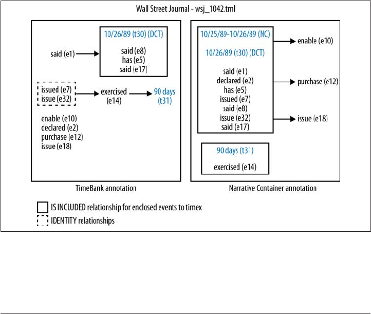
Consider a news article that begins with this: “The White House announced the presi
dent’s intention….” In a standard TimeML annotation, the “announced” event would be
given a “before” relationship with the document creation time. While this is technically
true (clearly, the announcement couldn’t have happened before the article was written),
it’s also extremely open-ended. How long before the writing of the article was the an
nouncement made? Presumably it was made fairly close to the Document Creation Time
(DCT) of the article—if it’s being reported in a newspaper, then the event most likely
occurred the day before. But a TLINK with a relType of before doesn’t distinguish be
tween an event occurring the previous day and an event occurring 100 years ago.
As a way to impose reasonable limits on when an event is likely to have occurred, the
idea of Narrative Containers was introduced (Pustejovsky and Stubbs 2011). Essentially,
a Narrative Container is a special type of time expression that acts like a bucket into
which events can be placed. Consider the difference between knowing that an event
occurred before January 13, 2012, and knowing that it occurred between January 11 and
January 13, 2012. Having extra restrictions on where an event can be placed in a timeline
allows for better temporal reasoning to be done over a document. Figure 10-1 shows the
difference between the TimeBank annotation of a document for TLINKs, and a TLINK
annotation using a Narrative Container instead of a DCT.
Figure 10-1. TimeML TLINKs versus Narrative Container TLINKs
The temporal value of a Narrative Container varies by genre: a daily newspaper will have
a much smaller Narrative Container than a monthly magazine and a much bigger one
214 | Chapter 10: Annotation: TimeML

than a broadcast on a 24-hour news service. However, the idea is both intuitive for
annotators and extremely prevalent in news articles: an experimental annotation that
incorporated Narrative Containers showed that nearly 50% of events in TimeBank were
linked to their document’s Narrative Container with an is_included relation type.
Eventually, Narrative Containers will be included in the official TimeML specifications
and guidelines.
Expanding TimeML to Other Domains
The original specifications for TimeML were designed for news articles, but temporal
annotation of other types of documents is also needed. The THYME (Temporal His
tories of Your Medical Event) Project is working to adapt the TimeML guidelines to the
clinical domain so that electronic health records can be automatically processed [see the
THYME Project wiki for more information]. Because events and their relations in med
ical documents have some special properties that are important to encode, some changes
must be made to TimeML to fully express what is being described by the document.
While the new guidelines are not out yet (as of summer 2012), a preliminary paper by
Savova et al. (2009) outlines some of the suggested changes to TimeML that would make
the system better for clinical documents, some of which we will describe here. For ex
ample, in traditional TimeML, the word postoperative would not be considered an event,
but rather a temporal marker, yet for clinical notes, it should be considered an EVENT,
along with other adjectives that indicate a person’s state of health. Clearly, for the pur
poses of clinical notes, it is important to be able to determine what a person’s condition
is at any given time, and marking statements such as “patient is feverish” is a good way
to incorporate their conditions into the temporal framework of the annotation.
Another change that was proposed is modifying the use of the EVENT tag’s tense at
tribute. In TimeML, this was used to indicate the tense of the verb being annotated (as
in “we went to the store” would have tense='past', “we will go” would have tense='fu
ture'). However, most medical documents are written in the past tense, because they
are written after the doctor meets with the patient, not while the meeting is taking place.
Therefore, the majority of the verbs in the documents are in the past tense, regardless
of whether they describe actions that occurred before the patient went to seek medical
attention or actions that occurred during the visit. As a result, the tense of the verb
doesn’t help to determine when an action occurred in the timeline, and so the use of the
tense attribute was modified to reflect the event’s relationship to the time of the patient’s
meeting with the doctor instead of reflecting the syntactic tense of the verb. So, for
example, “He woke with a headache” would be tense='past', whereas “rash under right
arm observed” would be tense='present'.
Modeling the Future: Directions for TimeML | 215

Whether or not an event caused another event to happen is also extremely important
to record in an annotation of a clinical document, and while TimeML does have the
tools to encode those relationships, the implementation and guidelines would need to
be greatly expanded to have the full coverage needed for medical records.
In addition to making changes to TimeML, Savova et al. note that other resources will
have to be expanded to the medical domain, such as PropBank (Palmer 2005), which is
a resource that provides semantic roles for verbs, but does not have a large medical
vocabulary. Similarly, part-of-speech (POS) and syntactic tree building systems will
need to be retrained for the clinical domain, because many sentences in medical records
are fragments rather than complete sentences.
The proposed changes to TimeML that we have outlined here based on Savova et al.’s
preliminary work are not necessarily going to be implemented the same way in the
THYME specifications and guidelines, but this discussion should give you an idea of
what aspects of clinical notes would need to be accounted for to make TimeML fully
useful for the clinical domain. The full set of specifications, when finished, will be posted
on the THYME project wiki page, https://clear.colorado.edu/TemporalWiki/index.php/
Main_Page.
Event Structures
We mentioned earlier that event structures didn’t get included in the model for TimeML
because of how difficult it would be to annotate all the information associated with
them. An event structure is basically the information that can be inferred from an event’s
occurrence. For example, in the sentence “He gave the book to his brother yesterday,”
despite not knowing who the sentence is describing, we can state that the following
subevents occurred:
• Prior to the giving event, “he” had the book.
• Prior to the giving event, his brother did not have the book.
• A giving event occurred.
• After the giving event, his brother had the book.
• After the giving event, he did not have the book.
Having access to this level of information makes any Question Answering System (QAS)
vastly more robust, but the level of detail required to annotate all those stages makes the
task nearly impossible for a manual annotation assignment.
While there are no plans to make event structure part of the annotation guidelines for
TimeML, work is being done to create a TimeML-compliant framework that can be
applied automatically to the EVENTs in an annotated document (Im and Pustejovsky
2010).
216 | Chapter 10: Annotation: TimeML

The approach being taken is to divide verbal events into aspectual classes (as described
in Vendler [1967], Dowty [1979], and Pustejovsky [1995], and incorporated into the
TimeML EVENT/MAKEINSTANCE tags), determine the verb’s class and subclass (e.g., “state”
or “change_of_location”), and then use that information to assign the event an Event
Structure Frame (ESF). The ESF is essentially a more formalized version of the subevent
list shown a few paragraphs up. With an event assigned an ESF, a lot more information
is known about the different states and processes being described in the text. The ESF
for the sentence we discussed earlier looks like this (Im forthcoming):
a. SENTENCE: He gave the book to his brother yesterday.
b. ESF of give
se1: pre-state: have (he, the_book)
se2: pre-state: not_have (his_brother, the_book)
se3: process: giving (he, the_book)
se4: post-state: not_have (he, the_book)
se5: post-state: have (his_brother, the_book)
This is a fairly complicated example of an event structure, as a lot is going on in that one
sentence. However, most verbs can be broken down into subevents, and so have similar
subevents embedded within them. We won’t go into a full description of exactly what
the different types of ESFs look like, and how the verb classes affect the frames; that
would be a book unto itself—or a dissertation; which, actually, it is! Check out (Im
forthcoming) for a complete overview of the event structures and subevent classifica
tions.
Summary
In this chapter we provided an overview of the MAMA cycle for TimeML, including a
discussion of the changes in goal, model, and specification. In particular, we looked at
the following:
•TimeML (formerly TenseML) was developed to provide a way to annotate events
and their temporal anchorings in text, specifically news articles. The bulk of the
TimeML specification development was done at a workshop in early 2002.
•One of the workshop’s goals was to create a gold standard annotated corpus, called
TimeBank. While initially TimeBank was going to contain 300–500 articles, the
density of the TimeML annotation eventually left that to be cut down to 183. How
ever, those articles are available for use as a resource from http://timeml.org/.
•TimeML didn’t spring from the minds of the workshop’s working group fully
formed; it was based on some existing temporal and event annotations, and a lot of
existing theories about linguistics and temporal reasoning.
Summary | 217

•A primary source for TimeML was the dissertation work of Andrea Setzer, which
resulted in the Sheffield Temporal Annotation Guidelines (STAG). The TIMEX2 tag
was also an influencing factor, though eventually the working group created their
own temporal annotation tag, TIMEX3.
•The specification for TimeML went through multiple iterations of the MAMA cycle,
both during the course of the working group and afterward, as more refinements
were made to the tags and attributes.
• During the workshop, periodic “annotation fests” were held, which allowed mem
bers of the working group to try out the current specifications on a small set of
documents, which proved to be a very effective way of finding places where the spec
wasn’t suited to the reality of the texts.
•The final pre-ISO TimeML specification (version 1.2.1) consisted of tags: TIMEX3,
EVENT, MAKEINSTANCE, SIGNAL, TLINK, ALINK, SLINK, and CONFIDENCE.
•Each of the TimeML tags has a set of attributes that is used to capture the relevant
information about the text, such as the verb tenses, modality, relation type of the
links, and value of the temporal expression (such as a calendar date or date relative
to another event).
•The current version of TimeBank (version 1.2) is annotated with version 1.2.1 of
TimeML. Because the specifications changed over the years, most of the annotations
in the current TimeBank are modifications of the previous annotation efforts, which
was more efficient than reannotating the entire corpus from scratch.
•ISO-TimeML is an expanded version of TimeML that allows for the annotation of
temporal information in languages other than English, and provides more robust
handling of complex temporal expressions. It is also compliant with other ISO
standards, and provides more interoperability options for different annotation
frameworks.
•Even though TimeML is currently an ISO standard, it is still undergoing changes
as more research is done into temporal information and events. Some of these
changes include adding new types of temporal objects, called Narrative Containers;
adapting the TimeML specification and guidelines to new domains, such as clinical
texts; and adding information about event classes and structures to TimeML-
compliant resources.
218 | Chapter 10: Annotation: TimeML

CHAPTER 11
Automatic Annotation: Generating TimeML
As you can see from the preceding chapter, modeling events, times, and their temporal
relationships in an annotation is a large and complicated task. In this chapter we will
discuss the TARSQI Toolkit, as well as other systems that were created to generate
TimeML as part of the TempEval-2 challenge held in 2010. In this chapter, we will:
• Discuss how a complicated annotation can be broken down into different compo
nents for easier processing
•Provide an in-depth discussion of the first attempt to create a system for creating
TimeML
• Show examples of how that system has been improved over the years
•Explain the approaches taken by other examples of systems designed to create
TimeML
•Discuss the differences between rule-based and machine learning (ML) systems for
complex annotation tasks
•Provide examples of ways that the TARSQI Toolkit could be expanded in the future
Overall, in this chapter we won’t be going into detail about how each aspect of TimeML
was automated; rather, we will provide a breakdown of how the task was approached,
and give a sense of some of the different options available for tackling a complicated
annotation.
219

The TARSQI Toolkit is not the creation of a single person, and we would
like to acknowledge all of the people who have contributed to its creation
and improvement (in alphabetical order): Alex Baron, Russell Entrikin,
Catherine Havasi, Jerry Hobbs, Seo-Hyun Im, Seok Bae Jang, Bob
Knippen, Inderjeet Mani, Jessica (Littman) Moszkowicz, Feng Pan, Jon
Phillips, Alex Plotnik, James Pustejovsky, Alan Rubenstein, Anna
Rumshisky, Roser Saurí, Amber Stubbs, and Ben Wellner. Special
thanks go to Marc Verhagen, the curator of the TARSQI Toolkit, who
provided and fact-checked much of the information in this chapter.
The TARSQI Components
When it comes to creating algorithms to perform automatic annotations, sometimes it’s
a good idea to break down a complicated task the same way that complicated annotations
are performed: one tag at a time. This is the approach taken with the TARSQI Toolkit
(TTK), the first system built for automatic creation of TimeML-annotated documents.
The TTK uses different components to create each of the different tags in TimeML. As
with any project that’s part of a Training–Evaluation cycle, the TTK has gone through
various stages of existence and improvement over the years. In this chapter we’ll walk
you through the different components of the first version of the TTK, as well as some
of the improvements that were made in later versions. We will also discuss some of the
other systems that have been created to automatically annotate documents with
TimeML.
The TARSQI (Temporal Awareness and Reasoning Systems for Question Interpretation)
Project was a government-funded research initiative that aimed to create systems for
enhancing documents with temporal and event information. The first versions of the
TARSQI components were released in 2005. Technically speaking, they weren’t actually
a toolkit yet, as each component was created individually and then linked together later.
TARSQI was a collaborative effort between Brandeis University, Georgetown University,
and ISI (Information Sciences Institute, part of the University of Southern California).
The primary paper on the components is from Verhagen et al. 2005.
Figure 11-1 shows the layout of the different components.
In the rest of this section, we’ll discuss how the automated creation of TimeML got
broken down into different components, and how each of those components works.
220 | Chapter 11: Automatic Annotation: Generating TimeML
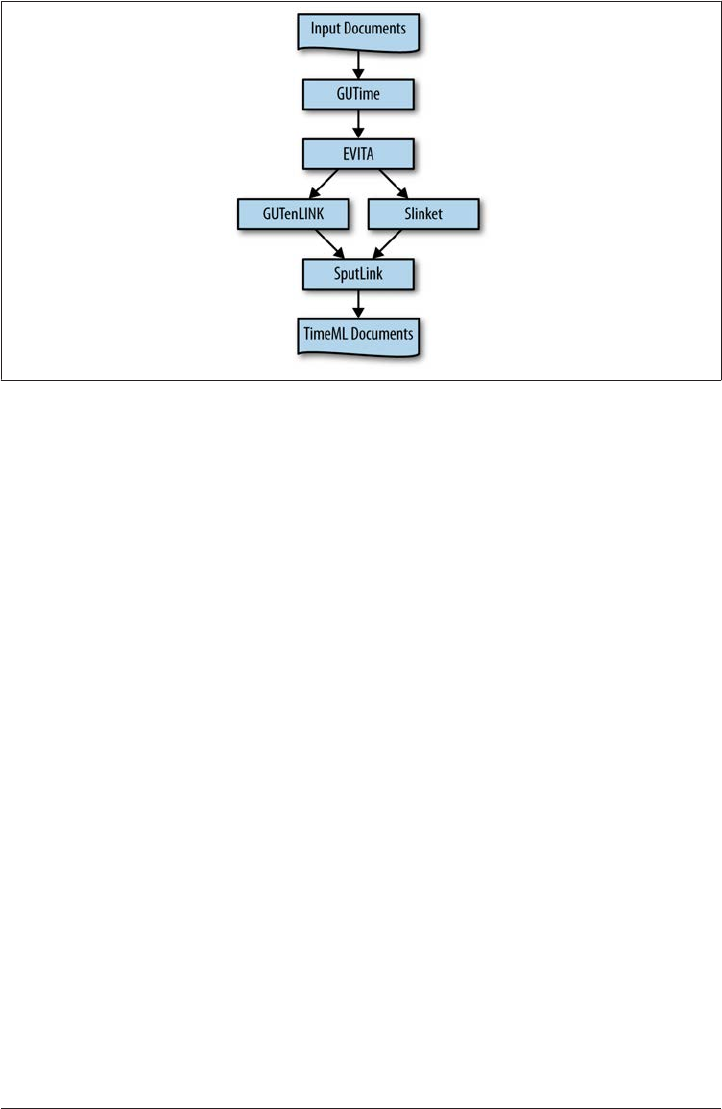
Figure 11-1. The TARSQI components in 2005
GUTime: Temporal Marker Identification
As we discussed in Chapter 10, temporal information in TimeML is marked with TIMEX3
tags, which not only encode time-related phrases in the text, but also contain other
attributes such as date/time values for those expressions, which can be evaluated relative
to other times in the text.
GUTime (Georgetown University Time) was used to create TIMEX3 tags as part of the
TARSQI set of components. GUTime extended the TempEx tagger from MITRE, and
used a rule-based system of regular expressions and phrase libraries to identify temporal
expressions and provide them with normalized values. Therefore, it was able to identify
and evaluate dates, such as “June 2, 2003,” as well as relative phrases such as “yesterday”
and “next month” (Verhagen et al. 2005).
Because GUTime was designed for newspaper articles, time expressions that relied on
context to interpret, such as “today,” were evaluated relative to the publication date of
the article, like this (example from http://www.timeml.org/site/tarsqi/modules/gutime/
index.html):
In Washington <TIMEX3 tid="t1” TYPE="DATE” VAL="PRESENT_REF” tempora
lFunction="true” valueFromFunction="tf1” anchorTimeID="t0">today</TIMEX3>,
the Federal Aviation Administration released air traffic control tapes from the night the
TWA Flight eight hundred went down.
The TARSQI Components | 221

In TimeML-annotated news articles, VAL="PRESENT_REF" is evaluated as a reference to
the publication date of the article, which here was given the TimeID of t0. You’ll notice
that the output from GUTime is in the form of inline annotation, rather than stand-off:
most systems available around 2005 had not yet adapted stand-off annotation, so the
practice has taken some time to become a standard.
EVITA: Event Recognition and Classification
TimeML EVENT tags in the TARSQI components were identified by EVITA—Events in
Text Analyzer, described in Saurí et al. (2005). Because events in text can be verbs (“We
went to the store”), nouns (“The investigation led to six arrests”), and even adjectives
(“The water levels have been high for months”), EVITA takes in texts marked up with
part-of-speech (POS) tags and syntactic chunks to identify parts of sentences likely to
contain events, then evaluates EVENT candidates based on their part of speech.
Verbal chunks are evaluated based on their content to determine the head of the verb
phrase, which is then checked to remove certain types of verbs, such as copular verbs
like “is.” Nominal events (i.e., nouns that function as events in the text) are identified in
two steps. First, the head of the noun chunk is checked against WordNet to determine
if it is a noun that is always associated with an event. If it isn’t clear whether the noun is
an event or not (words such as party, for example, can be events in the sense of “We had
a party last night,” or not, as in “The Republican Party”), then a determination of the
noun’s event status is made by a Bayesian classifier. Adjectives are rarely identified as
events, unless they were marked as such in TimeBank.
EVITA gives identified events an EVENT tag as well as the EVENT’s class type, and it also
generates MAKEINSTANCE tags for each identified event and provides values for the MAKE
INSTANCE tag attributes. Here is a sample of output from EVITA (provided by http://
www.timeml.org/site/tarsqi/modules/evita/index.html):
In Washington today, the Federal Aviation Administration <EVENT eid="e1”
class="OCCURRENCE"> released </EVENT> air traffic control tapes from the night
the TWA Flight eight hundred <EVENT eid="e2” class="OCCURRENCE"> went </
EVENT> down.
<MAKEINSTANCE eventID="e1” eiid="ei1” pos="VERB” tense="PAST”
aspect="NONE"/>
<MAKEINSTANCE eventID="e2” eiid="ei2” pos="VERB” tense="PAST”
aspect="NONE"/>
EVITA also provides information about event polarity, aspect, and the other attributes
that are part of the MAKEINSTANCE class.
222 | Chapter 11: Automatic Annotation: Generating TimeML

GUTenLINK
TLINKs in the TARSQI Toolkit were created by GUTenLINK, as described in Verhagen
et al. 2005. GUTenLINK used “hand-developed syntactic and lexical rules” (ibid.) to
create TLINKs. It created TLINKs based on three sets of circumstances in the text:
•If an event and time expression were in the same clause and no signal was present.
For example:
The Olympics will be held in London this year.
GUTenLINK: held is_included this year
•If an event was anchored to the Document Creation Time or DCT (such as reporting
verbs in a news article). For example:
Feb. 2, 2010
The president said in a press release that…
GUTenLINK: said before Feb. 2, 2010
•If the main event in one sentence is anchored to the main event in a previous sen
tence through clues such as tense or aspect. For example:
The cat woke up. It had been sleeping all day.
GUTenLINK: sleeping before woke up
Sample GUTenLINK output is shown here (from http://www.timeml.org/site/tarsqi/
modules/gutenlink/index.html):
In Washington <TIMEX3 tid="t1” TYPE="DATE” VAL="PRESENT_REF” tempora
lFunction="true” valueFromFunction="tf1” anchorTimeID="t0"> today </TIMEX3>,
the Federal Aviation Administration <EVENT eid="e1” class="OCCURRENCE"> re
leased </EVENT> air traffic control tapes from the night the TWA Flight eight hundred
<EVENT eid="e2” class="OCCURRENCE"> went </EVENT> down. There’s nothing
new on why the plane <EVENT eid="e3” class="OCCURRENCE"> exploded </
EVENT>, but you <EVENT eid="e4” class="OCCURRENCE"> cannot </EVENT>
<EVENT eid="e5” class="OCCURRENCE"> miss </EVENT> the moment. ABC’s Lisa
Stark <EVENT eid="e6” class="OCCURRENCE"> has </EVENT> more.
<MAKEINSTANCE eventID="e1” pos="VERB” eiid="ei1” tense="PAST”
aspect="NONE"/>
<MAKEINSTANCE eventID="e2” pos="VERB” eiid="ei2” tense="PAST”
aspect="NONE"/>
<MAKEINSTANCE eventID="e3” pos="VERB” eiid="ei3” tense="PAST”
aspect="NONE"/>
<MAKEINSTANCE eventID="e4” pos="VERB” eiid="ei4” tense="PRESENT”
aspect="NONE"/>
The TARSQI Components | 223

<MAKEINSTANCE eventID="e5” pos="VERB” eiid="ei5” tense="INFINITIVE”
aspect="NONE"/>
<MAKEINSTANCE eventID="e6” pos="NONE” eiid="ei6” tense="PRESENT”
aspect="NONE"/>
<TLINK eventInstanceID="ei1” relatedToTime="t1” relType="IS_INCLUDED”
rule="2-1” />
<TLINK eventInstanceID="ei2” relatedToTime="t1” relType="IS_INCLUDED”
rule="2-1” />
<TLINK eventInstanceID="ei1” relatedToEventInstance="ei3” relType="BEFORE”
rule="3-19” />
<TLINK eventInstanceID="ei3” relatedToEventInstance="ei4” relType="BEFORE”
rule="6-1” />
<TLINK eventInstanceID="ei3” relatedToEventInstance="ei6” relType="BEFORE”
rule="3-23” />
Slinket
The TARSQI component used to create SLINKs, or subordination links, was Slinket
(SLINK Events in Text) (Verhagen et al. 2005; Sauri et al. 2006). Slinket was a rule-based
system in which, once a subordinating event (such as say, promise, plan, etc.) was iden
tified in the text, shallow syntactic parses were used to determine the scope of the sub
ordination, and SLINKs were created between the subordinating event and any other
events deemed to be within its scope.
The SLINK also included information about the type of subordination being performed
and included that information in the relType attribute. Here is an example of the output
from Slinket (from http://www.timeml.org/site/tarsqi/modules/slinket/index.html):
The Soviet Union <EVENT eid="e12” class="REPORTING">said</EVENT> today it
had <EVENT eid="e13” class="OCCURRENCE">sent</EVENT> an envoy to the Mid
dle East.
<MAKEINSTANCE eventID="e12” eiid="ei12” tense="PAST” aspect="NONE”
pos="VERB"/>
<MAKEINSTANCE eventID="e13” eiid="ei13” tense="PAST” aspect="PERFECTIVE”
pos="VERB"/>
<SLINK lid="l2” relType="EVIDENTIAL” eventInstanceID="ei12” subordinatedE
ventInstance="ei13"syntax="thatClause_NOT_that"/>
224 | Chapter 11: Automatic Annotation: Generating TimeML
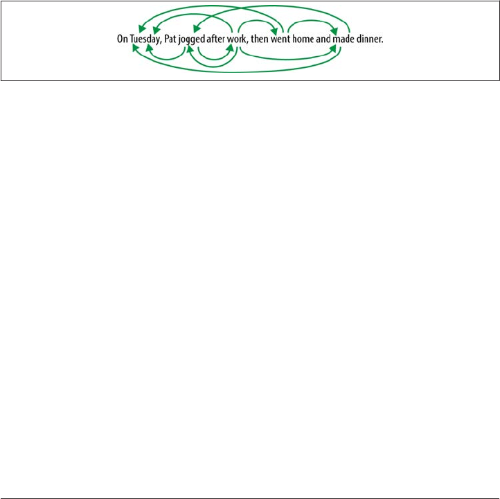
SputLink
SputLink is the TARSQI component that performed temporal closure calculations
(Verhagen et al. 2005); that is to say, given the set of TLINKs and SLINKs created by
GUTenLINK and Slinket, SputLink used interval algebra to infer relationships between
events and times based on existing links, and to create new TLINKs based on what was
already created.
In many ways, SputLink does what a human annotator can’t do, in that it fills in all the
possible relationships between events and times in the text (or at least, those that can
be determined to be accurate). Remember in “Refining Your Goal: Informativity Versus
Correctness” (page 35) when we used the example “On Tuesday, Pat jogged after leaving
work. Then Pat went home, made dinner, and laid out clothes for the next day.” We
showed how difficult it would be to have a human create all the possible links between
times and events that exist in those sentences. The diagram is shown in Figure 11-2.
Figure 11-2. All temporal relations over events and times
It’s clear why asking a human to create all those relations would be difficult, but it should
also be clear why having all those relationships would be good for a Question Answering
System (QAS): the greater number of relationships that were already worked out, the
easier it would be to answer questions about any given pair. SputLink provided the ability
to create most of those relationships without being trained on complicated annotations,
or relying on complicated rule libraries in GUTenLINK and Slinket to create the
TLINKs instead. Here is a sample of some TLINKs that SputLink could create:
On Tuesday, Pat jogged after work, went home and made dinner
Given: jogged AFTER work; went AFTER jogged; made AFTER went
SputLink: went AFTER work; made AFTER work; made AFTER jogged; etc…
Naturally, because temporal information in text can be vague, and because it’s not always
easy to determine what relationships can be extracted from a mixed set of TLINK
relTypes, “complete” sets of links like the one in Figure 11-2 can’t always be created. For
a more in-depth discussion of how closure can be run over temporal links, please see
Verhagen (2004).
The TARSQI Components | 225

Machine Learning in the TARSQI Components
You may have noticed that, aside from the nominal event classifier in EVITA, there are
no ML algorithms in the TARSQI components. As we said in Chapter 7, sometimes it’s
a good idea to start with rule-based systems as a way to suss out what features would be
good for an ML algorithm later on. There is also the fact that rule-based systems still
outperform machine learning algorithms on some types of annotation tasks. As it hap
pens, temporal expression annotation is one of them: as of the TempEval-2 challenge
(Verhagen et al. 2010), the top-performing system for identifying and evaluating tem
poral events in text was HeidelTime, a purely rule-based system (http://code.google.com/
p/heideltime/). However, more ML algorithms were incorporated into later versions of
the TARSQI system, as we will see in the next section. In the TempEval challenges,
different groups of researchers compete to create TimeML-generating systems, and dif
ferent teams will use rule-based, ML, and combination architectures to obtain their
results. We will discuss relative performances between the different types of systems in
“TimeML Challenges: TempEval-2” (page 230).
Improvements to the TTK
Although we haven’t provided details of the Training–Evaluation cycle for each com
ponent of TARSQI, we are providing an overview of the progression of the system as a
whole. We won’t go into excruciating detail about all the changes that have been made
over the years, but in this section, we will provide information about how some of the
individual components have changed, and how the system as a whole has been expanded
since it was first released in 2005.
In 2008, a paper was published detailing the transformation of the TARSQI components
into the pipeline that is now referred to as the TTK (TARSQI Toolkit) (Verhagen and
Pustejovsky 2008), and over the years, further improvements have been made, resulting
in the current TTK pipeline, which looks like the one shown in Figure 11-3 (Verhagen
and Pustejovsky 2012).
Clearly, this diagram is a lot more complicated than the one we showed you earlier in
the chapter, as it includes more stages before the TimeML processing starts, GUTime
and GUTenLINK are no longer part of the system, and there are more temporal relation
modules than there were before. Let’s go through these one at a time.
226 | Chapter 11: Automatic Annotation: Generating TimeML
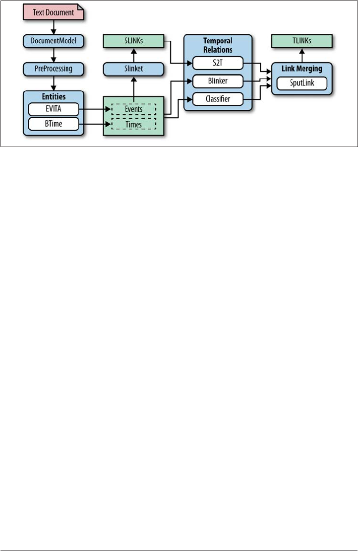
Figure 11-3. The TTK in 2012
Structural Changes
The new DocumentModel step cleans up input to the toolkit and provides support for
encoding and metatags (Verhagen and Pustejovsky 2008). The preprocessing modules
that provide the POS tags and chunks for EVITA are now part of the entire system, and
the TTK has recently moved from using inline annotation to a stand-off representation
that is compliant with the Linguistic Annotation Framework or LAF (Verhagen and
Pustejovsky 2012).
While these changes don’t directly affect the quality of the TimeML annotation that the
system creates, they do provide more stability for the system and make processing the
entire set of tags easier.
Improvements to Temporal Entity Recognition: BTime
In the newest release of the TTK, GUTime has been replaced with BTime, a temporal
expression tagger developed at Brandeis University. While still rule-based, BTime uses
a context-free grammar to create standardized representations of temporal expressions,
which provides a code base that is much easier to keep updated than the regular ex
pression libraries used in GUTime. While regular expressions are, of course, still a part
of identifying temporal expressions, it is now much easier to convert a phrase in the text
into a TIMEX3 tag. Here is a sample rule from the context-free grammar (Verhagen and
Pustejovsky 2012):
date —>
day month year (
CalendarDate(_(2), _(1),_(0) )
| month day year (
CalendarDate(_(2), _(0),_(1) )
| day month "," year (
CalendarDate(_(3), _(1),_(0) )
Improvements to the TTK | 227

This representation allows for various forms of a date to be transformed into a stand
ardized representation: “13 January 1982”, “January 13 1982”, and “January 13, 1982”
would all be turned into the calendar date form of “1982, January, 13” (or perhaps,
“1982, 01, 13”). This format is also very easy to add to; if a document contained a string
in the form “01-13-1982”, a new variation of the “date” grammar could be added,
like so:
| month "-" day "-" year (
CalendarDate(_(4), _(0),_(2) )
BTime also includes a set of rules used to take underspecified TIMEX3s, such as those
created for phrases like “yesterday” and “next month,” and provide them with normal
ized values based on the most likely temporal anchor for those expressions (usually, this
anchor is the DCT).
Temporal Relation Identification
In later versions of the TTK, the TLINK creator GUTenLINK was replaced with a suite
of temporal processing components. First, Blinker was developed as a replacement for
GUTenLINK. While Blinker is still rule-based, its library of rules has been expanded to
account for even more temporal relationships (Verhagen and Pustejovsky 2008):
• An event and Timex in the same noun phrase:
“Saturday’s party” —> party IS_INCLUDED Saturday
• An event being linked to the DCT:
“The New York Times reported that…” —> reported BEFORE DCT
• Events and syntactically subordinated events:
“The school board says they already voted on the matter” —> says AFTER voted
• Events in conjunctions:
“We swam and played all day” —> swam IS_INCLUDED play
• Two main events in consecutive sentences:
“I have been running from place to place all day. My cat, however, has been sleep
ing the whole time.” —> running SIMULTANEOUS sleeping
• Timexes with other Timexes:
“On Monday and Wednesday I went to the gym.” —> Monday BEFORE Wednesday
228 | Chapter 11: Automatic Annotation: Generating TimeML

In addition to Blinker, the S2T program takes the output from Slinket and turns the
SLINKs into TLINKs through a set of predefined rules. For example, in the sentence “Mary
said she went to the store,” an SLINK exists between “said” and “went,” but that would
be turned into a TLINK with the relation set “went BEFORE said.” The third addition to
the set of TLINK-creation components was a Maximum Entropy (MaxEnt) classifier
trained on the event relationships in TimeBank (Verhagen and Pustejovsky 2008).
Temporal Relation Validation
Naturally, with three different components creating TLINKs, the system needs some way
to determine which links are most likely to be correct, since it’s possible that Blinker,
S2T, and the classifier would come up with different relationships between the same
events. To deal with that possibility, the new TTK includes a Link Merging stage that
first orders links by their confidence values, and then merges them into a graph of TIMEX3
and EVENT tag nodes with the TLINKs as edges. As each link is added, SputLink checks
that the new edge will maintain the consistency of the graph. If it doesn’t, the link is
thrown out and the program proceeds to the next one (Verhagen and Pustejovsky 2012).
The confidence interval attached to each link is assigned to the links by the component
that created it, with the rule-based systems having hardwired confidence scores and the
classifier generating its own confidence scores based on the intervals. Finally, each score
is weighted based on the general accuracy of each component.
Temporal Relation Visualization
TLINKs can be very difficult to validate due to how hard they are to read, and the problem
becomes more difficult as the number of links in a document increases. As a way to deal
with this problem, a program for visualizing links was added to the TTK. This program,
called TBox, creates graphs of the document events and times and displays their rela
tionships with arrows to indicate directionality. The created timelines are read left to
right to indicate that the events on the left occurred before the events on the right; events
occurring at the same time are put in boxes together, and events with no known rela
tionship are stacked vertically. This system allows the output of the TTK to be much
more easily validated than simply trying to read the TLINK texts. Figure 11-4 shows a
TBox representation from Verhagen and Pustejovsky (2008).
Improvements to the TTK | 229
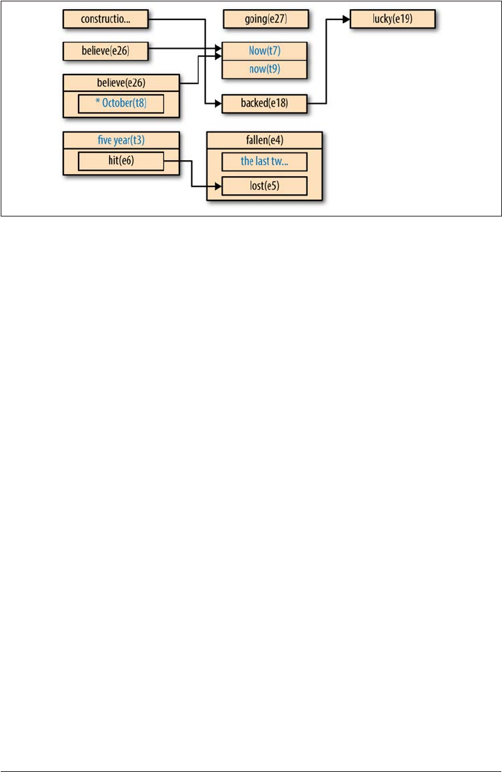
Figure 11-4. TBox representation of TLINKs between times and events
TimeML Challenges: TempEval-2
While so far we’ve only discussed the TTK as a way to create TimeML, other systems
have been built to automatically generate temporal annotations. Many of them have
been used at the TempEval challenges that were held as part of SemEval 2007 and
SemEval 2010. These evaluation challenges are often held prior to conferences, with the
results of the system’s accuracy scores released at the conference, at which point papers
on all the participating systems are also presented.
Because these challenges take place over the course of months rather than years, they
often take advantage of smaller subsets of existing linguistic problems, as that allows
participants to focus on particular aspects of a larger task. This is the approach that was
used for the TempEval tasks, where TimeML was reduced to a smaller set of tags to test
systems on only a few of the components of TimeML.
In particular, TempEval-2 (as described in Verhagen et al. 2010) used only TIMEX3,
EVENT, and TLINK tags as part of the corpus that was provided to event participants.
Additionally, the attribute values of those tags were cut down, as TIMEX3 tags were limited
to four temporal types—time, date, duration, and set—and the TLINK relTypes were
limited to before, after, overlap, before-or-overlap, overlap-and-after, and vague.
The TempEval-2 challenge was split into six tasks:
•A: Find the text extent of time expressions in a text and determine their type and
val attributes.
•B: Find the text extent of event expressions in a text and determine their class, tense,
aspect, polarity, and modality attribute values.
230 | Chapter 11: Automatic Annotation: Generating TimeML

•C: Determine the TLINK relationship between an event and a Timex in the same
sentence.
• D: Determine the TLINK relationship between an event and the DCT.
• E: Determine the TLINK relationship between two main events in consecutive sen
tences.
•F: Determine the TLINK relationship between two events where one syntactically
dominates the other.
Challenge participants could choose to participate in all the tasks or focus on the Timex
(A), event (B), or TLINK tasks (C–F). Additionally, they could choose to build systems
to create TimeML for Chinese, English, French, Italian, Korean, or Spanish (though not
all aspects of the tasks were available for all languages).
For tasks A and B, evaluation was performed by calculating precision, recall, and F-
measure for the TIMEX3 and EVENT tag locations, and the attributes were evaluated solely
with percentage accuracy. Percentage accuracy was also used for calculating the results
of the temporal relation tasks.
TempEval-2: System Summaries
Eight teams participated in TempEval-2, and combined, they submitted more than 18
systems, though only English and Spanish corpora were used for training and evaluation
(Verhagen et al. 2010). Accuracy scores varied widely between systems, and in the rest
of this section, we will go over how some of the participating groups created their systems
and how well those systems performed. The systems are presented in alphabetical order.
Edinburgh-LTG (Grover et al. 2010)
This system participated in tasks A and B on the English corpus. It provides a pipe
line of preprocessing modules that lemmatize, chunk, and provide POS tags for
input data. For the TempEval-2 event and Timex recognition tasks they used rule-
based systems to identify likely text extents and supply attribute information. Over
all the system obtained .85 precision, .82 recall, and .84 F-measure for the TIMEX3
task (with .84 accuracy for the type attribute and .63 for value), and for the event
recognition task, it obtained .75 precision, .85 recall, and .80 F-measure, with at
tribute values of .99, .99, .92, .98, and .76 for polarity, modality, tense, aspect, and
class.
HeidelTime (Strötgen and Gertz 2010)
HeidelTime is a system for identifying temporal expressions and assigning values
to them. It participated in task A of TempEval-2 on the English corpus. HeidelTime
is a purely rule-based system that uses the UIMA framework to provide sentence
boundaries, tokenization, and POS tags prior to identifying temporal expressions.
TimeML Challenges: TempEval-2 | 231

HeidelTime was run over the evaluation data using two sets of rules: one to optimize
precision, the other to optimize recall. Both systems obtained F-measures of .86 for
task A, making HeidelTime the most accurate system for temporal expression iden
tification and evaluation in English that participated in the challenge.
JU_CSE_TEMP (Kolya et al. 2010)
This system participated in all the TempEval-2 tasks on the English corpus. For
tasks A and B, it used rule-based systems to identify Timexes and events and to
assign attribute values. For tasks C–F, the system builders used a Conditional Ran
dom Field (CRF) ML algorithm, and used combinations of POS tags and event
attribute values (such as tense, polarity, class, etc.) as features. For the TIMEX3 task,
JU_CSE_TEMP obtained precision, recall, and F-measure scores of .55, .17,
and .26, respectively, but did not submit attribute values. For EVENTs, the system
obtained precision, recall, and F-measure scores of .48, .56, and .52, with attribute
scores of .98 for polarity and modality, .95 for aspect, .53 for class, and .30 for tense.
KUL (Kolomiyets and Moens 2010)
The KUL system participated in task A of TempEval-2 on the English corpus. The
system uses a MaxEnt classifier to identify likely temporal expressions, then uses
rules to normalize the output. A preprocessing step performs sentence detection,
tokenization, POS tagging, and parsing. Feature candidates for the classifier were
the last token in the selected phrase, lemma of the last token, POS tags, character
patterns in the phrase and final token, syntactic depth of the phrase, and other
syntactic features. Overall, the KUL system was run six times on the evaluation data,
with the best run obtaining precision, recall, and F-measure values of .85, .84,
and .84, and type and value attribute accuracy scores of .91 and .55, though other
evaluation runs resulted in more variable scores.
NCSU (Ha et al. 2010)
NCSU participated in tasks C–F on the English corpus, with two systems, NCSU-
indi and NCSU-joint. Both systems used a supervised ML system built on a Markov
Model, but the NCSU-indi system had a classifier trained for each task, while the
NCSU-joint system had one classifier trained for all four tasks combined. Each
system used a combination of lexical features, syntactic features, and semantic re
lation features to train its algorithms. Overall, NCSU-indi obtained accuracy scores
of .63, .68, .48, and .66 for tasks C, D, E, and F, and NCSU-joint obtained scores
of .62, .21, .51, and .25 for the same tasks. NCSU-indi had the highest accuracy score
for task F.
TERSEO + T2T3 (Saquete 2010)
This system participated in task A on the English corpus, and was a mix of the
TIMEX2 recognition system, TERSEO, and the T2T3 system. TERSEO was a rule-
based system for identifying temporal expressions as TIMEX2 tags in Spanish, which
was then automatically extended to recognize temporal expressions in English and
232 | Chapter 11: Automatic Annotation: Generating TimeML

other languages. The T2T3 system was also rule-based, and provided a way to con
vert TERSEO’s TIMEX2 tags into the TimeML TIMEX3 tags. Overall, this combination
of systems obtained precision, recall, and F-measure scores of .76, .66, and .71 for
TIMEX3 tag creation, and accuracy scores of .98 and .65 for the type and value at
tributes.
TIPSem (Llorens et al. 2010)
The TIPSem system participated in all of the TempEval-2 tasks in both Spanish and
English, and used CRF models using morphological, syntactic, and event informa
tion as features, as well as semantic information such as semantic roles and gov
erning verbs for TIMEX3 and EVENT recognition. For the TLINK relations, they used
combinations of attribute values, syntactic information, and semantic roles about
the Timexes and events participating in the links as classifier features. TIPSem was
run twice over the evaluation data in both Spanish and English. It obtained the
highest results for Spanish task A (against one other system), and was the only entry
for the other Spanish corpus tasks (where it scored a .88 F-measure for task B, .81
for task C, and .59 for task D). For task A on the English corpus, it scored (.
92, .80, .85, .92, and .65) and (.88, .60, .71, .88, and and .59) for precision, recall, F-
measure, type, and value, respectively, for each run. For tasks C–F on the English
corpus, it scored (.55, .82, .55, and .59) and (.54, .81, .55, and .60).
TRIPS and TRIOS (UzZaman and Allen 2010)
TRIPS and TRIOS were two different programs submitted by the same team of
researchers, though both used combinations of Markov chains and CRF models
trained on various syntactic and attribute features. The systems returned the same
results for task A: .85 precision, .85 recall, .85 F-measure, .94 type accuracy, and .76
value accuracy. For task B, TRIOS obtained precision, recall, and F-measure values
of .80, .74, and .77, while TRIPS scored .55, .88, and .68, respectively. TRIOS ob
tained the highest score (.65) for task C, while TRIPS obtained the highest score
(.58) for task E.
UC3M (Vicente-Díez et al. 2010)
The UC3M system participated in task A for the Spanish corpus and used a rule-
based system for both identifying temporal expressions and evaluating the expres
sions. Overall, the system obtained precision, recall, and F-measure scores
of .90, .87, and .88, respectively, and .91 for type accuracy and .83 for value accuracy.
USFD2 (Derczynski and Gaizauskas 2010)
The USFD2 system participated in tasks A, C, and E in TempEval-2. The system
uses a mix of rules and classifiers: a rule-based system identifies and evaluates tem
poral expressions, while a MaxEnt classifier is trained on features that describe
temporal signals. For task A, the system obtained precision, recall, and F-measure
values of .84, .79, and .82, with accuracy scores of .90 for type and .17 for value. It
also scored .63 accuracy for task C and .45 accuracy for task E.
TimeML Challenges: TempEval-2 | 233

Overview of Results
Of the participating systems, there was a strong mix of rule-based and ML-based sys
tems, with no clear winner as the “best” way to tackle automated TimeML annotation.
While the classifier-based systems obtained the highest scores on the temporal relation
tasks, not much can be drawn from that statement, because no rule-based systems par
ticipated in tasks C–F for TempEval-2 in the first place [although the best-performing
system from the previous TempEval, which had tasks similar to C–F, was a mixed rule-
based and statistical learning system (Puscasu 2007)].
For the temporal expression recognition task, the best-performing system was Heidel
Time, which is a purely rule-based system, whereas the ML system TIPSem obtained
the best results on the event recognition task. However, it should also be noted that, due
to the time constraints inherent in participating in a challenge like TempEval (or any of
the SemEval challenges), the situation may favor ML algorithms, because they are much
faster to select features for and train on different combinations in a short period of time,
while rule-based systems take time to build.
Essentially, we would argue that for complex tasks, the question of whether rule-based
or ML systems (or combinations of the two) are “best” has not been entirely settled, and
we anticipate that the question will remain open for some time to come.
Future of the TTK
As with any ongoing project, the TTK is still undergoing improvements and being ex
panded, in terms of improving the quality of the output, increasing the flexibility of the
system, adding to the domains where the TTK can be used, and incorporating new
theories and the changes to TimeML that are still ongoing. In the rest of this section, we
provide an overview of some of the proposed changes and improvements to the TTK,
and some discussion of how those changes would be made (Verhagen 2012).
New Input Formats
Currently, the TTK is a start-to-finish pipeline: all the processing that needs to be done
to a document to generate TimeML is already in the TTK, including tasks that are not
directly TimeML-related but are necessary for some of the modules, such as POS tagging
and syntactic chunking. However, because these systems are built into the TTK, other
researchers who may wish to provide their own POS taggers, temporal expression rec
ognizers, or other types of information have no way to do so short of rebuilding the
TTK themselves.
Of course, building a system that can accept input from other algorithms is always a bit
tricky, because it’s difficult to ensure that the input data will be compatible with the rest
of the pipeline. This is particularly difficult if, for example, a user wants to input inline
annotations when the TTK has switched to using stand-off representations. Of course,
234 | Chapter 11: Automatic Annotation: Generating TimeML

the technical aspects of this modification to the TTK don’t directly affect the MATTER
cycle, so we won’t go into much detail about them: suffice it to say that if you are inter
ested in creating a processing pipeline like the TTK for your own task (or taking ad
vantage of an existing pipeline or set of algorithms), ensuring compatibility between the
components can be very tricky, so it’s something to think about carefully before diving
into a project.
Narrative Containers/Narrative Times
Just at TimeML and TimeBank are being augmented with Narrative Containers [as we
discussed in “Narrative Containers” (page 213)], there are also plans to add a new set
of rules to the temporal linking components of the TTK to take advantage of the Nar
rative Container concept. Because Narrative Containers primarily influence where
events and times in the text are anchored, most of the changes to the TTK to accom
modate the idea would be in BTime and Blinker.
First of all, BTime’s rules for assigning temporal values would have to be modified to
incorporate the idea of Narrative Containers and Narrative Times. While in some cases
this would be relatively trivial (e.g., changing the default anchor for times from the
Document Creation Time to the Document Narrative Container), others require much
more thought. Consider what rules would have to be written to resolve the values in this
sentence:
June 12, 2012
Last Sunday was the closing day of Pippin at the local theater. The show, which ran from
the previous Sunday…
Here, “Last Sunday” would be evaluated in relation to the DCT, which would give it a
value of June 10. However, the phrase “previous Sunday” is referring to the Sunday before
the 10th, which would be June 3; June 10 has been established as the local Narrative
Time, and the interpretation of the second sentence relies on that information. How far
the scope of a Narrative Time extends into the document is highly variable, however,
and so it is not easy to write a set of rules that will determine what the anchor for each
new temporal expression will be. Consider this alternate press release:
June 12, 2012
Last Sunday was the closing day of Pippin at the local theater. But next Monday a different
group will start a run of The Phantom Tollbooth…
In this case, both temporal expressions must be given values relative to the DCT—the
influence of “Last Sunday” as a Narrative Time does not extend to the next sentence.
Future of the TTK | 235

This may be a system where a robust set of rules could perform well at determining
where a temporal expression’s anchor should be, but it may also be the case that a clas
sifier trained to examine other features could make a guess at what the Narrative Time
is at each part of the document, which could then be used to inform BTime.
Similarly, Blinker would have to be modified to also take into account Narrative Times
and containers so that correct temporal links could be produced. We’ll talk a little more
about the effect of Narrative Containers on linking tasks in the next section.
Medical Documents
As we mentioned previously, TimeBank is a set of news articles and transcripts that was
annotated with TimeML. Therefore, the components of the TTK have been optimized
to provide the best possible output for those document types. However, a new corpus
often brings with it new challenges, and one of the goals for the TTK is to expand the
different types of corpora that it can reliably process.
One of the first new areas that is being explored with the TTK is medical documents
such as hospital discharge summaries. A preliminary study (Stubbs and Harshfield
2010) examined what would need to be done to make the TTK able to process electronic
health records (EHRs). In particular, that study looked at what was needed to identify
whether the TTK could be used to determine if the patient described in each record was
taking a particular type of medication—cholesterol-lowering drugs called statins—
when the patient was admitted to the hospital.
The necessary changes were not fully implemented in the TTK; rather, the gaps in the
toolkit’s capabilities were filled in with auxiliary Perl scripts so that results could be
obtained more quickly. However, the study identified some important aspects of changes
that would need to be made to the TTK to make it more useful in the medical domain.
Using an existing system and adding to it from the outside is a perfectly
valid way to test your own theories about what will and won’t work with
your own corpus and features. While ideally you would eventually build
a complete system for your own task, sometimes it’s best to find a work
around to make sure your idea will work.
One of the first problems that was encountered was that EVITA didn’t have the vo
cabulary to recognize medical events, specifically drug prescriptions. To work around
that, a list of statins was obtained from an MD, then augmented with alternative names
and spellings from websites such as PubMedHealth. Then this list was used to identify
mentions of those drugs in the patient records and mark them using TimeML EVENT
tags with the special attribute value class="MEDICINE".
236 | Chapter 11: Automatic Annotation: Generating TimeML

The next aspect of the medical records that had to be addressed was the impact of the
document structure on the interpretation of events. It is common for EHRs to be divided
into sections, such as “Patient Medical History,” “Current Medications,” Family History,”
“Course of Treatment,” and so on. Naturally, these section headers have important tem
poral information regarding when the events occurred—they essentially provide a new
Narrative Container for each section of the document. Therefore, a Perl script that rec
ognized section headers was written, and each one was marked as a TIMEX3 tag with the
modified attributes type="HEAD". The mod attribute was also given special values, which
indicated whether the Narrative Container for that section occurred prior to hospital
admission, during the hospital stay, after release from the hospital, or did not contain
any temporal information.
To take advantage of the new EVENT and TIMEX3 tags in the documents, the Blinker
component of the TTK was given a new set of rules that took into account the infor
mation about the Narrative Containers that were now part of the section headers.
Blinker then created TLINKs for each medication EVENT tag related to the section headers,
and those were evaluated by a small program to determine whether the patients in
question were on statins at their hospital admission date.
Using these modifications compared to a human-annotated corpus the TTK had an
accuracy rating of 84% overall, and 95% accuracy on the files that the human annotators
found to be unambiguous. These results were promising, and there are plans to incor
porate some of these changes into a version of the TTK that can be used in the medical
domain.
Cross-Document Analysis
Currently, the TTK only analyzes a single document at a time, and TLINKs only connect
events and times in each document as it’s processed. However, there are many fields
where being able to process multiple documents all at once, and generate relationships
between the events and times in those documents, would be incredibly useful, partic
ularly when evaluating the progress of news stories or medical records. Of course, by
adding more times and events, the jobs of the temporal closure algorithms become even
more complicated, and to provide the most useful information on these topics it would
be best if the TTK was also able to perform cross-document event coreference resolution.
But identifying two different events in two different articles (or even in the same article)
as referring to the same event is not an easy task, and more work needs to be done in
this area before cross-document analysis will be truly useful.
Future of the TTK | 237

Summary
In this chapter we discussed the process used to automate the creation of TimeML-
annotated texts through the building of the TARSQI Toolkit. In particular, we discussed
the following:
•The TARSQI Toolkit (TTK) provides an example of a long-term production cycle
for a system built to reproduce human annotation. While this chapter didn’t go into
details of the Training–Evaluation cycles of each individual component, it did pro
vide a “big picture” look at a complex system.
•Each component in the TTK is designed to recreate a tag in the TimeML specifi
cation—and later versions of the TTK use multiple components for some of the
tags.
•Using a divide-and-conquer approach may be the best way to approach your own
annotation, especially if you have a task where some parts of the annotation rely on
the existence of others (e.g., TLINKs can be made without TIMEX3 and EVENT tags
already in the document).
•Rule-based systems can be an excellent way to try out ideas about how to automat
ically create your annotations, and in some cases will still outperform ML algo
rithms.
•The question of whether rule-based or statistics-based systems are superior for
complicated tasks such as temporal processing has not yet been answered, as both
systems tend to perform at nearly the same accuracy levels.
•There is always more that can be done to improve an automatic annotation system,
whether it’s simply improving accuracy, or expanding the genres or domains that
the system can be used to annotate.
238 | Chapter 11: Automatic Annotation: Generating TimeML

CHAPTER 12
Afterword: The Future of Annotation
In this book we have endeavored to give you a taste of what it’s like to go through the
entire process of doing annotation for training machine learning (ML) algorithms. The
MATTER development cycle provides a tested and well-understood methodology for
all the steps required in this endeavor, but it doesn’t tell you everything there is to know
about annotation. In this chapter we look toward the future of annotation projects and
ML algorithms, and show you some ways that the field of Natural Language Processing
(NLP) is changing, as well as how those changes can help (or hurt) your own annotation
and ML projects.
Crowdsourcing Annotation
As you have learned from working your way through the MATTER cycle, annotation
is an expensive and time-consuming task. Therefore, you want to maximize the utility
of your corpus to make the most of the time and energy you put into your task.
One way that people have tried to ameliorate the cost of large annotation projects is to
use crowdsourcing—by making the task available to a large group of (usually untrained)
people, it becomes both cheaper and faster to obtain annotated data, because the an
notation is no longer being done by a handful of selected annotators, but rather by large
groups of people.
If the concept of crowdsourcing seems strange, think about asking your friends on
Facebook to recommend a restaurant, or consider what happens when a famous person
uses Twitter to ask her followers for a piece of information, or their preferences for an
upcoming event. These are examples of crowdsourcing—instead of just asking one per
son, or a focus group, the question is asked of as many people as can be reached, and
the answer is extracted from there.
239

Naturally, asking questions about linguistic annotation on Facebook or Twitter isn’t
going to be a very efficient way of collecting the desired information. However, other
platforms exist for just that purpose, and here we’re going to go over a few of them. Each
of these methods can be performed within the MATTER cycle—they still require com
ing up with an annotation goal, finding a specification, and defining guidelines for how
the annotation will be applied, but the guidelines here aren’t the traditional approach of
writing an instruction manual and having the annotators read and apply what they learn.
Amazon’s Mechanical Turk
One approach to crowdsourcing is this: rather than hire a small number of annotators
to annotate a corpus at relatively high wages, the annotation task is divided into very
small tasks, which are then distributed over a large number of people for very small
amounts of money per task. The most widely used resource for this at the moment is
Amazon’s Mechanical Turk (MTurk), where researchers (or businesses) create Human
Intelligence Tasks (HITs) which are then posted on something like a job board, and
Turkers (as the workers are called) have the option to take on a task, and get paid for
completing it. Turkers are usually only paid a few cents for each HIT they complete, so
it’s easy to see why researchers are interested in using this system: paying a few cents per
annotated phrase will almost always be cheaper than paying an hourly wage for anno
tators to perform the full annotation described in your specification and guidelines.
Also, because the individual annotation tasks can be done in minutes or even seconds,
annotations can be gathered very quickly, whereas full document annotation can take
much longer when only a few annotators are working on the entire corpus and specifi
cation.
While the cost- and time-saving measures certainly make the MTurk paradigm sound
ideal, the HIT system is by no means perfect. First of all, it requires that each annotation
task be broken down into “microtasks” to present the Turkers with a simple and efficient
interface. However, not all annotation tasks are suited to be turned into microtasks or
are compatible with the HIT interface (e.g., it would be very difficult to design an in
terface that would make it easy to create syntactic trees). Even if an annotation specifi
cation can be turned into a series of microtasks, doing so may remove the annotator’s
ability to develop intuitions about the annotation, which may affect the results.
In addition to the interface problems, there may be problems with the quality of the
data. A recent survey (Fort et al. 2011) of articles on the MTurk system showed that it
was difficult for researchers to enforce requirements about their annotators (such as
their native language being English), and that the quality of data varied greatly from
Turker to Turker, which made it difficult to separate the good annotations from the bad.
240 | Chapter 12: Afterword: The Future of Annotation

Aside from the problems with data quality, Fort et al. also looked into the ethical issues
surrounding the use of MTurk systems, and found that a significant number of Turkers
use HITs as a main source of income. However, because each HIT only pays a few cents,
the average income for a Turker is around $2/hour, so it’s somewhat difficult to justify
using the MTurk interface as a source of labor.
In terms of the MAMA cycle, the key to using MTurk is to test your HITs to make sure
the annotation goal of each HIT is small enough to be performed quickly and accurately,
and that the annotation guidelines are only a few sentences long. As with any project,
it will take a few tries to get a HIT design that gets you the annotation you need in the
degree of detail you want.
Games with a Purpose (GWAP)
Fortunately, other ways of crowdsourcing data also exist. One widely talked about
method is that of using “games with a purpose”—essentially, computer games designed
to make an annotation task fun so that people will do it voluntarily. A few successful
annotation games are:
Phrase Detective
Purpose: Collect information about coreference relations in text.
This game asks players to examine a short piece of text, with a section of the text (a
word or phrase) highlighted in orange. The players are then asked if the phrase is
referred to earlier in the text. An example given on the website for the game (using
bold text instead of orange) is “‘It is for me,’ he said.” The correct answer is to indicate
that “he” refers to the same object as “me” in that sentence.
Sentiment Quiz
Purpose: Collect user intuitions about the sentiment (positive or negative) of
phrases.
This game asks players to determine whether the word, phrase, or sentence ex
presses a positive, neutral, or negative emotion. For example, the website shows the
sentence “We are headed down a path that is certain to end in the destruction of
our experiment in democracy.” The players use a scale of five options to rate the
sentiment, and their answers are scored against the rest of the players to determine
accuracy.
Guess What?
Purpose: Collect single-word descriptions of pictures for image recognition
training.
From the website: “is a two-player game where players have to choose an image
from an array of images based on clues sent to them by the networked partner. The
partner sees only one image and what their partner is guessing.”
Crowdsourcing Annotation | 241

ESP Game
Purpose: Collect descriptions of pictures for image recognition training.
This game pairs up players anonymously and shows them both the same picture.
Players are then given two and a half minutes to come up with the same word to
describe 15 images. To increase the difficulty, the players are given a list of words
that are “banned” for each picture, to get them to use less common descriptors.
These games avoid the potentially exploitative nature of MTurk, as they entice users to
spend their free time providing the annotations because they enjoy the game. However,
GWAPs may not completely avoid the problem of messy data. A well-designed game
can put in place mechanisms that help curate content and reward players for inputting
higher-quality data, but it can be difficult to design a game that executes these actions
well.
Effective GWAPs can be extremely difficult to design effectively, and
even well-designed games don’t produce perfect data. People will cheat
at games to obtain higher scores, and they will often produce data that
is incorrect or in other ways “dirty,” and therefore needs to be cleaned
up. For more information on this, see Speer et al. 2010.
Here, the MAMA cycle relies on the guidelines being incorporated into the rules
and/or strategy of the games. Having a way to reward players for providing good data
will help increase the quality of the annotations obtained.
A list of games with a purpose can be found at http://semanticgames.org/category/text-
annotation-games/ and http://www.gwap.com/.
User-Generated Content
Finally, another way to crowdsource data is to simply ask for it! The MIT Open Mind
Common Sense project is a website that allows users to input information they find to
be “common sense”—that is, that relays knowledge about the world that wouldn’t nec
essarily be stated in a text because “everybody knows it,” such as the fact that a cat is an
animal and can be a pet. This information will be used “to make indoor mobile robots
that work in environments like homes and offices more intelligent.”
Again, because this information is freely given by participants, it avoids the problems
of exploitation. Like the GWAPs, however, users can input data that is false, though the
fact that people aren’t receiving any general benefit from the system (other than
participating in research) may mean that users are less likely to input bad data. Like the
other crowdsourcing paradigms described in this chapter, getting good annotations
requires having a task and guidelines suited to the presentation, but also requires that
the task is something people will be willing to spend time doing.
242 | Chapter 12: Afterword: The Future of Annotation

Handling Big Data
You already know that when it comes to corpora, bigger is better. However, the Big Data
mantra comes with its own set of problems, particularly when it comes to annotating
large amounts of data in accurate and useful ways. We just talked about some of the
ways people are tackling the problem from the annotation side, but there are also some
techniques that can be used on the ML side, particularly for corpora that are large, but
perhaps not fully annotated.
Almost all of the techniques that attempt to handle Big Data in computational linguistics
(and Artificial Intelligence in general) approach the phenomenon as an opportunity
rather than a problem. With so much information, so this reasoning goes, is there some
way to leverage particular properties of the dataset that will allow us to build even better
learning algorithms? The strategy shared by all of the approaches we’ll cover in this
section is to try to make the best of as little annotated (training) data as possible, and to
leverage different properties of the Big Data. As many ML researchers have pointed out,
the content on the Web is highly redundant, and this can be used to the advantage of
weak learners (as in boosting) or partial learners (as in co-training and other semi-
supervised approaches).
Generally, people who talk about Big Data talk about the “3 Vs”: volume, velocity, and
variety. These were posited by Doug Laney (2001), and are generally taken to be:
Volume
The size of the data that has been collected. Because this is “Big Data,” the volume
of a dataset is often measured in gigabytes or terabytes, rather than in number of
documents or words.
Velocity
The speed at which data can be collected and processed. The faster the data is
collected and brought into the set, the more up-to-date and relevant the dataset
becomes.
Variety
Not only refers to collecting different types of web pages, or pages in different lan
guages (though that is a factor), but also refers to collecting different types of data,
from different sources and in different formats, to create as complete a picture of
the state of your chosen field as possible.
Boosting
One approach that might be useful for handling the Big Data problem with applying
learning algorithms over language data is called boosting. This is a meta-algorithm, that
is, a strategy for directing supervised learning algorithms that tries to come up with a
Handling Big Data | 243
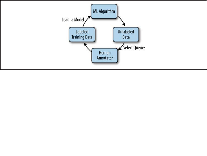
strong learner from a bunch of weak learners, given a dataset. The algorithm AdaBoost
(Freund and Schapire 1995), for example, has been used in conjunction with many
different supervised learning classifiers for NLP purposes, and has been shown to work
well when there are lots of noisy contexts, dirtying up the classifier dataset.
Boosting algorithms work by creating an overarching classification system that itera
tively adds new, less accurate classifiers. As each new classifier is added, the results of
each classifier are weighted based on the accuracy of all the classifiers. This allows the
overarching system to obtain progressively better models for how to classify the data
being examined, and each new classifier is trained in a way to focus on the data that the
other algorithms are misclassifying. This allows the full system to have a set of classifiers
that individually will only perform adequately over a set of data, but combined can create
much more accurate classifications when the outputs of all the internal algorithms are
weighted against one another.
Active Learning
Active learning is a kind of supervised learning where the learner can query the user to
obtain information about the labeling of a sample that it is trying to identify. That is,
the learning algorithm itself is able to choose the data from which it is learning, posing
a query to a human annotator about an unlabeled instance. Figure 12-1 shows the active
learning process.
Figure 12-1. The active learning process (based on an illustration from Settles 2010)
The active learning process has been applied successfully to several areas of NLP, in
cluding information extraction, Named Entity (NE) recognition, part-of-speech (POS)
tagging, text categorization, word sense disambiguation, and other areas (Settles 2010;
Olsson 2009). The trick is for the learning algorithm to automatically figure out how to
ask the most appropriate question to the oracle (the human annotator). There are several
different strategies for selecting the next document to present to the annotator, such as
the following (paraphrased from Settles 2010):
244 | Chapter 12: Afterword: The Future of Annotation

Uncertainty sampling
Using this strategy, the learner selects the object for which he is least sure of the
correct categorization to present to the user.
Query-by-committee
Here, the “committee” is a set of models using different hypotheses about the data
that get to “vote” on what is queried next by determining what parts of the corpus
they disagree on the most.
Expected model change
This strategy selects the query that would most affect the current algorithm if the
label for the query was known; that is, the query that will add the most information
to the model (as best as can be determined beforehand).
Expected error reduction
This is similar to the preceding strategy, but this method selects the query that it
deems will lead to the greatest reduction in the amount of error being generated by
the learner. However, expected error reduction is usually very expensive (compu
tationally) to calculate.
Variance reduction
Rather than trying to reduce the amount of error, this method tries to reduce the
amount of noise in the model.
Density-weighted methods
These strategies use the idea of choosing the data that is most representative
(feature-wise) of the rest of the pool, using the assumption that learning more about
the features that most of the data shares will more quickly allow all the data to be
classified.
One other method that can be used is to simply select the query randomly from the set
of unlabeled data; while this method is certainly the fastest way of choosing a query, it
does not improve the algorithm as quickly as some of the other methods can in terms
of the number of times the human annotator is asked to provide input. Regardless of
the selection strategy that you use, however, active learning can be an excellent way to
train an algorithm to create the wanted annotations by direct user input (though it does
require that the user have a good grasp of the annotation task at hand!).
Semi-Supervised Learning
We already described the methodology of semi-supervised learning (SSL) in “Semi-
Supervised Learning” (page 163), but it’s worth revisiting here. SSL is an excellent way
to work with Big Data in an annotation/ML project, because it allows for a small an
notated set to be used more effectively over a larger corpus. The co-training and “coupled
training” approaches to SSL are particularly effective for datasets that already have some
sort of user-generated annotation, such as data from Twitter or Flickr, where users tag
Handling Big Data | 245

their input themselves. This can function as the first set of input into a co-training
algorithm, and then a MATTER-type annotation can be done by a researcher to capture
other features of the data that would be useful in an ML model. Because so many dif
ferent online platforms come with ways for users to tag or annotate their data in other
ways, SSL techniques don’t require that a researcher create and annotate two separate
models over the data, since one of the models is already provided by the users (though
there is, of course, always some messiness in user-generated content).
NLP Online and in the Cloud
The idea of cloud computing has been invading nearly every aspect of people’s lives:
from using cloud storage to store music and back up data to the return of the idea of
distributed computers. Additionally, there has been a lot of movement to create central
repositories, and more efforts to create interoperability standards as well as software
that adheres to those standards. In this section we will examine some of the ways that
cloud computing can affect NLP and annotation, and ways that the Internet is being
used to organize NLP resources.
Distributed Computing
A common problem with NLP systems is that they are often very processing-intensive.
Consider all the steps involved in the most recent version of the TARSQI Toolkit that
we described in Chapter 11: starting from an unlabeled document, the text is separated
into sentences, chunked and marked with POS tags, and examined for events and time
expressions, the time expressions are evaluated, temporal signals are identified, SLINKs
are created, three different systems are used to create TLINKs, those links are evaluated
and merged, and then closure is run over the links that were kept. That requires a lot of
steps, and when all of them are being run on a single machine, even a small document
can take minutes to annotate, and a large corpus could take days.
Obviously, every year there are increases in the speed of computer CPUs and the memory
available for processing, but the fact remains that a single computer running all of those
processes is not going to be very fast. Even if you are only trying to train an ML algorithm,
the process can still be very slow because of the “bigger is better” rule for corpora: a
bigger dataset may be better for training a learning algorithm, but it’s going to take even
longer to use.
However, distributed computing frameworks such as Hadoop make using multiple
computers for the same task much more practical, and services such as the Amazon
Elastic Compute Cloud make access to multiple powerful computers cheap and easy. Of
course, the process to transfer NLP tools to distributed frameworks isn’t trivial: among
other problems (such as that most NLP tools are not optimized for distribution), NLP
246 | Chapter 12: Afterword: The Future of Annotation
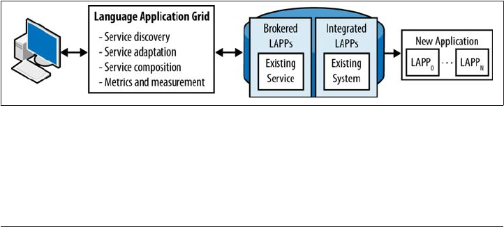
tools tend to be written in Python, while the Hadoop architecture is written entirely in
Java. Fortunately, work is already being done to distribute NLP programs over Hadoop
networks (Madnani and Lin 2010), as well as the MapReduce framework (Lin and Dyer
2010).
Shared Language Resources
The Language Grid is “an online multilingual service platform which enables easy reg
istration and sharing of language services such as online dictionaries, bilingual corpora,
and machine translators.” In addition to providing a central repository for translation
resources, it is affiliated with a number of language research projects, such as the Wi
kipedia Translation Project. The Grid is built around the idea of multilingual collabo
ration and interoperability for different types of multilanguage resources (Ishida 2011).
By making these resources available to a community, and encouraging the members of
the community to share their own resources and research results, the entire field of NLP
is enriched much more than it would be if everyone was working in isolation. The
Language Grid focuses on translation projects and related language resources (such as
dictionaries). Translation projects can be notoriously difficult, particularly when ex
amining data that uses metaphors or other euphemistic language, or data that might be
“dirty” (containing spelling or grammatical errors), so a repository for these types of
resources is invaluable.
Shared Language Applications
The LAPPs (Language Applications) Grid (see Figure 12-2) is a project whose goal is to
build a network of interoperable language processing resources (Ide and Pustejovsky
forthcoming). It was inspired by the Language Grid, and will be built on the same soft
ware platform. It will also provide support for testing applications, application reuse,
and error detection. The LAPPs Grid is still under construction at this time (summer
2012), but preliminary services should be available soon.
Figure 12-2. The LAPPs Grid system (Ide and Pustejovsky forthcoming)
Creating resources that are interoperable in some way is a difficult but necessary goal
for NLP research. Just as the LAF and GrAF (Graph Annotation Framework) annotation
NLP Online and in the Cloud | 247

standards try to provide a common ground for linguistic annotations, these concepts
are being built into other projects as well, making progress in NLP much faster, as people
no longer always have to build their own resources but can more reliably use those built
by others.
And Finally...
In this chapter our goal was to show you the role that annotation is playing in cutting-
edge developments in computational linguistics and machine learning. We pointed out
how the different components of the MATTER development cycle are being experi
mented with and improved, including new ways to collect annotations, better methods
for training algorithms, ways of leveraging cloud computing and distributed data, and
stronger communities for resource sharing and collaboration.
Because of a lack of understanding of the role that annotation plays in the development
of computational linguistics systems, there is always some discussion that the role of
annotation is outdated; that with enough data, accurate clusters can be found without
the need for human-vetted categories or other labels. But in fact, what we hope to have
shown here is that the exact opposite is true. Namely, that only with a better under
standing of how annotation reflects one’s understanding of linguistic phenomena will
a better set of features for the model and algorithm be created, whether it is rule-based
or statistical.
248 | Chapter 12: Afterword: The Future of Annotation

APPENDIX A
List of Available Corpora and Specifications
This appendix was compiled primarily from the LRE Resource Map. Many thanks to
Nicoletta Calzolari and Riccardo del Gratta for their help in creating this appendix, and
for allowing us to reprint this information here.
Please note that this appendix does not represent a complete list of all the existing soft
ware for the various tasks listed here. It is intended to provide a general overview of the
different corpora and specifications available, to give you an idea of what resources you
can use in your own annotation and machine learning (ML) tasks. For the most up-to-
date list of resources, check the LRE Resource Map, or just do a web search to see what
else is available.
Corpora
A Reference Dependency Bank for Analyzing Complex Predicates
Modality: Written
Languages: Hindi/Urdu
Annotation: Semantic dependencies
URL: http://ling.uni-konstanz.de/pages/home/pargram_urdu/main/Resources.html
A Treebank for Finnish (FinnTreeBank)
Modality: Written
Language: Finnish
Annotation: Treebank
Size: 17,000 model sentences
URL: http://www.ling.helsinki.fi/kieliteknologia/tutkimus/treebank/index.shtml
249

ALLEGRA (ALigned press reLEases of the GRisons Administration)
Modality: Written
Languages: German, Romansh, Italian
URL: http://www.latl.unige.ch/allegra/
AnCora
Modality: Written
Language: Catalan
Annotations: Lemma and part of speech, syntactic constituents and functions, ar
gument structure and thematic roles, semantic classes of the verb, Named Entities,
coreference relations
URL: http://clic.ub.edu/ancora/
American Sign Language Lexicon Video Dataset
Modality: Sign language
Language: American Sign Language
URL: http://vlm1.uta.edu/~athitsos/asl_lexicon/
Aozora Bunko
Modality: Written
Language: Word Sense Disambiguation Japanese
URL: http://www.aozora.gr.jp/
Australian National Corpus
Modality: Multimodal/multimedia
Language: Australian English
URL: http://www.ausnc.org.au/
BioInfer
Modality: Written
Language: English
Annotation: Dependency parsing
URL: http://mars.cs.utu.fi/BioInfer/
250 | Appendix A: List of Available Corpora and Specifications

BioScope
Modality: Written
Language: English
Annotations: Negation, speculation, linguistic scope
URL: http://www.inf.u-szeged.hu/rgai/bioscope
British National Corpus (BNC)
Modality: Speech/written
Language: British English
Size: 100 million words
URL: http://www.natcorp.ox.ac.uk/
Brown Corpus
Modality: Written
Language: English
Size: 1,014,312 words
URL: http://icame.uib.no/brown/bcm.html
CALBC (Collaborative Annotation of a Large Biomedical Corpus) corpora
Production status: Newly created–finished
Language: English
Annotations: Various
URL: http://www.ebi.ac.uk/Rebholz-srv/CALBC/corpora/resources.html
CHILDES
Modality: Multimedia
Languages: Various
Annotation: Transcriptions
URL: http://childes.psy.cmu.edu/
CLC FCE (Cambridge ESOL First Certificate) dataset
Modality: Written
Language: English
Size: 1,244 exam scripts
URL: http://ilexir.co.uk/applications/clc-fce-dataset/
Corpora | 251

CoreSC/ART corpus
Modality: Written
Language: English
Size: 225 papers
Annotations: Scientific concepts
URL: http://www.aber.ac.uk/en/cs/research/cb/projects/art/art-corpus/
Corpus de Referencia del Español Actual (CREA)
Modality: Written
Language: Spanish
URL: http://corpus.rae.es/creanet.html
Corpus del Español
Modality: Written
Language: Spanish
Size: 100 million words
URL: http://www.corpusdelespanol.org/
Cross Language Entity Linking in 21 Languages (XLEL-21)
Modality: Written
Languages: 21 non-English languages, plus English
Size: 55,000 queries
URL: http://hltcoe.jhu.edu/datasets/
DUC (Document Understanding Conferences)
Modality: Written
Language: English
Annotation: Document summarization
URL: http://duc.nist.gov/
EASC (Essex Arabic Summaries Corpus)
Modality: Written
Language: Arabic
Size: 153 articles, 765 human-generated summaries
URL: http://privatewww.essex.ac.uk/~melhaj/easc.htm
252 | Appendix A: List of Available Corpora and Specifications

Enron Email Corpus
Modality: Written
Language: English
Size: 500,000 messages
URL: http://sgi.nu/enron/
Estonian Reference Corpus
Modality: Written
Language: Estonian
URL: http://www.cl.ut.ee/korpused/segakorpus/index.php?lang=en
Europarl—A Parallel Corpus for Statistical Machine Translation
Modality: Written
Languages: French, Italian, Spanish, Portuguese, Romanian, English, Dutch, Ger
man, Danish, Swedish, Bulgarian, Czech, Polish, Slovak, Slovene, Finnish, Hun
garian, Estonian, Latvian, Lithuanian, Greek
URL: http://www.statmt.org/europarl/
FrameNet
Modality: Written
Language: English
Annotation: Semantic frames
URL: https://framenet.icsi.berkeley.edu/fndrupal/
GENIA Corpus
Modality: Written
Language: English
Annotations: Coreference, syntactic, semantic, part-of-speech, Treebank
URL: http://www.nactem.ac.uk/genia/
Genre Collection Repository
Modality: Written
Language: English
Annotations: Various
Size: Various
URL: http://www.webgenrewiki.org/index.php5/Genre_Collection_Repository
Corpora | 253

GRID
Modality: Multimodal/multimedia
Language: English
URL: http://www.dcs.shef.ac.uk/spandh/gridcorpus/
Icelandic Parsed Historical Corpus (IcePaHC)
Modality: Written
Language: Icelandic
Annotation: Treebank
Size: 1,002,390 words
URL: http://www.linguist.is/icelandic_treebank/
Irony Detection
Modality: Written
Language: English
Annotations: Sarcasm and irony
URL: http://storm.cis.fordham.edu/~filatova/SarcasmCorpus.html
Italian CCG Treebank (CCG-TUT)
Modality: Written
Language: Italian
Annotation: Treebank
URL: http://www.di.unito.it/~tutreeb/CCG-TUT/
JRC-Acquis Multilingual Parallel Corpus
Modality: Written
Languages: Bulgarian, Czech, Danish, German, Greek, English, Spanish, Estonian,
Finnish, French, Hungarian, Italian, Lithuanian, Latvian, Maltese, Dutch, Polish,
Portuguese, Romanian, Slovak, Slovene, Swedish
Size: Average of 18,833 aligned documents per language
URL: http://langtech.jrc.ec.europa.eu/JRC-Acquis.html
La Repubblica
Modality: Written
Language: Italian
URL: http://dev.sslmit.unibo.it/corpora/corpus.php?path=%26name=Repubblica
254 | Appendix A: List of Available Corpora and Specifications

Large Movie Review Dataset
Modality: Written
Language: English
Size: 50,000 reviews
URL: http://www.andrew-maas.net/data/sentiment
Leipzig Corpus-Based Monolingual Dictionaries
Modality: Written
Languages: 155 different languages
URL: http://corpora.uni-leipzig.de/
LIPS 2008 Speech Synthesis AV Corpus
Modality: Multimodal/Multimedia
Language: English
URL: http://lips2008.org/
MASC (Manually Annotated Sub-Corpus)
Modality: Speech/written
Language: American English
Size: 500,000 words
Annotations: Various
URL: http://www.anc.org/MASC/Home.html
Message Understanding Conference (MUC) Corpora
Modality: Written
Language: Information Extraction Information Retrieval English
URL: http://www-nlpir.nist.gov/related_projects/muc/
Movie Review Dataset
Modality: Written
Language: English
Annotation: Movie ratings
URL: http://www.cs.cornell.edu/people/pabo/movie-review-data/
MPQA Opinion Corpus
Modality: Written
Language: English
Corpora | 255

Annotation: Opinion
URL: http://www.cs.pitt.edu/mpqa/
Multi-Domain Sentiment Dataset 2.0
Modality: Written
Language: English
Annotations: Positive and negative reviews
URL: http://www.cs.jhu.edu/~mdredze/datasets/sentiment/
Multilingual UN Parallel Text 2000–2009 (MultiUN)
Modality: Written
Languages: English, French, Spanish, Arabic, Russian, Chinese, German
Size: 300 million+ words per language
URL: http://www.euromatrixplus.net/multi-un/
Multimodal Russian Corpus (MURCO)
Modality: Multimodal/multimedia
Language: Russian
Size: 300 million+ words
URL: http://www.ruscorpora.ru
NAIST Text Corpus
Modality: Written
Language: Japanese
Annotations: Anaphoric relations, coreference
URL: http://cl.naist.jp/nldata/corpus/
National Corpus of Polish
Modality: Written
Language: Polish
URL: http://nkjp.pl
Near-Identity Relations for Co-reference (NIdent) CA
Modality: Written
Languages: English, Catalan
Annotation: Near-identity relations
URL: http://clic.ub.edu/corpus/nident
256 | Appendix A: List of Available Corpora and Specifications

NLEL corpora
Modality: Written
Languages: Various
Size: Various
Annotations: Various
URL: http://users.dsic.upv.es/grupos/nle/?file=kop4.php
Online Database of Interlinear Text (ODIN)
Modality: Written
Languages: 1,274 languages
Size: 2,017 documents
URL: http://odin.linguistlist.org/
OntoNotes
Modality: Written
Languages: English, Chinese, Arabic
Size: Varies by language
URL: http://www.bbn.com/ontonotes/
Open American National Corpus (OANC)
Modality: Speech/written
Language: American English
Size: 14 million+ words
Annotations: Structural markup, sentence boundaries, part-of-speech annotations,
noun chunks, verb chunks
URL: http://www.anc.org/OANC
OPUS (Open Parallel Corpus)
Modality: Written
Use: Machine Translation
Languages: Various
URL: http://opus.lingfil.uu.se/
Corpora | 257

PAN-PC-11 Plagiarism Detection Corpus
Modality: Written
Language: English
URL: http://www.uni-weimar.de/medien/webis/research/events/pan-11/pan11-web/
plagiarism-detection.html
Penn TreeBank Project
Modality: Written
Language: English
Annotation: Treebank
URL: http://www.cis.upenn.edu/~treebank/
Persian Treebank (PerTreeBank)
Modality: Written
Language: Persian
Annotations: Part-of-speech, Treebank
URL: http://hpsg.fu-berlin.de/~ghayoomi/PTB.html
PiTu—Danish Nonsense Syllable Project
Modality: Speech
Language: Danish nonsense syllables
URL: http://amtoolbox.sourceforge.net/pitu/
Polish Sejm Corpus
Modality: Multimodal/multimedia
Use: Language modeling
Language: Polish
Annotations: Segmentation, tokenization, lemmatization, disambiguated morpho
syntactic description, syntactic words, syntactic groups, Named Entities
URL: http://clip.ipipan.waw.pl/PSC
PropBank
Modality: Written
Language: English
Annotation: Semantic role labeling
URL: http://verbs.colorado.edu/~mpalmer/projects/ace.html
258 | Appendix A: List of Available Corpora and Specifications

Real Word Error Corpus
Modality: Written
Language: English
Size: 833 dyslexic real-word errors in context
URL: http://www.dcs.bbk.ac.uk/~jenny/resources.html
Recognising Textual Entailment (RTE) 2 Test Set
Modality: Written
Language: English
Annotations: Textual entailments
URL: http://pascallin.ecs.soton.ac.uk/Challenges/RTE2/
Reuters-21578 Text Categorization Collection
Modality: Written
Language: English
Annotation: Categories
URL: http://kdd.ics.uci.edu/databases/reuters21578/reuters21578.html
RODRIGO
Modality: Written
Use: Handwriting recognition
Language: Old Spanish
URL: http://prhlt.iti.upv.es/rodrigo.php
RWTH-Fingerspelling
Modality: Sign language
Language: German Sign Language
URL: http://www-i6.informatik.rwth-aachen.de/aslr/
Sighan 2005 Bakeoff Data
Modality: Written
Language: Word segmentation Chinese
Annotation: Word segmentation
URL: http://www.sighan.org/bakeoff2005/
Corpora | 259

South-East European Times—parallel corpus of Balkan languages
Modality: Written
Languages: Balkan languages
Size: 72 files
URL: http://opus.lingfil.uu.se/SETIMES.php
Spanish Learner Language Oral Corpora (SPLLOC)
Modality: Speech
Language: Spanish
Size: 1000+ hours
URL: http://www.splloc.soton.ac.uk/index.html
The Switchboard-1 Telephone Speech Corpus
Modality: Spoken
Language: English
Size: 2,400 conversations
URL: http://www.ldc.upenn.edu/Catalog/CatalogEntry.jsp?catalogId=LDC97S62
Syntax-oriented Corpus of Portuguese Dialects (CORDIAL-SIN)
Modality: Written
Languages: Portuguese dialects
Annotations: Part-of-speech and syntactic annotations
URL: http://www.clul.ul.pt/english/sectores/variacao/cordialsin/projecto_cordial
sin_corpus.php
TalkBank
Modality: Multimodal/multimedia
Languages: Various
Size: Various
URL: http://talkbank.org
Tamil Dependency Treebank (TamilTB)
Modality: Written
Language: Tamil
Size: 600 sentences
Annotation: Morphology and dependency syntax
260 | Appendix A: List of Available Corpora and Specifications

URL: http://ufal.mff.cuni.cz/~ramasamy/tamiltb/0.1/
Text_Classification_Reuters_Corpus
Modality: Written
Language: English
Size: 22 files
Annotation: Categories
URL: http://kdd.ics.uci.edu/databases/reuters21578/reuters21578.html
The 4 Universities Data Set
Modality: Websites
Language: English
Size: 8,282 pages
Annotation: Categories
URL: http://www.cs.cmu.edu/afs/cs.cmu.edu/project/theo-20/www/data
The basic dictionary of FinSL example text corpus (Suvi)
Modality: Sign language
Languages: Finnish, Sign Language
URL: http://suvi.viittomat.net
The CONCISUS Corpus of Event Summaries
Modality: Written
Languages: Spanish, English
URL: http://www.taln.upf.edu/pages/concisus/
The EMIME Mandarin/English Bilingual Database
Modality: Speech
Languages: Finnish/English, German/English, Mandarin/English
URL: http://www.emime.org/participate/emime-bilingual-database
The Quranic Arabic Corpus
Modality: Written
Language: Arabic
Annotations: Grammar, syntax, morphology
URL: http://corpus.quran.com
Corpora | 261

The Wenzhou Spoken Corpus
Modality: Transcribed speech
Language: Wenzhou
Size: 150,000 words
URL: http://corpora.tapor.ualberta.ca/wenzhou/aboutCorpus.html
TIGER Corpus
Modality: Written
Language: German
Size: 50,000 sentences
URL: http://www.ims.uni-stuttgart.de/projekte/TIGER/TIGERCorpus/
TimeBank
Modality: Written
Language: English
Size: 183 articles
Annotation: TimeML
URL: http://www.timeml.org/site/timebank/timebank.html
TimeBankPT
Modality: Written
Language: Portuguese
Size: 70,000 words
Annotation: TimeML
URL: http://nlx.di.fc.ul.pt/~fcosta/TimeBankPT/
TREC Corpora
Modality: Written
Language: English
Annotations: Various
URL: http://trec.nist.gov/
TRIOS-TimeBank corpus
Modality: Written
Language: English
Annotation: TimeML
262 | Appendix A: List of Available Corpora and Specifications

URL: http://www.cs.rochester.edu/u/naushad/trios-timebank-corpus
TUT (Turin University Treebank)
Modality: Written
Language: Italian
Size: 2,860 sentences
URL: http://www.di.unito.it/~tutreeb
Tycho Brahe Parsed Corpus of Historical Portuguese
Modality: Written
Language: Portuguese
Size: 53 texts
URL: http://www.tycho.iel.unicamp.br/~tycho/corpus/en/
TYPO (misspelling) CORPUS
Modality: Written
Language: English
Size: 19,000+ errors
URL: http://luululu.com/tweet/
UIUC Question Classification Dataset
Modality: Written
Use: Question Answering
Language: English
Size: 15,500 questions
URL: http://l2r.cs.uiuc.edu/~cogcomp/Data/QA/QC
University of Maryland Parallel Corpus Project: The Bible
Modality: Written
Languages: Cebuano, Chinese, Danish, English, Finnish, French, Greek, Indonesi
an, Latin, Spanish, Swahili, Swedish, Vietnamese
URL: http://www.umiacs.umd.edu/~resnik/parallel/bible.html
USENET corpus
Modality: Written
Use: Language modeling
Language: English
Corpora | 263

Size: 30 billion+ words
URL: http://www.psych.ualberta.ca/~westburylab/downloads/usenetcorpus.down
load.html
Utsunomiya University Spoken Dialogue Database for Paralinguistic Information
Studies
Modality: Speech
Language: Japanese
URL: http://uudb.speech-lab.org/
W2C–Web To Corpus
Modality: Written
Languages: 120
Size: Varies per language
URL: http://ufal.mff.cuni.cz/~majlis/w2c/
Webcorpora
Modality: Written
Languages: Catalan, Croatian, Czech, Danish, Dutch, Finnish, Indonesian, Lith
uanian, Norwegian, Polish, Portuguese, Romanian, Serbian_sh, Serbian_sr, Slovak,
Spanish, Swedish
Size: Varies by language
URL: http://hlt.sztaki.hu/resources/webcorpora.html
WikiWars
Modality: Written
Size: 22 documents
Language: English
Annotation: TIMEX2
URL: http://www.timexportal.info/wikiwars
WikiWoods
Production status: Newly created–in progress
Modality: Written
Size: 1.3 million+ articles
Language: English
URL: http://www.delph-in.net/wikiwoods/
264 | Appendix A: List of Available Corpora and Specifications

World Wide English Corpus
Modality: Written
Language: English
Size: 200,000-word web-corpora
URL: http://www.comp.leeds.ac.uk/eric/wwe.shtml
Specifications, Guidelines, and Other Resources
ACE Entity and Relation Annotation Guidelines
Use: Entity (Person, Organization, Location, Facility, and Geo-Political Entity, with
subtypes) and relation (ordered pairs of entities, modality, tense) annotation
Languages: English, Arabic
URL: http://projects.ldc.upenn.edu/ace/annotation/
CoreSC Annotation Guidelines
Use: Scientific concept annotation
Language: English
URL: http://www.aber.ac.uk/en/cs/research/cb/projects/art/art-corpus/ (guidelines
available upon request)
EAGLES Recommendations for the Morphosyntactic and Syntactic Annotation of Cor
poraUse: Morphosyntactic annotation
Languages: Various
URL: http://www.ilc.cnr.it/EAGLES96/browse.html
FrameNet
Use: Semantic frames
Languages: Various
URL: https://framenet.icsi.berkeley.edu/fndrupal/home
GALE (Global Autonomous Language Exploitation) annotation guidelines
Use: Data collection, transcription, translation, word alignment
Languages: Chinese, English, Arabic
URL: http://projects.ldc.upenn.edu/gale/index.html
Specifications, Guidelines, and Other Resources | 265

GALE LDC translation guidelines
Use: Translation guidelines
Languages: Arabic, Chinese
URL: http://projects.ldc.upenn.edu/gale/Translation/
GENIA Annotation Guidelines
Use: Biomedical text annotations
Language: English
URL: http://www.nactem.ac.uk/genia/
Grammatical Framework
Use: Programming language for multilingual grammar applications
Languages: Amharic (partial), Arabic (partial), Bulgarian, Catalan, Danish, Dutch,
English, Finnish, French, German, Hindi (fragments), Interlingua, Italian, Latin
(fragments), Latvian, Nepali, Norwegian bokmål, Persian, Polish, Punjabi, Roma
nian, Russian, Spanish, Swedish, Thai, Turkish (fragments), Urdu
URL: http://www.grammaticalframework.org
Guidelines for the Syntactic Annotation of Latin and Greek Treebanks
Use: Syntactic Treebank annotation
Language: Latin (written in English and Spanish)
URL: http://nlp.perseus.tufts.edu/syntax/treebank/index.html
International Phonetic Alphabet
Use: Phonetic transcription/notation
Language: Language-independent
URL: http://www.langsci.ucl.ac.uk/ipa/ipachart.html
ISO 639-3
Use: Codes for the representation of names of languages
Languages: Various
URL: http://www.sil.org/ISO639-3/default.asp
ISO-Space
Use: Annotating spatiotemporal information in text
Language: English
URL: https://sites.google.com/site/wikiisospace/
266 | Appendix A: List of Available Corpora and Specifications

Language-Independent Named Entity Recognition
Use: Named Entity annotation
Language: Language-independent
URL: http://www.cnts.ua.ac.be/conll2003/ner/
LinES guidelines
Use: Swedish–English parallel Treebanking
Languages: English, Swedish
URL: http://www.ida.liu.se/~lah/transmap/Corpus/
Prague Dependency Treebank annotation guidelines
Use: Morphological, analytical, tectogrammatical
Language: Czech (written in English)
URL: http://ufal.mff.cuni.cz/pdt2.0/doc/pdt-guide/en/html/ch02.html
PropBank Annotation Guidelines
Use: Propositional annotation over parse trees
Languages: Hindi, Chinese, English
URL: http://clear.colorado.edu/compsem/index.php?page=annotation&sub=prop
bank
Simple Named Entity Guidelines
Use: Named Entity annotation
Language: Language-independent
URL: http://projects.ldc.upenn.edu/LCTL/Specifications/
SpatialML
Use: Annotation of named and nominal references to places in text
Language: English
URL: http://www.lrec-conf.org/proceedings/lrec2008/summaries/106.html
Stuttgart-Tbingen Tagset of German
Use: Part-of-speech tagging
Language: Linguistic Research German
URL: http://www.sfs.uni-tuebingen.de/Elwis/stts/stts.html
Syntactic Annotation Guidelines for the Quranic Arabic Dependency Treebank
Use: Part-of-speech tagging
Language: Quranic Arabic
Specifications, Guidelines, and Other Resources | 267

URL: http://corpus.quran.com
TAC Knowledge Base Population Annotation and Assessment Guidelines
Use: Question Answering, information extraction
Languages: English, Chinese
URL: http://nlp.cs.qc.cuny.edu/kbp/2011
TimeML/ISO TimeML
Use: Event, time, temporal relation annotation
Languages: English, various (adapted for other languages)
URL: http://www.timeml.org/site/publications/specs.html
TreeBank Annotation Guidelines for Biomedical Text
Use: Treebanking biomedical texts
Language: English
URL: http://clear.colorado.edu/compsem/documents/treebank_guidelines.pdf
WordNet
Use: Lexical database
Language: English
URL: http://wordnet.princeton.edu/
WordNet–FrameNet Annotations
Use: Consolidating WordNet and FrameNet annotations
Language: English
URL: http://www.anc.org/MASC/WordNet_Annotations.html
Representation Standards
Graph Annotation Framework (GrAF, ISO TC37SC4 working group 1)
Use: Graphical representation of linguistic annotations
Language: Language-independent
URL: http://www.cs.vassar.edu/~ide/papers/LAW.pdf
Lexical Markup Framework (LMF) (ISO-24613:2008)
Use: Standardization of Natural Language Processing lexicons and machine-
readable dictionaries
Language: Language-independent
URL: http://www.lexicalmarkupframework.org/
268 | Appendix A: List of Available Corpora and Specifications

Linguistic Annotation Framework (LAF) (ISO 24612)
Use: Representing annotation information over corpora
Language: Language-independent
URL: http://www.iso.org/iso/iso_catalogue/catalogue_tc/catalogue_detail.htm?
csnumber=37326, http://www.cs.vassar.edu/~ide/papers/ide-romary-clergerie.pdf
MLIF/MultiLingual Information Framework (ISO 24616-2011)
Use: Specification platform for computer-oriented representation of multilingual
data
Language: Language-independent
URL: http://mlif.loria.fr
Text Encoding Initiative (TEI)
Use: Standard for the representation of texts in digital form
Language: Language-independent
URL: http://www.tei-c.org/index.xml
Unicode Character Database
Use: Cross-linguistic written character representation
Language: Multilingual
URL: http://unicode.org/ucd/
Representation Standards | 269

APPENDIX B
List of Software Resources
This appendix was compiled primarily from the LRE Resource Map. Many thanks to
Nicoletta Calzolari and Riccardo del Gratta for their help in creating this appendix, and
for allowing us to reprint this information here.
Please note that this appendix does not represent a complete list of all the existing soft
ware for the various tasks listed here. It is intended to provide a general overview of the
different tools available, to give you an idea of what resources you can use in your own
annotation and machine learning (ML) tasks. For the most up-to-date list of resources,
check the LRE Resource Map, or just do a web search to see what else is available.
Annotation and Adjudication Software
Multipurpose Tools
GATE
Modality: Written
Use: Corpus creation and management, automatic annotation, manual correction
of annotation, part-of-speech tagging, Named Entity recognition, word sense dis
ambiguation, etc.
Languages: Various
URL: http://gate.ac.uk/
NLTK
Modality: Written
Use: Classification, tokenization, stemming, tagging, parsing, semantic reasoning,
machine learning
271

Languages: Various, language-independent
URL: http://nltk.org/
OpenNLP (Apache)
Modality: Written
Use: Tokenization, sentence segmentation, part-of-speech tagging, Named Entity
extraction, chunking, parsing, coreference resolution
Languages: Various
URL: http://opennlp.apache.org
WordFreak
Modality: Written
Use: Hand annotation, automated annotation
Language: Language-independent
URL: http://wordfreak.sourceforge.net/
Corpus Creation and Exploration Tools
Djangology: A lightweight web-based tool for distributed collaborative text annotation
Modality: Written
Use: Distributed collaborative text annotation
Language: Language-independent
URL: http://sourceforge.net/projects/djangology/
Ellogon
Modality: Written
Use: Hand annotation, machine annotation, project management
Language: Language-independent
URL: http://www.ellogon.org/
Unitex
Modality: Written
Use: Corpus processing
Language: Language-independent
URL: http://www-igm.univ-mlv.fr/~unitex/
272 | Appendix B: List of Software Resources

Wikipedia Miner
Modality: Written
Use: Corpus collection
Language: Language-independent
URL: http://wikipedia-miner.cms.waikato.ac.nz
Manual Annotation Tools
ANVIL tool
Modality: Video
Use: Manual annotation
URL: http://www.anvil-software.de
BAT (Brandeis Annotation Tool)
Modality: Written
Use: Corpus annotation
Language: Language-independent
URL: http://timeml.org/site/bat/
Callisto
Modality: Written
Use: Annotation
Language: Language-independent
URL: http://callisto.mitre.org/
Djangology: A lightweight web-based tool for distributed collaborative text annotation
Modality: Written
Use: Distributed collaborative text annotation
Language: Language-independent
URL: http://sourceforge.net/projects/djangology/
ELAN
Modality: Video/audio
Use: Manual annotation
Language: Language-independent
URL: http://www.lat-mpi.eu/tools/elan/
Annotation and Adjudication Software | 273

Ellogon
Modality: Written
Use: Hand annotation, machine annotation, project management
Language: Language-independent
URL: http://www.ellogon.org/
EMU Speech Database System
Modality: Speech
Use: Speech annotation
Language: Language-independent
URL: http://emu.sourceforge.net
EXMARaLDA (Extensible Markup Language for Discourse Annotation)
Modality: Multimodal/multimedia
Use: Discourse annotation
Language: Language-independent
URL: http://www.exmaralda.org
feat (Flexible Error Annotation Tool)
Modality: Speech/written
Use: Error transcription
Language: Language-independent
URL: http://ufal.mff.cuni.cz/~hana/feat.html
FOLKER
Modality: Speech
Use: Transcription
Language: Language-independent
URL: http://agd.ids-mannheim.de/folker_en.shtml
GATE
Modality: Written
Use: Corpus creation and management, automatic annotation, manual correction
of annotation, part-of-speech tagging, Named Entity recognition, word sense dis
ambiguation, etc.
Languages: Various
274 | Appendix B: List of Software Resources

URL: http://gate.ac.uk/
Jubilee
Modality: Written
Use: PropBank annotation editor
Languages: English, Arabic, Chinese
URL: http://code.google.com/p/propbank/
Knowtator
Modality: Written
Use: Manual annotation
Language: Language-independent
URL: http://knowtator.sourceforge.net/index.shtml
MAE (Multipurpose Annotation Environment)
Modality: Written
Use: Manual annotation
Language: Language-independent
URL: http://code.google.com/p/mae-annotation/
MMAX2
Modality: Written
Use: Manual annotation
Language: Language-independent
URL: http://www.eml-research.de/english/research/nlp/download/mmax.php
PALinkA (Perspicuous and Adjustable Links Annotator)
Modality: Written
Use: Manual link annotation
Language: Language-independent
URL: http://clg.wlv.ac.uk/projects/PALinkA/
Praat
Modality: Speech
Use: Manual annotation
Language: Language-independent
URL: http://www.praat.org
Annotation and Adjudication Software | 275

Sanchay
Modality: Written
Use: Manual annotation
Languages: South Asian languages
URL: http://sanchay.co.in/
SAPIENT: Semantic Annotation of Papers Interface and Enrichment Tool
Modality: Written
Use: Manual semantic annotation of scientific concepts
Language: Document Classification Text categorization English
URL: http://www.aber.ac.uk/en/cs/research/cb/projects/sapienta/software/
Scheherazade
Modality: Written
Use: Manual semantic annotation
Language: Discourse English
URL: http://www.cs.columbia.edu/~delson/software.shtml
Sextant (Standoff EXMARaLDA Transcription Annotation Tool)
Modality: Speech
Use: Manual transcription annotation
Language: Language-independent
URL: http://exmaralda.org/sextant/
SSI (Social Signal Interpretation)
Modality: Multimodal/multimedia
Use: Manual human behavior annotation
Language: Language-independent
URL: http://mm-werkstatt.informatik.uni-augsburg.de/ssi.html
SMORE
Modality: Written
Use: OWL markup of websites
Language: Language-independent
URL: http://www.mindswap.org/2005/SMORE/
276 | Appendix B: List of Software Resources

TrEd
Modality: Written
Use: Treebank creation/annotation
Language: Language-independent
URL: http://ufal.mff.cuni.cz/tred/
WebAnnotator
Modality: Websites
Use: Web annotation
Language: Language-independent
URL: http://www.limsi.fr/Individu/xtannier/en/WebAnnotator/
WordAligner
Modality: Written
Use: Machine Translation word alignment
Language: Language-independent
URL: http://www.bultreebank.bas.bg/aligner/index.php
Automated Annotation Tools
Multipurpose tools
fnTBL
Modality: Written
Use: Part-of-speech tagging, base noun phrase chunking, text chunking, end-of-
sentence detection, word sense disambiguation
Languages: Various
URL: http://www.cs.jhu.edu/~rflorian/fntbl/
FreeLing
Modality: Written
Use: Tokenization, sentence splitting, morpheme identification, Named Entity de
tection, part-of-speech tagging, shallow parsing, Named Entity classification, nom
inal coreference resolution
Languages: Spanish, Catalan, Galician, Italian, English, Russian, Portuguese, Welsh,
Austrian
URL: http://nlp.lsi.upc.edu/freeling
Annotation and Adjudication Software | 277

GATE
Modality: Written
Use: Corpus creation and management, automatic annotation, manual correction
of annotation, part-of-speech tagging, Named Entity recognition, word sense dis
ambiguation, etc.
Languages: Various
URL: http://gate.ac.uk/
Illinois NLP tools
Modality: Written
Use: Part-of-speech tagging, chunking, coreference, Named Entity tagging, seman
tic role labeling
Language: Language-independent
URL: http://cogcomp.cs.illinois.edu/page/software
MADA + TOKAN
Production status: Existing–used
Modality: Written
Use: Tokenization, diacritization, morphological disambiguation, part-of-speech,
tagging, stemming, and lemmatization
Language: Arabic
URL: http://www1.ccls.columbia.edu/~cadim/
MorphAdorner
Modality: Written
Use: Tokenizing text, recognizing sentence boundaries, extracting names and places
Language: English
URL: http://morphadorner.northwestern.edu/
NLTK
Modality: Written
Use: Classification, tokenization, stemming, tagging, parsing, semantic reasoning,
machine learning
Language: English
URL: http://nltk.org/
278 | Appendix B: List of Software Resources

RACAI web service
Modality: Written
Use: Tokenization, sentence splitting, C-tagset part-of-speech tagging, MSD-tagset
part-of-speech tagging, lemmatization, identify language (57 languages)
Languages: English, Romanian
URL: http://www.racai.ro/webservices
Standford NLP tools
Modality: Written
Use: Parsing, part-of-speech tagging, Named Entity recognition, word segmenta
tion, tokenizing, temporal tagging, topic modeling
Language: English
URL: http://nlp.stanford.edu/software/
Phonetic annotation
FOLKER
Modality: Speech
Use: Transcription
Language: Language-independent
URL: http://agd.ids-mannheim.de/folker_en.shtml
Julius
Modality: Speech
Use: Speech Recognition/understanding
Language: Japanese
URL: http://julius.sourceforge.jp/
SPPAS (SPeech Phonetization Alignment and Syllabification)
Modality: Speech
Use: Automatic phonetic transcription and segmentation
Language: Basque
URL: http://www.lpl-aix.fr/~bigi/sppas/
Annotation and Adjudication Software | 279

Part-of-speech taggers/syntactic parsers
Alpino
Modality: Written
Use: Dependency parser
Language: Dutch
URL: http://www.let.rug.nl/vannoord/alp/Alpino/
Apertium-kir
Modality: Written
Use: Machine Translation
Languages: Various
URL: http://sourceforge.net/projects/apertium/
Automatic Syntactic Analysis for Polish Language (ASA-PL)
Modality: Written
Use: Syntactic analysis
Language: Polish
URL: http://seagrass.man.poznan.pl/~michzimny/asa-pl/
Berkeley Parser
Modality: Written
Use: Parsing
Languages: Various
URL: http://code.google.com/p/berkeleyparser/
BitPar
Modality: Software
Use: Syntactic parsing
Language: English
URL: http://www.ims.uni-stuttgart.de/tcl/SOFTWARE/BitPar.html
C&C Toolkit
Modality: Written
Use: Parsing, tagging
Language: English
280 | Appendix B: List of Software Resources

URL: http://svn.ask.it.usyd.edu.au/trac/candc/wiki
Charniak Parser
Modality: Written
Use: Parsing
Language: English
URL: http://www.cs.brown.edu/people/ec/#software
CombiTagger
Modality: Written
Use: Part-of-speech tagging
Language: Language-independent
URL: http://combitagger.sourceforge.net
Dependency Shift Reduce parser (DeSR)
Modality: Written
Use: Dependency parsing
Language: English
URL: http://sites.google.com/site/desrparser/
DepPattern
Production status: Newly created–in progress
Modality: Written
Use: Grammar compiler, part-of-speech tagger, dependency-based parser
Languages: English, Spanish, Galician, French, Portuguese
URL: http://gramatica.usc.es/pln/tools/deppattern.html
DeSR
Modality: Written
Use: Parsing
Languages: Various
URL: http://desr.sourceforge.net/doc/
EnjuModality: Written
Use: Syntactic parser
Language: English
Annotation and Adjudication Software | 281

URL: http://www-tsujii.is.s.u-tokyo.ac.jp/enju/
Granska tagger
Modality: Written
Use: Part-of-speech tagger
Language: Swedish
URL: http://www.csc.kth.se/tcs/humanlang/tools.html
Greek POS Tagger
Modality: Written
Use: Part-of-speech tagger
Language: Koine Greek
URL: http://nlp.cs.aueb.gr/software.html
Hunpos
Modality: Written
Use: Part-of-speech tagger
Languages: Various
URL: http://mokk.bme.hu/resources/hunpos
IceNLP
Modality: Written
Use: Tokenization, part-of-speech tagging, parsing
Language: Icelandic
URL: http://icenlp.sourceforge.net/
J-Safran (Java Syntaxico-semantic French Analyser)
Modality: Written
Use: Syntactic dependency parsing
Language: French
URL: http://rapsodis.loria.fr/jsafran/index.html
KyTea, the Kyoto Text Analysis Toolkit
Modality: Written
Use: Word segmentation, tagging
Languages: Japanese, Chinese
URL: http://www.phontron.com/kytea
282 | Appendix B: List of Software Resources

LGTagger
Modality: Written
Use: Part-of-speech tagging
Language: French
URL: http://igm.univ-mlv.fr/~mconstan/research/software/
Linguistica
Modality: Written
Use: Morpheme recognition
Language: Language-independent
URL: http://linguistica.uchicago.edu/linguistica.html
Link Parser
Modality: Written
Use: Syntactic parsing
Language: English
URL: http://www.link.cs.cmu.edu/link/
LX-Parser
Modality: Written
Use: Text parsing
Language: Portuguese
URL: http://lxparser.di.fc.ul.pt
MaltParser
Modality: Written
Use: Parsing
Language: Language-independent
URL: http://maltparser.org/
MiniPar
Modality: Written
Use: Parsing
Language: English
URL: http://www.cs.ualberta.ca/~lindek/minipar.htm
Annotation and Adjudication Software | 283

Mogura
Modality: Written
Use: Syntactic parsing
Language: English
URL: http://www-tsujii.is.s.u-tokyo.ac.jp/enju/
Morče
Modality: Written
Use: Czech morphological tagger
Language: Czech
URL: http://ufal.mff.cuni.cz/morce/
MSTParser (maximum spanning tree parser)
Modality: Written
Use: Parsing
Language: Language-independent
URL: http://sourceforge.net/projects/mstparser
MuNPEx
Modality: Written
Use: Noun phrase extraction
Languages: English, German, French, Spanish
URL: http://www.semanticsoftware.info/munpex
Pantera-tagger
Modality: Not applicable
Use: Morphosyntactic tagging
Languages: Various
URL: http://code.google.com/p/pantera-tagger/
RASP
Modality: Written
Use: Parsing
Language: English
URL: http://www.informatics.sussex.ac.uk/research/groups/nlp/rasp/
284 | Appendix B: List of Software Resources

RelEx
Modality: Written
Use: Semantic dependency parsing
Language: English
URL: http://opencog.org/wiki/RelEx
SEMAFOR 2.0
Modality: Written
Use: Shallow semantic parsing
Language: English
URL: http://www.ark.cs.cmu.edu/SEMAFOR/
Shalmaneser
Modality: Written
Use: Automatic semantic parsing
Languages: English, German
URL: http://www.coli.uni-saarland.de/projects/salsa/shal/
SVMTool
Modality: Written
Use: Part-of-speech tagging and chunking
Languages: Various
URL: http://www.lsi.upc.edu/~nlp/SVMTool/
SET (Syntax in Elements of Text)
Modality: Written
Use: Syntactic parsing
Language: Czech
URL: http://nlp.fi.muni.cz/trac/set
TreeTagger
Modality: Written
Use: Part-of-speech tagging
Language: Language-independent
URL: http://www.ims.uni-stuttgart.de/projekte/corplex/TreeTagger/
Annotation and Adjudication Software | 285

upparse
Modality: Written
Use: Partial parsing
Language: Language-independent
URL: http://elias.ponvert.net/upparse
WMBT
Modality: Not applicable
Use: Morphosyntactic tagging
Language: Polish
URL: http://nlp.pwr.wroc.pl/redmine/projects/wmbt/wiki
Word clAss taGGER (WAGGER)
Modality: Written
Use: Part-of-speech tagging
Languages: English, Portuguese
URL: http://www.inf.pucrs.br/afonso.sales/wagger
Tokenizers/chunkers/stemmers
JOS ToTaLe text analyser
Modality: Written
Use: Morphological disambiguation and lemmatization
Language: Slovenian
URL: http://nl.ijs.si/jos/analyse/
MMSEG
Modality: Written
Use: Word segmentation
Language: Chinese
URL: http://code.google.com/p/pymmseg-cpp/
MorphTagger
Modality: Written
Use: Morpheme annotation
Language: Arabic
URL: http://www-i6.informatik.rwth-aachen.de/~mansour/MorphSegmenter/
286 | Appendix B: List of Software Resources

Snowball
Modality: Written
Use: Stemming
Language: English
URL: http://snowball.tartarus.org/download.php
Yet Another Multipurpose CHunk Annotator (YamCha)
Modality: Written
Use: Text chunking
Language: English
URL: http://chasen.org/~taku/software/yamcha/
Other
BART Anaphora Resolution Toolkit
Modality: Written
Use: Coreference/anaphora resolution
Language: English
URL: http://www.bart-coref.org/
GIZA++
Modality: Written
Use: Machine Translation
Languages: Various
URL: http://code.google.com/p/giza-pp/
Google Translate
Modality: Written
Use: Machine Translation
Languages: Various
URL: http://www.translate.google.com
HeidelTime
Modality: Written
Use: Temporal expression tagger
Languages: Various
URL: http://dbs.ifi.uni-heidelberg.de/heideltime
Annotation and Adjudication Software | 287

Illinois Coreference Package
Modality: Written
Use: Coreference resolution
Language: English
URL: http://cogcomp.cs.illinois.edu/page/software_view/18
MAZEA-Web
Modality: Written
Use: Rhetorical structure annotation
Language: Discourse English
URL: http://www.nilc.icmc.usp.br/mazea-web/
TARSQI Toolkit
Modality: Written
Use: Temporal expression and event tagging, temporal linking
Language: English
URL: http://www.timeml.org/site/tarsqi/toolkit/
Machine Learning Resources
GATE (General Architecture for Text Engineering)
Modality: Written
Use: Corpus creation and management, automatic annotation, manual correction
of annotation, part-of-speech tagging, Named Entity recognition, word sense dis
ambiguation, etc.
Languages: Various
URL: http://gate.ac.uk/
MALLET (MAchine Learning for LanguagE Toolkit)
Modality: Written, graphical (with add-on)
Use: Document classification, clustering, topic modeling, information extraction,
other machine learning applications
Language: Language-independent
URL: http://mallet.cs.umass.edu/
288 | Appendix B: List of Software Resources

NLTK (Natural Language Toolkit)
Modality: Written
Use: Classification, tokenization, stemming, tagging, parsing, semantic reasoning,
machine learning
Languages: Various, language-independent
URL: http://nltk.org/
OpenNLP Toolkit
Modality: Written
Uses: Tokenization, sentence segmentation, part-of-speech tagging, Named Entity
extraction, chunking, parsing, and coreference resolution; Maximum Entropy and
perception-based machine learning
URL: http://incubator.apache.org/opennlp/
WEKA
Modality: Written
Use: Data preprocessing, classification, regression, clustering, association rules,
visualization, machine learning
Language: Language-independent
URL: http://www.cs.waikato.ac.nz/ml/weka/
Machine Learning Resources | 289

APPENDIX C
MAE User Guide
MAE (Multipurpose Annotation Environment) was written by Amber Stubbs, and is
provided free for use from http://code.google.com/p/mae-annotation/. Although many
other annotation tools are available for use, MAE provides a simple interface that re
quires little setup, and so we are providing the user guide here for those readers who
would like to start annotating right away.
Input to MAE is in the form of DTD-like files that describe the task name, elements,
and attributes. A sample task definition is included with the MAE distribution, and
instructions for creating your own tasks are included in this appendix. MAE was written
in Java on an Ubuntu Linux system, and has been tested on Windows XP, Windows 7,
and Mac OS X. It uses the SQLiteJDBC Java driver (more information is available at
https://github.com/crawshaw/sqlitejdbc).
MAE is free software: you can redistribute it and/or modify it under the terms of the
GNU General Public License as published by the Free Software Foundation, either ver
sion 3 of the License, or (at your option) any later version. This program is distributed
in the hope that it will be useful, but without any warranty; without even the implied
warranty of merchantability or fitness for a particular purpose. See the GNU General
Public License for more details (http://www.gnu.org/licenses/).
Installing and Running MAE
MAE requires Java to run. On Windows and Unix systems, it should be used with the
most recent version of Java 6 (it must have at least update 14 to run properly on Windows
and Unix), though it can also be compiled under Java 5, so it can also be run on older
Macs. To run MAE on any operating system, open a terminal and navigate to the di
rectory where the .jar file exists, then run this command:
java -jar MAEversion.jar
291
On most platforms, it is also possible to open the program by double-clicking on
the .jar file. However, doing so will not allow all error messages to be displayed, so using
the terminal is recommended. On all systems, you should see the window shown in
Figure C-1.
Figure C-1. MAE startup screen
Loading Tasks and Files
Loading a Task
To use MAE, you must load both a task definition file (.dtd) and a file to be annotated
(.txt or .xml). The task definition must be loaded first, by selecting Load DTD from the
File menu. Once the DTD is loaded, the lower section of the MAE window will be filled
with tabs representing the different elements. The MAE distribution includes a sample
DTD and file for annotation, located in the samples directory.
292 | Appendix C: MAE User Guide

Loading a File
Once the task is loaded, it is now possible to annotate files. To load a file for annotation,
use the Load File option in the File menu. The easiest way to begin annotating is to load
a UTF-8 encoded text file that contains only the text you wish to annotate. You may
also, of course, load a file that has been previously annotated in MAE or in any other
program, as long as it adheres to the following format:
<TaskName>
<TEXT><![CDATA[
this is the text that will be annotated.
More text to be annotated.
]]></TEXT>
<TAGS>
<tag1... />
<tag2... />
</TAGS>
</TaskName>
\end{verbatim}
When the input file is loaded, the text for annotation will appear in the top MAE window.
The file being loaded must use UTF-8 encoding, especially if you are trying to annotate
files in languages that use characters other than those in the English alphabet.
Annotating Entities
Entity annotation is done with the mouse. Simply highlight the word to be annotated
with the left mouse button. With the word highlighted, right-click with the mouse to
open a menu of possible entity tags. Select the desired tag from the menu, and the
information about the tag will be added to the appropriate tab at the bottom of the
screen. The ID, start, end, and text features are automatically generated by MAE, and
are best left unmodified. The other features can be changed by the annotator as needed.
Attribute information
Once a tag has been created and appears in the table at the bottom of the screen, it is
possible to set values for the different attributes contained in the tag. Depending on the
task, the attribute values can either be entered as free text or be selected from a list, as
shown in Figure C-2.
Loading Tasks and Files | 293
Figure C-2. Annotation in MAE
Nonconsuming tags
It is possible in MAE to have annotation schemes that have entity tags that do not require
extents to be associated with them. This can be useful for entities that are implied, but
not explicitly mentioned. Nonconsuming tags can be added to the annotation by se
lecting the tag type from the “Nonconsuming tags” menu at the top of the MAE window.
These will be given ID tags, but the start and end elements will be set to –1. All non
consuming tags will be listed as options for linking to and from in the link creation
window.
Annotating Links
To create links between two entities, simply make sure the text window is active (left-
clicking anywhere on the text will suffice for that), hold down the Ctrl key (or the Com
mand key, if you are on a Mac), and left-click each entity that will be included in the
link, in the order you want them to appear in the link. Once this is done, a window will
pop up that will allow you to select where the link starts and where it ends, and the type
of link that you want to create between them. When you click on the “Create link” button
at the bottom of the pop-up window, the link will be added to the appropriate table,
where you can fill in the rest of the information about it.
Deleting Tags
There are two ways to delete entity tags. One way is to highlight all or part of the tagged
text in the window, and right-click on it. The pop-up menu will list all the tags at that
location, with the option to remove each of them. The other way to remove an extent
tag also works for links and nonconsuming tags: just select the row of the tag that you
294 | Appendix C: MAE User Guide

want to remove in the table, and right-click. You will have the option to remove all the
highlighted rows in the active tab. When an extent tag is removed, all the link tags that
it is a part of are removed as well to maintain consistency. The reverse is not true for
link tags—removing a link tag will have no effect on extent tags. Please note that there
is no undo function.
Saving Files
To save the information you have annotated, select “Save as XML” from the File menu.
This will create a file that contains the text and the tags that you have created, with the
tags in stand-off format. Once you have created this file, you will be able to load it back
into MAE to continue, or edit existing annotations. There is another option in the File
menu called Create RTF. This option will not save all the information about the tags and
annotation you created, but it is a handy way to look at the annotation of each word.
Defining Your Own Task
Creating an annotation task for MAE is fairly straightforward. The format of the input
is similar to DTDs (Document Type Definitions) used for XML. There are three main
parts of task creation: the task name, the tag names, and the tag attributes. DTDs are
simply text files with a .dtd extension—you can create them in any text editing program.
The specifics of how these lines should be formatted might not work well in a .pdf file, so
please refer to the included sample DTD (samples/sampleTask.dtd) for help if
necessary.
Task Name
The task name is defined with the !ENTITY tag. If you wanted to create a task called
"myTask", then you would create the !ENTITY line with name and the name of the task
in quotes. The line to do so would look like this:
<!ENTITY name "myTask">
This simply provides a name to be used in the output files.
Elements (a.k.a. Tags)
Elements (defined by !ELEMENT tags) are used to define the names of the tags being used
in your annotation task. MAE recognizes two types of tags: extent tags (tags used to
label actual words in the document) and link tags (tags that identify a relationship be
tween two extent tags). To define an extent tag for your task, the line in your DTD will
look like this:
<!ELEMENT TagName ( #PCDATA ) >
Saving Files | 295

while a link tag will look like this:
<!ELEMENT LinkName EMPTY >
The ( #PCDATA ) marker indicates that the tag will have extents, while the EMPTY
indicates that the tag will be used for linking. You cannot have two tags with the same
name, even if they are of different types.
Currently, there is a limited number of font colors that are being as
signed to tags—the colors will repeat, which may make annotation
confusing if you have more than 11 tags.
Attributes
Attributes (defined by the !ATTLIST tags) contain the information associated with each
tag. Some attributes are predefined by MAE—extent tags will always have start, end,
text, and id attributes, even if they are not defined in the DTD. Link tags will always
have to, from, toText, fromText, and id attributes. Attributes must include the name
of the element that they refer to, followed by the name of the attribute and the type of
the attribute, like so:
<!ATTLIST TagName attribute1 ( YES | NO ) #IMPLIED >
<!ATTLIST TagName attribute2 CDATA #IMPLIED >
In the following subsections I will go over the details of the attribute descriptions.
id attributes
If no id attribute is created, then MAE will assume by default that the prefix for the
ids for that tag will be the first letter of that tag name. So, for example, a tag called Verb
will have the ids V1, V2, V3, and so on. ID values are automatically assigned by the
program to help prevent two tags from having the same ID. If you want to specify your
own prefix, add prefix="MC" to your element attribute, like so:
<!ATTLIST TagName id ID prefix="MC" #REQUIRED >
In a future version of MAE, the \#REQUIRED and \#IMPLIED values will have an impact
on how the files are output to XML (whether an exception will be thrown if a required
attribute is left blank), but at the moment, they don’t actually do anything, except when
used for the start attribute.
start attribute
As previously mentioned, all extent tags have an attribute called start, which denotes
where the tag begins in the text. It is possible in MAE to create a nonconsuming extent
296 | Appendix C: MAE User Guide

tag—an extent tag that doesn’t actually cover any text, but instead exists as a placeholder.
By default, MAE will not allow a tag to be nonconsuming, but by putting a line for the
start attribute with the value \#IMPLIED, the tag that the start attribute belongs to
will be added to the list of nonconsuming tags. For example, this line:
<!ATTLIST Tag1 start #IMPLIED >
will make it so that the tag Tag1 is allowed to be nonconsuming. If you do not want to
allow a tag to be nonconsuming, it is not necessary to mention the start attribute in
the DTD at all.
Attribute types
It is possible in MAE to have a set of options for an attribute value, rather than asking
the annotators to fill in their own values each time. If you want to have a list of values,
create the attribute and include a list of options in parentheses, separated by “| ”, like so:
<!ATTLIST TagName attribute1 ( YES | NO ) #IMPLIED >
If, on the other hand, you want the annotator to be able to enter her own values into the
field for that attribute, assign the #CDATA value:
<!ATTLIST TagName attribute2 CDATA #IMPLIED >
Again, the #IMPLIED and #REQUIRED values for these attributes don’t currently have an
impact on how MAE operates, and it is fine to not include them.
Default attribute values
Starting in version 0.9, MAE allows you to set default values for any attribute by placing
the desired value in quotes at the end of the attribute definition, like so:
<!ATTLIST TagName attribute1 ( YES | NO ) #IMPLIED "YES">
<!ATTLIST TagName attribute2 CDATA #IMPLIED "default">
Please note that if a list of options is defined in an attribute but the default value does
not appear in the list, MAE will not provide that default value when creating a new tag.
Frequently Asked Questions
What does it mean when text is underlined?
Text in the annotation window is underlined when there is more than one extent
tag at that location. I experimented with mixing the colors of the two (or more)
overlapping tags, but the colors were muddy and difficult to distinguish. Under
lining seemed like a more recognizable visual clue.
Why doesn’t MAE do XYZ?/Hey, this doesn’t work!
MAE is a work in progress. If you find any bugs or have any suggestions for im
provement, please contact the creator, Amber Stubbs, at astubbs@cs.brandeis.edu.
Frequently Asked Questions | 297


APPENDIX D
MAI User Guide
MAI (Multidocument Adjudication Interface) was created as a companion program to
the annotation tool MAE (Multipurpose Annotation Environment). MAI was written
by Amber Stubbs, and is provided free for use from http://code.google.com/p/mai-
adjudication/. While many other annotation and adjudication tools are available for use,
MAI was designed specifically for use in adjudicating the output from MAE, and so we
are providing the user guide here for those readers who would like to start annotating
and adjudicating right away.
Input to MAI is in the form of annotated stand-off XML files that are the output of MAE,
as well as the DTD file used to create the annotations. Sample files are included with
the MAI distribution, and instructions for adjudicating annotated files are included in
this appendix. MAI was written in Java on an Ubuntu Linux system, and has been tested
on Windows XP, Windows 7, and Mac OS X. It uses the SQLiteJDBC Java driver (more
information is available at https://github.com/crawshaw/sqlitejdbc).
MAI is free software: you can redistribute it and/or modify it under the terms of the
GNU General Public License as published by the Free Software Foundation, either ver
sion 3 of the License, or (at your option) any later version. This program is distributed
in the hope that it will be useful, but without any warranty; without even the implied
warranty of merchantability or fitness for a particular purpose. See the GNU General
Public License for more details (http://www.gnu.org/licenses/).
Installing and Running MAI
MAI requires Java to run. On Windows and Unix systems, it should be used with the
most recent version of Java 6 (it must have at least update 14 to run properly on Windows
and Unix), though it can also be compiled under Java 5, so it can also be run on older
Macs. To run MAI on any operating system, open a terminal and navigate to the direc
tory where the .jar file exists, then run this command:
299
java -jar MAIversion.jar
On most platforms, it is also possible to open the program by double-clicking on
the .jar file. However, doing so will not allow all error messages to be displayed, so using
the terminal is recommended. On all systems, you should see the window shown in
Figure D-1.
Figure D-1. MAI with a DTD loaded
Loading Tasks and Files
Loading a Task
To use MAI, you must load both a task definition file (.dtd) and the files to be adjudicated
(.xml). The task definition must be loaded first, by selecting Load DTD from the File
menu. Once the DTD is loaded, the left side of the screen will contain the names of the
different tags in the DTD.
300 | Appendix D: MAI User Guide

Loading Files
Once the DTD is loaded, it is possible to adjudicate files. To start a new adjudication
task, go to the File menu and select “Start new adjudication,” then load the first file that
you want to adjudicate. The text of the file will be loaded in the center window, and a
table will be created to the right that will show the tag attributes of a selected extent.
To add a file to an adjudication task, go to the File menu and select “Add file to adjudi
cation.” The file that is added must have the same base text as the other files being
adjudicated; otherwise, it cannot be loaded. That is to say, all the text in the files between
the <TEXT> and </TEXT> tags cannot be different; otherwise, the character locations will
be different and the tags cannot be matched up.
To add a gold standard file to the task (i.e., a file where the tags have already been vetted
by an adjudicator), go to the File menu and select “Add gold standard file.” Please note
that a gold standard file cannot be added to the adjudication unless another file with
the same text has already been loaded (if you want to only view the gold standard file,
you can load it first as a regular adjudication file, then again as a gold standard file). Any
tags that have already been added to the gold standard prior to loading the file will still
exist, so be careful of ID overlaps.
Adjudicating
The MAI Window
Each tag type is adjudicated individually. Select the tag that will be adjudicated from the
options on the left. The text will be highlighted according to the agreement for each
character.
For extent tags:
BlueAll the annotators agree that the selected tag should be at that location (this does
not mean that the annotators all agree on the values of the tag attribute).
Red At least one annotator believes that the tag should be at a location, but not all of
them do.
Black
No annotator placed the selected tag at that location.
Green
A tag has been placed at this location in the gold standard.
Adjudicating | 301

For link tags:
BlueAll the annotators agree that the text at that location is either a to or from anchor
in a link of the selected type.
Red At least one annotator believes that the text at that location is either a to or from
anchor in a link of the selected type.
Black
No gold standard extent tag that is participating in the selected link tag exists at
that location.
Green
The text at that location is either a to or from anchor in a link of the selected type
in the gold standard.
Light gray
The text at this location is included in a tag that is in the gold standard, but none
of the files being adjudicated have an extent tag that is participating in a link at the
same location.
Magenta
Areas of the text that have been viewed by the adjudicator for the selected tag are
displayed in magenta to help the adjudicator keep track of the locations in the text
that have been adjudicated.
Adjudicating a Tag
For all tag types, when a tag from a file being adjudicated is copied to the gold standard,
the information from the copied tag is automatically assigned a gold standard ID and
added to the database. If you wish to change an attribute on a gold standard tag, you
must only make the appropriate changes and then click the “Add/modify” button in the
rightmost table column. Changes are not saved automatically, however—modifications
to attributes are only committed when the button is clicked.
Extent Tags
By selecting an extent where a tag exists in at least one of the annotations, the information
for all the tags at that location will populate the table at the bottom of the screen. There,
if you agree with an annotator about the location and attributes of a tag, you can copy
the contents of the annotator’s tag by clicking the “Copy to gold standard” button in the
annotation column. This will copy the contents of the link to the gold standard, and
generate a new ID for that tag in the gold standard file.
302 | Appendix D: MAI User Guide

Once a tag has been added to the gold standard, you may modify any of the tag’s attributes
except for the filename. It is, however, generally not advisable to change the computer-
generated ID of the tag, as this may cause problems with the database.
Link Tags
If a link tag is selected from the lefthand display, the interface behaves slightly differently
than when displaying information about an extent tag. The colors are displayed ac
cording to the preceding guide. It should be noted that information about any link is
only displayed if the to and from anchors for the tags in the files being adjudicated
overlap with extents of the same type in the gold standard. This is so that the adjudicator’s
screen will not be cluttered with information about links pertaining to extents that he
has not placed in the gold standard.
When a span of text is selected in the window, the link information displayed in the
table, while originating from the files being adjudicated, will have the attribute infor
mation in the fromID and toID and fromText and toText fields replaced with the cor
responding information from the gold standard tags at those locations. This ensures
that there will not be any errors pertaining to text spans or ID numbers.
Nonconsuming Tags
Tags that have the option of being nonconsuming (if they are described so in the DTD;
see the MAE User Guide for details) are added to the bottom of the tag list on the left
side of the screen as NC-(tagname). When one of these is selected from the left side of
the screen, all nonconsuming tags of that type are displayed in the tag table.
Adding New Tags
You may also add a tag to the gold standard that does not exist in any of the files being
adjudicated. The functionality of this feature is much like that of MAE. To add a new
extent tag, use the mouse to highlight the text where the tag should be placed, then right-
click and select the tag name from the pop-up menu. This will add the tag to the table
at the bottom of the MAI window, where the adjudicator can enter any missing attribute
information.
To add a link tag, you must select the text window, then hold down the Ctrl key (or the
Command key, if using a Mac), and left-click each entity that will be included in the
link, in the order you want them to appear in the link (i.e., the first entity that is clicked
on will be in the “from” position, and the second will be in the “to” position). Once this
is done, a window will pop up that will allow you to select where the link starts and
Adjudicating | 303

where it ends, and the type of link that you want to create between them. When you
click on the “Create link” button at the bottom of the pop-up window, the link will be
added to the appropriate table, where you can fill in the rest of the information about
it.
If you wish to add a new nonconsuming tag, you must simply highlight an area of the
text and right-click, then proceed as with adding a regular extent tag (the area selected
doesn’t matter, as the start and end will both be set to –1).
Deleting tags
Tags may be deleted from the gold standard (not from the files being adjudicated) by
selecting the row in the table of the tag that should be deleted and right-clicking. You
will have the option to remove all the highlighted rows in the table.
When an extent tag is removed, all the link tags that it is a part of are removed as well
to maintain consistency in the database. The reverse is not true for link tags—removing
a link tag will have no effect on extent tags.
Please note that there is no undo function.
Saving Files
To save the information you have annotated, select “Save as XML” from the File menu.
This will create a file that contains the text and the tags that you have created, with the
tags in stand-off format.
304 | Appendix D: MAI User Guide

APPENDIX E
Bibliography
Allen, James. 1984. “Towards a General Theory of Action and Time.” Artificial Intelli
gence 23:123–154.
Artstein, Ron, and Massimo Poesio. December 2008. “Inter-coder agreement for com
putational linguistics.” Computational Linguistics 34(4):555–596.
Atkins, Sue, and N. Ostler. 1992. “Predictable Meaning Shift: Some Linguistic Properties
of Lexical Implication Rules.” In Lexical Semantics and Commonsense Reasoning. J. Pus
tejovsky and S. Bergler (Eds.). New York: Springer-Verlag.
Baroni, M. 2009. “Distributions in text.” In Anke Lüdeling and Merja Kytö (eds.), Corpus
linguistics: An international handbook, Volume 2, Berlin: Mouton de Gruyter: 803–821.
Bayerl, Petra Saskia, and Karsten Ingmar Paul. December 2011. “What Determines
Inter-Coder Agreement in Manual Annotations? A Meta-Analytic Investigation.” Com
putational Linguistics 37(4):699–725.
Belnap, Nuel. 1992. “Branching Space-Time.” Synthese 92:385–434.
Biber, Douglas. 1993. “Representativeness in Corpus Design.” Literary and Linguistic
Computing 8:243–257.
Bird, Steven, Ewan Klein, and Edward Loper. 2010. Natural Language Processing with
Python. Sebastopol, CA: O’Reilly.
Blum, Avrim, and Tom Mitchell. 1998. “Combining labeled and unlabeled data with co-
training.” In COLT: Proceedings of the Workshop on Computational Learning Theory.
Madison, WI: Morgan Kaufmann.
Blunsom, Phil. 2004. “Maximum Entropy Markov Models for Semantic Role Labelling.”
In Proceedings of the Australasian Language Technology Workshop.
305

Brill, Eric. December 1995. “Transformation-Based Error-Driven Learning and Natural
Language Processing: A Case Study in Part of Speech Tagging.” Computational Linguis
tics 21(4):543–565.
Carlson, Andrew, Justin Betteridge, Richard C. Wang, Estevam R. Hruschka Jr., and
Tom M. Mitchell. 2010. “Coupled Semi-Supervised Learning for Information Extrac
tion.” In Proceedings of the 3rd ACM International Conference on Web Search and Data
Mining (WSDM).
Chomsky, Noam. 1957. Syntactic Structures. Paris: Mouton.
Chuzhanova, N.A., A.J. Jones, and S. Margetts.1998. “Feature selection for genetic se
quence classification. “Bioinformatics 14(2):139–143.
Culotta, Aron, Michael Wick, Robert Hall, and Andrew McCallum. 2007. “First-Order
Probabilistic Models for Coreference Resolution.” In Proceedings of the Human Language
Technology Conference of the North American Chapter of the Association of Computa
tional Linguistics (HLT/NAACL).
Derczynski, Leon, and Robert Gaizauskas. 2010. “USFD2: Annotating Temporal Ex
pressions and TLINKs for TempEval-2.” In Proceedings of the 5th International Workshop
on Semantic Evaluation.
Dipper, Stefanie, Michael Götze, and Stavros Skopeteas. 2004. “Towards User-Adaptive
Annotation Guidelines.” In Proceedings of the COLING Workshop on Linguistically In
terpreted Corpora, LINC-2004, pp. 23–30, Geneva.
Dowty, David. 1979. Word Meaning and Montague Grammar. Dordrecht, The Nether
lands: Kluwer.
Dowty, David. 1991. “Thematic proto-roles and argument selection.” Language 67:547–
619.
Fan, Jung-wei, Rashmi Prasad, Rommel M. Yabut, Richard M. Loomis, Daniel S. Zisook,
John E. Mattison, and Yang Huang. 2011. “Part-of-speech tagging for clinical text: Wall
or bridge between institutions?” In Proceedings of the AMIA Annual Symposium, pp.
382–391.
Filatova, Elena, and Eduard Hovy. 2001. “Assigning Time-Stamps to Event-Clauses.” In
Proceedings of the ACL Workshop on Temporal and Spatial Reasoning, Toulouse, France.
Fort, Karën, Gilles Adda, and K. Bretonnel Cohen. 2011. “Amazon Mechanical Turk:
Gold Mine or Coal Mine?” Computational Linguistics 37(2):413–420.
Francis, W.N., and H. Kucera. 1964 (Revised 1971 and 1979). Brown Corpus Manual.
Available online: http://khnt.aksis.uib.no/icame/manuals/brown/. Accessed Aug. 2011.
306 | Appendix E: Bibliography

Freund, Yoav, and Robert E. Schapire. 1995. “A Decision-Theoretic Generalization of
On-Line Learning and an Application to Boosting. In EuroCOLT ’95 Proceedings of the
2nd European Conference on Computational Learning Theory.
Goldman, Sally, and Yah Zhou. 2000. “Enhancing supervised learning with unlabeled
data.” In Proceedings of the 17th International Conference on Machine Learning, pp. 327–
334. San Francisco: Morgan Kaufmann.
Grant, Barry Keith. 2007. Film Genre: From Iconography to Ideology. London: Wallflower
Press.
Grover, Claire, Richard Tobin, Beatrice Alex, and Kate Byrne. 2010. “Edinburgh-LTG:
TempEval-2 System Description.” In Proceedings of the 5th International Workshop on
Semantic Evaluation.
Ha, Eun, Alok Baikadi, Carlyle Licata, and James Lester. 2010. “NCSU: Modeling Tem
poral Relations with Markov Logic and Lexical Ontology.” In Proceedings of the 5th
International Workshop on Semantic Evaluation.
Hanks, Patrick, and James Pustejovsky. 2005. “A Pattern Dictionary for Natural Lan
guage Processing.” In Revue Française de Linguistique Appliquee.
Herzig, Livnat, Alex Nunes, and Batia Snir. 2011. “An Annotation Scheme for Automated
Bias Detection in Wikipedia.” In Proceedings of the 5th Linguistic Annotation Workshop.
Ide, Nancy, and James Pustejovsky. “The Language Application Grid: A Framework for
Rapid Adaptation and Reuse.” Language, Resource, and Evaluation, submitted. Forth
coming.
Ide, Nancy, and Laurent Romary. 2004. “International standard for a linguistic annota
tion framework.” Journal of Natural Language Engineering 10(3–4):211–225.
Ide, Nancy, and Laurent Romary. 2006. “Representing Linguistic Corpora and Their
Annotations.” In Proceedings of the 5th Language Resources and Evaluation Conference
(LREC), Genoa, Italy.
Im, Seohyun. Generator of the Event Structure Lexicon (GESL): Automatic Annotation
of Lexically Entailed Subevents for Textual Inference Tasks. PhD dissertation, Brandeis
University. Forthcoming.
Im, Seohyun, and James Pustejovsky. 2010. “Annotating Lexically Entailed Subevents
for Textual Inference Tasks.” In Proceedings of FLAIRS 23, Daytona Beach, FL, May 17–
20, 2010.
Ishida, Toru (Ed.). 2011. The Language Grid. New York: Springer.
Jackendoff, Ray S. 1983. Semantics and Cognition. Cambridge, MA: The MIT Press.
Jurafsky, Daniel, and James H. Martin. 2008. Speech and Language Processing (2 ed.).
Upper Saddle River, NJ: Pearson Prentice Hall.
Saving Files | 307

Kamp, Hans. 1988. “Discourse Representation Theory: What it is and where it ought to
go.” In A. Bläser (Ed.), Natural Language and the Computer. Berlin: Springer.
Kenny, Anthony. 1963. Action, Emotion and Will. London: Routledge & Kegan.
Kolomiyets, Oleksandr, and Marie-Francine Moens. 2010. “KUL: Recognition and Nor
malization of Temporal Expressions.” In Proceedings of the 5th International Workshop
on Semantic Evaluation.
Kolya, Anup Kumar, Asif Ekbal, and Sivaji Bandyopadhyay. 2010. “JU_CSE_TEMP: A
First Step Towards Evaluating Events, Time Expressions and Temporal Relations.” In
Proceedings of the 5th International Workshop on Semantic Evaluation.
Kuhn, Thomas. 1961. The Function of Measurement in Modern Physical Science. Chicago:
The University of Chicago Press.
Lafferty, J., A. McCallum, and F. Pereira. 2001. “Conditional random fields: Probabilistic
models for segmenting and labeling sequence data.” In Proceedings of the ICML-01, pp.
282–289.
Landis, J.R., and G. Koch. 1977. “The measurement of observer agreement for catego
rical data.” Biometrics 33(1):159–174.
Laney, Douglas. February 2001. 3D Data Management: Controlling Data Volume, Ve
locity and Variety. MetaGroup. Available online: http://blogs.gartner.com/doug-laney/
files/2012/01/ad949-3D-Data-Management-Controlling-Data-Volume-Velocity-and-
Variety.pdf. Retrieved Aug. 7, 2012.
Leech, Geoffrey. 1991. “The state of the art in corpus linguistics.” In English Corpus
Linguistics: Linguistic Studies in Honour of Jan Svartvik. London: Longman, pp. 8–29.
Leslie, Christina, Eleazar Eskin, and William Stafford Noble. 2002. “The spectrum ker
nel: A string kernel for SVM protein classification.” In Pacific Symposium on Biocom
puting, pp. 566–575.
Lim, Joon-Ho, Young-Sook Hwang, So-Young Park, and Hae-Chang Rim. 2004. “Se
mantic role labeling using maximum entropy model.” In Proceedings of the CoNLL-2004
Shared Task.
Lin, Jimmy, and Chris Dyer. 2010. Data-Intensive Text Processing with MapReduce.
Morgan & Claypool Publishers. Available at http://bit.ly/RckgZ8.
Liu, Bing. 2012. Sentiment Analysis and Opinion Mining. Morgan & Claypool Publishers.
Available at http://bit.ly/Vgq8pp.
Llorens, Hector, Estela Saquete, and Borja Navarro. 2010. “TIPSem (English and Span
ish): Evaluating CRFs and Semantic Roles in TempEval-2.” In Proceedings of the 5th
International Workshop on Semantic Evaluation.
308 | Appendix E: Bibliography

Madnani, Nitin. 2007. “Getting Started on Natural Language Processing with Python.”
ACM Crossroads 13(4). Updated version available at http://www.desilinguist.org/. Ac
cessed May 16, 2012.
Madnani, Nitin, and Jimmy Lin. Natural Language Processing with Hadoop and
Python. http://www.cloudera.com/blog/2010/03/natural-language-processing-with-
hadoopand-python/. Posted March 16, 2010.
Mani, Inderjeet, Marc Verhagen, Ben Wellner, Chong Min Lee, and James Pustejovsky.
2006. Proceedings of Machine Learning of Temporal Relations. ACL 2006, Sydney, Aus
tralia.
Manning, Chris, and Hinrich Schütze. 1999. Foundations of Statistical Natural Language
Processing. Cambridge, MA: The MIT Press.
Manning, Christopher D., Prabhakar Raghavan, and Hinrich Schütze. 2008. Introduc
tion to Information Retrieval (1 ed.). Cambridge, UK: Cambridge University Press.
Marcus, Mitchell P., Beatrice Santorini, and Mary Ann Marcinkiewicz. 1994. “Building
a Large Annotated Corpus of English: The Penn Treebank.” Computational Linguistics
19(2):313–330.
McCallum, D. Freitag, and F. Pereira. 2000. “Maximum entropy Markov models for
information extraction and segmentation.” In Proceedings of ICML 2000, Stanford, CA:
pp. 591–598.
McCarthy, John, and Patrick J. Hayes. 1969. “Some Philosophical Problems from the
Standpoint of Artificial Intelligence.” In B. Meltzer and D. Michie (Eds.), Machine In
telligence 4, pp. 463–502. Edinburgh, Scotland: Edinburgh University Press.
McDermott, Drew. 1923. “A Temporal Logic for Reasoning about Processes and Plans.”
Cognitive Science 6:101–155.
McEnery, Tony, Richard Xiao, and Yukio Tono. 2006. Corpus-based Language Studies:
An Advanced Resource Book. London and New York: Routledge.
McLachlan, Geoffrey J., and Thriyambakam Krishnan. 1996. The EM Algorithm and
Extensions. New York: Wiley-Interscience.
Mitchell, Tom. 1997. Machine Learning. New York: McGraw-Hill.
Montague, Richard. 1970. “English as a Formal Language.” In Bruno Visentini (Ed.),
Linguaggi nella società e nella tecnica. Milan: Edizioni di Comunità, pp. 189–224. Re
printed in Montague (1974), pp. 188–221.
Ng, Vincent, and Claire Cardie. 2002. “Improving Machine Learning Approaches to
Coreference Resolution.” In Proceedings of the 40th Annual Meeting of the Association
for Computational Linguistics.
Saving Files | 309

Ng, Vincent, and Claire Cardie. 2003. “Bootstrapping Coreference Classifiers with Mul
tiple Machine Learning Algorithms.” In Proceedings of the 2003 Conference on Empirical
Methods in Natural Language Processing (EMNLP-2003), Association for Computational
Linguistics.
Nigam, Kamal, John Lafferty, and Andrew McCallum. 1999. “Using maximum entropy
for text classification.” In Proceedings of the IJCAI-99 Workshop on Machine Learning for
Information Filtering, pp. 61–67.
Olsson, Fredrik. 2009. A literature survey of active machine learning in the context of
natural language processing. [SICS Report]
Palmer, Martha, Dan Gildea, and Paul Kingsbury. 2005. “The Proposition Bank: A Cor
pus Annotated with Semantic Roles.” Computational Linguistics Journal 31(1):71–106.
Panchenko, Alexander, Sergey Adeykin, Alexey Romanov, and Pavel Romanov. 2012.
“Extraction of Semantic Relations between Concepts with KNN Algorithms on Wiki
pedia.” In Proceedings of Concept Discovery in Unstructured Data 2012, Leuven, Belgium,
May 10, 2012.
Pang, Bo, and Lillian Lee. 2004. “A sentimental education: Sentiment analysis using
subjectivity summarization based on minimum cuts.” In Proceedings of the 42nd Annual
Meeting of the Association for Computational Linguistics (ACL ’04), Stroudsburg, PA,
Article 271.
Pang, Bo, Lillian Lee, and Shivakumar Vaithyanathan. 2002. “Thumbs Up? Sentiment
Classification Using Machine Learning Techniques.” In Proceedings of the ACL-02 Con
ference on Empirical Methods in Natural Language Processing (vol. 10, EMNLP ’02, pp.
79–86), Stroudsburg, PA; Association for Computational Linguistics.
Parsons, Terence. 1990. Events in the Semantics of English: A Study of Subatomic Seman
tics. Cambridge, MA: The MIT Press.
Pomikálek, Jan, Miloš Jakubíček, and Pavel Rychlý. 2012. “Building a 70-billion word
corpus of English from ClueWeb.” In Proceedings of the 8th International Conference on
Language Resources and Evaluation (LREC).
Pradhan, Sameer, Kadri Hacioglu, Wayne Ward, James H. Martin, and Daniel Jurafsky.
2003. “Semantic Role Parsing: Adding Semantic Structure to Unstructured Text.” In
Proceedings of the International Conference on Data Mining (ICDM-2003), Melbourne,
FL, Nov. 19–22, 2003.
Prior, Arthur. 1968. Papers on Time and Tense. Oxford, UK: Oxford University Press.
Puscasu, Georgiana. 2007. “WVALI: Temporal Relation Identification by Syntactico-
Semantic Analysis.” In Proceedings of the 4th International Workshop on Semantic Eval
uation.
Pustejovsky, James. 1991. “The Syntax of Event Structure.” Cognition 41(1–3):47–81.
310 | Appendix E: Bibliography

Pustejovsky, James. 1995. The Generative Lexicon. Cambridge, MA: The MIT Press.
Pustejovsky, James. 2001. ARDA Workshop Proposal: Temporal Issues. Archived at http://
www.timeml.org/site/terqas/documentation/ARDA-proposal3.html.
Pustejovsky, James. 2006. “Unifying Linguistic Annotations: A TimeML Case Study.” In
Proceedings of the Text, Speech, and Dialogue Conference.
Pustejovsky, James, José Castaño, Robert Ingria, Roser Saurí, Robert Gaizauskas, Andrea
Setzer, and Graham Katz. 2003. “TimeML: Robust Specification of Event and Temporal
Expressions in Text.” In Proceedings of IWCS-5, the 5th International Workshop on Com
putational Semantics.
Pustejovsky, James, Robert Knippen, Jessica Littman, and Roser Sauri. 2005. “Temporal
and Event Information in Natural Language Text.” Language Resources and Evaluation
39(2):123–164.
Pustejovsky, James, Kiyong Lee, Harry Bunt, and Laurent Romary. 2010. “ISO-TimeML:
An International Standard for Semantic Annotation.” In Proceedings of LREC 2010,
Malta, May 18–21, 2010.
Pustejovsky, James, Kiyong Lee, Harry Bunt, and Laurent Romary. “ISO-TimeML: A
Standard for Annotating Temporal Information in Language.” Submitted to the Journal
of Language Resources and Evaluation: Special Issue on Standards. Forthcoming.
Pustejovsky, James, Patrick Hanks, and Anna Rumshisky. 2004. “Automated Induction
of Sense in Context.” In Proceedings of ACL-COLING, Geneva.
Pustejovsky, James, and Amber Stubbs. 2011. “Increasing Informativeness in Temporal
Annotation.” In 2011 Proceedings of the Linguistic Annotation Workshop V, Association
of Computational Linguistics, Portland, OR, July 23–24, 2011.
Quirk, Randolph, Sidney Greenbaum, Geoffrey Leech, and Jan Svartik.1985. A Com
prehensive Grammar of the English Language. London and New York: Longman.
Randell, David A., Zhan Cui, and Anthony G. Cohn. 1992. “A spatial logic based on
regions and Q17 connections.” In M. Kaufmann (Ed.), Proceedings of the 3rd Interna
tional 905 Conference on Knowledge Representation and Reasoning, San Mateo, CA: pp.
165–176.
Reichenbach, Hans. 1947. Elements of Symbolic Logic. New York: Macmillan Co.; New
York: Dover Publications, 1980 (reprint).
Rumshisky, Anna. 2008. Verbal Polysemy Resolution through Contextualized Clustering
of Arguments. PhD Dissertation, Brandeis University.
Russell, David A. 2011. Mining the Social Web. Sebastopol, CA: O’Reilly.
Saving Files | 311

Saquete, Estela. 2010. “ID 392:TERSEO + T2T3 Transducer. A System for Recognizing
and Normalizing TIMEX3.” In Proceedings of the 5th International Workshop on Se
mantic Evaluation.
Saurí, Roser, Robert Knippen, Marc Verhagen, and James Pustejovsky. 2005. “Evita: A
Robust Event Recognizer for QA Systems.” In Proceedings of HLT/EMNLP 2005.
Saurí, Roser, Marc Verhagen, and James Pustejovsky. 2006. “SlinkET: A Partial Modal
Parser for Events.” In Proceedings of LREC 2006, Genoa, Italy, May 23–26, 2006.
Savova, Guergana, Steven Bethard, Will Styler, James Martin, Martha Palmer, James
Masanz, and Wayne Ward. 2009. “Towards Temporal Relation Discovery from the
Clinical Narrative.” In Proceedings of the AMIA 2009 Symposium.
Settles, Burr. “Active Learning Literature Survey.” Computer Sciences Technical Report
1648, University of Wisconsin-Madison. Updated Jan. 26, 2010.
Setzer, Andrea. 2001. Temporal Information in Newswire Articles: An Annotation Scheme
and Corpus Study. PhD thesis. University of Sheffield, UK.
Sinclair, J. 2005. “Corpus and Text: Basic Principles.” In M. Wynne (Ed.), Developing
Linguistic Corpora: A Guide to Good Practice. Oxford, UK: Oxbow Books, pp. 1–16.
Available online: http://ahds.ac.uk/linguistic-corpora/. Accessed June 18, 2012.
Singh, Aarti, Robert Nowak, and Xiaojin Zhu. 2008. “Unlabeled data: Now it helps, now
it doesn’t.” In Proceedings of Neural Information Processing Systems (NIPS) 22:1513–
1520.
Speer, Robert, Catherine Havasi, and Harshit Surana. “Using Verbosity: Common Sense
Data from Games with a Purpose.” In Proceedings of the 23rd International FLAIRS
Conference.
Strötgen, Jannik, and Michael Gertz. 2010. “HeidelTime: High Quality Rule-Based Ex
traction and Normalization of Temporal Expressions.” In Proceedings of the 5th Inter
national Workshop on Semantic Evaluation.
Stubbs, Amber. A Methodology for Using Professional Knowledge in Corpus Annotation.
Doctoral dissertation. Brandeis University, August 2012; to be published February 2013.
Stubbs, Amber, and Benjamin Harshfield. 2010. “Applying the TARSQI Toolkit to aug
ment text mining of EHRs.” BioNLP ’10 poster session: In Proceedings of the 2010 Work
shop on Biomedical Natural Language Processing.
Tenny, Carol. 2000. “Core events and adverbial modification.” In J. Pustejovsky and C.
Tenny (Eds.), Events as Grammatical Objects. Stanford, CA: Stanford: Center for the
Study of Language and Information, pp. 285–334.
312 | Appendix E: Bibliography

Tsuruoka, Yoshimasa, Yuka Tateishi, Jin-Dong Kim, Tomoko Ohta, John McNaught,
Sophia Ananiadou, and Jun’ichi Tsujii. 2005. “Developing a Robust Part-of-Speech Tag
ger for Biomedical Text.” Advances in Informatics: 10th Panhellenic Conference on In
formatics (vol. 3746, pp. 382–392).
UzZaman, Naushad, and James Allen. 2010. “TRIPS and TRIOS System for TempEval-2:
Extracting Temporal Information from Text.” In Proceedings of the 5th International
Workshop on Semantic Evaluation.
Vendler, Zeno. 1957. “Verbs and Times.” The Philosophical Review 66(2):143–160.
Vendler, Zeno. 1967. Linguistics in Philosophy. Ithaca, NY: Cornell University Press.
Verhagen, Marc. 2004. Times Between the Lines. PhD thesis. Brandeis University.
Verhagen, Marc. 2012. TTK Wish List. Internal document, Brandeis University.
Verhagen, Marc, Inderjeet Mani, Roser Sauri, Robert Knippen, Seok Bae Jang, Jessica
Littman, Anna Rumshisky, John Phillips, and James Pustejovsky. 2005. “Automating
Temporal Annotation with TARSQI.” In Proceedings of the ACL 2005 on Interactive
Poster and Demonstration Sessions.
Verhagen, Marc, and James Pustejovsky. 2008. “Temporal processing with the TARSQI
Toolkit.” In Proceedings of COLING ’08, the 22nd International Conference on Compu
tational Linguistics: Demonstration Papers.
Verhagen, Marc, and James Pustejovsky. 2012. “The TARSQI Toolkit.” In Proceedings of
the 8th International Conference on Language Resources and Evaluation (LREC’12), Eu
ropean Language Resources Association (ELRA).
Verhagen, Marc, Roser Sauri, Tommaso Caselli, and James Pustejovsky. 2010.
“SemEval-2010 Task 13: TempEval-2.” In Proceedings of the 5th International Workshop
on Semantic Evaluation.
Vicente-Díez, María Teresa, Julián Moreno-Schneider, and Paloma Martínez. 2010.
“UC3M System: Determining the Extent, Type and Value of Time Expressions in
TempEval-2.” In Proceedings of the 5th International Workshop on Semantic Evaluation.
Wellner, Ben, Andrew McCallum, Fuchun Peng, and Michael Hay. 2004. “An Integrated,
Conditional Model of Information Extraction and Coreference with Application to Ci
tation Matching.” In Proceedings of the Conference on Uncertainty in Artificial Intelligence
(UAI), July 2004, Banff, Canada.
Wiebe, Janyce, Theresa Wilson, and Claire Cardie. 2005. “Annotating expressions of
opinions and emotions in language.” Language Resources and Evaluation 39(2–3):
165–210.
Saving Files | 313

References for Using Amazon’s Mechanical Turk/
Crowdsourcing
Aker, Ahmet, Mahmoud El-Haj, M-Dyaa Albakour, and Udo Kruschwitz. 2012.
“Assessing Crowdsourcing Quality through Objective Tasks.” In Proceedings of the 8th
International Conference on Language Resources and Evaluation (LREC’12), Istanbul,
Turkey.
Filatova, Elena. 2012. “Irony and Sarcasm: Corpus Generation and Analysis Using
Crowdsourcing.” In Proceedings of the 8th International Conference on Language Re
sources and Evaluation (LREC’12), Istanbul, Turkey.
Fort, Karën, Gilles Adda, and K. Bretonnel Cohen. 2011. “Amazon Mechanical Turk:
Gold Mine or Coal Mine?” Computational Linguistics 37(2):413–420.
Kittur, E.H. Chi, and B. Suh. 2008. “Crowdsourcing user studies with Mechanical Turk.”
In Proceedings of CHI ’08: The 26th Annual SIGCHI Conference on Human Factors in
Computing Systems.
Kunchukuttan, Anoop, Shourya Roy, Pratik Patel, Kushal Ladha, Somya Gupta, Mitesh
M. Khapra, and Pushpak Bhattacharyya. 2012. “Experiences in Resource Generation
for Machine Translation through Crowdsourcing.” In Proceedings of the 8th International
Conference on Language Resources and Evaluation (LREC’12), Istanbul, Turkey.
Marujo, Luís, Anatole Gershman, Jaime Carbonell, Robert Frederking, and João P.
Neto. 2012. “Supervised Topical Key Phrase Extraction of News Stories using Crowd
sourcing, Light Filtering and Co-reference Normalization.” In Proceedings of the 8th
International Conference on Language Resources and Evaluation (LREC’12), Istanbul,
Turkey.
Rumshisky, Anna. 2011. “Crowdsourcing Word Sense Definition.” In Proceedings of the
5th Linguistic Annotation Workshop (LAW-V), ACL-HLT 2011, Portland, OR.
Rumshisky, Anna, Nick Botchan, Sophie Kushkuley, and James Pustejovsky. 2012.
“Word Sense Inventories by Non-Experts.” In Proceedings of the 8th International Con
ference on Language Resources and Evaluation (LREC’12), Istanbul, Turkey.
Scharl, Arno, Marta Sabou, Stefan Gindl, Walter Rafelsberger, and Albert Weichsel
braun. 2012. “Leveraging the Wisdom of the Crowds for the Acquisition of Multilingual
Language Resources.” In Proceedings of the 8th International Conference on Language
Resources and Evaluation (LREC’12), Istanbul, Turkey.
314 | Appendix E: Bibliography

Snow, Rion, Brendan O’Connor, Daniel Jurafsky, and Andrew Y. Ng. 2008. “Cheap and
Fast—But Is It Good? Evaluating Non-Expert Annotations for Natural Language Tasks.”
In Proceedings of EMNLP-08.
Sorokin, Alexander, and David Forsyth. 2008. “Utility data annotation with Amazon
Mechanical Turk.” In Proceedings of the Computer Vision and Pattern Recognition Work
shops.
References for Using Amazon’s Mechanical Turk/Crowdsourcing | 315

We’d like to hear your suggestions for improving our indexes. Send email to index@oreilly.com.
Index
Symbols
(κ) Kappa scores, 28
Cohen’s Kappa (κ), 127–128
Fleiss’s Kappa (κ), 128–131
Χ-squared (chi-squared) test, 177
A
A Standard Corpus of Present-Day American
English (Kucera and Francis) (see Brown
Corpus)
active learning algorithms, 244
adjudication, 134
MAI as tool for, 299–304
Allen, James, 80, 200
Amazon Elastic Compute Cloud, 246
Amazon’s Mechanical Turk (MTurk), 107
American Medical Informatics Association
(AMIA), 42
American National Corpus (ANC), 7
Analysis of variance (ANOVA) test, 176
Analyzing Linguistic Data: A Practical Intro
duction to Statistics using R (Baayen), 54
annotated corpus, 2
annotation environments
annotation units, support for, 125
chosing, 124
MAE (Multipurpose Annotation Environ
ment), 291–298
process enforcement in, 125
revising, 189
annotation guideline(s), 27, 112
categories, using in, 118
classifications, defining and clarifying, 113
labels, importance of clear definitions for,
116
limits on number of labels, effects of, 116
link tags, 120
list of available, 265–268
multiple lables, use of and considerations
needed for, 115
named entities, defining, 119
and outside information, 119
reproducibility, 117
revising, 188
revising, need for, 109
semantic roles, 120
specifications vs., 108
writing, 112
annotation standards, 80–84, 87–102
community-driven, 83
data storage format and, 83
date format and, 84
ISO standards, 80–83
LAF (Linguistic Annotation Framework)
standard, 102
linked extent annotation, 101
naming conventions and, 84
317

and semantic roles, 101
sources of error, 89
XML and, 91
annotation(s), 14–21, 105–135
automatic, 219–237
Big Data, handling, 243–246
data preperation for, 110–113
distributed method of, 105
evaluating, 126–135
future of, 239–248
gold standard data set, 134
guidelines, writing, 112–121
infrastructure of project for, 105
light annotation task, 74
machine learning algorithms, matching to,
165
MAMA cycle, 109
metadata, 88–93
multimodel, 74
POS tagsets and, 14–18
process of, 15
reporting on, 192
semantic value, 18
specification vs. guidelines, 108
splitting files for, 111
standards, 80–84, 87–102
(see also annotation standards)
syntactic bracketing, 17
text extent, 94–101
TimeBank, creation of, 209–211
annotation-dependent feature, 147
annotators, 122–124
bias with, potential for and avoiding, 110
chosing, 122
crowdsourcing as source of, 107, 239–242
finding, 124
guidelines, writing for, 112–121
and outside information, 119
practical considerations for, 123
preprocessed data and, 110
reporting on, 192
revising, 188
SputLink vs., 225
AP (Associated Press), 201
ARDA workshop, and the TimeML, 197
arity, 69
Artificial Intelligence (AI), 21
Association for Computational Linguistics
(ACL), 42
ATIS, as source for Penn TreeBank, 8
automatic annotation, 219–237
Automatic Content Extraction (ACE) corpus,
201, 201
available feature space, 142
B
babeling, 27
Backus–Naur Form, 70
Bank of English corpus, 6
BAT (Brandeis Annotation Tool), 124
Bayes Rule, 57
(see also Naïve Bayes learning)
Big Data, 243–246
active learning, 244
boosting, 243
semi-supervised learning (SSL), 245
bigram probability, 62
bigram profile, 62
binary classification task, 144
binary classifier, 144
BioNLP workshop, 43
Blinker (TTK), 228
blogs, as text corpora, 7
BNC (British National Corpus), 8, 50
categorization within, 9
branching futures, 200
Brandeis Annotation Tool (BAT), 124
Brandeis University, 220
British National Corpus (BNC), 6
Brown Corpus (Francis and Kucera), 6, 8
as source for Penn TreeBank, 8
categorization within, 9
Brown Corpus Manual (Francis and Kucera), 8
Brown University, 8
BTime (TTK), 227
C
Callisto, 124
Child Language Data Exchange System
(CHILDES) Corpus, 6
Chomsky, Noam, 6
classification algorithms, 22
clustering vs., 162–165
K-nearest neighbor, 158
Maximum Entropy classifiers (MaxEnt), 157
Naïve Bayes learning, 151–157
Support Vector Machine (SVM), 159
318 | Index

classifier algorithms, 144–159
decision tree learning, 145–147
macro-averaging, 159
micro-averaging, 159
closure rules, 36
Cloud computing and NLP, 246–248
distributed computing, 246
shared language resources, 247, 247
ClueWeb09 corpus, 14
clustering, 162
classification vs., 162–165
exclusive clustering, 162
hierarchical clustering, 162
overlapping clustering, 162
probabilistic clustering, 162
clustering algorithms, 22
Cohen’s Kappa (κ), 127–128
and confusion matrices, 171
Fleiss’s Kappa (κ), 128
interpreting, 131–134
skewed data, potential for, 132
collocations, 62
concordances, 10
Corpus Pattern Analysis, 11
Key Word in Context index (KWIC), 10
condition-action pair, 143
conditional probability, 56
Conditional Random Field models (CRF), 23,
161
Conference on Computational Linguistics
(COLING), 42
Conference on Natural Language Learning
(CoNLL) Shared Task (Special Interest
Group on Natural Language Learning of the
Association for Computational Linguistics),
43
confusion matrix, 127, 171
consuming tags, 27
corpus analytics, 53–65
joint probability distributions, 55–57
language models, 63
lexical statistics for, 58–63
probability principles for, 54–58
(see also probability)
corpus linguistics, 5–14
history of, 5–8
Corpus of Contemporary American English
(COCA), 7
Corpus Pattern Analysis, 11
corpus, corpora
analyzing, 53–65
assembling, 43–47
balanced sampling in, 8
balanced sampling, importance of, 45
concordances, 10
current usage of, 13
defined, 2, 8
distribution of sources, 49
gold standard corpus, 28
Google Ngram corpus, 13
guidelines for creating, 44
and the Internet, 14
Internet, collecting data from, 46
legal concerns with eliciting data from peo
ple, 47
linguists, as source for preassembled, 41
list of available corpora, 249–265
NLP challenges, as sources for preassembled
corpora, 43
organizations/conferences, as source for pre
assembled, 42
people, eliciting data from, 46
read vs. spontaneous speech in, 47
reporting on, 191
representative sampling in, 8
representative sampling, importance of, 45
resources for existing, 41–43
revising distributions/content of, 186
size considerations with, 48
size, comparing with other corpora, 48
TimeML, building for, and evolution of, 201
crowdsourcing (of annotation tasks), 107, 239–
242
Games with a Purpose (GWAP), 241–242
Mechanical Turk (MTurk), 240
user-generated content, 242
D
DARPA (Defense Advanced Research Projects
Agency), 199
Data Category Registry (DCR), 81
data preperation for annotation, 110–113
metadata and the potential for bias in, 110
preprocessed data, advantages/concerns
with, 110
splitting files for annotation/testing, 111
data sparseness problem, 153
dataset (see corpus, corpora)
Index | 319

DCR (Data Category Registry), 81
decision tree, 22
decision tree learning, 145–147
development corpus, 29
development-test set, 29
directed acyclic graph (DAG), 18
distributed method of annotation, 105
document annotation, 25
document classification, 5
Document Type Definition (see DTD (Docu
ment Type Definition)
Document Understanding Conferences (DUC),
201
DTD (Document Type Definition), 68, 118
attributes, 69
linking element, 69
E
Edinburgh-LTG, TempEval-2 system, 231
ELRA (European Language Resources Associa
tion), 42, 83
entropy, 150
ESP Game (GWAP), 242
European Language Resources Association (EL
RA), 42
evaluating annotations, 126–135
Cohen’s Kappa (κ), 127–128
confusion matrix, 127
Fleiss’s Kappa (κ), 128–131
Kappa (κ) scores, interpreting, 131–134
skewed data, potential for, 132
evaluation, 170–182
confusion matrix, 171
final scores, 181
scores, calculating, 172–178
evaluation score(s), 172–178
Analysis of variance (ANOVA) test, 176
F-measure, 175
interpreting, 177
percentage accuracy, 172
precision and recall, 173
Receiver Operator Characteristic (ROC)
curves, 177
T-test, 176
Χ-squared (chi-squared) test, 177
evaluation set, 170
Event Structure Frame (ESF), 217
events, 26
EVITA—Events in Text Analyzer (TTK), 222
exclusive clustering, 162
Expectation-Maximization (EM) algorithm, 163
extent annotation (see text extent annotation)
F
F-measure evaluation score, 30, 175
F-score (see F-measure evaluation score)
F1 score (see F-measure evaluation score)
Facebook, as text corpora, 7
Factiva Media Base, 201
false negative0, 173
false positive, 173
feature selection, 141
Feature-based sequence classification, 160
Film Genre: From Iconography to Ideology
(Grant), 117
Fleiss’s Kappa (κ), 128–131
Cohen’s Kappa (κ), 128
interpreting, 131–134
skewed data, potential for, 132
FrameNet, 77
Francis, W. Nelson, 8
frequency spectrum metric, 60
Fuzzy C-Means (FCM), 22
G
Georgetown University, 220
GNU General Public License, 291
goals (of annotation), 33–41
corpus, determining scope of, 39
desired outcomes, 38
informativity vs. correctness, 35
process, defining, 40
purpose, 38
scope of task, 36
statement of purpose, 34
gold standard data set, 28, 134
Google, 13, 116, 117
Google Ngram corpus, 7, 13
English subsets available in, 13
languages available in, 13
Google Ngram Viewer, 13
grammar, 3
Grammar of English, 6
Guess What? (GWAP), 241
guidelines (see annotation guidelines)
GUTenLINK (TTK), 223
GUTime (Georgetown University Time), 221
320 | Index

H
Hadoop, 246
Hanks, Patrick, 11
hapax legomena, 60
HeidelTime, TempEval-2 system, 231, 234
Hidden Markov Models (see HMMS (Hidden
Markov Models))
hierarchical clustering, 22, 162
HITs (human intelligence tasks), 2, 107, 240
HMMS (Hidden Markov Models), 13, 13, 23,
160
I
i2b2 NLP Shared Tasks, 43
IAA scores (inter-coder/inter-tagger agreement
scores), 126
Imaginative topic area (Brown Corpus), 9
IMDb, 53, 70, 113
inductive learning, 164
information gain, 150
Information Retrieval (IR) tasks, 6
precision and recall evaluations, 173
Informative topic area (Brown Corpus), 9
inline annotation, 94
and Named Entities, 96
Institute of Electrical and Electronics Engineers
(IEEE), 42
Inter-Annotator Agreement, 28
inter-coder agreement scores (IAA scores), 126
inter-tagger agreement scores (IAA scores), 126
ISI (Information Sciences Institute, 220
ISO (International Organization for Standardi
zation), 80–83
annotation specifications defined by, 82
Data Category Registry (DCR), 81
Linguistic Annotation Framework (LAF), 81
and text encoding formats, 7
TimeML, modifying to match ISO standards,
211–213
ISO-Space, 80, 266
ISO-TimeML, 211–213
J
joint probability distributions, 55–57
joint-features, 158
JU_CSE_TEMP, TempEval-2 system, 232
K
k-means, 22
K-nearest neighbor, 158
(κ) Kappa scores, 28
Cohen’s Kappa (κ), 127–128
Fleiss’s Kappa (κ), 128–131
Kernel Principle Component Analysis, 22
Key Word in Context index (KWIC), 6
concordances, 10
Kucera, Henry, 8
Kuhn, Thomas, 7
KUL, TempEval-2 system, 232
L
LAF (Linguistic Annotation Framework), 81,
212
development timeline, 82
Lancaster-Oslo-Bergen (LOB) Corpus, 6, 6
Laney, Doug, 243
language annotation, 1–2
annotation, methods of, 105–135
consuming tags, 27
extent annotations, 119
Human language technologies (HLTs), 2
MATTER methodology, 23–24
as metadata, 2
nonconsuming tags, 27
span of the tag, 27
Language Grid, 247
language models, 61, 63
Markov assumption, 65
maximum likelihood estimation (MLE), 65
Language Resources and Evaluation Conference
(LREC), 42
LAPPs (Language Applications) Grid, 247
LDC (Linguistic Data Consortium), 41, 120
and Google Ngram Corpus, 13
learning tasks, 142
Learning XML (Ray), 68
lemma, 58
lexical features, 146
lexical statistics, 58–63
bigram probability, 62
bigram profile, 62
collocations, 62
frequency spectrum, 60
hapax legomena, 60
n-grams, 61
Index | 321

pointwise mutual information (PMI), 62
rank/frequency profile, 60
unigram profile, 62
Zipf’s Law, 61
light annotation task, 74
LINGUIST List, 42
Linguistic Annotation Framework (see LAF
(Linguistic Annotation Framework))
Linguistic Data Consortium (see LDC (Linguis
tic Data Consortium))
linguistic description, 3–4
grammar, 3
linguistic intuition, 38
Linguistic Resources and Evaluation (LRE) Map
(see LRE (Linguistic Resources and Evalua
tion) Map)
linguists, as sources for preassembled corpora,
41
Link Merging (TTK), 229
link tags, 101, 120
complications with, 121
linked extent annotation, 101
linking element, 69
London-Lund Corpus (LLC), 6
LRE (Linguistic Resources and Evaluation)
Map, 42, 83
M
machine learning (ML), 1, 4, 21–23, 139–166
(see also training)
algorithm, reporting on, 193
annotations, matching to algorithms, 165
classification algorithms, 22
classifier algorithms, 144–159
clustering, 162
clustering algorithms, 22
defined, 140
feature choices, 141
K-nearest neighbor, 158
learning tasks, defined, 142
Maximum Entropy classifiers (MaxEnt), 157
Naïve Bayes learning, 151–157
overfit algorithms, 2, 180
Rule-based Systems, 143
semi-supervised learning, 141
sequence induction algorithms, 160–161
SSL (semi-supervised learning), 163–165
structured pattern induction, 22
supervised learning, 141
Support Vector Machine (SVM), 159
in TARSQI Tool Kit (TTK), 226
unsupervised learning, 141, 162
macro-averaging, 159
MAE (Multipurpose Annotation Environment),
93, 124, 291–298
attribute types, 297
attributes
default values, 297
defining, 296–297
setting values for, 293
entities, annotating in, 293
FAQ, 297
files
loading, 293
saving, 295
id attributes, 296
installation/running, 291
links, annotating in, 294
nonconsuming tags in, 294
start attribute, 296
tags, deleting, 294
tasks
defining, 295
loading, 292
MAI (Multidocument Adjudication Interface),
299–304
adjudicating with, 301–304
files, loading, 301
installing/running, 299
MAI Window, 301
tasks, loading, 300
MAMA cycle (Model-Annotate-Model-
Annotate), 27, 109
Markov assumption, 65
MATTER methodology, 23–24
adjudication, 29, 134
annotation, 105–135
annotation guideline, 27, 112–121
goals/datasets, defining, 33–51
gold standard corpus, 28
machine learning, 139–166
MAMA cycle, 27, 109
model/specification, building, 67–84
modeling, 24–27
Precision and Recall metric, 30
reporting, importance of, 189–194
revising, 185–189
revising the algorithm, 31
322 | Index

specification, 27
testing/evaluation, 169–182
training/testing, 29
use of, in the TimeML and TimeBank, 197–
217
maximum a posteriori (MAP) hypothesis, 152
Maximum Entropy classifiers (MaxEnt), 22, 157
Naïve Bayes vs., 157
Maximum Entropy Markov Models (MEMMs),
23, 161
Maximum Likelihood Estimation (see MLE
(maximum likelihood estimation))
Message Understanding Conference (MUC),
120
Message Understanding Conferences (MUCs),
77
Metacritic.com, 90, 114
metadata, 2
metadata annotation, 88–93
multiple lables, 90
unique lables, 88
XML and, 91
micro-averaging, 159
Mining the Social Web (Russell), 46
Mitchell, Tom, 142
MLE (maximum likelihood estimation), 65, 153
model(s), 67–84
arity, 69
creating new vs. using existing, 75–80
creating, advantages/disadvantages of, 76–77
defined, 25, 67
existing, advantages/disadvantages of, 78–79
multimodel annotations, 74
Named Entities, adding to, 71
planning for the future with, 213–217
reporting on, 192
revising, 187
semantic roles and, 72
specifications, using without, 79
TimeML, defining and evolution of, 201–203
TimeML, results of MAMA cycle, 204–209
Model-Annotate-Model-Annotate (MAMA) cy
cle (see MAMA cycle)
Model-based sequence classification, 160
Movie Review Corpus (MRC), 113
MPQA Opinion Corpus, 156
Multidocument Adjudication Interface (see
MAI (Multidocument Adjudication Inter
face))
multimodel annotation, 26, 74
Multipurpose Annotation Environment (see
MAE (Multipurpose Annotation Environ
ment))
N
n-grams
defined, 14
and lexical statistics, 61
Naïve Bayes learning, 22, 151–157
Classifier, 57
MaxEnt vs., 157
maximum a posteriori (MAP) hypothesis,
152
sentiment classification, 155
Named Entities (NEs), 24
as extent tags, 119
and inline tagging, 96
and models, 71
Simple Named Entity Guidelines V6.5, 120
Narrative Containers, 213–215
natural language processing (see NLP (natural
language processing))
Natural Language Processing with Python (Bird,
Klein, and Loper), 5, 46, 139
gender identification problem in, 147–151
NCSU, TempEval-2 system, 232
neg-content-term, 147
Netflix, 70, 117
New York Times, 201
NIST TREC Tracks, 43
NLP (natural language processing), 4–5
annotations and, 14–21
Cloud computing and, 246–248
corpus linguistics, 5–14
language annotation, 1–2
linguistic description, 3–4
machine learning, 21–23, 139–166
MATTER methodology, 23–24
multimodel annotation, 26
n-grams, 14
ontology, 19
POS tagsets and, 14–18
semantic value, 18
syntactic bracketing, 17
nonconsuming tags, 27
Index | 323

O
ontology, 19
overfit algorithms, 2, 180
overlapping clustering, 162
P
parsing, 143
part of speech (POS) tagsets, 14–18
Penn TreeBank corpus, 6, 8
POS tagset, 14
syntactic bracketing in, 17
“The Penn TreeBank: Annotating Predicate Ar
gument Structure” (Marcus et al.), 95
percentage accuracy evaluation, 172
Phrase Detective (GWAP), 241
PMI (pointwise mutual information), 62
pointwise mutual information (PMI), 62
precision and recall evaluation, 173
probabilistic clustering, 162
probability, 54–58
Bayes Rule, 57
conditional probability, 56
joint distributions, 55–57
Naïve Bayes Classifier, 57
Probability for Linguists (Goldsmith), 54
Project Gutenberg library, 46
PropBank corpus, 201, 201
PubMedHealth, 236
Q
question answering systems (QAS), 4
R
Radev, Dragomir, 201
rank/frequency profile, 60
Receiver Operator Characteristic (ROC) curves,
177
relationship tags, 101
reporting, 189–194
annotation, 192
annotators, 192
corpus, 191
final test scores, 181
ML Algorithm, 193
model, 192
on revisions, 194
specification, 192
representation standards
LAF (Linguistic Annotation Framework)
standard, 102
list of available, 268–269
XML, 91
reproducibility, 117
Reuters, 201
Reuters-21578 text collection, 201
revising, 185–189
annotation environments, 189
annotation guidelines, 188
and annotators, 188
corpus, distributions/content of, 186
model/specicication, 187
reporting on, 194
testing/training, 189
RottenTomatoes.com, 90, 114
rule-based systems, 143
S
S2T program (TTK), 228
scope (of annotation task), 36
semantic roles, 101
and annotation guidelines, 120
labels, 20
and model definition, 72
semantic typing and ontology, 19
semantic value, 18
SemEval 2007 and 2010, 230
SemEval challenge (Association for Computa
tional Linguistics), 43
semi-supervised learning (SSL) (see SSL (semi-
supervised learning))
Sentiment Quiz (GWAP), 241
sequence classifiers, 160
sequence induction algorithms, 160–161
Conditional Random Field (CRF) models,
161
Hidden Markov Model (HMM), 160
Maximum Entropy Markov Models
(MEMMs), 161
SSL (semi-supervised learning), 163–165
Setzer, Andrea, 199, 201
Simon, Herbert, 140
Simple Named Entity Guidelines V6.5, 120
Sinclair, John, 44
SLATE, 124
Slinket (SLINK Events in Text), 224
spec (see tag specification)
324 | Index

specification(s), 27, 67–84
annotation standards, 80–84
Backus–Naur Form, using to define, 70
creating new vs. using existing, 75–80
creating tags to define, 70
creating, advantages/disadvantages of, 76–77
defined, 67
DTD, using to define, 68
existing, advantages/disadvantages of, 78–79
guidelines vs., 108
list of available, 265–268
reporting on, 192
revising, 187
revising, need for, 109
TimeML
, results of MAMA cycle, 204–209
defining and evolution of, 201–203
initial testing and refining, 204
speech recognition, 4
SputLink (TTK), 225
SSL (semi-supervised learning)
and Big Data problems, 245
defined, 21
Expectation-Maximization (EM) algorithm,
163
inductive learning, 164
transductive learning, 164
STAG (Sheffield Temporal Annotation Guide
lines), 201
stand-off annotation, 93
by character location, 99–101
by token, 96–99
and Named Entities, 98
standards, annotation (see annotation stand
ards)
Stanford Dependency Parser, 95
Statistics for Linguistics with R: A Practical In
troduction (Gries), 54
structure-dependent (SD) features, 148
structured pattern induction, 22
summarization, 4
supervised learning, 144
defined, 21
Support Vector Machine (SVM), 22, 159
Survey of English Usage, 6
Switchboard Corpus, 10
as source for Penn TreeBank, 8
syntactic bracketing, 17
directed acyclic graph (DAG), 18
parsing, full vs. shallow, 18
T
T-test evaluation, 176
TARSQI (Temporal Awareness and Reasoning
Systems for Question Interpretation) Project,
220–229
TARSQI Tool Kit (TTK), 220–229
Blinker, as replacement to GUTenLINK, 228
BTime
as replacement to GUTime, 227
improvements to, 235
cross-document analysis and, 237
DocumentModel step of, 227
EVITA—Events in Text Analyzer, 222
evolution of, 226–229
GUTenLINK, 223
GUTime (Georgetown University Time), 221
input formats, expansion of, 234
Link Merging stage, for temporal relation
validation, 229
and machine learning, 226
medical documentation and, 236
Narrative Containers and, 235
ongoing projects for, 234–237
S2T, as replacement to GUTenLINK, 228
Slinket (SLINK Events in Text), 224
SputLink, 225
TBox, for temporal relation visualization,
229
TBox (TTK), 229
TDT corpus, 201
TempEval-2 (TimeML Challenges), 230–234
temporal relations, 26
TERSEO + T2T3, TempEval-2 system, 232
test corpus, 29
testing, 170, 170
(see also evaluation)
dataset over-annotated, 181
dataset size issues, 178
final scores, 181
revising, 189
Text Encoding Initiative (TEI), 6
text extent annotation, 94–101
inline annotation, 94
stand-off annotation by character location,
99–101
stand-off annotation by token, 96–99
Index | 325

Think Stats: Probability and Statistics for Pro
grammers (Downey), 177
THYME (Temporal Histories of Your Medical
Event) Project, 215
time expressions, 26
TimeBank corpus, 49
accuracy scores of, 210
creation of, 209–211
TimeML, as corpus of, 201
TimeML, 79, 197–217
CONFIDENCE annotation tag, attributes of,
208
corpus, building for and evolution of, 201
defining the goals, 198
EVENT annotation tag
attributes of, 205
evolution of, 203
Event Structure Frame (ESF), 217
generating, 219–237
link annotation tags, 203, 207
model
defining and evolution of, 201–203
results of MAMA cycle, 204–209
models
planning for the future with, 213–217
modifying to match ISO standards, 211–213
Narrative Containers, 213–215
related research process for, 199
signal annotation tags, attributes of, 206
specifications
, defining and evolution of, 201–203
testing and refining, 204
specifications, results of MAMA cycle, 204–
209
TARSQI components, 220–229
TARSQI Tool Kit (TTK) evolution of, 226–
229
TempEval-2 Challenges, 230–234
temporal annotation tags, evolution of, 202
temporal signal annotation tags, evolution
of, 202
THYME (Temporal Histories of Your Medi
cal Event) Project, 215
TimeBank, creation of, 209–211
TimeML Historical Specification (version 0.2,
201
TIMEX2 specification (DARPA), 199
TIMEX3 annotation tag (TimeML)
attributes, 204
evolution of, 202
GUTime, as basis for, 221
TIPSem, TempEval-2 system, 233, 234
TLINK tag (ISO-TimeML), 80
training set, 29
training, revising, 189
transductive learning, 164
TREC corpus, 201
TRIPS and TRIOS, TempEval-2 systems, 233
true negatives, 173
true positives, 173
Turkers, 240
Twitter, as text corpora, 7
U
UC3M, TempEval-2 system, 233
UML (Unified Modeling Language), 211
unigram profile, 62
University of Pennsylvania, 41
University of Southern California, 220
unsupervised learning, 162
defined, 21
USFD2, TempEval-2 system, 233
UTF8 encoding standards and Windows, 101
W
W3schools.com, 68
Wall Street Journal, 201
as source for Penn TreeBank, 8
Wikipedia Translation Project, 247
Windows and UTF8 encoding standards, 101
Word Sketch Engine, 11
X
XML (see DTD (Document Type Definition))
XML in a Nutshell (Harold, Means), 68
Z
Zipf’s Law, 61
326 | Index

About the Authors
James Pustejovsky teaches and does research in Artificial Intelligence and computa
tional linguistics in the Computer Science Department at Brandeis University. His main
areas of interest include lexical meaning, computational semantics, temporal and spatial
reasoning, and corpus linguistics. He is active in the development of standards for in
teroperability between language processing applications, and he led the creation of the
recently adopted ISO standard for time annotation, ISO-TimeML. He is currently head
ing the development of a standard for annotating spatial information in language. More
information on publications and research activities can be found at his web page, http://
pusto.com.
Amber Stubbs recently completed her PhD in Computer Science at Brandeis University
in the Laboratory for Linguistics and Computation. Her dissertation is focused on cre
ating an annotation methodology to aid in extracting high-level information from nat
ural language files, particularly biomedical texts. Information about her publications
and other projects can be found on her website, http://pages.cs.brandeis.edu/~astubbs/.
Colophon
The animal on the cover of Natural Language Annotation for Machine Learning is the
cockatiel (Nymphicus hollandicus). Their scientific name came about from European
travelers who found the birds so beautiful, they named them for mythical nymphs.
Hollandicus refers to “New Holland,” an older name for Australia, the continent to which
these birds are native. In the wild, cockatiels can be found in arid habitats like brushland
or the outback, yet they remain close to water. They are usually seen in pairs, though
flocks will congregate around a single body of water.
Until six to nine months after hatching, female and male cockatiels are indistinguishable,
as both have horizontal yellow stripes on the surface of their tail feathers and a dull
orange patch on each cheek. When molting begins, males lose some white or yellow
feathers and gain brighter yellow feathers. In addition, the orange patches on the face
become much more prominent. The lifespan of a cockatiel in captivity is typically 15–
20 years, but they generally live between 10–30 years in the wild.
The cockatiel was considered either a parrot or a cockatoo for some time, as scientists
and biologists hotly debated which bird it actually was. It is now classified as part of the
cockatoo family because they both have the same biological features—namely, upright
crests, gallbladders, and powder down (a special type of feather where the tips of barbules
disintegrate, forming a fine dust among the feathers).
The cover image is from Johnson’s Natural History. The cover font is Adobe ITC Gara
mond. The text font is Minion Pro by Robert Slimbach; the heading font is Myriad Pro
by Robert Slimbach and Carol Twombly; and the code font is UbuntuMono by Dalton
Maag.
