Nimble User Manual
User Manual:
Open the PDF directly: View PDF ![]() .
.
Page Count: 192 [warning: Documents this large are best viewed by clicking the View PDF Link!]
- I Introduction
- II Models in NIMBLE
- III Algorithms in NIMBLE
- MCMC
- One-line invocation of MCMC: nimbleMCMC
- The MCMC configuration
- Building and compiling the MCMC
- User-friendly execution of MCMC algorithms: runMCMC
- Running the MCMC
- Extracting MCMC samples
- Calculating WAIC
- k-fold cross-validation
- Samplers provided with NIMBLE
- Detailed MCMC example: litters
- Comparing different MCMCs with MCMCsuite and compareMCMCs
- Sequential Monte Carlo and MCEM
- Spatial models
- Bayesian nonparametric models
- MCMC
- IV Programming with NIMBLE
- Overview
- Writing simple nimbleFunctions
- Creating user-defined BUGS distributions and functions
- Working with NIMBLE models
- Data structures in NIMBLE
- Writing nimbleFunctions to interact with models
- Overview
- Using and compiling nimbleFunctions
- Writing setup code
- Writing run code
- Driving models: calculate, calculateDiff, simulate, getLogProb
- Getting and setting variable and node values
- Getting parameter values and node bounds
- Using modelValues objects
- Using model variables and modelValues in expressions
- Including other methods in a nimbleFunction
- Using other nimbleFunctions
- Virtual nimbleFunctions and nimbleFunctionLists
- Character objects
- User-defined data structures
- Example: writing user-defined samplers to extend NIMBLE's MCMC engine
- Copying nimbleFunctions (and NIMBLE models)
- Debugging nimbleFunctions
- Timing nimbleFunctions with run.time
- Clearing and unloading compiled objects
- Reducing memory usage

2
Contents
I Introduction 9
1 Welcome to NIMBLE 11
1.1 WhatdoesNIMBLEdo?.................................. 11
1.2 Howtousethismanual .................................. 12
2 Lightning introduction 13
2.1 Abriefexample....................................... 13
2.2 Creatingamodel...................................... 13
2.3 Compilingthemodel.................................... 18
2.4 One-line invocation of MCMC . . . . . . . . . . . . . . . . . . . . . . . . . . . . . . . 18
2.5 Creating, compiling and running a basic MCMC conguration . . . . . . . . . . . . . 20
2.6 CustomizingtheMCMC.................................. 21
2.7 RunningMCEM ...................................... 23
2.8 Creating your own functions . . . . . . . . . . . . . . . . . . . . . . . . . . . . . . . . 24
3 More introduction 29
3.1 NIMBLE adopts and extends the BUGS language for specifying models . . . . . . . 29
3.2 nimbleFunctions for writing algorithms . . . . . . . . . . . . . . . . . . . . . . . . . . 30
3.3 The NIMBLE algorithm library . . . . . . . . . . . . . . . . . . . . . . . . . . . . . . 31
4 Installing NIMBLE 33
4.1 Requirements to run NIMBLE . . . . . . . . . . . . . . . . . . . . . . . . . . . . . . 33
4.2 Installing a C++ compiler for NIMBLE to use . . . . . . . . . . . . . . . . . . . . . 33
4.2.1 OSX ........................................ 34
4.2.2 Linux ........................................ 34
4.2.3 Windows ...................................... 34
4.3 Installing the NIMBLE package . . . . . . . . . . . . . . . . . . . . . . . . . . . . . . 34
3
4CONTENTS
4.3.1 Problems with installation . . . . . . . . . . . . . . . . . . . . . . . . . . . . . 35
4.4 Customizing your installation . . . . . . . . . . . . . . . . . . . . . . . . . . . . . . . 35
4.4.1 Using your own copy of Eigen . . . . . . . . . . . . . . . . . . . . . . . . . . . 35
4.4.2 Usinglibnimble................................... 35
4.4.3 BLASandLAPACK................................ 36
4.4.4 Customizing compilation of the NIMBLE-generated C++ . . . . . . . . . . . 36
II Models in NIMBLE 37
5 Writing models in NIMBLE’s dialect of BUGS 39
5.1 Comparison to BUGS dialects supported by WinBUGS, OpenBUGS and JAGS . . . 39
5.1.1 Supported features of BUGS and JAGS . . . . . . . . . . . . . . . . . . . . . 39
5.1.2 NIMBLE’s Extensions to BUGS and JAGS . . . . . . . . . . . . . . . . . . . 39
5.1.3 Not-yet-supported features of BUGS and JAGS . . . . . . . . . . . . . . . . . 40
5.2 Writingmodels ....................................... 40
5.2.1 Declaring stochastic and deterministic nodes . . . . . . . . . . . . . . . . . . 41
5.2.2 More kinds of BUGS declarations . . . . . . . . . . . . . . . . . . . . . . . . . 43
5.2.3 Vectorized versus scalar declarations . . . . . . . . . . . . . . . . . . . . . . . 45
5.2.4 Available distributions . . . . . . . . . . . . . . . . . . . . . . . . . . . . . . . 46
5.2.5 Available BUGS language functions . . . . . . . . . . . . . . . . . . . . . . . . 50
5.2.6 Available link functions . . . . . . . . . . . . . . . . . . . . . . . . . . . . . . 52
5.2.7 Truncation, censoring, and constraints . . . . . . . . . . . . . . . . . . . . . . 53
6 Building and using models 57
6.1 Creatingmodelobjects................................... 57
6.1.1 Using nimbleModel tocreateamodel....................... 57
6.1.2 Creating a model from standard BUGS and JAGS input les . . . . . . . . . 61
6.1.3 Making multiple instances from the same model denition . . . . . . . . . . . 62
6.2 NIMBLE models are objects you can query and manipulate . . . . . . . . . . . . . . 63
6.2.1 What are variables and nodes? . . . . . . . . . . . . . . . . . . . . . . . . . . 63
6.2.2 Determining the nodes and variables in a model . . . . . . . . . . . . . . . . 63
6.2.3 Accessingnodes................................... 64
6.2.4 Hownodesarenamed ............................... 66
6.2.5 Whyusenodenames?............................... 66
6.2.6 Checking if a node holds data . . . . . . . . . . . . . . . . . . . . . . . . . . . 66
CONTENTS 5
III Algorithms in NIMBLE 69
7 MCMC 71
7.1 One-line invocation of MCMC: nimbleMCMC ...................... 72
7.2 TheMCMCconguration................................. 73
7.2.1 Default MCMC conguration . . . . . . . . . . . . . . . . . . . . . . . . . . . 74
7.2.2 Customizing the MCMC conguration . . . . . . . . . . . . . . . . . . . . . . 75
7.3 Building and compiling the MCMC . . . . . . . . . . . . . . . . . . . . . . . . . . . . 81
7.4 User-friendly execution of MCMC algorithms: runMCMC ............... 82
7.5 RunningtheMCMC .................................... 83
7.5.1 Measuring sampler computation times: getTimes ................ 84
7.6 ExtractingMCMCsamples ................................ 84
7.7 CalculatingWAIC ..................................... 85
7.8 k-foldcross-validation ................................... 85
7.9 Samplers provided with NIMBLE . . . . . . . . . . . . . . . . . . . . . . . . . . . . . 85
7.9.1 Conjugate (‘Gibbs’) samplers . . . . . . . . . . . . . . . . . . . . . . . . . . . 85
7.9.2 Customized log-likelihood evaluations: RW_llFunction sampler ........ 86
7.9.3 Particle MCMC sampler . . . . . . . . . . . . . . . . . . . . . . . . . . . . . . 88
7.10 Detailed MCMC example: litters ............................. 88
7.11 Comparing dierent MCMCs with MCMCsuite and compareMCMCs ......... 90
7.11.1 MCMC Suite example: litters ........................... 91
7.11.2 MCMCSuiteoutputs ............................... 91
7.11.3 Customizing MCMC Suite . . . . . . . . . . . . . . . . . . . . . . . . . . . . . 92
8 Sequential Monte Carlo and MCEM 95
8.1 Particle Filters / Sequential Monte Carlo . . . . . . . . . . . . . . . . . . . . . . . . 95
8.1.1 FilteringAlgorithms................................ 95
8.1.2 Particle MCMC (PMCMC) . . . . . . . . . . . . . . . . . . . . . . . . . . . . 98
8.2 Monte Carlo Expectation Maximization (MCEM) . . . . . . . . . . . . . . . . . . . . 99
8.2.1 Estimating the Asymptotic Covariance From MCEM . . . . . . . . . . . . . . 102
9 Spatial models 103
9.1 Intrinsic Gaussian CAR model: dcar_normal ......................103
9.1.1 Specication and density . . . . . . . . . . . . . . . . . . . . . . . . . . . . . 103
9.1.2 Example.......................................105
6CONTENTS
9.2 Proper Gaussian CAR model: dcar_proper .......................106
9.2.1 Specication and density . . . . . . . . . . . . . . . . . . . . . . . . . . . . . 106
9.2.2 Example.......................................107
9.3 MCMC Sampling of CAR models . . . . . . . . . . . . . . . . . . . . . . . . . . . . . 109
9.3.1 Initialvalues ....................................109
9.3.2 Zero-neighborregions ...............................109
9.3.3 Zero-meanconstraint................................110
10 Bayesian nonparametric models 111
10.1 Bayesian nonparametric mixture models . . . . . . . . . . . . . . . . . . . . . . . . . 111
10.2 Chinese Restaurant Process model . . . . . . . . . . . . . . . . . . . . . . . . . . . . 112
10.2.1 Specication and density . . . . . . . . . . . . . . . . . . . . . . . . . . . . . 112
10.2.2 Example.......................................113
10.3Stick-breakingmodel....................................114
10.3.1 Specication and function . . . . . . . . . . . . . . . . . . . . . . . . . . . . . 114
10.3.2 Example.......................................115
10.4 MCMC sampling of BNP models . . . . . . . . . . . . . . . . . . . . . . . . . . . . . 116
10.4.1 SamplingCRPmodels...............................116
10.4.2 Sampling stick-breaking models . . . . . . . . . . . . . . . . . . . . . . . . . . 117
IV Programming with NIMBLE 119
Overview 121
11 Writing simple nimbleFunctions 123
11.1 Introduction to simple nimbleFunctions . . . . . . . . . . . . . . . . . . . . . . . . . 123
11.2 R functions (or variants) implemented in NIMBLE . . . . . . . . . . . . . . . . . . . 124
11.2.1 Finding help for NIMBLE’s versions of R functions . . . . . . . . . . . . . . . 124
11.2.2 Basicoperations ..................................124
11.2.3 Math and linear algebra . . . . . . . . . . . . . . . . . . . . . . . . . . . . . . 126
11.2.4 Distribution functions . . . . . . . . . . . . . . . . . . . . . . . . . . . . . . . 128
11.2.5 Flow control: if-then-else,for,while, and stop ..................129
11.2.6 print and cat ....................................130
11.2.7 Checking for user interrupts: checkInterrupt ...................130
11.2.8 Optimization: optim and nimOptim .......................130
CONTENTS 7
11.2.9 ‘nim’ synonyms for some functions . . . . . . . . . . . . . . . . . . . . . . . . 130
11.3 How NIMBLE handles types of variables . . . . . . . . . . . . . . . . . . . . . . . . . 131
11.3.1 nimbleList data structures . . . . . . . . . . . . . . . . . . . . . . . . . . . . . 131
11.3.2 How numeric types work . . . . . . . . . . . . . . . . . . . . . . . . . . . . . . 131
11.4 Declaring argument and return types . . . . . . . . . . . . . . . . . . . . . . . . . . . 135
11.5 Compiled nimbleFunctions pass arguments by reference . . . . . . . . . . . . . . . . 135
11.6 Calling external compiled code . . . . . . . . . . . . . . . . . . . . . . . . . . . . . . 136
11.7 Calling uncompiled R functions from compiled nimbleFunctions . . . . . . . . . . . . 136
12 Creating user-dened BUGS distributions and functions 137
12.1User-denedfunctions ...................................137
12.2 User-dened distributions . . . . . . . . . . . . . . . . . . . . . . . . . . . . . . . . . 138
12.2.1 Using registerDistributions for alternative parameterizations and providing
otherinformation..................................141
13 Working with NIMBLE models 143
13.1 The variables and nodes in a NIMBLE model . . . . . . . . . . . . . . . . . . . . . . 143
13.1.1 Determining the nodes in a model . . . . . . . . . . . . . . . . . . . . . . . . 143
13.1.2 Understanding lifted nodes . . . . . . . . . . . . . . . . . . . . . . . . . . . . 145
13.1.3 Determining dependencies in a model . . . . . . . . . . . . . . . . . . . . . . 145
13.2 Accessing information about nodes and variables . . . . . . . . . . . . . . . . . . . . 147
13.2.1 Getting distributional information about a node . . . . . . . . . . . . . . . . 147
13.2.2 Getting information about a distribution . . . . . . . . . . . . . . . . . . . . 148
13.2.3 Getting distribution parameter values for a node . . . . . . . . . . . . . . . . 148
13.2.4 Getting distribution bounds for a node . . . . . . . . . . . . . . . . . . . . . . 149
13.3 Carrying out model calculations . . . . . . . . . . . . . . . . . . . . . . . . . . . . . . 150
13.3.1 Core model operations: calculation and simulation . . . . . . . . . . . . . . . 150
13.3.2 Pre-dened nimbleFunctions for operating on model nodes: simNodes,calc-
Nodes, and getLogProbNodes ............................152
13.3.3 Accessing log probabilities via logProb variables.................154
14 Data structures in NIMBLE 157
14.1 The modelValues data structure . . . . . . . . . . . . . . . . . . . . . . . . . . . . . 157
14.1.1 Creating modelValues objects . . . . . . . . . . . . . . . . . . . . . . . . . . . 157
14.1.2 Accessing contents of modelValues . . . . . . . . . . . . . . . . . . . . . . . . 159
14.2 The nimbleList data structure . . . . . . . . . . . . . . . . . . . . . . . . . . . . . . . 163
14.2.1 Using eigen and svd in nimbleFunctions . . . . . . . . . . . . . . . . . . . . . 165
8CONTENTS
15 Writing nimbleFunctions to interact with models 169
15.1Overview ..........................................169
15.2 Using and compiling nimbleFunctions . . . . . . . . . . . . . . . . . . . . . . . . . . 171
15.3Writingsetupcode.....................................172
15.3.1 Useful tools for setup functions . . . . . . . . . . . . . . . . . . . . . . . . . . 172
15.3.2 Accessing and modifying numeric values from setup . . . . . . . . . . . . . . 172
15.3.3 Determining numeric types in nimbleFunctions . . . . . . . . . . . . . . . . . 173
15.3.4 Control of setup outputs . . . . . . . . . . . . . . . . . . . . . . . . . . . . . . 173
15.4Writingruncode ......................................173
15.4.1 Driving models: calculate,calculateDi,simulate,getLogProb .........174
15.4.2 Getting and setting variable and node values . . . . . . . . . . . . . . . . . . 174
15.4.3 Getting parameter values and node bounds . . . . . . . . . . . . . . . . . . . 176
15.4.4 Using modelValues objects . . . . . . . . . . . . . . . . . . . . . . . . . . . . 177
15.4.5 Using model variables and modelValues in expressions . . . . . . . . . . . . . 180
15.4.6 Including other methods in a nimbleFunction . . . . . . . . . . . . . . . . . . 181
15.4.7 Using other nimbleFunctions . . . . . . . . . . . . . . . . . . . . . . . . . . . 182
15.4.8 Virtual nimbleFunctions and nimbleFunctionLists . . . . . . . . . . . . . . . . 183
15.4.9 Characterobjects..................................185
15.4.10 User-dened data structures . . . . . . . . . . . . . . . . . . . . . . . . . . . . 185
15.5 Example: writing user-dened samplers to extend NIMBLE’s MCMC engine . . . . 187
15.6 Copying nimbleFunctions (and NIMBLE models) . . . . . . . . . . . . . . . . . . . . 188
15.7 Debugging nimbleFunctions . . . . . . . . . . . . . . . . . . . . . . . . . . . . . . . . 189
15.8 Timing nimbleFunctions with run.time ..........................189
15.9 Clearing and unloading compiled objects . . . . . . . . . . . . . . . . . . . . . . . . . 190
15.10Reducingmemoryusage..................................190
Part I
Introduction
9

Chapter 1
Welcome to NIMBLE
NIMBLE is a system for building and sharing analysis methods for statistical models from R, espe-
cially for hierarchical models and computationally-intensive methods. While NIMBLE is embedded
in R, it goes beyond R by supporting separate programming of models and algorithms along with
compilation for fast execution.
As of version 0.6.13, NIMBLE has been around for a while and is reasonably stable, but we have
a lot of plans to expand and improve it. The algorithm library provides MCMC with a lot of
user control and ability to write new samplers easily. Other algorithms include particle ltering
(sequential Monte Carlo) and Monte Carlo Expectation Maximization (MCEM).
But NIMBLE is about much more than providing an algorithm library. It provides a language for
writing model-generic algorithms. We hope you will program in NIMBLE and make an R package
providing your method. Of course, NIMBLE is open source, so we also hope you’ll contribute to
its development.
Please join the mailing lists (see R-nimble.org/more/issues-and-groups) and help improve NIMBLE
by telling us what you want to do with it, what you like, and what could be better. We have a
lot of ideas for how to improve it, but we want your help and ideas too. You can also follow and
contribute to developer discussions on the wiki of our GitHub repository.
If you use NIMBLE in your work, please cite us, as this helps justify past and future funding for
the development of NIMBLE. For more information, please call citation('nimble') in R.
1.1 What does NIMBLE do?
NIMBLE makes it easier to program statistical algorithms that will run eciently and work on
many dierent models from R.
You can think of NIMBLE as comprising four pieces:
1. A system for writing statistical models exibly, which is an extension of the BUGS language1.
2. A library of algorithms such as MCMC.
1See Chapter 5for information about NIMBLE’s version of BUGS.
11

12 CHAPTER 1. WELCOME TO NIMBLE
3. A language, called NIMBLE, embedded within and similar in style to R, for writing algorithms
that operate on models written in BUGS.
4. A compiler that generates C++ for your models and algorithms, compiles that C++, and
lets you use it seamlessly from R without knowing anything about C++.
NIMBLE stands for Numerical Inference for statistical Models for Bayesian and Likelihood Esti-
mation.
Although NIMBLE was motivated by algorithms for hierarchical statistical models, it’s useful for
other goals too. You could use it for simpler models. And since NIMBLE can automatically
compile R-like functions into C++ that use the Eigen library for fast linear algebra, you can use it
to program fast numerical functions without any model involved2.
One of the beauties of R is that many of the high-level analysis functions are themselves written in
R, so it is easy to see their code and modify them. The same is true for NIMBLE: the algorithms
are themselves written in the NIMBLE language.
1.2 How to use this manual
We suggest everyone start with the Lightning Introduction in Chapter 2.
Then, if you want to jump into using NIMBLE’s algorithms without learning about NIMBLE’s
programming system, go to Part II to learn how to build your model and Part III to learn how to
apply NIMBLE’s built-in algorithms to your model.
If you want to learn about NIMBLE programming (nimbleFunctions), go to Part IV. This teaches
how to program user-dened function or distributions to use in BUGS code, compile your R code
for faster operations, and write algorithms with NIMBLE. These algorithms could be specic algo-
rithms for your particular model (such as a user-dened MCMC sampler for a parameter in your
model) or general algorithms you can distribute to others. In fact the algorithms provided as part
of NIMBLE and described in Part III are written as nimbleFunctions.
2The packages Rcpp and RcppEigen provide dierent ways of connecting C++, the Eigen library and R. In those
packages you program directly in C++, while in NIMBLE you program in R in a nimbleFunction and the NIMBLE
compiler turns it into C++.

Chapter 2
Lightning introduction
2.1 A brief example
Here we’ll give a simple example of building a model and running some algorithms on the model,
as well as creating our own user-specied algorithm. The goal is to give you a sense for what one
can do in the system. Later sections will provide more detail.
We’ll use the pump model example from BUGS1. We could load the model from the standard BUGS
example le formats (Section 6.1.2), but instead we’ll show how to enter it directly in R.
In this ‘lightning introduction’ we will:
1. Create the model for the pump example.
2. Compile the model.
3. Create a basic MCMC conguration for the pump model.
4. Compile and run the MCMC
5. Customize the MCMC conguration and compile and run that.
6. Create, compile and run a Monte Carlo Expectation Maximization (MCEM) algorithm, which
illustrates some of the exibility NIMBLE provides to combine R and NIMBLE.
7. Write a short nimbleFunction to generate simulations from designated nodes of any model.
2.2 Creating a model
First we dene the model code, its constants, data, and initial values for MCMC.
pumpCode <- nimbleCode({
for (i in 1:N){
theta[i] ~ dgamma(alpha,beta)
lambda[i] <- theta[i]*t[i]
x[i] ~ dpois(lambda[i])
}
alpha ~ dexp(1.0)
1The data set describes failure rates of some pumps.
13

14 CHAPTER 2. LIGHTNING INTRODUCTION
beta ~ dgamma(0.1,1.0)
})
pumpConsts <- list(N = 10,
t = c(94.3,15.7,62.9,126,5.24,
31.4,1.05,1.05,2.1,10.5))
pumpData <- list(x = c(5,1,5,14,3,19,1,1,4,22))
pumpInits <- list(alpha = 1,beta = 1,
theta = rep(0.1, pumpConsts$N))
Here x[i] is the number of failures recorded during a time duration of length t[i] for the ith
pump. theta[i] is a failure rate, and the goal is estimate parameters alpha and beta. Now let’s
create the model and look at some of its nodes.
pump <- nimbleModel(code = pumpCode, name = "pump",constants = pumpConsts,
data = pumpData, inits = pumpInits)
pump$getNodeNames()
## [1] "alpha" "beta" "lifted_d1_over_beta"
## [4] "theta[1]" "theta[2]" "theta[3]"
## [7] "theta[4]" "theta[5]" "theta[6]"
## [10] "theta[7]" "theta[8]" "theta[9]"
## [13] "theta[10]" "lambda[1]" "lambda[2]"
## [16] "lambda[3]" "lambda[4]" "lambda[5]"
## [19] "lambda[6]" "lambda[7]" "lambda[8]"
## [22] "lambda[9]" "lambda[10]" "x[1]"
## [25] "x[2]" "x[3]" "x[4]"
## [28] "x[5]" "x[6]" "x[7]"
## [31] "x[8]" "x[9]" "x[10]"
pump$x
## [1] 5 1 5 14 3 19 1 1 4 22
pump$logProb_x
## [1] -2.998011 -1.118924 -1.882686 -2.319466 -4.254550 -20.739651
## [7] -2.358795 -2.358795 -9.630645 -48.447798
pump$alpha
## [1] 1

2.2. CREATING A MODEL 15
pump$theta
## [1] 0.1 0.1 0.1 0.1 0.1 0.1 0.1 0.1 0.1 0.1
pump$lambda
## [1] 9.430 1.570 6.290 12.600 0.524 3.140 0.105 0.105 0.210 1.050
Notice that in the list of nodes, NIMBLE has introduced a new node, lifted_d1_over_beta. We
call this a ‘lifted’ node. Like R, NIMBLE allows alternative parameterizations, such as the scale or
rate parameterization of the gamma distribution. Choice of parameterization can generate a lifted
node, as can using a link function or a distribution argument that is an expression. It’s helpful to
know why they exist, but you shouldn’t need to worry about them.
Thanks to the plotting capabilities of the igraph package that NIMBLE uses to represent the
directed acyclic graph, we can plot the model (Figure 2.1).
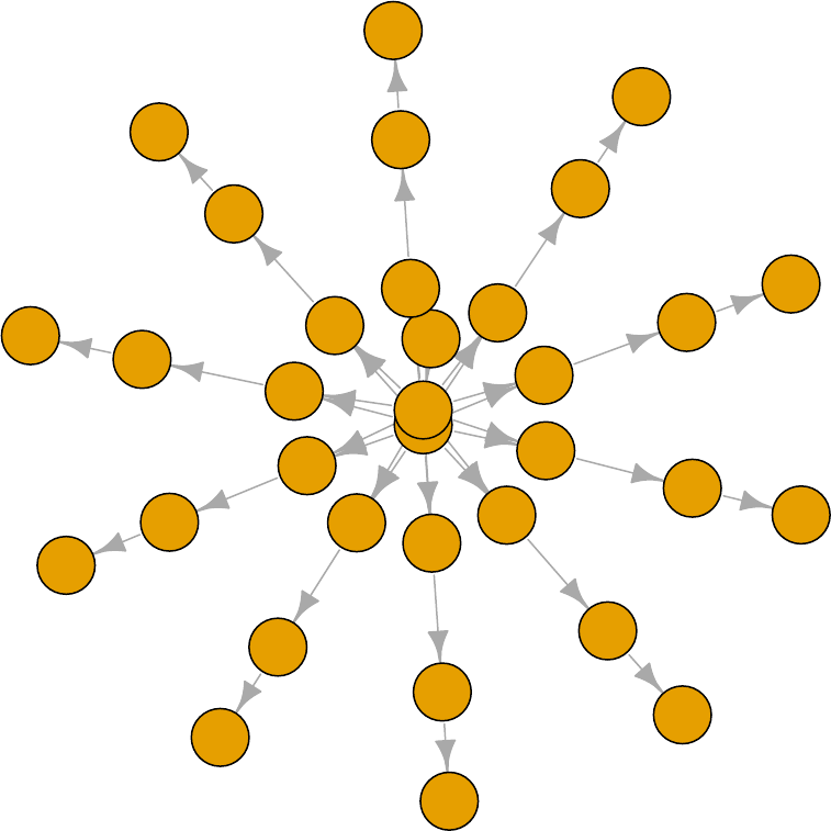
pump$plotGraph()
You are in control of the model. By default, nimbleModel does its best to initialize a model, but
let’s say you want to re-initialize theta. To simulate from the prior for theta (overwriting the
initial values previously in the model) we rst need to be sure the parent nodes of all theta[i]
nodes are fully initialized, including any non-stochastic nodes such as lifted nodes. We then use
the simulate function to simulate from the distribution for theta. Finally we use the calculate
function to calculate the dependencies of theta, namely lambda and the log probabilities of xto
ensure all parts of the model are up to date. First we show how to use the model’s getDependencies
method to query information about its graph.
# Show all dependencies of alpha and beta terminating in stochastic nodes
pump$getDependencies(c("alpha","beta"))
## [1] "alpha" "beta" "lifted_d1_over_beta"
## [4] "theta[1]" "theta[2]" "theta[3]"
## [7] "theta[4]" "theta[5]" "theta[6]"
## [10] "theta[7]" "theta[8]" "theta[9]"
## [13] "theta[10]"
# Now show only the deterministic dependencies
pump$getDependencies(c("alpha","beta"), determOnly = TRUE)
## [1] "lifted_d1_over_beta"
16 CHAPTER 2. LIGHTNING INTRODUCTION
alpha
beta
lifted_d1_over_beta
theta[1]
theta[2]
theta[3]
theta[4]
theta[5]
theta[6]
theta[7]
theta[8] theta[9]
theta[10]
lambda[1]
lambda[2]
lambda[3]
lambda[4]
lambda[5]
lambda[6]
lambda[7]
lambda[8]
lambda[9]
lambda[10]
x[1]
x[2]
x[3]
x[4]
x[5]
x[6]
x[7]
x[8]
x[9]
x[10]
Figure 2.1: Directed Acyclic Graph plot of the pump model, thanks to the igraph package

2.2. CREATING A MODEL 17
# Check that the lifted node was initialized.
pump[["lifted_d1_over_beta"]] # It was.
## [1] 1
# Now let's simulate new theta values
set.seed(1)# This makes the simulations here reproducible
pump$simulate("theta")
pump$theta # the new theta values
## [1] 0.15514136 1.88240160 1.80451250 0.83617765 1.22254365 1.15835525
## [7] 0.99001994 0.30737332 0.09461909 0.15720154
# lambda and logProb_x haven't been re-calculated yet
pump$lambda # these are the same values as above
## [1] 9.430 1.570 6.290 12.600 0.524 3.140 0.105 0.105 0.210 1.050
pump$logProb_x
## [1] -2.998011 -1.118924 -1.882686 -2.319466 -4.254550 -20.739651
## [7] -2.358795 -2.358795 -9.630645 -48.447798
pump$getLogProb("x")# The sum of logProb_x
## [1] -96.10932
pump$calculate(pump$getDependencies(c("theta")))
## [1] -262.204
pump$lambda # Now they have.
## [1] 14.6298299 29.5537051 113.5038360 105.3583839 6.4061287
## [6] 36.3723548 1.0395209 0.3227420 0.1987001 1.6506161
pump$logProb_x
## [1] -6.002009 -26.167496 -94.632145 -65.346457 -2.626123 -7.429868
## [7] -1.000761 -1.453644 -9.840589 -39.096527
Notice that the rst getDependencies call returned dependencies from alpha and beta down to the
next stochastic nodes in the model. The second call requested only deterministic dependencies. The
call to pump$simulate("theta") expands "theta" to include all nodes in theta. After simulating
into theta, we can see that lambda and the log probabilities of xstill reect the old values of theta,
so we calculate them and then see that they have been updated.

18 CHAPTER 2. LIGHTNING INTRODUCTION
2.3 Compiling the model
Next we compile the model, which means generating C++ code, compiling that code, and loading
it back into R with an object that can be used just like the uncompiled model. The values in
the compiled model will be initialized from those of the original model in R, but the original and
compiled models are distinct objects so any subsequent changes in one will not be reected in the
other.
Cpump <- compileNimble(pump)
Cpump$theta
## [1] 0.15514136 1.88240160 1.80451250 0.83617765 1.22254365 1.15835525
## [7] 0.99001994 0.30737332 0.09461909 0.15720154
Note that the compiled model is used when running any NIMBLE algorithms via C++, so the
model needs to be compiled before (or at the same time as) any compilation of algorithms, such as
the compilation of the MCMC done in the next section.
2.4 One-line invocation of MCMC
The most direct approach to invoking NIMBLE’s MCMC engine is using the nimbleMCMC function.
This function would generally take the code, data, constants, and initial values as input, but it can
also accept the (compiled or uncompiled) model object as an argument. It provides a variety of
options for executing and controlling multiple chains of NIMBLE’s default MCMC algorithm, and
returning posterior samples, posterior summary statistics, and/or WAIC values.
For example, to execute two MCMC chains of 10,000 samples each, and return samples, summary
statistics, and WAIC values:
mcmc.out <- nimbleMCMC(code = pumpCode, constants = pumpConsts,
data = pumpData, inits = pumpInits,
nchains = 2,niter = 10000,
summary = TRUE,WAIC = TRUE,monitors = c('alpha','beta','theta'))
names(mcmc.out)
## [1] "samples" "summary" "WAIC"
mcmc.out$summary
## $chain1
## Mean Median St.Dev. 95%CI_low 95%CI_upp
## alpha 0.69804352 0.65835063 0.27037676 0.287898244 1.3140461
## beta 0.92862598 0.82156847 0.54969128 0.183699137 2.2872696
## theta[1] 0.06019274 0.05676327 0.02544956 0.021069950 0.1199230
## theta[2] 0.10157737 0.08203988 0.07905076 0.008066869 0.3034085

2.4. ONE-LINE INVOCATION OF MCMC 19
## theta[3] 0.08874755 0.08396502 0.03760562 0.031186960 0.1769982
## theta[4] 0.11567784 0.11301465 0.03012598 0.064170937 0.1824525
## theta[5] 0.60382223 0.54935089 0.31219612 0.159731108 1.3640771
## theta[6] 0.61204831 0.60085518 0.13803302 0.372712375 0.9135269
## theta[7] 0.90263434 0.70803389 0.73960182 0.074122175 2.7598261
## theta[8] 0.89021051 0.70774794 0.72668155 0.072571029 2.8189252
## theta[9] 1.57678136 1.44390008 0.76825189 0.455195149 3.4297368
## theta[10] 1.98954127 1.96171250 0.42409802 1.241383787 2.9012192
##
## $chain2
## Mean Median St.Dev. 95%CI_low 95%CI_upp
## alpha 0.69101961 0.65803654 0.26548378 0.277195564 1.2858148
## beta 0.91627273 0.81434426 0.53750825 0.185772263 2.2702428
## theta[1] 0.05937364 0.05611283 0.02461866 0.020956151 0.1161870
## theta[2] 0.10017726 0.08116259 0.07855024 0.008266343 0.3010355
## theta[3] 0.08908126 0.08390782 0.03704170 0.031330829 0.1736876
## theta[4] 0.11592652 0.11356920 0.03064645 0.063595333 0.1829574
## theta[5] 0.59755632 0.54329373 0.31871551 0.149286703 1.3748728
## theta[6] 0.61080189 0.59946693 0.13804343 0.371373877 0.9097319
## theta[7] 0.89902759 0.70901502 0.72930369 0.076243503 2.7441445
## theta[8] 0.89954594 0.70727079 0.73345905 0.071250926 2.8054633
## theta[9] 1.57530029 1.45005738 0.75242164 0.469959364 3.3502795
## theta[10] 1.98911473 1.96227061 0.42298189 1.246910723 2.9102326
##
## $all.chains
## Mean Median St.Dev. 95%CI_low 95%CI_upp
## alpha 0.69453156 0.65803654 0.26795776 0.28329854 1.2999319
## beta 0.92244935 0.81828160 0.54365539 0.18549077 2.2785444
## theta[1] 0.05978319 0.05646474 0.02504028 0.02102807 0.1183433
## theta[2] 0.10087731 0.08162361 0.07880204 0.00811108 0.3017967
## theta[3] 0.08891440 0.08394667 0.03732417 0.03123228 0.1749967
## theta[4] 0.11580218 0.11326039 0.03038683 0.06385253 0.1827382
## theta[5] 0.60068928 0.54668011 0.31548032 0.15363752 1.3686801
## theta[6] 0.61142510 0.60015416 0.13803618 0.37203765 0.9122467
## theta[7] 0.90083096 0.70852800 0.73445465 0.07550465 2.7534885
## theta[8] 0.89487822 0.70761105 0.73007484 0.07211191 2.8067373
## theta[9] 1.57604083 1.44719278 0.76035931 0.46374515 3.3866706
## theta[10] 1.98932800 1.96195345 0.42352979 1.24334249 2.9068229
mcmc.out$WAIC
## [1] 48.69896
See Section 7.1 or help(nimbleMCMC) for more details about using nimbleMCMC.
Note that the WAIC value varies depending on what quantities are treated as parameters; see
Section 7.7 for more details.

20 CHAPTER 2. LIGHTNING INTRODUCTION
2.5 Creating, compiling and running a basic MCMC conguration
At this point we have initial values for all of the nodes in the model, and we have both the original
and compiled versions of the model. As a rst algorithm to try on our model, let’s use NIMBLE’s
default MCMC. Note that conjugate relationships are detected for all nodes except for alpha, on
which the default sampler is a random walk Metropolis sampler.
pumpConf <- configureMCMC(pump, print = TRUE)
## [1] RW sampler: alpha
## [2] conjugate_dgamma_dgamma sampler: beta
## [3] conjugate_dgamma_dpois sampler: theta[1]
## [4] conjugate_dgamma_dpois sampler: theta[2]
## [5] conjugate_dgamma_dpois sampler: theta[3]
## [6] conjugate_dgamma_dpois sampler: theta[4]
## [7] conjugate_dgamma_dpois sampler: theta[5]
## [8] conjugate_dgamma_dpois sampler: theta[6]
## [9] conjugate_dgamma_dpois sampler: theta[7]
## [10] conjugate_dgamma_dpois sampler: theta[8]
## [11] conjugate_dgamma_dpois sampler: theta[9]
## [12] conjugate_dgamma_dpois sampler: theta[10]
pumpConf$addMonitors(c("alpha","beta","theta"))
## thin = 1: alpha, beta, theta
pumpMCMC <- buildMCMC(pumpConf)
CpumpMCMC <- compileNimble(pumpMCMC, project = pump)
niter <- 1000
set.seed(1)
samples <- runMCMC(CpumpMCMC, niter = niter)
par(mfrow = c(1,4), mai = c(.6, .4, .1, .2))
plot(samples[ , "alpha"], type = "l",xlab = "iteration",
ylab = expression(alpha))
plot(samples[ , "beta"], type = "l",xlab = "iteration",
ylab = expression(beta))
plot(samples[ , "alpha"], samples[ , "beta"], xlab = expression(alpha),
ylab = expression(beta))
plot(samples[ , "theta[1]"], type = "l",xlab = "iteration",
ylab = expression(theta[1]))
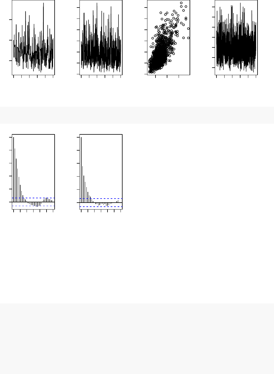
2.6. CUSTOMIZING THE MCMC 21
0 400 800
0.5 1.0 1.5
iteration
α
0 400 800
0.0 0.5 1.0 1.5 2.0 2.5 3.0
iteration
β
0.5 1.0 1.5
0.0 0.5 1.0 1.5 2.0 2.5 3.0
α
β
0 400 800
0.02 0.06 0.10 0.14
iteration
θ1
acf(samples[, "alpha"]) # plot autocorrelation of alpha sample
acf(samples[, "beta"]) # plot autocorrelation of beta sample
0 5 15 25
0.0 0.2 0.4 0.6 0.8 1.0
Lag
ACF
0 5 15 25
0.0 0.2 0.4 0.6 0.8 1.0
Lag
ACF
Notice the posterior correlation between alpha and beta. A measure of the mixing for each is the
autocorrelation for each parameter, shown by the acf plots.
2.6 Customizing the MCMC
Let’s add an adaptive block sampler on alpha and beta jointly and see if that improves the mixing.
pumpConf$addSampler(target = c("alpha","beta"), type = "RW_block",
control = list(adaptInterval = 100))
pumpMCMC2 <- buildMCMC(pumpConf)
# need to reset the nimbleFunctions in order to add the new MCMC
CpumpNewMCMC <- compileNimble(pumpMCMC2, project = pump,
resetFunctions = TRUE)
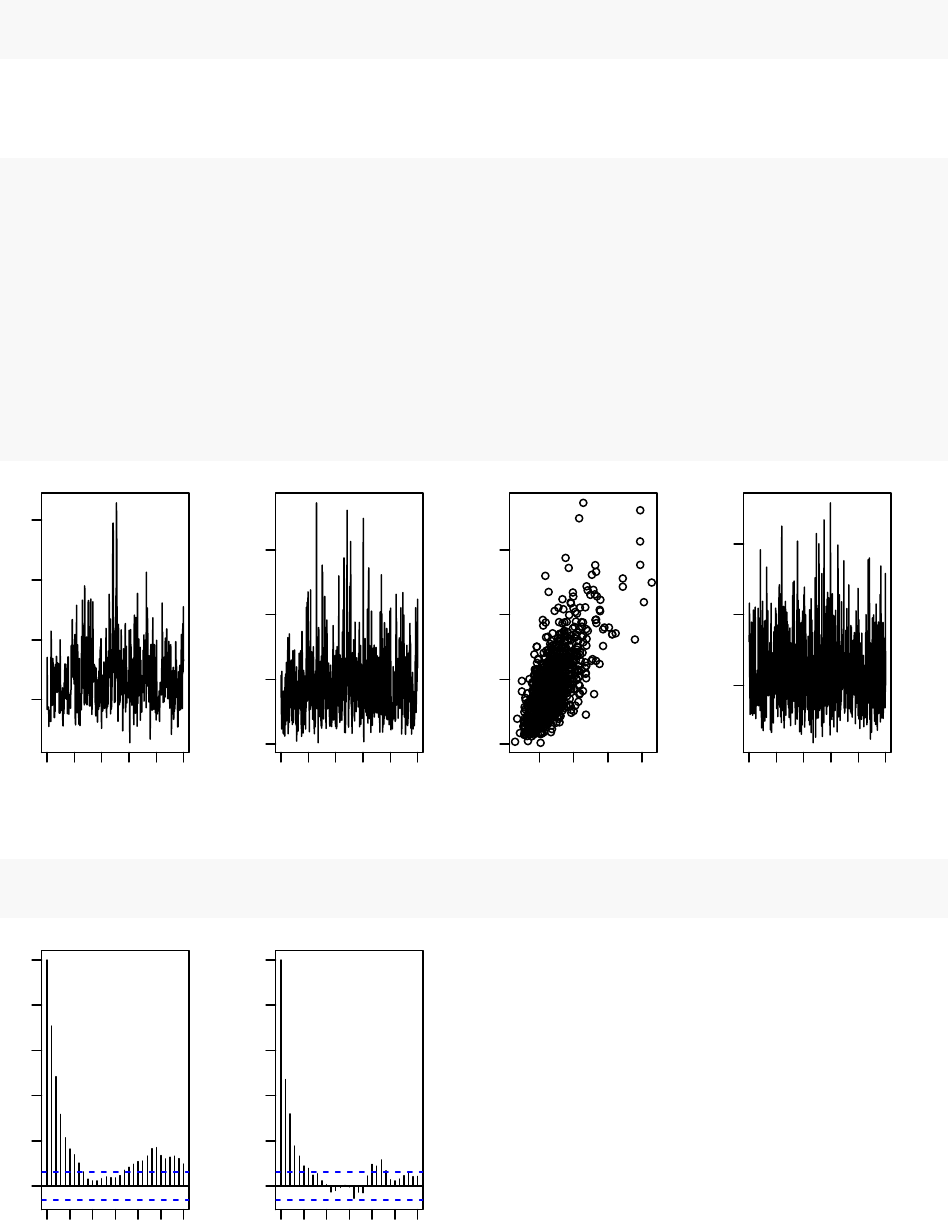
22 CHAPTER 2. LIGHTNING INTRODUCTION
set.seed(1)
CpumpNewMCMC$run(niter)
## NULL
samplesNew <- as.matrix(CpumpNewMCMC$mvSamples)
par(mfrow = c(1,4), mai = c(.6, .4, .1, .2))
plot(samplesNew[ , "alpha"], type = "l",xlab = "iteration",
ylab = expression(alpha))
plot(samplesNew[ , "beta"], type = "l",xlab = "iteration",
ylab = expression(beta))
plot(samplesNew[ , "alpha"], samplesNew[ , "beta"], xlab = expression(alpha),
ylab = expression(beta))
plot(samplesNew[ , "theta[1]"], type = "l",xlab = "iteration",
ylab = expression(theta[1]))
0 400 800
0.5 1.0 1.5 2.0
iteration
α
0 400 800
0 1 2 3
iteration
β
0.5 1.5
0 1 2 3
α
β
0 400 800
0.05 0.10 0.15
iteration
θ1
acf(samplesNew[, "alpha"]) # plot autocorrelation of alpha sample
acf(samplesNew[, "beta"]) # plot autocorrelation of beta sample
0 5 15 25
0.0 0.2 0.4 0.6 0.8 1.0
Lag
ACF
0 5 15 25
0.0 0.2 0.4 0.6 0.8 1.0
Lag
ACF

2.7. RUNNING MCEM 23
We can see that the block sampler has decreased the autocorrelation for both alpha and beta. Of
course these are just short runs, and what we are really interested in is the eective sample size of
the MCMC per computation time, but that’s not the point of this example.
Once you learn the MCMC system, you can write your own samplers and include them. The entire
system is written in nimbleFunctions.
2.7 Running MCEM
NIMBLE is a system for working with algorithms, not just an MCMC engine. So let’s try maxi-
mizing the marginal likelihood for alpha and beta using Monte Carlo Expectation Maximization2.
pump2 <- pump$newModel()
box = list(list(c("alpha","beta"), c(0,Inf)))
pumpMCEM <- buildMCEM(model = pump2, latentNodes = "theta[1:10]",
boxConstraints = box)
pumpMLE <- pumpMCEM$run()
## Iteration Number: 1.
## Current number of MCMC iterations: 1000.
## Parameter Estimates:
## alpha beta
## 0.8160625 1.1230921
## Convergence Criterion: 1.001.
## Iteration Number: 2.
## Current number of MCMC iterations: 1000.
## Parameter Estimates:
## alpha beta
## 0.8045037 1.1993128
## Convergence Criterion: 0.0223464.
## Monte Carlo error too big: increasing MCMC sample size.
## Iteration Number: 3.
## Current number of MCMC iterations: 1250.
## Parameter Estimates:
## alpha beta
## 0.8203178 1.2497067
## Convergence Criterion: 0.004913688.
## Monte Carlo error too big: increasing MCMC sample size.
## Monte Carlo error too big: increasing MCMC sample size.
## Monte Carlo error too big: increasing MCMC sample size.
## Iteration Number: 4.
## Current number of MCMC iterations: 3032.
2Note that for this model, one could analytically integrate over theta and then numerically maximize the resulting
marginal likelihood.

24 CHAPTER 2. LIGHTNING INTRODUCTION
## Parameter Estimates:
## alpha beta
## 0.8226618 1.2602452
## Convergence Criterion: 0.0004201048.
pumpMLE
## alpha beta
## 0.8226618 1.2602452
Both estimates are within 0.01 of the values reported by George et al. (1993)3. Some discrepancy
is to be expected since it is a Monte Carlo algorithm.
2.8 Creating your own functions
Now let’s see an example of writing our own algorithm and using it on the model. We’ll do
something simple: simulating multiple values for a designated set of nodes and calculating every
part of the model that depends on them. More details on programming in NIMBLE are in Part
IV.
Here is our nimbleFunction:
simNodesMany <- nimbleFunction(
setup = function(model, nodes) {
mv <- modelValues(model)
deps <- model$getDependencies(nodes)
allNodes <- model$getNodeNames()
},
run = function(n = integer()) {
resize(mv, n)
for(i in 1:n) {
model$simulate(nodes)
model$calculate(deps)
copy(from = model, nodes = allNodes,
to = mv, rowTo = i, logProb = TRUE)
}
})
simNodesTheta1to5 <- simNodesMany(pump, "theta[1:5]")
simNodesTheta6to10 <- simNodesMany(pump, "theta[6:10]")
Here are a few things to notice about the nimbleFunction.
1. The setup function is written in R. It creates relevant information specic to our model for
use in the run-time code.
3Table 2 of the paper accidentally swapped the two estimates.

2.8. CREATING YOUR OWN FUNCTIONS 25
2. The setup code creates a modelValues object to hold multiple sets of values for variables in
the model provided.
3. The run function is written in NIMBLE. It carries out the calculations using the information
determined once for each set of model and nodes arguments by the setup code. The run-time
code is what will be compiled.
4. The run code requires type information about the argument n. In this case it is a scalar
integer.
5. The for-loop looks just like R, but only sequential integer iteration is allowed.
6. The functions calculate and simulate, which were introduced above in R, can be used in
NIMBLE.
7. The special function copy is used here to record values from the model into the modelValues
object.
8. Multiple instances, or ‘specializations’, can be made by calling simNodesMany with dierent ar-
guments. Above, simNodesTheta1to5 has been made by calling simNodesMany with the pump
model and nodes "theta[1:5]" as inputs to the setup function, while simNodesTheta6to10
diers by providing "theta[6:10]" as an argument. The returned objects are objects of a
uniquely generated R reference class with elds (member data) for the results of the setup
code and a run method (member function).
By the way, simNodesMany is very similar to a standard nimbleFunction provided with NIMBLE,
simNodesMV.
Now let’s execute this nimbleFunction in R, before compiling it.
set.seed(1)# make the calculation repeatable
pump$alpha <- pumpMLE[1]
pump$beta <- pumpMLE[2]
# make sure to update deterministic dependencies of the altered nodes
pump$calculate(pump$getDependencies(c("alpha","beta"), determOnly = TRUE))
## [1] 0
saveTheta <- pump$theta
simNodesTheta1to5$run(10)
simNodesTheta1to5$mv[["theta"]][1:2]
## [[1]]
## [1] 0.21829875 1.93210969 0.62296551 0.34197266 3.45729601 1.15835525
## [7] 0.99001994 0.30737332 0.09461909 0.15720154
##
## [[2]]
## [1] 0.82759981 0.08784057 0.34414959 0.29521943 0.14183505 1.15835525
## [7] 0.99001994 0.30737332 0.09461909 0.15720154

26 CHAPTER 2. LIGHTNING INTRODUCTION
simNodesTheta1to5$mv[["logProb_x"]][1:2]
## [[1]]
## [1] -10.250111 -26.921849 -25.630612 -15.594173 -11.217566 -7.429868
## [7] -1.000761 -1.453644 -9.840589 -39.096527
##
## [[2]]
## [1] -61.043876 -1.057668 -11.060164 -11.761432 -3.425282 -7.429868
## [7] -1.000761 -1.453644 -9.840589 -39.096527
In this code we have initialized the values of alpha and beta to their MLE and then recorded
the theta values to use below. Then we have requested 10 simulations from simNodesTheta1to5.
Shown are the rst two simulation results for theta and the log probabilities of x. Notice that
theta[6:10] and the corresponding log probabilities for x[6:10] are unchanged because the nodes
being simulated are only theta[1:5]. In R, this function runs slowly.
Finally, let’s compile the function and run that version.
CsimNodesTheta1to5 <- compileNimble(simNodesTheta1to5,
project = pump, resetFunctions = TRUE)
Cpump$alpha <- pumpMLE[1]
Cpump$beta <- pumpMLE[2]
Cpump$calculate(Cpump$getDependencies(c("alpha","beta"), determOnly = TRUE))
## [1] 0
Cpump$theta <- saveTheta
set.seed(1)
CsimNodesTheta1to5$run(10)
## NULL
CsimNodesTheta1to5$mv[["theta"]][1:2]
## [[1]]
## [1] 0.21829875 1.93210969 0.62296551 0.34197266 3.45729601 1.15835525
## [7] 0.99001994 0.30737332 0.09461909 0.15720154
##
## [[2]]
## [1] 0.82759981 0.08784057 0.34414959 0.29521943 0.14183505 1.15835525
## [7] 0.99001994 0.30737332 0.09461909 0.15720154

2.8. CREATING YOUR OWN FUNCTIONS 27
CsimNodesTheta1to5$mv[["logProb_x"]][1:2]
## [[1]]
## [1] -10.250111 -26.921849 -25.630612 -15.594173 -11.217566 -2.782156
## [7] -1.042151 -1.004362 -1.894675 -3.081102
##
## [[2]]
## [1] -61.043876 -1.057668 -11.060164 -11.761432 -3.425282 -2.782156
## [7] -1.042151 -1.004362 -1.894675 -3.081102
Given the same initial values and the same random number generator seed, we got identical results
for theta[1:5] and their dependencies, but it happened much faster.
28 CHAPTER 2. LIGHTNING INTRODUCTION
Chapter 3
More introduction
Now that we have shown a brief example, we will introduce more about the concepts and design of
NIMBLE.
One of the most important concepts behind NIMBLE is to allow a combination of high-level pro-
cessing in R and low-level processing in C++. For example, when we write a Metropolis-Hastings
MCMC sampler in the NIMBLE language, the inspection of the model structure related to one
node is done in R, and the actual sampler calculations are done in C++. This separation between
setup and run steps will become clearer as we go.
3.1 NIMBLE adopts and extends the BUGS language for specify-
ing models
We adopted the BUGS language, and we have extended it to make it more exible. The BUGS
language became widely used in WinBUGS, then in OpenBUGS and JAGS. These systems all
provide automatically-generated MCMC algorithms, but we have adopted only the language for
describing models, not their systems for generating MCMCs.
NIMBLE extends BUGS by:
1. allowing you to write new functions and distributions and use them in BUGS models;
2. allowing you to dene multiple models in the same code using conditionals evaluated when
the BUGS code is processed;
3. supporting a variety of more exible syntax such as R-like named parameters and more general
algebraic expressions.
By supporting new functions and distributions, NIMBLE makes BUGS an extensible language,
which is a major departure from previous packages that implement BUGS.
We adopted BUGS because it has been so successful, with over 30,000 users by the time they
stopped counting (Lunn et al.,2009). Many papers and books provide BUGS code as a way to
document their statistical models. We describe NIMBLE’s version of BUGS later. The web sites
for WinBUGS, OpenBUGS and JAGS provide other useful documntation on writing models in
BUGS. For the most part, if you have BUGS code, you can try NIMBLE.
NIMBLE does several things with BUGS code:
29

30 CHAPTER 3. MORE INTRODUCTION
1. NIMBLE creates a model denition object that knows everything about the variables and
their relationships written in the BUGS code. Usually you’ll ignore the model denition and
let NIMBLE’s default options take you directly to the next step.
2. NIMBLE creates a model object1. This can be used to manipulate variables and operate
the model from R. Operating the model includes calculating, simulating, or querying the log
probability value of model nodes. These basic capabilities, along with the tools to query
model structure, allow one to write programs that use the model and adapt to its structure.
3. When you’re ready, NIMBLE can generate customized C++ code representing the model,
compile the C++, load it back into R, and provide a new model object that uses the compiled
model internally. We use the word ‘compile’ to refer to all of these steps together.
As an example of how radical a departure NIMBLE is from previous BUGS implementations,
consider a situation where you want to simulate new data from a model written in BUGS code.
Since NIMBLE creates model objects that you can control from R, simulating new data is trivial.
With previous BUGS-based packages, this isn’t possible.
More information about specifying and manipulating models is in Chapters 6and 13.
3.2 nimbleFunctions for writing algorithms
NIMBLE provides nimbleFunctions for writing functions that can (but don’t have to) use BUGS
models. The main ways that nimbleFunctions can use BUGS models are:
1. inspecting the structure of a model, such as determining the dependencies between variables,
in order to do the right calculations with each model;
2. accessing values of the model’s variables;
3. controlling execution of the model’s probability calculations or corresponding simulations;
4. managing modelValues data structures for multiple sets of model values and probabilities.
In fact, the calculations of the model are themselves constructed as nimbleFunctions, as are the
algorithms provided in NIMBLE’s algorithm library2.
Programming with nimbleFunctions involves a fundamental distinction between two stages of pro-
cessing:
1. A setup function within a nimbleFunction gives the steps that need to happen only once for
each new situation (e.g., for each new model). Typically such steps include inspecting the
model’s variables and their relationships, such as determining which parts of a model will
need to be calculated for a MCMC sampler. Setup functions are executed in R and never
compiled.
2. One or more run functions within a nimbleFunction give steps that need to happen multiple
times using the results of the setup function, such as the iterations of a MCMC sampler.
Formally, run code is written in the NIMBLE language, which you can think of as a small
1or multiple model objects
2That’s why it’s easy to use new functions and distributions written as nimbleFunctions in BUGS code.
3.3. THE NIMBLE ALGORITHM LIBRARY 31
subset of R along with features for operating models and related data structures. The NIM-
BLE language is what the NIMBLE compiler can automatically turn into C++ as part of a
compiled nimbleFunction.
What NIMBLE does with a nimbleFunction is similar to what it does with a BUGS model:
1. NIMBLE creates a working R version of the nimbleFunction. This is most useful for debugging
(Section 15.7).
2. When you are ready, NIMBLE can generate C++ code, compile it, load it back into R and
give you new objects that use the compiled C++ internally. Again, we refer to these steps all
together as ‘compilation’. The behavior of compiled nimbleFunctions is usually very similar,
but not identical, to their uncompiled counterparts.
If you are familiar with object-oriented programming, you can think of a nimbleFunction as a class
denition. The setup function initializes a new object and run functions are class methods. Member
data are determined automatically as the objects from a setup function needed in run functions. If
no setup function is provided, the nimbleFunction corresponds to a simple (compilable) function
rather than a class.
More about writing algorithms is in Chapter 15.
3.3 The NIMBLE algorithm library
In Version 0.6.13, the NIMBLE algorithm library includes:
1. MCMC with samplers including conjugate (Gibbs), slice, adaptive random walk (with options
for reection or sampling on a log scale), adaptive block random walk, and elliptical slice,
among others. You can modify sampler choices and congurations from R before compiling
the MCMC. You can also write new samplers as nimbleFunctions.
2. WAIC calculation for model comparison after an MCMC algorithm has been run.
3. A set of particle lter (sequential Monte Carlo) methods including a basic bootstrap lter,
auxiliary particle lter, and Liu-West lter.
4. An ascent-based Monte Carlo Expectation Maximization (MCEM) algorithm.
5. A variety of basic functions that can be used as programming tools for larger algorithms.
These include:
a. A likelihood function for arbitrary parts of any model.
b. Functions to simulate one or many sets of values for arbitrary parts of any model.
c. Functions to calculate the summed log probability (density) for one or many sets of
values for arbitrary parts of any model along with stochastic dependencies in the model
structure.
More about the NIMBLE algorithm library is in Chapter 8.
32 CHAPTER 3. MORE INTRODUCTION

Chapter 4
Installing NIMBLE
4.1 Requirements to run NIMBLE
You can run NIMBLE on any of the three common operating systems: Linux, Mac OS X, or
Windows.
The following are required to run NIMBLE.
1. R, of course.
2. The igraph and coda R packages.
3. A working C++ compiler that NIMBLE can use from R on your system. There are standard
open-source C++ compilers that the R community has already made easy to install. See
Section 4.2 for instructions. You don’t need to know anything about C++ to use NIMBLE.
This must be done before installing NIMBLE.
NIMBLE also uses a couple of C++ libraries that you don’t need to install, as they will already be
on your system or are provided by NIMBLE.
1. The Eigen C++ library for linear algebra. This comes with NIMBLE, or you can use your
own copy.
2. The BLAS and LAPACK numerical libraries. These come with R, but see Section 4.4.3 for
how to use a faster version of the BLAS.
Most fairly recent versions of these requirements should work.
4.2 Installing a C++ compiler for NIMBLE to use
NIMBLE needs a C++ compiler and the standard utility make in order to generate and compile
C++ for models and algorithms.1
1This diers from most packages, which might need a C++ compiler only when the package is built. If you
normally install R packages using install.packages on Windows or OS X, the package arrives already built to your
system.
33

34 CHAPTER 4. INSTALLING NIMBLE
4.2.1 OS X
On OS X, you should install Xcode. The command-line tools, which are available as a smaller
installation, should be sucient. This is freely available from the Apple developer site and the App
Store.
For the compiler to work correctly for OS X, the installed R must be for the correct version of OS
X. For example, R for Snow Leopard (OS X version 10.8) will attempt to use an incorrect C++
compiler if the installed OS X is actually version 10.9 or higher.
In the somewhat unlikely event you want to install from the source package rather than the CRAN
binary package, the easiest approach is to use the source package provided at R-nimble.org. If you
do want to install from the source package provided by CRAN, you’ll need to install this gfortran
package.
4.2.2 Linux
On Linux, you can install the GNU compiler suite (gcc/g++). You can use the package manager
to install pre-built binaries. On Ubuntu, the following command will install or update make,gcc
and libc.
sudo apt-get install build-essential
4.2.3 Windows
On Windows, you should download and install Rtools.exe available from https://cran.r-project.
org/bin/windows/Rtools/. Select the appropriate executable corresponding to your version of R
(and follow the urge to update your version of R if you notice it is not the most recent). This installer
leads you through several ‘pages’. We think you can accept the defaults with one exception: check
the PATH checkbox (page 5) so that the installer will add the location of the C++ compiler and
related tools to your system’s PATH, ensuring that R can nd them. After you click ‘Next’, you
will get a page with a window for customizing the new PATH variable. You shouldn’t need to do
anything there, so you can simply click ‘Next’ again.
The checkbox for the ‘R 2.15+ toolchain’ (page 4) must be checked (in order to have gcc/g++,
make, etc. installed). This should be checked by default.
4.3 Installing the NIMBLE package
Since NIMBLE is an R package, you can install it in the usual way, via install.packages("nimble")
in R or using the R CMD INSTALL method if you download the package source directly.
NIMBLE can also be obtained from the NIMBLE website. To install from our website, please see
our Download page for the specic invocation of install.packages.

4.4. CUSTOMIZING YOUR INSTALLATION 35
4.3.1 Problems with installation
We have tested the installation on the three commonly used platforms – MacOS, Linux, Windows2.
We don’t anticipate problems with installation, but we want to hear about any and help resolve
them. Please post about installation problems to the nimble-users Google group or email nimble.
stats@gmail.com.
4.4 Customizing your installation
For most installations, you can ignore low-level details. However, there are some options that some
users may want to utilize.
4.4.1 Using your own copy of Eigen
NIMBLE uses the Eigen C++ template library for linear algebra. Version 3.2.1 of Eigen is included
in the NIMBLE package and that version will be used unless the package’s conguration script nds
another version on the machine. This works well, and the following is only relevant if you want to
use a dierent (e.g., newer) version.
The conguration script looks in the standard include directories, e.g. /usr/include and
/usr/local/include for the header le Eigen/Dense. You can specify a particular location in
either of two ways:
1. Set the environment variable EIGEN_DIR before installing the R package, for example: export
EIGEN_DIR=/usr/include/eigen3 in the bash shell.
2. Use R CMD INSTALL --configure-args='--with-eigen=/path/to/eigen' nimble_VERSION.tar.gz
or install.packages("nimble", configure.args = "--with-eigen=/path/to/eigen")
In these cases, the directory should be the full path to the directory that contains the Eigen
directory, e.g., /usr/include/eigen3. It is not the full path to the Eigen directory itself, i.e.,
NOT /usr/include/eigen3/Eigen.
4.4.2 Using libnimble
NIMBLE generates specialized C++ code for user-specied models and nimbleFunctions. This
code uses some NIMBLE C++ library classes and functions. By default, on Linux the library code
is compiled once as a linkable library - libnimble.so. This single instance of the library is then linked
with the code for each generated model. In contrast, the default for Windows and Mac OS X is to
compile the library code as a static library - libnimble.a - that is compiled into each model’s and
each algorithm’s own dynamically loadable library (DLL). This does repeat the same code across
models and so occupies more memory. There may be a marginal speed advantage. If one would
like to enable the linkable library in place of the static library (do this only on Mac OS X and other
UNIX variants and not on Windows), one can install the source package with the conguration
argument --enable-dylib set to true. First obtain the NIMBLE source package (which will have
2We’ve tested NIMBLE on Windows 7, 8 and 10.

36 CHAPTER 4. INSTALLING NIMBLE
the extension .tar.gz from our website and then install as follows, replacing VERSION with the
appropriate version number:
RCMD INSTALL --configure-args='--enable-dylib=true' nimble_VERSION.tar.gz
4.4.3 BLAS and LAPACK
NIMBLE also uses BLAS and LAPACK for some of its linear algebra (in particular calculating
density values and generating random samples from multivariate distributions). NIMBLE will use
the same BLAS and LAPACK installed on your system that R uses. Note that a fast (and where
appropriate, threaded) BLAS can greatly increase the speed of linear algebra calculations. See
Section A.3.1 of the R Installation and Administration manual available on CRAN for more details
on providing a fast BLAS for your R installation.
4.4.4 Customizing compilation of the NIMBLE-generated C++
For each model or nimbleFunction, NIMBLE can generate and compile C++. To compile generated
C++, NIMBLE makes system calls starting with R CMD SHLIB and therefore uses the regular R
conguration in ${R_HOME}/etc/${R_ARCH}/Makeconf. NIMBLE places a Makevars le in the
directory in which the code is generated, and R CMD SHLIB uses this le as usual.
In all but specialized cases, the general compilation mechanism will suce. However, one can
customize this. One can specify the location of an alternative Makevars (or Makevars.win) le
to use. Such an alternative le should dene the variables PKG_CPPFLAGS and PKG_LIBS. These
should contain, respectively, the pre-processor ag to locate the NIMBLE include directory, and
the necessary libraries to link against (and their location as necessary), e.g., Rlapack and Rblas on
Windows, and libnimble. Advanced users can also change their default compilers by editing the
Makevars le, see Section 1.2.1 of the Writing R Extensions manual available on CRAN.
Use of this le allows users to specify additional compilation and linking ags. See the Writing R
Extensions manual for more details of how this can be used and what it can contain.
Part II
Models in NIMBLE
37

Chapter 5
Writing models in NIMBLE’s dialect
of BUGS
Models in NIMBLE are written using a variation on the BUGS language. From BUGS code,
NIMBLE creates a model object. This chapter describes NIMBLE’s version of BUGS. The next
chapter explains how to build and manipulate model objects.
5.1 Comparison to BUGS dialects supported by WinBUGS,
OpenBUGS and JAGS
Many users will come to NIMBLE with some familiarity with WinBUGS, OpenBUGS, or JAGS, so
we start by summarizing how NIMBLE is similar to and dierent from those before documenting
NIMBLE’s version of BUGS more completely. In general, NIMBLE aims to be compatible with the
original BUGS language and also JAGS’ version. However, at this point, there are some features
not supported by NIMBLE, and there are some extensions that are planned but not implemented.
5.1.1 Supported features of BUGS and JAGS
1. Stochastic and deterministic1node declarations.
2. Most univariate and multivariate distributions.
3. Link functions.
4. Most mathematical functions.
5. ‘for’ loops for iterative declarations.
6. Arrays of nodes up to 4 dimensions.
7. Truncation and censoring as in JAGS using the T() notation and dinterval.
5.1.2 NIMBLE’s Extensions to BUGS and JAGS
NIMBLE extends the BUGS language in the following ways:
1NIMBLE calls non-stochastic nodes ‘deterministic’, whereas BUGS calls them ‘logical’. NIMBLE uses ‘logical’ in
the way R does, to refer to boolean (TRUE/FALSE) variables.
39

40 CHAPTER 5. WRITING MODELS IN NIMBLE’S DIALECT OF BUGS
1. User-dened functions and distributions – written as nimbleFunctions – can be used in model
code. See Chapter 12.
2. Multiple parameterizations for distributions, similar to those in R, can be used.
3. Named parameters for distributions and functions, similar to R function calls, can be used.
4. Linear algebra, including for vectorized calculations of simple algebra, can be used in deter-
ministic declarations.
5. Distribution parameters can be expressions, as in JAGS but not in WinBUGS. Caveat: pa-
rameters to multivariate distributions (e.g., dmnorm) cannot be expressions (but an expression
can be dened in a separate deterministic expression and the resulting variable then used).
6. Alternative models can be dened from the same model code by using if-then-else statements
that are evaluated when the model is dened.
7. More exible indexing of vector nodes within larger variables is allowed. For example one can
place a multivariate normal vector arbitrarily within a higher-dimensional object, not just in
the last index.
8. More general constraints can be declared using dconstraint, which extends the concept of
JAGS’ dinterval.
9. Link functions can be used in stochastic, as well as deterministic, declarations.2
10. Data values can be reset, and which parts of a model are agged as data can be changed,
allowing one model to be used for dierent data sets without rebuilding the model each time.
11. As of Version 0.6-6 we now support stochastic/dynamic indexes. More specically in earlier
versions all indexes needed to be constants. Now indexes can be other nodes or functions
of other nodes. For a given dimension of a node being indexed, if the index is not con-
stant, it must be a scalar value. So expressions such as mu[k[i], 3] or mu[k[i], 1:3] or
mu[k[i], j[i]] are allowed, but not mu[k[i]:(k[i]+1)]. Nested dynamic indexes such as
mu[k[j[i]]] are also allowed.
5.1.3 Not-yet-supported features of BUGS and JAGS
In this release, the following are not supported.
1. The appearance of the same node on the left-hand side of both a <- and a ∼declaration
(used in WinBUGS for data assignment for the value of a stochastic node).
2. Multivariate nodes must appear with brackets, even if they are empty. E.g., xcannot be
multivariate but x[] or x[2:5] can be.
3. NIMBLE generally determines the dimensionality and sizes of variables from the BUGS code.
However, when a variable appears with blank indices, such as in x.sum <- sum(x[]), and
if the dimensions of the variable are not clearly dened in other declarations, NIMBLE cur-
rently requires that the dimensions of x be provided when the model object is created (via
nimbleModel).
5.2 Writing models
Here we introduce NIMBLE’s version of BUGS. The WinBUGS, OpenBUGS and JAGS manuals
are also useful resources for writing BUGS models, including many examples.
2But beware of the possibility of needing to set values for ‘lifted’ nodes created by NIMBLE.

5.2. WRITING MODELS 41
5.2.1 Declaring stochastic and deterministic nodes
BUGS is a declarative language for graphical (or hierarchical) models. Most programming languages
are imperative, which means a series of commands will be executed in the order they are written. A
declarative language like BUGS is more like building a machine before using it. Each line declares
that a component should be plugged into the machine, but it doesn’t matter in what order they
are declared as long as all the right components are plugged in by the end of the code.
The machine in this case is a graphical model3. A node (sometimes called a vertex) holds one value,
which may be a scalar or a vector. Edges dene the relationships between nodes. A huge variety
of statistical models can be thought of as graphs.
Here is the code to dene and create a simple linear regression model with four observations.
library(nimble)
mc <- nimbleCode({
intercept ~ dnorm(0,sd = 1000)
slope ~ dnorm(0,sd = 1000)
sigma ~ dunif(0,100)
for(i in 1:4) {
predicted.y[i] <- intercept + slope * x[i]
y[i] ~ dnorm(predicted.y[i], sd = sigma)
}
})
model <- nimbleModel(mc, data = list(y = rnorm(4)))
library(igraph)
layout <- matrix(ncol = 2,byrow = TRUE,
# These seem to be rescaled to fit in the plot area,
# so I'll just use 0-100 as the scale
data = c(33,100,
66,100,
50,0,# first three are parameters
15,50,35,50,55,50,75,50,# x's
20,75,40,75,60,75,80,75,# predicted.y's
25,25,45,25,65,25,85,25)# y's
)
sizes <- c(45,30,30,
rep(20,4),
rep(50,4),
rep(20,4))
edge.color <- "black"
# c(
3Technically, a directed acyclic graph
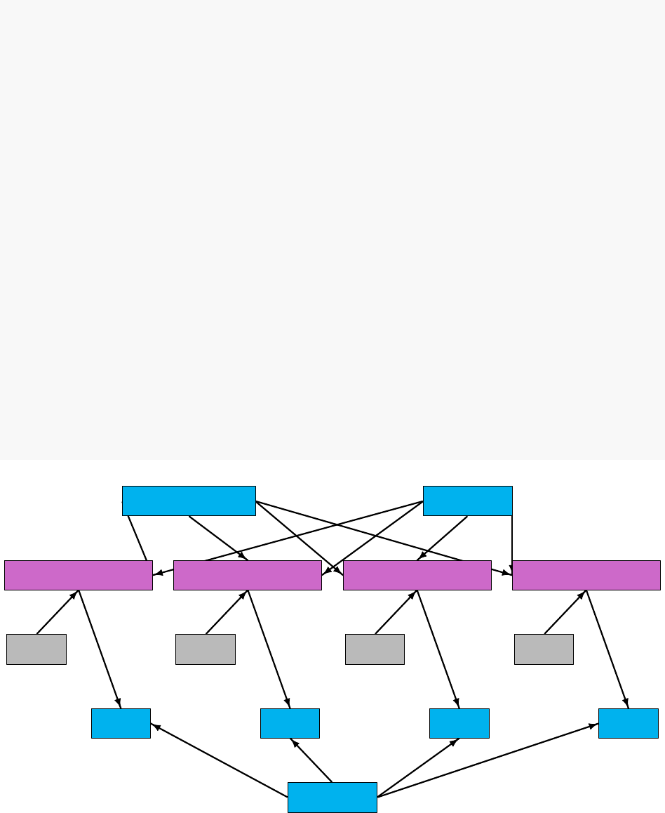
42 CHAPTER 5. WRITING MODELS IN NIMBLE’S DIALECT OF BUGS
# rep("green", 8),
# rep("red", 4),
# rep("blue", 4),
# rep("purple", 4))
stoch.color <- "deepskyblue2"
det.color <- "orchid3"
rhs.color <- "gray73"
fill.color <- c(
rep(stoch.color, 3),
rep(rhs.color, 4),
rep(det.color, 4),
rep(stoch.color, 4)
)
plot(model$graph, vertex.shape = "crectangle",
vertex.size = sizes,
vertex.size2 = 20,
layout = layout,
vertex.label.cex = 3.0,
vertex.color = fill.color,
edge.width = 3,
asp = 0.5,
edge.color = edge.color)
intercept slope
sigma
x[1] x[2] x[3] x[4]
predicted.y[1] predicted.y[2] predicted.y[3] predicted.y[4]
y[1] y[2] y[3] y[4]
Figure 5.1: Graph of a linear regression model
The graph representing the model is shown in Figure 5.1. Each observation, y[i], is a node whose
edges say that it follows a normal distribution depending on a predicted value, predicted.y[i],

5.2. WRITING MODELS 43
and standard deviation, sigma, which are each nodes. Each predicted value is a node whose edges
say how it is calculated from slope,intercept, and one value of an explanatory variable, x[i],
which are each nodes.
This graph is created from the following BUGS code:
{
intercept ~ dnorm(0,sd = 1000)
slope ~ dnorm(0,sd = 1000)
sigma ~ dunif(0,100)
for(i in 1:4) {
predicted.y[i] <- intercept + slope * x[i]
y[i] ~ dnorm(predicted.y[i], sd = sigma)
}
}
In this code, stochastic relationships are declared with ‘∼’ and deterministic relationships are de-
clared with ‘<-’. For example, each y[i] follows a normal distribution with mean predicted.y[i]
and standard deviation sigma. Each predicted.y[i] is the result of intercept + slope * x[i].
The for-loop yields the equivalent of writing four lines of code, each with a dierent value of i.
It does not matter in what order the nodes are declared. Imagine that each line of code draws
part of Figure 5.1, and all that matters is that the everything gets drawn in the end. Available
distributions, default and alternative parameterizations, and functions are listed in Section 5.2.4.
An equivalent graph can be created by this BUGS code:
{
intercept ~ dnorm(0,sd = 1000)
slope ~ dnorm(0,sd = 1000)
sigma ~ dunif(0,100)
for(i in 1:4) {
y[i] ~ dnorm(intercept + slope * x[i], sd = sigma)
}
}
In this case, the predicted.y[i] nodes in Figure 5.1 will be created automatically by NIMBLE
and will have a dierent name, generated by NIMBLE.
5.2.2 More kinds of BUGS declarations
Here are some examples of valid lines of BUGS code. This code does not describe a sensible or
complete model, and it includes some arbitrary indices (e.g. mvx[8:10, i]) to illustrate exibility.
Instead the purpose of each line is to illustrate a feature of NIMBLE’s version of BUGS.
{
# 1. normal distribution with BUGS parameter order
x ~ dnorm(a + b * c, tau)
# 2. normal distribution with a named parameter

44 CHAPTER 5. WRITING MODELS IN NIMBLE’S DIALECT OF BUGS
y ~ dnorm(a + b * c, sd = sigma)
# 3. For-loop and nested indexing
for(i in 1:N) {
for(j in 1:M[i]) {
z[i,j] ~ dexp(r[ blockID[i] ])
}
}
# 4. multivariate distribution with arbitrary indexing
for(i in 1:3)
mvx[8:10, i] ~ dmnorm(mvMean[3:5], cov = mvCov[1:3,1:3, i])
# 5. User-provided distribution
w ~ dMyDistribution(hello = x, world = y)
# 6. Simple deterministic node
d1 <- a + b
# 7. Vector deterministic node with matrix multiplication
d2[] <- A[ , ] %*% mvMean[1:5]
# 8. Deterministic node with user-provided function
d3 <- foo(x, hooray = y)
}
When a variable appears only on the right-hand side, it can be provided via constants (in which
case it can never be changed) or via data or inits, as discussed in Chapter 6.
Notes on the comment-numbered lines are:
1. xfollows a normal distribution with mean a + b*c and precision tau (default BUGS second
parameter for dnorm).
2. yfollows a normal distribution with the same mean as xbut a named standard deviation
parameter instead of a precision parameter (sd = 1/sqrt(precision)).
3. z[i, j] follows an exponential distribution with parameter r[ blockID[i] ]. This shows
how for-loops can be used for indexing of variables containing multiple nodes. Variables that
dene for-loop indices (Nand M) must also be provided as constants.
4. The arbitrary block mvx[8:10, i] follows a multivariate normal distribution, with a named
covariance matrix instead of BUGS’ default of a precision matrix. As in R, curly braces for
for-loop contents are only needed if there is more than one line.
5. wfollows a user-dened distribution. See Chapter 12.
6. d1 is a scalar deterministic node that, when calculated, will be set to a + b.
7. d2 is a vector deterministic node using matrix multiplication in R’s syntax.
8. d3 is a deterministic node using a user-provided function. See Chapter 12.
5.2.2.1 More about indexing
Examples of allowed indexing include:
•x[i] # a single index
•x[i:j] # a range of indices

5.2. WRITING MODELS 45
•x[i:j,k:l] # multiple single indices or ranges for higher-dimensional arrays
•x[i:j, ] # blank indices indicating the full range
•x[3*i+7] # computed indices
•x[(3*i):(5*i+1)] # computed lower and upper ends of an index range
•x[k[i]+1] # a dynamic (and computed) index
•x[k[j[i]]] # nested dynamic indexes
•x[k[i], 1:3] # nested indexing of rows or columns
NIMBLE does not allow multivariate nodes to be used without square brackets, which is an incom-
patibility with JAGS. Therefore a statement like xbar <- mean(x) in JAGS must be converted to
xbar <- mean(x[]) (if xis a vector) or xbar <- mean(x[,]) (if xis a matrix) for NIMBLE4.
Section 6.1.1.5 discusses how to provide NIMBLE with dimensions of xwhen needed.
Generally NIMBLE supports R-like linear algebra expressions and attempts to follow the same
rules as R about dimensions (although in some cases this is not possible). For example, x[1:3]
%*% y[1:3] converts x[1:3] into a row vector and thus computes the inner product, which is
returned as a 1×1matrix (use inprod to get it as a scalar, which it typically easier). Like in R, a
scalar index will result in dropping a dimension unless the argument drop=FALSE is provided. For
example, mymatrix[i, 1:3] will be a vector of length 3, but mymatrix[i, 1:3, drop=FALSE]
will be a 1×3matrix. More about indexing and dimensions is discussed in Section 11.3.2.6.
5.2.3 Vectorized versus scalar declarations
Suppose you need nodes logY[i] that should be the log of the corresponding Y[i], say for ifrom
1 to 10. Conventionally this would be created with a for loop:
{
for(i in 1:10) {
logY[i] <- log(Y[i])
}
}
Since NIMBLE supports R-like algebraic expressions, an alternative in NIMBLE’s dialect of BUGS
is to use a vectorized declaration like this:
{
logY[1:10] <- log(Y[1:10])
}
There is an important dierence between the models that are created by the above two methods.
The rst creates 10 scalar nodes, logY[1] , . . . , logY[10]. The second creates one vector node,
logY[1:10]. If each logY[i] is used separately by an algorithm, it may be more ecient compu-
tationally if they are declared as scalars. If they are all used together, it will often make sense to
declare them as a vector.
4In nimbleFunctions, as explained in later chapters, square brackets with blank indices are not necessary for
multivariate objects.

46 CHAPTER 5. WRITING MODELS IN NIMBLE’S DIALECT OF BUGS
5.2.4 Available distributions
5.2.4.1 Distributions
NIMBLE supports most of the distributions allowed in BUGS and JAGS. Table 5.1 lists the distri-
butions that are currently supported, with their default parameterizations, which match those of
BUGS5. NIMBLE also allows one to use alternative parameterizations for a variety of distributions
as described next. See Section 12.2 to learn how to write new distributions using nimbleFunctions.
Table 5.1: Distributions with their default order of parame-
ters. The value of the random variable is denoted by x.
Name Usage Density Lower Upper
Bernoulli dbern(prob = p) px(1 −p)1−x0 1
0< p < 1
Beta dbeta(shape1 = a, xa−1(1−x)b−1
β(a,b)0 1
shape2 = b),a > 0,b > 0
Binomial dbin(prob = p, size = n) n
xpx(1 −p)n−x0n
0< p < 1,n∈N∗
CAR dcar_normal(adj, weights, see chapter 9for details
(intrinsic) num, tau, c, zero_mean
CAR dcar_proper(mu, C, adj, see chapter 9for details
(proper) num, M, tau, gamma)
Categorical dcat(prob = p) px
ipi1N
p∈(R+)N
Chi-square dchisq(df = k),k > 0xk
2−1exp(−x/2)
2k
2Γ( k
2)0
Double ddexp(location = µ, rate = τ
2exp(−τ|x−µ|)
exponential τ),τ > 0
Dirichlet ddirch(alpha = α)Γ(jαj)j
xαj−1
j
Γ(αj)0
αj≥0
Exponential dexp(rate = λ),λ > 0λexp(−λx) 0
Flat dflat() ∝1(improper)
Gamma dgamma(shape = r, rate = λ)λrxr−1exp(−λx)
Γ(r)0
λ > 0,r > 0
Half at dhalfflat() ∝1(improper) 0
Inverse dinvgamma(shape = r, scale = λ)λrx−(r+1) exp(−λ/x)
Γ(r)0
gamma λ > 0,r > 0
Logistic dlogis(location = µ,τexp{(x−µ)τ}
[1+exp{(x−µ)τ}]2
rate = τ),τ > 0
Log-normal dlnorm(meanlog = µ,τ
2π1
2x−1exp −τ(log(x)−µ)2/20
taulog = τ), τ > 0
5Note that the same distributions are available for writing nimbleFunctions, but in that case the default param-
eterizations and function names match R’s when possible. Please see Section 11.2.4 for how to use distributions in
nimbleFunctions.

5.2. WRITING MODELS 47
Name Usage Density Lower Upper
Multinomial dmulti(prob = p, size = n) n!j
pxj
j
xj!
jxj=n
Multivariate dmnorm(mean = µ, prec = Λ)(2π)−d
2|Λ|1
2exp{−(x−µ)TΛ(x−µ)
2}
normal Λpositive denite
Multivariate dmvt(mu = µ, prec = Λ)Γ( ν+d
2)
Γ( ν
2)(νπ)d/2|Λ|1/2(1 + (x−µ)TΛ(x−µ)
ν)−ν+d
2
Student t df = ν), Λpositive def.
Negative dnegbin(prob = p, size = r) x+r−1
xpr(1 −p)x0
binomial 0< p ≤1,r≥0
Normal dnorm(mean = µ, tau = τ)τ
2π1
2exp{−τ(x−µ)2/2}
τ > 0
Poisson dpois(lambda = λ)exp(−λ)λx
x!0
λ > 0
Student t dt(mu = µ, tau = τ, df = k) Γ( k+1
2)
Γ( k
2)τ
kπ 1
21 + τ(x−µ)2
k−(k+1)
2
τ > 0,k > 0
Uniform dunif(min = a, max = b) 1
b−aa b
a < b
Weibull dweib(shape = v, lambda = λ)vλxv−1exp(−λxv) 0
v > 0,λ > 0
Wishart dwish(R = R, df = k) |x|(k−p−1)/2|R|k/2exp{−tr(Rx)/2}
2pk/2πp(p−1)/4p
i=1 Γ((k+1−i)/2)
Rp×ppos. def., k≥p
Inverse dinvwish(S = S, df = k) |x|−(k+p+1)/2|S|k/2exp{−tr(Sx−1)/2}
2pk/2πp(p−1)/4p
i=1 Γ((k+1−i)/2)
Wishart Sp×ppos. def., k≥p
5.2.4.1.1 Improper distributions
Note that dcar_normal,dflat and dhalfflat specify improper prior distributions and should
only be used when the posterior distribution of the model is known to be proper. Also for these
distributions, the density function returns the unnormalized density and the simulation function
returns NaN so these distributions are not appropriate for algorithms that need to simulate from
the prior or require proper (normalized) densities.
5.2.4.2 Alternative parameterizations for distributions
NIMBLE allows one to specify distributions in model code using a variety of parameterizations,
including the BUGS parameterizations. Available parameterizations are listed in Table 5.2. To
understand how NIMBLE handles alternative parameterizations, it is useful to distinguish three
cases, using the gamma distribution as an example:
1. A canonical parameterization is used directly for computations6. For gamma, this is (shape,
6Usually this is the parameterization in the Rmath header of R’s C implementation of distributions.

48 CHAPTER 5. WRITING MODELS IN NIMBLE’S DIALECT OF BUGS
scale).
2. The BUGS parameterization is the one dened in the original BUGS language. In general this
is the parameterization for which conjugate MCMC samplers can be executed most eciently.
For dgamma, this is (shape, rate).
3. An alternative parameterization is one that must be converted into the canonical parameter-
ization. For dgamma, NIMBLE provides both (shape, rate) and (mean, sd) parameterization
and creates nodes to calculate (shape, scale) from either (shape, rate) or (mean, sd). In the
case of dgamma, the BUGS parameterization is also an alternative parameterization.
Since NIMBLE provides compatibility with existing BUGS and JAGS code, the order of parame-
ters places the BUGS parameterization rst. For example, the order of parameters for dgamma is
dgamma(shape, rate, scale, mean, sd). Like R, if parameter names are not given, they are
taken in order, so that (shape, rate) is the default. This happens to match R’s order of parameters,
but it need not. If names are given, they can be given in any order. NIMBLE knows that rate is
an alternative to scale and that (mean, sd) are an alternative to (shape, scale or rate).
Table 5.2: Distribution parameterizations allowed in NIM-
BLE. The rst column indicates the supported parameteriza-
tions for distributions given in Table 5.1. The second column
indicates the relationship to the canonical parameterization
used in NIMBLE.
Parameterization NIMBLE re-parameterization
dbern(prob) dbin(size = 1, prob)
dbeta(shape1, shape2) canonical
dbeta(mean, sd) dbeta(shape1 = meanˆ2 * (1-mean) / sdˆ2 - mean,
shape2 = mean * (1 - mean)ˆ2 / sdˆ2 + mean - 1)
dbin(prob, size) canonical
dcat(prob) canonical
dchisq(df) canonical
ddexp(location, scale) canonical
ddexp(location, rate) ddexp(location, scale = 1 / rate)
ddexp(location, var) ddexp(location, scale = sqrt(var / 2))
ddirch(alpha) canonical
dexp(rate) canonical
dexp(scale) dexp(rate = 1/scale)
dgamma(shape, scale) canonical
dgamma(shape, rate) dgamma(shape, scale = 1 / rate)
dgamma(mean, sd) dgamma(shape = meanˆ2/sdˆ2, scale = sdˆ2/mean)
dinvgamma(shape, rate) canonical
dinvgamma(shape, scale) dgamma(shape, rate = 1 / scale)
dlogis(location, scale) canonical
dlogis(location, rate) dlogis(location, scale = 1 / rate
dlnorm(meanlog, sdlog) canonical
dlnorm(meanlog, taulog) dlnorm(meanlog, sdlog = 1 / sqrt(taulog)
dlnorm(meanlog, varlog) dlnorm(meanlog, sdlog = sqrt(varlog)
dmulti(prob, size) canonical

5.2. WRITING MODELS 49
Parameterization NIMBLE re-parameterization
dmnorm(mean, cholesky, canonical (precision)
...prec_param=1)
dmnorm(mean, cholesky, canonical (covariance)
...prec_param=0)
dmnorm(mean, prec) dmnorm(mean, cholesky = chol(prec), prec_param=1)
dmnorm(mean, cov) dmnorm(mean, cholesky = chol(cov), prec_param=0)
dmvt(mu, cholesky, df, canonical (precision/inverse scale)
...prec_param=1)
dmvt(mu, cholesky, df, canonical (scale)
...prec_param=0)
dmvt(mu, prec, df) dmvt(mu, cholesky = chol(prec), df, prec_param=1)
dmvt(mu, scale, df) dmvt(mu, cholesky = chol(scale), df, prec_param=0)
dnegbin(prob, size) canonical
dnorm(mean, sd) canonical
dnorm(mean, tau) dnorm(mean, sd = 1 / sqrt(var))
dnorm(mean, var) dnorm(mean, sd = sqrt(var))
dpois(lambda) canonical
dt(mu, sigma, df) canonical
dt(mu, tau, df) dt(mu, sigma = 1 / sqrt(tau), df)
dt(mu, sigma2, df) dt(mu, sigma = sqrt(sigma2), df)
dunif(min, max) canonical
dweib(shape, scale) canonical
dweib(shape, rate) dweib(shape, scale = 1 / rate)
dweib(shape, lambda) dweib(shape, scale = lambdaˆ(- 1 / shape)
dwish(cholesky, df, canonical (scale)
...scale_param=1)
dwish(cholesky, df, canonical (inverse scale)
...scale_param=0)
dwish(R, df) dwish(cholesky = chol(R), df, scale_param = 0)
dwish(S, df) dwish(cholesky = chol(S), df, scale_param = 1)
dinvwish(cholesky, df, canonical (scale)
...scale_param=1)
dinvwish(cholesky, df, canonical (inverse scale)
...scale_param=0)
dinvwish(R, df) dinvwish(cholesky = chol(R), df, scale_param = 0)
dinvwish(S, df) dinvwish(cholesky = chol(S), df, scale_param = 1)
Note that for multivariate normal, multivariate t, Wishart, and Inverse Wishart, the canonical
parameterization uses the Cholesky decomposition of one of the precision/inverse scale or covari-
ance/scale matrix. For example, for the multivariate normal, if prec_param=TRUE, the cholesky
argument is treated as the Cholesky decomposition of a precision matrix. Otherwise it is treated
as the Cholesky decomposition of a covariance matrix.
In addition, NIMBLE supports alternative distribution names, known as aliases, as in JAGS, as
specied in Table 5.3.

50 CHAPTER 5. WRITING MODELS IN NIMBLE’S DIALECT OF BUGS
Table 5.3: Distributions with alternative names (aliases)
Distribution Canonical name Alias
Binomial dbin dbinom
Chi-square dchisq dchisqr
Double exponential ddexp dlaplace
Dirichlet ddirch ddirich
Multinomial dmulti dmultinom
Negative binomial dnegbin dnbinom
Weibull dweib dweibull
Wishart dwish dwishart
We plan to, but do not currently, include the following distributions as part of core NIMBLE: double
exponential (Laplace), beta-binomial, Dirichlet-multinomial, F, Pareto, or forms of the multivariate
t other than the standard one provided.
5.2.5 Available BUGS language functions
Tables 11.2-11.3 show the available operators and functions. Support for more general R expressions
is covered in Chapter 11 about programming with nimbleFunctions.
For the most part NIMBLE supports the functions used in BUGS and JAGS, with exceptions
indicated in the table. Additional functions provided by NIMBLE are also listed. Note that we
provide distribution functions for use in calculations, namely the ‘p’, ‘q’, and ‘d’ functions. See
Section 11.2.4 for details on the syntax for using distribution functions as functions in deterministic
calculations, as only some parameterizations are allowed and the names of some distributions dier
from those used to dene stochastic nodes in a model.
Table 5.4: Functions operating on scalars, many of which
can operate on each element (component-wise) of vectors and
matrices. Status column indicates if the function is currently
provided in NIMBLE. Vector input column indicates if the
function can take a vector as an argument (i.e., if the function
is vectorized).
Usage Description Comments Status Vector input
x|y,x&y logical OR (|) and AND(&) yes yes
!x logical not yes yes
x>y,x>=y greater than (and or equal to) yes yes
x<y,x<=y less than (and or equal to) yes yes
x!=y,x==y (not) equals yes yes
x+y,x-y,x*y component-wise operators mix of scalar and vector yes yes
x/y component-wise division vector xand scalar yyes yes
xˆy, pow(x, y) power xy; vector x,scalar yyes yes
x %% y modulo (remainder) yes no
min(x1, x2), min. (max.) of two scalars yes See pmin,

5.2. WRITING MODELS 51
Usage Description Comments Status Vector input
max(x1, x2) pmax
exp(x) exponential yes yes
log(x) natural logarithm yes yes
sqrt(x) square root yes yes
abs(x) absolute value yes yes
step(x) step function at 0 0 if x < 0, 1 if x >= 0 yes yes
equals(x) equality of two scalars 1 if x== y, 0 if x! = yyes yes
cube(x) third power x3yes yes
sin(x), cos(x), trigonometric functions yes yes
tan(x)
asin(x), acos(x), inverse trigonometric functions yes yes
atan(x)
asinh(x), acosh(x), inv. hyperbolic trig. functions yes yes
atanh(x)
logit(x) logit log(x/(1 −x)) yes yes
ilogit(x), expit(x) inverse logit exp(x)/(1 + exp(x)) yes yes
probit(x) probit (Gaussian quantile) Φ−1(x)yes yes
iprobit(x), phi(x) inverse probit (Gaussian CDF) Φ(x)yes yes
cloglog(x) complementary log log log(−log(1 −x)) yes yes
icloglog(x) inverse complementary log log 1−exp(−exp(x)) yes yes
ceiling(x) ceiling function ⌈(x)⌉yes yes
floor(x) oor function ⌊(x)⌋yes yes
round(x) round to integer yes yes
trunc(x) truncation to integer yes yes
lgamma(x), loggam(x) log gamma function log Γ(x)yes yes
besselK(k, nu, modied bessel function yes yes
...expon.scaled) of the second kind
log1p(x) log of 1 + x log(1 + x)yes yes
lfactorial(x), log factorial log x!yes yes
logfact(x)
qDIST(x, PARAMS) “q” distribution functions canonical parameterization yes yes
pDIST(x, PARAMS) “p” distribution functions canonical parameterization yes yes
rDIST(x, PARAMS) “r” distribution functions canonical parameterization yes yes
dDIST(x, PARAMS) “d” distribution functions canonical parameterization yes yes
sort(x) no
rank(x, s) no
ranked(x, s) no
order(x) no
Table 5.5: Functions operating on vectors and matrices. Sta-
tus column indicates if the function is currently provided in
NIMBLE.
Usage Description Comments Status
inverse(x) matrix inverse xsymmetric, positive def. yes

52 CHAPTER 5. WRITING MODELS IN NIMBLE’S DIALECT OF BUGS
Usage Description Comments Status
chol(x) matrix Cholesky factorization xsymmetric, positive def. yes
t(x) matrix transpose x⊤yes
x%*%y matrix multiply xy;x,yconformant yes
inprod(x, y) dot product x⊤y;xand yvectors yes
solve(x) solve system of equations x−1y;ymatrix or vector yes
forwardsolve(x, y) solve lower-triangular system of equations x−1y;xlower-triangular yes
backsolve(x, y) solve upper-triangular system of equations x−1y;xupper-triangular yes
logdet(x) log matrix determinant log |x|yes
asRow(x) convert vector to 1-row matrix sometimes automatic yes
asCol(x) convert vector to 1-column matrix sometimes automatic yes
sum(x) sum of elements of xyes
mean(x) mean of elements of xyes
sd(x) standard deviation of elements of xyes
prod(x) product of elements of xyes
min(x), max(x) min. (max.) of elements of xyes
pmin(x, y), pmax(x,y) vector of mins (maxs) of elements of yes
xand y
interp.lin(x, v1, v2) linear interpolation no
eigen(x)$values matrix eigenvalues xsymmetric yes
eigen(x)$vectors matrix eigenvectors xsymmetric yes
svd(x)$d matrix singular values yes
svd(x)$u matrix left singular vectors yes
svd(x)$v matrix right singular vectors yes
See Section 12.1 to learn how to use nimbleFunctions to write new functions for use in BUGS code.
5.2.6 Available link functions
NIMBLE allows the link functions listed in Table 5.6.
Table 5.6: Link functions.
Link function Description Range Inverse
cloglog(y) <- x Complementary log log 0< y < 1y <- icloglog(x)
log(y) <- x Log 0< y y <- exp(x)
logit(y) <- x Logit 0< y < 1y <- expit(x)
probit(y) <- x Probit 0< y < 1y <- iprobit(x)
Link functions are specied as functions applied to a node on the left hand side of a BUGS expression.
To handle link functions in deterministic declarations, NIMBLE converts the declaration into an
equivalent inverse declaration. For example, log(y) <- x is converted into y <- exp(x). In other
words, the link function is just a simple variant for conceptual clarity.
To handle link functions in a stochastic declaration, NIMBLE does some processing that inserts an
additional node into the model. For example, the declaration logit(p[i]) ~ dnorm(mu[i],1), is

5.2. WRITING MODELS 53
equivalent to the following two declarations:
•logit_p[i] ~ dnorm(mu[i], 1),
•p[i] <- expit(logit_p[i])
where expit is the inverse of logit.
Note that NIMBLE does not provide an automatic way of initializing the additional node
(logit_p[i] in this case), which is a parent node of the explicit node (p[i]), without explicitly
referring to the additional node by the name that NIMBLE generates.
5.2.7 Truncation, censoring, and constraints
NIMBLE provides three ways to declare boundaries on the value of a variable, each for dierent
situations. We introduce these and comment on their relationships to related features of JAGS and
BUGS. The three methods are:
5.2.7.1 Truncation
Either of the following forms,
x ~ dnorm(0, sd = 10) T(0, a)
x ~ T(dnorm(0, sd = 10), 0, a)
declares that xfollows a normal distribution between 0 and a(inclusive of 0 and a). Either boundary
may be omitted or may be another node, such as ain this example. The rst form is compatible
with JAGS, but in NIMBLE it can only be used when reading code from a text le. When writing
model code in R, the second version must be used.
Truncation means the possible values of xare limited a priori, hence the probability density of x
must be normalized7. In this example it would be the normal probability density divided by its
integral from 0 to a. Like JAGS, NIMBLE also provides Ias a synonym for Tto accommodate
older BUGS code, but Tis preferred because it disambiguates multiple usages of Iin BUGS.
5.2.7.2 Censoring
Censoring refers to the situation where one datum gives the lower or upper bound on an unobserved
random variable. This is common in survival analysis, when for an individual still surviving at the
end of a study, the age of death is not known and hence is ‘censored’ (right-censoring). NIMBLE
adopts JAGS syntax for censoring, as follows:
censored[i] ~ dinterval(t[i], c[i])
t[i] ~ dweib(r, mu[i])
7NIMBLE uses the CDF and inverse CDF (quantile) functions of a distribution to do this; in some cases if one
uses truncation to include only the extreme tail of a distribution, numerical diculties can arise.

54 CHAPTER 5. WRITING MODELS IN NIMBLE’S DIALECT OF BUGS
In the case of right-censoring, censored[i] should be given as data with a value of 1 if t[i]
is right-censored (t[i] > c[i]) and 0 if it is observed. The data vector for tshould have NA
(indicating missing data) for any censored t[i] entries. (As a result, these nodes will be sampled
in an MCMC.) The data vector for cshould give the censoring times corresponding to censored
entries and a value above the observed times for uncensored entries (e.g., Inf). Left-censored
observations would be specied by setting censored[i] to 0 and t[i] to NA.
The dinterval is not really a distribution but rather a trick: in the above example when
censored[i] = 1 it gives a ‘probability’ of 1 if t[i] > c[i] and 0 otherwise. This means
that t[i] <= c[i] is treated as impossible. More generally than simple right- or left-censoring,
censored[i] ~ dinterval(t[i], c[i, ]) is dened such that for a vector of increasing
cutpoints, c[i, ],t[i] is enforced to fall within the censored[i]-th cutpoint interval. This is
done by setting data censored[i] as follows:
censored[i] = 0 if t[i] <= c[i, 1]
censored[i] = m if c[i, m] < t[i] <= c[i, m+1] for 1≤m≤M
censored[i] = M if c[i, M] < t[i]
(The iindex is provided only for consistency with the previous example.) The most common uses
of dinterval will be for left- and right-censored data, in which case c[i,] will be a single value
(and typically given as simply c[i]), and for interval-censored data, in which case c[i,] will be a
vector of two values.
Nodes following a dinterval distribution should normally be set as data with known values. Oth-
erwise, the node may be simulated during initialization in some algorithms (e.g., MCMC) and
thereby establish a permanent, perhaps unintended, constraint.
Censoring diers from truncation because censoring an observation involves bounds on a random
variable that could have taken any value, while in truncation we know a priori that a datum could
not have occurred outside the truncation range.
5.2.7.3 Constraints and ordering
NIMBLE provides a more general way to enforce constraints using dconstraint(cond). For ex-
ample, we could specify that the sum of mu1 and mu2 must be positive like this:
mu1 ~ dnorm(0,1)
mu2 ~ dnorm(0,1)
constraint_data ~ dconstraint( mu1 + mu2 > 0)
with constraint_data set (as data) to 1. This is equivalent to a half-normal distribution on the
half-plane µ1+µ2>0. Nodes following dconstraint should be provided as data for the same
reason of avoiding unintended initialization described above for dinterval.
Formally, dconstraint(cond) is a probability distribution on {0,1}such that P(1) = 1 if cond is
TRUE and P(0) = 1 if cond is FALSE.
Of course, in many cases, parameterizing the model so that the constraints are automatically
respected may be a better strategy than using dconstraint. One should be cautious about con-
straints that would make it hard for an MCMC or optimization to move through the parameter

5.2. WRITING MODELS 55
space (such as equality constraints that involve two or more parameters). For such restrictive con-
straints, general purpose algorithms that are not tailored to the constraints may fail or be inecient.
If constraints are used, it will generally be wise to ensure the model is initialized with values that
satisfy them.
5.2.7.3.1 Ordering
To specify an ordering of parameters, such as α1<=α2<=α3one can use dconstraint as follows:
constraint_data ~ dconstraint( alpha1 <= alpha2 & alpha2 <= alpha3 )
Note that unlike in BUGS, one cannot specify prior ordering using syntax such as
alpha[1] ~ dnorm(0,1)I(, alpha[2])
alpha[2] ~ dnorm(0,1)I(alpha[1], alpha[3])
alpha[3] ~ dnorm(0,1)I(alpha[2], )
as this does not represent a directed acyclic graph.
Also note that specifying prior ordering using T(,) can result in possibly unexpected results. For
example:
alpha1 ~ dnorm(0,1)
alpha2 ~ dnorm(0,1)T(alpha1, )
alpha3 ~ dnorm(0,1)T(alpha2, )
will enforce alpha1 ≤alpha2 ≤alpha3, but it does not treat the three parameters symmetrically.
Instead it puts a marginal prior on alpha1 that is standard normal and then constrains alpha2
and alpha3 to follow truncated normal distributions. This is not equivalent to a symmetric prior
on the three alphas that assigns zero probability density when values are not in order.
NIMBLE does not support the JAGS sort syntax.
56 CHAPTER 5. WRITING MODELS IN NIMBLE’S DIALECT OF BUGS

Chapter 6
Building and using models
This chapter explains how to build and manipulate model objects starting from BUGS code.
6.1 Creating model objects
NIMBLE provides two functions for creating model objects: nimbleModel and readBUGSmodel. The
rst, nimbleModel, is more general and was illustrated in Chapter 2. The second, readBUGSmodel
provides compatibility with BUGS le formats for models, variables, data, and initial values for
MCMC.
In addition one can create new model objects from existing model objects.
6.1.1 Using nimbleModel to create a model
nimbleModel processes BUGS code to determine all the nodes, variables, and their relationships
in a model. Any constants must be provided at this step. Data and initial values can optionally
be provided. BUGS code passed to nimbleModel must go through nimbleCode.
We look again at the pump example from the introduction:
pumpCode <- nimbleCode({
for (i in 1:N){
theta[i] ~ dgamma(alpha,beta);
lambda[i] <- theta[i]*t[i];
x[i] ~ dpois(lambda[i])
}
alpha ~ dexp(1.0);
beta ~ dgamma(0.1,1.0);
})
pumpConsts <- list(N = 10,
t = c(94.3,15.7,62.9,126,5.24,
31.4,1.05,1.05,2.1,10.5))
57

58 CHAPTER 6. BUILDING AND USING MODELS
pumpData <- list(x = c(5,1,5,14,3,19,1,1,4,22))
pumpInits <- list(alpha = 1,beta = 1,
theta = rep(0.1, pumpConsts$N))
pump <- nimbleModel(code = pumpCode, name = "pump",constants = pumpConsts,
data = pumpData, inits = pumpInits)
6.1.1.1 Data and constants
NIMBLE makes a distinction between data and constants:
•Constants can never be changed and must be provided when a model is dened. For example,
a vector of known index values, such as for block indices, helps dene the model graph itself
and must be provided as constants. Variables used in the index ranges of for-loops must also
be provided as constants.
•Data is a label for the role a node plays in the model. Nodes marked as data will by default
be protected from any functions that would simulate over their values (see simulate in
Chapter 13), but it is possible to over-ride that default or to change their values by direct
assignment. This allows an algorithm to be applied to many data sets in the same model
without re-creating the model each time. It also allows simulation of data in a model.
WinBUGS, OpenBUGS and JAGS do not allow data values to be changed or dierent nodes to be
labeled as data without starting from the beginning again. Hence they do not distinguish between
constants and data.
For compatibility with BUGS and JAGS, NIMBLE allows both to be provided in the constants
argument to nimbleModel, in which case NIMBLE handles values for stochastic nodes as data and
everything else as constants.
Values for nodes that appear only on the right-hand side of BUGS declarations (e.g., covari-
ates/predictors) can be provided as constants or as data or initial values. There is no real dierence
between providing as data or initial values and the values can be added after building a model via
setInits or setData.
6.1.1.2 Providing data and initial values to an existing model
Whereas constants must be provided during the call to nimbleModel, data and initial values can be
provided later via the model member functions setData and setInits. For example, if pumpData
is a named list of data values (as above), then pump$setData(pumpData) sets the named variables
to the values in the list.
setData does two things: it sets the values of the data nodes, and it ags those nodes as containing
data. nimbleFunction programmers can then use that information to control whether an algorithm
should over-write data or not. For example, NIMBLE’s simulate functions by default do not
overwrite data values but can be told to do so. Values of data variables can be replaced, and the

6.1. CREATING MODEL OBJECTS 59
indication of which nodes should be treated as data can be reset by using the resetData method,
e.g. pump$resetData().
6.1.1.3 Missing data values
Sometimes one needs a model variable to have a mix of data and non-data, often due to missing
data values. In NIMBLE, when data values are provided, any nodes with NA values will not be
labeled as data. A node following a multivariate distribution must be either entirely observed or
entirely missing.
Here’s an example of running an MCMC on the pump model, with two of the observations taken
to be missing. Some of the steps in this example are documented more below. NIMBLE’s default
MCMC conguration will treat the missing values as unknowns to be sampled, as can be seen in
the MCMC output here.
pumpMiss <- pump$newModel()
pumpMiss$resetData()
pumpDataNew <- pumpData
pumpDataNew$x[c(1,3)] <- NA
pumpMiss$setData(pumpDataNew)
pumpMissConf <- configureMCMC(pumpMiss)
pumpMissConf$addMonitors('x','alpha','beta','theta')
## thin = 1: alpha, beta, x, theta
pumpMissMCMC <- buildMCMC(pumpMissConf)
Cobj <- compileNimble(pumpMiss, pumpMissMCMC)
niter <- 10
set.seed(0)
Cobj$pumpMissMCMC$run(niter)
## NULL
samples <- as.matrix(Cobj$pumpMissMCMC$mvSamples)
samples[1:5,13:17]
## x[1] x[2] x[3] x[4] x[5]
## [1,] 17 1 2 14 3
## [2,] 11 1 4 14 3
## [3,] 14 1 9 14 3
## [4,] 11 1 24 14 3
## [5,] 9 1 29 14 3

60 CHAPTER 6. BUILDING AND USING MODELS
Missing values may also occur in explanatory/predictor variables. Values for such variables should
be passed in via the data argument to nimbleModel, with NA for the missing values. In some
contexts, one would want to specify distributions for such explanatory variables, for example so
that an MCMC would impute the missing values.
6.1.1.4 Dening alternative models with the same code
Avoiding code duplication is a basic principle of good programming. In NIMBLE, one can use
denition-time if-then-else statements to create dierent models from the same code. As a simple
example, say we have a linear regression model and want to consider including or omitting x[2] as
an explanatory variable:
regressionCode <- nimbleCode({
intercept ~ dnorm(0,sd = 1000)
slope1 ~ dnorm(0,sd = 1000)
if(includeX2) {
slope2 ~ dnorm(0,sd = 1000)
for(i in 1:N)
predictedY[i] <- intercept + slope1 * x1[i] + slope2 * x2[i]
} else {
for(i in 1:N) predictedY[i] <- intercept + slope1 * x1[i]
}
sigmaY ~ dunif(0,100)
for(i in 1:N) Y[i] ~ dnorm(predictedY[i], sigmaY)
})
includeX2 <- FALSE
modelWithoutX2 <- nimbleModel(regressionCode, constants = list(N = 30),
check=FALSE)
modelWithoutX2$getVarNames()
## [1] "intercept" "slope1"
## [3] "predictedY" "sigmaY"
## [5] "lifted_d1_over_sqrt_oPsigmaY_cP" "Y"
## [7] "x1"
includeX2 <- TRUE
modelWithX2 <- nimbleModel(regressionCode, constants = list(N = 30),
check = FALSE)
modelWithX2$getVarNames()
## [1] "intercept" "slope1"
## [3] "slope2" "predictedY"
## [5] "sigmaY" "lifted_d1_over_sqrt_oPsigmaY_cP"
## [7] "Y" "x1"
## [9] "x2"

6.1. CREATING MODEL OBJECTS 61
Whereas the constants are a property of the model denition – since they may help determine the
model structure itself – data nodes can be dierent in dierent copies of the model generated from
the same model denition. The setData and setInits described above can be used for each copy
of the model.
6.1.1.5 Providing dimensions via nimbleModel
nimbleModel can usually determine the dimensions of every variable from the declarations in the
BUGS code. However, it is possible to use a multivariate object only with empty indices (e.g. x[,]),
in which case the dimensions must be provided as an argument to nimbleModel.
Here’s an example with multivariate nodes. The rst provides indices, so no dimensions argument
is needed, while the second omits the indices and provides a dimensions argument instead.
code <- nimbleCode({
y[1:K] ~ dmulti(p[1:K], n)
p[1:K] ~ ddirch(alpha[1:K])
log(alpha[1:K]) ~ dmnorm(alpha0[1:K], R[1:K, 1:K])
})
K <- 5
model <- nimbleModel(code, constants = list(n = 3,K = K,
alpha0 = rep(0, K), R = diag(K)),
check = FALSE)
codeAlt <- nimbleCode({
y[] ~ dmulti(p[], n)
p[] ~ ddirch(alpha[])
log(alpha[]) ~ dmnorm(alpha0[], R[ , ])
})
model <- nimbleModel(codeAlt, constants = list(n = 3,K = K, alpha0 = rep(0, K),
R = diag(K)),
dimensions = list(y = K, p = K, alpha = K),
check = FALSE)
In that example, since alpha0 and Rare provided as constants, we don’t need to specify their
dimensions.
6.1.2 Creating a model from standard BUGS and JAGS input les
Users with BUGS and JAGS experience may have les set up in standard formats for use in
BUGS and JAGS. readBUGSmodel can read in the model, data/constant values and initial values
in those formats. It can also take information directly from R objects somewhat more exibly than
nimbleModel, specically allowing inputs set up similarly to those for BUGS and JAGS. In either
case, after processing the inputs, it calls nimbleModel. Note that unlike BUGS and JAGS, only a

62 CHAPTER 6. BUILDING AND USING MODELS
single set of initial values can be specied in creating a model. Please see help(readBUGSmodel)
for argument details.
As an example of using readBUGSmodel, let’s create a model for the pump example from BUGS.
pumpDir <- system.file('classic-bugs','vol1','pump',package = 'nimble')
pumpModel <- readBUGSmodel('pump.bug',data = 'pump-data.R',
inits = 'pump-init.R',dir = pumpDir)
## Detected x as data within 'constants'.
Note that readBUGSmodel allows one to include var and data blocks in the model le as in some
of the BUGS examples (such as inhaler). The data block pre-computes constant and data values.
Also note that if data and inits are provided as les, the les should contain R code that creates
objects analogous to what would populate the list if a list were provided instead. Please see the
JAGS manual examples or the classic_bugs directory in the NIMBLE package for example syntax.
NIMBLE by and large does not need the information given in a var block but occasionally this is
used to determine dimensionality, such as in the case of syntax like xbar <- mean(x[]) where xis
a variable that appears only on the right-hand side of BUGS expressions.
Note that NIMBLE does not handle formatting such as in some of the original BUGS examples in
which data was indicated with syntax such as data x in 'x.txt'.
6.1.3 Making multiple instances from the same model denition
Sometimes it is useful to have more than one copy of the same model. For example, an algorithm
(i.e., nimbleFunction) such as an MCMC will be bound to a particular model before it is run. A user
could build multiple algorithms to use the same model instance, or they may want each algorithm
to have its own instance of the model.
There are two ways to create new instances of a model, shown in this example:
simpleCode <- nimbleCode({
for(i in 1:N) x[i] ~ dnorm(0,1)
})
# Return the model definition only, not a built model
simpleModelDefinition <- nimbleModel(simpleCode, constants = list(N = 10),
returnDef = TRUE,check = FALSE)
# Make one instance of the model
simpleModelCopy1 <- simpleModelDefinition$newModel(check = FALSE)
# Make another instance from the same definition
simpleModelCopy2 <- simpleModelDefinition$newModel(check = FALSE)
# Ask simpleModelCopy2 for another copy of itself
simpleModelCopy3 <- simpleModelCopy2$newModel(check = FALSE)
Each copy of the model can have dierent nodes agged as data and dierent values in any nodes.
They cannot have dierent values of Nbecause that is a constant; it must be a constant because it
helps dene the model.

6.2. NIMBLE MODELS ARE OBJECTS YOU CAN QUERY AND MANIPULATE 63
6.2 NIMBLE models are objects you can query and manipulate
NIMBLE models are objects that can be modied and manipulated from R. In this section we
introduce some basic ways to use a model object. Chapter 13 covers more topics for writing
algorithms that use models.
6.2.1 What are variables and nodes?
This section discusses some basic concepts and terminology to be able to speak about NIMBLE
models clearly.
Suppose we have created a model from the following BUGS code.
mc <- nimbleCode({
a ~ dnorm(0,0.001)
for(i in 1:5) {
y[i] ~ dnorm(a, sd = 0.1)
for(j in 1:3)
z[i,j] ~ dnorm(y[i], tau)
}
tau ~ dunif(0,20)
y.squared[1:5] <- y[1:5]^2
})
model <- nimbleModel(mc, data = list(z = matrix(rnorm(15), nrow = 5)))
In NIMBLE terminology:
• The variables of this model are a,y,z, and y.squared.
• The nodes of this model are a,y[1] , . . . , y[5],z[1,1] , . . . , z[5, 3], and y.squared[1:5].
In graph terminology, nodes are vertices in the model graph.
• The node functions of this model are a ~ dnorm(0, 0.001),y[i] ~ dnorm(a, 0.1),
z[i,j] ~ dnorm(y[i], sd = 0.1), and y.squared[1:5] <- y[1:5]ˆ2. Each node’s
calculations are handled by a node function. Sometimes the distinction between nodes and
node functions is important, but when it is not important we may refer to both simply as
nodes.
• The scalar elements of this model include all the scalar nodes as well as the scalar elements
y.squared[1] , . . . , y.squared[5] of the multivariate node y.squared[1:5].
6.2.2 Determining the nodes and variables in a model
One can determine the variables in a model using getVarNames and the nodes in a model using
getNodeNames. Optional arguments to getNodeNames allow you to select only certain types of
nodes, as discussed in Section 13.1.1 and in the R help for getNodeNames.

64 CHAPTER 6. BUILDING AND USING MODELS
model$getVarNames()
## [1] "a" "y"
## [3] "lifted_d1_over_sqrt_oPtau_cP" "z"
## [5] "tau" "y.squared"
model$getNodeNames()
## [1] "a" "tau"
## [3] "y[1]" "y[2]"
## [5] "y[3]" "y[4]"
## [7] "y[5]" "lifted_d1_over_sqrt_oPtau_cP"
## [9] "y.squared[1:5]" "z[1, 1]"
## [11] "z[1, 2]" "z[1, 3]"
## [13] "z[2, 1]" "z[2, 2]"
## [15] "z[2, 3]" "z[3, 1]"
## [17] "z[3, 2]" "z[3, 3]"
## [19] "z[4, 1]" "z[4, 2]"
## [21] "z[4, 3]" "z[5, 1]"
## [23] "z[5, 2]" "z[5, 3]"
Note that some of the nodes may be ‘lifted’ nodes introduced by NIMBLE (Section 13.1.2). In this
case lifted_d1_over_sqrt_oPtau_cP (this is a node for the standard deviation of the znodes
using NIMBLE’s canonical parameterization of the normal distribution) is the only lifted node in
the model.
To determine the dependencies of one or more nodes in the model, you can use getDependencies
as discussed in Section 13.1.3.
6.2.3 Accessing nodes
Model variables can be accessed and set just as in R using $and [[ ]]. For example
model$a <- 5
model$a
## [1] 5
model[["a"]]
## [1] 5

6.2. NIMBLE MODELS ARE OBJECTS YOU CAN QUERY AND MANIPULATE 65
model$y[2:4] <- rnorm(3)
model$y
## [1] NA -0.9261095 -0.1771040 0.4020118 NA
model[["y"]][c(1,5)] <- rnorm(2)
model$y
## [1] -0.7317482 -0.9261095 -0.1771040 0.4020118 0.8303732
model$z[1,]
## [1] -0.3340008 1.2079084 0.5210227
While nodes that are part of a variable can be accessed as above, each node also has its own name
that can be used to access it directly. For example, y[2] has the name ‘y[2]’ and can be accessed
by that name as follows:
model[["y[2]"]]
## [1] -0.9261095
model[["y[2]"]] <- -5
model$y
## [1] -0.7317482 -5.0000000 -0.1771040 0.4020118 0.8303732
model[["z[2, 3]"]]
## [1] -0.1587546
model[["z[2:4, 1:2]"]][1,2]
## [1] -1.231323
model$z[2,2]
## [1] -1.231323
Notice that node names can include index blocks, such as model[["z[2:4, 1:2]"]], and these are
not strictly required to correspond to actual nodes. Such blocks can be subsequently sub-indexed
in the regular R manner, such as model[["z[2:4, 1:2]"]][1, 2].

66 CHAPTER 6. BUILDING AND USING MODELS
6.2.4 How nodes are named
Every node has a name that is a character string including its indices, with a space after every
comma. For example, X[1, 2, 3] has the name ‘X[1, 2, 3]’. Nodes following multivariate distri-
butions have names that include their index blocks. For example, a multivariate node for X[6:10,
3] has the name ‘X[6:10, 3]’.
The denitive source for node names in a model is getNodeNames, described previously.
In the event you need to ensure that a name is formatted correctly, you can use the
expandNodeNames method. For example, to get the spaces correctly inserted into ‘X[1,1:5]’:
multiVarCode <- nimbleCode({
X[1,1:5] ~ dmnorm(mu[], cov[,])
X[6:10,3] ~ dmnorm(mu[], cov[,])
})
multiVarModel <- nimbleModel(multiVarCode, dimensions =
list(mu = 5,cov = c(5,5)), calculate = FALSE)
multiVarModel$expandNodeNames("X[1,1:5]")
## [1] "X[1, 1:5]"
Alternatively, for those inclined to R’s less commonly used features, a nice trick is to use its parse
and deparse functions.
deparse(parse(text = "X[1,1:5]",keep.source = FALSE)[[1]])
## [1] "X[1, 1:5]"
The keep.source = FALSE makes parse more ecient.
6.2.5 Why use node names?
Syntax like model[["z[2, 3]"]] may seem strange at rst, because the natural habit of an R user
would be model[["z"]][2,3]. To see its utility, consider the example of writing the nimbleFunction
given in Section 2.8. By giving every scalar node a name, even if it is part of a multivariate variable,
one can write functions in R or NIMBLE that access any single node by a name, regardless of the
dimensionality of the variable in which it is embedded. This is particularly useful for NIMBLE,
which resolves how to access a particular node during the compilation process.
6.2.6 Checking if a node holds data
Finally, you can query whether a node is agged as data using the isData method applied to one
or more nodes or nodes within variables:

6.2. NIMBLE MODELS ARE OBJECTS YOU CAN QUERY AND MANIPULATE 67
model$isData('z[1]')
## [1] TRUE
model$isData(c('z[1]','z[2]','a'))
## [1] TRUE TRUE FALSE
model$isData('z')
## [1] TRUE TRUE TRUE TRUE TRUE TRUE TRUE TRUE TRUE TRUE TRUE TRUE TRUE TRUE
## [15] TRUE
model$isData('z[1:3, 1]')
## [1] TRUE TRUE TRUE
68 CHAPTER 6. BUILDING AND USING MODELS
Part III
Algorithms in NIMBLE
69
Chapter 7
MCMC
NIMBLE provides a variety of paths to creating and executing an MCMC algorithm, which dier
greatly in their simplicity of use, and also in the options available and customizability.
The most direct approach to invoking the MCMC engine is using the nimbleMCMC function (Section
7.1). This one-line call creates and executes an MCMC, and provides a wide range of options for
controlling the MCMC: specifying monitors, burn-in, and thinning, running multiple MCMC chains
with dierent initial values, and returning posterior samples, summary statistics, and/or a WAIC
value. However, this approach is restricted to using NIMBLE’s default MCMC algorithm; further
customization of, for example, the specic samplers employed, is not possible.
The lengthier and more customizable approach to invoking the MCMC engine on a particular
NIMBLE model object involves the following steps:
1. (Optional) Create and customize an MCMC conguration for a particular model:
a. Use configureMCMC to create an MCMC conguration (see Section 7.2). The congura-
tion contains a list of samplers with the node(s) they will sample.
b. (Optional) Customize the MCMC conguration:
i. Add, remove, or re-order the list of samplers (Section 7.9 and help(samplers) in
R for details), including adding your own samplers (Section 15.5);
ii. Change the tuning parameters or adaptive properties of individual samplers;
iii. Change the variables to monitor (record for output) and thinning intervals for
MCMC samples.
2. Use buildMCMC to build the MCMC object and its samplers either from the model (using
default MCMC conguration) or from a customized MCMC conguration (Section 7.3).
3. Compile the MCMC object (and the model), unless one is debugging and wishes to run the
uncompiled MCMC.
4. Run the MCMC and extract the samples (Sections 7.4,7.5 and 7.6).
5. Optionally, calculate the WAIC using the posterior samples (Section 7.7).
NIMBLE provides two additional functions which facilitate the comparison of multiple, dierent,
MCMC algorithms:
71
72 CHAPTER 7. MCMC
•MCMCsuite can run multiple, dierent MCMCs for the same model. These can include multi-
ple NIMBLE MCMCs from dierent congurations as well as external MCMCs such as from
WinBUGS, OpenBUGS, JAGS or Stan (Section 7.11).
•compareMCMCs manages multiple calls to MCMCsuite and generates html pages comparing
performance of dierent MCMCs.
End-to-end examples of MCMC in NIMBLE can be found in Sections 2.5-2.6 and Section 7.10.
7.1 One-line invocation of MCMC: nimbleMCMC
The most direct approach to executing an MCMC algorithm in NIMBLE is using nimbleMCMC.
This single function can be used to create an underlying model and associated MCMC algorithm,
compile both of these, execute the MCMC, and return samples, summary statistics, and a WAIC
value. This approach circumvents the longer (and more exible) approach using nimbleModel,
configureMCMC,buildMCMC,compileNimble, and runMCMC, which is described subsequently.
The nimbleMCMC function provides control over the:
• number of MCMC iterations in each chain;
• number of MCMC chains to execute;
• number of burn-in samples to discard from each chain;
• thinning interval on which samples should be recorded;
• model variables to monitor and return posterior samples;
• initial values, or a function for generating initial values for each chain;
• setting the random number seed;
• returning posterior samples as a matrix or a coda mcmc object;
• returning posterior summary statistics; and
• returning a WAIC value calculated using samples from all chains.
This entry point for using nimbleMCMC is the code,constants,data, and inits arguments that
are used for building a NIMBLE model (see Chapters 5and 6). However, when using nimbleMCMC,
the inits argument can also specify a list of lists of initial values that will be used for each MCMC
chain, or a function that generates a list of initial values, which will be generated at the onset
of each chain. As an alternative entry point, a NIMBLE model object can also be supplied to
nimbleMCMC, in which case this model will be used to build the MCMC algorithm.
Based on its arguments, nimbleMCMC optionally returns any combination of
• Posterior samples,
• Posterior summary statistics, and
• WAIC value.
The above are calculated and returned for each MCMC chain. Additionally, posterior summary
statistics are calculated for all chains combined when multiple chains are run.
Several example usages of nimbleMCMC are shown below:

7.2. THE MCMC CONFIGURATION 73
code <- nimbleCode({
mu ~ dnorm(0,sd = 1000)
sigma ~ dunif(0,1000)
for(i in 1:10)
x[i] ~ dnorm(mu, sd = sigma)
})
data <- list(x = c(2,5,3,4,1,0,1,3,5,3))
initsFunction <- function() list(mu = rnorm(1,0,1), sigma = runif(1,0,10))
# execute one MCMC chain, monitoring the "mu" and "sigma" variables,
# with thinning interval 10. fix the random number seed for reproducible
# results. by default, only returns posterior samples.
mcmc.out <- nimbleMCMC(code = code, data = data, inits = initsFunction,
monitors = c("mu","sigma"), thin = 10,
niter = 20000,nchains = 1,setSeed = TRUE)
# note that the inits argument to nimbleModel must be a list of
# initial values, whereas nimbleMCMC can accept inits as a function
# for generating new initial values for each chain.
initsList <- initsFunction()
Rmodel <- nimbleModel(code, data = data, inits = initsList)
# using the existing Rmodel object, execute three MCMC chains with
# specified burn-in. return samples, summary statistics, and WAIC.
mcmc.out <- nimbleMCMC(model = Rmodel,
niter = 20000,nchains = 3,nburnin = 2000,
summary = TRUE,WAIC = TRUE)
# run ten chains, generating random initial values for each
# chain using the inits function specified above.
# only return summary statistics from each chain; not all the samples.
mcmc.out <- nimbleMCMC(model = Rmodel, nchains = 10,inits = initsFunction,
samples = FALSE,summary = TRUE)
See help(nimbleMCMC) for further details.
7.2 The MCMC conguration
The MCMC conguration contains information needed for building an MCMC. When no customiza-
tion is needed, one can jump directly to the buildMCMC step below. An MCMC conguration is an
object of class MCMCconf, which includes:
• The model on which the MCMC will operate
• The model nodes which will be sampled (updated) by the MCMC
• The samplers and their internal congurations, called control parameters

74 CHAPTER 7. MCMC
• Two sets of variables that will be monitored (recorded) during execution of the MCMC and
thinning intervals for how often each set will be recorded. Two sets are allowed because it
can be useful to monitor dierent variables at dierent intervals
7.2.1 Default MCMC conguration
Assuming we have a model named Rmodel, the following will generate a default MCMC congura-
tion:
mcmcConf <- configureMCMC(Rmodel)
The default conguration will contain a single sampler for each node in the model, and the default
ordering follows the topological ordering of the model.
7.2.1.1 Default assignment of sampler algorithms
The default sampler assigned to a stochastic node is determined by the following, in order of
precedence:
1. If the node has no stochastic dependents, a posterior_predictive sampler is assigned. This
sampler sets the new value for the node simply by simulating from its distribution.
2. If the node has a conjugate relationship between its prior distribution and the distributions
of its stochastic dependents, a conjugate (‘Gibbs’) sampler is assigned.
3. If the node follows a multinomial distribution, then a RW_multinomial sampler is assigned.
This is a discrete random-walk sampler in the space of multinomial outcomes.
4. If a node follows a Dirichlet distribution, then a RW_dirichlet sampler is assigned. This is
a random walk sampler in the space of the simplex dened by the Dirichlet.
5. If the node follows any other multivariate distribution, then a RW_block sampler is assigned for
all elements. This is a Metropolis-Hastings adaptive random-walk sampler with a multivariate
normal proposal (Roberts and Sahu,1997).
6. If the node is binary-valued (strictly taking values 0 or 1), then a binary sampler is assigned.
This sampler calculates the conditional probability for both possible node values and draws
the new node value from the conditional distribution, in eect making a Gibbs sampler.
7. If the node is otherwise discrete-valued, then a slice sampler is assigned (Neal,2003).
8. If none of the above criteria are satised, then a RW sampler is assigned. This is a Metropolis-
Hastings adaptive random-walk sampler with a univariate normal proposal distribution.
These sampler assignment rules can be inspected, reordered, and easily modied using the
system option nimbleOptions("MCMCdefaultSamplerAssignmentRules") and customized
samplerAssignmentRules objects.
Details of each sampler and its control parameters can be found by invoking help(samplers).

7.2. THE MCMC CONFIGURATION 75
7.2.1.2 Sampler assignment rules
The behavior of configureMCMC can be customized to control how samplers are assigned. A new
set of sampler assignment rules can be created using samplerAssignmentRules, which can be mod-
ied using the addRule and reorder methods, then passed as an argument to configureMCMC.
Alternatively, the default behavior of configureMCMC can be altered by setting the system op-
tion MCMCdefaultSamplerAssignmentRules to a custom samplerAssignmentRules object. See
help(samplerAssignmentRules) for details.
7.2.1.3 Options to control default sampler assignments
As a lightweight alternative to using samplerAssignmentRules, very basic control of default sam-
pler assignments is provided via two arguments to configureMCMC. The useConjugacy argument
controls whether conjugate samplers are assigned when possible, and the multivariateNodesAsScalars
argument controls whether scalar elements of multivariate nodes are sampled individually. See
help(configureMCMC) for usage details.
7.2.1.4 Default monitors
The default MCMC conguration includes monitors on all top-level stochastic nodes of the model.
Only variables that are monitored will have their samples saved for use outside of the MCMC.
MCMC congurations include two sets of monitors, each with dierent thinning intervals. By
default, the second set of monitors (monitors2) is empty.
7.2.1.5 Automated parameter blocking
The default conguration may be replaced by one generated from an automated parameter blocking
algorithm. This algorithm determines groupings of model nodes that, when jointly sampled with a
RW_block sampler, increase overall MCMC eciency. Overall eciency is dened as the eective
sample size of the slowest-mixing node divided by computation time. This is done by:
autoBlockConf <- configureMCMC(Rmodel, autoBlock = TRUE)
Note that this using autoBlock = TRUE compiles and runs MCMCs, progressively exploring dierent
sampler assignments, so it takes some time and generates some output. It is most useful for
determining eective blocking strategies that can be re-used for later runs. The additional control
argument autoIt may also be provided to indicate the number of MCMC samples to be used in
each trial of the automated blocking procedure (default 20,000).
7.2.2 Customizing the MCMC conguration
The MCMC conguration may be customized in a variety of ways, either through additional named
arguments to configureMCMC or by calling methods of an existing MCMCconf object.

76 CHAPTER 7. MCMC
7.2.2.1 Controlling which nodes to sample
One can create an MCMC conguration with default samplers on just a particular set of nodes
using the nodes argument to configureMCMC. The value for the nodes argument may be a character
vector containing node and/or variable names. In the case of a variable name, a default sampler
will be added for all stochastic nodes in the variable. The order of samplers will match the order
of nodes. Any deterministic nodes will be ignored.
If a data node is included in nodes,it will be assigned a sampler. This is the only way in which
a default sampler may be placed on a data node and will result in overwriting data values in the
node.
7.2.2.2 Creating an empty conguration
If you plan to customize the choice of all samplers, it can be useful to obtain a conguration with
no sampler assignments at all. This can be done by any of nodes = NULL,nodes = character(),
or nodes = list().
7.2.2.3 Overriding the default sampler assignment rules
The default rules used for assigning samplers to model nodes can be overridden using the rules
argument to configureMCMC. This argument must be an object of class samplerAssignmentRules,
which denes an ordered set of rules for assigning samplers. Rules can be modied and reordered, to
give dierent precedence to particular samplers, or to assign user-dened samplers (see section 15.5).
The following example creates a new set of rules (which initially contains the default assignment
rules), reorders the rules, adds a new rule, then uses these rules to create an MCMC conguration
object.
my_rules <- samplerAssignmentRules()
my_rules$reorder(c(8,1:7))
my_rules$addRule(condition = quote(model$getDistribution(node) == "dmnorm"),
sampler = new_dmnorm_sampler)
mcmcConf <- configureMCMC(Rmodel, rules = my_rules)
In addition, the default behavior of configureMCMC can be altered by setting the system
option nimbleOptions(MCMCdefaultSamplerAssignmentRules = my_rules), or reset to
the original default behavior using nimbleOptions(MCMCdefaultSamplerAssignmentRules =
samplerAssignmentRules()).
7.2.2.4 Overriding the default sampler control list values
The default values of control list elements for all sampling algorithms may be overridden through
use of the control argument to configureMCMC, which should be a named list. Named elements in
the control argument will be used for all default samplers and any subsequent sampler added via
addSampler (see below). For example, the following will create the default MCMC conguration,
except all RW samplers will have their initial scale set to 3, and none of the samplers (RW, or
otherwise) will be adaptive.

7.2. THE MCMC CONFIGURATION 77
mcmcConf <- configureMCMC(Rmodel, control = list(scale = 3,adaptive = FALSE))
When adding samplers to a conguration using addSampler, the default control list can also be
over-ridden.
7.2.2.5 Adding samplers to the conguration: addSampler
Samplers may be added to a conguration using the addSampler method of the MCMCconf object.
The rst argument gives the node(s) to be sampled, called the target, as a character vector. The
second argument gives the type of sampler, which may be provided as a character string or a
nimbleFunction object. Valid character strings are indicated in help(samplers) (do not include
"sampler_"). Added samplers can be labeled with a name argument, which is used in output of
printSamplers.
Writing a new sampler as a nimbleFunction is covered in Section 15.5.
The hierarchy of precedence for control list elements for samplers is:
1. The control list argument to addSampler;
2. The control list argument to configureMCMC;
3. The default values, as dened in the sampling algorithm setup function.
Samplers added by addSampler will be appended to the end of current sampler list. Adding a
sampler for a node will not automatically remove any existing samplers on that node.
7.2.2.6 Printing, re-ordering, modifying and removing samplers: printSamplers,re-
moveSamplers,setSamplers, and getSamplerDenition
The current, ordered, list of all samplers in the MCMC conguration may be printed by calling
the printSamplers method. When you want to see only samplers acting on specic model nodes
or variables, provide those names as an argument to printSamplers. The printSamplers method
accepts arguments controlling the level of detail displayed as discussed in its R help information.
# Print all samplers
mcmcConf$printSamplers()
# Print all samplers operating on node "a[1]",
# or any of the "beta[]" variables
mcmcConf$printSamplers(c("a[1]","beta"))
# Print all conjugate and slice samplers
mcmcConf$printSamplers(type = c("conjugate","slice"))
# Print all RW samplers operating on "x"
mcmcConf$printSamplers("x",type = "RW")

78 CHAPTER 7. MCMC
# Print the first 100 samplers
mcmcConf$printSamplers(1:100)
# Print all samplers in their order of execution
mcmcConf$printSamplers(executionOrder = TRUE)
Samplers may be removed from the conguration object using removeSamplers, which accepts a
character vector of node or variable names, or a numeric vector of indices.
# Remove all samplers acting on "x" or any component of it
mcmcConf$removeSamplers("x")
# Remove all samplers acting on "alpha[1]" and "beta[1]"
mcmcConf$removeSamplers(c("alpha[1]","beta[1]"))
# Remove the first five samplers
mcmcConf$removeSamplers(1:5)
# Providing no argument removes all samplers
mcmcConf$removeSamplers()
Samplers to retain may be specied reordered using setSamplers, which also accepts a character
vector of node or variable names, or a numeric vector of indices.
# Set the list of samplers to those acting on any components of the
# model variables "x", "y", or "z".
mcmcConf$setSamplers(c("x","y","z"))
# Set the list of samplers to only those acting on model nodes
# "alpha[1]", "alpha[2]", ..., "alpha[10]"
mcmcConf$setSamplers("alpha[1:10]")
# Truncate the current list of samplers to the first 10 and the 100th
mcmcConf$setSamplers(ind = c(1:10,100))
The nimbleFunction denition underlying a particular sampler may be viewed using the
getSamplerDefinition method, using the sampler index as an argument. A node name argument
may also be supplied, in which case the denition of the rst sampler acting on that node is
returned. In all cases, getSamplerDefinition only returns the denition of the rst sampler
specied either by index or node name.
# Return the definition of the third sampler in the mcmcConf object
mcmcConf$getSamplerDefinition(3)
# Return the definition of the first sampler acting on node "x",
# or the first of any indexed nodes comprising the variable "x"
mcmcConf$getSamplerDefinition("x")

7.2. THE MCMC CONFIGURATION 79
7.2.2.7 Customizing individual sampler congurations: getSamplers,setSamplers,
setName,setSamplerFunction,setTarget, and setControl
Each sampler in an MCMCconf object is represented by a sampler conguration as a samplerConf
object. Each samplerConf is a reference class object containing the following (required) elds: name
(a character string), samplerFunction (a valid nimbleFunction sampler), target (the model node
to be sampled), and control (list of control arguments). The MCMCconf method getSamplers
allows access to the samplerConf objects. These can be modied and then passed as an argu-
ment to setSamplers to over-write the current list of samplers in the MCMC conguration object.
However, no checking of the validity of this modied list is performed; if the list of samplerConf
objects is corrupted to be invalid, incorrect behavior will result at the time of calling buildMCMC.
The elds of a samplerConf object can be modied using the access functions setName(name),
setSamplerFunction(fun),setTarget(target, model), and setControl(control).
Here are some examples:
# retrieve samplerConf list
samplerConfList <- mcmcConf$getSamplers()
# change the name of the first sampler
samplerConfList[[1]]$setName("newNameForThisSampler")
# change the sampler function of the second sampler,
# assuming existance of a nimbleFunction 'anotherSamplerNF',
# which represents a valid nimbleFunction sampler.
samplerConfList[[2]]$setSamplerFunction(anotherSamplerNF)
# change the 'adaptive' element of the control list of the third sampler
control <- samplerConfList[[3]]$control
control$adaptive <- FALSE
samplerConfList[[3]]$setControl(control)
# change the target node of the fourth sampler
samplerConfList[[4]]$setTarget("y", model) # model argument required
# use this modified list of samplerConf objects in the MCMC configuration
mcmcConf$setSamplers(samplerConfList)
7.2.2.8 Customizing the sampler execution order
The ordering of sampler execution can be controlled as well. This allows for sampler functions
to execute multiple times within a single MCMC iteration, or the execution of dierent sampler
functions to be interleaved with one another.
The sampler execution order is set using the function setSamplerExecutionOrder, and the current
ordering of execution is retrieved using getSamplerExecutionOrder. For example, assuming the
MCMC conguration object mcmcConf contains ve samplers:

80 CHAPTER 7. MCMC
# first sampler to execute twice, in succession:
mcmcConf$setSamplerExecutionOrder(c(1,1,2,3,4,5))
# first sampler to execute multiple times, interleaved:
mcmcConf$setSamplerExecutionOrder(c(1,2,1,3,1,4,1,5))
# fourth sampler to execute 10 times, only
mcmcConf$setSamplerExecutionOrder(rep(4,10))
# omitting the argument to setSamplerExecutionOrder()
# resets the ordering to each sampler executing once, sequentially
mcmcConf$setSamplerExecutionOrder()
# retrieve the current ordering of sampler execution
ordering <- mcmcConf$getSamplerExecutionOrder()
# print the sampler functions in the order of execution
mcmcConf$printSamplers(executionOrder = TRUE)
7.2.2.9 Monitors and thinning intervals: printMonitors,getMonitors,addMonitors,
setThin, and resetMonitors
An MCMC conguration object contains two independent sets of variables to monitor, each
with their own thinning interval: thin corresponding to monitors, and thin2 corresponding to
monitors2. Monitors operate at the variable level. Only entire model variables may be monitored.
Specifying a monitor on a node, e.g., x[1], will result in the entire variable xbeing monitored.
The variables specied in monitors and monitors2 will be recorded (with thinning interval thin)
into objects called mvSamples and mvSamples2, contained within the MCMC object. These are
both modelValues objects; modelValues are NIMBLE data structures used to store multiple sets of
values of model variables1. These can be accessed as the member data mvSamples and mvSamples2
of the MCMC object, and they can be converted to matrices using as.matrix (see Section 7.6).
Monitors may be added to the MCMC conguration either in the original call to configureMCMC
or using the addMonitors method:
# Using an argument to configureMCMC
mcmcConf <- configureMCMC(Rmodel, monitors = c("alpha","beta"),
monitors2 = "x")
# Calling a member method of the mcmcconf object
# This results in the same monitors as above
mcmcConf$addMonitors("alpha","beta")
mcmcConf$addMonitors2("x")
Similarly, either thinning interval may be set at either step:
1See Section 14.1 for general information on modelValues.

7.3. BUILDING AND COMPILING THE MCMC 81
# Using an argument to configureMCMC
mcmcConf <- configureMCMC(Rmodel, thin = 1,thin2 = 100)
# Calling a member method of the mcmcConf object
# This results in the same thinning intervals as above
mcmcConf$setThin(1)
mcmcConf$setThin2(100)
The current lists of monitors and thinning intervals may be displayed using the printMonitors
method. Both sets of monitors (monitors and monitors2) may be reset to empty character vectors
by calling the resetMonitors method. The methods getMonitors and getMonitors2 return the
currently specied monitors and monitors2 as character vectors.
7.2.2.10 Monitoring model log-probabilities
To record model log-probabilities from an MCMC, one can add monitors for logProb variables
(which begin with the prex logProb_) that correspond to variables with (any) stochastic nodes.
For example, to record and extract log-probabilities for the variables alpha,sigma_mu, and Y:
mcmcConf <- configureMCMC(Rmodel)
mcmcConf$addMonitors("logProb_alpha","logProb_sigma_mu","logProb_Y")
Rmcmc <- buildMCMC(mcmcConf)
Cmodel <- compileNimble(Rmodel)
Cmcmc <- compileNimble(Rmcmc, project = Rmodel)
Cmcmc$run(10000)
samples <- as.matrix(Cmcmc$mvSamples)
The samples matrix will contain both MCMC samples and model log-probabilities.
7.3 Building and compiling the MCMC
Once the MCMC conguration object has been created, and customized to one’s liking, it may be
used to build an MCMC function:
Rmcmc <- buildMCMC(mcmcConf, enableWAIC = TRUE)
buildMCMC is a nimbleFunction. The returned object Rmcmc is an instance of the nimbleFunction
specic to conguration mcmcConf (and of course its associated model).
Note that if you would like to be able to calculate the WAIC of the model after the MCMC
function has been run, you must set enableWAIC = TRUE as an argument to either configureMCMC
or buildMCMC, or set nimbleOptions(enableWAIC = TRUE), which will enable WAIC calculations
for all subsequently built MCMC functions. For more information on WAIC calculations, see
Section 7.7 or help(buildMCMC) in R.
When no customization is needed, one can skip configureMCMC and simply provide a model object
to buildMCMC. The following two MCMC functions will be identical:

82 CHAPTER 7. MCMC
mcmcConf <- configureMCMC(Rmodel) # default MCMC configuration
Rmcmc1 <- buildMCMC(mcmcConf)
Rmcmc2 <- buildMCMC(Rmodel) # uses the default configuration for Rmodel
For speed of execution, we usually want to compile the MCMC function to C++ (as is the case
for other NIMBLE functions). To do so, we use compileNimble. If the model has already been
compiled, it should be provided as the project argument so the MCMC will be part of the same
compiled project. A typical compilation call looks like:
Cmcmc <- compileNimble(Rmcmc, project = Rmodel)
Alternatively, if the model has not already been compiled, they can be compiled together in one
line:
Cmcmc <- compileNimble(Rmodel, Rmcmc)
Note that if you compile the MCMC with another object (the model in this case), you’ll need to
explicitly refer to the MCMC component of the resulting object to be able to run the MCMC:
Cmcmc$Rmcmc$run(niter = 1000)
7.4 User-friendly execution of MCMC algorithms: runMCMC
Once an MCMC algorithm has been created using buildMCMC, the function runMCMC can be used
to run multiple chains and extract posterior samples, summary statistics and/or a WAIC value.
This is a simpler approach to executing an MCMC algorithm, than the process of executing and
extracting samples as described in Sections 7.5 and 7.6.
runMCMC also provides several user-friendly options such as burn-in, thinning, running multiple
chains, and dierent initial values for each chain. However, using runMCMC does not support several
lower-level options, such as timing the individual samplers internal to the MCMC, continuing an
exisiting MCMC run (picking up where it left o), or modifying the sampler execution ordering.
runMCMC takes arguments that will control the following aspects of the MCMC:
• Number of iterations in each chain;
• Number of chains;
• Number of burn-in samples to discard from each chain;
• Thinning interval for recording samples;
• Initial values, or a function for generating initial values for each chain;
• Setting the random number seed;
• Returning the posterior samples as a coda mcmc object;
• Returning summary statistics calculated from each chains; and
• Returning a WAIC value calculated using samples from all chains.

7.5. RUNNING THE MCMC 83
The following examples demonstrate some uses of runMCMC, and assume the existence of Cmcmc, a
compiled MCMC algorithm.
# run a single chain, and return a matrix of samples
mcmc.out <- runMCMC(Cmcmc)
# run three chains of 10000 samples, discard initial burnin of 1000,
# record samples thereafter using a thinning interval of 10,
# and return of list of sample matrices
mcmc.out <- runMCMC(Cmcmc, niter=10000,nburnin=1000,thin=10,nchains=3)
# run three chains, returning posterior samples, summary statistics,
# and the WAIC value for each chain
mcmc.out <- runMCMC(Cmcmc, nchains = 3,summary = TRUE,WAIC = TRUE)
# run two chains, and specify the initial values for each
initsList <- list(list(mu = 1,sigma = 1),
list(mu = 2,sigma = 10))
mcmc.out <- runMCMC(Cmcmc, nchains = 2,inits = initsList)
# run ten chains of 100,000 iterations each, using a function to
# generate initial values and a fixed random number seed for each chain.
# only return summary statistics from each chain; not all the samples.
initsFunction <- function()
list(mu = rnorm(1,0,1), sigma = runif(1,0,100))
mcmc.out <- runMCMC(Cmcmc, niter = 100000,nchains = 10,
inits = initsFunction, setSeed = TRUE,
samples = FALSE,summary = TRUE)
See help(runMCMC) for further details.
7.5 Running the MCMC
The MCMC algorithm (either the compiled or uncompiled version) can be executed using the mem-
ber method mcmc$run (see help(buildMCMC) in R). The run method has one required argument,
niter, the number of iterations to be run.
The run} method has optional argumentsnburnin,thinandthin2. These can be used to
specify the number of pre-thinning burnin samples to discard, and the post-burnin
thinning intervals for recording samples (corresponding tomonitorsandmonitors2). If
eitherthinandthin2‘ are provided, they will override the thinning intervals that were specied in
the original MCMC conguration object.
The run method has an optional reset argument. When reset = TRUE (the default value), the
following occurs prior to running the MCMC:
1. All model nodes are checked and lled or updated as needed, in valid (topological) order.
If a stochastic node is missing a value, it is populated using a call to simulate and its log

84 CHAPTER 7. MCMC
probability value is calculated. The values of deterministic nodes are calculated from their
parent nodes. If any right-hand-side-only nodes (e.g., explanatory variables) are missing a
value, an error results.
2. All MCMC sampler functions are reset to their initial state: the initial values of any sampler
control parameters (e.g., scale,sliceWidth, or propCov) are reset to their initial values, as
were specied by the original MCMC conguration.
3. The internal modelValues objects mvSamples and mvSamples2 are each resized to the appro-
priate length for holding the requested number of samples (niter/thin, and niter/thin2,
respectively).
When mcmc$run(niter, reset = FALSE) is called, the MCMC picks up from where it left o,
continuing the previous chain and expanding the output as needed. No values in the model are
checked or altered, and sampler functions are not reset to their initial states.
7.5.1 Measuring sampler computation times: getTimes
If you want to obtain the computation time spent in each sampler, you can set time=TRUE as a
run-time argument and then use the method getTimes() obtain the times. For example,
Cmcmc$run(niter, time = TRUE)
Cmcmc$getTimes()
will return a vector of the total time spent in each sampler, measured in seconds.
7.6 Extracting MCMC samples
After executing the MCMC, the output samples can be extracted as follows:
mvSamples <- mcmc$mvSamples
mvSamples2 <- mcmc$mvSamples2
These modelValues objects can be converted into matrices using as.matrix:
samplesMatrix <- as.matrix(mvSamples)
samplesMatrix2 <- as.matrix(mvSamples2)
The column names of the matrices will be the node names of nodes in the monitored variables.
Then, for example, the mean of the samples for node x[2] could be calculated as:
mean(samplesMatrix[, "x[2]"])
Obtaining samples as matrices is most common, but see Section 14.1 for more about programming
with modelValues objects, especially if you want to write nimbleFunctions to use the samples.

7.7. CALCULATING WAIC 85
7.7 Calculating WAIC
Once an MCMC algorithm has been run, as described in Section 7.5, the WAIC (Watanabe,2010)
can be calculated from the posterior samples produced by the MCMC algorithm. Note that in
order to calculate the WAIC value after running an MCMC algorithm, the argument enableWAIC
= TRUE must have been supplied to configureMCMC or to buildMCMC, or the enableWAIC NIMBLE
option must have been set to TRUE.
The WAIC is calculated by calling the member method mcmc$calculateWAIC (see help(buildMCMC)
in R for more details). The calculateWAIC method has one required argument, nburnin, the
number of initial samples to discard prior to WAIC calculation. nburnin defaults to 0.
Cmcmc$calculateWAIC(nburnin = 100)
Note that there is not a unique value of WAIC for a model. WAIC is calculated from Equations
5, 12, and 13 in (Gelman et al.,2014) (i.e. using pWAIC2). In NIMBLE, the set of all stochastic
nodes monitored by the MCMC object will be treated as θfor the purposes of Equation 5 from
(Gelman et al.,2014).
In many cases one would want θto be the set of all stochastic nodes in the model, in which case the
user must set the MCMC monitors to include all stochastic nodes; by default the MCMC monitors
are only the top-level nodes of the model.
7.8 k-fold cross-validation
The runCrossValidate function in NIMBLE performs k-fold cross-validation on a nimbleModel
t via MCMC. More information can be found by calling help(runCrossValidate).
7.9 Samplers provided with NIMBLE
Most documentation of MCMC samplers provided with NIMBLE can be found by invoking
help(samplers) in R. Here we provide additional explanation of conjugate samplers and how
complete customization can be achieved by making a sampler use an arbitrary log-likelihood
function, such as to build a particle MCMC algorithm.
7.9.1 Conjugate (‘Gibbs’) samplers
By default, configureMCMC() and buildMCMC() will assign conjugate samplers to all nodes satis-
fying a conjugate relationship, unless the option useConjugacy = FALSE is specied.
The current release of NIMBLE supports conjugate sampling of the relationships listed in Table
7.12.
2NIMBLE’s internal denitions of these relationships can be viewed with
nimble:::conjugacyRelationshipsInputList.

86 CHAPTER 7. MCMC
Table 7.1: Conjugate relationships supported by NIMBLE’s
MCMC engine.
Prior Distribution Sampling (Dependent Node) Distribution Parameter
Beta Bernoulli prob
Binomial prob
Negative Binomial prob
Dirichlet Multinomial prob
Categorical prob
Flat Normal mean
Lognormal meanlog
Gamma Poisson lambda
Normal tau
Lognormal taulog
Gamma rate
Inverse Gamma scale
Exponential rate
Weibull lambda
Halat Normal sd
Lognormal sdlog
Inverse Gamma Normal var
Lognormal varlog
Gamma scale
Inverse Gamma rate
Exponential scale
Normal Normal mean
Lognormal meanlog
Multivariate Normal Multivariate Normal mean
Wishart Multivariate Normal prec
Inverse Wishart Multivariate Normal cov
Conjugate sampler functions may (optionally) dynamically check that their own posterior likelihood
calculations are correct. If incorrect, a warning is issued. However, this functionality will roughly
double the run-time required for conjugate sampling. By default, this option is disabled in NIMBLE.
This option may be enabled with nimbleOptions(verifyConjugatePosteriors = TRUE).
If one wants information about conjugate node relationships for other purposes, they can be ob-
tained using the checkConjugacy method on a model. This returns a named list describing all
conjugate relationships. The checkConjugacy method can also accept a character vector argument
specifying a subset of node names to check for conjugacy.
7.9.2 Customized log-likelihood evaluations: RW_llFunction sampler
Sometimes it is useful to control the log-likelihood calculations used for an MCMC updater instead
of simply using the model. For example, one could use a sampler with a log-likelihood that analyt-
ically (or numerically) integrates over latent model nodes. Or one could use a sampler with a log-
likelihood that comes from a stochastic approximation such as a particle lter (see below), allowing

7.9. SAMPLERS PROVIDED WITH NIMBLE 87
composition of a particle MCMC (PMCMC) algorithm (Andrieu et al.,2010). The RW_llFunction
sampler handles this by using a Metropolis-Hastings algorithm with a normal proposal distribution
and a user-provided log-likelihood function. To allow compiled execution, the log-likelihood func-
tion must be provided as a specialized instance of a nimbleFunction. The log-likelihood function
may use the same model as the MCMC as a setup argument (as does the example below), but
if so the state of the model should be unchanged during execution of the function (or you must
understand the implications otherwise).
The RW_llFunction sampler can be customized using the control list argument to set the initial
proposal distribution scale and the adaptive properties for the Metropolis-Hastings sampling. In
addition, the control list argument must contain a named llFunction element. This is the
specialized nimbleFunction that calculates the log-likelihood; it must accept no arguments and
return a scalar double number. The return value must be the total log-likelihood of all stochastic
dependents of the target nodes – and, if includesTarget = TRUE, of the target node(s) themselves
– or whatever surrogate is being used for the total log-likelihood. This is a required control list
element with no default. See help(samplers) for details.
Here is a complete example:
code <- nimbleCode({
p ~ dunif(0,1)
y ~ dbin(p, n)
})
Rmodel <- nimbleModel(code, data = list(y=3), inits = list(p=0.5,n=10))
llFun <- nimbleFunction(
setup = function(model) { },
run = function() {
y <- model$y
p <- model$p
n <- model$n
ll <- lfactorial(n) - lfactorial(y) - lfactorial(n-y) +
y * log(p) + (n-y) * log(1-p)
returnType(double())
return(ll)
}
)
RllFun <- llFun(Rmodel)
mcmcConf <- configureMCMC(Rmodel, nodes = NULL)
mcmcConf$addSampler(target = "p",type = "RW_llFunction",
control = list(llFunction = RllFun, includesTarget = FALSE))
Rmcmc <- buildMCMC(mcmcConf)

88 CHAPTER 7. MCMC
7.9.3 Particle MCMC sampler
For state space models, a particle MCMC (PMCMC) sampler can be specied for top-level param-
eters. This sampler is described in Section 8.1.2.
7.10 Detailed MCMC example: litters
Here is a detailed example of specifying, building, compiling, and running two MCMC algorithms.
We use the litters example from the BUGS examples.
###############################
##### model configuration #####
###############################
# define our model using BUGS syntax
litters_code <- nimbleCode({
for (i in 1:G) {
a[i] ~ dgamma(1, .001)
b[i] ~ dgamma(1, .001)
for (j in 1:N) {
r[i,j] ~ dbin(p[i,j], n[i,j])
p[i,j] ~ dbeta(a[i], b[i])
}
mu[i] <- a[i] / (a[i] + b[i])
theta[i] <- 1/ (a[i] + b[i])
}
})
# list of fixed constants
constants <- list(G = 2,
N = 16,
n = matrix(c(13,12,12,11,9,10,9,9,8,11,8,10,13,
10,12,9,10,9,10,5,9,9,13,7,5,10,7,6,
10,10,10,7), nrow = 2))
# list specifying model data
data <- list(r = matrix(c(13,12,12,11,9,10,9,9,8,10,8,9,12,9,
11,8,9,8,9,4,8,7,11,4,4,5,5,3,7,3,
7,0), nrow = 2))
# list specifying initial values
inits <- list(a = c(1,1),
b = c(1,1),
p = matrix(0.5,nrow = 2,ncol = 16),
mu = c(.5, .5),
theta = c(.5, .5))

7.10. DETAILED MCMC EXAMPLE: LITTERS 89
# build the R model object
Rmodel <- nimbleModel(litters_code,
constants = constants,
data = data,
inits = inits)
###########################################
##### MCMC configuration and building #####
###########################################
# generate the default MCMC configuration;
# only wish to monitor the derived quantity "mu"
mcmcConf <- configureMCMC(Rmodel, monitors = "mu")
# check the samplers assigned by default MCMC configuration
mcmcConf$printSamplers()
# double-check our monitors, and thinning interval
mcmcConf$printMonitors()
# build the executable R MCMC function
mcmc <- buildMCMC(mcmcConf)
# let's try another MCMC, as well,
# this time using the crossLevel sampler for top-level nodes
# generate an empty MCMC configuration
# we need a new copy of the model to avoid compilation errors
Rmodel2 <- Rmodel$newModel()
mcmcConf_CL <- configureMCMC(Rmodel2, nodes = NULL,monitors = "mu")
# add two crossLevel samplers
mcmcConf_CL$addSampler(target = c("a[1]","b[1]"), type = "crossLevel")
mcmcConf_CL$addSampler(target = c("a[2]","b[2]"), type = "crossLevel")
# let's check the samplers
mcmcConf_CL$printSamplers()
# build this second executable R MCMC function
mcmc_CL <- buildMCMC(mcmcConf_CL)
###################################
##### compile to C++, and run #####
###################################

90 CHAPTER 7. MCMC
# compile the two copies of the model
Cmodel <- compileNimble(Rmodel)
Cmodel2 <- compileNimble(Rmodel2)
# compile both MCMC algorithms, in the same
# project as the R model object
# NOTE: at this time, we recommend compiling ALL
# executable MCMC functions together
Cmcmc <- compileNimble(mcmc, project = Rmodel)
Cmcmc_CL <- compileNimble(mcmc_CL, project = Rmodel2)
# run the default MCMC function,
# and example the mean of mu[1]
Cmcmc$run(1000)
cSamplesMatrix <- as.matrix(Cmcmc$mvSamples)
mean(cSamplesMatrix[, "mu[1]"])
# run the crossLevel MCMC function,
# and examine the mean of mu[1]
Cmcmc_CL$run(1000)
cSamplesMatrix_CL <- as.matrix(Cmcmc_CL$mvSamples)
mean(cSamplesMatrix_CL[, "mu[1]"])
###################################
#### run multiple MCMC chains #####
###################################
# run 3 chains of the crossLevel MCMC
samplesList <- runMCMC(Cmcmc_CL, niter=1000,nchains=3)
lapply(samplesList, dim)
7.11 Comparing dierent MCMCs with MCMCsuite and com-
pareMCMCs
NIMBLE’s MCMCsuite function automatically runs WinBUGS, OpenBUGS, JAGS, Stan, and/or
multiple NIMBLE congurations on the same model. Note that the BUGS code must be compatible
with whichever BUGS packages are included, and separate Stan code must be provided. NIMBLE’s
compareMCMCs manages calls to MCMCsuite for multiple sets of comparisons and organizes the
output(s) for generating html pages summarizing results. It also allows multiple results to be
combined and allows some dierent options for how results are processed, such as how eective
sample size is estimated.
We rst show how to use MCMCsuite for the same litters example used in Section 7.10. Subse-
quently, additional details of the MCMCsuite are given. Since use of compareMCMCs is similar, we

7.11. COMPARING DIFFERENT MCMCS WITH MCMCSUITE AND COMPAREMCMCS 91
refer readers to help(compareMCMCs) and the functions listed under ‘See also’ on that R help page.
7.11.1 MCMC Suite example: litters
The following code executes the following MCMC algorithms on the litters example:
• WinBUGS
• JAGS
• NIMBLE default conguration
• NIMBLE custom conguration using two crossLevel samplers
output <- MCMCsuite(
code = litters_code,
constants = constants,
data = data,
inits = inits,
monitors = 'mu',
MCMCs = c('winbugs','jags','nimble','nimble_CL'),
MCMCdefs = list(
nimble_CL = quote({
mcmcConf <- configureMCMC(Rmodel, nodes = NULL)
mcmcConf$addSampler(target = c('a[1]','b[1]'),
type = 'crossLevel')
mcmcConf$addSampler(target = c('a[2]','b[2]'),
type = 'crossLevel')
mcmcConf
})),
plotName = 'littersSuite'
)
7.11.2 MCMC Suite outputs
Executing the MCMC Suite returns a named list containing various outputs, as well as generates
and saves traceplots and posterior density plots. The default elements of this return list object are:
Samples
samples is a three-dimensional array, containing all MCMC samples from each algorithm. The rst
dimension of the samples array corresponds to each MCMC algorithm, and may be indexed by
the name of the algorithm. The second dimension of the samples array corresponds to each node
which was monitored, and may be indexed by the node name. The third dimension of samples
contains the MCMC samples, and has length niter/thin - burnin.
Summary
The MCMC suite output contains a variety of pre-computed summary statistics, which are stored
in the summary matrix. For each monitored node and each MCMC algorithm, the following default
summary statistics are calculated: mean,median,sd, the 2.5% quantile, and the 97.5% quantile.
These summary statistics are easily viewable, as:

92 CHAPTER 7. MCMC
output$summary
# , , mu[1]
# mean median sd quant025 quant975
# winbugs 0.8795868 0.8889000 0.04349589 0.7886775 0.9205025
# jags 0.8872778 0.8911989 0.02911325 0.8287991 0.9335317
# nimble 0.8562232 0.8983763 0.12501395 0.4071524 0.9299781
# nimble_CL 0.8871314 0.8961146 0.05243039 0.7640730 0.9620532
#
# , , mu[2]
# mean median sd quant025 quant975
# winbugs 0.7626974 0.7678000 0.04569705 0.6745975 0.8296025
# jags 0.7635539 0.7646913 0.03803033 0.6824946 0.8313314
# nimble 0.7179094 0.7246935 0.06061116 0.6058669 0.7970130
# nimble_CL 0.7605938 0.7655945 0.09138471 0.5822785 0.9568195
Timing
timing contains a named vector of the runtime for each MCMC algorithm, the total compile time
for the NIMBLE model and MCMC algorithms, and the compile time for Stan (if specied). All
run- and compile- times are given in seconds.
Eciency
Using the MCMCsuite option calculateEfficiency = TRUE will also provide several measures of
MCMC sampling eciency. Additional summary statistics are provided for each node: the total
number of samples collected (n), the eective sample size resulting from these samples (ess), and
the eective sample size per second of algorithm runtime (efficiency).
In addition to these node-by-node measures of eciency, an additional return list element is also
provided. This element, efficiency, is itself a named list containing two elements: min and mean,
which contain the minimal and mean eciencies (eective sample size per second of algorithm
run-time) across all monitored nodes, separately for each algorithm.
Plots
Executing MCMCsuite provides and saves several plots. These include trace plots and posterior
density plots for each monitored node, under each algorithm.
Note that the generation of MCMC Suite plots in Rstudio may result in several warning messages
from R (regarding graphics devices), but will function without any problems.
7.11.3 Customizing MCMC Suite
MCMCsuite is customizable in terms of all of the following:
• MCMC algorithms to execute, optionally including WinBUGS, OpenBUGS, JAGS, Stan, and
various avors of NIMBLE’s MCMC;
• custom-congured NIMBLE MCMC algorithms;
• automated parameter blocking for ecient MCMC sampling;
• nodes to monitor;

7.11. COMPARING DIFFERENT MCMCS WITH MCMCSUITE AND COMPAREMCMCS 93
• number of MCMC iterations;
• thinning interval;
• burn-in;
• summary statistics to report;
• calculating sampling eciency (eective sample size per second of algorithm run-time); and
• generating and saving plots.
NIMBLE MCMC algorithms may be specied using the MCMCs argument to MCMCsuite, which is
character vector dening the MCMC algorithms to run. The MCMCs argument may include any of
the following algorithms:
• “winbugs”: WinBUGS MCMC algorithm
• “openbugs”: OpenBUGS MCMC algorithm
• “jags”: JAGS MCMC algorithm
• “Stan”: Stan default MCMC algorithm
• “nimble”: NIMBLE MCMC using the default conguration
• “nimble_noConj”: NIMBLE MCMC using the default conguration with useConjugacy =
FALSE
• “autoBlock”: NIMBLE MCMC algorithm with block sampling of dynamically determined
parameter groups attempting to maximize sampling eciency
The default value for the MCMCs argument is "nimble", which species only the default NIMBLE
MCMC algorithm.
The names of additional, custom, MCMC algorithms may also be provided in the MCMCs argument,
so long as these custom algorithms are dened in the MCMCdefs argument. An example of this
usage is given with the crossLevel algorithm in the litters example in 7.11.2.
The MCMCdefs argument should be a named list of denitions, for any custom MCMC algorithms
specied in the MCMCs argument. If MCMCs specied an algorithm called "myMCMC", then MCMCdefs
must contain an element named "myMCMC". The contents of this element must be a block of code
that, when executed, returns the desired MCMC conguration object. This block of code may
assume the existence of the R model object, Rmodel. Further, this block of code need not worry
about adding monitors to the MCMC conguration; it need only specify the samplers.
As a nal important point, execution of this block of code must return the MCMC conguration
object. Therefore, elements supplied in the MCMCdefs argument should usually take the form:
MCMCdefs = list(
myMCMC = quote({
mcmcConf <- configureMCMC(Rmodel, ....)
mcmcConf$addSampler(.....)
mcmcConf # returns the MCMC configuration object
})
)
Full details of the arguments and customization of the MCMC Suite is available via
help(MCMCsuite).
94 CHAPTER 7. MCMC

Chapter 8
Sequential Monte Carlo and MCEM
The NIMBLE algorithm library is growing and as of version 0.6-7 includes a suite of Sequential
Monte Carlo algorithms as well as a more robust MCEM and k-fold cross-validation.
8.1 Particle Filters / Sequential Monte Carlo
8.1.1 Filtering Algorithms
NIMBLE includes algorithms for four dierent types of sequential Monte Carlo (also known as
particle lters), which can be used to sample from the latent states and approximate the log
likelihood of a state space model. The particle lters currently implemented in NIMBLE are the
bootstrap lter, the auxiliary particle lter, the Liu-West lter, and the ensemble Kalman lter,
which can be built, respectively, with calls to buildBootstrapFilter,buildAuxiliaryFilter,
buildLiuWestFilter, and buildEnsembleKF. Each particle lter requires setup arguments model
and nodes; the latter should be a character vector specifying latent model nodes. In addition, each
particle lter can be customized using a control list argument. Details on the control options and
specics of the ltering algorithms can be found in the help pages for the functions.
Once built, each lter can be run by specifying the number of particles. Each lter has a modelVal-
ues object named mvEWSamples that is populated with equally-weighted samples from the posterior
distribution of the latent states (and in the case of the Liu-West lter, the posterior distribution of
the top level parameters as well) as the lter is run. The bootstrap, auxiliary, and Liu-West lters
also have another modelValues object, mvWSamples, which has unequally-weighted samples from
the posterior distribution of the latent states, along with weights for each particle. In addition,
the bootstrap and auxiliary particle lters return estimates of the log-likelihood of the given state
space model.
We rst create a linear state-space model to use as an example for our particle lter algorithms.
# Building a simple linear state-space model.
# x is latent space, y is observed data
timeModelCode <- nimbleCode({
x[1] ~ dnorm(mu_0, 1)
y[1] ~ dnorm(x[1], 1)
95

96 CHAPTER 8. SEQUENTIAL MONTE CARLO AND MCEM
for(i in 2:t){
x[i] ~ dnorm(x[i-1] * a + b, 1)
y[i] ~ dnorm(x[i] * c, 1)
}
a ~ dunif(0,1)
b ~ dnorm(0,1)
c ~ dnorm(1,1)
mu_0 ~ dnorm(0,1)
})
# simulate some data
t <- 25; mu_0 <- 1
x <- rnorm(1,mu_0, 1)
y <- rnorm(1, x, 1)
a <- 0.5; b <- 1; c <- 1
for(i in 2:t){
x[i] <- rnorm(1, x[i-1] * a + b, 1)
y[i] <- rnorm(1, x[i] * c, 1)
}
# build the model
rTimeModel <- nimbleModel(timeModelCode, constants = list(t = t),
data <- list(y = y), check = FALSE )
# Set parameter values and compile the model
rTimeModel$a <- 0.5
rTimeModel$b <- 1
rTimeModel$c <- 1
rTimeModel$mu_0 <- 1
cTimeModel <- compileNimble(rTimeModel)
Here is an example of building and running the bootstrap lter.
# Build bootstrap filter
rBootF <- buildBootstrapFilter(rTimeModel, "x",
control = list(thresh = 0.8,saveAll = TRUE,
smoothing = FALSE))
# Compile filter
cBootF <- compileNimble(rBootF,project = rTimeModel)
# Set number of particles
parNum <- 5000
# Run bootstrap filter, which returns estimate of model log-likelihood
bootLLEst <- cBootF$run(parNum)
# The bootstrap filter can also return an estimate of the effective
# sample size (ESS) at each time point

8.1. PARTICLE FILTERS / SEQUENTIAL MONTE CARLO 97
bootESS <- cBootF$returnESS()
Next, we provide an example of building and running the auxiliary particle lter. Note that a lter
cannot be built on a model that already has a lter specialized to it, so we create a new copy of
our state space model rst.
# Copy our state-space model for use with the auxiliary filter
auxTimeModel <- rTimeModel$newModel(replicate = TRUE)
compileNimble(auxTimeModel)
# Build auxiliary filter
rAuxF <- buildAuxiliaryFilter(auxTimeModel, "x",
control = list(thresh = 0.5,saveAll = TRUE))
# Compile filter
cAuxF <- compileNimble(rAuxF,project = auxTimeModel)
# Run auxiliary filter, which returns estimate of model log-likelihood
auxLLEst <- cAuxF$run(parNum)
# The auxiliary filter can also return an estimate of the effective
# sample size (ESS) at each time point
auxESS <- cAuxF$returnESS()
Now we give an example of building and running the Liu and West lter, which can sample from
the posterior distribution of top-level parameters as well as latent states. The Liu and West lter
accepts an additional params argument, specifying the top-level parameters to be sampled.
# Copy model
LWTimeModel <- rTimeModel$newModel(replicate = TRUE)
compileNimble(LWTimeModel)
# Build Liu-West filter, also
# specifying which top level parameters to estimate
rLWF <- buildLiuWestFilter(LWTimeModel, "x",params = c("a","b","c"),
control = list(saveAll = FALSE))
## Warning in buildLiuWestFilter(LWTimeModel, "x", params = c("a", "b",
## "c"), : The Liu-West filter ofen performs poorly and is provided primarily
## for didactic purposes.
# Compile filter
cLWF <- compileNimble(rLWF,project = LWTimeModel)
# Run Liu-West filter
cLWF$run(parNum)
Finally, we give an example of building and running the ensemble Kalman lter, which can sample
from the posterior distribution of latent states.

98 CHAPTER 8. SEQUENTIAL MONTE CARLO AND MCEM
# Copy model
ENKFTimeModel <- rTimeModel$newModel(replicate = TRUE)
compileNimble(ENKFTimeModel)
# Build and compile ensemble Kalman filter
rENKF <- buildEnsembleKF(ENKFTimeModel, "x",
control = list(saveAll = FALSE))
cENKF <- compileNimble(rENKF,project = ENKFTimeModel)
# Run ensemble Kalman filter
cENKF$run(parNum)
Once each lter has been run, we can extract samples from the posterior distribution of our latent
states as follows:
# Equally-weighted samples (available from all filters)
bootEWSamp <- as.matrix(cBootF$mvEWSamples)
auxEWSamp <- as.matrix(cAuxF$mvEWSamples)
LWFEWSamp <- as.matrix(cLWF$mvEWSamples)
ENKFEWSamp <- as.matrix(cENKF$mvEWSamples)
# Unequally-weighted samples, along with weights (available
# from bootstrap, auxiliary, and Liu and West filters)
bootWSamp <- as.matrix(cBootF$mvWSamples, "x")
bootWts <- as.matrix(cBootF$mvWSamples, "wts")
auxWSamp <- as.matrix(xAuxF$mvWSamples, "x")
auxWts <- as.matrix(cAuxF$mvWSamples, "wts")
# Liu and West filter also returns samples
# from posterior distribution of top-level parameters:
aEWSamp <- as.matrix(cLWF$mvEWSamples, "a")
8.1.2 Particle MCMC (PMCMC)
Particle MCMC (PMCMC) is a method that uses MCMC for top-level model parameters and uses
a particle lter to approximate the time-series likelihood for use in determining MCMC acceptance
probabilities (Andrieu et al.,2010). NIMBLE implements PMCMC by providing random-walk
Metropolis-Hastings samplers for model parameters that make use of particle lters in this way.
These samplers can use NIMBLE’s bootstrap lter or auxiliary particle lter, or they can use a
user-dened lter. Whichever lter is specied will be used to obtain estimates of the likelihood
of the state-space model (marginalizing over the latent states), which is used for calculation of the
Metropolis-Hastings acceptance probability. The RW_PF sampler uses a univariate normal proposal
distribution, and can be used to sample scalar top-level parameters. The RW_PF_block sampler
uses a multivariate normal proposal distribution and can be used to jointly sample vectors of top-
level parameters. The PMCMC samplers can be specied with a call to addSampler with type
= "RW_PF" or type = "RW_PF_block", a syntax similar to the other MCMC samplers listed in
Section 7.9.

8.2. MONTE CARLO EXPECTATION MAXIMIZATION (MCEM) 99
The RW_PF sampler and RW_PF_block sampler can be customized using the control list argument
to set the adaptive properties of the sampler and options for the particle lter algorithm to be
used. In addition, providing pfOptimizeNparticles=TRUE in the control list will use an exper-
imental algorithm to estimate the optimal number of particles to use in the particle lter. See
help(samplers) for details. The MCMC conguration for the timeModel in the previous section
will serve as an example for the use of our PMCMC sampler. Here we use the identity matrix as
our proposal covariance matrix.
timeConf <- configureMCMC(rTimeModel) # default MCMC configuration
# Add random walk PMCMC sampler with particle number optimization.
timeConf$addSampler(target = c("a","b","c","mu_0"), type = "RW_PF_block",
control <- list(propCov= diag(4), adaptScaleOnly = FALSE,
latents = "x",pfOptimizeNparticles = TRUE))
The type = "RW_PF" and type = "RW_PF_block" samplers default to using a bootstrap lter.
However, more ecient results can often be obtained by using a custom ltering algorithm. Choice
of ltering algorithm can be controlled by the pfType control list entry. The pfType entry can be set
either to 'bootstrap' (the default), 'auxiliary', or the name of a user-dened nimbleFunction
that returns a likelihood approximation.
Any user-dened ltering nimbleFunction named in the pfType control list entry must satsify the
following:
1. The nimbleFunction must be the result of a call to nimbleFunction().
2. The nimbleFunction must have setup code that accepts the following (and only the following)
arguments:
•model, the NIMBLE model object that the MCMC algorithm is dened on.
•latents, a character vector specifying the latent model nodes over which the particle
lter will stochastically integrate over to estimate the log-likelihood function.
•control, an R list object. Note that the control list can be used to pass in any
additional information or arguments that the custom lter may require.
3. The nimbleFunction must have a run function that accepts a single integer arugment (the
number of particles to use), and returns a scalar double (the log-likelihood estimate).
4. The nimbleFunction must dene, in setup code, a modelValues object named mvEWSamples
that is used to contain equally weighted samples of the latent states (that is, the latents
argument to the setup function). Each time the run() method of the nimbleFunction is
called with number of particles m, the mvEWSamples modelValues object should be resized to
be of size mvia a call to resize(mvEWSamples, m).
8.2 Monte Carlo Expectation Maximization (MCEM)
Suppose we have a model with missing data (or a layer of latent variables that can be treated as
missing data), and we would like to maximize the marginal likelihood of the model, integrating

100 CHAPTER 8. SEQUENTIAL MONTE CARLO AND MCEM
over the missing data. A brute-force method for doing this is MCEM. This is an EM algorithm
in which the missing data are simulated via Monte Carlo (often MCMC, when the full conditional
distributions cannot be directly sampled from) at each iteration. MCEM can be slow, and there
are other methods for maximizing marginal likelihoods that can be implemented in NIMBLE. The
reason we started with MCEM is to explore the exibility of NIMBLE and illustrate the ability to
combine R and NIMBLE to run an algorithm, with R managing the highest-level processing of the
algorithm and calling nimbleFunctions for computations.
NIMBLE provides an ascent-based MCEM algorithm, created using buildMCEM, that automatically
determines when the algorithm has converged by examining the size of the changes in the likelihood
between each iteration. Additionally, the MCEM algorithm can provide an estimate of the asymp-
totic covariance matrix of the parameters. An example of calculating the asymptotic covariance
can be found in Section 8.2.1.
We will revisit the pump example to illustrate the use of NIMBLE’s MCEM algorithm.
pump <- nimbleModel(code = pumpCode, name = "pump",constants = pumpConsts,
data = pumpData, inits = pumpInits, check = FALSE)
compileNimble(pump)
# build an MCEM algorithm with ascent-based convergence criterion
pumpMCEM <- buildMCEM(model = pump,
latentNodes = "theta",burnIn = 300,
mcmcControl = list(adaptInterval = 100),
boxConstraints = list(list(c("alpha","beta"),
limits = c(0,Inf) ) ),
buffer = 1e-6)
The rst argument buildMCEM,model, is a NIMBLE model, which can be either the uncompiled or
compiled version. At the moment, the model provided cannot be part of another MCMC sampler.
The ascent-based MCEM algorithm has a number of control options:
The latentNodes argument should indicate the nodes that will be integrated over (sampled via
MCMC), rather than maximized. These nodes must be stochastic, not deterministic! latentNodes
will be expanded as described in Section 13.3.1.1. I.e., either latentNodes = "x" or latentNodes
= c("x[1]", "x[2]") will treat x[1] and x[2] as latent nodes if xis a vector of two values. All
other non-data nodes will be maximized over. Note that latentNodes can include discrete nodes,
but the nodes to be maximized cannot.
The burnIn argument indicates the number of samples from the MCMC for the E-step that should
be discarded when computing the expected likelihood in the M-step. Note that burnIn can be set
to values lower than in standard MCMC computations, as each iteration will start where the last
left o.
The mcmcControl argument will be passed to configureMCMC to dene the MCMC to be used.
The MCEM algorithm automatically detects box constraints for the nodes that will be optimized,
using NIMBLE’s getBounds function. It is also possible for a user to manually specify constraints
via the boxConstraints argument. Each constraint given should be a list in which the rst element
is the names of the nodes or variables that the constraint will be applied to and the second element

8.2. MONTE CARLO EXPECTATION MAXIMIZATION (MCEM) 101
is a vector of length two, in which the rst value is the lower limit and the second is the upper limit.
Values of Inf and -Inf are allowed. If a node is not listed, its constraints will be automatically
determined by NIMBLE. These constraint arguments are passed as the lower and upper arguments
to R’s optim function, using method = "L-BFGS-B". Note that NIMBLE will give a warning if a
user-provided constraint is more extreme than the constraint determined by NIMBLE.
The value of the buffer argument shrinks the boxConstraints by this amount. This can help
protect against non-nite values occurring when a parameter is on the boundary.
In addition, the MCEM has some extra control options that can be used to further tune the
convergence criterion. See help(buildMCEM) for more information.
The buildMCEM function returns a list with two elements. The rst element is a function called
run, which will use the MCEM algorithm to estimate the MLEs. The second function is called
estimateCov, and is described in Section 8.2.1. The run function can be run as follows. There
is only one run-time argument, initM, which is the number of MCMC iterations to use when the
algorithm is initialized.
pumpMLE <- pumpMCEM$run(initM = 1000)
## Iteration Number: 1.
## Current number of MCMC iterations: 1000.
## Parameter Estimates:
## alpha beta
## 0.8156929 1.1437769
## Convergence Criterion: 1.001.
## Iteration Number: 2.
## Current number of MCMC iterations: 1000.
## Parameter Estimates:
## alpha beta
## 0.8310559 1.2637092
## Convergence Criterion: 0.02684197.
## Monte Carlo error too big: increasing MCMC sample size.
## Monte Carlo error too big: increasing MCMC sample size.
## Iteration Number: 3.
## Current number of MCMC iterations: 1875.
## Parameter Estimates:
## alpha beta
## 0.8211969 1.2482232
## Convergence Criterion: 0.001014128.
## Monte Carlo error too big: increasing MCMC sample size.
## Monte Carlo error too big: increasing MCMC sample size.
## Monte Carlo error too big: increasing MCMC sample size.
## Iteration Number: 4.
## Current number of MCMC iterations: 5618.
## Parameter Estimates:
## alpha beta
## 0.8219203 1.2552947
## Convergence Criterion: 0.0002462065.

102 CHAPTER 8. SEQUENTIAL MONTE CARLO AND MCEM
pumpMLE
## alpha beta
## 0.8219203 1.2552947
Direct maximization after analytically integrating over the latent nodes (possible for this model
but often not feasible) gives estimates of ˆα= 0.823 and ˆ
β= 1.261, so the MCEM seems to do
pretty well, though tightening the convergence criteria may be warranted in actual usage.
8.2.1 Estimating the Asymptotic Covariance From MCEM
The second element of the list returned by a call to buildMCEM is a function called estimateCov,
which estimates the asymptotic covariance of the parameters at their MLE values. If the run
function has been called previously, the estimateCov function will automatically use the MLE
values produced by the run function to estimate the covariance. Alternatively, a user can supply
their own MLE values using the MLEs argument, which allows the covariance to be estimated
without having called the run function. More details about the estimateCov function can be
found by calling help(buildMCEM). Below is an example of using the estimateCov function.
pumpCov <- pumpMCEM$estimateCov()
pumpCov
## alpha beta
## alpha 0.1252970 0.2111132
## beta 0.2111132 0.6160782
# Alternatively, you can manually specify the MLE values as a named vector.
pumpCov <- pumpMCEM$estimateCov(MLEs = c(alpha = 0.823,beta = 1.261))
Chapter 9
Spatial models
NIMBLE supports two variations of conditional autoregressive (CAR) model structures: the im-
proper intrinsic Gaussian CAR (ICAR) model, and a proper Gaussian CAR model. This includes
distributions to represent these spatially-dependent model structures in a BUGS model, as well as
specialized MCMC samplers for these distributions.
9.1 Intrinsic Gaussian CAR model: dcar_normal
The intrinsic Gaussian conditional autoregressive (ICAR) model used to model dependence of block-
level values (e.g., spatial areas or temporal blocks) is implemented in NIMBLE as the dcar_normal
distribution. Additional details for using this distribution are available using help('CAR-Normal').
ICAR models are improper priors for random elds (e.g., temporal or spatial processes). The
prior is a joint prior across a collection of latent process values. For more technical details on CAR
models, including higher-order CAR models, please see Rue and Held (2005), Banerjee et al. (2015),
and Paciorek (2009). Since the distribution is improper it should not be used as the distribution
for data values, but rather to specify a prior for an unknown process. As discussed in the references
above, the distribution can be seen to be a proper density in a reduced dimension subspace; thus
the impropriety only holds on one or more linear combinations of the latent process values.
In addition to our focus here on CAR modeling for spatial data, the ICAR model can also be used
in other contexts, such as for temporal data in a discrete time context.
9.1.1 Specication and density
NIMBLE uses the same parameterization as WinBUGS / GeoBUGS for the dcar_normal distribu-
tion, providing compatibility with existing WinBUGS code. NIMBLE also provides the WinBUGS
name car.normal as an alias.
9.1.1.1 Specication
The dcar_normal distribution is specied for a set of Nspatially dependent regions as:
x[1:N] ~ dcar_normal(adj, weights, num, tau, c, zero_mean)
103
104 CHAPTER 9. SPATIAL MODELS
The adj,weights and num parameters dene the adjacency structure and associated weights of
the spatially-dependent eld. See help('CAR-Normal') for details of these parameters. When
specifying a CAR distribution, these parameters must have constant values. They do not necessarily
have to be specied as constants when creating a model object using nimbleModel, but they
should be dened in a static way: as right-hand-side only variables with initial values provided as
constants,data or inits, or using xed numerical deterministic declarations. Each of these two
approaches for specifying values are shown in the example.
The adjacency structure dened by adj and the associated weights must be symmetric. That is,
if region iis neighbor of region j, then region jmust also be a neighbor of region i. Further, the
weights associated with these reciprocating relationships must be equal. NIMBLE performs a check
of these symmetries and will issue an error message if asymmetry is detected.
The scalar precision tau may be treated as an unknown model parameter and itself assigned a
prior distribution. Care should be taken in selecting a prior distribution for tau, and WinBUGS
suggests that users be prepared to carry out a sensitivity analysis for this choice.
When specifying a higher-order CAR process, the number of constraints ccan be explicitly provided
in the model specication. This would be the case, for example, when specifying a thin-plate spline
(second-order) CAR model, for which cshould be 2 for a one-dimensional process and 3 for a two-
dimensional (e.g., spatial) process, as discussed in Rue and Held (2005) and Paciorek (2009). If c
is omitted, NIMBLE will calculate cas the number of disjoint groups of regions in the adjacency
structure, which implicitly assumes a rst-order CAR process for each group.
By default there is no zero-mean constraint imposed on the CAR process, and thus the mean is
implicit within the CAR process values, with an implicit improper at prior on the mean. To
avoid non-identiability, one should not include an additional parameter for the mean (e.g., do
not include an intercept term in a simple CAR model with rst-order neighborhood structure).
When there are disjoint groups of regions and the constraint is not imposed, there is an implicit
distinct improper at prior on the mean for each group, and it would not make sense to impose
the constraint since the constraint holds across all regions. Similarly, if one sets up a neighborhood
structure for higher-order CAR models, it would not make sense to impose the zero-mean constraint
as that would account for only one of the eigenvalues that are zero. Imposing this constraint (by
specifying the parameter zero_mean = 1) allows users to model the process mean separately, and
hence a separate intercept term should be included in the model.
NIMBLE provides a convenience function as.carAdjacency for converting other representations of
the adjacency information into the required adj,weights,num format. This function can convert:
• A symmetric adjacency matrix of weights (with diagonal elements equal to zero), using
as.carAdjacency(weightMatrix)
• Two length-Nlists with numeric vector elements giving the neighboring indices and associated
weights for each region, using as.carAdjacency(neighborList, weightList)
These conversions should be done in R, and the resulting adj,weights,num vectors can be passed
as constants into nimbleModel.
9.1.1.2 Density
For process values x= (x1, . . . , xN)and precision τ, the improper CAR density is given as:

9.1. INTRINSIC GAUSSIAN CAR MODEL: DCAR_NORMAL 105
p(x|τ)∝τ(N−c)/2e−τ
2i̸=jwij (xi−xj)2
where the summation over all (i, j)pairs, with the weight between regions iand jgiven by wij , is
equivalent to summing over all pairs for which region iis a neighbor of region j. Note that the
value of cmodies the power to which the precision is raised, accounting for the impropriety of the
density based on the number of zero eigenvalues in the implicit precision matrix for x.
For the purposes of MCMC sampling the individual CAR process values, the resulting conditional
prior of region iis:
p(xi|x−i, τ)∼N1
wi+j∈Niwij xj, wi+τ
where x−irepresents all elements of xexcept xi, the neighborhood Niof region iis the set of all
jfor which region jis a neighbor of region i,wi+=j∈Niwij , and the Normal distribution is
parameterized in terms of precision.
9.1.2 Example
Here we provide an example model using the intrinsic Gaussian dcar_normal distribution. The
CAR process values are used in a spatially-dependent Poisson regression.
To mimic the behavior of WinBUGS, we specify zero_mean = 1 to enforce a zero-mean constraint
on the CAR process, and therefore include a separate intercept term alpha in the model. Note
that we do not necessarily recommend imposing this constraint, per the discussion earlier in this
chapter.
code <- nimbleCode({
alpha ~ dflat()
beta ~ dnorm(0,0.0001)
tau ~ dgamma(0.001,0.001)
for(k in 1:L)
weights[k] <- 1
s[1:N] ~ dcar_normal(adj[1:L], weights[1:L], num[1:N], tau, zero_mean = 1)
for(i in 1:N) {
log(lambda[i]) <- alpha + beta*x[i] + s[i]
y[i] ~ dpois(lambda[i])
}
})
constants <- list(N = 4,L = 8,num = c(3,2,2,1),
adj = c(2,3,4,1,3,1,2,1), x = c(0,2,2,8))
data <- list(y = c(6,9,7,12))
inits <- list(alpha = 0,beta = 0,tau = 1,s = c(0,0,0,0))
Rmodel <- nimbleModel(code, constants, data, inits)
The resulting model may be carried through to MCMC sampling. NIMBLE will assign a specialized
sampler to the update the elements of the CAR process. See Chapter 7for information about
NIMBLE’s MCMC engine, and Section 9.3 for details on MCMC sampling of the CAR processes.
106 CHAPTER 9. SPATIAL MODELS
9.2 Proper Gaussian CAR model: dcar_proper
The proper Gaussian conditional autoregressive model used to model dependence of block-level
values (e.g., spatial areas or temporal blocks) is implemented in NIMBLE as the dcar_proper
distribution. Additional details of using this distribution are available using help('CAR-Proper').
Proper CAR models are proper priors for random elds (e.g., temporal or spatial processes). The
prior is a joint prior across a collection of latent process values. For more technical details on proper
CAR models please see Banerjee et al. (2015), including considerations of why the improper CAR
model may be preferred.
In addition to our focus here on CAR modeling for spatial data, the proper CAR model can also
be used in other contexts, such as for temporal data in a discrete time context.
9.2.1 Specication and density
NIMBLE uses the same parameterization as WinBUGS / GeoBUGS for the dcar_proper distribu-
tion, providing compatibility with existing WinBUGS code. NIMBLE also provides the WinBUGS
name car.proper as an alias.
9.2.1.1 Specication
The dcar_proper distribution is specied for a set of Nspatially dependent regions as:
x[1:N] ~ dcar_proper(mu, C, adj, num, M, tau, gamma)
There is no option of a zero-mean constraint for proper CAR process, and instead the mean for
each region is specied by the mu parameter. The elements of mu can be assigned xed values or
may be specied using one common, or multiple, prior distributions.
The C,adj,num and Mparameters dene the adjacency structure, normalized weights, and con-
ditional variances of the spatially-dependent eld. See help('CAR-Proper') for details of these
parameters. When specifying a CAR distribution, these parameters must have constant values.
They do not necessarily have to be specied as constants when creating a model object using
nimbleModel, but they should be dened in a static way: as right-hand-side only variables with
initial values provided as constants,data or inits, or using xed numerical deterministic decla-
rations.
The adjacency structure dened by adj must be symmetric. That is, if region iis neighbor of
region j, then region jmust also be a neighbor of region i. In addition, the normalized weights
specied in Cmust satisfy a symmetry constraint jointly with the conditional variances given in
M. This constraint requires that M−1Cis symmetric, where Mis a diagonal matrix of conditional
variances and Cis the normalized (each row sums to one) weight matrix. Equivalently, this implies
that CijMjj =CjiMii for all pairs of neighboring regions iand j. NIMBLE performs a check of
these symmetries and will issue an error message if asymmetry is detected.
Two options are available to simplify the process of constructing the Cand Marguments; both options
are demonstrated in the example. First, these arguments may be omitted from the dcar_proper
specication. In this case, values of Cand Mwill be generated that correspond to all weights being
equal to one, or equivalently, a symmetric weight matrix containing only zeros and ones. Note that
Cand Mshould either both be provided, or both be omitted from the specication.

9.2. PROPER GAUSSIAN CAR MODEL: DCAR_PROPER 107
Second, a convenience function as.carCM is provided to generate the Cand Marguments corre-
sponding to a specied set of symmetric unnormalized weights. If weights contains the non-zero
weights corresponding to an unnormalized weight matrix (weights is precisely the argument that
can be used in the dcar_normal specication), then a list containing Cand Mcan be generated
using as.carCM(adj, weights, num). In this case, the resulting Ccontains the row-normalized
weights, and the resulting Mis a vector of the inverse row-sums of the unnormalized weight matrix.
The scalar precision tau may be treated as an unknown model parameter and itself assigned a
prior distribution. Care should be taken in selecting a prior distribution for tau, and WinBUGS
suggests that users be prepared to carry out a sensitivity analysis for this choice.
An appropriate value of the gamma parameter ensures the propriety of the dcar_proper distribution.
The value of gamma must lie between xed bounds, which are given by the reciprocals of the largest
and smallest eigenvalues of M−1/2CM1/2. These bounds can be calculated using the function
carBounds or separately using the functions carMinBound and carMaxBound. For compatibility
with WinBUGS, NIMBLE provides min.bound and max.bound as aliases for carMinBound and
carMaxBound. Rather than selecting a xed value of gamma within these bounds, it is recommended
that gamma be assigned a uniform prior distribution over the region of permissible values.
Note that when Cand Mare omitted from the dcar_proper specication (and hence all weights are
taken as one), or Cand Mare calculated from a symmetric weight matrix using the utility function
as.carCM, then the bounds on gamma are necessarily (−1,1). In this case, gamma can simply be
assigned a prior over that region. This approach is shown in both examples.
9.2.1.2 Density
The proper CAR density is given as:
p(x|µ, C, M, τ, γ)∼MVN µ, 1
τ(I−γC)−1M
where the multivariate normal distribution is parameterized in terms of covariance.
For the purposes of MCMC sampling the individual CAR process values, the resulting conditional
prior of region iis:
p(xi|x−i, µ, C, M, τ, γ)∼Nµi+j∈Niγ Cij (xj−µi),Mii
τ
where x−irepresents all elements of xexcept xi, the neighborhood Niof region iis the set of all j
for which region jis a neighbor of region i, and the Normal distribution is parameterized in terms
of variance.
9.2.2 Example
We provide two example models using the proper Gaussian dcar_proper distribution. In both,
the CAR process values are used in a spatially-dependent logistic regression to model binary pres-
ence/absence data. In the rst example, the Cand Mparameters are omitted, which uses weights
equal to one for all neighbor relationships. In the second example, symmetric unnormalized weights

108 CHAPTER 9. SPATIAL MODELS
are specied, and as.carCM is used to construct the Cand Mparameters to the dcar_proper dis-
tribution.
# omitting C and M sets all non-zero weights to one
code <- nimbleCode({
mu0 ~ dnorm(0,0.0001)
tau ~ dgamma(0.001,0.001)
gamma ~ dunif(-1,1)
s[1:N] ~ dcar_proper(mu[1:N], adj=adj[1:L], num=num[1:N], tau=tau,
gamma=gamma)
for(i in 1:N) {
mu[i] <- mu0
logit(p[i]) <- s[i]
y[i] ~ dbern(p[i])
}
})
adj <- c(2,1,3,2,4,3)
num <- c(1,2,2,1)
constants <- list(adj = adj, num = num, N = 4,L = 6)
data <- list(y = c(1,0,1,1))
inits <- list(mu0 = 0,tau = 1,gamma = 0,s = rep(0,4))
Rmodel <- nimbleModel(code, constants, data, inits)
# specify symmetric unnormalized weights, use as.carCM to generate C and M
code <- nimbleCode({
mu0 ~ dnorm(0,0.0001)
tau ~ dgamma(0.001,0.001)
gamma ~ dunif(-1,1)
s[1:N] ~ dcar_proper(mu[1:N], C[1:L], adj[1:L], num[1:N], M[1:N], tau,
gamma)
for(i in 1:N) {
mu[i] <- mu0
logit(p[i]) <- s[i]
y[i] ~ dbern(p[i])
}
})
weights <- c(2,2,3,3,4,4)
CM <- as.carCM(adj, weights, num)
constants <- list(C = CM$C, adj = adj, num = num, M = CM$M, N = 4,L = 6)
Rmodel <- nimbleModel(code, constants, data, inits)
Each of the resulting models may be carried through to MCMC sampling. NIMBLE will assign
a specialized sampler to update the elements of the CAR process. See Chapter 7for information
about NIMBLE’s MCMC engine, and Section 9.3 for details on MCMC sampling of the CAR
processes.
9.3. MCMC SAMPLING OF CAR MODELS 109
9.3 MCMC Sampling of CAR models
NIMBLE’s MCMC engine provides specialized samplers for the dcar_normal and dcar_proper
distributions. These samplers perform sequential univariate updates on the components of the
CAR process. Internally, each sampler assigns one of three specialized univariate samplers to each
component, based on inspection of the model structure:
1. A conjugate sampler in the case of conjugate Normal dependencies.
2. A random walk Metropolis-Hastings sampler in the case of non-conjugate dependencies.
3. A posterior predictive sampler in the case of no dependencies.
Note that these univariate CAR samplers are not the same as NIMBLE’s standard conjugate,
RW, and posterior_predictive samplers, but rather specialized versions for operating on a CAR
distribution. Details of these assignments are strictly internal to the CAR samplers.
In future versions of NIMBLE we expect to provide block samplers that update the entire CAR
process as a single sample. This may provide improved MCMC performance by accounting for
dependence between elements, particularly when conjugacy is available.
9.3.1 Initial values
Valid initial values should be provided for all elements of the process specied by a CAR structure
before running an MCMC. This ensures that the conditional prior distribution is well-dened for
each region. A simple and safe choice of initial values is setting all components of the process equal
to zero, as is done in the preceding CAR examples.
For compatibility with WinBUGS, NIMBLE also allows an initial value of NA to be provided for
regions with zero neighbors. This particular initialization is required in WinBUGS, so this allows
users to make use of existing WinBUGS code.
9.3.2 Zero-neighbor regions
Regions with zero neighbors (dened by a 0 appearing in the num parameter) are a special case
for both the dcar_normal and dcar_proper distribution. The corresponding neighborhood Nof
such a region contains no elements, and hence the conditional prior is improper and uninformative,
tantamount to a dflat prior distribution. Thus, the conditional posterior distribution of those
regions is entirely determined by the dependent nodes, if any. Sampling of these zero-neighbor
regions proceeds as:
1. In the conjugate case, sampling proceeds according to the conjugate posterior.
2. In the non-conjugate case, sampling proceeds using random walk Metropolis-Hastings, where
the posterior is determined entirely by the dependencies.
3. In the case of no dependents, the posterior is entirely undened. Here, no changes will
be made to the process value, and it will remain equal to its initial value throughout. By
virtue of having no neighbors, this region does not contribute to the density evaluation of
the subsuming dcar_normal node nor to the conditional prior of any other regions, hence its
value (even NA) is of no consequence.
110 CHAPTER 9. SPATIAL MODELS
This behavior is dierent from that of WinBUGS, where the value of zero-neighbor regions of
car.normal nodes is set to and xed at zero.
9.3.3 Zero-mean constraint
A zero-mean constraint is available for the intrinsic Gaussian dcar_normal distribution. This con-
straint on the ICAR process values is imposed during MCMC sampling, if the argument zero_mean
= 1, mimicking the behavior of WinBUGS. Following the univariate updates on each component,
the mean is subtracted away from all process values, resulting in a zero-mean process.
Note that this is not equivalent to sampling under the constraint that the mean is zero (see p. 36
of Rue and Held (2005)) so should be treated as an ad hoc approach and employed with caution.
Chapter 10
Bayesian nonparametric models
As of version 0.6-11, NIMBLE provides initial support for Bayesian nonparametric (BNP) mixture
modeling. These features are currently considered EXPERIMENTAL – please let us know (via the
NIMBLE user mailing list or by emailing us) if you have any problems or have suggestions about
functionality you would like NIMBLE to support or the NIMBLE interface for using BNP.
10.1 Bayesian nonparametric mixture models
NIMBLE provides support for Bayesian nonparametric (BNP) mixture modeling. The current
implementation provides support for hierarchical specications involving Dirichlet process (DP)
mixtures (Ferguson,1973,1974;Lo,1984;Escobar,1994;Escobar and West,1995). More speci-
cally, a DP mixture model takes the form
yi|Giid
∼h(yi|θ)G(dθ),
G|α, G0∼DP (α, G0),
where h(· | θ)is a suitable kernel with parameter θ, and αand G0are the concentration and
baseline distribution parameters of the DP, respectively. DP mixture models can be written with
dierent levels of hierarchy, all being equivalent to the model above.
When the random measure Gis integrated out from the model, the DP mixture model can be
written using latent or membership variables, zi, following a Chinese Restaurant Process (CRP)
distribution (Blackwell and MacQueen,1973), discussed in Section 10.2. The model takes the form
yi|˜
θ, ziind
∼h(· | ˜
θzi),
z|α∼CRP(α),˜
θjiid
∼G0,
where CRP(α)denotes the CRP distribution with concentration parameter α.
If a stick-breaking representation (Sethuraman,1994), discussed in section 10.3, is assumed for the
random measure G, then the model takes the form
111
112 CHAPTER 10. BAYESIAN NONPARAMETRIC MODELS
yi|θ⋆,vind
∼
∞
l=1
vl
m<l
(1 −vm)
h(· | θ⋆
l),
vl|αiid
∼Beta(1, α), θ⋆
l
iid
∼G0.
More general representations of the random measure can be specify by considering vl|νl, αlind
∼
Beta(νl, αl). Finite dimensional approximations can be obtained by truncating the innite sum to
have Lcomponents.
Dierent representations of DP mixtures lead to dierent computational algorithms. NIMBLE
supports sampling algorithms based on the CRP representation, as well as on the stick-breaking
representation. NIMBLE includes denitions of structures required to implement the CRP and
stick-breaking distributions, and the associated MCMC algorithms.
10.2 Chinese Restaurant Process model
The CRP is a distribution over the space of partitions of positive integers and is implemented
in NIMBLE as the dCRP distribution. More details for using this distribution are available using
help(CRP).
The CRP can be described as a stochastic process in which customers arrive at a restaurant,
potentially with an innite number of tables. Each customer sits at an empty or occupied table
according to probabilities that depend on the number of customers in the occupied tables. Thus,
the CRP partitions the set of customers, through their assignment to tables in the restaurant.
10.2.1 Specication and density
NIMBLE parametrizes the dCRP distribution by a concentration parameter and a size parameter.
10.2.1.1 Specication
The dCRP distribution is specied in NIMBLE for a membership vector zas
z[1:N] ~ dCRP(conc, size)
The conc parameter is the concentration parameter of the CRP, controlling the probability of a
customer sitting on a new table, i.e., creating a new cluster. The size parameter denes the size
of the set of integers to be partitioned.
The conc parameter is a positive real value that can be treated as known or unknown. When a
gamma prior is assumed for the conc parameter, a specialized sampler is assigned. See more on
this in section 10.4.1.
The size parameter is a positive integer that has to be xed and equal to the length of vector z.
It denes the set of consecutive integers from 1to Nto be partitioned. Each element in zcan be
an integer from 1to N, and repetitions are allowed.

10.2. CHINESE RESTAURANT PROCESS MODEL 113
10.2.1.2 Density
The CRP distribution partitions the set of positive integers 1, . . . , N , into N⋆≤Ndisjoint subsets,
indicating to which subset each element belongs. For instance, if N= 6, the set {1,2,3,4,5,6}
can be partitioned into the subsets S1={1,2,6},S2={4,5}, and S3={3}. Note that N⋆= 3,
and this is one partition from out of 203 possibilities. The CRP-distributed vector zencodes this
partition and its observed values would be (1,1,3,2,2,1), for this example. In mixture modeling,
this indicates that observations 1, 2, and 6 belong to cluster 1, observations 4 and 5 to cluster 2,
and observation 3 to cluster 3. Note that this representation is not unique, vector (2,2,1,3,3,2)
encodes the same partition.
The joint probability function of z= (z1, . . . , zN), with concentration parameter α, is given by
p(z|α)∝Γ(α)
Γ(α+n)αN⋆(z)
N⋆(z)
k=1
Γ(mk(z)),
where mk(z)denotes the number of elements in zthat are equal to k. The full conditional distri-
bution for zigiven z−iis
p(zi=m|z−i, α) = 1
n−1 + α
j̸=i
1{zj}(m) + α
n−1 + α1{znew}(m),
where z−idenotes vector zafter removing its i−th component, znew is a value not in z−i, and 1A
denotes the indicator function at set A.
Note that the probability of creating a new cluster is proportional to α: the larger the concentration
parameter, the more clusters are created.
10.2.2 Example
The following example illustrates how to use NIMBLE to perform single density estimation for real-
valued data, under a BNP approach, using the dCRP distribution. (Note that the BNP approach is
also often used to perform density estimation on random eects.) The model is given by
yi|˜
θ,˜
σ2, ziind
∼N(˜
θzi,˜σ2
zi,)i= 1, . . . , N,
z∼CRP(α), α ∼Gamma(1,1),
˜
θjiid
∼N(0,100),˜σ2
j
iid
∼InvGamma(1,1), j = 1, . . . , M.
code <- nimbleCode({
z[1:N] ~ dCRP(alpha, size = N)
alpha ~ dgamma(1,1)
for(i in 1:M) {
thetatilde[i] ~ dnorm(0,100)
s2tilde[i] ~ dinvgamma(1,1)
}
for(i in 1:N)

114 CHAPTER 10. BAYESIAN NONPARAMETRIC MODELS
y[i] ~ dnorm(thetatilde[z[i]], var = s2tilde[z[i]])
})
set.seed(1)
constants <- list(N = 100,M = 50)
data <- list(y = c(rnorm(50, -5,sqrt(3)), rnorm(50,5,sqrt(4))))
inits <- list(thetatilde = rnorm(constants$N, 0,10),
s2tilde = rinvgamma(constants$N, 1,1),
z = sample(1:10,size = constants$N, replace = TRUE),
alpha = 1)
Rmodel <- nimbleModel(code, constants, data, inits)
The resulting model may be tted through MCMC sampling. NIMBLE will assign a specialized
sampler to update zand alpha. See Chapter 7for information about NIMBLE’s MCMC engine,
and Section 10.4.1 for details on MCMC sampling of the CRP.
One of the advantages of BNP mixture models is that the number of clusters is treated as random.
Therefore, in MCMC sampling, the number of cluster parameters varies with the iteration. Since
NIMBLE does not currently allow dynamic length allocation, the number of unique cluster param-
eters, N⋆, has to be xed. One safe option is to set this number to N, but this is inecient, both
in terms of computation and in terms of storage, because in practice it is often that N⋆< N. In
addition, conguring and building the MCMC can be slow (and use a lot of memory) for large M.
In an eort to mitigate these ineciencies, we allow the user to set N⋆=M, with M < N, as
seen in the example above. However, if this number is too small and is exceeded in any iteration a
warning is issued.
10.3 Stick-breaking model
In NIMBLE, weights dened by sequentially breaking a stick, as in the stick-breaking process,
are implemented as the stick_breaking link function. More details for using this function are
available using help(stick_breaking).
10.3.1 Specication and function
NIMBLE parametrizes the stick_breaking function by vector of values in (0,1).
10.3.1.1 Function
The weights (w1, . . . , wL)follow a nite stick-breaking construction if
w1=v1,
wl=vl
m<l
(1 −vm), l = 2, . . . , L −1
wL=
m<L
(1 −vm).

10.3. STICK-BREAKING MODEL 115
for vl∈[0,1], l = 1, . . . , L −1.
10.3.1.2 Specication
The stick_breaking function is specied in NIMBLE for a vector wof probabilities as
w[1:L] <- stick_breaking(v[1:(L-1)])
The argument vis a vector of values between 0 and 1 dening the sequential breaking points of
the stick after removing the previous portions already broken o. It is of length L−1, implicitly
assuming that its last component is equal to 1.
In order to complete the denition of the weights in the stick-breaking representation of G, a prior
distribution on (0,1) should to be assumed for vl,l= 1, . . . , L −1, for instance a beta prior.
10.3.2 Example
Here we illustrate how to use NIMBLE for the example described in section 10.2.2, but considering
a stick-breaking representation for G. The model is given by
yi|θ⋆,σ⋆2, ziind
∼N(θ⋆zi, σ2⋆
zi), i = 1, . . . , N,
z∼Discrete(w), vliid
∼Beta(1, α), l = 1, . . . , L −1,
α∼Gamma(1,1),
θ⋆
l
iid
∼N(0,100), σ2⋆
l
iid
∼InvGamma(1,1), l = 1, . . . , L.
where w1=v1,wl=vlm<l(1 −vm), for l= 1, . . . , L −1, and wL=m<L(1 −vm).
code <- nimbleCode({
for(i in 1:(L-1)){
v[i] ~ dbeta(1, alpha)
}
alpha ~ dgamma(1,1)
w[1:L] <- stick_breaking(v[1:(L-1)])
for(i in 1:L) {
thetastar[i] ~ dnorm(0,100)
s2star[i] ~ dinvgamma(1,1)
}
for(i in 1:N) {
z[i] ~ dcat(w[1:L])
y[i] ~ dnorm(thetastar[z[i]], var = s2star[z[i]])
}
})
set.seed(1)
constants <- list(N = 100,L=50)
data <- list(y = c(rnorm(50, -5,sqrt(3)), rnorm(50,5,sqrt(4))))

116 CHAPTER 10. BAYESIAN NONPARAMETRIC MODELS
inits <- list(thetastar = rnorm(constants$L, 0,100),
s2star = rinvgamma(constants$L, 1,1),
z = sample(1:10,size = constants$N, replace = TRUE),
v = rbeta(constants$L, 1,1),
alpha = 1)
RmodelSB <- nimbleModel(code, constants, data, inits)
The resulting model may be carried through to MCMC sampling. NIMBLE will assign a specialized
sampler to update v. See Chapter 7for information about NIMBLE’s MCMC engine, and Section
10.4.2 for details on MCMC sampling of the stick-breaking weights.
10.4 MCMC sampling of BNP models
BNP models can be specied in dierent, yet equivalent, manners. Examples 10.2.2 and 10.3.2
are examples of density estimation for real-valued data, and are specied through the CRP and
the stick-breaking process, respectively. Dierent specications lead NIMBLE to assign dierent
sampling algorithms for the model. When the model is specied through a CRP, a collapsed sampler
(Neal,2000) is assigned. Under this specication, the random measure Gis integrated out from
the model. When a stick-breaking representation is used, a blocked Gibbs sampler is assigned, see
Ishwaran and James (2001) and Ishwaran and James (2002).
10.4.1 Sampling CRP models
NIMBLE’s MCMC engine provides specialized samplers for the dCRP distribution, updating each
component of the membership vector sequentially. Internally, the sampler is assigned based on
inspection of the model structure, evaluating conjugacy between the mixture kernel and the baseline
distribution, as follows:
1. A conjugate sampler in the case of the baseline distribution being conjugate for the mixture
kernel.
2. A non-conjugate sampler in the case of the baseline distribution not being conjugate for the
mixture kernel.
Note that both samplers are specialized versions that operate on a vector having a CRP distribution.
Details of these assignments are strictly internal to the CRP samplers. Additionally, a specialized
sampler is assigned to the conc hyper parameter when a gamma hyper prior is assigned, see section
6 in Escobar and West (1995) for more details. Otherwise, a random walk Metropolis-Hastings
sampler is assigned.
10.4.1.1 Initial values
Valid initial values should be provided for all elements of the process specied by a CRP structure
before running the MCMC. A simple and safe choice for zis to provide a sample of size N, the same
as its length, of values between 1 and some reasonable number of clusters (less than or equal to
the length of z), with replacement, as done in the preceding CRP example. For the concentration
parameter, a safe initial value is 1.

10.4. MCMC SAMPLING OF BNP MODELS 117
10.4.1.2 Sampling the random measure
In BNP models, it is oftenly of interest to make inference about the unknown measure G. NIMBLE
provides a sampler, getSamplesDPmeasure, for this random measure when a CRP structure is
involved in the model.
The argument of the getsamplesDPmeasure function is a compiled or uncompiled MCMC object.
The MCMC object should monitor the membership (clustering) variable, the cluster parameters,
all stochastic nodes of the cluster parameters, and the concentration parameter, if it is random.
Use the monitors argument when conguring the MCMC to ensure these variables are monitored
in the MCMC.
The sampler is used only after the MCMC for the model has been run; more details are available
from help(getsamplesDPmeasure).
The following code exemplies how to generate samples from Gafter dening the model as in
Section 10.2.2.
cRmodel <- compileNimble(Rmodel)
monitors <- c('z','thetatilde','s2tilde' ,'alpha')
RmodelConf <- configureMCMC(Rmodel, monitors = monitors)
RmodelMCMC <- buildMCMC(RmodelConf)
CmodelMCMC <- compileNimble(RmodelMCMC, project = Rmodel)
CmodelMCMC$run(1000)
samplesG <- getSamplesDPmeasure(CmodelMCMC)
10.4.2 Sampling stick-breaking models
NIMBLE’s MCMC engine provides specialized samplers for the beta-distributed random variables
that are the arguments to the stick-breaking function, updating each component of the weight vector
sequentially. The sampler is assigned based on inspection of the model structure. Specically, the
specialized sampler is assigned when the membership vector has a categorical distribution, its
weights are dened by a stick-breaking function, and the vector dening the weights follows a beta
distribution.
10.4.2.1 Initial values
Valid initial values should be provided for all elements of the stick-breaking function and member-
ship variable before running the MCMC. A simple and safe choice for zis to provide a sample of
size N, of values between 1 and some value less than L, with replacement, as done in the preceding
stick-breaking example. For the stick variables, safe initial values can be simulated from a beta
distribution.
118 CHAPTER 10. BAYESIAN NONPARAMETRIC MODELS
Part IV
Programming with NIMBLE
119
Overview
Part IV is the programmer’s guide to NIMBLE. At the heart of programming in NIMBLE are
nimbleFunctions. These support two principal features: (1) a setup function that is run once for
each model, nodes, or other setup arguments, and (2) run functions that will be compiled to C++
and are written in a subset of R enhanced with features to operate models. Formally, what can be
compiled comprises the NIMBLE language, which is designed to be R-like.
This part of the manual is organized as follows:
• Chapter 11 describes how to write simple nimbleFunctions, which have no setup code and
hence don’t interact with models, to compile parts of R for fast calculations. This covers the
subset of R that is compilable, how to declare argument types and return types, and other
information.
• Chapter 12 explains how to write nimbleFunctions that can be included in BUGS code as
user-dened distributions or user-dened functions.
• Chapter 13 introduces more features of NIMBLE models that are useful for writing nimble-
Functions to use models, focusing on how to query model structure and carry out model
calculations.
• Chapter 14 introduces two kinds of data structures: modelValues are used for holding mul-
tiple sets of values of model variables; nimbleList data structures are similar to R lists but
require xed element names and types, allowing the NIMBLE compiler to use them.
• Chapter 15 draws on the previous chapters to show how to write nimbleFunctions that work
with models, or more generally that have a setup function for any purpose. Typically a
setup function queries model structure (Chapter 13) and may establish some modelValues or
nimbleList data structures or congurations (Chapter 14). Then run functions written in
the same way as simple nimbleFunctions (Chapter 11) along with model operations (Chapter
13) dene algorithm computations that can be compiled via C++.
121
122

Chapter 11
Writing simple nimbleFunctions
11.1 Introduction to simple nimbleFunctions
nimbleFunctions are the heart of programming in NIMBLE. In this chapter, we introduce simple
nimbleFunctions that contain only one function to be executed, in either compiled or uncompiled
form, but no setup function or additional methods.
Dening a simple nimbleFunction is like dening an R function: nimbleFunction returns a function
that can be executed, and it can also be compiled. Simple nimbleFunctions are useful for doing
math or the other kinds of processing available in NIMBLE when no model or modelValues is
needed. These can be used for any purpose in R programming. They can also be used as new
functions and distributions in NIMBLE’s extension of BUGS (Chapter 12).
Here’s a basic example implementing the textbook calculation of least squares estimation of linear
regression parameters1:
solveLeastSquares <- nimbleFunction(
run = function(X = double(2), y = double(1)) { # type declarations
ans <- inverse(t(X) %*% X) %*% (t(X) %*% y)
return(ans)
returnType(double(2)) # return type declaration
} )
X <- matrix(rnorm(400), nrow = 100)
y <- rnorm(100)
solveLeastSquares(X, y)
## [,1]
## [1,] 0.15448951
## [2,] 0.02707736
## [3,] -0.05432358
## [4,] -0.05100693
1Of course, in general, explicitly calculating the inverse is not the recommended numerical recipe for least squares.
123

124 CHAPTER 11. WRITING SIMPLE NIMBLEFUNCTIONS
CsolveLeastSquares <- compileNimble(solveLeastSquares)
CsolveLeastSquares(X, y)
## [,1]
## [1,] 0.15448951
## [2,] 0.02707736
## [3,] -0.05432358
## [4,] -0.05100693
In this example, we t a linear model for 100 random response values (y) to four columns of
randomly generated explanatory variables (X). We ran the nimbleFunction solveLeastSquares
uncompiled, natively in R, allowing testing and debugging (Section 15.7). Then we compiled it and
showed that the compiled version does the same thing, but faster2. NIMBLE’s compiler creates
C++ that uses the Eigen (http://eigen.tuxfamily.org) library for linear algebra.
Notice that the actual NIMBLE code is written as an R function denition that is passed to
nimbleFunction as the run argument. Hence we call it the run code. run code is written in the
NIMBLE language. This is similar to a narrow subset of R with some additional features. Formally,
we view it as a distinct language that encompasses what can be compiled from a nimbleFunction.
To write nimbleFunctions, you will need to learn:
• what R functions are supported for NIMBLE compilation and any ways they dier from their
regular R counterparts;
• how NIMBLE handles types of variables;
• how to declare types of nimbleFunction arguments and return values;
• that compiled nimbleFunctions always pass arguments to each other by reference.
The next sections cover each of these topics in turn.
11.2 R functions (or variants) implemented in NIMBLE
11.2.1 Finding help for NIMBLE’s versions of R functions
Often, R help pages are available for NIMBLE’s versions of R functions using the prex ‘nim’ and
capitalizing the next letter. For example, help on NIMBLE’s version of numeric can be found
by help(nimNumeric). In some cases help is found directly using the name of the function as it
appears in R.
11.2.2 Basic operations
Basic R operations supported for NIMBLE compilation are listed in Table 11.1.
2On the machine this is being written on, the compiled version runs a few times faster than the uncompiled version.
However we refrain from formal speed tests.

11.2. R FUNCTIONS (OR VARIANTS) IMPLEMENTED IN NIMBLE 125
Table 11.1: Basic R manipulation functions in NIMBLE. To
nd help in R for NIMBLE’s version of a function, use the
“nim” prex and capitalize the next letter. E.g. help(nimC)
for help with c().
Function Comments (dierences from R)
c() No recursive argument.
rep() No rep.int or rep_len arguments.
seq() and ‘:’ Negative integer sequences from ‘:’, e.g. , 2:1 do not work.
which() No arr.ind or useNames arguments.
diag() Works like R in three ways: diag(vector) returns a matrix with vector on the diagonal;
diag(matrix) returns the diagonal vector of matrix;
diag(n) returns an n×nidentity matrix. No nrow or ncol arguments.
diag()<- Works for assigning the diagonal vector of a matrix.
dim() Works on a vector as well as higher-dimensional arguments.
length()
is.na() Does not correctly handle NAs from R that are type 'logical',
so convert these using as.numeric() before passing from R to NIMBLE.
is.nan()
numeric() Allows additional arguments to control initialization.
logical() Allows additional arguments to control initialization.
integer() Allows additional arguments to control initialization.
matrix() Allows additional arguments to control initialization.
array() Allows additional arguments to control initialization.
indexing Arbitrary integer and logical indexing is supported for objects of one or two dimensions.
For higher-dimensional objects, only :indexing works and then only to create an object
of at most two dimensions.
Other R functions with numeric arguments and return value can be called during compiled execution
by wrapping them as a nimbleRcall (see Section 11.7).
Next we cover some of these functions in more detail.
11.2.2.1 numeric,integer,logical,matrix and array
numeric,integer, or logical will create a 1-dimensional vector of oating-point (or ‘double’
[precision]), integer, or logical values, respectively. The length argument species the vector length
(default 0), and the value argument species the initial value either as a scalar (used for all vector
elements, with default 0) or a vector. If a vector and its length is not equal to length, the remaining
values will be zero, but we plan to implement R-style recycling in the next version of NIMBLE. The
init argument species whether or not to initialize the elements in compiled code (default TRUE).
If rst use of the variable does not rely on initial values, using init = FALSE will yield slightly
more ecient performance.
matrix creates a 2-dimensional matrix object of either oating-point (if type = "double", the
default), integer (if type = "integer"), or logical (if type = "logical") values. As in R, nrow
and ncol arguments specify the number of rows and columns, respectively. The value and init
arguments are used in the same way as for numeric,integer, and logical.

126 CHAPTER 11. WRITING SIMPLE NIMBLEFUNCTIONS
array creates a vector or higher-dimensional object, depending on the dim argument, which takes
a vector of sizes for each dimension. The type,value and init argument behave the same as for
matrix.
The best way to create an identity matrix is with diag(n), which returns an n×nidentity matrix.
NIMBLE also provides a deprecated nimbleFunction identityMatrix that does the same thing.
Examples of these functions, and the related function ‘setSize‘for changing the size of a numeric
object, are given in Section 11.3.2.3.
11.2.2.2 length and dim
length behaves like R’s length function. It returns the entire length of X. That means if Xis
multivariate, length(X) returns the product of the sizes of the dimensions. NIMBLE’s version of
dim, which has synonym nimDim, behaves like R’s dim function for matrices or arrays and like R’s
length function for vectors. In other words, regardless of whether the number of dimensions is 1
or more, it returns a vector of the sizes.
11.2.2.3 Deprecated creation of non-scalar objects using declare
Previous versions of NIMBLE provided a function declare for declaring variables. The more R-
like functions numeric,integer,logical,matrix and array are intended to replace declare, but
declare is still supported for backward compatibility. In a future version of NIMBLE, declare
may be removed.
11.2.3 Math and linear algebra
Numeric scalar and matrix mathematical operations are listed in Tables @ref{cha:RCfunctions}.2-
@ref{cha:RCfunctions}.3.
As in R, many scalar operations in NIMBLE will work component-wise on vectors or higher dimen-
sional objects. For example if B and C are vectors, A =B+Cwill add them and create vector C
by component-wise addition of B and C. In the current version of NIMBLE, component-wise opera-
tions generally only work for vectors and matrices, not arrays with more than two dimensions. The
only exception is assignment: A = B will work up to NIMBLE’s current limit of four dimensions.
Table 11.2: Functions operating on scalars, many of which
can operate on each element (component-wise) of vectors and
matrices. Status column indicates if the function is currently
provided in NIMBLE. Vector input column indicates if the
function can take a vector as an argument (i.e., if the function
is vectorized).
Usage Description Comments Status Vector input
x|y,x&y logical OR (|) and AND(&) yes yes
!x logical not yes yes
x>y,x>=y greater than (and or equal to) yes yes
x<y,x<=y less than (and or equal to) yes yes

11.2. R FUNCTIONS (OR VARIANTS) IMPLEMENTED IN NIMBLE 127
Usage Description Comments Status Vector input
x!=y,x==y (not) equals yes yes
x+y,x-y,x*y component-wise operators mix of scalar and vector yes yes
x/y component-wise division vector xand scalar yyes yes
xˆy, pow(x, y) power xy; vector x,scalar yyes yes
x %% y modulo (remainder) yes no
min(x1, x2), min. (max.) of two scalars yes See pmin,
max(x1, x2) pmax
exp(x) exponential yes yes
log(x) natural logarithm yes yes
sqrt(x) square root yes yes
abs(x) absolute value yes yes
step(x) step function at 0 0 if x < 0, 1 if x >= 0 yes yes
equals(x) equality of two scalars 1 if x== y, 0 if x! = yyes yes
cube(x) third power x3yes yes
sin(x), cos(x), trigonometric functions yes yes
tan(x)
asin(x), acos(x), inverse trigonometric functions yes yes
atan(x)
asinh(x), acosh(x), inv. hyperbolic trig. functions yes yes
atanh(x)
logit(x) logit log(x/(1 −x)) yes yes
ilogit(x), expit(x) inverse logit exp(x)/(1 + exp(x)) yes yes
probit(x) probit (Gaussian quantile) Φ−1(x)yes yes
iprobit(x), phi(x) inverse probit (Gaussian CDF) Φ(x)yes yes
cloglog(x) complementary log log log(−log(1 −x)) yes yes
icloglog(x) inverse complementary log log 1−exp(−exp(x)) yes yes
ceiling(x) ceiling function ⌈(x)⌉yes yes
floor(x) oor function ⌊(x)⌋yes yes
round(x) round to integer yes yes
trunc(x) truncation to integer yes yes
lgamma(x), loggam(x) log gamma function log Γ(x)yes yes
besselK(k, nu, modied bessel function yes yes
...expon.scaled) of the second kind
log1p(x) log of 1 + x log(1 + x)yes yes
lfactorial(x), log factorial log x!yes yes
logfact(x)
qDIST(x, PARAMS) “q” distribution functions canonical parameterization yes yes
pDIST(x, PARAMS) “p” distribution functions canonical parameterization yes yes
rDIST(x, PARAMS) “r” distribution functions canonical parameterization yes yes
dDIST(x, PARAMS) “d” distribution functions canonical parameterization yes yes
sort(x) no
rank(x, s) no
ranked(x, s) no
order(x) no

128 CHAPTER 11. WRITING SIMPLE NIMBLEFUNCTIONS
Table 11.3: Functions operating on vectors and matrices. Sta-
tus column indicates if the function is currently provided in
NIMBLE.
Usage Description Comments Status
inverse(x) matrix inverse xsymmetric, positive def. yes
chol(x) matrix Cholesky factorization xsymmetric, positive def. yes
t(x) matrix transpose x⊤yes
x%*%y matrix multiply xy;x,yconformant yes
inprod(x, y) dot product x⊤y;xand yvectors yes
solve(x) solve system of equations x−1y;ymatrix or vector yes
forwardsolve(x, y) solve lower-triangular system of equations x−1y;xlower-triangular yes
backsolve(x, y) solve upper-triangular system of equations x−1y;xupper-triangular yes
logdet(x) log matrix determinant log |x|yes
asRow(x) convert vector to 1-row matrix sometimes automatic yes
asCol(x) convert vector to 1-column matrix sometimes automatic yes
sum(x) sum of elements of xyes
mean(x) mean of elements of xyes
sd(x) standard deviation of elements of xyes
prod(x) product of elements of xyes
min(x), max(x) min. (max.) of elements of xyes
pmin(x, y), pmax(x,y) vector of mins (maxs) of elements of yes
xand y
interp.lin(x, v1, v2) linear interpolation no
eigen(x) matrix eigendecomposition; returns a xsymmetric yes
nimbleList of type eigenNimbleList
svd(x) matrix singular value decomposition; yes
returns a nimbleList of type
svdNimbleList
More information on the nimbleLists returned by the eigen and svd functions in NIMBLE can be
found in Section 14.2.1.
11.2.4 Distribution functions
Distribution ‘d’, ‘r’, ‘p’, and ‘q’ functions can all be used from nimbleFunctions (and in BUGS
model code), but care is needed in the syntax, as follows.
• Names of the distributions generally (but not always) match those of R, which sometimes
dier from BUGS. See the list below.
• Supported parameterizations are also indicated in the list below.
• For multivariate distributions (multivariate normal, Dirichlet, and Wishart), ‘r’ functions only
return one random draw at a time, and the rst argument must always be 1.
• R’s recycling rule (re-use of an argument as needed to accommodate longer values of other
arguments) is generally followed, but the returned object is always a scalar or a vector, not a
matrix or array.

11.2. R FUNCTIONS (OR VARIANTS) IMPLEMENTED IN NIMBLE 129
As in R (and nimbleFunctions), arguments are matched by order or by name (if given). Standard
arguments to distribution functions in R (log,log.p,lower.tail) can be used and have the same
defaults. User-dened distributions for BUGS (Chapter 12) can also be used from nimbleFunctions.
For standard distributions, we rely on R’s regular help pages (e.g., help(dgamma). For distributions
unique to NIMBLE (e.g., dexp_nimble,ddirch), we provide help pages.
Supported distributions, listed by their ‘d’ function, include:
•dbinom(x, size, prob, log)
•dcat(x, prob, log)
•dmulti(x, size, prob, log)
•dnbinom(x, size, prob, log)
•dpois(x, lambda, log)
•dbeta(x, shape1, shape2, log)
•dchisq(x, df, log)
•dexp(x, rate, log)
•dexp_nimble(x, rate, log)
•dexp_nimble(x, scale, log)
•dgamma(x, shape, rate, log)
•dgamma(x, shape, scale, log)
•dinvgamma(x, shape, rate, log)
•dinvgamma(x, shape, scale, log)
•dlnorm(x, meanlog, sdlog, log)
•dlogis(x, location, scale, log)
•dnorm(x, mean, sd, log)
•dt_nonstandard(x, df, mu, sigma, log)
•dt(x, df, log)
•dunif(x, min, max, log)
•dweibull(x, shape, scale, log)
•ddirch(x, alpha, log)
•dmnorm_chol(x, mean, cholesky, prec_param, log)
•dmvt_chol(x, mu, cholesky, df, prec_param, log)
•dwish_chol(x, cholesky, df, scale_param, log)
In the last three, cholesky stands for Cholesky decomposition of the relevant matrix; prec_param
is a logical indicating whether the Cholesky is of a precision matrix (TRUE) or covariance matrix
(FALSE)3; and scale_param is a logical indicating whether the Cholesky is of a scale matrix (TRUE)
or an inverse scale matrix (FALSE).
11.2.5 Flow control: if-then-else,for,while, and stop
These basic ow-control structures use the same syntax as in R. However, for-loops are limited to
sequential integer indexing. For example, for(i in 2:5) {...} works as it does in R. Decreasing
index sequences are not allowed. Unlike in R, if is not itself a function that returns a value.
3For the multivariate t, these are more properly termed the ‘inverse scale’ and ‘scale’ matrices
130 CHAPTER 11. WRITING SIMPLE NIMBLEFUNCTIONS
We plan to include more exible for-loops in the future, but for now we’ve included just
one additional useful feature: for(i in seq_along(NFL)) will work as in R, where NFL is a
nimbleFunctionList. This is described in Section 15.4.8.
stop, or equivalently nimStop, throws control to R’s error-handling system and can take a character
argument that will be displayed in an error message.
11.2.6 print and cat
print, or equivalently nimPrint, prints an arbitrary set of outputs in order and adds a newline
character at the end. cat or nimCat is identical, except without a newline at the end.
11.2.7 Checking for user interrupts: checkInterrupt
When you write algorithms that will run for a long time in C++, you may want to explicitly check
whether a user has tried to interrupt the execution (i.e., by pressing Control-C). Simply include
checkInterrupt in run code at places where a check should be done. If there has been an interrupt
waiting to be handled, the process will stop and return control to R.
11.2.8 Optimization: optim and nimOptim
NIMBLE provides a nimOptim function that partially implement’s R’s optim function with some mi-
nor dierences. nimOptim supports optimization methods ‘Nelder-Mead’, ‘BFGS’, ‘CG’, ‘L-BFGS-
B’, but does not support methods ‘SANN’ and ‘Brent’. NIMBLE’s nimOptim supports gradients
using user-provided functions if available or nite dierences otherwise, but it does not currently
support Hessian computations. Currently nimOptim does not support extra parameters to the
function being optimized (via \dots), but a work-around is to create a new nimbleFunction that
binds those xed parameters. Finally, nimOptim requires a nimbleList datatype for the control
parameter, whereas R’s optim uses a simple R list. To dene the control parameter, create a
default value with the nimOptimDefaultControl function, and set any desired elds. For example
usage, see the unit tests in tests/test-optim.R.
11.2.9 ‘nim’ synonyms for some functions
NIMBLE uses some keywords, such as dim and print, in ways similar but not identical to R. In
addition, there are some keywords in NIMBLE that have the same names as R functions with
quite dierent functionality. For example, step is part of the BUGS language, but it is also an R
function for stepwise model selection. And equals is part of the BUGS language but is also used
in the testthat package, which we use in testing NIMBLE.
NIMBLE tries to avoid conicts by replacing some keywords immediately upon creating a nimble-
Function. These replacements include
•c→nimC
•copy →nimCopy
•dim →nimDim
11.3. HOW NIMBLE HANDLES TYPES OF VARIABLES 131
•print →nimPrint
•cat →nimCat
•step →nimStep
•equals →nimEquals
•rep →nimRep
•round →nimRound
•seq →nimSeq
•stop →nimStop
•switch →nimSwitch
•numeric, integer, logical →nimNumeric, nimInteger, nimLogical
•matrix, array →nimMatrix, nimArray
This system gives programmers the choice between using the keywords like nimPrint directly, to
avoid confusion in their own code about which ‘print’ is being used, or to use the more intuitive
keywords like print but remember that they are not the same as R’s functions.
11.3 How NIMBLE handles types of variables
Variables in the NIMBLE language are statically typed. Once a variable is used for one type, it
can’t subsequently be used for a dierent type. This rule facilitates NIMBLE’s compilation to C++.
The NIMBLE compiler often determines types automatically, but sometimes the programmer needs
to explicitly provide them.
The elemental types supported by NIMBLE include double (oating-point), integer,logical, and
character. The type of a numeric or logical object refers to the number of dimensions and the
elemental type of the elements. Hence if xis created as a double matrix, it can only be used
subsequently for a double matrix. The size of each dimension is not part of its type and thus can
be changed. Up to four dimensions are supported for double, integer, and logical. Only vectors
(one dimension) are supported for character. Unlike R, NIMBLE supports true scalars, which have
0 dimensions.
11.3.1 nimbleList data structures
AnimbleList is a data structure that can contain arbitrary other NIMBLE objects, including
other nimbleLists. Like other NIMBLE types, nimbleLists are strongly typed: each nimbleList
is created from a conguration that declares what types of objects it will hold. nimbleLists are
covered in Chapter 14.2.
11.3.2 How numeric types work
R’s dynamic types support easy programming because one type can sometimes be transformed
to another type automatically when an expression is evaluated. NIMBLE’s static types makes it
stricter than R.

132 CHAPTER 11. WRITING SIMPLE NIMBLEFUNCTIONS
11.3.2.1 When NIMBLE can automatically set a numeric type
When a variable is rst created by assignment, its type is determined automatically by that assign-
ment. For example, if xhas not appeared before, then
x <- A %*% B # assume A and B are double matrices or vectors
will create xto be a double matrix of the correct size (determined during execution).
11.3.2.1.1 Avoid changing types of a variable within a nimbleFunction
Because NIMBLE is statically typed, you cannot use the same variable name for two objects of
dierent types (including objects of dierent dimensions).
Suppose we have (implicitly) created xas a double matrix. If xis used subsequently, it can only
be used as a double matrix. This is true even if it is assigned a new value, which will again set its
size automatically but cannot change its type.
x <- A %*% B # assume A and B are double matrices or vectors
x <- nimMatrix(0,nrow = 5,ncol = 2)# OK: 'x' is still a double matrix
x <- rnorm(10)# NOT OK: 'x' is a double vector
11.3.2.2 When a numeric object needs to be created before being used
If the contents of a variable are to be populated by assignment into some indices in steps, the
variable must be created rst. Further, it must be large enough for its eventual contents; it will
not be automatically resized if assignments are made beyond its current size. For example, in the
following code, xmust be created before being lled with contents for specic indices.
x <- numeric(10)
for(i in 1:10)
x[i] <- foo(y[i])
11.3.2.3 Changing the sizes of existing objects: setSize
setSize changes the size of an object, preserving its contents in column-major order.
# Example of creating and resizing a floating-point vector
# myNumericVector will be of length 10, with all elements initialized to 2
myNumericVector <- numeric(10,value = 2)
# resize this numeric vector to be length 20; last 10 elements will be 0
setSize(myNumericVector, 20)

11.3. HOW NIMBLE HANDLES TYPES OF VARIABLES 133
# Example of creating a 1-by-10 matrix with values 1:10 and resizing it
myMatrix <- matrix(1:10,nrow = 1,ncol = 10)
# resize this matrix to be a 10-by-10 matrix
setSize(myMatrix, c(10,10))
# The first column will have the 1:10
11.3.2.4 Confusions between scalars and length-one vectors
In R, there is no such thing is a true scalar; scalars can always be treated as vectors of length one.
NIMBLE allows true scalars, which can create confusions. For example, consider the following
code:
myfun <- nimbleFunction(
run = function(i = integer()) { # i is an integer scalar
randomValues <- rnorm(10)# double vector
a <- randomValues[i] # double scalar
b <- randomValues[i:i] # double vector
d <- a + b # double vector
f <- c(i) # integer vector
})
In the line that creates b, the index range i:i is not evaluated until run time. Even though i:i
will always evaluate to simpy i, the compiler does not determine that. Since there is a vector index
range provided, the result of randomValues[i:i] is determined to be a vector. The following line
then creates das a vector, because a vector plus a scalar returns a vector. Another way to create
a vector from a scalar is to use c, as illustrated in the last line.
11.3.2.5 Confusions between vectors and one-column or one-row matrices
Consider the following code:
myfun <- nimbleFunction(
run = function() {
A <- matrix(value = rnorm(9), nrow = 3)
B <- rnorm(3)
Cmatrix <- A %*% B # double matrix, one column
Cvector <- (A %*% B)[,1]# double vector
Cmatrix <- (A %*% B)[,1]# error, vector assigned to matrix
Cmatrix[,1] <- (A %*% B)[,1]# ok, if Cmatrix is large enough
})
This creates a matrix A, a vector B, and matrix-multiplies them. The vector Bis automatically
treated as a one-column matrix in matrix algebra computations. The result of matrix multiplication
is always a matrix, but a programmer may expect a vector, since they know the result will have
one column. To make it a vector, simply extract the rst column. More information about such
handling is provided in the next section.
134 CHAPTER 11. WRITING SIMPLE NIMBLEFUNCTIONS
11.3.2.6 Understanding dimensions and sizes from linear algebra
As much as possible, NIMBLE behaves like R when determining types and sizes returned from linear
algebra expressions, but in some cases this is not possible because R uses run-time information while
NIMBLE must determine dimensions at compile time. For example, when matrix multiplying a
matrix by a vector, R treats the vector as a one-column matrix unless treating it as a one-row
matrix is the only way to make the expression valid, as determined at run time. NIMBLE usually
must assume during compilation that it should be a one-column matrix, unless it can determine
not just the number of dimensions but the actual sizes during compilation. When needed asRow
and asCol can control how a vector will be treated as a matrix.
Here is a guide to such issues. Suppose v1 and v2 are vectors, and M1 is a matrix. Then
•v1 + M1 generates a compilation error unless one dimension of M1 is known at compile-time
to be 1. If so, then v1 is promoted to a 1-row or 1-column matrix to conform with M1, and
the result is a matrix of the same sizes. This behavior occurs for all component-wise binary
functions.
•v1 %*% M1 defaults to promoting v1 to a 1-row matrix, unless it is known at compile-time
that M1 has 1 row, in which case v1 is promoted to a 1-column matrix.
•M1 %*% v1 defaults to promoting v1 to a 1-column matrix, unless it is known at compile time
that M1 has 1 column, in which case v1 is promoted to a 1-row matrix.
•v1 %*% v2 promotes v1 to a 1-row matrix and v2 to a 1-column matrix, so the returned
values is a 1x1 matrix with the inner product of v1 and v2. If you want the inner product as
a scalar, use inprod(v1, v2).
•asRow(v1) explicitly promotes v1 to a 1-row matrix. Therefore v1 %*% asRow(v2) gives the
outer product of v1 and v2.
•asCol(v1) explicitly promotes v1 to a 1-column matrix.
• The default promotion for a vector is to a 1-column matrix. Therefore, v1 %*% t(v2) is
equivalent to v1 %*% asRow(v2) .
• When indexing, dimensions with scalar indices will be dropped. For example, M1[1,] and
M1[,1] are both vectors. If you do not want this behavior, use drop=FALSE just as in R. For
example, M1[1,,drop=FALSE] is a matrix.
• The left-hand side of an assignment can use indexing, but if so it must already be correctly
sized for the result. For example, Y[5:10, 20:30] <- x will not work – and could crash
your R session with a segmentation fault – if Y is not already at least 10x30 in size. This
can be done by setSize(Y, c(10, 30)). See Section 11.3.2.3 for more details. Note that
non-indexed assignment to Y, such as Y <- x, will automatically set Yto the necessary size.
Here are some examples to illustrate the above points, assuming M2 is a square matrix.
•Y <- v1 + M2 %*% v2 will return a 1-column matrix. If Y is created by this statement, it
will be a 2-dimensional variable. If Y already exists, it must already be 2-dimesional, and it
will be automatically re-sized for the result.
•Y <- v1 + (M2 %*% v2)[,1] will return a vector. Y will either be created as a vector or
must already exist as a vector and will be re-sized for the result.

11.4. DECLARING ARGUMENT AND RETURN TYPES 135
11.3.2.7 Size warnings and the potential for crashes
For matrix algebra, NIMBLE cannot ensure perfect behavior because sizes are not known until
run time. Therefore, it is possible for you to write code that will crash your R session. In Version
0.6.13, NIMBLE attempts to issue a warning if sizes are not compatible, but it does not halt
execution. Therefore, if you execute A <- M1 %*% M2, and M1 and M2 are not compatible for matrix
multiplication, NIMBLE will output a warning that the number of rows of M1 does not match the
number of columns of M2. After that warning the statement will be executed and may result in
a crash. Another easy way to write code that will crash is to do things like Y[5:10, 20:30] <-
xwithout ensuring Y is at least 10x30. In the future we hope to prevent crashes, but in Version
0.6.13 we limit ourselves to trying to provide useful information.
11.4 Declaring argument and return types
NIMBLE requires that types of arguments and the type of the return value be explicitly declared.
As illustrated in the example in Section 11.1, the syntax for a type declaration is:
type(nDim, sizes)
where type is double,integer,logical or character. (In more general nimbleFunction program-
ming, a type can also be a nimbleList type, discussed in Section 14.2.)
For example run = function(x = double(1)) { ...} sets the single argument of the run function
to be a vector of numeric values of unknown size.
For type(nDim, sizes),nDim is the number of dimensions, with 0 indicating scalar and omission
of nDim defaulting to a scalar. sizes is an optional vector of xed, known sizes.
For example, double(2, c(4, 5)) declares a 4×5matrix. If sizes are omitted, they will be set
either by assignment or by setSize.
In the case of scalar arguments only, a default value can be provided. For example, to provide 1.2
as a default:
myfun <- nimbleFunction(
run = function(x = double(0,default = 1.2)) {
})
Functions with return values must have their return type explicitly declared using returnType,
which can occur anywhere in the run code. For example returnType(integer(2)) declares the
return type to be a matrix of integers. A return type of void() means there is no return value,
which is the default if no returnType statement is included.
11.5 Compiled nimbleFunctions pass arguments by reference
Uncompiled nimbleFunctions pass arguments like R does, by copy. If xis passed as an argument
to function foo, and foo modies xinternally, it is modifying its copy of x, not the original xthat
was passed to it.
136 CHAPTER 11. WRITING SIMPLE NIMBLEFUNCTIONS
Compiled nimbleFunctions pass arguments to other compiled nimbleFunctions by reference (or
pointer). This is very dierent. Now if foo modies xinternally, it is modifying the same xthat
was passed to it. This allows much faster execution but is obviously a fundamentally dierent
behavior.
Uncompiled execution of nimbleFunctions is primarily intended for debugging. However, debugging
of how nimbleFunctions interact via arguments requires testing the compiled versions.
11.6 Calling external compiled code
If you have a function in your own compiled C or C++ code and an appropriate header le, you
can generate a nimbleFunction that wraps access to that function, which can then be used in other
nimbleFunctions. See help(nimbleExternalCall) for an example. This also contains an example
of using an externally compiled function in the BUGS code of a model.
11.7 Calling uncompiled R functions from compiled nimbleFunc-
tions
Sometimes one may want to combine R functions with compiled nimbleFunctions. Obviously a
compiled nimbleFunction can be called from R. An R function with numeric inputs and output can
be called from compiled nimbleFunctions. The call to the R function is wrapped in a nimbleFunction
returned by nimbleRcall. See help(nimbleRcall) for an example, including an example of using
the resulting function in the BUGS code of a model.

Chapter 12
Creating user-dened BUGS
distributions and functions
NIMBLE allows you to dene your own functions and distributions as nimbleFunctions for use
in BUGS code. As a result, NIMBLE frees you from being constrained to the functions and
distributions discussed in Chapter 5. For example, instead of setting up a Dirichlet prior with
multinomial data and needing to use MCMC, one could recognize that this results in a Dirichlet-
multinomial distribution for the data and provide that as a user-dened distribution instead.
Since NIMBLE allows you to wrap calls to external compiled code or arbitrary R functions as
nimbleFunctions, and since you can dene model functions and distributions as nimbleFunctions,
you can combine these features to build external compiled code or arbitrary R functions into a
model. See Sections 11.6-11.7.
12.1 User-dened functions
To provide a new function for use in BUGS code, simply create a nimbleFunction that has no setup
code as discussed in Chapter 11. Then use it in your BUGS code. That’s it.
Writing nimbleFunctions requires that you declare the dimensionality of arguments and the returned
object (Section 11.4). Make sure that the dimensionality specied in your nimbleFunction matches
how you use it in BUGS code. For example, if you dene scalar parameters in your BUGS code you
will want to dene nimbleFunctions that take scalar arguments. Here is an example that returns
twice its input argument:
timesTwo <- nimbleFunction(
run = function(x = double(0)) {
returnType(double(0))
return(2*x)
})
code <- nimbleCode({
for(i in 1:3) {
mu[i] ~ dnorm(0,1)
137

138CHAPTER 12. CREATING USER-DEFINED BUGS DISTRIBUTIONS AND FUNCTIONS
mu_times_two[i] <- timesTwo(mu[i])
}
})
The x = double(0) argument and returnType(double(0)) establish that the input and output
will both be zero-dimensional (scalar) numbers.
You can dene nimbleFunctions that take inputs and outputs with more dimensions. Here is an
example that takes a vector (1-dimensional) as input and returns a vector with twice the input
values:
vectorTimesTwo <- nimbleFunction(
run = function(x = double(1)) {
returnType(double(1))
return(2*x)
}
)
code <- nimbleCode({
for(i in 1:3) {
mu[i] ~ dnorm(0,1)
}
mu_times_two[1:3] <- vectorTimesTwo(mu[1:3])
})
There is a subtle dierence between the mu_times_two variables in the two examples. In the rst
example, there are individual nodes for each mu_times_two[i]. In the second example, there is
a single multivariate node, mu_times_two[1:3]. Each implementation could be more ecient for
dierent needs. For example, suppose an algorithm modies the value of mu[2] and then updates
nodes that depend on it. In the rst example, mu_times_two[2] would be updated. In the second
example mu_times_two[1:3] would be updated because it is a single, vector node.
At present in compiled use of a model, you cannot provide a scalar argument where the user-dened
nimbleFunction expects a vector; unlike in R, scalars are not simply vectors of length 1.
12.2 User-dened distributions
To provide a user-dened distribution, you need to dene density (‘d’) and simulation (‘r’)
nimbleFunctions, without setup code, for your distribution. In some cases you can then simply
use your distribution in BUGS code as you would any distribution already provided by NIMBLE,
while in others you need to explicitly register your distribution as described in Section 12.2.1.
You can optionally provide distribution (‘p’) and quantile (‘q’) functions, which will allow trun-
cation to be applied to a user-dened distribution. You can also provide a list of alternative
parameterizations, but only if you explicitly register the distribution.
Here is an extended example of providing a univariate exponential distribution (solely for illustration
as this is already provided by NIMBLE) and a multivariate Dirichlet-multinomial distribution.

12.2. USER-DEFINED DISTRIBUTIONS 139
dmyexp <- nimbleFunction(
run = function(x = double(0), rate = double(0,default = 1),
log = integer(0,default = 0)) {
returnType(double(0))
logProb <- log(rate) - x*rate
if(log) return(logProb)
else return(exp(logProb))
})
rmyexp <- nimbleFunction(
run = function(n = integer(0), rate = double(0,default = 1)) {
returnType(double(0))
if(n != 1)print("rmyexp only allows n = 1; using n = 1.")
dev <- runif(1,0,1)
return(-log(1-dev) / rate)
})
pmyexp <- nimbleFunction(
run = function(q = double(0), rate = double(0,default = 1),
lower.tail = integer(0,default = 1),
log.p = integer(0,default = 0)) {
returnType(double(0))
if(!lower.tail) {
logp <- -rate * q
if(log.p) return(logp)
else return(exp(logp))
} else {
p <- 1-exp(-rate * q)
if(!log.p) return(p)
else return(log(p))
}
})
qmyexp <- nimbleFunction(
run = function(p = double(0), rate = double(0,default = 1),
lower.tail = integer(0,default = 1),
log.p = integer(0,default = 0)) {
returnType(double(0))
if(log.p) p <- exp(p)
if(!lower.tail) p <- 1- p
return(-log(1- p) / rate)
})
ddirchmulti <- nimbleFunction(
run = function(x = double(1), alpha = double(1), size = double(0),
log = integer(0,default = 0)) {
returnType(double(0))

140CHAPTER 12. CREATING USER-DEFINED BUGS DISTRIBUTIONS AND FUNCTIONS
logProb <- lgamma(size) - sum(lgamma(x)) + lgamma(sum(alpha)) -
sum(lgamma(alpha)) + sum(lgamma(alpha + x)) - lgamma(sum(alpha) +
size)
if(log) return(logProb)
else return(exp(logProb))
})
rdirchmulti <- nimbleFunction(
run = function(n = integer(0), alpha = double(1), size = double(0)) {
returnType(double(1))
if(n != 1)print("rdirchmulti only allows n = 1; using n = 1.")
p <- rdirch(1, alpha)
return(rmulti(1,size = size, prob = p))
})
code <- nimbleCode({
y[1:K] ~ ddirchmulti(alpha[1:K], n)
for(i in 1:K) {
alpha[i] ~ dmyexp(1/3)
}
})
model <- nimbleModel(code, constants = list(K = 5,n = 10))
## Registering the following user-provided distributions: ddirchmulti .
## NIMBLE has registered ddirchmulti as a distribution based on its use in BUGS code. Note that if you make changes to the nimbleFunctions for the distribution, you must call 'deregisterDistributions' before using the distribution in BUGS code for those changes to take effect.
## Registering the following user-provided distributions: dmyexp .
## NIMBLE has registered dmyexp as a distribution based on its use in BUGS code. Note that if you make changes to the nimbleFunctions for the distribution, you must call 'deregisterDistributions' before using the distribution in BUGS code for those changes to take effect.
The distribution-related functions should take as input the parameters for a single parameterization,
which will be the canonical parameterization that NIMBLE will use.
Here are more details on the requirements for distribution-related nimbleFunctions, which follow
R’s conventions:
• Your distribution-related functions must have names that begin with ‘d’, ‘r’, ‘p’ and ‘q’. The
name of the distribution must not be identical to any of the NIMBLE-provided distributions.
• All simulation (‘r’) functions must take nas their rst argument. Note that you may simply
have your function only handle n=1 and return an warning for other values of n.
• NIMBLE uses doubles for numerical calculations, so we suggest simply using doubles in
general, even for integer-valued parameters or values of random variables.
• All density functions must have as their last argument log and implement return of the log
probability density. NIMBLE algorithms typically use only log = 1, but we recommend you
implement the log = 0 case for completeness.
• All distribution and quantile functions must have their last two arguments be (in order)
lower.tail and log.p. These functions must work for lower.tail = 1 (i.e., TRUE) and
log.p = 0 (i.e., FALSE), as these are the inputs we use when working with truncated

12.2. USER-DEFINED DISTRIBUTIONS 141
distributions. It is your choice whether you implement the necessary calculations for other
combinations of these inputs, but again we recommend doing so for completeness.
• Dene the nimbleFunctions in R’s global environment. Don’t expect R’s standard scoping to
work1.
12.2.1 Using registerDistributions for alternative parameterizations and pro-
viding other information
Behind the scenes, NIMBLE uses the function registerDistributions to set up new distributions
for use in BUGS code. In some circumstances, you will need to call registerDistributions
directly to provide information that NIMBLE can’t obtain automatically from the nimbleFunctions
you write.
The cases in which you’ll need to explicitly call registerDistributions are when you want to do
any of the following:
• provide alternative parameterizations,
• indicate a distribution is discrete, and
• provide the range of possible values for a distribution.
If you would like to allow for multiple parameterizations, you can do this via the Rdist element
of the list provided to registerDistributions as illustrated below. If you provide CDF (‘p’)
and inverse CDF (quantile, i.e. ‘q’) functions, be sure to specify pqAvail = TRUE when you
call registerDistributions. Here’s an example of using registerDistributions to provide an
alternative parameterization (scale instead of rate) and to provide the range for the user-dened
exponential distribution. We can then use the alternative parameterization in our BUGS code.
registerDistributions(list(
dmyexp = list(
BUGSdist = "dmyexp(rate, scale)",
Rdist = "dmyexp(rate = 1/scale)",
altParams = c("scale = 1/rate","mean = 1/rate"),
pqAvail = TRUE,
range = c(0,Inf)
)
))
## Registering the following user-provided distributions: dmyexp .
## Overwriting the following user-supplied distributions: dmyexp .
code <- nimbleCode({
y[1:K] ~ ddirchmulti(alpha[1:K], n)
for(i in 1:K) {
alpha[i] ~ T(dmyexp(scale = 3), 0,100)
1NIMBLE can’t use R’s standard scoping because it doesn’t work for R reference classes, and nimbleFunctions
are implemented as custom-generated reference classes.

142CHAPTER 12. CREATING USER-DEFINED BUGS DISTRIBUTIONS AND FUNCTIONS
}
})
model <- nimbleModel(code, constants = list(K = 5,n = 10),
inits = list(alpha = rep(1,5)))
There are a few rules for how you specify the information about a distribution that you provide to
registerDistributions:
• The function name in the BUGSdist entry in the list provided to registerDistributions
will be the name you can use in BUGS code.
• The names of your nimbleFunctions must match the function name in the Rdist entry. If
missing, the Rdist entry defaults to be the same as the BUGSdist entry.
• Your distribution-related functions must take as arguments the parameters in default order,
starting as the second argument and in the order used in the parameterizations in the Rdist
argument to registerDistributions or the BUGSdist argument if there are no alternative
parameterizations.
• You must specify a types entry in the list provided to registerDistributions if the distri-
bution is multivariate or if any parameter is non-scalar.
Further details on using registerDistributions can be found via R help on registerDistributions.
NIMBLE uses the same list format as registerDistributions to dene its distributions. This
list can be found in the R/distributions_inputList.R le in the package source code directory
or as the R list nimble:::distributionsInputList.

Chapter 13
Working with NIMBLE models
Here we describe how one can get information about NIMBLE models and carry out operations on
a model. While all of this functionality can be used from R, its primary use occurs when writing
nimbleFunctions (see Chapter 15). Information about node types, distributions, and dimensions
can be used to determine algorithm behavior in setup code of nimbleFunctions. Information about
node or variable values or the parameter and bound values of a node would generally be used for
algorithm calculations in run code of nimbleFunctions. Similarly, carrying out numerical operations
on a model, including setting node or variable values, would generally be done in run code.
13.1 The variables and nodes in a NIMBLE model
Section 6.2 denes what we mean by variables and nodes in a NIMBLE model and discusses how to
determine and access the nodes in a model and their dependency relationships. Here we’ll review
and go into more detail on the topics of determining the nodes and node dependencies in a model.
13.1.1 Determining the nodes in a model
One can determine the variables in a model using getVarNames and the nodes in a model using
getNodeNames, with optional arguments allowing you to select only certain types of nodes. We
illustrate here with the pump model from Chapter 2.
pump$getVarNames()
## [1] "lifted_d1_over_beta" "theta" "lambda"
## [4] "x" "alpha" "beta"
pump$getNodeNames()
## [1] "alpha" "beta" "lifted_d1_over_beta"
## [4] "theta[1]" "theta[2]" "theta[3]"
## [7] "theta[4]" "theta[5]" "theta[6]"
143

144 CHAPTER 13. WORKING WITH NIMBLE MODELS
## [10] "theta[7]" "theta[8]" "theta[9]"
## [13] "theta[10]" "lambda[1]" "lambda[2]"
## [16] "lambda[3]" "lambda[4]" "lambda[5]"
## [19] "lambda[6]" "lambda[7]" "lambda[8]"
## [22] "lambda[9]" "lambda[10]" "x[1]"
## [25] "x[2]" "x[3]" "x[4]"
## [28] "x[5]" "x[6]" "x[7]"
## [31] "x[8]" "x[9]" "x[10]"
pump$getNodeNames(determOnly = TRUE)
## [1] "lifted_d1_over_beta" "lambda[1]" "lambda[2]"
## [4] "lambda[3]" "lambda[4]" "lambda[5]"
## [7] "lambda[6]" "lambda[7]" "lambda[8]"
## [10] "lambda[9]" "lambda[10]"
pump$getNodeNames(stochOnly = TRUE)
## [1] "alpha" "beta" "theta[1]" "theta[2]" "theta[3]"
## [6] "theta[4]" "theta[5]" "theta[6]" "theta[7]" "theta[8]"
## [11] "theta[9]" "theta[10]" "x[1]" "x[2]" "x[3]"
## [16] "x[4]" "x[5]" "x[6]" "x[7]" "x[8]"
## [21] "x[9]" "x[10]"
pump$getNodeNames(dataOnly = TRUE)
## [1] "x[1]" "x[2]" "x[3]" "x[4]" "x[5]" "x[6]" "x[7]" "x[8]"
## [9] "x[9]" "x[10]"
You can see one lifted node (see next section), lifted_d1_over_beta, involved in a reparameteri-
zation to NIMBLE’s canonical parameterization of the gamma distribution for the theta nodes.
We can determine the set of nodes contained in one or more nodes or variables us-
ing expandNodeNames, illustrated here for an example with multivariate nodes. The
returnScalarComponents argument also allows us to return all of the scalar elements of
multivariate nodes.
multiVarCode2 <- nimbleCode({
X[1,1:5] ~ dmnorm(mu[], cov[,])
X[6:10,3] ~ dmnorm(mu[], cov[,])
for(i in 1:4)
Y[i] ~ dnorm(mn, 1)
})
multiVarModel2 <- nimbleModel(multiVarCode2,

13.1. THE VARIABLES AND NODES IN A NIMBLE MODEL 145
dimensions = list(mu = 5,cov = c(5,5)),
calculate = FALSE)
multiVarModel2$expandNodeNames("Y")
## [1] "Y[1]" "Y[2]" "Y[3]" "Y[4]"
multiVarModel2$expandNodeNames(c("X","Y"), returnScalarComponents = TRUE)
## [1] "X[1, 1]" "X[1, 2]" "X[1, 3]" "X[6, 3]" "X[7, 3]" "X[8, 3]"
## [7] "X[9, 3]" "X[10, 3]" "X[1, 4]" "X[1, 5]" "Y[1]" "Y[2]"
## [13] "Y[3]" "Y[4]"
As discussed in Section 6.2.6, you can determine whether a node is agged as data using isData.
13.1.2 Understanding lifted nodes
In some cases, NIMBLE introduces new nodes into the model that were not specied in the BUGS
code for the model, such as the lifted_d1_over_beta node in the introductory example. For this
reason, it is important that programs written to adapt to dierent model structures use NIMBLE’s
systems for querying the model graph. For example, a call to pump$getDependencies("beta")
will correctly include lifted_d1_over_beta in the results. If one skips this step and assumes the
nodes are only those that appear in the BUGS code, one may not get correct results.
It can be helpful to know the situations in which lifted nodes are generated. These include:
1. When distribution parameters are expressions, NIMBLE creates a new deterministic node
that contains the expression for a given parameter. The node is then a direct descendant
of the new deterministic node. This is an optional feature, but it is currently enabled in all
cases.
2. As discussed in Section 5.2.6, the use of link functions causes new nodes to be introduced.
This requires care if you need to initialize values in stochastic declarations with link functions.
3. Use of alternative parameterizations of distributions, described in Section 5.2.4 causes new
nodes to be introduced. For example when a user provides the precision of a normal distri-
bution as tau, NIMBLE creates a new node sd <- 1/sqrt(tau) and uses sd as a parameter
in the normal distribution. If many nodes use the same tau, only one new sd node will be
created, so the computation 1/sqrt(tau) will not be repeated redundantly.
13.1.3 Determining dependencies in a model
Next we’ll see how to determine the node dependencies (or ‘descendants’) in a model. There
are a variety of arguments to getDependencies that allow one to specify whether to include the
node itself, whether to include deterministic or stochastic or data dependents, etc. By default
getDependencies returns descendants up to the next stochastic node on all edges emanating from

146 CHAPTER 13. WORKING WITH NIMBLE MODELS
the node(s) specied as input. This is what would be needed to calculate a Metropolis-Hastings
acceptance probability in MCMC, for example.
pump$getDependencies("alpha")
## [1] "alpha" "theta[1]" "theta[2]" "theta[3]" "theta[4]"
## [6] "theta[5]" "theta[6]" "theta[7]" "theta[8]" "theta[9]"
## [11] "theta[10]"
pump$getDependencies(c("alpha","beta"))
## [1] "alpha" "beta" "lifted_d1_over_beta"
## [4] "theta[1]" "theta[2]" "theta[3]"
## [7] "theta[4]" "theta[5]" "theta[6]"
## [10] "theta[7]" "theta[8]" "theta[9]"
## [13] "theta[10]"
pump$getDependencies("theta[1:3]",self = FALSE)
## [1] "lambda[1]" "lambda[2]" "lambda[3]" "x[1]" "x[2]" "x[3]"
pump$getDependencies("theta[1:3]",stochOnly = TRUE,self = FALSE)
## [1] "x[1]" "x[2]" "x[3]"
# get all dependencies, not just the direct descendants
pump$getDependencies("alpha",downstream = TRUE)
## [1] "alpha" "theta[1]" "theta[2]" "theta[3]" "theta[4]"
## [6] "theta[5]" "theta[6]" "theta[7]" "theta[8]" "theta[9]"
## [11] "theta[10]" "lambda[1]" "lambda[2]" "lambda[3]" "lambda[4]"
## [16] "lambda[5]" "lambda[6]" "lambda[7]" "lambda[8]" "lambda[9]"
## [21] "lambda[10]" "x[1]" "x[2]" "x[3]" "x[4]"
## [26] "x[5]" "x[6]" "x[7]" "x[8]" "x[9]"
## [31] "x[10]"
pump$getDependencies("alpha",downstream = TRUE,dataOnly = TRUE)
## [1] "x[1]" "x[2]" "x[3]" "x[4]" "x[5]" "x[6]" "x[7]" "x[8]"
## [9] "x[9]" "x[10]"

13.2. ACCESSING INFORMATION ABOUT NODES AND VARIABLES 147
13.2 Accessing information about nodes and variables
13.2.1 Getting distributional information about a node
We briey demonstrate some of the functionality for information about a node here, but refer
readers to the R help on modelBaseClass for full details.
Here is an example model, with use of various functions to determine information about nodes or
variables.
code <- nimbleCode({
for(i in 1:4)
y[i] ~ dnorm(mu, sd = sigma)
mu ~ T(dnorm(0,5), -20,20)
sigma ~ dunif(0,10)
})
m <- nimbleModel(code, data = list(y = rnorm(4)),
inits = list(mu = 0,sigma = 1))
m$isEndNode('y')
## y[1] y[2] y[3] y[4]
## TRUE TRUE TRUE TRUE
m$getDistribution('sigma')
## sigma
## "dunif"
m$isDiscrete(c('y','mu','sigma'))
## y[1] y[2] y[3] y[4] mu sigma
## FALSE FALSE FALSE FALSE FALSE FALSE
m$isDeterm('mu')
## mu
## FALSE
m$getDimension('mu')
## value
## 0

148 CHAPTER 13. WORKING WITH NIMBLE MODELS
m$getDimension('mu',includeParams = TRUE)
## value mean sd tau var
##00000
Note that any variables provided to these functions are expanded into their constituent node names,
so the length of results may not be the same length as the input vector of node and variable names.
However the order of the results should be preserved relative to the order of the inputs, once the
expansion is accounted for.
13.2.2 Getting information about a distribution
One can also get generic information about a distribution based on the name of the distribution
using the function getDistributionInfo. In particular, one can determine whether a distribution
was provided by the user (isUserDefined), whether a distribution provides CDF and quantile
functions (pqDefined), whether a distribution is a discrete distribution (isDiscrete), the param-
eter names (include alternative parameterizations) for a distribution (getParamNames), and the
dimension of the distribution and its parameters (getDimension). For more extensive information,
please see the R help for getDistributionInfo.
13.2.3 Getting distribution parameter values for a node
The function getParam provides access to values of the parameters of a node’s distribution.
getParam can be used as global function taking a model as the rst argument, or it can be used
as a model member function. The next two arguments must be the name of one (stochastic) node
and the name of a parameter for the distribution followed by that node. The parameter does not
have to be one of the parameters used when the node was declared. Alternative parameterization
values can also be obtained. See Section 5.2.4.1 for available parameterizations. (These can also
be seen in nimble:::distributionsInputList.)
Here is an example:
gammaModel <- nimbleModel(
nimbleCode({
a ~ dlnorm(0,1)
x ~ dgamma(shape = 2,scale = a)
}), data = list(x = 2.4), inits = list(a = 1.2))
getParam(gammaModel, 'x','scale')
## [1] 1.2
getParam(gammaModel, 'x','rate')
## [1] 0.8333333

13.2. ACCESSING INFORMATION ABOUT NODES AND VARIABLES 149
gammaModel$getParam('x','rate')
## [1] 0.8333333
getParam is part of the NIMBLE language, so it can be used in run code of nimbleFunctions.
13.2.4 Getting distribution bounds for a node
The function getBound provides access to the lower and upper bounds of the distribution for a node.
In most cases these bounds will be xed based on the distribution, but for the uniform distribution
the bounds are the parameters of the distribution, and when truncation is used (Section 5.2.7),
the bounds will be determined by the truncation. Like the functions described in the previous
section, getBound can be used as global function taking a model as the rst argument, or it can be
used as a model member function. The next two arguments must be the name of one (stochastic)
node and either "lower" or "upper" indicating whether the lower or upper bound is desired. For
multivariate nodes the bound is a scalar that is the bound for all elements of the node, as we do
not handle truncation for multivariate nodes.
Here is an example:
exampleModel <- nimbleModel(
nimbleCode({
y ~ T(dnorm(mu, sd = sig), a, Inf)
a ~ dunif(-1, b)
b ~ dgamma(1,1)
}), inits = list(a = -0.5,mu = 1,sig = 1,b = 4),
data = list(y = 4))
getBound(exampleModel, 'y','lower')
## [1] -0.5
getBound(exampleModel, 'y','upper')
## [1] Inf
exampleModel$b <- 3
exampleModel$calculate(exampleModel$getDependencies('b'))
## [1] -4.386294
getBound(exampleModel, 'a','upper')
## [1] 3

150 CHAPTER 13. WORKING WITH NIMBLE MODELS
exampleModel$getBound('b','lower')
## [1] 0
getBound is part of the NIMBLE language, so it can be used in run code of nimbleFunctions. In
fact, we anticipate that most use of getBound will be for algorithms, such as for the reection
version of the random walk MCMC sampler.
13.3 Carrying out model calculations
13.3.1 Core model operations: calculation and simulation
The four basic ways to operate a model are to calculate nodes, simulate into nodes, get the log
probabilities (or probability densities) that have already been calculated, and compare the log
probability of a new value to that of an old value. In more detail:
•calculate For a stochastic node, calculate determines the log probability value, stores it
in the appropriate logProb variable, and returns it. For a deterministic node, calculate
executes the deterministic calculation and returns 0.
•simulate For a stochastic node, simulate generates a random draw. For deterministic nodes,
simulate is equivalent to calculate without returning 0. simulate always returns NULL (or
void in C++).
•getLogProb getLogProb simply returns the most recently calculated log probability value,
or 0 for a deterministic node.
•calculateDi calculateDiff is identical to calculate, but it returns the new log prob-
ability value minus the one that was previously stored. This is useful when one wants to
change the value or values of node(s) in the model (e.g., by setting a value or simulate) and
then determine the change in the log probability, such as needed for a Metropolis-Hastings
acceptance probability.
Each of these functions is accessed as a member function of a model object, taking a vector of node
names as an argument1. If there is more than one node name, calculate and getLogProb return
the sum of the log probabilities from each node, while calculateDiff returns the sum of the new
values minus the old values. Next we show an example using simulate.
13.3.1.1 Example: simulating arbitrary collections of nodes
mc <- nimbleCode({
a ~ dnorm(0,0.001)
for(i in 1:5) {
y[i] ~ dnorm(a, 0.1)
1Standard usage is model$calculate(nodes) but calculate(model, nodes) is synonymous.

13.3. CARRYING OUT MODEL CALCULATIONS 151
for(j in 1:3)
z[i,j] ~ dnorm(y[i], sd = 0.1)
}
y.squared[1:5] <- y[1:5]^2
})
model <- nimbleModel(mc, data = list(z = matrix(rnorm(15), nrow = 5)))
model$a <- 1
model$y
## [1] NA NA NA NA NA
model$simulate("y[1:3]")
# simulate(model, "y[1:3]")
model$y
## [1] -5.5477219 10.6631058 0.1735369 NA NA
model$simulate("y")
model$y
## [1] -0.4369177 1.4982502 3.9516343 1.9576271 -5.1858901
model$z
## [,1] [,2] [,3]
## [1,] -1.26959907 1.8001123 2.2363228
## [2,] 2.34949332 1.0114402 0.3022651
## [3,] -1.41200541 -0.5637166 -1.0425066
## [4,] -0.01696149 0.2054208 -0.9835423
## [5,] -0.54431935 1.1654620 2.0057186
model$simulate(c("y[1:3]","z[1:5, 1:3]"))
model$y
## [1] 2.117981 2.424367 3.085683 1.957627 -5.185890
model$z
## [,1] [,2] [,3]
## [1,] -1.26959907 1.8001123 2.2363228
## [2,] 2.34949332 1.0114402 0.3022651
## [3,] -1.41200541 -0.5637166 -1.0425066
## [4,] -0.01696149 0.2054208 -0.9835423
## [5,] -0.54431935 1.1654620 2.0057186

152 CHAPTER 13. WORKING WITH NIMBLE MODELS
model$simulate(c("z[1:5, 1:3]"), includeData = TRUE)
model$z
## [,1] [,2] [,3]
## [1,] 2.014839 1.880879 2.085524
## [2,] 2.329938 2.347778 2.328989
## [3,] 3.045883 3.054561 3.165292
## [4,] 2.056270 1.878174 1.926745
## [5,] -5.149746 -5.046011 -5.191497
The example illustrates a number of features:
1. simulate(model, nodes) is equivalent to model$simulate(nodes). You can use either, but
the latter is encouraged and the former may be deprecated inthe future.
2. Inputs like "y[1:3]" are automatically expanded into c("y[1]", "y[2]", "y[3]"). In fact,
simply "y" will be expanded into all nodes within y.
3. An arbitrary number of nodes can be provided as a character vector.
4. Simulations will be done in the order provided, so in practice the nodes should often be
obtained by functions such as getDependencies. These return nodes in topologically-sorted
order, which means no node is manipulated before something it depends on.
5. The data nodes zwere not simulated into until includeData = TRUE was used.
Use of calculate,calculateDiff and getLogProb are similar to simulate, except that they
return a value (described above) and they have no includeData argument.
13.3.2 Pre-dened nimbleFunctions for operating on model nodes: simNodes,
calcNodes, and getLogProbNodes
simNodes,calcNodes and getLogProbNodes are basic nimbleFunctions that simulate, calculate, or
get the log probabilities (densities), respectively, of the same set of nodes each time they are called.
Each of these takes a model and a character string of node names as inputs. If nodes is left blank,
then all the nodes of the model are used.
For simNodes, the nodes provided will be topologically sorted to simulate in the correct order. For
calcNodes and getLogProbNodes, the nodes will be sorted and dependent nodes will be included.
Recall that the calculations must be up to date (from a calculate call) for getLogProbNodes to
return the values you are probably looking for.
simpleModelCode <- nimbleCode({
for(i in 1:4){
x[i] ~ dnorm(0,1)
y[i] ~ dnorm(x[i], 1)# y depends on x
z[i] ~ dnorm(y[i], 1)# z depends on y
# z conditionally independent of x
}
})

13.3. CARRYING OUT MODEL CALCULATIONS 153
simpleModel <- nimbleModel(simpleModelCode, check = FALSE)
cSimpleModel <- compileNimble(simpleModel)
# simulates all the x's and y's
rSimXY <- simNodes(simpleModel, nodes = c('x','y') )
# calls calculate on x and its dependents (y, but not z)
rCalcXDep <- calcNodes(simpleModel, nodes = 'x')
# calls getLogProb on x's and y's
rGetLogProbXDep <- getLogProbNodes(simpleModel,
nodes = 'x')
# compiling the functions
cSimXY <- compileNimble(rSimXY, project = simpleModel)
cCalcXDep <- compileNimble(rCalcXDep, project = simpleModel)
cGetLogProbXDep <- compileNimble(rGetLogProbXDep, project = simpleModel)
cSimpleModel$x
## [1] NA NA NA NA
cSimpleModel$y
## [1] NA NA NA NA
# simulating x and y
cSimXY$run()
## NULL
cSimpleModel$x
## [1] -1.6988735 0.2318525 -0.1190907 1.7724929
cSimpleModel$y
## [1] -1.3554513 -0.3911972 -0.5586130 1.2671961
cCalcXDep$run()
## [1] -10.87675

154 CHAPTER 13. WORKING WITH NIMBLE MODELS
# gives correct answer because logProbs
# updated by 'calculate' after simulation
cGetLogProbXDep$run()
## [1] -10.87675
cSimXY$run()
## NULL
# gives old answer because logProbs
# not updated after 'simulate'
cGetLogProbXDep$run()
## [1] -10.87675
cCalcXDep$run()
## [1] -8.568001
13.3.3 Accessing log probabilities via logProb variables
For each variable that contains at least one stochastic node, NIMBLE generates a model variable
with the prex ‘logProb_’. In general users will not need to access these logProb variables directly
but rather will use getLogProb. However, knowing they exist can be useful, in part because these
variables can be monitored in an MCMC.
When the stochastic node is scalar, the logProb variable will have the same size. For example:
model$logProb_y
## [1] NA NA NA NA NA
model$calculate("y")
## [1] -12.69171
model$logProb_y
## [1] -2.132725 -2.171672 -2.287735 -2.116084 -3.983493

13.3. CARRYING OUT MODEL CALCULATIONS 155
Creation of logProb variables for stochastic multivariate nodes is trickier, because they can repre-
sent an arbitrary block of a larger variable. In general NIMBLE records the logProb values using
the lowest possible indices. For example, if x[5:10, 15:20] follows a Wishart distribution, its
log probability (density) value will be stored in logProb_x[5, 15]. When possible, NIMBLE will
reduce the dimensions of the corresponding logProb variable. For example, in
for(i in 1:10) x[i,] ~ dmnorm(mu[], prec[,])
xmay be 10 ×20 (dimensions must be provided), but logProb_x will be 10 ×1. For the most part
you do not need to worry about how NIMBLE is storing the log probability values, because you
can always get them using getLogProb.
156 CHAPTER 13. WORKING WITH NIMBLE MODELS

Chapter 14
Data structures in NIMBLE
NIMBLE provides several data structures useful for programming.
We’ll rst describe modelValues, which are containers designed for storing values for models. Then
in Section 14.2 we’ll describe nimbleLists, which have a similar purpose to lists in R, allowing you
to store heterogeneous information in a single object.
modelValues can be created in either R or in nimbleFunction setup code. nimbleLists can be created
in R code, in nimbleFunction setup code, and in nimbleFunction run code, from a nimbleList
denition created in R or setup code. Once created, modelValues and nimbleLists can then be
used either in R or in nimbleFunction setup or run code. If used in run code, they will be compiled
along with the nimbleFunction.
14.1 The modelValues data structure
modelValues are containers designed for storing values for models. They may be used for model
outputs or model inputs. A modelValues object will contain rows of variables. Each row contains
one object of each variable, which may be multivariate. The simplest way to build a modelValues
object is from a model object. This will create a modelValues object with the same variables as
the model. Although they were motivated by models, one is free to set up a modelValues with any
variables one wants.
As with the material in the rest of this chapter, modelValues objects will generally be used in
nimbleFunctions that interact with models (see Chapter 15)1. modelValues objects can be dened
either in setup code or separately in R (and then passed as an argument to setup code). The
modelValues object can then used in run code of nimbleFunctions.
14.1.1 Creating modelValues objects
Here is a simple example of creating a modelValues object:
1One may want to read this section after an initial reading of Chapter 15.
157

158 CHAPTER 14. DATA STRUCTURES IN NIMBLE
pumpModelValues = modelValues(pumpModel, m = 2)
pumpModel$x
## [1] 5 1 5 14 3 19 1 1 4 22
pumpModelValues$x
## [[1]]
## [1] NA NA NA NA NA NA NA NA NA NA
##
## [[2]]
## [1] NA NA NA NA NA NA NA NA NA NA
In this example, pumpModelValues has the same variables as pumpModel, and we set
pumpModelValues to have m = 2 rows. As you can see, the rows are stored as elements of
a list.
Alternatively, one can dene a modelValues object manually by rst dening a modelValues cong-
uration via the modelValuesConf function, and then creating an instance from that conguration,
like this:
mvConf = modelValuesConf(vars = c('a','b','c'),
type = c('double','int','double'),
size = list(a = 2,b =c(2,2), c = 1) )
customMV = modelValues(mvConf, m = 2)
customMV$a
## [[1]]
## [1] NA NA
##
## [[2]]
## [1] NA NA
The arguments to modelValuesConf are matching lists of variable names, types, and sizes. See
help(modelValuesConf) for more details. Note that in R execution, the types are not enforced.
But they will be the types created in C++ code during compilation, so they should be specied
carefully.
The object returned by modelValues is an uncompiled modelValues object. When a nimbleFunction
is compiled, any modelValues objects it uses are also compiled. A NIMBLE model always contains
a modelValues object that it uses as a default location to store the values of its variables.
Here is an example where the customMV created above is used as the setup argument for a nimble-
Function, which is then compiled. Its compiled modelValues is then accessed with $.

14.1. THE MODELVALUES DATA STRUCTURE 159
# simple nimbleFunction that uses a modelValues object
resizeMV <- nimbleFunction(
setup = function(mv){},
run = function(k = integer() ){
resize(mv,k)})
rResize <- resizeMV(customMV)
cResize <- compileNimble(rResize)
cResize$run(5)
## NULL
cCustomMV <- cResize$mv
# cCustomMV is a compiled modelValues object
cCustomMV[['a']]
## [[1]]
## [1] NA NA
##
## [[2]]
## [1] NA NA
##
## [[3]]
## [1] 0 0
##
## [[4]]
## [1] 0 0
##
## [[5]]
## [1] 0 0
Compiled modelValues objects can be accessed and altered in all the same ways as uncompiled ones.
However, only uncompiled modelValues can be used as arguments to setup code in nimbleFunctions.
In the example above a modelValues object is passed to setup code, but a modelValues conguration
can also be passed, with creation of modelValues object(s) from the conguration done in setup
code.
14.1.2 Accessing contents of modelValues
The values in a modelValues object can be accessed in several ways from R, and in fewer ways from
NIMBLE.
# sets the first row of a to (0, 1). R only.
customMV[['a']][[1]] <- c(0,1)

160 CHAPTER 14. DATA STRUCTURES IN NIMBLE
# sets the second row of a to (2, 3)
customMV['a',2] <- c(2,3)
# can access subsets of each row
customMV['a',2][2] <- 4
# accesses all values of 'a'. Output is a list. R only.
customMV[['a']]
## [[1]]
## [1] 0 1
##
## [[2]]
## [1] 2 4
# sets the first row of b to a matrix with values 1. R only.
customMV[['b']][[1]] <- matrix(1,nrow = 2,ncol = 2)
# sets the second row of b. R only.
customMV[['b']][[2]] <- matrix(2,nrow = 2,ncol = 2)
# make sure the size of inputs is correct
# customMV['a', 1] <- 1:10 "
# problem: size of 'a' is 2, not 10!
# will cause problems when compiling nimbleFunction using customMV
Currently, only the syntax customMV["a", 2] works in the NIMBLE language, not
customMV[["a"][[2]].
We can query and change the number of rows using getsize and resize, respectively. These work
in both R and NIMBLE. Note that we don’t specify the variables in this case: all variables in a
modelValues object will have the same number of rows.
getsize(customMV)
## [1] 2
resize(customMV, 3)
getsize(customMV)
## [1] 3
customMV$a

14.1. THE MODELVALUES DATA STRUCTURE 161
## [[1]]
## [1] 0 1
##
## [[2]]
## [1] 2 4
##
## [[3]]
## [1] NA NA
Often it is useful to convert a modelValues object to a matrix for use in R. For example, we may
want to convert MCMC output into a matrix for use with the coda package for processing MCMC
samples. This can be done with the as.matrix method for modelValues objects. This will generate
column names from every scalar element of variables (e.g. “b[1, 1]” ,“b[2, 1]”, etc.). The rows of
the modelValues will be the rows of the matrix, with any matrices or arrays converted to a vector
based on column-major ordering.
as.matrix(customMV, 'a')# convert 'a'
## a[1] a[2]
## [1,] 0 1
## [2,] 2 4
## [3,] NA NA
as.matrix(customMV) # convert all variables
## a[1] a[2] b[1, 1] b[2, 1] b[1, 2] b[2, 2] c[1]
## [1,] 0 1 1 1 1 1 NA
## [2,] 2 4 2 2 2 2 NA
## [3,] NA NA NA NA NA NA NA
If a variable is a scalar, using unlist in R to extract all rows as a vector can be useful.
customMV['c',1] <- 1
customMV['c',2] <- 2
customMV['c',3] <- 3
unlist(customMV['c', ])
## [1] 1 2 3
Once we have a modelValues object, we can see the structure of its contents via the varNames and
sizes components of the object.
customMV$varNames
## [1] "a" "b" "c"

162 CHAPTER 14. DATA STRUCTURES IN NIMBLE
customMV$sizes
## $a
## [1] 2
##
## $b
## [1] 2 2
##
## $c
## [1] 1
As with most NIMBLE objects, modelValues are passed by reference, not by value. That means any
modications of modelValues objects in either R functions or nimbleFunctions will persist outside
of the function. This allows for more ecient computation, as stored values are immediately shared
among nimbleFunctions.
alter_a <- function(mv){
mv['a',1][1] <- 1
}
customMV['a',1]
## [1] 0 1
alter_a(customMV)
customMV['a',1]
## [1] 1 1
However, when you retrieve a variable from a modelValues object, the result is a standard R list,
which is subsequently passed by value, as usual in R.
14.1.2.1 Automating calculation and simulation using modelValues
The nimbleFunctions simNodesMV,calcNodesMV, and getLogProbsMV can be used to operate on
a model based on rows in a modelValues object. For example, simNodesMV will simulate in the
model multiple times and record each simulation in a row of its modelValues. calcNodesMV and
getLogProbsMV iterate over the rows of a modelValues, copy the nodes into the model, and then
do their job of calculating or collecting log probabilities (densities), respectively. Each of these
returns a numeric vector with the summed log probabilities of the chosen nodes from each row.
calcNodesMV will save the log probabilities back into the modelValues object if saveLP = TRUE, a
run-time argument.
Here are some examples:

14.2. THE NIMBLELIST DATA STRUCTURE 163
mv <- modelValues(simpleModel)
rSimManyXY <- simNodesMV(simpleModel, nodes = c('x','y'), mv = mv)
rCalcManyXDeps <- calcNodesMV(simpleModel, nodes = 'x',mv = mv)
rGetLogProbMany <- getLogProbNodesMV(simpleModel, nodes = 'x',mv = mv)
cSimManyXY <- compileNimble(rSimManyXY, project = simpleModel)
cCalcManyXDeps <- compileNimble(rCalcManyXDeps, project = simpleModel)
cGetLogProbMany <- compileNimble(rGetLogProbMany, project = simpleModel)
cSimManyXY$run(m = 5)# simulating 5 times
## NULL
cCalcManyXDeps$run(saveLP = TRUE)# calculating
## [1] -12.43447 -17.17085 -16.52450 -16.49514 -12.73522
cGetLogProbMany$run() #
## [1] -12.43447 -17.17085 -16.52450 -16.49514 -12.73522
14.2 The nimbleList data structure
nimbleLists provide a container for storing dierent types of objects in NIMBLE, similar to the list
data structure in R. Before a nimbleList can be created and used, a denition2for that nimbleList
must be created that provides the names, types, and dimensions of the elements in the nimbleList.
nimbleList denitions must be created in R (either in R’s global environment or in setup code), but
the nimbleList instances can be created in run code.
Unlike lists in R, nimbleLists must have the names and types of all list elements provided by a
denition before the list can be used. A nimbleList denition can be made by using the nimbleList
function in one of two manners. The rst manner is to provide the nimbleList function with a
series of expressions of the form name = type(nDim), similar to the specication of run-time
arguments to nimbleFunctions. The types allowed for a nimbleList are the same as those allowed
as run-time arguments to a nimbleFunction, described in Section 11.4. For example, the following
line of code creates a nimbleList denition with two elements: x, which is a scalar integer, and Y,
which is a matrix of doubles.
exampleNimListDef <- nimbleList(x = integer(0), Y = double(2))
The second method of creating a nimbleList denition is by providing an R list of nimbleType
objects to the nimbleList() function. A nimbleType object can be created using the nimbleType
2The conguration for a modelValues object is the same concept as a denition here; in a future release of NIMBLE
we may make the usage more consistent between modelValues and nimbleLists.

164 CHAPTER 14. DATA STRUCTURES IN NIMBLE
function, which must be provided with three arguments: the name of the element being created,
the type of the element being created, and the dim of the element being created. For example,
the following code creates a list with two nimbleType objects and uses these objects to create a
nimbleList denition.
nimbleListTypes <- list(nimbleType(name = 'x',type = 'integer',dim = 0),
nimbleType(name = 'Y',type = 'double',dim = 2))
# this nimbleList definition is identical to the one created above
exampleNimListDef2 <- nimbleList(nimbleListTypes)
Creating denitions using a list of nimbleTypes can be useful, as it allows for programmatic gener-
ation of nimbleList elements.
Once a nimbleList denition has been created, new instances of nimbleLists can be made from that
denition using the new member function. The new function can optionally take initial values for
the list elements as arguments. Below, we create a new nimbleList from our exampleNimListDef
and specify values for the two elements of our list:
exampleNimList <- exampleNimListDef$new(x = 1,Y = diag(2))
Once created, nimbleList elements can be accessed using the $operator, just as with lists in R. For
example, the value of the xelement of our exampleNimbleList can be set to 7using
exampleNimList$x <- 7
nimbleList denitions can be created either in R’s global environment or in setup code of a nimble-
Function. Once a nimbleList denition has been made, new instances of nimbleLists can be created
using the new function in R’s global environment, in setup code, or in run code of a nimbleFunction.
nimbleLists can also be passed as arguments to run code of nimbleFunctions and returned from
nimbleFunctions. To use a nimbleList as a run function argument, the name of the nimbleList
denition should be provided as the argument type, with a set of parentheses following. To return
a nimbleList from the run code of a nimbleFunction, the returnType of that function should be
the name of the nimbleList denition, again using a following set of parentheses.
Below, we demonstrate a function that takes the exampleNimList as an argument, modies its Y
element, and returns the nimbleList.
mynf <- nimbleFunction(
run = function(vals = exampleNimListDef()){
onesMatrix <- matrix(value = 1,nrow = 2,ncol = 2)
vals$Y <- onesMatrix
returnType(exampleNimListDef())
return(vals)
})
# pass exampleNimList as argument to mynf
mynf(exampleNimList)

14.2. THE NIMBLELIST DATA STRUCTURE 165
## nimbleList object of type nfRefClass_64
## Field "x":
## [1] 7
## Field "Y":
## [,1] [,2]
## [1,] 1 1
## [2,] 1 1
nimbleList arguments to run functions are passed by reference – this means that if an element
of a nimbleList argument is modied within a function, that element will remain modied when
the function has nished running. To see this, we can inspect the value of the Yelement of the
exampleNimList object and see that it has been modied.
exampleNimList$Y
## [,1] [,2]
## [1,] 1 1
## [2,] 1 1
In addition to storing basic data types, nimbleLists can also store other nimbleLists. To achieve this,
we must create a nimbleList denition that declares the types of nested nimbleLists a nimbleList
will store. Below, we create two types of nimbleLists: the rst, named innerNimList, will be stored
inside the second, named outerNimList:
# first, create definitions for both inner and outer nimbleLists
innerNimListDef <- nimbleList(someText = character(0))
outerNimListDef <- nimbleList(xList = innerNimListDef(),
z = double(0))
# then, create outer nimbleList
outerNimList <- outerNimListDef$new(z = 3.14)
# access element of inner nimbleList
outerNimList$xList$someText <- "hello, world"
Note that denitions for inner, or nested, nimbleLists must be created before the denition for an
outer nimbleList.
14.2.1 Using eigen and svd in nimbleFunctions
NIMBLE has two linear algebra functions that return nimbleLists. The eigen function takes a sym-
metic matrix, x, as an argument and returns a nimbleList of type eigenNimbleList. nimbleLists of
type eigenNimbleList have two elements: values, a vector with the eigenvalues of x, and vectors,
a square matrix with the same dimension as xwhose columns are the eigenvectors of x. The eigen
function has two additional arguments: symmetric and only.values. The symmetric argument
can be used to specify if xis a symmetric matrix or not. If symmetric = FALSE (the default value),

166 CHAPTER 14. DATA STRUCTURES IN NIMBLE
xwill be checked for symmetry. Eigendecompositions in NIMBLE for symmetric matrices are both
faster and more accurate. Additionally, eigendecompostions of non-symmetric matrices can have
complex entries, which are not supported by NIMBLE. If a complex entry is detected, NIMBLE
will issue a warning and that entry will be set to NaN. The only.values arument defaults to FALSE.
If only.values = TRUE, the eigen function will not calculate the eigenvectors of x, leaving the
vectors nimbleList element empty. This can reduce calculation time if only the eigenvalues of x
are needed.
The svd function takes an n×pmatrix xas an argument, and returns a nimbleList of type
svdNimbleList. nimbleLists of type svdNimbleList have three elements: d, a vector with the
singular values of x,ua matrix with the left singular vectors of x, and v, a matrix with the right
singular vectors of x. The svd function has an optional argument vectors which defaults to a
value of "full". The vectors argument can be used to specify the number of singular vectors that
are returned. If vectors = "full",vwill be an n×nmatrix and uwill be an p×pmatrix. If
vectors = "thin",vwill be ann×mmatrix, where m= min(n, p), and uwill be an m×pmatrix.
If vectors = "none", the uand velements of the returned nimbleList will not be populated.
nimbleLists created by either eigen or svd can be returned from a nimbleFunction, using
returnType(eigenNimbleList()) or returnType(svdNimbleList()) respectively. nimbleLists
created by eigen and svd can also be used within other nimbleLists by specifying the nimbleList
element types as eigenNimbleList() and svdNimbleList(). The below example demonstrates
the use of eigen and svd within a nimbleFunction.
eigenListFunctionGenerator <- nimbleFunction(
setup = function(){
demoMatrix <- diag(4) + 2
eigenAndSvdListDef <- nimbleList(demoEigenList = eigenNimbleList(),
demoSvdList = svdNimbleList())
eigenAndSvdList <- eigenAndSvdListDef$new()
},
run = function(){
# we will take the eigendecomposition and svd of a symmetric matrix
eigenAndSvdList$demoEigenList <<- eigen(demoMatrix, symmetric = TRUE,
only.values = TRUE)
eigenAndSvdList$demoSvdList <<- svd(demoMatrix, vectors = 'none')
returnType(eigenAndSvdListDef())
return(eigenAndSvdList)
})
eigenListFunction <- eigenListFunctionGenerator()
outputList <- eigenListFunction$run()
outputList$demoEigenList$values
##[1]9111
outputList$demoSvdList$d
##[1]9111
14.2. THE NIMBLELIST DATA STRUCTURE 167
The eigenvalues and singular values returned from the above function are the same since the matrix
being decomposed was symmetric. However, note that both eigendecompositions and singular value
decompositions are numerical procedures, and computed solutions may have slight dierences even
for a symmetric input matrix.
168 CHAPTER 14. DATA STRUCTURES IN NIMBLE

Chapter 15
Writing nimbleFunctions to interact
with models
15.1 Overview
When you write an R function, you say what the input arguments are, you provide the code for
execution, and in that code you give the value to be returned1. Using the function keyword in R
triggers the operation of creating an object that is the function.
Creating nimbleFunctions is similar, but there are two kinds of code and two steps of execution:
1. Setup code is provided as a regular R function, but the programmer does not control what
it returns. Typically the inputs to setup code are objects like a model, a vector of nodes, a
modelValues object or a modelValues conguration, or another nimbleFunction. The setup
code, as its name implies, sets up information for run-time code. It is executed in R, so it
can use any aspect of R.
2. Run code is provided in the NIMBLE language, which was introduced in Chapter 11. This is
similar to a narrow subset of R, but it is important to remember that it is dierent – dened
by what can be compiled – and much more limited. Run code can use the objects created by
the setup code. In addition, some information on variable types must be provided for input
arguments, the return value, and in some circumstances for local variables. There are two
kinds of run code:
a. There is always a primary function, given as the argument run2.
b. There can optionally be other functions, or ‘methods’ in the language of object-oriented
programming, that share the same objects created by the setup function.
Here is a small example to x ideas:
1Normally this is the value of the last evaluated code, or the argument to return.
2This can be omitted if you don’t need it.
169

170 CHAPTER 15. WRITING NIMBLEFUNCTIONS TO INTERACT WITH MODELS
logProbCalcPlus <- nimbleFunction(
setup = function(model, node) {
dependentNodes <- model$getDependencies(node)
valueToAdd <- 1
},
run = function(P = double(0)) {
model[[node]] <<- P + valueToAdd
return(model$calculate(dependentNodes))
returnType(double(0))
})
code <- nimbleCode({
a ~ dnorm(0,1)
b ~ dnorm(a, 1)
})
testModel <- nimbleModel(code, check = FALSE)
logProbCalcPlusA <- logProbCalcPlus(testModel, "a")
testModel$b <- 1.5
logProbCalcPlusA$run(0.25)
## [1] -2.650377
dnorm(1.25,0,1,TRUE)+dnorm(1.5,1.25,1,TRUE)# direct validation
## [1] -2.650377
testModel$a # "a" was set to 0.5 + valueToAdd
## [1] 1.25
The call to the R function called nimbleFunction returns a function, similarly to dening a func-
tion in R. That function, logProbCalcPlus, takes arguments for its setup function, executes it,
and returns an object, logProbCalcPlusA, that has a run member function (method) accessed
by $run. In this case, the setup function obtains the stochastic dependencies of the node us-
ing the getDependencies member function of the model (see Section 13.1.3) and stores them in
dependentNodes. In this way, logProbCalcPlus can adapt to any model. It also creates a variable,
valueToAdd, that can be used by the nimbleFunction.
The object logProbCalcPlusA, returned by logProbCalcPlus, is permanently bound to the results
of the processed setup function. In this case, logProbCalcPlusA$run takes a scalar input value,
P, assigns P + valueToAdd to the given node in the model, and returns the sum of the log proba-
bilities of that node and its stochastic dependencies3. We say logProbCalcPlusA is an ‘instance’
3Note the use of the global assignment operator to assign into the model. This is necessary for assigning into
variables from the setup function, at least if you want to avoid warnings from R. These warnings come from R’s
reference class system.

15.2. USING AND COMPILING NIMBLEFUNCTIONS 171
of logProbCalcPlus that is ‘specialized’ or ‘bound’ to aand testModel. Usually, the setup code
will be where information about the model structure is determined, and then the run code can use
that information without repeatedly, redundantly recomputing it. A nimbleFunction can be called
repeatedly (one can think of it as a generator), each time returning a specialized nimbleFunction.
Readers familiar with object-oriented programming may nd it useful to think in terms of class
denitions and objects. nimbleFunction creates a class denition. Each specialized nimbleFunction
is one object in the class. The setup arguments are used to dene member data in the object.
15.2 Using and compiling nimbleFunctions
To compile the nimbleFunction, together with its model, we use compileNimble:
CnfDemo <- compileNimble(testModel, logProbCalcPlusA)
CtestModel <- CnfDemo$testModel
ClogProbCalcPlusA <- CnfDemo$logProbCalcPlusA
These have been initialized with the values from their uncompiled versions and can be used in the
same way:
CtestModel$a # values were initialized from testModel
## [1] 1.25
CtestModel$b
## [1] 1.5
lpA <- ClogProbCalcPlusA$run(1.5)
lpA
## [1] -5.462877
# verify the answer:
dnorm(CtestModel$b, CtestModel$a, 1,log = TRUE) +
dnorm(CtestModel$a, 0,1,log = TRUE)
## [1] -5.462877
CtestModel$a # a was modified in the compiled model
## [1] 2.5

172 CHAPTER 15. WRITING NIMBLEFUNCTIONS TO INTERACT WITH MODELS
testModel$a # the uncompiled model was not modified
## [1] 1.25
15.3 Writing setup code
15.3.1 Useful tools for setup functions
The setup function is typically used to determine information on nodes in a model, set up model-
Values or nimbleList objects, set up (nested) nimbleFunctions or nimbleFunctionLists, and set up
any persistent numeric objects. For example, the setup code of an MCMC nimbleFunction creates
the nimbleFunctionList of sampler nimbleFunctions. The values of numeric objects created in setup
code can be modied by run code and will persist across calls.
Some of the useful tools and objects to create in setup functions include:
•vectors of node names, often from a model Often these are obtained from the
getNodeNames,getDependencies, and other methods of a model, described in Sections
13.1-13.2.
•modelValues objects These are discussed in Sections 14.1 and 15.4.4.
•nimbleList objects New instances of nimbleLists can be created from a nimbleList deni-
tion in either setup or run code. See Section 14.2 for more information.
•specializations of other nimbleFunctions A useful NIMBLE programming technique is
to have one nimbleFunction contain other nimbleFunctions, which it can use in its run-time
code (Section 15.4.7).
•lists of other nimbleFunctions In addition to containing single other nimbleFunctions, a
nimbleFunction can contain a list of other nimbleFunctions (Section 15.4.8).
If one wants a nimbleFunction that does get specialized but has empty setup code, use setup =
function() {} or setup = TRUE.
15.3.2 Accessing and modifying numeric values from setup
While models and nodes created during setup cannot be modied4, numeric values and modelValues
can be, as illustrated by extending the example from above.
logProbCalcPlusA$valueToAdd # in the uncompiled version
## [1] 1
logProbCalcPlusA$valueToAdd <- 2
ClogProbCalcPlusA$valueToAdd # or in the compiled version
4Actually, they can be, but only for uncompiled nimbleFunctions.

15.4. WRITING RUN CODE 173
## [1] 1
ClogProbCalcPlusA$valueToAdd <- 3
ClogProbCalcPlusA$run(1.5)
## [1] -16.46288
CtestModel$a #a==1.5+3
## [1] 4.5
15.3.3 Determining numeric types in nimbleFunctions
For numeric variables from the setup function that appear in the run function or other member
functions (or are declared in setupOutputs), the type is determined from the values created by
the setup code. The types created by setup code must be consistent across all specializations
of the nimbleFunction. For example if Xis created as a matrix (two-dimensional double) in one
specialization but as a vector (one-dimensional double) in another, there will be a problem during
compilation. The sizes may dier in each specialization.
Treatment of vectors of length one presents special challenges because they could be treated as
scalars or vectors. Currently they are treated as scalars. If you want a vector, ensure that the
length is greater than one in the setup code and then use setSize in the run-time code.
15.3.4 Control of setup outputs
Sometimes setup code may create variables that are not used in run code. By default, NIMBLE
inspects run code and omits variables from setup that do not appear in run code from compila-
tion. However, sometimes a programmer may want to force a numeric or character variable to be
included in compilation, even if it is not used directly in run code. As shown below, such variables
can be directly accessed in one nimbleFunction from another, which provides a way of using nim-
bleFunctions as general data structures. To force NIMBLE to include variables during compilation,
for example Xand Y, simply include
setupOutputs(X, Y)
anywhere in the setup code.
15.4 Writing run code
In Chapter 11 we described the functionality of the NIMBLE language that could be used in run
code without setup code (typically in cases where no models or modelValues are needed). Next we
explain the additional features that allow use of models and modelValues in the run code.

174 CHAPTER 15. WRITING NIMBLEFUNCTIONS TO INTERACT WITH MODELS
15.4.1 Driving models: calculate,calculateDi,simulate,getLogProb
These four functions are the primary ways to operate a model. Their syntax was explained in
Section 13.3. Except for getLogProb, it is usually important for the nodes vector to be sorted in
topological order. Model member functions such as getDependencies and expandNodeNames will
always return topoligically sorted node names.
Most R-like indexing of a node vector is allowed within the argument to calculate,calculateDiff,
simulate, and getLogProb. For example, all of the following are allowed:
myModel$calculate(nodes)
myModel$calculate(nodes[i])
myModel$calculate(nodes[1:3])
myModel$calculate(nodes[c(1,3)])
myModel$calculate(nodes[2:i])
myModel$calculate(nodes[ values(model, nodes) + 0.1 < x ])
Note that in the last line of code, one must have that the length of nodes is equal to that of
values(model, nodes), which means that all the nodes in nodes must be scalar nodes.
Also note that one cannot create new vectors of nodes in run code. They can only be indexed
within a call to calculate,calculateDiff,simulate or getLogProb.
15.4.2 Getting and setting variable and node values
15.4.2.1 Using indexing with nodes
Here is an example that illustrates getting and setting of nodes, subsets of nodes, or variables. Note
the following:
• In model[[v]],vcan only be a single node or variable name, not a vector of multiple nodes
nor an element of such a vector (model[[ nodes[i] ]] does not work). The node itself may
be a vector, matrix or array node.
• In fact, vcan be a node-name-like character string, even if it is not actually a node in the
model. See example 4 in the code below.
• One can also use model$varName, with the caveat that varName must be a variable name.
This usage would only make sense for a nimbleFunction written for models known to have
a specic variable. (Note that if ais a scalar node in model, then model[['a']] will be a
scalar but model$a will be a vector of length -)
• one should use the <<- global assignment operator to assign into model nodes.
Note that NIMBLE does not allow variables to change dimensions. Model nodes are the same, and
indeed are more restricted because they can’t change sizes. In addition, NIMBLE distinguishes
between scalars and vectors of length 1. These rules, and ways to handle them correctly, are
illustrated in the following code as well as in Section 11.3.

15.4. WRITING RUN CODE 175
code <- nimbleCode({
z ~ dnorm(0,sd = sigma)
sigma ~ dunif(0,10)
y[1:n] ~ dmnorm(zeroes[1:n], cov = C[1:5,1:5])
})
n <- 5
m <- nimbleModel(code, constants = list(n = n, zeroes = rep(0, n),
C = diag(n)))
cm <- compileNimble(m)
nfGen <- nimbleFunction(
setup = function(model) {
# node1 and node2 would typically be setup arguments, so they could
# have different values for different models. We are assigning values
# here so the example is clearer.
node1 <- 'sigma' # a scalar node
node2 <- 'y[1:5]' # a vector node
notReallyANode <- 'y[2:4]' # y[2:4] allowed even though not a node!
},
run = function(vals = double(1)) {
tmp0 <- model[[node1]] # 1. tmp0 will be a scalar
tmp1 <- model[[node2]] # 2. tmp1 will be a vector
tmp2 <- model[[node2]][1]# 3. tmp2 will be a scalar
tmp3 <- model[[notReallyANode]] # 4. tmp3 will be a vector
tmp4 <- model$y[3:4]# 5. hard-coded access to a model variable
# 6. node1 is scalar so can be assigned a scalar:
model[[node1]] <<- runif(1)
model[[node2]][1] <<- runif(1)
# 7. an element of node2 can be assigned a scalar
model[[node2]] <<- runif(length(model[[node2]]))
# 8. a vector can be assigned to the vector node2
model[[node2]][1:3] <<- vals[1:3]
# elements of node2 can be indexed as needed
returnType(double(1))
out <- model[[node2]] # we can return a vector
return(out)
}
)
Rnf <- nfGen(m)
Cnf <- compileNimble(Rnf)
Cnf$run(rnorm(10))
## [1] -1.1339167 0.4213353 -0.9245563 0.5280435 0.5232784
Use of [[ ]] allows one to programmatically access a node based on a character variable containing
the node name; this character variable would generally be set in setup code. In contrast, use of $

176 CHAPTER 15. WRITING NIMBLEFUNCTIONS TO INTERACT WITH MODELS
hard codes the variable name and would not generally be suitable for nimbleFunctions intended for
use with arbitrary models.
15.4.2.2 Getting and setting more than one model node or variable at a time using
values
Sometimes it is useful to set a collection of nodes or variables at one time. For example, one might
want a nimbleFunction that will serve as the objective function for an optimizer. The input to the
nimbleFunction would be a vector, which should be used to ll a collection of nodes in the model
before calculating their log probabilities. This can be done using values:
# get values from a set of model nodes into a vector
P <- values(model, nodes)
# or put values from a vector into a set of model nodes
values(model, nodes) <- P
where the rst line would assign the collection of values from nodes into P, and the second would
do the inverse. In both cases, values from nodes with two or more dimensions are attened into a
vector in column-wise order.
values(model, nodes) may be used as a vector in other expressions, e.g.,
Y <- A %*% values(model, nodes) + b
One can also index elements of nodes in the argument to values, in the same manner as discussed
for calculate and related functions in Section 15.4.1.
Note again the potential for confusion between scalars and vectors of length 1. values returns a
vector and expects a vector when used on the left-hand side of an assignment. If only a single value
is being assigned, it must be a vector of length 1, not a scalar. This can be achieved by wrapping
a scalar in c() when necessary. For example:
# c(rnorm(1)) creates vector of length one:
values(model, nodes[1]) <- c(rnorm(1))
# won't compile because rnorm(1) is a scalar
# values(model, nodes[1]) <- rnorm(1)
out <- values(model, nodes[1]) # out is a vector
out2 <- values(model, nodes[1])[1]# out2 is a scalar
15.4.3 Getting parameter values and node bounds
Sections 13.2.3-13.2.4 describe how to get the parameter values for a node and the range (bounds)
of possible values for the node using getParam and getBound. Both of these can be used in run
code.

15.4. WRITING RUN CODE 177
15.4.4 Using modelValues objects
The modelValues structure was introduced in Section 14.1. Inside nimbleFunctions, modelValues
are designed to easily save values from a model object during the running of a nimbleFunction. A
modelValues object used in run code must always exist in the setup code, either by passing it in as
a setup argument or creating it in the setup code.
To illustrate this, we will create a nimbleFunction for computing importance weights for impor-
tance sampling. This function will use two modelValues objects. propModelValues will contain
a set of values simulated from the importance sampling distribution and a eld propLL for their
log probabilities (densities). savedWeights will contain the dierence in log probability (density)
between the model and the propLL value provided for each set of values.
# Accepting modelValues as a setup argument
swConf <- modelValuesConf(vars = "w",
types = "double",
sizes = 1)
setup = function(propModelValues, model, savedWeightsConf){
# Building a modelValues in the setup function
savedWeights <- modelValues(conf = savedWeightsConf)
# List of nodes to be used in run function
modelNodes <- model$getNodeNames(stochOnly = TRUE,
includeData = FALSE)
}
The simplest way to pass values back and forth between models and modelValues inside of a
nimbleFunction is with copy, which has the synonym nimCopy. See help(nimCopy) for argument
details.
Alternatively, the values may be accessed via indexing of individual rows, using the notation
mv[var, i], where mv is a modelValues object, var is a variable name (not a node name), and i
is a row number. Likewise, the getsize and resize functions can be used as discussed in Section
14.1. However the function as.matrix does not work in run code.
Here is a run function to use these modelValues:
run = function(){
# gets the number of rows of propSamples
m <- getsize(propModelValues)
# resized savedWeights to have the proper rows
resize(savedWeights, m)
for(i in 1:m){
# Copying from propSamples to model.
# Node names of propSamples and model must match!
nimCopy(from = propModelValues, to = model, row = i,
nodes = modelNodes, logProb = FALSE)
# calculates the log likelihood of the model
targLL <- model$calculate()

178 CHAPTER 15. WRITING NIMBLEFUNCTIONS TO INTERACT WITH MODELS
# retreaves the saved log likelihood from the proposed model
propLL <- propModelValues["propLL",i][1]
# saves the importance weight for the i-th sample
savedWeights["w", i][1] <<- exp(targLL - propLL)
}
# does not return anything
}
Once the nimbleFunction is built, the modelValues object can be accessed using $, which is shown
in more detail below. In fact, since modelValues, like most NIMBLE objects, are reference class
objects, one can get a reference to them before the function is executed and then use that reference
afterwards.
# simple model and modelValues for example use with code above
targetModelCode <- nimbleCode({
x ~ dnorm(0,1)
for(i in 1:4)
y[i] ~ dnorm(0,1)
})
# code for proposal model
propModelCode <- nimbleCode({
x ~ dnorm(0,2)
for(i in 1:4)
y[i] ~ dnorm(0,2)
})
# creating the models
targetModel = nimbleModel(targetModelCode, check = FALSE)
propModel = nimbleModel(propModelCode, check = FALSE)
cTargetModel = compileNimble(targetModel)
cPropModel = compileNimble(propModel)
sampleMVConf = modelValuesConf(vars = c("x","y","propLL"),
types = c("double","double","double"),
sizes = list(x = 1,y = 4,propLL = 1) )
sampleMV <- modelValues(sampleMVConf)
# nimbleFunction for generating proposal sample
PropSamp_Gen <- nimbleFunction(
setup = function(mv, propModel){
nodeNames <- propModel$getNodeNames()
},
run = function(m = integer() ){
resize(mv, m)

15.4. WRITING RUN CODE 179
for(i in 1:m){
propModel$simulate()
nimCopy(from = propModel, to = mv, nodes = nodeNames, row = i)
mv["propLL", i][1] <<- propModel$calculate()
}
}
)
# nimbleFunction for calculating importance weights
# uses setup and run functions as defined in previous code chunk
impWeights_Gen <- nimbleFunction(setup = setup,
run = run)
# making instances of nimbleFunctions
# note that both functions share the same modelValues object
RPropSamp <- PropSamp_Gen(sampleMV, propModel)
RImpWeights <- impWeights_Gen(sampleMV, targetModel, swConf)
# compiling
CPropSamp <- compileNimble(RPropSamp, project = propModel)
CImpWeights <- compileNimble(RImpWeights, project = targetModel)
# generating and saving proposal sample of size 10
CPropSamp$run(10)
## NULL
# calculating the importance weights and saving to mv
CImpWeights$run()
## NULL
# retrieving the modelValues objects
# extracted objects are C-based modelValues objects
savedPropSamp_1 = CImpWeights$propModelValues
savedPropSamp_2 = CPropSamp$mv
# Subtle note: savedPropSamp_1 and savedPropSamp_2
# both provide interface to the same compiled modelValues objects!
# This is because they were both built from sampleMV.
savedPropSamp_1["x",1]
## [1] 0.5615461

180 CHAPTER 15. WRITING NIMBLEFUNCTIONS TO INTERACT WITH MODELS
savedPropSamp_2["x",1]
## [1] 0.5615461
savedPropSamp_1["x",1] <- 0# example of directly setting a value
savedPropSamp_2["x",1]
## [1] 0
# viewing the saved importance weights
savedWeights <- CImpWeights$savedWeights
unlist(savedWeights[["w"]])
## [1] 0.3159913 0.3114850 1.3655582 0.3969088 41.3934032 0.2732388
## [7] 0.7972150 1.5456142 0.4199902 1.8547728
# viewing first 3 rows -- note that savedPropSsamp_1["x", 1] was altered
as.matrix(savedPropSamp_1)[1:3, ]
## propLL[1] x[1] y[1] y[2] y[3] y[4]
## [1,] -4.023479 0.0000000 -0.4634227 -0.4790402 0.1299793 0.6206335
## [2,] -3.994752 -0.2773491 -0.4730179 -0.7142721 -0.5309174 -0.2005022
## [3,] -6.950687 -0.8243472 0.4887699 -1.4541917 -0.1090178 -1.0216946
Importance sampling could also be written using simple vectors for the weights, but we illustrated
putting them in a modelValues object along with model variables.
15.4.5 Using model variables and modelValues in expressions
Each way of accessing a variable, node, or modelValues can be used amidst mathematical expres-
sions, including with indexing, or passed to another nimbleFunction as an argument. For example,
the following two statements would be valid:
model[["x[2:8, ]"]][2:4,1:3] %*% Z
if Z is a vector or matrix, and
C[6:10] <- mv[v, i][1:5, k] + B
if B is a vector or matrix.
The NIMBLE language allows scalars, but models dened from BUGS code are never created as
purely scalar nodes. Instead, a single node such as dened by z ~ dnorm(0, 1) is implemented as
a vector of length 1, similar to R. When using zvia model$z or model[["z"]], NIMBLE will try
to do the right thing by treating this as a scalar. In the event of problems5, a more explicit way to
access zis model$z[1] or model[["z"]][1].
5Please tell us!

15.4. WRITING RUN CODE 181
15.4.6 Including other methods in a nimbleFunction
Other methods can be included with the methods argument to nimbleFunction. These methods
can use the objects created in setup code in just the same ways as the run function. In fact, the
run function is just a default main method name. Any method can then call another method.
methodsDemo <- nimbleFunction(
setup = function() {sharedValue <- 1},
run = function(x = double(1)) {
print("sharedValues = ", sharedValue, "\n")
increment()
print("sharedValues = ", sharedValue, "\n")
A <- times(5)
return(A * x)
returnType(double(1))
},
methods = list(
increment = function() {
sharedValue <<- sharedValue + 1
},
times = function(factor = double()) {
return(factor * sharedValue)
returnType(double())
}))
methodsDemo1 <- methodsDemo()
methodsDemo1$run(1:10)
## sharedValues = 1
##
## sharedValues = 2
## [1] 10 20 30 40 50 60 70 80 90 100
methodsDemo1$sharedValue <- 1
CmethodsDemo1 <- compileNimble(methodsDemo1)
CmethodsDemo1$run(1:10)
## sharedValues = 1
##
## sharedValues = 2
## [1] 10 20 30 40 50 60 70 80 90 100

182 CHAPTER 15. WRITING NIMBLEFUNCTIONS TO INTERACT WITH MODELS
15.4.7 Using other nimbleFunctions
One nimbleFunction can use another nimbleFunction that was passed to it as a setup argument or
was created in the setup function. This can be an eective way to program. When a nimbleFunction
needs to access a setup variable or method of another nimbleFunction, use $.
usePreviousDemo <- nimbleFunction(
setup = function(initialSharedValue) {
myMethodsDemo <- methodsDemo()
},
run = function(x = double(1)) {
myMethodsDemo$sharedValue <<- initialSharedValue
print(myMethodsDemo$sharedValue)
A <- myMethodsDemo$run(x[1:5])
print(A)
B <- myMethodsDemo$times(10)
return(B)
returnType(double())
})
usePreviousDemo1 <- usePreviousDemo(2)
usePreviousDemo1$run(1:10)
## 2
## sharedValues = 2
##
## sharedValues = 3
##
## 15 30 45 60 75
## [1] 30
CusePreviousDemo1 <- compileNimble(usePreviousDemo1)
CusePreviousDemo1$run(1:10)
## 2
## sharedValues = 2
##
## sharedValues = 3
##
## 15
## 30
## 45
## 60
## 75
## [1] 30

15.4. WRITING RUN CODE 183
15.4.8 Virtual nimbleFunctions and nimbleFunctionLists
Often it is useful for one nimbleFunction to have a list of other nimbleFunctions, all of whose
methods have the same arguments and return types. For example, NIMBLE’s MCMC engine
contains a list of samplers that are each nimbleFunctions.
To make such a list, NIMBLE provides a way to declare the arguments and return types of methods:
virtual nimbleFunctions created by nimbleFunctionVirtual. Other nimbleFunctions can inherit
from virtual nimbleFunctions, which in R is called ‘containing’ them. Readers familiar with object
oriented programming will recognize this as a simple class inheritance system. In Version 0.6.13 it
is limited to simple, single-level inheritance.
Here is how it works:
baseClass <- nimbleFunctionVirtual(
run = function(x = double(1)) {returnType(double())},
methods = list(
foo = function() {returnType(double())}
))
derived1 <- nimbleFunction(
contains = baseClass,
setup = function(){},
run = function(x = double(1)) {
print("run 1")
return(sum(x))
returnType(double())
},
methods = list(
foo = function() {
print("foo 1")
return(rnorm(1,0,1))
returnType(double())
}))
derived2 <- nimbleFunction(
contains = baseClass,
setup = function(){},
run = function(x = double(1)) {
print("run 2")
return(prod(x))
returnType(double())
},
methods = list(
foo = function() {
print("foo 2")
return(runif(1,100,200))
returnType(double())
}))

184 CHAPTER 15. WRITING NIMBLEFUNCTIONS TO INTERACT WITH MODELS
useThem <- nimbleFunction(
setup = function() {
nfl <- nimbleFunctionList(baseClass)
nfl[[1]] <- derived1()
nfl[[2]] <- derived2()
},
run = function(x = double(1)) {
for(i in seq_along(nfl)) {
print( nfl[[i]]$run(x) )
print( nfl[[i]]$foo() )
}
}
)
useThem1 <- useThem()
set.seed(1)
useThem1$run(1:5)
## run 1
## 15
## foo 1
## -0.6264538
## run 2
## 120
## foo 2
## 157.2853
CuseThem1 <- compileNimble(useThem1)
set.seed(1)
CuseThem1$run(1:5)
## run 1
## 15
## foo 1
## -0.626454
## run 2
## 120
## foo 2
## 157.285
## NULL
One can also use seq_along with nimbleFunctionLists (and only with nimbleFunctionLists). As
in R, seq_along(myFunList) is equivalent to 1:length(myFunList) if the length of myFunList is
greater than zero. It is an empty sequence if the length is zero.
Virtual nimbleFunctions cannot dene setup values to be inherited.

15.4. WRITING RUN CODE 185
15.4.9 Character objects
NIMBLE provides limited uses of character objects in run code. Character vectors created in setup
code will be available in run code, but the only thing you can really do with them is include them
in a print or stop statement.
Note that character vectors of model node and variable names are processed during compilation. For
example, in model[[node]],node may be a character object, and the NIMBLE compiler processes
this dierently than print("The node name was ", node). In the former, the NIMBLE compiler
sets up a C++ pointer directly to the node in the model, so that the character content of node is
never needed in C++. In the latter, node is used as a C++ string and therefore is needed in C++.
15.4.10 User-dened data structures
Before the introduction of nimbleLists in Version 0.6-4, NIMBLE did not explicitly have user-dened
data structures. An alternative way to create a data structure in NIMBLE is to use nimbleFunctions
to achieve a similar eect. To do so, one can dene setup code with whatever variables are wanted
and ensure they are compiled using setupOutputs. Here is an example:
dataNF <- nimbleFunction(
setup = function() {
X <- 1
Y <- as.numeric(c(1,2))
Z <- matrix(as.numeric(1:4), nrow = 2)
setupOutputs(X, Y, Z)
})
useDataNF <- nimbleFunction(
setup = function(myDataNF) {},
run = function(newX = double(), newY = double(1), newZ = double(2)) {
myDataNF$X <<- newX
myDataNF$Y <<- newY
myDataNF$Z <<- newZ
})
myDataNF <- dataNF()
myUseDataNF <- useDataNF(myDataNF)
myUseDataNF$run(as.numeric(100), as.numeric(100:110),
matrix(as.numeric(101:120), nrow = 2))
myDataNF$X
## [1] 100
myDataNF$Y
## [1] 100 101 102 103 104 105 106 107 108 109 110

186 CHAPTER 15. WRITING NIMBLEFUNCTIONS TO INTERACT WITH MODELS
myDataNF$Z
## [,1] [,2] [,3] [,4] [,5] [,6] [,7] [,8] [,9] [,10]
## [1,] 101 103 105 107 109 111 113 115 117 119
## [2,] 102 104 106 108 110 112 114 116 118 120
myUseDataNF$myDataNF$X
## [1] 100
nimbleOptions(buildInterfacesForCompiledNestedNimbleFunctions = TRUE)
CmyUseDataNF <- compileNimble(myUseDataNF)
CmyUseDataNF$run(-100, -(100:110), matrix(-(101:120), nrow = 2))
## NULL
CmyDataNF <- CmyUseDataNF$myDataNF
CmyDataNF$X
## [1] -100
CmyDataNF$Y
## [1] -100 -101 -102 -103 -104 -105 -106 -107 -108 -109 -110
CmyDataNF$Z
## [,1] [,2] [,3] [,4] [,5] [,6] [,7] [,8] [,9] [,10]
## [1,] -101 -103 -105 -107 -109 -111 -113 -115 -117 -119
## [2,] -102 -104 -106 -108 -110 -112 -114 -116 -118 -120
You’ll notice that:
• After execution of the compiled function, access to the X,Y, and Zis the same as for
the uncompiled case. This occurs because CmyUseDataNF is an interface to the compiled
version of myUseDataNF, and it provides access to member objects and functions. In this
case, one member object is myDataNF, which is an interface to the compiled version of
myUseDataNF$myDataNF, which in turn provides access to X,Y, and Z. To reduce memory
use, NIMBLE defaults to not providing full interfaces to nested nimbleFunctions like
myUseDataNF$myDataNF. In this example we made it provide full interfaces by setting
the buildInterfacesForCompiledNestedNimbleFunctions option via nimbleOptions to
TRUE. If we had left that option FALSE (its default value), we could still get to the values
of interest using valueInCompiledNimbleFunction(CmyDataNF, 'X')
• We need to take care that at the time of compilation, the X,Yand Zvalues contain doubles
via as.numeric so that they are not compiled as integer objects.
• The myDataNF could be created in the setup code. We just provided it as a setup argument
to illustrate that option.

15.5. EXAMPLE: WRITING USER-DEFINED SAMPLERS TO EXTEND NIMBLE’S MCMC ENGINE187
15.5 Example: writing user-dened samplers to extend NIM-
BLE’s MCMC engine
One important use of nimbleFunctions is to write additional samplers that can be used in NIMBLE’s
MCMC engine. This allows a user to write a custom sampler for one or more nodes in a model, as
well as for programmers to provide general samplers for use in addition to the library of samplers
provided with NIMBLE.
The following code illustrates how a NIMBLE developer would implement and use a Metropolis-
Hastings random walk sampler with xed proposal standard deviation.
my_RW <- nimbleFunction(
contains = sampler_BASE,
setup = function(model, mvSaved, target, control) {
# proposal standard deviation
scale <- if(!is.null(control$scale)) control$scale else 1
calcNodes <- model$getDependencies(target)
},
run = function() {
# initial model logProb
model_lp_initial <- getLogProb(model, calcNodes)
# generate proposal
proposal <- rnorm(1, model[[target]], scale)
# store proposal into model
model[[target]] <<- proposal
# proposal model logProb
model_lp_proposed <- calculate(model, calcNodes)
# log-Metropolis-Hastings ratio
log_MH_ratio <- model_lp_proposed - model_lp_initial
# Metropolis-Hastings step: determine whether or
# not to accept the newly proposed value
u <- runif(1,0,1)
if(u < exp(log_MH_ratio)) jump <- TRUE
else jump <- FALSE
# keep the model and mvSaved objects consistent
if(jump) copy(from = model, to = mvSaved, row = 1,
nodes = calcNodes, logProb = TRUE)
else copy(from = mvSaved, to = model, row = 1,
nodes = calcNodes, logProb = TRUE)
},
methods = list(reset = function () {} )

188 CHAPTER 15. WRITING NIMBLEFUNCTIONS TO INTERACT WITH MODELS
)
The name of this sampler function, for the purposes of using it in an
MCMC algorithm, is my_RW. Thus, this sampler can be added to an exisiting MCMC conguration
object conf using:
mcmcConf$addSampler(target = 'x',type = 'my_RW',
control = list(scale = 0.1))
To be used within the MCMC engine, sampler functions denitions must adhere exactly to the
following:
• The nimbleFunction must include the contains statement contains = sampler_BASE.
• The setup function must have the four arguments model, mvSaved, target, control, in
that order.
• The run function must accept no arguments, and have no return value. Further, after execu-
tion it must leave the mvSaved modelValues object as an up-to-date copy of the values and
logProb values in the model object.
• The nimbleFunction must have a member method called reset, which takes no arguments
and has no return value.
The purpose of the setup function is generally two-fold. First, to extract control parameters from
the control list; in the example, the proposal standard deviation scale. It is good practice to
specify default values for any control parameters that are not provided in the control argument,
as done in the example. Second, to generate any sets of nodes needed in the run function. In
many sampling algorithms, as here, calcNodes is used to represent the target node(s) and depen-
dencies up to the rst layer of stochastic nodes, as this is precisely what is required for calculating
the Metropolis-Hastings acceptance probability. These probability calculations are done using
model$calculate(calcNodes).
In the run function, the mvSaved modelValues object is kept up-to-date with the current state of
the model, depending on whether the proposed changed was accepted. This is done using the copy
function, to copy values between the model and mvSaved objects.
15.6 Copying nimbleFunctions (and NIMBLE models)
NIMBLE relies heavily on R’s reference class system. When models, modelValues, and nimbleFunc-
tions with setup code are created, NIMBLE generates a new, customized reference class denition
for each. As a result, objects of these types are passed by reference and hence modied in place
by most NIMBLE operations. This is necessary to avoid a great deal of copying and returning and
having to reassign large objects, both in processing models and nimbleFunctions and in running
algorithms.
One cannot generally copy NIMBLE models or nimbleFunctions (specializations or generators)
in a safe fashion, because of the references to other objects embedded within NIMBLE objects.
However, the model member function newModel will create a new copy of the model from the

15.7. DEBUGGING NIMBLEFUNCTIONS 189
same model denition (Section 6.1.3). This new model can then be used with newly instantiated
nimbleFunctions.
The reliable way to create new copies of nimbleFunctions is to re-run the R function called
nimbleFunction and record the result in a new object. For example, say you have a
nimbleFunction called foo and 1000 instances of foo are compiled as part of an algorithm
related to a model called model1. If you then need to use foo in an algorithm for another model,
model2, doing so may work without any problems. However, there are cases where the NIMBLE
compiler will tell you during compilation that the second set of foo instances cannot be built
from the previous compiled version. A solution is to re-dene foo from the beginning – i.e. call
nimbleFunction again – and then proceed with building and compiling the algorithm for model2.
15.7 Debugging nimbleFunctions
One of the main reasons that NIMBLE provides an R (uncompiled) version of each nimbleFunction
is for debugging. One can call debug on nimbleFunction methods (in particular the main run
method, e.g., debug(mynf$run) and then step through the code in R using R’s debugger. One can
also insert browser calls into run code and then run the nimbleFunction from R.
In contrast, directly debugging a compiled nimbleFunction is dicult, although those familiar
with running R through a debugger and accessing the underlying C code may be able to operate
similarly with NIMBLE code. We often resort to using print statements for debugging compiled
code. Expert users uent in C++ may also try setting nimbleOptions(pauseAfterWritingFiles
= TRUE) and adding debugging code into the generated C++ les.
15.8 Timing nimbleFunctions with run.time
If your nimbleFunctions are correct but slow to run, you can use benchmarking tools to look for
bottlenecks and to compare dierent implementations. If your functions are very long-running (say
1ms or more), then standard R benchmarking tools may suce, e.g. the microbenchmark package
library(microbenchmark)
microbenchmark(myCompiledFunVersion1(1.234),
myCompiledFunVersion2(1.234)) # Beware R <--> C++ overhead!
If your nimbleFunctions are very fast, say under 1ms, then microbenchmark will be inaccurate due
to R-to-C++ conversion overhead (that won’t happen in your actual functions). To get timing
information in C++, NIMBLE provides a run.time function that avoids the R-to-C++ overhead.
myMicrobenchmark <- compileNimble(nimbleFunction(
run = function(iters = integer(0)){
time1 <- run.time({
for (t in 1:iters) myCompiledFunVersion1(1.234)
})
time2 <- run.time({
for (t in 1:iters) myCompiledFunVersion2(1.234)

190 CHAPTER 15. WRITING NIMBLEFUNCTIONS TO INTERACT WITH MODELS
})
return(c(time1, time2))
returnType(double(1))
}))
print(myMicroBenchmark(100000))
15.9 Clearing and unloading compiled objects
Sometimes it is useful to clear all the compiled objects from a project and unload the shared library
produced by your C++ compiler. To do so, you can use nimble:::clearCompiled(obj) where
obj is a compiled object such as a compiled model or nimbleFunction (e.g., a compiled MCMC
algorithm). This will clear all compiled objects associated with your NIMBLE project. For example,
if cModel is a compiled model, nimble:::clearCompiled(cModel) will clear both the model and
all associated nimbleFunctions such as compiled MCMCs that use that model. Be careful, use of
nimble:::clearCompiled can be dangerous. There is some risk that if you have copies of the
R objects that interfaced to compiled C++ objects that have been removed, and you attempt to
use those R objects after clearing their compiled counterparts, you will crash R. We have tried to
minimize that risk, but we can’t guarantee safe behavior.
15.10 Reducing memory usage
NIMBLE can create a lot of objects in its processing, and some of them use R features such as
reference classes that are heavy in memory usage. We have noticed that building large models can
use lots of memory. To help alleviate this, we provide two options, which can be controlled via
nimbleOptions.
As noted above, the option buildInterfacesForCompiledNestedNimbleFunctions defaults to
FALSE, which means NIMBLE will not build full interfaces to compiled nimbleFunctions that ony
appear within other nimbleFunctions. If you want access to all such nimbleFunctions, use the option
buildInterfacesForCompiledNestedNimbleFunctions = TRUE. This will use more memory but
can be useful for debugging.
The option clearNimbleFunctionsAfterCompiling is more drastic, and it is experimental, so
‘buyer beware’. This will clear much of the contents of an uncompiled nimbleFunction object after
it has been compiled in an eort to free some memory. We expect to be able to keep making
NIMBLE more ecient – faster execution and lower memory use – in the future.
Bibliography
Andrieu, C., Doucet, A., and Holenstein, R. (2010). Particle Markov chain Monte Carlo methods.
Journal of the Royal Statistical Society: Series B (Statistical Methodology), 72(3):269––342.
Banerjee, S., Carlin, B., and Gelfand, A. (2015). Hierarchical Modeling and Analysis for Spatial
Data. Chapman & Hall, Boca Raton, 2 edition.
Blackwell, D. and MacQueen, J. (1973). Ferguson distributions via Pólya urn schemes. The Annals
of Statistics, 1:353–355.
Escobar, M. D. (1994). Estimating normal means with a Dirichlet process prior. Journal of the
American Statistical Association, 89:268–277.
Escobar, M. D. and West, M. (1995). Bayesian density estimation and inference using mixtures.
Journal of the American Statistical Association, 90:577–588.
Ferguson, T. S. (1973). A Bayesian analysis of some nonparametric problems. Annals of Statistics,
1:209–230.
Ferguson, T. S. (1974). Prior distribution on the spaces of probability measures. Annals of Statistics,
2:615–629.
Gelman, A., Hwang, J., and Vehtari, A. (2014). Understanding predictive information criteria for
Bayesian model. Statistics and Computing, 24(6):997–1016.
George, E., Makov, U., and Smith, A. (1993). Conjugate likelihood distributions. Scandinavian
Journal of Statistics, 20(2):147––156.
Ishwaran, H. and James, L. F. (2001). Gibbs sampling methods for stick-breaking priors. Journal
of the American Statistical Association, 96(453):161–173.
Ishwaran, H. and James, L. F. (2002). Approximate Dirichlet process computing in nite normal
mixtures: smoothing and prior information. Journal of Computational and Graphical Statistics,
11:508–532.
Lo, A. Y. (1984). On a class of Bayesian nonparametric estimates I: Density estimates. The Annals
of Statistics, 12:351–357.
Lunn, D., Spiegelhalter, D., Thomas, A., and Best, N. (2009). The BUGS project: Evolution,
critique and future directions. Statistics in Medicine, 28(25):3049––3067.
Neal, R. (2000). Markov chain sampling methods for Dirichlet process mixture models. Journal of
Computational and Graphical Statistics, 9:249–265.
191
192 BIBLIOGRAPHY
Neal, R. M. (2003). Slice sampling. The Annals of Statistics, 31(3):705–741.
Paciorek, C. (2009). Understanding intrinsic Gaussian Markov random eld spatial models, in-
cluding intrinsic conditional autoregressive models. Technical report, University of California,
Berkeley.
Roberts, G. O. and Sahu, S. K. (1997). Updating schemes, correlation structure, blocking and
parameterization for the Gibbs sampler. Journal of the Royal Statistical Society: Series B
(Statistical Methodology), 59(2):291–317.
Rue, H. and Held, L. (2005). Gaussian Markov Random Fields: Theory and Applications. Chapman
& Hall, Boca Raton.
Sethuraman, J. (1994). A constructive denition of Dirichlet prior. Statistica Sinica, 2:639–650.
Watanabe, S. (2010). Asymptotic equivalence of Bayes cross validation and widely applica-
ble information criterion in singular learning theory. Journal of Machine Learning Research,
11(Dec):3571–3594.
