Num Py Beginner's Guide(3rd)
User Manual:
Open the PDF directly: View PDF ![]() .
.
Page Count: 348 [warning: Documents this large are best viewed by clicking the View PDF Link!]
- Cover
- Copyright
- Credits
- About the Author
- About the Reviewers
- www.PacktPub.com
- Table of Contents
- Preface
- 1: NumPy Quick Start
- Python
- Time for action – installing Python on different operating systems
- The Python help system
- Time for action – using the Python help system
- Basic arithmetic and variable assignment
- Time for action – using Python as a calculator
- Time for action – assigning values to variables
- The print() function
- Time for action – printing with the print() function
- Code comments
- Time for action – commenting code
- The if statement
- Time for action – deciding with the if statement
- The for loop
- Time for action – repeating instructions with loops
- Python functions
- Time for action – defining functions
- Python modules
- Time for action – importing modules
- NumPy on Windows
- Time for action – installing NumPy, matplotlib, SciPy, and IPython on Windows
- NumPy on Linux
- Time for action – installing NumPy, matplotlib, SciPy, and IPython on Linux
- NumPy on Mac OS X
- Time for action – installing NumPy, SciPy, matplotlib, and IPython with MacPorts or Fink
- Building from source
- Arrays
- Time for action – adding vectors
- IPython – an interactive shell
- Online resources and help
- Summary
- 2: Beginning with NumPy Fundamentals
- NumPy array object
- Time for action – creating a multidimensional array
- Time for action – creating a record data type
- One-dimensional slicing and indexing
- Time for action – slicing and indexing multidimensional arrays
- Time for action – manipulating array shapes
- Time for action – stacking arrays
- Time for action – splitting arrays
- Time for action – converting arrays
- Summary
- 3: Getting Familiar with Commonly Used Functions
- File I/O
- Time for action – reading and writing files
- Comma Separated Values files
- Time for action – loading from CSV files
- Volume Weighted Average Price
- Time for action – calculating volume weighted average price
- Value range
- Time for action – finding highest and lowest values
- Statistics
- Time for action – doing simple statistics
- Stock returns
- Time for action – analyzing stock returns
- Dates
- Time for action – dealing with dates
- Time for action – using the datetime64 data type
- Weekly summary
- Time for action – summarizing data
- Average True Range
- Time for action – calculating the average true range
- Simple Moving Average
- Time for action – computing the simple moving average
- Exponential Moving Average
- Time for action – calculating the exponential moving average
- Bollinger Bands
- Time for action – enveloping with Bollinger bands
- Linear model
- Time for action – predicting price with a linear model
- Trend lines
- Time for action – drawing trend lines
- Methods of ndarray
- Time for action – clipping and compressing arrays
- Factorial
- Time for action – calculating the factorial
- Missing values and Jackknife resampling
- Time for action – handling NaNs with the nanmean(), nanvar(), and nanstd() functions
- Summary
- 4: Convenience Functions for Your Convenience
- Correlation
- Time for action – trading correlated pairs
- Polynomials
- Time for action – fitting to polynomials
- On-balance Volume
- Time for action – balancing volume
- Simulation
- Time for action – avoiding loops with vectorize()
- Smoothing
- Time for action – smoothing with the hanning() function
- Initialization
- Time for action – creating value initialized arrays with the full() and full_like() functions
- Summary
- 5: Working with Matrices and ufuncs
- Matrices
- Time for action – creating matrices
- Creating a matrix from other matrices
- Time for action – creating a matrix from other matrices
- Universal functions
- Time for action – creating universal functions
- Universal function methods
- Time for action – applying the ufunc methods on the add function
- Arithmetic functions
- Time for action – dividing arrays
- Modulo operation
- Time for action – computing the modulo
- Fibonacci numbers
- Time for action – computing Fibonacci numbers
- Lissajous curves
- Time for action – drawing Lissajous curves
- Square waves
- Time for action – drawing a square wave
- Sawtooth and triangle waves
- Time for action – drawing sawtooth and triangle waves
- Bitwise and comparison functions
- Time for action – twiddling bits
- Fancy indexing
- Time for action – fancy indexing in-place for ufuncs with the at() method
- Summary
- 6: Moving Further with NumPy Modules
- Linear algebra
- Time for action – inverting matrices
- Solving linear systems
- Time for action – solving a linear system
- Finding eigenvalues and eigenvectors
- Time for action – determining eigenvalues and eigenvectors
- Singular value decomposition
- Time for action – decomposing a matrix
- Pseudo inverse
- Time for action – computing the pseudo inverse of a matrix
- Determinants
- Time for action – calculating the determinant of a matrix
- Fast Fourier transform
- Time for action – calculating the Fourier transform
- Shifting
- Time for action – shifting frequencies
- Random numbers
- Time for action – gambling with the binomial
- Hypergeometric distribution
- Time for action – simulating a game show
- Continuous distributions
- Time for action – drawing a normal distribution
- Lognormal distribution
- Time for action – drawing the lognormal distribution
- Bootstrapping in statistics
- Time for action – sampling with numpy.random.choice()
- Summary
- 7: Peeking Into Special Routines
- Sorting
- Time for action – sorting lexically
- Time for action – partial sorting via selection for a fast median with the partition() function
- Complex numbers
- Time for action – sorting complex numbers
- Searching
- Time for action – using searchsorted
- Array elements extraction
- Time for action – extracting elements from an array
- Financial functions
- Time for action – determining future value
- Present value
- Time for action – getting the present value
- Net present value
- Time for action – calculating the net present value
- Internal rate of return
- Time for action – determining the internal rate of return
- Periodic payments
- Time for action – calculating the periodic payments
- Number of payments
- Time for action – determining the number of periodic payments
- Interest rate
- Time for action – figuring out the rate
- Window functions
- Time for action – plotting the Bartlett window
- Blackman window
- Time for action – smoothing stock prices with the Blackman window
- Hamming window
- Time for action – plotting the Hamming window
- Kaiser window
- Time for action – plotting the Kaiser window
- Special mathematical functions
- Time for action – plotting the modified Bessel function
- Sinc
- Time for action – plotting the sinc function
- Summary
- 8: Assure Quality with Testing
- Assert functions
- Time for action – asserting almost equal
- Approximately equal arrays
- Time for action – asserting approximately equal
- Almost equal arrays
- Time for action – asserting arrays almost equal
- Equal arrays
- Time for action – comparing arrays
- Ordering arrays
- Time for action – checking the array order
- Objects comparison
- Time for action – comparing objects
- String comparison
- Time for action – comparing strings
- Floating-point comparisons
- Time for action – comparing with assert_array_almost_equal_nulp
- Comparison of floats with more ULPs
- Time for action – comparing using maxulp of 2
- Unit tests
- Time for action – writing a unit test
- Nose tests decorators
- Time for action – decorating tests
- Docstrings
- Time for action – executing doctests
- Summary
- 9: Plotting with matplotlib
- Simple plots
- Time for action – plotting a polynomial function
- Plot format string
- Time for action – plotting a polynomial and its derivative
- Subplots
- Time for action – plotting a polynomial and its derivatives
- Finance
- Time for action – plotting a year's worth of stock quotes
- Histograms
- Time for action – charting stock price distributions
- Logarithmic plots
- Time for action – plotting stock volume
- Scatter plots
- Time for action – plotting price and volume returns with a scatter plot
- Fill between
- Time for action – shading plot regions based on a condition
- Legend and annotations
- Time for action – using a legend and annotations
- Three-dimensional plots
- Time for action – plotting in three dimension
- Contour plots
- Time for action – drawing a filled contour plot
- Animation
- Time for action – animating plots
- Summary
- 10: When NumPy is Not Enough – SciPy and Beyond
- MATLAB and Octave
- Time for action – saving and loading a .mat file
- Statistics
- Time for action – analyzing random values
- Samples comparison and SciKits
- Time for action – comparing stock log returns
- Signal processing
- Time for action – detecting a trend in QQQ
- Fourier analysis
- Time for action – filtering a detrended signal
- Mathematical optimization
- Time for action – fitting to a sine
- Numerical integration
- Time for action – calculating the Gaussian integral
- Interpolation
- Time for action – interpolating in one dimension
- Image processing
- Time for action – manipulating Lena
- Audio processing
- Time for action – replaying audio clips
- Summary
- 11: Playing with Pygame
- Pygame
- Time for action – installing Pygame
- Hello World
- Time for action – creating a simple game
- Animation
- Time for action – animating objects with NumPy and Pygame
- matplotlib
- Time for Action – using matplotlib in Pygame
- Surface pixels
- Time for Action – accessing surface pixel data with NumPy
- Artificial Intelligence
- Time for Action – clustering points
- OpenGL and Pygame
- Time for Action – drawing the Sierpinski gasket
- Simulation Game with Pygame
- Time for Action – simulating life
- Summary
- Appendix A: Pop Quiz Answers
- Appendix B: Additional Online Resources
- Appendix C: NumPy Functions' References
- Index


NumPy Beginner's Guide
Third Edition
Copyright © 2015 Packt Publishing
All rights reserved. No part of this book may be reproduced, stored in a retrieval system,
or transmied in any form or by any means, without the prior wrien permission of the
publisher, except in the case of brief quotaons embedded in crical arcles or reviews.
Every eort has been made in the preparaon of this book to ensure the accuracy of the
informaon presented. However, the informaon contained in this book is sold without
warranty, either express or implied. Neither the author, nor Packt Publishing, and its dealers
and distributors will be held liable for any damages caused or alleged to be caused directly
or indirectly by this book.
Packt Publishing has endeavored to provide trademark informaon about all of the
companies and products menoned in this book by the appropriate use of capitals.
However, Packt Publishing cannot guarantee the accuracy of this informaon.
First published: November 2011
Second edion: April 2013
Third edion: June 2015
Producon reference: 1160615
Published by Packt Publishing Ltd.
Livery Place
35 Livery Street
Birmingham B3 2PB, UK.
ISBN 978-1-78528-196-9
www.packtpub.com

Credits
Author
Ivan Idris
Reviewers
Alexandre Devert
Davide Fiacconi
Ardo Illaste
Commissioning Editor
Amarabha Banerjee
Acquision Editors
Shaon Basu
Usha Iyer
Rebecca Youe
Content Development Editor
Neeshma Ramakrishnan
Technical Editor
Rupali R. Shrawane
Copy Editors
Charloe Carneiro
Vikrant Phadke
Sameen Siddiqui
Project Coordinator
Shweta H. Birwatkar
Proofreader
Sas Eding
Indexer
Rekha Nair
Graphics
Sheetal Aute
Jason Monteiro
Producon Coordinator
Aparna Bhagat
Cover Work
Aparna Bhagat

About the Author
Ivan Idris has an MSc in experimental physics. His graduaon thesis had a strong emphasis
on applied computer science. Aer graduang, he worked for several companies as a Java
developer, data warehouse developer, and QA Analyst. His main professional interests are
business intelligence, big data, and cloud compung. Ivan enjoys wring clean, testable
code and interesng technical arcles. He is the author of NumPy Beginner's Guide, NumPy
Cookbook, Learning NumPy Array, and Python Data Analysis. You can nd more informaon
about him and a blog with a few examples of NumPy at http://ivanidris.net/
wordpress/.
I would like to take this opportunity to thank the reviewers and the team
at Packt Publishing for making this book possible. Also thanks go to my
teachers, professors, colleagues, Wikipedia contributors, Stack Overow
contributors, and other authors who taught me science and programming.
Last but not least, I would like to acknowledge my parents, family, and
friends for their support.
About the Reviewers
Davide Fiacconi is compleng his PhD in theorecal astrophysics from the Instute for
Computaonal Science at the University of Zurich. He did his undergraduate and graduate
studies at the University of Milan-Bicocca, studying the evoluon of collisional ring galaxies
using hydrodynamic numerical simulaons. Davide's research now focuses on the formaon
and coevoluon of supermassive black holes and galaxies, using both massively parallel
simulaons and analycal techniques. In parcular, his interests include the formaon of the
rst supermassive black hole seeds, the dynamics of binary black holes, and the evoluon of
high-redshi galaxies.
Ardo Illaste is a data scienst. He wants to provide everyone with easy access to data for
making major life and career decisions. He completed his PhD in computaonal biophysics,
prior to fully delving into data mining and machine learning. Ardo has worked and studied in
Estonia, the USA, and Switzerland.

www.PacktPub.com
Support les, eBooks, discount offers, and more
For support les and downloads related to your book, please visit www.PacktPub.com.
Did you know that Packt oers eBook versions of every book published, with PDF and ePub
les available? You can upgrade to the eBook version at www.PacktPub.com and as a print
book customer, you are entled to a discount on the eBook copy. Get in touch with us at
service@packtpub.com for more details.
At www.PacktPub.com, you can also read a collecon of free technical arcles, sign up
for a range of free newsleers and receive exclusive discounts and oers on Packt books
and eBooks.
TM
https://www2.packtpub.com/books/subscription/packtlib
Do you need instant soluons to your IT quesons? PacktLib is Packt's online digital book
library. Here, you can search, access, and read Packt's enre library of books.
Why subscribe?
Fully searchable across every book published by Packt
Copy and paste, print, and bookmark content
On demand and accessible via a web browser
Free access for Packt account holders
If you have an account with Packt at www.PacktPub.com, you can use this to access
PacktLib today and view 9 enrely free books. Simply use your login credenals for
immediate access.

[ i ]
Table of Contents
Preface ix
Chapter 1: NumPy Quick Start 1
Python 1
Time for acon – installing Python on dierent operang systems 2
The Python help system 3
Time for acon – using the Python help system 3
Basic arithmec and variable assignment 4
Time for acon – using Python as a calculator 4
Time for acon – assigning values to variables 5
The print() funcon 6
Time for acon – prinng with the print() funcon 6
Code comments 7
Time for acon – commenng code 7
The if statement 8
Time for acon – deciding with the if statement 8
The for loop 9
Time for acon – repeang instrucons with loops 9
Python funcons 11
Time for acon – dening funcons 11
Python modules 12
Time for acon – imporng modules 12
NumPy on Windows 13
Time for acon – installing NumPy, matplotlib, SciPy, and IPython on Windows 13
NumPy on Linux 15
Time for acon – installing NumPy, matplotlib, SciPy, and IPython on Linux 15
NumPy on Mac OS X 16
Time for acon – installing NumPy, SciPy, matplotlib, and IPython with
MacPorts or Fink 16

Table of Contents
[ ii ]
Building from source 16
Arrays 17
Time for acon – adding vectors 17
IPython – an interacve shell 21
Online resources and help 25
Summary 26
Chapter 2: Beginning with NumPy Fundamentals 27
NumPy array object 28
Time for acon – creang a muldimensional array 29
Selecng elements 30
NumPy numerical types 31
Data type objects 33
Character codes 33
The dtype constructors 34
The dtype aributes 35
Time for acon – creang a record data type 35
One-dimensional slicing and indexing 36
Time for acon – slicing and indexing muldimensional arrays 36
Time for acon – manipulang array shapes 39
Time for acon – stacking arrays 41
Time for acon – spling arrays 46
Time for acon – converng arrays 51
Summary 51
Chapter 3: Geng Familiar with Commonly Used Funcons 53
File I/O 53
Time for acon – reading and wring les 54
Comma-seperated value les 55
Time for acon – loading from CSV les 55
Volume Weighted Average Price 56
Time for acon – calculang Volume Weighted Average Price 56
The mean() funcon 56
Time-weighted average price 57
Value range 58
Time for acon – nding highest and lowest values 58
Stascs 59
Time for acon – performing simple stascs 59
Stock returns 62
Time for acon – analyzing stock returns 63
Dates 65

Table of Contents
[ iii ]
Time for acon – dealing with dates 65
Time for acon – using the dateme64 data type 69
Weekly summary 70
Time for acon – summarizing data 70
Average True Range 74
Time for acon – calculang Average True Range 75
Simple Moving Average 77
Time for acon – compung the Simple Moving Average 77
Exponenal Moving Average 80
Time for acon – calculang the Exponenal Moving Average 80
Bollinger Bands 82
Time for acon – enveloping with Bollinger Bands 83
Linear model 86
Time for acon – predicng price with a linear model 86
Trend lines 89
Time for acon – drawing trend lines 90
Methods of ndarray 94
Time for acon – clipping and compressing arrays 94
Factorial 95
Time for acon – calculang the factorial 95
Missing values and Jackknife resampling 96
Time for acon – handling NaNs with the nanmean(), nanvar(),
and nanstd() funcons 97
Summary 98
Chapter 4: Convenience Funcons for Your Convenience 99
Correlaon 100
Time for acon – trading correlated pairs 100
Polynomials 104
Time for acon – ng to polynomials 105
On-balance volume 108
Time for acon – balancing volume 109
Simulaon 111
Time for acon – avoiding loops with vectorize() 111
Smoothing 114
Time for acon – smoothing with the hanning() funcon 114
Inializaon 118
Time for acon – creang value inialized arrays with the full() and
full_like() funcons 119
Summary 120

Table of Contents
[ iv ]
Chapter 5: Working with Matrices and ufuncs 121
Matrices 122
Time for acon – creang matrices 122
Creang a matrix from other matrices 123
Time for acon – creang a matrix from other matrices 123
Universal funcons 125
Time for acon – creang universal funcons 125
Universal funcon methods 126
Time for acon – applying the ufunc methods to the add funcon 127
Arithmec funcons 129
Time for acon – dividing arrays 129
Modulo operaon 131
Time for acon – compung the modulo 131
Fibonacci numbers 132
Time for acon – compung Fibonacci numbers 133
Lissajous curves 134
Time for acon – drawing Lissajous curves 135
Square waves 136
Time for acon – drawing a square wave 137
Sawtooth and triangle waves 138
Time for acon – drawing sawtooth and triangle waves 139
Bitwise and comparison funcons 140
Time for acon – twiddling bits 141
Fancy indexing 143
Time for acon – fancy indexing in-place for ufuncs with the at() method 144
Summary 144
Chapter 6: Moving Further with NumPy Modules 145
Linear algebra 145
Time for acon – inverng matrices 146
Solving linear systems 148
Time for acon – solving a linear system 148
Finding eigenvalues and eigenvectors 149
Time for acon – determining eigenvalues and eigenvectors 150
Singular value decomposion 151
Time for acon – decomposing a matrix 152
Pseudo inverse 154
Time for acon – compung the pseudo inverse of a matrix 154
Determinants 155
Time for acon – calculang the determinant of a matrix 155
Fast Fourier transform 156

Table of Contents
[ v ]
Time for acon – calculang the Fourier transform 156
Shiing 158
Time for acon – shiing frequencies 158
Random numbers 160
Time for acon – gambling with the binomial 161
Hypergeometric distribuon 163
Time for acon – simulang a game show 163
Connuous distribuons 165
Time for acon – drawing a normal distribuon 165
Lognormal distribuon 167
Time for acon – drawing the lognormal distribuon 167
Bootstrapping in stascs 169
Time for acon – sampling with numpy.random.choice() 169
Summary 171
Chapter 7: Peeking into Special Rounes 173
Sorng 173
Time for acon – sorng lexically 174
Time for acon – paral sorng via selecon for a fast median
with the paron() funcon 175
Complex numbers 176
Time for acon – sorng complex numbers 177
Searching 178
Time for acon – using searchsorted 178
Array elements extracon 179
Time for acon – extracng elements from an array 179
Financial funcons 180
Time for acon – determining the future value 181
Present value 183
Time for acon – geng the present value 183
Net present value 183
Time for acon – calculang the net present value 184
Internal rate of return 184
Time for acon – determining the internal rate of return 185
Periodic payments 185
Time for acon – calculang the periodic payments 185
Number of payments 186
Time for acon – determining the number of periodic payments 186
Interest rate 186
Time for acon – guring out the rate 186
Window funcons 187

Table of Contents
[ vi ]
Time for acon – plong the Bartle window 187
Blackman window 188
Time for acon – smoothing stock prices with the Blackman window 189
Hamming window 190
Time for acon – plong the Hamming window 190
Kaiser window 191
Time for acon – plong the Kaiser window 192
Special mathemacal funcons 192
Time for acon – plong the modied Bessel funcon 193
sinc 194
Time for acon – plong the sinc funcon 194
Summary 196
Chapter 8: Assuring Quality with Tesng 197
Assert funcons 198
Time for acon – asserng almost equal 198
Approximately equal arrays 199
Time for acon – asserng approximately equal 200
Almost equal arrays 200
Time for acon – asserng arrays almost equal 201
Equal arrays 202
Time for acon – comparing arrays 202
Ordering arrays 203
Time for acon – checking the array order 203
Object comparison 204
Time for acon – comparing objects 204
String comparison 204
Time for acon – comparing strings 205
Floang-point comparisons 205
Time for acon – comparing with assert_array_almost_equal_nulp 206
Comparison of oats with more ULPs 207
Time for acon – comparing using maxulp of 2 207
Unit tests 207
Time for acon – wring a unit test 208
Nose test decorators 210
Time for acon – decorang tests 211
Docstrings 213
Time for acon – execung doctests 214
Summary 215

Table of Contents
[ vii ]
Chapter 9: Plong with matplotlib 217
Simple plots 217
Time for acon – plong a polynomial funcon 218
Plot format string 219
Time for acon – plong a polynomial and its derivaves 219
Subplots 221
Time for acon – plong a polynomial and its derivaves 221
Finance 223
Time for acon – plong a year's worth of stock quotes 223
Histograms 226
Time for acon – charng stock price distribuons 226
Logarithmic plots 228
Time for acon – plong stock volume 228
Scaer plots 230
Time for acon – plong price and volume returns with a scaer plot 230
Fill between 232
Time for acon – shading plot regions based on a condion 232
Legend and annotaons 234
Time for acon – using a legend and annotaons 235
Three-dimensional plots 238
Time for acon – plong in three dimensions 238
Contour plots 240
Time for acon – drawing a lled contour plot 240
Animaon 241
Time for acon – animang plots 241
Summary 243
Chapter 10: When NumPy Is Not Enough – SciPy and Beyond 245
MATLAB and Octave 245
Time for acon – saving and loading a .mat le 246
Stascs 247
Time for acon – analyzing random values 247
Sample comparison and SciKits 250
Time for acon – comparing stock log returns 250
Signal processing 253
Time for acon – detecng a trend in QQQ 253
Fourier analysis 256
Time for acon – ltering a detrended signal 256
Mathemacal opmizaon 259
Time for acon – ng to a sine 259
Numerical integraon 263

Table of Contents
[ viii ]
Time for acon – calculang the Gaussian integral 263
Interpolaon 264
Time for acon – interpolang in one dimension 264
Image processing 266
Time for acon – manipulang Lena 266
Audio processing 268
Time for acon – replaying audio clips 268
Summary 270
Chapter 11: Playing with Pygame 271
Pygame 271
Time for acon – installing Pygame 272
Hello World 272
Time for acon – creang a simple game 272
Animaon 275
Time for acon – animang objects with NumPy and Pygame 275
matplotlib 278
Time for Acon – using matplotlib in Pygame 278
Surface pixels 282
Time for Acon – accessing surface pixel data with NumPy 282
Arcial Intelligence 284
Time for Acon – clustering points 284
OpenGL and Pygame 287
Time for Acon – drawing the Sierpinski gasket 287
Simulaon game with Pygame 290
Time for Acon – simulang life 290
Summary 294
Appendix A: Pop Quiz Answers 295
Appendix B: Addional Online Resources 299
Python 299
Mathemacs and stascs 300
Appendix C: NumPy Funcons' References 301
Index 307
Preface
Sciensts, engineers, and quantave data analysts face many challenges nowadays. Data
sciensts want to be able to perform numerical analysis on large datasets with minimal
programming eort. They also want to write readable, ecient, and fast code that is as close
as possible to the mathemacal language they are used to. A number of accepted soluons
are available in the scienc compung world.
The C, C++, and Fortran programming languages have their benets, but they are not
interacve and considered too complex by many. The common commercial alternaves,
such as MATLAB, Maple, and Mathemaca, provide powerful scripng languages that are
even more limited than any general-purpose programming language. Other open source
tools similar to MATLAB exist, such as R, GNU Octave, and Scilab. Obviously, they too lack
the power of a language such as Python.
Python is a popular general-purpose programming language that is widely used in the
scienc community. You can access legacy C, Fortran, or R code easily from Python. It
is object-oriented and considered to be of a higher level than C or Fortran. It allows you
to write readable and clean code with minimal fuss. However, it lacks an out-of-the-box
MATLAB equivalent. That's where NumPy comes in. This book is about NumPy and related
Python libraries, such as SciPy and matplotlib.
What is NumPy?
NumPy (short for numerical Python) is an open source Python library for scienc
compung. It lets you work with arrays and matrices in a natural way. The library contains
a long list of useful mathemacal funcons, including some funcons for linear algebra,
Fourier transformaon, and random number generaon rounes. LAPACK, a linear algebra
library, is used by the NumPy linear algebra module if you have it installed on your system.
Otherwise, NumPy provides its own implementaon. LAPACK is a well-known library,
originally wrien in Fortran, on which MATLAB relies as well. In a way, NumPy replaces some
of the funconality of MATLAB and Mathemaca, allowing rapid interacve prototyping.

Preface
[ x ]
We will not be discussing NumPy from a developing contributor's perspecve, but from more
of a user's perspecve. NumPy is a very acve project and has a lot of contributors. Maybe,
one day you will be one of them!
History
NumPy is based on its predecessor Numeric. Numeric was rst released in 1995 and has
deprecated status now. Neither Numeric nor NumPy made it into the standard Python library
for various reasons. However, you can install NumPy separately, which will be explained in
Chapter 1, NumPy Quick Start.
In 2001, a number of people inspired by Numeric created SciPy, an open source scienc
compung Python library that provides funconality similar to that of MATLAB, Maple, and
Mathemaca. Around this me, people were growing increasingly unhappy with Numeric.
Numarray was created as an alternave to Numeric. That is also deprecated now. It was
beer in some areas than Numeric, but worked very dierently. For that reason, SciPy kept
on depending on the Numeric philosophy and the Numeric array object. As is customary
with new latest and greatest soware, the arrival of Numarray led to the development of
an enre ecosystem around it, with a range of useful tools.
In 2005, Travis Oliphant, an early contributor to SciPy, decided to do something about this
situaon. He tried to integrate some of Numarray's features into Numeric. A complete
rewrite took place, and it culminated in the release of NumPy 1.0 in 2006. At that me,
NumPy had all the features of Numeric and Numarray, and more. Tools were available to
facilitate the upgrade from Numeric and Numarray. The upgrade is recommended since
Numeric and Numarray are not acvely supported any more.
Originally, the NumPy code was a part of SciPy. It was later separated and is now used by
SciPy for array and matrix processing.
Why use NumPy?
NumPy code is much cleaner than straight Python code and it tries to accomplish the
same tasks. There are fewer loops required because operaons work directly on arrays
and matrices. The many convenience and mathemacal funcons make life easier as well.
The underlying algorithms have stood the test of me and have been designed with high
performance in mind.
NumPy's arrays are stored more eciently than an equivalent data structure in base Python,
such as a list of lists. Array IO is signicantly faster too. The improvement in performance
scales with the number of elements of the array. For large arrays, it really pays o to use
NumPy. Files as large as several terabytes can be memory-mapped to arrays, leading to
opmal reading and wring of data.

Preface
[ xi ]
The drawback of NumPy arrays is that they are more specialized than plain lists. Outside the
context of numerical computaons, NumPy arrays are less useful. The technical details of
NumPy arrays will be discussed in later chapters.
Large porons of NumPy are wrien in C. This makes NumPy faster than pure Python code.
A NumPy C API exists as well, and it allows further extension of funconality with the help
of the C language. The C API falls outside the scope of the book. Finally, since NumPy is open
source, you get all the related advantages. The price is the lowest possible—as free as a
beer. You don't have to worry about licenses every me somebody joins your team or you
need an upgrade of the soware. The source code is available for everyone. This of course is
benecial to code quality.
Limitations of NumPy
If you are a Java programmer, you might be interested in Jython, the Java implementaon of
Python. In that case, I have bad news for you. Unfortunately, Jython runs on the Java Virtual
Machine and cannot access NumPy because NumPy's modules are mostly wrien in C. You
could say that Jython and Python are two totally dierent worlds, though they do implement
the same specicaons. There are some workarounds for this discussed in NumPy Cookbook
- Second Edion, Packt Publishing, wrien by Ivan Idris.
What this book covers
Chapter 1, NumPy Quick Start, guides you through the steps needed to install NumPy on
your system and create a basic NumPy applicaon.
Chapter 2, Beginning with NumPy Fundamentals, introduces NumPy arrays and
fundamentals.
Chapter 3, Geng Familiar with Commonly Used Funcons, teaches you the most commonly
used NumPy funcons—the basic mathemacal and stascal funcons.
Chapter 4, Convenience Funcons for Your Convenience, tells you about funcons that
make working with NumPy easier. This includes funcons that select certain parts of your
arrays, for instance, based on a Boolean condion. You also learn about polynomials and
manipulang the shapes of NumPy objects.
Chapter 5, Working with Matrices and ufuncs, covers matrices and universal funcons.
Matrices are well-known in mathemacs and have their representaon in NumPy as well.
Universal funcons (ufuncs) work on arrays element by element, or on scalars. ufuncs expect
a set of scalars as the input and produce a set of scalars as the output.

Preface
[ xii ]
Chapter 6, Moving Further with NumPy Modules, discusses a number of basic modules
of universal funcons. These funcons can typically be mapped to their mathemacal
counterparts, such as addion, subtracon, division, and mulplicaon.
Chapter 7, Peeking into Special Rounes, describes some of the more specialized NumPy
funcons. As NumPy users, we somemes nd ourselves having special requirements.
Fortunately, NumPy sases most of our needs.
Chapter 8, Assuring Quality with Tesng, teaches you how to write NumPy unit tests.
Chapter 9, Plong with matplotlib, covers matplotlib in depth, a very useful Python plong
library. NumPy cannot be used on its own to create graphs and plots. matplotlib integrates
nicely with NumPy and has plong capabilies comparable to MATLAB.
Chapter 10, When NumPy Is Not Enough – SciPy and Beyond, covers more details about
SciPy. We know that SciPy and NumPy are historically related. SciPy, as menoned in the
History secon, is a high-level Python scienc compung framework built on top of NumPy.
It can be used in conjuncon with NumPy.
Chapter 11, Playing with Pygame, is the dessert of this book. You learn how to create fun
games with NumPy and Pygame. You also get a taste of arcial intelligence in this chapter.
Appendix A, Pop Quiz Answers, has the answers to all the pop quiz quesons within
the chapters.
Appendix B, Addional Online Resources, contains links to Python, mathemacs, and
stascs websites.
Appendix C, NumPy Funcons' References, lists some useful NumPy funcons and
their descripons.
What you need for this book
To try out the code samples in this book, you will need a recent build of NumPy. This means
that you will need one of the Python versions supported by NumPy as well. Some code
samples make use of matplotlib for illustraon purposes. matplotlib is not strictly required
to follow the examples, but it is recommended that you install it too. The last chapter is
about SciPy and has one example involving SciKits.
Here is a list of the soware used to develop and test the code examples:
Python 2.7
NumPy 1.9
SciPy 0.13

Preface
[ xiii ]
matplotlib 1.3.1
Pygame 1.9.1
IPython 2.4.1
Needless to say, you don't need exactly this soware and these versions on your computer.
Python and NumPy constute the absolute minimum you will need.
Who this book is for
This book is for the sciensts, engineers, programmers, or analysts looking for a high-quality,
open source mathemacal library. Knowledge of Python is assumed. Also, some anity, or
at least interest, in mathemacs and stascs is required. However, I have provided brief
explanaons and pointers to learning resources.
Sections
In this book, you will nd several headings that appear frequently (Time for acon, What just
happened?, Have a go hero, and Pop quiz).
To give clear instrucons on how to complete a procedure or task, we use the following
secons.
Time for action – heading
1. Acon 1
2. Acon 2
3. Acon 3
Instrucons oen need some extra explanaon to ensure that they make sense, so they are
followed by these secons.
What just happened?
This secon explains the working of the tasks or instrucons that you have just completed.
You will also nd some other learning aids in the book.

Preface
[ xiv ]
Pop quiz – heading
These are short mulple-choice quesons intended to help you test your own understanding.
Have a go hero – heading
These are praccal challenges that give you ideas to experiment with what you have learned.
Conventions
In this book, you will nd a number of styles of text that disnguish between dierent
kinds of informaon. Here are some examples of these styles, and an explanaon of
their meaning.
Code words in text are shown as follows: "Noce that numpysum() does not need a
for loop."
A block of code is set as follows:
def numpysum(n):
a = numpy.arange(n) ** 2
b = numpy.arange(n) ** 3
c = a + b
return c
When we wish to draw your aenon to a parcular part of a code block, the relevant lines
or items are set in bold:
reals = np.isreal(xpoints)
print "Real number?", reals
Real number? [ True True True True False False False False]
Any command-line input or output is wrien as follows:
>>>fromnumpy.testing import rundocs
>>>rundocs('docstringtest.py')
New terms and important words are shown in bold. Words that you see on the screen, in
menus or dialog boxes for example, appear in the text like this: "Clicking on the Next buon
moves you to the next screen."

Preface
[ xv ]
Warnings or important notes appear in a box like this.
Tips and tricks appear like this.
Reader feedback
Feedback from our readers is always welcome. Let us know what you think about this
book—what you liked or disliked. Reader feedback is important for us as it helps us develop
tles that you will really get the most out of.
To send us general feedback, simply e-mail feedback@packtpub.com, and menon the
book's tle in the subject of your message.
If there is a topic that you have experse in and you are interested in either wring or
contribung to a book, see our author guide at www.packtpub.com/authors.
Customer support
Now that you are the proud owner of a Packt book, we have a number of things to help you
to get the most from your purchase.
Downloading the example code
You can download the example code les from your account at http://www.packtpub.
com for all the Packt Publishing books you have purchased. If you purchased this book
elsewhere, you can visit http://www.packtpub.com/support and register to have the
les e-mailed directly to you.
Downloading the color images of this book
We also provide you with a PDF le that has color images of the screenshots/diagrams used
in this book. The color images will help you beer understand the changes in the output.
You can download this le from https://www.packtpub.com/sites/default/files/
downloads/NumpyBeginner'sGuide_Third_Edition_ColorImages.pdf.

Preface
[ xvi ]
Errata
Although we have taken every care to ensure the accuracy of our content, mistakes do happen.
If you nd a mistake in one of our books—maybe a mistake in the text or the code—we
would be grateful if you could report this to us. By doing so, you can save other readers from
frustraon and help us improve subsequent versions of this book. If you nd any errata, please
report them by vising http://www.packtpub.com/submit-errata, selecng your book,
clicking on the Errata Submission Form link, and entering the details of your errata. Once your
errata are veried, your submission will be accepted and the errata will be uploaded to our
website or added to any list of exisng errata under the Errata secon of that tle.
To view the previously submied errata, go to https://www.packtpub.com/books/
content/support and enter the name of the book in the search eld. The required
informaon will appear under the Errata secon.
Piracy
Piracy of copyrighted material on the Internet is an ongoing problem across all media.
At Packt, we take the protecon of our copyright and licenses very seriously. If you come
across any illegal copies of our works in any form on the Internet, please provide us with
the locaon address or website name immediately so that we can pursue a remedy.
Please contact us at copyright@packtpub.com with a link to the suspected pirated material.
We appreciate your help in protecng our authors and our ability to bring you
valuable content.
Questions
If you have a problem with any aspect of this book, you can contact us at
questions@packtpub.com, and we will do our best to address the problem.

[ 1 ]
NumPy Quick Start
Let's get started. We will install NumPy and related software on different
operating systems and have a look at some simple code that uses NumPy. This
chapter briefly introduces the IPython interactive shell. SciPy is closely related
to NumPy, so you will see the SciPy name appearing here and there. At the end
of this chapter, you will find pointers on how to find additional information
online if you get stuck or are uncertain about the best way to solve problems.
In this chapter, you will cover the following topics:
Install Python, SciPy, matplotlib, IPython, and NumPy on Windows, Linux,
and Macintosh
Do a short refresher of Python
Write simple NumPy code
Get to know IPython
Browse online documentaon and resources
Python
NumPy is based on Python, so you need to have Python installed. On some operang
systems, Python is already installed. However, you need to check whether the Python version
corresponds with the NumPy version you want to install. There are many implementaons of
Python, including commercial implementaons and distribuons. In this book, we focus on
the standard CPython implementaon, which is guaranteed to be compable with NumPy.
1

NumPy Quick Start
[ 2 ]
Time for action – installing Python on different operating
systems
NumPy has binary installers for Windows, various Linux distribuons, and Mac OS X
at http://sourceforge.net/projects/numpy/files/. There is also a source
distribuon, if you prefer that. You need to have Python 2.4.x or above installed on your
system. We will go through the various steps required to install Python on the following
operang systems:
Debian and Ubuntu: Python might already be installed on Debian and Ubuntu,
but the development headers are usually not. On Debian and Ubuntu, install the
python and python-dev packages with the following commands:
$ [sudo] apt-get install python
$ [sudo] apt-get install python-dev
Windows: The Windows Python installer is available at https://www.python.
org/downloads/. On this website, we can also nd installers for Mac OS X and
source archives for Linux, UNIX, and Mac OS X.
Mac: Python comes preinstalled on Mac OS X. We can also get Python through
MacPorts, Fink, Homebrew, or similar projects.
Install, for instance, the Python 2.7 port by running the following command:
$ [sudo] port install python27
Linear Algebra PACKage (LAPACK) does not need to be present but, if it is,
NumPy will detect it and use it during the installaon phase. It is recommended
that you install LAPACK for serious numerical analysis as it has useful numerical
linear algebra funconality.
What just happened?
We installed Python on Debian, Ubuntu, Windows, and the Mac OS X.
You can download the example code les for all the Packt books you have
purchased from your account at https://www.packtpub.com/. If you
purchased this book elsewhere, you can visit https://www.packtpub.
com/books/content/support and register to have the les e-mailed
directly to you.

Chapter 1
[ 3 ]
The Python help system
Before we start the NumPy introducon, let's take a brief tour of the Python help system,
in case you have forgoen how it works or are not very familiar with it. The Python help
system allows you to look up documentaon from the interacve Python shell. A shell is
an interacve program, which accepts commands and executes them for you.
Time for action – using the Python help system
Depending on your operang system, you can access the Python shell with special
applicaons, usually a terminal of some sort.
1. In such a terminal, type the following command to start a Python shell:
$ python
2. You will get a short message with the Python version and other informaon and the
following prompt:
>>>
Type the following in the prompt:
>>> help()
Another message appears and the prompt changes as follows:
help>
3. If you type, for instance, keywords as the message says, you get a list of keywords.
The topics command gives a list of topics. If you type any of the topic names (such
as LISTS) in the prompt, you get addional informaon about the topic. Typing q
quits the informaon screen. Pressing Ctrl + D together returns you to the normal
Python prompt:
>>>
Pressing Ctrl + D together again ends the Python shell session.
What just happened?
We learned about the Python interacve shell and the Python help system.

NumPy Quick Start
[ 4 ]
Basic arithmetic and variable assignment
In the Time for acon – using the Python help system secon, we used the Python shell to
look up documentaon. We can also use Python as a calculator. By the way, this is just a
refresher, so if you are completely new to Python, I recommend taking some me to learn
the basics. If you put your mind to it, learning basic Python should not take you more than a
couple of weeks.
Time for action – using Python as a calculator
We can use Python as a calculator as follows:
1. In a Python shell, add 2 and 2 as follows:
>>> 2 + 2
4
2. Mulply 2 and 2 as follows:
>>> 2 * 2
4
3. Divide 2 and 2 as follows:
>>> 2/2
1
4. If you have programmed before, you probably know that dividing is a bit tricky since
there are dierent types of dividing. For a calculator, the result is usually adequate,
but the following division may not be what you were expecng:
>>> 3/2
1
We will discuss what this result is about in several later chapters of this book. Take
the cube of 2 as follows:
>>> 2 ** 3
8
What just happened?
We used the Python shell as a calculator and performed addion, mulplicaon, division,
and exponenaon.

Chapter 1
[ 5 ]
Time for action – assigning values to variables
Assigning values to variables in Python works in a similar way to most programming
languages.
1. For instance, assign the value of 2 to a variable named var as follows:
>>> var = 2
>>> var
2
2. We dened the variable and assigned it a value. In this Python code, the type of the
variable is not xed. We can make the variable in to a list, which is a built-in Python
type corresponding to an ordered sequence of values. Assign a list to var as follows:
>>> var = [2, 'spam', 'eggs']
>>> var
[2, 'spam', 'eggs']
We can assign a new value to a list item using its index number (counng starts from
0). Assign a new value to the rst list element:
>>> var
['ham', 'spam', 'eggs']
3. We can also swap values easily. Dene two variables and swap their values:
>>> a = 1
>>> b = 2
>>> a, b = b, a
>>> a
2
>>> b
1
What just happened?
We assigned values to variables and Python list items. This secon is by no means
exhausve; therefore, if you are struggling, please read Appendix B, Addional Online
Resources, to nd recommended Python tutorials.

NumPy Quick Start
[ 6 ]
The print() function
If you haven't programmed in Python for a while or are a Python novice, you may be
confused about the Python 2 versus Python 3 discussions. In a nutshell, the latest version
Python 3 is not backward compable with the older Python 2 because the Python
development team felt that some issues were fundamental and therefore warranted a
radical change. The Python team has commied to maintain Python 2 unl 2020. This may
be problemac for the people who sll depend on Python 2 in some way. The consequence
for the print() funcon is that we have two types of syntax.
Time for action – printing with the print() function
We can print using the print() funcon as follows:
1. The old syntax is as follows:
>>> print 'Hello'
Hello
2. The new Python 3 syntax is as follows:
>>> print('Hello')
Hello
The parentheses are now mandatory in Python 3. In this book, I try to use the
new syntax as much as possible; however, I use Python 2 to be on the safe side. To
enforce the syntax, each Python 2 script with print() calls in this book starts with:
>>> from __future__ import print_function
3. Try to use the old syntax to get the following error message:
>>> print 'Hello'
File "<stdin>", line 1
print 'Hello'
^
SyntaxError: invalid syntax
4. To print a newline, use the following syntax:
>>> print()
5. To print mulple items, separate them with commas:
>>> print(2, 'ham', 'egg')
2 ham egg

Chapter 1
[ 7 ]
6. By default, Python separates the printed values with spaces and prints output to the
screen. You can customize these sengs. Read more about this funcon by typing
the following command:
>>> help(print)
You can exit again by typing q.
What just happened?
We learned about the print() funcon and its relaon to Python 2 and Python 3.
Code comments
Commenng code is a best pracce with the goal of making code clearer for yourself and
other coders (see https://google-styleguide.googlecode.com/svn/trunk/
pyguide.html?showone=Comments#Comments). Usually, companies and other
organizaons have policies regarding code comment such as comment templates. In this
book, I did not comment the code in such a fashion for brevity and because the text in the
book should clarify the code.
Time for action – commenting code
The most basic comment starts with a hash sign and connues unl the end of the line:
1. Comment code with this type of comment as follows:
>>> # Comment from hash to end of line
2. However, if the hash sign is between single or double quotes, then we have a string,
which is an ordered sequence of characters:
>>> astring = '# This is not a comment'
>>> astring
'# This is not a comment'
3. We can also comment mulple lines as a block. This is useful if you want to write a
more detailed descripon of the code. Comment mulple lines as follows:
"""
Chapter 1 of NumPy Beginners Guide.
Another line of comment.
"""
We refer to this type of comment as triple-quoted for obvious reasons.
It also is used to test code. You can read about tesng in Chapter 8, Assuring
Quality with Tesng.

NumPy Quick Start
[ 8 ]
The if statement
The if statement in Python has a bit dierent syntax to other languages, such as C++ and
Java. The most important dierence is that indentaon maers, which I hope you are
aware of.
Time for action – deciding with the if statement
We can use the if statement in the following ways:
1. Check whether a number is negave as follows:
>>> if 42 < 0:
... print('Negative')
... else:
... print('Not negative')
...
Not negative
In the preceding example, Python decided that 42 is not negave. The else clause
is oponal. The comparison operators are equivalent to the ones in C++, Java, and
similar languages.
2. Python also has a chained branching logic compound statement for mulple tests
similar to the switch statement in C++, Java, and other programming languages.
Decide whether a number is negave, 0, or posive as follows:
>>> a = -42
>>> if a < 0:
... print('Negative')
... elif a == 0:
... print('Zero')
... else:
... print('Positive')
...
Negative
This me, Python decided that 42 is negave.
What just happened?
We learned how to do branching logic in Python.

Chapter 1
[ 9 ]
The for loop
Python has a for statement with the same purpose as the equivalent construct in C++,
Pascal, Java, and other languages. However, the mechanism of looping is a bit dierent.
Time for action – repeating instructions with loops
We can use the for loop in the following ways:
1. Loop over an ordered sequence, such as a list, and print each item as follows:
>>> food = ['ham', 'egg', 'spam']
>>> for snack in food:
... print(snack)
...
ham
egg
spam
2. And remember that, as always, indentaon maers in Python. We loop over a range
of values with the built-in range() or xrange() funcons. The laer funcon is
slightly more ecient in certain cases. Loop over the numbers 1-9 with a step of 2
as follows:
>>> for i in range(1, 9, 2):
... print(i)
...
1
3
5
7
3. The start and step parameter of the range() funcon are oponal with default
values of 1. We can also prematurely end a loop. Loop over the numbers 0-9 and
break out of the loop when you reach 3:
>>> for i in range(9):
... print(i)
... if i == 3:
... print('Three')
... break

NumPy Quick Start
[ 10 ]
...
0
1
2
3
Three
4. The loop stopped at 3 and we did not print the higher numbers. Instead of leaving
the loop, we can also get out of the current iteraon. Print the numbers 0-4,
skipping 3 as follows:
>>> for i in range(5):
... if i == 3:
... print('Three')
... continue
... print(i)
...
0
1
2
Three
4
5. The last line in the loop was not executed when we reached 3 because of the
continue statement. In Python, the for loop can have an else statement
aached to it. Add an else clause as follows:
>>> for i in range(5):
... print(i)
... else:
... print(i, 'in else clause')
...
0
1
2
3
4
(4, 'in else clause')
6. Python executes the code in the else clause last. Python also has a while loop. I
do not use it that much because the for loop is more useful in my opinion.

Chapter 1
[ 11 ]
What just happened?
We learned how to repeat instrucons in Python with loops. This secon included the break
and continue statements, which exit and connue looping.
Python functions
Funcons are callable blocks of code. We call funcons by the name we give them.
Time for action – dening functions
Let's dene the following simple funcon:
1. Print Hello and a given name in the following way:
>>> def print_hello(name):
... print('Hello ' + name)
...
Call the funcon as follows:
>>> print_hello('Ivan')
Hello Ivan
2. Some funcons do not have arguments, or the arguments have default values. Give
the funcon a default argument value as follows:
>>> def print_hello(name='Ivan'):
... print('Hello ' + name)
...
>>> print_hello()
Hello Ivan
3. Usually, we want to return a value. Dene a funcon, which doubles input values
as follows:
>>> def double(number):
... return 2 * number
...
>>> double(3)
6

NumPy Quick Start
[ 12 ]
What just happened?
We learned how to dene funcons. Funcons can have default argument values and
return values.
Python modules
A le containing Python code is called a module. A module can import other modules,
funcons in other modules, and other parts of modules. The lenames of Python modules
end with .py. The name of the module is the same as the lename minus the .py sux.
Time for action – importing modules
Imporng modules can be done in the following manner:
1. If the lename is, for instance, mymodule.py, import it as follows:
>>> import mymodule
2. The standard Python distribuon has a math module. Aer imporng it, list the
funcons and aributes in the module as follows:
>>> import math
>>> dir(math)
['__doc__', '__file__', '__name__', '__package__', 'acos',
'acosh', 'asin', 'asinh', 'atan', 'atan2', 'atanh', 'ceil',
'copysign', 'cos', 'cosh', 'degrees', 'e', 'erf', 'erfc', 'exp',
'expm1', 'fabs', 'factorial', 'floor', 'fmod', 'frexp', 'fsum',
'gamma', 'hypot', 'isinf', 'isnan', 'ldexp', 'lgamma', 'log',
'log10', 'log1p', 'modf', 'pi', 'pow', 'radians', 'sin', 'sinh',
'sqrt', 'tan', 'tanh', 'trunc']
3. Call the pow() funcon in the math module:
>>> math.pow(2, 3)
8.0
Noce the dot in the syntax. We can also import a funcon directly and call it by its
short name. Import and call the pow() funcon as follows:
>>> from math import pow
>>> pow(2, 3)
8.0
Chapter 1
[ 13 ]
4. Python lets us dene aliases for imported modules and funcons. This is a good me
to introduce the import convenons we are going to use for NumPy and a plong
library we will use a lot:
import numpy as np
import matplotlib.pyplot as plt
What just happened?
We learned about modules, imporng modules, imporng funcons, calling funcons in
modules, and the import convenons of this book. This concludes the Python refresher.
NumPy on Windows
Installing NumPy on Windows is straighorward. You only need to download an installer,
and a wizard will guide you through the installaon steps.
Time for action – installing NumPy, matplotlib, SciPy, and
IPython on Windows
Installing NumPy on Windows is necessary but this is, fortunately, a straighorward task that
we will cover in detail. It is recommended that you install matplotlib, SciPy, and IPython.
However, this is not required to enjoy this book. The acons we will take are as follows:
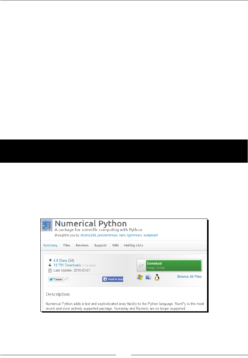
1. Download a NumPy installer for Windows from the SourceForge website
http://sourceforge.net/projects/numpy/files/.
Choose the appropriate NumPy version according to your Python version. In
the preceding screen shot, we chose numpy-1.9.2-win32-superpack-
python2.7.exe.
NumPy Quick Start
[ 14 ]
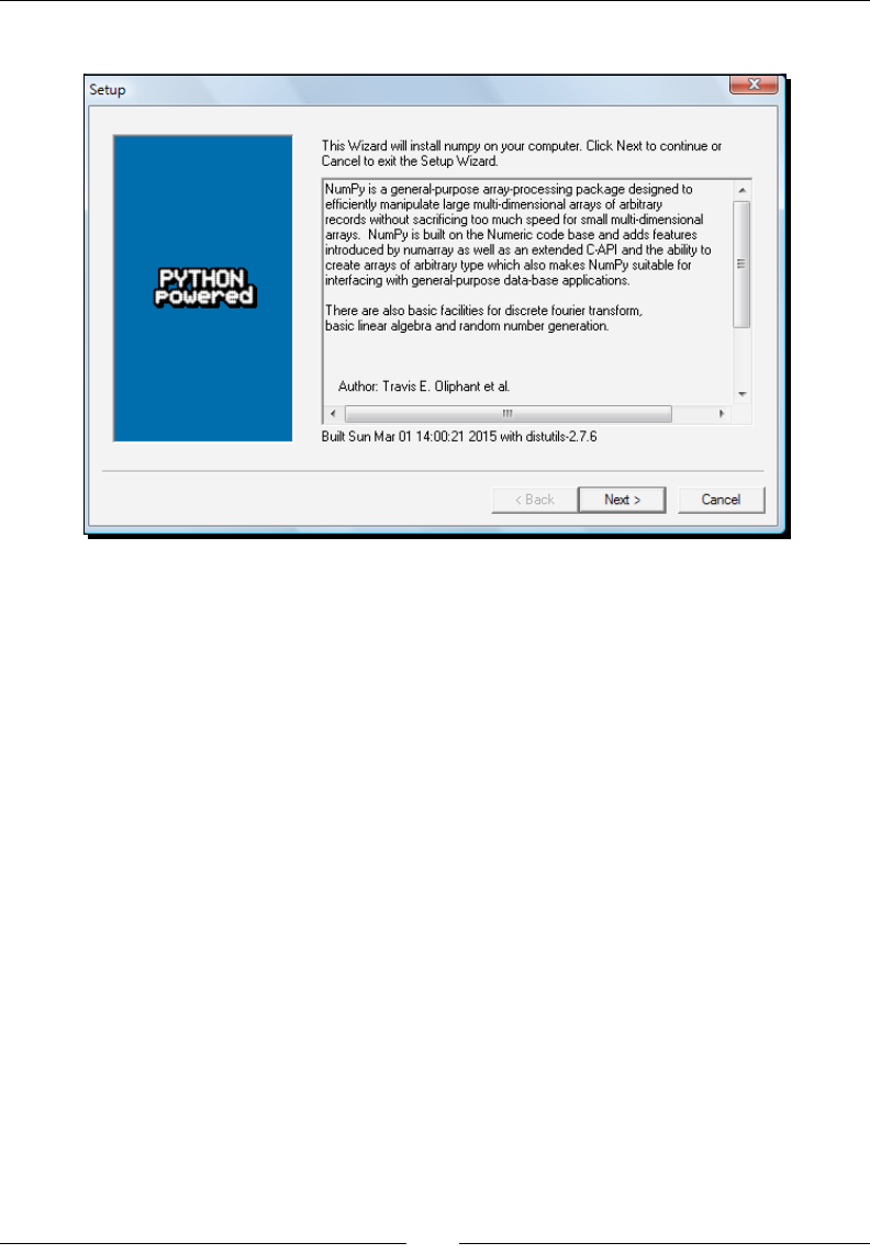
2. Open the EXE installer by double-clicking on it as shown in the following screen shot:
3. Now, we can see a descripon of NumPy and its features. Click on Next.
4. If you have Python installed, it should automacally be detected. If it is not
detected, your path sengs might be wrong. At the end of this chapter, we have
listed resources in case you have problems with installing NumPy.
5. In this example, Python 2.7 was found. Click on Next if Python is found; otherwise,
click on Cancel and install Python (NumPy cannot be installed without Python).
Click on Next. This is the point of no return. Well, kind of, but it is best to make sure
that you are installing to the proper directory and so on and so forth. Now the real
installaon starts. This may take a while.
Install SciPy and matplotlib with the Enthought Canopy distribuon (https://
www.enthought.com/products/canopy/). It might be necessary to put the
msvcp71.dll le in your C:\Windows\system32 directory. You can get it from
http://www.dll-files.com/dllindex/dll-files.shtml?msvcp71
A Windows IPython installer is available on the IPython website (see http://
ipython.org/).
What just happened?
We installed NumPy, SciPy, matplotlib, and IPython on Windows.

Chapter 1
[ 15 ]
NumPy on Linux
Installing NumPy and its related recommended soware on Linux depends on the
distribuon you have. We will discuss how you will install NumPy from the command line,
although you can probably use graphical installers; it depends on your distribuon (distro).
The commands to install matplotlib, SciPy, and IPython are the same—only the package
names are dierent. Installing matplotlib, SciPy, and IPython is recommended, but oponal.
Time for action – installing NumPy, matplotlib, SciPy, and
IPython on Linux
Most Linux distribuons have NumPy packages. We will go through the necessary commands
for some of the most popular Linux distros:
Installing NumPy on Red Hat: Run the following instrucons from the
command line:
$ yum install python-numpy
Installing NumPy on Mandriva: To install NumPy on Mandriva, run the following
command line instrucon:
$ urpmi python-numpy
Installing NumPy on Gentoo: To install NumPy on Gentoo, run the following
command line instrucon:
$ [sudo] emerge numpy
Installing NumPy on Debian and Ubuntu: On Debian or Ubuntu, type the following
on the command line:
$ [sudo] apt-get install python-numpy
The following table gives an overview of the Linux distribuons and the
corresponding package names for NumPy, SciPy, matplotlib, and IPython:
Linux distribution NumPy SciPy matplotlib IPython
Arch Linux python-numpy python-
scipy
python-
matplotlib
ipython
Debian python-numpy python-
scipy
python-
matplotlib
ipython
Fedora numpy python-
scipy
python-
matplotlib
ipython
Gentoo dev-python/
numpy
scipy matplotlib ipython

NumPy Quick Start
[ 16 ]
Linux distribution NumPy SciPy matplotlib IPython
OpenSUSE python-numpy,
python-numpy-
devel
python-
scipy
python-
matplotlib
ipython
Slackware numpy scipy matplotlib ipython
NumPy on Mac OS X
You can install NumPy, matplotlib, and SciPy on the Mac OS X with a GUI installer (not
possible for all versions) or from the command line with a port manager such as MacPorts,
Homebrew, or Fink, depending on your preference. You can also install using a script from
https://github.com/fonnesbeck/ScipySuperpack.
Time for action – installing NumPy, SciPy, matplotlib, and
IPython with MacPorts or Fink
Alternavely, we can install NumPy, SciPy, matplotlib, and IPython through the MacPorts
route or with Fink. The following installaon steps show how to install all these packages:
Installing with MacPorts: Type the following command:
$ [sudo] port install py-numpy py-scipy py-matplotlib py-ipython
Installing with Fink: Fink also has packages for NumPy—scipy-core-py24, scipy-
core-py25, and scipy-core-py26. The SciPy packages are scipy-py24, scipy-
py25 and scipy-py26. We can install NumPy and the addional recommended
packages, referring to this book on Python 2.7, using the following command:
$ fink install scipy-core-py27 scipy-py27 matplotlib-py27
What just happened?
We installed NumPy and the addional recommended soware on Mac OS X with
MacPorts and Fink.
Building from source
We can retrieve the source code for NumPy with git as follows:
$ git clone git://github.com/numpy/numpy.git numpy
Alternavely, download the source from http://sourceforge.net/projects/numpy/
files/.

Chapter 1
[ 17 ]
Install in /usr/local with the following command:
$ python setup.py build
$ [sudo] python setup.py install --prefix=/usr/local
To build, we need a C compiler such as GCC and the Python header les in the python-dev
or python-devel packages.
Arrays
Aer going through the installaon of NumPy, it's me to have a look at NumPy arrays.
NumPy arrays are more ecient than Python lists when it comes to numerical operaons.
NumPy code requires less explicit loops than the equivalent Python code.
Time for action – adding vectors
Imagine that we want to add two vectors called a and b (see https://www.khanacademy.
org/science/physics/one-dimensional-motion/displacement-velocity-
time/v/introduction-to-vectors-and-scalars). Vector is used here in the
mathemacal sense meaning a one-dimensional array. We will learn in Chapter 5, Working
with Matrices and ufuncs, about specialized NumPy arrays, which represent matrices. Vector
a holds the squares of integers 0 to n, for instance, if n is equal to 3, then a is equal to (0,1,
4). Vector b holds the cubes of integers 0 to n, so if n is equal to 3, then b is equal to (0,1,
8). How will you do that using plain Python? Aer we come up with a soluon, we will
compare it to the NumPy equivalent.
1. Adding vectors using pure Python: The following funcon solves the vector addion
problem using pure Python without NumPy:
def pythonsum(n):
a = range(n)
b = range(n)
c = []
for i in range(len(a)):
a[i] = i ** 2
b[i] = i ** 3
c.append(a[i] + b[i])
return c

NumPy Quick Start
[ 18 ]
Downloading the example code les
You can download the example code les from your account at
http://www.packtpub.com for all the Packt Publishing books you
have purchased. If you purchased this book elsewhere, you can visit
http://www.packtpub.com/support and register to have the
les e-mailed directly to you.
2. Adding vectors using NumPy: Following is a funcon that achieves the same result
with NumPy:
def numpysum(n):
a = np.arange(n) ** 2
b = np.arange(n) ** 3
c = a + b
return c
Noce that numpysum() does not need a for loop. Also, we used the arange() funcon
from NumPy that creates a NumPy array for us with integers 0 to n. The arange() funcon
was imported; that is why it is prexed with numpy (actually, it is customary to abbreviate it
via an alias to np).
Now comes the fun part. The preface menons that NumPy is faster when it comes to
array operaons. How much faster is NumPy, though? The following program will show us
by measuring the elapsed me, in microseconds, for the numpysum() and pythonsum()
funcons. It also prints the last two elements of the vector sum. Let's check that we get the
same answers by using Python and NumPy:
#!/usr/bin/env/python
from __future__ import print_function
import sys
from datetime import datetime
import numpy as np
"""
Chapter 1 of NumPy Beginners Guide.
This program demonstrates vector addition the Python way.
Run from the command line as follows
python vectorsum.py n
where n is an integer that specifies the size of the vectors.

Chapter 1
[ 19 ]
The first vector to be added contains the squares of 0 up to n.
The second vector contains the cubes of 0 up to n.
The program prints the last 2 elements of the sum and the elapsed
time.
"""
def numpysum(n):
a = np.arange(n) ** 2
b = np.arange(n) ** 3
c = a + b
return c
def pythonsum(n):
a = range(n)
b = range(n)
c = []
for i in range(len(a)):
a[i] = i ** 2
b[i] = i ** 3
c.append(a[i] + b[i])
return c
size = int(sys.argv[1])
start = datetime.now()
c = pythonsum(size)
delta = datetime.now() - start
print("The last 2 elements of the sum", c[-2:])
print("PythonSum elapsed time in microseconds", delta.microseconds)
start = datetime.now()
c = numpysum(size)
delta = datetime.now() - start
print("The last 2 elements of the sum", c[-2:])
print("NumPySum elapsed time in microseconds", delta.microseconds)

NumPy Quick Start
[ 20 ]
The output of the program for 1000, 2000, and 3000 vector elements is as follows:
$ python vectorsum.py 1000
The last 2 elements of the sum [995007996, 998001000]
PythonSum elapsed time in microseconds 707
The last 2 elements of the sum [995007996 998001000]
NumPySum elapsed time in microseconds 171
$ python vectorsum.py 2000
The last 2 elements of the sum [7980015996, 7992002000]
PythonSum elapsed time in microseconds 1420
The last 2 elements of the sum [7980015996 7992002000]
NumPySum elapsed time in microseconds 168
$ python vectorsum.py 4000
The last 2 elements of the sum [63920031996, 63968004000]
PythonSum elapsed time in microseconds 2829
The last 2 elements of the sum [63920031996 63968004000]
NumPySum elapsed time in microseconds 274
What just happened?
Clearly, NumPy is much faster than the equivalent normal Python code. One thing is certain,
we get the same results whether we use NumPy or not. However, the result printed diers
in representaon. Noce that the result from the numpysum() funcon does not have any
commas. How come? Obviously, we are not dealing with a Python list but with a NumPy
array. It was menoned in the Preface that NumPy arrays are specialized data structures for
numerical data. We will learn more about NumPy arrays in the next chapter.
Pop quiz – Functioning of the arange() function
Q1. What does arange(5) do?
1. Creates a Python list of 5 elements with the values 1-5.
2. Creates a Python list of 5 elements with the values 0-4.
3. Creates a NumPy array with the values 1-5.
4. Creates a NumPy array with the values 0-4.
5. None of the above.

Chapter 1
[ 21 ]
Have a go hero – continue the analysis
The program we used to compare the speed of NumPy and regular Python is not very
scienc. We should at least repeat each measurement a couple of mes. It will be nice to
be able to calculate some stascs such as average mes. Also, you might want to show
plots of the measurements to friends and colleagues.
Hints to help can be found in the online documentaon and the resources listed
at the end of this chapter. NumPy has stascal funcons that can calculate
averages for you. I recommend using matplotlib to produce plots. Chapter 9,
Plong with matplotlib, gives a quick overview of matplotlib.
IPython – an interactive shell
Sciensts and engineers are used to experiment. Sciensts created IPython with
experimentaon in mind. Many view the interacve environment that IPython provides
as a direct answer to MATLAB, Mathemaca, and Maple. You can nd more informaon,
including installaon instrucons, at http://ipython.org/.
IPython is free, open source, and available for Linux, UNIX, Mac OS X, and Windows. The
IPython authors only request that you cite IPython in any scienc work that uses IPython.
The following is a list of the basic IPython features:
Tab compleon
History mechanism
Inline eding
Ability to call external Python scripts with %run
Access to system commands
Pylab switch
Access to Python debugger and proler
The Pylab switch imports all the SciPy, NumPy, and matplotlib packages. Without this switch,
we will have to import every package we need ourselves.

NumPy Quick Start
[ 22 ]
All we need to do is enter the following instrucon on the command line:
$ ipython --pylab
IPython 2.4.1 -- An enhanced Interactive Python.
? -> Introduction and overview of IPython's features.
%quickref -> Quick reference.
help -> Python's own help system.
object? -> Details about 'object', use 'object??' for extra details.
Using matplotlib backend: MacOSX
In [1]: quit()
The quit()command or Ctrl + D quits the IPython shell. We may want to be able to go back
to our experiments. In IPython, it is easy to save a session for later:
In [1]: %logstart
Activating auto-logging. Current session state plus future input saved.
Filename : ipython_log.py
Mode : rotate
Output logging : False
Raw input log : False
Timestamping : False
State : active
Let's say we have the vector addion program that we made in the current directory. Run
the script as follows:
In [1]: ls
README vectorsum.py
In [2]: %run -i vectorsum.py 1000
As you probably remember, 1000 species the number of elements in a vector. The -d
switch of %run starts an ipdb debugger with c the script is started. n steps through the
code. Typing quit at the ipdb prompt exits the debugger:
In [2]: %run -d vectorsum.py 1000
*** Blank or comment
*** Blank or comment
Breakpoint 1 at: /Users/…/vectorsum.py:3

Chapter 1
[ 23 ]
Enter c at the ipdb> prompt to start your script.
><string>(1)<module>()
ipdb> c
> /Users/…/vectorsum.py(3)<module>()
2
1---> 3 import sys
4 from datetime import datetime
ipdb> n
>
/Users/…/vectorsum.py(4)<module>()
1 3 import sys
----> 4 from datetime import datetime
5 import numpy
ipdb> n
> /Users/…/vectorsum.py(5)<module>()
4 from datetime import datetime
----> 5 import numpy
6
ipdb> quit
We can also prole our script by passing the -p opon to %run:
In [4]: %run -p vectorsum.py 1000
1058 function calls (1054 primitive calls) in 0.002 CPU seconds
Ordered by: internal time
ncalls tottime percall cumtime percall filename:lineno(function)
1 0.001 0.001 0.001 0.001 vectorsum.py:28(pythonsum)
1 0.001 0.001 0.002 0.002 {execfile}
1000 0.000 0.0000.0000.000 {method 'append' of 'list' objects}
1 0.000 0.000 0.002 0.002 vectorsum.py:3(<module>)
1 0.000 0.0000.0000.000 vectorsum.py:21(numpysum)
3 0.000 0.0000.0000.000 {range}
1 0.000 0.0000.0000.000 arrayprint.py:175(_array2string)
3/1 0.000 0.0000.0000.000 arrayprint.py:246(array2string)

NumPy Quick Start
[ 24 ]
2 0.000 0.0000.0000.000 {method 'reduce' of 'numpy.ufunc' objects}
4 0.000 0.0000.0000.000 {built-in method now}
2 0.000 0.0000.0000.000 arrayprint.py:486(_formatInteger)
2 0.000 0.0000.0000.000 {numpy.core.multiarray.arange}
1 0.000 0.0000.0000.000 arrayprint.py:320(_formatArray)
3/1 0.000 0.0000.0000.000 numeric.py:1390(array_str)
1 0.000 0.0000.0000.000 numeric.py:216(asarray)
2 0.000 0.0000.0000.000 arrayprint.py:312(_extendLine)
1 0.000 0.0000.0000.000 fromnumeric.py:1043(ravel)
2 0.000 0.0000.0000.000 arrayprint.py:208(<lambda>)
1 0.000 0.000 0.002 0.002<string>:1(<module>)
11 0.000 0.0000.0000.000 {len}
2 0.000 0.0000.0000.000 {isinstance}
1 0.000 0.0000.0000.000 {reduce}
1 0.000 0.0000.0000.000 {method 'ravel' of 'numpy.ndarray' objects}
4 0.000 0.0000.0000.000 {method 'rstrip' of 'str' objects}
3 0.000 0.0000.0000.000 {issubclass}
2 0.000 0.0000.0000.000 {method 'item' of 'numpy.ndarray' objects}
1 0.000 0.0000.0000.000 {max}
1 0.000 0.0000.0000.000 {method 'disable' of '_lsprof.Profiler'
objects}
This gives us a bit more insight in to the workings of our program. In addion, we can now
idenfy performance bolenecks. The %hist command shows the commands history:
In [2]: a=2+2
In [3]: a
Out[3]: 4
In [4]: %hist
1: _ip.magic("hist ")
2: a=2+2
3: a
I hope you agree that IPython is a really useful tool!
Chapter 1
[ 25 ]
Online resources and help
When we are in IPython's pylab mode, we can open manual pages for NumPy funcons
with the help command. It is not necessary to know the name of a funcon. We can type
a few characters and then let tab compleon do its work. Let's, for instance, browse the
available informaon for the arange() funcon:
In [2]: help ar<Tab>
In [2]: help arange
Another opon is to put a queson mark behind the funcon name:
In [3]: arange?
The main documentaon website for NumPy and SciPy is at http://docs.scipy.org/
doc/. Through this web page, we can browse the NumPy reference at http://docs.
scipy.org/doc/numpy/reference/, the user guide, and several tutorials.
The popular Stack Overow soware development forum has hundreds of quesons tagged
numpy. To view them, go to http://stackoverflow.com/questions/tagged/numpy.
If you are really stuck with a problem or you want to be kept informed of NumPy
development, you can subscribe to the NumPy discussion mailing list. The e-mail address
is numpy-discussion@scipy.org. The number of e-mails per day is not too high with
almost no spam to speak of. Most importantly, the developers acvely involved with NumPy
also answer quesons asked on the discussion group. The complete list can be found at
http://www.scipy.org/scipylib/mailing-lists.html.
For IRC users, there is an IRC channel on irc://irc.freenode.net. The channel is called
#scipy, but you can also ask NumPy quesons since SciPy users also have knowledge of
NumPy, as SciPy is based on NumPy. There are at least 50 members on the SciPy channel at
all mes.

NumPy Quick Start
[ 26 ]
Summary
In this chapter, we installed NumPy and other recommended soware that we will be using
in some secons of this book. We got a vector addion program working and convinced
ourselves that NumPy has superior performance. You were introduced to the IPython
interacve shell. In addion, you explored the available NumPy documentaon and
online resources.
In the next chapter, you will take a look under the hood and explore some fundamental
concepts including arrays and data types.

[ 27 ]
Beginning with NumPy Fundamentals
After installing NumPy and getting some code to work, it's time to cover
NumPy basics.
The topics we shall cover in this chapter are as follows:
Data types
Array types
Type conversions
Array creaon
Indexing
Slicing
Shape manipulaon
Before we start, let me make a few remarks about the code examples in this chapter. The
code snippets in this chapter show input and output from several IPython sessions. Recall
that IPython was introduced in Chapter 1, NumPy Quick Start, as the interacve Python shell
of choice for scienc compung. The advantages of IPython are the --pylab switch that
imports many scienc compung Python packages, including NumPy, and the fact that
it is not necessary to explicitly call the print() funcon to display variable values. Other
features include easy parallel computaon and the notebook interface in the form of
a persistent worksheet in a web browser.
However, the source code delivered alongside the book is a regular Python code that uses
import and print statements.
2

Beginning with NumPy Fundamentals
[ 28 ]
NumPy array object
NumPy has a muldimensional array object called ndarray. It consists of two parts:
The actual data
Some metadata describing the data
The majority of array operaons leave the raw data untouched. The only aspect that changes
is the metadata.
In the previous chapter, we have already learned how to create an array using the arange()
funcon. Actually, we created a one-dimensional array that contained a set of numbers.
The ndarray object can have more than one dimension.
The NumPy array is in general homogeneous (there is a special array type that is
heterogeneous as described in the Time for acon – creang a record data type secon)—the
items in the array have to be of the same type. The advantage is that, if we know that the items
in the array are of the same type, it is easy to determine the storage size required for the array.
NumPy arrays are indexed starng from 0, just like in Python. Data types are represented by
special objects. We will discuss these objects comprehensively in this chapter.
Let's create an array with the arange() funcon again. Get the data type of an array using
the following code:
In: a = arange(5)
In: a.dtype
Out: dtype('int64')
The data type of array a is int64 (at least on my machine), but you may get int32 as
output if you are using 32-bit Python. In both the cases, we are dealing with integers
(64-bit or 32-bit). Besides the data type of an array, it is important to know its shape.
In Chapter 1, NumPy Quick Start, we demonstrated how to create a vector (actually,
a one-dimensional NumPy array). A vector is commonly used in mathemacs, but most
of the me, we need higher dimensional objects. Determine the shape of the vector we
created a few minutes ago. The following code is an example of creang a vector:
In [4]: a
Out[4]: array([0, 1, 2, 3, 4])
In: a.shape
Out: (5,)
As you can see, the vector has ve elements with values ranging from 0 to 4. The shape
aribute of the array is a tuple, in this case a tuple of 1 element, which contains the length
in each dimension.

Chapter 2
[ 29 ]
A tuple in Python is an immutable (it can't change) sequence of values. Once
tuples are created, we are not allowed to change the values of tuple elements
or append new elements. This makes tuples safer than lists because you can't
mutate them by accident. A common use case for tuples is as return value of
funcons. For more examples, have a look at the Introducing Tuples secon of
Chapter 3, Dive into Python, available at http://www.diveintopython.
net/native_data_types/tuples.html.
Time for action – creating a multidimensional array
Now that we know how to create a vector, we are ready to create a muldimensional NumPy
array. Aer we create the array, we will again want to display its shape:
1. Create a two-by-two array:
In: m = array([arange(2), arange(2)])
In: m
Out:
array([[0, 1],
[0, 1]])
2. Show the array shape:
In: m.shape
Out: (2, 2)
What just happened?
We created a two-by-two array with the arange() and array() funcons we have come to
trust and love. Without any warning, the array() funcon appeared on the stage.
The array() funcon creates an array from an object that you give to it. The object needs
to be array-like, for instance, a Python list. In the preceding example, we passed in a list of
arrays. The object is the only required argument of the array() funcon. NumPy funcons
tend to have a lot of oponal arguments with predened defaults. View the documentaon
for this funcon from the IPython shell with the help() funcon given here:
In [1]: help(array)
Or use the following shorthand:
In [2]: array?
Of course, you can substute array in this example with another NumPy funcon you are
interested in.

Beginning with NumPy Fundamentals
[ 30 ]
Pop quiz – the shape of ndarray
Q1. How is the shape of an ndarray stored?
1. It is stored in a comma-separated string.
2. It is stored in a list.
3. It is stored in a tuple.
Have a go hero – create a three-by-three array
It shouldn't be too hard now to create a three-by-three array. Give it a go and check whether
the array shape is as expected.
Selecting elements
From me to me, we will want to select a parcular element of an array. We will take a look
at how to do this, but, rst, create a two-by-two array again:
In: a = array([[1,2],[3,4]])
In: a
Out:
array([[1, 2],
[3, 4]])
The array was created this me by passing a list of lists to the array() funcon. We will
now select one by one each item of the matrix. Remember, the indices are numbered
starng from 0:
In: a[0,0]
Out: 1
In: a[0,1]
Out: 2
In: a[1,0]
Out: 3
In: a[1,1]
Out: 4
As you can see, selecng elements of the array is prey simple. For the array a, we just use
the notaon a[m,n], where m and n are the indices of the item in the array (the array can
have even more dimensions than in this example). This screenshot shows a simple example
of an array:

Chapter 2
[ 31 ]
NumPy numerical types
Python has an integer type, a oat type, and a complex type; however, this is not enough
for scienc compung and, for this reason, NumPy has a lot more data types with varying
precision, dependent on memory requirements.
Integers represent whole numbers, such as -1, 0, and 1. Floang-point
numbers correspond to real numbers as used in mathemacs, for example,
fracons or irraonal numbers such as pi. Because of the way computers
work, we are able to represent integers exactly, but oang-point numbers
are approximated. Complex numbers can have an imaginary component
usually denoted with i or j. By denion, i is the square root of -1. For
instance, 2.5 + 3.7i is a complex number (for more informaon, refer
to https://www.khanacademy.org/math/precalculus/
imaginary_complex_precalc).
In pracce, we need even more types with varying precision and, therefore, dierent
memory size of the type. The majority of the NumPy numerical types end with a number.
This number indicates the number of bits associated with the type. The following table
(adapted from the NumPy user guide) gives an overview of NumPy numerical types:
Type Description
bool Boolean (True or False) stored as a bit
inti Platform integer (normally either int32 or int64)
int8 Byte (-128 to 127)
int16 Integer (-32768 to 32767)
int32 Integer (-2 ** 31 to 2 ** 31 -1)
int64 Integer (-2 ** 63 to 2 ** 63 -1)
uint8 Unsigned integer (0 to 255)
uint16 Unsigned integer (0 to 65535)
uint32 Unsigned integer (0 to 2 ** 32 - 1)
uint64 Unsigned integer (0 to 2 ** 64 - 1)
float16 Half precision float: sign bit, 5 bits exponent, 10 bits mantissa
float32 Single precision float: sign bit, 8 bits exponent, 23 bits mantissa
float64 or float Double precision float: sign bit, 11 bits exponent, 52 bits mantissa

Beginning with NumPy Fundamentals
[ 32 ]
Type Description
complex64 Complex number, represented by two 32-bit floats (real and
imaginary components)
complex128 or
complex
Complex number, represented by two 64-bit floats (real and
imaginary components)
For oang-point types, we can request informaon with the finfo() funcon given here:
In: finfo(float16)
Out: finfo(resolution=0.0010004, min=-6.55040e+04, max=6.55040e+04,
dtype=float16)
For each data type, there exists a corresponding conversion funcon:
In: float64(42)
Out: 42.0
In: int8(42.0)
Out: 42
In: bool(42)
Out: True
In: bool(0)
Out: False
In: bool(42.0)
Out: True
In: float(True)
Out: 1.0
In: float(False)
Out: 0.0
Many funcons have a data type argument, which is oen oponal:
In: arange(7, dtype=uint16)
Out: array([0, 1, 2, 3, 4, 5, 6], dtype=uint16)
It is important to know that you are not allowed to convert a complex number into an integer
or oat. Trying to do that triggers a TypeError, as shown in the following screenshot:
The same goes for conversion of a complex number into a oat.

Chapter 2
[ 33 ]
An excepon in Python is an abnormal condion, which we usually try
to avoid. A TypeError is a Python built-in excepon, occurring when
we specify the wrong type for an argument.
The j part is the imaginary coecient of the complex number. However, you can convert a
oat in to a complex number, for instance, complex(1.0).
Data type objects
Data type objects are instances of the numpy.dtype class. Once again, arrays have a data
type. To be precise, every element in a NumPy array has the same data type. The data type
object can tell you the size of the data in bytes. The size in bytes is given by the itemsize
aribute of the dtype class:
In: a.dtype.itemsize
Out: 8
Character codes
Character codes are included for backward compability with Numeric. Numeric is
the predecessor of NumPy. Their use is not recommended, but the codes are provided
here because they pop up in several places. We should instead use the dtype objects.
The table shows the character codes:
Type Character code
Integer i
Unsigned integer u
Single precision float f
Double precision float d
Boolean b
Complex D
String S
Unicode U
Void V
Look at the following code to create an array of single precision oats:
In: arange(7, dtype='f')
Out: array([ 0., 1., 2., 3., 4., 5., 6.], dtype=float32)
Likewise this creates an array of complex numbers.

Beginning with NumPy Fundamentals
[ 34 ]
In: arange(7, dtype='D')
Out: array([ 0.+0.j, 1.+0.j, 2.+0.j, 3.+0.j, 4.+0.j, 5.+0.j,
6.+0.j])
The dtype constructors
Python classes have funcons, which are called methods, if they belong to a class. Some of
these methods are special and used to create new objects. These specialized methods are
called constructors.
You can read more about Python classes at https://docs.python.
org/2/tutorial/classes.html.
We have a variety of ways to create data types. Take the case of oang point data:
Use the general Python oat:
In: dtype(float)
Out: dtype('float64')
Specify a single precision oat with a character code:
In: dtype('f')
Out: dtype('float32')
Use a double precision oat character code:
In: dtype('d')
Out: dtype('float64')
We can give the data type constructor a two-character code. The rst character
signies the type and the second character is a number specifying the number of
bytes in the type (the numbers 2, 4, and 8 correspond to 16, 32, and 64-bit oats):
In: dtype('f8')
Out: dtype('float64')
A lisng of all full data type names can be found with the sctypeDict.keys() funcon:
In: sctypeDict.keys()
Out: [0, …
'i2',
'int0']

Chapter 2
[ 35 ]
The dtype attributes
The dtype class has a number of useful aributes. For example, get informaon about the
character code of a data type through the aributes of dtype:
In: t = dtype('Float64')
In: t.char
Out: 'd'
The type aribute corresponds to the type of object of the array elements:
In: t.type
Out: <type 'numpy.float64'>
The str aribute of the dtype class gives a string representaon of the data type. It starts
with a character represenng endianness, if appropriate, then a character code, followed by
a number corresponding to the number of bytes that each array item requires. Endianness,
here, refers to the way bytes are ordered within a 32- or 64-bit word. In big-endian order, the
most signicant byte is stored rst, indicated by >. In lile-endian order, the least signicant
byte is stored rst, indicated by <:
In: t.str
Out: '<f8'
Time for action – creating a record data type
The record data type is a heterogeneous data type—think of it as represenng a row in a
spreadsheet or a database. To give an example of a record data type, we will create a record
for a shop inventory. The record contains the name of the item, a 40-character string, the
number of items in the store represented by a 32-bit integer, and, nally, a price represented
by a 32-bit oat. These consecuve steps show how to create a record data type:
1. Create the record:
In: t = dtype([('name', str_, 40), ('numitems', int32), ('price',
float32)])
In: t
Out: dtype([('name', '|S40'), ('numitems', '<i4'), ('price',
'<f4')])
2. View the type (we can view the type of a eld as well):
In: t['name']
Out: dtype('|S40')

Beginning with NumPy Fundamentals
[ 36 ]
If you don't give the array() funcon a data type, it will assume that it is dealing with
oang point numbers. To create the array now, we really have to specify the data type;
otherwise, we will get a TypeError:
In: itemz = array([('Meaning of life DVD', 42, 3.14), ('Butter', 13,
2.72)], dtype=t)
In: itemz[1]
Out: ('Butter', 13, 2.7200000286102295)
What just happened?
We created a record data type, which is a heterogeneous data type. The record contained
a name as a character string, a number as an integer, and a price represented by a oat.
The code for this example can be found in the record.py le in this book's code bundle.
One-dimensional slicing and indexing
Slicing of one-dimensional NumPy arrays works just like slicing of Python lists. Select a piece
of an array from index 3 to 7 that extracts the elements 3 through 6:
In: a = arange(9)
In: a[3:7]
Out: array([3, 4, 5, 6])
Select elements from index 0 to 7 with step 2 as follows:
In: a[:7:2]
Out: array([0, 2, 4, 6])
Similarly, as in Python, use negave indices and reverse the array with this code snippet:
In: a[::-1]
Out: array([8, 7, 6, 5, 4, 3, 2, 1, 0])
Time for action – slicing and indexing multidimensional arrays
The ndarray class supports slicing over mulple dimensions. For convenience, we refer to
many dimensions at once, with an ellipsis.
1. To illustrate, create an array with the arange() funcon and reshape it:
In: b = arange(24).reshape(2,3,4)
In: b.shape
Out: (2, 3, 4)

Chapter 2
[ 37 ]
In: b
Out:
array([[[ 0, 1, 2, 3],
[ 4, 5, 6, 7],
[ 8, 9, 10, 11]],
[[12, 13, 14, 15],
[16, 17, 18, 19],
[20, 21, 22, 23]]])
The array b has 24 elements with values 0 to 23 and we reshaped it to be a two-by-
three-by-four, three-dimensional array. We can visualize this as a two-story building
with 12 rooms on each oor, 3 rows and 4 columns (alternavely we can think of it as
a spreadsheet with sheets, rows, and columns). As you have probably guessed, the
reshape() funcon changes the shape of an array. We give it a tuple of integers,
corresponding to the new shape. If the dimensions are not compable with the data,
an excepon is thrown.
2. We can select a single room using its three coordinates, namely, the oor, column,
and row. For example, the room on the rst oor, in the rst row, and in the rst
column (we can have oor 0 and room 0—it's just a maer of convenon) can be
represented by the following:
In: b[0,0,0]
Out: 0
3. If we don't care about the oor, but sll want the rst column and row, we replace
the rst index by a: (colon) because we just need to specify the oor number and
omit the other indices:
In: b[:,0,0]
Out: array([ 0, 12])
Select the rst oor in this code:
In: b[0]
Out:
array([[ 0, 1, 2, 3],
[ 4, 5, 6, 7],
[ 8, 9, 10, 11]])
We can also write this:
In: b[0, :, :]
Out:
array([[ 0, 1, 2, 3],
[ 4, 5, 6, 7],
[ 8, 9, 10, 11]])

Beginning with NumPy Fundamentals
[ 38 ]
An ellipsis (…) replaces mulple colons, so, the preceding code is equivalent to this:
In: b[0, ...]
Out:
array([[ 0, 1, 2, 3],
[ 4, 5, 6, 7],
[ 8, 9, 10, 11]])
Furthermore, get the second row on the rst oor:
In: b[0,1]
Out: array([4, 5, 6, 7])
4. Using steps to slice: Furthermore, also select every second element of this selecon:
In: b[0,1,::2]
Out: array([4, 6])
5. Using an ellipsis to slice: If we want to select all the rooms on both oors that are in
the second column, regardless of the row, type this code:
In: b[...,1]
Out:
array([[ 1, 5, 9],
[13, 17, 21]])
Similarly, select all the rooms on the second row, regardless of oor and column,
by wring the following code snippet:
In: b[:,1]
Out:
array([[ 4, 5, 6, 7],
[16, 17, 18, 19]])
If we want to select rooms on the ground oor second column, then type this:
In: b[0,:,1]
Out: array([1, 5, 9])
6. Using negave indices: If we want to select the rst oor, last column, then type the
following code snippet:
In: b[0,:,-1]
Out: array([ 3, 7, 11])
If we want to select rooms on the ground oor, last column reversed, then type the
following code snippet:
In: b[0,::-1, -1]
Out: array([11, 7, 3])

Chapter 2
[ 39 ]
Select every second element of that slice as follows:
In: b[0,::2,-1]
Out: array([ 3, 11])
The command that reverses a one-dimensional array puts the top oor following the
ground oor as follows:
In: b[::-1]
Out:
array([[[12, 13, 14, 15],
[16, 17, 18, 19],
[20, 21, 22, 23]],
[[ 0, 1, 2, 3],
[ 4, 5, 6, 7],
[ 8, 9, 10, 11]]])
What just happened?
We sliced a muldimensional NumPy array using several dierent methods. The code for this
example can be found in the slicing.py le in this book's code bundle.
Time for action – manipulating array shapes
We already learned about the reshape() funcon. Another recurring task is aening of
arrays. When we aen muldimensional NumPy arrays, the result is a one-dimensional
array with the same data.
1. Ravel: Accomplish this with the ravel() funcon:
In: b
Out:
array([[[ 0, 1, 2, 3],
[ 4, 5, 6, 7],
[ 8, 9, 10, 11]],
[[12, 13, 14, 15],
[16, 17, 18, 19],
[20, 21, 22, 23]]])
In: b.ravel()
Out:
array([ 0, 1, 2, 3, 4, 5, 6, 7, 8, 9, 10, 11, 12, 13, 14,
15, 16,
17, 18, 19, 20, 21, 22, 23])

Beginning with NumPy Fundamentals
[ 40 ]
2. Flaen: The appropriately named funcon, flatten() does the same as ravel(),
but flatten() always allocates new memory whereas ravel() might return a
view of the array. A view is a way to share an array, but you need to be careful with
views because modifying the view aects the underlying array, and therefore this
impacts other views. An array copy is safer; however, it uses more memory:
In: b.flatten()
Out:
array([ 0, 1, 2, 3, 4, 5, 6, 7, 8, 9, 10, 11, 12, 13, 14,
15, 16,
17, 18, 19, 20, 21, 22, 23])
3. Seng the shape with a tuple: Besides the reshape() funcon, we can also set
the shape directly with a tuple, which is shown here:
In: b.shape = (6,4)
In: b
Out:
array([[ 0, 1, 2, 3],
[ 4, 5, 6, 7],
[ 8, 9, 10, 11],
[12, 13, 14, 15],
[16, 17, 18, 19],
[20, 21, 22, 23]])
As you can see, this changes the array directly. Now, we have a six-by-four array.
4. Transpose: In linear algebra, it is common to transpose matrices.
Linear algebra is a branch of mathematics dealing among others with
matrices. Matrices are the two-dimensional equivalent of vectors and
contain numbers in a rectangular or square grid. Transposing a matrix entails
flipping the matrix in such a manner that the matrix rows become the matrix
columns and vice versa. Khan Academy has a course on linear algebra, which
includes transposing matrices at https://www.khanacademy.org/
math/linear-algebra/matrix_transformations/matrix_
transpose/v/linear-algebra-transpose-of-a-matrix.
We can do this too using the following code:
In: b.transpose()
Out:
array([[ 0, 4, 8, 12, 16, 20],
[ 1, 5, 9, 13, 17, 21],
[ 2, 6, 10, 14, 18, 22],
[ 3, 7, 11, 15, 19, 23]])

Chapter 2
[ 41 ]
5. Resize: The resize() method works just like the reshape() funcon, but
modies the array it operates on:
In: b.resize((2,12))
In: b
Out:
array([[ 0, 1, 2, 3, 4, 5, 6, 7, 8, 9, 10, 11],
[12, 13, 14, 15, 16, 17, 18, 19, 20, 21, 22, 23]])
What just happened?
We manipulated the shapes of NumPy arrays using the ravel() funcon, the flatten()
funcon, the reshape() funcon, and the resize() method, as explained in the
following table:
Function Description
ravel() This function returns a one-dimensional array
with the same data as the input array and
doesn't always return a copy
flatten() This is a method of ndarray, which flattens
arrays and always returns a copy of the array
reshape() This function modifies the shape of an array
resize() This function changes the shape of an array and
adds copies of the input array if necessary
The code for this example is in the shapemanipulation.py le in this book's code bundle.
Stacking
Arrays can be stacked horizontally, depth wise, or vercally. We can use, for that
purpose, the vstack(), dstack(), hstack(), column_stack(), row_stack(),
and concatenate() funcons.
Time for action – stacking arrays
First, set up some arrays:
In: a = arange(9).reshape(3,3)
In: a
Out:
array([[0, 1, 2],
[3, 4, 5],
[6, 7, 8]])
In: b = 2 * a
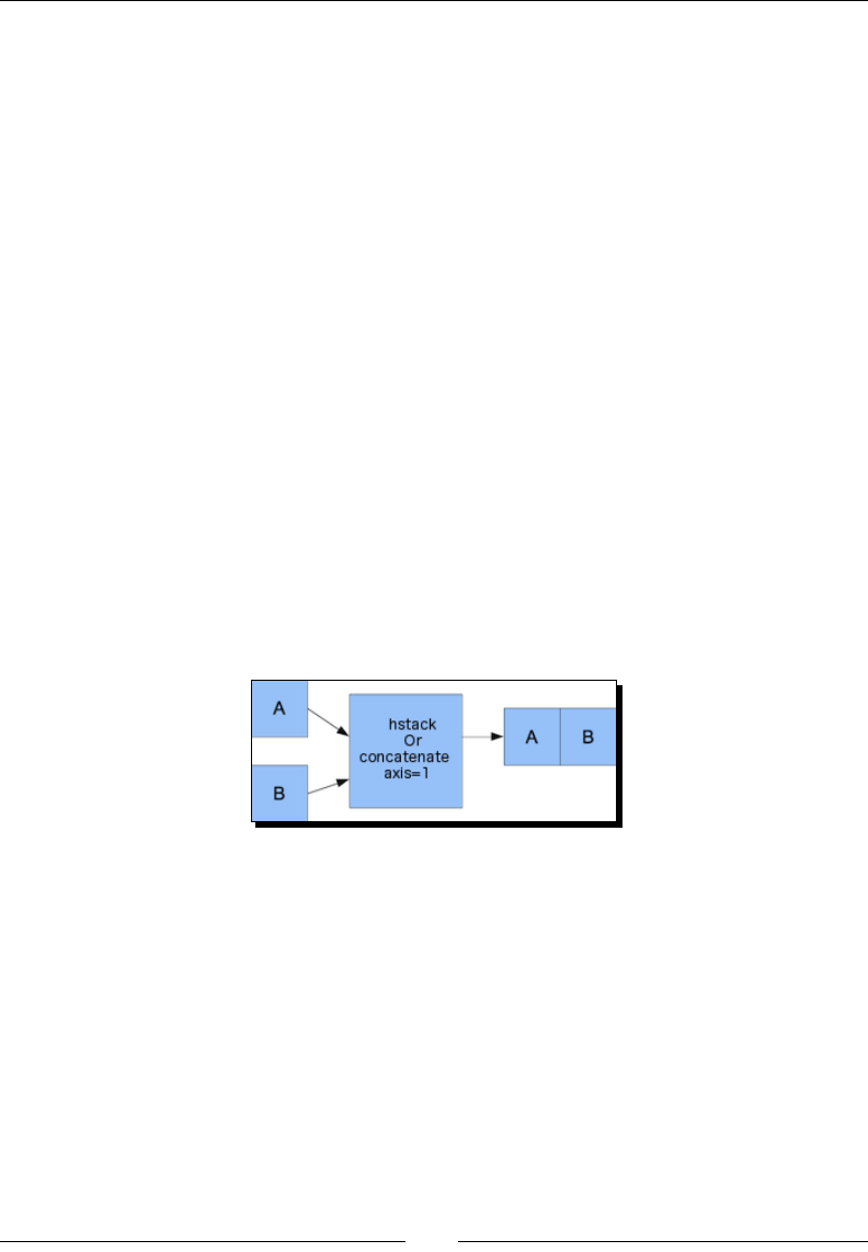
Beginning with NumPy Fundamentals
[ 42 ]
In: b
Out:
array([[ 0, 2, 4],
[ 6, 8, 10],
[12, 14, 16]])
1. Horizontal stacking: Starng with horizontal stacking, form a tuple of the ndarray
objects and give it to the hstack() funcon as follows:
In: hstack((a, b))
Out:
array([[ 0, 1, 2, 0, 2, 4],
[ 3, 4, 5, 6, 8, 10],
[ 6, 7, 8, 12, 14, 16]])
Achieve the same with the concatenate() funcon as follows (the axis argument
here is equivalent to axes in a Cartesian coordinate system and corresponds to the
array dimensions):
In: concatenate((a, b), axis=1)
Out:
array([[ 0, 1, 2, 0, 2, 4],
[ 3, 4, 5, 6, 8, 10],
[ 6, 7, 8, 12, 14, 16]])
This image shows horizontal stacking with the concatenate() funcon:
2. Vercal stacking: With vercal stacking, again, a tuple is formed. This me, it is
given to the vstack() funcon as follows:
In: vstack((a, b))
Out:
array([[ 0, 1, 2],
[ 3, 4, 5],
[ 6, 7, 8],
[ 0, 2, 4],
[ 6, 8, 10],
[12, 14, 16]])
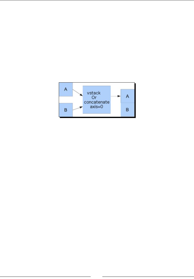
Chapter 2
[ 43 ]
The concatenate() funcon produces the same result with the axis set to 0.
This is the default value for the axis argument:
In: concatenate((a, b), axis=0)
Out:
array([[ 0, 1, 2],
[ 3, 4, 5],
[ 6, 7, 8],
[ 0, 2, 4],
[ 6, 8, 10],
[12, 14, 16]])
The following diagram shows vercal stacking with concatenate() funcon:
3. Depth stacking: Addionally, depth-wise stacking using dstack() and a tuple stacks a
list of arrays along the third axis (depth). For instance, stack two-dimensional arrays of
image data on top of each other:
In: dstack((a, b))
Out:
array([[[ 0, 0],
[ 1, 2],
[ 2, 4]],
[[ 3, 6],
[ 4, 8],
[ 5, 10]],
[[ 6, 12],
[ 7, 14],
[ 8, 16]]])
4. Column stacking: Stack the one-dimensional arrays with the column_stack()
funcon column-wise as follows:
In: oned = arange(2)
In: oned
Out: array([0, 1])
In: twice_oned = 2 * oned
In: twice_oned
Out: array([0, 2])

Beginning with NumPy Fundamentals
[ 44 ]
In: column_stack((oned, twice_oned))
Out:
array([[0, 0],
[1, 2]])
Two-dimensional arrays are stacked the way hstack() stacks them:
In: column_stack((a, b))
Out:
array([[ 0, 1, 2, 0, 2, 4],
[ 3, 4, 5, 6, 8, 10],
[ 6, 7, 8, 12, 14, 16]])
In: column_stack((a, b)) == hstack((a, b))
Out:
array([[ True, True, True, True, True, True],
[ True, True, True, True, True, True],
[ True, True, True, True, True, True]], dtype=bool)
Yes, you guessed it right! We compared two arrays with the == operator.
The == operator is used in Python to compare for equality. When applied
to NumPy arrays, the operator performs element-wise comparisons. For
more information about the Python comparison operators, have a look at
http://www.pythonlearn.com/html-009/book004.html.
5. Row stacking: NumPy, of course, also has a funcon that does row-wise stacking.
It is called row_stack(), and, for one-dimensional arrays, it just stacks the arrays
in rows into a two-dimensional array:
In: row_stack((oned, twice_oned))
Out:
array([[0, 1],
[0, 2]])
The row_stack() funcon results for two-dimensional arrays are equal to, yes,
exactly, the vstack() funcon results:
In: row_stack((a, b))
Out:
array([[ 0, 1, 2],
[ 3, 4, 5],
[ 6, 7, 8],

Chapter 2
[ 45 ]
[ 0, 2, 4],
[ 6, 8, 10],
[12, 14, 16]])
In: row_stack((a,b)) == vstack((a, b))
Out:
array([[ True, True, True],
[ True, True, True],
[ True, True, True],
[ True, True, True],
[ True, True, True],
[ True, True, True]], dtype=bool)
What just happened?
We stacked arrays horizontally, depth wise, and vercally. We used the vstack(),
dstack(), hstack(), column_stack(), row_stack(), and concatenate()
funcons as summarized in the following table:
Function Description
vstack() This function stacks arrays vertically
dstack() This function stacks arrays depth-wise along the
third axis
hstack() This function stacks arrays horizontally
column_stack() This function stacks one-dimensional arrays as
columns to create a two-dimensional array
row_stack() This function stacks array vertically
concatenate() This function concatenates a list or a tuple of
arrays
The code for this example is in the stacking.py le in this book's code bundle.
Splitting
Arrays can be split vercally, horizontally, or depth wise. The funcons involved are
hsplit(), vsplit(), dsplit(), and split(). We can either split into arrays of
the same shape or indicate the posion aer which the split should occur.

Beginning with NumPy Fundamentals
[ 46 ]
Time for action – splitting arrays
The following steps demonstrate arrays spling:
1. Horizontal spling: The ensuing code splits an array along its horizontal axis into
three pieces of the same size and shape:
In: a
Out:
array([[0, 1, 2],
[3, 4, 5],
[6, 7, 8]])
In: hsplit(a, 3)
Out:
[array([[0],
[3],
[6]]),
array([[1],
[4],
[7]]),
array([[2],
[5],
[8]])]
Compare it with a call of the split() funcon, with extra parameter axis=1:
In: split(a, 3, axis=1)
Out:
[array([[0],
[3],
[6]]),
array([[1],
[4],
[7]]),
array([[2],
[5],
[8]])]
2. Vercal spling: vsplit() splits along the vercal axis:
In: vsplit(a, 3)
Out: [array([[0, 1, 2]]), array([[3, 4, 5]]), array([[6, 7, 8]])]
The split() funcon, with axis=0, also splits along the vercal axis:
In: split(a, 3, axis=0)
Out: [array([[0, 1, 2]]), array([[3, 4, 5]]), array([[6, 7, 8]])]

Chapter 2
[ 47 ]
3. Depth-wise spling: The dsplit() funcon, unsurprisingly, splits depth-wise.
Create an array of rank 3 rst before spling:
In: c = arange(27).reshape(3, 3, 3)
In: c
Out:
array([[[ 0, 1, 2],
[ 3, 4, 5],
[ 6, 7, 8]],
[[ 9, 10, 11],
[12, 13, 14],
[15, 16, 17]],
[[18, 19, 20],
[21, 22, 23],
[24, 25, 26]]])
In: dsplit(c, 3)
Out:
[array([[[ 0],
[ 3],
[ 6]],
[[ 9],
[12],
[15]],
[[18],
[21],
[24]]]),
array([[[ 1],
[ 4],
[ 7]],
[[10],
[13],
[16]],
[[19],
[22],
[25]]]),
array([[[ 2],
[ 5],
[ 8]],
[[11],
[14],
[17]],
[[20],
[23],
[26]]])]

Beginning with NumPy Fundamentals
[ 48 ]
What just happened?
We split arrays using the hsplit(), vsplit(), dsplit(), and split() funcons.
These funcons dier in the axis along which the split occurs. The code for this example
is in the splitting.py le in this book's code bundle.
Array attributes
Besides the shape and dtype aributes, ndarray has a number of other aributes, as
shown in the following list:
The ndim aribute gives the number of dimensions:
In: b
Out:
array([[ 0, 1, 2, 3, 4, 5, 6, 7, 8, 9, 10, 11],
[12, 13, 14, 15, 16, 17, 18, 19, 20, 21, 22, 23]])
In: b.ndim
Out: 2
The size aribute contains the number of elements. This is shown as follows:
In: b.size
Out: 24
The itemsize aribute gives the number of bytes for each element in the array:
In: b.itemsize
Out: 8
If you want the total number of bytes the array requires, you can have a look at
nbytes. This is just a product of the itemsize and size aributes:
In: b.nbytes
Out: 192
In: b.size * b.itemsize
Out: 192
The T aribute has the same eect as the transpose() funcon, which is shown
as follows:
In: b.resize(6,4)
In: b
Out:
array([[ 0, 1, 2, 3],
[ 4, 5, 6, 7],
[ 8, 9, 10, 11],
[12, 13, 14, 15],
[16, 17, 18, 19],

Chapter 2
[ 49 ]
[20, 21, 22, 23]])
In: b.T
Out:
array([[ 0, 4, 8, 12, 16, 20],
[ 1, 5, 9, 13, 17, 21],
[ 2, 6, 10, 14, 18, 22],
[ 3, 7, 11, 15, 19, 23]])
If the array has a rank lower than 2, we will just get a view of the array:
In: b.ndim
Out: 1
In: b.T
Out: array([0, 1, 2, 3, 4])
Complex numbers in NumPy are represented by j. For example, create an array
with complex numbers as in the following code:
In: b = array([1.j + 1, 2.j + 3])
In: b
Out: array([ 1.+1.j, 3.+2.j])
The real aribute gives us the real part of the array, or the array itself if it only
contains real numbers:
In: b.real
Out: array([ 1., 3.])
The imag aribute contains the imaginary part of the array:
In: b.imag
Out: array([ 1., 2.])
If the array contains complex numbers, then the data type is automacally
also complex:
In: b.dtype
Out: dtype('complex128')
In: b.dtype.str
Out: '<c16'
The flat aribute returns a numpy.flatiter object. This is the only way to
acquire a flatiter—we do not have access to a flatiter constructor. The at
iterator enables us to loop through an array as if it is a at array, as shown in the
following example:
In: b = arange(4).reshape(2,2)
In: b
Out:
array([[0, 1],
[2, 3]])

Beginning with NumPy Fundamentals
[ 50 ]
In: f = b.flat
In: f
Out: <numpy.flatiter object at 0x103013e00>
In: for item in f: print item
.....:
0
1
2
3
It is possible to get an element directly with the flatiter object:
In: b.flat[2]
Out: 2
And, it is also possible to directly get mulple elements:
In: b.flat[[1,3]]
Out: array([1, 3])
The flat aribute is seable. Seng the value of the flat aribute leads to
overwring the values of the whole array:
In: b.flat = 7
In: b
Out:
array([[7, 7],
[7, 7]])
Or, it can also lead to overwring the values of selected elements:
In: b.flat[[1,3]] = 1
In: b
Out:
array([[7, 1],
[7, 1]])
The following diagram shows the dierent types of aributes of the ndarray class:

Chapter 2
[ 51 ]
Time for action – converting arrays
Convert a NumPy array to a Python list with the tolist() funcon:
1. Convert to a list:
In: b
Out: array([ 1.+1.j, 3.+2.j])
In: b.tolist()
Out: [(1+1j), (3+2j)]
2. The astype() funcon converts the array to an array of the specied type:
In: b
Out: array([ 1.+1.j, 3.+2.j])
In: b.astype(int)
/usr/local/bin/ipython:1: ComplexWarning: Casting complex values
to real discards the imaginary part
#!/usr/bin/python
Out: array([1, 3])
We are losing the imaginary part when casting from the NumPy complex
type (not the plain vanilla Python one) to int. The astype() function
also accepts the name of a type as a string.
In: b.astype('complex')
Out: array([ 1.+1.j, 3.+2.j])
It won't show any warning this me because we used the proper data type.
What just happened?
We converted NumPy arrays to a list and to arrays of dierent data types. The code for this
example is in the arrayconversion.py le in this book's code bundle.
Summary
In this chapter, you learned a lot about NumPy fundamentals: data types and arrays. Arrays
have several aributes describing them. You learned that one of these aributes is the data
type, which, in NumPy, is represented by a fully-edged object.
NumPy arrays can be sliced and indexed in an ecient manner, just like Python lists. NumPy
arrays have the added ability of working with mulple dimensions.

Beginning with NumPy Fundamentals
[ 52 ]
The shape of an array can be manipulated in many ways—stacking, resizing, reshaping,
and spling. A great number of convenience funcons for shape manipulaon were
demonstrated in this chapter.
Having learned about the basics, it's me to move on to the study of commonly used
funcons in Chapter 3, Geng Familiar with Commonly Used Funcons, which includes
basic stascal and mathemacal funcons.

[ 53 ]
3
Getting Familiar with Commonly
Used Functions
In this chapter, we will have a look at common NumPy functions. In particular,
we will learn how to load data from files by using an example involving
historical stock prices. Also, we will get to see the basic NumPy mathematical
and statistical functions.
We will learn how to read from and write to files. Also, we will get a taste of the
functional programming and linear algebra possibilities in NumPy.
In this chapter, we shall cover the following topics:
Funcons working on arrays
Loading arrays from les
Wring arrays to les
Simple mathemacal and stascal funcons
File I/O
First, we will learn about le I/O with NumPy. Data is usually stored in les. You would not
get far if you were not able to read from and write to les.

Geng Familiar with Commonly Used Funcons
[ 54 ]
Time for action – reading and writing les
As an example of le I/O, we will create an identy matrix and store its contents in a le.
In this and other chapters, we will use the following line by convenon
to import NumPy:
import numpy as np
Perform the following steps to do so:
1. The identy matrix is a square matrix with ones on the main diagonal and zeros for
the rest (see https://www.khanacademy.org/math/precalculus/precalc-
matrices/zero-identity-matrix-tutorial/v/identity-matrix).
The identy matrix can be created with the eye() funcon. The only argument that
we need to give the eye() funcon is the number of ones. So, for instance, for a
two-by-two matrix, write the following code:
i2 = np.eye(2)
print(i2)
The output is:
[[ 1. 0.]
[ 0. 1.]]
2. Save the data in a plain text le with the savetxt() funcon. Specify the name of
the le that we want to save the data in and the array containing the data itself:
np.savetxt("eye.txt", i2)
A le called eye.txt should have been created in the same directory as the Python script.
What just happened?
Reading and wring les is a necessary skill for data analysis. We wrote to a le with
savetxt(). We made an identy matrix with the eye() funcon.
Instead of a lename, we can also provide a le handle. A le handle is a term
in many programming languages, which means a variable poinng to a le, like
a postal address. For more informaon on how to get a le handle in Python,
please refer to http://www.diveintopython3.net/files.html.

Chapter 3
[ 55 ]
You can check for yourself whether the contents are as expected. The code for this example
can be downloaded from the book support website: https://www.packtpub.com/
books/content/support (see save.py)
import numpy as np
i2 = np.eye(2)
print(i2)
np.savetxt("eye.txt", i2))
Comma-seperated value les
Files in the Comma-seperated value (CSV) format are encountered quite frequently. Oen,
the CSV le is just a dump from a database. Usually, each eld in the CSV le corresponds to
a database table column. As we all know, spreadsheet programs, such as Excel, can produce
CSV les, as well.
Time for action – loading from CSV les
How do we deal with CSV les? Luckily, the loadtxt() funcon can conveniently read CSV
les, split up the elds, and load the data into NumPy arrays. In the following example, we
will load historical stock price data for Apple (the company, not the fruit). The data is in CSV
format and is part of the code bundle for this book. The rst column contains a symbol that
idenes the stock. In our case, it is AAPL. Second is the date in dd-mm-yyyy format. The
third column is empty. Then, in order, we have the open, high, low, and close price. Last,
but not least, is the trading volume of the day. This is what a line looks like:
AAPL,28-01-2011, ,344.17,344.4,333.53,336.1,21144800
For now, we are only interested in the close price and volume. In the preceding sample, that
will be 336.1 and 21144800. Store the close price and volume in two arrays as follows:
c,v=np.loadtxt('data.csv', delimiter=',', usecols=(6,7), unpack=True)
As you can see, data is stored in the data.csv le. We have set the delimiter to, (comma),
since we are dealing with a CSV le. The usecols parameter is set through a tuple to get
the seventh and eighth elds, which correspond to the close price and volume. The unpack
argument is set to True, which means that data will be unpacked and assigned to the c and
v variables that will hold the close price and volume, respecvely.

Geng Familiar with Commonly Used Funcons
[ 56 ]
Volume Weighted Average Price
Volume Weighted Average Price (VWAP) is a very important quanty in nance. It represents
an average price for a nancial asset (see https://www.khanacademy.org/math/
probability/descriptive-statistics/old-stats-videos/v/statistics-the-
average). The higher the volume, the more signicant a price move typically is. VWAP is
oen used in algorithmic trading and is calculated using volume values as weights.
Time for action – calculating Volume Weighted Average Price
The following are the acons that we will take:
1. Read the data into arrays.
2. Calculate VWAP:
from __future__ import print_function
import numpy as np
c,v=np.loadtxt('data.csv', delimiter=',', usecols=(6,7),
unpack=True)
vwap = np.average(c, weights=v)
print("VWAP =", vwap)
The output is as follows:
VWAP = 350.589549353
What just happened?
That wasn't very hard, was it? We just called the average() funcon and set its weights
parameter to use the v array for weights. By the way, NumPy also has a funcon to calculate
the arithmec mean. This is an unweighted average with all the weights equal to 1.
The mean() function
The mean() funcon is quite friendly and not so mean. This funcon calculates the
arithmec mean of an array.

Chapter 3
[ 57 ]
The arithmec mean is given by the following formula:
1
1n
i
i
a
n=
∑
It sums the values in an array a and divides the sum by the number
of elements n (see https://www.khanacademy.org/math/
probability/descriptive-statistics/central_
tendency/e/mean_median_and_mode).
Let's see it in acon:
print("mean =", np.mean(c))
As a result, we get the following printout:
mean = 351.037666667
Time-weighted average price
In nance, me-weighted average price (TWAP) is another average price measure. Now that
we are at it, let's compute the TWAP too. It is just a variaon on a theme really. The idea is
that recent price quotes are more important, so we should give recent prices higher weights.
The easiest way is to create an array with the arange() funcon of increasing values from
zero to the number of elements in the close price array. This is not necessarily the correct
way. In fact, most of the examples concerning stock price analysis in this book are only
illustrave. The following is the TWAP code:
t = np.arange(len(c))
print("twap =", np.average(c, weights=t))
It produces the following output:
twap = 352.428321839
The TWAP is even higher than the mean.
Pop quiz – computing the weighted average
Q1. Which funcon returns the weighted average of an array?
1. weighted average
2. waverage
3. average
4. avg

Geng Familiar with Commonly Used Funcons
[ 58 ]
Have a go hero – calculating other averages
Try doing the same calculaon using the open price. Calculate the mean for the volume and
the other prices.
Value range
Usually, we don't only want to know the average or arithmec mean of a set of values,
which are in the middle, to know we also want the extremes, the full range—the highest and
lowest values. The sample data that we are using here already has those values per day—the
high and low price. However, we need to know the highest value of the high price and the
lowest price value of the low price.
Time for action – nding highest and lowest values
The min() and max() funcons are the answer for our requirement. Perform the following
steps to nd the highest and lowest values:
1. First, read our le again and store the values for the high and low prices into arrays:
h,l=np.loadtxt('data.csv', delimiter=',', usecols=(4,5),
unpack=True)
The only thing that changed is the usecols parameter, since the high and low
prices are situated in dierent columns.
2. The following code gets the price range:
print("highest =", np.max(h))
print("lowest =", np.min(l))
These are the values returned:
highest = 364.9
lowest = 333.53
Now, it's easy to get a midpoint, so it is le as an exercise for you to aempt.
3. NumPy allows us to compute the spread of an array with a funcon called ptp().
The ptp() funcon returns the dierence between the maximum and minimum
values of an array. In other words, it is equal to max(array)—min(array). Call
the ptp() funcon:
print("Spread high price", np.ptp(h))
print("Spread low price", np.ptp(l))

Chapter 3
[ 59 ]
You will see this text printed:
Spread high price 24.86
Spread low price 26.97
What just happened?
We dened a range of highest to lowest values for the price. The highest value was given by
applying the max() funcon to the high price array. Similarly, the lowest value was found
by calling the min() funcon to the low price array. We also calculated the peak-to-peak
distance with the ptp() funcon:
from __future__ import print_function
import numpy as np
h,l=np.loadtxt('data.csv', delimiter=',', usecols=(4,5), unpack=True)
print("highest =", np.max(h))
print("lowest =", np.min(l))
print((np.max(h) + np.min(l)) /2)
print("Spread high price", np.ptp(h))
print("Spread low price", np.ptp(l))
Statistics
Stock traders are interested in the most probable close price. Common sense says that
this should be close to some kind of an average as the price dances around a mean, due to
random uctuaons. The arithmec mean and weighted average are ways to nd the center
of a distribuon of values. However, neither are robust and both are sensive to outliers.
Outliers are extreme values that are much bigger or smaller than the typical values in a
dataset. Usually, outliers are caused by a rare phenomenon or a measurement error. For
instance, if we have a close price value of a million dollars, this will inuence the outcome
of our calculaons.
Time for action – performing simple statistics
We can use some kind of threshold to weed out outliers, but there is a beer way. It is called
the median, and it basically picks the middle value of a sorted set of values (see https://
www.khanacademy.org/math/probability/descriptive-statistics/central_
tendency/e/mean_median_and_mode). One half of the data is below the median and the
other half is above it. For example, if we have the values of 1, 2, 3, 4, and 5, then the median
will be 3, since it is in the middle.
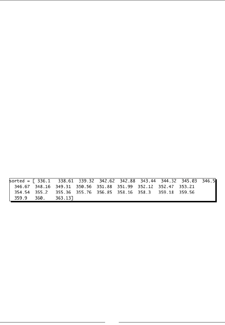
Geng Familiar with Commonly Used Funcons
[ 60 ]
These are the steps to calculate the median:
1. Create a new Python script and call it simplestats.py. You already know how to
load the data from a CSV le into an array. So, copy that line of code and make sure
that it only gets the close price. The code should appear like this:
c=np.loadtxt('data.csv', delimiter=',', usecols=(6,), unpack=True)
2. The funcon that will do the magic for us is called median(). We will call it and
print the result immediately. Add the following line of code:
print("median =", np.median(c))
The program prints the following output:
median = 352.055
3. Since it is our rst me using the median() funcon, we would like to check
whether this is correct. Obviously, we can do it by just going through the le and
nding the correct value, but that is no fun. Instead, we will just mimic the median
algorithm by sorng the close price array and prinng the middle value of the sorted
array. The msort() funcon does the rst part for us. Call the funcon, store the
sorted array, and then print it:
sorted_close = np.msort(c)
print("sorted =", sorted_close)
This prints the following output:
Yup, it works! Let's now get the middle value of the sorted array:
N = len(c)
print "middle =", sorted[(N - 1)/2]
The preceding snippet gives us the following output:
middle = 351.99
4. Hey, that's a dierent value than the one the median() funcon gave us. How
come? Upon further invesgaon, we nd that the median() funcon return value
doesn't even appear in our le. That's even stranger! Before ling bugs with the
NumPy team, let's have a look at the documentaon:
$ python
>>> import numpy as np
>>> help(np.median)

Chapter 3
[ 61 ]
This mystery is easy to solve. It turns out that our naive algorithm only works for
arrays with odd lengths. For even-length arrays, the median is calculated from the
average of the two array values in the middle. Therefore, type the following code:
print("average middle =", (sorted[N /2] + sorted[(N - 1) / 2]) /
2)
This prints the following output:
average middle = 352.055
5. Another stascal measure that we are concerned with is variance. Variance tells
us how much a variable varies (see https://www.khanacademy.org/math/
probability/descriptive-statistics/variance_std_deviation/e/
variance). In our case, it also tells us how risky an investment is, since a stock
price that varies too wildly is bound to get us into trouble.
Calculate the variance of the close price (with NumPy, this is just a one-liner):
print("variance =", np.var(c))
This gives us the following output:
variance = 50.1265178889
6. Not that we don't trust NumPy or anything, but let's double-check using the
denion of variance, as found in the documentaon. Mind you, this denion
might be dierent than the one in your stascs book, but that is quite common
in the eld of stascs.
The population variance is defined as the mean
of the square of deviations from the mean, divided by the
number of elements in the array:
( )
2
1
1n
i
ia mean
n=−
∑
Some books tell us to divide by the number of elements in the array minus one (this
is called a sample variance):
print("variance from definition =", np.mean((c - c.mean())**2))
The output is as follows:
variance from definition = 50.1265178889

Geng Familiar with Commonly Used Funcons
[ 62 ]
What just happened?
Maybe you noced something new. We suddenly called the mean() funcon on the c
array. Yes, this is legal, because the ndarray class has a mean() method. This is for your
convenience. For now, just keep in mind that this is possible. The code for this example
can be found in simplestats.py:
from __future__ import print_function
import numpy as np
c=np.loadtxt('data.csv', delimiter=',', usecols=(6,), unpack=True)
print("median =", np.median(c))
sorted = np.msort(c)
print("sorted =", sorted)
N = len(c)
print("middle =", sorted[(N - 1)/2])
print("average middle =", (sorted[N /2] + sorted[(N - 1) / 2]) / 2)
print("variance =", np.var(c))
print("variance from definition =", np.mean((c - c.mean())**2))
Stock returns
In academic literature, it is more common to base analysis on stock returns and log returns
of the close price. Simple returns are just the rate of change from one value to the next.
Logarithmic returns, or log returns, are determined by taking the log of all the prices and
calculang the dierences between them. In high school, we learned that:
( ) ( )
log log loga
a b b
− =
Log returns, therefore, also measure the rate of change. Returns are dimensionless, since,
in the act of dividing, we divide dollar by dollar (or some other currency). Anyway, investors
are most likely to be interested in the variance or standard deviaon of the returns, as this
represents risk.

Chapter 3
[ 63 ]
Time for action – analyzing stock returns
Perform the following steps to analyze stock returns:
1. First, let's calculate simple returns. NumPy has the diff() funcon that returns an
array that is built up of the dierence between two consecuve array elements. This
is sort of like dierenaon in calculus (the derivave of price with respect to me).
To get the returns, we also have to divide by the value of the previous day. We must
be careful though. The array returned by diff() is one element shorter than the
close prices array. Aer careful deliberaon, we get the following code:
returns = np.diff( arr ) / arr[ : -1]
Noce that we don't use the last value in the divisor. The standard deviaon is
equal to the square root of variance. Compute the standard deviaon using the
std() funcon:
print("Standard deviation =", np.std(returns))
This results in the following output:
Standard deviation = 0.0129221344368
2. The log return or logarithmic return is even easier to calculate. Use the log()
funcon to get the natural logarithm of the close price and then unleash the
diff() funcon on the result:
logreturns = np.diff(np.log(c))
Normally, we have to check that the input array doesn't have zeros or negave
numbers. If it does, we will get an error. Stock prices are, however, always posive,
so we didn't have to check.
3. Quite likely, we will be interested in days when the return is posive. In the current
setup, we can get the next best thing with the where() funcon, which returns the
indices of an array that sases a condion. Just type the following code:
posretindices = np.where(returns > 0)
print("Indices with positive returns", posretindices)
This gives us a number of indices for the array elements that are posive as a tuple,
recognizable by the round brackets on both sides of the printout:
Indices with positive returns (array([ 0, 1, 4, 5, 6, 7, 9,
10, 11, 12, 16, 17, 18, 19, 21, 22, 23, 25, 28]),)

Geng Familiar with Commonly Used Funcons
[ 64 ]
4. In invesng, volality measures price variaon of a nancial security. Historical
volality is calculated from historical price data. The logarithmic returns are
interesng if you want to know the historical volality—for instance, the annualized
or monthly volality. The annualized volality is equal to the standard deviaon of
the log returns as a rao of its mean, divided by one over the square root of the
number of business days in a year, usually one assumes 252. Calculate it with the
std() and mean() funcons, as in the following code:
annual_volatility = np.std(logreturns)/np.mean(logreturns)
annual_volatility = annual_volatility / np.sqrt(1./252.)
print(annual_volatility)
Take noce of the division within the sqrt() funcon. Since, in Python, integer
division works dierently than oat division, we needed to use oats to make
sure that we get the proper results. The monthly volality is similarly given by
the following code:
print("Monthly volatility", annual_volatility * np.sqrt(1./12.))
What just happened?
We calculated the simple stock returns with the diff() funcon, which calculates
dierences between sequenal elements. The log() funcon computes the natural
logarithms of array elements. We used it to calculate the logarithmic returns. At the
end of this secon, we calculated the annual and monthly volality (see returns.py):
from __future__ import print_function
import numpy as np
c=np.loadtxt('data.csv', delimiter=',', usecols=(6,), unpack=True)
returns = np.diff( c ) / c[ : -1]
print("Standard deviation =", np.std(returns))
logreturns = np.diff( np.log(c) )
posretindices = np.where(returns > 0)
print("Indices with positive returns", posretindices)
annual_volatility = np.std(logreturns)/np.mean(logreturns)
annual_volatility = annual_volatility / np.sqrt(1./252.)
print("Annual volatility", annual_volatility)
print("Monthly volatility", annual_volatility * np.sqrt(1./12.))

Chapter 3
[ 65 ]
Dates
Do you somemes have the Monday blues or Friday fever? Ever wondered whether
the stock market suers from these phenomena? Well, I think this certainly warrants
extensive research.
Time for action – dealing with dates
First, we will read the close price data. Second, we will split the prices according to the day
of the week. Third, for each weekday, we will calculate the average price. Finally, we will
nd out which day of the week has the highest average and which has the lowest average.
A word of warning before we commence: you might be tempted to use the result to buy
stock on one day and sell on the other. However, we don't have enough data to make this
kind of decisions.
Coders hate dates because they are so complicated! NumPy is very much oriented toward
oang point operaons. For this reason, we need to take extra eort to process dates. Try it
out yourself; put the following code in a script or use the one that comes with this book:
dates, close=np.loadtxt('data.csv', delimiter=',',
usecols=(1,6), unpack=True)
Execute the script and the following error will appear:
ValueError: invalid literal for float(): 28-01-2011
Now, perform the following steps to deal with dates:
1. Obviously, NumPy tried to convert the dates into oats. What we have to do is tell
NumPy explicitly how to convert the dates. The loadtxt() funcon has a special
parameter for this purpose. The parameter is called converters and is a diconary
that links columns with the so-called converter funcons. It is our responsibility to
write the converter funcon. Write the funcon down:
# Monday 0
# Tuesday 1
# Wednesday 2
# Thursday 3
# Friday 4
# Saturday 5
# Sunday 6
def datestr2num(s):
return datetime.datetime.strptime(s, "%d-%m-%Y").date().
weekday()

Geng Familiar with Commonly Used Funcons
[ 66 ]
We give the datestr2num() funcon dates as a string, such as 28-01-2011. The
string is rst turned into a datetime object, using a specied format %d-%m-%Y. By
the way, this is standard Python and is not related to NumPy itself (see https://
docs.python.org/2/library/datetime.html#strftime-and-strptime-
behavior). Second, the datetime object is turned into a day. Finally, the weekday
method is called on the date to return a number. As you can read in the comments,
the number is between 0 and 6. 0 is, for instance, Monday, and 6 is Sunday. The actual
number, of course, is not important for our algorithm; it is only used as idencaon.
2. Now, hook up our date converter funcon:
dates, close=np.loadtxt('data.csv', delimiter=',', usecols=(1,6),
converters={1: datestr2num}, unpack=True)
print "Dates =", dates
This prints the following output:
Dates = [ 4. 0. 1. 2. 3. 4. 0. 1. 2. 3. 4. 0. 1. 2.
3. 4. 1. 2. 4. 0. 1. 2. 3. 4. 0. 1. 2. 3. 4.]
No Saturdays and Sundays, as you can see. Exchanges are closed over the weekend.
3. We will now make an array that has ve elements for each day of the week. Inialize
the values of the array to 0:
averages = np.zeros(5)
This array will hold the averages for each weekday.
4. We already learned about the where() funcon that returns indices of the array
for elements that conform to a specied condion. The take() funcon can use
these indices and takes the values of the corresponding array items. We will use the
take() funcon to get the close prices for each weekday. In the following loop,
we go through the date values 0 to 4, beer known as Monday to Friday. We get
the indices with the where() funcon for each day and store it in the indices
array. Then, we retrieve the values corresponding to the indices, using the take()
funcon. Finally, compute an average for each weekday and store it in the averages
array, like this:
for i in range(5):
indices = np.where(dates == i)
prices = np.take(close, indices)
avg = np.mean(prices)
print("Day", i, "prices", prices, "Average", avg)
averages[i] = avg

Chapter 3
[ 67 ]
The loop prints the following output:
Day 0 prices [[ 339.32 351.88 359.18 353.21 355.36]] Average
351.79
Day 1 prices [[ 345.03 355.2 359.9 338.61 349.31 355.76]]
Average 350.635
Day 2 prices [[ 344.32 358.16 363.13 342.62 352.12 352.47]]
Average 352.136666667
Day 3 prices [[ 343.44 354.54 358.3 342.88 359.56 346.67]]
Average 350.898333333
Day 4 prices [[ 336.1 346.5 356.85 350.56 348.16 360.
351.99]] Average 350.022857143
5. If you want, you can go ahead and nd out which day has the highest average, and
which the lowest. However, it is just as easy to nd this out with the max() and
min() funcons, as shown here:
top = np.max(averages)
print("Highest average", top)
print("Top day of the week", np.argmax(averages))
bottom = np.min(averages)
print("Lowest average", bottom)
print("Bottom day of the week", np.argmin(averages))
The output is as follows:
Highest average 352.136666667
Top day of the week 2
Lowest average 350.022857143
Bottom day of the week 4
What just happened?
The argmin() funcon returned the index of the lowest value in the averages array.
The index returned was 4, which corresponds to Friday. The argmax() funcon returned
the index of the highest value in the averages array. The index returned was 2, which
corresponds to Wednesday (see weekdays.py):
from __future__ import print_function
import numpy as np
from datetime import datetime
# Monday 0
# Tuesday 1
# Wednesday 2

Geng Familiar with Commonly Used Funcons
[ 68 ]
# Thursday 3
# Friday 4
# Saturday 5
# Sunday 6
def datestr2num(s):
return datetime.strptime(s, "%d-%m-%Y").date().weekday()
dates, close=np.loadtxt('data.csv', delimiter=',', usecols=(1,6),
converters={1: datestr2num}, unpack=True)
print("Dates =", dates)
averages = np.zeros(5)
for i in range(5):
indices = np.where(dates == i)
prices = np.take(close, indices)
avg = np.mean(prices)
print("Day", i, "prices", prices, "Average", avg)
averages[i] = avg
top = np.max(averages)
print("Highest average", top)
print("Top day of the week", np.argmax(averages))
bottom = np.min(averages)
print("Lowest average", bottom)
print("Bottom day of the week", np.argmin(averages))
Have a go hero – looking at VWAP and TWAP
Hey, that was fun! For the sample data, it appears that Friday is the cheapest day and
Wednesday is the day when your Apple stock will be worth the most. Ignoring the fact that
we have very lile data, is there a beer method to compute the averages? Shouldn't we
involve volume data as well? Maybe it makes more sense to you to do a me-weighted
average. Give it a go! Calculate the VWAP and TWAP. You can nd some hints on how to go
about doing this at the beginning of this chapter.

Chapter 3
[ 69 ]
Time for action – using the datetime64 data type
The datetime64 data type was introduced in NumPy 1.7.0 (see http://docs.scipy.
org/doc/numpy/reference/arrays.datetime.html).
1. To learn about the datetime64 data type, start a Python shell and import NumPy
as follows:
$ python
>>> import numpy as np
Create a datetime64 from a string (you can use another date if you like):
>>> np.datetime64('2015-04-22')
numpy.datetime64('2015-04-22')
In the preceding code, we created a datetime64 for April 22, 2015, which happens
to be Earth Day. We used the YYYY-MM-DD format, where Y corresponds to the year,
M corresponds to the month, and D corresponds to the day of the month. NumPy
uses the ISO 8601 standard (see http://en.wikipedia.org/wiki/ISO_8601).
This is an internaonal standard to represent dates and mes. ISO 8601 allows the
YYYY-MM-DD, YYYY-MM, and YYYYMMDD formats. Check for yourself, as follows:
>>> np.datetime64('2015-04-22')
numpy.datetime64('2015-04-22')
>>> np.datetime64('2015-04')
numpy.datetime64('2015-04')
2. By default, ISO 8601 uses the local me zone. Times can be specied using the
format T[hh:mm:ss]. For example, dene January 1, 1677 at 8:19 p.m. as follows:
>>> local = np.datetime64('1677-01-01T20:19')
>>> local
numpy.datetime64('1677-01-01T20:19Z')
Addionally, a string in the format [hh:mm] species an oset that is relave to the
UTC me zone. Create a datetime64 with 9 hours oset, as follows:
>>> with_offset = np.datetime64('1677-01-01T20:19-0900')
>>> with_offset
numpy.datetime64('1677-01-02T05:19Z')
The Z at the end stands for Zulu me, which is how UTC is somemes referred to.
Subtract the two datetime64 objects from each other:
>>> local - with_offset
numpy.timedelta64(-540,'m')

Geng Familiar with Commonly Used Funcons
[ 70 ]
The subtracon creates a NumPy timedelta64 object, which in this case, indicates
a 540 minute dierence. We can also add or subtract a number of days to a
datetime64 object. For instance, April 22, 2015 happens to be a Wednesday. With
the arange() funcon, create an array holding all the Wednesdays from April 22,
2015 unl May 22, 2015 as follows:
>>> np.arange('2015-04-22', '2015-05-22', 7, dtype='datetime64')
array(['2015-04-22', '2015-04-29', '2015-05-06', '2015-05-13',
'2015-05-20'], dtype='datetime64[D]')
Note that in this case, it is mandatory to specify the dtype argument, otherwise
NumPy thinks that we are dealing with strings.
What just happened?
We learned about the NumPy datetime64 type. This data type allows us to manipulate
dates and mes with ease. Its features include simple arithmec and creaon of arrays
using the normal NumPy capabilies.
Weekly summary
The data that we used in the previous Time for acon secon is end-of-day data. In essence,
it is summarized data compiled from the trade data for a certain day. If you are interested in
the market and have decades of data, you might want to summarize and compress the data
even further. Let's summarize the data of Apple stocks to give us weekly summaries.
Time for action – summarizing data
The data we will summarize will be for a whole business week, running from Monday
to Friday. During the period covered by the data, there was one holiday on February 21,
President's Day. This happened to be a Monday and the US stock exchanges were closed on
this day. As a consequence, there is no entry for this day, in the sample. The rst day in the
sample is a Friday, which is inconvenient. Use the following instrucons to summarize data:
1. To simplify, just have a look at the rst three weeks in the sample— later, you can
have a go at improving this:
close = close[:16]
dates = dates[:16]
We will be building on the code from the previous Time for acon secon.

Chapter 3
[ 71 ]
2. Commencing, we will nd the rst Monday in our sample data. Recall that Mondays
have the code 0 in Python. This is what we will put in the condion of the where()
funcon. Then, we will need to extract the rst element that has index 0. The result
will be a muldimensional array. Flaen this with the ravel() funcon:
# get first Monday
first_monday = np.ravel(np.where(dates == 0))[0]
print("The first Monday index is", first_monday)
This will print the following output:
The first Monday index is 1
3. The next logical step is to nd the Friday before last Friday in the sample. The
logic is similar to the one for nding the rst Monday, and the code for Friday is 4.
Addionally, we are looking for the second to last element with index 2:
# get last Friday
last_friday = np.ravel(np.where(dates == 4))[-2]
print("The last Friday index is", last_friday)
This will give us the following output:
The last Friday index is 15
4. Next, create an array with the indices of all the days in the three weeks:
weeks_indices = np.arange(first_monday, last_friday + 1)
print("Weeks indices initial", weeks_indices)
5. Split the array in pieces of size 5 with the split() funcon:
weeks_indices = np.split(weeks_indices, 3)
print("Weeks indices after split", weeks_indices)
This splits the array as follows:
Weeks indices after split [array([1, 2, 3, 4, 5]), array([ 6, 7,
8, 9, 10]), array([11, 12, 13, 14, 15])]
6. In NumPy, array dimensions are called axes. Now, we will get fancy with the apply_
along_axis() funcon. This funcon calls another funcon, which we will provide,
to operate on each of the elements of an array. Currently, we have an array with three
elements. Each array item corresponds to one week in our sample and contains indices
of the corresponding items. Call the apply_along_axis() funcon by supplying
the name of our funcon, called summarize(), which we will dene shortly.
Furthermore, specify the axis or dimension number (such as 1), the array to operate
on, and a variable number of arguments for the summarize() funcon, if any:
weeksummary = np.apply_along_axis(summarize, 1,
weeks_indices, open, high, low, close)
print("Week summary", weeksummary)

Geng Familiar with Commonly Used Funcons
[ 72 ]
7. For each week, the summarize() funcon returns a tuple that holds the open,
high, low, and close price for the week, similar to end-of-day data:
def summarize(a, o, h, l, c):
monday_open = o[a[0]]
week_high = np.max( np.take(h, a) )
week_low = np.min( np.take(l, a) )
friday_close = c[a[-1]]
return("APPL", monday_open, week_high,
week_low, friday_close)
Noce that we used the take() funcon to get the actual values from indices.
Calculang the high and low values for the week was easily done with the max()
and min() funcons. The open for the week is the open for the rst day in the
week—Monday. Likewise, the close is the close for the last day of the week—Friday:
Week summary [['APPL' '335.8' '346.7' '334.3' '346.5']
['APPL' '347.89' '360.0' '347.64' '356.85']
['APPL' '356.79' '364.9' '349.52' '350.56']]
8. Store the data in a le with the NumPy savetxt() funcon:
np.savetxt("weeksummary.csv", weeksummary, delimiter=",",
fmt="%s")
As you can see, have specied a lename, the array we want to store, a delimiter
(in this case a comma), and the format we want to store oang point numbers in.
The format string starts with a percent sign. Second is an oponal ag. The—flag
means le jusfy, 0 means le pad with zeros, and + means precede with + or -.
Third is an oponal width. The width indicates the minimum number of characters.
Fourth, a dot is followed by a number linked to precision. Finally, there comes a
character specier; in our example, the character specier is a string. The character
codes are described as follows:
Character code Description
ccharacter
d or isigned decimal integer
e or Escientific notation with e or E.
fdecimal floating point
g,Guse the shorter of e,E or f
osigned octal

Chapter 3
[ 73 ]
Character code Description
sstring of characters
uunsigned decimal integer
x,Xunsigned hexadecimal integer
View the generated le in your favorite editor or type at the command line:
$ cat weeksummary.csv
APPL,335.8,346.7,334.3,346.5
APPL,347.89,360.0,347.64,356.85
APPL,356.79,364.9,349.52,350.56
What just happened?
We did something that is not even possible in some programming languages. We dened a
funcon and passed it as an argument to the apply_along_axis() funcon.
The programming paradigm described here is called funconal programming.
You can read more about funconal programming in Python at
https://docs.python.org/2/howto/functional.html.
Arguments for the summarize() funcon were neatly passed by apply_along_axis()
(see weeksummary.py):
from __future__ import print_function
import numpy as np
from datetime import datetime
# Monday 0
# Tuesday 1
# Wednesday 2
# Thursday 3
# Friday 4
# Saturday 5
# Sunday 6
def datestr2num(s):
return datetime.strptime(s, "%d-%m-%Y").date().weekday()
dates, open, high, low, close=np.loadtxt('data.csv', delimiter=',',
usecols=(1, 3, 4, 5, 6), converters={1: datestr2num}, unpack=True)
close = close[:16]
dates = dates[:16]

Geng Familiar with Commonly Used Funcons
[ 74 ]
# get first Monday
first_monday = np.ravel(np.where(dates == 0))[0]
print("The first Monday index is", first_monday)
# get last Friday
last_friday = np.ravel(np.where(dates == 4))[-1]
print("The last Friday index is", last_friday)
weeks_indices = np.arange(first_monday, last_friday + 1)
print("Weeks indices initial", weeks_indices)
weeks_indices = np.split(weeks_indices, 3)
print("Weeks indices after split", weeks_indices)
def summarize(a, o, h, l, c):
monday_open = o[a[0]]
week_high = np.max( np.take(h, a) )
week_low = np.min( np.take(l, a) )
friday_close = c[a[-1]]
return("APPL", monday_open, week_high, week_low, friday_close)
weeksummary = np.apply_along_axis(summarize, 1, weeks_indices, open,
high, low, close)
print("Week summary", weeksummary)
np.savetxt("weeksummary.csv", weeksummary, delimiter=",", fmt="%s")
Have a go hero – improving the code
Change the code to deal with a holiday. Time the code to see how big the speedup due to
apply_along_axis() is.
Average True Range
The Average True Range (ATR) is a technical indicator that measures volality of stock prices.
The ATR calculaon is not important further but will serve as an example of several NumPy
funcons, including the maximum() funcon.

Chapter 3
[ 75 ]
Time for action – calculating the Average True Range
To calculate the ATR, perform the following steps:
1. The ATR is based on the low and high price of N days, usually the last 20 days.
N = 5
h = h[-N:]
l = l[-N:]
2. We also need to know the close price of the previous day:
previousclose = c[-N -1: -1]
For each day, we calculate the following:
The daily range—the dierence between the high and low price:
h – l
The dierence between the high and previous close:
h – previousclose
The dierence between the previous close and the low price:
previousclose – l
3. The max() funcon returns the maximum of an array. Based on those three values,
we calculate the so-called true range, which is the maximum of these values. We are
now interested in the element-wise maxima across arrays—meaning the maxima of
the rst elements in the arrays, the second elements in the arrays, and so on. Use
the NumPy maximum() funcon instead of the max() funcon for this purpose:
truerange = np.maximum(h - l, h - previousclose, previousclose -
l)
4. Create an atr array of size N and inialize its values to 0:
atr = np.zeros(N)
5. The rst value of the array is just the average of the truerange array:
atr[0] = np.mean(truerange)
Calculate the other values with the following formula:
( )
( )
1NPATR TR
N
− +

Geng Familiar with Commonly Used Funcons
[ 76 ]
Here, PATR is the previous day's ATR; TR is the true range:
for i in range(1, N):
atr[i] = (N - 1) * atr[i - 1] + truerange[i]
atr[i] /= N
What just happened?
We formed three arrays, one for each of the three ranges—daily range, the gap between the
high of today and the close of yesterday, and the gap between the close of yesterday and the
low of today. This tells us how much the stock price moved and, therefore, how volale it is.
The algorithm requires us to nd the maximum value for each day. The max() funcon that
we used before can give us the maximum value within an array, but that is not what we want
here. We need the maximum value across arrays, so we want the maximum value of the rst
elements in the three arrays, the second elements, and so on. In preceding Time for acon
secon, we saw that the maximum() funcon can do this. Aer this, we computed a moving
average of the true range values (see atr.py):
from __future__ import print_function
import numpy as np
h, l, c = np.loadtxt('data.csv', delimiter=',', usecols=(4, 5, 6),
unpack=True)
N = 5
h = h[-N:]
l = l[-N:]
print("len(h)", len(h), "len(l)", len(l))
print("Close", c)
previousclose = c[-N -1: -1]
print("len(previousclose)", len(previousclose))
print("Previous close", previousclose)
truerange = np.maximum(h - l, h - previousclose, previousclose - l)
print("True range", truerange)
atr = np.zeros(N)
atr[0] = np.mean(truerange)

Chapter 3
[ 77 ]
for i in range(1, N):
atr[i] = (N - 1) * atr[i - 1] + truerange[i]
atr[i] /= N
print("ATR", atr)
In the following secons, we will learn beer ways to calculate moving averages.
Have a go hero – taking the minimum() function for a spin
Besides the maximum() funcon, there is a minimum() funcon. You can probably guess
what it does. Make a small script or start an interacve session in IPython to test your
assumpons.
Simple Moving Average
The Simple Moving Average (SMA) is commonly used to analyze me-series data. To
calculate it, we dene a moving window of N periods, N days in our case. We move this
window along the data and calculate the mean of the values inside the window.
Time for action – computing the Simple Moving Average
The moving average is easy enough to compute with a few loops and the mean() funcon,
but NumPy has a beer alternave—the convolve() funcon. The SMA is, aer all,
nothing more than a convoluon with equal weights or, if you like, unweighted.
Convoluon is a mathemacal operaon on two funcons dened as the
integral of the product of the two funcons aer one of the funcons is
reversed and shied.
( )( ) ( ) ( ) ( ) ( )
f g t f g t d f t g d
τ τ τ τ τ τ
∞ ∞
−∞ −∞
∗ = − = −
∫ ∫
Convoluon is described on Wikipedia at https://en.wikipedia.org/
wiki/Convolution. Khan Academy also has a tutorial on convoluon
at https://www.khanacademy.org/math/differential-
equations/laplace-transform/convolution-integral/v/
introduction-to-the-convolution.

Geng Familiar with Commonly Used Funcons
[ 78 ]
Use the following steps to compute the SMA:
1. Use the ones() funcon to create an array of size N and elements inialized to 1,
and then, divide the array by N to give us the weights:
N = 5
weights = np.ones(N) / N
print("Weights", weights)
For N = 5, this gives us the following output:
Weights [ 0.2 0.2 0.2 0.2 0.2]
2. Now, call the convolve() funcon with these weights:
c = np.loadtxt('data.csv', delimiter=',', usecols=(6,),
unpack=True)
sma = np.convolve(weights, c)[N-1:-N+1]
3. From the array returned by convolve(), we extracted the data in the center of size
N. The following code makes an array of me values and plots with matplotlib
that we will cover in a later chapter:
c = np.loadtxt('data.csv', delimiter=',', usecols=(6,),
unpack=True)
sma = np.convolve(weights, c)[N-1:-N+1]
t = np.arange(N - 1, len(c))
plt.plot(t, c[N-1:], lw=1.0, label="Data")
plt.plot(t, sma, '--', lw=2.0, label="Moving average")
plt.title("5 Day Moving Average")
plt.xlabel("Days")
plt.ylabel("Price ($)")
plt.grid()
plt.legend()
plt.show()
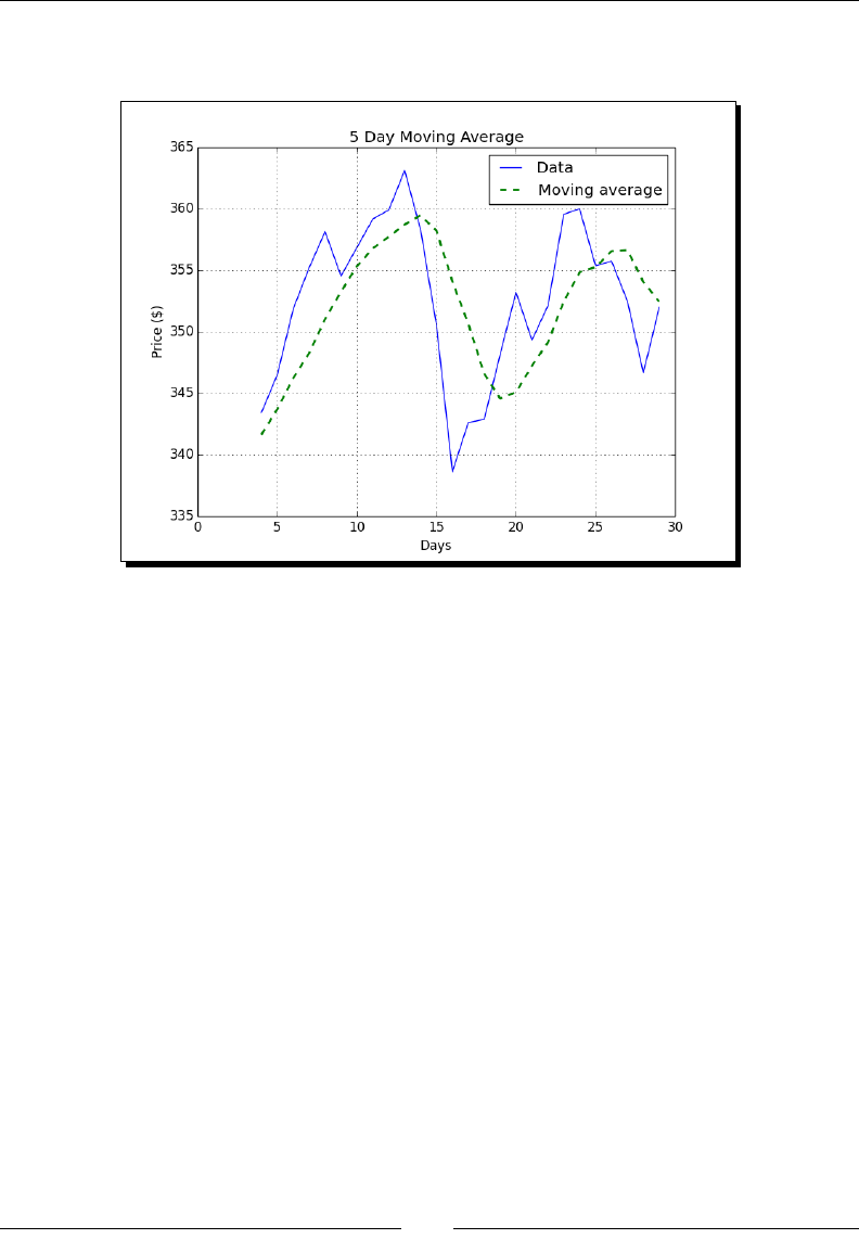
Chapter 3
[ 79 ]
In the following chart, the smooth dashed line is the 5 day SMA and the jagged thin
line is the close price:
What just happened?
We computed the SMA for the close stock price. It turns out that the SMA is just a signal
processing technique—a convoluon with weights 1/N, where N is the size of the moving
average window. We learned that the ones() funcon can create an array with ones and
the convolve() funcon calculates the convoluon of a dataset with specied weights
(see sma.py):
from __future__ import print_function
import numpy as np
import matplotlib.pyplot as plt
N = 5
weights = np.ones(N) / N
print("Weights", weights)
c = np.loadtxt('data.csv', delimiter=',', usecols=(6,), unpack=True)
sma = np.convolve(weights, c)[N-1:-N+1]
t = np.arange(N - 1, len(c))
plt.plot(t, c[N-1:], lw=1.0, label="Data")
plt.plot(t, sma, '--', lw=2.0, label="Moving average")

Geng Familiar with Commonly Used Funcons
[ 80 ]
plt.title("5 Day Moving Average")
plt.xlabel("Days")
plt.ylabel("Price ($)")
plt.grid()
plt.legend()
plt.show()
Exponential Moving Average
The Exponenal Moving Average (EMA) is a popular alternave to the SMA. This method
uses exponenally decreasing weights. The weights for points in the past decrease
exponenally but never reach zero. We will learn about the exp() and linspace()
funcons while calculang the weights.
Time for action – calculating the Exponential Moving Average
Given an array, the exp() funcon calculates the exponenal of each array element. For
example, look at the following code:
x = np.arange(5)
print("Exp", np.exp(x))
It gives the following output:
Exp [ 1. 2.71828183 7.3890561 20.08553692 54.59815003]
The linspace() funcon takes as parameters a start value, a stop value, and oponally an
array size. It returns an array of evenly spaced numbers. This is an example:
print("Linspace", np.linspace(-1, 0, 5))
This will give us the following output:
Linspace [-1. -0.75 -0.5 -0.25 0. ]
Calculate the EMA for our data:
1. Now, back to the weights, calculate them with exp() and linspace():
N = 5
weights = np.exp(np.linspace(-1., 0., N))
2. Normalize the weights with the ndarray sum() method:
weights /= weights.sum()
print("Weights", weights)
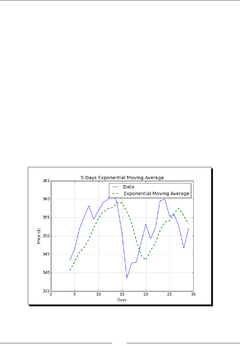
Chapter 3
[ 81 ]
For N = 5, we get these weights:
Weights [ 0.11405072 0.14644403 0.18803785 0.24144538
0.31002201]
3. Aer this, use the convolve() funcon that we learned about in the SMA secon
and also plot the results:
c = np.loadtxt('data.csv', delimiter=',', usecols=(6,),
unpack=True)
ema = np.convolve(weights, c)[N-1:-N+1]
t = np.arange(N - 1, len(c))
plt.plot(t, c[N-1:], lw=1.0, label='Data')
plt.plot(t, ema, '--', lw=2.0, label='Exponential Moving Average')
plt.title('5 Days Exponential Moving Average')
plt.xlabel('Days')
plt.ylabel('Price ($)')
plt.legend()
plt.grid()
plt.show()
This gives us a nice chart where, again, the close price is the thin jagged line and the
EMA is the smooth dashed line:

Geng Familiar with Commonly Used Funcons
[ 82 ]
What just happened?
We calculated the EMA of the close price. First, we computed exponenally decreasing
weights with the exp() and linspace() funcons. The linspace() funcon gave us
an array with evenly spaced elements, and, then, we calculated the exponenal for these
numbers. We called the ndarray sum() method in order to normalize the weights. Aer
this, we applied the convolve() trick that we learned in the SMA secon (see ema.py):
from __future__ import print_function
import numpy as np
import matplotlib.pyplot as plt
x = np.arange(5)
print("Exp", np.exp(x))
print("Linspace", np.linspace(-1, 0, 5))
# Calculate weights
N = 5
weights = np.exp(np.linspace(-1., 0., N))
# Normalize weights
weights /= weights.sum()
print("Weights", weights)
c = np.loadtxt('data.csv', delimiter=',', usecols=(6,), unpack=True)
ema = np.convolve(weights, c)[N-1:-N+1]
t = np.arange(N - 1, len(c))
plt.plot(t, c[N-1:], lw=1.0, label='Data')
plt.plot(t, ema, '--', lw=2.0, label='Exponential Moving Average')
plt.title('5 Days Exponential Moving Average')
plt.xlabel('Days')
plt.ylabel('Price ($)')
plt.legend()
plt.grid()
plt.show()
Bollinger Bands
Bollinger Bands are yet another technical indicator. Yes, there are thousands of them. This
one is named aer its inventor and indicates a range for the price of a nancial security. It
consists of three parts:
1. A Simple Moving Average.

Chapter 3
[ 83 ]
2. An upper band of two standard deviaons above this moving average—the
standard deviaon is derived from the same data with which the moving average
is calculated.
3. A lower band of two standard deviaons below the moving average.
Time for action – enveloping with Bollinger Bands
We already know how to calculate the SMA. So, if you need to refresh your memory, please
review the Time for acon – compung the simple average secon in this chapter. This
example will introduce the NumPy fill() funcon. The fill() funcon sets the value of
an array to a scalar value. The funcon should be faster than array.flat = scalar or
seng the values of the array one-by-one in a loop. Perform the following steps to envelope
with the Bollinger Bands:
1. Starng with an array called sma that contains the moving average values, we
will loop through all the datasets corresponding to those values. Aer forming
the dataset, calculate the standard deviaon. Note that at a certain point, it
will be necessary to calculate the dierence between each data point and the
corresponding average value. If we do not have NumPy, we will loop through these
points and subtract each of the values one-by-one from the corresponding average.
However, the NumPy fill() funcon allows us to construct an array that has
elements set to the same value. This enables us to save on one loop and subtract
arrays in one go:
deviation = []
C = len(c)
for i in range(N - 1, C):
if i + N < C:
dev = c[i: i + N]
else:
dev = c[-N:]
averages = np.zeros(N)
averages.fill(sma[i - N - 1])
dev = dev - averages
dev = dev ** 2
dev = np.sqrt(np.mean(dev))
deviation.append(dev)
deviation = 2 * np.array(deviation)
print(len(deviation), len(sma))
upperBB = sma + deviation
lowerBB = sma - deviation
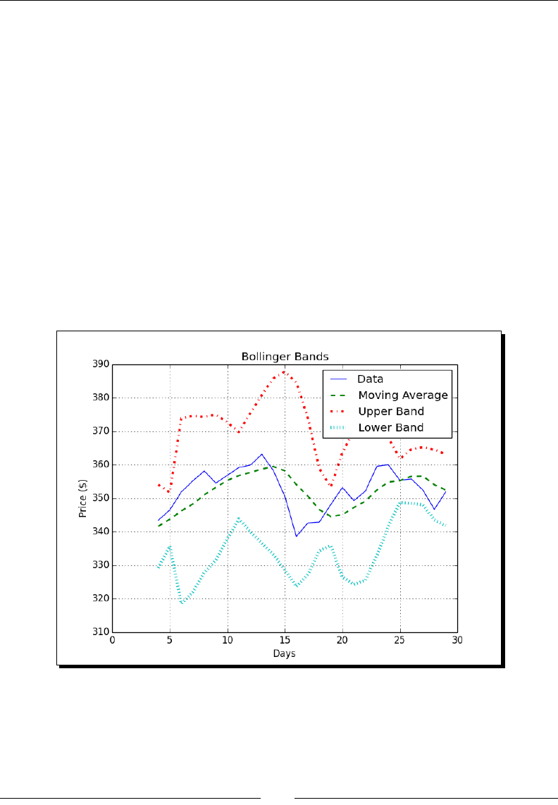
Geng Familiar with Commonly Used Funcons
[ 84 ]
2. To plot, we will use the following code (don't worry about it now; we will see how
this works in Chapter 9, Plong with matplotlib):
t = np.arange(N - 1, C)
plt.plot(t, c_slice, lw=1.0, label='Data')
plt.plot(t, sma, '--', lw=2.0, label='Moving Average')
plt.plot(t, upperBB, '-.', lw=3.0, label='Upper Band')
plt.plot(t, lowerBB, ':', lw=4.0, label='Lower Band')
plt.title('Bollinger Bands')
plt.xlabel('Days')
plt.ylabel('Price ($)')
plt.grid()
plt.legend()
plt.show()
Following is a chart showing the Bollinger Bands for our data. The jagged thin line in
the middle represents the close price, and the dashed, smoother line crossing it is
the moving average:

Chapter 3
[ 85 ]
What just happened?
We worked out the Bollinger Bands that envelope the close price of our data. More
importantly, we got acquainted with the NumPy fill() funcon. This funcon lls
an array with a scalar value. This is the only parameter of the fill() funcon (see
bollingerbands.py):
from __future__ import print_function
import numpy as np
import matplotlib.pyplot as plt
N = 5
weights = np.ones(N) / N
print("Weights", weights)
c = np.loadtxt('data.csv', delimiter=',', usecols=(6,), unpack=True)
sma = np.convolve(weights, c)[N-1:-N+1]
deviation = []
C = len(c)
for i in range(N - 1, C):
if i + N < C:
dev = c[i: i + N]
else:
dev = c[-N:]
averages = np.zeros(N)
averages.fill(sma[i - N - 1])
dev = dev - averages
dev = dev ** 2
dev = np.sqrt(np.mean(dev))
deviation.append(dev)
deviation = 2 * np.array(deviation)
print(len(deviation), len(sma))
upperBB = sma + deviation
lowerBB = sma - deviation
c_slice = c[N-1:]
between_bands = np.where((c_slice < upperBB) & (c_slice > lowerBB))
print(lowerBB[between_bands])
print(c[between_bands])
print(upperBB[between_bands])

Geng Familiar with Commonly Used Funcons
[ 86 ]
between_bands = len(np.ravel(between_bands))
print("Ratio between bands", float(between_bands)/len(c_slice))
t = np.arange(N - 1, C)
plt.plot(t, c_slice, lw=1.0, label='Data')
plt.plot(t, sma, '--', lw=2.0, label='Moving Average')
plt.plot(t, upperBB, '-.', lw=3.0, label='Upper Band')
plt.plot(t, lowerBB, ':', lw=4.0, label='Lower Band')
plt.title('Bollinger Bands')
plt.xlabel('Days')
plt.ylabel('Price ($)')
plt.grid()
plt.legend()
plt.show()
Have a go hero – switching to Exponential Moving Average
It is customary to choose the SMA to center the Bollinger Band on. The second most popular
choice is the EMA, so try that as an exercise. You can nd a suitable example in this chapter,
if you need pointers.
Check whether the fill() funcon is faster or is as fast as array.flat = scalar, or
seng the value in a loop.
Linear model
Many phenomena in science have a related linear relaonship model. The NumPy linalg
package deals with linear algebra computaons. We will begin with the assumpon that a
price value can be derived from N previous prices based on a linear relaonship relaon.
Time for action – predicting price with a linear model
Keeping an open mind, let's assume that we can express a stock price p as a linear
combinaon of previous values, that is, a sum of those values mulplied by certain
coecients we need to determine:
1
N
t t i t i
i
p b a p
− −
=
= + ∑

Chapter 3
[ 87 ]
In linear algebra terms, this boils down to nding a least-squares method (see https://
www.khanacademy.org/math/linear-algebra/alternate_bases/orthogonal_
projections/v/linear-algebra-least-squares-approximation).
Independently of each other, the astronomers Legendre and
Gauss created the least squares method around 1805 (see
http://en.wikipedia.org/wiki/Least_squares).
The method was inially used to analyze the moon of celesal
bodies. The algorithm minimizes the sum of the squared residuals
(the dierence between measured and predicted values):
( )
2
1
n
i i
i
measured predicted
=
−
∑
The recipe goes as follows:
1. First, form a vector b containing N price values:
b = c[-N:]
b = b[::-1]
print("b", x)
The result is as follows:
b [ 351.99 346.67 352.47 355.76 355.36]
2. Second, pre-inialize the matrix A to be N-by-N and contain zeros:
A = np.zeros((N, N), float)
Print("Zeros N by N", A)
The following should be printed on your screen:
Zeros N by N [[ 0. 0. 0. 0. 0.]
[ 0. 0. 0. 0. 0.]
[ 0. 0. 0. 0. 0.]
[ 0. 0. 0. 0. 0.]
[ 0. 0. 0. 0. 0.]]
3. Third, ll the matrix A with N preceding price values for each value in b:
for i in range(N):
A[i, ] = c[-N - 1 - i: - 1 - i]
print("A", A)

Geng Familiar with Commonly Used Funcons
[ 88 ]
Now, A looks like this:
A [[ 360. 355.36 355.76 352.47 346.67]
[ 359.56 360. 355.36 355.76 352.47]
[ 352.12 359.56 360. 355.36 355.76]
[ 349.31 352.12 359.56 360. 355.36]
[ 353.21 349.31 352.12 359.56 360. ]]
4. The objecve is to determine the coecients that sasfy our linear model by solving
the least squares problem. Employ the lstsq() funcon of the NumPy linalg
package to do this:
(x, residuals, rank, s) = np.linalg.lstsq(A, b)
print(x, residuals, rank, s)
The result is as follows:
[ 0.78111069 -1.44411737 1.63563225 -0.89905126 0.92009049]
[] 5 [ 1.77736601e+03 1.49622969e+01 8.75528492e+00
5.15099261e+00 1.75199608e+00]
The tuple returned contains the coecient x that we were aer, an array comprising
residuals, the rank of matrix A, and the singular values of A.
5. Once we have the coecients of our linear model, we can predict the next
price value. Compute the dot product (with the NumPy dot() funcon) of the
coecients and the last known N prices:
print(np.dot(b, x))
The dot product (see https://www.khanacademy.org/math/linear-
algebra/vectors_and_spaces/dot_cross_products/v/vector-dot-
product-and-vector-length) is the linear combinaon of the coecients b
and the prices x. As a result, we get:
357.939161015
I looked it up; the actual close price of the next day was 353.56. So, our esmate with N = 5
was not that far o.

Chapter 3
[ 89 ]
What just happened?
We predicted tomorrow's stock price today. If this works in pracce, we can rere early! See,
this book was a good investment, aer all! We designed a linear model for the predicons.
The nancial problem was reduced to a linear algebraic one. NumPy's linalg package has a
praccal lstsq() funcon that helped us with the task at hand, esmang the coecients
of a linear model. Aer obtaining a soluon, we plugged the numbers in the NumPy dot()
funcon that presented us an esmate through linear regression (see linearmodel.py):
from __future__ import print_function
import numpy as np
N = 5
c = np.loadtxt('data.csv', delimiter=',', usecols=(6,), unpack=True)
b = c[-N:]
b = b[::-1]
print("b", b)
A = np.zeros((N, N), float)
print("Zeros N by N", A)
for i in range(N):
A[i, ] = c[-N - 1 - i: - 1 - i]
print("A", A)
(x, residuals, rank, s) = np.linalg.lstsq(A, b)
print(x, residuals, rank, s)
print(np.dot(b, x))
Trend lines
A trend line is a line among a number of the so-called pivot points on a stock chart. As the
name suggests, the line's trend portrays the trend of the price development. In the past,
traders drew trend lines on paper but nowadays, we can let a computer draw it for us. In this
secon, we shall use a very simple approach that probably won't be very useful in real life,
but should clarify the principle well.

Geng Familiar with Commonly Used Funcons
[ 90 ]
Time for action – drawing trend lines
Perform the following steps to draw trend lines:
1. First, we need to determine the pivot points. We shall pretend they are equal to the
arithmec mean of the high, low, and close price:
h, l, c = np.loadtxt('data.csv', delimiter=',', usecols=(4, 5,
6), unpack=True)
pivots = (h + l + c) / 3
print("Pivots", pivots)
From the pivots, we can deduce the so-called resistance and support levels.
The support level is the lowest level at which the price rebounds. The resistance
level is the highest level at which the price bounces back. These are not natural
phenomena, they are merely esmates. Based on these esmates, it is possible to
draw support and resistance trend lines. We will dene the daily spread to be the
dierence of the high and low price.
2. Dene a funcon to t line to data to a line where y = at + b. The funcon should
return a and b. This is another opportunity to apply the lstsq() funcon of the
NumPy linalg package. Rewrite the line equaon to y = Ax, where A = [t 1]
and x = [a b]. Form A with the NumPy ones_like(), which creates an array,
where all the values are equal to 1, using an input array as a template for the
array dimensions:
def fit_line(t, y):
A = np.vstack([t, np.ones_like(t)]).T
return np.linalg.lstsq(A, y)[0]
3. Assuming that support levels are one daily spread below the pivots, and that
resistance levels are one daily spread above the pivots, t the support and
resistance trend lines:
t = np.arange(len(c))
sa, sb = fit_line(t, pivots - (h - l))
ra, rb = fit_line(t, pivots + (h - l))
support = sa * t + sb
resistance = ra * t + rb

Chapter 3
[ 91 ]
4. At this juncture, we have all the necessary informaon to draw the trend lines;
however, it is wise to check how many points fall between the support and resistance
levels. Obviously, if only a small percentage of the data is between the trend lines,
then this setup is of no use to us. Make up a condion for points between the bands
and select with the where() funcon, based on the following condion:
condition = (c > support) & (c < resistance)
print("Condition", condition)
between_bands = np.where(condition)
These are the printed condion values:
Condition [False False True True True True True False False
True False False
False False False True False False False True True True True
False False True True True False True]
Double-check the values:
print(support[between_bands])
print( c[between_bands])
print( resistance[between_bands])
The array returned by the where() funcon has rank 2, so call the ravel()
funcon before calling the len() funcon:
between_bands = len(np.ravel(between_bands))
print("Number points between bands", between_bands)
print("Ratio between bands", float(between_bands)/len(c))
You will get the following result:
Number points between bands 15
Ratio between bands 0.5
As an extra bonus, we gained a predicve model. Extrapolate the next day resistance
and support levels:
print("Tomorrows support", sa * (t[-1] + 1) + sb)
print("Tomorrows resistance", ra * (t[-1] + 1) + rb)
This results in the following output:
Tomorrows support 349.389157088
Tomorrows resistance 360.749340996
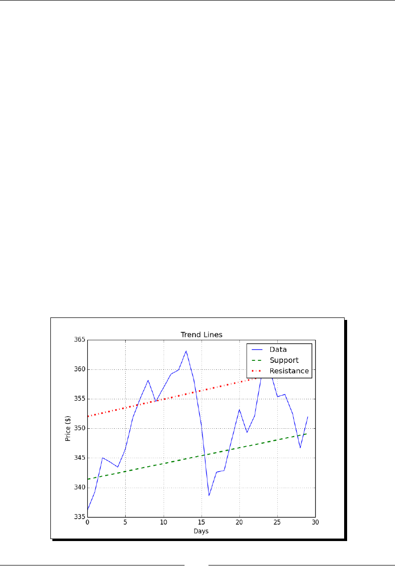
Geng Familiar with Commonly Used Funcons
[ 92 ]
Another approach to gure out how many points are between the support and
resistance esmates is to use [] and intersect1d(). Dene selecon criteria
in the [] operator and intersect the results with the intersect1d() funcon:
a1 = c[c > support]
a2 = c[c < resistance]
print("Number of points between bands 2nd approach" ,len(np.
intersect1d(a1, a2)))
Not surprisingly, we get:
Number of points between bands 2nd approach 15
5. Once more, plot the results:
plt.plot(t, c, label='Data')
plt.plot(t, support, '--', lw=2.0, label='Support')
plt.plot(t, resistance, '-.', lw=3.0, label='Resistance')
plt.title('Trend Lines')
plt.xlabel('Days')
plt.ylabel('Price ($)')
plt.grid()
plt.legend()
plt.show()
In the following plot, we have the price data and the corresponding support and
resistance lines:

Chapter 3
[ 93 ]
What just happened?
We drew trend lines without having to mess around with rulers, pencils, and paper charts.
We dened a funcon that can t data to a line with the NumPy vstack(), ones_like(),
and lstsq() funcons. We t the data in order to dene support and resistance trend lines.
Then, we gured out how many points are within the support and resistance range. We did
this using two separate methods that produced the same result.
The rst method used the where() funcon with a Boolean condion. The second method
made use of the [] operator and the intersect1d() funcon. The intersect1d()
funcon returns an array of common elements from two arrays (see trendline.py):
from __future__ import print_function
import numpy as np
import matplotlib.pyplot as plt
def fit_line(t, y):
''' Fits t to a line y = at + b '''
A = np.vstack([t, np.ones_like(t)]).T
return np.linalg.lstsq(A, y)[0]
# Determine pivots
h, l, c = np.loadtxt('data.csv', delimiter=',', usecols=(4, 5, 6),
unpack=True)
pivots = (h + l + c) / 3
print("Pivots", pivots)
# Fit trend lines
t = np.arange(len(c))
sa, sb = fit_line(t, pivots - (h - l))
ra, rb = fit_line(t, pivots + (h - l))
support = sa * t + sb
resistance = ra * t + rb
condition = (c > support) & (c < resistance)
print("Condition", condition)
between_bands = np.where(condition)
print(support[between_bands])
print(c[between_bands])
print(resistance[between_bands])
between_bands = len(np.ravel(between_bands))

Geng Familiar with Commonly Used Funcons
[ 94 ]
print("Number points between bands", between_bands)
print("Ratio between bands", float(between_bands)/len(c))
print("Tomorrows support", sa * (t[-1] + 1) + sb)
print("Tomorrows resistance", ra * (t[-1] + 1) + rb)
a1 = c[c > support]
a2 = c[c < resistance]
print("Number of points between bands 2nd approach" ,len(np.
intersect1d(a1, a2)))
# Plotting
plt.plot(t, c, label='Data')
plt.plot(t, support, '--', lw=2.0, label='Support')
plt.plot(t, resistance, '-.', lw=3.0, label='Resistance')
plt.title('Trend Lines')
plt.xlabel('Days')
plt.ylabel('Price ($)')
plt.grid()
plt.legend()
plt.show()
Methods of ndarray
The NumPy ndarray class has a lot of methods that work on the array. Most of the me,
these methods return an array. You may have noced that many of the funcons part of the
NumPy library have a counterpart with the same name and funconality in the ndarray
class. This is mostly due to the historical development of NumPy.
The list of ndarray methods is prey long, so we cannot cover them all. The mean(),
var(), sum(), std(), argmax(), argmin(), and mean() funcons that we saw earlier
are also ndarray methods.
Time for action – clipping and compressing arrays
Here are a few examples of ndarray methods. Perform the following steps to clip and
compress arrays:
1. The clip() method returns a clipped array, so that all values above a maximum
value are set to the maximum and values below a minimum are set to the minimum
value. Clip an array with values 0 to 4 to 1 and 2:
a = np.arange(5)
print("a =", a)
print("Clipped", a.clip(1, 2))

Chapter 3
[ 95 ]
This gives the following output:
a = [0 1 2 3 4]
Clipped [1 1 2 2 2]
2. The ndarray compress() method returns an array based on a condion. For
instance, look at the following code:
a = np.arange(4)
print(a)
print("Compressed", a.compress(a > 2))
This returns the following output:
[0 1 2 3]
Compressed [3]
What just happened?
We created an array with values 0 to 3 and selected the last element with the compress()
funcon based on the a > 2 condion.
Factorial
Many programming books have an example of calculang the factorial. We should not break
with this tradion.
Time for action – calculating the factorial
The ndarray class has the prod() method, which computes the product of the elements in
an array. Perform the following steps to calculate the factorial:
1. Calculate the factorial of 8. To do this, generate an array with values 1 to 8 and call
the prod() funcon on it:
b = np.arange(1, 9)
print("b =", b)
print("Factorial", b.prod())
Check the result with your pocket calculator:
b = [1 2 3 4 5 6 7 8]
Factorial 40320
This is nice, but what if we want to know all the factorials from 1 to 8?

Geng Familiar with Commonly Used Funcons
[ 96 ]
2. No problem! Call the cumprod() method, which computes the cumulave product
of an array:
print("Factorials", b.cumprod())
It's pocket calculator me again:
Factorials [ 1 2 6 24 120 720 5040 40320]
What just happened?
We used the prod() and cumprod() funcons to calculate factorials (see
ndarraymethods.py):
from __future__ import print_function
import numpy as np
a = np.arange(5)
print("a =", a)
print("Clipped", a.clip(1, 2))
a = np.arange(4)
print(a)
print("Compressed", a.compress(a > 2))
b = np.arange(1, 9)
print("b =", b)
print("Factorial", b.prod())
print("Factorials", b.cumprod())
Missing values and Jackknife resampling
Data oen misses values because of errors or technical issues. Even if we are not missing
values, we may have cause to suspect certain values. Once we doubt data values, derived
values such as the arithmec mean, which we learned to calculate in this chapter, become
quesonable too. It is common for these reasons to try to esmate how reliable the
arithmec mean, variance, and standard deviaon are.
A simple but eecve method is called Jackknife resampling (see http://en.wikipedia.
org/wiki/Jackknife_resampling). The idea behind jackknife resampling is to
systemacally generate datasets from the original dataset by leaving one value out at a me.
In eect, we are trying to establish what will happen if at least one of the values is wrong.
For each new generated dataset, we recalculate the arithmec mean, variance, and standard
deviaon. This gives us an idea of how much those values can vary.

Chapter 3
[ 97 ]
Time for action – handling NaNs with the nanmean(), nanvar(),
and nanstd() functions
We will apply jackknife resampling to the stock data. Each value will be omied by seng it
to Not a Number (NaN). The nanmean(), nanvar(), and nanstd() can then be used to
compute the arithmec mean, variance, and standard deviaon.
1. First, inialize a 30-by-3 array for the esmates as follows:
estimates = np.zeros((len(c), 3))
2. Loop through the values and generate a new dataset by seng one value to NaN at
each iteraon of the loop. For each new set of values, compute the esmates:
for i in xrange(len(c)):
a = c.copy()
a[i] = np.nan
estimates[i,] = [np.nanmean(a), np.nanvar(a), np.nanstd(a)]
3. Print the variance for each esmate (you can also print the mean or standard
deviaon if you prefer):
print("Estimates variance", estimates.var(axis=0))
The following is printed on the screen:
Estimates variance [ 0.05960347 3.63062943 0.01868965]
What just happened?
We esmated the variances of the arithmec mean, variance, and standard deviaon of a
small dataset using jackknife resampling. This gives us an idea of how much the arithmec
mean, variance, and standard deviaon vary. The code for this example can be found in the
jackknife.py le in this book's code bundle:
from __future__ import print_function
import numpy as np
c = np.loadtxt('data.csv', delimiter=',', usecols=(6,), unpack=True)
# Initialize estimates array
estimates = np.zeros((len(c), 3))
for i in xrange(len(c)):

Geng Familiar with Commonly Used Funcons
[ 98 ]
# Create a temporary copy and omit one value
a = c.copy()
a[i] = np.nan
# Compute estimates
estimates[i,] = [np.nanmean(a), np.nanvar(a), np.nanstd(a)]
print("Estimates variance", estimates.var(axis=0))
Summary
This chapter informed us about a great number of common NumPy funcons. A few
common stascs funcons were also menoned.
Aer this tour through the common NumPy funcons, we will connue covering
convenience NumPy funcons such as polyfit(), sign(), and piecewise()
in the next chapter.

[ 99 ]
Convenience Functions
for Your Convenience
As we have seen, NumPy has a great number of functions. Many of those
functions exist just for convenience, and knowing them will greatly increase
your productivity. This includes functions that select certain parts of your arrays
(based on a Boolean condition, for instance) or manipulate polynomials. This
chapter has an example of computing correlation to give you a taste of data
analysis with NumPy.
In this chapter, we shall cover the following topics:
Data selecon and extracon
Simple data analysis
Examples of correlaon of returns
Polynomials
Linear algebra funcons
In Chapter 3, Geng Familiar with Commonly Used Funcons, we had one data le
to play around with. Things have improved in this chapter—we now have two data les.
Let's explore the data with NumPy.
4

Convenience Funcons for Your Convenience
[ 100 ]
Correlation
Have you noced that the stock price of some companies will be closely followed by another,
usually a rival in the same sector? The theorecal explanaon is that because these two
companies are in the same type of business, they share the same challenges, require the
same materials and resources, and compete for the same type of customers.
You could think of many possible pairs, but you need to check for a real relaonship. One
way is to take a look at the correlaon of the stock returns of both stocks (see https://
www.khanacademy.org/math/probability/statistical-studies/types-of-
studies/v/correlation-and-causality). A high correlaon implies a relaonship of
some sort. It is not proof of causality though, especially if you don't use sucient data.
Time for action – trading correlated pairs
For this secon, we will use two sample datasets, containing end-of-day price data. The rst
company is BHP Billiton (BHP), which is acve in mining of petroleum, metals, and diamonds.
The second is Vale (VALE), which is also a metals and mining company. So, there is some
overlap of acvity, albeit not 100 percent. For evaluang correlated pairs, follow these steps:
1. First, load the data, specically the close price of the two securies, from the CSV
les in the example code directory of this chapter and calculate the returns. If you
don't remember how to do it, look at the examples in Chapter 3, Geng Familiar
with Commonly Used Funcons.
2. Covariance tells us how two variables vary together; which is nothing more
than unnormalized correlaon (see https://www.khanacademy.org/math/
probability/regression/regression-correlation/v/covariance-and-
the-regression-line):
( ) ( )
( )
( )
( )
1
1
,
N
j j
i
cov a b a mean a b mean b
N=
= − −
∑
Compute the covariance matrix from the returns with the cov() funcon
(it's not strictly necessary to do this, but it will allow us to demonstrate a
few matrix operaons):
covariance = np.cov(bhp_returns, vale_returns)
print("Covariance", covariance)
The covariance matrix is as follows:
Covariance [[ 0.00028179 0.00019766]
[ 0.00019766 0.00030123]]

Chapter 4
[ 101 ]
3. View the values on the diagonal with the diagonal() method:
print("Covariance diagonal", covariance.diagonal())
The diagonal values of the covariance matrix are as follows:
Covariance diagonal [ 0.00028179 0.00030123]
Noce that the values on the diagonal are not equal to each other. This is dierent
from the correlaon matrix.
4. Compute the trace, the sum of the diagonal values, with the trace() method:
print("Covariance trace", covariance.trace())
The trace values of the covariance matrix are as follows:
Covariance trace 0.00058302354992
5. The correlaon of two vectors is dened as the covariance, divided by the product
of the respecve standard deviaons of the vectors. The equaon for vectors a and
b is as follows:
print(covariance/ (bhp_returns.std() * vale_returns.std()))
The correlaon matrix is as follows:
[[ 1.00173366 0.70264666]
[ 0.70264666 1.0708476 ]]
6. We will measure the correlaon of our pair with the correlaon coecient. The
correlaon coecient takes values between -1 and 1. The correlaon of a set of
values with itself is 1 by denion. This would be the ideal value; however, we will
also be happy with a slightly lower value. Calculate the correlaon coecient (or,
more accurately, the correlaon matrix) with the corrcoef() funcon:
print("Correlation coefficient", np.corrcoef(bhp_returns, vale_
returns))
The coecients are as follows:
[[ 1. 0.67841747]
[ 0.67841747 1. ]]
The values on the diagonal are just the correlaons of the BHP and VALE with
themselves and are, therefore, equal to 1. In all likelihood, no real calculaon takes
place. The other two values are equal to each other since correlaon is symmetrical,
meaning that the correlaon of BHP with VALE is equal to the correlaon of VALE
with BHP. It seems that here the correlaon is not that strong.

Convenience Funcons for Your Convenience
[ 102 ]
7. Another important point is whether the two stocks under consideraon are in sync
or not. Two stocks are considered out of sync if their dierence is two standard
deviaons from the mean of the dierences.
If they are out of sync, we could iniate a trade, hoping that they will eventually
get back in sync again. Compute the dierence between the close prices of the
two securies to check the synchronizaon:
difference = bhp - vale
Check whether the last dierence in price is out of sync; see the following code:
avg = np.mean(difference)
dev = np.std(difference)
print("Out of sync", np.abs(difference[-1] – avg) > 2 * dev)
Unfortunately, we cannot trade yet:
Out of sync False
8. Plong requires matplotlib; this will be discussed in Chapter 9, Plong with
matplotlib. Plong can be done as follows:
t = np.arange(len(bhp_returns))
plt.plot(t, bhp_returns, lw=1, label='BHP returns')
plt.plot(t, vale_returns, '--', lw=2, label='VALE returns')
plt.title('Correlating arrays')
plt.xlabel('Days')
plt.ylabel('Returns')
plt.grid()
plt.legend(loc='best')
plt.show()
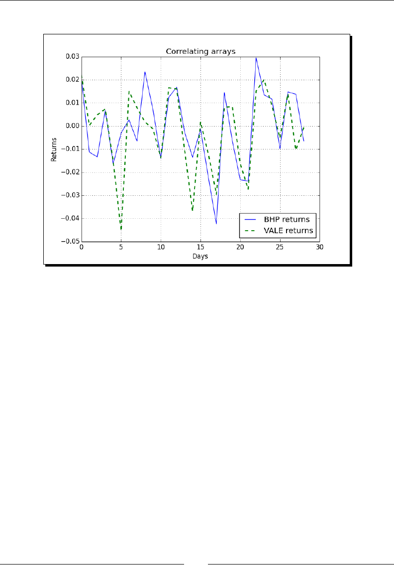
Chapter 4
[ 103 ]
The resulng plot is shown here:
What just happened?
We analyzed the relaon of the closing stock prices of BHP and VALE. To be precise, we
calculated the correlaon of their stock returns. We achieved this with the corrcoef()
funcon. Furthermore, we saw how to compute the covariance matrix from which the
correlaon can be derived. As a bonus, we demonstrated the diagonal() and trace()
methods that give us the diagonal values and the trace of a matrix, respecvely. For the
source code, see the correlation.py le in this book's code bundle:
from __future__ import print_function
import numpy as np
import matplotlib.pyplot as plt
bhp = np.loadtxt('BHP.csv', delimiter=',', usecols=(6,), unpack=True)
bhp_returns = np.diff(bhp) / bhp[ : -1]
vale = np.loadtxt('VALE.csv', delimiter=',', usecols=(6,),
unpack=True)
vale_returns = np.diff(vale) / vale[ : -1]
covariance = np.cov(bhp_returns, vale_returns)

Convenience Funcons for Your Convenience
[ 104 ]
print("Covariance", covariance)
print("Covariance diagonal", covariance.diagonal())
print("Covariance trace", covariance.trace())
print(covariance/ (bhp_returns.std() * vale_returns.std()))
print("Correlation coefficient", np.corrcoef(bhp_returns, vale_
returns))
difference = bhp - vale
avg = np.mean(difference)
dev = np.std(difference)
print("Out of sync", np.abs(difference[-1] - avg) > 2 * dev)
t = np.arange(len(bhp_returns))
plt.plot(t, bhp_returns, lw=1, label='BHP returns')
plt.plot(t, vale_returns, '--', lw=2, label='VALE returns')
plt.title('Correlating arrays')
plt.xlabel('Days')
plt.ylabel('Returns')
plt.grid()
plt.legend(loc='best')
plt.show()
Pop quiz – calculating covariance
Q1. Which funcon returns the covariance of two arrays?
1. covariance
2. covar
3. cov
4. cvar
Polynomials
Do you like calculus? Well I love it! One of the ideas in calculus is Taylor expansion,
that is, represenng a dierenable funcon as an innite series (see https://www.
khanacademy.org/math/integral-calculus/sequences_series_approx_calc/
taylor-series/v/generalized-taylor-series-approximation and
http://en.wikipedia.org/wiki/Taylor_series.).

Chapter 4
[ 105 ]
The Taylor series is dened as the following sum:
()
( ) ( )
0!
n
n
n
f a x a
n
∞
=−
∑
( )
( )
n
f a
in this denion is the nth derivave of the funcon f computed at the
point a.
In pracce, this means that we can esmate any dierenable, and therefore connuous,
funcon with a polynomial of a high degree. We would then assume that the terms of the
higher degrees are negligibly small.
Time for action – tting to polynomials
The NumPy polyfit() funcon ts a set of data points to a polynomial, even if the
underlying funcon is not connuous:
1. Connuing with the price data of BHP and VALE, look at the dierence of their
close prices and t it to a polynomial of the third power:
bhp=np.loadtxt('BHP.csv', delimiter=',', usecols=(6,),
unpack=True)
vale=np.loadtxt('VALE.csv', delimiter=',', usecols=(6,),
unpack=True)
t = np.arange(len(bhp))
poly = np.polyfit(t, bhp - vale, 3)
print("Polynomial fit", poly)
The polynomial t (in this example, a cubic polynomial was chosen) is as follows:
Polynomial fit [ 1.11655581e-03 -5.28581762e-02 5.80684638e-01
5.79791202e+01]
2. The numbers you see are the coecients of the polynomial. Extrapolate to the
next value with the polyval() funcon and the polynomial object that we got
from the t:
print("Next value", np.polyval(poly, t[-1] + 1))
The next value we predict will be this:
Next value 57.9743076081

Convenience Funcons for Your Convenience
[ 106 ]
3. Ideally, the dierence between the close prices of BHP and VALE should be as small
as possible. In an extreme case, it might be zero at some point. Find out when our
polynomial t reaches zero with the roots() funcon:
print( "Roots", np.roots(poly))
The roots of the polynomial are as follows:
Roots [ 35.48624287+30.62717062j 35.48624287-30.62717062j
-23.63210575 +0.j ]
4. Another thing you may have learned in calculus class was to nd extrema—these
could be potenal maxima or minima. Remember, from calculus, that these are the
points where the derivave of our funcon is zero. Dierenate the polynomial t
with the polyder() funcon:
der = np.polyder(poly)
print("Derivative", der)
The coecients of the derivave polynomial are as follows:
Derivative [ 0.00334967 -0.10571635 0.58068464]
5. Get the roots of the derivave:
print("Extremas", np.roots(der))
The extremas that we get are as follows:
Extremas [ 24.47820054 7.08205278]
Let's double-check and compute the values of the t with the polyval() funcon:
vals = np.polyval(poly, t)
6. Now, nd the maximum and minimum values with the argmax() and the
argmin() funcon:
vals = np.polyval(poly, t)
print(np.argmax(vals))
print(np.argmin(vals))
This gives us the expected results shown in the following screenshot. OK, not quite the
same results, but, if we backtrack to step 1, we can see that t was dened with the
arange() funcon:
7
24
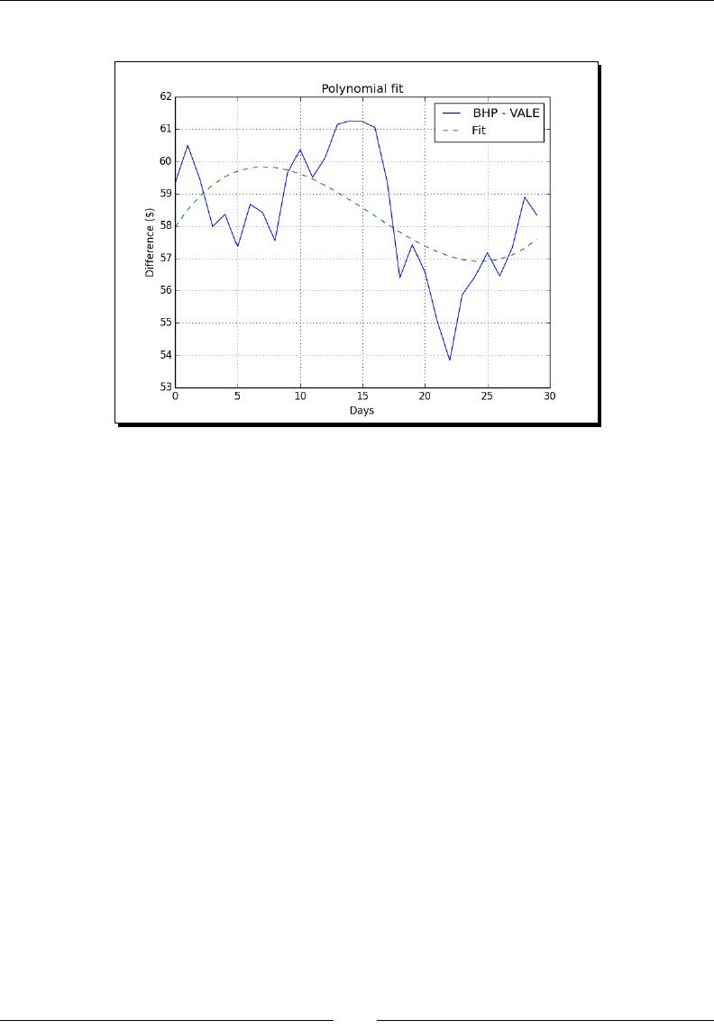
Chapter 4
[ 107 ]
Plot the data and the t it to get the following plot:
Obviously, the smooth line is the t and the jagged line is the underlying data.
But as it's not that good a t, you might want to try a higher order polynomial.
What just happened?
We t data to a polynomial with the polyfit() funcon. We learned about the polyval()
funcon that computes the values of a polynomial, the roots() funcon that returns the
roots of the polynomial, and the polyder() funcon that gives back the derivave of a
polynomial (see polynomials.py):
from __future__ import print_function
import numpy as np
import sys
import matplotlib.pyplot as plt
bhp=np.loadtxt('BHP.csv', delimiter=',', usecols=(6,), unpack=True)
vale=np.loadtxt('VALE.csv', delimiter=',', usecols=(6,), unpack=True)
t = np.arange(len(bhp))
poly = np.polyfit(t, bhp - vale, 3)
print("Polynomial fit", poly)
print("Next value", np.polyval(poly, t[-1] + 1))

Convenience Funcons for Your Convenience
[ 108 ]
print("Roots", np.roots(poly))
der = np.polyder(poly)
print("Derivative", der)
print("Extremas", np.roots(der))
vals = np.polyval(poly, t)
print(np.argmax(vals))
print(np.argmin(vals))
plt.plot(t, bhp - vale, label='BHP - VALE')
plt.plot(t, vals, '-—', label='Fit')
plt.title('Polynomial fit')
plt.xlabel('Days')
plt.ylabel('Difference ($)')
plt.grid()
plt.legend()
plt.show()
Have a go hero – improving the t
You could do a number of things to improve the t. For example, try a dierent power as, in
this secon, a cubic polynomial was chosen. Consider smoothing the data before ng it. One
way you could smooth the data is with a moving average. You can nd examples of simple and
EMA calculaons in the Chapter 3, Geng Familiar with Commonly Used Funcons.
On-balance volume
Volume is a very important variable in invesng; it indicates how big a price move is. The
on-balance volume indicator is one of the simplest stock price indicators. It is based on the
close price of the current and previous days and the volume of the current day. For each day,
if the close price today is higher than the close price of yesterday, then the value of the on-
balance volume is equal to the volume of today. On the other hand, if today's close price is
lower than yesterday's close price, then the value of the on-balance volume indicator is the
dierence between the on-balance volume and the volume of today. However, if the close
price did not change, then the value of the on-balance volume is zero.

Chapter 4
[ 109 ]
Time for action – balancing volume
In other words, we need to mulply the sign of the close price and the volume. In this
secon, we look at two approaches to this problem: one using the NumPy sign() funcon
and the other using the NumPy piecewise() funcon.
1. Load the BHP data into a close and volume array:
c, v=np.loadtxt('BHP.csv', delimiter=',', usecols=(6, 7),
unpack=True)
Compute the absolute value changes. Calculate the change of the closing price with
the diff() funcon. The diff() funcon computes the dierence between two
sequenal array elements and returns an array containing these dierences:
change = np.diff(c)
print("Change", change)
The changes of the close price are shown as follows:
Change [ 1.92 -1.08 -1.26 0.63 -1.54 -0.28 0.25 -0.6 2.15
0.69 -1.33 1.16
1.59 -0.26 -1.29 -0.13 -2.12 -3.91 1.28 -0.57 -2.07 -2.07 2.5
1.18
-0.88 1.31 1.24 -0.59]
2. The NumPy sign() funcon returns the signs for each element in an array. -1 is
returned for a negave number, 1 for a posive number, and 0, otherwise. Apply
the sign() funcon to the change array:
signs = np.sign(change)
print("Signs", signs)
The signs of the change array are as follows:
Signs [ 1. -1. -1. 1. -1. -1. 1. -1. 1. 1. -1. 1. 1. -1. -1.
-1. -1. -1.
-1. -1. -1. 1. 1. 1. -1. 1. 1. -1.]
Alternavely, we can calculate the signs with the piecewise() funcon. The
piecewise() funcon, as its name suggests, evaluates a funcon piece-by-piece.
Call the funcon with the appropriate return values and condions:
pieces = np.piecewise(change, [change < 0, change > 0], [-1,
1])
print("Pieces", pieces)

Convenience Funcons for Your Convenience
[ 110 ]
The signs are shown again as follows:
Pieces [ 1. -1. -1. 1. -1. -1. 1. -1. 1. 1. -1. 1. 1. -1.
-1. -1. -1. -1.
-1. -1. -1. 1. 1. 1. -1. 1. 1. -1.]
Check that the outcome is the same:
print("Arrays equal?", np.array_equal(signs, pieces))
And the outcome is as follows:
Arrays equal? True
3. The on-balance volume depends on the change of the previous close, so we cannot
calculate it for the rst day in our sample:
print("On balance volume", v[1:] * signs)
The on-balance volume is as follows:
[ 2620800. -2461300. -3270900. 2650200. -4667300. -5359800.
7768400.
-4799100. 3448300. 4719800. -3898900. 3727700. 3379400.
-2463900.
-3590900. -3805000. -3271700. -5507800. 2996800. -3434800.
-5008300.
-7809799. 3947100. 3809700. 3098200. -3500200. 4285600.
3918800.
-3632200.]
What just happened?
We computed the on-balance volume that depends on the change of the closing price.
Using the NumPy sign() and piecewise() funcons, we went over two dierent
methods to determine the sign of the change (see obv.py) as follows:
from __future__ import print_function
import numpy as np
c, v=np.loadtxt('BHP.csv', delimiter=',', usecols=(6, 7), unpack=True)
change = np.diff(c)
print("Change", change)
signs = np.sign(change)
print("Signs", signs)

Chapter 4
[ 111 ]
pieces = np.piecewise(change, [change < 0, change > 0], [-1, 1])
print("Pieces", pieces)
print("Arrays equal?", np.array_equal(signs, pieces))
print("On balance volume", v[1:] * signs)
Simulation
Oen, you would want to try something out rst. Play around, experiment, but preferably
without blowing things up or geng dirty! NumPy is perfect for experimentaon. We will
use NumPy to simulate a trading day, without actually losing money. Many people like to buy
on the dip or, in other words, wait for the price of stocks to drop before buying. A variant of
this is to wait for the price to drop a small percentage, say 0.1 percent below the opening
price of the day.
Time for action – avoiding loops with vectorize()
The vectorize() funcon is a yet another trick to reduce the number of loops in your
programs. Calculate the prot of a single trading day following these steps:
1. First, load the data:
o, h, l, c = np.loadtxt('BHP.csv', delimiter=',', usecols=(3, 4,
5, 6), unpack=True)
2. The vectorize() funcon is the NumPy equivalent of the Python map() funcon.
Call the vectorize() funcon, giving it as an argument the calc_profit()
funcon:
func = np.vectorize(calc_profit)
3. We can now apply func() as if it is a funcon. Apply the func() funcon result
that we got to the price arrays:
profits = func(o, h, l, c)
4. The calc_profit() funcon is prey simple. First, we try to buy slightly below
the open price. If this is outside of the daily range, then, obviously, our aempt
failed and no prot was made, or we incurred a loss, therefore, will return 0.
Otherwise, we sell at the close price and the prot is simply the dierence between
the buy price and the close price. Actually, it is, in fact, more interesng to have a
look at the relave prot:
def calc_profit(open, high, low, close):
#buy just below the open
buy = open * 0.999

Convenience Funcons for Your Convenience
[ 112 ]
# daily range
if low < buy < high:
return (close - buy)/buy
else:
return 0
print("Profits", profits)
5. Assume that there are two days with zero prots, where there was either no net
gain or a loss. Select the days with trades and calculate the averages:
real_trades = profits[profits != 0]
print("Number of trades", len(real_trades), round(100.0 *
len(real_trades)/len(c), 2), "%")
print("Average profit/loss %", round(np.mean(real_trades) * 100,
2))
The trades summary is shown as follows:
Number of trades 28 93.33 %
Average profit/loss % 0.02
6. As opmists, we are interested in winning trades with a gain greater than zero.
Select the days with winning trades and calculate the averages:
winning_trades = profits[profits > 0]
print("Number of winning trades", len(winning_trades),
round(100.0 * len(winning_trades)/len(c), 2), "%")
print("Average profit %", round(np.mean(winning_trades) * 100,
2))
The winning trades stascs are as follows:
Number of winning trades 16 53.33 %
Average profit % 0.72
7. Alternavely, as pessimists, we are interested in losing trades with a prot less than
zero. Select the days with losing trades and calculate the averages:
losing_trades = profits[profits < 0]
print("Number of losing trades", len(losing_trades), round(100.0 *
len(losing_trades)/len(c), 2), "%")
print("Average loss %", round(np.mean(losing_trades) * 100, 2))
The losing trades stascs are as follows:
Number of losing trades 12 40.0 %
Average loss % -0.92

Chapter 4
[ 113 ]
What just happened?
We vectorized a funcon, which is just another way to avoid using loops. We simulated
a trading day with a funcon, which returned the relave prot of each day's trade. We
printed a stascs summary of the losing and winning trades (see simulation.py):
from __future__ import print_function
import numpy as np
o, h, l, c = np.loadtxt('BHP.csv', delimiter=',', usecols=(3, 4, 5,
6), unpack=True)
def calc_profit(open, high, low, close):
#buy just below the open
buy = open * 0.999
# daily range
if low < buy < high:
return (close - buy)/buy
else:
return 0
func = np.vectorize(calc_profit)
profits = func(o, h, l, c)
print("Profits", profits)
real_trades = profits[profits != 0]
print("Number of trades", len(real_trades), round(100.0 * len(real_
trades)/len(c), 2), "%")
print("Average profit/loss %", round(np.mean(real_trades) * 100, 2))
winning_trades = profits[profits > 0]
print("Number of winning trades", len(winning_trades), round(100.0 *
len(winning_trades)/len(c), 2), "%")
print("Average profit %", round(np.mean(winning_trades) * 100, 2))
losing_trades = profits[profits < 0]
print("Number of losing trades", len(losing_trades), round(100.0 *
len(losing_trades)/len(c), 2), "%")
print("Average loss %", round(np.mean(losing_trades) * 100, 2))

Convenience Funcons for Your Convenience
[ 114 ]
Have a go hero – analyzing consecutive wins and losses
Although the average prot is posive, it is also important to know whether we had to
endure a long streak of consecuve losses. If this is the case, we might be le with lile or
no capital, and then the average prot would not maer.
Find out if there was such a losing streak. If you want, you can also nd out if there was a
prolonged winning streak.
Smoothing
Noisy data is dicult to deal with, so we oen need to do some smoothing. Besides
calculang moving averages, we can use one of the NumPy funcons to smooth data.
The hanning() funcon is a window funcon formed by a weighted cosine
(see http://en.wikipedia.org/wiki/Hann_function):
( )
2
0.5 0.5cos1
n
w n N
π
= −
−
In the preceding formula, N corresponds to the size of the window. We will cover the other
window funcons in later chapters.
Time for action – smoothing with the hanning() function
We will use the hanning() funcon to smooth arrays of stock returns, as shown in the
following steps:
1. Call the hanning() funcon to compute weights for a certain length window (in
this example 8) as follows:
N = 8
weights = np.hanning(N)
print("Weights", weights)
The weights are as follows:
Weights [ 0. 0.1882551 0.61126047 0.95048443
0.95048443 0.61126047
0.1882551 0. ]
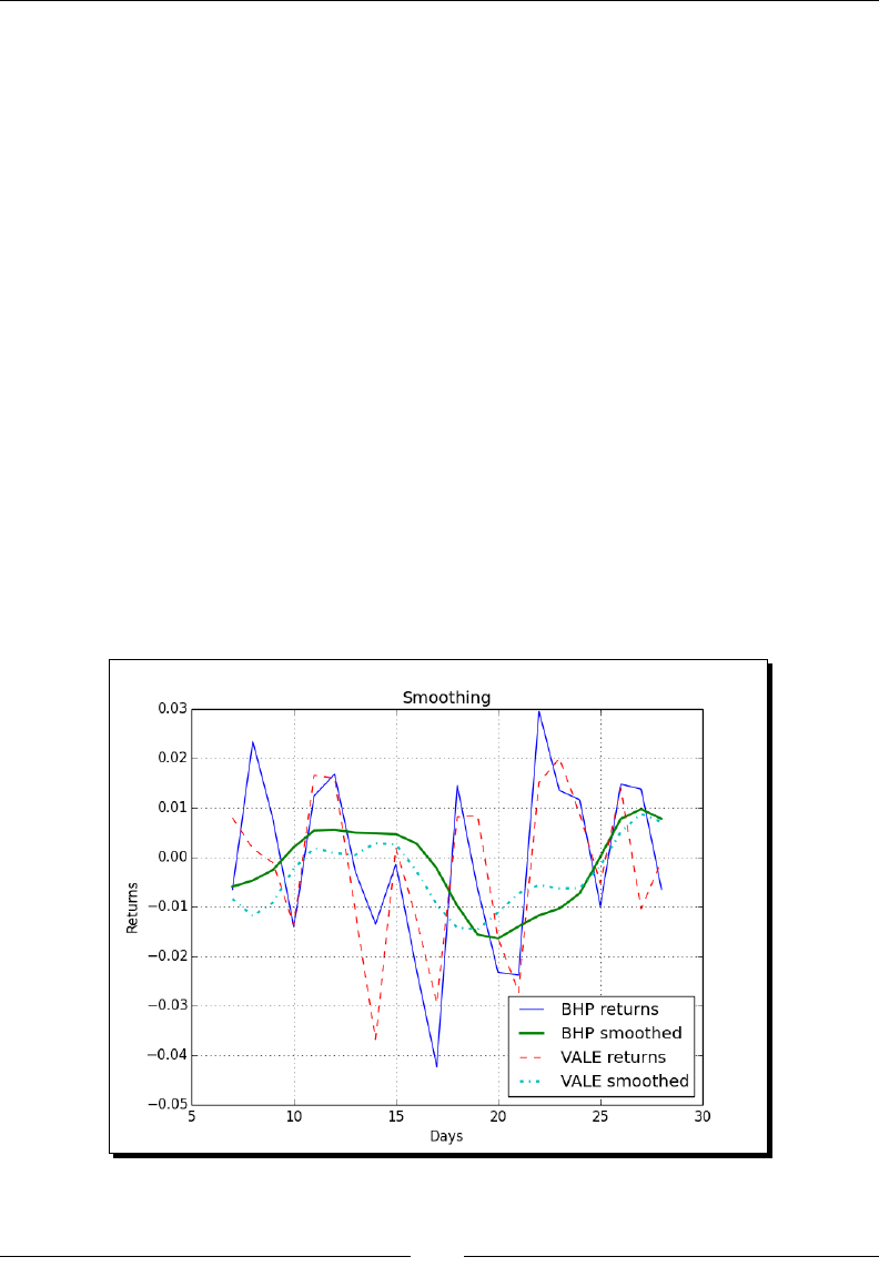
Chapter 4
[ 115 ]
2. Calculate the stock returns for the BHP and VALE quotes using convolve() with
normalized weights:
bhp = np.loadtxt('BHP.csv', delimiter=',', usecols=(6,),
unpack=True)
bhp_returns = np.diff(bhp) / bhp[ : -1]
smooth_bhp = np.convolve(weights/weights.sum(),
bhp_returns)[N-1:-N+1]
vale = np.loadtxt('VALE.csv', delimiter=',', usecols=(6,),
unpack=True)
vale_returns = np.diff(vale) / vale[ : -1]
smooth_vale = np.convolve(weights/weights.sum(),
vale_returns)[N-1:-N+1]
3. Plot with matplotlib using this code:
t = np.arange(N - 1, len(bhp_returns))
plt.plot(t, bhp_returns[N-1:], lw=1.0)
plt.plot(t, smooth_bhp, lw=2.0)
plt.plot(t, vale_returns[N-1:], lw=1.0)
plt.plot(t, smooth_vale, lw=2.0)
plt.show()
The chart would appear as follows:

Convenience Funcons for Your Convenience
[ 116 ]
The thin lines on the preceding chart are the stock returns and the thick lines are the
result of smoothing. As you can see, the lines cross a few mes. These points might
be important because the trend might have changed there. Or, at least, the relaon
of BHP to VALE might have changed. These turning inecon points probably occur
oen, so we might want to project into the future.
4. Fit the result of the smoothing step to polynomials as follows:
K = 8
t = np.arange(N - 1, len(bhp_returns))
poly_bhp = np.polyfit(t, smooth_bhp, K)
poly_vale = np.polyfit(t, smooth_vale, K)
5. Next, we need to evaluate the situaon, where the polynomials we found in
the previous step were equal to each other. This boils down to subtracng the
polynomials and nding the roots of the resulng polynomial. Subtract the
polynomials using polysub():
poly_sub = np.polysub(poly_bhp, poly_vale)
xpoints = np.roots(poly_sub)
print("Intersection points", xpoints)
The points are shown as follows:
Intersection points [ 27.73321597+0.j 27.51284094+0.j
24.32064343+0.j
18.86423973+0.j 12.43797190+1.73218179j 12.43797190-
1.73218179j
6.34613053+0.62519463j 6.34613053-0.62519463j]
6. The numbers we get are complex, and that is not good for us (unless there
is such a thing as imaginary me). Check which numbers are real with the
isreal() funcon:
reals = np.isreal(xpoints)
print("Real number?", reals)
The result is as follows:
Real number? [ True True True True False False False False]
Some of the numbers are real, so select them with the select() funcon. The
select() funcon forms an array by taking elements from a list of choices, based
on a list of condions:
xpoints = np.select([reals], [xpoints])
xpoints = xpoints.real
print("Real intersection points", xpoints)

Chapter 4
[ 117 ]
The real intersecon points are as follows:
Real intersection points [ 27.73321597 27.51284094 24.32064343
18.86423973 0. 0. 0. 0.]
7. We managed to pick up some zeroes. The trim_zeros() funcon strips the
leading and trailing zeroes from a one-dimensional array. Get rid of the zeroes
with the trim_zeros() funcon:
print("Sans 0s", np.trim_zeros(xpoints))
The zeroes are gone, and the output is shown as follows:
Sans 0s [ 27.73321597 27.51284094 24.32064343 18.86423973]
What just happened?
We applied the hanning() funcon to smooth arrays containing stock returns. We
subtracted two polynomials with the polysub() funcon. We then checked for real
numbers with the isreal() funcon and selected the real numbers with the select()
funcon. Finally, we stripped zeroes from an array with the trim_zeros() funcon
(see smoothing.py):
from __future__ import print_function
import numpy as np
import matplotlib.pyplot as plt
N = 8
weights = np.hanning(N)
print("Weights", weights)
bhp = np.loadtxt('BHP.csv', delimiter=',', usecols=(6,), unpack=True)
bhp_returns = np.diff(bhp) / bhp[ : -1]
smooth_bhp = np.convolve(weights/weights.sum(), bhp_returns)[N-1:-N+1]
vale = np.loadtxt('VALE.csv', delimiter=',', usecols=(6,),
unpack=True)
vale_returns = np.diff(vale) / vale[ : -1]
smooth_vale = np.convolve(weights/weights.sum(), vale_returns)
[N-1:-N+1]
K = 8
t = np.arange(N - 1, len(bhp_returns))
poly_bhp = np.polyfit(t, smooth_bhp, K)

Convenience Funcons for Your Convenience
[ 118 ]
poly_vale = np.polyfit(t, smooth_vale, K)
poly_sub = np.polysub(poly_bhp, poly_vale)
xpoints = np.roots(poly_sub)
print("Intersection points", xpoints)
reals = np.isreal(xpoints)
print("Real number?", reals)
xpoints = np.select([reals], [xpoints])
xpoints = xpoints.real
print("Real intersection points", xpoints)
print("Sans 0s", np.trim_zeros(xpoints))
plt.plot(t, bhp_returns[N-1:], lw=1.0, label='BHP returns')
plt.plot(t, smooth_bhp, lw=2.0, label='BHP smoothed')
plt.plot(t, vale_returns[N-1:], '--', lw=1.0, label='VALE returns')
plt.plot(t, smooth_vale, '-.', lw=2.0, label='VALE smoothed')
plt.title('Smoothing')
plt.xlabel('Days')
plt.ylabel('Returns')
plt.grid()
plt.legend(loc='best')
plt.show()
Have a go hero – smoothing variations
Experiment with the other smoothing funcons—hamming(), blackman(), bartlett(),
and kaiser(). They work in more or less the same way as the hanning() funcon.
Initialization
So far in this book, we encountered several convenient funcons for inalizing arrays. The
full() and full_like() funcons were recently added to NumPy to make inializaon
even easier.

Chapter 4
[ 119 ]
The following short Python session shows (abbreviated) documentaon for these
two funcons:
$ python
>>> import numpy as np
>>> help(np.full)
Return a new array of given shape and type, filled with `fill_value`.
>>> help(np.full_like)
Return a full array with the same shape and type as a given array.
Time for action – creating value initialized arrays with the full()
and full_like() functions
Let's demonstrate how the full() and full_like() funcons work. If you are not in a
Python shell already, type the following:
$ python
>>> import numpy as np
1. Create a one-by-two array with the full() funcon lled with the number 42
as follows:
>>> np.full((1, 2), 42)
array([[ 42., 42.]])
As you can deduce from the output, the array elements are oang-point numbers,
which is the default data type for NumPy arrays. Specify an integer data type
as follows:
>>> np.full((1, 2), 42, dtype=np.int)
array([[42, 42]])
2. The full_like() funcon looks at the metadata of an input array and uses that
informaon to create a new array, lled with a specied value. For instance, aer
creang an array with the linspace() funcon, use that as a template for the
full_like() funcon:
>>> a = np.linspace(0, 1, 5)
>>> a
array([ 0. , 0.25, 0.5 , 0.75, 1. ])
>>> np.full_like(a, 42)
array([ 42., 42., 42., 42., 42.])

Convenience Funcons for Your Convenience
[ 120 ]
Again we have an array lled with 42. To change the data type to integer, type the
following:
>>> np.full_like(a, 42, dtype=np.int)
array([42, 42, 42, 42, 42])
What just happened?
We created arrays using the full() and full_like() funcons. The full() funcon
lled the array with the number 42. The full_like() funcon uses the metadata of an
input array to create a new array. Both funcons allow you to specify the data type.
Summary
We calculated the correlaon of the stock returns of two stocks with the corrcoef()
funcon. As a bonus, we demonstrated the diagonal() and trace() funcons,
which can give us the diagonal and trace of a matrix.
We t data to a polynomial with the polyfit() funcon. We learned about the
polyval() funcon that computes the values of a polynomial, the roots() funcon
that returns the roots of the polynomial, and the polyder() funcon, which gives back
the derivave of a polynomial.
We saw that the full() funcon lls an array with a number, and the full_like()
funcon uses the metadata of an input array to create a new array. Both funcons allow
you to specify the data type.
Hopefully, you have increased your producvity, so that we can connue in the next chapter
with matrices and Universal Funcons (ufuncs).

[ 121 ]
5
Working with Matrices and ufuncs
This chapter covers matrices and Universal functions (ufuncs). Matrices are
well known in mathematics and have their representation in NumPy as well.
Universal functions work on arrays, element by element, or on scalars. ufuncs
expect a set of scalars as input and produce a set of scalars as output. Universal
functions can typically be mapped to their mathematical counterparts such as
add, subtract, divide, multiply, and so on. We will also introduce trigonometric,
bitwise, and comparison universal functions.
In this chapter, we will cover the following topics:
Matrix creaon
Matrix operaons
Basic ufuncs
Trigonometric funcons
Bitwise funcons
Comparison funcons

Working with Matrices and ufuncs
[ 122 ]
Matrices
Matrices in NumPy are subclasses of ndarray. We can create matrices using a special
string format. They are, just like in mathemacs, two-dimensional (see https://www.
khanacademy.org/math/precalculus/precalc-matrices). Matrix mulplicaon is, as
you would expect, dierent from the normal NumPy mulplicaon. The same is true for the
power operator. We can create matrices with the mat(), matrix(), and bmat() funcons.
Time for action – creating matrices
The mat() funcon does not make a copy if the input is already a matrix or an ndarray.
Calling this funcon is equivalent to calling matrix(data, copy=False). We will also
demonstrate transposing and inverng matrices.
1. Rows are delimited by a semicolon and values by a space. Call the mat() funcon
with the following string to create a matrix:
A = np.mat('1 2 3; 4 5 6; 7 8 9')
print("Creation from string", A)
The matrix output should be the following matrix:
Creation from string [[1 2 3]
[4 5 6]
[7 8 9]]
2. Transpose the matrix with the T aribute as follows:
print("transpose A", A.T)
The following is the transposed matrix:
transpose A [[1 4 7]
[2 5 8]
[3 6 9]]
3. The matrix can be inverted with the I aribute as follows (see https://www.
khanacademy.org/math/precalculus/precalc-matrices/inverting_
matrices/v/inverse-matrix-part-1):
print("Inverse A", A.I)
The inverse matrix is printed as follows (be warned that this is a O(n3) operaon,
meaning that it takes on average cubic me):
Inverse A [[ -4.50359963e+15 9.00719925e+15 -4.50359963e+15]
[ 9.00719925e+15 -1.80143985e+16 9.00719925e+15]
[ -4.50359963e+15 9.00719925e+15 -4.50359963e+15]]

Chapter 5
[ 123 ]
4. Instead of using a string to create a matrix, do it with an array:
print("Creation from array", np.mat(np.arange(9).reshape(3, 3)))
The newly created array is printed as follows:
Creation from array [[0 1 2]
[3 4 5]
[6 7 8]]
What just happened?
We created matrices with the mat() funcon. We transposed the matrices with the T
aribute and inverted them with the I aribute (see matrixcreation.py):
from __future__ import print_function
import numpy as np
A = np.mat('1 2 3; 4 5 6; 7 8 9')
print("Creation from string", A)
print("transpose A", A.T)
print("Inverse A", A.I)
print("Check Inverse", A * A.I)
print("Creation from array", np.mat(np.arange(9).reshape(3, 3)))
Creating a matrix from other matrices
Somemes, we want to create a matrix from other smaller matrices. We can do this with the
bmat() funcon. The b here stands for block matrix.
Time for action – creating a matrix from other matrices
We will create a matrix from two smaller matrices as follows:
1. First, create a 2-by-2 identy matrix:
A = np.eye(2)
print("A", A)
The identy matrix looks like the following:
A [[ 1. 0.]
[ 0. 1.]]

Working with Matrices and ufuncs
[ 124 ]
2. Create another matrix like A and mulply it by 2:
B = 2 * A
print("B", B)
The second matrix is as follows:
B [[ 2. 0.]
[ 0. 2.]]
3. Create the compound matrix from a string. The string uses the same format as the
mat() funcon—use matrices instead of numbers:
print("Compound matrix\n", np.bmat("A B; A B"))
The compound matrix is shown as follows:
Compound matrix
[[ 1. 0. 2. 0.]
[ 0. 1. 0. 2.]
[ 1. 0. 2. 0.]
[ 0. 1. 0. 2.]]
What just happened?
We created a block matrix from two smaller matrices with the bmat() funcon. We
gave the funcon a string containing the names of matrices instead of numbers (see
bmatcreation.py):
from __future__ import print_function
import numpy as np
A = np.eye(2)
print("A", A)
B = 2 * A
print("B", B)
print("Compound matrix\n", np.bmat("A B; A B"))
Pop quiz – dening a matrix with a string
Q1. What is the row delimiter in a string accepted by the mat() and bmat() funcons?
1. Semicolon
2. Colon
3. Comma
4. Space

Chapter 5
[ 125 ]
Universal functions
Universal funcons (ufuncs) expect a set of scalars as input and produce a set of scalars as
output. They are actually Python objects that encapsulate the behavior of a funcon. We
can typically map ufuncs to their mathemacal counterparts such as add, subtract, divide,
mulply, and so on. Universal funcons are, in general, faster because of their special
opmizaons and because they run on the nave level.
Time for action – creating universal functions
We can create a ufunc from a Python funcon with the NumPy the frompyfunc() funcon
as follows:
1. Dene a Python funcon that answers the ulmate queson to the universe,
existence, and the rest (it's from The Hitchhiker's Guide to the Galaxy, Douglas
Adam, Pan Books, if you haven't read it, you can safely ignore this!):
def ultimate_answer(a):
So far, nothing special; we gave the funcon the name ultimate_answer() and
dened one parameter, a.
2. Create a result consisng of all zeros that has the same shape as a, with the
zeros_like() funcon:
result = np.zeros_like(a)
3. Now, set the elements of the inialized array to the answer 42 and return the
result. The complete funcon should appear as shown in the following code snippet.
The flat aribute gives us access to a at iterator that allows us to set the value of
the array.
def ultimate_answer(a):
result = np.zeros_like(a)
result.flat = 42
return result
4. Create a ufunc with frompyfunc(); specify 1 as the number of input parameter
followed by 1 as the number of output parameters:
ufunc = np.frompyfunc(ultimate_answer, 1, 1)
print("The answer", ufunc(np.arange(4)))
The result for a one-dimensional array is shown as follows:
The answer [42 42 42 42]

Working with Matrices and ufuncs
[ 126 ]
Do the same for a two-dimensional array with the following code:
print("The answer", ufunc(np.arange(4).reshape(2, 2)))
The output for a two dimensional array is shown as follows:
The answer [[42 42]
[42 42]]
What just happened?
We dened a Python funcon. In this funcon, we inialized to zero the elements of an
array, based on the shape of an input argument, with the zeros_like() funcon. Then,
with the flat aribute of ndarray, we set the array elements to the ulmate answer, 42
(see answer42.py):
from __future__ import print_function
import numpy as np
def ultimate_answer(a):
result = np.zeros_like(a)
result.flat = 42
return result
ufunc = np.frompyfunc(ultimate_answer, 1, 1)
print("The answer", ufunc(np.arange(4)))
print("The answer", ufunc(np.arange(4).reshape(2, 2)))
Universal function methods
How can funcons have methods? As we said earlier, universal funcons are not funcons
but Python objects represenng funcons. Universal funcons have ve important methods
listed as follows:
1. ufunc.reduce(a[, axis, dtype, out, keepdims])
2. ufunc.accumulate(array[, axis, dtype, out])
3. ufunc.reduceat(a, indices[, axis, dtype, out])
4. ufunc.outer(A, B)
5. ufunc.at(a, indices[, b])])])

Chapter 5
[ 127 ]
Time for action – applying the ufunc methods to the
add function
Let's call the rst four methods on the add() funcon:
1. The universal funcon reduces the input array recursively along a specied axis on
consecuve elements. For the add() funcon, the result of reducing is similar to
calculang the sum of an array. Call the reduce() method:
a = np.arange(9)
print("Reduce", np.add.reduce(a))
The reduced array should be as follows:
Reduce 36
2. The accumulate() method also recursively goes through the input array. But,
contrary to the reduce() method, it stores the intermediate results in an array and
returns that. The result, in the case of the add() funcon, is equivalent to calling
the cumsum() funcon. Call the accumulate() method on the add() funcon:
print("Accumulate", np.add.accumulate(a))
The accumulated array is as follows:
Accumulate [ 0 1 3 6 10 15 21 28 36]
3. The reduceat() method is a bit complicated to explain, so let's call it and go
through its algorithm, step by step. The reduceat() method requires as arguments
an input array and a list of indices:
print("Reduceat", np.add.reduceat(a, [0, 5, 2, 7]))
The result is shown as follows:
Reduceat [10 5 20 15]
The rst step concerns the indices 0 and 5. This step results in a reduce operaon of
the array elements between indices 0 and 5:
print("Reduceat step I", np.add.reduce(a[0:5]))
The output of step 1 is as follows:
Reduceat step I 10
The second step concerns indices 5 and 2. Since 2 is less than 5, the array element
at index 5 is returned:
print("Reduceat step II", a[5])

Working with Matrices and ufuncs
[ 128 ]
The second step results in the following output:
Reduceat step II 5
The third step concerns indices 2 and 7. This step results in a reduce operaon of
the array elements between indices 2 and 7:
print("Reduceat step III", np.add.reduce(a[2:7]))
The result of the third step is shown as follows:
Reduceat step III 20
The fourth step concerns index 7. This step results in a reduce operaon of the array
elements from index 7 to the end of the array:
print("Reduceat step IV", np.add.reduce(a[7:]))
The fourth step result is shown as follows:
Reduceat step IV 15
4. The outer() method returns an array that has a rank, which is the sum of the ranks
of its two input arrays. The method is applied to all possible pairs of the input array
elements. Call the outer() method on the add() funcon:
print("Outer", np.add.outer(np.arange(3), a))
The outer sum output result is as follows:
Outer [[ 0 1 2 3 4 5 6 7 8]
[ 1 2 3 4 5 6 7 8 9]
[ 2 3 4 5 6 7 8 9 10]]
What just happened?
We applied the rst four methods, reduce(), accumulate(), reduceat(), and outer(),
of universal funcons to the add() funcon (see ufuncmethods.py):
from __future__ import print_function
import numpy as np
a = np.arange(9)
print("Reduce", np.add.reduce(a))
print("Accumulate", np.add.accumulate(a))
print("Reduceat", np.add.reduceat(a, [0, 5, 2, 7]))
print("Reduceat step I", np.add.reduce(a[0:5]))
print("Reduceat step II", a[5])

Chapter 5
[ 129 ]
print("Reduceat step III", np.add.reduce(a[2:7]))
print("Reduceat step IV", np.add.reduce(a[7:]))
print("Outer", np.add.outer(np.arange(3), a))
Arithmetic functions
The common arithmec operators +, -, and * are implicitly linked to the add, subtract,
and mulply universal funcons, respecvely. This means that when you use one of these
operators on a NumPy array, the corresponding universal funcon will get called. Division
involves a slightly more complex process. The three universal funcons that have to do with
array division are divide(), true_divide(), and floor_division(). Two operators
correspond to division: / and //.
Time for action – dividing arrays
Let's see the array division in acon:
1. The divide() funcon does truncated integer division and normal oang-point
division:
a = np.array([2, 6, 5])
b = np.array([1, 2, 3])
print("Divide", np.divide(a, b), np.divide(b, a))
The result of the divide() funcon is shown as follows:
Divide [2 3 1] [0 0 0]
As you can see, truncaon took place.
2. The true_divide() funcon comes closer to the mathemacal denion of
division. Integer division returns a oang-point result and no truncaon occurs:
print("True Divide", np.true_divide(a, b), np.true_divide(b, a))
The result of the true_divide() funcon is as follows:
True Divide [ 2. 3. 1.66666667] [ 0.5
0.33333333 0.6 ]
3. The floor_divide() funcon always returns an integer result. It is equivalent to
calling the floor() funcon aer calling the divide() funcon. The floor()
funcon discards the decimal part of a oang-point number and returns an integer:
print("Floor Divide", np.floor_divide(a, b), np.floor_divide(b, a))
c = 3.14 * b
print("Floor Divide 2", np.floor_divide(c, b),
np.floor_divide(b, c))

Working with Matrices and ufuncs
[ 130 ]
The floor_divide() funcon call results in:
Floor Divide [2 3 1] [0 0 0]
Floor Divide 2 [ 3. 3. 3.] [ 0. 0. 0.]
4. By default, the / operator is equivalent to calling the divide() funcon:
from __future__ import division
However, if this line is found at the beginning of a Python program, the
true_divide() funcon is called instead. So, this code will appear as follows:
print("/ operator", a/b, b/a)
The result is shown as follows:
/ operator [ 2. 3. 1.66666667] [ 0.5
0.33333333 0.6 ]
5. The // operator is equivalent to calling the floor_divide() funcon. For
example, look at the following code snippet:
print("// operator", a//b, b//a)
print("// operator 2", c//b, b//c)
The // operator result is shown as follows:
// operator [2 3 1] [0 0 0]
// operator 2 [ 3. 3. 3.] [ 0. 0. 0.]
What just happened?
The divide() funcon truncates the integer division and normal oang-point division. The
true_divide() funcon always returns a oang-point result without any truncaon. The
floor_divide() funcon always returns an integer result; the result is the same that you
will get by calling the divide() and floor() funcons consecuvely (see dividing.py):
from __future__ import print_function
from __future__ import division
import numpy as np
a = np.array([2, 6, 5])
b = np.array([1, 2, 3])
print("Divide", np.divide(a, b), np.divide(b, a))
print("True Divide", np.true_divide(a, b), np.true_divide(b, a))

Chapter 5
[ 131 ]
print("Floor Divide", np.floor_divide(a, b), np.floor_divide(b, a))
c = 3.14 * b
print("Floor Divide 2", np.floor_divide(c, b), np.floor_divide(b, c))
print("/ operator", a/b, b/a)
print("// operator", a//b, b//a)
print("// operator 2", c//b, b//c)
Have a go hero – experimenting with __future__.division
Experiment to conrm the impact of imporng __future__.division.
Modulo operation
We can calculate the modulo or remainder using the NumPy mod(), remainder(), and
fmod() funcons. Also, we can use the % operator. The main dierence among these
funcons is how they deal with negave numbers. The odd one out in this group is the
fmod() funcon.
Time for action – computing the modulo
Let's call the previously menoned funcons:
1. The remainder() funcon returns the remainder of the two arrays, element-wise.
0 is returned if the second number is 0:
a = np.arange(-4, 4)
print("Remainder", np.remainder(a, 2))
The result of the remainder() funcon is shown as follows:
Remainder [0 1 0 1 0 1 0 1]
2. The mod() funcon does exactly the same as the remainder() funcon:
print("Mod", np.mod(a, 2))
The result of the mod() funcon is shown as follows:
Mod [0 1 0 1 0 1 0 1]
3. The % operator is just shorthand for the remainder() funcon:
print("% operator", a % 2)
The result of the % operator is shown as follows:
% operator [0 1 0 1 0 1 0 1]

Working with Matrices and ufuncs
[ 132 ]
4. The fmod() funcon handles negave numbers dierently than mod(), fmod(),
and % do. The sign of the remainder is the sign of the dividend, and the sign of the
divisor has no inuence on the results:
print("Fmod", np.fmod(a, 2))
The fmod() result is printed as follows:
Fmod [ 0 -1 0 -1 0 1 0 1]
What just happened?
We demonstrated the NumPy the mod(), remainder(), and fmod() funcons, which
compute the modulo or remainder (see modulo.py):
from __future__ import print_function
import numpy as np
a = np.arange(-4, 4)
print("Remainder", np.remainder(a, 2))
print("Mod", np.mod(a, 2))
print("% operator", a % 2)
print("Fmod", np.fmod(a, 2))
Fibonacci numbers
The Fibonacci numbers (see http://en.wikipedia.org/wiki/Fibonacci_number)
are based on a recurrence relaon:
1 2n n n
F F F
− −
= +
It is dicult to express this relaon directly with NumPy code. However, we can express this
relaon in a matrix form or use the following golden rao formula:
( )
5
n
n
n
F
ϕ ϕ
−
− −
=
with
1 5
2
ϕ
+
=

Chapter 5
[ 133 ]
This will introduce the matrix() and rint() funcons. The matrix() funcon creates
matrices and the rint() funcon rounds numbers to the closest integer, but the result is
not an integer.
Time for action – computing Fibonacci numbers
A matrix can represent the Fibonacci recurrence relaon. We can express the calculaon of
Fibonacci numbers as a repeated matrix mulplicaon:
1. Create the Fibonacci matrix as follows:
F = np.matrix([[1, 1], [1, 0]])
print("F", F)
The Fibonacci matrix appears as follows:
F [[1 1]
[1 0]]
2. Calculate the 8th Fibonacci number (ignoring 0), by subtracng 1 from 8 and taking
the power of the matrix. The Fibonacci number then appears on the diagonal:
print("8th Fibonacci", (F ** 7)[0, 0])
The Fibonacci number is as follows:
8th Fibonacci 21
3. The golden rao formula, beer known as Binet's formula, allows us to calculate
Fibonacci numbers with a rounding step at the end. Calculate the rst eight
Fibonacci numbers:
n = np.arange(1, 9)
sqrt5 = np.sqrt(5)
phi = (1 + sqrt5)/2
fibonacci = np.rint((phi**n - (-1/phi)**n)/sqrt5)
print("Fibonacci", fibonacci)
The rst eight Fibonacci numbers are as follows:
Fibonacci [ 1. 1. 2. 3. 5. 8. 13. 21.]

Working with Matrices and ufuncs
[ 134 ]
What just happened?
We computed Fibonacci numbers in two ways. In the process, we learned about the
matrix() funcon that creates matrices. We also learned about the rint() funcon
that rounds numbers to the closest integer but does not change the type to integer
(see fibonacci.py):
from __future__ import print_function
import numpy as np
F = np.matrix([[1, 1], [1, 0]])
print("F", F)
print("8th Fibonacci", (F ** 7)[0, 0])
n = np.arange(1, 9)
sqrt5 = np.sqrt(5)
phi = (1 + sqrt5)/2
fibonacci = np.rint((phi**n - (-1/phi)**n)/sqrt5)
print("Fibonacci", fibonacci)
Have a go hero – timing the calculations
You are probably wondering which approach is faster, so go ahead and me it. Create a
universal Fibonacci funcon with frompyfunc() and me that too.
Lissajous curves
All the standard trigonometric funcons such as sin, cos, tan, and so on are represented
by universal funcons in NumPy (see https://www.khanacademy.org/math/
trigonometry). Lissajous curves are a fun way of using trigonometry. I remember
producing Lissajous gures on an oscilloscope in the physics lab. Two parametric equaons
describe the gures:
x = A sin(at + π/2)
y = B sin(bt)
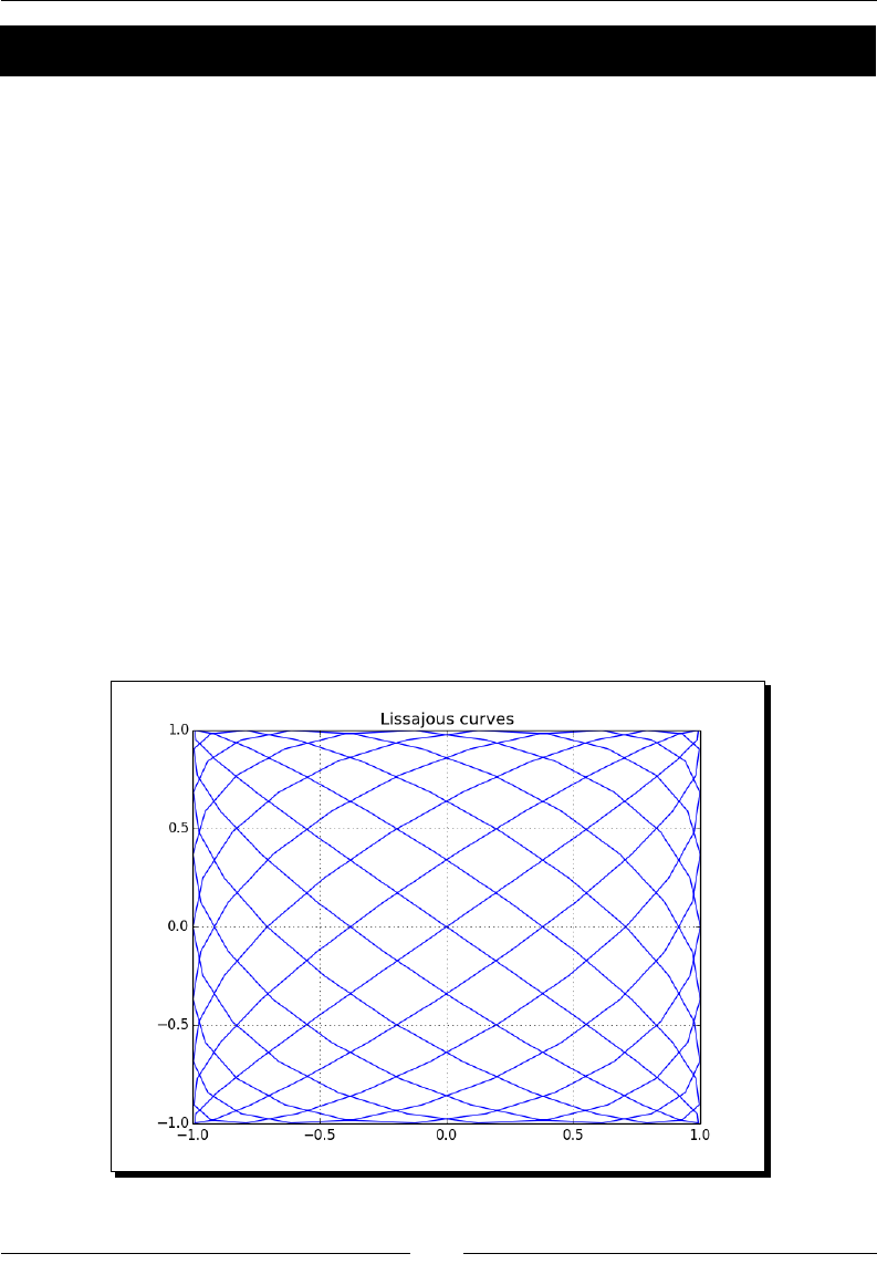
Chapter 5
[ 135 ]
Time for action – drawing Lissajous curves
The Lissajous gures are determined by four parameters: A, B, a, and b. Let's set A and B to 1
for simplicity:
1. Inialize t with the linspace() funcon from -pi to pi with 201 points:
a = 9
b = 8
t = np.linspace(-np.pi, np.pi, 201)
2. Calculate x with the sin() funcon and np.pi:
x = np.sin(a * t + np.pi/2)
3. Calculate y with the sin() funcon:
y = np.sin(b * t)
4. Plot as shown in the following:
plt.plot(x, y)
plt.title('Lissajous curves')
plt.grid()
plt.show()
The result for a = 9 and b = 8 is as follows:

Working with Matrices and ufuncs
[ 136 ]
What just happened?
We ploed the Lissajous curve with the aforemenoned parametric equaons where A=B=1,
a=9, and b=8. We used the sin() and linspace() funcons, as well as the NumPy pi
constant (see lissajous.py):
import numpy as np
import matplotlib.pyplot as plt
a = 9
b = 8
t = np.linspace(-np.pi, np.pi, 201)
x = np.sin(a * t + np.pi/2)
y = np.sin(b * t)
plt.plot(x, y)
plt.title('Lissajous curves')
plt.grid()
plt.show()
Square waves
Square waves are also one of those neat things that you can view on an oscilloscope. They
can be approximated prey well with sine waves; aer all, a square wave is a signal that can
be represented by an innite Fourier series.
A Fourier series is the sum of a series of sine and cosine terms named aer the
famous mathemacian Jean-Bapste Fourier (see http://en.wikipedia.
org/wiki/Fourier_series).
The formula of this parcular series represenng the square wave is as follows:
( )
( )
( )
1
4sin 2 2 1
2 1
k
k ft
k
π
π
∞
=
−
−
∑
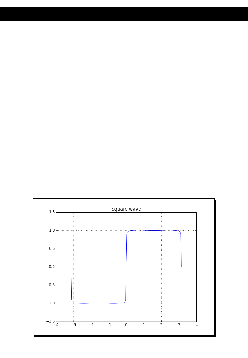
Chapter 5
[ 137 ]
Time for action – drawing a square wave
We will inialize t just as in the previous secon. We need to sum a number of terms. The
higher the number of terms, the more accurate the result; k = 99 should be sucient. In
order to draw a square wave, follow these steps:
1. We will start by inializing t and k. Set the inial values for the funcon to 0:
t = np.linspace(-np.pi, np.pi, 201)
k = np.arange(1, 99)
k = 2 * k - 1
f = np.zeros_like(t)
2. Compute the funcon values with the sin() and sum() funcons:
for i, ti in enumerate(t):
f[i] = np.sum(np.sin(k * ti)/k)
f = (4 / np.pi) * f
3. The code to plot is almost idencal to the one in the previous secon:
plt.plot(t, f)
plt.title('Square wave')
plt.grid()
plt.show()
The resulng square wave generated with k = 99 is as follows:

Working with Matrices and ufuncs
[ 138 ]
What just happened?
We generated a square wave or, at least, a fair approximaon of it, using the sin() funcon.
The input values were assembled with the linspace() funcon and the k values with the
arange() funcon (see squarewave.py):
import numpy as np
import matplotlib.pyplot as plt
t = np.linspace(-np.pi, np.pi, 201)
k = np.arange(1, 99)
k = 2 * k - 1
f = np.zeros_like(t)
for i, ti in enumerate(t):
f[i] = np.sum(np.sin(k * ti)/k)
f = (4 / np.pi) * f
plt.plot(t, f)
plt.title('Square wave')
plt.grid()
plt.show()
Have a go hero – getting rid of the loop
You may have noced that there is one loop in the code. Get rid of it with NumPy funcons
and make sure the performance is also improved.
Sawtooth and triangle waves
Sawtooth and triangle waves are also a phenomenon easily viewed on an oscilloscope. Just
as with square waves, we can dene an innite Fourier series. The triangle waves can be
found by taking the absolute value of a sawtooth wave. The formula for the representaon
of a series of sawtooth waves is as follows:
( )
1
2sin 2
k
kft
k
π
π
∞
=
−
∑

Chapter 5
[ 139 ]
Time for action – drawing sawtooth and triangle waves
We will inialize t just like in the previous secon. Again, k = 99 should be sucient. In
order to draw sawtooth and triangle waves, follow these steps:
1. Set inial values for the funcon to zero:
t = np.linspace(-np.pi, np.pi, 201)
k = np.arange(1, 99)
f = np.zeros_like(t)
2. Compute the funcon values with the sin() and sum() funcons:
for i, ti in enumerate(t):
f[i] = np.sum(np.sin(2 * np.pi * k * ti)/k)
f = (-2 / np.pi) * f
3. It's easy to plot the sawtooth and triangle waves since the value of the triangle
wave should be equal to the absolute value of the sawtooth wave. Plot the waves
as shown in the following:
plt.plot(t, f, lw=1.0, label='Sawtooth')
plt.plot(t, np.abs(f), '--', lw=2.0, label='Triangle')
plt.title('Triangle and sawtooth waves')
plt.grid()
plt.legend(loc='best')
plt.show()
In the following gure, the triangle wave is the one with the dashed line:

Working with Matrices and ufuncs
[ 140 ]
What just happened?
We drew a sawtooth wave using the sin() funcon. We assembled the input values with
the linspace() funcon and the k values with the arange() funcon. A triangle wave
was derived from the sawtooth wave by taking the absolute value (see sawtooth.py):
import numpy as np
import matplotlib.pyplot as plt
t = np.linspace(-np.pi, np.pi, 201)
k = np.arange(1, 99)
f = np.zeros_like(t)
for i, ti in enumerate(t):
f[i] = np.sum(np.sin(2 * np.pi * k * ti)/k)
f = (-2 / np.pi) * f
plt.plot(t, f, lw=1.0, label='Sawtooth')
plt.plot(t, np.abs(f), '--', lw=2.0, label='Triangle')
plt.title('Triangle and sawtooth waves')
plt.grid()
plt.legend(loc='best')
plt.show()
Have a go hero – getting rid of the loop
Your challenge, should you choose to accept it, is to get rid of the loop in the program. It
should be doable with NumPy funcons and the performance should improve.
Bitwise and comparison functions
Bitwise funcons operate on the bits of integers or integer arrays since they are universal
funcons. The operators ^, &, |, <<, >>, and so on have their NumPy counterparts. The same
goes for comparison operators such as <, >, ==, and so on. These operators allow you to do
clever tricks, which should be good for performance; however, they can make your code
quite unreadable, so use them with care.

Chapter 5
[ 141 ]
Time for action – twiddling bits
We will now cover three tricks—checking whether the signs of integers are dierent,
checking whether a number is a power of 2, and calculang the modulus of a number that
is a power of 2. We will show an operators-only notaon and one using the corresponding
NumPy funcons:
1. The rst trick depends on the XOR or ^ operator. The XOR operator is also called
the inequality operator; so, if the sign bit of the two operands is dierent, the
XOR operaon will lead to a negave number (see https://www.khanacademy.
org/computing/computer-science/cryptography/ciphers/a/xor-
bitwise-operation).
The following truth table illustrates the XOR operator:
Input 1 Input 2 XOR
True True False
False True True
True False True
False False False
The ^ operator corresponds to the bitwise_xor() funcon, and the < operator
corresponds to the less() funcon:
x = np.arange(-9, 9)
y = -x
print("Sign different?", (x ^ y) < 0)
print("Sign different?", np.less(np.bitwise_xor(x, y), 0))
The result is shown as follows:
Sign different? [ True True True True True True True True
True False True True
True True True True True True]
Sign different? [ True True True True True True True True
True False True True
True True True True True True]
As expected, all the signs dier, except for zero.

Working with Matrices and ufuncs
[ 142 ]
2. A power of 2 is represented by a 1, followed by a series of trailing zeroes in binary
notaon. For instance, 10, 100, or 1000. A number one less than a power of 2 will
be represented by a row of ones in binary. For instance, 11, 111, or 1111 (or 3, 7,
and 15 in the decimal system). Now, if we bitwise AND a power of 2, and the integer
that is one less than that, then we should get 0.
The truth table for the AND operator looks like the following:
Input 1 Input 2 AND
True True True
False True False
True False False
False False False
The NumPy counterpart of & is bitwise_and(), and the counterpart of == is the
equal() universal funcon:
print("Power of 2?\n", x, "\n", (x & (x - 1)) == 0)
print("Power of 2?\n", x, "\n", np.equal(np.bitwise_and(x,
(x - 1)), 0))
The result is shown as follows:
Power of 2?
[-9 -8 -7 -6 -5 -4 -3 -2 -1 0 1 2 3 4 5 6 7 8]
[False False False False False False False False False True True
True
False True False False False True]
Power of 2?
[-9 -8 -7 -6 -5 -4 -3 -2 -1 0 1 2 3 4 5 6 7 8]
[False False False False False False False False False True True
True
False True False False False True]
3. The trick of compung the modulus of 4 actually works when taking the modulus
of integers that are a power of 2 such as 4, 8, 16, and so on. A bitwise le
shi leads to doubling of values (see https://wiki.python.org/moin/
BitwiseOperators). We saw in the previous step that subtracng one from a
power of 2 leads to a number in binary notaon that has a row of ones such as 11,
111, or 1111. This basically gives us a mask. Bitwise-ANDing with such a number
gives you the remainder with a power of 2. The NumPy equivalent of << is the
left_shift() universal funcon:
print("Modulus 4\n", x, "\n", x & ((1 << 2) - 1))

Chapter 5
[ 143 ]
print("Modulus 4\n", x, "\n", np.bitwise_and(x,
np.left_shift(1, 2) - 1))
The result is shown as follows:
Modulus 4
[-9 -8 -7 -6 -5 -4 -3 -2 -1 0 1 2 3 4 5 6 7 8]
[3 0 1 2 3 0 1 2 3 0 1 2 3 0 1 2 3 0]
Modulus 4
[-9 -8 -7 -6 -5 -4 -3 -2 -1 0 1 2 3 4 5 6 7 8]
[3 0 1 2 3 0 1 2 3 0 1 2 3 0 1 2 3 0]
What just happened?
We covered three bit twiddling hacks—checking whether the signs of integers are dierent,
checking whether a number is a power of 2, and calculang the modulus of a number
that is a power of 2. We saw the NumPy counterparts of the operators ^, &, <<, and <
(see bittwidling.py):
from __future__ import print_function
import numpy as np
x = np.arange(-9, 9)
y = -x
print("Sign different?", (x ^ y) < 0)
print("Sign different?", np.less(np.bitwise_xor(x, y), 0))
print("Power of 2?\n", x, "\n", (x & (x - 1)) == 0)
print("Power of 2?\n", x, "\n", np.equal(np.bitwise_and(x, (x - 1)),
0))
print("Modulus 4\n", x, "\n", x & ((1 << 2) - 1))
print("Modulus 4\n", x, "\n", np.bitwise_and(x, np.left_shift(1, 2)
- 1))
Fancy indexing
The at() method was added in NumPy 1.8. This method allows fancy indexing in-place.
Fancy indexing is indexing that does not involve integers or slices, which is normal indexing.
In-place means that the array we operate on will be modied.
The signature for the at() method is ufunc.at(a,indices[,b]). The indices array
species the elements to operate on. We need the b array only for universal funcons with
two operands. The following Time for acon secon gives examples of the at() method.

Working with Matrices and ufuncs
[ 144 ]
Time for action – fancy indexing in-place for ufuncs with the at()
method
To demonstrate how the at() method works, start a Python or IPython shell and import
NumPy. You should know how to do this by now.
1. Create an array with seven random integers from -3 to 3 with a seed of 42:
>>> a = np.random.random_integers(-3, 3, 7)
>>> a
array([ 1, 0, -1, 2, 1, -2, 0])
When we talk about random numbers in programming, we usually talk about
pseudo-random numbers (see https://www.khanacademy.org/computing/
computer-science/cryptography/crypt/v/random-vs-pseudorandom-
number-generators). The numbers appear random, but in fact are calculated
using a seed.
2. Apply the at() method of the sign() universal funcon to the fourth and sixth
array elements:
>>> np.sign.at(a, [3, 5])
>>> a
array([ 1, 0, -1, 1, 1, -1, 0])
What just happened?
We used the at() method to select array elements and performed an in-place
operaon—determining the sign. We also learned how to create random integers.
Summary
In this chapter, you learned, about matrices and universal funcons. We covered how to
create matrices and looked at how universal funcons work. You had a brief introducon
to arithmec, trigonometric, bitwise, and comparison universal funcons.
In the next chapter, you will cover the NumPy modules.

[ 145 ]
6
Moving Further with NumPy Modules
NumPy has a number of modules inherited from its predecessor, Numeric.
Some of these packages have a SciPy counterpart, which may have fuller
functionality. We will discuss SciPy in a later chapter.
In this chapter, we will cover the following topics:
The linalg package
The fft package
Random numbers
Connuous and discrete distribuons
Linear algebra
Linear algebra is an important branch of mathemacs. The numpy.linalg package
contains linear algebra funcons. With this module, you can invert matrices, calculate
eigenvalues, solve linear equaons, and determine determinants, among other things
(see http://docs.scipy.org/doc/numpy/reference/routines.linalg.html).

Moving Further with NumPy Modules
[ 146 ]
Time for action – inverting matrices
The inverse of a matrix A in linear algebra is the matrix A-1, which, when mulplied with the
original matrix, is equal to the identy matrix I. This can be wrien as follows:
A A-1 = I
The inv() funcon in the numpy.linalg package can invert an example matrix with the
following steps:
1. Create the example matrix with the mat() funcon we used in the previous chapters:
A = np.mat("0 1 2;1 0 3;4 -3 8")
print("A\n", A)
The A matrix appears as follows:
A
[[ 0 1 2]
[ 1 0 3]
[ 4 -3 8]]
2. Invert the matrix with the inv() funcon:
inverse = np.linalg.inv(A)
print("inverse of A\n", inverse)
The inverse matrix appears as follows:
inverse of A
[[-4.5 7. -1.5]
[-2. 4. -1. ]
[ 1.5 -2. 0.5]]
If the matrix is singular, or not square, a LinAlgError is
raised. If you want, you can check the result manually with a
pen and paper. This is left as an exercise for the reader.
3. Check the result by mulplying the original matrix with the result of the
inv() funcon:
print("Check\n", A * inverse)

Chapter 6
[ 147 ]
The result is the identy matrix, as expected:
Check
[[ 1. 0. 0.]
[ 0. 1. 0.]
[ 0. 0. 1.]]
What just happened?
We calculated the inverse of a matrix with the inv() funcon of the numpy.linalg
package. We checked, with matrix mulplicaon, whether this is indeed the inverse matrix
(see inversion.py):
from __future__ import print_function
import numpy as np
A = np.mat("0 1 2;1 0 3;4 -3 8")
print("A\n", A)
inverse = np.linalg.inv(A)
print("inverse of A\n", inverse)
print("Check\n", A * inverse)
Pop quiz – creating a matrix
Q1. Which funcon can create matrices?
1. array
2. create_matrix
3. mat
4. vector
Have a go hero – inverting your own matrix
Create your own matrix and invert it. The inverse is only dened for square matrices. The
matrix must be square and inverble; otherwise, a LinAlgError excepon is raised.

Moving Further with NumPy Modules
[ 148 ]
Solving linear systems
A matrix transforms a vector into another vector in a linear way. This transformaon
mathemacally corresponds to a system of linear equaons. The numpy.linalg funcon
solve() solves systems of linear equaons of the form Ax = b, where A is a matrix, b can
be a one-dimensional or two-dimensional array, and x is an unknown variable. We will see the
dot() funcon in acon. This funcon returns the dot product of two oang-point arrays.
The dot() funcon calculates the dot product (see https://www.khanacademy.org/
math/linear-algebra/vectors_and_spaces/dot_cross_products/v/vector-
dot-product-and-vector-length). For a matrix A and vector b, the dot product is equal
to the following sum:
ij i
i
A B
∑
Time for action – solving a linear system
Solve an example of a linear system with the following steps:
1. Create A and b:
A = np.mat("1 -2 1;0 2 -8;-4 5 9")
print("A\n", A)
b = np.array([0, 8, -9])
print("b\n", b)
A and b appear as follows:
2. Solve this linear system with the solve() funcon:
x = np.linalg.solve(A, b)
print("Solution", x)
The soluon of the linear system is as follows:
Solution [ 29. 16. 3.]

Chapter 6
[ 149 ]
3. Check whether the soluon is correct with the dot() funcon:
print("Check\n", np.dot(A , x))
The result is as expected:
Check
[[ 0. 8. -9.]]
What just happened?
We solved a linear system using the solve() funcon from the NumPy linalg module and
checked the soluon with the dot() funcon. Please refer to the solution.py le in this
book's code bundle:
from __future__ import print_function
import numpy as np
A = np.mat("1 -2 1;0 2 -8;-4 5 9")
print("A\n", A)
b = np.array([0, 8, -9])
print("b\n", b)
x = np.linalg.solve(A, b)
print("Solution", x)
print("Check\n", np.dot(A , x))
Finding eigenvalues and eigenvectors
Eigenvalues are scalar soluons to the equaon Ax = ax, where A is a two-dimensional
matrix and x is a one-dimensional vector. Eigenvectors are vectors corresponding to
eigenvalues (see https://www.khanacademy.org/math/linear-algebra/
alternate_bases/eigen_everything/v/linear-algebra-introduction-to-
eigenvalues-and-eigenvectors). The eigvals() funcon in the numpy.linalg
package calculates eigenvalues. The eig() funcon returns a tuple containing eigenvalues
and eigenvectors.

Moving Further with NumPy Modules
[ 150 ]
Time for action – determining eigenvalues and eigenvectors
Let's calculate the eigenvalues of a matrix:
1. Create a matrix as shown in the following:
A = np.mat("3 -2;1 0")
print("A\n", A)
The matrix we created looks like the following:
A
[[ 3 -2]
[ 1 0]]
2. Call the eigvals() funcon:
print("Eigenvalues", np.linalg.eigvals(A))
The eigenvalues of the matrix are as follows:
Eigenvalues [ 2. 1.]
3. Determine eigenvalues and eigenvectors with the eig() funcon. This funcon
returns a tuple, where the rst element contains eigenvalues and the second
element contains corresponding eigenvectors, arranged column-wise:
eigenvalues, eigenvectors = np.linalg.eig(A)
print("First tuple of eig", eigenvalues)
print("Second tuple of eig\n", eigenvectors)
The eigenvalues and eigenvectors appear as follows:
First tuple of eig [ 2. 1.]
Second tuple of eig
[[ 0.89442719 0.70710678]
[ 0.4472136 0.70710678]]
4. Check the result with the dot() funcon by calculang the right and le side of the
eigenvalues equaon Ax = ax:
for i, eigenvalue in enumerate(eigenvalues):
print("Left", np.dot(A, eigenvectors[:,i]))
print("Right", eigenvalue * eigenvectors[:,i])
print()

Chapter 6
[ 151 ]
The output is as follows:
Left [[ 1.78885438]
[ 0.89442719]]
Right [[ 1.78885438]
[ 0.89442719]]
What just happened?
We found the eigenvalues and eigenvectors of a matrix with the eigvals() and eig()
funcons of the numpy.linalg module. We checked the result using the dot() funcon
(see eigenvalues.py):
from __future__ import print_function
import numpy as np
A = np.mat("3 -2;1 0")
print("A\n", A)
print("Eigenvalues", np.linalg.eigvals(A) )
eigenvalues, eigenvectors = np.linalg.eig(A)
print("First tuple of eig", eigenvalues)
print("Second tuple of eig\n", eigenvectors)
for i, eigenvalue in enumerate(eigenvalues):
print("Left", np.dot(A, eigenvectors[:,i]))
print("Right", eigenvalue * eigenvectors[:,i])
print()
Singular value decomposition
Singular value decomposion (SVD) is a type of factorizaon that decomposes a matrix
into a product of three matrices. The SVD is a generalizaon of the previously discussed
eigenvalue decomposion. SVD is very useful for algorithms such as the pseudo inverse,
which we will discuss in the next secon. The svd() funcon in the numpy.linalg package
can perform this decomposion. This funcon returns three matrices U, ∑, and V such that U
and V are unitary and ∑ contains the singular values of the input matrix:
M U V ∗
= ∑

Moving Further with NumPy Modules
[ 152 ]
The asterisk denotes the Hermian conjugate or the conjugate transpose. The complex
conjugate changes the sign of the imaginary part of a complex number and is therefore not
relevant for real numbers.
A complex square matrix A is unitary if A*A = AA* = I (the identy matrix).
We can interpret SVD as a sequence of three operaons—rotaon, scaling, and
another rotaon.
We already transposed matrices in this book. The transpose ips matrices, turning rows into
columns, and columns into rows.
Time for action – decomposing a matrix
It's me to decompose a matrix with the SVD using the following steps:
1. First, create a matrix as shown in the following:
A = np.mat("4 11 14;8 7 -2")
print("A\n", A)
The matrix we created looks like the following:
A
[[ 4 11 14]
[ 8 7 -2]]
2. Decompose the matrix with the svd() funcon:
U, Sigma, V = np.linalg.svd(A, full_matrices=False)
print("U")
print(U)
print("Sigma")
print(Sigma)
print("V")
print(V)
Because of the full_matrices=False specicaon, NumPy performs a reduced
SVD decomposion, which is faster to compute. The result is a tuple containing the
two unitary matrices U and V on the le and right, respecvely, and the singular
values of the middle matrix:
U
[[-0.9486833 -0.31622777]
[-0.31622777 0.9486833 ]]

Chapter 6
[ 153 ]
Sigma
[ 18.97366596 9.48683298]
V
[[-0.33333333 -0.66666667 -0.66666667]
[ 0.66666667 0.33333333 -0.66666667]]
3. We do not actually have the middle matrix—we only have the diagonal values. The
other values are all 0. Form the middle matrix with the diag() funcon. Mulply
the three matrices as follows:
print("Product\n", U * np.diag(Sigma) * V)
The product of the three matrices is equal to the matrix we created in the rst step:
Product
[[ 4. 11. 14.]
[ 8. 7. -2.]]
What just happened?
We decomposed a matrix and checked the result by matrix mulplicaon. We used the
svd() funcon from the NumPy linalg module (see decomposition.py):
from __future__ import print_function
import numpy as np
A = np.mat("4 11 14;8 7 -2")
print("A\n", A)
U, Sigma, V = np.linalg.svd(A, full_matrices=False)
print("U")
print(U)
print("Sigma")
print(Sigma)
print("V")
print(V)
print("Product\n", U * np.diag(Sigma) * V)

Moving Further with NumPy Modules
[ 154 ]
Pseudo inverse
The Moore-Penrose pseudo inverse of a matrix can be computed with the pinv()
funcon of the numpy.linalg module (see http://en.wikipedia.org/wiki/
Moore%E2%80%93Penrose_pseudoinverse). The pseudo inverse is calculated using
the SVD (see previous example). The inv() funcon only accepts square matrices; the
pinv() funcon does not have this restricon and is therefore considered a generalizaon
of the inverse.
Time for action – computing the pseudo inverse of a matrix
Let's compute the pseudo inverse of a matrix:
1. First, create a matrix:
A = np.mat("4 11 14;8 7 -2")
print("A\n", A)
The matrix we created looks like the following:
A
[[ 4 11 14]
[ 8 7 -2]]
2. Calculate the pseudo inverse matrix with the pinv() funcon:
pseudoinv = np.linalg.pinv(A)
print("Pseudo inverse\n", pseudoinv)
The pseudo inverse result is as follows:
Pseudo inverse
[[-0.00555556 0.07222222]
[ 0.02222222 0.04444444]
[ 0.05555556 -0.05555556]]
3. Mulply the original and pseudo inverse matrices:
print("Check", A * pseudoinv)
What we get is not an identy matrix, but it comes close to it:
Check [[ 1.00000000e+00 0.00000000e+00]
[ 8.32667268e-17 1.00000000e+00]]

Chapter 6
[ 155 ]
What just happened?
We computed the pseudo inverse of a matrix with the pinv() funcon of the numpy.
linalg module. The check by matrix mulplicaon resulted in a matrix that is
approximately an identy matrix (see pseudoinversion.py):
from __future__ import print_function
import numpy as np
A = np.mat("4 11 14;8 7 -2")
print("A\n", A)
pseudoinv = np.linalg.pinv(A)
print("Pseudo inverse\n", pseudoinv)
print("Check", A * pseudoinv)
Determinants
The determinant is a value associated with a square matrix. It is used throughout
mathemacs; for more details, please refer to http://en.wikipedia.org/wiki/
Determinant. For a n x n real value matrix, the determinant corresponds to the scaling
a n-dimensional volume undergoes when transformed by the matrix. The posive sign of
the determinant means the volume preserves its orientaon (clockwise or anclockwise),
while a negave sign means reversed orientaon. The numpy.linalg module has a det()
funcon that returns the determinant of a matrix.
Time for action – calculating the determinant of a matrix
To calculate the determinant of a matrix, follow these steps:
1. Create the matrix:
A = np.mat("3 4;5 6")
print("A\n", A)
The matrix we created appears as follows:
A
[[ 3. 4.]
[ 5. 6.]]

Moving Further with NumPy Modules
[ 156 ]
2. Compute the determinant with the det() funcon:
print("Determinant", np.linalg.det(A))
The determinant appears as follows:
Determinant -2.0
What just happened?
We calculated the determinant of a matrix with the det() funcon from the numpy.
linalg module (see determinant.py):
from __future__ import print_function
import numpy as np
A = np.mat("3 4;5 6")
print("A\n", A)
print("Determinant", np.linalg.det(A))
Fast Fourier transform
The Fast Fourier transform (FFT) is an ecient algorithm to calculate the discrete Fourier
transform (DFT).
The Fourier transform is related to the Fourier series, which was menoned in
the previous chapter—Chapter 5, Working with Matrices and ufuncs. The Fourier
series represents a signal as a sum of sine and cosine terms.
FFT improves on more naïve algorithms and is of order O(N log N). DFT has applicaons in
signal processing, image processing, solving paral dierenal equaons, and more. NumPy
has a module called fft that oers FFT funconality. Many funcons in this module are
paired; for those funcons, another funcon does the inverse operaon. For instance, the
fft() and ifft() funcon form such a pair.
Time for action – calculating the Fourier transform
First, we will create a signal to transform. Calculate the Fourier transform with the
following steps:
1. Create a cosine wave with 30 points as follows:
x = np.linspace(0, 2 * np.pi, 30)
wave = np.cos(x)
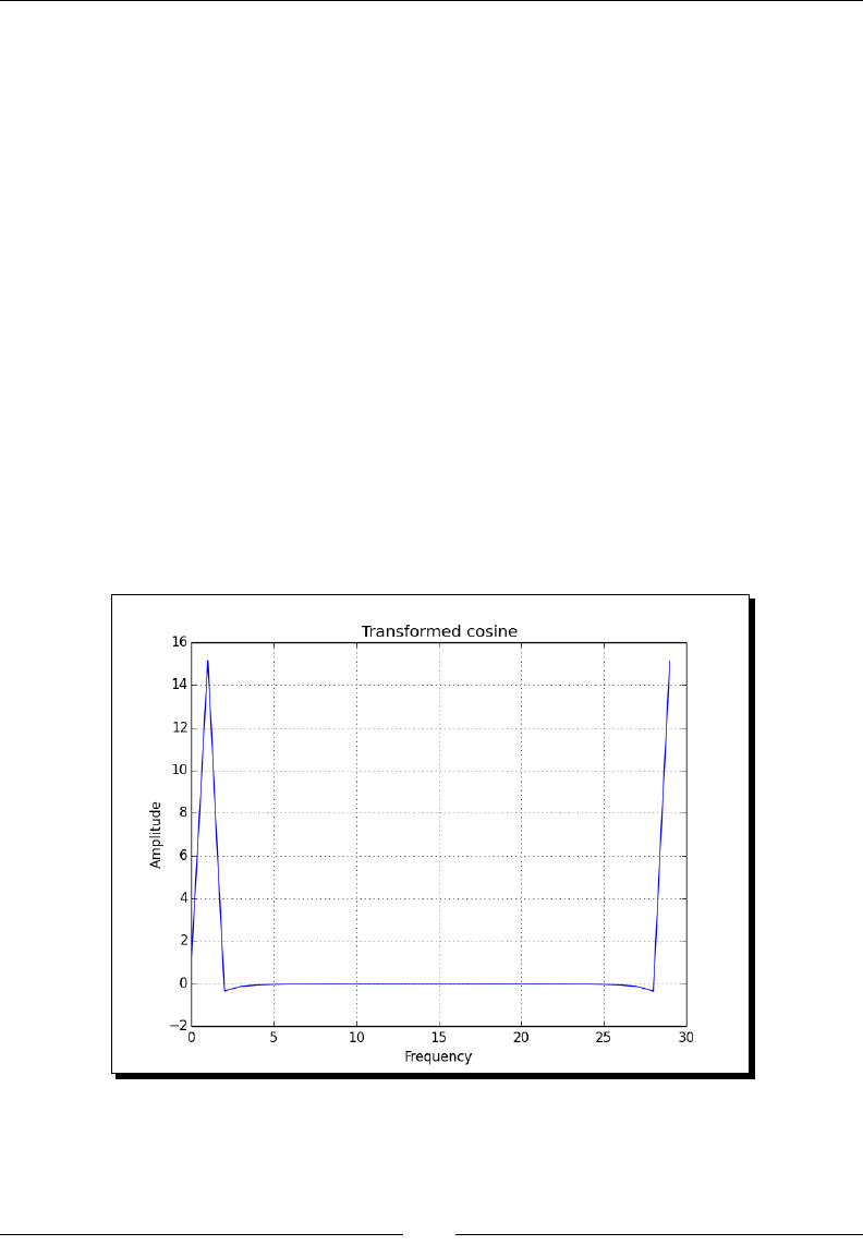
Chapter 6
[ 157 ]
2. Transform the cosine wave with the fft() funcon:
transformed = np.fft.fft(wave)
3. Apply the inverse transform with the ifft() funcon. It should approximately
return the original signal. Check with the following line:
print(np.all(np.abs(np.fft.ifft(transformed) - wave)
< 10 ** -9))
The result appears as follows:
True
4. Plot the transformed signal with matplotlib:
plt.plot(transformed)
plt.title('Transformed cosine')
plt.xlabel('Frequency')
plt.ylabel('Amplitude')
plt.grid()
plt.show()
The following resulng diagram shows the FFT result:

Moving Further with NumPy Modules
[ 158 ]
What just happened?
We applied the fft() funcon to a cosine wave. Aer applying the ifft() funcon, we
got our signal back (see fourier.py):
from __future__ import print_function
import numpy as np
import matplotlib.pyplot as plt
x = np.linspace(0, 2 * np.pi, 30)
wave = np.cos(x)
transformed = np.fft.fft(wave)
print(np.all(np.abs(np.fft.ifft(transformed) - wave) < 10 ** -9))
plt.plot(transformed)
plt.title('Transformed cosine')
plt.xlabel('Frequency')
plt.ylabel('Amplitude')
plt.grid()
plt.show()
Shifting
The fftshift() funcon of the numpy.linalg module shis zero-frequency components
to the center of a spectrum. The zero-frequency component corresponds to the mean of the
signal. The ifftshift() funcon reverses this operaon.
Time for action – shifting frequencies
We will create a signal, transform it, and then shi the signal. Shi the frequencies with the
following steps:
1. Create a cosine wave with 30 points:
x = np.linspace(0, 2 * np.pi, 30)
wave = np.cos(x)
2. Transform the cosine wave with the fft() funcon:
transformed = np.fft.fft(wave)
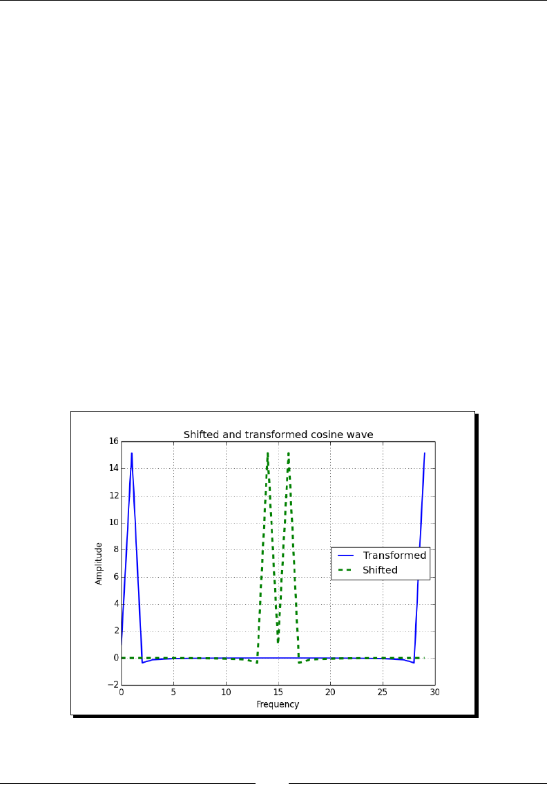
Chapter 6
[ 159 ]
3. Shi the signal with the fftshift() funcon:
shifted = np.fft.fftshift(transformed)
4. Reverse the shi with the ifftshift() funcon. This should undo the shi. Check
with the following code snippet:
print(np.all((np.fft.ifftshift(shifted) - transformed)
< 10 ** -9))
The result appears as follows:
True
5. Plot the signal and transform it with matplotlib:
plt.plot(transformed, lw=2, label="Transformed")
plt.plot(shifted, '--', lw=3, label="Shifted")
plt.title('Shifted and transformed cosine wave')
plt.xlabel('Frequency')
plt.ylabel('Amplitude')
plt.grid()
plt.legend(loc='best')
plt.show()
The following diagram shows the eect of the shi and the FFT:

Moving Further with NumPy Modules
[ 160 ]
What just happened?
We applied the fftshift() funcon to a cosine wave. Aer applying the ifftshift()
funcon, we got our signal back (see fouriershift.py):
import numpy as np
import matplotlib.pyplot as plt
x = np.linspace(0, 2 * np.pi, 30)
wave = np.cos(x)
transformed = np.fft.fft(wave)
shifted = np.fft.fftshift(transformed)
print(np.all(np.abs(np.fft.ifftshift(shifted) - transformed) < 10 **
-9))
plt.plot(transformed, lw=2, label="Transformed")
plt.plot(shifted, '--', lw=3, label="Shifted")
plt.title('Shifted and transformed cosine wave')
plt.xlabel('Frequency')
plt.ylabel('Amplitude')
plt.grid()
plt.legend(loc='best')
plt.show()
Random numbers
Random numbers are used in Monte Carlo methods, stochasc calculus, and more. Real
random numbers are hard to generate, so, in pracce, we use pseudo random numbers,
which are random enough for most intents and purposes, except for some very special
cases. These numbers appear random, but if you analyze them more closely, you will realize
that they follow a certain paern. The random numbers-related funcons are in the NumPy
random module. The core random number generator is based on the Mersenne Twister
algorithm—a standard and well-known algorithm (see https://en.wikipedia.org/
wiki/Mersenne_Twister). We can generate random numbers from discrete or connuous
distribuons. The distribuon funcons have an oponal size parameter, which tells NumPy
how many numbers to generate. You can specify either an integer or a tuple as size. This will
result in an array lled with random numbers of appropriate shape. Discrete distribuons
include the geometric, hypergeometric, and binomial distribuons.

Chapter 6
[ 161 ]
Time for action – gambling with the binomial
The binomial distribuon models the number of successes in an integer number of
independent trials of an experiment, where the probability of success in each experiment is
a xed number (see https://www.khanacademy.org/math/probability/random-
variables-topic/binomial_distribution).
Imagine a 17th century gambling house where you can bet on ipping pieces of eight. Nine
coins are ipped. If less than ve are heads, then you lose one piece of eight, otherwise
you win one. Let's simulate this, starng with 1,000 coins in our possession. Use the
binomial() funcon from the random module for that purpose.
To understand the binomial() funcon, look at the following secon:
1. Inialize an array, which represents the cash balance, to zeros. Call the
binomial() funcon with a size of 10000. This represents 10,000 coin
ips in our casino:
cash = np.zeros(10000)
cash[0] = 1000
outcome = np.random.binomial(9, 0.5, size=len(cash))
2. Go through the outcomes of the coin ips and update the cash array. Print the
minimum and maximum of the outcome, just to make sure we don't have any
strange outliers:
for i in range(1, len(cash)):
if outcome[i] < 5:
cash[i] = cash[i - 1] - 1
elif outcome[i] < 10:
cash[i] = cash[i - 1] + 1
else:
raise AssertionError("Unexpected outcome " + outcome)
print(outcome.min(), outcome.max())
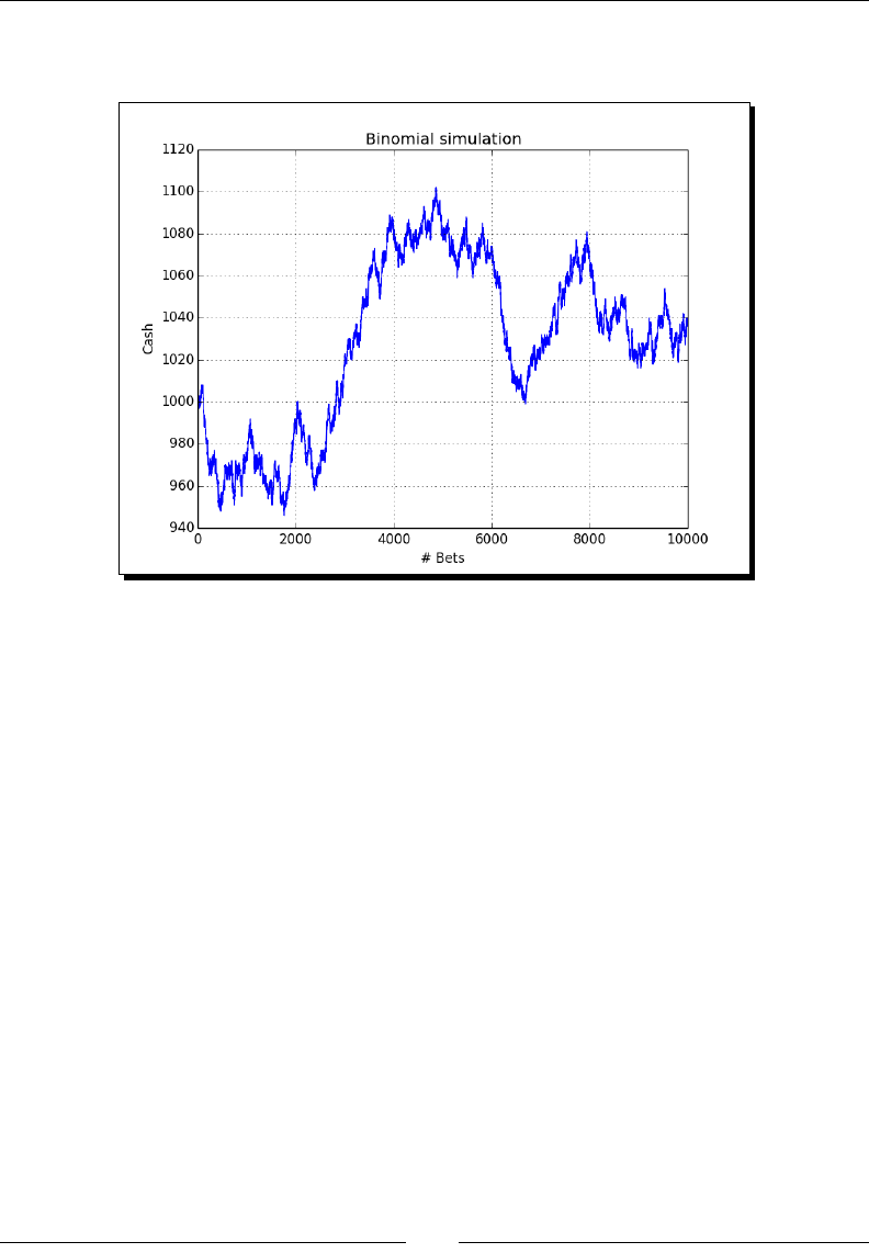
Moving Further with NumPy Modules
[ 162 ]
As expected, the values are between 0 and 9. In the following diagram, you can see
the cash balance performing a random walk:
What just happened?
We did a random walk experiment using the binomial() funcon from the NumPy random
module (see headortail.py):
from __future__ import print_function
import numpy as np
import matplotlib.pyplot as plt
cash = np.zeros(10000)
cash[0] = 1000
np.random.seed(73)
outcome = np.random.binomial(9, 0.5, size=len(cash))
for i in range(1, len(cash)):
if outcome[i] < 5:
cash[i] = cash[i - 1] - 1
elif outcome[i] < 10:
cash[i] = cash[i - 1] + 1
else:

Chapter 6
[ 163 ]
raise AssertionError("Unexpected outcome " + outcome)
print(outcome.min(), outcome.max())
plt.plot(np.arange(len(cash)), cash)
plt.title('Binomial simulation')
plt.xlabel('# Bets')
plt.ylabel('Cash')
plt.grid()
plt.show()
Hypergeometric distribution
The hypergeometric distribuon models a jar with two types of objects in it. The model tells
us how many objects of one type we can get if we take a specied number of items out of the
jar without replacing them (see https://en.wikipedia.org/wiki/Hypergeometric_
distribution). The NumPy random module has a hypergeometric() funcon that
simulates this situaon.
Time for action – simulating a game show
Imagine a game show where every me the contestants answer a queson correctly, they
get to pull three balls from a jar and then put them back. Now, there is a catch, one ball in
the jar is bad. Every me it is pulled out, the contestants lose six points. If, however, they
manage to get out 3 of the 25 normal balls, they get one point. So, what is going to happen
if we have 100 quesons in total? Look at the following secon for the soluon:
1. Inialize the outcome of the game with the hypergeometric() funcon. The
rst parameter of this funcon is the number of ways to make a good selecon,
the second parameter is the number of ways to make a bad selecon, and the
third parameter is the number of items sampled:
points = np.zeros(100)
outcomes = np.random.hypergeometric(25, 1, 3, size=len(points))
2. Set the scores based on the outcomes from the previous step:
for i in range(len(points)):
if outcomes[i] == 3:
points[i] = points[i - 1] + 1
elif outcomes[i] == 2:
points[i] = points[i - 1] - 6
else:
print(outcomes[i])
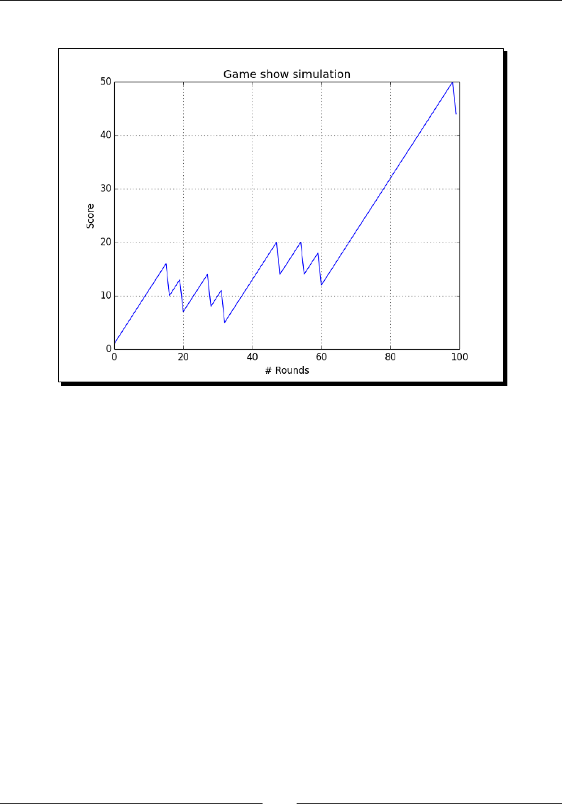
Moving Further with NumPy Modules
[ 164 ]
The following diagram shows how the scoring evolved:
What just happened?
We simulated a game show using the hypergeometric() funcon from the NumPy
random module. The game scoring depends on how many good and how many bad balls
the contestants pulled out of a jar in each session (see urn.py):
from __future__ import print_function
import numpy as np
import matplotlib.pyplot as plt
points = np.zeros(100)
np.random.seed(16)
outcomes = np.random.hypergeometric(25, 1, 3, size=len(points))
for i in range(len(points)):
if outcomes[i] == 3:
points[i] = points[i - 1] + 1
elif outcomes[i] == 2:
points[i] = points[i - 1] - 6
else:

Chapter 6
[ 165 ]
print(outcomes[i])
plt.plot(np.arange(len(points)), points)
plt.title('Game show simulation')
plt.xlabel('# Rounds')
plt.ylabel('Score')
plt.grid()
plt.show()
Continuous distributions
We usually model connuous distribuons with probability density funcons (PDF). The
probability that a value is in a certain interval is determined by integraon of the PDF
(see https://www.khanacademy.org/math/probability/random-variables-
topic/random_variables_prob_dist/v/probability-density-functions).
The NumPy random module has funcons that represent connuous distribuons—
beta(), chisquare(), exponential(), f(), gamma(), gumbel(), laplace(),
lognormal(), logistic(), multivariate_normal(), noncentral_chisquare(),
noncentral_f(), normal(), and others.
Time for action – drawing a normal distribution
We can generate random numbers from a normal distribuon and visualize their distribuon
with a histogram (see https://www.khanacademy.org/math/probability/
statistics-inferential/normal_distribution/v/introduction-to-the-
normal-distribution). Draw a normal distribuon with the following steps:
1. Generate random numbers for a given sample size using the normal() funcon
from the random NumPy module:
N=10000
normal_values = np.random.normal(size=N)
2. Draw the histogram and theorecal PDF with a center value of 0 and standard
deviaon of 1. Use matplotlib for this purpose:
_, bins, _ = plt.hist(normal_values,
np.sqrt(N), normed=True, lw=1)
sigma = 1
mu = 0
plt.plot(bins, 1/(sigma * np.sqrt(2 * np.pi))
* np.exp( - (bins - mu)**2 / (2 * sigma**2) ),lw=2)
plt.show()
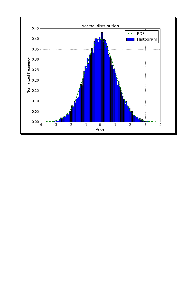
Moving Further with NumPy Modules
[ 166 ]
In the following diagram, we see the familiar bell curve:
What just happened?
We visualized the normal distribuon using the normal() funcon from the random NumPy
module. We did this by drawing the bell curve and a histogram of randomly generated values
(see normaldist.py):
import numpy as np
import matplotlib.pyplot as plt
N=10000
np.random.seed(27)
normal_values = np.random.normal(size=N)
_, bins, _ = plt.hist(normal_values, np.sqrt(N), normed=True, lw=1,
label="Histogram")
sigma = 1
mu = 0

Chapter 6
[ 167 ]
plt.plot(bins, 1/(sigma * np.sqrt(2 * np.pi)) * np.exp( - (bins -
mu)**2 / (2 * sigma**2) ), '--', lw=3, label="PDF")
plt.title('Normal distribution')
plt.xlabel('Value')
plt.ylabel('Normalized Frequency')
plt.grid()
plt.legend(loc='best')
plt.show()
Lognormal distribution
A lognormal distribuon is a distribuon of a random variable whose natural logarithm
is normally distributed. The lognormal() funcon of the random NumPy module models
this distribuon.
Time for action – drawing the lognormal distribution
Let's visualize the lognormal distribuon and its PDF with a histogram:
1. Generate random numbers using the normal() funcon from the random
NumPy module:
N=10000
lognormal_values = np.random.lognormal(size=N)
2. Draw the histogram and theorecal PDF with a center value of 0 and standard
deviaon of 1:
_, bins, _ = plt.hist(lognormal_values,
np.sqrt(N), normed=True, lw=1)
sigma = 1
mu = 0
x = np.linspace(min(bins), max(bins), len(bins))
pdf = np.exp(-(numpy.log(x) - mu)**2 / (2 * sigma**2))/ (x *
sigma * np.sqrt(2 * np.pi))
plt.plot(x, pdf,lw=3)
plt.show()
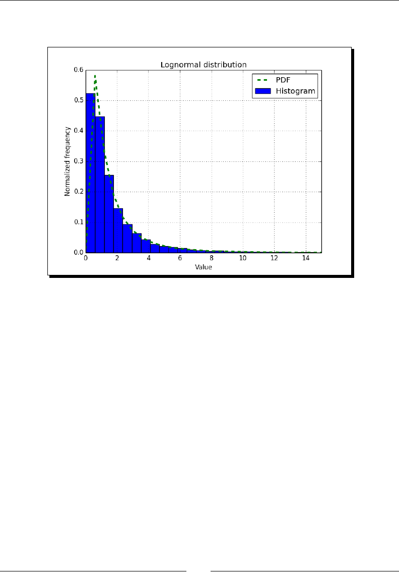
Moving Further with NumPy Modules
[ 168 ]
The t of the histogram and theorecal PDF is excellent, as you can see in the
following diagram:
What just happened?
We visualized the lognormal distribuon using the lognormal() funcon from the random
NumPy module. We did this by drawing the curve of the theorecal PDF and a histogram of
randomly generated values (see lognormaldist.py):
import numpy as np
import matplotlib.pyplot as plt
N=10000
np.random.seed(34)
lognormal_values = np.random.lognormal(size=N)
_, bins, _ = plt.hist(lognormal_values,
np.sqrt(N), normed=True, lw=1, label="Histogram")
sigma = 1
mu = 0
x = np.linspace(min(bins), max(bins), len(bins))
pdf = np.exp(-(np.log(x) - mu)**2 / (2 * sigma**2))/ (x * sigma *
np.sqrt(2 * np.pi))
plt.xlim([0, 15])
plt.plot(x, pdf,'--', lw=3, label="PDF")

Chapter 6
[ 169 ]
plt.title('Lognormal distribution')
plt.xlabel('Value')
plt.ylabel('Normalized frequency')
plt.grid()
plt.legend(loc='best')
plt.show()
Bootstrapping in statistics
Bootstrapping is a method used to esmate variance, accuracy, and other metrics of sample
esmates, such as the arithmec mean. The simplest bootstrapping procedure consists of
the following steps:
1. Generate a large number of samples from the original data sample having the
same size N. You can think of the original data as a jar containing numbers. We
create the new samples by N mes randomly picking a number from the jar. Each
me we return the number into the jar, so a number can occur mulple mes in a
generated sample.
2. With the new samples, we calculate the stascal esmate under invesgaon for
each sample (for example, the arithmec mean). This gives us a sample of possible
values for the esmator.
Time for action – sampling with numpy.random.choice()
We will use the numpy.random.choice() funcon to perform bootstrapping.
1. Start the IPython or Python shell and import NumPy:
$ ipython
In [1]: import numpy as np
2. Generate a data sample following the normal distribuon:
In [2]: N = 500
In [3]: np.random.seed(52)
In [4]: data = np.random.normal(size=N)
3. Calculate the mean of the data:
In [5]: data.mean()
Out[5]: 0.07253250605445645

Moving Further with NumPy Modules
[ 170 ]
Generate 100 samples from the original data and calculate their means (of course,
more samples may lead to a more accurate result):
In [6]: bootstrapped = np.random.choice(data, size=(N, 100))
In [7]: means = bootstrapped.mean(axis=0)
In [8]: means.shape
Out[8]: (100,)
4. Calculate the mean, variance, and standard deviaon of the arithmec means
we obtained:
In [9]: means.mean()
Out[9]: 0.067866373318115278
In [10]: means.var()
Out[10]: 0.001762807104774598
In [11]: means.std()
Out[11]: 0.041985796464692651
If we are assuming a normal distribuon for the means, it may be relevant to know
the z-score, which is dened as follows:
x
z
µ
σ
−
=
In [12]: (data.mean() - means.mean())/means.std()
Out[12]: 0.11113598238549766
From the z-score value, we get an idea of how probable the actual mean is.

Chapter 6
[ 171 ]
What just happened?
We bootstrapped a data sample by generang samples and calculang the means of each
sample. Then we computed the mean, standard deviaon, variance, and z-score of the
means. We used the numpy.random.choice() funcon for bootstrapping.
Summary
You learned a lot in this chapter about NumPy modules. We covered linear algebra, the Fast
Fourier transform, connuous and discrete distribuons, and random numbers.
In the next chapter, we will cover specialized rounes. These are funcons that you probably
will not use oen, but are very useful when you do need them.

[ 173 ]
7
Peeking into Special Routines
As NumPy users, we sometimes find ourselves having special needs, for
instance, financial calculations or signal processing. Fortunately, NumPy
provides for most of our needs. This chapter describes some of the more
specialized NumPy functions.
In this chapter, we will cover the following topics:
Sorng and searching
Special funcons
Financial ulies
Window funcons
Sorting
NumPy has several data sorng rounes:
The sort() funcon returns a sorted array
The lexsort() funcon performs sorng with a list of keys
The argsort() funcon returns the indices that will sort an array
The ndarray class has a sort() method that performs in-place sorng
The msort() funcon sorts an array along the rst axis
The sort_complex() funcon sorts complex numbers by their real part and then
their imaginary part

Peeking into Special Rounes
[ 174 ]
From this list, the argsort() and sort() funcons are available as methods on NumPy
arrays as well.
Time for action – sorting lexically
The NumPy lexsort() funcon returns an array of indices of the input array elements
corresponding to lexically sorng an array. We need to give the funcon an array or tuple
of sort keys:
1. Let's go back to Chapter 3, Geng Familiar with Commonly Used Funcons. In that
chapter, we used stock price data of AAPL. We will load the close prices and the
(always complex) dates. In fact, create a converter funcon just for the dates:
def datestr2num(s):
return datetime.datetime.strptime(s, "%d-%m-%Y").toordinal()
dates, closes=np.loadtxt('AAPL.csv', delimiter=',',
usecols=(1, 6), converters={1:datestr2num}, unpack=True)
2. Sort the names lexically with the lexsort() funcon. The data is already sorted
by date, but sort it by close as well:
indices = np.lexsort((dates, closes))
print("Indices", indices)
print(["%s %s" % (datetime.date.fromordinal(dates[i]),
closes[i]) for i in indices])
The code prints the following:
Indices [ 0 16 1 17 18 4 3 2 5 28 19 21 15 6 29 22 27 20 9
7 25 26 10 8 14 11 23 12 24 13]
['2011-01-28 336.1', '2011-02-22 338.61', '2011-01-31 339.32',
'2011-02-23 342.62', '2011-02-24 342.88', '2011-02-03 343.44',
'2011-02-02 344.32', '2011-02-01 345.03', '2011-02-04 346.5',
'2011-03-10 346.67', '2011-02-25 348.16', '2011-03-01 349.31',
'2011-02-18 350.56', '2011-02-07 351.88', '2011-03-11 351.99',
'2011-03-02 352.12', '2011-03-09 352.47', '2011-02-28 353.21',
'2011-02-10 354.54', '2011-02-08 355.2', '2011-03-07 355.36',
'2011-03-08 355.76', '2011-02-11 356.85', '2011-02-09 358.16',
'2011-02-17 358.3', '2011-02-14 359.18', '2011-03-03 359.56',
'2011-02-15 359.9', '2011-03-04 360.0', '2011-02-16 363.13']

Chapter 7
[ 175 ]
What just happened?
We sorted the close prices of AAPL lexically using the NumPy lexsort() funcon. The
funcon returned the indices corresponding with sorng the array (see lex.py):
from __future__ import print_function
import numpy as np
import datetime
def datestr2num(s):
return datetime.datetime.strptime(s, "%d-%m-%Y").toordinal()
dates, closes=np.loadtxt('AAPL.csv', delimiter=',',
usecols=(1, 6), converters={1:datestr2num}, unpack=True)
indices = np.lexsort((dates, closes))
print("Indices", indices)
print(["%s %s" % (datetime.date.fromordinal(int(dates[i])),
closes[i])
for i in indices])
Have a go hero – trying a different sort order
We sorted using the dates and the close price sort order. Try a dierent order. Generate
random numbers using the random module we learned about in the previous chapter and
sort those using lexsort().
Time for action – partial sorting via selection for a fast median
with the partition() function
The partition() funcon does paral sorng, which should be faster than full sorng,
because it's less work.
For more informaon, please refer to http://en.wikipedia.org/
wiki/Partial_sorting. A common use case is geng the top 10
elements of a collecon. Paral sorng doesn't guarantee the correct order
within the group of top elements itself.

Peeking into Special Rounes
[ 176 ]
The rst argument of the funcon is the array to parally sort. The second argument
is an integer or a sequence of integers corresponding to indices of array elements. The
partition() funcon sorts elements in those indices correctly. With one specied index,
we get two parons; with mulple indices, we get more than one paron. The sorng
algorithm makes sure that elements in parons, which are smaller than a correctly sorted
element, come before this element. Otherwise, they are placed behind this element. Let's
illustrate this explanaon with an example. Start a Python or IPython shell and import NumPy:
$ ipython
In [1]: import numpy as np
Create an array with random elements to sort:
In [2]: np.random.seed(20)
In [3]: a = np.random.random_integers(0, 9, 9)
In [4]: a
Out[4]: array([3, 9, 4, 6, 7, 2, 0, 6, 8])
Parally sort the array by paroning it in two roughly equal parts:
In [5]: np.partition(a, 4)
Out[5]: array([0, 2, 3, 4, 6, 6, 7, 9, 8])
We get an almost perfect sorng except for the last two elements.
What just happened?
We parally sorted a nine-element array. The sorng only guaranteed that one element in
the middle at index 4 is at the correct posion. This corresponds to trying to get the top ve
elements of the array without caring about the order within the top ve group. Since the
correctly sorted element is in the middle, this also gives the median of the array.
Complex numbers
Complex numbers are numbers that have a real and imaginary part. As you remember from
previous chapters, NumPy has special complex data types that represent complex numbers by
two oang-point numbers. These numbers can be sorted using the NumPy sort_complex()
funcon. This funcon sorts the real part rst and then the imaginary part.

Chapter 7
[ 177 ]
Time for action – sorting complex numbers
We will create an array of complex numbers and sort it:
1. Generate ve random numbers for the real part of the complex numbers and ve
numbers for the imaginary part. Seed the random generator to 42:
np.random.seed(42)
complex_numbers = np.random.random(5) + 1j *
np.random.random(5)
print("Complex numbers\n", complex_numbers)
2. Call the sort_complex() funcon to sort the complex numbers we generated in
the previous step:
print("Sorted\n", np.sort_complex(complex_numbers))
The sorted numbers would be:
Sorted
[ 0.39342751+0.34955771j 0.40597665+0.77477433j
0.41516850+0.26221878j
0.86631422+0.74612422j 0.92293095+0.81335691j]
What just happened?
We generated random complex numbers and sorted them using the sort_complex()
funcon (see sortcomplex.py):
from __future__ import print_function
import numpy as np
np.random.seed(42)
complex_numbers = np.random.random(5) + 1j * np.random.random(5)
print("Complex numbers\n", complex_numbers)
print("Sorted\n", np.sort_complex(complex_numbers))
Pop quiz – generating random numbers
Q1. Which NumPy module deals with random numbers?
1. Randnum
2. random
3. randomul
4. rand

Peeking into Special Rounes
[ 178 ]
Searching
NumPy has several funcons that can search through arrays:
The argmax() funcon gives the indices of the maximum values of an array:
>>> a = np.array([2, 4, 8])
>>> np.argmax(a)
2
The nanargmax() funcon does the same, but ignores NaN values:
>>> b = np.array([np.nan, 2, 4])
>>> np.nanargmax(b)
2
The argmin() and nanargmin() funcons provide similar funconality but
pertaining to minimum values. The argmax() and nanargmax() funcons are
also available as methods of the ndarray class.
The argwhere() funcon searches for non-zero values and returns the
corresponding indices grouped by element:
>>> a = np.array([2, 4, 8])
>>> np.argwhere(a <= 4)
array([[0],
[1]])
The searchsorted() funcon tells you the index in an array where a specied
value belongs to maintain the sort order. It uses binary search (see https://www.
khanacademy.org/computing/computer-science/algorithms/binary-
search/a/binary-search), which is a O(log n) algorithm. We will see this
funcon in acon shortly.
The extract() funcon retrieves values from an array based on a condion.
Time for action – using searchsorted
The searchsorted() funcon gets the index of a value in a sorted array. An example
should make this clear:
1. To demonstrate, create an array with arange(), which of course is sorted:
a = np.arange(5)
2. Time to call the searchsorted() funcon:
indices = np.searchsorted(a, [-2, 7])
print("Indices", indices)

Chapter 7
[ 179 ]
The indices, which should maintain the sort order:
Indices [0 5]
3. Construct the full array with the insert() funcon:
print("The full array", np.insert(a, indices, [-2, 7]))
This gives us the full array:
The full array [-2 0 1 2 3 4 7]
What just happened?
The searchsorted() funcon gave us indices 5 and 0 for 7 and -2. With these indices,
we made the array [-2, 0, 1, 2, 3, 4, 7], so the array remains sorted (see
sortedsearch.py):
from __future__ import print_function
import numpy as np
a = np.arange(5)
indices = np.searchsorted(a, [-2, 7])
print("Indices", indices)
print("The full array", np.insert(a, indices, [-2, 7]))
Array elements extraction
The NumPy extract() funcon allows us to extract items from an array based on a
condion. This funcon is similar to the where() funcon we encountered in Chapter 3,
Geng Familiar with Commonly Used Funcons. The special nonzero() funcon selects
non-zero elements.
Time for action – extracting elements from an array
Let's extract the even elements of an array:
1. Create the array with the arange() funcon:
a = np.arange(7)
2. Create the condion that selects the even elements:
condition = (a % 2) == 0

Peeking into Special Rounes
[ 180 ]
3. Extract the even elements using our condion with the extract() funcon:
print("Even numbers", np.extract(condition, a))
This gives us the even numbers as required (np.extract(condition, a) is
equivalent to a[np.where(condition)[0]]):
Even numbers [0 2 4 6]
4. Select non-zero values with the nonzero() funcon:
print("Non zero", np.nonzero(a))
This prints all the non-zero values of the array:
Non zero (array([1, 2, 3, 4, 5, 6]),)
What just happened?
We extracted the even elements from an array using a Boolean condion with the NumPy
extract() funcon (see extracted.py):
from __future__ import print_function
import numpy as np
a = np.arange(7)
condition = (a % 2) == 0
print("Even numbers", np.extract(condition, a))
print("Non zero", np.nonzero(a))
Financial functions
NumPy has a number of nancial funcons:
The fv() funcon calculates the so-called future value. The future value gives the
value of a nancial instrument at a future date, based on certain assumpons.
The pv() funcon computes the present value (see https://www.khanacademy.
org/economics-finance-domain/core-finance/interest-tutorial/
present-value/v/time-value-of-money). The present value is the value of
an asset today.
The npv() funcon returns the net present value. The net present value is dened
as the sum of all the present value cash ows.
The pmt() funcon computes the payment against loan principal plus interest.

Chapter 7
[ 181 ]
The irr() funcon calculates the internal rate of return. The internal rate of return
is the eecve interested rate, which does not take into account inaon.
The mirr() funcon calculates the modied internal rate of return. The modied
internal rate of return is an improved version of the internal rate of return.
The nper() funcon returns the number of periodic payments.
The rate() funcon calculates the rate of interest.
Time for action – determining the future value
The future value gives the value of a nancial instrument at a future date, based on certain
assumpons. The future value depends on four parameters—the interest rate, the number
of periods, a periodic payment, and the present value.
Read more about future value at http://en.wikipedia.org/
wiki/Future_value. The formula for future value with compound
interest is as follows:
( )
1n
PV r+
In the preceding formula, PV is the present value, r is the interest rate,
and n is the number of periods.
In this secon, let's take an interest rate of 3 percent, a quarterly payment of 10 for 5 years,
and a present value of 1000. Call the fv() funcon with the appropriate values (negave
values represent outgoing cash ow):
print("Future value", np.fv(0.03/4, 5 * 4, -10, -1000))
The future value is as follows:
Future value 1376.09633204
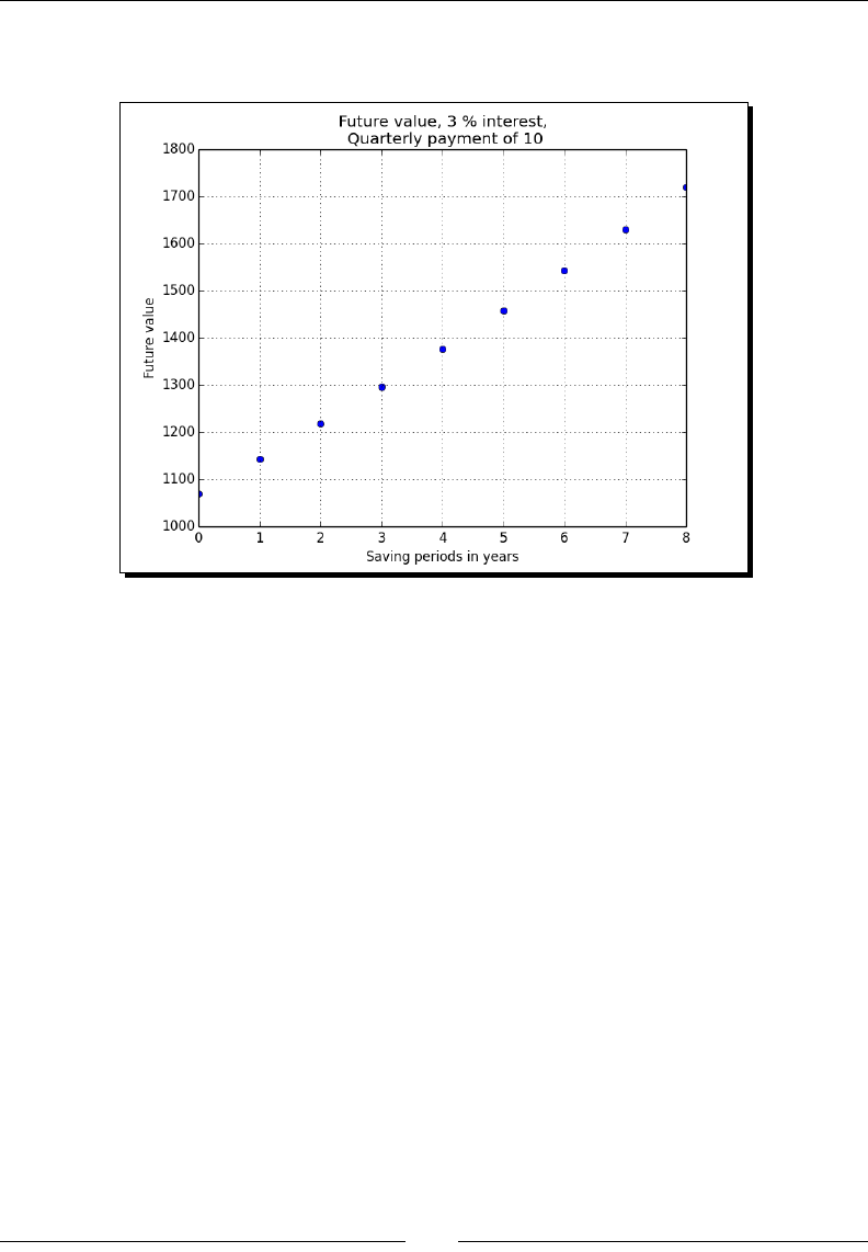
Peeking into Special Rounes
[ 182 ]
If we vary the number of years we save and keep the other parameters constant, we get the
following plot:
What just happened?
We calculated the future value using the NumPy fv() funcon starng with a present value
of 1000, an interest rate of 3 percent, and quarterly payments of 10 for 5 years. We ploed
the future value for various saving periods (see futurevalue.py):
from __future__ import print_function
import numpy as np
import matplotlib.pyplot as plt
print("Future value", np.fv(0.03/4, 5 * 4, -10, -1000))
fvals = []
for i in xrange(1, 10):
fvals.append(np.fv(.03/4, i * 4, -10, -1000))
plt.plot(range(1, 10), fvals, 'bo')
plt.title('Future value, 3 % interest,\n Quarterly payment of 10')
plt.xlabel('Saving periods in years')
plt.ylabel('Future value')
plt.grid()
plt.legend(loc='best')
plt.show()

Chapter 7
[ 183 ]
Present value
The present value is the value of an asset today. The NumPy pv() funcon can calculate the
present value. This funcon mirrors the fv() funcon and requires the interest rate, number
of periods, and the periodic payment as well, but here we start with the future value.
Read more about the present value at http://en.wikipedia.org/wiki/Present_
value. It should be easy to derive the formula for the present value from the formula for
the future value, if you want.
Time for action – getting the present value
Let's reverse compute the present value with the numbers from the Time for acon –
determining the future value secon:
Plug in the gures from the Time for acon – determining the future value secon:
print("Present value", np.pv(0.03/4, 5 * 4, -10, 1376.09633204))
This gives us 1000 as expected apart from a ny numerical error. Actually, it is not an error
but a representaon issue. We are dealing here with outgoing cash ow, that is the reason
for the negave value:
Present value -999.999999999
What just happened?
We did the reverse computaon of the Time for acon – determining the future value secon
to get the present value from the future value. This was done with the NumPy pv() funcon.
Net present value
The net present value is dened as the sum of all the present value cash ows. The NumPy
npv() funcon returns the net present value of cash ows. The funcon requires two
arguments: the rate and an array represenng the cash ows.
Read more about the net present value at http://en.wikipedia.org/wiki/Net_
present_value. In the formula of the net present value, Rt is the cash ow of a me
period, r is the discount rate, and t is the index of the me period:
( )
01
N
t
t
t
R
r
=+
∑

Peeking into Special Rounes
[ 184 ]
Time for action – calculating the net present value
We will calculate the net present value for a random generated cash ow series:
1. Generate ve random values for the cash ow series. Insert -100 as the start value:
cashflows = np.random.randint(100, size=5)
cashflows = np.insert(cashflows, 0, -100)
print("Cashflows", cashflows)
The cash ows would be as follows:
Cashflows [-100 38 48 90 17 36]
2. Call the npv() funcon to calculate the net present value from the cash ow series
we generated in the previous step. Use a rate of 3 percent:
print("Net present value", np.npv(0.03, cashflows))
The net present value:
Net present value 107.435682443
What just happened?
We computed the net present value from a random generated cash ow series with the
NumPy npv() funcon (see netpresentvalue.py):
from __future__ import print_function
import numpy as np
cashflows = np.random.randint(100, size=5)
cashflows = np.insert(cashflows, 0, -100)
print("Cashflows", cashflows)
print("Net present value", np.npv(0.03, cashflows))
Internal rate of return
The internal rate of return is the eecve interested rate, which does not take into account
inaon. The NumPy irr() funcon returns the internal rate of return for a given cash
ow series.

Chapter 7
[ 185 ]
Time for action – determining the internal rate of return
Let's reuse the cash ow series from the Time for acon – calculang the net present value
secon. Call the irr() funcon with the cash ow series from the Time for acon secon:
print("Internal rate of return", np.irr([-100, 38, 48, 90,
17, 36]))
The internal rate of return:
Internal rate of return 0.373420226888
What just happened?
We calculated the internal rate of return from the cash ow series of the Time for acon –
calculang the net present value secon. The value was given by the NumPy irr() funcon.
Periodic payments
The NumPy pmt() funcon allows you to compute periodic payments for a loan, based on
an interest rate and the number of periodic payments.
Time for action – calculating the periodic payments
Suppose you have a loan of 10 million with an interest rate of 1 percent. You have 30 years
to pay the loan back. How much do you have to pay each month? Let's nd out.
Call the pmt() funcon with the aforemenoned values:
print("Payment", np.pmt(0.01/12, 12 * 30, 10000000))
The monthly payment:
Payment -32163.9520447
What just happened?
We calculated the monthly payment for a loan of 10 million at an annual rate of 1 percent.
Given that we have 30 years to repay the loan the pmt() funcon tells us that we need
to pay 32163.95 per month.

Peeking into Special Rounes
[ 186 ]
Number of payments
The NumPy nper() funcon tells us how many periodic payments are necessary to pay o
a loan. The required parameters are the interest rate of the loan, the xed amount periodic
payment, and the present value.
Time for action – determining the number of periodic payments
Consider a loan of 9000 at a rate of 10 percent with xed monthly payments of 100.
Find out how many payments are required with the NumPy nper() funcon:
print("Number of payments", np.nper(0.10/12, -100, 9000))
The number of payments:
Number of payments 167.047511801
What just happened?
We determined the number of payments needed to pay o a loan of 9000 with an interest
rate of 10 percent and monthly payments of 100. The number of payments returned
was 167.
Interest rate
The NumPy rate() funcon calculates the interest rate given the number of periodic
payments, the payment amount or amounts, the present value, and the future value.
Time for action – guring out the rate
Let's take the values from the Time for acon – determining the number of periodic
payments secon and reverse compute the interest rate from the other parameters.
Fill in the numbers from the previous Time for acon secon:
print("Interest rate", 12 * np.rate(167, -100, 9000, 0))
The interest rate is approximately 10 percent as expected:
Interest rate 0.0999756420664

Chapter 7
[ 187 ]
What just happened?
We used the NumPy rate() funcon and the values from the Time for acon – determining
the number of periodic payments secon to compute the interest rate of the loan. Ignoring
the rounding errors, we got the inial 10 percent we started with.
Window functions
Window funcons are mathemacal funcons commonly used in signal processing.
Applicaons include spectral analysis and lter design. These funcons are dened to be
0 outside a specied domain. NumPy has a number of window funcons: bartlett(),
blackman(), hamming(), hanning(), and kaiser(). You can nd an example of the
hanning() funcon in Chapter 4, Convenience Funcons for Your Convenience, and
Chapter 3, Geng Familiar with Commonly Used Funcons.
Time for action – plotting the Bartlett window
The Bartle window is a triangular smoothing window:
( )
1
2
11
2
N
n
w n N
−
−
= − −
1. Call the NumPy bartlett() funcon:
window = np.bartlett(42)
2. Plong is easy with matplotlib:
plt.plot(window)
plt.show()
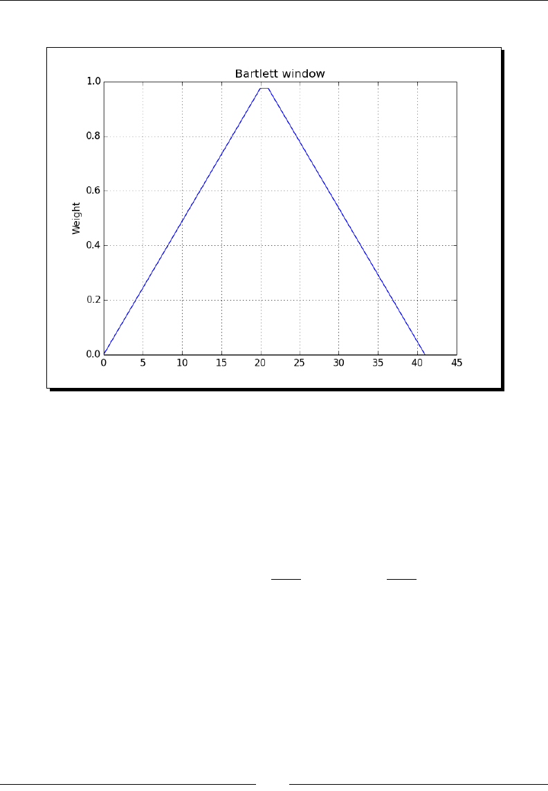
Peeking into Special Rounes
[ 188 ]
The following is the Bartle window, which is triangular, as expected:
What just happened?
We ploed the Bartle window with the NumPy bartlett() funcon.
Blackman window
The Blackman window is the sum of the following cosines:
( )
2 4
0.42 0.5cos 0.08 cos
n n
w n M M
π π
= − +
The NumPy blackman() funcon returns the Blackman window. The only parameter is the
number of points M in the output window. If this number is 0 or less than 0, the funcon
returns an empty array.
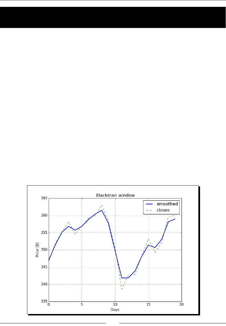
Chapter 7
[ 189 ]
Time for action – smoothing stock prices with the Blackman
window
Let's smooth the close prices from the small AAPL stock prices data le:
1. Load the data into a NumPy array. Call the NumPy blackman() funcon to form a
window, and then use this window to smooth the price signal:
closes=np.loadtxt('AAPL.csv', delimiter=',', usecols=(6,),
converters={1:datestr2num}, unpack=True)
N = 5
window = np.blackman(N)
smoothed = np.convolve(window/window.sum(),
closes, mode='same')
2. Plot the smoothed prices with matplotlib. In this example, we will omit the rst ve
data points and the last ve data points. The reason for this is that there is a strong
boundary eect:
plt.plot(smoothed[N:-N], lw=2, label="smoothed")
plt.plot(closes[N:-N], label="closes")
plt.legend(loc='best')
plt.show()
The closing prices of AAPL smoothed with the Blackman window should appear
as follows:

Peeking into Special Rounes
[ 190 ]
What just happened?
We ploed the closing price of AAPL from our sample data le that was smoothed using the
Blackman window with the NumPy blackman() funcon (see plot_blackman.py):
import numpy as np
import matplotlib.pyplot as plt
from matplotlib.dates import datestr2num
closes=np.loadtxt('AAPL.csv', delimiter=',', usecols=(6,),
converters={1:datestr2num}, unpack=True)
N = 5
window = np.blackman(N)
smoothed = np.convolve(window/window.sum(), closes, mode='same')
plt.plot(smoothed[N:-N], lw=2, label="smoothed")
plt.plot(closes[N:-N], '--', label="closes")
plt.title('Blackman window')
plt.xlabel('Days')
plt.ylabel('Price ($)')
plt.grid()
plt.legend(loc='best')
plt.show()
Hamming window
The Hamming window is formed by a weighted cosine. The formula is as follows:
( )
2
0.54 0.46 cos 0 1
1
n
w n n M
M
π
= + ≤ ≤ −
−
The NumPy hamming() funcon returns the Hamming window. The only parameter is the
number of points M in the output window. If this number is 0 or less than 0, an empty array
is returned.
Time for action – plotting the Hamming window
Let's plot the Hamming window:
1. Call the NumPy hamming() funcon:
window = np.hamming(42)
2. Plot the window with matplotlib:
plt.plot(window)
plt.show()
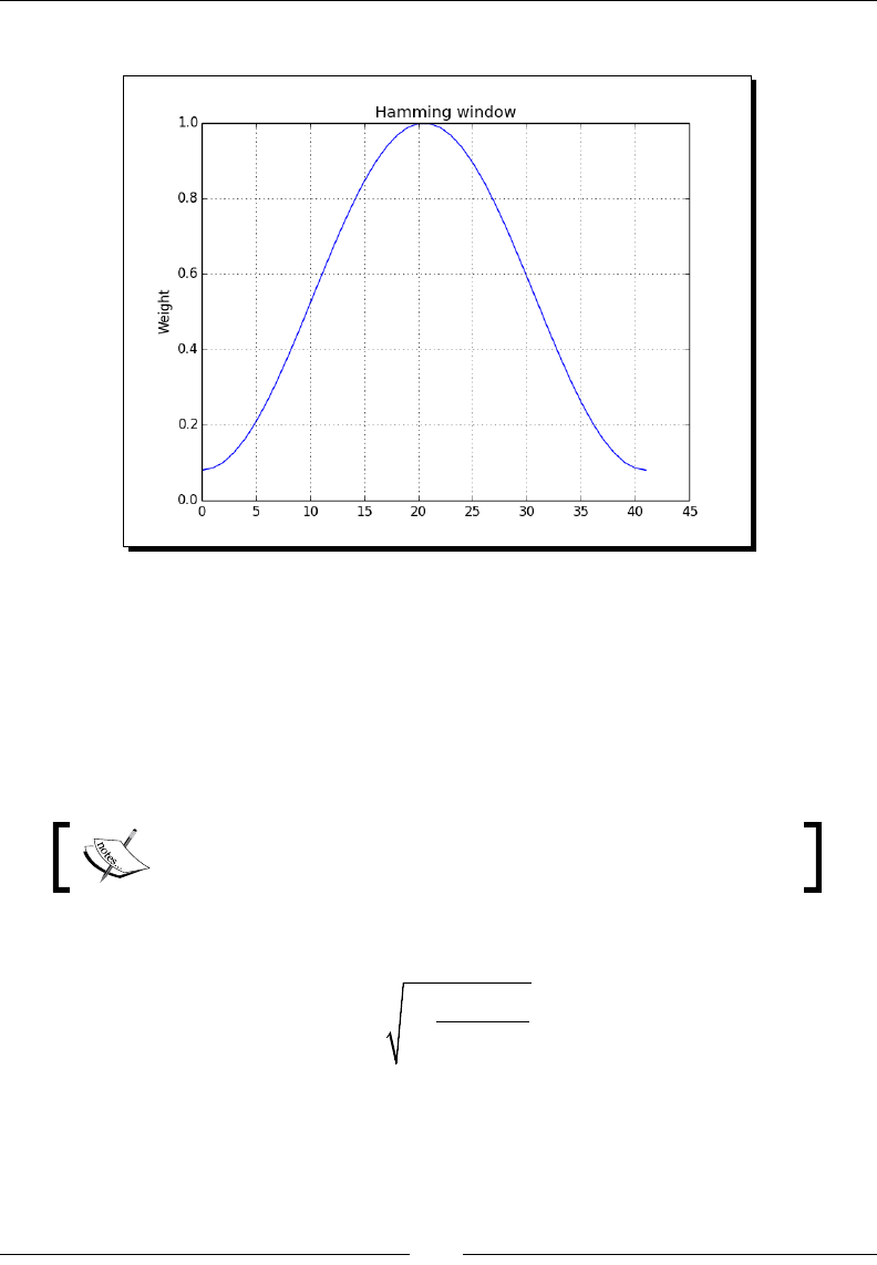
Chapter 7
[ 191 ]
The Hamming window plot appears as follows:
What just happened?
We ploed the Hamming window with the NumPy hamming() funcon.
Kaiser window
The Kaiser window is formed by the Bessel funcon.
Bessel funcons are soluons of the Bessel dierenal equaons (see
http://en.wikipedia.org/wiki/Bessel_function).
The formula is as follows:
( ) ( ) ( )
2
0 0
2
4
1 /
1
n
w n I I
M
β β
= −
−
Here I0 is the zero order Bessel funcon. The NumPy kaiser() funcon returns the Kaiser
window. The rst parameter is the number of points in the output window. If this number is
0 or less than 0, the funcon returns an empty array. The second parameter is the beta.
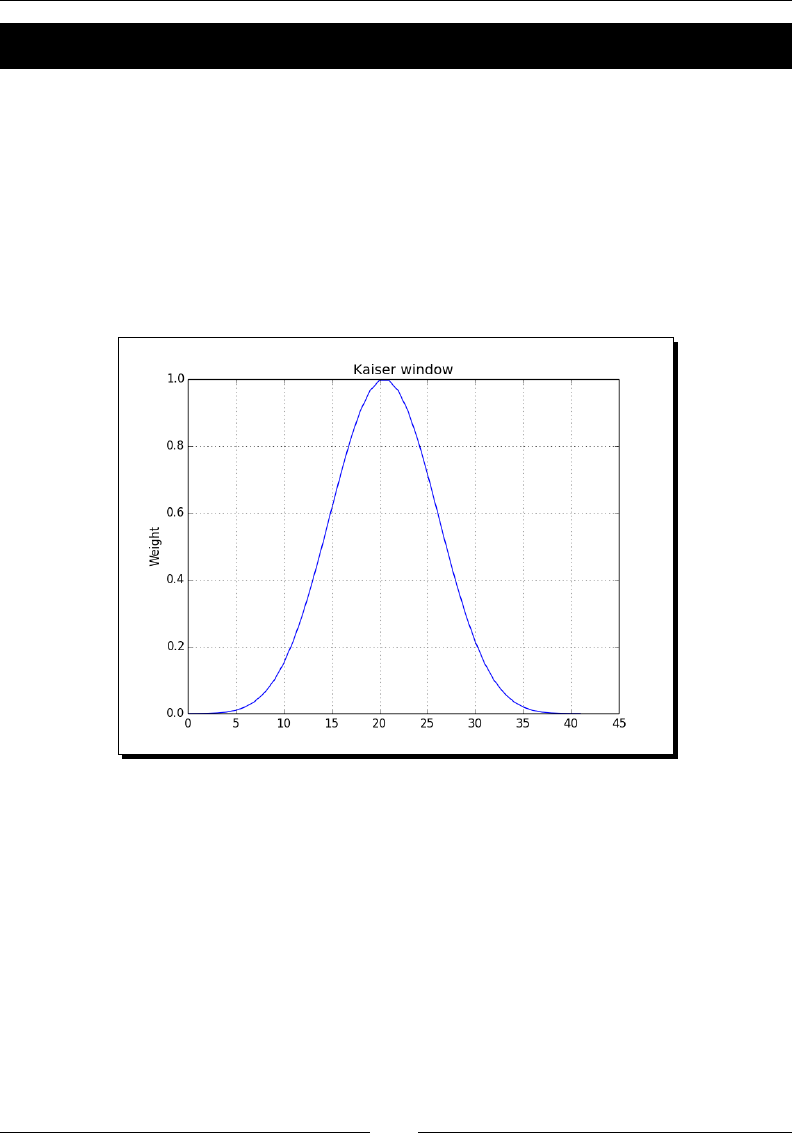
Peeking into Special Rounes
[ 192 ]
Time for action – plotting the Kaiser window
Let's plot the Kaiser window:
1. Call the NumPy kaiser() funcon:
window = np.kaiser(42, 14)
2. Plot the window with matplotlib:
plt.plot(window)
plt.show()
The Kaiser window appears as follows:
What just happened?
We ploed the Kaiser window with the NumPy kaiser() funcon.
Special mathematical functions
We will end this chapter with some special mathemacal funcons. The modied Bessel
funcon of the rst kind 0th order is represented in NumPy by i0(). The sinc funcon is
represented in NumPy by a funcon with the same name, and there is also a two-dimensional
version of this funcon. Sinc is a trigonometric funcon; for more details, see http://
en.wikipedia.org/wiki/Sinc_function. The sinc() funcon has two denions.
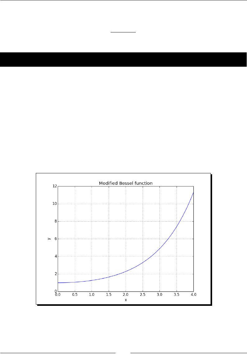
Chapter 7
[ 193 ]
The NumPy sinc() funcon complies with the following denion:
( )
sinx
x
π
π
Time for action – plotting the modied Bessel function
Let's see what the modied Bessel funcon of the rst kind 0th order looks like:
1. Compute evenly spaced values with the NumPy linspace() funcon:
x = np.linspace(0, 4, 100)
2. Call the NumPy i0() funcon:
vals = np.i0(x)
3. Plot the modied Bessel funcon with matplotlib:
plt.plot(x, vals)
plt.show()
The modied Bessel funcon will have the following output:
What just happened?
We ploed the modied Bessel funcon of the rst kind 0th order with the NumPy i0()
funcon.
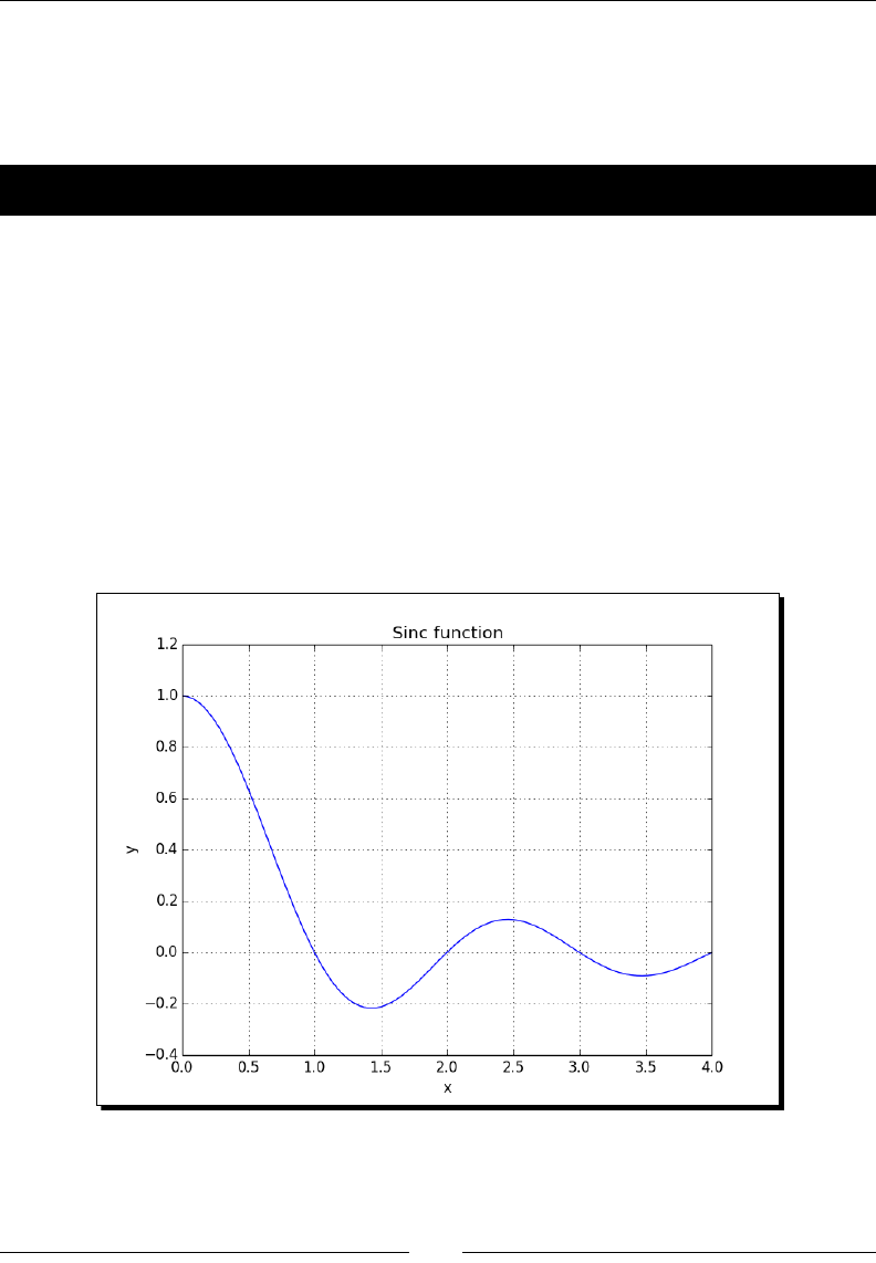
Peeking into Special Rounes
[ 194 ]
sinc
The sinc() funcon is widely used in mathemacs and signal processing. NumPy has a
funcon with the same name. A two-dimensional funcon exists as well.
Time for action – plotting the sinc function
We will plot the sinc() funcon:
1. Compute evenly spaced values with the NumPy linspace() funcon:
x = np.linspace(0, 4, 100)
2. Call the NumPy sinc() funcon:
vals = np.sinc(x)
3. Plot the sinc() funcon with matplotlib:
plt.plot(x, vals)
plt.show()
The sinc() funcon will have the following output:
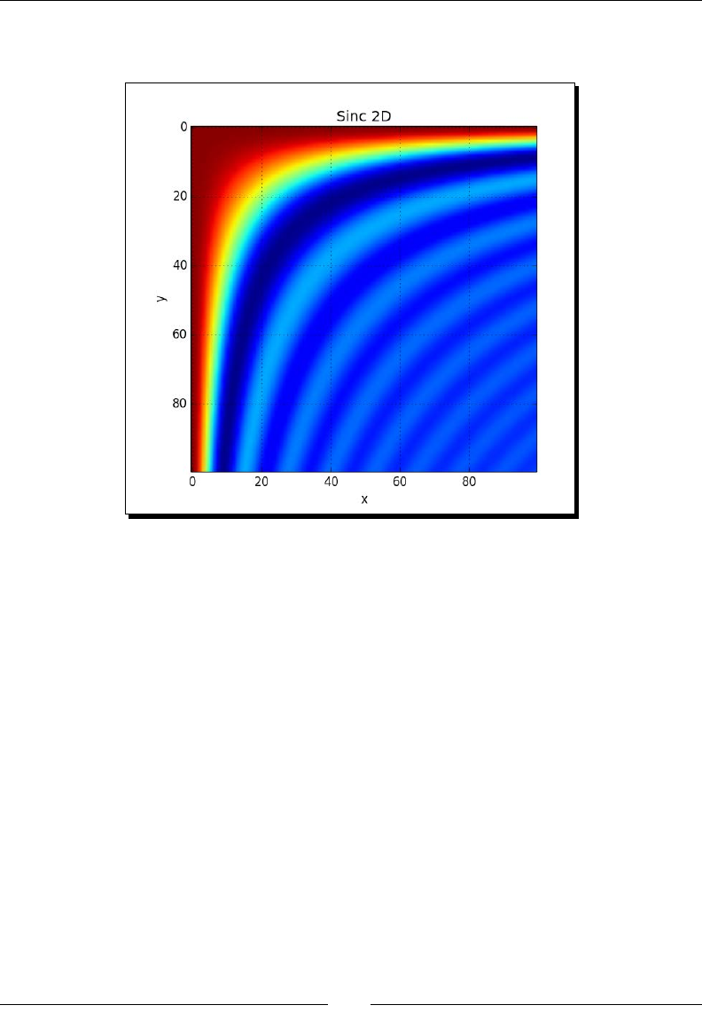
Chapter 7
[ 195 ]
The sinc2d() funcon requires a two-dimensional array. We can create it with the
outer() funcon, resulng in this plot (code is in the following secon):
What just happened?
We ploed the well-known sinc funcon with the NumPy sinc() funcon
(see plot_sinc.py):
import numpy as np
import matplotlib.pyplot as plt
x = np.linspace(0, 4, 100)
vals = np.sinc(x)
plt.plot(x, vals)
plt.title('Sinc function')
plt.xlabel('x')
plt.ylabel('y')
plt.grid()
plt.show()

Peeking into Special Rounes
[ 196 ]
We did the same for two dimensions (see sinc2d.py):
import numpy as np
import matplotlib.pyplot as plt
x = np.linspace(0, 4, 100)
xx = np.outer(x, x)
vals = np.sinc(xx)
plt.imshow(vals)
plt.title('Sinc 2D')
plt.xlabel('x')
plt.ylabel('y')
plt.grid()
plt.show()
Summary
This was a special chapter covering more specialized NumPy topics. We covered sorng and
searching, special funcons, nancial ulies, and window funcons.
The next chapter is about the very important subject of tesng.

[ 197 ]
8
Assuring Quality with Testing
Some programmers test only in production. If you are not one of them,
then you're probably familiar with the concept of unit testing. Unit tests are
automated tests written by a programmer to test his or her code. These tests
could, for example, test a function or part of a function in isolation. Each test
covers only a small unit of code. The benefits are increased confidence in the
quality of the code, reproducible tests, and, as a side effect, clearer code.
Python has good support for unit testing. Additionally, NumPy adds the
numpy.testing package to that for NumPy code unit testing.
Test-driven development (TDD) is one of the most important things that happened to
soware development. TDD focuses a lot on automated unit tesng. The goal is to test
automacally the code as much as possible. The next me we change the code, we can run
the tests and catch potenal regressions. In other words, any funconality already present
will sll work.
The topics in this chapter include the following:
Unit tesng
Asserts
Floang-point precision

Assuring Quality with Tesng
[ 198 ]
Assert functions
Unit tests usually use funcons, which assert something as part of the test. When doing
numerical calculaons, oen we have the fundamental issue of trying to compare oang-
point numbers that are almost equal. For integers, comparison is a trivial operaon, but for
oang-point numbers it is not, because of the inexact representaon by computers. The
NumPy testing package has a number of ulity funcons that test whether a precondion
is true or not, taking into account the problem of oang-point comparisons. The following
table shows the dierent ulity funcons:
Funcon Description
assert_almost_equal() This function raises an exception if two numbers are not equal
up to a specified precision
assert_approx_equal() This function raises an exception if two numbers are not equal
up to a certain significance
assert_array_almost_
equal()
This function raises an exception if two arrays are not equal up
to a specified precision
assert_array_equal() This function raises an exception if two arrays are not equal.
assert_array_less() This function raises an exception if two arrays do not have the
same shape, and the elements of the first array are strictly less
than the elements of the second array
assert_equal() This function raises an exception if two objects are not equal
assert_raises() This function fails if a specified exception is not raised by a
callable invoked with defined arguments
assert_warns() This function fails if a specified warning is not thrown
assert_string_equal() This function asserts that two strings are equal
assert_allclose() This function raise an assertion if two objects are not equal up
to desired tolerance
Time for action – asserting almost equal
Imagine that you have two numbers that are almost equal. Let's use the assert_almost_
equal() funcon to check whether they are equal:
1. Call the funcon with low precision (up to 7 decimal places):
print("Decimal 6", np.testing.assert_almost_equal(0.123456789,
0.123456780, decimal=7))
Note that no excepon is raised, as you can see in the following result:
Decimal 6 None

Chapter 8
[ 199 ]
2. Call the funcon with higher precision (up to 8 decimal places):
print("Decimal 7", np.testing.assert_almost_equal(0.123456789,
0.123456780, decimal=8))
The result is as follows:
Decimal 7
Traceback (most recent call last):
…
raise AssertionError(msg)
AssertionError:
Arrays are not almost equal
ACTUAL: 0.123456789
DESIRED: 0.12345678
What just happened?
We used the assert_almost_equal() funcon from the NumPy testing package to
check whether 0.123456789 and 0.123456780 are equal for dierent decimal precisions.
Pop quiz – specifying decimal precision
Q1. Which parameter of the assert_almost_equal() funcon species the
decimal precision?
1. decimal
2. precision
3. tolerance
4. signicant
Approximately equal arrays
The assert_approx_equal() funcon raises an excepon if two numbers are not equal
up to a certain number of signicant digits. The funcon raises an excepon triggered by the
following condion:
abs(actual - expected) >= 10**-(significant - 1)

Assuring Quality with Tesng
[ 200 ]
Time for action – asserting approximately equal
Let's take the numbers from the previous Time for acon secon and let the
assert_approx_equal() funcon work on them:
1. Call the funcon with low signicance:
print("Significance 8",
np.testing.assert_approx_equal
(0.123456789, 0.123456780,significant=8))
The result is as follows:
Significance 8 None
2. Call the funcon with high signicance:
print("Significance 9",
np.testing.assert_approx_equal
(0.123456789, 0.123456780, significant=9))
The funcon raises an AssertionError:
Significance 9
Traceback (most recent call last):
...
raise AssertionError(msg)
AssertionError:
Items are not equal to 9 significant digits:
ACTUAL: 0.123456789
DESIRED: 0.12345678
What just happened?
We used the assert_approx_equal() funcon from the NumPy testing package to
check whether 0.123456789 and 0.123456780 are equal for dierent decimal precisions.
Almost equal arrays
The assert_array_almost_equal() funcon raises an excepon if two arrays are not
equal up to a specied precision. The funcon checks whether the two arrays have the same
shape. Then, the values of the arrays are compared element by element with the following:
|expected - actual| < 0.5 10-decimal

Chapter 8
[ 201 ]
Time for action – asserting arrays almost equal
Let's form arrays with the values from the previous Time for acon secon by adding a 0 to
each array:
1. Call the funcon with lower precision:
print("Decimal 8", np.testing.assert_array_almost_equal([0,
0.123456789], [0, 0.123456780], decimal=8))
The result is as follows:
Decimal 8 None
2. Call the funcon with higher precision:
print("Decimal 9", np.testing.assert_array_almost_equal([0,
0.123456789], [0, 0.123456780], decimal=9))
The test raises an AssertionError:
Decimal 9
Traceback (most recent call last):
…
assert_array_compare
raise AssertionError(msg)
AssertionError:
Arrays are not almost equal
(mismatch 50.0%)
x: array([ 0. , 0.12345679])
y: array([ 0. , 0.12345678])
What just happened?
We compared two arrays with the NumPy array_almost_equal() funcon.
Have a go hero – comparing arrays with different shapes
Use the NumPy array_almost_equal() funcon to compare two arrays with
dierent shapes.

Assuring Quality with Tesng
[ 202 ]
Equal arrays
The assert_array_equal() funcon raises an excepon if two arrays are not equal. The
shapes of the arrays have to be equal and the elements of each array must be equal. NaNs are
allowed in the arrays. Alternavely, arrays can be compared with the array_allclose()
funcon. This funcon has the parameters absolute tolerance (atol) and relave tolerance
(rtol). For two arrays a and b, these parameters sasfy the following equaon:
|a - b| <= (atol + rtol * |b|)
Time for action – comparing arrays
Let's compare two arrays with the funcons we just menoned. We will reuse the arrays
from the previous Time for acon secon and add a NaN to them:
1. Call the array_allclose() funcon:
print("Pass", np.testing.assert_allclose([0, 0.123456789,
np.nan], [0, 0.123456780, np.nan], rtol=1e-7, atol=0))
The result is as follows:
Pass None
2. Call the array_equal() funcon:
print("Fail", np.testing.assert_array_equal([0, 0.123456789,
np.nan], [0, 0.123456780, np.nan]))
The test fails with an AssertionError:
Fail
Traceback (most recent call last):
…
assert_array_compare
raise AssertionError(msg)
AssertionError:
Arrays are not equal
(mismatch 50.0%)
x: array([ 0. , 0.12345679, nan])
y: array([ 0. , 0.12345678, nan])

Chapter 8
[ 203 ]
What just happened?
We compared two arrays with the array_allclose() funcon and the array_equal()
funcon.
Ordering arrays
The assert_array_less() funcon raises an excepon if two arrays do not have the
same shape, and the elements of the rst array are strictly less than the elements of the
second array.
Time for action – checking the array order
Let's check whether one array is strictly greater than another array:
1. Call the assert_array_less() funcon with two strictly ordered arrays:
print("Pass", np.testing.assert_array_less([0, 0.123456789,
np.nan], [1, 0.23456780, np.nan]))
The result is as follows:
Pass None
2. Call the assert_array_less() funcon:
print("Fail", np.testing.assert_array_less([0, 0.123456789,
np.nan], [0, 0.123456780, np.nan]))
The test raises an excepon:
Fail
Traceback (most recent call last):
...
raise AssertionError(msg)
AssertionError:
Arrays are not less-ordered
(mismatch 100.0%)
x: array([ 0. , 0.12345679, nan])
y: array([ 0. , 0.12345678, nan])

Assuring Quality with Tesng
[ 204 ]
What just happened?
We checked the ordering of two arrays with the assert_array_less() funcon.
Object comparison
The assert_equal() funcon raises an excepon if two objects are not equal. The objects
do not have to be NumPy arrays—they can also be lists, tuples, or diconaries.
Time for action – comparing objects
Suppose you need to compare two tuples. We can use the assert_equal() funcon to
do that.
Call the assert_equal() funcon:
print("Equal?", np.testing.assert_equal((1, 2), (1, 3)))
The call raises an error because the items are not equal:
Equal?
Traceback (most recent call last):
...
raise AssertionError(msg)
AssertionError:
Items are not equal:
item=1
ACTUAL: 2
DESIRED: 3
What just happened?
We compared two tuples with the assert_equal() funcon—an excepon was raised
because the tuples were not equal to each other.
String comparison
The assert_string_equal() funcon asserts that two strings are equal. If the test fails,
the funcon throws an excepon and shows the dierence between the strings. The case of
the string characters maers.

Chapter 8
[ 205 ]
Time for action – comparing strings
Let's compare strings. Both strings are the word "NumPy":
1. Call the assert_string_equal() funcon to compare a string with itself. This
test, of course, should pass:
print("Pass", np.testing.assert_string_equal("NumPy", "NumPy"))
The test passes:
Pass None
2. Call the assert_string_equal() funcon to compare a string with another
string with the same leers, but dierent casing. This test should throw
an excepon:
print("Fail", np.testing.assert_string_equal("NumPy", "Numpy"))
The test raises an error:
Fail
Traceback (most recent call last):
…
raise AssertionError(msg)
AssertionError: Differences in strings:
- NumPy? ^
+ Numpy? ^
What just happened?
We compared two strings with the assert_string_equal() funcon. The test threw an
excepon when the casing did not match.
Floating-point comparisons
The representaon of oang-point numbers in computers is not exact. This leads to issues
when comparing oang-point numbers. The assert_array_almost_equal_nulp()
and assert_array_max_ulp() NumPy funcons provide consistent oang-point
comparisons. Unit of Least Precision (ULP) of oang-point numbers, according to the IEEE
754 specicaon, a half ULP precision is required for elementary arithmec operaons.
You can compare this to a ruler. A metric system ruler usually has cks for millimeters,
but beyond that you can only esmate half millimeters.

Assuring Quality with Tesng
[ 206 ]
Machine epsilon is the largest relave rounding error in oang-point arithmec. Machine
epsilon is equal to ULP relave to 1. The NumPy finfo() funcon allows us to determine
the machine epsilon. The Python standard library also can give you the machine epsilon
value. The value should be the same as that given by NumPy.
Time for action – comparing with assert_array_almost_equal_
nulp
Let's see the assert_array_almost_equal_nulp() funcon in acon:
1. Determine the machine epsilon with the finfo() funcon:
eps = np.finfo(float).eps
print("EPS", eps)
The epsilon would be as follows:
EPS 2.22044604925e-16
2. Compare 1.0 with 1 + epsilon using the assert_almost_equal_nulp()
funcon. Do the same for 1 + 2 * epsilon:
print("1",
np.testing.assert_array_almost_equal_nulp(1.0, 1.0 + eps))
print("2",
np.testing.assert_array_almost_equal_nulp(1.0, 1.0 + 2 * eps))
The result is as follows:
1 None
2
Traceback (most recent call last):
…
assert_array_almost_equal_nulp
raise AssertionError(msg)
AssertionError: X and Y are not equal to 1 ULP (max is 2)
What just happened?
We determined the machine epsilon with the finfo() funcon. We then compared 1.0
with 1 + epsilon with the assert_almost_equal_nulp() funcon. This test passed
however, adding another epsilon resulted in an excepon.

Chapter 8
[ 207 ]
Comparison of oats with more ULPs
The assert_array_max_ulp() funcon allows you to specify an upper bound for the
number of ULPs you would allow. The maxulp parameter accepts an integer value for the
limit. The value of this parameter is 1 by default.
Time for action – comparing using maxulp of 2
Let's do the same comparisons as in the previous Time for acon secon, but specify a
maxulp of 2 when necessary:
1. Determine the machine epsilon with the finfo() funcon:
eps = np.finfo(float).eps
print("EPS", eps)
The epsilon would be as follows:
EPS 2.22044604925e-16
2. Do the comparisons as done in the previous Time for acon secon, but use the
assert_array_max_ulp() funcon with the appropriate maxulp value:
print("1", np.testing.assert_array_max_ulp(1.0, 1.0 + eps))
print("2", np.testing.assert_array_max_ulp(1.0, 1 + 2 * eps,
maxulp=2))
The output is as follows:
1 1.0
2 2.0
What just happened?
We compared the same values as the previous Time for acon secon, but specied a
maxulp of 2 in the second comparison. Using the assert_array_max_ulp() funcon
with the appropriate maxulp value, these tests passed with a return value of the number
of ULPs.
Unit tests
Unit tests are automated tests, which test a small piece of code, usually a funcon or
method. Python has the PyUnit API for unit tesng. As NumPy users, we can make
use of the assert funcons we saw in acon before.

Assuring Quality with Tesng
[ 208 ]
Time for action – writing a unit test
We will write tests for a simple factorial funcon. The tests will check for the so-called happy
path and abnormal condions.
1. Start by wring the factorial funcon:
import numpy as np
import unittest
def factorial(n):
if n == 0:
return 1
if n < 0:
raise ValueError, "Unexpected negative value"
return np.arange(1, n+1).cumprod()
The code uses the arange() and cumprod() funcons to create arrays
and calculate the cumulave product, but we added a few checks for
boundary condions.
2. Now we will write the unit test. Let's write a class that will contain the unit tests.
It extends the TestCase class from the unittest module, which is part of
standard Python. Test for calling the factorial funcon with the following three
aributes:
a positive number, the happy path
boundary condition 0
negative numbers, which should result in an error
class FactorialTest(unittest.TestCase):
def test_factorial(self):
#Test for the factorial of 3 that should pass.
self.assertEqual(6, factorial(3)[-1])
np.testing.assert_equal(np.array([1, 2, 6]),
factorial(3))
def test_zero(self):
#Test for the factorial of 0 that should pass.
self.assertEqual(1, factorial(0))
def test_negative(self):
#Test for the factorial of negative numbers that
should fail.
# It should throw a ValueError, but we expect
IndexError
self.assertRaises(IndexError, factorial(-10))

Chapter 8
[ 209 ]
We rigged one of the tests to fail, as you can see in the following output:
$ python unit_test.py
.E.
==================================================================
====
ERROR: test_negative (__main__.FactorialTest)
------------------------------------------------------------------
----
Traceback (most recent call last):
File "unit_test.py", line 26, in test_negative
self.assertRaises(IndexError, factorial(-10))
File "unit_test.py", line 9, in factorial
raise ValueError, "Unexpected negative value"
ValueError: Unexpected negative value
------------------------------------------------------------------
----
Ran 3 tests in 0.003s
FAILED (errors=1)
What just happened?
We made some happy path tests for the factorial funcon code. We let the boundary
condion test fail on purpose (see unit_test.py):
import numpy as np
import unittest
def factorial(n):
if n == 0:
return 1
if n < 0:
raise ValueError, "Unexpected negative value"
return np.arange(1, n+1).cumprod()
class FactorialTest(unittest.TestCase):
def test_factorial(self):
#Test for the factorial of 3 that should pass.
self.assertEqual(6, factorial(3)[-1])
np.testing.assert_equal(np.array([1, 2, 6]), factorial(3))

Assuring Quality with Tesng
[ 210 ]
def test_zero(self):
#Test for the factorial of 0 that should pass.
self.assertEqual(1, factorial(0))
def test_negative(self):
#Test for the factorial of negative numbers that should fail.
# It should throw a ValueError, but we expect IndexError
self.assertRaises(IndexError, factorial(-10))
if __name__ == '__main__':
unittest.main()
Nose test decorators
A nose is an organ above the mouth that is used by humans and animals to breathe and
smell. It is also a Python framework that makes (unit) tesng easier. Nose helps you organize
tests. According to the nose documentaon:
"Any python source le, directory or package that matches the testMatch regular
expression (by default: (?:^|[b_.-])[Tt]est) will be collected as a test."
Nose makes extensive use of decorators. Python decorators are annotaons that indicate
something about a method or a funcon (see http://thecodeship.com/patterns/
guide-to-python-function-decorators/). The numpy.testing module has a
number of decorators. The following table shows the dierent decorators in the
numpy.testing module:
Decorator Description
numpy.testing.decorators.deprecated This function filters deprecation warnings
when running tests
numpy.testing.decorators.
knownfailureif
This function raises KnownFailureTest
exception based on a condition
numpy.testing.decorators.setastest This decorator marks a function as being a
test or not being a test
numpy.testing.decorators.skipif This function raises a SkipTest exception
based on a condition
numpy.testing.decorators.slow This function labels test functions or
methods as slow
Addionally, we can call the decorate_methods() funcon to apply decorators on
methods of a class matching a regular expression or a string.

Chapter 8
[ 211 ]
Time for action – decorating tests
We will apply the @setastest decorator directly to test funcons. Then we will apply the
same decorator to a method to disable it. Also, we will skip one of the tests and fail another.
First, install nose in case you don't have it yet.
1. Install nose with setuptools:
$ [sudo] easy_install nose
Or pip:
$ [sudo] pip install nose
2. Apply one funcon as being a test and another as not being a test:
@setastest(False)
def test_false():
pass
@setastest(True)
def test_true():
pass
3. Skip tests with the @skipif decorator. Let's use a condion that always leads to a
test being skipped:
@skipif(True)
def test_skip():
pass
4. Add a test funcon that always passes. Then, decorate it with the
@knownfailureif decorator so that the test always fails:
@knownfailureif(True)
def test_alwaysfail():
pass
5. Dene some test classes with methods that normally should be executed by nose:
class TestClass():
def test_true2(self):
pass
class TestClass2():
def test_false2(self):
pass

Assuring Quality with Tesng
[ 212 ]
6. Let's disable the second test method from the previous step:
decorate_methods(TestClass2, setastest(False), 'test_false2')
7. Run the tests with the following command:
$ nosetests -v decorator_setastest.py
decorator_setastest.TestClass.test_true2 ... ok
decorator_setastest.test_true ... ok
decorator_test.test_skip ... SKIP: Skipping test: test_skipTest
skipped due to test condition
decorator_test.test_alwaysfail ... ERROR
==================================================================
====
ERROR: decorator_test.test_alwaysfail
------------------------------------------------------------------
----
Traceback (most recent call last):
File "…/nose/case.py", line 197, in runTest
self.test(*self.arg)
File …/numpy/testing/decorators.py", line 213, in knownfailer
raise KnownFailureTest(msg)
KnownFailureTest: Test skipped due to known failure
------------------------------------------------------------------
----
Ran 4 tests in 0.001s
FAILED (SKIP=1, errors=1)
What just happened?
We decorated some funcons and methods as not being tests so that they were ignored by
nose. We skipped one test and failed another too. We did this by applying decorators directly
and with the decorate_methods() funcon (see decorator_test.py):
from numpy.testing.decorators import setastest
from numpy.testing.decorators import skipif

Chapter 8
[ 213 ]
from numpy.testing.decorators import knownfailureif
from numpy.testing import decorate_methods
@setastest(False)
def test_false():
pass
@setastest(True)
def test_true():
pass
@skipif(True)
def test_skip():
pass
@knownfailureif(True)
def test_alwaysfail():
pass
class TestClass():
def test_true2(self):
pass
class TestClass2():
def test_false2(self):
pass
decorate_methods(TestClass2, setastest(False), 'test_false2')
Docstrings
Doctests are strings embedded in Python code that resemble interacve sessions. These
strings can be used to test certain assumpons or just to provide examples. The numpy.
testing module has a funcon to run these tests.

Assuring Quality with Tesng
[ 214 ]
Time for action – executing doctests
Let's write a simple example that is supposed to calculate the well-known factorial, but
doesn't cover all of the possible boundary condions. In other words, some tests will fail.
1. The docstring will look like text you would see in a Python shell (including a
prompt). Rig one of the tests to fail, just to see what will happen:
"""
Test for the factorial of 3 that should pass.
>>> factorial(3)
6
Test for the factorial of 0 that should fail.
>>> factorial(0)
1
"""
2. Write the following line of NumPy code:
return np.arange(1, n+1).cumprod()[-1]
We want this code to fail from me to me for demonstraon purposes.
3. Run the doctest by calling the rundocs() funcon of the numpy.testing
module, for instance, in the Python shell:
>>> from numpy.testing import rundocs
>>> rundocs('docstringtest.py')
Traceback (most recent call last):
File "<stdin>", line 1, in <module>
File "…/numpy/testing/utils.py", line 998, in rundocs
raise AssertionError("Some doctests failed:\n%s" % "\n".
join(msg))
AssertionError: Some doctests failed:
******************************************************************
****
File "docstringtest.py", line 10, in docstringtest.factorial
Failed example:
factorial(0)

Chapter 8
[ 215 ]
Exception raised:
Traceback (most recent call last):
File "…/doctest.py", line 1254, in __run
compileflags, 1) in test.globs
File "<doctest docstringtest.factorial[1]>", line 1, in
<module>
factorial(0)
File "docstringtest.py", line 13, in factorial
return np.arange(1, n+1).cumprod()[-1]
IndexError: index -1 is out of bounds for axis 0 with size 0
What just happened?
We wrote a docstring test, which didn't take into account 0 and negave numbers. We ran
the test with the rundocs() funcon from the numpy.testing module and got an index
error as a result (see docstringtest.py):
import numpy as np
def factorial(n):
"""
Test for the factorial of 3 that should pass.
>>> factorial(3)
6
Test for the factorial of 0 that should fail.
>>> factorial(0)
1
"""
return np.arange(1, n+1).cumprod()[-1]
Summary
You learned about tesng and NumPy tesng ulies in this chapter. We covered unit
tesng, docstring tests, assert funcons, and oang-point precision. Most of the NumPy
assert funcons take care of the complexies of oang-point numbers. We demonstrated
NumPy decorators that can be used by nose. Decorators make tesng easier and document
the developer intenon.
The topic of the next chapter is matplotlib—the Python scienc visualizaon and graphing
open source library.

[ 217 ]
Plotting with matplotlib
matplotlib is a very useful Python plotting library. It integrates nicely with
NumPy but is a separate open source project. You can find a gallery of beautiful
examples at http://matplotlib.org/gallery.html.
matplotlib also has utility functions to download and manipulate data from
Yahoo Finance. We will see several examples of stock charts.
This chapter features extended coverage of the following topics:
Simple plots
Subplots
Histograms
Plot customizaon
Three-dimensional plots
Contour plots
Animaon
Logplots
Simple plots
The matplotlib.pyplot package contains funconality for simple plots. It is important
to remember that each subsequent funcon call changes the state of the current plot.
Eventually, we will want to either save the plot in a le or display it with the show()
funcon. However, if we are in IPython running on a Qt or Wx backend, the gure updates
interacvely without waing for the show() funcon. This is comparable to the way text
output is printed on the y.
9
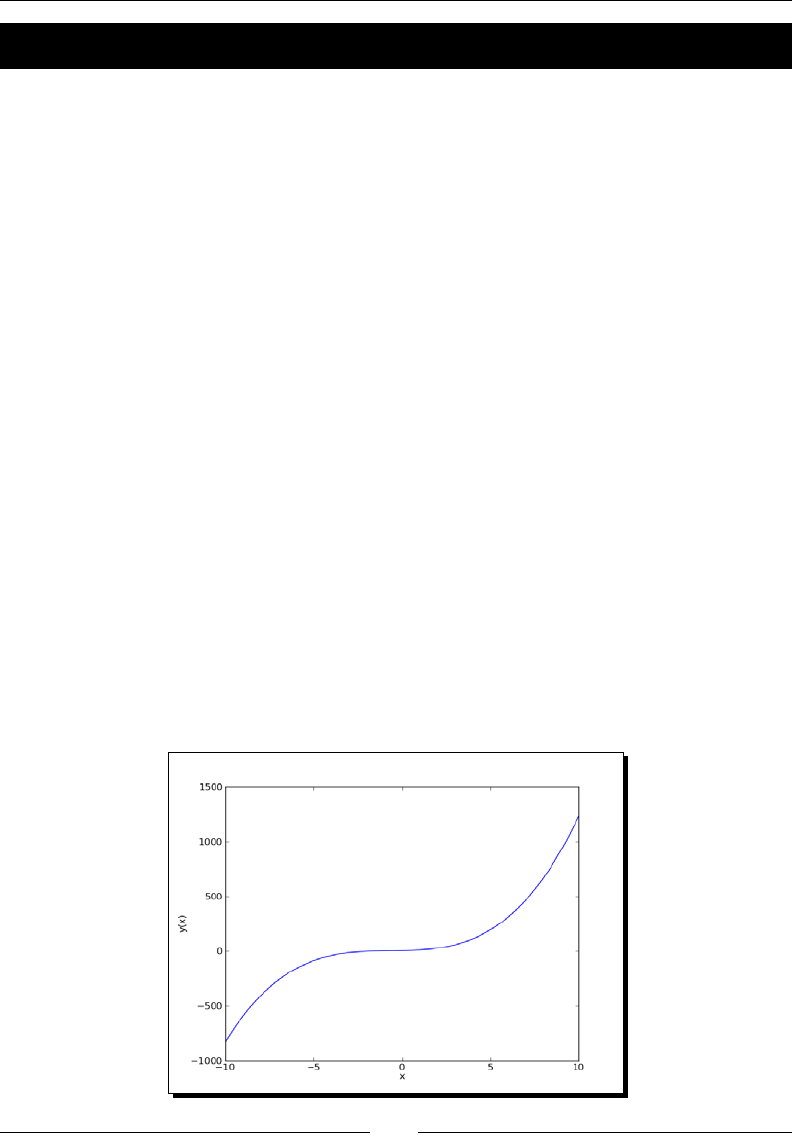
Plong with matplotlib
[ 218 ]
Time for action – plotting a polynomial function
To illustrate how plong works, let's display some polynomial graphs. We will use the
NumPy polynomial funcon poly1d() to create a polynomial.
1. Take the standard input values as polynomial coecients. Use the NumPy
poly1d() funcon to create a polynomial:
func = np.poly1d(np.array([1, 2, 3, 4]).astype(float))
2. Create the x values with the NumPy the linspace() funcon. Use the range -10
to 10 and create 30 even spaced values:
x = np.linspace(-10, 10, 30)
3. Calculate the polynomial values using the polynomial we created in the rst step:
y = func(x)
4. Call the plot() funcon; this does not immediately display the graph:
plt.plot(x, y)
5. Add a label to the x axis with the xlabel() funcon:
plt.xlabel('x')
6. Add a label to the y axis with the ylabel() funcon:
plt.ylabel('y(x)')
7. Call the show() funcon to display the graph:
plt.show()
The following is a plot with polynomial coecients 1, 2, 3, and 4:

Chapter 9
[ 219 ]
What just happened?
We displayed a polynomial graph on our screen. We added labels to the x and y axes
(see polyplot.py):
import numpy as np
import matplotlib.pyplot as plt
func = np.poly1d(np.array([1, 2, 3, 4]).astype(float))
x = np.linspace(-10, 10, 30)
y = func(x)
plt.plot(x, y)
plt.xlabel('x')
plt.ylabel('y(x)')
plt.show()
Pop quiz – the plot() function
Q1. What does the plot() funcon do?
1. It displays two-dimensional plots on screen.
2. It saves an image of a two-dimensional plot in a le.
3. It does both a and b.
4. It does neither a, b, or c.
Plot format string
The plot() funcon accepts an unlimited number of arguments. In the previous secon,
we gave it two arrays as arguments. We could also specify the line color and style with an
oponal format string. By default, it is a solid blue line denoted as b-, but you can specify
a dierent color and style, such as red dashes.
Time for action – plotting a polynomial and its derivatives
Let's plot a polynomial and its rst-order derivave using the deriv() funcon with m as 1.
We already did the rst part in the previous Time for acon secon. We want two dierent
line styles to discern what is what.
1. Create and dierenate the polynomial:
func = np.poly1d(np.array([1, 2, 3, 4]).astype(float))
func1 = func.deriv(m=1)
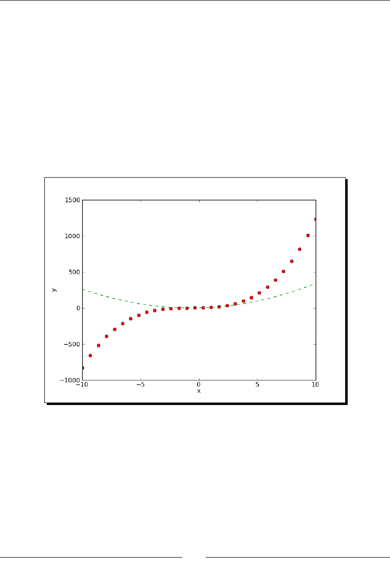
Plong with matplotlib
[ 220 ]
x = np.linspace(-10, 10, 30)
y = func(x)
y1 = func1(x)
2. Plot the polynomial and its derivave in two styles: red circles and green dashes. You
cannot see the colors in a print copy of this book, so you will have to try the code
out for yourself:
plt.plot(x, y, 'ro', x, y1, 'g--')
plt.xlabel('x')
plt.ylabel('y')
plt.show()
The graph with polynomial coecients 1, 2, 3, and 4 is as follows:
What just happened?
We ploed a polynomial and its derivave using two dierent line styles and one call of the
plot() funcon (see polyplot2.py):
import numpy as np
import matplotlib.pyplot as plt
func = np.poly1d(np.array([1, 2, 3, 4]).astype(float))

Chapter 9
[ 221 ]
func1 = func.deriv(m=1)
x = np.linspace(-10, 10, 30)
y = func(x)
y1 = func1(x)
plt.plot(x, y, 'ro', x, y1, 'g--')
plt.xlabel('x')
plt.ylabel('y')
plt.show()
Subplots
At a certain point, you will have too many lines in one plot. However, you would sll like
everything grouped together. We can do this with the subplot() funcon. This funcon
creates mulple plots in a grid.
Time for action – plotting a polynomial and its derivatives
Let's plot a polynomial and its rst and second derivave. We will make three subplots for
the sake of clarity:
1. Create a polynomial and its derivaves using the following code:
func = np.poly1d(np.array([1, 2, 3, 4]).astype(float))
x = np.linspace(-10, 10, 30)
y = func(x)
func1 = func.deriv(m=1)
y1 = func1(x)
func2 = func.deriv(m=2)
y2 = func2(x)
2. Create the rst subplot of the polynomial with the subplot() funcon. The rst
parameter of this funcon is the number of rows, the second parameter is the
number of columns, and the third parameter is an index number starng with 1.
Alternavely, combine the three parameters into a single number, such as 311. The
subplots will be organized in three rows and one column. Give the subplot the tle
Polynomial. Make a solid red line:
plt.subplot(311)
plt.plot(x, y, 'r-')
plt.title("Polynomial")

Plong with matplotlib
[ 222 ]
3. Create the third subplot of the rst derivave with the subplot() funcon. Give
the subplot the tle First Derivave. Use a line of blue triangles:
plt.subplot(312)
plt.plot(x, y1, 'b^')
plt.title("First Derivative")
4. Create the second subplot of the second derivave with the subplot() funcon.
Give the subplot the tle Second Derivave. Use a line of green circles:
plt.subplot(313)
plt.plot(x, y2, 'go')
plt.title("Second Derivative")
plt.xlabel('x')
plt.ylabel('y')
plt.show()
The three subplots with polynomial coecients 1, 2, 3, and 4 are as follows:

Chapter 9
[ 223 ]
What just happened?
We ploed a polynomial and its rst and second derivaves using three dierent line styles
and three subplots in three rows and one column (see polyplot3.py):
import numpy as np
import matplotlib.pyplot as plt
func = np.poly1d(np.array([1, 2, 3, 4]).astype(float))
x = np.linspace(-10, 10, 30)
y = func(x)
func1 = func.deriv(m=1)
y1 = func1(x)
func2 = func.deriv(m=2)
y2 = func2(x)
plt.subplot(311)
plt.plot(x, y, 'r-')
plt.title("Polynomial")
plt.subplot(312)
plt.plot(x, y1, 'b^')
plt.title("First Derivative")
plt.subplot(313)
plt.plot(x, y2, 'go')
plt.title("Second Derivative")
plt.xlabel('x')
plt.ylabel('y')
plt.show()
Finance
matplotlib can help monitor our stock investments. The matplotlib.finance
package has ulies with which we can download stock quotes from Yahoo Finance at
http://finance.yahoo.com/. We can then plot the data as candlescks.
Time for action – plotting a year's worth of stock quotes
We can plot a year's worth of stock quotes data with the matplotlib.finance package.
This requires a connecon to Yahoo Finance, which is the data source.
1. Determine the start date by subtracng one year from today:
from matplotlib.dates import DateFormatter
from matplotlib.dates import DayLocator
from matplotlib.dates import MonthLocator

Plong with matplotlib
[ 224 ]
from matplotlib.finance import quotes_historical_yahoo
from matplotlib.finance import candlestick
import sys
from datetime import date
import matplotlib.pyplot as plt
today = date.today()
start = (today.year - 1, today.month, today.day)
2. We need to create the so-called locators. These objects from the matplotlib.
dates package locate months and days on the x axis:
alldays = DayLocator()
months = MonthLocator()
3. Create a date formaer to format the dates on the x axis. This formaer creates a
string containing the short name of a month and the year:
month_formatter = DateFormatter("%b %Y")
4. Download the stock quote data from Yahoo nance with the following code:
quotes = quotes_historical_yahoo(symbol, start, today)
5. Create a matplotlib Figure object—this is a top-level container for plot
components:
fig = plt.figure()
6. Add a subplot to the gure:
ax = fig.add_subplot(111)
7. Set the major locator on the x axis to the months locator. This locator is responsible
for the big cks on the x axis:
ax.xaxis.set_major_locator(months)
8. Set the minor locator on the x axis to the days locator. This locator is responsible for
the small cks on the x axis:
ax.xaxis.set_minor_locator(alldays)
9. Set the major formaer on the x axis to the months formaer. This formaer is
responsible for the labels of the big cks on the x axis:
ax.xaxis.set_major_formatter(month_formatter)
10. A funcon in the matplotlib.finance package allows us to display candlescks.
Create the candlescks using the quotes data. It is possible to specify the width of
the candlescks. For now, use the default value:
candlestick(ax, quotes)
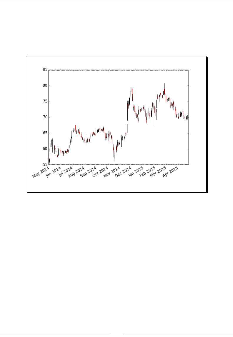
Chapter 9
[ 225 ]
11. Format the labels on the x axis as dates. This rotates the labels on the x axis so that
they t beer:
fig.autofmt_xdate()
plt.show()
The candlesck chart for DISH (Dish Network Corp) appears as follows:
What just happened?
We downloaded a year's worth of data from Yahoo Finance. We charted this data using
candlescks (see candlesticks.py):
from matplotlib.dates import DateFormatter
from matplotlib.dates import DayLocator
from matplotlib.dates import MonthLocator
from matplotlib.finance import quotes_historical_yahoo
from matplotlib.finance import candlestick
import sys
from datetime import date
import matplotlib.pyplot as plt
today = date.today()
start = (today.year - 1, today.month, today.day)

Plong with matplotlib
[ 226 ]
alldays = DayLocator()
months = MonthLocator()
month_formatter = DateFormatter("%b %Y")
symbol = 'DISH'
if len(sys.argv) == 2:
symbol = sys.argv[1]
quotes = quotes_historical_yahoo(symbol, start, today)
fig = plt.figure()
ax = fig.add_subplot(111)
ax.xaxis.set_major_locator(months)
ax.xaxis.set_minor_locator(alldays)
ax.xaxis.set_major_formatter(month_formatter)
candlestick(ax, quotes)
fig.autofmt_xdate()
plt.show()
Histograms
Histograms visualize the distribuon of numerical data. matplotlib has the handy hist()
funcon that graphs histograms. The hist() funcon has two main arguments—the array
containing the data and the number of bars.
Time for action – charting stock price distributions
Let's chart the stock price distribuon of quotes from Yahoo Finance.
1. Download the data going back one year:
today = date.today()
start = (today.year - 1, today.month, today.day)
quotes = quotes_historical_yahoo(symbol, start, today)
2. The quotes data in the previous step is stored in a Python list. Convert this to a
NumPy array and extract the close prices:
quotes = np.array(quotes)
close = quotes.T[4]
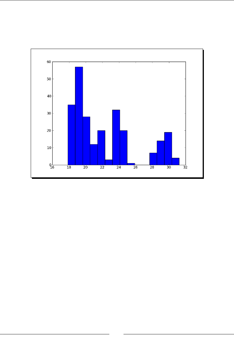
Chapter 9
[ 227 ]
3. Draw the histogram with a reasonable number of bars:
plt.hist(close, np.sqrt(len(close)))
plt.show()
The histogram for DISH appears as follows:
What just happened?
We charted the stock price distribuon of DISH as a histogram (see stockhistogram.py):
from matplotlib.finance import quotes_historical_yahoo
import sys
from datetime import date
import matplotlib.pyplot as plt
import numpy as np
today = date.today()
start = (today.year - 1, today.month, today.day)
symbol = 'DISH'
if len(sys.argv) == 2:
symbol = sys.argv[1]

Plong with matplotlib
[ 228 ]
quotes = quotes_historical_yahoo(symbol, start, today)
quotes = np.array(quotes)
close = quotes.T[4]
plt.hist(close, np.sqrt(len(close)))
plt.show()
Have a go hero – drawing a bell curve
Overlay a bell curve (related to the Gaussian or normal distribuon) using the average price
and standard deviaon. This is, of course, only an exercise.
Logarithmic plots
Logarithmic plots are useful when the data has a wide range of values. matplotlib has
the funcons semilogx() (logarithmic x axis), semilogy() (logarithmic y axis), and
loglog() (x and y axes logarithmic).
Time for action – plotting stock volume
Stock volume varies a lot, so let's plot it on a logarithmic scale. First, we need to download
historical data from Yahoo Finance, extract the dates and volume, create locators and a date
formaer, and create the gure and add it to a subplot. We already went through these
steps in the previous Time for acon secon, so we will skip them here.
Plot the volume using a logarithmic scale:
plt.semilogy(dates, volume)
Now, set the locators and format the x axis as dates. Instrucons for these steps can be
found in the previous Time for acon secon as well.
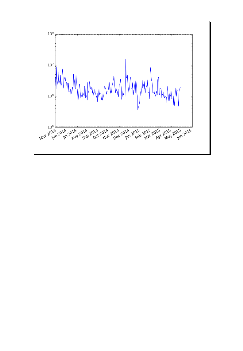
Chapter 9
[ 229 ]
The stock volume using a logarithmic scale for DISH appears as follows:
What just happened?
We ploed stock volume using a logarithmic scale (see logy.py):
from matplotlib.finance import quotes_historical_yahoo
from matplotlib.dates import DateFormatter
from matplotlib.dates import DayLocator
from matplotlib.dates import MonthLocator
import sys
from datetime import date
import matplotlib.pyplot as plt
import numpy as np
today = date.today()
start = (today.year - 1, today.month, today.day)
symbol = 'DISH'
if len(sys.argv) == 2:
symbol = sys.argv[1]

Plong with matplotlib
[ 230 ]
quotes = quotes_historical_yahoo(symbol, start, today)
quotes = np.array(quotes)
dates = quotes.T[0]
volume = quotes.T[5]
alldays = DayLocator()
months = MonthLocator()
month_formatter = DateFormatter("%b %Y")
fig = plt.figure()
ax = fig.add_subplot(111)
plt.semilogy(dates, volume)
ax.xaxis.set_major_locator(months)
ax.xaxis.set_minor_locator(alldays)
ax.xaxis.set_major_formatter(month_formatter)
fig.autofmt_xdate()
plt.show()
Scatter plots
A scaer plot displays values for two numerical variables in the same dataset. The matplotlib
scatter() funcon creates a scaer plot. Oponally, we can specify the color and size of
the data points, as well as alpha transparency, in the plot.
Time for action – plotting price and volume returns with a
scatter plot
We can easily make a scaer plot of the stock price and volume returns. Again, let's
download the necessary data from Yahoo Finance.
1. The quotes data in the previous step is stored in a Python list. Convert this to a
NumPy array and extract the close and volume values:
dates = quotes.T[4]
volume = quotes.T[5]
2. Calculate the close price and volume returns:
ret = np.diff(close)/close[:-1]
volchange = np.diff(volume)/volume[:-1]
3. Create a matplotlib gure object:
fig = plt.figure()
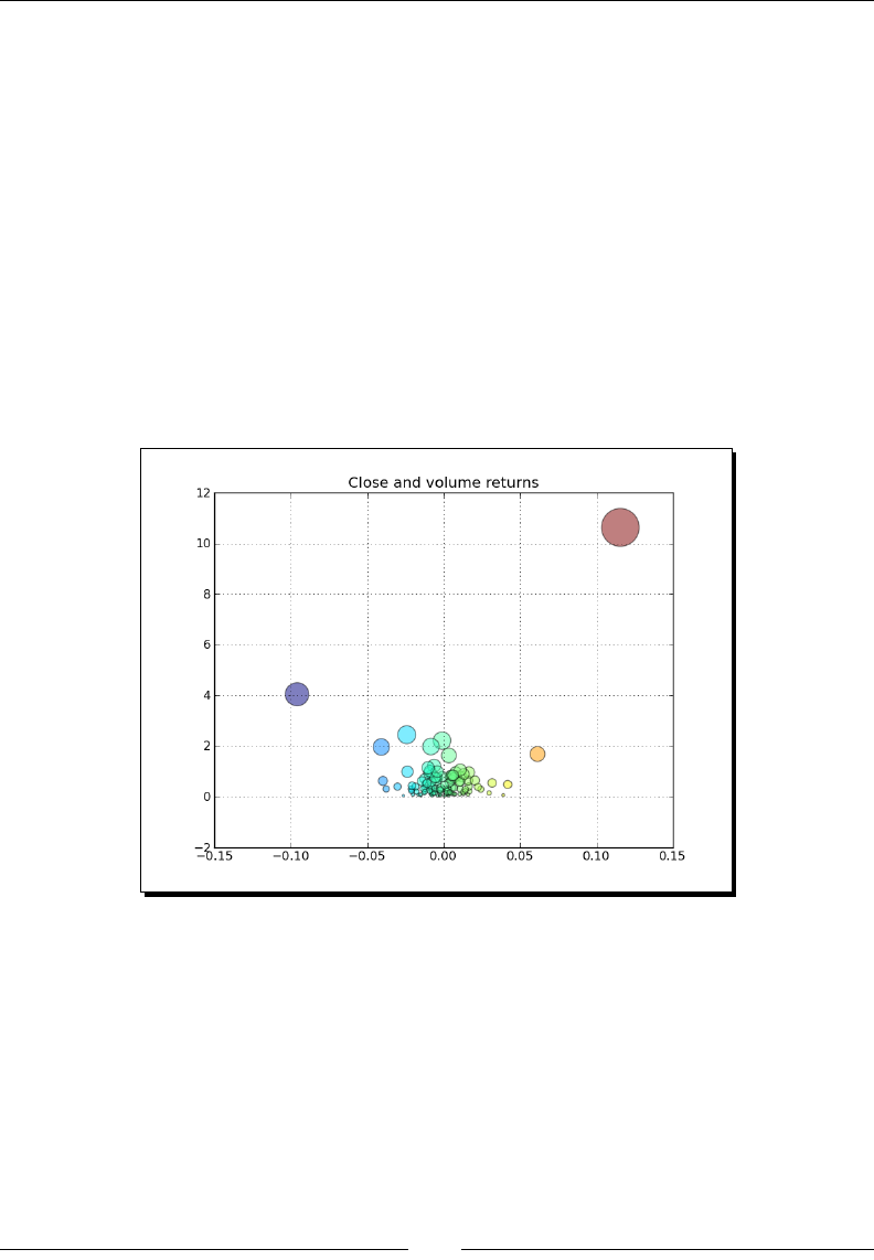
Chapter 9
[ 231 ]
4. Add a subplot to the gure:
ax = fig.add_subplot(111)
5. Create the scaer plot with the color of the data points linked to the close return,
and the size linked to the volume change:
ax.scatter(ret, volchange, c=ret * 100,
s=volchange * 100, alpha=0.5)
6. Set the tle of the plot and put a grid on it:
ax.set_title('Close and volume returns')
ax.grid(True)
plt.show()
The scaer plot for DISH appears as follows:
What just happened?
We made a scaer plot of the close price and volume returns for DISH
(see scatterprice.py):
from matplotlib.finance import quotes_historical_yahoo
import sys
from datetime import date
import matplotlib.pyplot as plt
import numpy as np

Plong with matplotlib
[ 232 ]
today = date.today()
start = (today.year - 1, today.month, today.day)
symbol = 'DISH'
if len(sys.argv) == 2:
symbol = sys.argv[1]
quotes = quotes_historical_yahoo(symbol, start, today)
quotes = np.array(quotes)
close = quotes.T[4]
volume = quotes.T[5]
ret = np.diff(close)/close[:-1]
volchange = np.diff(volume)/volume[:-1]
fig = plt.figure()
ax = fig.add_subplot(111)
ax.scatter(ret, volchange, c=ret * 100, s=volchange * 100, alpha=0.5)
ax.set_title('Close and volume returns')
ax.grid(True)
plt.show()
Fill between
The fill_between() funcon lls a plot region with a specied color. We can choose an
oponal alpha channel value. The funcon also has a where parameter so that we can shade
a region based on a condion.
Time for action – shading plot regions based on a condition
Imagine that you want to shade a region of a stock chart, where the closing price is below
average, with a dierent color than when it is above the mean. The fill_between()
funcon is the best choice for the job. We will, again, omit the steps of downloading
historical data going back one year, extracng dates and close prices, and creang locators
and date formaer.
1. Create a matplotlib Figure object:
fig = plt.figure()
2. Add a subplot to the gure:
ax = fig.add_subplot(111)
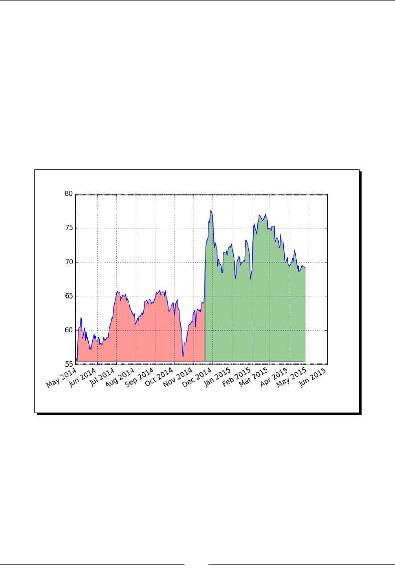
Chapter 9
[ 233 ]
3. Plot the closing price:
ax.plot(dates, close)
4. Shade the regions of the plot below the closing price using dierent colors
depending on whether the values are below or above the average price:
plt.fill_between(dates, close.min(), close,
where=close>close.mean(), facecolor="green", alpha=0.4)
plt.fill_between(dates, close.min(), close,
where=close<close.mean(), facecolor="red", alpha=0.4)
Now we can nish the plot as shown by seng locators and formang the x axis
values as dates. The stock price using condional shading for DISH is as follows:
What just happened?
We shaded the region of a stock chart, where the closing price is below average, with
a dierent color than when it is above the mean (see fillbetween.py):
from matplotlib.finance import quotes_historical_yahoo
from matplotlib.dates import DateFormatter
from matplotlib.dates import DayLocator
from matplotlib.dates import MonthLocator
import sys

Plong with matplotlib
[ 234 ]
from datetime import date
import matplotlib.pyplot as plt
import numpy as np
today = date.today()
start = (today.year - 1, today.month, today.day)
symbol = 'DISH'
if len(sys.argv) == 2:
symbol = sys.argv[1]
quotes = quotes_historical_yahoo(symbol, start, today)
quotes = np.array(quotes)
dates = quotes.T[0]
close = quotes.T[4]
alldays = DayLocator()
months = MonthLocator()
month_formatter = DateFormatter("%b %Y")
fig = plt.figure()
ax = fig.add_subplot(111)
ax.plot(dates, close)
plt.fill_between(dates, close.min(), close, where=close>close.mean(),
facecolor="green", alpha=0.4)
plt.fill_between(dates, close.min(), close, where=close<close.mean(),
facecolor="red", alpha=0.4)
ax.xaxis.set_major_locator(months)
ax.xaxis.set_minor_locator(alldays)
ax.xaxis.set_major_formatter(month_formatter)
ax.grid(True)
fig.autofmt_xdate()
plt.show()
Legend and annotations
Legends and annotaons are essenal for good plots. We can create transparent legends
with the legend() funcon and let matplotlib gure out where to place them. Also, with
the annotate() funcon, we can accurately annotate on a plot. There are a large number
of annotaon and arrow styles.

Chapter 9
[ 235 ]
Time for action – using a legend and annotations
In Chapter 3, Geng Familiar with Commonly Used Funcons, we learned how to calculate
the EMA of stock prices. We will plot the close price of a stock and three of its EMA. To
clarify the plot, we will add a legend. We will also indicate crossovers of two of the averages
with annotaons. Some steps are again omied to avoid repeon.
1. Go back to Chapter 3, Geng Familiar with Commonly Used Funcons, if needed,
and review the EMA algorithm. Calculate and plot the EMAs of 9, 12, and 15 periods:
emas = []
for i in range(9, 18, 3):
weights = np.exp(np.linspace(-1., 0., i))
weights /= weights.sum()
ema = np.convolve(weights, close)[i-1:-i+1]
idx = (i - 6)/3
ax.plot(dates[i-1:], ema, lw=idx, label="EMA(%s)" % (i))
data = np.column_stack((dates[i-1:], ema))
emas.append(np.rec.fromrecords(
data, names=["dates", "ema"]))
Noce that the plot() funcon call needs a label for the legend. We stored the
moving averages in record arrays for the next step.
2. Let's nd the crossover points of the rst two moving averages:
first = emas[0]["ema"].flatten()
second = emas[1]["ema"].flatten()
bools = np.abs(first[-len(second):] - second)/second < 0.0001
xpoints = np.compress(bools, emas[1])
3. Now that we have the crossover points, annotate them with arrows. Make sure that
the annotaon text is slightly away from the crossover points:
for xpoint in xpoints:
ax.annotate('x', xy=xpoint, textcoords='offset points',
xytext=(-50, 30),
arrowprops=dict(arrowstyle="->"))
4. Add a legend and let matplotlib decide where to put it:
leg = ax.legend(loc='best', fancybox=True))
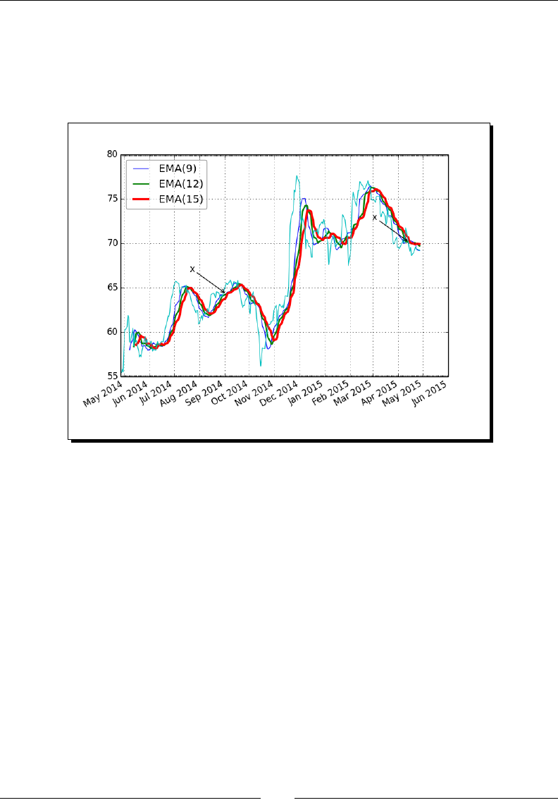
Plong with matplotlib
[ 236 ]
5. Make the legend transparent by seng the alpha channel value:
leg.get_frame().set_alpha(0.5)
The stock price and moving averages with a legend and annotaons appears
as follows:
What just happened?
We ploed the close price of a stock and three of its EMAs. We added a legend to the
plot. We annotated the crossover points of the rst two averages with annotaons
(see emalegend.py):
from matplotlib.finance import quotes_historical_yahoo
from matplotlib.dates import DateFormatter
from matplotlib.dates import DayLocator
from matplotlib.dates import MonthLocator
import sys
from datetime import date
import matplotlib.pyplot as plt
import numpy as np
today = date.today()
start = (today.year - 1, today.month, today.day)

Chapter 9
[ 237 ]
symbol = 'DISH'
if len(sys.argv) == 2:
symbol = sys.argv[1]
quotes = quotes_historical_yahoo(symbol, start, today)
quotes = np.array(quotes)
dates = quotes.T[0]
close = quotes.T[4]
fig = plt.figure()
ax = fig.add_subplot(111)
emas = []
for i in range(9, 18, 3):
weights = np.exp(np.linspace(-1., 0., i))
weights /= weights.sum()
ema = np.convolve(weights, close)[i-1:-i+1]
idx = (i - 6)/3
ax.plot(dates[i-1:], ema, lw=idx, label="EMA(%s)" % (i))
data = np.column_stack((dates[i-1:], ema))
emas.append(np.rec.fromrecords(data, names=["dates", "ema"]))
first = emas[0]["ema"].flatten()
second = emas[1]["ema"].flatten()
bools = np.abs(first[-len(second):] - second)/second < 0.0001
xpoints = np.compress(bools, emas[1])
for xpoint in xpoints:
ax.annotate('x', xy=xpoint, textcoords='offset points',
xytext=(-50, 30),
arrowprops=dict(arrowstyle="->"))
leg = ax.legend(loc='best', fancybox=True)
leg.get_frame().set_alpha(0.5)
alldays = DayLocator()
months = MonthLocator()
month_formatter = DateFormatter("%b %Y")
ax.plot(dates, close, lw=1.0, label="Close")
ax.xaxis.set_major_locator(months)
ax.xaxis.set_minor_locator(alldays)

Plong with matplotlib
[ 238 ]
ax.xaxis.set_major_formatter(month_formatter)
ax.grid(True)
fig.autofmt_xdate()
plt.show()
Three-dimensional plots
Three-dimensional plots are prey spectacular, so we have to cover them here too. For
three-dimensional plots, we need an Axes3D object associated with a 3D projecon.
Time for action – plotting in three dimensions
We will plot a simple three-dimensional funcon:
2 2
z x y= +
1. Use the 3D keyword to specify a three-dimensional projecon for the plot:
ax = fig.add_subplot(111, projection='3d')
2. To create a square two-dimensional grid, use the meshgrid() funcon to inialize
the x and y values:
u = np.linspace(-1, 1, 100)
x, y = np.meshgrid(u, u)
3. We will specify the row strides, column strides, and the color map for the surface
plot. The strides determine the size of the les in the surface. The choice for color
map is a maer of taste:
ax.plot_surface(x, y, z, rstride=4, cstride=4,
cmap=cm.YlGnBu_r)
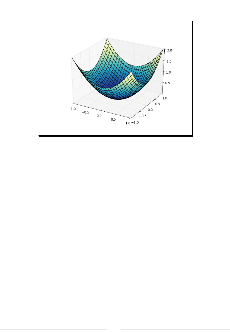
Chapter 9
[ 239 ]
The result is the following three-dimensional plot:
What just happened?
We created a plot of a three-dimensional funcon (see three_d.py):
from mpl_toolkits.mplot3d import Axes3D
import matplotlib.pyplot as plt
import numpy as np
from matplotlib import cm
fig = plt.figure()
ax = fig.add_subplot(111, projection='3d')
u = np.linspace(-1, 1, 100)
x, y = np.meshgrid(u, u)
z = x ** 2 + y ** 2
ax.plot_surface(x, y, z, rstride=4,
cstride=4, cmap=cm.YlGnBu_r)
plt.show()
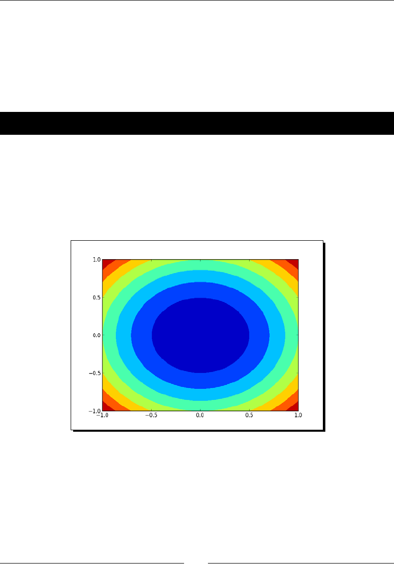
Plong with matplotlib
[ 240 ]
Contour plots
matplotlib contour three-dimensional plots come in two avors—lled and unlled.
Contour plots use the so-called contour lines. You may be familiar with contour lines from
geographic maps. In such maps, contour lines connect points of the same elevaon above
sea level. We can create normal contour plots with the contour() funcon. For lled
contour plots, we use the contourf() funcon.
Time for action – drawing a lled contour plot
We will draw a lled contour plot of the three-dimensional mathemacal funcon in the
previous Time for acon secon. The code is also prey similar. One key dierence is that we
don't need the 3D projecon parameter any more. To draw the lled contour plot, use the
following line of code:
ax.contourf(x, y, z)
This gives us the following lled contour plot:
What just happened?
We created a lled contour plot of a three-dimensional mathemacal funcon (see
contour.py):
import matplotlib.pyplot as plt
import numpy as np
from matplotlib import cm

Chapter 9
[ 241 ]
fig = plt.figure()
ax = fig.add_subplot(111)
u = np.linspace(-1, 1, 100)
x, y = np.meshgrid(u, u)
z = x ** 2 + y ** 2
ax.contourf(x, y, z)
plt.show()
Animation
matplotlib oers fancy animaon capabilies via a special animaon module. We need
to dene a callback funcon that is used to regularly update the screen. We also need a
funcon to generate data to be ploed.
Time for action – animating plots
We will plot three random datasets and display them as circles, dots, and triangles. However,
we will only update two of those datasets with random values.
1. Plot three random datasets as circles, dots, and triangles in dierent colors:
circles, triangles, dots = ax.plot(x, 'ro', y, 'g^', z, 'b.')
2. This funcon gets called to update the screen regularly. Update two of the plots with
new y values:
def update(data):
circles.set_ydata(data[0])
triangles.set_ydata(data[1])
return circles, triangles
3. Generate random data with NumPy:
def generate():
while True: yield np.random.rand(2, N)
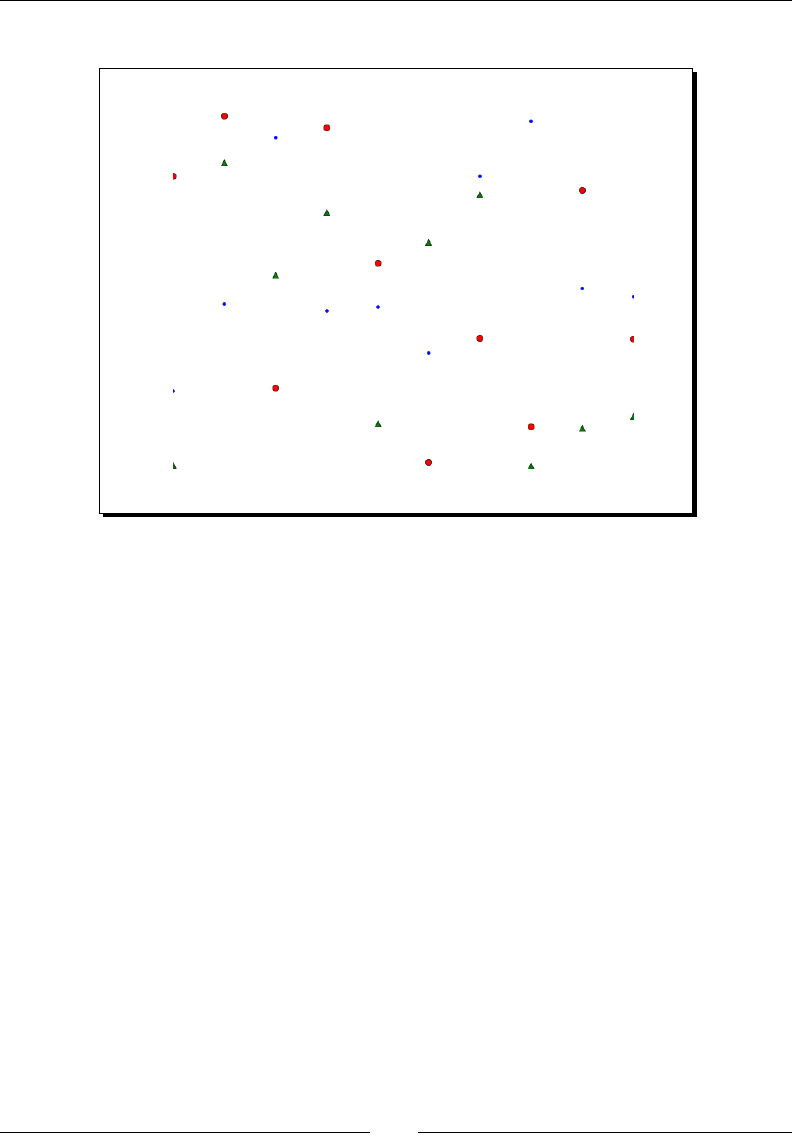
Plong with matplotlib
[ 242 ]
The following is a snapshot of the animaon in acon:
What just happened?
We created an animaon of random data points (see animation.py):
import numpy as np
import matplotlib.pyplot as plt
import matplotlib.animation as animation
fig = plt.figure()
ax = fig.add_subplot(111)
N = 10
x = np.random.rand(N)
y = np.random.rand(N)
z = np.random.rand(N)
circles, triangles, dots = ax.plot(x, 'ro', y, 'g^', z, 'b.')
ax.set_ylim(0, 1)
plt.axis('off')
def update(data):
circles.set_ydata(data[0])
triangles.set_ydata(data[1])
return circles, triangles

Chapter 9
[ 243 ]
def generate():
while True: yield np.random.rand(2, N)
anim = animation.FuncAnimation(fig, update,
generate, interval=150)
plt.show()
Summary
This chapter was about matplotlib—a Python plong library. We covered simple plots,
histograms, plot customizaon, subplots, three-dimensional plots, contour plots, and
logarithmic plots. You also saw a few examples of displaying stock charts. Obviously, we
only scratched the surface and just saw the p of the iceberg. matplotlib is very feature
rich, so we didn't have space to cover Latex support, polar coordinates support, and other
funconality.
The author of matplotlib, John Hunter, passed away in August 2012. One of the technical
reviewers of this book suggested menoning the John Hunter Memorial Fund (http://
numfocus.org/news/2012/08/28/johnhunter/). The memorial fund set up by the
NumFocus Foundaon is an opportunity for us, fans of John Hunter's work, to "give back".
Again, for more details, check out the preceding link to the NumFocus website.
The next chapter is about SciPy—a scienc Python framework that is built on top of NumPy.

[ 245 ]
When NumPy Is Not Enough – SciPy
and Beyond
SciPy is a world famous Python open source scientific computing library
built on top of NumPy. It adds functionalitties such as numerical integration,
optimization, statistics, and special functions.
In this chapter, we will cover the following topics:
File I/O
Stascs
Signal processing
Opmizaon
Interpolaon
Image and audio processing
MATLAB and Octave
MATLAB and its open source alternave, Octave, are popular mathemacal programs. The
scipy.io package has funcons that let you load MATLAB or Octave matrices and arrays
of numbers or strings in Python programs, and vice versa. The loadmat() funcon loads a
.mat le. The savemat() funcon saves a diconary of names and arrays into a .mat le.
10

When NumPy Is Not Enough – SciPy and Beyond
[ 246 ]
Time for action – saving and loading a .mat le
If we start with NumPy arrays and decide to use said arrays within a MATLAB or Octave
environment, the easiest thing to do is create a .mat le. We can, then, load the le within
MATLAB or Octave. Let's go through the necessary steps:
1. Create a NumPy array and call the savemat() funcon to create a .mat le. This
funcon has two parameters: a le name and a diconary containing variable names
and values:
a = np.arange(7)
io.savemat("a.mat", {"array": a})
2. Within a MATLAB or Octave environment, load the .mat le and check the
stored array:
octave-3.4.0:7> load a.mat
octave-3.4.0:8> a
octave-3.4.0:8> array
array =
0
1
2
3
4
5
6
What just happened?
We created a .mat le from NumPy code and loaded it within Octave. We checked the
NumPy array that was created (see scipyio.py):
import numpy as np
from scipy import io
a = np.arange(7)
io.savemat("a.mat", {"array": a})

Chapter 10
[ 247 ]
Pop quiz – loading .mat les
Q1. Which funcon loads .mat les?
1. Loadmatlab
2. loadmat
3. loadoct
4. frommat
Statistics
The SciPy stascs module is called scipy.stats. There is one class that implements
connuous distribuons and one class that implements discrete distribuons. Also, in this
module, funcons that perform a great number of stascal tests can be found.
Time for action – analyzing random values
We will generate random values that mimic a normal distribuon and analyze the generated
data with stascal funcons from the scipy.stats package.
1. Generate random values from a normal distribuon using the scipy.stats package:
generated = stats.norm.rvs(size=900)
2. Fit the generated values to a normal distribuon. This basically gives the mean and
standard deviaon of the dataset:
print("Mean", "Std", stats.norm.fit(generated))
The mean and standard deviaon appear as follows:
Mean Std (0.0071293257063200707, 0.95537708218972528)
3. Skewness tells us how skewed (asymmetric) a probability distribuon is (see
http://en.wikipedia.org/wiki/Skewness). Perform a skewness test. This
test returns two values. The second value is the p-value—the probability that the
skewness of the dataset does not correspond to a normal distribuon.
Generally speaking, the p-value is the probability of an outcome
different than what was expected given the null hypothesis—in this
case, the probability of getting a skewness different from that of a
normal distribution (which is 0 because of symmetry).
P-values range from 0 to 1:
print("Skewtest", "pvalue", stats.skewtest(generated))

When NumPy Is Not Enough – SciPy and Beyond
[ 248 ]
The result of the skewness test appears as follows:
Skewtest pvalue (-0.62120640688766893, 0.5344638245033837)
So, there is a 53 percent chance we are not dealing with a normal distribuon. It is
instrucve to see what happens if we generate more points, because if we generate
more points, we should have a more normal distribuon. For 900,000 points, we get
a p-value of 0.16. For 20 generated values, the p-value is 0.50.
4. Kurtosis tells us how curved a probability distribuon is. Perform a kurtosis test. This
test is set up similarly to the skewness test, but, of course, applies to kurtosis:
print("Kurtosistest", "pvalue",
stats.kurtosistest(generated))
The result of the kurtosis test appears as follows:
Kurtosistest pvalue (1.3065381019536981, 0.19136963054975586)
The p-value for 900,000 values is 0.028. For 20 generated values, the p-values
is 0.88.
5. A normality test tells us how likely it is that a dataset complies the normal
distribuon. Perform a normality test. This test also returns two values,
of which the second is a p-value:
print("Normaltest", "pvalue", stats.normaltest(generated))
The result of the normality test appears as follows:
Normaltest pvalue (2.09293921181506, 0.35117535059841687)
The p-value for 900,000 generated values is 0.035. For 20 generated values,
the p-value is 0.79.
6. We can nd the value at a certain percenle easily with SciPy:
print("95 percentile",
stats.scoreatpercentile(generated, 95))
The value at the 95th percenle appears as follows:
95 percentile 1.54048860252
7. Do the opposite of the previous step to nd the percenle at 1:
print("Percentile at 1",
stats.percentileofscore(generated, 1))
The percenle at 1 appears as follows:
Percentile at 1 85.5555555556
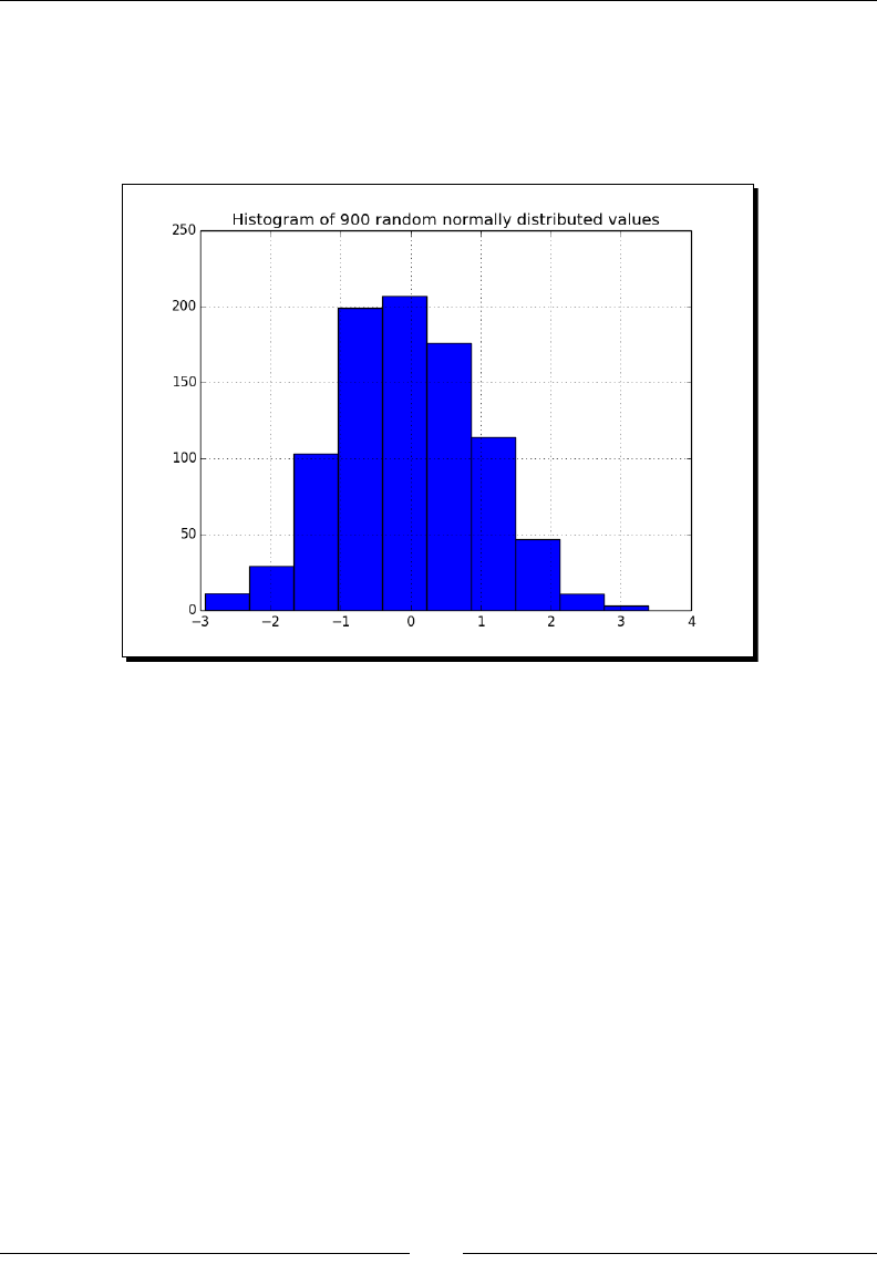
Chapter 10
[ 249 ]
8. Plot the generated values in a histogram with matplotlib (more informaon about
matplotlib can be found in the previous Chapter 9, Plong with matplotlib):
plt.hist(generated)
The histogram of the generated random values is as follows:
What just happened?
We created a dataset from a normal distribuon and analyzed it with the scipy.stats
module (see statistics.py):
from __future__ import print_function
from scipy import stats
import matplotlib.pyplot as plt
generated = stats.norm.rvs(size=900)
print("Mean", "Std", stats.norm.fit(generated))
print("Skewtest", "pvalue", stats.skewtest(generated))
print("Kurtosistest", "pvalue", stats.kurtosistest(generated))
print("Normaltest", "pvalue", stats.normaltest(generated))
print("95 percentile", stats.scoreatpercentile(generated, 95))
print("Percentile at 1", stats.percentileofscore(generated, 1))
plt.title('Histogram of 900 random normally distributed values')
plt.hist(generated)
plt.grid()
plt.show()

When NumPy Is Not Enough – SciPy and Beyond
[ 250 ]
Have a go hero – improving the data generation
Judging from the histogram in the previous Time for acon secon, there is room for
improvement when it comes to generang the data. Try using NumPy or dierent
parameters of the scipy.stats.norm.rvs() funcon.
Sample comparison and SciKits
Oen we have two data samples, maybe from dierent experiments, that are somehow
related. Stascal tests exist that can compare the samples. Some of these are implemented
in the scipy.stats module.
Another stascal test that I like is the Jarque–Bera normality test from scikits.
statsmodels.stattools. SciKits are small experimental Python soware toolkits. They
are not part of SciPy. There is also pandas, which is an oshoot of scikits.statsmodels.
A list of SciKits can be found at https://scikits.appspot.com/scikits. You can
install statsmodels using setuptools with:
$ [sudo] easy_install statsmodels
Time for action – comparing stock log returns
We will download the stock quotes for the last year of two trackers using matplotlib. As
menoned in the previous Chapter 9, Plong with matplotlib, we can retrieve quotes from
Yahoo Finance. We will compare the log returns of the close price of DIA and SPY (DIA tracks
the Dow Jones index; SPY tracks the S & P 500 index). We will also perform the Jarque–Bera
test on the dierence of the log returns.
1. Write a funcon that can return the close price for a specied stock:
def get_close(symbol):
today = date.today()
start = (today.year - 1, today.month, today.day)
quotes = quotes_historical_yahoo(symbol, start, today)
quotes = np.array(quotes)
return quotes.T[4]
2. Calculate the log returns for DIA and SPY. Compute the log returns by taking the
natural logarithm of the close price and then taking the dierence of consecuve
values:
spy = np.diff(np.log(get_close("SPY")))
dia = np.diff(np.log(get_close("DIA")))

Chapter 10
[ 251 ]
3. The means comparison test checks whether two dierent samples could have the
same mean value. Two values are returned, of which the second is the p-value from
0 to 1:
print("Means comparison", stats.ttest_ind(spy, dia))
The result of the means comparison test appears as follows:
Means comparison (-0.017995865641886155, 0.98564930169871368)
So, there is about a 98 percent chance that the two samples have the same mean
log return. Actually, the documentaon has the following to say:
If we observe a large p-value, for example, larger than 0.05 or 0.1,
then we cannot reject the null hypothesis of identical average
scores. If the p-value is smaller than the threshold, e.g. 1%, 5% or
10%, then we reject the null hypothesis of equal averages.
4. The Kolmogorov–Smirnov two samples test tells us how likely it is that two samples
are drawn from the same distribuon:
print("Kolmogorov smirnov test", stats.ks_2samp(spy, dia))
Again, two values are returned, of which the second value is the p-value:
Kolmogorov smirnov test (0.063492063492063516,
0.67615647616238039)
5. Unleash the Jarque–Bera normality test on the dierence of the log returns:
print("Jarque Bera test",
jarque_bera(spy – dia)[1])
The p-value of the Jarque–Bera normality test appears as follows:
Jarque Bera test 0.596125711042
6. Plot the histograms of the log returns and the dierence thereof with matplotlib:
plt.hist(spy, histtype="step", lw=1, label="SPY")
plt.hist(dia, histtype="step", lw=2, label="DIA")
plt.hist(spy - dia, histtype="step", lw=3,
label="Delta")
plt.legend()
plt.show()
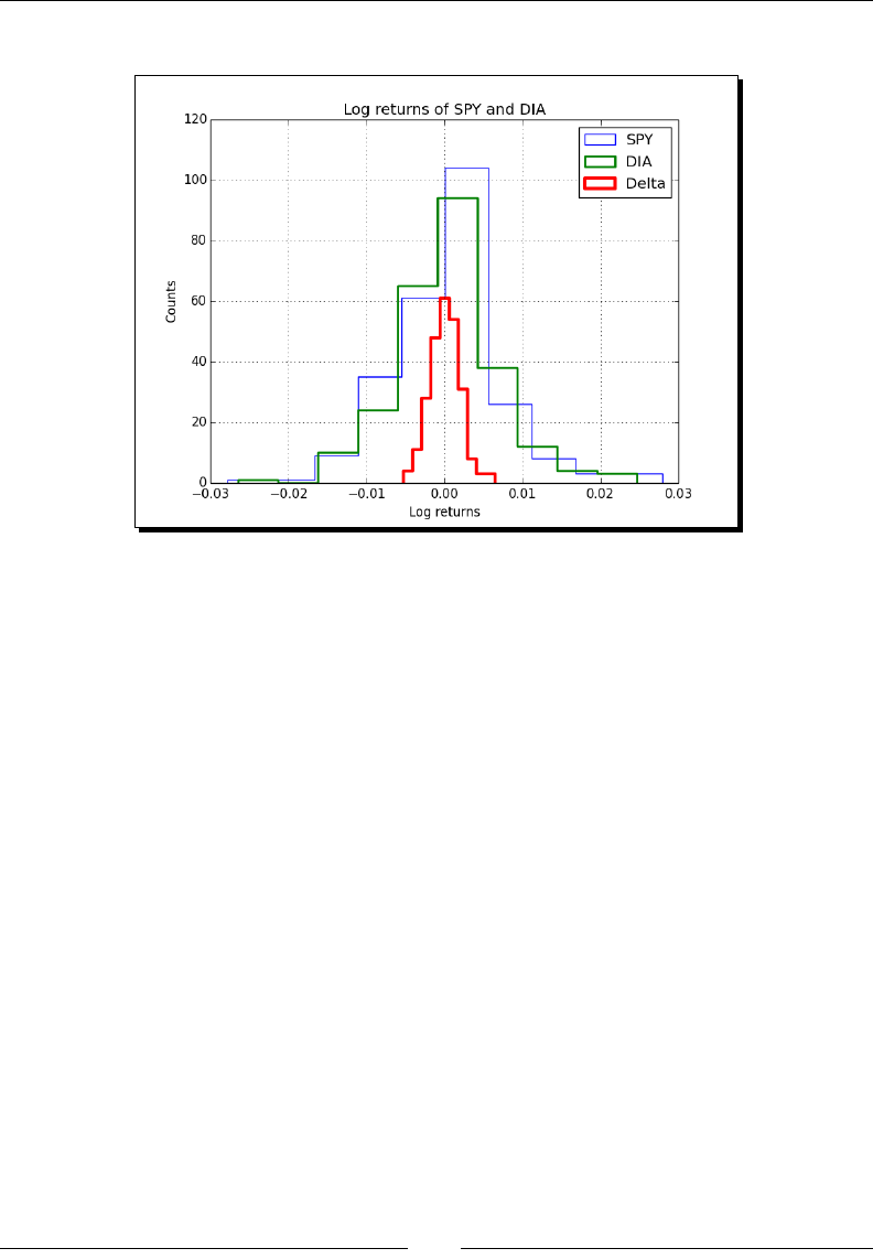
When NumPy Is Not Enough – SciPy and Beyond
[ 252 ]
The histograms of the log returns and dierence are shown as follows:
What just happened?
We compared samples of log returns for DIA and SPY. Also, we performed the Jarque-Bera
test on the dierence of the log returns (see pair.py):
from __future__ import print_function
from matplotlib.finance import quotes_historical_yahoo
from datetime import date
import numpy as np
from scipy import stats
from statsmodels.stats.stattools import jarque_bera
import matplotlib.pyplot as plt
def get_close(symbol):
today = date.today()
start = (today.year - 1, today.month, today.day)
quotes = quotes_historical_yahoo(symbol, start, today)
quotes = np.array(quotes)
return quotes.T[4]
spy = np.diff(np.log(get_close("SPY")))
dia = np.diff(np.log(get_close("DIA")))

Chapter 10
[ 253 ]
print("Means comparison", stats.ttest_ind(spy, dia))
print("Kolmogorov smirnov test", stats.ks_2samp(spy, dia))
print("Jarque Bera test", jarque_bera(spy - dia)[1])
plt.title('Log returns of SPY and DIA')
plt.hist(spy, histtype="step", lw=1, label="SPY")
plt.hist(dia, histtype="step", lw=2, label="DIA")
plt.hist(spy - dia, histtype="step", lw=3, label="Delta")
plt.xlabel('Log returns')
plt.ylabel('Counts')
plt.grid()
plt.legend(loc='best')
plt.show()
Signal processing
The scipy.signal module contains lter funcons and B-spline interpolaon algorithms.
Spline interpolaon uses a polynomial called a spline for interpolaon (see
http://en.wikipedia.org/wiki/Spline_interpolation).
The interpolaon then tries to glue splines together to t the data. B-spline
is a type of spline.
A SciPy signal is dened as an array of numbers. An example of a lter is the detrend()
funcon. This funcon takes a signal and does a linear t on it. This trend is then subtracted
from the original input data.
Time for action – detecting a trend in QQQ
Oen we are more interested in the trend of a data sample than in detrending it. We can sll
get the trend back easily aer detrending. Let's do that for one year of price data for QQQ.
1. Write code that gets the close price and corresponding dates for QQQ:
today = date.today()
start = (today.year - 1, today.month, today.day)
quotes = quotes_historical_yahoo("QQQ", start, today)
quotes = np.array(quotes)
dates = quotes.T[0]
qqq = quotes.T[4]
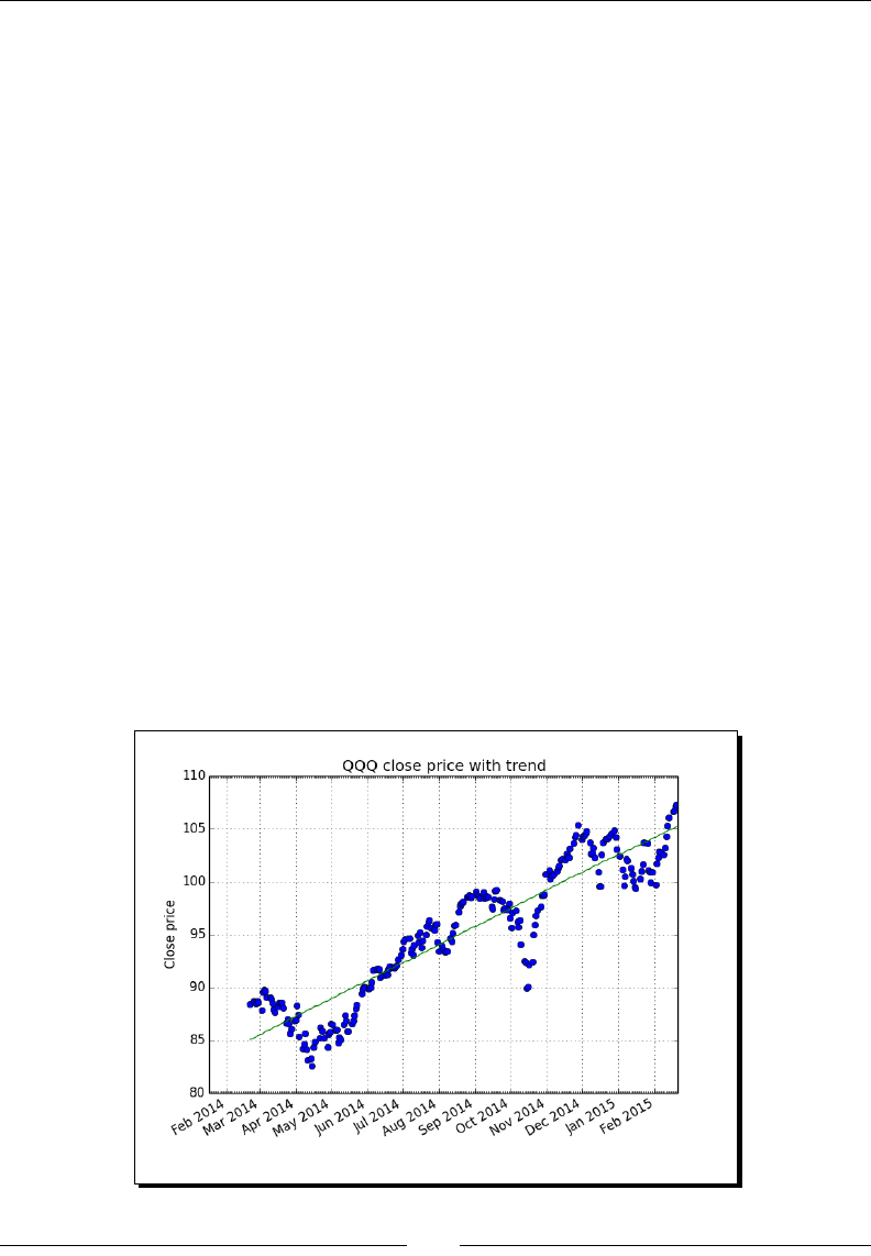
When NumPy Is Not Enough – SciPy and Beyond
[ 254 ]
2. Detrend the signal:
y = signal.detrend(qqq)
3. Create month and day locators for the dates:
alldays = DayLocator()
months = MonthLocator()
4. Create a date formaer that creates a string of month name and year:
month_formatter = DateFormatter("%b %Y")
5. Create a gure and subplot:
fig = plt.figure()
ax = fig.add_subplot(111)
6. Plot the data and underlying trend by subtracng the detrended signal:
plt.plot(dates, qqq, 'o', dates, qqq - y, '-')
7. Set the locators and formaer:
ax.xaxis.set_minor_locator(alldays)
ax.xaxis.set_major_locator(months)
ax.xaxis.set_major_formatter(month_formatter)
8. Format the x-axis labels as dates:
fig.autofmt_xdate()
plt.show()
The following gure shows the QQQ prices with a trend line:

Chapter 10
[ 255 ]
What just happened?
We ploed the closing price for QQQ with a trend line (see trend.py):
from matplotlib.finance import quotes_historical_yahoo
from datetime import date
import numpy as np
from scipy import signal
import matplotlib.pyplot as plt
from matplotlib.dates import DateFormatter
from matplotlib.dates import DayLocator
from matplotlib.dates import MonthLocator
today = date.today()
start = (today.year - 1, today.month, today.day)
quotes = quotes_historical_yahoo("QQQ", start, today)
quotes = np.array(quotes)
dates = quotes.T[0]
qqq = quotes.T[4]
y = signal.detrend(qqq)
alldays = DayLocator()
months = MonthLocator()
month_formatter = DateFormatter("%b %Y")
fig = plt.figure()
ax = fig.add_subplot(111)
plt.title('QQQ close price with trend')
plt.ylabel('Close price')
plt.plot(dates, qqq, 'o', dates, qqq - y, '-')
ax.xaxis.set_minor_locator(alldays)
ax.xaxis.set_major_locator(months)
ax.xaxis.set_major_formatter(month_formatter)
fig.autofmt_xdate()
plt.grid()
plt.show()

When NumPy Is Not Enough – SciPy and Beyond
[ 256 ]
Fourier analysis
Signals in the real world oen have a periodic nature. A commonly used tool to deal
with these signals is the Discrete Fourier transform (see https://en.wikipedia.
org/wiki/Discrete-time_Fourier_transform). The Discrete Fourier transform
is a transformaon from the me domain into the frequency domain, that is, the linear
decomposion of a periodic signal into sine and cosine funcons with various frequencies:
Funcons for Fourier transforms can be found in the scipy.fftpack module (NumPy
also has its own Fourier package numpy.fft). Included in the package are Fast Fourier
transforms, dierenal and pseudo-dierenal operators, as well as several helper funcons.
MATLAB users will be pleased to know that a number of funcons in the scipy.fftpack
module have the same name as their MATLAB counterparts, and a similar funcon as their
MATLAB equivalents.
Time for action – ltering a detrended signal
We learned in the previous Time for acon secon how to detrend a signal. This detrended
signal could have a cyclical component. Let's try to visualize this. Some of the steps are a
repeon of steps in the previous Time for acon secon, such as downloading the data and
seng up matplotlib objects. These steps are omied here.
1. Apply the Fourier transform, giving us the frequency spectrum:
amps = np.abs(fftpack.fftshift(fftpack.rfft(y)))
2. Filter out the noise. Let's say, if the magnitude of a frequency component is below
10 percent of the strongest component, throw it out:
amps[amps < 0.1 * amps.max()] = 0
3. Transform the ltered signal back to the original domain and plot it together with
the detrended signal:
plt.plot(dates, y, 'o', label="detrended")
plt.plot(dates,
-fftpack.irfft(fftpack.ifftshift(amps)),
label="filtered")
4. Format the x-axis labels as dates and add a legend with extra large size:
fig.autofmt_xdate()
plt.legend(prop={'size':'x-large'})
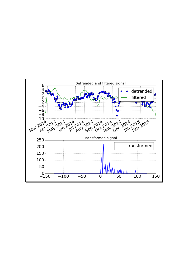
Chapter 10
[ 257 ]
5. Add a second subplot and plot the frequency spectrum aer ltering:
ax2 = fig.add_subplot(212)
N = len(qqq)
plt.plot(np.linspace(-N/2, N/2, N), amps,
label="transformed")
6. Display the legend and plot:
plt.legend(prop={'size':'x-large'})
plt.show()
The following plots are of the signal and frequency spectrum:
What just happened?
We detrended a signal and applied a simple lter on it using the scipy.fftpack module
(see frequencies.py):
from matplotlib.finance import quotes_historical_yahoo
from datetime import date
import numpy as np
from scipy import signal
import matplotlib.pyplot as plt
from scipy import fftpack
from matplotlib.dates import DateFormatter

When NumPy Is Not Enough – SciPy and Beyond
[ 258 ]
from matplotlib.dates import DayLocator
from matplotlib.dates import MonthLocator
today = date.today()
start = (today.year - 1, today.month, today.day)
quotes = quotes_historical_yahoo("QQQ", start, today)
quotes = np.array(quotes)
dates = quotes.T[0]
qqq = quotes.T[4]
y = signal.detrend(qqq)
alldays = DayLocator()
months = MonthLocator()
month_formatter = DateFormatter("%b %Y")
fig = plt.figure()
fig.subplots_adjust(hspace=.3)
ax = fig.add_subplot(211)
ax.xaxis.set_minor_locator(alldays)
ax.xaxis.set_major_locator(months)
ax.xaxis.set_major_formatter(month_formatter)
# make font size bigger
ax.tick_params(axis='both', which='major', labelsize='x-large')
amps = np.abs(fftpack.fftshift(fftpack.rfft(y)))
amps[amps < 0.1 * amps.max()] = 0
plt.title('Detrended and filtered signal')
plt.plot(dates, y, 'o', label="detrended")
plt.plot(dates, -fftpack.irfft(fftpack.ifftshift(amps)),
label="filtered")
fig.autofmt_xdate()
plt.legend(prop={'size':'x-large'})
plt.grid()

Chapter 10
[ 259 ]
ax2 = fig.add_subplot(212)
plt.title('Transformed signal')
ax2.tick_params(axis='both', which='major', labelsize='x-large')
N = len(qqq)
plt.plot(np.linspace(-N/2, N/2, N), amps, label="transformed")
plt.legend(prop={'size':'x-large'})
plt.grid()
plt.tight_layout()
plt.show()
Mathematical optimization
Opmizaon algorithms try to nd the opmal soluon for a problem, for instance, nding
the maximum or the minimum of a funcon. The funcon can be linear or non-linear. The
soluon could also have special constraints. For example, the soluon may not be allowed
to have negave values. The scipy.optimize module provides several opmizaon
algorithms. One of the algorithms is a least squares ng funcon, leastsq(). When
calling this funcon, we provide a residuals (error terms) funcon. This funcon minimizes
the sum of the squares of the residuals; it corresponds to our mathemacal model for the
soluon. It is also necessary to give the algorithm a starng point. This should be a best
guess—as close as possible to the real soluon. Otherwise, execuon will stop aer about
100 * (N+1) iteraons, where N is the number of parameters to opmize.
Time for action – tting to a sine
In the previous Time for acon secon, we created a simple lter for detrended data. Now,
let's use a more restricve lter that will leave us only with the main frequency component.
We will t a sinusoidal paern to it and plot our results. This model has four parameters—
amplitude, frequency, phase, and vercal oset.
1. Dene a residuals funcon based on a sine wave model:
def residuals(p, y, x):
A,k,theta,b = p
err = y-A * np.sin(2* np.pi* k * x + theta) + b
return err
2. Transform the ltered signal back to the original domain:
filtered = -fftpack.irfft(fftpack.ifftshift(amps))

When NumPy Is Not Enough – SciPy and Beyond
[ 260 ]
3. Guess the values of the parameters of which we are trying to esmate a
transformaon from the me domain into the frequency domain:
N = len(qqq)
f = np.linspace(-N/2, N/2, N)
p0 = [filtered.max(), f[amps.argmax()]/(2*N), 0, 0]
print("P0", p0)
The inial values appear as follows:
P0 [2.6679532410065212, 0.00099598469163686377, 0, 0]
4. Call the leastsq()funcon:
plsq = optimize.leastsq(residuals, p0, args=(filtered,
dates))
p = plsq[0]
print("P", p)
The nal parameter values are as follows:
P [ 2.67678014e+00 2.73033206e-03 -8.00007036e+03
-5.01260321e-03]
5. Finish the rst subplot with detrended data, ltered data, and t of the ltered data.
Use a date format for the horizontal axis and add a legend:
plt.plot(dates, y, 'o', label="detrended")
plt.plot(dates, filtered, label="filtered")
plt.plot(dates, p[0] * np.sin(2 * np.pi *
dates * p[1] + p[2]) + p[3], '^', label="fit")
fig.autofmt_xdate()
plt.legend(prop={'size':'x-large'})
6. Add a second subplot with a legend of the main component of the frequency
spectrum:
ax2 = fig.add_subplot(212)
plt.plot(f, amps, label="transformed")
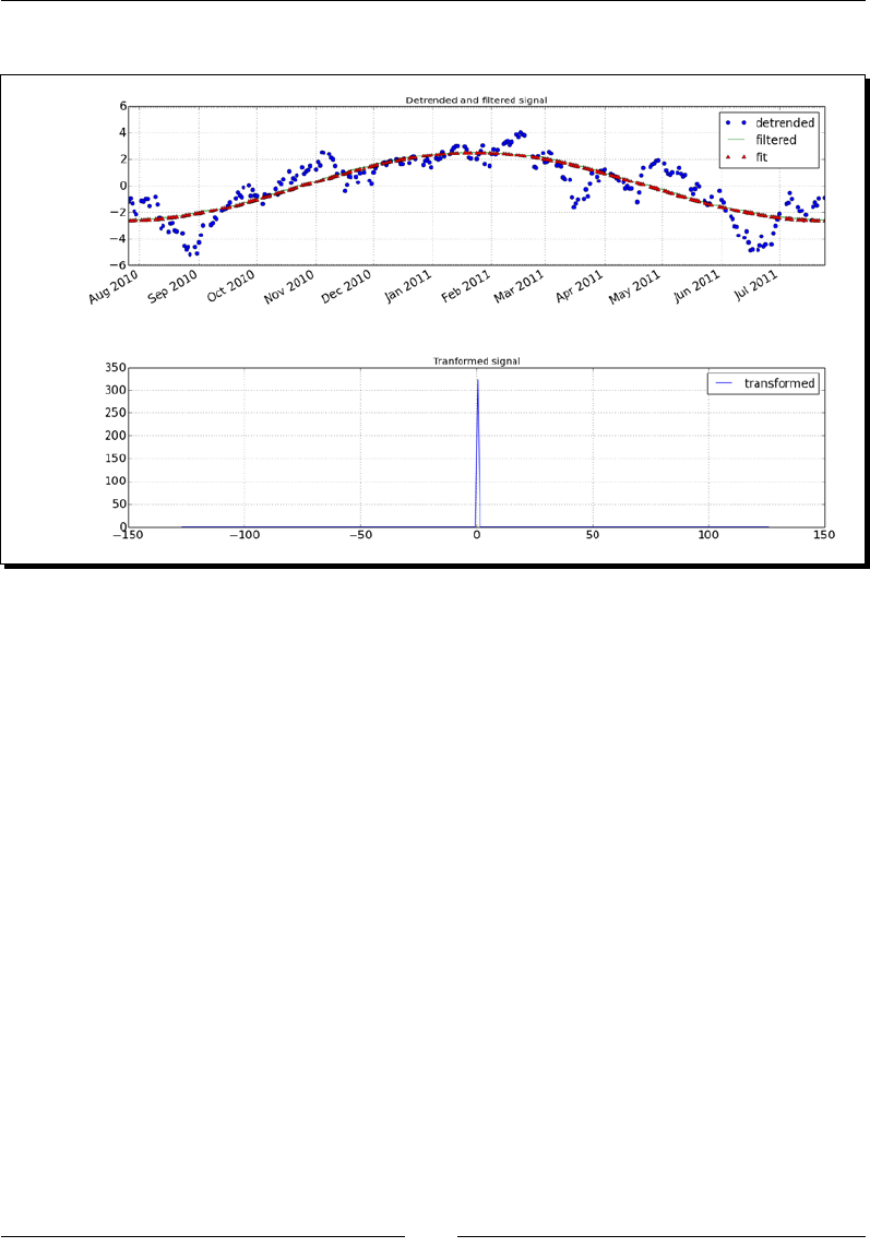
Chapter 10
[ 261 ]
The following are the resulng charts:
What just happened?
We detrended one year of price data for QQQ. This signal was then ltered unl only the
main component of the frequency spectrum was le over. We ed a sine to the ltered
signal using the scipy.optimize module (see optfit.py):
from __future__ import print_function
from matplotlib.finance import quotes_historical_yahoo
import numpy as np
import matplotlib.pyplot as plt
from scipy import fftpack
from scipy import signal
from matplotlib.dates import DateFormatter
from matplotlib.dates import DayLocator
from matplotlib.dates import MonthLocator
from scipy import optimize
start = (2010, 7, 25)
end = (2011, 7, 25)

When NumPy Is Not Enough – SciPy and Beyond
[ 262 ]
quotes = quotes_historical_yahoo("QQQ", start, end)
quotes = np.array(quotes)
dates = quotes.T[0]
qqq = quotes.T[4]
y = signal.detrend(qqq)
alldays = DayLocator()
months = MonthLocator()
month_formatter = DateFormatter("%b %Y")
fig = plt.figure()
fig.subplots_adjust(hspace=.3)
ax = fig.add_subplot(211)
ax.xaxis.set_minor_locator(alldays)
ax.xaxis.set_major_locator(months)
ax.xaxis.set_major_formatter(month_formatter)
ax.tick_params(axis='both', which='major', labelsize='x-large')
amps = np.abs(fftpack.fftshift(fftpack.rfft(y)))
amps[amps < amps.max()] = 0
def residuals(p, y, x):
A,k,theta,b = p
err = y-A * np.sin(2* np.pi* k * x + theta) + b
return err
filtered = -fftpack.irfft(fftpack.ifftshift(amps))
N = len(qqq)
f = np.linspace(-N/2, N/2, N)
p0 = [filtered.max(), f[amps.argmax()]/(2*N), 0, 0]
print("P0", p0)
plsq = optimize.leastsq(residuals, p0, args=(filtered, dates))
p = plsq[0]
print("P", p)
plt.title('Detrended and filtered signal')
plt.plot(dates, y, 'o', label="detrended")
plt.plot(dates, filtered, label="filtered")

Chapter 10
[ 263 ]
plt.plot(dates, p[0] * np.sin(2 * np.pi * dates * p[1] + p[2]) + p[3],
'^', label="fit")
fig.autofmt_xdate()
plt.legend(prop={'size':'x-large'})
plt.grid()
ax2 = fig.add_subplot(212)
plt.title('Tranformed signal')
ax2.tick_params(axis='both', which='major', labelsize='x-large')
plt.plot(f, amps, label="transformed")
plt.legend(prop={'size':'x-large'})
plt.grid()
plt.tight_layout()
plt.show()
Numerical integration
SciPy has a numerical integraon package, scipy.integrate, which has no equivalent
in NumPy. The quad() funcon can integrate a one-variable funcon between two points.
These points can be at innity. The funcon uses the simplest numerical integraon method:
the trapezoid rule.
Time for action – calculating the Gaussian integral
The Gaussian integral is related to the error() funcon (also known in mathemacs as
erf), but has no nite limits. It evaluates to the square root of pi.
Let's calculate the integral with the quad() funcon (for the imports check the le in the
code bundle):
print("Gaussian integral", np.sqrt(np.pi),
integrate.quad(lambda x: np.exp(-x**2),
-np.inf, np.inf))
The return value is the outcome and its error would be as follows:
Gaussian integral 1.77245385091 (1.7724538509055159, 1.4202636780944923e-
08)

When NumPy Is Not Enough – SciPy and Beyond
[ 264 ]
What just happened?
We calculated the Gaussian integral with the quad() funcon.
Have a go hero – experiment a bit more
Try out other integraon funcons from the same package. It should just be a maer
of replacing one funcon call. We should get the same outcome, so you may also want
to read the documentaon to learn more.
Interpolation
Interpolaon lls in the blanks between known data points in a dataset. The scipy.
interpolate() funcon interpolates a funcon based on experimental data. The
interp1d class can create a linear or cubic interpolaon funcon. By default, a linear
interpolaon funcon is constructed, but if the kind parameter is set, a cubic interpolaon
funcon is created instead. The interp2d class works the same way, but in 2D.
Time for action – interpolating in one dimension
We will create data points using a sinc() funcon and add some random noise to it. Aer
this, we will do a linear and cubic interpolaon and plot the results.
1. Create the data points and add noise to it:
x = np.linspace(-18, 18, 36)
noise = 0.1 * np.random.random(len(x))
signal = np.sinc(x) + noise
2. Create a linear interpolaon funcon and apply it to an input array with ve mes as
many data points:
interpreted = interpolate.interp1d(x, signal)
x2 = np.linspace(-18, 18, 180)
y = interpreted(x2)
3. Do the same as in the previous step, but with cubic interpolaon:
cubic = interpolate.interp1d(x, signal, kind="cubic")
y2 = cubic(x2)
4. Plot the results with matplotlib:
plt.plot(x, signal, 'o', label="data")
plt.plot(x2, y, '-', label="linear")
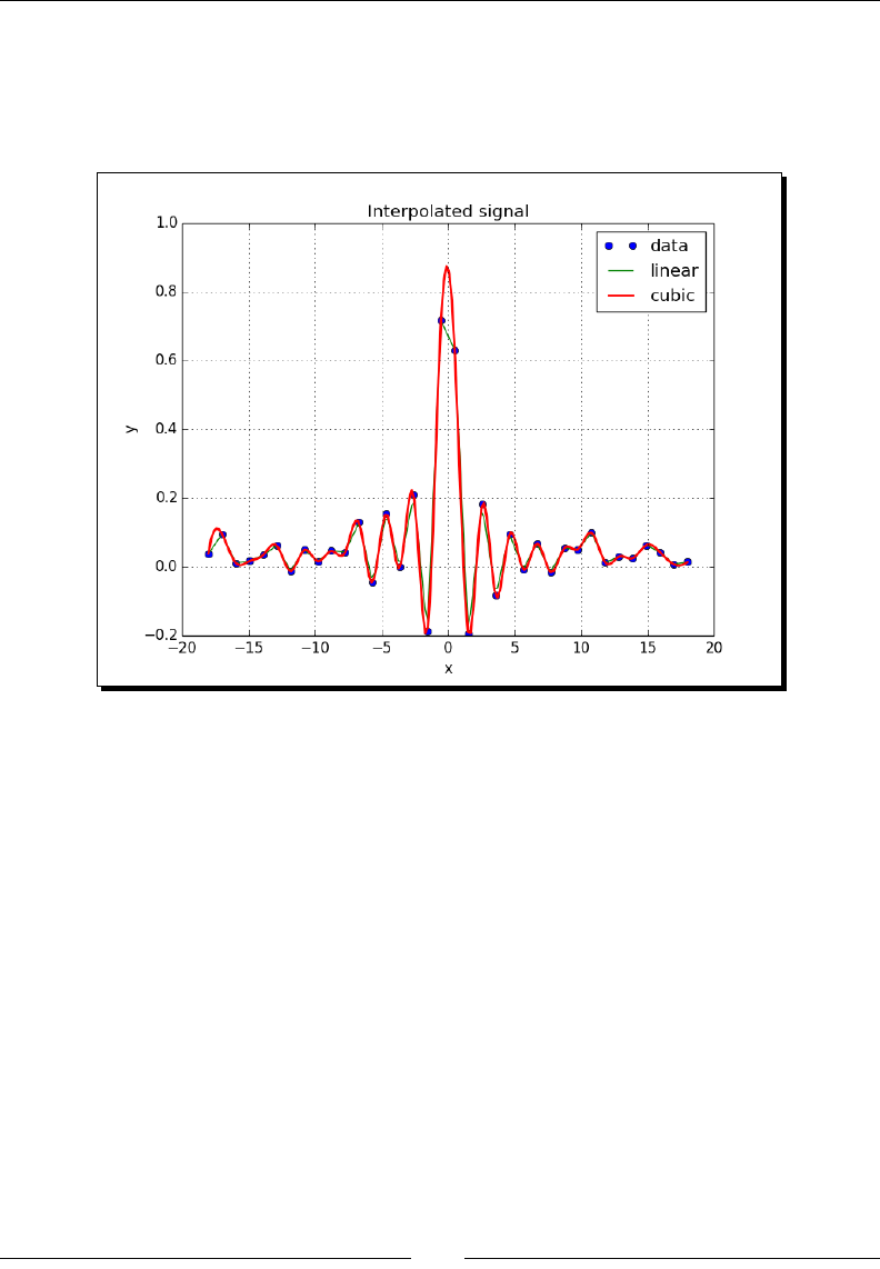
Chapter 10
[ 265 ]
plt.plot(x2, y2, '-', lw=2, label="cubic")
plt.legend()
plt.show()
The following diagram is a plot of the data, linear, and cubic interpolaon:
What just happened?
We created a dataset from the sinc() funcon and added noise to it. We then did linear
and cubic interpolaon using the interp1d class of the scipy.interpolate module
(see sincinterp.py):
import numpy as np
from scipy import interpolate
import matplotlib.pyplot as plt
x = np.linspace(-18, 18, 36)
noise = 0.1 * np.random.random(len(x))
signal = np.sinc(x) + noise
interpreted = interpolate.interp1d(x, signal)
x2 = np.linspace(-18, 18, 180)
y = interpreted(x2)

When NumPy Is Not Enough – SciPy and Beyond
[ 266 ]
cubic = interpolate.interp1d(x, signal, kind="cubic")
y2 = cubic(x2)
plt.plot(x, signal, 'o', label="data")
plt.plot(x2, y, '-', label="linear")
plt.plot(x2, y2, '-', lw=2, label="cubic")
plt.title('Interpolated signal')
plt.xlabel('x')
plt.ylabel('y')
plt.grid()
plt.legend(loc='best')
plt.show()
Image processing
With SciPy, we can do image processing using the scipy.ndimage package. The module
contains various image lters and ulies.
Time for action – manipulating Lena
The scipy.misc module is a ulity that loads the image of "Lena". This is the image of Lena
Soderberg, tradionally used for image processing examples. We will apply some lters to
this image and rotate it. Perform the following steps to do so:
1. Load the Lena image and display it in a subplot with grayscale colormap:
image = misc.lena().astype(np.float32)
plt.subplot(221)
plt.title("Original Image")
img = plt.imshow(image, cmap=plt.cm.gray)
Note that we are dealing with a float32 array.
2. The median lter scans the image and replaces each item by the median of
neighboring data points. Apply a median lter to the image and display it in
a second subplot:
plt.subplot(222)
plt.title("Median Filter")
filtered = ndimage.median_filter(image, size=(42,42))
plt.imshow(filtered, cmap=plt.cm.gray)

Chapter 10
[ 267 ]
3. Rotate the image and display it in the third subplot:
plt.subplot(223)
plt.title("Rotated")
rotated = ndimage.rotate(image, 90)
plt.imshow(rotated, cmap=plt.cm.gray)
4. The Prewi lter is based on compung the gradient of image intensity. Apply a
Prewi lter to the image and display it in the fourth subplot:
plt.subplot(224)
plt.title("Prewitt Filter")
filtered = ndimage.prewitt(image)
plt.imshow(filtered, cmap=plt.cm.gray)
plt.show()
The following are the resulng images:
What just happened?
We manipulated the image of Lena in several ways using the scipy.ndimage module (see
images.py):
from scipy import misc
import numpy as np
import matplotlib.pyplot as plt
from scipy import ndimage

When NumPy Is Not Enough – SciPy and Beyond
[ 268 ]
image = misc.lena().astype(np.float32)
plt.subplot(221)
plt.title("Original Image")
img = plt.imshow(image, cmap=plt.cm.gray)
plt.axis("off")
plt.subplot(222)
plt.title("Median Filter")
filtered = ndimage.median_filter(image, size=(42,42))
plt.imshow(filtered, cmap=plt.cm.gray)
plt.axis("off")
plt.subplot(223)
plt.title("Rotated")
rotated = ndimage.rotate(image, 90)
plt.imshow(rotated, cmap=plt.cm.gray)
plt.axis("off")
plt.subplot(224)
plt.title("Prewitt Filter")
filtered = ndimage.prewitt(image)
plt.imshow(filtered, cmap=plt.cm.gray)
plt.axis("off")
plt.show()
Audio processing
Now that we have done some image processing, you will probably not be surprised that we
can do excing things with WAV les too. Let's download a WAV le and replay it a couple of
mes. We will skip the explanaon of the download part, which is just regular Python.
Time for action – replaying audio clips
We will download a WAV le of Ausn Powers exclaiming "Smashing baby". This le can
be converted to a NumPy array with the read() funcon from the scipy.io.wavfile
module. The write() funcon from the same package will be used to create a new WAV le
at the end of this secon. We will further use the tile() funcon to replay the audio clip
several mes.
1. Read the le with the read() funcon:
sample_rate, data = wavfile.read(WAV_FILE)
This gives us two items – sample rate and audio data. For this secon we are only
interested in the audio data.
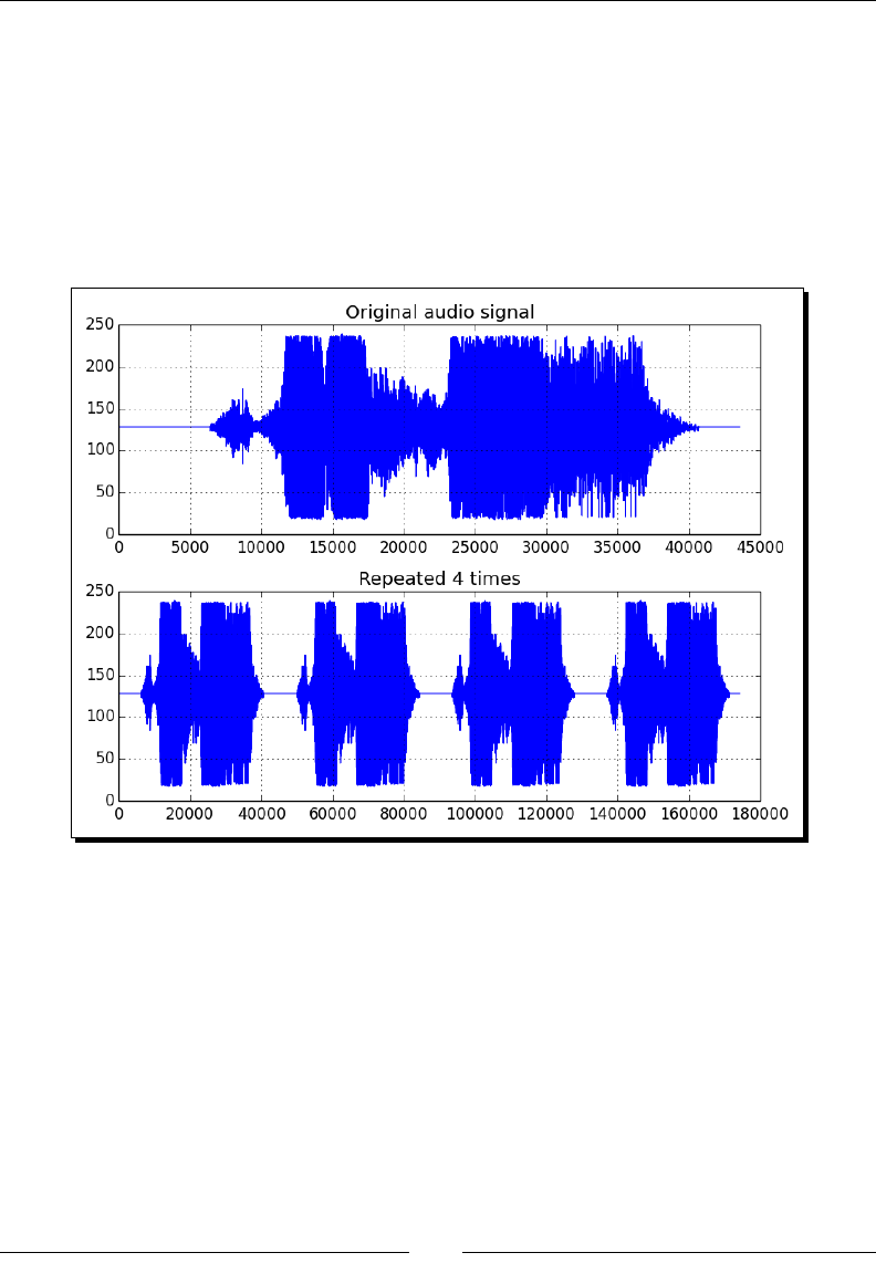
Chapter 10
[ 269 ]
2. Apply the tile() funcon:
repeated = np.tile(data, 4)
3. Write a new le with the write() funcon:
wavfile.write("repeated_yababy.wav",
sample_rate, repeated)
The original audio data and the audio clip repeated four mes appear in the
following plot:
What just happened?
We read an audio clip, repeated it four mes, and then created a new WAV le with the new
array (see repeat_audio.py):
from __future__ import print_function
from scipy.io import wavfile
import matplotlib.pyplot as plt
import urllib.request
import numpy as np
response = urllib.request.urlopen('http://www.thesoundarchive.com/
austinpowers/smashingbaby.wav')

When NumPy Is Not Enough – SciPy and Beyond
[ 270 ]
print(response.info())
WAV_FILE = 'smashingbaby.wav'
filehandle = open(WAV_FILE, 'wb')
filehandle.write(response.read())
filehandle.close()
sample_rate, data = wavfile.read(WAV_FILE)
print("Data type", data.dtype, "Shape", data.shape)
plt.subplot(2, 1, 1)
plt.title("Original audio signal")
plt.plot(data)
plt.grid()
plt.subplot(2, 1, 2)
# Repeat the audio fragment
repeated = np.tile(data, 4)
# Plot the audio data
plt.title("Repeated 4 times")
plt.plot(repeated)
wavfile.write("repeated_yababy.wav",
sample_rate, repeated)
plt.grid()
plt.tight_layout()
plt.show()
Summary
In this chapter, we only scratched the surface of what is possible with SciPy and SciKits.
Sll, we learned a bit about le I/O, stascs, signal processing, opmizaon, interpolaon,
audio, and image processing.
In the next chapter, we will create some simple, yet fun, games with Pygame—the open
source Python game library. In the process, we will learn about NumPy integraon with
Pygame, a machine learning Scikits module, and more.

[ 271 ]
Playing with Pygame
This chapter is for developers who want to create games quickly and easily
with NumPy and Pygame. Basic game development experience would help,
but it isn't necessary.
The things you will learn are as follows:
Pygame basics
matplotlib integraon
Surface pixel arrays
Arcial intelligence
Animaon
OpenGL
Pygame
Pygame is a Python framework, originally wrien by Pete Shinners, which, as its name
suggests, can be used to create video games. Pygame is free, open source since 2004 and
licensed under the GPL license, which means that you are allowed to basically make any type
of game. Pygame is built on top of the Simple DirectMedia Layer (SDL). SDL is a C framework
that gives access to graphics, sound, keyboard, and other input devices on various operang
systems including Linux, Mac OS X, and Windows.
11

Playing with Pygame
[ 272 ]
Time for action – installing Pygame
We will install Pygame in this secon. Pygame should be compable with all Python versions.
At the me of wring, there were some incompability issues with Python 3, but in all
probability, these will be xed soon.
Installing on Debian and Ubuntu: Pygame can be found in the Debian archives at
https://packages.qa.debian.org/p/pygame.html.
Installing on Windows: From the Pygame website (http://www.pygame.org/
download.shtml), download the appropriate binary installer for the Python
version you are using.
Installing Pygame on the Mac: Binary Pygame packages for Mac OS X 10.3 and up
can be found at http://www.pygame.org/download.shtml.
Installing from source: Pygame is using the distutils system for compiling
and installing. To start installing Pygame with the default opons, simply run the
following command:
$ python setup.py
If you need more informaon about the available opons, type the following:
$ python setup.py help
To compile the code, you need a compiler for your operang system. Seng this
up is beyond the scope of this book. More informaon about compiling Pygame on
Windows can be found at http://pygame.org/wiki/CompileWindows. For
more informaon about compiling Pygame on Mac OS X, refer to http://pygame.
org/wiki/MacCompile.
Hello World
We will create a simple game that we will improve on further in this chapter. As is tradional
in programming books, we start with a Hello World! example.
Time for action – creating a simple game
It's important to noce the so-called main game loop, where all the acon happens, and
the usage of the Font module to render text. In this program, we will manipulate a Pygame
Surface object that is used for drawing, and we will handle a quit event.
1. First, import the required Pygame modules. If Pygame is installed properly, we
should get no errors, otherwise please return to the installaon Time for acon:
import pygame, sys
from pygame.locals import *

Chapter 11
[ 273 ]
2. Inialize Pygame, create a display of 400 by 300 pixels, and set the window tle
to Hello world!:
pygame.init()
screen = pygame.display.set_mode((400, 300))
pygame.display.set_caption('Hello World!')
3. Games usually have a game loop, which runs forever unl, for instance, a quit event
occurs. In this example, only set a label with the text Hello world! at coordinates
(100, 100). The text has font size 19 and a red color:
while True:
sysFont = pygame.font.SysFont("None", 19)
rendered = sysFont.render('Hello World', 0, (255, 100, 100))
screen.blit(rendered, (100, 100))
for event in pygame.event.get():
if event.type == QUIT:
pygame.quit()
sys.exit()
pygame.display.update()
We get the following screenshot as an end result:

Playing with Pygame
[ 274 ]
Following is the complete code for the Hello World! example:
import pygame, sys
from pygame.locals import *
pygame.init()
screen = pygame.display.set_mode((400, 300))
pygame.display.set_caption('Hello World!')
while True:
sysFont = pygame.font.SysFont("None", 19)
rendered = sysFont.render('Hello World', 0, (255, 100, 100))
screen.blit(rendered, (100, 100))
for event in pygame.event.get():
if event.type == QUIT:
pygame.quit()
sys.exit()
pygame.display.update()
What just happened?
It may not seem like much, but we learned a lot in this secon. The funcons that passed the
review are summarized in the following table:
Function Description
pygame.init() This function performs initialization and you must call
it before calling other Pygame functions.
pygame.display.set_
mode((400, 300))
This function creates a so-called Surface object to
draw on. We give this function a tuple representing
the dimensions of the surface.
pygame.display.set_
caption('Hello World!')
This function sets the window title to a specified
string value.
pygame.font.SysFont("None",
19)
This function creates a system font from a comma-
separated list of fonts (in this case none) and an
integer font size parameter.
sysFont.render('Hello
World', 0, (255, 100, 100))
This function draws text on a Surface. The last
parameter is a tuple representing the RGB values of
a color.
screen.blit(rendered, (100,
100))
This function draws on a Surface.

Chapter 11
[ 275 ]
Function Description
pygame.event.get() This function gets a list of Event objects. Events
represent a special occurrence in the system, such as
a user quitting the game.
pygame.quit() This function cleans up the resources used by
Pygame. Call this function before exiting the game.
pygame.display.update() This function refreshes the surface.
Animation
Most games, even the most stac ones, have some level of animaon. From a programmer's
standpoint, animaon is nothing more than displaying an object at a dierent place at a
dierent me, thus simulang movement.
Pygame oers a Clock object, which manages how many frames are drawn per second. This
ensures that the animaon is independent of how fast the user's CPU is.
Time for action – animating objects with NumPy and Pygame
We will load an image and use NumPy again to dene a clockwise path around the screen.
1. Create a Pygame clock as follows:
clock = pygame.time.Clock()
2. As part of the source code accompanying this book, there should be a picture of a
head. Load this image and move it around on the screen:
img = pygame.image.load('head.jpg')
3. Dene some arrays to hold the coordinates of the posions, where we would like to
put the image during the animaon. Since we will move the object, there are four
logical secons of the path: right, down, left, and up. Each of these secons will
have 40 equidistant steps. Inialize all the values in the secons to 0:
steps = np.linspace(20, 360, 40).astype(int)
right = np.zeros((2, len(steps)))
down = np.zeros((2, len(steps)))
left = np.zeros((2, len(steps)))
up = np.zeros((2, len(steps)))
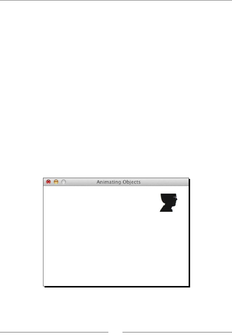
Playing with Pygame
[ 276 ]
4. It's straight-forward to set the coordinates of the posions of the image. However,
there is one tricky bit to noce—the [::-1] notaon leads to reversing the order
of the array elements:
right[0] = steps
right[1] = 20
down[0] = 360
down[1] = steps
left[0] = steps[::-1]
left[1] = 360
up[0] = 20
up[1] = steps[::-1]
5. We can join the path secons, but before doing this, transpose the arrays with the T
operator because they are not aligned properly for concatenaon:
pos = np.concatenate((right.T, down.T, left.T, up.T))
6. In the main event loop, let the clock ck at a rate of 30 frames per second:
clock.tick(30)
A screenshot of the moving head is as follows:
You should be able to watch a movie of this animaon at https://www.youtube.
com/watch?v=m2TagGiq1fs, and it is also part of the code bundle
(animation.mp4).

Chapter 11
[ 277 ]
The code of this example uses almost everything we have learnt so far, but should
sll be simple enough to understand:
import pygame, sys
from pygame.locals import *
import numpy as np
pygame.init()
clock = pygame.time.Clock()
screen = pygame.display.set_mode((400, 400))
pygame.display.set_caption('Animating Objects')
img = pygame.image.load('head.jpg')
steps = np.linspace(20, 360, 40).astype(int)
right = np.zeros((2, len(steps)))
down = np.zeros((2, len(steps)))
left = np.zeros((2, len(steps)))
up = np.zeros((2, len(steps)))
right[0] = steps
right[1] = 20
down[0] = 360
down[1] = steps
left[0] = steps[::-1]
left[1] = 360
up[0] = 20
up[1] = steps[::-1]
pos = np.concatenate((right.T, down.T, left.T, up.T))
i = 0
while True:
# Erase screen
screen.fill((255, 255, 255))
if i >= len(pos):
i = 0
screen.blit(img, pos[i])
i += 1
for event in pygame.event.get():
if event.type == QUIT:

Playing with Pygame
[ 278 ]
pygame.quit()
sys.exit()
pygame.display.update()
clock.tick(30)
What just happened?
We learned a bit about animaon in this secon. The most important concept we learned
about is the clock. The following table describes the new funcons we used:
Function Description
pygame.time.Clock() This creates a game clock.
clock.tick(30) This function executes a tick of the game clock. Here, 30 is
the number of frames per second.
matplotlib
matplotlib is an open source library for easy plong, which we learned about in Chapter
9, Plong with matplotlib. We can integrate matplotlib into a Pygame game and create
various plots.
Time for Action – using matplotlib in Pygame
In this recipe, we take the posion coordinates of the previous secon and make a graph
of them.
1. To integrate matplotlib with Pygame, we need to use a non-interacve backend;
otherwise matplotlib will present us with a GUI window by default. We will
import the main matplotlib module and call the use() funcon. Call this funcon
immediately aer imporng the main matplotlib module and before imporng
other matplotlib modules:
import matplotlib as mpl
mpl.use("Agg")
2. We can draw non-interacve plots on a matplotlib canvas. Creang this canvas
requires imports, creang a gure and a subplot. Specify the gure to be 3 by 3
inches large. More details can be found at the end of this recipe:
import matplotlib.pyplot as plt
import matplotlib.backends.backend_agg as agg
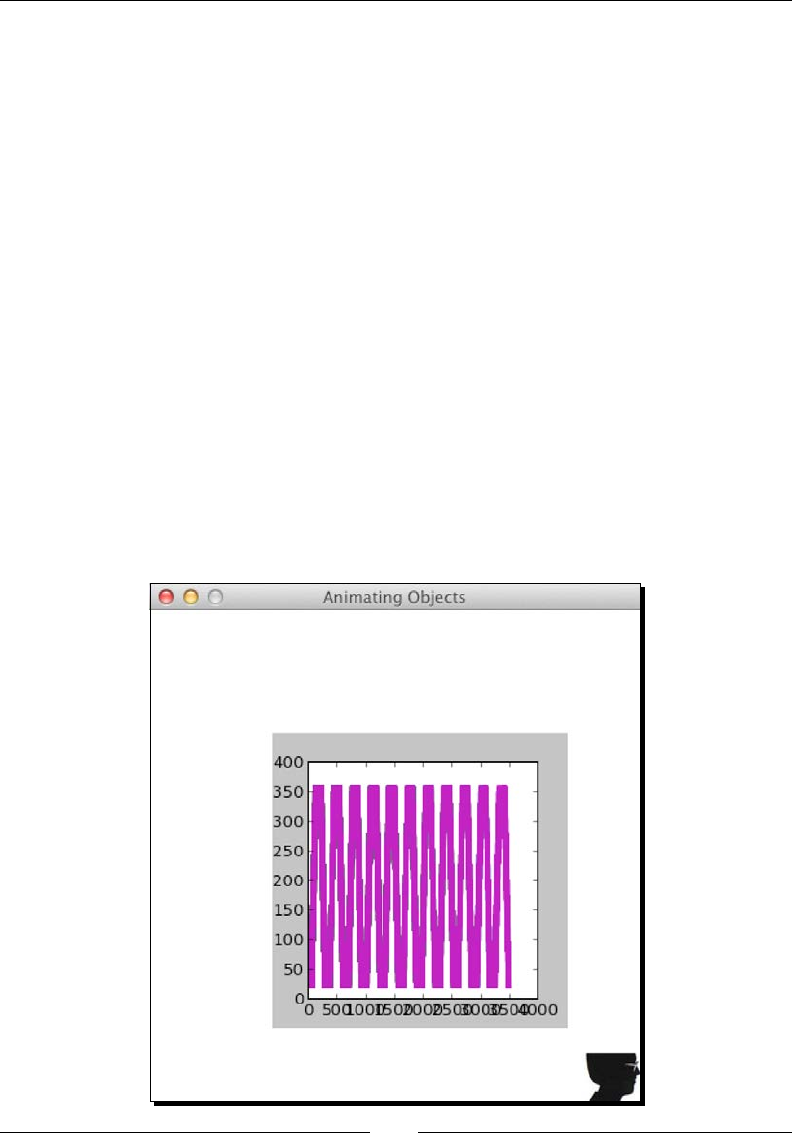
Chapter 11
[ 279 ]
fig = plt.figure(figsize=[3, 3])
ax = fig.add_subplot(111)
canvas = agg.FigureCanvasAgg(fig)
3. In non-interacve mode, plong data is a bit more complicated than in the default
mode. Since we need to plot repeatedly, it makes sense to organize the plong
code in a funcon. Pygame eventually draws the plot on the canvas. The canvas
adds a bit of complexity to our setup. At the end of this example, you can nd
more detailed explanaon of the funcons:
def plot(data):
ax.plot(data)
canvas.draw()
renderer = canvas.get_renderer()
raw_data = renderer.tostring_rgb()
size = canvas.get_width_height()
return pygame.image.fromstring(raw_data, size, "RGB")
The following screenshot shows the animaon in acon. You can also view
a screencast in the code bundle (matplotlib.mp4) and on YouTube at:
https://www.youtube.com/watch?v=t6qTeXxtnl4.

Playing with Pygame
[ 280 ]
We get the following code aer the changes:
import pygame, sys
from pygame.locals import *
import numpy as np
import matplotlib as mpl
mpl.use("Agg")
import matplotlib.pyplot as plt
import matplotlib.backends.backend_agg as agg
fig = plt.figure(figsize=[3, 3])
ax = fig.add_subplot(111)
canvas = agg.FigureCanvasAgg(fig)
def plot(data):
ax.plot(data)
canvas.draw()
renderer = canvas.get_renderer()
raw_data = renderer.tostring_rgb()
size = canvas.get_width_height()
return pygame.image.fromstring(raw_data, size, "RGB")
pygame.init()
clock = pygame.time.Clock()
screen = pygame.display.set_mode((400, 400))
pygame.display.set_caption('Animating Objects')
img = pygame.image.load('head.jpg')
steps = np.linspace(20, 360, 40).astype(int)
right = np.zeros((2, len(steps)))
down = np.zeros((2, len(steps)))
left = np.zeros((2, len(steps)))
up = np.zeros((2, len(steps)))
right[0] = steps
right[1] = 20
down[0] = 360
down[1] = steps

Chapter 11
[ 281 ]
left[0] = steps[::-1]
left[1] = 360
up[0] = 20
up[1] = steps[::-1]
pos = np.concatenate((right.T, down.T, left.T, up.T))
i = 0
history = np.array([])
surf = plot(history)
while True:
# Erase screen
screen.fill((255, 255, 255))
if i >= len(pos):
i = 0
surf = plot(history)
screen.blit(img, pos[i])
history = np.append(history, pos[i])
screen.blit(surf, (100, 100))
i += 1
for event in pygame.event.get():
if event.type == QUIT:
pygame.quit()
sys.exit()
pygame.display.update()
clock.tick(30)
What just happened?
The following table explains the plong related funcons:
Function Description
mpl.use("Agg") This function specifies to use the non-interactive backend
plt.figure(figsize=[3, 3]) This function creates a figure of 3 by 3 inches
agg.FigureCanvasAgg(fig) This function creates a canvas in non-interactive mode
canvas.draw() This function draws on the canvas
canvas.get_renderer() This function gets a renderer for the canvas

Playing with Pygame
[ 282 ]
Surface pixels
The Pygame surfarray module handles the conversion between Pygame Surface
objects and NumPy arrays. As you may recall, NumPy can manipulate big arrays in a
fast and ecient manner.
Time for Action – accessing surface pixel data with NumPy
In this secon, we will le a small image to ll the game screen.
1. The array2d() funcon copies pixels into a two-dimensional array (and there is
a similar funcon for three-dimensional arrays). Copy the pixels from the avatar
image into an array:
pixels = pygame.surfarray.array2d(img)
2. Create the game screen from the shape of the pixels array using the shape aribute
of the array. Make the screen seven mes larger in both direcons:
X = pixels.shape[0] * 7
Y = pixels.shape[1] * 7
screen = pygame.display.set_mode((X, Y))
3. Tiling the image is easy with the NumPy the tile() funcon. The data needs to be
converted into integer values, because Pygame denes colors as integers:
new_pixels = np.tile(pixels, (7, 7)).astype(int)
4. The surfarray module has a special funcon blit_array() to display the array
on the screen:
pygame.surfarray.blit_array(screen, new_pixels)

Chapter 11
[ 283 ]
The following code performs the ling of the image:
import pygame, sys
from pygame.locals import *
import numpy as np
pygame.init()
img = pygame.image.load('head.jpg')
pixels = pygame.surfarray.array2d(img)
X = pixels.shape[0] * 7
Y = pixels.shape[1] * 7
screen = pygame.display.set_mode((X, Y))
pygame.display.set_caption('Surfarray Demo')
new_pixels = np.tile(pixels, (7, 7)).astype(int)
while True:
screen.fill((255, 255, 255))
pygame.surfarray.blit_array(screen, new_pixels)
for event in pygame.event.get():
if event.type == QUIT:
pygame.quit()
sys.exit()
pygame.display.update()
What just happened?
Following is a brief descripon of the new funcons and aributes we used:
Function Description
pygame.surfarray.array2d(img) This function copies pixel data into a two-
dimensional array
pygame.surfarray.blit_
array(screen, new_pixels)
This function displays array values on the screen

Playing with Pygame
[ 284 ]
Articial Intelligence
Oen we need to mimic intelligent behavior within a game. The scikit-learn project
aims to provide an API for machine learning, and what I like most about it is its amazing
documentaon. We can install scikit-learn with the package manager of our operang
system, though this opon may or may not be available, depending on your operang system,
but should be the most convenient route. Windows users can just download an installer
from the project website. On Debian and Ubuntu, the project is called python-sklearn.
On MacPorts, the ports are called py26-scikits-learn and py27-scikits-learn. We
can also install from source or using easy_install. There are third-party distribuons from
Python(x,y), Enthought, and NetBSD.
We can install scikit-learn by typing at command line:
$ [sudo] pip install -U scikit-learn
We can also type the following instead of the preceding line:
$ [sudo] easy_install -U scikit-learn
This may not work because of permissions, so you might need to put sudo in front of the
commands or log in as admin.
Time for Action – clustering points
We will generate some random points and cluster them, which means that the points that
are close to each other are put into the same cluster. This is just one of the many techniques
that you can apply with scikit-learn. Clustering is a type of machine learning algorithm,
which aims to group items based on similaries. Next, we will calculate a square anity
matrix. An anity matrix is a matrix containing anity values: for instance, the distances
between points. Finally, we will cluster the points with the AffinityPropagation class
from scikit-learn.
1. Generate 30 random point posions within a square of 400 by 400 pixels:
positions = np.random.randint(0, 400, size=(30, 2))
2. Calculate the anity matrix using the Euclidean distance to the origin as the
anity metric:
positions_norms = np.sum(positions ** 2, axis=1)
S = - positions_norms[:, np.newaxis] -
positions_norms[np.newaxis, :] + 2 *
np.dot(positions, positions.T)

Chapter 11
[ 285 ]
3. Give the AffinityPropagation class the result from the previous step. This class
labels the points with the appropriate cluster number:
aff_pro = sklearn.cluster.AffinityPropagation().fit(S)
labels = aff_pro.labels_
4. Draw polygons for each cluster. The funcon involved requires a list of points, a
color (let's paint it red), and a surface:
pygame.draw.polygon(screen, (255, 0, 0), polygon_points[i])
The result is a bunch of polygons for each cluster, as shown in the following picture:
The clustering example code is as follows:
import numpy as np
import sklearn.cluster
import pygame, sys
from pygame.locals import *
np.random.seed(42)
positions = np.random.randint(0, 400, size=(30, 2))
positions_norms = np.sum(positions ** 2, axis=1)
S = - positions_norms[:, np.newaxis] - positions_norms[np.newaxis,
:] + 2 * np.dot(positions,
positions.T)

Playing with Pygame
[ 286 ]
aff_pro = sklearn.cluster.AffinityPropagation().fit(S)
labels = aff_pro.labels_
polygon_points = []
for i in xrange(max(labels) + 1):
polygon_points.append([])
# Sorting points by cluster
for label, position in zip(labels, positions):
polygon_points[labels[i]].append(positions[i])
pygame.init()
screen = pygame.display.set_mode((400, 400))
while True:
for point in polygon_points:
pygame.draw.polygon(screen, (255, 0, 0), point)
for event in pygame.event.get():
if event.type == QUIT:
pygame.quit()
sys.exit()
pygame.display.update()
What just happened?
The most important lines in the arcial intelligence example are described in more detail in
the following table:
Function Description
sklearn.cluster.
AffinityPropagation().fit(S)
This function creates an
AffinityPropagation object and
performs a fit using an affinity matrix
pygame.draw.polygon(screen, (255,
0, 0), point)
This function draws a polygon given a
surface, a color (red in this case), and a list
of points

Chapter 11
[ 287 ]
OpenGL and Pygame
OpenGL species an API for two-dimensional and three-dimensional computer graphics.
The API consists of funcons and constants. We will be concentrang on the Python
implementaon called PyOpenGL. Install PyOpenGL with the following command:
$ [sudo] pip install PyOpenGL PyOpenGL_accelerate
You might need to have root access to execute this command. The corresponding
easy_install command is as follows:
$ [sudo] easy_install PyOpenGL PyOpenGL_accelerate
Time for Action – drawing the Sierpinski gasket
For the purpose of demonstraon, we will draw a Sierpinski gasket, also known as Sierpinski
triangle or Sierpinski Sieve with OpenGL. This is a fractal paern in the shape of a triangle
created by the mathemacian Waclaw Sierpinski. The triangle is obtained via a recursive
and, in principle innite procedure.
1. First, start out by inializing some of the OpenGL related primives. This includes
seng the display mode and background color. A line-by-line explanaon is given
at the end of this secon:
def display_openGL(w, h):
pygame.display.set_mode((w,h),
pygame.OPENGL|pygame.DOUBLEBUF)
glClearColor(0.0, 0.0, 0.0, 1.0)
glClear(GL_COLOR_BUFFER_BIT|GL_DEPTH_BUFFER_BIT)
gluOrtho2D(0, w, 0, h)
2. The algorithm requires us to display points, the more the beer. First, we set the
drawing color to red. Second, we dene the verces (I call them points myself) of
a triangle. Then, we dene random indices, which are to be used to choose one of
the three triangle verces. We pick a random point somewhere in the middle—it
doesn't really maer where. Aer this, draw points halfway between the previous
point and one of the verces picked at random. Finally, ush the result:
glColor3f(1.0, 0, 0)
vertices = np.array([[0, 0], [DIM/2, DIM], [DIM, 0]])
NPOINTS = 9000
indices = np.random.random_integers(0, 2, NPOINTS)
point = [175.0, 150.0]

Playing with Pygame
[ 288 ]
for i in xrange(NPOINTS):
glBegin(GL_POINTS)
point = (point + vertices[indices[i]])/2.0
glVertex2fv(point)
glEnd()
glFlush()
The Sierpinski triangle looks like the following:
The full Sierpinski gasket demo code with all the imports is as follows:
import pygame
from pygame.locals import *
import numpy as np
from OpenGL.GL import *
from OpenGL.GLU import *
def display_openGL(w, h):
pygame.display.set_mode((w,h), pygame.OPENGL|pygame.DOUBLEBUF)
glClearColor(0.0, 0.0, 0.0, 1.0)
glClear(GL_COLOR_BUFFER_BIT|GL_DEPTH_BUFFER_BIT)

Chapter 11
[ 289 ]
gluOrtho2D(0, w, 0, h)
def main():
pygame.init()
pygame.display.set_caption('OpenGL Demo')
DIM = 400
display_openGL(DIM, DIM)
glColor3f(1.0, 0, 0)
vertices = np.array([[0, 0], [DIM/2, DIM], [DIM, 0]])
NPOINTS = 9000
indices = np.random.random_integers(0, 2, NPOINTS)
point = [175.0, 150.0]
for i in xrange(NPOINTS):
glBegin(GL_POINTS)
point = (point + vertices[indices[i]])/2.0
glVertex2fv(point)
glEnd()
glFlush()
pygame.display.flip()
while True:
for event in pygame.event.get():
if event.type == QUIT:
return
if __name__ == '__main__':
main()
What just happened?
As promised, the following is a line-by-line explanaon of the most important parts of
the example:
Function Description
pygame.display.set_mode((w,h),
pygame.OPENGL|pygame.DOUBLEBUF)
This function sets the display mode to the required
width, height, and OpenGL display
glClear(GL_COLOR_BUFFER_BIT|GL_
DEPTH_BUFFER_BIT)
This function clears the buffers using a mask. Here
we clear the color buffer and depth buffer bits
gluOrtho2D(0, w, 0, h) This function defines a two-dimensional
orthographic projection matrix with the coordinates
of the left, right, top, and bottom clipping planes

Playing with Pygame
[ 290 ]
Function Description
glColor3f(1.0, 0, 0) This function defines the current drawing color
using three float values for RGB (red, green, blue).
In this case, we will be painting in red
glBegin(GL_POINTS) This function delimits the vertices of primitives or a
group of primitives. Here the primitives are points
glVertex2fv(point) This function renders a point given a vertex
glEnd() This function closes a section of code started with
glBegin()
glFlush() This function forces the execution of GL commands
Simulation game with Pygame
As a last example, we will simulate life with Conway's Game of Life. The original game
of life is based on a few basic rules. We start out with a random conguraon on a two-
dimensional square grid. Each cell in the grid can be either dead or alive. This state depends
on the neighbors of the cell. You can read more about the rules at http://en.wikipedia.
org/wiki/Conway%27s_Game_of_Life#Rules At each step in me, the following
transions occur:
1. Live cells with less than two live neighbors die.
2. Live cells with two or three live neighbors live on to the next generaon.
3. Live cells with more than three live neighbors die.
4. Dead cells with exactly three live neighbors become a live cell.
Convoluon can be used to evaluate the basic rules of the game. We need the SciPy package
for the convoluon process.
Time for Action – simulating life
The following code is an implementaon of the Game of Life, with some modicaons:
Clicking once with the mouse draws a cross unl we click again
The r key resets the grid to a random state
Pressing b creates blocks based on the mouse posion
g creates gliders

Chapter 11
[ 291 ]
The most important data structure in the code is a two-dimensional array, holding the color
values of the pixels on the game screen. This array is inialized with random values and then
recalculated for each iteraon of the game loop. Find more informaon about the involved
funcons in the next secon.
1. To evaluate the rules, use the convoluon as follows:
def get_pixar(arr, weights):
states = ndimage.convolve(arr, weights, mode='wrap')
bools = (states == 13) | (states == 12 ) | (states == 3)
return bools.astype(int)
2. Draw a cross using the basic indexing tricks that we learned in Chapter 2, Beginning
with NumPy Fundamentals:
def draw_cross(pixar):
(posx, posy) = pygame.mouse.get_pos()
pixar[posx, :] = 1
pixar[:, posy] = 1
3. Inialize the grid with random values:
def random_init(n):
return np.random.random_integers(0, 1, (n, n))
The following is the code in its enrety:
from __future__ import print_function
import os, pygame
from pygame.locals import *
import numpy as np
from scipy import ndimage
def get_pixar(arr, weights):
states = ndimage.convolve(arr, weights, mode='wrap')
bools = (states == 13) | (states == 12 ) | (states == 3)
return bools.astype(int)
def draw_cross(pixar):
(posx, posy) = pygame.mouse.get_pos()
pixar[posx, :] = 1
pixar[:, posy] = 1

Playing with Pygame
[ 292 ]
def random_init(n):
return np.random.random_integers(0, 1, (n, n))
def draw_pattern(pixar, pattern):
print(pattern)
if pattern == 'glider':
coords = [(0,1), (1,2), (2,0), (2,1), (2,2)]
elif pattern == 'block':
coords = [(3,3), (3,2), (2,3), (2,2)]
elif pattern == 'exploder':
coords = [(0,1), (1,2), (2,0), (2,1), (2,2), (3,3)]
elif pattern == 'fpentomino':
coords = [(2,3),(3,2),(4,2),(3,3),(3,4)]
pos = pygame.mouse.get_pos()
xs = np.arange(0, pos[0], 10)
ys = np.arange(0, pos[1], 10)
for x in xs:
for y in ys:
for i, j in coords:
pixar[x + i, y + j] = 1
def main():
pygame.init ()
N = 400
pygame.display.set_mode((N, N))
pygame.display.set_caption("Life Demo")
screen = pygame.display.get_surface()
pixar = random_init(N)
weights = np.array([[1,1,1], [1,10,1], [1,1,1]])
cross_on = False
while True:
pixar = get_pixar(pixar, weights)
if cross_on:
draw_cross(pixar)
pygame.surfarray.blit_array(screen, pixar * 255 ** 3)
pygame.display.flip()

Chapter 11
[ 293 ]
for event in pygame.event.get():
if event.type == QUIT:
return
if event.type == MOUSEBUTTONDOWN:
cross_on = not cross_on
if event.type == KEYDOWN:
if event.key == ord('r'):
pixar = random_init(N)
print("Random init")
if event.key == ord('g'):
draw_pattern(pixar, 'glider')
if event.key == ord('b'):
draw_pattern(pixar, 'block')
if event.key == ord('e'):
draw_pattern(pixar, 'exploder')
if event.key == ord('f'):
draw_pattern(pixar, 'fpentomino')
if __name__ == '__main__':
main()
You should be able to view a screencast from the code bundle (life.mp4) or on
YouTube (https://www.youtube.com/watch?v=NNsU-yWTkXM). A screenshot
of the game in acon is as follows:

Playing with Pygame
[ 294 ]
What just happened?
We used some NumPy and SciPy funcons that need explaining:
Function Description
ndimage.convolve(arr,
weights, mode='wrap')
This function applies the convolve operation on the
given array, using weights in the wrap mode. The mode
has to do with the array borders.
bools.astype(int) This function converts the array of Booleans to integers.
np.arange(0, pos[0], 10) This function creates an array from 0 to pos[0] in
steps of 10. So, if pos[0] is equal to 1000, we will get
0, 10, 20, … 990.
Summary
You might nd the menon of Pygame in this book a bit odd. However, aer reading this
chapter, I hope you realized that NumPy and Pygame go well together. Games aer all involve
lots of computaon for which NumPy and SciPy are ideal choices, and they also require
arcial intelligence capabilies as found in scikit-learn. In any event, making games is
fun and we hope this last chapter was the equivalent of a nice dessert or coee aer a ten-
course meal! If you are sll hungry for more, please check out NumPy Cookbook, Second
Edion, Ivan Idris, Packt Publishing, which builds further on this book with minimum overlap.

[ 295 ]
Pop Quiz Answers
Chapter 1, NumPy Quick Start
Pop quiz – functioning of the arange() function
What does arange(5) do? It creates a NumPy array with values 0-4
The created NumPy array has values 0, 1, 2, 3, and 4
Chapter 2, Beginning with NumPy Fundamentals
Pop quiz – the shape of ndarray
How is the shape of an ndarray
stored?
It is stored in a tuple
A

Pop Quiz Answers
[ 296 ]
Chapter 3, Getting Familiar with Commonly
Used Functions
Pop quiz – computing the weighted average
Which function returns the
weighted average of an array?
average
Chapter 4, Convenience Functions for Your Convenience
Pop quiz – calculating covariance
Which function returns the
covariance of two arrays?
cov
Chapter 5, Working with Matrices and ufuncs
Pop quiz – dening a matrix with a string
What is the row delimiter in a string
accepted by the mat and bmat
functions?
Semicolon
Chapter 6, Move Further with NumPy Modules
Pop quiz – creating a matrix
Which function can create matrices? mat

Appendix A
[ 297 ]
Chapter 7, Peeking into Special Routines
Pop quiz – generating random numbers
Which NumPy module deals with
random numbers?
random
Chapter 8, Assuring Quality with Testing
Pop quiz – specifying decimal precision
Which parameter of the assert_
almost_equal function specifies
the decimal precision?
decimal
Chapter 9, Plotting with matplotlib
Pop quiz – the plot() function
What does the plot function do? It does neither 1, 2, or 3
Chapter 10, When NumPy Is Not Enough –Scipy
and Beyond
Pop quiz – loading .mat les
Which function loads .mat files? loadmat

[ 299 ]
Additional Online Resources
This appendix contains links to the relevant websites.
Python
Learn Python the Hard Way (for Python 2) at http://learnpythonthehardway.
org/
Dive Into Python 3 (for Python 3) at http://www.diveintopython3.net/
Beginner's Guide to Python at https://wiki.python.org/moin/
BeginnersGuide
Non-programmers Tutorial for Python 3 can be found at http://en.wikibooks.
org/wiki/Non-Programmer%27s_Tutorial_for_Python_3
A Byte of Python is available at http://www.swaroopch.com/notes/python/
An Introducon to Interacve Programming in Python can be found at
https://www.coursera.org/course/interactivepython1
Learn Python online by Code Mentor at https://www.codementor.io/learn-
python-online
Learn Python by visualizing code execuon at http://pythontutor.com/
Find Codecademy Python exercises at http://www.codecademy.com/tracks/
python
Google's Python class is available at https://developers.google.com/edu/
python/
A Python style guide from Google can be found at https://google-
styleguide.googlecode.com/svn/trunk/pyguide.html
The IPython website can be found at http://ipython.org/
matplotlib a Python plong library at http://matplotlib.org/
B

Addional Online Resources
[ 300 ]
NumPy and SciPy documentaon can be accessed at http://docs.scipy.org/
doc/
NumPy and SciPy mailing lists can be found at http://www.scipy.org/
scipylib/mailing-lists.html
Mathematics and statistics
Linear algebra tutorials are available from Khan Academy at https://www.
khanacademy.org/math/linear-algebra
Pre-calculus tutorials from Khan Academy are available at https://www.
khanacademy.org/math/precalculus
Probability and stascs tutorials from Khan Academy can be found at
https://www.khanacademy.org/math/probability
Trigonometry tutorials from Khan Academy can be found at
https://www.khanacademy.org/math/trigonometry
Access Alcumus by Art of Problem Solving(AoPS) at http://www.
artofproblemsolving.com/alcumus
Find the Pre-Calculus Coursera course at https://www.coursera.org/course/
precalculus
The Coursera course on linear algebra, which uses Python, can be found at
https://www.coursera.org/course/matrix
An introducon to probability by Harvard University can be accessed at
https://itunes.apple.com/us/course/statistics-110-probability/
id502492375
The stascs wikibook is available at https://en.wikibooks.org/wiki/
Statistics
The Electronic Stascs Textbook. Tulsa, OK: StatSo. WEB can be found at:
http://www.statsoft.com/Textbook

[ 301 ]
NumPy Functions' References
This appendix contains a list of useful NumPy funcons and their descripons.
numpy.apply_along_axis(func1d, axis, arr, *args): Applies the funcon
func1d along an axis on 1D slices of arr.
numpy.arange([start,] stop[, step,], dtype=None): Creates a NumPy
array with evenly spaced values within a specied range.
numpy.argsort(a, axis=-1, kind='quicksort', order=None): Returns
the indices that would sort the input array.
numpy.argmax(a, axis=None): Returns the indices of the maximum values
along an axis.
numpy.argmin(a, axis=None): Returns the indices of the minimum values
along an axis.
numpy.argwhere(a): Finds the indices of non-zero elements.
numpy.array(object, dtype=None, copy=True, order=None,
subok=False, ndmin=0): Creates a NumPy array from an array-like sequence,
such as a Python list.
numpy.testing.assert_allclose((actual, desired, rtol=1e-07,
atol=0, err_msg='', verbose=True): Raises an error if two objects are
unequal up to a specied precision.
numpy.testing.assert_almost_equal(): Raises an excepon if two numbers
are not equal up to a specied precision.
numpy.testing.assert_approx_equal(): Raises an excepon if two numbers
are not equal up to a certain signicance.
numpy.testing.assert_array_almost_equal(): Raises an excepon if two
arrays are not equal up to a specied precision.
C

NumPy Funcons' References
[ 302 ]
numpy.testing.assert_array_almost_equal_nulp(x, y, nulp=1):
Compares arrays to their unit of least precision (ULP).
numpy.testing.assert_array_equal(): Raises an excepon if two arrays are
not equal.
numpy.testing.assert_array_less(): Raises an excepon if two arrays do
not have the same shape, and the elements of the rst array are strictly less than
the elements of the second array.
numpy.testing.assert_array_max_ulp(a, b, maxulp=1, dtype=None):
Determines whether the array elements dier by, at most, a specied number
of ULP.
numpy.testing.assert_equal(): Tests whether two NumPy arrays are equal.
numpy.testing.assert_raises(): Fails if a specied excepon is not raised by
a callable invoked with dened arguments.
numpy.testing.assert_string_equal(): Asserts that two strings are equal.
numpy.testing.assert_warns(): Fails if a specied warning is not thrown.
numpy.bartlett(M): Returns the Bartle window with M points. This window is
similar to a triangular window.
numpy.random.binomial(n, p, size=None): Draws random samples from
the binomial distribuon.
numpy.bitwise_and(x1, x2[, out]): Calculates the bit-wise AND of arrays.
numpy.bitwise_xor(x1, x2[, out]): Calculates the bit-wise XOR of arrays.
numpy.blackman(M): Returns a Blackman window with M points, which is close
to opmal and a lile bit worse than a Kaiser window.
numpy.column_stack(tup): Stacks 1D arrays provided as a tuple column wise.
numpy.concatenate ((a1, a2, ...), axis=0): Concatenates a sequence
of arrays.
numpy.convolve(a, v, mode='full'): Computes the linear convoluon
of 1D arrays.
numpy.dot(a, b, out=None): Calculates the dot product of two arrays.
numpy.diff(a, n=1, axis=-1): Computes the nth dierence for a given axis.
numpy.dsplit(ary, indices_or_sections): Splits an array into subarrays
along the third axis.
numpy.dstack(tup): Stacks arrays given as a tuple along the third axis.
numpy.eye(N, M=None, k=0, dtype=<type 'float'>): Returns the
identy matrix.

Appendix C
[ 303 ]
numpy.extract(condition, arr): Selects elements of an array using
a condion.
numpy.fft.fftshift(x, axes=None): Shis the zero-frequency component
of a signal to the center of the spectrum.
numpy.hamming(M): Returns the Hamming window with M points.
numpy.hanning(M): Returns the Hanning window with M points.
numpy.hstack(tup): Stacks arrays given as a tuple horizontally.
numpy.isreal(x): Returns a Boolean array, where True corresponds to an
element of the input array, which is a real number (as opposed to a complex
number).
numpy.kaiser(M, beta): Returns a Kaiser window with M points for a given
beta parameter.
numpy.load(file, mmap_mode=None): Loads NumPy arrays or pickled objects
from .npy, .npz or pickles. A memory-mapped array is stored in the lesystem
and doesn't have to be completely loaded in memory. This is especially useful for
large arrays.
numpy.loadtxt(fname, dtype=<type 'float'>, comments='#',
delimiter=None, converters=None, skiprows=0, usecols=None,
unpack=False, ndmin=0): Loads data from a text le into a NumPy array.
numpy.lexsort (keys, axis=-1): Sorts using mulple keys.
numpy.linspace(start, stop, num=50, endpoint=True,
retstep=False, dtype=None): Returns evenly spaced numbers over an interval.
numpy.max(a, axis=None, out=None, keepdims=False): Returns the
maximum of an array along an axis.
numpy.mean(a, axis=None, dtype=None, out=None, keepdims=False):
Calculates the arithmec mean along the given axis.
numpy.median(a, axis=None, out=None, overwrite_input=False):
Calculates the median along the given axis.
numpy.meshgrid(*xi, **kwargs): Returns coordinate matrices for coordinate
vectors. For instance:
In: numpy.meshgrid([1, 2], [3, 4])
Out:
[array([[1, 2],
[1, 2]]), array([[3, 3],
[4, 4]])]

NumPy Funcons' References
[ 304 ]
numpy.min(a, axis=None, out=None, keepdims=False): Returns the
minimum of an array along an axis.
numpy.msort(a): Returns a copy of an array sorted along the rst axis.
numpy.nanargmax(a, axis=None): Returns the indices of the maximums given
an axis ignoring NaNs.
numpy.nanargmin(a, axis=None): Returns the indices of the minimums given
an axis ignoring NaNs.
numpy.nonzero(a): Returns indices of non-zero array elements.
numpy.ones(shape, dtype=None, order='C'): Creates a NumPy array of
specied shape and data type, containing 1s.
numpy.piecewise(x, condlist, funclist, *args, **kw): Evaluates a
funcon piecewise.
numpy.polyder(p, m=1): Dierenates a polynomial to a given order.
numpy.polyfit(x, y, deg, rcond=None, full=False, w=None,
cov=False): Performs a least squares polynomial t.
numpy.polysub(a1, a2): Subtracts polynomials.
numpy.polyval(p, x): Evaluates a polynomial at specied values.
numpy.prod(a, axis=None, dtype=None, out=None, keepdims=False):
Returns the product of array elements over a specied axis.
numpy.ravel(a, order='C'): Flaens an array or returns a copy if necessary.
numpy.reshape(a, newshape, order='C'): Changes the shape of a NumPy
array.
numpy.row_stack(tup): Stacks arrays row wise.
numpy.save(file, arr): Saves a NumPy array to a le in the NumPy .npy
format.
numpy.savetxt(fname, X, fmt='%.18e', delimiter=' ',
newline='\n', header='', footer='', comments='# '): Saves a NumPy
array to a text le.
numpy.sinc(a): Computes the sinc funcon.
numpy.sort_complex(a): Sorts array elements with the real part rst, then
followed by the imaginary part.
numpy.split(a, indices_or_sections, axis=0): Splits an array into
subarrays.

Appendix C
[ 305 ]
numpy.std(a, axis=None, dtype=None, out=None, ddof=0,
keepdims=False): Returns the standard deviaon along the given axis.
numpy.take(a, indices, axis=None, out=None, mode='raise'):
Selects elements from an array using specied indices.
numpy.vsplit(a, indices_or_sections): Splits an array into subarrays
vercally.
numpy.vstack(tup): Stacks arrays vercally.
numpy.where(condition, [x, y]): Selects array elements from input arrays
based on a Boolean condion.
numpy.zeros(shape, dtype=float, order='C'): Creates a NumPy array of
specied shape and data type, containing zeros.

[ 307 ]
Index
Symbols
.mat le
loading 246
saving 246
== operator 44
A
absolute tolerance (atol) 202
add() funcon
ufuncs methods, applying 127, 128
anity matrix 284
animaon
about 241
clock.ck(30) funcon 278
in Pygame 275
pygame.me.Clock() funcon 278
URL 276
YouTube, URL 279
annotate() funcon 234
annotaons
about 234
using 235, 236
argmax() funcon 178
argmin() funcon 178
argwhere() funcon 178
arithmec funcons 129
arithmec mean
about 57
reference link 57
array2d() funcon 282
array inializaon 118
arrays
about 17
clipping 94, 95
comparing 202, 203
compressing 94, 95
dividing 129, 130
extracng, from element 179, 180
ndarray methods, using 94
ordering 203
vectors, adding 17-20
arcial intelligence
about 284
points, clustering 284-286
pygame.draw.polygon () funcon 286
sklearn.cluster.AnityPropagaon().t(S)
funcon 286
assert_almost_equal() funcon
using 198
assert_approx_equal() funcon
using 199
assert_array_almost_equal() funcon
using 200
assert_array_almost_equal_nulp() funcon
using 206
assert_array_less() funcon 203
assert_array_max_ulp() funcon
using 207
assert_equal() funcon
using 204
assert funcons
about 198
assert_allclose() 198

[ 308 ]
assert_almost_equal() 198
assert_approx_equal() 198
assert_array_almost_equal() 198
assert_array_equal() 198
assert_array_less() 198
assert_equal() 198
assert_raises() 198
assert_string_equal() 198
assert_warns() 198
assert_string_equal() funcon
using 204, 205
at() method
using, for fancy indexing 144
aributes, one-dimensional NumPy arrays
at aribute 49, 50
imag aribute 49
itemsize aribute 48
ndim aribute 48
real aribute 49
size aribute 48
T aribute 48
audio clips
replaying 268, 269
audio processing
about 268
audio clips, replaying 268, 269
Average True Range (ATR)
about 74
calculang 75, 76
minimum() funcon, using 77
axes 71
B
bartle() funcon 187
Bartle window
plong 187, 188
basic arithmec, Python 4
Bessel funcon
about 191
URL 191
Binet's formula 133
binomial distribuon models 161
binomial() funcon
using 161, 162
bits
twiddling 141, 142
bitwise funcons 140
blackman() funcon 188
Blackman window
about 188
used, for smoothing stock prices 189, 190
bmat() funcon 123
Bollinger Bands
about 82
components 82, 83
enveloping 83-85
Exponenal Moving Average, switching 86
bootstrapping 169
B-spline interpolaon algorithms 253
C
calc_prot() funcon 111
calculus 104
character codes 33
clustering 284
comma-separated value (CSV) les
about 55
loading 55
complex conjugate 152
complex numbers
about 176
sorng 177
concatenate() funcon 43
conjugate transpose 152
constructors 34
connuous distribuons
about 165
normal distribuon, drawing 165, 166
contour plots
about 240
drawing 240
convoluon
about 77
references 77
corrcoef() funcon 101-103
correlaon
about 100
correlated pairs, trading 100-104
URL 100

[ 309 ]
covariance
URL 100
Cowboy's Game of Life
about 290
implementaon 290-293
transions 290
URL 290
D
data type objects 33
dates
about 65
dateme64 data type, using 69, 70
dealing with 65-67
TWAP, calculang 68
VWAP, calculang 68
dateme64 data type
about 69
URL 69
using 69, 70
dateme object
reference link 66
deriv() funcon 219
determinant
about 155
of matrix, calculang 155, 156
URL 155
detrended signal
ltering 256, 257
diagonal() method 101
di() funcon 109
Discrete Fourier transform
about 156
URL 256
Dish Network Corp (DISH) 225
distribuon (distro) 15
divide() funcon 129, 130
docstring 213
doctests
execung 214, 215
dot() funcon 149
dtype aribute
about 35
record data type, creang 35, 36
E
eigenvalues
about 149
determining 150
URL 149
eigenvectors
about 149
determining 150
eig() funcon 149
eigvals() funcon 149
element
array, extracng from 179, 180
Enthought
about 284
URL 14
error() funcon 263
Exponenal Moving Average (EMA)
about 80
calculang 80-82
extract() funcon
using, for array element extracon 179, 180
extrema 106
F
factorial
about 95
calculang 95, 96
fancy indexing
about 143
using, with at() method 144
Fast Fourier transform (FFT)
about 156
calculang 156-158
() funcon 157
shi() funcon 158
Fibonacci numbers
about 132, 133
calculaons, ming 134
compung 133, 134
URL 132
le handle
about 54
reference link 54

[ 310 ]
le I/O
about 53
les, reading 54, 55
les, wring 54, 55
ll_between() funcon 232, 233
nancial funcons
fv() funcon 180
irr() funcon 181
mirr() funcon 181
nper() funcon 181
npv() funcon 180
pmt() funcon 180
pv() funcon 180
rate() funcon 181
used, for determining future value 181, 182
Fink
used, for installing Numpy 16
aen() funcon 41
oang-point numbers
comparing 205
comparing, with assert_array_almost_
equal_nulp funcon 206
oats
comparing 207
comparing, with maxulp of 2 207
oor_divide() funcon 129
oor() funcon 129
fmod() funcon 132
for loop
about 9
implemenng 9, 10
format string
plong 219
polynomial derivaves, plong 219, 220
Fourier analysis
about 256
detrended signal, ltering 256, 257
Fourier series
about 136, 156
URL 136
frequencies
shiing 158-160
frompyfunc() funcon 125
full() funcon
used, for creang value inialized
arrays 119, 120
full_like() funcon
used, for creang value inialized
arrays 119, 120
funconal programming
about 73
reference link 73
funcons, Python
dening 11
future value
about 180
determining, with nancial funcons 181, 182
URL 181
fv() funcon 180
G
Gaussian integral
calculang 263, 264
golden rao formula 132, 133
H
hamming() funcon 190
Hamming window
about 190
plong 190, 191
hanning() funcon
used, for smoothing 114
Hello World game
about 272
creang 272-274
pygame.display.set_capon () funcon 274
pygame.display.set_mode() funcon 274
pygame.display.update() funcon 275
pygame.event.get() funcon 275
pygame.font.SysFont () funcon 274
pygame.init() funcon 274
pygame.quit() funcon 275
screen.blit() funcon 274
sysFont.render() funcon 274
Hermian conjugate 152
hist() funcon 226
histograms
about 226
bell curve, drawing 228
stock price distribuons, charng 226-228

[ 311 ]
hypergeometric distribuon
about 163
game show, simulang 163, 164
hypergeometric() funcon 164
I
identy matrix
URL 54
i() funcon 157
if statement
about 8
implemenng 8
image processing
about 266
Lena, manipulang 266, 267
interest rate
about 186
guring 186, 187
internal rate of return
about 181-184
determining 185
interpolaon
about 264
in one direcon 264, 265
inv() funcon 146
IPython
about 21-24
features 21
installing, on Linux 15
installing, on Windows 13, 14
URL 21
IRC channel
URL 25
irr() funcon 181
isreal() funcon 117
J
Jackknife resampling
about 96
Not a Number (NaN), handling 97
URL 96
Jarque-Bera normality test 250, 251
K
kaiser() funcon 191
Kaiser window
about 191
plong 192
Kolmogorov-Smirnov 251
kurtosis 248
L
leastsq() funcon 259
least-squares method
about 87
reference link 87
legend() funcon 234
legends
about 234
using 235, 236
Lena Soderberg
manipulang 266, 267
lexsort() funcon
sorng lexically 174, 175
linear algebra
about 145
matrices, inverng 146, 147
URL 145
Linear Algebra PACKage (LAPACK) 2
linear model
about 86
price, predicng 86-89
linear systems
solving 148
linspace() funcon 138, 218
Linux
IPython, installing 15
matplotlib, installing 15
NumPy, installing 15
SciPy, installing 15
Lissajous curves
about 134
drawing 135, 136
loadmat() funcon 245
locators 224

[ 312 ]
logarithmic plots
about 228
stock volume, plong 228, 229
lognormal distribuon
about 167
drawing 167, 168
lognormal() funcon 167
M
MacPorts
used, for installing Numpy 16
Maple 21
mat() funcon 122, 123, 146
Mathemaca 21
mathemacal opmizaon
about 259
sinusoidal paern, ng 259-261
MATLAB 21, 245
matplotlib
about 217
installing, on Linux 15
installing, on Windows 13, 14
URL 217
using, in Pygame 278-281
matplotlib.nance package
about 223
used, for plong year's worth of stock
quotes 223-225
matrices
about 40, 121, 122
creang 122, 123
matrix, creang from 123, 124
transposing, URL 40
URL 122
matrix
creang, from other matrices 123, 124
decomposing, with SVD 152
determinant, calculang 155, 156
inverng, in linear algebra 146, 147
inverng, URL 122
pseudo inverse, compung 154, 155
matrix() funcon 133
median
about 59
reference link 59
Mersenne Twister algorithm
URL 160
methods 34
mirr() funcon 181
missing values 96
mod() funcon 131
modied Bessel funcon
plong 193
modied internal rate of return 181
modules, Python
about 12
imporng 12
modulo
calculang 131
compung 131, 132
msvcp71.dll le
URL 14
muldimensional arrays
indexing 36-39
slicing 36-39
N
nanargmax() funcon 178
nanargmin() funcon 178
NetBSD 284
net present value
about 180-183
calculang 184
URL 183
normal distribuon
drawing 165, 166
URL 165
normality test 248
nose tests, decorators
about 210
numpy.tesng.decorators.deprecated 210
numpy.tesng.decorators.knownfailureif 210
numpy.tesng.decorators.setastest 210
numpy.tesng.decorators.skipif 210
numpy.tesng.decorators.slow 210
Not a Number (NaN)
handling, with nanmean() funcon 97
handling, with nanstd() funcon 97
handling, with nanvar() funcon 97
npv() funcon 180, 183

[ 313 ]
number of periodic payments
about 181-186
determining 186
numerical integraon
about 263
Gaussian integral, calculang 263, 264
NumPy
about 1
array object 28
nancial funcons 180
funcons 301-305
installing, on Debian and Ubuntu 15
installing, on Gentoo 15
installing, on Linux 15
installing, on Mac OS X 16
installing, on Mandriva 15
installing, on Red Hat 15
installing, on Windows 13, 14
installing, with Fink 16
installing, with MacPorts 16
matrices 122
numerical types 31
search funcons 178
sorng rounes 173
URL 2
used, for accessing surface pixels 282, 283
used, for animang objects 275, 276
NumPy 1.8 143
NumPy and SciPy funcons
bools.astype() funcon 294
ndimage.convolve() funcon 294
np.arange() funcon 294
NumPy array object
about 28, 29
character codes 33
data type objects 33
dtype aribute 35
dtype constructor 34
elements, selecng 30-32
muldimensional array, creang 29, 30
numerical types 31
three-by-three array, creang 30
numpy.random.choice() funcon
used, for sampling 169, 170
numpy.tesng.assert_array_almost_equal_
nulp() funcon 302
O
objects
comparing 204
Octave matrices 245
on-balance volume indicator 108
one-dimensional NumPy arrays
aributes 48-50
column_stack() funcon 45
column stacking 43, 44
concatenate() funcon 45
converng 51
depth stacking 43
depth-wise spling 47
dstack() funcon 45
horizontal spling 46
horizontal stacking 42
hstack() funcon 45
row_stack() funcon 45
row stacking 44
shapes, manipulang 39-41
slicing 36
spling 45-48
stacking 41
vercal spling 46
vercal stacking 42
vstack() funcon 45
online resources, Python 299
OpenGL
and Pygame 287
outer() method 128
P
paral sorng
paron() funcon, using 175, 176
URL 175
paron() funcon
about 176
used, for paral sorng 175, 176
payment against loan 180
periodic payments
about 185
calculang 185
piecewise() funcon 109
pinv() funcon 154

[ 314 ]
plot() funcon 218, 219
plot regions, based on condion
shading 232, 233
plots
animang 241, 242
pmt() funcon 180
points
clustering 284
poly1d() funcon 218
polyt() funcon 105, 107
polynomials
about 104
ng to 105-108
polysub() funcon 117
present value
about 183
obtaining 183
URL 183
print() funcon
about 6
used, for prinng 6
pseudo inverse, of matrix
compung 154, 155
URL 154
pseudo-random numbers
about 160
URL 144
p-value 247
pv() funcon 180
Pygame
about 271
agg.FigureCanvasAgg() funcon 281
and OpenGL 287
canvas.draw() funcon 281
canvas.get_renderer() funcon 281
installing 272
installing, on Debian and Ubuntu 272
matplotlib, using 278-281
mpl.use () funcon 281
plt.gure() funcon 281
Sierpinski gasket, drawing 287
used, for animang objects 275-277
Pygame installaon
from source 272
on Debian and Ubuntu, URL 272
on Mac OS X, URL 272
on Mac, URL 272
on Windows, URL 272
Python
about 1
basic arithmec 4
classes, URL 34
comparison operators, URL 44
decorators, URL 210
funcons 11
help system 3
installer, URL 2
installing, on Debian and Ubuntu 2
installing, on dierent operang systems 2
installing, on Mac 2
installing, on Windows 2
mathemacs and stascs, URLs 300
modules 12
online resources 299
URLs 299, 300
using, as calculator 4
values, assigning to variables 5
Python shell 3
Q
QQQ
trend, detecng 253-255
quad() funcon 263
R
random numbers
about 160
binomial() funcon 161
rate() funcon 181, 186
rate of interest 181
ravel() funcon 39, 41
read() funcon 268
regression line
URL 100
relave tolerance (rtol) 202
remainder() funcon 131
reshape() funcon 41
resistance levels 90
resize() funcon 41
rint() funcon 133, 134
row_stack() funcon 44

[ 315 ]
S
sample variance 61
savemat() funcon 245, 246
sawtooth
about 138
drawing 139, 140
scaer() funcon 230
scaer plot
about 230
used, for plong price 230, 231
used, for plong volume returns 230, 231
SciKits
about 250
URL 250
SciPy
installing, on Linux 15
installing, on Windows 13, 14
URL 25
scipy.interpolate() funcon 264
scipy.stats module 247
ScipySuperpack
URL 16
search funcons
argmax() funcon 178
argmin() funcon 178
argwhere() funcon 178
extract() funcon 178
nanargmax() funcon 178
nanargmin() funcon 178
searchsorted() funcon
about 178
using 178, 179
select() funcon 116
semilogx() funcon 228
semilogy() funcon 228
shapes, one-dimensional NumPy arrays
aen 40
ravel 39
resize() method 41
seng, up with tuple 40
transpose 40
show() funcon 217, 218
Sierpinski gasket
drawing 287-290
glBegin() funcon 290
glColor3f() funcon 290
glEnd() funcon 290
glFlush() funcon 290
gluOrtho2D() funcon 289
glVertex2fv() funcon 290
pygame.display.set_mode((w,h) funcon 289
Sierpinski triangle 287
signal processing
about 253
trend, detecng in QQQ 253-255
sign() funcon 109
Simple DirectMedia Layer (SDL) 271
Simple Moving Average (SMA)
about 77
compung 77-79
simple plots
about 217
polynomial funcon, plong 218, 219
simulaon
about 111
loops, avoiding with vectorize()
funcon 111-114
sinc() funcon
about 192, 264
plong 194, 195
URL 192
sin() funcon 138
singular value decomposion. See SVD
skewness
about 247
URL 247
smoothing
about 114
hanning() funcon, using 114-117
variaons 118
solve() funcon 148
sorng rounes
about 173
argsort() funcon 173
lexsort() funcon 173
msort() funcon 173
ndarray class 173
sort_complex() funcon 173
sort() funcon 173
source code, for Numpy
building 16
URL 16

[ 316 ]
special mathemacal funcons
about 192
modied Bessel funcon, plong 193
sinc() funcon 192
spline interpolaon
URL 253
square waves
about 136
drawing 137, 138
Stack Overow
URL 25
stascs
about 59, 247
bootstrapping 169
data generaon, improving 250
numpy.random.choice() funcon,
using 169
performing 59-62
random values, analyzing 247-249
stock log returns
comparing 250-252
DIA 250
SPY 250
stock price distribuons
charng 226, 227
stock returns
about 62
analyzing 63, 64
stock volume
plong 228, 229
strings
comparing 204, 205
subplot() funcon 221
subplots
about 221
First Derivave 222
Polynomial 221
polynomial derivaves, plong 221-223
Second Derivave 222
support levels 90
surface pixels
accessing, with NumPy 282, 283
pygame.surfarray.array2d(img) funcon 283
pygame.surfarray.blit_array(screen,
new_pixels) funcon 283
SVD
about 151
matrix, decomposing 152, 153
svd() funcon 151
T
Taylor series
URL 105
test-driven development (TDD) 197
three-dimensional funcon
plong 238, 239
three-dimensional plots 238
le() funcon 268, 282
me-weighted average price (TWAP)
about 57
averages, calculang 58
weighted average, compung 57
trace() method 101
trend line
about 89
drawing 90-93
triangle waves
about 138
drawing 139, 140
trim_zeros() funcon 117
true_divide() funcon 129
U
ufuncs
about 125
creang 125, 126
fancy indexing, using with at() method 144
methods 126
ufuncs methods
about 126
applying, to add() funcon 127, 128
Unit of Least Precision (ULP) 205
unit tests
about 207
wring 208, 209
universal funcons. See ufuncs

[ 317 ]
V
value inialized arrays
creang, with full() funcons 119
creang, with full_like() funcon 119
value range
about 58
highest value, searching 58, 59
lowest value, searching 58, 59
variable assignment, Python 4
variance
about 61
reference link 61
vectorize() funcon
used, for avoiding loops 111
vectors
adding, with NumPy 18, 20
adding, with Python 17
volume
about 108
balancing 109, 110
Volume Weighted Average Price (VWAP)
about 56
calculang 56
mean() funcon 56, 57
reference link 56
vstack() funcon 42
W
weekly summary
about 70
code, modifying 74
data, summarizing 70-73
window funcons
about 187
bartle() funcon 187
Bartle window, plong 187, 188
blackman() funcon 188
hamming() funcon 190
kaiser() funcon 191
Windows
IPython, installing 13, 14
matplotlib, installing 13, 14
Numpy, installing 13, 14
SciPy, installing 13, 14
Windows IPython installer
URL 14
write() funcon 268, 269
X
xlabel() funcon 218
XOR operaon
URL 141
Y
year's worth of stock quotes
plong 223-225
ylabel() funcon 218
Z
zeros_like() funcon 126

Thank you for buying
NumPy Beginner's Guide
Third Edition
About Packt Publishing
Packt, pronounced 'packed', published its rst book, Mastering phpMyAdmin for Eecve
MySQL Management, in April 2004, and subsequently connued to specialize in publishing
highly focused books on specic technologies and soluons.
Our books and publicaons share the experiences of your fellow IT professionals in adapng
and customizing today's systems, applicaons, and frameworks. Our soluon-based books
give you the knowledge and power to customize the soware and technologies you're
using to get the job done. Packt books are more specic and less general than the IT books
you have seen in the past. Our unique business model allows us to bring you more focused
informaon, giving you more of what you need to know, and less of what you don't.
Packt is a modern yet unique publishing company that focuses on producing quality,
cung-edge books for communies of developers, administrators, and newbies alike.
For more informaon, please visit our website at www.packtpub.com.
About Packt Open Source
In 2010, Packt launched two new brands, Packt Open Source and Packt Enterprise, in order
to connue its focus on specializaon. This book is part of the Packt Open Source brand,
home to books published on soware built around open source licenses, and oering
informaon to anybody from advanced developers to budding web designers. The Open
Source brand also runs Packt's Open Source Royalty Scheme, by which Packt gives a royalty
to each open source project about whose soware a book is sold.
Writing for Packt
We welcome all inquiries from people who are interested in authoring. Book proposals
should be sent to author@packtpub.com. If your book idea is sll at an early stage and
you would like to discuss it rst before wring a formal book proposal, then please contact
us; one of our commissioning editors will get in touch with you.
We're not just looking for published authors; if you have strong technical skills but no wring
experience, our experienced editors can help you develop a wring career, or simply get
some addional reward for your experse.

Learning SciPy for Numerical and Scientic
Computing
Second Edition
ISBN: 978-1-78398-770-2 Paperback: 188 pages
Quick soluons to complex numerical problems in
physics, applied mathemacs, and science with SciPy
1. Use dierent modules and rounes from the SciPy
library quickly and eciently.
2. Create vectors and matrices and learn how to
perform standard mathemacal operaons
between them or on the respecve array in a
funconal form.
3. A step-by-step tutorial that will help users solve
research-based problems from various areas of
science using Scipy.
IPython Interactive Computing and
Visualization Cookbook
ISBN: 978-1-78328-481-8 Paperback: 512 pages
Over 100 hands-on recipes to sharpen your skills in
high-performance numerical compung and data
science with Python
1. Find out how to improve your Code to write
high-quality, readable, and well-tested programs
with IPython.
2. Master all of the new features of the
IPython Notebook, including interacve
HTML/JavaScript widgets.
3. Analyze data eecvely using Bayesian and
Frequenst data models with Pandas, PyMC, and R.
Please check www.PacktPub.com for information on our titles

Learning pandas
ISBN: 978-1-78398-512-8 Paperback: 504 pages
Get to grips with pandas—a versale and high-
performance Python library for data manipulaon,
analysis, and discovery
1. Employ the use of pandas for data analysis closely
to focus more on analysis and less on programming.
2. Get programmers comfortable in performing data
exploraon and analysis on Python using pandas.
3. Step-by-step demonstraon of using Python and
pandas with interacve and incremental examples
to facilitate learning.
IPython Notebook Essentials
ISBN: 978-1-78398-834-1 Paperback: 190 pages
Compute scienc data and execute code
interacvely with NumPy and SciPy
1. Perform Computaonal Analysis interacvely.
2. Create quality displays using matplotlib and Python
Data Analysis.
3. Step-by-step guide with a rich set of examples and a
thorough presentaon of The IPython Notebook.
Please check www.PacktPub.com for information on our titles
