Spark: The Definitive Guide, 1st Edition OReilly.Spark.The.Definitive.Guide.1491912219 Early.Release
OReilly.Spark.The.Definitive.Guide.1491912219_Early.Release
OReilly.Spark.The.Definitive.Guide.1491912219_Early.Release
OReilly.Spark.The.Definitive.Guide.1491912219_Early.Release
OReilly.Spark.The.Definitive.Guide.1491912219_Early.Release
OReilly.Spark.The.Definitive.Guide.1491912219_Early.Release
User Manual:
Open the PDF directly: View PDF ![]() .
.
Page Count: 630 [warning: Documents this large are best viewed by clicking the View PDF Link!]
- Chapter 1. A Gentle Introduction to Spark What is Apache Spark? Apache Spark is a processing system that makes working with big data simple. It is a group of much more than a programming paradigm but an ecosystem of a variety of packages, libraries, and systems built on top of the Core of Spark. Spark Core consists of two APIs. The Unstructured and Structured APIs. The Unstructured API is Spark’s lower level set of APIs including Resilient Distributed Datasets (RDDs), Accumulators, and Broadcast variables. The Structured API consists of DataFrames, Datasets, Spark SQL and is the interface that most users should use. The difference between the two is that one is optimized to work with structured data in a spreadsheet-like interface while the other is meant for manipulation of raw java objects. Outside of Spark Core sit a variety of tools, libraries, and languages like MLlib for performing machine learning, the GraphX module for performing graph processing, and SparkR for working with Sp
- Chapter 1. A Gentle Introduction to Spark
- Chapter 2. Structured API Overview Spark’s Structured APIs For our purposes there is a spectrum of types of data. The two extremes of the spectrum are structured and unstructured. Structured and semi-structured data refer to to data that have structure that a computer can understand relatively easily. Unstructured data, like a poem or prose, is much harder to a computer to understand. Spark’s Structured APIs allow for transformations and actions on structured and semi-structured data. The Structured APIs specifically refer to operations on DataFrames, Datasets, and in Spark SQL and were created as a high level interface for users to manipulate big data. This section will cover all the principles of the Structured APIs. Although distinct in the book, the vast majority of these user-facing operations apply to both batch as well as streaming computation. The Structured API is the fundamental abstraction that you will leverage to write your data flows. Thus far in this book we have taken a
- Chapter 2. Structured API Overview
- Chapter 3. Basic Structured Operations Chapter Overview In the previous chapter we introduced the core abstractions of the Structured API. This chapter will move away from the architectural concepts and towards the tactical tools you will use to manipulate DataFrames and the data within them. This chapter will focus exclusively on single DataFrame operations and avoid aggregations, window functions, and joins which will all be discussed in depth later in this section. Definitionally, a DataFrame consists of a series of records (like rows in a table), that are of type Row, and a number of columns (like columns in a spreadsheet) that represent an computation expression that can performed on each individual record in the dataset. The schema defines the name as well as the type of data in each column. The partitioning of the DataFrame defines the layout of the DataFrame or Dataset’s physical distribution across the cluster. The partitioning scheme defines how that is broken up, this can be
- Chapter 3. Basic Structured Operations
- Chapter Overview
- Chapter 4. Working with Different Types of Data Chapter Overview In the previous chapter, we covered basic DataFrame concepts and abstractions. this chapter will cover building expressions, which are the bread and butter of Spark’s structured operations. This chapter will cover working with a variety of different kinds of data including: Booleans Numbers Strings Dates and Timestamps Handling Null Complex Types User Defined Functions Where to Look for APIs Before we get started, it’s worth explaining where you as a user should start looking for transformations. Spark is a growing project and any book (including this one) is a snapshot in time. Therefore it is our priority to educate you as a user as to where you should look for functions in order to transform your data. The key places to look for transformations are: DataFrame (Dataset) Methods. This is actually a bit of a trick because a DataFrame is just a Dataset of Row types so you’ll actually end up looking at the Dataset methods.
- Chapter 4. Working with Different Types of Data
- Chapter Overview
- Chapter 5. Aggregations What are aggregations? Aggregating is the act of collecting something together and is a cornerstone of big data analytics. In an aggregation you will specify a key or grouping and an aggregation function that specifies how you should transform one or more columns. This function must produce one result for each group given multiple input values. Spark’s aggregation capabilities sophisticated and mature, with a variety of different use cases and possibilities. In general, we use aggregations to summarize numerical data usually by means of some grouping. This might be a summation, a product, or simple counting. Spark also allows us aggregate any kind of value into an array, list or map as we will see in the complex types part of this chapter. In addition to working with any types of values, Spark also allows us to create a variety of different groupings types. The simplest grouping is to just summarize a complete DataFrame by performing an aggregation in a select s
- Chapter 5. Aggregations
- Chapter 6. Joins Joins will be an essential part of your Spark workloads. Spark’s ability to talk to a variety of data sources means your ability to tap into a variety of data sources across your company. What is a join? Join Expressions A join brings together two sets of data, the left and the right, by comparing the value of one or more keys of the left and right and evaluating the result of a join expression that determines whether or not Spark should join the left set of data with the right set of data on that given row. The most common join expression is that of an equi-join, where we compare whether or not the keys are equal, however there are other join expressions that we can specify like whether or not a value is greater than or equal to another value. Join expressions can be a variety of different things, we can even leverage complex types and perform something like checking whether or not key exists inside of an array. Join Types While the join expressions determines whether
- Chapter 6. Joins
- Chapter 7. Data Sources The Data Source APIs One of the reasons for Spark’s immense popularity is its ability to read and write to a variety of data sources. Thus far in this book we read data in CSV and JSON file format. This chapter will formally introduce the variety of other data sources that you can use with Spark. Spark has six “core” data sources and hundreds of external data sources written by the community. Spark’s core Data Sources are: CSV, JSON, Parquet, ORC, JDBC/ODBC Connections, and plain text files. As mentioned Spark has numerous community-created data sources including: Cassandra HBase MongoDB AWS Redshift and many others. This chapter will not cover writing your own data sources but rather the core concepts that you will need to work with any of the above data sources. After introducing the the core concepts, we will move onto demonstrations of each of Spark’s core data sources. Basics of Reading Data The foundation for reading data in Spark is the DataFrameReader. W
- Chapter 7. Data Sources
- Chapter 8. Spark SQL Spark SQL Concepts Spark SQL is arguably one of the most important and powerful concepts in Spark. This chapter will introduce the core concepts in Spark SQL that you need to understand. This chapter will not rewrite the ANSI-SQL specification or enumerate every single kind of SQL expression. If you read any other parts of this book, you will notice that we try to include SQL code wherever we include DataFrame code to make it easy to cross reference with code examples. Other examples are available in the appendix and reference sections. In a nutshell, Spark SQL allows the user to execute SQL queries against views or tables organized into databases. Users can also use system functions or define user functions and analyze query plans in order to optimize their workloads. What is SQL? SQL or Structured Query Language is a domain specific language for expressing relational operations over data. It is used in all relational databases and many “NoSQL” databases create th
- Chapter 8. Spark SQL
- Chapter 9. Datasets What are Datasets? Datasets are the foundational type of the Structured APIs. Earlier in this section we worked with DataFrames, which are Datasets of Type Row, and are available across Spark’s different languages. Datasets are a strictly JVM language feature that only work with Scala and Java. Datasets allow you to define the object that each row in your Dataset will consist of. In Scala this will be a case class object that essentially defines a schema that you can leverage and in Java you will define a Java Bean. Experienced users often refer to Datasets as the “typed set of APIs” in Spark. See the Structured API Overview Chapter for more information. In the introduction to the Structured APIs we discussed that Spark has types like StringType, BigIntType, StructType and so on. Those Spark specific types map to types available in each of Spark’s languages like String, Integer, Double. When you use the DataFrame API, you do not create Strings or Integers but Spark
- Chapter 9. Datasets
- Chapter 10. Low Level API Overview The Low Level APIs In the previous section we presented Spark’s Structured APIs which are what most users should be using regularly to manipulate their data. There are times where this high level manipulation will not fit the business or engineering problem you are trying to solve. In those cases you may need to use Spark’s lower level APIs specifically the Resilient Distributed Dataset (RDD), the SparkContext, and shared variables like accumulators and broadcast variables. These lower level APIs should be used for two core reasons: If you need some functionality that you cannot find in the higher level APIs. For the most part this case should be the exception. You need to maintain some legacy codebase that runs on RDDs. While those are the reasons you should use these lower level tools, it is well worth understanding these tools because all Spark workloads compile now to this fundamental primitives. When you’re calling a DataFrame transformation - it
- Chapter 10. Low Level API Overview
- Chapter 11. Basic RDD Operations RDD Overview Resilient Distributed Datasets (RDDs) are Spark’s oldest and lowest level abstraction made available to users. They were the primary API in the 1.X Series and are still available in 2.X, but are not commonly used by end users. An important fact to note, however, is that virtually all Spark code you run, where DataFrames or Datasets, compiles down to an RDD. The Spark UI, mentioned in later chapters, also describes things in terms of RDDs and therefore it behooves users to have at least a basic understanding of what an RDD is and how to use it. While many users forego RDDs because virtually all functionality they provide is available in Datasets and RDDs, users can still use RDDs if they are handling legacy code. A Resilient Distributed Dataset (RDD), the basic abstraction in Spark, represents an immutable, partitioned collection of elements that can be operated on in parallel. RDDs give the user complete control because every row in an RDD
- Chapter 11. Basic RDD Operations
- Chapter 12. Advanced RDDs Operations The previous chapter explored RDDs, which are Spark’s most stable API. This chapter will include relevant examples and point to the documentation for others. There is a wealth of information available about RDDs across the web and because the APIs have not changed for years, we will focus on the core concepts as opposed to just API examples. Advanced RDD operations revolve around three main concepts: Advanced single RDD Partition Level Operations Aggregations and Key-Value RDDs Custom Partitioning RDD Joins Advanced “Single RDD” Operations Pipe RDDs to System Commands The pipe method is probably one of the more interesting methods that Spark has. It allows you to return an RDD created by piping elements to a forked external process. The resulting RDD is computed by executing the given process once per partition. All elements of each input partition are written to a process’s stdin as lines of input separated by a newline. The resulting partition con
- Chapter 12. Advanced RDDs Operations
- Chapter 13. Distributed Variables Chapter Overview Spark, in addition to the RDD interface, maintains two level level variable types that you can leverage to make your processing more efficient. These are broadcast variables and accumulator variables. These variables serve two opposite purposes. Broadcast Variables Broadcast variables intend to share an immutable value efficiently around the cluster. This might be to share some immutable value and use it around the cluster without having to serialize it in a function to every node. We demonstrate this tool in the following figure. Now you might Broadcast variables are shared, immutable variables that is cached on every machine in the cluster instead of serialized with every single task. A use case might be a look up table accessed by an RDD. Serializing this lookup table with every task is wasteful because the driver must perform all of this work. You can achieve the same result with a broadcast variable. For example, let’s imagine tha
- Chapter 13. Distributed Variables
- Chapter Overview
- Chapter 14. Advanced Analytics and Machine Learning Spark is an incredible tool for a variety of different use cases. Beyond large scale SQL analysis and Streaming, Spark also provides mature support for large scale machine learning and graph analysis. This sort of computation is what is commonly referred to as “advanced analytics”. This part of the book will focus on how you can use Spark to perform advanced analytics, from linear regression, to connected components graph analysis, and deep learning. Before covering those topics, we should define advanced analytics more formally. Gartner defines advanced analytics as follows: Advanced Analytics is the autonomous or semi-autonomous examination of data or content using sophisticated techniques and tools, typically beyond those of traditional business intelligence (BI), to discover deeper insights, make predictions, or generate recommendations. Advanced analytic techniques include those such as data/text mining, machine learning, pattern
- Chapter 14. Advanced Analytics and Machine Learning
- Chapter 15. Preprocessing and Feature Engineering Any data scientist worth her salt knows that one of the biggest challenges in advanced analytics is preprocessing. Not because it’s particularly complicated work, it just requires deep knowledge of the data you are working with and an understanding of what your model needs in order to successfully leverage this data. This chapter will cover the details of how you can use Spark to perform preprocessing and feature engineering. We will walk through the core requirements that you’re going to need to meet in order to train an MLlib model in terms of how your data is structured. We will then walk through the different tools Spark has to perform this kind of work. Formatting your models according to your use case To preprocess data for Spark’s different advanced analytics tools, you must consider your end objective. In the case of classification and regression, you want to get your data into a column of type Double to represent the label and
- Chapter 15. Preprocessing and Feature Engineering
- Chapter 16. Preprocessing Any data scientist worth her salt knows that one of the biggest challenges in advanced analytics is preprocessing. Not because it’s particularly complicated work, it just requires deep knowledge of the data you are working with and an understanding of what your model needs in order to successfully leverage this data. Formatting your models according to your use case To preprocess data for Spark’s different advanced analytics tools, you must consider your end objective. In the case of classification and regression, you want to get your data into a column of type Double to represent the label and a column of type Vector (either dense or sparse) to represent the features. In the case of recommendation, you want to get your data into a column of users, a column of targets (say movies or books), and a column of ratings. In the case of unsupervised learning, a column of type Vector (either dense or sparse) to represent the features. In the case of graph analytics, y
- Chapter 16. Preprocessing
- Chapter 17. Classification Classification is the task of predicting a label, category, class or qualitative variable given some input features. The simplest case is binary classification, where there are only two labels that you hope to predict. A typical example is fraud analytics, a given transaction can be fraudalent or not; or email spam, a given email can be spam or not spam. Beyond binary classification lies multiclass classification where one label is chosen from more than two distinct labels that can be produced. A typical example would be Facebook predicting the people in a given photo or a meterologist predicting the weather (rainy, sunny, cloudy, etc.). Finally, there is multilabel classification where a given input can produce multiple labels. For example you might want to predict weight and height from some lifestyle observations like athletic activities. Like our other advanced analytics chapters, this one cannot teach you the mathematical underpinnings of every model. Se
- Chapter 17. Classification
- Chapter 18. Regression Regression is the task of predicting quantitative values from a given set of features. This obviously differs from classification where the outputs are qualitative. A typical example might be predicting the value of a stock after a set amount of time or the temperature on a given day. This is a more difficult task that classification because there are infinite possible outputs. Like our other advanced analytics chapters, this one cannot teach you the mathematical underpinnings of every model. See chapter three in ISL and ESL for a review of regression. Now that we reviewed regression, it’s time to review the model scalability of each model. For the most part this should seem similar to the classification chapter, as there is significant overlap between the available models. This is as of Spark 2.2. Model Number Features Training Examples Linear Regression 1 to 10 million no limit Generalized Linear Regression 4096 no limit Isotonic Regression NA millions Decision
- Chapter 18. Regression
- Chapter 19. Recommendation Recommendation is, thus far, one of the best use cases for big data. At their core, recommendation algorithms are powerful tools to connect users with content. Amazon uses recommendation algorithms to recommend items to purchase, Google websites to visit, and Netflix movies to watch. There are many use cases for recommendation algorithms and in the big data space, Spark is the tool of choice used across a variety of companies in production. In fact, Netflix uses Spark as one of the core engines for making recommendations. To learn more about this use case you can see the talk by DB Tsai, a Spark Committer from Netflix at Spark Summit - https://spark-summit.org/east-2017/events/netflixs-recommendation-ml-pipeline-using-apache-spark/ Currently in Spark, there is one recommendation workhorse algorithm, Alternating Least Squares (ALS). This algorithm leverages a technique called collaborative filtering where large amounts of data are collected on user activity or
- Chapter 19. Recommendation
- Chapter 20. Clustering In addition to supervised learning, Spark includes a number of tools for performing unsupervised learning and in particular, clustering. The clustering methods in MLlib are not cutting edge but they are fundamental approaches found in industry. As things like deep learning in Spark mature, we are sure that more unsupervised models will pop up in Spark’s MLlib. Cluster is a bit different form supervised learning because it is not as straightforward to recommend scaling parameters. For instance, when clustering in high dimensional spaces, you are quite likely to overfit. Therefore in the following table we include both computational limits as well as a set of statistical recommendations. These are purely rules of thumb and should be helpful guides, not necessary strict requirements. Model Statistical Recommendation Computation Limits Training Examples K-means 50 to 100 maximum Features x clusters < 10 million no limit Bisecting K-means 50 to 100 maximum Features x
- Chapter 20. Clustering
- Chapter 21. Graph Analysis Graphs are an intuitive and natural way of describing relationships between objects. In the context of graphs, nodes or vertices are the units while edges define the relationships between those nodes. The process of graph analysis is the process of analyzing these relationships. An example analysis might be your friend group, in the context of graph analysis each vertex or node would represent a person and each edge would represent a relationship. You can see the above image is a representation of a directed graph where the edges are directional. There are also undirected graphs in which there is no start and beginning for given edges. Using our example, the length of the edge might represent the intimacy between different friends; acquaintances would have long edges between them while married individuals would have extremely short edges. We could infer this by looking at communication frequency between nodes and weighting the edges accordingly. Graph are a n
- Chapter 21. Graph Analysis
- Chapter 22. Deep Learning In order to define deep learning, we must first define neural networks. Neural networks allow computers to understand concepts by layering simple representations on top of one another. For the most part, each one of these representations, or layers, consist of a variety of inputs connected together that are activated when combined together, similar in concept to a neuron in the brain. Our goal is to train the network to associate certain inputs with certain outputs. Deep learning, or deep neural networks, just combine many of these layers together in various different architectures. Deep learning has gone through several periods of fading and resurgence and has only recently become popular in the past decade because of its ability to solve an incredibly diverse set of complex problems. Spark being a robust tool for performing operations in parallel has a number of good opportunities for end users to leverage both Spark and deep learning together. warning if yo
- Chapter 22. Deep Learning
1. Spark Applications
3. Using Spark from Scala, Java, SQL, Python, or R
1. Key Concepts
4. Starting Spark
5. SparkSession
6. DataFrames
1. Partitions
7. Transformations
1. Lazy Evaluation
8. Actions
9. Spark UI
10. A Basic Transformation Data Flow
11. DataFrames and SQL
2. 2. Structured API Overview
1. Spark’s Structured APIs
2. DataFrames and Datasets
3. Schemas
4. Overview of Structured Spark Types
1. Columns
2. Rows
3. Spark Value Types
4. Encoders
5. Overview of Spark Execution
1. Logical Planning
2. Physical Planning
3. Execution
3. 3. Basic Structured Operations
1. Chapter Overview
2. Schemas
3. Columns and Expressions
1. Columns
2. Expressions
4. Records and Rows
1. Creating Rows
5. DataFrame Transformations
1. Creating DataFrames
2. Select & SelectExpr
3. Converting to Spark Types (Literals)
4. Adding Columns
5. Renaming Columns
6. Reserved Characters and Keywords in Column Names
7. Removing Columns
8. Changing a Column’s Type (cast)
9. Filtering Rows
10. Getting Unique Rows
11. Random Samples
12. Random Splits
13. Concatenating and Appending Rows to a DataFrame
14. Sorting Rows
15. Limit
16. Repartition and Coalesce
17. Collecting Rows to the Driver
4. 4. Working with Different Types of Data
1. Chapter Overview
1. Where to Look for APIs
2. Working with Booleans
3. Working with Numbers
4. Working with Strings
1. Regular Expressions
5. Working with Dates and Timestamps
6. Working with Nulls in Data
1. Drop
2. Fill
3. Replace
7. Working with Complex Types
1. Structs
2. Arrays
3. split
4. Array Contains
5. Explode
6. Maps
8. Working with JSON
9. User-Defined Functions
5. 5. Aggregations
1. What are aggregations?
2. Aggregation Functions
1. count
2. Count Distinct
3. Approximate Count Distinct
4. First and Last
5. Min and Max
6. Sum
7. sumDistinct
8. Average
9. Variance and Standard Deviation
10. Skewness and Kurtosis
11. Covariance and Correlation
12. Aggregating to Complex Types
3. Grouping
1. Grouping with expressions
2. Grouping with Maps
4. Window Functions
1. Rollups
2. Cube
3. Pivot
5. User-Defined Aggregation Functions
6. 6. Joins
1. What is a join?
1. Join Expressions
2. Join Types
2. Inner Joins
3. Outer Joins
4. Left Outer Joins
5. Right Outer Joins
6. Left Semi Joins
7. Left Anti Joins
8. Cross (Cartesian) Joins
9. Challenges with Joins
1. Joins on Complex Types
2. Handling Duplicate Column Names
10. How Spark Performs Joins
1. Node-to-Node Communication Strategies
7. 7. Data Sources
1. The Data Source APIs
1. Basics of Reading Data
2. Basics of Writing Data
3. Options
2. CSV Files
1. CSV Options
2. Reading CSV Files
3. Writing CSV Files
3. JSON Files
1. JSON Options
2. Reading JSON Files
3. Writing JSON Files
4. Parquet Files
1. Reading Parquet Files
2. Writing Parquet Files
5. ORC Files
1. Reading Orc Files
2. Writing Orc Files
6. SQL Databases
1. Reading from SQL Databases
2. Query Pushdown
3. Writing to SQL Databases
7. Text Files
1. Reading Text Files
2. Writing Out Text Files
8. Advanced IO Concepts
1. Reading Data in Parallel
2. Writing Data in Parallel
3. Writing Complex Types
8. 8. Spark SQL
1. Spark SQL Concepts
1. What is SQL?
2. Big Data and SQL: Hive
3. Big Data and SQL: Spark SQL
2. How to Run Spark SQL Queries
1. SparkSQL Thrift JDBC/ODBC Server
2. Spark SQL CLI
3. Spark’s Programmatic SQL Interface
3. Tables
1. Creating Tables
2. Inserting Into Tables
3. Describing Table Metadata
4. Refreshing Table Metadata
5. Dropping Tables
4. Views
1. Creating Views
2. Dropping Views
5. Databases
1. Creating Databases
2. Setting The Database
3. Dropping Databases
6. Select Statements
1. Case When Then Statements
7. Advanced Topics
1. Complex Types
2. Functions
3. Spark Managed Tables
4. Subqueries
5. Correlated Predicated Subqueries
8. Conclusion
9. 9. Datasets
1. What are Datasets?
1. Encoders
2. Creating Datasets
1. Case Classes
3. Actions
4. Transformations
1. Filtering
2. Mapping
5. Joins
6. Grouping and Aggregations
1. When to use Datasets
10. 10. Low Level API Overview
1. The Low Level APIs
1. When to use the low level APIs?
2. The SparkConf
3. The SparkContext
4. Resilient Distributed Datasets
5. Broadcast Variables
6. Accumulators
11. 11. Basic RDD Operations
1. RDD Overview
1. Python vs Scala/Java
2. Creating RDDs
1. From a Collection
2. From Data Sources
3. Manipulating RDDs
4. Transformations
1. Distinct
2. Filter
3. Map
4. Sorting
5. Random Splits
5. Actions
1. Reduce
2. Count
3. First
4. Max and Min
5. Take
6. Saving Files
1. saveAsTextFile
2. SequenceFiles
3. Hadoop Files
7. Caching
8. Interoperating between DataFrames, Datasets, and RDDs
9. When to use RDDs?
1. Performance Considerations: Scala vs Python
2. RDD of Case Class VS Dataset
12. 12. Advanced RDDs Operations
1. Advanced “Single RDD” Operations
1. Pipe RDDs to System Commands
2. mapPartitions
3. foreachPartition
4. glom
2. Key Value Basics (Key-Value RDDs)
1. keyBy
2. Mapping over Values
3. Extracting Keys and Values
4. Lookup
3. Aggregations
1. countByKey
2. Understanding Aggregation Implementations
3. aggregate
4. AggregateByKey
5. CombineByKey
6. foldByKey
7. sampleByKey
4. CoGroups
5. Joins
1. Inner Join
2. zips
6. Controlling Partitions
1. coalesce
7. repartitionAndSortWithinPartitions
1. Custom Partitioning
8. repartitionAndSortWithinPartitions
9. Serialization
13. 13. Distributed Variables
1. Chapter Overview
2. Broadcast Variables
3. Accumulators
1. Basic Example
2. Custom Accumulators
14. 14. Advanced Analytics and Machine Learning
1. The Advanced Analytics Workflow
2. Different Advanced Analytics Tasks
1. Supervised Learning
2. Recommendation
3. Unsupervised Learning
4. Graph Analysis
3. Spark’s Packages for Advanced Analytics
1. What is MLlib?
4. High Level MLlib Concepts
5. MLlib in Action
1. Transformers
2. Estimators
3. Pipelining our Workflow
4. Evaluators
5. Persisting and Applying Models
6. Deployment Patterns
15. 15. Preprocessing and Feature Engineering
1. Formatting your models according to your use case
2. Properties of Transformers
3. Different Transformer Types
4. High Level Transformers
1. RFormula
2. SQLTransformers
3. VectorAssembler
5. Text Data Transformers
1. Tokenizing Text
2. Removing Common Words
3. Creating Word Combinations
4. Converting Words into Numbers
6. Working with Continuous Features
1. Bucketing
2. Scaling and Normalization
3. StandardScaler
7. Working with Categorical Features
1. StringIndexer
2. Converting Indexed Values Back to Text
3. Indexing in Vectors
4. One Hot Encoding
8. Feature Generation
1. PCA
2. Interaction
3. PolynomialExpansion
9. Feature Selection
1. ChisqSelector
10. Persisting Transformers
11. Writing a Custom Transformer
16. 16. Preprocessing
1. Formatting your models according to your use case
2. Properties of Transformers
3. Different Transformer Types
4. High Level Transformers
1. RFormula
2. SQLTransformers
3. VectorAssembler
5. Text Data Transformers
1. Tokenizing Text
2. Removing Common Words
3. Creating Word Combinations
4. Converting Words into Numbers
6. Working with Continuous Features
1. Bucketing
2. Scaling and Normalization
3. StandardScaler
7. Working with Categorical Features
1. StringIndexer
2. Converting Indexed Values Back to Text
3. Indexing in Vectors
4. One Hot Encoding
8. Feature Generation
1. PCA
2. Interaction
3. PolynomialExpansion
9. Feature Selection
1. ChisqSelector
10. Persisting Transformers
11. Writing a Custom Transformer
17. 17. Classification
1. Logistic Regression
1. Model Hyperparameters
2. Training Parameters
3. Prediction Parameters
4. Example
5. Model Summary
2. Decision Trees
1. Model Hyperparameters
2. Training Parameters
3. Prediction Parameters
4. Example
3. Random Forest and Gradient Boosted Trees
1. Model Hyperparameters
2. Training Parameters
3. Prediction Parameters
4. Example
4. Multilayer Perceptrons
1. Model Hyperparameters
2. Training Parameters
3. Example
5. Naive Bayes
1. Model Hyperparameters
2. Training Parameters
3. Prediction Parameters
4. Example.
6. Evaluators
7. Metrics
18. 18. Regression
1. Linear Regression
1. Example
2. Training Summary
2. Generalized Linear Regression
1. Model Hyperparameters
2. Training Parameters
3. Prediction Parameters
4. Example
5. Training Summary
3. Decision Trees
4. Random Forest and Gradient-boosted Trees
5. Survival Regression
1. Model Hyperparameters
2. Training Parameters
3. Prediction Parameters
4. Example
6. Isotonic Regression
7. Evaluators
8. Metrics
19. 19. Recommendation
1. Alternating Least Squares
1. Model Hyperparameters
2. Training Parameters
2. Evaluators
3. Metrics
1. Regression Metrics
2. Ranking Metrics
20. 20. Clustering
1. K-means
1. Model Hyperparameters
2. Training Parameters
3. K-means Summary
2. Bisecting K-means
1. Model Hyperparameters
2. Training Parameters
3. Bisecting K-means Summary
3. Latent Dirichlet Allocation
1. Model Hyperparameters
2. Training Parameters
3. Prediction Parameters
4. Gaussian Mixture Models
1. Model Hyperparameters
2. Training Parameters
3. Gaussian Mixture Model Summary
21. 21. Graph Analysis
1. Building A Graph
2. Querying the Graph
1. Subgraphs
3. Graph Algorithms
1. PageRank
2. In and Out Degrees
3. Breadth-first Search
4. Connected Components
5. Motif Finding
6. Advanced Tasks
22. 22. Deep Learning
1. Ways of using Deep Learning in Spark
2. Deep Learning Projects on Spark
3. A Simple Example with TensorFrames
Spark: The Definitive Guide
by Matei Zaharia and Bill Chambers
Copyright © 2017 Databricks. All rights reserved.
Printed in the United States of America.
Published by O’Reilly Media, Inc. , 1005 Gravenstein Highway North,
Sebastopol, CA 95472.
O’Reilly books may be purchased for educational, business, or sales
promotional use. Online editions are also available for most titles (
http://oreilly.com/safari ). For more information, contact our
corporate/institutional sales department: 800-998-9938 or
corporate@oreilly.com .
Editor: Ann Spencer
Production Editor: FILL IN PRODUCTION EDITOR
Copyeditor: FILL IN COPYEDITOR
Proofreader: FILL IN PROOFREADER
Indexer: FILL IN INDEXER
Interior Designer: David Futato
Cover Designer: Karen Montgomery
Illustrator: Rebecca Demarest
January -4712: First Edition

Revision History for the First
Edition
2017-01-24: First Early Release
2017-03-01: Second Early Release
2017-04-27: Third Early Release
See http://oreilly.com/catalog/errata.csp?isbn=9781491912157 for release
details.
The O’Reilly logo is a registered trademark of O’Reilly Media, Inc. Spark:
The Definitive Guide, the cover image, and related trade dress are trademarks
of O’Reilly Media, Inc.
While the publisher and the author(s) have used good faith efforts to ensure that
the information and instructions contained in this work are accurate, the
publisher and the author(s) disclaim all responsibility for errors or omissions,
including without limitation responsibility for damages resulting from the use
of or reliance on this work. Use of the information and instructions contained
in this work is at your own risk. If any code samples or other technology this
work contains or describes is subject to open source licenses or the
intellectual property rights of others, it is your responsibility to ensure that
your use thereof complies with such licenses and/or rights.
978-1-491-91215-7
[FILL IN]
Spark: The Definitive Guide
Big data processing made simple
Bill Chambers, Matei Zaharia
Chapter 1. A Gentle Introduction to
Spark
What is Apache Spark?
Apache Spark is a processing system that makes working with big data simple.
It is a group of much more than a programming paradigm but an ecosystem of a
variety of packages, libraries, and systems built on top of the Core of Spark.
Spark Core consists of two APIs. The Unstructured and Structured APIs. The
Unstructured API is Spark’s lower level set of APIs including Resilient
Distributed Datasets (RDDs), Accumulators, and Broadcast variables. The
Structured API consists of DataFrames, Datasets, Spark SQL and is the
interface that most users should use. The difference between the two is that one
is optimized to work with structured data in a spreadsheet-like interface while
the other is meant for manipulation of raw java objects. Outside of Spark Core
sit a variety of tools, libraries, and languages like MLlib for performing
machine learning, the GraphX module for performing graph processing, and
SparkR for working with Spark clusters from the R langauge.
We will cover all of these tools in due time however this chapter will cover
the cornerstone concepts you need to write Spark programs and understand. We
will frequently return to these cornerstone concepts throughout the book.
Spark’s Basic Architecture
Typically when you think of a “computer” you think about one machine sitting
on your desk at home or at work. This machine works perfectly well for
watching movies, or working with spreadsheet software but as many users
likely experienced at some point, there are somethings that your computer is
not powerful enough to perform. One particularly challenging area is data
processing. Single machines simply cannot have enough power and resources
to perform computations on huge amounts of information (or the user may not
have time to wait for the computation to finish). A cluster, or group of
machines, pools the resources of many machines together. Now a group of
machines alone is not powerful, you need a framework to coordinate work
across them. Spark is a tool for just that, managing and coordinating the
resources of a cluster of computers.
In order to understand how to use Spark, let’s take a little time and understand
the basics of Spark’s architecture.
Spark Applications
Spark Applications consist of a driver process and a set of executor
processes. The driver process, Figure 1-2, sits on the driver node and is
responsible for three things: maintaining information about the Spark
application, responding to a user’s program, and analyzing, distributing, and
scheduling work across the executors. As suggested by figure 1-1, the driver
process is absolutely essential - it’s the heart of a Spark Application and
maintains all relevant information during the lifetime of the application.
An executor is responsible for two things: executing code assigned to it by the
driver and reporting the state of the computation back to the driver node.
The last piece relevant piece for us is the cluster manager. The cluster manager
controls physical machines and allocates resources to Spark applications. This
can be one of several core cluster managers: Spark’s standalone cluster
manager, YARN, or Mesos. This means that there can be multiple Spark
appliications running on a cluster at the same time.
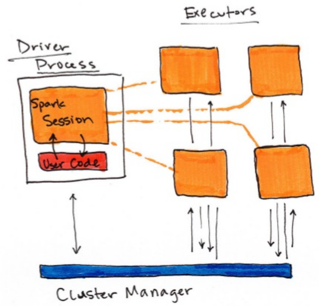
Figure 1-1 shows, on the left, our driver and on the right the four worker nodes
on the right.
NOTE:
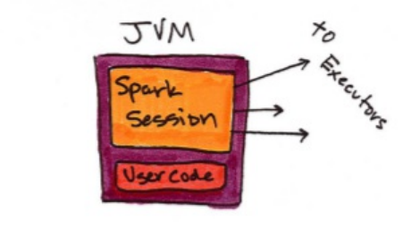
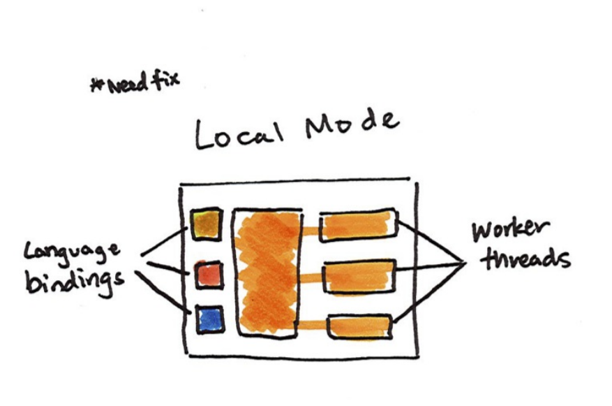
Spark, in addition to its cluster mode, also has a local mode. Remember how
the driver and executors are processes? This means that Spark does not dictate
where these processes live. In local mode, these processes run on your
individual computer instead of a cluster. See figure 1-3 for a high level
diagram of this architecture. This is the easiest way to get started with Spark
and what the demonstrations in this book should run on.
Using Spark from Scala, Java, SQL,
Python, or R
As you likely noticed in the previous figures, Spark works with multiple
languages. These language APIs allow you to run Spark code from another
language. When using the Structured APIs, code written in any of Spark’s
supported languages should perform the same, there are some caveats to this
but in general this is the case. Before diving into the details, let’s just touch a
bit on each of these langauges and their integration with Spark.
Scala
Spark is primarily written in Scala, making it Spark’s “default” language. This
book will include examples of Scala where ever there are code samples.
Python
Python supports nearly everything that Scala supports. This book will include
Python API examples wherever possible.
Java
Even though Spark is written in Scala, Spark’s authors have been careful to
ensure that you can write Spark code in Java. This book will focus primarily
on Scala but will provide Java examples where relevant.
SQL
Spark supports user code written in ANSI 2003 Compliant SQL. This makes it
easy for analysts and non-programmers to leverage the big data powers of
Spark. This book will include numerous SQL examples.
R
Spark supports the execution of R code through a project called SparkR. We
will cover this in the Ecosystem section of the book along with other
interesting projects that aim to do the same thing like Sparklyr.

Key Concepts
Now we have not exhaustively explored every detail about Spark’s
architecture because at this point it’s not necessary to get us closer to running
our own Spark code. The key points are that:
Spark has some cluster manager that maintains an understanding of the
resources available.
The driver process is responsible for executing our driver program’s
commands accross the executors in order to complete our task.
There are two modes that you can use, cluster mode (on multiple
machines) and local mode (on a single machine).
Starting Spark
Now in the previous chapter we talked about what you need to do to get started
with Spark by setting your Java, Scala, and Python versions. Now it’s time to
start Spark’s local mode, this means running ./bin/spark-shell. Once you
start that you will see a console, into which you can enter commands. If you
would like to work in Python you would run ./bin/pyspark.
SparkSession
From the beginning of this chapter we know that we leverage a driver process
to maintain our Spark Application. This driver process manifests itself to the
user as something called the SparkSession. The SparkSession instance is the
entrance point to executing code in Spark, in any language, and is the user-
facing part of a Spark Application. In Scala and Python the variable is
available as spark when you start up the Spark console. Let’s go ahead and
look at the SparkSession in both Scala and/or Python.
%scala
spark
%python
spark
In Scala, you should see something like:
res0: org.apache.spark.sql.SparkSession = org.apache.spark.sql.SparkSession@27159a24
In Python you’ll see something like:
<pyspark.sql.session.SparkSession at 0x7efda4c1ccd0>
Now you need to understand how to submit commands to the SparkSession.
Let’s do that by performing one of the simplest tasks that we can - creating a
range of numbers. This range of numbers is just like a named column in a
spreadsheet.
%scala
val myRange = spark.range(1000).toDF("number")
%python
myRange = spark.range(1000).toDF("number")
You just ran your first Spark code! We created a DataFrame with one column
containing 1000 rows with values from 0 to 999. This range of number
represents a distributed collection. Running on a cluster, each part of this
range of numbers would exist on a different executor. You’ll notice that the
value of myRange is a DataFrame, let’s introduce DataFrames!
DataFrames
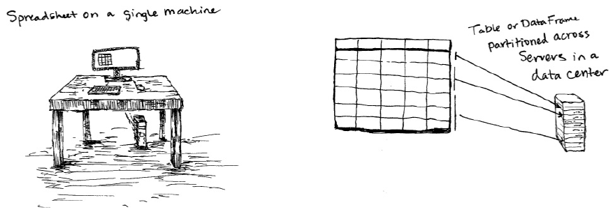
A DataFrame is a table of data with rows and columns. We call the list of
columns and their types a schema. A simple analogy would be a spreadsheet
with named columns. The fundamental difference is that while a spreadsheet
sits on one computer in one specific location, a Spark DataFrame can span
potentially thousands of computers. The reason for putting the data on more
than one computer should be intuitive: either the data is too large to fit on one
machine or it would simply take too long to perform that computation on one
machine.
The DataFrame concept is not unique to Spark. The R Language has a similar
concept as do certain libraries in the Python programming language. However,
Python/R DataFrames (with some exceptions) exist on one machine rather than
multiple machines. This limits what you can do with a given DataFrame in
python and R to the resources that exist on that specific machine. However,
since Spark has language interfaces for both Python and R, it’s quite easy to
convert to Pandas (Python) DataFrames to Spark DataFrames and R
DataFrames to Spark DataFrames (in R).
Note
Spark has several core abstractions: Datasets, DataFrames, SQL Tables, and
Resilient Distributed Datasets (RDDs). These abstractions all represent
distributed collections of data however they have different interfaces for
working with that data. The easiest and most efficient are DataFrames, which
are available in all languages. We cover Datasets in Section II, Chapter 8 and
RDDs in depth in Section III Chapter 2 and 3. The following concepts apply to
all of the core abstractions.
Partitions
In order to leverage the the resources of the machines in cluster, Spark breaks
up the data into chunks, called partitions. A partition is a collection of rows
that sit on one physical machine in our cluster. A DataFrame consists of zero or
more partitions.
When we perform some computation, Spark will operate on each partition in
parallel unless an operation calls for a shuffle, where multiple partitions need
to share data. Think about it this way, if you need to run some errands you
typically have to do those one by one, or serially. What if you could instead
give one errand to a worker who would then complete that task and then report
back to you? In that scenario, the key is to break up errands efficiently so that
you can get as much work done in as little time as possible. In the Spark world
an “errand” is equivalent to computation + data and a “worker” is equivalent
to an executor.
Now with DataFrames, we do not manipulate partitions individually, Spark
gives us the DataFrame interface for doing that. Now when we ran the above
code, you’ll notice there was no list of numbers, only a type signature. This is
because Spark organizes computation into two categories, transformations and
actions. When we create a DataFrame, we perform a transformation.
Transformations
In Spark, the core data structures are immutable meaning they cannot be
changed once created. This might seem like a strange concept at first, if you
cannot change it, how are you supposed to use it? In order to “change” a
DataFrame you will have to instruct Spark how you would like to modify the
DataFrame you have into the one that you want. These instructions are called
transformations. Transformations are how you, as user, specify how you
would like to transform the DataFrame you currently have to the DataFrame
that you want to have. Let’s show an example. To computer whether or not a
number is divisible by two, we use the modulo operation to see the remainder
left over from dividing one number by another.
We can use this operation to perform a transformation from our current
DataFrame to a DataFrame that only contains numbers divisible by two. To do
this, we perform the modulo operation on each row in the data and filter out the
results that do not result in zero. We can specify this filter using a where
clause.
%scala
val divisBy2 = myRange.where("number % 2 = 0")
%python
divisBy2 = myRange.where("number % 2 = 0")
Note
Now if you worked with any relational databases in the past, this should feel
quite familiar. You might say, aha! I know the exact expression I should use if
this was a table.
SELECT * FROM myRange WHERE number % 2 = 0
When we get to the next part of this chapter to discuss Spark SQL, you will
find out that this expression is perfectly valid. We’ll show you how to turn any
DataFrame into a table.
These operations create a new DataFrame but do not execute any computation.
The reason for this is that DataFrame transformations do not trigger Spark to
execute your code, they are lazily evaluated.
Lazy Evaluation
Lazy evaulation means that Spark will wait until the very last moment to
execute your transformations. In Spark, instead of modifying the data quickly,
we build up a plan of the transformations that we would like to apply. Spark,
by waiting for the last minute to execute your code, can try and make this plan
run as efficiently as possible across the cluster.
Actions
To trigger the computation, we run an action. An action instructs Spark to
compute a result from a series of transformations. The simplest action is
count which gives us the total number of records in the DataFrame.
%scala
divisBy2.count()
%python
divisBy2.count()
We now see a result! There are 500 number divisible by two from o to 999
(big surprise!). Now count is not the only action. There are three kinds of
actions: actions to view data in the console, actions to collect data to native
objects in the respective language, and actions to write to output data sources.
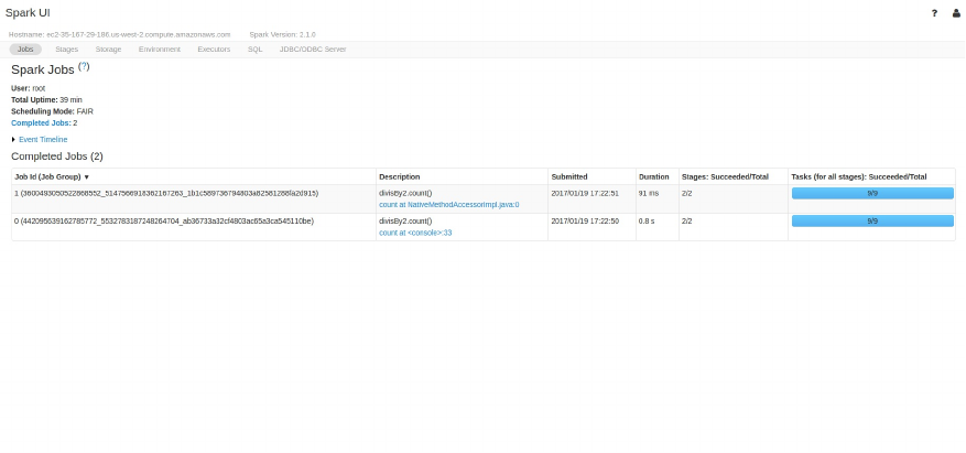
Spark UI
During Spark’s execution of the previous code block, users can monitor the
progress of their job through the Spark UI. The Spark UI is available on port
4040 of the driver node. If you are running in local mode this will just be the
http://localhost:4040. The Spark UI maintains information on the state of
our Spark jobs, environment, and cluster state. It’s very useful, especially for
tuning and debugging. In this case, we can see one Spark job with one stage
and nine tasks were executed.
In this chapter we will avoid the details of Spark jobs and the Spark UI, at this
point you should understand that a Spark job represents a set of transformations
triggered by an individual action. We talk in depth about the Spark UI and the
breakdown of a Spark job in Section IV.

A Basic Transformation Data Flow
In the previous example, we created a DataFrame from a range of data.
Interesting, but not exactly applicable to industry problems. Let’s create some
DataFrames with real data in order to better understand how they work. We’ll
be using some flight data from the United States Bureau of Transportation
statistics.
We touched briefly on the SparkSession as the interface the entry point to
performing work on the Spark cluster. the SparkSession can do much more than
simply parallelize an array it can create DataFrames directly from a file or set
of files. In this case, we will create our DataFrames from a JavaScript Object
Notation (JSON) file that contains some summary flight information as
collected by the United States Bureau of Transport Statistics. In the folder
provided, you’ll see that we have one file per year.
%fs ls /mnt/defg/chapter-1-data/json/
This file has one JSON object per line and is typically refered to as line-
delimited JSON.
%fs head /mnt/defg/chapter-1-data/json/2015-summary.json
What we’ll do is start with one specific year and then work up to a larger set
of data. Let’s go ahead and create a DataFrame from 2015. To do this we will
use the DataFrameReader (via spark.read) interface, specify the format and
the path.
%scala
val flightData2015 = spark
.read
.json("/mnt/defg/chapter-1-data/json/2015-summary.json")
%python
flightData2015 = spark\
.read\
.json("/mnt/defg/chapter-1-data/json/2015-summary.json")
flightData2015
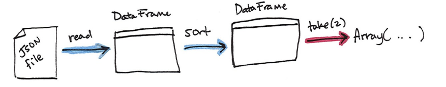
You’ll see that our two DataFrames (in Scala and Python) each have a set of
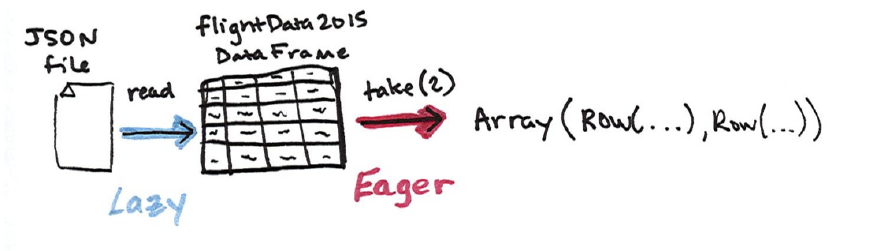
columns with an unspecified number of rows. Let’s take a peek at the data with
a new action, take, which allows us to view the first couple of rows in our
DataFrame. Figure 1-7 illustrates the conceptual actions that we perform in the
process. We lazily create the DataFrame then call an action to take the first two
values.
%scala
flightData2015.take(2)
%python
flightData2015.take(2)
Remember how we talked about Spark building up a plan, this is not just a
conceptual tool, this is actually what happens under the hood. We can see the
actual plan built by Spark by running the explain method.
flightData2015.explain()
%python
flightData2015.explain()
Congratulations, you’ve just read your first explain plan! This particular plan
just describes reading data from a certain location however as we continue,
you will start to notice patterns in the explain plans. Without going into too
much detail at this point, the explain plan represents the logical combination of
transformations Spark will run on the cluster. We can use this to make sure that
our code is as optimized as possible. We will not cover that in this chapter, but
will touch on it in the optimization chapter.
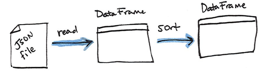
Now in order to gain a better understanding of transformations and plans, let’s
create a slightly more complicated plan. We will specify an intermediate step
which will be to sort the DataFrame by the values in the first column. We can
tell from our DataFrame’s column types that it’s a string so we know that it
will sort the data from A to Z.
Note
Remember, we cannot modify this DataFrame by specifying the sort
transformation, we can only create a new DataFrame by transforming that
previous DataFrame. We can see that even though we’re seeming to ask for
computation to be completed Spark doesn’t yet execute this command, we’re
just building up a plan. The illustration in figure 1-8 represents the spark plan
we see in the explain plan for that DataFrame.
%scala
val sortedFlightData2015 = flightData2015.sort("count")
sortedFlightData2015.explain()
%python
sortedFlightData2015 = flightData2015.sort("count")
sortedFlightData2015.explain()
Now, just like we did before, we can specify an action in order to kick off this
plan.
%scala
sortedFlightData2015.take(2)
%python
sortedFlightData2015.take(2)
The conceptual plan that we executed previously is illustrated in Figure-9.
Now this planning process is essentially defining lineage for the DataFrame so
that at any given point in time Spark knows how to recompute any partition of a
given DataFrame all the way back to a robust data source be it a file or
database. Now that we performed this action, remember that we can navigate
to the Spark UI (port 4040) and see the information about this jobs stages and
tasks.
Now hopefully you have grasped the basics but let’s just reinforce some of the
core concepts with another data pipeline. We’re going to be using the same
flight data used except that this time we’ll be using a copy of the data in comma
seperated value (CSV) format.
If you look at the previous code, you’ll notice that the column names appeared
in our results. That’s because each line is a json object that has a defined
structure or schema. As mentioned, the schema defines the column names and
types. This is a term that is used in the database world to describe what types
are in every column of a table and it’s no different in Spark. In this case the
schema defines ORIGIN_COUNTRY_NAME to be a string. JSON and CSVs qualify
as semi-structured data formats and Spark supports a range of data sources in
its APIs and ecosystem.
Let’s go ahead and define our DataFrame just like we did before however this
time we’re going to specify an option for our DataFrameReader. Options
allow you to control how you read in a given file format and tell Spark to take
advantage of some of the structures or information available in the files. In this
case we’re going to use two popular options inferSchema and header.
%scala
val flightData2015 = spark.read
.option("inferSchema", "true")
.option("header", "true")
.csv("/mnt/defg/chapter-1-data/csv/2015-summary.csv")
flightData2015
%python
flightData2015 = spark.read\
.option("inferSchema", "true")\
.option("header", "true")\
.csv("/mnt/defg/chapter-1-data/csv/2015-summary.csv")
flightData2015
After running the code you should notice that we’ve basically arrived at the
same DataFrame that we had when we read in our data from json with the
correct looking column names and types. However, we had to be more explicit
when it came to reading in the CSV file as opposed to json because json
provides a bit more structure than CSVs because JSON has a notion of types.
Looking at them, the header option should feel like it makes sense. The first
row in our csv file is the header (column names) and because CSV files are not
guaranteed to have this information we must specify it manually. The
inferSchema option might feel a bit more unfamiliar. JSON objects provides
a bit more structure than csvs because JSON has a notion of types. We can get
past this by infering the schema of the csv file we are reading in. Now it cannot
do this magically, it must scan (read in) some of the data in order to infer this,
but this saves us from having to specify the types for each column manually at
the risk of Spark potentially making an errorneous guess as to what the type for
a column should be.
A discerning reader might notice that the schema returned by our CSV reader
does not exactly match that of the json reader.
val csvSchema = spark.read.format("csv")
.option("inferSchema", "true")
.option("header", "true")
.load("/mnt/defg/chapter-1-data/csv/2015-summary.csv")
.schema
val jsonSchema = spark
.read.format("json")
.load("/mnt/defg/chapter-1-data/json/2015-summary.json")
.schema
println(csvSchema)
println(jsonSchema)
%python
csvSchema = spark.read.format("csv")\
.option("inferSchema", "true")\
.option("header", "true")\
.load("/mnt/defg/chapter-1-data/csv/2015-summary.csv")\
.schema
jsonSchema = spark.read.format("json")\
.load("/mnt/defg/chapter-1-data/json/2015-summary.json")\
.schema
print(csvSchema)
print(jsonSchema)
The csv schema:
StructType(StructField(DEST_COUNTRY_NAME,StringType,true),
StructField(ORIGIN_COUNTRY_NAME,StringType,true),
StructField(count,IntegerType,true))
The JSON schema:
StructType(StructField(DEST_COUNTRY_NAME,StringType,true),
StructField(ORIGIN_COUNTRY_NAME,StringType,true),
StructField(count,LongType,true))
For our purposes the difference between a LongType and an IntegerType is
of little consequence however this may be of greater significance in production
scenarios. Naturally we can always explicitly set a schema (rather than
inferring it) when we read in data as well. These are just a few of the options
we have when we read in data, to learn more about these options see the
chapter on reading and writing data.
%scala
val flightData2015 = spark.read
.schema(jsonSchema)
.option("header", "true")
.csv("/mnt/defg/chapter-1-data/csv/2015-summary.csv")
%python
flightData2015 = spark.read\
.schema(jsonSchema)\
.option("header", "true")\
.csv("/mnt/defg/chapter-1-data/csv/2015-summary.csv")
DataFrames and SQL
Spark provides another way to query and operate on our DataFrames, and
that’s with SQL! Spark SQL allows you as a user to register any DataFrame as
a table or view (a temporary table) and query it using pure SQL. There is no
performance difference between writing SQL queries or writing DataFrame
code, they both “compile” to the same underlying plan that we specify in
DataFrame code.
Any DataFrame can be made into a table or view with one simple method call.
%scala
flightData2015.createOrReplaceTempView("flight_data_2015")
%python
flightData2015.createOrReplaceTempView("flight_data_2015")
Now we can query our data in SQL. To execute a SQL query, we’ll use the
spark.sql function (remember spark is our SparkSession variable?) that
conveniently, returns a new DataFrame. While this may seem a bit circular in
logic - that a SQL query against a DataFrame returns another DataFrame, it’s
actually quite powerful. As a user, you can specify transformations in the
manner most convenient to you at any given point in time and not have to trade
any efficiency to do so! To understand that this is happening, let’s take a look at
two explain plans.
Vi%scala
val sqlWay = spark.sql("""
SELECT DEST_COUNTRY_NAME, count(1)
FROM flight_data_2015
GROUP BY DEST_COUNTRY_NAME
""")
val dataFrameWay = flightData2015
.groupBy('DEST_COUNTRY_NAME)
.count()
sqlWay.explain
dataFrameWay.explain
%python
sqlWay = spark.sql("""
SELECT DEST_COUNTRY_NAME, count(1)
FROM flight_data_2015
GROUP BY DEST_COUNTRY_NAME
""")
dataFrameWay = flightData2015\
.groupBy("DEST_COUNTRY_NAME")\
.count()
sqlWay.explain()
dataFrameWay.explain()
We can see that these plans compile to the exact same underlying plan!
To reinforce the tools available to us, let’s pull out some interesting stats from
our data. Our first question will use our first imported function, the max
function, to find out what the maximum number of flights to and from any given
location are. This just scans each value in relevant column the DataFrame and
sees if it’s bigger than the previous values that have been seen. This is a
transformation, as we are effectively filtering down to one row. Let’s see what
that looks like.
// scala or python
spark.sql("SELECT max(count) from flight_data_2015").take(1)
%scala
import org.apache.spark.sql.functions.max
flightData2015.select(max("count")).take(1)
%python
from pyspark.sql.functions import max
flightData2015.select(max("count")).take(1)
Let’s move onto something a bit more complicated. What are the top five
destination countries in the data set? This is a our first multi-transformation
query so we’ll take it step by step. We will start with a fairly straightforward
SQL aggregation.
%scala
val maxSql = spark.sql("""
SELECT DEST_COUNTRY_NAME, sum(count) as destination_total
FROM flight_data_2015
GROUP BY DEST_COUNTRY_NAME
ORDER BY sum(count) DESC
LIMIT 5""")
maxSql.collect()
%python
maxSql = spark.sql("""
SELECT DEST_COUNTRY_NAME, sum(count) as destination_total
FROM flight_data_2015
GROUP BY DEST_COUNTRY_NAME
ORDER BY sum(count) DESC
LIMIT 5""")
maxSql.collect()
Now let’s move to the DataFrame syntax that is semantically similar but
slightly different in implementation and ordering. But, as we mentioned, the
underlying plans for both of them are the same. Let’s execute the queries and
see their results as a sanity check.
%scala
import org.apache.spark.sql.functions.desc
flightData2015
.groupBy("DEST_COUNTRY_NAME")
.sum("count")
.withColumnRenamed("sum(count)", "destination_total")
.sort(desc("destination_total"))
.limit(5)
.collect()
%python
from pyspark.sql.functions import desc
flightData2015\
.groupBy("DEST_COUNTRY_NAME")\
.sum("count")\
.withColumnRenamed("sum(count)", "destination_total")\
.sort(desc("destination_total"))\
.limit(5)\
.collect()
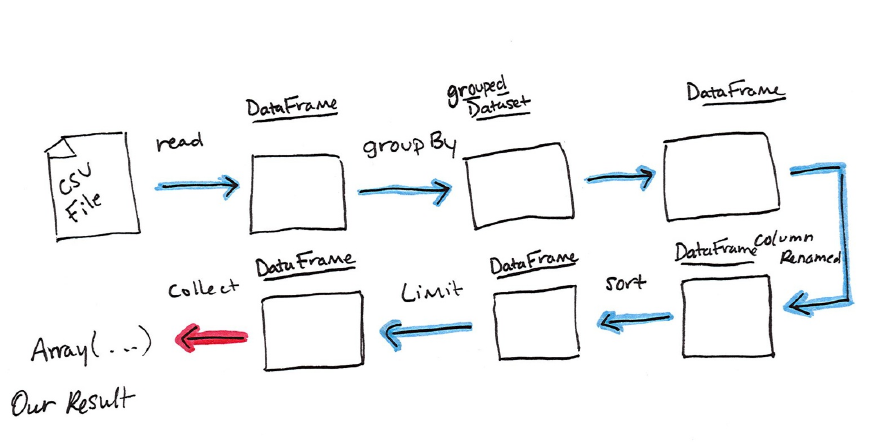
Now there are 7 steps that take us all the way back to the source data.
Illustrated below are the set of steps that we perform in “code”. The true
execution plan (the one visible in explain) will differ from what we have
below because of optimizations in physical execution, however the illustration
is as good of a starting point as any. With Spark, we are always building up a
directed acyclic graph of transformations resulting in immutable objects that
we can subsequently call an action on to see a result.
The first step is to read in the data. We defined the DataFrame previously but,
as a reminder, Spark does not actually read it in until an action is called on that
DataFrame or one derived from the original DataFrame.
The second step is our grouping, technically when we call “groupBy” we end
up with a RelationalGroupedDataset which is a fancy name for a DataFrame
that has a grouping specified but needs a user to specify an aggregation before
it can be queried further. We can see this by trying to perform an action on it
(which will not work). We still haven’t performed any computation (besides
relational algebra) - we’re simply passing along information about the layout
of the data.
Therefore the third step is to specify the aggregation. Let’s use the sum
aggregation method. This takes as input a column expression or simply, a
column name. The result of the sum method call is a new dataFrame. You’ll see
that it has a new schema but that it does know the type of each column. It’s
important to reinforce (again!) that no computation has been performed. This is
simply another transformation that we’ve expressed and Spark is simply able
to trace the type information we have supplied.
The fourth step is a simple renaming, we use the withColumnRenamed method
that takes two arguments, the original column name and the new column name.
Of course, this doesn’t perform computation - this is just another
transformation!
The fifth step sorts the data such that if we were to take results off of the top of
the DataFrame, they would be the largest values found in the
destination_total column.
You likely noticed that we had to import a function to do this, the desc
function. You might also notice that desc does not return a string but a Column.
In general, many DataFrame methods will accept Strings (as column names) or
Column types or expressions. Columns and expressions are actually the exact
same thing
The final step is just a limit. This just specifies that we only want five values.
This is just like a filter except that it filters by position (lazily) instead of by
value. It’s safe to say that it basically just specifies a DataFrame of a certain
size.
The last step is our action! Now we actually begin the process of collecting the
results of our DataFrame above and Spark will give us back a list or array in
the language that we’re executing. Now to reinforce all of this, let’s look at the
explain plan for the above query.
flightData2015
.groupBy("DEST_COUNTRY_NAME")
.sum("count")
.withColumnRenamed("sum(count)", "destination_total")
.sort(desc("destination_total"))
.limit(5)
.explain()
== Physical Plan ==
TakeOrderedAndProject(limit=5, orderBy=[destination_total#16194L DESC], output=[DEST_COUNTRY_NAME#7323,destination_total#16194L])
+- *HashAggregate(keys=[DEST_COUNTRY_NAME#7323], functions=[sum(count#7325L)])
+- Exchange hashpartitioning(DEST_COUNTRY_NAME#7323, 5)
+- *HashAggregate(keys=[DEST_COUNTRY_NAME#7323], functions=[partial_sum(count#7325L)])
+- InMemoryTableScan [DEST_COUNTRY_NAME#7323, count#7325L]
+- InMemoryRelation [DEST_COUNTRY_NAME#7323, ORIGIN_COUNTRY_NAME#7324, count#7325L], true, 10000, StorageLevel(disk, memory, deserialized, 1 replicas)
+- *Scan csv [DEST_COUNTRY_NAME#7578,ORIGIN_COUNTRY_NAME#7579,count#7580L] Format: CSV, InputPaths: dbfs:/mnt/defg/chapter-1-data/csv/2015-summary.csv, PartitionFilters: [], PushedFilters: [], ReadSchema: struct<DEST_COUNTRY_NAME:string,ORIGIN_COUNTRY_NAME:string,count:bigint>
While this explain plan doesn’t match our exact “conceptual plan” all of the
pieces are there. You can see the limit statement as well as the orderBy (in the
first line). You can also see how our aggregation happens in two phases, in the
partial_sum calls. This is because summing a list of numbers is commutative
and Spark can perform the sum, partition by partition. Of course we can see
how we read in the DataFrame as well.
You are now equipped with the Spark knowledge to writing your own Spark
code. In the next chapter we will explore some of Spark’s more advanced
features.
Chapter 2. Structured API
Overview
Spark’s Structured APIs
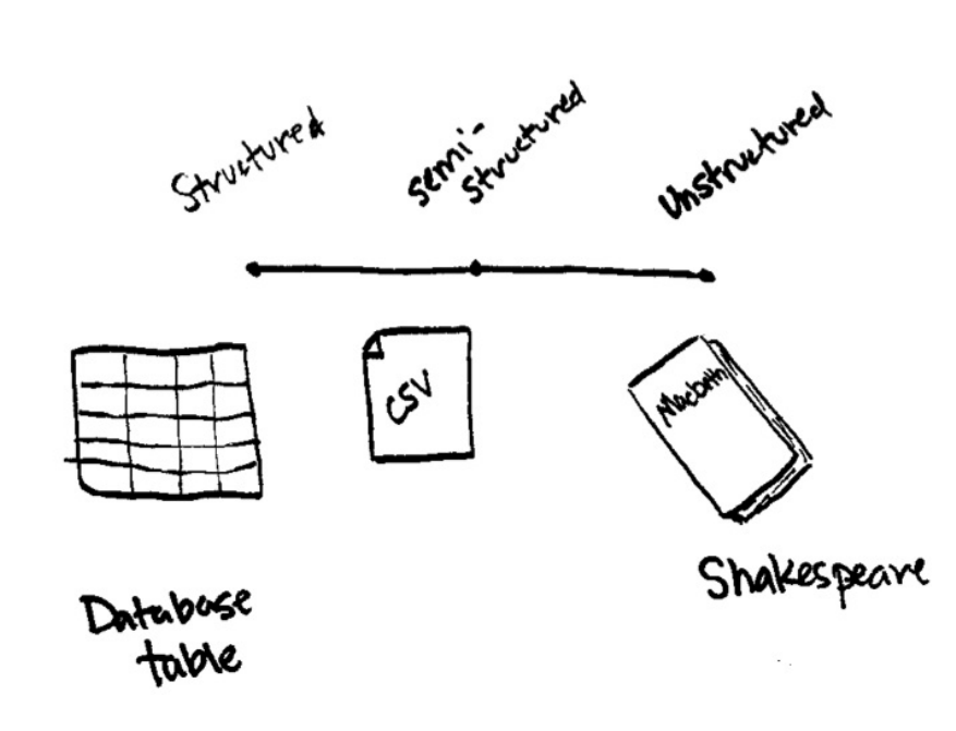
For our purposes there is a spectrum of types of data. The two extremes of the
spectrum are structured and unstructured. Structured and semi-structured data
refer to to data that have structure that a computer can understand relatively
easily. Unstructured data, like a poem or prose, is much harder to a computer
to understand. Spark’s Structured APIs allow for transformations and actions
on structured and semi-structured data.
The Structured APIs specifically refer to operations on DataFrames, Datasets,
and in Spark SQL and were created as a high level interface for users to
manipulate big data. This section will cover all the principles of the Structured
APIs. Although distinct in the book, the vast majority of these user-facing
operations apply to both batch as well as streaming computation.
The Structured API is the fundamental abstraction that you will leverage to
write your data flows. Thus far in this book we have taken a tutorial-based
approach, meandering our way through much of what Spark has to offer. In this
section, we will perform a deeper dive into the Structured APIs. This
introductory chapter will introduce the fundamental concepts that you should
understand: the typed and untyped APIs (and their differences); how to work
with different kinds of data using the structured APIs; and deep dives into
different data flows with Spark.
BOX
Before proceeding, let’s review the fundamental concepts and definitions
that we covered in the previous section. Spark is a distributed
programming model where the user specifies transformations, which
build up a directed-acyclic-graph of instructions, and actions, which
begin the process of executing that graph of instructions, as a single job,
by breaking it down into stages and tasks to execute across the cluster.
The way we store data on which to perform transformations and actions
are DataFrames and Datasets. To create a new DataFrame or Dataset, you
call a transformation. To start computation or convert to native language
types, you call an action.
DataFrames and Datasets
In Section I, we talked all about DataFrames. Spark has two notions of
“structured” data structures: DataFrames and Datasets. We will touch on the
(nuanced) differences shortly but let’s define what they both represent first.
To the user, DataFrames and Datasets are (distributed) tables with rows and
columns. Each column must have the same number of rows as all the other
columns (although you can use null to specify the lack of a value) and columns
have type information that tells the user what exists in each column.
To Spark, DataFrames and Datasets represent by immutable, lazily evaluated
plans that specify how to perform a series of transformations to generate the
correct output. When we perform an action on a DataFrame we instruct Spark
to perform the actual transformations that represent that DataFrame. These
represent plans of how to manipulate rows and columns to compute the user’s
desired result. Let’s go over rows and column to more precisely define those
concepts.
Schemas
One core concept that differentiates the Structured APIs from the lower level
APIs is the concept of a schema. A schema defines the column names and types
of a DataFrame. Users can define schemas manually or users can read a
schema from a data source (often called schema on read). Now that we know
what defines DataFrames and Datasets and how they get their structure, via a
Schema, let’s see an overview of all of the types.
Overview of Structured Spark
Types
Spark is effectively a programming language of its own. When you perform
operations with Spark, it maintains its own type information throughout the
process. This allows it to perform a wide variety of optimizations during the
execution process. These types correspond to the types that Spark connects to
in each of Scala, Java, Python, SQL, and R. Even if we use Spark’s Structured
APIs from Python, the majority of our manipulations will operate strictly on
Spark types, not Python types. For example, the below code does not perform
addition in Scala or Python, it actually performs addition purely in Spark.
%scala
val df = spark.range(500).toDF("number")
df.select(df.col("number") + 10)
// org.apache.spark.sql.DataFrame = [(number + 10): bigint]
%python
df = spark.range(500).toDF("number")
df.select(df["number"] + 10)
# DataFrame[(number + 10): bigint]
This is because, as mentioned, Spark maintains its own type information,
stored as a schema, and through some magic in each languages bindings, can
convert an expression in one language to Spark’s representation of that.
NOTE
There are two distinct APIs within the In the Structured APIs. There is the
API that goes across languages, more commonly referred to as the
DataFrame or “untyped API”. THe second API is the “typed API” or
“Dataset API”, that is only available to JVM based languages (Scala and
Java). This is a bit of a misnomer because the “untyped API” does have
types but it only operates on Spark types at run time. The “typed API”
allows you to define your own types to represent each record in your
dataset with “case classes or Java Beans” and types are checked at
compile time. Each record (or row) in the “untyped API” consists of a
Row object that are available across languages and still have types, but
only Spark types, not native types. The “typed API” is covered in the
Datasets Chapter at the end of Section II. The majority of Section II will
cover the “untyped API” however all of this still applies to the “typed
API”.
Notice how the following code produces a Dataset of type Long, but also has
an internal Spark type (bigint).
%scala
spark.range(500)
Notice how the following code produces a DataFrame with an internal Spark
type (bigint).
%python
spark.range(500)
Columns
For now, all you need to understand about columns is that they can represent a
simple type like an integer or string, a complex types like an array or map, or a
null value. Spark tracks all of this type information to you and has a variety of
ways that you can transform columns. Columns are discussed extensively in the
next chapter but for the most part you can think about Spark Column types as
columns in a table.
Rows
There are two ways of getting data into Spark, through Rows and Encoders.
Row objects are the most general way of getting data into, and out of, Spark
and are available in all languages. Each record in a DataFrame must be of Row
type as we can see when we collect the following DataFrames.
%scala
spark.range(2).toDF().collect()
%python
spark.range(2).collect()
Spark Value Types
On the next page you will find a large table of all Spark types along with the
corresponding language specific types. Caveats and details are included for the
reader as well to make it easier to reference.
To work with the correct Scala types:
import org.apache.spark.sql.types._
val b = ByteType()
To work with the correct Java types you should use the factory methods in the
following package:
import org.apache.spark.sql.types.DataTypes;
ByteType x = DataTypes.ByteType();
Python types at time have certain requirements (like the listed requirement for
ByteType below.To work with the correct Python types:
from pyspark.sql.types import *
b = byteType()
Spark Type Scala Value Type Scala API
ByteType Byte ByteType
ShortType Short ShortType
IntegerType Int IntegerType
LongType Long LongType
FloatType Float FloatType
DoubleType Double DoubleType
DecimalType java.math.BigDecimal DecimalType
StringType String StringType
BinaryType Array[Byte] BinaryType
TimestampType java.sql.Timestamp TimestampType
DateType java.sql.Date DateType
ArrayType scala.collection.Seq ArrayType(elementType,
[valueContainsNull]) **
MapType scala.collection.Map MapType(keyType, valueType,
[valueContainsNull]) **
StructType org.apache.spark.sql.Row StructType(Seq(StructFields))
*
StructField StructField with
DataType contents.
StructField(name, dataType,
nullable)
Numbers will be converted to 1-byte signed integer numbers at runtime.
Make sure that numbers are within the range of -128 to 127.
Numbers will be converted to 2-byte signed integer numbers at
runtime. Please make sure that numbers are within the range of
-32768 to 32767.
Numbers will be converted to 8-byte signed integer numbers at
runtime. Please make sure that numbers are within the range of
-9223372036854775808 to 9223372036854775807.
Otherwise, please convert data to decimal.Decimal and use
DecimalType.
valueContainsNull is true by default.
No two fields can have the same name.
Encoders
Using Spark from Scala and Java allows you to define your own JVM types to
use in place of Rows that consist of the above data types. To do this, we use an
Encoder. Encoders are only available in Scala, with case classes, and Java,
with JavaBeans. For some types, like Long, Spark already includes an
Encoder. For instance we can collect a Dataset of type Long and get native
Scala types back. We will cover encoders in the Datasets chapter.
spark.range(2).collect()
Overview of Spark Execution
In order to help you understand (and potentially debug) the process of writing
and executing code on clusters, let’s walk through the execution of a single
structured API query from user code to executed code. As an overview the
steps are:
1. Write DataFrame/Dataset/SQL Code
2. If valid code, Spark converts this to a Logical Plan
3. Spark transforms this Logical Plan to a Physical Plan
4. Spark then executes this Physical Plan on the cluster
To execute code, we have to write code. This code is then submitted to Spark
either through the console or via a submitted job. This code then passes
through the Catalyst Optimizer which decides how the code should be executed
and lays out a plan for doing so, before finally the code is run and the result is
returned to the user.
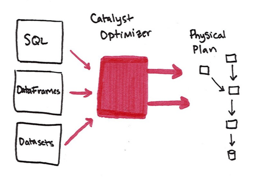
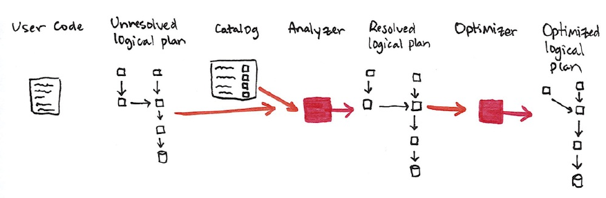
Logical Planning
The first phase of execution is meant to take user code and convert it into a
logical plan. This process in illustrated in the next figure.
This logical plan only represents a set of abstract transformations that do not
refer to executors or drivers, it’s purely to convert the user’s set of expressions
into the most optimized version. It does this by converting user code into an
unresolved logical plan. This unresolved because while your code may be
valid, the tables or columns that it refers to may or may not exist. Spark uses
the catalog, a repository of all table and DataFrame information, in order to
resolve columns and tables in the analyzer. The analyzer may reject the
unresolved logical plan if it the required table or column name does not exist
in the catalog. If it can resolve it, this result is passed through the optimizer, a
collection of rules, which attempts to optimize the logical plan by pushing
down predicates or selections.
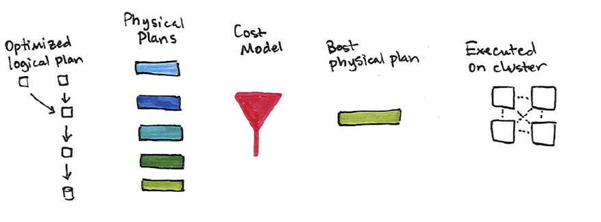
Physical Planning
After successfully creating an optimized logical plan, Spark then begins the
physical planning process. The physical plan, often called a Spark plan,
specifies how the logical plan will execute on the cluster by generating
different physical execution strategies and comparing them through a cost
model. An example of the cost comparison might be choosing how to perform a
given join by looking at the physical attributes of a given table (how big the
table is or how big its partitions are.)
Physical planning results in a series of RDDs and transformations. This result
is why you may have heard Spark referred to as a compiler, it takes queries in
DataFrames, Datasets, and SQL and compiles them into RDD transformations
for you.
Execution
Upon selecting a physical plan, Spark runs all of this code over RDDs, the
lower-level programming interface of Spark covered in Part III. Spark
performs further optimizations by, at runtime, generating native Java Bytecode
that can remove whole tasks or stages during execution. Finally the result is
returned to the user.
Chapter 3. Basic Structured
Operations
Chapter Overview
In the previous chapter we introduced the core abstractions of the Structured
API. This chapter will move away from the architectural concepts and towards
the tactical tools you will use to manipulate DataFrames and the data within
them. This chapter will focus exclusively on single DataFrame operations and
avoid aggregations, window functions, and joins which will all be discussed
in depth later in this section.
Definitionally, a DataFrame consists of a series of records (like rows in a
table), that are of type Row, and a number of columns (like columns in a
spreadsheet) that represent an computation expression that can performed on
each individual record in the dataset. The schema defines the name as well as
the type of data in each column. The partitioning of the DataFrame defines the
layout of the DataFrame or Dataset’s physical distribution across the cluster.
The partitioning scheme defines how that is broken up, this can be set to be
based on values in a certain column or non-deterministically.
Let’s define a DataFrame to work with.
%scala
val df = spark.read.format("json")
.load("/mnt/defg/flight-data/json/2015-summary.json")
%python
df = spark.read.format("json")\
.load("/mnt/defg/flight-data/json/2015-summary.json")
We discussed that a DataFame will have columns, and we use a “schema” to
view all of those. We can run the following command in Scala or in Python.
df.printSchema()
The schema ties the logical pieces together and is the starting point to better
understand DataFrames.
Schemas
A schema defines the column names and types of a DataFrame. We can either
let a data source define the schema (called schema on read) or we can define
it explicitly ourselves.
NOTE
Deciding whether or not you need to define a schema prior to reading in
your data depends your use case. Often times for ad hoc analysis, schema
on read works just fine (although at times it can be a bit slow with plain
text file formats like csv or json). However, this can also lead to
precision issues like a long type incorrectly set as an integer when
reading in a file. When using Spark for production ETL, it is often a good
idea to define your schemas manually, especially when working with
untyped data sources like csv and json because schema inference can vary
depending on the type of data that you read in.
Let’s start with a simple file we saw in the previous chapter and let the semi-
structured nature of line-delimited JSON define the structure. This data is flight
data from the United States Bureau of Transportation statistics.
%scala
spark.read.format("json")
.load("/mnt/defg/flight-data/json/2015-summary.json")
.schema
Scala will return:
org.apache.spark.sql.types.StructType = ...
StructType(StructField(DEST_COUNTRY_NAME,StringType,true),
StructField(ORIGIN_COUNTRY_NAME,StringType,true),
StructField(count,LongType,true))
%python
spark.read.format("json")\
.load("/mnt/defg/flight-data/json/2015-summary.json")\
.schema
Python will return:
StructType(List(StructField(DEST_COUNTRY_NAME,StringType,true),
StructField(ORIGIN_COUNTRY_NAME,StringType,true),
StructField(count,LongType,true)))
A schema is a StructType made up of a number of fields, StructFields, that
have a name, type, and a boolean flag which specifies whether or not that
column can contain missing or null values. Schemas can also contain other
StructType (Spark’s complex types). We will see this in the next chapter
when we discuss working with complex types.
Here’s out to create, and enforce a specific schema on a DataFrame. If the
types in the data (at runtime), do not match the schema. Spark will throw an
error.
%scala
import org.apache.spark.sql.types.{StructField, StructType, StringType
val myManualSchema = new StructType(Array(
new StructField("DEST_COUNTRY_NAME", StringType, true),
new StructField("ORIGIN_COUNTRY_NAME", StringType, true),
new StructField("count", LongType, false) // just to illustrate flipping this flag
))
val df = spark.read.format("json")
.schema(myManualSchema)
.load("/mnt/defg/flight-data/json/2015-summary.json")
Here’s how to do the same in Python.
%python
from pyspark.sql.types import StructField, StructType, StringType
myManualSchema = StructType([
StructField("DEST_COUNTRY_NAME", StringType(), True),
StructField("ORIGIN_COUNTRY_NAME", StringType(), True),
StructField("count", LongType(), False)
])
df = spark.read.format("json")\
.schema(myManualSchema)\
.load("/mnt/defg/flight-data/json/2015-summary.json")
As discussed in the previous chapter, we cannot simply set types via the per
language types because Spark maintains its own type information. Let’s now
discuss what schemas define, columns.
Columns and Expressions
To users, columns in Spark are similar to columns in a spreadsheet, R
dataframe, pandas DataFrame. We can select, manipulate, and remove columns
from DataFrames and these operations are represented as expressions.
To Spark, columns are logical constructions that simply represent a value
computed on a per-record basis by means of an expression. This means, in
order to have a real value for a column, we need to have a row, and in order to
have a row we need to have a DataFrame. This means that we cannot
manipulate an actual column outside of a DataFrame, we can only manipulate a
logical column’s expressions then perform that expression within the context of
a DataFrame.
Columns
There are a lot of different ways to construct and or refer to columns but the
two simplest ways are with the col or column functions. To use either of these
functions, we pass in a column name.
%scala
import org.apache.spark.sql.functions.{col, column}
col("someColumnName")
column("someColumnName")
%python
from pyspark.sql.functions import col, column
col("someColumnName")
column("someColumnName")
We will stick to using col throughout this book. As mentioned, this column
may or may not exist in our of our DataFrames. This is because, as we saw in
the previous chapter, columns are not resolved until we compare the column
names with those we are maintaining in the catalog. Column and table
resolution happens in the analyzer phase as discussed in the first chapter in
this section.
NOTE
Above we mentioned two different ways of referring to columns. Scala
has some unique language features that allow for more shorthand ways of
referring to columns. These bits of syntactic sugar perform the exact same
thing as what we have already, namely creating a column, and provide no
performance improvement.
%scala
$"myColumn"
'myColumn
The $ allows us to designate a string as a special string that should refer to an
expression. The tick mark ' is a special thing called a symbol, that is Scala-
specific construct of referring to some identifier. They both perform the same
thing and are shorthand ways of referring to columns by name. You’ll likely see
all the above references when you read different people’s spark code. We
leave it to the reader for you to use whatever is most comfortable and
maintainable for you.
Explicit Column References
If you need to refer to a specific DataFrame’s column, you can use the col
method on the specific DataFrame. This can be useful when you are performing
a join and need to refer to a specific column in one DataFrame that may share a
name with another column in the joined DataFrame. We will see this in the
joins chapter. As an added benefit, Spark does not need to resolve this column
itself (during the analyzer phase) because we did that for Spark.
df.col("count")
Expressions
Now we mentioned that columns are expressions, so what is an expression?
An expression is a set of transformations on one or more values in a record in
a DataFrame. Think of it like a function that takes as input one or more column
names, resolves them and then potentially applies more expressions to create a
single value for each record in the dataset. Importantly, this “single value” can
actually be a complex type like a Map type or Array type.
In the simplest case, an expression, created via the expr function, is just a
DataFrame column reference.
import org.apache.spark.sql.functions.{expr, col}
In this simple instance, expr("someCol") is equivalent to col("someCol").
Columns as Expressions
Columns provide a subset of expression functionality. If you use col() and
wish to perform transformations on that column, you must perform those on that
column reference. When using an expression, the expr function can actually
parse transformations and column references from a string and can
subsequently be passed into further transformations. Let’s look at some
examples.
expr("someCol - 5") is the same transformation as performing
col("someCol") - 5 or even expr("someCol") - 5. That’s because Spark
compiles these to a logical tree specifying the order of operations. This might
be a bit confusing at first, but remember a couple of key points.
1. Columns are just expressions.
2. Columns and transformations of those column compile to the same logical
plan as parsed expressions.
Let’s ground this with an example.
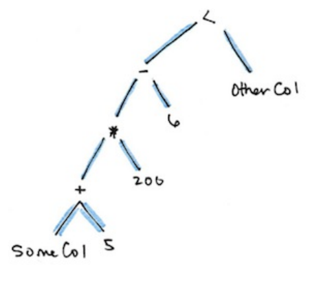
(((col("someCol") + 5) * 200) - 6) < col("otherCol")
Figure 1 shows an illustration of that logical tree.
This might look familiar because it’s a directed acyclic graph. This graph is
represented equivalently with the following code.
%scala
import org.apache.spark.sql.functions.expr
expr("(((someCol + 5) * 200) - 6) < otherCol")
%python
from pyspark.sql.functions import expr
expr("(((someCol + 5) * 200) - 6) < otherCol")
This is an extremely important point to reinforce. Notice how the previous
expression is actually valid SQL code as well, just like you might put in a
SELECT statement? That’s because this SQL expression and the previous
DataFrame code compile to the same underlying logical tree prior to
execution. This means you can write your expressions as DataFrame code or
as SQL expressions and get the exact same benefits. You likely saw all of this
in the first chapters of the book and we covered this more extensively in the
Overview of the Structured APIs chapter.
Accessing a DataFrame’s Columns
Sometimes you’ll need to see a DataFrame’s columns, you can do this by doing
something like printSchema however if you want to programmatically access
columns, you can use the columns method to see all columns listed.
spark.read.format("json")
.load("/mnt/defg/flight-data/json/2015-summary.json")
.columns
Records and Rows
In Spark, a record or row makes up a “row” in a DataFrame. A logical record
or row is an object of type Row. Row objects are the objects that column
expressions operate on to produce some usable value. Row objects represent
physical byte arrays. The byte array interface is never shown to users because
we only use column expressions to manipulate them.
You’ll notice collections that return values will always return one or more Row
types.
Note
we will use lowercase “row” and “record” interchangeably in this chapter,
with a focus on the latter. A capitalized “Row” will refer to the Row object.
We can see a row by calling first on our DataFrame.
%scala
df.first()
%python
df.first()
Creating Rows
You can create rows by manually instantiating a Row object with the values that
below in each column. It’s important to note that only DataFrames have
schema. Rows themselves do not have schemas. This means if you create a Row
manually, you must specify the values in the same order as the schema of the
DataFrame they may be appended to. We will see this when we discuss
creating DataFrames.
%scala
import org.apache.spark.sql.Row
val myRow = Row("Hello", null, 1, false)
%python
from pyspark.sql import Row
myRow = Row("Hello", None, 1, False)
Accessing data in rows is equally as easy. We just specify the position.
However because Spark maintains its own type information, we will have to
manually coerce this to the correct type in our respective language.
For example in Scala, we have to either use the helper methods or explicitly
coerce the values.
%scala
myRow(0) // type Any
myRow(0).asInstanceOf[String] // String
myRow.getString(0) // String
myRow.getInt(2) // String
There exist one of these helper functions for each corresponding Spark and
Scala type. In Python, we do not have to worry about this, Spark will
automatically return the correct type by location in the Row Object.
%python
myRow[0]
myRow[2]
You can also explicitly return a set of Data in the corresponding JVM objects
by leverage the Dataset APIs. This is covered at the end of the Structured API
section.
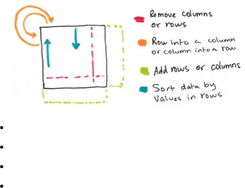
DataFrame Transformations
Now that we briefly defined the core parts of a DataFrame, we will move onto
manipulating DataFrames. When working with individual DataFrames there
are some fundamental objectives. These break down into several core
operations.
We can add rows or columns
We can remove rows or columns
We can transform a row into a column (or vice versa)
We can change the order of rows based on the values in columns
Luckily we can translate all of these into simple transformations, the most
common being those that take one column, change it row by row, and then
return our results.
Creating DataFrames
As we saw previously, we can create DataFrames from raw data sources. This
is covered extensively in the Data Sources chapter however we will use them
now to create an example DataFrame. For illustration purposes later in this
chapter, we will also register this as a temporary view so that we can query it
with SQL.
%scala
val df = spark.read.format("json")
.load("/mnt/defg/flight-data/json/2015-summary.json")
df.createOrReplaceTempView("dfTable")
%python
df = spark.read.format("json")\
.load("/mnt/defg/flight-data/json/2015-summary.json")
df.createOrReplaceTempView("dfTable")
We can also create DataFrames on the fly by taking a set of rows and
converting them to a DataFrame.
%scala
import org.apache.spark.sql.Row
import org.apache.spark.sql.types.{StructField, StructType,
StringType, LongType}
val myManualSchema = new StructType(Array(
new StructField("some", StringType, true),
new StructField("col", StringType, true),
new StructField("names", LongType, false) // just to illustrate flipping this flag
))
val myRows = Seq(Row("Hello", null, 1L))
val myRDD = spark.sparkContext.parallelize(myRows)
val myDf = spark.createDataFrame(myRDD, myManualSchema)
myDf.show()
Note
In Scala we can also take advantage of Spark’s implicits in the console (and if
you import them in your jar code), by running toDF on a Seq type. This does
not play well with null types, so it’s not necessarily recommended for
production use cases.
%scala
val myDF = Seq(("Hello", 2, 1L)).toDF()
%python
from pyspark.sql import Row
from pyspark.sql.types import StructField, StructType,\
StringType, LongType
myManualSchema = StructType([
StructField("some", StringType(), True),
StructField("col", StringType(), True),
StructField("names", LongType(), False)
])
myRow = Row("Hello", None, 1)
myDf = spark.createDataFrame([myRow], myManualSchema)
myDf.show()
Now that we know how to create DataFrames, let’s go over their most useful
methods that you’re going to be using are: the select method when you’re
working with columns or expressions and the selectExpr method when
you’re working with expressions in strings. Naturally some transformations are
not specified as a methods on columns, therefore there exists a group of
functions found in the org.apache.spark.sql.functions package.
With these three tools, you should be able to solve the vast majority of
transformation challenges that you may encourage in DataFrames.
Select & SelectExpr
Select and SelectExpr allow us to do the DataFrame equivalent of SQL
queries on a table of data.
SELECT * FROM dataFrameTable
SELECT columnName FROM dataFrameTable
SELECT columnName * 10, otherColumn, someOtherCol as c FROM dataFrameTable
In the simplest possible terms, it allows us to manipulate columns in our
DataFrames. Let’s walk through some examples on DataFrames to talk about
some of the different ways of approaching this problem. The easiest way is just
to use the select method and pass in the column names as string that you
would like to work with.
%scala
df.select("DEST_COUNTRY_NAME").show(2)
%python
df.select("DEST_COUNTRY_NAME").show(2)
%sql
SELECT DEST_COUNTRY_NAME
FROM dfTable
LIMIT 2
You can select multiple columns using the same style of query, just add more
column name strings to our select method call.
%scala
df.select(
"DEST_COUNTRY_NAME",
"ORIGIN_COUNTRY_NAME")
.show(2)
%python
df.select(
"DEST_COUNTRY_NAME",
"ORIGIN_COUNTRY_NAME")\
.show(2)
%sql
SELECT
DEST_COUNTRY_NAME,
ORIGIN_COUNTRY_NAME
FROM
dfTable
LIMIT 2
As covered in Columns and Expressions, we can refer to columns in a number
of different ways; as a user all you need to keep in mind is that we can use
them interchangeably.
%scala
import org.apache.spark.sql.functions.{expr, col, column}
df.select(
df.col("DEST_COUNTRY_NAME"),
col("DEST_COUNTRY_NAME"),
column("DEST_COUNTRY_NAME"),
'DEST_COUNTRY_NAME,
$"DEST_COUNTRY_NAME",
expr("DEST_COUNTRY_NAME")
).show(2)
%python
from pyspark.sql.functions import expr, col, column
df.select(
expr("DEST_COUNTRY_NAME"),
col("DEST_COUNTRY_NAME"),
column("DEST_COUNTRY_NAME"))\
.show(2)
One common error is attempting to mix Column objects and strings. For
example, the below code will result in a compiler error.
df.select(col("DEST_COUNTRY_NAME"), "DEST_COUNTRY_NAME")
As we’ve seen thus far, expr is the most flexible reference that we can use. It
can refer to a plain column or a string manipulation of a column. To illustrate,
let’s change our column name, then change it back as an example using the AS
keyword and then the alias method on the column.
%scala
df.select(expr("DEST_COUNTRY_NAME AS destination"))
%python
df.select(expr("DEST_COUNTRY_NAME AS destination"))
%sql
SELECT
DEST_COUNTRY_NAME as destination
FROM
dfTable
We can further manipulate the result of our expression as another expression.
%scala
df.select(
expr("DEST_COUNTRY_NAME as destination").alias("DEST_COUNTRY_NAME"
)
%python
df.select(
expr("DEST_COUNTRY_NAME as destination").alias("DEST_COUNTRY_NAME"
)
Because select followed by a series of expr is such a common pattern, Spark
has a shorthand for doing so efficiently: selectExpr. This is probably the
most convenient interface for everyday use.
%scala
df.selectExpr(
"DEST_COUNTRY_NAME as newColumnName",
"DEST_COUNTRY_NAME")
.show(2)
%python
df.selectExpr(
"DEST_COUNTRY_NAME as newColumnName",
"DEST_COUNTRY_NAME"
).show(2)
This opens up the true power of Spark. We can treat selectExpr as a simple
way to build up complex expressions that create new DataFrames. In fact, we
can add any valid non-aggregating SQL statement and as long as the columns
resolve - it will be valid! Here’s a simple example that adds a new column
withinCountry to our DataFrame that specifies whether or not the destination
and origin are the same.
%scala
df.selectExpr(
"*", // all original columns
"(DEST_COUNTRY_NAME = ORIGIN_COUNTRY_NAME) as withinCountry"
).show(2)
%python
df.selectExpr(
"*", # all original columns
"(DEST_COUNTRY_NAME = ORIGIN_COUNTRY_NAME) as withinCountry")
.show(2)
%sql
SELECT
*,
(DEST_COUNTRY_NAME = ORIGIN_COUNTRY_NAME) as withinCountry
FROM
dfTable
Now we’ve learning about select and select expression. With these we can
specify aggregations over the entire DataFrame by leveraging the functions that
we have. These look just like what we have been showing so far.
%scala
df.selectExpr("avg(count)", "count(distinct(DEST_COUNTRY_NAME))"
%python
df.selectExpr("avg(count)", "count(distinct(DEST_COUNTRY_NAME))"
%sql
SELECT
avg(count),
count(distinct(DEST_COUNTRY_NAME))
FROM
dfTable
Converting to Spark Types (Literals)
Sometimes we need to pass explicit values into Spark that aren’t a new column
but are just a value. This might be a constant value or something we’ll need to
compare to later on. The way we do this is through literals. This is basically a
translation from a given programming language’s literal value to one that Spark
understands. Literals are expressions and can be used in the same way.
%scala
import org.apache.spark.sql.functions.lit
df.select(
expr("*"),
lit(1).as("something")
).show(2)
%python
from pyspark.sql.functions import lit
df.select(
expr("*"),
lit(1).alias("One")
).show(2)
In SQL, literals are just the specific value.
%sql
SELECT
*,
1 as One
FROM
dfTable
LIMIT 2
This will come up when you might need to check if a date is greater than some
constant or some value.
Adding Columns
There’s also a more formal way of adding a new column to a DataFrame using
the withColumn method on our DataFrame. For example, let’s add a column
that just adds the number one as a column.
%scala
df.withColumn("numberOne", lit(1)).show(2)
%python
df.withColumn("numberOne", lit(1)).show(2)
%sql
SELECT
1 as numberOne
FROM
dfTable
LIMIT 2
Let’s do something a bit more interesting and make it an actual expression.
Let’s set a boolean flag for when the origin country is the same as the
destination country.
%scala
df.withColumn(
"withinCountry",
expr("ORIGIN_COUNTRY_NAME == DEST_COUNTRY_NAME")
).show(2)
%python
df.withColumn(
"withinCountry",
expr("ORIGIN_COUNTRY_NAME == DEST_COUNTRY_NAME"))\
.show(2)
You should notice that the withColumn function takes two arguments: the
column name and the expression that will create the value for that given row in
the DataFrame. Interestingly, we can also rename a column this way.
%scala
df.withColumn(
"Destination",
df.col("DEST_COUNTRY_NAME"))
.columns
Renaming Columns
Although we can rename a column in the above manner, it’s often much easier
(and readable) to use the withColumnRenamed method. This will rename the
column with the name of the string in the first argument, to the string in the
second argument.
%scala
df.withColumnRenamed("DEST_COUNTRY_NAME", "dest").columns
%python
df.withColumnRenamed("DEST_COUNTRY_NAME", "dest").columns
Reserved Characters and Keywords in
Column Names
One thing that you may come across is reserved characters like spaces or
dashes in column names. Handling these means escaping column names
appropriately. In Spark this is done with backtick () characters. Let's
use the `withColumn that we just learned about to create a Column with
reserved characters.
%scala
import org.apache.spark.sql.functions.expr
val dfWithLongColName = df
.withColumn(
"This Long Column-Name",
expr("ORIGIN_COUNTRY_NAME"))
%python
dfWithLongColName = df\
.withColumn(
"This Long Column-Name",
expr("ORIGIN_COUNTRY_NAME"))
We did not have to escape the column above because the first argument to
withColumn is just a string for the new column name. We only have to use
backticks when referencing a column in an expression.
%scala
dfWithLongColName
.selectExpr(
"`This Long Column-Name`",
"`This Long Column-Name` as `new col`")
.show(2)
%python
dfWithLongColName\
.selectExpr(
"`This Long Column-Name`",
"`This Long Column-Name` as `new col`")\
.show(2)
dfWithLongColName.createOrReplaceTempView("dfTableLong")
%sql
SELECT `This Long Column-Name` FROM dfTableLong
We can refer to columns with reserved characters (and not escape them) if
doing an explicit string to column reference, which gets interpreted as a literal
instead of an expression. We only have to escape expressions that leverage
reserved characters or keywords. The following two examples both result in
the same DataFrame.
%scala
dfWithLongColName.select(col("This Long Column-Name")).columns
%python
dfWithLongColName.select(expr("`This Long Column-Name`")).columns
Removing Columns
Now that we’ve created this column, let’s take a look at how we can remove
columns from DataFrames. You likely already noticed that we can do this with
select. However there is also a dedicated method called drop.
df.drop("ORIGIN_COUNTRY_NAME").columns
We can drop multiple columns by passing in multiple columns as arguments.
dfWithLongColName.drop("ORIGIN_COUNTRY_NAME", "DEST_COUNTRY_NAME"
Changing a Column’s Type (cast)
Sometimes we may need to convert from one type to another, for example if we
have a set of StringType that should be integers. We can convert columns
from one type to another by casting the column from one type to another. For
instance let’s convert our count column from an integer to a Long type.
df.printSchema()
df.withColumn("count", col("count").cast("int")).printSchema()
%sql
SELECT
cast(count as int)
FROM
dfTable
Filtering Rows
To filter rows we create an expression that evaluates to true or false. We then
filter out the rows that have expression that is equal to false. The most common
way to do this with DataFrames is to create either an expression as a String or
build an expression with a set of column manipulations. There are two methods
to perform this operation, we can use where or filter and they both will
perform the same operation and accept the same argument types when used
with DataFrames. The Dataset API has slightly different options and please
refer to the Dataset chapter for more information.
The following filters are equivalent.
%scala
val colCondition = df.filter(col("count") < 2).take(2)
val conditional = df.where("count < 2").take(2)
%python
colCondition = df.filter(col("count") < 2).take(2)
conditional = df.where("count < 2").take(2)
%sql
SELECT
*
FROM dfTable
WHERE
count < 2
Instinctually you may want to put multiple filters into the same expression.
While this is possible, it is not always useful because Spark automatically
performs all filtering operations at the same time. This is called pipelining and
helps make Spark very efficient. As a user, that means if you want to specify
multiple AND filters, just chain them sequentially and let Spark handle the rest.
%scala
df.where(col("count") < 2)
.where(col("ORIGIN_COUNTRY_NAME") =!= "Croatia")
.show(2)
%python
df.where(col("count") < 2)\
.where(col("ORIGIN_COUNTRY_NAME") != "Croatia")\
.show(2)
%sql
SELECT
*
FROM dfTable
WHERE
count < 2 AND
ORIGIN_COUNTRY_NAME != "Croatia"
Getting Unique Rows
A very common use case is to get the unique or distinct values in a DataFrame.
These values can be in one or more columns. The way we do this is with the
distinct method on a DataFrame that will allow us to deduplicate any rows
that are in that DataFrame. For instance let’s get the unique origins in our
dataset. This of course is a transformation that will return a new DataFrame
with only unique rows.
%scala
df.select("ORIGIN_COUNTRY_NAME", "DEST_COUNTRY_NAME").count()
%python
df.select("ORIGIN_COUNTRY_NAME", "DEST_COUNTRY_NAME").count()
%sql
SELECT
COUNT(DISTINCT ORIGIN_COUNTRY_NAME, DEST_COUNTRY_NAME)
FROM dfTable
%scala
df.select("ORIGIN_COUNTRY_NAME").distinct().count()
%python
df.select("ORIGIN_COUNTRY_NAME").distinct().count()
%sql
SELECT
COUNT(DISTINCT ORIGIN_COUNTRY_NAME)
FROM dfTable
Random Samples
Sometimes you may just want to sample some random records from your
DataFrame. This is done with the sample method on a DataFrame that allows
you to specify a fraction of rows to extract from a DataFrame and whether
you’d like to sample with or without replacement.
val seed = 5
val withReplacement = false
val fraction = 0.5
df.sample(withReplacement, fraction, seed).count()
%python
seed = 5
withReplacement = False
fraction = 0.5
df.sample(withReplacement, fraction, seed).count()
Random Splits
Random splits can be helpful when you need to break up your DataFrame,
randomly, in such a way that sampling random cannot guarantee that all records
are in one of the DataFrames that you’re sampling from. This is often used with
machine learning algorithms to create training, validation, and test sets. In this
example we’ll split our DataFrame into two different DataFrames by setting
the weights by which we will split the DataFrame (these are the arguments to
the function). Since this method involves some randomness, we will also
specify a seed. It’s important to note that if you don’t specify a proportion for
each DataFrame that adds up to one, they will be normalized so that they do.
%scala
val dataFrames = df.randomSplit(Array(0.25, 0.75), seed)
dataFrames(0).count() > dataFrames(1).count()
%python
dataFrames = df.randomSplit([0.25, 0.75], seed)
dataFrames[0].count() > dataFrames[1].count()
Concatenating and Appending Rows to a
DataFrame
As we learned in the previous section, DataFrames are immutable. This means
users cannot append to DataFrames because that would be changing it. In order
to append to a DataFrame, you must union the original DataFrame along with
the new DataFrame. This just concatenates the two DataFrames together. To
union two DataFrames, you have to be sure that they have the same schema and
number of columns, else the union will fail.
%scala
import org.apache.spark.sql.Row
val schema = df.schema
val newRows = Seq(
Row("New Country", "Other Country", 5L),
Row("New Country 2", "Other Country 3", 1L)
)
val parallelizedRows = spark.sparkContext.parallelize(newRows)
val newDF = spark.createDataFrame(parallelizedRows, schema)
df.union(newDF)
.where("count = 1")
.where($"ORIGIN_COUNTRY_NAME" =!= "United States")
.show() // get all of them and we'll see our new rows at the end
%python
from pyspark.sql import Row
schema = df.schema
newRows = [
Row("New Country", "Other Country", 5L),
Row("New Country 2", "Other Country 3", 1L)
]
parallelizedRows = spark.sparkContext.parallelize(newRows)
newDF = spark.createDataFrame(parallelizedRows, schema)
%python
df.union(newDF)\
.where("count = 1")\
.where(col("ORIGIN_COUNTRY_NAME") != "United States")\
.show()
As expected, you’ll have to use this new DataFrame reference in order to refer
to the DataFrame with the newly appended rows. A common way to do this is
to make the DataFrame into a view or register it as a table so that you can
reference it more dynamically in your code.
Sorting Rows
When we sort the values in a DataFrame, we always want to sort with either
the largest or smallest values at the top of a DataFrame. There are two
equivalent operations to do this sort and orderBy that work the exact same
way. They accept both column expressions and strings as well as multiple
columns. The default is to sort in ascending order.
%scala
df.sort("count").show(5)
df.orderBy("count", "DEST_COUNTRY_NAME").show(5)
df.orderBy(col("count"), col("DEST_COUNTRY_NAME")).show(5)
%python
df.sort("count").show(5)
df.orderBy("count", "DEST_COUNTRY_NAME").show(5)
df.orderBy(col("count"), col("DEST_COUNTRY_NAME")).show(5)
To more explicit specify sort direction we have to use the asc and desc
functions if operating on a column. These allow us to specify the order that a
given column should be sorted in.
%scala
import org.apache.spark.sql.functions.{desc, asc}
df.orderBy(expr("count desc")).show(2)
df.orderBy(desc("count"), asc("DEST_COUNTRY_NAME")).show(2)
%python
from pyspark.sql.functions import desc, asc
df.orderBy(expr("count desc")).show(2)
df.orderBy(desc(col("count")), asc(col("DEST_COUNTRY_NAME"))).show
%sql
SELECT *
FROM dfTable
ORDER BY count DESC, DEST_COUNTRY_NAME ASC
For optimization purposes, it can sometimes be advisable to sort within each
partition before another set of transformations. We can do this with the
sortWithinPartitions method.
%scala
spark.read.format("json")
.load("/mnt/defg/flight-data/json/*-summary.json")
.sortWithinPartitions("count")
%python
spark.read.format("json")\
.load("/mnt/defg/flight-data/json/*-summary.json")\
.sortWithinPartitions("count")
We will discuss this more when discussing tuning and optimization in Section
3.
Limit
Often times you may just want the top ten of some DataFrame. For example,
you might want to only work with the top 50 of some dataset. We do this with
the limit method.
%scala
df.limit(5).show()
%python
df.limit(5).show()
%scala
df.orderBy(expr("count desc")).limit(6).show()
%python
df.orderBy(expr("count desc")).limit(6).show()
%sql
SELECT *
FROM dfTable
LIMIT 6
Repartition and Coalesce
Another important optimization opportunity is to partition the data according to
some frequently filtered columns which controls the physical layout of data
across the cluster including the partitioning scheme and the number of
partitions.
Repartition will incur a full shuffle of the data, regardless of whether or not
one is necessary. This means that you should typically only repartition when
the future number of partitions is greater than your current number of partitions
or when you are looking to partition by a set of columns. C
%scala
df.rdd.getNumPartitions
%python
df.rdd.getNumPartitions()
%scala
df.repartition(5)
%python
df.repartition(5)
If we know we are going to be filtering by a certain column often, it can be
worth repartitioning based on that column.
%scala
df.repartition(col("DEST_COUNTRY_NAME"))
%python
df.repartition(col("DEST_COUNTRY_NAME"))
We can optionally specify the number of partitions we would like too.
%scala
df.repartition(5, col("DEST_COUNTRY_NAME"))
%python
df.repartition(5, col("DEST_COUNTRY_NAME"))
Coalesce on the other hand will not incur a full shuffle and will try to combine
partitions. This operation will shuffle our data into 5 partitions based on the
destination country name, then coalesce them (without a full shuffle).
%scala
df.repartition(5, col("DEST_COUNTRY_NAME")).coalesce(2)
%python
df.repartition(5, col("DEST_COUNTRY_NAME")).coalesce(2)
Collecting Rows to the Driver
As we covered in the previous chapters. Spark has a Driver that maintains
cluster information and runs user code. This means that when we call some
method to collect data, this is collected to the Spark Driver.
Thus far we did not talk explicitly about this operation however we used
several different methods for doing that that are effectively all the same.
collect gets all data from the entire DataFrame, take selects the first N rows,
show prints out a number of rows nicely. See the appendix for collecting data
for the complete list.
%scala
val collectDF = df.limit(10)
collectDF.take(5) // take works with an Integer count
collectDF.show() // this prints it out nicely
collectDF.show(5, false)
collectDF.collect()
%python
collectDF = df.limit(10)
collectDF.take(5) # take works with an Integer count
collectDF.show() # this prints it out nicely
collectDF.show(5, False)
collectDF.collect()
Chapter 4. Working with Different
Types of Data

Chapter Overview
In the previous chapter, we covered basic DataFrame concepts and
abstractions. this chapter will cover building expressions, which are the bread
and butter of Spark’s structured operations. This chapter will cover working
with a variety of different kinds of data including:
Booleans
Numbers
Strings
Dates and Timestamps
Handling Null
Complex Types
User Defined Functions
Where to Look for APIs
Before we get started, it’s worth explaining where you as a user should start
looking for transformations. Spark is a growing project and any book
(including this one) is a snapshot in time. Therefore it is our priority to educate
you as a user as to where you should look for functions in order to transform
your data. The key places to look for transformations are:
DataFrame (Dataset) Methods. This is actually a bit of a trick because a
DataFrame is just a Dataset of Row types so you’ll actually end up looking at
the Dataset methods. These are available at:
http://spark.apache.org/docs/latest/api/scala/index.html#org.apache.spark.sql.Dataset
Dataset sub-modules like DataFrameStatFunctions and
DataFrameNaFunctions that have more methods. These are usually domain
specific sets of functions and methods that only make sense in a certain context.
For example, DataFrameStatFunctions holds a variety of statistically
related functions while DataFrameNaFunctions refers to functions that are
relevant when working with null data.
Null Functions:
http://spark.apache.org/docs/latest/api/scala/index.html#org.apache.spark.sql.DataFrameStatFunctions
Stat Functions:
http://spark.apache.org/docs/latest/api/scala/index.html#org.apache.spark.sql.DataFrameNaFunctions
Column Methods. These were introduced for the most part in the previous
chapter are hold a variety of general column related methods like alias or
contains. These are available at:
http://spark.apache.org/docs/latest/api/scala/index.html#org.apache.spark.sql.Column
org.apache.spark.sql.functions contains a variety of functions for a
variety of different data types. Often you’ll see the entire package imported
because they are used so often. These are available at:
http://spark.apache.org/docs/latest/api/scala/index.html#org.apache.spark.sql.functions$
Now this may feel a bit overwhelming but have no fear, the majority of these
functions are ones that you will find in SQL and analytics systems. All of these
tools exist to achieve one purpose, to transform rows of data in one format or
structure to another. This may create more rows or reduce the number of rows
available. To get stated, let’s read in the DataFrame that we’ll be using for this
analysis.
%scala
val df = spark.read.format("csv")
.option("header", "true")
.option("inferSchema", "true")
.load("/mnt/defg/retail-data/by-day/2010-12-01.csv")
df.printSchema()
df.createOrReplaceTempView("dfTable")
%python
df = spark.read.format("csv")\
.option("header", "true")\
.option("inferSchema", "true")\
.load("/mnt/defg/retail-data/by-day/2010-12-01.csv")
df.printSchema()
df.createOrReplaceTempView("dfTable")
These will print the schema nicely.
root
|-- InvoiceNo: string (nullable = true)
|-- StockCode: string (nullable = true)
|-- Description: string (nullable = true)
|-- Quantity: integer (nullable = true)
|-- InvoiceDate: timestamp (nullable = true)
|-- UnitPrice: double (nullable = true)
|-- CustomerID: double (nullable = true)
|-- Country: string (nullable = true)
Working with Booleans
Booleans are foundational when it comes to data analysis because they are the
foundation for all filtering. Boolean statements consist of four elements: and,
or, true and false. We use these simple structures to build logical statements
that evaluate to either true or false. These statements are often used as
conditional requirements where a row of data must either pass this test
(evaluate to true) or else it will be filtered out.
Let’s use our retail dataset to explore working with booleans. We can specify
equality as well as less or greater than.
%scala
import org.apache.spark.sql.functions.col
df.where(col("InvoiceNo").equalTo(536365))
.select("InvoiceNo", "Description")
.show(5, false)
NOTE
Scala has some particular semantics around the use of == and ===. In
Spark, if you wish to filter by equality you should use === (equal) or =!=
(not equal). You can also use not function and the equalTo method.
%scala
import org.apache.spark.sql.functions.col
df.where(col("InvoiceNo") === 536365)
.select("InvoiceNo", "Description")
.show(5, false)
Python keeps a more conventional notation.
%python
from pyspark.sql.functions import col
df.where(col("InvoiceNo") != 536365)\
.select("InvoiceNo", "Description")\
.show(5, False)
Now we mentioned that we can specify boolean expressions with multiple
parts when we use and or or. In Spark you should always chain together and
filters as a sequential filter.
The reason for this is that even if boolean expressions are expressed serially
(one after the other) Spark will flatten all of these filters into one statement and
perform the filter at the same time, creating the and statement for us. While you
may specify your statements explicitly using and if you like, it’s often easier to
reason about and to read if you specify them serially. or statements need to be
specified in the same statement.
%scala
val priceFilter = col("UnitPrice") > 600
val descripFilter = col("Description").contains("POSTAGE")
df.where(col("StockCode").isin("DOT"))
.where(priceFilter.or(descripFilter))
.show(5)
%python
from pyspark.sql.functions import instr
priceFilter = col("UnitPrice") > 600
descripFilter = instr(df.Description, "POSTAGE") >= 1
df.where(df.StockCode.isin("DOT"))\
.where(priceFilter | descripFilter)\
.show(5)
%sql
SELECT
*
FROM dfTable
WHERE
StockCode in ("DOT") AND
(UnitPrice > 600 OR
instr(Description, "POSTAGE") >= 1)
Boolean expressions are not just reserved to filters. In order to filter a
DataFrame we can also just specify a boolean column.
val DOTCodeFilter = col("StockCode") === "DOT"
val priceFilter = col("UnitPrice") > 600
val descripFilter = col("Description").contains("POSTAGE")
df.withColumn("isExpensive",
DOTCodeFilter.and(priceFilter.or(descripFilter)))
.where("isExpensive")
.select("unitPrice", "isExpensive")
.show(5)
%python
from pyspark.sql.functions import instr
DOTCodeFilter = col("StockCode") == "DOT"
priceFilter = col("UnitPrice") > 600
descripFilter = instr(col("Description"), "POSTAGE") >= 1
df.withColumn("isExpensive",
DOTCodeFilter & (priceFilter | descripFilter))\
.where("isExpensive")\
.select("unitPrice", "isExpensive")\
.show(5)
%sql
SELECT
UnitPrice,
(StockCode = 'DOT' AND
(UnitPrice > 600 OR
instr(Description, "POSTAGE") >= 1)) as isExpensive
FROM dfTable
WHERE
(StockCode = 'DOT' AND
(UnitPrice > 600 OR
instr(Description, "POSTAGE") >= 1))
Notice how we did not have to specify our filter as an expression and how we
could use a column name without any extra work.
If you’re coming from a SQL background all of these statements should seem
quite familiar. Indeed, all of them can be expressed as a where clause. In fact,
it’s often easier to just express filters as SQL statements than using the
programmatic DataFrame interface and Spark SQL allows us to do this
without paying any performance penalty. For example, the two following
statements are equivalent.
import org.apache.spark.sql.functions.{expr, not, col}
df.withColumn("isExpensive", not(col("UnitPrice").leq(250)))
.filter("isExpensive")
.select("Description", "UnitPrice").show(5)
df.withColumn("isExpensive", expr("NOT UnitPrice <= 250"))
.filter("isExpensive")
.select("Description", "UnitPrice").show(5)
%python
from pyspark.sql.functions import expr
df.withColumn("isExpensive", expr("NOT UnitPrice <= 250"))\
.where("isExpensive")\
.select("Description", "UnitPrice").show(5)
Working with Numbers
When working with big data, the second most common task you will do after
filtering things is counting things. For the most part, we simply need to express
our computation and that should be valid assuming we’re working with
numerical data types.
To fabricate a contrived example, let’s imagine that we found out that we mis-
recorded the quantity in our retail dataset and true quantity is equal to (the
current quantity * the unit price) ^ 2 + 5. This will introduce our first numerical
function as well the pow function that raises a column to the expressed power.
%scala
import org.apache.spark.sql.functions.{expr, pow}
val fabricatedQuantity = pow(col("Quantity") * col("UnitPrice"),
df.select(
expr("CustomerId"),
fabricatedQuantity.alias("realQuantity"))
.show(2)
%python
from pyspark.sql.functions import expr, pow
fabricatedQuantity = pow(col("Quantity") * col("UnitPrice"), 2)
df.select(
expr("CustomerId"),
fabricatedQuantity.alias("realQuantity"))\
.show(2)
You’ll notice that we were able to multiply our columns together because they
were both numerical. Naturally we can add and subtract as necessary as well.
In fact we can do all of this a SQL expression as well.
%scala
df.selectExpr(
"CustomerId",
"(POWER((Quantity * UnitPrice), 2.0) + 5) as realQuantity")
.show(2)
%python
df.selectExpr(
"CustomerId",
"(POWER((Quantity * UnitPrice), 2.0) + 5) as realQuantity")\
.show(2)
%sql
SELECT
customerId,
(POWER((Quantity * UnitPrice), 2.0) + 5) as realQuantity
FROM dfTable
Another common numerical task is rounding. Now if you’d like to just round to
a whole number, often times you can cast it to an integer and that will work just
fine. However Spark also has more detailed functions for performing this
explicitly and to a certain level of precision. In this case we will round to one
decimal place.
%scala
import org.apache.spark.sql.functions.{round, bround}
df.select(
round(col("UnitPrice"), 1).alias("rounded"),
col("UnitPrice"))
.show(5)
By default, the round function will round up if you’re exactly in between two
numbers. You can round down with the bround.
%scala
import org.apache.spark.sql.functions.lit
df.select(
round(lit("2.5")),
bround(lit("2.5")))
.show(2)
%python
from pyspark.sql.functions import lit, round, bround
df.select(
round(lit("2.5")),
bround(lit("2.5")))\
.show(2)
%sql
SELECT
round(2.5),
bround(2.5)
Another numerical task is to compute the correlation of two columns. For
example, we can see the Pearson Correlation Coefficient for two columns to
see if cheaper things are typically bought in greater quantities. We can do this
through a function as well as through the DataFrame statistic methods.
%scala
import org.apache.spark.sql.functions.{corr}
df.stat.corr("Quantity", "UnitPrice")
df.select(corr("Quantity", "UnitPrice")).show()
%python
from pyspark.sql.functions import corr
df.stat.corr("Quantity", "UnitPrice")
df.select(corr("Quantity", "UnitPrice")).show()
%sql
SELECT
corr(Quantity, UnitPrice)
FROM
dfTable
A common task is to compute summary statistics for a column or set of
columns. We can use the describe method to achieve exactly this. This will
take all numeric columns and calculate the count, mean, standard deviation,
min, and max. This should be used primarily for viewing in the console as the
schema may change in the future.
%scala
df.describe().show()
%python
df.describe().show()
+-------+------------------+------------------+------------------+
|summary| Quantity| UnitPrice| CustomerID|
+-------+------------------+------------------+------------------+
| count| 3108| 3108| 1968|
| mean| 8.627413127413128| 4.151946589446603|15661.388719512195|
| stddev|26.371821677029203|15.638659854603892|1854.4496996893627|
| min| -24| 0.0| 12431.0|
| max| 600| 607.49| 18229.0|
+-------+------------------+------------------+------------------+
If you need these exact numbers you can also perform this as an aggregation
yourself by importing the functions and applying them to the columns that you
need.
%scala
import org.apache.spark.sql.functions.{count, mean, stddev_pop,
%python
from pyspark.sql.functions import count, mean, stddev_pop, min,
There are a number of statistical functions available in the StatFunctions
Package. These are DataFrame methods that allow you to calculate a vareity of
different things. For instance, we can calculate either exact or approximate
quantiles of our data using the approxQuantile method.
%scala
val colName = "UnitPrice"
val quantileProbs = Array(0.5)
val relError = 0.05
df.stat.approxQuantile("UnitPrice", quantileProbs, relError)
%python
colName = "UnitPrice"
quantileProbs = [0.5]
relError = 0.05
df.stat.approxQuantile("UnitPrice", quantileProbs, relError)
We can also use this to see a cross tabulation or frequent item pairs (Be
careful, this output will be large).
%scala
df.stat.crosstab("StockCode", "Quantity").show()
%python
df.stat.crosstab("StockCode", "Quantity").show()
%scala
df.stat.freqItems(Seq("StockCode", "Quantity")).show()
%python
df.stat.freqItems(["StockCode", "Quantity"]).show()
Spark is home to a variety of other features and functionality. For example, you
can use Spark to construct a Bloom Filter or Count Min Sketch using the stat
sub-package. There are also a multitude of other functions available that are
self-explanatory and need not be explained individually.
Working with Strings
String manipulation shows up in nearly every data flow and its worth
explaining what you can do with strings. You may be manipulating log files
performing regular expression extraction or substitution, or checking for
simple string existence, or simply making all strings upper or lower case.
We will start with the last task as it’s one of the simplest. The initcap
function will capitalize every word in a given string when that word is
separated from another via whitespace.
%scala
import org.apache.spark.sql.functions.{initcap}
df.select(initcap(col("Description"))).show(2, false)
%python
from pyspark.sql.functions import initcap
df.select(initcap(col("Description"))).show()
%sql
SELECT
initcap(Description)
FROM
dfTable
As mentioned above, we can also quite simply lower case and upper case
strings as well.
%scala
import org.apache.spark.sql.functions.{lower, upper}
df.select(
col("Description"),
lower(col("Description")),
upper(lower(col("Description"))))
.show(2)
%python
from pyspark.sql.functions import lower, upper
df.select(
col("Description"),
lower(col("Description")),
upper(lower(col("Description"))))\
.show(2)
%sql
SELECT
Description,
lower(Description),
Upper(lower(Description))
FROM
dfTable
Another trivial task is adding or removing whitespace around a string. We can
do this with lpad, ltrim, rpad and rtrim, trim.
%scala
import org.apache.spark.sql.functions.{lit, ltrim, rtrim, rpad,
df.select(
ltrim(lit(" HELLO ")).as("ltrim"),
rtrim(lit(" HELLO ")).as("rtrim"),
trim(lit(" HELLO ")).as("trim"),
lpad(lit("HELLO"), 3, " ").as("lp"),
rpad(lit("HELLO"), 10, " ").as("rp"))
.show(2)
%python
from pyspark.sql.functions import lit, ltrim, rtrim, rpad, lpad
df.select(
ltrim(lit(" HELLO ")).alias("ltrim"),
rtrim(lit(" HELLO ")).alias("rtrim"),
trim(lit(" HELLO ")).alias("trim"),
lpad(lit("HELLO"), 3, " ").alias("lp"),
rpad(lit("HELLO"), 10, " ").alias("rp"))\
.show(2)
%sql
SELECT
ltrim(' HELLLOOOO '),
rtrim(' HELLLOOOO '),
trim(' HELLLOOOO '),
lpad('HELLOOOO ', 3, ' '),
rpad('HELLOOOO ', 10, ' ')
FROM
dfTable
+---------+---------+-----+---+----------+
| ltrim| rtrim| trim| lp| rp|
+---------+---------+-----+---+----------+
|HELLO | HELLO|HELLO| HE|HELLO |
|HELLO | HELLO|HELLO| HE|HELLO |
+---------+---------+-----+---+----------+
only showing top 2 rows
You’ll notice that if lpad or rpad takes a number less than the length of the
string, it will always remove values from the right side of the string.
Regular Expressions
Probably one of the most frequently performed tasks is searching for the
existance of one string on another or replacing all mentions of a string with
another value. This is often done with a tool called “Regular Expressions” that
exist in many programming languages. Regular expressions give the user an
ability to specify a set of rules to use to either extract values from a string or
replace them with some other values.
Spark leverages the complete power of Java Regular Expressions. The syntax
departs slightly from other programming languages so it is worth reviewing
before putting anything into production.. There are two key functions in Spark
that you’ll need to perform regular expression tasks: regexp_extract and
regexp_replace. These functions extract values and replace values
respectively.
Let’s explore how to use the regexp_replace function to replace substitute
colors names in our description column.
%scala
import org.apache.spark.sql.functions.regexp_replace
val simpleColors = Seq("black", "white", "red", "green", "blue"
val regexString = simpleColors.map(_.toUpperCase).mkString("|")
// the | signifies `OR` in regular expression syntax
df.select(
regexp_replace(col("Description"), regexString, "COLOR")
.alias("color_cleaned"),
col("Description"))
.show(2)
%python
from pyspark.sql.functions import regexp_replace
regex_string = "BLACK|WHITE|RED|GREEN|BLUE"
df.select(
regexp_replace(col("Description"), regex_string, "COLOR")
.alias("color_cleaned"),
col("Description"))\
.show(2)
%sql
SELECT
regexp_replace(Description, 'BLACK|WHITE|RED|GREEN|BLUE', 'COLOR'
Description
FROM
dfTable
+--------------------+--------------------+
| color_cleaned| Description|
+--------------------+--------------------+
|COLOR HANGING HEA...|WHITE HANGING HEA...|
| COLOR METAL LANTERN| WHITE METAL LANTERN|
+--------------------+--------------------+
Another task may be to replace given characters with other characters.
Building this as regular expression could be tedious so Spark also provides the
translate function to replace these values. This is done at the character level
and will replace all instances of a character with the indexed character in the
replacement string.
%scala
import org.apache.spark.sql.functions.translate
df.select(
translate(col("Description"), "LEET", "1337"),
col("Description"))
.show(2)
%python
from pyspark.sql.functions import translate
df.select(
translate(col("Description"), "LEET", "1337"),
col("Description"))\
.show(2)
%sql
SELECT
translate(Description, 'LEET', '1337'),
Description
FROM
dfTable
+----------------------------------+--------------------+
|translate(Description, LEET, 1337)| Description|
+----------------------------------+--------------------+
| WHI73 HANGING H3A...|WHITE HANGING HEA...|
| WHI73 M37A1 1AN73RN| WHITE METAL LANTERN|
+----------------------------------+--------------------+
We can also perform something similar like pulling out the first mentioned
color.
%scala
import org.apache.spark.sql.functions.regexp_extract
val regexString = simpleColors
.map(_.toUpperCase)
.mkString("(", "|", ")")
// the | signifies OR in regular expression syntax
df.select(
regexp_extract(col("Description"), regexString, 1)
.alias("color_cleaned"),
col("Description"))
.show(2)
%python
from pyspark.sql.functions import regexp_extract
extract_str = "(BLACK|WHITE|RED|GREEN|BLUE)"
df.select(
regexp_extract(col("Description"), extract_str, 1)
.alias("color_cleaned"),
col("Description"))\
.show(2)
%sql
SELECT
regexp_extract(Description, '(BLACK|WHITE|RED|GREEN|BLUE)', 1
Description
FROM
dfTable
Sometimes, rather than extracting values, we simply want to check for
existence. We can do this with the contains method on each column. This will
return a boolean declaring whether it can find that string in the column’s string.
%scala
val containsBlack = col("Description").contains("BLACK")
val containsWhite = col("DESCRIPTION").contains("WHITE")
df.withColumn("hasSimpleColor", containsBlack.or(containsWhite))
.filter("hasSimpleColor")
.select("Description")
.show(3, false)
In Python we can use the instr function.
%python
from pyspark.sql.functions import instr
containsBlack = instr(col("Description"), "BLACK") >= 1
containsWhite = instr(col("Description"), "WHITE") >= 1
df.withColumn("hasSimpleColor", containsBlack | containsWhite)\
.filter("hasSimpleColor")\
.select("Description")\
.show(3, False)
%sql
SELECT
Description
FROM
dfTable
WHERE
instr(Description, 'BLACK') >= 1 OR
instr(Description, 'WHITE') >= 1
+----------------------------------+
|Description |
+----------------------------------+
|WHITE HANGING HEART T-LIGHT HOLDER|
|WHITE METAL LANTERN |
|RED WOOLLY HOTTIE WHITE HEART. |
+----------------------------------+
only showing top 3 rows
This is trivial with just two values but gets much more complicated with more
values.
Let’s work through this in a more dynamic way and take advantage of Spark’s
ability to accept a dynamic number of arguments. When we convert a list of
values into a set of arguments and pass them into a function, we use a language
feature called varargs. This feature allows us to effectively unravel an array of
arbitrary length and pass it as arguments to a function. This, coupled with
select allows us to create arbitrary numbers of columns dynamically.
%scala
val simpleColors = Seq("black", "white", "red", "green", "blue"
val selectedColumns = simpleColors.map(color => {
col("Description")
.contains(color.toUpperCase)
.alias(s"is_$color")
}):+expr("*") // could also append this value
df
.select(selectedColumns:_*)
.where(col("is_white").or(col("is_red")))
.select("Description")
.show(3, false)
+----------------------------------+
|Description |
+----------------------------------+
|WHITE HANGING HEART T-LIGHT HOLDER|
|WHITE METAL LANTERN |
|RED WOOLLY HOTTIE WHITE HEART. |
+----------------------------------+
We can also do this quite easily in Python. In this case we’re going to use a
different function locate that returns the integer location (1 based location).
We then convert that to a boolean before using it as a the same basic feature.
%python
from pyspark.sql.functions import expr, locate
simpleColors = ["black", "white", "red", "green", "blue"]
def color_locator(column, color_string):
"""This function creates a column declaring whether or
not a given pySpark column contains the UPPERCASED
color.
Returns a new column type that can be used
in a select statement.
"""
return locate(color_string.upper(), column)\
.cast("boolean")\
.alias("is_" + c)
selectedColumns = [color_locator(df.Description, c) for c in simpleColors
selectedColumns.append(expr("*")) # has to a be Column type
df\
.select(*selectedColumns)\
.where(expr("is_white OR is_red"))\
.select("Description")\
.show(3, False)
This simple feature is often one that can help you programmatically generate
columns or boolean filters in a way that is simple to reason about and extend.
We could extend this to calculating the smallest common denominator for a
given input value or whether or not a number is a prime.
Working with Dates and
Timestamps
Dates and times are a constant challenge in programming languages and
databases. It’s always necessary to keep track of timezones and make sure that
formats are correct and valid. Spark does its best to keep things simple by
focusing explicitly on two kinds of time related information. There are dates,
which focus exclusively on calendar dates, and timestamps that include both
date and time information.
Now as we hinted at above, working with dates and timestamps closely relates
to working with strings because we often store our timestamps or dates as
strings and convert them into date types at runtime. This is less common when
working with databases and structured data but much more common when we
are working with text and csv files.
Now Spark, as we saw with our current dataset, will make a best effort to
correctly identify column types, including dates and timestamps when we
enable inferSchema. We can see that this worked quite well with our current
dataset because it was able to identify and read our date format without us
having to provide some specification for it.
df.printSchema()
root
|-- InvoiceNo: string (nullable = true)
|-- StockCode: string (nullable = true)
|-- Description: string (nullable = true)
|-- Quantity: integer (nullable = true)
|-- InvoiceDate: timestamp (nullable = true)
|-- UnitPrice: double (nullable = true)
|-- CustomerID: double (nullable = true)
|-- Country: string (nullable = true)
While Spark will do this on a best effort basis, sometimes there will be no
getting around working with strangely formatted dates and times. Now the key
to reasoning about the transformations that you are going to need to apply is to
ensure that you know exactly what type and format you have at each given step
of the way. Another common gotcha is that Spark’s TimestampType only
supports second-level precision, this means that if you’re going to be working
with milliseconds or microseconds, you’re going to have to work around this
problem by potentially operating on them as longs. Any more precision when
coercing to a TimestampType will be removed.
Spark can be a bit particular about what format you have at any given point in
time. It’s important to be explicit when parsing or converting to make sure
there are no issues in doing so. At the end of the day, Spark is working with
Java dates and timestamps and therefore conforms to those standards. Let’s
start with the basics and get the current date and the current timestamps.
%scala
import org.apache.spark.sql.functions.{current_date, current_timestamp
val dateDF = spark.range(10)
.withColumn("today", current_date())
.withColumn("now", current_timestamp())
dateDF.createOrReplaceTempView("dateTable")
%python
from pyspark.sql.functions import current_date, current_timestamp
dateDF = spark.range(10)\
.withColumn("today", current_date())\
.withColumn("now", current_timestamp())
dateDF.createOrReplaceTempView("dateTable")
dateDF.printSchema()
Now that we have a simple DataFrame to work with, let’s add and subtract 5
days from today. These functions take a column and then the number of days to
either add or subtract as the arguments.
%scala
import org.apache.spark.sql.functions.{date_add, date_sub}
dateDF
.select(
date_sub(col("today"), 5),
date_add(col("today"), 5))
.show(1)
%python
from pyspark.sql.functions import date_add, date_sub
dateDF\
.select(
date_sub(col("today"), 5),
date_add(col("today"), 5))\
.show(1)
%sql
SELECT
date_sub(today, 5),
date_add(today, 5)
FROM
dateTable
Another common task is to take a look at the difference between two dates. We
can do this with the datediff function that will return the number of days in
between two dates. Most often we just care about the days although since
months can have a strange number of days there also exists a function
months_between that gives you the number of months between two dates.
%scala
import org.apache.spark.sql.functions.{datediff, months_between
dateDF
.withColumn("week_ago", date_sub(col("today"), 7))
.select(datediff(col("week_ago"), col("today")))
.show(1)
dateDF
.select(
to_date(lit("2016-01-01")).alias("start"),
to_date(lit("2017-05-22")).alias("end"))
.select(months_between(col("start"), col("end")))
.show(1)
%python
from pyspark.sql.functions import datediff, months_between, to_date
dateDF\
.withColumn("week_ago", date_sub(col("today"), 7))\
.select(datediff(col("week_ago"), col("today")))\
.show(1)
dateDF\
.select(
to_date(lit("2016-01-01")).alias("start"),
to_date(lit("2017-05-22")).alias("end"))\
.select(months_between(col("start"), col("end")))\
.show(1)
%sql
SELECT
to_date('2016-01-01'),
months_between('2016-01-01', '2017-01-01'),
datediff('2016-01-01', '2017-01-01')
FROM
dateTable
You’ll notice that I introduced a new function above, the to_date function.
This function allows us to convert a date of the format "2017-01-01" to a
Spark date. Of course, for this to work our date must be in the year-month-day
format. You’ll notice that in order to perform this I’m also using the lit
function which ensures that we’re returning a literal value in our expression
not trying to evaluate subtraction.
%scala
import org.apache.spark.sql.functions.{to_date, lit}
spark.range(5).withColumn("date", lit("2017-01-01"))
.select(to_date(col("date")))
.show(1)
%python
from pyspark.sql.functions import to_date, lit
spark.range(5).withColumn("date", lit("2017-01-01"))\
.select(to_date(col("date")))\

.show(1)
WARNING
Spark will not throw an error if it cannot parse the date, it’ll just return
null. This can be a bit tricky in larger pipelines because you may be
expecting your data in one format and getting it in another. To illustrate,
let’s take a look at the date format that has switched from year-month-day
to year-day-month. Spark will fail to parse this date and silently return
null instead.
dateDF.select(to_date(lit("2016-20-12")),to_date(lit("2017-12-11"
+-------------------+-------------------+
|to_date(2016-20-12)|to_date(2017-12-11)|
+-------------------+-------------------+
| null| 2017-12-11|
+-------------------+-------------------+
We find this to be an especially tricky situation for bugs because some dates
may match the correct format while others do not. See how above, the second
date is show to be Decembers 11th instead of the correct day, November 12th?
Spark doesn’t throw an error because it cannot know whether the days are
mixed up or if that specific row is incorrect.
Let’s fix this pipeline, step by step and come up with a robust way to avoid
these issues entirely. The first step is to remember that we need to specify our
date format according to the Java SimpleDateFormat standard as documented
in
https://docs.oracle.com/javase/8/docs/api/java/text/SimpleDateFormat.html.
By using the unix_timestamp we can parse our date into a bigInt that
specifies the Unix timestamp in seconds. We can then cast that to a literal
timestamp before passing that into the to_date format which accepts
timestamps, strings, and other dates.
import org.apache.spark.sql.functions.{unix_timestamp, from_unixtime
val dateFormat = "yyyy-dd-MM"
val cleanDateDF = spark.range(1)
.select(
to_date(unix_timestamp(lit("2017-12-11"), dateFormat).cast(
.alias("date"),
to_date(unix_timestamp(lit("2017-20-12"), dateFormat).cast(
.alias("date2"))
cleanDateDF.createOrReplaceTempView("dateTable2")
%python
from pyspark.sql.functions import unix_timestamp, from_unixtime
dateFormat = "yyyy-dd-MM"
cleanDateDF = spark.range(1)\
.select(
to_date(unix_timestamp(lit("2017-12-11"), dateFormat).cast(
.alias("date"),
to_date(unix_timestamp(lit("2017-20-12"), dateFormat).cast(
.alias("date2"))
cleanDateDF.createOrReplaceTempView("dateTable2")
%sql
SELECT
to_date(cast(unix_timestamp(date, 'yyyy-dd-MM') as timestamp)),
to_date(cast(unix_timestamp(date2, 'yyyy-dd-MM') as timestamp
to_date(date)
FROM
dateTable2
The above example code also shows us how easy it is to cast between
timestamps and dates.
%scala
cleanDateDF
.select(
unix_timestamp(col("date"), dateFormat).cast("timestamp"))
.show()
%python
cleanDateDF\
.select(
unix_timestamp(col("date"), dateFormat).cast("timestamp"))\
.show()
Once we’ve gotten our date or timestamp into the correct format and
type,Comparing between them is actually quite easy. We just need to be sure to
either use a date/timestamp type or specify our string according to the right
format of yyyy-MM-dd if we’re comparing a date.
cleanDateDF.filter(col("date2") > lit("2017-12-12")).show()
One minor point is that we can also set this as a string which Spark parses to a
literal.
cleanDateDF.filter(col("date2") > "'2017-12-12'").show()
Working with Nulls in Data
As a best practice, you should always use nulls to represent missing or empty
data in your DataFrames. Spark can optimize working with null values more
than it can if you use empty strings or other values. The primary way of
interacting with null values, at DataFrame scale, is to use the .na subpackage
on a DataFrame.
In Spark there are two things you can do with null values. You can explicitly
drop nulls or you can fill them with a value (globally or on a per column
basis).
Let’s experiment with each of these now.
Drop
The simplest is probably drop, which simply removes rows that contain nulls.
The default is to drop any row where any value is null.
df.na.drop()
df.na.drop("any")
In SQL we have to do this column by column.
%sql
SELECT
*
FROM
dfTable
WHERE
Description IS NOT NULL
Passing in “any” as an argument will drop a row if any of the values are null.
Passing in “all” will only drop the row if all values are null or NaN for that
row.
df.na.drop("all")
We can also apply this to certain sets of columns by passing in an array of
columns.
%scala
df.na.drop("all", Seq("StockCode", "InvoiceNo"))
%python
df.na.drop("all", subset=["StockCode", "InvoiceNo"])
Fill
Fill allows you to fill one or more columns with a set of values. This can be
done by specifying a map, specific value and a set of columns.
For example to fill all null values in String columns I might specify.
df.na.fill("All Null values become this string")
We could do the same for integer columns with df.na.fill(5:Integer) or
for Doubles df.na.fill(5:Double). In order to specify columns, we just
pass in an array of column names like we did above.
%scala
df.na.fill(5, Seq("StockCode", "InvoiceNo"))
%python
df.na.fill("all", subset=["StockCode", "InvoiceNo"])
We can also do with with a Scala Map where the key is the column name and
the value is the value we would like to use to fill null values.
%scala
val fillColValues = Map(
"StockCode" -> 5,
"Description" -> "No Value"
)
df.na.fill(fillColValues)
%python
fill_cols_vals = {
"StockCode": 5,
"Description" : "No Value"
}
df.na.fill(fill_cols_vals)
Replace
In addition to replacing null values like we did with drop and fill, there are
more flexible options that we can use with more than just null values. Probably
the most common use case is to replace all values in a certain column
according to their current value. The only requirement is that this value be the
same type as the original value.
%scala
df.na.replace("Description", Map("" -> "UNKNOWN"))
%python
df.na.replace([""], ["UNKNOWN"], "Description")
Working with Complex Types
Complex types can help you organize and structure your data in ways that make
more sense for the problem you are hoping to solve. There are three kinds of
complex types, structs, arrays, and maps.
Structs
You can think of structs as DataFrames within DataFrames. A worked example
will illustrate this more clearly. We can create a struct by wrapping a set of
columns in parenthesis in a query.
df.selectExpr("(Description, InvoiceNo) as complex", "*")
df.selectExpr("struct(Description, InvoiceNo) as complex", "*")
%scala
import org.apache.spark.sql.functions.struct
val complexDF = df
.select(struct("Description", "InvoiceNo").alias("complex"))
complexDF.createOrReplaceTempView("complexDF")
%python
from pyspark.sql.functions import struct
complexDF = df\
.select(struct("Description", "InvoiceNo").alias("complex"))
complexDF.createOrReplaceTempView("complexDF")
We now have a DataFrame with a column complex. We can query it just as we
might another DataFrame, the only difference is that we use a dot syntax to do
so.
complexDF.select("complex.Description")
We can also query all values in the struct with *. This brings up all the columns
to the top level DataFrame.
complexDF.select("complex.*")
%sql
SELECT
complex.*
FROM
complexDF
Arrays
To define arrays, let’s work through a use case. With our current data, our
object is to take every single word in our Description column and convert
that into a row in our DataFrame.
The first task is to turn our Description column into a complex type, an array.
split
We do this with the split function and specify the delimiter.
%scala
import org.apache.spark.sql.functions.split
df.select(split(col("Description"), " ")).show(2)
%python
from pyspark.sql.functions import split
df.select(split(col("Description"), " ")).show(2)
%sql
SELECT
split(Description, ' ')
FROM
dfTable
This is quite powerful because Spark will allow us to manipulate this complex
type as another column. We can also query the values of the array with a
python-like syntax.
%scala
df.select(split(col("Description"), " ").alias("array_col"))
.selectExpr("array_col[0]")
.show(2)
%python
df.select(split(col("Description"), " ").alias("array_col"))\
.selectExpr("array_col[0]")\
.show(2)
%sql
SELECT
split(Description, ' ')[0]
FROM
dfTable
Array Contains
For instance we can see if this array contains a value.
import org.apache.spark.sql.functions.array_contains
df.select(array_contains(split(col("Description"), " "), "WHITE"
%python
from pyspark.sql.functions import array_contains
df.select(array_contains(split(col("Description"), " "), "WHITE"
%sql
SELECT
array_contains(split(Description, ' '), 'WHITE')
FROM
dfTable
However this does not solve our current problem. In order to convert a
complex type into a set of rows (one per value in our array), we use the
explode function.

Explode
The explode function takes a column that consists of arrays and creates one
row (with the rest of the values duplicated) per value in the array. The
following figure illustrates the process.
%scala
import org.apache.spark.sql.functions.{split, explode}
df.withColumn("splitted", split(col("Description"), " "))
.withColumn("exploded", explode(col("splitted")))
.select("Description", "InvoiceNo", "exploded")
%python
from pyspark.sql.functions import split, explode
df.withColumn("splitted", split(col("Description"), " "))\
.withColumn("exploded", explode(col("splitted")))\
.select("Description", "InvoiceNo", "exploded")\
Maps
Maps are used less frequently but are still important to cover. We create them
with the map function and key value pairs of columns. Then we can select them
just like we might select from an array.
import org.apache.spark.sql.functions.map
df.select(map(col("Description"), col("InvoiceNo")).alias("complex_map"
.selectExpr("complex_map['Description']")
%sql
SELECT
map(Description, InvoiceNo) as complex_map
FROM
dfTable
WHERE
Description IS NOT NULL
We can also explode map types which will turn them into columns.
import org.apache.spark.sql.functions.map
df.select(map(col("Description"), col("InvoiceNo")).alias("complex_map"
.selectExpr("explode(complex_map)")
.take(5)
Working with JSON
Spark has some unique support for working with JSON data. You can operate
directly on strings of JSON in Spark and parse from JSON or extract JSON
objects. Let’s start by creating a JSON column.
%scala
val jsonDF = spark.range(1)
.selectExpr("""
'{"myJSONKey" : {"myJSONValue" : [1, 2, 3]}}' as jsonString
""")
%python
jsonDF = spark.range(1)\
.selectExpr("""
'{"myJSONKey" : {"myJSONValue" : [1, 2, 3]}}' as jsonString
""")
We can use the get_json_object to inline query a JSON object, be it a
dictionary or array. We can use json_tuple if this object has only one level of
nesting.
%scala
import org.apache.spark.sql.functions.{get_json_object, json_tuple
jsonDF.select(
get_json_object(col("jsonString"), "$.myJSONKey.myJSONValue[1]"
json_tuple(col("jsonString"), "myJSONKey"))
.show()
%python
from pyspark.sql.functions import get_json_object, json_tuple
jsonDF.select(
get_json_object(col("jsonString"), "$.myJSONKey.myJSONValue[1]"
json_tuple(col("jsonString"), "myJSONKey"))\
.show()
The equivalent in SQL would be.
jsonDF.selectExpr("json_tuple(jsonString, '$.myJSONKey.myJSONValue[1]') as res"
We can also turn a StructType into a JSON string using the to_json function.
%scala
import org.apache.spark.sql.functions.to_json
df.selectExpr("(InvoiceNo, Description) as myStruct")
.select(to_json(col("myStruct")))
%python
from pyspark.sql.functions import to_json
df.selectExpr("(InvoiceNo, Description) as myStruct")\
.select(to_json(col("myStruct")))
This function also accepts a dictionary (map) of parameters that are the same
as the JSON data source. We can use the from_json function to parse this (or
other json) back in. This naturally requires us to specify a schema and
optionally we can specify a Map of options as well.
%scala
import org.apache.spark.sql.functions.from_json
import org.apache.spark.sql.types._
val parseSchema = new StructType(Array(
new StructField("InvoiceNo",StringType,true),
new StructField("Description",StringType,true)))
df.selectExpr("(InvoiceNo, Description) as myStruct")
.select(to_json(col("myStruct")).alias("newJSON"))
.select(from_json(col("newJSON"), parseSchema), col("newJSON"
%python
from pyspark.sql.functions import from_json
from pyspark.sql.types import *
parseSchema = StructType((
StructField("InvoiceNo",StringType(),True),
StructField("Description",StringType(),True)))
df.selectExpr("(InvoiceNo, Description) as myStruct")\
.select(to_json(col("myStruct")).alias("newJSON"))\
.select(from_json(col("newJSON"), parseSchema), col("newJSON"
User-Defined Functions
One of the most powerful things that you can do in Spark is define your own
functions. These allow you to write your own custom transformations using
Python or Scala and even leverage external libraries like numpy in doing so.
These functions are called user defined functions or UDFs and can take
and return one or more columns as input. Spark UDFs are incredibly powerful
because they can be written in several different programming languages and do
not have to be written in an esoteric format or DSL. They’re just functions that
operate on the data, record by record.
While we can write our functions in Scala, Python, or Java, there are
performance considerations that you should be aware of. To illustrate this,
we’re going to walk through exactly what happens when you create UDF, pass
that into Spark, and then execute code using that UDF.
The first step is the actual function, we’ll just a take a simple one for this
example. We’ll write a power3 function that takes a number and raises it to a
power of three.
%scala
val udfExampleDF = spark.range(5).toDF("num")
def power3(number:Double):Double = {
number * number * number
}
power3(2.0)
%python
udfExampleDF = spark.range(5).toDF("num")
def power3(double_value):
return double_value ** 3
power3(2.0)
In this trivial example, we can see that our functions work as expected. We are
able to provide an individual input and produce the expected result (with this
simple test case). Thus far our expectations for the input are high, it must be a
specific type and cannot be a null value. See the section in this chapter titled
“Working with Nulls in Data”.
Now that we’ve created these functions and tested them, we need to register
them with Spark so that we can used them on all of our worker machines.
Spark will serialize the function on the driver and transfer it over the network
to all executor processes. This happens regardless of language.
Once we go to use the function, there are essentially two different things that
occur. If the function is written in Scala or Java then we can use that function
within the JVM. This means there will be little performance penalty aside from
the fact that we can’t take advantage of code generation capabilities that Spark
has for built-in functions. There can be performance issues if you create or use
a lot of objects which we will cover in the optimization section.
If the function is written in Python, something quite different happens. Spark
will start up a python process on the worker, serialize all of the data to a
format that python can understand (remember it was in the JVM before),
execute the function row by row on that data in the python process, before
finally returning the results of the row operations to the JVM and Spark.
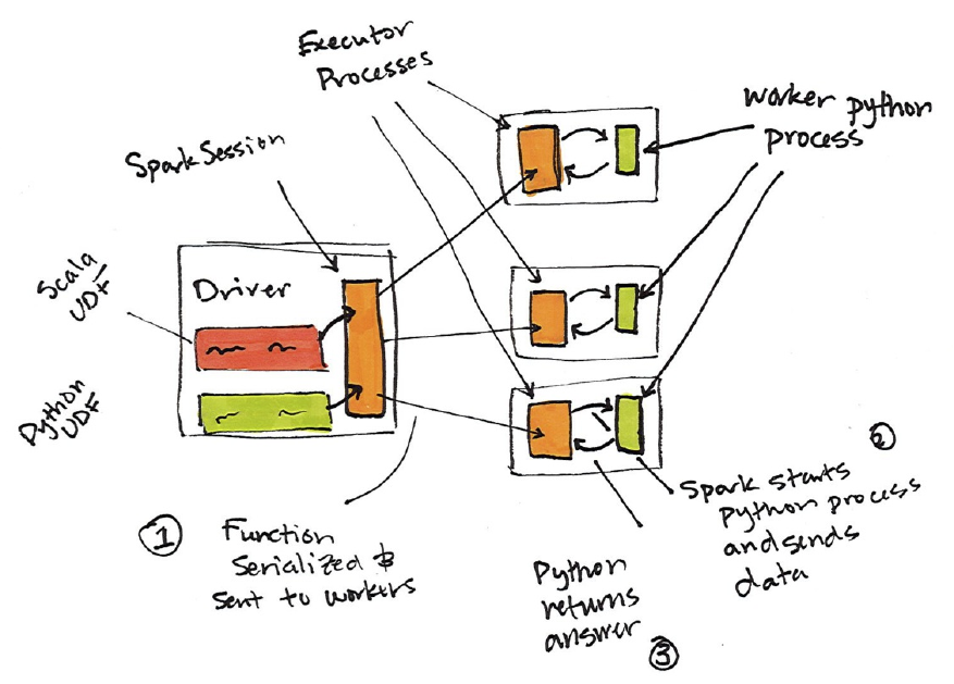
Warning
Starting up this Python process is expensive but the real cost is in serializing
the data to Python. This is costly for two reasons, it is an expensive
computation but also once the data enters Python, Spark cannot manage the
memory of the worker. This means that you could potentially cause a worker to
fail if it becomes resource constrained (because both the JVM and python are
competing for memory on the same machine). We recommend that you write
your UDFs in Scala - the small amount of time it should take you to write the
function in Scala will always yield significant speed ups and on top of that,
you can still use the function from Python!
Now that we have an understanding of the process, let’s work through our
example. First we need to register the function to be available as a DataFrame
function.
%scala
import org.apache.spark.sql.functions.udf
val power3udf = udf(power3(_:Double):Double)
Now we can use that just like any other DataFrame function.
%scala
udfExampleDF.select(power3udf(col("num"))).show()
The same applies to Python, we first register it.
%python
from pyspark.sql.functions import udf
power3udf = udf(power3)
Then we can use it in our DataFrame code.
%python
from pyspark.sql.functions import col
udfExampleDF.select(power3udf(col("num"))).show()
Now as of now, we can only use this as DataFrame function. That is to say, we
can’t use it within a string expression, only on an expression. However, we can
also register this UDF as a Spark SQL function. This is valuable because it
makes it simple to use this function inside of SQL as well as across languages.
Let’s register the function in Scala.
%scala
spark.udf.register("power3", power3(_:Double):Double)
udfExampleDF.selectExpr("power3(num)").show()
Now because this function is registered with Spark SQL, and we’ve learned
that any Spark SQL function or epxression is valid to use as an expression
when working with DataFrames, we can turn around and use the UDF that we
wrote in Scala, in Python. However rather than using it as a DataFrame
function we use it as a SQL expression.
%python
udfExampleDF.selectExpr("power3(num)").show()
# registered in Scala
We can also register our Python function to be available as SQL function and
use that in any language as well.
One thing we can also do to make sure that our functions are working correctly
is specify a return type. As we saw in the beginning of this section, Spark
manages its own type information that does not align exactly with Python’s
types. Therefore it’s a best practice to define the return type for your function
when you define it. It is important to note that specifying the return type is not
necessary but is a best practice.
If you specify the type that doesn’t align with the actual type returned by the
function - Spark will not error but rather just return null to designate a failure.
You can see this if you were to switch the return type in the below function to
be a DoubleType.
%python
from pyspark.sql.types import IntegerType, DoubleType
spark.udf.register("power3py", power3, DoubleType())
%python
udfExampleDF.selectExpr("power3py(num)").show()
# registered via Python
This is because the range above creates Integers. When Integers are operated
on in Python, Python won’t convert them into floats (the corresponding type to
Spark’s Double type), therefore we see null. We can remedy this by ensuring
our Python function returns a float instead of an Integer and the function will
behave correctly.
Naturally we can use either of these from SQL too once we register them.
%sql
SELECT
power3py(12), -- doesn't work because of return type
power3(12)
This chapter demonstrated how easy it is to extend Spark SQL to your own
purposes and do so in a way that is not some esoteric, domain-specific
language but rather simple functions that are easy to test and maintain without
even using Spark! This is an amazingly powerful tool we can use to specify
sophisticated business logic that can run on 5 rows on our local machines or on
terabytes of data on a hundred node cluster!
Chapter 5. Aggregations

What are aggregations?
Aggregating is the act of collecting something together and is a cornerstone of
big data analytics. In an aggregation you will specify a key or grouping and an
aggregation function that specifies how you should transform one or more
columns. This function must produce one result for each group given multiple
input values. Spark’s aggregation capabilities sophisticated and mature, with a
variety of different use cases and possibilities. In general, we use aggregations
to summarize numerical data usually by means of some grouping. This might be
a summation, a product, or simple counting. Spark also allows us aggregate
any kind of value into an array, list or map as we will see in the complex types
part of this chapter.
In addition to working with any types of values, Spark also allows us to create
a variety of different groupings types.
The simplest grouping is to just summarize a complete DataFrame by
performing an aggregation in a select statement.
A “group by” allows us to specify one or more keys as well as one or
more aggregation functions to transform the value columns.
A “roll up” allows us to specify one or more keys as well as one or more
aggregation functions to transform the value columns which will be
summarized hierarchically.
a “cube” allows us to specify one or more keys as well as one or more
aggregation functions to transform the value columns which will be
summarized across all combinations of columes.
a “window” allows us to specify one or more keys as well as one or
more aggregation functions to transform the value columns. However the
rows input to the function are somehow related to the current row.
Each grouping returns a RelationalGroupedDataset on which we specify
our aggregations.
Let’s get started by reading in our data on purchases, repartitioning the data to
have far fewer partitions (because we know it’s small data stored in a lot of
small files), and caching the results for rapid access.
%scala
val df = spark.read.format("csv")
.option("header", "true")
.option("inferSchema", "true")
.load("dbfs:/mnt/defg/streaming/*.csv")
.coalesce(5)
df.cache()
df.createOrReplaceTempView("dfTable")
%python
df = spark.read.format("csv")\
.option("header", "true")\
.option("inferSchema", "true")\
.load("dbfs:/mnt/defg/streaming/*.csv")\
.coalesce(5)
df.cache()
df.createOrReplaceTempView("dfTable")
As mentioned, basic aggregations apply to an entire DataFrame. The simplest
example is the count method.
df.count()
If you read chapter by chapter you will know that count is actually an action
as opposed to a transformation and so it returns immediately. You can use
count to get an idea of the total size of your dataset but another common
pattern is to use it to cache an entire DataFrame in memory, just like we did in
this example.
Now this method is a bit of an outlier because it exists as a method (in this
case) as opposed to a function and is eagerly evaluated instead of a lazy
transformation. In the next part of this chapter we will see count used as lazy
function as well.
Aggregation Functions
All aggregations are available as functions, in addition to the special cases that
can appear on DataFrames or sub-packages themselves. Most aggregations are
functions that can be found in the org.apache.spark.sql.functions
package.
count
The first function worth going over is count, except this will perform count as a
transformation instead of an action. In this case we can do one of two things,
we can specify a specific column to count, all the columns (with count(*)) or
count(1) to represent that we want to count every row as the literal one.
%scala
import org.apache.spark.sql.functions.count
df.select(count("StockCode")).collect()
%python
from pyspark.sql.functions import count
df.select(count("StockCode")).collect()
%sql
SELECT COUNT(*) FROM dfTable
Count Distinct
Sometimes the total number is not relevant, but rather the number of unique
groups. To get this number we can use the countDistinct function. This is a
bit more relevant for individual columns.
%scala
import org.apache.spark.sql.functions.countDistinct
df.select(countDistinct("StockCode")).collect()
%python
from pyspark.sql.functions import countDistinct
df.select(countDistinct("StockCode")).collect()
%sql
SELECT COUNT(DISTINCT *) FROM DFTABLE
Approximate Count Distinct
However often times we are working with really large datasets and the exact
distinct count is irrelevant. In fact, getting the distinct count is a very expensive
operation and for large datasets it might take a very long time to calculate the
exact result. There are times when an approximation to a certain degree of
accuracy will work just fine.
%scala
import org.apache.spark.sql.functions.approx_count_distinct
df.select(approx_count_distinct("StockCode", 0.1)).collect()
%python
from pyspark.sql.functions import approx_count_distinct
df.select(approx_count_distinct("StockCode", 0.1)).collect()
%sql
SELECT approx_count_distinct(StockCode, 0.1) FROM DFTABLE
You will notice that approx_count_distinct took another parameter that
allows you to specify the maximum estimation error allowed. In this case, we
specified a rather large error and thus receive an answer that is quite far off
but does complete more quickly than countDistinct. You will see much
greater gains with much larger datasets.
First and Last
We can get the first and last values from a DataFrame with the obviously
named functions. This will be based on the rows in the DataFrame, not on the
values in the DataFrame.
%scala
import org.apache.spark.sql.functions.{first, last}
df.select(first("StockCode"), last("StockCode")).collect()
%python
from pyspark.sql.functions import first, last
df.select(first("StockCode"), last("StockCode")).collect()
%sql
SELECT first(StockCode), last(StockCode) FROM dfTable
Min and Max
We can get the minimum and maximum values from a DataFrame with the
relevant functions.
%scala
import org.apache.spark.sql.functions.{min, max}
df.select(min("Quantity"), max("Quantity")).collect()
%python
from pyspark.sql.functions import min, max
df.select(min("Quantity"), max("Quantity")).collect()
%sql
SELECT min(Quantity), max(Quantity) FROM dfTable
Sum
Another simple task is to sum up all the values in a row.
%scala
import org.apache.spark.sql.functions.sum
df.select(sum("Quantity")).show()
%python
from pyspark.sql.functions import sum
df.select(sum("Quantity")).show()
%sql
SELECT sum(Quantity) FROM dfTable
sumDistinct
In addition to summing up a total, we can also sum up a distinct set of values
with the sumDistinct function.
%scala
import org.apache.spark.sql.functions.sumDistinct
df.select(sumDistinct("Quantity")).show()
%python
from pyspark.sql.functions import sumDistinct
df.select(sumDistinct("Quantity")).show()
%sql
SELECT SUM(DISTINCT Quantity) FROM dfTable
Average
Now the average is the calculation of the sum over the total number of items.
While we can run that calculation using the previous counts and sums, Spark
also allows us to calculate that with the avg or mean functions. We will use
alias in order to more easily reuse these columns later.
%scala
import org.apache.spark.sql.functions.{sum, count, avg, expr}
df.select(
count("Quantity").alias("total_transactions"),
sum("Quantity").alias("total_purchases"),
avg("Quantity").alias("avg_purchases"),
expr("mean(Quantity)").alias("mean_purchases"))
.selectExpr(
"total_purchases/total_transactions",
"avg_purchases",
"mean_purchases")
.collect()
%python
from pyspark.sql.functions import sum, count, avg, expr
df.select(
count("Quantity").alias("total_transactions"),
sum("Quantity").alias("total_purchases"),
avg("Quantity").alias("avg_purchases"),
expr("mean(Quantity)").alias("mean_purchases"))\
.selectExpr(
"total_purchases/total_transactions",
"avg_purchases",
"mean_purchases")\
.collect()
Variance and Standard Deviation
Calculating the mean naturally brings up questions about the variance and
standard deviation. These are both measures of the spread of the data around
the mean. The variance is the average of the squared differences from the mean
and the standard deviation is the square root of the variance. These can be
calculated in Spark with their respective functions, however something to note
is that Spark has both the formula for the sample standard deviation as well as
the formula for the population standard deviation. These are fundamental
different statistical formulae that it is important to differentiate between. By
default, Spark will perform the formula for the sample standard deviation or
variance if you use the variance or stddev functions.
You can also specify these explicitly or refer to the population standard
deviation or variance.
%scala
import org.apache.spark.sql.functions.{var_pop, stddev_pop}
import org.apache.spark.sql.functions.{var_samp, stddev_samp}
df.select(
var_pop("Quantity"),
var_samp("Quantity"),
stddev_pop("Quantity"),
stddev_samp("Quantity"))
.collect()
%python
from pyspark.sql.functions import var_pop, stddev_pop
from pyspark.sql.functions import var_samp, stddev_samp
df.select(
var_pop("Quantity"),
var_samp("Quantity"),
stddev_pop("Quantity"),
stddev_samp("Quantity"))\
.collect()
%sql
SELECT
var_pop(Quantity),
var_samp(Quantity),
stddev_pop(Quantity),
stddev_samp(Quantity)
FROM
dfTable
Skewness and Kurtosis
Skewness and kurtosis are both measurements of extreme points in your data.
Skewness measures the asymmetry the values in your data around the mean
while kurtosis is a measure of the tail of data. These are both relevant
specifically when modeling yuor data as a probability distribution of a random
variable. While we won’t go into the math behind these specifically, you can
look up definitions quite easily on the internet. We can calculate these by the
functions of the same name.
import org.apache.spark.sql.functions.{skewness, kurtosis}
df.select(
skewness("Quantity"),
kurtosis("Quantity"))
.collect()
%python
from pyspark.sql.functions import skewness, kurtosis
df.select(
skewness("Quantity"),
kurtosis("Quantity"))\
.collect()
%sql
SELECT
skewness(Quantity),
kurtosis(Quantity)
FROM
dfTable
Covariance and Correlation
We discussed single column aggregations but some functions compare the
interactions of the values in two difference columns together. Two of these
functions are the covariance and correlation. Correlation measures the Pearson
correlation coefficient, which is scaled between -1 and +1. The covariance is
scaled according to the inputs in the data.
Covariance, like variance above, can be calculated either as the sample
covariance or the population covariance. Therefore it can be important to
specify which formula you want to be using. Correlation has no notion of this
and therefore does not have calculations for population or sample.
%scala
import org.apache.spark.sql.functions.{corr, covar_pop, covar_samp
df.select(
corr("InvoiceNo", "Quantity"),
covar_samp("InvoiceNo", "Quantity"),
covar_pop("InvoiceNo", "Quantity"))
.show()
%python
from pyspark.sql.functions import corr, covar_pop, covar_samp
df.select(
corr("InvoiceNo", "Quantity"),
covar_samp("InvoiceNo", "Quantity"),
covar_pop("InvoiceNo", "Quantity"))\
.show()
%sql
SELECT
corr(InvoiceNo, Quantity),
covar_samp(InvoiceNo, Quantity),
covar_pop(InvoiceNo, Quantity)
FROM
dfTable
Aggregating to Complex Types
Spark allows users to perform aggregations not just of numerical values using
formulas but also to Spark’s complex types. For example, we can collect a list
of values present in a given column or only the unique values by collecting to a
set.
This can be used to perform some more programmatic access later on in the
pipeline or pass the entire collection in a UDF.
%scala
import org.apache.spark.sql.functions.{collect_set, collect_list
df.agg(
collect_set("Country"),
collect_list("Country"))
.show()
%python
from pyspark.sql.functions import collect_set, collect_list
df.agg(
collect_set("Country"),
collect_list("Country"))\
.show()
%sql
SELECT
collect_set(Country),
collect_set(Country)
FROM
dfTable
Grouping
Thus far we only performed DataFrame level aggregations. A more common
task is to perform calculations based on groups in the data. This is most
commonly performed on categorical data where we group our data on one
column and perform some calculations on the other columns that end up in that
group.
The best explanation for this is probably to start performing some groupings.
The first we will perform will be a count, just as we did before. We will group
by each unique invoice number and get the count of items on that invoice.
Notice that this returns another DataFrame and is lazily performed.
When we perform this grouping we do it in two phases. First we specify the
column(s) that we would like to group on, then we specify our aggregation(s).
The first step returns a RelationalGroupedDataset and the second step
returns a DataFrame.
df.groupBy("invoiceNo").count().show()
As mentioned, we can specify any number of columns that we want to group
on.
df.groupBy("InvoiceNo", "CustomerId")
.count()
.show()
%sql
SELECT
count(*)
FROM
dfTable
GROUP BY
InvoiceNo, CustomerId
Grouping with expressions
Now counting, as we saw previously, is a bit of a special case because it
exists as a method. Usually we prefer to use the count function (the same
function that we saw earlier in this chapter). However rather than passing that
function as an expression into a select statement, we specify it as inside of
agg. This allows for passing in arbitrary expressions that just need to have
some aggregation specified. We can even do things like alias a column after
transforming it for later use in our data flow.
import org.apache.spark.sql.functions.count
df.groupBy("InvoiceNo")
.agg(
count("Quantity").alias("quan"),
expr("count(Quantity)"))
.show()
%python
from pyspark.sql.functions import count
df.groupBy("InvoiceNo")\
.agg(
count("Quantity").alias("quan"),
expr("count(Quantity)"))\
.show()
Grouping with Maps
Sometimes it can be easier to specify your transformations as a series of Maps
where the key is the column and the value is the aggregation function (as a
string) that you would like to perform. You can reuse multiple column names if
you specify them inline as well.
%scala
df.groupBy("InvoiceNo")
.agg(
"Quantity" ->"avg",
"Quantity" -> "stddev_pop")
.show()
%python
df.groupBy("InvoiceNo")\
.agg(expr("avg(Quantity)"),
expr("stddev_pop(Quantity)"))\
.show()
%sql
SELECT
avg(Quantity),
stddev_pop(Quantity),
InvoiceNo
FROM
dfTable
GROUP BY
InvoiceNo
Window Functions
Window functions allow us to perform some unique aggregations by either
computing some aggregation on a specific “window” of data where we define
the window with reference to the current data. This window specification
determines which rows will be passed into this function. Now this is a bit
abstract and probably similar to a standard group by so lets differentiate them
a bit more.
A group by takes data and every row can only go into one grouping. A window
function calculates a return value for every input row of a table based on a
group of rows, called a frame. A common use case is to take a look at a rolling
average of some value where each row represents one day. If we were to do
this, each row ends up in seven different frames. We will cover defining
frames below but for your reference, spark supports three kinds of window
functions: ranking functions, analytic functions, and aggregate functions.
In order to demonstrate, we will add a date column that will convert our
invoice date into a column that contains only date information (not time
information too).
%scala
import org.apache.spark.sql.functions.col
val dfWithDate = df.withColumn("date", col("InvoiceDate").cast(
dfWithDate.createOrReplaceTempView("dfWithDate")
%python
from pyspark.sql.functions import col
dfWithDate = df.withColumn("date", col("InvoiceDate").cast("date"
dfWithDate.createOrReplaceTempView("dfWithDate")
The first step to a window function is the creation of a window specification.
The partition by is unrelated to the partitioning scheme that we have
covered thus far. It’s just a similar concept that describes how we will be
breaking up our group. The ordering determines the ordering within a given
partition and the finally the frame specification (the rowsBetween statement)
states which rows will be included in the frame based on its reference to the
current input row. In our case we look at all previous rows up to the current
row.
%scala
import org.apache.spark.sql.expressions.Window
import org.apache.spark.sql.functions.col
val windowSpec = Window
.partitionBy("CustomerId", "date")
.orderBy(col("Quantity").desc)
.rowsBetween(Window.unboundedPreceding, Window.currentRow)
%python
from pyspark.sql.window import Window
from pyspark.sql.functions import desc
windowSpec = Window\
.partitionBy("CustomerId", "date")\
.orderBy(desc("Quantity"))\
.rowsBetween(Window.unboundedPreceding, Window.currentRow)
Now we want to use an aggregation function to learn more about each specific
customer. For instance we might want to know the max purchase quantity over
all time. We use aggregation functions in much the same way that we saw
above, we passing a column name or expression. However in addition we also
specify the window specification that this function show apply over.
import org.apache.spark.sql.functions.max
val maxPurchaseQuantity = max(col("Quantity"))
.over(windowSpec)
%python
from pyspark.sql.functions import max
maxPurchaseQuantity = max(col("Quantity"))\
.over(windowSpec)
You will notice that this returns a column (or expressions). We can now use
this in a DataFrame select statement. However before doing so, we will create
the purchase quantity rank. To do that we will use the dense_rank rank function
to determine which date had the max purchase quantity for every customer. We
will use dense_rank as opposed to rank to avoid gaps in the ranking sequence
when there are tied values (or in our case, duplicate rows).
%scala
import org.apache.spark.sql.functions.{dense_rank, rank}
val purchaseDenseRank = dense_rank()
.over(windowSpec)
val purchaseRank = rank()
.over(windowSpec)
%python
from pyspark.sql.functions import dense_rank, rank
purchaseDenseRank = dense_rank()\
.over(windowSpec)
purchaseRank = rank()\
.over(windowSpec)
This also returns a column that we can use in select statements. Now we can
perform a select and we will see our calculated window values.
%scala
import org.apache.spark.sql.functions.col
dfWithDate
.where("CustomerId IS NOT NULL")
.orderBy("CustomerId")
.select(
col("CustomerId"),
col("date"),
col("Quantity"),
purchaseRank.alias("quantityRank"),
purchaseDenseRank.alias("quantityDenseRank"),
maxPurchaseQuantity.alias("maxPurchaseQuantity"))
.show()
%python
from pyspark.sql.functions import col
dfWithDate\
.where("CustomerId IS NOT NULL")\
.orderBy("CustomerId")\
.select(
col("CustomerId"),
col("date"),
col("Quantity"),
purchaseRank.alias("quantityRank"),
purchaseDenseRank.alias("quantityDenseRank"),
maxPurchaseQuantity.alias("maxPurchaseQuantity"))\
.show()
%sql
SELECT
CustomerId,
date,
Quantity,
rank(Quantity) OVER (PARTITION BY CustomerId, date
ORDER BY Quantity DESC NULLS LAST
ROWS BETWEEN
UNBOUNDED PRECEDING AND
CURRENT ROW) as rank,
dense_rank(Quantity) OVER (PARTITION BY CustomerId, date
ORDER BY Quantity DESC NULLS LAST
ROWS BETWEEN
UNBOUNDED PRECEDING AND
CURRENT ROW) as dRank,
max(Quantity) OVER (PARTITION BY CustomerId, date
ORDER BY Quantity DESC NULLS LAST
ROWS BETWEEN
UNBOUNDED PRECEDING AND
CURRENT ROW) as maxPurchase
FROM
dfWithDate
WHERE
CustomerId IS NOT NULL
ORDER BY
CustomerId
Rollups
Now thus far we’ve been looking at explicit groupings. When we set our
grouping keys of multiple columns, Spark will look at those and look at the
actual combinations that are visible in the dataset. A Rollup is a multi-
dimensional aggregation that performs a variety of group by style calculations
for us.
Now that we prepared our data, we can perform our rollup. This rollup will
look across time (with our new date column) and space (with the Country
column) and will create a new DataFrame that includes the grand total over all
dates, the grand total for each date in the DataFrame, and the sub total for each
country on each date in the dataFrame.
val rolledUpDF = dfWithDate.rollup("Date", "Country")
.agg(sum("Quantity"))
.selectExpr("Date", "Country", "`sum(Quantity)` as total_quantity"
.orderBy("Date")
rolledUpDF.show(20)
%python
rolledUpDF = dfWithDate.rollup("Date", "Country")\
.agg(sum("Quantity"))\
.selectExpr("Date", "Country", "`sum(Quantity)` as total_quantity"
.orderBy("Date")
rolledUpDF.show(20)
Now where you see the null values is where you’ll find the grand totals. A
null in both rollup columns specifies the grand total across both of those
column.
rolledUpDF.where("Country IS NULL").show()
rolledUpDF.where("Date IS NULL").show()

Cube
A cube takes the rollup takes a rollup to a level deeper. Rather than treating
things hierarchically a cube does the same thing across all dimensions. This
means that it won’t just go by date over the entire time period but also the
country. To pose this as a question again,
Can you make a table that includes:
The grand total across all dates and countries
The grand total for each date across all countries
The grand total for each country on each date
The grand total for each country across all dates
The method call is quite similar, instead of calling rollup, we call cube.
%scala
dfWithDate.cube("Date", "Country")
.agg(sum(col("Quantity")))
.select("Date", "Country", "sum(Quantity)")
.orderBy("Date")
.show(20)
%python
dfWithDate.cube("Date", "Country")\
.agg(sum(col("Quantity")))\
.select("Date", "Country", "sum(Quantity)")\
.orderBy("Date")\
.show(20)
This is a quick and easily accessible summary of nearly all summary
information in our table and is a great way of creating a quick summary table
that others can use later on.
Pivot
Pivots allow you to convert a row into a column. For example, in our current
data we have a country column. With a pivot we can aggregate according to
some function for each of those given countries and display them in an easy to
query way.
%scala
val pivoted = dfWithDate
.groupBy("date")
.pivot("Country")
.agg("quantity" -> "sum")
%python
pivoted = dfWithDate\
.groupBy("date")\
.pivot("Country")\
.agg({"quantity":"sum"})
This DataFrame will now have a column for each Country in the dataset.
pivoted.columns
pivoted.where("date > '2011-12-05'").select("USA").show()
Now all of the can be calculated with single groupings, but the value of a pivot
comes down to how you or users would like to explore the data. It can be
useful, if you have low enough cardinality in a certain column to transform it
into columns so that users can see the schema and immediately know what to
query for.

User-Defined Aggregation Functions
User-Defined Aggregation Functions or UDAFs are a way for users to define
their own aggregation functions based on custom formulae or business rules.
These UDAFs can be used to compute custom calculations over groups of input
data (as opposed to single rows). Spark maintains a single AggregationBuffer
to store intermediate results for every group of input data.
To create a UDAF you must inherit from the base class
UserDefinedAggregateFunction and implement the following methods.
inputSchema represents input arguments as a StructType.
bufferSchema represents intermediate UDAF results as a StructType.
dataType represents the return DataType.
deterministic is a boolean value that describes whether or not this
UDAF will return the same result for a given input.
initialize allows you to initialize values of an aggregation buffer.
update describes how you should update the internal buffer based on a
given row.
merge describes how two aggregation buffers should be merged.
evaluate will generate the final result of the aggregation.
The below example implements a Boolean And which will tell us if all the
rows (for a given column) are True or else it will return false.
import org.apache.spark.sql.expressions.MutableAggregationBuffer
import org.apache.spark.sql.expressions.UserDefinedAggregateFunction
import org.apache.spark.sql.Row
import org.apache.spark.sql.types._
class BoolAnd extends UserDefinedAggregateFunction {
def inputSchema: org.apache.spark.sql.types.StructType =
StructType(StructField("value", BooleanType) :: Nil)
def bufferSchema: StructType = StructType(
StructField("result", BooleanType) :: Nil
)
def dataType: DataType = BooleanType
def deterministic: Boolean = true
def initialize(buffer: MutableAggregationBuffer): Unit = {
buffer(0) = true
}
def update(buffer: MutableAggregationBuffer, input: Row): Unit
buffer(0) = buffer.getAs[Boolean](0) && input.getAs[Boolean
}
def merge(buffer1: MutableAggregationBuffer, buffer2: Row): Unit
buffer1(0) = buffer1.getAs[Boolean](0) && buffer2.getAs[Boolean
}
def evaluate(buffer: Row): Any = {
buffer(0)
}
}
Now we simply instantiate our class and/or register it as a function.
val ba = new BoolAnd
spark.udf.register("booland", ba)
import org.apache.spark.sql.functions._
spark.range(1)
.selectExpr("explode(array(TRUE, TRUE, TRUE)) as t")
.selectExpr("explode(array(TRUE, FALSE, TRUE)) as f", "t")
.select(ba(col("t")), expr("booland(f)"))
.show()
UDAFs are currently only available in Scala or Java.
Chapter 6. Joins
Joins will be an essential part of your Spark workloads. Spark’s ability to talk
to a variety of data sources means your ability to tap into a variety of data
sources across your company.
What is a join?
Join Expressions
A join brings together two sets of data, the left and the right, by comparing the
value of one or more keys of the left and right and evaluating the result of a
join expression that determines whether or not Spark should join the left set of
data with the right set of data on that given row. The most common join
expression is that of an equi-join, where we compare whether or not the keys
are equal, however there are other join expressions that we can specify like
whether or not a value is greater than or equal to another value. Join
expressions can be a variety of different things, we can even leverage complex
types and perform something like checking whether or not key exists inside of
an array.

Join Types
While the join expressions determines whether or not two rows should join,
the join type determines how the join should be performed. There are a variety
of different joins types available in Spark for you to use. These include:
inner joins (keep rows with keys that exist in the left and right datasets),
outer joins (keep rows with keys in either the left or right datasets),
left outer joins (keep rows with keys in the left dataset),
right outer joins (keep rows with keys in the right dataset),
left semi joins (keep the rows in the left (and only the left) dataset where
the key appears in the right dataset),
left anti joins (keep the rows in the left (and only the left) dataset where
they does not appear in the right dataset)
cross (or cartesian) joins (match every row in the left dataset with every
row in the right dataset).
Now that we defined a baseline definition for each type of join, we will create
a dataset with which we can see the behavior of each kind of join.
val person = Seq(
(0, "Bill Chambers", 0, Seq(100)),
(1, "Matei Zaharia", 1, Seq(500, 250, 100)),
(2, "Michael Armbrust", 1, Seq(250, 100)))
.toDF("id", "name", "graduate_program", "spark_status")
val graduateProgram = Seq(
(0, "Masters", "School of Information", "UC Berkeley"),
(2, "Masters", "EECS", "UC Berkeley"),
(1, "Ph.D.", "EECS", "UC Berkeley"))
.toDF("id", "degree", "department", "school")
val sparkStatus = Seq(
(500, "Vice President"),
(250, "PMC Member"),
(100, "Contributor"))
.toDF("id", "status")
%python
person = spark.createDataFrame([
(0, "Bill Chambers", 0, [100]),
(1, "Matei Zaharia", 1, [500, 250, 100]),
(2, "Michael Armbrust", 1, [250, 100])])\
.toDF("id", "name", "graduate_program", "spark_status")
graduateProgram = spark.createDataFrame([
(0, "Masters", "School of Information", "UC Berkeley"),
(2, "Masters", "EECS", "UC Berkeley"),
(1, "Ph.D.", "EECS", "UC Berkeley")])\
.toDF("id", "degree", "department", "school")
sparkStatus = spark.createDataFrame([
(500, "Vice President"),
(250, "PMC Member"),
(100, "Contributor")])\
.toDF("id", "status")
person.createOrReplaceTempView("person")
graduateProgram.createOrReplaceTempView("graduateProgram")
sparkStatus.createOrReplaceTempView("sparkStatus")
Inner Joins
Inner joins will look at the keys in both of the DataFrames or tables and only
include (and join together) the rows that evaluate to true. In this case we will
join the graduate program to the person to create a DataFrame that graduate
program information joined to the individual’s information.
%scala
val joinExpression = person.col("graduate_program") === graduateProgram
%python
joinExpression = person["graduate_program"] == graduateProgram[
Keys that do not exist in both DataFrames will not show in the resulting
DataFrame. For example the following expression would result in zero values
in the resulting DataFrame.
%scala
val wrongJoinExpression = person.col("name") === graduateProgram
%python
wrongJoinExpression = person["name"] == graduateProgram["school"
Inner joins are the default when we perform a join, so we just need to specify
our left DataFrame and join the right on the join expression.
person.join(graduateProgram, joinExpression).show()
%sql
SELECT
*
FROM
person
JOIN graduateProgram
ON person.graduate_program = graduateProgram.id
We can also specify this explicitly by passing in a third parameter, the join
type.
%scala
var joinType = "inner"
%python
joinType = "inner"
person.join(graduateProgram, joinExpression, joinType).show()
%sql
SELECT
*
FROM
person
INNER JOIN graduateProgram
ON person.graduate_program = graduateProgram.id
Outer Joins
Outer joins will look at the keys in both of the DataFrames or tables and will
include (and join together) the rows that evaluate to true or false. “Null”
values will be filled in where there is not a equivalent row in the left or right
DataFrames.
joinType = "outer"
person.join(graduateProgram, joinExpression, joinType).show()
%sql
SELECT
*
FROM
person
OUTER JOIN graduateProgram
ON graduate_program = graduateProgram.id
Left Outer Joins
Left outer joins will look at the keys in both of the DataFrames or tables and
will include all rows from the left DataFrame as well as any rows in the right
DataFrame that have a match in the left DataFrame. “Null” values will be
filled in where there is not a equivalent row in the right DataFrame.
joinType = "left_outer"
graduateProgram.join(person, joinExpression, joinType).show()
%sql
SELECT
*
FROM
graduateProgram
JOIN person
ON person.graduate_program = graduateProgram.id
Right Outer Joins
Right outer joins will look at the keys in both of the DataFrames or tables and
will include all rows from the right DataFrame as well as any rows in the left
DataFrame that have a match in the right DataFrame. “Null” values will be
filled in where there is not a equivalent row in the left DataFrame.
joinType = "right_outer"
person.join(graduateProgram, joinExpression, joinType).show()
%sql
SELECT
*
FROM
person
RIGHT OUTER JOIN graduateProgram
ON person.graduate_program = graduateProgram.id
Left Semi Joins
Semi joins are a bit of a departure from our other joins. They do not actually
include any values from the right DataFrame, they only compare values to see
if the value exists in the second DataFrame. If they do those rows will be kept
in the result even if there are duplicate keys in the left DataFrame. Left semi
joins can be thought of as filters on a DataFrame and less of a conventional
join.
joinType = "left_semi"
graduateProgram.join(person, joinExpression, joinType).show()
%scala
val gradProgram2 = graduateProgram
.union(Seq(
(0, "Masters", "Duplicated Row", "Duplicated School")).toDF
gradProgram2.createOrReplaceTempView("gradProgram2")
%python
gradProgram2 = graduateProgram\
.union(spark.createDataFrame([
(0, "Masters", "Duplicated Row", "Duplicated School")]))
gradProgram2.createOrReplaceTempView("gradProgram2")
gradProgram2.join(person, joinExpression, joinType).show()
%sql
SELECT
*
FROM
gradProgram2
LEFT SEMI JOIN person
ON gradProgram2.id = person.graduate_program
Left Anti Joins
Left anti joins are the opposite of left semi joins. Like left semi joins, they do
not actually include any values from the right DataFrame, they only compare
values to see if the value exists in the second DataFrame. However rather than
keeping the values that exist in the second DataFrame, they only keep the
values that do not have a corresponding key in the second DataFrame. They
can be thought of as a not in filter.
joinType = "left_anti"
graduateProgram.join(person, joinExpression, joinType).show()
%sql
SELECT
*
FROM
graduateProgram
LEFT ANTI JOIN person
ON graduateProgram.id = person.graduate_program
Cross (Cartesian) Joins
The last of our joins are cross joins or cartesian products. Cross joins in
simplest terms are inner joins that do not specify a predicate. Cross joins will
join every single row in the left DataFrame to ever single row in the right
DataFrame. This will cause an absolute explosion in the number of rows that
the resulting DataFrame will have. For example if you have 1,000 rows in two
different DataFrames. The cross join of these will result in 1,000,000 (1000 x
1000) rows. If we specify a join condition, but still specify cross it will be the
same as an inner join.
joinType = "cross"
graduateProgram.join(person, joinExpression, joinType).show()
%sql
SELECT
*
FROM
graduateProgram
CROSS JOIN person
ON graduateProgram.id = person.graduate_program
If we truly intend to have a cross join, we can call that out explicitly.
person.crossJoin(graduateProgram).show()
%sql
SELECT
*
FROM
graduateProgram
CROSS JOIN person
WARNING
Only use cross joins if you are absolutely, 100% sure that this is the join
you need. There is a reason in Spark that they must be explicitly stated as
a cross join. They’re dangerous!
Challenges with Joins
When performing joins, there are some specific challenges that can come up.
This part of the chapter aims to help you resolve these.
Joins on Complex Types
While this may seem like a challenge, it’s actually not. Any expression is a
valid join expression assuming it returns a boolean.
import org.apache.spark.sql.functions.expr
person
.withColumnRenamed("id", "personId")
.join(sparkStatus, expr("array_contains(spark_status, id)"))
.take(5)
%python
from pyspark.sql.functions import expr
person\
.withColumnRenamed("id", "personId")\
.join(sparkStatus, expr("array_contains(spark_status, id)"))\
.take(5)
%sql
SELECT
*
FROM
(select id as personId, name, graduate_program, spark_status
INNER JOIN sparkStatus
on array_contains(spark_status, id)

Handling Duplicate Column Names
Arguably one of the most nuisance things that comes up is duplicate column
names in your results DataFrame. In a DataFrame, each column has a unique ID
inside of Spark’s SQL Engine, Catalyst. This unique ID is purely internal and
not something that user can directly reference. That means when you have a
DataFrame with duplicate column names, referring to one column can be quite
difficult.
This arises in two distinct situations:
the join expression that you specify does not remove one key from one of
the input DataFrames and the keys have the same column name or,
two columns that you are not performing the join on have the same name.
Let’s create a problem dataset that we can use to illustrate these problems.
val gradProgramDupe = graduateProgram.withColumnRenamed("id", "graduate_program"
val joinExpr = gradProgramDupe.col("graduate_program") === person
We will now see that there are two graduate_program columns even though
we joined on that key.
person.join(gradProgramDupe, joinExpr).show()
The challenge is that when we go to refer to one of these columns, we will
receive an error. I this case the following code with generate
org.apache.spark.sql.AnalysisException: Reference
'graduate_program' is ambiguous, could be:
graduate_program#40, graduate_program#1079.;.
person
.join(gradProgramDupe, joinExpr)
.select("graduate_program")
.show()
Approach 1: Different Join Expression
When you have two keys that have the same name, probably the easiest fix is to
change the join expression from a boolean expression to a string or sequence.
This will automatically remove one of the columns for you during the join.
person
.join(gradProgramDupe, "graduate_program")
.select("graduate_program")
.show()
Approach 2: Dropping the Column After the Join
Another approach is to drop the offending column after the join. When doing
this we have to refer to the column via the original source DataFrame. We can
do this if the join uses the same key names or if the source DataFrames have
columns that simply have the same name.
person
.join(gradProgramDupe, joinExpr)
.drop(person.col("graduate_program"))
.select("graduate_program")
.show()
val joinExpr = person.col("graduate_program") === graduateProgram
person
.join(graduateProgram, joinExpr)
.drop(graduateProgram.col("id"))
.show()
This is an artifact of Spark’s SQL analysis process where an explicitly
referenced column will pass analysis because Spark has no need to resolve the
column. Notice how the column uses the .col method instead of a column
function. That allows us to implicitly specify that column with its specific id.
Approach 3: Renaming a Column Before the Join
This issue does not arise, at least in an unmanageable way, if we rename one of
our columns before the join.
val gradProgram3 = graduateProgram
.withColumnRenamed("id", "grad_id")
val joinExpr = person.col("graduate_program") === gradProgram3.
person
.join(gradProgram3, joinExpr)
.show()
How Spark Performs Joins
Understanding how Spark performs joins means understanding the two core
resources at play, the node-to-node communication strategy and per node
computation strategy. These internals are likely irrelevant to your business
problem, however understanding how Sparrk performs joins can mean the
difference between a job that completely quickly or never completes at all.
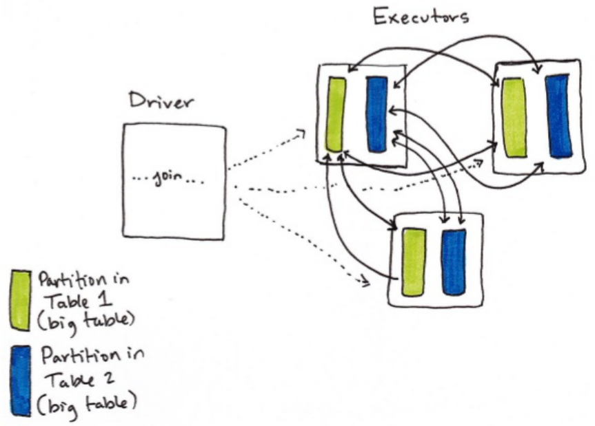
Node-to-Node Communication Strategies
There are two different approachs Spark can take when it comes to
communication. Spark will either incur a shuffle join, which results in an all-
to-all communication or a broadcast join where one of the DataFrames you
work with is duplicated around the cluster which, in general, results in lower
total communication that a shuffle join. Let’s talk through these in a little bit
less abstract terms.
In Spark you will have either a big table or a small table. While this is
obviously a spectrum, it can help to be binary about the distinction.
Big Table to Big Table
When you join a big table to another big table, you end up with a shuffle join.
In a shuffle join, every node will talk to every other node and they will share
data according to which node has a certain key or set of keys (that you are
joining on). These joins are expensive because the network can get congested
with traffic, especially if your data is not partitioned well.
This join describes taking a large table of data and joining it to another large
table of data. An example of this might be that a company receive trillions of
internet-of-things messages every day. You need to compare day over day
change by joining on deviceId, messageType and date in one column and
date - 1 day in order to see changes in day over day traffic and message
types.
Referring to our image above, in this example DataFrame one and DataFrame
two are both large DataFrames. This means that all worker nodes (and
potentially every partition) will have to communicate with one another during
the entire join process (with no intelligent partitioning of data). We can see
this in the previous figure.
Big Table to Small Table
When the table is small enough to fit into a single worker nodes memory, with
some breathing room of course, we can optimize our join. While we can use a
large table to large table communication strategy it can often be more efficient
to use a broadcast join. What this means is that we will replicate our small
DataFrame onto every worker node in the cluster (be it located on one machine
or many currently). Now this sounds expensive, however what this does is
prevent us from performing the all to all communication during the entire join
process, instead we only perform it once at the beginning and then let each
individual worker node perform the work without having to wait or
communicate with any other worker node.
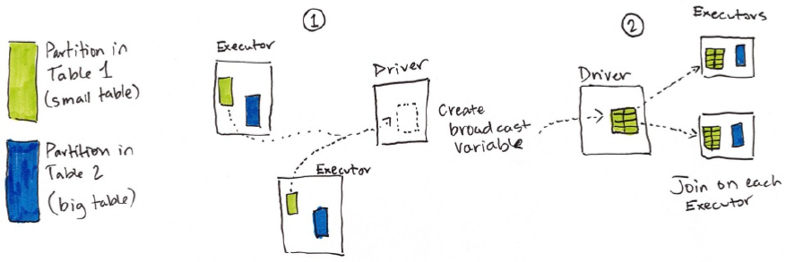
At the beginning of the join will be a large communication, just like in the
previous type of join however immediately after that first set up there will be
no communication happening between nodes. This means that joins will be
performed on every single node individually, making cpu the biggest
bottleneck. For our current set of data, we can see that Spark has automatically
set this up as a broadcast join by looking at the explain plan.
val joinExpr = person.col("graduate_program") === graduateProgram
person
.join(graduateProgram, joinExpr)
.explain()
== Physical Plan ==
*BroadcastHashJoin [graduate_program#40], [id#56], Inner, BuildRight
:- LocalTableScan [id#38, name#39, graduate_program#40, spark_status#41]
+- BroadcastExchange HashedRelationBroadcastMode(List(cast(input[0, int, false] as bigint)))
+- LocalTableScan [id#56, degree#57, department#58, school#59]
We can force a broadcast join too by using the correct function around the
small DataFrame in question. In this example, these result in the same physical
plan, however it can be more consequential for other tables.
import org.apache.spark.sql.functions.broadcast
val joinExpr = person.col("graduate_program") === graduateProgram
person
.join(broadcast(graduateProgram), joinExpr)
.explain()
Little Table to Little Table
When performing joins with small tables, it’s usually best to let Spark decide
how to join them, however you can employ both of the strategies above.
CODE TK
Chapter 7. Data Sources

The Data Source APIs
One of the reasons for Spark’s immense popularity is its ability to read and
write to a variety of data sources. Thus far in this book we read data in CSV
and JSON file format. This chapter will formally introduce the variety of other
data sources that you can use with Spark.
Spark has six “core” data sources and hundreds of external data sources
written by the community. Spark’s core Data Sources are:
CSV,
JSON,
Parquet,
ORC,
JDBC/ODBC Connections,
and plain text files.
As mentioned Spark has numerous community-created data sources including:
Cassandra
HBase
MongoDB
AWS Redshift
and many others.
This chapter will not cover writing your own data sources but rather the core
concepts that you will need to work with any of the above data sources. After
introducing the the core concepts, we will move onto demonstrations of each
of Spark’s core data sources.
Basics of Reading Data
The foundation for reading data in Spark is the DataFrameReader. We access
this through our instantiated SparkSession via the read attribute.
Once we have a DataFrame reader, we specify several values: the format (1),
the schema (2), the read mode (3), a series of options (4) and finally the path
(5). At a minimum, you must supply a format and a path. the format, options,
and schema each return a DataFrameReader that can undergo further
transformations. Each data source has a specific set of options that determine
how the data is read into Spark. We will cover these options shortly.
spark.read.format("csv")
.schema(someSchema)
.option("mode", "FAILFAST")
.option("inferSchema", "true")
.load("path/to/file(s)")
Read Mode
Read modes what will happen when Spark encounters malformed records.
These modes are:
readMode Description
permissive Sets all fields to null when it encounters a corrupted record.
dropMalformed Drops the row that contains malformed records.
failFast Fails immediately upon encountering malformed records.
The default is permissive.
Basics of Writing Data
The foundation for reading data in Spark is the DataFrameWriter. We access
this through a given DataFrame via the write attribute.
dataFrame.write
Once we have a DataFrameWritier, we specify several values: the format (1),
the save mode (2), a series of options (3) and finally the path (4). At a
minimum, you must supply a path. We will cover the required options
afterwards.
dataframe.write.format("csv")
.option("mode", "OVERWRITE")
.option("dateFormat", "yyyy-MM-dd")
.save("path/to/file(s)")
Save Mode
Save modes specify what will happen if Spark finds data at the specified
location (assuming all else equal). These modes are:
saveMode Description
append Appends the output files to the list of files that already exist
at that location.
overwrite Will completely overwrite any data that already exists there.
errorIfExists Throws an error and fails the write if data or files already
exist at the specified location.
If data or files exist at the location, do nothing with the
ignore current DataFrame.
The default is error if exists.
Options
Now every data source has a set of options that can be used to control how the
data is read or written. Each set of options varies based on the data source. We
will cover the options for each specific data source as we go through them.
CSV Files
CSV stands for commma-separated values and is common text file format
where each line represents a single record consisting of a variety of columns.
CSV files, while seeming well structured, are actually one of the trickiest file
formats you will encounter because not many assumptions can be made in
production scenarios about what they contain or how they are structured. For
this reason, the CSV reader has the largest number of options.
This allows us to work around issues like certain characters needing to be
escaped like commas inside of columns when the file is also comma delimited
or null values labelled in an unconventional way.
CSV Options
Read/Write Key Potential Values Default
both sep any single string
character ,
both header TRUE, FALSE FALSE
read escape any string character \
read inferSchema TRUE, FALSE FALSE
read ignoreLeadingWhiteSpace TRUE, FALSE FALSE
read ignoreTrailingWhiteSpace TRUE, FALSE FALSE
both nullValue any string character “”
both nanValue any string character NaN
both positiveInf any string or
character Inf
both negativeInf any string or
character -Inf
both compression or codec
none, uncompressed,
bzip2, deflate, gzip,
lz4, or snappy
none
both dateFormat Any string or
character that
conforms to java’s
SimpleDataFormat.
yyyy-MM-dd
both timestampFormat
Any string or
character that
conforms to java’s
SimpleDataFormat.
yyyy-MM-
dd’T’HH:mm:ss.SSSZZ
read maxColumns Any integer 20480
read maxCharsPerColumn Any integer 1000000
read escapeQuotes TRUE, FALSE TRUE
read maxMalformedLogPerPartition Any integer 10
quoteAll TRUE, FALSE FALSE
Reading CSV Files
To read a csv file, like any other format, we must first create a
DataFrameReader for that specific format to do that. We specify the format to
be CSV.
spark.read.format("csv")
After this we have the option of specifying a schema as well as modes an
options. Let’s set a couple of options, some that we saw from the beginning of
the book and others that we haven’t seen so far. We’ll set the header to be true
for our csv file, we’ll set the mode to be FAILFAST, and we will flag on
inferSchema.
spark.read.format("csv")
.option("header", "true")
.option("mode", "FAILFAST")
.option("inferSchema", "true")
.load("some/path/to/file.csv")
As mentioned, the mode allows us to specify how much tolerance we have for
malformed data. For example, we can use these modes and the schema that we
created in Chapter two of this section to ensure that our file(s) conform to the
data that we expected.
import org.apache.spark.sql.types.{StructField, StructType, StringType
val myManualSchema = new StructType(Array(
new StructField("DEST_COUNTRY_NAME", StringType, true),
new StructField("ORIGIN_COUNTRY_NAME", StringType, true),
new StructField("count", LongType, false)
))
myManualSchema
spark.read.format("csv")
.option("header", "true")
.option("mode", "FAILFAST")
.schema(myManualSchema)
.load("dbfs:/mnt/defg/flight-data/csv/2010-summary.csv")
.take(5)
Things get tricky when we don’t expect data to be in a certain format. For
example, Let’s take our current schema and change all column types to
LongType. this does not match the actual schema but Spark has no problem
with us doing this. The problem will only manifest itself once Spark actually
goes to read the data. Once we trigger our Spark job, Spark will immediately
fail (once we execute a job) due to the data not conforming to the specified
schema.
val myManualSchema = new StructType(Array(
new StructField("DEST_COUNTRY_NAME", LongType, true),
new StructField("ORIGIN_COUNTRY_NAME", LongType, true),
new StructField("count", LongType, false)
))
spark.read.format("csv")
.option("header", "true")
.option("mode", "FAILFAST")
.schema(myManualSchema)
.load("dbfs:/mnt/defg/chapter-1-data/csv/2010-summary.csv")
.take(5)
In general, Spark will only fail at job execution time rather than DataFrame
definition time - even if for example we point to a file that does not exist.
Writing CSV Files
Just like with reading data there are a variety of options (listed previously in
this chapter) for writing data when we write CSV files. This is a subset of the
reading options because many do not apply when writing data (like
maxColumns and inferSchema).
val csvFile = spark.read.format("csv")
.option("header", "true")
.option("mode", "FAILFAST")
.schema(myManualSchema)
.load("dbfs:/mnt/defg/chapter-1-data/csv/2010-summary.csv")
For example we can take our csv file and write it out as a tsv file quite easily.
csvFile.write.format("csv")
.mode("overwrite")
.option("sep", "\t")
.save("/tmp/my-tsv-file.tsv")
When you list the destination directory, you can see that my-tsv-file is actually
a folder with numerous files inside of it. This actually reflects the number of
partitions at write time. If we were to repartition our data before then, we
would end up with a larger number of files. We discuss this tradeoff at the end
of this chapter.
%fs ls /tmp/my-tsv-file.tsv/
JSON Files
Those coming from the world of JavaScript are likely familiar with JSON
notation (JavaScript Object Notation). There are some catches when working
with this kind of data that are worth considering before hand. In Spark when
we refer to JSON files we refer to line-delimited JSON files. This contrasts
with files that have a large JSON object or array per file.
The line-delimited vs. whole file trade off is controlled by a single option
wholeFile.[NOTE: This isn’t merged as of the time of this writing but will be
in by 2.2] When you set this to true, you can read an entire file as one json
object and Spark will go through the work of parsing that into a DataFrame.
With that being said, line-delimited JSON is actually a much more stable
format because it allows you to append to a file with a new record (rather than
having to read in a whole file and then write it out). Another key reason for the
popularity of line-delimited JSON is because JSON objects have structure and
JavaScript (on which JSON is based) has types. This makes it easier to work
with because Spark can make more assumptions on our behalf about the data.
You’ll noitice that there are significantly less options than we saw for CSV
because of the objects.
JSON Options
Read/Write Key Potential Values
both compression or codec
none, uncompressed,
bzip2, deflate, gzip,
lz4, or snappy
none
both dateFormat
Any string or
character that
conforms to java’s
SimpleDataFormat.
yyyy-MM-dd
both timestampFormat
Any string or
character that
conforms to java’s
SimpleDataFormat.
yyyy-MM-dd’T’HH:mm:ss.SSSZZ
read primitiveAsString TRUE, FALSE FALSE
read allowComments TRUE, FALSE FALSE
read allowUnquotedFieldNames TRUE, FALSE FALSE
read allowSingleQuotes TRUE, FALSE TRUE
read allowNumericLeadingZeros TRUE, FALSE FALSE
read allowBackslashEscapingAnyCharacter TRUE, FALSE FALSE
read columnNameOfCorruptRecord Any string value of
spark.sql.columnNameOfCorruptRecord
read wholeFile TRUE, FALSE FALSE
Now reading a line-delimited JSON file only varies in the format and the
options that we specify.
spark.read.format("json")
Reading JSON Files
Let’s have an example of reading a JSON file and compare the options that
we’re seeing.
spark.read.format("json")
.option("mode", "FAILFAST")
.schema(myManualSchema)
.load("dbfs:/mnt/defg/flight-data/json/2010-summary.json")
.show(5)
Writing JSON Files
Now writing JSON files is just as simple as reading them and as you might
expect, the data source does not matter. Therefore we can reuse the CSV
DataFrame that we created above in order to write out our JSON file. This too
follows the rules that we specified above, one file per partition will be written
out and the entire DataFrame will be written out as a folder. It will also have
one JSON object per line.
csvFile.write.format("json")
.mode("overwrite")
.save("/tmp/my-json-file.json")
%fs ls /tmp/my-json-file.json/
Parquet Files
Apache Parquet is an open source column-oriented data store that provides a
variety of storage optimizations, especially for analytics workloads. It
provides columnar compression in order to save storage space and allows for
reading individual columns instead of entire files. It is a file format that works
exceptionally well with Apache Spark and is the default file format. We
recommend writing data out to Parquet for long-term storage as reading from a
parquet file always be more efficient than json or csv. Another advantage of
Parquet is that it supports complex types. That means that if your column is an
array (which would fail with a csv file for example), map, or struct - you’ll
still be able to read and write that file without issue.
spark.read.format("parquet")
Reading Parquet Files
Parquet has exceptionally few options because it enforces its own schema
when storing data. Additionally all we have to set is the format and we are
good to go. We can set the schema if we have strict requirements for what our
DataFrame should look like, however often times this is not necessary because
we can leverage schema on read which is similar to the inferSchema of csv
files however it is more powerful because the schema is built into the file
itself (so no inference needed).
Parquet Options
There are few parquet options because it has a well defined specification that
aligns well with the concepts in Spark.
The only options are:
Read/Write Key Potential
Values Default Description
write compression
or codec
none,
uncompressed,
bzip2, deflate,
gzip, lz4, or
snappy
none
Declares
what
compression
codec Spark
should use to
read or write
the file.
sets whether
we should
merge
schemas
collected
read mergeSchema TRUE, FALSE value of
spark.sql.parquet.mergeSchema
from all
Parquet part-
files. This
will
override the
configuration
value.
Even though there are few options, there can be conflict where different
versions of Parquet files are incompatible with one another. Be careful when
you write out Parquet files with different versions of Spark (especially older
ones) because this can cause significant headache.
spark.read.format("parquet")
spark.read.format("parquet")
.load("/mnt/defg/flight-data/parquet/2010-summary.parquet")
.show(5)
Writing Parquet Files
Writing parquet is as easy as reading it. We simply specify the location for the
file. The same partitioning rules apply.
csvFile.write.format("parquet")
.mode("overwrite")
.save("/tmp/my-parquet-file.parquet")
ORC Files
ORC or Optimized Row Columnar file format is an efficient file format
borrowed from Hive. Orc actually has no options to for reading in data as
Spark understands the file format quite well. An often asked question is, what
is the difference between ORC and Parquet and for the most part, they’re quite
similar. The fundamental difference is that Parquet is further optimized for use
with Spark.
Reading Orc Files
spark.read.format("orc")
.load("/mnt/defg/flight-data/orc/2010-summary.orc")
.show(5)
Writing Orc Files
At this point in the chapter you should feel pretty comfortable taking a guess at
how to write out orc files. It really follows the exact same pattern that we have
seen so far where we specify the format and then save the file.
csvFile.write.format("orc")
.mode("overwrite")
.save("/tmp/my-json-file.orc")
SQL Databases
SQL datasources are one of the more powerful connectors because they allow
you to connect to a variety of systems (as long as that system speaks SQL). For
instance you can connect to a MySQL database, a PostgreSQL Database, or an
Oracle database. We can also connect to SQLite which we’ll be doing in this
example.
NOTE
a primer on SQLite. SQLite is the most used database engine in the entire
world and then are some pretty amazing use cases for it. Personally I think
it is an amazing companion to Spark because it allows you to span the
spectrum of big and little data and when things are small enough to be
placed on a local machine, then we can write them to a SQLite database
and report on them from there.
Now because databases aren’t just a set of raw files, there are some more
options to consider around how you connect to the database. Namely you’re
going to have to start considering things like authentication and connectivity (is
the network of your Spark cluster connected to the network of your database
system). SQLite is going to allow us to skip a lot of these details because it
should work with minimal setup on your local machine.
Reading from SQL Databases
Let’s get started with out example, SQLite isn’t a file format at all, therefore it
lacks the format option. What we do is instead set a list of properties that
specify how we will be connecting to our data source. In this case I’m just
going to declare these as variables to make it apparent what is happening
where.
val props = new java.util.Properties
props.setProperty("driver", "org.sqlite.JDBC")
val path = "/dbfs/mnt/defg/flight-data/jdbc/my-sqlite.db"
val url = s"jdbc:sqlite:/${path}"
val tablename = "flight_info"
If this were a more complex database like MySQL, we might need to set some
more sophisticated parameters.
val props = new java.util.Properties
props.setProperty("driver", "org.sqlite.JDBC") // set to postgres
// dbProperties.setProperty("username", "some-username")
// dbProperties.setProperty("password", "some-password")
val hostname = "192.168.1.5"
val port = "2345"
// we would set a username and a password in the properties file.
val dbDatabase = "DATABASE"
val dbTable = "test"
Once we have defined our connection properties, we can test our connection to
the database itself to make sure that it is functional. This is an excellent
troubleshooting technique to ensure that your database is available to (at the
very least) the Spark driver. This is much less relevant for SQLite because it is
a file on our machine but if we were using something like MySQL we could
test our connection with code like.
import java.sql.DriverManager
val connection = DriverManager.getConnection(url)
connection.isClosed()
connection.close()
If we can see that this connection succeeds, we should have a robust
connection to our database. Now let’s go ahead and read in a DataFrame from
our table.
val dbDataFrame = spark.read.jdbc(url, tablename, props)
As we create this DataFrame it is no different from any other, we can query it,
transform it, and join it without issue. You’ll also notice that we already have a
schema as well. That’s because Spark just gets this information from the table
itself and maps the types to Spark data types. Let’s just get the distinct
locations to verify that we can query it as expected.
dbDataFrame.select("DEST_COUNTRY_NAME").distinct().show(5)
Awesome, we can query our database! Now there are a couple of nuanced
details that are worth understanding.
Query Pushdown
Firstly, Spark will make a best effort to try and filter data in the database itself
before creating the DataFrame. For example in our above query, we can see
from the query plan that it only selects the relevant column name from the table.
dbDataFrame.select("DEST_COUNTRY_NAME").distinct().explain
== Physical Plan ==
*HashAggregate(keys=[DEST_COUNTRY_NAME#8108], functions=[])
+- Exchange hashpartitioning(DEST_COUNTRY_NAME#8108, 200)
+- *HashAggregate(keys=[DEST_COUNTRY_NAME#8108], functions=[])
+- *Scan JDBCRelation(flight_info) [numPartitions=1] [DEST_COUNTRY_NAME#8108] ReadSchema: struct<DEST_COUNTRY_NAME:string>
Spark can actually do better than this on certain queries. For example if we
were to specify a filter on our DataFrame, then Spark will be able to ask the
database to do that for us. This is conveniently called predicate pushdown. We
can again see this in the explain plan.
dbDataFrame
.filter("DEST_COUNTRY_NAME in ('Anguilla', 'Sweden')")
.explain
Spark can’t translate all of its own functions into the functions available in the
SQL database that you’re working with. Therefore sometimes you’re going to
want to pass an entire query into your SQL which will return the results as a
DataFrame. Now this seems like it might be a bit complicated but it’s actually
quite straightforward. Rather than specifying a table name, we just specify a
SQL query. Now we do have to specify this in a special way as we can see
below. We have to wrap our query in parenthesis and rename it to something -
in this case I just gave it the same table name.
val pushdownQuery = """
(SELECT DISTINCT(DEST_COUNTRY_NAME)
FROM flight_info) as flight_info
"""
val dbDataFrame = spark.read.jdbc(url, pushdownQuery, props)
Now when we query this table, we’ll actually be querying the results of that
query. We can see this in the explain plan. Now Spark doesn’t even know
about the actual schema of the table, just the one that results from our query
above.
dbDataFrame.explain
Reading from Databases in Parallel
All throughout this book we have talked about partitioning and its importance
in data processing. When we read in a set of parquet files for example, we will
get one Spark partition per file. When we reading from SQL databases, we by
default will always get one partition. Now this can be helpful if that dataset is
small and we’d like to broadcast it out to all other workers but if it’s a larger
dataset sometimes it is better to read it into multiple partitions and even
control what the keys of those partitions are.
Partitioning Via Predicates
One way is to specify an array of predicates that determine what should go in a
particular partition. For example, say we wanted one partition to have all the
flights to Sweden and another to the United States (and no others) Then we
would speciy these predicates and pass them into our JDBC connection.
?val predicates = Array(
"DEST_COUNTRY_NAME = 'Sweden'",
"DEST_COUNTRY_NAME = 'United States'")
val dbDataFrame = spark.read.jdbc(url, tablename, predicates, props
We can see that this will result in exactly what we expect, two partitions and
the country names that we specified above.
dbDataFrame.rdd.getNumPartitions
dbDataFrame.select("DEST_COUNTRY_NAME").distinct().show()
Now we don’t have to specify predicates that are disjoint from one another.
This would mean that we would get rows from our database duplicated into
multiple partitions. For example, we have a total of 255 rows in our database.
spark.read.jdbc(url, tablename, props).count()
If we specify predicates that are not disjoint we can end up with lots of
duplicate rows.
val predicates = Array(
"DEST_COUNTRY_NAME != 'Sweden'",
"Origin_COUNTRY_NAME != 'United States'")
spark.read.jdbc(url, tablename, predicates, props).count()
Partitioning Based on a Sliding Window
Now we saw how we can partition based on predicates, let’s partition based
on our numerical count column. What we do here is specify a minimum, a
maximum for our first partition and our last partition. Anything outside of these
bounds will be in the first partition or final partition. Then we set the number
of partitions we would like total (this is the level of parallelism). Spark will
then query our database in parallel and return numPartitions partitions. We
simply modify the upper and lower bounds in order to place certain values in
certain partitions. No filtering is taking place like we saw in the previous
example.
val colName = "count"
val lowerBound = 0L
val upperBound = 348113L // this is the max count in our database
val numPartitions = 10
This will will distribute the intervals equally from low to high.
spark.read.jdbc(url,
tablename,
colName,
lowerBound,
upperBound,
numPartitions,
props)
.count()
Writing to SQL Databases
Now writing out to SQL Database is just as easy as before. We simply specify
our URI and write out the data according to the specified write mode we
would like. In this case I’m going to specify overwrite, which will overwrite
the entire table. I’ll be using the CSV DataFrame that we defined above in
order to do this.
val newPath = "jdbc:sqlite://tmp/my-sqlite.db"
csvFile.write.mode("overwrite").jdbc(newPath, tablename, props)
Now we can see the results.
spark.read.jdbc(newPath, tablename, props).count()
Of course we can append to the table that we just created just as easily.
csvFile.write.mode("append").jdbc(newPath, tablename, props)
And naturally see the count increase.
spark.read.jdbc(newPath, tablename, props).count()
Text Files
Spark also allows you to read in plain text files. For the most part you
shouldn’t really need to do this, however if you do you will then have to parse
the text file as a set of strings. For the most part this is only relevant for
Datasets which will be covered in the next chapter.
Reading Text Files
Reading text files is simple, we just specify the type to be textFile.
spark.read.textFile("/tmp/five-csv-files.csv")
.map(stringRow => stringRow.split(","))
.show()
Writing Out Text Files
When we write out a text file, we need to be sure to only have one column,
otherwise the write will fail.
spark.read.textFile("/tmp/five-csv-files.csv")
.write.text("/tmp/my-text-file.txt")
Advanced IO Concepts
We saw previously that we can control the parallelism of files that we write by
controlling the partitions prior to a write. We can also control specific data
layout by controlling two things, bucketing and partitioning.
Reading Data in Parallel
While multiple executors cannot read from the same file as the same time, they
can read different files at the same time. This means when you read from a
folder with multiple files in it, each one of those files will become a partition
in your DataFrame and be read in by available executors in parallel (with the
remaining queueing up behind the others).
Writing Data in Parallel
The number of files that are written is a function of the number of partitions the
DataFrame at the time your look to write it out. One file is written out per
partition of the data by default meaning that although we specify a “file” it’s
actually a number of files inside of a folder with the name of the specified file
with a file per each partition that is written out.
For example the following code.
csvFile.repartition(5).write.format("csv").save("/tmp/multiple.csv"
Will end up with five files inside of that folder. As you can see from the list
call.
ls /tmp/multiple.csv
/tmp/multiple.csv/_SUCCESS
/tmp/multiple.csv/part-00000-767df509-ec97-4740-8e15-4e173d365a8b.csv
/tmp/multiple.csv/part-00001-767df509-ec97-4740-8e15-4e173d365a8b.csv
/tmp/multiple.csv/part-00002-767df509-ec97-4740-8e15-4e173d365a8b.csv
/tmp/multiple.csv/part-00003-767df509-ec97-4740-8e15-4e173d365a8b.csv
/tmp/multiple.csv/part-00004-767df509-ec97-4740-8e15-4e173d365a8b.csv
Bucketing and Partitioning
Now one other thing we do is control even more specifically the layout. We
can write out files in a given partitioning scheme which basically encodes the
files into a certain folder structure. We will go into why you want to do this in
the optimizations chapter but the core reason is that you’re able to filter out
data when you read it in later much more easily, reducing the amount of data
you need to handle in the first place. These are supported for all file-based
data sources.
csvFile.write
.mode("overwrite")
.partitionBy("DEST_COUNTRY_NAME")
.save("/tmp/partitioned-files.parquet")
%fs ls /tmp/partitioned-files.json
%fs ls /tmp/partitioned-files.json/DEST_COUNTRY_NAME=Australia/
Rather than partitioning on a specific column (which might write out a ton of
files), it’s probably more worth it to explore bucketing the data. This will
create a certain number of files and organize our data into those “buckets”.
val numberBuckets = 10
val columnToBucketBy = "count"
csvFile.write.format("parquet")
.mode("overwrite")
.bucketBy(numberBuckets, columnToBucketBy)
.saveAsTable("bucketedFiles")
%fs ls "dbfs:/user/hive/warehouse/bucketedfiles/"
The above write will give us one file per partition because the number of
DataFrame partitions was less than the total number of output partitions. Now
as is, this can get even worse if we were to have a higher number of partitions
in our DataFrame and were writing out to a partitioning scheme that had fewer
total partitions. This is because we could end up with many files per partition -
and if we have a small DataFrame then reading this data back in will be very
slow.
Controlling partitioning in-flight as well as at read and write time is the source
of almost all Spark optimizations. We will cover this in Part IV of the book.
Writing Complex Types
As we covered in the “Working with Different Types of Data” Chapter, Spark
as a variety of different internal types. While Spark can work with all of these
types, not every single type works well with every data format. For instance,
CSV files do not support complex types while Parquet and ORC do.
Chapter 8. Spark SQL
Spark SQL Concepts
Spark SQL is arguably one of the most important and powerful concepts in
Spark. This chapter will introduce the core concepts in Spark SQL that you
need to understand. This chapter will not rewrite the ANSI-SQL specification
or enumerate every single kind of SQL expression. If you read any other parts
of this book, you will notice that we try to include SQL code wherever we
include DataFrame code to make it easy to cross reference with code
examples. Other examples are available in the appendix and reference
sections.
In a nutshell, Spark SQL allows the user to execute SQL queries against views
or tables organized into databases. Users can also use system functions or
define user functions and analyze query plans in order to optimize their
workloads.

What is SQL?
SQL or Structured Query Language is a domain specific language for
expressing relational operations over data. It is used in all relational databases
and many “NoSQL” databases create their SQL dialect in order to make
working with their databases easier. SQL is everywhere and even though tech
pundits prophesized its death, it is an extremely resilient data tool that many
business depend on. Spark implements a subset of the ANSI SQL:2003
Standard. This SQL standard is one that is available in the majority of SQL
databases and this support means that Spark successfully runs the popular
benchmark TPC-DS.
Big Data and SQL: Hive
Before Spark’s rise, Hive was the de facto big data SQL access layer.
Originally developed at Facebook, Hive became an incredibly popular tool
across industry for performing SQL operations on big data. In many ways it
helped propel Hadoop into different industries because analysts could run SQL
queries. While Spark began as a general processing engine with RDDs, and
was successful when doing so, Spark took off further when it because
supporting a subset of SQL with the sqlContext and nearly all of the
capabilities of Hive with the HiveContext in Spark 1.x.

Big Data and SQL: Spark SQL
With Spark 2.0’s release the authors of Spark created a superset of Hive’s
support, writing a native SQL parser that supports both ANSI-SQL as well as
Hive QL queries. In late 2016, Facebook announced that they would be
throwing their weight behind Spark SQL and put Spark SQL into production in
place of Hive (and seeing huge benefits in doing so).
The power of Spark SQL derives from several key facts: SQL analysts can
now leverage Spark’s computation abilities by plugging into the Thrift Server
or Spark’s SQL interface while Data Engineers and Scientists can use Spark’s
programmatic SQL interface in any of Spark’s supported languages via the
method sql on the SparkSession object. This code then can be manipulated
as a DataFrame, passed into one of Spark MLlibs large scale machine learning
algorithms, written out to another data source and everything in between.
Spark SQL is intended to operate as a OLAP (online analytic processing)
database, not an OLTP (online transaction processing) database. This means
that it is not intended very extremely low latency queries.
How to Run Spark SQL Queries
Spark provides several interfaces to execute SQL queries.
SparkSQL Thrift JDBC/ODBC Server
Spark provides a JDBC interface by which either you or a remote program
connects to the Spark driver into order to execute Spark SQL queries. A
common use case might be a for a business analyst to connect a business
intelligence software like Tableau to Spark. The Thrift JDBC/ODBC server
implemented here corresponds to the HiveServer2 in Hive 1.2.1 You can test
the JDBC server with the beeline script that comes with either Spark or Hive
1.2.1.
To start the JDBC/ODBC server, run the following in the Spark directory:
./sbin/start-thriftserver.sh
This script accepts all bin/spark-submit command line options. Run
./sbin/start-thriftserver.sh --help to see all available options for
configuring this Thrift Server. By default, the server listens on
localhost:10000. You may override this behavior through environmental
variables or system properties.
For environment configuration:
export HIVE_SERVER2_THRIFT_PORT=<listening-port>
export HIVE_SERVER2_THRIFT_BIND_HOST=<listening-host>
./sbin/start-thriftserver.sh \
--master <master-uri> \
...
For system properties:
./sbin/start-thriftserver.sh \
--hiveconf hive.server2.thrift.port=<listening-port> \
--hiveconf hive.server2.thrift.bind.host=<listening-host> \
--master <master-uri>
...
You can then test this connect by running the commands below.
./bin/beeline
beeline> !connect jdbc:hive2://localhost:10000
Beeline will ask you for a username and password. In non-secure mode,
simply enter the username on your machine and a blank password. For secure
mode, please follow the instructions given in the beeline documentation.
To learn more about the Thrift server see the Spark SQL Appendix.
Spark SQL CLI
The Spark SQL CLI is a convenient tool to run the Hive metastore service in
local mode and execute queries input from the command line. Note that the
Spark SQL CLI cannot talk to the Thrift JDBC server. To start the Spark SQL
CLI, run the following in the Spark directory:
./bin/spark-sql
Configuration of Hive is done by placing your hive-site.xml, core-site.xml and
hdfs-site.xml files in conf/. You may run ./bin/spark-sql --help for a
complete list of all available options.
Spark’s Programmatic SQL Interface
In addition to setting up a server, you can also execute sql in an ad hoc manner
via any of Spark’s language. This is done via the method sql on the
SparkSession object. This will return a DataFrame as we will see later in
this chapter. For example in Scala, we can run.
%scala
spark.sql("SELECT 1 + 1").collect()
The python interface is essentially the exact same.
%python
spark.sql("SELECT 1 + 1").collect()
The command spark.sql("SELECT 1 + 1") will return a DataFrame that
we can then evaluate programmatically. Just like other transformations, this
will not be executed eagerly but lazily. This is an immensely powerful
interface because there are some transformations that are much simpler to
express in SQL code as opposed to DataFrames.
You can express multi-line queries quite simply, just pass a multi-line string
into the function. For example we could execute something like the following
code in Python or Scala.
spark.sql("""
SELECT
user_id,
department,
first_name
FROM
professors
WHERE
department IN
(SELECT name
FROM department
WHERE created_date >= '2016-01-01')
""")
For the remainder of this chapter will only show the SQL being executed, just
keep in mind if you’re using the programmatic interface that you need to wrap
everything in a spark.sql function call in order to execute the relevant code.
Tables
To do anything useful with Spark SQL, we first need to define tables. Tables
are logically equivalent to a DataFrame in that they are a structure of data that
we execute commands against. We can join tables, filter then, aggregate them
and many different manipulations that we saw in previous chapters. The core
difference between tables and DataFrames is that while we define DataFrames
in the scope of a programming language, we define tables inside of a database.
This means when you create a table (assuming you never changed the
database), it will belong to the default database. We will discuss databases
more later on in the chapter.
We can see the already defined tables by running the following command.
%sql
SHOW TABLES
case class Table(database:String, tableName:String, isTemporary
spark.sql("SHOW TABLES").as[Table].collect().map {t =>
try {
spark.sql(s"DROP TABLE IF EXISTS ${t.tableName}").collect()
}
catch {
case e: org.apache.spark.sql.AnalysisException => {
spark.sql(s"DROP VIEW IF EXISTS ${t.tableName}").collect
}
}
}
// will delete this, just to help me iterate on all these tables
You will notice in the results that a database is listed. We discuss databases
later in this chapter but it is of note that we can also see tables in a Specific
database with the following query show tables IN databaseName where
databaseName represents the name of the database we’d like to query.
If you are running on a new cluster or local mode, this should return zero
results.
Creating Tables
Tables can be created from a variety of sources. Something fairly unique to
Spark is the capability of reusing the entire Data Source API within SQL. This
means that you do not have to define a table and then load data into it, Spark
let’s you create one on the fly. We can even specify all sorts of sophisticated
options when we read in a file. For example, here’s a simple way to read our
flights data in from previous chapters.
%sql
CREATE TABLE flights (
DEST_COUNTRY_NAME STRING,
ORIGIN_COUNTRY_NAME STRING,
count LONG)
USING JSON
OPTIONS (
path '/mnt/defg/chapter-1-data/json/2015-summary.json')
We can also add comments to certain columns in a table, this can help other
people understand the data in the tables.
%sql
CREATE TABLE flights_csv (
DEST_COUNTRY_NAME STRING,
ORIGIN_COUNTRY_NAME STRING COMMENT "remember that the most prevalent will be the US"
count LONG)
USING csv
OPTIONS (
inferSchema true,
header true,
path '/mnt/defg/chapter-1-data/csv/2015-summary.csv')
We can also create a table from a query.
%sql
CREATE TABLE flights_from_select
AS
SELECT * FROM flights
We can also specify to create a table only if it does not currently exist as we
see in the following snippet.
%sql
CREATE TABLE IF NOT EXISTS flights_from_select
AS
SELECT * FROM flights
LIMIT 5
We can also control the layout of the data by writing out a partitioned dataset
as we saw in the previous chapter.
%sql
CREATE TABLE partitioned_flights
USING parquet
PARTITIONED BY (DEST_COUNTRY_NAME)
AS
SELECT DEST_COUNTRY_NAME, ORIGIN_COUNTRY_NAME, count FROM flights
LIMIT 5 -- so we don't create a ton of files
These tables will be available in Spark even through sessions, temporary
tables do not currently exist in Spark. You must create a temporary view as we
will demonstrate later in this chapter.
Inserting Into Tables
Insertions follow the standard SQL syntax.
%sql
INSERT INTO flights_from_select
SELECT DEST_COUNTRY_NAME, ORIGIN_COUNTRY_NAME, count FROM flights
LIMIT 20
We can optionally provide a partition specification if we only want to write
into a certain partition. Note that a write will respect a partitioning scheme as
well (which may cause the above query to run quite slowly), however it will
only add additional files into the end partitions.
%fs ls /user/hive/warehouse/partitioned_flights/
%sql
INSERT INTO partitioned_flights
PARTITION (DEST_COUNTRY_NAME="UNITED STATES")
SELECT count, ORIGIN_COUNTRY_NAME FROM flights
WHERE DEST_COUNTRY_NAME='UNITED STATES'
LIMIT 12
Now that we created our tables, we can query them and see our results.
%sql
SELECT * FROM flights_csv
%sql
SELECT * FROM flights
Describing Table Metadata
We saw above that we can add a comment when we create a table, we can
view this by describing the table metadata which will show us the relevant
comment.
%sql
DESCRIBE TABLE flights_csv
We can also see the partitioning scheme for the data with the following
command, however this only works on partitioned tables.
%sql
SHOW PARTITIONS partitioned_flights
Refreshing Table Metadata
There are two commands to refresh table metadata.
REFRESH TABLE will refresh all cached entries associated with the table. If
the table was previously cached, then it would be cached lazily the next time it
is scanned.
%sql
REFRESH table partitioned_flights
%sql
MSCK REPAIR TABLE partitioned_flights
Dropping Tables
Tables cannot be deleted, they are only “dropped”. We can drop a table with
the DROP keyword. If we are dropping a managed table (e.g., flights_csv),
both the data and the table definition will be removed.
WARNING This can and will delete your data, be care when you are
dropping tables.
%sql
DROP TABLE flights_csv;
If you try to drop a table that does not exist, you will receive an error. To only
delete a table if it already exists use DROP TABLE IF EXISTS.
%sql
DROP TABLE IF EXISTS flights_csv;
Views
Now that we created a table another thing we can define a view. A view
specifies a set of transformations on top of an existing table. Views can be
either just a saved query plan to be executed against the source table or they
can be materialized which means that the results are precomputed (at the risk
of going stable if the underlying table changes).
Spark has several different notions of views. Views can be global, set to a
database, or per session.
Creating Views
To an end user, views are displayed as tables except rather than rewriting all
of the data to a new location, they simply perform a transformation on the
source data at query time. this might be a filter, select, or potentially an
even larger GROUP BY or ROLLUP. For example, we can create a view where
the destination must be United States in order to see only flights to the USA.
%sql
CREATE VIEW just_usa_view AS
SELECT *
FROM flights
WHERE dest_country_name = 'United States'
We can make it global by leveraging the GLOBAL keyword.
%sql
CREATE VIEW just_usa_global AS
SELECT *
FROM flights
WHERE dest_country_name = 'United States'
Views, like tables, can be created as temporary views which will only be
available during the current Spark Session and are not registered to a database.
%sql
CREATE TEMP VIEW just_usa_view_temp AS
SELECT *
FROM flights
WHERE dest_country_name = 'United States'
Or it can be a global temp view. Global temp views are resolved regardless of
database and are viewable across the entire Spark application but are removed
at the end of the session.
%sql
CREATE GLOBAL TEMP VIEW just_usa_global_view_temp AS
SELECT *
FROM flights
WHERE dest_country_name = 'United States'
%sql SHOW TABLES
We can also specify that we would like to overwite a view if one already
exists with the following keywords. We can overwrite both temp views and
regular view.
%sql
CREATE OR REPLACE TEMP VIEW just_usa_view_temp AS
SELECT *
FROM flights
WHERE dest_country_name = 'United States'
Now we can query this view just as if it were another table.
%sql
SELECT * FROM just_usa_view
A view is effectively a transformation and Spark will only perform it at query
time. This means that it will only apply that filter once we actually go to query
the table and (and not earlier). Effectively, views are equivalent to creating a
new DataFrame from an existing DataFrame.
In fact we can see this by comparing the query plans generated by Spark
DataFrames and Spark SQL. In DataFrames we would write.
val flights = spark.read.format("json")
.load("/mnt/defg/chapter-1-data/json/2015-summary.json")
val just_usa_df = flights
.where("dest_country_name = 'United States'")
just_usa_df
.selectExpr("*")
.explain
In SQL we would write (querying from our view).
%sql
EXPLAIN SELECT * FROM just_usa_view
Or equivalently.
%sql
EXPLAIN
SELECT *
FROM flights
WHERE dest_country_name = 'United States'
Due to this fact, you should feel comfortable in writing your logic either on
DataFrames or SQL - which ever is most comfortable and maintainable for
you.
Dropping Views
You can drop views in the same way that you drop tables but specify that what
you intend to drop is a view instead of a table. If we are dropping a view no
underlying data will be removed, only the view definition itself.
%sql
DROP VIEW IF EXISTS just_usa_view;
Databases
Databases are a tool for organizing tables. As mentioned above, if you do not
define a database Spark will use the default one. Any SQL statements you
execute from within Spark (including DataFrame commands) execute within
the context of a database. That means if you change the database, any user
defined tables will remain in the previous database and will have to be
queried different.
WARNING
this can be a source of confusion for your co-workers so make sure to set
your databases appropriately.
We can see all databases with the following command.
%sql
SHOW DATABASES
Creating Databases
Creating databases follows the same patterns we saw previously in this
chapter, we use the CREATE DATABASE keywords.
%sql
CREATE DATABASE some_db
Setting The Database
You may want to set a database to perform a certain query. To do this use the
USE keyword followed by the database name.
%sql
USE some_db
Once we set this database, all queries will try to resolve tables names to this
database. Queries that were working just fine will now may fail or give
different results because we are in a different database.
%sql
SHOW tables
%sql
SELECT * FROM flights
However we can query different databases by using the correct prefix.
%sql
SELECT * FROM default.flights
We can see what database we are currently using with the following command.
%sql
SELECT current_database()
We can, of course, switch back to the default database.
%sql
USE default;
Dropping Databases
Dropping or removing databases is equally as easy. We simply use the DROP
DATABASE keyword.
%sql
DROP DATABASE IF EXISTS some_db;
Select Statements
Queries in Spark support follow ANSI SQL requirements. The follow lists the
layout of SELECT expression.
SELECT [ALL|DISTINCT] named_expression[, named_expression, ...]
FROM relation[, relation, ...]
[lateral_view[, lateral_view, ...]]
[WHERE boolean_expression]
[aggregation [HAVING boolean_expression]]
[ORDER BY sort_expressions]
[CLUSTER BY expressions]
[DISTRIBUTE BY expressions]
[SORT BY sort_expressions]
[WINDOW named_window[, WINDOW named_window, ...]]
[LIMIT num_rows]
named_expression:
: expression [AS alias]
relation:
| join_relation
| (table_name|query|relation) [sample] [AS alias]
: VALUES (expressions)[, (expressions), ...]
[AS (column_name[, column_name, ...])]
expressions:
: expression[, expression, ...]
sort_expressions:
: expression [ASC|DESC][, expression [ASC|DESC], ...]
Case When Then Statements
Often times you may need to conditionally replace values in your SQL queries.
This can be achieved with a case...when...then...end style statement.
This are essentially the equivalent of programmatic if statements.
%sql
SELECT
CASE WHEN DEST_COUNTRY_NAME = 'UNITED STATES' THEN 1
WHEN DEST_COUNTRY_NAME = 'Egypt' THEN 0
ELSE -1 END
FROM
partitioned_flights
Advanced Topics
Now that we defined where data lives and how to organize it, let’s move onto
querying data. A SQL query is a SQL statement that requests that some set of
commands be executed. SQL statements can define manipulations, definitions,
or controls. The most common case are the manipulations which is what we
will primarily be focusing on. We can execute these statements without
necessarily pointing to a set of data to execute our statement on.
While we do not want to define the entire SQL standard over again. We
encourage you to look through the entire structured API section, in this we have
included a SQL query in almost every location that we included a DataFrame
manipulation. Or pick up a SQL language book as it will provide nearly all the
information that you need in order to leverage Spark SQL.
Complex Types
Complex types are a departure from standard SQL and are an incredibly
powerful feature that does not exist in standard SQL. Understanding how to
manipulate them appropriately in SQL is essential. There are three core
complex types in Spark SQL, sets, lists, and structs.
Structs
Structs on the other hand are more akin to maps. They provide a way of
creating or querying nested data in Spark. To create one, you simply need to
wrap a set of columns (or expressions in parentheses).
%sql
CREATE VIEW IF NOT EXISTS
nested_data
AS
SELECT
(DEST_COUNTRY_NAME, ORIGIN_COUNTRY_NAME) as country,
count
FROM flights
Now we can query this data to see what it looks like.
%sql
SELECT * FROM nested_data
We can even query individual columns within a struct, all we have to do is use
dot syntax.
%sql
SELECT country.DEST_COUNTRY_NAME, count
FROM nested_data
We can also select all the sub-values from a struct if we like by using the
struct’s name and select all of the sub-columns. While these aren’t truly sub-
columns it does provide a simpler way to think about them because we can do
everything that we like with them as if they were a column.
%sql
SELECT country.*, count
FROM nested_data
Sets and Lists
Sets and lists are the same that you should be familiar with in programming
languages. Sets have no ordering and no duplicates, lists can have both. We
create sets and lists with the collect_set and collect_list functions,
respectively. However we must do this within an aggregation because these
are aggregation functions.
%sql
SELECT
DEST_COUNTRY_NAME as new_name,
collect_list(count) as flight_counts,
collect_set(ORIGIN_COUNTRY_NAME) as origin_set
FROM
flights
GROUP BY
DEST_COUNTRY_NAME
We can also query these types by position by using a python like array query
syntax.
%sql
SELECT
DEST_COUNTRY_NAME as new_name,
collect_list(count)[0]
FROM
flights
GROUP BY
DEST_COUNTRY_NAME
We can also do things like convert an array back into rows. The way we do
this is with the explode function. To demonstrate, let’s create a new view as
our aggregation.
%sql
CREATE OR REPLACE TEMP VIEW flights_agg
AS
SELECT
DEST_COUNTRY_NAME,
collect_list(count) as collected_counts
FROM
flights
GROUP BY
DEST_COUNTRY_NAME
Now let’s explode the complex type to one row in our result for every value in
the array. The DEST_COUNTRY_NAME will duplicate for every value in the
array, performing the exact opposite of the original collect and returning us to
the original DataFrame.
%sql
SELECT explode(collected_counts), DEST_COUNTRY_NAME
FROM flights_agg
Functions
In addition to complex types, Spark SQL provides a variety of sophisticated
functions. Most of these functions can be found in the DataFrames function
reference however it is worth understanding how to find these functions in SQL
as well. To see a list of functions in Spark SQL, you simply need to use the
SHOW FUNCTIONS statement in order to see a list of all available functions.
%sql
SHOW FUNCTIONS
You can also more specifically specify whether or not you would like to see
the system functions (i.e., those built into Spark) as well as user functions.
%sql
SHOW SYSTEM FUNCTIONS
User functions are those that you, or someone else sharing your Spark
environment, defined. These are the same User-Defined Functions that we
talked about in previous chapters. We will discuss how to create them later on
in this chapter.
%sql
SHOW USER FUNCTIONS
All SHOW commands can be filtered by passing a string with wildcard (*)
characters. We can see all functions that start with “s”.
%sql
SHOW FUNCTIONS "s*";
Optionally, you can include the LIKE keyword although this is not necessary.
%sql
SHOW FUNCTIONS LIKE "collect*";
While listing functions is certain useful, often times you may want to know
more about specific functions themselves. Use the DESCRIBE keyword in order
to return the documentation for a specific function.
User Defined Functions
As we saw in Section two, Chapters three and four, Spark allows you to define
your own functions and use them in a distributed manner. We define functions
and register them, just as we would do before, writing the function in the
language of our choice and then registering it appropriately.
def power3(number:Double):Double = {
number * number * number
}
spark.udf.register("power3", power3(_:Double):Double)
%sql
SELECT count, power3(count)
FROM flights
Spark Managed Tables
One important note is the concept of managed vs unmanaged tables. Tables
store two important pieces of information. The data within the tables as well
as the data about the tables, that is the metadata. You can have Spark manage
the metadata for a set of files, as well as the data. When you define a table
from files on disk, you are defining an unmanaged table. When you use
saveAsTable on a DataFrame you are creating a managed table where Spark
will keep track of all of the relevant information for you.
This will read in our table and write it out to a new location in Spark format.
We can see this reflected in the new explain plan. In the explain plan you will
also notice that this writes to the default hive warehouse location. You can set
this by setting the spark.sql.warehouse.dir configuration to the directory
of your choosing at SparkSession creation time. By default Spark sets this to
/user/hive/warehouse.
Creating External Tables
Now as we mentioned in the beginning of this chapter, Hive was one of the
first big data SQL systems and Spark SQL is completely compatible with Hive
SQL (HiveQL) statements. One of the use cases you may have here will be to
port your legacy hive statements to Spark SQL. Luckily you can just copy and
paste your Hive statements directly into Spark SQL. For example below I am
creating an unmanaged table. Spark will manage the metadata about this table
however, the files are not managed by Spark at all. We create this table with
the CREATE EXTERNAL TABLE statement.
%sql
CREATE EXTERNAL TABLE hive_flights (
DEST_COUNTRY_NAME STRING,
ORIGIN_COUNTRY_NAME STRING,
count LONG)
ROW FORMAT DELIMITED FIELDS TERMINATED BY ','
LOCATION '/mnt/defg/flight-data-hive/'
You can also create an external table from a select clause.
%sql
CREATE EXTERNAL TABLE hive_flights_2
ROW FORMAT DELIMITED FIELDS TERMINATED BY ','
LOCATION '/mnt/defg/flight-data-hive/'
AS SELECT * FROM flights
%sql
SELECT * FROM hive_flights
Dropping Unmanaged Tables
If we are dropping an unmanaged table (e.g., hive_flights) no data will be
removed but we won’t be able to refer to this data by the table name any
longer.
Subqueries
Subqueries allow you to specify queries within other queries. This can allow
you to specify some sophisticated logic inside of your SQL. In Spark there are
two fundamental subqueries. Correlated Subqueries use some information
from the outer scope of the query in order to supplement information in the
subquery. Uncorrelated subqueries include no information from the outer
scope. Each of these queries can return one (scalar subquery) or more values.
Spark also includes support for predicate subqueries which allow for filtering
based on values.
Uncorrelated Predicate Subqueries
For example, let’s take a look at a predicate subquery. This is going to be
composed of two uncorrelated queries. The first query is just to get the top
five country destinations based on the data we have.
%sql
SELECT dest_country_name
FROM flights
GROUP BY dest_country_name
ORDER BY sum(count) DESC
LIMIT 5
This gives us the result:
+-----------------+
|dest_country_name|
+-----------------+
| United States|
| Canada|
| Mexico|
| United Kingdom|
| Japan|
+-----------------+
Now we place this subquery inside of the filter and check to see if our origin
country exists in that list.
%sql
SELECT *
FROM flights
WHERE
origin_country_name IN (
SELECT dest_country_name
FROM flights
GROUP BY dest_country_name
ORDER BY sum(count) DESC
LIMIT 5)
This query is uncorrelated because it does not include any information from the
outer scope of the query. It’s a query that can be executed on its own.
Correlated Predicated Subqueries
Correlated predicate subqueries allows us to use information from the outer
scope in our inner query. For example, if we want to see whether or not we
have a flight that will take you back from your destination country we could do
so by checking whether or not there was a flight that had the destination country
as an origin and a flight that had the origin country as a destination.
%sql
SELECT *
FROM flights f1
WHERE EXISTS (
SELECT 1
FROM flights f2
WHERE f1.dest_country_name = f2.origin_country_name
AND EXISTS (
SELECT 1
FROM flights f2
WHERE f2.dest_country_name = f1.origin_country_name
EXISTS just checks for some existence in the subquery and returns true if there
is a value. We can flip this by placing the NOT operator in front of it. This
would be equivalent to finding a flight that you won’t be able to get back from!
Uncorrelated Scalar Queries
Uncorrelated scalar queries allows us to bring in some supplemental
information that we might not have previously. For example if we wanted to
include the maximum value as its own column from the entire counts dataset in
order to
%sql
SELECT *,
(SELECT max(count) FROM flights) AS maximum
FROM flights
Conclusion
Many concepts in Spark SQL transfer directly to DataFrames (and vice versa)
you should be able to leverage many of the examples through this book, and
with a little manipulation, get them to work in any of Spark’s supported
languages.
Chapter 9. Datasets
What are Datasets?
Datasets are the foundational type of the Structured APIs. Earlier in this
section we worked with DataFrames, which are Datasets of Type Row, and are
available across Spark’s different languages. Datasets are a strictly JVM
language feature that only work with Scala and Java. Datasets allow you to
define the object that each row in your Dataset will consist of. In Scala this
will be a case class object that essentially defines a schema that you can
leverage and in Java you will define a Java Bean. Experienced users often
refer to Datasets as the “typed set of APIs” in Spark. See the Structured API
Overview Chapter for more information.
In the introduction to the Structured APIs we discussed that Spark has types
like StringType, BigIntType, StructType and so on. Those Spark specific
types map to types available in each of Spark’s languages like String,
Integer, Double. When you use the DataFrame API, you do not create Strings
or Integers but Spark manipulates the data for you by manipulating the Row.
When you use the Dataset API, for every row it touches with user code (not
Spark code), Spark converts the Spark Row format to the case class object you
specify when you create your Dataset. This will slow down your operations
but can provide more flexibilty. You will notice a performance difference but
this is a far different order of magnitude from what you might see from
something like a Python UDF because the performance costs are not as extreme
as switching programming languages but it is an important thing to keep in
mind.
Encoders
As mentioned in the Structured API Overview, when working with JVM
languages, we can define specific types in order to operate on user defined
types instead of JVM Types. To do this, we use an Encoder. Encoders are only
available in Scala, with case classes, and Java, with JavaBeans. For some
types, like Long or Integer, Spark already includes an Encoder. For instance
we can collect a Dataset of type Long and get native Scala types back.
As of early 2017, users cannot define their own arbitrary types like a custom
Scala class.
Creating Datasets
Case Classes
To create Datasets in Scala, we define a Scala case class.
A case class is a regular class that is:
immutable,
decomposable through pattern matching,
allows for comparison based on structure instead of reference, and
easy to use and operate on.
These traits make it quite valuable for data analysis because it is quite easy to
reason about a case class. Probably the most important feature is that case
classes are immutable and allow for comparison by structure instead of value.
According to the Scala Documentation:
Immutability frees you from needing to keep track of where and when
things are mutated
Comparison-by-value allows you compare instances as if they are
primitive values - no more uncertainty regarding whether instances of a
class is compared by value or reference
Pattern matching simplifies branching logic, which leads to less bugs and
more readable code.
http://docs.scala-lang.org/tutorials/tour/case-classes.html
These advantages carry over to their usage within Spark as well.
To get started creating a Dataset let’s define a case class for one of our
datasets.
case class Flight(DEST_COUNTRY_NAME: String, ORIGIN_COUNTRY_NAME
Now that we defined a case class, this will represent a single record in our
dataset. More succintly, we now have a Dataset of Flights. This doesn’t define
any methods for us but simply the schema. Now when we read in our data
we’ll get a DataFrame However we simply use the as method to cast it to our
specified row type.
val flightsDF = spark.read.parquet("/mnt/defg/chapter-1-data/parquet/2010-summary.parquet/"
val flights = flightsDF.as[Flight]
Actions
While we can see the power of Datasets what’s important to understand is that
actions like collect, take, and count apply to whether we are using Datasets
or DataFrames.
flights.take(2)
You’ll also notice that when we actually go to access one of the case classes
we have to do no type coercion, we simply specify the named attribute of the
case class and get back, not just the expected value but the expected type as
well.
flights.first.DEST_COUNTRY_NAME
Transformations
Now transformations on Datasets are the same as those that we saw on
DataFrames. Any transformation that you read about in this section is valid on
a Dataset and we encourage you to look through the specific sections on
relevant aggregations or joins.
In addition to those transformations, Datasets allow us to specify more
complex and strongly typed transformations than we could perform on
DataFrames alone because we can manipulate raw JVM types. Let’s look at an
example with filtering down or dataset.
Filtering
Let’s look at a simple example by creating a simple function that accepts a
Flight and returns a boolean value that describes whether or not the origin and
destination are the same. This is not a UDF (at least in the way that Spark SQL
defines UDF) but a generic function.
def originIsDestination(flight_row: Flight): Boolean = {
return flight_row.ORIGIN_COUNTRY_NAME == flight_row.DEST_COUNTRY_NAME
}
We can now pass this function into the filter method specifying that for each
row it should verify that this function returns true and in the process will filter
our Dataset down accordingly.
flights.filter(flight_row => originIsDestination(flight_row)).first
As we saw above, this function does not need to execute in Spark code at all.
Similar to our UDFs, we can use it and test it on data on our local machines
before using it within Spark.
For example, this dataset is small enough for us to collect to the driver (as an
Array of Flights) on which we can operate and perform the exact same filtering
operation.
flights.collect().filter(flight_row => originIsDestination(flight_row
We can see that we get the exact same answer as before.
Mapping
Now filtering is a simple transformation but sometimes you need to map one
value to another value. We did this with our function above, it accepts a flight
and returns a boolean, but other times we may actually need to perform
something more sophisticated like extract a value, compare a set of values, or
something similar.
The simplest example is manipulating our Dataset such that we extract one
value from each row. This is effectively performing a DataFrame like select
on our Dataset. Let’s extract the destination.
val destinations = flights.map(f => f.DEST_COUNTRY_NAME)
You’ll notice that we end up with a Dataset of type String. That is because
Spark already knows the JVM type that that result should return and allows us
to benefit from compile time checking if, for some reason, it is invalid.
We can collect this and get back an array of strings on the driver.
val localDestinations = destinations.take(10)
Now this may feel trivial and unnecessary, we can do the majority of this right
on DataFrames. We in fact recommend that you do this because you gain so
many benefits from doing so. You will gain advantages like code generation
that are simply not possible with arbitrary user-defined functions. However
this can come in handy with much more sophisticated row-by-row
manipulation.
Joins
Joins, as we covered earlier in this section, apply just the same as they did for
DataFrames. However Datasets also provide a more sophisticated method, the
joinWith method. The joinWith method is roughly equal to a co-group (in
RDD terminology) and you basically end up with two nested Datasets inside of
one. Each column represents one Dataset and these can be manipulated
accordingly. This can be useful when you need to maintain more information in
the join or perofrm some more sophisticated manipulation on the entire result
like performing an advanced map or filter.
Let’s create a fake flight metadata dataset to demonstrate joinWith.
case class FlightMetadata(count: BigInt, randomData: BigInt)
val flightsMeta = spark.range(500)
.map(x => (x, scala.util.Random.nextLong))
.withColumnRenamed("_1", "count")
.withColumnRenamed("_2", "randomData")
.as[FlightMetadata]
val flights2 = flights
.joinWith(flightsMeta,
flights.col("count") === flightsMeta.col("count"))
Now you will notice taht we end up with a Dataset of a sort of key value pair,
where each row represents a Flight and the Flight Metadata. We can of course
query these as a Dataset or a DataFrame with complex types.
flights2.selectExpr("_1.DEST_COUNTRY_NAME")
We can collect them just as we did before.
flights2.take(2)
Of course a “regular” join would work quite well too although we’ll notice in
this case that we end up with a DataFrame (and thus lose our JVM type
information).
val flights2 = flights.join(flightsMeta, Seq("count"))
We can, of course, define another Dataset in order to gain this back. Now it’s
also important to note that there are no problems joining a DataFrame and a
Dataset, we will end up with the same result.
val flights2 = flights.join(flightsMeta.toDF(), Seq("count"))
Grouping and Aggregations
Grouping and aggregations follow the same fundamental standards that we saw
in the previous aggregation chapter, so groupBy rollup and cube still apply
but these return DataFrames instead of datasets (you lose type information).
s"${sc.uiWebUrl.get}/api/v1/applications/${sc.applicationId}"
flights.groupBy("DEST_COUNTRY_NAME").count()
This often is not too big of a deal but if you want to keep type information
around there are other groupings and aggregations that you can perform. An
excellent example is the groupByKey method. This will allow you to group by
a specific key in the Dataset and get a typed Dataset in return. This function
however doesn’t accept a specific column name but rather a function. This
allows you to specific more sophisticated grouping functions that are much
more akin to something
flights.groupByKey(x => x.DEST_COUNTRY_NAME).count()
Now although this provides flexibility, it’s a tradeoff because now we are
introducing JVM types as well as functions that cannot be optimized by Spark.
This means that you will see a performance difference and we can see this
once we inspect the explain plan. Belo we can see that we are effectivelly
appending a new column to the DataFrame (the result of our function) and then
performing the grouping on that.
flights.groupByKey(x => x.DEST_COUNTRY_NAME).count().explain
However this doesn’t just apply to standard functions. We can now operate on
the Key Value Dataset with functions that will manipulate the groupings as raw
objects.
def grpSum(countryName:String, values: Iterator[Flight]) = {
values.dropWhile(_.count < 5).map(x => (countryName, x))
}
flights.groupByKey(x => x.DEST_COUNTRY_NAME).flatMapGroups(grpSum
def grpSum2(f:Flight):Integer = {
1
}
flights.groupByKey(x => x.DEST_COUNTRY_NAME).mapValues(grpSum2).
def sum2(left:Flight, right:Flight) = {
Flight(left.DEST_COUNTRY_NAME, null, left.count + right.count
}
flights.groupByKey(x => x.DEST_COUNTRY_NAME).reduceGroups((l, r
it should be straightfoward enough to understand that this is a more expensive
process than aggregating immediately after scanning, especially since it ends
up in the same end result.
flights.groupBy("DEST_COUNTRY_NAME").count().explain
When to use Datasets
You might ponder, if I am going to pay a performance penalty when I use
Datasets, why should I use Datasets at all?
There are several reasons that are worth considering when you use the Dataset
API. One consideration is that operations that are invalid, say subtracting two
String types, will fail at compilation time not at runtime because Datasets are
strongly typed. If correctness and bulletproof code is your highest priority at
the sacrifice of performance, this can be a great choice for you.
Another time you may want to use Datasets is when you would like to reuse a
variety of transformations of entire rows between single node workloads and
Spark workloads. If you have some experience with Scala, you may notice that
Spark’s APIs reflect those of Native Scala Sequence Types, but in a distributed
fashion. If you define all of your data and transformations as accepting case
classes it is trivial to reuse them for both distributed and local workloads.
Additionally when you collect your DataFrames to local disk they will be of
the correct class and type, sometimes making further manipulation easier.
It’s also worth considering that you can use both DataFrames and Datasets,
using whatever is most convenient for you at the time. For instance one
common pattern one of the authors uses is to write their core ETL workflow in
DataFrames and then when finally collecting some data to the driver, creating a
Dataset in order to do so.
case class Transaction(customerId: BigInt, amount: Integer, unitCost
case class Receipt(customerId: BigInt, totalCost: Double)
val localTransactions = Seq(
Transaction(1, 5, 5.5, 37),
Transaction(1, 10, 8.24, 67),
Transaction(1, 1, 3.5, 22)
)
val SparkTransactions = localTransactions.toDF().as[Transaction
def isBigTransaction(transaction: Transaction) = {
(transaction.amount * transaction.unitCost) > 15
}
Now that we defined our filter function, we can reuse it with ease.
localTransactions.filter(isBigTransaction(_))
SparkTransactions.filter(isBigTransaction(_))
Also, when we go to collect our data, say for more local manipulation, you
will be able to get that as a sequence or array of that specific data type, not of
a Spark row. This, just as operating on the case classes you define, can help
you reuse code and logic in both distributed and non-distributed settings.
A recommended approach if you don’t have significant logical that requires
you to manipulate raw JVM objects is to perform all of your manipulations
inside of Spark’s DataFrames and finally collecting the final dataset as a
Dataset that can fit on a local machine. This allows you to manipulate the
results using strong typing.
Chapter 10. Low Level API
Overview
The Low Level APIs
In the previous section we presented Spark’s Structured APIs which are what
most users should be using regularly to manipulate their data. There are times
where this high level manipulation will not fit the business or engineering
problem you are trying to solve. In those cases you may need to use Spark’s
lower level APIs specifically the Resilient Distributed Dataset (RDD), the
SparkContext, and shared variables like accumulators and broadcast variables.
These lower level APIs should be used for two core reasons:
1. If you need some functionality that you cannot find in the higher level
APIs. For the most part this case should be the exception.
2. You need to maintain some legacy codebase that runs on RDDs.
While those are the reasons you should use these lower level tools, it is well
worth understanding these tools because all Spark workloads compile now to
this fundamental primitives. When you’re calling a DataFrame transformation -
it actually just becomes a set of RDD transformations. It can be useful to
understand how these parts of Spark work in order to debug and troubleshoot
your jobs.
This part of the book will introduce these tools and teach you how to leverage
them for your work.
When to use the low level APIs?
Warning
If you are brand new to Spark, this is not the place to start. Start with the
Structured APIs, you’ll be more productive more quickly!
If you are an advanced developer hoping to get the most out of Spark, we still
recommend focusing on the Structured APIs. However there are sometimes
when you may want to “drop down” to some of the lower level tools in order
to complete your task. These tools give you more fine-grained control at the
expense of preventing you from shooting yourself in the foot. You may need to
drop down to these APIs in order to use some legacy code, implement some
custom partitioner, leverage a Broadcast variable or an Accumulator.
The SparkConf
The SparkConf manages all of the configurations for our environment. We
create one via the import below.
import org.apache.spark.SparkConf
val myConf = new SparkConf().setAppName("My Application")
The SparkContext
A SparkContext represents the connection to a Spark cluster, and can be used
to create RDDs, accumulators and broadcast variables on that cluster.
Prior to the consolidation of the SparkSession, the entrance point to executing
Spark code that we used in previous chapters, Spark had two different
contexts. Spark had a SparkContext and a SQLContext. The former focused
on more fine grained control of Spark’s central abstractions while the latter
focused on the higher level tools like Spark SQL. The creators of Spark, in the
version two of Spark, combined the two APIs into the centralized
SparkSession that we have today. With that being said, both of these APIs can
still be found in Spark today. We access both of them through the SparkSession
variable. It is important to note that you should never need to use the
SQLContext and rarely need to use the SparkContext. Here’s how we access it.
spark.sparkContext
It is also of note that we can create the SparkContext if we need to. However
because of the variety of environments your Spark workloads may run in, it is
worth creating the SparkContext in the most general way. The way to do this is
with the getOrCreate method.
import org.apache.spark.SparkContext
val sc = SparkContext.getOrCreate()
Resilient Distributed Datasets
Resilient Distributed Datasets (RDDs) are Spark’s oldest and lowest level
abstraction made available to users. They were the primary API in the 1.X
Series and are still available in 2.X, but much less commonly used. An
important fact to note, however, is that virtually all Spark code you run, where
DataFrames or Datasets, “compiles” down to an RDD. While many users
forego RDDs because virtually all functionality they provide is available in
Datasets and DataFrames, users can still use RDDs. A Resilient Distributed
Dataset (RDD) represents an immutable, partitioned collection of elements
that can be operated on in parallel.
Broadcast Variables
Broadcast variables are immutable constants that Spark can replicate across
every node in the cluster from the driver node. The use case for doing this
would be to replicate some non-trivialy sized constant (like a look up table)
around the cluster such that Spark does not have to serialize it in a function to
every node itself. This is commonly referred to as a Map-Side Join and can
provide immense speed ups when used correctly. We will touch on the
implementation and use cases in the Distributed Variables Chapter.
Accumulators
Accumulators, in a sense, are the opposite of a Broadcast Variable. Instead of
replicating an immutable variable to all the nodes in the cluster, Accumulators
create a mutable variable that each executor can update accordingly. This
allows you to update a raw variable from each partition in the dataset in a safe
way while even visualizing the results along the way in the Spark UI. We will
touch on the implementation and use cases in the Distributed Variables
Chapter.
Chapter 11. Basic RDD Operations

RDD Overview
Resilient Distributed Datasets (RDDs) are Spark’s oldest and lowest level
abstraction made available to users. They were the primary API in the 1.X
Series and are still available in 2.X, but are not commonly used by end users.
An important fact to note, however, is that virtually all Spark code you run,
where DataFrames or Datasets, compiles down to an RDD. The Spark UI,
mentioned in later chapters, also describes things in terms of RDDs and
therefore it behooves users to have at least a basic understanding of what an
RDD is and how to use it. While many users forego RDDs because virtually
all functionality they provide is available in Datasets and RDDs, users can still
use RDDs if they are handling legacy code. A Resilient Distributed Dataset
(RDD), the basic abstraction in Spark, represents an immutable, partitioned
collection of elements that can be operated on in parallel.
RDDs give the user complete control because every row in an RDD is a just a
Java object. Therefore RDDs do not need to have a Schema defined, or frankly
anything defined. This gives the user great power but also makes manipulating
data much more manual as a user has to “reinvent the wheel” for whatever task
they are hoping to achieve. for example, users have to make sure that their Java
objects have an efficient memory representation. Users will also have to
implement their own filtering and mapping functions even to perform simple
tasks like compute and average. Spark SQL obviates the need for the vast
majority of this kind of work and does so in a highly optimized and efficient
manner.
Internally, each RDD is characterized by five main properties.
A list of partitions.
A function for computing each split.
A list of dependencies on other RDDs.
Optionally, a Partitioner for key-value RDDs (e.g., to say that the RDD

is hash-partitioned).
Optionally, a list of preferred locations to compute each split on (e.g.,
block locations for an HDFS file).
note
The Partitioner is probably one of the core motivations for why you might
want to use RDDs in your code. Specifying your own custom partitioner
can give you significant performance and stability improvements if used
correctly. These are discussed towards the end of the next Chapter when
we introduce Key-Value Pair RDDs.
These properties determine all of Spark’s ability to schedule and execute the
user program. Different kinds of RDDs implement their own versions of each
of the above properties allow you to define new data sources.
RDDs follow the exact same Spark programming paradigms that we discussed
in earlier chapters. We define transformations, which evaluate lazily, and
actions, which evaluate eagerly, to manipulate data in a distributed fashion.
The transformations and actions that we defined previously apply conceptually
to RDDs however in a much lower level interface. There is no concept of a
“row” in RDDs, individual records are actually raw Java/Scala/Python
objects and we manipulate those manually instead of tapping into the
repository of functions that we have in the structured APIs. This chapter will
show examples in Scala but the APIs are quite similar across languages and
there are countless examples across the web.
The whole point of RDDs is they provide a way for users to gain more control
of exactly how data is distributed and operated on upon the cluster.
Python vs Scala/Java
For Scala and Java, the performance is largely the same, the large costs are
going to be incurred in manipulating the raw objects. Python however suffers
greatly when you use RDDs. This is because each function is essentially a
UDF where data and code must get serialized to the python process running
with each executor. This causes stability problems and serious challenges. If
you’re going to write code using RDDs, you should definitely do it using Scala
or Java.
Creating RDDs
From a Collection
To create an RDD from a list, we leverage the parallelize method on a
SparkContext (within a SparkSession). This will turn a single node collection
into a parallel collection. We can explicitly set the number of partitions that we
would like to distribute this array (in this case that number is two).
val myCollection = "Spark The Definitive Guide : Big Data Processing Made Simple"
val words = spark.sparkContext.parallelize(myCollection, 2)
An additional feature is that we can then name this RDD to show up in the
Spark UI according to a given name.
words.setName("myWords")
words.name
From Data Sources
While you can create RDDs from data sources or text files. It’s often
preferable to use the Data Source APIs. RDDs do not have a notion of “Data
Source APIs” like DataFrames do, they primarily define their dependency
structures and lists of partitions. If you are reading from any sort of Structured
or Semi-Structured data source, we recommend using the Data Source API.
This is assuming that a data source connector already exists for your data
source. You can also create RDDs from plain-text files (either line-by-line or
as a complete file) is quite simple.
To do this we use the SparkContext that we defined previously and specify
that we would like to read a file line by line.
sc.textFile("/some/path/withTextFiles")
Or alternatively that each partition should consist of an entire text file. The use
case here would be where each file is a file that consists of a large JSON
object or some document that you will operate on as an individual.
sc.wholeTextFiles("/some/path/withTextFiles")
Manipulating RDDs
We manipulate RDDs in much the same way that we manipulate DataFrames.
As mentioned, the core difference being that we manipulate raw Java or Scala
objects instead of Spark types. There are also a dearth of “helper” methods or
functions that we can draw upon to simple calculations. We must define filter
functions, map functions, and other manipulations manually instead of
leveraging those that already exist like we do in the Structured APIs.
Let’s use the simple RDD (myCollection) we created previously to define
some more details.
Transformations
Let’s walk through some of the transformations on RDDs. For the most part,
these will mirror functionality that we find in the Structured APIs. Just as we
do with DataFrames and Datasets, we specify transformations on one RDD to
create another. In doing so, we define a RDD as a dependency to another along
with some manipulation of the data contained in that RDD.
Distinct
a distinct method call on an RDD will remove duplicates from the RDD.
words.distinct().count()
Filter
Filtering is equivalent to creating a SQL like where clase. We look through our
records in our RDD and see which ones match some predicate function. This
function just needs to return a boolean type to be used as a filter function. The
input should be whatever our given row is. Let’s filter our RDD to only keep
the words that start with the letter “S”.
def startsWithS(individual:String) = {
individual.startsWith("S")
}
Now that we defined the function, let’s filter the data. This should feel quite
familiar if you read the Dataset Chapter in the Structured APIs section because
we simply use a function that operates record by record in the RDD. The
function is defined to work on each record in the RDD individually.
val onlyS = words.filter(word => startsWithS(word))
We can see our results with a simple action.
onlyS.collect()
We can see, like the Dataset API, that this returns native types. That is because
we never coerce our data into type Row, nor do we need to convert the data
after collecting it. This means that we lose efficiency by operating on native
types but gain some flexibility.
Map
Mapping is again the same operation that you can read about in the Datasets
Chapter. We specify a function that returns the value that we want, given the
correct input. We then apply that record by record. Let’s perform something
similar to what we did above. Map our current word, to the word, its starting
letter, and whether or not it starts with “S”.
You will notice that in this instance we define our functions completely inline
using the relevant lambda syntax.
val words2 = words.map(word => (word, word(0), word.startsWith(
We can subsequently filter on this by selecting the relevant boolean value in a
new function
words2.filter(record => record._3).take(5)
FlatMap
FlatMap provides a simple extension of the map function we see above.
Sometimes each current row should return multiple rows instead. For example
we might want to take our set of words and flatmap it into a set of characters.
Since each word has multiple characters, we should use flatmap to expand it.
Flatmap requires that the ouput of the map function be an iterable that can be
expanded.
val characters = words.flatMap(word => word.toSeq)
characters.take(5)
Sorting
To sort an RDD you must use the sortBy method and just like any other RDD
operation we do this by specifying a function to extract a value from the
objects in our RDDs and then sorting based on that. For example, let’s sort by
word length from longest to shortest.
words.sortBy(word => word.length() * -1).take(2)
Random Splits
We can also randomly split an RDD into an Array of RDDs through the
randomSplit method which accepts an Array of weights and a random seed.
val fiftyFiftySplit = words.randomSplit(Array[Double](0.5, 0.5))
This returns an array of RDDs that we can manipulate individually.
Actions
Just as we do with DataFrames and Datasets, we specify actions to kick off
our specified transformations. This action will either write to an external Data
source or collect some value to the driver.
Reduce
Reduce allows us to specify a function to “reduce” an RDD of any kind of
value to one value. For instance, given a set of numbers, we can reduce this to
their sum in this way.
sc.parallelize(1 to 20).reduce(_ + _)
We can also use this to get something like the longest word in our set of words
that we defined above. The key is just to define the correct function.
def wordLengthReducer(leftWord:String, rightWord:String): String
if (leftWord.length >= rightWord.length)
return leftWord
else
return rightWord
}
words.reduce(wordLengthReducer)
Count
This method is fairly self explanatory, we could the number of rows in the
RDD.
words.count()
countApprox
While the return signature for this type is a bit strange, it’s quite sophisticated.
This is an approximation of the above count that must execute within a timeout
(and may return incomplete results if it exceeds the timeout).
The confidence is the probability that the error bounds of the result will
contain the true value. That is, if countApprox were called repeatedly with
confidence 0.9, we would expect 90% of the results to contain the true count.
The confidence must be in the range [0,1] or an exception will be thrown.
val confidence = 0.95
val timeoutMilliseconds = 400
words.countApprox(timeoutMilliseconds, confidence)
countApproxDistinct
There are two implementations of this, both based on streamlib’s
implementation of “HyperLogLog in Practice: Algorithmic Engineering of a
State of The Art Cardinality Estimation Algorithm”.
In the first implementation, the argument we pass into the function is the
relative accuracy. Smaller values create counters that require more space. The
value must be greater than 0.000017.
words.countApproxDistinct(0.05)
The other implementation allows you a bit more control, you specify the
relative accuracy based on two parameters one for “regular” data and another
for a sparse representation.
The two arguments are “p” and “sp” where p is precision and “sp” is sparse
precision. The relative accuracy is approximately 1.054 / sqrt(2^p).
Setting a nonzero (sp > p) triggers sparse representation of registers, which
may reduce the memory consumption and increase accuracy when the
cardinality is small. Both values are integers where
words.countApproxDistinct(4, 10)
countByValue
This method counts the number of values in a given RDD. However it does so
by finally loading the result set into the memory of the driver. This method
should only be used if the resulting map is expected to be small because the
whole thing is loaded into the driver’s memory. Thus, this method only makes
sense in a scenario where either the total number of rows is low or the number
of distinct items is low.
words.countByValue()
countByValueApprox
This performs the same as the previous function but does so as an
approximation. This must execute within the specified timeout (first parameter)
(and may return incomplete results if it exceeds the timeout).
The confidence is the probability that the error bounds of the result will
contain the true value. That is, if countApprox were called repeatedly with
confidence 0.9, we would expect 90% of the results to contain the true count.
The confidence must be in the range [0,1] or an exception will be thrown.
words.countByValueApprox(1000, 0.95)
First
The first method returns the first value in the dataset.
words.first()
Max and Min
Max and min return the maximum values and minimum values respectively.
sc.parallelize(1 to 20).max()
sc.parallelize(1 to 20).min()
Take
Take and its derivative methods take a number of values from our RDD. This
works by first scanning one partition, and use the results from that partition to
estimate the number of additional partitions needed to satisfy the limit.
There are various variations on this function to like takeOrdered,
takeSample, and top. We can use takeSample to specify a fixed-size random
sample from our RDD. We can specify whether or not this should be done
withReplacement, the number of values, as well as the random seed. Top is
effectively the opposite of takeOrdered and selects the top values according
to the implicit ordering.
words.take(5)
words.takeOrdered(5)
words.top(5)
val withReplacement = true
val numberToTake = 6
val randomSeed = 100L
words.takeSample(withReplacement, numberToTake, randomSeed)
Saving Files
Saving files means writing to plain-text files. With RDDs, you cannot actually
“save” to a data source in the conventional sense. You have to iterate over the
partitions in order to save the contents of each partition to some external
database.
saveAsTextFile
If order to save to a text file however we just specify a path and optionally a
compression codec.
%fs rm -r file:/tmp/bookTitle*
words.saveAsTextFile("file:/tmp/bookTitle")
To set a compression codec, we have to import the proper codec from Hadoop.
These can be found in the org.apache.hadoop.io.compress library.
import org.apache.hadoop.io.compress.BZip2Codec
words.saveAsTextFile("file:/tmp/bookTitleCompressed", classOf[BZip2Codec
SequenceFiles
Spark originally grew out of the Hadoop Ecosystem so it has a fairly tight
integration with a variety of Hadoop tools. A SequenceFile is a flat file
consisting of binary key/value pairs. It is extensively used in MapReduce as
input/output formats.
Spark can write to SequenceFiles using the saveAsObjectFile method or by
writing explicitly key value pairs as described in the next chapter.
words.saveAsObjectFile("file:/tmp/my/sequenceFilePath")
Hadoop Files
There are a variety of different hadoop file formats that you can save two.
These allow you to specify classes, output formats, hadoop configurations, and
compression schemes. Please see Hadoop: The Definitive Guide for
information on these formats. These are largely irrelevant except if you’re
working deeply in the hadoop ecosystem or with some legacy mapreduce jobs.
Caching
The same principles for caching DataFrames and Datasets. We can either
cache or persist an RDD. Cache and persist by default only cache data in
memory.
words.cache()
We can specify a storage level as any of the storage levels in the singleton
object: org.apache.spark.storage.StorageLevel which are combinations
of memory only, disk only, and separately, off heap.
We can subsequently query for this storage level.
words.getStorageLevel
Interoperating between
DataFrames, Datasets, and RDDs
There may be times when you need to drop down to a RDD in order to perform
some very specific sampling, operation, or specific MLlib algorithm not
available in the DataFrame API. Doing this is simple, simply leverage the
RDD property on any structured data types. You’ll notice that if we do a
conversion from a Dataset to an RDD, you’ll get the appropriate native type
back.
spark.range(10).rdd
However if we convert from a DataFrame to a RDD, we will get an RDD of
type Row.
spark.range(10).toDF().rdd
In order to operate on this data, you will have to convert this Row object to the
correct data type or extract values out of it like you see below.
spark.range(10).toDF().rdd.map(rowObject => rowObject.getLong(0
This same methodology allows us to create a DataFrame or Dataset from a
RDD. All we have to do is call the toDF method on the RDD.
spark.range(10).rdd.toDF()
%python
spark.range(10).rdd.toDF()
When to use RDDs?
In general RDDs should not be manually created by users unless you have a
very, very specific reason for doing so. They are a much lower-level API that
provides a lot of power but also lacks a lot of the optimizations that are
available in the Structured APIs. For the vast majority of use cases,
DataFrames will be more efficient, more stable, and more expressive that
RDDs.
The most likely candidate for why you need to use RDDs is because you need
fine grained control of the physical distribution of data.
Performance Considerations: Scala vs
Python
Running Python RDDs equates to running Python UDFs row by row. Just as we
saw in Chapter 3 of Part 2. We serialize the data to the python process, operate
on it in Python, then serialize it back to the JVM. This causes an immense
overhead for Python RDD manipulations. While many people ran production
code with them in the past, we recommend building on the Structured APIs and
only dropping down to RDDs if absolutely necessary. If you do drop down to
RDDs, do so in Scala or Java and not Python.
RDD of Case Class VS Dataset
We noticed this question on the web and found it to be an interesting question.
The difference between RDDs of Case Classes and Datasets is that Datasets
can still take advantage of the wealth of functions that the Structured APIs have
to offer. With Datasets, we do not have to choose between only operating on
JVM types or on Spark types, we can choose whatever is either easiest to do
or most flexible. We get the both of best worlds.

Chapter 12. Advanced RDDs
Operations
The previous chapter explored RDDs, which are Spark’s most stable API. This
chapter will include relevant examples and point to the documentation for
others. There is a wealth of information available about RDDs across the web
and because the APIs have not changed for years, we will focus on the core
concepts as opposed to just API examples.
Advanced RDD operations revolve around three main concepts:
Advanced single RDD Partition Level Operations
Aggregations and Key-Value RDDs
Custom Partitioning
RDD Joins
Advanced “Single RDD” Operations
Pipe RDDs to System Commands
The pipe method is probably one of the more interesting methods that Spark
has. It allows you to return an RDD created by piping elements to a forked
external process. The resulting RDD is computed by executing the given
process once per partition. All elements of each input partition are written to a
process’s stdin as lines of input separated by a newline. The resulting partition
consists of the process’s stdout output, with each line of stdout resulting in one
element of the output partition. A process is invoked even for empty partitions.
The print behavior can be customized by providing two functions.
%scala
val myCollection = "Spark The Definitive Guide : Big Data Processing Made Simple"
val words = spark.sparkContext.parallelize(myCollection, 2)
mapPartitions
You may notice that the return signature of a map function on an RDD is
actually MapPartitionsRDD. That is because map is just a row-wise alias for
mapPartitions which allows you to map an individual partition (represented
as an iterator). That’s because physically on the cluster we operate on each
partition individually (and not a specific row). A simple example creates the
value “1” for every partition in our data and the sum of the following
expression will count the number of Partitions we have.
words.mapPartitions(part => Iterator[Int](1)).sum()
This also allows you to perform partition level operations. The value of this
would be that you could pipe this through some custom machine learning
algorithm and train an individual model for that given portion of the dataset.
Other functions like mapPartitions include mapPartitionsWithIndex. With this
you specify a function that accepts an index (within the partition) and an
iterator that goes through all items within the partition.
def indexedFunc(partitionIndex:Int, withinPartIterator: Iterator
withinPartIterator.toList.map(value => s"Partition: $partitionIndex
}
words.mapPartitionsWithIndex(indexedFunc).collect()
foreachPartition
While map partitions will result in a return value, foreachPartition will
simply iterate over all the partitions of the data except the function that we pass
into foreachPartition is not expected to have a return value. This makes it
great for doing something with each partition like writing it out to a database.
In fact, this is how many data source connectors are written. We can create our
own text file source if we want by specifying outputs to the temp directory with
a random id.
words.foreachPartition { iter =>
import java.io._
import scala.util.Random
val randomFileName = new Random().nextInt()
val pw = new PrintWriter(new File(s"/tmp/random-file-${randomFileName
while (iter.hasNext) {
pw.write(iter.next())
}
pw.close()
}
You’ll find these two files if you scan your /tmp directory.
glom
Glom is an interesting function. Rather than trying to break apart data, it’s a
way of gather data back up. Glom takes every partition in your dataset and
turns it into an array of the values in that partition. For example, if we create a
RDD with two partitions and two values, we can then glom the RDD to see
what is in each partition. In this case we have our two words in a separate
partition!
sc.parallelize(Seq("Hello", "World"), 2).glom().collect()
Key Value Basics (Key-Value RDDs)
There are many methods that require us to do something byKey whenever you
see this in the API, that means you have to create a PairRDD in order to
perform this operation. The easiest is to just map over your current RDD to a
key-value structure.
words
.map(word => (word.toLowerCase, 1))
keyBy
Creating keys from your data is relatively straightforward with a map but
Spark RDDs have a convenience function to key an RDD by a given function
that we pass in. In this case we are keying by the first letter in the word. This
will keep the current value as the value for that row.
words
.keyBy(word => word.toLowerCase.toSeq(0))
Mapping over Values
We can map over the values, ignoring the keys.
words
.map(word => (word.toLowerCase.toSeq(0), word))
.mapValues(word => word.toUpperCase)
.collect()
Or flatMap over the values if we hope to expand the number of rows.
words
.map(word => (word.toLowerCase.toSeq(0), word))
.flatMapValues(word => word.toUpperCase)
.collect()
Extracting Keys and Values
We can also extract individual RDDs of the keys or values with the below
methods.
words
.map(word => (word.toLowerCase.toSeq(0), word))
.keys
.collect()
words
.map(word => (word.toLowerCase.toSeq(0), word))
.values
.collect()
Lookup
You can look up the value in a key-pair RDD as well.
words
.map(word => (word.toLowerCase, 1))
.lookup("spark")
Aggregations
Aggregations can be performed on plain RDDs or on PairRDDs, depending on
the method that you are using. Let’s leverage some of our datasets to
demonstrate this.
// we created words at the beginning of this chapter
val chars = words
.flatMap(word => word.toLowerCase.toSeq)
val KVcharacters = chars
.map(letter => (letter, 1))
def maxFunc(left:Int, right:Int) = math.max(left, right)
def addFunc(left:Int, right:Int) = left + right
val nums = sc.parallelize(1 to 30, 5)
Once we have this we can do something like countByKey which will count the
items per each key.
countByKey
Count the number of elements for each key, collecting the results to a local
Map. We can also do this with an approximation which allows us to specify a
timeout and confidence.
KVcharacters.countByKey()
val timeout = 1000L //milliseconds
val confidence = 0.95
KVcharacters.countByKeyApprox(timeout, confidence)
Understanding Aggregation
Implementations
There are several ways to create your Key-Value PairRDDs however the
implementation is actually quite important for job stability. Let’s compare the
two fundamental choices, groupBy and reduce. We’ll do these in the context of
a key, but the same basic principles apply to the groupBy and reduce methods.
groupByKey
Looking at the API documentation, you might think groupByKey with a map
over each grouping is the best way to sum up the counts for each key.
KVcharacters
.groupByKey()
.map(row => (row._1, row._2.reduce(addFunc)))
.collect()
This is the incorrect way to approach this problem. The issue here is that for
the grouping, Spark has to hold all key-value pairs for any given key in
memory. If a key has too many values, it can result in an OutOfMemoryError.
This obviously doesn’t cause an issue with our current dataset but can cause
serious problems at scale.
There are obviously use cases for this grouping and given properly partitioned
data, you can perform it in a stable manner.
reduceByKey
Since we are performing a simple count, a much more stable approach is to
perform the same flatMap, however then we just perform a map to map each
letter instance to the number one, then perform a reduceByKey with a
summation in order to collect back the array. This implementation is much
more stable because the reduce happens inside of each partition and doesn’t
have to put everything in memory. Additionally, there is no incurred shuffle
during this operation, everything happens at each worker individually. This
greatly enhances the speed at which we can perform the operation as well as
the stability of the operation.
KVcharacters.reduceByKey(addFunc).collect()
This method returns an RDD of a group and an array of values. Each group
consists of a key and a sequence of elements mapping to that key. The ordering
of elements within each group is not guaranteed, and may even differ each time
the resulting RDD is evaluated. While this operation is completely valid, it
may be very inefficient based on the end result computation that you’d like to
perform.
aggregate
First we specify a null / start value, then we specify two functions. The first
will aggregate within partitions, the second will aggregate across partitions.
The start value will be used at both aggregation levels.
nums.aggregate(0)(maxFunc, addFunc)
treeAggregate follows the same pattern except that it has a multi-level tree
pattern implementation and allows us to specify the depth of the tree that we
would like to use. The initial value is not used in the across partition
aggregation as well.
nums.treeAggregate(0)(maxFunc, addFunc)
AggregateByKey
This function does the same as above but instead of doing it partition by
partition, it does it by key. The start value and functions follow the same
properties.
KVcharacters.aggregateByKey(0)(addFunc, maxFunc).collect()
CombineByKey
Instead of specifying a n aggregation function, we specify a combiner. This
combiner operates on a given key and merges the values according to some
function. It then goes to merge the different outputs of the combiners to give us
our result. We can specify the number of output partitions as well as a custom
output partitioner as well.
val valToCombiner = (value:Int) => List(value)
val mergeValuesFunc = (vals:List[Int], valToAppend:Int) => valToAppend
val mergeCombinerFunc = (vals1:List[Int], vals2:List[Int]) => vals1
// not we define these as function variables
val outputPartitions = 6
KVcharacters
.combineByKey(
valToCombiner,
mergeValuesFunc,
mergeCombinerFunc,
outputPartitions)
.collect()
foldByKey
Merge the values for each key using an associative function and a neutral “zero
value” which may be added to the result an arbitrary number of times, and must
not change the result (e.g., Nil for list concatenation, 0 for addition, or 1 for
multiplication.).
KVcharacters
.foldByKey(0)(addFunc)
.collect()
sampleByKey
There are two ways to sample an RDD by a set of keys. First we can do it via
an approximation or exactly. Both operations can do so with or without
replacement, as well as sampling by a Franction by a given key. This is done
via simple random sampling with one pass over the RDD, to produce a sample
of size that’s approximately equal to the sum of math.ceil(numItems *
samplingRate) over all key values.
val distinctChars = words
.flatMap(word => word.toLowerCase.toSeq)
.distinct
.collect()
import scala.util.Random
val sampleMap = distinctChars.map(c => (c, new Random().nextDouble
words
.map(word => (word.toLowerCase.toSeq(0), word))
.sampleByKey(true, sampleMap, 6L)
.collect()
This method differs from sampleByKey in that we make additional passes over
the RDD to create a sample size that’s exactly equal to the sum of
math.ceil(numItems * samplingRate) over all key values with a 99.99%
confidence. When sampling without replacement, we need one additional pass
over the RDD to guarantee sample size; when sampling with replacement, we
need two additional passes.
words
.map(word => (word.toLowerCase.toSeq(0), word))
.sampleByKeyExact(true, sampleMap, 6L)
.collect()
CoGroups
CoGroups allow you as a user to group together up to three key-value RDDs
together. When doing this we can also specify a number of output partitions or
a custom Partitioner.
import scala.util.Random
val distinctChars = words
.flatMap(word => word.toLowerCase.toSeq)
.distinct
val charRDD = distinctChars.map(c => (c, new Random().nextDouble
val charRDD2 = distinctChars.map(c => (c, new Random().nextDouble
val charRDD3 = distinctChars.map(c => (c, new Random().nextDouble
charRDD.cogroup(charRDD2, charRDD3).take(5)
The result is a group with our key on one side and all of the relevant values on
the other side.
Joins
RDDs have much the same joins as we saw in the Structured API although
naturally they are a bit more manual to perform. They all follow the same basic
format: the two RDDs we would like to join and optionally either the number
of output partitions or the customer Partitioner that they should output to.

Inner Join
We’ll demonstrate an inner join now.
val keyedChars = sc.parallelize(distinctChars.map(c => (c, new
val outputPartitions = 10
KVcharacters.join(keyedChars).count()
KVcharacters.join(keyedChars, outputPartitions).count()
We won’t provide an example for the other joins but they all follow the same
function signature. You can learn about these join types in the Structured API
chapter.
fullOuterJoin
leftOuterJoin
rightOuterJoin
cartesian (this, again, is very dangerous! It does not accept a join key
and can have a massive output.)
zips
The final type of join isn’t really a join at all, but it does combine two RDDs
so it’s worth labelling as a join. Zip allows you to “zip” together two RDDs
assuming they have the same length. This creates a PairRDD. The two RDDs
must have the same number of partitions as well as the same number of
elements.
val numRange = sc.parallelize(0 to 9, 2)
words.zip(numRange).collect()
Controlling Partitions
coalesce
Coalesce effectivelly collapses partitions on the same worker in order to
avoid a shuffle of the data when repartitioning. For instance our words RDD is
currently two partitions, we can collapse that to one partition with coalesce
without bringing about a shuffle of the data.
words.coalesce(1)
Repartition
Repartition allows us to repartition our data up or down but performs a shuffle
across nodes in the process. Increasing the number of partitions can increase
the level of parallelism when operating in map and filter type operations.
words.repartition(10)
repartitionAndSortWithinPartitions
Custom Partitioning
To perform custom partitioning you need to implement your own own class that
extends Partitioner. You only need to do this when you have lots of domain
knowledge about your problem space, if you’re just looking to partition on a
value, it’s worth just doing it in the DataFrame API. The canonical use case for
this operation is PageRank where we seek to control the layout of the data on
the cluster and avoid shuffles. In our shopping dataset, this might mean
partitioning by each customerId.
val df = spark.read
.option("header", "true")
.option("inferSchema", "true")
.csv("dbfs:/mnt/defg/streaming/*.csv")
val rdd = df.coalesce(10).rdd
Spark has two built in Partitioners, a HashPartitioner for discrete values
and a RangePartitioner. These two work for discrete values and continuous
values respectively. Spark’s Structured APIs will already leverage these
although we can use the same thing in RDDs.
rdd.map(r => r(6)).take(5).foreach(println)
val keyedRDD = rdd.keyBy(row => row(6).asInstanceOf[Double])
import org.apache.spark.{HashPartitioner}
keyedRDD
.partitionBy(new HashPartitioner(10))
However at times we might have more information, for example say that the
first two digits of our CustomerID dictate something like original purchase
location. We could partition by these values explicitly using something like a
HashPartitioner like what we saw above but we could also do the same by
implementing our own customer partitioner.
import org.apache.spark.{Partitioner}
class DomainPartitioner extends Partitioner {
def numPartitions = 20
def getPartition(key: Any): Int = {
(key.asInstanceOf[Double] / 1000).toInt
}
}
val res = keyedRDD
.partitionBy(new DomainPartitioner)
Now we can see how many values are in each partition by gloming each
partition and counting the values. This won’t work for big data because it’ll be
too many values in each partition but it does help with the explanation! This
also shows us that some partitions are skewed. Handling skew will be a topic
in the optimization section.
res
.glom()
.collect()
.map(arr => {
if (arr.length > 0) {
arr.map(_._2(6)).toSet.toSeq.length
}
})
When we have a custom partitioner, we can do all kinds of cool things!
repartitionAndSortWithinPartitions
This will repartition our data and sort it according to the keys in each partition.
keyedRDD.repartitionAndSortWithinPartitions(new DomainPartitioner
Serialization
The last advanced topic that is worth talking about is the issue of Kryo
Serialization. Any object that you hope to parallelize (or function) must be
serializable.
class SomeClass extends Serializable {
var someValue = 0
def setSomeValue(i:Int) = {
someValue = i
this
}
}
sc.parallelize(1 to 10).map(num => new SomeClass().setSomeValue
The default serialization is actually quite slow. To speed things up, you need to
register your classes with Kryo propr to using them.
Chapter 13. Distributed Variables
Chapter Overview
Spark, in addition to the RDD interface, maintains two level level variable
types that you can leverage to make your processing more efficient. These are
broadcast variables and accumulator variables.
These variables serve two opposite purposes.
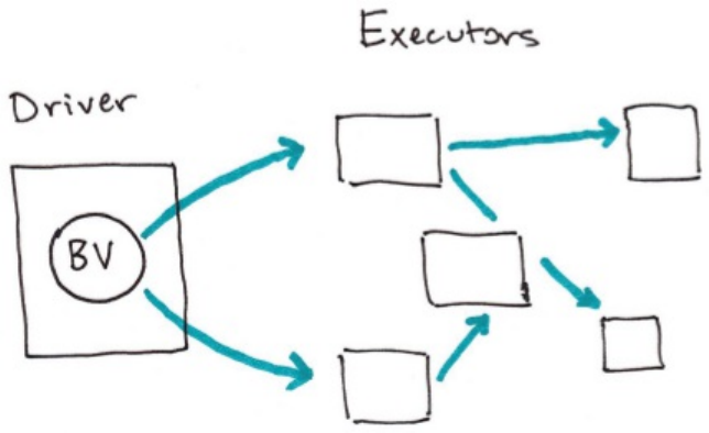
Broadcast Variables
Broadcast variables intend to share an immutable value efficiently around the
cluster. This might be to share some immutable value and use it around the
cluster without having to serialize it in a function to every node. We
demonstrate this tool in the following figure.
Now you might
Broadcast variables are shared, immutable variables that is cached on every
machine in the cluster instead of serialized with every single task. A use case
might be a look up table accessed by an RDD. Serializing this lookup table
with every task is wasteful because the driver must perform all of this work.
You can achieve the same result with a broadcast variable.
For example, let’s imagine that we have a list of words or values.
%scala
val myCollection = "Spark The Definitive Guide : Big Data Processing Made Simple"
val words = spark.sparkContext.parallelize(myCollection, 2)
%python
my_collection = "Spark The Definitive Guide : Big Data Processing Made Simple"
words = spark.sparkContext.parallelize(my_collection, 2)
And we would like to supplement these values with some information. Now
this is technically a right outer join (if we thought in terms of SQL) but
sometimes this can be a bit inefficient. Therefore we can take advantage of
something that we call a Map-Side join, where Data is sent to each worker and
Spark performs the join there instead of incurring an all-to-all communication.
Let’s suppose that our values are sitting in a Map structure.
val supplementalData = Map(
"Spark" -> 1000,
"Definitive" -> 200,
"Big" -> -300,
"Simple" -> 100
)
We can broadcast this structure across Spark and reference it using
suppBroadcast. This value is immutable and is lazily replicated across all
nodes in the cluster when we trigger an action.
val suppBroadcast = spark.sparkContext.broadcast(supplementalData
We reference this variable via the value method which will return the exact
value that we had before. This method is accessible within serialized functions
without having to serialize the data. This can save you a great deal of
serialization and deserialization costs as Spark transfers data more efficiently
around the cluster using broadcasts.
suppBroadcast.value
Now we could transform our RDD using this value. In this instance we will
create a key-value pair according to the value we may have in the map. If we
lack the value we will simple replace it with 0.
val suppWords = words.map(word => (word, suppBroadcast.value.getOrElse
suppWords.sortBy(wordPair => wordPair._2).collect()
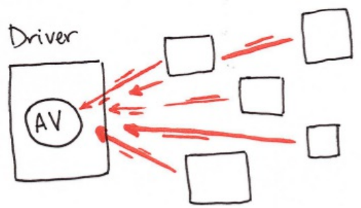
Accumulators
Accumulator variables on the other hand are a way of updating a value inside
of a variety of transformations and propagating that value to the driver node at
the end in an efficient and faul-tolerant way. We demonstrate accumulators in
the following figure.
Accumulators provide a mutable variable that can be updated safely on a per
row basis by a Spark cluster. These can be used for debugging purposes (say
to track the values of a certain variable per partition in order to intelligently
leverage it over time) or to create low level aggregation. Accumulators are
variables that are only “added"”” to through an associative and commutative
operation and can therefore be efficiently supported in parallel. They can be
used to implement counters (as in MapReduce) or sums. Spark natively
supports accumulators of numeric types, and programmers can add support for
new types.
For accumulator updates performed inside actions only, Spark guarantees that
each task’s update to the accumulator will only be applied once, i.e. restarted
tasks will not update the value. In transformations, users should be aware of
that each task’s update may be applied more than once if tasks or job stages are
re-executed.
Accumulators do not change the lazy evaluation model of Spark. If they are
being updated within an operation on an RDD, their value is only updated once
that RDD is computed as part of an action. Consequently, accumulator updates
are not guaranteed to be executed when made within a lazy transformation like
map().
Accumulators can be both named and unnamed. Named accumulators will
display their running results in the Spark UI while unnamed ones will not.
Basic Example
Let’s experiment by performing a custom aggregation on our Flight dataset. In
this example, we will use the Dataset API as opposed to the RDD API, but the
extension is quite similar.
case class Flight(DEST_COUNTRY_NAME: String, ORIGIN_COUNTRY_NAME
val flights = spark.read
.parquet("/mnt/defg/chapter-1-data/parquet/2010-summary.parquet/"
.as[Flight]
Now let’s create an accumulator that will count the number of flights to or from
China. While we could do this in a fairly straightfoward manner in SQL, many
things may not be so straightfoward. Accumulators provide a programmatic
way of allowing for us to do these sorts of counts. The following demonstrates
creating an unnamed accumulator.
import org.apache.spark.util.LongAccumulator
val accUnnamed = new LongAccumulator
sc.register(accUnnamed)
However for our use case it is better to give the accumulator a name. There are
two ways to do this, one short hand and one long hand. The simplest is just to
use the SparkContext, equivalently we can instantiate the accumulator and
register it with a name.
val accChina = new LongAccumulator
sc.register(accChina, "China")
val accChina2 = sc.longAccumulator("China")
We specify the name of the accumulator in the String value that we pass into the
function, or as the second parameter into the register function. Named
accumulators will display in the Spark UI, while unnamed ones will not.
The next step is to define the way we add to our accumulator. This is a fairly
straight forward function.
def accChinaFunc(flight_row: Flight) = {
val destination = flight_row.DEST_COUNTRY_NAME
val origin = flight_row.ORIGIN_COUNTRY_NAME
if (destination == "China") {
accChina.add(flight_row.count.toLong)
}
if (origin == "China") {
accChina.add(flight_row.count.toLong)
}
}
Now let’s iterate over every row in our flights dataset via the foreach
method. The reason for this is because foreach is an action, and the Spark can
only provide guarantees that perform inside of actions.
The foreach method will run once for each row in the input DataFrame
(assuming we did not filter it) and will run our function against each row.
Incrementing the accumulator accordingly.
flights.foreach(flight_row => accChinaFunc(flight_row))
This will completely fairly quickly but if you navigate to the Spark UI, you can
see the relevant value, on a per Executor level even before querying it
programmatically.
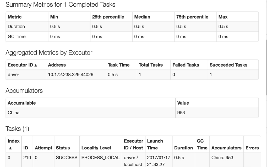
Of course we can query it programmatically as well, to do this we use the
value property.
accChina.value
Custom Accumulators
While Spark does provide some default accumulator types. Sometimes you
may want to build your own custom accumulator. To do this you need to
subclass the AccumulatorV2 class. There are several abstract methods that
need to be implemented, as we can see below. In this example we will only
add values that are even to the accumulator, while this is again simplistic, it
should show you how easy it is to build up your own accumulators.
import scala.collection.mutable.ArrayBuffer
val arr = ArrayBuffer[BigInt]()
import scala.collection.mutable.ArrayBuffer
import org.apache.spark.util.AccumulatorV2
class EvenAccumulator extends AccumulatorV2[BigInt, BigInt] {
private var num:BigInt = 0
def reset(): Unit = {
this.num = 0
}
def add(intValue: BigInt): Unit = {
if (intValue % 2 == 0) {
this.num += intValue
}
}
def merge(other: AccumulatorV2[BigInt,BigInt]): Unit = {
this.num += other.value
}
def value():BigInt = {
this.num
}
def copy(): AccumulatorV2[BigInt,BigInt] = {
new EvenAccumulator
}
def isZero():Boolean = {
this.num == 0
}
}
val acc = new EvenAccumulator
val newAcc = sc.register(acc, "evenAcc")
acc.value
flights.foreach(flight_row => acc.add(flight_row.count))
acc.value

Chapter 14. Advanced Analytics and
Machine Learning
Spark is an incredible tool for a variety of different use cases. Beyond large
scale SQL analysis and Streaming, Spark also provides mature support for
large scale machine learning and graph analysis. This sort of computation is
what is commonly referred to as “advanced analytics”. This part of the book
will focus on how you can use Spark to perform advanced analytics, from
linear regression, to connected components graph analysis, and deep learning.
Before covering those topics, we should define advanced analytics more
formally.
Gartner defines advanced analytics as follows:
Advanced Analytics is the autonomous or semi-autonomous examination
of data or content using sophisticated techniques and tools, typically
beyond those of traditional business intelligence (BI), to discover deeper
insights, make predictions, or generate recommendations. Advanced
analytic techniques include those such as data/text mining, machine
learning, pattern matching, forecasting, visualization, semantic analysis,
sentiment analysis, network and cluster analysis, multivariate statistics,
graph analysis, simulation, complex event processing, neural networks.
As their definition suggests, it is a bit of a grab bag of techniques to try and
solve a core problem of deriving and potentially delivering insights and
making predictions or recommendations. Spark provides strong tooling for
nearly all of these different approaches and this part of the book will cover the
different tools and tool areas available to end users to perform advanced
analytics.
This part of the book will cover the different parts of Spark your organization
can leverage for advanced analytics including:
Preprocessing (Cleaning Data)
Feature Engineering
Supervised Learning
Unsupervised Learning
Recommendation Engines
Graph Analysis
Before diving into these topics in depth, it is worth mentioning the goal of this
part of the book as well as what it will and will not cover. This part of the
book is not an algorithm guide that will teach you what every algorithm means
via Spark. There is simply too much to cover the intricacies of each algorithm.
What this part of the book will cover is how you can be successful using these
algorithms in real world scenarios. This means covering the scalability of
individual algorithms and teaching you the high level concepts you will need to
be successful. Unfortunately, this means eschewing strict mathematical
definitions and formulations - not for lack of importance but simply because
it’s too much information to cover in this context.
We will reference three books for those of you that would like to understand
more about the individual methods.
An Introduction to Statistical Learning by Gareth James, Daniela Witten,
Trevor Hastie, and Robert Tibshirani - available at: http://www-
bcf.usc.edu/~gareth/ISL/. We will refer to this book as “ISL”.
Elements of Statistical Learning by Trevor Hastie, Robert Tibshirani, and
Jerome Friedman- available at:
http://statweb.stanford.edu/~tibs/ElemStatLearn/. We will refer to this
book as “ESL”.
Deep Learning by Ian Goodfellow, Yoshua Bengio, and Aaron Courville -
available at: http://www.deeplearningbook.org/. We will refer to this
book as “DLB”.
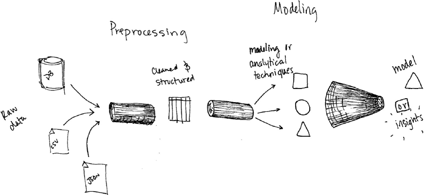
The Advanced Analytics Workflow
The first step of almost any advanced analytics task is to gather and clean data,
data scientists report that this takes up the majority of their time and is one of
the places that Spark performs extremely well (See part II of this book). Once
you clean your data you may need to manipulate it according to the task you
would like to complete. However the process does not end there, sometimes
you may need to create new features including creating new ones, combining
from other sources, or looking at interactions of variables. Once you
performed all preparation of your data, it’s time for the next step in the
process: modeling. A model is just a simplified conceptual representation of
some process. We can create different kinds of models according to our task.
For instance, do you want to predict whether or not something will happen?
Assign a probability to that happening? Do you simply want to understand what
properties are associated with other properties?
Different Advanced Analytics Tasks
To build out a model, we first need to specify the task that we want to perform.
At high level these fall into the following categories.
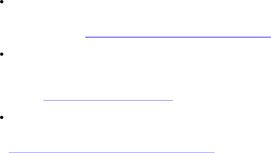
Supervised Learning
Supervised learning occurs when you train a model to predict a particular
outcome based on historical information. This task might be classification
where the dependent variable is a categorical variable, meaning the output
consists of a finite set of values. This task might be a regression, where the
output variable may take on one of an infinite number of values. In simplest
terms, we know what we want to be predicting and have values that represent
that in our dataset. Some examples of supervised learning include:
Spam email detection - Spam detection systems leverage supervised
learning to predict whether or not a message is spam or not. It does like
by analzing the contents of a given email. An example dataset for doing
this can be found at: https://archive.ics.uci.edu/ml/datasets/Spambase.
Classifying handwritten digits - The United States Postal Service had a
use case where they wanted to be able to read handwritten addresses on
letters. To do this they leverage machine learning to train a classifier to
them the value of a given digit. The canonical dataset for doing this can be
found at: http://yann.lecun.com/exdb/mnist/
Predicting heart disease - A doctor or hospital might want to predict the
likelihood of a person’s body characteristics or lifestyle leading to heart
disease later in life. An example dataset for doing this can be found at:
https://archive.ics.uci.edu/ml/datasets/Heart+Disease.

Recommendation
The task of recommendation is likely one of the most intuitive. By studying
what people either explicitly state that they like and dislike (through ratings) or
by what they implicitly state that they like and dislike (through observed
behavior) you can make recommendations on what one user may like by
drawing similarities between those individuals and other individuals. This use
case is quite well suited to Spark as we will see in the coming chapter. Some
examples of recommendations are:
Movie Recommendations - Netflix uses Spark to make large scale movie
recommendations to their users. More generally, movies can be
recommended based on what you watch as well as what you rated
previously.
Product Recommendations - In order to promote high purchases,
companies use product recommendations to suggest new products to buy
to their customers. This can be based on previous purchases or simply
viewing behavior.
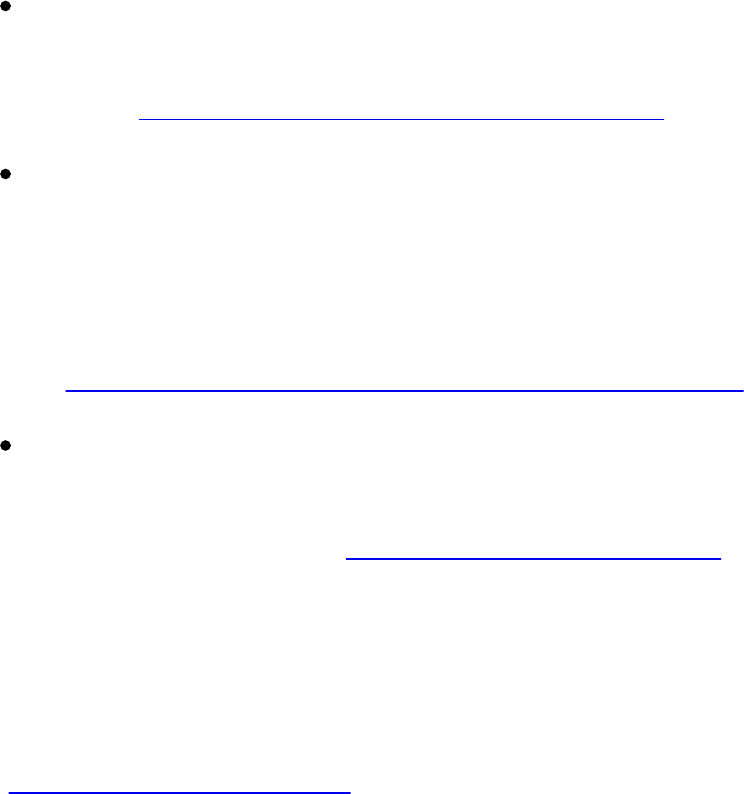
Unsupervised Learning
Unsupervised learning occurs when you train a model on data that does not
have a a specific outcome variable. The goal is to discover and describe some
underlying structure or clusters in the data. We may use this to create a set of
labels to use as output variables in a supervised learning situation later on or
to find outliers, data points that are far away from most other data points.
Some examples of unsupervised learning include:
Clustering - Given some traits in plant types, we might want to cluster
them by these attributes in order to try and find similiarities (or
differences) between them. An example dataset for doing this can be
found at: https://archive.ics.uci.edu/ml/datasets/Iris/.
Anomaly Detection - Given some standard event type often occuring over
time, we might want to report when a non-standard type of event occurs
(non-standard being a potentially difficult term to define generally.) An
example of this might be that a security officer would like to receive a
notification when a strange object (think vehicle, skater or bicyclist) is
observed on a pathway. An example dataset for doing this can be found
at: http://www.svcl.ucsd.edu/projects/anomaly/dataset.html.
Topic Modeling - Given a set of documents, we might want to infer some
underlying structure in these documents like the latent topics that identify
each document (or subset of documents) the best. An example dataset for
doing this can be found at: http://www.cs.cmu.edu/~enron/.
note
We linked to a number of datasets that work well for these tasks. Many of
the linked datasets are courtesy of the UCI Machine Learning Repository.
Citation: Lichman, M. (2013). UCI Machine Learning Repository
[http://archive.ics.uci.edu/ml]. Irvine, CA: University of California,
School of Information and Computer Science.

Graph Analysis
Graph analysis is a bit more of a sophisticated analytical tool that can absorb
aspects of all of the above. Graph analysis is effectively the study of
relationships where we specify “vertices” which are objects and “edges”
which represent relationships between those objects. Some examples of graph
analysis include:
Fraud Prediction - Capital One uses Spark’s graph analytics capabilities
to better understand fraud networks. This includes assigning probabilities
to certain bits of information to make a decision about whether or not a
given piece of information suggests that a charge it fraudulent.
Anomaly Detection - By looking at how networks of individuals connect
with one another, outliers and anomalies can be flagged for manual
analysis.
Classification - Given some facts about certain vertices in the network,
you can classify other vertices according to their connection to that
original node. An example might be looking at classifying influencers in
friend groups.
Recommendation - Google’s original web recommendation algorithm,
PageRank, is a graph algorithm that analyzed the relationships between
certain web pages by looking at how they linked to one another.
Spark’s Packages for Advanced
Analytics
Spark includes several core packages and many external packages for
performing advanced analytics. The primary package is MLlib which provides
an interface for bulding machine learning pipelines. We elaborate on other
packages in later chapters.
What is MLlib?
MLlib is a package, built on and included in Spark, that provides interfaces for
1. gathering and cleaning data,
2. generating and selecting features,
3. training and tuning large scale supervised and unsupervised machine
learning models,
4. and using those models in production.
This means that it helps with all three steps of the process although it really
shines in steps one and two for reason that we will touch on shortly. MLlib
consists of two packages that leverage different core data structures. The
package org.apache.spark.ml maintains an interface for use with Spark
DataFrames. This package also maintains a high level interface for building
machine learning pipelines that help standardize the way in which you perform
the above steps. The lower level package, org.apache.spark.mllib,
maintains interfaces for Spark’s Low-Level, RDD APIs. This book will focus
on the DataFrame API because the RDD API is both well documented and is
currently in maintenance mode (meaning it will only receive bug fixes, not new
features) at the time of this writing.
When and why should you use MLlib (vs scikit learn
or another package)?
Now, at a high level, this sounds like a lot of other machine learning packages
you have probably heard of like scikit-learn for Python or the variety of R
packages for performing similar tasks. So why should you bother MLlib at all?
The answer is simple, scale. There are numerous tools for performing machine
learning on a single machine. They do quite well at this and will continue to be
great tools. However they reach a limit, either in data size or processing time.
This is where Spark excels. The fact that they hit a limit in terms of scale
makes them complementary tools, not competitive ones. When your input data
or model size become too difficult or inconvenient to put on one machine, use
Spark to do the heavy lifting. Spark makes big data machine learning simple.
An important caveat to the previous paragraph is that while training and data
prep are made extremely simple, there are still some complexities that you will
need to keep in mind. For example, some models like a recommender system
end up being way too large for use on a single machine for prediction, yet we
still need to make predictions to derive value from our model. Another
example might be a logistic regression model trained in Spark. Spark’s
execution engine is not a low-latency execution engine and therefore making
single predictions quickly (< 500ms) is still challenging because of the costs of
starting up and executing a Spark jobs - even on a single machine. Some
models have good answers to this problem, others are still open questions. We
will discuss the state of the art at the end of this chapter. This is a fruitful
research area and likely to change overtime as new systems come out to solve
this problem.
High Level MLlib Concepts
In MLlib there are several fundamental architectural types: transformers,
estimators, evaluator and pipelines. The following is a diagram of the overall
workflow.
Transformers are just functions that convert raw data into another, usually
more structured representation. Additionally they allow you to create new
features from your data like interactions between variables. An example of a
transformer is one converts string categorical variables into a better
representation for our algorithms. Transformers are primarily used in the first
step of the machine learning process we described previously. Estimators
represent different models (or variations of the same model) that are trained
and then tested using an evaluation. An evaluator allows us to see how a given
estimator performs according to some criteria that we specify like a ROC
curve. Once we select the best model from the ones that we tested, we can then
use it to make predictions.
From a high level we can specify each of the above steps one by one however
it is often more much easier to specify our steps as stages in a pipeline. This
pipeline is similar to Scikit-learn’s Pipeline concept where transformations
and estimators are specified together.
This is not just a conceptual framework. These are the high level data types
that we actually use to build our out advanced analytics pipelines.
Low Level Data Types
In addition to the high level architectural types, there are also several lower
level primitives that you may need to leverage. The most common that you will
come across is the Vector. Whenever we pass a set of features into a machine
learning model, we must do it as a vector that consists of `Double`s. This
vector can be either sparse (where most of the elements are zero) or dense
(where there are many unique values). These are specified in different ways,
one where we specify the exact values(dense) and the other where we specify
the total size and which values are nonzero(sparse). Sparse is appropriate, as
you might have guessed, when the majority of the values are zero as this is a
more compressed representation that other formats.
%scala
import org.apache.spark.ml.linalg.Vectors
val denseVec = Vectors.dense(1.0, 2.0, 3.0)
val size = 3
val idx = Array(1,2) // locations in vector
val values = Array(2.0,3.0)
val sparseVec = Vectors.sparse(size, idx, values)
sparseVec.toDense
denseVec.toSparse
%python
from pyspark.ml.linalg import Vectors
denseVec = Vectors.dense(1.0, 2.0, 3.0)
size = 3
idx = [1, 2] # locations in vector
values = [2.0, 3.0]
sparseVec = Vectors.sparse(size, idx, values)
# sparseVec.toDense() # these two don't work, not sure why
# denseVec.toSparse() # will debug later
warning
Confusingly, there are similar types that refer to ones that can be used in
DataFrames and others than can only be used in RDDs. The RDD
implementations fall under the mllib package while the DataFrame
implementations under ml.

MLlib in Action
Now we described some of the core pieces that we are going to come across,
let’s create a simple pipeline to demostrate each of the component parts. We’ll
use a small synthetic dataset that will help illustrate our point. This dataset
consists of a categorical label, a categorical variable (color), and two
numerical variables. You should immediately recognize that this will be a
classification task where we hope to predict our binary output variable based
on the inputs.
%scala
var df = spark.read.json("/mnt/defg/simple-ml")
%python
df = spark.read.json("/mnt/defg/simple-ml")
df.orderBy("value2").show()
Spark can also quickly read from LIBSVM formatted datasets. For more
information on the LIBSVM format see the documentation here:
http://www.csie.ntu.edu.tw/~cjlin/libsvm/.
%scala
val libsvmData = spark.read.format("libsvm")
.load("/mnt/defg/sample_libsvm_data.txt")
%python
libsvmData = spark.read.format("libsvm")\
.load("/mnt/defg/sample_libsvm_data.txt")

Transformers
Transformers exist to either cut down on the number of features, add more
features, manipulate current ones or simply help us format our data correctly.
All inputs to machine learning algorithms in Spark must consist of type Double
(for labels) and Vector[Double] for features. Note that our current data does
not meet that requirement and therefore we need to transform it to the proper
format.
To achieve this, we are going to do this by specifying an RFormula. This is a
declarative language for specifying machine learning models and is incredibly
simple to use once you understand the syntax. Currently RFormula supports a
limited subset of the R operators that in practice work quite well for simple
models. The basic operators are:
~ separate target and terms
+ concat terms, “+ 0” means removing intercept
- remove a term, “- 1” means removing intercept
: interaction (multiplication for numeric values, or binarized categorical
values)
. all columns except target
In order to specify our transformations with this syntax, we need to import the
relevant class.
%scala
import org.apache.spark.ml.feature.RFormula
%python
from pyspark.ml.feature import RFormula
Then we go through the process of defining our formula. In this case we want
to use all available variables (the .) and then specify a interactions between
value1 and color and value2 and color.
val supervised = new RFormula()
.setFormula("lab ~ . + color:value1 + color:value2")
%python
supervised = RFormula()\
.setFormula("lab ~ . + color:value1 + color:value2")
At this point we created, but have not used out model. The above transformer
object is actually a special kind of transformer that will modify itself
according to the underlying data. Not all transformers have this requirement but
because RFormula will automatically handle categorical variables for us, it
needs to figure out which columns are categorical and which are now. For this
reason, we have to call the fit method. Once we call fit, this returns a
“trained” version of our transformer that we can then use to actually transform
our data.
%scala
val fittedRF = supervised.fit(df)
val preparedDF = fittedRF.transform(df)
%python
fittedRF = supervised.fit(df)
preparedDF = fittedRF.transform(df)
preparedDF.show()
We used that to transform our data. What’s happening behind the scenes is
actually quite simple. RFormula inspects our data during the fit call and
outputs an object that will transform our data according to the specified
formula. This “trained” transformer always has the word Model in the type
signature. When we use this transformer, you will notice that Spark
automatically converts our categorical variable to Doubles so that we can
input this into a (yet to be specified) machine learning model. It does this with
several calls to the StringIndexer, Interaction, and VectorAssembler
transformers covered in the next chapter. We then call tranform on that object
in order to transform our input data into the expected output data.
After preparing our data for use in an estimator, we must now prepare a test set
with which we can use to evaluate our model.
%scala
val Array(train, test) = preparedDF.randomSplit(Array(0.7, 0.3))
%python
train, test = preparedDF.randomSplit([0.7, 0.3])
Estimators
Now that we transformed our data into the correct format and created some
valuable features. It’s time to actually fit our model. In this case we will use
logistic regression. To create our classifier we instantiate an instance of
LogisticRegression, using the default hyperparameters. We then set the
label columns and the feature columns. The values we are setting are actually
the default labels for all Estimators in the DataFrame API in Spark MLlib and
you will see in later chapters that we omit them.
%scala
import org.apache.spark.ml.classification.LogisticRegression
val lr = new LogisticRegression()
.setLabelCol("label")
.setFeaturesCol("features")
%python
from pyspark.ml.classification import LogisticRegression
lr = LogisticRegression()\
.setLabelCol("label")\
.setFeaturesCol("features")
Once we instantiate the model, we can train it. This is done with the fit
method which returns a LogisticRegressionModel. This is just the trained
version of logistic regression and is conceptually the same as fitting the
RFormula that we saw above.
%scala
val fittedLR = lr.fit(train)
%python
fittedLR = lr.fit(train)
This previous code will kick off a spark job, fitting an ML model is always
eagerly performed.
Now that we trained the model, we can use it to make predictions. Logically
this represents a transformation of features into labels. We make predictions
with the transform method. For example, we can transform our training
dataset to see what labels our model assigned to the training data and how
those compare to the true outputs. This, again, is just another DataFrame that
we can manipulate.
fittedLR.transform(train).select("label", "prediction").show()
Our next step would be to manually evaluate this model and calculate the true
positive rate, false negative rate, etc. We might then turn around and try a
different set of parameters to see if those perform better. This process, while
useful, is actually quite tedious and well defined. Spark helps you avoid this
by allowing you to specify your workload as a declarative pipeline of work
that includes all your transformations and includes tuning your
hyperparameters.
Pipelining our Workflow
As you likely noticed above, if you are performing a lot of transformations,
writing all the steps and keeping track of DataFrames ends up being quite
tedious. That’s why Spark includes the concept of a Pipeline. A pipeline
allows you to set up a dataflow of the relevant transformations, ending with an
estimator that is automatically tuned according to your specifications resulting
a tuned model ready for a production use case. The following diagram
illustrates this process.
One important detail is that it is essential that instances of transformers or
models are not reused across pipelines or different models. Always create a
new instance of a model before creating another pipeline.
In order to make sure that we don’t overfit, we are going to create a holdout
test set and tune our hyperparameters based on a validation set. Note that this
is our raw dataset.
%scala
val Array(train, test) = df.randomSplit(Array(0.7, 0.3))
%python
train, test = df.randomSplit([0.7, 0.3])
While in this case we opt for just using the RFormula a common pattern is to
set up a pipeline of many different transformations in conjunction with the
RFormula (for the simpler features). We cover these preprocessing techniques
in the following chapter, just keep in kind that there can be far more stages than
just two. In this case we will not specify a formula.
%scala
val rForm = new RFormula()
val lr = new LogisticRegression()
.setLabelCol("label")
.setFeaturesCol("features")
%python
rForm = RFormula()
%python
lr = LogisticRegression()\
.setLabelCol("label")\
.setFeaturesCol("features")
Now instead of manually using our transformations and then tuning our model.
Now we just make them stages in the overall pipeline. This makes them just
logical transformations, or a specification for chain of commands for Spark to
run in a pipeline.
import org.apache.spark.ml.Pipeline
val stages = Array(rForm, lr)
val pipeline = new Pipeline().setStages(stages)
%python
from pyspark.ml import Pipeline
stages = [rForm, lr]
pipeline = Pipeline().setStages(stages)

Evaluators
At this point we set up a set up our pipeline. The next step will be evaluating
the performance of this pipeline. Spark does this by setting up a parameter grid
of all the combinations of the parameters that you specify. You should
immediately notice in the following code snippet that even our RFormula is
tuning specific parameters. In a pipeline, we can modify more than just the
model’s hyperparameters, we can even modify the transformer’s properties.
%scala
import org.apache.spark.ml.tuning.ParamGridBuilder
val params = new ParamGridBuilder()
.addGrid(rForm.formula, Array(
"lab ~ . + color:value1",
"lab ~ . + color:value1 + color:value2"))
.addGrid(lr.elasticNetParam, Array(0.0, 0.5, 1.0))
.addGrid(lr.regParam, Array(0.1, 2.0))
.build()
%python
from pyspark.ml.tuning import ParamGridBuilder
params = ParamGridBuilder()\
.addGrid(rForm.formula, [
"lab ~ . + color:value1",
"lab ~ . + color:value1 + color:value2"])\
.addGrid(lr.elasticNetParam, [0.0, 0.5, 1.0])\
.addGrid(lr.regParam, [0.1, 2.0])\
.build()
In our current grid there are three hyperparameters that will diverge from the
defaults.
two different options for the R formula
three different options for the elastic net parameter
two different options for the regularization parameter
This gives us a total of twelve different combinations of these parameters,
which means we will be training twelve different versions of logistic
regression.
With the grid built it is now time to specify our evaluation. There are
evaluators for classifiers (binary and multilabel) and regression, which we
cover in subsequent chapters however in this case we will be using the
BinaryClassificationEvaluator. This evaluator allows us to
automatically optimize our model training according to some specific criteria
that we specify. In this case we will specify areaUnderROC which is the total
area under the receiver operating characteristic. (CITE)
Now that we have a pipeline that specifies how our data should be
transformed. Let’s take it to the next level and automatically perform model
selection by trying out different hyper-parameters in our logistic regression
model. We do this by specifying a parameter grid, a splitting measuer, and
lastly an Evaluator. An evaluator allows us to automatically optimize our
model training according to some criteria (specified in the evaluator) however
in order to leverage this we need a simple way of trying out different model
parameters to see which ones perform best. We cover all the different
evaluation metrics in each task’s chapter.
%scala
import org.apache.spark.ml.evaluation.BinaryClassificationEvaluator
val evaluator = new BinaryClassificationEvaluator()
.setMetricName("areaUnderROC")
.setRawPredictionCol("prediction")
.setLabelCol("label")
%python
from pyspark.ml.evaluation import BinaryClassificationEvaluator
evaluator = BinaryClassificationEvaluator()\
.setMetricName("areaUnderROC")\
.setRawPredictionCol("prediction")\
.setLabelCol("label")
As you may know, it is a best practice in machine learning to fit your
hyperparameters on a validation set (instead of your test set). The reasons for
this are to prevent overfitting. Therefore we cannot use our holdout test set
(that we created before) to tune these parameters. Luckily Spark provides two
options for performing this hyperparameter tuning in an automated way. We can
use a TrainValidationSplit, which will simply perform an arbitrary
random split of our data into two different groups, or a CrossValidator,
which performs K-fold cross validation by splitting the dataset into non-
overlapping randomly partitioned folds.
%scala
import org.apache.spark.ml.tuning.TrainValidationSplit
val tvs = new TrainValidationSplit()
.setTrainRatio(0.75) // also the default.
.setEstimatorParamMaps(params)
.setEstimator(pipeline)
.setEvaluator(evaluator)
%python
from pyspark.ml.tuning import TrainValidationSplit
tvs = TrainValidationSplit()\
.setTrainRatio(0.75)\
.setEstimatorParamMaps(params)\
.setEstimator(pipeline)\
.setEvaluator(evaluator)
Now we can fit our entire pipeline. This will test out every version of the
model against the validation set. You will notice that the the type of tvsFitted
is TrainValidationSplitModel. Any time that we fit a given model, it
outputs a “model” type.
%scala
val tvsFitted = tvs.fit(train)
%python
tvsFitted = tvs.fit(train)
And naturally evaluate how it performs on the test set!
evaluator.evaluate(tvsFitted.transform(test))
We can also see a training summary for particular models. To do this we
extract it from the pipeline, cast it to the proper type and print our results. The
metrics available depend on the models which are covered in some of the
following chapters. The only key thing to understand is that an unfitted
estimator has the same name as the estimator, e.g. LogisticRegression.
import org.apache.spark.ml.PipelineModel
import org.apache.spark.ml.classification.LogisticRegressionModel
val trainedPipeline = tvsFitted.bestModel.asInstanceOf[PipelineModel
val TrainedLR = trainedPipeline.stages(1)
.asInstanceOf[LogisticRegressionModel]
val summaryLR = TrainedLR.summary
summaryLR.objectiveHistory
Persisting and Applying Models
Now that we trained this model, we can persist it to disk to use it in an online
predicting fashion later.
tvsFitted.write.overwrite().save("/tmp/modelLocation")
Now that we wrote out the model we can load it back into a program
(potentially in a different location) in ordre to make predictions. In order to do
this we need to use the companion object to the model, tuning class, or
transformer that we originally used. In this case, we used
TrainValidationSplit which outputs a TrainValidationSplitModel. We
will now use the “model” version to load our persisted model. If we were to
use a CrossValidator, we’d have to read in the persisted version as the
CrossValidatorModel and if we were to use LogisticRegression
manually we would have to use LogisticRegressionModel.
%scala
import org.apache.spark.ml.tuning.TrainValidationSplitModel
val model = TrainValidationSplitModel.load("/tmp/modelLocation"
model.transform(test)
%python
# not currently available in python but bet it's coming...
# will remove if not.
# from pyspark.ml.tuning import TrainValidationSplitModel
# model = TrainValidationSplitModel.load("/tmp/modelLocation")
# model.transform(test)
Deployment Patterns
When it comes to Spark there are several different deployment patterns for
putting machine learning models into production in Spark. The following
diagram aims to illustrate that.

1. Train your ML algorithm offline and then put the results into a database
(usually a key-value store). This works well for something like
recommendation but poorly for something like classification or regression
where you cannot just lookup a value for a given user but must calculate
one.
2. Train your ML algorithm offline, persist the model to disk, then use that
for serving. This is not a low latency solution as the overhead of starting
up a Spark job can be quite high - even if you’re not running on a cluster.
Additionally this does not parallelize well so you’ll likely have to put a
load balancer of multiple model replicas. There are some interesting
potential solutions to this problem, but nothing quite production ready yet.
3. Manually (or via some other software) convert your distributed model to
one that can run much more quickly on a single machine. This works well
when there is not too much manipulation of the raw data in Spark and can
be hard to maintain over time. Again there are solutions that are working
on this specification as well but nothing production ready. This cannot be
found in the previous illustration because it’s something that requires
manual work.
4. Train your ML algorithm online and use it online, this is possible when
used in conjunction like streaming but is quite sophisticated. This
landscape will likely continue to mature as Structured Streaming
development continues.
While these are some of the options, there are more potential ways of
performing this deployment. This is a heavy area for development that is
certainly likely to change and progress quickly.
Chapter 15. Preprocessing and
Feature Engineering
Any data scientist worth her salt knows that one of the biggest challenges in
advanced analytics is preprocessing. Not because it’s particularly complicated
work, it just requires deep knowledge of the data you are working with and an
understanding of what your model needs in order to successfully leverage this
data. This chapter will cover the details of how you can use Spark to perform
preprocessing and feature engineering. We will walk through the core
requirements that you’re going to need to meet in order to train an MLlib model
in terms of how your data is structured. We will then walk through the different
tools Spark has to perform this kind of work.

Formatting your models according
to your use case
To preprocess data for Spark’s different advanced analytics tools, you must
consider your end objective.
In the case of classification and regression, you want to get your data into
a column of type Double to represent the label and a column of type
Vector (either dense or sparse) to represent the features.
In the case of recommendation, you want to get your data into a column of
users, a column of targets (say movies or books), and a column of ratings.
In the case of unsupervised learning, a column of type Vector (either
dense or sparse) to represent the features.
In the case of graph analytics, you will want a DataFrame of vertices and
a DataFrame of edges.
The best way to do this is through transformers. Transformers are function that
accepts a DataFrame as an argument and returns a modified DataFrame as a
response. These tools are well documented in Spark’s ML Guide and the list of
transformers continues to grow. This chapter will focus on what transformers
are relevant for particular use cases rather than attempting to enumerate every
possible transformer.
note
Spark provides a number of transformers under the
org.apache.spark.ml.feature package. The corresponding package
in Python is pyspark.ml.feature. The most up to date list can be found
on the Spark documentation site. http://spark.apache.org/docs/latest/ml-
features.html
Before we proceed, we’re going to read in several different datasets. Each of
these have different properties that we will want to manipulate in this chapter.
%scala
val sales = spark.read.format("csv")
.option("header", "true")
.option("inferSchema", "true")
.load("dbfs:/mnt/defg/retail-data/by-day/*.csv")
.coalesce(5)
.where("Description IS NOT NULL")
val fakeIntDF = spark.read.parquet("/mnt/defg/simple-ml-integers"
var simpleDF = spark.read.json("/mnt/defg/simple-ml")
val scaleDF = spark.read.parquet("/mnt/defg/simple-ml-scaling")
%python
sales = spark.read.format("csv")\
.option("header", "true")\
.option("inferSchema", "true")\
.load("dbfs:/mnt/defg/retail-data/by-day/*.csv")\
.coalesce(5)\
.where("Description IS NOT NULL")
fakeIntDF = spark.read.parquet("/mnt/defg/simple-ml-integers")
simpleDF = spark.read.json("/mnt/defg/simple-ml")
scaleDF = spark.read.parquet("/mnt/defg/simple-ml-scaling")
sales.cache()
warning
It is important to note that we filtered out null values above. MLlib does
not play nicely with null values at this point in time. This is a frequent
cause for problems and errors and a great first step when you are
debugging.
Properties of Transformers
All transformers require you to specify, at a minimum the inputCol and the
outputCol, obviously representing the column name of the input and output.
You set these with the setInputCol and setOutputCol. At times there are
defaults (you can find these in the documentation) but it is a best practice to
manually specify them yourself for clarity. In addition to input and outpul
columns, all transformers have different parameters that you can tune,
whenever we mention a parameter in this chapter you must set it with
set<PARAMETER_NAME>.
note
Spark MLlib stores metadata about the columns that it uses as an attribute
on the column itself. This allows it to properly store (and annotate) that a
column of doubles may actually represent a series of categorical
variables which should not just blindly be used as numerical values. As
demonstrated later on this chapter under the “Working with Categorical
Variables Section”, this is why it’s important to index variables (and
potentially one hot encode them) before inputting them into your model.
One catch is that this will not show up when you print the schema of a
column.
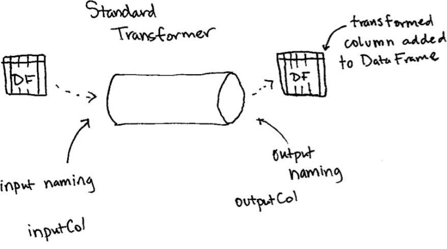
Different Transformer Types
In the previous chapter we mentioned the simplified concept of “transformers”
however there are actually two different kinds of tranformers. The “standard”
transformer only includes a “transform” method, this is because it will not
change based on the input data.
An example of this is the Tokenizer transformer. It has nothing to “learn” from
out data.
import org.apache.spark.ml.feature.Tokenizer
val tkn = new Tokenizer().setInputCol("Description")
tkn.transform(sales).show()
The other kind of transformer is actually an estimator. This just means that it
needs to be fit prior to being used as a transformer because it must tune itself
according to the input data set. While technically incorrect, it can be helpful to
think about this as simply generating a transformer at runtime based on the
input data.
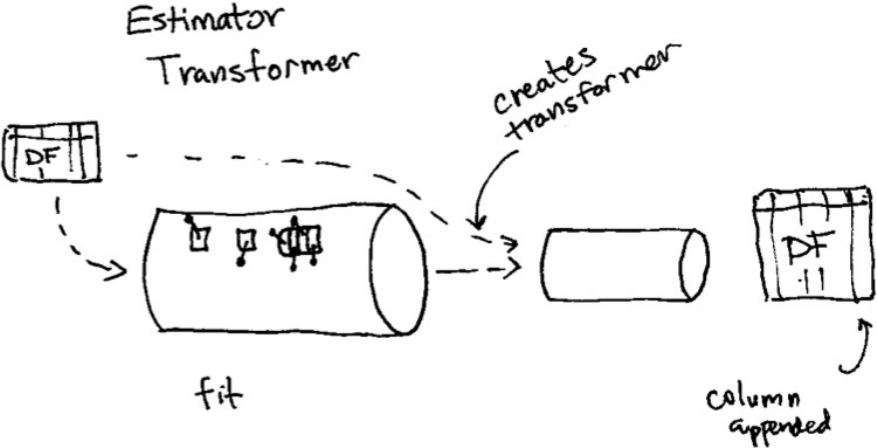
An example of this is the StandardScaler that must modify itself according to
the numbers in the relevant column in order to scale the data appropriately.
import org.apache.spark.ml.feature.StandardScaler
val ss = new StandardScaler().setInputCol("features")
ss.fit(scaleDF).transform(scaleDF).show(false)
High Level Transformers
In general, you should try to use the highest level transformers that you can, this
will minimize the risk of error and help you focus on the business problem
instead of the smaller details of implementation. While this is not always
possible, it’s a good goal.
RFormula
You likely noticed in the previous chapter that the RFormula is the easiest
transformer to use when you have “conventionally” formatted data. Spark
borrows this transformer from the R language and makes it simple to
declaratively specify a set of transformations for your data. What we mean by
this is that values are either numerical or categorical and you do not need to
extract values from the strings or manipulate them in anyway. This will
automatically handle categorical inputs (specified as strings) by one hot
encoding them. Numeric columns will be cast to Double but will not be one
hot encoded. If the label column is of type string, it will be first transformed to
double with StringIndexer.
warning
This has some strong implications. If you have numerically valued
categorical variables, they will only be cast to Double, implicitly
specifying an order. It is important to ensure that the input types
correspond to the expected conversion. For instance, if you have
categorical variables, they should be String. You can also manually
index columns, see “Working with Categorical Variables” in this chapter.
RFormula also uses default columns of label and features respectively. This
makes it very easy to pass it immediately into models which will require those
exact column names by default.
%scala
import org.apache.spark.ml.feature.RFormula
val supervised = new RFormula()
.setFormula("lab ~ . + color:value1 + color:value2")
supervised.fit(simpleDF).transform(simpleDF).show()
%python
from pyspark.ml.feature import RFormula
supervised = RFormula()\
.setFormula("lab ~ . + color:value1 + color:value2")
supervised.fit(simpleDF).transform(simpleDF).show()
SQLTransformers
The SQLTransformer allows you to codify the SQL manipulations that you
make as a ML transformation. Any SELECT statement is a valid
transformation, the only thing that you need to change is that instead of using the
table name, you should just use the keyword __THIS__. You might want to use
this if you want to formally codify some DataFrame manipulation as a
preprocessing step. One thing to note as well is that the output of this
transformation will be appended as a column to the output DataFrame.
%scala
import org.apache.spark.ml.feature.SQLTransformer
val basicTransformation = new SQLTransformer()
.setStatement("""
SELECT sum(Quantity), count(*), CustomerID
FROM __THIS__
GROUP BY CustomerID
""")
basicTransformation.transform(sales).show()
%python
from pyspark.ml.feature import SQLTransformer
basicTransformation = SQLTransformer()\
.setStatement("""
SELECT sum(Quantity), count(*), CustomerID
FROM __THIS__
GROUP BY CustomerID
""")
basicTransformation.transform(sales).show()
For extensive samples of these transformations see Part II of the book.

VectorAssembler
The VectorAssembler is the tool that you’ll use in every single pipeline that
you generate. It helps gather all your features into one big vector that you can
then pass into an estimator. It’s used typically in the last step of a machine
learning pipeline and takes as input a number of columns of Double or Vector.
import org.apache.spark.ml.feature.VectorAssembler
val va = new VectorAssembler()
.setInputCols(Array("int1", "int2", "int3"))
va.transform(fakeIntDF).show()
%python
from pyspark.ml.feature import VectorAssembler
va = VectorAssembler().setInputCols(["int1", "int2", "int3"])
va.transform(fakeIntDF).show()
Text Data Transformers
Text is always a tricky input because it often requires lots of manipulation to
conform to some input data that a machine learning model will be able to use
effectively. There’s generally two kinds of formats that you’ll deal with,
freeform text and text categorical variables. This section of the chapter
primarily focuses on text while later on in this chapter we discuss categorical
variables.
Tokenizing Text
Tokenization is the process of converting free form text into a list of “tokens”
or individual words. The easiest way to do this is through the Tokenizer. This
transformer will take a string of words, separated by white space, and convert
them into an array of words. For example, in our dataset we might want to
convert the Description field into a list of tokens.
import org.apache.spark.ml.feature.Tokenizer
val tkn = new Tokenizer()
.setInputCol("Description")
.setOutputCol("DescriptionOut")
val tokenized = tkn.transform(sales)
tokenized.show()
%python
from pyspark.ml.feature import Tokenizer
tkn = Tokenizer()\
.setInputCol("Description")\
.setOutputCol("DescriptionOut")
tokenized = tkn.transform(sales)
tokenized.show()
We can also create a tokenizer that is not just based off of white space but a
regular expression with the RegexTokenizer. The format of the regular
expression should conform to the Java Regular Expression Syntax.
%scala
import org.apache.spark.ml.feature.RegexTokenizer
val rt = new RegexTokenizer()
.setInputCol("Description")
.setOutputCol("DescriptionOut")
.setPattern(" ") // starting simple
.setToLowercase(true)
rt.transform(sales).show()
%python
from pyspark.ml.feature import RegexTokenizer
rt = RegexTokenizer()\
.setInputCol("Description")\
.setOutputCol("DescriptionOut")\
.setPattern(" ")\
.setToLowercase(True)
rt.transform(sales).show()
You can also have this match words (as opposed to splitting on a given value)
by setting the gaps parameter to false.
Removing Common Words
A common task after tokenization is the filtering of common words or stop
words. These words are not relevant for a particular analysis and should
therefore be removed from our lists of words. Common stop words in English
include “the”, “and”, “but” and other common words. Spark contains a list of
default stop words which you can see by calling the method below. THis can
be made case insensitive if necessary. Support languages for stopwords are:
“danish”, “dutch”, “english”, “finnish”, “french”, “german”, “hungarian”,
“italian”, “norwegian”, “portuguese”, “russian”, “spanish”, “swedish”, and
“turkish” as of Spark 2.2.
%scala
import org.apache.spark.ml.feature.StopWordsRemover
val englishStopWords = StopWordsRemover
.loadDefaultStopWords("english")
val stops = new StopWordsRemover()
.setStopWords(englishStopWords)
.setInputCol("DescriptionOut")
stops.transform(tokenized).show()
%python
from pyspark.ml.feature import StopWordsRemover
englishStopWords = StopWordsRemover\
.loadDefaultStopWords("english")
stops = StopWordsRemover()\
.setStopWords(englishStopWords)\
.setInputCol("DescriptionOut")
stops.transform(tokenized).show()
Creating Word Combinations
Tokenizing our strings and filtering stop words leaves us with a clean set of
words to use as features. Often time it is of interest to look at combinations of
words, usually by looking at co-located words. Word combinations are
technically referred to as n-grams. N-grams are sequences of words of length
N. N-grams of length one are called unigrams, length two are bigrams, length
three are trigrams. Anything above those are just four-gram, five-gram, etc.
Order matters with N-grams, so a converting three words into bigrams would
contain two bigrams. For example, the bigrams of “Bill Spark Matei” would
be “Bill Spark”, “Spark Matei”.
We can see this below. The use case for ngrams is to look at what words
commonly co-occur and potentially learn some machine learning algorithm
based on those inputs.
import org.apache.spark.ml.feature.NGram
val unigram = new NGram()
.setInputCol("DescriptionOut")
.setN(1)
val bigram = new NGram()
.setInputCol("DescriptionOut")
.setN(2)
unigram.transform(tokenized).show()
bigram.transform(tokenized).show()
Converting Words into Numbers
Once we created word features, it’s time to start counting instances of words
and word combinations. The simplest way is just to include binary counts of
the existence of a word in a given document (in our case, a row). However we
can also count those up (CountVectorizer) as well as reweigh them
according to the prevalence of a given word in all the documents TF-IDF.
A CountVectorizer operates on our tokenized data and does two things.
1. During the fit process it gathers information about the vocabulary in this
dataset. For instance for our current data, it would look at all the tokens in
each DescriptionOut column and then call that the vocabulary.
2. It then counts the occurrences of a given word in each row of the
DataFrame column during the transform process and outputs a vector
with the terms that occur in that row.
Conceptually this tranformer treats every row as a document and every word
as a term and the total collection of all terms as the vocabulary. These are all
tunable parameters, meaning we can set the minimum term frequency (minTF)
for it to be included in the vocabulary (effectively removing rare words from
the vocabulary), minimum number of documents a term must appear in (minDF)
before being included in the vocabulary (another way to remove rare words
from the vocabulary), and finally the total maximum vocabulary size
(vocabSize). Lastly, by default the count vectorizer will output the counts of a
term in a document. We can use setBinary(true) to have it output simple
word existence instead.
%scala
import org.apache.spark.ml.feature.CountVectorizer
val cv = new CountVectorizer()
.setInputCol("DescriptionOut")
.setOutputCol("countVec")
.setVocabSize(500)
.setMinTF(1)

.setMinDF(2)
val fittedCV = cv.fit(tokenized)
fittedCV.transform(tokenized).show()
%python
from pyspark.ml.feature import CountVectorizer
cv = CountVectorizer()\
.setInputCol("DescriptionOut")\
.setOutputCol("countVec")\
.setVocabSize(500)\
.setMinTF(1)\
.setMinDF(2)
fittedCV = cv.fit(tokenized)
fittedCV.transform(tokenized).show()
TF-IDF
Another way to approach the problem in a bit more sophisticated way than
simple counting is to use TF-IDF or term frequency-inverse document
frequency. The complete explanation of TF-IDF beyond the scope of this book
but in simplest terms it finds words that are most representative of certain
rows by finding out how often those words are used and weighing a given term
according to the number of documents those terms show up in. A more
complete explanation can be found
http://billchambers.me/tutorials/2014/12/21/tf-idf-explained-in-python.html.
In practice, TF-IDF helps find documents that share similar topics. Let’s see a
worked example.
%scala
val tfIdfIn = tokenized
.where("array_contains(DescriptionOut, 'red')")
.select("DescriptionOut")
.limit(10)
tfIdfIn.show(false)
%python
tfIdfIn = tokenized\
.where("array_contains(DescriptionOut, 'red')")\
.select("DescriptionOut")\
.limit(10)
tfIdfIn.show(10, False)
+---------------------------------------+
|DescriptionOut |
+---------------------------------------+
|[gingham, heart, , doorstop, red] |
...
|[red, retrospot, oven, glove] |
|[red, retrospot, plate] |
+---------------------------------------+
We can see some overlapping words in these documents so those won’t be
perfect identifiers for individual documents but do identify that “topic” of sort
across those documents. Now let’s input that into TF-IDF. First we perform a
hashing of each word then we perform the IDF weighting of the vocabulary.
%scala
import org.apache.spark.ml.feature.{HashingTF, IDF}
val tf = new HashingTF()
.setInputCol("DescriptionOut")
.setOutputCol("TFOut")
.setNumFeatures(10000)
val idf = new IDF()
.setInputCol("TFOut")
.setOutputCol("IDFOut")
.setMinDocFreq(2)
%python
from pyspark.ml.feature import HashingTF, IDF
tf = HashingTF()\
.setInputCol("DescriptionOut")\
.setOutputCol("TFOut")\
.setNumFeatures(10000)
idf = IDF()\
.setInputCol("TFOut")\
.setOutputCol("IDFOut")\
.setMinDocFreq(2)
%scala
idf.fit(tf.transform(tfIdfIn))
.transform(tf.transform(tfIdfIn))
.show(false)
%python
idf.fit(tf.transform(tfIdfIn))\
.transform(tf.transform(tfIdfIn))\
.show(10, False)
While the output is too large to include here what you will notice is that a
certain value is assigned to “red” and that value appears in every document.
You will then notice that this term is weighted extremely low because it
appears in every document. The output format is a Vector that we can
subsequently input into a machine learning model in a form like:
(10000,[2591,4291,4456],[1.0116009116784799,0.0,0.0])
This vector is composed of three different values, the total vocabulary size, the
hash of every word appearing in the document, and the weighting of each of
those terms.
Advanced Techniques
The last text manipulation tool we have at our disposal is Word2vec.
Word2vec is a sophisticated neural network style natural language processing
tool. Word2vec uses a technique called “skip-grams” to convert a sentence of
words into an embedded vector representation. It does this by building a
vocabulary, then for every sentence, removes a token and trains the model to
predict the missing token in the “n-gram” representation. With the sentence,
“the Queen of England” it might be trained to try to predict the missing token
“Queen” in “the of England”. Word2vec works best with continuous, free form
text in the form of tokens, so we won’t expect great results from our
description field which does not include freeform text. Spark’s Word2vec
implementation includes a variety of tuning parameters that can be found on the
documentation.
Working with Continuous Features
Continuous features are just values on the number line, from positive infinity to
negative infinity. There are two transformers for continuous features. First you
can convert continuous features into categorical features via a process called
bucketing or you can scale and normalize your features according to several
different requirements. These transformers will only work on Double types, so
make sure that you’ve turned any other numerical values to Double.
%scala
val contDF = spark.range(500)
.selectExpr("cast(id as double)")
%python
contDF = spark.range(500)\
.selectExpr("cast(id as double)")

Bucketing
The most straightforward approach to bucketing or binning is the Bucketizer.
This will split a given continuous feature into the buckets of your designation.
You specify how buckets should be created via an array or list of Double
values. This method is confusing because we specify bucket borders via the
splits method, however these are not actually splits. They are actually bucket
borders.
For example setting splits to 5.0, 10.0, 250.0 on our contDF because we
don’t cover all possible ranges input ranges. To specify your bucket points, the
values you pass into splits must satisfy three requirements.
The minimum value in your splits array must be less than the minimum
value in your DataFrame.
The maximum value in your splits array must be greater than the maximum
value in your DataFrame.
You need to specify at a minimum three values in the splits array, which
creates two buckets.
To cover all possible ranges, Another split option could be
scala.Double.NegativeInfinity and scala.Double.PositiveInfinity
to cover all possible ranges outside of the inner splits. Or in python
float("inf"), float("-inf").
In order to handle null or NaN values, we must specify the handleInvalid
parameter to a certain value. We can either keep those values (keep), error on
null error, or skip those rows.
%scala
import org.apache.spark.ml.feature.Bucketizer
val bucketBorders = Array(-1.0, 5.0, 10.0, 250.0, 600.0)
val bucketer = new Bucketizer()
.setSplits(bucketBorders)
.setInputCol("id")
bucketer.transform(contDF).show()
%python
from pyspark.ml.feature import Bucketizer
bucketBorders = [-1.0, 5.0, 10.0, 250.0, 600.0]
bucketer = Bucketizer()\
.setSplits(bucketBorders)\
.setInputCol("id")
bucketer.transform(contDF).show()
As opposed to splitting based on hardcoded values, another option is to split
based on percentiles in our data. This is done with the QuantileDiscretizer
which will bucket the values in the a number of user-specified buckets with the
splits being determined by approximate quantiles values. You can control how
finely the buckets should be split by setting the relative error for the
approximate quantiles calculation using setRelativeError.
%scala
import org.apache.spark.ml.feature.QuantileDiscretizer
val bucketer = new QuantileDiscretizer()
.setNumBuckets(5)
.setInputCol("id")
val fittedBucketer = bucketer.fit(contDF)
fittedBucketer.transform(contDF).show()
%python
from pyspark.ml.feature import QuantileDiscretizer
bucketer = QuantileDiscretizer()\
.setNumBuckets(5)\
.setInputCol("id")
fittedBucketer = bucketer.fit(contDF)
fittedBucketer.transform(contDF).show()
Advanced Bucketing Techniques
There are other bucketing techniques like locality sensitive hashing.
Conceptually these are no different from the above (in that they create buckets
out of discrete variables) but do some according to different algorithms. Please
see the documentation for more information on these techniques.
Scaling and Normalization
Bucketing is straightforward for creating groups out of continuous variables.
The other frequent task is to scale and normalize continuous data such that
large values do not overly emphasize one feature simply because their scale is
different. This is a well studied process and the transformers available are
routinely found in other machine learning libraries. Each of these transformers
operate on a column of type Vector and for every row (of type Vector) in that
column it will apply the normalization component wise to the values in the
vector. It effectively treats every value in the vector as its own column.
Normalizer
Probably the simplest technique is that of the normalizer. This normalizes a an
input vector to have unit norm to the user-supplied p-norm. For example we
can get the taxicab norm with p = 1, Euclidean norm with p= 2, and so on.
%scala
import org.apache.spark.ml.feature.Normalizer
val taxicab = new Normalizer()
.setP(1)
.setInputCol("features")
taxicab.transform(scaleDF).show(false)
%python
from pyspark.ml.feature import Normalizer
taxicab = Normalizer()\
.setP(1)\
.setInputCol("features")
taxicab.transform(scaleDF).show()
StandardScaler
The StandardScaler standardizes a set of feature to have zero mean and unit
standard deviation. the flag withStd will scale the data to unit standard
deviation while the flag withMean (false by default) will center the data prior
to scaling it.
warning
this centering can be very expensive on sparse vectors, so be careful
before centering your data.
import org.apache.spark.ml.feature.StandardScaler
val sScaler = new StandardScaler()
.setInputCol("features")
sScaler.fit(scaleDF).transform(scaleDF).show(false)
MinMaxScaler
The MinMaxScaler will scale the values in a vector (component wise) to the
proportional values on a Scale from the min value to the max value. The min is
0 and the max is 1 by default, however we can change this as seen in the
following example.
import org.apache.spark.ml.feature.MinMaxScaler
val minMax = new MinMaxScaler()
.setMin(5)
.setMax(10)
.setInputCol("features")
val fittedminMax = minMax.fit(scaleDF)
fittedminMax.transform(scaleDF).show(false)
%python
from pyspark.ml.feature import MinMaxScaler
minMax = MinMaxScaler()\
.setMin(5)\
.setMax(10)\
.setInputCol("features")
fittedminMax = minMax.fit(scaleDF)
fittedminMax.transform(scaleDF).show()
MaxAbsScaler
The max absolutely scales the data by dividing each value (component wise)
by the maximum absolute value in each feature. It does not shift or center data.
import org.apache.spark.ml.feature.MaxAbsScaler
val maScaler = new MaxAbsScaler()
.setInputCol("features")
val fittedmaScaler = maScaler.fit(scaleDF)
fittedmaScaler.transform(scaleDF).show(false)
ElementwiseProduct
This just performs component wise multiplication of a user specified vector
and each vector in each row or your data. For example given the vector below
and the row “1, 0.1, -1” the output will be “10, 1.5, -20”. Naturally the
dimensions of the scaling vector must match the dimensions of the vector
inside the relevant column.
%scala
import org.apache.spark.ml.feature.ElementwiseProduct
import org.apache.spark.ml.linalg.Vectors
val scaleUpVec = Vectors.dense(10.0, 15.0, 20.0)
val scalingUp = new ElementwiseProduct()
.setScalingVec(scaleUpVec)
.setInputCol("features")
scalingUp.transform(scaleDF).show()
%python
from pyspark.ml.feature import ElementwiseProduct
from pyspark.ml.linalg import Vectors
scaleUpVec = Vectors.dense(10.0, 15.0, 20.0)
scalingUp = ElementwiseProduct()\
.setScalingVec(scaleUpVec)\
.setInputCol("features")
scalingUp.transform(scaleDF).show()
Working with Categorical Features
The most common task with categorical features is indexing. This converts a
categorical variable in a column to a numerical one that you can plug into
Spark’s machine learning algorithms. While this is conceptually simple, there
are some catches that are important to keep in mind so that Spark can do this in
a stable and repeatable manner.
What might come as a surprise is that you should use indexing with every
categorical variable in your DataFrame. This is because it will ensure that all
values not just the correct type but that the largest value in the output will
represent the number of groups that you have (as opposed to just encoding
business logic). This can also be helpful in order to maintain consistency as
your business logic and representation may evolve and groups change.
StringIndexer
The simplest way to index is via the StringIndexer. Spark’s StringIndexer
creates metadata attached to the DataFrame that specify what inputs
correspond to what outputs. This allows us later to get inputs back from their
respective output values.
%scala
import org.apache.spark.ml.feature.StringIndexer
val labelIndexer = new StringIndexer()
.setInputCol("lab")
.setOutputCol("labelInd")
val idxRes = labelIndexer.fit(simpleDF).transform(simpleDF)
idxRes.show()
%python
from pyspark.ml.feature import StringIndexer
labelIndexer = StringIndexer()\
.setInputCol("lab")\
.setOutputCol("labelInd")
idxRes = labelIndexer.fit(simpleDF).transform(simpleDF)
idxRes.show()
As mentioned, we can apply StringIndexer to columns that are not strings.
%scala
val valIndexer = new StringIndexer()
.setInputCol("value1")
.setOutputCol("valueInd")
valIndexer.fit(simpleDF).transform(simpleDF).show()
%python
valIndexer = StringIndexer()\
.setInputCol("value1")\
.setOutputCol("valueInd")
valIndexer.fit(simpleDF).transform(simpleDF).show()
Keep in mind that the StringIndexer is a transformer that must be fit on the
input data. This means that it must see all inputs to create a respective output. If
you train a StringIndexer on inputs “a”, “b”, and “c” then go to use it against
input “d”, it will throw an error by default. There is another option which is to
skip the entire row if it has not seen that label before. We can set this before or
after training. More options may be added to this in the future but as of Spark
2.2, you can only skip or error on invalid inputs.
valIndexer.setHandleInvalid("skip")
valIndexer.fit(simpleDF).setHandleInvalid("skip")
Converting Indexed Values Back to Text
When inspecting your machine learning results, you’re likely going to want to
map back to the original values. We can do this with IndexToString. You’ll
notice that we do not have to input our value to string key, Spark’s MLlib
maintains this metadata for you. You can optionally specify the outputs.
%scala
import org.apache.spark.ml.feature.IndexToString
val labelReverse = new IndexToString()
.setInputCol("labelInd")
labelReverse.transform(idxRes).show()
%python
from pyspark.ml.feature import IndexToString
labelReverse = IndexToString()\
.setInputCol("labelInd")
labelReverse.transform(idxRes).show()
Indexing in Vectors
VectorIndexer is a helpful tool for working with categorical variables that
are already found inside of vectors in your dataset. It can automatically decide
which features are categorical and then convert those categorical features into
0-based category indices for each categorical feature. For example, in the
DataFrame below the first column in our Vector is a categorical variable with
two different categories. By setting maxCategories to 2 we instruct the
VectorIndexer that any column in our vector with less than two distinct values
should be treated as categorical.
%scala
import org.apache.spark.ml.feature.VectorIndexer
import org.apache.spark.ml.linalg.Vectors
val idxIn = spark.createDataFrame(Seq(
(Vectors.dense(1, 2, 3),1),
(Vectors.dense(2, 5, 6),2),
(Vectors.dense(1, 8, 9),3)
)).toDF("features", "label")
val indxr = new VectorIndexer()
.setInputCol("features")
.setOutputCol("idxed")
.setMaxCategories(2)
indxr.fit(idxIn).transform(idxIn).show
%python
from pyspark.ml.feature import VectorIndexer
from pyspark.ml.linalg import Vectors
idxIn = spark.createDataFrame([
(Vectors.dense(1, 2, 3),1),
(Vectors.dense(2, 5, 6),2),
(Vectors.dense(1, 8, 9),3)
]).toDF("features", "label")
indxr = VectorIndexer()\
.setInputCol("features")\
.setOutputCol("idxed")\
.setMaxCategories(2)
indxr.fit(idxIn).transform(idxIn).show
One Hot Encoding
Now indexing categorical values gets our data into the correct data type
however, it does not always represent our data in the correct format. When we
index our “color” column you’ll notice that implicitly some colors will receive
a higher number than others (in my case blue is 1 and green is 2).
%scala
val labelIndexer = new StringIndexer()
.setInputCol("color")
.setOutputCol("colorInd")
val colorLab = labelIndexer.fit(simpleDF).transform(simpleDF)
%python
labelIndexer = StringIndexer()\
.setInputCol("color")\
.setOutputCol("colorInd")
colorLab = labelIndexer.fit(simpleDF).transform(simpleDF)
Some algorithms will treat this as “green” being greater than “blue” - which
does not make sense. To avoid this we use a OneHotEncoder which will
convert each distinct value as a boolean flag (1 or 0) as a component in a
vector. We can see this when we encode the color value that these are no
longer ordered but a categorical representation in our vector.
%scala
import org.apache.spark.ml.feature.OneHotEncoder
val ohe = new OneHotEncoder()
.setInputCol("colorInd")
ohe.transform(colorLab).show()
%python
from pyspark.ml.feature import OneHotEncoder
ohe = OneHotEncoder()\
.setInputCol("colorInd")
ohe.transform(colorLab).show()
Feature Generation
While nearly every transformer in ML manipulates the feature space in some
way, the following algorithms and tools are automated means of either
expanding the input feature vectors or reducing them to ones that are more
important.
PCA
PCA or Principal Components Analysis performs a decomposition of the input
matrix (your features) into its component parts. This can help you reduce the
number of features you have to the principal components (or the features that
truly matter), just as the name suggests. Using this tool is straightforward, you
simply specify the number of components, k, you would like.
%scala
import org.apache.spark.ml.feature.PCA
val pca = new PCA()
.setInputCol("features")
.setK(2)
pca.fit(scaleDF).transform(scaleDF).show(false)
%python
from pyspark.ml.feature import PCA
pca = PCA()\
.setInputCol("features")\
.setK(2)
pca.fit(scaleDF).transform(scaleDF).show()
Interaction
Often you might have some domain knowledge about specific variables in your
dataset. For example, you might know that some interaction between the two is
an important variable to include in a down stream estimator. The Interaction
feature transformer allows you to create this manually. It just multiplies the two
features together. This is currently only available in Scala and mostly used
internally by the RFormula. We recommend users to just use RFormula from
any language instead of manually creating interactions.
PolynomialExpansion
Polynomial expansion is used to generate interaction variables of all of the
inputs. It’s effectively taking every value in your feature vector, multiplying it
by every other value, and then storing each of those results as features. In
Spark, we can control the degree polynomial when we create the polynomial
expansion.
warning
This can have a significant effect on your feature space and so it should
be used with caution.
%scala
import org.apache.spark.ml.feature.PolynomialExpansion
val pe = new PolynomialExpansion()
.setInputCol("features")
.setDegree(2)
pe.transform(scaleDF).show(false)
%python
from pyspark.ml.feature import PolynomialExpansion
pe = PolynomialExpansion()\
.setInputCol("features")\
.setDegree(2)
pe.transform(scaleDF).show()
Feature Selection
ChisqSelector
In simplest terms, the Chi-Square Selector is a tool for performing feature
selection of categorical data. It is often used to reduce the dimensionality of
text data (in the form of frequencies or counts) to better aid the usage of these
features in classification. Since this method is based on the Chi-Square test,
there are several different ways that we can pick the “best” features. The
methods are “numTopFeatures” which is ordered by p-value, “percentile”
which takes a proportion of the input features (instead of just the top N
features), “fpr” which sets a cut off p-value.
We will demonstrate this with the output of the CountVectorizer created
previous in this chapter.
%scala
import org.apache.spark.ml.feature.ChiSqSelector
val prechi = fittedCV.transform(tokenized)
.where("CustomerId IS NOT NULL")
val chisq = new ChiSqSelector()
.setFeaturesCol("countVec")
.setLabelCol("CustomerID")
.setNumTopFeatures(2)
chisq.fit(prechi).transform(prechi).show()
%python
from pyspark.ml.feature import ChiSqSelector
prechi = fittedCV.transform(tokenized)\
.where("CustomerId IS NOT NULL")
chisq = ChiSqSelector()\
.setFeaturesCol("countVec")\
.setLabelCol("CustomerID")\
.setNumTopFeatures(2)
chisq.fit(prechi).transform(prechi).show()
Persisting Transformers
Once you’ve used an estimator, it can be helpful to write it to disk and simply
load it when necessary. We saw this in the previous chapter were we persisted
an entire pipeline. To persist a transformer we use the write method on the
fitted transformer (or the standard transformer) and specify the location.
val fittedPCA = pca.fit(scaleDF)
fittedPCA.write.overwrite().save("/tmp/fittedPCA")
TODO: not sure why this isn’t working right now…
val loadedPCA = PCA.load("/tmp/fittedPCA")
loadedPCA.transform(scaleDF).sow()
Writing a Custom Transformer
Writing a custom transformer can be valuable when you would like to encode
some of your own business logic as something that other folks in your
organization can use. In general you should try to use the built-in modules (e.g.,
SQLTransformer) as much as possible because they are optimized to run
efficiently, however sometimes we do not have that luxury. Let’s create a
simple tokenizer to demonstrate.
import org.apache.spark.ml.UnaryTransformer
import org.apache.spark.ml.util.{DefaultParamsReadable, DefaultParamsWritable
import org.apache.spark.sql.types.{ArrayType, StringType, DataType
import org.apache.spark.ml.param.{IntParam, ParamValidators}
class MyTokenizer(override val uid: String)
extends UnaryTransformer[String, Seq[String], MyTokenizer] with
def this() = this(Identifiable.randomUID("myTokenizer"))
val maxWords: IntParam = new IntParam(this, "maxWords", "The max number of words to return."
ParamValidators.gtEq(0))
def setMaxWords(value: Int): this.type = set(maxWords, value)
def getMaxWords: Integer = $(maxWords)
override protected def createTransformFunc: String => Seq[String
inputString.split("\\s").take($(maxWords))
}
override protected def validateInputType(inputType: DataType)
require(inputType == StringType, s"Bad input type: $inputType
}
override protected def outputDataType: DataType = new ArrayType
}
// this will allow you to read it back in by using this object.
object MyTokenizer extends DefaultParamsReadable[MyTokenizer]
val myT = new MyTokenizer()
.setInputCol("someCol")
.setMaxWords(2)
display(myT.transform(Seq("hello world. This text won't show.").
myT.write.overwrite().save("/tmp/something")
It is also possible to write a custom Estimator where you must customize the
transformation based on the actual input data.
Chapter 16. Preprocessing
Any data scientist worth her salt knows that one of the biggest challenges in
advanced analytics is preprocessing. Not because it’s particularly complicated
work, it just requires deep knowledge of the data you are working with and an
understanding of what your model needs in order to successfully leverage this
data.
Formatting your models according
to your use case
To preprocess data for Spark’s different advanced analytics tools, you must
consider your end objective.
In the case of classification and regression, you want to get your data into
a column of type Double to represent the label and a column of type
Vector (either dense or sparse) to represent the features.
In the case of recommendation, you want to get your data into a column of
users, a column of targets (say movies or books), and a column of ratings.
In the case of unsupervised learning, a column of type Vector (either
dense or sparse) to represent the features.
In the case of graph analytics, you will want a DataFrame of vertices and
a DataFrame of edges.
The best way to do this is through transformers. Transformers are function that
accepts a DataFrame as an argument and returns a modified DataFrame as a
response. These tools are well documented in Spark’s ML Guide and the list of
transformers continues to grow. This chapter will focus on what transformers
are relevant for particular use cases rather than attempting to enumerate every
possible transformer.
note
Spark provides a number of transformers under the
org.apache.spark.ml.feature package. The corresponding package
in Python is pyspark.ml.feature. The most up to date list can be found
on the Spark documentation site. http://spark.apache.org/docs/latest/ml-
features.html
Before we proceed, we’re going to read in several different datasets. Each of
these have different properties that we will want to manipulate in this chapter.
%scala
val sales = spark.read.format("csv")
.option("header", "true")
.option("inferSchema", "true")
.load("dbfs:/mnt/defg/retail-data/by-day/*.csv")
.coalesce(5)
.where("Description IS NOT NULL")
val fakeIntDF = spark.read.parquet("/mnt/defg/simple-ml-integers"
var simpleDF = spark.read.json("/mnt/defg/simple-ml")
val scaleDF = spark.read.parquet("/mnt/defg/simple-ml-scaling")
%python
sales = spark.read.format("csv")\
.option("header", "true")\
.option("inferSchema", "true")\
.load("dbfs:/mnt/defg/retail-data/by-day/*.csv")\
.coalesce(5)\
.where("Description IS NOT NULL")
fakeIntDF = spark.read.parquet("/mnt/defg/simple-ml-integers")
simpleDF = spark.read.json("/mnt/defg/simple-ml")
scaleDF = spark.read.parquet("/mnt/defg/simple-ml-scaling")
sales.cache()
warning
It is important to note that we filtered out null values above. MLlib does
not play nicely with null values at this point in time. This is a frequent
cause for problems and errors and a great first step when you are
debugging.
Properties of Transformers
All transformers require you to specify, at a minimum the inputCol and the
outputCol, obviously representing the column name of the input and output.
You set these with the setInputCol and setOutputCol. At times there are
defaults (you can find these in the documentation) but it is a best practice to
manually specify them yourself for clarity. In addition to input and outpul
columns, all transformers have different parameters that you can tune,
whenever we mention a parameter in this chapter you must set it with
set<PARAMETER_NAME>.
note
Spark MLlib stores metadata about the columns that it uses as an attribute
on the column itself. This allows it to properly store (and annotate) that a
column of doubles may actually represent a series of categorical
variables which should not just blindly be used as numerical values. As
demonstrated later on this chapter under the “Working with Categorical
Variables Section”, this is why it’s important to index variables (and
potentially one hot encode them) before inputting them into your model.
One catch is that this will not show up when you print the schema of a
column.

Different Transformer Types
In the previous chapter we mentioned the simplified concept of “transformers”
however there are actually two different kinds of tranformers. The “standard”
transformer only includes a “transform” method, this is because it will not
change based on the input data.
An example of this is the Tokenizer transformer. It has nothing to “learn” from
out data.
import org.apache.spark.ml.feature.Tokenizer
val tkn = new Tokenizer().setInputCol("Description")
tkn.transform(sales).show()
The other kind of transformer is actually an estimator. This just means that it
needs to be fit prior to being used as a transformer because it must tune itself
according to the input data set. While technically incorrect, it can be helpful to
think about this as simply generating a transformer at runtime based on the
input data.

An example of this is the StandardScaler that must modify itself according to
the numbers in the relevant column in order to scale the data appropriately.
import org.apache.spark.ml.feature.StandardScaler
val ss = new StandardScaler().setInputCol("features")
ss.fit(scaleDF).transform(scaleDF).show(false)
High Level Transformers
In general, you should try to use the highest level transformers that you can, this
will minimize the risk of error and help you focus on the business problem
instead of the smaller details of implementation. While this is not always
possible, it’s a good goal.
RFormula
You likely noticed in the previous chapter that the RFormula is the easiest
transformer to use when you have “conventionally” formatted data. Spark
borrows this transformer from the R language and makes it simple to
declaratively specify a set of transformations for your data. What we mean by
this is that values are either numerical or categorical and you do not need to
extract values from the strings or manipulate them in anyway. This will
automatically handle categorical inputs (specified as strings) by one hot
encoding them. Numeric columns will be cast to Double but will not be one
hot encoded. If the label column is of type string, it will be first transformed to
double with StringIndexer.
warning
This has some strong implications. If you have numerically valued
categorical variables, they will only be cast to Double, implicitly
specifying an order. It is important to ensure that the input types
correspond to the expected conversion. For instance, if you have
categorical variables, they should be String. You can also manually
index columns, see “Working with Categorical Variables” in this chapter.
RFormula also uses default columns of label and features respectively. This
makes it very easy to pass it immediately into models which will require those
exact column names by default.
%scala
import org.apache.spark.ml.feature.RFormula
val supervised = new RFormula()
.setFormula("lab ~ . + color:value1 + color:value2")
supervised.fit(simpleDF).transform(simpleDF).show()
%python
from pyspark.ml.feature import RFormula
supervised = RFormula()\
.setFormula("lab ~ . + color:value1 + color:value2")
supervised.fit(simpleDF).transform(simpleDF).show()
SQLTransformers
The SQLTransformer allows you to codify the SQL manipulations that you
make as a ML transformation. Any SELECT statement is a valid
transformation, the only thing that you need to change is that instead of using the
table name, you should just use the keyword __THIS__. You might want to use
this if you want to formally codify some DataFrame manipulation as a
preprocessing step. One thing to note as well is that the output of this
transformation will be appended as a column to the output DataFrame.
%scala
import org.apache.spark.ml.feature.SQLTransformer
val basicTransformation = new SQLTransformer()
.setStatement("""
SELECT sum(Quantity), count(*), CustomerID
FROM __THIS__
GROUP BY CustomerID
""")
basicTransformation.transform(sales).show()
%python
from pyspark.ml.feature import SQLTransformer
basicTransformation = SQLTransformer()\
.setStatement("""
SELECT sum(Quantity), count(*), CustomerID
FROM __THIS__
GROUP BY CustomerID
""")
basicTransformation.transform(sales).show()
For extensive samples of these transformations see Part II of the book.

VectorAssembler
The VectorAssembler is the tool that you’ll use in every single pipeline that
you generate. It helps gather all your features into one big vector that you can
then pass into an estimator. It’s used typically in the last step of a machine
learning pipeline and takes as input a number of columns of Double or Vector.
import org.apache.spark.ml.feature.VectorAssembler
val va = new VectorAssembler()
.setInputCols(Array("int1", "int2", "int3"))
va.transform(fakeIntDF).show()
%python
from pyspark.ml.feature import VectorAssembler
va = VectorAssembler().setInputCols(["int1", "int2", "int3"])
va.transform(fakeIntDF).show()
Text Data Transformers
Text is always a tricky input because it often requires lots of manipulation to
conform to some input data that a machine learning model will be able to use
effectively. There’s generally two kinds of formats that you’ll deal with,
freeform text and text categorical variables. This section of the chapter
primarily focuses on text while later on in this chapter we discuss categorical
variables.
Tokenizing Text
Tokenization is the process of converting free form text into a list of “tokens”
or individual words. The easiest way to do this is through the Tokenizer. This
transformer will take a string of words, separated by white space, and convert
them into an array of words. For example, in our dataset we might want to
convert the Description field into a list of tokens.
import org.apache.spark.ml.feature.Tokenizer
val tkn = new Tokenizer()
.setInputCol("Description")
.setOutputCol("DescriptionOut")
val tokenized = tkn.transform(sales)
tokenized.show()
%python
from pyspark.ml.feature import Tokenizer
tkn = Tokenizer()\
.setInputCol("Description")\
.setOutputCol("DescriptionOut")
tokenized = tkn.transform(sales)
tokenized.show()
We can also create a tokenizer that is not just based off of white space but a
regular expression with the RegexTokenizer. The format of the regular
expression should conform to the Java Regular Expression Syntax.
%scala
import org.apache.spark.ml.feature.RegexTokenizer
val rt = new RegexTokenizer()
.setInputCol("Description")
.setOutputCol("DescriptionOut")
.setPattern(" ") // starting simple
.setToLowercase(true)
rt.transform(sales).show()
%python
from pyspark.ml.feature import RegexTokenizer
rt = RegexTokenizer()\
.setInputCol("Description")\
.setOutputCol("DescriptionOut")\
.setPattern(" ")\
.setToLowercase(True)
rt.transform(sales).show()
You can also have this match words (as opposed to splitting on a given value)
by setting the gaps parameter to false.
Removing Common Words
A common task after tokenization is the filtering of common words or stop
words. These words are not relevant for a particular analysis and should
therefore be removed from our lists of words. Common stop words in English
include “the”, “and”, “but” and other common words. Spark contains a list of
default stop words which you can see by calling the method below. THis can
be made case insensitive if necessary. Support languages for stopwords are:
“danish”, “dutch”, “english”, “finnish”, “french”, “german”, “hungarian”,
“italian”, “norwegian”, “portuguese”, “russian”, “spanish”, “swedish”, and
“turkish” as of Spark 2.2.
%scala
import org.apache.spark.ml.feature.StopWordsRemover
val englishStopWords = StopWordsRemover
.loadDefaultStopWords("english")
val stops = new StopWordsRemover()
.setStopWords(englishStopWords)
.setInputCol("DescriptionOut")
stops.transform(tokenized).show()
%python
from pyspark.ml.feature import StopWordsRemover
englishStopWords = StopWordsRemover\
.loadDefaultStopWords("english")
stops = StopWordsRemover()\
.setStopWords(englishStopWords)\
.setInputCol("DescriptionOut")
stops.transform(tokenized).show()
Creating Word Combinations
Tokenizing our strings and filtering stop words leaves us with a clean set of
words to use as features. Often time it is of interest to look at combinations of
words, usually by looking at co-located words. Word combinations are
technically referred to as n-grams. N-grams are sequences of words of length
N. N-grams of length one are called unigrams, length two are bigrams, length
three are trigrams. Anything above those are just four-gram, five-gram, etc.
Order matters with N-grams, so a converting three words into bigrams would
contain two bigrams. For example, the bigrams of “Bill Spark Matei” would
be “Bill Spark”, “Spark Matei”.
We can see this below. The use case for ngrams is to look at what words
commonly co-occur and potentially learn some machine learning algorithm
based on those inputs.
import org.apache.spark.ml.feature.NGram
val unigram = new NGram()
.setInputCol("DescriptionOut")
.setN(1)
val bigram = new NGram()
.setInputCol("DescriptionOut")
.setN(2)
unigram.transform(tokenized).show()
bigram.transform(tokenized).show()
Converting Words into Numbers
Once we created word features, it’s time to start counting instances of words
and word combinations. The simplest way is just to include binary counts of
the existence of a word in a given document (in our case, a row). However we
can also count those up (CountVectorizer) as well as reweigh them
according to the prevalence of a given word in all the documents TF-IDF.
A CountVectorizer operates on our tokenized data and does two things.
1. During the fit process it gathers information about the vocabulary in this
dataset. For instance for our current data, it would look at all the tokens in
each DescriptionOut column and then call that the vocabulary.
2. It then counts the occurrences of a given word in each row of the
DataFrame column during the transform process and outputs a vector
with the terms that occur in that row.
Conceptually this tranformer treats every row as a document and every word
as a term and the total collection of all terms as the vocabulary. These are all
tunable parameters, meaning we can set the minimum term frequency (minTF)
for it to be included in the vocabulary (effectively removing rare words from
the vocabulary), minimum number of documents a term must appear in (minDF)
before being included in the vocabulary (another way to remove rare words
from the vocabulary), and finally the total maximum vocabulary size
(vocabSize). Lastly, by default the count vectorizer will output the counts of a
term in a document. We can use setBinary(true) to have it output simple
word existence instead.
%scala
import org.apache.spark.ml.feature.CountVectorizer
val cv = new CountVectorizer()
.setInputCol("DescriptionOut")
.setOutputCol("countVec")
.setVocabSize(500)
.setMinTF(1)

.setMinDF(2)
val fittedCV = cv.fit(tokenized)
fittedCV.transform(tokenized).show()
%python
from pyspark.ml.feature import CountVectorizer
cv = CountVectorizer()\
.setInputCol("DescriptionOut")\
.setOutputCol("countVec")\
.setVocabSize(500)\
.setMinTF(1)\
.setMinDF(2)
fittedCV = cv.fit(tokenized)
fittedCV.transform(tokenized).show()
TF-IDF
Another way to approach the problem in a bit more sophisticated way than
simple counting is to use TF-IDF or term frequency-inverse document
frequency. The complete explanation of TF-IDF beyond the scope of this book
but in simplest terms it finds words that are most representative of certain
rows by finding out how often those words are used and weighing a given term
according to the number of documents those terms show up in. A more
complete explanation can be found
http://billchambers.me/tutorials/2014/12/21/tf-idf-explained-in-python.html.
In practice, TF-IDF helps find documents that share similar topics. Let’s see a
worked example.
%scala
val tfIdfIn = tokenized
.where("array_contains(DescriptionOut, 'red')")
.select("DescriptionOut")
.limit(10)
tfIdfIn.show(false)
%python
tfIdfIn = tokenized\
.where("array_contains(DescriptionOut, 'red')")\
.select("DescriptionOut")\
.limit(10)
tfIdfIn.show(10, False)
+---------------------------------------+
|DescriptionOut |
+---------------------------------------+
|[gingham, heart, , doorstop, red] |
...
|[red, retrospot, oven, glove] |
|[red, retrospot, plate] |
+---------------------------------------+
We can see some overlapping words in these documents so those won’t be
perfect identifiers for individual documents but do identify that “topic” of sort
across those documents. Now let’s input that into TF-IDF. First we perform a
hashing of each word then we perform the IDF weighting of the vocabulary.
%scala
import org.apache.spark.ml.feature.{HashingTF, IDF}
val tf = new HashingTF()
.setInputCol("DescriptionOut")
.setOutputCol("TFOut")
.setNumFeatures(10000)
val idf = new IDF()
.setInputCol("TFOut")
.setOutputCol("IDFOut")
.setMinDocFreq(2)
%python
from pyspark.ml.feature import HashingTF, IDF
tf = HashingTF()\
.setInputCol("DescriptionOut")\
.setOutputCol("TFOut")\
.setNumFeatures(10000)
idf = IDF()\
.setInputCol("TFOut")\
.setOutputCol("IDFOut")\
.setMinDocFreq(2)
%scala
idf.fit(tf.transform(tfIdfIn))
.transform(tf.transform(tfIdfIn))
.show(false)
%python
idf.fit(tf.transform(tfIdfIn))\
.transform(tf.transform(tfIdfIn))\
.show(10, False)
While the output is too large to include here what you will notice is that a
certain value is assigned to “red” and that value appears in every document.
You will then notice that this term is weighted extremely low because it
appears in every document. The output format is a Vector that we can
subsequently input into a machine learning model in a form like:
(10000,[2591,4291,4456],[1.0116009116784799,0.0,0.0])
This vector is composed of three different values, the total vocabulary size, the
hash of every word appearing in the document, and the weighting of each of
those terms.
Advanced Techniques
The last text manipulation tool we have at our disposal is Word2vec.
Word2vec is a sophisticated neural network style natural language processing
tool. Word2vec uses a technique called “skip-grams” to convert a sentence of
words into an embedded vector representation. It does this by building a
vocabulary, then for every sentence, removes a token and trains the model to
predict the missing token in the “n-gram” representation. With the sentence,
“the Queen of England” it might be trained to try to predict the missing token
“Queen” in “the of England”. Word2vec works best with continuous, free form
text in the form of tokens, so we won’t expect great results from our
description field which does not include freeform text. Spark’s Word2vec
implementation includes a variety of tuning parameters that can be found on the
documentation.
Working with Continuous Features
Continuous features are just values on the number line, from positive infinity to
negative infinity. There are two transformers for continuous features. First you
can convert continuous features into categorical features via a process called
bucketing or you can scale and normalize your features according to several
different requirements. These transformers will only work on Double types, so
make sure that you’ve turned any other numerical values to Double.
%scala
val contDF = spark.range(500)
.selectExpr("cast(id as double)")
%python
contDF = spark.range(500)\
.selectExpr("cast(id as double)")

Bucketing
The most straightforward approach to bucketing or binning is the Bucketizer.
This will split a given continuous feature into the buckets of your designation.
You specify how buckets should be created via an array or list of Double
values. This method is confusing because we specify bucket borders via the
splits method, however these are not actually splits. They are actually bucket
borders.
For example setting splits to 5.0, 10.0, 250.0 on our contDF because we
don’t cover all possible ranges input ranges. To specify your bucket points, the
values you pass into splits must satisfy three requirements.
The minimum value in your splits array must be less than the minimum
value in your DataFrame.
The maximum value in your splits array must be greater than the maximum
value in your DataFrame.
You need to specify at a minimum three values in the splits array, which
creates two buckets.
To cover all possible ranges, Another split option could be
scala.Double.NegativeInfinity and scala.Double.PositiveInfinity
to cover all possible ranges outside of the inner splits. Or in python
float("inf"), float("-inf").
In order to handle null or NaN values, we must specify the handleInvalid
parameter to a certain value. We can either keep those values (keep), error on
null error, or skip those rows.
%scala
import org.apache.spark.ml.feature.Bucketizer
val bucketBorders = Array(-1.0, 5.0, 10.0, 250.0, 600.0)
val bucketer = new Bucketizer()
.setSplits(bucketBorders)
.setInputCol("id")
bucketer.transform(contDF).show()
%python
from pyspark.ml.feature import Bucketizer
bucketBorders = [-1.0, 5.0, 10.0, 250.0, 600.0]
bucketer = Bucketizer()\
.setSplits(bucketBorders)\
.setInputCol("id")
bucketer.transform(contDF).show()
As opposed to splitting based on hardcoded values, another option is to split
based on percentiles in our data. This is done with the QuantileDiscretizer
which will bucket the values in the a number of user-specified buckets with the
splits being determined by approximate quantiles values. You can control how
finely the buckets should be split by setting the relative error for the
approximate quantiles calculation using setRelativeError.
%scala
import org.apache.spark.ml.feature.QuantileDiscretizer
val bucketer = new QuantileDiscretizer()
.setNumBuckets(5)
.setInputCol("id")
val fittedBucketer = bucketer.fit(contDF)
fittedBucketer.transform(contDF).show()
%python
from pyspark.ml.feature import QuantileDiscretizer
bucketer = QuantileDiscretizer()\
.setNumBuckets(5)\
.setInputCol("id")
fittedBucketer = bucketer.fit(contDF)
fittedBucketer.transform(contDF).show()
Advanced Bucketing Techniques
There are other bucketing techniques like locality sensitive hashing.
Conceptually these are no different from the above (in that they create buckets
out of discrete variables) but do some according to different algorithms. Please
see the documentation for more information on these techniques.
Scaling and Normalization
Bucketing is straightforward for creating groups out of continuous variables.
The other frequent task is to scale and normalize continuous data such that
large values do not overly emphasize one feature simply because their scale is
different. This is a well studied process and the transformers available are
routinely found in other machine learning libraries. Each of these transformers
operate on a column of type Vector and for every row (of type Vector) in that
column it will apply the normalization component wise to the values in the
vector. It effectively treats every value in the vector as its own column.
Normalizer
Probably the simplest technique is that of the normalizer. This normalizes a an
input vector to have unit norm to the user-supplied p-norm. For example we
can get the taxicab norm with p = 1, Euclidean norm with p= 2, and so on.
%scala
import org.apache.spark.ml.feature.Normalizer
val taxicab = new Normalizer()
.setP(1)
.setInputCol("features")
taxicab.transform(scaleDF).show(false)
%python
from pyspark.ml.feature import Normalizer
taxicab = Normalizer()\
.setP(1)\
.setInputCol("features")
taxicab.transform(scaleDF).show()
StandardScaler
The StandardScaler standardizes a set of feature to have zero mean and unit
standard deviation. the flag withStd will scale the data to unit standard
deviation while the flag withMean (false by default) will center the data prior
to scaling it.
warning
this centering can be very expensive on sparse vectors, so be careful
before centering your data.
import org.apache.spark.ml.feature.StandardScaler
val sScaler = new StandardScaler()
.setInputCol("features")
sScaler.fit(scaleDF).transform(scaleDF).show(false)
MinMaxScaler
The MinMaxScaler will scale the values in a vector (component wise) to the
proportional values on a Scale from the min value to the max value. The min is
0 and the max is 1 by default, however we can change this as seen in the
following example.
import org.apache.spark.ml.feature.MinMaxScaler
val minMax = new MinMaxScaler()
.setMin(5)
.setMax(10)
.setInputCol("features")
val fittedminMax = minMax.fit(scaleDF)
fittedminMax.transform(scaleDF).show(false)
%python
from pyspark.ml.feature import MinMaxScaler
minMax = MinMaxScaler()\
.setMin(5)\
.setMax(10)\
.setInputCol("features")
fittedminMax = minMax.fit(scaleDF)
fittedminMax.transform(scaleDF).show()
MaxAbsScaler
The max absolutely scales the data by dividing each value (component wise)
by the maximum absolute value in each feature. It does not shift or center data.
import org.apache.spark.ml.feature.MaxAbsScaler
val maScaler = new MaxAbsScaler()
.setInputCol("features")
val fittedmaScaler = maScaler.fit(scaleDF)
fittedmaScaler.transform(scaleDF).show(false)
ElementwiseProduct
This just performs component wise multiplication of a user specified vector
and each vector in each row or your data. For example given the vector below
and the row “1, 0.1, -1” the output will be “10, 1.5, -20”. Naturally the
dimensions of the scaling vector must match the dimensions of the vector
inside the relevant column.
%scala
import org.apache.spark.ml.feature.ElementwiseProduct
import org.apache.spark.ml.linalg.Vectors
val scaleUpVec = Vectors.dense(10.0, 15.0, 20.0)
val scalingUp = new ElementwiseProduct()
.setScalingVec(scaleUpVec)
.setInputCol("features")
scalingUp.transform(scaleDF).show()
%python
from pyspark.ml.feature import ElementwiseProduct
from pyspark.ml.linalg import Vectors
scaleUpVec = Vectors.dense(10.0, 15.0, 20.0)
scalingUp = ElementwiseProduct()\
.setScalingVec(scaleUpVec)\
.setInputCol("features")
scalingUp.transform(scaleDF).show()
Working with Categorical Features
The most common task with categorical features is indexing. This converts a
categorical variable in a column to a numerical one that you can plug into
Spark’s machine learning algorithms. While this is conceptually simple, there
are some catches that are important to keep in mind so that Spark can do this in
a stable and repeatable manner.
What might come as a surprise is that you should use indexing with every
categorical variable in your DataFrame. This is because it will ensure that all
values not just the correct type but that the largest value in the output will
represent the number of groups that you have (as opposed to just encoding
business logic). This can also be helpful in order to maintain consistency as
your business logic and representation may evolve and groups change.
StringIndexer
The simplest way to index is via the StringIndexer. Spark’s StringIndexer
creates metadata attached to the DataFrame that specify what inputs
correspond to what outputs. This allows us later to get inputs back from their
respective output values.
%scala
import org.apache.spark.ml.feature.StringIndexer
val labelIndexer = new StringIndexer()
.setInputCol("lab")
.setOutputCol("labelInd")
val idxRes = labelIndexer.fit(simpleDF).transform(simpleDF)
idxRes.show()
%python
from pyspark.ml.feature import StringIndexer
labelIndexer = StringIndexer()\
.setInputCol("lab")\
.setOutputCol("labelInd")
idxRes = labelIndexer.fit(simpleDF).transform(simpleDF)
idxRes.show()
As mentioned, we can apply StringIndexer to columns that are not strings.
%scala
val valIndexer = new StringIndexer()
.setInputCol("value1")
.setOutputCol("valueInd")
valIndexer.fit(simpleDF).transform(simpleDF).show()
%python
valIndexer = StringIndexer()\
.setInputCol("value1")\
.setOutputCol("valueInd")
valIndexer.fit(simpleDF).transform(simpleDF).show()
Keep in mind that the StringIndexer is a transformer that must be fit on the
input data. This means that it must see all inputs to create a respective output. If
you train a StringIndexer on inputs “a”, “b”, and “c” then go to use it against
input “d”, it will throw an error by default. There is another option which is to
skip the entire row if it has not seen that label before. We can set this before or
after training. More options may be added to this in the future but as of Spark
2.2, you can only skip or error on invalid inputs.
valIndexer.setHandleInvalid("skip")
valIndexer.fit(simpleDF).setHandleInvalid("skip")
Converting Indexed Values Back to Text
When inspecting your machine learning results, you’re likely going to want to
map back to the original values. We can do this with IndexToString. You’ll
notice that we do not have to input our value to string key, Spark’s MLlib
maintains this metadata for you. You can optionally specify the outputs.
%scala
import org.apache.spark.ml.feature.IndexToString
val labelReverse = new IndexToString()
.setInputCol("labelInd")
labelReverse.transform(idxRes).show()
%python
from pyspark.ml.feature import IndexToString
labelReverse = IndexToString()\
.setInputCol("labelInd")
labelReverse.transform(idxRes).show()
Indexing in Vectors
VectorIndexer is a helpful tool for working with categorical variables that
are already found inside of vectors in your dataset. It can automatically decide
which features are categorical and then convert those categorical features into
0-based category indices for each categorical feature. For example, in the
DataFrame below the first column in our Vector is a categorical variable with
two different categories. By setting maxCategories to 2 we instruct the
VectorIndexer that any column in our vector with less than two distinct values
should be treated as categorical.
%scala
import org.apache.spark.ml.feature.VectorIndexer
import org.apache.spark.ml.linalg.Vectors
val idxIn = spark.createDataFrame(Seq(
(Vectors.dense(1, 2, 3),1),
(Vectors.dense(2, 5, 6),2),
(Vectors.dense(1, 8, 9),3)
)).toDF("features", "label")
val indxr = new VectorIndexer()
.setInputCol("features")
.setOutputCol("idxed")
.setMaxCategories(2)
indxr.fit(idxIn).transform(idxIn).show
%python
from pyspark.ml.feature import VectorIndexer
from pyspark.ml.linalg import Vectors
idxIn = spark.createDataFrame([
(Vectors.dense(1, 2, 3),1),
(Vectors.dense(2, 5, 6),2),
(Vectors.dense(1, 8, 9),3)
]).toDF("features", "label")
indxr = VectorIndexer()\
.setInputCol("features")\
.setOutputCol("idxed")\
.setMaxCategories(2)
indxr.fit(idxIn).transform(idxIn).show
One Hot Encoding
Now indexing categorical values gets our data into the correct data type
however, it does not always represent our data in the correct format. When we
index our “color” column you’ll notice that implicitly some colors will receive
a higher number than others (in my case blue is 1 and green is 2).
%scala
val labelIndexer = new StringIndexer()
.setInputCol("color")
.setOutputCol("colorInd")
val colorLab = labelIndexer.fit(simpleDF).transform(simpleDF)
%python
labelIndexer = StringIndexer()\
.setInputCol("color")\
.setOutputCol("colorInd")
colorLab = labelIndexer.fit(simpleDF).transform(simpleDF)
Some algorithms will treat this as “green” being greater than “blue” - which
does not make sense. To avoid this we use a OneHotEncoder which will
convert each distinct value as a boolean flag (1 or 0) as a component in a
vector. We can see this when we encode the color value that these are no
longer ordered but a categorical representation in our vector.
%scala
import org.apache.spark.ml.feature.OneHotEncoder
val ohe = new OneHotEncoder()
.setInputCol("colorInd")
ohe.transform(colorLab).show()
%python
from pyspark.ml.feature import OneHotEncoder
ohe = OneHotEncoder()\
.setInputCol("colorInd")
ohe.transform(colorLab).show()
Feature Generation
While nearly every transformer in ML manipulates the feature space in some
way, the following algorithms and tools are automated means of either
expanding the input feature vectors or reducing them to ones that are more
important.
PCA
PCA or Principal Components Analysis performs a decomposition of the input
matrix (your features) into its component parts. This can help you reduce the
number of features you have to the principal components (or the features that
truly matter), just as the name suggests. Using this tool is straightforward, you
simply specify the number of components, k, you would like.
%scala
import org.apache.spark.ml.feature.PCA
val pca = new PCA()
.setInputCol("features")
.setK(2)
pca.fit(scaleDF).transform(scaleDF).show(false)
%python
from pyspark.ml.feature import PCA
pca = PCA()\
.setInputCol("features")\
.setK(2)
pca.fit(scaleDF).transform(scaleDF).show()
Interaction
Often you might have some domain knowledge about specific variables in your
dataset. For example, you might know that some interaction between the two is
an important variable to include in a down stream estimator. The Interaction
feature transformer allows you to create this manually. It just multiplies the two
features together. This is currently only available in Scala and mostly used
internally by the RFormula. We recommend users to just use RFormula from
any language instead of manually creating interactions.
PolynomialExpansion
Polynomial expansion is used to generate interaction variables of all of the
inputs. It’s effectively taking every value in your feature vector, multiplying it
by every other value, and then storing each of those results as features. In
Spark, we can control the degree polynomial when we create the polynomial
expansion.
warning
This can have a significant effect on your feature space and so it should
be used with caution.
%scala
import org.apache.spark.ml.feature.PolynomialExpansion
val pe = new PolynomialExpansion()
.setInputCol("features")
.setDegree(2)
pe.transform(scaleDF).show(false)
%python
from pyspark.ml.feature import PolynomialExpansion
pe = PolynomialExpansion()\
.setInputCol("features")\
.setDegree(2)
pe.transform(scaleDF).show()
Feature Selection
ChisqSelector
In simplest terms, the Chi-Square Selector is a tool for performing feature
selection of categorical data. It is often used to reduce the dimensionality of
text data (in the form of frequencies or counts) to better aid the usage of these
features in classification. Since this method is based on the Chi-Square test,
there are several different ways that we can pick the “best” features. The
methods are “numTopFeatures” which is ordered by p-value, “percentile”
which takes a proportion of the input features (instead of just the top N
features), “fpr” which sets a cut off p-value.
We will demonstrate this with the output of the CountVectorizer created
previous in this chapter.
%scala
import org.apache.spark.ml.feature.ChiSqSelector
val prechi = fittedCV.transform(tokenized)
.where("CustomerId IS NOT NULL")
val chisq = new ChiSqSelector()
.setFeaturesCol("countVec")
.setLabelCol("CustomerID")
.setNumTopFeatures(2)
chisq.fit(prechi).transform(prechi).show()
%python
from pyspark.ml.feature import ChiSqSelector
prechi = fittedCV.transform(tokenized)\
.where("CustomerId IS NOT NULL")
chisq = ChiSqSelector()\
.setFeaturesCol("countVec")\
.setLabelCol("CustomerID")\
.setNumTopFeatures(2)
chisq.fit(prechi).transform(prechi).show()
Persisting Transformers
Once you’ve used an estimator, it can be helpful to write it to disk and simply
load it when necessary. We saw this in the previous chapter were we persisted
an entire pipeline. To persist a transformer we use the write method on the
fitted transformer (or the standard transformer) and specify the location.
val fittedPCA = pca.fit(scaleDF)
fittedPCA.write.overwrite().save("/tmp/fittedPCA")
TODO: not sure why this isn’t working right now…
val loadedPCA = PCA.load("/tmp/fittedPCA")
loadedPCA.transform(scaleDF).sow()
Writing a Custom Transformer
Writing a custom transformer can be valuable when you would like to encode
some of your own business logic as something that other folks in your
organization can use. In general you should try to use the built-in modules (e.g.,
SQLTransformer) as much as possible because they are optimized to run
efficiently, however sometimes we do not have that luxury. Let’s create a
simple tokenizer to demonstrate.
import org.apache.spark.ml.UnaryTransformer
import org.apache.spark.ml.util.{DefaultParamsReadable, DefaultParamsWritable
import org.apache.spark.sql.types.{ArrayType, StringType, DataType
import org.apache.spark.ml.param.{IntParam, ParamValidators}
class MyTokenizer(override val uid: String)
extends UnaryTransformer[String, Seq[String], MyTokenizer] with
def this() = this(Identifiable.randomUID("myTokenizer"))
val maxWords: IntParam = new IntParam(this, "maxWords", "The max number of words to return."
ParamValidators.gtEq(0))
def setMaxWords(value: Int): this.type = set(maxWords, value)
def getMaxWords: Integer = $(maxWords)
override protected def createTransformFunc: String => Seq[String
inputString.split("\\s").take($(maxWords))
}
override protected def validateInputType(inputType: DataType)
require(inputType == StringType, s"Bad input type: $inputType
}
override protected def outputDataType: DataType = new ArrayType
}
// this will allow you to read it back in by using this object.
object MyTokenizer extends DefaultParamsReadable[MyTokenizer]
val myT = new MyTokenizer()
.setInputCol("someCol")
.setMaxWords(2)
display(myT.transform(Seq("hello world. This text won't show.").
myT.write.overwrite().save("/tmp/something")
It is also possible to write a custom Estimator where you must customize the
transformation based on the actual input data.
Chapter 17. Classification
Classification is the task of predicting a label, category, class or qualitative
variable given some input features. The simplest case is binary classification,
where there are only two labels that you hope to predict. A typical example is
fraud analytics, a given transaction can be fraudalent or not; or email spam, a
given email can be spam or not spam. Beyond binary classification lies
multiclass classification where one label is chosen from more than two
distinct labels that can be produced. A typical example would be Facebook
predicting the people in a given photo or a meterologist predicting the weather
(rainy, sunny, cloudy, etc.). Finally, there is multilabel classification where a
given input can produce multiple labels. For example you might want to
predict weight and height from some lifestyle observations like athletic
activities.
Like our other advanced analytics chapters, this one cannot teach you the
mathematical underpinnings of every model. See chapter four in ISL and ESL
for a review of classification.
Now that we agree on what types of classification there are, you should think
about what task you are looking to solve. Spark has good support for both
binary and multiclass classification with the models. As of Spark 2.2, nearly
all classification methods support multiclass classification except for Gradient
Boosted Trees, which only support binary classification. However, Spark does
not support making multilabel predictions natively. In orer to train a multilabel
model, you must train one model per label and and combine them manually.
Once manually constructed, there are built in tools that support measuring these
kinds of models that we cover at the end of the chapter.
One thing that can be limiting when you go to choose your model is the
scalability of that model. For the most part, Spark has great support for large
scale machine learning, with that being said, here’s a simple scorecard for
understanding which model might be best for your task. Naturally these will
depend on your configuration, machine size, and more but they’re a good
heuristic.
Model Features
Count
Training
Examples Output Classes
Logistic Regression 1 to 10
million no limit Features x Classes < 10
million
Decision Trees 1,000s no limit Features x Classes <
10,000s
Random Forest 10,000s no limit Features x Classes <
100,000s
Gradient Boosted
Trees 1,000s no limit Features x Classes <
10,000s
Multilayer
Perceptron depends no limit depends
We can see that nearly all these models scale quite well and there is ongoing
work to scale them even further. The reason no limit is in place for the number
of training examples is because these are trained using methods like stochastic
gradient descent and L-BFGS which are optimized for large data. Diving into
the details of these two methods is far beyond the scope of this book but you
can rest easy in knowing that these models will scale. Some of this scalability
will depend on how large of a cluster you have, naturally there are tradeoffs
but from a theoretical standpoint, these algorithms can scale significantly.
For each type of model, we will include several details:
1. A simple explanation of the model,
2. model hyperparameters,
3. training parameters,
4. and prediction parameters.
You can set the hyperparameters and training parameters as parameters in a
ParamGrid as we saw in the Advanced Analytics and Machine Learning
overview.
%scala
val bInput = spark.read.load("/mnt/defg/binary-classification")
.selectExpr("features", "cast(label as double) as label")
%python
bInput = spark.read.load("/mnt/defg/binary-classification")\
.selectExpr("features", "cast(label as double) as label")
Logistic Regression
Logistic regression is a popular method for predicting a binary outcome via a
linear combination of the inputs and and randomized noise in the form of a
logistic random variable. This is a great starting place for any classification
task because it’s simple to reason about and interpret.
See ISL 4.3 and ESL 4.4 for more information.

Model Hyperparameters
family: “multinomial” (multiple labels) or “binary” (two labels).
elasticNetParam: This parameters specifies how you would like to mix
L1 and L2 regularization.
fitIntercept: Boolean, whether or not to fit the intercept.
regParam: Determines how the inputs should be regularized before being
passed in the model.
standardization: Boolean, whether or not to standardize the inputs
before passing them into the model.

Training Parameters
maxIter: Total number of interations before stopping.
tol: convergence tolerance for the algorithm.
weightCol: the name of the weight column to weigh certain rows more
than others.

Prediction Parameters
threshold: probability threshold for binary prediction. This determines
the minimum probability for a given class to be predicted.
thresholds: probability threshold for multinomial prediction. This
determines the minimum probability for a given class to be predicted.
Example
%scala
import org.apache.spark.ml.classification.LogisticRegression
val lr = new LogisticRegression()
var lrModel = lr.fit(bInput)
%python
from pyspark.ml.classification import LogisticRegression
lr = LogisticRegression()
lrModel = lr.fit(bInput)
Once the model is trained you can get some information about the model by
taking a look at the coefficients and the intercept. This will naturally vary from
model to model based on the parameters of the model itself.
lrModel.coefficients
lrModel.intercept
note
For a multinomial model use lrModel.coefficientMatrix and
lrModel.interceptVector respectively. These will return Matrix and
Vector types representing the values or each of the given classes.
Model Summary
Once you train your logistic regression model, you can view some useful
summarization techniques just like you might find in R. This is currently only
available for binary logistic regression, multiclass summaries will likely be
added in the future. Using the binary summary, we can get all sorts of
information about the model itself including the area under the ROC curve, the
f measure by threshold, the precision, the recall, the recall by thresholds and
the roc curve itself.
%scala
import org.apache.spark.ml.classification.BinaryLogisticRegressionSummary
val summary = lrModel.summary
val bSummary = summary
.asInstanceOf[BinaryLogisticRegressionSummary]
bSummary.areaUnderROC
bSummary.roc
bSummary.pr.show()
%python
summary = lrModel.summary
summary.areaUnderROC
summary.roc
summary.pr.show()
The speed at which the model descends to the final solution is shown in the
objective history.
summary.objectiveHistory
Decision Trees
Decision trees are one of the more friendly and interpretable models for
performing classification. This model is a great starting plass for any
classification task because it is extremely simple to reason about. Rather than
trying to train coeffiecients in order to model a function, this simply creates a
big giant tree to predict the output. This supports multiclass classification and
provides outputs as predictions and probabilities in two different columns.
See ISL 8.1 and ESL 9.2 for more information.

Model Hyperparameters
impurity: To determine splits, the model need a metric to calculate
information gain. This can either be “entropy” or “gini”.
maxBins: Determines the total number of bins that can be used for
discretizing continuous features and for choosing how to split on features
at each node.
maxDepth: Determines how deep the total tree can be.
minInfoGain: determines the minimum information gain that can be used
for a split. A higher value can prevent overfitting.
minInstancePerNode: determines the minimum number of instances that
need to be in a node. A higher value can prevent overfitting.

Training Parameters
checkpointInterval: determines how often that the model will get
checkpointed, a value of 10 means it will get checkpointed every 10
iterations. For more information on checkpointing see the optimization
and debugging part of this book.

Prediction Parameters
thresholds: probability threshold for multinomial prediction.
Example
%scala
import org.apache.spark.ml.classification.DecisionTreeClassifier
val dt = new DecisionTreeClassifier()
val dtModel = dt.fit(bInput)
%python
from pyspark.ml.classification import DecisionTreeClassifier
dt = DecisionTreeClassifier()
dtModel = dt.fit(bInput)

Random Forest and Gradient
Boosted Trees
These methods are logical extensions of the decision tree. Rather than training
one tree on all of the data, you train multiple trees on varying subsets of the
data (typically called weak learners). Random Forests and Gradient Boosted
trees are two distinct ways of approaching this problem. In random forests,
many de-correlated trees are trained and then averaged. With gradient boosted
trees, each tree makes a weighted prediction (such that some trees have more
predictive power for some classes over others). They have largely the same
parameters and their differences are noted below. GBT’s currently only
support binary labels.
note
There exist other libraries, namely XGBoost, which are very popular
tools for learning tree based models. XGBoost provides an integration
with Spark where Spark can be used for training models. These, again,
should be considered complementary. They may have better performance
in some instances and not in others. Read about XGBoost here:
https://xgboost.readthedocs.io/en/latest/
See ISL 8.2 and ESL 10.1 for more information.

Model Hyperparameters
impurity: To determine splits, the model need a metric to calculate
information gain. This can either be “entropy” or “gini”.
maxBins: Determines the total number of bins that can be used for
discretizing continuous features and for choosing how to split on features
at each node.
maxDepth: Determines how deep the total tree can be.
minInfoGain: determines the minimum information gain that can be used
for a split. A higher value can prevent overfitting.
minInstancePerNode: determines the minimum number of instances that
need to be in a node. A higher value can prevent overfitting.
subsamplingRate: the franction of the training data that should be used
for learning each decision tree. This varies how much information each
tree should be trained on.
Random Forest Only
featureSubsetStrategy: determines how many features should be
considered for splits. This can be a variety of different values including
“auto”, “all”, “sqrt”, “log2”, and “n” where n is in the range (0, 1.0], use
n * number of features. When n is in the range (1, number of features), use
n features.
numTrees: the total number of trees to train.
GBT Only
lossType: loss function for gradient boosted trees to minimize. This is
how it determines tree success.

maxIter: Maximum number of iterations that should be performed.
stepSize: The learning rate for the algorithm.

Training Parameters
checkpointInterval: determines how often that the model will get
checkpointed, a value of 10 means it will get checkpointed every 10
iterations. For more information on checkpointing see the optimization
and debugging part of this book.

Prediction Parameters
Random Forest Only
thresholds: probability threshold for multinomial prediction.
Example
%scala
import org.apache.spark.ml.classification.RandomForestClassifier
val model = new RandomForestClassifier()
val trainedModel = dt.fit(bInput)
%scala
import org.apache.spark.ml.classification.GBTClassifier
val model = new GBTClassifier()
val trainedModel = dt.fit(bInput)
%python
from pyspark.ml.classification import RandomForestClassifier
model = RandomForestClassifier()
trainedModel = dt.fit(bInput)
%python
from pyspark.ml.classification import GBTClassifier
model = GBTClassifier()
trainedModel = dt.fit(bInput)
Multilayer Perceptrons
The multilayer perceptron in Spark is feedforward neural network with
multiple layers of fully connected nodes. The hidden nodes use the sigmoid
activation function with some weight and bias applied and the output layer uses
softmax regression. Spark trains the network with backpropagation and logistic
loss as the loss function. The number of inputs must be equal in size to the first
layer while the number of outputs should be equal to the last layer.
As you may have noticed at the beginning of this chapter. The scalability of this
model depends significantly on a number of factors. These are a function of the
number of inputs, the number of layers, and the number of outputs. Larger
networks will have much more scalability issues.
See DLB chapter 6 for more information.

Model Hyperparameters
layers: An array that specifies the size of each layer in the network.

Training Parameters
maxIter: the limit on the number of iterations over the dataset.
stepSize: the learning rate or how much the the model should descend
based off a training example.
tol: determines the convergence tolerance for training.
Example
%scala
import org.apache.spark.ml.classification.MultilayerPerceptronClassifier
val model = new MultilayerPerceptronClassifier()
val trainedModel = dt.fit(bInput)
%python
from pyspark.ml.classification import MultilayerPerceptronClassifier
model = MultilayerPerceptronClassifier()
trainedModel = dt.fit(bInput)
Naive Bayes
Naive Bayes is primarily used in text or document classification tasks although
it can be used as a general classifier as well. There are two different model
types: either a multivariate bernoulli model, where indicator variables
represent the existence of a term in a document; or the multinomial model,
where the total count of terms is used.
See ISL 4.4 and ESL 6.6 for more information.

Model Hyperparameters
modelType: either “bernoulli” or “multinomial”.
weightCol: an optional column that represents manual weighting of
documents.

Training Parameters
smoothing: This determines the amount of regularization that should take
place.

Prediction Parameters
thresholds: probability threshold for multinomial prediction.
Example.
%scala
import org.apache.spark.ml.classification.NaiveBayes
val model = new NaiveBayes()
val trainedModel = dt.fit(bInput)
%python
from pyspark.ml.classification import NaiveBayes
model = NaiveBayes()
trainedModel = dt.fit(bInput)
Evaluators
Evaluators, as we saw, allow us to perform an automated grid search that
optimizes for a given metric. In classification there are two evaluators. In
general, they expect two columns a prediction and a true label. For binary
classification we use the BinaryClassificationEvaluator. This supports
optimizing for two different metrics “areaUnderROC” and areaUnderPR”. For
multiclass classification we use MulticlassClassificationEvaluator.
This supports optimizing for “f1”, “weightedPrecision”, “weightedRecall”,
and “accuracy”. See the Advanced Analytics and Machine Learning capter for
how to use than evaluator.
%scala
import org.apache.spark.ml.evaluation.BinaryClassificationEvaluator
import org.apache.spark.ml.evaluation.MulticlassClassificationEvaluator
%python
from pyspark.ml.evaluation import BinaryClassificationEvaluator
from pyspark.ml.evaluation import MulticlassClassificationEvaluator

Metrics
Metrics are a way of seeing how your model performs according to a variety
of different success criteria. Rather than just optimizing for one metric (as an
evaluator does), this allows you to see a variety of different criteria.
Unfortunately, metrics have not been ported over to Spark’s ML package from
the underlying RDD framework. Therefore at the time of this writing you still
have to create an RDD to use these. In the future, this functionality will be
ported to DataFrames and the below may no longer be the best way to see
metrics (although you will still be able to use these APIs).
There are three different classification metrics we can use:
Binary Classification Metrics
Multiclass Classification Metrics
Multilabel Classification Metrics
All of these different measure follow the same approximate style, we’ll
compare generated outputs with true values and it will calculate all of the
relevant metrics for us. After which we can query the object for the values for
each of the metrics.
%scala
import org.apache.spark.mllib.evaluation.BinaryClassificationMetrics
val out = lrModel.transform(bInput)
.select("prediction", "label")
.rdd
.map(x => (x(0).asInstanceOf[Double], x(1).asInstanceOf[Double
val metrics = new BinaryClassificationMetrics(out)
%python
from pyspark.mllib.evaluation import BinaryClassificationMetrics
out = lrModel.transform(bInput)\

.select("prediction", "label")\
.rdd\
.map(lambda x: (float(x[0]), float(x[1])))
metrics = BinaryClassificationMetrics(out)
metrics.pr.toDF().show()
metrics.areaUnderROC
There are more metrics available and being released, please refer to the
documentation for the latest methods.
http://spark.apache.org/docs/latest/mllib-evaluation-metrics.html
Chapter 18. Regression
Regression is the task of predicting quantitative values from a given set of
features. This obviously differs from classification where the outputs are
qualitative. A typical example might be predicting the value of a stock after a
set amount of time or the temperature on a given day. This is a more difficult
task that classification because there are infinite possible outputs.
Like our other advanced analytics chapters, this one cannot teach you the
mathematical underpinnings of every model. See chapter three in ISL and ESL
for a review of regression.
Now that we reviewed regression, it’s time to review the model scalability of
each model. For the most part this should seem similar to the classification
chapter, as there is significant overlap between the available models. This is
as of Spark 2.2.
Model Number Features Training Examples
Linear Regression 1 to 10 million no limit
Generalized Linear Regression 4096 no limit
Isotonic Regression NA millions
Decision Trees 1000s no limit
Random Forest 10000s no limit
Gradient Boosted Trees 1000s no limit
Survival Regression 1 to 10 million no limit
We can see that these methods also scale quite well.
Now let’s go over the models themselves, again we will include the following
details for each model.
1. A simple explanation of the model,
2. model hyperparameters,
3. training parameters,
4. and prediction parameters.
You can set the hyperparameters and training parameters as parameters in a
ParamGrid as we saw in the Advanced Analytics and Machine Learning
overview.
%scala
val df = spark.read.load("/mnt/defg/regression")
%python
df = spark.read.load("/mnt/defg/regression")
Linear Regression
Linear regression assumes that the regression function to produce your output
is a linear combination of the input variables with gaussian noise. Spark
implements the elastic net regularization version of this model. This allows
you to mix L1 and L2 regularization. A value of 0 sets the model to regularize
via lasso regularization(L1) while a value of 1 sets the model to regularize via
ridge regression(L2). This shares largely the same hyperparameters and
training parameters that we saw for logistic regression so they have are not
included in this chapter.
See ISL 3.2 and ESL 3.2 for more information.
Example
import org.apache.spark.ml.regression.LinearRegression
val lr = new LinearRegression()
.setMaxIter(10)
.setRegParam(0.3)
.setElasticNetParam(0.8)
val lrModel = lr.fit(df)
%python
from pyspark.ml.regression import LinearRegression
lr = LinearRegression()\
.setMaxIter(10)\
.setRegParam(0.3)\
.setElasticNetParam(0.8)
lrModel = lr.fit(df)
Training Summary
Similar to logistic regression, we get detailed training information back from
our model.
%scala
val summary = lrModel.summary
summary.residuals.show()
summary.totalIterations
summary.objectiveHistory
summary.rootMeanSquaredError
summary.r2
Some of these summary values may not show up if you use L1 regulariation or
many features.
%python
summary = lrModel.summary
summary.residuals.show()
summary.totalIterations
summary.objectiveHistory
summary.rootMeanSquaredError
summary.r2
Generalized Linear Regression
In addition to the “standard” linear regression. Spark also includes an interface
for performing more general cases of linear regression. These allow you to set
the expected noise distribution to a variey of families including gaussian
(linear regression), binomial (logistic regression), poisson (poisson
regression), and gamma (gamma regression). The generalized models also
support the specification of a link function which specifies the relationship
between the linear predictor and the mean of the distribution function. The
available link functions depend on the family specified and new ones continue
to be added so they are not enumerated here.
See ISL 3.2 and ESL 3.2 for more information.
warning
A fundamental limitation as of Spark 2.2 is that generalized linear
regression only accepts a maximum of 4096 features for inputs. This will
likely change for later versions of Spark so be sure to refer to the
documentation in the future.

Model Hyperparameters
family: defines the family for the error distribution.
fitIntercept: a boolean value determining whether or not you should
fit the intercept.
link: defines the link function name. See the documentation for the
complete list.
regParam: regularization parameter.
solver: the solver algorithm to be used for optimization.

Training Parameters
tol: This is the convergence tolerance for each iteration.
weightCol: this selects a certain column to weigh certain examples more
than others.

Prediction Parameters
linkPredictionCol: The output of our link function for that given
prediction.
Example
%scala
import org.apache.spark.ml.regression.GeneralizedLinearRegression
val glr = new GeneralizedLinearRegression()
.setFamily("gaussian")
.setLink("identity")
.setMaxIter(10)
.setRegParam(0.3)
.setLinkPredictionCol("linkOut")
val glrModel = glr.fit(df)
%python
from pyspark.ml.regression import GeneralizedLinearRegression
glr = GeneralizedLinearRegression()\
.setFamily("gaussian")\
.setLink("identity")\
.setMaxIter(10)\
.setRegParam(0.3)\
.setLinkPredictionCol("linkOut")
glrModel = glr.fit(df)

Training Summary
Generalized linear regression also provides an extensive training summary.
This includes:
Coefficient Standard Errors
T Values
P Values
Dispersion
Null Deviance
Residual Degree Of Freedom Null
Deviance
Residual Degree Of Freedom
AIC
Deviance Residuals
%scala
val summary = glrModel.summary
%python
glrModel.summary
Decision Trees
Decision trees are one of the more friendly and interpretable models that we
saw for classification and the same applies for regression. Rather than trying to
train coeffiecients in order to model a function, we simply creates a big giant
tree to predict the output. Like with classification, this model provides outputs
as predictions and probabilities (in two different columns.) Decision tree
regression has the same model hyperparameters and training parameters as the
DecisionTreeClassifier that we saw in the previous chapter except that the
only supported impurity measure is variance for the regressor. To use the
DecisionTreeRegressor you simply import it and run it just like you would
the classifier.
import org.apache.spark.ml.regression.DecisionTreeRegressor
%python
from pyspark.ml.regression.DecisionTreeRegressor
Random Forest and Gradient-
boosted Trees
Both of these methods, rather than just training one decision tree, train an
ensemble of trees. In random forests, many de-correlated trees are trained and
then averaged. With gradient boosted trees, each tree makes a weighted
prediction (such that some trees have more predictive power for some classes
over others). Random Forest and Gradient-boosted tree regression has the
same model hyperparameters and training parameters as the corresponding
classification models except for the purity measure (as is the case with
DecisionTreeRegressor). The proper imports can be found below.
%scala
import org.apache.spark.ml.regression.RandomForestRegressor
import org.apache.spark.ml.regression.GBTRegressor
%python
from pyspark.ml.regression import RandomForestRegressor
from pyspark.ml.regression import GBTRegressor

Survival Regression
Statisticians use survival analysis to analyze the survival rate of individuals,
typically in controlled experiments. Spark implements the accelerated failure
time model which, rather that describing the actual survival time, models the
log of the survival time. Spark does not implement the more well known Cox
Proportional Hazard’s model because of it’s non-parametric requirements. The
core difference between these two is covered in this paper.
http://www.biostat.harvard.edu/robins/publications/structura\_accelerated\_failure\_time.pdf
The requirement for input is quite similar to other regressions, we will tune
coefficients according to feature values. However there is one departure and
that is the introduction of a censor variable. An individual test subject censors
during a scientific study when they either drop out of a study and therefore their
end state at the end of the experiment is unknown. This is important because
we cannot assume an outcome for someone that censors halfway through a
study.

Model Hyperparameters
fitIntecept: whether or not to fit the intercept.

Training Parameters
censorCol: column containing censoring of individuals.
tol: Convergence tolerance.
maxIter: the maximum number of iterations over the data.

Prediction Parameters
quantilesCol: The output column for the quantiles.
quantileProbabilities: Because this method estimates a distribution,
as opposed to point values, we specify the quantile probabilities that we
would like to get values for as parameters to the model.
Example
%scala
import org.apache.spark.ml.regression.AFTSurvivalRegression
val AFT = new AFTSurvivalRegression()
.setFeaturesCol("features")
.setCensorCol("censor")
.setQuantileProbabilities(Array(0.5, 0.5))
%python
from pyspark.ml.regression import AFTSurvivalRegression
AFT = AFTSurvivalRegression()\
.setFeaturesCol("features")\
.setCensorCol("censor")\
.setQuantileProbabilities([0.5, 0.5])
Isotonic Regression
Isotonic regression is a non-parametric regression that makes no assumptions
about the input data but does require that the data be always positively
increasing and negatively decreasing but never varying between the two.
Isotonic regression is commonly used in conjunction with a classifier in order
to
%scala
import org.apache.spark.ml.regression.IsotonicRegression
val ir = new IsotonicRegression().setIsotonic(true)
val model = ir.fit(df)
println(s"Boundaries in increasing order: ${model.boundaries}\n"
println(s"Predictions associated with the boundaries: ${model.predictions
%python
from pyspark.ml.regression import IsotonicRegression
ir = IsotonicRegression().setIsotonic(True)
model = ir.fit(df)
model.boundaries
model.predictions
Evaluators
The regression evaluator is similar to the evaluator that we saw in previous
chapters. We build the evaluator, pick an output metric, and fit our model
according to that metric in a given pipeline. The evaluator for regression, as
you may have guessed is the RegressionEvaluator.
%scala
import org.apache.spark.ml.evaluation.RegressionEvaluator
%python
from pyspark.ml.evaluation import RegressionEvaluator
Metrics
Evaluators provide us a way to evaluate and fit a model according to one
specific metric, as we saw with classification. There are also a number of
regression metrics that we can use and see as well. Once we train a model, we
can see how it performs according to our training, validation, and test sets
according to a number of metrics, not just one evaluation metric.
%scala
import org.apache.spark.mllib.evaluation.RegressionMetrics
val out = lrModel.transform(df)
.select("prediction", "label")
.rdd
.map(x => (x(0).asInstanceOf[Double], x(1).asInstanceOf[Double
val metrics = new RegressionMetrics(out)
// Squared error
println(s"MSE = ${metrics.meanSquaredError}")
println(s"RMSE = ${metrics.rootMeanSquaredError}")
// R-squared
println(s"R-squared = ${metrics.r2}")
// Mean absolute error
println(s"MAE = ${metrics.meanAbsoluteError}")
// Explained variance
println(s"Explained variance = ${metrics.explainedVariance}")
%python
from pyspark.mllib.evaluation import RegressionMetrics
out = lrModel.transform(df)\
.select("prediction", "label")\
.rdd\
.map(lambda x: (float(x[0]), float(x[1])))
metrics = RegressionMetrics(out)
%python
metrics.meanSquaredError

Chapter 19. Recommendation
Recommendation is, thus far, one of the best use cases for big data. At their
core, recommendation algorithms are powerful tools to connect users with
content. Amazon uses recommendation algorithms to recommend items to
purchase, Google websites to visit, and Netflix movies to watch. There are
many use cases for recommendation algorithms and in the big data space,
Spark is the tool of choice used across a variety of companies in production. In
fact, Netflix uses Spark as one of the core engines for making
recommendations. To learn more about this use case you can see the talk by DB
Tsai, a Spark Committer from Netflix at Spark Summit - https://spark-
summit.org/east-2017/events/netflixs-recommendation-ml-pipeline-using-
apache-spark/
Currently in Spark, there is one recommendation workhorse algorithm,
Alternating Least Squares (ALS). This algorithm leverages a technique called
collaborative filtering where large amounts of data are collected on user
activity or ratings and that information is used to fill in recommendations for
others users that may share similar historical behavior or ratings. Spark’s RDD
API also includes a lower level matrix factorization method that will not be
covered in this book.
Alternating Least Squares
ALS is the workhorse algorithm that achieves the above goal or recommending
things to similar users by finding the latent factors that describe the users and
the movies and alternating between predicting one, given the inputs of the
other. Therefore this method requires three inputs. A user column, an item
column (like a movie), and a rating column (which either is a implicit behavior
or explicit rating). It should be noted that user and item columns must be
integers as opposed to Double as we have seen elsewhere in MLlib.
ALS in Spark can scale extremely well too. In general, you can scale this to
millions of users, millions of items, and billions of ratings.

Model Hyperparameters
alpha: sets the baseline confidence for preference when training on
implicit feedback.
rank: determines the number of latent factors that the algorithm should
use.
regParam: determines the regularization of the inputs.
implicitPrefs: states whether or not users made implicit or passive
endorsement (say by clicks) or whether those were explicit or active
endorsements (say via a rating.)
nonnegative: states whether or not predicted ratings can be negative or
not. If this is true, they will be set to zero.

Training Parameters
A good rule of thump is to shoot for approximately one to five million ratings
per block. If you have less than that, more blocks will not improve the
algorithm’s performance.
numUserBlocks: This determines the physical partitioning of the users in
order to help parallelize computation.
numItemBlocks: This determines the physical partitioning of the items in
order to help parallelize computation.
maxIter: The total number of iterations that should be performed.
checkpointInterval: How often Spark should checkpoint the model at
that current state in time in order to be able to recover from failures.
%scala
import org.apache.spark.ml.recommendation.ALS
val ratings = spark.read.textFile("/mnt/defg/sample_movielens_ratings.txt"
.selectExpr("split(value , '::') as col")
.selectExpr(
"cast(col[0] as int) as userId",
"cast(col[1] as int) as movieId",
"cast(col[1] as float) as rating",
"cast(col[1] as long) as timestamp")
val Array(training, test) = ratings.randomSplit(Array(0.8, 0.2))
val als = new ALS()
.setMaxIter(5)
.setRegParam(0.01)
.setUserCol("userId")
.setItemCol("movieId")
.setRatingCol("rating")
val alsModel = als.fit(training)
val predictions = alsModel.transform(test)
%python
from pyspark.ml.recommendation import ALS
from pyspark.sql import Row
ratings = spark.read.text("/mnt/defg/sample_movielens_ratings.txt"
.rdd.toDF()\
.selectExpr("split(value , '::') as col")\
.selectExpr(
"cast(col[0] as int) as userId",
"cast(col[1] as int) as movieId",
"cast(col[1] as float) as rating",
"cast(col[1] as long) as timestamp")
training, test = ratings.randomSplit([0.8, 0.2])
als = ALS()\
.setMaxIter(5)\
.setRegParam(0.01)\
.setUserCol("userId")\
.setItemCol("movieId")\
.setRatingCol("rating")
alsModel = als.fit(training)
predictions = alsModel.transform(test)
Evaluators
The proper way to evaulate ALS in the context of Spark is actually the same as
the RegressionEvaluator that we saw in the previous chapter. Just like with
a conventional regression, we are trying to predict a real value. In the ALS
case this is a rating or preference level. See the previous chapter for more
information on evaluating regression.
%scala
import org.apache.spark.ml.evaluation.RegressionEvaluator
val evaluator = new RegressionEvaluator()
.setMetricName("rmse")
.setLabelCol("rating")
.setPredictionCol("prediction")
val rmse = evaluator.evaluate(predictions)
println(s"Root-mean-square error = $rmse")
%python
from pyspark.ml.evaluation import RegressionEvaluator
evaluator = RegressionEvaluator()\
.setMetricName("rmse")\
.setLabelCol("rating")\
.setPredictionCol("prediction")
rmse = evaluator.evaluate(predictions)
Metrics
There are two metrics for recommendation. The first is regression and the
second is ranking.
Regression Metrics
Again, as we saw in the previous chapter, we can recycle the regression
metrics for ALS. This is because we can effectively see how close the
prediction is to the actual rating and train our model that way.
import org.apache.spark.mllib.evaluation.{
RankingMetrics,
RegressionMetrics}
val regComparison = predictions.select("rating", "prediction")
.rdd
.map(x => (
x(0).asInstanceOf[Float].toDouble,
x(1).asInstanceOf[Float].toDouble))
val metrics = new RegressionMetrics(regComparison)
%python
from pyspark.mllib.evaluation import RegressionMetrics
regComparison = predictions.select("rating", "prediction")\
.rdd\
.map(lambda x: (float(x(0)), float(x(1))))
metrics = RegressionMetrics(regComparison)
Ranking Metrics
There is also another way of measuring how well a recommendation algorithm
performs. A RankingMetric allows us to compare our recommendations with
an actual set of rating by a given user. This does not focus on the value of the
rank but rather whether or not our algorithm recommends an already ranked
item again to a user. To prepare our predictions for this requires several steps.
First we need to collect a set of all ranked movies for a given user.
%scala
import org.apache.spark.mllib.evaluation.{RankingMetrics, RegressionMetrics
import org.apache.spark.sql.functions.{col, expr}
val perUserActual = predictions
.where("rating > 2.5")
.groupBy("userId")
.agg(expr("collect_set(movieId) as movies"))
%python
from pyspark.mllib.evaluation import RankingMetrics, RegressionMetrics
from pyspark.sql.functions import col, expr
perUserActual = predictions\
.where("rating > 2.5")\
.groupBy("userId")\
.agg(expr("collect_set(movieId) as movies"))
Now we have a truth set of previously ranked movies on a per user basis. Now
we can get our top ten recommendations per user in order to see how well our
algorithm reveals user preference to previously ranked movies. This should be
high if it’s a good algorithm.
%scala
val perUserPredictions = predictions
.orderBy(col("userId"), col("prediction").desc)
.groupBy("userId")
.agg(expr("collect_list(movieId) as movies"))
%python
perUserPredictions = predictions\
.orderBy(col("userId"), expr("prediction DESC"))\
.groupBy("userId")\
.agg(expr("collect_list(movieId) as movies"))
Now that we gathered these two indepedently, we can compare the ordered list
of predictions to our truth set of ranked items.
val perUserActualvPred = perUserActual.join(perUserPredictions,
.map(row => (
row(1).asInstanceOf[Seq[Integer]].toArray,
row(2).asInstanceOf[Seq[Integer]].toArray.take(15)
))
val ranks = new RankingMetrics(perUserActualvPred.rdd)
%python
perUserActualvPred = perUserActual.join(perUserPredictions, ["userId"
.map(lambda row: (row[1], row[2][:15]))
ranks = RankingMetrics(perUserActualvPred)
Now we can see the metrics from that ranking. For instance we can see how
precise our algorithm is with the mean average precision. We can also get the
precision at certain ranking points, for instance to see where the majority of the
positive recommendations fall.
%scala
ranks.meanAveragePrecision
ranks.precisionAt(5)
%python
ranks.meanAveragePrecision
ranks.precisionAt(2)
Chapter 20. Clustering
In addition to supervised learning, Spark includes a number of tools for
performing unsupervised learning and in particular, clustering. The clustering
methods in MLlib are not cutting edge but they are fundamental approaches
found in industry. As things like deep learning in Spark mature, we are sure
that more unsupervised models will pop up in Spark’s MLlib.
Cluster is a bit different form supervised learning because it is not as
straightforward to recommend scaling parameters. For instance, when
clustering in high dimensional spaces, you are quite likely to overfit. Therefore
in the following table we include both computational limits as well as a set of
statistical recommendations. These are purely rules of thumb and should be
helpful guides, not necessary strict requirements.
Model Statistical
Recommendation Computation Limits Training
Examples
K-means 50 to 100 maximum Features x clusters < 10
million no limit
Bisecting K-
means 50 to 100 maximum Features x clusters < 10
million no limit
GMM 50 to 100 maximum Features x clusters < 10
million no limit
Let’s read in our data for clustering.
%scala
val df = spark.read.load("/mnt/defg/clustering")
val sales = spark.read.format("csv")
.option("header", "true")
.option("inferSchema", "true")
.load("dbfs:/mnt/defg/retail-data/by-day/*.csv")
.coalesce(5)
.where("Description IS NOT NULL")
%python
df = spark.read.load("/mnt/defg/clustering")
sales = spark.read.format("csv")\
.option("header", "true")\
.option("inferSchema", "true")\
.load("dbfs:/mnt/defg/retail-data/by-day/*.csv")\
.coalesce(5)\
.where("Description IS NOT NULL")
K-means
K-means is an extremely common algorithm for performing bottom up
clustering. The user sets the number of clusters and the algorithm iteratively
groups the data according to their distance from a cluster center. This process
is reapeated for a number of iterations.

Model Hyperparameters
k: the number of clusters to find in the data.

Training Parameters
maxIter: the number of iterations.
tol: the convergence tolerance threshold
%scala
import org.apache.spark.ml.clustering.KMeans
val km = new KMeans().setK(2)
val kmModel = km.fit(df)
%python
from pyspark.ml.clustering import KMeans
km = KMeans().setK(2)
kmModel = km.fit(df)
K-means Summary
K-means includes a summary class that we can use to evaluate our model. This
includes information about the clusters created as well as their relative sizes
(number of examples).
%scala
val summary = kmModel.summary
%python
summary = kmModel.summary
summary.cluster.show()
summary.clusterSizes
Bisecting K-means
Bisecting K-means is (obviously) similar to K-means. The core difference is
that instead of clustering things together it starts by creating groups and then
continually splitting those based on cluster cetners.

Model Hyperparameters
k: the number of clusters to find in the data.

Training Parameters
maxIter: the number of iterations.
import org.apache.spark.ml.clustering.BisectingKMeans
val bkm = new BisectingKMeans().setK(2)
val bkmModel = bkm.fit(df)
%python
from pyspark.ml.clustering import BisectingKMeans
bkm = BisectingKMeans().setK(2)
bkmModel = bkm.fit(df)
Bisecting K-means Summary
Bisecting K-means includes a summary class that we can use to evaluate our
model. This includes information about the clusters created as well as their
relative sizes (number of examples).
%scala
val summary = bkmModel.summary
%python
summary = bkmModel.summary
summary.cluster.show()
summary.clusterSizes
Latent Dirichlet Allocation
Latent Dirichlet Allocation (LDA) is hierarchical clustering model typically
used to perform topic modelling on text documents. LDA tries to extact high
level topics from a series of documents and keywords associated with those
topics. There are two implementations that you can use (the optimizer choices).
In general online LDA will work better when there are more examples and the
expectation maximization optimizer will work better when there is a larger
input vocabulary. This method is also capable of scaling to hundreds or
thousands of topics.

Model Hyperparameters
docConcentration: The prior placed on documents’ distribution over
topics.
k: the total number of topics to find.
optimizer: This determines whether to use EM or online training
optimization to determine the LDA model.
topicConcentration: The prior placed on topics’ distribution over
terms

Training Parameters
checkpointInterval: determines how often that the model will get
checkpointed, a value of 10 means it will get checkpointed every 10
iterations.
maxIter: the number of iterations.

Prediction Parameters
topicDistributionCol: The column that has the output of the topic
mixture distribution for each document.
%scala
import org.apache.spark.ml.feature.{Tokenizer, CountVectorizer}
val tkn = new Tokenizer()
.setInputCol("Description")
.setOutputCol("DescriptionOut")
val tokenized = tkn.transform(sales)
val cv = new CountVectorizer()
.setInputCol("DescriptionOut")
.setOutputCol("features")
.setVocabSize(500)
.setMinTF(0)
.setMinDF(0)
.setBinary(true)
val prepped = cv.fit(tokenized).transform(tokenized)
%python
from pyspark.ml.feature import Tokenizer, CountVectorizer
tkn = Tokenizer()\
.setInputCol("Description")\
.setOutputCol("DescriptionOut")
tokenized = tkn.transform(sales)
cv = CountVectorizer()\
.setInputCol("DescriptionOut")\
.setOutputCol("features")\
.setVocabSize(500)\
.setMinTF(0)\
.setMinDF(0)\
.setBinary(True)
prepped = cv.fit(tokenized).transform(tokenized)
import org.apache.spark.ml.clustering.LDA
val lda = new LDA().setK(10).setMaxIter(10)
val model = lda.fit(prepped)
%python
from pyspark.ml.clustering import LDA
lda = LDA().setK(10).setMaxIter(10)
model = lda.fit(prepped)
model.logLikelihood(df)
model.logPerplexity(df)
model.describeTopics(3).show()
Gaussian Mixture Models
Gaussian mixture model are a somewhat top down clustering algorithm with an
assumption that there are k clusters that produce data based upon drawing from
a gaussian distribution. Each gassian cluster can be of arbitrary size with its
own mean and standard deviation.

Model Hyperparameters
k: the number of clusters to find in the data.

Training Parameters
maxIter: the number of iterations.
tol: the convergence tolerance threshold
%scala
import org.apache.spark.ml.clustering.GaussianMixture
val gmm = new GaussianMixture().setK(2)
val model = gmm.fit(df)
for (i <- 0 until model.getK) {
println(s"Gaussian $i:\nweight=${model.weights(i)}\n" +
s"mu=${model.gaussians(i).mean}\nsigma=\n${model.gaussians
}
%python
from pyspark.ml.clustering import GaussianMixture
gmm = GaussianMixture().setK(2)
model = gmm.fit(df)
for x in model.getK:
print x
Gaussian Mixture Model Summary
Gaussian mixture models include a summary class that we can use to evaluate
our model. This includes information about the clusters created as well as their
relative sizes (number of examples). It also includes information like the
probability of each cluster.
soft versions of cluster assignments.
%scala
val summary = model.summary
%python
summary = model.summary
summary.cluster.show()
summary.clusterSizes
summary.probability.show()
Chapter 21. Graph Analysis
Graphs are an intuitive and natural way of describing relationships between
objects. In the context of graphs, nodes or vertices are the units while edges
define the relationships between those nodes. The process of graph analysis is
the process of analyzing these relationships. An example analysis might be
your friend group, in the context of graph analysis each vertex or node would
represent a person and each edge would represent a relationship.
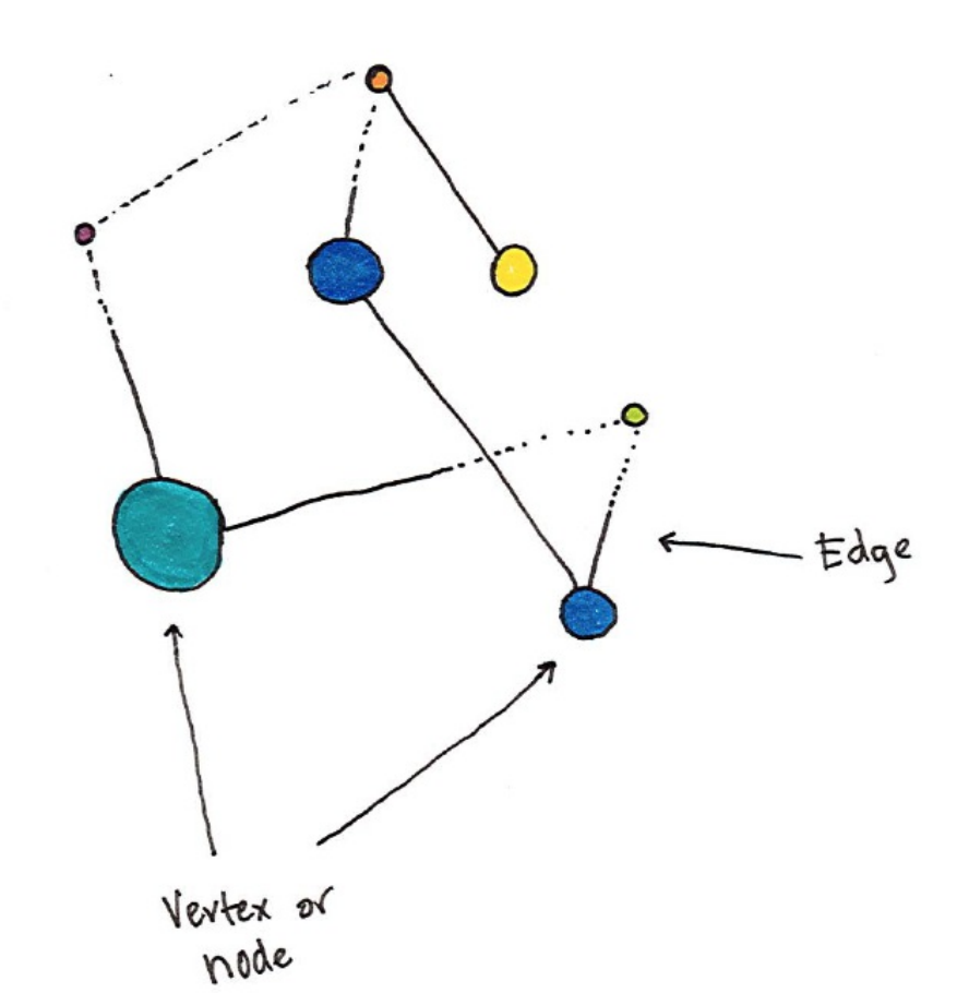
You can see the above image is a representation of a directed graph where the
edges are directional. There are also undirected graphs in which there is no
start and beginning for given edges.
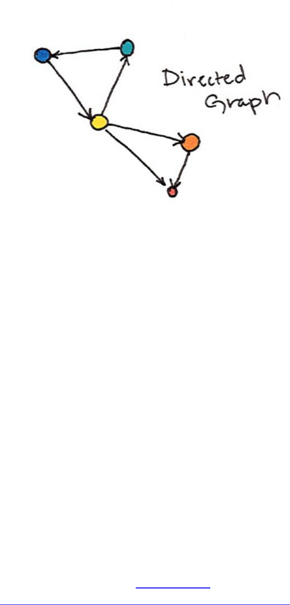
Using our example, the length of the edge might represent the intimacy between
different friends; acquaintances would have long edges between them while
married individuals would have extremely short edges. We could infer this by
looking at communication frequency between nodes and weighting the edges
accordingly. Graph are a natural way of describing relationships and many
different problem sets and Spark provides several ways of working in this
analytics paradigm. Some business use cases could be detecting credit card
fraud, importance of papers in bibliographic networks [which papers are most
referenced], and ranking web pages as Google famously used the PageRank
algorithm to do.
When Spark first came out, in its core was a package called GraphX that
provides an interface for performing graph analysis on top of RDDs. This
package was not available in Python and is quite low level. GraphX still exists
and companies build production products on top of it, however recently the
next generation graph analytics library on Spark called GraphFrames has
popped up. GraphFrames is currently available as a Spark Package, an
external package that you need to load when you start up your Spark
application, but will likely be merged into the core of Spark in the future. The
package is available at http://spark-
packages.org/package/graphframes/graphframes and we will cover how to
install it shortly. For the the most part, there should be little difference in

performance between the two (except for a huge user experience improvement
in GraphFrames). There is some overhead when using GraphFrames but for the
most part it tries to call down to GraphX where appropriate.
note
How does GraphFrames compare to Graph Databases? There are many
graph databases on the market and some of them are quite popular. Like
most of Spark, GraphFrames is not a drop in replacement for a
transactional database. It can scale to much larger workloads than many
graph databases and you should use it primarily for analytics instead of a
online transaction processing workloads.
The goal of this chapter is to show you how to use GraphFrames to perform
graph analysis on Spark. We are going to be doing this with publicly available
bike data from the Bay Area Bike Share portal.
To get setup you’re going to need to point to the proper package. In order to do
this from the command line you’ll run.
./bin/spark-shell --packages graphframes:graphframes:0.3.0-spark2.0-s_2.11
%scala
val bikeStations = spark.read
.option("header","true")
.csv("/mnt/defg/bike-data/201508_station_data.csv")
val tripData = spark.read
.option("header","true")
.csv("/mnt/defg/bike-data/201508_trip_data.csv")
%python
bikeStations = spark.read\
.option("header","true")\
.csv("/mnt/defg/bike-data/201508_station_data.csv")
tripData = spark.read\
.option("header","true")\
.csv("/mnt/defg/bike-data/201508_trip_data.csv")
Building A Graph
The first step is to build the graph, to do this we need to define the vertices and
edges. In our case we’re creating a directed graph. This graph will point from
the source to the location. In the context of this bike trip data, this will point
from a trip’s starting location to a trip’s ending location.To define the graph,
we use the naming conventions presented in the GraphFrames library. In the
vertices table we define our identifier as id and in the edges table we label the
source id as src and the destination id as dst.
val stationVertices = bikeStations
.withColumnRenamed("name", "id")
.distinct()
val tripEdges = tripData
.withColumnRenamed("Start Station", "src")
.withColumnRenamed("End Station", "dst")
%python
stationVertices = bikeStations\
.withColumnRenamed("name", "id")\
.distinct()
tripEdges = tripData\
.withColumnRenamed("Start Station", "src")\
.withColumnRenamed("End Station", "dst")
This allows us to build out graph out of the DataFrames we have so far. We
will also leverage caching because we’ll be accessing this data frequently in
the following queries.
%scala
import org.graphframes.GraphFrame
val stationGraph = GraphFrame(stationVertices, tripEdges)
tripEdges.cache()
stationVertices.cache()
%python
from graphframes import GraphFrame
stationGraph = GraphFrame(stationVertices, tripEdges)
tripEdges.cache()
stationVertices.cache()
Now we can see the basic statistics about data (and query our original
DataFrame to ensure that we see the expected results).
stationGraph.vertices.count
stationGraph.edges.count
tripData.count
This returns the following results.
Total Number of Stations: 70
Total Number of Trips in Graph: 354152
Total Number of Trips in Original Data: 354152
Querying the Graph
The most basic way of interacting with the graph is simply querying it,
performing things like counting trips and filtering by given destinations.
GraphFrames provides simple access to both vertices and edges.
%scala
import org.apache.spark.sql.functions.desc
stationGraph
.edges
.groupBy("src", "dst")
.count()
.orderBy(desc("count"))
.show(10)
%python
from pyspark.sql.functions import desc
stationGraph\
.edges\
.groupBy("src", "dst")\
.count()\
.orderBy(desc("count"))\
.show(10)
We can also filter by any valid DataFrame expression. In this instance I want to
look at one specific station and the count of trips in and out of that station.
%scala
stationGraph
.edges
.where("src = 'Townsend at 7th' OR dst = 'Townsend at 7th'")
.groupBy("src", "dst")
.count()
.orderBy(desc("count"))
.show(10)
%python
stationGraph\
.edges\
.where("src = 'Townsend at 7th' OR dst = 'Townsend at 7th'")\
.groupBy("src", "dst")\
.count()\
.orderBy(desc("count"))\
.show(10)
Subgraphs
Subgraphs are just smaller graphs within the larger one. We saw above how
we can query a given set of edges and vertices. We can use this in order to
create subgraphs.
%scala
val townAnd7thEdges = stationGraph
.edges
.where("src = 'Townsend at 7th' OR dst = 'Townsend at 7th'")
val subgraph = GraphFrame(stationGraph.vertices, townAnd7thEdges
%python
townAnd7thEdges = stationGraph\
.edges\
.where("src = 'Townsend at 7th' OR dst = 'Townsend at 7th'")
subgraph = GraphFrame(stationGraph.vertices, townAnd7thEdges)
We can then apply the following algorithms to either the original or the
subgraph.
Graph Algorithms
A graph is just a logical representation of data. Graph theory provides
numerous algorithms for describing data in this format and GraphFrames
allows us to leverage many algorithms out of the box. Development continues
as new algorithms are added to GraphFrames so this list is likely to continue to
grow.

PageRank
Arguably one of the most prolific graph algorithms is PageRank
https://en.wikipedia.org/wiki/PageRank. Larry Page, founder of Google,
created PageRank as a research project for how to rank webpages.
Unfortunately an in depth explanation of how PageRank works is outside the
scope of this book, however to quote Wikipedia the high level explanation is
as follows.
PageRank works by counting the number and quality of links to a page to
determine a rough estimate of how important the website is. The
underlying assumption is that more important websites are likely to
receive more links from other websites.
However PageRank generalizes quite well outside of the web domain. We can
apply this right to our own data and get a sense for important bike stations.
%scala
val ranks = stationGraph.pageRank
.resetProbability(0.15)
.maxIter(10)
.run()
ranks.vertices
.orderBy(desc("pagerank"))
.select("id", "pagerank")
.show(10)
%python
ranks = stationGraph.pageRank(resetProbability=0.15, maxIter=10
ranks.vertices\
.orderBy(desc("pagerank"))\
.select("id", "pagerank")\
.show(10)
+--------------------+------------------+
| id| pagerank|
+--------------------+------------------+
|San Jose Diridon ...| 3.211176118037002|
...
|Embarcadero at Sa...|1.2343689576475716|
+--------------------+------------------+
Interestingly, we see that Caltrain stations rank quite highly. This makes sense
because these are natural connection points where a lot of bike trips might end
up. Either as commuters move from home to the Caltrain station for their
commute or from the Caltrain station to home.
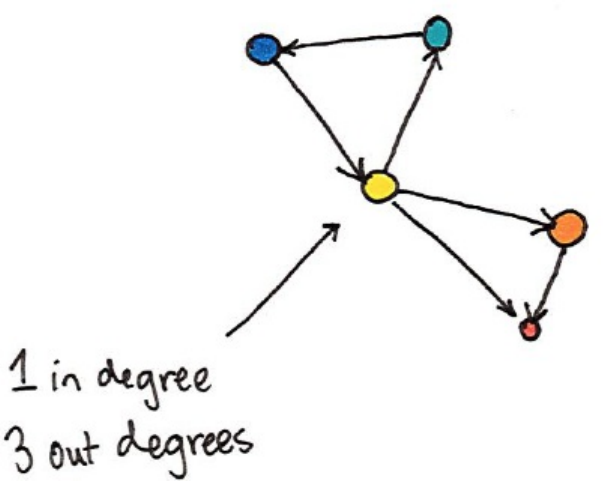
In and Out Degrees
Our graph is a directed graph. This is due to the bike trips being directional,
starting in one location and ending in another. One common task is to count the
number of trips into or out of a given station. We counted trips previously, in
this case we want to count trips into and out of a given station. We measure
these with in and out degrees respectively. GraphFrames provides a simple
way to query this information.
%scala
val inDeg = stationGraph.inDegrees
inDeg.orderBy(desc("inDegree")).show(5, false)
%python
inDeg = stationGraph.inDegrees
inDeg.orderBy(desc("inDegree")).show(5, False)
We can query the out degrees in the same fashion.
val outDeg = stationGraph.outDegrees
outDeg.orderBy(desc("outDegree")).show(5, false)
%python
outDeg = stationGraph.outDegrees
outDeg.orderBy(desc("outDegree")).show(5, False)
The ratio of these two values is an interesting metric to look at. A higher ratio
value will tell us where a large number of trips end (but rarely begin) while a
lower value tells us where trips often begin (but infrequently end).
%scala
val degreeRatio = inDeg.join(outDeg, Seq("id"))
.selectExpr("id", "double(inDegree)/double(outDegree) as degreeRatio"
degreeRatio
.orderBy(desc("degreeRatio"))
.show(10, false)
degreeRatio
.orderBy("degreeRatio")
.show(10, false)
%python
degreeRatio = inDeg.join(outDeg, "id")\
.selectExpr("id", "double(inDegree)/double(outDegree) as degreeRatio"
degreeRatio\
.orderBy(desc("degreeRatio"))\
.show(10, False)
degreeRatio\
.orderBy("degreeRatio")\
.show(10, False)
Breadth-first Search
Breadth-first Search will search our graph for how to connect two given nodes
based on the edges in the graph. In our context, we might want to do this to find
the shortest paths to different stations.
%scala
val bfsResult = stationGraph.bfs
.fromExpr("id = 'Townsend at 7th'")
.toExpr("id = 'Redwood City Medical Center'")
.maxPathLength(4)
.run()
%python
bfsResult = stationGraph.bfs(
fromExpr="id = 'Townsend at 7th'",
toExpr="id = 'Redwood City Medical Center'",
maxPathLength=4)
bfsResult.show(10)
This command will take some time to run if you’re running on your local
machine and actually won’t find a result. This is because these two stations are
so distant from one another that it would not be feasible to ride a bike from one
station to another, at least not by combining four different edges (the
maxPathLength). We can also specify an edgeFilter to filter out certain
edges that do not meet a certain requirement like trips during non-business
hours.
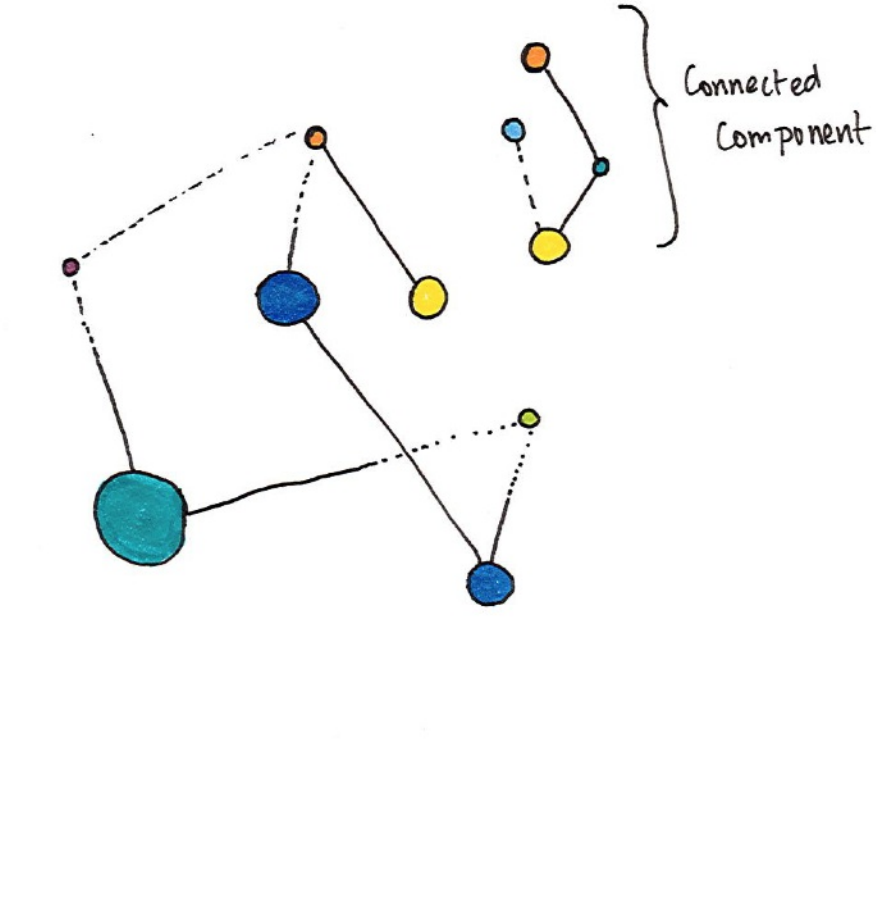
Connected Components
A connected component simply defines a graph that has connections to itself
but does not connect to the greater graph. As illustrated in the following image.
Connected components do not directly relate to our current problem because
we have a directed graph, however we can still run the algorithm which just
assumes that there are is no directionality associated with our edges. In fact if
we look at the bike share map, we assume that we would get two distinct
connected components.

In order to run this algorithm you will need to set a checkpoint directory which
will store the state of the job at every iteration. This allows you to continue
where you left off if for some reason the job crashes.
%scala
spark.sparkContext.setCheckpointDir("/tmp/checkpoints")
%python
spark.sparkContext.setCheckpointDir("/tmp/checkpoints")
%scala
cc = stationGraph.connectedComponents.run()
%python
cc = stationGraph.connectedComponents()
Interesting, we actually get three distinct connected components. Why we get
this might be an opportunity for further analysis but we can assume that
someone might be taking a bike in a car or something similar.
Strongly Connected Components
However GraphFrames also include another version of the algorithm that does
relate to directed graphs called strongly connected components. This does the
same approximate task as finding connected components but takes
directionality into account. A strongly connected component effectively has one
way into a subgraph and no way out.
TODO: (Should this get an image too?)
%scala
val scc = stationGraph
.stronglyConnectedComponents
.maxIter(3)
.run()
%python
scc = stationGraph.stronglyConnectedComponents(maxIter=3)
scc.groupBy("component").count().show()
Motif Finding
Motifs are a way of expresssing structural patterns in a graph. When we
specify a motif, we are querying for patterns in the data instead of actual data.
Our current dataset does not suit this sort of querying because our graph
consists of individual trips, not repeated interactions of certain individuals or
identifiers. In GraphFrames, we specify our query in a Domain-Specific
Language. We specify combinations of vertices and edges. For example, if we
want to specify a given vertex to another vertex we would specify (a)-[ab]->
(b). The letters inside of parenthesis or brackets do not signify values but
signify what the columns should be named in the resulting DataFrame. We can
omit the names (e.g., (a)-[]->()) if we do not intend to query the resulting
values.
Let’s perform a query. In plain english, let’s find all the round trip rides with
two stations in between. We express this with the following motif using the
find method to query our GraphFrame for that pattern.
%scala
val motifs = stationGraph
.find("(a)-[ab]->(b); (b)-[bc]->(c); (c)-[ca]->(a)")
%python
motifs = stationGraph\
.find("(a)-[ab]->(b); (b)-[bc]->(c); (c)-[ca]->(a)")
Here’s a visual representation of this query.
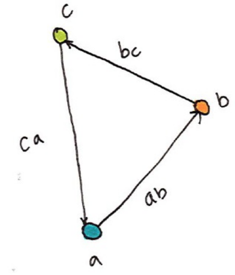
The resulting DataFrame contains nested fields for vertices a, b, and c as well
as the respective edges. Now we can query this data as if it were a DataFrame.
Now we can query that to answer a specific question. Given a certain bike
what is the shortest round trip time where that bike is taken from one station
(a), ridden to another, dropped off(b), ridden to another, dropped off(c), and
then ridden back to the original station (a). This is just going to be a lot of
filtering, as we can see below.
%scala
import org.apache.spark.sql.functions.expr
motifs
// first simplify dates for comparisons
.selectExpr("*", """
cast(unix_timestamp(ab.`Start Date`, 'MM/dd/yyyy HH:mm')
as timestamp) as abStart
""",
"""
cast(unix_timestamp(bc.`Start Date`, 'MM/dd/yyyy HH:mm')
as timestamp) as bcStart
""",
"""
cast(unix_timestamp(ca.`Start Date`, 'MM/dd/yyyy HH:mm')
as timestamp) as caStart
""")
// ensure the same bike
.where("ca.`Bike #` = bc.`Bike #`")
.where("ab.`Bike #` = bc.`Bike #`")
// ensure different stations
.where("a.id != b.id")
.where("b.id != c.id")
// start times are correct
.where("abStart < bcStart")
.where("bcStart < caStart")
// order them all
.orderBy(expr("cast(caStart as long) - cast(abStart as long)"
.selectExpr("a.id", "b.id", "c.id",
"ab.`Start Date`", "ca.`End Date`")
.limit(1)
.show(false)
%python
motifs
# first simplify dates for comparisons
.selectExpr("*", """
cast(unix_timestamp(ab.`Start Date`, 'MM/dd/yyyy HH:mm')
as timestamp) as abStart
""",
"""
cast(unix_timestamp(bc.`Start Date`, 'MM/dd/yyyy HH:mm')
as timestamp) as bcStart
""",
"""
cast(unix_timestamp(ca.`Start Date`, 'MM/dd/yyyy HH:mm')
as timestamp) as caStart
""")
# ensure the same bike
.where("ca.`Bike #` = bc.`Bike #`")
.where("ab.`Bike #` = bc.`Bike #`")
# ensure different stations
.where("a.id != b.id")
.where("b.id != c.id")
# start times are correct
.where("abStart < bcStart")
.where("bcStart < caStart")
# order them all
.orderBy(expr("cast(caStart as long) - cast(abStart as long)"
.selectExpr("a.id", "b.id", "c.id",
"ab.`Start Date`", "ca.`End Date`")
.limit(1)
.show(False)
We see the fastest trip is approximately 20 minutes. Pretty fast for three
different people (we assume) using the same bike!
Advanced Tasks
This is just a short selection of some of the things GraphFrames allows you to
achieve. Development continues as well and so you will be able to continue to
find new algorithms and features being added the library. Some of these
advanced features include writing your own algorithms via a message passing
interface, triangle counting, converting to and from GraphX among other tasks.
It is also likely that in the future this library will join GraphX in the core of
Spark.
Chapter 22. Deep Learning
In order to define deep learning, we must first define neural networks. Neural
networks allow computers to understand concepts by layering simple
representations on top of one another. For the most part, each one of these
representations, or layers, consist of a variety of inputs connected together that
are activated when combined together, similar in concept to a neuron in the
brain. Our goal is to train the network to associate certain inputs with certain
outputs. Deep learning, or deep neural networks, just combine many of these
layers together in various different architectures. Deep learning has gone
through several periods of fading and resurgence and has only recently become
popular in the past decade because of its ability to solve an incredibly diverse
set of complex problems.
Spark being a robust tool for performing operations in parallel has a number of
good opportunities for end users to leverage both Spark and deep learning
together.
warning
if you have little experience with machine learning and deep learning, this
is not the chapter for you. We recommend spending some time learning
about the core methods of machine learning before embarking on using
deep learning with Spark.
Ways of using Deep Learning in
Spark
For the most part, when it comes to large scale machine learning, you can
either parallelize the data or parallelize the model (Dean 2016). Parallelizing
the data is quite trivial and Spark does quite well with this workload. A much
harder problem, is in parallelizing the model because the model itself is too
large to fit into memory. Both of these areas are fruitful areas of research
however for the most part if you are looking to get started with machine
learning on Spark it is much easier to use models that are pretrained by the
massive companies with large amount of time, and money, to throw at the
problem than to try and train your own.
Spark currently has native support for one deep learning algorithm, the
multilayer perceptron classifier. While it does work, it is not particularly
flexible or tunable according to different architectures or workloads and has
not received a significant amount of innovation since it was first introduced.
This chapter will not focus on packages that are necessarily core to Spark but
will rather focus on the massive amount of innovation in libraries built on top
of Spark. We will start with several theoretical approaches to deep learning on
Spark, discuss those of which you are likely to succeed in using in practice
today, and discuss some of the libraries that make this possible.
There are associated tradeoffs with these implementations but for the most
part, Spark is not structured for model parallelization because of synchronous
communication overhead and immutability. This does not mean that Spark is
not used for deep learning workloads because the volume of libraries proves
otherwise. Below is an incomplete list of different ways that Spark can be
used in conjunction with deep learning.
note
in the following examples we use the term “small data” and “big data” to
differentiate that which can fit on a single node and that which must be
distributed. To be clear this is not actuall small data (say 100s of rows)
this is many gigabytes of data that can still fit on one machine.
1. Distributed training of many deep learning models. “Small learning, small
data”.
Spark can parallelize work efficiently when there is little communication
required between the nodes. This makes it an excellent tool for performing
distributed training of one deep learning model per worker node that might
have different architectures or initialization. There are many libraries that take
advantage of Spark in this way.
1. Distributed usage of deep learning models. “Small model, big data”
As we mentioned in the previous bullet, Spark makes it extremely easy to
parallelize tasks across a large number of machines. One wonderful thing
about machine learning research is that many models are available to the
public as pretrained deep learning models that you can use without having to
perform any training yourself. These can do things like identify humans in an
image or provide a translation of a Chinese character into an english word or
phrase. Spark makes it easy for you to get immediate value out of these
networks by applying them, at scale, to your own data.
If you are lookign to get started with Spark and deep learning, get started here!
1. Large Scale ETL and preprocessing leading to learning a deep learning
model on a single node. “Small learning, big data”
This is often referred to as “learn small with big data”. Rather than trying to
collect all of your data onto one node right away you can use Spark to iterate
over your entire (distributed) dataset on the driver itself with the
toLocalIterator method. You can, of course, use Spark for feature
generation and simply collect the dataset to a large node as well but this does
limit the total datasize that you can train on.
1. Distributed training of a large deep learning model. “Big learning, big
data”
This use cases stretches Spark more than any other. As you saw throughout the
book, Spark has its own notions of how to schedule transformations and
communication across a cluster. The efficiency of Spark’s ability to perform
large scale data manipulation with little overhead, at times, conflicts with the
type of system that a can efficiently train a single, massive deep learning
model. This is a fruitful area of research and some of the below projects
attempt to bring this functionality to Spark.
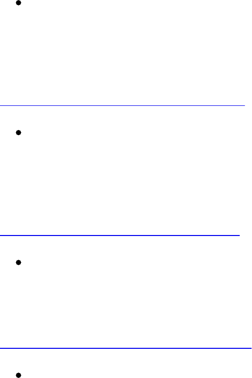
Deep Learning Projects on Spark
There exist a number of projects that attempt to bring deep learning to Spark in
the aforementioned ways. This part of the chapter will focus on sharing some
of the more well known projects and some code samples. As mentioned, this is
a fruitful area of research and it is likely that the state of the art will progress
by the time this book is published and in your hand. Visit the Spark
documentation site for the latest news. The projects are listed in alphabetical
order.
BigDL
BigDL (pronounced big deal) is a distributed deep learning framework for
Spark. It aims to support the training of large models as wekk as the loading
and usage of pre-trained models into Spark.
https://github.com/intel-analytics/BigDL
CaffeOnSpark
Caffe is a popular deep learning framework focused on image processing.
CaffeOnSpark is an open source package for using Caffe on top of Spark that
includes model training, testing, and feature extraction.
https://github.com/yahoo/CaffeOnSpark
DeepDist
DeepDist accelerates the training by distributing stochastic gradient descent
for data stored in Spark.
https://github.com/dirkneumann/deepdist/
Deeplearning4J
Deeplearning4j is an open-source, distributed deep-learning preojct in Java
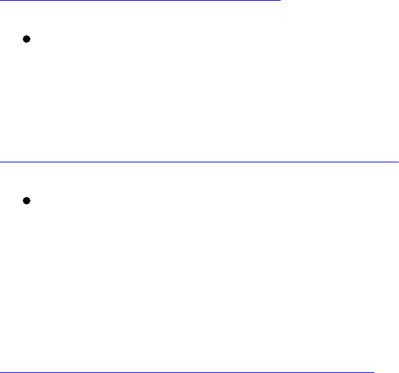
and Scala which provides both single node and distributed training options.
https://deeplearning4j.org/spark
TensorFlowOnSpark
TensorFlow is a popular open source deep learning framework and aims to
make TensorFlow easier to operate in a distributed setting.
https://github.com/yahoo/TensorFlowOnSpark
TensorFrames
TensorFrames lets you manipulate Spark DataFrames with TensorFlow
Programs. It supports Python and Scala interfaces and focuses on providing a
simple interface to use single node deep learning models at scale as well as
distributed hyperparameter tuning of single node models.
https://github.com/databricks/tensorframes
Here’s a simple project scorecard of the various deep learning projects.
Deep Learning
Framework Focus
BigDL BigDL big model training, ETL
CaffeOnSpark Caffe small model training, ETL
DeepLearning4J DeepLearning4J big/small model training, ETL
DeepDist DeepDist big model training
TensorFlowOnSpark TensorFlow small model training, ETL
TensorFrames TensorFlow Spark integration, small model
training, ETL
A Simple Example with
TensorFrames
TODO: This example will be coming but we are waiting for Spark 2.2 to
officially come out in order to upgrade the package.
