Spark OReilly.Spark.The.Definitive.Guide.2018.2
User Manual:
Open the PDF directly: View PDF ![]() .
.
Page Count: 792 [warning: Documents this large are best viewed by clicking the View PDF Link!]
- Preface
- I. Gentle Overview of Big Data and Spark
- 1. What Is Apache Spark?
- 2. A Gentle Introduction to Spark
- 3. A Tour of Spark’s Toolset
- II. Structured APIs—DataFrames, SQL, and Datasets
- 4. Structured API Overview
- 5. Basic Structured Operations
- Schemas
- Columns and Expressions
- Records and Rows
- DataFrame Transformations
- Creating DataFrames
- select and selectExpr
- Converting to Spark Types (Literals)
- Adding Columns
- Renaming Columns
- Reserved Characters and Keywords
- Case Sensitivity
- Removing Columns
- Changing a Column’s Type (cast)
- Filtering Rows
- Getting Unique Rows
- Random Samples
- Random Splits
- Concatenating and Appending Rows (Union)
- Sorting Rows
- Limit
- Repartition and Coalesce
- Collecting Rows to the Driver
- Conclusion
- 6. Working with Different Types of Data
- 7. Aggregations
- 8. Joins
- 9. Data Sources
- 10. Spark SQL
- 11. Datasets
- III. Low-Level APIs
- 12. Resilient Distributed Datasets (RDDs)
- 13. Advanced RDDs
- 14. Distributed Shared Variables
- IV. Production Applications
- 15. How Spark Runs on a Cluster
- 16. Developing Spark Applications
- 17. Deploying Spark
- 18. Monitoring and Debugging
- The Monitoring Landscape
- What to Monitor
- Spark Logs
- The Spark UI
- Debugging and Spark First Aid
- Spark Jobs Not Starting
- Errors Before Execution
- Errors During Execution
- Slow Tasks or Stragglers
- Slow Aggregations
- Slow Joins
- Slow Reads and Writes
- Driver OutOfMemoryError or Driver Unresponsive
- Executor OutOfMemoryError or Executor Unresponsive
- Unexpected Nulls in Results
- No Space Left on Disk Errors
- Serialization Errors
- Conclusion
- 19. Performance Tuning
- V. Streaming
- 20. Stream Processing Fundamentals
- 21. Structured Streaming Basics
- 22. Event-Time and Stateful Processing
- 23. Structured Streaming in Production
- VI. Advanced Analytics and Machine Learning
- 24. Advanced Analytics and Machine Learning Overview
- 25. Preprocessing and Feature Engineering
- 26. Classification
- 27. Regression
- 28. Recommendation
- 29. Unsupervised Learning
- 30. Graph Analytics
- 31. Deep Learning
- VII. Ecosystem
- 32. Language Specifics: Python (PySpark) and R (SparkR and sparklyr)
- 33. Ecosystem and Community
- Index

Spark: The Definitive Guide
Big Data Processing Made Simple
Bill Chambers and Matei Zaharia
Spark: The Definitive Guide
by Bill Chambers and Matei Zaharia
Copyright © 2018 Databricks. All rights reserved.
Printed in the United States of America.
Published by O’Reilly Media, Inc., 1005 Gravenstein Highway North,
Sebastopol, CA 95472.
O’Reilly books may be purchased for educational, business, or sales
promotional use. Online editions are also available for most titles
(http://oreilly.com/safari). For more information, contact our
corporate/institutional sales department: 800-998-9938 or
corporate@oreilly.com.
Editor: Nicole Tache
Production Editor: Justin Billing
Copyeditor: Octal Publishing, Inc., Chris Edwards, and Amanda
Kersey
Proofreader: Jasmine Kwityn
Indexer: Judith McConville
Interior Designer: David Futato
Cover Designer: Karen Montgomery
Illustrator: Rebecca Demarest
February 2018: First Edition
Revision History for the First Edition

2018-02-08: First Release
See http://oreilly.com/catalog/errata.csp?isbn=9781491912218 for release
details.
The O’Reilly logo is a registered trademark of O’Reilly Media, Inc. Spark:
The Definitive Guide, the cover image, and related trade dress are trademarks
of O’Reilly Media, Inc. Apache, Spark and Apache Spark are trademarks of
the Apache Software Foundation.
While the publisher and the authors have used good faith efforts to ensure
that the information and instructions contained in this work are accurate, the
publisher and the authors disclaim all responsibility for errors or omissions,
including without limitation responsibility for damages resulting from the use
of or reliance on this work. Use of the information and instructions contained
in this work is at your own risk. If any code samples or other technology this
work contains or describes is subject to open source licenses or the
intellectual property rights of others, it is your responsibility to ensure that
your use thereof complies with such licenses and/or rights.
978-1-491-91221-8
[M]

Preface
Welcome to this first edition of Spark: The Definitive Guide! We are excited
to bring you the most complete resource on Apache Spark today, focusing
especially on the new generation of Spark APIs introduced in Spark 2.0.
Apache Spark is currently one of the most popular systems for large-scale
data processing, with APIs in multiple programming languages and a wealth
of built-in and third-party libraries. Although the project has existed for
multiple years—first as a research project started at UC Berkeley in 2009,
then at the Apache Software Foundation since 2013—the open source
community is continuing to build more powerful APIs and high-level
libraries over Spark, so there is still a lot to write about the project. We
decided to write this book for two reasons. First, we wanted to present the
most comprehensive book on Apache Spark, covering all of the fundamental
use cases with easy-to-run examples. Second, we especially wanted to
explore the higher-level “structured” APIs that were finalized in Apache
Spark 2.0—namely DataFrames, Datasets, Spark SQL, and Structured
Streaming—which older books on Spark don’t always include. We hope this
book gives you a solid foundation to write modern Apache Spark applications
using all the available tools in the project.
In this preface, we’ll tell you a little bit about our background, and explain
who this book is for and how we have organized the material. We also want
to thank the numerous people who helped edit and review this book, without
whom it would not have been possible.
About the Authors
Both of the book’s authors have been involved in Apache Spark for a long
time, so we are very excited to be able to bring you this book.
Bill Chambers started using Spark in 2014 on several research projects.
Currently, Bill is a Product Manager at Databricks where he focuses on
enabling users to write various types of Apache Spark applications. Bill also
regularly blogs about Spark and presents at conferences and meetups on the
topic. Bill holds a Master’s in Information Management and Systems from
the UC Berkeley School of Information.
Matei Zaharia started the Spark project in 2009, during his time as a PhD
student at UC Berkeley. Matei worked with other Berkeley researchers and
external collaborators to design the core Spark APIs and grow the Spark
community, and has continued to be involved in new initiatives such as the
structured APIs and Structured Streaming. In 2013, Matei and other members
of the Berkeley Spark team co-founded Databricks to further grow the open
source project and provide commercial offerings around it. Today, Matei
continues to work as Chief Technologist at Databricks, and also holds a
position as an Assistant Professor of Computer Science at Stanford
University, where he does research on large-scale systems and AI. Matei
received his PhD in Computer Science from UC Berkeley in 2013.
Who This Book Is For
We designed this book mainly for data scientists and data engineers looking
to use Apache Spark. The two roles have slightly different needs, but in
reality, most application development covers a bit of both, so we think the
material will be useful in both cases. Specifically, in our minds, the data
scientist workload focuses more on interactively querying data to answer
questions and build statistical models, while the data engineer job focuses on
writing maintainable, repeatable production applications—either to use the
data scientist’s models in practice, or just to prepare data for further analysis
(e.g., building a data ingest pipeline). However, we often see with Spark that
these roles blur. For instance, data scientists are able to package production
applications without too much hassle and data engineers use interactive
analysis to understand and inspect their data to build and maintain pipelines.
While we tried to provide everything data scientists and engineers need to get
started, there are some things we didn’t have space to focus on in this book.
First, this book does not include in-depth introductions to some of the
analytics techniques you can use in Apache Spark, such as machine learning.
Instead, we show you how to invoke these techniques using libraries in
Spark, assuming you already have a basic background in machine learning.
Many full, standalone books exist to cover these techniques in formal detail,
so we recommend starting with those if you want to learn about these areas.
Second, this book focuses more on application development than on
operations and administration (e.g., how to manage an Apache Spark cluster
with dozens of users). Nonetheless, we have tried to include comprehensive
material on monitoring, debugging, and configuration in Parts V and VI of
the book to help engineers get their application running efficiently and tackle
day-to-day maintenance. Finally, this book places less emphasis on the older,
lower-level APIs in Spark—specifically RDDs and DStreams—to introduce
most of the concepts using the newer, higher-level structured APIs. Thus, the
book may not be the best fit if you need to maintain an old RDD or DStream
application, but should be a great introduction to writing new applications.
Conventions Used in This Book
The following typographical conventions are used in this book:
Italic
Indicates new terms, URLs, email addresses, filenames, and file
extensions.
Constant width
Used for program listings, as well as within paragraphs to refer to
program elements such as variable or function names, databases, data
types, environment variables, statements, and keywords.
Constant width bold
Shows commands or other text that should be typed literally by the user.
Constant width italic
Shows text that should be replaced with user-supplied values or by values
determined by context.
TIP
This element signifies a tip or suggestion.
NOTE
This element signifies a general note.
WARNING
This element indicates a warning or caution.
Using Code Examples
We’re very excited to have designed this book so that all of the code content
is runnable on real data. We wrote the whole book using Databricks
notebooks and have posted the data and related material on GitHub. This
means that you can run and edit all the code as you follow along, or copy it
into working code in your own applications.
We tried to use real data wherever possible to illustrate the challenges you’ll
run into while building large-scale data applications. Finally, we also include
several larger standalone applications in the book’s GitHub repository for
examples that it does not make sense to show inline in the text.
The GitHub repository will remain a living document as we update based on
Spark’s progress. Be sure to follow updates there.
This book is here to help you get your job done. In general, if example code
is offered with this book, you may use it in your programs and
documentation. You do not need to contact us for permission unless you’re
reproducing a significant portion of the code. For example, writing a program
that uses several chunks of code from this book does not require permission.
Selling or distributing a CD-ROM of examples from O’Reilly books does
require permission. Answering a question by citing this book and quoting
example code does not require permission. Incorporating a significant
amount of example code from this book into your product’s documentation
does require permission.
We appreciate, but do not require, attribution. An attribution usually includes
the title, author, publisher, and ISBN. For example: “Spark: The Definitive
Guide by Bill Chambers and Matei Zaharia (O’Reilly). Copyright 2018
Databricks, Inc., 978-1-491-91221-8.”
If you feel your use of code examples falls outside fair use or the permission
given above, feel free to contact us at permissions@oreilly.com.
O’Reilly Safari
Safari (formerly Safari Books Online) is a membership-based training and
reference platform for enterprise, government, educators, and individuals.
Members have access to thousands of books, training videos, Learning Paths,
interactive tutorials, and curated playlists from over 250 publishers, including
O’Reilly Media, Harvard Business Review, Prentice Hall Professional,
Addison-Wesley Professional, Microsoft Press, Sams, Que, Peachpit Press,
Adobe, Focal Press, Cisco Press, John Wiley & Sons, Syngress, Morgan
Kaufmann, IBM Redbooks, Packt, Adobe Press, FT Press, Apress, Manning,
New Riders, McGraw-Hill, Jones & Bartlett, and Course Technology, among
others.
For more information, please visit http://oreilly.com/safari.
How to Contact Us
Please address comments and questions concerning this book to the
publisher:
O’Reilly Media, Inc.
1005 Gravenstein Highway North
Sebastopol, CA 95472
800-998-9938 (in the United States or Canada)
707-829-0515 (international or local)
707-829-0104 (fax)
To comment or ask technical questions about this book, send email to
bookquestions@oreilly.com.
For more information about our books, courses, conferences, and news, see
our website at http://www.oreilly.com.

Find us on Facebook: http://facebook.com/oreilly
Follow us on Twitter: http://twitter.com/oreillymedia
Watch us on YouTube: http://www.youtube.com/oreillymedia
Acknowledgments
There were a huge number of people that made this book possible.
First, we would like to thank our employer, Databricks, for allocating time
for us to work on this book. Without the support of the company, this book
would not have been possible. In particular, we would like to thank Ali
Ghodsi, Ion Stoica, and Patrick Wendell for their support.
Additionally, there are numerous people that read drafts of the book and
individual chapters. Our reviewers were best-in-class, and provided
invaluable feedback.
These reviewers, in alphabetical order by last name, are:
Lynn Armstrong
Mikio Braun
Jules Damji
Denny Lee
Alex Thomas
In addition to the formal book reviewers, there were numerous other Spark
users, contributors, and committers who read over specific chapters or helped
formulate how topics should be discussed. In alphabetical order by last name,
the people who helped are:
Sameer Agarwal
Bagrat Amirbekian
Michael Armbrust

Joseph Bradley
Tathagata Das
Hossein Falaki
Wenchen Fan
Sue Ann Hong
Yin Huai
Tim Hunter
Xiao Li
Cheng Lian
Xiangrui Meng
Kris Mok
Josh Rosen
Srinath Shankar
Takuya Ueshin
Herman van Hövell
Reynold Xin
Philip Yang
Burak Yavuz
Shixiong Zhu
Lastly, we would like to thank friends, family, and loved ones. Without their
support, patience, and encouragement, we would not have been able to write
the definitive guide to Spark.

Part I. Gentle Overview of Big
Data and Spark
Chapter 1. What Is Apache
Spark?
Apache Spark is a unified computing engine and a set of libraries for parallel
data processing on computer clusters. As of this writing, Spark is the most
actively developed open source engine for this task, making it a standard tool
for any developer or data scientist interested in big data. Spark supports
multiple widely used programming languages (Python, Java, Scala, and R),
includes libraries for diverse tasks ranging from SQL to streaming and
machine learning, and runs anywhere from a laptop to a cluster of thousands
of servers. This makes it an easy system to start with and scale-up to big data
processing or incredibly large scale.
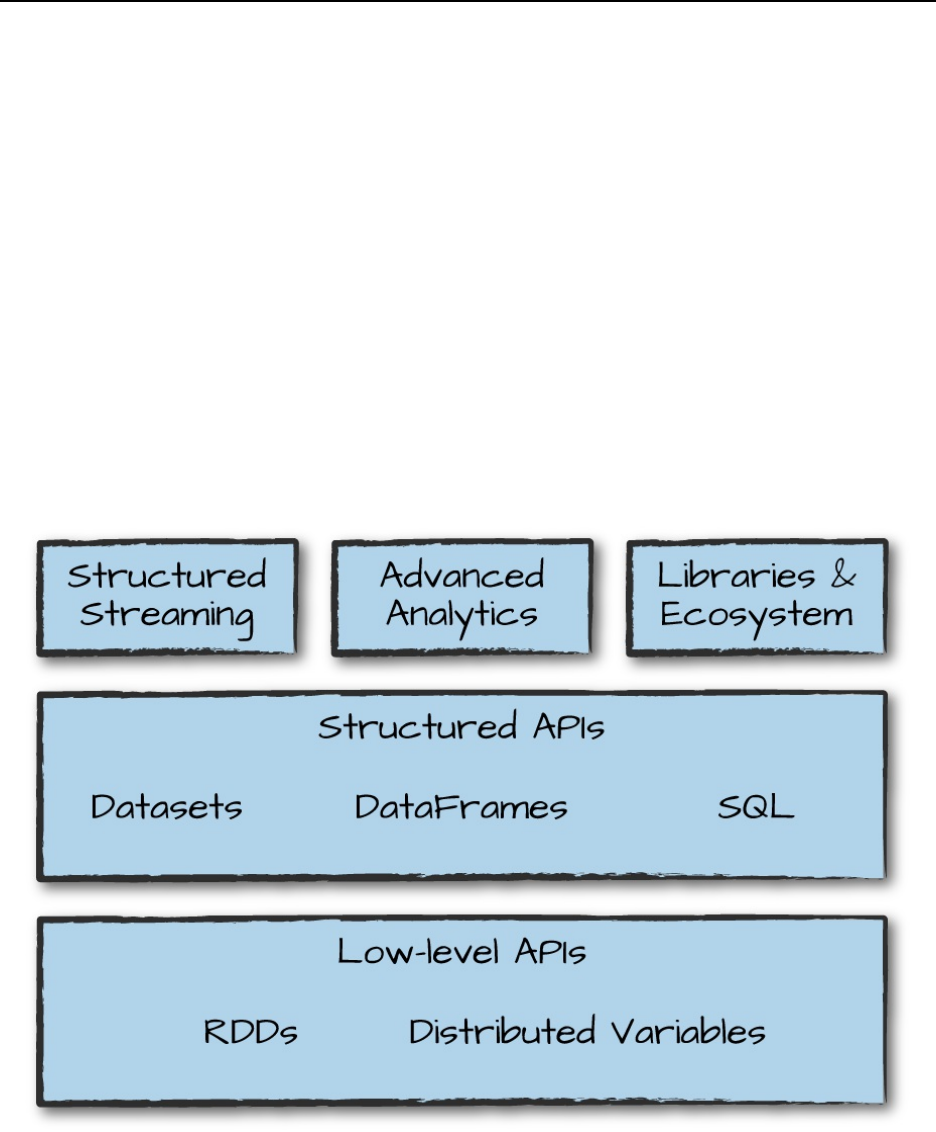
Figure 1-1 illustrates all the components and libraries Spark offers to end-
users.
Figure 1-1. Spark’s toolkit
You’ll notice the categories roughly correspond to the different parts of this
book. That should really come as no surprise; our goal here is to educate you
on all aspects of Spark, and Spark is composed of a number of different
components.
Given that you’re reading this book, you might already know a little bit about
Apache Spark and what it can do. Nonetheless, in this chapter, we want to
briefly cover the overriding philosophy behind Spark as well as the context it
was developed in (why is everyone suddenly excited about parallel data
processing?) and its history. We will also outline the first few steps to
running Spark.
Apache Spark’s Philosophy
Let’s break down our description of Apache Spark—a unified computing
engine and set of libraries for big data—into its key components:
Unified
Spark’s key driving goal is to offer a unified platform for writing big data
applications. What do we mean by unified? Spark is designed to support a
wide range of data analytics tasks, ranging from simple data loading and
SQL queries to machine learning and streaming computation, over the
same computing engine and with a consistent set of APIs. The main
insight behind this goal is that real-world data analytics tasks—whether
they are interactive analytics in a tool such as a Jupyter notebook, or
traditional software development for production applications—tend to
combine many different processing types and libraries.
Spark’s unified nature makes these tasks both easier and more efficient to
write. First, Spark provides consistent, composable APIs that you can use
to build an application out of smaller pieces or out of existing libraries. It
also makes it easy for you to write your own analytics libraries on top.
However, composable APIs are not enough: Spark’s APIs are also
designed to enable high performance by optimizing across the different
libraries and functions composed together in a user program. For
example, if you load data using a SQL query and then evaluate a machine
learning model over it using Spark’s ML library, the engine can combine
these steps into one scan over the data. The combination of general APIs
and high-performance execution, no matter how you combine them,
makes Spark a powerful platform for interactive and production
applications.
Spark’s focus on defining a unified platform is the same idea behind
unified platforms in other areas of software. For example, data scientists
benefit from a unified set of libraries (e.g., Python or R) when doing
modeling, and web developers benefit from unified frameworks such as
Node.js or Django. Before Spark, no open source systems tried to provide
this type of unified engine for parallel data processing, meaning that users
had to stitch together an application out of multiple APIs and systems.
Thus, Spark quickly became the standard for this type of development.
Over time, Spark has continued to expand its built-in APIs to cover more
workloads. At the same time, the project’s developers have continued to
refine its theme of a unified engine. In particular, one major focus of this
book will be the “structured APIs” (DataFrames, Datasets, and SQL) that
were finalized in Spark 2.0 to enable more powerful optimization under
user applications.
Computing engine
At the same time that Spark strives for unification, it carefully limits its
scope to a computing engine. By this, we mean that Spark handles
loading data from storage systems and performing computation on it, not
permanent storage as the end itself. You can use Spark with a wide
variety of persistent storage systems, including cloud storage systems
such as Azure Storage and Amazon S3, distributed file systems such as
Apache Hadoop, key-value stores such as Apache Cassandra, and
message buses such as Apache Kafka. However, Spark neither stores data
long term itself, nor favors one over another. The key motivation here is
that most data already resides in a mix of storage systems. Data is
expensive to move so Spark focuses on performing computations over the
data, no matter where it resides. In user-facing APIs, Spark works hard to
make these storage systems look largely similar so that applications do
not need to worry about where their data is.
Spark’s focus on computation makes it different from earlier big data
software platforms such as Apache Hadoop. Hadoop included both a
storage system (the Hadoop file system, designed for low-cost storage
over clusters of commodity servers) and a computing system
(MapReduce), which were closely integrated together. However, this
choice makes it difficult to run one of the systems without the other.
More important, this choice also makes it a challenge to write
applications that access data stored anywhere else. Although Spark runs
well on Hadoop storage, today it is also used broadly in environments for
which the Hadoop architecture does not make sense, such as the public
cloud (where storage can be purchased separately from computing) or
streaming applications.
Libraries
Spark’s final component is its libraries, which build on its design as a
unified engine to provide a unified API for common data analysis tasks.
Spark supports both standard libraries that ship with the engine as well as
a wide array of external libraries published as third-party packages by the
open source communities. Today, Spark’s standard libraries are actually
the bulk of the open source project: the Spark core engine itself has
changed little since it was first released, but the libraries have grown to
provide more and more types of functionality. Spark includes libraries for
SQL and structured data (Spark SQL), machine learning (MLlib), stream
processing (Spark Streaming and the newer Structured Streaming), and
graph analytics (GraphX). Beyond these libraries, there are hundreds of
open source external libraries ranging from connectors for various storage
systems to machine learning algorithms. One index of external libraries is
available at spark-packages.org.
Context: The Big Data Problem
Why do we need a new engine and programming model for data analytics in
the first place? As with many trends in computing, this is due to changes in
the economic factors that underlie computer applications and hardware.
For most of their history, computers became faster every year through
processor speed increases: the new processors each year could run more
instructions per second than the previous year’s. As a result, applications also
automatically became faster every year, without any changes needed to their
code. This trend led to a large and established ecosystem of applications
building up over time, most of which were designed to run only on a single
processor. These applications rode the trend of improved processor speeds to
scale up to larger computations and larger volumes of data over time.
Unfortunately, this trend in hardware stopped around 2005: due to hard limits
in heat dissipation, hardware developers stopped making individual
processors faster, and switched toward adding more parallel CPU cores all
running at the same speed. This change meant that suddenly applications
needed to be modified to add parallelism in order to run faster, which set the
stage for new programming models such as Apache Spark.
On top of that, the technologies for storing and collecting data did not slow
down appreciably in 2005, when processor speeds did. The cost to store 1 TB
of data continues to drop by roughly two times every 14 months, meaning
that it is very inexpensive for organizations of all sizes to store large amounts
of data. Moreover, many of the technologies for collecting data (sensors,
cameras, public datasets, etc.) continue to drop in cost and improve in
resolution. For example, camera technology continues to improve in
resolution and drop in cost per pixel every year, to the point where a 12-
megapixel webcam costs only $3 to $4; this has made it inexpensive to
collect a wide range of visual data, whether from people filming video or
automated sensors in an industrial setting. Moreover, cameras are themselves
the key sensors in other data collection devices, such as telescopes and even
gene-sequencing machines, driving the cost of these technologies down as
well.
The end result is a world in which collecting data is extremely inexpensive—
many organizations today even consider it negligent not to log data of
possible relevance to the business—but processing it requires large, parallel
computations, often on clusters of machines. Moreover, in this new world,
the software developed in the past 50 years cannot automatically scale up,
and neither can the traditional programming models for data processing
applications, creating the need for new programming models. It is this world
that Apache Spark was built for.
History of Spark
Apache Spark began at UC Berkeley in 2009 as the Spark research project,
which was first published the following year in a paper entitled “Spark:
Cluster Computing with Working Sets” by Matei Zaharia, Mosharaf
Chowdhury, Michael Franklin, Scott Shenker, and Ion Stoica of the UC
Berkeley AMPlab. At the time, Hadoop MapReduce was the dominant
parallel programming engine for clusters, being the first open source system
to tackle data-parallel processing on clusters of thousands of nodes. The
AMPlab had worked with multiple early MapReduce users to understand the
benefits and drawbacks of this new programming model, and was therefore
able to synthesize a list of problems across several use cases and begin
designing more general computing platforms. In addition, Zaharia had also
worked with Hadoop users at UC Berkeley to understand their needs for the
platform—specifically, teams that were doing large-scale machine learning
using iterative algorithms that need to make multiple passes over the data.
Across these conversations, two things were clear. First, cluster computing
held tremendous potential: at every organization that used MapReduce, brand
new applications could be built using the existing data, and many new groups
began using the system after its initial use cases. Second, however, the
MapReduce engine made it both challenging and inefficient to build large
applications. For example, the typical machine learning algorithm might need
to make 10 or 20 passes over the data, and in MapReduce, each pass had to
be written as a separate MapReduce job, which had to be launched separately
on the cluster and load the data from scratch.
To address this problem, the Spark team first designed an API based on
functional programming that could succinctly express multistep applications.
The team then implemented this API over a new engine that could perform
efficient, in-memory data sharing across computation steps. The team also
began testing this system with both Berkeley and external users.
The first version of Spark supported only batch applications, but soon enough
another compelling use case became clear: interactive data science and ad
hoc queries. By simply plugging the Scala interpreter into Spark, the project
could provide a highly usable interactive system for running queries on
hundreds of machines. The AMPlab also quickly built on this idea to develop
Shark, an engine that could run SQL queries over Spark and enable
interactive use by analysts as well as data scientists. Shark was first released
in 2011.
After these initial releases, it quickly became clear that the most powerful
additions to Spark would be new libraries, and so the project began to follow
the “standard library” approach it has today. In particular, different AMPlab
groups started MLlib, Spark Streaming, and GraphX. They also ensured that
these APIs would be highly interoperable, enabling writing end-to-end big
data applications in the same engine for the first time.
In 2013, the project had grown to widespread use, with more than 100
contributors from more than 30 organizations outside UC Berkeley. The
AMPlab contributed Spark to the Apache Software Foundation as a long-
term, vendor-independent home for the project. The early AMPlab team also
launched a company, Databricks, to harden the project, joining the
community of other companies and organizations contributing to Spark.
Since that time, the Apache Spark community released Spark 1.0 in 2014 and
Spark 2.0 in 2016, and continues to make regular releases, bringing new
features into the project.
Finally, Spark’s core idea of composable APIs has also been refined over
time. Early versions of Spark (before 1.0) largely defined this API in terms of
functional operations—parallel operations such as maps and reduces over
collections of Java objects. Beginning with 1.0, the project added Spark SQL,
a new API for working with structured data—tables with a fixed data format
that is not tied to Java’s in-memory representation. Spark SQL enabled
powerful new optimizations across libraries and APIs by understanding both
the data format and the user code that runs on it in more detail. Over time, the
project added a plethora of new APIs that build on this more powerful
structured foundation, including DataFrames, machine learning pipelines, and
Structured Streaming, a high-level, automatically optimized streaming API.
In this book, we will spend a signficant amount of time explaining these next-
generation APIs, most of which are marked as production-ready.
The Present and Future of Spark
Spark has been around for a number of years but continues to gain in
popularity and use cases. Many new projects within the Spark ecosystem
continue to push the boundaries of what’s possible with the system. For
example, a new high-level streaming engine, Structured Streaming, was
introduced in 2016. This technology is a huge part of companies solving
massive-scale data challenges, from technology companies like Uber and
Netflix using Spark’s streaming and machine learning tools, to institutions
like NASA, CERN, and the Broad Institute of MIT and Harvard applying
Spark to scientific data analysis.
Spark will continue to be a cornerstone of companies doing big data analysis
for the foreseeable future, especially given that the project is still developing
quickly. Any data scientist or engineer who needs to solve big data problems
probably needs a copy of Spark on their machine—and hopefully, a copy of
this book on their bookshelf!
Running Spark
This book contains an abundance of Spark-related code, and it’s essential that
you’re prepared to run it as you learn. For the most part, you’ll want to run
the code interactively so that you can experiment with it. Let’s go over some
of your options before we begin working with the coding parts of the book.
You can use Spark from Python, Java, Scala, R, or SQL. Spark itself is
written in Scala, and runs on the Java Virtual Machine (JVM), so therefore to
run Spark either on your laptop or a cluster, all you need is an installation of
Java. If you want to use the Python API, you will also need a Python
interpreter (version 2.7 or later). If you want to use R, you will need a version
of R on your machine.
There are two options we recommend for getting started with Spark:
downloading and installing Apache Spark on your laptop, or running a web-
based version in Databricks Community Edition, a free cloud environment
for learning Spark that includes the code in this book. We explain both of
those options next.
Downloading Spark Locally
If you want to download and run Spark locally, the first step is to make sure
that you have Java installed on your machine (available as java), as well as a
Python version if you would like to use Python. Next, visit the project’s
official download page, select the package type of “Pre-built for Hadoop 2.7
and later,” and click “Direct Download.” This downloads a compressed TAR
file, or tarball, that you will then need to extract. The majority of this book
was written using Spark 2.2, so downloading version 2.2 or later should be a
good starting point.
Downloading Spark for a Hadoop cluster
Spark can run locally without any distributed storage system, such as Apache
Hadoop. However, if you would like to connect the Spark version on your
laptop to a Hadoop cluster, make sure you download the right Spark version
for that Hadoop version, which can be chosen at
http://spark.apache.org/downloads.html by selecting a different package
type. We discuss how Spark runs on clusters and the Hadoop file system in
later chapters, but at this point we recommend just running Spark on your
laptop to start out.

NOTE
In Spark 2.2, the developers also added the ability to install Spark for Python via pip
install pyspark. This functionality came out as this book was being written, so we
weren’t able to include all of the relevant instructions.
Building Spark from source
We won’t cover this in the book, but you can also build and configure Spark
from source. You can select a source package on the Apache download page
to get just the source and follow the instructions in the README file for
building.
After you’ve downloaded Spark, you’ll want to open a command-line prompt
and extract the package. In our case, we’re installing Spark 2.2. The
following is a code snippet that you can run on any Unix-style command line
to unzip the file you downloaded from Spark and move into the directory:
cd ~/Downloads
tar -xf spark-2.2.0-bin-hadoop2.7.tgz
cd spark-2.2.0-bin-hadoop2.7.tgz
Note that Spark has a large number of directories and files within the project.
Don’t be intimidated! Most of these directories are relevant only if you’re
reading source code. The next section will cover the most important
directories—the ones that let us launch Spark’s different consoles for
interactive use.
Launching Spark’s Interactive Consoles
You can start an interactive shell in Spark for several different programming
languages. The majority of this book is written with Python, Scala, and SQL
in mind; thus, those are our recommended starting points.
Launching the Python console
You’ll need Python 2 or 3 installed in order to launch the Python console.
From Spark’s home directory, run the following code:
./bin/pyspark
After you’ve done that, type “spark” and press Enter. You’ll see the
SparkSession object printed, which we cover in Chapter 2.
Launching the Scala console
To launch the Scala console, you will need to run the following command:
./bin/spark-shell
After you’ve done that, type “spark” and press Enter. As in Python, you’ll see
the SparkSession object, which we cover in Chapter 2.
Launching the SQL console
Parts of this book will cover a large amount of Spark SQL. For those, you
might want to start the SQL console. We’ll revisit some of the more relevant
details after we actually cover these topics in the book.
./bin/spark-sql
Running Spark in the Cloud
If you would like to have a simple, interactive notebook experience for
learning Spark, you might prefer using Databricks Community Edition.
Databricks, as we mentioned earlier, is a company founded by the Berkeley
team that started Spark, and offers a free community edition of its cloud
service as a learning environment. The Databricks Community Edition
includes a copy of all the data and code examples for this book, making it
easy to quickly run any of them. To use the Databricks Community Edition,
follow the instructions at https://github.com/databricks/Spark-The-Definitive-
Guide. You will be able to use Scala, Python, SQL, or R from a web
browser–based interface to run and visualize results.
Data Used in This Book
We’ll use a number of data sources in this book for our examples. If you
want to run the code locally, you can download them from the official code
repository in this book as desribed at https://github.com/databricks/Spark-
The-Definitive-Guide. In short, you will download the data, put it in a folder,
and then run the code snippets in this book!

Chapter 2. A Gentle Introduction
to Spark
Now that our history lesson on Apache Spark is completed, it’s time to begin
using and applying it! This chapter presents a gentle introduction to Spark, in
which we will walk through the core architecture of a cluster, Spark
Application, and Spark’s structured APIs using DataFrames and SQL. Along
the way we will touch on Spark’s core terminology and concepts so that you
can begin using Spark right away. Let’s get started with some basic
background information.
Spark’s Basic Architecture
Typically, when you think of a “computer,” you think about one machine
sitting on your desk at home or at work. This machine works perfectly well
for watching movies or working with spreadsheet software. However, as
many users likely experience at some point, there are some things that your
computer is not powerful enough to perform. One particularly challenging
area is data processing. Single machines do not have enough power and
resources to perform computations on huge amounts of information (or the
user probably does not have the time to wait for the computation to finish). A
cluster, or group, of computers, pools the resources of many machines
together, giving us the ability to use all the cumulative resources as if they
were a single computer. Now, a group of machines alone is not powerful, you
need a framework to coordinate work across them. Spark does just that,
managing and coordinating the execution of tasks on data across a cluster of
computers.
The cluster of machines that Spark will use to execute tasks is managed by a
cluster manager like Spark’s standalone cluster manager, YARN, or Mesos.
We then submit Spark Applications to these cluster managers, which will
grant resources to our application so that we can complete our work.
Spark Applications
Spark Applications consist of a driver process and a set of executor
processes. The driver process runs your main() function, sits on a node in the
cluster, and is responsible for three things: maintaining information about the
Spark Application; responding to a user’s program or input; and analyzing,
distributing, and scheduling work across the executors (discussed
momentarily). The driver process is absolutely essential—it’s the heart of a
Spark Application and maintains all relevant information during the lifetime
of the application.
The executors are responsible for actually carrying out the work that the
driver assigns them. This means that each executor is responsible for only
two things: executing code assigned to it by the driver, and reporting the state
of the computation on that executor back to the driver node.
Figure 2-1 demonstrates how the cluster manager controls physical machines
and allocates resources to Spark Applications. This can be one of three core
cluster managers: Spark’s standalone cluster manager, YARN, or Mesos.
This means that there can be multiple Spark Applications running on a cluster
at the same time. We will discuss cluster managers more in Part IV.
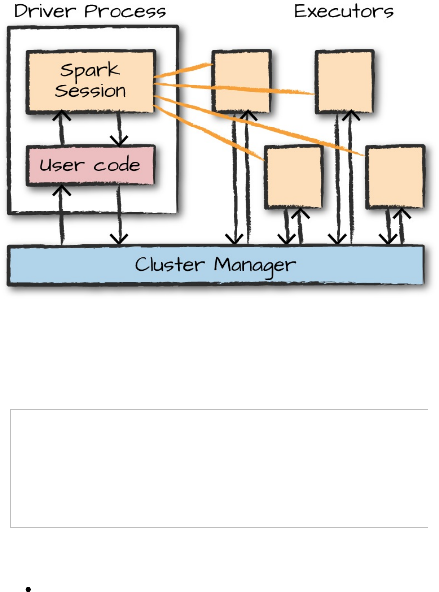
Figure 2-1. The architecture of a Spark Application
In Figure 2-1, we can see the driver on the left and four executors on the
right. In this diagram, we removed the concept of cluster nodes. The user can
specify how many executors should fall on each node through configurations.
NOTE
Spark, in addition to its cluster mode, also has a local mode. The driver and executors are
simply processes, which means that they can live on the same machine or different
machines. In local mode, the driver and executurs run (as threads) on your individual
computer instead of a cluster. We wrote this book with local mode in mind, so you should
be able to run everything on a single machine.
Here are the key points to understand about Spark Applications at this point:
Spark employs a cluster manager that keeps track of the resources
available.

The driver process is responsible for executing the driver program’s
commands across the executors to complete a given task.
The executors, for the most part, will always be running Spark code.
However, the driver can be “driven” from a number of different languages
through Spark’s language APIs. Let’s take a look at those in the next section.
Spark’s Language APIs
Spark’s language APIs make it possible for you to run Spark code using
various programming languages. For the most part, Spark presents some core
“concepts” in every language; these concepts are then translated into Spark
code that runs on the cluster of machines. If you use just the Structured APIs,
you can expect all languages to have similar performance characteristics.
Here’s a brief rundown:
Scala
Spark is primarily written in Scala, making it Spark’s “default” language.
This book will include Scala code examples wherever relevant.
Java
Even though Spark is written in Scala, Spark’s authors have been careful
to ensure that you can write Spark code in Java. This book will focus
primarily on Scala but will provide Java examples where relevant.
Python
Python supports nearly all constructs that Scala supports. This book will
include Python code examples whenever we include Scala code examples
and a Python API exists.
SQL
Spark supports a subset of the ANSI SQL 2003 standard. This makes it
easy for analysts and non-programmers to take advantage of the big data
powers of Spark. This book includes SQL code examples wherever
relevant.

R
Spark has two commonly used R libraries: one as a part of Spark core
(SparkR) and another as an R community-driven package (sparklyr). We
cover both of these integrations in Chapter 32.
Figure 2-2 presents a simple illustration of this relationship.
Figure 2-2. The relationship between the SparkSession and Spark’s Language API
Each language API maintains the same core concepts that we described
earlier. There is a SparkSession object available to the user, which is the
entrance point to running Spark code. When using Spark from Python or R,
you don’t write explicit JVM instructions; instead, you write Python and R
code that Spark translates into code that it then can run on the executor
JVMs.
Spark’s APIs
Although you can drive Spark from a variety of languages, what it makes
available in those languages is worth mentioning. Spark has two fundamental
sets of APIs: the low-level “unstructured” APIs, and the higher-level
structured APIs. We discuss both in this book, but these introductory chapters
will focus primarily on the higher-level structured APIs.
Starting Spark

Thus far, we covered the basic concepts of Spark Applications. This has all
been conceptual in nature. When we actually go about writing our Spark
Application, we are going to need a way to send user commands and data to
it. We do that by first creating a SparkSession.
NOTE
To do this, we will start Spark’s local mode, just like we did in Chapter 1. This means
running ./bin/spark-shell to access the Scala console to start an interactive session.
You can also start the Python console by using ./bin/pyspark. This starts an interactive
Spark Application. There is also a process for submitting standalone applications to Spark
called spark-submit, whereby you can submit a precompiled application to Spark. We’ll
show you how to do that in Chapter 3.
When you start Spark in this interactive mode, you implicitly create a
SparkSession that manages the Spark Application. When you start it through
a standalone application, you must create the SparkSession object yourself in
your application code.
The SparkSession
As discussed in the beginning of this chapter, you control your Spark
Application through a driver process called the SparkSession. The
SparkSession instance is the way Spark executes user-defined manipulations
across the cluster. There is a one-to-one correspondence between a
SparkSession and a Spark Application. In Scala and Python, the variable is
available as spark when you start the console. Let’s go ahead and look at the
SparkSession in both Scala and/or Python:
spark
In Scala, you should see something like the following:
res0: org.apache.spark.sql.SparkSession = org.apache.spark.sql.SparkSession@...
In Python you’ll see something like this:
<pyspark.sql.session.SparkSession at 0x7efda4c1ccd0>
Let’s now perform the simple task of creating a range of numbers. This range
of numbers is just like a named column in a spreadsheet:
// in Scala
val myRange = spark.range(1000).toDF("number")
# in Python
myRange = spark.range(1000).toDF("number")
You just ran your first Spark code! We created a DataFrame with one
column containing 1,000 rows with values from 0 to 999. This range of
numbers represents a distributed collection. When run on a cluster, each part
of this range of numbers exists on a different executor. This is a Spark
DataFrame.
DataFrames
A DataFrame is the most common Structured API and simply represents a
table of data with rows and columns. The list that defines the columns and the
types within those columns is called the schema. You can think of a
DataFrame as a spreadsheet with named columns. Figure 2-3 illustrates the
fundamental difference: a spreadsheet sits on one computer in one specific
location, whereas a Spark DataFrame can span thousands of computers. The
reason for putting the data on more than one computer should be intuitive:
either the data is too large to fit on one machine or it would simply take too
long to perform that computation on one machine.

Figure 2-3. Distributed versus single-machine analysis
The DataFrame concept is not unique to Spark. R and Python both have
similar concepts. However, Python/R DataFrames (with some exceptions)
exist on one machine rather than multiple machines. This limits what you can
do with a given DataFrame to the resources that exist on that specific
machine. However, because Spark has language interfaces for both Python
and R, it’s quite easy to convert Pandas (Python) DataFrames to Spark
DataFrames, and R DataFrames to Spark DataFrames.
NOTE
Spark has several core abstractions: Datasets, DataFrames, SQL Tables, and Resilient
Distributed Datasets (RDDs). These different abstractions all represent distributed
collections of data. The easiest and most efficient are DataFrames, which are available in
all languages. We cover Datasets at the end of Part II, and RDDs in Part III.
Partitions
To allow every executor to perform work in parallel, Spark breaks up the data
into chunks called partitions. A partition is a collection of rows that sit on
one physical machine in your cluster. A DataFrame’s partitions represent
how the data is physically distributed across the cluster of machines during
execution. If you have one partition, Spark will have a parallelism of only
one, even if you have thousands of executors. If you have many partitions but
only one executor, Spark will still have a parallelism of only one because
there is only one computation resource.
An important thing to note is that with DataFrames you do not (for the most
part) manipulate partitions manually or individually. You simply specify
high-level transformations of data in the physical partitions, and Spark
determines how this work will actually execute on the cluster. Lower-level
APIs do exist (via the RDD interface), and we cover those in Part III.
Transformations
In Spark, the core data structures are immutable, meaning they cannot be
changed after they’re created. This might seem like a strange concept at first:
if you cannot change it, how are you supposed to use it? To “change” a
DataFrame, you need to instruct Spark how you would like to modify it to do
what you want. These instructions are called transformations. Let’s perform a
simple transformation to find all even numbers in our current DataFrame:
// in Scala
val divisBy2 = myRange.where("number % 2 = 0")
# in Python
divisBy2 = myRange.where("number % 2 = 0")
Notice that these return no output. This is because we specified only an
abstract transformation, and Spark will not act on transformations until we
call an action (we discuss this shortly). Transformations are the core of how
you express your business logic using Spark. There are two types of
transformations: those that specify narrow dependencies, and those that
specify wide dependencies.
Transformations consisting of narrow dependencies (we’ll call them narrow
transformations) are those for which each input partition will contribute to
only one output partition. In the preceding code snippet, the where statement
specifies a narrow dependency, where only one partition contributes to at
most one output partition, as you can see in Figure 2-4.
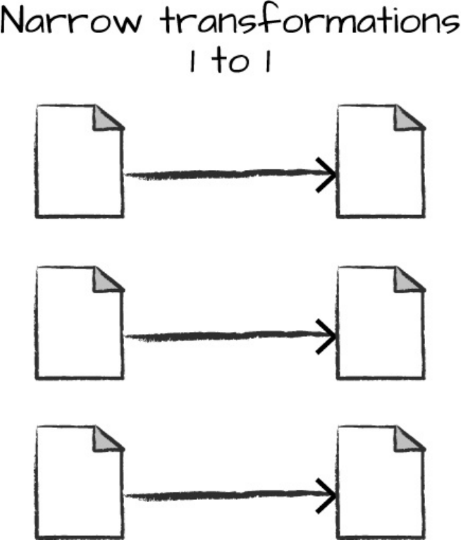
Figure 2-4. A narrow dependency
A wide dependency (or wide transformation) style transformation will have
input partitions contributing to many output partitions. You will often hear
this referred to as a shuffle whereby Spark will exchange partitions across the
cluster. With narrow transformations, Spark will automatically perform an
operation called pipelining, meaning that if we specify multiple filters on
DataFrames, they’ll all be performed in-memory. The same cannot be said
for shuffles. When we perform a shuffle, Spark writes the results to disk.
Wide transformations are illustrated in Figure 2-5.
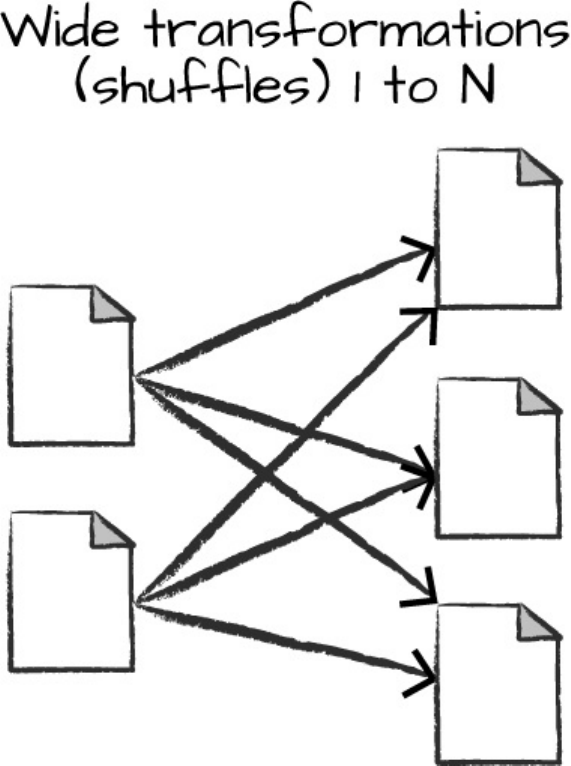
Figure 2-5. A wide dependency
You’ll see a lot of discussion about shuffle optimization across the web
because it’s an important topic, but for now, all you need to understand is that
there are two kinds of transformations. You now can see how transformations
are simply ways of specifying different series of data manipulation. This
leads us to a topic called lazy evaluation.
Lazy Evaluation
Lazy evaulation means that Spark will wait until the very last moment to
execute the graph of computation instructions. In Spark, instead of modifying
the data immediately when you express some operation, you build up a plan
of transformations that you would like to apply to your source data. By

waiting until the last minute to execute the code, Spark compiles this plan
from your raw DataFrame transformations to a streamlined physical plan that
will run as efficiently as possible across the cluster. This provides immense
benefits because Spark can optimize the entire data flow from end to end. An
example of this is something called predicate pushdown on DataFrames. If
we build a large Spark job but specify a filter at the end that only requires us
to fetch one row from our source data, the most efficient way to execute this
is to access the single record that we need. Spark will actually optimize this
for us by pushing the filter down automatically.
Actions
Transformations allow us to build up our logical transformation plan. To
trigger the computation, we run an action. An action instructs Spark to
compute a result from a series of transformations. The simplest action is
count, which gives us the total number of records in the DataFrame:
divisBy2.count()
The output of the preceding code should be 500. Of course, count is not the
only action. There are three kinds of actions:
Actions to view data in the console
Actions to collect data to native objects in the respective language
Actions to write to output data sources
In specifying this action, we started a Spark job that runs our filter
transformation (a narrow transformation), then an aggregation (a wide
transformation) that performs the counts on a per partition basis, and then a
collect, which brings our result to a native object in the respective language.
You can see all of this by inspecting the Spark UI, a tool included in Spark
with which you can monitor the Spark jobs running on a cluster.
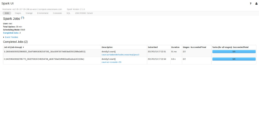
Spark UI
You can monitor the progress of a job through the Spark web UI. The Spark
UI is available on port 4040 of the driver node. If you are running in local
mode, this will be http://localhost:4040. The Spark UI displays information
on the state of your Spark jobs, its environment, and cluster state. It’s very
useful, especially for tuning and debugging. Figure 2-6 shows an example UI
for a Spark job where two stages containing nine tasks were executed.
Figure 2-6. The Spark UI
This chapter will not go into detail about Spark job execution and the Spark
UI. We will cover that in Chapter 18. At this point, all you need to
understand is that a Spark job represents a set of transformations triggered by
an individual action, and you can monitor that job from the Spark UI.
An End-to-End Example
In the previous example, we created a DataFrame of a range of numbers; not
exactly groundbreaking big data. In this section, we will reinforce everything
we learned previously in this chapter with a more realistic example, and
explain step by step what is happening under the hood. We’ll use Spark to
analyze some flight data from the United States Bureau of Transportation
statistics.
Inside of the CSV folder, you’ll see that we have a number of files. There’s
also a number of other folders with different file formats, which we discuss in
Chapter 9. For now, let’s focus on the CSV files.
Each file has a number of rows within it. These files are CSV files, meaning
that they’re a semi-structured data format, with each row in the file
representing a row in our future DataFrame:
$ head /data/flight-data/csv/2015-summary.csv
DEST_COUNTRY_NAME,ORIGIN_COUNTRY_NAME,count
United States,Romania,15
United States,Croatia,1
United States,Ireland,344
Spark includes the ability to read and write from a large number of data
sources. To read this data, we will use a DataFrameReader that is associated
with our SparkSession. In doing so, we will specify the file format as well as
any options we want to specify. In our case, we want to do something called
schema inference, which means that we want Spark to take a best guess at
what the schema of our DataFrame should be. We also want to specify that
the first row is the header in the file, so we’ll specify that as an option, too.
To get the schema information, Spark reads in a little bit of the data and then
attempts to parse the types in those rows according to the types available in
Spark. You also have the option of strictly specifying a schema when you
read in data (which we recommend in production scenarios):
// in Scala
val flightData2015 = spark
.read
.option("inferSchema", "true")
.option("header", "true")
.csv("/data/flight-data/csv/2015-summary.csv")
# in Python
flightData2015 = spark\
.read\
.option("inferSchema", "true")\
.option("header", "true")\
.csv("/data/flight-data/csv/2015-summary.csv")
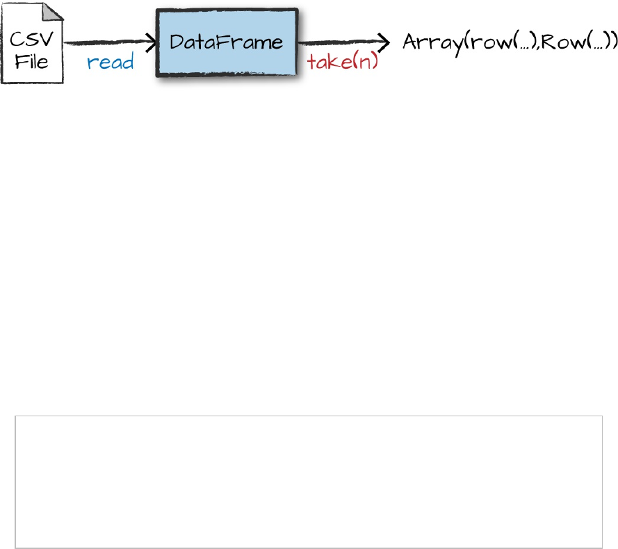
Each of these DataFrames (in Scala and Python) have a set of columns with
an unspecified number of rows. The reason the number of rows is unspecified
is because reading data is a transformation, and is therefore a lazy operation.
Spark peeked at only a couple of rows of data to try to guess what types each
column should be. Figure 2-7 provides an illustration of the CSV file being
read into a DataFrame and then being converted into a local array or list of
rows.
Figure 2-7. Reading a CSV file into a DataFrame and converting it to a local array or list of rows
If we perform the take action on the DataFrame, we will be able to see the
same results that we saw before when we used the command line:
flightData2015.take(3)
Array([United States,Romania,15], [United States,Croatia...
Let’s specify some more transformations! Now, let’s sort our data according
to the count column, which is an integer type. Figure 2-8 illustrates this
process.
NOTE
Remember, sort does not modify the DataFrame. We use sort as a transformation that
returns a new DataFrame by transforming the previous DataFrame. Let’s illustrate what’s
happening when we call take on that resulting DataFrame (Figure 2-8).
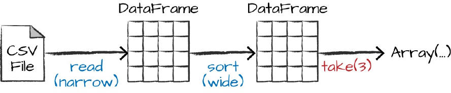
Figure 2-8. Reading, sorting, and collecting a DataFrame
Nothing happens to the data when we call sort because it’s just a
transformation. However, we can see that Spark is building up a plan for how
it will execute this across the cluster by looking at the explain plan. We can
call explain on any DataFrame object to see the DataFrame’s lineage (or
how Spark will execute this query):
flightData2015.sort("count").explain()
== Physical Plan ==
*Sort [count#195 ASC NULLS FIRST], true, 0
+- Exchange rangepartitioning(count#195 ASC NULLS FIRST, 200)
+- *FileScan csv [DEST_COUNTRY_NAME#193,ORIGIN_COUNTRY_NAME#194,count#195]
...
Congratulations, you’ve just read your first explain plan! Explain plans are a
bit arcane, but with a bit of practice it becomes second nature. You can read
explain plans from top to bottom, the top being the end result, and the bottom
being the source(s) of data. In this case, take a look at the first keywords. You
will see sort, exchange, and FileScan. That’s because the sort of our data is
actually a wide transformation because rows will need to be compared with
one another. Don’t worry too much about understanding everything about
explain plans at this point, they can just be helpful tools for debugging and
improving your knowledge as you progress with Spark.
Now, just like we did before, we can specify an action to kick off this plan.
However, before doing that, we’re going to set a configuration. By default,
when we perform a shuffle, Spark outputs 200 shuffle partitions. Let’s set
this value to 5 to reduce the number of the output partitions from the shuffle:
spark.conf.set("spark.sql.shuffle.partitions", "5")
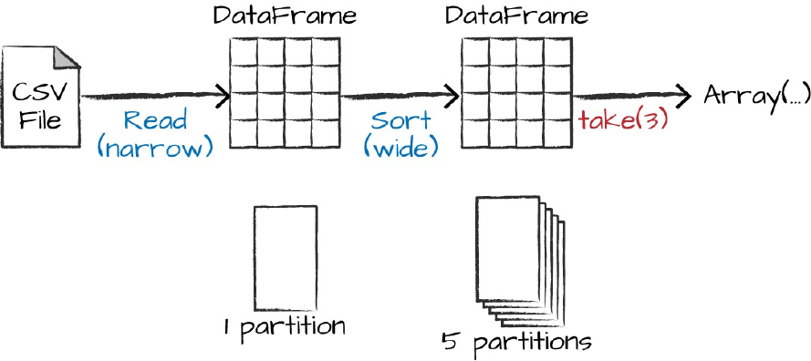
flightData2015.sort("count").take(2)
... Array([United States,Singapore,1], [Moldova,United States,1])
Figure 2-9 illustrates this operation. Notice that in addition to the logical
transformations, we include the physical partition count, as well.
Figure 2-9. The process of logical and physical DataFrame manipulation
The logical plan of transformations that we build up defines a lineage for the
DataFrame so that at any given point in time, Spark knows how to recompute
any partition by performing all of the operations it had before on the same
input data. This sits at the heart of Spark’s programming model—functional
programming where the same inputs always result in the same outputs when
the transformations on that data stay constant.
We do not manipulate the physical data; instead, we configure physical
execution characteristics through things like the shuffle partitions parameter
that we set a few moments ago. We ended up with five output partitions
because that’s the value we specified in the shuffle partition. You can change
this to help control the physical execution characteristics of your Spark jobs.
Go ahead and experiment with different values and see the number of
partitions yourself. In experimenting with different values, you should see
drastically different runtimes. Remember that you can monitor the job
progress by navigating to the Spark UI on port 4040 to see the physical and
logical execution characteristics of your jobs.
DataFrames and SQL
We worked through a simple transformation in the previous example, let’s
now work through a more complex one and follow along in both DataFrames
and SQL. Spark can run the same transformations, regardless of the language,
in the exact same way. You can express your business logic in SQL or
DataFrames (either in R, Python, Scala, or Java) and Spark will compile that
logic down to an underlying plan (that you can see in the explain plan) before
actually executing your code. With Spark SQL, you can register any
DataFrame as a table or view (a temporary table) and query it using pure
SQL. There is no performance difference between writing SQL queries or
writing DataFrame code, they both “compile” to the same underlying plan
that we specify in DataFrame code.
You can make any DataFrame into a table or view with one simple method
call:
flightData2015.createOrReplaceTempView("flight_data_2015")
Now we can query our data in SQL. To do so, we’ll use the spark.sql
function (remember, spark is our SparkSession variable) that conveniently
returns a new DataFrame. Although this might seem a bit circular in logic—
that a SQL query against a DataFrame returns another DataFrame—it’s
actually quite powerful. This makes it possible for you to specify
transformations in the manner most convenient to you at any given point in
time and not sacrifice any efficiency to do so! To understand that this is
happening, let’s take a look at two explain plans:
// in Scala
val sqlWay = spark.sql("""
SELECT DEST_COUNTRY_NAME, count(1)
FROM flight_data_2015
GROUP BY DEST_COUNTRY_NAME
""")
val dataFrameWay = flightData2015
.groupBy('DEST_COUNTRY_NAME)
.count()
sqlWay.explain
dataFrameWay.explain
# in Python
sqlWay = spark.sql("""
SELECT DEST_COUNTRY_NAME, count(1)
FROM flight_data_2015
GROUP BY DEST_COUNTRY_NAME
""")
dataFrameWay = flightData2015\
.groupBy("DEST_COUNTRY_NAME")\
.count()
sqlWay.explain()
dataFrameWay.explain()
== Physical Plan ==
*HashAggregate(keys=[DEST_COUNTRY_NAME#182], functions=[count(1)])
+- Exchange hashpartitioning(DEST_COUNTRY_NAME#182, 5)
+- *HashAggregate(keys=[DEST_COUNTRY_NAME#182], functions=[partial_count(1)])
+- *FileScan csv [DEST_COUNTRY_NAME#182] ...
== Physical Plan ==
*HashAggregate(keys=[DEST_COUNTRY_NAME#182], functions=[count(1)])
+- Exchange hashpartitioning(DEST_COUNTRY_NAME#182, 5)
+- *HashAggregate(keys=[DEST_COUNTRY_NAME#182], functions=[partial_count(1)])
+- *FileScan csv [DEST_COUNTRY_NAME#182] ...
Notice that these plans compile to the exact same underlying plan!
Let’s pull out some interesting statistics from our data. One thing to
understand is that DataFrames (and SQL) in Spark already have a huge
number of manipulations available. There are hundreds of functions that you
can use and import to help you resolve your big data problems faster. We will
use the max function, to establish the maximum number of flights to and from
any given location. This just scans each value in the relevant column in the
DataFrame and checks whether it’s greater than the previous values that have
been seen. This is a transformation, because we are effectively filtering down
to one row. Let’s see what that looks like:
spark.sql("SELECT max(count) from flight_data_2015").take(1)
// in Scala
import org.apache.spark.sql.functions.max
flightData2015.select(max("count")).take(1)
# in Python
from pyspark.sql.functions import max
flightData2015.select(max("count")).take(1)
Great, that’s a simple example that gives a result of 370,002. Let’s perform
something a bit more complicated and find the top five destination countries
in the data. This is our first multi-transformation query, so we’ll take it step
by step. Let’s begin with a fairly straightforward SQL aggregation:
// in Scala
val maxSql = spark.sql("""
SELECT DEST_COUNTRY_NAME, sum(count) as destination_total
FROM flight_data_2015
GROUP BY DEST_COUNTRY_NAME
ORDER BY sum(count) DESC
LIMIT 5
""")
maxSql.show()
# in Python
maxSql = spark.sql("""
SELECT DEST_COUNTRY_NAME, sum(count) as destination_total
FROM flight_data_2015
GROUP BY DEST_COUNTRY_NAME
ORDER BY sum(count) DESC
LIMIT 5
""")
maxSql.show()
+-----------------+-----------------+
|DEST_COUNTRY_NAME|destination_total|
+-----------------+-----------------+
| United States| 411352|
| Canada| 8399|
| Mexico| 7140|
| United Kingdom| 2025|
| Japan| 1548|
+-----------------+-----------------+
Now, let’s move to the DataFrame syntax that is semantically similar but
slightly different in implementation and ordering. But, as we mentioned, the
underlying plans for both of them are the same. Let’s run the queries and see
their results as a sanity check:
// in Scala
import org.apache.spark.sql.functions.desc
flightData2015
.groupBy("DEST_COUNTRY_NAME")
.sum("count")
.withColumnRenamed("sum(count)", "destination_total")
.sort(desc("destination_total"))
.limit(5)
.show()
# in Python
from pyspark.sql.functions import desc
flightData2015\
.groupBy("DEST_COUNTRY_NAME")\
.sum("count")\
.withColumnRenamed("sum(count)", "destination_total")\
.sort(desc("destination_total"))\
.limit(5)\
.show()
+-----------------+-----------------+
|DEST_COUNTRY_NAME|destination_total|
+-----------------+-----------------+
| United States| 411352|
| Canada| 8399|
| Mexico| 7140|
| United Kingdom| 2025|
| Japan| 1548|
+-----------------+-----------------+
Now there are seven steps that take us all the way back to the source data.
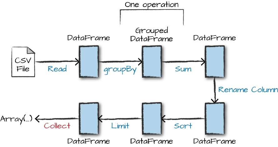
You can see this in the explain plan on those DataFrames. Figure 2-10 shows
the set of steps that we perform in “code.” The true execution plan (the one
visible in explain) will differ from that shown in Figure 2-10 because of
optimizations in the physical execution; however, the llustration is as good of
a starting point as any. This execution plan is a directed acyclic graph (DAG)
of transformations, each resulting in a new immutable DataFrame, on which
we call an action to generate a result.
Figure 2-10. The entire DataFrame transformation flow
The first step is to read in the data. We defined the DataFrame previously but,
as a reminder, Spark does not actually read it in until an action is called on
that DataFrame or one derived from the original DataFrame.
The second step is our grouping; technically when we call groupBy, we end
up with a RelationalGroupedDataset, which is a fancy name for a
DataFrame that has a grouping specified but needs the user to specify an
aggregation before it can be queried further. We basically specified that we’re
going to be grouping by a key (or set of keys) and that now we’re going to
perform an aggregation over each one of those keys.
Therefore, the third step is to specify the aggregation. Let’s use the sum
aggregation method. This takes as input a column expression or, simply, a
column name. The result of the sum method call is a new DataFrame. You’ll
see that it has a new schema but that it does know the type of each column.
It’s important to reinforce (again!) that no computation has been performed.
This is simply another transformation that we’ve expressed, and Spark is
simply able to trace our type information through it.
The fourth step is a simple renaming. We use the withColumnRenamed
method that takes two arguments, the original column name and the new
column name. Of course, this doesn’t perform computation: this is just
another transformation!
The fifth step sorts the data such that if we were to take results off of the top
of the DataFrame, they would have the largest values in the
destination_total column.
You likely noticed that we had to import a function to do this, the desc
function. You might also have noticed that desc does not return a string but a
Column. In general, many DataFrame methods will accept strings (as column
names) or Column types or expressions. Columns and expressions are actually
the exact same thing.
Penultimately, we’ll specify a limit. This just specifies that we only want to
return the first five values in our final DataFrame instead of all the data.
The last step is our action! Now we actually begin the process of collecting
the results of our DataFrame, and Spark will give us back a list or array in the
language that we’re executing. To reinforce all of this, let’s look at the
explain plan for the previous query:
// in Scala
flightData2015
.groupBy("DEST_COUNTRY_NAME")
.sum("count")
.withColumnRenamed("sum(count)", "destination_total")
.sort(desc("destination_total"))
.limit(5)
.explain()
# in Python
flightData2015\
.groupBy("DEST_COUNTRY_NAME")\
.sum("count")\
.withColumnRenamed("sum(count)", "destination_total")\
.sort(desc("destination_total"))\
.limit(5)\
.explain()
== Physical Plan ==
TakeOrderedAndProject(limit=5, orderBy=[destination_total#16194L DESC], outpu...
+- *HashAggregate(keys=[DEST_COUNTRY_NAME#7323], functions=[sum(count#7325L)])
+- Exchange hashpartitioning(DEST_COUNTRY_NAME#7323, 5)
+- *HashAggregate(keys=[DEST_COUNTRY_NAME#7323], functions=[partial_sum...
+- InMemoryTableScan [DEST_COUNTRY_NAME#7323, count#7325L]
+- InMemoryRelation [DEST_COUNTRY_NAME#7323, ORIGIN_COUNTRY_NA...
+- *Scan csv [DEST_COUNTRY_NAME#7578,ORIGIN_COUNTRY_NAME...
Although this explain plan doesn’t match our exact “conceptual plan,” all of
the pieces are there. You can see the limit statement as well as the orderBy
(in the first line). You can also see how our aggregation happens in two
phases, in the partial_sum calls. This is because summing a list of numbers
is commutative, and Spark can perform the sum, partition by partition. Of
course we can see how we read in the DataFrame, as well.
Naturally, we don’t always need to collect the data. We can also write it out
to any data source that Spark supports. For instance, suppose we want to store
the information in a database like PostgreSQL or write them out to another
file.
Conclusion
This chapter introduced the basics of Apache Spark. We talked about
transformations and actions, and how Spark lazily executes a DAG of
transformations in order to optimize the execution plan on DataFrames. We
also discussed how data is organized into partitions and set the stage for
working with more complex transformations. In Chapter 3 we take you on a
tour of the vast Spark ecosystem and look at some more advanced concepts
and tools that are available in Spark, from streaming to machine learning.

Chapter 3. A Tour of Spark’s
Toolset
In Chapter 2, we introduced Spark’s core concepts, like transformations and
actions, in the context of Spark’s Structured APIs. These simple conceptual
building blocks are the foundation of Apache Spark’s vast ecosystem of tools
and libraries (Figure 3-1). Spark is composed of these primitives—the lower-
level APIs and the Structured APIs—and then a series of standard libraries
for additional functionality.
Figure 3-1. Spark’s toolset
Spark’s libraries support a variety of different tasks, from graph analysis and
machine learning to streaming and integrations with a host of computing and
storage systems. This chapter presents a whirlwind tour of much of what
Spark has to offer, including some of the APIs we have not yet covered and a
few of the main libraries. For each section, you will find more detailed
information in other parts of this book; our purpose here is provide you with
an overview of what’s possible.

This chapter covers the following:
Running production applications with spark-submit
Datasets: type-safe APIs for structured data
Structured Streaming
Machine learning and advanced analytics
Resilient Distributed Datasets (RDD): Spark’s low level APIs
SparkR
The third-party package ecosystem
After you’ve taken the tour, you’ll be able to jump to the corresponding parts
of the book to find answers to your questions about particular topics.
Running Production Applications
Spark makes it easy to develop and create big data programs. Spark also
makes it easy to turn your interactive exploration into production applications
with spark-submit, a built-in command-line tool. spark-submit does one
thing: it lets you send your application code to a cluster and launch it to
execute there. Upon submission, the application will run until it exits
(completes the task) or encounters an error. You can do this with all of
Spark’s support cluster managers including Standalone, Mesos, and YARN.
spark-submit offers several controls with which you can specify the
resources your application needs as well as how it should be run and its
command-line arguments.
You can write applications in any of Spark’s supported languages and then
submit them for execution. The simplest example is running an application
on your local machine. We’ll show this by running a sample Scala
application that comes with Spark, using the following command in the
directory where you downloaded Spark:
./bin/spark-submit \
--class org.apache.spark.examples.SparkPi \
--master local \
./examples/jars/spark-examples_2.11-2.2.0.jar 10
This sample application calculates the digits of pi to a certain level of
estimation. Here, we’ve told spark-submit that we want to run on our local
machine, which class and which JAR we would like to run, and some
command-line arguments for that class.
We can also run a Python version of the application using the following
command:
./bin/spark-submit \
--master local \
./examples/src/main/python/pi.py 10
By changing the master argument of spark-submit, we can also submit the
same application to a cluster running Spark’s standalone cluster manager,
Mesos or YARN.
spark-submit will come in handy to run many of the examples we’ve
packaged with this book. In the rest of this chapter, we’ll go through
examples of some APIs that we haven’t yet seen in our introduction to Spark.
Datasets: Type-Safe Structured APIs
The first API we’ll describe is a type-safe version of Spark’s structured API
called Datasets, for writing statically typed code in Java and Scala. The
Dataset API is not available in Python and R, because those languages are
dynamically typed.
Recall that DataFrames, which we saw in the previous chapter, are a
distributed collection of objects of type Row that can hold various types of
tabular data. The Dataset API gives users the ability to assign a Java/Scala
class to the records within a DataFrame and manipulate it as a collection of
typed objects, similar to a Java ArrayList or Scala Seq. The APIs available
on Datasets are type-safe, meaning that you cannot accidentally view the
objects in a Dataset as being of another class than the class you put in
initially. This makes Datasets especially attractive for writing large
applications, with which multiple software engineers must interact through
well-defined interfaces.
The Dataset class is parameterized with the type of object contained inside:
Dataset<T> in Java and Dataset[T] in Scala. For example, a
Dataset[Person] will be guaranteed to contain objects of class Person. As
of Spark 2.0, the supported types are classes following the JavaBean pattern
in Java and case classes in Scala. These types are restricted because Spark
needs to be able to automatically analyze the type T and create an appropriate
schema for the tabular data within your Dataset.
One great thing about Datasets is that you can use them only when you need
or want to. For instance, in the following example, we’ll define our own data
type and manipulate it via arbitrary map and filter functions. After we’ve
performed our manipulations, Spark can automatically turn it back into a
DataFrame, and we can manipulate it further by using the hundreds of
functions that Spark includes. This makes it easy to drop down to lower level,
perform type-safe coding when necessary, and move higher up to SQL for
more rapid analysis. Here is a small example showing how you can use both
type-safe functions and DataFrame-like SQL expressions to quickly write
business logic:
// in Scala
case class Flight(DEST_COUNTRY_NAME: String,
ORIGIN_COUNTRY_NAME: String,
count: BigInt)
val flightsDF = spark.read
.parquet("/data/flight-data/parquet/2010-summary.parquet/")
val flights = flightsDF.as[Flight]
One final advantage is that when you call collect or take on a Dataset, it
will collect objects of the proper type in your Dataset, not DataFrame Rows.
This makes it easy to get type safety and securely perform manipulation in a
distributed and a local manner without code changes:
// in Scala
flights
.filter(flight_row => flight_row.ORIGIN_COUNTRY_NAME != "Canada")
.map(flight_row => flight_row)
.take(5)
flights
.take(5)
.filter(flight_row => flight_row.ORIGIN_COUNTRY_NAME != "Canada")
.map(fr => Flight(fr.DEST_COUNTRY_NAME, fr.ORIGIN_COUNTRY_NAME, fr.count + 5))
We cover Datasets in depth in Chapter 11.
Structured Streaming
Structured Streaming is a high-level API for stream processing that became
production-ready in Spark 2.2. With Structured Streaming, you can take the
same operations that you perform in batch mode using Spark’s structured
APIs and run them in a streaming fashion. This can reduce latency and allow
for incremental processing. The best thing about Structured Streaming is that
it allows you to rapidly and quickly extract value out of streaming systems
with virtually no code changes. It also makes it easy to conceptualize because
you can write your batch job as a way to prototype it and then you can
convert it to a streaming job. The way all of this works is by incrementally
processing that data.
Let’s walk through a simple example of how easy it is to get started with
Structured Streaming. For this, we will use a retail dataset, one that has
specific dates and times for us to be able to use. We will use the “by-day” set
of files, in which one file represents one day of data.
We put it in this format to simulate data being produced in a consistent and
regular manner by a different process. This is retail data so imagine that these
are being produced by retail stores and sent to a location where they will be
read by our Structured Streaming job.
It’s also worth sharing a sample of the data so you can reference what the
data looks like:
InvoiceNo,StockCode,Description,Quantity,InvoiceDate,UnitPrice,CustomerID,Countr
y
536365,85123A,WHITE HANGING HEART T-LIGHT HOLDER,6,2010-12-01
08:26:00,2.55,17...
536365,71053,WHITE METAL LANTERN,6,2010-12-01 08:26:00,3.39,17850.0,United
Kin...
536365,84406B,CREAM CUPID HEARTS COAT HANGER,8,2010-12-01 08:26:00,2.75,17850...
To ground this, let’s first analyze the data as a static dataset and create a
DataFrame to do so. We’ll also create a schema from this static dataset (there
are ways of using schema inference with streaming that we will touch on in
Part V):
// in Scala
val staticDataFrame = spark.read.format("csv")
.option("header", "true")
.option("inferSchema", "true")
.load("/data/retail-data/by-day/*.csv")
staticDataFrame.createOrReplaceTempView("retail_data")
val staticSchema = staticDataFrame.schema
# in Python
staticDataFrame = spark.read.format("csv")\
.option("header", "true")\
.option("inferSchema", "true")\
.load("/data/retail-data/by-day/*.csv")
staticDataFrame.createOrReplaceTempView("retail_data")
staticSchema = staticDataFrame.schema
Because we’re working with time–series data, it’s worth mentioning how we
might go along grouping and aggregating our data. In this example we’ll take
a look at the sale hours during which a given customer (identified by
CustomerId) makes a large purchase. For example, let’s add a total cost
column and see on what days a customer spent the most.
The window function will include all data from each day in the aggregation.
It’s simply a window over the time–series column in our data. This is a
helpful tool for manipulating date and timestamps because we can specify our
requirements in a more human form (via intervals), and Spark will group all
of them together for us:
// in Scala
import org.apache.spark.sql.functions.{window, column, desc, col}
staticDataFrame
.selectExpr(
"CustomerId",
"(UnitPrice * Quantity) as total_cost",
"InvoiceDate")
.groupBy(
col("CustomerId"), window(col("InvoiceDate"), "1 day"))
.sum("total_cost")
.show(5)
# in Python
from pyspark.sql.functions import window, column, desc, col
staticDataFrame\
.selectExpr(
"CustomerId",
"(UnitPrice * Quantity) as total_cost",
"InvoiceDate")\
.groupBy(
col("CustomerId"), window(col("InvoiceDate"), "1 day"))\
.sum("total_cost")\
.show(5)
It’s worth mentioning that you can also run this as SQL code, just as we saw
in the previous chapter.
Here’s a sample of the output that you’ll see:
+----------+--------------------+------------------+
|CustomerId| window| sum(total_cost)|
+----------+--------------------+------------------+
| 17450.0|[2011-09-20 00:00...| 71601.44|
...
| null|[2011-12-08 00:00...|31975.590000000007|
+----------+--------------------+------------------+
The null values represent the fact that we don’t have a customerId for some
transactions.
That’s the static DataFrame version; there shouldn’t be any big surprises in
there if you’re familiar with the syntax.
Because you’re likely running this in local mode, it’s a good practice to set
the number of shuffle partitions to something that’s going to be a better fit for
local mode. This configuration specifies the number of partitions that should
be created after a shuffle. By default, the value is 200, but because there
aren’t many executors on this machine, it’s worth reducing this to 5. We did
this same operation in Chapter 2, so if you don’t remember why this is
important, feel free to flip back to review.
spark.conf.set("spark.sql.shuffle.partitions", "5")
Now that we’ve seen how that works, let’s take a look at the streaming code!
You’ll notice that very little actually changes about the code. The biggest
change is that we used readStream instead of read, additionally you’ll notice
the maxFilesPerTrigger option, which simply specifies the number of files we
should read in at once. This is to make our demonstration more “streaming,”
and in a production scenario this would probably be omitted.
val streamingDataFrame = spark.readStream
.schema(staticSchema)
.option("maxFilesPerTrigger", 1)
.format("csv")
.option("header", "true")
.load("/data/retail-data/by-day/*.csv")
# in Python
streamingDataFrame = spark.readStream\
.schema(staticSchema)\
.option("maxFilesPerTrigger", 1)\
.format("csv")\
.option("header", "true")\
.load("/data/retail-data/by-day/*.csv")
Now we can see whether our DataFrame is streaming:
streamingDataFrame.isStreaming // returns true
Let’s set up the same business logic as the previous DataFrame manipulation.
We’ll perform a summation in the process:
// in Scala
val purchaseByCustomerPerHour = streamingDataFrame
.selectExpr(
"CustomerId",
"(UnitPrice * Quantity) as total_cost",
"InvoiceDate")
.groupBy(
$"CustomerId", window($"InvoiceDate", "1 day"))
.sum("total_cost")
# in Python
purchaseByCustomerPerHour = streamingDataFrame\
.selectExpr(
"CustomerId",
"(UnitPrice * Quantity) as total_cost",
"InvoiceDate")\
.groupBy(
col("CustomerId"), window(col("InvoiceDate"), "1 day"))\
.sum("total_cost")
This is still a lazy operation, so we will need to call a streaming action to start
the execution of this data flow.
Streaming actions are a bit different from our conventional static action
because we’re going to be populating data somewhere instead of just calling
something like count (which doesn’t make any sense on a stream anyways).
The action we will use will output to an in-memory table that we will update
after each trigger. In this case, each trigger is based on an individual file (the
read option that we set). Spark will mutate the data in the in-memory table
such that we will always have the highest value as specified in our previous
aggregation:
// in Scala
purchaseByCustomerPerHour.writeStream
.format("memory") // memory = store in-memory table
.queryName("customer_purchases") // the name of the in-memory table
.outputMode("complete") // complete = all the counts should be in the table
.start()
# in Python
purchaseByCustomerPerHour.writeStream\
.format("memory")\
.queryName("customer_purchases")\
.outputMode("complete")\
.start()
When we start the stream, we can run queries against it to debug what our
result will look like if we were to write this out to a production sink:
// in Scala
spark.sql("""
SELECT *
FROM customer_purchases
ORDER BY `sum(total_cost)` DESC
""")
.show(5)
# in Python
spark.sql("""
SELECT *
FROM customer_purchases
ORDER BY `sum(total_cost)` DESC
""")\
.show(5)
You’ll notice that the composition of our table changes as we read in more
data! With each file, the results might or might not be changing based on the
data. Naturally, because we’re grouping customers, we hope to see an
increase in the top customer purchase amounts over time (and do for a period
of time!). Another option you can use is to write the results out to the
console:
purchaseByCustomerPerHour.writeStream
.format("console")
.queryName("customer_purchases_2")
.outputMode("complete")
.start()
You shouldn’t use either of these streaming methods in production, but they
do make for convenient demonstration of Structured Streaming’s power.
Notice how this window is built on event time, as well, not the time at which

Spark processes the data. This was one of the shortcomings of Spark
Streaming that Structured Streaming has resolved. We cover Structured
Streaming in depth in Part V.
Machine Learning and Advanced Analytics
Another popular aspect of Spark is its ability to perform large-scale machine
learning with a built-in library of machine learning algorithms called MLlib.
MLlib allows for preprocessing, munging, training of models, and making
predictions at scale on data. You can even use models trained in MLlib to
make predictions in Strucutred Streaming. Spark provides a sophisticated
machine learning API for performing a variety of machine learning tasks,
from classification to regression, and clustering to deep learning. To
demonstrate this functionality, we will perform some basic clustering on our
data using a standard algorithm called -means.
WHAT IS K-MEANS?
-means is a clustering algorithm in which “” centers are randomly assigned within the
data. The points closest to that point are then “assigned” to a class and the center of the
assigned points is computed. This center point is called the centroid. We then label the
points closest to that centroid, to the centroid’s class, and shift the centroid to the new
center of that cluster of points. We repeat this process for a finite set of iterations or until
convergence (our center points stop changing).
Spark includes a number of preprocessing methods out of the box. To
demonstrate these methods, we will begin with some raw data, build up
transformations before getting the data into the right format, at which point
we can actually train our model and then serve predictions:
staticDataFrame.printSchema()
root
|-- InvoiceNo: string (nullable = true)
|-- StockCode: string (nullable = true)
|-- Description: string (nullable = true)
|-- Quantity: integer (nullable = true)
|-- InvoiceDate: timestamp (nullable = true)
|-- UnitPrice: double (nullable = true)
|-- CustomerID: double (nullable = true)
|-- Country: string (nullable = true)
Machine learning algorithms in MLlib require that data is represented as
numerical values. Our current data is represented by a variety of different
types, including timestamps, integers, and strings. Therefore we need to
transform this data into some numerical representation. In this instance, we’ll
use several DataFrame transformations to manipulate our date data:
// in Scala
import org.apache.spark.sql.functions.date_format
val preppedDataFrame = staticDataFrame
.na.fill(0)
.withColumn("day_of_week", date_format($"InvoiceDate", "EEEE"))
.coalesce(5)
# in Python
from pyspark.sql.functions import date_format, col
preppedDataFrame = staticDataFrame\
.na.fill(0)\
.withColumn("day_of_week", date_format(col("InvoiceDate"), "EEEE"))\
.coalesce(5)
We are also going to need to split the data into training and test sets. In this
instance, we are going to do this manually by the date on which a certain
purchase occurred; however, we could also use MLlib’s transformation APIs
to create a training and test set via train validation splits or cross validation
(these topics are covered at length in Part VI):
// in Scala
val trainDataFrame = preppedDataFrame
.where("InvoiceDate < '2011-07-01'")
val testDataFrame = preppedDataFrame
.where("InvoiceDate >= '2011-07-01'")
# in Python
trainDataFrame = preppedDataFrame\
.where("InvoiceDate < '2011-07-01'")
testDataFrame = preppedDataFrame\
.where("InvoiceDate >= '2011-07-01'")
Now that we’ve prepared the data, let’s split it into a training and test set.
Because this is a time–series set of data, we will split by an arbitrary date in
the dataset. Although this might not be the optimal split for our training and
test, for the intents and purposes of this example it will work just fine. We’ll
see that this splits our dataset roughly in half:
trainDataFrame.count()
testDataFrame.count()
Note that these transformations are DataFrame transformations, which we
cover extensively in Part II. Spark’s MLlib also provides a number of
transformations with which we can automate some of our general
transformations. One such transformer is a StringIndexer:
// in Scala
import org.apache.spark.ml.feature.StringIndexer
val indexer = new StringIndexer()
.setInputCol("day_of_week")
.setOutputCol("day_of_week_index")
# in Python
from pyspark.ml.feature import StringIndexer
indexer = StringIndexer()\
.setInputCol("day_of_week")\
.setOutputCol("day_of_week_index")
This will turn our days of weeks into corresponding numerical values. For
example, Spark might represent Saturday as 6, and Monday as 1. However,
with this numbering scheme, we are implicitly stating that Saturday is greater
than Monday (by pure numerical values). This is obviously incorrect. To fix
this, we therefore need to use a OneHotEncoder to encode each of these
values as their own column. These Boolean flags state whether that day of
week is the relevant day of the week:
// in Scala
import org.apache.spark.ml.feature.OneHotEncoder
val encoder = new OneHotEncoder()
.setInputCol("day_of_week_index")
.setOutputCol("day_of_week_encoded")
# in Python
from pyspark.ml.feature import OneHotEncoder
encoder = OneHotEncoder()\
.setInputCol("day_of_week_index")\
.setOutputCol("day_of_week_encoded")
Each of these will result in a set of columns that we will “assemble” into a
vector. All machine learning algorithms in Spark take as input a Vector type,
which must be a set of numerical values:
// in Scala
import org.apache.spark.ml.feature.VectorAssembler
val vectorAssembler = new VectorAssembler()
.setInputCols(Array("UnitPrice", "Quantity", "day_of_week_encoded"))
.setOutputCol("features")
# in Python
from pyspark.ml.feature import VectorAssembler
vectorAssembler = VectorAssembler()\
.setInputCols(["UnitPrice", "Quantity", "day_of_week_encoded"])\
.setOutputCol("features")
Here, we have three key features: the price, the quantity, and the day of week.
Next, we’ll set this up into a pipeline so that any future data we need to
transform can go through the exact same process:
// in Scala
import org.apache.spark.ml.Pipeline
val transformationPipeline = new Pipeline()
.setStages(Array(indexer, encoder, vectorAssembler))
# in Python
from pyspark.ml import Pipeline
transformationPipeline = Pipeline()\
.setStages([indexer, encoder, vectorAssembler])
Preparing for training is a two-step process. We first need to fit our
transformers to this dataset. We cover this in depth in Part VI, but basically
our StringIndexer needs to know how many unique values there are to be
indexed. After those exist, encoding is easy but Spark must look at all the
distinct values in the column to be indexed in order to store those values later
on:
// in Scala
val fittedPipeline = transformationPipeline.fit(trainDataFrame)
# in Python
fittedPipeline = transformationPipeline.fit(trainDataFrame)
After we fit the training data, we are ready to take that fitted pipeline and use
it to transform all of our data in a consistent and repeatable way:
// in Scala
val transformedTraining = fittedPipeline.transform(trainDataFrame)
# in Python
transformedTraining = fittedPipeline.transform(trainDataFrame)
At this point, it’s worth mentioning that we could have included our model
training in our pipeline. We chose not to in order to demonstrate a use case
for caching the data. Instead, we’re going to perform some hyperparameter
tuning on the model because we do not want to repeat the exact same
transformations over and over again; specifically, we’ll use caching, an
optimization that we discuss in more detail in Part IV. This will put a copy of
the intermediately transformed dataset into memory, allowing us to
repeatedly access it at much lower cost than running the entire pipeline again.
If you’re curious to see how much of a difference this makes, skip this line
and run the training without caching the data. Then try it after caching; you’ll
see the results are significant:
transformedTraining.cache()
We now have a training set; it’s time to train the model. First we’ll import the
relevant model that we’d like to use and instantiate it:
// in Scala
import org.apache.spark.ml.clustering.KMeans
val kmeans = new KMeans()
.setK(20)
.setSeed(1L)
# in Python
from pyspark.ml.clustering import KMeans
kmeans = KMeans()\
.setK(20)\
.setSeed(1L)
In Spark, training machine learning models is a two-phase process. First, we
initialize an untrained model, and then we train it. There are always two types
for every algorithm in MLlib’s DataFrame API. They follow the naming
pattern of Algorithm, for the untrained version, and AlgorithmModel for the
trained version. In our example, this is KMeans and then KMeansModel.
Estimators in MLlib’s DataFrame API share roughly the same interface that
we saw earlier with our preprocessing transformers like the StringIndexer.
This should come as no surprise because it makes training an entire pipeline
(which includes the model) simple. For our purposes here, we want to do
things a bit more step by step, so we chose to not do this in this example:
// in Scala
val kmModel = kmeans.fit(transformedTraining)
# in Python
kmModel = kmeans.fit(transformedTraining)
After we train this model, we can compute the cost according to some
success merits on our training set. The resulting cost on this dataset is
actually quite high, which is likely due to the fact that we did not properly
preprocess and scale our input data, which we cover in depth in Chapter 25:
kmModel.computeCost(transformedTraining)
// in Scala
val transformedTest = fittedPipeline.transform(testDataFrame)
# in Python
transformedTest = fittedPipeline.transform(testDataFrame)
kmModel.computeCost(transformedTest)
Naturally, we could continue to improve this model, layering more
preprocessing as well as performing hyperparameter tuning to ensure that
we’re getting a good model. We leave that discussion for Part VI.
Lower-Level APIs
Spark includes a number of lower-level primitives to allow for arbitrary Java
and Python object manipulation via Resilient Distributed Datasets (RDDs).
Virtually everything in Spark is built on top of RDDs. As we will discuss in
Chapter 4, DataFrame operations are built on top of RDDs and compile down
to these lower-level tools for convenient and extremely efficient distributed
execution. There are some things that you might use RDDs for, especially
when you’re reading or manipulating raw data, but for the most part you
should stick to the Structured APIs. RDDs are lower level than DataFrames
because they reveal physical execution characteristics (like partitions) to end
users.
One thing that you might use RDDs for is to parallelize raw data that you
have stored in memory on the driver machine. For instance, let’s parallelize
some simple numbers and create a DataFrame after we do so. We then can
convert that to a DataFrame to use it with other DataFrames:
// in Scala
spark.sparkContext.parallelize(Seq(1, 2, 3)).toDF()
# in Python
from pyspark.sql import Row
spark.sparkContext.parallelize([Row(1), Row(2), Row(3)]).toDF()
RDDs are available in Scala as well as Python. However, they’re not
equivalent. This differs from the DataFrame API (where the execution
characteristics are the same) due to some underlying implementation details.
We cover lower-level APIs, including RDDs in Part IV. As end users, you
shouldn’t need to use RDDs much in order to perform many tasks unless
you’re maintaining older Spark code. There are basically no instances in
modern Spark, for which you should be using RDDs instead of the structured
APIs beyond manipulating some very raw unprocessed and unstructured data.
SparkR
SparkR is a tool for running R on Spark. It follows the same principles as all
of Spark’s other language bindings. To use SparkR, you simply import it into
your environment and run your code. It’s all very similar to the Python API
except that it follows R’s syntax instead of Python. For the most part, almost
everything available in Python is available in SparkR:
# in R
library(SparkR)
sparkDF <- read.df("/data/flight-data/csv/2015-summary.csv",
source = "csv", header="true", inferSchema = "true")
take(sparkDF, 5)
# in R
collect(orderBy(sparkDF, "count"), 20)
R users can also use other R libraries like the pipe operator in magrittr to
make Spark transformations a bit more R-like. This can make it easy to use
with other libraries like ggplot for more sophisticated plotting:
# in R
library(magrittr)
sparkDF %>%
orderBy(desc(sparkDF$count)) %>%
groupBy("ORIGIN_COUNTRY_NAME") %>%
count() %>%
limit(10) %>%
collect()
We will not include R code samples as we do in Python, because almost
every concept throughout this book that applies to Python also applies to
SparkR. The only difference will by syntax. We cover SparkR and sparklyr in
Part VII.
Spark’s Ecosystem and Packages
One of the best parts about Spark is the ecosystem of packages and tools that
the community has created. Some of these tools even move into the core
Spark project as they mature and become widely used. As of this writing, the
list of packages is rather long, numbering over 300—and more are added
frequently. You can find the largest index of Spark Packages at spark-
packages.org, where any user can publish to this package repository. There
are also various other projects and packages that you can find on the web; for
example, on GitHub.
Conclusion
We hope this chapter showed you the sheer variety of ways in which you can
apply Spark to your own business and technical challenges. Spark’s simple,
robust programming model makes it easy to apply to a large number of
problems, and the vast array of packages that have crept up around it, created
by hundreds of different people, are a true testament to Spark’s ability to
robustly tackle a number of business problems and challenges. As the
ecosystem and community grows, it’s likely that more and more packages
will continue to crop up. We look forward to seeing what the community has
in store!
The rest of this book will provide deeper dives into the product areas in
Figure 3-1.
You may read the rest of the book any way that you prefer, we find that most
people hop from area to area as they hear terminology or want to apply Spark
to certain problems they’re facing.

Part II. Structured APIs—
DataFrames, SQL, and Datasets
Chapter 4. Structured API
Overview
This part of the book will be a deep dive into Spark’s Structured APIs. The
Structured APIs are a tool for manipulating all sorts of data, from
unstructured log files to semi-structured CSV files and highly structured
Parquet files. These APIs refer to three core types of distributed collection
APIs:
Datasets
DataFrames
SQL tables and views
Although they are distinct parts of the book, the majority of the Structured
APIs apply to both batch and streaming computation. This means that when
you work with the Structured APIs, it should be simple to migrate from batch
to streaming (or vice versa) with little to no effort. We’ll cover streaming in
detail in Part V.
The Structured APIs are the fundamental abstraction that you will use to
write the majority of your data flows. Thus far in this book, we have taken a
tutorial-based approach, meandering our way through much of what Spark
has to offer. This part offers a more in-depth exploration. In this chapter,
we’ll introduce the fundamental concepts that you should understand: the
typed and untyped APIs (and their differences); what the core terminology is;
and, finally, how Spark actually takes your Structured API data flows and
executes it on the cluster. We will then provide more specific task-based
information for working with certain types of data or data sources.
NOTE

Before proceeding, let’s review the fundamental concepts and definitions that we covered
in Part I. Spark is a distributed programming model in which the user specifies
transformations. Multiple transformations build up a directed acyclic graph of
instructions. An action begins the process of executing that graph of instructions, as a
single job, by breaking it down into stages and tasks to execute across the cluster. The
logical structures that we manipulate with transformations and actions are DataFrames and
Datasets. To create a new DataFrame or Dataset, you call a transformation. To start
computation or convert to native language types, you call an action.
DataFrames and Datasets
Part I discussed DataFrames. Spark has two notions of structured collections:
DataFrames and Datasets. We will touch on the (nuanced) differences
shortly, but let’s define what they both represent first.
DataFrames and Datasets are (distributed) table-like collections with well-
defined rows and columns. Each column must have the same number of rows
as all the other columns (although you can use null to specify the absence of
a value) and each column has type information that must be consistent for
every row in the collection. To Spark, DataFrames and Datasets represent
immutable, lazily evaluated plans that specify what operations to apply to
data residing at a location to generate some output. When we perform an
action on a DataFrame, we instruct Spark to perform the actual
transformations and return the result. These represent plans of how to
manipulate rows and columns to compute the user’s desired result.
NOTE
Tables and views are basically the same thing as DataFrames. We just execute SQL
against them instead of DataFrame code. We cover all of this in Chapter 10, which focuses
specifically on Spark SQL.
To add a bit more specificity to these definitions, we need to talk about
schemas, which are the way you define the types of data you’re storing in this
distributed collection.
Schemas
A schema defines the column names and types of a DataFrame. You can
define schemas manually or read a schema from a data source (often called
schema on read). Schemas consist of types, meaning that you need a way of
specifying what lies where.
Overview of Structured Spark Types
Spark is effectively a programming language of its own. Internally, Spark
uses an engine called Catalyst that maintains its own type information
through the planning and processing of work. In doing so, this opens up a
wide variety of execution optimizations that make significant differences.
Spark types map directly to the different language APIs that Spark maintains
and there exists a lookup table for each of these in Scala, Java, Python, SQL,
and R. Even if we use Spark’s Structured APIs from Python or R, the
majority of our manipulations will operate strictly on Spark types, not Python
types. For example, the following code does not perform addition in Scala or
Python; it actually performs addition purely in Spark:
// in Scala
val df = spark.range(500).toDF("number")
df.select(df.col("number") + 10)
# in Python
df = spark.range(500).toDF("number")
df.select(df["number"] + 10)
This addition operation happens because Spark will convert an expression
written in an input language to Spark’s internal Catalyst representation of that
same type information. It then will operate on that internal representation. We
touch on why this is the case momentarily, but before we can, we need to
discuss Datasets.
DataFrames Versus Datasets

In essence, within the Structured APIs, there are two more APIs, the
“untyped” DataFrames and the “typed” Datasets. To say that DataFrames are
untyped is aslightly inaccurate; they have types, but Spark maintains them
completely and only checks whether those types line up to those specified in
the schema at runtime. Datasets, on the other hand, check whether types
conform to the specification at compile time. Datasets are only available to
Java Virtual Machine (JVM)–based languages (Scala and Java) and we
specify types with case classes or Java beans.
For the most part, you’re likely to work with DataFrames. To Spark (in
Scala), DataFrames are simply Datasets of Type Row. The “Row” type is
Spark’s internal representation of its optimized in-memory format for
computation. This format makes for highly specialized and efficient
computation because rather than using JVM types, which can cause high
garbage-collection and object instantiation costs, Spark can operate on its
own internal format without incurring any of those costs. To Spark (in Python
or R), there is no such thing as a Dataset: everything is a DataFrame and
therefore we always operate on that optimized format.
NOTE
The internal Catalyst format is well covered in numerous Spark presentations. Given that
this book is intended for a more general audience, we’ll refrain from going into the
implementation. If you’re curious, there are some excellent talks by Josh Rosen and
Herman van Hovell, both of Databricks, about their work in the development of Spark’s
Catalyst engine.
Understanding DataFrames, Spark Types, and Schemas takes some time to
digest. What you need to know is that when you’re using DataFrames, you’re
taking advantage of Spark’s optimized internal format. This format applies
the same efficiency gains to all of Spark’s language APIs. If you need strict
compile-time checking, read Chapter 11 to learn more about it.
Let’s move onto some friendlier and more approachable concepts: columns
and rows.
Columns
Columns represent a simple type like an integer or string, a complex type like
an array or map, or a null value. Spark tracks all of this type information for
you and offers a variety of ways, with which you can transform columns.
Columns are discussed extensively in Chapter 5, but for the most part you
can think about Spark Column types as columns in a table.
Rows
A row is nothing more than a record of data. Each record in a DataFrame
must be of type Row, as we can see when we collect the following
DataFrames. We can create these rows manually from SQL, from Resilient
Distributed Datasets (RDDs), from data sources, or manually from scratch.
Here, we create one by using a range:
// in Scala
spark.range(2).toDF().collect()
# in Python
spark.range(2).collect()
These both result in an array of Row objects.
Spark Types
We mentioned earlier that Spark has a large number of internal type
representations. We include a handy reference table on the next several pages
so that you can most easily reference what type, in your specific language,
lines up with the type in Spark.
Before getting to those tables, let’s talk about how we instantiate, or declare,
a column to be of a certain type.
To work with the correct Scala types, use the following:
import org.apache.spark.sql.types._
val b = ByteType
To work with the correct Java types, you should use the factory methods in
the following package:
import org.apache.spark.sql.types.DataTypes;
ByteType x = DataTypes.ByteType;
Python types at times have certain requirements, which you can see listed in
Table 4-1, as do Scala and Java, which you can see listed in Tables 4-2 and 4-
3, respectively. To work with the correct Python types, use the following:
from pyspark.sql.types import *
b = ByteType()
The following tables provide the detailed type information for each of
Spark’s language bindings.
Table 4-1. Python type reference
Data type Value type in Python API to access or
create a data type
ByteType
int or long. Note: Numbers will be converted to 1-
byte signed integer numbers at runtime. Ensure that
numbers are within the range of –128 to 127.
ByteType()
ShortType
int or long. Note: Numbers will be converted to 2-
byte signed integer numbers at runtime. Ensure that
numbers are within the range of –32768 to 32767.
ShortType()
IntegerType
int or long. Note: Python has a lenient definition of
“integer.” Numbers that are too large will be
rejected by Spark SQL if you use the IntegerType().
It’s best practice to use LongType.
IntegerType()
LongType
long. Note: Numbers will be converted to 8-byte
signed integer numbers at runtime. Ensure that
numbers are within the range of –
9223372036854775808 to 9223372036854775807.
Otherwise, convert data to decimal.Decimal and use
DecimalType.
LongType()
float. Note: Numbers will be converted to 4-byte

FloatType single-precision floating-point numbers at runtime. FloatType()
DoubleType float DoubleType()
DecimalType decimal.Decimal DecimalType()
StringType string StringType()
BinaryType bytearray BinaryType()
BooleanType bool BooleanType()
TimestampType datetime.datetime TimestampType()
DateType datetime.date DateType()
ArrayType list, tuple, or array
ArrayType(elementType,
[containsNull]). Note:
The default value of
containsNull is True.
MapType dict
MapType(keyType,
valueType,
[valueContainsNull]).
Note: The default value
of valueContainsNull is
True.
StructType list or tuple
StructType(fields). Note:
fields is a list of
StructFields. Also, fields
with the same name are
not allowed.
StructField
The value type in Python of the data type of this
field (for example, Int for a StructField with the
data type IntegerType)
StructField(name,
dataType, [nullable])
Note: The default value
of nullable is True.
Table 4-2. Scala type reference
Data type Value type in Scala API to access or create a data
type

ByteType Byte ByteType
ShortType Short ShortType
IntegerType Int IntegerType
LongType Long LongType
FloatType Float FloatType
DoubleType Double DoubleType
DecimalType java.math.BigDecimal DecimalType
StringType String StringType
BinaryType Array[Byte] BinaryType
BooleanType Boolean BooleanType
TimestampType java.sql.Timestamp TimestampType
DateType java.sql.Date DateType
ArrayType scala.collection.Seq
ArrayType(elementType,
[containsNull]). Note: The default
value of containsNull is true.
MapType scala.collection.Map
MapType(keyType, valueType,
[valueContainsNull]). Note: The
default value of valueContainsNull is
true.
StructType org.apache.spark.sql.Row
StructType(fields). Note: fields is an
Array of StructFields. Also, fields
with the same name are not allowed.
StructField
The value type in Scala of the data type
of this field (for example, Int for a
StructField with the data type
IntegerType)
StructField(name, dataType,
[nullable]). Note: The default value
of nullable is true.
Table 4-3. Java type reference
Data type Value type in Java API to access or create a data type

ByteType byte or Byte DataTypes.ByteType
ShortType short or Short DataTypes.ShortType
IntegerType int or Integer DataTypes.IntegerType
LongType long or Long DataTypes.LongType
FloatType float or Float DataTypes.FloatType
DoubleType double or Double DataTypes.DoubleType
DecimalType java.math.BigDecimal
DataTypes.createDecimalType()
DataTypes.createDecimalType(precision,
scale).
StringType String DataTypes.StringType
BinaryType byte[] DataTypes.BinaryType
BooleanType boolean or Boolean DataTypes.BooleanType
TimestampType java.sql.Timestamp DataTypes.TimestampType
DateType java.sql.Date DataTypes.DateType
ArrayType java.util.List
DataTypes.createArrayType(elementType).
Note: The value of containsNull will be true
DataTypes.createArrayType(elementType,
containsNull).
MapType java.util.Map
DataTypes.createMapType(keyType,
valueType). Note: The value of
valueContainsNull will be true.
DataTypes.createMapType(keyType,
valueType, valueContainsNull)
StructType org.apache.spark.sql.Row
DataTypes.createStructType(fields). Note:
fields is a List or an array of StructFields.
Also, two fields with the same name are not
allowed.
StructField
The value type in Java of the
data type of this field (for
example, int for a StructField
with the data type IntegerType)
DataTypes.createStructField(name, dataType,
nullable)
It’s worth keeping in mind that the types might change over time as Spark
SQL continues to grow so you may want to reference Spark’s documentation
for future updates. Of course, all of these types are great, but you almost
never work with purely static DataFrames. You will always manipulate and
transform them. Therefore it’s important that we give you an overview of the
execution process in the Structured APIs.
Overview of Structured API Execution
This section will demonstrate how this code is actually executed across a
cluster. This will help you understand (and potentially debug) the process of
writing and executing code on clusters, so let’s walk through the execution of
a single structured API query from user code to executed code. Here’s an
overview of the steps:
1. Write DataFrame/Dataset/SQL Code.
2. If valid code, Spark converts this to a Logical Plan.
3. Spark transforms this Logical Plan to a Physical Plan, checking for
optimizations along the way.
4. Spark then executes this Physical Plan (RDD manipulations) on the
cluster.
To execute code, we must write code. This code is then submitted to Spark
either through the console or via a submitted job. This code then passes
through the Catalyst Optimizer, which decides how the code should be
executed and lays out a plan for doing so before, finally, the code is run and
the result is returned to the user. Figure 4-1 shows the process.
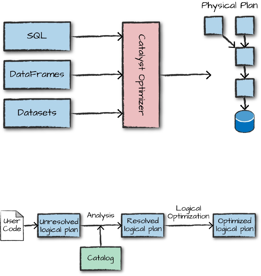
Figure 4-1. The Catalyst Optimizer
Logical Planning
The first phase of execution is meant to take user code and convert it into a
logical plan. Figure 4-2 illustrates this process.
Figure 4-2. The structured API logical planning process
This logical plan only represents a set of abstract transformations that do not
refer to executors or drivers, it’s purely to convert the user’s set of
expressions into the most optimized version. It does this by converting user
code into an unresolved logical plan. This plan is unresolved because
although your code might be valid, the tables or columns that it refers to
might or might not exist. Spark uses the catalog, a repository of all table and
DataFrame information, to resolve columns and tables in the analyzer. The
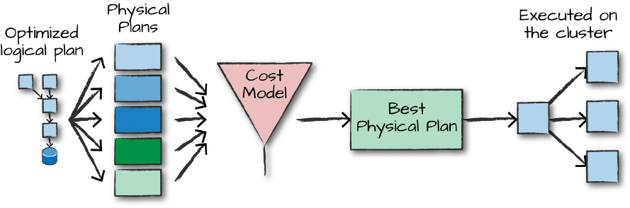
analyzer might reject the unresolved logical plan if the required table or
column name does not exist in the catalog. If the analyzer can resolve it, the
result is passed through the Catalyst Optimizer, a collection of rules that
attempt to optimize the logical plan by pushing down predicates or selections.
Packages can extend the Catalyst to include their own rules for domain-
specific optimizations.
Physical Planning
After successfully creating an optimized logical plan, Spark then begins the
physical planning process. The physical plan, often called a Spark plan,
specifies how the logical plan will execute on the cluster by generating
different physical execution strategies and comparing them through a cost
model, as depicted in Figure 4-3. An example of the cost comparison might
be choosing how to perform a given join by looking at the physical attributes
of a given table (how big the table is or how big its partitions are).
Figure 4-3. The physical planning process
Physical planning results in a series of RDDs and transformations. This result
is why you might have heard Spark referred to as a compiler—it takes queries
in DataFrames, Datasets, and SQL and compiles them into RDD
transformations for you.
Execution
Upon selecting a physical plan, Spark runs all of this code over RDDs, the
lower-level programming interface of Spark (which we cover in Part III).
Spark performs further optimizations at runtime, generating native Java
bytecode that can remove entire tasks or stages during execution. Finally the
result is returned to the user.
Conclusion
In this chapter, we covered Spark Structured APIs and how Spark transforms
your code into what will physically execute on the cluster. In the chapters
that follow, we cover core concepts and how to use the key functionality of
the Structured APIs.

Chapter 5. Basic Structured
Operations
In Chapter 4, we introduced the core abstractions of the Structured API. This
chapter moves away from the architectural concepts and toward the tactical
tools you will use to manipulate DataFrames and the data within them. This
chapter focuses exclusively on fundamental DataFrame operations and avoids
aggregations, window functions, and joins. These are discussed in subsequent
chapters.
Definitionally, a DataFrame consists of a series of records (like rows in a
table), that are of type Row, and a number of columns (like columns in a
spreadsheet) that represent a computation expression that can be performed
on each individual record in the Dataset. Schemas define the name as well as
the type of data in each column. Partitioning of the DataFrame defines the
layout of the DataFrame or Dataset’s physical distribution across the cluster.
The partitioning scheme defines how that is allocated. You can set this to be
based on values in a certain column or nondeterministically.
Let’s create a DataFrame with which we can work:
// in Scala
val df = spark.read.format("json")
.load("/data/flight-data/json/2015-summary.json")
# in Python
df = spark.read.format("json").load("/data/flight-data/json/2015-summary.json")
We discussed that a DataFame will have columns, and we use a schema to
define them. Let’s take a look at the schema on our current DataFrame:
df.printSchema()
Schemas tie everything together, so they’re worth belaboring.

Schemas
A schema defines the column names and types of a DataFrame. We can either
let a data source define the schema (called schema-on-read) or we can define
it explicitly ourselves.
WARNING
Deciding whether you need to define a schema prior to reading in your data depends on
your use case. For ad hoc analysis, schema-on-read usually works just fine (although at
times it can be a bit slow with plain-text file formats like CSV or JSON). However, this
can also lead to precision issues like a long type incorrectly set as an integer when reading
in a file. When using Spark for production Extract, Transform, and Load (ETL), it is often
a good idea to define your schemas manually, especially when working with untyped data
sources like CSV and JSON because schema inference can vary depending on the type of
data that you read in.
Let’s begin with a simple file, which we saw in Chapter 4, and let the semi-
structured nature of line-delimited JSON define the structure. This is flight
data from the United States Bureau of Transportation statistics:
// in Scala
spark.read.format("json").load("/data/flight-data/json/2015-
summary.json").schema
Scala returns the following:
org.apache.spark.sql.types.StructType = ...
StructType(StructField(DEST_COUNTRY_NAME,StringType,true),
StructField(ORIGIN_COUNTRY_NAME,StringType,true),
StructField(count,LongType,true))
# in Python
spark.read.format("json").load("/data/flight-data/json/2015-
summary.json").schema
Python returns the following:
StructType(List(StructField(DEST_COUNTRY_NAME,StringType,true),
StructField(ORIGIN_COUNTRY_NAME,StringType,true),
StructField(count,LongType,true)))
A schema is a StructType made up of a number of fields, StructFields,
that have a name, type, a Boolean flag which specifies whether that column
can contain missing or null values, and, finally, users can optionally specify
associated metadata with that column. The metadata is a way of storing
information about this column (Spark uses this in its machine learning
library).
Schemas can contain other StructTypes (Spark’s complex types). We will
see this in Chapter 6 when we discuss working with complex types. If the
types in the data (at runtime) do not match the schema, Spark will throw an
error. The example that follows shows how to create and enforce a specific
schema on a DataFrame.
// in Scala
import org.apache.spark.sql.types.{StructField, StructType, StringType,
LongType}
import org.apache.spark.sql.types.Metadata
val myManualSchema = StructType(Array(
StructField("DEST_COUNTRY_NAME", StringType, true),
StructField("ORIGIN_COUNTRY_NAME", StringType, true),
StructField("count", LongType, false,
Metadata.fromJson("{\"hello\":\"world\"}"))
))
val df = spark.read.format("json").schema(myManualSchema)
.load("/data/flight-data/json/2015-summary.json")
Here’s how to do the same in Python:
# in Python
from pyspark.sql.types import StructField, StructType, StringType, LongType
myManualSchema = StructType([
StructField("DEST_COUNTRY_NAME", StringType(), True),
StructField("ORIGIN_COUNTRY_NAME", StringType(), True),
StructField("count", LongType(), False, metadata={"hello":"world"})
])
df = spark.read.format("json").schema(myManualSchema)\
.load("/data/flight-data/json/2015-summary.json")
As discussed in Chapter 4, we cannot simply set types via the per-language
types because Spark maintains its own type information. Let’s now discuss
what schemas define: columns.
Columns and Expressions
Columns in Spark are similar to columns in a spreadsheet, R dataframe, or
pandas DataFrame. You can select, manipulate, and remove columns from
DataFrames and these operations are represented as expressions.
To Spark, columns are logical constructions that simply represent a value
computed on a per-record basis by means of an expression. This means that
to have a real value for a column, we need to have a row; and to have a row,
we need to have a DataFrame. You cannot manipulate an individual column
outside the context of a DataFrame; you must use Spark transformations
within a DataFrame to modify the contents of a column.
Columns
There are a lot of different ways to construct and refer to columns but the two
simplest ways are by using the col or column functions. To use either of
these functions, you pass in a column name:
// in Scala
import org.apache.spark.sql.functions.{col, column}
col("someColumnName")
column("someColumnName")
# in Python
from pyspark.sql.functions import col, column
col("someColumnName")
column("someColumnName")
We will stick to using col throughout this book. As mentioned, this column

might or might not exist in our DataFrames. Columns are not resolved until
we compare the column names with those we are maintaining in the catalog.
Column and table resolution happens in the analyzer phase, as discussed in
Chapter 4.
NOTE
We just mentioned two different ways of referring to columns. Scala has some unique
language features that allow for more shorthand ways of referring to columns. The
following bits of syntactic sugar perform the exact same thing, namely creating a column,
but provide no performance improvement:
// in Scala
$"myColumn"
'myColumn
The $ allows us to designate a string as a special string that should refer to an expression.
The tick mark (') is a special thing called a symbol; this is a Scala-specific construct of
referring to some identifier. They both perform the same thing and are shorthand ways of
referring to columns by name. You’ll likely see all of the aforementioned references when
you read different people’s Spark code. We leave it to you to use whatever is most
comfortable and maintainable for you and those with whom you work.
Explicit column references
If you need to refer to a specific DataFrame’s column, you can use the col
method on the specific DataFrame. This can be useful when you are
performing a join and need to refer to a specific column in one DataFrame
that might share a name with another column in the joined DataFrame. We
will see this in Chapter 8. As an added benefit, Spark does not need to resolve
this column itself (during the analyzer phase) because we did that for Spark:
df.col("count")
Expressions
We mentioned earlier that columns are expressions, but what is an
expression? An expression is a set of transformations on one or more values

in a record in a DataFrame. Think of it like a function that takes as input one
or more column names, resolves them, and then potentially applies more
expressions to create a single value for each record in the dataset.
Importantly, this “single value” can actually be a complex type like a Map or
Array. We’ll see more of the complex types in Chapter 6.
In the simplest case, an expression, created via the expr function, is just a
DataFrame column reference. In the simplest case, expr("someCol") is
equivalent to col("someCol").
Columns as expressions
Columns provide a subset of expression functionality. If you use col() and
want to perform transformations on that column, you must perform those on
that column reference. When using an expression, the expr function can
actually parse transformations and column references from a string and can
subsequently be passed into further transformations. Let’s look at some
examples.
expr("someCol - 5") is the same transformation as performing
col("someCol") - 5, or even expr("someCol") - 5. That’s because
Spark compiles these to a logical tree specifying the order of operations. This
might be a bit confusing at first, but remember a couple of key points:
Columns are just expressions.
Columns and transformations of those columns compile to the same
logical plan as parsed expressions.
Let’s ground this with an example:
(((col("someCol") + 5) * 200) - 6) < col("otherCol")
Figure 5-1 shows an overview of that logical tree.
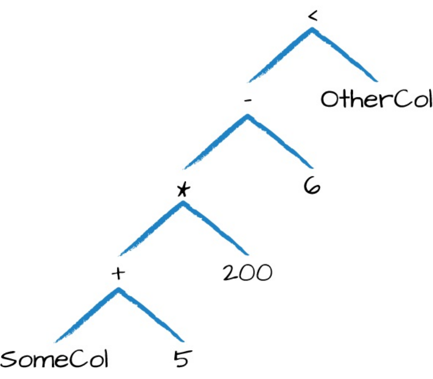
Figure 5-1. A logical tree
This might look familiar because it’s a directed acyclic graph. This graph is
represented equivalently by the following code:
// in Scala
import org.apache.spark.sql.functions.expr
expr("(((someCol + 5) * 200) - 6) < otherCol")
# in Python
from pyspark.sql.functions import expr
expr("(((someCol + 5) * 200) - 6) < otherCol")
This is an extremely important point to reinforce. Notice how the previous
expression is actually valid SQL code, as well, just like you might put in a

SELECT statement? That’s because this SQL expression and the previous
DataFrame code compile to the same underlying logical tree prior to
execution. This means that you can write your expressions as DataFrame
code or as SQL expressions and get the exact same performance
characteristics. This is discussed in Chapter 4.
Accessing a DataFrame’s columns
Sometimes, you’ll need to see a DataFrame’s columns, which you can do by
using something like printSchema; however, if you want to
programmatically access columns, you can use the columns property to see
all columns on a DataFrame:
spark.read.format("json").load("/data/flight-data/json/2015-summary.json")
.columns
Records and Rows
In Spark, each row in a DataFrame is a single record. Spark represents this
record as an object of type Row. Spark manipulates Row objects using column
expressions in order to produce usable values. Row objects internally
represent arrays of bytes. The byte array interface is never shown to users
because we only use column expressions to manipulate them.
You’ll notice commands that return individual rows to the driver will always
return one or more Row types when we are working with DataFrames.
NOTE
We use lowercase “row” and “record” interchangeably in this chapter, with a focus on the
latter. A capitalized Row refers to the Row object.
Let’s see a row by calling first on our DataFrame:
df.first()
Creating Rows
You can create rows by manually instantiating a Row object with the values
that belong in each column. It’s important to note that only DataFrames have
schemas. Rows themselves do not have schemas. This means that if you
create a Row manually, you must specify the values in the same order as the
schema of the DataFrame to which they might be appended (we will see this
when we discuss creating DataFrames):
// in Scala
import org.apache.spark.sql.Row
val myRow = Row("Hello", null, 1, false)
# in Python
from pyspark.sql import Row
myRow = Row("Hello", None, 1, False)
Accessing data in rows is equally as easy: you just specify the position that
you would like. In Scala or Java, you must either use the helper methods or
explicitly coerce the values. However, in Python or R, the value will
automatically be coerced into the correct type:
// in Scala
myRow(0) // type Any
myRow(0).asInstanceOf[String] // String
myRow.getString(0) // String
myRow.getInt(2) // Int
# in Python
myRow[0]
myRow[2]
You can also explicitly return a set of Data in the corresponding Java Virtual
Machine (JVM) objects by using the Dataset APIs. This is covered in
Chapter 11.
DataFrame Transformations
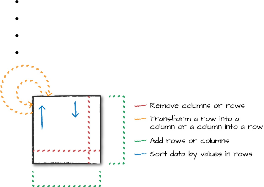
Now that we briefly defined the core parts of a DataFrame, we will move
onto manipulating DataFrames. When working with individual DataFrames
there are some fundamental objectives. These break down into several core
operations, as depicted in Figure 5-2:
We can add rows or columns
We can remove rows or columns
We can transform a row into a column (or vice versa)
We can change the order of rows based on the values in columns
Figure 5-2. Different kinds of transformations
Luckily, we can translate all of these into simple transformations, the most
common being those that take one column, change it row by row, and then
return our results.
Creating DataFrames
As we saw previously, we can create DataFrames from raw data sources. This
is covered extensively in Chapter 9; however, we will use them now to create
an example DataFrame (for illustration purposes later in this chapter, we will
also register this as a temporary view so that we can query it with SQL and
show off basic transformations in SQL, as well):

// in Scala
val df = spark.read.format("json")
.load("/data/flight-data/json/2015-summary.json")
df.createOrReplaceTempView("dfTable")
# in Python
df = spark.read.format("json").load("/data/flight-data/json/2015-summary.json")
df.createOrReplaceTempView("dfTable")
We can also create DataFrames on the fly by taking a set of rows and
converting them to a DataFrame.
// in Scala
import org.apache.spark.sql.Row
import org.apache.spark.sql.types.{StructField, StructType, StringType,
LongType}
val myManualSchema = new StructType(Array(
new StructField("some", StringType, true),
new StructField("col", StringType, true),
new StructField("names", LongType, false)))
val myRows = Seq(Row("Hello", null, 1L))
val myRDD = spark.sparkContext.parallelize(myRows)
val myDf = spark.createDataFrame(myRDD, myManualSchema)
myDf.show()
NOTE
In Scala, we can also take advantage of Spark’s implicits in the console (and if you import
them in your JAR code) by running toDF on a Seq type. This does not play well with null
types, so it’s not necessarily recommended for production use cases.
// in Scala
val myDF = Seq(("Hello", 2, 1L)).toDF("col1", "col2", "col3")
# in Python
from pyspark.sql import Row
from pyspark.sql.types import StructField, StructType, StringType, LongType
myManualSchema = StructType([
StructField("some", StringType(), True),
StructField("col", StringType(), True),
StructField("names", LongType(), False)
])
myRow = Row("Hello", None, 1)
myDf = spark.createDataFrame([myRow], myManualSchema)
myDf.show()
Giving an output of:
+-----+----+-----+
| some| col|names|
+-----+----+-----+
|Hello|null| 1|
+-----+----+-----+
Now that you know how to create DataFrames, let’s take a look at their most
useful methods that you’re going to be using: the select method when
you’re working with columns or expressions, and the selectExpr method
when you’re working with expressions in strings. Naturally some
transformations are not specified as methods on columns; therefore, there
exists a group of functions found in the org.apache.spark.sql.functions
package.
With these three tools, you should be able to solve the vast majority of
transformation challenges that you might encounter in DataFrames.
select and selectExpr
select and selectExpr allow you to do the DataFrame equivalent of SQL
queries on a table of data:
-- in SQL
SELECT * FROM dataFrameTable
SELECT columnName FROM dataFrameTable
SELECT columnName * 10, otherColumn, someOtherCol as c FROM dataFrameTable
In the simplest possible terms, you can use them to manipulate columns in
your DataFrames. Let’s walk through some examples on DataFrames to talk
about some of the different ways of approaching this problem. The easiest
way is just to use the select method and pass in the column names as strings
with which you would like to work:
// in Scala
df.select("DEST_COUNTRY_NAME").show(2)
# in Python
df.select("DEST_COUNTRY_NAME").show(2)
-- in SQL
SELECT DEST_COUNTRY_NAME FROM dfTable LIMIT 2
Giving an output of:
+-----------------+
|DEST_COUNTRY_NAME|
+-----------------+
| United States|
| United States|
+-----------------+
You can select multiple columns by using the same style of query, just add
more column name strings to your select method call:
// in Scala
df.select("DEST_COUNTRY_NAME", "ORIGIN_COUNTRY_NAME").show(2)
# in Python
df.select("DEST_COUNTRY_NAME", "ORIGIN_COUNTRY_NAME").show(2)
-- in SQL
SELECT DEST_COUNTRY_NAME, ORIGIN_COUNTRY_NAME FROM dfTable LIMIT 2
Giving an output of:
+-----------------+-------------------+
|DEST_COUNTRY_NAME|ORIGIN_COUNTRY_NAME|
+-----------------+-------------------+
| United States| Romania|
| United States| Croatia|
+-----------------+-------------------+
As discussed in “Columns and Expressions”, you can refer to columns in a
number of different ways; all you need to keep in mind is that you can use
them interchangeably:
// in Scala
import org.apache.spark.sql.functions.{expr, col, column}
df.select(
df.col("DEST_COUNTRY_NAME"),
col("DEST_COUNTRY_NAME"),
column("DEST_COUNTRY_NAME"),
'DEST_COUNTRY_NAME,
$"DEST_COUNTRY_NAME",
expr("DEST_COUNTRY_NAME"))
.show(2)
# in Python
from pyspark.sql.functions import expr, col, column
df.select(
expr("DEST_COUNTRY_NAME"),
col("DEST_COUNTRY_NAME"),
column("DEST_COUNTRY_NAME"))\
.show(2)
One common error is attempting to mix Column objects and strings. For
example, the following code will result in a compiler error:
df.select(col("DEST_COUNTRY_NAME"), "DEST_COUNTRY_NAME")
As we’ve seen thus far, expr is the most flexible reference that we can use. It
can refer to a plain column or a string manipulation of a column. To illustrate,
let’s change the column name, and then change it back by using the AS
keyword and then the alias method on the column:
// in Scala
df.select(expr("DEST_COUNTRY_NAME AS destination")).show(2)
# in Python
df.select(expr("DEST_COUNTRY_NAME AS destination")).show(2)
-- in SQL
SELECT DEST_COUNTRY_NAME as destination FROM dfTable LIMIT 2
This changes the column name to “destination.” You can further manipulate
the result of your expression as another expression:
// in Scala
df.select(expr("DEST_COUNTRY_NAME as destination").alias("DEST_COUNTRY_NAME"))
.show(2)
# in Python
df.select(expr("DEST_COUNTRY_NAME as destination").alias("DEST_COUNTRY_NAME"))\
.show(2)
The preceding operation changes the column name back to its original name.
Because select followed by a series of expr is such a common pattern,
Spark has a shorthand for doing this efficiently: selectExpr. This is
probably the most convenient interface for everyday use:
// in Scala
df.selectExpr("DEST_COUNTRY_NAME as newColumnName", "DEST_COUNTRY_NAME").show(2)
# in Python
df.selectExpr("DEST_COUNTRY_NAME as newColumnName", "DEST_COUNTRY_NAME").show(2)
This opens up the true power of Spark. We can treat selectExpr as a simple
way to build up complex expressions that create new DataFrames. In fact, we
can add any valid non-aggregating SQL statement, and as long as the
columns resolve, it will be valid! Here’s a simple example that adds a new
column withinCountry to our DataFrame that specifies whether the
destination and origin are the same:
// in Scala
df.selectExpr(
"*", // include all original columns
"(DEST_COUNTRY_NAME = ORIGIN_COUNTRY_NAME) as withinCountry")
.show(2)
# in Python
df.selectExpr(
"*", # all original columns
"(DEST_COUNTRY_NAME = ORIGIN_COUNTRY_NAME) as withinCountry")\
.show(2)
-- in SQL
SELECT *, (DEST_COUNTRY_NAME = ORIGIN_COUNTRY_NAME) as withinCountry
FROM dfTable
LIMIT 2
Giving an output of:
+-----------------+-------------------+-----+-------------+
|DEST_COUNTRY_NAME|ORIGIN_COUNTRY_NAME|count|withinCountry|
+-----------------+-------------------+-----+-------------+
| United States| Romania| 15| false|
| United States| Croatia| 1| false|
+-----------------+-------------------+-----+-------------+
With select expression, we can also specify aggregations over the entire
DataFrame by taking advantage of the functions that we have. These look just
like what we have been showing so far:
// in Scala
df.selectExpr("avg(count)", "count(distinct(DEST_COUNTRY_NAME))").show(2)
# in Python
df.selectExpr("avg(count)", "count(distinct(DEST_COUNTRY_NAME))").show(2)
-- in SQL
SELECT avg(count), count(distinct(DEST_COUNTRY_NAME)) FROM dfTable LIMIT 2
Giving an output of:
+-----------+---------------------------------+
| avg(count)|count(DISTINCT DEST_COUNTRY_NAME)|
+-----------+---------------------------------+
|1770.765625| 132|
+-----------+---------------------------------+
Converting to Spark Types (Literals)
Sometimes, we need to pass explicit values into Spark that are just a value
(rather than a new column). This might be a constant value or something
we’ll need to compare to later on. The way we do this is through literals. This
is basically a translation from a given programming language’s literal value
to one that Spark understands. Literals are expressions and you can use them
in the same way:
// in Scala
import org.apache.spark.sql.functions.lit
df.select(expr("*"), lit(1).as("One")).show(2)
# in Python
from pyspark.sql.functions import lit
df.select(expr("*"), lit(1).alias("One")).show(2)
In SQL, literals are just the specific value:
-- in SQL
SELECT *, 1 as One FROM dfTable LIMIT 2
Giving an output of:
+-----------------+-------------------+-----+---+
|DEST_COUNTRY_NAME|ORIGIN_COUNTRY_NAME|count|One|
+-----------------+-------------------+-----+---+
| United States| Romania| 15| 1|
| United States| Croatia| 1| 1|
+-----------------+-------------------+-----+---+
This will come up when you might need to check whether a value is greater
than some constant or other programmatically created variable.
Adding Columns
There’s also a more formal way of adding a new column to a DataFrame, and
that’s by using the withColumn method on our DataFrame. For example, let’s
add a column that just adds the number one as a column:
// in Scala
df.withColumn("numberOne", lit(1)).show(2)
# in Python
df.withColumn("numberOne", lit(1)).show(2)
-- in SQL
SELECT *, 1 as numberOne FROM dfTable LIMIT 2
Giving an output of:
+-----------------+-------------------+-----+---------+
|DEST_COUNTRY_NAME|ORIGIN_COUNTRY_NAME|count|numberOne|
+-----------------+-------------------+-----+---------+
| United States| Romania| 15| 1|
| United States| Croatia| 1| 1|
+-----------------+-------------------+-----+---------+
Let’s do something a bit more interesting and make it an actual expression. In
the next example, we’ll set a Boolean flag for when the origin country is the
same as the destination country:
// in Scala
df.withColumn("withinCountry", expr("ORIGIN_COUNTRY_NAME == DEST_COUNTRY_NAME"))
.show(2)
# in Python
df.withColumn("withinCountry", expr("ORIGIN_COUNTRY_NAME ==
DEST_COUNTRY_NAME"))\
.show(2)
Notice that the withColumn function takes two arguments: the column name
and the expression that will create the value for that given row in the
DataFrame. Interestingly, we can also rename a column this way. The SQL
syntax is the same as we had previously, so we can omit it in this example:
df.withColumn("Destination", expr("DEST_COUNTRY_NAME")).columns
Resulting in:
... DEST_COUNTRY_NAME, ORIGIN_COUNTRY_NAME, count, Destination
Renaming Columns
Although we can rename a column in the manner that we just described,
another alternative is to use the withColumnRenamed method. This will
rename the column with the name of the string in the first argument to the
string in the second argument:
// in Scala
df.withColumnRenamed("DEST_COUNTRY_NAME", "dest").columns
# in Python
df.withColumnRenamed("DEST_COUNTRY_NAME", "dest").columns
... dest, ORIGIN_COUNTRY_NAME, count
Reserved Characters and Keywords
One thing that you might come across is reserved characters like spaces or
dashes in column names. Handling these means escaping column names
appropriately. In Spark, we do this by using backtick (`) characters. Let’s use
withColumn, which you just learned about to create a column with reserved
characters. We’ll show two examples—in the one shown here, we don’t need
escape characters, but in the next one, we do:
// in Scala
import org.apache.spark.sql.functions.expr
val dfWithLongColName = df.withColumn(
"This Long Column-Name",
expr("ORIGIN_COUNTRY_NAME"))
# in Python
dfWithLongColName = df.withColumn(
"This Long Column-Name",
expr("ORIGIN_COUNTRY_NAME"))
We don’t need escape characters here because the first argument to
withColumn is just a string for the new column name. In this example,
however, we need to use backticks because we’re referencing a column in an
expression:
// in Scala
dfWithLongColName.selectExpr(
"`This Long Column-Name`",
"`This Long Column-Name` as `new col`")
.show(2)
# in Python
dfWithLongColName.selectExpr(
"`This Long Column-Name`",
"`This Long Column-Name` as `new col`")\
.show(2)
dfWithLongColName.createOrReplaceTempView("dfTableLong")
-- in SQL
SELECT `This Long Column-Name`, `This Long Column-Name` as `new col`
FROM dfTableLong LIMIT 2
We can refer to columns with reserved characters (and not escape them) if
we’re doing an explicit string-to-column reference, which is interpreted as a
literal instead of an expression. We only need to escape expressions that use
reserved characters or keywords. The following two examples both result in
the same DataFrame:
// in Scala
dfWithLongColName.select(col("This Long Column-Name")).columns
# in Python
dfWithLongColName.select(expr("`This Long Column-Name`")).columns
Case Sensitivity
By default Spark is case insensitive; however, you can make Spark case
sensitive by setting the configuration:
-- in SQL
set spark.sql.caseSensitive true

Removing Columns
Now that we’ve created this column, let’s take a look at how we can remove
columns from DataFrames. You likely already noticed that we can do this by
using select. However, there is also a dedicated method called drop:
df.drop("ORIGIN_COUNTRY_NAME").columns
We can drop multiple columns by passing in multiple columns as arguments:
dfWithLongColName.drop("ORIGIN_COUNTRY_NAME", "DEST_COUNTRY_NAME")
Changing a Column’s Type (cast)
Sometimes, we might need to convert from one type to another; for example,
if we have a set of StringType that should be integers. We can convert
columns from one type to another by casting the column from one type to
another. For instance, let’s convert our count column from an integer to a
type Long:
df.withColumn("count2", col("count").cast("long"))
-- in SQL
SELECT *, cast(count as long) AS count2 FROM dfTable
Filtering Rows
To filter rows, we create an expression that evaluates to true or false. You
then filter out the rows with an expression that is equal to false. The most
common way to do this with DataFrames is to create either an expression as a
String or build an expression by using a set of column manipulations. There
are two methods to perform this operation: you can use where or filter and
they both will perform the same operation and accept the same argument
types when used with DataFrames. We will stick to where because of its
familiarity to SQL; however, filter is valid as well.

NOTE
When using the Dataset API from either Scala or Java, filter also accepts an arbitrary
function that Spark will apply to each record in the Dataset. See Chapter 11 for more
information.
The following filters are equivalent, and the results are the same in Scala and
Python:
df.filter(col("count") < 2).show(2)
df.where("count < 2").show(2)
-- in SQL
SELECT * FROM dfTable WHERE count < 2 LIMIT 2
Giving an output of:
+-----------------+-------------------+-----+
|DEST_COUNTRY_NAME|ORIGIN_COUNTRY_NAME|count|
+-----------------+-------------------+-----+
| United States| Croatia| 1|
| United States| Singapore| 1|
+-----------------+-------------------+-----+
Instinctually, you might want to put multiple filters into the same expression.
Although this is possible, it is not always useful, because Spark automatically
performs all filtering operations at the same time regardless of the filter
ordering. This means that if you want to specify multiple AND filters, just
chain them sequentially and let Spark handle the rest:
// in Scala
df.where(col("count") < 2).where(col("ORIGIN_COUNTRY_NAME") =!= "Croatia")
.show(2)
# in Python
df.where(col("count") < 2).where(col("ORIGIN_COUNTRY_NAME") != "Croatia")\
.show(2)
-- in SQL
SELECT * FROM dfTable WHERE count < 2 AND ORIGIN_COUNTRY_NAME != "Croatia"
LIMIT 2
Giving an output of:
+-----------------+-------------------+-----+
|DEST_COUNTRY_NAME|ORIGIN_COUNTRY_NAME|count|
+-----------------+-------------------+-----+
| United States| Singapore| 1|
| Moldova| United States| 1|
+-----------------+-------------------+-----+
Getting Unique Rows
A very common use case is to extract the unique or distinct values in a
DataFrame. These values can be in one or more columns. The way we do this
is by using the distinct method on a DataFrame, which allows us to
deduplicate any rows that are in that DataFrame. For instance, let’s get the
unique origins in our dataset. This, of course, is a transformation that will
return a new DataFrame with only unique rows:
// in Scala
df.select("ORIGIN_COUNTRY_NAME", "DEST_COUNTRY_NAME").distinct().count()
# in Python
df.select("ORIGIN_COUNTRY_NAME", "DEST_COUNTRY_NAME").distinct().count()
-- in SQL
SELECT COUNT(DISTINCT(ORIGIN_COUNTRY_NAME, DEST_COUNTRY_NAME)) FROM dfTable
Results in 256.
// in Scala
df.select("ORIGIN_COUNTRY_NAME").distinct().count()
# in Python
df.select("ORIGIN_COUNTRY_NAME").distinct().count()
-- in SQL
SELECT COUNT(DISTINCT ORIGIN_COUNTRY_NAME) FROM dfTable
Results in 125.
Random Samples
Sometimes, you might just want to sample some random records from your
DataFrame. You can do this by using the sample method on a DataFrame,
which makes it possible for you to specify a fraction of rows to extract from a
DataFrame and whether you’d like to sample with or without replacement:
val seed = 5
val withReplacement = false
val fraction = 0.5
df.sample(withReplacement, fraction, seed).count()
# in Python
seed = 5
withReplacement = False
fraction = 0.5
df.sample(withReplacement, fraction, seed).count()
Giving an output of 126.
Random Splits
Random splits can be helpful when you need to break up your DataFrame
into a random “splits” of the original DataFrame. This is often used with
machine learning algorithms to create training, validation, and test sets. In
this next example, we’ll split our DataFrame into two different DataFrames
by setting the weights by which we will split the DataFrame (these are the
arguments to the function). Because this method is designed to be
randomized, we will also specify a seed (just replace seed with a number of
your choosing in the code block). It’s important to note that if you don’t
specify a proportion for each DataFrame that adds up to one, they will be
normalized so that they do:
// in Scala
val dataFrames = df.randomSplit(Array(0.25, 0.75), seed)
dataFrames(0).count() > dataFrames(1).count() // False

# in Python
dataFrames = df.randomSplit([0.25, 0.75], seed)
dataFrames[0].count() > dataFrames[1].count() # False
Concatenating and Appending Rows (Union)
As you learned in the previous section, DataFrames are immutable. This
means users cannot append to DataFrames because that would be changing it.
To append to a DataFrame, you must union the original DataFrame along
with the new DataFrame. This just concatenates the two DataFramess. To
union two DataFrames, you must be sure that they have the same schema and
number of columns; otherwise, the union will fail.
WARNING
Unions are currently performed based on location, not on the schema. This means that
columns will not automatically line up the way you think they might.
// in Scala
import org.apache.spark.sql.Row
val schema = df.schema
val newRows = Seq(
Row("New Country", "Other Country", 5L),
Row("New Country 2", "Other Country 3", 1L)
)
val parallelizedRows = spark.sparkContext.parallelize(newRows)
val newDF = spark.createDataFrame(parallelizedRows, schema)
df.union(newDF)
.where("count = 1")
.where($"ORIGIN_COUNTRY_NAME" =!= "United States")
.show() // get all of them and we'll see our new rows at the end
In Scala, you must use the =!= operator so that you don’t just compare the
unevaluated column expression to a string but instead to the evaluated one:
# in Python
from pyspark.sql import Row
schema = df.schema
newRows = [
Row("New Country", "Other Country", 5L),
Row("New Country 2", "Other Country 3", 1L)
]
parallelizedRows = spark.sparkContext.parallelize(newRows)
newDF = spark.createDataFrame(parallelizedRows, schema)
# in Python
df.union(newDF)\
.where("count = 1")\
.where(col("ORIGIN_COUNTRY_NAME") != "United States")\
.show()
Giving the output of:
+-----------------+-------------------+-----+
|DEST_COUNTRY_NAME|ORIGIN_COUNTRY_NAME|count|
+-----------------+-------------------+-----+
| United States| Croatia| 1|
...
| United States| Namibia| 1|
| New Country 2| Other Country 3| 1|
+-----------------+-------------------+-----+
As expected, you’ll need to use this new DataFrame reference in order to
refer to the DataFrame with the newly appended rows. A common way to do
this is to make the DataFrame into a view or register it as a table so that you
can reference it more dynamically in your code.
Sorting Rows
When we sort the values in a DataFrame, we always want to sort with either
the largest or smallest values at the top of a DataFrame. There are two
equivalent operations to do this sort and orderBy that work the exact same
way. They accept both column expressions and strings as well as multiple
columns. The default is to sort in ascending order:
// in Scala
df.sort("count").show(5)
df.orderBy("count", "DEST_COUNTRY_NAME").show(5)
df.orderBy(col("count"), col("DEST_COUNTRY_NAME")).show(5)
# in Python
df.sort("count").show(5)
df.orderBy("count", "DEST_COUNTRY_NAME").show(5)
df.orderBy(col("count"), col("DEST_COUNTRY_NAME")).show(5)
To more explicitly specify sort direction, you need to use the asc and desc
functions if operating on a column. These allow you to specify the order in
which a given column should be sorted:
// in Scala
import org.apache.spark.sql.functions.{desc, asc}
df.orderBy(expr("count desc")).show(2)
df.orderBy(desc("count"), asc("DEST_COUNTRY_NAME")).show(2)
# in Python
from pyspark.sql.functions import desc, asc
df.orderBy(expr("count desc")).show(2)
df.orderBy(col("count").desc(), col("DEST_COUNTRY_NAME").asc()).show(2)
-- in SQL
SELECT * FROM dfTable ORDER BY count DESC, DEST_COUNTRY_NAME ASC LIMIT 2
An advanced tip is to use asc_nulls_first, desc_nulls_first,
asc_nulls_last, or desc_nulls_last to specify where you would like
your null values to appear in an ordered DataFrame.
For optimization purposes, it’s sometimes advisable to sort within each
partition before another set of transformations. You can use the
sortWithinPartitions method to do this:
// in Scala
spark.read.format("json").load("/data/flight-data/json/*-summary.json")
.sortWithinPartitions("count")
# in Python
spark.read.format("json").load("/data/flight-data/json/*-summary.json")\
.sortWithinPartitions("count")
We will discuss this more when we look at tuning and optimization in
Part III.
Limit
Oftentimes, you might want to restrict what you extract from a DataFrame;
for example, you might want just the top ten of some DataFrame. You can do
this by using the limit method:
// in Scala
df.limit(5).show()
# in Python
df.limit(5).show()
-- in SQL
SELECT * FROM dfTable LIMIT 6
// in Scala
df.orderBy(expr("count desc")).limit(6).show()
# in Python
df.orderBy(expr("count desc")).limit(6).show()
-- in SQL
SELECT * FROM dfTable ORDER BY count desc LIMIT 6
Repartition and Coalesce
Another important optimization opportunity is to partition the data according
to some frequently filtered columns, which control the physical layout of data
across the cluster including the partitioning scheme and the number of
partitions.
Repartition will incur a full shuffle of the data, regardless of whether one is
necessary. This means that you should typically only repartition when the
future number of partitions is greater than your current number of partitions
or when you are looking to partition by a set of columns:
// in Scala
df.rdd.getNumPartitions // 1
# in Python
df.rdd.getNumPartitions() # 1
// in Scala
df.repartition(5)
# in Python
df.repartition(5)
If you know that you’re going to be filtering by a certain column often, it can
be worth repartitioning based on that column:
// in Scala
df.repartition(col("DEST_COUNTRY_NAME"))
# in Python
df.repartition(col("DEST_COUNTRY_NAME"))
You can optionally specify the number of partitions you would like, too:
// in Scala
df.repartition(5, col("DEST_COUNTRY_NAME"))
# in Python
df.repartition(5, col("DEST_COUNTRY_NAME"))
Coalesce, on the other hand, will not incur a full shuffle and will try to
combine partitions. This operation will shuffle your data into five partitions
based on the destination country name, and then coalesce them (without a full
shuffle):
// in Scala
df.repartition(5, col("DEST_COUNTRY_NAME")).coalesce(2)
# in Python
df.repartition(5, col("DEST_COUNTRY_NAME")).coalesce(2)
Collecting Rows to the Driver
As discussed in previous chapters, Spark maintains the state of the cluster in

the driver. There are times when you’ll want to collect some of your data to
the driver in order to manipulate it on your local machine.
Thus far, we did not explicitly define this operation. However, we used
several different methods for doing so that are effectively all the same.
collect gets all data from the entire DataFrame, take selects the first N
rows, and show prints out a number of rows nicely.
// in Scala
val collectDF = df.limit(10)
collectDF.take(5) // take works with an Integer count
collectDF.show() // this prints it out nicely
collectDF.show(5, false)
collectDF.collect()
# in Python
collectDF = df.limit(10)
collectDF.take(5) # take works with an Integer count
collectDF.show() # this prints it out nicely
collectDF.show(5, False)
collectDF.collect()
There’s an additional way of collecting rows to the driver in order to iterate
over the entire dataset. The method toLocalIterator collects partitions to
the driver as an iterator. This method allows you to iterate over the entire
dataset partition-by-partition in a serial manner:
collectDF.toLocalIterator()
WARNING
Any collection of data to the driver can be a very expensive operation! If you have a large
dataset and call collect, you can crash the driver. If you use toLocalIterator and have
very large partitions, you can easily crash the driver node and lose the state of your
application. This is also expensive because we can operate on a one-by-one basis, instead
of running computation in parallel.
Chapter 6. Working with
Different Types of Data
Chapter 5 presented basic DataFrame concepts and abstractions. This chapter
covers building expressions, which are the bread and butter of Spark’s
structured operations. We also review working with a variety of different
kinds of data, including the following:
Booleans
Numbers
Strings
Dates and timestamps
Handling null
Complex types
User-defined functions
Where to Look for APIs
Before we begin, it’s worth explaining where you as a user should look for
transformations. Spark is a growing project, and any book (including this
one) is a snapshot in time. One of our priorities in this book is to teach where,
as of this writing, you should look to find functions to transform your data.
Following are the key places to look:
DataFrame (Dataset) Methods
This is actually a bit of a trick because a DataFrame is just a Dataset of
Row types, so you’ll actually end up looking at the Dataset methods,
which are available at this link.
Dataset submodules like DataFrameStatFunctions and
DataFrameNaFunctions have more methods that solve specific sets of
problems. DataFrameStatFunctions, for example, holds a variety of
statistically related functions, whereas DataFrameNaFunctions refers to
functions that are relevant when working with null data.
Column Methods
These were introduced for the most part in Chapter 5. They hold a variety
of general column-related methods like alias or contains. You can find
the API Reference for Column methods here.
org.apache.spark.sql.functions contains a variety of functions for a
range of different data types. Often, you’ll see the entire package imported
because they are used so frequently. You can find SQL and DataFrame
functions here.
Now this may feel a bit overwhelming but have no fear, the majority of these
functions are ones that you will find in SQL and analytics systems. All of
these tools exist to achieve one purpose, to transform rows of data in one
format or structure to another. This might create more rows or reduce the
number of rows available. To begin, let’s read in the DataFrame that we’ll be
using for this analysis:
// in Scala
val df = spark.read.format("csv")
.option("header", "true")
.option("inferSchema", "true")
.load("/data/retail-data/by-day/2010-12-01.csv")
df.printSchema()
df.createOrReplaceTempView("dfTable")
# in Python
df = spark.read.format("csv")\
.option("header", "true")\
.option("inferSchema", "true")\
.load("/data/retail-data/by-day/2010-12-01.csv")
df.printSchema()
df.createOrReplaceTempView("dfTable")
Here’s the result of the schema and a small sample of the data:
root
|-- InvoiceNo: string (nullable = true)
|-- StockCode: string (nullable = true)
|-- Description: string (nullable = true)
|-- Quantity: integer (nullable = true)
|-- InvoiceDate: timestamp (nullable = true)
|-- UnitPrice: double (nullable = true)
|-- CustomerID: double (nullable = true)
|-- Country: string (nullable = true)
+---------+---------+--------------------+--------+-------------------+----...
|InvoiceNo|StockCode| Description|Quantity| InvoiceDate|Unit...
+---------+---------+--------------------+--------+-------------------+----...
| 536365| 85123A|WHITE HANGING HEA...| 6|2010-12-01 08:26:00| ...
| 536365| 71053| WHITE METAL LANTERN| 6|2010-12-01 08:26:00| ...
...
| 536367| 21755|LOVE BUILDING BLO...| 3|2010-12-01 08:34:00| ...
| 536367| 21777|RECIPE BOX WITH M...| 4|2010-12-01 08:34:00| ...
+---------+---------+--------------------+--------+-------------------+----...
Converting to Spark Types
One thing you’ll see us do throughout this chapter is convert native types to
Spark types. We do this by using the first function that we introduce here, the
lit function. This function converts a type in another language to its
correspnding Spark representation. Here’s how we can convert a couple of
different kinds of Scala and Python values to their respective Spark types:
// in Scala
import org.apache.spark.sql.functions.lit
df.select(lit(5), lit("five"), lit(5.0))
# in Python
from pyspark.sql.functions import lit
df.select(lit(5), lit("five"), lit(5.0))
There’s no equivalent function necessary in SQL, so we can use the values
directly:

-- in SQL
SELECT 5, "five", 5.0
Working with Booleans
Booleans are essential when it comes to data analysis because they are the
foundation for all filtering. Boolean statements consist of four elements: and,
or, true, and false. We use these simple structures to build logical statements
that evaluate to either true or false. These statements are often used as
conditional requirements for when a row of data must either pass the test
(evaluate to true) or else it will be filtered out.
Let’s use our retail dataset to explore working with Booleans. We can specify
equality as well as less-than or greater-than:
// in Scala
import org.apache.spark.sql.functions.col
df.where(col("InvoiceNo").equalTo(536365))
.select("InvoiceNo", "Description")
.show(5, false)
WARNING
Scala has some particular semantics regarding the use of == and ===. In Spark, if you want
to filter by equality you should use === (equal) or =!= (not equal). You can also use the
not function and the equalTo method.
// in Scala
import org.apache.spark.sql.functions.col
df.where(col("InvoiceNo") === 536365)
.select("InvoiceNo", "Description")
.show(5, false)
Python keeps a more conventional notation:
# in Python
from pyspark.sql.functions import col
df.where(col("InvoiceNo") != 536365)\
.select("InvoiceNo", "Description")\
.show(5, False)
+---------+-----------------------------+
|InvoiceNo|Description |
+---------+-----------------------------+
|536366 |HAND WARMER UNION JACK |
...
|536367 |POPPY'S PLAYHOUSE KITCHEN |
+---------+-----------------------------+
Another option—and probably the cleanest—is to specify the predicate as an
expression in a string. This is valid for Python or Scala. Note that this also
gives you access to another way of expressing “does not equal”:
df.where("InvoiceNo = 536365")
.show(5, false)
df.where("InvoiceNo <> 536365")
.show(5, false)
We mentioned that you can specify Boolean expressions with multiple parts
when you use and or or. In Spark, you should always chain together and
filters as a sequential filter.
The reason for this is that even if Boolean statements are expressed serially
(one after the other), Spark will flatten all of these filters into one statement
and perform the filter at the same time, creating the and statement for us.
Although you can specify your statements explicitly by using and if you like,
they’re often easier to understand and to read if you specify them serially. or
statements need to be specified in the same statement:
// in Scala
val priceFilter = col("UnitPrice") > 600
val descripFilter = col("Description").contains("POSTAGE")
df.where(col("StockCode").isin("DOT")).where(priceFilter.or(descripFilter))
.show()
# in Python
from pyspark.sql.functions import instr
priceFilter = col("UnitPrice") > 600
descripFilter = instr(df.Description, "POSTAGE") >= 1
df.where(df.StockCode.isin("DOT")).where(priceFilter | descripFilter).show()
-- in SQL
SELECT * FROM dfTable WHERE StockCode in ("DOT") AND(UnitPrice > 600 OR
instr(Description, "POSTAGE") >= 1)
+---------+---------+--------------+--------+-------------------+---------+...
|InvoiceNo|StockCode| Description|Quantity| InvoiceDate|UnitPrice|...
+---------+---------+--------------+--------+-------------------+---------+...
| 536544| DOT|DOTCOM POSTAGE| 1|2010-12-01 14:32:00| 569.77|...
| 536592| DOT|DOTCOM POSTAGE| 1|2010-12-01 17:06:00| 607.49|...
+---------+---------+--------------+--------+-------------------+---------+...
Boolean expressions are not just reserved to filters. To filter a DataFrame,
you can also just specify a Boolean column:
// in Scala
val DOTCodeFilter = col("StockCode") === "DOT"
val priceFilter = col("UnitPrice") > 600
val descripFilter = col("Description").contains("POSTAGE")
df.withColumn("isExpensive", DOTCodeFilter.and(priceFilter.or(descripFilter)))
.where("isExpensive")
.select("unitPrice", "isExpensive").show(5)
# in Python
from pyspark.sql.functions import instr
DOTCodeFilter = col("StockCode") == "DOT"
priceFilter = col("UnitPrice") > 600
descripFilter = instr(col("Description"), "POSTAGE") >= 1
df.withColumn("isExpensive", DOTCodeFilter & (priceFilter | descripFilter))\
.where("isExpensive")\
.select("unitPrice", "isExpensive").show(5)
-- in SQL
SELECT UnitPrice, (StockCode = 'DOT' AND
(UnitPrice > 600 OR instr(Description, "POSTAGE") >= 1)) as isExpensive
FROM dfTable
WHERE (StockCode = 'DOT' AND
(UnitPrice > 600 OR instr(Description, "POSTAGE") >= 1))
Notice how we did not need to specify our filter as an expression and how we

could use a column name without any extra work.
If you’re coming from a SQL background, all of these statements should
seem quite familiar. Indeed, all of them can be expressed as a where clause.
In fact, it’s often easier to just express filters as SQL statements than using
the programmatic DataFrame interface and Spark SQL allows us to do this
without paying any performance penalty. For example, the following two
statements are equivalent:
// in Scala
import org.apache.spark.sql.functions.{expr, not, col}
df.withColumn("isExpensive", not(col("UnitPrice").leq(250)))
.filter("isExpensive")
.select("Description", "UnitPrice").show(5)
df.withColumn("isExpensive", expr("NOT UnitPrice <= 250"))
.filter("isExpensive")
.select("Description", "UnitPrice").show(5)
Here’s our state definition:
# in Python
from pyspark.sql.functions import expr
df.withColumn("isExpensive", expr("NOT UnitPrice <= 250"))\
.where("isExpensive")\
.select("Description", "UnitPrice").show(5)
WARNING
One “gotcha” that can come up is if you’re working with null data when creating Boolean
expressions. If there is a null in your data, you’ll need to treat things a bit differently.
Here’s how you can ensure that you perform a null-safe equivalence test:
df.where(col("Description").eqNullSafe("hello")).show()
Although not currently available (Spark 2.2), IS [NOT] DISTINCT FROM will
be coming in Spark 2.3 to do the same thing in SQL.
Working with Numbers
When working with big data, the second most common task you will do after
filtering things is counting things. For the most part, we simply need to
express our computation, and that should be valid assuming that we’re
working with numerical data types.
To fabricate a contrived example, let’s imagine that we found out that we
mis-recorded the quantity in our retail dataset and the true quantity is equal to
(the current quantity * the unit price) + 5. This will introduce our first
numerical function as well as the pow function that raises a column to the
expressed power:
// in Scala
import org.apache.spark.sql.functions.{expr, pow}
val fabricatedQuantity = pow(col("Quantity") * col("UnitPrice"), 2) + 5
df.select(expr("CustomerId"), fabricatedQuantity.alias("realQuantity")).show(2)
# in Python
from pyspark.sql.functions import expr, pow
fabricatedQuantity = pow(col("Quantity") * col("UnitPrice"), 2) + 5
df.select(expr("CustomerId"), fabricatedQuantity.alias("realQuantity")).show(2)
+----------+------------------+
|CustomerId| realQuantity|
+----------+------------------+
| 17850.0|239.08999999999997|
| 17850.0| 418.7156|
+----------+------------------+
Notice that we were able to multiply our columns together because they were
both numerical. Naturally we can add and subtract as necessary, as well. In
fact, we can do all of this as a SQL expression, as well:
// in Scala
df.selectExpr(
"CustomerId",
"(POWER((Quantity * UnitPrice), 2.0) + 5) as realQuantity").show(2)
# in Python
2
df.selectExpr(
"CustomerId",
"(POWER((Quantity * UnitPrice), 2.0) + 5) as realQuantity").show(2)
-- in SQL
SELECT customerId, (POWER((Quantity * UnitPrice), 2.0) + 5) as realQuantity
FROM dfTable
Another common numerical task is rounding. If you’d like to just round to a
whole number, oftentimes you can cast the value to an integer and that will
work just fine. However, Spark also has more detailed functions for
performing this explicitly and to a certain level of precision. In the following
example, we round to one decimal place:
// in Scala
import org.apache.spark.sql.functions.{round, bround}
df.select(round(col("UnitPrice"), 1).alias("rounded"), col("UnitPrice")).show(5)
By default, the round function rounds up if you’re exactly in between two
numbers. You can round down by using the bround:
// in Scala
import org.apache.spark.sql.functions.lit
df.select(round(lit("2.5")), bround(lit("2.5"))).show(2)
# in Python
from pyspark.sql.functions import lit, round, bround
df.select(round(lit("2.5")), bround(lit("2.5"))).show(2)
-- in SQL
SELECT round(2.5), bround(2.5)
+-------------+--------------+
|round(2.5, 0)|bround(2.5, 0)|
+-------------+--------------+
| 3.0| 2.0|
| 3.0| 2.0|
+-------------+--------------+
Another numerical task is to compute the correlation of two columns. For
example, we can see the Pearson correlation coefficient for two columns to
see if cheaper things are typically bought in greater quantities. We can do this
through a function as well as through the DataFrame statistic methods:
// in Scala
import org.apache.spark.sql.functions.{corr}
df.stat.corr("Quantity", "UnitPrice")
df.select(corr("Quantity", "UnitPrice")).show()
# in Python
from pyspark.sql.functions import corr
df.stat.corr("Quantity", "UnitPrice")
df.select(corr("Quantity", "UnitPrice")).show()
-- in SQL
SELECT corr(Quantity, UnitPrice) FROM dfTable
+-------------------------+
|corr(Quantity, UnitPrice)|
+-------------------------+
| -0.04112314436835551|
+-------------------------+
Another common task is to compute summary statistics for a column or set of
columns. We can use the describe method to achieve exactly this. This will
take all numeric columns and calculate the count, mean, standard deviation,
min, and max. You should use this primarily for viewing in the console
because the schema might change in the future:
// in Scala
df.describe().show()
# in Python
df.describe().show()
+-------+------------------+------------------+------------------+
|summary| Quantity| UnitPrice| CustomerID|
+-------+------------------+------------------+------------------+
| count| 3108| 3108| 1968|
| mean| 8.627413127413128| 4.151946589446603|15661.388719512195|
| stddev|26.371821677029203|15.638659854603892|1854.4496996893627|
| min| -24| 0.0| 12431.0|
| max| 600| 607.49| 18229.0|
+-------+------------------+------------------+------------------+
If you need these exact numbers, you can also perform this as an aggregation
yourself by importing the functions and applying them to the columns that
you need:
// in Scala
import org.apache.spark.sql.functions.{count, mean, stddev_pop, min, max}
# in Python
from pyspark.sql.functions import count, mean, stddev_pop, min, max
There are a number of statistical functions available in the StatFunctions
Package (accessible using stat as we see in the code block below). These are
DataFrame methods that you can use to calculate a variety of different things.
For instance, you can calculate either exact or approximate quantiles of your
data using the approxQuantile method:
// in Scala
val colName = "UnitPrice"
val quantileProbs = Array(0.5)
val relError = 0.05
df.stat.approxQuantile("UnitPrice", quantileProbs, relError) // 2.51
# in Python
colName = "UnitPrice"
quantileProbs = [0.5]
relError = 0.05
df.stat.approxQuantile("UnitPrice", quantileProbs, relError) # 2.51
You also can use this to see a cross-tabulation or frequent item pairs (be
careful, this output will be large and is omitted for this reason):
// in Scala
df.stat.crosstab("StockCode", "Quantity").show()
# in Python
df.stat.crosstab("StockCode", "Quantity").show()
// in Scala
df.stat.freqItems(Seq("StockCode", "Quantity")).show()
# in Python
df.stat.freqItems(["StockCode", "Quantity"]).show()
As a last note, we can also add a unique ID to each row by using the function
monotonically_increasing_id. This function generates a unique value for
each row, starting with 0:
// in Scala
import org.apache.spark.sql.functions.monotonically_increasing_id
df.select(monotonically_increasing_id()).show(2)
# in Python
from pyspark.sql.functions import monotonically_increasing_id
df.select(monotonically_increasing_id()).show(2)
There are functions added with every release, so check the documentation for
more methods. For instance, there are some random data generation tools
(e.g., rand(), randn()) with which you can randomly generate data;
however, there are potential determinism issues when doing so. (You can find
discussions about these challenges on the Spark mailing list.) There are also a
number of more advanced tasks like bloom filtering and sketching algorithms
available in the stat package that we mentioned (and linked to) at the
beginning of this chapter. Be sure to search the API documentation for more
information and functions.
Working with Strings
String manipulation shows up in nearly every data flow, and it’s worth
explaining what you can do with strings. You might be manipulating log files
performing regular expression extraction or substitution, or checking for
simple string existence, or making all strings uppercase or lowercase.
Let’s begin with the last task because it’s the most straightforward. The
initcap function will capitalize every word in a given string when that word
is separated from another by a space.
// in Scala
import org.apache.spark.sql.functions.{initcap}
df.select(initcap(col("Description"))).show(2, false)
# in Python
from pyspark.sql.functions import initcap
df.select(initcap(col("Description"))).show()
-- in SQL
SELECT initcap(Description) FROM dfTable
+----------------------------------+
|initcap(Description) |
+----------------------------------+
|White Hanging Heart T-light Holder|
|White Metal Lantern |
+----------------------------------+
As just mentioned, you can cast strings in uppercase and lowercase, as well:
// in Scala
import org.apache.spark.sql.functions.{lower, upper}
df.select(col("Description"),
lower(col("Description")),
upper(lower(col("Description")))).show(2)
# in Python
from pyspark.sql.functions import lower, upper
df.select(col("Description"),
lower(col("Description")),
upper(lower(col("Description")))).show(2)
-- in SQL
SELECT Description, lower(Description), Upper(lower(Description)) FROM dfTable
+--------------------+--------------------+-------------------------+
| Description| lower(Description)|upper(lower(Description))|
+--------------------+--------------------+-------------------------+
|WHITE HANGING HEA...|white hanging hea...| WHITE HANGING HEA...|
| WHITE METAL LANTERN| white metal lantern| WHITE METAL LANTERN|
+--------------------+--------------------+-------------------------+
Another trivial task is adding or removing spaces around a string. You can do
this by using lpad, ltrim, rpad and rtrim, trim:
// in Scala
import org.apache.spark.sql.functions.{lit, ltrim, rtrim, rpad, lpad, trim}
df.select(
ltrim(lit(" HELLO ")).as("ltrim"),
rtrim(lit(" HELLO ")).as("rtrim"),
trim(lit(" HELLO ")).as("trim"),
lpad(lit("HELLO"), 3, " ").as("lp"),
rpad(lit("HELLO"), 10, " ").as("rp")).show(2)
# in Python
from pyspark.sql.functions import lit, ltrim, rtrim, rpad, lpad, trim
df.select(
ltrim(lit(" HELLO ")).alias("ltrim"),
rtrim(lit(" HELLO ")).alias("rtrim"),
trim(lit(" HELLO ")).alias("trim"),
lpad(lit("HELLO"), 3, " ").alias("lp"),
rpad(lit("HELLO"), 10, " ").alias("rp")).show(2)
-- in SQL
SELECT
ltrim(' HELLLOOOO '),
rtrim(' HELLLOOOO '),
trim(' HELLLOOOO '),
lpad('HELLOOOO ', 3, ' '),
rpad('HELLOOOO ', 10, ' ')
FROM dfTable
+---------+---------+-----+---+----------+
| ltrim| rtrim| trim| lp| rp|
+---------+---------+-----+---+----------+
|HELLO | HELLO|HELLO| HE|HELLO |
|HELLO | HELLO|HELLO| HE|HELLO |
+---------+---------+-----+---+----------+
Note that if lpad or rpad takes a number less than the length of the string, it
will always remove values from the right side of the string.
Regular Expressions
Probably one of the most frequently performed tasks is searching for the
existence of one string in another or replacing all mentions of a string with
another value. This is often done with a tool called regular expressions that
exists in many programming languages. Regular expressions give the user an
ability to specify a set of rules to use to either extract values from a string or
replace them with some other values.
Spark takes advantage of the complete power of Java regular expressions.
The Java regular expression syntax departs slightly from other programming
languages, so it is worth reviewing before putting anything into production.
There are two key functions in Spark that you’ll need in order to perform
regular expression tasks: regexp_extract and regexp_replace. These
functions extract values and replace values, respectively.
Let’s explore how to use the regexp_replace function to replace substitute
color names in our description column:
// in Scala
import org.apache.spark.sql.functions.regexp_replace
val simpleColors = Seq("black", "white", "red", "green", "blue")
val regexString = simpleColors.map(_.toUpperCase).mkString("|")
// the | signifies `OR` in regular expression syntax
df.select(
regexp_replace(col("Description"), regexString, "COLOR").alias("color_clean"),
col("Description")).show(2)
# in Python
from pyspark.sql.functions import regexp_replace
regex_string = "BLACK|WHITE|RED|GREEN|BLUE"
df.select(
regexp_replace(col("Description"), regex_string,
"COLOR").alias("color_clean"),
col("Description")).show(2)
-- in SQL
SELECT
regexp_replace(Description, 'BLACK|WHITE|RED|GREEN|BLUE', 'COLOR') as
color_clean, Description
FROM dfTable
+--------------------+--------------------+
| color_clean| Description|
+--------------------+--------------------+
|COLOR HANGING HEA...|WHITE HANGING HEA...|
| COLOR METAL LANTERN| WHITE METAL LANTERN|
+--------------------+--------------------+
Another task might be to replace given characters with other characters.
Building this as a regular expression could be tedious, so Spark also provides
the translate function to replace these values. This is done at the character
level and will replace all instances of a character with the indexed character
in the replacement string:
// in Scala
import org.apache.spark.sql.functions.translate
df.select(translate(col("Description"), "LEET", "1337"), col("Description"))
.show(2)
# in Python
from pyspark.sql.functions import translate
df.select(translate(col("Description"), "LEET", "1337"),col("Description"))\
.show(2)
-- in SQL
SELECT translate(Description, 'LEET', '1337'), Description FROM dfTable
+----------------------------------+--------------------+
|translate(Description, LEET, 1337)| Description|
+----------------------------------+--------------------+
| WHI73 HANGING H3A...|WHITE HANGING HEA...|
| WHI73 M37A1 1AN73RN| WHITE METAL LANTERN|
+----------------------------------+--------------------+
We can also perform something similar, like pulling out the first mentioned
color:
// in Scala
import org.apache.spark.sql.functions.regexp_extract
val regexString = simpleColors.map(_.toUpperCase).mkString("(", "|", ")")
// the | signifies OR in regular expression syntax
df.select(
regexp_extract(col("Description"), regexString, 1).alias("color_clean"),
col("Description")).show(2)
# in Python
from pyspark.sql.functions import regexp_extract
extract_str = "(BLACK|WHITE|RED|GREEN|BLUE)"
df.select(
regexp_extract(col("Description"), extract_str, 1).alias("color_clean"),
col("Description")).show(2)
-- in SQL
SELECT regexp_extract(Description, '(BLACK|WHITE|RED|GREEN|BLUE)', 1),
Description
FROM dfTable
+-------------+--------------------+
| color_clean| Description|
+-------------+--------------------+
| WHITE|WHITE HANGING HEA...|
| WHITE| WHITE METAL LANTERN|
+-------------+--------------------+
Sometimes, rather than extracting values, we simply want to check for their
existence. We can do this with the contains method on each column. This
will return a Boolean declaring whether the value you specify is in the
column’s string:
// in Scala
val containsBlack = col("Description").contains("BLACK")
val containsWhite = col("DESCRIPTION").contains("WHITE")
df.withColumn("hasSimpleColor", containsBlack.or(containsWhite))
.where("hasSimpleColor")
.select("Description").show(3, false)
In Python and SQL, we can use the instr function:
# in Python
from pyspark.sql.functions import instr
containsBlack = instr(col("Description"), "BLACK") >= 1
containsWhite = instr(col("Description"), "WHITE") >= 1
df.withColumn("hasSimpleColor", containsBlack | containsWhite)\
.where("hasSimpleColor")\
.select("Description").show(3, False)
-- in SQL
SELECT Description FROM dfTable
WHERE instr(Description, 'BLACK') >= 1 OR instr(Description, 'WHITE') >= 1
+----------------------------------+
|Description |
+----------------------------------+
|WHITE HANGING HEART T-LIGHT HOLDER|
|WHITE METAL LANTERN |
|RED WOOLLY HOTTIE WHITE HEART. |
+----------------------------------+
This is trivial with just two values, but it becomes more complicated when
there are values.
Let’s work through this in a more rigorous way and take advantage of
Spark’s ability to accept a dynamic number of arguments. When we convert a
list of values into a set of arguments and pass them into a function, we use a
language feature called varargs. Using this feature, we can effectively
unravel an array of arbitrary length and pass it as arguments to a function.
This, coupled with select makes it possible for us to create arbitrary
numbers of columns dynamically:
// in Scala
val simpleColors = Seq("black", "white", "red", "green", "blue")
val selectedColumns = simpleColors.map(color => {
col("Description").contains(color.toUpperCase).alias(s"is_$color")
}):+expr("*") // could also append this value
df.select(selectedColumns:_*).where(col("is_white").or(col("is_red")))
.select("Description").show(3, false)
+----------------------------------+
|Description |
+----------------------------------+
|WHITE HANGING HEART T-LIGHT HOLDER|
|WHITE METAL LANTERN |
|RED WOOLLY HOTTIE WHITE HEART. |
+----------------------------------+
We can also do this quite easily in Python. In this case, we’re going to use a
different function, locate, that returns the integer location (1 based location).
We then convert that to a Boolean before using it as the same basic feature:
# in Python
from pyspark.sql.functions import expr, locate
simpleColors = ["black", "white", "red", "green", "blue"]
def color_locator(column, color_string):
return locate(color_string.upper(), column)\
.cast("boolean")\
.alias("is_" + c)
selectedColumns = [color_locator(df.Description, c) for c in simpleColors]
selectedColumns.append(expr("*")) # has to a be Column type
df.select(*selectedColumns).where(expr("is_white OR is_red"))\
.select("Description").show(3, False)
This simple feature can often help you programmatically generate columns or
Boolean filters in a way that is simple to understand and extend. We could
extend this to calculating the smallest common denominator for a given input
value, or whether a number is a prime.
Working with Dates and Timestamps
Dates and times are a constant challenge in programming languages and
databases. It’s always necessary to keep track of timezones and ensure that
formats are correct and valid. Spark does its best to keep things simple by
focusing explicitly on two kinds of time-related information. There are dates,
which focus exclusively on calendar dates, and timestamps, which include
both date and time information. Spark, as we saw with our current dataset,
will make a best effort to correctly identify column types, including dates and
timestamps when we enable inferSchema. We can see that this worked quite
well with our current dataset because it was able to identify and read our date
format without us having to provide some specification for it.
As we hinted earlier, working with dates and timestamps closely relates to
working with strings because we often store our timestamps or dates as
strings and convert them into date types at runtime. This is less common
when working with databases and structured data but much more common
when we are working with text and CSV files. We will experiment with that
shortly.

WARNING
There are a lot of caveats, unfortunately, when working with dates and timestamps,
especially when it comes to timezone handling. In version 2.1 and before, Spark parsed
according to the machine’s timezone if timezones are not explicitly specified in the value
that you are parsing. You can set a session local timezone if necessary by setting
spark.conf.sessionLocalTimeZone in the SQL configurations. This should be set
according to the Java TimeZone format.
df.printSchema()
root
|-- InvoiceNo: string (nullable = true)
|-- StockCode: string (nullable = true)
|-- Description: string (nullable = true)
|-- Quantity: integer (nullable = true)
|-- InvoiceDate: timestamp (nullable = true)
|-- UnitPrice: double (nullable = true)
|-- CustomerID: double (nullable = true)
|-- Country: string (nullable = true)
Although Spark will do read dates or times on a best-effort basis. However,
sometimes there will be no getting around working with strangely formatted
dates and times. The key to understanding the transformations that you are
going to need to apply is to ensure that you know exactly what type and
format you have at each given step of the way. Another common “gotcha” is
that Spark’s TimestampType class supports only second-level precision,
which means that if you’re going to be working with milliseconds or
microseconds, you’ll need to work around this problem by potentially
operating on them as longs. Any more precision when coercing to a
TimestampType will be removed.
Spark can be a bit particular about what format you have at any given point in
time. It’s important to be explicit when parsing or converting to ensure that
there are no issues in doing so. At the end of the day, Spark is working with
Java dates and timestamps and therefore conforms to those standards. Let’s
begin with the basics and get the current date and the current timestamps:
// in Scala
import org.apache.spark.sql.functions.{current_date, current_timestamp}
val dateDF = spark.range(10)
.withColumn("today", current_date())
.withColumn("now", current_timestamp())
dateDF.createOrReplaceTempView("dateTable")
# in Python
from pyspark.sql.functions import current_date, current_timestamp
dateDF = spark.range(10)\
.withColumn("today", current_date())\
.withColumn("now", current_timestamp())
dateDF.createOrReplaceTempView("dateTable")
dateDF.printSchema()
root
|-- id: long (nullable = false)
|-- today: date (nullable = false)
|-- now: timestamp (nullable = false)
Now that we have a simple DataFrame to work with, let’s add and subtract
five days from today. These functions take a column and then the number of
days to either add or subtract as the arguments:
// in Scala
import org.apache.spark.sql.functions.{date_add, date_sub}
dateDF.select(date_sub(col("today"), 5), date_add(col("today"), 5)).show(1)
# in Python
from pyspark.sql.functions import date_add, date_sub
dateDF.select(date_sub(col("today"), 5), date_add(col("today"), 5)).show(1)
-- in SQL
SELECT date_sub(today, 5), date_add(today, 5) FROM dateTable
+------------------+------------------+
|date_sub(today, 5)|date_add(today, 5)|
+------------------+------------------+
| 2017-06-12| 2017-06-22|
+------------------+------------------+
Another common task is to take a look at the difference between two dates.
We can do this with the datediff function that will return the number of
days in between two dates. Most often we just care about the days, and
because the number of days varies from month to month, there also exists a
function, months_between, that gives you the number of months between
two dates:
// in Scala
import org.apache.spark.sql.functions.{datediff, months_between, to_date}
dateDF.withColumn("week_ago", date_sub(col("today"), 7))
.select(datediff(col("week_ago"), col("today"))).show(1)
dateDF.select(
to_date(lit("2016-01-01")).alias("start"),
to_date(lit("2017-05-22")).alias("end"))
.select(months_between(col("start"), col("end"))).show(1)
# in Python
from pyspark.sql.functions import datediff, months_between, to_date
dateDF.withColumn("week_ago", date_sub(col("today"), 7))\
.select(datediff(col("week_ago"), col("today"))).show(1)
dateDF.select(
to_date(lit("2016-01-01")).alias("start"),
to_date(lit("2017-05-22")).alias("end"))\
.select(months_between(col("start"), col("end"))).show(1)
-- in SQL
SELECT to_date('2016-01-01'), months_between('2016-01-01', '2017-01-01'),
datediff('2016-01-01', '2017-01-01')
FROM dateTable
+-------------------------+
|datediff(week_ago, today)|
+-------------------------+
| -7|
+-------------------------+
+--------------------------+
|months_between(start, end)|
+--------------------------+
| -16.67741935|
+--------------------------+
Notice that we introduced a new function: the to_date function. The
to_date function allows you to convert a string to a date, optionally with a
specified format. We specify our format in the Java SimpleDateFormat which
will be important to reference if you use this function:
// in Scala
import org.apache.spark.sql.functions.{to_date, lit}
spark.range(5).withColumn("date", lit("2017-01-01"))
.select(to_date(col("date"))).show(1)
# in Python
from pyspark.sql.functions import to_date, lit
spark.range(5).withColumn("date", lit("2017-01-01"))\
.select(to_date(col("date"))).show(1)
Spark will not throw an error if it cannot parse the date; rather, it will just
return null. This can be a bit tricky in larger pipelines because you might be
expecting your data in one format and getting it in another. To illustrate, let’s
take a look at the date format that has switched from year-month-day to year-
day-month. Spark will fail to parse this date and silently return null instead:
dateDF.select(to_date(lit("2016-20-12")),to_date(lit("2017-12-11"))).show(1)
+-------------------+-------------------+
|to_date(2016-20-12)|to_date(2017-12-11)|
+-------------------+-------------------+
| null| 2017-12-11|
+-------------------+-------------------+
We find this to be an especially tricky situation for bugs because some dates
might match the correct format, whereas others do not. In the previous
example, notice how the second date appears as Decembers 11th instead of
the correct day, November 12th. Spark doesn’t throw an error because it
cannot know whether the days are mixed up or that specific row is incorrect.
Let’s fix this pipeline, step by step, and come up with a robust way to avoid
these issues entirely. The first step is to remember that we need to specify our
date format according to the Java SimpleDateFormat standard.
We will use two functions to fix this: to_date and to_timestamp. The
former optionally expects a format, whereas the latter requires one:
// in Scala
import org.apache.spark.sql.functions.to_date
val dateFormat = "yyyy-dd-MM"
val cleanDateDF = spark.range(1).select(
to_date(lit("2017-12-11"), dateFormat).alias("date"),
to_date(lit("2017-20-12"), dateFormat).alias("date2"))
cleanDateDF.createOrReplaceTempView("dateTable2")
# in Python
from pyspark.sql.functions import to_date
dateFormat = "yyyy-dd-MM"
cleanDateDF = spark.range(1).select(
to_date(lit("2017-12-11"), dateFormat).alias("date"),
to_date(lit("2017-20-12"), dateFormat).alias("date2"))
cleanDateDF.createOrReplaceTempView("dateTable2")
-- in SQL
SELECT to_date(date, 'yyyy-dd-MM'), to_date(date2, 'yyyy-dd-MM'), to_date(date)
FROM dateTable2
+----------+----------+
| date| date2|
+----------+----------+
|2017-11-12|2017-12-20|
+----------+----------+
Now let’s use an example of to_timestamp, which always requires a format
to be specified:
// in Scala
import org.apache.spark.sql.functions.to_timestamp
cleanDateDF.select(to_timestamp(col("date"), dateFormat)).show()
# in Python
from pyspark.sql.functions import to_timestamp
cleanDateDF.select(to_timestamp(col("date"), dateFormat)).show()
-- in SQL
SELECT to_timestamp(date, 'yyyy-dd-MM'), to_timestamp(date2, 'yyyy-dd-MM')
FROM dateTable2

+----------------------------------+
|to_timestamp(`date`, 'yyyy-dd-MM')|
+----------------------------------+
| 2017-11-12 00:00:00|
+----------------------------------+
Casting between dates and timestamps is simple in all languages—in SQL,
we would do it in the following way:
-- in SQL
SELECT cast(to_date("2017-01-01", "yyyy-dd-MM") as timestamp)
After we have our date or timestamp in the correct format and type,
comparing between them is actually quite easy. We just need to be sure to
either use a date/timestamp type or specify our string according to the right
format of yyyy-MM-dd if we’re comparing a date:
cleanDateDF.filter(col("date2") > lit("2017-12-12")).show()
One minor point is that we can also set this as a string, which Spark parses to
a literal:
cleanDateDF.filter(col("date2") > "'2017-12-12'").show()
WARNING
Implicit type casting is an easy way to shoot yourself in the foot, especially when dealing
with null values or dates in different timezones or formats. We recommend that you parse
them explicitly instead of relying on implicit conversions.
Working with Nulls in Data
As a best practice, you should always use nulls to represent missing or empty
data in your DataFrames. Spark can optimize working with null values more
than it can if you use empty strings or other values. The primary way of
interacting with null values, at DataFrame scale, is to use the .na subpackage

on a DataFrame. There are also several functions for performing operations
and explicitly specifying how Spark should handle null values. For more
information, see Chapter 5 (where we discuss ordering), and also refer back
to “Working with Booleans”.
WARNING
Nulls are a challenging part of all programming, and Spark is no exception. In our opinion,
being explicit is always better than being implicit when handling null values. For instance,
in this part of the book, we saw how we can define columns as having null types.
However, this comes with a catch. When we declare a column as not having a null time,
that is not actually enforced. To reiterate, when you define a schema in which all columns
are declared to not have null values, Spark will not enforce that and will happily let null
values into that column. The nullable signal is simply to help Spark SQL optimize for
handling that column. If you have null values in columns that should not have null values,
you can get an incorrect result or see strange exceptions that can be difficult to debug.
There are two things you can do with null values: you can explicitly drop
nulls or you can fill them with a value (globally or on a per-column basis).
Let’s experiment with each of these now.
Coalesce
Spark includes a function to allow you to select the first non-null value from
a set of columns by using the coalesce function. In this case, there are no
null values, so it simply returns the first column:
// in Scala
import org.apache.spark.sql.functions.coalesce
df.select(coalesce(col("Description"), col("CustomerId"))).show()
# in Python
from pyspark.sql.functions import coalesce
df.select(coalesce(col("Description"), col("CustomerId"))).show()
ifnull, nullIf, nvl, and nvl2
There are several other SQL functions that you can use to achieve similar
things. ifnull allows you to select the second value if the first is null, and
defaults to the first. Alternatively, you could use nullif, which returns null
if the two values are equal or else returns the second if they are not. nvl
returns the second value if the first is null, but defaults to the first. Finally,
nvl2 returns the second value if the first is not null; otherwise, it will return
the last specified value (else_value in the following example):
-- in SQL
SELECT
ifnull(null, 'return_value'),
nullif('value', 'value'),
nvl(null, 'return_value'),
nvl2('not_null', 'return_value', "else_value")
FROM dfTable LIMIT 1
+------------+----+------------+------------+
| a| b| c| d|
+------------+----+------------+------------+
|return_value|null|return_value|return_value|
+------------+----+------------+------------+
Naturally, we can use these in select expressions on DataFrames, as well.
drop
The simplest function is drop, which removes rows that contain nulls. The
default is to drop any row in which any value is null:
df.na.drop()
df.na.drop("any")
In SQL, we have to do this column by column:
-- in SQL
SELECT * FROM dfTable WHERE Description IS NOT NULL
Specifying "any" as an argument drops a row if any of the values are null.
Using “all” drops the row only if all values are null or NaN for that row:
df.na.drop("all")
We can also apply this to certain sets of columns by passing in an array of
columns:
// in Scala
df.na.drop("all", Seq("StockCode", "InvoiceNo"))
# in Python
df.na.drop("all", subset=["StockCode", "InvoiceNo"])
fill
Using the fill function, you can fill one or more columns with a set of
values. This can be done by specifying a map—that is a particular value and a
set of columns.
For example, to fill all null values in columns of type String, you might
specify the following:
df.na.fill("All Null values become this string")
We could do the same for columns of type Integer by using
df.na.fill(5:Integer), or for Doubles df.na.fill(5:Double). To
specify columns, we just pass in an array of column names like we did in the
previous example:
// in Scala
df.na.fill(5, Seq("StockCode", "InvoiceNo"))
# in Python
df.na.fill("all", subset=["StockCode", "InvoiceNo"])
We can also do this with with a Scala Map, where the key is the column name
and the value is the value we would like to use to fill null values:
// in Scala
val fillColValues = Map("StockCode" -> 5, "Description" -> "No Value")
df.na.fill(fillColValues)
# in Python
fill_cols_vals = {"StockCode": 5, "Description" : "No Value"}
df.na.fill(fill_cols_vals)
replace
In addition to replacing null values like we did with drop and fill, there are
more flexible options that you can use with more than just null values.
Probably the most common use case is to replace all values in a certain
column according to their current value. The only requirement is that this
value be the same type as the original value:
// in Scala
df.na.replace("Description", Map("" -> "UNKNOWN"))
# in Python
df.na.replace([""], ["UNKNOWN"], "Description")
Ordering
As we discussed in Chapter 5, you can use asc_nulls_first,
desc_nulls_first, asc_nulls_last, or desc_nulls_last to specify
where you would like your null values to appear in an ordered DataFrame.
Working with Complex Types
Complex types can help you organize and structure your data in ways that
make more sense for the problem that you are hoping to solve. There are
three kinds of complex types: structs, arrays, and maps.
Structs
You can think of structs as DataFrames within DataFrames. A worked
example will illustrate this more clearly. We can create a struct by wrapping a
set of columns in parenthesis in a query:
df.selectExpr("(Description, InvoiceNo) as complex", "*")
df.selectExpr("struct(Description, InvoiceNo) as complex", "*")
// in Scala
import org.apache.spark.sql.functions.struct
val complexDF = df.select(struct("Description", "InvoiceNo").alias("complex"))
complexDF.createOrReplaceTempView("complexDF")
# in Python
from pyspark.sql.functions import struct
complexDF = df.select(struct("Description", "InvoiceNo").alias("complex"))
complexDF.createOrReplaceTempView("complexDF")
We now have a DataFrame with a column complex. We can query it just as
we might another DataFrame, the only difference is that we use a dot syntax
to do so, or the column method getField:
complexDF.select("complex.Description")
complexDF.select(col("complex").getField("Description"))
We can also query all values in the struct by using *. This brings up all the
columns to the top-level DataFrame:
complexDF.select("complex.*")
-- in SQL
SELECT complex.* FROM complexDF
Arrays
To define arrays, let’s work through a use case. With our current data, our
objective is to take every single word in our Description column and
convert that into a row in our DataFrame.
The first task is to turn our Description column into a complex type, an
array.
split
We do this by using the split function and specify the delimiter:
// in Scala
import org.apache.spark.sql.functions.split
df.select(split(col("Description"), " ")).show(2)
# in Python
from pyspark.sql.functions import split
df.select(split(col("Description"), " ")).show(2)
-- in SQL
SELECT split(Description, ' ') FROM dfTable
+---------------------+
|split(Description, )|
+---------------------+
| [WHITE, HANGING, ...|
| [WHITE, METAL, LA...|
+---------------------+
This is quite powerful because Spark allows us to manipulate this complex
type as another column. We can also query the values of the array using
Python-like syntax:
// in Scala
df.select(split(col("Description"), " ").alias("array_col"))
.selectExpr("array_col[0]").show(2)
# in Python
df.select(split(col("Description"), " ").alias("array_col"))\
.selectExpr("array_col[0]").show(2)
-- in SQL
SELECT split(Description, ' ')[0] FROM dfTable
This gives us the following result:
+------------+
|array_col[0]|
+------------+
| WHITE|
| WHITE|
+------------+
Array Length
We can determine the array’s length by querying for its size:
// in Scala
import org.apache.spark.sql.functions.size
df.select(size(split(col("Description"), " "))).show(2) // shows 5 and 3
# in Python
from pyspark.sql.functions import size
df.select(size(split(col("Description"), " "))).show(2) # shows 5 and 3
array_contains
We can also see whether this array contains a value:
// in Scala
import org.apache.spark.sql.functions.array_contains
df.select(array_contains(split(col("Description"), " "), "WHITE")).show(2)
# in Python
from pyspark.sql.functions import array_contains
df.select(array_contains(split(col("Description"), " "), "WHITE")).show(2)
-- in SQL
SELECT array_contains(split(Description, ' '), 'WHITE') FROM dfTable
This gives us the following result:
+--------------------------------------------+
|array_contains(split(Description, ), WHITE)|
+--------------------------------------------+
| true|
| true|
+--------------------------------------------+
However, this does not solve our current problem. To convert a complex type

into a set of rows (one per value in our array), we need to use the explode
function.
explode
The explode function takes a column that consists of arrays and creates one
row (with the rest of the values duplicated) per value in the array. Figure 6-1
illustrates the process.
Figure 6-1. Exploding a column of text
// in Scala
import org.apache.spark.sql.functions.{split, explode}
df.withColumn("splitted", split(col("Description"), " "))
.withColumn("exploded", explode(col("splitted")))
.select("Description", "InvoiceNo", "exploded").show(2)
# in Python
from pyspark.sql.functions import split, explode
df.withColumn("splitted", split(col("Description"), " "))\
.withColumn("exploded", explode(col("splitted")))\
.select("Description", "InvoiceNo", "exploded").show(2)
-- in SQL
SELECT Description, InvoiceNo, exploded
FROM (SELECT *, split(Description, " ") as splitted FROM dfTable)
LATERAL VIEW explode(splitted) as exploded
This gives us the following result:
+--------------------+---------+--------+
| Description|InvoiceNo|exploded|
+--------------------+---------+--------+
|WHITE HANGING HEA...| 536365| WHITE|
|WHITE HANGING HEA...| 536365| HANGING|
+--------------------+---------+--------+
Maps
Maps are created by using the map function and key-value pairs of columns.
You then can select them just like you might select from an array:
// in Scala
import org.apache.spark.sql.functions.map
df.select(map(col("Description"),
col("InvoiceNo")).alias("complex_map")).show(2)
# in Python
from pyspark.sql.functions import create_map
df.select(create_map(col("Description"),
col("InvoiceNo")).alias("complex_map"))\
.show(2)
-- in SQL
SELECT map(Description, InvoiceNo) as complex_map FROM dfTable
WHERE Description IS NOT NULL
This produces the following result:
+--------------------+
| complex_map|
+--------------------+
|Map(WHITE HANGING...|
|Map(WHITE METAL L...|
+--------------------+
You can query them by using the proper key. A missing key returns null:
// in Scala
df.select(map(col("Description"), col("InvoiceNo")).alias("complex_map"))
.selectExpr("complex_map['WHITE METAL LANTERN']").show(2)
# in Python
df.select(map(col("Description"), col("InvoiceNo")).alias("complex_map"))\
.selectExpr("complex_map['WHITE METAL LANTERN']").show(2)
This gives us the following result:
+--------------------------------+
|complex_map[WHITE METAL LANTERN]|
+--------------------------------+
| null|
| 536365|
+--------------------------------+
You can also explode map types, which will turn them into columns:
// in Scala
df.select(map(col("Description"), col("InvoiceNo")).alias("complex_map"))
.selectExpr("explode(complex_map)").show(2)
# in Python
df.select(map(col("Description"), col("InvoiceNo")).alias("complex_map"))\
.selectExpr("explode(complex_map)").show(2)
This gives us the following result:
+--------------------+------+
| key| value|
+--------------------+------+
|WHITE HANGING HEA...|536365|
| WHITE METAL LANTERN|536365|
+--------------------+------+
Working with JSON
Spark has some unique support for working with JSON data. You can operate
directly on strings of JSON in Spark and parse from JSON or extract JSON
objects. Let’s begin by creating a JSON column:
// in Scala
val jsonDF = spark.range(1).selectExpr("""
'{"myJSONKey" : {"myJSONValue" : [1, 2, 3]}}' as jsonString""")
# in Python
jsonDF = spark.range(1).selectExpr("""
'{"myJSONKey" : {"myJSONValue" : [1, 2, 3]}}' as jsonString""")
You can use the get_json_object to inline query a JSON object, be it a
dictionary or array. You can use json_tuple if this object has only one level
of nesting:
// in Scala
import org.apache.spark.sql.functions.{get_json_object, json_tuple}
jsonDF.select(
get_json_object(col("jsonString"), "$.myJSONKey.myJSONValue[1]") as
"column",
json_tuple(col("jsonString"), "myJSONKey")).show(2)
# in Python
from pyspark.sql.functions import get_json_object, json_tuple
jsonDF.select(
get_json_object(col("jsonString"), "$.myJSONKey.myJSONValue[1]") as
"column",
json_tuple(col("jsonString"), "myJSONKey")).show(2)
Here’s the equivalent in SQL:
jsonDF.selectExpr(
"json_tuple(jsonString, '$.myJSONKey.myJSONValue[1]') as column").show(2)
This results in the following table:
+------+--------------------+
|column| c0|
+------+--------------------+
| 2|{"myJSONValue":[1...|
+------+--------------------+
You can also turn a StructType into a JSON string by using the to_json
function:
// in Scala
import org.apache.spark.sql.functions.to_json
df.selectExpr("(InvoiceNo, Description) as myStruct")
.select(to_json(col("myStruct")))
# in Python
from pyspark.sql.functions import to_json
df.selectExpr("(InvoiceNo, Description) as myStruct")\
.select(to_json(col("myStruct")))
This function also accepts a dictionary (map) of parameters that are the same
as the JSON data source. You can use the from_json function to parse this
(or other JSON data) back in. This naturally requires you to specify a schema,
and optionally you can specify a map of options, as well:
// in Scala
import org.apache.spark.sql.functions.from_json
import org.apache.spark.sql.types._
val parseSchema = new StructType(Array(
new StructField("InvoiceNo",StringType,true),
new StructField("Description",StringType,true)))
df.selectExpr("(InvoiceNo, Description) as myStruct")
.select(to_json(col("myStruct")).alias("newJSON"))
.select(from_json(col("newJSON"), parseSchema), col("newJSON")).show(2)
# in Python
from pyspark.sql.functions import from_json
from pyspark.sql.types import *
parseSchema = StructType((
StructField("InvoiceNo",StringType(),True),
StructField("Description",StringType(),True)))
df.selectExpr("(InvoiceNo, Description) as myStruct")\
.select(to_json(col("myStruct")).alias("newJSON"))\
.select(from_json(col("newJSON"), parseSchema), col("newJSON")).show(2)
This gives us the following result:
+----------------------+--------------------+
|jsontostructs(newJSON)| newJSON|
+----------------------+--------------------+
| [536365,WHITE HAN...|{"InvoiceNo":"536...|
| [536365,WHITE MET...|{"InvoiceNo":"536...|
+----------------------+--------------------+
User-Defined Functions
One of the most powerful things that you can do in Spark is define your own
functions. These user-defined functions (UDFs) make it possible for you to
write your own custom transformations using Python or Scala and even use
external libraries. UDFs can take and return one or more columns as input.
Spark UDFs are incredibly powerful because you can write them in several
different programming languages; you do not need to create them in an
esoteric format or domain-specific language. They’re just functions that
operate on the data, record by record. By default, these functions are
registered as temporary functions to be used in that specific SparkSession or
Context.
Although you can write UDFs in Scala, Python, or Java, there are
performance considerations that you should be aware of. To illustrate this,
we’re going to walk through exactly what happens when you create UDF,
pass that into Spark, and then execute code using that UDF.
The first step is the actual function. We’ll create a simple one for this
example. Let’s write a power3 function that takes a number and raises it to a
power of three:
// in Scala
val udfExampleDF = spark.range(5).toDF("num")
def power3(number:Double):Double = number * number * number
power3(2.0)
# in Python
udfExampleDF = spark.range(5).toDF("num")
def power3(double_value):
return double_value ** 3
power3(2.0)
In this trivial example, we can see that our functions work as expected. We
are able to provide an individual input and produce the expected result (with
this simple test case). Thus far, our expectations for the input are high: it
must be a specific type and cannot be a null value (see “Working with Nulls
in Data”).
Now that we’ve created these functions and tested them, we need to register
them with Spark so that we can use them on all of our worker machines.
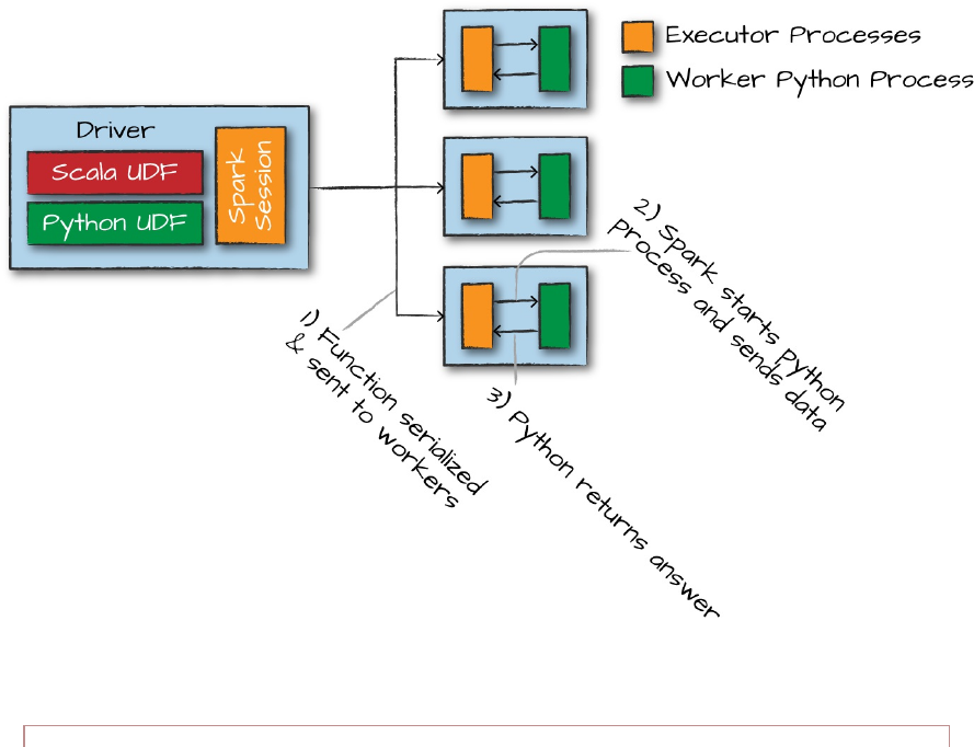
Spark will serialize the function on the driver and transfer it over the network
to all executor processes. This happens regardless of language.
When you use the function, there are essentially two different things that
occur. If the function is written in Scala or Java, you can use it within the
Java Virtual Machine (JVM). This means that there will be little performance
penalty aside from the fact that you can’t take advantage of code generation
capabilities that Spark has for built-in functions. There can be performance
issues if you create or use a lot of objects; we cover that in the section on
optimization in Chapter 19.
If the function is written in Python, something quite different happens. Spark
starts a Python process on the worker, serializes all of the data to a format
that Python can understand (remember, it was in the JVM earlier), executes
the function row by row on that data in the Python process, and then finally
returns the results of the row operations to the JVM and Spark. Figure 6-2
provides an overview of the process.
Figure 6-2. Figure caption

WARNING
Starting this Python process is expensive, but the real cost is in serializing the data to
Python. This is costly for two reasons: it is an expensive computation, but also, after the
data enters Python, Spark cannot manage the memory of the worker. This means that you
could potentially cause a worker to fail if it becomes resource constrained (because both
the JVM and Python are competing for memory on the same machine). We recommend
that you write your UDFs in Scala or Java—the small amount of time it should take you to
write the function in Scala will always yield significant speed ups, and on top of that, you
can still use the function from Python!
Now that you have an understanding of the process, let’s work through an
example. First, we need to register the function to make it available as a
DataFrame function:
// in Scala
import org.apache.spark.sql.functions.udf
val power3udf = udf(power3(_:Double):Double)
We can use that just like any other DataFrame function:
// in Scala
udfExampleDF.select(power3udf(col("num"))).show()
The same applies to Python—first, we register it:
# in Python
from pyspark.sql.functions import udf
power3udf = udf(power3)
Then, we can use it in our DataFrame code:
# in Python
from pyspark.sql.functions import col
udfExampleDF.select(power3udf(col("num"))).show(2)
+-----------+
|power3(num)|
+-----------+
| 0|
| 1|
+-----------+
At this juncture, we can use this only as a DataFrame function. That is to say,
we can’t use it within a string expression, only on an expression. However,
we can also register this UDF as a Spark SQL function. This is valuable
because it makes it simple to use this function within SQL as well as across
languages.
Let’s register the function in Scala:
// in Scala
spark.udf.register("power3", power3(_:Double):Double)
udfExampleDF.selectExpr("power3(num)").show(2)
Because this function is registered with Spark SQL—and we’ve learned that
any Spark SQL function or expression is valid to use as an expression when
working with DataFrames—we can turn around and use the UDF that we
wrote in Scala, in Python. However, rather than using it as a DataFrame
function, we use it as a SQL expression:
# in Python
udfExampleDF.selectExpr("power3(num)").show(2)
# registered in Scala
We can also register our Python function to be available as a SQL function
and use that in any language, as well.
One thing we can also do to ensure that our functions are working correctly is
specify a return type. As we saw in the beginning of this section, Spark
manages its own type information, which does not align exactly with
Python’s types. Therefore, it’s a best practice to define the return type for
your function when you define it. It is important to note that specifying the
return type is not necessary, but it is a best practice.
If you specify the type that doesn’t align with the actual type returned by the
function, Spark will not throw an error but will just return null to designate a
failure. You can see this if you were to switch the return type in the following
function to be a DoubleType:
# in Python
from pyspark.sql.types import IntegerType, DoubleType
spark.udf.register("power3py", power3, DoubleType())
# in Python
udfExampleDF.selectExpr("power3py(num)").show(2)
# registered via Python
This is because the range creates integers. When integers are operated on in
Python, Python won’t convert them into floats (the corresponding type to
Spark’s double type), therefore we see null. We can remedy this by ensuring
that our Python function returns a float instead of an integer and the function
will behave correctly.
Naturally, we can use either of these from SQL, too, after we register them:
-- in SQL
SELECT power3(12), power3py(12) -- doesn't work because of return type
When you want to optionally return a value from a UDF, you should return
None in Python and an Option type in Scala:
## Hive UDFs
As a last note, you can also use UDF/UDAF creation via a Hive syntax. To
allow for this, first you must enable Hive support when they create their
SparkSession (via SparkSession.builder().enableHiveSupport()).
Then you can register UDFs in SQL. This is only supported with precompiled
Scala and Java packages, so you’ll need to specify them as a dependency:
-- in SQL
CREATE TEMPORARY FUNCTION myFunc AS 'com.organization.hive.udf.FunctionName'
Additionally, you can register this as a permanent function in the Hive
Metastore by removing TEMPORARY.
Conclusion
This chapter demonstrated how easy it is to extend Spark SQL to your own
purposes and do so in a way that is not some esoteric, domain-specific
language but rather simple functions that are easy to test and maintain
without even using Spark! This is an amazingly powerful tool that you can
use to specify sophisticated business logic that can run on five rows on your
local machines or on terabytes of data on a 100-node cluster!
Chapter 7. Aggregations
Aggregating is the act of collecting something together and is a cornerstone
of big data analytics. In an aggregation, you will specify a key or grouping
and an aggregation function that specifies how you should transform one or
more columns. This function must produce one result for each group, given
multiple input values. Spark’s aggregation capabilities are sophisticated and
mature, with a variety of different use cases and possibilities. In general, you
use aggregations to summarize numerical data usually by means of some
grouping. This might be a summation, a product, or simple counting. Also,
with Spark you can aggregate any kind of value into an array, list, or map, as
we will see in “Aggregating to Complex Types”.
In addition to working with any type of values, Spark also allows us to create
the following groupings types:
The simplest grouping is to just summarize a complete DataFrame
by performing an aggregation in a select statement.
A “group by” allows you to specify one or more keys as well as one
or more aggregation functions to transform the value columns.
A “window” gives you the ability to specify one or more keys as
well as one or more aggregation functions to transform the value
columns. However, the rows input to the function are somehow
related to the current row.
A “grouping set,” which you can use to aggregate at multiple
different levels. Grouping sets are available as a primitive in SQL
and via rollups and cubes in DataFrames.
A “rollup” makes it possible for you to specify one or more keys as
well as one or more aggregation functions to transform the value
columns, which will be summarized hierarchically.

A “cube” allows you to specify one or more keys as well as one or
more aggregation functions to transform the value columns, which
will be summarized across all combinations of columns.
Each grouping returns a RelationalGroupedDataset on which we specify
our aggregations.
NOTE
An important thing to consider is how exact you need an answer to be. When performing
calculations over big data, it can be quite expensive to get an exact answer to a question,
and it’s often much cheaper to simply request an approximate to a reasonable degree of
accuracy. You’ll note that we mention some approximation functions throughout the book
and oftentimes this is a good opportunity to improve the speed and execution of your
Spark jobs, especially for interactive and ad hoc analysis.
Let’s begin by reading in our data on purchases, repartitioning the data to
have far fewer partitions (because we know it’s a small volume of data stored
in a lot of small files), and caching the results for rapid access:
// in Scala
val df = spark.read.format("csv")
.option("header", "true")
.option("inferSchema", "true")
.load("/data/retail-data/all/*.csv")
.coalesce(5)
df.cache()
df.createOrReplaceTempView("dfTable")
# in Python
df = spark.read.format("csv")\
.option("header", "true")\
.option("inferSchema", "true")\
.load("/data/retail-data/all/*.csv")\
.coalesce(5)
df.cache()
df.createOrReplaceTempView("dfTable")
Here’s a sample of the data so that you can reference the output of some of
the functions:
+---------+---------+--------------------+--------+--------------+---------+----
-
|InvoiceNo|StockCode| Description|Quantity|
InvoiceDate|UnitPrice|Cu...
+---------+---------+--------------------+--------+--------------+---------+----
-
| 536365| 85123A|WHITE HANGING... | 6|12/1/2010 8:26| 2.55|
...
| 536365| 71053|WHITE METAL... | 6|12/1/2010 8:26| 3.39|
...
...
| 536367| 21755|LOVE BUILDING BLO...| 3|12/1/2010 8:34| 5.95|
...
| 536367| 21777|RECIPE BOX WITH M...| 4|12/1/2010 8:34| 7.95|
...
+---------+---------+--------------------+--------+--------------+---------+----
-
As mentioned, basic aggregations apply to an entire DataFrame. The simplest
example is the count method:
df.count() == 541909
If you’ve been reading this book chapter by chapter, you know that count is
actually an action as opposed to a transformation, and so it returns
immediately. You can use count to get an idea of the total size of your
dataset but another common pattern is to use it to cache an entire DataFrame
in memory, just like we did in this example.
Now, this method is a bit of an outlier because it exists as a method (in this
case) as opposed to a function and is eagerly evaluated instead of a lazy
transformation. In the next section, we will see count used as a lazy function,
as well.
Aggregation Functions
All aggregations are available as functions, in addition to the special cases

that can appear on DataFrames or via .stat, like we saw in Chapter 6. You
can find most aggregation functions in the
org.apache.spark.sql.functions package.
NOTE
There are some gaps between the available SQL functions and the functions that we can
import in Scala and Python. This changes every release, so it’s impossible to include a
definitive list. This section covers the most common functions.
count
The first function worth going over is count, except in this example it will
perform as a transformation instead of an action. In this case, we can do one
of two things: specify a specific column to count, or all the columns by using
count(*) or count(1) to represent that we want to count every row as the
literal one, as shown in this example:
// in Scala
import org.apache.spark.sql.functions.count
df.select(count("StockCode")).show() // 541909
# in Python
from pyspark.sql.functions import count
df.select(count("StockCode")).show() # 541909
-- in SQL
SELECT COUNT(*) FROM dfTable
WARNING
There are a number of gotchas when it comes to null values and counting. For instance,
when performing a count(*), Spark will count null values (including rows containing all
nulls). However, when counting an individual column, Spark will not count the null
values.
countDistinct
Sometimes, the total number is not relevant; rather, it’s the number of unique
groups that you want. To get this number, you can use the countDistinct
function. This is a bit more relevant for individual columns:
// in Scala
import org.apache.spark.sql.functions.countDistinct
df.select(countDistinct("StockCode")).show() // 4070
# in Python
from pyspark.sql.functions import countDistinct
df.select(countDistinct("StockCode")).show() # 4070
-- in SQL
SELECT COUNT(DISTINCT *) FROM DFTABLE
approx_count_distinct
Often, we find ourselves working with large datasets and the exact distinct
count is irrelevant. There are times when an approximation to a certain
degree of accuracy will work just fine, and for that, you can use the
approx_count_distinct function:
// in Scala
import org.apache.spark.sql.functions.approx_count_distinct
df.select(approx_count_distinct("StockCode", 0.1)).show() // 3364
# in Python
from pyspark.sql.functions import approx_count_distinct
df.select(approx_count_distinct("StockCode", 0.1)).show() # 3364
-- in SQL
SELECT approx_count_distinct(StockCode, 0.1) FROM DFTABLE
You will notice that approx_count_distinct took another parameter with
which you can specify the maximum estimation error allowed. In this case,
we specified a rather large error and thus receive an answer that is quite far
off but does complete more quickly than countDistinct. You will see much
greater performance gains with larger datasets.
first and last
You can get the first and last values from a DataFrame by using these two
obviously named functions. This will be based on the rows in the DataFrame,
not on the values in the DataFrame:
// in Scala
import org.apache.spark.sql.functions.{first, last}
df.select(first("StockCode"), last("StockCode")).show()
# in Python
from pyspark.sql.functions import first, last
df.select(first("StockCode"), last("StockCode")).show()
-- in SQL
SELECT first(StockCode), last(StockCode) FROM dfTable
+-----------------------+----------------------+
|first(StockCode, false)|last(StockCode, false)|
+-----------------------+----------------------+
| 85123A| 22138|
+-----------------------+----------------------+
min and max
To extract the minimum and maximum values from a DataFrame, use the min
and max functions:
// in Scala
import org.apache.spark.sql.functions.{min, max}
df.select(min("Quantity"), max("Quantity")).show()
# in Python
from pyspark.sql.functions import min, max
df.select(min("Quantity"), max("Quantity")).show()
-- in SQL
SELECT min(Quantity), max(Quantity) FROM dfTable
+-------------+-------------+
|min(Quantity)|max(Quantity)|
+-------------+-------------+
| -80995| 80995|
+-------------+-------------+
sum
Another simple task is to add all the values in a row using the sum function:
// in Scala
import org.apache.spark.sql.functions.sum
df.select(sum("Quantity")).show() // 5176450
# in Python
from pyspark.sql.functions import sum
df.select(sum("Quantity")).show() # 5176450
-- in SQL
SELECT sum(Quantity) FROM dfTable
sumDistinct
In addition to summing a total, you also can sum a distinct set of values by
using the sumDistinct function:
// in Scala
import org.apache.spark.sql.functions.sumDistinct
df.select(sumDistinct("Quantity")).show() // 29310
# in Python
from pyspark.sql.functions import sumDistinct
df.select(sumDistinct("Quantity")).show() # 29310
-- in SQL
SELECT SUM(Quantity) FROM dfTable -- 29310
avg
Although you can calculate average by dividing sum by count, Spark
provides an easier way to get that value via the avg or mean functions. In this

example, we use alias in order to more easily reuse these columns later:
// in Scala
import org.apache.spark.sql.functions.{sum, count, avg, expr}
df.select(
count("Quantity").alias("total_transactions"),
sum("Quantity").alias("total_purchases"),
avg("Quantity").alias("avg_purchases"),
expr("mean(Quantity)").alias("mean_purchases"))
.selectExpr(
"total_purchases/total_transactions",
"avg_purchases",
"mean_purchases").show()
# in Python
from pyspark.sql.functions import sum, count, avg, expr
df.select(
count("Quantity").alias("total_transactions"),
sum("Quantity").alias("total_purchases"),
avg("Quantity").alias("avg_purchases"),
expr("mean(Quantity)").alias("mean_purchases"))\
.selectExpr(
"total_purchases/total_transactions",
"avg_purchases",
"mean_purchases").show()
+--------------------------------------+----------------+----------------+
|(total_purchases / total_transactions)| avg_purchases| mean_purchases|
+--------------------------------------+----------------+----------------+
| 9.55224954743324|9.55224954743324|9.55224954743324|
+--------------------------------------+----------------+----------------+
NOTE
You can also average all the distinct values by specifying distinct. In fact, most aggregate
functions support doing so only on distinct values.
Variance and Standard Deviation
Calculating the mean naturally brings up questions about the variance and
standard deviation. These are both measures of the spread of the data around
the mean. The variance is the average of the squared differences from the
mean, and the standard deviation is the square root of the variance. You can
calculate these in Spark by using their respective functions. However,
something to note is that Spark has both the formula for the sample standard
deviation as well as the formula for the population standard deviation. These
are fundamentally different statistical formulae, and we need to differentiate
between them. By default, Spark performs the formula for the sample
standard deviation or variance if you use the variance or stddev functions.
You can also specify these explicitly or refer to the population standard
deviation or variance:
// in Scala
import org.apache.spark.sql.functions.{var_pop, stddev_pop}
import org.apache.spark.sql.functions.{var_samp, stddev_samp}
df.select(var_pop("Quantity"), var_samp("Quantity"),
stddev_pop("Quantity"), stddev_samp("Quantity")).show()
# in Python
from pyspark.sql.functions import var_pop, stddev_pop
from pyspark.sql.functions import var_samp, stddev_samp
df.select(var_pop("Quantity"), var_samp("Quantity"),
stddev_pop("Quantity"), stddev_samp("Quantity")).show()
-- in SQL
SELECT var_pop(Quantity), var_samp(Quantity),
stddev_pop(Quantity), stddev_samp(Quantity)
FROM dfTable
+------------------+------------------+--------------------+-------------------+
| var_pop(Quantity)|var_samp(Quantity)|stddev_pop(Quantity)|stddev_samp(Quan...|
+------------------+------------------+--------------------+-------------------+
|47559.303646609056|47559.391409298754| 218.08095663447796| 218.081157850...|
+------------------+------------------+--------------------+-------------------+
skewness and kurtosis
Skewness and kurtosis are both measurements of extreme points in your data.
Skewness measures the asymmetry of the values in your data around the
mean, whereas kurtosis is a measure of the tail of data. These are both
relevant specifically when modeling your data as a probability distribution of
a random variable. Although here we won’t go into the math behind these
specifically, you can look up definitions quite easily on the internet. You can
calculate these by using the functions:
import org.apache.spark.sql.functions.{skewness, kurtosis}
df.select(skewness("Quantity"), kurtosis("Quantity")).show()
# in Python
from pyspark.sql.functions import skewness, kurtosis
df.select(skewness("Quantity"), kurtosis("Quantity")).show()
-- in SQL
SELECT skewness(Quantity), kurtosis(Quantity) FROM dfTable
+-------------------+------------------+
| skewness(Quantity)|kurtosis(Quantity)|
+-------------------+------------------+
|-0.2640755761052562|119768.05495536952|
+-------------------+------------------+
Covariance and Correlation
We discussed single column aggregations, but some functions compare the
interactions of the values in two difference columns together. Two of these
functions are cov and corr, for covariance and correlation, respectively.
Correlation measures the Pearson correlation coefficient, which is scaled
between –1 and +1. The covariance is scaled according to the inputs in the
data.
Like the var function, covariance can be calculated either as the sample
covariance or the population covariance. Therefore it can be important to
specify which formula you want to use. Correlation has no notion of this and
therefore does not have calculations for population or sample. Here’s how
they work:
// in Scala
import org.apache.spark.sql.functions.{corr, covar_pop, covar_samp}
df.select(corr("InvoiceNo", "Quantity"), covar_samp("InvoiceNo", "Quantity"),
covar_pop("InvoiceNo", "Quantity")).show()
# in Python
from pyspark.sql.functions import corr, covar_pop, covar_samp
df.select(corr("InvoiceNo", "Quantity"), covar_samp("InvoiceNo", "Quantity"),
covar_pop("InvoiceNo", "Quantity")).show()
-- in SQL
SELECT corr(InvoiceNo, Quantity), covar_samp(InvoiceNo, Quantity),
covar_pop(InvoiceNo, Quantity)
FROM dfTable
+-------------------------+-------------------------------+---------------------
+
|corr(InvoiceNo, Quantity)|covar_samp(InvoiceNo,
Quantity)|covar_pop(InvoiceN...|
+-------------------------+-------------------------------+---------------------
+
| 4.912186085635685E-4| 1052.7280543902734|
1052.7...|
+-------------------------+-------------------------------+---------------------
+
Aggregating to Complex Types
In Spark, you can perform aggregations not just of numerical values using
formulas, you can also perform them on complex types. For example, we can
collect a list of values present in a given column or only the unique values by
collecting to a set.
You can use this to carry out some more programmatic access later on in the
pipeline or pass the entire collection in a user-defined function (UDF):
// in Scala
import org.apache.spark.sql.functions.{collect_set, collect_list}
df.agg(collect_set("Country"), collect_list("Country")).show()
# in Python
from pyspark.sql.functions import collect_set, collect_list
df.agg(collect_set("Country"), collect_list("Country")).show()
-- in SQL
SELECT collect_set(Country), collect_set(Country) FROM dfTable
+--------------------+---------------------+
|collect_set(Country)|collect_list(Country)|
+--------------------+---------------------+
|[Portugal, Italy,...| [United Kingdom, ...|
+--------------------+---------------------+
Grouping
Thus far, we have performed only DataFrame-level aggregations. A more
common task is to perform calculations based on groups in the data. This is
typically done on categorical data for which we group our data on one
column and perform some calculations on the other columns that end up in
that group.
The best way to explain this is to begin performing some groupings. The first
will be a count, just as we did before. We will group by each unique invoice
number and get the count of items on that invoice. Note that this returns
another DataFrame and is lazily performed.
We do this grouping in two phases. First we specify the column(s) on which
we would like to group, and then we specify the aggregation(s). The first step
returns a RelationalGroupedDataset, and the second step returns a
DataFrame.
As mentioned, we can specify any number of columns on which we want to
group:
df.groupBy("InvoiceNo", "CustomerId").count().show()
-- in SQL
SELECT count(*) FROM dfTable GROUP BY InvoiceNo, CustomerId
+---------+----------+-----+
|InvoiceNo|CustomerId|count|
+---------+----------+-----+
| 536846| 14573| 76|
...
| C544318| 12989| 1|
+---------+----------+-----+
Grouping with Expressions
As we saw earlier, counting is a bit of a special case because it exists as a
method. For this, usually we prefer to use the count function. Rather than
passing that function as an expression into a select statement, we specify it
as within agg. This makes it possible for you to pass-in arbitrary expressions
that just need to have some aggregation specified. You can even do things
like alias a column after transforming it for later use in your data flow:
// in Scala
import org.apache.spark.sql.functions.count
df.groupBy("InvoiceNo").agg(
count("Quantity").alias("quan"),
expr("count(Quantity)")).show()
# in Python
from pyspark.sql.functions import count
df.groupBy("InvoiceNo").agg(
count("Quantity").alias("quan"),
expr("count(Quantity)")).show()
+---------+----+---------------+
|InvoiceNo|quan|count(Quantity)|
+---------+----+---------------+
| 536596| 6| 6|
...
| C542604| 8| 8|
+---------+----+---------------+
Grouping with Maps
Sometimes, it can be easier to specify your transformations as a series of
Maps for which the key is the column, and the value is the aggregation
function (as a string) that you would like to perform. You can reuse multiple
column names if you specify them inline, as well:
// in Scala
df.groupBy("InvoiceNo").agg("Quantity"->"avg", "Quantity"->"stddev_pop").show()
# in Python
df.groupBy("InvoiceNo").agg(expr("avg(Quantity)"),expr("stddev_pop(Quantity)"))\
.show()
-- in SQL
SELECT avg(Quantity), stddev_pop(Quantity), InvoiceNo FROM dfTable
GROUP BY InvoiceNo
+---------+------------------+--------------------+
|InvoiceNo| avg(Quantity)|stddev_pop(Quantity)|
+---------+------------------+--------------------+
| 536596| 1.5| 1.1180339887498947|
...
| C542604| -8.0| 15.173990905493518|
+---------+------------------+--------------------+
Window Functions
You can also use window functions to carry out some unique aggregations by
either computing some aggregation on a specific “window” of data, which
you define by using a reference to the current data. This window specification
determines which rows will be passed in to this function. Now this is a bit
abstract and probably similar to a standard group-by, so let’s differentiate
them a bit more.
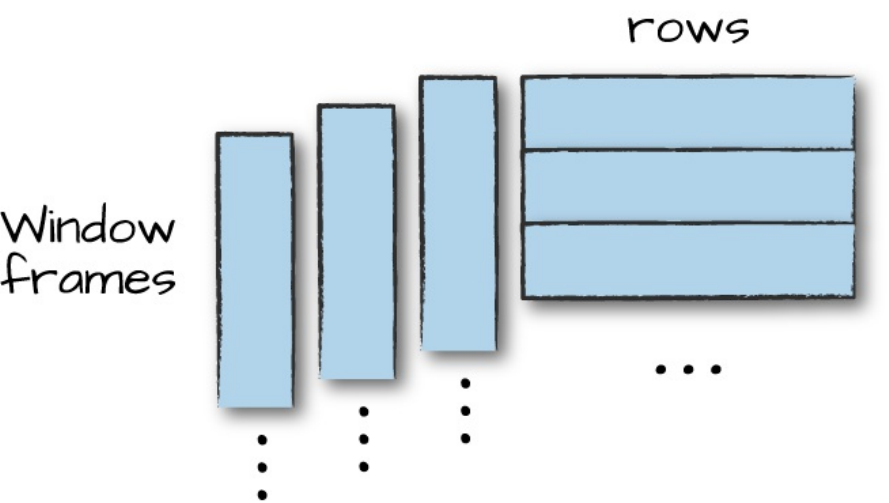
A group-by takes data, and every row can go only into one grouping. A
window function calculates a return value for every input row of a table
based on a group of rows, called a frame. Each row can fall into one or more
frames. A common use case is to take a look at a rolling average of some
value for which each row represents one day. If you were to do this, each row
would end up in seven different frames. We cover defining frames a little
later, but for your reference, Spark supports three kinds of window functions:
ranking functions, analytic functions, and aggregate functions.
Figure 7-1 illustrates how a given row can fall into multiple frames.
Figure 7-1. Visualizing window functions
To demonstrate, we will add a date column that will convert our invoice date
into a column that contains only date information (not time information, too):
// in Scala
import org.apache.spark.sql.functions.{col, to_date}
val dfWithDate = df.withColumn("date", to_date(col("InvoiceDate"),
"MM/d/yyyy H:mm"))
dfWithDate.createOrReplaceTempView("dfWithDate")
# in Python
from pyspark.sql.functions import col, to_date
dfWithDate = df.withColumn("date", to_date(col("InvoiceDate"), "MM/d/yyyy
H:mm"))
dfWithDate.createOrReplaceTempView("dfWithDate")
The first step to a window function is to create a window specification. Note
that the partition by is unrelated to the partitioning scheme concept that
we have covered thus far. It’s just a similar concept that describes how we
will be breaking up our group. The ordering determines the ordering within a
given partition, and, finally, the frame specification (the rowsBetween
statement) states which rows will be included in the frame based on its
reference to the current input row. In the following example, we look at all
previous rows up to the current row:
// in Scala
import org.apache.spark.sql.expressions.Window
import org.apache.spark.sql.functions.col
val windowSpec = Window
.partitionBy("CustomerId", "date")
.orderBy(col("Quantity").desc)
.rowsBetween(Window.unboundedPreceding, Window.currentRow)
# in Python
from pyspark.sql.window import Window
from pyspark.sql.functions import desc
windowSpec = Window\
.partitionBy("CustomerId", "date")\
.orderBy(desc("Quantity"))\
.rowsBetween(Window.unboundedPreceding, Window.currentRow)
Now we want to use an aggregation function to learn more about each
specific customer. An example might be establishing the maximum purchase
quantity over all time. To answer this, we use the same aggregation functions
that we saw earlier by passing a column name or expression. In addition, we
indicate the window specification that defines to which frames of data this
function will apply:
import org.apache.spark.sql.functions.max
val maxPurchaseQuantity = max(col("Quantity")).over(windowSpec)
# in Python
from pyspark.sql.functions import max
maxPurchaseQuantity = max(col("Quantity")).over(windowSpec)
You will notice that this returns a column (or expressions). We can now use
this in a DataFrame select statement. Before doing so, though, we will create
the purchase quantity rank. To do that we use the dense_rank function to
determine which date had the maximum purchase quantity for every
customer. We use dense_rank as opposed to rank to avoid gaps in the
ranking sequence when there are tied values (or in our case, duplicate rows):
// in Scala
import org.apache.spark.sql.functions.{dense_rank, rank}
val purchaseDenseRank = dense_rank().over(windowSpec)
val purchaseRank = rank().over(windowSpec)
# in Python
from pyspark.sql.functions import dense_rank, rank
purchaseDenseRank = dense_rank().over(windowSpec)
purchaseRank = rank().over(windowSpec)
This also returns a column that we can use in select statements. Now we can
perform a select to view the calculated window values:
// in Scala
import org.apache.spark.sql.functions.col
dfWithDate.where("CustomerId IS NOT NULL").orderBy("CustomerId")
.select(
col("CustomerId"),
col("date"),
col("Quantity"),
purchaseRank.alias("quantityRank"),
purchaseDenseRank.alias("quantityDenseRank"),
maxPurchaseQuantity.alias("maxPurchaseQuantity")).show()
# in Python
from pyspark.sql.functions import col
dfWithDate.where("CustomerId IS NOT NULL").orderBy("CustomerId")\
.select(
col("CustomerId"),
col("date"),
col("Quantity"),
purchaseRank.alias("quantityRank"),
purchaseDenseRank.alias("quantityDenseRank"),
maxPurchaseQuantity.alias("maxPurchaseQuantity")).show()
-- in SQL
SELECT CustomerId, date, Quantity,
rank(Quantity) OVER (PARTITION BY CustomerId, date
ORDER BY Quantity DESC NULLS LAST
ROWS BETWEEN
UNBOUNDED PRECEDING AND
CURRENT ROW) as rank,
dense_rank(Quantity) OVER (PARTITION BY CustomerId, date
ORDER BY Quantity DESC NULLS LAST
ROWS BETWEEN
UNBOUNDED PRECEDING AND
CURRENT ROW) as dRank,
max(Quantity) OVER (PARTITION BY CustomerId, date
ORDER BY Quantity DESC NULLS LAST
ROWS BETWEEN
UNBOUNDED PRECEDING AND
CURRENT ROW) as maxPurchase
FROM dfWithDate WHERE CustomerId IS NOT NULL ORDER BY CustomerId
+----------+----------+--------+------------+-----------------+---------------+
|CustomerId| date|Quantity|quantityRank|quantityDenseRank|maxP...Quantity|
+----------+----------+--------+------------+-----------------+---------------+
| 12346|2011-01-18| 74215| 1| 1| 74215|
| 12346|2011-01-18| -74215| 2| 2| 74215|
| 12347|2010-12-07| 36| 1| 1| 36|
| 12347|2010-12-07| 30| 2| 2| 36|
...
| 12347|2010-12-07| 12| 4| 4| 36|
| 12347|2010-12-07| 6| 17| 5| 36|
| 12347|2010-12-07| 6| 17| 5| 36|
+----------+----------+--------+------------+-----------------+---------------+
Grouping Sets
Thus far in this chapter, we’ve seen simple group-by expressions that we can
use to aggregate on a set of columns with the values in those columns.
However, sometimes we want something a bit more complete—an
aggregation across multiple groups. We achieve this by using grouping sets.
Grouping sets are a low-level tool for combining sets of aggregations
together. They give you the ability to create arbitrary aggregation in their
group-by statements.
Let’s work through an example to gain a better understanding. Here, we
would like to get the total quantity of all stock codes and customers. To do
so, we’ll use the following SQL expression:
// in Scala
val dfNoNull = dfWithDate.drop()
dfNoNull.createOrReplaceTempView("dfNoNull")
# in Python
dfNoNull = dfWithDate.drop()
dfNoNull.createOrReplaceTempView("dfNoNull")
-- in SQL
SELECT CustomerId, stockCode, sum(Quantity) FROM dfNoNull
GROUP BY customerId, stockCode
ORDER BY CustomerId DESC, stockCode DESC
+----------+---------+-------------+
|CustomerId|stockCode|sum(Quantity)|
+----------+---------+-------------+
| 18287| 85173| 48|
| 18287| 85040A| 48|
| 18287| 85039B| 120|
...
| 18287| 23269| 36|
+----------+---------+-------------+
You can do the exact same thing by using a grouping set:
-- in SQL
SELECT CustomerId, stockCode, sum(Quantity) FROM dfNoNull
GROUP BY customerId, stockCode GROUPING SETS((customerId, stockCode))
ORDER BY CustomerId DESC, stockCode DESC
+----------+---------+-------------+
|CustomerId|stockCode|sum(Quantity)|
+----------+---------+-------------+

| 18287| 85173| 48|
| 18287| 85040A| 48|
| 18287| 85039B| 120|
...
| 18287| 23269| 36|
+----------+---------+-------------+
WARNING
Grouping sets depend on null values for aggregation levels. If you do not filter-out null
values, you will get incorrect results. This applies to cubes, rollups, and grouping sets.
Simple enough, but what if you also want to include the total number of
items, regardless of customer or stock code? With a conventional group-by
statement, this would be impossible. But, it’s simple with grouping sets: we
simply specify that we would like to aggregate at that level, as well, in our
grouping set. This is, effectively, the union of several different groupings
together:
-- in SQL
SELECT CustomerId, stockCode, sum(Quantity) FROM dfNoNull
GROUP BY customerId, stockCode GROUPING SETS((customerId, stockCode),())
ORDER BY CustomerId DESC, stockCode DESC
+----------+---------+-------------+
|customerId|stockCode|sum(Quantity)|
+----------+---------+-------------+
| 18287| 85173| 48|
| 18287| 85040A| 48|
| 18287| 85039B| 120|
...
| 18287| 23269| 36|
+----------+---------+-------------+
The GROUPING SETS operator is only available in SQL. To perform the same
in DataFrames, you use the rollup and cube operators—which allow us to
get the same results. Let’s go through those.
Rollups
Thus far, we’ve been looking at explicit groupings. When we set our
grouping keys of multiple columns, Spark looks at those as well as the actual
combinations that are visible in the dataset. A rollup is a multidimensional
aggregation that performs a variety of group-by style calculations for us.
Let’s create a rollup that looks across time (with our new Date column) and
space (with the Country column) and creates a new DataFrame that includes
the grand total over all dates, the grand total for each date in the DataFrame,
and the subtotal for each country on each date in the DataFrame:
val rolledUpDF = dfNoNull.rollup("Date", "Country").agg(sum("Quantity"))
.selectExpr("Date", "Country", "`sum(Quantity)` as total_quantity")
.orderBy("Date")
rolledUpDF.show()
# in Python
rolledUpDF = dfNoNull.rollup("Date", "Country").agg(sum("Quantity"))\
.selectExpr("Date", "Country", "`sum(Quantity)` as total_quantity")\
.orderBy("Date")
rolledUpDF.show()
+----------+--------------+--------------+
| Date| Country|total_quantity|
+----------+--------------+--------------+
| null| null| 5176450|
|2010-12-01|United Kingdom| 23949|
|2010-12-01| Germany| 117|
|2010-12-01| France| 449|
...
|2010-12-03| France| 239|
|2010-12-03| Italy| 164|
|2010-12-03| Belgium| 528|
+----------+--------------+--------------+
Now where you see the null values is where you’ll find the grand totals. A
null in both rollup columns specifies the grand total across both of those
columns:
rolledUpDF.where("Country IS NULL").show()

rolledUpDF.where("Date IS NULL").show()
+----+-------+--------------+
|Date|Country|total_quantity|
+----+-------+--------------+
|null| null| 5176450|
+----+-------+--------------+
Cube
A cube takes the rollup to a level deeper. Rather than treating elements
hierarchically, a cube does the same thing across all dimensions. This means
that it won’t just go by date over the entire time period, but also the country.
To pose this as a question again, can you make a table that includes the
following?
The total across all dates and countries
The total for each date across all countries
The total for each country on each date
The total for each country across all dates
The method call is quite similar, but instead of calling rollup, we call cube:
// in Scala
dfNoNull.cube("Date", "Country").agg(sum(col("Quantity")))
.select("Date", "Country", "sum(Quantity)").orderBy("Date").show()
# in Python
from pyspark.sql.functions import sum
dfNoNull.cube("Date", "Country").agg(sum(col("Quantity")))\
.select("Date", "Country", "sum(Quantity)").orderBy("Date").show()
+----+--------------------+-------------+
|Date| Country|sum(Quantity)|
+----+--------------------+-------------+
|null| Japan| 25218|
|null| Portugal| 16180|
|null| Unspecified| 3300|

|null| null| 5176450|
|null| Australia| 83653|
...
|null| Norway| 19247|
|null| Hong Kong| 4769|
|null| Spain| 26824|
|null| Czech Republic| 592|
+----+--------------------+-------------+
This is a quick and easily accessible summary of nearly all of the information
in our table, and it’s a great way to create a quick summary table that others
can use later on.
Grouping Metadata
Sometimes when using cubes and rollups, you want to be able to query the
aggregation levels so that you can easily filter them down accordingly. We
can do this by using the grouping_id, which gives us a column specifying
the level of aggregation that we have in our result set. The query in the
example that follows returns four distinct grouping IDs:
Table 7-1. Purpose of grouping IDs
Grouping
ID Description
3This will appear for the highest-level aggregation, which will gives us the total
quantity regardless of customerId and stockCode.
2This will appear for all aggregations of individual stock codes. This gives us the
total quantity per stock code, regardless of customer.
1This will give us the total quantity on a per-customer basis, regardless of item
purchased.
0This will give us the total quantity for individual customerId and stockCode
combinations.
This is a bit abstract, so it’s well worth trying out to understand the behavior
yourself:
// in Scala
import org.apache.spark.sql.functions.{grouping_id, sum, expr}
dfNoNull.cube("customerId", "stockCode").agg(grouping_id(), sum("Quantity"))
.orderBy(expr("grouping_id()").desc)
.show()
+----------+---------+-------------+-------------+
|customerId|stockCode|grouping_id()|sum(Quantity)|
+----------+---------+-------------+-------------+
| null| null| 3| 5176450|
| null| 23217| 2| 1309|
| null| 90059E| 2| 19|
...
+----------+---------+-------------+-------------+
Pivot
Pivots make it possible for you to convert a row into a column. For example,
in our current data we have a Country column. With a pivot, we can
aggregate according to some function for each of those given countries and
display them in an easy-to-query way:
// in Scala
val pivoted = dfWithDate.groupBy("date").pivot("Country").sum()
# in Python
pivoted = dfWithDate.groupBy("date").pivot("Country").sum()
This DataFrame will now have a column for every combination of country,
numeric variable, and a column specifying the date. For example, for USA
we have the following columns: USA_sum(Quantity),
USA_sum(UnitPrice), USA_sum(CustomerID). This represents one for each
numeric column in our dataset (because we just performed an aggregation
over all of them).
Here’s an example query and result from this data:
pivoted.where("date > '2011-12-05'").select("date"
,"`USA_sum(Quantity)`").show()

+----------+-----------------+
| date|USA_sum(Quantity)|
+----------+-----------------+
|2011-12-06| null|
|2011-12-09| null|
|2011-12-08| -196|
|2011-12-07| null|
+----------+-----------------+
Now all of the columns can be calculated with single groupings, but the value
of a pivot comes down to how you would like to explore the data. It can be
useful, if you have low enough cardinality in a certain column to transform it
into columns so that users can see the schema and immediately know what to
query for.
User-Defined Aggregation Functions
User-defined aggregation functions (UDAFs) are a way for users to define
their own aggregation functions based on custom formulae or business rules.
You can use UDAFs to compute custom calculations over groups of input
data (as opposed to single rows). Spark maintains a single
AggregationBuffer to store intermediate results for every group of input
data.
To create a UDAF, you must inherit from the
UserDefinedAggregateFunction base class and implement the following
methods:
inputSchema represents input arguments as a StructType
bufferSchema represents intermediate UDAF results as a
StructType
dataType represents the return DataType
deterministic is a Boolean value that specifies whether this
UDAF will return the same result for a given input

initialize allows you to initialize values of an aggregation buffer
update describes how you should update the internal buffer based
on a given row
merge describes how two aggregation buffers should be merged
evaluate will generate the final result of the aggregation
The following example implements a BoolAnd, which will inform us whether
all the rows (for a given column) are true; if they’re not, it will return false:
// in Scala
import org.apache.spark.sql.expressions.MutableAggregationBuffer
import org.apache.spark.sql.expressions.UserDefinedAggregateFunction
import org.apache.spark.sql.Row
import org.apache.spark.sql.types._
class BoolAnd extends UserDefinedAggregateFunction {
def inputSchema: org.apache.spark.sql.types.StructType =
StructType(StructField("value", BooleanType) :: Nil)
def bufferSchema: StructType = StructType(
StructField("result", BooleanType) :: Nil
)
def dataType: DataType = BooleanType
def deterministic: Boolean = true
def initialize(buffer: MutableAggregationBuffer): Unit = {
buffer(0) = true
}
def update(buffer: MutableAggregationBuffer, input: Row): Unit = {
buffer(0) = buffer.getAs[Boolean](0) && input.getAs[Boolean](0)
}
def merge(buffer1: MutableAggregationBuffer, buffer2: Row): Unit = {
buffer1(0) = buffer1.getAs[Boolean](0) && buffer2.getAs[Boolean](0)
}
def evaluate(buffer: Row): Any = {
buffer(0)
}
}
Now, we simply instantiate our class and/or register it as a function:
// in Scala
val ba = new BoolAnd
spark.udf.register("booland", ba)
import org.apache.spark.sql.functions._
spark.range(1)
.selectExpr("explode(array(TRUE, TRUE, TRUE)) as t")
.selectExpr("explode(array(TRUE, FALSE, TRUE)) as f", "t")
.select(ba(col("t")), expr("booland(f)"))
.show()
+----------+----------+
|booland(t)|booland(f)|
+----------+----------+
| true| false|
+----------+----------+
UDAFs are currently available only in Scala or Java. However, in Spark 2.3,
you will also be able to call Scala or Java UDFs and UDAFs by registering
the function just as we showed in the UDF section in Chapter 6. For more
information, go to SPARK-19439.
Conclusion
This chapter walked through the different types and kinds of aggregations
that you can perform in Spark. You learned about simple grouping-to
window functions as well as rollups and cubes. Chapter 8 discusses how to
perform joins to combine different data sources together.

Chapter 8. Joins
Chapter 7 covered aggregating single datasets, which is helpful, but more
often than not, your Spark applications are going to bring together a large
number of different datasets. For this reason, joins are an essential part of
nearly all Spark workloads. Spark’s ability to talk to different data means that
you gain the ability to tap into a variety of data sources across your company.
This chapter covers not just what joins exist in Spark and how to use them,
but some of the basic internals so that you can think about how Spark
actually goes about executing the join on the cluster. This basic knowledge
can help you avoid running out of memory and tackle problems that you
could not solve before.
Join Expressions
A join brings together two sets of data, the left and the right, by comparing
the value of one or more keys of the left and right and evaluating the result of
a join expression that determines whether Spark should bring together the left
set of data with the right set of data. The most common join expression, an
equi-join, compares whether the specified keys in your left and right
datasets are equal. If they are equal, Spark will combine the left and right
datasets. The opposite is true for keys that do not match; Spark discards the
rows that do not have matching keys. Spark also allows for much more
sophsticated join policies in addition to equi-joins. We can even use complex
types and perform something like checking whether a key exists within an
array when you perform a join.
Join Types
Whereas the join expression determines whether two rows should join, the
join type determines what should be in the result set. There are a variety of

different join types available in Spark for you to use:
Inner joins (keep rows with keys that exist in the left and right
datasets)
Outer joins (keep rows with keys in either the left or right datasets)
Left outer joins (keep rows with keys in the left dataset)
Right outer joins (keep rows with keys in the right dataset)
Left semi joins (keep the rows in the left, and only the left, dataset
where the key appears in the right dataset)
Left anti joins (keep the rows in the left, and only the left, dataset
where they do not appear in the right dataset)
Natural joins (perform a join by implicitly matching the columns
between the two datasets with the same names)
Cross (or Cartesian) joins (match every row in the left dataset with
every row in the right dataset)
If you have ever interacted with a relational database system, or even an
Excel spreadsheet, the concept of joining different datasets together should
not be too abstract. Let’s move on to showing examples of each join type.
This will make it easy to understand exactly how you can apply these to your
own problems. To do this, let’s create some simple datasets that we can use
in our examples:
// in Scala
val person = Seq(
(0, "Bill Chambers", 0, Seq(100)),
(1, "Matei Zaharia", 1, Seq(500, 250, 100)),
(2, "Michael Armbrust", 1, Seq(250, 100)))
.toDF("id", "name", "graduate_program", "spark_status")
val graduateProgram = Seq(
(0, "Masters", "School of Information", "UC Berkeley"),
(2, "Masters", "EECS", "UC Berkeley"),
(1, "Ph.D.", "EECS", "UC Berkeley"))
.toDF("id", "degree", "department", "school")
val sparkStatus = Seq(
(500, "Vice President"),
(250, "PMC Member"),
(100, "Contributor"))
.toDF("id", "status")
# in Python
person = spark.createDataFrame([
(0, "Bill Chambers", 0, [100]),
(1, "Matei Zaharia", 1, [500, 250, 100]),
(2, "Michael Armbrust", 1, [250, 100])])\
.toDF("id", "name", "graduate_program", "spark_status")
graduateProgram = spark.createDataFrame([
(0, "Masters", "School of Information", "UC Berkeley"),
(2, "Masters", "EECS", "UC Berkeley"),
(1, "Ph.D.", "EECS", "UC Berkeley")])\
.toDF("id", "degree", "department", "school")
sparkStatus = spark.createDataFrame([
(500, "Vice President"),
(250, "PMC Member"),
(100, "Contributor")])\
.toDF("id", "status")
Next, let’s register these as tables so that we use them throughout the chapter:
person.createOrReplaceTempView("person")
graduateProgram.createOrReplaceTempView("graduateProgram")
sparkStatus.createOrReplaceTempView("sparkStatus")
Inner Joins
Inner joins evaluate the keys in both of the DataFrames or tables and include
(and join together) only the rows that evaluate to true. In the following
example, we join the graduateProgram DataFrame with the person
DataFrame to create a new DataFrame:
// in Scala
val joinExpression = person.col("graduate_program") ===
graduateProgram.col("id")
# in Python
joinExpression = person["graduate_program"] == graduateProgram['id']
Keys that do not exist in both DataFrames will not show in the resulting
DataFrame. For example, the following expression would result in zero
values in the resulting DataFrame:
// in Scala
val wrongJoinExpression = person.col("name") === graduateProgram.col("school")
# in Python
wrongJoinExpression = person["name"] == graduateProgram["school"]
Inner joins are the default join, so we just need to specify our left DataFrame
and join the right in the JOIN expression:
person.join(graduateProgram, joinExpression).show()
-- in SQL
SELECT * FROM person JOIN graduateProgram
ON person.graduate_program = graduateProgram.id
+---+----------------+----------------+---------------+---+-------+----------+--
-
| id| name|graduate_program| spark_status| id|
degree|department|...
+---+----------------+----------------+---------------+---+-------+----------+--
-
| 0| Bill Chambers| 0| [100]| 0|Masters|
School...|...
| 1| Matei Zaharia| 1|[500, 250, 100]| 1| Ph.D.|
EECS|...
| 2|Michael Armbrust| 1| [250, 100]| 1| Ph.D.|
EECS|...
+---+----------------+----------------+---------------+---+-------+----------+--
-
We can also specify this explicitly by passing in a third parameter, the
joinType:
// in Scala
var joinType = "inner"
# in Python
joinType = "inner"
person.join(graduateProgram, joinExpression, joinType).show()
-- in SQL
SELECT * FROM person INNER JOIN graduateProgram
ON person.graduate_program = graduateProgram.id
+---+----------------+----------------+---------------+---+-------+-------------
-
| id| name|graduate_program| spark_status| id| degree|
department...
+---+----------------+----------------+---------------+---+-------+-------------
-
| 0| Bill Chambers| 0| [100]| 0|Masters|
School...
| 1| Matei Zaharia| 1|[500, 250, 100]| 1| Ph.D.|
EECS...
| 2|Michael Armbrust| 1| [250, 100]| 1| Ph.D.|
EECS...
+---+----------------+----------------+---------------+---+-------+-------------
-
Outer Joins
Outer joins evaluate the keys in both of the DataFrames or tables and
includes (and joins together) the rows that evaluate to true or false. If there is
no equivalent row in either the left or right DataFrame, Spark will insert
null:
joinType = "outer"
person.join(graduateProgram, joinExpression, joinType).show()
-- in SQL
SELECT * FROM person FULL OUTER JOIN graduateProgram
ON graduate_program = graduateProgram.id
+----+----------------+----------------+---------------+---+-------+------------
-
| id| name|graduate_program| spark_status| id| degree|
departmen...
+----+----------------+----------------+---------------+---+-------+------------
-
| 1| Matei Zaharia| 1|[500, 250, 100]| 1| Ph.D.|
EEC...
| 2|Michael Armbrust| 1| [250, 100]| 1| Ph.D.|
EEC...
|null| null| null| null| 2|Masters|
EEC...
| 0| Bill Chambers| 0| [100]| 0|Masters|
School...
+----+----------------+----------------+---------------+---+-------+------------
-
Left Outer Joins
Left outer joins evaluate the keys in both of the DataFrames or tables and
includes all rows from the left DataFrame as well as any rows in the right
DataFrame that have a match in the left DataFrame. If there is no equivalent
row in the right DataFrame, Spark will insert null:
joinType = "left_outer"
graduateProgram.join(person, joinExpression, joinType).show()
-- in SQL
SELECT * FROM graduateProgram LEFT OUTER JOIN person
ON person.graduate_program = graduateProgram.id
+---+-------+----------+-----------+----+----------------+----------------+---
| id| degree|department| school| id| name|graduate_program|...
+---+-------+----------+-----------+----+----------------+----------------+---
| 0|Masters| School...|UC Berkeley| 0| Bill Chambers| 0|...
| 2|Masters| EECS|UC Berkeley|null| null| null|...
| 1| Ph.D.| EECS|UC Berkeley| 2|Michael Armbrust| 1|...
| 1| Ph.D.| EECS|UC Berkeley| 1| Matei Zaharia| 1|...
+---+-------+----------+-----------+----+----------------+----------------+---
Right Outer Joins
Right outer joins evaluate the keys in both of the DataFrames or tables and
includes all rows from the right DataFrame as well as any rows in the left
DataFrame that have a match in the right DataFrame. If there is no equivalent
row in the left DataFrame, Spark will insert null:
joinType = "right_outer"
person.join(graduateProgram, joinExpression, joinType).show()
-- in SQL
SELECT * FROM person RIGHT OUTER JOIN graduateProgram
ON person.graduate_program = graduateProgram.id
+----+----------------+----------------+---------------+---+-------+------------
+
| id| name|graduate_program| spark_status| id| degree|
department|
+----+----------------+----------------+---------------+---+-------+------------
+
| 0| Bill Chambers| 0| [100]| 0|Masters|School
of...|
|null| null| null| null| 2|Masters|
EECS|
| 2|Michael Armbrust| 1| [250, 100]| 1| Ph.D.|
EECS|
| 1| Matei Zaharia| 1|[500, 250, 100]| 1| Ph.D.|
EECS|
+----+----------------+----------------+---------------+---+-------+------------
+
Left Semi Joins
Semi joins are a bit of a departure from the other joins. They do not actually
include any values from the right DataFrame. They only compare values to
see if the value exists in the second DataFrame. If the value does exist, those
rows will be kept in the result, even if there are duplicate keys in the left
DataFrame. Think of left semi joins as filters on a DataFrame, as opposed to
the function of a conventional join:
joinType = "left_semi"
graduateProgram.join(person, joinExpression, joinType).show()
+---+-------+--------------------+-----------+
| id| degree| department| school|
+---+-------+--------------------+-----------+
| 0|Masters|School of Informa...|UC Berkeley|
| 1| Ph.D.| EECS|UC Berkeley|
+---+-------+--------------------+-----------+
// in Scala
val gradProgram2 = graduateProgram.union(Seq(
(0, "Masters", "Duplicated Row", "Duplicated School")).toDF())
gradProgram2.createOrReplaceTempView("gradProgram2")
# in Python
gradProgram2 = graduateProgram.union(spark.createDataFrame([
(0, "Masters", "Duplicated Row", "Duplicated School")]))
gradProgram2.createOrReplaceTempView("gradProgram2")
gradProgram2.join(person, joinExpression, joinType).show()
-- in SQL
SELECT * FROM gradProgram2 LEFT SEMI JOIN person
ON gradProgram2.id = person.graduate_program
+---+-------+--------------------+-----------------+
| id| degree| department| school|
+---+-------+--------------------+-----------------+
| 0|Masters|School of Informa...| UC Berkeley|
| 1| Ph.D.| EECS| UC Berkeley|
| 0|Masters| Duplicated Row|Duplicated School|
+---+-------+--------------------+-----------------+
Left Anti Joins
Left anti joins are the opposite of left semi joins. Like left semi joins, they do
not actually include any values from the right DataFrame. They only compare
values to see if the value exists in the second DataFrame. However, rather
than keeping the values that exist in the second DataFrame, they keep only
the values that do not have a corresponding key in the second DataFrame.
Think of anti joins as a NOT IN SQL-style filter:
joinType = "left_anti"
graduateProgram.join(person, joinExpression, joinType).show()
-- in SQL
SELECT * FROM graduateProgram LEFT ANTI JOIN person
ON graduateProgram.id = person.graduate_program
+---+-------+----------+-----------+
| id| degree|department| school|
+---+-------+----------+-----------+
| 2|Masters| EECS|UC Berkeley|
+---+-------+----------+-----------+
Natural Joins
Natural joins make implicit guesses at the columns on which you would like

to join. It finds matching columns and returns the results. Left, right, and
outer natural joins are all supported.
WARNING
Implicit is always dangerous! The following query will give us incorrect results because
the two DataFrames/tables share a column name (id), but it means different things in the
datasets. You should always use this join with caution.
-- in SQL
SELECT * FROM graduateProgram NATURAL JOIN person
Cross (Cartesian) Joins
The last of our joins are cross-joins or cartesian products. Cross-joins in
simplest terms are inner joins that do not specify a predicate. Cross joins will
join every single row in the left DataFrame to ever single row in the right
DataFrame. This will cause an absolute explosion in the number of rows
contained in the resulting DataFrame. If you have 1,000 rows in each
DataFrame, the cross-join of these will result in 1,000,000 (1,000 x 1,000)
rows. For this reason, you must very explicitly state that you want a cross-
join by using the cross join keyword:
joinType = "cross"
graduateProgram.join(person, joinExpression, joinType).show()
-- in SQL
SELECT * FROM graduateProgram CROSS JOIN person
ON graduateProgram.id = person.graduate_program

+---+-------+----------+-----------+---+----------------+----------------+------
-
| id| degree|department| school| id|
name|graduate_program|spar...
+---+-------+----------+-----------+---+----------------+----------------+------
-
| 0|Masters| School...|UC Berkeley| 0| Bill Chambers| 0|
...
| 1| Ph.D.| EECS|UC Berkeley| 2|Michael Armbrust| 1|
[2...
| 1| Ph.D.| EECS|UC Berkeley| 1| Matei Zaharia| 1|
[500...
+---+-------+----------+-----------+---+----------------+----------------+------
-
If you truly intend to have a cross-join, you can call that out explicitly:
person.crossJoin(graduateProgram).show()
-- in SQL
SELECT * FROM graduateProgram CROSS JOIN person
+---+----------------+----------------+---------------+---+-------+-------------
+
| id| name|graduate_program| spark_status| id| degree|
departm...|
+---+----------------+----------------+---------------+---+-------+-------------
+
| 0| Bill Chambers| 0| [100]| 0|Masters|
School...|
...
| 1| Matei Zaharia| 1|[500, 250, 100]| 0|Masters|
School...|
...
| 2|Michael Armbrust| 1| [250, 100]| 0|Masters|
School...|
...
+---+----------------+----------------+---------------+---+-------+-------------
+
WARNING
You should use cross-joins only if you are absolutely, 100 percent sure that this is the join

you need. There is a reason why you need to be explicit when defining a cross-join in
Spark. They’re dangerous! Advanced users can set the session-level configuration
spark.sql.crossJoin.enable to true in order to allow cross-joins without warnings or
without Spark trying to perform another join for you.
Challenges When Using Joins
When performing joins, there are some specific challenges and some
common questions that arise. The rest of the chapter will provide answers to
these common questions and then explain how, at a high level, Spark
performs joins. This will hint at some of the optimizations that we are going
to cover in later parts of this book.
Joins on Complex Types
Even though this might seem like a challenge, it’s actually not. Any
expression is a valid join expression, assuming that it returns a Boolean:
import org.apache.spark.sql.functions.expr
person.withColumnRenamed("id", "personId")
.join(sparkStatus, expr("array_contains(spark_status, id)")).show()
# in Python
from pyspark.sql.functions import expr
person.withColumnRenamed("id", "personId")\
.join(sparkStatus, expr("array_contains(spark_status, id)")).show()
-- in SQL
SELECT * FROM
(select id as personId, name, graduate_program, spark_status FROM person)
INNER JOIN sparkStatus ON array_contains(spark_status, id)
+--------+----------------+----------------+---------------+---+--------------+
|personId| name|graduate_program| spark_status| id| status|
+--------+----------------+----------------+---------------+---+--------------+
| 0| Bill Chambers| 0| [100]|100| Contributor|
| 1| Matei Zaharia| 1|[500, 250, 100]|500|Vice President|
| 1| Matei Zaharia| 1|[500, 250, 100]|250| PMC Member|

| 1| Matei Zaharia| 1|[500, 250, 100]|100| Contributor|
| 2|Michael Armbrust| 1| [250, 100]|250| PMC Member|
| 2|Michael Armbrust| 1| [250, 100]|100| Contributor|
+--------+----------------+----------------+---------------+---+--------------+
Handling Duplicate Column Names
One of the tricky things that come up in joins is dealing with duplicate
column names in your results DataFrame. In a DataFrame, each column has a
unique ID within Spark’s SQL Engine, Catalyst. This unique ID is purely
internal and not something that you can directly reference. This makes it
quite difficult to refer to a specific column when you have a DataFrame with
duplicate column names.
This can occur in two distinct situations:
The join expression that you specify does not remove one key from
one of the input DataFrames and the keys have the same column
name
Two columns on which you are not performing the join have the
same name
Let’s create a problem dataset that we can use to illustrate these problems:
val gradProgramDupe = graduateProgram.withColumnRenamed("id",
"graduate_program")
val joinExpr = gradProgramDupe.col("graduate_program") === person.col(
"graduate_program")
Note that there are now two graduate_program columns, even though we
joined on that key:
person.join(gradProgramDupe, joinExpr).show()
The challenge arises when we refer to one of these columns:
person.join(gradProgramDupe, joinExpr).select("graduate_program").show()
Given the previous code snippet, we will receive an error. In this particular
example, Spark generates this message:
org.apache.spark.sql.AnalysisException: Reference 'graduate_program' is
ambiguous, could be: graduate_program#40, graduate_program#1079.;
Approach 1: Different join expression
When you have two keys that have the same name, probably the easiest fix is
to change the join expression from a Boolean expression to a string or
sequence. This automatically removes one of the columns for you during the
join:
person.join(gradProgramDupe,"graduate_program").select("graduate_program").show(
)
Approach 2: Dropping the column after the join
Another approach is to drop the offending column after the join. When doing
this, we need to refer to the column via the original source DataFrame. We
can do this if the join uses the same key names or if the source DataFrames
have columns that simply have the same name:
person.join(gradProgramDupe, joinExpr).drop(person.col("graduate_program"))
.select("graduate_program").show()
val joinExpr = person.col("graduate_program") === graduateProgram.col("id")
person.join(graduateProgram, joinExpr).drop(graduateProgram.col("id")).show()
This is an artifact of Spark’s SQL analysis process in which an explicitly
referenced column will pass analysis because Spark has no need to resolve
the column. Notice how the column uses the .col method instead of a
column function. That allows us to implicitly specify that column by its
specific ID.
Approach 3: Renaming a column before the join
We can avoid this issue altogether if we rename one of our columns before
the join:
val gradProgram3 = graduateProgram.withColumnRenamed("id", "grad_id")
val joinExpr = person.col("graduate_program") === gradProgram3.col("grad_id")
person.join(gradProgram3, joinExpr).show()
How Spark Performs Joins
To understand how Spark performs joins, you need to understand the two
core resources at play: the node-to-node communication strategy and per
node computation strategy. These internals are likely irrelevant to your
business problem. However, comprehending how Spark performs joins can
mean the difference between a job that completes quickly and one that never
completes at all.
Communication Strategies
Spark approaches cluster communication in two different ways during joins.
It either incurs a shuffle join, which results in an all-to-all communication or a
broadcast join. Keep in mind that there is a lot more detail than we’re letting
on at this point, and that’s intentional. Some of these internal optimizations
are likely to change over time with new improvements to the cost-based
optimizer and improved communication strategies. For this reason, we’re
going to focus on the high-level examples to help you understand exactly
what’s going on in some of the more common scenarios, and let you take
advantage of some of the low-hanging fruit that you can use right away to try
to speed up some of your workloads.
The core foundation of our simplified view of joins is that in Spark you will
have either a big table or a small table. Although this is obviously a spectrum
(and things do happen differently if you have a “medium-sized table”), it can
help to be binary about the distinction for the sake of this explanation.
Big table–to–big table
When you join a big table to another big table, you end up with a shuffle join,
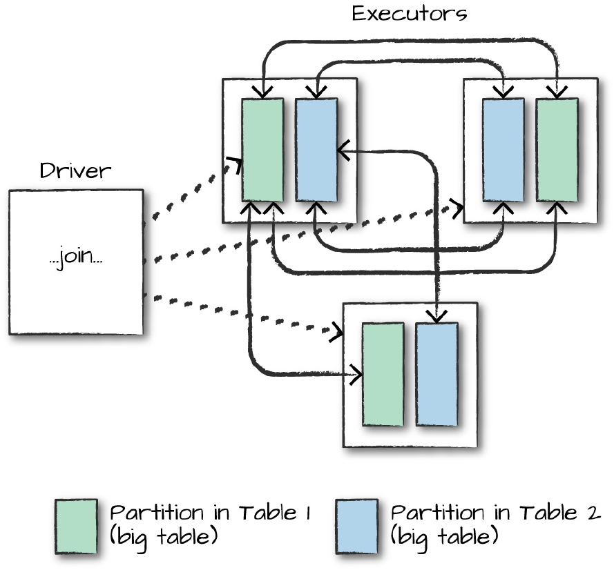
such as that illustrates in Figure 8-1.
Figure 8-1. Joining two big tables
In a shuffle join, every node talks to every other node and they share data
according to which node has a certain key or set of keys (on which you are
joining). These joins are expensive because the network can become
congested with traffic, especially if your data is not partitioned well.
This join describes taking a big table of data and joining it to another big
table of data. An example of this might be a company that receives billions of
messages every day from the Internet of Things, and needs to identify the
day-over-day changes that have occurred. The way to do this is by joining on

deviceId, messageType, and date in one column, and date - 1 day in the
other column.
In Figure 8-1, DataFrame 1 and DataFrame 2 are both large DataFrames. This
means that all worker nodes (and potentially every partition) will need to
communicate with one another during the entire join process (with no
intelligent partitioning of data).
Big table–to–small table
When the table is small enough to fit into the memory of a single worker
node, with some breathing room of course, we can optimize our join.
Although we can use a big table–to–big table communication strategy, it can
often be more efficient to use a broadcast join. What this means is that we
will replicate our small DataFrame onto every worker node in the cluster (be
it located on one machine or many). Now this sounds expensive. However,
what this does is prevent us from performing the all-to-all communication
during the entire join process. Instead, we perform it only once at the
beginning and then let each individual worker node perform the work without
having to wait or communicate with any other worker node, as is depicted in
Figure 8-2.
Figure 8-2. A broadcast join
At the beginning of this join will be a large communication, just like in the
previous type of join. However, immediately after that first, there will be no
further communication between nodes. This means that joins will be
performed on every single node individually, making CPU the biggest
bottleneck. For our current set of data, we can see that Spark has
automatically set this up as a broadcast join by looking at the explain plan:
val joinExpr = person.col("graduate_program") === graduateProgram.col("id")
person.join(graduateProgram, joinExpr).explain()
== Physical Plan ==
*BroadcastHashJoin [graduate_program#40], [id#5....
:- LocalTableScan [id#38, name#39, graduate_progr...
+- BroadcastExchange HashedRelationBroadcastMode(....
+- LocalTableScan [id#56, degree#57, departmen....
With the DataFrame API, we can also explicitly give the optimizer a hint that
we would like to use a broadcast join by using the correct function around the
small DataFrame in question. In this example, these result in the same plan
we just saw; however, this is not always the case:
import org.apache.spark.sql.functions.broadcast
val joinExpr = person.col("graduate_program") === graduateProgram.col("id")
person.join(broadcast(graduateProgram), joinExpr).explain()
The SQL interface also includes the ability to provide hints to perform joins.
These are not enforced, however, so the optimizer might choose to ignore
them. You can set one of these hints by using a special comment syntax.
MAPJOIN, BROADCAST, and BROADCASTJOIN all do the same thing and are all
supported:
-- in SQL
SELECT /*+ MAPJOIN(graduateProgram) */ * FROM person JOIN graduateProgram
ON person.graduate_program = graduateProgram.id
This doesn’t come for free either: if you try to broadcast something too large,
you can crash your driver node (because that collect is expensive). This is
likely an area for optimization in the future.
Little table–to–little table
When performing joins with small tables, it’s usually best to let Spark decide
how to join them. You can always force a broadcast join if you’re noticing
strange behavior.
Conclusion
In this chapter, we discussed joins, probably one of the most common use
cases. One thing we did not mention but is important to consider is if you
partition your data correctly prior to a join, you can end up with much more
efficient execution because even if a shuffle is planned, if data from two
different DataFrames is already located on the same machine, Spark can
avoid the shuffle. Experiment with some of your data and try partitioning
beforehand to see if you can notice the increase in speed when performing
those joins. In Chapter 9, we will discuss Spark’s data source APIs. There are
additional implications when you decide what order joins should occur in.
Because some joins act as filters, this can be a low-hanging improvement in
your workloads, as you are guaranteed to reduce data exchanged over the
network.
The next chapter will depart from user manipulation, as we’ve seen in the last
several chapters, and touch on reading and writing data using the Structured
APIs.
Chapter 9. Data Sources
This chapter formally introduces the variety of other data sources that you
can use with Spark out of the box as well as the countless other sources built
by the greater community. Spark has six “core” data sources and hundreds of
external data sources written by the community. The ability to read and write
from all different kinds of data sources and for the community to create its
own contributions is arguably one of Spark’s greatest strengths. Following
are Spark’s core data sources:
CSV
JSON
Parquet
ORC
JDBC/ODBC connections
Plain-text files
As mentioned, Spark has numerous community-created data sources. Here’s
just a small sample:
Cassandra
HBase
MongoDB
AWS Redshift
XML
And many, many others
The goal of this chapter is to give you the ability to read and write from

Spark’s core data sources and know enough to understand what you should
look for when integrating with third-party data sources. To achieve this, we
will focus on the core concepts that you need to be able to recognize and
understand.
The Structure of the Data Sources API
Before proceeding with how to read and write from certain formats, let’s visit
the overall organizational structure of the data source APIs.
Read API Structure
The core structure for reading data is as follows:
DataFrameReader.format(...).option("key", "value").schema(...).load()
We will use this format to read from all of our data sources. format is
optional because by default Spark will use the Parquet format. option allows
you to set key-value configurations to parameterize how you will read data.
Lastly, schema is optional if the data source provides a schema or if you
intend to use schema inference. Naturally, there are some required options for
each format, which we will discuss when we look at each format.
NOTE
There is a lot of shorthand notation in the Spark community, and the data source read API
is no exception. We try to be consistent throughout the book while still revealing some of
the shorthand notation along the way.
Basics of Reading Data
The foundation for reading data in Spark is the DataFrameReader. We access
this through the SparkSession via the read attribute:
spark.read
After we have a DataFrame reader, we specify several values:
The format
The schema
The read mode
A series of options
The format, options, and schema each return a DataFrameReader that can
undergo further transformations and are all optional, except for one option.
Each data source has a specific set of options that determine how the data is
read into Spark (we cover these options shortly). At a minimum, you must
supply the DataFrameReader a path to from which to read.
Here’s an example of the overall layout:
spark.read.format("csv")
.option("mode", "FAILFAST")
.option("inferSchema", "true")
.option("path", "path/to/file(s)")
.schema(someSchema)
.load()
There are a variety of ways in which you can set options; for example, you
can build a map and pass in your configurations. For now, we’ll stick to the
simple and explicit way that you just saw.
Read modes
Reading data from an external source naturally entails encountering
malformed data, especially when working with only semi-structured data
sources. Read modes specify what will happen when Spark does come across
malformed records. Table 9-1 lists the read modes.
Table 9-1. Spark’s read modes

Read mode Description
permissive Sets all fields to null when it encounters a corrupted record and places all
corrupted records in a string column called _corrupt_record
dropMalformed Drops the row that contains malformed records
failFast Fails immediately upon encountering malformed records
The default is permissive.
Write API Structure
The core structure for writing data is as follows:
DataFrameWriter.format(...).option(...).partitionBy(...).bucketBy(...).sortBy(
...).save()
We will use this format to write to all of our data sources. format is optional
because by default, Spark will use the arquet format. option, again, allows
us to configure how to write out our given data. PartitionBy, bucketBy,
and sortBy work only for file-based data sources; you can use them to
control the specific layout of files at the destination.
Basics of Writing Data
The foundation for writing data is quite similar to that of reading data. Instead
of the DataFrameReader, we have the DataFrameWriter. Because we
always need to write out some given data source, we access the
DataFrameWriter on a per-DataFrame basis via the write attribute:
// in Scala
dataFrame.write
After we have a DataFrameWriter, we specify three values: the format, a
series of options, and the save mode. At a minimum, you must supply a
path. We will cover the potential for options, which vary from data source to

data source, shortly.
// in Scala
dataframe.write.format("csv")
.option("mode", "OVERWRITE")
.option("dateFormat", "yyyy-MM-dd")
.option("path", "path/to/file(s)")
.save()
Save modes
Save modes specify what will happen if Spark finds data at the specified
location (assuming all else equal). Table 9-2 lists the save modes.
Table 9-2. Spark’s save modes
Save mode Description
append Appends the output files to the list of files that already exist at that location
overwrite Will completely overwrite any data that already exists there
errorIfExists Throws an error and fails the write if data or files already exist at the specified
location
ignore If data or files exist at the location, do nothing with the current DataFrame
The default is errorIfExists. This means that if Spark finds data at the
location to which you’re writing, it will fail the write immediately.
We’ve largely covered the core concepts that you’re going to need when
using data sources, so now let’s dive into each of Spark’s native data sources.
CSV Files
CSV stands for commma-separated values. This is a common text file format
in which each line represents a single record, and commas separate each field
within a record. CSV files, while seeming well structured, are actually one of
the trickiest file formats you will encounter because not many assumptions

can be made in production scenarios about what they contain or how they are
structured. For this reason, the CSV reader has a large number of options.
These options give you the ability to work around issues like certain
characters needing to be escaped—for example, commas inside of columns
when the file is also comma-delimited or null values labeled in an
unconventional way.
CSV Options
Table 9-3 presents the options available in the CSV reader.
Table 9-3. CSV data source options
Read/write Key Potential values Default Description
Both sep Any single string
character ,
The single
character that
is used as
separator for
each field
and value.
Both header true, false false
A Boolean
flag that
declares
whether the
first line in
the file(s) are
the names of
the columns.
Read escape Any string character \
The character
Spark should
use to escape
other
characters in
the file.
Read inferSchema true, false false
Specifies
whether
Spark should
infer column
types when
reading the
file.
Read ignoreLeadingWhiteSpace true, false false
Declares
whether
leading
spaces from
values being
read should
be skipped.
Read ignoreTrailingWhiteSpace true, false false
Declares
whether
trailing
spaces from
values being
read should
be skipped.
Both nullValue Any string character “”
Declares
what
character
represents a
null value in
the file.
Both nanValue Any string character NaN
Declares
what
character
represents a
NaN or
missing
character in
the CSV file.
Both positiveInf Any string or
character Inf
Declares
what
character(s)
represent a
positive
infinite value.
Both negativeInf Any string or
character -Inf
Declares
what
character(s)
represent a
negative
infinite value.
Both compression or codec
None,
uncompressed,
bzip2, deflate,
gzip, lz4, or
snappy
none
Declares
what
compression
codec Spark
should use to
read or write
the file.
Both dateFormat
Any string or
character that
conforms to java’s
SimpleDataFormat.
yyyy-MM-dd
Declares the
date format
for any
columns that
are date type.
Both timestampFormat
Any string or
character that
conforms to java’s
SimpleDataFormat.
yyyy-MM-
dd’T’HH:mm
:ss.SSSZZ
Declares the
timestamp
format for
any columns
that are
timestamp
type.
Read maxColumns Any integer 20480
Declares the
maximum
number of
columns in
the file.
Read maxCharsPerColumn Any integer 1000000
Declares the
maximum
number of
characters in
a column.
Read escapeQuotes true, false true
Declares
whether
Spark should
escape quotes
that are found
in lines.
Sets the
maximum
number of
malformed

Read maxMalformedLogPerPartition Any integer 10
rows Spark
will log for
each
partition.
Malformed
records
beyond this
number will
be ignored.
Write quoteAll true, false false
Specifies
whether all
values should
be enclosed
in quotes, as
opposed to
just escaping
values that
have a quote
character.
Read multiLine true, false false
This option
allows you to
read multiline
CSV files
where each
logical row in
the CSV file
might span
multiple rows
in the file
itself.
Reading CSV Files
To read a CSV file, like any other format, we must first create a
DataFrameReader for that specific format. Here, we specify the format to be
CSV:
spark.read.format("csv")
After this, we have the option of specifying a schema as well as modes as
options. Let’s set a couple of options, some that we saw from the beginning
of the book and others that we haven’t seen yet. We’ll set the header to true
for our CSV file, the mode to be FAILFAST, and inferSchema to true:
// in Scala
spark.read.format("csv")
.option("header", "true")
.option("mode", "FAILFAST")
.option("inferSchema", "true")
.load("some/path/to/file.csv")
As mentioned, we can use the mode to specify how much tolerance we have
for malformed data. For example, we can use these modes and the schema
that we created in Chapter 5 to ensure that our file(s) conform to the data that
we expected:
// in Scala
import org.apache.spark.sql.types.{StructField, StructType, StringType,
LongType}
val myManualSchema = new StructType(Array(
new StructField("DEST_COUNTRY_NAME", StringType, true),
new StructField("ORIGIN_COUNTRY_NAME", StringType, true),
new StructField("count", LongType, false)
))
spark.read.format("csv")
.option("header", "true")
.option("mode", "FAILFAST")
.schema(myManualSchema)
.load("/data/flight-data/csv/2010-summary.csv")
.show(5)
Things get tricky when we don’t expect our data to be in a certain format, but
it comes in that way, anyhow. For example, let’s take our current schema and
change all column types to LongType. This does not match the actual
schema, but Spark has no problem with us doing this. The problem will only
manifest itself when Spark actually reads the data. As soon as we start our
Spark job, it will immediately fail (after we execute a job) due to the data not
conforming to the specified schema:
// in Scala
val myManualSchema = new StructType(Array(
new StructField("DEST_COUNTRY_NAME", LongType, true),
new StructField("ORIGIN_COUNTRY_NAME", LongType, true),
new StructField("count", LongType, false) ))
spark.read.format("csv")
.option("header", "true")
.option("mode", "FAILFAST")
.schema(myManualSchema)
.load("/data/flight-data/csv/2010-summary.csv")
.take(5)
In general, Spark will fail only at job execution time rather than DataFrame
definition time—even if, for example, we point to a file that does not exist.
This is due to lazy evaluation, a concept we learned about in Chapter 2.
Writing CSV Files
Just as with reading data, there are a variety of options (listed in Table 9-3)
for writing data when we write CSV files. This is a subset of the reading
options because many do not apply when writing data (like maxColumns and
inferSchema). Here’s an example:
// in Scala
val csvFile = spark.read.format("csv")
.option("header", "true").option("mode", "FAILFAST").schema(myManualSchema)
.load("/data/flight-data/csv/2010-summary.csv")
# in Python
csvFile = spark.read.format("csv")\
.option("header", "true")\
.option("mode", "FAILFAST")\
.option("inferSchema", "true")\
.load("/data/flight-data/csv/2010-summary.csv")
For instance, we can take our CSV file and write it out as a TSV file quite
easily:
// in Scala
csvFile.write.format("csv").mode("overwrite").option("sep", "\t")
.save("/tmp/my-tsv-file.tsv")
# in Python
csvFile.write.format("csv").mode("overwrite").option("sep", "\t")\
.save("/tmp/my-tsv-file.tsv")
When you list the destination directory, you can see that my-tsv-file is
actually a folder with numerous files within it:
$ ls /tmp/my-tsv-file.tsv/
/tmp/my-tsv-file.tsv/part-00000-35cf9453-1943-4a8c-9c82-9f6ea9742b29.csv
This actually reflects the number of partitions in our DataFrame at the time
we write it out. If we were to repartition our data before then, we would end
up with a different number of files. We discuss this trade-off at the end of this
chapter.
JSON Files
Those coming from the world of JavaScript are likely familiar with
JavaScript Object Notation, or JSON, as it’s commonly called. There are
some catches when working with this kind of data that are worth considering
before we jump in. In Spark, when we refer to JSON files, we refer to line-
delimited JSON files. This contrasts with files that have a large JSON object
or array per file.
The line-delimited versus multiline trade-off is controlled by a single option:
multiLine. When you set this option to true, you can read an entire file as
one json object and Spark will go through the work of parsing that into a
DataFrame. Line-delimited JSON is actually a much more stable format
because it allows you to append to a file with a new record (rather than
having to read in an entire file and then write it out), which is what we
recommend that you use. Another key reason for the popularity of line-
delimited JSON is because JSON objects have structure, and JavaScript (on
which JSON is based) has at least basic types. This makes it easier to work
with because Spark can make more assumptions on our behalf about the data.
You’ll notice that there are significantly less options than we saw for CSV
because of the objects.
JSON Options
Table 9-4 lists the options available for the JSON object, along with their
descriptions.
Table 9-4. JSON data source options
Read/write Key Potential values Default
Both compression or codec
None,
uncompressed,
bzip2, deflate,
gzip, lz4, or
snappy
none
Both dateFormat
Any string or
character that
conforms to Java’s
SimpleDataFormat.
yyyy-MM-dd
Both timestampFormat
Any string or
character that
conforms to Java’s
SimpleDataFormat.
yyyy-MM-dd’T’HH:mm:ss.SSSZZ
Read primitiveAsString true, false false
Read allowComments true, false false

Read allowUnquotedFieldNames true, false false
Read allowSingleQuotes true, false true
Read allowNumericLeadingZeros true, false false
Read allowBackslashEscapingAnyCharacter true, false false
Read columnNameOfCorruptRecord Any string Value of
spark.sql.column&NameOfCorruptRecord
Read multiLine true, false false
Now, reading a line-delimited JSON file varies only in the format and the
options that we specify:
spark.read.format("json")
Reading JSON Files
Let’s look at an example of reading a JSON file and compare the options that
we’re seeing:
// in Scala
spark.read.format("json").option("mode", "FAILFAST").schema(myManualSchema)
.load("/data/flight-data/json/2010-summary.json").show(5)
# in Python
spark.read.format("json").option("mode", "FAILFAST")\
.option("inferSchema", "true")\
.load("/data/flight-data/json/2010-summary.json").show(5)
Writing JSON Files
Writing JSON files is just as simple as reading them, and, as you might
expect, the data source does not matter. Therefore, we can reuse the CSV
DataFrame that we created earlier to be the source for our JSON file. This,
too, follows the rules that we specified before: one file per partition will be
written out, and the entire DataFrame will be written out as a folder. It will
also have one JSON object per line:
// in Scala
csvFile.write.format("json").mode("overwrite").save("/tmp/my-json-file.json")
# in Python
csvFile.write.format("json").mode("overwrite").save("/tmp/my-json-file.json")
$ ls /tmp/my-json-file.json/
/tmp/my-json-file.json/part-00000-tid-543....json
Parquet Files
Parquet is an open source column-oriented data store that provides a variety
of storage optimizations, especially for analytics workloads. It provides
columnar compression, which saves storage space and allows for reading
individual columns instead of entire files. It is a file format that works
exceptionally well with Apache Spark and is in fact the default file format.
We recommend writing data out to Parquet for long-term storage because
reading from a Parquet file will always be more efficient than JSON or CSV.
Another advantage of Parquet is that it supports complex types. This means
that if your column is an array (which would fail with a CSV file, for
example), map, or struct, you’ll still be able to read and write that file without
issue. Here’s how to specify Parquet as the read format:
spark.read.format("parquet")
Reading Parquet Files
Parquet has very few options because it enforces its own schema when
storing data. Thus, all you need to set is the format and you are good to go.
We can set the schema if we have strict requirements for what our DataFrame
should look like. Oftentimes this is not necessary because we can use schema
on read, which is similar to the inferSchema with CSV files. However, with
Parquet files, this method is more powerful because the schema is built into
the file itself (so no inference needed).
Here are some simple examples reading from parquet:
spark.read.format("parquet")
// in Scala
spark.read.format("parquet")
.load("/data/flight-data/parquet/2010-summary.parquet").show(5)
# in Python
spark.read.format("parquet")\
.load("/data/flight-data/parquet/2010-summary.parquet").show(5)
Parquet options
As we just mentioned, there are very few Parquet options—precisely two, in
fact—because it has a well-defined specification that aligns closely with the
concepts in Spark. Table 9-5 presents the options.
WARNING
Even though there are only two options, you can still encounter problems if you’re
working with incompatible Parquet files. Be careful when you write out Parquet files with
different versions of Spark (especially older ones) because this can cause significant
headache.
Table 9-5. Parquet data source options
Read/Write Key Potential
Values Default Description
Write compression
or codec
None,
uncompressed,
bzip2,
deflate, gzip,
lz4, or snappy
None
Declares
what
compression
codec Spark
should use to
read or write
the file.
Read mergeSchema true, false Value of the configuration
spark.sql.parquet.mergeSchema
You can
incrementally
add columns
to newly
written
Parquet files
in the same
table/folder.
Use this
option to
enable or
disable this
feature.
Writing Parquet Files
Writing Parquet is as easy as reading it. We simply specify the location for
the file. The same partitioning rules apply:
// in Scala
csvFile.write.format("parquet").mode("overwrite")
.save("/tmp/my-parquet-file.parquet")
# in Python
csvFile.write.format("parquet").mode("overwrite")\
.save("/tmp/my-parquet-file.parquet")
ORC Files
ORC is a self-describing, type-aware columnar file format designed for
Hadoop workloads. It is optimized for large streaming reads, but with
integrated support for finding required rows quickly. ORC actually has no
options for reading in data because Spark understands the file format quite
well. An often-asked question is: What is the difference between ORC and
Parquet? For the most part, they’re quite similar; the fundamental difference
is that Parquet is further optimized for use with Spark, whereas ORC is
further optimized for Hive.
Reading Orc Files
Here’s how to read an ORC file into Spark:
// in Scala
spark.read.format("orc").load("/data/flight-data/orc/2010-summary.orc").show(5)
# in Python
spark.read.format("orc").load("/data/flight-data/orc/2010-summary.orc").show(5)
Writing Orc Files
At this point in the chapter, you should feel pretty comfortable taking a guess
at how to write ORC files. It really follows the exact same pattern that we
have seen so far, in which we specify the format and then save the file:

// in Scala
csvFile.write.format("orc").mode("overwrite").save("/tmp/my-json-file.orc")
# in Python
csvFile.write.format("orc").mode("overwrite").save("/tmp/my-json-file.orc")
SQL Databases
SQL datasources are one of the more powerful connectors because there are a
variety of systems to which you can connect (as long as that system speaks
SQL). For instance you can connect to a MySQL database, a PostgreSQL
database, or an Oracle database. You also can connect to SQLite, which is
what we’ll do in this example. Of course, databases aren’t just a set of raw
files, so there are more options to consider regarding how you connect to the
database. Namely you’re going to need to begin considering things like
authentication and connectivity (you’ll need to determine whether the
network of your Spark cluster is connected to the network of your database
system).
To avoid the distraction of setting up a database for the purposes of this book,
we provide a reference sample that runs on SQLite. We can skip a lot of these
details by using SQLite, because it can work with minimal setup on your
local machine with the limitation of not being able to work in a distributed
setting. If you want to work through these examples in a distributed setting,
you’ll want to connect to another kind of database.
A PRIMER ON SQLITE
SQLite is the most used database engine in the entire world, and for good
reason. It’s powerful, fast, and easy to understand. This is because a
SQLite database is just a file. That’s going to make it very easy for you to
get up and running because we include the source file in the official
repository for this book. Simply download that file to your local machine,
and you will be able to read from it and write to it. We’re using SQLite,
but all of the code here works with more traditional relational databases,
as well, like MySQL. The primary difference is in the properties that you
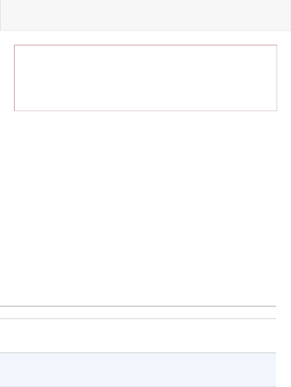
include when you connect to the database. When we’re working with
SQLite, there’s no notion of user or password.
WARNING
Although SQLite makes for a good reference example, it’s probablu not what you want to
use in production. Also, SQLite will not necessarily work well in a distributed setting
because of its requirement to lock the entire database on write. The example we present
here will work in a similar way using MySQL or PostgreSQL, as well.
To read and write from these databases, you need to do two things: include
the Java Database Connectivity (JDBC) driver for you particular database on
the spark classpath, and provide the proper JAR for the driver itself. For
example, to be able to read and write from PostgreSQL, you might run
something like this:
./bin/spark-shell \
--driver-class-path postgresql-9.4.1207.jar \
--jars postgresql-9.4.1207.jar
Just as with our other sources, there are a number of options that are available
when reading from and writing to SQL databases. Only some of these are
relevant for our current example, but Table 9-6 lists all of the options that you
can set when working with JDBC databases.
Table 9-6. JDBC data source options
Property Name Meaning
url
The JDBC URL to which to connect. The source-specific
connection properties can be specified in the URL; for example,
jdbc:postgresql://localhost/test?user=fred&password=secret.
dbtable
The JDBC table to read. Note that anything that is valid in a FROM
clause of a SQL query can be used. For example, instead of a full
table you could also use a subquery in parentheses.
driver The class name of the JDBC driver to use to connect to this URL.

partitionColumn,
lowerBound, upperBound
If any one of these options is specified, then all others must be set
as well. In addition, numPartitions must be specified. These
properties describe how to partition the table when reading in
parallel from multiple workers. partitionColumn must be a
numeric column from the table in question. Notice that lowerBound
and upperBound are used only to decide the partition stride, not for
filtering the rows in the table. Thus, all rows in the table will be
partitioned and returned. This option applies only to reading.
numPartitions
The maximum number of partitions that can be used for parallelism
in table reading and writing. This also determines the maximum
number of concurrent JDBC connections. If the number of
partitions to write exceeds this limit, we decrease it to this limit by
calling coalesce(numPartitions) before writing.
fetchsize
The JDBC fetch size, which determines how many rows to fetch per
round trip. This can help performance on JDBC drivers, which
default to low fetch size (e.g., Oracle with 10 rows). This option
applies only to reading.
batchsize
The JDBC batch size, which determines how many rows to insert
per round trip. This can help performance on JDBC drivers. This
option applies only to writing. The default is 1000.
isolationLevel
The transaction isolation level, which applies to current connection.
It can be one of NONE, READ_COMMITTED, READ_UNCOMMITTED,
REPEATABLE_READ, or SERIALIZABLE, corresponding to standard
transaction isolation levels defined by JDBC’s Connection object.
The default is READ_UNCOMMITTED. This option applies only to
writing. For more information, refer to the documentation in
java.sql.Connection.
truncate
This is a JDBC writer-related option. When SaveMode.Overwrite
is enabled, Spark truncates an existing table instead of dropping and
re-creating it. This can be more efficient, and it prevents the table
metadata (e.g., indices) from being removed. However, it will not
work in some cases, such as when the new data has a different
schema. The default is false. This option applies only to writing.
createTableOptions
This is a JDBC writer-related option. If specified, this option allows
setting of database-specific table and partition options when
creating a table (e.g., CREATE TABLE t (name string)
ENGINE=InnoDB). This option applies only to writing.
The database column data types to use instead of the defaults, when

createTableColumnTypes
creating the table. Data type information should be specified in the
same format as CREATE TABLE columns syntax (e.g., “name
CHAR(64), comments VARCHAR(1024)”). The specified types
should be valid Spark SQL data types. This option applies only to
writing.
Reading from SQL Databases
When it comes to reading a file, SQL databases are no different from the
other data sources that we looked at earlier. As with those sources, we specify
the format and options, and then load in the data:
// in Scala
val driver = "org.sqlite.JDBC"
val path = "/data/flight-data/jdbc/my-sqlite.db"
val url = s"jdbc:sqlite:/${path}"
val tablename = "flight_info"
# in Python
driver = "org.sqlite.JDBC"
path = "/data/flight-data/jdbc/my-sqlite.db"
url = "jdbc:sqlite:" + path
tablename = "flight_info"
After you have defined the connection properties, you can test your
connection to the database itself to ensure that it is functional. This is an
excellent troubleshooting technique to confirm that your database is available
to (at the very least) the Spark driver. This is much less relevant for SQLite
because that is a file on your machine but if you were using something like
MySQL, you could test the connection with the following:
import java.sql.DriverManager
val connection = DriverManager.getConnection(url)
connection.isClosed()
connection.close()
If this connection succeeds, you’re good to go. Let’s go ahead and read the
DataFrame from the SQL table:
// in Scala
val dbDataFrame = spark.read.format("jdbc").option("url", url)
.option("dbtable", tablename).option("driver", driver).load()
# in Python
dbDataFrame = spark.read.format("jdbc").option("url", url)\
.option("dbtable", tablename).option("driver", driver).load()
SQLite has rather simple configurations (no users, for example). Other
databases, like PostgreSQL, require more configuration parameters. Let’s
perform the same read that we just performed, except using PostgreSQL this
time:
// in Scala
val pgDF = spark.read
.format("jdbc")
.option("driver", "org.postgresql.Driver")
.option("url", "jdbc:postgresql://database_server")
.option("dbtable", "schema.tablename")
.option("user", "username").option("password","my-secret-password").load()
# in Python
pgDF = spark.read.format("jdbc")\
.option("driver", "org.postgresql.Driver")\
.option("url", "jdbc:postgresql://database_server")\
.option("dbtable", "schema.tablename")\
.option("user", "username").option("password", "my-secret-password").load()
As we create this DataFrame, it is no different from any other: you can query
it, transform it, and join it without issue. You’ll also notice that there is
already a schema, as well. That’s because Spark gathers this information
from the table itself and maps the types to Spark data types. Let’s get only the
distinct locations to verify that we can query it as expected:
dbDataFrame.select("DEST_COUNTRY_NAME").distinct().show(5)
+-----------------+
|DEST_COUNTRY_NAME|
+-----------------+
| Anguilla|
| Russia|
| Paraguay|
| Senegal|
| Sweden|
+-----------------+
Awesome, we can query the database! Before we proceed, there are a couple
of nuanced details that are worth understanding.
Query Pushdown
First, Spark makes a best-effort attempt to filter data in the database itself
before creating the DataFrame. For example, in the previous sample query,
we can see from the query plan that it selects only the relevant column name
from the table:
dbDataFrame.select("DEST_COUNTRY_NAME").distinct().explain
== Physical Plan ==
*HashAggregate(keys=[DEST_COUNTRY_NAME#8108], functions=[])
+- Exchange hashpartitioning(DEST_COUNTRY_NAME#8108, 200)
+- *HashAggregate(keys=[DEST_COUNTRY_NAME#8108], functions=[])
+- *Scan JDBCRelation(flight_info) [numPartitions=1] ...
Spark can actually do better than this on certain queries. For example, if we
specify a filter on our DataFrame, Spark will push that filter down into the
database. We can see this in the explain plan under PushedFilters.
// in Scala
dbDataFrame.filter("DEST_COUNTRY_NAME in ('Anguilla', 'Sweden')").explain
# in Python
dbDataFrame.filter("DEST_COUNTRY_NAME in ('Anguilla', 'Sweden')").explain()
== Physical Plan ==
*Scan JDBCRel... PushedFilters: [*In(DEST_COUNTRY_NAME, [Anguilla,Sweden])],
...
Spark can’t translate all of its own functions into the functions available in
the SQL database in which you’re working. Therefore, sometimes you’re
going to want to pass an entire query into your SQL that will return the
results as a DataFrame. Now, this might seem like it’s a bit complicated, but
it’s actually quite straightforward. Rather than specifying a table name, you
just specify a SQL query. Of course, you do need to specify this in a special
way; you must wrap the query in parenthesis and rename it to something—in
this case, I just gave it the same table name:
// in Scala
val pushdownQuery = """(SELECT DISTINCT(DEST_COUNTRY_NAME) FROM flight_info)
AS flight_info"""
val dbDataFrame = spark.read.format("jdbc")
.option("url", url).option("dbtable", pushdownQuery).option("driver", driver)
.load()
# in Python
pushdownQuery = """(SELECT DISTINCT(DEST_COUNTRY_NAME) FROM flight_info)
AS flight_info"""
dbDataFrame = spark.read.format("jdbc")\
.option("url", url).option("dbtable", pushdownQuery).option("driver",
driver)\
.load()
Now when you query this table, you’ll actually be querying the results of that
query. We can see this in the explain plan. Spark doesn’t even know about
the actual schema of the table, just the one that results from our previous
query:
dbDataFrame.explain()
== Physical Plan ==
*Scan JDBCRelation(
(SELECT DISTINCT(DEST_COUNTRY_NAME)
FROM flight_info) as flight_info
) [numPartitions=1] [DEST_COUNTRY_NAME#788] ReadSchema: ...
Reading from databases in parallel
All throughout this book, we have talked about partitioning and its
importance in data processing. Spark has an underlying algorithm that can
read multiple files into one partition, or conversely, read multiple partitions
out of one file, depending on the file size and the “splitability” of the file type
and compression. The same flexibility that exists with files, also exists with
SQL databases except that you must configure it a bit more manually. What
you can configure, as seen in the previous options, is the ability to specify a
maximum number of partitions to allow you to limit how much you are
reading and writing in parallel:
// in Scala
val dbDataFrame = spark.read.format("jdbc")
.option("url", url).option("dbtable", tablename).option("driver", driver)
.option("numPartitions", 10).load()
# in Python
dbDataFrame = spark.read.format("jdbc")\
.option("url", url).option("dbtable", tablename).option("driver", driver)\
.option("numPartitions", 10).load()
In this case, this will still remain as one partition because there is not too
much data. However, this configuration can help you ensure that you do not
overwhelm the database when reading and writing data:
dbDataFrame.select("DEST_COUNTRY_NAME").distinct().show()
There are several other optimizations that unfortunately only seem to be
under another API set. You can explicitly push predicates down into SQL
databases through the connection itself. This optimization allows you to
control the physical location of certain data in certain partitions by specifying
predicates. That’s a mouthful, so let’s look at a simple example. We only
need data from two countries in our data: Anguilla and Sweden. We could
filter these down and have them pushed into the database, but we can also go
further by having them arrive in their own partitions in Spark. We do that by
specifying a list of predicates when we create the data source:
// in Scala
val props = new java.util.Properties
props.setProperty("driver", "org.sqlite.JDBC")
val predicates = Array(
"DEST_COUNTRY_NAME = 'Sweden' OR ORIGIN_COUNTRY_NAME = 'Sweden'",
"DEST_COUNTRY_NAME = 'Anguilla' OR ORIGIN_COUNTRY_NAME = 'Anguilla'")
spark.read.jdbc(url, tablename, predicates, props).show()
spark.read.jdbc(url, tablename, predicates, props).rdd.getNumPartitions // 2
# in Python
props = {"driver":"org.sqlite.JDBC"}
predicates = [
"DEST_COUNTRY_NAME = 'Sweden' OR ORIGIN_COUNTRY_NAME = 'Sweden'",
"DEST_COUNTRY_NAME = 'Anguilla' OR ORIGIN_COUNTRY_NAME = 'Anguilla'"]
spark.read.jdbc(url, tablename, predicates=predicates, properties=props).show()
spark.read.jdbc(url,tablename,predicates=predicates,properties=props)\
.rdd.getNumPartitions() # 2
+-----------------+-------------------+-----+
|DEST_COUNTRY_NAME|ORIGIN_COUNTRY_NAME|count|
+-----------------+-------------------+-----+
| Sweden| United States| 65|
| United States| Sweden| 73|
| Anguilla| United States| 21|
| United States| Anguilla| 20|
+-----------------+-------------------+-----+
If you specify predicates that are not disjoint, you can end up with lots of
duplicate rows. Here’s an example set of predicates that will result in
duplicate rows:
// in Scala
val props = new java.util.Properties
props.setProperty("driver", "org.sqlite.JDBC")
val predicates = Array(
"DEST_COUNTRY_NAME != 'Sweden' OR ORIGIN_COUNTRY_NAME != 'Sweden'",
"DEST_COUNTRY_NAME != 'Anguilla' OR ORIGIN_COUNTRY_NAME != 'Anguilla'")
spark.read.jdbc(url, tablename, predicates, props).count() // 510
# in Python
props = {"driver":"org.sqlite.JDBC"}
predicates = [
"DEST_COUNTRY_NAME != 'Sweden' OR ORIGIN_COUNTRY_NAME != 'Sweden'",
"DEST_COUNTRY_NAME != 'Anguilla' OR ORIGIN_COUNTRY_NAME != 'Anguilla'"]
spark.read.jdbc(url, tablename, predicates=predicates, properties=props).count()
Partitioning based on a sliding window
Let’s take a look to see how we can partition based on predicates. In this
example, we’ll partition based on our numerical count column. Here, we
specify a minimum and a maximum for both the first partition and last
partition. Anything outside of these bounds will be in the first partition or
final partition. Then, we set the number of partitions we would like total (this
is the level of parallelism). Spark then queries our database in parallel and
returns numPartitions partitions. We simply modify the upper and lower
bounds in order to place certain values in certain partitions. No filtering is
taking place like we saw in the previous example:
// in Scala
val colName = "count"
val lowerBound = 0L
val upperBound = 348113L // this is the max count in our database
val numPartitions = 10
# in Python
colName = "count"
lowerBound = 0L
upperBound = 348113L # this is the max count in our database
numPartitions = 10
This will distribute the intervals equally from low to high:
// in Scala
spark.read.jdbc(url,tablename,colName,lowerBound,upperBound,numPartitions,props)
.count() // 255
# in Python
spark.read.jdbc(url, tablename, column=colName, properties=props,
lowerBound=lowerBound, upperBound=upperBound,
numPartitions=numPartitions).count() # 255
Writing to SQL Databases
Writing out to SQL databases is just as easy as before. You simply specify
the URI and write out the data according to the specified write mode that you
want. In the following example, we specify overwrite, which overwrites the
entire table. We’ll use the CSV DataFrame that we defined earlier in order to
do this:
// in Scala
val newPath = "jdbc:sqlite://tmp/my-sqlite.db"
csvFile.write.mode("overwrite").jdbc(newPath, tablename, props)
# in Python
newPath = "jdbc:sqlite://tmp/my-sqlite.db"
csvFile.write.jdbc(newPath, tablename, mode="overwrite", properties=props)
Let’s look at the results:
// in Scala
spark.read.jdbc(newPath, tablename, props).count() // 255
# in Python
spark.read.jdbc(newPath, tablename, properties=props).count() # 255
Of course, we can append to the table this new table just as easily:
// in Scala
csvFile.write.mode("append").jdbc(newPath, tablename, props)
# in Python
csvFile.write.jdbc(newPath, tablename, mode="append", properties=props)
Notice that count increases:
// in Scala
spark.read.jdbc(newPath, tablename, props).count() // 765
# in Python
spark.read.jdbc(newPath, tablename, properties=props).count() # 765
Text Files
Spark also allows you to read in plain-text files. Each line in the file becomes
a record in the DataFrame. It is then up to you to transform it accordingly. As
an example of how you would do this, suppose that you need to parse some
Apache log files to some more structured format, or perhaps you want to
parse some plain text for natural-language processing. Text files make a great
argument for the Dataset API due to its ability to take advantage of the
flexibility of native types.
Reading Text Files
Reading text files is straightforward: you simply specify the type to be
textFile. With textFile, partitioned directory names are ignored. To read
and write text files according to partitions, you should use text, which
respects partitioning on reading and writing:
spark.read.textFile("/data/flight-data/csv/2010-summary.csv")
.selectExpr("split(value, ',') as rows").show()
+--------------------+
| rows|
+--------------------+
|[DEST_COUNTRY_NAM...|
|[United States, R...|
...
|[United States, A...|
|[Saint Vincent an...|
|[Italy, United St...|
+--------------------+
Writing Text Files
When you write a text file, you need to be sure to have only one string
column; otherwise, the write will fail:
csvFile.select("DEST_COUNTRY_NAME").write.text("/tmp/simple-text-file.txt")
If you perform some partitioning when performing your write (we’ll discuss
partitioning in the next couple of pages), you can write more columns.
However, those columns will manifest as directories in the folder to which
you’re writing out to, instead of columns on every single file:
// in Scala
csvFile.limit(10).select("DEST_COUNTRY_NAME", "count")
.write.partitionBy("count").text("/tmp/five-csv-files2.csv")
# in Python
csvFile.limit(10).select("DEST_COUNTRY_NAME", "count")\
.write.partitionBy("count").text("/tmp/five-csv-files2py.csv")
Advanced I/O Concepts
We saw previously that we can control the parallelism of files that we write
by controlling the partitions prior to writing. We can also control specific
data layout by controlling two things: bucketing and partitioning (discussed
momentarily).
Splittable File Types and Compression
Certain file formats are fundamentally “splittable.” This can improve speed
because it makes it possible for Spark to avoid reading an entire file, and
access only the parts of the file necessary to satisfy your query. Additionally
if you’re using something like Hadoop Distributed File System (HDFS),
splitting a file can provide further optimization if that file spans multiple
blocks. In conjunction with this is a need to manage compression. Not all
compression schemes are splittable. How you store your data is of immense
consequence when it comes to making your Spark jobs run smoothly. We
recommend Parquet with gzip compression.
Reading Data in Parallel
Multiple executors cannot read from the same file at the same time
necessarily, but they can read different files at the same time. In general, this
means that when you read from a folder with multiple files in it, each one of
those files will become a partition in your DataFrame and be read in by
available executors in parallel (with the remaining queueing up behind the
others).
Writing Data in Parallel
The number of files or data written is dependent on the number of partitions
the DataFrame has at the time you write out the data. By default, one file is
written per partition of the data. This means that although we specify a “file,”
it’s actually a number of files within a folder, with the name of the specified
file, with one file per each partition that is written.
For example, the following code
csvFile.repartition(5).write.format("csv").save("/tmp/multiple.csv")
will end up with five files inside of that folder. As you can see from the list
call:
ls /tmp/multiple.csv
/tmp/multiple.csv/part-00000-767df509-ec97-4740-8e15-4e173d365a8b.csv
/tmp/multiple.csv/part-00001-767df509-ec97-4740-8e15-4e173d365a8b.csv
/tmp/multiple.csv/part-00002-767df509-ec97-4740-8e15-4e173d365a8b.csv
/tmp/multiple.csv/part-00003-767df509-ec97-4740-8e15-4e173d365a8b.csv
/tmp/multiple.csv/part-00004-767df509-ec97-4740-8e15-4e173d365a8b.csv
Partitioning
Partitioning is a tool that allows you to control what data is stored (and
where) as you write it. When you write a file to a partitioned directory (or
table), you basically encode a column as a folder. What this allows you to do
is skip lots of data when you go to read it in later, allowing you to read in
only the data relevant to your problem instead of having to scan the complete
dataset. These are supported for all file-based data sources:
// in Scala
csvFile.limit(10).write.mode("overwrite").partitionBy("DEST_COUNTRY_NAME")
.save("/tmp/partitioned-files.parquet")
# in Python
csvFile.limit(10).write.mode("overwrite").partitionBy("DEST_COUNTRY_NAME")\
.save("/tmp/partitioned-files.parquet")
Upon writing, you get a list of folders in your Parquet “file”:
$ ls /tmp/partitioned-files.parquet
...
DEST_COUNTRY_NAME=Costa Rica/
DEST_COUNTRY_NAME=Egypt/
DEST_COUNTRY_NAME=Equatorial Guinea/
DEST_COUNTRY_NAME=Senegal/
DEST_COUNTRY_NAME=United States/
Each of these will contain Parquet files that contain that data where the
previous predicate was true:
$ ls /tmp/partitioned-files.parquet/DEST_COUNTRY_NAME=Senegal/
part-00000-tid.....parquet
This is probably the lowest-hanging optimization that you can use when you
have a table that readers frequently filter by before manipulating. For
instance, date is particularly common for a partition because, downstream,
often we want to look at only the previous week’s data (instead of scanning
the entire list of records). This can provide massive speedups for readers.
Bucketing
Bucketing is another file organization approach with which you can control
the data that is specifically written to each file. This can help avoid shuffles
later when you go to read the data because data with the same bucket ID will
all be grouped together into one physical partition. This means that the data is
prepartitioned according to how you expect to use that data later on, meaning
you can avoid expensive shuffles when joining or aggregating.
Rather than partitioning on a specific column (which might write out a ton of
directories), it’s probably worthwhile to explore bucketing the data instead.
This will create a certain number of files and organize our data into those
“buckets”:
val numberBuckets = 10
val columnToBucketBy = "count"
csvFile.write.format("parquet").mode("overwrite")
.bucketBy(numberBuckets, columnToBucketBy).saveAsTable("bucketedFiles")
$ ls /user/hive/warehouse/bucketedfiles/
part-00000-tid-1020575097626332666-8....parquet
part-00000-tid-1020575097626332666-8....parquet
part-00000-tid-1020575097626332666-8....parquet
...
Bucketing is supported only for Spark-managed tables. For more information
on bucketing and partitioning, watch this talk from Spark Summit 2017.
Writing Complex Types
As we covered in Chapter 6, Spark has a variety of different internal types.
Although Spark can work with all of these types, not every single type works
well with every data file format. For instance, CSV files do not support
complex types, whereas Parquet and ORC do.
Managing File Size
Managing file sizes is an important factor not so much for writing data but
reading it later on. When you’re writing lots of small files, there’s a
significant metadata overhead that you incur managing all of those files.
Spark especially does not do well with small files, although many file
systems (like HDFS) don’t handle lots of small files well, either. You might
hear this referred to as the “small file problem.” The opposite is also true: you
don’t want files that are too large either, because it becomes inefficient to
have to read entire blocks of data when you need only a few rows.
Spark 2.2 introduced a new method for controlling file sizes in a more
automatic way. We saw previously that the number of output files is a
derivative of the number of partitions we had at write time (and the
partitioning columns we selected). Now, you can take advantage of another
tool in order to limit output file sizes so that you can target an optimum file
size. You can use the maxRecordsPerFile option and specify a number of
your choosing. This allows you to better control file sizes by controlling the
number of records that are written to each file. For example, if you set an
option for a writer as df.write.option("maxRecordsPerFile", 5000),
Spark will ensure that files will contain at most 5,000 records.
Conclusion
In this chapter we discussed the variety of options available to you for
reading and writing data in Spark. This covers nearly everything you’ll need
to know as an everyday user of Spark. For the curious, there are ways of
implementing your own data source; however, we omitted instructions for
how to do this because the API is currently evolving to better support
Structured Streaming. If you’re interested in seeing how to implement your
own custom data sources, the Cassandra Connector is well organized and
maintained and could provide a reference for the adventurous.
In Chapter 10, we discuss Spark SQL and how it interoperates with
everything else we’ve seen so far in the Structured APIs.

Chapter 10. Spark SQL
Spark SQL is arguably one of the most important and powerful features in
Spark. This chapter introduces the core concepts in Spark SQL that you need
to understand. This chapter will not rewrite the ANSI-SQL specification or
enumerate every single kind of SQL expression. If you read any other parts
of this book, you will notice that we try to include SQL code wherever we
include DataFrame code to make it easy to cross-reference with code
samples. Other examples are available in the appendix and reference sections.
In a nutshell, with Spark SQL you can run SQL queries against views or
tables organized into databases. You also can use system functions or define
user functions and analyze query plans in order to optimize their workloads.
This integrates directly into the DataFrame and Dataset API, and as we saw
in previous chapters, you can choose to express some of your data
manipulations in SQL and others in DataFrames and they will compile to the
same underlying code.
What Is SQL?
SQL or Structured Query Language is a domain-specific language for
expressing relational operations over data. It is used in all relational
databases, and many “NoSQL” databases create their SQL dialect in order to
make working with their databases easier. SQL is everywhere, and even
though tech pundits prophesized its death, it is an extremely resilient data tool
that many businesses depend on. Spark implements a subset of ANSI
SQL:2003. This SQL standard is one that is available in the majority of SQL
databases and this support means that Spark successfully runs the popular
benchmark TPC-DS.
Big Data and SQL: Apache Hive

Before Spark’s rise, Hive was the de facto big data SQL access layer.
Originally developed at Facebook, Hive became an incredibly popular tool
across industry for performing SQL operations on big data. In many ways it
helped propel Hadoop into different industries because analysts could run
SQL queries. Although Spark began as a general processing engine with
Resilient Distributed Datasets (RDDs), a large cohort of users now use Spark
SQL.
Big Data and SQL: Spark SQL
With the release of Spark 2.0, its authors created a superset of Hive’s support,
writing a native SQL parser that supports both ANSI-SQL as well as HiveQL
queries. This, along with its unique interoperability with DataFrames, makes
it a powerful tool for all sorts of companies. For example, in late 2016,
Facebook announced that it had begun running Spark workloads and seeing
large benefits in doing so. In the words of the blog post’s authors:
We challenged Spark to replace a pipeline that decomposed to hundreds of
Hive jobs into a single Spark job. Through a series of performance and
reliability improvements, we were able to scale Spark to handle one of our
entity ranking data processing use cases in production…. The Spark-based
pipeline produced significant performance improvements (4.5–6x CPU, 3–
4x resource reservation, and ~5x latency) compared with the old Hive-
based pipeline, and it has been running in production for several months.
The power of Spark SQL derives from several key facts: SQL analysts can
now take advantage of Spark’s computation abilities by plugging into the
Thrift Server or Spark’s SQL interface, whereas data engineers and scientists
can use Spark SQL where appropriate in any data flow. This unifying API
allows for data to be extracted with SQL, manipulated as a DataFrame,
passed into one of Spark MLlibs’ large-scale machine learning algorithms,
written out to another data source, and everything in between.
NOTE

Spark SQL is intended to operate as an online analytic processing (OLAP) database, not
an online transaction processing (OLTP) database. This means that it is not intended to
perform extremely low-latency queries. Even though support for in-place modifications is
sure to be something that comes up in the future, it’s not something that is currently
available.
Spark’s Relationship to Hive
Spark SQL has a great relationship with Hive because it can connect to Hive
metastores. The Hive metastore is the way in which Hive maintains table
information for use across sessions. With Spark SQL, you can connect to
your Hive metastore (if you already have one) and access table metadata to
reduce file listing when accessing information. This is popular for users who
are migrating from a legacy Hadoop environment and beginning to run all
their workloads using Spark.
The Hive metastore
To connect to the Hive metastore, there are several properties that you’ll
need. First, you need to set the Metastore version
(spark.sql.hive.metastore.version) to correspond to the proper Hive
metastore that you’re accessing. By default, this value is 1.2.1. You also need
to set spark.sql.hive.metastore.jars if you’re going to change the way
that the HiveMetastoreClient is initialized. Spark uses the default versions,
but you can also specify Maven repositories or a classpath in the standard
format for the Java Virtual Machine (JVM). In addition, you might need to
supply proper class prefixes in order to communicate with different databases
that store the Hive metastore. You’ll set these as shared prefixes that both
Spark and Hive will share (spark.sql.hive.metastore.sharedPrefixes).
If you’re connecting to your own metastore, it’s worth checking the
documentation for further updates and more information.
How to Run Spark SQL Queries
Spark provides several interfaces to execute SQL queries.
Spark SQL CLI
The Spark SQL CLI is a convenient tool with which you can make basic
Spark SQL queries in local mode from the command line. Note that the Spark
SQL CLI cannot communicate with the Thrift JDBC server. To start the
Spark SQL CLI, run the following in the Spark directory:
./bin/spark-sql
You configure Hive by placing your hive-site.xml, core-site.xml, and hdfs-
site.xml files in conf/. For a complete list of all available options, you can run
./bin/spark-sql --help.
Spark’s Programmatic SQL Interface
In addition to setting up a server, you can also execute SQL in an ad hoc
manner via any of Spark’s language APIs. You can do this via the method
sql on the SparkSession object. This returns a DataFrame, as we will see
later in this chapter. For example, in Python or Scala, we can run the
following:
spark.sql("SELECT 1 + 1").show()
The command spark.sql("SELECT 1 + 1") returns a DataFrame that we
can then evaluate programmatically. Just like other transformations, this will
not be executed eagerly but lazily. This is an immensely powerful interface
because there are some transformations that are much simpler to express in
SQL code than in DataFrames.
You can express multiline queries quite simply by passing a multiline string
into the function. For example, you could execute something like the
following code in Python or Scala:
spark.sql("""SELECT user_id, department, first_name FROM professors
WHERE department IN
(SELECT name FROM department WHERE created_date >= '2016-01-01')""")
Even more powerful, you can completely interoperate between SQL and
DataFrames, as you see fit. For instance, you can create a DataFrame,
manipulate it with SQL, and then manipulate it again as a DataFrame. It’s a
powerful abstraction that you will likely find yourself using quite a bit:
// in Scala
spark.read.json("/data/flight-data/json/2015-summary.json")
.createOrReplaceTempView("some_sql_view") // DF => SQL
spark.sql("""
SELECT DEST_COUNTRY_NAME, sum(count)
FROM some_sql_view GROUP BY DEST_COUNTRY_NAME
""")
.where("DEST_COUNTRY_NAME like 'S%'").where("`sum(count)` > 10")
.count() // SQL => DF
# in Python
spark.read.json("/data/flight-data/json/2015-summary.json")\
.createOrReplaceTempView("some_sql_view") # DF => SQL
spark.sql("""
SELECT DEST_COUNTRY_NAME, sum(count)
FROM some_sql_view GROUP BY DEST_COUNTRY_NAME
""")\
.where("DEST_COUNTRY_NAME like 'S%'").where("`sum(count)` > 10")\
.count() # SQL => DF
SparkSQL Thrift JDBC/ODBC Server
Spark provides a Java Database Connectivity (JDBC) interface by which
either you or a remote program connects to the Spark driver in order to
execute Spark SQL queries. A common use case might be a for a business
analyst to connect business intelligence software like Tableau to Spark. The
Thrift JDBC/Open Database Connectivity (ODBC) server implemented here
corresponds to the HiveServer2 in Hive 1.2.1. You can test the JDBC server
with the beeline script that comes with either Spark or Hive 1.2.1.
To start the JDBC/ODBC server, run the following in the Spark directory:
./sbin/start-thriftserver.sh
This script accepts all bin/spark-submit command-line options. To see all
available options for configuring this Thrift Server, run ./sbin/start-
thriftserver.sh --help. By default, the server listens on localhost:10000.
You can override this through environmental variables or system properties.
For environment configuration, use this:
export HIVE_SERVER2_THRIFT_PORT=<listening-port>
export HIVE_SERVER2_THRIFT_BIND_HOST=<listening-host>
./sbin/start-thriftserver.sh \
--master <master-uri> \
...
For system properties:
./sbin/start-thriftserver.sh \
--hiveconf hive.server2.thrift.port=<listening-port> \
--hiveconf hive.server2.thrift.bind.host=<listening-host> \
--master <master-uri>
...
You can then test this connection by running the following commands:
./bin/beeline
beeline> !connect jdbc:hive2://localhost:10000
Beeline will ask you for a username and password. In nonsecure mode,
simply type the username on your machine and a blank password. For secure
mode, follow the instructions given in the beeline documentation.
Catalog
The highest level abstraction in Spark SQL is the Catalog. The Catalog is an
abstraction for the storage of metadata about the data stored in your tables as
well as other helpful things like databases, tables, functions, and views. The
catalog is available in the org.apache.spark.sql.catalog.Catalog
package and contains a number of helpful functions for doing things like
listing tables, databases, and functions. We will talk about all of these things
shortly. It’s very self-explanatory to users, so we will omit the code samples
here but it’s really just another programmatic interface to Spark SQL. This
chapter shows only the SQL being executed; thus, if you’re using the
programmatic interface, keep in mind that you need to wrap everything in a
spark.sql function call to execute the relevant code.
Tables
To do anything useful with Spark SQL, you first need to define tables. Tables
are logically equivalent to a DataFrame in that they are a structure of data
against which you run commands. We can join tables, filter them, aggregate
them, and perform different manipulations that we saw in previous chapters.
The core difference between tables and DataFrames is this: you define
DataFrames in the scope of a programming language, whereas you define
tables within a database. This means that when you create a table (assuming
you never changed the database), it will belong to the default database. We
discuss databases more fully later on in the chapter.
An important thing to note is that in Spark 2.X, tables always contain data.
There is no notion of a temporary table, only a view, which does not contain
data. This is important because if you go to drop a table, you can risk losing
the data when doing so.
Spark-Managed Tables
One important note is the concept of managed versus unmanaged tables.
Tables store two important pieces of information. The data within the tables
as well as the data about the tables; that is, the metadata. You can have Spark
manage the metadata for a set of files as well as for the data. When you
define a table from files on disk, you are defining an unmanaged table. When
you use saveAsTable on a DataFrame, you are creating a managed table for
which Spark will track of all of the relevant information.

This will read your table and write it out to a new location in Spark format.
You can see this reflected in the new explain plan. In the explain plan, you
will also notice that this writes to the default Hive warehouse location. You
can set this by setting the spark.sql.warehouse.dir configuration to the
directory of your choosing when you create your SparkSession. By default
Spark sets this to /user/hive/warehouse:
Note in the results that a database is listed. Spark also has databases which
we will discuss later in this chapter, but for now you should keep in mind that
you can also see tables in a specific database by using the query show
tables IN databaseName, where databaseName represents the name of the
database that you want to query.
If you are running on a new cluster or local mode, this should return zero
results.
Creating Tables
You can create tables from a variety of sources. Something fairly unique to
Spark is the capability of reusing the entire Data Source API within SQL.
This means that you do not need to define a table and then load data into it;
Spark lets you create one on the fly. You can even specify all sorts of
sophisticated options when you read in a file. For example, here’s a simple
way to read in the flight data we worked with in previous chapters:
CREATE TABLE flights (
DEST_COUNTRY_NAME STRING, ORIGIN_COUNTRY_NAME STRING, count LONG)
USING JSON OPTIONS (path '/data/flight-data/json/2015-summary.json')
USING AND STORED AS
The specification of the USING syntax in the previous example is of
significant importance. If you do not specify the format, Spark will
default to a Hive SerDe configuration. This has performance implications
for future readers and writers because Hive SerDes are much slower than
Spark’s native serialization. Hive users can also use the STORED AS

syntax to specify that this should be a Hive table.
You can also add comments to certain columns in a table, which can help
other developers understand the data in the tables:
CREATE TABLE flights_csv (
DEST_COUNTRY_NAME STRING,
ORIGIN_COUNTRY_NAME STRING COMMENT "remember, the US will be most prevalent",
count LONG)
USING csv OPTIONS (header true, path '/data/flight-data/csv/2015-summary.csv')
It is possible to create a table from a query as well:
CREATE TABLE flights_from_select USING parquet AS SELECT * FROM flights
In addition, you can specify to create a table only if it does not currently
exist:
NOTE
In this example, we are creating a Hive-compatible table because we did not explicitly
specify the format via USING. We can also do the following:
CREATE TABLE IF NOT EXISTS flights_from_select
AS SELECT * FROM flights
Finally, you can control the layout of the data by writing out a partitioned
dataset, as we saw in Chapter 9:
CREATE TABLE partitioned_flights USING parquet PARTITIONED BY
(DEST_COUNTRY_NAME)
AS SELECT DEST_COUNTRY_NAME, ORIGIN_COUNTRY_NAME, count FROM flights LIMIT 5
These tables will be available in Spark even through sessions; temporary
tables do not currently exist in Spark. You must create a temporary view,
which we demonstrate later in this chapter.
Creating External Tables
As we mentioned in the beginning of this chapter, Hive was one of the first
big data SQL systems, and Spark SQL is completely compatible with Hive
SQL (HiveQL) statements. One of the use cases that you might encounter is
to port your legacy Hive statements to Spark SQL. Luckily, you can, for the
most part, just copy and paste your Hive statements directly into Spark SQL.
For example, in the example that follows, we create an unmanaged table.
Spark will manage the table’s metadata; however, the files are not managed
by Spark at all. You create this table by using the CREATE EXTERNAL TABLE
statement.
You can view any files that have already been defined by running the
following command:
CREATE EXTERNAL TABLE hive_flights (
DEST_COUNTRY_NAME STRING, ORIGIN_COUNTRY_NAME STRING, count LONG)
ROW FORMAT DELIMITED FIELDS TERMINATED BY ',' LOCATION '/data/flight-data-hive/'
You can also create an external table from a select clause:
CREATE EXTERNAL TABLE hive_flights_2
ROW FORMAT DELIMITED FIELDS TERMINATED BY ','
LOCATION '/data/flight-data-hive/' AS SELECT * FROM flights
Inserting into Tables
Insertions follow the standard SQL syntax:
INSERT INTO flights_from_select
SELECT DEST_COUNTRY_NAME, ORIGIN_COUNTRY_NAME, count FROM flights LIMIT 20
You can optionally provide a partition specification if you want to write only
into a certain partition. Note that a write will respect a partitioning scheme, as
well (which may cause the above query to run quite slowly); however, it will
add additional files only into the end partitions:
INSERT INTO partitioned_flights
PARTITION (DEST_COUNTRY_NAME="UNITED STATES")
SELECT count, ORIGIN_COUNTRY_NAME FROM flights
WHERE DEST_COUNTRY_NAME='UNITED STATES' LIMIT 12
Describing Table Metadata
We saw earlier that you can add a comment when creating a table. You can
view this by describing the table metadata, which will show us the relevant
comment:
DESCRIBE TABLE flights_csv
You can also see the partitioning scheme for the data by using the following
(note, however, that this works only on partitioned tables):
SHOW PARTITIONS partitioned_flights
Refreshing Table Metadata
Maintaining table metadata is an important task to ensure that you’re reading
from the most recent set of data. There are two commands to refresh table
metadata. REFRESH TABLE refreshes all cached entries (essentially, files)
associated with the table. If the table were previously cached, it would be
cached lazily the next time it is scanned:
REFRESH table partitioned_flights
Another related command is REPAIR TABLE, which refreshes the partitions
maintained in the catalog for that given table. This command’s focus is on
collecting new partition information—an example might be writing out a new
partition manually and the need to repair the table accordingly:
MSCK REPAIR TABLE partitioned_flights

Dropping Tables
You cannot delete tables: you can only “drop” them. You can drop a table by
using the DROP keyword. If you drop a managed table (e.g., flights_csv),
both the data and the table definition will be removed:
DROP TABLE flights_csv;
WARNING
Dropping a table deletes the data in the table, so you need to be very careful when doing
this.
If you try to drop a table that does not exist, you will receive an error. To
only delete a table if it already exists, use DROP TABLE IF EXISTS.
DROP TABLE IF EXISTS flights_csv;
WARNING
This deletes the data in the table, so exercise caution when doing this.
Dropping unmanaged tables
If you are dropping an unmanaged table (e.g., hive_flights), no data will
be removed but you will no longer be able to refer to this data by the table
name.
Caching Tables
Just like DataFrames, you can cache and uncache tables. You simply specify
which table you would like using the following syntax:
CACHE TABLE flights
Here’s how you uncache them:
UNCACHE TABLE FLIGHTS
Views
Now that you created a table, another thing that you can define is a view. A
view specifies a set of transformations on top of an existing table—basically
just saved query plans, which can be convenient for organizing or reusing
your query logic. Spark has several different notions of views. Views can be
global, set to a database, or per session.
Creating Views
To an end user, views are displayed as tables, except rather than rewriting all
of the data to a new location, they simply perform a transformation on the
source data at query time. This might be a filter, select, or potentially an
even larger GROUP BY or ROLLUP. For instance, in the following example, we
create a view in which the destination is United States in order to see only
those flights:
CREATE VIEW just_usa_view AS
SELECT * FROM flights WHERE dest_country_name = 'United States'
Like tables, you can create temporary views that are available only during the
current session and are not registered to a database:
CREATE TEMP VIEW just_usa_view_temp AS
SELECT * FROM flights WHERE dest_country_name = 'United States'
Or, it can be a global temp view. Global temp views are resolved regardless
of database and are viewable across the entire Spark application, but they are
removed at the end of the session:
CREATE GLOBAL TEMP VIEW just_usa_global_view_temp AS
SELECT * FROM flights WHERE dest_country_name = 'United States'
SHOW TABLES
You can also specify that you would like to overwite a view if one already
exists by using the keywords shown in the sample that follows. We can
overwrite both temp views and regular views:
CREATE OR REPLACE TEMP VIEW just_usa_view_temp AS
SELECT * FROM flights WHERE dest_country_name = 'United States'
Now you can query this view just as if it were another table:
SELECT * FROM just_usa_view_temp
A view is effectively a transformation and Spark will perform it only at query
time. This means that it will only apply that filter after you actually go to
query the table (and not earlier). Effectively, views are equivalent to creating
a new DataFrame from an existing DataFrame.
In fact, you can see this by comparing the query plans generated by Spark
DataFrames and Spark SQL. In DataFrames, we would write the following:
val flights = spark.read.format("json")
.load("/data/flight-data/json/2015-summary.json")
val just_usa_df = flights.where("dest_country_name = 'United States'")
just_usa_df.selectExpr("*").explain
In SQL, we would write (querying from our view) this:
EXPLAIN SELECT * FROM just_usa_view
Or, equivalently:
EXPLAIN SELECT * FROM flights WHERE dest_country_name = 'United States'
Due to this fact, you should feel comfortable in writing your logic either on
DataFrames or SQL—whichever is most comfortable and maintainable for
you.

Dropping Views
You can drop views in the same way that you drop tables; you simply specify
that what you intend to drop is a view instead of a table. The main difference
between dropping a view and dropping a table is that with a view, no
underlying data is removed, only the view definition itself:
DROP VIEW IF EXISTS just_usa_view;
Databases
Databases are a tool for organizing tables. As mentioned earlier, if you do not
define one, Spark will use the default database. Any SQL statements that you
run from within Spark (including DataFrame commands) execute within the
context of a database. This means that if you change the database, any user-
defined tables will remain in the previous database and will need to be
queried differently.
WARNING
This can be a source of confusion, especially if you’re sharing the same context or session
for your coworkers, so be sure to set your databases appropriately.
You can see all databases by using the following command:
SHOW DATABASES
Creating Databases
Creating databases follows the same patterns you’ve seen previously in this
chapter; however, here you use the CREATE DATABASE keywords:
CREATE DATABASE some_db
Setting the Database
You might want to set a database to perform a certain query. To do this, use
the USE keyword followed by the database name:
USE some_db
After you set this database, all queries will try to resolve table names to this
database. Queries that were working just fine might now fail or yield
different results because you are in a different database:
SHOW tables
SELECT * FROM flights -- fails with table/view not found
However, you can query different databases by using the correct prefix:
SELECT * FROM default.flights
You can see what database you’re currently using by running the following
command:
SELECT current_database()
You can, of course, switch back to the default database:
USE default;
Dropping Databases
Dropping or removing databases is equally as easy: you simply use the DROP
DATABASE keyword:
DROP DATABASE IF EXISTS some_db;
Select Statements
Queries in Spark support the following ANSI SQL requirements (here we list
the layout of the SELECT expression):
SELECT [ALL|DISTINCT] named_expression[, named_expression, ...]
FROM relation[, relation, ...]
[lateral_view[, lateral_view, ...]]
[WHERE boolean_expression]
[aggregation [HAVING boolean_expression]]
[ORDER BY sort_expressions]
[CLUSTER BY expressions]
[DISTRIBUTE BY expressions]
[SORT BY sort_expressions]
[WINDOW named_window[, WINDOW named_window, ...]]
[LIMIT num_rows]
named_expression:
: expression [AS alias]
relation:
| join_relation
| (table_name|query|relation) [sample] [AS alias]
: VALUES (expressions)[, (expressions), ...]
[AS (column_name[, column_name, ...])]
expressions:
: expression[, expression, ...]
sort_expressions:
: expression [ASC|DESC][, expression [ASC|DESC], ...]
case…when…then Statements
Oftentimes, you might need to conditionally replace values in your SQL
queries. You can do this by using a case...when...then...end style
statement. This is essentially the equivalent of programmatic if statements:
SELECT
CASE WHEN DEST_COUNTRY_NAME = 'UNITED STATES' THEN 1
WHEN DEST_COUNTRY_NAME = 'Egypt' THEN 0
ELSE -1 END
FROM partitioned_flights
Advanced Topics
Now that we defined where data lives and how to organize it, let’s move on
to querying it. A SQL query is a SQL statement requesting that some set of
commands be run. SQL statements can define manipulations, definitions, or
controls. The most common case are the manipulations, which is the focus of
this book.
Complex Types
Complex types are a departure from standard SQL and are an incredibly
powerful feature that does not exist in standard SQL. Understanding how to
manipulate them appropriately in SQL is essential. There are three core
complex types in Spark SQL: structs, lists, and maps.
Structs
Structs are more akin to maps. They provide a way of creating or querying
nested data in Spark. To create one, you simply need to wrap a set of columns
(or expressions) in parentheses:
CREATE VIEW IF NOT EXISTS nested_data AS
SELECT (DEST_COUNTRY_NAME, ORIGIN_COUNTRY_NAME) as country, count FROM flights
Now, you can query this data to see what it looks like:
SELECT * FROM nested_data
You can even query individual columns within a struct—all you need to do is
use dot syntax:
SELECT country.DEST_COUNTRY_NAME, count FROM nested_data
If you like, you can also select all the subvalues from a struct by using the
struct’s name and select all of the subcolumns. Although these aren’t truly
subcolumns, it does provide a simpler way to think about them because we
can do everything that we like with them as if they were a column:
SELECT country.*, count FROM nested_data
Lists
If you’re familiar with lists in programming languages, Spark SQL lists will
feel familiar. There are several ways to create an array or list of values. You
can use the collect_list function, which creates a list of values. You can
also use the function collect_set, which creates an array without duplicate
values. These are both aggregation functions and therefore can be specified
only in aggregations:
SELECT DEST_COUNTRY_NAME as new_name, collect_list(count) as flight_counts,
collect_set(ORIGIN_COUNTRY_NAME) as origin_set
FROM flights GROUP BY DEST_COUNTRY_NAME
You can, however, also create an array manually within a column, as shown
here:
SELECT DEST_COUNTRY_NAME, ARRAY(1, 2, 3) FROM flights
You can also query lists by position by using a Python-like array query
syntax:
SELECT DEST_COUNTRY_NAME as new_name, collect_list(count)[0]
FROM flights GROUP BY DEST_COUNTRY_NAME
You can also do things like convert an array back into rows. You do this by
using the explode function. To demonstrate, let’s create a new view as our
aggregation:
CREATE OR REPLACE TEMP VIEW flights_agg AS
SELECT DEST_COUNTRY_NAME, collect_list(count) as collected_counts
FROM flights GROUP BY DEST_COUNTRY_NAME
Now let’s explode the complex type to one row in our result for every value
in the array. The DEST_COUNTRY_NAME will duplicate for every value in the
array, performing the exact opposite of the original collect and returning us
to the original DataFrame:
SELECT explode(collected_counts), DEST_COUNTRY_NAME FROM flights_agg
Functions
In addition to complex types, Spark SQL provides a variety of sophisticated
functions. You can find most of these functions in the DataFrames function
reference; however, it is worth understanding how to find these functions in
SQL, as well. To see a list of functions in Spark SQL, you use the SHOW
FUNCTIONS statement:
SHOW FUNCTIONS
You can also more specifically indicate whether you would like to see the
system functions (i.e., those built into Spark) as well as user functions:
SHOW SYSTEM FUNCTIONS
User functions are those defined by you or someone else sharing your Spark
environment. These are the same user-defined functions that we talked about
in earlier chapters (we will discuss how to create them later on in this
chapter):
SHOW USER FUNCTIONS
You can filter all SHOW commands by passing a string with wildcard (*)
characters. Here, we can see all functions that begin with “s”:
SHOW FUNCTIONS "s*";
Optionally, you can include the LIKE keyword, although this is not necessary:
SHOW FUNCTIONS LIKE "collect*";
Even though listing functions is certainly useful, often you might want to
know more about specific functions themselves. To do this, use the DESCRIBE
keyword, which returns the documentation for a specific function.
User-defined functions
As we saw in Chapters 3 and 4, Spark gives you the ability to define your
own functions and use them in a distributed manner. You can define
functions, just as you did before, writing the function in the language of your
choice and then registering it appropriately:
def power3(number:Double):Double = number * number * number
spark.udf.register("power3", power3(_:Double):Double)
SELECT count, power3(count) FROM flights
You can also register functions through the Hive CREATE TEMPORARY
FUNCTION syntax.
Subqueries
With subqueries, you can specify queries within other queries. This makes it
possible for you to specify some sophisticated logic within your SQL. In
Spark, there are two fundamental subqueries. Correlated subqueries use
some information from the outer scope of the query in order to supplement
information in the subquery. Uncorrelated subqueries include no information
from the outer scope. Each of these queries can return one (scalar subquery)
or more values. Spark also includes support for predicate subqueries, which
allow for filtering based on values.
Uncorrelated predicate subqueries
For example, let’s take a look at a predicate subquery. In this example, this is
composed of two uncorrelated queries. The first query is just to get the top
five country destinations based on the data we have:
SELECT dest_country_name FROM flights
GROUP BY dest_country_name ORDER BY sum(count) DESC LIMIT 5
This gives us the following result:
+-----------------+
|dest_country_name|
+-----------------+
| United States|
| Canada|
| Mexico|
| United Kingdom|
| Japan|
+-----------------+
Now we place this subquery inside of the filter and check to see if our origin
country exists in that list:
SELECT * FROM flights
WHERE origin_country_name IN (SELECT dest_country_name FROM flights
GROUP BY dest_country_name ORDER BY sum(count) DESC LIMIT 5)
This query is uncorrelated because it does not include any information from
the outer scope of the query. It’s a query that you can run on its own.
Correlated predicate subqueries
Correlated predicate subqueries allow you to use information from the outer
scope in your inner query. For example, if you want to see whether you have
a flight that will take you back from your destination country, you could do
so by checking whether there is a flight that has the destination country as an
origin and a flight that had the origin country as a destination:
SELECT * FROM flights f1
WHERE EXISTS (SELECT 1 FROM flights f2
WHERE f1.dest_country_name = f2.origin_country_name)
AND EXISTS (SELECT 1 FROM flights f2
WHERE f2.dest_country_name = f1.origin_country_name)
EXISTS just checks for some existence in the subquery and returns true if
there is a value. You can flip this by placing the NOT operator in front of it.
This would be equivalent to finding a flight to a destination from which you
won’t be able to return!

Uncorrelated scalar queries
Using uncorrelated scalar queries, you can bring in some supplemental
information that you might not have previously. For example, if you wanted
to include the maximum value as its own column from the entire counts
dataset, you could do this:
SELECT *, (SELECT max(count) FROM flights) AS maximum FROM flights
Miscellaneous Features
There are some features in Spark SQL that don’t quite fit in previous sections
of this chapter, so we’re going to include them here in no particular order.
These can be relevant when performing optimizations or debugging your
SQL code.
Configurations
There are several Spark SQL application configurations, which we list in
Table 10-1. You can set these either at application initialization or over the
course of application execution (like we have seen with shuffle partitions
throughout this book).
Table 10-1. Spark SQL configurations
Property Name Default Meaning
spark.sql.inMemoryColumnarStorage.compressed true
When set to true, Spark
SQL automatically selects a
compression codec for each
column based on statistics
of the data.
spark.sql.inMemoryColumnarStorage.batchSize 10000
Controls the size of batches
for columnar caching.
Larger batch sizes can
improve memory
utilization and

compression, but risk
OutOfMemoryErrors
(OOMs) when caching
data.
spark.sql.files.maxPartitionBytes 134217728
(128 MB)
The maximum number of
bytes to pack into a single
partition when reading
files.
spark.sql.files.openCostInBytes 4194304 (4
MB)
The estimated cost to open
a file, measured by the
number of bytes that could
be scanned in the same
time. This is used when
putting multiple files into a
partition. It is better to
overestimate; that way the
partitions with small files
will be faster than
partitions with bigger files
(which is scheduled first).
spark.sql.broadcastTimeout 300
Timeout in seconds for the
broadcast wait time in
broadcast joins.
spark.sql.autoBroadcastJoinThreshold 10485760
(10 MB)
Configures the maximum
size in bytes for a table that
will be broadcast to all
worker nodes when
performing a join. You can
disable broadcasting by
setting this value to -1.
Note that currently
statistics are supported only
for Hive Metastore tables
for which the command
ANALYZE TABLE COMPUTE
STATISTICS noscan has
been run.
spark.sql.shuffle.partitions 200
Configures the number of
partitions to use when
shuffling data for joins or
aggregations.
Setting Configuration Values in SQL
We talk about configurations in Chapter 15, but as a preview, it’s worth
mentioning how to set configurations from SQL. Naturally, you can only set
Spark SQL configurations that way, but here’s how you can set shuffle
partitions:
SET spark.sql.shuffle.partitions=20
Conclusion
It should be clear from this chapter that Spark SQL and DataFrames are very
closely related and that you should be able to use nearly all of the examples
throughout this book with only small syntactical tweaks. This chapter
illustrated more of the Spark SQL–related specifics. Chapter 11 focuses on a
new concept: Datasets that allow for type-safe structured transformations.

Chapter 11. Datasets
Datasets are the foundational type of the Structured APIs. We already worked
with DataFrames, which are Datasets of type Row, and are available across
Spark’s different languages. Datasets are a strictly Java Virtual Machine
(JVM) language feature that work only with Scala and Java. Using Datasets,
you can define the object that each row in your Dataset will consist of. In
Scala, this will be a case class object that essentially defines a schema that
you can use, and in Java, you will define a Java Bean. Experienced users
often refer to Datasets as the “typed set of APIs” in Spark. For more
information, see Chapter 4.
In Chapter 4, we discussed that Spark has types like StringType,
BigIntType, StructType, and so on. Those Spark-specific types map to
types available in each of Spark’s languages like String, Integer, and
Double. When you use the DataFrame API, you do not create strings or
integers, but Spark manipulates the data for you by manipulating the Row
object. In fact, if you use Scala or Java, all “DataFrames” are actually
Datasets of type Row. To efficiently support domain-specific objects, a special
concept called an “Encoder” is required. The encoder maps the domain-
specific type T to Spark’s internal type system.
For example, given a class Person with two fields, name (string) and age
(int), an encoder directs Spark to generate code at runtime to serialize the
Person object into a binary structure. When using DataFrames or the
“standard” Structured APIs, this binary structure will be a Row. When we
want to create our own domain-specific objects, we specify a case class in
Scala or a JavaBean in Java. Spark will allow us to manipulate this object (in
place of a Row) in a distributed manner.
When you use the Dataset API, for every row it touches, this domain
specifies type, Spark converts the Spark Row format to the object you

specified (a case class or Java class). This conversion slows down your
operations but can provide more flexibility. You will notice a hit in
performance but this is a far different order of magnitude from what you
might see from something like a user-defined function (UDF) in Python,
because the performance costs are not as extreme as switching programming
languages, but it is an important thing to keep in mind.
When to Use Datasets
You might ponder, if I am going to pay a performance penalty when I use
Datasets, why should I use them at all? If we had to condense this down into
a canonical list, here are a couple of reasons:
When the operation(s) you would like to perform cannot be
expressed using DataFrame manipulations
When you want or need type-safety, and you’re willing to accept the
cost of performance to achieve it
Let’s explore these in more detail. There are some operations that cannot be
expressed using the Structured APIs we have seen in the previous chapters.
Although these are not particularly common, you might have a large set of
business logic that you’d like to encode in one specific function instead of in
SQL or DataFrames. This is an appropriate use for Datasets. Additionally, the
Dataset API is type-safe. Operations that are not valid for their types, say
subtracting two string types, will fail at compilation time not at runtime. If
correctness and bulletproof code is your highest priority, at the cost of some
performance, this can be a great choice for you. This does not protect you
from malformed data but can allow you to more elegantly handle and
organize it.
Another potential time for which you might want to use Datasets is when you
would like to reuse a variety of transformations of entire rows between
single-node workloads and Spark workloads. If you have some experience
with Scala, you might notice that Spark’s APIs reflect those of Scala
Sequence Types, but they operate in a distributed fashion. In fact, Martin
Odersky, the inventor of Scala, said just that in 2015 at Spark Summit
Europe. Due to this, one advantage of using Datasets is that if you define all
of your data and transformations as accepting case classes it is trivial to reuse
them for both distributed and local workloads. Additionally, when you collect
your DataFrames to local disk, they will be of the correct class and type,
sometimes making further manipulation easier.
Probably the most popular use case is to use DataFrames and Datasets in
tandem, manually trading off between performance and type safety when it is
most relevant for your workload. This might be at the end of a large,
DataFrame-based extract, transform, and load (ETL) transformation when
you’d like to collect data to the driver and manipulate it by using single-node
libraries, or it might be at the beginning of a transformation when you need to
perform per-row parsing before performing filtering and further manipulation
in Spark SQL.
Creating Datasets
Creating Datasets is somewhat of a manual operation, requiring you to know
and define the schemas ahead of time.
In Java: Encoders
Java Encoders are fairly simple, you simply specify your class and then
you’ll encode it when you come upon your DataFrame (which is of type
Dataset<Row>):
import org.apache.spark.sql.Encoders;
public class Flight implements Serializable{
String DEST_COUNTRY_NAME;
String ORIGIN_COUNTRY_NAME;
Long DEST_COUNTRY_NAME;
}
Dataset<Flight> flights = spark.read
.parquet("/data/flight-data/parquet/2010-summary.parquet/")
.as(Encoders.bean(Flight.class));

In Scala: Case Classes
To create Datasets in Scala, you define a Scala case class. A case class
is a regular class that has the following characteristics:
Immutable
Decomposable through pattern matching
Allows for comparison based on structure instead of reference
Easy to use and manipulate
These traits make it rather valuable for data analysis because it is quite easy
to reason about a case class. Probably the most important feature is that case
classes are immutable and allow for comparison by structure instead of value.
Here’s how the Scala documentation describes it:
Immutability frees you from needing to keep track of where and
when things are mutated
Comparison-by-value allows you to compare instances as if they
were primitive values—no more uncertainty regarding whether
instances of a class are compared by value or reference
Pattern matching simplifies branching logic, which leads to less bugs
and more readable code.
These advantages carry over to their usage within Spark, as well.
To begin creating a Dataset, let’s define a case class for one of our
datasets:
case class Flight(DEST_COUNTRY_NAME: String,
ORIGIN_COUNTRY_NAME: String, count: BigInt)
Now that we defined a case class, this will represent a single record in our
dataset. More succintly, we now have a Dataset of Flights. This doesn’t
define any methods for us, simply the schema. When we read in our data,
we’ll get a DataFrame. However, we simply use the as method to cast it to
our specified row type:
val flightsDF = spark.read
.parquet("/data/flight-data/parquet/2010-summary.parquet/")
val flights = flightsDF.as[Flight]
Actions
Even though we can see the power of Datasets, what’s important to
understand is that actions like collect, take, and count apply to whether
we are using Datasets or DataFrames:
flights.show(2)
+-----------------+-------------------+-----+
|DEST_COUNTRY_NAME|ORIGIN_COUNTRY_NAME|count|
+-----------------+-------------------+-----+
| United States| Romania| 1|
| United States| Ireland| 264|
+-----------------+-------------------+-----+
You’ll also notice that when we actually go to access one of the case
classes, we don’t need to do any type coercion, we simply specify the
named attribute of the case class and get back, not just the expected value
but the expected type, as well:
flights.first.DEST_COUNTRY_NAME // United States
Transformations
Transformations on Datasets are the same as those that we saw on
DataFrames. Any transformation that you read about in this section is valid
on a Dataset, and we encourage you to look through the specific sections on
relevant aggregations or joins.
In addition to those transformations, Datasets allow us to specify more

complex and strongly typed transformations than we could perform on
DataFrames alone because we manipulate raw Java Virtual Machine (JVM)
types. To illustrate this raw object manipulation, let’s filter the Dataset that
you just created.
Filtering
Let’s look at a simple example by creating a simple function that accepts a
Flight and returns a Boolean value that describes whether the origin and
destination are the same. This is not a UDF (at least, in the way that Spark
SQL defines UDF) but a generic function.
TIP
You’ll notice in the following example that we’re going to create a function to define this
filter. This is an important difference from what we have done thus far in the book. By
specifying a function, we are forcing Spark to evaluate this function on every row in our
Dataset. This can be very resource intensive. For simple filters it is always preferred to
write SQL expressions. This will greatly reduce the cost of filtering out the data while still
allowing you to manipulate it as a Dataset later on:
def originIsDestination(flight_row: Flight): Boolean = {
return flight_row.ORIGIN_COUNTRY_NAME == flight_row.DEST_COUNTRY_NAME
}
We can now pass this function into the filter method specifying that for each
row it should verify that this function returns true and in the process will
filter our Dataset down accordingly:
flights.filter(flight_row => originIsDestination(flight_row)).first()
The result is:
Flight = Flight(United States,United States,348113)
As we saw earlier, this function does not need to execute in Spark code at all.
Similar to our UDFs, we can use it and test it on data on our local machines
before using it within Spark.
For example, this dataset is small enough for us to collect to the driver (as an
Array of Flights) on which we can operate and perform the exact same
filtering operation:
flights.collect().filter(flight_row => originIsDestination(flight_row))
The result is:
Array[Flight] = Array(Flight(United States,United States,348113))
We can see that we get the exact same answer as before.
Mapping
Filtering is a simple transformation, but sometimes you need to map one
value to another value. We did this with our function in the previous
example: it accepts a flight and returns a Boolean, but other times we might
actually need to perform something more sophisticated like extract a value,
compare a set of values, or something similar.
The simplest example is manipulating our Dataset such that we extract one
value from each row. This is effectively performing a DataFrame like select
on our Dataset. Let’s extract the destination:
val destinations = flights.map(f => f.DEST_COUNTRY_NAME)
Notice that we end up with a Dataset of type String. That is because Spark
already knows the JVM type that this result should return and allows us to
benefit from compile-time checking if, for some reason, it is invalid.
We can collect this and get back an array of strings on the driver:
val localDestinations = destinations.take(5)
This might feel trivial and unnecessary; we can do the majority of this right
on DataFrames. We in fact recommend that you do this because you gain so
many benefits from doing so. You will gain advantages like code generation
that are simply not possible with arbitrary user-defined functions. However,
this can come in handy with much more sophisticated row-by-row
manipulation.
Joins
Joins, as we covered earlier, apply just the same as they did for DataFrames.
However Datasets also provide a more sophisticated method, the joinWith
method. joinWith is roughly equal to a co-group (in RDD terminology) and
you basically end up with two nested Datasets inside of one. Each column
represents one Dataset and these can be manipulated accordingly. This can be
useful when you need to maintain more information in the join or perform
some more sophisticated manipulation on the entire result, like an advanced
map or filter.
Let’s create a fake flight metadata dataset to demonstrate joinWith:
case class FlightMetadata(count: BigInt, randomData: BigInt)
val flightsMeta = spark.range(500).map(x => (x, scala.util.Random.nextLong))
.withColumnRenamed("_1", "count").withColumnRenamed("_2", "randomData")
.as[FlightMetadata]
val flights2 = flights
.joinWith(flightsMeta, flights.col("count") === flightsMeta.col("count"))
Notice that we end up with a Dataset of a sort of key-value pair, in which
each row represents a Flight and the Flight Metadata. We can, of course,
query these as a Dataset or a DataFrame with complex types:
flights2.selectExpr("_1.DEST_COUNTRY_NAME")
We can collect them just as we did before:
flights2.take(2)
Array[(Flight, FlightMetadata)] = Array((Flight(United States,Romania,1),...
Of course, a “regular” join would work quite well, too, although you’ll notice
in this case that we end up with a DataFrame (and thus lose our JVM type
information).
val flights2 = flights.join(flightsMeta, Seq("count"))
We can always define another Dataset to gain this back. It’s also important to
note that there are no problems joining a DataFrame and a Dataset—we end
up with the same result:
val flights2 = flights.join(flightsMeta.toDF(), Seq("count"))
Grouping and Aggregations
Grouping and aggregations follow the same fundamental standards that we
saw in the previous aggregation chapter, so groupBy rollup and cube still
apply, but these return DataFrames instead of Datasets (you lose type
information):
flights.groupBy("DEST_COUNTRY_NAME").count()
This often is not too big of a deal, but if you want to keep type information
around there are other groupings and aggregations that you can perform. An
excellent example is the groupByKey method. This allows you to group by a
specific key in the Dataset and get a typed Dataset in return. This function,
however, doesn’t accept a specific column name but rather a function. This
makes it possible for you to specify more sophisticated grouping functions
that are much more akin to something like this:
flights.groupByKey(x => x.DEST_COUNTRY_NAME).count()
Although this provides flexibility, it’s a trade-off because now we are
introducing JVM types as well as functions that cannot be optimized by
Spark. This means that you will see a performance difference and we can see
this when we inspect the explain plan. In the following, you can see that we
are effectivelly appending a new column to the DataFrame (the result of our
function) and then performing the grouping on that:
flights.groupByKey(x => x.DEST_COUNTRY_NAME).count().explain
== Physical Plan ==
*HashAggregate(keys=[value#1396], functions=[count(1)])
+- Exchange hashpartitioning(value#1396, 200)
+- *HashAggregate(keys=[value#1396], functions=[partial_count(1)])
+- *Project [value#1396]
+- AppendColumns <function1>, newInstance(class ...
[staticinvoke(class org.apache.spark.unsafe.types.UTF8String, ...
+- *FileScan parquet [D...
After we perform a grouping with a key on a Dataset, we can operate on the
Key Value Dataset with functions that will manipulate the groupings as raw
objects:
def grpSum(countryName:String, values: Iterator[Flight]) = {
values.dropWhile(_.count < 5).map(x => (countryName, x))
}
flights.groupByKey(x => x.DEST_COUNTRY_NAME).flatMapGroups(grpSum).show(5)
+--------+--------------------+
| _1| _2|
+--------+--------------------+
|Anguilla|[Anguilla,United ...|
|Paraguay|[Paraguay,United ...|
| Russia|[Russia,United St...|
| Senegal|[Senegal,United S...|
| Sweden|[Sweden,United St...|
+--------+--------------------+
def grpSum2(f:Flight):Integer = {
1
}
flights.groupByKey(x => x.DEST_COUNTRY_NAME).mapValues(grpSum2).count().take(5)
We can even create new manipulations and define how groups should be
reduced:
def sum2(left:Flight, right:Flight) = {
Flight(left.DEST_COUNTRY_NAME, null, left.count + right.count)
}
flights.groupByKey(x => x.DEST_COUNTRY_NAME).reduceGroups((l, r) => sum2(l, r))
.take(5)
It should be straightfoward enough to understand that this is a more
expensive process than aggregating immediately after scanning, especially
because it ends up in the same end result:
flights.groupBy("DEST_COUNTRY_NAME").count().explain
== Physical Plan ==
*HashAggregate(keys=[DEST_COUNTRY_NAME#1308], functions=[count(1)])
+- Exchange hashpartitioning(DEST_COUNTRY_NAME#1308, 200)
+- *HashAggregate(keys=[DEST_COUNTRY_NAME#1308], functions=
[partial_count(1)])
+- *FileScan parquet [DEST_COUNTRY_NAME#1308] Batched: tru...
This should motivate using Datasets only with user-defined encoding
surgically and only where it makes sense. This might be at the beginning of a
big data pipeline or at the end of one.
Conclusion
In this chapter, we covered the basics of Datasets and provided some
motivating examples. Although short, this chapter actually teaches you
basically all that you need to know about Datasets and how to use them. It
can be helpful to think of them as a blend between the higher-level Structured
APIs and the low-level RDD APIs, which is the topic of Chapter 12.

Part III. Low-Level APIs

Chapter 12. Resilient Distributed
Datasets (RDDs)
The previous part of the book covered Spark’s Structured APIs. You should
heavily favor these APIs in almost all scenarios. That being said, there are
times when higher-level manipulation will not meet the business or
engineering problem you are trying to solve. For those cases, you might need
to use Spark’s lower-level APIs, specifically the Resilient Distributed Dataset
(RDD), the SparkContext, and distributed shared variables like accumulators
and broadcast variables. The chapters that follow in this part cover these APIs
and how to use them.
WARNING
If you are brand new to Spark, this is not the place to start. Start with the Structured APIs,
you’ll be more productive more quickly!
What Are the Low-Level APIs?
There are two sets of low-level APIs: there is one for manipulating
distributed data (RDDs), and another for distributing and manipulating
distributed shared variables (broadcast variables and accumulators).
When to Use the Low-Level APIs?
You should generally use the lower-level APIs in three situations:
You need some functionality that you cannot find in the higher-level
APIs; for example, if you need very tight control over physical data
placement across the cluster.

You need to maintain some legacy codebase written using RDDs.
You need to do some custom shared variable manipulation. We will
discuss shared variables more in Chapter 14.
Those are the reasons why you should use these lower-level tools, buts it’s
still helpful to understand these tools because all Spark workloads compile
down to these fundamental primitives. When you’re calling a DataFrame
transformation, it actually just becomes a set of RDD transformations. This
understanding can make your task easier as you begin debugging more and
more complex workloads.
Even if you are an advanced developer hoping to get the most out of Spark,
we still recommend focusing on the Structured APIs. However, there are
times when you might want to “drop down” to some of the lower-level tools
to complete your task. You might need to drop down to these APIs to use
some legacy code, implement some custom partitioner, or update and track
the value of a variable over the course of a data pipeline’s execution. These
tools give you more fine-grained control at the expense of safeguarding you
from shooting yourself in the foot.
How to Use the Low-Level APIs?
A SparkContext is the entry point for low-level API functionality. You
access it through the SparkSession, which is the tool you use to perform
computation across a Spark cluster. We discuss this further in Chapter 15 but
for now, you simply need to know that you can access a SparkContext via the
following call:
spark.sparkContext
About RDDs
RDDs were the primary API in the Spark 1.X series and are still available in
2.X, but they are not as commonly used. However, as we’ve pointed out
earlier in this book, virtually all Spark code you run, whether DataFrames or
Datasets, compiles down to an RDD. The Spark UI, covered in the next part
of the book, also describes job execution in terms of RDDs. Therefore, it will
behoove you to have at least a basic understanding of what an RDD is and
how to use it.
In short, an RDD represents an immutable, partitioned collection of records
that can be operated on in parallel. Unlike DataFrames though, where each
record is a structured row containing fields with a known schema, in RDDs
the records are just Java, Scala, or Python objects of the programmer’s
choosing.
RDDs give you complete control because every record in an RDD is a just a
Java or Python object. You can store anything you want in these objects, in
any format you want. This gives you great power, but not without potential
issues. Every manipulation and interaction between values must be defined
by hand, meaning that you must “reinvent the wheel” for whatever task you
are trying to carry out. Also, optimizations are going to require much more
manual work, because Spark does not understand the inner structure of your
records as it does with the Structured APIs. For instance, Spark’s Structured
APIs automatically store data in an optimzied, compressed binary format, so
to achieve the same space-efficiency and performance, you’d also need to
implement this type of format inside your objects and all the low-level
operations to compute over it. Likewise, optimizations like reordering filters
and aggregations that occur automatically in Spark SQL need to be
implemented by hand. For this reason and others, we highly recommend
using the Spark Structured APIs when possible.
The RDD API is similar to the Dataset, which we saw in the previous part
of the book, except that RDDs are not stored in, or manipulated with, the
structured data engine. However, it is trivial to convert back and forth
between RDDs and Datasets, so you can use both APIs to take advantage of
each API’s strengths and weaknesses. We’ll show how to do this throughout
this part of the book.
Types of RDDs

If you look through Spark’s API documentation, you will notice that there are
lots of subclasses of RDD. For the most part, these are internal
representations that the DataFrame API uses to create optimized physical
execution plans. As a user, however, you will likely only be creating two
types of RDDs: the “generic” RDD type or a key-value RDD that provides
additional functions, such as aggregating by key. For your purposes, these
will be the only two types of RDDs that matter. Both just represent a
collection of objects, but key-value RDDs have special operations as well as
a concept of custom partitioning by key.
Let’s formally define RDDs. Internally, each RDD is characterized by five
main properties:
A list of partitions
A function for computing each split
A list of dependencies on other RDDs
Optionally, a Partitioner for key-value RDDs (e.g., to say that the
RDD is hash-partitioned)
Optionally, a list of preferred locations on which to compute each
split (e.g., block locations for a Hadoop Distributed File System
[HDFS] file)
NOTE
The Partitioner is probably one of the core reasons why you might want to use RDDs in
your code. Specifying your own custom Partitioner can give you significant
performance and stability improvements if you use it correctly. This is discussed in more
depth in Chapter 13 when we introduce Key–Value Pair RDDs.
These properties determine all of Spark’s ability to schedule and execute the
user program. Different kinds of RDDs implement their own versions of each
of the aforementioned properties, allowing you to define new data sources.
RDDs follow the exact same Spark programming paradigms that we saw in
earlier chapters. They provide transformations, which evaluate lazily, and
actions, which evaluate eagerly, to manipulate data in a distributed fashion.
These work the same way as transformations and actions on DataFrames and
Datasets. However, there is no concept of “rows” in RDDs; individual
records are just raw Java/Scala/Python objects, and you manipulate those
manually instead of tapping into the repository of functions that you have in
the structured APIs.
The RDD APIs are available in Python as well as Scala and Java. For Scala
and Java, the performance is for the most part the same, the large costs
incurred in manipulating the raw objects. Python, however, can lose a
substantial amount of performance when using RDDs. Running Python
RDDs equates to running Python user-defined functions (UDFs) row by row.
Just as we saw in Chapter 6. We serialize the data to the Python process,
operate on it in Python, and then serialize it back to the Java Virtual Machine
(JVM). This causes a high overhead for Python RDD manipulations. Even
though many people ran production code with them in the past, we
recommend building on the Structured APIs in Python and only dropping
down to RDDs if absolutely necessary.
When to Use RDDs?
In general, you should not manually create RDDs unless you have a very,
very specific reason for doing so. They are a much lower-level API that
provides a lot of power but also lacks a lot of the optimizations that are
available in the Structured APIs. For the vast majority of use cases,
DataFrames will be more efficient, more stable, and more expressive than
RDDs.
The most likely reason for why you’ll want to use RDDs is because you need
fine-grained control over the physical distribution of data (custom
partitioning of data).
Datasets and RDDs of Case Classes
We noticed this question on the web and found it to be an interesting one:
what is the difference between RDDs of Case Classes and Datasets? The
difference is that Datasets can still take advantage of the wealth of functions
and optimizations that the Structured APIs have to offer. With Datasets, you
do not need to choose between only operating on JVM types or on Spark
types, you can choose whatever is either easiest to do or most flexible. You
get the both of best worlds.
Creating RDDs
Now that we discussed some key RDD properties, let’s begin applying them
so that you can better understand how to use them.
Interoperating Between DataFrames, Datasets, and
RDDs
One of the easiest ways to get RDDs is from an existing DataFrame or
Dataset. Converting these to an RDD is simple: just use the rdd method on
any of these data types. You’ll notice that if you do a conversion from a
Dataset[T] to an RDD, you’ll get the appropriate native type T back
(remember this applies only to Scala and Java):
// in Scala: converts a Dataset[Long] to RDD[Long]
spark.range(500).rdd
Because Python doesn’t have Datasets—it has only DataFrames—you will
get an RDD of type Row:
# in Python
spark.range(10).rdd
To operate on this data, you will need to convert this Row object to the correct
data type or extract values out of it, as shown in the example that follows.
This is now an RDD of type Row:
// in Scala
spark.range(10).toDF().rdd.map(rowObject => rowObject.getLong(0))
# in Python
spark.range(10).toDF("id").rdd.map(lambda row: row[0])
You can use the same methodology to create a DataFrame or Dataset from an
RDD. All you need to do is call the toDF method on the RDD:
// in Scala
spark.range(10).rdd.toDF()
# in Python
spark.range(10).rdd.toDF()
This command creates an RDD of type Row. This row is the internal Catalyst
format that Spark uses to represent data in the Structured APIs. This
functionality makes it possible for you to jump between the Structured and
low-level APIs as it suits your use case. (We talk about this in Chapter 13.)
The RDD API will feel quite similar to the Dataset API in Chapter 11
because they are extremely similar to each other (RDDs being a lower-level
representation of Datasets) that do not have a lot of the convenient
functionality and interfaces that the Structured APIs do.
From a Local Collection
To create an RDD from a collection, you will need to use the parallelize
method on a SparkContext (within a SparkSession). This turns a single node
collection into a parallel collection. When creating this parallel collection,
you can also explicitly state the number of partitions into which you would
like to distribute this array. In this case, we are creating two partitions:
// in Scala
val myCollection = "Spark The Definitive Guide : Big Data Processing Made
Simple"
.split(" ")
val words = spark.sparkContext.parallelize(myCollection, 2)
# in Python
myCollection = "Spark The Definitive Guide : Big Data Processing Made Simple"\
.split(" ")
words = spark.sparkContext.parallelize(myCollection, 2)
An additional feature is that you can then name this RDD to show up in the
Spark UI according to a given name:
// in Scala
words.setName("myWords")
words.name // myWords
# in Python
words.setName("myWords")
words.name() # myWords
From Data Sources
Although you can create RDDs from data sources or text files, it’s often
preferable to use the Data Source APIs. RDDs do not have a notion of “Data
Source APIs” like DataFrames do; they primarily define their dependency
structures and lists of partitions. The Data Source API that we saw in
Chapter 9 is almost always a better way to read in data. That being said, you
can also read data as RDDs using sparkContext. For example, let’s read a
text file line by line:
spark.sparkContext.textFile("/some/path/withTextFiles")
This creates an RDD for which each record in the RDD represents a line in
that text file or files. Alternatively, you can read in data for which each text
file should become a single record. The use case here would be where each
file is a file that consists of a large JSON object or some document that you
will operate on as an individual:
spark.sparkContext.wholeTextFiles("/some/path/withTextFiles")
In this RDD, the name of the file is the first object and the value of the text
file is the second string object.
Manipulating RDDs
You manipulate RDDs in much the same way that you manipulate
DataFrames. As mentioned, the core difference being that you manipulate
raw Java or Scala objects instead of Spark types. There is also a dearth of
“helper” methods or functions that you can draw upon to simplify
calculations. Rather, you must define each filter, map functions, aggregation,
and any other manipulation that you want as a function.
To demonstrate some data manipulation, let’s use the simple RDD (words)
we created previously to define some more details.
Transformations
For the most part, many transformations mirror the functionality that you find
in the Structured APIs. Just as you do with DataFrames and Datasets, you
specify transformations on one RDD to create another. In doing so, we define
an RDD as a dependency to another along with some manipulation of the
data contained in that RDD.
distinct
A distinct method call on an RDD removes duplicates from the RDD:
words.distinct().count()
This gives a result of 10.
filter
Filtering is equivalent to creating a SQL-like where clause. You can look
through our records in the RDD and see which ones match some predicate
function. This function just needs to return a Boolean type to be used as a
filter function. The input should be whatever your given row is. In this next
example, we filter the RDD to keep only the words that begin with the letter
“S”:
// in Scala
def startsWithS(individual:String) = {
individual.startsWith("S")
}
# in Python
def startsWithS(individual):
return individual.startswith("S")
Now that we defined the function, let’s filter the data. This should feel quite
familiar if you read Chapter 11 because we simply use a function that
operates record by record in the RDD. The function is defined to work on
each record in the RDD individually:
// in Scala
words.filter(word => startsWithS(word)).collect()
# in Python
words.filter(lambda word: startsWithS(word)).collect()
This gives a result of Spark and Simple. We can see, like the Dataset API,
that this returns native types. That is because we never coerce our data into
type Row, nor do we need to convert the data after collecting it.
map
Mapping is again the same operation that you can read about in Chapter 11.
You specify a function that returns the value that you want, given the correct
input. You then apply that, record by record. Let’s perform something similar
to what we just did. In this example, we’ll map the current word to the word,
its starting letter, and whether the word begins with “S.”
Notice in this instance that we define our functions completely inline using
the relevant lambda syntax:
// in Scala
val words2 = words.map(word => (word, word(0), word.startsWith("S")))
# in Python
words2 = words.map(lambda word: (word, word[0], word.startswith("S")))
You can subsequently filter on this by selecting the relevant Boolean value in
a new function:
// in Scala
words2.filter(record => record._3).take(5)
# in Python
words2.filter(lambda record: record[2]).take(5)
This returns a tuple of “Spark,” “S,” and “true,” as well as “Simple,” “S,” and
“True.”
flatMap
flatMap provides a simple extension of the map function we just looked at.
Sometimes, each current row should return multiple rows, instead. For
example, you might want to take your set of words and flatMap it into a set
of characters. Because each word has multiple characters, you should use
flatMap to expand it. flatMap requires that the ouput of the map function be
an iterable that can be expanded:
// in Scala
words.flatMap(word => word.toSeq).take(5)
# in Python
words.flatMap(lambda word: list(word)).take(5)
This yields S, P, A, R, K.
sort
To sort an RDD you must use the sortBy method, and just like any other
RDD operation, you do this by specifying a function to extract a value from
the objects in your RDDs and then sort based on that. For instance, the
following example sorts by word length from longest to shortest:
// in Scala
words.sortBy(word => word.length() * -1).take(2)
# in Python
words.sortBy(lambda word: len(word) * -1).take(2)
Random Splits
We can also randomly split an RDD into an Array of RDDs by using the
randomSplit method, which accepts an Array of weights and a random
seed:
// in Scala
val fiftyFiftySplit = words.randomSplit(Array[Double](0.5, 0.5))
# in Python
fiftyFiftySplit = words.randomSplit([0.5, 0.5])
This returns an array of RDDs that you can manipulate individually.
Actions
Just as we do with DataFrames and Datasets, we specify actions to kick off
our specified transformations. Actions either collect data to the driver or write
to an external data source.
reduce
You can use the reduce method to specify a function to “reduce” an RDD of
any kind of value to one value. For instance, given a set of numbers, you can
reduce this to its sum by specifying a function that takes as input two values
and reduces them into one. If you have experience in functional
programming, this should not be a new concept:
// in Scala
spark.sparkContext.parallelize(1 to 20).reduce(_ + _) // 210
# in Python
spark.sparkContext.parallelize(range(1, 21)).reduce(lambda x, y: x + y) # 210
You can also use this to get something like the longest word in our set of
words that we defined a moment ago. The key is just to define the correct
function:
// in Scala
def wordLengthReducer(leftWord:String, rightWord:String): String = {
if (leftWord.length > rightWord.length)
return leftWord
else
return rightWord
}
words.reduce(wordLengthReducer)
# in Python
def wordLengthReducer(leftWord, rightWord):
if len(leftWord) > len(rightWord):
return leftWord
else:
return rightWord
words.reduce(wordLengthReducer)
This reducer is a good example because you can get one of two outputs.
Because the reduce operation on the partitions is not deterministic, you can
have either “definitive” or “processing” (both of length 10) as the “left”
word. This means that sometimes you can end up with one, whereas other
times you end up with the other.
count
This method is fairly self-explanatory. Using it, you could, for example,
count the number of rows in the RDD:
words.count()
countApprox
Even though the return signature for this type is a bit strange, it’s quite
sophisticated. This is an approximation of the count method we just looked
at, but it must execute within a timeout (and can return incomplete results if it
exceeds the timeout).
The confidence is the probability that the error bounds of the result will
contain the true value. That is, if countApprox were called repeatedly with
confidence 0.9, we would expect 90% of the results to contain the true count.
The confidence must be in the range [0,1], or an exception will be thrown:
val confidence = 0.95
val timeoutMilliseconds = 400
words.countApprox(timeoutMilliseconds, confidence)
countApproxDistinct
There are two implementations of this, both based on streamlib’s
implementation of “HyperLogLog in Practice: Algorithmic Engineering of a
State-of-the-Art Cardinality Estimation Algorithm.”
In the first implementation, the argument we pass into the function is the
relative accuracy. Smaller values create counters that require more space. The
value must be greater than 0.000017:
words.countApproxDistinct(0.05)
With the other implementation you have a bit more control; you specify the
relative accuracy based on two parameters: one for “regular” data and another
for a sparse representation.
The two arguments are p and sp where p is precision and sp is sparse
precision. The relative accuracy is approximately 1.054 / sqrt(2 ). Setting
a nonzero (sp > p) can reduce the memory consumption and increase
accuracy when the cardinality is small. Both values are integers:
words.countApproxDistinct(4, 10)
P
countByValue
This method counts the number of values in a given RDD. However, it does
so by finally loading the result set into the memory of the driver. You should
use this method only if the resulting map is expected to be small because the
entire thing is loaded into the driver’s memory. Thus, this method makes
sense only in a scenario in which either the total number of rows is low or the
number of distinct items is low:
words.countByValue()
countByValueApprox
This does the same thing as the previous function, but it does so as an
approximation. This must execute within the specified timeout (first
parameter) (and can return incomplete results if it exceeds the timeout).
The confidence is the probability that the error bounds of the result will
contain the true value. That is, if countApprox were called repeatedly with
confidence 0.9, we would expect 90% of the results to contain the true count.
The confidence must be in the range [0,1], or an exception will be thrown:
words.countByValueApprox(1000, 0.95)
first
The first method returns the first value in the dataset:
words.first()
max and min
max and min return the maximum values and minimum values, respectively:
spark.sparkContext.parallelize(1 to 20).max()
spark.sparkContext.parallelize(1 to 20).min()
take
take and its derivative methods take a number of values from your RDD.
This works by first scanning one partition and then using the results from that
partition to estimate the number of additional partitions needed to satisfy the
limit.
There are many variations on this function, such as takeOrdered,
takeSample, and top. You can use takeSample to specify a fixed-size
random sample from your RDD. You can specify whether this should be
done by using withReplacement, the number of values, as well as the
random seed. top is effectively the opposite of takeOrdered in that it selects
the top values according to the implicit ordering:
words.take(5)
words.takeOrdered(5)
words.top(5)
val withReplacement = true
val numberToTake = 6
val randomSeed = 100L
words.takeSample(withReplacement, numberToTake, randomSeed)
Saving Files
Saving files means writing to plain-text files. With RDDs, you cannot
actually “save” to a data source in the conventional sense. You must iterate
over the partitions in order to save the contents of each partition to some
external database. This is a low-level approach that reveals the underlying
operation that is being performed in the higher-level APIs. Spark will take
each partition, and write that out to the destination.
saveAsTextFile
To save to a text file, you just specify a path and optionally a compression
codec:
words.saveAsTextFile("file:/tmp/bookTitle")
To set a compression codec, we must import the proper codec from Hadoop.
You can find these in the org.apache.hadoop.io.compress library:
// in Scala
import org.apache.hadoop.io.compress.BZip2Codec
words.saveAsTextFile("file:/tmp/bookTitleCompressed", classOf[BZip2Codec])
SequenceFiles
Spark originally grew out of the Hadoop ecosystem, so it has a fairly tight
integration with a variety of Hadoop tools. A sequenceFile is a flat file
consisting of binary key–value pairs. It is extensively used in MapReduce as
input/output formats.
Spark can write to sequenceFiles using the saveAsObjectFile method or
by explicitly writing key–value pairs, as described in Chapter 13:
words.saveAsObjectFile("/tmp/my/sequenceFilePath")
Hadoop Files
There are a variety of different Hadoop file formats to which you can save.
These allow you to specify classes, output formats, Hadoop configurations,
and compression schemes. (For information on these formats, read Hadoop:
The Definitive Guide [O’Reilly, 2015].) These formats are largely irrelevant
except if you’re working deeply in the Hadoop ecosystem or with some
legacy mapReduce jobs.
Caching
The same principles apply for caching RDDs as for DataFrames and
Datasets. You can either cache or persist an RDD. By default, cache and
persist only handle data in memory. We can name it if we use the setName
function that we referenced previously in this chapter:
words.cache()
We can specify a storage level as any of the storage levels in the singleton
object: org.apache.spark.storage.StorageLevel, which are
combinations of memory only; disk only; and separately, off heap.
We can subsequently query for this storage level (we talk about storage levels
when we discuss persistence in Chapter 20):
// in Scala
words.getStorageLevel
# in Python
words.getStorageLevel()
Checkpointing
One feature not available in the DataFrame API is the concept of
checkpointing. Checkpointing is the act of saving an RDD to disk so that
future references to this RDD point to those intermediate partitions on disk
rather than recomputing the RDD from its original source. This is similar to
caching except that it’s not stored in memory, only disk. This can be helpful
when performing iterative computation, similar to the use cases for caching:
spark.sparkContext.setCheckpointDir("/some/path/for/checkpointing")
words.checkpoint()
Now, when we reference this RDD, it will derive from the checkpoint instead
of the source data. This can be a helpful optimization.
Pipe RDDs to System Commands
The pipe method is probably one of Spark’s more interesting methods. With
pipe, you can return an RDD created by piping elements to a forked external
process. The resulting RDD is computed by executing the given process once
per partition. All elements of each input partition are written to a process’s
stdin as lines of input separated by a newline. The resulting partition consists
of the process’s stdout output, with each line of stdout resulting in one
element of the output partition. A process is invoked even for empty
partitions.
The print behavior can be customized by providing two functions.
We can use a simple example and pipe each partition to the command wc.
Each row will be passed in as a new line, so if we perform a line count, we
will get the number of lines, one per partition:
words.pipe("wc -l").collect()
In this case, we got five lines per partition.
mapPartitions
The previous command revealed that Spark operates on a per-partition basis
when it comes to actually executing code. You also might have noticed
earlier that the return signature of a map function on an RDD is actually
MapPartitionsRDD. This is because map is just a row-wise alias for
mapPartitions, which makes it possible for you to map an individual
partition (represented as an iterator). That’s because physically on the cluster
we operate on each partition individually (and not a specific row). A simple
example creates the value “1” for every partition in our data, and the sum of
the following expression will count the number of partitions we have:
// in Scala
words.mapPartitions(part => Iterator[Int](1)).sum() // 2
# in Python
words.mapPartitions(lambda part: [1]).sum() # 2
Naturally, this means that we operate on a per-partition basis and allows us to
perform an operation on that entire partition. This is valuable for performing
something on an entire subdataset of your RDD. You can gather all values of
a partition class or group into one partition and then operate on that entire
group using arbitrary functions and controls. An example use case of this
would be that you could pipe this through some custom machine learning
algorithm and train an individual model for that company’s portion of the
dataset. A Facebook engineer has an interesting demonstration of their
particular implementation of the pipe operator with a similar use case
demonstrated at Spark Summit East 2017.
Other functions similar to mapPartitions include
mapPartitionsWithIndex. With this you specify a function that accepts an
index (within the partition) and an iterator that goes through all items within
the partition. The partition index is the partition number in your RDD, which
identifies where each record in our dataset sits (and potentially allows you to
debug). You might use this to test whether your map functions are behaving
correctly:
// in Scala
def indexedFunc(partitionIndex:Int, withinPartIterator: Iterator[String]) = {
withinPartIterator.toList.map(
value => s"Partition: $partitionIndex => $value").iterator
}
words.mapPartitionsWithIndex(indexedFunc).collect()
# in Python
def indexedFunc(partitionIndex, withinPartIterator):
return ["partition: {} => {}".format(partitionIndex,
x) for x in withinPartIterator]
words.mapPartitionsWithIndex(indexedFunc).collect()
foreachPartition
Although mapPartitions needs a return value to work properly, this next
function does not. foreachPartition simply iterates over all the partitions
of the data. The difference is that the function has no return value. This
makes it great for doing something with each partition like writing it out to a
database. In fact, this is how many data source connectors are written. You
can create our own text file source if you want by specifying outputs to the
temp directory with a random ID:
words.foreachPartition { iter =>
import java.io._
import scala.util.Random
val randomFileName = new Random().nextInt()
val pw = new PrintWriter(new File(s"/tmp/random-file-${randomFileName}.txt"))
while (iter.hasNext) {
pw.write(iter.next())
}
pw.close()
}
You’ll find these two files if you scan your /tmp directory.
glom
glom is an interesting function that takes every partition in your dataset and
converts them to arrays. This can be useful if you’re going to collect the data
to the driver and want to have an array for each partition. However, this can
cause serious stability issues because if you have large partitions or a large
number of partitions, it’s simple to crash the driver.
In the following example, you can see that we get two partitions and each
word falls into one partition each:
// in Scala
spark.sparkContext.parallelize(Seq("Hello", "World"), 2).glom().collect()
// Array(Array(Hello), Array(World))
# in Python
spark.sparkContext.parallelize(["Hello", "World"], 2).glom().collect()
# [['Hello'], ['World']]
Conclusion
In this chapter, you saw the basics of the RDD APIs, including single RDD
manipulation. Chapter 13 touches on more advanced RDD concepts, such as
joins and key-value RDDs.

Chapter 13. Advanced RDDs
Chapter 12 explored the basics of single RDD manipulation. You learned
how to create RDDs and why you might want to use them. In addition, we
discussed map, filter, reduce, and how to create functions to transform single
RDD data. This chapter covers the advanced RDD operations and focuses on
key–value RDDs, a powerful abstraction for manipulating data. We also
touch on some more advanced topics like custom partitioning, a reason you
might want to use RDDs in the first place. With a custom partitioning
function, you can control exactly how data is laid out on the cluster and
manipulate that individual partition accordingly. Before we get there, let’s
summarize the key topics we will cover:
Aggregations and key–value RDDs
Custom partitioning
RDD joins
NOTE
This set of APIs has been around since, essentially, the beginning of Spark, and there are a
ton of examples all across the web on this set of APIs. This makes it trivial to search and
find examples that will show you how to use these operations.
Let’s use the same dataset we used in the last chapter:
// in Scala
val myCollection = "Spark The Definitive Guide : Big Data Processing Made
Simple"
.split(" ")
val words = spark.sparkContext.parallelize(myCollection, 2)
# in Python
myCollection = "Spark The Definitive Guide : Big Data Processing Made Simple"\
.split(" ")
words = spark.sparkContext.parallelize(myCollection, 2)
Key-Value Basics (Key-Value RDDs)
There are many methods on RDDs that require you to put your data in a key–
value format. A hint that this is required is that the method will include
<some-operation>ByKey. Whenever you see ByKey in a method name, it
means that you can perform this only on a PairRDD type. The easiest way is
to just map over your current RDD to a basic key–value structure. This
means having two values in each record of your RDD:
// in Scala
words.map(word => (word.toLowerCase, 1))
# in Python
words.map(lambda word: (word.lower(), 1))
keyBy
The preceding example demonstrated a simple way to create a key. However,
you can also use the keyBy function to achieve the same result by specifying
a function that creates the key from your current value. In this case, you are
keying by the first letter in the word. Spark then keeps the record as the value
for the keyed RDD:
// in Scala
val keyword = words.keyBy(word => word.toLowerCase.toSeq(0).toString)
# in Python
keyword = words.keyBy(lambda word: word.lower()[0])
Mapping over Values
After you have a set of key–value pairs, you can begin manipulating them as
such. If we have a tuple, Spark will assume that the first element is the key,
and the second is the value. When in this format, you can explicitly choose to
map-over the values (and ignore the individual keys). Of course, you could
do this manually, but this can help prevent errors when you know that you are
just going to modify the values:
// in Scala
keyword.mapValues(word => word.toUpperCase).collect()
# in Python
keyword.mapValues(lambda word: word.upper()).collect()
Here’s the output in Python:
[('s', 'SPARK'),
('t', 'THE'),
('d', 'DEFINITIVE'),
('g', 'GUIDE'),
(':', ':'),
('b', 'BIG'),
('d', 'DATA'),
('p', 'PROCESSING'),
('m', 'MADE'),
('s', 'SIMPLE')]
(The values in Scala are the same but omitted for brevity.)
You can flatMap over the rows, as we saw in Chapter 12, to expand the
number of rows that you have to make it so that each row represents a
character. In the following example, we will omit the output, but it would
simply be each character as we converted them into arrays:
// in Scala
keyword.flatMapValues(word => word.toUpperCase).collect()
# in Python
keyword.flatMapValues(lambda word: word.upper()).collect()
Extracting Keys and Values
When we are in the key–value pair format, we can also extract the specific
keys or values by using the following methods:
// in Scala
keyword.keys.collect()
keyword.values.collect()
# in Python
keyword.keys().collect()
keyword.values().collect()
lookup
One interesting task you might want to do with an RDD is look up the result
for a particular key. Note that there is no enforcement mechanism with
respect to there being only one key for each input, so if we lookup “s”, we
are going to get both values associated with that—“Spark” and “Simple”:
keyword.lookup("s")
sampleByKey
There are two ways to sample an RDD by a set of keys. We can do it via an
approximation or exactly. Both operations can do so with or without
replacement as well as sampling by a fraction by a given key. This is done
via simple random sampling with one pass over the RDD, which produces a
sample of size that’s approximately equal to the sum of
math.ceil(numItems * samplingRate) over all key values:
// in Scala
val distinctChars = words.flatMap(word => word.toLowerCase.toSeq).distinct
.collect()
import scala.util.Random
val sampleMap = distinctChars.map(c => (c, new Random().nextDouble())).toMap
words.map(word => (word.toLowerCase.toSeq(0), word))
.sampleByKey(true, sampleMap, 6L)
.collect()
# in Python
import random
distinctChars = words.flatMap(lambda word: list(word.lower())).distinct()\
.collect()
sampleMap = dict(map(lambda c: (c, random.random()), distinctChars))
words.map(lambda word: (word.lower()[0], word))\
.sampleByKey(True, sampleMap, 6).collect()
This method differs from sampleByKey in that you make additional passes
over the RDD to create a sample size that’s exactly equal to the sum of
math.ceil(numItems * samplingRate) over all key values with a 99.99%
confidence. When sampling without replacement, you need one additional
pass over the RDD to guarantee sample size; when sampling with
replacement, you need two additional passes:
// in Scala
words.map(word => (word.toLowerCase.toSeq(0), word))
.sampleByKeyExact(true, sampleMap, 6L).collect()
Aggregations
You can perform aggregations on plain RDDs or on PairRDDs, depending on
the method that you are using. Let’s use some of our datasets to demonstrate
this:
// in Scala
val chars = words.flatMap(word => word.toLowerCase.toSeq)
val KVcharacters = chars.map(letter => (letter, 1))
def maxFunc(left:Int, right:Int) = math.max(left, right)
def addFunc(left:Int, right:Int) = left + right
val nums = sc.parallelize(1 to 30, 5)
# in Python
chars = words.flatMap(lambda word: word.lower())
KVcharacters = chars.map(lambda letter: (letter, 1))
def maxFunc(left, right):
return max(left, right)
def addFunc(left, right):
return left + right
nums = sc.parallelize(range(1,31), 5)
After you have this, you can do something like countByKey, which counts
the items per each key.
countByKey
You can count the number of elements for each key, collecting the results to a
local Map. You can also do this with an approximation, which makes it
possible for you to specify a timeout and confidence when using Scala or
Java:
// in Scala
val timeout = 1000L //milliseconds
val confidence = 0.95
KVcharacters.countByKey()
KVcharacters.countByKeyApprox(timeout, confidence)
# in Python
KVcharacters.countByKey()
Understanding Aggregation Implementations
There are several ways to create your key–value PairRDDs; however, the
implementation is actually quite important for job stability. Let’s compare the
two fundamental choices, groupBy and reduce. We’ll do these in the context
of a key, but the same basic principles apply to the groupBy and reduce
methods.
groupByKey
Looking at the API documentation, you might think groupByKey with a map
over each grouping is the best way to sum up the counts for each key:
// in Scala
KVcharacters.groupByKey().map(row => (row._1, row._2.reduce(addFunc))).collect()
# in Python
KVcharacters.groupByKey().map(lambda row: (row[0], reduce(addFunc, row[1])))\
.collect()
# note this is Python 2, reduce must be imported from functools in Python 3
However, this is, for the majority of cases, the wrong way to approach the
problem. The fundamental issue here is that each executor must hold all
values for a given key in memory before applying the function to them. Why
is this problematic? If you have massive key skew, some partitions might be
completely overloaded with a ton of values for a given key, and you will get
OutOfMemoryErrors. This obviously doesn’t cause an issue with our current
dataset, but it can cause serious problems at scale. This is not guaranteed to
happen, but it can happen.
There are use cases when groupByKey does make sense. If you have
consistent value sizes for each key and know that they will fit in the memory
of a given executor, you’re going to be just fine. It’s just good to know
exactly what you’re getting yourself into when you do this. There is a
preferred approach for additive use cases: reduceByKey.
reduceByKey
Because we are performing a simple count, a much more stable approach is
to perform the same flatMap and then just perform a map to map each letter
instance to the number one, and then perform a reduceByKey with a
summation function in order to collect back the array. This implementation is
much more stable because the reduce happens within each partition and
doesn’t need to put everything in memory. Additionally, there is no incurred
shuffle during this operation; everything happens at each worker individually
before performing a final reduce. This greatly enhances the speed at which
you can perform the operation as well as the stability of the operation:
KVcharacters.reduceByKey(addFunc).collect()
Here’s the result of the operation:
Array((d,4), (p,3), (t,3), (b,1), (h,1), (n,2),
...
(a,4), (i,7), (k,1), (u,1), (o,1), (g,3), (m,2), (c,1))
The reduceByKey method returns an RDD of a group (the key) and sequence
of elements that are not guranteed to have an ordering. Therefore this method
is completely appropriate when our workload is associative but inappropriate
when the order matters.
Other Aggregation Methods
There exist a number of advanced aggregation methods. For the most part
these are largely implementation details depending on your specific
workload. We find it very rare that users come across this sort of workload
(or need to perform this kind of operation) in modern-day Spark. There just
aren’t that many reasons for using these extremely low-level tools when you
can perform much simpler aggregations using the Structured APIs. These
functions largely allow you very specific, very low-level control on exactly
how a given aggregation is performed on the cluster of machines.
aggregate
Another function is aggregate. This function requires a null and start value
and then requires you to specify two different functions. The first aggregates
within partitions, the second aggregates across partitions. The start value will
be used at both aggregation levels:
// in Scala
nums.aggregate(0)(maxFunc, addFunc)
# in Python
nums.aggregate(0, maxFunc, addFunc)
aggregate does have some performance implications because it performs the
final aggregation on the driver. If the results from the executors are too large,
they can take down the driver with an OutOfMemoryError. There is another
method, treeAggregate that does the same thing as aggregate (at the user
level) but does so in a different way. It basically “pushes down” some of the
subaggregations (creating a tree from executor to executor) before
performing the final aggregation on the driver. Having multiple levels can
help you to ensure that the driver does not run out of memory in the process
of the aggregation. These tree-based implementations are often to try to
improve stability in certain operations:
// in Scala
val depth = 3
nums.treeAggregate(0)(maxFunc, addFunc, depth)
# in Python
depth = 3
nums.treeAggregate(0, maxFunc, addFunc, depth)
aggregateByKey
This function does the same as aggregate but instead of doing it partition by
partition, it does it by key. The start value and functions follow the same
properties:
// in Scala
KVcharacters.aggregateByKey(0)(addFunc, maxFunc).collect()
# in Python
KVcharacters.aggregateByKey(0, addFunc, maxFunc).collect()
combineByKey
Instead of specifying an aggregation function, you can specify a combiner.
This combiner operates on a given key and merges the values according to
some function. It then goes to merge the different outputs of the combiners to
give us our result. We can specify the number of output partitions as a custom
output partitioner as well:
// in Scala
val valToCombiner = (value:Int) => List(value)
val mergeValuesFunc = (vals:List[Int], valToAppend:Int) => valToAppend :: vals
val mergeCombinerFunc = (vals1:List[Int], vals2:List[Int]) => vals1 ::: vals2
// now we define these as function variables
val outputPartitions = 6
KVcharacters
.combineByKey(
valToCombiner,
mergeValuesFunc,
mergeCombinerFunc,
outputPartitions)
.collect()
# in Python
def valToCombiner(value):
return [value]
def mergeValuesFunc(vals, valToAppend):
vals.append(valToAppend)
return vals
def mergeCombinerFunc(vals1, vals2):
return vals1 + vals2
outputPartitions = 6
KVcharacters\
.combineByKey(
valToCombiner,
mergeValuesFunc,
mergeCombinerFunc,
outputPartitions)\
.collect()
foldByKey
foldByKey merges the values for each key using an associative function and
a neutral “zero value,” which can be added to the result an arbitrary number
of times, and must not change the result (e.g., 0 for addition, or 1 for
multiplication):
// in Scala
KVcharacters.foldByKey(0)(addFunc).collect()
# in Python
KVcharacters.foldByKey(0, addFunc).collect()
CoGroups
CoGroups give you the ability to group together up to three key–value RDDs
together in Scala and two in Python. This joins the given values by key. This
is effectively just a group-based join on an RDD. When doing this, you can
also specify a number of output partitions or a custom partitioning function to
control exactly how this data is distributed across the cluster (we talk about
partitioning functions later on in this chapter):
// in Scala
import scala.util.Random
val distinctChars = words.flatMap(word => word.toLowerCase.toSeq).distinct
val charRDD = distinctChars.map(c => (c, new Random().nextDouble()))
val charRDD2 = distinctChars.map(c => (c, new Random().nextDouble()))
val charRDD3 = distinctChars.map(c => (c, new Random().nextDouble()))
charRDD.cogroup(charRDD2, charRDD3).take(5)
# in Python
import random
distinctChars = words.flatMap(lambda word: word.lower()).distinct()
charRDD = distinctChars.map(lambda c: (c, random.random()))
charRDD2 = distinctChars.map(lambda c: (c, random.random()))
charRDD.cogroup(charRDD2).take(5)
The result is a group with our key on one side, and all of the relevant values
on the other side.
Joins
RDDs have much the same joins as we saw in the Structured API, although
RDDs are much more involved for you. They all follow the same basic
format: the two RDDs we would like to join, and, optionally, either the
number of output partitions or the customer partition function to which they
should output. We’ll talk about partitioning functions later on in this chapter.
Inner Join
We’ll demonstrate an inner join now. Notice how we are setting the number
of output partitions we would like to see:
// in Scala
val keyedChars = distinctChars.map(c => (c, new Random().nextDouble()))
val outputPartitions = 10
KVcharacters.join(keyedChars).count()
KVcharacters.join(keyedChars, outputPartitions).count()
# in Python
keyedChars = distinctChars.map(lambda c: (c, random.random()))
outputPartitions = 10
KVcharacters.join(keyedChars).count()

KVcharacters.join(keyedChars, outputPartitions).count()
We won’t provide an example for the other joins, but they all follow the same
basic format. You can learn about the following join types at the conceptual
level in Chapter 8:
fullOuterJoin
leftOuterJoin
rightOuterJoin
cartesian (This, again, is very dangerous! It does not accept a join
key and can have a massive output.)
zips
The final type of join isn’t really a join at all, but it does combine two RDDs,
so it’s worth labeling it as a join. zip allows you to “zip” together two RDDs,
assuming that they have the same length. This creates a PairRDD. The two
RDDs must have the same number of partitions as well as the same number
of elements:
// in Scala
val numRange = sc.parallelize(0 to 9, 2)
words.zip(numRange).collect()
# in Python
numRange = sc.parallelize(range(10), 2)
words.zip(numRange).collect()
This gives us the following result, an array of keys zipped to the values:
[('Spark', 0),
('The', 1),
('Definitive', 2),
('Guide', 3),
(':', 4),
('Big', 5),
('Data', 6),
('Processing', 7),
('Made', 8),
('Simple', 9)]
Controlling Partitions
With RDDs, you have control over how data is exactly physically distributed
across the cluster. Some of these methods are basically the same from what
we have in the Structured APIs but the key addition (that does not exist in the
Structured APIs) is the ability to specify a partitioning function (formally a
custom Partitioner, which we discuss later when we look at basic
methods).
coalesce
coalesce effectively collapses partitions on the same worker in order to
avoid a shuffle of the data when repartitioning. For instance, our words RDD
is currently two partitions, we can collapse that to one partition by using
coalesce without bringing about a shuffle of the data:
// in Scala
words.coalesce(1).getNumPartitions // 1
# in Python
words.coalesce(1).getNumPartitions() # 1
repartition
The repartition operation allows you to repartition your data up or down
but performs a shuffle across nodes in the process. Increasing the number of
partitions can increase the level of parallelism when operating in map- and
filter-type operations:
words.repartition(10) // gives us 10 partitions
repartitionAndSortWithinPartitions
This operation gives you the ability to repartition as well as specify the
ordering of each one of those output partitions. We’ll omit the example
because the documentation for it is good, but both the partitioning and the
key comparisons can be specified by the user.
Custom Partitioning
This ability is one of the primary reasons you’d want to use RDDs. Custom
partitioners are not available in the Structured APIs because they don’t really
have a logical counterpart. They’re a low-level, implementation detail that
can have a significant effect on whether your jobs run successfully. The
canonical example to motivate custom partition for this operation is
PageRank whereby we seek to control the layout of the data on the cluster
and avoid shuffles. In our shopping dataset, this might mean partitioning by
each customer ID (we’ll get to this example in a moment).
In short, the sole goal of custom partitioning is to even out the distribution of
your data across the cluster so that you can work around problems like data
skew.
If you’re going to use custom partitioners, you should drop down to RDDs
from the Structured APIs, apply your custom partitioner, and then convert it
back to a DataFrame or Dataset. This way, you get the best of both worlds,
only dropping down to custom partitioning when you need to.
To perform custom partitioning you need to implement your own class that
extends Partitioner. You need to do this only when you have lots of
domain knowledge about your problem space—if you’re just looking to
partition on a value or even a set of values (columns), it’s worth just doing it
in the DataFrame API.
Let’s dive into an example:
// in Scala
val df = spark.read.option("header", "true").option("inferSchema", "true")
.csv("/data/retail-data/all/")
val rdd = df.coalesce(10).rdd
# in Python
df = spark.read.option("header", "true").option("inferSchema", "true")\
.csv("/data/retail-data/all/")
rdd = df.coalesce(10).rdd
df.printSchema()
Spark has two built-in Partitioners that you can leverage off in the RDD API,
a HashPartitioner for discrete values and a RangePartitioner. These two
work for discrete values and continuous values, respectively. Spark’s
Structured APIs will already use these, although we can use the same thing in
RDDs:
// in Scala
import org.apache.spark.HashPartitioner
rdd.map(r => r(6)).take(5).foreach(println)
val keyedRDD = rdd.keyBy(row => row(6).asInstanceOf[Int].toDouble)
keyedRDD.partitionBy(new HashPartitioner(10)).take(10)
Although the hash and range partitioners are useful, they’re fairly
rudimentary. At times, you will need to perform some very low-level
partitioning because you’re working with very large data and large key skew.
Key skew simply means that some keys have many, many more values than
other keys. You want to break these keys as much as possible to improve
parallelism and prevent OutOfMemoryErrors during the course of execution.
One instance might be that you need to partition more keys if and only if the
key matches a certain format. For instance, we might know that there are two
customers in your dataset that always crash your analysis and we need to
break them up further than other customer IDs. In fact, these two are so
skewed that they need to be operated on alone, whereas all of the others can
be lumped into large groups. This is obviously a bit of a caricatured example,
but you might see similar situations in your data, as well:
// in Scala
import org.apache.spark.Partitioner
class DomainPartitioner extends Partitioner {
def numPartitions = 3
def getPartition(key: Any): Int = {
val customerId = key.asInstanceOf[Double].toInt
if (customerId == 17850.0 || customerId == 12583.0) {
return 0
} else {
return new java.util.Random().nextInt(2) + 1
}
}
}
keyedRDD
.partitionBy(new DomainPartitioner).map(_._1).glom().map(_.toSet.toSeq.length)
.take(5)
After you run this, you will see the count of results in each partition. The
second two numbers will vary, because we’re distributing them randomly (as
you will see when we do the same in Python) but the same principles apply:
# in Python
def partitionFunc(key):
import random
if key == 17850 or key == 12583:
return 0
else:
return random.randint(1,2)
keyedRDD = rdd.keyBy(lambda row: row[6])
keyedRDD\
.partitionBy(3, partitionFunc)\
.map(lambda x: x[0])\
.glom()\
.map(lambda x: len(set(x)))\
.take(5)
This custom key distribution logic is available only at the RDD level. Of
course, this is a simple example, but it does show the power of using arbitrary
logic to distribute the data around the cluster in a physical manner.
Custom Serialization
The last advanced topic that is worth talking about is the issue of Kryo
serialization. Any object that you hope to parallelize (or function) must be
serializable:
// in Scala
class SomeClass extends Serializable {
var someValue = 0
def setSomeValue(i:Int) = {
someValue = i
this
}
}
sc.parallelize(1 to 10).map(num => new SomeClass().setSomeValue(num))
The default serialization can be quite slow. Spark can use the Kryo library
(version 2) to serialize objects more quickly. Kryo is significantly faster and
more compact than Java serialization (often as much as 10x), but does not
support all serializable types and requires you to register the classes you’ll
use in the program in advance for best performance.
You can use Kryo by initializing your job with a SparkConf and setting the
value of "spark.serializer" to
"org.apache.spark.serializer.KryoSerializer" (we discuss this in the
next part of the book). This setting configures the serializer used for shuffling
data between worker nodes and serializing RDDs to disk. The only reason
Kryo is not the default is because of the custom registration requirement, but
we recommend trying it in any network-intensive application. Since Spark
2.0.0, we internally use Kryo serializer when shuffling RDDs with simple
types, arrays of simple types, or string type.
Spark automatically includes Kryo serializers for the many commonly used
core Scala classes covered in the AllScalaRegistrar from the Twitter chill
library.
To register your own custom classes with Kryo, use the
registerKryoClasses method:
// in Scala
val conf = new SparkConf().setMaster(...).setAppName(...)
conf.registerKryoClasses(Array(classOf[MyClass1], classOf[MyClass2]))
val sc = new SparkContext(conf)
Conclusion
In this chapter we discussed many of the more advanced topics regarding
RDDs. Of particular note was the section on custom partitioning, which
allows you very specific functions to layout your data. In Chapter 14, we
discuss another of Spark’s low-level tools: distributed variables.

Chapter 14. Distributed Shared
Variables
In addition to the Resilient Distributed Dataset (RDD) interface, the second
kind of low-level API in Spark is two types of “distributed shared variables”:
broadcast variables and accumulators. These are variables you can use in
your user-defined functions (e.g., in a map function on an RDD or a
DataFrame) that have special properties when running on a cluster.
Specifically, accumulators let you add together data from all the tasks into a
shared result (e.g., to implement a counter so you can see how many of your
job’s input records failed to parse), while broadcast variables let you save a
large value on all the worker nodes and reuse it across many Spark actions
without re-sending it to the cluster. This chapter discusses some of the
motivation for each of these variable types as well as how to use them.
Broadcast Variables
Broadcast variables are a way you can share an immutable value efficiently
around the cluster without encapsulating that variable in a function closure.
The normal way to use a variable in your driver node inside your tasks is to
simply reference it in your function closures (e.g., in a map operation), but
this can be inefficient, especially for large variables such as a lookup table or
a machine learning model. The reason for this is that when you use a variable
in a closure, it must be deserialized on the worker nodes many times (one per
task). Moreover, if you use the same variable in multiple Spark actions and
jobs, it will be re-sent to the workers with every job instead of once.
This is where broadcast variables come in. Broadcast variables are shared,
immutable variables that are cached on every machine in the cluster instead
of serialized with every single task. The canonical use case is to pass around
a large lookup table that fits in memory on the executors and use that in a
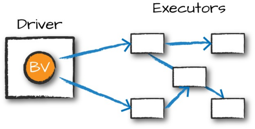
function, as illustrated in Figure 14-1.
Figure 14-1. Broadcast variables
For example, suppose that you have a list of words or values:
// in Scala
val myCollection = "Spark The Definitive Guide : Big Data Processing Made
Simple"
.split(" ")
val words = spark.sparkContext.parallelize(myCollection, 2)
# in Python
my_collection = "Spark The Definitive Guide : Big Data Processing Made Simple"\
.split(" ")
words = spark.sparkContext.parallelize(my_collection, 2)
You would like to supplement your list of words with other information that
you have, which is many kilobytes, megabytes, or potentially even gigabytes
in size. This is technically a right join if we thought about it in terms of SQL:
// in Scala
val supplementalData = Map("Spark" -> 1000, "Definitive" -> 200,
"Big" -> -300, "Simple" -> 100)
# in Python
supplementalData = {"Spark":1000, "Definitive":200,
"Big":-300, "Simple":100}
We can broadcast this structure across Spark and reference it by using
suppBroadcast. This value is immutable and is lazily replicated across all
nodes in the cluster when we trigger an action:
// in Scala
val suppBroadcast = spark.sparkContext.broadcast(supplementalData)
# in Python
suppBroadcast = spark.sparkContext.broadcast(supplementalData)
We reference this variable via the value method, which returns the exact
value that we had earlier. This method is accessible within serialized
functions without having to serialize the data. This can save you a great deal
of serialization and deserialization costs because Spark transfers data more
efficiently around the cluster using broadcasts:
// in Scala
suppBroadcast.value
# in Python
suppBroadcast.value
Now we could transform our RDD using this value. In this instance, we will
create a key–value pair according to the value we might have in the map. If
we lack the value, we will simply replace it with 0:
// in Scala
words.map(word => (word, suppBroadcast.value.getOrElse(word, 0)))
.sortBy(wordPair => wordPair._2)
.collect()
# in Python
words.map(lambda word: (word, suppBroadcast.value.get(word, 0)))\
.sortBy(lambda wordPair: wordPair[1])\
.collect()
This returns the following value in Python and the same values in an array
type in Scala:
[('Big', -300),
('The', 0),
...
('Definitive', 200),
('Spark', 1000)]
The only difference between this and passing it into the closure is that we
have done this in a much more efficient manner (Naturally, this depends on
the amount of data and the number of executors. For very small data (low
KBs) on small clusters, it might not be). Although this small dictionary
probably is not too large of a cost, if you have a much larger value, the cost
of serializing the data for every task can be quite significant.
One thing to note is that we used this in the context of an RDD; we can also
use this in a UDF or in a Dataset and achieve the same result.
Accumulators
Accumulators (Figure 14-2), Spark’s second type of shared variable, are a
way of updating a value inside of a variety of transformations and
propagating that value to the driver node in an efficient and fault-tolerant
way.
Figure 14-2. Accumulator variable
Accumulators provide a mutable variable that a Spark cluster can safely
update on a per-row basis. You can use these for debugging purposes (say to
track the values of a certain variable per partition in order to intelligently use
it over time) or to create low-level aggregation. Accumulators are variables
that are “added” to only through an associative and commutative operation
and can therefore be efficiently supported in parallel. You can use them to
implement counters (as in MapReduce) or sums. Spark natively supports
accumulators of numeric types, and programmers can add support for new
types.
For accumulator updates performed inside actions only, Spark guarantees that
each task’s update to the accumulator will be applied only once, meaning that
restarted tasks will not update the value. In transformations, you should be
aware that each task’s update can be applied more than once if tasks or job
stages are reexecuted.
Accumulators do not change the lazy evaluation model of Spark. If an
accumulator is being updated within an operation on an RDD, its value is
updated only once that RDD is actually computed (e.g., when you call an
action on that RDD or an RDD that depends on it). Consequently,
accumulator updates are not guaranteed to be executed when made within a
lazy transformation like map().
Accumulators can be both named and unnamed. Named accumulators will
display their running results in the Spark UI, whereas unnamed ones will not.
Basic Example
Let’s experiment by performing a custom aggregation on the Flight dataset
that we created earlier in the book. In this example, we will use the Dataset
API as opposed to the RDD API, but the extension is quite similar:
// in Scala
case class Flight(DEST_COUNTRY_NAME: String,
ORIGIN_COUNTRY_NAME: String, count: BigInt)
val flights = spark.read
.parquet("/data/flight-data/parquet/2010-summary.parquet")
.as[Flight]
# in Python
flights = spark.read\
.parquet("/data/flight-data/parquet/2010-summary.parquet")
Now let’s create an accumulator that will count the number of flights to or
from China. Even though we could do this in a fairly straightfoward manner
in SQL, many things might not be so straightfoward. Accumulators provide a
programmatic way of allowing for us to do these sorts of counts. The
following demonstrates creating an unnamed accumulator:
// in Scala
import org.apache.spark.util.LongAccumulator
val accUnnamed = new LongAccumulator
val acc = spark.sparkContext.register(accUnnamed)
# in Python
accChina = spark.sparkContext.accumulator(0)
Our use case fits a named accumulator a bit better. There are two ways to do
this: a short-hand method and a long-hand one. The simplest is to use the
SparkContext. Alternatively, we can instantiate the accumulator and register
it with a name:
// in Scala
val accChina = new LongAccumulator
val accChina2 = spark.sparkContext.longAccumulator("China")
spark.sparkContext.register(accChina, "China")
We specify the name of the accumulator in the string value that we pass into
the function, or as the second parameter into the register function. Named
accumulators will display in the Spark UI, whereas unnamed ones will not.
The next step is to define the way we add to our accumulator. This is a fairly
straightforward function:
// in Scala
def accChinaFunc(flight_row: Flight) = {
val destination = flight_row.DEST_COUNTRY_NAME
val origin = flight_row.ORIGIN_COUNTRY_NAME
if (destination == "China") {
accChina.add(flight_row.count.toLong)
}
if (origin == "China") {
accChina.add(flight_row.count.toLong)
}
}
# in Python
def accChinaFunc(flight_row):
destination = flight_row["DEST_COUNTRY_NAME"]
origin = flight_row["ORIGIN_COUNTRY_NAME"]
if destination == "China":
accChina.add(flight_row["count"])
if origin == "China":
accChina.add(flight_row["count"])
Now, let’s iterate over every row in our flights dataset via the foreach
method. The reason for this is because foreach is an action, and Spark can
provide guarantees that perform only inside of actions.
The foreach method will run once for each row in the input DataFrame
(assuming that we did not filter it) and will run our function against each row,
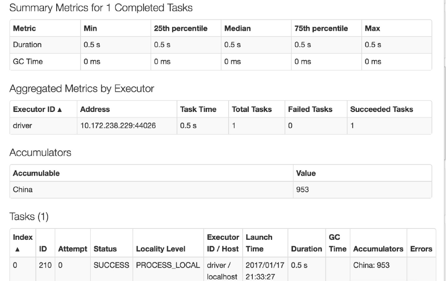
incrementing the accumulator accordingly:
// in Scala
flights.foreach(flight_row => accChinaFunc(flight_row))
# in Python
flights.foreach(lambda flight_row: accChinaFunc(flight_row))
This will complete fairly quickly, but if you navigate to the Spark UI, you
can see the relevant value, on a per-Executor level, even before querying it
programmatically, as demonstrated in Figure 14-3.
Figure 14-3. Executor Spark UI
Of course, we can query it programmatically, as well. To do this, we use the
value property:
// in Scala
accChina.value // 953
# in Python
accChina.value # 953
Custom Accumulators
Although Spark does provide some default accumulator types, sometimes
you might want to build your own custom accumulator. In order to do this
you need to subclass the AccumulatorV2 class. There are several abstract
methods that you need to implement, as you can see in the example that
follows. In this example, you we will add only values that are even to the
accumulator. Although this is again simplistic, it should show you how easy
it is to build up your own accumulators:
// in Scala
import scala.collection.mutable.ArrayBuffer
import org.apache.spark.util.AccumulatorV2
val arr = ArrayBuffer[BigInt]()
class EvenAccumulator extends AccumulatorV2[BigInt, BigInt] {
private var num:BigInt = 0
def reset(): Unit = {
this.num = 0
}
def add(intValue: BigInt): Unit = {
if (intValue % 2 == 0) {
this.num += intValue
}
}
def merge(other: AccumulatorV2[BigInt,BigInt]): Unit = {
this.num += other.value
}
def value():BigInt = {
this.num
}
def copy(): AccumulatorV2[BigInt,BigInt] = {
new EvenAccumulator
}
def isZero():Boolean = {
this.num == 0
}
}
val acc = new EvenAccumulator
val newAcc = sc.register(acc, "evenAcc")
// in Scala
acc.value // 0
flights.foreach(flight_row => acc.add(flight_row.count))
acc.value // 31390
If you are predominantly a Python user, you can also create your own custom
accumulators by subclassing AccumulatorParam and using it as we saw in the
previous example.
Conclusion
In this chapter, we covered distributed variables. These can be helpful tools
for optimizations or for debugging. In Chapter 15, we define how Spark runs
on a cluster to better understand when these can be helpful.

Part IV. Production Applications

Chapter 15. How Spark Runs on
a Cluster
Thus far in the book, we focused on Spark’s properties as a programming
interface. We have discussed how the structured APIs take a logical
operation, break it up into a logical plan, and convert that to a physical plan
that actually consists of Resilient Distributed Dataset (RDD) operations that
execute across the cluster of machines. This chapter focuses on what happens
when Spark goes about executing that code. We discuss this in an
implementation-agnostic way—this depends on neither the cluster manager
that you’re using nor the code that you’re running. At the end of the day, all
Spark code runs the same way.
This chapter covers several key topics:
The architecture and components of a Spark Application
The life cycle of a Spark Application inside and outside of Spark
Important low-level execution properties, such as pipelining
What it takes to run a Spark Application, as a segue into Chapter 16.
Let’s begin with the architecture.
The Architecture of a Spark Application
In Chapter 2, we discussed some of the high-level components of a Spark
Application. Let’s review those again:
The Spark driver
The driver is the process “in the driver seat” of your Spark Application. It
is the controller of the execution of a Spark Application and maintains all
of the state of the Spark cluster (the state and tasks of the executors). It
must interface with the cluster manager in order to actually get physical
resources and launch executors. At the end of the day, this is just a
process on a physical machine that is responsible for maintaining the state
of the application running on the cluster.
The Spark executors
Spark executors are the processes that perform the tasks assigned by the
Spark driver. Executors have one core responsibility: take the tasks
assigned by the driver, run them, and report back their state (success or
failure) and results. Each Spark Application has its own separate executor
processes.
The cluster manager
The Spark Driver and Executors do not exist in a void, and this is where
the cluster manager comes in. The cluster manager is responsible for
maintaining a cluster of machines that will run your Spark Application(s).
Somewhat confusingly, a cluster manager will have its own “driver”
(sometimes called master) and “worker” abstractions. The core difference
is that these are tied to physical machines rather than processes (as they
are in Spark). Figure 15-1 shows a basic cluster setup. The machine on
the left of the illustration is the Cluster Manager Driver Node. The circles
represent daemon processes running on and managing each of the
individual worker nodes. There is no Spark Application running as of yet
—these are just the processes from the cluster manager.
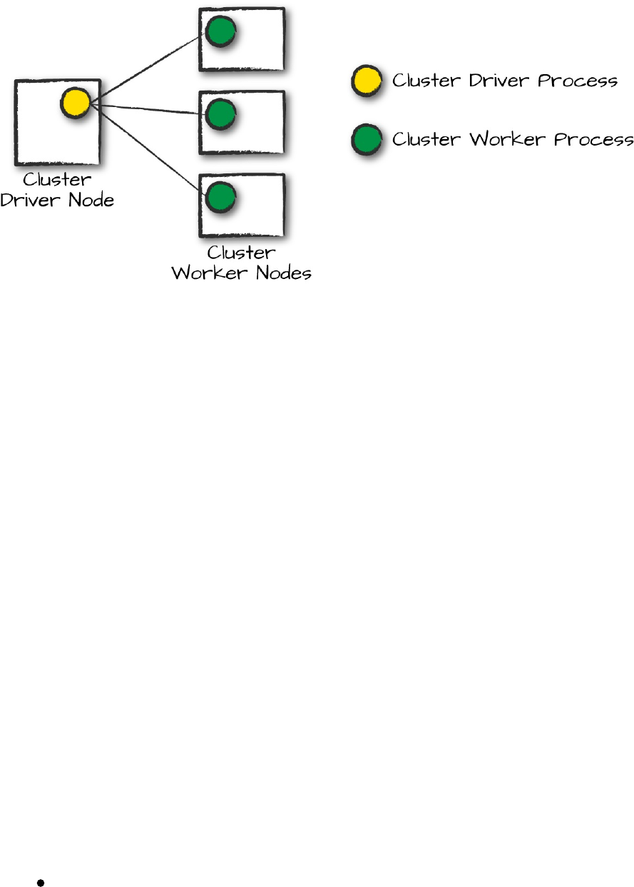
Figure 15-1. A cluster driver and worker (no Spark Application yet)
When it comes time to actually run a Spark Application, we request resources
from the cluster manager to run it. Depending on how our application is
configured, this can include a place to run the Spark driver or might be just
resources for the executors for our Spark Application. Over the course of
Spark Application execution, the cluster manager will be responsible for
managing the underlying machines that our application is running on.
Spark currently supports three cluster managers: a simple built-in standalone
cluster manager, Apache Mesos, and Hadoop YARN. However, this list will
continue to grow, so be sure to check the documentation for your favorite
cluster manager.
Now that we’ve covered the basic components of an application, let’s walk
through one of the first choices you will need to make when running your
applications: choosing the execution mode.
Execution Modes
An execution mode gives you the power to determine where the
aforementioned resources are physically located when you go to run your
application. You have three modes to choose from:
Cluster mode

Client mode
Local mode
We will walk through each of these in detail using Figure 15-1 as a template.
In the following section, rectangles with solid borders represent Spark driver
process whereas those with dotted borders represent the executor processes.
Cluster mode
Cluster mode is probably the most common way of running Spark
Applications. In cluster mode, a user submits a pre-compiled JAR, Python
script, or R script to a cluster manager. The cluster manager then launches the
driver process on a worker node inside the cluster, in addition to the executor
processes. This means that the cluster manager is responsible for maintaining
all Spark Application–related processes. Figure 15-2 shows that the cluster
manager placed our driver on a worker node and the executors on other
worker nodes.
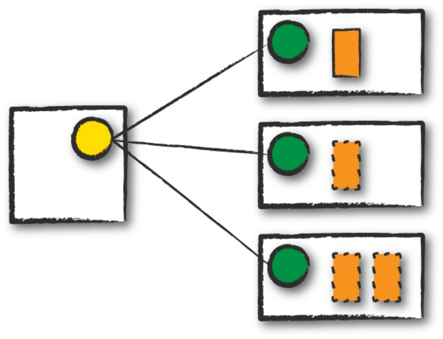
Figure 15-2. Spark’s cluster mode
Client mode
Client mode is nearly the same as cluster mode except that the Spark driver
remains on the client machine that submitted the application. This means that
the client machine is responsible for maintaining the Spark driver process,
and the cluster manager maintains the executor processses. In Figure 15-3,
we are running the Spark Application from a machine that is not colocated on
the cluster. These machines are commonly referred to as gateway machines
or edge nodes. In Figure 15-3, you can see that the driver is running on a
machine outside of the cluster but that the workers are located on machines in
the cluster.
Figure 15-3. Spark’s client mode
Local mode
Local mode is a significant departure from the previous two modes: it runs
the entire Spark Application on a single machine. It achieves parallelism
through threads on that single machine. This is a common way to learn Spark,
to test your applications, or experiment iteratively with local development.
However, we do not recommend using local mode for running production
applications.
The Life Cycle of a Spark Application (Outside

Spark)
This chapter has thus far covered the vocabulary necessary for discussing
Spark Applications. It’s now time to talk about the overall life cycle of Spark
Applications from “outside” the actual Spark code. We will do this with an
illustrated example of an application run with spark-submit (introduced in
Chapter 3). We assume that a cluster is already running with four nodes, a
driver (not a Spark driver but cluster manager driver) and three worker nodes.
The actual cluster manager does not matter at this point: this section uses the
vocabulary from the previous section to walk through a step-by-step Spark
Application life cycle from initialization to program exit.
NOTE
This section also makes use of illustrations and follows the same notation that we
introduced previously. Additionally, we now introduce lines that represent network
communication. Darker arrows represent communication by Spark or Spark-related
processes, whereas dashed lines represent more general communication (like cluster
management communication).
Client Request
The first step is for you to submit an actual application. This will be a pre-
compiled JAR or library. At this point, you are executing code on your local
machine and you’re going to make a request to the cluster manager driver
node (Figure 15-4). Here, we are explicitly asking for resources for the Spark
driver process only. We assume that the cluster manager accepts this offer
and places the driver onto a node in the cluster. The client process that
submitted the original job exits and the application is off and running on the
cluster.
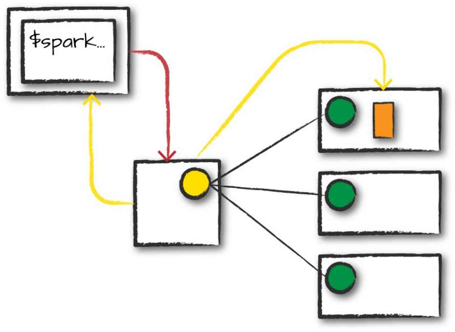
Figure 15-4. Requesting resources for a driver
To do this, you’ll run something like the following command in your
terminal:
./bin/spark-submit \
--class <main-class> \
--master <master-url> \
--deploy-mode cluster \
--conf <key>=<value> \
... # other options
<application-jar> \
[application-arguments]
Launch
Now that the driver process has been placed on the cluster, it begins running
user code (Figure 15-5). This code must include a SparkSession that
initializes a Spark cluster (e.g., driver + executors). The SparkSession will
subsequently communicate with the cluster manager (the darker line), asking
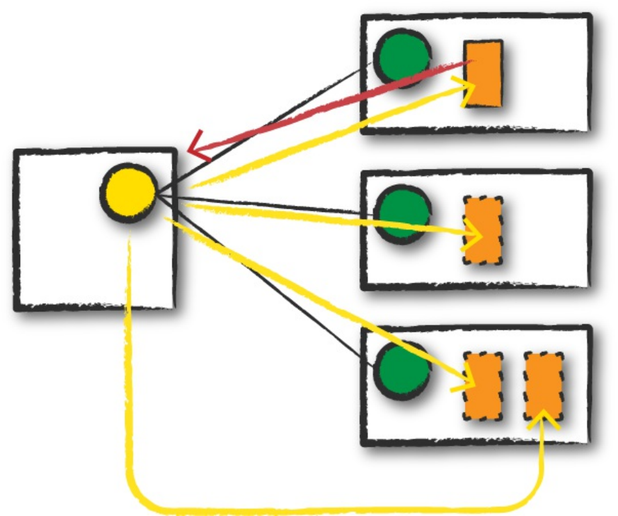
it to launch Spark executor processes across the cluster (the lighter lines). The
number of executors and their relevant configurations are set by the user via
the command-line arguments in the original spark-submit call.
Figure 15-5. Launching the Spark Application
The cluster manager responds by launching the executor processes (assuming
all goes well) and sends the relevant information about their locations to the
driver process. After everything is hooked up correctly, we have a “Spark
Cluster” as you likely think of it today.
Execution
Now that we have a “Spark Cluster,” Spark goes about its merry way
executing code, as shown in Figure 15-6. The driver and the workers
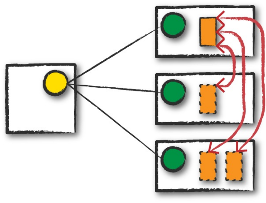
communicate among themselves, executing code and moving data around.
The driver schedules tasks onto each worker, and each worker responds with
the status of those tasks and success or failure. (We cover these details
shortly.)
Figure 15-6. Application execution
Completion
After a Spark Application completes, the driver processs exits with either
success or failure (Figure 15-7). The cluster manager then shuts down the
executors in that Spark cluster for the driver. At this point, you can see the
success or failure of the Spark Application by asking the cluster manager for
this information.
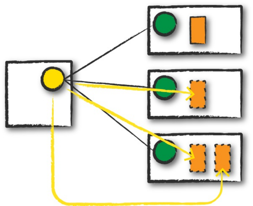
Figure 15-7. Shutting down the application
The Life Cycle of a Spark Application (Inside
Spark)
We just examined the life cycle of a Spark Application outside of user code
(basically the infrastructure that supports Spark), but it’s arguably more
important to talk about what happens within Spark when you run an
application. This is “user-code” (the actual code that you write that defines
your Spark Application). Each application is made up of one or more Spark
jobs. Spark jobs within an application are executed serially (unless you use
threading to launch multiple actions in parallel).
The SparkSession
The first step of any Spark Application is creating a SparkSession. In many
interactive modes, this is done for you, but in an application, you must do it
manually.
Some of your legacy code might use the new SparkContext pattern. This
should be avoided in favor of the builder method on the SparkSession,
which more robustly instantiates the Spark and SQL Contexts and ensures
that there is no context conflict, given that there might be multiple libraries
trying to create a session in the same Spark Appication:
// Creating a SparkSession in Scala
import org.apache.spark.sql.SparkSession
val spark = SparkSession.builder().appName("Databricks Spark Example")
.config("spark.sql.warehouse.dir", "/user/hive/warehouse")
.getOrCreate()
# Creating a SparkSession in Python
from pyspark.sql import SparkSession
spark = SparkSession.builder.master("local").appName("Word Count")\
.config("spark.some.config.option", "some-value")\
.getOrCreate()
After you have a SparkSession, you should be able to run your Spark code.
From the SparkSession, you can access all of low-level and legacy contexts
and configurations accordingly, as well. Note that the SparkSession class
was only added in Spark 2.X. Older code you might find would instead
directly create a SparkContext and a SQLContext for the structured APIs.
The SparkContext
A SparkContext object within the SparkSession represents the connection
to the Spark cluster. This class is how you communicate with some of
Spark’s lower-level APIs, such as RDDs. It is commonly stored as the
variable sc in older examples and documentation. Through a SparkContext,
you can create RDDs, accumulators, and broadcast variables, and you can run
code on the cluster.
For the most part, you should not need to explicitly initialize a
SparkContext; you should just be able to access it through the
SparkSession. If you do want to, you should create it in the most general
way, through the getOrCreate method:
// in Scala
import org.apache.spark.SparkContext
val sc = SparkContext.getOrCreate()

THE SPARKSESSION, SQLCONTEXT, AND
HIVECONTEXT
In previous versions of Spark, the SQLContext and HiveContext
provided the ability to work with DataFrames and Spark SQL and were
commonly stored as the variable sqlContext in examples,
documentation, and legacy code. As a historical point, Spark 1.X had
effectively two contexts. The SparkContext and the SQLContext. These
two each performed different things. The former focused on more fine-
grained control of Spark’s central abstractions, whereas the latter focused
on the higher-level tools like Spark SQL. In Spark 2.X, the communtiy
combined the two APIs into the centralized SparkSession that we have
today. However, both of these APIs still exist and you can access them
via the SparkSession. It is important to note that you should never need
to use the SQLContext and rarely need to use the SparkContext.
After you initialize your SparkSession, it’s time to execute some code. As we
know from previous chapters, all Spark code compiles down to RDDs.
Therefore, in the next section, we will take some logical instructions (a
DataFrame job) and walk through, step by step, what happens over time.
Logical Instructions
As you saw in the beginning of the book, Spark code essentially consists of
transformations and actions. How you build these is up to you—whether it’s
through SQL, low-level RDD manipulation, or machine learning algorithms.
Understanding how we take declarative instructions like DataFrames and
convert them into physical execution plans is an important step to
understanding how Spark runs on a cluster. In this section, be sure to run this
in a fresh environment (a new Spark shell) to follow along with the job,
stage, and task numbers.
Logical instructions to physical execution

We mentioned this in Part II, but it’s worth reiterating so that you can better
understand how Spark takes your code and actually runs the commands on
the cluster. We will walk through some more code, line by line, explain
what’s happening behind the scenes so that you can walk away with a better
understanding of your Spark Applications. In later chapters, when we discuss
monitoring, we will perform a more detailed tracking of a Spark job through
the Spark UI. In this current example, we’ll take a simpler approach. We are
going to do a three-step job: using a simple DataFrame, we’ll repartition it,
perform a value-by-value manipulation, and then aggregate some values and
collect the final result.
NOTE
This code was written and runs with Spark 2.2 in Python (you’ll get the same result in
Scala, so we’ve omitted it). The number of jobs is unlikely to change drastically but there
might be improvements to Spark’s underlying optimizations that change physical
execution strategies.
# in Python
df1 = spark.range(2, 10000000, 2)
df2 = spark.range(2, 10000000, 4)
step1 = df1.repartition(5)
step12 = df2.repartition(6)
step2 = step1.selectExpr("id * 5 as id")
step3 = step2.join(step12, ["id"])
step4 = step3.selectExpr("sum(id)")
step4.collect() # 2500000000000
When you run this code, we can see that your action triggers one complete
Spark job. Let’s take a look at the explain plan to ground our understanding
of the physical execution plan. We can access this information on the SQL
tab (after we actually run a query) in the Spark UI, as well:
step4.explain()
== Physical Plan ==
*HashAggregate(keys=[], functions=[sum(id#15L)])

+- Exchange SinglePartition
+- *HashAggregate(keys=[], functions=[partial_sum(id#15L)])
+- *Project [id#15L]
+- *SortMergeJoin [id#15L], [id#10L], Inner
:- *Sort [id#15L ASC NULLS FIRST], false, 0
: +- Exchange hashpartitioning(id#15L, 200)
: +- *Project [(id#7L * 5) AS id#15L]
: +- Exchange RoundRobinPartitioning(5)
: +- *Range (2, 10000000, step=2, splits=8)
+- *Sort [id#10L ASC NULLS FIRST], false, 0
+- Exchange hashpartitioning(id#10L, 200)
+- Exchange RoundRobinPartitioning(6)
+- *Range (2, 10000000, step=4, splits=8)
What you have when you call collect (or any action) is the execution of a
Spark job that individually consist of stages and tasks. Go to localhost:4040
if you are running this on your local machine to see the Spark UI. We will
follow along on the “jobs” tab eventually jumping to stages and tasks as we
proceed to further levels of detail.
A Spark Job
In general, there should be one Spark job for one action. Actions always
return results. Each job breaks down into a series of stages, the number of
which depends on how many shuffle operations need to take place.
This job breaks down into the following stages and tasks:
Stage 1 with 8 Tasks
Stage 2 with 8 Tasks
Stage 3 with 6 Tasks
Stage 4 with 5 Tasks
Stage 5 with 200 Tasks
Stage 6 with 1 Task
I hope you’re at least somewhat confused about how we got to these numbers
so that we can take the time to better understand what is going on!

Stages
Stages in Spark represent groups of tasks that can be executed together to
compute the same operation on multiple machines. In general, Spark will try
to pack as much work as possible (i.e., as many transformations as possible
inside your job) into the same stage, but the engine starts new stages after
operations called shuffles. A shuffle represents a physical repartitioning of the
data—for example, sorting a DataFrame, or grouping data that was loaded
from a file by key (which requires sending records with the same key to the
same node). This type of repartitioning requires coordinating across
executors to move data around. Spark starts a new stage after each shuffle,
and keeps track of what order the stages must run in to compute the final
result.
In the job we looked at earlier, the first two stages correspond to the range
that you perform in order to create your DataFrames. By default when you
create a DataFrame with range, it has eight partitions. The next step is the
repartitioning. This changes the number of partitions by shuffling the data.
These DataFrames are shuffled into six partitions and five partitions,
corresponding to the number of tasks in stages 3 and 4.
Stages 3 and 4 perform on each of those DataFrames and the end of the stage
represents the join (a shuffle). Suddenly, we have 200 tasks. This is because
of a Spark SQL configuration. The spark.sql.shuffle.partitions
default value is 200, which means that when there is a shuffle performed
during execution, it outputs 200 shuffle partitions by default. You can change
this value, and the number of output partitions will change.
TIP
We cover the number of partitions in a bit more detail in Chapter 19 because it’s such an
important parameter. This value should be set according to the number of cores in your
cluster to ensure efficient execution. Here’s how to set it:
spark.conf.set("spark.sql.shuffle.partitions", 50)
A good rule of thumb is that the number of partitions should be larger than
the number of executors on your cluster, potentially by multiple factors
depending on the workload. If you are running code on your local machine, it
would behoove you to set this value lower because your local machine is
unlikely to be able to execute that number of tasks in parallel. This is more of
a default for a cluster in which there might be many more executor cores to
use. Regardless of the number of partitions, that entire stage is computed in
parallel. The final result aggregates those partitions individually, brings them
all to a single partition before finally sending the final result to the driver.
We’ll see this configuration several times over the course of this part of the
book.
Tasks
Stages in Spark consist of tasks. Each task corresponds to a combination of
blocks of data and a set of transformations that will run on a single executor.
If there is one big partition in our dataset, we will have one task. If there are
1,000 little partitions, we will have 1,000 tasks that can be executed in
parallel. A task is just a unit of computation applied to a unit of data (the
partition). Partitioning your data into a greater number of partitions means
that more can be executed in parallel. This is not a panacea, but it is a simple
place to begin with optimization.
Execution Details
Tasks and stages in Spark have some important properties that are worth
reviewing before we close out this chapter. First, Spark automatically
pipelines stages and tasks that can be done together, such as a map operation
followed by another map operation. Second, for all shuffle operations, Spark
writes the data to stable storage (e.g., disk), and can reuse it across multiple
jobs. We’ll discuss these concepts in turn because they will come up when
you start inspecting applications through the Spark UI.
Pipelining
An important part of what makes Spark an “in-memory computation tool” is
that unlike the tools that came before it (e.g., MapReduce), Spark performs as
many steps as it can at one point in time before writing data to memory or
disk. One of the key optimizations that Spark performs is pipelining, which
occurs at and below the RDD level. With pipelining, any sequence of
operations that feed data directly into each other, without needing to move it
across nodes, is collapsed into a single stage of tasks that do all the operations
together. For example, if you write an RDD-based program that does a map,
then a filter, then another map, these will result in a single stage of tasks
that immediately read each input record, pass it through the first map, pass it
through the filter, and pass it through the last map function if needed. This
pipelined version of the computation is much faster than writing the
intermediate results to memory or disk after each step. The same kind of
pipelining happens for a DataFrame or SQL computation that does a select,
filter, and select.
From a practical point of view, pipelining will be transparent to you as you
write an application—the Spark runtime will automatically do it—but you
will see it if you ever inspect your application through the Spark UI or
through its log files, where you will see that multiple RDD or DataFrame
operations were pipelined into a single stage.
Shuffle Persistence
The second property you’ll sometimes see is shuffle persistence. When Spark
needs to run an operation that has to move data across nodes, such as a
reduce-by-key operation (where input data for each key needs to first be
brought together from many nodes), the engine can’t perform pipelining
anymore, and instead it performs a cross-network shuffle. Spark always
executes shuffles by first having the “source” tasks (those sending data) write
shuffle files to their local disks during their execution stage. Then, the stage
that does the grouping and reduction launches and runs tasks that fetch their
corresponding records from each shuffle file and performs that computation
(e.g., fetches and processes the data for a specific range of keys). Saving the
shuffle files to disk lets Spark run this stage later in time than the source stage
(e.g., if there are not enough executors to run both at the same time), and also
lets the engine re-launch reduce tasks on failure without rerunning all the
input tasks.
One side effect you’ll see for shuffle persistence is that running a new job
over data that’s already been shuffled does not rerun the “source” side of the
shuffle. Because the shuffle files were already written to disk earlier, Spark
knows that it can use them to run the later stages of the job, and it need not
redo the earlier ones. In the Spark UI and logs, you will see the pre-shuffle
stages marked as “skipped”. This automatic optimization can save time in a
workload that runs multiple jobs over the same data, but of course, for even
better performance you can perform your own caching with the DataFrame or
RDD cache method, which lets you control exactly which data is saved and
where. You’ll quickly grow accustomed to this behavior after you run some
Spark actions on aggregated data and inspect them in the UI.
Conclusion
In this chapter, we discussed what happens to Spark Applications when we
go to execute them on a cluster. This means how the cluster will actually go
about running that code as well as what happens within Spark Applications
during the process. At this point, you should feel quite comfortable
understanding what happens within and outside of a Spark Application. This
will give you a starting point for debugging your applications. Chapter 16
will discuss writing Spark Applications and the things you should consider
when doing so.

Chapter 16. Developing Spark
Applications
In Chapter 15, you learned about how Spark runs your code on the cluster.
We’ll now show you how easy it is to develop a standalone Spark application
and deploy it on a cluster. We’ll do this using a simple template that shares
some easy tips for how to structure your applications, including setting up
build tools and unit testing. This template is available in the book’s code
repository. This template is not really necessary, because writing applications
from scratch isn’t hard, but it helps. Let’s get started with our first
application.
Writing Spark Applications
Spark Applications are the combination of two things: a Spark cluster and
your code. In this case, the cluster will be local mode and the application will
be one that is pre-defined. Let’s walk through an application in each
langauge.
A Simple Scala-Based App
Scala is Spark’s “native” language and naturally makes for a great way to
write applications. It’s really no different than writing a Scala application.
TIP
Scala can seem intimidating, depending on your background, but it’s worth learning if
only to understand Spark just a bit better. Additionally, you do not need to learn all the
language’s ins and outs; begin with the basics and you’ll see that it’s easy to be productive
in Scala in no time. Using Scala will also open up a lot of doors. With a little practice, it’s
not to difficult to do code-level tracing through Spark’s codebase.

You can build applications using sbt or Apache Maven, two Java Virtual
Machine (JVM)–based build tools. As with any build tool, they each have
their own quirks, but it’s probably easiest to begin with sbt. You can
download, install, and learn about sbt on the sbt website. You can install
Maven from its respective website, as well.
To configure an sbt build for our Scala application, we specify a build.sbt file
to manage the package information. Inside the build.sbt file, there are a few
key things to include:
Project metadata (package name, package versioning information,
etc.)
Where to resolve dependencies
Dependencies needed for your library
There are many more options that you can specify; however, they are beyond
the scope of this book (you can find information about this on the web and in
the sbt documentation). There are also some books on the subject that can
serve as a helpful reference as soon as you’ve gone beyond anything
nontrivial. Here’s what a sample Scala built.sbt file might look like (and the
one that we include in the template). Notice how we must specify the Scala
version as well as the Spark version:
name := "example"
organization := "com.databricks"
version := "0.1-SNAPSHOT"
scalaVersion := "2.11.8"
// Spark Information
val sparkVersion = "2.2.0"
// allows us to include spark packages
resolvers += "bintray-spark-packages" at
"https://dl.bintray.com/spark-packages/maven/"
resolvers += "Typesafe Simple Repository" at
"http://repo.typesafe.com/typesafe/simple/maven-releases/"
resolvers += "MavenRepository" at
"https://mvnrepository.com/"
libraryDependencies ++= Seq(
// spark core
"org.apache.spark" %% "spark-core" % sparkVersion,
"org.apache.spark" %% "spark-sql" % sparkVersion,
// the rest of the file is omitted for brevity
)
Now that we’ve defined the build file, we can actually go about adding code
to our project. We’ll use the standard Scala project structure, which you can
find in the sbt reference manual (this is the same directory structure as Maven
projects):
src/
main/
resources/
<files to include in main jar here>
scala/
<main Scala sources>
java/
<main Java sources>
test/
resources
<files to include in test jar here>
scala/
<test Scala sources>
java/
<test Java sources>
We put the source code in the Scala and Java directories. In this case, we put
something like the following in a file; this initializes the SparkSession, runs
the application, and then exits:
object DataFrameExample extends Serializable {
def main(args: Array[String]) = {
val pathToDataFolder = args(0)
// start up the SparkSession
// along with explicitly setting a given config
val spark = SparkSession.builder().appName("Spark Example")
.config("spark.sql.warehouse.dir", "/user/hive/warehouse")
.getOrCreate()
// udf registration
spark.udf.register("myUDF", someUDF(_:String):String)
val df = spark.read.json(pathToDataFolder + "data.json")
val manipulated = df.groupBy(expr("myUDF(group)")).sum().collect()
.foreach(x => println(x))
}
}
Notice how we defined a main class that we can run from the command line
when we use spark-submit to submit it to our cluster for execution.
Now that we have our project set up and have added some code to it, it’s time
to build it. We can use sbt assemble to build an “uber-jar” or “fat-jar” that
contains all of the dependencies in one JAR. This can be simple for some
deployments but cause complications (especially dependency conflicts) for
others. A lighter-weight approach is to run sbt package, which will gather
all of your dependencies into the target folder but will not package all of them
into one big JAR.
Running the application
The target folder contains the JAR that we can use as an argument to spark-
submit. After building the Scala package, you end up with something that
you can spark-submit on your local machine by using the following code
(this snippet takes advantage of aliasing to create the $SPARK_HOME variable;
you could replace $SPARK_HOME with the exact directory that contains your
downloaded version of Spark):
$SPARK_HOME/bin/spark-submit \
--class com.databricks.example.DataFrameExample \
--master local \
target/scala-2.11/example_2.11-0.1-SNAPSHOT.jar "hello"
Writing Python Applications
Writing PySpark Applications is really no different than writing normal
Python applications or packages. It’s quite similar to writing command-line
applications in particular. Spark doesn’t have a build concept, just Python
scripts, so to run an application, you simply execute the script against the
cluster.
To facilitate code reuse, it is common to package multiple Python files into
egg or ZIP files of Spark code. To include those files, you can use the --py-
files argument of spark-submit to add .py, .zip, or .egg files to be
distributed with your application.
When it’s time to run your code, you create the equivalent of a “Scala/Java
main class” in Python. Specify a certain script as an executable script that
builds the SparkSession. This is the one that we will pass as the main
argument to spark-submit:
# in Python
from __future__ import print_function
if __name__ == '__main__':
from pyspark.sql import SparkSession
spark = SparkSession.builder \
.master("local") \
.appName("Word Count") \
.config("spark.some.config.option", "some-value") \
.getOrCreate()
print(spark.range(5000).where("id > 500").selectExpr("sum(id)").collect())
When you do this, you’re going to get a SparkSession that you can pass
around your application. It is best practice to pass around this variable at
runtime rather than instantiating it within every Python class.
One helpful tip when developing in Python is to use pip to specify PySpark
as a dependency. You can do this by running the command pip install
pyspark. This allows you to use it in a way that you might use other Python
packages. This makes for very helpful code completion in many editors, as
well. This is brand new in Spark 2.2, so it might take a version or two to be
completely production ready, but Python is very popular in the Spark
community, and it’s sure to be a cornerstone of Spark’s future.
Running the application
After you’ve written your code, it’s time to submit it for execution. (We’re
executing the same code that we have in the project template.) You just need
to call spark-submit with that information:
$SPARK_HOME/bin/spark-submit --master local pyspark_template/main.py
Writing Java Applications
Writing Java Spark Applications is, if you squint, the same as writing Scala
applications. The core differences involve how you specify your
dependencies.
This example assumes that you are using Maven to specify your
dependencies. In this case, you’ll use the following format. In Maven, you
must add the Spark Packages repository so that you can fetch dependencies
from those locations:
<dependencies>
<dependency>
<groupId>org.apache.spark</groupId>
<artifactId>spark-core_2.11</artifactId>
<version>2.1.0</version>
</dependency>
<dependency>
<groupId>org.apache.spark</groupId>
<artifactId>spark-sql_2.11</artifactId>
<version>2.1.0</version>
</dependency>
<dependency>
<groupId>graphframes</groupId>
<artifactId>graphframes</artifactId>
<version>0.4.0-spark2.1-s_2.11</version>
</dependency>
</dependencies>
<repositories>
<!-- list of other repositories -->
<repository>
<id>SparkPackagesRepo</id>
<url>http://dl.bintray.com/spark-packages/maven</url>
</repository>
</repositories>
Naturally, you follow the same directory structure as in the Scala project
version (seeing as they both conform to the Maven specification). We then
just follow the relevant Java examples to actually build and execute the code.
Now we can create a simple example that specifies a main class for us to
execute against (more on this at the end of the chapter):
import org.apache.spark.sql.SparkSession;
public class SimpleExample {
public static void main(String[] args) {
SparkSession spark = SparkSession
.builder()
.getOrCreate();
spark.range(1, 2000).count();
}
}
We then package it by using mvn package (you need to have Maven installed
to do so).
Running the application
This operation is going to be the exact same as running the Scala application
(or the Python application, for that matter). Simply use spark-submit:
$SPARK_HOME/bin/spark-submit \
--class com.databricks.example.SimpleExample \
--master local \
target/spark-example-0.1-SNAPSHOT.jar "hello"
Testing Spark Applications
You now know what it takes to write and run a Spark Application, so let’s
move on to a less exciting but still very important topic: testing. Testing
Spark Applications relies on a couple of key principles and tactics that you
should keep in mind as you’re writing your applications.
Strategic Principles
Testing your data pipelines and Spark Applications is just as important as
actually writing them. This is because you want to ensure that they are
resilient to future change, in data, logic, and output. In this section, we’ll first
discuss what you might want to test in a typical Spark Application, then
discuss how to organize your code for easy testing.
Input data resilience
Being resilient to different kinds of input data is something that is quite
fundamental to how you write your data pipelines. The data will change
because the business needs will change. Therefore your Spark Applications
and pipelines should be resilient to at least some degree of change in the
input data or otherwise ensure that these failures are handled in a graceful and
resilient way. For the most part this means being smart about writing your
tests to handle those edge cases of different inputs and making sure that the
pager only goes off when it’s something that is truly important.
Business logic resilience and evolution
The business logic in your pipelines will likely change as well as the input
data. Even more importantly, you want to be sure that what you’re deducing
from the raw data is what you actually think that you’re deducing. This
means that you’ll need to do robust logical testing with realistic data to
ensure that you’re actually getting what you want out of it. One thing to be
wary of here is trying to write a bunch of “Spark Unit Tests” that just test
Spark’s functionality. You don’t want to be doing that; instead, you want to
be testing your business logic and ensuring that the complex business
pipeline that you set up is actually doing what you think it should be doing.
Resilience in output and atomicity
Assuming that you’re prepared for departures in the structure of input data
and that your business logic is well tested, you now want to ensure that your
output structure is what you expect. This means you will need to gracefully
handle output schema resolution. It’s not often that data is simply dumped in
some location, never to be read again—most of your Spark pipelines are
probably feeding other Spark pipelines. For this reason you’re going to want
to make certain that your downstream consumers understand the “state” of
the data—this could mean how frequently it’s updated as well as whether the
data is “complete” (e.g., there is no late data) or that there won’t be any last-
minute corrections to the data.
All of the aforementioned issues are principles that you should be thinking
about as you build your data pipelines (actually, regardless of whether you’re
using Spark). This strategic thinking is important for laying down the
foundation for the system that you would like to build.
Tactical Takeaways
Although strategic thinking is important, let’s talk a bit more in detail about
some of the tactics that you can actually use to make your application easy to
test. The highest value approach is to verify that your business logic is correct
by employing proper unit testing and to ensure that you’re resilient to
changing input data or have structured it so that schema evolution will not
become unwielding in the future. The decision for how to do this largely falls
on you as the developer because it will vary according to your business
domain and domain expertise.
Managing SparkSessions
Testing your Spark code using a unit test framework like JUnit or ScalaTest
is relatively easy because of Spark’s local mode—just create a local mode
SparkSession as part of your test harness to run it. However, to make this
work well, you should try to perform dependency injection as much as
possible when managing SparkSessions in your code. That is, initialize the
SparkSession only once and pass it around to relevant functions and classes
at runtime in a way that makes it easy to substitute during testing. This makes
it much easier to test each individual function with a dummy SparkSession in
unit tests.
Which Spark API to Use?
Spark offers several choices of APIs, ranging from SQL to DataFrames and
Datasets, and each of these can have different impacts for maintainability and
testability of your application. To be perfectly honest, the right API depends
on your team and its needs: some teams and projects will need the less strict
SQL and DataFrame APIs for speed of development, while others will want
to use type-safe Datasets or RDDs.
In general, we recommend documenting and testing the input and output
types of each function regardless of which API you use. The type-safe API
automatically enforces a minimal contract for your function that makes it
easy for other code to build on it. If your team prefers to use DataFrames or
SQL, then spend some time to document and test what each function returns
and what types of inputs it accepts to avoid surprises later, as in any
dynamically typed programming language. While the lower-level RDD API
is also statically typed, we recommend going into it only if you need low-
level features such as partitioning that are not present in Datasets, which
should not be very common; the Dataset API allows more performance
optimizations and is likely to provide even more of them in the future.
A similar set of considerations applies to which programming language to use
for your application: there certainly is no right answer for every team, but
depending on your needs, each language will provide different benefits. We
generally recommend using statically typed languages like Scala and Java for
larger applications or those where you want to be able to drop into low-level
code to fully control performance, but Python and R may be significantly
better in other cases—for example, if you need to use some of their other
libraries. Spark code should easily be testable in the standard unit testing
frameworks in every language.
Connecting to Unit Testing Frameworks
To unit test your code, we recommend using the standard frameworks in your
langage (e.g., JUnit or ScalaTest), and setting up your test harnesses to create
and clean up a SparkSession for each test. Different frameworks offer
different mechanisms to do this, such as “before” and “after” methods. We
have included some sample unit testing code in the application templates for
this chapter.
Connecting to Data Sources
As much as possible, you should make sure your testing code does not
connect to production data sources, so that developers can easily run it in
isolation if these data sources change. One easy way to make this happen is to
have all your business logic functions take DataFrames or Datasets as input
instead of directly connecting to various sources; after all, subsequent code
will work the same way no matter what the data source was. If you are using
the structured APIs in Spark, another way to make this happen is named
tables: you can simply register some dummy datasets (e.g., loaded from small
text file or from in-memory objects) as various table names and go from
there.
The Development Process
The development process with Spark Applications is similar to development
workflows that you have probably already used. First, you might maintain a
scratch space, such as an interactive notebook or some equivalent thereof,
and then as you build key components and algorithms, you move them to a
more permanent location like a library or package. The notebook experience
is one that we often recommend (and are using to write this book) because of
its simplicity in experimentation. There are also some tools, such as
Databricks, that allow you to run notebooks as production applications as
well.
When running on your local machine, the spark-shell and its various
language-specific implementations are probably the best way to develop
applications. For the most part, the shell is for interactive applications,
whereas spark-submit is for production applications on your Spark cluster.
You can use the shell to interactively run Spark, just as we showed you at the
beginning of this book. This is the mode with which you will run PySpark,
Spark SQL, and SparkR. In the bin folder, when you download Spark, you
will find the various ways of starting these shells. Simply run spark-
shell(for Scala), spark-sql, pyspark, and sparkR.
After you’ve finished your application and created a package or script to run,
spark-submit will become your best friend to submit this job to a cluster.
Launching Applications
The most common way for running Spark Applications is through spark-
submit. Previously in this chapter, we showed you how to run spark-
submit; you simply specify your options, the application JAR or script, and
the relevant arguments:
./bin/spark-submit \
--class <main-class> \
--master <master-url> \
--deploy-mode <deploy-mode> \
--conf <key>=<value> \
... # other options
<application-jar-or-script> \
[application-arguments]
You can always specify whether to run in client or cluster mode when you
submit a Spark job with spark-submit. However, you should almost always
favor running in cluster mode (or in client mode on the cluster itself) to
reduce latency between the executors and the driver.
When submitting applciations, pass a .py file in the place of a .jar, and add
Python .zip, .egg, or .py to the search path with --py-files.
For reference, Table 16-1 lists all of the available spark-submit options,
including those that are particular to some cluster managers. To enumerate all
these options yourself, run spark-submit with --help.
Table 16-1. Spark submit help text
Parameter Description
--master
MASTER_URL spark://host:port, mesos://host:port, yarn, or local
--deploy-
mode
DEPLOY_MODE
Whether to launch the driver program locally (“client”) or on one of the worker
machines inside the cluster (“cluster”) (Default: client)
--class
CLASS_NAME Your application’s main class (for Java / Scala apps).
--name NAME A name of your application.
--jars JARS Comma-separated list of local JARs to include on the driver and executor
classpaths.
--packages
Comma-separated list of Maven coordinates of JARs to include on the driver
and executor classpaths. Will search the local Maven repo, then Maven Central
and any additional remote repositories given by --repositories. The format
for the coordinates should be groupId:artifactId:version.
--exclude-
packages
Comma-separated list of groupId:artifactId, to exclude while resolving the
dependencies provided in --packages to avoid dependency conflicts.
--
repositories
Comma-separated list of additional remote repositories to search for the Maven
coordinates given with --packages.
--py-files
PY_FILES
Comma-separated list of .zip, .egg, or .py files to place on the PYTHONPATH for
Python apps.
--files
FILES
Comma-separated list of files to be placed in the working directory of each
executor.
--conf
PROP=VALUE Arbitrary Spark configuration property.
--
properties-
file FILE
Path to a file from which to load extra properties. If not specified, this will look
for conf/spark-defaults.conf.
--driver-
memory MEM Memory for driver (e.g., 1000M, 2G) (Default: 1024M).
--driver-
java-options Extra Java options to pass to the driver.
--driver-
library-path Extra library path entries to pass to the driver.
--driver-
class-path
Extra class path entries to pass to the driver. Note that JARs added with --jars
are automatically included in the classpath.
--executor-
memory MEM Memory per executor (e.g., 1000M, 2G) (Default: 1G).
--proxy-user
NAME
User to impersonate when submitting the application. This argument does not
work with --principal / --keytab.
--help, -h Show this help message and exit.
--verbose, -
vPrint additional debug output.
--version Print the version of current Spark.
There are some deployment-specific configurations as well (see Table 16-2).
Table 16-2. Deployment Specific Configurations
Cluster
Managers Modes Conf Description
Standalone Cluster --driver-
cores NUM Cores for driver (Default: 1).
Standalone/Mesos Cluster --supervise If given, restarts the driver on failure.
Standalone/Mesos Cluster --kill
SUBMISSION_ID If given, kills the driver specified.
Standalone/Mesos Cluster --status
SUBMISSION_ID
If given, requests the status of the driver
specified.
Standalone/Mesos Either
--total-
executor-
cores NUM
Total cores for all executors.
Standalone/YARN Either --executor-
cores NUM1
Number of cores per executor. (Default: 1 in
YARN mode or all available cores on the worker
in standalone mode)
YARN Either --driver-
cores NUM
Number of cores used by the driver, only in
cluster mode (Default: 1).
YARN Either queue
QUEUE_NAME
The YARN queue to submit to (Default:
“default”).
YARN Either --num-
executors NUM
Number of executors to launch (Default: 2). If
dynamic allocation is enabled, the initial number
of executors will be at least NUM.
YARN Either --archives
ARCHIVES
Comma-separated list of archives to be extracted
into the working directory of each executor.
YARN Either --principal
PRINCIPAL
Principal to be used to log in to KDC, while
running on secure HDFS.
YARN Either --keytab
KEYTAB
The full path to the file that contains the keytab
for the principal specified above. This keytab
will be copied to the node running the
Application Master via the Secure Distributed
Cache, for renewing the login tickets and the
delegation tokens periodically.
Application Launch Examples
We already covered some local-mode application examples previously in this
chapter, but it’s worth looking at how we use some of the aforementioned
options, as well. Spark also includes several examples and demonstration
applications in the examples directory that is included when you download
Spark. If you’re stuck on how to use certain parameters, simply try them first
on your local machine and use the SparkPi class as the main class:
./bin/spark-submit \
--class org.apache.spark.examples.SparkPi \
--master spark://207.184.161.138:7077 \
--executor-memory 20G \
--total-executor-cores 100 \
replace/with/path/to/examples.jar \
1000
The following snippet does the same for Python. You run it from the Spark
directory and this will allow you to submit a Python application (all in one
script) to the standalone cluster manager. You can also set the same executor
limits as in the preceding example:
./bin/spark-submit \
--master spark://207.184.161.138:7077 \

examples/src/main/python/pi.py \
1000
You can change this to run in local mode as well by setting the master to
local or local[*] to run on all the cores on your machine. You will also
need to change the /path/to/examples.jar to the relevant Scala and Spark
versions you are running.
Configuring Applications
Spark includes a number of different configurations, some of which we
covered in Chapter 15. There are many different configurations, depending
on what you’re hoping to achieve. This section covers those very details. For
the most part, this information is included for reference and is probably worth
skimming only, unless you’re looking for something in particular. The
majority of configurations fall into the following categories:
Application properties
Runtime environment
Shuffle behavior
Spark UI
Compression and serialization
Memory management
Execution behavior
Networking
Scheduling
Dynamic allocation
Security
Encryption

Spark SQL
Spark streaming
SparkR
Spark provides three locations to configure the system:
Spark properties control most application parameters and can be set
by using a SparkConf object
Java system properties
Hardcoded configuration files
There are several templates that you can use, which you can find in the /conf
directory available in the root of the Spark home folder. You can set these
properties as hardcoded variables in your applications or by specifying them
at runtime. You can use environment variables to set per-machine settings,
such as the IP address, through the conf/spark-env.sh script on each node.
Lastly, you can configure logging through log4j.properties.
The SparkConf
The SparkConf manages all of our application configurations. You create
one via the import statement, as shown in the example that follows. After
you create it, the SparkConf is immutable for that specific Spark
Application:
// in Scala
import org.apache.spark.SparkConf
val conf = new SparkConf().setMaster("local[2]").setAppName("DefinitiveGuide")
.set("some.conf", "to.some.value")
# in Python
from pyspark import SparkConf
conf = SparkConf().setMaster("local[2]").setAppName("DefinitiveGuide")\
.set("some.conf", "to.some.value")

You use the SparkConf to configure individual Spark Applications with
Spark properties. These Spark properties control how the Spark Application
runs and how the cluster is configured. The example that follows configures
the local cluster to have two threads and specifies the application name that
shows up in the Spark UI.
You can configure these at runtime, as you saw previously in this chapter
through command-line arguments. This is helpful when starting a Spark Shell
that will automatically include a basic Spark Application for you; for
instance:
./bin/spark-submit --name "DefinitiveGuide" --master local[4] ...
Of note is that when setting time duration-based properties, you should use
the following format:
25ms (milliseconds)
5s (seconds)
10m or 10min (minutes)
3h (hours)
5d (days)
1y (years)
Application Properties
Application properties are those that you set either from spark-submit or
when you create your Spark Application. They define basic application
metadata as well as some execution characteristics. Table 16-3 presents a list
of current application properties.
Table 16-3. Application properties
Property name Default Meaning

spark.app.name (none) The name of your application. This will appear in the
UI and in log data.
spark.driver.cores 1 Number of cores to use for the driver process, only
in cluster mode.
spark.driver.maxResultSize 1g
Limit of total size of serialized results of all
partitions for each Spark action (e.g., collect).
Should be at least 1M, or 0 for unlimited. Jobs will be
aborted if the total size exceeds this limit. Having a
high limit can cause OutOfMemoryErrors in the
driver (depends on spark.driver.memory and
memory overhead of objects in JVM). Setting a
proper limit can protect the driver from
OutOfMemoryErrors.
spark.driver.memory 1g
Amount of memory to use for the driver process,
where SparkContext is initialized. (e.g. 1g, 2g).
Note: in client mode, this must not be set through the
SparkConf directly in your application, because the
driver JVM has already started at that point. Instead,
set this through the --driver-memory command-
line option or in your default properties file.
spark.executor.memory 1g Amount of memory to use per executor process (e.g.,
2g, 8g).
spark.extraListeners (none)
A comma-separated list of classes that implement
SparkListener; when initializing SparkContext,
instances of these classes will be created and
registered with Spark’s listener bus. If a class has a
single-argument constructor that accepts a
SparkConf, that constructor will be called;
otherwise, a zero-argument constructor will be
called. If no valid constructor can be found, the
SparkContext creation will fail with an exception.
spark.logConf FALSE Logs the effective SparkConf as INFO when a
SparkContext is started.
spark.master (none) The cluster manager to connect to. See the list of
allowed master URLs.
spark.submit.deployMode (none)
The deploy mode of the Spark driver program, either
“client” or “cluster,” which means to launch driver
program locally (“client”) or remotely (“cluster”) on

one of the nodes inside the cluster.
spark.log.callerContext (none)
Application information that will be written into
Yarn RM log/HDFS audit log when running on
Yarn/HDFS. Its length depends on the Hadoop
configuration hadoop.caller.context.max.size. It
should be concise, and typically can have up to 50
characters.
spark.driver.supervise FALSE
If true, restarts the driver automatically if it fails with
a non-zero exit status. Only has effect in Spark
standalone mode or Mesos cluster deploy mode.
You can ensure that you’ve correctly set these values by checking the
application’s web UI on port 4040 of the driver on the “Environment” tab.
Only values explicitly specified through spark-defaults.conf, SparkConf, or
the command line will appear. For all other configuration properties, you can
assume the default value is used.
Runtime Properties
Although less common, there are times when you might also need to
configure the runtime environment of your application. Due to space
limitations, we cannot include the entire configuration set here. Refer to the
relevant table on the Runtime Environment in the Spark documentation.
These properties allow you to configure extra classpaths and python paths for
both drivers and executors, Python worker configurations, as well as
miscellaneous logging properties.
Execution Properties
These configurations are some of the most relevant for you to configure
because they give you finer-grained control on actual execution. Due to space
limitations, we cannot include the entire configuration set here. Refer to the
relevant table on Execution Behavior in the Spark documentation. The most
common configurations to change are spark.executor.cores (to control
the number of available cores) and spark.files.maxPartitionBytes
(maximum partition size when reading files).
Configuring Memory Management
There are times when you might need to manually manage the memory
options to try and optimize your applications. Many of these are not
particularly relevant for end users because they involve a lot of legacy
concepts or fine-grained controls that were obviated in Spark 2.X because of
automatic memory management. Due to space limitations, we cannot include
the entire configuration set here. Refer to the relevant table on Memory
Management in the Spark documentation.
Configuring Shuffle Behavior
We’ve emphasized how shuffles can be a bottleneck in Spark jobs because of
their high communication overhead. Therefore there are a number of low-
level configurations for controlling shuffle behavior. Due to space
limitations, we cannot include the entire configuration set here. Refer to the
relevant table on Shuffle Behavior in the Spark documentation.
Environmental Variables
You can configure certain Spark settings through environment variables,
which are read from the conf/spark-env.sh script in the directory where Spark
is installed (or conf/spark-env.cmd on Windows). In Standalone and Mesos
modes, this file can give machine-specific information such as hostnames. It
is also sourced when running local Spark Applications or submission scripts.
Note that conf/spark-env.sh does not exist by default when Spark is installed.
However, you can copy conf/spark-env.sh.template to create it. Be sure to
make the copy executable.
The following variables can be set in spark-env.sh:
JAVA_HOME
Location where Java is installed (if it’s not on your default PATH).

PYSPARK_PYTHON
Python binary executable to use for PySpark in both driver and workers
(default is python2.7 if available; otherwise, python). Property
spark.pyspark.python takes precedence if it is set.
PYSPARK_DRIVER_PYTHON
Python binary executable to use for PySpark in driver only (default is
PYSPARK_PYTHON). Property spark.pyspark.driver.python takes
precedence if it is set.
SPARKR_DRIVER_R
R binary executable to use for SparkR shell (default is R). Property
spark.r.shell.command takes precedence if it is set.
SPARK_LOCAL_IP
IP address of the machine to which to bind.
SPARK_PUBLIC_DNS
Hostname your Spark program will advertise to other machines.
In addition to the variables ust listed, there are also options for setting up the
Spark standalone cluster scripts, such as number of cores to use on each
machine and maximum memory. Because spark-env.sh is a shell script, you
can set some of these programmatically; for example, you might compute
SPARK_LOCAL_IP by looking up the IP of a specific network interface.
NOTE
When running Spark on YARN in cluster mode, you need to set environment variables by
using the spark.yarn.appMasterEnv.[EnvironmentVariableName] property in your
conf/spark-defaults.conf file. Environment variables that are set in spark-env.sh will not be
reflected in the YARN Application Master process in cluster mode. See the YARN-related
Spark Properties for more information.
Job Scheduling Within an Application
Within a given Spark Application, multiple parallel jobs can run
simultaneously if they were submitted from separate threads. By job, in this
section, we mean a Spark action and any tasks that need to run to evaluate
that action. Spark’s scheduler is fully thread-safe and supports this use case to
enable applications that serve multiple requests (e.g., queries for multiple
users).
By default, Spark’s scheduler runs jobs in FIFO fashion. If the jobs at the
head of the queue don’t need to use the entire cluster, later jobs can begin to
run right away, but if the jobs at the head of the queue are large, later jobs
might be delayed significantly.
It is also possible to configure fair sharing between jobs. Under fair sharing,
Spark assigns tasks between jobs in a round-robin fashion so that all jobs get
a roughly equal share of cluster resources. This means that short jobs
submitted while a long job is running can begin receiving resources right
away and still achieve good response times without waiting for the long job
to finish. This mode is best for multiuser settings.
To enable the fair scheduler, set the spark.scheduler.mode property to
FAIR when configuring a SparkContext.
The fair scheduler also supports grouping jobs into pools, and setting
different scheduling options, or weights, for each pool. This can be useful to
create a high-priority pool for more important jobs or to group the jobs of
each user together and give users equal shares regardless of how many
concurrent jobs they have instead of giving jobs equal shares. This approach
is modeled after the Hadoop Fair Scheduler.
Without any intervention, newly submitted jobs go into a default pool, but
jobs pools can be set by adding the spark.scheduler.pool local property to
the SparkContext in the thread that’s submitting them. This is done as
follows (assuming sc is your SparkContext:
sc.setLocalProperty("spark.scheduler.pool", "pool1")
After setting this local property, all jobs submitted within this thread will use
this pool name. The setting is per-thread to make it easy to have a thread run
multiple jobs on behalf of the same user. If you’d like to clear the pool that a
thread is associated with, set it to null.
Conclusion
This chapter covered a lot about Spark Applications; we learned how to
write, test, run, and configure them in all of Spark’s languages. In
Chapter 17, we talk about deploying and the cluster management options you
have when it comes to running Spark Applications.
Chapter 17. Deploying Spark
This chapter explores the infrastructure you need in place for you and your
team to be able to run Spark Applications:
Cluster deployment choices
Spark’s different cluster managers
Deployment considerations and configuring deployments
For the most, part Spark should work similarly with all the supported cluster
managers; however, customizing the setup means understanding the
intricacies of each of the cluster management systems. The hard part is
deciding on the cluster manager (or choosing a managed service). Although
we would be happy to include all the minute details about how you can
configure different cluster with different cluster managers, it’s simply
impossible for this book to provide hyper-specific details for every situation
in every single enviroment. The goal of this chapter, therefore, is not to
discuss each of the cluster managers in full detail, but rather to look at their
fundamental differences and to provide a reference for a lot of the material
already available on the Spark website. Unfortunately, there is no easy
answer to “which is the easiest cluster manager to run” because it varies so
much by use case, experience, and resources. The Spark documentation site
offers a lot of detail about deploying Spark with actionable examples. We do
our best to discuss the most relevant points.
As of this writing, Spark has three officially supported cluster managers:
Standalone mode
Hadoop YARN
Apache Mesos
These cluster managers maintain a set of machines onto which you can
deploy Spark Applications. Naturally, each of these cluster managers has an
opinionated view toward management, and so there are trade-offs and
semantics that you will need to keep in mind. However, they all run Spark
applications the same way (as covered in Chapter 16). Let’s begin with the
first point: where to deploy your cluster.
Where to Deploy Your Cluster to Run Spark
Applications
There are two high-level options for where to deploy Spark clusters: deploy
in an on-premises cluster or in the public cloud. This choice is consequential
and is therefore worth discussing.
On-Premises Cluster Deployments
Deploying Spark to an on-premises cluster is sometimes a reasonable option,
especially for organizations that already manage their own datacenters. As
with everything else, there are trade-offs to this approach. An on-premises
cluster gives you full control over the hardware used, meaning you can
optimize performance for your specific workload. However, it also introduces
some challenges, especially when it comes to data analytics workloads like
Spark. First, with on-premises deployment, your cluster is fixed in size,
whereas the resource demands of data analytics workloads are often elastic. If
you make your cluster too small, it will be hard to launch the occasional very
large analytics query or training job for a new machine learning model,
whereas if you make it large, you will have resources sitting idle. Second, for
on-premises clusters, you need to select and operate your own storage
system, such as a Hadoop file system or scalable key-value store. This
includes setting up georeplication and disaster recovery if required.
If you are going to deploy on-premises, the best way to combat the resource
utilization problem is to use a cluster manager that allows you to run many
Spark applications and dynamically reassign resources between them, or even
allows non-Spark applications on the same cluster. All of Spark’s supported
cluster managers allow multiple concurrent applications, but YARN and
Mesos have better support for dynamic sharing and also additionally support
non-Spark workloads. Handling resource sharing is likely going to be the
biggest difference your users see day to day with Spark on-premise versus in
the cloud: in public clouds, it’s easy to give each application its own cluster
of exactly the required size for just the duration of that job.
For storage, you have several different options, but covering all the trade-offs
and operational details in depth would probably require its own book. The
most common storage systems used for Spark are distributed file systems
such as Hadoop’s HDFS and key-value stores such as Apache Cassandra.
Streaming message bus systems such as Apache Kafka are also often used for
ingesting data. All these systems have varying degrees of support for
management, backup, and georeplication, sometimes built into the system
and sometimes only through third-party commercial tools. Before choosing a
storage option, we recommend evaluating the performance of its Spark
connector and evaluating the available management tools.
Spark in the Cloud
While early big data systems were designed for on-premises deployment, the
cloud is now an increasingly common platform for deploying Spark. The
public cloud has several advantages when it comes to big data workloads.
First, resources can be launched and shut down elastically, so you can run
that occasional “monster” job that takes hundreds of machines for a few
hours without having to pay for them all the time. Even for normal operation,
you can choose a different type of machine and cluster size for each
application to optimize its cost performance—for example, launch machines
with Graphics Processing Units (GPUs) just for your deep learning jobs.
Second, public clouds include low-cost, georeplicated storage that makes it
easier to manage large amounts of data.
Many companies looking to migrate to the cloud imagine they’ll run their
applications in the same way that they run their on-premises clusters. All the
major cloud providers (Amazon Web Services [AWS], Microsoft Azure,
Google Cloud Platform [GCP], and IBM Bluemix) include managed Hadoop
clusters for their customers, which provide HDFS for storage as well as
Apache Spark. This is actually not a great way to run Spark in the cloud,
however, because by using a fixed-size cluster and file system, you are not
going to be able to take advantage of elasticity. Instead, it is generally a better
idea to use global storage systems that are decoupled from a specific cluster,
such as Amazon S3, Azure Blob Storage, or Google Cloud Storage and spin
up machines dynamically for each Spark workload. With decoupled compute
and storage, you will be able to pay for computing resources only when
needed, scale them up dynamically, and mix different hardware types.
Basically, keep in mind that running Spark in the cloud need not mean
migrating an on-premises installation to virtual machines: you can run Spark
natively against cloud storage to take full advantage of the cloud’s elasticity,
cost-saving benefit, and management tools without having to manage an on-
premise computing stack within your cloud environment.
Several companies provide “cloud-native” Spark-based services, and all
installations of Apache Spark can of course connect to cloud storage.
Databricks, the company started by the Spark team from UC Berkeley, is one
example of a service provider built specifically for Spark in the cloud.
Databricks provides a simple way to run Spark workloads without the heavy
baggage of a Hadoop installation. The company provides a number of
features for running Spark more efficiently in the cloud, such as auto-scaling,
auto-termination of clusters, and optimized connectors to cloud storage, as
well as a collaborative environment for working on notebooks and standalone
jobs. The company also provides a free Community Edition for learning
Spark where you can run notebooks on a small cluster and share them live
with others. A fun fact is that this entire book was written using the free
Community Edition of Databricks, because we found the integrated Spark
notebooks, live collaboration, and cluster management the easiest way to
produce and test this content.
If you run Spark in the cloud, much of the content in this chapter might not
be relevant because you can often create a separate, short-lived Spark cluster
for each job you execute. In that case, the standalone cluster manager is likely
the easiest to use. However, you may still want to read this content if you’d
like to share a longer-lived cluster among many applications, or to install
Spark on virtual machines yourself.
Cluster Managers
Unless you are using a high-level managed service, you will have to decide
on the cluster manager to use for Spark. Spark supports three aforementioned
cluster managers: standalone clusters, Hadoop YARN, and Mesos. Let’s
review each of these.
Standalone Mode
Spark’s standalone cluster manager is a lightweight platform built
specifically for Apache Spark workloads. Using it, you can run multiple
Spark Applications on the same cluster. It also provides simple interfaces for
doing so but can scale to large Spark workloads. The main disadvantage of
the standalone mode is that it’s more limited than the other cluster managers
—in particular, your cluster can only run Spark. It’s probably the best starting
point if you just want to quickly get Spark running on a cluster, however, and
you do not have experience using YARN or Mesos.
Starting a standalone cluster
Starting a standalone cluster requires provisioning the machines for doing so.
That means starting them up, ensuring that they can talk to one another over
the network, and getting the version of Spark you would like to run on those
sets of machines. After that, there are two ways to start the cluster: by hand or
using built-in launch scripts.
Let’s first launch a cluster by hand. The first step is to start the master process
on the machine that we want that to run on, using the following command:
$SPARK_HOME/sbin/start-master.sh
When we run this command, the cluster manager master process will start up
on that machine. Once started, the master prints out a spark://HOST:PORT
URI. You use this when you start each of the worker nodes of the cluster, and
you can use it as the master argument to your SparkSession on application
initialization. You can also find this URI on the master’s web UI, which is
http://master-ip-address:8080 by default. With that URI, start the worker
nodes by logging in to each machine and running the following script using
the URI you just received from the master node. The master machine must be
available on the network of the worker nodes you are using, and the port must
be open on the master node, as well:
$SPARK_HOME/sbin/start-slave.sh <master-spark-URI>
As soon as you’ve run that on another machine, you have a Spark cluster
running! This process is naturally a bit manual; thankfully there are scripts
that can help to automate this process.
Cluster launch scripts
You can configure cluster launch scripts that can automate the launch of
standalone clusters. To do this, create a file called conf/slaves in your Spark
directory that will contain the hostnames of all the machines on which you
intend to start Spark workers, one per line. If this file does not exist,
everything will launch locally. When you go to actually start the cluster, the
master machine will access each of the worker machines via Secure Shell
(SSH). By default, SSH is run in parallel and requires that you configure
password-less (using a private key) access. If you do not have a password-
less setup, you can set the environment variable SPARK_SSH_FOREGROUND and
serially provide a password for each worker.
After you set up this file, you can launch or stop your cluster by using the
following shell scripts, based on Hadoop’s deploy scripts, and available in
$SPARK_HOME/sbin:
$SPARK_HOME/sbin/start-master.sh
Starts a master instance on the machine on which the script is executed.
$SPARK_HOME/sbin/start-slaves.sh
Starts a slave instance on each machine specified in the conf/slaves file.
$SPARK_HOME/sbin/start-slave.sh
Starts a slave instance on the machine on which the script is executed.
$SPARK_HOME/sbin/start-all.sh
Starts both a master and a number of slaves as described earlier.
$SPARK_HOME/sbin/stop-master.sh
Stops the master that was started via the bin/start-master.sh script.
$SPARK_HOME/sbin/stop-slaves.sh
Stops all slave instances on the machines specified in the conf/slaves file.
$SPARK_HOME/sbin/stop-all.sh
Stops both the master and the slaves as described earlier.
Standalone cluster configurations
Standalone clusters have a number of configurations that you can use to tune
your application. These control everything from what happens to old files on
each worker for terminated applications to the worker’s core and memory
resources. These are controlled via environment variables or via application
properties. Due to space limitations, we cannot include the entire
configuration set here. Refer to the relevant table on Standalone Environment
Variables in the Spark documentation.
Submitting applications
After you create the cluster, you can submit applications to it using the
spark:// URI of the master. You can do this either on the master node itself
or another machine using spark-submit. There are some specific command-
line arguments for standalone mode, which we covered in “Launching
Applications”.
Spark on YARN

Hadoop YARN is a framework for job scheduling and cluster resource
management. Even though Spark is often (mis)classified as a part of the
“Hadoop Ecosystem,” in reality, Spark has little to do with Hadoop. Spark
does natively support the Hadoop YARN cluster manager but it requires
nothing from Hadoop itself.
You can run your Spark jobs on Hadoop YARN by specifying the master as
YARN in the spark-submit command-line arguments. Just like with
standalone mode, there are a number of knobs that you are able to tune
according to what you would like the cluster to do. The number of knobs is
naturally larger than that of Spark’s standalone mode because Hadoop YARN
is a generic scheduler for a large number of different execution frameworks.
Setting up a YARN cluster is beyond the scope of this book, but there are
some great books on the topic as well as managed services that can simplify
this experience.
Submitting applications
When submitting applications to YARN, the core difference from other
deployments is that --master will become yarn as opposed the master node
IP, as it is in standalone mode. Instead, Spark will find the YARN
configuration files using the environment variable HADOOP_CONF_DIR or
YARN_CONF_DIR. Once you have set those environment variables to your
Hadoop installation’s configuration directory, you can just run spark-
submit like we saw in Chapter 16.
NOTE
There are two deployment modes that you can use to launch Spark on YARN. As
discussed in previous chapters, cluster mode has the spark driver as a process managed by
the YARN cluster, and the client can exit after creating the application. In client mode, the
driver will run in the client process and therefore YARN will be responsible only for
granting executor resources to the application, not maintaining the master node. Also of
note is that in cluster mode, Spark doesn’t necessarily run on the same machine on which
you’re executing. Therefore libraries and external jars must be distributed manually or
through the --jars command-line argument.

There are a few YARN-specific properties that you can set by using spark-
submit. These allow you to control priority queues and things like keytabs
for security. We covered these in “Launching Applications” in Chapter 16.
Configuring Spark on YARN Applications
Deploying Spark as YARN applications requires you to understand the
variety of different configurations and their implications for your Spark
applications. This section covers some best practices for basic configurations
and includes references to some of the important configuration for running
your Spark applications.
Hadoop configurations
If you plan to read and write from HDFS using Spark, you need to include
two Hadoop configuration files on Spark’s classpath: hdfs-site.xml, which
provides default behaviors for the HDFS client; and core-site.xml, which sets
the default file system name. The location of these configuration files varies
across Hadoop versions, but a common location is inside of /etc/hadoop/conf.
Some tools create these configurations on the fly, as well, so it’s important to
understand how your managed service might be deploying these, as well.
To make these files visible to Spark, set HADOOP_CONF_DIR in
$SPARK_HOME/spark-env.sh to a location containing the configuration files
or as an environment variable when you go to spark-submit your
application.
Application properties for YARN
There are a number of Hadoop-related configurations and things that come up
that largely don’t have much to do with Spark, just running or securing
YARN in a way that influences how Spark runs. Due to space limitations, we
cannot include the configuration set here. Refer to the relevant table on
YARN Configurations in the Spark documentation.

Spark on Mesos
Apache Mesos is another clustering system that Spark can run on. A fun fact
about Mesos is that the project was also started by many of the original
authors of Spark, including one of the authors of this book. In the Mesos
project’s own words:
Apache Mesos abstracts CPU, memory, storage, and other compute
resources away from machines (physical or virtual), enabling fault-
tolerant and elastic distributed systems to easily be built and run
effectively.
For the most part, Mesos intends to be a datacenter scale-cluster manager that
manages not just short-lived applications like Spark, but long-running
applications like web applications or other resource interfaces. Mesos is the
heaviest-weight cluster manager, simply because you might choose this
cluster manager only if your organization already has a large-scale
deployment of Mesos, but it makes for a good cluster manager nonetheless.
Mesos is a large piece of infrastructure, and unfortunately there’s simply too
much information for us to cover how to deploy and maintain Mesos clusters.
There are many great books on the subject for that, including Dipa Dubhashi
and Akhil Das’s Mastering Mesos (O’Reilly, 2016). The goal here is to bring
up some of the considerations that you’ll need to think about when running
Spark Applications on Mesos.
For instance, one common thing you will hear about Spark on Mesos is fine-
grained versus coarse-grained mode. Historically Mesos supported a variety
of different modes (fine-grained and coarse-grained), but at this point, it
supports only coarse-grained scheduling (fine-grained has been deprecated).
Coarse-grained mode means that each Spark executor runs as a single Mesos
task. Spark executors are sized according to the following application
properties:
spark.executor.memory
spark.executor.cores

spark.cores.max/spark.executor.cores
Submitting applications
Submitting applications to a Mesos cluster is similar to doing so for Spark’s
other cluster managers. For the most part you should favor cluster mode
when using Mesos. Client mode requires some extra configuration on your
part, especially with regard to distributing resources around the cluster.
For instance, in client mode, the driver needs extra configuration information
in spark-env.sh to work with Mesos.
In spark-env.sh set some environment variables:
export MESOS_NATIVE_JAVA_LIBRARY=<path to libmesos.so>
This path is typically <prefix>/lib/libmesos.so where the prefix is /usr/local
by default. On Mac OS X, the library is called libmesos.dylib instead of
libmesos.so:
export SPARK_EXECUTOR_URI=<URL of spark-2.2.0.tar.gz uploaded above>
Finally, set the Spark Application property spark.executor.uri to <URL of
spark-2.2.0.tar.gz>. Now, when starting a Spark application against the
cluster, pass a mesos:// URL as the master when creating a SparkContex,
and set that property as a parameter in your SparkConf variable or the
initialization of a SparkSession:
// in Scala
import org.apache.spark.sql.SparkSession
val spark = SparkSession.builder
.master("mesos://HOST:5050")
.appName("my app")
.config("spark.executor.uri", "<path to spark-2.2.0.tar.gz uploaded above>")
.getOrCreate()
Submitting cluster mode applications is fairly straightforward and follows the
same spark-submit structure you read about before. We covered these in
“Launching Applications”.
Configuring Mesos
Just like any other cluster manager, there are a number of ways that we can
configure our Spark Applications when they’re running on Mesos. Due to
space limitations, we cannot include the entire configuration set here. Refer
to the relevant table on Mesos Configurations in the Spark documentation.
Secure Deployment Configurations
Spark also provides some low-level ability to make your applications run
more securely, especially in untrusted environments. Note that the majority
of this setup will happen outside of Spark. These configurations are primarily
network-based to help Spark run in a more secure manner. This means
authentication, network encryption, and setting TLS and SSL configurations.
Due to space limitations, we cannot include the entire configuration set here.
Refer to the relevant table on Security Configurations in the Spark
documentation.
Cluster Networking Configurations
Just as shuffles are important, there can be some things worth tuning on the
network. This can also be helpful when performing custom deployment
configurations for your Spark clusters when you need to use proxies in
between certain nodes. If you’re looking to increase Spark’s performance,
these should not be the first configurations you go to tune, but may come up
in custom deployment scenarios. Due to space limitations, we cannot include
the entire configuration set here. Refer to the relevant table on Networking
Configurations in the Spark documentation.
Application Scheduling
Spark has several facilities for scheduling resources between computations.
First, recall that, as described earlier in the book, each Spark Application runs
an independent set of executor processes. Cluster managers provide the
facilities for scheduling across Spark applications. Second, within each Spark
application, multiple jobs (i.e., Spark actions) may be running concurrently if
they were submitted by different threads. This is common if your application
is serving requests over the network. Spark includes a fair scheduler to
schedule resources within each application. We introduced this topic in the
previous chapter.
If multiple users need to share your cluster and run different Spark
Applications, there are different options to manage allocation, depending on
the cluster manager. The simplest option, available on all cluster managers, is
static partitioning of resources. With this approach, each application is given
a maximum amount of resources that it can use, and holds onto those
resources for the entire duration. In spark-submit there are a number of
properties that you can set to control the resource allocation of a particular
application. Refer to Chapter 16 for more information. In addition, dynamic
allocation (described next) can be turned on to let applications scale up and
down dynamically based on their current number of pending tasks. If,
instead, you want users to be able to share memory and executor resources in
a fine-grained manner, you can launch a single Spark Application and use
thread scheduling within it to serve multiple requests in parallel.
Dynamic allocation
If you would like to run multiple Spark Applications on the same cluster,
Spark provides a mechanism to dynamically adjust the resources your
application occupies based on the workload. This means that your application
can give resources back to the cluster if they are no longer used, and request
them again later when there is demand. This feature is particularly useful if
multiple applications share resources in your Spark cluster.
This feature is disabled by default and available on all coarse-grained cluster
managers; that is, standalone mode, YARN mode, and Mesos coarse-grained
mode. There are two requirements for using this feature. First, your
application must set spark.dynamicAllocation.enabled to true. Second,
you must set up an external shuffle service on each worker node in the same
cluster and set spark.shuffle.service.enabled to true in your
application. The purpose of the external shuffle service is to allow executors
to be removed without deleting shuffle files written by them. This is set up
differently for each cluster manager and is described in the job scheduling
configuration. Due to space limitations, we cannot include the configuration
set for dynamic allocation. Refer to the relevant table on Dynamic Allocation
Configurations.
Miscellaneous Considerations
There several other topics to consider when deploying Spark applications that
may affect your choice of cluster manager and its setup. These are just things
that you should think about when comparing different deployment options.
One of the more important considerations is the number and type of
applications you intend to be running. For instance, YARN is great for
HDFS-based applications but is not commonly used for much else.
Additionally, it’s not well designed to support the cloud, because it expects
information to be available on HDFS. Also, compute and storage is largely
coupled together, meaning that scaling your cluster involves scaling both
storage and compute instead of just one or the other. Mesos does improve on
this a bit conceptually, and it supports a wide range of application types, but
it still requires pre-provisioning machines and, in some sense, requires buy-in
at a much larger scale. For instance, it doesn’t really make sense to have a
Mesos cluster for only running Spark Applications. Spark standalone mode is
the lightest-weight cluster manager and is relatively simple to understand and
take advantage of, but then you’re going to be building more application
management infrastructure that you could get much more easily by using
YARN or Mesos.
Another challenge is managing different Spark versions. Your hands are
largely tied if you want to try to run a variety of different applications
running different Spark versions, and unless you use a well-managed service,
you’re going to need to spend a fair amount of time either managing different
setup scripts for different Spark services or removing the ability for your
users to use a variety of different Spark applications.
Regardless of the cluster manager that you choose, you’re going to want to
consider how you’re going to set up logging, store logs for future reference,
and allow end users to debug their applications. These are more “out of the
box” for YARN or Mesos and might need some tweaking if you’re using
standalone.
One thing you might want to consider—or that might influence your decision
making—is maintaining a metastore in order to maintain metadata about your
stored datasets, such as a table catalog. We saw how this comes up in Spark
SQL when we are creating and maintaining tables. Maintaining an Apache
Hive metastore, a topic beyond the scope of this book, might be something
that’s worth doing to facilitate more productive, cross-application referencing
to the same datasets.
Depending on your workload, it might be worth considering using Spark’s
external shuffle service. Typically Spark stores shuffle blocks (shuffle
output) on a local disk on that particular node. An external shuffle service
allows for storing those shuffle blocks so that they are available to all
executors, meaning that you can arbitrarily kill executors and still have their
shuffle outputs available to other applications.
Finally, you’re going to need to configure at least some basic monitoring
solution and help users debug their Spark jobs running on their clusters. This
is going to vary across cluster management options and we touch on some of
the things that you might want to set up in Chapter 18.
Conclusion
This chapter looked at the world of configuration options that you have when
choosing how to deploy Spark. Although most of the information is irrelevant
to the majority of users, it is worth mentioning if you’re performing more
advanced use cases. It might seem fallacious, but there are other
configurations that we have omitted that control even lower-level behavior.
You can find these in the Spark documentation or in the Spark source code.
Chapter 18 talks about some of the options that we have when monitoring
Spark Applications.

Chapter 18. Monitoring and
Debugging
This chapter covers the key details you need to monitor and debug your
Spark Applications. To do this, we will walk through the Spark UI with an
example query designed to help you understand how to trace your own jobs
through the execution life cycle. The example we’ll look at will also help you
understand how to debug your jobs and where errors are likely to occur.
The Monitoring Landscape
At some point, you’ll need to monitor your Spark jobs to understand where
issues are occuring in them. It’s worth reviewing the different things that we
can actually monitor and outlining some of the options for doing so. Let’s
review the components we can monitor (see Figure 18-1).
Spark Applications and Jobs
The first thing you’ll want to begin monitoring when either debugging or
just understanding better how your application executes against the
cluster is the Spark UI and the Spark logs. These report information about
the applications currently running at the level of concepts in Spark, such
as RDDs and query plans. We talk in detail about how to use these Spark
monitoring tools throughout this chapter.
JVM
Spark runs the executors in individual Java Virtual Machines (JVMs).
Therefore, the next level of detail would be to monitor the individual
virtual machines (VMs) to better understand how your code is running.
JVM utilities such as jstack for providing stack traces, jmap for creating
heap-dumps, jstat for reporting time–series statistics, and jconsole for
visually exploring various JVM properties are useful for those
comfortable with JVM internals. You can also use a tool like jvisualvm to
help profile Spark jobs. Some of this information is provided in the Spark
UI, but for very low-level debugging, the aforementioned tools can come
in handy.
OS/Machine
The JVMs run on a host operating system (OS) and it’s important to
monitor the state of those machines to ensure that they are healthy. This
includes monitoring things like CPU, network, and I/O. These are often
reported in cluster-level monitoring solutions; however, there are more
specific tools that you can use, including dstat, iostat, and iotop.
Cluster
Naturally, you can monitor the cluster on which your Spark
Application(s) will run. This might be a YARN, Mesos, or standalone
cluster. Usually it’s important to have some sort of monitoring solution
here because, somewhat obviously, if your cluster is not working, you
should probably know pretty quickly. Some popular cluster-level
monitoring tools include Ganglia and Prometheus.
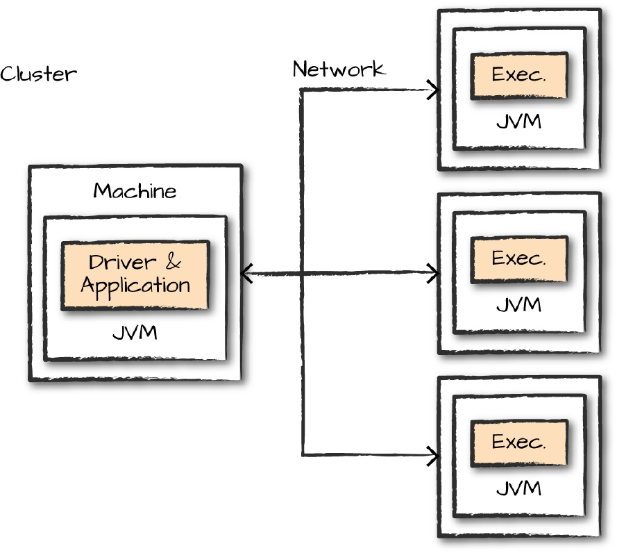
Figure 18-1. Components of a Spark application that you can monitor
What to Monitor
After that brief tour of the monitoring landscape, let’s discuss how we can go
about monitoring and debugging our Spark Applications. There are two main
things you will want to monitor: the processes running your application (at
the level of CPU usage, memory usage, etc.), and the query execution inside
it (e.g., jobs and tasks).
Driver and Executor Processes
When you’re monitoring a Spark application, you’re definitely going to want
to keep an eye on the driver. This is where all of the state of your application
lives, and you’ll need to be sure it’s running in a stable manner. If you could
monitor only one machine or a single JVM, it would definitely be the driver.
With that being said, understanding the state of the executors is also
extremely important for monitoring individual Spark jobs. To help with this
challenge, Spark has a configurable metrics system based on the Dropwizard
Metrics Library. The metrics system is configured via a configuration file that
Spark expects to be present at $SPARK_HOME/conf/metrics.properties. A
custom file location can be specified by changing the spark.metrics.conf
configuration property. These metrics can be output to a variety of different
sinks, including cluster monitoring solutions like Ganglia.
Queries, Jobs, Stages, and Tasks
Although the driver and executor processes are important to monitor,
sometimes you need to debug what’s going on at the level of a specific query.
Spark provides the ability to dive into queries, jobs, stages, and tasks. (We
learned about these in Chapter 15.) This information allows you to know
exactly what’s running on the cluster at a given time. When looking for
performance tuning or debugging, this is where you are most likely to start.
Now that we know what we want to monitor, let’s look at the two most
common ways of doing so: the Spark logs and the Spark UI.
Spark Logs
One of the most detailed ways to monitor Spark is through its log files.
Naturally, strange events in Spark’s logs, or in the logging that you added to
your Spark Application, can help you take note of exactly where jobs are
failing or what is causing that failure. If you use the application template
provided with the book, the logging framework we set up in the template will
allow your application logs to show up along Spark’s own logs, making them
very easy to correlate. One challenge, however, is that Python won’t be able
to integrate directly with Spark’s Java-based logging library. Using Python’s
logging module or even simple print statements will still print the results to
standard error, however, and make them easy to find.
To change Spark’s log level, simply run the following command:
spark.sparkContext.setLogLevel("INFO")
This will allow you to read the logs, and if you use our application template,
you can log your own relevant information along with these logs, allowing
you to inspect both your own application and Spark. The logs themselves will
be printed to standard error when running a local mode application, or saved
to files by your cluster manager when running Spark on a cluster. Refer to
each cluster manager’s documentation about how to find them—typically,
they are available through the cluster manager’s web UI.
You won’t always find the answer you need simply by searching logs, but it
can help you pinpoint the given problem that you’re encountering and
possibly add new log statements in your application to better understand it.
It’s also convenient to collect logs over time in order to reference them in the
future. For instance, if your application crashes, you’ll want to debug why,
without access to the now-crashed application. You may also want to ship
logs off the machine they were written on to hold onto them if a machine
crashes or gets shut down (e.g., if running in the cloud).
The Spark UI
The Spark UI provides a visual way to monitor applications while they are
running as well as metrics about your Spark workload, at the Spark and JVM
level. Every SparkContext running launches a web UI, by default on port
4040, that displays useful information about the application. When you run
Spark in local mode, for example, just navigate to http://localhost:4040 to see
the UI when running a Spark Application on your local machine. If you’re
running multiple applications, they will launch web UIs on increasing port
numbers (4041, 4042, …). Cluster managers will also link to each
application’s web UI from their own UI.
Figure 18-2 shows all of the tabs available in the Spark UI.
Figure 18-2. Spark UI tabs
These tabs are accessible for each of the things that we’d like to monitor. For
the most part, each of these should be self-explanatory:
The Jobs tab refers to Spark jobs.
The Stages tab pertains to individual stages (and their relevant
tasks).
The Storage tab includes information and the data that is currently
cached in our Spark Application.
The Environment tab contains relevant information about the
configurations and current settings of the Spark application.
The SQL tab refers to our Structured API queries (including SQL
and DataFrames).
The Executors tab provides detailed information about each executor
running our application.
Let’s walk through an example of how you can drill down into a given query.
Open a new Spark shell, run the following code, and we will trace its
execution through the Spark UI:
# in Python
spark.read\
.option("header", "true")\
.csv("/data/retail-data/all/online-retail-dataset.csv")\
.repartition(2)\
.selectExpr("instr(Description, 'GLASS') >= 1 as is_glass")\
.groupBy("is_glass")\
.count()\
.collect()
This results in three rows of various values. The code kicks off a SQL query,
so let’s navigate to the SQL tab, where you should see something similar to
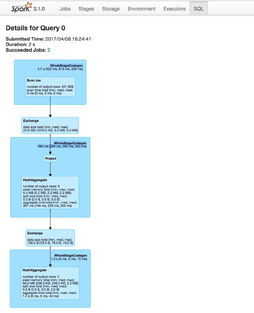
Submitted Time: 2017/04/08 16:24:41
Duration: 2 s
Succeeded Jobs: 2
These will become important in a minute, but first let’s take a look at the
Directed Acyclic Graph (DAG) of Spark stages. Each blue box in these tabs
represent a stage of Spark tasks. The entire group of these stages represent
our Spark job. Let’s take a look at each stage in detail so that we can better
understand what is going on at each level, starting with Figure 18-4.
Figure 18-4. Stage one
The box on top, labeled WholeStateCodegen, represents a full scan of the
CSV file. The box below that represents a shuffle that we forced when we
called repartition. This turned our original dataset (of a yet to be specified
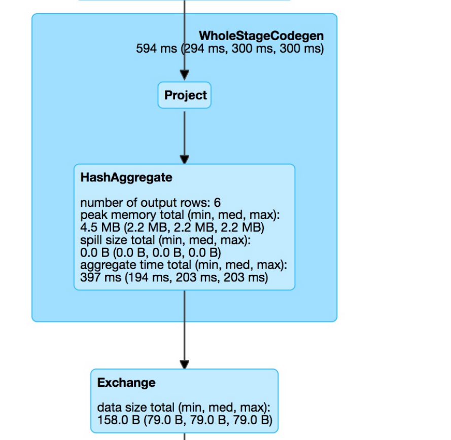
number of partitions) into two partitions.
The next step is our projection (selecting/adding/filtering columns) and the
aggregation. Notice that in Figure 18-5 the number of output rows is six. This
convienently lines up with the number of output rows multiplied by the
number of partitions at aggregation time. This is because Spark performs an
aggregation for each partition (in this case a hash-based aggregation) before
shuffling the data around in preparation for the final stage.
Figure 18-5. Stage two
The last stage is the aggregation of the subaggregations that we saw happen
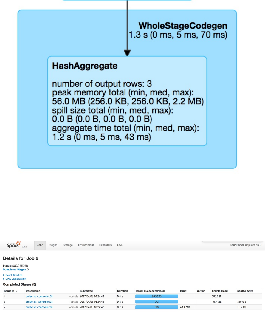
on a per-partition basis in the previous stage. We combine those two
partitions in the final three rows that are the output of our total query
(Figure 18-6).
Figure 18-6. Stage three
Let’s look further into the job’s execution. On the Jobs tab, next to Succeeded
Jobs, click 2. As Figure 18-7 demonstrates, our job breaks down into three
stages (which corresponds to what we saw on the SQL tab).
Figure 18-7. The Jobs tab
These stages have more or less the same information as what’s shown in
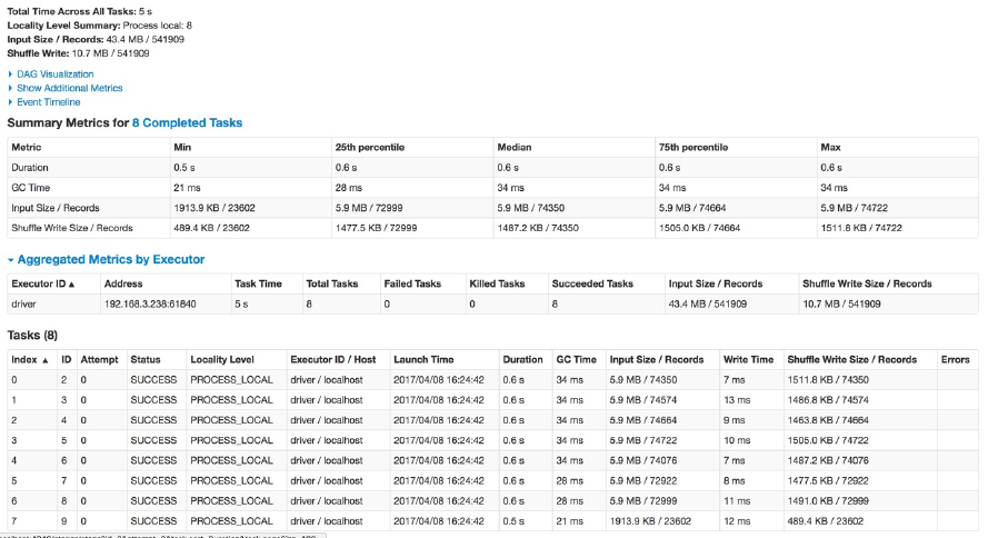
Figure 18-6, but clicking the label for one of them will show the details for a
given stage. In this example, three stages ran, with eight, two, and then two
hundred tasks each. Before diving into the stage detail, let’s review why this
is the case.
The first stage has eight tasks. CSV files are splittable, and Spark broke up
the work to be distributed relatively evenly between the different cores on the
machine. This happens at the cluster level and points to an important
optimization: how you store your files. The following stage has two tasks
because we explicitly called a repartition to move the data into two partitions.
The last stage has 200 tasks because the default shuffle partitions value is
200.
Now that we reviewed how we got here, click the stage with eight tasks to
see the next level of detail, as shown in Figure 18-8.
Figure 18-8. Spark tasks
Spark provides a lot of detail about what this job did when it ran. Toward the
top, notice the Summary Metrics section. This provides a synopsis of
statistics regarding various metrics. What you want to be on the lookout for is
uneven distributions of the values (we touch on this in Chapter 19). In this
case, everything looks very consistent; there are no wide swings in the
distribution of values. In the table at the bottom, we can also examine on a
per-executor basis (one for every core on this particular machine, in this
case). This can help identify whether a particular executor is struggling with
its workload.
Spark also makes available a set of more detailed metrics, as shown in
Figure 18-8, which are probably not relevant to the large majority of users.
To view those, click Show Additional Metrics, and then either choose
(De)select All or select individual metrics, depending on what you want to
see.
You can repeat this basic analysis for each stage that you want to analyze.
We leave that as an exercise for the reader.
Other Spark UI tabs
The remaining Spark tabs, Storage, Environment, and Executors, are fairly
self-explanatory. The Storage tab shows information about the cached
RDDs/DataFrames on the cluster. This can help you see if certain data has
been evicted from the cache over time. The Environment tab shows you
information about the Runtime Environment, including information about
Scala and Java as well as the various Spark Properties that you configured on
your cluster.
Configuring the Spark user interface
There are a number of configurations that you can set regarding the Spark UI.
Many of them are networking configurations such as enabling access control.
Others let you configure how the Spark UI will behave (e.g., how many jobs,
stages, and tasks are stored). Due to space limitations, we cannot include the
entire configuration set here. Consult the relevant table on Spark UI
Configurations in the Spark documentation.
Spark REST API
In addition to the Spark UI, you can also access Spark’s status and metrics
via a REST API. This is is available at http://localhost:4040/api/v1 and is a
way of building visualizations and monitoring tools on top of Spark itself.
For the most part this API exposes the same information presented in the web
UI, except that it doesn’t include any of the SQL-related information. This
can be a useful tool if you would like to build your own reporting solution
based on the information available in the Spark UI. Due to space limitations,
we cannot include the list of API endpoints here. Consult the relevant table
on REST API Endpoints in the Spark documentation.
Spark UI History Server
Normally, the Spark UI is only available while a SparkContext is running, so
how can you get to it after your application crashes or ends? To do this,
Spark includes a tool called the Spark History Server that allows you to
reconstruct the Spark UI and REST API, provided that the application was
configured to save an event log. You can find up-to-date information about
how to use this tool in the Spark documentation.
To use the history server, you first need to configure your application to store
event logs to a certain location. You can do this by by enabling
spark.eventLog.enabled and the event log location with the configuration
spark.eventLog.dir. Then, once you have stored the events, you can run
the history server as a standalone application, and it will automatically
reconstruct the web UI based on these logs. Some cluster managers and cloud
services also configure logging automatically and run a history server by
default.
There are a number of other configurations for the history server. Due to
space limitations, we cannot include the entire configuration set here. Refer
to the relevant table on Spark History Server Configurations in the Spark
documentation.
Debugging and Spark First Aid
The previous sections defined some core “vital signs”—that is, things that we
can monitor to check the health of a Spark Application. For the remainder of

the chapter we’re going to take a “first aid” approach to Spark debugging:
We’ll review some signs and symptoms of problems in your Spark jobs,
including signs that you might observe (e.g., slow tasks) as well as symptoms
from Spark itself (e.g., OutOfMemoryError). There are many issues that may
affect Spark jobs, so it’s impossible to cover everything. But we will discuss
some of the more common Spark issues you may encounter. In addition to
the signs and symptoms, we’ll also look at some potential treatments for
these issues.
Most of the recommendations about fixing issues refer to the configuration
tools discussed in Chapter 16.
Spark Jobs Not Starting
This issue can arise frequently, especially when you’re just getting started
with a fresh deployment or environment.
Signs and symptoms
Spark jobs don’t start.
The Spark UI doesn’t show any nodes on the cluster except the
driver.
The Spark UI seems to be reporting incorrect information.
Potential treatments
This mostly occurs when your cluster or your application’s resource demands
are not configured properly. Spark, in a distributed setting, does make some
assumptions about networks, file systems, and other resources. During the
process of setting up the cluster, you likely configured something incorrectly,
and now the node that runs the driver cannot talk to the executors. This might
be because you didn’t specify what IP and port is open or didn’t open the
correct one. This is most likely a cluster level, machine, or configuration
issue. Another option is that your application requested more resources per
executor than your cluster manager currently has free, in which case the

driver will be waiting forever for executors to be launched.
Ensure that machines can communicate with one another on the
ports that you expect. Ideally, you should open up all ports between
the worker nodes unless you have more stringent security
constraints.
Ensure that your Spark resource configurations are correct and that
your cluster manager is properly set up for Spark. Try running a
simple application first to see if that works. One common issue may
be that you requested more memory per executor than the cluster
manager has free to allocate, so check how much it is reporting free
(in its UI) and your spark-submit memory configuration.
Errors Before Execution
This can happen when you’re developing a new application and have
previously run code on this cluster, but now some new code won’t work.
Signs and symptoms
Commands don’t run at all and output large error messages.
You check the Spark UI and no jobs, stages, or tasks seem to run.
Potential treatments
After checking and confirming that the Spark UI environment tab shows the
correct information for your application, it’s worth double-checking your
code. Many times, there might be a simple typo or incorrect column name
that is preventing the Spark job from compiling into its underlying Spark plan
(when using the DataFrame API).
You should take a look at the error returned by Spark to confirm that
there isn’t an issue in your code, such as providing the wrong input
file path or field name.
Double-check to verify that the cluster has the network connectivity

that you expect between your driver, your workers, and the storage
system you are using.
There might be issues with libraries or classpaths that are causing the
wrong version of a library to be loaded for accessing storage. Try
simplifying your application until you get a smaller version that
reproduces the issue (e.g., just reading one dataset).
Errors During Execution
This kind of issue occurs when you already are working on a cluster or parts
of your Spark Application run before you encounter an error. This can be a
part of a scheduled job that runs at some interval or a part of some interactive
exploration that seems to fail after some time.
Signs and symptoms
One Spark job runs successfully on the entire cluster but the next
one fails.
A step in a multistep query fails.
A scheduled job that ran yesterday is failing today.
Difficult to parse error message.
Potential treatments
Check to see if your data exists or is in the format that you expect.
This can change over time or some upstream change may have had
unintended consequences on your application.
If an error quickly pops up when you run a query (i.e., before tasks
are launched), it is most likely an analysis error while planning the
query. This means that you likely misspelled a column name
referenced in the query or that a column, view, or table you
referenced does not exist.
Read through the stack trace to try to find clues about what

components are involved (e.g., what operator and stage it was
running in).
Try to isolate the issue by progressively double-checking input data
and ensuring the data conforms to your expectations. Also try
removing logic until you can isolate the problem in a smaller version
of your application.
If a job runs tasks for some time and then fails, it could be due to a
problem with the input data itself, wherein the schema might be
specified incorrectly or a particular row does not conform to the
expected schema. For instance, sometimes your schema might
specify that the data contains no nulls but your data does actually
contain nulls, which can cause certain transformations to fail.
It’s also possible that your own code for processing the data is
crashing, in which case Spark will show you the exception thrown
by your code. In this case, you will see a task marked as “failed” on
the Spark UI, and you can also view the logs on that machine to
understand what it was doing when it failed. Try adding more logs
inside your code to figure out which data record was being
processed.
Slow Tasks or Stragglers
This issue is quite common when optimizing applications, and can occur
either due to work not being evenly distributed across your machines
(“skew”), or due to one of your machines being slower than the others (e.g.,
due to a hardware problem).
Signs and symptoms
Any of the following are appropriate symptoms of the issue:
Spark stages seem to execute until there are only a handful of tasks
left. Those tasks then take a long time.
These slow tasks show up in the Spark UI and occur consistently on

the same dataset(s).
These occur in stages, one after the other.
Scaling up the number of machines given to the Spark Application
doesn’t really help—some tasks still take much longer than others.
In the Spark metrics, certain executors are reading and writing much
more data than others.
Potential treatments
Slow tasks are often called “stragglers.” There are many reasons they may
occur, but most often the source of this issue is that your data is partitioned
unevenly into DataFrame or RDD partitions. When this happens, some
executors might need to work on much larger amounts of work than others.
One particularly common case is that you use a group-by-key operation and
one of the keys just has more data than others. In this case, when you look at
the Spark UI, you might see that the shuffle data for some nodes is much
larger than for others.
Try increasing the number of partitions to have less data per
partition.
Try repartitioning by another combination of columns. For example,
stragglers can come up when you partition by a skewed ID column,
or a column where many values are null. In the latter case, it might
make sense to first filter out the null values.
Try increasing the memory allocated to your executors if possible.
Monitor the executor that is having trouble and see if it is the same
machine across jobs; you might also have an unhealthy executor or
machine in your cluster—for example, one whose disk is nearly full.
If this issue is associated with a join or an aggregation, see “Slow
Joins” or “Slow Aggregations”.
Check whether your user-defined functions (UDFs) are wasteful in

their object allocation or business logic. Try to convert them to
DataFrame code if possible.
Ensure that your UDFs or User-Defined Aggregate Functions
(UDAFs) are running on a small enough batch of data. Oftentimes
an aggregation can pull a lot of data into memory for a common key,
leading to that executor having to do a lot more work than others.
Turning on speculation, which we discuss in “Slow Reads and
Writes”, will have Spark run a second copy of tasks that are
extremely slow. This can be helpful if the issue is due to a faulty
node because the task will get to run on a faster one. Speculation
does come at a cost, however, because it consumes additional
resources. In addition, for some storage systems that use eventual
consistency, you could end up with duplicate output data if your
writes are not idempotent. (We discussed speculation configurations
in Chapter 17.)
Another common issue can arise when you’re working with
Datasets. Because Datasets perform a lot of object instantiation to
convert records to Java objects for UDFs, they can cause a lot of
garbage collection. If you’re using Datasets, look at the garbage
collection metrics in the Spark UI to see if they’re consistent with
the slow tasks.
Stragglers can be one of the most difficult issues to debug, simply because
there are so many possible causes. However, in all likelihood, the cause will
be some kind of data skew, so definitely begin by checking the Spark UI for
imbalanced amounts of data across tasks.
Slow Aggregations
If you have a slow aggregation, start by reviewing the issues in the “Slow
Tasks” section before proceeding. Having tried those, you might continue to
see the same problem.

Signs and symptoms
Slow tasks during a groupBy call.
Jobs after the aggregation are slow, as well.
Potential treatments
Unfortunately, this issue can’t always be solved. Sometimes, the data in your
job just has some skewed keys, and the operation you want to run on them
needs to be slow.
Increasing the number of partitions, prior to an aggregation, might
help by reducing the number of different keys processed in each
task.
Increasing executor memory can help alleviate this issue, as well. If
a single key has lots of data, this will allow its executor to spill to
disk less often and finish faster, although it may still be much slower
than executors processing other keys.
If you find that tasks after the aggregation are also slow, this means
that your dataset might have remained unbalanced after the
aggregation. Try inserting a repartition call to partition it
randomly.
Ensuring that all filters and SELECT statements that can be are above
the aggregation can help to ensure that you’re working only on the
data that you need to be working on and nothing else. Spark’s query
optimizer will automatically do this for the structured APIs.
Ensure null values are represented correctly (using Spark’s concept
of null) and not as some default value like " " or "EMPTY". Spark
often optimizes for skipping nulls early in the job when possible, but
it can’t do so for your own placeholder values.
Some aggregation functions are also just inherently slower than
others. For instance, collect_list and collect_set are very slow

aggregation functions because they must return all the matching
objects to the driver, and should be avoided in performance-critical
code.
Slow Joins
Joins and aggregations are both shuffles, so they share some of the same
general symptoms as well as treatments.
Signs and symptoms
A join stage seems to be taking a long time. This can be one task or
many tasks.
Stages before and after the join seem to be operating normally.
Potential treatments
Many joins can be optimized (manually or automatically) to other
types of joins. We covered how to select different join types in
Chapter 8.
Experimenting with different join orderings can really help speed up
jobs, especially if some of those joins filter out a large amount of
data; do those first.
Partitioning a dataset prior to joining can be very helpful for
reducing data movement across the cluster, especially if the same
dataset will be used in multiple join operations. It’s worth
experimenting with different prejoin partitioning. Keep in mind,
again, that this isn’t “free” and does come at the cost of a shuffle.
Slow joins can also be caused by data skew. There’s not always a lot
you can do here, but sizing up the Spark application and/or
increasing the size of executors can help, as described in earlier
sections.
Ensuring that all filters and select statements that can be are above

the join can help to ensure that you’re working only on the data that
you need for the join.
Ensure that null values are handled correctly (that you’re using
null) and not some default value like " " or "EMPTY", as with
aggregations.
Sometimes Spark can’t properly plan for a broadcast join if it
doesn’t know any statistics about the input DataFrame or table. If
you know that one of the tables that you are joining is small, you can
try to force a broadcast (as discussed in Chapter 8), or use Spark’s
statistics collection commands to let it analyze the table.
Slow Reads and Writes
Slow I/O can be difficult to diagnose, especially with networked file systems.
Signs and symptoms
Slow reading of data from a distributed file system or external
system.
Slow writes from network file systems or blob storage.
Potential treatments
Turning on speculation (set spark.speculation to true) can help
with slow reads and writes. This will launch additional tasks with the
same operation in an attempt to see whether it’s just some transient
issue in the first task. Speculation is a powerful tool and works well
with consistent file systems. However, it can cause duplicate data
writes with some eventually consistent cloud services, such as
Amazon S3, so check whether it is supported by the storage system
connector you are using.
Ensuring sufficient network connectivity can be important—your
Spark cluster may simply not have enough total network bandwidth

to get to your storage system.
For distributed file systems such as HDFS running on the same
nodes as Spark, make sure Spark sees the same hostnames for nodes
as the file system. This will enable Spark to do locality-aware
scheduling, which you will be able to see in the “locality” column in
the Spark UI. We’ll talk about locality a bit more in the next chapter.
Driver OutOfMemoryError or Driver Unresponsive
This is usually a pretty serious issue because it will crash your Spark
Application. It often happens due to collecting too much data back to the
driver, making it run out of memory.
Signs and symptoms
Spark Application is unresponsive or crashed.
OutOfMemoryErrors or garbage collection messages in the driver
logs.
Commands take a very long time to run or don’t run at all.
Interactivity is very low or non-existent.
Memory usage is high for the driver JVM.
Potential treatments
There are a variety of potential reasons for this happening, and diagnosis is
not always straightforward.
Your code might have tried to collect an overly large dataset to the
driver node using operations such as collect.
You might be using a broadcast join where the data to be broadcast
is too big. Use Spark’s maximum broadcast join configuration to
better control the size it will broadcast.

A long-running application generated a large number of objects on
the driver and is unable to release them. Java’s jmap tool can be
useful to see what objects are filling most of the memory of your
driver JVM by printing a histogram of the heap. However, take note
that jmap will pause that JVM while running.
Increase the driver’s memory allocation if possible to let it work
with more data.
Issues with JVMs running out of memory can happen if you are
using another language binding, such as Python, due to data
conversion between the two requiring too much memory in the JVM.
Try to see whether your issue is specific to your chosen language
and bring back less data to the driver node, or write it to a file
instead of bringing it back as in-memory objects.
If you are sharing a SparkContext with other users (e.g., through the
SQL JDBC server and some notebook environments), ensure that
people aren’t trying to do something that might be causing large
amounts of memory allocation in the driver (like working overly
large arrays in their code or collecting large datasets).
Executor OutOfMemoryError or Executor Unresponsive
Spark applications can sometimes recover from this automatically, depending
on the true underlying issue.
Signs and symptoms
OutOfMemoryErrors or garbage collection messages in the executor
logs. You can find these in the Spark UI.
Executors that crash or become unresponsive.
Slow tasks on certain nodes that never seem to recover.
Potential treatments

Try increasing the memory available to executors and the number of
executors.
Try increasing PySpark worker size via the relevant Python
configurations.
Look for garbage collection error messages in the executor logs.
Some of the tasks that are running, especially if you’re using UDFs,
can be creating lots of objects that need to be garbage collected.
Repartition your data to increase parallelism, reduce the amount of
records per task, and ensure that all executors are getting the same
amount of work.
Ensure that null values are handled correctly (that you’re using
null) and not some default value like " " or "EMPTY", as we
discussed earlier.
This is more likely to happen with RDDs or with Datasets because
of object instantiations. Try using fewer UDFs and more of Spark’s
structured operations when possible.
Use Java monitoring tools such as jmap to get a histogram of heap
memory usage on your executors, and see which classes are taking
up the most space.
If executors are being placed on nodes that also have other
workloads running on them, such as a key-value store, try to isolate
your Spark jobs from other jobs.
Unexpected Nulls in Results
Signs and symptoms
Unexpected null values after transformations.
Scheduled production jobs that used to work no longer work, or no
longer produce the right results.

Potential treatments
It’s possible that your data format has changed without adjusting
your business logic. This means that code that worked before is no
longer valid.
Use an accumulator to try to count records or certain types, as well
as parsing or processing errors where you skip a record. This can be
helpful because you might think that you’re parsing data of a certain
format, but some of the data doesn’t. Most often, users will place the
accumulator in a UDF when they are parsing their raw data into a
more controlled format and perform the counts there. This allows
you to count valid and invalid records and then operate accordingly
after the fact.
Ensure that your transformations actually result in valid query plans.
Spark SQL sometimes does implicit type coercions that can cause
confusing results. For instance, the SQL expression SELECT 5*"23"
results in 115 because the string “25” converts to an the value 25 as
an integer, but the expression SELECT 5 * " " results in null
because casting the empty string to an integer gives null. Make sure
that your intermediate datasets have the schema you expect them to
(try using printSchema on them), and look for any CAST operations
in the final query plan.
No Space Left on Disk Errors
Signs and symptoms
You see “no space left on disk” errors and your jobs fail.
Potential treatments
The easiest way to alleviate this, of course, is to add more disk
space. You can do this by sizing up the nodes that you’re working on
or attaching external storage in a cloud environment.

If you have a cluster with limited storage space, some nodes may run
out first due to skew. Repartitioning the data as described earlier
may help here.
There are also a number of storage configurations with which you
can experiment. Some of these determine how long logs should be
kept on the machine before being removed. For more information,
see the Spark executor logs rolling configurations in Chapter 16.
Try manually removing some old log files or old shuffle files from
the machine(s) in question. This can help alleviate some of the issue
although obviously it’s not a permanent fix.
Serialization Errors
Signs and symptoms
You see serialization errors and your jobs fail.
Potential treatments
This is very uncommon when working with the Structured APIs, but
you might be trying to perform some custom logic on executors with
UDFs or RDDs and either the task that you’re trying to serialize to
these executors or the data you are trying to share cannot be
serialized. This often happens when you’re working with either
some code or data that cannot be serialized into a UDF or function,
or if you’re working with strange data types that cannot be
serialized. If you are using (or intend to be using Kryo serialization),
verify that you’re actually registering your classes so that they are
indeed serialized.
Try not to refer to any fields of the enclosing object in your UDFs
when creating UDFs inside a Java or Scala class. This can cause
Spark to try to serialize the whole enclosing object, which may not
be possible. Instead, copy the relevant fields to local variables in the
same scope as closure and use those.
Conclusion
This chapter covered some of the main tools that you can use to monitor and
debug your Spark jobs and applications, as well as the most common issues
we see and their resolutions. As with debugging any complex software, we
recommend taking a principled, step-by-step approach to debug issues. Add
logging statements to figure out where your job is crashing and what type of
data arrives at each stage, try to isolate the problem to the smallest piece of
code possible, and work up from there. For data skew issues, which are
unique to parallel computing, use Spark’s UI to get a quick overview of how
much work each task is doing. In Chapter 19, we discuss performance tuning
in particular and various tools you can use for that.

Chapter 19. Performance Tuning
Chapter 18 covered the Spark user interface (UI) and basic first-aid for your
Spark Application. Using the tools outlined in that chapter, you should be
able to ensure that your jobs run reliably. However, sometimes you’ll also
need them to run faster or more efficiently for a variety of reasons. That’s
what this chapter is about. Here, we present a discussion of some of the
performance choices that are available to make your jobs run faster.
Just as with monitoring, there are a number of different levels that you can try
to tune at. For instance, if you had an extremely fast network, that would
make many of your Spark jobs faster because shuffles are so often one of the
costlier steps in a Spark job. Most likely, you won’t have much ability to
control such things; therefore, we’re going to discuss the things you can
control through code choices or configuration.
There are a variety of different parts of Spark jobs that you might want to
optimize, and it’s valuable to be specific. Following are some of the areas:
Code-level design choices (e.g., RDDs versus DataFrames)
Data at rest
Joins
Aggregations
Data in flight
Individual application properties
Inside of the Java Virtual Machine (JVM) of an executor
Worker nodes
Cluster and deployment properties
This list is by no means exhaustive, but it does at least ground the
conversation and the topics that we cover in this chapter. Additionally, there
are two ways of trying to achieve the execution characteristics that we would
like out of Spark jobs. We can either do so indirectly by setting configuration
values or changing the runtime environment. These should improve things
across Spark Applications or across Spark jobs. Alternatively, we can try to
directly change execution characteristic or design choices at the individual
Spark job, stage, or task level. These kinds of fixes are very specific to that
one area of our application and therefore have limited overall impact. There
are numerous things that lie on both sides of the indirect versus direct divide,
and we will draw lines in the sand accordingly.
One of the best things you can do to figure out how to improve performance
is to implement good monitoring and job history tracking. Without this
information, it can be difficult to know whether you’re really improving job
performance.
Indirect Performance Enhancements
As discussed, there are a number of indirect enhancements that you can
perform to help your Spark jobs run faster. We’ll skip the obvious ones like
“improve your hardware” and focus more on the things within your control.
Design Choices
Although good design choices seem like a somewhat obvious way to
optimize performance, we often don’t prioritize this step in the process.
When designing your applications, making good design choices is very
important because it not only helps you to write better Spark applications but
also to get them to run in a more stable and consistent manner over time and
in the face of external changes or variations. We’ve already discussed some
of these topics earlier in the book, but we’ll summarize some of the
fundamental ones again here.
Scala versus Java versus Python versus R
This question is nearly impossible to answer in the general sense because a
lot will depend on your use case. For instance, if you want to perform some
single-node machine learning after performing a large ETL job, we might
recommend running your Extract, Transform, and Load (ETL) code as
SparkR code and then using R’s massive machine learning ecosystem to run
your single-node machine learning algorithms. This gives you the best of
both worlds and takes advantage of the strength of R as well as the strength
of Spark without sacrifices. As we mentioned numerous times, Spark’s
Structured APIs are consistent across languages in terms of speed and
stability. That means that you should code with whatever language you are
most comfortable using or is best suited for your use case.
Things do get a bit more complicated when you need to include custom
transformations that cannot be created in the Structured APIs. These might
manifest themselves as RDD transformations or user-defined functions
(UDFs). If you’re going to do this, R and Python are not necessarily the best
choice simply because of how this is actually executed. It’s also more
difficult to provide stricter guarantees of types and manipulations when
you’re defining functions that jump across languages. We find that using
Python for the majority of the application, and porting some of it to Scala or
writing specific UDFs in Scala as your application evolves, is a powerful
technique—it allows for a nice balance between overall usability,
maintainability, and performance.
DataFrames versus SQL versus Datasets versus RDDs
This question also comes up frequently. The answer is simple. Across all
languages, DataFrames, Datasets, and SQL are equivalent in speed. This
means that if you’re using DataFrames in any of these languages,
performance is equal. However, if you’re going to be defining UDFs, you’ll
take a performance hit writing those in Python or R, and to some extent a
lesser performance hit in Java and Scala. If you want to optimize for pure
performance, it would behoove you to try and get back to DataFrames and
SQL as quickly as possible. Although all DataFrame, SQL, and Dataset code
compiles down to RDDs, Spark’s optimization engine will write “better”
RDD code than you can manually and certainly do it with orders of
magnitude less effort. Additionally, you will lose out on new optimizations
that are added to Spark’s SQL engine every release.
Lastly, if you want to use RDDs, we definitely recommend using Scala or
Java. If that’s not possible, we recommend that you restrict the “surface area”
of RDDs in your application to the bare minimum. That’s because when
Python runs RDD code, it’s serializes a lot of data to and from the Python
process. This is very expensive to run over very big data and can also
decrease stability.
Although it isn’t exactly relevant to performance tuning, it’s important to
note that there are also some gaps in what functionality is supported in each
of Spark’s languages. We discussed this in Chapter 16.
Object Serialization in RDDs
In Part III, we briefly discussed the serialization libraries that can be used
within RDD transformations. When you’re working with custom data types,
you’re going to want to serialize them using Kryo because it’s both more
compact and much more efficient than Java serialization. However, this does
come at the inconvenience of registering the classes that you will be using in
your application.
You can use Kryo serialization by setting spark.serializer to
org.apache.spark.serializer.KryoSerializer. You will also need to
explicitly register the classes that you would like to register with the Kryo
serializer via the spark.kryo.classesToRegister configuration. There are
also a number of advanced parameters for controlling this in greater detail
that are described in the Kryo documentation.
To register your classes, use the SparkConf that you just created and pass in
the names of your classes:
conf.registerKryoClasses(Array(classOf[MyClass1], classOf[MyClass2]))
Cluster Configurations
This area has huge potential benefits but is probably one of the more difficult
to prescribe because of the variation across hardware and use cases. In
general, monitoring how the machines themselves are performing will be the
most valuable approach toward optimizing your cluster configurations,
especially when it comes to running multiple applications (whether they are
Spark or not) on a single cluster.
Cluster/application sizing and sharing
This somewhat comes down to a resource sharing and scheduling problem;
however, there are a lot of options for how you want to share resources at the
cluster level or at the application level. Take a look at the configurations
listed at the end of Chapter 16 as well as some configurations in Chapter 17.
Dynamic allocation
Spark provides a mechanism to dynamically adjust the resources your
application occupies based on the workload. This means that your application
can give resources back to the cluster if they are no longer used, and request
them again later when there is demand. This feature is particularly useful if
multiple applications share resources in your Spark cluster. This feature is
disabled by default and available on all coarse-grained cluster managers; that
is, standalone mode, YARN mode, and Mesos coarse-grained mode. If you’d
like to enable this feature, you should set
spark.dynamicAllocation.enabled to true. The Spark documentation
presents a number of individual parameters that you can tune.
Scheduling
Over the course of the previous chapters, we discussed a number of different
potential optimizations that you can take advantage of to either help Spark
jobs run in parallel with scheduler pools or help Spark applications run in
parallel with something like dynamic allocation or setting max-executor-
cores. Scheduling optimizations do involve some research and
experimentation, and unfortunately there are not super-quick fixes beyond
setting spark.scheduler.mode to FAIR to allow better sharing of resources
across multiple users, or setting --max-executor-cores, which specifies the
maximum number of executor cores that your application will need.
Specifying this value can ensure that your application does not take up all the
resources on the cluster. You can also change the default, depending on your
cluster manager, by setting the configuration spark.cores.max to a default
of your choice. Cluster managers also provide some scheduling primitives
that can be helpful when optimizing multiple Spark Applications, as
discussed in Chapters 16 and 17.
Data at Rest
More often that not, when you’re saving data it will be read many times as
other folks in your organization access the same datasets in order to run
different analyses. Making sure that you’re storing your data for effective
reads later on is absolutely essential to successful big data projects. This
involves choosing your storage system, choosing your data format, and
taking advantage of features such as data partitioning in some storage
formats.
File-based long-term data storage
There are a number of different file formats available, from simple comma-
separated values (CSV) files and binary blobs, to more sophisticated formats
like Apache Parquet. One of the easiest ways to optimize your Spark jobs is
to follow best practices when storing data and choose the most efficient
storage format possible.
Generally you should always favor structured, binary types to store your data,
especially when you’ll be accessing it frequently. Although files like “CSV”
seem well-structured, they’re very slow to parse, and often also full of edge
cases and pain points. For instance, improperly escaped new-line characters
can often cause a lot of trouble when reading a large number of files. The
most efficient file format you can generally choose is Apache Parquet.
Parquet stores data in binary files with column-oriented storage, and also
tracks some statistics about each file that make it possible to quickly skip data
not needed for a query. It is well integrated with Spark through the built-in
Parquet data source.
Splittable file types and compression
Whatever file format you choose, you should make sure it is “splittable”,
which means that different tasks can read different parts of the file in parallel.
We saw why this is important in Chapter 18. When we read in the file, all
cores were able to do part of the work. That’s because the file was splittable.
If we didn’t use a splittable file type—say something like a malformed JSON
file—we’re going to need to read in the entire file on a single machine,
greatly reducing parallelism.
The main place splittability comes in is compression formats. A ZIP file or
TAR archive cannot be split, which means that even if we have 10 files in a
ZIP file and 10 cores, only one core can read in that data because we cannot
parallelize access to the ZIP file. This is a poor use of resources. In contrast,
files compressed using gzip, bzip2, or lz4 are generally splittable if they were
written by a parallel processing framework like Hadoop or Spark. For your
own input data, the simplest way to make it splittable is to upload it as
separate files, ideally each no larger than a few hundred megabytes.
Table partitioning
We discussed table partitioning in Chapter 9, and will only use this section as
a reminder. Table partitioning refers to storing files in separate directories
based on a key, such as the date field in the data. Storage managers like
Apache Hive support this concept, as do many of Spark’s built-in data
sources. Partitioning your data correctly allows Spark to skip many irrelevant
files when it only requires data with a specific range of keys. For instance, if
users frequently filter by “date” or “customerId” in their queries, partition
your data by those columns. This will greatly reduce the amount of data that
end users must read by most queries, and therefore dramatically increase
speed.
The one downside of partitioning, however, is that if you partition at too fine
a granularity, it can result in many small files, and a great deal of overhead
trying to list all the files in the storage system.
Bucketing
We also discussed bucketing in Chapter 9, but to recap, the essense is that
bucketing your data allows Spark to “pre-partition” data according to how
joins or aggregations are likely to be performed by readers. This can improve
performance and stability because data can be consistently distributed across
partitions as opposed to skewed into just one or two. For instance, if joins are
frequently performed on a column immediately after a read, you can use
bucketing to ensure that the data is well partitioned according to those values.
This can help prevent a shuffle before a join and therefore help speed up data
access. Bucketing generally works hand-in-hand with partitioning as a second
way of physically splitting up data.
The number of files
In addition to organizing your data into buckets and partitions, you’ll also
want to consider the number of files and the size of files that you’re storing.
If there are lots of small files, you’re going to pay a price listing and fetching
each of those individual files. For instance, if you’re reading a data from
Hadoop Distributed File System (HDFS), this data is managed in blocks that
are up to 128 MB in size (by default). This means if you have 30 files, of 5
MB each, you’re going to have to potentially request 30 blocks, even though
the same data could have fit into 2 blocks (150 MB total).
Although there is not necessarily a panacea for how you want to store your
data, the trade-off can be summarized as such. Having lots of small files is
going to make the scheduler work much harder to locate the data and launch
all of the read tasks. This can increase the network and scheduling overhead
of the job. Having fewer large files eases the pain off the scheduler but it will
also make tasks run longer. In this case, though, you can always launch more
tasks than there are input files if you want more parallelism—Spark will split
each file across multiple tasks assuming you are using a splittable format. In
general, we recommend sizing your files so that they each contain at least a
few tens of megatbytes of data.
One way of controlling data partitioning when you write your data is through
a write option introduced in Spark 2.2. To control how many records go into
each file, you can specify the maxRecordsPerFile option to the write
operation.
Data locality
Another aspect that can be important in shared cluster environments is data
locality. Data locality basically specifies a preference for certain nodes that
hold certain data, rather than having to exchange these blocks of data over the
network. If you run your storage system on the same nodes as Spark, and the
system supports locality hints, Spark will try to schedule tasks close to each
input block of data. For example HDFS storage provides this option. There
are several configurations that affect locality, but it will generally be used by
default if Spark detects that it is using a local storage system. You will also
see data-reading tasks marked as “local” in the Spark web UI.
Statistics collection
Spark includes a cost-based query optimizer that plans queries based on the
properties of the input data when using the structured APIs. However, to
allow the cost-based optimizer to make these sorts of decisions, you need to
collect (and maintain) statistics about your tables that it can use. There are
two kinds of statistics: table-level and column-level statistics. Statistics
collection is available only on named tables, not on arbitrary DataFrames or
RDDs.
To collect table-level statistics, you can run the following command:
ANALYZE TABLE table_name COMPUTE STATISTICS
To collect column-level statistics, you can name the specific columns:
ANALYZE TABLE table_name COMPUTE STATISTICS FOR
COLUMNS column_name1, column_name2, ...
Column-level statistics are slower to collect, but provide more information
for the cost-based optimizer to use about those data columns. Both types of
statistics can help with joins, aggregations, filters, and a number of other
potential things (e.g., automatically choosing when to do a broadcast join).

This is a fast-growing part of Spark, so different optimizations based on
statistics will likely be added in the future.
NOTE
You can follow the progress of cost-based optimization on its JIRA issue. You can also
read through the design document on SPARK-16026 to learn more about this feature. This
is an active area of development in Spark at the time of writing.
Shuffle Configurations
Configuring Spark’s external shuffle service (discussed in Chapters 16 and
17) can often increase performance because it allows nodes to read shuffle
data from remote machines even when the executors on those machines are
busy (e.g., with garbage collection). This does come at the cost of complexity
and maintenance, however, so it might not be worth it in your deployment.
Beyond configuring this external service, there are also a number of
configurations for shuffles, such as the number of concurrent connections per
executor, although these usually have good defaults.
In addition, for RDD-based jobs, the serialization format has a large impact
on shuffle performance—always prefer Kryo over Java serialization, as
described in “Object Serialization in RDDs”. Furthermore, for all jobs, the
number of partitions of a shuffle matters. If you have too few partitions, then
too few nodes will be doing work and there may be skew, but if you have too
many partitions, there is an overhead to launching each one that may start to
dominate. Try to aim for at least a few tens of megabytes of data per output
partition in your shuffle.
Memory Pressure and Garbage Collection
During the course of running Spark jobs, the executor or driver machines
may struggle to complete their tasks because of a lack of sufficient memory
or “memory pressure.” This may occur when an application takes up too
much memory during execution or when garbage collection runs too

frequently or is slow to run as large numbers of objects are created in the
JVM and subsequently garbage collected as they are no longer used. One
strategy for easing this issue is to ensure that you’re using the Structured
APIs as much as possible. These will not only increase the efficiency with
which your Spark jobs will execute, but it will also greatly reduce memory
pressure because JVM objects are never realized and Spark SQL simply
performs the computation on its internal format.
The Spark documentation includes some great pointers on tuning garbage
collection for RDD and UDF based applications, and we paraphrase the
following sections from that information.
Measuring the impact of garbage collection
The first step in garbage collection tuning is to gather statistics on how
frequently garbage collection occurs and the amount of time it takes. You can
do this by adding -verbose:gc -XX:+PrintGCDetails -
XX:+PrintGCTimeStamps to Spark’s JVM options using the
spark.executor.extraJavaOptions configuration parameter. The next
time you run your Spark job, you will see messages printed in the worker’s
logs each time a garbage collection occurs. These logs will be on your
cluster’s worker nodes (in the stdout files in their work directories), not in the
driver.
Garbage collection tuning
To further tune garbage collection, you first need to understand some basic
information about memory management in the JVM:
Java heap space is divided into two regions: Young and Old. The
Young generation is meant to hold short-lived objects whereas the
Old generation is intended for objects with longer lifetimes.
The Young generation is further divided into three regions: Eden,
Survivor1, and Survivor2.
Here’s a simplified description of the garbage collection procedure:
1. When Eden is full, a minor garbage collection is run on Eden and
objects that are alive from Eden and Survivor1 are copied to
Survivor2.
2. The Survivor regions are swapped.
3. If an object is old enough or if Survivor2 is full, that object is moved
to Old.
4. Finally, when Old is close to full, a full garbage collection is
invoked. This involves tracing through all the objects on the heap,
deleting the unreferenced ones, and moving the others to fill up
unused space, so it is generally the slowest garbage collection
operation.
The goal of garbage collection tuning in Spark is to ensure that only long-
lived cached datasets are stored in the Old generation and that the Young
generation is sufficiently sized to store all short-lived objects. This will help
avoid full garbage collections to collect temporary objects created during task
execution. Here are some steps that might be useful.
Gather garbage collection statistics to determine whether it is being run too
often. If a full garbage collection is invoked multiple times before a task
completes, it means that there isn’t enough memory available for executing
tasks, so you should decrease the amount of memory Spark uses for caching
(spark.memory.fraction).
If there are too many minor collections but not many major garbage
collections, allocating more memory for Eden would help. You can set the
size of the Eden to be an over-estimate of how much memory each task will
need. If the size of Eden is determined to be E, you can set the size of the
Young generation using the option -Xmn=4/3*E. (The scaling up by 4/3 is to
account for space used by survivor regions, as well.)
As an example, if your task is reading data from HDFS, the amount of
memory used by the task can be estimated by using the size of the data block
read from HDFS. Note that the size of a decompressed block is often two or
three times the size of the block. So if you want to have three or four tasks’
worth of working space, and the HDFS block size is 128 MB, we can
estimate size of Eden to be 43,128 MB.
Try the G1GC garbage collector with -XX:+UseG1GC. It can improve
performance in some situations in which garbage collection is a bottleneck
and you don’t have a way to reduce it further by sizing the generations. Note
that with large executor heap sizes, it can be important to increase the G1
region size with -XX:G1HeapRegionSize.
Monitor how the frequency and time taken by garbage collection changes
with the new settings.
Our experience suggests that the effect of garbage collection tuning depends
on your application and the amount of memory available. There are many
more tuning options described online, but at a high level, managing how
frequently full garbage collection takes place can help in reducing the
overhead. You can specify garbage collection tuning flags for executors by
setting spark.executor.extraJavaOptions in a job’s configuration.
Direct Performance Enhancements
In the previous section, we touched on some general performance
enhancements that apply to all jobs. Be sure to skim the previous couple of
pages before jumping to this section and the solutions here. These solutions
here are intended as “band-aids” of sorts for issues with specific stages or
jobs, but they require inspecting and optimizing each stage or job separately.
Parallelism
The first thing you should do whenever trying to speed up a specific stage is
to increase the degree of parallelism. In general, we recommend having at
least two or three tasks per CPU core in your cluster if the stage processes a
large amount of data. You can set this via the spark.default.parallelism
property as well as tuning the spark.sql.shuffle.partitions according
to the number of cores in your cluster.
Improved Filtering
Another frequent source of performance enhancements is moving filters to
the earliest part of your Spark job that you can. Sometimes, these filters can
be pushed into the data sources themselves and this means that you can avoid
reading and working with data that is irrelevant to your end result. Enabling
partitioning and bucketing also helps achieve this. Always look to be filtering
as much data as you can early on, and you’ll find that your Spark jobs will
almost always run faster.
Repartitioning and Coalescing
Repartition calls can incur a shuffle. However, doing some can optimize the
overall execution of a job by balancing data across the cluster, so they can be
worth it. In general, you should try to shuffle the least amount of data
possible. For this reason, if you’re reducing the number of overall partitions
in a DataFrame or RDD, first try coalesce method, which will not perform a
shuffle but rather merge partitions on the same node into one partition. The
slower repartition method will also shuffle data across the network to
achieve even load balancing. Repartitions can be particularly helpful when
performing joins or prior to a cache call. Remember that repartitioning is not
free, but it can improve overall application performance and parallelism of
your jobs.
Custom partitioning
If your jobs are still slow or unstable, you might want to explore performing
custom partitioning at the RDD level. This allows you to define a custom
partition function that will organize the data across the cluster to a finer level
of precision than is available at the DataFrame level. This is very rarely
necessary, but it is an option. For more information, see Part III.
User-Defined Functions (UDFs)
In general, avoiding UDFs is a good optimization opportunity. UDFs are
expensive because they force representing data as objects in the JVM and
sometimes do this multiple times per record in a query. You should try to use
the Structured APIs as much as possible to perform your manipulations
simply because they are going to perform the transformations in a much more
efficient manner than you can do in a high-level language. There is also
ongoing work to make data available to UDFs in batches, such as the
Vectorized UDF extension for Python that gives your code multiple records
at once using a Pandas data frame. We discussed UDFs and their costs in
Chapter 18.
Temporary Data Storage (Caching)
In applications that reuse the same datasets over and over, one of the most
useful optimizations is caching. Caching will place a DataFrame, table, or
RDD into temporary storage (either memory or disk) across the executors in
your cluster, and make subsequent reads faster. Although caching might
sound like something we should do all the time, it’s not always a good thing
to do. That’s because caching data incurs a serialization, deserialization, and
storage cost. For example, if you are only going to process a dataset once (in
a later transformation), caching it will only slow you down.
The use case for caching is simple: as you work with data in Spark, either
within an interactive session or a standalone application, you will often want
to reuse a certain dataset (e.g., a DataFrame or RDD). For example, in an
interactive data science session, you might load and clean your data and then
reuse it to try multiple statistical models. Or in a standalone application, you
might run an iterative algorithm that reuses the same dataset. You can tell
Spark to cache a dataset using the cache method on DataFrames or RDDs.
Caching is a lazy operation, meaning that things will be cached only as they
are accessed. The RDD API and the Structured API differ in how they
actually perform caching, so let’s review the gory details before going over
the storage levels. When we cache an RDD, we cache the actual, physical
data (i.e., the bits). The bits. When this data is accessed again, Spark returns
the proper data. This is done through the RDD reference. However, in the
Structured API, caching is done based on the physical plan. This means that
we effectively store the physical plan as our key (as opposed to the object

reference) and perform a lookup prior to the execution of a Structured job.
This can cause confusion because sometimes you might be expecting to
access raw data but because someone else already cached the data, you’re
actually accessing their cached version. Keep that in mind when using this
feature.
There are different storage levels that you can use to cache your data,
specifying what type of storage to use. Table 19-1 lists the levels.
Table 19-1. Data cache storage levels
Storage level Meaning
MEMORY_ONLY
Store RDD as deserialized Java objects in the JVM. If the RDD does
not fit in memory, some partitions will not be cached and will be
recomputed on the fly each time they’re needed. This is the default
level.
MEMORY_AND_DISK
Store RDD as deserialized Java objects in the JVM. If the RDD does
not fit in memory, store the partitions that don’t fit on disk, and read
them from there when they’re needed.
MEMORY_ONLY_SER
(Java and Scala)
Store RDD as serialized Java objects (one byte array per partition).
This is generally more space-efficient than deserialized objects,
especially when using a fast serializer, but more CPU-intensive to read.
MEMORY_AND_DISK_SER
(Java and Scala)
Similar to MEMORY_ONLY_SER, but spill partitions that don’t fit in
memory to disk instead of recomputing them on the fly each time
they’re needed.
DISK_ONLY Store the RDD partitions only on disk.
MEMORY_ONLY_2,
MEMORY_AND_DISK_2,
etc.
Same as the previous levels, but replicate each partition on two cluster
nodes.
OFF_HEAP
(experimental)
Similar to MEMORY_ONLY_SER, but store the data in off-heap memory.
This requires off-heap memory to be enabled.
For more information on these options, take a look at “Configuring Memory
Management”.
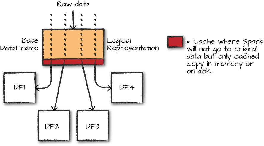
Figure 19-1 presents a simple illustrations of the process. We load an initial
DataFrame from a CSV file and then derive some new DataFrames from it
using transformations. We can avoid having to recompute the original
DataFrame (i.e., load and parse the CSV file) many times by adding a line to
cache it along the way.
Figure 19-1. A cached DataFrame
Now let’s walk through the code:
# in Python
# Original loading code that does *not* cache DataFrame
DF1 = spark.read.format("csv")\
.option("inferSchema", "true")\
.option("header", "true")\
.load("/data/flight-data/csv/2015-summary.csv")
DF2 = DF1.groupBy("DEST_COUNTRY_NAME").count().collect()
DF3 = DF1.groupBy("ORIGIN_COUNTRY_NAME").count().collect()
DF4 = DF1.groupBy("count").count().collect()
You’ll see here that we have our “lazily” created DataFrame (DF1), along
with three other DataFrames that access data in DF1. All of our downstream
DataFrames share that common parent (DF1) and will repeat the same work
when we perform the preceding code. In this case, it’s just reading and
parsing the raw CSV data, but that can be a fairly intensive process,
especially for large datasets.
On my machine, those commands take a second or two to run. Luckily
caching can help speed things up. When we ask for a DataFrame to be
cached, Spark will save the data in memory or on disk the first time it
computes it. Then, when any other queries come along, they’ll just refer to
the one stored in memory as opposed to the original file. You do this using
the DataFrame’s cache method:
DF1.cache()
DF1.count()
We used the count above to eagerly cache the data (basically perform an
action to force Spark to store it in memory), because caching itself is lazy—
the data is cached only on the first time you run an action on the DataFrame.
Now that the data is cached, the previous commands will be faster, as we can
see by running the following code:
# in Python
DF2 = DF1.groupBy("DEST_COUNTRY_NAME").count().collect()
DF3 = DF1.groupBy("ORIGIN_COUNTRY_NAME").count().collect()
DF4 = DF1.groupBy("count").count().collect()
When we ran this code, it cut the time by more than half! This might not
seem that wild, but picture a large dataset or one that requires a lot of
computation to create (not just reading in a file). The savings can be
immense. It’s also great for iterative machine learning workloads because
they’ll often need to access the same data a number of times, which we’ll see
shortly.
The cache command in Spark always places data in memory by default,
caching only part of the dataset if the cluster’s total memory is full. For more
control, there is also a persist method that takes a StorageLevel object to
specify where to cache the data: in memory, on disk, or both.
Joins
Joins are a common area for optimization. The biggest weapon you have
when it comes to optimizing joins is simply educating yourself about what
each join does and how it’s performed. This will help you the most.
Additionally, equi-joins are the easiest for Spark to optimize at this point and
therefore should be preferred wherever possible. Beyond that, simple things
like trying to use the filtering ability of inner joins by changing join ordering
can yield large speedups. Additionally, using broadcast join hints can help
Spark make intelligent planning decisions when it comes to creating query
plans, as described in Chapter 8. Avoiding Cartesian joins or even full outer
joins is often low-hanging fruit for stability and optimizations because these
can often be optimized into different filtering style joins when you look at the
entire data flow instead of just that one particular job area. Lastly, following
some of the other sections in this chapter can have a significant effect on
joins. For example, collecting statistics on tables prior to a join will help
Spark make intelligent join decisions. Additionally, bucketing your data
appropriately can also help Spark avoid large shuffles when joins are
performed.
Aggregations
For the most part, there are not too many ways that you can optimize specific
aggregations beyond filtering data before the aggregation having a
sufficiently high number of partitions. However, if you’re using RDDs,
controlling exactly how these aggregations are performed (e.g., using
reduceByKey when possible over groupByKey) can be very helpful and
improve the speed and stability of your code.
Broadcast Variables
We touched on broadcast joins and variables in previous chapters, and these
are a good option for optimization. The basic premise is that if some large
piece of data will be used across multiple UDF calls in your program, you
can broadcast it to save just a single read-only copy on each node and avoid
re-sending this data with each job. For example, broadcast variables may be
useful to save a lookup table or a machine learning model. You can also
broadcast arbitrary objects by creating broadcast variables using your
SparkContext, and then simply refer to those variables in your tasks, as we
discussed in Chapter 14.
Conclusion
There are many different ways to optimize the performance of your Spark
Applications and make them run faster and at a lower cost. In general, the
main things you’ll want to prioritize are (1) reading as little data as possible
through partitioning and efficient binary formats, (2) making sure there is
sufficient parallellism and no data skew on the cluster using partitioning, and
(3) using high-level APIs such as the Structured APIs as much as possible to
take already optimized code. As with any other software optimization work,
you should also make sure you are optimizing the right operations for your
job: the Spark monitoring tools described in Chapter 18 will let you see
which stages are taking the longest time and focus your efforts on those.
Once you have identified the work that you believe can be optimized, the
tools in this chapter will cover the most important performance optimization
opportunities for the majority of users.

Part V. Streaming

Chapter 20. Stream Processing
Fundamentals
Stream processing is a key requirement in many big data applications. As
soon as an application computes something of value—say, a report about
customer activity, or a new machine learning model—an organization will
want to compute this result continuously in a production setting. As a result,
organizations of all sizes are starting to incorporate stream processing, often
even in the first version of a new application.
Luckily, Apache Spark has a long history of high-level support for streaming.
In 2012, the project incorporated Spark Streaming and its DStreams API, one
of the first APIs to enable stream processing using high-level functional
operators like map and reduce. Hundreds of organizations now use DStreams
in production for large real-time applications, often processing terabytes of
data per hour. Much like the Resilient Distributed Dataset (RDD) API,
however, the DStreams API is based on relatively low-level operations on
Java/Python objects that limit opportunities for higher-level optimization.
Thus, in 2016, the Spark project added Structured Streaming, a new
streaming API built directly on DataFrames that supports both rich
optimizations and significantly simpler integration with other DataFrame and
Dataset code. The Structured Streaming API was marked as stable in Apache
Spark 2.2, and has also seen swift adoption throughout the Spark community.
In this book, we will focus only on the Structured Streaming API, which
integrates directly with the DataFrame and Dataset APIs we discussed earlier
in the book and is the framework of choice for writing new streaming
applications. If you are interested in DStreams, many other books cover that
API, including several dedicated books on Spark Streaming only, such as
Learning Spark Streaming by Francois Garillot and Gerard Maas (O’Reilly,
2017). Much as with RDDs versus DataFrames, however, Structured
Streaming offers a superset of the majority of the functionality of DStreams,
and will often perform better due to code generation and the Catalyst
optimizer.
Before we discuss the streaming APIs in Spark, let’s more formally define
streaming and batch processing. This chapter will discuss some of the core
concepts in this area that we will need throughout this part of the book. It
won’t be a dissertation on this topic, but will cover enough of the concepts to
let you make sense of systems in this space.
What Is Stream Processing?
Stream processing is the act of continuously incorporating new data to
compute a result. In stream processing, the input data is unbounded and has
no predetermined beginning or end. It simply forms a series of events that
arrive at the stream processing system (e.g., credit card transactions, clicks on
a website, or sensor readings from Internet of Things [IoT] devices). User
applications can then compute various queries over this stream of events
(e.g., tracking a running count of each type of event or aggregating them into
hourly windows). The application will output multiple versions of the result
as it runs, or perhaps keep it up to date in an external “sink” system such as a
key-value store.
Naturally, we can compare streaming to batch processing, in which the
computation runs on a fixed-input dataset. Oftentimes, this might be a large-
scale dataset in a data warehouse that contains all the historical events from
an application (e.g., all website visits or sensor readings for the past month).
Batch processing also takes a query to compute, similar to stream processing,
but only computes the result once.
Although streaming and batch processing sound different, in practice, they
often need to work together. For example, streaming applications often need
to join input data against a dataset written periodically by a batch job, and the
output of streaming jobs is often files or tables that are queried in batch jobs.
Moreover, any business logic in your applications needs to work consistently
across streaming and batch execution: for example, if you have a custom
code to compute a user’s billing amount, it would be harmful to get a
different result when running it in a streaming versus batch fashion! To
handle these needs, Structured Streaming was designed from the beginning to
interoperate easily with the rest of Spark, including batch applications.
Indeed, the Structured Streaming developers coined the term continuous
applications to capture end-to-end applications that consist of streaming,
batch, and interactive jobs all working on the same data to deliver an end
product. Structured Streaming is focused on making it simple to build such
applications in an end-to-end fashion instead of only handling stream-level
per-record processing.
Stream Processing Use Cases
We defined stream processing as the incremental processing of unbounded
datasets, but that’s a strange way to motivate a use case. Before we get into
advantages and disadvantages of streaming, let’s explain why you might want
to use streaming. We’ll describe six common use cases with varying
requirements from the underlying stream processing system.
Notifications and alerting
Probably the most obvious streaming use case involves notifications and
alerting. Given some series of events, a notification or alert should be
triggered if some sort of event or series of events occurs. This doesn’t
necessarily imply autonomous or preprogrammed decision making; alerting
can also be used to notify a human counterpart of some action that needs to
be taken. An example might be driving an alert to an employee at a
fulfillment center that they need to get a certain item from a location in the
warehouse and ship it to a customer. In either case, the notification needs to
happen quickly.
Real-time reporting
Many organizations use streaming systems to run real-time dashboards that
any employee can look at. For example, this book’s authors leverage
Structured Streaming every day to run real-time reporting dashboards
throughout Databricks (where both authors of this book work). We use these
dashboards to monitor total platform usage, system load, uptime, and even
usage of new features as they are rolled out, among other applications.
Incremental ETL
One of the most common streaming applications is to reduce the latency
companies must endure while retreiving information into a data warehouse—
in short, “my batch job, but streaming.” Spark batch jobs are often used for
Extract, Transform, and Load (ETL) workloads that turn raw data into a
structured format like Parquet to enable efficient queries. Using Structured
Streaming, these jobs can incorporate new data within seconds, enabling
users to query it faster downstream. In this use case, it is critical that data is
processed exactly once and in a fault-tolerant manner: we don’t want to lose
any input data before it makes it to the warehouse, and we don’t want to load
the same data twice. Moreover, the streaming system needs to make updates
to the data warehouse transactionally so as not to confuse the queries running
on it with partially written data.
Update data to serve in real time
Streaming systems are frequently used to compute data that gets served
interactively by another application. For example, a web analytics product
such as Google Analytics might continuously track the number of visits to
each page, and use a streaming system to keep these counts up to date. When
users interact with the product’s UI, this web application queries the latest
counts. Supporting this use case requires that the streaming system can
perform incremental updates to a key–value store (or other serving system) as
a sync, and often also that these updates are transactional, as in the ETL case,
to avoid corrupting the data in the application.
Real-time decision making
Real-time decision making on a streaming system involves analyzing new
inputs and responding to them automatically using business logic. An
example use case would be a bank that wants to automatically verify whether
a new transaction on a customer’s credit card represents fraud based on their
recent history, and deny the transaction if the charge is determined fradulent.
This decision needs to be made in real-time while processing each
transaction, so developers could implement this business logic in a streaming
system and run it against the stream of transactions. This type of application
will likely need to maintain a significant amount of state about each user to
track their current spending patterns, and automatically compare this state
against each new transaction.
Online machine learning
A close derivative of the real-time decision-making use case is online
machine learning. In this scenario, you might want to train a model on a
combination of streaming and historical data from multiple users. An
example might be more sophisticated than the aforementioned credit card
transaction use case: rather than reacting with hardcoded rules based on one
customer’s behavior, the company may want to continuously update a model
from all customers’ behavior and test each transaction against it. This is the
most challenging use case of the bunch for stream processing systems
because it requires aggregation across multiple customers, joins against static
datasets, integration with machine learning libraries, and low-latency
response times.
Advantages of Stream Processing
Now that we’ve seen some use cases for streaming, let’s crystallize some of
the advantages of stream processing. For the most part, batch is much simpler
to understand, troubleshoot, and write applications in for the majority of use
cases. Additionally, the ability to process data in batch allows for vastly
higher data processing throughput than many streaming systems. However,
stream processing is essential in two cases. First, stream processing enables
lower latency: when your application needs to respond quickly (on a
timescale of minutes, seconds, or milliseconds), you will need a streaming
system that can keep state in memory to get acceptable performance. Many of
the decision making and alerting use cases we described fall into this camp.
Second, stream processing can also be more efficient in updating a result than
repeated batch jobs, because it automatically incrementalizes the
computation. For example, if we want to compute web traffic statistics over
the past 24 hours, a naively implemented batch job might scan all the data
each time it runs, always processing 24 hours’ worth of data. In contrast, a
streaming system can remember state from the previous computation and
only count the new data. If you tell the streaming system to update your
report every hour, for example, it would only need to process 1 hour’s worth
of data each time (the new data since the last report). In a batch system, you
would have to implement this kind of incremental computation by hand to get
the same performance, resulting in a lot of extra work that the streaming
system will automatically give you out of the box.
Challenges of Stream Processing
We discussed motivations and advantages of stream processing, but as you
likely know, there’s never a free lunch. Let’s discuss some of the challenges
of operating on streams.
To ground this example, let’s imagine that our application receives input
messages from a sensor (e.g., inside a car) that report its value at different
times. We then want to search within this stream for certain values, or certain
patterns of values. One specific challenge is that the input records might
arrive to our application out-of-order: due to delays and retransmissions, for
example, we might receive the following sequence of updates in order, where
the time field shows the time when the value was actually measured:
{value: 1, time: "2017-04-07T00:00:00"}
{value: 2, time: "2017-04-07T01:00:00"}
{value: 5, time: "2017-04-07T02:00:00"}
{value: 10, time: "2017-04-07T01:30:00"}
{value: 7, time: "2017-04-07T03:00:00"}
In any data processing system, we can construct logic to perform some action
based on receiving the single value of “5.” In a streaming system, we can also
respond to this individual event quickly. However, things become more
complicated if you want only to trigger some action based on a specific
sequence of values received, say, 2 then 10 then 5. In the case of batch

processing, this is not particularly difficult because we can simply sort all the
events we have by time field to see that 10 did come between 2 and 5.
However, this is harder for stream processing systems. The reason is that the
streaming system is going to receive each event individually, and will need to
track some state across events to remember the 2 and 5 events and realize that
the 10 event was between them. The need to remember such state over the
stream creates more challenges. For instance, what if you have a massive data
volume (e.g., millions of sensor streams) and the state itself is massive? What
if a machine in the sytem fails, losing some state? What if the load is
imbalanced and one machine is slow? And how can your application signal
downstream consumers when analysis for some event is “done” (e.g., the
pattern 2-10-5 did not occur)? Should it wait a fixed amount of time or
remember some state indefinitely? All of these challenges and others—such
as making the input and the output of the system transactional—can come up
when you want to deploy a streaming application.
To summarize, the challenges we described in the previous paragraph and a
couple of others, are as follows:
Processing out-of-order data based on application timestamps (also
called event time)
Maintaining large amounts of state
Supporting high-data throughput
Processing each event exactly once despite machine failures
Handling load imbalance and stragglers
Responding to events at low latency
Joining with external data in other storage systems
Determining how to update output sinks as new events arrive
Writing data transactionally to output systems
Updating your application’s business logic at runtime
Each of these topics are an active area of research and development in large-
scale streaming systems. To understand how different streaming systems
have tackled these challenges, we describe a few of the most common design
concepts you will see across them.
Stream Processing Design Points
To support the stream processing challenges we described, including high
throughput, low latency, and out-of-order data, there are multiple ways to
design a streaming system. We describe the most common design options
here, before describing Spark’s choices in the next section.
Record-at-a-Time Versus Declarative APIs
The simplest way to design a streaming API would be to just pass each event
to the application and let it react using custom code. This is the approach that
many early streaming systems, such as Apache Storm, implemented, and it
has an important place when applications need full control over the
processing of data. Streaming that provide this kind of record-at-a-time API
just give the user a collection of “plumbing” to connect together into an
application. However, the downside of these systems is that most of the
complicating factors we described earlier, such as maintaining state, are
solely governed by the application. For example, with a record-at-a-time API,
you are responsible for tracking state over longer time periods, dropping it
after some time to clear up space, and responding differently to duplicate
events after a failure. Programming these systems correctly can be quite
challenging. At its core, low-level APIs require deep expertise to be develop
and maintain.
As a result, many newer streaming systems provide declarative APIs, where
your application specifies what to compute but not how to compute it in
response to each new event and how to recover from failure. Spark’s original
DStreams API, for example, offered functional API based on operations like
map, reduce and filter on streams. Internally, the DStream API automatically
tracked how much data each operator had processed, saved any relevant state
reliably, and recovered the computation from failure when needed. Systems
such as Google Dataflow and Apache Kafka Streams provide similar,
functional APIs. Spark’s Structured Streaming actually takes this concept
even further, switching from functional operations to relational (SQL-like)
ones that enable even richer automatic optimization of the execution without
programming effort.
Event Time Versus Processing Time
For the systems with declarative APIs, a second concern is whether the
system natively supports event time. Event time is the idea of processing data
based on timestamps inserted into each record at the source, as opposed to the
time when the record is received at the streaming application (which is called
processing time). In particular, when using event time, records may arrive to
the system out of order (e.g., if they traveled back on different network
paths), and different sources may also be out of sync with each other (some
records may arrive later than other records for the same event time). If your
application collects data from remote sources that may be delayed, such as
mobile phones or IoT devices, event-time processing is crucial: without it,
you will miss important patterns when some data is late. In contrast, if your
application only processes local events (e.g., ones generated in the same
datacenter), you may not need sophisticated event-time processing.
When using event-time, several issues become common concerns across
applications, including tracking state in a manner that allows the system to
incorporate late events, and determining when it is safe to output a result for a
given time window in event time (i.e., when the system is likely to have
received all the input up to that point). Because of this, many declarative
systems, including Structured Streaming, have “native” support for event
time integrated into all their APIs, so that these concerns can be handled
automatically across your whole program.
Continuous Versus Micro-Batch Execution
The final design decision you will often see come up is about continuous
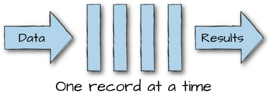
versus micro-batch execution. In continuous processing-based systems, each
node in the system is continually listening to messages from other nodes and
outputting new updates to its child nodes. For example, suppose that your
application implements a map-reduce computation over several input
streams. In a continuous processing system, each of the nodes implementing
map would read records one by one from an input source, compute its
function on them, and send them to the appropriate reducer. The reducer
would then update its state whenever it gets a new record. The key idea is
that this happens on each individual record, as illustrated in Figure 20-1.
Figure 20-1. Continuous processing
Continuous processing has the advantage of offering the lowest possible
latency when the total input rate is relatively low, because each node
responds immediately to a new message. However, continuous processing
systems generally have lower maximum throughput, because they incur a
significant amount of overhead per-record (e.g., calling the operating system
to send a packet to a downstream node). In addition, continous systems
generally have a fixed topology of operators that cannot be moved at runtime
without stopping the whole system, which can introduce load balancing
issues.
In contrast, micro-batch systems wait to accumulate small batches of input
data (say, 500 ms’ worth), then process each batch in parallel using a
distributed collection of tasks, similar to the execution of a batch job in
Spark. Micro-batch systems can often achieve high throughput per node
because they leverage the same optimizations as batch systems (e.g.,
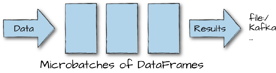
vectorized processing), and do not incur any extra per-record overhead, as
illustrated in Figure 20-2.
Figure 20-2. Micro-batch
Thus, they need fewer nodes to process the same rate of data. Micro-batch
systems can also use dynamic load balancing techniques to handle changing
workloads (e.g., increasing or decreasing the number of tasks). The
downside, however, is a higher base latency due to waiting to accumulate a
micro-batch. In practice, the streaming applications that are large-scale
enough to need to distribute their computation tend to prioritize throughput,
so Spark has traditionally implemented micro-batch processing. In Structured
Streaming, however, there is an active development effort to also support a
continuous processing mode beneath the same API.
When choosing between these two execution modes, the main factors you
should keep in mind are your desired latency and total cost of operation
(TCO). Micro-batch systems can comfortably deliver latencies from 100 ms
to a second, depending on the application. Within this regime, they will
generally require fewer nodes to achieve the same throughput, and hence
lower operational cost (including lower maintenance cost due to less frequent
node failures). For much lower latencies, you should consider a continuous
processing system, or using a micro-batch system in conjunction with a fast
serving layer to provide low-latency queries (e.g., outputting data into
MySQL or Apache Cassandra, where it can be served to clients in
milliseconds).
Spark’s Streaming APIs
We covered some high-level design approaches to stream processing, but
thus far we have not discussed Spark’s APIs in detail. Spark includes two
streaming APIs, as we discussed at the beginning of this chapter. The earlier
DStream API in Spark Streaming is purely micro-batch oriented. It has a
declarative (functional-based) API but no support for event time. The newer
Structured Streaming API adds higher-level optimizations, event time, and
support for continuous processing.
The DStream API
Spark’s original DStream API has been used broadly for stream processing
since its first release in 2012. For example, DStreams was the most widely
used processing engine in Datanami’s 2016 survey. Many companies use and
operate Spark Streaming at scale in production today due to its high-level
API interface and simple exactly-once semantics. Interactions with RDD
code, such as joins with static data, are also natively supported in Spark
Streaming. Operating Spark Streaming isn’t much more difficult than
operating a normal Spark cluster. However, the DStreams API has several
limitations. First, it is based purely on Java/Python objects and functions, as
opposed to the richer concept of structured tables in DataFrames and
Datasets. This limits the engine’s opportunity to perform optimizations.
Second, the API is purely based on processing time—to handle event-time
operations, applications need to implement them on their own. Finally,
DStreams can only operate in a micro-batch fashion, and exposes the
duration of micro-batches in some parts of its API, making it difficult to
support alternative execution modes.
Structured Streaming
Structured Streaming is a higher-level streaming API built from the ground
up on Spark’s Structured APIs. It is available in all the environments where
structured processing runs, including Scala, Java, Python, R, and SQL. Like
DStreams, it is a declarative API based on high-level operations, but by
building on the structured data model introduced in the previous part of the
book, Structured Streaming can perform more types of optimizations
automatically. However, unlike DStreams, Structured Streaming has native
support for event time data (all of its the windowing operators automatically
support it). As of Apache Spark 2.2, the system only runs in a micro-batch
model, but the Spark team at Databricks has announced an effort called
Continuous Processing to add a continuous execution mode. This should
become an option for users in Spark 2.3.
More fundamentally, beyond simplifying stream processing, Structured
Streaming is also designed to make it easy to build end-to-end continuous
applications using Apache Spark that combine streaming, batch, and
interactive queries. For example, Structured Streaming does not use a
separate API from DataFrames: you simply write a normal DataFrame (or
SQL) computation and launch it on a stream. Structured Streaming will
automatically update the result of this computation in an incremental fashion
as data arrives. This is a major help when writing end-to-end data
applications: developers do not need to maintain a separate streaming version
of their batch code, possibly for a different execution system, and risk having
these two versions of the code fall out of sync. As another example,
Structured Streaming can output data to standard sinks usable by Spark SQL,
such as Parquet tables, making it easy to query your stream state from
another Spark applications. In future versions of Apache Spark, we expect
more and more components of the project to integrate with Structured
Streaming, including online learning algorithms in MLlib.
In general, Structured Streaming is meant to be an easier-to-use and higher-
performance evolution of Spark Streaming’s DStream API, so we will focus
solely on this new API in this book. Many of the concepts, such as building a
computation out of a graph of transformations, also apply to DStreams, but
we leave the exposition of that to other books.
Conclusion
This chapter covered the basic concepts and ideas that you’re going to need
to understand stream processing. The design approaches introduced in this
chapter should clarify how you can evaluate streaming systems for a given
application. You should also feel comfortable understanding what trade-offs
the authors of DStreams and Structured Streaming have made, and why the
direct support for DataFrame programs is a big help when using Structured
Streaming: there is no need to duplicate your application logic. In the
upcoming chapters, we’ll dive right into Structured Streaming to understand
how to use it.

Chapter 21. Structured
Streaming Basics
Now that we have covered a brief overview of stream processing, let’s dive
right into Structured Streaming. In this chapter, we will, again, state some of
the key concepts behind Structured Streaming and then apply them with some
code examples that show how easy the system is to use.
Structured Streaming Basics
Structured Streaming, as we discussed at the end of Chapter 20, is a stream
processing framework built on the Spark SQL engine. Rather than
introducing a separate API, Structured Streaming uses the existing structured
APIs in Spark (DataFrames, Datasets, and SQL), meaning that all the
operations you are familiar with there are supported. Users express a
streaming computation in the same way they’d write a batch computation on
static data. Upon specifying this, and specifying a streaming destination, the
Structured Streaming engine will take care of running your query
incrementally and continuously as new data arrives into the system. These
logical instructions for the computation are then executed using the same
Catalyst engine discussed in Part II of this book, including query
optimization, code generation, etc. Beyond the core structured processing
engine, Structured Streaming includes a number of features specifically for
streaming. For instance, Structured Streaming ensures end-to-end, exactly-
once processing as well as fault-tolerance through checkpointing and write-
ahead logs.
The main idea behind Structured Streaming is to treat a stream of data as a
table to which data is continuously appended. The job then periodically
checks for new input data, process it, updates some internal state located in a
state store if needed, and updates its result. A cornerstone of the API is that
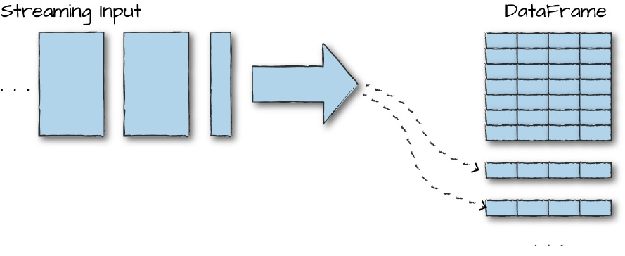
you should not have to change your query’s code when doing batch or stream
processing—you should have to specify only whether to run that query in a
batch or streaming fashion. Internally, Structured Streaming will
automatically figure out how to “incrementalize” your query, i.e., update its
result efficiently whenever new data arrives, and will run it in a fault-tolerant
fashion.
Figure 21-1. Structured streaming input
In simplest terms, Structured Streaming is “your DataFrame, but streaming.”
This makes it very easy to get started using streaming applications. You
probably already have the code for them! There are some limits to the types
of queries Structured Streaming will be able to run, however, as well as some
new concepts you have to think about that are specific to streaming, such as
event-time and out-of-order data. We will discuss these in this and the
following chapters.
Finally, by integrating with the rest of Spark, Structured Streaming enables
users to build what we call continuous applications. A continous application
is an end-to-end application that reacts to data in real time by combining a
variety of tools: streaming jobs, batch jobs, joins between streaming and
offline data, and interactive ad-hoc queries. Because most streaming jobs
today are deployed within the context of a larger continuous application, the
Spark developers sought to make it easy to specify the whole application in
one framework and get consistent results across these different portions of it.
For example, you can use Structured Streaming to continuously update a

table that users query interactively with Spark SQL, serve a machine learning
model trained by MLlib, or join streams with offline data in any of Spark’s
data sources—applications that would be much more complex to build using
a mix of different tools.
Core Concepts
Now that we introduced the high-level idea, let’s cover some of the important
concepts in a Structured Streaming job. One thing you will hopefully find is
that there aren’t many. That’s because Structured Streaming is designed to be
simple. Read some other big data streaming books and you’ll notice that they
begin by introducing terminology like distributed stream processing
topologies for skewed data reducers (a caricature, but accurate) and other
complex verbiage. Spark’s goal is to handle these concerns automatically and
give users a simple way to run any Spark computation on a stream.
Transformations and Actions
Structured Streaming maintains the same concept of transformations and
actions that we have seen throughout this book. The transformations available
in Structured Streaming are, with a few restrictions, the exact same
transformations that we saw in Part II. The restrictions usually involve some
types of queries that the engine cannot incrementalize yet, although some of
the limitations are being lifted in new versions of Spark. There is generally
only one action available in Structured Streaming: that of starting a stream,
which will then run continuously and output results.
Input Sources
Structured Streaming supports several input sources for reading in a
streaming fashion. As of Spark 2.2, the supported input sources are as
follows:
Apache Kafka 0.10

Files on a distributed file system like HDFS or S3 (Spark will
continuously read new files in a directory)
A socket source for testing
We discuss these in depth later in this chapter, but it’s worth mentioning that
the authors of Spark are working on a stable source API so that you can build
your own streaming connectors.
Sinks
Just as sources allow you to get data into Structured Streaming, sinks specify
the destination for the result set of that stream. Sinks and the execution
engine are also responsible for reliably tracking the exact progress of data
processing. Here are the supported output sinks as of Spark 2.2:
Apache Kafka 0.10
Almost any file format
A foreach sink for running arbitary computation on the output
records
A console sink for testing
A memory sink for debugging
We discuss these in more detail later in the chapter when we discuss sources.
Output Modes
Defining a sink for our Structured Streaming job is only half of the story. We
also need to define how we want Spark to write data to that sink. For
instance, do we only want to append new information? Do we want to update
rows as we receive more information about them over time (e.g., updating the
click count for a given web page)? Do we want to completely overwrite the
result set every single time (i.e. always write a file with the complete click
counts for all pages)? To do this, we define an output mode, similar to how

we define output modes in the static Structured APIs.
The supported output modes are as follows:
Append (only add new records to the output sink)
Update (update changed records in place)
Complete (rewrite the full output)
One important detail is that certain queries, and certain sinks, only support
certain output modes, as we will discuss later in the book. For example,
suppose that your job is just performing a map on a stream. The output data
will grow indefinitely as new records arrive, so it would not make sense to
use Complete mode, which requires writing all the data to a new file at once.
In contrast, if you are doing an aggregation into a limited number of keys,
Complete and Update modes would make sense, but Append would not,
because the values of some keys’ need to be updated over time.
Triggers
Whereas output modes define how data is output, triggers define when data is
output—that is, when Structured Streaming should check for new input data
and update its result. By default, Structured Streaming will look for new
input records as soon as it has finished processing the last group of input data,
giving the lowest latency possible for new results. However, this behavior
can lead to writing many small output files when the sink is a set of files.
Thus, Spark also supports triggers based on processing time (only look for
new data at a fixed interval). In the future, other types of triggers may also be
supported.
Event-Time Processing
Structured Streaming also has support for event-time processing (i.e.,
processing data based on timestamps included in the record that may arrive
out of order). There are two key ideas that you will need to understand here
for the moment; we will talk about both of these in much more depth in the
next chapter, so don’t worry if you’re not perfectly clear on them at this
point.
Event-time data
Event-time means time fields that are embedded in your data. This means that
rather than processing data according to the time it reaches your system, you
process it according to the time that it was generated, even if records arrive
out of order at the streaming application due to slow uploads or network
delays. Expressing event-time processing is simple in Structured Streaming.
Because the system views the input data as a table, the event time is just
another field in that table, and your application can do grouping, aggregation,
and windowing using standard SQL operators. However, under the hood,
Structured Streaming can take some special actions when it knows that one of
your columns is an event-time field, including optimizing query execution or
determining when it is safe to forget state about a time window. Many of
these actions can be controlled using watermarks.
Watermarks
Watermarks are a feature of streaming systems that allow you to specify how
late they expect to see data in event time. For example, in an application that
processes logs from mobile devices, one might expect logs to be up to 30
minutes late due to upload delays. Systems that support event time, including
Structured Streaming, usually allow setting watermarks to limit how long
they need to remember old data. Watermarks can also be used to control
when to output a result for a particular event time window (e.g., waiting until
the watermark for it has passed).
Structured Streaming in Action
Let’s get to an applied example of how you might use Structured Streaming.
For our examples, we’re going to be working with the Heterogeneity Human
Activity Recognition Dataset. The data consists of smartphone and
smartwatch sensor readings from a variety of devices—specifically, the

accelerometer and gyroscope, sampled at the highest possible frequency
supported by the devices. Readings from these sensors were recorded while
users performed activities like biking, sitting, standing, walking, and so on.
There are several different smartphones and smartwatches used, and nine
total users. You can download the data here, in the activity data folder.
TIP
This Dataset is fairly large. If it’s too large for your machine, you can remove some of the
files and it will work just fine.
Let’s read in the static version of the dataset as a DataFrame:
// in Scala
val static = spark.read.json("/data/activity-data/")
val dataSchema = static.schema
# in Python
static = spark.read.json("/data/activity-data/")
dataSchema = static.schema
Here’s the schema:
root
|-- Arrival_Time: long (nullable = true)
|-- Creation_Time: long (nullable = true)
|-- Device: string (nullable = true)
|-- Index: long (nullable = true)
|-- Model: string (nullable = true)
|-- User: string (nullable = true)
|-- _corrupt_record: string (nullable = true)
|-- gt: string (nullable = true)
|-- x: double (nullable = true)
|-- y: double (nullable = true)
|-- z: double (nullable = true)
Here’s a sample of the DataFrame:
+-------------+------------------+--------+-----+------+----+--------+-----+----
-
| Arrival_Time| Creation_Time| Device|Index| Model|User|_c...ord|. gt|
x
|1424696634224|142469663222623685|nexus4_1| 62|nexus4| a|
null|stand|-0...
...
|1424696660715|142469665872381726|nexus4_1| 2342|nexus4| a|
null|stand|-0...
+-------------+------------------+--------+-----+------+----+--------+-----+----
-
You can see in the preceding example, which includes a number of
timestamp columns, models, user, and device information. The gt field
specifies what activity the user was doing at that time.
Next, let’s create a streaming version of the same Dataset, which will read
each input file in the dataset one by one as if it was a stream.
Streaming DataFrames are largely the same as static DataFrames. We create
them within Spark applications and then perform transformations on them to
get our data into the correct format. Basically, all of the transformations that
are available in the static Structured APIs apply to Streaming DataFrames.
However, one small difference is that Structured Streaming does not let you
perform schema inference without explicitly enabling it. You can enable
schema inference for this by setting the configuration
spark.sql.streaming.schemaInference to true. Given that fact, we will
read the schema from one file (that we know has a valid schema) and pass the
dataSchema object from our static DataFrame to our streaming DataFrame.
As mentioned, you should avoid doing this in a production scenario where
your data may (accidentally) change out from under you:
// in Scala
val streaming = spark.readStream.schema(dataSchema)
.option("maxFilesPerTrigger", 1).json("/data/activity-data")
# in Python
streaming = spark.readStream.schema(dataSchema).option("maxFilesPerTrigger", 1)\
.json("/data/activity-data")

NOTE
We discuss maxFilesPerTrigger a little later on in this chapter but essentially it allows
you to control how quickly Spark will read all of the files in the folder. By specifying this
value lower, we’re artificially limiting the flow of the stream to one file per trigger. This
helps us demonstrate how Structured Streaming runs incrementally in our example, but
probably isn’t something you’d use in production.
Just like with other Spark APIs, streaming DataFrame creation and execution
is lazy. In particular, we can now specify transformations on our streaming
DataFrame before finally calling an action to start the stream. In this case,
we’ll show one simple transformation—we will group and count data by the
gt column, which is the activity being performed by the user at that point in
time:
// in Scala
val activityCounts = streaming.groupBy("gt").count()
# in Python
activityCounts = streaming.groupBy("gt").count()
Because this code is being written in local mode on a small machine, we are
going to set the shuffle partitions to a small value to avoid creating too many
shuffle partitions:
spark.conf.set("spark.sql.shuffle.partitions", 5)
Now that we set up our transformation, we need only to specify our action to
start the query. As mentioned previously in the chapter, we will specify an
output destination, or output sink for our result of this query. For this basic
example, we are going to write to a memory sink which keeps an in-memory
table of the results.
In the process of specifying this sink, we’re going to need to define how
Spark will output that data. In this example, we use the complete output
mode. This mode rewrites all of the keys along with their counts after every
trigger:
// in Scala
val activityQuery = activityCounts.writeStream.queryName("activity_counts")
.format("memory").outputMode("complete")
.start()
# in Python
activityQuery = activityCounts.writeStream.queryName("activity_counts")\
.format("memory").outputMode("complete")\
.start()
We are now writing out our stream! You’ll notice that we set a unique query
name to represent this stream, in this case activity_counts. We specified
our format as an in-memory table and we set the output mode.
When we run the preceding code, we also want to include the following line:
activityQuery.awaitTermination()
After this code is executed, the streaming computation will have started in the
background. The query object is a handle to that active streaming query, and
we must specify that we would like to wait for the termination of the query
using activityQuery.awaitTermination() to prevent the driver process
from exiting while the query is active. We will omit this from our future parts
of the book for readability, but it must be included in your production
applications; otherwise, your stream won’t be able to run.
Spark lists this stream, and other active ones, under the active streams in our
SparkSession. We can see a list of those streams by running the following:
spark.streams.active
Spark also assigns each stream a UUID, so if need be you could iterate
through the list of running streams and select the above one. In this case, we
assigned it to a variable, so that’s not necessary.
Now that this stream is running, we can experiment with the results by
querying the in-memory table it is maintaining of the current output of our
streaming aggregation. This table will be called activity_counts, the same
as the stream. To see the current data in this output table, we simply need to
query it! We’ll do this in a simple loop that will print the results of the
streaming query every second:
// in Scala
for( i <- 1 to 5 ) {
spark.sql("SELECT * FROM activity_counts").show()
Thread.sleep(1000)
}
# in Python
from time import sleep
for x in range(5):
spark.sql("SELECT * FROM activity_counts").show()
sleep(1)
As the preceding queries run, you should see the counts for each activity
change over time. For instance, the first show call displays the following
result (because we queried it while the stream was reading the first file):
+---+-----+
| gt|count|
+---+-----+
+---+-----+
The previous show call shows the following result—note that the result will
probably vary when you’re running this code personally because you will
likely start it at a different time:
+----------+-----+
| gt|count|
+----------+-----+
| sit| 8207|
...
| null| 6966|
| bike| 7199|
+----------+-----+
With this simple example, the power of Structured Streaming should become
clear. You can take the same operations that you use in batch and run them
on a stream of data with very few code changes (essentially just specifying
that it’s a stream). The rest of this chapter touches on some of the details
about the various manipulations, sources, and sinks that you can use with
Structured Streaming.
Transformations on Streams
Streaming transformations, as we mentioned, include almost all static
DataFrame transformations that you already saw in Part II. All select, filter,
and simple transformations are supported, as are all DataFrame functions and
individual column manipulations. The limitations arise on transformations
that do not make sense in context of streaming data. For example, as of
Apache Spark 2.2, users cannot sort streams that are not aggregated, and
cannot perform multiple levels of aggregation without using Stateful
Processing (covered in the next chater). These limitations may be lifted as
Structured Streaming continues to develop, so we encourage you to check the
documentation of your version of Spark for updates.
Selections and Filtering
All select and filter transformations are supported in Structured Streaming, as
are all DataFrame functions and individual column manipulations. We show
a simple example using selections and filtering below. In this case, because
we are not updating any keys over time, we will use the Append output
mode, so that new results are appended to the output table:
// in Scala
import org.apache.spark.sql.functions.expr
val simpleTransform = streaming.withColumn("stairs", expr("gt like '%stairs%'"))
.where("stairs")
.where("gt is not null")
.select("gt", "model", "arrival_time", "creation_time")
.writeStream
.queryName("simple_transform")
.format("memory")
.outputMode("append")
.start()
# in Python
from pyspark.sql.functions import expr
simpleTransform = streaming.withColumn("stairs", expr("gt like '%stairs%'"))\
.where("stairs")\
.where("gt is not null")\
.select("gt", "model", "arrival_time", "creation_time")\
.writeStream\
.queryName("simple_transform")\
.format("memory")\
.outputMode("append")\
.start()
Aggregations
Structured Streaming has excellent support for aggregations. You can specify
arbitrary aggregations, as you saw in the Structured APIs. For example, you
can use a more exotic aggregation, like a cube, on the phone model and
activity and the average x, y, z accelerations of our sensor (jump back to
Chapter 7 in order to see potential aggregations that you can run on your
stream):
// in Scala
val deviceModelStats = streaming.cube("gt", "model").avg()
.drop("avg(Arrival_time)")
.drop("avg(Creation_Time)")
.drop("avg(Index)")
.writeStream.queryName("device_counts").format("memory").outputMode("complete")
.start()
# in Python
deviceModelStats = streaming.cube("gt", "model").avg()\
.drop("avg(Arrival_time)")\
.drop("avg(Creation_Time)")\
.drop("avg(Index)")\
.writeStream.queryName("device_counts").format("memory")\
.outputMode("complete")\
.start()
Querying that table allows us to see the results:

SELECT * FROM device_counts
+----------+------+------------------+--------------------+--------------------+
| gt| model| avg(x)| avg(y)| avg(z)|
+----------+------+------------------+--------------------+--------------------+
| sit| null|-3.682775300344...|1.242033094787975...|-4.22021191297611...|
| stand| null|-4.415368069618...|-5.30657295890281...|2.264837548081631...|
...
| walk|nexus4|-0.007342235359...|0.004341030525168...|-6.01620400184307...|
|stairsdown|nexus4|0.0309175199508...|-0.02869185568293...| 0.11661923308518365|
...
+----------+------+------------------+--------------------+--------------------+
In addition to these aggregations on raw columns in the dataset, Structured
Streaming has special support for columns that represent event time,
including watermark support and windowing. We will discuss these in more
detail in Chapter 22.
NOTE
As of Spark 2.2, the one limitation of aggregations is that multiple “chained” aggregations
(aggregations on streaming aggregations) are not supported at this time. However, you can
achieve this by writing out to an intermediate sink of data, like Kafka or a file sink. This
will change in the future as the Structured Streaming community adds this functionality.
Joins
As of Apache Spark 2.2, Structured Streaming supports joining streaming
DataFrames to static DataFrames. Spark 2.3 will add the ability to join
multiple streams together. You can do multiple column joins and supplement
streaming data with that from static data sources:
// in Scala
val historicalAgg = static.groupBy("gt", "model").avg()
val deviceModelStats = streaming.drop("Arrival_Time", "Creation_Time", "Index")
.cube("gt", "model").avg()
.join(historicalAgg, Seq("gt", "model"))
.writeStream.queryName("device_counts").format("memory").outputMode("complete")
.start()
# in Python
historicalAgg = static.groupBy("gt", "model").avg()
deviceModelStats = streaming.drop("Arrival_Time", "Creation_Time", "Index")\
.cube("gt", "model").avg()\
.join(historicalAgg, ["gt", "model"])\
.writeStream.queryName("device_counts").format("memory")\
.outputMode("complete")\
.start()
In Spark 2.2, full outer joins, left joins with the stream on the right side, and
right joins with the stream on the left are not supported. Structured Streaming
also does not yet support stream-to-stream joins, but this is also a feature
under active development.
Input and Output
This section dives deeper into the details of how sources, sinks, and output
modes work in Structured Streaming. Specifically, we discuss how, when,
and where data flows into and out of the system. As of this writing,
Structured Streaming supports several sources and sinks, including Apache
Kafka, files, and several sources and sinks for testing and debugging. More
sources may be added over time, so be sure to check the documentation for
the most up-to-date information. We discuss the source and sink for a
particular storage system together in this chapter, but in reality you can mix
and match them (e.g., use a Kafka input source with a file sink).
Where Data Is Read and Written (Sources and Sinks)
Structured Streaming supports several production sources and sinks (files and
Apache Kafka), as well as some debugging tools like the memory table sink.
We mentioned these at the beginning of the chapter, but now let’s cover the
details of each one.
File source and sink
Probably the simplest source you can think of is the simple file source. It’s
easy to reason about and understand. While essentially any file source should
work, the ones that we see in practice are Parquet, text, JSON, and CSV.
The only difference between using the file source/sink and Spark’s static file
source is that with streaming, we can control the number of files that we read
in during each trigger via the maxFilesPerTrigger option that we saw
earlier.
Keep in mind that any files you add into an input directory for a streaming
job need to appear in it atomically. Otherwise, Spark will process partially
written files before you have finished. On file systems that show partial
writes, such as local files or HDFS, this is best done by writing the file in an
external directory and moving it into the input directory when finished. On
Amazon S3, objects normally only appear once fully written.
Kafka source and sink
Apache Kafka is a distributed publish-and-subscribe system for streams of
data. Kafka lets you publish and subscribe to streams of records like you
might do with a message queue—these are stored as streams of records in a
fault-tolerant way. Think of Kafka like a distributed buffer. Kafka lets you
store streams of records in categories that are referred to as topics. Each
record in Kafka consists of a key, a value, and a timestamp. Topics consist of
immutable sequences of records for which the position of a record in a
sequence is called an offset. Reading data is called subscribing to a topic and
writing data is as simple as publishing to a topic.
Spark allows you to read from Kafka with both batch and streaming
DataFrames.
As of Spark 2.2, Structured Streaming supports Kafka version 0.10. This too
is likely to expand in the future, so be sure to check the documentation for
more information about the Kafka versions available. There are only a few
options that you need to specify when you read from Kafka.
Reading from the Kafka Source
To read, you first need to choose one of the following options: assign,
subscribe, or subscribePattern. Only one of these can be present as an
option when you go to read from Kafka. Assign is a fine-grained way of
specifying not just the topic but also the topic partitions from which you
would like to read. This is specified as a JSON string {"topicA":
[0,1],"topicB":[2,4]}. subscribe and subscribePattern are ways of
subscribing to one or more topics either by specifying a list of topics (in the
former) or via a pattern (via the latter).
Second, you will need to specify the kafka.bootstrap.servers that Kafka
provides to connect to the service.
After you have specified your options, you have several other options to
specify:
startingOffsets and endingOffsets
The start point when a query is started, either earliest, which is from
the earliest offsets; latest, which is just from the latest offsets; or a
JSON string specifying a starting offset for each TopicPartition. In the
JSON, -2 as an offset can be used to refer to earliest, -1 to latest. For
example, the JSON specification could be {"topicA":
{"0":23,"1":-1},"topicB":{"0":-2}}. This applies only when a new
Streaming query is started, and that resuming will always pick up from
where the query left off. Newly discovered partitions during a query will
start at earliest. The ending offsets for a given query.
failOnDataLoss
Whether to fail the query when it’s possible that data is lost (e.g., topics
are deleted, or offsets are out of range). This might be a false alarm. You
can disable it when it doesn’t work as you expected. The default is true.
maxOffsetsPerTrigger
The total number of offsets to read in a given trigger.
There are also options for setting Kafka consumer timeouts, fetch retries, and

intervals.
To read from Kafka, do the following in Structured Streaming:
// in Scala
// Subscribe to 1 topic
val ds1 = spark.readStream.format("kafka")
.option("kafka.bootstrap.servers", "host1:port1,host2:port2")
.option("subscribe", "topic1")
.load()
// Subscribe to multiple topics
val ds2 = spark.readStream.format("kafka")
.option("kafka.bootstrap.servers", "host1:port1,host2:port2")
.option("subscribe", "topic1,topic2")
.load()
// Subscribe to a pattern of topics
val ds3 = spark.readStream.format("kafka")
.option("kafka.bootstrap.servers", "host1:port1,host2:port2")
.option("subscribePattern", "topic.*")
.load()
Python is quite similar:
# in Python
# Subscribe to 1 topic
df1 = spark.readStream.format("kafka")\
.option("kafka.bootstrap.servers", "host1:port1,host2:port2")\
.option("subscribe", "topic1")\
.load()
# Subscribe to multiple topics
df2 = spark.readStream.format("kafka")\
.option("kafka.bootstrap.servers", "host1:port1,host2:port2")\
.option("subscribe", "topic1,topic2")\
.load()
# Subscribe to a pattern
df3 = spark.readStream.format("kafka")\
.option("kafka.bootstrap.servers", "host1:port1,host2:port2")\
.option("subscribePattern", "topic.*")\
.load()
Each row in the source will have the following schema:
key: binary
value: binary

topic: string
partition: int
offset: long
timestamp: long
Each message in Kafka is likely to be serialized in some way. Using native
Spark functions in the Structured APIs, or a User-Defined Function (UDF),
you can parse the message into a more structured format analysis. A common
pattern is to use JSON or Avro to read and write to Kafka.
Writing to the Kafka Sink
Writing to Kafka queries is largely the same as reading from them except for
fewer parameters. You’ll still need to specify the Kafka bootstrap servers, but
the only other option you will need to supply is either a column with the topic
specification or supply that as an option. For example, the following writes
are equivalent:
// in Scala
ds1.selectExpr("topic", "CAST(key AS STRING)", "CAST(value AS STRING)")
.writeStream.format("kafka")
.option("checkpointLocation", "/to/HDFS-compatible/dir")
.option("kafka.bootstrap.servers", "host1:port1,host2:port2")
.start()
ds1.selectExpr("CAST(key AS STRING)", "CAST(value AS STRING)")
.writeStream.format("kafka")
.option("kafka.bootstrap.servers", "host1:port1,host2:port2")
.option("checkpointLocation", "/to/HDFS-compatible/dir")\
.option("topic", "topic1")
.start()
# in Python
df1.selectExpr("topic", "CAST(key AS STRING)", "CAST(value AS STRING)")\
.writeStream\
.format("kafka")\
.option("kafka.bootstrap.servers", "host1:port1,host2:port2")\
.option("checkpointLocation", "/to/HDFS-compatible/dir")\
.start()

df1.selectExpr("CAST(key AS STRING)", "CAST(value AS STRING)")\
.writeStream\
.format("kafka")\
.option("kafka.bootstrap.servers", "host1:port1,host2:port2")\
.option("checkpointLocation", "/to/HDFS-compatible/dir")\
.option("topic", "topic1")\
.start()
Foreach sink
The foreach sink is akin to foreachPartitions in the Dataset API. This
operation allows arbitrary operations to be computed on a per-partition basis,
in parallel. This is available in Scala and Java initially, but it will likely be
ported to other languages in the future. To use the foreach sink, you must
implement the ForeachWriter interface, which is available in the Scala/Java
documents, which contains three methods: open, process, and close. The
relevant methods will be called whenever there is a sequence of rows
generated as output after a trigger.
Here are some important details:
The writer must be Serializable, as it were a UDF or a Dataset map
function.
The three methods (open, process, close) will be called on each
executor.
The writer must do all its initialization, like opening connections or
starting transactions only in the open method. A common source of
errors is that if initialization occurs outside of the open method (say
in the class that you’re using), that happens on the driver instead of
the executor.
Because the Foreach sink runs arbitrary user code, one key issue you must
consider when using it is fault tolerance. If Structured Streaming asked your
sink to write some data, but then crashed, it cannot know whether your
original write succeeded. Therefore, the API provides some additional
parameters to help you achieve exactly-once processing.
First, the open call on your ForeachWriter receives two parameters that
uniquely identify the set of rows that need to be acted on. The version
parameter is a monotonically increasing ID that increases on a per-trigger
basis, and partitionId is the ID of the partition of the output in your task.
Your open method should return whether to process this set of rows. If you
track your sink’s output externally and see that this set of rows was already
output (e.g., you wrote the last version and partitionId written in your
storage system), you can return false from open to skip processing this set
of rows. Otherwise, return true. Your ForeachWriter will be opened again
for each trigger’s worth of data to write.
Next, the process method will be called for each record in the data,
assuming your open method returned true. This is fairly straightforward—
just process or write your data.
Finally, whenever open is called, the close method is also called (unless the
node crashed before that), regardless of whether open returned true. If Spark
witnessed an error during processing, the close method receives that error. It
is your responsibility to clean up any open resources during close.
Together, the ForeachWriter interface effectively lets you implement your
own sink, including your own logic for tracking which triggers’ data has been
written or safely overwriting it on failures. We show an example of passing a
ForeachWriter below:
//in Scala
datasetOfString.write.foreach(new ForeachWriter[String] {
def open(partitionId: Long, version: Long): Boolean = {
// open a database connection
}
def process(record: String) = {
// write string to connection
}
def close(errorOrNull: Throwable): Unit = {
// close the connection
}
})
Sources and sinks for testing
Spark also includes several test sources and sinks that you can use for
prototyping or debugging your streaming queries (these should be used only
during development and not in production scenarios, because they do not
provide end-to-end fault tolerance for your application):
Socket source
The socket source allows you to send data to your Streams via TCP
sockets. To start one, specify a host and port to read data from. Spark will
open a new TCP connection to read from that address. The socket source
should not be used in production because the socket sits on the driver and
does not provide end-to-end fault-tolerance guarantees.
Here is a short example of setting up this source to read from
localhost:9999:
// in Scala
val socketDF = spark.readStream.format("socket")
.option("host", "localhost").option("port", 9999).load()
# in Python
socketDF = spark.readStream.format("socket")\
.option("host", "localhost").option("port", 9999).load()
If you’d like to actually write data to this application, you will need to run
a server that listens on port 9999. On Unix-like systems, you can do this
using the NetCat utility, which will let you type text into the first
connection that is opened to port 9999. Run the command below before
starting your Spark application, then write into it:
nc -lk 9999
The socket source will return a table of text strings, one per line in the
input data.
Console sink
The console sink allows you to write out some of your streaming query to
the console. This is useful for debugging but is not fault-tolerant. Writing
out to the console is simple and only prints some rows of your streaming
query to the console. This supports both append and complete output
modes:
activityCounts.format("console").write()
Memory sink
The memory sink is a simple source for testing your streaming system.
It’s similar to the console sink except that rather than printing to the
console, it collects the data to the driver and then makes the data available
as an in-memory table that is available for interactive querying. This sink
is not fault tolerant, and you shouldn’t use it in production, but is great for
testing and querying your stream during development. This supports both
append and complete output modes:
// in Scala
activityCounts.writeStream.format("memory").queryName("my_device_table")
If you do want to output data to a table for interactive SQL queries in
production, the authors recommend using the Parquet file sink on a
distributed file system (e.g., S3). You can then query the data from any Spark
application.
How Data Is Output (Output Modes)
Now that you know where your data can go, let’s discuss how the result
Dataset will look when it gets there. This is what we call the output mode. As
we mentioned, they’re the same concept as save modes on static DataFrames.
There are three modes supported by Structured Streaming. Let’s look at each
of them.
Append mode
Append mode is the default behavior and the simplest to understand. When
new rows are added to the result table, they will be output to the sink based
on the trigger (explained next) that you specify. This mode ensures that each
row is output once (and only once), assuming that you have a fault-tolerant
sink. When you use append mode with event-time and watermarks (covered
in Chapter 22), only the final result will output to the sink.
Complete mode
Complete mode will output the entire state of the result table to your output
sink. This is useful when you’re working with some stateful data for which
all rows are expected to change over time or the sink you are writing does not
support row-level updates. Think of it like the state of a stream at the time the
previous batch had run.
Update mode
Update mode is similar to complete mode except that only the rows that are
different from the previous write are written out to the sink. Naturally, your
sink must support row-level updates to support this mode. If the query
doesn’t contain aggregations, this is equivalent to append mode.
When can you use each mode?
Structured Streaming limits your use of each mode to queries where it makes
sense. For example, if your query just does a map operation, Structured
Streaming will not allow complete mode, because this would require it to
remember all input records since the start of the job and rewrite the whole
output table. This requirement is bound to get prohibitively expensive as the
job runs. We will discuss when each mode is supported in more detail in the
next chapter, once we also cover event-time processing and watermarks. If
your chosen mode is not available, Spark Streaming will throw an exception
when you start your stream.
Here’s a handy table from the documentation that lays all of this out. Keep in
mind that this will change in the future, so you’ll want to check the
documentation for the most up-to-date version.

Table 21-1 shows when you can use each output mode.
Table 21-1. Structured streaming output modes as of Spark 2.2
Query Type Query type
(continued)
Supported
Output
Modes
Notes
Queries with aggregation
Aggregation
on event-time
with
watermark
Append,
Update,
Complete
Append mode uses watermark to drop
old aggregation state. This means that as
new rows are brought into the table,
Spark will only keep around rows that
are below the “watermark”. Update
mode also uses the watermark to remove
old aggregation state. By definition,
complete mode does not drop old
aggregation state since this mode
preserves all data in the Result Table.
Other
aggregations
Complete,
Update
Since no watermark is defined (only
defined in other category), old
aggregation state is not dropped. Append
mode is not supported as aggregates can
update thus violating the semantics of
this mode.
Queries with
mapGroupsWithState Update
Queries with
flatMapGroupsWithState
Append
operation
mode
Append Aggregations are allowed after
flatMapGroupsWithState.
Update
operation
mode
Update Aggregations not allowed after
flatMapGroupsWithState.
Other queries Append,
Update
Complete mode not supported as it is
infeasible to keep all unaggregated data
in the Result Table.
When Data Is Output (Triggers)
To control when data is output to our sink, we set a trigger. By default,
Structured Streaming will start data as soon as the previous trigger completes
processing. You can use triggers to ensure that you do not overwhelm your
output sink with too many updates or to try and control file sizes in the
output. Currently, there is one periodic trigger type, based on processing
time, as well as a “once” trigger to manually run a processing step once.
More triggers will likely be added in the future.
Processing time trigger
For the processing time trigger, we simply specify a duration as a string (you
may also use a Duration in Scala or TimeUnit in Java). We’ll show the
string format below.
// in Scala
import org.apache.spark.sql.streaming.Trigger
activityCounts.writeStream.trigger(Trigger.ProcessingTime("100 seconds"))
.format("console").outputMode("complete").start()
# in Python
activityCounts.writeStream.trigger(processingTime='5 seconds')\
.format("console").outputMode("complete").start()
The ProcessingTime trigger will wait for multiples of the given duration in
order to output data. For example, with a trigger duration of one minute, the
trigger will fire at 12:00, 12:01, 12:02, and so on. If a trigger time is missed
because the previous processing has not yet completed, then Spark will wait
until the next trigger point (i.e., the next minute), rather than firing
immediately after the previous processing completes.
Once trigger
You can also just run a streaming job once by setting that as the trigger. This
might seem like a weird case, but it’s actually extremely useful in both
development and production. During development, you can test your
application on just one trigger’s worth of data at a time. During production,
the Once trigger can be used to run your job manually at a low rate (e.g.,
import new data into a summary table just occasionally). Because Structured
Streaming still fully tracks all the input files processed and the state of the
computation, this is easier than writing your own custom logic to track this in
a batch job, and saves a lot of resources over running a continuous job 24/7:
// in Scala
import org.apache.spark.sql.streaming.Trigger
activityCounts.writeStream.trigger(Trigger.Once())
.format("console").outputMode("complete").start()
# in Python
activityCounts.writeStream.trigger(once=True)\
.format("console").outputMode("complete").start()
Streaming Dataset API
One final thing to note about Structured Streaming is that you are not limited
to just the DataFrame API for streaming. You can also use Datasets to
perform the same computation but in type-safe manner. You can turn a
streaming DataFrame into a Dataset the same way you did with a static one.
As before, the Dataset’s elements need to be Scala case classes or Java bean
classes. Other than that, the DataFrame and Dataset operators work as they
did in a static setting, and will also turn into a streaming execution plan when
run on a stream.
Here’s an example using the same dataset that we used in Chapter 11:
// in Scala
case class Flight(DEST_COUNTRY_NAME: String, ORIGIN_COUNTRY_NAME: String,
count: BigInt)
val dataSchema = spark.read
.parquet("/data/flight-data/parquet/2010-summary.parquet/")
.schema
val flightsDF = spark.readStream.schema(dataSchema)
.parquet("/data/flight-data/parquet/2010-summary.parquet/")
val flights = flightsDF.as[Flight]
def originIsDestination(flight_row: Flight): Boolean = {
return flight_row.ORIGIN_COUNTRY_NAME == flight_row.DEST_COUNTRY_NAME
}
flights.filter(flight_row => originIsDestination(flight_row))
.groupByKey(x => x.DEST_COUNTRY_NAME).count()
.writeStream.queryName("device_counts").format("memory").outputMode("complete")
.start()
Conclusion
It should be clear that Structured Streaming presents a powerful way to write
streaming applications. Taking a batch job you already run and turning it into
a streaming job with almost no code changes is both simple and extremely
helpful from an engineering standpoint if you need to have this job interact
closely with the rest of your data processing application. Chapter 22 dives
into two advanced streaming-related concepts: event-time processing and
stateful processing. Then, after that, Chapter 23 addresses what you need to
do to run Structured Streaming in production.

Chapter 22. Event-Time and
Stateful Processing
Chapter 21 covered the core concepts and basic APIs; this chapter dives into
event-time and stateful processing. Event-time processing is a hot topic
because we analyze information with respect to the time that it was created,
not processed. The key idea between this style of processing is that over the
lifetime of the job, Spark will maintain relevant state that it can update over
the course of the job before outputting it to the sink.
Let’s cover these concepts in greater detail before we begin working with
code to show they work.
Event Time
Event time is an important topic to cover discretely because Spark’s DStream
API does not support processing information with respect to event-time. At a
higher level, in stream-processing systems there are effectively two relevant
times for each event: the time at which it actually occurred (event time), and
the time that it was processed or reached the stream-processing system
(processing time).
Event time
Event time is the time that is embedded in the data itself. It is most often,
though not required to be, the time that an event actually occurs. This is
important to use because it provides a more robust way of comparing
events against one another. The challenge here is that event data can be
late or out of order. This means that the stream processing system must be
able to handle out-of-order or late data.
Processing time

Processing time is the time at which the stream-processing system
actually receives data. This is usually less important than event time
because when it’s processed is largely an implementation detail. This
can’t ever be out of order because it’s a property of the streaming system
at a certain time (not an external system like event time).
Those explanations are nice and abstract, so let’s use a more tangible
example. Suppose that we have a datacenter located in San Francisco. An
event occurs in two places at the same time: one in Ecuador, the other in
Virginia (see Figure 22-1).
Figure 22-1. Event Time Across the World
Due to the location of the datacenter, the event in Virginia is likely to show
up in our datacenter before the event in Ecuador. If we were to analyze this
data based on processing time, it would appear that the event in Virginia
occurred before the event in Ecuador: something that we know to be wrong.
However, if we were to analyze the data based on event time (largely
ignoring the time at which it’s processed), we would see that these events
occurred at the same time.
As we mentioned, the fundamental idea is that the order of the series of
events in the processing system does not guarantee an ordering in event time.
This can be somewhat unintuitive, but is worth reinforcing. Computer
networks are unreliable. That means that events can be dropped, slowed
down, repeated, or be sent without issue. Because individual events are not
guaranteed to suffer one fate or the other, we must acknowledge that any
number of things can happen to these events on the way from the source of
the information to our stream processing system. For this reason, we need to
operate on event time and look at the overall stream with reference to this
information contained in the data rather than on when it arrives in the system.
This means that we hope to compare events based on the time at which those
events occurred.
Stateful Processing
The other topic we need to cover in this chapter is stateful processing.
Actually, we already demonstrated this many times in Chapter 21. Stateful
processing is only necessary when you need to use or update intermediate
information (state) over longer periods of time (in either a microbatch or a
record-at-a-time approach). This can happen when you are using event time
or when you are performing an aggregation on a key, whether that involves
event time or not.
For the most part, when you’re performing stateful operations. Spark handles
all of this complexity for you. For example, when you specify a grouping,

Structured Streaming maintains and updates the information for you. You
simply specify the logic. When performing a stateful operation, Spark stores
the intermediate information in a state store. Spark’s current state store
implementation is an in-memory state store that is made fault tolerant by
storing intermediate state to the checkpoint directory.
Arbitrary Stateful Processing
The stateful processing capabilities described above are sufficient to solve
many streaming problems. However, there are times when you need fine-
grained control over what state should be stored, how it is updated, and when
it should be removed, either explicitly or via a time-out. This is called
arbitrary (or custom) stateful processing and Spark allows you to essentially
store whatever information you like over the course of the processing of a
stream. This provides immense flexibility and power and allows for some
complex business logic to be handled quite easily. Just as we did before, let’s
ground this with some examples:
You’d like to record information about user sessions on an
ecommerce site. For instance, you might want to track what pages
users visit over the course of this session in order to provide
recommendations in real time during their next session. Naturally,
these sessions have completely arbitrary start and stop times that are
unique to that user.
Your company would like to report on errors in the web application
but only if five events occur during a user’s session. You could do
this with count-based windows that only emit a result if five events
of some type occur.
You’d like to deduplicate records over time. To do so, you’re going
to need to keep track of every record that you see before
deduplicating it.
Now that we’ve explained the core concepts that we’re going to need in this
chapter, let’s cover all of this with some examples that you can follow along
with and explain some of the important caveats that you need to consider
when processing in this manner.
Event-Time Basics
Let’s begin with the same dataset from the previous chapter. When working
with event time, it’s just another column in our dataset, and that’s really all
we need to concern ourselves with; we simply use that column, as
demonstrated here:
// in Scala
spark.conf.set("spark.sql.shuffle.partitions", 5)
val static = spark.read.json("/data/activity-data")
val streaming = spark
.readStream
.schema(static.schema)
.option("maxFilesPerTrigger", 10)
.json("/data/activity-data")
# in Python
spark.conf.set("spark.sql.shuffle.partitions", 5)
static = spark.read.json("/data/activity-data")
streaming = spark\
.readStream\
.schema(static.schema)\
.option("maxFilesPerTrigger", 10)\
.json("/data/activity-data")
streaming.printSchema()
root
|-- Arrival_Time: long (nullable = true)
|-- Creation_Time: long (nullable = true)
|-- Device: string (nullable = true)
|-- Index: long (nullable = true)
|-- Model: string (nullable = true)
|-- User: string (nullable = true)
|-- gt: string (nullable = true)
|-- x: double (nullable = true)
|-- y: double (nullable = true)
|-- z: double (nullable = true)
In this dataset, there are two time-based columns. The Creation_Time
column defines when an event was created, whereas the Arrival_Time
defines when an event hit our servers somewhere upstream. We will use
Creation_Time in this chapter. This example reads from a file but, as we
saw in the previous chapter, it would be simple to change it to Kafka if you
already have a cluster up and running.
Windows on Event Time
The first step in event-time analysis is to convert the timestamp column into
the proper Spark SQL timestamp type. Our current column is unixtime
nanoseconds (represented as a long), therefore we’re going to have to do a
little manipulation to get it into the proper format:
// in Scala
val withEventTime = streaming.selectExpr(
"*",
"cast(cast(Creation_Time as double)/1000000000 as timestamp) as event_time")
# in Python
withEventTime = streaming\.selectExpr(
"*",
"cast(cast(Creation_Time as double)/1000000000 as timestamp) as event_time")
We’re now prepared to do arbitrary operations on event time! Note how this
experience is just like we’d do in batch operations—there’s no special API or
DSL. We simply use columns, just like we might in batch, the aggregation,
and we’re working with event time.
Tumbling Windows
The simplest operation is simply to count the number of occurrences of an
event in a given window. Figure 22-2 depicts the process when performing a
simple summation based on the input data and a key.
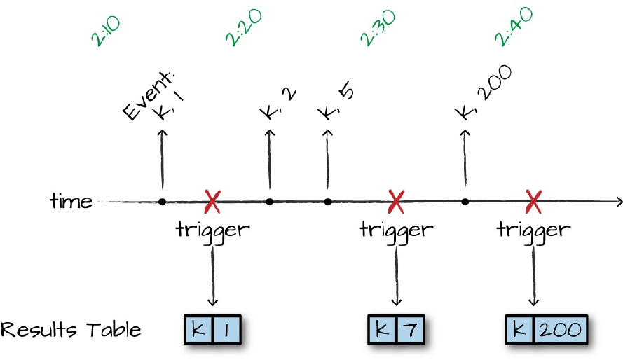
Figure 22-2. Tumbling Windows
We’re performing an aggregation of keys over a window of time. We update
the result table (depending on the output mode) when every trigger runs,
which will operate on the data received since the last trigger. In the case of
our actual dataset (and Figure 22-2), we’ll do so in 10-minute windows
without any overlap between them (each, and only one event can fall into one
window). This will update in real time, as well, meaning that if new events
were being added upstream to our system, Structured Streaming would
update those counts accordingly. This is the complete output mode, Spark
will output the entire result table regardless of whether we’ve seen the entire
dataset:
// in Scala
import org.apache.spark.sql.functions.{window, col}
withEventTime.groupBy(window(col("event_time"), "10 minutes")).count()
.writeStream
.queryName("events_per_window")
.format("memory")
.outputMode("complete")
.start()
# in Python
from pyspark.sql.functions import window, col
withEventTime.groupBy(window(col("event_time"), "10 minutes")).count()\
.writeStream\
.queryName("pyevents_per_window")\
.format("memory")\
.outputMode("complete")\
.start()
Now we’re writing out to the in-memory sink for debugging, so we can query
it with SQL after we have the stream running:
spark.sql("SELECT * FROM events_per_window").printSchema()
SELECT * FROM events_per_window
This shows us something like the following result, depending on the amount
of data processed when you had run the query:
+---------------------------------------------+-----+
|window |count|
+---------------------------------------------+-----+
|[2015-02-23 10:40:00.0,2015-02-23 10:50:00.0]|11035|
|[2015-02-24 11:50:00.0,2015-02-24 12:00:00.0]|18854|
...
|[2015-02-23 13:40:00.0,2015-02-23 13:50:00.0]|20870|
|[2015-02-23 11:20:00.0,2015-02-23 11:30:00.0]|9392 |
+---------------------------------------------+-----+
For reference, here’s the schema we get from the previous query:
root
|-- window: struct (nullable = false)
| |-- start: timestamp (nullable = true)
| |-- end: timestamp (nullable = true)
|-- count: long (nullable = false)
Notice how window is actually a struct (a complex type). Using this we can
query this struct for the start and end times of a particular window.
Of importance is the fact that we can also perform an aggregation on multiple
columns, including the event time column. Just like we saw in the previous
chapter, we can even perform these aggregations using methods like cube.
While we won’t repeat the fact that we can perform the multi-key aggregation
below, this does apply to any window-style aggregation (or stateful
computation) we would like:
// in Scala
import org.apache.spark.sql.functions.{window, col}
withEventTime.groupBy(window(col("event_time"), "10 minutes"), "User").count()
.writeStream
.queryName("events_per_window")
.format("memory")
.outputMode("complete")
.start()
# in Python
from pyspark.sql.functions import window, col
withEventTime.groupBy(window(col("event_time"), "10 minutes"), "User").count()\
.writeStream\
.queryName("pyevents_per_window")\
.format("memory")\
.outputMode("complete")\
.start()
Sliding windows
The previous example was simple counts in a given window. Another
approach is that we can decouple the window from the starting time of the
window. Figure 22-3 illustrates what we mean.

Figure 22-3. Sliding Windows
In the figure, we are running a sliding window through which we look at an
hour increment, but we’d like to get the state every 10 minutes. This means
that we will update the values over time and will include the last hours of
data. In this example, we have 10-minute windows, starting every five
minutes. Therefore each event will fall into two different windows. You can
tweak this further according to your needs:
// in Scala
import org.apache.spark.sql.functions.{window, col}
withEventTime.groupBy(window(col("event_time"), "10 minutes", "5 minutes"))
.count()
.writeStream
.queryName("events_per_window")
.format("memory")
.outputMode("complete")
.start()
# in Python
from pyspark.sql.functions import window, col
withEventTime.groupBy(window(col("event_time"), "10 minutes", "5 minutes"))\
.count()\
.writeStream\
.queryName("pyevents_per_window")\
.format("memory")\
.outputMode("complete")\
.start()
Naturally, we can query the in-memory table:
SELECT * FROM events_per_window
This query gives us the following result. Note that the starting times for each
window are now in 5-minute intervals instead of 10, like we saw in the
previous query:
+---------------------------------------------+-----+
|window |count|
+---------------------------------------------+-----+
|[2015-02-23 14:15:00.0,2015-02-23 14:25:00.0]|40375|
|[2015-02-24 11:50:00.0,2015-02-24 12:00:00.0]|56549|
...
|[2015-02-24 11:45:00.0,2015-02-24 11:55:00.0]|51898|
|[2015-02-23 10:40:00.0,2015-02-23 10:50:00.0]|33200|
+---------------------------------------------+-----+
Handling Late Data with Watermarks
The preceding examples are great, but they have a flaw. We never specified
how late we expect to see data. This means that Spark is going to need to
store that intermediate data forever because we never specified a watermark,
or a time at which we don’t expect to see any more data. This applies to all
stateful processing that operates on event time. We must specify this
watermark in order to age-out data in the stream (and, therefore, state) so that
we don’t overwhelm the system over a long period of time.
Concretely, a watermark is an amount of time following a given event or set
of events after which we do not expect to see any more data from that time.
We know this can happen due to delays on the network, devices that lose a
connection, or any number of other issues. In the DStreams API, there was no
robust way to handle late data in this way—if an event occurred at a certain
time but did not make it to the processing system by the time the batch for a
given window started, it would show up in other processing batches.

Structured Streaming remedies this. In event time and stateful processing, a
given window’s state or set of data is decoupled from a processing window.
That means that as more events come in, Structured Streaming will continue
to update a window with more information.
Let’s return back to our event time example from the beginning of the
chapter, shown now in Figure 22-4.
Figure 22-4. Event Time Watermarking
In this example, let’s imagine that we frequently see some amount of delay
from our customers in Latin America. Therefore, we specify a watermark of
10 minutes. When doing this, we instruct Spark that any event that occurs
more than 10 “event-time” minutes past a previous event should be ignored.
Conversely, this also states that we expect to see every event within 10
minutes. After that, Spark should remove intermediate state and, depending
on the output mode, do something with the result. As mentioned at the
beginning of the chapter, we need to specify watermarks because if we did
not, we’d need to keep all of our windows around forever, expecting them to
be updated forever. This brings us to the core question when working with
event-time: “how late do I expect to see data?” The answer to this question
will be the watermark that you’ll configure for your data.
Returning to our dataset, if we know that we typically see data as produced
downstream in minutes but we have seen delays in events up to five hours
after they occur (perhaps the user lost cell phone connectivity), we’d specify
the watermark in the following way:
// in Scala
import org.apache.spark.sql.functions.{window, col}
withEventTime
.withWatermark("event_time", "5 hours")
.groupBy(window(col("event_time"), "10 minutes", "5 minutes"))
.count()
.writeStream
.queryName("events_per_window")
.format("memory")
.outputMode("complete")
.start()
# in Python
from pyspark.sql.functions import window, col
withEventTime\
.withWatermark("event_time", "30 minutes")\
.groupBy(window(col("event_time"), "10 minutes", "5 minutes"))\
.count()\
.writeStream\
.queryName("pyevents_per_window")\
.format("memory")\
.outputMode("complete")\
.start()
It’s pretty amazing, but almost nothing changed about our query. We
essentially just added another configuration. Now, Structured Streaming will
wait until 30 minutes after the final timestamp of this 10-minute rolling
window before it finalizes the result of that window. We can query our table
and see the intermediate results because we’re using complete mode—
they’ll be updated over time. In append mode, this information won’t be
output until the window closes.
SELECT * FROM events_per_window
+---------------------------------------------+-----+
|window |count|
+---------------------------------------------+-----+
|[2015-02-23 14:15:00.0,2015-02-23 14:25:00.0]|9505 |
|[2015-02-24 11:50:00.0,2015-02-24 12:00:00.0]|13159|
...
|[2015-02-24 11:45:00.0,2015-02-24 11:55:00.0]|12021|
|[2015-02-23 10:40:00.0,2015-02-23 10:50:00.0]|7685 |
+---------------------------------------------+-----+
At this point, you really know all that you need to know about handling late
data. Spark does all of the heavy lifting for you. Just to reinforce the point, if
you do not specify how late you think you will see data, then Spark will
maintain that data in memory forever. Specifying a watermark allows it to
free those objects from memory, allowing your stream to continue running
for a long time.
Dropping Duplicates in a Stream
One of the more difficult operations in record-at-a-time systems is removing
duplicates from the stream. Almost by definition, you must operate on a
batch of records at a time in order to find duplicates—there’s a high
coordination overhead in the processing system. Deduplication is an
important tool in many applications, especially when messages might be
delivered multiple times by upstream systems. A perfect example of this are
Internet of Things (IoT) applications that have upstream producers generating
messages in nonstable network environments, and the same message might

end up being sent multiple times. Your downstream applications and
aggregations should be able to assume that there is only one of each message.
Essentially, Structured Streaming makes it easy to take message systems that
provide at-least-once semantics, and convert them into exactly-once by
dropping duplicate messages as they come in, based on arbitrary keys. To de-
duplicate data, Spark will maintain a number of user specified keys and
ensure that duplicates are ignored.
WARNING
Just like other stateful processing applications, you need to specify a watermark to ensure
that the maintained state does not grow infinitely over the course of your stream.
Let’s begin the de-duplication process. The goal here will be to de-duplicate
the number of events per user by removing duplicate events. Notice how you
need to specify the event time column as a duplicate column along with the
column you should de-duplicate. The core assumption is that duplicate events
will have the same timestamp as well as identifier. In this model, rows with
two different timestamps are two different records:
// in Scala
import org.apache.spark.sql.functions.expr
withEventTime
.withWatermark("event_time", "5 seconds")
.dropDuplicates("User", "event_time")
.groupBy("User")
.count()
.writeStream
.queryName("deduplicated")
.format("memory")
.outputMode("complete")
.start()
# in Python
from pyspark.sql.functions import expr
withEventTime\

.withWatermark("event_time", "5 seconds")\
.dropDuplicates(["User", "event_time"])\
.groupBy("User")\
.count()\
.writeStream\
.queryName("pydeduplicated")\
.format("memory")\
.outputMode("complete")\
.start()
The result will be similar to the following and will continue to update over
time as more data is read by your stream:
+----+-----+
|User|count|
+----+-----+
| a| 8085|
| b| 9123|
| c| 7715|
| g| 9167|
| h| 7733|
| e| 9891|
| f| 9206|
| d| 8124|
| i| 9255|
+----+-----+
Arbitrary Stateful Processing
The first section if this chapter demonstrates how Spark maintains
information and updates windows based on our specifications. But things
differ when you have more complex concepts of windows; this is, where
arbitrary stateful processing comes in. This section includes several examples
of different use cases along with examples that show you how you might go
about setting up your business logic. Stateful processing is available only in
Scala in Spark 2.2. This will likely change in the future.
When performing stateful processing, you might want to do the following:
Create window based on counts of a given key

Emit an alert if there is a number of events within a certain time
frame
Maintain user sessions of an undetermined amount of time and save
those sessions to perform some analysis on later.
At the end of the day, there are two things you will want to do when
performing this style of processing:
Map over groups in your data, operate on each group of data, and
generate at most a single row for each group. The relevant API for
this use case is mapGroupsWithState.
Map over groups in your data, operate on each group of data, and
generate one or more rows for each group. The relevant API for this
use case is flatMapGroupsWithState.
When we say “operate” on each group of data, that means that you can
arbitrarily update each group independent of any other group of data. This
means that you can define arbitrary window types that don’t conform to
tumbling or sliding windows like we saw previously in the chapter. One
important benefit that we get when we perform this style of processing is
control over configuring time-outs on state. With windows and watermarks,
it’s very simple: you simply time-out a window when the watermark passes
the window start. This doesn’t apply to arbitrary stateful processing, because
you manage the state based on user-defined concepts. Therefore, you need to
properly time-out your state. Let’s discuss this a bit more.
Time-Outs
As mentioned in Chapter 21, a time-out specifies how long you should wait
before timing-out some intermediate state. A time-out is a global parameter
across all groups that is configured on a per-group basis. Time-outs can be
either based on processing time
(GroupStateTimeout.ProcessingTimeTimeout) or event time
(GroupStateTimeout.EventTimeTimeout). When using time-outs, check

for time-out first before processing the values. You can get this information
by checking the state.hasTimedOut flag or checking whether the values
iterator is empty. You need to set some state (i.e., state must be defined, not
removed) for time-outs to be set.
With a time-out based on processing time, you can set the time-out duration
by calling GroupState.setTimeoutDuration (we’ll see code examples of
this later in this section of the chapter). The time-out will occur when the
clock has advanced by the set duration. Guarantees provided by this time-out
with a duration of D ms are as follows:
Time-out will never occur before the clock time has advanced by D
ms
Time-out will occur eventually when there is a trigger in the query
(i.e., after D ms). So there is a no strict upper bound on when the
time-out would occur. For example, the trigger interval of the query
will affect when the time-out actually occurs. If there is no data in
the stream (for any group) for a while, there won’t be any trigger and
the time-out function call will not occur until there is data.
Because the processing time time-out is based on the clock time, it is affected
by the variations in the system clock. This means that time zone changes and
clock skew are important variables to consider.
With a time-out based on event time, the user also must specify the event-
time watermark in the query using watermarks. When set, data older than the
watermark is filtered out. As the developer, you can set the timestamp that
the watermark should reference by setting a time-out timestamp using the
GroupState.setTimeoutTimestamp(...) API. The time-out would occur
when the watermark advances beyond the set timestamp. Naturally, you can
control the time-out delay by either specifying longer watermarks or simply
updating the time-out as you process your stream. Because you can do this in
arbitrary code, you can do it on a per-group basis. The guarantee provided by
this time-out is that it will never occur before the watermark has exceeded the
set time-out.

Similar to processing-time time-outs, there is a no strict upper bound on the
delay when the time-out actually occurs. The watermark can advance only
when there is data in the stream, and the event time of the data has actually
advanced.
NOTE
We mentioned this a few moments ago, but it’s worth reinforcing. Although time-outs are
important, they might not always function as you expect. For instance, as of this writing,
Structured Streaming does not have asynchronous job execution, which means that Spark
will not output data (or time-out data) between the time that a epoch finishes and the next
one starts, because it is not processing any data at that time. Also, if a processing batch of
data has no records (keep in mind this is a batch, not a group), there are no updates and
there cannot be an event-time time-out. This might change in future versions.
Output Modes
One last “gotcha” when working with this sort of arbitrary stateful processing
is the fact that not all output modes discussed in Chapter 21 are supported.
This is sure to change as Spark continues to change, but, as of this writing,
mapGroupsWithState supports only the update output mode, whereas
flatMapGroupsWithState supports append and update. append mode
means that only after the time-out (meaning the watermark has passed) will
data show up in the result set. This does not happen automatically, it is your
responsibility to output the proper row or rows.
Please see Table 21-1 to see which output modes can be used when.
mapGroupsWithState
Our first example of stateful processing uses a feature called
mapGroupsWithState. This is similar to a user-defined aggregation function
that takes as input an update set of data and then resolves it down to a
specific key with a set of values. There are several things you’re going to
need to define along the way:

Three class definitions: an input definition, a state definition, and
optionally an output definition.
A function to update the state based on a key, an iterator of events,
and a previous state.
A time-out parameter (as described in the time-outs section).
With these objects and definitions, you can control arbitrary state by creating
it, updating it over time, and removing it. Let’s begin with a example of
simply updating the key based on a certain amount of state, and then move
onto more complex things like sessionization.
Because we’re working with sensor data, let’s find the first and last
timestamp that a given user performed one of the activities in the dataset.
This means that the key we will be grouping on (and mapping on) is a user
and activity combination.
NOTE
When you use mapGroupsWithState, the output of the dream will contain only one row
per key (or group) at all times. If you would like each group to have multiple outputs, you
should use flatMapGroupsWithState (covered shortly).
Let’s establish the input, state, and output definitions:
case class InputRow(user:String, timestamp:java.sql.Timestamp, activity:String)
case class UserState(user:String,
var activity:String,
var start:java.sql.Timestamp,
var end:java.sql.Timestamp)
For readability, set up the function that defines how you will update your
state based on a given row:
def updateUserStateWithEvent(state:UserState, input:InputRow):UserState = {
if (Option(input.timestamp).isEmpty) {
return state
}
if (state.activity == input.activity) {
if (input.timestamp.after(state.end)) {
state.end = input.timestamp
}
if (input.timestamp.before(state.start)) {
state.start = input.timestamp
}
} else {
if (input.timestamp.after(state.end)) {
state.start = input.timestamp
state.end = input.timestamp
state.activity = input.activity
}
}
state
}
Now, write the function that defines the way state is updated based on an
epoch of rows:
import org.apache.spark.sql.streaming.{GroupStateTimeout, OutputMode,
GroupState}
def updateAcrossEvents(user:String,
inputs: Iterator[InputRow],
oldState: GroupState[UserState]):UserState = {
var state:UserState = if (oldState.exists) oldState.get else UserState(user,
"",
new java.sql.Timestamp(6284160000000L),
new java.sql.Timestamp(6284160L)
)
// we simply specify an old date that we can compare against and
// immediately update based on the values in our data
for (input <- inputs) {
state = updateUserStateWithEvent(state, input)
oldState.update(state)
}
state
}
When we have that, it’s time to start your query by passing in the relevant
information. The one thing that you’re going to have to add when you specify

mapGroupsWithState is whether you need to time-out a given group’s state.
This just gives you a mechanism to control what should be done with state
that receives no update after a certain amount of time. In this case, you want
to maintain state indefinitely, so specify that Spark should not time-out.
Use the update output mode so that you get updates on the user activity:
import org.apache.spark.sql.streaming.GroupStateTimeout
withEventTime
.selectExpr("User as user",
"cast(Creation_Time/1000000000 as timestamp) as timestamp", "gt as
activity")
.as[InputRow]
.groupByKey(_.user)
.mapGroupsWithState(GroupStateTimeout.NoTimeout)(updateAcrossEvents)
.writeStream
.queryName("events_per_window")
.format("memory")
.outputMode("update")
.start()
SELECT * FROM events_per_window order by user, start
Here’s a sample of our result set:
+----+--------+--------------------+--------------------+
|user|activity| start| end|
+----+--------+--------------------+--------------------+
| a| bike|2015-02-23 13:30:...|2015-02-23 14:06:...|
| a| bike|2015-02-23 13:30:...|2015-02-23 14:06:...|
...
| d| bike|2015-02-24 13:07:...|2015-02-24 13:42:...|
+----+--------+--------------------+--------------------+
An interesting aspect of our data is that the last activity performed at any
given time is “bike.” This is related to how the experiment was likely run, in
which they had each participant perform the same activities in order.
EXAMPLE: COUNT-BASED WINDOWS
Typical window operations are built from start and end times for which

all events that fall in between those two points contribute to the counting
or summation that you’re performing. However, there are times when
instead of creating windows based on time, you’d rather create them
based on a number of events regardless of state and event times, and
perform some aggregation on that window of data. For example, we may
want to compute a value for every 500 events received, regardless of
when they are received.
The next example analyzes the activity dataset from this chapter and
outputs the average reading of each device periodically, creating a
window based on the count of events and outputting it each time it has
accumulated 500 events for that device. You define two case classes for
this task: the input row format (which is simply a device and a
timestamp); and the state and output rows (which contain the current
count of records collected, device ID, and an array of readings for the
events in the window).
Here are our various, self-describing case class definitions:
case class InputRow(device: String, timestamp: java.sql.Timestamp, x:
Double)
case class DeviceState(device: String, var values: Array[Double],
var count: Int)
case class OutputRow(device: String, previousAverage: Double)
Now, you can define the function to update the individual state based on
a single input row. You could write this inline or in a number of other
ways, but this example makes it easy to see exactly how you update
based on a given row:
def updateWithEvent(state:DeviceState, input:InputRow):DeviceState = {
state.count += 1
// maintain an array of the x-axis values
state.values = state.values ++ Array(input.x)
state
}
Now it’s time to define the function that updates across a series of input

rows. Notice in the example that follows that we have a specific key, the
iterator of inputs, and the old state, and we update that old state over time
as we receive new events. This, in turn, will return our output rows with
the updates on a per-device level based on the number of counts it sees.
This case is quite straightforward, after a given number of events, you
update the state and reset it. You then create an output row. You can see
this row in the output table:
import org.apache.spark.sql.streaming.{GroupStateTimeout, OutputMode,
GroupState}
def updateAcrossEvents(device:String, inputs: Iterator[InputRow],
oldState: GroupState[DeviceState]):Iterator[OutputRow] = {
inputs.toSeq.sortBy(_.timestamp.getTime).toIterator.flatMap { input =>
val state = if (oldState.exists) oldState.get
else DeviceState(device, Array(), 0)
val newState = updateWithEvent(state, input)
if (newState.count >= 500) {
// One of our windows is complete; replace our state with an empty
// DeviceState and output the average for the past 500 items from
// the old state
oldState.update(DeviceState(device, Array(), 0))
Iterator(OutputRow(device,
newState.values.sum / newState.values.length.toDouble))
}
else {
// Update the current DeviceState object in place and output no
// records
oldState.update(newState)
Iterator()
}
}
}
Now you can run your stream. You will notice that you need to explicitly
state the output mode, which is append. You also need to set a
GroupStateTimeout. This time-out specifies the amount of time you
want to wait before a window should be output as complete (even if it did
not reach the required count). In that case, set an infinite time-out,
meaning if a device never gets to that required 500 count threshold, it will

maintain that state forever as “incomplete” and not output it to the result
table.
By specifying both of those parameters you can pass in the
updateAcrossEvents function and start the stream:
import org.apache.spark.sql.streaming.GroupStateTimeout
withEventTime
.selectExpr("Device as device",
"cast(Creation_Time/1000000000 as timestamp) as timestamp", "x")
.as[InputRow]
.groupByKey(_.device)
.flatMapGroupsWithState(OutputMode.Append,
GroupStateTimeout.NoTimeout)(updateAcrossEvents)
.writeStream
.queryName("count_based_device")
.format("memory")
.outputMode("append")
.start()
After you start the stream, it’s time to query it. Here are the results:
SELECT * FROM count_based_device
+--------+--------------------+
| device| previousAverage|
+--------+--------------------+
|nexus4_1| 4.660034012E-4|
|nexus4_1|0.001436279298199...|
...
|nexus4_1|1.049804683999999...|
|nexus4_1|-0.01837188737960...|
+--------+--------------------+
You can see the values change over each of those windows as you
append new data to the result set.
flatMapGroupsWithState
Our second example of stateful processing will use a feature called

flatMapGroupsWithState. This is quite similar to mapGroupsWithState
except that rather than just having a single key with at most one output, a
single key can have many outputs. This can provide us a bit more flexibility
and the same fundamental structure as mapGroupsWithState applies. Here’s
what we’ll need to define.
Three class definitions: an input definition, a state definition, and
optionally an output definition.
A function to update the state based on a key, an iterator of events,
and a previous state.
A time-out parameter (as described in the time-outs section).
With these objects and definitions, we can control arbitrary state by creating
it, updating it over time, and removing it. Let’s start with an example of
sessionization.

EXAMPLE: SESSIONIZATION
Sessions are simply unspecified time windows with a series of events that
occur. Typically, you want to record these different events in an array in
order to compare these sessions to other sessions in the future. In a
session, you will likely have arbitrary logic to maintain and update your
state over time as well as certain actions to define when state ends (like a
count) or a simple time-out. Let’s build on the previous example and
define it a bit more strictly as a session.
At times, you might have an explicit session ID that you can use in your
function. This obviously makes it much easier because you can just
perform a simple aggregation and might not even need your own stateful
logic. In this case, you’re creating sessions on the fly from a user ID and
some time information and if you see no new event from that user in five
seconds, the session terminates. You’ll also notice that this code uses
time-outs differently than we have in other examples.
You can follow the same process of creating your classes, defining our
single event update function and then the multievent update function:
case class InputRow(uid:String, timestamp:java.sql.Timestamp, x:Double,
activity:String)
case class UserSession(val uid:String, var timestamp:java.sql.Timestamp,
var activities: Array[String], var values: Array[Double])
case class UserSessionOutput(val uid:String, var activities: Array[String],
var xAvg:Double)
def updateWithEvent(state:UserSession, input:InputRow):UserSession = {
// handle malformed dates
if (Option(input.timestamp).isEmpty) {
return state
}
state.timestamp = input.timestamp
state.values = state.values ++ Array(input.x)
if (!state.activities.contains(input.activity)) {
state.activities = state.activities ++ Array(input.activity)
}
state

}
import org.apache.spark.sql.streaming.{GroupStateTimeout, OutputMode,
GroupState}
def updateAcrossEvents(uid:String,
inputs: Iterator[InputRow],
oldState: GroupState[UserSession]):Iterator[UserSessionOutput] = {
inputs.toSeq.sortBy(_.timestamp.getTime).toIterator.flatMap { input =>
val state = if (oldState.exists) oldState.get else UserSession(
uid,
new java.sql.Timestamp(6284160000000L),
Array(),
Array())
val newState = updateWithEvent(state, input)
if (oldState.hasTimedOut) {
val state = oldState.get
oldState.remove()
Iterator(UserSessionOutput(uid,
state.activities,
newState.values.sum / newState.values.length.toDouble))
} else if (state.values.length > 1000) {
val state = oldState.get
oldState.remove()
Iterator(UserSessionOutput(uid,
state.activities,
newState.values.sum / newState.values.length.toDouble))
} else {
oldState.update(newState)
oldState.setTimeoutTimestamp(newState.timestamp.getTime(), "5
seconds")
Iterator()
}
}
}
You’ll see in this one that we only expect to see an event at most five
seconds late. Anything other than that and we will ignore it. We will use
an EventTimeTimeout to set that we want to time-out based on the event
time in this stateful operation:
import org.apache.spark.sql.streaming.GroupStateTimeout

withEventTime.where("x is not null")
.selectExpr("user as uid",
"cast(Creation_Time/1000000000 as timestamp) as timestamp",
"x", "gt as activity")
.as[InputRow]
.withWatermark("timestamp", "5 seconds")
.groupByKey(_.uid)
.flatMapGroupsWithState(OutputMode.Append,
GroupStateTimeout.EventTimeTimeout)(updateAcrossEvents)
.writeStream
.queryName("count_based_device")
.format("memory")
.start()
Querying this table will show you the output rows for each user over this
time period:
SELECT * FROM count_based_device
+---+--------------------+--------------------+
|uid| activities| xAvg|
+---+--------------------+--------------------+
| a| [stand, null, sit]|-9.10908533566433...|
| a| [sit, null, walk]|-0.00654280428601...|
...
| c|[null, stairsdown...|-0.03286657789999995|
+---+--------------------+--------------------+
As you might expect, sessions that have a number of activities in them
have a higher x-axis gyroscope value than ones that have fewer activities.
It should be trivial to extend this example to problem sets more relevant
to your own domain, as well.
Conclusion
This chapter covered some of the more advanced topics in Structured
Streaming, including event time and stateful processing. This is effectively
the user guide to help you actually build out your application logic and turn it
into something that provides value. Next, we will discuss what we’ll need to
do in order to take this application to production and maintain and update it
over time.

Chapter 23. Structured
Streaming in Production
The previous chapters of this part of the book have covered Structured
Streaming from a user’s perspective. Naturally this is the core of your
application. This chapter covers some of the operational tools needed to run
Structured Streaming robustly in production after you’ve developed an
application.
Structured Streaming was marked as production-ready in Apache Spark
2.2.0, meaning that this release has all the features required for production
use and stabilizes the API. Many organizations are already using the system
in production because, frankly, it’s not much different from running other
production Spark applications. Indeed, through features such as transactional
sources/sinks and exactly-once processing, the Structured Streaming
designers sought to make it as easy to operate as possible. This chapter will
walk you through some of the key operational tasks specific to Structured
Streaming. This should supplement everything we saw and learned about
Spark operations in Part II.
Fault Tolerance and Checkpointing
The most important operational concern for a streaming application is failure
recovery. Faults are inevitable: you’re going to lose a machine in the cluster,
a schema will change by accident without a proper migration, or you may
even intentionally restart the cluster or application. In any of these cases,
Structured Streaming allows you to recover an application by just restarting
it. To do this, you must configure the application to use checkpointing and
write-ahead logs, both of which are handled automatically by the engine.
Specifically, you must configure a query to write to a checkpoint location on
a reliable file system (e.g., HDFS, S3, or any compatible filesystem).
Structured Streaming will then periodically save all relevant progress
information (for instance, the range of offsets processed in a given trigger) as
well as the current intermediate state values to the checkpoint location. In a
failure scenario, you simply need to restart your application, making sure to
point to the same checkpoint location, and it will automatically recover its
state and start processing data where it left off. You do not have to manually
manage this state on behalf of the application—Structured Streaming does it
for you.
To use checkpointing, specify your checkpoint location before starting your
application through the checkpointLocation option on writeStream. You
can do this as follows:
// in Scala
val static = spark.read.json("/data/activity-data")
val streaming = spark
.readStream
.schema(static.schema)
.option("maxFilesPerTrigger", 10)
.json("/data/activity-data")
.groupBy("gt")
.count()
val query = streaming
.writeStream
.outputMode("complete")
.option("checkpointLocation", "/some/location/")
.queryName("test_stream")
.format("memory")
.start()
# in Python
static = spark.read.json("/data/activity-data")
streaming = spark\
.readStream\
.schema(static.schema)\
.option("maxFilesPerTrigger", 10)\
.json("/data/activity-data")\
.groupBy("gt")\
.count()
query = streaming\
.writeStream\
.outputMode("complete")\
.option("checkpointLocation", "/some/python/location/")\
.queryName("test_python_stream")\
.format("memory")\
.start()
If you lose your checkpoint directory or the information inside of it, your
application will not be able to recover from failures and you will have to
restart your stream from scratch.
Updating Your Application
Checkpointing is probably the most important thing to enable in order to run
your applications in production. This is because the checkpoint will store all
of the information about what your stream has processed thus far and what
the intermediate state it may be storing is. However, checkpointing does
come with a small catch—you’re going to have to reason about your old
checkpoint data when you update your streaming application. When you
update your application, you’re going to have to ensure that your update is
not a breaking change. Let’s cover these in detail when we review the two
types of updates: either an update to your application code or running a new
Spark version.
Updating Your Streaming Application Code
Structured Streaming is designed to allow certain types of changes to the
application code between application restarts. Most importantly, you are
allowed to change user-defined functions (UDFs) as long as they have the
same type signature. This feature can be very useful for bug fixes. For
example, imagine that your application starts receiving a new type of data,
and one of the data parsing functions in your current logic crashes. With
Structured Streaming, you can recompile the application with a new version
of that function and pick up at the same point in the stream where it crashed
earlier.
While small adjustments like adding a new column or changing a UDF are
not breaking changes and do not require a new checkpoint directory, there are
larger changes that do require an entirely new checkpoint directory. For
example, if you update your streaming application to add a new aggregation
key or fundamentally change the query itself, Spark cannot construct the
required state for the new query from an old checkpoint directory. In these
cases, Structured Streaming will throw an exception saying it cannot begin
from a checkpoint directory, and you must start from scratch with a new
(empty) directory as your checkpoint location.
Updating Your Spark Version
Structured Streaming applications should be able to restart from an old
checkpoint directory across patch version updates to Spark (e.g., moving
from Spark 2.2.0 to 2.2.1 to 2.2.2). The checkpoint format is designed to be
forward-compatible, so the only way it may be broken is due to critical bug
fixes. If a Spark release cannot recover from old checkpoints, this will be
clearly documented in its release notes. The Structured Streaming developers
also aim to keep the format compatible across minor version updates (e.g.,
Spark 2.2.x to 2.3.x), but you should check the release notes to see whether
this is supported for each upgrade. In either case, if you cannot start from a
checkpoint, you will need to start your application again using a new
checkpoint directory.
Sizing and Rescaling Your Application
In general, the size of your cluster should be able to comfortably handle
bursts above your data rate. The key metrics you should be monitoring in
your application and cluster are discussed as follows. In general, if you see
that your input rate is much higher than your processing rate (elaborated upon
momentarily), it’s time to scale up your cluster or application. Depending on
your resource manager and deployment, you may just be able to dynamically
add executors to your application. When it comes time, you can scale-down
your application in the same way—remove executors (potentially through
your cloud provider) or restart your application with lower resource counts.
These changes will likely incur some processing delay (as data is recomputed
or partitions are shuffled around when executors are removed). In the end,
it’s a business decision as to whether it’s worthwhile to create a system with
more sophisticated resource management capabilities.
While making underlying infrastructure changes to the cluster or application
are sometimes necessary, other times a change may only require a restart of
the application or stream with a new configuration. For instance, changing
spark.sql.shuffle.partitions is not supported while a stream is
currently running (it won’t actually change the number of shuffle partitions).
This requires restarting the actual stream, not necessarily the entire
application. Heavier weight changes, like changing arbitrary Spark
application configurations, will likely require an application restart.
Metrics and Monitoring
Metrics and monitoring in streaming applications is largely the same as for
general Spark applications using the tools described in Chapter 18. However,
Structured Streaming does add several more specifics in order to help you
better understand the state of your application. There are two key APIs you
can leverage to query the status of a streaming query and see its recent
execution progress. With these two APIs, you can get a sense of whether or
not your stream is behaving as expected.
Query Status
The query status is the most basic monitoring API, so it’s a good starting
point. It aims to answer the question, “What processing is my stream
performing right now?” This information is reported in the status field of
the query object returned by startStream. For example, you might have a
simple counts stream that provides counts of IOT devices defined by the
following query (here we’re just using the same query from the previous
chapter without the initialization code):
query.status
To get the status of a given query, simply running the command
query.status will return the current status of the stream. This gives us

details about what is happening at that point in time in the stream. Here’s a
sample of what you’ll get back when querying this status:
{
"message" : "Getting offsets from ...",
"isDataAvailable" : true,
"isTriggerActive" : true
}
The above snippet describes getting the offsets from a Structured Streaming
data source (hence the message describing getting offsets). There are a
variety of messages to describe the stream’s status.
NOTE
We have shown the status command inline here the way you would call it in a Spark shell.
However, for a standalone application, you may not have a shell attached to run arbitrary
code inside your process. In that case, you can expose its status by implementing a
monitoring server, such as a small HTTP server that listens on a port and returns
query.status when it gets a request. Alternatively, you can use the richer
StreamingQueryListener API described later to listen to more events.
Recent Progress
While the query’s current status is useful to see, equally important is an
ability to view the query’s progress. The progress API allows us to answer
questions like “At what rate am I processing tuples?” or “How fast are tuples
arriving from the source?” By running query.recentProgress, you’ll get
access to more time-based information like the processing rate and batch
durations. The streaming query progress also includes information about the
input sources and output sinks behind your stream.
query.recentProgress
Here’s the result of the Scala version after we ran the code from before; the
Python one will be similar:
Array({
"id" : "d9b5eac5-2b27-4655-8dd3-4be626b1b59b",
"runId" : "f8da8bc7-5d0a-4554-880d-d21fe43b983d",
"name" : "test_stream",
"timestamp" : "2017-08-06T21:11:21.141Z",
"numInputRows" : 780119,
"processedRowsPerSecond" : 19779.89350912779,
"durationMs" : {
"addBatch" : 38179,
"getBatch" : 235,
"getOffset" : 518,
"queryPlanning" : 138,
"triggerExecution" : 39440,
"walCommit" : 312
},
"stateOperators" : [ {
"numRowsTotal" : 7,
"numRowsUpdated" : 7
} ],
"sources" : [ {
"description" : "FileStreamSource[/some/stream/source/]",
"startOffset" : null,
"endOffset" : {
"logOffset" : 0
},
"numInputRows" : 780119,
"processedRowsPerSecond" : 19779.89350912779
} ],
"sink" : {
"description" : "MemorySink"
}
})
As you can see from the output just shown, this includes a number of details
about the state of the stream. It is important to note that this is a snapshot in
time (according to when we asked for the query progress). In order to
consistently get output about the state of the stream, you’ll need to query this
API for the updated state repeatedly. The majority of the fields in the
previous output should be self-explanatory. However, let’s review some of
the more consequential fields in detail.
Input rate and processing rate
The input rate specifies how much data is flowing into Structured Streaming

from our input source. The processing rate is how quickly the application is
able to analyze that data. In the ideal case, the input and processing rates
should vary together. Another case might be when the input rate is much
greater than the processing rate. When this happens, the stream is falling
behind and you will need to scale the cluster up to handle the larger load.
Batch duration
Nearly all streaming systems utilize batching to operate at any reasonable
throughput (some have an option of high latency in exchange for lower
throughput). Structured Streaming achieves both. As it operates on the data,
you will likely see batch duration oscillate as Structured Streaming processes
varying numbers of events over time. Naturally, this metric will have little to
no relevance when the continuous processing engine is made an execution
option.
TIP
Generally it’s a best practice to visualize the changes in batch duration and input and
processing rates. It’s much more helpful than simply reporting changes over time.
Spark UI
The Spark web UI, covered in detail in Chapter 18, also shows tasks, jobs,
and data processing metrics for Structured Streaming applications. On the
Spark UI, each streaming application will appear as a sequence of short jobs,
one for each trigger. However, you can use the same UI to see metrics, query
plans, task durations, and logs from your application. One departure of note
from the DStream API is that the Streaming Tab is not used by Structured
Streaming.
Alerting
Understanding and looking at the metrics for your Structured Streaming
queries is an important first step. However, this involves constantly watching
a dashboard or the metrics in order to discover potential issues. You’re going
to need robust automatic alerting to notify you when your jobs are failing or
not keeping up with the input data rate without monitoring them manually.
There are several ways to integrate existing alerting tools with Spark,
generally building on the recent progress API we covered before. For
example, you may directly feed the metrics to a monitoring system such as
the open source Coda Hale Metrics library or Prometheus, or you may simply
log them and use a log aggregation system like Splunk. In addition to
monitoring and alerting on queries, you’re also going to want to monitor and
alert on the state of the cluster and the overall application (if you’re running
multiple queries together).
Advanced Monitoring with the Streaming
Listener
We already touched on some of the high-level monitoring tools in Structured
Streaming. With a bit of glue logic, you can use the status and queryProgress
APIs to output monitoring events into your organization’s monitoring
platform of choice (e.g., a log aggregation system or Prometheus dashboard).
Beyond these approaches, there is also a lower-level but more powerful way
to observe an application’s execution: the StreamingQueryListener class.
The StreamingQueryListener class will allow you to receive asynchronous
updates from the streaming query in order to automatically output this
information to other systems and implement robust monitoring and alerting
mechanisms. You start by developing your own object to extend
StreamingQueryListener, then attach it to a running SparkSession. Once
you attach your custom listener with
sparkSession.streams.addListener(), your class will receive
notifications when a query is started or stopped, or progress is made on an
active query. Here’s a simple example of a listener from the Structured
Streaming documentation:
val spark: SparkSession = ...
spark.streams.addListener(new StreamingQueryListener() {
override def onQueryStarted(queryStarted: QueryStartedEvent): Unit = {
println("Query started: " + queryStarted.id)
}
override def onQueryTerminated(
queryTerminated: QueryTerminatedEvent): Unit = {
println("Query terminated: " + queryTerminated.id)
}
override def onQueryProgress(queryProgress: QueryProgressEvent): Unit = {
println("Query made progress: " + queryProgress.progress)
}
})
Streaming listeners allow you to process each progress update or status
change using custom code and pass it to external systems. For example, the
following code for a StreamingQueryListener that will forward all query
progress information to Kafka. You’ll have to parse this JSON string once
you read data from Kafka in order to access the actual metrics:
class KafkaMetrics(servers: String) extends StreamingQueryListener {
val kafkaProperties = new Properties()
kafkaProperties.put(
"bootstrap.servers",
servers)
kafkaProperties.put(
"key.serializer",
"kafkashaded.org.apache.kafka.common.serialization.StringSerializer")
kafkaProperties.put(
"value.serializer",
"kafkashaded.org.apache.kafka.common.serialization.StringSerializer")
val producer = new KafkaProducer[String, String](kafkaProperties)
import org.apache.spark.sql.streaming.StreamingQueryListener
import org.apache.kafka.clients.producer.KafkaProducer
override def onQueryProgress(event:
StreamingQueryListener.QueryProgressEvent): Unit = {
producer.send(new ProducerRecord("streaming-metrics",
event.progress.json))
}
override def onQueryStarted(event:
StreamingQueryListener.QueryStartedEvent): Unit = {}
override def onQueryTerminated(event:
StreamingQueryListener.QueryTerminatedEvent): Unit = {}
}
Using the StreamingQueryListener interface, you can even monitor
Structured Streaming applications on one cluster by running a Structured
Streaming application on that same (or another) cluster. You could also
manage multiple streams in this way.
Conclusion
In this chapter, we covered the main tools needed to run Structured Streaming
in production: checkpoints for fault tolerance and various monitoring APIs
that let you observe how your application is running. Lucky for you, if you’re
running Spark in production already, many of the concepts and tools are
similar, so you should be able to reuse a lot of your existing knowledge. Be
sure to check Part IV to see some other helpful tools for monitoring Spark
Applications.

Part VI. Advanced Analytics and
Machine Learning
Chapter 24. Advanced Analytics
and Machine Learning Overview
Thus far, we have covered fairly general data flow APIs. This part of the
book will dive deeper into some of the more specific advanced analytics APIs
available in Spark. Beyond large-scale SQL analysis and streaming, Spark
also provides support for statistics, machine learning, and graph analytics.
These encompass a set of workloads that we will refer to as advanced
analytics. This part of the book will cover advanced analytics tools in Spark,
including:
Preprocessing your data (cleaning data and feature engineering)
Supervised learning
Recommendation learning
Unsupervised engines
Graph analytics
Deep learning
This chapter offers a basic overview of advanced analytics, some example
use cases, and a basic advanced analytics workflow. Then we’ll cover the
analytics tools just listed and teach you how to apply them.
WARNING
This book is not intended to teach you everything you need to know about machine
learning from scratch. We won’t go into strict mathematical definitions and formulations
—not for lack of importance but simply because it’s too much information to include. This
part of the book is not an algorithm guide that will teach you the mathematical
underpinnings of every available algorithm nor the in-depth implementation strategies
used. The chapters included here serve as a guide for users, with the purpose of outlining
what you need to know to use Spark’s advanced analytics APIs.
A Short Primer on Advanced Analytics
Advanced analytics refers to a variety of techniques aimed at solving the core
problem of deriving insights and making predictions or recommendations
based on data. The best ontology for machine learning is structured based on
the task that you’d like to perform. The most common tasks include:
Supervised learning, including classification and regression, where
the goal is to predict a label for each data point based on various
features.
Recommendation engines to suggest products to users based on
behavior.
Unsupervised learning, including clustering, anomaly detection, and
topic modeling, where the goal is to discover structure in the data.
Graph analytics tasks such as searching for patterns in a social
network.
Before discussing Spark’s APIs in detail, let’s review each of these tasks
along with some common machine learning and advanced analytics use
cases. While we have certainly tried to make this introduction as accessible as
possible, at times you may need to consult other resources in order to fully
understand the material. O’Reilly should we link to or mention any specific
ones? Additionally, we will cite the following books throughout the next few
chapters because they are great resources for learning more about the
individual analytics (and, as a bonus, they are freely available on the web):
An Introduction to Statistical Learning by Gareth James, Daniela
Witten, Trevor Hastie, and Robert Tibshirani. We refer to this book
as “ISL.”
Elements of Statistical Learning by Trevor Hastie, Robert
Tibshirani, and Jerome Friedman. We refer to this book as “ESL.”

Deep Learning by Ian Goodfellow, Yoshua Bengio, and Aaron
Courville. We refer to this book as “DLB.”
Supervised Learning
Supervised learning is probably the most common type of machine learning.
The goal is simple: using historical data that already has labels (often called
the dependent variables), train a model to predict the values of those labels
based on various features of the data points. One example would be to predict
a person’s income (the dependent variable) based on age (a feature). This
training process usually proceeds through an iterative optimization algorithm
such as gradient descent. The training algorithm starts with a basic model and
gradually improves it by adjusting various internal parameters (coefficients)
during each training iteration. The result of this process is a trained model
that you can use to make predictions on new data. There are a number of
different tasks we’ll need to complete as part of the process of training and
making predictions, such as measuring the success of trained models before
using them in the field, but the fundamental principle is simple: train on
historical data, ensure that it generalizes to data we didn’t train on, and then
make predictions on new data.
We can further organize supervised learning based on the type of variable
we’re looking to predict. We’ll get to that next.
Classification
One common type of supervised learning is classification. Classification is
the act of training an algorithm to predict a dependent variable that is
categorical (belonging to a discrete, finite set of values). The most common
case is binary classification, where our resulting model will make a
prediction that a given item belongs to one of two groups. The canonical
example is classifying email spam. Using a set of historical emails that are
organized into groups of spam emails and not spam emails, we train an
algorithm to analyze the words in, and any number of properties of, the
historical emails and make predictions about them. Once we are satisfied with
the algorithm’s performance, we use that model to make predictions about
future emails the model has never seen before.
When we classify items into more than just two categories, we call this
multiclass classification. For example, we may have four different categories
of email (as opposed to the two categories in the previous paragraph): spam,
personal, work related, and other. There are many use cases for classification,
including:
Predicting disease
A doctor or hospital might have a historical dataset of behavioral and
physiological attributes of a set of patients. They could use this dataset to
train a model on this historical data (and evaluate its success and ethical
implications before applying it) and then leverage it to predict whether or
not a patient has heart disease or not. This is an example of binary
classification (healthy heart, unhealthy heart) or multiclass classification
(healthly heart, or one of several different diseases).
Classifying images
There are a number of applications from companies like Apple, Google,
or Facebook that can predict who is in a given photo by running a
classification model that has been trained on historical images of people
in your past photos. Another common use case is to classify images or
label the objects in images.
Predicting customer churn
A more business-oriented use case might be predicting customer churn—
that is, which customers are likely to stop using a service. You can do this
by training a binary classifier on past customers that have churned (and
not churned) and using it to try and predict whether or not current
customers will churn.
Buy or won’t buy
Companies often want to predict whether visitors of their website will
purchase a given product. They might use information about users’
browsing pattern or attributes such as location in order to drive this
prediction.
There are many more use cases for classification beyond these examples. We
will introduce more use cases, as well as Spark’s classification APIs, in
Chapter 26.
Regression
In classification, our dependent variable is a set of discrete values. In
regression, we instead try to predict a continuous variable (a real number). In
simplest terms, rather than predicting a category, we want to predict a value
on a number line. The rest of the process is largely the same, which is why
they’re both forms of supervised learning. We will train on historical data to
make predictions about data we have never seen. Here are some typical
examples:
Predicting sales
A store may want to predict total product sales on given data using
historical sales data. There are a number of potential input variables, but a
simple example might be using last week’s sales data to predict the next
day’s data.
Predicting height
Based on the heights of two individuals, we might want to predict the
heights of their potential children.
Predicting the number of viewers of a show
A media company like Netflix might try to predict how many of their
subscribers will watch a particular show.
We will introduce more use cases, as well as Spark’s methods for regression,
in Chapter 27.
Recommendation
Recommendation is one of the most intuitive applications of advanced
analytics. By studying people’s explicit preferences (through ratings) or
implicit ones (through observed behavior) for various products or items, an
algorithm can make recommendations on what a user may like by drawing
similarities between the users or items. By looking at these similarities, the
algorithm makes recommendations to users based on what similar users liked,
or what other products resemble the ones the user already purchased.
Recommendation is a common use case for Spark and well suited to big data.
Here are some example use cases:
Movie recommendations
Netflix uses Spark, although not necessarily its built-in libraries, to make
large-scale movie recommendations to its users. It does this by studying
what movies users watch and do not watch in the Netflix application. In
addition, Netflix likely takes into consideration how similar a given user’s
ratings are to other users’.
Product recommendations
Amazon uses product recommendations as one of its main tools to
increase sales. For instance, based on the items in our shopping cart,
Amazon may recommend other items that were added to similar shopping
carts in the past. Likewise, on every product page, Amazon shows similar
products purchased by other users.
We will introduce more recommendation use cases, as well as Spark’s
methods for generating recommendations, in Chapter 28.
Unsupervised Learning
Unsupervised learning is the act of trying to find patterns or discover the
underlying structure in a given set of data. This differs from supervised
learning because there is no dependent variable (label) to predict.
Some example use cases for unsupervised learning include:
Anomaly detection
Given some standard event type often occuring over time, we might want
to report when a nonstandard type of event occurs. For example, a
security officer might want to receive notifications when a strange object
(think vehicle, skater, or bicyclist) is observed on a pathway.
User segmentation
Given a set of user behaviors, we might want to better understand what
attributes certain users share with other users. For instance, a gaming
company might cluster users based on properties like the number of hours
played in a given game. The algorithm might reveal that casual players
have very different behavior than hardcore gamers, for example, and
allow the company to offer different recommendations or rewards to each
player.
Topic modeling
Given a set of documents, we might analyze the different words
contained therein to see if there is some underlying relation between
them. For example, given a number of web pages on data analytics, a
topic modeling algorithm can cluster them into pages about machine
learning, SQL, streaming, and so on based on groups of words that are
more common in one topic than in others.
Intuitively, it is easy to see how segmenting customers could help a platform
cater better to each set of users. However, it may be hard to discover whether
or not this set of user segments is “correct”. For this reason, it can be difficult
to determine whether a particular model is good or not. We will discuss
unsupervised learning in detail in Chapter 29.
Graph Analytics
While less common than classification and regression, graph analytics is a
powerful tool. Fundamentally, graph analytics is the study of structures in
which we specify vertices (which are objects) and edges (which represent the
relationships between those objects). For example, the vertices might
represent people and products, and edges might represent a purchase. By
looking at the properties of vertices and edges, we can better understand the
connections between them and the overall structure of the graph. Since
graphs are all about relationships, anything that specifies a relationship is a
great use case for graph analytics. Some examples include:
Fraud prediction
Capital One uses Spark’s graph analytics capabilities to better understand
fraud networks. By using historical fraudulent information (like phone
numbers, addresses, or names) they discover fraudulent credit requests or
transactions. For instance, any user accounts within two hops of a
fraudulent phone number might be considered suspicious.
Anomaly detection
By looking at how networks of individuals connect with one another,
outliers and anomalies can be flagged for manual analysis. For instance, if
typically in our data each vertex has ten edges associated with it and a
given vertex only has one edge, that might be worth investigating as
something strange.
Classification
Given some facts about certain vertices in a network, you can classify
other vertices according to their connection to the original node. For
instance, if a certain individual is labeled as an influencer in a social
network, we could classify other individuals with similar network
structures as influencers.
Recommendation
Google’s original web recommendation algorithm, PageRank, is a graph
algorithm that analyzes website relationships in order to rank the
importance of web pages. For example, a web page that has a lot of links
to it is ranked as more important than one with no links to it.
We’ll discuss more examples of graph analytics in Chapter 30.
The Advanced Analytics Process
You should have a firm grasp of some fundamental use cases for machine
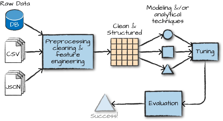
learning and advanced analytics. However, finding a use case is only a small
part of the actual advanced analytics process. There is a lot of work in
preparing your data for analysis, testing different ways of modeling it, and
evaluating these models. This section will provide structure to the overall
anaytics process and the steps we have to take to not just perform one of the
tasks just outlined, but actually evaluate success objectively in order to
understand whether or not we should apply our model to the real world
(Figure 24-1).
Figure 24-1. The machine learning workflow
The overall process involves, the following steps (with some variation):
1. Gathering and collecting the relevant data for your task.
2. Cleaning and inspecting the data to better understand it.
3. Performing feature engineering to allow the algorithm to leverage
the data in a suitable form (e.g., converting the data to numerical
vectors).
4. Using a portion of this data as a training set to train one or more
algorithms to generate some candidate models.
5. Evaluating and comparing models against your success criteria by
objectively measuring results on a subset of the same data that was
not used for training. This allows you to better understand how your
model may perform in the wild.
6. Leveraging the insights from the above process and/or using the
model to make predictions, detect anomalies, or solve more general
business challenges.
These steps won’t be the same for every advanced analytics task. However,
this workflow does serve as a general framework for what you’re going to
need to be successful with advanced analytics. Just as we did with the various
advanced analytics tasks earlier in the chapter, let’s break down the process
to better understand the overall objective of each step.
Data collection
Naturally it’s hard to create a training set without first collecting data.
Typically this means at least gathering the datasets you’ll want to leverage to
train your algorithm. Spark is an excellent tool for this because of its ability
to speak to a variety of data sources and work with data big and small.
Data cleaning
After you’ve gathered the proper data, you’re going to need to clean and
inspect it. This is typically done as part of a process called exploratory data
analysis, or EDA. EDA generally means using interactive queries and
visualization methods in order to better understand distributions, correlations,
and other details in your data. During this process you may notice you need
to remove some values that may have been misrecorded upstream or that
other values may be missing. Whatever the case, it’s always good to know
what is in your data to avoid mistakes down the road. The multitude of Spark
functions in the structured APIs will provide a simple way to clean and report
on your data.
Feature engineering

Now that you collected and cleaned your dataset, it’s time to convert it to a
form suitable for machine learning algorithms, which generally means
numerical features. Proper feature engineering can often make or break a
machine learning application, so this is one task you’ll want to do carefully.
The process of feature engineering includes a variety of tasks, such as
normalizing data, adding variables to represent the interactions of other
variables, manipulating categorical variables, and converting them to the
proper format to be input into our machine learning model. In MLlib, Spark’s
machine learning library, all variables will usually have to be input as vectors
of doubles (regardless of what they actually represent). We cover the process
of feature engineering in great depth in Chapter 25. As you will see in that
chapter, Spark provides the essentials you’ll need to manipulate your data
using a variety of machine learning statistical techniques.
NOTE
The following few steps (training models, model tuning, and evaluation) are not relevant
to all use cases. This is a general workflow that may vary significantly based on the end
objective you would like to achieve.
Training models
At this point in the process we have a dataset of historical information (e.g.,
spam or not spam emails) and a task we would like to complete (e.g.,
classifying spam emails). Next, we will want to train a model to predict the
correct output, given some input. During the training process, the parameters
inside of the model will change according to how well the model performed
on the input data. For instance, to classify spam emails, our algorithm will
likely find that certain words are better predictors of spam than others and
therefore weight the parameters associated with those words higher. In the
end, the trained model will find that certain words should have more
influence (because of their consistent association with spam emails) than
others. The output of the training process is what we call a model. Models
can then be used to gain insights or to make future predictions. To make

predictions, you will give the model an input and it will produce an output
based on a mathematical manipulation of these inputs. Using the
classification example, given the properties of an email, it will predict
whether that email is spam or not by comparing to the historical spam and not
spam emails that it was trained on.
However, just training a model isn’t the objective—we want to leverage our
model to produce insights. Thus, we must answer the question: how do we
know our model is any good at what it’s supposed to do? That’s where model
tuning and evaluation come in.
Model tuning and evaluation
You likely noticed earlier that we mentioned that you should split your data
into multiple portions and use only one for training. This is an essential step
in the machine learning process because when you build an advanced
analytics model you want that model to generalize to data it has not seen
before. Splitting our dataset into multiple portions allows us to objectively
test the effectiveness of the trained model against a set of data that it has
never seen before. The objective is to see if your model understands
something fundamental about this data process or whether or not it just
noticed the things particular to only the training set (sometimes called
overfitting). That’s why it is called a test set. In the process of training
models, we also might take another, separate subset of data and treat that as
another type of test set, called a validation set, in order to try out different
hyperparameters (parameters that affect the training process) and compare
different variations of the same model without overfitting to the test set.
WARNING
Following proper training, validation, and test set best practices is essential to successfully
using machine learning. It’s easy to end up overfitting (training a model that does not
generalize well to new data) if we do not properly isolate these sets of data. We cannot
cover this problem in depth in this book, but almost any machine learning book will cover
this topic.

To continue with the classification example we referenced previously, we
have three sets of data: a training set for training models, a validation set for
testing different variations of the models that we’re training, and lastly, a test
set we will use for the final evaluation of our different model variations to see
which one performed the best.
Leveraging the model and/or insights
After running the model through the training process and ending up with a
well-performing model, you are now ready to use it! Taking your model to
production can be a significant challenge in and of itself. We will discuss
some tactics later on in this chapter.
Spark’s Advanced Analytics Toolkit
The previous overview is just an example workflow and doesn’t encompass
all use cases or potential workflows. In addition, you probably noticed that
we did not discuss Spark almost at all. This section will discuss Spark’s
advanced analytics capabilities. Spark includes several core packages and
many external packages for performing advanced analytics. The primary
package is MLlib, which provides an interface for building machine learning
pipelines.
What Is MLlib?
MLlib is a package, built on and included in Spark, that provides interfaces
for gathering and cleaning data, feature engineering and feature selection,
training and tuning large-scale supervised and unsupervised machine learning
models, and using those models in production.
WARNING
MLlib actually consists of two packages that leverage different core data structures. The
package org.apache.spark.ml includes an interface for use with DataFrames. This
package also offers a high-level interface for building machine learning pipelines that help
standardize the way in which you perform the preceding steps. The lower-level package,

org.apache.spark.mllib, includes interfaces for Spark’s low-level RDD APIs. This
book will focus exclusively on the DataFrame API. The RDD API is the lower-level
interface, which is in maintenance mode (meaning it will only receive bug fixes, not new
features) at this time. It has also been covered fairly extensively in older books on Spark
and is therefore omitted here.
When and why should you use MLlib (versus scikit-learn,
TensorFlow, or foo package)
At a high level, MLlib might sound like a lot of other machine learning
packages you’ve probably heard of, such as scikit-learn for Python or the
variety of R packages for performing similar tasks. So why should you bother
with MLlib at all? There are numerous tools for performing machine learning
on a single machine, and while there are several great options to choose from,
these single machine tools do have their limits either in terms of the size of
data you can train on or the processing time. This means single-machine tools
are usually complementary to MLlib. When you hit those scalability issues,
take advantage of Spark’s abilities.
There are two key use cases where you want to leverage Spark’s ability to
scale. First, you want to leverage Spark for preprocessing and feature
generation to reduce the amount of time it might take to produce training and
test sets from a large amount of data. Then you might leverage single-
machine learning libraries to train on those given data sets. Second, when
your input data or model size become too difficult or inconvenient to put on
one machine, use Spark to do the heavy lifting. Spark makes distributed
machine learning very simple.
An important caveat to all of this is that while training and data preparation
are made simple, there are still some complexities you will need to keep in
mind, especially when it comes to deploying a trained model. For example,
Spark does not provide a built-in way to serve low-latency predictions from a
model, so you may want to export the model to another serving system or a
custom application to do that. MLlib is generally designed to allow
inspecting and exporting models to other tools where possible.
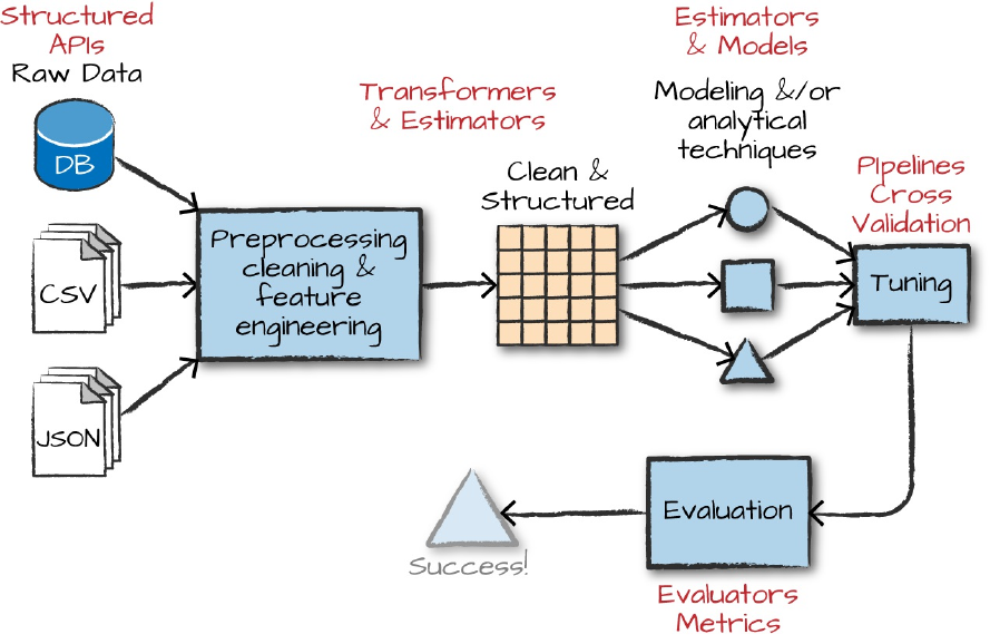
High-Level MLlib Concepts
In MLlib there are several fundamental “structural” types: transformers,
estimators, evaluators, and pipelines. By structural, we mean you will think in
terms of these types when you define an end-to-end machine learning
pipeline. They’ll provide the common language for defining what belongs in
what part of the pipeline. Figure 24-2 illustrates the overall workflow that
you will follow when developing machine learning models in Spark.
Figure 24-2. The machine learning workflow, in Spark
Transformers are functions that convert raw data in some way. This might be
to create a new interaction variable (from two other variables), normalize a
column, or simply change an Integer into a Double type to be input into a
model. An example of a transformer is one that converts string categorical
variables into numerical values that can be used in MLlib. Transformers are
primarily used in preprocessing and feature engineering. Transformers take a
DataFrame as input and produce a new DataFrame as output, as illustrated in
Figure 24-3.

Figure 24-3. A standard transformer
Estimators are one of two kinds of things. First, estimators can be a kind of
transformer that is initialized with data. For instance, to normalize numerical
data we’ll need to initialize our transformation with some information about
the current values in the column we would like to normalize. This requires
two passes over our data—the initial pass generates the initialization values
and the second actually applies the generated function over the data. In the
Spark’s nomenclature, algorithms that allow users to train a model from data
are also referred to as estimators.
An evaluator allows us to see how a given model performs according to
criteria we specify like a receiver operating characteristic (ROC) curve. After
we use an evaluator to select the best model from the ones we tested, we can
then use that model to make predictions.
From a high level we can specify each of the transformations, estimations,
and evaluations one by one, but it is often easier to specify our steps as stages
in a pipeline. This pipeline is similar to scikit-learn’s pipeline concept.
Low-level data types
In addition to the structural types for building pipelines, there are also several
lower-level data types you may need to work with in MLlib (Vector being
the most common). Whenever we pass a set of features into a machine
learning model, we must do it as a vector that consists of Doubles. This

vector can be either sparse (where most of the elements are zero) or dense
(where there are many unique values). Vectors are created in different ways.
To create a dense vector, we can specify an array of all the values. To create a
sparse vector, we can specify the total size and the indices and values of the
non-zero elements. Sparse is the best format, as you might have guessed,
when the majority of values are zero as this is a more compressed
representation. Here is an example of how to manually create a Vector:
// in Scala
import org.apache.spark.ml.linalg.Vectors
val denseVec = Vectors.dense(1.0, 2.0, 3.0)
val size = 3
val idx = Array(1,2) // locations of non-zero elements in vector
val values = Array(2.0,3.0)
val sparseVec = Vectors.sparse(size, idx, values)
sparseVec.toDense
denseVec.toSparse
# in Python
from pyspark.ml.linalg import Vectors
denseVec = Vectors.dense(1.0, 2.0, 3.0)
size = 3
idx = [1, 2] # locations of non-zero elements in vector
values = [2.0, 3.0]
sparseVec = Vectors.sparse(size, idx, values)
WARNING
Confusingly, there are similar datatypes that refer to ones that can be used in DataFrames
and others that can only be used in RDDs. The RDD implementations fall under the mllib
package while the DataFrame implementations fall under ml.
MLlib in Action
Now that we have described some of the core pieces you can expect to come
across, let’s create a simple pipeline to demonstrate each of the components.
We’ll use a small synthetic dataset that will help illustrate our point. Let’s
read the data in and see a sample before talking about it further:

// in Scala
var df = spark.read.json("/data/simple-ml")
df.orderBy("value2").show()
# in Python
df = spark.read.json("/data/simple-ml")
df.orderBy("value2").show()
Here’s a sample of the data:
+-----+----+------+------------------+
|color| lab|value1| value2|
+-----+----+------+------------------+
|green|good| 1|14.386294994851129|
...
| red| bad| 16|14.386294994851129|
|green|good| 12|14.386294994851129|
+-----+----+------+------------------+
This dataset consists of a categorical label with two values (good or bad), a
categorical variable (color), and two numerical variables. While the data is
synthetic, let’s imagine that this dataset represents a company’s customer
health. The “color” column represents some categorical health rating made by
a customer service representative. The “lab” column represents the true
customer health. The other two values are some numerical measures of
activity within an application (e.g., minutes spent on site and purchases).
Suppose that we want to train a classification model where we hope to predict
a binary variable—the label—from the other values.
TIP
Apart from JSON, there are some specific data formats commonly used for supervised
learning, including LIBSVM. These formats have real valued labels and sparse input data.
Spark can read and write for these formats using its data source API. Here’s an example of
how to read in data from a libsvm file using that Data Source API.
spark.read.format("libsvm").load(
"/data/sample_libsvm_data.txt")
For more information on LIBSVM, see the documentation.

Feature Engineering with Transformers
As already mentioned, transformers help us manipulate our current columns
in one way or another. Manipulating these columns is often in pursuit of
building features (that we will input into our model). Transformers exist to
either cut down the number of features, add more features, manipulate current
ones, or simply to help us format our data correctly. Transformers add new
columns to DataFrames.
When we use MLlib, all inputs to machine learning algorithms (with several
exceptions discussed in later chapters) in Spark must consist of type Double
(for labels) and Vector[Double] (for features). The current dataset does not
meet that requirement and therefore we need to transform it to the proper
format.
To achieve this in our example, we are going to specify an RFormula. This is
a declarative language for specifying machine learning transformations and is
simple to use once you understand the syntax. RFormula supports a limited
subset of the R operators that in practice work quite well for simple models
and manipulations (we demonstrate the manual approach to this problem in
Chapter 25). The basic RFormula operators are:
~
Separate target and terms
+
Concat terms; “+ 0” means removing the intercept (this means that the y-
intercept of the line that we will fit will be 0)
-
Remove a term; “- 1” means removing the intercept (this means that the
y-intercept of the line that we will fit will be 0—yes, this does the same
thing as “+ 0”

:
Interaction (multiplication for numeric values, or binarized categorical
values)
.
All columns except the target/dependent variable
In order to specify transformations with this syntax, we need to import the
relevant class. Then we go through the process of defining our formula. In
this case we want to use all available variables (the .) and also add in the
interactions between value1 and color and value2 and color, treating
those as new features:
// in Scala
import org.apache.spark.ml.feature.RFormula
val supervised = new RFormula()
.setFormula("lab ~ . + color:value1 + color:value2")
# in Python
from pyspark.ml.feature import RFormula
supervised = RFormula(formula="lab ~ . + color:value1 + color:value2")
At this point, we have declaratively specified how we would like to change
our data into what we will train our model on. The next step is to fit the
RFormula transformer to the data to let it discover the possible values of each
column. Not all transformers have this requirement but because RFormula
will automatically handle categorical variables for us, it needs to determine
which columns are categorical and which are not, as well as what the distinct
values of the categorical columns are. For this reason, we have to call the fit
method. Once we call fit, it returns a “trained” version of our transformer
we can then use to actually transform our data.
NOTE
We’re using the RFormula transformer because it makes performing several
transformations extremely easy to do. In Chapter 25, we’ll show other ways to specify a

similar set of transformations and outline the component parts of the RFormula when we
cover the specific transformers in MLlib.
Now that we covered those details, let’s continue on and prepare our
DataFrame:
// in Scala
val fittedRF = supervised.fit(df)
val preparedDF = fittedRF.transform(df)
preparedDF.show()
# in Python
fittedRF = supervised.fit(df)
preparedDF = fittedRF.transform(df)
preparedDF.show()
Here’s the output from the training and transformation process:
+-----+----+------+------------------+--------------------+-----+
|color| lab|value1| value2| features|label|
+-----+----+------+------------------+--------------------+-----+
|green|good| 1|14.386294994851129|(10,[1,2,3,5,8],[...| 1.0|
...
| red| bad| 2|14.386294994851129|(10,[0,2,3,4,7],[...| 0.0|
+-----+----+------+------------------+--------------------+-----+
In the output we can see the result of our transformation—a column called
features that has our previously raw data. What’s happening behind the
scenes is actually pretty simple. RFormula inspects our data during the fit
call and outputs an object that will transform our data according to the
specified formula, which is called an RFormulaModel. This “trained”
transformer always has the word Model in the type signature. When we use
this transformer, Spark automatically converts our categorical variable to
Doubles so that we can input it into a (yet to be specified) machine learning
model. In particular, it assigns a numerical value to each possible color
category, creates additional features for the interaction variables between
colors and value1/value2, and puts them all into a single vector. We then call

transform on that object in order to transform our input data into the
expected output data.
Thus far you (pre)processed the data and added some features along the way.
Now it is time to actually train a model (or a set of models) on this dataset. In
order to do this, you first need to prepare a test set for evaluation.
TIP
Having a good test set is probably the most important thing you can do to ensure you train
a model you can actually use in the real world (in a dependable way). Not creating a
representative test set or using your test set for hyperparameter tuning are surefire ways to
create a model that does not perform well in real-world scenarios. Don’t skip creating a
test set—it’s a requirement to know how well your model actually does!
Let’s create a simple test set based off a random split of the data now (we’ll
be using this test set throughout the remainder of the chapter):
// in Scala
val Array(train, test) = preparedDF.randomSplit(Array(0.7, 0.3))
# in Python
train, test = preparedDF.randomSplit([0.7, 0.3])
Estimators
Now that we have transformed our data into the correct format and created
some valuable features, it’s time to actually fit our model. In this case we will
use a classification algorithm called logistic regression. To create our
classifier we instantiate an instance of LogisticRegression, using the
default configuration or hyperparameters. We then set the label columns and
the feature columns; the column names we are setting—label and features
—are actually the default labels for all estimators in Spark MLlib, and in later
chapters we omit them:
// in Scala
import org.apache.spark.ml.classification.LogisticRegression
val lr = new
LogisticRegression().setLabelCol("label").setFeaturesCol("features")
# in Python
from pyspark.ml.classification import LogisticRegression
lr = LogisticRegression(labelCol="label",featuresCol="features")
Before we actually go about training this model, let’s inspect the parameters.
This is also a great way to remind yourself of the options available for each
particular model:
// in Scala
println(lr.explainParams())
# in Python
print lr.explainParams()
While the output is too large to reproduce here, it shows an explanation of all
of the parameters for Spark’s implementation of logistic regression. The
explainParams method exists on all algorithms available in MLlib.
Upon instantiating an untrained algorithm, it becomes time to fit it to data. In
this case, this returns a LogisticRegressionModel:
// in Scala
val fittedLR = lr.fit(train)
# in Python
fittedLR = lr.fit(train)
This code will kick off a Spark job to train the model. As opposed to the
transformations that you saw throughout the book, the fitting of a machine
learning model is eager and performed immediately.
Once complete, you can use the model to make predictions. Logically this
means tranforming features into labels. We make predictions with the
transform method. For example, we can transform our training dataset to
see what labels our model assigned to the training data and how those
compare to the true outputs. This, again, is just another DataFrame we can

manipulate. Let’s perform that prediction with the following code snippet:
fittedLR.transform(train).select("label", "prediction").show()
This results in:
+-----+----------+
|label|prediction|
+-----+----------+
| 0.0| 0.0|
...
| 0.0| 0.0|
+-----+----------+
Our next step would be to manually evaluate this model and calculate
performance metrics like the true positive rate, false negative rate, and so on.
We might then turn around and try a different set of parameters to see if those
perform better. However, while this is a useful process, it can also be quite
tedious. Spark helps you avoid manually trying different models and
evaluation criteria by allowing you to specify your workload as a declarative
pipeline of work that includes all your transformations as well as tuning your
hyperparameters.
A REVIEW OF HYPERPARAMETERS
Although we mentioned them previously, let’s more formally define
hyperparameters. Hyperparameters are configuration parameters that
affect the training process, such as model architecture and regularization.
They are set prior to starting training. For instance, logistic regression has
a hyperparameter that determines how much regularization should be
performed on our data through the training phase (regularization is a
technique that pushes models against overfitting data). You’ll see in the
next couple of pages that we can set up our pipeline to try different
hyperparameter values (e.g., different regularization values) in order to
compare different variations of the same model against one another.
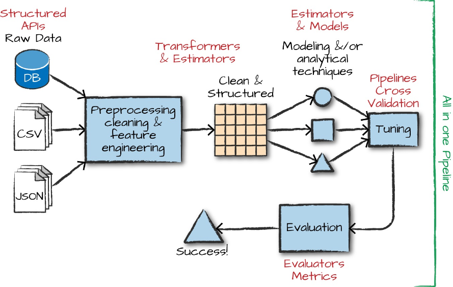
Pipelining Our Workflow
As you probably noticed, if you are performing a lot of transformations,
writing all the steps and keeping track of DataFrames ends up being quite
tedious. That’s why Spark includes the Pipeline concept. A pipeline allows
you to set up a dataflow of the relevant transformations that ends with an
estimator that is automatically tuned according to your specifications,
resulting in a tuned model ready for use. Figure 24-4 illustrates this process.
Figure 24-4. Pipelining the ML workflow
Note that it is essential that instances of transformers or models are not
reused across different pipelines. Always create a new instance of a model
before creating another pipeline.
In order to make sure we don’t overfit, we are going to create a holdout test
set and tune our hyperparameters based on a validation set (note that we
create this validation set based on the original dataset, not the preparedDF
used in the previous pages):
// in Scala
val Array(train, test) = df.randomSplit(Array(0.7, 0.3))
# in Python
train, test = df.randomSplit([0.7, 0.3])
Now that you have a holdout set, let’s create the base stages in our pipeline.
A stage simply represents a transformer or an estimator. In our case, we will
have two estimators. The RFomula will first analyze our data to understand
the types of input features and then transform them to create new features.
Subsequently, the LogisticRegression object is the algorithm that we will
train to produce a model:
// in Scala
val rForm = new RFormula()
val lr = new
LogisticRegression().setLabelCol("label").setFeaturesCol("features")
# in Python
rForm = RFormula()
lr = LogisticRegression().setLabelCol("label").setFeaturesCol("features")
We will set the potential values for the RFormula in the next section. Now
instead of manually using our transformations and then tuning our model we
just make them stages in the overall pipeline, as in the following code
snippet:
// in Scala
import org.apache.spark.ml.Pipeline
val stages = Array(rForm, lr)
val pipeline = new Pipeline().setStages(stages)
# in Python
from pyspark.ml import Pipeline
stages = [rForm, lr]
pipeline = Pipeline().setStages(stages)
Training and Evaluation
Now that you arranged the logical pipeline, the next step is training. In our

case, we won’t train just one model (like we did previously); we will train
several variations of the model by specifying different combinations of
hyperparameters that we would like Spark to test. We will then select the best
model using an Evaluator that compares their predictions on our validation
data. We can test different hyperparameters in the entire pipeline, even in the
RFormula that we use to manipulate the raw data. This code shows how we
go about doing that:
// in Scala
import org.apache.spark.ml.tuning.ParamGridBuilder
val params = new ParamGridBuilder()
.addGrid(rForm.formula, Array(
"lab ~ . + color:value1",
"lab ~ . + color:value1 + color:value2"))
.addGrid(lr.elasticNetParam, Array(0.0, 0.5, 1.0))
.addGrid(lr.regParam, Array(0.1, 2.0))
.build()
# in Python
from pyspark.ml.tuning import ParamGridBuilder
params = ParamGridBuilder()\
.addGrid(rForm.formula, [
"lab ~ . + color:value1",
"lab ~ . + color:value1 + color:value2"])\
.addGrid(lr.elasticNetParam, [0.0, 0.5, 1.0])\
.addGrid(lr.regParam, [0.1, 2.0])\
.build()
In our current paramter grid, there are three hyperparameters that will diverge
from the defaults:
Two different versions of the RFormula
Three different options for the ElasticNet parameter
Two different options for the regularization parameter
This gives us a total of 12 different combinations of these parameters, which
means we will be training 12 different versions of logistic regression. We
explain the ElasticNet parameter as well as the regularization options in
Chapter 26.
Now that the grid is built, it’s time to specify our evaluation process. The
evaluator allows us to automatically and objectively compare multiple
models to the same evaluation metric. There are evaluators for classification
and regression, covered in later chapters, but in this case we will use the
BinaryClassificationEvaluator, which has a number of potential
evaluation metrics, as we’ll discuss in Chapter 26. In this case we will use
areaUnderROC, which is the total area under the receiver operating
characteristic, a common measure of classification performance:
// in Scala
import org.apache.spark.ml.evaluation.BinaryClassificationEvaluator
val evaluator = new BinaryClassificationEvaluator()
.setMetricName("areaUnderROC")
.setRawPredictionCol("prediction")
.setLabelCol("label")
# in Python
from pyspark.ml.evaluation import BinaryClassificationEvaluator
evaluator = BinaryClassificationEvaluator()\
.setMetricName("areaUnderROC")\
.setRawPredictionCol("prediction")\
.setLabelCol("label")
Now that we have a pipeline that specifies how our data should be
transformed, we will perform model selection to try out different
hyperparameters in our logistic regression model and measure success by
comparing their performance using the areaUnderROC metric.
As we discussed, it is a best practice in machine learning to fit
hyperparameters on a validation set (instead of your test set) to prevent
overfitting. For this reason, we cannot use our holdout test set (that we
created before) to tune these parameters. Luckily, Spark provides two options
for performing hyperparameter tuning automatically. We can use
TrainValidationSplit, which will simply perform an arbitrary random
split of our data into two different groups, or CrossValidator, which
performs K-fold cross-validation by splitting the dataset into k non-
overlapping, randomly partitioned folds:
// in Scala
import org.apache.spark.ml.tuning.TrainValidationSplit
val tvs = new TrainValidationSplit()
.setTrainRatio(0.75) // also the default.
.setEstimatorParamMaps(params)
.setEstimator(pipeline)
.setEvaluator(evaluator)
# in Python
from pyspark.ml.tuning import TrainValidationSplit
tvs = TrainValidationSplit()\
.setTrainRatio(0.75)\
.setEstimatorParamMaps(params)\
.setEstimator(pipeline)\
.setEvaluator(evaluator)
Let’s run the entire pipeline we constructed. To review, running this pipeline
will test out every version of the model against the validation set. Note the
type of tvsFitted is TrainValidationSplitModel. Any time we fit a given
model, it outputs a “model” type:
// in Scala
val tvsFitted = tvs.fit(train)
# in Python
tvsFitted = tvs.fit(train)
And of course evaluate how it performs on the test set!
evaluator.evaluate(tvsFitted.transform(test)) // 0.9166666666666667
We can also see a training summary for some models. To do this we extract it
from the pipeline, cast it to the proper type, and print our results. The metrics
available on each model are discussed throughout the next several chapters.
Here’s how we can see the results:
// in Scala
import org.apache.spark.ml.PipelineModel
import org.apache.spark.ml.classification.LogisticRegressionModel
val trainedPipeline = tvsFitted.bestModel.asInstanceOf[PipelineModel]
val TrainedLR = trainedPipeline.stages(1).asInstanceOf[LogisticRegressionModel]
val summaryLR = TrainedLR.summary
summaryLR.objectiveHistory // 0.6751425885789243, 0.5543659647777687,
0.473776...
The objective history shown here provides details related to how our
algorithm performed over each training iteration. This can be helpful because
we can note the progress our algorithm is making toward the best model.
Large jumps are typically expected at the beginning, but over time the values
should become smaller and smaller, with only small amounts of variation
between the values.
Persisting and Applying Models
Now that we trained this model, we can persist it to disk to use it for
prediction purposes later on:
tvsFitted.write.overwrite().save("/tmp/modelLocation")
After writing out the model, we can load it into another Spark program to
make predictions. To do this, we need to use a “model” version of our
particular algorithm to load our persisted model from disk. If we were to use
CrossValidator, we’d have to read in the persisted version as the
CrossValidatorModel, and if we were to use LogisticRegression
manually we would have to use LogisticRegressionModel. In this case, we
use TrainValidationSplit, which outputs TrainValidationSplitModel:
// in Scala
import org.apache.spark.ml.tuning.TrainValidationSplitModel
val model = TrainValidationSplitModel.load("/tmp/modelLocation")
model.transform(test)
Deployment Patterns
In Spark there are several different deployment patterns for putting machine
learning models into production. Figure 24-5 illustrates common workflows.
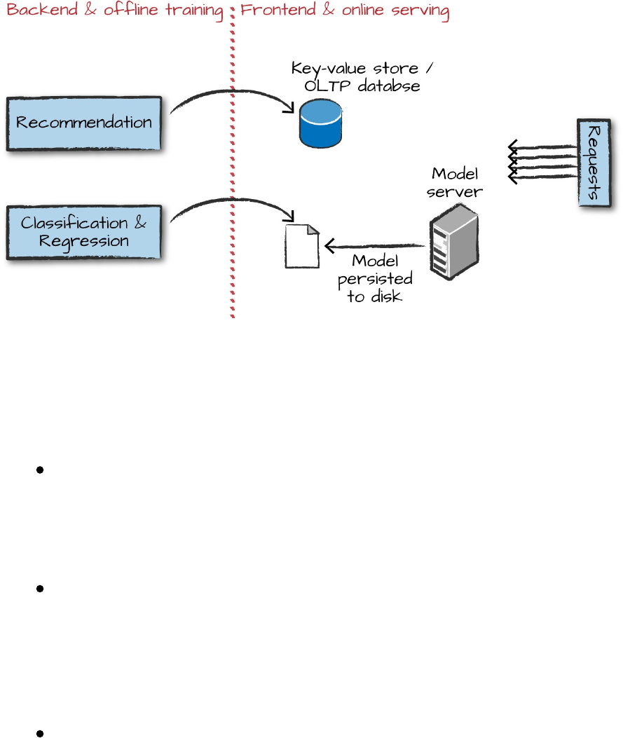
Figure 24-5. The productionization process
Here are the various options for how you might go about deploying a Spark
model. These are the general options you should be able to link to the process
illustrated in Figure 24-5.
Train your machine learning (ML) model offline and then supply it
with offline data. In this context, we mean offline data to be data that
is stored for analysis, and not data that you need to get an answer
from quickly. Spark is well suited to this sort of deployment.
Train your model offline and then put the results into a database
(usually a key-value store). This works well for something like
recommendation but poorly for something like classification or
regression where you cannot just look up a value for a given user but
must calculate one based on the input.
Train your ML algorithm offline, persist the model to disk, and then
use that for serving. This is not a low-latency solution if you use
Spark for the serving part, as the overhead of starting up a Spark job
can be high, even if you’re not running on a cluster. Additionally
this does not parallelize well, so you’ll likely have to put a load
balancer in front of multiple model replicas and build out some
REST API integration yourself. There are some interesting potential

solutions to this problem, but no standards currently exist for this
sort of model serving.
Manually (or via some other software) convert your distributed
model to one that can run much more quickly on a single machine.
This works well when there is not too much manipulation of the raw
data in Spark but can be hard to maintain over time. Again, there are
several solutions in progress. For example, MLlib can export some
models to PMML, a common model interchange format.
Train your ML algorithm online and use it online. This is possible
when used in conjunction with Structured Streaming, but can be
complex for some models.
While these are some of the options, there are many other ways of
performing model deployment and management. This is an area under heavy
development and many potential innovations are currently being worked on.
Conclusion
In this chapter we covered the core concepts behind advanced analytics and
MLlib. We also showed you how to use them. The next chapter will discuss
preprocessing in depth, including Spark’s tools for feature engineering and
data cleaning. Then we’ll move into detailed descriptions of each algorithm
available in MLlib along with some tools for graph analytics and deep
learning.

Chapter 25. Preprocessing and
Feature Engineering
Any data scientist worth her salt knows that one of the biggest challenges
(and time sinks) in advanced analytics is preprocessing. It’s not that it’s
particularly complicated programming, but rather that it requires deep
knowledge of the data you are working with and an understanding of what
your model needs in order to successfully leverage this data. This chapter
covers the details of how you can use Spark to perform preprocessing and
feature engineering. We’ll walk through the core requirements you’ll need to
meet in order to train an MLlib model in terms of how your data is structured.
We will then discuss the different tools Spark makes available for performing
this kind of work.
Formatting Models According to Your Use
Case
To preprocess data for Spark’s different advanced analytics tools, you must
consider your end objective. The following list walks through the
requirements for input data structure for each advanced analytics task in
MLlib:
In the case of most classification and regression algorithms, you
want to get your data into a column of type Double to represent the
label and a column of type Vector (either dense or sparse) to
represent the features.
In the case of recommendation, you want to get your data into a
column of users, a column of items (say movies or books), and a
column of ratings.

In the case of unsupervised learning, a column of type Vector
(either dense or sparse) is needed to represent the features.
In the case of graph analytics, you will want a DataFrame of vertices
and a DataFrame of edges.
The best way to get your data in these formats is through transformers.
Transformers are functions that accept a DataFrame as an argument and
return a new DataFrame as a response. This chapter will focus on what
transformers are relevant for particular use cases rather than attempting to
enumerate every possible transformer.
NOTE
Spark provides a number of transformers as part of the org.apache.spark.ml.feature
package. The corresponding package in Python is pyspark.ml.feature. New
transformers are constantly popping up in Spark MLlib and therefore it is impossible to
include a definitive list in this book. The most up-to-date information can be found on the
Spark documentation site.
Before we proceed, we’re going to read in several different sample datasets,
each of which has different properties we will manipulate in this chapter:
// in Scala
val sales = spark.read.format("csv")
.option("header", "true")
.option("inferSchema", "true")
.load("/data/retail-data/by-day/*.csv")
.coalesce(5)
.where("Description IS NOT NULL")
val fakeIntDF = spark.read.parquet("/data/simple-ml-integers")
var simpleDF = spark.read.json("/data/simple-ml")
val scaleDF = spark.read.parquet("/data/simple-ml-scaling")
# in Python
sales = spark.read.format("csv")\
.option("header", "true")\
.option("inferSchema", "true")\
.load("/data/retail-data/by-day/*.csv")\

.coalesce(5)\
.where("Description IS NOT NULL")
fakeIntDF = spark.read.parquet("/data/simple-ml-integers")
simpleDF = spark.read.json("/data/simple-ml")
scaleDF = spark.read.parquet("/data/simple-ml-scaling")
In addition to this realistic sales data, we’re going to use several simple
synthetic datasets as well. FakeIntDF, simpleDF, and scaleDF all have very
few rows. This will give you the ability to focus on the exact data
manipulation we are performing instead of the various inconsistencies of any
particular dataset. Because we’re going to be accessing the sales data a
number of times, we’re going to cache it so we can read it efficiently from
memory as opposed to reading it from disk every time we need it. Let’s also
check out the first several rows of data in order to better understand what’s in
the dataset:
sales.cache()
sales.show()
+---------+---------+--------------------+--------+-------------------+---------
|InvoiceNo|StockCode| Description|Quantity| InvoiceDate|UnitPr...
+---------+---------+--------------------+--------+-------------------+---------
| 580538| 23084| RABBIT NIGHT LIGHT| 48|2011-12-05 08:38:00| 1...
...
| 580539| 22375|AIRLINE BAG VINTA...| 4|2011-12-05 08:39:00| 4...
+---------+---------+--------------------+--------+-------------------+---------
NOTE
It is important to note that we filtered out null values here. MLlib does not always play
nicely with null values at this point in time. This is a frequent cause for problems and
errors and a great first step when you are debugging. Improvements are also made with
every Spark release to improve algorithm handling of null values.
Transformers
We discussed transformers in the previous chapter, but it’s worth reviewing
them again here. Transformers are functions that convert raw data in some
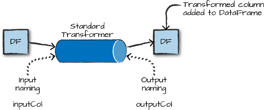
way. This might be to create a new interaction variable (from two other
variables), to normalize a column, or to simply turn it into a Double to be
input into a model. Transformers are primarily used in preprocessing or
feature generation.
Spark’s transformer only includes a transform method. This is because it will
not change based on the input data. Figure 25-1 is a simple illustration. On
the left is an input DataFrame with the column to be manipulated. On the
right is the input DataFrame with a new column representing the output
transformation.
Figure 25-1. A Spark transformer
The Tokenizer is an example of a transformer. It tokenizes a string, splitting
on a given character, and has nothing to learn from our data; it simply applies
a function. We’ll discuss the tokenizer in more depth later in this chapter, but
here’s a small code snippet showing how a tokenizer is built to accept the
input column, how it transforms the data, and then the output from that
transformation:
// in Scala
import org.apache.spark.ml.feature.Tokenizer
val tkn = new Tokenizer().setInputCol("Description")
tkn.transform(sales.select("Description")).show(false)
+-----------------------------------+------------------------------------------+
|Description |tok_7de4dfc81ab7__output |
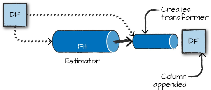
+-----------------------------------+------------------------------------------+
|RABBIT NIGHT LIGHT |[rabbit, night, light] |
|DOUGHNUT LIP GLOSS |[doughnut, lip, gloss] |
...
|AIRLINE BAG VINTAGE WORLD CHAMPION |[airline, bag, vintage, world, champion] |
|AIRLINE BAG VINTAGE JET SET BROWN |[airline, bag, vintage, jet, set, brown] |
+-----------------------------------+------------------------------------------+
Estimators for Preprocessing
Another tool for preprocessing are estimators. An estimator is necessary
when a transformation you would like to perform must be initialized with
data or information about the input column (often derived by doing a pass
over the input column itself). For example, if you wanted to scale the values
in our column to have mean zero and unit variance, you would need to
perform a pass over the entire data in order to calculate the values you would
use to normalize the data to mean zero and unit variance. In effect, an
estimator can be a transformer configured according to your particular input
data. In simplest terms, you can either blindly apply a transformation (a
“regular” transformer type) or perform a transformation based on your data
(an estimator type). Figure 25-2 is a simple illustration of an estimator fitting
to a particular input dataset, generating a transformer that is then applied to
the input dataset to append a new column (of the transformed data).
Figure 25-2. A Spark estimator
An example of this type of estimator is the StandardScaler, which scales
your input column according to the range of values in that column to have a
zero mean and a variance of 1 in each dimension. For that reason it must first
perform a pass over the data to create the transformer. Here’s a sample code
snippet showing the entire process, as well as the output:
// in Scala
import org.apache.spark.ml.feature.StandardScaler
val ss = new StandardScaler().setInputCol("features")
ss.fit(scaleDF).transform(scaleDF).show(false)
+---+--------------+------------------------------------------------------------
+
|id |features |stdScal_d66fbeac10ea__output
|
+---+--------------+------------------------------------------------------------
+
|0 |[1.0,0.1,-1.0]|
[1.1952286093343936,0.02337622911060922,-0.5976143046671968]|
...
|1 |[3.0,10.1,3.0]|[3.5856858280031805,2.3609991401715313,1.7928429140015902]
|
+---+--------------+------------------------------------------------------------
+
We will use both estimators and transformers throughout and cover more
about these particular estimators (and add examples in Python) later on in this
chapter.
Transformer Properties
All transformers require you to specify, at a minimum, the inputCol and the
outputCol, which represent the column name of the input and output,
respectively. You set these with setInputCol and setOutputCol. There are
some defaults (you can find these in the documentation), but it is a best
practice to manually specify them yourself for clarity. In addition to input and
output columns, all transformers have different parameters that you can tune
(whenever we mention a parameter in this chapter you must set it with a
set() method). In Python, we also have another method to set these values

with keyword arguments to the object’s constructor. We exclude these from
the examples in the next chapter for consistency. Estimators require you to
fit the transformer to your particular dataset and then call transform on the
resulting object.
NOTE
Spark MLlib stores metadata about the columns it uses in each DataFrame as an attribute
on the column itself. This allows it to properly store (and annotate) that a column of
Doubles may actually represent a series of categorical variables instead of continuous
values. However, metadata won’t show up when you print the schema or the DataFrame.
High-Level Transformers
High-level transformers, such as the RFormula we saw in the previous
chapter, allow you to concisely specify a number of transformations in one.
These operate at a “high level”, and allow you to avoid doing data
manipulations or transformations one by one. In general, you should try to
use the highest level transformers you can, in order to minimize the risk of
error and help you focus on the business problem instead of the smaller
details of implementation. While this is not always possible, it’s a good
objective.
RFormula
The RFormula is the easiest transfomer to use when you have
“conventionally” formatted data. Spark borrows this transformer from the R
language to make it simple to declaratively specify a set of transformations
for your data. With this transformer, values can be either numerical or
categorical and you do not need to extract values from strings or manipulate
them in any way. The RFormula will automatically handle categorical inputs
(specified as strings) by performing something called one-hot encoding. In
brief, one-hot encoding converts a set of values into a set of binary columns
specifying whether or not the data point has each particular value (we’ll

discuss one-hot encoding in more depth later in the chapter). With the
RFormula, numeric columns will be cast to Double but will not be one-hot
encoded. If the label column is of type String, it will be first transformed to
Double with StringIndexer.
WARNING
Automatic casting of numeric columns to Double without one-hot encoding has some
important implications. If you have numerically valued categorical variables, they will
only be cast to Double, implicitly specifying an order. It is important to ensure the input
types correspond to the expected conversion. If you have categorical variables that really
have no order relation, they should be cast to String. You can also manually index
columns (see “Working with Categorical Features”).
The RFormula allows you to specify your transformations in declarative
syntax. It is simple to use once you understand the syntax. Currently,
RFormula supports a limited subset of the R operators that in practice work
quite well for simple transformations. The basic operators are:
~
Separate target and terms
+
Concatenate terms; “+ 0” means removing the intercept (this means the y-
intercept of the line that we will fit will be 0)
-
Remove a term; “- 1” means removing intercept (this means the y-
intercept of the line that we will fit will be 0)
:
Interaction (multiplication for numeric values, or binarized categorical
values)
.
All columns except the target/dependent variable
RFormula also uses default columns of label and features to label, you
guessed it, the label and the set of features that it outputs (for supervised
machine learning). The models covered later on in this chapter by default
require those column names, making it easy to pass the resulting transformed
DataFrame into a model for training. If this doesn’t make sense yet, don’t
worry—it’ll become clear once we actually start using models in later
chapters.
Let’s use RFormula in an example. In this case, we want to use all available
variables (the .) and then specify an interaction between value1 and color
and value2 and color as additional features to generate:
// in Scala
import org.apache.spark.ml.feature.RFormula
val supervised = new RFormula()
.setFormula("lab ~ . + color:value1 + color:value2")
supervised.fit(simpleDF).transform(simpleDF).show()
# in Python
from pyspark.ml.feature import RFormula
supervised = RFormula(formula="lab ~ . + color:value1 + color:value2")
supervised.fit(simpleDF).transform(simpleDF).show()
+-----+----+------+------------------+--------------------+-----+
|color| lab|value1| value2| features|label|
+-----+----+------+------------------+--------------------+-----+
|green|good| 1|14.386294994851129|(10,[1,2,3,5,8],[...| 1.0|
| blue| bad| 8|14.386294994851129|(10,[2,3,6,9],[8....| 0.0|
...
| red| bad| 1| 38.97187133755819|(10,[0,2,3,4,7],[...| 0.0|
| red| bad| 2|14.386294994851129|(10,[0,2,3,4,7],[...| 0.0|
+-----+----+------+------------------+--------------------+-----+
SQL Transformers
A SQLTransformer allows you to leverage Spark’s vast library of SQL-
related manipulations just as you would a MLlib transformation. Any SELECT
statement you can use in SQL is a valid transformation. The only thing you
need to change is that instead of using the table name, you should just use the
keyword THIS. You might want to use SQLTransformer if you want to
formally codify some DataFrame manipulation as a preprocessing step, or try
different SQL expressions for features during hyperparameter tuning. Also
note that the output of this transformation will be appended as a column to
the output DataFrame.
You might want to use an SQLTransformer in order to represent all of your
manipulations on the very rawest form of your data so you can version
different variations of manipulations as transformers. This gives you the
benefit of building and testing varying pipelines, all by simply swapping out
transformers. The following is a basic example of using SQLTransformer:
// in Scala
import org.apache.spark.ml.feature.SQLTransformer
val basicTransformation = new SQLTransformer()
.setStatement("""
SELECT sum(Quantity), count(*), CustomerID
FROM __THIS__
GROUP BY CustomerID
""")
basicTransformation.transform(sales).show()
# in Python
from pyspark.ml.feature import SQLTransformer
basicTransformation = SQLTransformer()\
.setStatement("""
SELECT sum(Quantity), count(*), CustomerID
FROM __THIS__
GROUP BY CustomerID
""")
basicTransformation.transform(sales).show()
Here’s a sample of the output:
-------------+--------+----------+
|sum(Quantity)|count(1)|CustomerID|
+-------------+--------+----------+
| 119| 62| 14452.0|
...
| 138| 18| 15776.0|
+-------------+--------+----------+
For extensive samples of these transformations, refer back to Part II.
VectorAssembler
The VectorAssembler is a tool you’ll use in nearly every single pipeline you
generate. It helps concatenate all your features into one big vector you can
then pass into an estimator. It’s used typically in the last step of a machine
learning pipeline and takes as input a number of columns of Boolean,
Double, or Vector. This is particularly helpful if you’re going to perform a
number of manipulations using a variety of transformers and need to gather
all of those results together.
The output from the following code snippet will make it clear how this
works:
// in Scala
import org.apache.spark.ml.feature.VectorAssembler
val va = new VectorAssembler().setInputCols(Array("int1", "int2", "int3"))
va.transform(fakeIntDF).show()
# in Python
from pyspark.ml.feature import VectorAssembler
va = VectorAssembler().setInputCols(["int1", "int2", "int3"])
va.transform(fakeIntDF).show()
+----+----+----+--------------------------------------------+
|int1|int2|int3|VectorAssembler_403ab93eacd5585ddd2d__output|
+----+----+----+--------------------------------------------+
| 1| 2| 3| [1.0,2.0,3.0]|
| 4| 5| 6| [4.0,5.0,6.0]|
| 7| 8| 9| [7.0,8.0,9.0]|
+----+----+----+--------------------------------------------+

Working with Continuous Features
Continuous features are just values on the number line, from positive infinity
to negative infinity. There are two common transformers for continuous
features. First, you can convert continuous features into categorical features
via a process called bucketing, or you can scale and normalize your features
according to several different requirements. These transformers will only
work on Double types, so make sure you’ve turned any other numerical
values to Double:
// in Scala
val contDF = spark.range(20).selectExpr("cast(id as double)")
# in Python
contDF = spark.range(20).selectExpr("cast(id as double)")
Bucketing
The most straightforward approach to bucketing or binning is using the
Bucketizer. This will split a given continuous feature into the buckets of
your designation. You specify how buckets should be created via an array or
list of Double values. This is useful because you may want to simplify the
features in your dataset or simplify their representations for interpretation
later on. For example, imagine you have a column that represents a person’s
weight and you would like to predict some value based on this information.
In some cases, it might be simpler to create three buckets of “overweight,”
“average,” and “underweight.”
To specify the bucket, set its borders. For example, setting splits to 5.0,
10.0, 250.0 on our contDF will actually fail because we don’t cover all
possible input ranges. When specifying your bucket points, the values you
pass into splits must satisfy three requirements:
The minimum value in your splits array must be less than the
minimum value in your DataFrame.
The maximum value in your splits array must be greater than the

maximum value in your DataFrame.
You need to specify at a minimum three values in the splits array,
which creates two buckets.
WARNING
The Bucketizer can be confusing because we specify bucket borders via the splits
method, but these are not actually splits.
To cover all possible ranges, scala.Double.NegativeInfinity might be
another split option, with scala.Double.PositiveInfinity to cover all
possible ranges outside of the inner splits. In Python we specify this in the
following way: float("inf"), float("-inf").
In order to handle null or NaN values, we must specify the handleInvalid
parameter as a certain value. We can either keep those values (keep), error
or null, or skip those rows. Here’s an example of using bucketing:
// in Scala
import org.apache.spark.ml.feature.Bucketizer
val bucketBorders = Array(-1.0, 5.0, 10.0, 250.0, 600.0)
val bucketer = new Bucketizer().setSplits(bucketBorders).setInputCol("id")
bucketer.transform(contDF).show()
# in Python
from pyspark.ml.feature import Bucketizer
bucketBorders = [-1.0, 5.0, 10.0, 250.0, 600.0]
bucketer = Bucketizer().setSplits(bucketBorders).setInputCol("id")
bucketer.transform(contDF).show()
+----+---------------------------------------+
| id|Bucketizer_4cb1be19f4179cc2545d__output|
+----+---------------------------------------+
| 0.0| 0.0|
...
|10.0| 2.0|
|11.0| 2.0|
...
+----+---------------------------------------+
In addition to splitting based on hardcoded values, another option is to split
based on percentiles in our data. This is done with QuantileDiscretizer,
which will bucket the values into user-specified buckets with the splits being
determined by approximate quantiles values. For instance, the 90th quantile
is the point in your data at which 90% of the data is below that value. You
can control how finely the buckets should be split by setting the relative error
for the approximate quantiles calculation using setRelativeError. Spark
does this is by allowing you to specify the number of buckets you would like
out of the data and it will split up your data accordingly. The following is an
example:
// in Scala
import org.apache.spark.ml.feature.QuantileDiscretizer
val bucketer = new QuantileDiscretizer().setNumBuckets(5).setInputCol("id")
val fittedBucketer = bucketer.fit(contDF)
fittedBucketer.transform(contDF).show()
# in Python
from pyspark.ml.feature import QuantileDiscretizer
bucketer = QuantileDiscretizer().setNumBuckets(5).setInputCol("id")
fittedBucketer = bucketer.fit(contDF)
fittedBucketer.transform(contDF).show()
+----+----------------------------------------+
| id|quantileDiscretizer_cd87d1a1fb8e__output|
+----+----------------------------------------+
| 0.0| 0.0|
...
| 6.0| 1.0|
| 7.0| 2.0|
...
|14.0| 3.0|
|15.0| 4.0|
...
+----+----------------------------------------+
Advanced bucketing techniques
The techniques descriubed here are the most common ways of bucketing
data, but there are a number of other ways that exist in Spark today. All of
these processes are the same from a data flow perspective: start with
continuous data and place them in buckets so that they become categorical.
Differences arise depending on the algorithm used to compute these buckets.
The simple examples we just looked at are easy to intepret and work with, but
more advanced techniques such as locality sensitivity hashing (LSH) are also
available in MLlib.
Scaling and Normalization
We saw how we can use bucketing to create groups out of continuous
variables. Another common task is to scale and normalize continuous data.
While not always necessary, doing so is usually a best practice. You might
want to do this when your data contains a number of columns based on
different scales. For instance, say we have a DataFrame with two columns:
weight (in ounces) and height (in feet). If you don’t scale or normalize, the
algorithm will be less sensitive to variations in height because height values
in feet are much lower than weight values in ounces. That’s an example
where you should scale your data.
An example of normalization might involve transforming the data so that
each point’s value is a representation of its distance from the mean of that
column. Using the same example from before, we might want to know how
far a given individual’s height is from the mean height. Many algorithms
assume that their input data is normalized.
As you might imagine, there are a multitude of algorithms we can apply to
our data to scale or normalize it. Enumerating them all is unnecessary here
because they are covered in many other texts and machine learning libraries.
If you’re unfamiliar with the concept in detail, check out any of the books
referenced in the previous chapter. Just keep in mind the fundamental goal—
we want our data on the same scale so that values can easily be compared to
one another in a sensible way. In MLlib, this is always done on columns of
type Vector. MLlib will look across all the rows in a given column (of type
Vector) and then treat every dimension in those vectors as its own particular

column. It will then apply the scaling or normalization function on each
dimension separately.
A simple example might be the following vectors in a column:
1,2
3,4
When we apply our scaling (but not normalization) function, the “3” and the
“1” will be adjusted according to those two values while the “2” and the “4”
will be adjusted according to one another. This is commonly referred to as
component-wise comparisons.
StandardScaler
The StandardScaler standardizes a set of features to have zero mean and a
standard deviation of 1. The flag withStd will scale the data to unit standard
deviation while the flag withMean (false by default) will center the data prior
to scaling it.
WARNING
Centering can be very expensive on sparse vectors because it generally turns them into
dense vectors, so be careful before centering your data.
Here’s an example of using a StandardScaler:
// in Scala
import org.apache.spark.ml.feature.StandardScaler
val sScaler = new StandardScaler().setInputCol("features")
sScaler.fit(scaleDF).transform(scaleDF).show()
# in Python
from pyspark.ml.feature import StandardScaler
sScaler = StandardScaler().setInputCol("features")
sScaler.fit(scaleDF).transform(scaleDF).show()
The output is shown below:
+---+--------------+------------------------------------------------------------
+
|id |features |StandardScaler_41aaa6044e7c3467adc3__output
|
+---+--------------+------------------------------------------------------------
+
|0 |[1.0,0.1,-1.0]|
[1.1952286093343936,0.02337622911060922,-0.5976143046671968]|
...
|1 |[3.0,10.1,3.0]|[3.5856858280031805,2.3609991401715313,1.7928429140015902]
|
+---+--------------+------------------------------------------------------------
+
MinMaxScaler
The MinMaxScaler will scale the values in a vector (component wise) to the
proportional values on a scale from a given min value to a max value. If you
specify the minimum value to be 0 and the maximum value to be 1, then all
the values will fall in between 0 and 1:
// in Scala
import org.apache.spark.ml.feature.MinMaxScaler
val minMax = new MinMaxScaler().setMin(5).setMax(10).setInputCol("features")
val fittedminMax = minMax.fit(scaleDF)
fittedminMax.transform(scaleDF).show()
# in Python
from pyspark.ml.feature import MinMaxScaler
minMax = MinMaxScaler().setMin(5).setMax(10).setInputCol("features")
fittedminMax = minMax.fit(scaleDF)
fittedminMax.transform(scaleDF).show()
+---+--------------+-----------------------------------------+
| id| features|MinMaxScaler_460cbafafbe6b9ab7c62__output|
+---+--------------+-----------------------------------------+
| 0|[1.0,0.1,-1.0]| [5.0,5.0,5.0]|
...
| 1|[3.0,10.1,3.0]| [10.0,10.0,10.0]|
+---+--------------+-----------------------------------------+
MaxAbsScaler
The max absolute scaler (MaxAbsScaler) scales the data by dividing each
value by the maximum absolute value in this feature. All values therefore end
up between −1 and 1. This transformer does not shift or center the data at all
in the process:
// in Scala
import org.apache.spark.ml.feature.MaxAbsScaler
val maScaler = new MaxAbsScaler().setInputCol("features")
val fittedmaScaler = maScaler.fit(scaleDF)
fittedmaScaler.transform(scaleDF).show()
# in Python
from pyspark.ml.feature import MaxAbsScaler
maScaler = MaxAbsScaler().setInputCol("features")
fittedmaScaler = maScaler.fit(scaleDF)
fittedmaScaler.transform(scaleDF).show()
+---+--------------+----------------------------------------------------------+
|id |features |MaxAbsScaler_402587e1d9b6f268b927__output |
+---+--------------+----------------------------------------------------------+
|0 |[1.0,0.1,-1.0]|[0.3333333333333333,0.009900990099009901,-0.3333333333333]|
...
|1 |[3.0,10.1,3.0]|[1.0,1.0,1.0] |
+---+--------------+----------------------------------------------------------+
ElementwiseProduct
The ElementwiseProduct allows us to scale each value in a vector by an
arbitrary value. For example, given the vector below and the row “1, 0.1, -1”
the output will be “10, 1.5, -20.” Naturally the dimensions of the scaling
vector must match the dimensions of the vector inside the relevant column:
// in Scala
import org.apache.spark.ml.feature.ElementwiseProduct
import org.apache.spark.ml.linalg.Vectors
val scaleUpVec = Vectors.dense(10.0, 15.0, 20.0)
val scalingUp = new ElementwiseProduct()
.setScalingVec(scaleUpVec)
.setInputCol("features")
scalingUp.transform(scaleDF).show()
# in Python
from pyspark.ml.feature import ElementwiseProduct
from pyspark.ml.linalg import Vectors
scaleUpVec = Vectors.dense(10.0, 15.0, 20.0)
scalingUp = ElementwiseProduct()\
.setScalingVec(scaleUpVec)\
.setInputCol("features")
scalingUp.transform(scaleDF).show()
+---+--------------+-----------------------------------------------+
| id| features|ElementwiseProduct_42b29ea5a55903e9fea6__output|
+---+--------------+-----------------------------------------------+
| 0|[1.0,0.1,-1.0]| [10.0,1.5,-20.0]|
...
| 1|[3.0,10.1,3.0]| [30.0,151.5,60.0]|
+---+--------------+-----------------------------------------------+
Normalizer
The normalizer allows us to scale multidimensional vectors using one of
several power norms, set through the parameter “p”. For example, we can use
the Manhattan norm (or Manhattan distance) with p = 1, Euclidean norm with
p = 2, and so on. The Manhattan distance is a measure of distance where you
can only travel from point to point along the straight lines of an axis (like the
streets in Manhattan).
Here’s an example of using the Normalizer:
// in Scala
import org.apache.spark.ml.feature.Normalizer
val manhattanDistance = new Normalizer().setP(1).setInputCol("features")
manhattanDistance.transform(scaleDF).show()
# in Python
from pyspark.ml.feature import Normalizer
manhattanDistance = Normalizer().setP(1).setInputCol("features")
manhattanDistance.transform(scaleDF).show()
+---+--------------+-------------------------------+
| id| features|normalizer_1bf2cd17ed33__output|
+---+--------------+-------------------------------+
| 0|[1.0,0.1,-1.0]| [0.47619047619047...|
| 1| [2.0,1.1,1.0]| [0.48780487804878...|
| 0|[1.0,0.1,-1.0]| [0.47619047619047...|
| 1| [2.0,1.1,1.0]| [0.48780487804878...|
| 1|[3.0,10.1,3.0]| [0.18633540372670...|
+---+--------------+-------------------------------+
Working with Categorical Features
The most common task for categorical features is indexing. Indexing converts
a categorical variable in a column to a numerical one that you can plug into
machine learning algorithms. While this is conceptually simple, there are
some catches that are important to keep in mind so that Spark can do this in a
stable and repeatable manner.
In general, we recommend re-indexing every categorical variable when pre-
processing just for consistency’s sake. This can be helpful in maintaining
your models over the long run as your encoding practices may change over
time.
StringIndexer
The simplest way to index is via the StringIndexer, which maps strings to
different numerical IDs. Spark’s StringIndexer also creates metadata
attached to the DataFrame that specify what inputs correspond to what
outputs. This allows us later to get inputs back from their respective index
values:
// in Scala
import org.apache.spark.ml.feature.StringIndexer
val lblIndxr = new StringIndexer().setInputCol("lab").setOutputCol("labelInd")
val idxRes = lblIndxr.fit(simpleDF).transform(simpleDF)
idxRes.show()
# in Python
from pyspark.ml.feature import StringIndexer
lblIndxr = StringIndexer().setInputCol("lab").setOutputCol("labelInd")
idxRes = lblIndxr.fit(simpleDF).transform(simpleDF)
idxRes.show()
+-----+----+------+------------------+--------+
|color| lab|value1| value2|labelInd|
+-----+----+------+------------------+--------+
|green|good| 1|14.386294994851129| 1.0|
...
| red| bad| 2|14.386294994851129| 0.0|
+-----+----+------+------------------+--------+
We can also apply StringIndexer to columns that are not strings, in which
case, they will be converted to strings before being indexed:
// in Scala
val valIndexer = new StringIndexer()
.setInputCol("value1")
.setOutputCol("valueInd")
valIndexer.fit(simpleDF).transform(simpleDF).show()
# in Python
valIndexer = StringIndexer().setInputCol("value1").setOutputCol("valueInd")
valIndexer.fit(simpleDF).transform(simpleDF).show()
+-----+----+------+------------------+--------+
|color| lab|value1| value2|valueInd|
+-----+----+------+------------------+--------+
|green|good| 1|14.386294994851129| 1.0|
...
| red| bad| 2|14.386294994851129| 0.0|
+-----+----+------+------------------+--------+
Keep in mind that the StringIndexer is an estimator that must be fit on the
input data. This means it must see all inputs to select a mapping of inputs to
IDs. If you train a StringIndexer on inputs “a,” “b,” and “c” and then go to
use it against input “d,” it will throw an error by default. Another option is to
skip the entire row if the input value was not a value seen during training.
Going along with the previous example, an input value of “d” would cause
that row to be skipped entirely. We can set this option before or after training
the indexer or pipeline. More options may be added to this feature in the
future but as of Spark 2.2, you can only skip or throw an error on invalid
inputs.
valIndexer.setHandleInvalid("skip")
valIndexer.fit(simpleDF).setHandleInvalid("skip")
Converting Indexed Values Back to Text
When inspecting your machine learning results, you’re likely going to want
to map back to the original values. Since MLlib classification models make
predictions using the indexed values, this conversion is useful for converting
model predictions (indices) back to the original categories. We can do this
with IndexToString. You’ll notice that we do not have to input our value to
the String key; Spark’s MLlib maintains this metadata for you. You can
optionally specify the outputs.
// in Scala
import org.apache.spark.ml.feature.IndexToString
val labelReverse = new IndexToString().setInputCol("labelInd")
labelReverse.transform(idxRes).show()
# in Python
from pyspark.ml.feature import IndexToString
labelReverse = IndexToString().setInputCol("labelInd")
labelReverse.transform(idxRes).show()
+-----+----+------+------------------+--------+--------------------------------+
|color| lab|value1| value2|labelInd|IndexToString_415...2a0d__output|
+-----+----+------+------------------+--------+--------------------------------+
|green|good| 1|14.386294994851129| 1.0| good|
...
| red| bad| 2|14.386294994851129| 0.0| bad|
+-----+----+------+------------------+--------+--------------------------------+
Indexing in Vectors
VectorIndexer is a helpful tool for working with categorical variables that
are already found inside of vectors in your dataset. This tool will
automatically find categorical features inside of your input vectors and
convert them to categorical features with zero-based category indices. For
example, in the following DataFrame, the first column in our Vector is a
categorical variable with two different categories while the rest of the
variables are continuous. By setting maxCategories to 2 in our
VectorIndexer, we are instructing Spark to take any column in our vector
with two or less distinct values and convert it to a categorical variable. This
can be helpful when you know how many unique values there are in your
largest category because you can specify this and it will automatically index
the values accordingly. Conversely, Spark changes the data based on this
parameter, so if you have continuous variables that don’t appear particularly
continuous (lots of repeated values) these can be unintentionally converted to
categorical variables if there are too few unique values.
// in Scala
import org.apache.spark.ml.feature.VectorIndexer
import org.apache.spark.ml.linalg.Vectors
val idxIn = spark.createDataFrame(Seq(
(Vectors.dense(1, 2, 3),1),
(Vectors.dense(2, 5, 6),2),
(Vectors.dense(1, 8, 9),3)
)).toDF("features", "label")
val indxr = new VectorIndexer()
.setInputCol("features")
.setOutputCol("idxed")
.setMaxCategories(2)
indxr.fit(idxIn).transform(idxIn).show
# in Python
from pyspark.ml.feature import VectorIndexer
from pyspark.ml.linalg import Vectors
idxIn = spark.createDataFrame([
(Vectors.dense(1, 2, 3),1),
(Vectors.dense(2, 5, 6),2),
(Vectors.dense(1, 8, 9),3)
]).toDF("features", "label")
indxr = VectorIndexer()\
.setInputCol("features")\
.setOutputCol("idxed")\
.setMaxCategories(2)
indxr.fit(idxIn).transform(idxIn).show()
+-------------+-----+-------------+
| features|label| idxed|
+-------------+-----+-------------+
|[1.0,2.0,3.0]| 1|[0.0,2.0,3.0]|
|[2.0,5.0,6.0]| 2|[1.0,5.0,6.0]|
|[1.0,8.0,9.0]| 3|[0.0,8.0,9.0]|
+-------------+-----+-------------+
One-Hot Encoding
Indexing categorical variables is only half of the story. One-hot encoding is
an extremely common data transformation performed after indexing
categorical variables. This is because indexing does not always represent our
categorical variables in the correct way for downstream models to process.
For instance, when we index our “color” column, you will notice that some
colors have a higher value (or index number) than others (in our case, blue is
1 and green is 2).
This is incorrect because it gives the mathematical appearance that the input
to the machine learning algorithm seems to specify that green > blue, which
makes no sense in the case of the current categories. To avoid this, we use
OneHotEncoder, which will convert each distinct value to a Boolean flag (1
or 0) as a component in a vector. When we encode the color value, then we
can see these are no longer ordered, making them easier for downstream
models (e.g., a linear model) to process:
// in Scala
import org.apache.spark.ml.feature.{StringIndexer, OneHotEncoder}
val lblIndxr = new StringIndexer().setInputCol("color").setOutputCol("colorInd")
val colorLab = lblIndxr.fit(simpleDF).transform(simpleDF.select("color"))
val ohe = new OneHotEncoder().setInputCol("colorInd")
ohe.transform(colorLab).show()
# in Python
from pyspark.ml.feature import OneHotEncoder, StringIndexer
lblIndxr = StringIndexer().setInputCol("color").setOutputCol("colorInd")
colorLab = lblIndxr.fit(simpleDF).transform(simpleDF.select("color"))
ohe = OneHotEncoder().setInputCol("colorInd")
ohe.transform(colorLab).show()
+-----+--------+------------------------------------------+
|color|colorInd|OneHotEncoder_46b5ad1ef147bb355612__output|
+-----+--------+------------------------------------------+
|green| 1.0| (2,[1],[1.0])|
| blue| 2.0| (2,[],[])|
...
| red| 0.0| (2,[0],[1.0])|
| red| 0.0| (2,[0],[1.0])|
+-----+--------+------------------------------------------+
Text Data Transformers
Text is always tricky input because it often requires lots of manipulation to
map to a format that a machine learning model will be able to use effectively.
There are generally two kinds of texts you’ll see: free-form text and string
categorical variables. This section primarily focuses on free-form text
because we already discussed categorical variables.
Tokenizing Text
Tokenization is the process of converting free-form text into a list of “tokens”
or individual words. The easiest way to do this is by using the Tokenizer
class. This transformer will take a string of words, separated by whitespace,
and convert them into an array of words. For example, in our dataset we
might want to convert the Description field into a list of tokens.
// in Scala
import org.apache.spark.ml.feature.Tokenizer
val tkn = new Tokenizer().setInputCol("Description").setOutputCol("DescOut")
val tokenized = tkn.transform(sales.select("Description"))
tokenized.show(false)
# in Python
from pyspark.ml.feature import Tokenizer
tkn = Tokenizer().setInputCol("Description").setOutputCol("DescOut")
tokenized = tkn.transform(sales.select("Description"))
tokenized.show(20, False)
+-----------------------------------+------------------------------------------+
|Description DescOut |
+-----------------------------------+------------------------------------------+
|RABBIT NIGHT LIGHT |[rabbit, night, light] |
|DOUGHNUT LIP GLOSS |[doughnut, lip, gloss] |
...
|AIRLINE BAG VINTAGE WORLD CHAMPION |[airline, bag, vintage, world, champion] |
|AIRLINE BAG VINTAGE JET SET BROWN |[airline, bag, vintage, jet, set, brown] |
+-----------------------------------+------------------------------------------+
We can also create a Tokenizer that is not just based white space but a
regular expression with the RegexTokenizer. The format of the regular
expression should conform to the Java Regular Expression (RegEx) syntax:
// in Scala
import org.apache.spark.ml.feature.RegexTokenizer
val rt = new RegexTokenizer()
.setInputCol("Description")
.setOutputCol("DescOut")
.setPattern(" ") // simplest expression
.setToLowercase(true)
rt.transform(sales.select("Description")).show(false)
# in Python
from pyspark.ml.feature import RegexTokenizer
rt = RegexTokenizer()\
.setInputCol("Description")\
.setOutputCol("DescOut")\
.setPattern(" ")\
.setToLowercase(True)
rt.transform(sales.select("Description")).show(20, False)
+-----------------------------------+------------------------------------------+
|Description DescOut |
+-----------------------------------+------------------------------------------+
|RABBIT NIGHT LIGHT |[rabbit, night, light] |
|DOUGHNUT LIP GLOSS |[doughnut, lip, gloss] |
...
|AIRLINE BAG VINTAGE WORLD CHAMPION |[airline, bag, vintage, world, champion] |
|AIRLINE BAG VINTAGE JET SET BROWN |[airline, bag, vintage, jet, set, brown] |
+-----------------------------------+------------------------------------------+
Another way of using the RegexTokenizer is to use it to output values
matching the provided pattern instead of using it as a gap. We do this by
setting the gaps parameter to false. Doing this with a space as a pattern
returns all the spaces, which is not too useful, but if we made our pattern
capture individual words, we could return those:
// in Scala
import org.apache.spark.ml.feature.RegexTokenizer
val rt = new RegexTokenizer()
.setInputCol("Description")
.setOutputCol("DescOut")
.setPattern(" ")
.setGaps(false)
.setToLowercase(true)
rt.transform(sales.select("Description")).show(false)
# in Python
from pyspark.ml.feature import RegexTokenizer
rt = RegexTokenizer()\
.setInputCol("Description")\
.setOutputCol("DescOut")\
.setPattern(" ")\
.setGaps(False)\
.setToLowercase(True)
rt.transform(sales.select("Description")).show(20, False)
+-----------------------------------+------------------+
|Description DescOut |
+-----------------------------------+------------------+
|RABBIT NIGHT LIGHT |[ , ] |
|DOUGHNUT LIP GLOSS |[ , , ] |
...
|AIRLINE BAG VINTAGE WORLD CHAMPION |[ , , , , ] |
|AIRLINE BAG VINTAGE JET SET BROWN |[ , , , , ] |
+-----------------------------------+------------------+
Removing Common Words
A common task after tokenization is to filter stop words, common words that
are not relevant in many kinds of analysis and should thus be removed.
Frequently occurring stop words in English include “the,” “and,” and “but.”
Spark contains a list of default stop words you can see by calling the
following method, which can be made case insensitive if necessary (as of
Spark 2.2, supported languages for stopwords are “danish,” “dutch,”
“english,” “finnish,” “french,” “german,” “hungarian,” “italian,”
“norwegian,” “portuguese,” “russian,” “spanish,” “swedish,” and “turkish”):
// in Scala
import org.apache.spark.ml.feature.StopWordsRemover
val englishStopWords = StopWordsRemover.loadDefaultStopWords("english")
val stops = new StopWordsRemover()
.setStopWords(englishStopWords)
.setInputCol("DescOut")
stops.transform(tokenized).show()
# in Python
from pyspark.ml.feature import StopWordsRemover
englishStopWords = StopWordsRemover.loadDefaultStopWords("english")
stops = StopWordsRemover()\
.setStopWords(englishStopWords)\
.setInputCol("DescOut")
stops.transform(tokenized).show()
The following output shows how this works:
+--------------------+--------------------+------------------------------------+
| Description| DescOut|StopWordsRemover_4ab18...6ed__output|
+--------------------+--------------------+------------------------------------+
...
|SET OF 4 KNICK KN...|[set, of, 4, knic...| [set, 4, knick, k...|
...
+--------------------+--------------------+------------------------------------+
Notice how the word of is removed in the output column. That’s because it’s
such a common word that it isn’t relevant to any downstream manipulation
and simply adds noise to our dataset.
Creating Word Combinations
Tokenizing our strings and filtering stop words leaves us with a clean set of
words to use as features. It is often of interest to look at combinations of
words, usually by looking at colocated words. Word combinations are
technically referred to as n-grams—that is, sequences of words of length n.
An n-gram of length 1 is called a unigrams; those of length 2 are called
bigrams, and those of length 3 are called trigrams (anything above those are
just four-gram, five-gram, etc.), Order matters with n-gram creation, so
converting a sentence with three words into bigram representation would
result in two bigrams. The goal when creating n-grams is to better capture
sentence structure and more information than can be gleaned by simply
looking at all words individually. Let’s create some n-grams to illustrate this

concept.
The bigrams of “Big Data Processing Made Simple” are:
“Big Data”
“Data Processing”
“Processing Made”
“Made Simple”
While the trigrams are:
“Big Data Processing”
“Data Processing Made”
“Procesing Made Simple”
With n-grams, we can look at sequences of words that commonly co-occur
and use them as inputs to a machine learning algorithm. These can create
better features than simply looking at all of the words individually (say,
tokenized on a space character):
// in Scala
import org.apache.spark.ml.feature.NGram
val unigram = new NGram().setInputCol("DescOut").setN(1)
val bigram = new NGram().setInputCol("DescOut").setN(2)
unigram.transform(tokenized.select("DescOut")).show(false)
bigram.transform(tokenized.select("DescOut")).show(false)
# in Python
from pyspark.ml.feature import NGram
unigram = NGram().setInputCol("DescOut").setN(1)
bigram = NGram().setInputCol("DescOut").setN(2)
unigram.transform(tokenized.select("DescOut")).show(False)
bigram.transform(tokenized.select("DescOut")).show(False)
+-----------------------------------------+-------------------------------------
DescOut |ngram_104c4da6a01b__output ...
+-----------------------------------------+-------------------------------------
|[rabbit, night, light] |[rabbit, night, light] ...
|[doughnut, lip, gloss] |[doughnut, lip, gloss] ...
...
|[airline, bag, vintage, world, champion] |[airline, bag, vintage, world, cha...
|[airline, bag, vintage, jet, set, brown] |[airline, bag, vintage, jet, set, ...
+-----------------------------------------+-------------------------------------
And the result for bigrams:
+------------------------------------------+------------------------------------
DescOut |ngram_6e68fb3a642a__output ...
+------------------------------------------+------------------------------------
|[rabbit, night, light] |[rabbit night, night light] ...
|[doughnut, lip, gloss] |[doughnut lip, lip gloss] ...
...
|[airline, bag, vintage, world, champion] |[airline bag, bag vintage, vintag...
|[airline, bag, vintage, jet, set, brown] |[airline bag, bag vintage, vintag...
+------------------------------------------+------------------------------------
Converting Words into Numerical Representations
Once you have word features, it’s time to start counting instances of words
and word combinations for use in our models. The simplest way is just to
include binary counts of a word in a given document (in our case, a row).
Essentially, we’re measuring whether or not each row contains a given word.
This is a simple way to normalize for document sizes and occurrence counts
and get numerical features that allow us to classify documents based on
content. In addition, we can count words using a CountVectorizer, or
reweigh them according to the prevalence of a given word in all the
documents using a TF–IDF transformation (discussed next).
A CountVectorizer operates on our tokenized data and does two things:
1. During the fit process, it finds the set of words in all the documents
and then counts the occurrences of those words in those documents.
2. It then counts the occurrences of a given word in each row of the
DataFrame column during the transformation process and outputs a
vector with the terms that occur in that row.
Conceptually this tranformer treats every row as a document and every word
as a term and the total collection of all terms as the vocabulary. These are all
tunable parameters, meaning we can set the minimum term frequency
(minTF) for the term to be included in the vocabulary (effectively removing
rare words from the vocabulary); minimum number of documents a term
must appear in (minDF) before being included in the vocabulary (another way
to remove rare words from the vocabulary); and finally, the total maximum
vocabulary size (vocabSize). Lastly, by default the CountVectorizer will
output the counts of a term in a document. To just return whether or not a
word exists in a document, we can use setBinary(true). Here’s an example
of using CountVectorizer:
// in Scala
import org.apache.spark.ml.feature.CountVectorizer
val cv = new CountVectorizer()
.setInputCol("DescOut")
.setOutputCol("countVec")
.setVocabSize(500)
.setMinTF(1)
.setMinDF(2)
val fittedCV = cv.fit(tokenized)
fittedCV.transform(tokenized).show(false)
# in Python
from pyspark.ml.feature import CountVectorizer
cv = CountVectorizer()\
.setInputCol("DescOut")\
.setOutputCol("countVec")\
.setVocabSize(500)\
.setMinTF(1)\
.setMinDF(2)
fittedCV = cv.fit(tokenized)
fittedCV.transform(tokenized).show(False)
While the output looks a little complicated, it’s actually just a sparse vector
that contains the total vocabulary size, the index of the word in the
vocabulary, and then the counts of that particular word:
+---------------------------------+--------------------------------------------+
DescOut |countVec |
+---------------------------------+--------------------------------------------+
|[rabbit, night, light] |(500,[150,185,212],[1.0,1.0,1.0]) |
|[doughnut, lip, gloss] |(500,[462,463,492],[1.0,1.0,1.0]) |
...
|[airline, bag, vintage, world,...|(500,[2,6,328],[1.0,1.0,1.0]) |
|[airline, bag, vintage, jet, s...|(500,[0,2,6,328,405],[1.0,1.0,1.0,1.0,1.0]) |
+---------------------------------+--------------------------------------------+
Term frequency–inverse document frequency
Another way to approach the problem of converting text into a numerical
representation is to use term frequency–inverse document frequency (TF–
IDF). In simplest terms, TF–IDF measures how often a word occurs in each
document, weighted according to how many documents that word occurs in.
The result is that words that occur in a few documents are given more weight
than words that occur in many documents. In practice, a word like “the”
would be weighted very low because of its prevalence while a more
specialized word like “streaming” would occur in fewer documents and thus
would be weighted higher. In a way, TF–IDF helps find documents that share
similar topics. Let’s take a look at an example—first, we’ll inspect some of
the documents in our data containing the word “red”:
// in Scala
val tfIdfIn = tokenized
.where("array_contains(DescOut, 'red')")
.select("DescOut")
.limit(10)
tfIdfIn.show(false)
# in Python
tfIdfIn = tokenized\
.where("array_contains(DescOut, 'red')")\
.select("DescOut")\
.limit(10)
tfIdfIn.show(10, False)
+---------------------------------------+
DescOut |
+---------------------------------------+
|[gingham, heart, , doorstop, red] |
...
|[red, retrospot, oven, glove] |
|[red, retrospot, plate] |
+---------------------------------------+
We can see some overlapping words in these documents, but these words
provide at least a rough topic-like representation. Now let’s input that into
TF–IDF. To do this, we’re going to hash each word and convert it to a
numerical representation, and then weigh each word in the voculary
according to the inverse document frequency. Hashing is a similar process as
CountVectorizer, but is irreversible—that is, from our output index for a
word, we cannot get our input word (multiple words might map to the same
output index):
// in Scala
import org.apache.spark.ml.feature.{HashingTF, IDF}
val tf = new HashingTF()
.setInputCol("DescOut")
.setOutputCol("TFOut")
.setNumFeatures(10000)
val idf = new IDF()
.setInputCol("TFOut")
.setOutputCol("IDFOut")
.setMinDocFreq(2)
# in Python
from pyspark.ml.feature import HashingTF, IDF
tf = HashingTF()\
.setInputCol("DescOut")\
.setOutputCol("TFOut")\
.setNumFeatures(10000)
idf = IDF()\
.setInputCol("TFOut")\
.setOutputCol("IDFOut")\
.setMinDocFreq(2)
// in Scala
idf.fit(tf.transform(tfIdfIn)).transform(tf.transform(tfIdfIn)).show(false)
# in Python
idf.fit(tf.transform(tfIdfIn)).transform(tf.transform(tfIdfIn)).show(10, False)
While the output is too large to include here, notice that a certain value is
assigned to “red” and that this value appears in every document. Also note
that this term is weighted extremely low because it appears in every
document. The output format is a sparse Vector we can subsequently input
into a machine learning model in a form like this:
(10000,[2591,4291,4456],[1.0116009116784799,0.0,0.0])
This vector is represented using three different values: the total vocabulary
size, the hash of every word appearing in the document, and the weighting of
each of those terms. This is similar to the CountVectorizer output.
Word2Vec
Word2Vec is a deep learning–based tool for computing a vector
representation of a set of words. The goal is to have similar words close to
one another in this vector space, so we can then make generalizations about
the words themselves. This model is easy to train and use, and has been
shown to be useful in a number of natural language processing applications,
including entity recognition, disambiguation, parsing, tagging, and machine
translation.
Word2Vec is notable for capturing relationships between words based on
their semantics. For example, if v~king, v~queen, v~man, and v~women
represent the vectors for those four words, then we will often get a
representation where v~king − v~man + v~woman ~= v~queen. To do this,
Word2Vec uses a technique called “skip-grams” to convert a sentence of
words into a vector representation (optionally of a specific size). It does this
by building a vocabulary, and then for every sentence, it removes a token and
trains the model to predict the missing token in the "n-gram” representation.
Word2Vec works best with continuous, free-form text in the form of tokens.
Here’s a simple example from the documentation:
// in Scala
import org.apache.spark.ml.feature.Word2Vec
import org.apache.spark.ml.linalg.Vector
import org.apache.spark.sql.Row
// Input data: Each row is a bag of words from a sentence or document.
val documentDF = spark.createDataFrame(Seq(
"Hi I heard about Spark".split(" "),
"I wish Java could use case classes".split(" "),
"Logistic regression models are neat".split(" ")
).map(Tuple1.apply)).toDF("text")
// Learn a mapping from words to Vectors.
val word2Vec = new Word2Vec()
.setInputCol("text")
.setOutputCol("result")
.setVectorSize(3)
.setMinCount(0)
val model = word2Vec.fit(documentDF)
val result = model.transform(documentDF)
result.collect().foreach { case Row(text: Seq[_], features: Vector) =>
println(s"Text: [${text.mkString(", ")}] => \nVector: $features\n")
}
# in Python
from pyspark.ml.feature import Word2Vec
# Input data: Each row is a bag of words from a sentence or document.
documentDF = spark.createDataFrame([
("Hi I heard about Spark".split(" "), ),
("I wish Java could use case classes".split(" "), ),
("Logistic regression models are neat".split(" "), )
], ["text"])
# Learn a mapping from words to Vectors.
word2Vec = Word2Vec(vectorSize=3, minCount=0, inputCol="text",
outputCol="result")
model = word2Vec.fit(documentDF)
result = model.transform(documentDF)
for row in result.collect():
text, vector = row
print("Text: [%s] => \nVector: %s\n" % (", ".join(text), str(vector)))
Text: [Hi, I, heard, about, Spark] =>
Vector: [-0.008142343163490296,0.02051363289356232,0.03255096450448036]
Text: [I, wish, Java, could, use, case, classes] =>
Vector: [0.043090314205203734,0.035048123182994974,0.023512658663094044]
Text: [Logistic, regression, models, are, neat] =>
Vector: [0.038572299480438235,-0.03250147425569594,-0.01552378609776497]
Spark’s Word2Vec implementation includes a variety of tuning parameters
that can be found in the documentation.

Feature Manipulation
While nearly every transformer in ML manipulates the feature space in some
way, the following algorithms and tools are automated means of either
expanding the input feature vectors or reducing them to a lower number of
dimensions.
PCA
Principal Components Analysis (PCA) is a mathematical technique for
finding the most important aspects of our data (the principal components). It
changes the feature representation of our data by creating a new set of
features (“aspects”). Each new feature is a combination of the original
features. The power of PCA is that it can create a smaller set of more
meaningful features to be input into your model, at the potential cost of
interpretability.
You’d want to use PCA if you have a large input dataset and want to reduce
the total number of features you have. This frequently comes up in text
analysis where the entire feature space is massive and many of the features
are largely irrelevant. Using PCA, we can find the most important
combinations of features and only include those in our machine learning
model. PCA takes a parameter , specifying the number of output features to
create. Generally, this should be much smaller than your input vectors’
dimension.
NOTE
Picking the right is nontrivial and there’s no prescription we can give. Check out the
relevant chapters in ESL and ISL for more information.
Let’s train PCA with a of 2:
// in Scala
import org.apache.spark.ml.feature.PCA
val pca = new PCA().setInputCol("features").setK(2)
pca.fit(scaleDF).transform(scaleDF).show(false)
# in Python
from pyspark.ml.feature import PCA
pca = PCA().setInputCol("features").setK(2)
pca.fit(scaleDF).transform(scaleDF).show(20, False)
+---+--------------+------------------------------------------+
|id |features |pca_7c5c4aa7674e__output |
+---+--------------+------------------------------------------+
|0 |[1.0,0.1,-1.0]|[0.0713719499248418,-0.4526654888147822] |
...
|1 |[3.0,10.1,3.0]|[-10.872398139848944,0.030962697060150646]|
+---+--------------+------------------------------------------+
Interaction
In some cases, you might have domain knowledge about specific variables in
your dataset. For example, you might know that a certain interaction between
the two variables is an important variable to include in a downstream
estimator. The feature transformer Interaction allows you to create an
interaction between two variables manually. It just multiplies the two features
together—something that a typical linear model would not do for every
possible pair of features in your data. This transformer is currently only
available directly in Scala but can be called from any language using the
RFormula. We recommend users just use RFormula instead of manually
creating interactions.
Polynomial Expansion
Polynomial expansion is used to generate interaction variables of all the input
columns. With polynomial expansion, we specify to what degree we would
like to see various interactions. For example, for a degree-2 polynomial,
Spark takes every value in our feature vector, multiplies it by every other
value in the feature vector, and then stores the results as features. For
instance, if we have two input features, we’ll get four output features if we
use a second degree polynomial (2x2). If we have three input features, we’ll

get nine output features (3x3). If we use a third-degree polynomial, we’ll get
27 output features (3x3x3) and so on. This transformation is useful when you
want to see interactions between particular features but aren’t necessarily sure
about which interactions to consider.
WARNING
Polynomial expansion can greatly increase your feature space, leading to both high
computational costs and overfitting. Use it with caution, especially for higher degrees.
Here’s an example of a second degree polynomial:
// in Scala
import org.apache.spark.ml.feature.PolynomialExpansion
val pe = new PolynomialExpansion().setInputCol("features").setDegree(2)
pe.transform(scaleDF).show(false)
# in Python
from pyspark.ml.feature import PolynomialExpansion
pe = PolynomialExpansion().setInputCol("features").setDegree(2)
pe.transform(scaleDF).show()
+---+--------------+-----------------------------------------------------------+
|id |features |poly_9b2e603812cb__output |
+---+--------------+-----------------------------------------------------------+
|0 |[1.0,0.1,-1.0]|[1.0,1.0,0.1,0.1,0.010000000000000002,-1.0,-1.0,-0.1,1.0] |
...
|1 |[3.0,10.1,3.0]|[3.0,9.0,10.1,30.299999999999997,102.00999999999999,3.0... |
+---+--------------+-----------------------------------------------------------+
Feature Selection
Often, you will have a large range of possible features and want to select a
smaller subset to use for training. For example, many features might be
correlated, or using too many features might lead to overfitting. This process
is called feature selection. There are a number of ways to evaluate feature
importance once you’ve trained a model but another option is to do some
rough filtering beforehand. Spark has some simple options for doing that,
such as ChiSqSelector.
ChiSqSelector
ChiSqSelector leverages a statistical test to identify features that are not
independent from the label we are trying to predict, and drop the uncorrelated
features. It’s often used with categorical data in order to reduce the number of
features you will input into your model, as well as to reduce the
dimensionality of text data (in the form of frequencies or counts). Since this
method is based on the Chi-Square test, there are several different ways we
can pick the “best” features. The methods are numTopFeatures, which is
ordered by p-value; percentile, which takes a proportion of the input
features (instead of just the top N features); and fpr, which sets a cut off p-
value.
We will demonstrate this with the output of the CountVectorizer created
earlier in this chapter:
// in Scala
import org.apache.spark.ml.feature.{ChiSqSelector, Tokenizer}
val tkn = new Tokenizer().setInputCol("Description").setOutputCol("DescOut")
val tokenized = tkn
.transform(sales.select("Description", "CustomerId"))
.where("CustomerId IS NOT NULL")
val prechi = fittedCV.transform(tokenized)
val chisq = new ChiSqSelector()
.setFeaturesCol("countVec")
.setLabelCol("CustomerId")
.setNumTopFeatures(2)
chisq.fit(prechi).transform(prechi)
.drop("customerId", "Description", "DescOut").show()
# in Python
from pyspark.ml.feature import ChiSqSelector, Tokenizer
tkn = Tokenizer().setInputCol("Description").setOutputCol("DescOut")
tokenized = tkn\
.transform(sales.select("Description", "CustomerId"))\
.where("CustomerId IS NOT NULL")
prechi = fittedCV.transform(tokenized)\
.where("CustomerId IS NOT NULL")
chisq = ChiSqSelector()\
.setFeaturesCol("countVec")\
.setLabelCol("CustomerId")\
.setNumTopFeatures(2)
chisq.fit(prechi).transform(prechi)\
.drop("customerId", "Description", "DescOut").show()
Advanced Topics
There are several advanced topics surrounding transformers and estimators.
Here we touch on the two most common, persisting transformers as well as
writing custom ones.
Persisting Transformers
Once you’ve used an estimator to configure a transformer, it can be helpful to
write it to disk and simply load it when necessary (e.g., for use in another
Spark session). We saw this in the previous chapter when we persisted an
entire pipeline. To persist a transformer individually, we use the write
method on the fitted transformer (or the standard transformer) and specify the
location:
// in Scala
val fittedPCA = pca.fit(scaleDF)
fittedPCA.write.overwrite().save("/tmp/fittedPCA")
# in Python
fittedPCA = pca.fit(scaleDF)
fittedPCA.write().overwrite().save("/tmp/fittedPCA")
We can then load it back in:
// in Scala
import org.apache.spark.ml.feature.PCAModel
val loadedPCA = PCAModel.load("/tmp/fittedPCA")
loadedPCA.transform(scaleDF).show()
# in Python
from pyspark.ml.feature import PCAModel
loadedPCA = PCAModel.load("/tmp/fittedPCA")
loadedPCA.transform(scaleDF).show()
Writing a Custom Transformer
Writing a custom transformer can be valuable when you want to encode some
of your own business logic in a form that you can fit into an ML Pipeline,
pass on to hyperparameter search, and so on. In general you should try to use
the built-in modules (e.g., SQLTransformer) as much as possible because
they are optimized to run efficiently. But sometimes we do not have that
luxury. Let’s create a simple tokenizer to demonstrate:
import org.apache.spark.ml.UnaryTransformer
import org.apache.spark.ml.util.{DefaultParamsReadable, DefaultParamsWritable,
Identifiable}
import org.apache.spark.sql.types.{ArrayType, StringType, DataType}
import org.apache.spark.ml.param.{IntParam, ParamValidators}
class MyTokenizer(override val uid: String)
extends UnaryTransformer[String, Seq[String],
MyTokenizer] with DefaultParamsWritable {
def this() = this(Identifiable.randomUID("myTokenizer"))
val maxWords: IntParam = new IntParam(this, "maxWords",
"The max number of words to return.",
ParamValidators.gtEq(0))
def setMaxWords(value: Int): this.type = set(maxWords, value)
def getMaxWords: Integer = $(maxWords)
override protected def createTransformFunc: String => Seq[String] = (
inputString: String) => {
inputString.split("\\s").take($(maxWords))
}
override protected def validateInputType(inputType: DataType): Unit = {
require(
inputType == StringType, s"Bad input type: $inputType. Requires String.")
}
override protected def outputDataType: DataType = new ArrayType(StringType,
true)
}
// this will allow you to read it back in by using this object.
object MyTokenizer extends DefaultParamsReadable[MyTokenizer]
val myT = new MyTokenizer().setInputCol("someCol").setMaxWords(2)
myT.transform(Seq("hello world. This text won't show.").toDF("someCol")).show()
It is also possible to write a custom estimator where you must customize the
transformation based on the actual input data. However, this isn’t as common
as writing a standalone transformer and is therefore not included in this book.
A good way to do this is to look at one of the simple estimators we saw
before and modify the code to suit your use case. A good place to start might
be the StandardScaler.
Conclusion
This chapter gave a whirlwind tour of many of the most common
preprocessing transformations Spark has available. There are several domain-
specific ones we did not have enough room to cover (e.g., Discrete Cosine
Transform), but you can find more information in the documentation. This
area of Spark is also constantly growing as the community develops new
ones.
Another important aspect of this feature engineering toolkit is consistency. In
the previous chapter we covered the pipeline concept, an essential tool to
package and train end-to-end ML workflows. In the next chapter we will start
going through the variety of machine learning tasks you may have and what
algorithms are available for each one.

Chapter 26. Classification
Classification is the task of predicting a label, category, class, or discrete
variable given some input features. The key difference from other ML tasks,
such as regression, is that the output label has a finite set of possible values
(e.g., three classes).
Use Cases
Classification has many use cases, as we discussed in Chapter 24. Here are a
few more to consider as a reinforcement of the multitude of ways
classification can be used in the real world.
Predicting credit risk
A financing company might look at a number of variables before offering
a loan to a company or individual. Whether or not to offer the loan is a
binary classification problem.
News classification
An algorithm might be trained to predict the topic of a news article
(sports, politics, business, etc.).
Classifying human activity
By collecting data from sensors such as a phone accelerometer or smart
watch, you can predict the person’s activity. The output will be one of a
finite set of classes (e.g., walking, sleeping, standing, or running).
Types of Classification
Before we continue, let’s review several different types of classification.
Binary Classification
The simplest example of classification is binary classification, where there
are only two labels you can predict. One example is fraud analytics, where a
given transaction can be classified as fraudulent or not; or email spam, where
a given email can be classified as spam or not spam.
Multiclass Classification
Beyond binary classification lies multiclass classification, where one label is
chosen from more than two distinct possible labels. A typical example is
Facebook predicting the people in a given photo or a meterologist predicting
the weather (rainy, sunny, cloudy, etc.). Note how there is always a finite set
of classes to predict; it’s never unbounded. This is also called multinomial
classification.
Multilabel Classification
Finally, there is multilabel classification, where a given input can produce
multiple labels. For example, you might want to predict a book’s genre based
on the text of the book itself. While this could be multiclass, it’s probably
better suited for multilabel because a book may fall into multiple genres.
Another example of multilabel classification is identifying the number of
objects that appear in an image. Note that in this example, the number of
output predictions is not necessarily fixed, and could vary from image to
image.
Classification Models in MLlib

Spark has several models available for performing binary and multiclass
classification out of the box. The following models are available for
classification in Spark:
Logistic regression
Decision trees
Random forests
Gradient-boosted trees
Spark does not support making multilabel predictions natively. In order to
train a multilabel model, you must train one model per label and combine
them manually. Once manually constructed, there are built-in tools that
support measuring these kinds of models (discussed at the end of the
chapter).
This chapter will cover the basics of each of these models by providing:
A simple explanation of the model and the intuition behind it
Model hyperparameters (the different ways we can initialize the
model)
Training parameters (parameters that affect how the model is
trained)
Prediction parameters (parameters that affect how predictions are
made)
You can set the hyperparameters and training parameters in a ParamGrid as
we saw in Chapter 24.
Model Scalability
Model scalability is an important consideration when choosing your model.
In general, Spark has great support for training large-scale machine learning
models (note, these are large scale; on single-node workloads there are a

number of other tools that also perform well). Table 26-1 is a simple model
scalability scorecard to use to find the best model for your particular task (if
scalability is your core consideration). The actual scalability will depend on
your configuration, machine size, and other specifics but should make for a
good heuristic.
Table 26-1. Model scalability reference
Model Features
count
Training
examples Output classes
Logistic regression 1 to 10 million No limit Features x Classes < 10
million
Decision trees 1,000s No limit Features x Classes < 10,000s
Random forest 10,000s No limit Features x Classes < 100,000s
Gradient-boosted
trees 1,000s No limit Features x Classes < 10,000s
We can see that nearly all these models scale to large collections of input data
and there is ongoing work to scale them even further. The reason no limit is
in place for the number of training examples is because these are trained
using methods like stochastic gradient descent and L-BFGS. These methods
are optimized specifically for working with massive datasets and to remove
any constraints that might exist on the number of training examples you
would hope to learn on.
Let’s start looking at the classification models by loading in some data:
// in Scala
val bInput = spark.read.format("parquet").load("/data/binary-classification")
.selectExpr("features", "cast(label as double) as label")
# in Python
bInput = spark.read.format("parquet").load("/data/binary-classification")\
.selectExpr("features", "cast(label as double) as label")

NOTE
Like our other advanced analytics chapters, this one cannot teach you the mathematical
underpinnings of every model. See Chapter 4 in ISL and ESL for a review of
classification.
Logistic Regression
Logistic regression is one of the most popular methods of classification. It is
a linear method that combines each of the individual inputs (or features) with
specific weights (these weights are generated during the training process) that
are then combined to get a probability of belonging to a particular class.
These weights are helpful because they are good representations of feature
importance; if you have a large weight, you can assume that variations in that
feature have a significant effect on the outcome (assuming you performed
normalization). A smaller weight means the feature is less likely to be
important.
See ISL 4.3 and ESL 4.4 for more information.
Model Hyperparameters
Model hyperparameters are configurations that determine the basic structure
of the model itself. The following hyperparameters are available for logistic
regression:
family
Can be multinomial (two or more distinct labels; multiclass classification)
or binary (only two distinct labels; binary classification).
elasticNetParam
A floating-point value from 0 to 1. This parameter specifies the mix of L1
and L2 regularization according to elastic net regularization (which is a
linear combination of the two). Your choice of L1 or L2 depends a lot on
your particular use case but the intuition is as follows: L1 regularization
(a value of 1) will create sparsity in the model because certain feature
weights will become zero (that are of little consequence to the output).
For this reason, it can be used as a simple feature-selection method. On
the other hand, L2 regularization (a value of 0) does not create sparsity
because the corresponding weights for particular features will only be
driven toward zero, but will never completely reach zero. ElasticNet gives
us the best of both worlds—we can choose a value between 0 and 1 to
specify a mix of L1 and L2 regularization. For the most part, you should
be tuning this by testing different values.
fitIntercept
Can be true or false. This hyperparameter determines whether or not to fit
the intercept or the arbitrary number that is added to the linear
combination of inputs and weights of the model. Typically you will want
to fit the intercept if we haven’t normalized our training data.
regParam
A value ≥ 0. that determines how much weight to give to the
regularization term in the objective function. Choosing a value here is
again going to be a function of noise and dimensionality in our dataset. In
a pipeline, try a wide range of values (e.g., 0, 0.01, 0.1, 1).
standardization
Can be true or false, whether or not to standardize the inputs before
passing them into the model. See Chapter 25 for more information.
Training Parameters
Training parameters are used to specify how we perform our training. Here
are the training parameters for logistic regression.
maxIter
Total number of iterations over the data before stopping. Changing this
parameter probably won’t change your results a ton, so it shouldn’t be the
first parameter you look to adjust. The default is 100.
tol
This value specifies a threshold by which changes in parameters show
that we optimized our weights enough, and can stop iterating. It lets the
algorithm stop before maxIter iterations. The default value is 1.0E-6. This
also shouldn’t be the first parameter you look to tune.
weightCol
The name of a weight column used to weigh certain rows more than
others. This can be a useful tool if you have some other measure of how
important a particular training example is and have a weight associated
with it. For example, you might have 10,000 examples where you know
that some labels are more accurate than others. You can weigh the labels
you know are correct more than the ones you don’t.
Prediction Parameters
These parameters help determine how the model should actually be making
predictions at prediction time, but do not affect training. Here are the
prediction parameters for logistic regression:
threshold
A Double in the range of 0 to 1. This parameter is the probability
threshold for when a given class should be predicted. You can tune this
parameter according to your requirements to balance between false
positives and false negatives. For instance, if a mistaken prediction would
be costly—you might want to make its prediction threshold very high.
thresholds
This parameter lets you specify an array of threshold values for each class
when using multiclass classification. It works similarly to the single
threshold parameter described previously.
Example
Here’s a simple example using the LogisticRegression model. Notice how we
didn’t specify any parameters because we’ll leverage the defaults and our
data conforms to the proper column naming. In practice, you probably won’t
need to change many of the parameters:
// in Scala
import org.apache.spark.ml.classification.LogisticRegression
val lr = new LogisticRegression()
println(lr.explainParams()) // see all parameters
val lrModel = lr.fit(bInput)
# in Python
from pyspark.ml.classification import LogisticRegression
lr = LogisticRegression()
print lr.explainParams() # see all parameters
lrModel = lr.fit(bInput)
Once the model is trained you can get information about the model by taking
a look at the coefficients and the intercept. The coefficients correspond to the
individual feature weights (each feature weight is multiplied by each
respective feature to compute the prediction) while the intercept is the value
of the italics-intercept (if we chose to fit one when specifying the model).
Seeing the coefficients can be helpful for inspecting the model that you built
and comparing how features affect the prediction:
// in Scala
println(lrModel.coefficients)
println(lrModel.intercept)
# in Python
print lrModel.coefficients
print lrModel.intercept
For a multinomial model (the current one is binary),
lrModel.coefficientMatrix and lrModel.interceptVector can be used
to get the coefficients and intercept. These will return Matrix and Vector
types representing the values or each of the given classes.
Model Summary
Logistic regression provides a model summary that gives you information
about the final, trained model. This is analogous to the same types of
summaries we see in many R language machine learning packages. The
model summary is currently only available for binary logistic regression
problems, but multiclass summaries will likely be added in the future. Using
the binary summary, we can get all sorts of information about the model itself
including the area under the ROC curve, the f measure by threshold, the
precision, the recall, the recall by thresholds, and the ROC curve. Note that
for the area under the curve, instance weighting is not taken into account, so
if you wanted to see how you performed on the values you weighed more
highly, you’d have to do that manually. This will probably change in future
Spark versions. You can see the summary using the following APIs:
// in Scala
import org.apache.spark.ml.classification.BinaryLogisticRegressionSummary
val summary = lrModel.summary
val bSummary = summary.asInstanceOf[BinaryLogisticRegressionSummary]
println(bSummary.areaUnderROC)
bSummary.roc.show()
bSummary.pr.show()
# in Python
summary = lrModel.summary
print summary.areaUnderROC
summary.roc.show()
summary.pr.show()
The speed at which the model descends to the final result is shown in the
objective history. We can access this through the objective history on the
model summary:
summary.objectiveHistory
This is an array of doubles that specify how, over each training iteration, we
are performing with respect to our objective function. This information is
helpful to see if we have sufficient iterations or need to be tuning other
parameters.
Decision Trees
Decision trees are one of the more friendly and interpretable models for
performing classification because they’re similar to simple decision models
that humans use quite often. For example, if you have to predict whether or
not someone will eat ice cream when offered, a good feature might be
whether or not that individual likes ice cream. In pseudocode, if
person.likes(“ice_cream”), they will eat ice cream; otherwise, they won’t eat
ice cream. A decision tree creates this type of structure with all the inputs and
follows a set of branches when it comes time to make a prediction. This
makes it a great starting point model because it’s easy to reason about, easy
to inspect, and makes very few assumptions about the structure of the data. In
short, rather than trying to train coeffiecients in order to model a function, it
simply creates a big tree of decisions to follow at prediction time. This model
also supports multiclass classification and provides outputs as predictions and
probabilities in two different columns.
While this model is usually a great start, it does come at a cost. It can overfit
data extremely quickly. By that we mean that, unrestrained, the decision tree
will create a pathway from the start based on every single training example.
That means it encodes all of the information in the training set in the model.
This is bad because then the model won’t generalize to new data (you will
see poor test set prediction performance). However, there are a number of
ways to try and rein in the model by limiting its branching structure (e.g.,
limiting its height) to get good predictive power.
See ISL 8.1 and ESL 9.2 for more information.
Model Hyperparameters
There are many different ways to configure and train decision trees. Here are
the hyperparameters that Spark’s implementation supports:
maxDepth
Since we’re training a tree, it can be helpful to specify a max depth in
order to avoid overfitting to the dataset (in the extreme, every row ends
up as its own leaf node). The default is 5.
maxBins
In decision trees, continuous features are converted into categorical
features and maxBins determines how many bins should be created from
continous features. More bins gives a higher level of granularity. The
value must be greater than or equal to 2 and greater than or equal to the
number of categories in any categorical feature in your dataset. The
default is 32.
impurity
To build up a “tree” you need to configure when the model should
branch. Impurity represents the metric (information gain) to determine
whether or not the model should split at a particular leaf node. This
parameter can be set to either be “entropy” or “gini” (default), two
commonly used impurity metrics.
minInfoGain
This parameter determines the minimum information gain that can be
used for a split. A higher value can prevent overfitting. This is largely
something that needs to be determined from testing out different
variations of the decision tree model. The default is zero.
minInstancePerNode
This parameter determines the minimum number of training instances that
need to end in a particular node. Think of this as another manner of
controlling max depth. We can prevent overfitting by limiting depth or
we can prevent it by specifying that at minimum a certain number of
training values need to end up in a particular leaf node. If it’s not met we
would “prune” the tree until that requirement is met. A higher value can
prevent overfitting. The default is 1, but this can be any value greater than
1.
Training Parameters
These are configurations we specify in order to manipulate how we perform
our training. Here is the training parameter for decision trees:
checkpointInterval
Checkpointing is a way to save the model’s work over the course of
training so that if nodes in the cluster crash for some reason, you don’t
lose your work. A value of 10 means the model will get checkpointed
every 10 iterations. Set this to -1 to turn off checkpointing. This
parameter needs to be set together with a checkpointDir (a directory to
checkpoint to) and with useNodeIdCache=true. Consult the Spark
documentation for more information on checkpointing.
Prediction Parameters
There is only one prediction parameter for decision trees: thresholds. Refer
to the explanation for thresholds under “Logistic Regression”.
Here’s a minimal but complete example of using a decision tree classifier:
// in Scala
import org.apache.spark.ml.classification.DecisionTreeClassifier
val dt = new DecisionTreeClassifier()
println(dt.explainParams())
val dtModel = dt.fit(bInput)
# in Python
from pyspark.ml.classification import DecisionTreeClassifier
dt = DecisionTreeClassifier()
print dt.explainParams()
dtModel = dt.fit(bInput)
Random Forest and Gradient-Boosted Trees
These methods are extensions of the decision tree. Rather than training one
tree on all of the data, you train multiple trees on varying subsets of the data.
The intuition behind doing this is that various decision trees will become

“experts” in that particular domain while others become experts in others. By
combining these various experts, you then get a “wisdom of the crowds”
effect, where the group’s performance exceeds any individual. In addition,
these methods can help prevent overfitting.
Random forests and gradient-boosted trees are two distinct methods for
combining decision trees. In random forests, we simply train a lot of trees and
then average their response to make a prediction. With gradient-boosted trees,
each tree makes a weighted prediction (such that some trees have more
predictive power for some classes than others). They have largely the same
parameters, which we note below. One current limitation is that gradient-
boosted trees currently only support binary labels.
NOTE
There are several popular tools for learning tree-based models. For example, the XGBoost
library provides an integration package for Spark that can be used to run it on Spark.
See ISL 8.2 and ESL 10.1 for more information on these tree ensemble
models.
Model Hyperparameters
Random forests and gradient-boosted trees provide all of the same model
hyperparameters supported by decision trees. In addition, they add several of
their own.
Random forest only
numTrees
The total number of trees to train.
featureSubsetStrategy
This parameter determines how many features should be considered for
splits. This can be a variety of different values including “auto”, “all”,
“sqrt”, “log2”, or a number “n.” When your input is “n” the model will
use n * number of features during training. When n is in the range (1,
number of features), the model will use n features during training. There’s
no one-size-fits-all solution here, so it’s worth experimenting with
different values in your pipeline.
Gradient-boosted trees (GBT) only
lossType
This is the loss function for gradient-boosted trees to minimize during
training. Currently, only logistic loss is supported.
maxIter
Total number of iterations over the data before stopping. Changing this
probably won’t change your results a ton, so it shouldn’t be the first
parameter you look to adjust. The default is 100.
stepSize
This is the learning rate for the algorithm. A larger step size means that
larger jumps are made between training iterations. This can help in the
optimization process and is something that should be tested in training.
The default is 0.1 and this can be any value from 0 to 1.
Training Parameters
There is only one training parameter for these models, checkpointInterval.
Refer back to the explanation under “Decision Trees” for details on
checkpointing.
Prediction Parameters
These models have the same prediction parameters as decision trees. Consult
the prediction parameters under that model for more information.
Here’s a short code example of using each of these classifiers:
// in Scala
import org.apache.spark.ml.classification.RandomForestClassifier
val rfClassifier = new RandomForestClassifier()
println(rfClassifier.explainParams())
val trainedModel = rfClassifier.fit(bInput)
// in Scala
import org.apache.spark.ml.classification.GBTClassifier
val gbtClassifier = new GBTClassifier()
println(gbtClassifier.explainParams())
val trainedModel = gbtClassifier.fit(bInput)
# in Python
from pyspark.ml.classification import RandomForestClassifier
rfClassifier = RandomForestClassifier()
print rfClassifier.explainParams()
trainedModel = rfClassifier.fit(bInput)
# in Python
from pyspark.ml.classification import GBTClassifier
gbtClassifier = GBTClassifier()
print gbtClassifier.explainParams()
trainedModel = gbtClassifier.fit(bInput)
Naive Bayes
Naive Bayes classifiers are a collection of classifiers based on Bayes’
theorem. The core assumption behind the models is that all features in your
data are independent of one another. Naturally, strict independence is a bit
naive, but even if this is violated, useful models can still be produced. Naive
Bayes classifiers are commonly used in text or document classification,
although it can be used as a more general-purpose classifier as well. There are
two different model types: either a multivariate Bernoulli model, where
indicator variables represent the existence of a term in a document; or the
multinomial model, where the total counts of terms are used.
One important note when it comes to Naive Bayes is that all input features
must be non-negative.
See ISL 4.4 and ESL 6.6 for more background on these models.
Model Hyperparameters
These are configurations we specify to determine the basic structure of the
models:
modelType
Either “bernoulli” or “multinomial.” See the previous section for more
information on this choice.
weightCol
Allows weighing different data points differently. Refer back to “Training
Parameters” for the explanation of this hyperparameter.
Training Parameters
These are configurations that specify how we perform our training:
smoothing
This determines the amount of regularization that should take place using
additive smoothing. This helps smooth out categorical data and avoid
overfitting on the training data by changing the expected probability for
certain classes. The default value is 1.
Prediction Parameters
Naive Bayes shares the same prediction parameter, thresholds, as all of our
other models. Refer back to the previous explanation for threshold to see how
to use this.
Here’s an example of using a Naive Bayes classifier.
// in Scala
import org.apache.spark.ml.classification.NaiveBayes
val nb = new NaiveBayes()
println(nb.explainParams())
val trainedModel = nb.fit(bInput.where("label != 0"))
# in Python

from pyspark.ml.classification import NaiveBayes
nb = NaiveBayes()
print nb.explainParams()
trainedModel = nb.fit(bInput.where("label != 0"))
WARNING
Note that in this example dataset, we have features that have negative values. In this case,
the rows with negative features correspond to rows with label “0”. Therefore we’re just
going to filter them out (via the label) instead of processing them further to demonstrate
the naive bayes API.
Evaluators for Classification and Automating
Model Tuning
As we saw in Chapter 24, evaluators allow us to specify the metric of success
for our model. An evaluator doesn’t help too much when it stands alone;
however, when we use it in a pipeline, we can automate a grid search of our
various parameters of the models and transformers—trying all combinations
of the parameters to see which ones perform the best. Evaluators are most
useful in this pipeline and parameter grid context. For classification, there are
two evaluators, and they expect two columns: a predicted label from the
model and a true label. For binary classification we use the
BinaryClassificationEvaluator. This supports optimizing for two
different metrics “areaUnderROC” and areaUnderPR.” For multiclass
classification, we need to use the MulticlassClassificationEvaluator,
which supports optimizing for “f1”, “weightedPrecision”, “weightedRecall”,
and “accuracy”.
To use evaluators, we build up our pipeline, specify the parameters we would
like to test, and then run it and see the results. See Chapter 24 for a code
example.
Detailed Evaluation Metrics

MLlib also contains tools that let you evaluate multiple classification metrics
at once. Unfortunately, these metrics classes have not been ported over to
Spark’s DataFrame-based ML package from the underlying RDD framework.
So, at the time of this writing, you still have to create an RDD to use these. In
the future, this functionality will likely be ported to DataFrames and the
following may no longer be the best way to see metrics (although you will
still be able to use these APIs).
There are three different classification metrics we can use:
Binary classification metrics
Multiclass classification metrics
Multilabel classification metrics
All of these measures follow the same approximate style. We’ll compare
generated outputs with true values and the model calculates all of the relevant
metrics for us. Then we can query the object for the values for each of the
metrics:
// in Scala
import org.apache.spark.mllib.evaluation.BinaryClassificationMetrics
val out = model.transform(bInput)
.select("prediction", "label")
.rdd.map(x => (x(0).asInstanceOf[Double], x(1).asInstanceOf[Double]))
val metrics = new BinaryClassificationMetrics(out)
# in Python
from pyspark.mllib.evaluation import BinaryClassificationMetrics
out = model.transform(bInput)\
.select("prediction", "label")\
.rdd.map(lambda x: (float(x[0]), float(x[1])))
metrics = BinaryClassificationMetrics(out)
Once we’ve done that, we can see typical classification success metrics on
this metric’s object using a similar API to the one we saw with logistic
regression:
// in Scala
metrics.areaUnderPR
metrics.areaUnderROC
println("Receiver Operating Characteristic")
metrics.roc.toDF().show()
# in Python
print metrics.areaUnderPR
print metrics.areaUnderROC
print "Receiver Operating Characteristic"
metrics.roc.toDF().show()
One-vs-Rest Classifier
There are some MLlib models that don’t support multiclass classification. In
these cases, users can leverage a one-vs-rest classifier in order to perform
multiclass classification given only a binary classifier. The intuition behind
this is that for every class you hope to predict, the one-vs-rest classifier will
turn the problem into a binary classification problem by isolating one class as
the target class and grouping all of the other classes into one. Thus the
prediction of the class becomes binary (is it this class or not this class?).
One-vs-rest is implemented as an estimator. For the base classifier it takes
instances of the classifier and creates a binary classification problem for each
of the classes. The classifier for class i is trained to predict whether the
label is i or not, distinguishing class i from all other classes.
Predictions are done by evaluating each binary classifier and the index of the
most confident classifier is output as the label.
See the Spark documentation for a nice example of the use of one-vs-rest.
Multilayer Perceptron
The multilayer perceptron is a classifier based on neural networks with a
configurable number of layers (and layer sizes). We will discuss it in
Chapter 31.
Conclusion
In this chapter we covered the majority of tools Spark provides for
classification: predicting one of a finite set of labels for each data point based
on its features. In the next chapter, we’ll look at regression, where the
required output is continuous instead of categorical.

Chapter 27. Regression
Regression is a logical extension of classification. Rather than just predicting
a single value from a set of values, regression is the act of predicting a real
number (or continuous variable) from a set of features (represented as
numbers).
Regression can be harder than classification because, from a mathematical
perspective, there are an infinite number of possible output values.
Furthermore, we aim to optimize some metric of error between the predicted
and true value, as opposed to an accuracy rate. Aside from that, regression
and classification are fairly similar. For this reason, we will see a lot of the
same underlying concepts applied to regression as we did with classification.
Use Cases
The following is a small set of regression use cases that can get you thinking
about potential regression problems in your own domain:
Predicting movie viewership
Given information about a movie and the movie-going public, such as
how many people have watched the trailer or shared it on social media,
you might want to predict how many people are likely to watch the movie
when it comes out.
Predicting company revenue
Given a current growth trajectory, the market, and seasonality, you might
want to predict how much revenue a company will gain in the future.
Predicting crop yield
Given information about the particular area in which a crop is grown, as
well as the current weather throughout the year, you might want to predict

the total crop yield for a particular plot of land.
Regression Models in MLlib
There are several fundamental regression models in MLlib. Some of these
models are carryovers from Chapter 26. Others are only relevant to the
regression problem domain. This list is current as of Spark 2.2 but will grow:
Linear regression
Generalized linear regression
Isotonic regression
Decision trees
Random forest
Gradient-boosted trees
Survival regression
This chapter will cover the basics of each of these particular models by
providing:
A simple explanation of the model and the intuition behind the
algorithm
Model hyperparameters (the different ways that we can initialize the
model)
Training parameters (parameters that affect how the model is
trained)
Prediction parameters (parameters that affect how predictions are
made)
You can search over the hyperparameters and training parameters using a
ParamGrid, as we saw in Chapter 24.
Model Scalability
The regression models in MLlib all scale to large datasets. Table 27-1 is a
simple model scalability scorecard that will help you in choosing the best
model for your particular task (if scalability is your core consideration).
These will depend on your configuration, machine size, and other factors.
Table 27-1. Regression scalability reference
Model Number features Training examples
Linear regression 1 to 10 million No limit
Generalized linear regression 4,096 No limit
Isotonic regression N/A Millions
Decision trees 1,000s No limit
Random forest 10,000s No limit
Gradient-boosted trees 1,000s No limit
Survival regression 1 to 10 million No limit
NOTE
Like our other advanced analytics chapters, this one cannot teach you the mathematical
underpinnings of every model. See Chapter 3 in ISL and ESL for a review of regression.
Let’s read in some sample data that we will use throughout the chapter:
// in Scala
val df = spark.read.load("/data/regression")
# in Python
df = spark.read.load("/data/regression")
Linear Regression
Linear regression assumes that a linear combination of your input features
(the sum of each feature multiplied by a weight) results along with an amount
of Gaussian error in the output. This linear assumption (along with Gaussian
error) does not always hold true, but it does make for a simple, interpretable
model that’s hard to overfit. Like logistic regression, Spark implements
ElasticNet regularization for this, allowing you to mix L1 and L2
regularization.
See ISL 3.2 and ESL 3.2 for more information.
Model Hyperparameters
Linear regression has the same model hyperparameters as logistic regression.
See Chapter 26 for more information.
Training Parameters
Linear regression also shares all of the same training parameters from logistic
regression. Refer back to Chapter 26 for more on this topic.
Example
Here’s a short example of using linear regression on our sample dataset:
// in Scala
import org.apache.spark.ml.regression.LinearRegression
val lr = new LinearRegression().setMaxIter(10).setRegParam(0.3)\
.setElasticNetParam(0.8)
println(lr.explainParams())
val lrModel = lr.fit(df)
# in Python
from pyspark.ml.regression import LinearRegression
lr = LinearRegression().setMaxIter(10).setRegParam(0.3).setElasticNetParam(0.8)
print lr.explainParams()
lrModel = lr.fit(df)
Training Summary
Just as in logistic regression, we get detailed training information back from
our model. The code font method is a simple shorthand for accessing these
metrics. It reports several conventional metrics for measuring the success of a
regression model, allowing you to see how well your model is actually fitting
the line.
The summary method returns a summary object with several fields. Let’s go
through these in turn. The residuals are simply the weights for each of the
features that we input into the model. The objective history shows how our
training is going at every iteration. The root mean squared error is a measure
of how well our line is fitting the data, determined by looking at the distance
between each predicted value and the actual value in the data. The R-squared
variable is a measure of the proportion of the variance of the predicted
variable that is captured by the model.
There are a number of metrics and summary information that may be relevant
to your use case. This section demonstrates the API, but does not
comprehensively cover every metric (consult the API documentation for
more information).
Here are some of the attributes of the model summary for linear regression:
// in Scala
val summary = lrModel.summary
summary.residuals.show()
println(summary.objectiveHistory.toSeq.toDF.show())
println(summary.rootMeanSquaredError)
println(summary.r2)
# in Python
summary = lrModel.summary
summary.residuals.show()
print summary.totalIterations
print summary.objectiveHistory
print summary.rootMeanSquaredError
print summary.r2
Generalized Linear Regression
The standard linear regression that we saw in this chapter is actually a part of
a family of algorithms called generalized linear regression. Spark has two
implementations of this algorithm. One is optimized for working with very
large sets of features (the simple linear regression covered previously in this
chapter), while the other is more general, includes support for more
algorithms, and doesn’t currently scale to large numbers of features.
The generalized form of linear regression gives you more fine-grained control
over what kind of regression model you use. For instance, these allow you to
select the expected noise distribution from a variety of families, including
Gaussian (linear regression), binomial (logistic regression), poisson (poisson
regression), and gamma (gamma regression). The generalized models also
support setting a link function that specifies the relationship between the
linear predictor and the mean of the distribution function. Table 27-2 shows
the available link functions for each family.
Table 27-2. Regression families, response
types, and link functions
Family Response type Supported links
Gaussian Continuous Identity*, Log, Inverse
Binomial Binary Logit*, Probit, CLogLog
Poisson Count Log*, Identity, Sqrt
Gamma Continuous Inverse*, Idenity, Log
Tweedie Zero-inflated continuous Power link function
The asterisk signifies the canonical link function for each family.
See ISL 3.2 and ESL 3.2 for more information on generalized linear models.
WARNING

A fundamental limitation as of Spark 2.2 is that generalized linear regression only accepts
a maximum of 4,096 features for inputs. This will likely change for later versions of
Spark, so be sure to refer to the documentation.
Model Hyperparameters
These are configurations that we specify to determine the basic structure of
the model itself. In addition to fitIntercept and regParam (mentioned in
“Regression”), generalized linear regression includes several other
hyperparameters:
family
A description of the error distribution to be used in the model. Supported
options are Poisson, binomial, gamma, Gaussian, and tweedie.
link
The name of link function which provides the relationship between the
linear predictor and the mean of the distribution function. Supported
options are cloglog, probit, logit, inverse, sqrt, identity, and log (default:
identity).
solver
The solver algorithm to be used for optimization. The only currently
supported solver is irls (iteratively reweighted least squares).
variancePower
The power in the variance function of the Tweedie distribution, which
characterizes the relationship between the variance and mean of the
distribution. Only applicable to the Tweedie family. Supported values are
0 and [1, Infinity). The default is 0.
linkPower
The index in the power link function for the Tweedie family.
Training Parameters
The training parameters are the same that you will find for logistic regression.
Consult Chapter 26 for more information.
Prediction Parameters
This model adds one prediction parameter:
linkPredictionCol
A column name that will hold the output of our link function for each
prediction.
Example
Here’s an example of using GeneralizedLinearRegression:
// in Scala
import org.apache.spark.ml.regression.GeneralizedLinearRegression
val glr = new GeneralizedLinearRegression()
.setFamily("gaussian")
.setLink("identity")
.setMaxIter(10)
.setRegParam(0.3)
.setLinkPredictionCol("linkOut")
println(glr.explainParams())
val glrModel = glr.fit(df)
# in Python
from pyspark.ml.regression import GeneralizedLinearRegression
glr = GeneralizedLinearRegression()\
.setFamily("gaussian")\
.setLink("identity")\
.setMaxIter(10)\
.setRegParam(0.3)\
.setLinkPredictionCol("linkOut")
print glr.explainParams()
glrModel = glr.fit(df)
Training Summary
As for the simple linear model in the previous section, the training summary
provided by Spark for the generalized linear model can help you ensure that
your model is a good fit for the data that you used as the training set. It is
important to note that this does not replace running your algorithm against a
proper test set, but it can provide more information. This information
includes a number of different potential metrics for analyzing the fit of your
algorithm, including some of the most common success metrics:
R squared
The coefficient of determination; a measure of fit.
The residuals
The difference between the label and the predicted value.
Be sure to inspect the summary object on the model to see all the available
methods.
Decision Trees
Decision trees as applied to regression work fairly similarly to decision trees
applied to classification. The main difference is that decision trees for
regression output a single number per leaf node instead of a label (as we saw
with classification). The same interpretability properties and model structure
still apply. In short, rather than trying to train coeffiecients to model a
function, decision tree regression simply creates a tree to predict the
numerical outputs. This is of significant consequence because unlike
generalized linear regression, we can predict nonlinear functions in the input
data. This also creates a significant risk of overfitting the data, so we need to
be careful when tuning and evaluating these models.
We also covered decision trees in Chapter 26 (refer to “Decision Trees”). For
more information on this topic, consult ISL 8.1 and ESL 9.2.
Model Hyperparameters
The model hyperparameters that apply decision trees for regression are the
same as those for classification except for a slight change to the impurity
parameter. See Chapter 26 for more information on the other
hyperparameters:
impurity
The impurity parameter represents the metric (information gain) for
whether or not the model should split at a particular leaf node with a
particular value or keep it as is. The only metric currently supported for
regression trees is “variance.”
Training Parameters
In addition to hyperparameters, classification and regression trees also share
the same training parameters. See “Training Parameters” for these
parameters.
Example
Here’s a short example of using a decision tree regressor:
// in Scala
import org.apache.spark.ml.regression.DecisionTreeRegressor
val dtr = new DecisionTreeRegressor()
println(dtr.explainParams())
val dtrModel = dtr.fit(df)
# in Python
from pyspark.ml.regression import DecisionTreeRegressor
dtr = DecisionTreeRegressor()
print dtr.explainParams()
dtrModel = dtr.fit(df)
Random Forests and Gradient-Boosted Trees
The random forest and gradient-boosted tree models can be applied to both
classification and regression. As a review, these both follow the same basic
concept as the decision tree, except rather than training one tree, many trees
are trained to perform a regression. In the random forest model, many de-
correlated trees are trained and then averaged. With gradient-boosted trees,
each tree makes a weighted prediction (such that some trees have more
predictive power for some classes over others). Random forest and gradient-
boosted tree regression have the same model hyperparameters and training
parameters as the corresponding classification models, except for the purity
measure (as is the case with DecisionTreeRegressor).
See ISL 8.2 and ESL 10.1 for more information on tree ensembles.
Model Hyperparameters
These models share many of the same parameters as we saw in the previous
chapter as well as for regression decision trees. Refer back to “Model
Hyperparameters” for a thorough explanation of these parameters. As for a
single regression tree, however, the only impurity metric currently
supported is variance.
Training Parameters
These models support the same checkpointInterval parameter as
classification trees, as described in Chapter 26.
Example
Here’s a small example of how to use these two models to perform a
regression:
// in Scala
import org.apache.spark.ml.regression.RandomForestRegressor
import org.apache.spark.ml.regression.GBTRegressor
val rf = new RandomForestRegressor()
println(rf.explainParams())
val rfModel = rf.fit(df)
val gbt = new GBTRegressor()
println(gbt.explainParams())
val gbtModel = gbt.fit(df)
# in Python
from pyspark.ml.regression import RandomForestRegressor
from pyspark.ml.regression import GBTRegressor
rf = RandomForestRegressor()
print rf.explainParams()
rfModel = rf.fit(df)
gbt = GBTRegressor()
print gbt.explainParams()
gbtModel = gbt.fit(df)
Advanced Methods
The preceding methods are highly general methods for performing a
regression. The models are by no means exhaustive, but do provide the
essential regression types that many folks use. This next section will cover
some of the more specialized regression models that Spark includes. We omit
code examples simply because they follow the same patterns as the other
algorithms.
Survival Regression (Accelerated Failure Time)
Statisticians use survival analysis to understand the survival rate of
individuals, typically in controlled experiments. Spark implements the
accelerated failure time model, which, rather than describing the actual
survival time, models the log of the survival time. This variation of survival
regression is implemented in Spark because the more well-known Cox
Proportional Hazard’s model is semi-parametric and does not scale well to
large datasets. By contrast, accelerated failure time does because each
instance (row) contributes to the resulting model independently. Accelerated
failure time does have different assumptions than the Cox survival model and
therefore one is not necessarily a drop-in replacement for the other. Covering
these differing assumptions is outside of the scope of this book. See L. J.
Wei’s paper on accelerated failure time for more information.
The requirement for input is quite similar to that of other regressions. We will
tune coefficients according to feature values. However, there is one
departure, and that is the introduction of a censor variable column. A test
subject censors during a scientific study when that individual drops out of a
study, since their state at the end of the experiment may be unknown. This is
important because we cannot assume an outcome for an individual that
censors (doesn’t report that state to the researchers) at some intermediate
point in a study.
See more about survival regression with AFT in the documentation.
Isotonic Regression
Isotonic regression is another specialized regression model, with some unique
requirements. Essentially, isotonic regression specifies a piecewise linear
function that is always monotonically increasing. It cannot decrease. This
means that if your data is going up and to the right in a given plot, this is an
appropriate model. If it varies over the course of input values, then this is not
appropriate.
The illustration of isotonic regression’s behavior in Figure 27-1 makes it
much easier to understand.
Figure 27-1. Isotonic regression line
Notice how this gets a better fit than the simple linear regression. See more
about how to use this model in the Spark documentation.
Evaluators and Automating Model Tuning
Regression has the same core model tuning functionality that we saw with
classification. We can specify an evaluator, pick a metric to optimize for, and
then train our pipeline to perform that parameter tuning on our part. The
evaluator for regression, unsurprisingly, is called the RegressionEvaluator
and allows us to optimize for a number of common regression success
metrics. Just like the classification evaluator, RegressionEvaluator expects
two columns, a column representing the prediction and another representing
the true label. The supported metrics to optimize for are the root mean
squared error (“rmse”), the mean squared error (“mse”), the r metric (“r2”),
and the mean absolute error (“mae”).
To use RegressionEvaluator, we build up our pipeline, specify the
parameters we would like to test, and then run it. Spark will automatically
select the model that performs best and return this to us:
// in Scala
import org.apache.spark.ml.evaluation.RegressionEvaluator
import org.apache.spark.ml.regression.GeneralizedLinearRegression
import org.apache.spark.ml.Pipeline
import org.apache.spark.ml.tuning.{CrossValidator, ParamGridBuilder}
val glr = new GeneralizedLinearRegression()
.setFamily("gaussian")
.setLink("identity")
val pipeline = new Pipeline().setStages(Array(glr))
val params = new ParamGridBuilder().addGrid(glr.regParam, Array(0, 0.5, 1))
.build()
val evaluator = new RegressionEvaluator()
.setMetricName("rmse")
.setPredictionCol("prediction")
.setLabelCol("label")
val cv = new CrossValidator()
.setEstimator(pipeline)
.setEvaluator(evaluator)
.setEstimatorParamMaps(params)
.setNumFolds(2) // should always be 3 or more but this dataset is small
2
val model = cv.fit(df)
# in Python
from pyspark.ml.evaluation import RegressionEvaluator
from pyspark.ml.regression import GeneralizedLinearRegression
from pyspark.ml import Pipeline
from pyspark.ml.tuning import CrossValidator, ParamGridBuilder
glr = GeneralizedLinearRegression().setFamily("gaussian").setLink("identity")
pipeline = Pipeline().setStages([glr])
params = ParamGridBuilder().addGrid(glr.regParam, [0, 0.5, 1]).build()
evaluator = RegressionEvaluator()\
.setMetricName("rmse")\
.setPredictionCol("prediction")\
.setLabelCol("label")
cv = CrossValidator()\
.setEstimator(pipeline)\
.setEvaluator(evaluator)\
.setEstimatorParamMaps(params)\
.setNumFolds(2) # should always be 3 or more but this dataset is small
model = cv.fit(df)
Metrics
Evaluators allow us to evaluate and fit a model according to one specific
metric, but we can also access a number of regression metrics via the
RegressionMetrics object. As for the classification metrics in the previous
chapter, RegressionMetrics operates on RDDs of (prediction, label) pairs.
For instance, let’s see how we can inspect the results of the previously trained
model.
// in Scala
import org.apache.spark.mllib.evaluation.RegressionMetrics
val out = model.transform(df)
.select("prediction", "label")
.rdd.map(x => (x(0).asInstanceOf[Double], x(1).asInstanceOf[Double]))
val metrics = new RegressionMetrics(out)
println(s"MSE = ${metrics.meanSquaredError}")
println(s"RMSE = ${metrics.rootMeanSquaredError}")
println(s"R-squared = ${metrics.r2}")
println(s"MAE = ${metrics.meanAbsoluteError}")
println(s"Explained variance = ${metrics.explainedVariance}")
# in Python
from pyspark.mllib.evaluation import RegressionMetrics
out = model.transform(df)\
.select("prediction", "label").rdd.map(lambda x: (float(x[0]), float(x[1])))
metrics = RegressionMetrics(out)
print "MSE: " + str(metrics.meanSquaredError)
print "RMSE: " + str(metrics.rootMeanSquaredError)
print "R-squared: " + str(metrics.r2)
print "MAE: " + str(metrics.meanAbsoluteError)
print "Explained variance: " + str(metrics.explainedVariance)
Consult the Spark documentation for the latest methods.
Conclusion
In this chapter, we covered the basics of regression in Spark, including how
we train models and how we measure success. In the next chapter, we’ll take
a look at recommendation engines, one of the more popular applications of
MLlib.

Chapter 28. Recommendation
The task of recommendation is one of the most intuitive. By studying
people’s explicit preferences (through ratings) or implicit preferences
(through observed behavior), you can make recommendations on what one
user may like by drawing similarities between the user and other users, or
between the products they liked and other products. Using the underlying
similarities, recommendation engines can make new recommendations to
other users.
Use Cases
Recommendation engines are one of the best use cases for big data. It’s fairly
easy to collect training data about users’ past preferences at scale, and this
data can be used in many domains to connect users with new content. Spark
is an open source tool of choice used across a variety of companies for large-
scale recommendations:
Movie recommendations
Amazon, Netflix, and HBO all want to provide relevant film and TV
content to their users. Netflix utilizes Spark, to make large scale movie
recommendations to their users.
Course recommendations
A school might want to recommend courses to students by studying what
courses similar students have liked or taken. Past enrollment data makes
for a very easy to collect training dataset for this task.
In Spark, there is one workhorse recommendation algorithm, Alternating
Least Squares (ALS). This algorithm leverages a technique called
collaborative filtering, which makes recommendations based only on which
items users interacted with in the past. That is, it does not require or use any
additional features about the users or the items. It supports several ALS
variants (e.g., explicit or implicit feedback). Apart from ALS, Spark provides
Frequent Pattern Mining for finding association rules in market basket
analysis. Finally, Spark’s RDD API also includes a lower-level matrix
factorization method that will not be covered in this book.
Collaborative Filtering with Alternating Least
Squares
ALS finds a -dimensional feature vector for each user and item such that the
dot product of each user’s feature vector with each item’s feature vector
approximates the user’s rating for that item. Therefore this only requires an
input dataset of existing ratings between user-item pairs, with three columns:
a user ID column, an item ID column (e.g., a movie), and a rating column.
The ratings can either be explicit—a numerical rating that we aim to predict
directly—or implicit—in which case each rating represents the strength of
interactions observed between a user and item (e.g., number of visits to a
particular page), which measures our level of confidence in the user’s
preference for that item. Given this input DataFrame, the model will produce
feature vectors that you can use to predict users’ ratings for items they have
not yet rated.
One issue to note in practice is that this algorithm does have a preference for
serving things that are very common or that it has a lot of information on. If
you’re introducing a new product that no users have expressed a preference
for, the algorithm isn’t going to recommend it to many people. Additionally,
if new users are onboarding onto the platform, they may not have any ratings
in the training set. Therefore, the algorithm won’t know what to recommend
them. These are examples of what we call the cold start problem, which we
discuss later on in the chapter.
In terms of scalability, one reason for Spark’s popularity for this task is that
the algorithm and implementation in MLlib can scale to millions of users,
millions of items, and billions of ratings.
Model Hyperparameters
These are configurations that we can specify to determine the structure of the
model as well as the specific collaborative filtering problem we wish to solve:
rank
The rank term determines the dimension of the feature vectors learned for
users and items. This should normally be tuned through experimentation.
The core trade-off is that by specifying too high a rank, the algorithm
may overfit the training data; but by specifying a low rank, then it may
not make the best possible predictions. The default value is 10.
alpha
When training on implicit feedback (behavioral observations), the alpha
sets a baseline confidence for preference. This has a default of 1.0 and
should be driven through experimentation.
regParam
Controls regularization to prevent overfitting. You should test out
different values for the regularization parameter to find the optimal value
for your problem. The default is 0.1.
implicitPrefs
This Boolean value specifies whether you are training on implicit (true)
or explicit (false) (refer back to the preceding discussion for an
explanation of the difference between explicit and implicit). This value
should be set based on the data that you’re using as input to the model. If
the data is based off passive endorsement of a product (say, via a click or
page visit), then you should use implicit preferences. In contrast, if the
data is an explicit rating (e.g., the user gave this restaurant 4/5 stars), you
should use explicit preferences. Explicit preferences are the default.
nonnegative
If set to true, this parameter configures the model to place non-negative
constraints on the least-squares problem it solves and only return non-
negative feature vectors. This can improve performance in some
applications. The default value is false.
Training Parameters
The training parameters for alternating least squares are a bit different from
those that we have seen in other models. That’s because we’re going to get
more low-level control over how the data is distributed across the cluster. The
groups of data that are distributed around the cluster are called blocks.
Determining how much data to place in each block can have a significant
impact on the time it takes to train the algorithm (but not the final result). A
good rule of thumb is to aim for approximately one to five million ratings per
block. If you have less data than that in each block, more blocks will not
improve the algorithm’s performance.
numUserBlocks
This determines how many blocks to split the users into. The default is
10.
numItemBlocks
This determines how many blocks to split the items into. The default is
10.
maxIter
Total number of iterations over the data before stopping. Changing this
probably won’t change your results a ton, so this shouldn’t be the first
parameter you adjust. The default is 10. An example of when you might
want to increase this is that after inspecting your objective history and
noticing that it doesn’t flatline after a certain number of training
iterations.
checkpointInterval
Checkpointing allows you to save model state during training to more
quickly recover from node failures. You can set a checkpoint directory
using SparkContext.setCheckpointDir.
seed
Specifying a random seed can help you replicate your results.
Prediction Parameters
Prediction parameters determine how a trained model should actually make
predictions. In our case, there’s one parameter: the cold start strategy (set
through coldStartStrategy). This setting determines what the model
should predict for users or items that did not appear in the training set.
The cold start challenge commonly arises when you’re serving a model in
production, and new users and/or items have no ratings history, and therefore
the model has no recommendation to make. It can also occur when using
simple random splits as in Spark’s CrossValidator or
TrainValidationSplit, where it is very common to encounter users and/or
items in the evaluation set that are not in the training set.
By default, Spark will assign NaN prediction values when it encounters a user
and/or item that is not present in the actual model. This can be useful because
you design your overall system to fall back to some default recommendation
when a new user or item is in the system. However, this is undesirable during
training because it will ruin the ability for your evaluator to properly measure
the success of your model. This makes model selection impossible. Spark
allows users to set the coldStartStrategy parameter to drop in order to
drop any rows in the DataFrame of predictions that contain NaN values. The
evaluation metric will then be computed over the non-NaN data and will be
valid. drop and nan (the default) are the only currently supported cold-start
strategies.
Example
This example will make use of a dataset that we have not used thus far in the
book, the MovieLens movie rating dataset. This dataset, naturally, has
information relevant for making movie recommendations. We will first use
this dataset to train a model:
// in Scala
import org.apache.spark.ml.recommendation.ALS
val ratings = spark.read.textFile("/data/sample_movielens_ratings.txt")
.selectExpr("split(value , '::') as col")
.selectExpr(
"cast(col[0] as int) as userId",
"cast(col[1] as int) as movieId",
"cast(col[2] as float) as rating",
"cast(col[3] as long) as timestamp")
val Array(training, test) = ratings.randomSplit(Array(0.8, 0.2))
val als = new ALS()
.setMaxIter(5)
.setRegParam(0.01)
.setUserCol("userId")
.setItemCol("movieId")
.setRatingCol("rating")
println(als.explainParams())
val alsModel = als.fit(training)
val predictions = alsModel.transform(test)
# in Python
from pyspark.ml.recommendation import ALS
from pyspark.sql import Row
ratings = spark.read.text("/data/sample_movielens_ratings.txt")\
.rdd.toDF()\
.selectExpr("split(value , '::') as col")\
.selectExpr(
"cast(col[0] as int) as userId",
"cast(col[1] as int) as movieId",
"cast(col[2] as float) as rating",
"cast(col[3] as long) as timestamp")
training, test = ratings.randomSplit([0.8, 0.2])
als = ALS()\
.setMaxIter(5)\
.setRegParam(0.01)\
.setUserCol("userId")\
.setItemCol("movieId")\
.setRatingCol("rating")
print als.explainParams()
alsModel = als.fit(training)
predictions = alsModel.transform(test)
We can now output the top recommendations for each user or movie. The
model’s recommendForAllUsers method returns a DataFrame of a userId,
an array of recommendations, as well as a rating for each of those movies.
recommendForAllItems returns a DataFrame of a movieId, as well as the
top users for that movie:
// in Scala
alsModel.recommendForAllUsers(10)
.selectExpr("userId", "explode(recommendations)").show()
alsModel.recommendForAllItems(10)
.selectExpr("movieId", "explode(recommendations)").show()
# in Python
alsModel.recommendForAllUsers(10)\
.selectExpr("userId", "explode(recommendations)").show()
alsModel.recommendForAllItems(10)\
.selectExpr("movieId", "explode(recommendations)").show()
Evaluators for Recommendation
When covering the cold-start strategy, we can set up an automatic model
evaluator when working with ALS. One thing that may not be immediately
obvious is that this recommendation problem is really just a kind of
regression problem. Since we’re predicting values (ratings) for given users,
we want to optimize for reducing the total difference between our users’
ratings and the true values. We can do this using the same
RegressionEvaluator that we saw in Chapter 27. You can place this in a
pipeline to automate the training process. When doing this, you should also
set the cold-start strategy to be drop instead of NaN and then switch it back to
NaN when it comes time to actually make predictions in your production
system:
// in Scala
import org.apache.spark.ml.evaluation.RegressionEvaluator
val evaluator = new RegressionEvaluator()
.setMetricName("rmse")
.setLabelCol("rating")
.setPredictionCol("prediction")
val rmse = evaluator.evaluate(predictions)
println(s"Root-mean-square error = $rmse")
# in Python
from pyspark.ml.evaluation import RegressionEvaluator
evaluator = RegressionEvaluator()\
.setMetricName("rmse")\
.setLabelCol("rating")\
.setPredictionCol("prediction")
rmse = evaluator.evaluate(predictions)
print("Root-mean-square error = %f" % rmse)
Metrics
Recommendation results can be measured using both the standard regression
metrics and some recommendation-specific metrics. It should come as no
surprise that there are more sophisticated ways of measuring recommendation
success than simply evaluating based on regression. These metrics are
particularly useful for evaluating your final model.
Regression Metrics
We can recycle the regression metrics for recommendation. This is because
we can simply see how close each prediction is to the actual rating for that
user and item:
// in Scala
import org.apache.spark.mllib.evaluation.{
RankingMetrics,
RegressionMetrics}
val regComparison = predictions.select("rating", "prediction")
.rdd.map(x => (x.getFloat(0).toDouble,x.getFloat(1).toDouble))
val metrics = new RegressionMetrics(regComparison)
# in Python
from pyspark.mllib.evaluation import RegressionMetrics
regComparison = predictions.select("rating", "prediction")\
.rdd.map(lambda x: (x(0), x(1)))
metrics = RegressionMetrics(regComparison)
Ranking Metrics
More interestingly, we also have another tool: ranking metrics. A
RankingMetric allows us to compare our recommendations with an actual
set of ratings (or preferences) expressed by a given user. RankingMetric
does not focus on the value of the rank but rather whether or not our
algorithm recommends an already ranked item again to a user. This does
require some data preparation on our part. You may want to refer to Part II
for a refresher on some of the methods. First, we need to collect a set of
highly ranked movies for a given user. In our case, we’re going to use a
rather low threshold: movies ranked above 2.5. Tuning this value will largely
be a business decision:
// in Scala
import org.apache.spark.mllib.evaluation.{RankingMetrics, RegressionMetrics}
import org.apache.spark.sql.functions.{col, expr}
val perUserActual = predictions
.where("rating > 2.5")
.groupBy("userId")
.agg(expr("collect_set(movieId) as movies"))
# in Python
from pyspark.mllib.evaluation import RankingMetrics, RegressionMetrics
from pyspark.sql.functions import col, expr
perUserActual = predictions\
.where("rating > 2.5")\
.groupBy("userId")\
.agg(expr("collect_set(movieId) as movies"))
At this point, we have a collection of users, along with a truth set of
previously ranked movies for each user. Now we will get our top 10
recommendations from our algorithm on a per-user basis. We will then see if
the top 10 recommendations show up in our truth set. If we have a well-
trained model, it will correctly recommend the movies a user already liked. If
it doesn’t, it may not have learned enough about each particular user to
successfully reflect their preferences:
// in Scala
val perUserPredictions = predictions
.orderBy(col("userId"), col("prediction").desc)
.groupBy("userId")
.agg(expr("collect_list(movieId) as movies"))
# in Python
perUserPredictions = predictions\
.orderBy(col("userId"), expr("prediction DESC"))\
.groupBy("userId")\
.agg(expr("collect_list(movieId) as movies"))
Now we have two DataFrames, one of predictions and another the top-ranked
items for a particular user. We can pass them into the RankingMetrics
object. This object accepts an RDD of these combinations, as you can see in
the following join and RDD conversion:
// in Scala
val perUserActualvPred = perUserActual.join(perUserPredictions, Seq("userId"))
.map(row => (
row(1).asInstanceOf[Seq[Integer]].toArray,
row(2).asInstanceOf[Seq[Integer]].toArray.take(15)
))
val ranks = new RankingMetrics(perUserActualvPred.rdd)
# in Python
perUserActualvPred = perUserActual.join(perUserPredictions, ["userId"]).rdd\
.map(lambda row: (row[1], row[2][:15]))
ranks = RankingMetrics(perUserActualvPred)
Now we can see the metrics from that ranking. For instance, we can see how
precise our algorithm is with the mean average precision. We can also get the
precision at certain ranking points, for instance, to see where the majority of
the positive recommendations fall:
// in Scala
ranks.meanAveragePrecision
ranks.precisionAt(5)
# in Python
ranks.meanAveragePrecision
ranks.precisionAt(5)
Frequent Pattern Mining
In addition to ALS, another tool that MLlib provides for creating
recommendations is frequent pattern mining. Frequent pattern mining,
sometimes referred to as market basket analysis, looks at raw data and finds
association rules. For instance, given a large number of transactions it might
identify that users who buy hot dogs almost always purchase hot dog buns.
This technique can be applied in the recommendation context, especially
when people are filling shopping carts (either on or offline). Spark
implements the FP-growth algorithm for frequent pattern mining. See the
Spark documentation and ESL 14.2 for more information about this
algorithm.
Conclusion
In this chapter, we discussed one of Spark’s most popular machine learning
algorithms in practice—alternating least squares for recommendation. We
saw how we can train, tune, and evaluate this model. In the next chapter,
we’ll move to unsupervised learning and discuss clustering.

Chapter 29. Unsupervised
Learning
This chapter will cover the details of Spark’s available tools for unsupervised
learning, focusing specifically on clustering. Unsupervised learning is,
generally speaking, used less often than supervised learning because it’s
usually harder to apply and measure success (from an end-result perspective).
These challenges can become exacerbated at scale. For instance, clustering in
high-dimensional space can create odd clusters simply because of the
properties of high-dimensional spaces, something referred to as the curse of
dimensionality. The curse of dimensionality describes the fact that as a
feature space expands in dimensionality, it becomes increasingly sparse. This
means that the data needed to fill this space for statistically meaningful
results increases rapidly with any increase in dimensionality. Additionally,
with high dimensions comes more noise in the data. This, in turn, may cause
your model to hone in on noise instead of the true factors causing a particular
result or grouping. Therefore in the model scalability table, we include
computational limits, as well as a set of statistical recommendations. These
are heuristics and should be helpful guides, not requirements.
At its core, unsupervised learning is trying to discover patterns or derive a
concise representation of the underlying structure of a given dataset.
Use Cases
Here are some potential use cases. At its core, these patterns might reveal
topics, anomalies, or groupings in our data that may not have been obvious
beforehand:
Finding anomalies in data
If the majority of values in a dataset cluster into a larger group with
several small groups on the outside, those groups might warrant further
investigation.
Topic modeling
By looking at large bodies of text, it is possible to find topics that exist
across those different documents.
Model Scalability
Just like with our other models, it’s important to mention the basic model
scalability requirements along with statistical recommendations.
Table 29-1. Clustering model scalability reference
Model Statistical
recommendation Computation limits Training
examples
k-means 50 to 100 maximum Features x clusters < 10
million No limit
Bisecting k-
means 50 to 100 maximum Features x clusters < 10
million No limit
GMM 50 to 100 maximum Features x clusters < 10
million No limit
LDA An interpretable number 1,000s of topics No limit
Let’s get started by loading some example numerical data:
// in Scala
import org.apache.spark.ml.feature.VectorAssembler
val va = new VectorAssembler()
.setInputCols(Array("Quantity", "UnitPrice"))
.setOutputCol("features")
val sales = va.transform(spark.read.format("csv")
.option("header", "true")
.option("inferSchema", "true")
.load("/data/retail-data/by-day/*.csv")
.limit(50)
.coalesce(1)
.where("Description IS NOT NULL"))
sales.cache()
# in Python
from pyspark.ml.feature import VectorAssembler
va = VectorAssembler()\
.setInputCols(["Quantity", "UnitPrice"])\
.setOutputCol("features")
sales = va.transform(spark.read.format("csv")
.option("header", "true")
.option("inferSchema", "true")
.load("/data/retail-data/by-day/*.csv")
.limit(50)
.coalesce(1)
.where("Description IS NOT NULL"))
sales.cache()
k-means
-means is one of the most popular clustering algorithms. In this algorithm, a
user-specified number of clusters () are randomly assigned to different
points in the dataset. The unassigned points are then “assigned” to a cluster
based on their proximity (measured in Euclidean distance) to the previously
assigned point. Once this assignment happens, the center of this cluster
(called the centroid) is computed, and the process repeats. All points are
assigned to a particular centroid, and a new centroid is computed. We repeat
this process for a finite number of iterations or until convergence (i.e., when
our centroid locations stop changing). This does not, however, mean that our
clusters are always sensical. For instance, a given “logical” cluster of data
might be split right down the middle simply because of the starting points of
two distinct clusters. Thus, it is often a good idea to perform multiple runs of
-means starting with different initializations.
Choosing the right value for is an extremely important aspect of using this
algorithm successfully, as well as a hard task. There’s no real prescription for
the number of clusters you need, so you’ll likely have to experiment with
different values and consider what you would like the end result to be.
For more information on -means, see ISL 10.3 and ESL 14.3.
Model Hyperparameters
These are configurations that we specify to determine the basic structure of
the model:
This is the number of clusters that you would like to end up with.
Training Parameters
initMode
The initialization mode is the algorithm that determines the starting
locations of the centroids. The supported options are random and -
means|| (the default). The latter is a parallelized variant of the -
means|| method. While the details are not within the scope of this book,
the thinking behind the latter method is that rather than simply choosing
random initialization locations, the algorithm chooses cluster centers that
are already well spread out to generate a better clustering.
initSteps
The number of steps for -means|| initialization mode. Must be greater
than 0. (The default value is 2.)
maxIter
Total number of iterations over the data before stopping. Changing this
probably won’t change your results a ton, so don’t make this the first
parameter you look to adjust. The default is 20.
tol
Specifies a threshold by which changes in centroids show that we
optimized our model enough, and can stop iterating early, before maxIter
iterations. The default value is 0.0001.
This algorithm is generally robust to these parameters, and the main trade-off
is that running more initialization steps and iterations may lead to a better
clustering at the expense of longer training time:
Example
// in Scala
import org.apache.spark.ml.clustering.KMeans
val km = new KMeans().setK(5)
println(km.explainParams())
val kmModel = km.fit(sales)
# in Python
from pyspark.ml.clustering import KMeans
km = KMeans().setK(5)
print km.explainParams()
kmModel = km.fit(sales)
k-means Metrics Summary
-means includes a summary class that we can use to evaluate our model.
This class provides some common measures for -means success (whether
these apply to your problem set is another question). The -means summary
includes information about the clusters created, as well as their relative sizes
(number of examples).
We can also compute the within set sum of squared errors, which can help
measure how close our values are from each cluster centroid, using
computeCost. The implicit goal in -means is that we want to minimize the
within set sum of squared error, subject to the given number of clusters:
// in Scala
val summary = kmModel.summary
summary.clusterSizes // number of points
kmModel.computeCost(sales)
println("Cluster Centers: ")
kmModel.clusterCenters.foreach(println)
# in Python
summary = kmModel.summary
print summary.clusterSizes # number of points
kmModel.computeCost(sales)
centers = kmModel.clusterCenters()
print("Cluster Centers: ")
for center in centers:
print(center)
Bisecting k-means
Bisecting -means is a variant of -means. The core difference is that instead
of clustering points by starting “bottom-up” and assigning a bunch of
different groups in the data, this is a top-down clustering method. This means
that it will start by creating a single group and then splitting that group into
smaller groups in order to end up with the number of clusters specified by
the user. This is usually a faster method than -means and will yield different
results.
Model Hyperparameters
These are configurations that we specify to determine the basic structure of
the model:
This is the number of clusters that you would like to end up with.
Training Parameters
minDivisibleClusterSize
The minimum number of points (if greater than or equal to 1.0) or the
minimum proportion of points (if less than 1.0) of a divisible cluster. The
default is 1.0, meaning that there must be at least one point in each
cluster.
maxIter
Total number of iterations over the data before stopping. Changing this
probably won’t change your results a ton, so don’t make this the first
parameter you look to adjust. The default is 20.
Most of the parameters in this model should be tuned in order to find the best
result. There’s no rule that applies to all datasets.
Example
// in Scala
import org.apache.spark.ml.clustering.BisectingKMeans
val bkm = new BisectingKMeans().setK(5).setMaxIter(5)
println(bkm.explainParams())
val bkmModel = bkm.fit(sales)
# in Python
from pyspark.ml.clustering import BisectingKMeans
bkm = BisectingKMeans().setK(5).setMaxIter(5)
bkmModel = bkm.fit(sales)
Bisecting k-means Summary
Bisecting -means includes a summary class that we can use to evaluate our
model, that is largely the same as the -means summary. This includes
information about the clusters created, as well as their relative sizes (number
of examples):
// in Scala
val summary = bkmModel.summary
summary.clusterSizes // number of points
kmModel.computeCost(sales)
println("Cluster Centers: ")
kmModel.clusterCenters.foreach(println)
# in Python
summary = bkmModel.summary
print summary.clusterSizes # number of points
kmModel.computeCost(sales)
centers = kmModel.clusterCenters()
print("Cluster Centers: ")
for center in centers:
print(center)
Gaussian Mixture Models
Gaussian mixture models (GMM) are another popular clustering algorithm
that makes different assumptions than bisecting -means or -means do.
Those algorithms try to group data by reducing the sum of squared distances
from the center of the cluster. Gaussian mixture models, on the other hand,
assume that each cluster produces data based upon random draws from a
Gaussian distribution. This means that clusters of data should be less likely to
have data at the edge of the cluster (reflected in the Guassian distribution)
and much higher probability of having data in the center. Each Gaussian
cluster can be of arbitrary size with its own mean and standard deviation (and
hence a possibly different, ellipsoid shape). There are still user-specified
clusters that will be created during training.
A simplified way of thinking about Gaussian mixture models is that they’re
like a soft version of -means. -means creates very rigid clusters—each
point is only within one cluster. GMMs allow for a more nuanced cluster
associated with probabilities, instead of rigid boundaries.
For more information, see ESL 14.3.
Model Hyperparameters
These are configurations that we specify to determine the basic structure of
the model:
This is the number of clusters that you would like to end up with.
Training Parameters
maxIter
Total number of iterations over the data before stopping. Changing this
probably won’t change your results a ton, so don’t make this the first
parameter you look to adjust. The default is 100.
tol
This value simply helps us specify a threshold by which changes in
parameters show that we optimized our weights enough. A smaller value
can lead to higher accuracy at the cost of performing more iterations
(although never more than maxIter). The default value is 0.01.
As with our -means model, these training parameters are less likely to have
an impact than the number of clusters, .
Example
// in Scala
import org.apache.spark.ml.clustering.GaussianMixture
val gmm = new GaussianMixture().setK(5)
println(gmm.explainParams())
val model = gmm.fit(sales)
# in Python
from pyspark.ml.clustering import GaussianMixture
gmm = GaussianMixture().setK(5)
print gmm.explainParams()
model = gmm.fit(sales)
Gaussian Mixture Model Summary
Like our other clustering algorithms, Gaussian mixture models include a
summary class to help with model evaluation. This includes information
about the clusters created, like the weights, the means, and the covariance of
the Gaussian mixture, which can help us learn more about the underlying
structure inside of our data:
// in Scala
val summary = model.summary
model.weights
model.gaussiansDF.show()
summary.cluster.show()
summary.clusterSizes
summary.probability.show()
# in Python
summary = model.summary
print model.weights
model.gaussiansDF.show()
summary.cluster.show()
summary.clusterSizes
summary.probability.show()
Latent Dirichlet Allocation
Latent Dirichlet Allocation (LDA) is a hierarchical clustering model typically
used to perform topic modelling on text documents. LDA tries to extract
high-level topics from a series of documents and keywords associated with
those topics. It then interprets each document as having a variable number of
contributions from multiple input topics. There are two implementations that
you can use: online LDA and expectation maximization. In general, online
LDA will work better when there are more examples, and the expectation
maximization optimizer will work better when there is a larger input
vocabulary. This method is also capable of scaling to hundreds or thousands
of topics.
To input our text data into LDA, we’re going to have to convert it into a
numeric format. You can use the CountVectorizer to achieve this.
Model Hyperparameters
These are configurations that we specify to determine the basic structure of
the model:
The total number of topics to infer from the data. The default is 10 and
must be a positive number.
docConcentration
Concentration parameter (commonly named “alpha”) for the prior placed
on documents’ distributions over topics (“theta”). This is the parameter to
a Dirichlet distribution, where larger values mean more smoothing (more
regularization).
If not set by the user, then docConcentration is set automatically. If set
to singleton vector [alpha], then alpha is replicated to a vector of length k
in fitting. Otherwise, the docConcentration vector must be length .
topicConcentration
The concentration parameter (commonly named “beta” or “eta”) for the
prior placed on a topic’s distributions over terms. This is the parameter to
a symmetric Dirichlet distribution. If not set by the user, then
topicConcentration is set automatically.
Training Parameters
These are configurations that specify how we perform training:
maxIter
Total number of iterations over the data before stopping. Changing this
probably won’t change your results a ton, so don’t make this the first
parameter you look to adjust. The default is 20.
optimizer
This determines whether to use EM or online training optimization to
determine the LDA model. The default is online.
learningDecay
Learning rate, set as an exponential decay rate. This should be between
(0.5, 1.0] to guarantee asymptotic convergence. The default is 0.51 and
only applies to the online optimizer.
learningOffset
A (positive) learning parameter that downweights early iterations. Larger
values make early iterations count less. The default is 1,024.0 and only
applies to the online optimizer.
optimizeDocConcentration
Indicates whether the docConcentration (Dirichlet parameter for
document-topic distribution) will be optimized during training. The
default is true but only applies to the online optimizer.
subsamplingRate
The fraction of the corpus to be sampled and used in each iteration of
mini-batch gradient descent, in range (0, 1]. The default is 0.5 and only
applies to the online optimizer.
seed
This model also supports specifying a random seed for reproducibility.
checkpointInterval
This is the same checkpoint feature that we saw in Chapter 26.
Prediction Parameters
topicDistributionCol
The column that will hold the output of the topic mixture distribution for
each document.
Example
// in Scala
import org.apache.spark.ml.feature.{Tokenizer, CountVectorizer}
val tkn = new Tokenizer().setInputCol("Description").setOutputCol("DescOut")
val tokenized = tkn.transform(sales.drop("features"))
val cv = new CountVectorizer()
.setInputCol("DescOut")
.setOutputCol("features")
.setVocabSize(500)
.setMinTF(0)
.setMinDF(0)
.setBinary(true)
val cvFitted = cv.fit(tokenized)
val prepped = cvFitted.transform(tokenized)
# in Python
from pyspark.ml.feature import Tokenizer, CountVectorizer
tkn = Tokenizer().setInputCol("Description").setOutputCol("DescOut")
tokenized = tkn.transform(sales.drop("features"))
cv = CountVectorizer()\
.setInputCol("DescOut")\
.setOutputCol("features")\
.setVocabSize(500)\
.setMinTF(0)\
.setMinDF(0)\
.setBinary(True)
cvFitted = cv.fit(tokenized)
prepped = cvFitted.transform(tokenized)
// in Scala
import org.apache.spark.ml.clustering.LDA
val lda = new LDA().setK(10).setMaxIter(5)
println(lda.explainParams())
val model = lda.fit(prepped)
# in Python
from pyspark.ml.clustering import LDA
lda = LDA().setK(10).setMaxIter(5)
print lda.explainParams()
model = lda.fit(prepped)
After we train the model, you will see some of the top topics. This will return
the term indices, and we’ll have to look these up using the
CountVectorizerModel that we trained in order to find out the true words.
For instance, when we trained on the data our top 3 topics were hot, home,
and brown after looking them up in our vocabulary:
// in Scala
model.describeTopics(3).show()
cvFitted.vocabulary
# in Python
model.describeTopics(3).show()
cvFitted.vocabulary
These methods result in detailed information about the vocabulary used as
well as the emphasis on particular terms. These can be helpful for better
understanding the underlying topics. Due to space constraints, we can’t show
this output. Using similar APIs, we can get some more technical measures
like the log likelihood and perplexity. The goal of these tools is to help you
optimize the number of topics, based on your data. When using perplexity in
your success criteria, you should apply these metrics to a holdout set to
reduce the overall perplexity of the model. Another option is to optimize to
increase the log likelihood value on the holdout set. We can calculate each of
these by passing a dataset into the following functions:
model.logLikelihood and model.logPerplexity.
Conclusion
This chapter covered the most popular algorithms that Spark includes for
unsupervised learning. The next chapter will bring us out of MLlib and talk
about some of the advanced analytics ecosystem that has grown outside of
Spark.

Chapter 30. Graph Analytics
The previous chapter covered some conventional unsupervised techniques.
This chapter is going to dive into a more specialized toolset: graph
processing. Graphs are data structures composed of nodes, or vertices, which
are arbitrary objects, and edges that define relationships between these nodes.
Graph analytics is the process of analyzing these relationships. An example
graph might be your friend group. In the context of graph analytics, each
vertex or node would represent a person, and each edge would represent a
relationship. Figure 30-1 shows a sample graph.
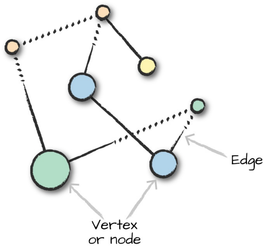
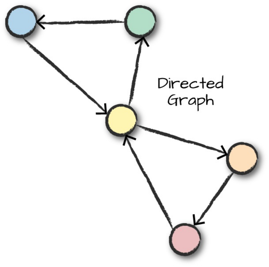
Figure 30-2. A directed graph
Edges and vertices in graphs can also have data associated with them. In our
friend example, the weight of the edge might represent the intimacy between
different friends; acquaintances would have low-weight edges between them,
while married individuals would have edges with large weights. We could set
this value by looking at communication frequency between nodes and
weighting the edges accordingly. Each vertex (person) might also have data
such as a name.
Graphs are a natural way of describing relationships and many different

problem sets, and Spark provides several ways of working in this analytics
paradigm. Some business use cases could be detecting credit card fraud,
motif finding, determining importance of papers in bibliographic networks
(i.e., which papers are most referenced), and ranking web pages, as Google
famously used the PageRank algorithm to do.
Spark has long contained an RDD-based library for performing graph
processing: GraphX. This provided a very low-level interface that was
extremely powerful, but just like RDDs, wasn’t easy to use or optimize.
GraphX remains a core part of Spark. Companies continue to build
production applications on top of it, and it still sees some minor feature
development. The GraphX API is well documented simply because it hasn’t
changed much since its creation. However, some of the developers of Spark
(including some of the original authors of GraphX) have recently created a
next-generation graph analytics library on Spark: GraphFrames.
GraphFrames extends GraphX to provide a DataFrame API and support for
Spark’s different language bindings so that users of Python can take
advantage of the scalability of the tool. In this book, we will focus on
GraphFrames.
GraphFrames is currently available as a Spark package, an external package
that you need to load when you start up your Spark application, but may be
merged into the core of Spark in the future. For the most part, there should be
little difference in performance between the two (except for a huge user
experience improvement in GraphFrames). There is some small overhead
when using GraphFrames, but for the most part it tries to call down to
GraphX where appropriate; and for most, the user experience gains greatly
outweigh this minor overhead.
HOW DOES GRAPHFRAMES COMPARE TO GRAPH
DATABASES?
Spark is not a database. Spark is a distributed computation engine, but it
does not store data long-term or perform transactions. You can build a
graph computation on top of Spark, but that’s fundamentally different
from a database. GraphFrames can scale to much larger workloads than

many graph databases and performs well for analytics but does not
support transactional processing and serving.
The goal of this chapter is to show you how to use GraphFrames to perform
graph analytics on Spark. We are going to be doing this with publicly
available bike data from the Bay Area Bike Share portal.
TIP
During the course of writing this book, this map and data have changed dramatically (even
the naming!). We include a copy of the dataset inside the data folder of this book’s
repository. Be sure to use that dataset to replicate the following results; and when you’re
feeling adventurous, expand to the whole dataset!
To get set up, you’re going to need to point to the proper package. To do this
from the command line, you’ll run:
./bin/spark-shell --packages graphframes:graphframes:0.5.0-spark2.2-s_2.11
// in Scala
val bikeStations = spark.read.option("header","true")
.csv("/data/bike-data/201508_station_data.csv")
val tripData = spark.read.option("header","true")
.csv("/data/bike-data/201508_trip_data.csv")
# in Python
bikeStations = spark.read.option("header","true")\
.csv("/data/bike-data/201508_station_data.csv")
tripData = spark.read.option("header","true")\
.csv("/data/bike-data/201508_trip_data.csv")
Building a Graph
The first step is to build the graph. To do this we need to define the vertices
and edges, which are DataFrames with some specifically named columns. In
our case, we’re creating a directed graph. This graph will point from the
source to the location. In the context of this bike trip data, this will point from
a trip’s starting location to a trip’s ending location. To define the graph, we
use the naming conventions for columns presented in the GraphFrames
library. In the vertices table we define our identifier as id (in our case this is
of string type), and in the edges table we label each edge’s source vertex ID
as src and the destination ID as dst:
// in Scala
val stationVertices = bikeStations.withColumnRenamed("name", "id").distinct()
val tripEdges = tripData
.withColumnRenamed("Start Station", "src")
.withColumnRenamed("End Station", "dst")
# in Python
stationVertices = bikeStations.withColumnRenamed("name", "id").distinct()
tripEdges = tripData\
.withColumnRenamed("Start Station", "src")\
.withColumnRenamed("End Station", "dst")
We can now build a GraphFrame object, which represents our graph, from
the vertex and edge DataFrames we have so far. We will also leverage
caching because we’ll be accessing this data frequently in later queries:
// in Scala
import org.graphframes.GraphFrame
val stationGraph = GraphFrame(stationVertices, tripEdges)
stationGraph.cache()
# in Python
from graphframes import GraphFrame
stationGraph = GraphFrame(stationVertices, tripEdges)
stationGraph.cache()
Now we can see the basic statistics about graph (and query our original
DataFrame to ensure that we see the expected results):
// in Scala
println(s"Total Number of Stations: ${stationGraph.vertices.count()}")
println(s"Total Number of Trips in Graph: ${stationGraph.edges.count()}")
println(s"Total Number of Trips in Original Data: ${tripData.count()}")
# in Python
print "Total Number of Stations: " + str(stationGraph.vertices.count())
print "Total Number of Trips in Graph: " + str(stationGraph.edges.count())
print "Total Number of Trips in Original Data: " + str(tripData.count())
This returns the following results:
Total Number of Stations: 70
Total Number of Trips in Graph: 354152
Total Number of Trips in Original Data: 354152
Querying the Graph
The most basic way of interacting with the graph is simply querying it,
performing things like counting trips and filtering by given destinations.
GraphFrames provides simple access to both vertices and edges as
DataFrames. Note that our graph retained all the additional columns in the
data in addition to IDs, sources, and destinations, so we can also query those
if needed:
// in Scala
import org.apache.spark.sql.functions.desc
stationGraph.edges.groupBy("src", "dst").count().orderBy(desc("count")).show(10)
# in Python
from pyspark.sql.functions import desc
stationGraph.edges.groupBy("src", "dst").count().orderBy(desc("count")).show(10)
+--------------------+--------------------+-----+
| src| dst|count|
+--------------------+--------------------+-----+
|San Francisco Cal...| Townsend at 7th| 3748|
|Harry Bridges Pla...|Embarcadero at Sa...| 3145|
...
| Townsend at 7th|San Francisco Cal...| 2192|
|Temporary Transba...|San Francisco Cal...| 2184|
+--------------------+--------------------+-----+
We can also filter by any valid DataFrame expression. In this instance, I want
to look at one specific station and the count of trips in and out of that station:
// in Scala
stationGraph.edges
.where("src = 'Townsend at 7th' OR dst = 'Townsend at 7th'")
.groupBy("src", "dst").count()
.orderBy(desc("count"))
.show(10)
# in Python
stationGraph.edges\
.where("src = 'Townsend at 7th' OR dst = 'Townsend at 7th'")\
.groupBy("src", "dst").count()\
.orderBy(desc("count"))\
.show(10)
+--------------------+--------------------+-----+
| src| dst|count|
+--------------------+--------------------+-----+
|San Francisco Cal...| Townsend at 7th| 3748|
| Townsend at 7th|San Francisco Cal...| 2734|
...
| Steuart at Market| Townsend at 7th| 746|
| Townsend at 7th|Temporary Transba...| 740|
+--------------------+--------------------+-----+
Subgraphs
Subgraphs are just smaller graphs within the larger one. We saw in the last
section how we can query a given set of edges and vertices. We can use this
query ability to create subgraphs:
// in Scala
val townAnd7thEdges = stationGraph.edges
.where("src = 'Townsend at 7th' OR dst = 'Townsend at 7th'")
val subgraph = GraphFrame(stationGraph.vertices, townAnd7thEdges)
# in Python
townAnd7thEdges = stationGraph.edges\
.where("src = 'Townsend at 7th' OR dst = 'Townsend at 7th'")
subgraph = GraphFrame(stationGraph.vertices, townAnd7thEdges)
We can then apply the following algorithms to either the original graph or the
subgraph.
Motif Finding
Motifs are a way of expresssing structural patterns in a graph. When we
specify a motif, we are querying for patterns in the data instead of actual data.
In GraphFrames, we specify our query in a domain-specific language similar
to Neo4J’s Cypher language. This language lets us specify combinations of
vertices and edges and assign then names. For example, if we want to specify
that a given vertex a connects to another vertex b through an edge ab, we
would specify (a)-[ab]->(b). The names inside parentheses or brackets do
not signify values but instead what the columns for matching vertices and
edges should be named in the resulting DataFrame. We can omit the names
(e.g., (a)-[]->()) if we do not intend to query the resulting values.
Let’s perform a query on our bike data. In plain English, let’s find all the
rides that form a “triangle” pattern between three stations. We express this
with the following motif, using the find method to query our GraphFrame
for that pattern. (a) signifies the starting station, and [ab] represents an edge
from (a) to our next station (b). We repeat this for stations (b) to (c) and
then from (c) to (a):
// in Scala
val motifs = stationGraph.find("(a)-[ab]->(b); (b)-[bc]->(c); (c)-[ca]->(a)")
# in Python
motifs = stationGraph.find("(a)-[ab]->(b); (b)-[bc]->(c); (c)-[ca]->(a)")
Figure 30-3 presents a visual representation of this query.
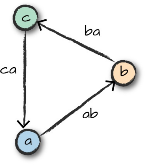
Figure 30-3. Triangle motif in our triangle query
The DataFrame we get from running this query contains nested fields for
vertices a, b, and c, as well as the respective edges. We can now query this as
we would a DataFrame. For example, given a certain bike, what is the
shortest trip the bike has taken from station a, to station b, to station c, and
back to station a? The following logic will parse our timestamps, into Spark
timestamps and then we’ll do comparisons to make sure that it’s the same
bike, traveling from station to station, and that the start times for each trip are
correct:
// in Scala
import org.apache.spark.sql.functions.expr
motifs.selectExpr("*",
"to_timestamp(ab.`Start Date`, 'MM/dd/yyyy HH:mm') as abStart",
"to_timestamp(bc.`Start Date`, 'MM/dd/yyyy HH:mm') as bcStart",
"to_timestamp(ca.`Start Date`, 'MM/dd/yyyy HH:mm') as caStart")
.where("ca.`Bike #` = bc.`Bike #`").where("ab.`Bike #` = bc.`Bike #`")
.where("a.id != b.id").where("b.id != c.id")
.where("abStart < bcStart").where("bcStart < caStart")
.orderBy(expr("cast(caStart as long) - cast(abStart as long)"))
.selectExpr("a.id", "b.id", "c.id", "ab.`Start Date`", "ca.`End Date`")
.limit(1).show(false)
# in Python
from pyspark.sql.functions import expr
motifs.selectExpr("*",
"to_timestamp(ab.`Start Date`, 'MM/dd/yyyy HH:mm') as abStart",
"to_timestamp(bc.`Start Date`, 'MM/dd/yyyy HH:mm') as bcStart",
"to_timestamp(ca.`Start Date`, 'MM/dd/yyyy HH:mm') as caStart")\
.where("ca.`Bike #` = bc.`Bike #`").where("ab.`Bike #` = bc.`Bike #`")\
.where("a.id != b.id").where("b.id != c.id")\
.where("abStart < bcStart").where("bcStart < caStart")\
.orderBy(expr("cast(caStart as long) - cast(abStart as long)"))\
.selectExpr("a.id", "b.id", "c.id", "ab.`Start Date`", "ca.`End Date`")
.limit(1).show(1, False)
We see the fastest trip is approximately 20 minutes. Pretty fast for three
different people (we assume) using the same bike!
Note also that we had to filter the triangles returned by our motif query in this
example. In general, different vertex IDs used in the query will not be forced
to match distinct vertices, so you should perform this type of filtering if you
want distinct vertices. One of the most powerful features of GraphFrames is
that you can combine motif finding with DataFarme queries over the
resulting tables to further narrow down, sort, or aggregate the patterns found.
Graph Algorithms
A graph is just a logical representation of data. Graph theory provides
numerous algorithms for analyzing data in this format, and GraphFrames
allows us to leverage many algorithms out of the box. Development
continues as new algorithms are added to GraphFrames, so this list will most
likely continue to grow.
PageRank
One of the most prolific graph algorithms is PageRank. Larry Page,
cofounder of Google, created PageRank as a research project for how to rank

web pages. Unfortunately, a complete explanation of how PageRank works is
outside the scope of this book. However, to quote Wikipedia, the high-level
explanation is as follows:
PageRank works by counting the number and quality of links to a page to
determine a rough estimate of how important the website is. The
underlying assumption is that more important websites are likely to receive
more links from other websites.
PageRank generalizes quite well outside of the web domain. We can apply
this right to our own data and get a sense for important bike stations
(specifically, those that receive a lot of bike traffic). In this example,
important bike stations will be assigned large PageRank values:
// in Scala
import org.apache.spark.sql.functions.desc
val ranks = stationGraph.pageRank.resetProbability(0.15).maxIter(10).run()
ranks.vertices.orderBy(desc("pagerank")).select("id", "pagerank").show(10)
# in Python
from pyspark.sql.functions import desc
ranks = stationGraph.pageRank(resetProbability=0.15, maxIter=10)
ranks.vertices.orderBy(desc("pagerank")).select("id", "pagerank").show(10)
+--------------------+------------------+
| id| pagerank|
+--------------------+------------------+
|San Jose Diridon ...| 4.051504835989922|
|San Francisco Cal...|3.3511832964279518|
...
| Townsend at 7th| 1.568456580534273|
|Embarcadero at Sa...|1.5414242087749768|
+--------------------+------------------+
GRAPH ALGORITHM APIS: PARAMETERS AND RETURN
VALUES
Most algorithms in GraphFrames are accessed as methods which take
parameters (e.g., resetProbability in this PageRank example). Most
algorithms return either a new GraphFrame or a single DataFrame. The

results of the algorithm are stored as one or more columns in the
GraphFrame’s vertices and/or edges or the DataFrame. For PageRank,
the algorithm returns a GraphFrame, and we can extract the estimated
PageRank values for each vertex from the new pagerank column.
WARNING
Depending on the resources available on your machine, this may take some time. You can
always try a smaller set of data before running this to see the results. On Databricks
Community Edition, this takes about 20 seconds to run, although some reviewers found it
to take much longer on their machines.
Interestingly, we see that Caltrain stations rank quite highly. This makes
sense because these are natural connection points where a lot of bike trips
might end up. Either as commuters move from home to the Caltrain station
for their commute or from the Caltrain station to home.
In-Degree and Out-Degree Metrics
Our graph is a directed graph. This is due to the bike trips being directional,
starting in one location and ending in another. One common task is to count
the number of trips into or out of a given station. To measure trips in and out
of stations, we will use a metric called in-degree and out-degree, respectively,
as seen in Figure 30-4.
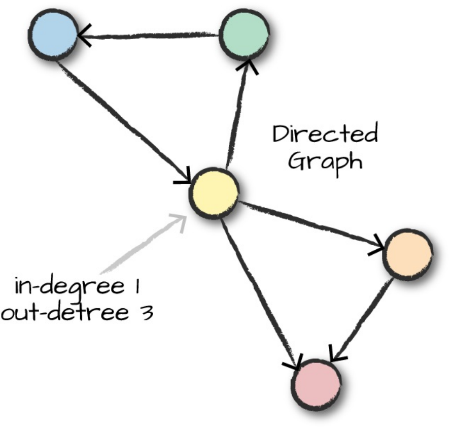
Figure 30-4. In-degree and out-degree
This is particularly applicable in the context of social networking because
certain users may have many more inbound connections (i.e., followers) than
outbound connections (i.e., people they follow). Using the following query,
you can find interesting people in the social network who might have more
influence than others. GraphFrames provides a simple way to query our
graph for this information:
// in Scala
val inDeg = stationGraph.inDegrees
inDeg.orderBy(desc("inDegree")).show(5, false)
# in Python
inDeg = stationGraph.inDegrees
inDeg.orderBy(desc("inDegree")).show(5, False)
The result of querying for the stations sorted by the highest in-degree:
+----------------------------------------+--------+
|id |inDegree|
+----------------------------------------+--------+
|San Francisco Caltrain (Townsend at 4th)|34810 |
|San Francisco Caltrain 2 (330 Townsend) |22523 |
|Harry Bridges Plaza (Ferry Building) |17810 |
|2nd at Townsend |15463 |
|Townsend at 7th |15422 |
+----------------------------------------+--------+
We can query the out degrees in the same fashion:
// in Scala
val outDeg = stationGraph.outDegrees
outDeg.orderBy(desc("outDegree")).show(5, false)
# in Python
outDeg = stationGraph.outDegrees
outDeg.orderBy(desc("outDegree")).show(5, False)
+---------------------------------------------+---------+
|id |outDegree|
+---------------------------------------------+---------+
|San Francisco Caltrain (Townsend at 4th) |26304 |
|San Francisco Caltrain 2 (330 Townsend) |21758 |
|Harry Bridges Plaza (Ferry Building) |17255 |
|Temporary Transbay Terminal (Howard at Beale)|14436 |
|Embarcadero at Sansome |14158 |
+---------------------------------------------+---------+
The ratio of these two values is an interesting metric to look at. A higher ratio
value will tell us where a large number of trips end (but rarely begin), while a
lower value tells us where trips often begin (but infrequently end):
// in Scala
val degreeRatio = inDeg.join(outDeg, Seq("id"))
.selectExpr("id", "double(inDegree)/double(outDegree) as degreeRatio")
degreeRatio.orderBy(desc("degreeRatio")).show(10, false)
degreeRatio.orderBy("degreeRatio").show(10, false)
# in Python
degreeRatio = inDeg.join(outDeg, "id")\
.selectExpr("id", "double(inDegree)/double(outDegree) as degreeRatio")
degreeRatio.orderBy(desc("degreeRatio")).show(10, False)
degreeRatio.orderBy("degreeRatio").show(10, False)
Those queries result in the following data:
+----------------------------------------+------------------+
|id |degreeRatio |
+----------------------------------------+------------------+
|Redwood City Medical Center |1.5333333333333334|
|San Mateo County Center |1.4724409448818898|
...
|Embarcadero at Vallejo |1.2201707365495336|
|Market at Sansome |1.2173913043478262|
+----------------------------------------+------------------+
+-------------------------------+------------------+
|id |degreeRatio |
+-------------------------------+------------------+
|Grant Avenue at Columbus Avenue|0.5180520570948782|
|2nd at Folsom |0.5909488686085761|
...
|San Francisco City Hall |0.7928849902534113|
|Palo Alto Caltrain Station |0.8064516129032258|
+-------------------------------+------------------+
Breadth-First Search
Breadth-first search will search our graph for how to connect two sets of
nodes, based on the edges in the graph. In our context, we might want to do
this to find the shortest paths to different stations, but the algorithm also
works for sets of nodes specified through a SQL expression. We can specify
the maximum of edges to follow with the maxPathLength, and we can also
specify an edgeFilter to filter out edges that do not meet a requirement, like
trips during nonbusiness hours.
We’ll choose two fairly close stations so that this does not run too long.
However, you can do interesting graph traversals when you have sparse
graphs that have distant connections. Feel free to play around with the
stations (especially those in other cities) to see if you can get distant stations
to connect:
// in Scala
stationGraph.bfs.fromExpr("id = 'Townsend at 7th'")
.toExpr("id = 'Spear at Folsom'").maxPathLength(2).run().show(10)
# in Python
stationGraph.bfs(fromExpr="id = 'Townsend at 7th'",
toExpr="id = 'Spear at Folsom'", maxPathLength=2).show(10)
+--------------------+--------------------+--------------------+
| from| e0| to|
+--------------------+--------------------+--------------------+
|[65,Townsend at 7...|[913371,663,8/31/...|[49,Spear at Fols...|
|[65,Townsend at 7...|[913265,658,8/31/...|[49,Spear at Fols...|
...
|[65,Townsend at 7...|[903375,850,8/24/...|[49,Spear at Fols...|
|[65,Townsend at 7...|[899944,910,8/21/...|[49,Spear at Fols...|
+--------------------+--------------------+--------------------+
Connected Components
A connected component defines an (undirected) subgraph that has
connections to itself but does not connect to the greater graph, as illustrated
in Figure 30-5.
Figure 30-5. A connected component
The connected components algorithm does not directly relate to our current
problem because they assume an undirected graph. However, we can still run
the algorithm, which just assumes that there are is no directionality associated
with our edges. In fact, if we look at the bike share map, we assume that we
would get two distinct connected components (Figure 30-6).
Figure 30-6. A map of Bay Area bike share locations
WARNING
To run this algorithm, you will need to set a checkpoint directory which will store the state
of the job at every iteration. This allows you to continue where you left off if the job
crashes. This is probably one of the most expensive algorithms currently in GraphFrames,
so expect delays.
One thing you will likely have to do to run this algorithm on your local
machine is take a sample of the data, just as we do in the following code
example (taking a sample can help you get to a result without crashing the
Spark application with garbage collection issues):
// in Scala
spark.sparkContext.setCheckpointDir("/tmp/checkpoints")
# in Python
spark.sparkContext.setCheckpointDir("/tmp/checkpoints")
// in Scala
val minGraph = GraphFrame(stationVertices, tripEdges.sample(false, 0.1))
val cc = minGraph.connectedComponents.run()
# in Python
minGraph = GraphFrame(stationVertices, tripEdges.sample(False, 0.1))
cc = minGraph.connectedComponents()
From this query we get two connected components but not necessarily the
ones we might expect. Our sample may not have all of the correct data or
information so we’d probably need more compute resources to investigate
further:
// in Scala
cc.where("component != 0").show()
# in Python
cc.where("component != 0").show()
+----------+------------------+---------+-----------+---------+------------+----
-
|station_id| id| lat| long|dockcount|
landmark|in...
+----------+------------------+---------+-----------+---------+------------+----
-
| 47| Post at Kearney|37.788975|-122.403452| 19|San Franc...|
...
| 46|Washington at K...|37.795425|-122.404767| 15|San Franc...|
...
+----------+------------------+---------+-----------+---------+------------+----
-
Strongly Connected Components
GraphFrames includes another related algorithm that relates to directed
graphs: strongly connected components, which takes directionality into
account. A strongly connected component is a subgraph that has paths
between all pairs of vertices inside it.
// in Scala
val scc = minGraph.stronglyConnectedComponents.maxIter(3).run()
# in Python
scc = minGraph.stronglyConnectedComponents(maxIter=3)
scc.groupBy("component").count().show()
Advanced Tasks
This is just a short selection of some of the features of GraphFrames. The
GraphFrames library also includes features such as writing your own
algorithms via a message-passing interface, triangle counting, and converting
to and from GraphX. You can find more information in the GraphFrames
documentation.
Conclusion
In this chapter, we took a tour of GraphFrames, a library for performing
graph analysis on Apache Spark. We took a more tutorial-based approach,
since this processing technique is not necessarily the first tool that people use
when performing advanced analytics. It is nonetheless a powerful tool for
analyzing relationships between different objects, and critical in many
domains. The next chapter will talk about more cutting-edge functionality—
specifically, deep learning.

Chapter 31. Deep Learning
Deep learning is one of the most exciting areas of development around Spark
due to its ability to solve several previously difficult machine learning
problems, especially those involving unstructured data such as images, audio,
and text. This chapter will cover how Spark works in tandem with deep
learning, and some of the different approaches you can use to work with
Spark and deep learning together.
Because deep learning is still a new field, many of the newest tools are
implemented in external libraries. This chapter will not focus on packages
that are necessarily core to Spark but rather on the massive amount of
innovation in libraries built on top of Spark. We will start with several high-
level ways to use deep learning on Spark, discuss when to use each one, and
then go over the libraries available for them. As usual, we will include end-
to-end examples.
NOTE
To make the most of this chapter you should know at least the basics of deep learning as
well as the basics of Spark. With that being said, we point to an excellent resource at the
beginning of this part of the book called the Deep Learning Book, by some of the top
researchers in this area.
What Is Deep Learning?
To define deep learning, we must first define neural networks. A neural
network is a graph of nodes with weights and activation functions. These
nodes are organized into layers that are stacked on top of one another. Each
layer is connected, either partially or completely, to the previous layer in the
network. By stacking layers one after the other, these simple functions can
learn to recognize more and more complex signals in the input: simple lines
with one layer, circles and squares with the next layer, complex textures in
another, and finally the full object or output you hope to identify. The goal is
to train the network to associate certain inputs with certain outputs by tuning
the weights associated with each connection and the values of each node in
the network. Figure 31-1 shows the simple neural network.
Figure 31-1. A neural network
Deep learning, or deep neural networks, stack many of these layers together
into various different architectures. Neural networks themselves have existed
for decades, and have waxed and waned in terms of popularity for various
machine learning problems. Recently, however, a combination of much
larger datasets (e.g., the ImageNet corpus for object recognition), powerful
hardware (clusters and GPUs), and new training algorithms have enabled
training much larger neural networks that outperform previous approaches in
many machine learning tasks. Typical machine learning techniques typically
cannot continue to perform well as more data is added; their performance hits
a ceiling. Deep learning can benefit from enormous amounts of data and
information and it is not uncommon for deep learning datasets to be orders of
magnitude larger than other machine learning datasets. Deep neural networks
have now become the standard in computer vision, speech processing, and
some natural language tasks, where they often “learn” better features than
previous hand-tuned models. They are also actively being applied in other
areas of machine learning. Apache Spark’s strength as a big data and parallel
computing system makes it a natural framework to use with deep learning.
Researchers and engineers have put a lot of effort into speeding up these
neural network-like calculations. Nowadays, the most popular way to use
neural networks or deep learning is to use a framework, implemented by a
research institute or corporation. The most popular as of the time of this
writing are TensorFlow, MXNet, Keras, and PyTorch. This area is rapidly
evolving so it’s always worth searching around for others.
Ways of Using Deep Learning in Spark
For the most part, regardless of which application you are targeting, there are
three major ways to use deep learning in Spark:
Inference
The simplest way to use deep learning is to take a pretrained model and
apply it to large datasets in parallel using Spark. For example, you could
use an image classification model, trained using a standard dataset like
ImageNet, and apply it to your own image collection to identify pandas,
flowers, or cars. Many organizations publish large, pretrained models on
common datasets (e.g., Faster R-CNN and YOLO for object detection),
so you can often take a model from your favorite deep learning
framework and apply it in parallel using a Spark function. Using PySpark,
you could simply call a framework such as TensorFlow or PyTorch in a
map function to get distributed inference, though some of the libraries we
discuss for it make further optimizations beyond simply calling these
libraries in a map function.
Featurization and transfer learning
The next level of complexity is to use an existing model as a featurizer
instead of taking its final output. Many deep learning models learn useful
feature representations in their lower layers as they get trained for an end-
to-end task. For example, a classifier trained on the ImageNet dataset will
also learn low-level features present in all natural images, such as edges
and textures. We can then use these features to learn models for a new
problem not covered by the original dataset. This method is called
transfer learning, and generally involves the last few layers of a
pretrained model and retraining them with the data of interest. Transfer
learning is also especially useful if you do not have a large amount of
training data: training a full-blown network from scratch requires a
dataset of hundreds of thousands of images, like ImageNet, to avoid
overfitting, which will not be available in many business contexts. In
contrast, transfer learning can work even with a few thousand images
because it updates fewer parameters.
Model training
Spark can also be used to train a new deep learning model from scratch.
There are two common methods here. First, you can use a Spark cluster to
parallelize the training of a single model over multiple servers,
communicating updates between them. Alternatively, some libraries let
the user train multiple instances of similar models in parallel to try
various model architectures and hyperparameters, accelerating the model
search and tuning process. In both cases, Spark’s deep learning libraries
make it simple to pass data from RDDs and DataFrames to deep learning
algorithms. Finally, even if you do not wish to train your model in
parallel, these libraries can be used to extract data from a cluster and
export it to a single-machine training script using the native data format
of frameworks like TensorFlow.
In all three cases, the deep learning code typically runs as part of a larger
application that includes Extract, Transform, and Load (ETL) steps to parse
the input data, I/O from various sources, and potentially batch or streaming
inference. For these other parts of the application, you can simply use the
DataFrame, RDD, and MLlib APIs described earlier in this book. One of
Spark’s strengths is the ease of combining these steps into a single parallel
workflow.
Deep Learning Libraries
In this section, we’ll survey a few of the most popular libraries available for
deep learning in Spark. We will describe the main use cases of the library and
link them to references or examples when possible. This list is not meant to
be exhaustive, because the field is rapidly evolving. We encourage you to
check each library’s website and the Spark documentation for the latest
updates.
MLlib Neural Network Support
Spark’s MLlib currently has native support for a single deep learning
algorithm: the ml.classification.MultilayerPerceptronClassifier
class’s multilayer perceptron classifier. This class is limited to training
relatively shallow networks containing fully connected layers with the
sigmoid activation function and an output layer with a softmax activation
function. This class is most useful for training the last few layers of a
classification model when using transfer learning on top of an existing deep
learning–based featurizer. For example, it can be added on top of the Deep
Learning Pipelines library we describe later in this chapter to quickly perform
transfer learning over Keras and TensorFlow models.
TensorFrames
TensorFrames is an inference and transfer learning-oriented library that
makes it easy to pass data between Spark DataFrames and TensorFlow. It
supports Python and Scala interfaces and focuses on providing a simple but
optimized interface to pass data from TensorFlow to Spark and back. In
particular, using TensorFrames to apply a model over Spark DataFrames is
generally more efficient than calling a Python map function that directly
invokes the TensorFlow model, due to faster data transfer and amortization of
the startup cost. TensorFrames is most useful for inference, in both streaming
and batch settings, and for transfer learning, where you can apply an existing
model over raw data to featurize it, then learn the last layers using a
MultilayerPerceptronClassifier or even a simpler logistic regression or
random forest classifier over the data.
BigDL
BigDL is a distributed deep learning framework for Apache Spark primarily
developed by Intel. It aims to support distributed training of large models as
well as fast applications of these models using inference. One key advantage
of BigDL over the other libraries described here is that it is primarily
optimized to use CPUs instead of GPUs, making it efficient to run on an
existing, CPU-based cluster (e.g., an Apache Hadoop deployment). BigDL
provides high-level APIs to build neural networks from scratch and
automatically distributes all operations by default. It can also train models
described with the Keras DL library.
TensorFlowOnSpark
TensorFlowOnSpark is a widely used library that can train TensorFlow
models in a parallel fashion on Spark clusters. TensorFlow includes some
foundations to do distributed training, but it still needs to rely on a cluster
manager for managing the hardware and data communications. It does not
come with a cluster manager or a distributed I/O layer out of the box.
TensorFlowOnSpark launches TensorFlow’s existing distributed mode inside
a Spark job, and automatically feeds data from Spark RDDs or DataFrames
into the TensorFlow job. If you already know how to use TensorFlow’s
distributed mode, TensorFlowOnSpark makes it easy to launch your job
inside a Spark cluster and pass it data processed with other Spark libraries
(e.g., DataFrame transformations) from any input source Spark supports.
TensorFlowOnSpark was originally developed at Yahoo! and is also used in

production at other large organizations. The project also integrates with
Spark’s ML Pipelines API.
DeepLearning4J
DeepLearning4j is an open-source, distributed deep learning project in Java
and Scala that provides both single-node and distributed training options. One
of its advantages over Python-based deep learning frameworks is that it was
primarily designed for the JVM, making it more convenient for groups that
do not wish to add Python to their development process. It includes a wide
variety of training algorithms and support for CPUs as well as GPUs.
Deep Learning Pipelines
Deep Learning Pipelines is an open source package from Databricks that
integrates deep learning functionality into Spark’s ML Pipelines API. The
package existing deep learning frameworks (TensorFlow and Keras at the
time of writing), but focuses on two goals:
Incorporating these frameworks into standard Spark APIs (such as
ML Pipelines and Spark SQL) to make them very easy to use
Distributing all computation by default
For example, Deep Learning Pipelines provides a DeepImageFeaturizer
class that acts as a transformer in the Spark ML Pipeline API, allowing you to
build a transfer learning pipeline in just a few lines of code (e.g., by adding a
perceptron or logistic regression classifier on top). Likewise, the library
supports parallel grid search over multiple model parameters using MLlib’s
grid search and cross-validation API. Finally, users can export an ML model
as a Spark SQL user-defined function and make it available to analysts using
SQL or streaming applications. At the time of writing (summer 2017), Deep
Learning Pipelines is under heavy development, so we encourage you to
check its website for the latest updates.
Table 31-1 summarizes the various deep learning libraries and the main use
cases they support:

Table 31-1. Deep learning libraries
Library Underlying DL
framework Use cases
BigDL BigDL Distributed training, inference, ML Pipeline
integration
DeepLearning4J DeepLearning4J Inference, transfer learning, distributed training
Deep Learning
Pipelines
TensorFlow,
Keras
Inference, transfer learning, multi-model training, ML
Pipeline and Spark SQL integration
MLlib Perceptron Spark Distributed training, ML Pipeline integration
TensorFlowOnSpark TensorFlow Distributed training, ML Pipeline integration
TensorFrames TensorFlow Inference, transfer learning, DataFrame integration
While there are several approaches different companies have taken to
integrating Spark and deep learning libraries, the one currently aiming for the
closest integration with MLlib and DataFrames is Deep Learning Pipelines.
This library aims to improve Spark’s support for image and tensor data
(which will be integrated into the core Spark codebase in Spark 2.3), and to
make all deep learning functionality available in the ML Pipeline API. Its
friendly API makes it the simplest way to run deep learning on Spark today
and will be the focus of the remaining sections in this chapter.
A Simple Example with Deep Learning
Pipelines
As we described, Deep Learning Pipelines provides high-level APIs for
scalable deep learning by integrating popular deep learning frameworks with
ML Pipelines and Spark SQL.
Deep Learning Pipelines builds on Spark’s ML Pipelines for training and on
Spark DataFrames and SQL for deploying models. It includes high-level

APIs for common aspects of deep learning so they can be done efficiently in
a few lines of code:
Working with images in Spark DataFrames;
Applying deep learning models at scale, whether they are your own
or standard popular models, to image and tensor data;
Transfer learning using common pretrained deep learning models;
Exporting models as Spark SQL functions to make it simple for all
kinds of users to take advantage of deep learning; and
Distributed deep learning hyperparameter tuning via ML Pipelines.
Deep Learning Pipelines currently only offers an API in Python, which is
designed to work closely with existing Python deep learning packages such
as TensorFlow and Keras.
Setup
Deep Learning Pipelines is a Spark Package, so we’ll load it just like we
loaded GraphFrames. Deep Learning Pipelines works on Spark 2.x and the
package can be found here. You’re going to need to install a few Python
dependencies, including TensorFrames, TensorFlow, Keras, and h5py. Make
sure these are installed across both your driver and worker machines.
We’ll use the flowers dataset from the TensorFlow retraining tutorial. Now if
you’re running this on a cluster of machines, you’re going to need a way to
put these files on a distributed file system once you download them. We
include a sample of these images in the book’s GitHub Repository.
Images and DataFrames
One of the historical challenges when working with images in Spark is that
getting them into a DataFrame was difficult and tedious. Deep Learning
Pipelines includes utility functions that make loading and decoding images in
a distributed fashion easy. This is an area that’s changing rapidly. Currently,
this is a part of Deep Learning Pipelines. Basic image loading and
representation will be included in Spark 2.3. While it is not released yet, all
of the examples in this chapter should be compatible with this upcoming
version of Spark:
from sparkdl import readImages
img_dir = '/data/deep-learning-images/'
image_df = readImages(img_dir)
The resulting DataFrame contains the path and then the image along with
some associated metadata:
image_df.printSchema()
root
|-- filePath: string (nullable = false)
|-- image: struct (nullable = true)
| |-- mode: string (nullable = false)
| |-- height: integer (nullable = false)
| |-- width: integer (nullable = false)
| |-- nChannels: integer (nullable = false)
| |-- data: binary (nullable = false)
Transfer Learning
Now that we have some data, we can get started with some simple transfer
learning. Remember, this means leveraging a model that someone else
created and modifying it to better suit our own purposes. First, we will load
the data for each type of flower and create a training and test set:
from sparkdl import readImages
from pyspark.sql.functions import lit
tulips_df = readImages(img_dir + "/tulips").withColumn("label", lit(1))
daisy_df = readImages(img_dir + "/daisy").withColumn("label", lit(0))
tulips_train, tulips_test = tulips_df.randomSplit([0.6, 0.4])
daisy_train, daisy_test = daisy_df.randomSplit([0.6, 0.4])
train_df = tulips_train.unionAll(daisy_train)
test_df = tulips_test.unionAll(daisy_test)
In the next step we will leverage a transformer called the
DeepImageFeaturizer. This will allow us to leverage a pretrained model
called Inception, a powerful neural network successfully used to identify
patterns in images. The version we are using is pretrained to work well with
images of various common objects and animals. This is one of the standard
pretrained models that ship with the Keras library. However, this particular
neural network is not trained to recognize daisies and roses. So we’re going
to use transfer learning in order to make it into something useful for our own
purposes: distinguishing different flower types.
Note that we can use the same ML Pipeline concepts we learned about
throughout this part of the book and leverage them with Deep Learning
Pipelines: DeepImageFeaturizer is just an ML transformer. Additionally,
all that we’ve done to extend this model is add on a logistic regression model
in order to facilitate the training of our end model. We could use another
classifier in its place. The following code snippet demonstrates adding this
model (note this may take time to complete as it’s a fairly resource intensive
process):
from pyspark.ml.classification import LogisticRegression
from pyspark.ml import Pipeline
from sparkdl import DeepImageFeaturizer
featurizer = DeepImageFeaturizer(inputCol="image", outputCol="features",
modelName="InceptionV3")
lr = LogisticRegression(maxIter=1, regParam=0.05, elasticNetParam=0.3,
labelCol="label")
p = Pipeline(stages=[featurizer, lr])
p_model = p.fit(train_df)
Once we’ve trained the model, we can use the same classification evaluator
we used in Chapter 25. We can specify the metric we’d like to test and then
evaluate it:
from pyspark.ml.evaluation import MulticlassClassificationEvaluator
tested_df = p_model.transform(test_df)
evaluator = MulticlassClassificationEvaluator(metricName="accuracy")
print("Test set accuracy = " + str(evaluator.evaluate(tested_df.select(
"prediction", "label"))))
With our DataFrame of examples, we can inspect the rows and images in
which we made mistakes in the previous training:
from pyspark.sql.types import DoubleType
from pyspark.sql.functions import expr
# a simple UDF to convert the value to a double
def _p1(v):
return float(v.array[1])
p1 = udf(_p1, DoubleType())
df = tested_df.withColumn("p_1", p1(tested_df.probability))
wrong_df = df.orderBy(expr("abs(p_1 - label)"), ascending=False)
wrong_df.select("filePath", "p_1", "label").limit(10).show()
Applying deep learning models at scale
Spark DataFrames are a natural construct for applying deep learning models
to a large-scale dataset. Deep Learning Pipelines provides a set of
Transformers for applying TensorFlow graphs and TensorFlow-backed Keras
models at scale. In addition, popular image models can be applied out of the
box, without requiring any TensorFlow or Keras code. The transformers,
backed by the Tensorframes library, efficiently handle the distribution of
models and data to Spark tasks.
Applying Popular Models
There are many standard deep learning models for images. If the task at hand
is very similar to what the models provide (e.g., object recognition with
ImageNet classes), or merely for exploration, you can use the transformer
DeepImagePredictor by simply specifying the model name. Deep Learning
Pipelines supports a variety of standard models included in Keras, which are
listed on its website. The following is an example of using
DeepImagePredictor:
from sparkdl import readImages, DeepImagePredictor
image_df = readImages(img_dir)
predictor = DeepImagePredictor(
inputCol="image",
outputCol="predicted_labels",
modelName="InceptionV3",
decodePredictions=True,
topK=10)
predictions_df = predictor.transform(image_df)
Notice that the predicted_labels column shows “daisy” as a high
probability class for all sample flowers using this base model. However, as
can be seen from the differences in the probability values, the neural network
has the information to discern the two flower types. As we can see, our
transfer learning example was able to properly learn the differences between
daisies and tulips starting from the base model:
df = p_model.transform(image_df)
Applying custom Keras models
Deep Learning Pipelines also allows us to apply a Keras model in a
distributed manner using Spark. To do this, check the user guide on the
KerasImageFileTransformer. This loads a Keras model and applies it to a
DataFrame column.
Applying TensorFlow models
Deep Learning Pipelines, through its integration with TensorFlow, can be
used to create custom transformers that manipulate images using
TensorFlow. For instance, you could create a transformer to change the size
of an image or modify the color spectrum. To do this, use the
TFImageTransformer class.
Deploying models as SQL functions
Another option is to deploy a model as a SQL function allowing any user
who knows SQL to be able to use a deep learning model. Once this function
is used, the resulting UDF function takes a column and produces the output
of the particular model. For instance, you could apply Inception v3 to a
variety of images by using the registerKeraImageUDF class:
from keras.applications import InceptionV3
from sparkdl.udf.keras_image_model import registerKerasImageUDF
from keras.applications import InceptionV3
registerKerasImageUDF("my_keras_inception_udf", InceptionV3(weights="imagenet"))
This way, the power of deep learning is available to any Spark user, not just
the specialist who built the model.
Conclusion
This chapter discussed several common approaches to using deep learning in
Spark. We covered a variety of available libraries and then worked through
some basic examples of common tasks. This area of Spark is under very
active development and will continue to advance as time moves on so it’s
worth checking in on the libraries to learn more as time goes on! Over time,
the authors of this book hope to keep this chapter up to date with current
developments.

Part VII. Ecosystem
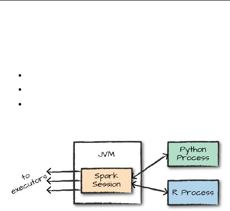
Chapter 32. Language Specifics:
Python (PySpark) and R (SparkR
and sparklyr)
This chapter will cover some of the more nuanced language specifics of
Apache Spark. We’ve seen a huge number of PySpark examples throughout
the book. In Chapter 1, we discussed at a high level how Spark runs code
from other languages. Let’s talk through some of the more specific
integrations:
PySpark
SparkR
sparklyr
As a reminder, Figure 32-1 shows the fundamental architecture for these
specific languages.
Figure 32-1. The Spark Driver
Now let’s cover each of these in depth.
PySpark
We covered a ton of PySpark throughout this book. In fact, PySpark is
included alongside Scala and SQL in nearly every chapter in this book.
Therefore, this section will be short and sweet, covering only the details that
are relevant to Spark itself. As we discussed in Chapter 1, Spark 2.2 included
a way to install PySpark with pip. Simply, pip install pyspark will make
it available as a package on your local machine. This is new, so there may be
some bugs to fix, but it is something that you can leverage in your projects
today.
Fundamental PySpark Differences
If you’re using the structured APIs, your code should run just about as fast as
if you had written it in Scala, except if you’re not using UDFs in Python. If
you’re using a UDF, you may have a performance impact. Refer back to
Chapter 6 for more information on why this is the case.
If you’re using the unstructured APIs, specifically RDDs, then your
performance is going to suffer (at the cost of a bit more flexibility). We touch
on this reasoning in Chapter 12, but the fundamental idea is that Spark is
going to have to work a lot harder converting information from something
that Spark and the JVM can understand to Python and back again. This
includes both functions as well as data and is a process known as
serialization. We’re not saying it never makes sense to use them; it’s just
something to be aware of when doing so.
Pandas Integration
One of the powers of PySpark is its ability to work across programming
models. For instance, a common pattern is to perform very large-scale ETL
work with Spark and then collect the (single-machine-sized) result to the
driver and then leverage Pandas to manipulate it further. This allows you to
use a best-in-class tool for the best task at hand—Spark for big data and
Pandas for small data:
import pandas as pd
df = pd.DataFrame({"first":range(200), "second":range(50,250)})
sparkDF = spark.createDataFrame(df)
newPDF = sparkDF.toPandas()
newPDF.head()
These niceties make working with data big and small easy with Spark.
Spark’s community continues to focus on improving this interoperability with
various other projects, so the integration between Spark and Python will
continue to improve. For example, at the time of writing, the community is
actively working on Vectorized UDFs (SPARK-21190), which add a
mapBatches API to let you process a Spark DataFrame as a series of Pandas
data frames in Python instead of converting each individual row to a Python
object. This feature is targeted to appear in Spark 2.3.
R on Spark
The rest of this chapter will cover R, Spark’s newest officially supported
language. R is a language and environment for statistical computing and
graphics. It is similar to the S language and environment developed at Bell
Laboratories by John Chambers (of no relation to one of the authors of this
book) and colleagues. The R langauge has been around for decades and is
consistently popular among statisticians and those doing research in
numerical computing. R is steadily becoming a first-class citizen in Spark
and provides the simplest open source interface for distributed computation
to the R language.
The popularity of R for performing single-machine data analysis and
advanced analytics makes it an excellent complement to Spark. There are two
core initiatives to making this partnership a reality: SparkR and sparklyr.
These packages take slightly different approaches to provide similar
functionality. SparkR provides a DataFrame API similar to R’s data.frame,
while sparklyr is based on the popular dplyr package for accessing

structured data. You can use whichever you prefer in your code, but over
time we expect that the community might converge toward a single integrated
package.
We will cover both packages here to let you choose which API you prefer.
For the most part, both of these projects are mature and well supported, albeit
by slightly different communities. They both support Spark’s structured APIs
and allow for machine learning. We will elaborate on their differences in the
next sections.
SparkR
SparkR is an R package (originating as a collaborative research project
between UC Berkeley, Databricks, and MIT CSAIL) that provides a frontend
to Apache Spark based on familiar R APIs. SparkR is conceptually similar to
R’s built-in data.frame API, except for some departures from the API
semantics, such as lazy evaluation. SparkR is a part of the official Spark
project and is supported as such. See the documentation for SparkR for more
information.
Pros and cons of using SparkR instead of other languages
The reasons we would recommend that you use SparkR as opposed to
PySpark are the following.
You are familiar with R and want to take the smallest step to
leverage the capabilities of Spark:
You want to leverage R-specific functionality or libraries (say the
excellent ggplot2 library) and would like to work with big data in
the process.
R is a powerful programming language that provides a lot of advantages over
other languages when it comes to certain tasks. However, it has its share of
shortcomings like natively working with distributed data. SparkR aims to fill
this gap and does a great job enabling users to be successful on both small
and large data, in a conceptual way similar to PySpark and Pandas.
Setup
Let’s take a look at how to use SparkR. Naturally, you will need to have R
installed on your system to follow along in this chapter. To start up the shell,
in your Spark home folder, run ./bin/sparkR to start SparkR. This will
automatically create a SparkSession for you. If you were to run SparkR from
RStudio, you would have to do something like the following:
library(SparkR)
spark <- sparkR.session()
Once we’ve started the shell, we can run Spark commands. For instance, we
can read in a CSV file like we saw in Chapter 9:
retail.data <- read.df(
"/data/retail-data/all/",
"csv",
header="true",
inferSchema="true")
print(str(retail.data))
We can take some rows from this SparkDataFrame and convert them to a
standard R data.frame type:
local.retail.data <- take(retail.data, 5)
print(str(local.retail.data))
Key Concepts
Now that we saw some very basic code, let’s reiterate key concepts. First,
SparkR is still Spark. Basically, all the tools that you have seen across the
entire book apply directly to SparkR. It runs according to the same principles
as PySpark and has almost all of the same functionality available as PySpark.
As shown in Figure 32-1, there is a gateway that connects the R process to
the JVM that contains a SparkSession, and SparkR converts user code into
structured Spark manipulations across the cluster. This makes its efficiency
on par with Python and Scala when using the structured APIs. SparkR has no
support for RDDs or other low-level APIs.
While SparkR is used less than PySpark or Scala, it’s still popular and
continues to grow. For those that want to know enough Spark to leverage
SparkR effectively, we recommend reading the following section, along with
Parts I and II of this book. When working through those other chapters, feel
free to try and use SparkR in place of Python or Scala. You’ll see that once
you get the hang of it, it’s easy to translate between the various languages.
The rest of this chapter will explain the most important differences between
SparkR and “standard” R to make it easier to be productive with SparkR
faster.
The first thing we should cover is the different between local types and Spark
types. A data.frame type’s core difference with the Spark version is that it
is available in memory and is usually directly available in that particular
process. A SparkDataFrame is just a logical representation of a series of
manipulations. Therefore when we manipulate a data.frame, we’ll see our
results right away. On a SparkDataFrame, we are going to logically
manipulate the data using the same transformation and action concepts that
we saw throughout the book.
Once we have a SparkDataFrame, we can collect it to a data.frame similar
to how we can read in data using Spark. We can also collect it into a local
data.frame with the following code (using the SparkDataFrame we created
in “Setup”):
# collect brings it from Spark to your local environment
collect(count(groupBy(retail.data, "country")))
# createDataFrame comverts a data.frame
# from your local environment to Spark
This difference is of consequence for end users. Certain functions or
assumptions that apply to local data.frames do not apply in Spark. For
instance, we cannot index a SparkDataFrame according to a particular row.
Additionally, we cannot change point values in a SparkDataFrame but can
do that in a local data.frame.
Function masking
One frequent “gotcha” when users come to SparkR is that certain functions
are masked by SparkR. When I imported SparkR, I received the following
message:
The following objects are masked from ‘package:stats’:
cov, filter, lag, na.omit, predict, sd, var, window
The following objects are masked from ‘package:base’:
as.data.frame, colnames, ...
This means that if we wish to call these masked functions, we need to be
explicit about the package that we’re calling them from or at least understand
which function masks another. The ? can be helpful in determining these
conflicts:
?na.omit # refers to SparkR due to package loading order
?stats::na.omit # refers explicitly to stats
?SparkR::na.omit # refers explicitly to sparkR's null value filtering
SparkR functions only apply to SparkDataFrames
One implication of function masking is that functions that worked on objects
previously may no longer work on them after you bring in the SparkR
package. This is because SparkR functions only apply on Spark objects. For
instance, we cannot use the sample function on a standard data.frame
because Spark takes that function name:
sample(mtcars) # fails
What you have to do instead is explicitly use the base sample function.
Additionally the function signatures differ between the two functions, which
means that even if you are familiar with the syntax and argument order for
one particular library, it does not necessarily mean it’s the same order for
SparkR:
base::sample(some.r.data.frame) # some.r.data.frame = R data.frame type
Data manipulation
Data manipulation in SparkR is conceptually the same as Spark’s DataFrame
API in other languages. The core difference is in the syntax, largely due to us
running R code and not another language. Aggregations, filtering, and many
of the functions that you can find in the other chapters throughout this book
are also available in R. For the most part, you can look at the names of
functions or manipulations that you find throughout this book and find out if
they are available in SparkR by running ?<function-name>. This should
work the vast majority of the time, as there is good coverage of structured
SQL functions:
?to_date # to Data DataFrame column manipulation
SQL is largely the same. We can specify SQL commands that we can then
manipulate as DataFrames. For instance, we can find all tables that contain
the word “production” in them:
tbls <- sql("SHOW TABLES")
collect(
select(
filter(tbls, like(tbls$tableName, "%production%")),
"tableName",
"isTemporary"))
We can also use the popular magrittr package to make this code more
readable, leveraging the piping operator to chain our transformations in a
more functional and readable syntax:
library(magrittr)
tbls %>%
filter(like(tbls$tableName, "%production%")) %>%
select("tableName", "isTemporary") %>%
collect()

Data sources
SparkR supports all of the data sources that Spark supports, including third-
party packages. We can see in the following snippet that we simply specify
the options using a slightly different syntax:
retail.data <- read.df(
"/data/retail-data/all/",
"csv",
header="true",
inferSchema="true")
flight.data <- read.df(
"/data/flight-data/parquet/2010-summary.parquet",
"parquet")
Refer back to Chapter 9 for more information.
Machine learning
Machine learning is a fundamental part of the R language, as well as of
Spark. From SparkR there is a decent availability of Spark MLlib algorithms.
Typically they arrive in R one or two versions after they are introduced in
Scala or Python. As of Spark 2.1, the following algorithms are supported in
SparkR:
spark.glm or glm: Generalized linear model
spark.survreg: Accelerated failure time (AFT) survival regression
model
spark.naiveBayes: Naive Bayes model
spark.kmeans: -means model
spark.logit: Logistic regression model
spark.isoreg: Isotonic regression model
spark.gaussianMixture: Gaussian mixture model
spark.lda: Latent Dirichlet allocation (LDA) model

spark.mlp: Multilayer perceptron classification model
spark.gbt: Gradient boosted tree model for regression and
classification
spark.randomForest: Random forest model for regression and
classification
spark.als: Alternating least squares (ALS) matrix factorization
model
spark.kstest: Kolmogorov-Smirnov test
Under the hood, SparkR uses MLlib to train the model, which means that
most everything covered in Part VI is relevant for SparkR users. Users can
call summary to print a summary of the fitted model, predict to make
predictions on new data, and write.ml/read.ml to save/load fitted models.
SparkR supports a subset of the available R formula operators for model
fitting, including ~, ., :, +, and -. Here’s an example of running a simple
regression on the retail dataset:
model <- spark.glm(retail.data, Quantity ~ UnitPrice + Country,
family='gaussian')
summary(model)
predict(model, retail.data)
write.ml(model, "/tmp/myModelOutput", overwrite=T)
newModel <- read.ml("/tmp/myModelOutput")
The API is consistent across models, although not all models support detailed
summary outputs like we saw with glm. For more information about specific
models or preprocessing techniques, see the corresponding chapters in
Part VI.
While this pales in comparison to R’s extensive collection of statistical
algorithms and analysis libraries, many users do not require the scale that
Spark provides for the actual training and usage of their machine learning
algorithms. Users have the opportunity to build training sets on large data
using Spark and then collect that dataset to their local environment for
training on a local data.frame.
User-defined functions
In SparkR, there are several ways of running user-defined functions. A user-
defined function is one that is created in the native language and run on the
server in that same native langauge. These run, for the most part, in the same
way that a Python UDF runs, by performing serialization into and out of the
JVM of the function.
The different kinds of UDFs you can define are as follows:
First, spark.lapply lets you run multiple instances of a function in Spark on
different parameter values provided in an R collection. This is a great way of
performing grid search and comparing the results:
families <- c("gaussian", "poisson")
train <- function(family) {
model <- glm(Sepal.Length ~ Sepal.Width + Species, iris, family = family)
summary(model)
}
# Return a list of model's summaries
model.summaries <- spark.lapply(families, train)
# Print the summary of each model
print(model.summaries)
Second, dapply and dapplyCollect let you process SparkDataFrame data
using custom code. In particular, these functions will take each partition of
the SparkDataFrame, convert it to an R data.frame inside of an executor,
and then call your R code over that partition (represented as an R
data.frame). They will then return the results: a SparkDataFrame for
dapply or a local data.frame for dapplyCollect.
To use dapply, which returns a SparkDataFrame, you must specify the
output schema that will result from the transformation so that Spark
understands what kind of data you will return. For example, the following
code will allow you to train a local R model per partition in your
SparkDataFrame, assuming you partition your data according to the correct
keys:
df <- withColumnRenamed(createDataFrame(as.data.frame(1:100)), "1:100", "col")
outputSchema <- structType(
structField("col", "integer"),
structField("newColumn", "double"))
udfFunc <- function (remote.data.frame) {
remote.data.frame['newColumn'] = remote.data.frame$col * 2
remote.data.frame
}
# outputs SparkDataFrame, so it requires a schema
take(dapply(df, udfFunc, outputSchema), 5)
# collects all results to a, so no schema required.
# however this will fail if the result is large
dapplyCollect(df, udfFunc)
Finally, the gapply and gapplyCollect functions apply a UDF to a group of
data in a fashion similar to dapply. In fact, these two methods are largely the
same, except that one operates on a generic SparkDataFrame, and the other
applies to a grouped DataFrame. The gapply function will apply this
function on a per-group basis and by passing in the key as the first parameter
to the function that you define. In this way, you can be sure to have a
function customized according to each particular group:
local <- as.data.frame(1:100)
local['groups'] <- c("a", "b")
df <- withColumnRenamed(createDataFrame(local), "1:100", "col")
outputSchema <- structType(
structField("col", "integer"),
structField("groups", "string"),
structField("newColumn", "double"))
udfFunc <- function (key, remote.data.frame) {
if (key == "a") {
remote.data.frame['newColumn'] = remote.data.frame$col * 2
} else if (key == "b") {
remote.data.frame['newColumn'] = remote.data.frame$col * 3
} else if (key == "c") {
remote.data.frame['newColumn'] = remote.data.frame$col * 4
}
remote.data.frame
}
# outputs SparkDataFrame, so it requires a schema
take(gapply(df,
"groups",
udfFunc,
outputSchema), 50)
gapplyCollect(df,
"groups",
udfFunc)
SparkR will continue to grow as a part of Spark; and if you’re familiar with R
and a little bit of Spark, this can be a very powerful tool.
sparklyr
sparklyr is a newer package from the RStudio team based on the popular
dplyr package for structured data. This package is fundamentally different
from SparkR and its authors take a more opinionated stance toward what the
integration between Spark and R should do. This means that sparklyr sheds
some of the Spark concepts that are available throughout this book, like the
SparkSession, and uses its own ideas instead. For some, this means that
sparklyr takes a R-first approach instead of SparkR’s approach of closely
matching Python and Scala APIs. That approach speaks to its origins as a
framework; sparklyr was created within the R community by the folks at
RStudio (the popular R IDE), rather than being created by the Spark
community. Whether sparklyr’s or SparkR’s approach is better or worse
completely depends on the end user’s preference.
In short, sparklyr provides an improved experience for R users familiar
with dplyr, with slightly less overall functionality than SparkR (which may
change over time). Specifically, sparklyr provides a complete dplyr
backend to Spark, making it easy to take the dplyr code that you run today
on your local machine and make it distributed. The implication of the dplyr
backend architecture is that the same functions you use on local data.frame
objects apply in a distributed manner to distributed Spark DataFrames. In
essence, scaling up requires no code changes. Since functions apply to both
single node and distributed DataFrames, this architecture addresses one of the
core challenges with SparkR today, where function masking can lead to
strange debugging scenarios. In addition, this architectural choice makes
sparklyr an easier transition than simply using SparkR. Like SparkR,
sparklyr is an evolving project; and when this book is published, the
sparklyr project will have evolved further. For the most up-to-date
reference, you should see the sparklyr website. The following sections
provide a lightweight comparison and won’t go into depth on this particular
project. Let’s get started with some hands-on examples of sparklyr. The
first thing we need to do is install the package:
install.packages("sparklyr")
library(sparklyr)
Key concepts
sparklyr ignores some of the fundamental concepts that Spark has and that
we discussed throughout this book. We posit that this is because these
concepts are unfamiliar (and potentially irrelevant) to the typical R user. For
instance, rather than a SparkSession, there’s simply spark_connect, which
allows you to connect to a Spark cluster:
sc <- spark_connect(master = "local")
The returned variable is a remote dplyr data source. This connection, even
though it resembles a SparkContext, is not the same SparkContext we
mentioned in this book. This is a purely sparklyr concept that represents a
Spark cluster connect. This function is largely the entire interface for how
you will define configurations that you would like to use in your spark
environment. Through this interface, you can specify initialization
configurations for the spark cluster as a whole:
spark_connect(master = "local", config = spark_config())
This works by using the config package in R to specify the configurations
you would like to set on your Spark cluster. These details are covered in the
sparklyr deployment documentation.
Using this variable, we can manipulate remote Spark data from a local R
process, thus the result of spark_connect performs roughly the same
administrative role for end users as a SparkContext.
No DataFrames
sparklyr ignores the concept of a unique SparkDataFrame type. Instead it
leverages tables (which are still mapped to DataFrames inside Spark) similar
to other dplyr data sources and allows you to manipulate those. This aligns
more with the typical R workflow, which is to use dplyr and magrittr to
functionally define transformations from a source table. However, it means
that some of Spark’s built-in functions and APIs may not be accessible unless
dplyr also supports them.
Data manipulation
Once we connect to our cluster, we can run all the available dplyr functions
and manipulations as if they were a local dplyr data.frame. This
architectural choice gives those familiar with R the ability to do the same
transformations using the same code, at scale. This means there’s no new
syntax or concepts for R users to learn.
While sparklyr does improve the R end-user experience, it comes at a cost
of reducing the overall power available to sparklyr users, since the concepts
are R concepts, not necessarily Spark concepts. For instance, sparklyr does
not support user-defined functions that you can create and apply in SparkR
using dapply, gapply, and lapply. As sparklyr continues to mature, it may
add this sort of functionality, but at the time of this writing this capability
does not exist. sparklyr is under very active development and more
functionality is being added so refer to the sparklyr homepage for more
information.

Executing SQL
While there is less direct Spark integration, users can execute arbitrary SQL
code against the cluster using the DBI library corresponding to almost the
same SQL interface we have seen in previous chapters:
library(DBI)
allTables <- dbGetQuery(sc, "SHOW TABLES")
This SQL interface provides a convenient lower-level interface to the
SparkSession. For instance, users can use DBI’s interface to set Spark SQL
specific properties on the Spark cluster:
setShufflePartitions <- dbGetQuery(sc, "SET spark.sql.shuffle.partitions=10")
Unfortunately, neither DBI nor spark_connect does not give you an
interface for setting Spark-specific properties, which you are going to have to
specify when you connect to your cluster.
Data sources
Users can leverage many of the same data sources available in Spark using
sparklyr. For example, you should be able to create table statements using
arbitrary data sources. However, only CSV, JSON, and Parquet formats are
supported as first-class citizens using the following function definitions:
spark_write_csv(tbl_name, location)
spark_write_json(tbl_name, location)
spark_write_parquet(tbl_name, location)
Machine learning
sparklyr also has support for some of the core machine learning algorithms
that we saw in previous chapters. A list of the supported algorithms (at the
time of this writing) includes:
ml_kmeans: -means clustering

ml_linear_regression: Linear regression
ml_logistic_regression: Logistic regression
ml_survival_regression: Survival regression
ml_generalized_linear_regression: Generalized linear
regression
ml_decision_tree: Decision trees
ml_random_forest: Random forests
ml_gradient_boosted_trees: Gradient-boosted trees
ml_pca: Principal components analysis
ml_naive_bayes: Naive-Bayes
ml_multilayer_perceptron: Multilayer perceptron
ml_lda: Latent Dirichlet allocation
ml_one_vs_rest: One versus rest (allowing you to make a binary
classifier into a multiclass classifier)
However, development does continue, so check MLlib for more information.
Conclusion
SparkR and sparklyr are areas of rapid growth in the Spark project, so visit
their websites to find out the latest updates about each one. Moreover, the
entire Spark project continues to grow as new members, tools, integrations,
and packages join the community. The next chapter will discuss the Spark
community and some of the other resources available to you.

Chapter 33. Ecosystem and
Community
One of Spark’s biggest selling points is the sheer volume of resources, tools,
and contributors. At the time of this writing, there are over 1,000 contributors
to the Spark codebase. This is orders of magnitude more than most other
projects dream of achieving and a testament to Spark’s amazing community
—both in terms of contributors and stewards. The Spark project shows no
sign of slowing down, as companies large and small seek to join the
community. This environment has stimulated a large number of projects that
complement and extend Spark’s features, including formal Spark packages
and informal extensions that users can use in Spark.
Spark Packages
Spark has a package repository for packages specific to Spark: Spark
Packages. These packages were discussed in Chapters 9 and 24. Spark
packages are libraries for Spark applications that can easily be shared with
the community. GraphFrames is a perfect example; it makes graph analysis
available on Spark’s structured APIs in ways much easier to use than the
lower-level (GraphX) API built into Spark. There are numerous other
packages, including many machine learning and deep learning ones, that
leverage Spark as the core and extend its functionality.
Beyond these advanced analytics packages, others exist to solve problems in
particular verticals. Healthcare and genomics have seen a surge in
opportunity for big data applications. For example, the ADAM Project
leverages unique, internal optimizations to Spark’s Catalyst engine to provide
a scalable API & CLI for genome processing. Another package, Hail, is an
open source, scalable framework for exploring and analyzing genomic data.
Starting from sequencing or microarray data in VCF and other formats, Hail
provides scalable algorithms to enable statistical analysis of gigabyte-scale
data on a laptop or terabyte-scale data on cluster.
At the time of this writing, there are nearly 400 different packages to choose.
As a user, you can specify Spark packages as dependencies in your build files
(as seen in this book’s book GitHub repository). You can also download the
pre-built jars and include them in your class path without explicitly adding
them to your build file. Spark packages can also be included at runtime by
passing a parameter to the spark-shell or spark-submit command-line tools.
An Abridged List of Popular Packages
As mentioned, there are nearly 400 Spark packages. Including all of these is
not relevant to you as a user because you can search for specific packages on
the Spark package website. However, it is worth mentioning some of the
more popular packages:
Spark Cassandra Connector
This connector helps you get data in and out of the Cassandra database.
Spark Redshift Connector
This connector helps you get data in and out of the Redshift database.
Spark bigquery
This connector helps you get data in and out of Google’s BigQuery.
Spark Avro
This package allows you to read and write Avro files.
Elasticsearch
This package allows you to get data into and out of Elasticsearch.
Magellan
Allows you to perform geo-spatial data analytics on top of Spark.
GraphFrames
Allows you to perform graph analysis with DataFrames.
Spark Deep Learning
Allows you to leverage Deep Learning and Spark together.
Using Spark Packages
There are two core ways you can include Spark Packages in your projects. In
Scala or Java, you can include it as a build dependency, or you can also
specify your packages at runtime (for Python or R). Let’s review the ways in
which you can include this information.
In Scala
Including the following resolver in your build.sbt file will allow you to
include Spark packages as dependencies. For example, we can add this
resolver:
// allows us to include spark packages
resolvers += "bintray-spark-packages" at
"https://dl.bintray.com/spark-packages/maven/"
Now that we added this line, we can include a library dependency for our
Spark package:
libraryDependencies ++= Seq(
...
// spark packages
"graphframes" % "graphframes" % "0.4.0-spark2.1-s_2.11",
)
This is to include the GraphFrames library. There are slight versioning
differences between packages, but you can always find this information on
the Spark packages website.
In Python
At the time of this writing , there is no explicit way to include a Spark
package as a dependency in a Python package. These sorts of dependencies
must be set at runtime.
At runtime
We saw how we can specify Spark packages in Scala packages, but we can
also include these packages at runtime. This is as simple as including a new
argument to the spark-shell and spark-submit that you would use to run
your code.
For example, to include the magellan library:
$SPARK_HOME/bin/spark-shell --packages harsha2010:magellan:1.0.4-s_2.11
External Packages
In addition to the formal Spark Packages, there are a number of informal
packages that are built on or leverage Spark’s capabilities. A prime example
is the popular gradient-boosted, decision-tree framework XGBoost, which
makes use of Spark for scheduling distributed training on individual
partitions. A number of these are liberally licensed, public projects available
on GitHub. Using your favorite search engine is a great way to discover
projects that may already exist, rather than having to write your own.
Community
Spark has a large, robust community. It is so much larger than the packages
and direct contributions. The ecosystem of end users who build Spark into
their products and write tutorials is an ever-growing group. As of this writing,
there are over 1,000 contributors to the repository on Github.
The official Spark website maintains the most up-to-date community
information, including mailing lists, improvement proposals, and project
committers. This website also includes many resources about new Spark
versions, documentation, and release notes for the community.
Spark Summit
Spark Summits are events that occur across the globe at various times a year.
This is the canonical event for Spark-related talks, where thousands of end
users and developers attend these summits to learn about the cutting edge in
Spark and hear about use cases. There are hundreds of tracks and training
courses over the course of several days. In 2016, there were three events:
New York (Spark Summit East), San Francisco (Spark Summit West), and
Amsterdam (Spark Summit Europe). In 2017, there were Spark Summits in
Boston, San Francisco, and Dublin. Coming in 2018—and beyond—there
will be even more events. Find out more at at the Spark Summit website.
There are hundreds of freely available Spark Summit videos for learning
about use cases, Spark’s development, and strategies and tactics that you can
use to get the most out of Spark. You can browse historical Spark Summit
talks and videos on the website.
Local Meetups
There are many Spark-related meetup groups on meetup.com. Figure 33-1
shows a map of Spark-related meetups on Meetup.com.
Figure 33-1. Spark meetup map
Spark’s “official meetup group” in the Bay Area (founded by one of the
authors of this book), can be found here. However, there are over 600 Spark-
related meetups around the world, totaling nearly 350,000 members. These
meetups continue to spring up and grow, so be sure to find one in your area.
Conclusion
This whirlwind chapter discussed nontechnical resources that Spark makes
available. One important fact is that one of Spark’s greatest assets is the
Spark community. We are extremely proud of the community’s involvement
in the development of Spark and love to hear about what companies,
academic institutions, and individuals build with Spark.
We sincerely hope that you’ve enjoyed this book and we look forward to
seeing you at a Spark Summit!
Index
Symbols
--jars command-line argument, Submitting applications
./bin/pyspark, Launching the Python console, Starting Spark
./bin/spark-shell, Launching the Scala console, Starting Spark
=!= operator, Concatenating and Appending Rows (Union), Working with
Booleans
== (equal to) expression, Working with Booleans
` (backtick) character, Reserved Characters and Keywords
A
Accelerated Failure Time (AFT), Survival Regression (Accelerated Failure
Time)
accumulators
basic example, Basic Example-Basic Example
custom, Custom Accumulators
overview of, Distributed Shared Variables, Accumulators
acknowledgements, Acknowledgments
actions, Actions
ADAM Project, Spark Packages
advanced analytics (see machine learning and advanced analytics)

aggregate function, aggregate
AggregateByKey function, aggregateByKey
AggregationBuffer, User-Defined Aggregation Functions
aggregations
aggregate function, aggregate
AggregateByKey function, aggregateByKey
aggregation functions, Aggregation Functions-Aggregating to Complex
Types
CombineByKey function, combineByKey
countByKey, countByKey
debugging, Slow Aggregations
foldByKey function, foldByKey
groupByKey, groupByKey
grouping, Grouping-Grouping with Maps
grouping sets, Grouping Sets-Pivot
on complex types, Aggregating to Complex Types
overview of, Aggregations-Aggregations
performance tuning, Aggregations
on RDDs, Aggregations-foldByKey
reduceByKey, reduceByKey
in Structured Streaming API, Aggregations

User-Defined Aggregation Functions (UDAFs), User-Defined Aggregation
Functions
window functions, Window Functions-Grouping Sets
alerting and notifications, Notifications and alerting, Alerting
Alternating Least Squares (ALS), Use Cases-Ranking Metrics
analytics (see machine learning and advanced analytics)
analyzer phase in Spark SQL, Logical Planning
anomaly detection
through graph analysis, Graph Analytics
through unsupervised learning, Unsupervised Learning
anti joins, Left Anti Joins
Apache Hadoop, Apache Spark’s Philosophy, Splittable File Types and
Compression, Hadoop Files
Apache Hive, Big Data and SQL: Apache Hive, The SparkContext,
Miscellaneous Considerations
Apache Maven, A Simple Scala-Based App
Apache Mesos, The Architecture of a Spark Application, Deploying Spark,
Spark on Mesos
Apache Spark (see also Spark applications; Spark SQL)
actions, Actions
API selection, Which Spark API to Use?
architecture of, Spark’s Basic Architecture

benefits of, What Is Apache Spark?, Context: The Big Data Problem,
Conclusion, Ecosystem and Community
building Spark from source, Building Spark from source
case sensitivity, Case Sensitivity
cloud deployment of, Spark in the Cloud
(see also deployment)
DataFrames, DataFrames
downloading, Downloading Spark Locally
ecosystem of packages and tools, Spark’s Ecosystem and Packages, Spark
Packages-External Packages
focus on computation, Apache Spark’s Philosophy
functional programming model underlying, History of Spark, An End-to-
End Example
fundamental APIs of, Spark’s APIs
history of, Preface, History of Spark
interactive nature of, History of Spark
internal type representations, Spark Types-Spark Types
language APIs, Spark’s Language APIs
launching interactive consoles, Launching Spark’s Interactive Consoles
libraries supported by, Apache Spark’s Philosophy
managing Spark versions, Miscellaneous Considerations, Updating Your
Spark Version

philosophy of, Apache Spark’s Philosophy
recent improvements to, The Present and Future of Spark
reserved characters and keywords, Reserved Characters and Keywords
running, Running Spark, Running Spark in the Cloud, How Spark Runs on
a Cluster-Conclusion
Spark UI, Spark UI
starting, Starting Spark
toolkit components and libraries, What Is Apache Spark?, A Tour of
Spark’s Toolset-Spark’s Ecosystem and Packages
topics covered, Preface
transformation end-to-end example, An End-to-End Example-DataFrames
and SQL
transformations basics, Transformations
unified nature of, Apache Spark’s Philosophy
append output mode, Append mode
application properties, Application Properties, Application properties for
YARN
applications (Structured Streaming) (see also production applications; Spark
applications; Structured Streaming API)
alerting, Alerting
monitoring, Metrics and Monitoring-Spark UI
sizing and rescaling, Sizing and Rescaling Your Application

Stream Listener monitoring, Advanced Monitoring with the Streaming
Listener
updating, Updating Your Application
approximations, Aggregations
approxQuantile method, Working with Numbers
approx_count_distinct function, approx_count_distinct
arrays, Arrays-explode
array_contains, array_contains
asynchronous job execution, Time-Outs
atomicity, Resilience in output and atomicity
attributions, Using Code Examples
automatic model tuning, Evaluators for Classification and Automating Model
Tuning, Evaluators and Automating Model Tuning
average, calculating, avg
Avro, An Abridged List of Popular Packages
B
backtick (`) character, Reserved Characters and Keywords
batch processing, What Is Stream Processing?, Batch duration
Bay Area Bike Share data, Graph Analytics
BigDL, BigDL
bigquery package, An Abridged List of Popular Packages

binary classification, Classification, Binary Classification
binning, Bucketing
(see also bucketing)
bisecting -means, Bisecting k-means Summary
Booleans, Working with Booleans
breadth-first search, Breadth-First Search
broadcast joins, Communication Strategies
broadcast variables, Distributed Shared Variables-Broadcast Variables,
Broadcast Variables
bucketing, Bucketing, Bucketing, Bucketing-Advanced bucketing techniques
business logic, Business logic resilience and evolution
ByKey, Key-Value Basics (Key-Value RDDs)
C
caching, Temporary Data Storage (Caching)-Temporary Data Storage
(Caching)
calendar dates, Working with Dates and Timestamps-Working with Dates
and Timestamps
capitalization, Working with Strings
Cartesian products, Cross (Cartesian) Joins
case classes, In Scala: Case Classes, Datasets and RDDs of Case Classes
case sensitivity, Case Sensitivity
case…when…then…end style statements, case…when…then Statements

Cassandra Connector, Conclusion, On-Premises Cluster Deployments, An
Abridged List of Popular Packages
casting, Changing a Column’s Type (cast)
catalog, Logical Planning, Miscellaneous Considerations
Catalog (Spark SQL), Catalog, Miscellaneous Considerations
Catalyst computation engine, Overview of Structured Spark Types, Spark
Packages
categorical features, preprocessing, Working with Categorical Features-Text
Data Transformers
centroid, Machine Learning and Advanced Analytics, k-means
(see also -means)
checkpointing, Checkpointing, Fault Tolerance and Checkpointing,
Connected Components
Chi-Square Selector, Feature Selection
classification
decision trees, Decision Trees-Prediction Parameters
evaluators and automating model tuning, Evaluators for Classification and
Automating Model Tuning
logistic regression, Logistic Regression-Model Summary
metrics, Detailed Evaluation Metrics
models in MLlib, Classification Models in MLlib-Model Scalability
multilayer perceptron classifier, MLlib Neural Network Support

Naive Bayes, Naive Bayes
One-vs-Rest, One-vs-Rest Classifier
random forests and gradient boosted trees, Random Forest and Gradient-
Boosted Trees-Prediction Parameters
through graph analysis, Graph Analytics
types of, Types of Classification
use cases for, Classification, Use Cases
client mode, Client mode
client requests, Client Request
cloud deployment, Spark in the Cloud
(see also deployment)
cluster managers (see also clusters)
cluster managers, Spark on YARN-Application properties for YARN
Mesos, Spark on Mesos
overview of, The Architecture of a Spark Application
purpose of, Spark’s Basic Architecture
selecting, Deploying Spark
standalone, Cluster Managers-Submitting applications
cluster mode, Cluster mode
clusters (see also cluster managers)
cluster networking configurations, Cluster Networking Configurations

creating, Launch
defined, Spark’s Basic Architecture
monitoring, The Monitoring Landscape
on-premises clusters, On-Premises Cluster Deployments
performance tuning, Cluster Configurations
sizing and sharing configuration, Cluster/application sizing and sharing
coalesce, Repartition and Coalesce, Coalesce, coalesce, Repartitioning and
Coalescing
code examples, obtaining and using, Using Code Examples, Data Used in
This Book
CoGroups, CoGroups
col function, Columns
cold start problem, Collaborative Filtering with Alternating Least Squares,
Prediction Parameters
collaborative filtering, Use Cases-Ranking Metrics
collect method, Datasets: Type-Safe Structured APIs, Collecting Rows to the
Driver, Actions
collect_list function, Lists
collect_set function, Lists
column function, Columns
columns
accessing, Accessing a DataFrame’s columns

adding, Adding Columns
case sensitivity, Case Sensitivity
changing type (cast), Changing a Column’s Type (cast)
converting rows to, Pivot
exploding, explode
instantiating, Spark Types
locating methods, Where to Look for APIs
manipulating with Select and SelectExpr, select and selectExpr
MLlib column metadata, Transformer Properties
overview of, Columns
removing, Removing Columns
renaming, Renaming Columns
reserved characters and keywords, Reserved Characters and Keywords
working with in Spark, Columns and Expressions
CombineByKey function, combineByKey
comments and questions, How to Contact Us
common words, removing, Removing Common Words
community, Spark’s Ecosystem and Packages
comparison (=!=) operator, Concatenating and Appending Rows (Union),
Working with Booleans
complete output mode, Complete mode

complex types, Columns, Writing Complex Types, Complex Types-Lists
compression formats, Splittable File Types and Compression, Splittable file
types and compression
computing engines, What Is Apache Spark?, Apache Spark’s Philosophy
concatenation, Concatenating and Appending Rows (Union)
conf/slaves file, Cluster launch scripts
configuration options
application properties, Application Properties
environmental variables, Environmental Variables
execution properties, Execution Properties
job scheduling, Job Scheduling Within an Application
memory management, Configuring Memory Management
overview of, Configuring Applications
runtime properties, Runtime Properties
shuffle behavior, Configuring Shuffle Behavior
SparkConf, The SparkConf
connected components algorithm, Connected Components
console sink, Sources and sinks for testing
console, launching interactive, Launching Spark’s Interactive Consoles
continuous applications, What Is Stream Processing?, Structured Streaming
Basics

continuous features, preprocessing of, Working with Continuous Features-
Normalizer
continuous processing-based systems, Continuous Versus Micro-Batch
Execution
correlated predicated subqueries, Correlated predicate subqueries
correlated subqueries, Subqueries
correlation, computing, Working with Numbers, Covariance and Correlation
cost-based optimizations, Statistics collection
(see also performance tuning)
count action, Aggregations, Actions, count
count-based windows, mapGroupsWithState-mapGroupsWithState
countApprox, countApprox
countApproxDistinct, countApproxDistinct
countByKey, Aggregations
countByValue, countByValue
countByValueApprox, countByValueApprox
countDistinct function, countDistinct
counting, Working with Numbers
CountVectorizer, Converting Words into Numerical Representations
covariance, calculating, Covariance and Correlation
CREATE EXTERNAL TABLE statement, Creating External Tables

cross (Cartesian) joins, Cross (Cartesian) Joins
CSV (comma-separated values) files
CSV reader options, CSV Files-Reading CSV Files
reading, Reading CSV Files
writing, Writing CSV Files
cube operator, Cube
curse of dimensionality, Unsupervised Learning
D
data locality, Data locality
data sources
community-created, Data Sources
CSV files, CSV Files-Writing CSV Files
data source APIs structure, The Structure of the Data Sources API-Save
modes
downloading data used in this book, Data Used in This Book
JSON files, JSON Files-Parquet Files
managing file size, Managing File Size
ORC files, ORC Files
Parquet files, Parquet Files-Writing Parquet Files
reading data in parallel, Reading Data in Parallel
Spark's core, Data Sources

splittable file formats, Splittable File Types and Compression
SQL databases, SQL Databases-Text Files
in Structured Streaming API, Input Sources, Where Data Is Read and
Written (Sources and Sinks)-Reading from the Kafka Source, Sources and
sinks for testing
text files, Text Files
writing complex types, Writing Complex Types
writing data in parallel, Writing Data in Parallel
data, cleaning, Data cleaning
data, reading
basics of, Basics of Reading Data
core API structure, Read API Structure
CSV files, Reading CSV Files
debugging, Slow Reads and Writes
in parallel, Reading Data in Parallel
read mode, Read modes
data, storing
bucketing, Bucketing
collecting statistics, Statistics collection
data locality, Data locality
file-based long-term, File-based long-term data storage

number of files, The number of files
splittable file types and compression, Splittable file types and compression
table partitioning, Table partitioning
temporary (caching), Temporary Data Storage (Caching)-Temporary Data
Storage (Caching)
data, types of
arrays, Arrays-explode
Booleans, Working with Booleans
converting to Spark types, Converting to Spark Types
dates and timestamps, Working with Dates and Timestamps-Working with
Dates and Timestamps
JSON data, Working with JSON
locating transformations, Where to Look for APIs
maps, Maps
null values, Working with Nulls in Data-Ordering, Signs and symptoms,
Formatting Models According to Your Use Case
numbers, Working with Numbers-Working with Numbers
ordering null values, Ordering
strings, Working with Strings-Regular Expressions
structs, Structs
user-defined functions (UDFs), User-Defined Functions-User-Defined
Functions, Aggregating to Complex Types, User-defined functions

data, updating in real time, Update data to serve in real time
data, writing
basics of, Basics of Writing Data
core API structure, Write API Structure
debugging, Slow Reads and Writes
in parallel, Writing Data in Parallel
save mode, Save modes
databases (Spark SQL) (see also SQL databases)
creating, Creating Databases
dropping, Dropping Databases
OLTP vs. OLAP, Big Data and SQL: Spark SQL
overview of, Databases
setting, Setting the Database
Databricks Community Edition, Running Spark, Running Spark in the Cloud,
The Development Process, Spark in the Cloud
DataFrameNaFunctions submodule, Where to Look for APIs
DataFrameReader, An End-to-End Example, Basics of Reading Data
DataFrames
basic structured operations, Basic Structured Operations-Conclusion
basics of, DataFrames, DataFrames and Datasets
components of, Basic Structured Operations

creating, Creating DataFrames
creating from RDDs, Interoperating Between DataFrames, Datasets, and
RDDs
vs. Datasets, DataFrames Versus Datasets, DataFrames versus SQL versus
Datasets versus RDDs
locating methods and functions, Where to Look for APIs
manipulating, Creating DataFrames-Conclusion
streaming, Structured Streaming in Action
DataFrameStatFunctions submodule, Where to Look for APIs
DataFrameWriter, Basics of Writing Data
Datasets
actions, Actions
benefits of, Datasets: Type-Safe Structured APIs, When to Use Datasets
creating, Creating Datasets
creating from RDDs, Interoperating Between DataFrames, Datasets, and
RDDs
vs. DataFrames, DataFrames Versus Datasets
filtering, Filtering
grouping and aggregations, Grouping and Aggregations
joins, Joins
locating methods, Where to Look for APIs
mapping, Mapping

overview of, Datasets: Type-Safe Structured APIs, DataFrames and
Datasets, Datasets
streaming, Streaming Dataset API
transformations, Transformations
when to use, When to Use Datasets, Which Spark API to Use?,
DataFrames versus SQL versus Datasets versus RDDs
dates and timestamps, Working with Dates and Timestamps-Working with
Dates and Timestamps
de-duplication, Dropping Duplicates in a Stream
debugging (see monitoring and debugging)
decision making, real-time, Real-time decision making
decision trees
applied to classification, Decision Trees-Prediction Parameters
applied to regression, Decision Trees
example, Prediction Parameters
model hyperparameters, Model Hyperparameters
overview of, Decision Trees
prediction parameters, Prediction Parameters
training parameters, Training Parameters
declarative APIs, Record-at-a-Time Versus Declarative APIs
deep learning
BigDL, BigDL

Deep Learning Pipelines, Deep Learning Pipelines-Conclusion
DeepLearning4j, DeepLearning4J
MLlib neural network support, MLlib Neural Network Support
overview of, What Is Deep Learning?
in Spark, Ways of Using Deep Learning in Spark-Ways of Using Deep
Learning in Spark
TensorFlowOnSpark, TensorFlowOnSpark
TensorFrames, TensorFrames
Deep Learning (Goodfellow), A Short Primer on Advanced Analytics
Deep Learning Pipelines, Deep Learning Pipelines-Conclusion
deep neural networks, What Is Deep Learning?
DeepLearning4j, DeepLearning4J
default stop words, Removing Common Words
dependencies, Transformations
deployment
application scheduling, Application Scheduling
cluster networking configurations, Cluster Networking Configurations
external shuffle service, Miscellaneous Considerations
logging considerations, Miscellaneous Considerations, The Monitoring
Landscape
managing Spark versions, Miscellaneous Considerations

Mesos, Spark on Mesos
metastores, Miscellaneous Considerations
monitoring, Miscellaneous Considerations
number and type of applications, Miscellaneous Considerations
overview of, Deploying Spark
secure deployment configurations, Secure Deployment Configurations
standalone cluster manager, Cluster Managers-Submitting applications
where to deploy, Where to Deploy Your Cluster to Run Spark
Applications-Spark in the Cloud
YARN framework, Spark on YARN-Application properties for YARN
describe method, Working with Numbers
development process, The Development Process
development template, Developing Spark Applications, Spark Logs
(see also Spark applications)
dimensionality, curse of, Unsupervised Learning
directed acyclic graph (DAG), DataFrames and SQL, Columns as
expressions, The Spark UI
directed graphs, Graph Analytics, Building a Graph
disks, no space left errors, Signs and symptoms
distinct method, distinct
distributed collections, The SparkSession

distributed shared variables
accumulators, Accumulators-Custom Accumulators
broadcast variables, Broadcast Variables-Broadcast Variables
distributed stream processing, Core Concepts
DLB (see Deep Learning (Goodfellow))
dplyr data sources, sparklyr
driver processes, Spark Applications, Collecting Rows to the Driver, The
Architecture of a Spark Application, Client Request, Driver and Executor
Processes, Driver OutOfMemoryError or Driver Unresponsive, Language
Specifics: Python (PySpark) and R (SparkR and sparklyr)
drop function, drop
Dropwizard Metrics Library, Driver and Executor Processes
dstat utility, The Monitoring Landscape
DStreams API, Stream Processing Fundamentals, The DStream API, Event
Time, Handling Late Data with Watermarks
duplicates, removing, Dropping Duplicates in a Stream
dynamic allocation, Application Scheduling, Dynamic allocation
E
edge nodes, Client mode
edges, Graph Analytics
ElasticNet model, Linear Regression
Elasticsearch, An Abridged List of Popular Packages

Elements of Statistical Learning (Hastie), A Short Primer on Advanced
Analytics
ElementwiseProduct, ElementwiseProduct
empty data, Working with Nulls in Data
end-to-end applications, What Is Stream Processing?, Structured Streaming,
Structured Streaming Basics
environmental variables, Environmental Variables
eponymous functions, skewness and kurtosis
equal to (==) expression, Working with Booleans
errors (see also monitoring and debugging)
before execution, Errors Before Execution
during execution, Errors During Execution
no space left on disk errors, Signs and symptoms
OutOfMemoryError, Driver OutOfMemoryError or Driver Unresponsive-
Potential treatments
serialization errors, Signs and symptoms
ESL (see Elements of Statistical Learning (Hastie))
estimators, High-Level MLlib Concepts, Estimators, Estimators for
Preprocessing
evaluators, High-Level MLlib Concepts, Training and Evaluation-Training
and Evaluation, Evaluators for Classification and Automating Model Tuning,
Evaluators and Automating Model Tuning, Evaluators for Recommendation
event logs, Spark UI History Server

event time, Event Time Versus Processing Time
event-time processing
basics of, Event-Time Basics
benefits of Spark for, Event-Time and Stateful Processing
defined, Event-Time and Stateful Processing
dropping duplicates, Dropping Duplicates in a Stream
event time defined, Event Time
example, Event Time
key ideas, Event-Time Processing
late data handling, Handling Late Data with Watermarks-Handling Late
Data with Watermarks
processing time defined, Event Time
windows, Windows on Event Time-Handling Late Data with Watermarks
execution modes, Execution Modes
execution plan, DataFrames and SQL, Logical Instructions
execution properties, Execution Properties
execution, of Spark applications, Execution
executor processes, Spark Applications, The Architecture of a Spark
Application, Driver and Executor Processes, Executor OutOfMemoryError or
Executor Unresponsive
explain plan, An End-to-End Example
explode function, explode

exploratory data analysis (EDA), Data cleaning
expr function, Columns as expressions
expressions
accessing DataFrame columns, Accessing a DataFrame’s columns
building, Working with Different Types of Data-Conclusion
(see also data, types of)
columns as expressions, Columns as expressions
defined, Columns and Expressions, Expressions
grouping with, Grouping with Expressions
joins, Join Expressions-Conclusion
external packages, External Packages
external shuffle service, Miscellaneous Considerations, Shuffle
Configurations
external tables, Creating External Tables
extract, transform, and load (ETL), Schemas, When to Use Datasets, Scala
versus Java versus Python versus R, Incremental ETL, Ways of Using Deep
Learning in Spark
F
failure recovery, Fault Tolerance and Checkpointing
fair scheduler, Application Scheduling, Scheduling
fault tolerance, Fault Tolerance and Checkpointing
feature engineering, Feature engineering
feature generation, Feature Manipulation-Polynomial Expansion
feature selection, Feature Selection
featurization, Ways of Using Deep Learning in Spark
file size, managing, Managing File Size
fill function, fill
filter method, Filtering Rows, Working with Booleans, Improved Filtering,
Selections and Filtering
first function, first and last
first method, first
fit method, Feature Engineering with Transformers
flatMap, flatMap, Mapping over Values
flatMapGroupsWithState, When can you use each mode?,
flatMapGroupsWithState-flatMapGroupsWithState
foldByKey function, foldByKey
foreach sink, Foreach sink
foreachPartition, foreachPartition
fraud prediction, Graph Analytics
frequent item pairs, Working with Numbers
frequent pattern mining, Frequent Pattern Mining
function (Spark SQL), Functions
G
gamma regression, Generalized Linear Regression

Ganglia, The Monitoring Landscape
garbage collection, Memory Pressure and Garbage Collection-Garbage
collection tuning
gateway machines, Client mode
Gaussian (linear regression), Generalized Linear Regression
Gaussian mixture models (GMM), Gaussian Mixture Models
generalized linear regression
example, Example
model hyperparameters, Model Hyperparameters
overview of, Generalized Linear Regression
prediction parameters, Prediction Parameters
training parameters, Training Parameters
training summary, Training Summary
geo-spatial data analytics, An Abridged List of Popular Packages
ggplot library, SparkR
glom function, glom
gradient boosted trees (GBT)
applied to classification, Random Forest and Gradient-Boosted Trees-
Prediction Parameters
applied to regression, Random Forests and Gradient-Boosted Trees
example, Prediction Parameters

model hyperparameters, Model Hyperparameters
overview of, Random Forest and Gradient-Boosted Trees
prediction parameters, Prediction Parameters
training parameters, Training Parameters
graph analysis
breadth-first search, Breadth-First Search
building graphs, Building a Graph
connected components, Connected Components
GraphFrames algorithms, Graph Algorithms
in-degree and out-degree metrics, In-Degree and Out-Degree Metrics-In-
Degree and Out-Degree Metrics
motif finding, Motif Finding-Motif Finding
overview of, Graph Analytics-Graph Analytics
PageRank algorithm, PageRank
querying graphs, Querying the Graph
strongly connected components, Strongly Connected Components
subgraphs, Subgraphs
use cases for, Graph Analytics
graph databases, Graph Analytics
GraphFrames, Graph Analytics-Conclusion, Graph Algorithms, Spark
Packages
GraphX, Graph Analytics
group-by function, DataFrames and SQL, Window Functions
groupByKey, groupByKey
grouping, Grouping-Grouping with Maps
grouping sets, Grouping Sets-Pivot
grouping_id operator, Grouping Metadata
gzip compression, Splittable File Types and Compression
H
Hadoop Distributed File System (HDFS), Apache Spark’s Philosophy,
Splittable File Types and Compression, Hadoop Files, On-Premises Cluster
Deployments, Hadoop configurations
Hadoop YARN, The Architecture of a Spark Application, Deploying Spark,
Spark on YARN-Application properties for YARN
Hail, Spark Packages
Heterogeneity Human Activity Recognition Dataset, Structured Streaming in
Action
History Server, Spark UI History Server
Hive, Big Data and SQL: Apache Hive
Hive metastore, The Hive metastore, Miscellaneous Considerations
HiveContext, The SparkContext
HiveQL, Creating External Tables
hyperparameters, Model tuning and evaluation, Estimators

I
ifnull function, ifnull, nullIf, nvl, and nvl2
image models, Applying Popular Models
immutability, Transformations
incremental data updates, Update data to serve in real time
incremental ETL, Incremental ETL
IndexToString, Converting Indexed Values Back to Text
inference, Ways of Using Deep Learning in Spark
informal packages, External Packages
initcap function, Working with Strings
inner joins, Inner Joins
input data resilience, Input data resilience
input/output (Structured Streaming API)
file source and sink, File source and sink
foreach sink, Foreach sink-Foreach sink
input rate monitoring, Input rate and processing rate
Kafka source and sink, Kafka source and sink
output modes, How Data Is Output (Output Modes)
reading from Kafka source, Reading from the Kafka Source
sources and sinks for testing, Sources and sinks for testing
triggers, When Data Is Output (Triggers)

writing to Kafka sink, Writing to the Kafka Sink
Interaction feature transformer, Interaction
interactive consoles, launching, Launching Spark’s Interactive Consoles
iostat utility, The Monitoring Landscape
iotop utility, The Monitoring Landscape
isotonic regression, Isotonic Regression
J
Java
Encoders, In Java: Encoders
SimpleDateFormat, Working with Dates and Timestamps
TimeZone format, Working with Dates and Timestamps
type reference, Spark Types
writing Spark applications in, Writing Java Applications
Java Database Connectivity (JDBC), SQL Databases, SparkSQL Thrift
JDBC/ODBC Server
Java Virtual Machine (JVM), The Hive metastore, Datasets, The Monitoring
Landscape
jconsole utility, The Monitoring Landscape
jmap utility, The Monitoring Landscape
joins
broadcast join, Communication Strategies

challenges when using, Challenges When Using Joins-Approach 3:
Renaming a column before the join
cross (Cartesian) joins, Cross (Cartesian) Joins
debugging, Slow Joins
how Spark performs joins, How Spark Performs Joins-Little table–to–little
table
inner joins, Inner Joins, Inner Join
left anti joins, Left Anti Joins
left outer joins, Left Outer Joins
left semi joins, Left Semi Joins
natural joins, Natural Joins
outer joins, Outer Joins
overview of, Join Expressions
performance tuning, Joins
in RDDs, Joins
right outer joins, Right Outer Joins
shuffle join, Communication Strategies
in Structured Streaming API, Joins
types available, Join Types
zips, zips
joinWith method, Joins

JSON data
line-delimited JSON files, JSON Files
options available, JSON Options
reading JSON files, Reading JSON Files
working with, Working with JSON
writing JSON files, Writing JSON Files
jstack utility, The Monitoring Landscape
jstat utility, The Monitoring Landscape
JUnit, Managing SparkSessions
jvisualvm utility, The Monitoring Landscape
K
-means algorithm, Machine Learning and Advanced Analytics
example, Training Parameters
model hyperparameters, Model Hyperparameters
overview of, k-means
summary class, k-means Metrics Summary
training parameters, Training Parameters
Kafka
overview of, Kafka source and sink
reading from, Reading from the Kafka Source
writing to, Writing to the Kafka Sink

Keras, Applying Popular Models
Key–Value RDDs
aggregate function, aggregate
AggregateByKey function, aggregateByKey
aggregations, Aggregations-foldByKey
CombineByKey function, combineByKey
creating, keyBy
extracting keys and values, Extracting Keys and Values
foldByKey function, foldByKey
groupByKey, groupByKey
mapping over values, Mapping over Values
reduceByKey, reduceByKey
when to use, Key-Value Basics (Key-Value RDDs), DataFrames versus
SQL versus Datasets versus RDDs
Kryo serialization, Custom Serialization
Kryo Serialization, Object Serialization in RDDs
kurtosis, calculating, skewness and kurtosis
L
L-BFGS (Limited memory Broyden-Fletcher-Goldfarb-Shanno), Model
Scalability
language APIs

Java, Spark’s Language APIs
overview of, Spark’s Language APIs
Python, Spark’s Language APIs, PySpark
R, Spark’s Language APIs, R on Spark-Machine learning
Scala, Spark’s Language APIs
selecting, Which Spark API to Use?, Scala versus Java versus Python
versus R
SQL, Spark’s Language APIs
last function, first and last
late data, handling, Handling Late Data with Watermarks-Handling Late Data
with Watermarks
Latent Dirichlet Allocation (LDA)
example, Training Parameters
model hyperparameters, Model Hyperparameters
overview of, Latent Dirichlet Allocation
prediction parameters, Prediction Parameters
training parameters, Training Parameters
lazy evaluation, Lazy Evaluation
left anti joins, Left Anti Joins
left outer joins, Left Outer Joins
left semi joins, Left Semi Joins

libraries, supported by Spark, Apache Spark’s Philosophy
LIBSVM data format, MLlib in Action
limit method, Limit
line-delimited JSON files, JSON Files
linear regression, Linear Regression
lists, Lists
lit function, Converting to Spark Types
literals, Converting to Spark Types (Literals)
local mode, Spark Applications, Local mode
logging, Miscellaneous Considerations, The Monitoring Landscape, Spark
Logs
logical plan, An End-to-End Example, Logical Planning, Logical Instructions
logistic regression
example, Example
model hyperparameters, Model Hyperparameters
model summary, Model Summary
overview of, Logistic Regression
prediction parameters, Prediction Parameters
training parameters, Training Parameters
lookup function, lookup
lower-level APIs

defined, What Are the Low-Level APIs?
distributed shared variables, Distributed Shared Variables-Conclusion
how to use, How to Use the Low-Level APIs?
overview of, Lower-Level APIs
RDD advanced applications, Advanced RDDs-Conclusion
RDD basics, About RDDs-Conclusion
when to use, When to Use the Low-Level APIs?, Which Spark API to
Use?, DataFrames versus SQL versus Datasets versus RDDs
lowercase, Working with Strings
M
machine learning and advanced analytics
advanced analytics process, The Advanced Analytics Process-Leveraging
the model and/or insights
classification, Classification-Conclusion
data cleaning, Data cleaning
data collection, Data collection
deep learning, Deep Learning-Conclusion
deployment patterns, Deployment Patterns
feature engineering, Feature engineering, Feature Manipulation-
ChiSqSelector
graph analysis, Graph Analytics, Graph Analytics-Conclusion
MLlib, Spark’s Advanced Analytics Toolkit-Persisting and Applying

Models
model training, Feature engineering
model tuning and evaluation, Model tuning and evaluation
online machine learning, Online machine learning
overview of, Machine Learning and Advanced Analytics-Machine
Learning and Advanced Analytics, Advanced Analytics and Machine
Learning Overview-A Short Primer on Advanced Analytics
persisting and applying models, Persisting and Applying Models
Pipeline concept, Pipelining Our Workflow
preprocessing, Preprocessing and Feature Engineering-Word2Vec
recommendation, Recommendation, Recommendation-Conclusion
regression, Regression-Conclusion
supervised learning, Supervised Learning-Regression
unsupervised learning, Unsupervised Learning, Unsupervised Learning-
Conclusion
Magellan, An Abridged List of Popular Packages
magrittr library, SparkR
main() function, Spark Applications
mapGroupsWithState, When can you use each mode?, mapGroupsWithState-
mapGroupsWithState
mapPartitions, mapPartitions
MapPartitionsRDD, mapPartitions

maps, Maps, Grouping with Maps
market basket analysis, Frequent Pattern Mining
Maven, A Simple Scala-Based App
max function, min and max, max and min
MaxAbsScaler, MaxAbsScaler
maxFilesPerTrigger, Structured Streaming in Action, File source and sink
meetup groups, Local Meetups
memory management
configuring, Configuring Memory Management
garbage collection, Memory Pressure and Garbage Collection-Garbage
collection tuning
OutOfMemoryError, Driver OutOfMemoryError or Driver Unresponsive-
Potential treatments
temporary data storage (caching), Temporary Data Storage (Caching)-
Temporary Data Storage (Caching)
memory sinks, Structured Streaming in Action, Sources and sinks for testing
Mesos (see Apache Mesos)
metadata
describing, Describing Table Metadata
grouping, Grouping Metadata
Hive metastore, Miscellaneous Considerations
MLlib column metadata, Transformer Properties

refreshing, Refreshing Table Metadata
tables (Spark SQL), Spark-Managed Tables
metastores, Miscellaneous Considerations
metrics, Driver and Executor Processes, Metrics and Monitoring-Spark UI,
Detailed Evaluation Metrics, Metrics, Metrics, In-Degree and Out-Degree
Metrics-In-Degree and Out-Degree Metrics
(see also monitoring and debugging)
micro-batch systems, Continuous Versus Micro-Batch Execution
min function, min and max, max and min
minDF, Converting Words into Numerical Representations
minimum term frequency (minTF), Converting Words into Numerical
Representations
MinMaxScaler, MinMaxScaler
missing data, Working with Nulls in Data
MLlib
benefits of, Machine Learning and Advanced Analytics, When and why
should you use MLlib (versus scikit-learn, TensorFlow, or foo package)
classification models in, Classification Models in MLlib-Model Scalability
estimators, High-Level MLlib Concepts
evaluators, High-Level MLlib Concepts
low-level data types, Low-level data types
neural network support, MLlib Neural Network Support

overview of, Machine Learning and Advanced Analytics-Machine
Learning and Advanced Analytics, What Is MLlib?
packages included in, What Is MLlib?
persisting and applying models, Persisting and Applying Models
pipeline example, MLlib in Action-Persisting and Applying Models
regression models in, Regression Models in MLlib-Conclusion
transformers, High-Level MLlib Concepts
models (see also individual models; machine learning and advanced
analytics; MLlib)
automatic model tuning, Evaluators for Classification and Automating
Model Tuning, Evaluators and Automating Model Tuning
classification models, Classification Models in MLlib-Conclusion
deep learning models, Deep Learning-Conclusion
formatting according to use case, Formatting Models According to Your
Use Case-Formatting Models According to Your Use Case
image models, Applying Popular Models
regression models, Regression-Conclusion
scalability of, Model Scalability, Model Scalability, Collaborative Filtering
with Alternating Least Squares, Model Scalability
training, Feature engineering
training deep learning models, Ways of Using Deep Learning in Spark
tuning and evaluation, Model tuning and evaluation

monitoring and debugging
column metadata, Transformer Properties
components to monitor, The Monitoring Landscape-The Monitoring
Landscape
deployment decisions, Miscellaneous Considerations
driver issues, Driver OutOfMemoryError or Driver Unresponsive
errors before execution, Errors Before Execution
errors during execution, Errors During Execution
executor issues, Executor OutOfMemoryError or Executor Unresponsive
no space left on disk errors, Signs and symptoms
processes to monitor, What to Monitor
role in performance tuning, Performance Tuning
serialization errors, Signs and symptoms
slow aggregation, Slow Aggregations
slow joins, Slow Joins
slow reads and writes, Slow Reads and Writes
slow tasks or stragglers, Slow Tasks or Stragglers
Spark jobs not starting, Spark Jobs Not Starting
Spark logs, Spark Logs
Spark UI, The Spark UI-Spark UI History Server
Structured Streaming API, Metrics and Monitoring-Spark UI

unexpected nulls in results, Signs and symptoms, Formatting Models
According to Your Use Case
monotonically_increasing_id function, Working with Numbers
motif finding algorithms, Motif Finding-Motif Finding
multiclass classification, Multiclass Classification
multilabel classification, Multilabel Classification
multilayer perceptron classifier, MLlib Neural Network Support
multinomial models, Naive Bayes
multivariate Bernoulli models, Naive Bayes
N
n-grams, Creating Word Combinations
Naive Bayes classifiers, Naive Bayes
narrow dependencies, Transformations
natural joins, Natural Joins
Netflix, Use Cases
node-to-node communication strategy, How Spark Performs Joins
nodes, Graph Analytics
normalization and scaling, Scaling and Normalization-Normalizer
notifications and alerting, Notifications and alerting
null values, Columns, Working with Nulls in Data-Ordering, Signs and
symptoms, Formatting Models According to Your Use Case

nullIf function, ifnull, nullIf, nvl, and nvl2
numbers, Working with Numbers-Working with Numbers
nvl function, ifnull, nullIf, nvl, and nvl2
nvl2 function, ifnull, nullIf, nvl, and nvl2
O
object serialization, Custom Serialization, Signs and symptoms, Object
Serialization in RDDs
official meetup group, Local Meetups
on-premises clusters, On-Premises Cluster Deployments
once trigger, Once trigger
One-vs-Rest, One-vs-Rest Classifier
OneHotEncoder, Machine Learning and Advanced Analytics, One-Hot
Encoding
online analytic processing (OLAP), Big Data and SQL: Spark SQL
online machine learning, Online machine learning
online transaction processing (OLTP), Big Data and SQL: Spark SQL
optimization, cost-based, Statistics collection
(see also performance tuning)
ORC files, ORC Files
org.apache.spark.sql.functions package, Creating DataFrames, Where to
Look for APIs, Aggregation Functions
out-degree metric, In-Degree and Out-Degree Metrics-In-Degree and Out-

Degree Metrics
outer joins, Outer Joins
OutOfMemoryError
drivers, Driver OutOfMemoryError or Driver Unresponsive
executors, Executor OutOfMemoryError or Executor Unresponsive
output modes, Output Modes, How Data Is Output (Output Modes), Output
Modes
output schema resolution, Resilience in output and atomicity
output sinks, Sinks
(see also sinks)
P
packages, Spark’s Ecosystem and Packages, Spark Packages-External
Packages
PageRank algorithm, Graph Analytics, PageRank
Pandas, Pandas Integration
parallelism, Parallelism
parallelize method, From a Local Collection
ParamGrid, Training and Evaluation
Parquet files
benefits of, Parquet Files
options available, Parquet options

reading, Reading Parquet Files
writing, Writing Parquet Files
Partitioner, Types of RDDs, Custom Partitioning
partitions
based on sliding windows, Partitioning based on a sliding window
controlling with RDDs, Controlling Partitions-Custom Partitioning
custom partitioning, Custom Partitioning-Custom Partitioning
defined, Partitions
partitioning schemes, Basic Structured Operations
performance tuning, Table partitioning, Repartitioning and Coalescing
purpose of, Partitioning
repartitioning, Repartition and Coalesce
role in application lifecycle, Stages
Pearson Correlation Coefficient, Working with Numbers, Covariance and
Correlation
per node computation strategy, How Spark Performs Joins
performance tuning
aggregations, Aggregations
automatic model tuning, Evaluators for Classification and Automating
Model Tuning, Evaluators and Automating Model Tuning
broadcast variables, Broadcast Variables

cluster configurations, Cluster Configurations
cluster networking configurations, Cluster Networking Configurations
data at rest, Data at Rest-Statistics collection
design choices, Design Choices
direct vs. indirect approaches, Performance Tuning
improved filtering, Improved Filtering
joins, Joins
memory pressure and garbage collection, Memory Pressure and Garbage
Collection-Garbage collection tuning
object serialization in RDDs, Object Serialization in RDDs
overview of, Performance Tuning
parallelism, Parallelism
repartitioning and coalescing, Repartitioning and Coalescing
role of monitoring in, Performance Tuning
scheduling, Scheduling
shuffle configurations, Shuffle Configurations
temporary data storage (caching), Temporary Data Storage (Caching)-
Temporary Data Storage (Caching)
User-Defined Functions (UDFs), User-Defined Functions (UDFs)
physical plan, Lazy Evaluation, Physical Planning, Logical instructions to
physical execution, Temporary Data Storage (Caching)
pip install pyspark, Downloading Spark for a Hadoop cluster

pipe method, Pipe RDDs to System Commands
Pipeline concept, Pipelining Our Workflow
pipelining, Transformations, Pipelining
pivots, Pivot
poisson regression, Generalized Linear Regression
polynomial expansion, Polynomial Expansion
predicate pushdown, Lazy Evaluation
predicate subqueries, Uncorrelated predicate subqueries
preprocessing
bucketing, Bucketing-Advanced bucketing techniques
categorical features, Working with Categorical Features-Text Data
Transformers
continuous features, Working with Continuous Features-Normalizer
converting indexed values back to text, Converting Indexed Values Back
to Text
converting words into numbers, Converting Words into Numerical
Representations-Term frequency–inverse document frequency
creating word combinations, Creating Word Combinations
estimators, Estimators for Preprocessing
feature generation, Feature Manipulation-Polynomial Expansion
formatting models according to use case, Formatting Models According to
Your Use Case-Formatting Models According to Your Use Case

high-level transformers, High-Level Transformers-VectorAssembler
indexing in vectors, Indexing in Vectors
one-hot encoding, One-Hot Encoding
removing common words, Removing Common Words
scaling and normalization, Scaling and Normalization
SQLTransformers, SQL Transformers
StringIndexer, StringIndexer
text data transformers, Text Data Transformers-Term frequency–inverse
document frequency
tokenizing text, Tokenizing Text
transformers, Transformers, Persisting Transformers-Writing a Custom
Transformer
VectorAssembler, VectorAssembler
Word2Vec, Word2Vec
Principal component analysis (PCA), PCA
processing time, Event Time Versus Processing Time, Event Time, Input rate
and processing rate
processing time trigger, Processing time trigger
production applications
benefits of Spark for, Running Production Applications
deploying, Deploying Spark-Conclusion
developing, Developing Spark Applications-Conclusion

how Spark runs on clusters, How Spark Runs on a Cluster-Conclusion
monitoring and debugging, Monitoring and Debugging-Conclusion
performance tuning, Performance Tuning-Conclusion
Structured Streaming API, Structured Streaming in Production-Conclusion
PushedFilters, Query Pushdown
PySpark, Downloading Spark for a Hadoop cluster, PySpark
Python
launching the console, Launching the Python console
PySpark, PySpark
type reference, Spark Types
writing Spark applications in, Writing Python Applications
Q
query execution, monitoring of, What to Monitor, Query Status-Batch
duration
query optimizer, Statistics collection
query pushdown, Query Pushdown-Partitioning based on a sliding window
questions and comments, How to Contact Us
R
R
overview of, Spark’s Language APIs, R on Spark
sparklyr, sparklyr-Machine learning

SparkR, SparkR-User-defined functions
random forests
applied to classification, Random Forest and Gradient-Boosted Trees-
Prediction Parameters
applied to regression, Random Forests and Gradient-Boosted Trees
example, Prediction Parameters
model hyperparameters, Model Hyperparameters
overview of, Random Forest and Gradient-Boosted Trees
prediction parameters, Prediction Parameters
training parameters, Training Parameters
random splits, Random Splits, Random Splits
rdd method, Interoperating Between DataFrames, Datasets, and RDDs
read attribute, Basics of Reading Data
reading data
basics of, Basics of Reading Data
core API structure, Read API Structure
debugging, Slow Reads and Writes
read mode, Read modes
real-time decision making, Real-time decision making
real-time reporting, Real-time reporting
recommendation

collaborative filtering with alternating least squares, Collaborative Filtering
with Alternating Least Squares
evaluators, Evaluators for Recommendation
example, Example
frequent pattern mining, Frequent Pattern Mining
metrics, Metrics-Ranking Metrics
model hyperparameters, Model Hyperparameters
prediction parameters, Prediction Parameters
through graph analysis, Graph Analytics
training parameters, Training Parameters
use cases for, Recommendation, Use Cases
record-at-a-time APIs, Record-at-a-Time Versus Declarative APIs
records (see also columns; rows)
random samples of, Random Samples
random splits of, Random Splits
repartition and coalesce, Repartition and Coalesce
restricting extraction of, Limit
vs. rows, Records and Rows
recovery, Fault Tolerance and Checkpointing
Redshift Connector, An Abridged List of Popular Packages
reduce method, reduce

reduceByKey, reduceByKey
REFRESH TABLE, Refreshing Table Metadata
RegexTokenizer, Tokenizing Text
regression
decision trees, Decision Trees
evaluators and automating model tuning, Evaluators and Automating
Model Tuning
generalized linear regression, Generalized Linear Regression-Training
Summary
isotonic regression, Isotonic Regression
linear regression, Linear Regression
metrics, Metrics
models in MLlib, Regression Models in MLlib-Model Scalability
random forests and gradient boosted trees, Random Forests and Gradient-
Boosted Trees
survival regression (accelerated failure time), Survival Regression
(Accelerated Failure Time)
use cases for, Regression, Use Cases
Regular Expressions (RegExes), Regular Expressions-Regular Expressions,
Tokenizing Text
RelationalGroupedDataset, DataFrames and SQL, Aggregations
repartition, Repartition and Coalesce, repartition, Stages, Repartitioning and
Coalescing

repartitionAndSortWithinPartitions, repartitionAndSortWithinPartitions
replace function, replace
reports, real-time, Real-time reporting
requests, Client Request
rescaling applications, Sizing and Rescaling Your Application
reserved characters, Reserved Characters and Keywords
resilience
of business logic, Business logic resilience and evolution
of output data, Resilience in output and atomicity
resilience, of input data, Input data resilience
Resilient Distributed Datasets (RDDs)
accessing values in, first
actions, Actions-take
aggregations, Aggregations-foldByKey
caching, Caching
checkpointing, Checkpointing
CoGroups, CoGroups
counting, count
creating, Creating RDDs-From Data Sources
filtering, filter
joins, Joins

Key–Value RDDs, Key-Value Basics (Key-Value RDDs)-foldByKey
manipulating, Manipulating RDDs
mapping, map
object serialization in, Object Serialization in RDDs
overview of, Lower-Level APIs, About RDDs
partitions, Controlling Partitions-Custom Partitioning
pipe RDDs to system commands, Pipe RDDs to System Commands-
Conclusion
random splits, Random Splits
RDDs of Case Classes vs. Datasets, Datasets and RDDs of Case Classes
reducing, reduce
removing duplicates from, distinct
saving files, Saving Files
serialization, Custom Serialization
sorting, sort
transformations, Transformations-Random Splits
types of, Types of RDDs
when to use, When to Use RDDs?, Which Spark API to Use?, DataFrames
versus SQL versus Datasets versus RDDs
resource utilization problem, On-Premises Cluster Deployments,
Cluster/application sizing and sharing
REST API Endpoints, Spark REST API

RFormula
benefits of, RFormula
column labels, RFormula
example, RFormula
operators, Feature Engineering with Transformers, RFormula
right outer joins, Right Outer Joins
rollup operator, Rollups
rounding numbers, Working with Numbers
Row type, DataFrames Versus Datasets, Records and Rows, Datasets
rows
accessing data in, Creating Rows
collecting to the driver, Collecting Rows to the Driver
concatenating and appending, Concatenating and Appending Rows
(Union)
converting to columns, Pivot
creating, Creating Rows
extracting unique, Getting Unique Rows
filtering, Filtering Rows
generating unique IDs for, Working with Numbers
sorting, Sorting Rows
runtime properties, Runtime Properties

S
sample method, Random Samples
sampleByKey function, sampleByKey
save modes, Save modes
saveAsTextFile, saveAsTextFile
sbt tool, A Simple Scala-Based App
Scala
benefits of, A Simple Scala-Based App
case classes, In Scala: Case Classes
column creation in, Columns
comparison operators in, Working with Booleans
launching the console, Launching the Scala console
symbols in, Columns
type reference, Spark Types
scalability, Model Scalability, Model Scalability, Collaborative Filtering with
Alternating Least Squares, Model Scalability
scalar queries, Uncorrelated scalar queries
ScalaTest, Managing SparkSessions
scaling and normalization, Scaling and Normalization-Normalizer
scheduling, Job Scheduling Within an Application, Application Scheduling,
Scheduling

schema inference, An End-to-End Example, Structured Streaming in Action
schema-on-read, Schemas, Schemas
schemas
components of, Schemas
defined, DataFrames
defining, Schemas
enforcing, Schemas
secure deployment configurations, Secure Deployment Configurations
Select method, select and selectExpr, Window Functions, Selections and
Filtering
select statements, Select Statements
SelectExpr method, select and selectExpr
semi joins, Left Semi Joins
sequenceFiles, SequenceFiles
serialization, Custom Serialization, Signs and symptoms, Object Serialization
in RDDs
sessionization, flatMapGroupsWithState-flatMapGroupsWithState
sets, grouping, Grouping Sets-Pivot
SHOW FUNCTIONS statement, Functions
shuffle
configuring behavior, Configuring Shuffle Behavior

defined, Transformations, Stages
efficiency of, Conclusion
external service, Miscellaneous Considerations
performance tuning, Shuffle Configurations
shuffle joins, Communication Strategies
shuffle persistence, Shuffle Persistence
simple types, Columns
sinks
console sink, Sources and sinks for testing
defined, Sinks
files, File source and sink
for testing, Sources and sinks for testing
memory sinks, Structured Streaming in Action, Sources and sinks for
testing
sizing applications, Sizing and Rescaling Your Application
skewness, calculating, skewness and kurtosis
sliding windows, Sliding windows-Sliding windows
social networking, In-Degree and Out-Degree Metrics
socket source, Sources and sinks for testing
sort action, An End-to-End Example
sortBy method, sort

spaces, removing, Working with Strings
Spark (see Apache Spark)
Spark applications
application properties, Application Properties
architecture and components of, The Architecture of a Spark Application-
Completion
basics of, Spark Applications
configuring, Configuring Applications-Job Scheduling Within an
Application
development process, The Development Process
development template, Developing Spark Applications, Spark Logs
execution details, Execution Details
execution modes, Execution Modes
launching, Launching Applications-Application Launch Examples
lifecycle of inside of Spark, The Life Cycle of a Spark Application (Inside
Spark)-Tasks
lifecycle of outside of Spark, The Life Cycle of a Spark Application
(Outside Spark)-Completion
monitoring and debugging, Monitoring and Debugging-Conclusion
performance tuning, Performance Tuning-Conclusion
scheduling, Application Scheduling, Scheduling
(see also deployment)

testing, Testing Spark Applications-Connecting to Data Sources
writing, Writing Spark Applications-Running the application
Spark community, Spark’s Ecosystem and Packages, Data Sources,
Community-Local Meetups
Spark Deep Learning, An Abridged List of Popular Packages
Spark jobs
asynchronous job execution, Time-Outs
debugging, Debugging and Spark First Aid-Potential treatments
defined, Spark UI
execution order, The Life Cycle of a Spark Application (Inside Spark)
improving speed and execution of, Aggregations
monitoring, Queries, Jobs, Stages, and Tasks
scheduling, Job Scheduling Within an Application, Application
Scheduling, Scheduling
stages and tasks in, Logical instructions to physical execution-Tasks
Spark logs, Spark Logs
Spark Packages, Spark’s Ecosystem and Packages, Spark Packages-External
Packages
Spark plan, Physical Planning
(see also physical plan)
Spark REST API, Spark REST API
Spark SQL

application configurations, Miscellaneous Features
benefits of, Big Data and SQL: Spark SQL
Catalog, Catalog, Miscellaneous Considerations
complex types, Complex Types-Lists
databases, Databases
vs. DataFrames and Datasets, DataFrames versus SQL versus Datasets
versus RDDs
functions, Functions
history of, Big Data and SQL: Apache Hive
launching the console, Launching the SQL console
lists, Lists
overview of, Spark SQL
relationship to Hive, Spark’s Relationship to Hive
running queries, How to Run Spark SQL Queries-SparkSQL Thrift
JDBC/ODBC Server
select statement, Select Statements
structs, Structs
subqueries, Subqueries-Uncorrelated scalar queries
tables, Tables-Caching Tables
views, Views-Dropping Views
Spark Streaming, Stream Processing Fundamentals

Spark Summits, Spark Summit
Spark UI
benefits of, Spark UI
configuring, Configuring the Spark user interface
History Server, Spark UI History Server
job execution investigation, The Spark UI-The Spark UI
overview of, The Spark UI
query investigation, The Spark UI-The Spark UI
Spark REST API, Spark REST API
Structured Streaming API and, Spark UI
tabs in, The Spark UI, Other Spark UI tabs
Spark Unti Tests, Business logic resilience and evolution
spark variable, The SparkSession
spark-packages.org, Apache Spark’s Philosophy
spark-shell, The Development Process
spark-submit, Running Production Applications, The Life Cycle of a Spark
Application (Outside Spark), A Simple Scala-Based App, Launching
Applications-Launching Applications
spark.sql function, DataFrames and SQL
spark.sql.hive.metastore.jars, The Hive metastore
spark.sql.hive.metastore.version, The Hive metastore

spark.sql.shuffle.partitions, Stages
SparkConf, The SparkConf
SparkContext, How to Use the Low-Level APIs?, The SparkSession-The
SparkContext
sparklyr
data manipulation, Data manipulation
data sources, Data sources
executing SQL, Executing SQL
key concepts, Key concepts
lack of DataFrames in, No DataFrames
machine learning, Machine learning
overview of, sparklyr
SparkR
benefits and drawbacks of, Pros and cons of using SparkR instead of other
languages
data manipulation, Data manipulation
data sources, Data sources
function masking, Function masking
key concepts, Key Concepts-User-defined functions
machine learning, Machine learning
overview of, SparkR, SparkR

setup, Setup
SparkR functions, SparkR functions only apply to SparkDataFrames
user-defined functions (UDFs), User-defined functions-User-defined
functions
SparkSession instances
creating, Starting Spark, The SparkSession
in Python, The SparkSession
in Scala, The SparkSession
managing, Managing SparkSessions
purpose of, The SparkSession
role in launch process, Launch
SparkContext and, The SparkContext-The SparkContext
split function, split
splittable file formats, Splittable File Types and Compression, Splittable file
types and compression
SQL (Structured Query Language), What Is SQL?
(see also Spark SQL; SQL databases)
SQL databases
Java Database Connectivity (JDBC) driver for, SQL Databases
JDBC data source options, SQL Databases
query pushdown, Query Pushdown-Partitioning based on a sliding window

reading from, Reading from SQL Databases-Reading from SQL Databases
reading in parallel, Reading from databases in parallel, Reading Data in
Parallel
SQLite, SQL Databases
systems available, SQL Databases
writing to, Writing to SQL Databases
SQLContext, The SparkSession
SQLite, SQL Databases
SQLTransformers, SQL Transformers
stages, Logical instructions to physical execution-Tasks, Queries, Jobs,
Stages, and Tasks
standalone cluster manager, Cluster Managers-Submitting applications
standard deviation, calculating, Variance and Standard Deviation
StandardScaler, Estimators for Preprocessing, StandardScaler
stateful processing
arbitrary, Arbitrary Stateful Processing
benefits of Spark for, Event-Time and Stateful Processing
considerations for, Arbitrary Stateful Processing
flatMapGroupsWithState, flatMapGroupsWithState-
flatMapGroupsWithState
mapGroupsWithState, mapGroupsWithState-mapGroupsWithState
output modes, Output Modes

overview of, Stateful Processing
time-outs, Time-Outs
StatFunctions Package, Working with Numbers
statistical functions, Working with Numbers
statistics, collecting and maintaining, Statistics collection
stddev function, Variance and Standard Deviation
stochastic gradient descent, Model Scalability
stop words, removing, Removing Common Words
STORED AS, Creating Tables
stragglers, Slow Tasks or Stragglers
stream processing
advantages of, Advantages of Stream Processing
API selection, Spark’s Streaming APIs
basics of, What Is Stream Processing?
challenges of, Challenges of Stream Processing
continuous vs. micro-batch execution, Continuous Versus Micro-Batch
Execution
design points, Stream Processing Design Points-Continuous Versus Micro-
Batch Execution
event time vs. processing time, Event Time Versus Processing Time
history of, Stream Processing Fundamentals

record-at-a-time vs. declarative APIs, Record-at-a-Time Versus
Declarative APIs
use cases for, Stream Processing Use Cases-Online machine learning
Streaming Listener, Advanced Monitoring with the Streaming Listener
string, Working with Strings-Regular Expressions
StringIndexer, Machine Learning and Advanced Analytics, StringIndexer
strongly connected components algorithm, Strongly Connected Components
StructFields, Schemas
structs, Structs, Structs
StructType, Schemas
Structured APIs
basic structured operations, Basic Structured Operations-Conclusion
code execution, Overview of Structured API Execution-Execution
DataFrames, DataFrames and Datasets
Datasets, Datasets: Type-Safe Structured APIs, DataFrames and Datasets
overview of, Structured API Overview
schemas and, Schemas
selecting over RDDs, Lower-Level APIs
Spark fundamental concepts, Structured API Overview
structured Spark types and, Overview of Structured Spark Types-Spark
Types, Converting to Spark Types (Literals)

Structured Streaming API
alerting, Alerting
application updates, Updating Your Application-Sizing and Rescaling
Your Application
applied example, Structured Streaming in Action-Structured Streaming in
Action
benefits of, What Is Stream Processing?, Structured Streaming, Structured
Streaming Basics
core concepts, Core Concepts-Watermarks
fault tolerance and checkpointing, Fault Tolerance and Checkpointing
history of, Stream Processing Fundamentals
input and output, Input and Output-Once trigger
lack of asynchronous job execution, Time-Outs
metrics and monitoring, Metrics and Monitoring-Spark UI
overview of, Structured Streaming-Structured Streaming, Structured
Streaming Basics
as production-ready, Structured Streaming in Production
sizing and rescaling applications, Sizing and Rescaling Your Application
streaming Dataset API, Streaming Dataset API
Streaming Listener monitoring, Advanced Monitoring with the Streaming
Listener
transformations on streams, Transformations on Streams-Joins

subgraphs, Subgraphs
subqueries, Subqueries
subqueries (Spark SQL), Subqueries-Uncorrelated scalar queries
sum aggregation method, DataFrames and SQL
sum function, sum
sumDistinct function, sumDistinct
summary statistics, computing, Working with Numbers
supervised learning
classification, Classification, Classification-Conclusion
goal of, Supervised Learning
regression, Regression, Regression-Conclusion
survival regression (Accelerated Failure Time), Survival Regression
(Accelerated Failure Time)
T
tables (Spark SQL)
caching, Caching Tables
creating, Creating Tables
creating external, Creating External Tables
dropping, Dropping Tables
inserting into, Inserting into Tables
managed vs. unmanaged tables, Spark-Managed Tables

metadata, Describing Table Metadata
overview of, Tables
take action, An End-to-End Example, Datasets: Type-Safe Structured APIs,
Actions, take
tasks, Logical instructions to physical execution-Tasks, Queries, Jobs, Stages,
and Tasks, Slow Tasks or Stragglers
template, Developing Spark Applications, Spark Logs
temporary data storage (caching), Temporary Data Storage (Caching)-
Temporary Data Storage (Caching)
TensorFlowOnSpark, TensorFlowOnSpark
TensorFrames, TensorFrames
testing
connecting to data sources, Connecting to Data Sources
connecting to unit testing frameworks, Connecting to Unit Testing
Frameworks
key principles and tactics, Strategic Principles
managing SparkSessions, Managing SparkSessions
Spark API selection, Which Spark API to Use?
tactical considerations, Tactical Takeaways
text data transformers, Text Data Transformers-Term frequency–inverse
document frequency
text files, Text Files

TF-IDF (term frequency-inverse document frequency), Term frequency–
inverse document frequency-Term frequency–inverse document frequency
the curse of dimensionality, Unsupervised Learning
Thrift JDBC/Open Database Connectivity (ODBC) server, SparkSQL Thrift
JDBC/ODBC Server
time-outs, Arbitrary Stateful Processing, Time-Outs
time-related information, Working with Dates and Timestamps-Working with
Dates and Timestamps
timestamps, Event-Time Processing
TimestampType class, Working with Dates and Timestamps
toDF method, Interoperating Between DataFrames, Datasets, and RDDs
Tokenizer transformer, Transformers, Tokenizing Text
toLocalIterator method, Collecting Rows to the Driver
toolkit components
Datasets API, Datasets: Type-Safe Structured APIs
ecosystem of packages and tools, Spark’s Ecosystem and Packages
lower-level APIs, Lower-Level APIs
machine learning and advanced analytics, Machine Learning and
Advanced Analytics-Machine Learning and Advanced Analytics
overview of, What Is Apache Spark?, A Tour of Spark’s Toolset
running production applications, Running Production Applications
SparkR, SparkR

Structured Streaming, Structured Streaming
topic modeling, Unsupervised Learning
to_date function, Working with Dates and Timestamps
to_timestamp function, Working with Dates and Timestamps
transfer learning, Ways of Using Deep Learning in Spark, Transfer Learning
transformations
basics of, Transformations
core operations, DataFrame Transformations
custom, User-Defined Functions-User-Defined Functions
DataFrame creation, Creating DataFrames
on Datasets, Transformations
end-to-end example, An End-to-End Example-DataFrames and SQL
locating APIs, Where to Look for APIs
in Structured Streaming API, Transformations and Actions,
Transformations on Streams-Joins
working with different data types, Working with Booleans-User-Defined
Functions
transformers
example, Feature Engineering with Transformers-Feature Engineering with
Transformers
formatting models according to use case, Formatting Models According to
Your Use Case

Interaction feature transformer, Interaction
locating, Formatting Models According to Your Use Case
persisting, Persisting Transformers
properties, Transformer Properties
purpose of, High-Level MLlib Concepts, Transformers
RFormula, RFormula
text data transformers, Text Data Transformers-Word2Vec
Tokenizer transformer, Transformers, Tokenizing Text
writing custom, Writing a Custom Transformer
treeAggregate method, aggregate
triggers, Structured Streaming, Triggers, When Data Is Output (Triggers)
tumbling windows, Tumbling Windows-Tumbling Windows
tuning (see performance tuning)
type safety, Datasets: Type-Safe Structured APIs, Which Spark API to Use?
typographical conventions, Conventions Used in This Book
U
uncorrelated predicate subqueries, Uncorrelated predicate subqueries
uncorrelated scalar queries, Uncorrelated scalar queries
uncorrelated subqueries, Subqueries
undirected graphs, Graph Analytics
unified software platforms, Apache Spark’s Philosophy

unions, Concatenating and Appending Rows (Union)
unit tests, Business logic resilience and evolution-Connecting to Unit Testing
Frameworks
unresolved logical plan, Logical Planning
unsupervised learning
bisecting -means, Bisecting k-means Summary
Gaussian mixture models, Gaussian Mixture Models
Latent Dirichlet Allocation, Latent Dirichlet Allocation-Example
model scalability, Model Scalability
use cases for, Unsupervised Learning, Use Cases
-means, k-means-k-means Metrics Summary
update output mode, Update mode
updates, real-time, Update data to serve in real time
updating applications, Updating Your Application-Sizing and Rescaling Your
Application
uppercase, Working with Strings
user segmentation, Unsupervised Learning
User-Defined Aggregation Functions (UDAFs), User-Defined Aggregation
Functions
user-defined functions (UDFs), User-Defined Functions-User-Defined
Functions, Aggregating to Complex Types, User-defined functions, Types of
RDDs, User-Defined Functions (UDFs), Updating Your Streaming
Application Code, User-defined functions-User-defined functions

USING, Creating Tables
V
variance, calculating, Variance and Standard Deviation
Vector data type (MLlib), Low-level data types, Scaling and Normalization
VectorAssembler, VectorAssembler
VectorIndexer, Indexing in Vectors
Vectorized UDF, User-Defined Functions (UDFs), Pandas Integration
versions, updating, Updating Your Spark Version
vertices, Graph Analytics
views (Spark SQL)
creating, Creating Views
dropping, Dropping Views
purpose of, Views
vocabulary size (vocabSize), Converting Words into Numerical
Representations
W
watermarks, Watermarks, Handling Late Data with Watermarks-Handling
Late Data with Watermarks
where method, Filtering Rows
whitespace, removing, Working with Strings
wide dependencies, Transformations

windows
count-based, mapGroupsWithState-mapGroupsWithState
over time-series columns, Structured Streaming
partitioning based on sliding, Partitioning based on a sliding window
sliding windows, Sliding windows-Sliding windows
timestamp conversion, Windows on Event Time
tumbling windows, Tumbling Windows-Tumbling Windows
unique aggregations using, Window Functions-Grouping Sets
withColumnRenamed method, DataFrames and SQL
word combinations, creating, Creating Word Combinations
Word2Vec, Word2Vec
words, converting into numbers, Converting Words into Numerical
Representations-Term frequency–inverse document frequency
write method, Persisting Transformers
writing data
basics of, Basics of Writing Data
core API structure, Write API Structure
debugging, Slow Reads and Writes
save mode, Save modes
X
XGBoost, Random Forest and Gradient-Boosted Trees, External Packages
About the Authors
Bill Chambers is a product manager at Databricks focused on helping
customers succeed with their large scale data science and analytics initiatives
using Spark and Databricks.
Bill also regularly blogs about data science and big data and presents at
conferences and meetups. He has a Master’s degree in Information Systems
from the UC Berkeley School of Information, where he focused on data
science.
Matei Zaharia is an assistant professor of computer science at Stanford
University and chief technologist at Databricks. He started the Spark project
at UC Berkeley in 2009, where he was a PhD student, and he continues to
serve as its vice president at Apache. Matei also co-started the Apache Mesos
project and is a committer on Apache Hadoop. Matei’s research work was
recognized through the 2014 ACM Doctoral Dissertation Award and the
VMware Systems Research Award.
Colophon
The animal on the cover of Spark: The Definitive Guide is the swallow-tailed
kite (Elanoides forficatus). Found in woodland and wetland locations ranging
from southern Brazil to the southeastern United States, these raptors subsist
on small reptiles, ambhibians, and mammals, as well as large insects. They
build their nests near water.
Swallow-tailed kites tend to be 20–27 inches in length, and coast through the
air on wings spanning around 4 feet, using their sharply forked tails to steer.
Their plumage grows in a strikingly contrasting black and white, and they
spend most of their time in the air, even grazing the surface of bodies of
water to drink rather than staying put on the ground.
Among the raptor species, Elanoides forficatus are social animals, and often
nest in close proximity or roost for the night in large communal groups.
During migration, they may travel in groups numbering in the hundreds or
thousands.
Many of the animals on O’Reilly covers are endangered; all of them are
important to the world. To learn more about how you can help, go to
animals.oreilly.com.
The cover image is from Lydekker’s The Royal Natural History. The cover
fonts are URW Typewriter and Guardian Sans. The text font is Adobe
Minion Pro; the heading font is Adobe Myriad Condensed; and the code font
is Dalton Maag’s Ubuntu Mono.
