OpenFOAM User Guide, Version 6 Open FOAMUser Guide V6

OpenFOAMUserGuide-A4

User Manual:

Open the PDF directly: View PDF .
Page Count: 237 [warning: Documents this large are best viewed by clicking the View PDF Link!]

Copyright Notice
Trademarks
Contents
1 Introduction
2 Tutorials
3 Applications and libraries
4 OpenFOAM cases
5 Mesh generation and conversion
6 Post-processing
7 Models and physical properties
Index

OpenFOAM

The OpenFOAM Foundation

User Guide

version 6

10th July 2018

https://openfoam.org

U-2

°2011-2018 OpenFOAM Foundation Ltd.

Author: Christopher J. Greenshields, CFD Direct Ltd.

This work is licensed under a

Creative Commons Attribution-NonCommercial-NoDerivs 3.0 Unported License.

Typeset in L

EX.

License

THE WORK (AS DEFINED BELOW) IS PROVIDED UNDER THE TERMS OF THIS CRE-

ATIVE COMMONS PUBLIC LICENSE (“CCPL” OR “LICENSE”). THE WORK IS PROTECTED

BY COPYRIGHT AND/OR OTHER APPLICABLE LAW. ANY USE OF THE WORK OTHER

THAN AS AUTHORIZED UNDER THIS LICENSE OR COPYRIGHT LAW IS PROHIBITED.

BY EXERCISING ANY RIGHTS TO THE WORK PROVIDED HERE, YOU ACCEPT AND

AGREE TO BE BOUND BY THE TERMS OF THIS LICENSE. TO THE EXTENT THIS LI-

CENSE MAY BE CONSIDERED TO BE A CONTRACT, THE LICENSOR GRANTS YOU

THE RIGHTS CONTAINED HERE IN CONSIDERATION OF YOUR ACCEPTANCE OF SUCH

TERMS AND CONDITIONS.

1. Deﬁnitions

a. “Adaptation” means a work based upon the Work, or upon the Work and other pre-existing

works, such as a translation, adaptation, derivative work, arrangement of music or other

alterations of a literary or artistic work, or phonogram or performance and includes cine-

matographic adaptations or any other form in which the Work may be recast, transformed,

or adapted including in any form recognizably derived from the original, except that a work

that constitutes a Collection will not be considered an Adaptation for the purpose of this

License. For the avoidance of doubt, where the Work is a musical work, performance or

phonogram, the synchronization of the Work in timed-relation with a moving image (“synch-

ing”) will be considered an Adaptation for the purpose of this License.

b. “Collection” means a collection of literary or artistic works, such as encyclopedias and an-

thologies, or performances, phonograms or broadcasts, or other works or subject matter other

than works listed in Section 1(f) below, which, by reason of the selection and arrangement of

their contents, constitute intellectual creations, in which the Work is included in its entirety

in unmodiﬁed form along with one or more other contributions, each constituting separate

and independent works in themselves, which together are assembled into a collective whole.

A work that constitutes a Collection will not be considered an Adaptation (as deﬁned above)

for the purposes of this License.

c. “Distribute” means to make available to the public the original and copies of the Work through

sale or other transfer of ownership.

d. “Licensor” means the individual, individuals, entity or entities that oﬀer(s) the Work under

the terms of this License.

e. “Original Author” means, in the case of a literary or artistic work, the individual, individuals,

entity or entities who created the Work or if no individual or entity can be identiﬁed, the

publisher; and in addition (i) in the case of a performance the actors, singers, musicians,

OpenFOAM-6

U-3

dancers, and other persons who act, sing, deliver, declaim, play in, interpret or otherwise

perform literary or artistic works or expressions of folklore; (ii) in the case of a phonogram the

producer being the person or legal entity who ﬁrst ﬁxes the sounds of a performance or other

sounds; and, (iii) in the case of broadcasts, the organization that transmits the broadcast.

f. “Work” means the literary and/or artistic work oﬀered under the terms of this License includ-

ing without limitation any production in the literary, scientiﬁc and artistic domain, whatever

may be the mode or form of its expression including digital form, such as a book, pamphlet

and other writing; a lecture, address, sermon or other work of the same nature; a dramatic

or dramatico-musical work; a choreographic work or entertainment in dumb show; a musical

composition with or without words; a cinematographic work to which are assimilated works

expressed by a process analogous to cinematography; a work of drawing, painting, archi-

tecture, sculpture, engraving or lithography; a photographic work to which are assimilated

works expressed by a process analogous to photography; a work of applied art; an illustration,

map, plan, sketch or three-dimensional work relative to geography, topography, architecture

or science; a performance; a broadcast; a phonogram; a compilation of data to the extent it

is protected as a copyrightable work; or a work performed by a variety or circus performer

to the extent it is not otherwise considered a literary or artistic work.

g. “You” means an individual or entity exercising rights under this License who has not pre-

viously violated the terms of this License with respect to the Work, or who has received

express permission from the Licensor to exercise rights under this License despite a previous

violation.

h. “Publicly Perform” means to perform public recitations of the Work and to communicate to

the public those public recitations, by any means or process, including by wire or wireless

means or public digital performances; to make available to the public Works in such a way that

members of the public may access these Works from a place and at a place individually chosen

by them; to perform the Work to the public by any means or process and the communication

to the public of the performances of the Work, including by public digital performance; to

broadcast and rebroadcast the Work by any means including signs, sounds or images.

i. “Reproduce” means to make copies of the Work by any means including without limitation

by sound or visual recordings and the right of ﬁxation and reproducing ﬁxations of the Work,

including storage of a protected performance or phonogram in digital form or other electronic

medium.

2. Fair Dealing Rights.

Nothing in this License is intended to reduce, limit, or restrict any uses free from copyright or

rights arising from limitations or exceptions that are provided for in connection with the copyright

protection under copyright law or other applicable laws.

3. License Grant.

Subject to the terms and conditions of this License, Licensor hereby grants You a worldwide, royalty-

free, non-exclusive, perpetual (for the duration of the applicable copyright) license to exercise the

rights in the Work as stated below:

a. to Reproduce the Work, to incorporate the Work into one or more Collections, and to Re-

produce the Work as incorporated in the Collections;

b. and, to Distribute and Publicly Perform the Work including as incorporated in Collections.

OpenFOAM-6

U-4

The above rights may be exercised in all media and formats whether now known or hereafter

devised. The above rights include the right to make such modiﬁcations as are technically necessary

to exercise the rights in other media and formats, but otherwise you have no rights to make

Adaptations. Subject to 8(f), all rights not expressly granted by Licensor are hereby reserved,

including but not limited to the rights set forth in Section 4(d).

4. Restrictions.

The license granted in Section 3 above is expressly made subject to and limited by the following

restrictions:

a. You may Distribute or Publicly Perform the Work only under the terms of this License. You

must include a copy of, or the Uniform Resource Identiﬁer (URI) for, this License with every

copy of the Work You Distribute or Publicly Perform. You may not oﬀer or impose any terms

on the Work that restrict the terms of this License or the ability of the recipient of the Work

to exercise the rights granted to that recipient under the terms of the License. You may not

sublicense the Work. You must keep intact all notices that refer to this License and to the

disclaimer of warranties with every copy of the Work You Distribute or Publicly Perform.

When You Distribute or Publicly Perform the Work, You may not impose any eﬀective

technological measures on the Work that restrict the ability of a recipient of the Work from

You to exercise the rights granted to that recipient under the terms of the License. This

Section 4(a) applies to the Work as incorporated in a Collection, but this does not require

the Collection apart from the Work itself to be made subject to the terms of this License. If

You create a Collection, upon notice from any Licensor You must, to the extent practicable,

remove from the Collection any credit as required by Section 4(c), as requested.

b. You may not exercise any of the rights granted to You in Section 3 above in any manner

that is primarily intended for or directed toward commercial advantage or private monetary

compensation. The exchange of the Work for other copyrighted works by means of digital ﬁle-

sharing or otherwise shall not be considered to be intended for or directed toward commercial

advantage or private monetary compensation, provided there is no payment of any monetary

compensation in connection with the exchange of copyrighted works.

c. If You Distribute, or Publicly Perform the Work or Collections, You must, unless a request

has been made pursuant to Section 4(a), keep intact all copyright notices for the Work

and provide, reasonable to the medium or means You are utilizing: (i) the name of the

Original Author (or pseudonym, if applicable) if supplied, and/or if the Original Author

and/or Licensor designate another party or parties (e.g., a sponsor institute, publishing

entity, journal) for attribution (“Attribution Parties”) in Licensor’s copyright notice, terms

of service or by other reasonable means, the name of such party or parties; (ii) the title of

the Work if supplied; (iii) to the extent reasonably practicable, the URI, if any, that Licensor

speciﬁes to be associated with the Work, unless such URI does not refer to the copyright

notice or licensing information for the Work. The credit required by this Section 4(c) may be

implemented in any reasonable manner; provided, however, that in the case of a Collection,

at a minimum such credit will appear, if a credit for all contributing authors of Collection

appears, then as part of these credits and in a manner at least as prominent as the credits

for the other contributing authors. For the avoidance of doubt, You may only use the credit

required by this Section for the purpose of attribution in the manner set out above and, by

exercising Your rights under this License, You may not implicitly or explicitly assert or imply

any connection with, sponsorship or endorsement by the Original Author, Licensor and/or

Attribution Parties, as appropriate, of You or Your use of the Work, without the separate,

express prior written permission of the Original Author, Licensor and/or Attribution Parties.

OpenFOAM-6

U-5

d. For the avoidance of doubt:

i. Non-waivable Compulsory License Schemes. In those jurisdictions in which the

right to collect royalties through any statutory or compulsory licensing scheme cannot

be waived, the Licensor reserves the exclusive right to collect such royalties for any

exercise by You of the rights granted under this License;

ii. Waivable Compulsory License Schemes. In those jurisdictions in which the right

to collect royalties through any statutory or compulsory licensing scheme can be waived,

the Licensor reserves the exclusive right to collect such royalties for any exercise by You

of the rights granted under this License if Your exercise of such rights is for a purpose

or use which is otherwise than noncommercial as permitted under Section 4(b) and

otherwise waives the right to collect royalties through any statutory or compulsory

licensing scheme; and,

iii. Voluntary License Schemes. The Licensor reserves the right to collect royalties,

whether individually or, in the event that the Licensor is a member of a collecting

society that administers voluntary licensing schemes, via that society, from any exercise

by You of the rights granted under this License that is for a purpose or use which is

otherwise than noncommercial as permitted under Section 4(b).

e. Except as otherwise agreed in writing by the Licensor or as may be otherwise permitted by

applicable law, if You Reproduce, Distribute or Publicly Perform the Work either by itself or

as part of any Collections, You must not distort, mutilate, modify or take other derogatory

action in relation to the Work which would be prejudicial to the Original Author’s honor or

reputation.

5. Representations, Warranties and Disclaimer

UNLESS OTHERWISE MUTUALLY AGREED BY THE PARTIES IN WRITING, LICENSOR

OFFERS THE WORK AS-IS AND MAKES NO REPRESENTATIONS OR WARRANTIES OF

ANY KIND CONCERNING THE WORK, EXPRESS, IMPLIED, STATUTORY OR OTHER-

WISE, INCLUDING, WITHOUT LIMITATION, WARRANTIES OF TITLE, MERCHANTIBIL-

ITY, FITNESS FOR A PARTICULAR PURPOSE, NONINFRINGEMENT, OR THE ABSENCE

OF LATENT OR OTHER DEFECTS, ACCURACY, OR THE PRESENCE OF ABSENCE OF

ERRORS, WHETHER OR NOT DISCOVERABLE. SOME JURISDICTIONS DO NOT ALLOW

THE EXCLUSION OF IMPLIED WARRANTIES, SO SUCH EXCLUSION MAY NOT APPLY

TO YOU.

6. Limitation on Liability.

EXCEPT TO THE EXTENT REQUIRED BY APPLICABLE LAW, IN NO EVENT WILL LI-

CENSOR BE LIABLE TO YOU ON ANY LEGAL THEORY FOR ANY SPECIAL, INCIDEN-

TAL, CONSEQUENTIAL, PUNITIVE OR EXEMPLARY DAMAGES ARISING OUT OF THIS

LICENSE OR THE USE OF THE WORK, EVEN IF LICENSOR HAS BEEN ADVISED OF

THE POSSIBILITY OF SUCH DAMAGES.

7. Termination

a. This License and the rights granted hereunder will terminate automatically upon any breach

by You of the terms of this License. Individuals or entities who have received Collections

from You under this License, however, will not have their licenses terminated provided such

individuals or entities remain in full compliance with those licenses. Sections 1, 2, 5, 6, 7,

and 8 will survive any termination of this License.

OpenFOAM-6

U-6

b. Subject to the above terms and conditions, the license granted here is perpetual (for the

duration of the applicable copyright in the Work). Notwithstanding the above, Licensor

reserves the right to release the Work under diﬀerent license terms or to stop distributing the

Work at any time; provided, however that any such election will not serve to withdraw this

License (or any other license that has been, or is required to be, granted under the terms

of this License), and this License will continue in full force and eﬀect unless terminated as

stated above.

8. Miscellaneous

a. Each time You Distribute or Publicly Perform the Work or a Collection, the Licensor oﬀers

to the recipient a license to the Work on the same terms and conditions as the license granted

to You under this License.

b. If any provision of this License is invalid or unenforceable under applicable law, it shall

not aﬀect the validity or enforceability of the remainder of the terms of this License, and

without further action by the parties to this agreement, such provision shall be reformed to

the minimum extent necessary to make such provision valid and enforceable.

c. No term or provision of this License shall be deemed waived and no breach consented to

unless such waiver or consent shall be in writing and signed by the party to be charged with

such waiver or consent.

d. This License constitutes the entire agreement between the parties with respect to the Work

licensed here. There are no understandings, agreements or representations with respect to

the Work not speciﬁed here. Licensor shall not be bound by any additional provisions that

may appear in any communication from You.

e. This License may not be modiﬁed without the mutual written agreement of the Licensor

and You. The rights granted under, and the subject matter referenced, in this License were

drafted utilizing the terminology of the Berne Convention for the Protection of Literary

and Artistic Works (as amended on September 28, 1979), the Rome Convention of 1961,

the WIPO Copyright Treaty of 1996, the WIPO Performances and Phonograms Treaty of

1996 and the Universal Copyright Convention (as revised on July 24, 1971). These rights

and subject matter take eﬀect in the relevant jurisdiction in which the License terms are

sought to be enforced according to the corresponding provisions of the implementation of

those treaty provisions in the applicable national law. If the standard suite of rights granted

under applicable copyright law includes additional rights not granted under this License, such

additional rights are deemed to be included in the License; this License is not intended to

restrict the license of any rights under applicable law.

OpenFOAM-6

U-7

Trademarks

ANSYS is a registered trademark of ANSYS Inc.

CFX is a registered trademark of Ansys Inc.

CHEMKIN is a registered trademark of Reaction Design Corporation.

EnSight is a registered trademark of Computational Engineering International Ltd.

Fieldview is a registered trademark of Intelligent Light.

Fluent is a registered trademark of Ansys Inc.

GAMBIT is a registered trademark of Ansys Inc.

Icem-CFD is a registered trademark of Ansys Inc.

I-DEAS is a registered trademark of Structural Dynamics Research Corporation.

Linux is a registered trademark of Linus Torvalds.

OpenFOAM is a registered trademark of ESI Group.

ParaView is a registered trademark of Kitware.

STAR-CD is a registered trademark of CD-Adapco.

UNIX is a registered trademark of The Open Group.

OpenFOAM-6

U-8

OpenFOAM-6

Contents

1. Deﬁnitions . . . . . . . . . . . . . . . . . . . . . . . . . . . . . . . . . . . U-2

2. Fair Dealing Rights. . . . . . . . . . . . . . . . . . . . . . . . . . . . . . . U-3

3. License Grant. . . . . . . . . . . . . . . . . . . . . . . . . . . . . . . . . . U-3

4. Restrictions. . . . . . . . . . . . . . . . . . . . . . . . . . . . . . . . . . . U-4

5. Representations, Warranties and Disclaimer . . . . . . . . . . . . . . . . . U-5

6. Limitation on Liability. . . . . . . . . . . . . . . . . . . . . . . . . . . . . U-5

7. Termination . . . . . . . . . . . . . . . . . . . . . . . . . . . . . . . . . . U-5

8. Miscellaneous . . . . . . . . . . . . . . . . . . . . . . . . . . . . . . . . . U-6

Trademarks U-7

Contents U-9

1 Introduction U-17

2 Tutorials U-19

2.1 Lid-driven cavity ﬂow . . . . . . . . . . . . . . . . . . . . . . . . . . . . U-20

2.1.1 Pre-processing . . . . . . . . . . . . . . . . . . . . . . . . . . . . U-20

2.1.1.1 Mesh generation . . . . . . . . . . . . . . . . . . . . . U-21

2.1.1.2 Boundary and initial conditions . . . . . . . . . . . . . U-23

2.1.1.3 Physical properties . . . . . . . . . . . . . . . . . . . . U-24

2.1.1.4 Control . . . . . . . . . . . . . . . . . . . . . . . . . . U-24

2.1.1.5 Discretisation and linear-solver settings . . . . . . . . . U-25

2.1.2 Viewing the mesh . . . . . . . . . . . . . . . . . . . . . . . . . . U-26

2.1.3 Running an application . . . . . . . . . . . . . . . . . . . . . . . U-28

2.1.4 Post-processing . . . . . . . . . . . . . . . . . . . . . . . . . . . U-28

2.1.4.1 Colouring surfaces . . . . . . . . . . . . . . . . . . . . U-28

2.1.4.2 Cutting plane (slice) . . . . . . . . . . . . . . . . . . . U-30

2.1.4.3 Contours . . . . . . . . . . . . . . . . . . . . . . . . . U-30

2.1.4.4 Vector plots . . . . . . . . . . . . . . . . . . . . . . . . U-30

2.1.4.5 Streamline plots . . . . . . . . . . . . . . . . . . . . . U-33

2.1.5 Increasing the mesh resolution . . . . . . . . . . . . . . . . . . . U-33

2.1.5.1 Creating a new case using an existing case . . . . . . . U-33

2.1.5.2 Creating the ﬁner mesh . . . . . . . . . . . . . . . . . U-35

2.1.5.3 Mapping the coarse mesh results onto the ﬁne mesh . . U-35

2.1.5.4 Control adjustments . . . . . . . . . . . . . . . . . . . U-36

2.1.5.5 Running the code as a background process . . . . . . . U-36

U-10 Contents

2.1.5.6 Vector plot with the reﬁned mesh . . . . . . . . . . . . U-36

2.1.5.7 Plotting graphs . . . . . . . . . . . . . . . . . . . . . . U-37

2.1.6 Introducing mesh grading . . . . . . . . . . . . . . . . . . . . . U-39

2.1.6.1 Creating the graded mesh . . . . . . . . . . . . . . . . U-40

2.1.6.2 Changing time and time step . . . . . . . . . . . . . . U-41

2.1.6.3 Mapping ﬁelds . . . . . . . . . . . . . . . . . . . . . . U-42

2.1.7 Increasing the Reynolds number . . . . . . . . . . . . . . . . . . U-42

2.1.7.1 Pre-processing . . . . . . . . . . . . . . . . . . . . . . U-43

2.1.7.2 Running the code . . . . . . . . . . . . . . . . . . . . . U-43

2.1.8 High Reynolds number ﬂow . . . . . . . . . . . . . . . . . . . . U-44

2.1.8.1 Pre-processing . . . . . . . . . . . . . . . . . . . . . . U-44

2.1.8.2 Running the code . . . . . . . . . . . . . . . . . . . . . U-46

2.1.9 Changing the case geometry . . . . . . . . . . . . . . . . . . . . U-46

2.1.10 Post-processing the modiﬁed geometry . . . . . . . . . . . . . . U-50

2.2 Stress analysis of a plate with a hole . . . . . . . . . . . . . . . . . . . U-50

2.2.1 Mesh generation . . . . . . . . . . . . . . . . . . . . . . . . . . U-51

2.2.1.1 Boundary and initial conditions . . . . . . . . . . . . . U-54

2.2.1.2 Mechanical properties . . . . . . . . . . . . . . . . . . U-55

2.2.1.3 Thermal properties . . . . . . . . . . . . . . . . . . . . U-55

2.2.1.4 Control . . . . . . . . . . . . . . . . . . . . . . . . . . U-56

2.2.1.5 Discretisation schemes and linear-solver control . . . . U-56

2.2.2 Running the code . . . . . . . . . . . . . . . . . . . . . . . . . . U-58

2.2.3 Post-processing . . . . . . . . . . . . . . . . . . . . . . . . . . . U-58

2.2.4 Exercises . . . . . . . . . . . . . . . . . . . . . . . . . . . . . . . U-60

2.2.4.1 Increasing mesh resolution . . . . . . . . . . . . . . . . U-60

2.2.4.2 Introducing mesh grading . . . . . . . . . . . . . . . . U-60

2.2.4.3 Changing the plate size . . . . . . . . . . . . . . . . . U-60

2.3 Breaking of a dam . . . . . . . . . . . . . . . . . . . . . . . . . . . . . U-61

2.3.1 Mesh generation . . . . . . . . . . . . . . . . . . . . . . . . . . U-61

2.3.2 Boundary conditions . . . . . . . . . . . . . . . . . . . . . . . . U-63

2.3.3 Setting initial ﬁeld . . . . . . . . . . . . . . . . . . . . . . . . . U-64

2.3.4 Fluid properties . . . . . . . . . . . . . . . . . . . . . . . . . . . U-65

2.3.5 Turbulence modelling . . . . . . . . . . . . . . . . . . . . . . . . U-66

2.3.6 Time step control . . . . . . . . . . . . . . . . . . . . . . . . . . U-66

2.3.7 Discretisation schemes . . . . . . . . . . . . . . . . . . . . . . . U-67

2.3.8 Linear-solver control . . . . . . . . . . . . . . . . . . . . . . . . U-68

2.3.9 Running the code . . . . . . . . . . . . . . . . . . . . . . . . . . U-68

2.3.10 Post-processing . . . . . . . . . . . . . . . . . . . . . . . . . . . U-68

2.3.11 Running in parallel . . . . . . . . . . . . . . . . . . . . . . . . . U-68

2.3.12 Post-processing a case run in parallel . . . . . . . . . . . . . . . U-71

3 Applications and libraries U-73

3.1 The programming language of OpenFOAM . . . . . . . . . . . . . . . . U-73

3.1.1 Language in general . . . . . . . . . . . . . . . . . . . . . . . . U-73

3.1.2 Object-orientation and C++ . . . . . . . . . . . . . . . . . . . . U-74

3.1.3 Equation representation . . . . . . . . . . . . . . . . . . . . . . U-74

3.1.4 Solver codes . . . . . . . . . . . . . . . . . . . . . . . . . . . . . U-75

3.2 Compiling applications and libraries . . . . . . . . . . . . . . . . . . . . U-75

OpenFOAM-6

Contents U-11

3.2.1 Header .H ﬁles . . . . . . . . . . . . . . . . . . . . . . . . . . . . U-75

3.2.2 Compiling with wmake . . . . . . . . . . . . . . . . . . . . . . . U-77

3.2.2.1 Including headers . . . . . . . . . . . . . . . . . . . . . U-77

3.2.2.2 Linking to libraries . . . . . . . . . . . . . . . . . . . . U-78

3.2.2.3 Source ﬁles to be compiled . . . . . . . . . . . . . . . . U-79

3.2.2.4 Running wmake . . . . . . . . . . . . . . . . . . . . . . U-79

3.2.2.5 wmake environment variables . . . . . . . . . . . . . . U-79

3.2.3 Removing dependency lists: wclean . . . . . . . . . . . . . . . . U-79

3.2.4 Compiling libraries . . . . . . . . . . . . . . . . . . . . . . . . . U-81

3.2.5 Compilation example: the pisoFoam application . . . . . . . . . U-81

3.2.6 Debug messaging and optimisation switches . . . . . . . . . . . U-84

3.2.7 Linking new user-deﬁned libraries to existing applications . . . . U-85

3.3 Running applications . . . . . . . . . . . . . . . . . . . . . . . . . . . . U-85

3.4 Running applications in parallel . . . . . . . . . . . . . . . . . . . . . . U-86

3.4.1 Decomposition of mesh and initial ﬁeld data . . . . . . . . . . . U-86

3.4.2 File input/output in parallel . . . . . . . . . . . . . . . . . . . . U-87

3.4.2.1 Selecting the ﬁle handler . . . . . . . . . . . . . . . . . U-89

3.4.2.2 Updating exisiting ﬁles . . . . . . . . . . . . . . . . . . U-89

3.4.2.3 Threading support . . . . . . . . . . . . . . . . . . . . U-89

3.4.3 Running a decomposed case . . . . . . . . . . . . . . . . . . . . U-90

3.4.4 Distributing data across several disks . . . . . . . . . . . . . . . U-90

3.4.5 Post-processing parallel processed cases . . . . . . . . . . . . . . U-91

3.4.5.1 Reconstructing mesh and data . . . . . . . . . . . . . U-91

3.4.5.2 Post-processing decomposed cases . . . . . . . . . . . . U-91

3.5 Standard solvers . . . . . . . . . . . . . . . . . . . . . . . . . . . . . . . U-91

3.5.1 ‘Basic’ CFD codes . . . . . . . . . . . . . . . . . . . . . . . . . U-92

3.5.2 Incompressible ﬂow . . . . . . . . . . . . . . . . . . . . . . . . . U-92

3.5.3 Compressible ﬂow . . . . . . . . . . . . . . . . . . . . . . . . . U-92

3.5.4 Multiphase ﬂow . . . . . . . . . . . . . . . . . . . . . . . . . . . U-93

3.5.5 Direct numerical simulation (DNS) . . . . . . . . . . . . . . . . U-94

3.5.6 Combustion . . . . . . . . . . . . . . . . . . . . . . . . . . . . . U-94

3.5.7 Heat transfer and buoyancy-driven ﬂows . . . . . . . . . . . . . U-95

3.5.8 Particle-tracking ﬂows . . . . . . . . . . . . . . . . . . . . . . . U-95

3.5.9 Discrete methods . . . . . . . . . . . . . . . . . . . . . . . . . . U-96

3.5.10 Electromagnetics . . . . . . . . . . . . . . . . . . . . . . . . . . U-96

3.5.11 Stress analysis of solids . . . . . . . . . . . . . . . . . . . . . . U-97

3.5.12 Finance . . . . . . . . . . . . . . . . . . . . . . . . . . . . . . . U-97

3.6 Standard utilities . . . . . . . . . . . . . . . . . . . . . . . . . . . . . . U-97

3.6.1 Pre-processing . . . . . . . . . . . . . . . . . . . . . . . . . . . . U-97

3.6.2 Mesh generation . . . . . . . . . . . . . . . . . . . . . . . . . . U-98

3.6.3 Mesh conversion . . . . . . . . . . . . . . . . . . . . . . . . . . . U-98

3.6.4 Mesh manipulation . . . . . . . . . . . . . . . . . . . . . . . . . U-99

3.6.5 Other mesh tools . . . . . . . . . . . . . . . . . . . . . . . . . . U-100

3.6.6 Post-processing . . . . . . . . . . . . . . . . . . . . . . . . . . . U-101

3.6.7 Post-processing data converters . . . . . . . . . . . . . . . . . . U-101

3.6.8 Surface mesh (e.g. OBJ/STL) tools . . . . . . . . . . . . . . . . U-102

3.6.9 Parallel processing . . . . . . . . . . . . . . . . . . . . . . . . . U-103

OpenFOAM-6

U-12 Contents

3.6.10 Thermophysical-related utilities . . . . . . . . . . . . . . . . . . U-103

3.6.11 Miscellaneous utilities . . . . . . . . . . . . . . . . . . . . . . . U-104

4 OpenFOAM cases U-105

4.1 File structure of OpenFOAM cases . . . . . . . . . . . . . . . . . . . . U-105

4.2 Basic input/output ﬁle format . . . . . . . . . . . . . . . . . . . . . . . U-106

4.2.1 General syntax rules . . . . . . . . . . . . . . . . . . . . . . . . U-106

4.2.2 Dictionaries . . . . . . . . . . . . . . . . . . . . . . . . . . . . . U-107

4.2.3 The data ﬁle header . . . . . . . . . . . . . . . . . . . . . . . . U-107

4.2.4 Lists . . . . . . . . . . . . . . . . . . . . . . . . . . . . . . . . . U-108

4.2.5 Scalars, vectors and tensors . . . . . . . . . . . . . . . . . . . . U-109

4.2.6 Dimensional units . . . . . . . . . . . . . . . . . . . . . . . . . . U-109

4.2.7 Dimensioned types . . . . . . . . . . . . . . . . . . . . . . . . . U-110

4.2.8 Fields . . . . . . . . . . . . . . . . . . . . . . . . . . . . . . . . U-110

4.2.9 Macro expansion . . . . . . . . . . . . . . . . . . . . . . . . . . U-111

4.2.10 Including ﬁles . . . . . . . . . . . . . . . . . . . . . . . . . . . . U-112

4.2.11 Regular expressions . . . . . . . . . . . . . . . . . . . . . . . . . U-113

4.2.12 Keyword ordering . . . . . . . . . . . . . . . . . . . . . . . . . . U-114

4.2.13 Inline calculations and code . . . . . . . . . . . . . . . . . . . . U-114

4.3 Time and data input/output control . . . . . . . . . . . . . . . . . . . U-115

4.3.1 Time control . . . . . . . . . . . . . . . . . . . . . . . . . . . . U-116

4.3.2 Data writing . . . . . . . . . . . . . . . . . . . . . . . . . . . . . U-116

4.3.3 Other settings . . . . . . . . . . . . . . . . . . . . . . . . . . . . U-117

4.4 Numerical schemes . . . . . . . . . . . . . . . . . . . . . . . . . . . . . U-118

4.4.1 Time schemes . . . . . . . . . . . . . . . . . . . . . . . . . . . . U-120

4.4.2 Gradient schemes . . . . . . . . . . . . . . . . . . . . . . . . . . U-120

4.4.3 Divergence schemes . . . . . . . . . . . . . . . . . . . . . . . . . U-121

4.4.4 Surface normal gradient schemes . . . . . . . . . . . . . . . . . U-123

4.4.5 Laplacian schemes . . . . . . . . . . . . . . . . . . . . . . . . . U-124

4.4.6 Interpolation schemes . . . . . . . . . . . . . . . . . . . . . . . . U-125

4.5 Solution and algorithm control . . . . . . . . . . . . . . . . . . . . . . . U-125

4.5.1 Linear solver control . . . . . . . . . . . . . . . . . . . . . . . . U-126

4.5.1.1 Solution tolerances . . . . . . . . . . . . . . . . . . . . U-127

4.5.1.2 Preconditioned conjugate gradient solvers . . . . . . . U-128

4.5.1.3 Smooth solvers . . . . . . . . . . . . . . . . . . . . . . U-128

4.5.1.4 Geometric-algebraic multi-grid solvers . . . . . . . . . U-129

4.5.2 Solution under-relaxation . . . . . . . . . . . . . . . . . . . . . U-130

4.5.3 PISO, SIMPLE and PIMPLE algorithms . . . . . . . . . . . . . U-131

4.5.4 Pressure referencing . . . . . . . . . . . . . . . . . . . . . . . . U-131

4.5.5 Other parameters . . . . . . . . . . . . . . . . . . . . . . . . . . U-131

4.6 Case management tools . . . . . . . . . . . . . . . . . . . . . . . . . . . U-132

4.6.1 File management scripts . . . . . . . . . . . . . . . . . . . . . . U-132

4.6.2 foamDictionary and foamSearch . . . . . . . . . . . . . . . . . . U-132

4.6.3 The foamGet script . . . . . . . . . . . . . . . . . . . . . . . . . U-134

4.6.4 The foamInfo script . . . . . . . . . . . . . . . . . . . . . . . . . U-135

OpenFOAM-6

Contents U-13

5 Mesh generation and conversion U-137

5.1 Mesh description . . . . . . . . . . . . . . . . . . . . . . . . . . . . . . U-137

5.1.1 Mesh speciﬁcation and validity constraints . . . . . . . . . . . . U-137

5.1.1.1 Points . . . . . . . . . . . . . . . . . . . . . . . . . . . U-137

5.1.1.2 Faces . . . . . . . . . . . . . . . . . . . . . . . . . . . U-138

5.1.1.3 Cells . . . . . . . . . . . . . . . . . . . . . . . . . . . . U-138

5.1.1.4 Boundary . . . . . . . . . . . . . . . . . . . . . . . . . U-139

5.1.2 The polyMesh description . . . . . . . . . . . . . . . . . . . . . . U-139

5.1.3 Cell shapes . . . . . . . . . . . . . . . . . . . . . . . . . . . . . U-140

5.1.4 1- and 2-dimensional and axi-symmetric problems . . . . . . . . U-140

5.2 Boundaries . . . . . . . . . . . . . . . . . . . . . . . . . . . . . . . . . U-140

5.2.1 Geometric (constraint) patch types . . . . . . . . . . . . . . . . U-143

5.2.2 Basic boundary conditions . . . . . . . . . . . . . . . . . . . . . U-144

5.2.3 Derived types . . . . . . . . . . . . . . . . . . . . . . . . . . . . U-145

5.2.3.1 The inlet/outlet condition . . . . . . . . . . . . . . . . U-145

5.2.3.2 Entrainment boundary conditions . . . . . . . . . . . . U-146

5.2.3.3 Fixed ﬂux pressure . . . . . . . . . . . . . . . . . . . . U-147

5.2.3.4 Time-varying boundary conditions . . . . . . . . . . . U-147

5.3 Mesh generation with the blockMesh utility . . . . . . . . . . . . . . . . U-149

5.3.1 Writing a blockMeshDict ﬁle . . . . . . . . . . . . . . . . . . . . U-151

5.3.1.1 The vertices . . . . . . . . . . . . . . . . . . . . . . . . U-151

5.3.1.2 The edges . . . . . . . . . . . . . . . . . . . . . . . . . U-152

5.3.1.3 The blocks . . . . . . . . . . . . . . . . . . . . . . . . U-152

5.3.1.4 Multi-grading of a block . . . . . . . . . . . . . . . . . U-153

5.3.1.5 The boundary . . . . . . . . . . . . . . . . . . . . . . . U-155

5.3.2 Multiple blocks . . . . . . . . . . . . . . . . . . . . . . . . . . . U-156

5.3.3 Projection of vertices, edges and faces . . . . . . . . . . . . . . . U-158

5.3.4 Naming vertices, edges, faces and blocks . . . . . . . . . . . . . U-159

5.3.5 Creating blocks with fewer than 8 vertices . . . . . . . . . . . . U-159

5.3.6 Running blockMesh . . . . . . . . . . . . . . . . . . . . . . . . . U-159

5.4 Mesh generation with the snappyHexMesh utility . . . . . . . . . . . . U-160

5.4.1 The mesh generation process of snappyHexMesh . . . . . . . . . U-161

5.4.2 Creating the background hex mesh . . . . . . . . . . . . . . . . U-162

5.4.3 Cell splitting at feature edges and surfaces . . . . . . . . . . . . U-162

5.4.4 Cell removal . . . . . . . . . . . . . . . . . . . . . . . . . . . . . U-164

5.4.5 Cell splitting in speciﬁed regions . . . . . . . . . . . . . . . . . . U-165

5.4.6 Snapping to surfaces . . . . . . . . . . . . . . . . . . . . . . . . U-165

5.4.7 Mesh layers . . . . . . . . . . . . . . . . . . . . . . . . . . . . . U-166

5.4.8 Mesh quality controls . . . . . . . . . . . . . . . . . . . . . . . . U-169

5.5 Mesh conversion . . . . . . . . . . . . . . . . . . . . . . . . . . . . . . . U-170

5.5.1 ﬂuentMeshToFoam . . . . . . . . . . . . . . . . . . . . . . . . . U-170

5.5.2 starToFoam . . . . . . . . . . . . . . . . . . . . . . . . . . . . . U-171

5.5.2.1 General advice on conversion . . . . . . . . . . . . . . U-171

5.5.2.2 Eliminating extraneous data . . . . . . . . . . . . . . . U-171

5.5.2.3 Removing default boundary conditions . . . . . . . . . U-172

5.5.2.4 Renumbering the model . . . . . . . . . . . . . . . . . U-173

5.5.2.5 Writing out the mesh data . . . . . . . . . . . . . . . . U-173

OpenFOAM-6

U-14 Contents

5.5.2.6 Problems with the .vrt ﬁle . . . . . . . . . . . . . . . . U-174

5.5.2.7 Converting the mesh to OpenFOAM format . . . . . . U-175

5.5.3 gambitToFoam . . . . . . . . . . . . . . . . . . . . . . . . . . . U-175

5.5.4 ideasToFoam . . . . . . . . . . . . . . . . . . . . . . . . . . . . U-175

5.5.5 cfx4ToFoam . . . . . . . . . . . . . . . . . . . . . . . . . . . . . U-175

5.6 Mapping ﬁelds between diﬀerent geometries . . . . . . . . . . . . . . . U-176

5.6.1 Mapping consistent ﬁelds . . . . . . . . . . . . . . . . . . . . . . U-176

5.6.2 Mapping inconsistent ﬁelds . . . . . . . . . . . . . . . . . . . . . U-176

5.6.3 Mapping parallel cases . . . . . . . . . . . . . . . . . . . . . . . U-177

6 Post-processing U-179

6.1 ParaView/paraFoam graphical user interface (GUI) . . . . . . . . . . . . U-179

6.1.1 Overview of ParaView/paraFoam . . . . . . . . . . . . . . . . . . U-179

6.1.2 The Parameters panel . . . . . . . . . . . . . . . . . . . . . . . . U-181

6.1.3 The Display panel . . . . . . . . . . . . . . . . . . . . . . . . . . U-182

6.1.4 The button toolbars . . . . . . . . . . . . . . . . . . . . . . . . U-183

6.1.5 Manipulating the view . . . . . . . . . . . . . . . . . . . . . . . U-183

6.1.5.1 View settings . . . . . . . . . . . . . . . . . . . . . . . U-183

6.1.5.2 General settings . . . . . . . . . . . . . . . . . . . . . U-184

6.1.6 Contour plots . . . . . . . . . . . . . . . . . . . . . . . . . . . . U-184

6.1.6.1 Introducing a cutting plane . . . . . . . . . . . . . . . U-184

6.1.7 Vector plots . . . . . . . . . . . . . . . . . . . . . . . . . . . . . U-184

6.1.7.1 Plotting at cell centres . . . . . . . . . . . . . . . . . . U-185

6.1.8 Streamlines . . . . . . . . . . . . . . . . . . . . . . . . . . . . . U-185

6.1.9 Image output . . . . . . . . . . . . . . . . . . . . . . . . . . . . U-185

6.1.10 Animation output . . . . . . . . . . . . . . . . . . . . . . . . . . U-185

6.2 Post-processing command line interface (CLI) . . . . . . . . . . . . . . U-186

6.2.1 Post-processing functionality . . . . . . . . . . . . . . . . . . . . U-186

6.2.1.1 Field calculation . . . . . . . . . . . . . . . . . . . . . U-187

6.2.1.2 Flow rate calculation . . . . . . . . . . . . . . . . . . . U-188

6.2.1.3 Forces and force coeﬃcients . . . . . . . . . . . . . . . U-188

6.2.1.4 Sampling for graph plotting . . . . . . . . . . . . . . . U-189

6.2.1.5 Lagrangian data . . . . . . . . . . . . . . . . . . . . . U-189

6.2.1.6 Monitoring minima and maxima . . . . . . . . . . . . U-189

6.2.1.7 Numerical data . . . . . . . . . . . . . . . . . . . . . . U-189

6.2.1.8 Pressure tools . . . . . . . . . . . . . . . . . . . . . . . U-189

6.2.1.9 Probes . . . . . . . . . . . . . . . . . . . . . . . . . . . U-190

6.2.1.10 ‘Pluggable’ solvers . . . . . . . . . . . . . . . . . . . . U-190

6.2.1.11 Visualisation tools . . . . . . . . . . . . . . . . . . . . U-190

6.2.2 Run-time data processing . . . . . . . . . . . . . . . . . . . . . U-190

6.2.3 The postProcess utility . . . . . . . . . . . . . . . . . . . . . . . U-191

6.2.4 Solver post-processing . . . . . . . . . . . . . . . . . . . . . . . U-192

6.3 Sampling and monitoring data . . . . . . . . . . . . . . . . . . . . . . . U-193

6.3.1 Probing data . . . . . . . . . . . . . . . . . . . . . . . . . . . . U-193

6.3.2 Sampling for graphs . . . . . . . . . . . . . . . . . . . . . . . . U-194

6.3.3 Sampling for visualisation . . . . . . . . . . . . . . . . . . . . . U-196

6.3.4 Live monitoring of data . . . . . . . . . . . . . . . . . . . . . . U-197

6.4 Third-Party post-processing . . . . . . . . . . . . . . . . . . . . . . . . U-198

OpenFOAM-6

Contents U-15

6.4.1 Post-processing with Ensight . . . . . . . . . . . . . . . . . . . . U-199

6.4.1.1 Converting data to Ensight format . . . . . . . . . . . U-199

6.4.1.2 The ensightFoamReader reader module . . . . . . . . . U-199

7 Models and physical properties U-201

7.1 Thermophysical models . . . . . . . . . . . . . . . . . . . . . . . . . . . U-201

7.1.1 Thermophysical and mixture models . . . . . . . . . . . . . . . U-202

7.1.2 Transport model . . . . . . . . . . . . . . . . . . . . . . . . . . U-203

7.1.3 Thermodynamic models . . . . . . . . . . . . . . . . . . . . . . U-204

7.1.4 Composition of each constituent . . . . . . . . . . . . . . . . . . U-204

7.1.5 Equation of state . . . . . . . . . . . . . . . . . . . . . . . . . . U-205

7.1.6 Selection of energy variable . . . . . . . . . . . . . . . . . . . . U-206

7.1.7 Thermophysical property data . . . . . . . . . . . . . . . . . . . U-206

7.2 Turbulence models . . . . . . . . . . . . . . . . . . . . . . . . . . . . . U-207

7.2.1 Reynolds-averaged simulation (RAS) modelling . . . . . . . . . U-208

7.2.1.1 Incompressible RAS turbulence models . . . . . . . . . U-208

7.2.1.2 Compressible RAS turbulence models . . . . . . . . . . U-209

7.2.2 Large eddy simulation (LES) modelling . . . . . . . . . . . . . . U-210

7.2.2.1 Incompressible LES turbulence models . . . . . . . . . U-210

7.2.2.2 Compressible LES turbulence models . . . . . . . . . . U-211

7.2.3 Model coeﬃcients . . . . . . . . . . . . . . . . . . . . . . . . . . U-211

7.2.4 Wall functions . . . . . . . . . . . . . . . . . . . . . . . . . . . . U-211

7.3 Transport/rheology models . . . . . . . . . . . . . . . . . . . . . . . . . U-212

7.3.1 Newtonian model . . . . . . . . . . . . . . . . . . . . . . . . . . U-212

7.3.2 Bird-Carreau model . . . . . . . . . . . . . . . . . . . . . . . . . U-213

7.3.3 Cross Power Law model . . . . . . . . . . . . . . . . . . . . . . U-213

7.3.4 Power Law model . . . . . . . . . . . . . . . . . . . . . . . . . . U-213

7.3.5 Herschel-Bulkley model . . . . . . . . . . . . . . . . . . . . . . . U-214

7.3.6 Casson model . . . . . . . . . . . . . . . . . . . . . . . . . . . . U-214

7.3.7 General strain-rate function . . . . . . . . . . . . . . . . . . . . U-215

Index U-217

OpenFOAM-6

U-16 Contents

OpenFOAM-6

Chapter 1

Introduction

This guide accompanies the release of version 6 of the Open Source Field Operation and

Manipulation (OpenFOAM) C++ libraries. It provides a description of the basic operation

of OpenFOAM, ﬁrst through a set of tutorial exercises in chapter 2and later by a more

detailed description of the individual components that make up OpenFOAM.

OpenFOAM is a framework for developing application executables that use packaged

functionality contained within a collection of approximately 100 C+ libraries. OpenFOAM is

shipped with approximately 250 pre-built applications that fall into two categories: solvers,

that are each designed to solve a speciﬁc problem in ﬂuid (or continuum) mechanics; and

utilities, that are designed to perform tasks that involve data manipulation. The solvers in

OpenFOAM cover a wide range of problems in ﬂuid dynamics, as described in chapter 3.

Users can extend the collection of solvers, utilities and libraries in OpenFOAM, using

some pre-requisite knowledge of the underlying method, physics and programming tech-

niques involved.

OpenFOAM is supplied with pre- and post-processing environments. The interface to the

pre- and post-processing are themselves OpenFOAM utilities, thereby ensuring consistent

data handling across all environments. The overall structure of OpenFOAM is shown in

Figure 1.1. The pre-processing and running of OpenFOAM cases is described in chapter 4.

Applications

User

Tools

Meshing

Utilities Standard

Applications Others

e.g.EnSight

Post-processingSolvingPre-processing

Open Source Field Operation and Manipulation (OpenFOAM) C++ Library

ParaView

Figure 1.1: Overview of OpenFOAM structure.

In chapter 5, we cover both the generation of meshes using the mesh generator supplied

with OpenFOAM and conversion of mesh data generated by third-party products. Post-

processing is described in chapter 6and some aspects of physical modelling, e.g. transport

and thermophysical modelling, are described in in chapter 7.

U-18 Introduction

OpenFOAM-6

Chapter 2

Tutorials

In this chapter we shall describe in detail the process of setup, simulation and post-processing

for some OpenFOAM test cases, with the principal aim of introducing a user to the ba-

sic procedures of running OpenFOAM. The $FOAM_TUTORIALS directory contains many

more cases that demonstrate the use of all the solvers and many utilities supplied with

OpenFOAM.

Before attempting to run the tutorials, the user must ﬁrst make sure that OpenFOAM

is installed correctly. Cases in the tutorials will be copied into the so-called run directory, an

OpenFOAM project directory in the user’s ﬁle system at $HOME/OpenFOAM/<USER>/-

run where <USER>is the account login name. The run directory is represented by the

$FOAM_RUN environment variable enabling the user to check its existence conveniently by

typing

ls $FOAM_RUN

If a message is returned saying no such directory exists, the user should create the directory

by typing

mkdir -p $FOAM_RUN

The tutorial cases describe the use of the meshing and pre-processing utilities, case setup

and running OpenFOAM solvers and post-processing using ParaView.

Copies of all tutorials are available from the tutorials directory of the OpenFOAM instal-

lation. The tutorials are organised into a set of directories according to the type of ﬂow and

then subdirectories according to solver. For example, all the simpleFoam cases are stored

within a subdirectory incompressible/simpleFoam, where incompressible indicates the type of

ﬂow. The user can copy cases from the tutorials directory into their local run directory as

needed. For example to run the pitzDaily tutorial case for the simpleFoam solver, the user

can copy it to the run directory by typing:

cd $FOAM_RUN

cp -r $FOAM_TUTORIALS/incompressible/simpleFoam/pitzDaily .

U-20 Tutorials

2.1 Lid-driven cavity ﬂow

This tutorial will describe how to pre-process, run and post-process a case involving isother-

mal, incompressible ﬂow in a two-dimensional square domain. The geometry is shown in

Figure 2.1 in which all the boundaries of the square are walls. The top wall moves in the

x-direction at a speed of 1 m/s while the other 3 are stationary. Initially, the ﬂow will be

assumed laminar and will be solved on a uniform mesh using the icoFoam solver for laminar,

isothermal, incompressible ﬂow. During the course of the tutorial, the eﬀect of increased

mesh resolution and mesh grading towards the walls will be investigated. Finally, the ﬂow

Reynolds number will be increased and the pisoFoam solver will be used for turbulent,

isothermal, incompressible ﬂow.

Ux=1 m/s

d=0.1 m

Figure 2.1: Geometry of the lid driven cavity.

2.1.1 Pre-processing

Cases are setup in OpenFOAM by editing case ﬁles. Users should select an editor of choice

with which to do this, such as emacs,vi,gedit,nedit,etc. Editing ﬁles is possible in Open-

FOAM because the I/O uses a dictionary format with keywords that convey suﬃcient mean-

ing to be understood by the users.

A case being simulated involves data for mesh, ﬁelds, properties, control parameters,

etc. As described in section 4.1, in OpenFOAM this data is stored in a set of ﬁles within a

case directory rather than in a single case ﬁle, as in many other CFD packages. The case

directory is given a suitably descriptive name. This tutorial consists of a set of cases located

in $FOAM_TUTORIALS/incompressible/icoFoam/cavity, the ﬁrst of which is simply named

cavity. As a ﬁrst step, the user should copy the cavity case directory to their run directory.

cd $FOAM_RUN

cp -r $FOAM_TUTORIALS/incompressible/icoFoam/cavity/cavity .

cd cavity

OpenFOAM-6

2.1 Lid-driven cavity ﬂow U-21

2.1.1.1 Mesh generation

OpenFOAM always operates in a 3 dimensional Cartesian coordinate system and all geome-

tries are generated in 3 dimensions. OpenFOAM solves the case in 3 dimensions by default

but can be instructed to solve in 2 dimensions by specifying a ‘special’ empty boundary

condition on boundaries normal to the (3rd) dimension for which no solution is required.

The cavity domain consists of a square of side length d= 0.1 m in the x-yplane. A

uniform mesh of 20 by 20 cells will be used initially. The block structure is shown in

Figure 2.2. The mesh generator supplied with OpenFOAM, blockMesh, generates meshes

3 2

4 5

7 6

Figure 2.2: Block structure of the mesh for the cavity.

from a description speciﬁed in an input dictionary, blockMeshDict located in the system (or

constant/polyMesh) directory for a given case. The blockMeshDict entries for this case are

as follows:

1/*--------------------------------*- C++ -*----------------------------------*\

2| ========= | |

3| \\ / F ield | OpenFOAM: The Open Source CFD Toolbox |

4| \\ / O peration | Version: 6 |

5| \\ / A nd | Website: https://openfoam.org |

6| \\/ M anipulation | |

7\*---------------------------------------------------------------------------*/

8FoamFile

10 version 2.0;

11 format ascii;

12 class dictionary;

13 object blockMeshDict;

14 }

15 //*************************************//

17 convertToMeters 0.1;

19 vertices

20 (

21 (0 0 0)

22 (1 0 0)

23 (1 1 0)

24 (0 1 0)

25 (0 0 0.1)

26 (1 0 0.1)

27 (1 1 0.1)

28 (0 1 0.1)

29 );

31 blocks

32 (

OpenFOAM-6

U-22 Tutorials

33 hex (0 1 2 3 4 5 6 7) (20 20 1) simpleGrading (1 1 1)

34 );

36 edges

37 (

38 );

40 boundary

41 (

42 movingWall

43 {

44 type wall;

45 faces

46 (

47 (3 7 6 2)

48 );

49 }

50 fixedWalls

51 {

52 type wall;

53 faces

54 (

55 (0 4 7 3)

56 (2 6 5 1)

57 (1 5 4 0)

58 );

59 }

60 frontAndBack

61 {

62 type empty;

63 faces

64 (

65 (0 3 2 1)

66 (4 5 6 7)

67 );

68 }

69 );

71 mergePatchPairs

72 (

73 );

75 // ************************************************************************* //

The ﬁle ﬁrst contains header information in the form of a banner (lines 1-7), then ﬁle

information contained in a FoamFile sub-dictionary, delimited by curly braces ({...}).

For the remainder of the manual:

For the sake of clarity and to save space, ﬁle headers, including the banner and

FoamFile sub-dictionary, will be removed from verbatim quoting of case ﬁles

The ﬁle ﬁrst speciﬁes coordinates of the block vertices; it then deﬁnes the blocks

(here, only 1) from the vertex labels and the number of cells within it; and ﬁnally, it deﬁnes

the boundary patches. The user is encouraged to consult section 5.3 to understand the

meaning of the entries in the blockMeshDict ﬁle.

The mesh is generated by running blockMesh on this blockMeshDict ﬁle. From within

the case directory, this is done, simply by typing in the terminal:

blockMesh

The running status of blockMesh is reported in the terminal window. Any mistakes in the

blockMeshDict ﬁle are picked up by blockMesh and the resulting error message directs the

user to the line in the ﬁle where the problem occurred. There should be no error messages

at this stage.

OpenFOAM-6

2.1 Lid-driven cavity ﬂow U-23

2.1.1.2 Boundary and initial conditions

Once the mesh generation is complete, the user can look at this initial ﬁelds set up for this

case. The case is set up to start at time t= 0 s, so the initial ﬁeld data is stored in a 0

sub-directory of the cavity directory. The 0sub-directory contains 2 ﬁles, pand U, one for

each of the pressure (p) and velocity (U) ﬁelds whose initial values and boundary conditions

must be set. Let us examine ﬁle p:

17 dimensions [0 2 -2 0 0 0 0];

19 internalField uniform 0;

21 boundaryField

22 {

23 movingWall

24 {

25 type zeroGradient;

26 }

28 fixedWalls

29 {

30 type zeroGradient;

31 }

33 frontAndBack

34 {

35 type empty;

36 }

37 }

39 // ************************************************************************* //

There are 3 principal entries in ﬁeld data ﬁles:

dimensions speciﬁes the dimensions of the ﬁeld, here kinematic pressure, i.e. m2s−2(see

section 4.2.6 for more information);

internalField the internal ﬁeld data which can be uniform, described by a single value;

or nonuniform, where all the values of the ﬁeld must be speciﬁed (see section 4.2.8

for more information);

boundaryField the boundary ﬁeld data that includes boundary conditions and data for all

the boundary patches (see section 4.2.8 for more information).

For this case cavity, the boundary consists of walls only, split into 2 patches named: (1)

fixedWalls for the ﬁxed sides and base of the cavity; (2) movingWall for the moving top

of the cavity. As walls, both are given a zeroGradient boundary condition for p, meaning

“the normal gradient of pressure is zero”. The frontAndBack patch represents the front and

back planes of the 2D case and therefore must be set as empty.

In this case, as in most we encounter, the initial ﬁelds are set to be uniform. Here the

pressure is kinematic, and as an incompressible case, its absolute value is not relevant, so is

set to uniform 0 for convenience.

The user can similarly examine the velocity ﬁeld in the 0/U ﬁle. The dimensions are

those expected for velocity, the internal ﬁeld is initialised as uniform zero, which in the case of

velocity must be expressed by 3 vector components, i.e.uniform (0 0 0) (see section 4.2.5

for more information).

The boundary ﬁeld for velocity requires the same boundary condition for the frontAnd-

Back patch. The other patches are walls: a no-slip condition is assumed on the fixedWalls,

hence a noSlip condition. The top surface moves at a speed of 1 m/s in the x-direction so

requires a ﬁxedValue condition with value of uniform (1 0 0).

OpenFOAM-6

U-24 Tutorials

2.1.1.3 Physical properties

The physical properties for the case are stored in dictionaries whose names are given the

suﬃx . . . Properties, located in the Dictionaries directory tree. For an icoFoam case, the

only property that must be speciﬁed is the kinematic viscosity which is stored from the

transportProperties dictionary. The user can check that the kinematic viscosity is set correctly

by opening the transportProperties dictionary to view/edit its entries. The keyword for

kinematic viscosity is nu, the phonetic label for the Greek symbol νby which it is represented

in equations. Initially this case will be run with a Reynolds number of 10, where the Reynolds

number is deﬁned as:

Re =d|U|

ν(2.1)

where dand |U|are the characteristic length and velocity respectively and νis the kinematic

viscosity. Here d=0.1 m, |U|=1 m/s, so that for Re =10, ν=0.01 m2s−1. The correct

ﬁle entry for kinematic viscosity is thus speciﬁed below:

18 nu [0 2 -1 0 0 0 0] 0.01;

21 // ************************************************************************* //

2.1.1.4 Control

Input data relating to the control of time and reading and writing of the solution data are

read in from the controlDict dictionary. The user should view this ﬁle; as a case control ﬁle,

it is located in the system directory.

The start/stop times and the time step for the run must be set. OpenFOAM oﬀers great

ﬂexibility with time control which is described in full in section 4.3. In this tutorial we

wish to start the run at time t= 0 which means that OpenFOAM needs to read ﬁeld data

from a directory named 0— see section 4.1 for more information of the case ﬁle structure.

Therefore we set the startFrom keyword to startTime and then specify the startTime

keyword to be 0.

For the end time, we wish to reach the steady state solution where the ﬂow is circulating

around the cavity. As a general rule, the ﬂuid should pass through the domain 10 times to

reach steady state in laminar ﬂow. In this case the ﬂow does not pass through this domain

as there is no inlet or outlet, so instead the end time can be set to the time taken for the

lid to travel ten times across the cavity, i.e. 1 s; in fact, with hindsight, we discover that

0.5 s is suﬃcient so we shall adopt this value. To specify this end time, we must specify the

stopAt keyword as endTime and then set the endTime keyword to 0.5.

Now we need to set the time step, represented by the keyword deltaT. To achieve

temporal accuracy and numerical stability when running icoFoam, a Courant number of less

than 1 is required. The Courant number is deﬁned for one cell as:

Co =δt|U|

δx (2.2)

where δt is the time step, |U|is the magnitude of the velocity through that cell and δx is

the cell size in the direction of the velocity. The ﬂow velocity varies across the domain and

we must ensure Co < 1everywhere. We therefore choose δt based on the worst case: the

maximum Co corresponding to the combined eﬀect of a large ﬂow velocity and small cell

OpenFOAM-6

2.1 Lid-driven cavity ﬂow U-25

size. Here, the cell size is ﬁxed across the domain so the maximum Co will occur next to

the lid where the velocity approaches 1 m s−1. The cell size is:

δx =d

n=0.1

20 = 0.005 m (2.3)

Therefore to achieve a Courant number less than or equal to 1 throughout the domain the

time step deltaT must be set to less than or equal to:

δt =Co δx

|U|=1×0.005

1= 0.005 s (2.4)

As the simulation progresses we wish to write results at certain intervals of time that we

can later view with a post-processing package. The writeControl keyword presents several

options for setting the time at which the results are written; here we select the timeStep

option which speciﬁes that results are written every nth time step where the value nis

speciﬁed under the writeInterval keyword. Let us decide that we wish to write our

results at times 0.1, 0.2,. . . , 0.5 s. With a time step of 0.005 s, we therefore need to output

results at every 20th time time step and so we set writeInterval to 20.

OpenFOAM creates a new directory named after the current time,e.g. 0.1 s, on each

occasion that it writes a set of data, as discussed in full in section 4.1. In the icoFoam solver,

it writes out the results for each ﬁeld, Uand p, into the time directories. For this case, the

entries in the controlDict are shown below:

18 application icoFoam;

20 startFrom startTime;

22 startTime 0;

24 stopAt endTime;

26 endTime 0.5;

28 deltaT 0.005;

30 writeControl timeStep;

32 writeInterval 20;

34 purgeWrite 0;

36 writeFormat ascii;

38 writePrecision 6;

40 writeCompression off;

42 timeFormat general;

44 timePrecision 6;

46 runTimeModifiable true;

49 // ************************************************************************* //

2.1.1.5 Discretisation and linear-solver settings

The user speciﬁes the choice of ﬁnite volume discretisation schemes in the fvSchemes dictio-

nary in the system directory. The speciﬁcation of the linear equation solvers and tolerances

and other algorithm controls is made in the fvSolution dictionary, similarly in the system

directory. The user is free to view these dictionaries but we do not need to discuss all their

OpenFOAM-6

U-26 Tutorials

entries at this stage except for pRefCell and pRefValue in the PISO sub-dictionary of the

fvSolution dictionary. In a closed incompressible system such as the cavity, pressure is rel-

ative: it is the pressure range that matters not the absolute values. In cases such as this,

the solver sets a reference level by pRefValue in cell pRefCell. In this example both are

set to 0. Changing either of these values will change the absolute pressure ﬁeld, but not, of

course, the relative pressures or velocity ﬁeld.

2.1.2 Viewing the mesh

Before the case is run it is a good idea to view the mesh to check for any errors. The mesh is

viewed in ParaView, the post-processing tool supplied with OpenFOAM. The ParaView post-

processing is conveniently launched on OpenFOAM case data by executing the paraFoam

script from within the case directory.

Any UNIX/Linux executable can be run in two ways: as a foreground process, i.e. one in

which the shell waits until the command has ﬁnished before giving a command prompt; as

a background process, which allows the shell to accept additional commands while it is still

running. Since it is convenient to keep ParaView open while running other commands from

the terminal, we will launch it in the background using the &operator by typing

paraFoam &

Alternatively, it can be launched from another directory location with an optional -case

argument giving the case directory, e.g.

paraFoam -case $FOAM_RUN/cavity &

This launches the ParaView window as shown in Figure 6.1. In the Pipeline Browser,

the user can see that ParaView has opened cavity.OpenFOAM, the module for the cavity

case. Before clicking the Apply button, the user needs to select some geometry from the

Mesh Parts panel. Because the case is small, it is easiest to select all the data by checking

the box adjacent to the Mesh Parts panel title, which automatically checks all individual

components within the respective panel. The user should then click the Apply button to

load the geometry into ParaView.

The user should then scroll down to the Display panel that controls the visual represen-

tation of the selected module. Within the Display panel the user should do the following as

shown in Figure 2.3:

1. in the Coloring section, select Solid Color;

2. click Edit (in Coloring) and select an appropriate colour e.g. black (for a white back-

ground);

3. select Wireframe from the Representation menu. The background colour can be set

in the View Render panel below the Display panel in the Properties window.

Especially the ﬁrst time the user starts ParaView,it is recommended that they manipulate

the view as described in section 6.1.5. In particular, since this is a 2D case, it is recommended

that Use Parallel Projection is selected near the bottom of the View Render panel, available

only with the Advanced Properties gearwheel button pressed at the top of the Properties

OpenFOAM-6

2.1 Lid-driven cavity ﬂow U-27

Set Solid Color,e.g. black

Select Wireframe

Scroll to Display title

Select Color by Solid Color

Figure 2.3: Viewing the mesh in paraFoam.

OpenFOAM-6

U-28 Tutorials

window, next to the search box. View Settings window selected from the Edit menu. The

Orientation Axes can be toggled on and oﬀ in the Annotation window or moved by drag and

drop with the mouse.

2.1.3 Running an application

Like any UNIX/Linux executable, OpenFOAM applications can be run either in the fore-

ground or background. On this occasion, we will run icoFoam in the foreground. The

icoFoam solver is executed either by entering the case directory and typing

icoFoam

at the command prompt, or with the optional -case argument giving the case directory,

e.g.

icoFoam -case $FOAM_RUN/cavity

The progress of the job is written to the terminal window. It tells the user the current

time, maximum Courant number, initial and ﬁnal residuals for all ﬁelds.

2.1.4 Post-processing

As soon as results are written to time directories, they can be viewed using paraFoam.

Return to the paraFoam window and select the Properties panel for the cavity.OpenFOAM

case module. If the correct window panels for the case module do not seem to be present at

any time, please ensure that: cavity.OpenFOAM is highlighted in blue; eye button alongside

it is switched on to show the graphics are enabled;

To prepare paraFoam to display the data of interest, we must ﬁrst load the data at the

required run time of 0.5 s. If the case was run while ParaView was open, the output data in

time directories will not be automatically loaded within ParaView. To load the data the user

should click Refresh Times at the top Properties window (scroll up the panel if necessary).

The time data will be loaded into ParaView.

In order to view the solution at t= 0.5s, the user can use the VCR Controls or Current

Time Controls to change the current time to 0.5. These are located in the toolbars at the

top of the ParaView window, as shown in Figure 6.4.

2.1.4.1 Colouring surfaces

To view pressure, the user should go to the Display panel since it controls the visual repre-

sentation of the selected module. To make a simple plot of pressure, the user should select

the following, as described in detail in Figure 2.4:

1. select Surface from the Representation menu;

2. select in Coloring

3. click the Rescale button to set the colour scale to the data range, if necessary.

OpenFOAM-6

2.1 Lid-driven cavity ﬂow U-29

Scroll to Display title

Select Color by interpolated p

Select Surface

Rescale to Data Range

Figure 2.4: Displaying pressure contours for the cavity case.

Figure 2.5: Pressures in the cavity case.

OpenFOAM-6

U-30 Tutorials

The pressure ﬁeld should appear as shown in Figure 2.5, with a region of low pressure at

the top left of the cavity and one of high pressure at the top right of the cavity.

With the point icon ( ) the pressure ﬁeld is interpolated across each cell to give a

continuous appearance. Instead if the user selects the cell icon, , from the Coloring

menu, a single value for pressure will be attributed to each cell so that each cell will be

denoted by a single colour with no grading.

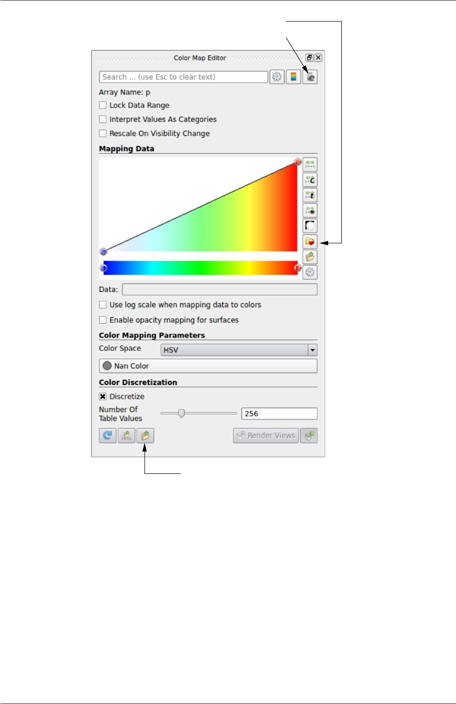
A colour legend can be added by either by clicking the Toggle Color Legend Visibility

button in the Active Variable Controls toolbar or the Show button in the Coloring section

of the Display panel. The legend can be located in the image window by drag and drop

with the mouse. The Edit button, either in the Active Variable Controls toolbar or in

the Coloring panel of the Display panel, opens the Color Map Editor window, as shown in

Figure 2.6, where the user can set a range of attributes of the colour scale and the color bar.

In particular, ParaView defaults to using a colour scale of blue to white to red rather than

the more common blue to green to red (rainbow). Therefore the ﬁrst time that the user

executes ParaView, they may wish to change the colour scale. This can be done by selecting

the Choose Preset button (with the heart icon) in the Color Scale Editor and selecting Blue

to Red Rainbow. After clicking the OK conﬁrmation button, the user can click the Save as

Default button at the bottom of the panel (disk drive symbol) so that ParaView will always

adopt this type of colour bar.

The user can also edit the color legend properties, such as text size, font selection and

numbering format for the scale, by clicking the Edit Color Legend Properties to the far right

of the search bar, as shown in Figure 2.6.

2.1.4.2 Cutting plane (slice)

If the user rotates the image, by holding down the left mouse button in the image window

and moving the cursor, they can see that they have now coloured the complete geometry

surface by the pressure. In order to produce a genuine 2-dimensional contour plot the user

should ﬁrst create a cutting plane, or ‘slice’. With the cavity.OpenFOAM module highlighted

in the Pipeline Browser, the user should select the Slice ﬁlter from the Filters menu in

the top menu of ParaView (accessible at the top of the screen on some systems). The Slice

ﬁlter can be initially found in the Common sub-menu, but once selected, it moves to the

Recent sub-menu, disappearing from the the Common sub-menu. The cutting plane should

be centred at (0.05,0.05,0.005) and its normal should be set to (0,0,1) (click the Z Normal

button).

2.1.4.3 Contours

Having generated the cutting plane, contours can be created using by applying the Contour

ﬁlter. With the Slice module highlighted in the Pipeline Browser, the user should select the

Contour ﬁlter. In the Properties panel, the user should select pressure from the Contour

By menu. Under Isosurfaces, the user could delete the default value with the minus

button, then add a range of 10 values. The contours can be displayed with a Wireframe

representation if the Coloring is solid or by a ﬁeld, e.g. pressure.

2.1.4.4 Vector plots

Before we start to plot the vectors of the ﬂow velocity, it may be useful to remove other

modules that have been created, e.g. using the Slice and Contour ﬁlters described above.

OpenFOAM-6

2.1 Lid-driven cavity ﬂow U-31

Save as Default

Choose preset

Conﬁgure Color Bar

Figure 2.6: Color Map Editor.

These can: either be deleted entirely, by highlighting the relevant module in the Pipeline

Browser and clicking Delete in their respective Properties panel; or, be disabled by toggling

the eye button for the relevant module in the Pipeline Browser.

We now wish to generate a vector glyph for velocity at the centre of each cell. We ﬁrst

need to ﬁlter the data to cell centres as described in section 6.1.7.1. With the cavity.Open-

FOAM module highlighted in the Pipeline Browser, the user should select Cell Centers from

the Filter->Alphabetical menu and then click Apply.

With these Centers highlighted in the Pipeline Browser, the user should then select Glyph

from the Filter->Common menu. The Properties window panel should appear as shown in

Figure 2.7. Note that newly selected ﬁlters are moved to the Filter->Recent menu and

are unavailable in the menus from where they were originally selected. In the resulting

Properties panel, the velocity ﬁeld, U, must be selected from the vectors menu. The user

OpenFOAM-6

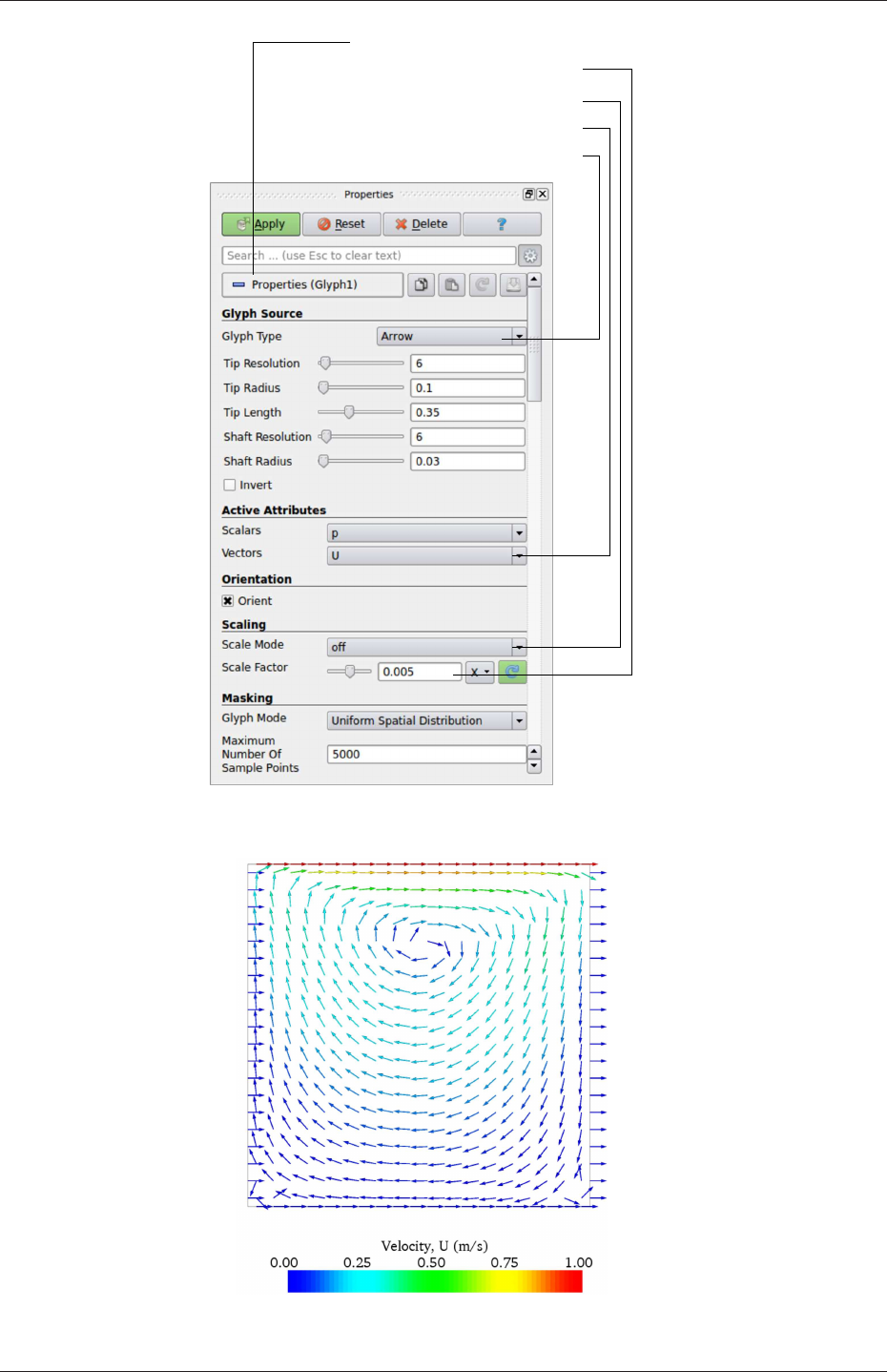
U-32 Tutorials

Open Properties panel

Select Scale Mode off

Specify Set Scale Factor 0.005

Select Glyph Type Arrow

Select vectors U

Figure 2.7: Properties panel for the Glyph ﬁlter.

Figure 2.8: Velocities in the cavity case.

OpenFOAM-6

2.1 Lid-driven cavity ﬂow U-33

should set the Scale Mode for the glyphs to be off, with Set Scale Factor set to 0.005. On

clicking Apply, the glyphs appear but, probably as a single colour, e.g. white. The user

should colour the glyphs by velocity magnitude which, as usual, is controlled by setting

Color by U in the Display panel. The user can also select Show Color Legend in Edit Color

Map. The output is shown in Figure 2.8, in which uppercase Times Roman fonts are selected

for the Color Legend headings and the labels are speciﬁed to 2 ﬁxed signiﬁcant ﬁgures by

deselecting Automatic Label Format and entering %-#6.2f in the Label Format text box. The

background colour is set to white in the General panel of View Settings as described in

section 6.1.5.1.

Note that at the left and right walls, glyphs appear to indicate ﬂow through the walls.

However, it is clear that, while the ﬂow direction is normal to the wall, its magnitude is 0.

This slightly confusing situation is caused by ParaView choosing to orientate the glyphs in

the x-direction when the glyph scaling off and the velocity magnitude is 0.

2.1.4.5 Streamline plots

Again, before the user continues to post-process in ParaView, they should disable modules

such as those for the vector plot described above. We now wish to plot streamlines of velocity

as described in section 6.1.8. With the cavity.OpenFOAM module highlighted in the Pipeline

Browser, the user should then select Stream Tracer from the Filter menu and then click

Apply. The Properties window panel should appear as shown in Figure 2.9. The Seed points

should be speciﬁed along a High Resolution Line Source running vertically through the

centre of the geometry, i.e. from (0.05,0,0.005) to (0.05,0.1,0.005). For the image in this

guide we used: a point Resolution of 21; Maximum Step Length of 0.5; Initial Step Length

of 0.2; and, Integration Direction BOTH. The Runge-Kutta 4/5 IntegratorType was used

with default parameters.

On clicking Apply the tracer is generated. The user should then select Tube from the

Filter menu to produce high quality streamline images. For the image in this report, we

used: Num. sides 6; Radius 0.0003; and, Radius factor 10. The streamtubes are coloured by

velocity magnitude. On clicking Apply the image in Figure 2.10 should be produced.

2.1.5 Increasing the mesh resolution

The mesh resolution will now be increased by a factor of two in each direction. The results

from the coarser mesh will be mapped onto the ﬁner mesh to use as initial conditions for

the problem. The solution from the ﬁner mesh will then be compared with those from the

coarser mesh.

2.1.5.1 Creating a new case using an existing case

We now wish to create a new case named cavityFine that is created from cavity. The user

should therefore clone the cavity case and edit the necessary ﬁles. First the user should go

to the run directory, by typing

cd $FOAM_RUN

Note that there is also a convenient alias, named run, that reproduces the command above

to change directory to $FOAM_RUN, simply by typing run.

OpenFOAM-6

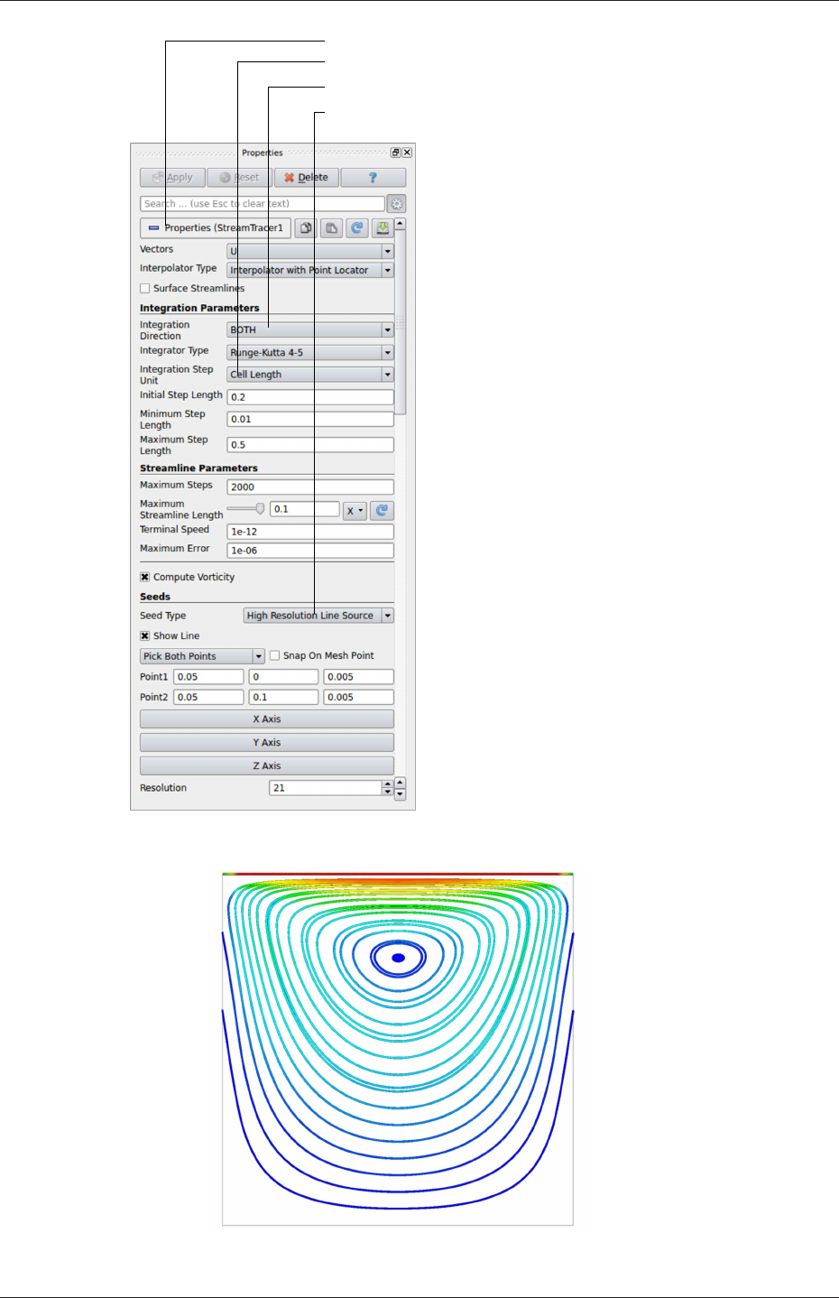
U-34 Tutorials

Set Integration Direction to BOTH

Set Initial Step Length to Cell Length 0.01

Specify Line Source and set points and resolution

Scroll to Properties title

Figure 2.9: Properties panel for the Stream Tracer ﬁlter.

Figure 2.10: Streamlines in the cavity case.

OpenFOAM-6

2.1 Lid-driven cavity ﬂow U-35

The cavityFine case can be created by making a new case directory and copying the

relevant directories from the cavity case.

mkdir cavityFine

cp -r cavity/constant cavityFine

cp -r cavity/system cavityFine

The user can then prepare to run the new case by changing into the case directory.

cd cavityFine

2.1.5.2 Creating the ﬁner mesh

We now wish to increase the number of cells in the mesh by using blockMesh. The user

should open the blockMeshDict ﬁle in the system directory in an editor and edit the block

speciﬁcation. The blocks are speciﬁed in a list under the blocks keyword. The syntax of

the block deﬁnitions is described fully in section 5.3.1.3; at this stage it is suﬃcient to know

that following hex is ﬁrst the list of vertices in the block, then a list (or vector) of numbers

of cells in each direction. This was originally set to (20 20 1) for the cavity case. The user

should now change this to (40 40 1) and save the ﬁle. The new reﬁned mesh should then

be created by running blockMesh as before.

2.1.5.3 Mapping the coarse mesh results onto the ﬁne mesh

The mapFields utility maps one or more ﬁelds relating to a given geometry onto the cor-

responding ﬁelds for another geometry. In our example, the ﬁelds are deemed ‘consistent’

because the geometry and the boundary types, or conditions, of both source and target ﬁelds

are identical. We use the -consistent command line option when executing mapFields in

this example.

The ﬁeld data that mapFields maps is read from the time directory speciﬁed by startFrom

and startTime in the controlDict of the target case, i.e. those into which the results are

being mapped. In this example, we wish to map the ﬁnal results of the coarser mesh from

case cavity onto the ﬁner mesh of case cavityFine. Therefore, since these results are stored in

the 0.5 directory of cavity, the startTime should be set to 0.5 s in the controlDict dictionary

and startFrom should be set to startTime.

The case is ready to run mapFields. Typing mapFields -help quickly shows that map-

Fields requires the source case directory as an argument. We are using the -consistent

option, so the utility is executed from withing the cavityFine directory by

mapFields ../cavity -consistent

The utility should run with output to the terminal including:

Source: ".." "cavity"

Target: "." "cavityFine"

Create databases as time

Source time: 0.5

Target time: 0.5

OpenFOAM-6

U-36 Tutorials

Create meshes

Source mesh size: 400 Target mesh size: 1600

Consistently creating and mapping fields for time 0.5

interpolating p

interpolating U

End

2.1.5.4 Control adjustments

To maintain a Courant number of less that 1, as discussed in section 2.1.1.4, the time step

must now be halved since the size of all cells has halved. Therefore deltaT should be set to

to 0.0025 s in the controlDict dictionary. Field data is currently written out at an interval

of a ﬁxed number of time steps. Here we demonstrate how to specify data output at ﬁxed

intervals of time. Under the writeControl keyword in controlDict, instead of requesting

output by a ﬁxed number of time steps with the timeStep entry, a ﬁxed amount of run time

can be speciﬁed between the writing of results using the runTime entry. In this case the

user should specify output every 0.1 and therefore should set writeInterval to 0.1 and

writeControl to runTime. Finally, since the case is starting with a the solution obtained on

the coarse mesh we only need to run it for a short period to achieve reasonable convergence

to steady-state. Therefore the endTime should be set to 0.7 s. Make sure these settings are

correct and then save the ﬁle.

2.1.5.5 Running the code as a background process

The user should experience running icoFoam as a background process, redirecting the ter-

minal output to a log ﬁle that can be viewed later. From the cavityFine directory, the user

should execute:

icoFoam > log &

cat log

2.1.5.6 Vector plot with the reﬁned mesh

The user can open multiple cases simultaneously in ParaView; essentially because each new

case is simply another module that appears in the Pipeline Browser. There is an inconvenience

when opening a new OpenFOAM case in ParaView because it expects that case data is

stored in a single ﬁle which has a ﬁle extension that enables it to establish the format.

However, OpenFOAM stores case data in multiple ﬁles without an extension in the name,

within a speciﬁc directory structure. The ParaView reader module works on the basis that,

when opening case data in OpenFOAM format, it is passed a dummy (empty) ﬁle with the

.OpenFOAM extension that resides in the case directory. The paraFoam script automatically

creates this ﬁle — hence, the cavity case module is called cavity.OpenFOAM.

If the user wishes to open a second case directly from within ParaView, they need to

create such a dummy ﬁle. They can do this ‘by hand’ or, more simply, use the paraFoam

script with the option -touch. For the cavityFine example, that involves executing from

the case directory:

OpenFOAM-6

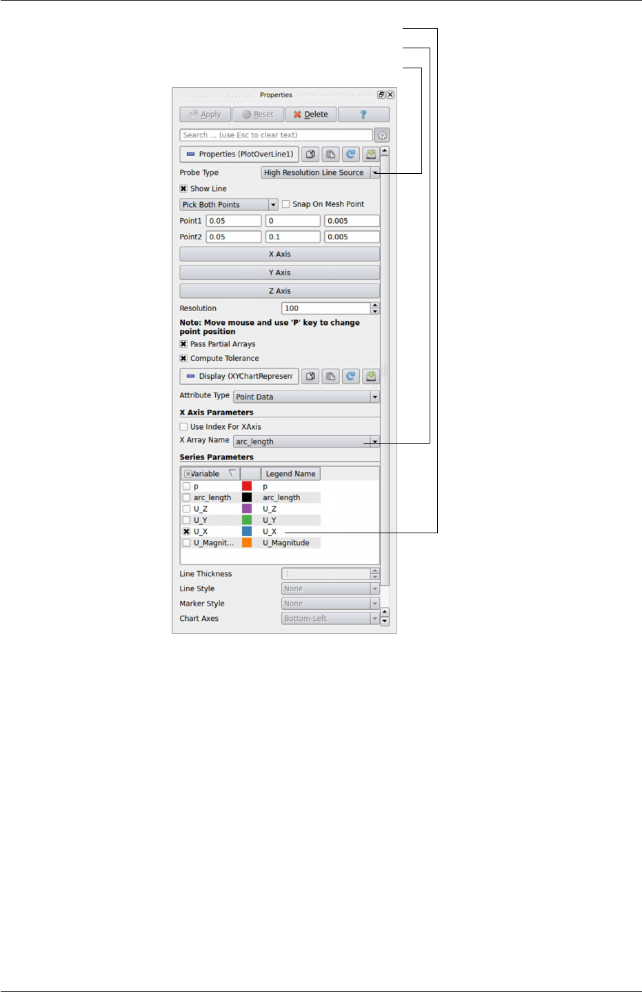
2.1 Lid-driven cavity ﬂow U-37

Select arc_length

Select U_x from Line Series

Select Line Source

Figure 2.11: Selecting ﬁelds for graph plotting.

paraFoam -touch

Now the cavityFine case can be loaded into ParaView by selecting Open from the File

menu, and having navigated to the cavityFine directory, opening cavityFine.OpenFOAM. The

user can now make a vector plot of the results from the reﬁned mesh in ParaView. The plot

can be compared with the cavity case by enabling glyph images for both case simultaneously.

2.1.5.7 Plotting graphs

The user may wish to visualise the results by extracting some scalar measure of velocity and

plotting 2-dimensional graphs along lines through the domain. OpenFOAM is well equipped

for this kind of data manipulation. There are numerous utilities that do specialised data

manipulations, and the postProcess utility that includes a broad range of generic post-

OpenFOAM-6

U-38 Tutorials

processing functionality. The functions within postProcess can be listed by typing:

postProcess -list

The components and mag functions provide useful scalar measures of velocity. When the

components function is executed on a case, e.g. cavity, it reads in the velocity vector ﬁeld

from each time directory and, in the corresponding time directories, writes scalar ﬁelds Ux,

Uy and Uz representing the x,yand zcomponents of velocity.

The user can run postProcess with the components function on both cavity and cavityFine

cases. For example, for the cavity case the user should go into the cavity directory and execute

postProcess as follows:

cd $FOAM_RUN/cavity

postProcess -func "components(U)"

The individual components can be plotted as a graph in ParaView. It is quick, convenient

and has reasonably good control over labelling and formatting, so the printed output is a

fairly good standard. However, to produce graphs for publication, users may prefer to write

raw data and plot it with a dedicated graphing tool, such as gnuplot or Grace/xmgr. To do

this, we recommend using the sampling tools, described in section 6.3.2 and section 2.2.3.

Before commencing plotting, the user needs to load the newly generated Ux,Uy and

Uz ﬁelds into ParaView. To do this, the user should click the Refresh Times at the top of

the Properties panel for the cavity.OpenFOAM module which will cause the new ﬁelds to

be loaded into ParaView and appear in the Volume Fields window. Ensure the new ﬁelds

are selected and the changes are applied, i.e. click Apply again if necessary. Also, data

is interpolated incorrectly at boundaries if the boundary regions are selected in the Mesh

Parts panel. Therefore the user should deselect the patches in the Mesh Parts panel, i.e.

movingWall,fixedWall and frontAndBack, and apply the changes.

Now, in order to display a graph in ParaView the user should select the module of

interest, e.g.cavity.OpenFOAM and apply the Plot Over Line ﬁlter from the Filter->Data

Analysis menu. This opens up a new XY Plot window below or beside the existing 3D View

window. A PlotOverLine module is created in which the user can specify the end points of

the line in the Properties panel. In this example, the user should position the line vertically

up the centre of the domain, i.e. from (0.05,0,0.005) to (0.05,0.1,0.005), in the Point1 and

Point2 text boxes. The Resolution can be set to 100.

On clicking Apply, a graph is generated in the XY Plot window. In the Display panel,

the user should set Attribute Mode to Point Data. The Use Data Array option can be

selected for the X Axis Data, taking the arc_length option so that the x-axis of the graph

represents distance from the base of the cavity.

The user can choose the ﬁelds to be displayed in the Line Series panel of the Display

window. From the list of scalar ﬁelds to be displayed, it can be seen that the magnitude

and components of vector ﬁelds are available by default, e.g. displayed as U_X, so that it was

not necessary to create Ux using the components function. Nevertheless, the user should

deselect all series except Ux (or U_x). A square colour box in the adjacent column to the

selected series indicates the line colour. The user can edit this most easily by a double click

of the mouse over that selection.

In order to format the graph, the user should modify the settings below the Line Series

panel, namely Line Color,Line Thickness,Line Style,Marker Style and Chart Axes.

OpenFOAM-6

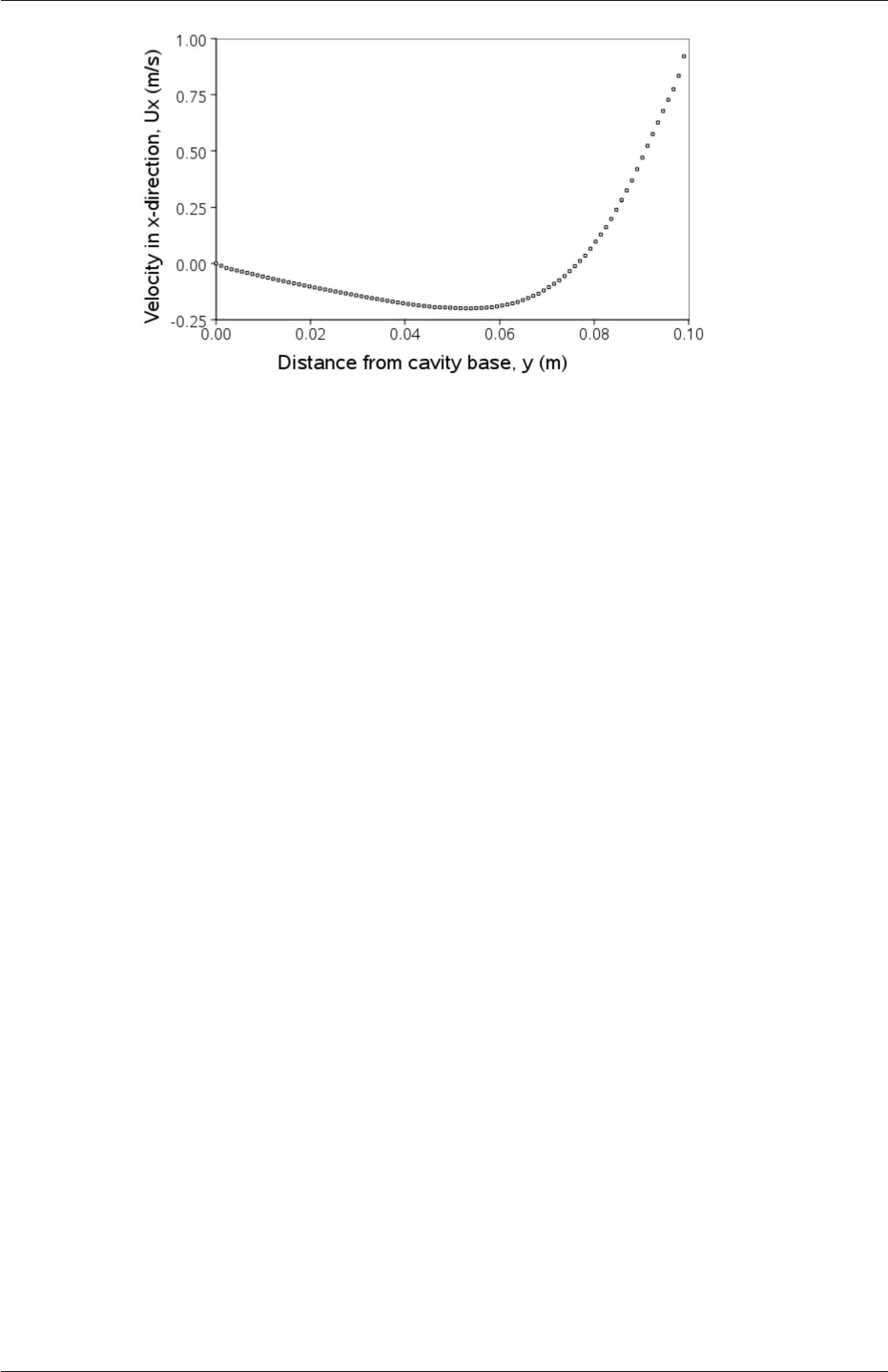
2.1 Lid-driven cavity ﬂow U-39

Figure 2.12: Plotting graphs in paraFoam.

Also the user can click one of the buttons above the top left corner of the XY Plot. The

third button, for example, allows the user to control View Settings in which the user can set

title and legend for each axis, for example. Also, the user can set font, colour and alignment

of the axes titles, and has several options for axis range and labels in linear or logarithmic

scales.

Figure 2.12 is a graph produced using ParaView. The user can produce a graph however

he/she wishes. For information, the graph in Figure 2.12 was produced with the options for

axes of: Standard type of Notation;Specify Axis Range selected; titles in Sans Serif 12

font. The graph is displayed as a set of points rather than a line by activating the Enable

Line Series button in the Display window. Note: if this button appears to be inactive by

being “greyed out”, it can be made active by selecting and deselecting the sets of variables

in the Line Series panel. Once the Enable Line Series button is selected, the Line Style and

Marker Style can be adjusted to the user’s preference.

2.1.6 Introducing mesh grading

The error in any solution will be more pronounced in regions where the form of the true

solution diﬀer widely from the form assumed in the chosen numerical schemes. For example

a numerical scheme based on linear variations of variables over cells can only generate an

exact solution if the true solution is itself linear in form. The error is largest in regions

where the true solution deviates greatest from linear form, i.e. where the change in gradient

is largest. Error decreases with cell size.

It is useful to have an intuitive appreciation of the form of the solution before setting

up any problem. It is then possible to anticipate where the errors will be largest and to

grade the mesh so that the smallest cells are in these regions. In the cavity case the large

variations in velocity can be expected near a wall and so in this part of the tutorial the

mesh will be graded to be smaller in this region. By using the same number of cells, greater

accuracy can be achieved without a signiﬁcant increase in computational cost.

A mesh of 20 ×20 cells with grading towards the walls will be created for the lid-driven

cavity problem and the results from the ﬁner mesh of section 2.1.5.2 will then be mapped

onto the graded mesh to use as an initial condition. The results from the graded mesh will

be compared with those from the previous meshes. Since the changes to the blockMeshDict

OpenFOAM-6

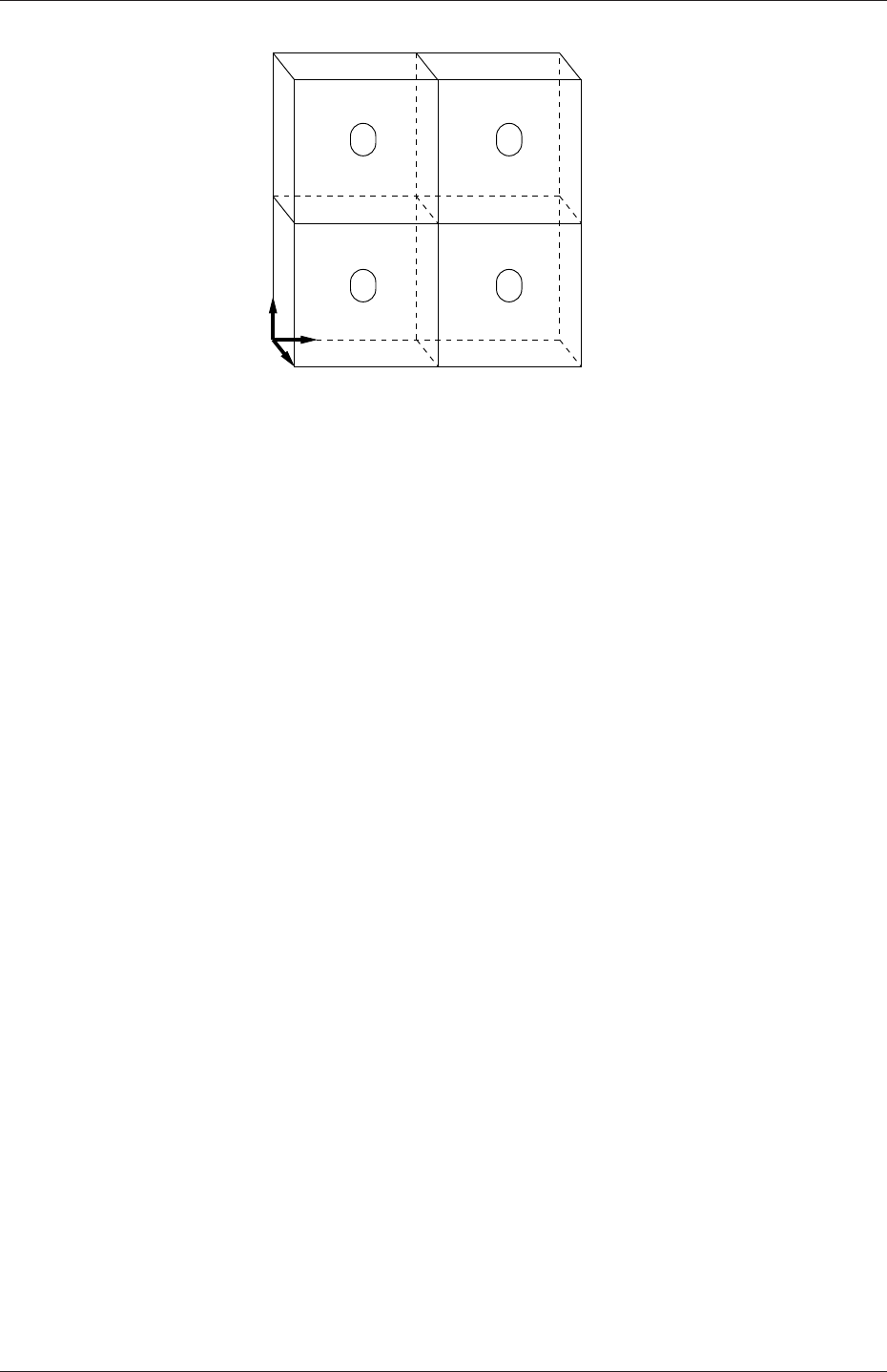
U-40 Tutorials

3 4 5

6 87

1 2

1715

911

12 13 14

0 1

2 3

Figure 2.13: Block structure of the graded mesh for the cavity (block numbers encircled).

dictionary are fairly substantial, the case used for this part of the tutorial, cavityGrade,

is supplied in the $FOAM_TUTORIALS/incompressible/icoFoam/cavity directory. The user

should copy the cavityGrade case into the run directory, then follow the steps below.

2.1.6.1 Creating the graded mesh

The mesh now needs 4 blocks as diﬀerent mesh grading is needed on the left and right and

top and bottom of the domain. The block structure for this mesh is shown in Figure 2.13.

The user can view the blockMeshDict ﬁle in the system subdirectory of cavityGrade; for

completeness the key elements of the blockMeshDict ﬁle are also reproduced below. Each

block now has 10 cells in the xand ydirections and the ratio between largest and smallest

cells is 2.

17 convertToMeters 0.1;

19 vertices

20 (

21 (0 0 0)

22 (0.5 0 0)

23 (1 0 0)

24 (0 0.5 0)

25 (0.5 0.5 0)

26 (1 0.5 0)

27 (0 1 0)

28 (0.5 1 0)

29 (1 1 0)

30 (0 0 0.1)

31 (0.5 0 0.1)

32 (1 0 0.1)

33 (0 0.5 0.1)

34 (0.5 0.5 0.1)

35 (1 0.5 0.1)

36 (0 1 0.1)

37 (0.5 1 0.1)

38 (1 1 0.1)

39 );

41 blocks

42 (

43 hex (0 1 4 3 9 10 13 12) (10 10 1) simpleGrading (2 2 1)

44 hex (1 2 5 4 10 11 14 13) (10 10 1) simpleGrading (0.5 2 1)

45 hex (3 4 7 6 12 13 16 15) (10 10 1) simpleGrading (2 0.5 1)

46 hex (4 5 8 7 13 14 17 16) (10 10 1) simpleGrading (0.5 0.5 1)

47 );

OpenFOAM-6

2.1 Lid-driven cavity ﬂow U-41

49 edges

50 (

51 );

53 boundary

54 (

55 movingWall

56 {

57 type wall;

58 faces

59 (

60 (6 15 16 7)

61 (7 16 17 8)

62 );

63 }

64 fixedWalls

65 {

66 type wall;

67 faces

68 (

69 (3 12 15 6)

70 (0 9 12 3)

71 (0 1 10 9)

72 (1 2 11 10)

73 (2 5 14 11)

74 (5 8 17 14)

75 );

76 }

77 frontAndBack

78 {

79 type empty;

80 faces

81 (

82 (0 3 4 1)

83 (1 4 5 2)

84 (3 6 7 4)

85 (4 7 8 5)

86 (9 10 13 12)

87 (10 11 14 13)

88 (12 13 16 15)

89 (13 14 17 16)

90 );

91 }

92 );

94 mergePatchPairs

95 (

96 );

98 // ************************************************************************* //

Once familiar with the blockMeshDict ﬁle for this case, the user can execute blockMesh from

the command line. The graded mesh can be viewed as before using paraFoam as described

in section 2.1.2.

2.1.6.2 Changing time and time step

The highest velocities and smallest cells are next to the lid, therefore the highest Courant

number will be generated next to the lid, for reasons given in section 2.1.1.4. It is therefore

useful to estimate the size of the cells next to the lid to calculate an appropriate time step

for this case.

When a nonuniform mesh grading is used, blockMesh calculates the cell sizes using a

geometric progression. Along a length l, if ncells are requested with a ratio of Rbetween

the last and ﬁrst cells, the size of the smallest cell, δxs, is given by:

δxs=lr−1

αr −1(2.5)

where ris the ratio between one cell size and the next which is given by:

r=R1

n−1(2.6)

OpenFOAM-6

U-42 Tutorials

and

α=(Rfor R > 1,

1−r−n+r−1for R < 1.(2.7)

For the cavityGrade case the number of cells in each direction in a block is 10, the ratio

between largest and smallest cells is 2and the block height and width is 0.05 m. Therefore

the smallest cell length is 3.45 mm. From Equation 2.2, the time step should be less than 3.45

ms to maintain a Courant of less than 1. To ensure that results are written out at convenient

time intervals, the time step deltaT should be reduced to 2.5 ms and the writeInterval

set to 40 so that results are written out every 0.1 s. These settings can be viewed in the

cavityGrade/system/controlDict ﬁle.

The startTime needs to be set to that of the ﬁnal conditions of the case cavityFine,i.e.

0.7. Since cavity and cavityFine converged well within the prescribed run time, we can set

the run time for case cavityGrade to 0.1 s, i.e. the endTime should be 0.8.

2.1.6.3 Mapping ﬁelds

As in section 2.1.5.3, use mapFields to map the ﬁnal results from case cavityFine onto the

mesh for case cavityGrade. Enter the cavityGrade directory and execute mapFields by:

cd $FOAM_RUN/cavityGrade

mapFields ../cavityFine -consistent

Now run icoFoam from the case directory and monitor the run time information. View

the converged results for this case and compare with other results using post-processing

tools described previously in section 2.1.5.6 and section 2.1.5.7.

2.1.7 Increasing the Reynolds number

The cases solved so far have had a Reynolds number of 10. This is very low and leads to

a stable solution quickly with only small secondary vortices at the bottom corners of the

cavity. We will now increase the Reynolds number to 100, at which point the solution takes

a noticeably longer time to converge. The coarsest mesh in case cavity will be used initially.

The user should clone the cavity case and name it cavityHighRe. Rather than copying

individual directories (system,constant,etc.) as described previously, the foamCloneCase can

be used, which copies the relevant directories in one step. By default the 0time directory is

copied, but here the user can use the -latestTime option to copy the latest time directory,

0.5, which can be used as the initial ﬁeld data for our simulation. The example also uses

the run alias as a quick way to change to the run directory.

run

foamCloneCase -latestTime cavity cavityHighRe

cd cavityHighRe

OpenFOAM-6

2.1 Lid-driven cavity ﬂow U-43

2.1.7.1 Pre-processing

Go into the cavityHighRe case and edit the transportProperties dictionary in the constant

directory. Since the Reynolds number is required to be increased by a factor of 10, decrease

the kinematic viscosity by a factor of 10, i.e. to 1×10−3m2s−1. We now run this case by

restarting from the solution at the end of the cavity case run. To do this we can use the

option of setting the startFrom keyword to latestTime so that icoFoam takes as its initial

data the values stored in the directory corresponding to the most recent time, i.e. 0.5. The

endTime should be set to 2 s.

2.1.7.2 Running the code

Run icoFoam for this case from the case directory and view the run time information. When

running a job in the background, the following UNIX commands can be useful:

nohup enables a command to keep running after the user who issues the command has

logged out;

nice changes the priority of the job in the kernel’s scheduler; a niceness of -20 is the highest

priority and 19 is the lowest priority.

This is useful, for example, if a user wishes to set a case running on a remote machine and

does not wish to monitor it heavily, in which case they may wish to give it low priority

on the machine. In that case the nohup command allows the user to log out of a remote

machine he/she is running on and the job continues running, while nice can set the priority

to 19. For our case of interest, we can execute the command in this manner as follows:

nohup nice -n 19 icoFoam > log &

cat log

In previous runs you may have noticed that icoFoam stops solving for velocity Uquite quickly

but continues solving for pressure pfor a lot longer or until the end of the run. In practice,

once icoFoam stops solving for Uand the initial residual of pis less than the tolerance

set in the fvSolution dictionary (typically 10−6), the run has eﬀectively converged and can

be stopped once the ﬁeld data has been written out to a time directory. For example, at

convergence a sample of the log ﬁle from the run on the cavityHighRe case appears as follows

in which the velocity has already converged after 1.395 s and initial pressure residuals are

small; No Iterations 0 indicates that the solution of Uhas stopped:

1Time = 1.43

3Courant Number mean: 0.221921 max: 0.839902

4smoothSolver: Solving for Ux, Initial residual = 8.73381e-06, Final residual = 8.73381e-06, No Iterations 0

5smoothSolver: Solving for Uy, Initial residual = 9.89679e-06, Final residual = 9.89679e-06, No Iterations 0

6DICPCG: Solving for p, Initial residual = 3.67506e-06, Final residual = 8.62986e-07, No Iterations 4

7time step continuity errors : sum local = 6.57947e-09, global = -6.6679e-19, cumulative = -6.2539e-18

8DICPCG: Solving for p, Initial residual = 2.60898e-06, Final residual = 7.92532e-07, No Iterations 3

9time step continuity errors : sum local = 6.26199e-09, global = -1.02984e-18, cumulative = -7.28374e-18

10 ExecutionTime = 0.37 s ClockTime = 0 s

12 Time = 1.435

14 Courant Number mean: 0.221923 max: 0.839903

15 smoothSolver: Solving for Ux, Initial residual = 8.53935e-06, Final residual = 8.53935e-06, No Iterations 0

16 smoothSolver: Solving for Uy, Initial residual = 9.71405e-06, Final residual = 9.71405e-06, No Iterations 0

17 DICPCG: Solving for p, Initial residual = 4.0223e-06, Final residual = 9.89693e-07, No Iterations 3

18 time step continuity errors : sum local = 8.15199e-09, global = 5.33614e-19, cumulative = -6.75012e-18

19 DICPCG: Solving for p, Initial residual = 2.38807e-06, Final residual = 8.44595e-07, No Iterations 3

20 time step continuity errors : sum local = 7.48751e-09, global = -4.42707e-19, cumulative = -7.19283e-18

21 ExecutionTime = 0.37 s ClockTime = 0 s

OpenFOAM-6

U-44 Tutorials

2.1.8 High Reynolds number ﬂow

View the results in paraFoam and display the velocity vectors. The secondary vortices in

the corners have increased in size. The user can then increase the Reynolds number further

by decreasing the viscosity and then rerun the case. The number of vortices increases so the

mesh resolution around them will need to increase in order to resolve the more complicated

ﬂow patterns. In addition, as the Reynolds number increases the time to convergence

increases. The user should monitor residuals and extend the endTime accordingly to ensure

convergence.

The need to increase spatial and temporal resolution then becomes impractical as the

ﬂow moves into the turbulent regime, where problems of solution stability may also occur. Of

course, many engineering problems have very high Reynolds numbers and it is infeasible to

bear the huge cost of solving the turbulent behaviour directly. Instead Reynolds-averaged

simulation (RAS) turbulence models are used to solve for the mean ﬂow behaviour and

calculate the statistics of the ﬂuctuations. The standard k−εmodel with wall functions

will be used in this tutorial to solve the lid-driven cavity case with a Reynolds number of

104. Two extra variables are solved for: k, the turbulent kinetic energy; and, ε, the turbulent

dissipation rate. The additional equations and models for turbulent ﬂow are implemented

into a OpenFOAM solver called pisoFoam.

2.1.8.1 Pre-processing

Go back to the run directory and copy the cavity case in the $FOAM_RUN/tutorials/-

incompressible/pisoFoam/RAS directory (N.B: the pisoFoam/RAS directory), renaming it

cavityRAS to avoid a clash with the existing cavity tutorial. Go into the new case directory.

run

cp -r $FOAM_TUTORIALS/incompressible/pisoFoam/RAS/cavity cavityRAS

cd cavityRAS

Generate the mesh by running blockMesh as before. Mesh grading towards the wall is not

necessary when using the standard k−εmodel with wall functions since the ﬂow in the

near wall cell is modelled, rather than having to be resolved.

A range of wall function models is available in OpenFOAM that are applied as boundary

conditions on individual patches. This enables diﬀerent wall function models to be applied to

diﬀerent wall regions. The choice of wall function models are speciﬁed through the turbulent

viscosity ﬁeld, νtin the 0/nut ﬁle:

18 dimensions [0 2 -1 0 0 0 0];

20 internalField uniform 0;

22 boundaryField

23 {

24 movingWall

25 {

26 type nutkWallFunction;

27 value uniform 0;

28 }

29 fixedWalls

30 {

31 type nutkWallFunction;

32 value uniform 0;

33 }

34 frontAndBack

OpenFOAM-6

2.1 Lid-driven cavity ﬂow U-45

35 {

36 type empty;

37 }

38 }

41 // ************************************************************************* //

This case uses standard wall functions, speciﬁed by the nutWallFunction type on the

movingWall and fixedWalls patches. Other wall function models include the rough wall

functions, speciﬁed though the nutRoughWallFunction keyword.

The user should now open the ﬁeld ﬁles for kand ε(0/k and 0/epsilon) and examine

their boundary conditions. For a wall boundary condition, εis assigned a epsilonWallFunction

boundary condition and a kqRwallFunction boundary condition is assigned to k. The latter

is a generic boundary condition that can be applied to any ﬁeld that are of a turbulent

kinetic energy type, e.g. k,qor Reynolds Stress R. The initial values for kand εare set

using an estimated ﬂuctuating component of velocity U′and a turbulent length scale, l.k

and εare deﬁned in terms of these parameters as follows:

k=1

2U′•U′(2.8)

ε=C0.75

µk1.5

l(2.9)

where Cµis a constant of the k−εmodel equal to 0.09. For a Cartesian coordinate system,

kis given by:

k=1

2(U′2

x+U′2

y+U′2

z)(2.10)

where U′2

x,U′2

yand U′2

zare the ﬂuctuating components of velocity in the x,yand z

directions respectively. Let us assume the initial turbulence is isotropic, i.e. U′2

x=U′2

U′2

z, and equal to 5% of the lid velocity and that l, is equal to 5% of the box width, 0.1 m,

then kand εare given by:

U′

x=U′

y=U′

z=5

1001 m s−1(2.11)

⇒k=3

2µ5

100¶2

m2s−2= 3.75 ×10−3m2s−2(2.12)

ε=C0.75

µk1.5

l≈7.54 ×10−3m2s−3(2.13)

These form the initial conditions for kand ε. The initial conditions for Uand pare (0,0,0)

and 0 respectively as before.

Turbulence modelling includes a range of methods, e.g. RAS or large-eddy simulation

(LES), that are provided in OpenFOAM. The choice of turbulence modelling method is

selectable at run-time through the simulationType keyword in turbulenceProperties dictio-

nary. The user can view this ﬁle in the constant directory:

18 simulationType RAS;

20 RAS

21 {

22 RASModel kEpsilon;

OpenFOAM-6

U-46 Tutorials

24 turbulence on;

26 printCoeffs on;

27 }

29 // ************************************************************************* //

The options for simulationType are laminar,RAS and LES. With RAS selected in this case,

the choice of RAS modelling is speciﬁed in a RAS subdictionary. The turbulence model

is selected by the RASModel entry from a long list of available models that are listed in

Section 7.2.1.1. The kEpsilon model should be selected which is is the standard k−ε

model; the user should also ensure that turbulence calculation is switched on.

The coeﬃcients for each turbulence model are stored within the respective code with

a set of default values. Setting the optional switch called printCoeffs to on will make

the default values be printed to standard output, i.e. the terminal, when the model is

called at run time. The coeﬃcients are printed out as a sub-dictionary whose name is

that of the model name with the word Coeffs appended, e.g. kEpsilonCoeffs in the case

of the kEpsilon model. The coeﬃcients of the model, e.g. kEpsilon, can be modiﬁed by

optionally including (copying and pasting) that sub-dictionary within the RAS sub-dictionary

and adjusting values accordingly.

The user should next set the laminar kinematic viscosity in the transportProperties dic-

tionary. To achieve a Reynolds number of 104, a kinematic viscosity of 10−5mis required

based on the Reynolds number deﬁnition given in Equation 2.1.

Finally the user should set the startTime,stopTime,deltaT and the writeInterval

in the controlDict. Set deltaT to 0.005 s to satisfy the Courant number restriction and the

endTime to 10 s.

2.1.8.2 Running the code

Execute pisoFoam by entering the case directory and typing “pisoFoam” in a terminal. In

this case, where the viscosity is low, the boundary layer next to the moving lid is very thin

and the cells next to the lid are comparatively large so the velocity at their centres are

much less than the lid velocity. In fact, after ≈100 time steps it becomes apparent that

the velocity in the cells adjacent to the lid reaches an upper limit of around 0.2 m s−1hence

the maximum Courant number does not rise much above 0.2. It is sensible to increase the

solution time by increasing the time step to a level where the Courant number is much closer

to 1. Therefore reset deltaT to 0.02 s and, on this occasion, set startFrom to latestTime.

This instructs pisoFoam to read the start data from the latest time directory, i.e.10.0. The

endTime should be set to 20 s since the run converges a lot slower than the laminar case.

Restart the run as before and monitor the convergence of the solution. View the results at

consecutive time steps as the solution progresses to see if the solution converges to a steady-

state or perhaps reaches some periodically oscillating state. In the latter case, convergence

may never occur but this does not mean the results are inaccurate.

2.1.9 Changing the case geometry

A user may wish to make changes to the geometry of a case and perform a new simulation.

It may be useful to retain some or all of the original solution as the starting conditions for

the new simulation. This is a little complex because the ﬁelds of the original solution are

not consistent with the ﬁelds of the new case. However the mapFields utility can map ﬁelds

that are inconsistent, either in terms of geometry or boundary types or both.

OpenFOAM-6

2.1 Lid-driven cavity ﬂow U-47

As an example, let us copy the cavityClipped case from the tutorials directory in the user’s

run directory, and change into the cavityClipped directory:

run

cp -r $FOAM_TUTORIALS/incompressible/icoFoam/cavity/cavityClipped .

cd cavityClipped

The case consists of the standard cavity geometry but with a square of length 0.04 m removed

from the bottom right of the cavity, according to the blockMeshDict below:

17 convertToMeters 0.1;

19 vertices

20 (

21 (0 0 0)

22 (0.6 0 0)

23 (0 0.4 0)

24 (0.6 0.4 0)

25 (1 0.4 0)

26 (0 1 0)

27 (0.6 1 0)

28 (1 1 0)

30 (0 0 0.1)

31 (0.6 0 0.1)

32 (0 0.4 0.1)

33 (0.6 0.4 0.1)

34 (1 0.4 0.1)

35 (0 1 0.1)

36 (0.6 1 0.1)

37 (1 1 0.1)

39 );

41 blocks

42 (

43 hex (0 1 3 2 8 9 11 10) (12 8 1) simpleGrading (1 1 1)

44 hex (2 3 6 5 10 11 14 13) (12 12 1) simpleGrading (1 1 1)

45 hex (3 4 7 6 11 12 15 14) (8 12 1) simpleGrading (1 1 1)

46 );

48 edges

49 (

50 );

52 boundary

53 (

54 lid

55 {

56 type wall;

57 faces

58 (

59 (5 13 14 6)

60 (6 14 15 7)

61 );

62 }

63 fixedWalls

64 {

65 type wall;

66 faces

67 (

68 (0 8 10 2)

69 (2 10 13 5)

70 (7 15 12 4)

71 (4 12 11 3)

72 (3 11 9 1)

73 (1 9 8 0)

74 );

75 }

76 frontAndBack

77 {

78 type empty;

79 faces

80 (

81 (0 2 3 1)

OpenFOAM-6

U-48 Tutorials

82 (2 5 6 3)

83 (3 6 7 4)

84 (8 9 11 10)

85 (10 11 14 13)

86 (11 12 15 14)

87 );

88 }

89 );

91 mergePatchPairs

92 (

93 );

95 // ************************************************************************* //

Generate the mesh with blockMesh. The patches are set accordingly as in previous cavity

cases. For the sake of clarity in describing the ﬁeld mapping process, the upper wall patch

is renamed lid, previously the movingWall patch of the original cavity.

In an inconsistent mapping, there is no guarantee that all the ﬁeld data can be mapped

from the source case. The remaining data must come from ﬁeld ﬁles in the target case itself.

Therefore ﬁeld data must exist in the time directory of the target case before mapping

takes place. In the cavityClipped case the mapping is set to occur at time 0.5 s, since the

startTime is set to 0.5 s in the controlDict. Therefore the user needs to copy initial ﬁeld

data to that directory, e.g. from time 0:

cp -r 0 0.5

Before mapping the data, the user should view the geometry and ﬁelds at 0.5 s.

Now we wish to map the velocity and pressure ﬁelds from cavity onto the new ﬁelds of

cavityClipped. Since the mapping is inconsistent, we need to edit the mapFieldsDict dictio-

nary, located in the system directory. The dictionary contains 2 keyword entries: patchMap

and cuttingPatches. The patchMap list contains a mapping of patches from the source

ﬁelds to the target ﬁelds. It is used if the user wishes a patch in the target ﬁeld to inherit

values from a corresponding patch in the source ﬁeld. In cavityClipped, we wish to inherit the

boundary values on the lid patch from movingWall in cavity so we must set the patchMap

as:

patchMap

(

lid movingWall

);

The cuttingPatches list contains names of target patches whose values are to be

mapped from the source internal ﬁeld through which the target patch cuts. In this case, the

fixedWalls patch is a noSlip condition so the internal values cannot be interpolated to the

patch. Therefore the cuttingPatches list can simply be empty:

cuttingPatches

(

);

If the user does wish to interpolate internal values from the source case to the fixedWalls

patch in the target case, a ﬁxedValue boundary condition needs to be speciﬁed on the patch,

OpenFOAM-6

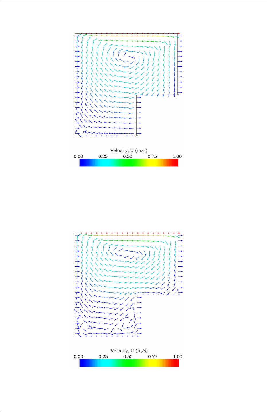
2.1 Lid-driven cavity ﬂow U-49

Figure 2.14: cavity solution velocity ﬁeld mapped onto cavityClipped.

Figure 2.15: cavityClipped solution for velocity ﬁeld.

OpenFOAM-6

U-50 Tutorials

whose value can then be overridden during the mapping process; the fixedWalls patch

then needs to be included in the cuttingPatches list.

The user should run mapFields, from within the cavityClipped directory:

mapFields ../cavity

The user can view the mapped ﬁeld as shown in Figure 2.14. The fixedWalls patch has

not inherited values from the source case as we expected. The user can then run the case

with icoFoam.

2.1.10 Post-processing the modiﬁed geometry

Velocity glyphs can be generated for the case as normal, ﬁrst at time 0.5 s and later at

time 0.6 s, to compare the initial and ﬁnal solutions. In addition, we provide an outline of

the geometry which requires some care to generate for a 2D case. The user should select

Extract Block from the Filter menu and, in the Parameter panel, highlight the patches

of interest, namely the lid and ﬁxedWalls. On clicking Apply, these items of geometry can be

displayed by selecting Wireframe in the Display panel. Figure 2.15 displays the patches in

black and shows vortices forming in the bottom corners of the modiﬁed geometry.

2.2 Stress analysis of a plate with a hole

This tutorial describes how to pre-process, run and post-process a case involving linear-

elastic, steady-state stress analysis on a square plate with a circular hole at its centre. The

plate dimensions are: side length 4 mand radius R=0.5 m. It is loaded with a uniform

traction of σ=10 kPa over its left and right faces as shown in Figure 2.16. Two symmetry

planes can be identiﬁed for this geometry and therefore the solution domain need only cover

a quarter of the geometry, shown by the shaded area in Figure 2.16.

The problem can be approximated as 2-dimensional since the load is applied in the plane

of the plate. In a Cartesian coordinate system there are two possible assumptions to take

in regard to the behaviour of the structure in the third dimension: (1) the plane stress

condition, in which the stress components acting out of the 2D plane are assumed to be

negligible; (2) the plane strain condition, in which the strain components out of the 2D

plane are assumed negligible. The plane stress condition is appropriate for solids whose

third dimension is thin as in this case; the plane strain condition is applicable for solids

where the third dimension is thick.

An analytical solution exists for loading of an inﬁnitely large, thin plate with a circular

hole. The solution for the stress normal to the vertical plane of symmetry is

(σxx)x=0 =





σµ1 + R2

2y2+3R4

2y4¶for |y| ≥ R

0for |y|< R

(2.14)

Results from the simulation will be compared with this solution. At the end of the tutorial,

the user can: investigate the sensitivity of the solution to mesh resolution and mesh grading;

and, increase the size of the plate in comparison to the hole to try to estimate the error in

comparing the analytical solution for an inﬁnite plate to the solution of this problem of a

ﬁnite plate.

OpenFOAM-6

2.2 Stress analysis of a plate with a hole U-51

xsymmetry plane

4.0 m

σ=10 kPa

R=0.5 m

symmetry plane

Figure 2.16: Geometry of the plate with a hole.

2.2.1 Mesh generation

The domain consists of four blocks, some of which have arc-shaped edges. The block struc-

ture for the part of the mesh in the x−yplane is shown in Figure 2.17. As already mentioned

in section 2.1.1.1, all geometries are generated in 3 dimensions in OpenFOAM even if the

case is to be as a 2 dimensional problem. Therefore a dimension of the block in the z

direction has to be chosen; here, 0.5 mis selected. It does not aﬀect the solution since the

traction boundary condition is speciﬁed as a stress rather than a force, thereby making the

solution independent of the cross-sectional area.

The user should change to the run directory and copy the plateHole case into it from

the $FOAM_TUTORIALS/stressAnalysis/solidDisplacementFoam directory. The user should

then go into the plateHole directory and open the blockMeshDict ﬁle in an editor, as listed

below

17 convertToMeters 1;

19 vertices

20 (

21 (0.5 0 0)

22 (1 0 0)

23 (2 0 0)

24 (2 0.707107 0)

25 (0.707107 0.707107 0)

26 (0.353553 0.353553 0)

27 (2 2 0)

28 (0.707107 2 0)

29 (0 2 0)

30 (0 1 0)

31 (0 0.5 0)

32 (0.5 0 0.5)

33 (1 0 0.5)

34 (2 0 0.5)

35 (2 0.707107 0.5)

36 (0.707107 0.707107 0.5)

37 (0.353553 0.353553 0.5)

38 (2 2 0.5)

39 (0.707107 2 0.5)

OpenFOAM-6

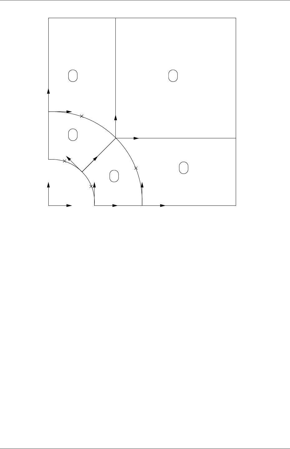
U-52 Tutorials

y x2

x1x1

x2x1

left

up 7up

right

down

hole

down

right

10 2

4 3

Figure 2.17: Block structure of the mesh for the plate with a hole.

40 (0 2 0.5)

41 (0 1 0.5)

42 (0 0.5 0.5)

43 );

45 blocks

46 (

47 hex (5 4 9 10 16 15 20 21) (10 10 1) simpleGrading (1 1 1)

48 hex (0 1 4 5 11 12 15 16) (10 10 1) simpleGrading (1 1 1)

49 hex (1 2 3 4 12 13 14 15) (20 10 1) simpleGrading (1 1 1)

50 hex (4 3 6 7 15 14 17 18) (20 20 1) simpleGrading (1 1 1)

51 hex (9 4 7 8 20 15 18 19) (10 20 1) simpleGrading (1 1 1)

52 );

54 edges

55 (

56 arc 0 5 (0.469846 0.17101 0)

57 arc 5 10 (0.17101 0.469846 0)

58 arc 1 4 (0.939693 0.34202 0)

59 arc 4 9 (0.34202 0.939693 0)

60 arc 11 16 (0.469846 0.17101 0.5)

61 arc 16 21 (0.17101 0.469846 0.5)

62 arc 12 15 (0.939693 0.34202 0.5)

63 arc 15 20 (0.34202 0.939693 0.5)

64 );

66 boundary

67 (

68 left

69 {

70 type symmetryPlane;

71 faces

72 (

73 (8 9 20 19)

OpenFOAM-6

2.2 Stress analysis of a plate with a hole U-53

74 (9 10 21 20)

75 );

76 }

77 right

78 {

79 type patch;

80 faces

81 (

82 (2 3 14 13)

83 (3 6 17 14)

84 );

85 }

86 down

87 {

88 type symmetryPlane;

89 faces

90 (

91 (0 1 12 11)

92 (1 2 13 12)

93 );

94 }

95 up

96 {

97 type patch;

98 faces

99 (

100 (7 8 19 18)

101 (6 7 18 17)

102 );

103 }

104 hole

105 {

106 type patch;

107 faces

108 (

109 (10 5 16 21)

110 (5 0 11 16)

111 );

112 }

113 frontAndBack

114 {

115 type empty;

116 faces

117 (

118 (10 9 4 5)

119 (5 4 1 0)

120 (1 4 3 2)

121 (4 7 6 3)

122 (4 9 8 7)

123 (21 16 15 20)

124 (16 11 12 15)

125 (12 13 14 15)

126 (15 14 17 18)

127 (15 18 19 20)

128 );

129 }

130 );

131

132 mergePatchPairs

133 (

134 );

135

136 // ************************************************************************* //

Until now, we have only speciﬁed straight edges in the geometries of previous tutorials but

here we need to specify curved edges. These are speciﬁed under the edges keyword entry

which is a list of non-straight edges. The syntax of each list entry begins with the type of

curve, including arc,simpleSpline,polyLine etc., described further in section 5.3.1. In

this example, all the edges are circular and so can be speciﬁed by the arc keyword entry.

The following entries are the labels of the start and end vertices of the arc and a point vector

through which the circular arc passes.

The blocks in this blockMeshDict do not all have the same orientation. As can be seen in

Figure 2.17 the x2direction of block 0 is equivalent to the −x1direction for block 4. This

means care must be taken when deﬁning the number and distribution of cells in each block

OpenFOAM-6

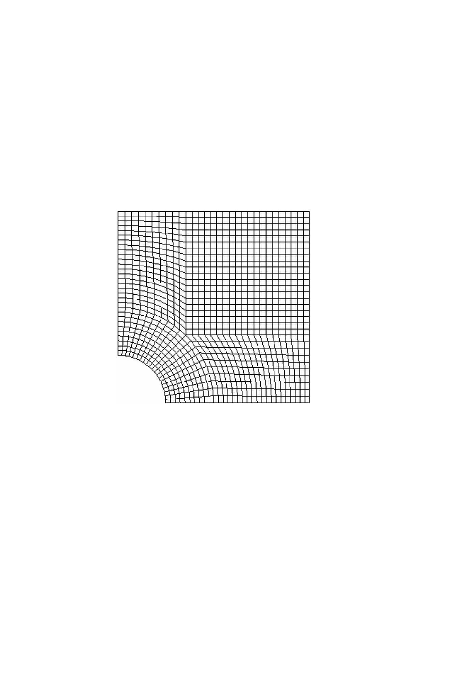
U-54 Tutorials

so that the cells match up at the block faces.

6 patches are deﬁned: one for each side of the plate, one for the hole and one for the

front and back planes. The left and down patches are both a symmetry plane. Since this is

ageometric constraint, it is included in the deﬁnition of the mesh, rather than being purely

a speciﬁcation on the boundary condition of the ﬁelds. Therefore they are deﬁned as such

using a special symmetryPlane type as shown in the blockMeshDict.

The frontAndBack patch represents the plane which is ignored in a 2D case. Again this

is a geometric constraint so is deﬁned within the mesh, using the empty type as shown in the

blockMeshDict. For further details of boundary types and geometric constraints, the user

should refer to section 5.2.

The remaining patches are of the regular patch type. The mesh should be generated

using blockMesh and can be viewed in paraFoam as described in section 2.1.2. It should

appear as in Figure 2.18.

Figure 2.18: Mesh of the hole in a plate problem.

2.2.1.1 Boundary and initial conditions

Once the mesh generation is complete, the initial ﬁeld with boundary conditions must be

set. For a stress analysis case without thermal stresses, only displacement Dneeds to be set.

The 0/D is as follows:

17 dimensions [0 1 0 0 0 0 0];

19 internalField uniform (0 0 0);

21 boundaryField

22 {

23 left

24 {

25 type symmetryPlane;

26 }

27 right

28 {

29 type tractionDisplacement;

30 traction uniform (10000 0 0);

31 pressure uniform 0;

32 value uniform (0 0 0);

33 }

34 down

OpenFOAM-6

2.2 Stress analysis of a plate with a hole U-55

35 {

36 type symmetryPlane;

37 }

38 up

39 {

40 type tractionDisplacement;

41 traction uniform (0 0 0);

42 pressure uniform 0;

43 value uniform (0 0 0);

44 }

45 hole

46 {

47 type tractionDisplacement;

48 traction uniform (0 0 0);

49 pressure uniform 0;

50 value uniform (0 0 0);

51 }

52 frontAndBack

53 {

54 type empty;

55 }

56 }

58 // ************************************************************************* //

Firstly, it can be seen that the displacement initial conditions are set to (0,0,0) m. The

left and down patches must be both of symmetryPlane type since they are speciﬁed as such

in the mesh description in the constant/polyMesh/boundary ﬁle. Similarly the frontAndBack

patch is declared empty.

The other patches are traction boundary conditions, set by a specialist traction bound-

ary type. The traction boundary conditions are speciﬁed by a linear combination of: (1) a

boundary traction vector under keyword traction; (2) a pressure that produces a traction

normal to the boundary surface that is deﬁned as negative when pointing out of the surface,

under keyword pressure. The up and hole patches are zero traction so the boundary trac-

tion and pressure are set to zero. For the right patch the traction should be (1e4,0,0) Pa

and the pressure should be 0 Pa.

2.2.1.2 Mechanical properties

The physical properties for the case are set in the mechanicalProperties dictionary in the con-

stant directory. For this problem, we need to specify the mechanical properties of steel given

in Table 2.1. In the mechanical properties dictionary, the user must also set planeStress

to yes.

Property Units Keyword Value

Density kg m−3rho 7854

Young’s modulus Pa E2×1011

Poisson’s ratio — nu 0.3

Table 2.1: Mechanical properties for steel

2.2.1.3 Thermal properties

The temperature ﬁeld variable Tis present in the solidDisplacementFoam solver since the user

may opt to solve a thermal equation that is coupled with the momentum equation through

the thermal stresses that are generated. The user speciﬁes at run time whether OpenFOAM

OpenFOAM-6

U-56 Tutorials

should solve the thermal equation by the thermalStress switch in the thermalProperties

dictionary. This dictionary also sets the thermal properties for the case, e.g. for steel as

listed in Table 2.2.

Property Units Keyword Value

Speciﬁc heat capacity Jkg−1K−1C434

Thermal conductivity Wm−1K−1k60.5

Thermal expansion coeﬀ. K−1alpha 1.1×10−5

Table 2.2: Thermal properties for steel

In this case we do not want to solve for the thermal equation. Therefore we must set

the thermalStress keyword entry to no in the thermalProperties dictionary.

2.2.1.4 Control

As before, the information relating to the control of the solution procedure are read in

from the controlDict dictionary. For this case, the startTime is 0 s. The time step is not

important since this is a steady state case; in this situation it is best to set the time step

deltaT to 1 so it simply acts as an iteration counter for the steady-state case. The endTime,

set to 100, then acts as a limit on the number of iterations. The writeInterval can be set

to 20.

The controlDict entries are as follows:

18 application solidDisplacementFoam;

20 startFrom startTime;

22 startTime 0;

24 stopAt endTime;

26 endTime 100;

28 deltaT 1;

30 writeControl timeStep;

32 writeInterval 20;

34 purgeWrite 0;

36 writeFormat ascii;

38 writePrecision 6;

40 writeCompression off;

42 timeFormat general;

44 timePrecision 6;

46 graphFormat raw;

48 runTimeModifiable true;

51 // ************************************************************************* //

2.2.1.5 Discretisation schemes and linear-solver control

Let us turn our attention to the fvSchemes dictionary. Firstly, the problem we are analysing

is steady-state so the user should select SteadyState for the time derivatives in timeScheme.

OpenFOAM-6

2.2 Stress analysis of a plate with a hole U-57

This essentially switches oﬀ the time derivative terms. Not all solvers, especially in ﬂuid

dynamics, work for both steady-state and transient problems but solidDisplacementFoam

does work, since the base algorithm is the same for both types of simulation.

The momentum equation in linear-elastic stress analysis includes several explicit terms

containing the gradient of displacement. The calculations beneﬁt from accurate and smooth

evaluation of the gradient. Normally, in the ﬁnite volume method the discretisation is based

on Gauss’s theorem The Gauss method is suﬃciently accurate for most purposes but, in this

case, the least squares method will be used. The user should therefore open the fvSchemes

dictionary in the system directory and ensure the leastSquares method is selected for the

grad(U) gradient discretisation scheme in the gradSchemes sub-dictionary:

18 d2dt2Schemes

19 {

20 default steadyState;

21 }

23 ddtSchemes

24 {

25 default Euler;

26 }

28 gradSchemes

29 {

30 default leastSquares;

31 grad(D) leastSquares;

32 grad(T) leastSquares;

33 }

35 divSchemes

36 {

37 default none;

38 div(sigmaD) Gauss linear;

39 }

41 laplacianSchemes

42 {

43 default none;

44 laplacian(DD,D) Gauss linear corrected;

45 laplacian(DT,T) Gauss linear corrected;

46 }

48 interpolationSchemes

49 {

50 default linear;

51 }

53 snGradSchemes

54 {

55 default none;

56 }

58 // ************************************************************************* //

The fvSolution dictionary in the system directory controls the linear equation solvers and

algorithms used in the solution. The user should ﬁrst look at the solvers sub-dictionary

and notice that the choice of solver for Dis GAMG. The solver tolerance should be set to

10−6for this problem. The solver relative tolerance, denoted by relTol, sets the required

reduction in the residuals within each iteration. It is uneconomical to set a tight (low)

relative tolerance within each iteration since a lot of terms in each equation are explicit and

are updated as part of the segregated iterative procedure. Therefore a reasonable value for

the relative tolerance is 0.01, or possibly even higher, say 0.1, or in some cases even 0.9(as

in this case).

18 solvers

OpenFOAM-6

U-58 Tutorials

19 {

20 "(D|T)"

21 {

22 solver GAMG;

23 tolerance 1e-06;

24 relTol 0.9;

25 smoother GaussSeidel;

26 nCellsInCoarsestLevel 20;

27 }

28 }

30 stressAnalysis

31 {

32 compactNormalStress yes;

33 nCorrectors 1;

34 D 1e-06;

35 }

38 // ************************************************************************* //

The fvSolution dictionary contains a sub-dictionary, stressAnalysis that contains some control

parameters speciﬁc to the application solver. Firstly there is nCorrectors which speciﬁes

the number of outer loops around the complete system of equations, including traction

boundary conditions within each time step. Since this problem is steady-state, we are

performing a set of iterations towards a converged solution with the ’time step’ acting

as an iteration counter. We can therefore set nCorrectors to 1.

The Dkeyword speciﬁes a convergence tolerance for the outer iteration loop, i.e. sets a

level of initial residual below which solving will cease. It should be set to the desired solver

tolerance speciﬁed earlier, 10−6for this problem.

2.2.2 Running the code

The user should run the code here in the background from the command line as speciﬁed

below, so he/she can look at convergence information in the log ﬁle afterwards.

solidDisplacementFoam > log &

The user should check the convergence information by viewing the generated log ﬁle which

shows the number of iterations and the initial and ﬁnal residuals of the displacement in each

direction being solved. The ﬁnal residual should always be less than 0.9 times the initial

residual as this iteration tolerance set. Once both initial residuals have dropped below the

convergence tolerance of 10−6the run has converged and can be stopped by killing the batch

job.

2.2.3 Post-processing

Post processing can be performed as in section 2.1.4. The solidDisplacementFoam solver

outputs the stress ﬁeld σas a symmetric tensor ﬁeld sigma. This is consistent with the way

variables are usually represented in OpenFOAM solvers by the mathematical symbol by

which they are represented; in the case of Greek symbols, the variable is named phonetically.

For post-processing individual scalar ﬁeld components, σxx,σxy etc., can be generated

by running the postProcess utility as before in section 2.1.5.7, this time on sigma:

postProcess -func "components(sigma)"

OpenFOAM-6

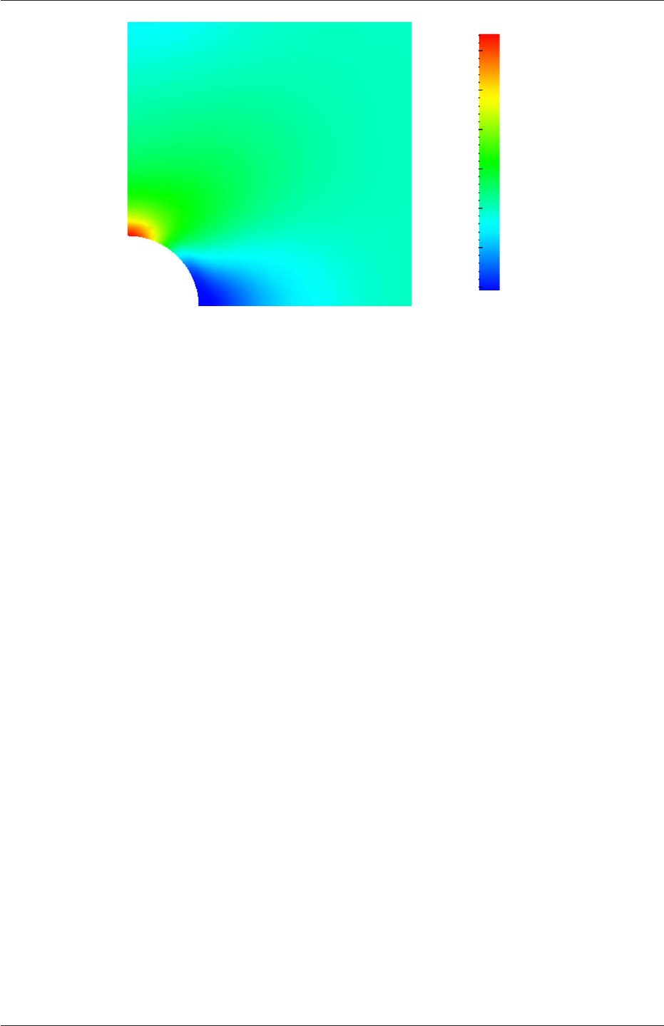
2.2 Stress analysis of a plate with a hole U-59

σxx (kPa)

Figure 2.19: σxx stress ﬁeld in the plate with hole.

Components named sigmaxx,sigmaxy etc. are written to time directories of the case. The

σxx stresses can be viewed in paraFoam as shown in Figure 2.19.

We would like to compare the analytical solution of Equation 2.14 to our solution.

We therefore must output a set of data of σxx along the left edge symmetry plane of our

domain. The user may generate the required graph data using the postProcess utility with

the singleGraph function. Unlike earlier examples of postProcess where no conﬁguration

is required, this example includes a singleGraph ﬁle pre-conﬁgured in the system directory.

The sample line is set between (0.0,0.5,0.25) and (0.0,2.0,0.25), and the ﬁelds are speciﬁed

in the fields list:

9singleGraph

10 {

11 start (0 0.5 0.25);

12 end (0 2 0.25);

13 fields (sigmaxx);

15 #includeEtc "caseDicts/postProcessing/graphs/sampleDict.cfg"

17 setConfig

18 {

19 axis y;

20 }

22 // Must be last entry

23 #includeEtc "caseDicts/postProcessing/graphs/graph.cfg"

24 }

26 // ************************************************************************* //

The user should execute postProcessing with the singleGraph function:

postProcess -func "singleGraph"

Data is written is raw 2 column format into ﬁles within time subdirectories of a post-

Processing/singleGraph directory, e.g. the data at t= 100 s is found within the ﬁle sin-

gleGraph/100/line_sigmaxx.xy. If the user has GnuPlot installed they launch it (by typing

gnuplot) and then plot both the numerical data and analytical solution as follows:

plot [0.5:2] [0:] "postProcessing/singleGraph/100/line_sigmaxx.xy",

OpenFOAM-6

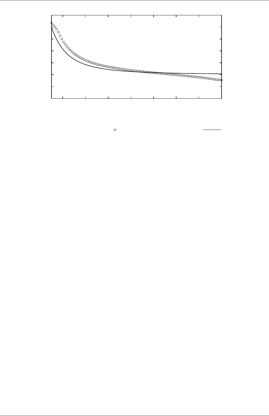
U-60 Tutorials

0.6 0.8 1.0 1.2 1.4 1.6 1.8 2.0

Stress (σxx)x=0 (kPa)

Distance, y(m)

Numerical prediction Analytical solution

Figure 2.20: Normal stress along the vertical symmetry (σxx)x=0

1e4*(1+(0.125/(x**2))+(0.09375/(x**4)))

An example plot is shown in Figure 2.20.

2.2.4 Exercises

The user may wish to experiment with solidDisplacementFoam by trying the following exer-

cises:

2.2.4.1 Increasing mesh resolution

Increase the mesh resolution in each of the xand ydirections. Use mapFields to map the

ﬁnal coarse mesh results from section 2.2.3 to the initial conditions for the ﬁne mesh.

2.2.4.2 Introducing mesh grading

Grade the mesh so that the cells near the hole are ﬁner than those away from the hole.

Design the mesh so that the ratio of sizes between adjacent cells is no more than 1.1 and so

that the ratio of cell sizes between blocks is similar to the ratios within blocks. Mesh grading

is described in section 2.1.6. Again use mapFields to map the ﬁnal coarse mesh results from

section 2.2.3 to the initial conditions for the graded mesh. Compare the results with those

from the analytical solution and previous calculations. Can this solution be improved upon

using the same number of cells with a diﬀerent solution?

2.2.4.3 Changing the plate size

The analytical solution is for an inﬁnitely large plate with a ﬁnite sized hole in it. Therefore

this solution is not completely accurate for a ﬁnite sized plate. To estimate the error,

increase the plate size while maintaining the hole size at the same value.

OpenFOAM-6

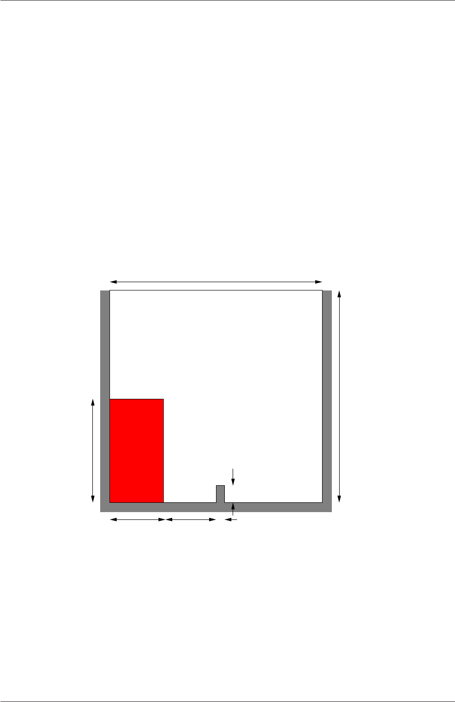
2.3 Breaking of a dam U-61

2.3 Breaking of a dam

In this tutorial we shall solve a problem of simpliﬁed dam break in 2 dimensions using the

interFoam.The feature of the problem is a transient ﬂow of two ﬂuids separated by a sharp

interface, or free surface. The two-phase algorithm in interFoam is based on the volume of

ﬂuid (VOF) method in which a specie transport equation is used to determine the relative

volume fraction of the two phases, or phase fraction α, in each computational cell. Physical

properties are calculated as weighted averages based on this fraction. The nature of the

VOF method means that an interface between the species is not explicitly computed, but

rather emerges as a property of the phase fraction ﬁeld. Since the phase fraction can have

any value between 0 and 1, the interface is never sharply deﬁned, but occupies a volume

around the region where a sharp interface should exist.

The test setup consists of a column of water at rest located behind a membrane on the

left side of a tank. At time t= 0 s, the membrane is removed and the column of water

collapses. During the collapse, the water impacts an obstacle at the bottom of the tank

and creates a complicated ﬂow structure, including several captured pockets of air. The

geometry and the initial setup is shown in Figure 2.21.

0.584 m

0.048 m

0.024 m

0.584 m

0.292 m

0.1459 m0.1461 m

water column

Figure 2.21: Geometry of the dam break.

2.3.1 Mesh generation

The user should go to their run directory and copy the damBreak case from the $FOAM_TUTO-

RIALS/multiphase/interFoam/laminar/damBreak directory, i.e.

run

cp -r $FOAM_TUTORIALS/multiphase/interFoam/laminar/damBreak/damBreak .

OpenFOAM-6

U-62 Tutorials

Go into the damBreak case directory and generate the mesh running blockMesh as described

previously. The damBreak mesh consist of 5 blocks; the blockMeshDict entries are given

below.

17 convertToMeters 0.146;

19 vertices

20 (

21 (0 0 0)

22 (2 0 0)

23 (2.16438 0 0)

24 (4 0 0)

25 (0 0.32876 0)

26 (2 0.32876 0)

27 (2.16438 0.32876 0)

28 (4 0.32876 0)

29 (0 4 0)

30 (2 4 0)

31 (2.16438 4 0)

32 (4 4 0)

33 (0 0 0.1)

34 (2 0 0.1)

35 (2.16438 0 0.1)

36 (4 0 0.1)

37 (0 0.32876 0.1)

38 (2 0.32876 0.1)

39 (2.16438 0.32876 0.1)

40 (4 0.32876 0.1)

41 (0 4 0.1)

42 (2 4 0.1)

43 (2.16438 4 0.1)

44 (4 4 0.1)

45 );

47 blocks

48 (

49 hex (0 1 5 4 12 13 17 16) (23 8 1) simpleGrading (1 1 1)

50 hex (2 3 7 6 14 15 19 18) (19 8 1) simpleGrading (1 1 1)

51 hex (4 5 9 8 16 17 21 20) (23 42 1) simpleGrading (1 1 1)

52 hex (5 6 10 9 17 18 22 21) (4 42 1) simpleGrading (1 1 1)

53 hex (6 7 11 10 18 19 23 22) (19 42 1) simpleGrading (1 1 1)

54 );

56 edges

57 (

58 );

60 boundary

61 (

62 leftWall

63 {

64 type wall;

65 faces

66 (

67 (0 12 16 4)

68 (4 16 20 8)

69 );

70 }

71 rightWall

72 {

73 type wall;

74 faces

75 (

76 (7 19 15 3)

77 (11 23 19 7)

78 );

79 }

80 lowerWall

81 {

82 type wall;

83 faces

84 (

85 (0 1 13 12)

86 (1 5 17 13)

87 (5 6 18 17)

88 (2 14 18 6)

89 (2 3 15 14)

90 );

91 }

OpenFOAM-6

2.3 Breaking of a dam U-63

92 atmosphere

93 {

94 type patch;

95 faces

96 (

97 (8 20 21 9)

98 (9 21 22 10)

99 (10 22 23 11)

100 );

101 }

102 );

103

104 mergePatchPairs

105 (

106 );

107

108 // ************************************************************************* //

2.3.2 Boundary conditions

The user can examine the boundary geometry generated by blockMesh by viewing the bound-

ary ﬁle in the constant/polyMesh directory. The ﬁle contains a list of 5 boundary patches:

leftWall,rightWall,lowerWall,atmosphere and defaultFaces. The user should notice

the type of the patches. The atmosphere is a standard patch,i.e. has no special attributes,

merely an entity on which boundary conditions can be speciﬁed. The defaultFaces patch

is empty since the patch normal is in the direction we will not solve in this 2D case. The

leftWall,rightWall and lowerWall patches are each a wall.

Like the generic patch, the wall type contains no geometric or topological information

about the mesh and only diﬀers from the plain patch in that it identiﬁes the patch as

a wall, should an application need to know, e.g. to apply special wall surface modelling.

For example, the interFoam solver includes modelling of surface tension and can include

wall adhesion at the contact point between the interface and wall surface. Wall adhesion

models can be applied through a special boundary condition on the alpha (α) ﬁeld, e.g. the

constantAlphaContactAngle boundary condition, which requires the user to specify a static

contact angle, theta0.

In this tutorial we would like to ignore surface tension eﬀects between the wall and

interface. We can do this by setting the static contact angle, θ0= 90◦. However, rather

than using the constantAlphaContactAngle boundary condition, the simpler zeroGradient can

be applied to alpha on the walls.

The top boundary is free to the atmosphere so needs to permit both outﬂow and inﬂow

according to the internal ﬂow. We therefore use a combination of boundary conditions for

pressure and velocity that does this while maintaining stability. They are:

•totalPressure which is a ﬁxedValue condition calculated from speciﬁed total pressure

p0 and local velocity U;

•pressureInletOutletVelocity, which applies zeroGradient on all components, except where

there is inﬂow, in which case a ﬁxedValue condition is applied to the tangential com-

ponent;

•inletOutlet, which is a zeroGradient condition when ﬂow outwards, ﬁxedValue when ﬂow

is inwards.

At all wall boundaries, the ﬁxedFluxPressure boundary condition is applied to the pressure

ﬁeld, which adjusts the pressure gradient so that the boundary ﬂux matches the velocity

boundary condition for solvers that include body forces such as gravity and surface tension.

OpenFOAM-6

U-64 Tutorials

The defaultFaces patch representing the front and back planes of the 2D problem, is,

as usual, an empty type.

2.3.3 Setting initial ﬁeld

Unlike the previous cases, we shall now specify a non-uniform initial condition for the phase

fraction αwater where

αwater =(1for the water phase

0for the air phase (2.15)

This will be done by running the setFields utility. It requires a setFieldsDict dictionary,

located in the system directory, whose entries for this case are shown below.

18 defaultFieldValues

19 (

20 volScalarFieldValue alpha.water 0

21 );

23 regions

24 (

25 boxToCell

26 {

27 box (0 0 -1) (0.1461 0.292 1);

28 fieldValues

29 (

30 volScalarFieldValue alpha.water 1

31 );

32 }

33 );

36 // ************************************************************************* //

The defaultFieldValues sets the default value of the ﬁelds, i.e. the value the ﬁeld takes

unless speciﬁed otherwise in the regions sub-dictionary. That sub-dictionary contains a list

of subdictionaries containing fieldValues that override the defaults in a speciﬁed region.

The region creates a set of points, cells or faces based on some topological constraint. Here,

boxToCell creates a bounding box within a vector minimum and maximum to deﬁne the

set of cells of the water region. The phase fraction αwater is deﬁned as 1 in this region.

The setFields utility reads ﬁelds from ﬁle and, after re-calculating those ﬁelds, will write

them back to ﬁle. In the damBreak tutorial, the alpha.water ﬁeld is initially stored as a

backup named alpha.water.orig. A ﬁeld ﬁle with the .orig extension is read in when the

actual ﬁle does not exist, so setFields will read alpha.water.orig but write the resulting

output to alpha.water (or alpha.water.gz if compression is switched on). This way the

original ﬁle is not overwritten, so can be reused.

The user should therefore execute setFields like any other utility by:

setFields

Using paraFoam, check that the initial alpha.water ﬁeld corresponds to the desired distri-

bution as in Figure 2.22.

OpenFOAM-6

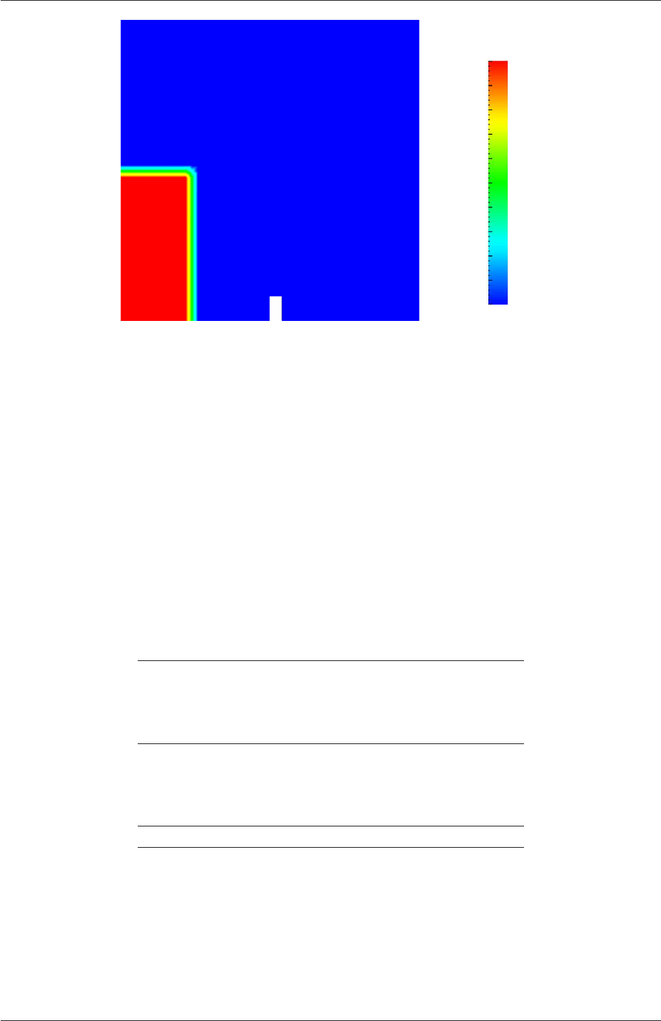
2.3 Breaking of a dam U-65

0.0

0.1

0.2

0.3

0.4

0.5

0.6

0.7

0.8

0.9

1.0

Phase fraction, α1

Figure 2.22: Initial conditions for phase fraction alpha.water.

2.3.4 Fluid properties

Let us examine the transportProperties ﬁle in the constant directory. The dictionary ﬁrst

contains the names of each ﬂuid phase in the phases list, here water and air. The material

properties for each ﬂuid are then separated into two dictionaries water and air. The trans-

port model for each phase is selected by the transportModel keyword. The user should

select Newtonian in which case the kinematic viscosity is single valued and speciﬁed under

the keyword nu. The viscosity parameters for other models, e.g.CrossPowerLaw, would oth-

erwise be speciﬁed as described in section 7.3. The density is speciﬁed under the keyword

rho.

The surface tension between the two phases is speciﬁed by the keyword sigma. The

values used in this tutorial are listed in Table 2.3.

water properties

Kinematic viscosity m2s−1nu 1.0×10−6

Density kg m−3rho 1.0×103

air properties

Kinematic viscosity m2s−1nu 1.48 ×10−5

Density kg m−3rho 1.0

Properties of both phases

Surface tension N m−1sigma 0.07

Table 2.3: Fluid properties for the damBreak tutorial

Gravitational acceleration is uniform across the domain and is speciﬁed in a ﬁle named

gin the constant directory. Unlike a normal ﬁeld ﬁle, e.g. Uand p,gis a uniformDimen-

sionedVectorField and so simply contains a set of dimensions and a value that represents

(0,9.81,0) m s−2for this tutorial:

OpenFOAM-6

U-66 Tutorials

18 dimensions [0 1 -2 0 0 0 0];

19 value (0 -9.81 0);

22 // ************************************************************************* //

2.3.5 Turbulence modelling

As in the cavity example, the choice of turbulence modelling method is selectable at run-time

through the simulationType keyword in turbulenceProperties dictionary. In this example,

we wish to run without turbulence modelling so we set laminar:

18 simulationType laminar;

21 // ************************************************************************* //

2.3.6 Time step control

Time step control is an important issue in transient simulation and the surface-tracking

algorithm in interface capturing solvers. The Courant number Co needs to be limited

depending on the choice of algorithm: with the “explicit” MULES algorithm, an upper limit

of Co ≈0.25 for stability is typical in the region of the interface; but with “semi-implicit”

MULES, speciﬁed by the MULESCorr keyword in the fvSolution ﬁle, there is really no upper

limit in Co for stability, but instead the level is determined by requirements of temporal

accuracy.

In general it is diﬃcult to specify a ﬁxed time-step to satisfy the Co criterion, so interFoam

oﬀers automatic adjustment of the time step as standard in the controlDict. The user should

specify adjustTimeStep to be on and the the maximum Co for the phase ﬁelds, maxAlphaCo,

and other ﬁelds, maxCo, to be 1.0. The upper limit on time step maxDeltaT can be set to a

value that will not be exceeded in this simulation, e.g. 1.0.

By using automatic time step control, the steps themselves are never rounded to a

convenient value. Consequently if we request that OpenFOAM saves results at a ﬁxed

number of time step intervals, the times at which results are saved are somewhat arbitrary.

However even with automatic time step adjustment, OpenFOAM allows the user to specify

that results are written at ﬁxed times; in this case OpenFOAM forces the automatic time

stepping procedure to adjust time steps so that it ‘hits’ on the exact times speciﬁed for write

output. The user selects this with the adjustableRunTime option for writeControl in the

controlDict dictionary. The controlDict dictionary entries should be:

18 application interFoam;

20 startFrom startTime;

22 startTime 0;

24 stopAt endTime;

26 endTime 1;

28 deltaT 0.001;

30 writeControl adjustableRunTime;

32 writeInterval 0.05;

34 purgeWrite 0;

OpenFOAM-6

2.3 Breaking of a dam U-67

36 writeFormat binary;

38 writePrecision 6;

40 writeCompression off;

42 timeFormat general;

44 timePrecision 6;

46 runTimeModifiable yes;

48 adjustTimeStep yes;

50 maxCo 1;

51 maxAlphaCo 1;

53 maxDeltaT 1;

56 // ************************************************************************* //

2.3.7 Discretisation schemes

The interFoam solver uses the multidimensional universal limiter for explicit solution (MULES)

method, created by Henry Weller, to maintain boundedness of the phase fraction indepen-

dent of underlying numerical scheme, mesh structure, etc. The choice of schemes for con-

vection are therfore not restricted to those that are strongly stable or bounded, e.g. upwind

diﬀerencing.

The convection schemes settings are made in the divSchemes sub-dictionary of the fv-

Schemes dictionary. In this example, the convection term in the momentum equation

(∇•(ρUU)), denoted by the div(rhoPhi,U) keyword, uses Gauss linearUpwind grad(U)

to produce good accuracy. Here, we have opted for best stability with φ= 1.0. The

∇•(Uα1)term, represented by the div(phi,alpha) keyword uses the vanLeer scheme.

The ∇•(Urbα1)term, represented by the div(phirb,alpha) keyword, can use second or-

der linear (central) diﬀerencing as boundedness is assured by the MULES algorithm.

The other discretised terms use commonly employed schemes so that the fvSchemes

dictionary entries should therefore be:

18 ddtSchemes

19 {

20 default Euler;

21 }

23 gradSchemes

24 {

25 default Gauss linear;

26 }

28 divSchemes

29 {

30 div(rhoPhi,U) Gauss linearUpwind grad(U);

31 div(phi,alpha) Gauss vanLeer;

32 div(phirb,alpha) Gauss linear;

33 div(((rho*nuEff)*dev2(T(grad(U))))) Gauss linear;

34 }

36 laplacianSchemes

37 {

38 default Gauss linear corrected;

39 }

41 interpolationSchemes

42 {

43 default linear;

44 }

OpenFOAM-6

U-68 Tutorials

46 snGradSchemes

47 {

48 default corrected;

49 }

52 // ************************************************************************* //

2.3.8 Linear-solver control

In the fvSolution ﬁle, the alpha.water sub-dictionary in solvers contains elements that are

speciﬁc to interFoam. Of particular interest are the nAlphaSubCycles and cAlpha keywords.

nAlphaSubCycles represents the number of sub-cycles within the αequation; sub-cycles are

additional solutions to an equation within a given time step. It is used to enable the solution

to be stable without reducing the time step and vastly increasing the solution time. Here

we specify 2 sub-cycles, which means that the αequation is solved in 2×half length time

steps within each actual time step.

The cAlpha keyword is a factor that controls the compression of the interface where: 0

corresponds to no compression; 1 corresponds to conservative compression; and, anything

larger than 1, relates to enhanced compression of the interface. We generally adopt a value

of 1.0 which is employed in this example.

2.3.9 Running the code

Running of the code has been described in detail in previous tutorials. Try the following,

that uses tee, a command that enables output to be written to both standard output and

ﬁles:

cd $FOAM_RUN/damBreak

interFoam | tee log

The code will now be run interactively, with a copy of output stored in the log ﬁle.

2.3.10 Post-processing

Post-processing of the results can now be done in the usual way. The user can monitor the

development of the phase fraction alpha.water in time, e.g. see Figure 2.23.

2.3.11 Running in parallel

The results from the previous example are generated using a fairly coarse mesh. We now

wish to increase the mesh resolution and re-run the case. The new case will typically take

a few hours to run with a single processor so, should the user have access to multiple

processors, we can demonstrate the parallel processing capability of OpenFOAM.

The user should ﬁrst clone the damBreak case, e.g. by

run

foamCloneCase damBreak damBreakFine

Enter the new case directory and change the blocks description in the blockMeshDict dic-

tionary to

OpenFOAM-6

2.3 Breaking of a dam U-69

0.0

0.1

0.2

0.3

0.4

0.5

0.6

0.7

0.8

0.9

1.0

Phase fraction, α1

(a) At t= 0.25 s.

0.0

0.1

0.2

0.3

0.4

0.5

0.6

0.7

0.8

0.9

1.0

Phase fraction, α1

(b) At t= 0.50 s.

Figure 2.23: Snapshots of phase α.

OpenFOAM-6

U-70 Tutorials

blocks

(

hex (0 1 5 4 12 13 17 16) (46 10 1) simpleGrading (1 1 1)

hex (2 3 7 6 14 15 19 18) (40 10 1) simpleGrading (1 1 1)

hex (4 5 9 8 16 17 21 20) (46 76 1) simpleGrading (1 2 1)

hex (5 6 10 9 17 18 22 21) (4 76 1) simpleGrading (1 2 1)

hex (6 7 11 10 18 19 23 22) (40 76 1) simpleGrading (1 2 1)

);

Here, the entry is presented as printed from the blockMeshDict ﬁle; in short the user must

change the mesh densities, e.g. the 46 10 1 entry, and some of the mesh grading entries to

121. Once the dictionary is correct, generate the mesh by running blockMesh.

As the mesh has now changed from the damBreak example, the user must re-initialise the

phase ﬁeld alpha.water in the 0time directory since it contains a number of elements that

is inconsistent with the new mesh. Note that there is no need to change the Uand p_rgh

ﬁelds since they are speciﬁed as uniform which is independent of the number of elements

in the ﬁeld. We wish to initialise the ﬁeld with a sharp interface, i.e. it elements would

have α= 1 or α= 0. Updating the ﬁeld with mapFields may produce interpolated values

0< α < 1at the interface, so it is better to rerun the setFields utility.

The mesh size is now inconsistent with the number of elements in the alpha.water.gz ﬁle

in the 0directory, so the user must delete that ﬁle so that the original alpha.water.orig ﬁle

is used instead.

rm 0/alpha.water.gz

setFields

The method of parallel computing used by OpenFOAM is known as domain decomposi-

tion, in which the geometry and associated ﬁelds are broken into pieces and allocated to sep-

arate processors for solution. The ﬁrst step required to run a parallel case is therefore to de-

compose the domain using the decomposePar utility. There is a dictionary associated with de-

composePar named decomposeParDict which is located in the system directory of the tutorial

case; also, like with many utilities, a default dictionary can be found in the directory of the

source code of the speciﬁc utility, i.e. in $FOAM_UTILITIES/parallelProcessing/decomposePar

for this case.

The ﬁrst entry is numberOfSubdomains which speciﬁes the number of subdomains into

which the case will be decomposed, usually corresponding to the number of processors

available for the case.

In this tutorial, the method of decomposition should be simple and the corresponding

simpleCoeffs should be edited according to the following criteria. The domain is split

into pieces, or subdomains, in the x,yand zdirections, the number of subdomains in each

direction being given by the vector n. As this geometry is 2 dimensional, the 3rd direction,

z, cannot be split, hence nzmust equal 1. The nxand nycomponents of nsplit the domain

in the xand ydirections and must be speciﬁed so that the number of subdomains speciﬁed

by nxand nyequals the speciﬁed numberOfSubdomains,i.e. nxny=numberOfSubdomains.

It is beneﬁcial to keep the number of cell faces adjoining the subdomains to a minimum so,

for a square geometry, it is best to keep the split between the xand ydirections should be

fairly even. The delta keyword should be set to 0.001.

OpenFOAM-6

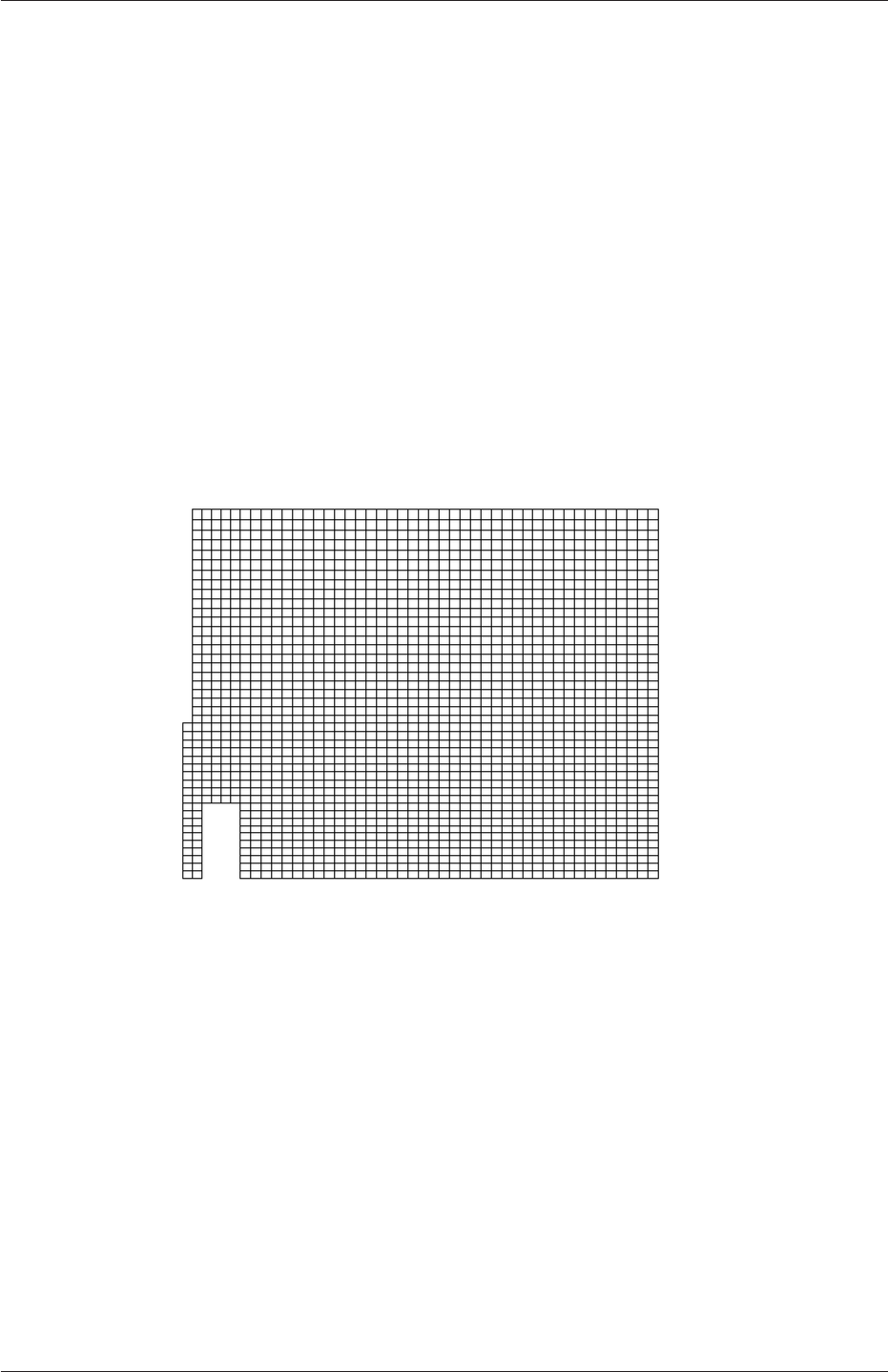
2.3 Breaking of a dam U-71

For example, let us assume we wish to run on 4 processors. We would set numberOf-

Subdomains to 4 and n= (2,2,1). The user should run decomposePar with:

decomposePar

The terminal output shows that the decomposition is distributed fairly even between the

processors.

The user should consult section 3.4 for details of how to run a case in parallel; in

this tutorial we merely present an example of running in parallel. We use the openMPI

implementation of the standard message-passing interface (MPI). As a test here, the user

can run in parallel on a single node, the local host only, by typing:

mpirun -np 4 interFoam -parallel >log &

The user may run on more nodes over a network by creating a ﬁle that lists the host

names of the machines on which the case is to be run as described in section 3.4.3. The case

should run in the background and the user can follow its progress by monitoring the log ﬁle

as usual.

Figure 2.24: Mesh of processor 2 in parallel processed case.

2.3.12 Post-processing a case run in parallel

Once the case has completed running, the decomposed ﬁelds and mesh can be reassembled

for post-processing using the reconstructPar utility. Simply execute it from the command

line. The results from the ﬁne mesh are shown in Figure 2.25. The user can see that the

resolution of interface has improved signiﬁcantly compared to the coarse mesh.

The user may also post-process an individual region of the decomposed domain individ-

ually by simply treating the individual processor directory as a case in its own right. For

example if the user starts paraFoam by

paraFoam -case processor1

then processor1 will appear as a case module in ParaView. Figure 2.24 shows the mesh from

processor 1 following the decomposition of the domain using the simple method.

OpenFOAM-6

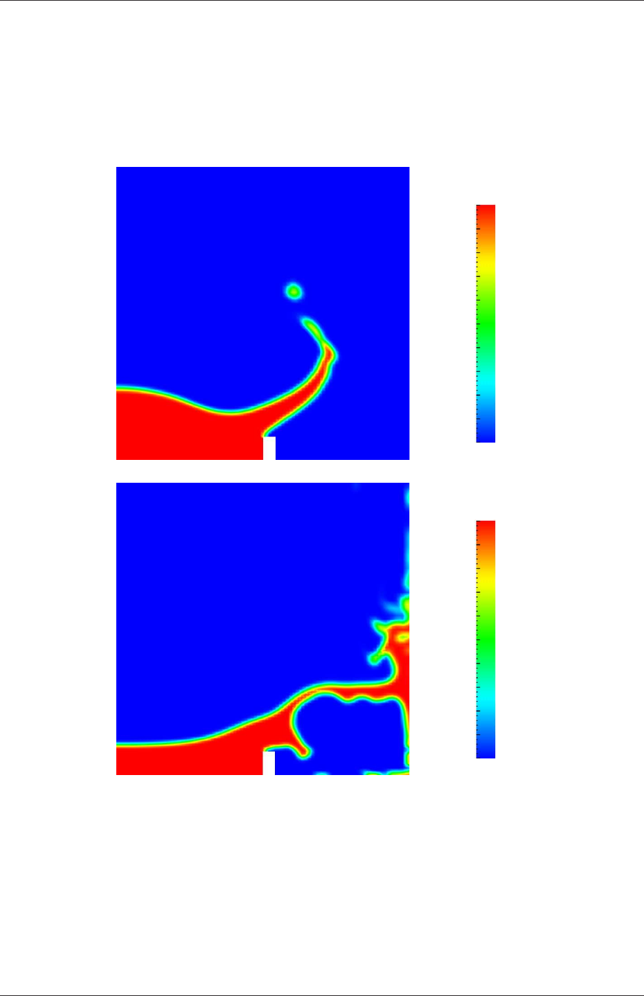
U-72 Tutorials

0.0

0.1

0.2

0.3

0.4

0.5

0.6

0.7

0.8

0.9

1.0

Phase fraction, α1

(a) At t= 0.25 s.

0.0

0.1

0.2

0.3

0.4

0.5

0.6

0.7

0.8

0.9

1.0

Phase fraction, α1

(b) At t= 0.50 s.

Figure 2.25: Snapshots of phase αwith reﬁned mesh.

OpenFOAM-6

Chapter 3

Applications and libraries

We should reiterate from the outset that OpenFOAM is a C++ library used primarily to

create executables, known as applications. OpenFOAM is distributed with a large set of

precompiled applications but users also have the freedom to create their own or modify

existing ones. Applications are split into two main categories:

solvers that are each designed to solve a speciﬁc problem in computational continuum

mechanics;

utilities that perform simple pre-and post-processing tasks, mainly involving data manip-

ulation and algebraic calculations.

OpenFOAM is divided into a set of precompiled libraries that are dynamically linked during

compilation of the solvers and utilities. Libraries such as those for physical models are

supplied as source code so that users may conveniently add their own models to the libraries.

This chapter gives an overview of solvers, utilities and libraries, their creation, modiﬁcation,

compilation and execution.

3.1 The programming language of OpenFOAM

In order to understand the way in which the OpenFOAM library works, some background

knowledge of C++, the base language of OpenFOAM, is required; the necessary information

will be presented in this chapter. Before doing so, it is worthwhile addressing the concept of

language in general terms to explain some of the ideas behind object-oriented programming

and our choice of C++ as the main programming language of OpenFOAM.

3.1.1 Language in general

The success of verbal language and mathematics is based on eﬃciency, especially in express-

ing abstract concepts. For example, in ﬂuid ﬂow, we use the term “velocity ﬁeld”, which has

meaning without any reference to the nature of the ﬂow or any speciﬁc velocity data. The

term encapsulates the idea of movement with direction and magnitude and relates to other

physical properties. In mathematics, we can represent velocity ﬁeld by a single symbol, e.g.

U, and express certain concepts using symbols, e.g. “the ﬁeld of velocity magnitude” by

|U|. The advantage of mathematics over verbal language is its greater eﬃciency, making it

possible to express complex concepts with extreme clarity.

U-74 Applications and libraries

The problems that we wish to solve in continuum mechanics are not presented in terms of

intrinsic entities, or types, known to a computer, e.g. bits, bytes, integers. They are usually

presented ﬁrst in verbal language, then as partial diﬀerential equations in 3 dimensions of

space and time. The equations contain the following concepts: scalars, vectors, tensors,

and ﬁelds thereof; tensor algebra; tensor calculus; dimensional units. The solution to these

equations involves discretisation procedures, matrices, solvers, and solution algorithms.

3.1.2 Object-orientation and C++

Progamming languages that are object-oriented, such as C++, provide the mechanism —

classes — to declare types and associated operations that are part of the verbal and mathe-

matical languages used in science and engineering. Our velocity ﬁeld introduced earlier can

be represented in programming code by the symbol Uand “the ﬁeld of velocity magnitude”

can be mag(U). The velocity is a vector ﬁeld for which there should exist, in an object-

oriented code, a vectorField class. The velocity ﬁeld Uwould then be an instance, or object,

of the vectorField class; hence the term object-oriented.

The clarity of having objects in programming that represent physical objects and abstract

entities should not be underestimated. The class structure concentrates code development

to contained regions of the code, i.e. the classes themselves, thereby making the code easier

to manage. New classes can be derived or inherit properties from other classes, e.g. the

vectorField can be derived from a vector class and a Field class. C++ provides the mechanism

of template classes such that the template class Field<Type>can represent a ﬁeld of any

<Type>,e.g.scalar,vector,tensor. The general features of the template class are passed on

to any class created from the template. Templating and inheritance reduce duplication of

code and create class hierarchies that impose an overall structure on the code.

3.1.3 Equation representation

A central theme of the OpenFOAM design is that the solver applications, written using the

OpenFOAM classes, have a syntax that closely resembles the partial diﬀerential equations

being solved. For example the equation

∂ρU

∂t +∇•φU− ∇ •µ∇U=−∇p

is represented by the code

solve

(

fvm::ddt(rho, U)

+ fvm::div(phi, U)

- fvm::laplacian(mu, U)

- fvc::grad(p)

);

This and other requirements demand that the principal programming language of Open-

FOAM has object-oriented features such as inheritance, template classes, virtual functions

and operator overloading. These features are not available in many languages that purport

OpenFOAM-6

3.2 Compiling applications and libraries U-75

to be object-orientated but actually have very limited object-orientated capability, such

as FORTRAN-90. C++, however, possesses all these features while having the additional

advantage that it is widely used with a standard speciﬁcation so that reliable compilers

are available that produce eﬃcient executables. It is therefore the primary language of

OpenFOAM.

3.1.4 Solver codes

Solver codes are largely procedural since they are a close representation of solution algo-

rithms and equations, which are themselves procedural in nature. Users do not need a deep

knowledge of object-orientation and C++ programming to write a solver but should know

the principles behind object-orientation and classes, and to have a basic knowledge of some

C++ code syntax. An understanding of the underlying equations, models and solution

method and algorithms is far more important.

There is often little need for a user to immerse themselves in the code of any of the

OpenFOAM classes. The essence of object-orientation is that the user should not have to

go through the code of each class they use; merely the knowledge of the class’ existence

and its functionality are suﬃcient to use the class. A description of each class, its functions

etc. is supplied with the OpenFOAM distribution in HTML documentation generated with

Doxygen at https://cpp.openfoam.org

3.2 Compiling applications and libraries

Compilation is an integral part of application development that requires careful management

since every piece of code requires its own set instructions to access dependent components

of the OpenFOAM library. In UNIX/Linux systems these instructions are often organised

and delivered to the compiler using the standard UNIXmake utility. OpenFOAM uses its

own wmake compilation script that is based on make but is considerably more versatile

and easier to use (wmake can be used on any code, not only the OpenFOAM library). To

understand the compilation process, we ﬁrst need to explain certain aspects of C++ and

its ﬁle structure, shown schematically in Figure 3.1. A class is deﬁned through a set of

instructions such as object construction, data storage and class member functions. The ﬁle

that deﬁnes these functions — the class deﬁnition — takes a .C extension, e.g. a class nc

would be written in the ﬁle nc.C. This ﬁle can be compiled independently of other code into

a binary executable library ﬁle known as a shared object library with the .so ﬁle extension,

i.e.nc.so. When compiling a piece of code, say newApp.C, that uses the nc class, nc.C need

not be recompiled, rather newApp.C calls the nc.so library at runtime. This is known as

dynamic linking.

3.2.1 Header .H ﬁles

As a means of checking errors, the piece of code being compiled must know that the classes

it uses and the operations they perform actually exist. Therefore each class requires a class

declaration, contained in a header ﬁle with a .H ﬁle extension, e.g. nc.H, that includes the

names of the class and its functions. This ﬁle is included at the beginning of any piece

of code using the class, using the #include directive described below, including the class

declaration code itself. Any piece of .C code can resource any number of classes and must

OpenFOAM-6

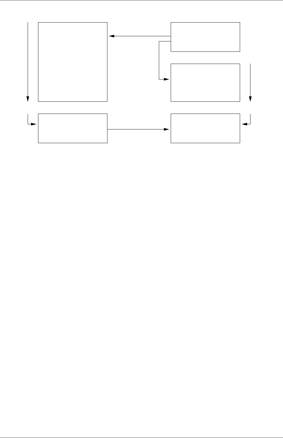
U-76 Applications and libraries

int main()

...

return(0);

{

}

nc.so

Library

option-I

#include "nc.H"

Main code

Code...

Compiled

nc.H

nc.C

#include "nc.H"

nc class

Definition...

Compiled

Executable

Header ﬁle

Linked

option-l

newApp.C

newApp

Figure 3.1: Header ﬁles, source ﬁles, compilation and linking

begin by including all the .H ﬁles required to declare these classes. Those classes in turn

can resource other classes and so also begin by including the relevant .H ﬁles. By searching

recursively down the class hierarchy we can produce a complete list of header ﬁles for all the

classes on which the top level .C code ultimately depends; these .H ﬁles are known as the

dependencies. With a dependency list, a compiler can check whether the source ﬁles have

been updated since their last compilation and selectively compile only those that need to

be.

Header ﬁles are included in the code using the # include directive, e.g.

# include "otherHeader.H";

This causes the compiler to suspend reading from the current ﬁle, to read the included ﬁle.

This mechanism allows any self-contained piece of code to be put into a header ﬁle and

included at the relevant location in the main code in order to improve code readability. For

example, in most OpenFOAM applications the code for creating ﬁelds and reading ﬁeld

input data is included in a ﬁle createFields.H which is called at the beginning of the code.

In this way, header ﬁles are not solely used as class declarations.

It is wmake that performs the task of maintaining ﬁle dependency lists amongst other

functions listed below.

•Automatic generation and maintenance of ﬁle dependency lists, i.e. lists of ﬁles which

are included in the source ﬁles and hence on which they depend.

•Multi-platform compilation and linkage, handled through appropriate directory struc-

ture.

•Multi-language compilation and linkage, e.g. C, C++, Java.

•Multi-option compilation and linkage, e.g. debug, optimised, parallel and proﬁling.

•Support for source code generation programs, e.g. lex, yacc, IDL, MOC.

OpenFOAM-6

3.2 Compiling applications and libraries U-77

•Simple syntax for source ﬁle lists.

•Automatic creation of source ﬁle lists for new codes.

•Simple handling of multiple shared or static libraries.

•Extensible to new machine types.

•Extremely portable, works on any machine with: make;sh,ksh or csh;lex,cc.

3.2.2 Compiling with wmake

OpenFOAM applications are organised using a standard convention that the source code

of each application is placed in a directory whose name is that of the application. The top

level source ﬁle then takes the application name with the .C extension. For example, the

source code for an application called newApp would reside is a directory newApp and the

top level ﬁle would be newApp.C as shown in Figure 3.2.wmake then requires the directory

newApp

newApp.C

otherHeader.H

Make

ﬁles

options

Figure 3.2: Directory structure for an application

must contain a Make subdirectory containing 2 ﬁles, options and ﬁles, that are described in

the following sections.

3.2.2.1 Including headers

The compiler searches for the included header ﬁles in the following order, speciﬁed with the

-I option in wmake:

1. the $WM_PROJECT_DIR/src/OpenFOAM/lnInclude directory;

2. a local lnInclude directory, i.e.newApp/lnInclude;

3. the local directory, i.e.newApp;

4. platform dependent paths set in ﬁles in the $WM_PROJECT_DIR/wmake/rules/-

$WM_ARCH/ directory, e.g./usr/X11/include and $(MPICH_ARCH_PATH)/include;

5. other directories speciﬁed explicitly in the Make/options ﬁle with the -I option.

The Make/options ﬁle contains the full directory paths to locate header ﬁles using the syntax:

OpenFOAM-6

U-78 Applications and libraries

EXE_INC = \

-I<directoryPath1>\

-I<directoryPath2>\

... \

-I<directoryPathN>

Notice ﬁrst that the directory names are preceeded by the -I ﬂag and that the syntax uses

the \to continue the EXE_INC across several lines, with no \after the ﬁnal entry.

3.2.2.2 Linking to libraries

The compiler links to shared object library ﬁles in the following directory paths, speciﬁed

with the -L option in wmake:

1. the $FOAM_LIBBIN directory;

2. platform dependent paths set in ﬁles in the $WM_DIR/rules/$WM_ARCH/ directory,

e.g./usr/X11/lib and $(MPICH_ARCH_PATH)/lib;

3. other directories speciﬁed in the Make/options ﬁle.

The actual library ﬁles to be linked must be speciﬁed using the -l option and removing

the lib preﬁx and .so extension from the library ﬁle name, e.g. libnew.so is included with

the ﬂag -lnew. By default, wmake loads the following libraries:

1. the libOpenFOAM.so library from the $FOAM_LIBBIN directory;

2. platform dependent libraries speciﬁed in set in ﬁles in the $WM_DIR/rules/$WM_ARCH/

directory, e.g. libm.so from /usr/X11/lib and liblam.so from $(LAM_ARCH_PATH)/lib;

3. other libraries speciﬁed in the Make/options ﬁle.

The Make/options ﬁle contains the full directory paths and library names using the syntax:

EXE_LIBS = \

-L<libraryPath>\

-l<library1>\

-l<library2>\

... \

-l<libraryN>

To summarise: the directory paths are preceeded by the -L ﬂag, the library names are

preceeded by the -l ﬂag.

OpenFOAM-6

3.2 Compiling applications and libraries U-79

3.2.2.3 Source ﬁles to be compiled

The compiler requires a list of .C source ﬁles that must be compiled. The list must contain

the main .C ﬁle but also any other source ﬁles that are created for the speciﬁc application

but are not included in a class library. For example, users may create a new class or some

new functionality to an existing class for a particular application. The full list of .C source

ﬁles must be included in the Make/ﬁles ﬁle. For many applications the list only includes the

name of the main .C ﬁle, e.g. newApp.C in the case of our earlier example.

The Make/ﬁles ﬁle also includes a full path and name of the compiled executable, speciﬁed

by the EXE = syntax. Standard convention stipulates the name is that of the application,

i.e.newApp in our example. The OpenFOAM release oﬀers two useful choices for path:

standard release applications are stored in $FOAM_APPBIN; applications developed by the

user are stored in $FOAM_USER_APPBIN.

If the user is developing their own applications, we recommend they create an applications

subdirectory in their $WM_PROJECT_USER_DIR directory containing the source code for

personal OpenFOAM applications. As with standard applications, the source code for each

OpenFOAM application should be stored within its own directory. The only diﬀerence

between a user application and one from the standard release is that the Make/ﬁles ﬁle

should specify that the user’s executables are written into their $FOAM_USER_APPBIN

directory. The Make/ﬁles ﬁle for our example would appear as follows:

newApp.C

EXE = $(FOAM_USER_APPBIN)/newApp

3.2.2.4 Running wmake

The wmake script is generally executed by typing:

wmake <optionalDirectory>

The <optionalDirectory>is the directory path of the application that is being compiled.

Typically, wmake is executed from within the directory of the application being compiled,

in which case <optionalDirectory>can be omitted.

3.2.2.5 wmake environment variables

For information, the environment variable settings used by wmake are listed in Table 3.1.

3.2.3 Removing dependency lists: wclean

On execution, wmake builds a dependency list ﬁle with a .dep ﬁle extension, e.g. newApp.C.dep

in our example, in a $WM_OPTIONS sub-directory of the Make directory, e.g. Make/linux-

GccDPInt64Opt. If the user wishes to remove these ﬁles, e.g. after making code changes, the

user can run the wclean script by typing:

wclean <optionalDirectory>

OpenFOAM-6

U-80 Applications and libraries

Main paths

$WM_PROJECT_INST_DIR Full path to installation directory,

e.g.$HOME/OpenFOAM

$WM_PROJECT Name of the project being compiled: OpenFOAM

$WM_PROJECT_VERSION Version of the project being compiled: 6

$WM_PROJECT_DIR Full path to locate binary executables of OpenFOAM

release, e.g. $HOME/OpenFOAM/OpenFOAM-6

$WM_PROJECT_USER_DIR Full path to locate binary executables of the user e.g.

$HOME/OpenFOAM/${USER}-6

$WM_THIRD_PARTY_DIR Full path to the ThirdParty software directory e.g.

$HOME/OpenFOAM/ThirdParty-6

Other paths/settings

$WM_ARCH Machine architecture: linux,linux64,linuxIa64,

linuxARM7,linuxPPC64,linuxPPC64le

$WM_ARCH_OPTION 32 or 64 bit architecture

$WM_COMPILER Compiler being used: Gcc -gcc,ICC - Intel, Clang -

LLVM Clang

$WM_COMPILE_OPTION Compilation option: Debug - debugging, Opt optimisa-

tion.

$WM_COMPILER_TYPE Choice of compiler: system,ThirdParty - compiled in

ThirdParty directory

$WM_DIR Full path of the wmake directory

$WM_LABEL_SIZE 32 or 64 bit size for labels (integers)

$WM_LABEL_OPTION Int32 or Int64 compilation of labels

$WM_LINK_LANGUAGE Compiler used to link libraries and executables c++.

$WM_MPLIB Parallel communications library: SYSTEMOPENMPI - sys-

tem version of openMPI,OPENMPI,SYSTEMMPI,MPICH,

MPICH-GM,HPMPI,MPI,QSMPI,SGIMPI.

$WM_OPTIONS =$WM_ARCH...

$WM_COMPILER...

$WM_PRECISION_OPTION...

$WM_LABEL_OPTION...

$WM_COMPILE_OPTION

e.g. linuxGccDPInt64Opt

$WM_PRECISION_OPTION Precision of the compiled binares, SP, single precision

or DP, double precision

Table 3.1: Environment variable settings for wmake.

OpenFOAM-6

3.2 Compiling applications and libraries U-81

Again, the <optionalDirectory>is a path to the directory of the application that is being

compiled. Typically, wclean is executed from within the directory of the application, in

which case the path can be omitted.

3.2.4 Compiling libraries

When compiling a library, there are 2 critical diﬀerences in the conﬁguration of the ﬁle in

the Make directory:

•in the ﬁles ﬁle, EXE = is replaced by LIB = and the target directory for the compiled

entity changes from $FOAM_APPBIN to $FOAM_LIBBIN (and an equivalent $FOAM_USER_-

LIBBIN directory);

•in the options ﬁle, EXE_LIBS = is replaced by LIB_LIBS = to indicate libraries linked

to library being compiled.

When wmake is executed it additionally creates a directory named lnInclude that contains

soft links to all the ﬁles in the library. The lnInclude directory is deleted by the wclean script

when cleaning library source code.

3.2.5 Compilation example: the pisoFoam application

The source code for application pisoFoam is in the $FOAM_APP/solvers/incompressible/piso-

Foam directory and the top level source ﬁle is named pisoFoam.C. The pisoFoam.C source

code is:

1/*---------------------------------------------------------------------------*\

2========= |

3\\ / F ield | OpenFOAM: The Open Source CFD Toolbox

4\\ / O peration |

6\\/ M anipulation |

7-------------------------------------------------------------------------------

8License

9This file is part of OpenFOAM.

11 OpenFOAM is free software: you can redistribute it and/or modify it

12 under the terms of the GNU General Public License as published by

13 the Free Software Foundation, either version 3 of the License, or

14 (at your option) any later version.

16 OpenFOAM is distributed in the hope that it will be useful, but WITHOUT

17 ANY WARRANTY; without even the implied warranty of MERCHANTABILITY or

18 FITNESS FOR A PARTICULAR PURPOSE. See the GNU General Public License

19 for more details.

21 You should have received a copy of the GNU General Public License

22 along with OpenFOAM. If not, see <http://www.gnu.org/licenses/>.

24 Application

25 pisoFoam

27 Description

28 Transient solver for incompressible, turbulent flow, using the PISO

29 algorithm.

31 Sub-models include:

32 - turbulence modelling, i.e. laminar, RAS or LES

33 - run-time selectable MRF and finite volume options, e.g. explicit porosity

35 \*---------------------------------------------------------------------------*/

37 #include "fvCFD.H"

38 #include "singlePhaseTransportModel.H"

39 #include "turbulentTransportModel.H"

OpenFOAM-6

U-82 Applications and libraries

40 #include "pisoControl.H"

41 #include "fvOptions.H"

43 //*************************************//

45 int main(int argc, char *argv[])

46 {

47 #include "postProcess.H"

49 #include "setRootCaseLists.H"

50 #include "createTime.H"

51 #include "createMesh.H"

52 #include "createControl.H"

53 #include "createFields.H"

54 #include "initContinuityErrs.H"

56 turbulence->validate();

58 //***********************************//

60 Info<< "\nStarting time loop\n" << endl;

62 while (runTime.loop())

63 {

64 Info<< "Time = " << runTime.timeName() << nl << endl;

66 #include "CourantNo.H"

68 // Pressure-velocity PISO corrector

69 {

70 #include "UEqn.H"

72 // --- PISO loop

73 while (piso.correct())

74 {

75 #include "pEqn.H"

76 }

77 }

79 laminarTransport.correct();

80 turbulence->correct();

82 runTime.write();

84 Info<< "ExecutionTime = " << runTime.elapsedCpuTime() << " s"

85 << " ClockTime = " << runTime.elapsedClockTime() << " s"

86 << nl << endl;

87 }

89 Info<< "End\n" << endl;

91 return 0;

92 }

95 // ************************************************************************* //

The code begins with a brief description of the application contained within comments over 1

line (//) and multiple lines (/*...*/). Following that, the code contains several # include

statements, e.g. # include "fvCFD.H", which causes the compiler to suspend reading from

the current ﬁle, pisoFoam.C to read the fvCFD.H.

pisoFoam resources the turbulence and transport model libraries and therefore requires

the necessary header ﬁles, speciﬁed by the EXE_INC = -I... option, and links to the

libraries with the EXE_LIBS = -l... option. The Make/options therefore contains the

following:

1EXE_INC = \

2-I$(LIB_SRC)/TurbulenceModels/turbulenceModels/lnInclude \

3-I$(LIB_SRC)/TurbulenceModels/incompressible/lnInclude \

4-I$(LIB_SRC)/transportModels \

5-I$(LIB_SRC)/transportModels/incompressible/singlePhaseTransportModel \

6-I$(LIB_SRC)/finiteVolume/lnInclude \

7-I$(LIB_SRC)/meshTools/lnInclude \

OpenFOAM-6

3.2 Compiling applications and libraries U-83

8-I$(LIB_SRC)/sampling/lnInclude

10 EXE_LIBS = \

11 -lturbulenceModels \

12 -lincompressibleTurbulenceModels \

13 -lincompressibleTransportModels \

14 -lfiniteVolume \

15 -lmeshTools \

16 -lfvOptions \

17 -lsampling

pisoFoam contains only the pisoFoam.C source and the executable is written to the $FOAM_-

APPBIN directory as all standard applications are. The Make/ﬁles therefore contains:

1pisoFoam.C

3EXE = $(FOAM_APPBIN)/pisoFoam

Following the recommendations of section 3.2.2.3, the user can compile a separate version

of pisoFoam into their local $FOAM_USER_DIR directory by the following:

•copying the pisoFoam source code to a local directory, e.g. $FOAM_RUN;

cd $FOAM_RUN

cp -r $FOAM_SOLVERS/incompressible/pisoFoam .

cd pisoFoam

•editing the Make/ﬁles ﬁle as follows;

1pisoFoam.C

3EXE = $(FOAM_USER_APPBIN)/pisoFoam

•executing wmake.

wmake

The code should compile and produce a message similar to the following

Making dependency list for source file pisoFoam.C

g++ -std=c++0x -m32...

...

-o ... platforms/linuxGccDPInt64Opt/bin/pisoFoam

The user can now try recompiling and will receive a message similar to the following to say

that the executable is up to date and compiling is not necessary:

make: ´

.../bin/pisoFoam´ is up to date.

The user can compile the application from scratch by removing the dependency list with

wclean

and running wmake.

OpenFOAM-6

U-84 Applications and libraries

3.2.6 Debug messaging and optimisation switches

OpenFOAM provides a system of messaging that is written during runtime, most of which

are to help debugging problems encountered during running of a OpenFOAM case. The

switches are listed in the $WM_PROJECT_DIR/etc/controlDict ﬁle; should the user wish

to change the settings they should make a copy to their $HOME directory, i.e. $HOME/-

.OpenFOAM/6/controlDict ﬁle. The list of possible switches is extensive and can be viewed

by running the foamDebugSwitches application. Most of the switches correspond to a class

or range of functionality and can be switched on by their inclusion in the controlDict ﬁle,

and by being set to 1. For example, OpenFOAM can perform the checking of dimensional

units in all calculations by setting the dimensionSet switch to 1. There are some switches

that control messaging at a higher level than most, listed in Table 3.2.

In addition, there are some switches that control certain operational and optimisa-

tion issues. These switches are also listed in Table 3.2. Of particular importance is

fileModificationSkew. OpenFOAM scans the write time of data ﬁles to check for mod-

iﬁcation. When running over a NFS with some disparity in the clock settings on diﬀerent

machines, ﬁeld data ﬁles appear to be modiﬁed ahead of time. This can cause a problem

if OpenFOAM views the ﬁles as newly modiﬁed and attempting to re-read this data. The

fileModificationSkew keyword is the time in seconds that OpenFOAM will subtract from

the ﬁle write time when assessing whether the ﬁle has been newly modiﬁed.

High level debugging switches - sub-dictionary DebugSwitches

level Overall level of debugging messaging for OpenFOAM- - 3 levels 0,

1,2

lduMatrix Messaging for solver convergence during a run - 3 levels 0,1,2

Optimisation switches - sub-dictionary OptimisationSwitches

fileModific-

ationSkew

A time in seconds that should be set higher than the maximum

delay in NFS updates and clock diﬀerence for running OpenFOAM

over a NFS.

fileModific-

ationChecking

Method of checking whether ﬁles have been modiﬁed during a

simulation, either reading the timeStamp or using inotify; ver-

sions that read only master-node data exist, timeStampMaster,

inotifyMaster.

commsType Parallel communications type: nonBlocking,scheduled,

blocking.

floatTransfer If 1, will compact numbers to float precision before transfer; de-

fault is 0

nProcsSimpleSum Optimises global sum for parallel processing; sets number of pro-

cessors above which hierarchical sum is performed rather than a

linear sum (default 16)

Table 3.2: Runtime message switches.

OpenFOAM-6

3.3 Running applications U-85

3.2.7 Linking new user-deﬁned libraries to existing applications

The situation may arise that a user creates a new library, say new, and wishes the features

within that library to be available across a range of applications. For example, the user

may create a new boundary condition, compiled into new, that would need to be recognised

by a range of solver applications, pre- and post-processing utilities, mesh tools, etc. Under

normal circumstances, the user would need to recompile every application with the new

linked to it.

Instead there is a simple mechanism to link one or more shared object libraries dy-

namically at run-time in OpenFOAM. Simply add the optional keyword entry libs to the

controlDict ﬁle for a case and enter the full names of the libraries within a list (as quoted

string entries). For example, if a user wished to link the libraries new1 and new2 at run-time,

they would simply need to add the following to the case controlDict ﬁle:

libs

(

"libnew1.so"

"libnew2.so"

);

3.3 Running applications

Each application is designed to be executed from a terminal command line, typically reading

and writing a set of data ﬁles associated with a particular case. The data ﬁles for a case are

stored in a directory named after the case as described in section 4.1; the directory name

with full path is here given the generic name <caseDir>.

For any application, the form of the command line entry for any can be found by simply

entering the application name at the command line with the -help option, e.g. typing

blockMesh -help

returns the usage

Usage: blockMesh [OPTIONS]

options:

-blockTopology write block edges and centres as .obj files

-case <dir> specify alternate case directory, default is the

cwd

-dict <file> specify alternative dictionary for the blockMesh

description

-noFunctionObjects do not execute functionObjects

-region <name> specify alternative mesh region

-srcDoc display source code in browser

-doc display application documentation in browser

-help print the usage

OpenFOAM-6

U-86 Applications and libraries

If the application is executed from within a case directory, it will operate on that case.

Alternatively, the -case <caseDir>option allows the case to be speciﬁed directly so that

the application can be executed from anywhere in the ﬁling system.

Like any UNIX/Linux executable, applications can be run as a background process, i.e.

one which does not have to be completed before the user can give the shell additional

commands. If the user wished to run the blockMesh example as a background process and

output the case progress to a log ﬁle, they could enter:

blockMesh > log &

3.4 Running applications in parallel

This section describes how to run OpenFOAM in parallel on distributed processors. The

method of parallel computing used by OpenFOAM is known as domain decomposition, in

which the geometry and associated ﬁelds are broken into pieces and allocated to separate

processors for solution. The process of parallel computation involves: decomposition of mesh

and ﬁelds; running the application in parallel; and, post-processing the decomposed case as

described in the following sections. The parallel running uses the public domain openMPI

implementation of the standard message passing interface (MPI) by default, although other

libraries can be used.

3.4.1 Decomposition of mesh and initial ﬁeld data

The mesh and ﬁelds are decomposed using the decomposePar utility. The underlying aim

is to break up the domain with minimal eﬀort but in such a way to guarantee an eco-

nomic solution. The geometry and ﬁelds are broken up according to a set of parameters

speciﬁed in a dictionary named decomposeParDict that must be located in the system di-

rectory of the case of interest. An example decomposeParDict dictionary is available from

the interFoam/damBreak tutorial if the user requires one; the dictionary entries within it are

reproduced below:

18 numberOfSubdomains 4;

20 method simple;

22 simpleCoeffs

23 {

24 n (2 2 1);

25 delta 0.001;

26 }

28 hierarchicalCoeffs

29 {

30 n (1 1 1);

31 delta 0.001;

32 order xyz;

33 }

35 manualCoeffs

36 {

37 dataFile "";

38 }

40 distributed no;

42 roots ( );

45 // ************************************************************************* //

OpenFOAM-6

3.4 Running applications in parallel U-87

The user has a choice of four methods of decomposition, speciﬁed by the method keyword

as described below.

simple Simple geometric decomposition in which the domain is split into pieces by direction,

e.g. 2 pieces in the xdirection, 1 in yetc.

hierarchical Hierarchical geometric decomposition which is the same as simple except

the user speciﬁes the order in which the directional split is done, e.g. ﬁrst in the

y-direction, then the x-direction etc.

scotch Scotch decomposition which requires no geometric input from the user and attempts

to minimise the number of processor boundaries. The user can specify a weighting for

the decomposition between processors, through an optional processorWeights key-

word which can be useful on machines with diﬀering performance between processors.

There is also an optional keyword entry strategy that controls the decomposition

strategy through a complex string supplied to Scotch. For more information, see the

source code ﬁle: $FOAM_SRC/parallel/decompose/scotchDecomp/scotchDecomp.C

manual Manual decomposition, where the user directly speciﬁes the allocation of each cell

to a particular processor.

For each method there are a set of coeﬃcients speciﬁed in a sub-dictionary of decomposi-

tionDict, named <method>Coeﬀs as shown in the dictionary listing. The full set of keyword

entries in the decomposeParDict dictionary are explained in Table 3.3.

The decomposePar utility is executed in the normal manner by typing

decomposePar

3.4.2 File input/output in parallel

Using standard ﬁle input/output completion, a set of subdirectories will have been created,

one for each processor, in the case directory. The directories are named processorNwhere

N= 0,1,...represents a processor number and contains a time directory, containing the de-

composed ﬁeld descriptions, and a constant/polyMesh directory containing the decomposed

mesh description.

While this ﬁle structure is well-organised, for large parallel cases, it generates a large

number of ﬁles. In very large simulations, users can experience problems including hitting

limits on the number of open ﬁles imposed by the operating system.

As an alternative, the collated ﬁle format was introduced in OpenFOAM in which the

data for each decomposed ﬁeld (and mesh) is collated into a single ﬁle that is written (and

read) on the master processor. The ﬁles are stored in a single directory named processors.

The ﬁle writing can be threaded allowing the simulation to continue running while the

data is being written to ﬁle — see below for details. NFS (Network File System) is not

needed when using the collated format and, additionally, there is a masterUncollated

option to write data with the original uncollated format without NFS.

The controls for the ﬁle handling are in the OptimisationSwitches of the global etc/-

controlDict ﬁle:

OpenFOAM-6

U-88 Applications and libraries

Compulsory entries

numberOfSubdomains Total number of subdomains N

method Method of decomposition simple/

hierarchical/

scotch/manual/

simpleCoeffs entries

nNumber of subdomains in x,y,z(nxnynz)

delta Cell skew factor Typically, 10−3

hierarchicalCoeffs entries

nNumber of subdomains in x,y,z(nxnynz)

delta Cell skew factor Typically, 10−3

order Order of decomposition xyz/xzy/yxz...

scotchCoeffs entries

processorWeights

(optional)

List of weighting factors for allocation

of cells to processors; <wt1>is the

weighting factor for processor 1, etc.;

weights are normalised so can take any

range of values.

(<wt1>...<wtN>)

strategy Decomposition strategy: optional and

complex

manualCoeffs entries

dataFile Name of ﬁle containing data of alloca-

tion of cells to processors

"<fileName>"

Distributed data entries (optional) — see section 3.4.4

distributed Is the data distributed across several

disks?

yes/no

roots Root paths to case directories; <rt1>

is the root path for node 1, etc.

(<rt1>...<rtN>)

Table 3.3: Keywords in decompositionDict dictionary.

OptimisationSwitches

{

...

//- Parallel IO file handler

// uncollated (default), collated or masterUncollated

fileHandler uncollated;

//- collated: thread buffer size for queued file writes.

// If set to 0 or not sufficient for the file size threading is not used.

// Default: 2e9

maxThreadFileBufferSize 2e9;

//- masterUncollated: non-blocking buffer size.

// If the file exceeds this buffer size scheduled transfer is used.

// Default: 2e9

OpenFOAM-6

3.4 Running applications in parallel U-89

maxMasterFileBufferSize 2e9;

}

3.4.2.1 Selecting the ﬁle handler

The fileHandler can be set for a speciﬁc simulation by:

•over-riding the global OptimisationSwitches {fileHandler ...;} in the case con-

trolDict ﬁle;

•using the -fileHandler command line argument to the solver;

•setting the $FOAM_FILEHANDLER environment variable.

3.4.2.2 Updating exisiting ﬁles

AfoamFormatConvert utility allows users to convert ﬁles between the collated and uncollated

formats, e.g.

mpirun -np 2 foamFormatConvert -parallel -fileHandler uncollated

An example case demonstrating the ﬁle handling methods is provided in:

$FOAM_TUTORIALS/IO/ﬁleHandling

3.4.2.3 Threading support

Collated ﬁle handling runs faster with threading, especially on large cases. But it requires

threading support to be enabled in the underlying MPI. Without it, the simulation will

“hang” or crash. For openMPI, threading support is not set by default prior to version 2,

but is generally switched on from version 2 onwards. The user can check whether openMPI

is compiled with threading support by the following command:

ompi_info -c | grep -oE "MPI_THREAD_MULTIPLE[^,]*"

When using the collated ﬁle handling, memory is allocated for the data in the thread.

maxThreadFileBufferSize sets the maximum size of memory that is allocated in bytes. If

the data exceeds this size, the write does not use threading.

Note: if threading is not enabled in the MPI, it must be disabled for collated ﬁle

handling by setting in the global etc/controlDict ﬁle:

maxThreadFileBufferSize 0;

When using the masterUncollated ﬁle handling, non-blocking MPI communication re-

quires a suﬃciently large memory buﬀer on the master node. maxMasterFileBufferSize

sets the maximum size of the buﬀer. If the data exceeds this size, the system uses scheduled

communication.

OpenFOAM-6

U-90 Applications and libraries

3.4.3 Running a decomposed case

A decomposed OpenFOAM case is run in parallel using the openMPI implementation of

MPI.

openMPI can be run on a local multiprocessor machine very simply but when running

on machines across a network, a ﬁle must be created that contains the host names of

the machines. The ﬁle can be given any name and located at any path. In the following

description we shall refer to such a ﬁle by the generic name, including full path, <machines>.

The <machines>ﬁle contains the names of the machines listed one machine per line. The

names must correspond to a fully resolved hostname in the /etc/hosts ﬁle of the machine

on which the openMPI is run. The list must contain the name of the machine running the

openMPI. Where a machine node contains more than one processor, the node name may be

followed by the entry cpu=nwhere nis the number of processors openMPI should run on

that node.

For example, let us imagine a user wishes to run openMPI from machine aaa on the

following machines: aaa;bbb, which has 2 processors; and ccc. The <machines>would

contain:

aaa

bbb cpu=2

ccc

An application is run in parallel using mpirun.

mpirun --hostfile <machines>-np <nProcs>

<foamExec> <otherArgs>-parallel > log &

where: <nProcs>is the number of processors; <foamExec>is the executable, e.g.icoFoam;

and, the output is redirected to a ﬁle named log. For example, if icoFoam is run on 4 nodes,

speciﬁed in a ﬁle named machines, on the cavity tutorial in the $FOAM_RUN/tutorials/-

incompressible/icoFoam directory, then the following command should be executed:

mpirun --hostfile machines -np 4 icoFoam -parallel > log &

3.4.4 Distributing data across several disks

Data ﬁles may need to be distributed if, for example, if only local disks are used in order to

improve performance. In this case, the user may ﬁnd that the root path to the case directory

may diﬀer between machines. The paths must then be speciﬁed in the decomposeParDict

dictionary using distributed and roots keywords. The distributed entry should read

distributed yes;

and the roots entry is a list of root paths, <root0>,<root1>, . . . , for each node

roots

(

OpenFOAM-6

3.5 Standard solvers U-91

"<root0>"

"<root1>"

...

);

where <nRoots>is the number of roots.

Each of the processorNdirectories should be placed in the case directory at each of

the root paths speciﬁed in the decomposeParDict dictionary. The system directory and ﬁles

within the constant directory must also be present in each case directory. Note: the ﬁles in

the constant directory are needed, but the polyMesh directory is not.

3.4.5 Post-processing parallel processed cases

When post-processing cases that have been run in parallel the user has two options:

•reconstruction of the mesh and ﬁeld data to recreate the complete domain and ﬁelds,

which can be post-processed as normal;

•post-processing each segment of decomposed domain individually.

3.4.5.1 Reconstructing mesh and data

After a case has been run in parallel, it can be reconstructed for post-processing. The case

is reconstructed by merging the sets of time directories from each processorNdirectory into

a single set of time directories. The reconstructPar utility performs such a reconstruction by

executing the command:

reconstructPar

When the data is distributed across several disks, it must be ﬁrst copied to the local case

directory for reconstruction.

3.4.5.2 Post-processing decomposed cases

The user may post-process decomposed cases using the paraFoam post-processor, described

in section 6.1. The whole simulation can be post-processed by reconstructing the case or

alternatively it is possible to post-process a segment of the decomposed domain individually

by simply treating the individual processor directory as a case in its own right.

3.5 Standard solvers

The solvers with the OpenFOAM distribution are in the $FOAM_SOLVERS directory,

reached quickly by typing sol at the command line. This directory is further subdivided into

several directories by category of continuum mechanics, e.g. incompressible ﬂow, combustion

and solid body stress analysis. Each solver is given a name that is reasonably descriptive,

e.g.icoFoam solves incompressible, laminar ﬂow. The current list of solvers distributed with

OpenFOAM is given in the following Sections.

OpenFOAM-6

U-92 Applications and libraries

3.5.1 ‘Basic’ CFD codes

laplacianFoam Solves a simple Laplace equation, e.g. for thermal diﬀusion in a solid.

potentialFoam Potential ﬂow solver which solves for the velocity potential, to calculate the

ﬂux-ﬁeld, from which the velocity ﬁeld is obtained by reconstructing the ﬂux.

scalarTransportFoam Solves the steady or transient transport equation for a passive scalar.

3.5.2 Incompressible ﬂow

adjointShapeOptimizationFoam Steady-state solver for incompressible, turbulent ﬂow of non-

Newtonian ﬂuids with optimisation of duct shape by applying "blockage" in regions

causing pressure loss as estimated using an adjoint formulation.

boundaryFoam Steady-state solver for incompressible, 1D turbulent ﬂow, typically to gen-

erate boundary layer conditions at an inlet, for use in a simulation.

icoFoam Transient solver for incompressible, laminar ﬂow of Newtonian ﬂuids.

nonNewtonianIcoFoam Transient solver for incompressible, laminar ﬂow of non-Newtonian

ﬂuids.

pimpleFoam Transient solver for incompressible, turbulent ﬂow of Newtonian ﬂuids, with

optional mesh motion and mesh topology changes.

SRFPimpleFoam Large time-step transient solver for incompressible, turbulent ﬂow in a

single rotating frame.

pisoFoam Transient solver for incompressible, turbulent ﬂow, using the PISO algorithm.

shallowWaterFoam Transient solver for inviscid shallow-water equations with rotation.

simpleFoam Steady-state solver for incompressible, turbulent ﬂow, using the SIMPLE algo-

rithm.

porousSimpleFoam Steady-state solver for incompressible, turbulent ﬂow with implicit or

explicit porosity treatment and support for multiple reference frames (MRF).

SRFSimpleFoam Steady-state solver for incompressible, turbulent ﬂow of non-Newtonian

ﬂuids in a single rotating frame.

3.5.3 Compressible ﬂow

rhoCentralFoam Density-based compressible ﬂow solver based on central-upwind schemes of

Kurganov and Tadmor.

rhoCentralDyMFoam Density-based compressible ﬂow solver based on central-upwind schemes

of Kurganov and Tadmor with support for mesh-motion and topology changes.

rhoPimpleFoam of compressible ﬂuids for HVAC and similar applications, with optional

mesh motion and mesh topology changes.

OpenFOAM-6

3.5 Standard solvers U-93

rhoSimpleFoam Steady-state solver for turbulent ﬂow of compressible ﬂuids.

rhoPorousSimpleFoam Steady-state solver for turbulent ﬂow of compressible ﬂuids, with im-

plicit or explicit porosity treatment and optional sources.

sonicFoam Transient solver for trans-sonic/supersonic, turbulent ﬂow of a compressible gas.

sonicDyMFoam Transient solver for trans-sonic/supersonic, turbulent ﬂow of a compressible

gas, with optional mesh motion and mesh topology changes.

sonicLiquidFoam Transient solver for trans-sonic/supersonic, laminar ﬂow of a compressible

liquid.

3.5.4 Multiphase ﬂow

cavitatingFoam Transient cavitation code based on the homogeneous equilibrium model from

which the compressibility of the liquid/vapour "mixture" is obtained.

cavitatingDyMFoam Transient cavitation code based on the homogeneous equilibrium model

from which the compressibility of the liquid/vapour "mixture" is obtained, with op-

tional mesh motion and mesh topology changes.

compressibleInterFoam Solver for 2 compressible, non-isothermal immiscible ﬂuids using a

VOF (volume of ﬂuid) phase-fraction based interface capturing approach.

compressibleInterDyMFoam Solver for 2 compressible, non-isothermal immiscible ﬂuids us-

ing a VOF (volume of ﬂuid) phase-fraction based interface capturing approach, with

optional mesh motion and mesh topology changes including adaptive re-meshing.

compressibleInterFilmFoam Solver for 2 compressible, non-isothermal immiscible ﬂuids using

a VOF (volume of ﬂuid) phase-fraction based interface capturing approach. [**]

compressibleMultiphaseInterFoam Solver for n compressible, non-isothermal immiscible ﬂuids

using a VOF (volume of ﬂuid) phase-fraction based interface capturing approach.

driftFluxFoam Solver for 2 incompressible ﬂuids using the mixture approach with the drift-

ﬂux approximation for relative motion of the phases.

interFoam Solver for 2 incompressible, isothermal immiscible ﬂuids using a VOF (volume of

ﬂuid) phase-fraction based interface capturing approach.

interDyMFoam Solver for 2 incompressible, isothermal immiscible ﬂuids using a VOF (vol-

ume of ﬂuid) phase-fraction based interface capturing approach, with optional mesh

motion and mesh topology changes including adaptive re-meshing.

interMixingFoam Solver for 3 incompressible ﬂuids, two of which are miscible, using a VOF

method to capture the interface.

interPhaseChangeFoam Solver for 2 incompressible, isothermal immiscible ﬂuids with phase-

change (e.g. cavitation). Uses a VOF (volume of ﬂuid) phase-fraction based interface

capturing approach.

OpenFOAM-6

U-94 Applications and libraries

interPhaseChangeDyMFoam Solver for 2 incompressible, isothermal immiscible ﬂuids with

phase-change (e.g. cavitation). Uses a VOF (volume of ﬂuid) phase-fraction based

interface capturing approach, with optional mesh motion and mesh topology changes

including adaptive re-meshing.

multiphaseEulerFoam Solver for a system of many compressible ﬂuid phases including heat-

transfer.

multiphaseInterFoam Solver for nincompressible ﬂuids which captures the interfaces and

includes surface-tension and contact-angle eﬀects for each phase, with optional mesh

motion and mesh topology changes.

potentialFreeSurfaceFoam Incompressible Navier-Stokes solver with inclusion of a wave height

ﬁeld to enable single-phase free-surface approximations

potentialFreeSurfaceDyMFoam Incompressible Navier-Stokes solver with inclusion of a wave

height ﬁeld to enable single-phase free-surface approximations, with optional mesh

motion and mesh topology changes.

reactingMultiphaseEulerFoam Solver for a system of any number of compressible ﬂuid phases

with a common pressure, but otherwise separate properties. The type of phase model

is run time selectable and can optionally represent multiple species and in-phase re-

actions. The phase system is also run time selectable and can optionally represent

diﬀerent types of momentun, heat and mass transfer.

reactingTwoPhaseEulerFoam Solver for a system of 2 compressible ﬂuid phases with a com-

mon pressure, but otherwise separate properties. The type of phase model is run time

selectable and can optionally represent multiple species and in-phase reactions. The

phase system is also run time selectable and can optionally represent diﬀerent types

of momentun, heat and mass transfer.

twoLiquidMixingFoam Solver for mixing 2 incompressible ﬂuids.

twoPhaseEulerFoam Solver for a system of 2 compressible ﬂuid phases with one phase dis-

persed, e.g. gas bubbles in a liquid including heat-transfer.

3.5.5 Direct numerical simulation (DNS)

dnsFoam Direct numerical simulation solver for boxes of isotropic turbulence.

3.5.6 Combustion

chemFoam Solver for chemistry problems, designed for use on single cell cases to provide

comparison against other chemistry solvers, that uses a single cell mesh, and ﬁelds

created from the initial conditions.

coldEngineFoam Solver for cold-ﬂow in internal combustion engines.

engineFoam Transient solver for compressible, turbulent engine ﬂow with a spray particle

cloud.

OpenFOAM-6

3.5 Standard solvers U-95

ﬁreFoam Transient solver for ﬁres and turbulent diﬀusion ﬂames with reacting particle

clouds, surface ﬁlm and pyrolysis modelling.

PDRFoam Solver for compressible premixed/partially-premixed combustion with turbulence

modelling.

reactingFoam Solver for combustion with chemical reactions.

rhoReactingBuoyantFoam Solver for combustion with chemical reactions using a density

based thermodynamics package with enhanced buoyancy treatment.

rhoReactingFoam Solver for combustion with chemical reactions using density based ther-

modynamics package.

XiengineFoam Solver for internal combustion engines using the b-Xi two-equation model.

XiFoam Solver for compressible premixed/partially-premixed combustion with turbulence

modelling.

3.5.7 Heat transfer and buoyancy-driven ﬂows

buoyantBoussinesqPimpleFoam Transient solver for buoyant, turbulent ﬂow of incompressible

ﬂuids.

buoyantBoussinesqSimpleFoam Steady-state solver for buoyant, turbulent ﬂow of incompress-

ible ﬂuids.

buoyantPimpleFoam Transient solver for buoyant, turbulent ﬂow of compressible ﬂuids for

ventilation and heat-transfer.

buoyantSimpleFoam Steady-state solver for buoyant, turbulent ﬂow of compressible ﬂuids,

including radiation, for ventilation and heat-transfer.

chtMultiRegionFoam Solver for steady or transient ﬂuid ﬂow and solid heat conduction, with

conjugate heat transfer between regions, buoyancy eﬀects, turbulence, reactions and

radiation modelling.

thermoFoam Solver for energy transport and thermodynamics on a frozen ﬂow ﬁeld.

3.5.8 Particle-tracking ﬂows

coalChemistryFoam Transient solver for compressible, turbulent ﬂow, with coal and lime-

stone particle clouds, an energy source, and combustion.

DPMFoam Transient solver for the coupled transport of a single kinematic particle cloud

including the eﬀect of the volume fraction of particles on the continuous phase.

DPMDyMFoam Transient solver for the coupled transport of a single kinematic particle

cloud including the eﬀect of the volume fraction of particles on the continuous phase,

with optional mesh motion and mesh topology changes.

OpenFOAM-6

U-96 Applications and libraries

MPPICFoam Transient solver for the coupled transport of a single kinematic particle cloud

including the eﬀect of the volume fraction of particles on the continuous phase. Multi-

Phase Particle In Cell (MPPIC) modeling is used to represent collisions without re-

solving particle-particle interactions.

MPPICDyMFoam Transient solver for the coupled transport of a single kinematic particle

cloud including the eﬀect of the volume fraction of particles on the continuous phase.

Multi-Phase Particle In Cell (MPPIC) modeling is used to represent collisions without

resolving particle-particle interactions, with optional mesh motion and mesh topology

changes.

icoUncoupledKinematicParcelFoam Transient solver for the passive transport of a single kine-

matic particle cloud.

icoUncoupledKinematicParcelDyMFoam Transient solver for the passive transport of a single

kinematic particle cloud, with optional mesh motion and mesh topology changes.

reactingParcelFoam Transient solver for compressible, turbulent ﬂow with a reacting, multi-

phase particle cloud, and surface ﬁlm modelling.

simpleReactingParcelFoam Steady state solver for compressible, turbulent ﬂow with reacting,

multiphase particle clouds and optional sources/constraints.

sprayFoam Transient solver for compressible, turbulent ﬂow with a spray particle cloud.

sprayDyMFoam Transient solver for compressible, turbulent ﬂow with a spray particle cloud,

with optional mesh motion and mesh topology changes.

uncoupledKinematicParcelFoam Transient solver for the passive transport of a particle cloud.

uncoupledKinematicParcelDyMFoam Transient solver for the passive transport of a particle

cloud, with optional mesh motion and mesh topology changes.

3.5.9 Discrete methods

dsmcFoam Direct simulation Monte Carlo (DSMC) solver for, transient, multi-species ﬂows.

mdEquilibrationFoam Solver to equilibrate and/or precondition molecular dynamics systems.

mdFoam Molecular dynamics solver for ﬂuid dynamics.

3.5.10 Electromagnetics

electrostaticFoam Solver for electrostatics.

magneticFoam Solver for the magnetic ﬁeld generated by permanent magnets.

mhdFoam Solver for magnetohydrodynamics (MHD): incompressible, laminar ﬂow of a con-

ducting ﬂuid under the inﬂuence of a magnetic ﬁeld.

OpenFOAM-6

3.6 Standard utilities U-97

3.5.11 Stress analysis of solids

solidDisplacementFoam Transient segregated ﬁnite-volume solver of linear-elastic, small-strain

deformation of a solid body, with optional thermal diﬀusion and thermal stresses.

solidEquilibriumDisplacementFoam Steady-state segregated ﬁnite-volume solver of linear-elastic,

small-strain deformation of a solid body, with optional thermal diﬀusion and thermal

stresses.

3.5.12 Finance

ﬁnancialFoam Solves the Black-Scholes equation to price commodities.

3.6 Standard utilities

The utilities with the OpenFOAM distribution are in the $FOAM_UTILITIES directory.

The names are reasonably descriptive, e.g. ideasToFoam converts mesh data from the for-

mat written by I-DEAS to the OpenFOAM format. The descriptions of current utilities

distributed with OpenFOAM are given in the following Sections.

3.6.1 Pre-processing

applyBoundaryLayer Apply a simpliﬁed boundary-layer model to the velocity and turbulence

ﬁelds based on the 1/7th power-law.

boxTurb Makes a box of turbulence which conforms to a given energy spectrum and is

divergence free.

changeDictionary Utility to change dictionary entries, e.g. can be used to change the patch

type in the ﬁeld and polyMesh/boundary ﬁles.

createExternalCoupledPatchGeometry Application to generate the patch geometry (points

and faces) for use with the externalCoupled boundary condition.

dsmcInitialise Initialise a case for dsmcFoam by reading the initialisation dictionary system/-

dsmcInitialise.

engineSwirl Generates a swirling ﬂow for engine calulations.

foamSetupCHT Sets up a multi-region case using template ﬁles for material properties, ﬁeld

and system ﬁles.

foamUpgradeCyclics Tool to upgrade mesh and ﬁelds for split cyclics.

mapFields Maps volume ﬁelds from one mesh to another, reading and interpolating all ﬁelds

present in the time directory of both cases. Parallel and non-parallel cases are handled

without the need to reconstruct them ﬁrst.

mapFieldsPar Maps volume ﬁelds from one mesh to another, reading and interpolating all

ﬁelds present in the time directory of both cases.

OpenFOAM-6

U-98 Applications and libraries

mdInitialise Initialises ﬁelds for a molecular dynamics (MD) simulation.

setFields Set values on a selected set of cells/patchfaces through a dictionary.

viewFactorsGen View factors are calculated based on a face agglomeration array (finalAgglom

generated by faceAgglomerate utility).

wallFunctionTable Generates a table suitable for use by tabulated wall functions.

3.6.2 Mesh generation

blockMesh A multi-block mesh generator.

extrudeMesh Extrude mesh from existing patch (by default outwards facing normals; op-

tional ﬂips faces) or from patch read from ﬁle.

extrudeToRegionMesh Extrude faceZones (internal or boundary faces) or faceSets (bound-

ary faces only) into a separate mesh (as a diﬀerent region).

foamyHexMesh Conformal Voronoi automatic mesh generator

foamyQuadMesh Conformal-Voronoi 2D extruding automatic mesher with grid or read initial

points and point position relaxation with optional "squariﬁcation".

snappyHexMesh Automatic split hex mesher. Reﬁnes and snaps to surface.

3.6.3 Mesh conversion

ansysToFoam Converts an ANSYS input mesh ﬁle, exported from I-DEAS, to OpenFOAM

format.

cfx4ToFoam Converts a CFX 4 mesh to OpenFOAM format.

datToFoam Reads in a datToFoam mesh ﬁle and outputs a points ﬁle. Used in conjunction

with blockMesh.

ﬂuent3DMeshToFoam Converts a Fluent mesh to OpenFOAM format.

ﬂuentMeshToFoam Converts a Fluent mesh to OpenFOAM format including multiple region

and region boundary handling.

foamMeshToFluent Writes out the OpenFOAM mesh in Fluent mesh format.

foamToStarMesh Reads an OpenFOAM mesh and writes a pro-STAR (v4) bnd/cel/vrt for-

mat.

foamToSurface Reads an OpenFOAM mesh and writes the boundaries in a surface format.

gambitToFoam Converts a GAMBIT mesh to OpenFOAM format.

gmshToFoam Reads .msh ﬁle as written by Gmsh.

ideasUnvToFoam I-Deas unv format mesh conversion.

OpenFOAM-6

3.6 Standard utilities U-99

kivaToFoam Converts a KIVA3v grid to OpenFOAM format.

mshToFoam Converts .msh ﬁle generated by the Adventure system.

netgenNeutralToFoam Converts neutral ﬁle format as written by Netgen v4.4.

ccm26ToFoam Reads CCM ﬁles as written by Prostar/ccm using ccm 2.6 (not 2.4)

plot3dToFoam Plot3d mesh (ascii/formatted format) converter.

sammToFoam Converts a Star-CD (v3) SAMM mesh to OpenFOAM format.

star3ToFoam Converts a Star-CD (v3) pro-STAR mesh into OpenFOAM format.

star4ToFoam Converts a Star-CD (v4) pro-STAR mesh into OpenFOAM format.

tetgenToFoam Converts .ele and .node and .face ﬁles, written by tetgen.

vtkUnstructuredToFoam Converts ascii .vtk (legacy format) ﬁle generated by vtk/paraview.

writeMeshObj For mesh debugging: writes mesh as three separate OBJ ﬁles which can be

viewed with e.g. javaview.

3.6.4 Mesh manipulation

attachMesh Attach topologically detached mesh using prescribed mesh modiﬁers.

autoPatch Divides external faces into patches based on (user supplied) feature angle.

checkMesh Checks validity of a mesh.

createBaﬄes Makes internal faces into boundary faces. Does not duplicate points, unlike

mergeOrSplitBaffles.

createPatch Utility to create patches out of selected boundary faces. Faces come either from

existing patches or from a faceSet.

deformedGeom Deforms a polyMesh using a displacement ﬁeld U and a scaling factor sup-

plied as an argument.

ﬂattenMesh Flattens the front and back planes of a 2D cartesian mesh.

insideCells Picks up cells with cell centre ’inside’ of surface. Requires surface to be closed

and singly connected.

mergeMeshes Merges two meshes.

mergeOrSplitBaﬄes Detects faces that share points (baﬄes). Either merge them or duplicate

the points.

mirrorMesh Mirrors a mesh around a given plane.

moveDynamicMesh Mesh motion and topological mesh changes utility.

moveEngineMesh Solver for moving meshes for engine calculations.

OpenFOAM-6

U-100 Applications and libraries

moveMesh Solver for moving meshes.

objToVTK Read obj line (not surface!) ﬁle and convert into vtk.

orientFaceZone Corrects orientation of faceZone.

polyDualMesh Calculates the dual of a polyMesh. Adheres to all the feature and patch

edges.

reﬁneMesh Utility to reﬁne cells in multiple directions.

renumberMesh Renumbers the cell list in order to reduce the bandwidth, reading and renum-

bering all ﬁelds from all the time directories.

rotateMesh Rotates the mesh and ﬁelds from the direction n1 to direction n2.

setSet Manipulate a cell/face/point/ set or zone interactively.

setsToZones Add pointZones/faceZones/cellZones to the mesh from similar named pointSets/-

faceSets/cellSets.

singleCellMesh Reads all ﬁelds and maps them to a mesh with all internal faces removed

(singleCellFvMesh) which gets written to region "singleCell".

splitMesh Splits mesh by making internal faces external. Uses attachDetach.

splitMeshRegions Splits mesh into multiple regions.

stitchMesh ’Stitches’ a mesh.

subsetMesh Selects a section of mesh based on a cellSet.

topoSet Operates on cellSets/faceSets/pointSets through a dictionary.

transformPoints Transforms the mesh points in the polyMesh directory according to the

translate, rotate and scale options.

zipUpMesh Reads in a mesh with hanging vertices and zips up the cells to guarantee that

all polyhedral cells of valid shape are closed.

3.6.5 Other mesh tools

autoReﬁneMesh Utility to reﬁne cells near to a surface.

collapseEdges Collapses short edges and combines edges that are in line.

combinePatchFaces Checks for multiple patch faces on same cell and combines them. Mul-

tiple patch faces can result from e.g. removal of reﬁned neighbouring cells, leaving 4

exposed faces with same owner.

modifyMesh Manipulates mesh elements.

PDRMesh Mesh and ﬁeld preparation utility for PDR type simulations.

OpenFOAM-6

3.6 Standard utilities U-101

reﬁneHexMesh Reﬁnes a hex mesh by 2x2x2 cell splitting.

reﬁnementLevel Tries to ﬁgure out what the reﬁnement level is on reﬁned cartesian meshes.

Run BEFORE snapping.

reﬁneWallLayer Utility to reﬁne cells next to patches.

removeFaces Utility to remove faces (combines cells on both sides).

selectCells Select cells in relation to surface.

splitCells Utility to split cells with ﬂat faces.

3.6.6 Post-processing

engineCompRatio Calculate the geometric compression ratio. Note that if you have valves

and/or extra volumes it will not work, since it calculates the volume at BDC and

TCD.

pdfPlot Generates a graph of a probability distribution function.

postChannel Post-processes data from channel ﬂow calculations.

temporalInterpolate Interpolate ﬁelds between time-steps e.g. for animation.

noise Utility to perform noise analysis of pressure data using the noiseFFT library.

postProcess Execute the set of functionObjects speciﬁed in the selected dictionary (which

defaults to system/controlDict) or on the command-line for the selected set of times

on the selected set of ﬁelds.

particleTracks Generates a VTK ﬁle of particle tracks for cases that were computed using a

tracked-parcel-type cloud.

steadyParticleTracks Generates a VTK ﬁle of particle tracks for cases that were computed

using a steady-state cloud NOTE: case must be re-constructed (if running in parallel)

before use

3.6.7 Post-processing data converters

foamDataToFluent Translates OpenFOAM data to Fluent format.

foamToEnsight Translates OpenFOAM data to EnSight format.

foamToEnsightParts Translates OpenFOAM data to Ensight format. An Ensight part is

created for each cellZone and patch.

foamToGMV Translates foam output to GMV readable ﬁles.

foamToTecplot360 Tecplot binary ﬁle format writer.

foamToTetDualMesh Converts polyMesh results to tetDualMesh.

foamToVTK Legacy VTK ﬁle format writer.

smapToFoam Translates a STAR-CD SMAP data ﬁle into OpenFOAM ﬁeld format.

OpenFOAM-6

U-102 Applications and libraries

3.6.8 Surface mesh (e.g. OBJ/STL) tools

surfaceAdd Add two surfaces. Does geometric merge on points. Does not check for overlap-

ping/intersecting triangles.

surfaceAutoPatch Patches surface according to feature angle. Like autoPatch.

surfaceCheck Checks geometric and topological quality of a surface.

surfaceClean - removes baﬄes - collapses small edges, removing triangles. - converts sliver

triangles into split edges by projecting point onto base of triangle.

surfaceCoarsen Surface coarsening using ’bunnylod’:

surfaceConvert Converts from one surface mesh format to another.

surfaceFeatureConvert Convert between edgeMesh formats.

surfaceFeatures Identiﬁes features in a surface geometry and writes them to ﬁle, based on

control parameters speciﬁed by the user.

surfaceFind Finds nearest face and vertex.

surfaceHookUp Find close open edges and stitches the surface along them

surfaceInertia Calculates the inertia tensor, principal axes and moments of a command line

speciﬁed triSurface. Inertia can either be of the solid body or of a thin shell.

surfaceLambdaMuSmooth Smooths a surface using lambda/mu smoothing.

surfaceMeshConvert Converts between surface formats with optional scaling or transforma-

tions (rotate/translate) on a coordinateSystem.

surfaceMeshConvertTesting Converts from one surface mesh format to another, but primarily

used for testing functionality.

surfaceMeshExport Export from surfMesh to various third-party surface formats with op-

tional scaling or transformations (rotate/translate) on a coordinateSystem.

surfaceMeshImport Import from various third-party surface formats into surfMesh with op-

tional scaling or transformations (rotate/translate) on a coordinateSystem.

surfaceMeshInfo Miscellaneous information about surface meshes.

surfaceMeshTriangulate Extracts surface from a polyMesh. Depending on output surface

format triangulates faces.

surfaceOrient Set normal consistent with respect to a user provided ’outside’ point. If the

-inside option is used the point is considered inside.

surfacePointMerge Merges points on surface if they are within absolute distance. Since

absolute distance use with care!

OpenFOAM-6

3.6 Standard utilities U-103

surfaceRedistributePar (Re)distribution of triSurface. Either takes an undecomposed sur-

face or an already decomposed surface and redistributes it so that each processor has

all triangles that overlap its mesh.

surfaceReﬁneRedGreen Reﬁne by splitting all three edges of triangle (’red’ reﬁnement). Neigh-

bouring triangles (which are not marked for reﬁnement get split in half (’green’ reﬁne-

ment). (R. Verfuerth, "A review of a posteriori error estimation and adaptive mesh

reﬁnement techniques", Wiley-Teubner, 1996)

surfaceSplitByPatch Writes regions of triSurface to separate ﬁles.

surfaceSplitNonManifolds Takes multiply connected surface and tries to split surface at mul-

tiply connected edges by duplicating points. Introduces concept of - borderEdge.

Edge with 4 faces connected to it. - borderPoint. Point connected to exactly 2

borderEdges. - borderLine. Connected list of borderEdges.

surfaceSubset A surface analysis tool which sub-sets the triSurface to choose only a part

of interest. Based on subsetMesh.

surfaceToPatch Reads surface and applies surface regioning to a mesh. Uses boundaryMesh

to do the hard work.

surfaceTransformPoints Transform (scale/rotate) a surface. Like transformPoints but for

surfaces.

3.6.9 Parallel processing

decomposePar Automatically decomposes a mesh and ﬁelds of a case for parallel execution

of OpenFOAM.

reconstructPar Reconstructs ﬁelds of a case that is decomposed for parallel execution of

OpenFOAM.

reconstructParMesh Reconstructs a mesh using geometric information only.

redistributePar Redistributes existing decomposed mesh and ﬁelds according to the current

settings in the decomposeParDict ﬁle.

3.6.10 Thermophysical-related utilities

adiabaticFlameT Calculates the adiabatic ﬂame temperature for a given fuel over a range of

unburnt temperatures and equivalence ratios.

chemkinToFoam Converts CHEMKINIII thermodynamics and reaction data ﬁles into Open-

FOAM format.

equilibriumCO Calculates the equilibrium level of carbon monoxide.

equilibriumFlameT Calculates the equilibrium ﬂame temperature for a given fuel and pres-

sure for a range of unburnt gas temperatures and equivalence ratios; the eﬀects of

dissociation on O2, H2O and CO2 are included.

OpenFOAM-6

U-104 Applications and libraries

mixtureAdiabaticFlameT Calculates the adiabatic ﬂame temperature for a given mixture at

a given temperature.

3.6.11 Miscellaneous utilities

foamDictionary Interrogates and manipulates dictionaries.

foamFormatConvert Converts all IOobjects associated with a case into the format speciﬁed

in the controlDict.

foamHelp Top level wrapper utility around foam help utilities

foamListTimes List times using timeSelector.

patchSummary Writes ﬁelds and boundary condition info for each patch at each requested

time instance.

OpenFOAM-6

Chapter 4

OpenFOAM cases

This chapter deals with the ﬁle structure and organisation of OpenFOAM cases. Normally,

a user would assign a name to a case, e.g. the tutorial case of ﬂow in a cavity is simply

named cavity. This name becomes the name of a directory in which all the case ﬁles and

subdirectories are stored. The case directories themselves can be located anywhere but we

recommend they are within a run subdirectory of the user’s project directory, i.e.$HOME/-

OpenFOAM/${USER}-6 as described at the beginning of chapter 2. One advantage of this is

that the $FOAM_RUN environment variable is set to $HOME/OpenFOAM/${USER}-6/run

by default; the user can quickly move to that directory by executing a preset alias, run, at

the command line.

The tutorial cases that accompany the OpenFOAM distribution provide useful examples

of the case directory structures. The tutorials are located in the $FOAM_TUTORIALS

directory, reached quickly by executing the tut alias at the command line. Users can view

tutorial examples at their leisure while reading this chapter.

4.1 File structure of OpenFOAM cases

The basic directory structure for a OpenFOAM case, that contains the minimum set of ﬁles

required to run an application, is shown in Figure 4.1 and described as follows:

Aconstant directory that contains a full description of the case mesh in a subdirectory

polyMesh and ﬁles specifying physical properties for the application concerned, e.g.

transportProperties.

Asystem directory for setting parameters associated with the solution procedure itself.

It contains at least the following 3 ﬁles: controlDict where run control parameters are

set including start/end time, time step and parameters for data output; fvSchemes

where discretisation schemes used in the solution may be selected at run-time; and,

fvSolution where the equation solvers, tolerances and other algorithm controls are set

for the run.

The ‘time’ directories containing individual ﬁles of data for particular ﬁelds, e.g. velocity

and pressure. The data can be: either, initial values and boundary conditions that the

user must specify to deﬁne the problem; or, results written to ﬁle by OpenFOAM. Note

that the OpenFOAM ﬁelds must always be initialised, even when the solution does

not strictly require it, as in steady-state problems. The name of each time directory

U-106 OpenFOAM cases

<case>

system

controlDict

fvSchemes

polyMesh

points

. . . Properties

constant

fvSolution

see section 4.3

see section 4.4

see section 4.5

see section 5.1.2

see chapter 7

boundary

time directories see section 4.2.8

faces

owner

neighbour

Figure 4.1: Case directory structure

is based on the simulated time at which the data is written and is described fully

in section 4.3. It is suﬃcient to say now that since we usually start our simulations

at time t= 0, the initial conditions are usually stored in a directory named 0or

0.000000e+00, depending on the name format speciﬁed. For example, in the cavity

tutorial, the velocity ﬁeld Uand pressure ﬁeld pare initialised from ﬁles 0/U and 0/p

respectively.

4.2 Basic input/output ﬁle format

OpenFOAM needs to read a range of data structures such as strings, scalars, vectors, tensors,

lists and ﬁelds. The input/output (I/O) format of ﬁles is designed to be extremely ﬂexible to

enable the user to modify the I/O in OpenFOAM applications as easily as possible. The I/O

follows a simple set of rules that make the ﬁles extremely easy to understand, in contrast to

many software packages whose ﬁle format may not only be diﬃcult to understand intuitively

but also not be published. The OpenFOAM ﬁle format is described in the following sections.

4.2.1 General syntax rules

The format follows some general principles of C++ source code.

•Files have free form, with no particular meaning assigned to any column and no need

to indicate continuation across lines.

•Lines have no particular meaning except to a // comment delimiter which makes

OpenFOAM ignore any text that follows it until the end of line.

•A comment over multiple lines is done by enclosing the text between /* and */ de-

limiters.

OpenFOAM-6

4.2 Basic input/output ﬁle format U-107

4.2.2 Dictionaries

OpenFOAM uses dictionaries as the most common means of specifying data. A dictionary

is an entity that contains data entries that can be retrieved by the I/O by means of keywords.

The keyword entries follow the general format

<keyword> <dataEntry1>... <dataEntryN>;

Most entries are single data entries of the form:

<keyword> <dataEntry>;

Most OpenFOAM data ﬁles are themselves dictionaries containing a set of keyword entries.

Dictionaries provide the means for organising entries into logical categories and can be

speciﬁed hierarchically so that any dictionary can itself contain one or more dictionary

entries. The format for a dictionary is to specify the dictionary name followed by keyword

entries enclosed in curly braces {} as follows.

{

... keyword entries ...

}

4.2.3 The data ﬁle header

All data ﬁles that are read and written by OpenFOAM begin with a dictionary named

FoamFile containing a standard set of keyword entries, listed in Table 4.1. The table

Keyword Description Entry

version I/O format version 2.0

format Data format ascii /binary

location Path to the ﬁle, in "..." (optional)

class OpenFOAM class constructed from the

data ﬁle concerned

typically dictionary or a

ﬁeld, e.g. volVectorField

object Filename e.g. controlDict

Table 4.1: Header keywords entries for data ﬁles.

provides brief descriptions of each entry, which is probably suﬃcient for most entries with

the notable exception of class. The class entry is the name of the C++ class in the

OpenFOAM library that will be constructed from the data in the ﬁle. Without knowledge

of the underlying code which calls the ﬁle to be read, and knowledge of the OpenFOAM

classes, the user will probably be unable to surmise the class entry correctly. However,

most data ﬁles with simple keyword entries are read into an internal dictionary class and

therefore the class entry is dictionary in those cases.

The following example shows the use of keywords to provide data for a case using the

types of entry described so far. The extract, from an fvSolution dictionary ﬁle, contains

2 dictionaries, solvers and PISO. The solvers dictionary contains multiple data entries for

OpenFOAM-6

U-108 OpenFOAM cases

solver and tolerances for each of the pressure and velocity equations, represented by the p

and Ukeywords respectively; the PISO dictionary contains algorithm controls.

18 solvers

19 {

20 p

21 {

22 solver PCG;

23 preconditioner DIC;

24 tolerance 1e-06;

25 relTol 0.05;

26 }

28 pFinal

29 {

30 $p;

31 relTol 0;

32 }

34 U

35 {

36 solver smoothSolver;

37 smoother symGaussSeidel;

38 tolerance 1e-05;

39 relTol 0;

40 }

41 }

43 PISO

44 {

45 nCorrectors 2;

46 nNonOrthogonalCorrectors 0;

47 pRefCell 0;

48 pRefValue 0;

49 }

52 // ************************************************************************* //

4.2.4 Lists

OpenFOAM applications contain lists, e.g. a list of vertex coordinates for a mesh description.

Lists are commonly found in I/O and have a format of their own in which the entries are

contained within round braces ( ). There is also a choice of format preceeding the round

braces:

simple the keyword is followed immediately by round braces

(

... entries ...

);

numbered the keyword is followed by the number of elements <n>in the list

<n>

(

... entries ...

);

token identiﬁer the keyword is followed by a class name identiﬁer Label<Type>where

<Type>states what the list contains, e.g. for a list of scalar elements is

OpenFOAM-6

4.2 Basic input/output ﬁle format U-109

List<scalar>

<n>// optional

(

... entries ...

);

Note that <scalar>in List<scalar>is not a generic name but the actual text that should

be entered.

The simple format is a convenient way of writing a list. The other formats allow the

code to read the data faster since the size of the list can be allocated to memory in advance

of reading the data. The simple format is therefore preferred for short lists, where read time

is minimal, and the other formats are preferred for long lists.

4.2.5 Scalars, vectors and tensors

A scalar is a single number represented as such in a data ﬁle. A vector is a VectorSpace of

rank 1 and dimension 3, and since the number of elements is always ﬁxed to 3, the simple

List format is used. Therefore a vector (1.0,1.1,1.2) is written:

(1.0 1.1 1.2)

In OpenFOAM, a tensor is a VectorSpace of rank 2 and dimension 3 and therefore the data

entries are always ﬁxed to 9 real numbers. Therefore the identity tensor can be written:

(

100

010

001

)

This example demonstrates the way in which OpenFOAM ignores the line return is so that

the entry can be written over multiple lines. It is treated no diﬀerently to listing the numbers

on a single line:

(100010001)

4.2.6 Dimensional units

In continuum mechanics, properties are represented in some chosen units, e.g. mass in

kilograms (kg), volume in cubic metres (m3), pressure in Pascals (kg m−1s−2). Algebraic

operations must be performed on these properties using consistent units of measurement; in

particular, addition, subtraction and equality are only physically meaningful for properties

of the same dimensional units. As a safeguard against implementing a meaningless opera-

tion, OpenFOAM attaches dimensions to ﬁeld data and physical properties and performs

dimension checking on any tensor operation.

The I/O format for a dimensionSet is 7 scalars delimited by square brackets, e.g.

OpenFOAM-6

U-110 OpenFOAM cases

No. Property SI unit USCS unit

1 Mass kilogram (kg) pound-mass (lbm)

2 Length metre (m) foot (ft)

3 Time second (s) second (s)

4 Temperature Kelvin (K) degree Rankine (◦R)

5 Quantity mole (mol) mole (mol)

6 Current ampere (A) ampere (A)

7 Luminous intensity candela (cd) candela (cd)

Table 4.2: Base units for SI and USCS

[0 2 -1 0 0 0 0]

where each of the values corresponds to the power of each of the base units of measure-

ment listed in Table 4.2. The table gives the base units for the Système International

(SI) and the United States Customary System (USCS) but OpenFOAM can be used with

any system of units. All that is required is that the input data is correct for the cho-

sen set of units. It is particularly important to recognise that OpenFOAM requires some

dimensioned physical constants, e.g. the Universal Gas Constant R, for certain calcula-

tions, e.g. thermophysical modelling. These dimensioned constants are speciﬁed in a Di-

mensionedConstant sub-dictionary of main controlDict ﬁle of the OpenFOAM installation

($WM_PROJECT_DIR/etc/controlDict). By default these constants are set in SI units.

Those wishing to use the USCS or any other system of units should modify these constants

to their chosen set of units accordingly.

4.2.7 Dimensioned types

Physical properties are typically speciﬁed with their associated dimensions. These entries

formally have the format that the following example of a dimensionedScalar demonstrates:

nu nu [0 2 -1 0 0 0 0] 1;

The ﬁrst nu is the keyword; the second nu is the word name stored in class word, usually

chosen to be the same as the keyword; the next entry is the dimensionSet and the ﬁnal entry

is the scalar value.

The majority of dimensioned keyword lookups set a default for the word name which

can therefore be omitted from the entry, so the more common syntax is:

nu [0 2 -1 0 0 0 0] 1;

4.2.8 Fields

Much of the I/O data in OpenFOAM are tensor ﬁelds, e.g. velocity, pressure data, that

are read from and written into the time directories. OpenFOAM writes ﬁeld data using

keyword entries as described in Table 4.3.

The data begins with an entry for its dimensions. Following that, is the internalField,

described in one of the following ways.

OpenFOAM-6

4.2 Basic input/output ﬁle format U-111

Keyword Description Example

dimensions Dimensions of ﬁeld [1 1 -2 0 0 0 0]

internalField Value of internal ﬁeld uniform (1 0 0)

boundaryField Boundary ﬁeld see ﬁle listing in section 4.2.8

Table 4.3: Main keywords used in ﬁeld dictionaries.

Uniform ﬁeld a single value is assigned to all elements within the ﬁeld, taking the form:

internalField uniform <entry>;

Nonuniform ﬁeld each ﬁeld element is assigned a unique value from a list, taking the

following form where the token identiﬁer form of list is recommended:

internalField nonuniform <List>;

The boundaryField is a dictionary containing a set of entries whose names correspond

to each of the names of the boundary patches listed in the boundary ﬁle in the polyMesh

directory. Each patch entry is itself a dictionary containing a list of keyword entries. The

mandatory entry, type, describes the patch ﬁeld condition speciﬁed for the ﬁeld. The

remaining entries correspond to the type of patch ﬁeld condition selected and can typically

include ﬁeld data specifying initial conditions on patch faces. A selection of patch ﬁeld

conditions available in OpenFOAM are listed in section 5.2.1, section 5.2.2 and section 5.2.3,

with a description and the data that must be speciﬁed with it. Example ﬁeld dictionary

entries for velocity Uare shown below:

17 dimensions [0 1 -1 0 0 0 0];

19 internalField uniform (0 0 0);

21 boundaryField

22 {

23 movingWall

24 {

25 type fixedValue;

26 value uniform (1 0 0);

27 }

29 fixedWalls

30 {

31 type noSlip;

32 }

34 frontAndBack

35 {

36 type empty;

37 }

38 }

40 // ************************************************************************* //

4.2.9 Macro expansion

OpenFOAM dictionary ﬁles include a macro syntax to allow convenient conﬁguration of

case ﬁles. The syntax uses the the dollar ($) symbol in front of a keyword to expand the

data associated with the keyword. For example the value set for keyword abelow, 10, is

expanded in the following line, so that the value of bis also 10.

a 10;

b $a;

OpenFOAM-6

U-112 OpenFOAM cases

Variables can be accessed within diﬀerent levels of sub-dictionaries, or scope. Scoping is

performed using a ‘.’ (dot) syntax, illustrated by the following example, where bis set to

the value of a, speciﬁed in a sub-dictionary called subdict.

subdict

{

a 10;

}

b $subdict.a;

There are further syntax rules for macro expansions:

•to traverse up one level of sub-dictionary, use the ‘..’ (double-dot) preﬁx, see below;

•to traverse up two levels use ‘...’ (triple-dot) preﬁx, etc.;

•to traverse to the top level dictionary use the ‘:’ (colon) preﬁx (most useful), see

below;

•for multiple levels of macro substitution, each speciﬁed with the ‘$’ dollar syntax, ‘{}’

brackets are required to protect the expansion, see below.

a 10;

b a;

c ${${b}}; // returns 10, since $b returns "a", and $a returns 10

subdict

{

b $..a; // double-dot takes scope up 1 level, then "a" is available

subsubdict

{

c $:a; // colon takes scope to top level, then "a" is available

}

4.2.10 Including ﬁles

There is additional ﬁle syntax that provides further ﬂexibility for setting up of OpenFOAM

case ﬁles, namely directives. Directives are commands that can be contained within case

ﬁles that begin with the hash (#) symbol. The ﬁrst set of directive commands are those for

reading a data ﬁle from within another data ﬁle. For example, let us say a user wishes to

set an initial value of pressure once to be used as the internal ﬁeld and initial value at a

boundary. We could create a ﬁle, e.g. named initialConditions, which contains the following

entries:

pressure 1e+05;

OpenFOAM-6

4.2 Basic input/output ﬁle format U-113

In order to use this pressure for both the internal and initial boundary ﬁelds, the user

would simply include the initialConditions ﬁle using the #include directive, then use macro

expansions for the pressure keyword, as follows.

#include "initialConditions"

internalField uniform $pressure;

boundaryField

{

patch1

{

type fixedValue;

value $internalField;

}

The ﬁle include directives are as follows:

#include "<path>/<fileName>"reads the ﬁle of name <ﬁleName>from an absolute or

relative directory path <path>;

#includeIfPresent "<path>/<fileName>"reads the ﬁle if it exists;

#includeEtc "<path>/<fileName>"reads the ﬁle of name <ﬁleName>from the directory

path <path>, relative to the $FOAM_ETC directory;

#includeFunc <fileName>reads the ﬁle of name <ﬁleName>, searched from the case sys-

tem directory, followed by the $FOAM_ETC directory;

#remove <keywordEntry>removes any included keyword entry; can take a word or regular

expression;

4.2.11 Regular expressions

When running an application, data is initialised by looking up keywords from dictionaries.

The user can either provide an entry with a keyword that directly matches the one being

looked up, or can provide a POSIX regular expression that matches the keyword, spec-

iﬁed inside double-quotations ("..."). Regular expressions have an extensive syntax for

various matches of text patterns but they are typically only used in the following ways in

OpenFOAM input ﬁles.

•"inlet.*" matches any word beginning inlet. . . , including inlet itself, because ‘.’

denotes “any character” and ‘*’ denotes “repeated any number of times, including 0

times”.

•"(inlet|output)" matches inlet and outlet because () speciﬁed an expression

grouping and |is an OR operator.

OpenFOAM-6

U-114 OpenFOAM cases

4.2.12 Keyword ordering

The order in which keywords are listed does not matter, except when the same keyword is

speciﬁed multiple times. Where the same keyword is duplicated, the last instance is used.

The most common example of a duplicate keyword occurs when a keyword is included from

the ﬁle or expanded from a macro, and then overridden. The example below demonstrates

this, where pFinal adopts all the keyword entries, including relTol 0.05 in the psub-

dictionary by the macro expansion $p, then overrides the relTol entry.

{

solver PCG;

preconditioner DIC;

tolerance 1e-6;

relTol 0.05;

}

pFinal

{

$p;

relTol 0;

}

Where a data lookup matches both a keyword and a regular expression, the keyword

match takes precedence irrespective of the order of the entries.

4.2.13 Inline calculations and code

There are two further directives that enable calculations from within input ﬁles: #calc, for

simple calculations; #codeStream, for more complex calculations.

The pipeCyclic tutorial in $FOAM_TUTORIALS/incompressible/simpleFoam demonstrates

the #calc directive through its blockMesh conﬁguration in blockMeshDict:

//- Half angle of wedge in degrees

halfAngle 45.0;

//- Radius of pipe [m]

radius 0.5;

radHalfAngle #calc "degToRad($halfAngle)";

y #calc "$radius*sin($radHalfAngle)";

minY #calc "-1.0*$y";

z #calc "$radius*cos($radHalfAngle)";

minZ #calc "-1.0*$z";

The ﬁle contains several calculations that calculate vertex ordinates, e.g. y,z,etc., from

geometry dimensions, e.g. radius. Calculations include standard C++ functions including

unit conversions, e.g. degToRad, and trigonometric functions, e.g. sin.

OpenFOAM-6

4.3 Time and data input/output control U-115

The #codeStream directive takes C++ code which is compiled and executed to deliver

the dictionary entry. The code and compilation instructions are speciﬁed through the fol-

lowing keywords.

•code: speciﬁes the code, called with arguments OStream& os and const dictionary&

dict which the user can use in the code, e.g. to lookup keyword entries from within

the current case dictionary (ﬁle).

•codeInclude (optional): speciﬁes additional C++ #include statements to include

OpenFOAM ﬁles.

•codeOptions (optional): speciﬁes any extra compilation ﬂags to be added to EXE_INC

in Make/options.

•codeLibs (optional): speciﬁes any extra compilation ﬂags to be added to LIB_LIBS

in Make/options.

Code, like any string, can be written across multiple lines by enclosing it within hash-bracket

delimiters, i.e. #{...#}. Anything in between these two delimiters becomes a string with

all newlines, quotes, etc. preserved.

An example of #codeStream is given below, where the code in the calculates moment of

inertia of a box shaped geometry.

momentOfInertia #codeStream

{

codeInclude

#include "diagTensor.H"

#};

code

scalar sqrLx = sqr($Lx);

scalar sqrLy = sqr($Ly);

scalar sqrLz = sqr($Lz);

os <<

$mass

*diagTensor(sqrLy + sqrLz, sqrLx + sqrLz, sqrLx + sqrLy)/12.0;

#};

};

4.3 Time and data input/output control

The OpenFOAM solvers begin all runs by setting up a database. The database controls

I/O and, since output of data is usually requested at intervals of time during the run, time

is an inextricable part of the database. The controlDict dictionary sets input parameters

essential for the creation of the database. The keyword entries in controlDict are listed in the

following sections. Only the time control and writeInterval entries are mandatory, with

the database using default values for any of the optional entries that are omitted. Example

entries from a controlDict dictionary are given below:

18 application icoFoam;

20 startFrom startTime;

22 startTime 0;

OpenFOAM-6

U-116 OpenFOAM cases

24 stopAt endTime;

26 endTime 0.5;

28 deltaT 0.005;

30 writeControl timeStep;

32 writeInterval 20;

34 purgeWrite 0;

36 writeFormat ascii;

38 writePrecision 6;

40 writeCompression off;

42 timeFormat general;

44 timePrecision 6;

46 runTimeModifiable true;

49 // ************************************************************************* //

4.3.1 Time control

startFrom Controls the start time of the simulation.

•firstTime: Earliest time step from the set of time directories.

•startTime: Time speciﬁed by the startTime keyword entry.

•latestTime: Most recent time step from the set of time directories.

startTime Start time for the simulation with startFrom startTime;

stopAt Controls the end time of the simulation.

•endTime: Time speciﬁed by the endTime keyword entry.

•writeNow: Stops simulation on completion of current time step and writes data.

•noWriteNow: Stops simulation on completion of current time step and does not

write out data.

•nextWrite: Stops simulation on completion of next scheduled write time, speci-

ﬁed by writeControl.

endTime End time for the simulation when stopAt endTime; is speciﬁed.

deltaT Time step of the simulation.

4.3.2 Data writing

writeControl Controls the timing of write output to ﬁle.

•timeStep: Writes data every writeInterval time steps.

•runTime: Writes data every writeInterval seconds of simulated time.

•adjustableRunTime: Writes data every writeInterval seconds of simulated

time, adjusting the time steps to coincide with the writeInterval if necessary

— used in cases with automatic time step adjustment.

OpenFOAM-6

4.3 Time and data input/output control U-117

•cpuTime: Writes data every writeInterval seconds of CPU time.

•clockTime: Writes data out every writeInterval seconds of real time.

writeInterval Scalar used in conjunction with writeControl described above.

purgeWrite Integer representing a limit on the number of time directories that are stored

by overwriting time directories on a cyclic basis. For example, if the simulations

starts at t= 5s and ∆t= 1s, then with purgeWrite 2;, data is ﬁrst written into 2

directories, 6and 7, then when 8is written, 6is deleted, and so on so that only 2 new

results directories exists at any time. To disable the purging, specify purgeWrite 0;

(default).

writeFormat Speciﬁes the format of the data ﬁles.

•ascii (default): ASCII format, written to writePrecision signiﬁcant ﬁgures.

•binary: binary format.

writePrecision Integer used in conjunction with writeFormat described above, 6 by de-

fault.

writeCompression Switch to specify whether ﬁles are compressed with gzip when written:

on/off (yes/no,true/false)

timeFormat Choice of format of the naming of the time directories.

•fixed:±m.dddddd where the number of ds is set by timePrecision.

•scientific:±m.dddddde±xx where the number of ds is set by timePrecision.

•general (default): Speciﬁes scientific format if the exponent is less than -4

or greater than or equal to that speciﬁed by timePrecision.

timePrecision Integer used in conjunction with timeFormat described above, 6 by default.

graphFormat Format for graph data written by an application.

•raw (default): Raw ASCII format in columns.

•gnuplot: Data in gnuplot format.

•xmgr: Data in Grace/xmgr format.

•jplot: Data in jPlot format.

4.3.3 Other settings

adjustTimeStep Switch used by some solvers to adjust the time step during the simulation,

usually according to maxCo.

maxCo Maximum Courant number, e.g. 0.5

runTimeModifiable Switch for whether dictionaries, e.g.controlDict, are re-read during a

simulation at the beginning of each time step, allowing the user to modify parameters

during a simulation.

OpenFOAM-6

U-118 OpenFOAM cases

libs List of additional libraries (on $LD_LIBRARY_PATH) to be loaded at run-time,

e.g.("libNew1.so" "libNew2.so")

functions Dictionary of functions, e.g. probes to be loaded at run-time; see examples in

$FOAM_TUTORIALS

4.4 Numerical schemes

The fvSchemes dictionary in the system directory sets the numerical schemes for terms, such

as derivatives in equations, that are calculated during a simulation. This section describes

how to specify the schemes in the fvSchemes dictionary.

The terms that must typically be assigned a numerical scheme in fvSchemes range from

derivatives, e.g. gradient ∇, to interpolations of values from one set of points to another. The

aim in OpenFOAM is to oﬀer an unrestricted choice to the user, starting with the choice

of discretisation practice which is generally standard Gaussian ﬁnite volume integration.

Gaussian integration is based on summing values on cell faces, which must be interpolated

from cell centres. The user has a wide range of options for interpolation scheme, with certain

schemes being speciﬁcally designed for particular derivative terms, especially the advection

divergence ∇•terms.

The set of terms, for which numerical schemes must be speciﬁed, are subdivided within

the fvSchemes dictionary into the categories below.

•timeScheme: ﬁrst and second time derivatives, e.g. ∂/∂t, ∂2/∂2t

•gradSchemes: gradient ∇

•divSchemes: divergence ∇•

•laplacianSchemes: Laplacian ∇2

•interpolationSchemes: cell to face interpolations of values.

•snGradSchemes: component of gradient normal to a cell face.

•wallDist: distance to wall calculation, where required.

Each keyword in represents the name of a sub-dictionary which contains terms of a particular

type, e.g.gradSchemes contains all the gradient derivative terms such as grad(p) (which

represents ∇p). Further examples can be seen in the extract from an fvSchemes dictionary

below:

18 ddtSchemes

19 {

20 default Euler;

21 }

23 gradSchemes

24 {

25 default Gauss linear;

26 }

28 divSchemes

29 {

30 default none;

31 div(phi,U) bounded Gauss linearUpwind grad(U);

32 div(phi,k) bounded Gauss upwind;

OpenFOAM-6

4.4 Numerical schemes U-119

33 div(phi,epsilon) bounded Gauss upwind;

34 div(phi,R) bounded Gauss upwind;

35 div(R) Gauss linear;

36 div(phi,nuTilda) bounded Gauss upwind;

37 div((nuEff*dev2(T(grad(U))))) Gauss linear;

38 }

40 laplacianSchemes

41 {

42 default Gauss linear corrected;

43 }

45 interpolationSchemes

46 {

47 default linear;

48 }

50 snGradSchemes

51 {

52 default corrected;

53 }

56 // ************************************************************************* //

The example shows that the fvSchemes dictionary contains 6 . . . Schemes subdictionaries

containing keyword entries for each term speciﬁed within including: a default entry;

other entries whose names correspond to a word identiﬁer for the particular term speci-

ﬁed, e.g.grad(p) for ∇pIf a default scheme is speciﬁed in a particular . . . Schemes sub-

dictionary, it is assigned to all of the terms to which the sub-dictionary refers, e.g. specifying

adefault in gradSchemes sets the scheme for all gradient terms in the application, e.g. ∇p,

∇U. When a default is speciﬁed, it is not necessary to specify each speciﬁc term itself

in that sub-dictionary, i.e. the entries for grad(p),grad(U) in this example. However, if

any of these terms are included, the speciﬁed scheme overrides the default scheme for that

term.

Alternatively the user can specify that no default scheme by the none entry, as in the

divSchemes in the example above. In this instance the user is obliged to specify all terms

in that sub-dictionary individually. Setting default to none may appear superﬂuous since

default can be overridden. However, specifying none forces the user to specify all terms

individually which can be useful to remind the user which terms are actually present in the

application.

OpenFOAM includes a vast number of discretisation schemes, from which only a few

are typically recommended for real-world, engineering applications. The user can get help

with scheme selection by interrogating the tutorial cases for example scheme settings. They

should look at the schemes used in relevant cases, e.g. for running a large-eddy simulation

(LES), look at schemes used in tutorials running LES. Additionally, foamSearch provides a

useful tool to get a quick list of schemes used in all the tutorials. For example, to print

all the default entries for ddtSchemes for cases in the $FOAM_TUTORIALS directory, the

user can type:

foamSearch $FOAM_TUTORIALS fvSchemes ddtSchemes.default

which prints:

default backward;

default CrankNicolson 0.9;

default Euler;

OpenFOAM-6

U-120 OpenFOAM cases

default localEuler;

default none;

default steadyState;

The schemes listed using foamSearch are described in the following sections.

4.4.1 Time schemes

The ﬁrst time derivative (∂/∂t) terms are speciﬁed in the ddtSchemes sub-dictionary. The

discretisation schemes for each term can be selected from those listed below.

•steadyState: sets time derivatives to zero.

•Euler: transient, ﬁrst order implicit, bounded.

•backward: transient, second order implicit, potentially unbounded.

•CrankNicolson: transient, second order implicit, bounded; requires an oﬀ-centering

coeﬃcient ψwhere:

ψ=(1corresponds to pure CrankNicolson,

0corresponds to Euler;

generally ψ= 0.9 is used to bound/stabilise the scheme for practical engineering

problems.

•localEuler: pseudo transient for accelerating a solution to steady-state using local-

time stepping; ﬁrst order implicit.

Solvers are generally conﬁgured to simulate either transient or steady-state. Changing the

time scheme from one which is steady-state to transient, or visa versa, does not aﬀect the

fundamental nature of the solver and so fails to achieve its purpose, yielding a nonsensical

solution.

Any second time derivative (∂2/∂t2) terms are speciﬁed in the d2dt2Schemes sub-dictionary.

Only the Euler scheme is available for d2dt2Schemes.

4.4.2 Gradient schemes

The gradSchemes sub-dictionary contains gradient terms. The default discretisation scheme

that is primarily used for gradient terms is:

default Gauss linear;

The Gauss entry speciﬁes the standard ﬁnite volume discretisation of Gaussian integration

which requires the interpolation of values from cell centres to face centres. The interpo-

lation scheme is then given by the linear entry, meaning linear interpolation or central

diﬀerencing.

In some tutorials cases, particular involving poorer quality meshes, the discretisation of

speciﬁc gradient terms is overridden to improve boundedness and stability. The terms that

are overridden in those cases are the velocity gradient

OpenFOAM-6

4.4 Numerical schemes U-121

grad(U) cellLimited Gauss linear 1;

and, less frequently, the gradient of turbulence ﬁelds, e.g.

grad(k) cellLimited Gauss linear 1;

grad(epsilon) cellLimited Gauss linear 1;

They use the cellLimited scheme which limits the gradient such that when cell values are

extrapolated to faces using the calculated gradient, the face values do not fall outside the

bounds of values in surrounding cells. A limiting coeﬃcient is speciﬁed after the underlying

scheme for which 1 guarantees boundedness and 0 applies no limiting; 1 is invariably used.

Other schemes that are rarely used are as follows.

•leastSquares: a second-order, least squares distance calculation using all neighbour

cells.

•Gauss cubic: third-order scheme that appears in the dnsFoam simulation on a regular

mesh.

4.4.3 Divergence schemes

The divSchemes sub-dictionary contains divergence terms, i.e. terms of the form ∇•...,

excluding Laplacian terms (of the form ∇•(Γ∇...)). This includes both advection terms,

e.g. ∇•(Uk), where velocity Uprovides the advective ﬂux, and other terms, that are often

diﬀusive in nature, e.g. ∇•ν(∇U)T.

The fact that terms that are fundamentally diﬀerent reside in one sub-dictionary means

that the default scheme in generally set to none in divSchemes. The non-advective terms

then generally use the Gauss integration with linear interpolation, e.g.

div(U) Gauss linear;

The treatment of advective terms is one of the major challenges in CFD numerics and so

the options are more extensive. The keyword identiﬁer for the advective terms are usually

of the form div(phi,...), where phi generally denotes the (volumetric) ﬂux of velocity

on the cell faces for constant-density ﬂows and the mass ﬂux for compressible ﬂows, e.g.

div(phi,U) for the advection of velocity, div(phi,e) for the advection of internal energy,

div(phi,k) for turbulent kinetic energy, etc. For advection of velocity, the user can run the

foamSearch script to extract the div(phi,U) keyword from all tutorials.

foamSearch $FOAM_TUTORIALS fvSchemes "divSchemes.div(phi,U)"

The schemes are all based on Gauss integration, using the ﬂux phi and the advected ﬁeld be-

ing interpolated to the cell faces by one of a selection of schemes, e.g. linear,linearUpwind,

etc. There is a bounded variant of the discretisation, discussed later.

Ignoring ‘V’-schemes (with keywords ending “V”), and rarely-used schemes such as Gauss

cubic and vanLeerV, the interpolation schemes used in the tutorials are as follows.

•linear: second order, unbounded.

OpenFOAM-6

U-122 OpenFOAM cases

•linearUpwind: second order, upwind-biased, unbounded (but much less so than

linear), that requires discretisation of the velocity gradient to be speciﬁed.

•LUST: blended 75% linear/ 25%linearUpwind scheme, that requires discretisation of

the velocity gradient to be speciﬁed.

•limitedLinear:linear scheme that limits towards upwind in regions of rapidly

changing gradient; requires a coeﬃcient, where 1 is strongest limiting, tending towards

linear as the coeﬃcient tends to 0.

•upwind: ﬁrst-order bounded, generally too inaccurate to be recommended.

Example syntax for these schemes is as follows.

div(phi,U) Gauss linear;

div(phi,U) Gauss linearUpwind grad(U);

div(phi,U) Gauss LUST grad(U);

div(phi,U) Gauss LUST unlimitedGrad(U);

div(phi,U) Gauss limitedLinear 1;

div(phi,U) Gauss upwind;

‘V’-schemes are specialised versions of schemes designed for vector ﬁelds. They diﬀer

from conventional schemes by calculating a single limiter which is applied to all components

of the vectors, rather than calculating separate limiters for each component of the vector.

The ‘V’-schemes’ single limiter is calculated based on the direction of most rapidly changing

gradient, resulting in the strongest limiter being calculated which is most stable but arguably

less accurate. Example syntax is as follows.

div(phi,U) Gauss limitedLinearV 1;

div(phi,U) Gauss linearUpwindV grad(U);

The bounded variants of schemes relate to the treatment of the material time derivative

which can be expressed in terms of a spatial time derivative and convection, e.g. for ﬁeld e

in incompressible ﬂow

Dt =∂e

∂t +U•∇e=∂e

∂t +∇•(Ue)−(∇•U)e(4.1)

For numerical solution of incompressible ﬂows, ∇•U= 0 at convergence, at which point

the third term on the right hand side is zero. Before convergence is reached, however,

∇•U6= 0 and in some circumstances, particularly steady-state simulations, it is better to

include the third term within a numerical solution because it helps maintain boundedness of

the solution variable and promotes better convergence. The bounded variant of the Gauss

scheme provides this, automatically including the discretisation of the third-term with the

advection term. Example syntax is as follows, as seen in fvSchemes ﬁles for steady-state

cases, e.g. for the simpleFoam tutorials

div(phi,U) bounded Gauss limitedLinearV 1;

div(phi,U) bounded Gauss linearUpwindV grad(U);

OpenFOAM-6

4.4 Numerical schemes U-123

The schemes used for advection of scalar ﬁelds are similar to those for advection of

velocity, although in general there is greater emphasis placed on boundedness than accuracy

when selecting the schemes. For example, a search for schemes for advection of internal

energy (e) reveals the following.

foamSearch $FOAM_TUTORIALS fvSchemes "divSchemes.div(phi,e)"

div(phi,e) bounded Gauss upwind;

div(phi,e) Gauss limitedLinear 1;

div(phi,e) Gauss LUST grad(e);

div(phi,e) Gauss upwind;

div(phi,e) Gauss vanLeer;

In comparison with advection of velocity, there are no cases set up to use linear or

linearUpwind. Instead the limitedLinear and upwind schemes are commonly used, with

the additional appearance of vanLeer, another limited scheme, with less strong limiting

than limitedLinear.

There are specialised versions of the limited schemes for scalar ﬁelds that are commonly

bounded between 0 and 1, e.g. the laminar ﬂame speed regress variable b. A search for the

discretisation used for advection in the laminar ﬂame transport equation yields:

div(phiSt,b) Gauss limitedLinear01 1;

The underlying scheme is limitedLinear, specialised for stronger bounding between 0 and

1 by adding 01 to the name of the scheme.

The multivariateSelection mechanism also exists for grouping multiple equation

terms together, and applying the same limiters on all terms, using the strongest limiter

calculated for all terms. A good example of this is in a set of mass transport equations for

ﬂuid species, where it is good practice to apply the same discretisation to all equations for

consistency. The example below comes from the smallPoolFire3D tutorial in $FOAM_TUT-

ORIALS/combustion/ﬁreFoam/les, in which the equation for enthalpy his included with the

specie mass transport equations in the calculation of a single limiter.

div(phi,Yi_h) Gauss multivariateSelection

{

O2 limitedLinear01 1;

CH4 limitedLinear01 1;

N2 limitedLinear01 1;

H2O limitedLinear01 1;

CO2 limitedLinear01 1;

h limitedLinear 1 ;

}

4.4.4 Surface normal gradient schemes

It is worth explaining the snGradSchemes sub-dictionary that contains surface normal gra-

dient terms, before discussion of laplacianSchemes, because they are required to evaluate a

OpenFOAM-6

U-124 OpenFOAM cases

Laplacian term using Gaussian integration. A surface normal gradient is evaluated at a cell

face; it is the component, normal to the face, of the gradient of values at the centres of the

2 cells that the face connects.

A search for the default scheme for snGradSchemes reveals the following entries.

default corrected;

default limited corrected 0.33;

default limited corrected 0.5;

default orthogonal;

default uncorrected;

The basis of the gradient calculation at a face is to subtract the value at the cell centre

on one side of the face from the value in the centre on the other side and divide by the

distance. The calculation is second-order accurate for the gradient normal to the face if

the vector connecting the cell centres is orthogonal to the face, i.e. they are at right-angles.

This is the orthogonal scheme.

Orthogonality requires a regular mesh, typically aligned with the Catersian co-ordinate

system, which does not normally occur in meshes for real world, engineering geometries.

Therefore, to maintain second-order accuracy, an explicit non-orthogonal correction can

be added to the orthogonal component, known as the corrected scheme. The correction

increases in size as the non-orthonality, the angle αbetween the cell-cell vector and face

normal vector, increases.

As αtends towards 90◦,e.g. beyond 70◦, the explicit correction can be so large to cause

a solution to go unstable. The solution can be stabilised by applying the limited scheme

to the correction which requires a coeﬃcient ψ, 0≤ψ≤1where

ψ=









0corresponds to uncorrected,

0.333 non-orthogonal correction ≤0.5×orthogonal part,

0.5non-orthogonal correction ≤orthogonal part,

1corresponds to corrected.

(4.2)

Typically, psi is chosen to be 0.33 or 0.5, where 0.33 oﬀers greater stability and 0.5 greater

accuracy.

The corrected scheme applies under-relaxation in which the implicit orthogonal calcu-

lation is increased by cos−1α, with an equivalent boost within the non-orthogonal correc-

tion. The uncorrected scheme is equivalent to the corrected scheme, without the non-

orthogonal correction, so includes is like orthogonal but with the cos−1αunder-relaxation.

Generally the uncorrected and orthogonal schemes are only recommended for meshes

with very low non-orthogonality (e.g. maximum 5◦). The corrected scheme is generally

recommended, but for maximum non-orthogonality above 70◦,limited may be required.

At non-orthogonality above 80◦, convergence is generally hard to achieve.

4.4.5 Laplacian schemes

The laplacianSchemes sub-dictionary contains Laplacian terms. A typical Laplacian term

is ∇•(ν∇U), the diﬀusion term in the momentum equations, which corresponds to the

keyword laplacian(nu,U) in laplacianSchemes. The Gauss scheme is the only choice of

discretisation and requires a selection of both an interpolation scheme for the diﬀusion

OpenFOAM-6

4.5 Solution and algorithm control U-125

coeﬃcient, i.e. νin our example, and a surface normal gradient scheme, i.e. ∇U. To

summarise, the entries required are:

Gauss <interpolationScheme> <snGradScheme>

The user can search for the default scheme for laplacianSchemes in all the cases in the

$FOAM_TUTORIALS directory.

foamSearch $FOAM_TUTORIALS fvSchemes laplacianSchemes.default

It reveals the following entries.

default Gauss linear corrected;

default Gauss linear limited corrected 0.33;

default Gauss linear limited corrected 0.5;

default Gauss linear orthogonal;

default Gauss linear uncorrected;

In all cases, the linear interpolation scheme is used for interpolation of the diﬀusivity.

The cases uses the same array of snGradSchemes based on level on non-orthogonality, as

described in section 4.4.4.

4.4.6 Interpolation schemes

The interpolationSchemes sub-dictionary contains terms that are interpolations of values

typically from cell centres to face centres, primarily used in the interpolation of velocity

to face centres for the calculation of ﬂux phi. There are numerous interpolation schemes

in OpenFOAM, but a search for the default scheme in all the tutorial cases reveals that

linear interpolation is used in almost every case, except for 2-3 unusual cases, e.g. DNS on

a regular mesh, stress analysis, where cubic interpolation is used.

4.5 Solution and algorithm control

The equation solvers, tolerances and algorithms are controlled from the fvSolution dictionary

in the system directory. Below is an example set of entries from the fvSolution dictionary

required for the icoFoam solver.

18 solvers

19 {

20 p

21 {

22 solver PCG;

23 preconditioner DIC;

24 tolerance 1e-06;

25 relTol 0.05;

26 }

28 pFinal

29 {

30 $p;

31 relTol 0;

32 }

34 U

OpenFOAM-6

U-126 OpenFOAM cases

35 {

36 solver smoothSolver;

37 smoother symGaussSeidel;

38 tolerance 1e-05;

39 relTol 0;

40 }

41 }

43 PISO

44 {

45 nCorrectors 2;

46 nNonOrthogonalCorrectors 0;

47 pRefCell 0;

48 pRefValue 0;

49 }

52 // ************************************************************************* //

fvSolution contains a set of subdictionaries, described in the remainder of this section that

includes: solvers;relaxationFactors; and, PISO,SIMPLE or PIMPLE.

4.5.1 Linear solver control

The ﬁrst sub-dictionary in our example is solvers. It speciﬁes each linear-solver that is used

for each discretised equation; here, the term linear-solver refers to the method of number-

crunching to solve a matrix equation, as opposed to an application solver, such as simpleFoam

which describes the entire set of equations and algorithms to solve a particular problem.

The term ‘linear-solver’ is abbreviated to ‘solver’ in much of what follows; hopefully the

context of the term avoids any ambiguity.

The syntax for each entry within solvers starts with a keyword that is of the variable

being solved in the particular equation. For example, icoFoam solves equations for velocity

Uand pressure p, hence the entries for Uand p. The keyword relates to a sub-dictionary

containing the type of solver and the parameters that the solver uses. The solver is selected

through the solver keyword from the options listed below. The parameters, including

tolerance,relTol,preconditioner,etc. are described in following sections.

•PCG/PBiCGStab: Stabilised preconditioned (bi-)conjugate gradient, for both symmet-

ric and asymmetric matrices.

•PCG/PBiCG: preconditioned (bi-)conjugate gradient, with PCG for symmetric matrices,

PBiCG for asymmetric matrices.

•smoothSolver: solver that uses a smoother.

•GAMG: generalised geometric-algebraic multi-grid.

•diagonal: diagonal solver for explicit systems.

The solvers distinguish between symmetric matrices and asymmetric matrices. The symme-

try of the matrix depends on the terms of the equation being solved, e.g. time derivatives and

Laplacian terms form coeﬃcients of a symmetric matrix, whereas an advective derivative

introduces asymmetry. If the user speciﬁes a symmetric solver for an asymmetric matrix,

or vice versa, an error message will be written to advise the user accordingly, e.g.

--> FOAM FATAL IO ERROR : Unknown asymmetric matrix solver PCG

Valid asymmetric matrix solvers are :

OpenFOAM-6

4.5 Solution and algorithm control U-127

(

PBiCG

smoothSolver

GAMG

)

4.5.1.1 Solution tolerances

The matrices are sparse, meaning they predominately include coeﬃcients of 0, in segregated,

decoupled, ﬁnite volume numerics. Consequently, the solvers are generally iterative, i.e.

they are based on reducing the equation residual over successive solutions. The residual is

ostensibly a measure of the error in the solution so that the smaller it is, the more accurate

the solution. More precisely, the residual is evaluated by substituting the current solution

into the equation and taking the magnitude of the diﬀerence between the left and right

hand sides; it is also normalised to make it independent of the scale of the problem being

analysed.

Before solving an equation for a particular ﬁeld, the initial residual is evaluated based

on the current values of the ﬁeld. After each solver iteration the residual is re-evaluated.

The solver stops if any one of the following conditions are reached:

•the residual falls below the solver tolerance,tolerance;

•the ratio of current to initial residuals falls below the solver relative tolerance,relTol;

•the number of iterations exceeds a maximum number of iterations,maxIter;

The solver tolerance should represent the level at which the residual is small enough that

the solution can be deemed suﬃciently accurate. The solver relative tolerance limits the

relative improvement from initial to ﬁnal solution. In transient simulations, it is usual to set

the solver relative tolerance to 0 to force the solution to converge to the solver tolerance in

each time step. The tolerances, tolerance and relTol must be speciﬁed in the dictionaries

for all solvers; maxIter is optional and defaults to a value of 1000.

Equations are very often solved multiple times within one solution step, or time step.

For example, when using the PISO algorithm, a pressure equation is solved according to

the number speciﬁed by nCorrectors, as described in section 4.5.3. Where this occurs, the

solver is very often set up to use diﬀerent settings when solving the particular equation for

the ﬁnal time, speciﬁed by a keyword that adds Final to the ﬁeld name. For example, in

the cavity tutorial in section 2.1, the solver settings for pressure are as follows.

{

solver PCG;

preconditioner DIC;

tolerance 1e-06;

relTol 0.05;

}

pFinal

OpenFOAM-6

U-128 OpenFOAM cases

{

$p;

relTol 0;

}

If the case is speciﬁed to solve pressure 4 times within one time step, then the ﬁrst 3

solutions would use the settings for pwith relTol of 0.05, so that the cost of solving each

equation is relatively low. Only when the equation is solved the ﬁnal (4th) time, it solves

to a residual level speciﬁed by tolerance (since relTol is 0, eﬀectively deactivating it) for

greater accuracy, but at greater cost.

4.5.1.2 Preconditioned conjugate gradient solvers

There are a range of options for preconditioning of matrices in the conjugate gradient solvers,

represented by the preconditioner keyword in the solver dictionary, listed below. Note

that the DIC/DILU preconditioners are exclusively speciﬁed in the tutorials in OpenFOAM.

•DIC/DILU: diagonal incomplete-Cholesky (symmetric) and incomplete-LU (asymmet-

ric)

•FDIC: faster diagonal incomplete-Cholesky (DIC with caching, symmetric)

•diagonal: diagonal preconditioning.

•GAMG: geometric-algebraic multi-grid.

•none: no preconditioning.

4.5.1.3 Smooth solvers

The solvers that use a smoother require the choice of smoother to be speciﬁed. The smoother

options are listed below. The symGaussSeidel and GaussSeidel smoothers are preferred

in the tutorials.

•GaussSeidel: Gauss-Seidel.

•symGaussSeidel: symmetric Gauss-Seidel.

•DIC/DILU: diagonal incomplete-Cholesky (symmetric), incomplete-LU (asymmetric).

•DICGaussSeidel: diagonal incomplete-Cholesky/LU with Gauss-Seidel (symmetric/-

asymmetric).

When using the smooth solvers, the user can optionally specify the number of sweeps, by

the nSweeps keyword, before the residual is recalculated. Without setting it, it reverts to a

default value of 1.

OpenFOAM-6

4.5 Solution and algorithm control U-129

4.5.1.4 Geometric-algebraic multi-grid solvers

The generalised method of geometric-algebraic multi-grid (GAMG) uses the principle of:

generating a quick solution on a mesh with a small number of cells; mapping this solution

onto a ﬁner mesh; using it as an initial guess to obtain an accurate solution on the ﬁne

mesh. GAMG is faster than standard methods when the increase in speed by solving ﬁrst

on coarser meshes outweighs the additional costs of mesh reﬁnement and mapping of ﬁeld

data. In practice, GAMG starts with the mesh speciﬁed by the user and coarsens/reﬁnes

the mesh in stages. The user is only required to specify an approximate mesh size at the

most coarse level in terms of the number of cells

The agglomeration of cells is performed by the method speciﬁed by the agglomerator

keyword. The tutorials all use the default faceAreaPair method, although the MGridGen

option is an alternative method that requires an additional entry specifying the shared

object library for MGridGen:

geometricGamgAgglomerationLibs ("libMGridGenGamgAgglomeration.so");

The agglomeration can be controlled using the following optional entries, most of which

default in the tutorials.

•cacheAgglomeration: switch specifying caching of the agglomeration strategy (de-

fault true).

•nCellsInCoarsestLevel: approximate mesh size at the most coarse level in terms of

the number of cells (default 10).

•directSolveCoarset: use a direct solver at the coarsest level (default false).

•mergeLevels: keyword controls the speed at which coarsening or reﬁnement is per-

formed; the default is 1, which is safest, but for simple meshes, the solution speed can

be increased by coarsening/reﬁning 2 levels at a time, i.e. setting mergeLevels 2.

Smoothing is speciﬁed by the smoother as described in section 4.5.1.3. The number of

sweeps used by the smoother at diﬀerent levels of mesh density are speciﬁed by the following

optional entries.

•nPreSweeps: number of sweeps as the algorithm is coarsening (default 0).

•preSweepsLevelMultiplier: multiplier for the the number of sweeps between each

coarsening level (default 1).

•maxPreSweeps: maximum number of sweeps as the algorithm is coarsening (default

4).

•nPostSweeps: number of sweeps as the algorithm is reﬁning (default 2).

•postSweepsLevelMultiplier: multiplier for the the number of sweeps between each

reﬁnement level (default 1).

•maxPostSweeps: maximum number of sweeps as the algorithm is reﬁning (default 4).

•nFinestSweeps: number of sweeps at ﬁnest level (default 2).

OpenFOAM-6

U-130 OpenFOAM cases

4.5.2 Solution under-relaxation

A second sub-dictionary of fvSolution that is often used in OpenFOAM is relaxationFactors

which controls under-relaxation, a technique used for improving stability of a computa-

tion, particularly in solving steady-state problems. Under-relaxation works by limiting the

amount which a variable changes from one iteration to the next, either by modifying the

solution matrix and source prior to solving for a ﬁeld or by modifying the ﬁeld directly. An

under-relaxation factor α, 0< α ≤1speciﬁes the amount of under-relaxation, as described

below.

•No speciﬁed α: no under-relaxation.

•α= 1: guaranteed matrix diagonal equality/dominance.

•αdecreases, under-relaxation increases.

•α= 0: solution does not change with successive iterations.

An optimum choice of αis one that is small enough to ensure stable computation but large

enough to move the iterative process forward quickly; values of αas high as 0.9 can ensure

stability in some cases and anything much below, say, 0.2 are prohibitively restrictive in

slowing the iterative process.

Relaxation factors for under-relaxation of ﬁelds are speciﬁed within a ﬁeld sub-dictionary;

relaxation factors for equation under-relaxation are within a equations sub-dictionary. An

example is shown below from tutorial example of simpleFoam, showing typical settings for

an incompressible steady-state solver. The factors are speciﬁed for pressure p, pressure U,

and turbulent ﬁelds grouped using a regular expression.

55 relaxationFactors

56 {

57 fields

58 {

59 p 0.3;

60 }

61 equations

62 {

63 U 0.7;

64 "(k|omega|epsilon).*" 0.7;

65 }

66 }

68 // ************************************************************************* //

Another example for pimpleFoam, a transient incompressible solver, just uses under-relaxation

to ensure matrix diagonal equality, typical of transient simulations.

61 relaxationFactors

62 {

63 equations

64 {

65 "U.*" 1;

66 "k.*" 1;

67 "epsilon.*" 1;

68 }

69 }

72 // ************************************************************************* //

OpenFOAM-6

4.5 Solution and algorithm control U-131

4.5.3 PISO, SIMPLE and PIMPLE algorithms

Most ﬂuid dynamics solver applications in OpenFOAM use either the pressure-implicit split-

operator (PISO), the semi-implicit method for pressure-linked equations (SIMPLE) algo-

rithms, or a combined PIMPLE algorithm. These algorithms are iterative procedures for

coupling equations for momentum and mass conservation, PISO and PIMPLE being used

for transient problems and SIMPLE for steady-state.

Within in time, or solution, step, both algorithms solve a pressure equation, to enforce

mass conservation, with an explicit correction to velocity to satisfy momentum conserva-

tion. They optionally begin each step by solving the momentum equation — the so-called

momentum predictor.

While all the algorithms solve the same governing equations (albeit in diﬀerent forms),

the algorithms principally diﬀer in how they loop over the equations. The looping is con-

trolled by input parameters that are listed below. They are set in a dictionary named after

the algorithm, i.e. SIMPLE,PISO or PIMPLE.

•nCorrectors: used by PISO, and PIMPLE, sets the number of times the algorithm

solves the pressure equation and momentum corrector in each step; typically set to 2

or 3.

•nNonOrthogonalCorrectors: used by all algorithms, speciﬁes repeated solutions of

the pressure equation, used to update the explicit non-orthogonal correction, described

in section 4.4.4, of the Laplacian term ∇•((1/A)∇p); typically set to 0 (particularly

for steady-state) or 1.

•nOuterCorrectors: used by PIMPLE, it enables looping over the entire system of

equations within on time step, representing the total number of times the system is

solved; must be ≥1and is typically set to 1, replicating the PISO algorithm.

•momentumPredictor: switch that controls solving of the momentum predictor; typi-

cally set to off for some ﬂows, including low Reynolds number and multiphase.

4.5.4 Pressure referencing

In a closed incompressible system, pressure is relative: it is the pressure range that matters

not the absolute values. In these cases, the solver sets a reference level of pRefValue in cell

pRefCell. These entries are generally stored in the SIMPLE,PISO or PIMPLE sub-dictionary

and are used by those solvers that require them when the case demands it.

4.5.5 Other parameters

The fvSolutions dictionaries in the majority of standard OpenFOAM solver applications

contain no other entries than those described so far in this section. However, in general the

fvSolution dictionary may contain any parameters to control the solvers, algorithms, or in

fact anything. If any parameter or sub-dictionary is missing when an solver is run, it will

terminate, printing a detailed error message. The user can then add missing parameters

accordingly.

OpenFOAM-6

U-132 OpenFOAM cases

4.6 Case management tools

There are a set of applications and scripts that help with managing case ﬁles and help the

user ﬁnd and set keyword data entries in case ﬁles. The tools are described in the following

sections.

4.6.1 File management scripts

The following tools help manage case ﬁles.

foamListTimes lists the time directories for a case, omitting the 0directory by default; the

-rm option deletes the listed time directories, so that a case can be cleaned of time

directories with results by the following command.

foamListTimes -rm

foamCloneCase creates a new case, by copying the 0,system and constant directories from

an existing case; executed simply by the following command, where oldCase refers to

an existing case directory.

foamCloneCase oldCase newCase

foamCleanPolyMesh deletes mesh ﬁles for a case; useful to execute before regenerating a

mesh, particularly with snappyHexMesh which generates reﬁnement history and other

ﬁles that might need to be removed when re-meshing.

4.6.2 foamDictionary and foamSearch

The foamDictionary utility oﬀer several options for writing, editing and adding keyword

entries in case ﬁles. The utility is executed with an OpenFOAM case dictionary ﬁle as an

argument, e.g. from within a case directory on the fvSchemes ﬁle.

foamDictionary system/fvSchemes

Without options, the utility lists all the keyword entries in the ﬁle, e.g. as follows for the

fvSchemes ﬁle in the pitzDaily tutorial case for simpleFoam.

{

FoamFile

{

version 2;

format ascii;

class dictionary;

location "system";

object fvSchemes;

}

ddtSchemes

{

default steadyState;

}

gradSchemes

{

default Gauss linear;

}

divSchemes

{

default none;

div(phi,U) bounded Gauss linearUpwind grad(U);

OpenFOAM-6

4.6 Case management tools U-133

div(phi,k) bounded Gauss limitedLinear 1;

div(phi,epsilon) bounded Gauss limitedLinear 1;

div(phi,omega) bounded Gauss limitedLinear 1;

div(phi,v2) bounded Gauss limitedLinear 1;

div((nuEff*dev2(T(grad(U))))) Gauss linear;

div(nonlinearStress) Gauss linear;

}

laplacianSchemes

{

default Gauss linear corrected;

}

interpolationSchemes

{

default linear;

}

snGradSchemes

{

default corrected;

}

wallDist

{

method meshWave;

}

The -entry option allows the user to print the entry for a particular keyword, e.g. divSchemes

in the example below

foamDictionary -entry divSchemes system/fvSchemes

The example clearly extracts the divSchemes dictionary.

divSchemes

{

default none;

div(phi,U) bounded Gauss linearUpwind grad(U);

div(phi,k) bounded Gauss limitedLinear 1;

div(phi,epsilon) bounded Gauss limitedLinear 1;

div(phi,omega) bounded Gauss limitedLinear 1;

div(phi,v2) bounded Gauss limitedLinear 1;

div((nuEff*dev2(T(grad(U))))) Gauss linear;

div(nonlinearStress) Gauss linear;

}

The “.” syntax allows access to keywords with levels of sub-dictionary. For example, the

div(phi,U) keyword can be accessed within the divSchemes sub-dictionary by the following

command.

foamDictionary -entry "divSchemes.div(phi,U)" system/fvSchemes

The example returns the single divSchemes.div(phi,U) entry.

div(phi,U) bounded Gauss linearUpwind grad(U);

The -value option causes only the entry to be written.

foamDictionary -entry "divSchemes.div(phi,U)" -value system/fvSchemes

The example removes the keyword and terminating semicolon, leaving just the data.

bounded Gauss linearUpwind grad(U)

OpenFOAM-6

U-134 OpenFOAM cases

The -keywords option causes only the keywords to be written.

foamDictionary -entry divSchemes -keywords system/fvSchemes

The example produces a list of keywords inside the divSchemes dictionary.

default

div(phi,U)

div(phi,k)

div(phi,epsilon)

div(phi,omega)

div(phi,v2)

div((nuEff*dev2(T(grad(U)))))

div(nonlinearStress)

The example removes the keyword and terminating semicolon, leaving just the data.

bounded Gauss linearUpwind grad(U)

foamDictionary can set entries with the -set option. If the user wishes to change the

div(phi,U) to the upwind scheme, they can enter the following.

foamDictionary -entry "divSchemes.div(phi,U)" \

-set "bounded Gauss upwind" system/fvSchemes

foamDictionary can add entries with the -add option. If the user wishes to add an entry

named turbulence to divSchemes with the upwind scheme, they can enter the following.

foamDictionary -entry "divSchemes.turbulence" \

-add "bounded Gauss upwind" system/fvSchemes

The foamSearch script, demonstrated extensively in section 4.4, uses foamDictionary func-

tionality to extract and sort keyword entries from all ﬁles of a speciﬁed name in a speciﬁed

dictionary. The -c option counts the number of entries of each type, e.g. the user could

searche for the choice of solver for the pequation in all the fvSolution ﬁles in the tutorials.

foamSearch -c $FOAM_TUTORIALS fvSolution solvers.p.solver

The search shows GAMG to be the most common choice in all the tutorials.

59 solver GAMG;

3 solver PBiCG;

18 solver PCG;

5 solver smoothSolver;

4.6.3 The foamGet script

The foamGet script copies conﬁguration ﬁles into a case quickly and conveniently. The user

must be inside a case directory to run the script or identify the case directory with the

-case option. Its operation can be described using an example case, e.g. the pitzDaily case

which can be obtained as follows:

OpenFOAM-6

4.6 Case management tools U-135

run

cp -r $FOAM_TUTORIALS/incompressible/simpleFoam/pitzDaily .

cd pitzDaily

The mesh is generated for the case by going into the case directory and running blockMesh:

cd pitzDaily

blockMesh

The user might decide before running the simulation to conﬁgure some automatic post-

processing as described in Section 6.2. For example, the user can list the pre-conﬁgured

function objects by the following command:

postProcess -list

From the output, the user could select the flowRatePatch function to monitor the ﬂow

rate at the outlet patch. The ﬂowRatePatch conﬁguration ﬁle can be copied into the system

directory using foamGet:

foamGet flowRatePatch

The user is presented with both ﬂowRatePatch and ﬂowRatePatch.cfg. The user should select

the option to copy ﬂowRatePatch and the ﬁle is copied into the case system directory. In

order to monitor the ﬂow through the outlet patch, the name entry in ﬂowRatePatch ﬁle

should be set as follows:

name outlet;

The ﬂowRatePatch conﬁguration is then included in the case by adding to the functions

sub-dictionary in the controlDict ﬁle:

functions

{

#includeFunc streamlines

#includeFunc flowRatePatch

}

4.6.4 The foamInfo script

The foamInfo script provides quick information and examples relating to a subject that

the user speciﬁes. The subject can relate to models (including boundary conditions and

packaged function objects), applications and scripts. For example, it prints information

about the simpleFoam solver by typing the following:

foamInfo simpleFoam

OpenFOAM-6

U-136 OpenFOAM cases

Information for the ﬂowRateInletVelocity boundary condition can similarly be obtained by

typing the following:

foamInfo flowRateInletVelocity

The output includes: the location of the source code header ﬁle for this boundary condition;

the description and usage details from the header ﬁle; and, a list of example cases that use

the boundary condition.

The example usage for volumetric ﬂow rate can be copied to replace the inlet boundary

condition in the pitzDaily example from Section 4.6.3. The volumetric ﬂow rate, equivalent

to a uniform ﬂow speed of 10 m/s, is 2.54 ×10−4m3/s so the modiﬁed inlet patch entry

in the Uﬁle in the 0directory should be:

inlet

{

type flowRateInletVelocity;

volumetricFlowRate 2.54e-4;

extrapolateProfile yes;

value uniform (0 0 0);

}

The simpleFoam solver can then be run. The solution at convergence (around 280 steps),

visualised in ParaView, shows a nonuniform velocity proﬁle at the inlet, due to the extrapol-

ateProfile being switched on. The ﬂow rate at the outlet, from the function object set up in

Section 4.6.3, is written to a surfaceFieldValue.dat ﬁle in the postProcessing/ﬂowRatePatch/0

directory. The value converges towards the inlet ﬂow rate.

OpenFOAM-6

Chapter 5

Mesh generation and conversion

This chapter describes all topics relating to the creation of meshes in OpenFOAM: section 5.1

gives an overview of the ways a mesh may be described in OpenFOAM; section 5.3 covers

the blockMesh utility for generating simple meshes of blocks of hexahedral cells; section 5.4

covers the snappyHexMesh utility for generating complex meshes of hexahedral and split-

hexahedral cells automatically from triangulated surface geometries; section 5.5 describes

the options available for conversion of a mesh that has been generated by a third-party

product into a format that OpenFOAM can read.

5.1 Mesh description

This section provides a speciﬁcation of the way the OpenFOAM C++ classes handle a mesh.

The mesh is an integral part of the numerical solution and must satisfy certain criteria to

ensure a valid, and hence accurate, solution. During any run, OpenFOAM checks that

the mesh satisﬁes a fairly stringent set of validity constraints and will cease running if the

constraints are not satisﬁed.

By default OpenFOAM deﬁnes a mesh of arbitrary polyhedral cells in 3-D, bounded by

arbitrary polygonal faces, i.e. the cells can have an unlimited number of faces where, for

each face, there is no limit on the number of edges nor any restriction on its alignment. A

mesh with this general structure is known in OpenFOAM as a polyMesh. This type of mesh

oﬀers great freedom in mesh generation and manipulation in particular when the geometry

of the domain is complex or changes over time.

5.1.1 Mesh speciﬁcation and validity constraints

Before describing the OpenFOAM mesh format, we will ﬁrst set out the validity constraints

used in OpenFOAM. The conditions that a mesh must satisfy are:

5.1.1.1 Points

A point is a location in 3-D space, deﬁned by a vector in units of metres (m). The points are

compiled into a list and each point is referred to by a label, which represents its position in

the list, starting from zero. The point list cannot contain two diﬀerent points at an exactly

identical position nor any point that is not part at least one face.

U-138 Mesh generation and conversion

5.1.1.2 Faces

A face is an ordered list of points, where a point is referred to by its label. The ordering of

point labels in a face is such that each two neighbouring points are connected by an edge,

i.e. you follow points as you travel around the circumference of the face. Faces are compiled

into a list and each face is referred to by its label, representing its position in the list. The

direction of the face normal vector is deﬁned by the right-hand rule, i.e. looking towards a

face, if the numbering of the points follows an anti-clockwise path, the normal vector points

towards you, as shown in Figure 5.1.

Figure 5.1: Face area vector from point numbering on the face

There are two types of face:

Internal faces Those faces that connect two cells (and it can never be more than two).

For each internal face, the ordering of the point labels is such that the face normal

points into the cell with the larger label, i.e. for cells 2 and 5, the normal points into

Boundary faces Those belonging to one cell since they coincide with the boundary of the

domain. A boundary face is therefore addressed by one cell(only) and a boundary

patch. The ordering of the point labels is such that the face normal points outside of

the computational domain.

Faces are generally expected to be convex; at the very least the face centre needs to be

inside the face. Faces are allowed to be warped, i.e. not all points of the face need to be

coplanar.

5.1.1.3 Cells

A cell is a list of faces in arbitrary order. Cells must have the properties listed below.

Contiguous The cells must completely cover the computational domain and must not

overlap one another.

Convex Every cell must be convex and its cell centre inside the cell.

Closed Every cell must be closed, both geometrically and topologically where:

OpenFOAM-6

5.1 Mesh description U-139

•geometrical closedness requires that when all face area vectors are oriented to

point outwards of the cell, their sum should equal the zero vector to machine

accuracy;

•topological closedness requires that all the edges in a cell are used by exactly two

faces of the cell in question.

5.1.1.4 Boundary

A boundary is a list of patches, each of which is associated with a boundary condition. A

patch is a list of face labels which clearly must contain only boundary faces and no internal

faces. The boundary is required to be closed, i.e. the sum all boundary face area vectors

equates to zero to machine tolerance.

5.1.2 The polyMesh description

The constant directory contains a full description of the case polyMesh in a subdirectory

polyMesh. The polyMesh description is based around faces and, as already discussed, internal

faces connect 2 cells and boundary faces address a cell and a boundary patch. Each face

is therefore assigned an ‘owner’ cell and ‘neighbour’ cell so that the connectivity across a

given face can simply be described by the owner and neighbour cell labels. In the case of

boundaries, the connected cell is the owner and the neighbour is assigned the label ‘-1’.

With this in mind, the I/O speciﬁcation consists of the following ﬁles:

points a list of vectors describing the cell vertices, where the ﬁrst vector in the list represents

vertex 0, the second vector represents vertex 1, etc.;

faces a list of faces, each face being a list of indices to vertices in the points list, where

again, the ﬁrst entry in the list represents face 0, etc.;

owner a list of owner cell labels, the index of entry relating directly to the index of the face,

so that the ﬁrst entry in the list is the owner label for face 0, the second entry is the

owner label for face 1, etc;

neighbour a list of neighbour cell labels;

boundary a list of patches, containing a dictionary entry for each patch, declared using the

patch name, e.g.

movingWall

{

type patch;

nFaces 20;

startFace 760;

}

The startFace is the index into the face list of the ﬁrst face in the patch, and nFaces

is the number of faces in the patch.

OpenFOAM-6

U-140 Mesh generation and conversion

5.1.3 Cell shapes

While OpenFOAM supports any shapes of cell, other tools and software generally do not.

Therefore conversion of meshes to and from OpenFOAM format often requires the use of

deﬁned cell shapes, such as tetrahedra, hexahedra, etc. The functionality is available in a

cellShape class that uses a set of shapes deﬁned in a cellModels ﬁle in the $FOAM_ETC

directory.

Cells of a given shape are then deﬁned by the ordering of point labels in accordance with

the numbering scheme contained in the shape model. For reference, the ordering schemes

for points, faces and edges are shown in Table 5.1. Any cell description then consists of two

parts: the name of a cell model and the ordered list of labels. Thus, using the following list

of points

(

(0 0 0)

(1 0 0)

(1 1 0)

(0 1 0)

(0 0 0.5)

(1 0 0.5)

(1 1 0.5)

(0 1 0.5)

)

A hexahedral cell would be written as follows using the keyword hex.

(hex 8(0 1 2 3 4 5 6 7))

This forms the basis for the input syntax for the blockMesh mesh generator, described in

section 5.3.

5.1.4 1- and 2-dimensional and axi-symmetric problems

OpenFOAM is designed as a code for 3-dimensional space and deﬁnes all meshes as such.

However, 1- and 2- dimensional and axi-symmetric problems can be simulated in Open-

FOAM by generating a mesh in 3 dimensions and applying special boundary conditions on

any patch in the plane(s) normal to the direction(s) of interest. More speciﬁcally, 1- and 2-

dimensional problems use the empty patch type and axi-symmetric problems use the wedge

type. The use of both are described in section 5.2.2 and the generation of wedge geometries

for axi-symmetric problems is discussed in section 5.3.5.

5.2 Boundaries

In this section we discuss the way in which boundaries are treated in OpenFOAM. The

subject of boundaries is quite complex because their role in modelling is not simply that

of a geometric entity but an integral part of the solution and numerics through boundary

conditions or inter-boundary ‘connections’. A discussion of boundaries sits uncomfortably

between a discussion on meshes, ﬁelds, discretisation, computational processing etc.

We ﬁrst need to consider that, for the purpose of applying boundary conditions, a bound-

ary is generally broken up into a set of patches. One patch may include one or more enclosed

OpenFOAM-6

5.2 Boundaries U-141

Cell type Keyword Vertex numbering Face numbering Edge numbering

Hexahedron hex

Wedge wedge

Prism prism

6 7

Pyramid pyr

4 5 6

Tetrahedron tet 0 1

Tet-wedge tetWedge

456

Table 5.1: Vertex, face and edge numbering for cellShapes.

OpenFOAM-6

U-142 Mesh generation and conversion

areas of the boundary surface which do not necessarily need to be physically connected. A

type is assigned to every patch as part of the mesh description, as part of the boundary ﬁle

described in section 5.1.2. It describes the type of patch in terms of geometry or a data

‘communication link’. An example boundary ﬁle is shown below for a sonicFoam case. A

type entry is clearly included for every patch (inlet,outlet,etc.), with types assigned

that include patch,symmetryPlane and empty.

18 6

19 (

20 inlet

21 {

22 type patch;

23 nFaces 50;

24 startFace 10325;

25 }

26 outlet

27 {

28 type patch;

29 nFaces 40;

30 startFace 10375;

31 }

32 bottom

33 {

34 type symmetryPlane;

35 inGroups 1(symmetryPlane);

36 nFaces 25;

37 startFace 10415;

38 }

39 top

40 {

41 type symmetryPlane;

42 inGroups 1(symmetryPlane);

43 nFaces 125;

44 startFace 10440;

45 }

46 obstacle

47 {

48 type patch;

49 nFaces 110;

50 startFace 10565;

51 }

52 defaultFaces

53 {

54 type empty;

55 inGroups 1(empty);

56 nFaces 10500;

57 startFace 10675;

58 }

59 )

61 // ************************************************************************* //

The user can scan the tutorials for mesh generation conﬁguration ﬁles, e.g. blockMeshDict

for blockMesh (see section 5.3) and snappyHexMeshDict for snappyHexMesh (see section 5.4,

for examples of diﬀerent types being used. The following example provides documentation

and lists cases that use the symmetryPlane condition.

foamInfo -a symmetryPlane

The next example searches for snappyHexMeshDict ﬁles that specify the wall condition.

find $FOAM_TUTORIALS -name snappyHexMeshDict | \

xargs grep -El "type[\t ]*wall"

OpenFOAM-6

5.2 Boundaries U-143

wedge aligned along

coordinate plane

<5◦Axis of symmetry

wedge patch 1

wedge patch 2

Figure 5.2: Axi-symmetric geometry using the wedge patch type.

5.2.1 Geometric (constraint) patch types

The main geometric types available in OpenFOAM are summarised below. This is not a

complete list; for all types see $FOAM_SRC/ﬁniteVolume/ﬁelds/fvPatchFields/constraint.

•patch: generic type containing no geometric or topological information about the mesh,

e.g. used for an inlet or an outlet.

•wall: for patch that coincides with a solid wall, required for some physical modelling,

e.g. wall functions in turbulence modelling.

•symmetryPlane: for a planar patch which is a symmetry plane.

•symmetry: for any (non-planar) patch which uses the symmetry plane (slip) condition.

•empty: for solutions in in 2 (or 1) dimensions (2D/1D), the type used on each patch

whose plane is normal to the 3rd (and 2nd) dimension for which no solution is required.

•wedge: for 2 dimensional axi-symmetric cases, e.g. a cylinder, the geometry is speciﬁed

as a wedge of small angle (e.g. 1◦) and 1 cell thick, running along the centre line,

straddling one of the coordinate planes, as shown in Figure 5.2; the axi-symmetric

wedge planes must be speciﬁed as separate patches of wedge type.

•cyclic: enables two patches to be treated as if they are physically connected; used for

repeated geometries; one cyclic patch is linked to another through a neighbourPatch

keyword in the boundary ﬁle; each pair of connecting faces must have similar area to

within a tolerance given by the matchTolerance keyword in the boundary ﬁle.

•cyclicAMI: like cyclic, but for 2 patches whose faces are non matching; used for sliding

interface in rotating geometry cases.

•processor: the type that describes inter-processor boundaries for meshes decomposed

for parallel running.

OpenFOAM-6

U-144 Mesh generation and conversion

5.2.2 Basic boundary conditions

Boundary conditions are speciﬁed in ﬁeld ﬁles, e.g. p,U, in time directories as described

in section 4.2.8. An example pressure ﬁeld ﬁle, p, is shown below for the sonicFoam case

corresponding to the boundary ﬁle presented in section 5.2.1.

17 dimensions [1 -1 -2 0 0 0 0];

19 internalField uniform 1;

21 boundaryField

22 {

23 inlet

24 {

25 type fixedValue;

26 value uniform 1;

27 }

29 outlet

30 {

31 type waveTransmissive;

32 field p;

33 psi thermo:psi;

34 gamma 1.4;

35 fieldInf 1;

36 lInf 3;

37 value uniform 1;

38 }

40 bottom

41 {

42 type symmetryPlane;

43 }

45 top

46 {

47 type symmetryPlane;

48 }

50 obstacle

51 {

52 type zeroGradient;

53 }

55 defaultFaces

56 {

57 type empty;

58 }

59 }

61 // ************************************************************************* //

Every patch includes a type entry that speciﬁes the type of boundary condition. They range

from a basic fixedValue condition applied to the inlet, to a complex waveTransmissive

condition applied to the outlet. The patches with non-generic types, e.g. symmetryPlane,

deﬁned in boundary, use consistent boundary condition types in the pﬁle.

The main basic boundary condition types available in OpenFOAM are summarised below

using a patch ﬁeld named Q. This is not a complete list; for all types see $FOAM_SRC/ﬁn-

iteVolume/ﬁelds/fvPatchFields/basic.

•ﬁxedValue: value of Qis speciﬁed by value.

•ﬁxedGradient: normal gradient of Q(∂Q/∂n) is speciﬁed by gradient.

•zeroGradient: normal gradient of Qis zero.

•calculated: patch ﬁeld Qcalculated from other patch ﬁelds.

OpenFOAM-6

5.2 Boundaries U-145

•mixed: mixed ﬁxedValue/ﬁxedGradient condition depending on valueFraction (0 ≤

valueFraction ≤1) where

valueFraction =(1corresponds to Q=refValue,

0corresponds to ∂Q/∂n =refGradient.(5.1)

•directionMixed:mixed condition with tensorial valueFraction, to allow diﬀerent con-

ditions in normal and tangential directions of a vector patch ﬁeld, e.g. ﬁxedValue in

the tangential direction, zeroGradient in the normal direction.

5.2.3 Derived types

There are numerous more complex boundary conditions derived from the basic conditions.

For example, many complex conditions are derived from ﬁxedValue, where the value is

calculated by a function of other patch ﬁelds, time, geometric information, etc. Some other

conditions derived from mixed/directionMixed switch between ﬁxedValue and ﬁxedGradient

(usually zeroGradient).

There are a number of ways the user can list the available boundary conditions in Open-

FOAM, with the -listScalarBCs and -listVectorBCs utility being the quickest. The boundary

conditions for scalar ﬁelds and vector ﬁelds, respectively, can be listed for a given solver,

e.g. simpleFoam, as follows.

simpleFoam -listScalarBCs -listVectorBCs

These produce longs lists which the user can scan through. If the user wants more informa-

tion of a particular condition, they can run the foamInfo script which provides a description

of the boundary condition and lists example cases where it is used. For example, for the

totalPressure boundary condition, run the following.

foamInfo totalPressure

In the following sections we will highlight some particular important, commonly used bound-

ary conditions.

5.2.3.1 The inlet/outlet condition

The inletOutlet condition is one derived from mixed, which switches between zeroGradient

when the ﬂuid ﬂows out of the domain at a patch face, and ﬁxedValue, when the ﬂuid is

ﬂowing into the domain. For inﬂow, the inlet value is speciﬁed by an inletValue entry.

A good example of its use can be seen in the damBreak tutorial, where it is applied to the

phase fraction on the upper atmosphere boundary. Where there is outﬂow, the condition is

well posed, where there is inﬂow, the phase fraction is ﬁxed with a value of 0, corresponding

to 100% air.

17 dimensions [0 0 0 0 0 0 0];

19 internalField uniform 0;

21 boundaryField

22 {

23 leftWall

OpenFOAM-6

U-146 Mesh generation and conversion

24 {

25 type zeroGradient;

26 }

28 rightWall

29 {

30 type zeroGradient;

31 }

33 lowerWall

34 {

35 type zeroGradient;

36 }

38 atmosphere

39 {

40 type inletOutlet;

41 inletValue uniform 0;

42 value uniform 0;

43 }

45 defaultFaces

46 {

47 type empty;

48 }

49 }

51 // ************************************************************************* //

5.2.3.2 Entrainment boundary conditions

The combination of the totalPressure condition on pressure and pressureInletOutletVelocity

on velocity is extremely common for patches where some inﬂow occurs and the inlet ﬂow

velocity is not known. That includes the atmosphere boundary in the damBreak tutorial,

inlet conditions where only pressure is known, outlets where ﬂow reversal may occur, and

where ﬂow in entrained, e.g. on boundaries surrounding a jet through a nozzle.

The totalPressure condition speciﬁes

p=(p0for outﬂow

p0−1

2|U2|for inﬂow (incompressible, subsonic) (5.2)

where the user speciﬁes p0through the p0 keyword. The pressureInletOutletVelocity condition

speciﬁes zeroGradient at all times, except on the tangential component which is set to ﬁxed-

Value for inﬂow, with the tangentialVelocity defaulting to 0.

The idea behind this combination is that the condition is a standard combination in the

case of outﬂow, but for inﬂow the normal velocity is allowed to ﬁnd its own value. Under

these circumstances, a rapid rise in velocity presents a risk of instability, but the rise is

moderated by the reduction of inlet pressure, and hence driving pressure gradient, as the

inﬂow velocity increases.

The speciﬁcation of these boundary conditions in the Uand p_rgh ﬁles, in the damBreak

case, are shown below.

18 dimensions [0 1 -1 0 0 0 0];

20 internalField uniform (0 0 0);

22 boundaryField

23 {

24 leftWall

25 {

26 type noSlip;

27 }

28 rightWall

OpenFOAM-6

5.2 Boundaries U-147

29 {

30 type noSlip;

31 }

32 lowerWall

33 {

34 type noSlip;

35 }

36 atmosphere

37 {

38 type pressureInletOutletVelocity;

39 value uniform (0 0 0);

40 }

41 defaultFaces

42 {

43 type empty;

44 }

45 }

48 // ************************************************************************* //

17 dimensions [1 -1 -2 0 0 0 0];

19 internalField uniform 0;

21 boundaryField

22 {

23 leftWall

24 {

25 type fixedFluxPressure;

26 value uniform 0;

27 }

29 rightWall

30 {

31 type fixedFluxPressure;

32 value uniform 0;

33 }

35 lowerWall

36 {

37 type fixedFluxPressure;

38 value uniform 0;

39 }

41 atmosphere

42 {

43 type totalPressure;

44 p0 uniform 0;

45 }

47 defaultFaces

48 {

49 type empty;

50 }

51 }

53 // ************************************************************************* //

5.2.3.3 Fixed ﬂux pressure

In the above example, it can be seen that all the wall boundaries use a boundary condition

named ﬁxedFluxPressure. This boundary condition is used for pressure in situations where

zeroGradient is generally used, but where body forces such as gravity and surface tension

are present in the solution equations. The condition adjusts the gradient accordingly.

5.2.3.4 Time-varying boundary conditions

There are several boundary conditions for which some input parameters are speciﬁed by a

function of time (using Function1 functionality) class. They can be searched by the following

command.

OpenFOAM-6

U-148 Mesh generation and conversion

find $FOAM_SRC/finiteVolume/fields/fvPatchFields -type f | \

xargs grep -l Function1 | xargs dirname | sort -u

They include conditions such as uniformFixedValue, which is a ﬁxedValue condition which

applies a single value which is a function of time through a uniformValue keyword entry.

The Function1 is speciﬁed by a keyword following the uniformValue entry, followed by

parameters that relate to the particular function. The Function1 options are list below.

•constant: constant value.

•table: inline list of (time value) pairs; interpolates values linearly between times.

•tableFile: as above, but with data supplied in a separate ﬁle.

•csvFile: time-value data supplied in a ﬁle in CSV format.

•square: square-wave function.

•sine: sine function.

•one and zero: constant one and zero values.

•polynomial: polynomial function using a list (coeff exponent) pairs.

•scale: scales a given value function by a scalar scale function; both entries can be

themselves Function1;scale function is often a ramp function (below), with value

controlling the ramp value.

•linearRamp,quadraticRamp,halfCosineRamp,quarterCosineRamp and quarter-

SineRamp: monotonic ramp functions which ramp from 0 to 1 over speciﬁed duration.

Examples or a time-varying inlet for a scalar are shown below.

inlet

{

type uniformFixedValue;

uniformValue constant 2;

}

inlet

{

type uniformFixedValue;

uniformValue table ((0 0) (10 2));

}

inlet

{

type uniformFixedValue;

uniformValue polynomial ((1 0) (2 2)); // = 1*t^0 + 2*t^2

}

inlet

{

type uniformFixedValue;

uniformValue

{

type tableFile;

file "dataTable.txt";

}

OpenFOAM-6

5.3 Mesh generation with the blockMesh utility U-149

}

inlet

{

type uniformFixedValue;

uniformValue

{

type csvFile;

nHeaderLine 4; // number of header lines

refColumn 0; // time column index

componentColumns (1); // data column index

separator ","; // optional (defaults to ",")

mergeSeparators no; // merge multiple separators

file "dataTable.csv";

}

inlet

{

type uniformFixedValue;

uniformValue

{

type square;

frequency 10;

amplitude 1;

scale 2; // Scale factor for wave

level 1; // Offset

}

inlet

{

type uniformFixedValue;

uniformValue

{

type sine;

frequency 10;

amplitude 1;

scale 2; // Scale factor for wave

level 1; // Offset

}

input // ramp from 0 -> 2, from t = 0 -> 0.4

{

type uniformFixedValue;

uniformValue

{

type scale;

scale linearRamp;

start 0;

duration 0.4;

value 2;

}

5.3 Mesh generation with the blockMesh utility

This section describes the mesh generation utility, blockMesh, supplied with OpenFOAM.

The blockMesh utility creates parametric meshes with grading and curved edges.

The mesh is generated from a dictionary ﬁle named blockMeshDict located in the system

(or constant/polyMesh) directory of a case. blockMesh reads this dictionary, generates the

mesh and writes out the mesh data to points and faces,cells and boundary ﬁles in the same

directory.

The principle behind blockMesh is to decompose the domain geometry into a set of 1 or

OpenFOAM-6

U-150 Mesh generation and conversion

more three dimensional, hexahedral blocks. Edges of the blocks can be straight lines, arcs

or splines. The mesh is ostensibly speciﬁed as a number of cells in each direction of the

block, suﬃcient information for blockMesh to generate the mesh data.

Each block of the geometry is deﬁned by 8 vertices, one at each corner of a hexahedron.

The vertices are written in a list so that each vertex can be accessed using its label, remem-

bering that OpenFOAM always uses the C++ convention that the ﬁrst element of the list

has label ‘0’. An example block is shown in Figure 5.3 with each vertex numbered according

to the list. The edge connecting vertices 1 and 5 is curved to remind the reader that curved

edges can be speciﬁed in blockMesh.

It is possible to generate blocks with less than 8 vertices by collapsing one or more pairs

of vertices on top of each other, as described in section 5.3.5.

Each block has a local coordinate system (x1, x2, x3)that must be right-handed. A right-

handed set of axes is deﬁned such that to an observer looking down the Oz axis, with O

nearest them, the arc from a point on the Ox axis to a point on the Oy axis is in a clockwise

sense.

The local coordinate system is deﬁned by the order in which the vertices are presented

in the block deﬁnition according to:

•the axis origin is the ﬁrst entry in the block deﬁnition, vertex 0 in our example;

•the x1direction is described by moving from vertex 0 to vertex 1;

•the x2direction is described by moving from vertex 1 to vertex 2;

•vertices 0, 1, 2, 3 deﬁne the plane x3= 0;

•vertex 4 is found by moving from vertex 0 in the x3direction;

•vertices 5,6 and 7 are similarly found by moving in the x3direction from vertices 1,2

and 3 respectively.

Figure 5.3: A single block

OpenFOAM-6

5.3 Mesh generation with the blockMesh utility U-151

Keyword Description Example/selection

convertToMeters Scaling factor for the vertex

coordinates

0.001 scales to mm

vertices List of vertex coordinates (0 0 0)

edges Used to describe arc or

spline edges

arc 1 4 (0.939 0.342 -0.5)

block Ordered list of vertex labels

and mesh size

hex (0 1 2 3 4 5 6 7)

(10 10 1)

simpleGrading (1.0 1.0 1.0)

patches List of patches symmetryPlane base

( (0 1 2 3) )

mergePatchPairs List of patches to be merged see section 5.3.2

Table 5.2: Keywords used in blockMeshDict.

5.3.1 Writing a blockMeshDict ﬁle

The blockMeshDict ﬁle is a dictionary using keywords described below.

•convertToMeters: scaling factor for the vertex coordinates, e.g. 0.001 scales to mm.

•vertices: list of vertex coordinates, see section 5.3.1.1.

•edges: used to describe curved geometry, see section 5.3.1.2.

•block: ordered list of vertex labels and mesh size, see section 5.3.1.3.

•boundary: sub-dictionary of boundary patches, see section 5.3.1.5.

•mergePatchPairs: list of patches to be merged, see section 5.3.2.

The convertToMeters keyword speciﬁes a scaling factor by which all vertex coordinates in

the mesh description are multiplied. For example,

convertToMeters 0.001;

means that all coordinates are multiplied by 0.001, i.e. the values quoted in the blockMesh-

Dict ﬁle are in mm.

5.3.1.1 The vertices

The vertices of the blocks of the mesh are given next as a standard list named vertices,

e.g. for our example block in Figure 5.3, the vertices are:

vertices

(

( 0 0 0 ) // vertex number 0

( 1 0 0.1) // vertex number 1

( 1.1 1 0.1) // vertex number 2

( 0 1 0.1) // vertex number 3

OpenFOAM-6

U-152 Mesh generation and conversion

(-0.1 -0.1 1 ) // vertex number 4

( 1.3 0 1.2) // vertex number 5

( 1.4 1.1 1.3) // vertex number 6

( 0 1 1.1) // vertex number 7

);

5.3.1.2 The edges

Each edge joining 2 vertex points is assumed to be straight by default. However any edge

may be speciﬁed to be curved by entries in a list named edges. The list is optional; if the

geometry contains no curved edges, it may be omitted.

Each entry for a curved edge begins with a keyword specifying the type of curve from

those listed in Table 5.3.

Keyword selection Description Additional entries

arc Circular arc Single interpolation point

spline Spline curve List of interpolation points

polyLine Set of lines List of interpolation points

BSpline B-spline curve List of interpolation points

line Straight line —

Table 5.3: Edge types available in the blockMeshDict dictionary.

The keyword is then followed by the labels of the 2 vertices that the edge connects.

Following that, interpolation points must be speciﬁed through which the edge passes. For

aarc, a single interpolation point is required, which the circular arc will intersect. For

spline,polyLine and BSpline, a list of interpolation points is required. The line edge is

directly equivalent to the option executed by default, and requires no interpolation points.

Note that there is no need to use the line edge but it is included for completeness. For our

example block in Figure 5.3 we specify an arc edge connecting vertices 1 and 5 as follows

through the interpolation point (1.1,0.0,0.5):

edges

(

arc 1 5 (1.1 0.0 0.5)

);

5.3.1.3 The blocks

The block deﬁnitions are contained in a list named blocks. Each block deﬁnition is a

compound entry consisting of a list of vertex labels whose order is described in section 5.3,

a vector giving the number of cells required in each direction, the type and list of cell

expansion ratio in each direction.

Then the blocks are deﬁned as follows:

blocks

(

OpenFOAM-6

5.3 Mesh generation with the blockMesh utility U-153

hex (0 1 2 3 4 5 6 7) // vertex numbers

(10 10 10) // numbers of cells in each direction

simpleGrading (1 2 3) // cell expansion ratios

);

The deﬁnition of each block is as follows:

Vertex numbering The ﬁrst entry is the shape identiﬁer of the block, as deﬁned in the

$FOAM_ETC-6/cellModels ﬁle. The shape is always hex since the blocks are always

hexahedra. There follows a list of vertex numbers, ordered in the manner described

on page U-150.

Number of cells The second entry gives the number of cells in each of the x1x2and x3

directions for that block.

Cell expansion ratios The third entry gives the cell expansion ratios for each direction in

the block. The expansion ratio enables the mesh to be graded, or reﬁned, in speciﬁed

directions. The ratio is that of the width of the end cell δealong one edge of a block

to the width of the start cell δsalong that edge, as shown in Figure 5.4. Each of

the following keywords specify one of two types of grading speciﬁcation available in

blockMesh.

simpleGrading The simple description speciﬁes uniform expansions in the local x1,

x2and x3directions respectively with only 3 expansion ratios, e.g.

simpleGrading (1 2 3)

edgeGrading The full cell expansion description gives a ratio for each edge of the

block, numbered according to the scheme shown in Figure 5.3 with the arrows

representing the direction from ﬁrst cell. . . to last cell e.g.

edgeGrading (1 1 1 1 2 2 2 2 3 3 3 3)

This means the ratio of cell widths along edges 0-3 is 1, along edges 4-7 is 2

and along 8-11 is 3 and is directly equivalent to the simpleGrading example

given above.

δsExpansion ratio =δe

δsδe

Expansion direction

Figure 5.4: Mesh grading along a block edge

5.3.1.4 Multi-grading of a block

Using a single expansion ratio to describe mesh grading permits only “one-way” grading

within a mesh block. In some cases, it reduces complexity and eﬀort to be able to control

grading within separate divisions of a single block, rather than have to deﬁne several blocks

with one grading per block. For example, to mesh a channel with two opposing walls and

grade the mesh towards the walls requires three regions: two with grading to the wall with

one in the middle without grading.

OpenFOAM-6

U-154 Mesh generation and conversion

OpenFOAM v2.4+ includes multi-grading functionality that can divide a block in an

given direction and apply diﬀerent grading within each division. This multi-grading is

speciﬁed by replacing any single value expansion ratio in the grading speciﬁcation of the

block, e.g. “1”, “2”, “3” in

blocks

(

hex (0 1 2 3 4 5 6 7) (100 300 100)

simpleGrading (1 2 3);

);

We will present multi-grading for the following example:

•split the block into 3 divisions in the y-direction, representing 20%, 60% and 20% of

the block length;

•include 30% of the total cells in the y-direction (300) in each divisions 1 and 3 and

the remaining 40% in division 2;

•apply 1:4 expansion in divisions 1 and 3, and zero expansion in division 2.

We can specify this by replacing the y-direction expansion ratio “2” in the example above

with the following:

blocks

(

hex (0 1 2 3 4 5 6 7) (100 300 100)

simpleGrading

(

1 // x-direction expansion ratio

(

(0.2 0.3 4) // 20% y-dir, 30% cells, expansion = 4

(0.6 0.4 1) // 60% y-dir, 40% cells, expansion = 1

(0.2 0.3 0.25) // 20% y-dir, 30% cells, expansion = 0.25 (1/4)

)

3 // z-direction expansion ratio

)

);

Both the fraction of the block and the fraction of the cells are normalized automatically.

They can be speciﬁed as percentages, fractions, absolute lengths, etc. and do not need to

sum to 100, 1, etc. The example above can be speciﬁed using percentages, e.g.

blocks

(

hex (0 1 2 3 4 5 6 7) (100 300 100)

simpleGrading

(

OpenFOAM-6

5.3 Mesh generation with the blockMesh utility U-155

(

(20 30 4) // 20%, 30%...

(60 40 1)

(20 30 0.25)

)

);

5.3.1.5 The boundary

The boundary of the mesh is given in a list named boundary. The boundary is broken into

patches (regions), where each patch in the list has its name as the keyword, which is the

choice of the user, although we recommend something that conveniently identiﬁes the patch,

e.g.inlet; the name is used as an identiﬁer for setting boundary conditions in the ﬁeld data

ﬁles. The patch information is then contained in sub-dictionary with:

•type: the patch type, either a generic patch on which some boundary conditions are

applied or a particular geometric condition, as listed in section 5.2.1;

•faces: a list of block faces that make up the patch and whose name is the choice of

the user, although we recommend something that conveniently identiﬁes the patch,

e.g.inlet; the name is used as an identiﬁer for setting boundary conditions in the ﬁeld

data ﬁles.

blockMesh collects faces from any boundary patch that is omitted from the boundary

list and assigns them to a default patch named defaultFaces of type empty. This means

that for a 2 dimensional geometry, the user has the option to omit block faces lying in the

2D plane, knowing that they will be collected into an empty patch as required.

Returning to the example block in Figure 5.3, if it has an inlet on the left face, an output

on the right face and the four other faces are walls then the patches could be deﬁned as

follows:

boundary // keyword

(

inlet // patch name

{

type patch; // patch type for patch 0

faces

(

(0 4 7 3) // block face in this patch

);

} // end of 0th patch definition

outlet // patch name

{

type patch; // patch type for patch 1

faces

(

OpenFOAM-6

U-156 Mesh generation and conversion

(1 2 6 5)

);

}

walls

{

type wall;

faces

(

(0 1 5 4)

(0 3 2 1)

(3 7 6 2)

(4 5 6 7)

);

}

);

Each block face is deﬁned by a list of 4 vertex numbers. The order in which the vertices are

given must be such that, looking from inside the block and starting with any vertex, the

face must be traversed in a clockwise direction to deﬁne the other vertices.

When specifying a cyclic patch in blockMesh, the user must specify the name of the

related cyclic patch through the neighbourPatch keyword. For example, a pair of cyclic

patches might be speciﬁed as follows:

left

{

type cyclic;

neighbourPatch right;

faces ((0 4 7 3));

}

right

{

type cyclic;

neighbourPatch left;

faces ((1 5 6 2));

}

5.3.2 Multiple blocks

A mesh can be created using more than 1 block. In such circumstances, the mesh is created

as has been described in the preceeding text; the only additional issue is the connection

between blocks, in which there are two distinct possibilities:

face matching the set of faces that comprise a patch from one block are formed from the

same set of vertices as a set of faces patch that comprise a patch from another block;

face merging a group of faces from a patch from one block are connected to another

group of faces from a patch from another block, to create a new set of internal faces

connecting the two blocks.

OpenFOAM-6

5.3 Mesh generation with the blockMesh utility U-157

To connect two blocks with face matching, the two patches that form the connection

should simply be ignored from the patches list. blockMesh then identiﬁes that the faces

do not form an external boundary and combines each collocated pair into a single internal

faces that connects cells from the two blocks.

The alternative, face merging, requires that the block patches to be merged are ﬁrst

deﬁned in the patches list. Each pair of patches whose faces are to be merged must then

be included in an optional list named mergePatchPairs. The format of mergePatchPairs

is:

mergePatchPairs

(

(<masterPatch> <slavePatch>) // merge patch pair 0

(<masterPatch> <slavePatch>) // merge patch pair 1

...

)

The pairs of patches are interpreted such that the ﬁrst patch becomes the master and the

second becomes the slave. The rules for merging are as follows:

•the faces of the master patch remain as originally deﬁned, with all vertices in their

original location;

•the faces of the slave patch are projected onto the master patch where there is some

separation between slave and master patch;

•the location of any vertex of a slave face might be adjusted by blockMesh to eliminate

any face edge that is shorter than a minimum tolerance;

•if patches overlap as shown in Figure 5.5, each face that does not merge remains as

an external face of the original patch, on which boundary conditions must then be

applied;

•if all the faces of a patch are merged, then the patch itself will contain no faces and is

removed.

The consequence is that the original geometry of the slave patch will not necessarily be

completely preserved during merging. Therefore in a case, say, where a cylindrical block

is being connected to a larger block, it would be wise to the assign the master patch to

the cylinder, so that its cylindrical shape is correctly preserved. There are some additional

recommendations to ensure successful merge procedures:

•in 2 dimensional geometries, the size of the cells in the third dimension, i.e. out of the

2D plane, should be similar to the width/height of cells in the 2D plane;

•it is inadvisable to merge a patch twice, i.e. include it twice in mergePatchPairs;

•where a patch to be merged shares a common edge with another patch to be merged,

both should be declared as a master patch.

OpenFOAM-6

U-158 Mesh generation and conversion

patch 1

patch 2

region of internal connecting faces

region of external boundary faces

Figure 5.5: Merging overlapping patches

5.3.3 Projection of vertices, edges and faces

blockMesh can be conﬁgured to create body ﬁtted meshes using projection of vertices, edges

and/or faces onto speciﬁed geometry. The functionality can be used to mesh spherical and

cylindrical geometries such as pipes and vessels conveniently. The user can specify within

the blockMeshDict ﬁle within an optional geometry dictionary with the same format as used

in the snappyHexMeshDict ﬁle. For example to specify a cylinder using the built in geometric

type the user could conﬁgure with the following:

geometry

{

cylinder

{

type searchableCylinder;

point1 (0 -4 0);

point2 (0 4 0);

radius 0.7;

}

};

The user can then project vertices, edges and/or faces onto the cylinder surface with the

project keyword using example syntax shown below:

vertices

(

project (-1 -0.1 -1) (cylinder)

project ( 1 -0.1 -1) (cylinder)

...

);

edges

(

project 0 1 (cylinder)

...

);

faces

(

project (0 4 7 3) cylinder

...

);

OpenFOAM-6

5.3 Mesh generation with the blockMesh utility U-159

The use of this functionality is demonstrated in tutorials which can be located by searching

for the project keyword in all the blockMeshDict ﬁles by:

find $FOAM_TUTORIALS -name blockMeshDict | xargs grep -l project

5.3.4 Naming vertices, edges, faces and blocks

Vertices, edges, faces and blocks can be named in the conﬁguration of a blockMeshDict ﬁle,

which can make it easier to manage more complex examples. It is done simply using the

name keyword. The following syntax shows naming using the example for projection in the

previous subsection:

vertices

(

name v0 project (-1 -0.1 -1) (cylinder)

name v1 project ( 1 -0.1 -1) (cylinder)

...

);

edges

(

project v0 v1 (cylinder)

...

);

When a name is provided for a given entity, it can be used to replace the index. In the

example about, rather than specify the edge using vertex indices 0and 1, the names v0 and

v1 are used.

5.3.5 Creating blocks with fewer than 8 vertices

It is possible to collapse one or more pair(s) of vertices onto each other in order to create

a block with fewer than 8 vertices. The most common example of collapsing vertices is

when creating a 6-sided wedge shaped block for 2-dimensional axi-symmetric cases that use

the wedge patch type described in section 5.2.2. The process is best illustrated by using a

simpliﬁed version of our example block shown in Figure 5.6. Let us say we wished to create

a wedge shaped block by collapsing vertex 7 onto 4 and 6 onto 5. This is simply done by

exchanging the vertex number 7 by 4 and 6 by 5 respectively so that the block numbering

would become:

hex (0 1 2 3 4 5 5 4)

The same applies to the patches with the main consideration that the block face contain-

ing the collapsed vertices, previously (4 5 6 7) now becomes (4 5 5 4). This is a block

face of zero area which creates a patch with no faces in the polyMesh, as the user can see in

aboundary ﬁle for such a case. The patch should be speciﬁed as empty in the blockMeshDict

and the boundary condition for any ﬁelds should consequently be empty also.

5.3.6 Running blockMesh

As described in section 3.3, the following can be executed at the command line to run

blockMesh for a case in the <case>directory:

OpenFOAM-6

U-160 Mesh generation and conversion

Figure 5.6: Creating a wedge shaped block with 6 vertices

blockMesh -case <case>

The blockMeshDict ﬁle must exist in the system (or constant/polyMesh) directory.

5.4 Mesh generation with the snappyHexMesh utility

This section describes the mesh generation utility, snappyHexMesh, supplied with Open-

FOAM. The snappyHexMesh utility generates 3-dimensional meshes containing hexahedra

(hex) and split-hexahedra (split-hex) automatically from triangulated surface geometries,

or tri-surfaces, in Stereolithography (STL) or Wavefront Object (OBJ) format. The mesh

approximately conforms to the surface by iteratively reﬁning a starting mesh and morphing

the resulting split-hex mesh to the surface. An optional phase will shrink back the resulting

mesh and insert cell layers. The speciﬁcation of mesh reﬁnement level is very ﬂexible and

the surface handling is robust with a pre-speciﬁed ﬁnal mesh quality. It runs in parallel

with a load balancing step every iteration.

STL surface

Figure 5.7: Schematic 2D meshing problem for snappyHexMesh

OpenFOAM-6

5.4 Mesh generation with the snappyHexMesh utility U-161

5.4.1 The mesh generation process of snappyHexMesh

The process of generating a mesh using snappyHexMesh will be described using the schematic

in Figure 5.7. The objective is to mesh a rectangular shaped region (shaded grey in the

ﬁgure) surrounding an object described by a tri-surface, e.g. typical for an external aerody-

namics simulation. Note that the schematic is 2-dimensional to make it easier to understand,

even though the snappyHexMesh is a 3D meshing tool.

In order to run snappyHexMesh, the user requires the following:

•one or more tri-surface ﬁles located in a constant/triSurface sub-directory of the case

directory;

•a background hex mesh which deﬁnes the extent of the computational domain and a

base level mesh density; typically generated using blockMesh, discussed in section 5.4.2.

•asnappyHexMeshDict dictionary, with appropriate entries, located in the system sub-

directory of the case.

The snappyHexMeshDict dictionary includes: switches at the top level that control the

various stages of the meshing process; and, individual sub-directories for each process. The

entries are listed below.

•castellatedMesh: to switch on creation of the castellated mesh.

•snap: to switch on surface snapping stage.

•addLayers: to switch on surface layer insertion.

•mergeTolerance: merge tolerance as fraction of bounding box of initial mesh.

•geometry: sub-dictionary of all surface geometry used.

•castellatedMeshControls: sub-dictionary of controls for castellated mesh.

•snapControls: sub-dictionary of controls for surface snapping.

•addLayersControls: sub-dictionary of controls for layer addition.

•meshQualityControls: sub-dictionary of controls for mesh quality.

All the geometry used by snappyHexMesh is speciﬁed in a geometry sub-dictionary in

the snappyHexMeshDict dictionary. The geometry can be speciﬁed through a tri-surface or

bounding geometry entities in OpenFOAM. An example is given below:

geometry

{

sphere1 // User defined region name

{

type triSurfaceMesh;

file "sphere1.obj"; // surface geometry OBJ file

regions

{

secondSolid // Named region in the OBJ file

{

name mySecondPatch; // User-defined patch name

} // otherwise given sphere1_secondSolid

}

OpenFOAM-6

U-162 Mesh generation and conversion

box1x1x1 // User defined region name

{

type searchableBox; // region defined by bounding box

min (1.5 1 -0.5);

max (3.5 2 0.5);

}

sphere2 // User defined region name

{

type searchableSphere; // region defined by bounding sphere

centre (1.5 1.5 1.5);

radius 1.03;

}

};

5.4.2 Creating the background hex mesh

Before snappyHexMesh is executed the user must create a background mesh of hexahedral

cells that ﬁlls the entire region within by the external boundary as shown in Figure 5.8.

This can be done simply using blockMesh. The following criteria must be observed when

Figure 5.8: Initial mesh generation in snappyHexMesh meshing process

creating the background mesh:

•the mesh must consist purely of hexes;

•the cell aspect ratio should be approximately 1, at least near surfaces at which the

subsequent snapping procedure is applied, otherwise the convergence of the snapping

procedure is slow, possibly to the point of failure;

•there must be at least one intersection of a cell edge with the tri-surface, i.e. a mesh

of one cell will not work.

5.4.3 Cell splitting at feature edges and surfaces

Cell splitting is performed according to the speciﬁcation supplied by the user in the castellat-

edMeshControls sub-dictionary in the snappyHexMeshDict. The entries for castellatedMesh-

Controls are presented below.

OpenFOAM-6

5.4 Mesh generation with the snappyHexMesh utility U-163

Figure 5.9: Cell splitting by feature edge in snappyHexMesh meshing process

•locationInMesh: location vector inside the region to be meshed; vector must not

coincide with a cell face either before or during reﬁnement.

•maxLocalCells: max number of cells per processor during reﬁnement.

•maxGlobalCells: overall cell limit during reﬁnement (i.e. before removal).

•minRefinementCells: if minRefinementCells ≥number of cells to be reﬁned, surface

reﬁnement stops.

•nCellsBetweenLevels: number of buﬀer layers of cells between successive levels of

reﬁnement (typically set to 3).

•resolveFeatureAngle: applies maximum level of reﬁnement to cells that can see

intersections whose angle exceeds resolveFeatureAngle (typically set to 30).

•features: list of features for reﬁnement.

•refinementSurfaces: dictionary of surfaces for reﬁnement.

•refinementRegions: dictionary of regions for reﬁnement.

The splitting process begins with cells being selected according to speciﬁed edge features

ﬁrst within the domain as illustrated in Figure 5.9. The features list in the castellat-

edMeshControls sub-dictionary permits dictionary entries containing a name of an edgeMesh

ﬁle and the level of reﬁnement, e.g.:

features

(

{

file "features.eMesh"; // file containing edge mesh

level 2; // level of refinement

}

);

The edgeMesh containing the features can be extracted from the tri-surface ﬁle using the

surfaceFeatures utility which speciﬁes the tri-surface and controls such as included angle

through a surfaceFeaturesDict conﬁguration ﬁle, examples of which can be found in several

tutorials and at $FOAM_ETC/caseDicts/surface/surfaceFeaturesDict. The utility is simply

run by executing the following in a terminal

OpenFOAM-6

U-164 Mesh generation and conversion

surfaceFeatures

Following feature reﬁnement, cells are selected for splitting in the locality of speciﬁed sur-

faces as illustrated in Figure 5.10. The refinementSurfaces dictionary in castellatedMesh-

Controls requires dictionary entries for each STL surface and a default level speciﬁcation of

the minimum and maximum reﬁnement in the form (<min> <max>). The minimum level

is applied generally across the surface; the maximum level is applied to cells that can see

intersections that form an angle in excess of that speciﬁed by resolveFeatureAngle.

The reﬁnement can optionally be overridden on one or more speciﬁc region of an STL

surface. The region entries are collected in a regions sub-dictionary. The keyword for each

region entry is the name of the region itself and the reﬁnement level is contained within a

further sub-dictionary. An example is given below:

refinementSurfaces

{

sphere1

{

level (2 2); // default (min max) refinement for whole surface

regions

{

secondSolid

{

level (3 3); // optional refinement for secondSolid region

}

5.4.4 Cell removal

Once the feature and surface splitting is complete a process of cell removal begins. Cell

removal requires one or more regions enclosed entirely by a bounding surface within the

domain. The region in which cells are retained are simply identiﬁed by a location vector

within that region, speciﬁed by the locationInMesh keyword in castellatedMeshControls.

Cells are retained if, approximately speaking, 50% or more of their volume lies within the

region. The remaining cells are removed accordingly as illustrated in Figure 5.11.

Figure 5.10: Cell splitting by surface in snappyHexMesh meshing process

OpenFOAM-6

5.4 Mesh generation with the snappyHexMesh utility U-165

Figure 5.11: Cell removal in snappyHexMesh meshing process

5.4.5 Cell splitting in speciﬁed regions

Those cells that lie within one or more speciﬁed volume regions can be further split as

illustrated in Figure 5.12 by a rectangular region shown by dark shading. The refinement-

Regions sub-dictionary in castellatedMeshControls contains entries for reﬁnement of the

volume regions speciﬁed in the geometry sub-dictionary. A reﬁnement mode is applied to

each region which can be:

•inside reﬁnes inside the volume region;

•outside reﬁnes outside the volume region

•distance reﬁnes according to distance to the surface; and can accommodate diﬀerent

levels at multiple distances with the levels keyword.

For the refinementRegions, the reﬁnement level is speciﬁed by the levels list of entries

with the format(<distance> <level>). In the case of inside and outside reﬁnement,

the <distance>is not required so is ignored (but it must be speciﬁed). Examples are shown

below:

refinementRegions

{

box1x1x1

{

mode inside;

levels ((1.0 4)); // refinement level 4 (1.0 entry ignored)

}

sphere1

{ // refinement level 5 within 1.0 m

mode distance; // refinement level 3 within 2.0 m

levels ((1.0 5) (2.0 3)); // levels must be ordered nearest first

}

5.4.6 Snapping to surfaces

The next stage of the meshing process involves moving cell vertex points onto surface ge-

ometry to remove the jagged castellated surface from the mesh. The process is:

OpenFOAM-6

U-166 Mesh generation and conversion

1. displace the vertices in the castellated boundary onto the STL surface;

2. solve for relaxation of the internal mesh with the latest displaced boundary vertices;

3. ﬁnd the vertices that cause mesh quality parameters to be violated;

4. reduce the displacement of those vertices from their initial value (at 1) and repeat

from 2 until mesh quality is satisﬁed.

The method uses the settings in the snapControls sub-dictionary in snappyHexMeshDict,

listed below.

•nSmoothPatch: number of patch smoothing iterations before ﬁnding correspondence

to surface (typically 3).

•tolerance: ratio of distance for points to be attracted by surface feature point or

edge, to local maximum edge length (typically 2.0).

•nSolveIter: number of mesh displacement relaxation iterations (typically 30-100).

•nRelaxIter: maximum number of snapping relaxation iterations (typically 5).

An example is illustrated in the schematic in Figure 5.13 (albeit with mesh motion that

looks slightly unrealistic).

5.4.7 Mesh layers

The mesh output from the snapping stage may be suitable for the purpose, although it

can produce some irregular cells along boundary surfaces. There is an optional stage of

the meshing process which introduces additional layers of hexahedral cells aligned to the

boundary surface as illustrated by the dark shaded cells in Figure 5.14.

The process of mesh layer addition involves shrinking the existing mesh from the bound-

ary and inserting layers of cells, broadly as follows:

1. the mesh is projected back from the surface by a speciﬁed thickness in the direction

normal to the surface;

2. solve for relaxation of the internal mesh with the latest projected boundary vertices;

3. check if validation criteria are satisﬁed otherwise reduce the projected thickness and

return to 2; if validation cannot be satisﬁed for any thickness, do not insert layers;

4. if the validation criteria can be satisﬁed, insert mesh layers;

5. the mesh is checked again; if the checks fail, layers are removed and we return to 2.

The layer addition procedure uses the settings in the addLayersControls sub-dictionary in

snappyHexMeshDict; entries are listed below. The user has the option of 4 diﬀerent layer

thickness parameters — expansionRatio,finalLayerThickness,firstLayerThickness,

thickness —from which they must specify 2 only; more than 2, and the problem is over-

speciﬁed.

•layers: dictionary specifying layers to be inserted.

OpenFOAM-6

5.4 Mesh generation with the snappyHexMesh utility U-167

Figure 5.12: Cell splitting by region in snappyHexMesh meshing process

Figure 5.13: Surface snapping in snappyHexMesh meshing process

Figure 5.14: Layer addition in snappyHexMesh meshing process

OpenFOAM-6

U-168 Mesh generation and conversion

•relativeSizes: switch that sets whether the speciﬁed layer thicknesses are relative

to undistorted cell size outside layer or absolute.

•expansionRatio: expansion factor for layer mesh, increase in size from one layer to

the next.

•finalLayerThickness: thickness of layer furthest from the wall, usually in combina-

tion with relative sizes according to the relativeSizes entry.

•firstLayerThickness: thickness of layer nearest the wall, usually in combination

with absolute sizes according to the relativeSizes entry.

•thickness: total thickness of all layers of cells, usually in combination with absolute

sizes according to the

•relativeSizes entry.

•minThickness: minimum thickness of cell layer, either relative or absolute (as above).

•nGrow: number of layers of connected faces that are not grown if points do not get

extruded; helps convergence of layer addition close to features.

•featureAngle: angle above which surface is not extruded.

•nRelaxIter: maximum number of snapping relaxation iterations (typcially 5).

•nSmoothSurfaceNormals: number of smoothing iterations of surface normals (typi-

cally 1).

•nSmoothNormals: number of smoothing iterations of interior mesh movement direction

(typically 3).

•nSmoothThickness: smooth layer thickness over surface patches (typically 10).

•maxFaceThicknessRatio: stop layer growth on highly warped cells (typically 0.5).

•maxThicknessToMedialRatio: reduce layer growth where ratio thickness to medial

distance is large (typically 0.3)

•minMedianAxisAngle: angle used to pick up medial axis points (typically 90).

•nBufferCellsNoExtrude: create buﬀer region for new layer terminations (typically

0).

•nLayerIter: overall max number of layer addition iterations (typically 50).

•nRelaxedIter: max number of iterations after which the controls in the relaxed sub

dictionary of meshQuality are used (typically 20).

The layers sub-dictionary contains entries for each patch on which the layers are to be

applied and the number of surface layers required. The patch name is used because the

layers addition relates to the existing mesh, not the surface geometry; hence applied to a

patch, not a surface region. An example layers entry is as follows:

OpenFOAM-6

5.4 Mesh generation with the snappyHexMesh utility U-169

layers

{

sphere1_firstSolid

{

nSurfaceLayers 1;

}

maxY

{

nSurfaceLayers 1;

}

5.4.8 Mesh quality controls

The mesh quality is controlled by the entries in the meshQualityControls sub-dictionary in

snappyHexMeshDict; entries are listed below.

•maxNonOrtho: maximum non-orthogonality allowed (degrees, typically 65).

•maxBoundarySkewness: max boundary face skewness allowed (typically 20).

•maxInternalSkewness: max internal face skewness allowed (typically 4).

•maxConcave: max concaveness allowed (typically 80).

•minFlatness: ratio of minimum projected area to actual area (typically 0.5)

•minTetQuality: minimum quality of tetrahedral cells from cell decomposition; gen-

erally deactivated by setting large negative number since v5.0 when new barycentric

tracking was introduced, which could handle negative tets.

•minVol: minimum cell pyramid volume (typically 1e-13, large negative number dis-

ables).

•minArea: minimum face area (typically -1).

•minTwist: minimum face twist (typically 0.05).

•minDeterminant: minimum normalised cell determinant; 1 =hex; ≤0 = illegal cell

(typically 0.001).

•minFaceWeight: 0→0.5 (typically 0.05).

•minVolRatio: 0→1.0 (typically 0.01).

•minTriangleTwist:>0 for Fluent compatibility (typically -1).

•nSmoothScale: number of error distribution iterations (typically 4).

•errorReduction: amount to scale back displacement at error points (typically 0.75).

•relaxed: sub-dictionary that can include modiﬁed values for the above keyword entries

to be used when nRelaxedIter is exceeded in the layer addition process.

OpenFOAM-6

U-170 Mesh generation and conversion

5.5 Mesh conversion

The user can generate meshes using other packages and convert them into the format that

OpenFOAM uses. There are numerous mesh conversion utilities listed in section 3.6.3.

Some of the more popular mesh converters are listed below and their use is presented in this

section.

ﬂuentMeshToFoam reads a Fluent.msh mesh ﬁle, working for both 2-D and 3-D cases;

starToFoam reads STAR-CD/PROSTAR mesh ﬁles.

gambitToFoam reads a GAMBIT.neu neutral ﬁle;

ideasToFoam reads an I-DEAS mesh written in ANSYS.ans format;

cfx4ToFoam reads a CFX mesh written in .geo format;

5.5.1 ﬂuentMeshToFoam

Fluent writes mesh data to a single ﬁle with a .msh extension. The ﬁle must be writ-

ten in ASCII format, which is not the default option in Fluent. It is possible to convert

single-stream Fluent meshes, including the 2 dimensional geometries. In OpenFOAM, 2 di-

mensional geometries are currently treated by deﬁning a mesh in 3 dimensions, where the

front and back plane are deﬁned as the empty boundary patch type. When reading a 2 di-

mensional Fluent mesh, the converter automatically extrudes the mesh in the third direction

and adds the empty patch, naming it frontAndBackPlanes.

The following features should also be observed.

•The OpenFOAM converter will attempt to capture the Fluent boundary condition

deﬁnition as much as possible; however, since there is no clear, direct correspondence

between the OpenFOAM and Fluent boundary conditions, the user should check the

boundary conditions before running a case.

•Creation of axi-symmetric meshes from a 2 dimensional mesh is currently not sup-

ported but can be implemented on request.

•Multiple material meshes are not permitted. If multiple ﬂuid materials exist, they will

be converted into a single OpenFOAM mesh; if a solid region is detected, the converter

will attempt to ﬁlter it out.

•Fluent allows the user to deﬁne a patch which is internal to the mesh, i.e. consists of

the faces with cells on both sides. Such patches are not allowed in OpenFOAM and

the converter will attempt to ﬁlter them out.

•There is currently no support for embedded interfaces and reﬁnement trees.

The procedure of converting a Fluent.msh ﬁle is ﬁrst to create a new OpenFOAM case

by creating the necessary directories/ﬁles: the case directory containing a controlDict ﬁle in

asystem subdirectory. Then at a command prompt the user should execute:

fluentMeshToFoam <meshFile>

where <meshFile>is the name of the .msh ﬁle, including the full or relative path.

OpenFOAM-6

5.5 Mesh conversion U-171

5.5.2 starToFoam

This section describes how to convert a mesh generated on the STAR-CD code into a form

that can be read by OpenFOAM mesh classes. The mesh can be generated by any of the

packages supplied with STAR-CD,i.e.PROSTAR,SAMM,ProAM and their derivatives. The

converter accepts any single-stream mesh including integral and arbitrary couple matching

and all cell types are supported. The features that the converter does not support are:

•multi-stream mesh speciﬁcation;

•baﬄes, i.e. zero-thickness walls inserted into the domain;

•partial boundaries, where an uncovered part of a couple match is considered to be a

boundary face;

•sliding interfaces.

For multi-stream meshes, mesh conversion can be achieved by writing each individual stream

as a separate mesh and reassemble them in OpenFOAM.

OpenFOAM adopts a policy of only accepting input meshes that conform to the fairly

stringent validity criteria speciﬁed in section 5.1. It will simply not run using invalid meshes

and cannot convert a mesh that is itself invalid. The following sections describe steps that

must be taken when generating a mesh using a mesh generating package supplied with

STAR-CD to ensure that it can be converted to OpenFOAM format. To avoid repetition

in the remainder of the section, the mesh generation tools supplied with STAR-CD will be

referred to by the collective name STAR-CD.

5.5.2.1 General advice on conversion

We strongly recommend that the user run the STAR-CD mesh checking tools before attempt-

ing a starToFoam conversion and, after conversion, the checkMesh utility should be run on

the newly converted mesh. Alternatively, starToFoam may itself issue warnings containing

PROSTAR commands that will enable the user to take a closer look at cells with problems.

Problematic cells and matches should be checked and ﬁxed before attempting to use the

mesh with OpenFOAM. Remember that an invalid mesh will not run with OpenFOAM, but

it may run in another environment that does not impose the validity criteria.

Some problems of tolerance matching can be overcome by the use of a matching tolerance

in the converter. However, there is a limit to its eﬀectiveness and an apparent need to

increase the matching tolerance from its default level indicates that the original mesh suﬀers

from inaccuracies.

5.5.2.2 Eliminating extraneous data

When mesh generation in is completed, remove any extraneous vertices and compress the

cells boundary and vertex numbering, assuming that ﬂuid cells have been created and all

other cells are discarded. This is done with the following PROSTAR commands:

CSET NEWS FLUID

CSET INVE

OpenFOAM-6

U-172 Mesh generation and conversion

The CSET should be empty. If this is not the case, examine the cells in CSET and adjust

the model. If the cells are genuinely not desired, they can be removed using the PROSTAR

command:

CDEL CSET

Similarly, vertices will need to be discarded as well:

CSET NEWS FLUID

VSET NEWS CSET

VSET INVE

Before discarding these unwanted vertices, the unwanted boundary faces have to be collected

before purging:

CSET NEWS FLUID

VSET NEWS CSET

BSET NEWS VSET ALL

BSET INVE

If the BSET is not empty, the unwanted boundary faces can be deleted using:

BDEL BSET

At this time, the model should contain only the ﬂuid cells and the supporting vertices,

as well as the deﬁned boundary faces. All boundary faces should be fully supported by the

vertices of the cells, if this is not the case, carry on cleaning the geometry until everything

is clean.

5.5.2.3 Removing default boundary conditions

By default, STAR-CD assigns wall boundaries to any boundary faces not explicitly associated

with a boundary region. The remaining boundary faces are collected into a default bound-

ary region, with the assigned boundary type 0. OpenFOAM deliberately does not have

a concept of a default boundary condition for undeﬁned boundary faces since it invites

human error, e.g. there is no means of checking that we meant to give all the unassociated

faces the default condition.

Therefore all boundaries for each OpenFOAM mesh must be speciﬁed for a mesh to

be successfully converted. The default boundary needs to be transformed into a real one

using the procedure described below:

1. Plot the geometry with Wire Surface option.

2. Deﬁne an extra boundary region with the same parameters as the default region 0

and add all visible faces into the new region, say 10, by selecting a zone option in the

boundary tool and drawing a polygon around the entire screen draw of the model.

This can be done by issuing the following commands in PROSTAR:

RDEF 10 WALL

BZON 10 ALL

OpenFOAM-6

5.5 Mesh conversion U-173

3. We shall remove all previously deﬁned boundary types from the set. Go through the

boundary regions:

BSET NEWS REGI 1

BSET NEWS REGI 2

... 3, 4, ...

Collect the vertices associated with the boundary set and then the boundary faces

associated with the vertices (there will be twice as many of them as in the original

set).

BSET NEWS REGI 1

VSET NEWS BSET

BSET NEWS VSET ALL

BSET DELE REGI 1

REPL

This should give the faces of boundary Region 10 which have been deﬁned on top of

boundary Region 1. Delete them with BDEL BSET. Repeat these for all regions.

5.5.2.4 Renumbering the model

Renumber and check the model using the commands:

CSET NEW FLUID

CCOM CSET

VSET NEWS CSET

VSET INVE (Should be empty!)

VSET INVE

VCOM VSET

BSET NEWS VSET ALL

BSET INVE (Should be empty also!)

BSET INVE

BCOM BSET

CHECK ALL

GEOM

Internal PROSTAR checking is performed by the last two commands, which may reveal

some other unforeseeable error(s). Also, take note of the scaling factor because PROSTAR

only applies the factor for STAR-CD and not the geometry. If the factor is not 1, use the

scalePoints utility in OpenFOAM.

5.5.2.5 Writing out the mesh data

Once the mesh is completed, place all the integral matches of the model into the couple

type 1. All other types will be used to indicate arbitrary matches.

CPSET NEWS TYPE INTEGRAL

CPMOD CPSET 1

OpenFOAM-6

U-174 Mesh generation and conversion

The components of the computational grid must then be written to their own ﬁles. This is

done using PROSTAR for boundaries by issuing the command

BWRITE

by default, this writes to a .23 ﬁle (versions prior to 3.0) or a .bnd ﬁle (versions 3.0 and

higher). For cells, the command

CWRITE

outputs the cells to a .14 or .cel ﬁle and for vertices, the command

VWRITE

outputs to ﬁle a .15 or .vrt ﬁle. The current default setting writes the ﬁles in ASCII format.

If couples are present, an additional couple ﬁle with the extension .cpl needs to be written

out by typing:

CPWRITE

After outputting to the three ﬁles, exit PROSTAR or close the ﬁles. Look through the

panels and take note of all STAR-CD sub-models, material and ﬂuid properties used – the

material properties and mathematical model will need to be set up by creating and editing

OpenFOAM dictionary ﬁles.

The procedure of converting the PROSTAR ﬁles is ﬁrst to create a new OpenFOAM

case by creating the necessary directories. The PROSTAR ﬁles must be stored within the

same directory and the user must change the ﬁle extensions: from .23,.14 and .15 (below

STAR-CD version 3.0), or .pcs,.cls and .vtx (STAR-CD version 3.0 and above); to .bnd,.cel

and .vrt respectively.

5.5.2.6 Problems with the .vrt ﬁle

The .vrt ﬁle is written in columns of data of speciﬁed width, rather than free format. A

typical line of data might be as follows, giving a vertex number followed by the coordinates:

19422 -0.105988957 -0.413711881E-02 0.000000000E+00

If the ordinates are written in scientiﬁc notation and are negative, there may be no space

between values, e.g.:

19423 -0.953953117E-01-0.338810333E-02 0.000000000E+00

The starToFoam converter reads the data using spaces to delimit the ordinate values and

will therefore object when reading the previous example. Therefore, OpenFOAM includes a

simple script, foamCorrectVrt to insert a space between values where necessary, i.e. it would

convert the previous example to:

19423 -0.953953117E-01 -0.338810333E-02 0.000000000E+00

The foamCorrectVrt script should therefore be executed if necessary before running the

starToFoam converter, by typing:

foamCorrectVrt <file>.vrt

OpenFOAM-6

5.5 Mesh conversion U-175

5.5.2.7 Converting the mesh to OpenFOAM format

The translator utility starToFoam can now be run to create the boundaries, cells and points

ﬁles necessary for a OpenFOAM run:

starToFoam <meshFilePrefix>

where <meshFilePreﬁx>is the name of the the preﬁx of the mesh ﬁles, including the full

or relative path. After the utility has ﬁnished running, OpenFOAM boundary types should

be speciﬁed by editing the boundary ﬁle by hand.

5.5.3 gambitToFoam

GAMBIT writes mesh data to a single ﬁle with a .neu extension. The procedure of converting

aGAMBIT.neu ﬁle is ﬁrst to create a new OpenFOAM case, then at a command prompt,

the user should execute:

gambitToFoam <meshFile>

where <meshFile>is the name of the .neu ﬁle, including the full or relative path.

The GAMBIT ﬁle format does not provide information about type of the boundary patch,

e.g. wall, symmetry plane, cyclic. Therefore all the patches have been created as type patch.

Please reset after mesh conversion as necessary.

5.5.4 ideasToFoam

OpenFOAM can convert a mesh generated by I-DEAS but written out in ANSYS format as

a.ans ﬁle. The procedure of converting the .ans ﬁle is ﬁrst to create a new OpenFOAM

case, then at a command prompt, the user should execute:

ideasToFoam <meshFile>

where <meshFile>is the name of the .ans ﬁle, including the full or relative path.

5.5.5 cfx4ToFoam

CFX writes mesh data to a single ﬁle with a .geo extension. The mesh format in CFX is

block-structured, i.e. the mesh is speciﬁed as a set of blocks with glueing information and

the vertex locations. OpenFOAM will convert the mesh and capture the CFX boundary

condition as best as possible. The 3 dimensional ‘patch’ deﬁnition in CFX, containing

information about the porous, solid regions etc. is ignored with all regions being converted

into a single OpenFOAM mesh. CFX supports the concept of a ‘default’ patch, where each

external face without a deﬁned boundary condition is treated as a wall. These faces are

collected by the converter and put into a defaultFaces patch in the OpenFOAM mesh and

given the type wall; of course, the patch type can be subsequently changed.

Like, OpenFOAM 2 dimensional geometries in CFX are created as 3 dimensional meshes

of 1 cell thickness. If a user wishes to run a 2 dimensional case on a mesh created by CFX,

the boundary condition on the front and back planes should be set to empty; the user should

OpenFOAM-6

U-176 Mesh generation and conversion

ensure that the boundary conditions on all other faces in the plane of the calculation are

set correctly. Currently there is no facility for creating an axi-symmetric geometry from a

2 dimensional CFX mesh.

The procedure of converting a CFX.geo ﬁle is ﬁrst to create a new OpenFOAM case,

then at a command prompt, the user should execute:

cfx4ToFoam <meshFile>

where <meshFile>is the name of the .geo ﬁle, including the full or relative path.

5.6 Mapping ﬁelds between diﬀerent geometries

The mapFields utility maps one or more ﬁelds relating to a given geometry onto the corre-

sponding ﬁelds for another geometry. It is completely generalised in so much as there does

not need to be any similarity between the geometries to which the ﬁelds relate. However, for

cases where the geometries are consistent, mapFields can be executed with a special option

that simpliﬁes the mapping process.

For our discussion of mapFields we need to deﬁne a few terms. First, we say that the

data is mapped from the source to the target. The ﬁelds are deemed consistent if the

geometry and boundary types, or conditions, of both source and target ﬁelds are identical.

The ﬁeld data that mapFields maps are those ﬁelds within the time directory speciﬁed by

startFrom/startTime in the controlDict of the target case. The data is read from the

equivalent time directory of the source case and mapped onto the equivalent time directory

of the target case.

5.6.1 Mapping consistent ﬁelds

A mapping of consistent ﬁelds is simply performed by executing mapFields on the (target)

case using the -consistent command line option as follows:

mapFields <source dir>-consistent

5.6.2 Mapping inconsistent ﬁelds

When the ﬁelds are not consistent, as shown in Figure 5.15,mapFields requires a mapFields-

Dict dictionary in the system directory of the target case. The following rules apply to the

mapping:

•the ﬁeld data is mapped from source to target wherever possible, i.e. in our example

all the ﬁeld data within the target geometry is mapped from the source, except those

in the shaded region which remain unaltered;

•the patch ﬁeld data is left unaltered unless speciﬁed otherwise in the mapFieldsDict

dictionary.

The mapFieldsDict dictionary contain two lists that specify mapping of patch data. The ﬁrst

list is patchMap that speciﬁes mapping of data between pairs of source and target patches

that are geometrically coincident, as shown in Figure 5.15. The list contains each pair of

OpenFOAM-6

5.6 Mapping ﬁelds between diﬀerent geometries U-177

names of source and target patch. The second list is cuttingPatches that contains names

of target patches whose values are to be mapped from the source internal ﬁeld through which

the target patch cuts. In the situation where the target patch only cuts through part of the

source internal ﬁeld, e.g. bottom left target patch in our example, those values within the

internal ﬁeld are mapped and those outside remain unchanged. An example mapFieldsDict

Internal target patches:

can be mapped using cuttingPatches

Target ﬁeld geometry

Source ﬁeld geometry

can be mapped using patchMap

Coincident patches:

Figure 5.15: Mapping inconsistent ﬁelds

dictionary is shown below:

18 patchMap (lid movingWall);

20 cuttingPatches ();

23 // ************************************************************************* //

mapFields <source dir>

5.6.3 Mapping parallel cases

If either or both of the source and target cases are decomposed for running in parallel,

additional options must be supplied when executing mapFields:

-parallelSource if the source case is decomposed for parallel running;

-parallelTarget if the target case is decomposed for parallel running.

OpenFOAM-6

U-178 Mesh generation and conversion

OpenFOAM-6

Chapter 6

Post-processing

This chapter describes options for post-processing with OpenFOAM. OpenFOAM is supplied

with a post-processing utility paraFoam that uses ParaView, an open source visualisation

application described in section 6.1.

Other methods of post-processing using third party products are oﬀered, including En-

Sight,Fieldview and the post-processing supplied with Fluent.

6.1 ParaView/paraFoam graphical user interface (GUI)

The main post-processing tool provided with OpenFOAM is a reader module to run with

ParaView, an open-source, visualization application. The module is compiled into 2 li-

braries, PVFoamReader and vtkPVFoam using version 5.4.0 of ParaView supplied with the

OpenFOAM release. It is recommended that this version of ParaView is used, although it

is possible that the latest binary release of the software will run adequately. Further details

about ParaView can be found at http://www.paraview.org.

ParaView uses the Visualisation Toolkit (VTK) as its data processing and rendering engine

and can therefore read any data in VTK format. OpenFOAM includes the foamToVTK utility

to convert data from its native format to VTK format, which means that any VTK-based

graphics tools can be used to post-process OpenFOAM cases. This provides an alternative

means for using ParaView with OpenFOAM.

In summary, we recommend the reader module for ParaView as the primary post-processing

tool for OpenFOAM. Alternatively OpenFOAM data can be converted into VTK format to

be read by ParaView or any other VTK-based graphics tools.

6.1.1 Overview of ParaView/paraFoam

paraFoam is a script that launches ParaView using the reader module supplied with Open-

FOAM. It is executed like any of the OpenFOAM utilities either by the single command

from within the case directory or with the -case option with the case path as an argument,

e.g.:

paraFoam -case <caseDir>

ParaView is launched and opens the window shown in Figure 6.1. The case is controlled

from the left panel, which contains the following:

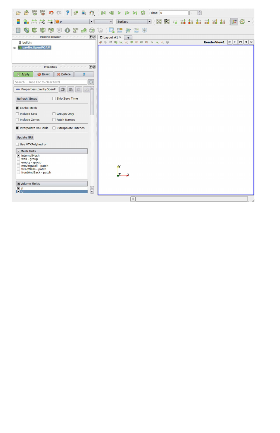
U-180 Post-processing

Figure 6.1: The paraFoam window

Pipeline Browser lists the modules opened in ParaView, where the selected modules are high-

lighted in blue and the graphics for the given module can be enabled/disabled by

clicking the eye button alongside;

Properties panel contains the input selections for the case, such as times, regions and ﬁelds;

it includes the Display panel that controls the visual representation of the selected

module, e.g. colours;

Other panels can be selected from the View menu, including the Information panel which

gives case statistics such as mesh geometry and size.

ParaView operates a tree-based structure in which data can be ﬁltered from the top-level

case module to create sets of sub-modules. For example, a contour plot of, say, pressure

could be a sub-module of the case module which contains all the pressure data. The strength

of ParaView is that the user can create a number of sub-modules and display whichever ones

they feel to create the desired image or animation. For example, they may add some solid

geometry, mesh and velocity vectors, to a contour plot of pressure, switching any of the

items on and oﬀ as necessary.

The general operation of the system is based on the user making a selection and then

clicking the green Apply button in the Properties panel. The additional buttons are: the

Reset button which can be used to reset the GUI if necessary; and, the Delete button that

will delete the active module.

OpenFOAM-6

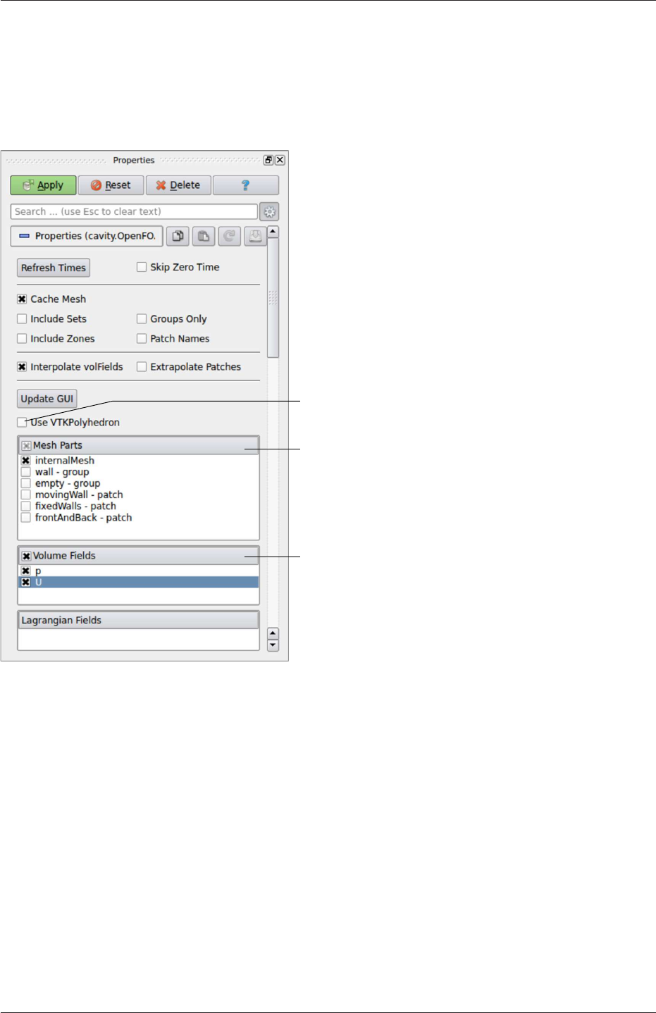
6.1 ParaView/paraFoam graphical user interface (GUI) U-181

6.1.2 The Parameters panel

The Properties window for the case module includes the Paramters panel that contains the

settings for mesh, ﬁelds and global controls. The controls are described in Figure 6.2. The

read into the case module

The user can select the ﬁelds

The user can select internalMesh

region and/or individual patches

Check this to enable ParaView to display

polyhedral cells and polygonal faces correctly

Figure 6.2: The Properties panel for the case module

user can select mesh and ﬁeld data which is loaded for all time directories into ParaView.

The buttons in the Current Time Controls and VCR Controls toolbars then select the

time data to be displayed, as shown is section 6.1.4.

As with any operation in paraFoam, the user must click Apply after making any changes

to any selections. The Apply button is highlighted in green to alert the user if changes have

been made but not accepted. This method of operation has the advantage of allowing the

user to make a number of selections before accepting them, which is particularly useful in

large cases where data processing is best kept to a minimum.

If new data is written to time directories while the user is running ParaView, the user

must load the additional time directories by checking the Refresh Times button. Where there

are occasions when the case data changes on ﬁle and ParaView needs to load the changes, the

user can also check the Update GUI button in the Parameters panel and apply the changes.

OpenFOAM-6

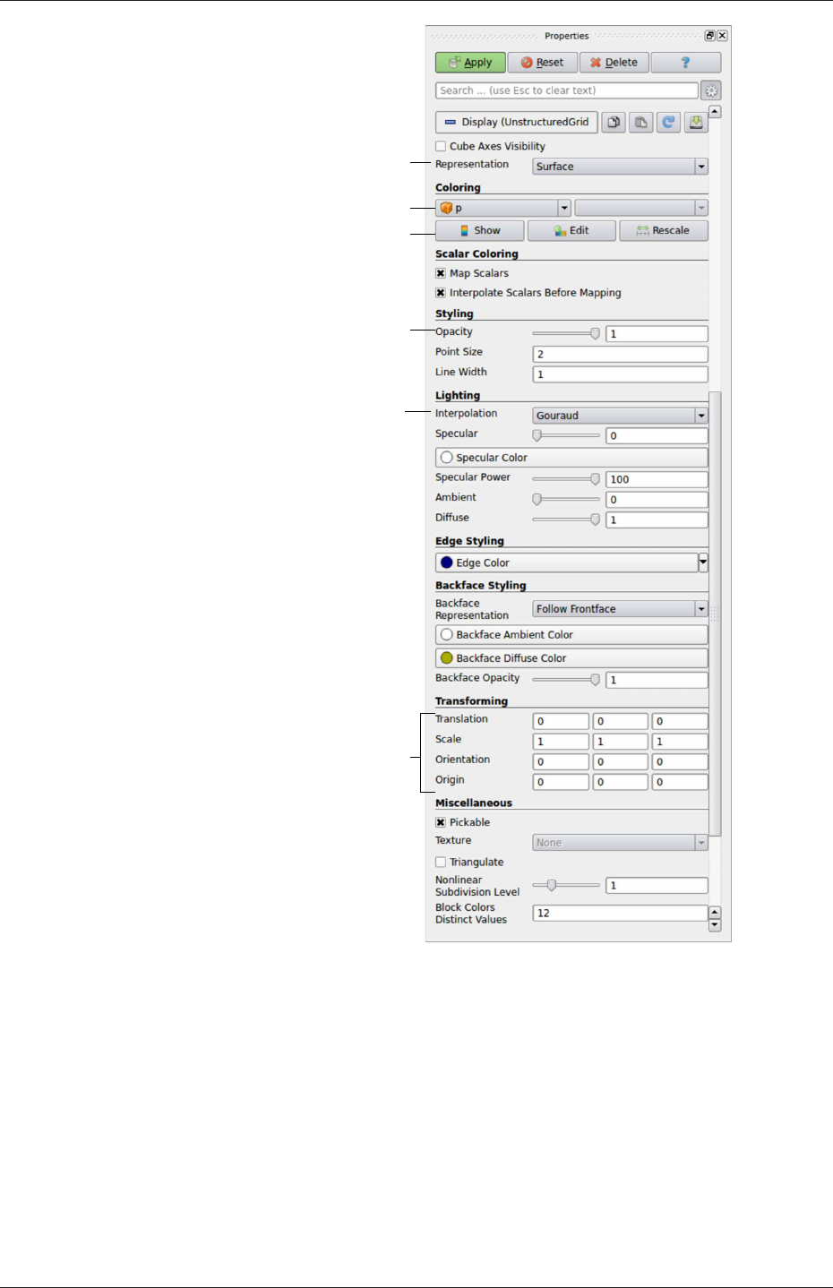
U-182 Post-processing

Change image opacity

e.g. to make transluscent

Set colour map range/appearance

Colour geometry/entity by. . .

Geometry manipulation tools

Data interpolation method

Outline, surface, wireframe or points

Figure 6.3: The Display panel

6.1.3 The Display panel

The Properties window contains the Display panel that includes the settings for visualising

the data for a given case module. The following points are particularly important:

•the data range may not be automatically updated to the max/min limits of a ﬁeld, so

the user should take care to select Rescale at appropriate intervals, in particular after

loading the initial case module;

•clicking the Edit Color Map button, brings up a window in which there are two panels:

OpenFOAM-6

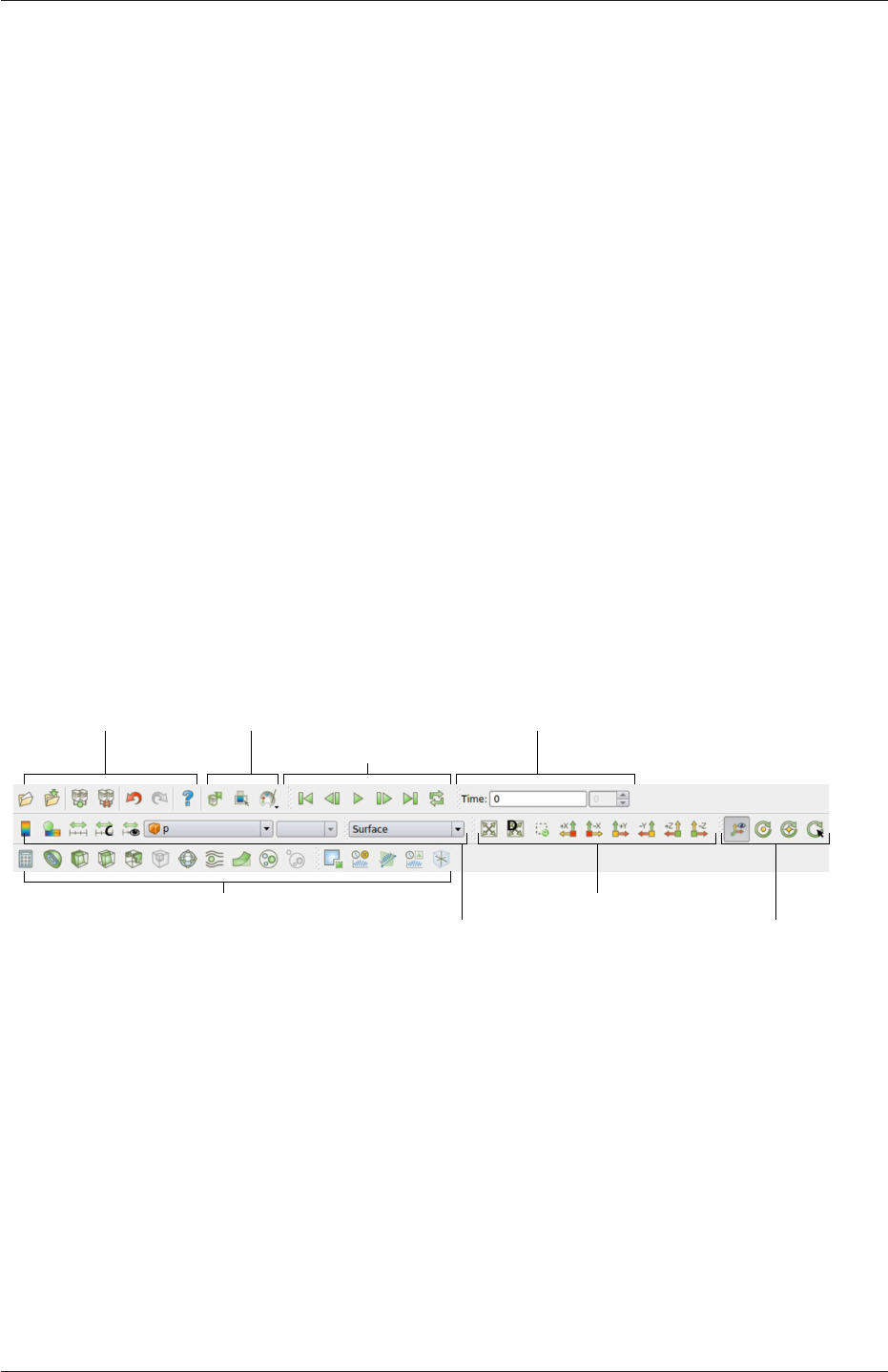
6.1 ParaView/paraFoam graphical user interface (GUI) U-183

1. The Color Scale panel in which the colours within the scale can be chosen. The

standard blue to red colour scale for CFD can be selected by clicking Choose

Preset and selecting Blue to Red Rainbox HSV.

2. The Color Legend panel has a toggle switch for a colour bar legend and contains

settings for the layout of the legend, e.g. font.

•the underlying mesh can be represented by selecting Wireframe in the Representat-

ion menu of the Style panel;

•the geometry, e.g. a mesh (if Wireframe is selected), can be visualised as a single

colour by selecting Solid Color from the Color By menu and specifying the colour

in the Set Ambient Color window;

•the image can be made translucent by editing the value in the Opacity text box (1 =

solid, 0 = invisible) in the Style panel.

6.1.4 The button toolbars

ParaView duplicates functionality from pull-down menus at the top of the main window

and the major panels, within the toolbars below the main pull-down menus. The displayed

toolbars can be selected from Toolbars in the main View menu. The default layout with

all toolbars is shown in Figure 6.4 with each toolbar labelled. The function of many of the

buttons is clear from their icon and, with tooltips enabled in the Help menu, the user is

given a concise description of the function of any button.

Undo/Redo Controls

Camera Controls

Centre Axes Controls

Main controls

VCR Controls

Current Time Controls

Common and Data Analysis Filters

Active Variable Controls |Representation

Figure 6.4: Toolbars in ParaView

6.1.5 Manipulating the view

This section describes operations for setting and manipulating the view of objects in paraFoam.

6.1.5.1 View settings

The View Settings are available in the Render View panel below the Display panel in the

Properties window. Settings that are generally important only appear when the user checks

the gearwheel button at the top of the Properties window, next to the search bar. These

advanced properties include setting the background colour, where white is often a preferred

choice for creating images for printed and website material.

OpenFOAM-6

U-184 Post-processing

The Lights button opens detailed lighting controls within the Light Kit panel. A separate

Headlight panel controls the direct lighting of the image. Checking the Headlight button with

white light colour of strength 1 seems to help produce images with strong bright colours,

e.g. with an isosurface.

The Camera Parallel Projection is is the usual choice for CFD, especially for 2D cases,

and so should generally be checked. Other settings include Cube Axes which displays axes

on the selected object to show the its orientation and geometric dimensions.

6.1.5.2 General settings

The general Settings are selected from the Edit menu, which opens a general Options

window with General,Colors,Animations,Charts and Render View menu items.

The General panel controls some default behaviour of ParaView. In particular, there is an

Auto Accept button that enables ParaView to accept changes automatically without clicking

the green Apply button in the Properties window. For larger cases, this option is generally

not recommended: the user does not generally want the image to be re-rendered between

each of a number of changes he/she selects, but be able to apply a number of changes to be

re-rendered in their entirety once.

The Render View panel contains 3 sub-items: General,Camera and Server. The General

panel includes the level of detail (LOD) which controls the rendering of the image while it

is being manipulated, e.g. translated, resized, rotated; lowering the levels set by the sliders,

allows cases with large numbers of cells to be re-rendered quickly during manipulation.

The Camera panel includes control settings for 3D and 2D movements. This presents the

user with a map of rotation, translate and zoom controls using the mouse in combination

with Shift- and Control-keys. The map can be edited to suit by the user.

6.1.6 Contour plots

A contour plot is created by selecting Contour from the Filter menu at the top menu

bar. The ﬁlter acts on a given module so that, if the module is the 3D case module itself,

the contours will be a set of 2D surfaces that represent a constant value, i.e. isosurfaces.

The Properties panel for contours contains an Isosurfaces list that the user can edit, most

conveniently by the New Range window. The chosen scalar ﬁeld is selected from a pull down

menu.

6.1.6.1 Introducing a cutting plane

Very often a user will wish to create a contour plot across a plane rather than producing

isosurfaces. To do so, the user must ﬁrst use the Slice ﬁlter to create the cutting plane,

on which the contours can be plotted. The Slice ﬁlter allows the user to specify a cutting

Plane,Box or Sphere in the Slice Type menu by a center and normal/radius respectively.

The user can manipulate the cutting plane like any other using the mouse.

The user can then run the Contour ﬁlter on the cut plane to generate contour lines.

6.1.7 Vector plots

Vector plots are created using the Glyph ﬁlter. The ﬁlter reads the ﬁeld selected in Vectors

and oﬀers a range of Glyph Types for which the Arrow provides a clear vector plot images.

OpenFOAM-6

6.1 ParaView/paraFoam graphical user interface (GUI) U-185

Each glyph has a selection of graphical controls in a panel which the user can manipulate

to best eﬀect.

The remainder of the Properties panel contains mainly the Scale Mode menu for the

glyphs. The most common options are Scale Mode are: Vector, where the glyph length is

proportional to the vector magnitude; and, Off where each glyph is the same length. The

Set Scale Factor parameter controls the base length of the glyphs.

6.1.7.1 Plotting at cell centres

Vectors are by default plotted on cell vertices but, very often, we wish to plot data at cell

centres. This is done by ﬁrst applying the Cell Centers ﬁlter to the case module, and then

applying the Glyph ﬁlter to the resulting cell centre data.

6.1.8 Streamlines

Streamlines are created by ﬁrst creating tracer lines using the Stream Tracer ﬁlter. The

tracer Seed panel speciﬁes a distribution of tracer points over a Line Source or Point

Cloud. The user can view the tracer source, e.g. the line, but it is displayed in white, so

they may need to change the background colour in order to see it.

The distance the tracer travels and the length of steps the tracer takes are speciﬁed in

the text boxes in the main Stream Tracer panel. The process of achieving desired tracer lines

is largely one of trial and error in which the tracer lines obviously appear smoother as the

step length is reduced but with the penalty of a longer calculation time.

Once the tracer lines have been created, the Tubes ﬁlter can be applied to the Tracer

module to produce high quality images. The tubes follow each tracer line and are not

strictly cylindrical but have a ﬁxed number of sides and given radius. When the number of

sides is set above, say, 10, the tubes do however appear cylindrical, but again this adds a

computational cost.

6.1.9 Image output

The simplest way to output an image to ﬁle from ParaView is to select Save Screenshot

from the File menu. On selection, a window appears in which the user can select the

resolution for the image to save. There is a button that, when clicked, locks the aspect

ratio, so if the user changes the resolution in one direction, the resolution is adjusted in the

other direction automatically. After selecting the pixel resolution, the image can be saved.

To achieve high quality output, the user might try setting the pixel resolution to 1000 or

more in the x-direction so that when the image is scaled to a typical size of a ﬁgure in an

A4 or US letter document, perhaps in a PDF document, the resolution is sharp.

6.1.10 Animation output

To create an animation, the user should ﬁrst select Save Animation from the File menu.

A dialogue window appears in which the user can specify a number of things including the

image resolution. The user should specify the resolution as required. The other noteworthy

setting is number of frames per timestep. While this would intuitively be set to 1, it can

be set to a larger number in order to introduce more frames into the animation artiﬁcially.

OpenFOAM-6

U-186 Post-processing

This technique can be particularly useful to produce a slower animation because some movie

players have limited speed control, particularly over mpeg movies.

On clicking the Save Animation button, another window appears in which the user spec-

iﬁes a ﬁle name root and ﬁle format for a set of images. On clicking OK, the set of ﬁles will

be saved according to the naming convention “<fileRoot>_<imageNo>.<fileExt>”, e.g.

the third image of a series with the ﬁle root “animation”, saved in jpg format would be

named “animation_0002.jpg” (<imageNo>starts at 0000).

Once the set of images are saved the user can convert them into a movie using their soft-

ware of choice. One option is to use the built in foamCreateVideo script from the command

line whose usage is shown with the -help option.

6.2 Post-processing command line interface (CLI)

In OpenFOAM version 4.0, the ‘non-GUI’ post-processing tools have been uniﬁed within

a single command line interface (CLI). Post-processing functionality includes data process-

ing, sampling (e.g. probes, graph plotting) visualisation, case control and run-time I/O.

Functionality can be executed by:

•conventional post-processing, a data processing activity that occurs after a simulation

has run;

•run-time processing, data processing that is performed during the running of a simu-

lation.

Both approaches have advantages. Conventional post-processing allows the user to choose

how to analyse data after the results are obtained. Run-time processing oﬀers greater

ﬂexibility because it has access to all the data in the database of the run at all times,

rather than just the data written during the simulation. It also allows the user to monitor

processed data during a simulation and provides a greater level of convenience because the

processed results can be available immediately to the user when the simulation ends.

There are 3 methods of post-processing that cover the options described above

•Every solver, e.g. simpleFoam can be conﬁgured to include run-time processing.

•The postProcess utility provides conventional post-processing of data written by a

simulation.

•Every solver can be run with the -postProcess option, which only executes post-

processing, but with additional access to data available on the database for the par-

ticular solver.

6.2.1 Post-processing functionality

All modes of post-processing access the same functionality implemented in OpenFOAM in

the function object framework. Function objects can be listed by running a solver with the

-listFunctionObjects option, e.g.

simpleFoam -listFunctionObjects

OpenFOAM-6

6.2 Post-processing command line interface (CLI) U-187

The list represents the underlying post-processing functionality. Almost all the functionality

is packaged into a set of conﬁgured tools that are conveniently integrated within the post-

processing CLI. Those tools are located in $FOAM_ETC/caseDicts/postProcessing and are

listed by running postProcess with the -list option.

postProcess -list

This produces a list of tools that are described in the following sections.

6.2.1.1 Field calculation

CourantNo Calculates the Courant Number ﬁeld from the ﬂux ﬁeld.

Lambda2 Calculates and writes the second largest eigenvalue of the sum of the square of

the symmetrical and anti-symmetrical parts of the velocity gradient tensor.

MachNo Calculates the Mach Number ﬁeld from the velocity ﬁeld.

PecletNo Calculates the Peclet Number ﬁeld from the ﬂux ﬁeld.

QCalculates the second invariant of the velocity gradient tensor.

RCalculates the Reynolds stress tensor ﬁeld and stores it on the database.

XiReactionRate Writes the turbulent ﬂame-speed and reaction-rate volScalarFields for

the Xi-based combustion models.

add Add a list of ﬁelds.

components Writes the component scalar ﬁelds (e.g. Ux, Uy, Uz) of a ﬁeld (e.g. U).

ddt Calculates the Eulerian time derivative of a ﬁeld.

div Calculates the divergence of a ﬁeld.

enstrophy Calculates the enstrophy of the velocity ﬁeld.

ﬂowType Calculates and writes the flowType of velocity ﬁeld where: -1 = rotational ﬂow;

0 = simple shear ﬂow; +1 = planar extensional ﬂow.

grad Calculates the gradient of a ﬁeld.

mag Calculates the magnitude of a ﬁeld.

magSqr Calculates the magnitude-squared of a ﬁeld.

randomise Adds a random component to a ﬁeld, with a speciﬁed perturbation magnitude.

scale Multiplies a ﬁeld by a scale factor

streamFunction Writes the steam-function pointScalarField, calculated from the speciﬁed

ﬂux surfaceScalarField.

subtract From the ﬁrst ﬁeld, subtracts the remaining ﬁelds in the list.

OpenFOAM-6

U-188 Post-processing

turbulenceFields Calculates speciﬁed turbulence ﬁelds and stores it on the database.

turbulenceIntensity Calculates and writes the turbulence intensity ﬁeld I.

vorticity Calculates the vorticity ﬁeld, i.e. the curl of the velocity ﬁeld.

wallHeatFlux Calculates the heat ﬂux at wall patches, outputting the data as a volVector-

Field.

wallHeatTransferCoeﬀ Calculates the estimated incompressible ﬂow heat transfer coeﬃcient

at wall patches, outputting the data as a volScalarField.

wallShearStress Calculates the shear stress at wall patches, outputting the data as a vol-

VectorField.

writeCellCentres Writes the cell-centres volVectorField and the three component ﬁelds as

volScalarFields; useful for post-processing thresholding.

writeCellVolumes Writes the cell-volumes volScalarField

writeObjects Writes out speciﬁed objects, e.g. ﬁelds, stored on the case database.

yPlus Calculates the turbulence y+, outputting the data as a yPlus ﬁeld.

6.2.1.2 Flow rate calculation

ﬂowRateFaceZone Calculates the ﬂow rate through a speciﬁed face zone by summing the ﬂux

on patch faces. For solvers where the ﬂux is volumetric, the ﬂow rate is volumetric;

where ﬂux is mass ﬂux, the ﬂow rate is mass ﬂow rate.

ﬂowRatePatch Calculates the ﬂow rate through a speciﬁed patch by summing the ﬂux on

patch faces. For solvers where the ﬂux is volumetric, the ﬂow rate is volumetric; where

ﬂux is mass ﬂux, the ﬂow rate is mass ﬂow rate.

volFlowRateSurface Calculates volumetric ﬂow rate through a speciﬁed triangulated surface

by interpolating velocity onto the triangles and integrating over the surface area.

Triangles need to be small (<= cell size) for an accurate result.

6.2.1.3 Forces and force coeﬃcients

forceCoeﬀsCompressible Calculates lift, drag and moment coeﬃcients by summing forces

on speciﬁed patches for a case where the solver is compressible (pressure is in units

M/(LTˆ2), e.g. Pa).

forceCoeﬀsIncompressible Calculates lift, drag and moment coeﬃcients by summing forces on

speciﬁed patches for a case where the solver is incompressible (pressure is kinematic,

e.g. mˆ2/sˆ2).

forcesCompressible Calculates pressure and viscous forces over speciﬁed patches for a case

where the solver is compressible (pressure is in units M/(LTˆ2), e.g. Pa).

forcesIncompressible Calculates pressure and viscous forces over speciﬁed patches for a case

where the solver is incompressible (pressure is kinematic, e.g. mˆ2/sˆ2).

OpenFOAM-6

6.2 Post-processing command line interface (CLI) U-189

6.2.1.4 Sampling for graph plotting

singleGraph Writes graph data for speciﬁed ﬁelds along a line, speciﬁed by start and end

points.

6.2.1.5 Lagrangian data

dsmcFields Calculate intensive ﬁelds UMean,translationalT,internalT,overallT from

averaged extensive ﬁelds from a DSMC calculation.

6.2.1.6 Monitoring minima and maxima

cellMax Writes out the maximum cell value for one or more ﬁelds.

cellMin Writes out the minimum cell value for one or more ﬁelds.

faceMax Writes out the maximum face value for one or more ﬁelds.

faceMin Writes out the minimum face value for one or more ﬁelds.

minMaxComponents Writes out the minimum and maximum values, by component for non-

scalar ﬁelds, and the locations where they occur.

minMaxMagnitude Writes out the minimum and maximum values, by magnitude for non-

scalar ﬁelds, and the locations where they occur.

6.2.1.7 Numerical data

residuals For speciﬁed ﬁelds, writes out the initial residuals for the ﬁrst solution of each

time step; for non-scalar ﬁelds (e.g. vectors), writes the largest of the residuals for

each component (e.g. x, y, z).

time Writes run time, CPU time and clock time and optionally the CPU and clock times

per time step.

6.2.1.8 Pressure tools

pressureDiﬀerencePatch Calculates the diﬀerence between the average pressures on 2 speci-

ﬁed patches.

pressureDiﬀerenceSurface Interpolates pressures onto 2 speciﬁed triangulated surfaces and

calculates the diﬀerence between the average pressures.

staticPressure Calculates the pressure ﬁeld in units M/(LTˆ2) (e.g. Pa) from kinematic

pressure by scaling by a speciﬁed density.

totalPressureCompressible Calculates the total pressure ﬁeld for a case where the solver is

compressible (pressure is in units M/(LTˆ2), e.g. Pa).

totalPressureIncompressible Calculates the total pressure ﬁeld for a case where the solver is

incompressible (pressure is kinematic, e.g. mˆ2/sˆ2).

OpenFOAM-6

U-190 Post-processing

6.2.1.9 Probes

boundaryCloud Writes out values of ﬁelds at a cloud of points, interpolated to speciﬁed

boundary patches.

interfaceHeight Reports the height of the interface above a set of locations. For each location,

it writes the vertical distance of the interface above both the location and the lowest

boundary. It also writes the point on the interface from which these heights are

computed.

internalCloud Writes out values of ﬁelds interpolated to a speciﬁed cloud of points.

probes Writes out values of ﬁelds from cells nearest to speciﬁed locations.

6.2.1.10 ‘Pluggable’ solvers

icoUncoupledKinematicCloud Tracks a cloud of parcels driven by the ﬂow of the continuous

phase.

scalarTransport Solves a transport equation for a scalar ﬁeld.

6.2.1.11 Visualisation tools

streamlines Writes out ﬁles of streamlines with interpolated ﬁeld data in VTK format.

surfaces Writes out surface ﬁles with interpolated ﬁeld data in VTK format, e.g. cutting

planes, iso-surfaces and patch boundary surfaces.

6.2.2 Run-time data processing

When a user wishes to process data during a simulation, they need to conﬁgure the case

accordingly. The conﬁguration process is as follows, using an example of monitoring ﬂow

rate at an outlet patch named outlet.

Firstly, the user should include the ﬂowRatePatch function in functions sub-dictionary

in the case controlDict ﬁle, using the #includeFunc directive.

functions

{

#includeFunc flowRatePatch

... other function objects here ...

}

That will include the functionality in the ﬂowRatePatch conﬁguration ﬁle, located in the

directory hierarchy beginning with $FOAM_ETC/caseDicts/postProcessing.

The conﬁguration of ﬂowRatePatch requires the name of the patch to be supplied. Op-

tion 1 for doing this is that the user copies the ﬂowRatePatch ﬁle into their case system

directory. The foamGet script copies the ﬁle conveniently, e.g.

foamGet flowRatePatch

OpenFOAM-6

6.2 Post-processing command line interface (CLI) U-191

The patch name can be edited in the copied ﬁle to be outlet. When the solver is run,

it will pick up an included function in the local case system directory, in precedence over

$FOAM_ETC/caseDicts/postProcessing. The ﬂow rate through the patch will be calculated

and written out into a ﬁle within a directory named postProcessing.

Option 2 for specifying the patch name is to provide the name as an argument to the

ﬂowRatePatch in the #includeFunc directive, using the syntax keyword=entry.

functions

{

#includeFunc flowRatePatch(name=outlet)

... other function objects here ...

}

In the case where the keyword is field or fields, only the entry is needed when

specifying an argument to a function. For example, if the user wanted to calculate and

write out the magnitude of velocity into time directories during a simulation they could

simply add the following to the functions sub-dictionary in controlDict.

functions

{

#includeFunc mag(U)

... other function objects here ...

}

This works because the function’s argument Uis represented by the keyword field, see

$FOAM_ETC/caseDicts/postProcessing/ﬁelds/mag.

Some functions require the setting of many parameters, e.g. forces,forceCoeﬀs,surfaces,

etc. For those functions, it is more reliable and convenient to copy and conﬁgure the function

using option 1 (above) rather than through arguments.

6.2.3 The postProcess utility

The user can execute post-processing functions after the simulation is complete using the

postProcess utility. Let us illustrate the use of postProcess using the pitzDaily case from the

tutorials directory. The case can be copied, e.g. into the user’s run directory; the user can

then go into the case directory, generate the mesh with blockMesh and then run simpleFoam

run

cp -r $FOAM_TUTORIALS/incompressible/simpleFoam/pitzDaily .

cd pitzDaily

blockMesh

simpleFoam

Now the user can run execute post-processing functions with postProcess. The -help option

provides a summary of its use.

postProcess -help

OpenFOAM-6

U-192 Post-processing

Simple functions like mag can be executed using the -func option; text on the command

line generally needs to be quoted ("...") if it contains punctuation characters.

postProcess -func "mag(U)"

This operation calculates and writes the ﬁeld of magnitude of velocity into a ﬁle named

mag(U) in each time directory. Similarly, the ﬂowRatePatch example can be executed using

postProcess.

postProcess -func "flowRatePatch(name=outlet)"

Let us say the user now wants to calculate total pressure =p+|U|2/2for incompressible

ﬂow with kinematic pressure, p. The function is available, named totalPressureIncompressible,

which the user could attempt ﬁrst to run as follows.

postProcess -func totalPressureIncompressible

This returns the following error message.

--> FOAM Warning : functionObject pressure: Cannot find required field p

The error message is telling the user that the pressure ﬁeld pis not loaded; the same is

true of the velocity ﬁeld U. For the function to work, both ﬁelds can be loaded as comma

separated arguments.

postProcess -func "totalPressureIncompressible(p,U)"

Alternatively the user can load a space separated list of ﬁelds using the -fields option,

which the function can access.

postProcess -fields "(p U)" -func totalPressureIncompressible

Both options work eﬀectively because the pressure and velocity data is available directly

from the ﬁles, pand U.

6.2.4 Solver post-processing

A more complex example is calculating wall shear stress using the wallShearStress function.

postProcess -fields "(p U)" -func wallShearStress

Even loading relevant ﬁelds, the post-processing fails with the following message.

--> FOAM FATAL ERROR:

Unable to find turbulence model in the database

OpenFOAM-6

6.3 Sampling and monitoring data U-193

The message is telling us that the postProcess utility has not constructed the necessary

models that the solver, simpleFoam, used when running the simulation, i.e. a turbulence

model. This is a situation where we need to post-process (as opposed to run-time process)

using the solver with the -postProcess option so that the modelling will be available that

the post-processing function needs. Help for this operation can be printed with the following

command.

simpleFoam -postProcess -help

It can be seen that the options for a solver with -postProcess are the same as when

running postProcess utility. This means that the -func option can be used to execute the

wallShearStress function eﬀectively.

simpleFoam -postProcess -func wallShearStress

Note that no ﬁelds need to be supplied, either by function arguments "(p,U)" or using

"-fields (p U)", because simpleFoam itself constructs and stores the required ﬁelds. Func-

tions can also be selected by the #includeFunc directive in functions in the controlDict

ﬁle, instead of the -func option.

6.3 Sampling and monitoring data

There are a set of general post-processing functions for sampling data across the domain for

graphs and visualisation. Several functions also provide data in a single ﬁle, in the form of

time versus values, that can be plotted onto graphs. This time-value data can be monitored

during a simulation with the foamMonitor script.

6.3.1 Probing data

The functions for probing data are boundaryCloud,internalCloud and probes as listed in

section 6.2.1.9. All functions work on the basis that the user provides some point locations

and a list of ﬁelds, and the function writes out values of the ﬁelds are those locations. The

diﬀerences between the cloud and probe functionality are as follows.

•probes identiﬁes the nearest cells to the probe locations and writes out the cell values;

data is written into a single ﬁle in time-value format, suitable for plotting a graph.

•boundaryCloud and internalCloud interpolate ﬁeld data to the probe locations, with the

locations being snapped onto boundaries for boundaryCloud; data sets are written to

separate ﬁles at scheduled write times (like ﬁelds). data.

Generally probes is more suitable for monitoring values at smaller numbers of locations,

whereas the cloud functions are typically for sampling at large numbers of locations.

As an example, the user could use the pitzDaily case set up in section 6.2.3. The probes

function is best conﬁgured by copying the ﬁle to the local system directory using foamGet.

foamGet probes

OpenFOAM-6

U-194 Post-processing

The user can modify the probeLocations in the probes ﬁle as follows.

13 #includeEtc "caseDicts/postProcessing/probes/probes.cfg"

15 fields (p U);

16 probeLocations

17 (

18 (0.01 0 0)

19 );

21 // ************************************************************************* //

The conﬁguration is completed by adding the #includeFunc directive to functions in the

the controlDict ﬁle.

functions

{

#includeFunc probes

... other function objects here ...

}

When simpleFoam is run, time-value data is written into pand Uﬁles in postProcessing/pro-

bes/0.

6.3.2 Sampling for graphs

The singleGraph function samples data for graph plotting. To use it, the singleGraph ﬁle

should be copied into the system directory to be conﬁgured. We will conﬁgure it here using

the pitzDaily case as before. The ﬁle is simply copied using foamGet.

foamGet singleGraph

The start and end points of the line, along which data is sampled, should be edited; the

entries below provide a vertical line across the full height of the geometry 0.01 m beyond

the back step.

14 start (0.01 0.025 0);

15 end (0.01 -0.025 0);

16 fields (U p);

18 // Sampling and I/O settings

19 #includeEtc "caseDicts/postProcessing/graphs/sampleDict.cfg"

21 // Override settings here, e.g.

22 // setConfig { type midPoint; }

24 // Must be last entry

25 #includeEtc "caseDicts/postProcessing/graphs/graph.cfg"

27 // ************************************************************************* //

The conﬁguration is completed by adding the #includeFunc directive to functions in the

the controlDict ﬁle.

functions

{

#includeFunc singleGraph

... other function objects here ...

}

OpenFOAM-6

6.3 Sampling and monitoring data U-195

simpleFoam can be then run; try running simply with the -postProcess option. Distance-

value data is written into ﬁles in time directories within postProcessing/singleGraph. The

user can quickly display the data for x-component of velocity, Uxin the last time 296, by

running gnuplot and plotting values.

gnuplot

gnuplot> set style data linespoints

gnuplot> plot "postProcessing/singleGraph/296/line_U.xy" u 2:1

This produces the graph shown in Figure 6.5. The formatting of the graph is speciﬁed in

Figure 6.5: Graph of Uxat x= 0.01, uniform sampling

conﬁguration ﬁles in $FOAM_ETC/caseDicts/postProcessing/graphs. The sampleDict.cfg ﬁle

in that directory contains a setConfig sub-dictionary as shown below.

9interpolationScheme cellPoint;

11 setFormat raw;

13 setConfig

14 {

15 type lineUniform; // lineCell, lineCellFace

16 axis distance; // x, y, z, xyz

17 nPoints 100;

18 }

20 // ************************************************************************* //

This shows that the sampling is at uniform distribution of 100 points and that the axis

labelling is based on the distance from the start point. Instead the user may wish to

sample at the mid-point of each cell, using the y-ordinate for the axis labelling. This can

be done by override the settings in setConfig in their singleGraph ﬁle, as shown below.

14 start (0.01 -0.025 0);

15 end (0.01 0.025 0);

16 fields (U p);

18 // Sampling and I/O settings

19 #includeEtc "caseDicts/postProcessing/graphs/sampleDict.cfg"

21 // Override settings here, e.g.

22 setConfig

OpenFOAM-6

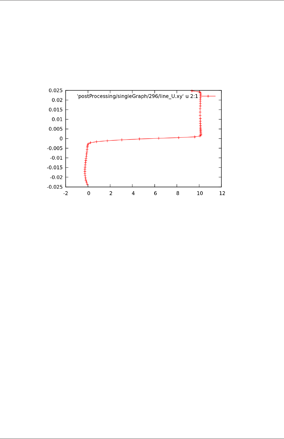
U-196 Post-processing

23 {

24 type lineCell;

25 axis y;

26 }

28 // Must be last entry

29 #includeEtc "caseDicts/postProcessing/graphs/graph.cfg"

31 // ************************************************************************* //

Running simpleFoam produces the graph in Figure 6.6.

Figure 6.6: Graph of Uxat x= 0.01, mid-point sampling

6.3.3 Sampling for visualisation

The surfaces and streamlines functions can be used to generate ﬁles for visualisation. The use

of streamlines is already conﬁgured in the pitzDaily case. The surfaces function is conﬁgured

by copying the surfaces ﬁle to the system directory using foamGet.

foamGet surfaces

The ﬁle is conﬁgured with a set of example surfaces that includes cutting planes, isosurfaces

and patch surfaces. We can edit the ﬁle to produce a cutting plane along the pitzDaily

geometry, normal to the z-direction.

17 #includeEtc "caseDicts/postProcessing/visualization/surfaces.cfg"

19 fields (p U);

21 surfaces

22 (

23 zNormal

24 {

25 $cuttingPlane;

26 pointAndNormalDict

27 {

28 normalVector $z;

29 }

30 }

31 );

33 // ************************************************************************* //

OpenFOAM-6

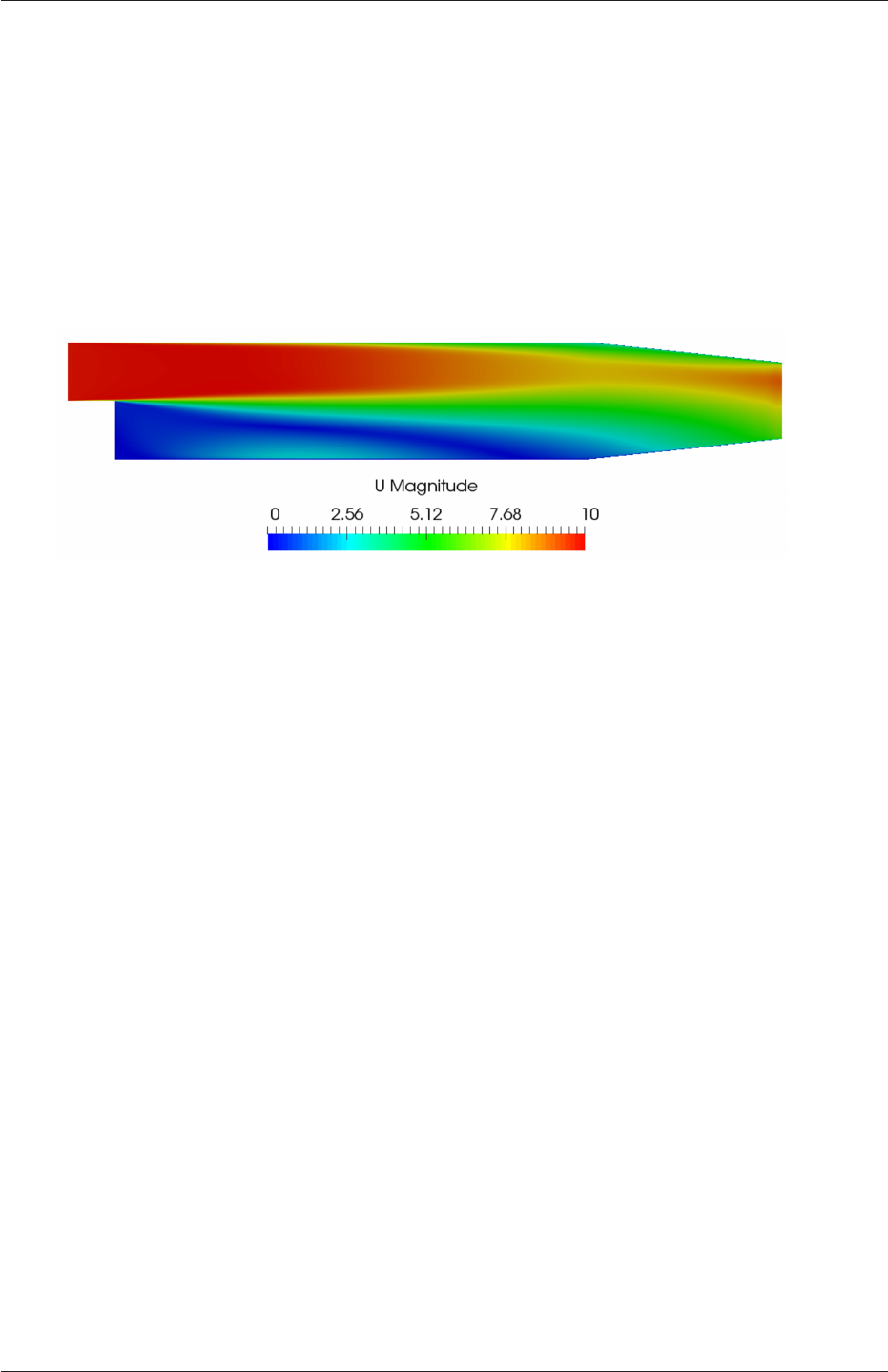
6.3 Sampling and monitoring data U-197

The function can be included as normal from the by adding the #includeFunc directive to

functions in the the controlDict ﬁle. Alternatively, the user could test running the function

using the solver post-processing by the following command.

simpleFoam -postProcess -func surfaces

This produces VTK format ﬁles of the cutting plane with pressure and velocity data in time

directories in the the postProcessing/surfaces directory. The user can display the cutting

plane by opening ParaView (type paraview), then doing File->Open and selecting one of

the ﬁles, e.g. postProcessing/surfaces/296/U_zNormal.vtk as shown in Figure 6.7.

Figure 6.7: Cutting plane with velocity

6.3.4 Live monitoring of data

Functions like probes produce a singe ﬁle of time-value data, suitable for graph plotting.

When the function is executed during a simulation, the user may wish to monitor the data

live on screen. The foamMonitor script enables this; to discover its functionality, the user

run it with the -help option. The help option includes an example of monitoring residuals

that we can demonstrate in this section.

Firstly, include the residuals function in the controlDict ﬁle.

functions

{

#includeFunc residuals

... other function objects here ...

}

The default ﬁelds whose residuals are captured are pand U. Should the user wish to conﬁgure

other ﬁelds, they should make copy the residuals ﬁle in their system and edit the fields

entry accordingly. All functions ﬁles are within the $FOAM_ETC/caseDicts directory. The

residuals ﬁle can be located using foamInfo:

foamInfo residuals

It can then be copied into the system directory conveniently using foamGet:

foamGet residuals

OpenFOAM-6

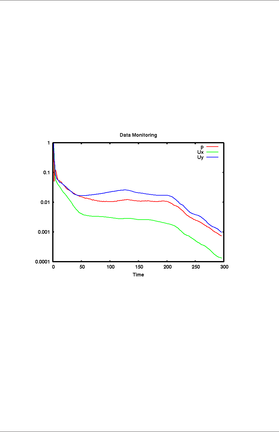
U-198 Post-processing

It is advisable to delete the postProcessing directory to avoid duplicate ﬁles for each

function. The user can delete the directory, then run simpleFoam in the background.

rm -rf postProcessing

simpleFoam > log &

The user should then run foamMonitor using the -l option for a log scale y-axis on the

residuals ﬁle as follows. If the command is executed before the simulation is complete, they

can see the graph being updated live.

foamMonitor -l postProcessing/residuals/0/residuals.dat

It produces the graph of residuals for pressure and velocity in Figure 6.8.

Figure 6.8: Live plot of residuals with foamMonitor

6.4 Third-Party post-processing

OpenFOAM includes the following applications for converting data to formats for post-

processing with several third-party tools. For EnSight, it additionally includes a reader

module, described in the next section.

foamDataToFluent Translates OpenFOAM data to Fluent format.

foamToEnsight Translates OpenFOAM data to EnSight format.

foamToEnsightParts Translates OpenFOAM data to Ensight format. An Ensight part is

created for each cellZone and patch.

foamToGMV Translates foam output to GMV readable ﬁles.

OpenFOAM-6

6.4 Third-Party post-processing U-199

foamToTecplot360 Tecplot binary ﬁle format writer.

foamToTetDualMesh Converts polyMesh results to tetDualMesh.

foamToVTK Legacy VTK ﬁle format writer.

smapToFoam Translates a STAR-CD SMAP data ﬁle into OpenFOAM ﬁeld format.

6.4.1 Post-processing with Ensight

OpenFOAM oﬀers the capability for post-processing OpenFOAM cases with EnSight, with

a choice of 2 options:

•converting the OpenFOAM data to EnSight format with the foamToEnsight utility;

•reading the OpenFOAM data directly into EnSight using the ensight74FoamExec mod-

ule.

6.4.1.1 Converting data to Ensight format

The foamToEnsight utility converts data from OpenFOAM to EnSight ﬁle format. For a

given case, foamToEnsight is executed like any normal application. foamToEnsight creates a

directory named Ensight in the case directory, deleting any existing Ensight directory in the

process. The converter reads the data in all time directories and writes into a case ﬁle and

a set of data ﬁles. The case ﬁle is named EnSight_Case and contains details of the data ﬁle

names. Each data ﬁle has a name of the form EnSight_nn.ext, where nn is an incremental

counter starting from 1 for the ﬁrst time directory, 2 for the second and so on and ext is a

ﬁle extension of the name of the ﬁeld that the data refers to, as described in the case ﬁle,

e.g.Tfor temperature, mesh for the mesh. Once converted, the data can be read into EnSight

by the normal means:

1. from the EnSight GUI, the user should select Data (Reader) from the File menu;

2. the appropriate EnSight_Case ﬁle should be highlighted in the Files box;

3. the Format selector should be set to Case, the EnSight default setting;

4. the user should click (Set) Case and Okay.

6.4.1.2 The ensightFoamReader reader module

EnSight provides the capability of using a user-deﬁned module to read data from a format

other than the standard EnSight format. OpenFOAM includes its own reader module en-

sightFoamReader that is compiled into a library named libuserd-foam. It is this library that

EnSight needs to use which means that it must be able to locate it on the ﬁling system as

described in the following section.

In order to run the EnSight reader, it is necessary to set some environment variables cor-

rectly. The settings are made in the bashrc (or cshrc) ﬁle in the $WM_PROJECT_DIR/etc/-

apps/ensightFoam directory. The environment variables associated with EnSight are preﬁxed

by $CEI_ or $ENSIGHT7_ and listed in Table 6.1. With a standard user setup, only

$CEI_HOME may need to be set manually, to the path of the EnSight installation.

OpenFOAM-6

U-200 Post-processing

Environment variable Description and options

$CEI_HOME Path where EnSight is installed, eg /usr/local/ensight, added

to the system path by default

$CEI_ARCH Machine architecture, from a choice of names cor-

responding to the machine directory names in

$CEI_HOME/ensight74/machines; default settings include

linux_2.4 and sgi_6.5_n32

$ENSIGHT7_READER Path that EnSight searches for the user deﬁned libuserd-foam

reader library, set by default to $FOAM_LIBBIN

$ENSIGHT7_INPUT Set by default to dummy

Table 6.1: Environment variable settings for EnSight.

The principal diﬃculty in using the EnSight reader lies in the fact that EnSight expects

that a case to be deﬁned by the contents of a particular ﬁle, rather than a directory as it is

in OpenFOAM. Therefore in following the instructions for the using the reader below, the

user should pay particular attention to the details of case selection, since EnSight does not

permit selection of a directory name.

1. from the EnSight GUI, the user should select Data (Reader) from the File menu;

2. The user should now be able to select the OpenFOAM from the Format menu; if not,

there is a problem with the conﬁguration described above.

3. The user should ﬁnd their case directory from the File Selection window, highlight one

of top 2 entries in the Directories box ending in /. or /.. and click (Set) Geometry.

4. The path ﬁeld should now contain an entry for the case. The (Set) Geometry text box

should contain a ‘/’.

5. The user may now click Okay and EnSight will begin reading the data.

6. When the data is read, a new Data Part Loader window will appear, asking which

part(s) are to be read. The user should select Load all.

7. When the mesh is displayed in the EnSight window the user should close the Data Part

Loader window, since some features of EnSight will not work with this window open.

OpenFOAM-6

Chapter 7

Models and physical properties

OpenFOAM includes a large range of solvers each designed for a speciﬁc class of problem.

The equations and algorithms diﬀer from one solver to another so that the selection of a

solver involves the user making some initial choices on the modelling for their particular case.

The choice of solver typically involves scanning through their descriptions in section 3.5 to

ﬁnd the one suitable for the case. It ultimately determines many of the parameters and

physical properties required to deﬁne the case but leaves the user with some modelling

options that can be speciﬁed at runtime through the entries in dictionary ﬁles in the constant

directory of a case. This chapter deals with many of the more common models and associated

properties that must be speciﬁed at runtime.

7.1 Thermophysical models

Thermophysical models are concerned with energy, heat and physical properties. The ther-

mophysicalProperties dictionary is read by any solver that uses the thermophysical model

library. A thermophysical model is constructed in OpenFOAM as a pressure-temperature

p−Tsystem from which other properties are computed. There is one compulsory dictio-

nary entry called thermoType which speciﬁes the package of thermophysical modelling that

is used in the simulation. OpenFOAM includes a large set of pre-compiled combinations

of modelling, built within the code using C++ templates. This coding approach assembles

thermophysical modelling packages beginning with the equation of state and then adding

more layers of thermophysical modelling that derive properties from the previous layer(s).

The keyword entries in thermoType reﬂects the multiple layers of modelling and the under-

lying framework in which they combined. Below is an example entry for thermoType:

thermoType

{

type hePsiThermo;

mixture pureMixture;

transport const;

thermo hConst;

equationOfState perfectGas;

specie specie;

energy sensibleEnthalpy;

}

U-202 Models and physical properties

The keyword entries specify the choice of thermophysical models, e.g. constant transport

(constant viscosity, thermal diﬀusion), Perfect Gas equationOfState,etc. In addition there

is a keyword entry named energy that allows the user to specify the form of energy to be

used in the solution and thermodynamics. The following sections explains the entries and

options in the thermoType package.

7.1.1 Thermophysical and mixture models

Each solver that uses thermophysical modelling constructs an object of a speciﬁc thermo-

physical model class. The model classes are listed below.

psiThermo Thermophysical model for ﬁxed composition, based on compressibility ψ=

(RT )−1, where Ris Gas Constant and Tis temperature. The solvers that construct

psiThermo include the compressible family of solvers (sonicFoam,simpleFoam,etc.,

excluding rhoPorousSimpleFoam) and uncoupledKinematicParcelFoam and coldEngine-

Foam.

rhoThermo Thermophysical model for ﬁxed composition, based on density ρ. The solvers

that construct rhoThermo include the heatTransfer family of solvers (buoyantSimple-

Foam, CHT solvers, etc., excluding Boussinesq solvers) and rhoPorousSimpleFoam,

twoPhaseEulerFoam and thermoFoam.

psiReactionThermo Thermophysical model for reacting mixture, based on ψ. The solvers

that construct psiReactionThermo include many of the combustion solvers, e.g.sprayFoam,

chemFoam,ﬁreFoam and reactingFoam, and some lagrangian solvers, e.g. coalChemistry-

Foam and reactingParcelFilmFoam.

psiuReactionThermo Thermophysical model for combustion, based on compressibility of un-

burnt gas ψu. The solvers that construct psiuReactionThermo include combustion

solvers that model combustion based on laminar ﬂame speed and regress variable,

e.g.XiFoam,PDRFoam and engineFoam.

rhoReactionThermo Thermophysical model for reacting mixture, based on ρ. The solvers

that construct rhoReactionThermo include some combustion solvers, e.g.rhoReactingFoam,

rhoReactingBuoyantFoam, and some lagrangian solvers, e.g. reactingParcelFoam and sim-

pleReactingParcelFoam.

multiphaseMixtureThermo Thermophysical models for multiple phases. The solvers that con-

struct multiphaseMixtureThermo include compressible multiphase interface-capturing

solvers, e.g.compressibleInterFoam, and compressibleMultiphaseInterFoam.

Note: a new generalised ﬂuidThermo model currently exists that allows the user to

specify the thermophysical model through the type entry (described below) at run-time.

Currently only the rhoSimpleFoam and rhoPimpleFoam solvers construct the generalised ﬂu-

idThermo.

The type keyword speciﬁes the underlying thermophysical model. Options are listed

below.

•hePsiThermo: for solvers that construct psiThermo and psiReactionThermo.

OpenFOAM-6

7.1 Thermophysical models U-203

•heRhoThermo: for solvers that construct rhoThermo,rhoReactionThermo and multi-

phaseMixtureThermo.

•heheuPsiThermo: for solvers that construct psiuReactionThermo.

The mixture speciﬁes the mixture composition. The option typically used for thermo-

physical models without reactions is pureMixture, which represents a mixture with ﬁxed

composition. When pureMixture is speciﬁed, the thermophysical models coeﬃcients are

speciﬁed within a sub-dictionary called mixture.

For mixtures with variable composition, required by thermophysical models with reac-

tions, the reactingMixture option is used. Species and reactions are listed in a chem-

istry ﬁle, speciﬁed by the foamChemistryFile keyword. The reactingMixture model then

requires the thermophysical models coeﬃcients to be speciﬁed for each specie within sub-

dictionaries named after each specie, e.g. O2,N2.

For combustion based on laminar ﬂame speed and regress variables, constituents are a

set of mixtures, such as fuel,oxidant and burntProducts. The available mixture mod-

els for this combustion modelling are homogeneousMixture,inhomogeneousMixture and

veryInhomogeneousMixture.

Other models for variable composition are egrMixture,multiComponentMixture and

singleStepReactingMixture.

7.1.2 Transport model

The transport modelling concerns evaluating dynamic viscosity µ, thermal conductivity κ

and thermal diﬀusivity α(for internal energy and enthalpy equations). The current transport

models are as follows:

const assumes a constant µand Prandtl number P r =cpµ/κ which is simply speciﬁed by a

two keywords, mu and Pr, respectively.

sutherland calculates µas a function of temperature Tfrom a Sutherland coeﬃcient Asand

Sutherland temperature Ts, speciﬁed by keywords As and Ts;µis calculated according

to:

µ=As√T

1 + Ts/T .(7.1)

polynomial calculates µand κas a function of temperature Tfrom a polynomial of any

order N,e.g.:

µ=

N−1

i=0

aiTi.(7.2)

logPolynomial calculates ln(µ)and ln(κ)as a function of ln(T)from a polynomial of any

order N; from which µ,κare calculated by taking the exponential, e.g.:

ln(µ) =

N−1

i=0

ai[ln(T)]i.(7.3)

OpenFOAM-6

U-204 Models and physical properties

7.1.3 Thermodynamic models

The thermodynamic models are concerned with evaluating the speciﬁc heat cpfrom which

other properties are derived. The current thermo models are as follows:

hConst assumes a constant cpand a heat of fusion Hfwhich is simply speciﬁed by a two

values cpHf, given by keywords Cp and Hf.

eConst assumes a constant cvand a heat of fusion Hfwhich is simply speciﬁed by a two

values cvHf, given by keywords Cv and Hf.

janaf calculates cpas a function of temperature Tfrom a set of coeﬃcients taken from JANAF

tables of thermodynamics. The ordered list of coeﬃcients is given in Table 7.1. The

function is valid between a lower and upper limit in temperature Tland Threspectively.

Two sets of coeﬃcients are speciﬁed, the ﬁrst set for temperatures above a common

temperature Tc(and below Th), the second for temperatures below Tc(and above Tl).

The function relating cpto temperature is:

cp=R((((a4T+a3)T+a2)T+a1)T+a0).(7.4)

In addition, there are constants of integration, a5and a6, both at high and low tem-

perature, used to evaluating hand srespectively.

hPolynomial calculates cpas a function of temperature by a polynomial of any order N:

cp=

N−1

i=0

aiTi.(7.5)

The following case provides an example of its use: $FOAM_TUTORIALS/lagrangian/-

porousExplicitSourceReactingParcelFoam/ﬁlter

Description Entry Keyword

Lower temperature limit Tl(K) Tlow

Upper temperature limit Th(K) Thigh

Common temperature Tc(K) Tcommon

High temperature coeﬃcients a0. . . a4highCpCoeffs (a0 a1 a2 a3 a4...

High temperature enthalpy oﬀset a5a5...

High temperature entropy oﬀset a6a6)

Low temperature coeﬃcients a0. . . a4lowCpCoeffs (a0 a1 a2 a3 a4...

Low temperature enthalpy oﬀset a5a5...

Low temperature entropy oﬀset a6a6)

Table 7.1: JANAF thermodynamics coeﬃcients.

7.1.4 Composition of each constituent

There is currently only one option for the specie model which speciﬁes the composition of

each constituent. That model is itself named specie, which is speciﬁed by the following

entries.

OpenFOAM-6

7.1 Thermophysical models U-205

•nMoles: number of moles of component. This entry is only used for combustion mod-

elling based on regress variable with a homogeneous mixture of reactants; otherwise

it is set to 1.

•molWeight in grams per mole of specie.

7.1.5 Equation of state

The following equations of state are available in the thermophysical modelling library.

rhoConst Constant density:

ρ=constant.(7.6)

perfectGas Perfect gas:

ρ=1

RT p. (7.7)

incompressiblePerfectGas Perfect gas for an incompressible ﬂuid:

ρ=1

RT pref,(7.8)

where pref is a reference pressure.

perfectFluid Perfect ﬂuid:

ρ=1

RT p+ρ0,(7.9)

where ρ0is the density at T= 0.

linear Linear equation of state:

ρ=ψp +ρ0,(7.10)

where ψis compressibility (not necessarily (RT )−1).

adiabaticPerfectFluid Adiabatic perfect ﬂuid:

ρ=ρ0µp+B

p0+B¶1/γ

,(7.11)

where ρ0, p0are reference density and pressure respectively, and Bis a model constant.

Boussinesq Boussinesq approximation

ρ=ρ0[1 −β(T−T0)] (7.12)

where βis the coeﬃent of volumetric expansion and ρ0is the reference density at

reference temperature T0.

OpenFOAM-6

U-206 Models and physical properties

PengRobinsonGas Peng Robinson equation of state:

ρ=1

zRT p, (7.13)

where the complex function z=z(p, T )can be referenced in the source code in Peng-

RobinsonGasI.H, in the $FOAM_SRC/thermophysicalModels/specie/equationOfState/ di-

rectory.

icoPolynomial Incompressible, polynomial equation of state:

ρ=

N−1

i=0

aiTi,(7.14)

where aiare polynomial coeﬃcients of any order N.

7.1.6 Selection of energy variable

The user must specify the form of energy to be used in the solution, either internal energy

eand enthalpy h, and in forms that include the heat of formation ∆hfor not. This choice

is speciﬁed through the energy keyword.

We refer to absolute energy where heat of formation is included, and sensible energy

where it is not. For example absolute enthalpy his related to sensible enthalpy hsby

h=hs+X

ci∆hi

f(7.15)

where ciand hi

fare the molar fraction and heat of formation, respectively, of specie i. In most

cases, we use the sensible form of energy, for which it is easier to account for energy change

due to reactions. Keyword entries for energy therefore include e.g. sensibleEnthalpy,

sensibleInternalEnergy and absoluteEnthalpy.

7.1.7 Thermophysical property data

The basic thermophysical properties are speciﬁed for each species from input data. Data

entries must contain the name of the specie as the keyword, e.g. O2,H2O,mixture, followed

by sub-dictionaries of coeﬃcients, including:

specie containing i.e. number of moles, nMoles, of the specie, and molecular weight,

molWeight in units of g/mol;

thermodynamics containing coeﬃcients for the chosen thermodynamic model (see below);

transport containing coeﬃcients for the chosen tranpsort model (see below).

The following is an example entry for a specie named fuel modelled using sutherland

transport and janaf thermodynamics:

fuel

{

specie

OpenFOAM-6

7.2 Turbulence models U-207

{

nMoles 1;

molWeight 16.0428;

}

thermodynamics

{

Tlow 200;

Thigh 6000;

Tcommon 1000;

highCpCoeffs (1.63543 0.0100844 -3.36924e-06 5.34973e-10

-3.15528e-14 -10005.6 9.9937);

lowCpCoeffs (5.14988 -0.013671 4.91801e-05 -4.84744e-08

1.66694e-11 -10246.6 -4.64132);

}

transport

{

As 1.67212e-06;

Ts 170.672;

}

The following is an example entry for a specie named air modelled using const transport

and hConst thermodynamics:

air

{

specie

{

nMoles 1;

molWeight 28.96;

}

thermodynamics

{

Cp 1004.5;

Hf 2.544e+06;

}

transport

{

mu 1.8e-05;

Pr 0.7;

}

7.2 Turbulence models

The turbulenceProperties dictionary is read by any solver that includes turbulence mod-

elling. Within that ﬁle is the simulationType keyword that controls the type of turbulence

OpenFOAM-6

U-208 Models and physical properties

modelling to be used, either:

laminar uses no turbulence models;

RAS uses Reynolds-averaged simulation (RAS) modelling;

LES uses large-eddy simulation (LES) modelling.

7.2.1 Reynolds-averaged simulation (RAS) modelling

If RAS is selected, the choice of RAS modelling is speciﬁed in a RAS sub-dictionary which

requires the following entries.

•RASModel: name of RAS turbulence model.

•turbulence: switch to turn the solving of turbulence modelling on/oﬀ.

•printCoeffs: switch to print model coeﬀs to terminal at simulation start up.

•<RASModel>Coeffs: optional dictionary of coeﬃcients for the respective RASModel,

to override the default coeﬃcients.

Turbulence models can be listed by running a solver with the -listTurbulenceModels

option, e.g.

simpleFoam -listTurbulenceModels

With simpleFoam, the incompressible models are listed. The compressible models are listed

for a compressible solver, e.g. rhoSimpleFoam.

The RAS models used in the tutorials can be listed using foamSearch with the following

command. The lists of available models are given in the following sections.

foamSearch $FOAM_TUTORIALS RAS.RASModel turbulenceProperties

Users can locate tutorials using a particular model, e.g. buoyantKEpsilon, using foamInfo.

foamInfo buoyantKEpsilon

7.2.1.1 Incompressible RAS turbulence models

For incompressible ﬂows, the RASModel can be chosen from the list below.

LRR Launder, Reece and Rodi Reynolds-stress turbulence model for incompressible ﬂows.

LamBremhorstKE Lam and Bremhorst low-Reynolds number k-epsilon turbulence model for

incompressible ﬂows.

LaunderSharmaKE Launder and Sharma low-Reynolds k-epsilon turbulence model for in-

compressible ﬂows.

LienCubicKE Lien cubic non-linear low-Reynolds k-epsilon turbulence models for incom-

pressible ﬂows.

OpenFOAM-6

7.2 Turbulence models U-209

LienLeschziner Lien and Leschziner low-Reynolds number k-epsilon turbulence model for

incompressible ﬂows.

RNGkEpsilon Renormalization group k-epsilon turbulence model for incompressible ﬂows.

SSG Speziale, Sarkar and Gatski Reynolds-stress turbulence model for incompressible ﬂows.

ShihQuadraticKE Shih’s quadratic algebraic Reynolds stress k-epsilon turbulence model for

incompressible ﬂows

SpalartAllmaras Spalart-Allmaras one-eqn mixing-length model for incompressible external

ﬂows.

kEpsilon Standard k-epsilon turbulence model for incompressible ﬂows.

kOmega Standard high Reynolds-number k-omega turbulence model for incompressible ﬂows.

kOmegaSST Implementation of the k-omega-SST turbulence model for incompressible ﬂows.

kOmegaSSTLM Langtry-Menter 4-equation transitional SST model based on the k-omega-

SST RAS model.

kOmegaSSTSAS Scale-adaptive URAS model based on the k-omega-SST RAS model.

kkLOmega Low Reynolds-number k-kl-omega turbulence model for incompressible ﬂows.

qZeta Gibson and Dafa’Alla’s q-zeta two-equation low-Re turbulence model for incompress-

ible ﬂows

realizableKE Realizable k-epsilon turbulence model for incompressible ﬂows.

v2f Lien and Kalitzin’s v2-f turbulence model for incompressible ﬂows, with a limit imposed

on the turbulent viscosity given by Davidson et al.

7.2.1.2 Compressible RAS turbulence models

For compressible ﬂows, the RASModel can be chosen from the list below.

LRR Launder, Reece and Rodi Reynolds-stress turbulence model for compressible ﬂows.

LaunderSharmaKE Launder and Sharma low-Reynolds k-epsilon turbulence model for com-

pressible and combusting ﬂows including rapid distortion theory (RDT) based com-

pression term.

RNGkEpsilon Renormalization group k-epsilon turbulence model for compressible ﬂows.

SSG Speziale, Sarkar and Gatski Reynolds-stress turbulence model for compressible ﬂows.

SpalartAllmaras Spalart-Allmaras one-eqn mixing-length model for compressible external

ﬂows.

buoyantKEpsilon Additional buoyancy generation/dissipation term applied to the k and ep-

silon equations of the standard k-epsilon model.

OpenFOAM-6

U-210 Models and physical properties

kEpsilon Standard k-epsilon turbulence model for compressible ﬂows including rapid distor-

tion theory (RDT) based compression term.

kOmega Standard high Reynolds-number k-omega turbulence model for compressible ﬂows.

kOmegaSST Implementation of the k-omega-SST turbulence model for compressible ﬂows.

kOmegaSSTLM Langtry-Menter 4-equation transitional SST model based on the k-omega-

SST RAS model.

kOmegaSSTSAS Scale-adaptive URAS model based on the k-omega-SST RAS model.

realizableKE Realizable k-epsilon turbulence model for compressible ﬂows.

v2f Lien and Kalitzin’s v2-f turbulence model for compressible ﬂows, with a limit imposed

on the turbulent viscosity given by Davidson et al.

7.2.2 Large eddy simulation (LES) modelling

If LES is selected, the choice of LES modelling is speciﬁed in a LES sub-dictionary which

requires the following entries.

•LESModel: name of LES turbulence model.

•delta: name of delta δmodel.

•<LESModel>Coeffs: dictionary of coeﬃcients for the respective LESModel, to override

the default coeﬃcients.

•<delta>Coeffs: dictionary of coeﬃcients for the delta model.

The LES models used in the tutorials can be listed using foamSearch with the following

command. The lists of available models are given in the following sections.

foamSearch $FOAM_TUTORIALS turbulenceProperties LES.LESModel

7.2.2.1 Incompressible LES turbulence models

For incompressible ﬂows, the LESModel can be chosen from the list below.

DeardorﬀDiﬀStress Diﬀerential SGS Stress Equation Model for incompressible ﬂows

Smagorinsky The Smagorinsky SGS model.

SpalartAllmarasDDES SpalartAllmaras DDES turbulence model for incompressible ﬂows

SpalartAllmarasDES SpalartAllmarasDES DES turbulence model for incompressible ﬂows

SpalartAllmarasIDDES SpalartAllmaras IDDES turbulence model for incompressible ﬂows

WALE The Wall-adapting local eddy-viscosity (WALE) SGS model.

dynamicKEqn Dynamic one equation eddy-viscosity model

OpenFOAM-6

7.2 Turbulence models U-211

dynamicLagrangian Dynamic SGS model with Lagrangian averaging

kEqn One equation eddy-viscosity model

kOmegaSSTDES Implementation of the k-omega-SST-DES turbulence model for incom-

pressible ﬂows.

7.2.2.2 Compressible LES turbulence models

For compressible ﬂows, the LESModel can be chosen from the list below.

DeardorﬀDiﬀStress Diﬀerential SGS Stress Equation Model for compressible ﬂows

Smagorinsky The Smagorinsky SGS model.

SpalartAllmarasDDES SpalartAllmaras DDES turbulence model for compressible ﬂows

SpalartAllmarasDES SpalartAllmarasDES DES turbulence model for compressible ﬂows

SpalartAllmarasIDDES SpalartAllmaras IDDES turbulence model for compressible ﬂows

WALE The Wall-adapting local eddy-viscosity (WALE) SGS model.

dynamicKEqn Dynamic one equation eddy-viscosity model

dynamicLagrangian Dynamic SGS model with Lagrangian averaging

kEqn One equation eddy-viscosity model

kOmegaSSTDES Implementation of the k-omega-SST-DES turbulence model for compress-

ible ﬂows.

7.2.3 Model coeﬃcients

The coeﬃcients for the RAS turbulence models are given default values in their respective

source code. If the user wishes to override these default values, then they can do so by

adding a sub-dictionary entry to the RAS sub-dictionary ﬁle, whose keyword name is that

of the model with Coeffs appended, e.g. kEpsilonCoeffs for the kEpsilon model. If the

printCoeffs switch is on in the RAS sub-dictionary, an example of the relevant ...Coeffs

dictionary is printed to standard output when the model is created at the beginning of a

run. The user can simply copy this into the RAS sub-dictionary ﬁle and edit the entries as

required.

7.2.4 Wall functions

A range of wall function models is available in OpenFOAM that are applied as boundary

conditions on individual patches. This enables diﬀerent wall function models to be applied

to diﬀerent wall regions. The choice of wall function model is speciﬁed through the turbulent

viscosity ﬁeld νtin the 0/nut ﬁle. Note for OpenFOAM versions prior to v3.0.0: wall

functions for compressible RAS are speciﬁed through the µtﬁeld in the 0/mut ﬁle, through

νsgs in the 0/nuSgs ﬁle for incompressible LES and µsgs in the 0/muSgs ﬁle for compressible

LES. For example, a 0/nut ﬁle:

OpenFOAM-6

U-212 Models and physical properties

18 dimensions [0 2 -1 0 0 0 0];

20 internalField uniform 0;

22 boundaryField

23 {

24 movingWall

25 {

26 type nutkWallFunction;

27 value uniform 0;

28 }

29 fixedWalls

30 {

31 type nutkWallFunction;

32 value uniform 0;

33 }

34 frontAndBack

35 {

36 type empty;

37 }

38 }

41 // ************************************************************************* //

There are a number of wall function models available in the release, e.g. nutWallFunction,

nutRoughWallFunction,nutUSpaldingWallFunction,nutkWallFunction and nutkAtm-

WallFunction. The user can get the ﬁll list of wall function models using foamInfo:

foamInfo wallFunctions

Within each wall function boundary condition the user can over-ride default settings for E,

κand Cµthrough optional E,kappa and Cmu keyword entries.

Having selected the particular wall functions on various patches in the nut/mut ﬁle,

the user should select epsilonWallFunction on corresponding patches in the epsilon ﬁeld and

kqRwallFunction on corresponding patches in the turbulent ﬁelds k,qand R.

7.3 Transport/rheology models

In OpenFOAM, solvers that do not include energy/heat, include a library of models for

viscosity ν. The models typically relate viscosity to strain rate ˙γand are speciﬁed by the

user in the transportProperties dictionary. The available models are listed in the following

sections.

7.3.1 Newtonian model

The Newtonian model assumes νis constant. Viscosity is speciﬁed by a dimensionedScalar

nu in transportProperties,e.g.

transportModel Newtonian;

nu [ 0 2 -1 0 0 0 0 ] 1.5e-05;

Note the units for kinematic viscosity are L2/T.

OpenFOAM-6

7.3 Transport/rheology models U-213

7.3.2 Bird-Carreau model

The Bird-Carreau model is:

ν=ν∞+ (ν0−ν∞) [1 + (k˙γ)a](n−1)/a (7.16)

where the coeﬃcient ahas a default value of 2. An example speciﬁcation of the model in

transportProperties is:

transportModel BirdCarreau;

BirdCarreauCoeffs

{

nu0 [ 0 2 -1 0 0 0 0 ] 1e-03;

nuInf [ 0 2 -1 0 0 0 0 ] 1e-05;

k [ 0 0 1 0 0 0 0 ] 1;

n [ 0 0 0 0 0 0 0 ] 0.5;

}

7.3.3 Cross Power Law model

The Cross Power Law model is:

ν=ν∞+ν0−ν∞

1 + (m˙γ)n(7.17)

An example speciﬁcation of the model in transportProperties is:

transportModel CrossPowerLaw;

CrossPowerLawCoeffs

{

nu0 [ 0 2 -1 0 0 0 0 ] 1e-03;

nuInf [ 0 2 -1 0 0 0 0 ] 1e-05;

m [ 0 0 1 0 0 0 0 ] 1;

n [ 0 0 0 0 0 0 0 ] 0.5;

}

7.3.4 Power Law model

The Power Law model provides a function for viscosity, limited by minimum and maximum

values, νmin and νmax respectively. The function is:

ν=k˙γn−1νmin ≤ν≤νmax (7.18)

An example speciﬁcation of the model in transportProperties is:

transportModel powerLaw;

powerLawCoeffs

{

nuMax [ 0 2 -1 0 0 0 0 ] 1e-03;

OpenFOAM-6

U-214 Models and physical properties

nuMin [ 0 2 -1 0 0 0 0 ] 1e-05;

k [ 0 2 -1 0 0 0 0 ] 1e-05;

n [00 00000]1;

}

7.3.5 Herschel-Bulkley model

The Herschel-Bulkley model combines the eﬀects of Bingham plastic and power-law behavior

in a ﬂuid. For low strain rates, the material is modelled as a very viscous ﬂuid with viscosity

ν0. Beyond a threshold in strain-rate corresponding to threshold stress τ0, the viscosity is

described by a power law. The model is:

ν= min ¡ν0, τ0/˙γ+k˙γn−1¢(7.19)

An example speciﬁcation of the model in transportProperties is:

transportModel HerschelBulkley;

HerschelBulkleyCoeffs

{

nu0 [ 0 2 -1 0 0 0 0 ] 1e-03;

tau0 [ 0 2 -2 0 0 0 0 ] 1;

k [ 0 2 -1 0 0 0 0 ] 1e-05;

n [00 00000]1;

}

7.3.6 Casson model

The Casson model is a basic model used in blood rheology that speciﬁes minimum and

maximum viscosities, νmin and νmax respectively. Beyond a threshold in strain-rate corre-

sponding to threshold stress τ0, the viscosity is described by a “square-root” relationship.

The model is:

ν=³pτ0/˙γ+√m´2νmin ≤ν≤νmax (7.20)

An example speciﬁcation of model parameters for blood is:

transportModel Casson;

CassonCoeffs

{

m [ 0 2 -1 0 0 0 0 ] 3.934986e-6;

tau0 [ 0 2 -2 0 0 0 0 ] 2.9032e-6;

nuMax [ 0 2 -1 0 0 0 0 ] 13.3333e-6;

nuMin [ 0 2 -1 0 0 0 0 ] 3.9047e-6;

}

OpenFOAM-6

7.3 Transport/rheology models U-215

7.3.7 General strain-rate function

AstrainRateFunction model exists that allows a user to specify viscosity as a function

of strain rate at run-time. It uses the same Function1 functionality to specify the function

of strain-rate, used by time varying properties in boundary conditions described in sec-

tion 5.2.3.4. An example speciﬁcation of the model in transportProperties is shown below

using the polynomial function:

transportModel strainRateFunction;

strainRateFunctionCoeffs

{

function polynomial ((0 0.1) (1 1.3));

}

OpenFOAM-6

U-216 Models and physical properties

OpenFOAM-6

Index U-217

Index

Symbols Numbers A B C D E F G H I J K L M N O P Q R S T U V W X Z

/*...*/

C++ syntax, U-82

OpenFOAM ﬁle syntax, U-106

# include

C++ syntax, U-76,U-82

bounded keyword, U-122

<LESModel>Coeffs keyword, U-210

<RASModel>Coeffs keyword, U-208

<delta>Coeffs keyword, U-210

0.000000e+00 directory, U-106

1-dimensional mesh, U-140

1D mesh, U-140

2-dimensional mesh, U-140

2D mesh, U-140

0directory, U-106

add post-processing, U-187

addLayers keyword, U-161

addLayersControls keyword, U-161

adiabaticFlameT utility, U-103

adiabaticPerfectFluid model, U-205

adjointShapeOptimizationFoam solver, U-92

adjustableRunTime

keyword entry, U-66,U-116

adjustTimeStep keyword, U-66,U-117

agglomerator keyword, U-129

Animations window panel, U-184

Annotation window panel, U-28

ansysToFoam utility, U-98

applications, U-73

Apply button, U-180,U-184

applyBoundaryLayer utility, U-97

arc

keyword entry, U-152

arc keyword, U-151

As keyword, U-203

ascii

keyword entry, U-117

attachMesh utility, U-99

Auto Accept button, U-184

autoPatch utility, U-99

autoReﬁneMesh utility, U-100

axes

right-handed, U-150

right-handed rectangular Cartesian, U-21

axi-symmetric cases, U-143,U-159

axi-symmetric mesh, U-140

background

process, U-26,U-86

backward

keyword entry, U-120

binary

keyword entry, U-117

block

expansion ratio, U-153

block keyword, U-151

blockMesh utility, U-98

blocking

keyword entry, U-84

blockMesh utility, U-41,U-149

blockMesh executable

vertex numbering, U-153

blockMeshDict

dictionary, U-21,U-22,U-40,U-53,U-149,

U-160

blocks keyword, U-22,U-35,U-152

boundaries, U-140

boundary, U-140

boundary

dictionary, U-139,U-149

boundary keyword, U-151,U-155

boundary condition

calculated,U-144

constantAlphaContactAngle,U-63

OpenFOAM-6

U-218 Index

cyclic,U-143,U-156

cyclicAMI,U-143

directionMixed,U-145

empty,U-21,U-140,U-143

ﬁxedGradient,U-144

ﬁxedValue,U-144,U-148

inletOutlet,U-145

mixed,U-145

noSlip,U-23

patch,U-143

pressureInletOutletVelocity,U-146

processor,U-143

setup, U-23

symmetry,U-143

symmetryPlane,U-142,U-143

totalPressure,U-146

uniformFixedValue,U-148

wall, U-45

wall,U-63,U-142,U-143

wedge,U-140,U-143,U-159

zeroGradient,U-144

boundaryCloud post-processing, U-190

boundaryFoam solver, U-92

boundaryField keyword, U-23,U-111

bounded keyword, U-122

Boussinesq model, U-205

boxTurb utility, U-97

boxToCell keyword, U-64

breaking of a dam, U-61

BSpline

keyword entry, U-152

buoyantBoussinesqPimpleFoam solver, U-95

buoyantBoussinesqSimpleFoam solver, U-95

buoyantPimpleFoam solver, U-95

buoyantSimpleFoam solver, U-95

buoyantKEpsilon model, U-209

burntProducts keyword, U-203

button

Apply,U-180,U-184

Auto Accept,U-184

Camera Parallel Projection,U-184

Choose Preset,U-183

Delete,U-180

Edit Color Legend Properties,U-30

Edit Color Map,U-182

Enable Line Series,U-39

Lights,U-184

Orientation Axes,U-28

Refresh Times,U-28,U-181

Rescale,U-28

Reset,U-180

Set Ambient Color,U-183

Update GUI,U-181

Use Parallel Projection,U-26

C++ syntax

/*...*/,U-82

//,U-82

# include,U-76,U-82

cacheAgglomeration keyword, U-129

calculated

boundary condition, U-144

cAlpha keyword, U-68

Camera Parallel Projection button, U-184

case

management, U-132

cases, U-105

castellatedMesh keyword, U-161

castellatedMeshControls

dictionary, U-162–U-165

castellatedMeshControls keyword, U-161

cavitatingDyMFoam solver, U-93

cavitatingFoam solver, U-93

cavity ﬂow, U-20

ccm26ToFoam utility, U-99

CEI_ARCH

environment variable, U-200

CEI_HOME

environment variable, U-200

cell

expansion ratio, U-153

cellMax post-processing, U-189

cellMin post-processing, U-189

cellLimited

keyword entry, U-121

cells

dictionary, U-149

cfx4ToFoam utility, U-98

cfx4ToFoam utility, U-170

changeDictionary utility, U-97

Charts window panel, U-184

checkMesh utility, U-99

checkMesh utility, U-171

chemFoam solver, U-94

chemkinToFoam utility, U-103

Choose Preset button, U-183

chtMultiRegionFoam solver, U-95

class

polyMesh,U-137,U-139

vector,U-109

class keyword, U-107

OpenFOAM-6

Index U-219

clockTime

keyword entry, U-117

coalChemistryFoam solver, U-95

coldEngineFoam solver, U-94

collapseEdges utility, U-100

Color By menu, U-183

Color Legend window, U-33

Color Legend window panel, U-183

Color Scale window panel, U-183

Colors window panel, U-184

combinePatchFaces utility, U-100

comments, U-82

Common menu, U-30

commsType keyword, U-84

components post-processing, U-187

compressibleInterDyMFoam solver, U-93

compressibleInterFilmFoam solver, U-93

compressibleInterFoam solver, U-93

compressibleMultiphaseInterFoam solver, U-93

constant directory, U-105,U-201

constant keyword, U-148

constantAlphaContactAngle

boundary condition, U-63

Contour

menu entry, U-30

control

of time, U-115

controlDict

dictionary, U-24,U-35,U-46,U-56,U-66,

U-105,U-176

convergence, U-43

convertToMeters keyword, U-151

coordinate system, U-21

corrected

keyword entry, U-124

Courant number, U-24

CourantNo post-processing, U-187

Cp keyword, U-204

cpuTime

keyword entry, U-117

CrankNicolson

keyword entry, U-120

createBaﬄes utility, U-99

createExternalCoupledPatchGeometry utility, U-97

createPatch utility, U-99

CrossPowerLaw

keyword entry, U-65

csvFile keyword, U-148

Current Time Controls menu, U-28,U-181

Cv keyword, U-204

cyclic

boundary condition, U-143,U-156

cyclicAMI

boundary condition, U-143

dam

breaking of a, U-61

datToFoam utility, U-98

ddt post-processing, U-187

DeardorﬀDiﬀStress model, U-210,U-211

decomposePar utility, U-103

decomposePar utility, U-86,U-87

decomposeParDict

dictionary, U-86

decomposition

of ﬁeld, U-86

of mesh, U-86

defaultFieldValues keyword, U-64

deformedGeom utility, U-99

Delete button, U-180

delta keyword, U-88,U-210

deltaT keyword, U-116

dependencies, U-76

dependency lists, U-76

diagonal

keyword entry, U-126,U-128

DIC

keyword entry, U-128

DICGaussSeidel

keyword entry, U-128

dictionary

PIMPLE,U-131

PISO,U-26,U-131

SIMPLE,U-131

blockMeshDict,U-21,U-22,U-40,U-53,

U-149,U-160

boundary,U-139,U-149

castellatedMeshControls,U-162–U-165

cells,U-149

controlDict,U-24,U-35,U-46,U-56,U-66,

U-105,U-176

decomposeParDict,U-86

faces,U-139,U-149

fvSchemes,U-67,U-105,U-118

fvSolution,U-105,U-125

fvSchemes,U-67

mechanicalProperties,U-55

neighbour,U-139

owner,U-139

points,U-139,U-149

OpenFOAM-6

U-220 Index

thermalProperties,U-56

thermophysicalProperties,U-201

transportProperties,U-24,U-43,U-46,U-212

turbulenceProperties,U-45,U-66,U-207

DILU

keyword entry, U-128

dimension

checking in OpenFOAM, U-109

dimensional units, U-109

dimensions keyword, U-23,U-111

directionMixed

boundary condition, U-145

OpenFOAM User Guide, Version 6 Open FOAMUser Guide V6

OpenFOAMUserGuide-A4

OpenFOAMUserGuide-A4

OpenFOAMUserGuide-A4

OpenFOAMUserGuide-A4

Navigation menu

Versions of this User Manual:

Views

Navigation